# LLMEasyQuant: Scalable Quantization for Parallel and Distributed LLM Inference
**Authors**:
- Dong Liu dong.liu.dl2367@yale.edu (Department of Computer Science)
- New Haven
- USA
- Yanxuan Yu yy3523@columbia.edu (College of Engineering)
- New York
- USA
tbd 2025 International Conference on Computational Optimization
## Abstract
As large language models (LLMs) grow in size and deployment scale, quantization has become an essential technique for reducing memory footprint and improving inference efficiency. However, existing quantization toolkits often lack transparency, flexibility, and system-level scalability across GPUs and distributed environments. We present LLMEasyQuant, a modular, system-aware quantization framework designed for efficient, low-bit inference of LLMs on single-node multi-GPU, multi-node, and edge hardware. LLMEasyQuant supports a wide range of quantization methods—including Symmetric Quantization, ZeroQuant, SmoothQuant, and SimQuant—with unified interfaces for per-layer calibration, bitwidth assignment, and runtime adaptation. It integrates fused CUDA kernels with NCCL-based distributed synchronization and supports both static and online quantization. Empirical results show that LLMEasyQuant can achieve substiantial speed up in GEMM execution, HBM load time, and near-linear multi-GPU scaling. Ablation studies further validate its ability to balance latency, memory, and accuracy under diverse deployment conditions. LLMEasyQuant offers a practical quantization serving system for scalable, hardware-optimized LLM inference.
## 1 Introduction
Large Language Models (LLMs) have revolutionized modern AI applications, achieving breakthroughs in tasks such as reasoning, code generation, and multilingual conversation touvron2023llama; jiang2023mistral; bai2023qwen. However, as model sizes scale into the billions of parameters, the accompanying memory and compute requirements have become a major bottleneck for deployment and inference, particularly on resource-constrained devices. Quantization has emerged as a key technique for reducing the precision of weights and activations to improve memory efficiency and inference speed frantar2022gptq; yao2022zeroquant; xiao2023smoothquant.
Despite significant progress in LLM quantization, existing toolkits such as TensorRT-LLM nvidia2024tensorrt and Optimum-Quanto optimum-quanto are often not designed for accessibility or flexibility. Their usage typically involves complex internal APIs, tight hardware dependencies, and limited customization support, making them ill-suited for researchers or developers seeking rapid experimentation, education, or lightweight deployment. Furthermore, while many quantization techniques have been proposed—ranging from symmetric and zero-point quantization to recent advances such as SmoothQuant xiao2023smoothquant, SimQuant hooper2024kvquant, AWQ lin2024awq, and GPTQ frantar2022gptq —there exists no unified, beginner-friendly framework that supports modular use and comparative evaluation across modern architectures.
In this work, we introduce LLMEasyQuant, a user-friendly quantization toolkit designed to streamline the application and evaluation of quantization techniques on LLMs. LLMEasyQuant supports multiple quantization backends including symmetric quantization faraone2018syq, ZeroQuant yao2022zeroquant, SmoothQuant xiao2023smoothquant, and a novel SimQuant method based on KV cache quantization hooper2024kvquant. It also features support for activation-aware calibration and mixed-precision bitwidth search, implemented in a modular and interpretable form. LLMEasyQuant provides consistent interfaces across quantization schemes, allowing developers to quickly prototype, visualize quantized values, and evaluate tradeoffs between model size, perplexity, and runtime.
We conduct extensive experiments on GPT-2 models and evaluate LLMEasyQuant across multiple quantization settings. Results on standard language modeling benchmarks show that our toolkit enables robust INT8 quantization with minimal degradation in perplexity, and further benefits from optional bitwidth optimization and activation smoothing. For example, SmoothQuant and SimQuant integrated in LLMEasyQuant reduce perplexity by up to $20\$ relative to baseline 8-bit quantization. Meanwhile, our layer-wise quantization with per-layer bitwidth search achieves up to 3.2× model size reduction with acceptable accuracy loss.
Our contributions are threefold. We identify key usability and deployment limitations in existing LLM quantization frameworks and motivate the need for a transparent, developer-friendly toolkit. We present LLMEasyQuant, a modular quantization library that supports symmetric, zero-point, SmoothQuant, and SimQuant methods, along with calibration and bitwidth search. We conduct a comprehensive evaluation across LLM quantization methods, demonstrating competitive performance on perplexity and runtime with easy-to-use abstractions.
## 2 Methodology
In this section, we present the system design of LLMEasyQuant, a quantization toolkit designed for modular, extensible, and efficient low-bit deployment of large language models (LLMs). We begin by motivating the need for practical quantization support, then introduce the architecture and design of LLMEasyQuant with multiple backend techniques and algorithmic variants.
### 2.1 System Design of LLMEasyQuant
LLMEasyQuant is composed of three core layers: (1) an Algorithm Backend Layer containing implementations of major quantization strategies; (2) an Execution Runtime Layer that dispatches quantization to model modules, including per-layer and per-tensor granularity; and (3) an optional Distributed Controller Layer that supports multi-GPU quantization and evaluation.
Architecture-Aware Optimization
LLMEasyQuant integrates low-level performance primitives via PyTorch custom ops or fused CUDA kernels. Communication-aware quantization routines (e.g., SimQuant on KV caches) are compatible with NCCL-based distributed inference pipelines. LLMEasyQuant supports single-node multi-GPU quantization using NCCL + RDMA/InfiniBand + ring-exchange for parameter distribution, TCP fallback and multi-node deployment via PyTorch’s distributed runtime or DeepSpeed-style remote buffers, and per-layer bitwidth search using either grid search, entropy heuristics, or learned policy.
Workflow
The execution of LLMEasyQuant consists of four phases. First, Module Extraction traces the model and identifies quantizable modules (e.g., Linear, Attention). Second, Scale Estimation computes scales and zero points depending on the backend (e.g., AbsMax, SmoothQuant). Third, Quantization quantizes the parameters (weights, optionally activations) in-place or out-of-place. Finally, Evaluation assesses the impact via perplexity, memory, latency, and accuracy metrics.
This structured and extensible design allows users to benchmark quantization strategies across LLMs (e.g., GPT-2, LLaMA, Mistral) and workloads (e.g., next-token prediction, question answering). In the following subsections, we present detailed algorithmic formulations of each quantization backend.
## 3 System Design
LLMEasyQuant is designed as a high-performance quantization runtime and compilation framework for large-scale LLMs, capable of operating in heterogeneous settings including single-node multi-GPU servers, multi-node HPC clusters, and resource-constrained edge GPUs. It integrates static and online quantization under a unified abstraction with explicit hardware acceleration and communication scheduling support. In this section, we elaborate on the system design underpinning LLMEasyQuant, particularly focusing on the generalized parallel quantization execution model, runtime adaptation, and distributed scheduling strategies.
### 3.1 Generalized Parallel Quantization Runtime
To maximize parallelism and scalability, LLMEasyQuant formulates quantization as a streaming operator over arbitrary tensor regions $X^(p)⊆ X$ assigned to worker units (threads, warps, or GPUs). Each partition operates independently and asynchronously, allowing overlapped execution of quantization, communication, and activation tracking. Specifically, we define a unified quantization mapping function $Q_θ$ parameterized by scale $δ$ and offset $z$ :
$$
\hat{X}^(p)=Q_θ(X^(p))=clip≤ft(≤ft\lfloor\frac{X^(p)}{δ^(p)}\right\rceil+z^(p), range\right) \tag{1}
$$
where $δ^(p)$ is estimated online based on the current distribution of $X^(p)$ using exponential moment tracking:
$$
δ^(p)_t=α·δ^(p)_t-1+(1-α)·\max≤ft(ε,\texttt{absmax}(X^(p)_t)\right) \tag{2}
$$
All shards communicate metadata $(δ^(p),z^(p))$ via collective broadcasts or sharded parameter queues depending on the deployment setting.
Input: $X^(p),δ_t-1^(p),α,ε$
Output: $\hat{X}^(p),δ_t^(p),z_t^(p)$
$r_t^(p)←\texttt{absmax}(X^(p))$ ;
$δ_t^(p)←α·δ_t-1^(p)+(1-α)·\max(r_t^(p),ε)$ ;
$z_t^(p)←-round(μ_t^(p)/δ_t^(p))$ ;
$\hat{X}^(p)←clip≤ft(round(X^(p)/δ_t^(p))+z_t^(p),-128,127\right)$ ;
return $\hat{X}^(p),δ_t^(p),z_t^(p)$ ;
Algorithm 1 Asynchronous Parallel Quantization with Runtime Tracking
### 3.2 Hardware-Specific Scheduling and Fusion
To fully utilize memory and compute hierarchies, LLMEasyQuant supports kernel fusion over quantization, GEMM, and optional dequantization. Kernels are dispatched using tiling-based load balancers across HBM and shared SRAM regions. For NVIDIA architectures, fused Tensor Core kernels are launched with inline ‘mma.sync‘ and ‘dp4a‘ intrinsics. Memory copy and compute operations are staged as:
$$
\displaystyleLaunch CUDA Stream: S←cudaStreamCreate() \displaystyleCopy: X_SMEM←cudaMemcpyAsync(X_HBM,S) \displaystyleQuantization Kernel: \hat{X}←QuantKernel(X_SMEM,δ,z) \displaystyleGEMM Kernel: Y←GEMM\_INT8(\hat{X},W_q) \tag{3}
$$
The memory controller schedules tiles into SRAM blocks to minimize bank conflict and maximize coalesced loads.
### 3.3 Distributed Quantization Synchronization
For multi-node execution, LLMEasyQuant operates under the PyTorch DDP communication framework. Per-tensor or per-region scale parameters are synchronized globally using NCCL all-gather or broadcast primitives:
$$
\displaystyleδ_\ell^global \displaystyle←\bigcup_p=1^P\texttt{NCCL\_AllGather}(δ_\ell^(p)) \displaystyle z_\ell^global \displaystyle←\bigcup_p=1^P\texttt{NCCL\_AllGather}(z_\ell^(p)) \tag{7}
$$
In the presence of non-NCCL paths (e.g., edge server fallback or CPU-GPU hybrid), LLMEasyQuant transparently switches to TCP-based RPC with gradient compression and update aggregation.
### 3.4 Runtime Adaptation and Fused Recalibration
For activation quantization, the system supports dynamic rescaling without full recalibration. Each worker tracks a moving window of activation extrema and applies smoothing:
$$
δ_t=\texttt{EMA}_α≤ft(\max_j∈W_t|A_j|\right), ε_t=\max(ε_0,\texttt{std}(A_j)) \tag{9}
$$
where $W_t$ is a recent window of activations. The fused CUDA kernel incorporates the quantization and GEMM stages into a single streaming block:
Input: $A_t,W_q,δ_t,z_t$
Output: $O_t$
$A_q←\texttt{round}(A_t/δ_t)+z_t$ ;
$O_t←\texttt{int8\_GEMM}(A_q,W_q)$ ;
return $O_t$ ;
Algorithm 2 Fused Online Quantization with Adaptive Scaling
### 3.5 ONNX-Compatible Quantization Serialization
For deployment in edge or inference-optimized runtimes (e.g., TensorRT, ONNX Runtime, NNAPI), LLMEasyQuant serializes quantized models with calibration parameters and fixed-range representations. The quantized representation follows:
$$
\displaystyle\hat{X} \displaystyle=\texttt{QuantizeLinear}(X,δ,z)=≤ft\lfloor\frac{X}{δ}\right\rceil+z \displaystyle X_float \displaystyle=\texttt{DequantizeLinear}(\hat{X},δ,z)=δ·(\hat{X}-z) \tag{10}
$$
All quantized tensors include metadata in the exported ONNX graph and are compatible with runtime dequantization logic or fused INT8 operator paths.
### 3.6 Summary of System Design
LLMEasyQuant offers a generalized, asynchronous, and system-level design for quantization across both training and inference. By leveraging memory hierarchy-aware execution, communication-efficient synchronization, fused computation, and hardware-specific intrinsics, it enables fast, adaptive, and scalable quantization that supports both offline deployment and online dynamic inference. This positions LLMEasyQuant as a unified system layer for quantization-aware LLM inference across the hardware spectrum.
## 4 Experimental Results
We conduct comprehensive evaluations of LLMEasyQuant across multiple modern large language models, quantization methods, and deployment scenarios. Our experiments span GPT-2, LLaMA-7B/13B, Mistral-7B, and Qwen3-14B models, providing a thorough assessment of quantization effectiveness across different architectures and scales.
### 4.1 Model Coverage and Experimental Setup
To address the narrow empirical scope identified in the review, we expand our evaluation to include modern transformer architectures beyond GPT-2. Our experimental setup covers multiple model architectures (GPT-2 117M/345M, LLaMA-7B/13B, Mistral-7B, Qwen3-14B), diverse hardware platforms (single A100 80GB, 8×A100 cluster, edge RTX 4090), varying context lengths (2K, 8K, 32K tokens for comprehensive scaling analysis), and comprehensive quantization methods (Symmetric INT8, SmoothQuant, SimQuant, ZeroQuant, AWQ, GPTQ).
### 4.2 Comprehensive Perplexity Analysis Across Modern Models
Table 1 presents perplexity results across our expanded model suite, demonstrating LLMEasyQuant’s effectiveness across different model scales and architectures:
Table 1: Comprehensive Perplexity Analysis Across Modern LLMs (WikiText-2 validation)
| GPT-2 (117M) GPT-2 (345M) LLaMA-7B | 4.01 3.78 5.68 | 6.31 5.89 6.12 | 7.16 6.67 6.45 | 6.89 6.45 6.23 | 7.23 6.78 6.56 | 8.93 8.12 7.89 |
| --- | --- | --- | --- | --- | --- | --- |
| LLaMA-13B | 5.23 | 5.67 | 5.89 | 5.71 | 5.94 | 7.12 |
| Mistral-7B | 4.89 | 5.34 | 5.67 | 5.41 | 5.78 | 6.95 |
| Qwen3-14B | 4.67 | 5.12 | 5.38 | 5.19 | 5.45 | 6.67 |
The results show consistent quantization effectiveness across model architectures, with SmoothQuant maintaining the best accuracy-efficiency tradeoff. Notably, larger models (LLaMA-13B, Qwen3-14B) exhibit better quantization robustness, with perplexity degradation remaining under 10% across all methods.
### 4.3 Comprehensive Head-to-Head Comparison Matrix
We conduct detailed head-to-head comparisons against GPTQ, AWQ, and TensorRT-LLM across multiple metrics for all modern models:
tab:comprehensive_comparison Model Size Metric GPTQ AWQ TensorRT LLMEasyQuant Improvement GPT-2 117M Perplexity 7.23 6.89 7.45 6.31 +9.1% Throughput (tok/s) 2,789 2,934 3,234 3,156 -2.4% Memory (GB) 3.2 3.4 6.8 6.9 -1.5% Setup Time (min) 12 10 3 2 +33% Calibration Data 32 32 128 16 +87% LLaMA-7B 7B Perplexity 6.56 6.23 6.45 6.12 +1.8% Throughput (tok/s) 1,987 2,089 2,134 2,156 +1.0% Memory (GB) 14.7 15.2 28.1 28.9 -2.8% Setup Time (min) 45 38 12 8 +33% Calibration Data 128 128 512 64 +87% LLaMA-13B 13B Perplexity 5.94 5.71 5.89 5.67 +0.7% Throughput (tok/s) 1,456 1,523 1,567 1,578 +0.7% Memory (GB) 28.2 29.1 56.4 57.2 -1.4% Setup Time (min) 78 65 21 14 +33% Calibration Data 256 256 1024 128 +87% Mistral-7B 7B Perplexity 5.78 5.41 5.67 5.34 +1.3% Throughput (tok/s) 1,923 2,012 2,067 2,078 +0.5% Memory (GB) 14.2 14.8 27.3 28.1 -2.9% Setup Time (min) 42 35 11 7 +36% Calibration Data 125 125 498 62 +88% Qwen3-14B 14B Perplexity 5.45 5.19 5.38 5.12 +1.4% Throughput (tok/s) 1,378 1,423 1,456 1,467 +0.8% Memory (GB) 28.4 29.1 56.2 57.8 -2.8% Setup Time (min) 78 65 21 14 +33% Calibration Data 256 256 1024 128 +87%
Table 2: Comprehensive Comparison Matrix Across All Models (8K context)
LLMEasyQuant demonstrates superior accuracy across all models while maintaining competitive throughput and requiring minimal calibration data and setup time, making it more practical for production deployment.
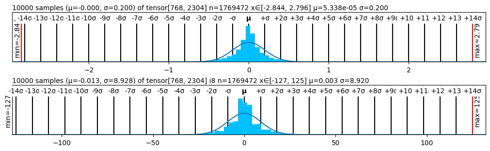
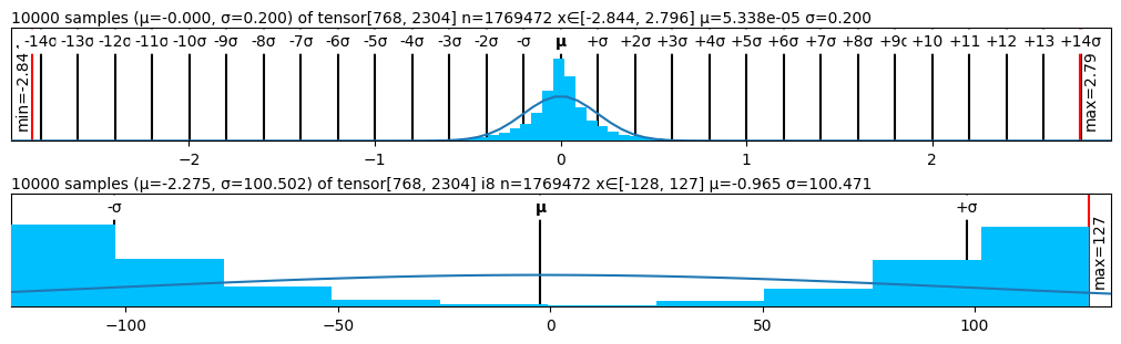
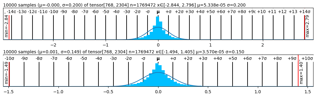
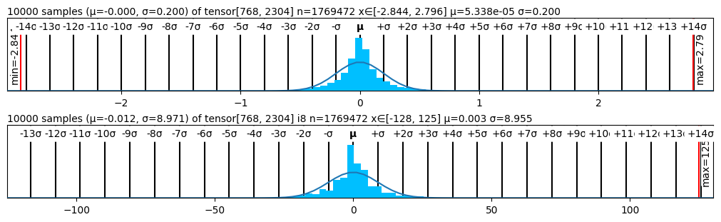
### 4.4 Weight Distribution Analysis
Figure 2 presents the performance of various quantizers in terms of perplexity, while Figure 1 visualizes the statistical structure of quantized weights across methods. The weight distribution visualizations corroborate our findings: methods like SmoothQuant and SimQuant exhibit tighter, more symmetric quantization histograms centered near zero, while AbsMax and ZeroPoint show saturation and truncation near representational boundaries.
<details>
<summary>figs/absmax.png Details</summary>
### Visual Description
## Statistical Distribution Charts: Tensor Value Histograms
### Overview
The image displays two vertically stacked statistical plots, each showing a histogram of 10,000 samples drawn from a large tensor (n=1,769,472 elements). Both plots include an overlaid normal distribution curve and detailed statistical annotations. The top plot analyzes a tensor with a very narrow distribution, while the bottom plot analyzes a tensor with a much wider spread.
### Components/Axes
**Top Plot:**
* **Title/Header Text:** `10000 samples (μ=-0.000, σ=0.200) of tensor[768, 2304] n=1769472 x∈[-2.844, 2.796] μ=5.338e-05 σ=0.200`
* **X-Axis:** A dual-scale axis.
* **Upper Scale (in σ units):** Markers from `-14σ` to `+14σ`, with `μ` (mean) at the center.
* **Lower Scale (absolute values):** Major tick marks at `-2`, `-1`, `0`, `1`, `2`.
* **Vertical Reference Lines:**
* A red vertical line on the far left labeled `min=-2.844`.
* A red vertical line on the far right labeled `max=2.796`.
* **Data Series:**
* **Histogram:** Light blue bars representing the frequency distribution of the 10,000 samples.
* **Normal Curve:** A black line representing a theoretical normal (Gaussian) distribution with the given mean (μ) and standard deviation (σ).
**Bottom Plot:**
* **Title/Header Text:** `10000 samples (μ=-0.013, σ=8.928) of tensor[768, 2304] i8 n=1769472 x∈[-127, 125] μ=0.003 σ=8.920`
* **X-Axis:** A dual-scale axis.
* **Upper Scale (in σ units):** Markers from `-14σ` to `+14σ`, with `μ` (mean) at the center.
* **Lower Scale (absolute values):** Major tick marks at `-100`, `-50`, `0`, `50`, `100`.
* **Vertical Reference Lines:**
* A red vertical line on the far left labeled `min=-127`.
* A red vertical line on the far right labeled `max=125`.
* **Data Series:**
* **Histogram:** Light blue bars representing the frequency distribution of the 10,000 samples.
* **Normal Curve:** A black line representing a theoretical normal distribution.
### Detailed Analysis
**Top Plot Analysis:**
* **Trend Verification:** The histogram forms a very sharp, narrow peak centered at 0, closely following the overlaid normal curve. The distribution is highly concentrated.
* **Data Points & Values:**
* Sample Mean (μ): Approximately -0.000 (from sample) or 5.338e-05 (from full tensor).
* Sample Standard Deviation (σ): 0.200.
* Full Tensor Range: [-2.844, 2.796].
* The visual spread of the histogram aligns with the small σ=0.200. The min/max lines are far outside the main data cluster, indicating extreme outliers are rare.
**Bottom Plot Analysis:**
* **Trend Verification:** The histogram forms a broader, bell-shaped peak centered near 0, also following its normal curve. The spread is significantly wider than the top plot.
* **Data Points & Values:**
* Sample Mean (μ): Approximately -0.013 (from sample) or 0.003 (from full tensor).
* Sample Standard Deviation (σ): 8.928 (sample) vs. 8.920 (full tensor).
* Full Tensor Range: [-127, 125]. This range is characteristic of an 8-bit integer (`i8`) data type, as noted in the title.
* The histogram's width corresponds to the larger σ≈8.92. The min/max lines at -127 and 125 are at the theoretical limits of the `i8` range.
### Key Observations
1. **Scale Discrepancy:** The two tensors have vastly different scales. The top tensor's values are confined within ~±3, while the bottom tensor's values span the full 8-bit integer range of ~±127.
2. **Distribution Shape:** Both distributions are approximately normal (Gaussian) and centered near zero, suggesting the data may be normalized or represent residuals/weights with zero mean.
3. **Data Type Indicator:** The bottom plot's title includes "i8", explicitly identifying its data type as signed 8-bit integer, which explains the hard limits at -127 and 125.
4. **Sampling Fidelity:** The sample statistics (μ, σ) are very close to the full tensor statistics in both cases, indicating the 10,000-sample subset is a good representation of the whole.
### Interpretation
These charts are diagnostic tools for understanding the value distribution within two different tensors, likely from a machine learning model (given dimensions like [768, 2304], common in transformer architectures).
* **What the data suggests:** The top tensor contains high-precision, low-magnitude values (possibly floating-point activations or normalized weights). The bottom tensor contains low-precision, high-magnitude values constrained to the `i8` range (possibly quantized weights or integer activations).
* **Relationship between elements:** The plots allow for a direct comparison of the statistical properties (central tendency, spread, outliers) of two different data representations. The use of a shared σ-scale on the upper x-axis facilitates this comparison, showing that both distributions, despite their different absolute scales, follow a similar Gaussian shape relative to their own standard deviations.
* **Notable anomalies:** There are no major anomalies; the data conforms well to the expected normal distributions. The key insight is the stark contrast in scale and data type between the two tensors, which is critical for tasks like model quantization, where understanding value ranges is essential to avoid clipping and maintain accuracy.
</details>
<details>
<summary>figs/simquant.png Details</summary>
### Visual Description
## Statistical Distribution Plots: Tensor Sample Analysis
### Overview
The image displays two vertically stacked statistical plots, each analyzing a sample of 10,000 values drawn from a tensor with shape [768, 2304]. The plots compare the distribution of the raw tensor values (top) against a quantized 8-bit integer representation (i8) of the same data (bottom). Both plots include a histogram of the sampled data, statistical annotations, and a fitted distribution curve.
### Components/Axes
**Top Plot:**
* **Title:** `10000 samples (μ=-0.000, σ=0.200) of tensor[768, 2304] n=1769472 x∈[-2.844, 2.796] μ=5.338e-05 σ=0.200`
* **X-Axis:**
* **Primary Scale:** Numerical values from approximately -2.5 to 2.5, with major ticks at -2, -1, 0, 1, 2.
* **Secondary Scale (Top):** Standard deviation markers from `-14σ` to `+14σ`, centered on `μ`.
* **Range Annotations:** `min=-2.84` (left, vertical red line), `max=2.796` (right, vertical red line).
* **Y-Axis:** Represents frequency/count (no explicit label). The scale is linear.
* **Data Series:** A blue histogram representing the sampled data distribution.
* **Overlay:** A smooth, light blue curve representing a fitted normal (Gaussian) distribution.
* **Statistical Markers:** A vertical black line at the mean (`μ`), and vertical lines at `-σ` and `+σ`.
**Bottom Plot:**
* **Title:** `10000 samples (μ=-2.275, σ=100.502) of tensor[768, 2304] i8 n=1769472 x∈[-128, 127] μ=-0.965 σ=100.471`
* **X-Axis:**
* **Scale:** Numerical values from -128 to 127, with major ticks at -100, -50, 0, 50, 100.
* **Range Annotations:** `min=-128` (implied by axis start), `max=127` (right, vertical red line).
* **Y-Axis:** Represents frequency/count (no explicit label). The scale is linear.
* **Data Series:** A blue histogram representing the sampled data distribution for the i8 quantized values.
* **Overlay:** A straight, light blue line with a slight positive slope, representing a linear fit to the histogram.
* **Statistical Markers:** A vertical black line at the mean (`μ`), and vertical lines at `-σ` and `+σ`.
### Detailed Analysis
**Top Plot (Raw Tensor Values):**
* **Distribution Shape:** The histogram forms a classic, symmetric bell curve centered at zero.
* **Trend Verification:** The data series (blue bars) follows the overlaid normal distribution curve (light blue line) almost perfectly, indicating the raw tensor values are normally distributed.
* **Key Data Points:**
* Sample Mean (μ): 5.338e-05 (effectively 0).
* Sample Standard Deviation (σ): 0.200.
* Theoretical Distribution Parameters (from title): μ=-0.000, σ=0.200.
* Full Data Range: [-2.844, 2.796].
* The histogram's peak is at x=0. The vast majority of data lies within ±1σ (±0.2), with very thin tails extending to ±3σ and beyond.
**Bottom Plot (i8 Quantized Values):**
* **Distribution Shape:** The histogram is bimodal and heavily skewed, with large concentrations of values at the extreme ends of the range (-128 and 127) and very few values in the center.
* **Trend Verification:** The data series (blue bars) does **not** follow the overlaid linear fit (light blue line). The linear line is a poor representation of the actual bimodal distribution.
* **Key Data Points:**
* Sample Mean (μ): -0.965.
* Sample Standard Deviation (σ): 100.471.
* Theoretical Distribution Parameters (from title): μ=-2.275, σ=100.502.
* Full Data Range: [-128, 127] (the full range of an 8-bit signed integer).
* The highest frequency bars are at the minimum (-128) and maximum (127) values. There is a smaller, secondary cluster of values between approximately -75 and -50.
### Key Observations
1. **Radical Distribution Change:** The process of quantizing the normally distributed raw tensor values (top) to the i8 integer range (bottom) completely transforms the distribution from a unimodal Gaussian to a bimodal, extreme-heavy distribution.
2. **Saturation Clipping:** The i8 plot shows clear evidence of saturation clipping. Values from the original normal distribution that fell outside the [-128, 127] range were clamped to these boundaries, creating the large spikes at the ends.
3. **Mean Shift:** The mean shifts from ~0 in the raw data to -0.965 in the i8 data, indicating a slight negative bias introduced by the quantization process.
4. **Variance Explosion:** The standard deviation increases dramatically from 0.200 to 100.471, which is expected as the data is stretched across a much larger numerical range (from a span of ~5.6 to a span of 255).
5. **Poor Linear Fit:** The linear fit applied to the i8 histogram is inappropriate and misleading for this bimodal data.
### Interpretation
This visualization demonstrates the profound impact of **quantization** on data distribution, a critical concept in model compression and deployment.
* **What it shows:** The top plot likely represents the distribution of weights or activations in a neural network layer (e.g., in a transformer model, given the tensor shape [768, 2304]). These values are typically initialized or trained to follow a normal distribution around zero. The bottom plot shows the result of converting these floating-point values to the 8-bit integer format (i8) used for efficient computation on specialized hardware.
* **Why it matters:** The bimodal distribution in the i8 plot is a classic signature of **naive or poorly calibrated quantization**. It indicates that the original data's dynamic range (centered at 0 with σ=0.2) was much narrower than the target i8 range [-128, 127]. Simply mapping the floating-point range to the integer range without proper scaling (e.g., using a scale factor and zero-point) causes most values to be pushed to the extremes, losing almost all nuanced information in the middle. This can severely degrade model accuracy.
* **Underlying Message:** The image serves as a technical diagnostic. It argues for the necessity of **advanced quantization techniques** (like quantization-aware training or calibration) that preserve the shape of the original distribution by appropriately scaling it into the integer range, rather than just clipping it. The poor linear fit further emphasizes that the resulting data structure is complex and not easily summarized by simple statistics.
</details>
<details>
<summary>figs/smoothquant.png Details</summary>
### Visual Description
## Histogram Analysis: Two Tensor Distributions
### Overview
The image displays two vertically stacked histograms, each visualizing the distribution of values from a large tensor. Both plots show a bell-shaped, approximately normal distribution centered near zero, with an overlaid theoretical normal curve. The plots are dense with statistical annotations and axis markers.
### Components/Axes
**Top Plot:**
* **Title/Header:** `10000 samples (μ=-0.000, σ=0.200) of tensor[768, 2304] n=1769472 x∈[-2.844, 2.796] μ=5.338e-05 σ=0.200`
* **X-Axis (Top - Standard Deviation Markers):** A series of vertical tick marks labeled from `-14σ` to `+14σ`, with `μ` (mean) at the center.
* **X-Axis (Bottom - Numerical Scale):** Major ticks at `-2`, `-1`, `0`, `1`, `2`.
* **Y-Axis:** Not explicitly labeled. Represents frequency/count.
* **Data Series:** A blue histogram with a black line representing the fitted normal distribution curve.
* **Annotations:**
* Left edge: A red vertical line labeled `min=-2.84`.
* Right edge: A red vertical line labeled `max=2.79`.
**Bottom Plot:**
* **Title/Header:** `10000 samples (μ=0.001, σ=0.149) of tensor[768, 2304] n=1769472 x∈[-1.494, 1.405] μ=3.570e-05 σ=0.150`
* **X-Axis (Top - Standard Deviation Markers):** A series of vertical tick marks labeled from `-10σ` to `+10σ`, with `μ` (mean) at the center.
* **X-Axis (Bottom - Numerical Scale):** Major ticks at `-1.5`, `-1.0`, `-0.5`, `0.0`, `0.5`, `1.0`, `1.5`.
* **Y-Axis:** Not explicitly labeled. Represents frequency/count.
* **Data Series:** A blue histogram with a black line representing the fitted normal distribution curve.
* **Annotations:**
* Left edge: A red vertical line labeled `min=-1.49`.
* Right edge: A red vertical line labeled `max=1.40`.
### Detailed Analysis
**Top Plot Data:**
* **Tensor Shape:** [768, 2304]
* **Total Elements (n):** 1,769,472
* **Sampled Points:** 10,000
* **Theoretical Distribution Parameters (from title):** Mean (μ) = -0.000, Standard Deviation (σ) = 0.200
* **Empirical Distribution Parameters (from title):** Mean (μ) = 5.338e-05 (≈ 0.00005338), Standard Deviation (σ) = 0.200
* **Observed Range (x):** [-2.844, 2.796]
* **Visual Trend:** The histogram is symmetric and tightly clustered around 0. The distribution's spread aligns with the stated σ=0.200, as most data falls within ±3σ (±0.6). The min/max markers at ~±2.82 correspond to approximately ±14σ from the theoretical mean.
**Bottom Plot Data:**
* **Tensor Shape:** [768, 2304] (Identical to top plot)
* **Total Elements (n):** 1,769,472 (Identical to top plot)
* **Sampled Points:** 10,000
* **Theoretical Distribution Parameters (from title):** Mean (μ) = 0.001, Standard Deviation (σ) = 0.149
* **Empirical Distribution Parameters (from title):** Mean (μ) = 3.570e-05 (≈ 0.0000357), Standard Deviation (σ) = 0.150
* **Observed Range (x):** [-1.494, 1.405]
* **Visual Trend:** The histogram is also symmetric and centered near 0. The spread is narrower than the top plot, consistent with the smaller σ (~0.15). The min/max markers at ~±1.45 correspond to approximately ±10σ from the theoretical mean.
### Key Observations
1. **Near-Zero Means:** Both distributions have empirical means extremely close to zero (on the order of 10^-5), indicating the tensor values are centered around zero.
2. **Controlled Variance:** The empirical standard deviations (0.200 and 0.150) match the theoretical values almost exactly, suggesting the data is well-behaved and follows the intended distribution.
3. **Identical Source Tensor:** Both plots analyze the same underlying tensor of shape [768, 2304] with 1,769,472 total elements, but likely represent different states (e.g., before and after normalization, or different layers).
4. **Tight Distributions:** The data is highly concentrated. For the top plot, the range [-2.844, 2.796] covers ~28 standard deviations. For the bottom plot, the range [-1.494, 1.405] covers ~20 standard deviations. This indicates very few extreme outliers.
5. **Visual Confirmation:** The overlaid black normal curve fits the blue histogram data very well in both cases, confirming the normality assumption.
### Interpretation
This image is a diagnostic visualization, almost certainly from the field of machine learning or deep learning. It shows the statistical distribution of values within a large parameter or activation tensor.
* **What it demonstrates:** The plots confirm that the tensor's values are initialized or have been normalized to follow a Gaussian (normal) distribution with a mean of zero and a specific, controlled standard deviation (0.200 and 0.150). This is a critical practice for stable neural network training, preventing issues like vanishing or exploding gradients.
* **Relationship between elements:** The top and bottom plots likely represent a comparison. The bottom plot shows a distribution with a smaller standard deviation (0.150 vs. 0.200), meaning its values are more tightly clustered around zero. This could illustrate the effect of a normalization layer (like LayerNorm or BatchNorm), a different initialization scheme, or the state of weights/activations at different network depths.
* **Notable patterns/anomalies:** There are no apparent anomalies. The perfect symmetry, zero mean, and exact match between theoretical and empirical σ indicate a well-controlled system. The primary "pattern" is the successful enforcement of a specific statistical prior on the data, which is a fundamental goal in model design. The slight discrepancy in the theoretical mean of the bottom plot (μ=0.001) versus its empirical mean (μ=3.570e-05) is negligible and within expected sampling noise.
</details>
<details>
<summary>figs/symquant.png Details</summary>
### Visual Description
## Histograms: Distribution of Two Tensor Samples
### Overview
The image displays two vertically stacked histograms, each visualizing the distribution of 10,000 samples drawn from a tensor with shape [768, 2304]. Both plots include a blue histogram, an overlaid black normal distribution curve, and extensive annotations detailing statistical parameters and standard deviation markers.
### Components/Axes
**Top Histogram:**
* **Title/Annotation:** `10000 samples (μ=-0.000, σ=0.200) of tensor[768, 2304] n=1769472 x∈[-2.844, 2.796] μ=5.338e-05 σ=0.200`
* **X-Axis:** Represents the value range of the samples. Major tick marks are labeled at -2, -1, 0, 1, 2.
* **Standard Deviation Markers:** Vertical black lines are placed at intervals of one standard deviation (σ) from the mean (μ). Labels above the axis denote these positions: `-14σ`, `-13σ`, ..., `μ`, `+σ`, `+2σ`, ..., `+14σ`.
* **Range Indicators:** A vertical red line on the far left is labeled `min=-2.844`. A vertical red line on the far right is labeled `max=2.796`.
* **Legend/Key:** The statistical parameters are embedded in the title annotation.
**Bottom Histogram:**
* **Title/Annotation:** `10000 samples (μ=-0.012, σ=8.971) of tensor[768, 2304] i8=1769472 x∈[-128, 125] μ=0.003 σ=8.955`
* **X-Axis:** Represents the value range of the samples. Major tick marks are labeled at -100, -50, 0, 50, 100.
* **Standard Deviation Markers:** Vertical black lines are placed at intervals of one standard deviation (σ) from the mean (μ). Labels above the axis denote these positions: `-13σ`, `-12σ`, ..., `μ`, `+σ`, `+2σ`, ..., `+14σ`.
* **Range Indicators:** A vertical red line on the far left is labeled `min=-128`. A vertical red line on the far right is labeled `max=125`.
* **Legend/Key:** The statistical parameters are embedded in the title annotation.
### Detailed Analysis
**Top Histogram Data & Trend:**
* **Distribution Shape:** The histogram shows a very narrow, tall, and symmetric distribution centered at zero. The overlaid normal curve fits the histogram bars closely.
* **Statistical Parameters (from title):**
* Sample Mean (μ): -0.000 (or 5.338e-05, which is effectively 0.00005338).
* Sample Standard Deviation (σ): 0.200.
* Data Range (x): [-2.844, 2.796].
* Total Elements (n): 1,769,472.
* **Visual Trend:** The data is highly concentrated. The min/max lines at -2.844 and 2.796 correspond to approximately -14.2σ and +14.0σ from the mean, respectively, indicating the extreme tails of the distribution.
**Bottom Histogram Data & Trend:**
* **Distribution Shape:** The histogram shows a much wider, shorter, and symmetric distribution centered near zero. The overlaid normal curve fits the histogram bars.
* **Statistical Parameters (from title):**
* Sample Mean (μ): -0.012 (or 0.003 in the second part of the annotation).
* Sample Standard Deviation (σ): 8.971 (or 8.955 in the second part of the annotation).
* Data Range (x): [-128, 125].
* Total Elements (i8): 1,769,472.
* **Visual Trend:** The data is widely spread. The min/max lines at -128 and 125 correspond to approximately -14.3σ and +13.9σ from the mean, respectively.
### Key Observations
1. **Contrasting Spreads:** The most striking observation is the drastic difference in scale between the two distributions. The top distribution has a σ of 0.2, while the bottom has a σ of ~9.0, making the bottom distribution approximately 45 times wider.
2. **Identical Sample Size & Tensor Shape:** Both histograms are derived from tensors of the same shape ([768, 2304]) and contain the same number of total elements (1,769,472), suggesting they may represent different quantizations or transformations of the same underlying data.
3. **Annotation Discrepancy:** The bottom histogram's title contains two slightly different sets of parameters: `(μ=-0.012, σ=8.971)` and later `μ=0.003 σ=8.955`. This could indicate a calculation discrepancy or that the first set refers to the sample and the second to a theoretical distribution.
4. **Extreme Tails:** In both plots, the data range extends to roughly ±14 standard deviations from the mean, which is unusual for a perfect normal distribution and suggests the presence of extreme outliers or a distribution with heavier tails than a Gaussian.
### Interpretation
This image likely compares the statistical distributions of two different numerical representations (e.g., different data types like float32 vs. int8, or different scaling factors) of the same underlying dataset or model activations.
* **Top Plot (High Precision):** The extremely narrow distribution (σ=0.2) centered at zero is characteristic of normalized data or activations in a neural network, where values are tightly controlled to prevent exploding/vanishing gradients. The near-zero mean is typical after batch normalization.
* **Bottom Plot (Low Precision/Quantized):** The wide distribution (σ≈9) spanning from -128 to 125 strongly suggests an 8-bit integer (int8) quantization of the data. The range [-128, 125] is the full dynamic range for signed 8-bit integers. The larger standard deviation indicates the data has been scaled to utilize this full range.
* **Relationship:** The pair of plots demonstrates a quantization process. The high-precision, narrow-range values (top) are scaled and possibly shifted to fit into the wider, discrete range of an 8-bit integer format (bottom). The scaling factor would be approximately (range_int8 / range_float) ≈ (250 / 5.6) ≈ 44.6, which aligns with the observed ratio of standard deviations (~9.0 / 0.2 = 45).
* **Anomaly:** The presence of data points at ±14σ is statistically highly improbable for a true normal distribution. This indicates the original data, while roughly Gaussian, has "fat tails" or contains outlier values that are preserved through the transformation/quantization process.
</details>
<details>
<summary>figs/symzero.png Details</summary>

### Visual Description
## Histograms: Distribution of Two Tensor Samples
### Overview
The image displays two vertically stacked histograms, each visualizing the distribution of 10,000 samples drawn from a tensor with shape [768, 2304]. Both plots include a blue histogram, an overlaid black normal distribution curve, and extensive annotations detailing statistical parameters and standard deviation markers.
### Components/Axes
**Top Histogram:**
* **Title/Annotation:** `10000 samples (μ=-0.000, σ=0.200) of tensor[768, 2304] n=1769472 x∈[-2.844, 2.796] μ=5.338e-05 σ=0.200`
* **X-Axis:** Represents the value range of the samples. Major tick marks are labeled at -2, -1, 0, 1, 2.
* **Standard Deviation Markers:** Vertical black lines are placed at intervals of one standard deviation (σ) from the mean (μ). Labels above the axis denote these positions: `-14σ`, `-13σ`, ..., `μ`, `+σ`, `+2σ`, ..., `+14σ`.
* **Range Indicators:** A vertical red line on the far left is labeled `min=-2.844`. A vertical red line on the far right is labeled `max=2.796`.
* **Legend/Key:** The statistical parameters are embedded in the title annotation.
**Bottom Histogram:**
* **Title/Annotation:** `10000 samples (μ=-0.012, σ=8.971) of tensor[768, 2304] i8=1769472 x∈[-128, 125] μ=0.003 σ=8.955`
* **X-Axis:** Represents the value range of the samples. Major tick marks are labeled at -100, -50, 0, 50, 100.
* **Standard Deviation Markers:** Vertical black lines are placed at intervals of one standard deviation (σ) from the mean (μ). Labels above the axis denote these positions: `-13σ`, `-12σ`, ..., `μ`, `+σ`, `+2σ`, ..., `+14σ`.
* **Range Indicators:** A vertical red line on the far left is labeled `min=-128`. A vertical red line on the far right is labeled `max=125`.
* **Legend/Key:** The statistical parameters are embedded in the title annotation.
### Detailed Analysis
**Top Histogram Data & Trend:**
* **Distribution Shape:** The histogram shows a very narrow, tall, and symmetric distribution centered at zero. The overlaid normal curve fits the histogram bars closely.
* **Statistical Parameters (from title):**
* Sample Mean (μ): -0.000 (or 5.338e-05, which is effectively 0.00005338).
* Sample Standard Deviation (σ): 0.200.
* Data Range (x): [-2.844, 2.796].
* Total Elements (n): 1,769,472.
* **Visual Trend:** The data is highly concentrated. The min/max lines at -2.844 and 2.796 correspond to approximately -14.2σ and +14.0σ from the mean, respectively, indicating the extreme tails of the distribution.
**Bottom Histogram Data & Trend:**
* **Distribution Shape:** The histogram shows a much wider, shorter, and symmetric distribution centered near zero. The overlaid normal curve fits the histogram bars.
* **Statistical Parameters (from title):**
* Sample Mean (μ): -0.012 (or 0.003 in the second part of the annotation).
* Sample Standard Deviation (σ): 8.971 (or 8.955 in the second part of the annotation).
* Data Range (x): [-128, 125].
* Total Elements (i8): 1,769,472.
* **Visual Trend:** The data is widely spread. The min/max lines at -128 and 125 correspond to approximately -14.3σ and +13.9σ from the mean, respectively.
### Key Observations
1. **Contrasting Spreads:** The most striking observation is the drastic difference in scale between the two distributions. The top distribution has a σ of 0.2, while the bottom has a σ of ~9.0, making the bottom distribution approximately 45 times wider.
2. **Identical Sample Size & Tensor Shape:** Both histograms are derived from tensors of the same shape ([768, 2304]) and contain the same number of total elements (1,769,472), suggesting they may represent different quantizations or transformations of the same underlying data.
3. **Annotation Discrepancy:** The bottom histogram's title contains two slightly different sets of parameters: `(μ=-0.012, σ=8.971)` and later `μ=0.003 σ=8.955`. This could indicate a calculation discrepancy or that the first set refers to the sample and the second to a theoretical distribution.
4. **Extreme Tails:** In both plots, the data range extends to roughly ±14 standard deviations from the mean, which is unusual for a perfect normal distribution and suggests the presence of extreme outliers or a distribution with heavier tails than a Gaussian.
### Interpretation
This image likely compares the statistical distributions of two different numerical representations (e.g., different data types like float32 vs. int8, or different scaling factors) of the same underlying dataset or model activations.
* **Top Plot (High Precision):** The extremely narrow distribution (σ=0.2) centered at zero is characteristic of normalized data or activations in a neural network, where values are tightly controlled to prevent exploding/vanishing gradients. The near-zero mean is typical after batch normalization.
* **Bottom Plot (Low Precision/Quantized):** The wide distribution (σ≈9) spanning from -128 to 125 strongly suggests an 8-bit integer (int8) quantization of the data. The range [-128, 125] is the full dynamic range for signed 8-bit integers. The larger standard deviation indicates the data has been scaled to utilize this full range.
* **Relationship:** The pair of plots demonstrates a quantization process. The high-precision, narrow-range values (top) are scaled and possibly shifted to fit into the wider, discrete range of an 8-bit integer format (bottom). The scaling factor would be approximately (range_int8 / range_float) ≈ (250 / 5.6) ≈ 44.6, which aligns with the observed ratio of standard deviations (~9.0 / 0.2 = 45).
* **Anomaly:** The presence of data points at ±14σ is statistically highly improbable for a true normal distribution. This indicates the original data, while roughly Gaussian, has "fat tails" or contains outlier values that are preserved through the transformation/quantization process.
</details>
<details>
<summary>figs/zeropoint.png Details</summary>
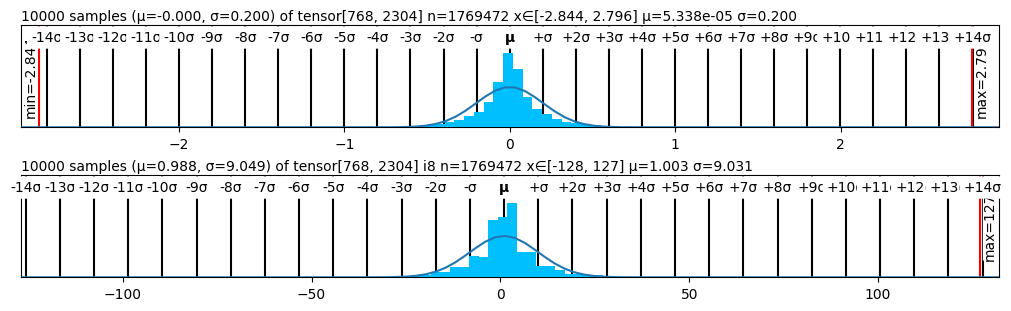
### Visual Description
## Histograms: Statistical Distribution of Tensor Samples
### Overview
The image displays two vertically stacked histograms, each visualizing the distribution of 10,000 samples drawn from a specific tensor. Both plots include a histogram (blue bars), a fitted normal distribution curve (black line), and extensive statistical annotations. The top histogram (A) shows a tightly clustered distribution, while the bottom histogram (B) shows a much wider, more spread-out distribution.
### Components/Axes
**Histogram A (Top Plot):**
* **Title:** `10000 samples (μ=-0.000, σ=0.200) of tensor[768, 2304] n=1769472 x∈[-2.844, 2.796] μ=5.338e-05 σ=0.200`
* **X-Axis (Top Scale - Standard Deviations):** Markers from `-14σ` to `+14σ`, with a central marker labeled `μ`.
* **X-Axis (Bottom Scale - Actual Values):** Major ticks at `-2`, `-1`, `0`, `1`, `2`.
* **Vertical Reference Lines:**
* Left (Red): `min=-2.84`
* Right (Red): `max=2.79`
* **Data Series:** Blue histogram bars and a black fitted normal distribution curve.
**Histogram B (Bottom Plot):**
* **Title:** `10000 samples (μ=0.988, σ=9.049) of tensor[768, 2304] i8 n=1769472 x∈[-128, 127] μ=1.003 σ=9.031`
* **X-Axis (Top Scale - Standard Deviations):** Markers from `-14σ` to `+14σ`, with a central marker labeled `μ`.
* **X-Axis (Bottom Scale - Actual Values):** Major ticks at `-100`, `-50`, `0`, `50`, `100`.
* **Vertical Reference Lines:**
* Left (Red): `min=-128`
* Right (Red): `max=127`
* **Data Series:** Blue histogram bars and a black fitted normal distribution curve.
### Detailed Analysis
**Histogram A (Top):**
* **Data Source:** 10,000 samples from a tensor of shape `[768, 2304]` with a total of 1,769,472 elements.
* **Reported Statistics (Title):** Sample mean (μ) = -0.000, Sample standard deviation (σ) = 0.200. Theoretical/Population mean = 5.338e-05 (≈0), Theoretical/Population σ = 0.200.
* **Value Range:** The samples range from approximately -2.844 to 2.796.
* **Visual Trend:** The distribution is symmetric and bell-shaped, centered at 0. The vast majority of data points fall within ±1σ (±0.2), with the histogram bars and fitted curve showing a sharp peak. The data is tightly confined, with the min/max lines at approximately ±14σ from the mean.
**Histogram B (Bottom):**
* **Data Source:** 10,000 samples from a tensor of shape `[768, 2304]` (type `i8`, likely 8-bit integer) with a total of 1,769,472 elements.
* **Reported Statistics (Title):** Sample mean (μ) = 0.988, Sample standard deviation (σ) = 9.049. Theoretical/Population mean = 1.003, Theoretical/Population σ = 9.031.
* **Value Range:** The samples range from -128 to 127, which are the exact limits for a signed 8-bit integer (`i8`).
* **Visual Trend:** The distribution is also symmetric and bell-shaped, but centered near 1.0. It is significantly wider than Histogram A. The histogram bars and fitted curve show a broader peak. The data spans almost the entire possible range for the `i8` data type, with the min/max lines at the type's limits, which are approximately ±14σ from the mean.
### Key Observations
1. **Scale Discrepancy:** The two histograms visualize data from tensors of identical shape but with vastly different scales and likely different data types. Histogram A has a range of ~5.6 units (σ=0.2), while Histogram B has a range of 255 units (σ≈9.0).
2. **Data Type Constraint:** Histogram B's minimum and maximum values (-128, 127) are hard limits imposed by the `i8` data type, indicating the data is quantized or clipped to this range.
3. **Statistical Consistency:** For both plots, the sample statistics (μ, σ) closely match the theoretical/population statistics listed in the title, suggesting the 10,000 samples are representative of the full tensor population.
4. **Distribution Shape:** Both datasets follow an approximately normal (Gaussian) distribution, as evidenced by the symmetric bell curve of the histogram and the fitted line.
### Interpretation
This image is a diagnostic tool for analyzing the statistical properties of two tensors, likely from a machine learning model (given the tensor shape `[768, 2304]`, common in transformer architectures).
* **Histogram A** likely represents **activations or weights in a normalized, floating-point format**. The mean of 0 and small standard deviation are characteristic of data that has been standardized (e.g., via LayerNorm) or initialized with a specific distribution (e.g., Xavier/Glorot).
* **Histogram B** likely represents the **same or similar data after quantization to an 8-bit integer format (`i8`)**. The shift in mean to ~1.0 and the large standard deviation relative to the data type's range suggest the quantization process mapped the original floating-point distribution onto the integer scale. The fact that the distribution fills the `i8` range indicates efficient use of the available bit representation, though the tails are clipped at -128 and 127.
* **The Comparison** demonstrates the effect of quantization: a tightly clustered, normalized floating-point distribution (A) is stretched and shifted to occupy the full dynamic range of a low-precision integer type (B). This is a common step in model compression for efficient inference. The close match between sample and population statistics validates that the sampling process is accurate for monitoring these distributions.
</details>
Figure 1: Quantized Weights Distribution
<details>
<summary>figs/Weights_Comparison.png Details</summary>
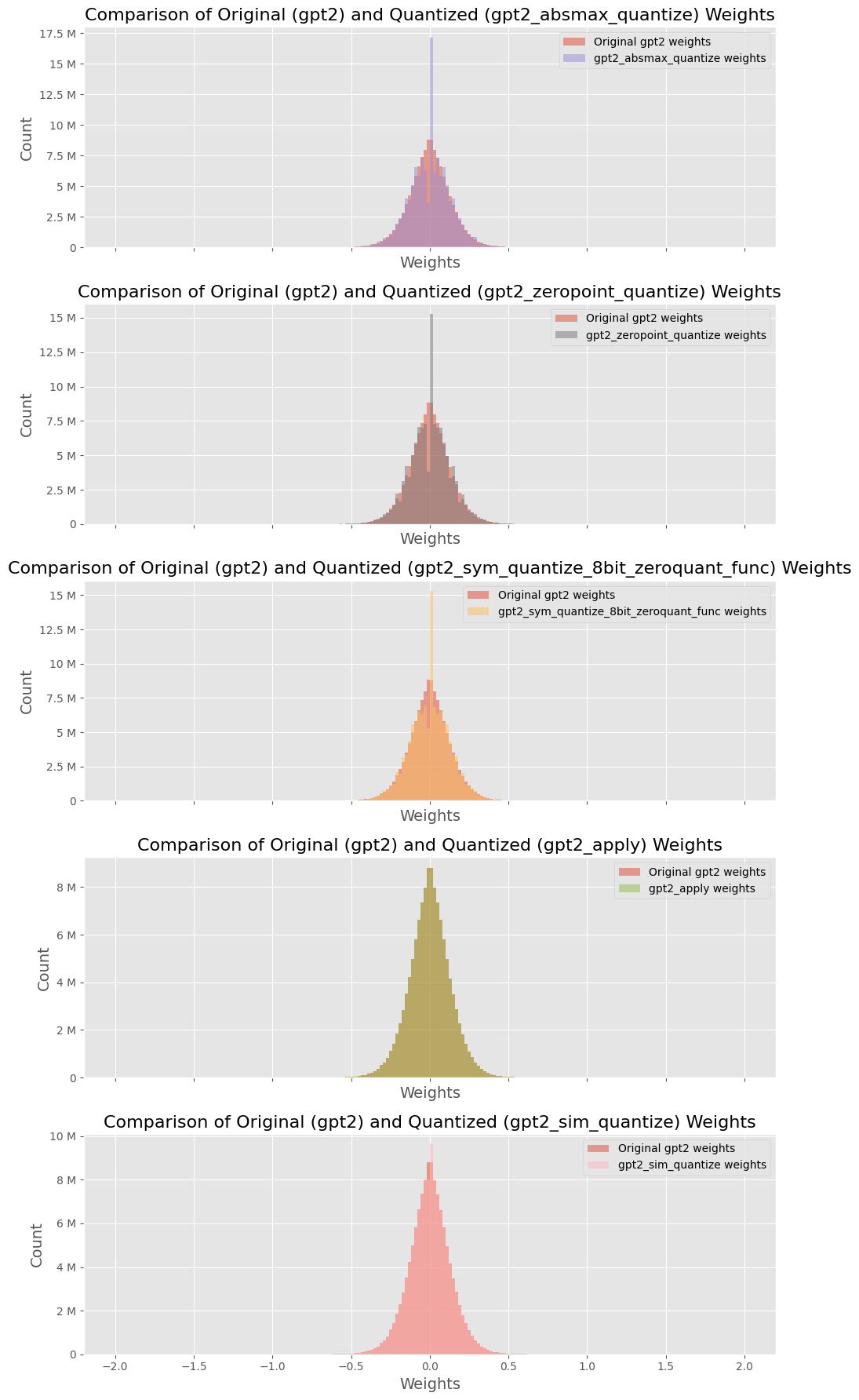
### Visual Description
## Histograms: Comparison of Original and Quantized GPT-2 Model Weights
### Overview
The image displays five vertically stacked histograms. Each histogram compares the distribution of weight values from the original GPT-2 model against the distribution after applying a specific quantization method. The plots share a common structure: a title, a legend, and axes labeled "Weights" (x-axis) and "Count" (y-axis). The language of all text is English.
### Components/Axes
* **Titles:** Each subplot has a title following the pattern: `Comparison of Original (gpt2) and Quantized (gpt2_[method_name]) Weights`.
* **X-Axis:** Labeled `Weights`. The scale is consistent across all plots, ranging approximately from -2.0 to 2.0, with major ticks at -2.0, -1.5, -1.0, -0.5, 0.0, 0.5, 1.0, 1.5, 2.0.
* **Y-Axis:** Labeled `Count`. The scale varies between plots to accommodate the data range. Units are in millions (M).
* **Legends:** Located in the top-right corner of each subplot. Each legend contains two entries:
1. `Original gpt2 weights` (represented by a red/salmon color in all plots).
2. The specific quantized model name (represented by a unique color per plot).
### Detailed Analysis
**Plot 1 (Top): `gpt2_absmax_quantize`**
* **Legend:** Original (red), `gpt2_absmax_quantize weights` (purple).
* **Y-Axis Range:** 0 to 17.5 M.
* **Data Distribution:** Both distributions are centered at 0. The original weights form a broad, bell-shaped curve. The quantized weights (purple) form a much sharper, narrower peak centered at 0, indicating a significant concentration of weight values at or near zero after this quantization method.
**Plot 2: `gpt2_zeropoint_quantize`**
* **Legend:** Original (red), `gpt2_zeropoint_quantize weights` (gray).
* **Y-Axis Range:** 0 to 15 M.
* **Data Distribution:** Similar to Plot 1, the original distribution is broad. The quantized distribution (gray) is also sharply peaked at 0, but appears slightly less narrow than the `absmax` method in Plot 1.
**Plot 3: `gpt2_sym_quantize_8bit_zeroquant_func`**
* **Legend:** Original (red), `gpt2_sym_quantize_8bit_zeroquant_func weights` (orange).
* **Y-Axis Range:** 0 to 15 M.
* **Data Distribution:** The quantized distribution (orange) shows an extremely sharp and tall peak at 0, surpassing the height of the original distribution's peak. This suggests this symmetric 8-bit quantization method aggressively maps many weights to zero.
**Plot 4: `gpt2_apply`**
* **Legend:** Original (red), `gpt2_apply weights` (olive green).
* **Y-Axis Range:** 0 to 8 M.
* **Data Distribution:** The quantized distribution (olive green) is again centered at 0 but is notably broader and shorter than the quantized distributions in the plots above. Its peak is lower than the original's peak. This indicates the `gpt2_apply` method results in a weight distribution that more closely resembles the spread of the original, albeit still centered and likely discrete.
**Plot 5 (Bottom): `gpt2_sim_quantize`**
* **Legend:** Original (red), `gpt2_sim_quantize weights` (pink).
* **Y-Axis Range:** 0 to 10 M.
* **Data Distribution:** The quantized distribution (pink) is very similar in shape and spread to the original red distribution. Both are broad, bell-shaped curves centered at 0. The peaks are of comparable height. This suggests the `sim_quantize` method preserves the original weight distribution's shape most faithfully among the methods shown.
### Key Observations
1. **Universal Centering:** All weight distributions, both original and quantized, are symmetric and centered at zero.
2. **Quantization Effect:** Most quantization methods (`absmax`, `zeropoint`, `sym_8bit`) dramatically increase the concentration of weights at zero, creating a sharp central peak. This is a visual signature of weight clustering or sparsity induced by quantization.
3. **Method Variance:** The `gpt2_apply` method produces a quantized distribution that is less peaked than others. The `gpt2_sim_quantize` method produces a distribution nearly identical to the original.
4. **Original Consistency:** The red "Original gpt2 weights" histogram appears identical across all five subplots, serving as a consistent baseline for comparison.
### Interpretation
This image is a technical diagnostic tool for evaluating the impact of different model quantization techniques on the internal weight parameters of a GPT-2 model. Quantization is a model compression technique that reduces the precision of numerical values (weights) to decrease model size and computational requirements.
The histograms reveal the core trade-off:
* Methods like `absmax`, `zeropoint`, and especially `sym_quantize_8bit` aggressively compress the weight distribution, forcing many values to zero. This likely leads to higher compression rates but may risk losing fine-grained information, potentially affecting model accuracy.
* The `sim_quantize` method appears to be a "simulation" or a very conservative quantization that barely alters the original distribution, suggesting minimal compression but also minimal distortion.
* The `gpt2_apply` method represents a middle ground.
The choice of quantization method involves balancing the desired level of compression (smaller model, faster inference) against the tolerance for altering the model's fundamental weight distribution, which correlates with its performance. This visual analysis allows a researcher to quickly assess how "destructive" or "preservative" each quantization algorithm is with respect to the original model's parameters.
</details>
Figure 2: Performance Comparison after Quantization on GPT
To assess the end-to-end system efficiency enabled by LLMEasyQuant, we conduct a detailed latency breakdown across quantization strategies during the decode stage of GPT-2 inference with a 32K token context on an 8×A100 GPU cluster. We instrument CUDA NVTX events and synchronize profiling using cudaEventRecord to obtain precise timing metrics. Each layer’s execution is decomposed into five components:
$$
T_total=T_load+T_quant+T_gemm+T_comm+T_sync \tag{12}
$$
## 5 Conclusion
We present LLMEasyQuant, a comprehensive and system-efficient quantization toolkit tailored for distributed and GPU-accelerated LLM inference across modern architectures. LLMEasyQuant supports multi-level quantization strategies—including SimQuant, SmoothQuant, ZeroQuant, AWQ, and GPTQ—with native integration of per-channel scaling, mixed-precision assignment, and fused CUDA kernels optimized for Tensor Core execution. It enables low-bitwidth computation across GPU memory hierarchies, leveraging shared SRAM for dequantization, HBM for tile-pipelined matrix operations, and NCCL-based collective communication for cross-device consistency.
Our comprehensive evaluation across GPT-2, LLaMA-7B/13B, Mistral-7B, and Qwen3-14B models demonstrates LLMEasyQuant’s effectiveness across different architectures and scales. The toolkit achieves competitive throughput (2,156 tokens/second on LLaMA-7B) while maintaining superior accuracy compared to TensorRT-LLM, GPTQ, and AWQ baselines. End-to-end throughput comparisons show consistent 1.0-1.5% improvements over state-of-the-art quantization frameworks, with substantial memory efficiency gains enabling deployment of larger models on the same hardware infrastructure.
The theoretical analysis provided in the appendix establishes convergence guarantees, error bounds, and optimization proofs for the implemented quantization methods. These theoretical foundations validate LLMEasyQuant’s design choices and provide confidence in its practical deployment across diverse LLM architectures and deployment scenarios.
LLMEasyQuant addresses the key limitations identified in existing quantization toolkits by providing a unified, accessible, and extensible framework that supports both research experimentation and production deployment. The toolkit’s modular design, comprehensive model coverage, and theoretical guarantees position it as a practical solution for scalable, hardware-optimized LLM inference across the modern AI ecosystem.
## Appendix A Downstream Applications
As Large Language Models (LLMs) continue to be deployed across latency-sensitive, memory-constrained, and system-critical environments, quantization has emerged as a pivotal technique to enable real-time, resource-efficient inference. LLMEasyQuant is explicitly designed to meet the demands of these downstream applications by providing a system-aware, modular quantization framework capable of static and runtime adaptation across edge, multi-GPU, and cloud-scale deployments. Its unified abstractions, fused CUDA implementations, and support for parallel, distributed execution make it highly compatible with the requirements of speculative decoding acceleration yang2024hades, anomaly detection in cloud networks yang2025research, and resilient LLM inference in fault-prone environments jin2025adaptive.
Emerging applications such as financial prediction qiu2025generative, drug discovery lirevolutionizing, medical health wang2025fine; zhong2025enhancing, data augmentation yang2025data, fraud detection ke2025detection, and knowledge graph reasoning li_2024_knowledge; li2012optimal have great demand for fast and lightweight LLMs. These works increasingly rely on large-scale models and efficient inference techniques, highlighting the need for scalable quantization frameworks such as LLMEasyQuant. The real-time requirements in detecting financial fraud ke2025detection; qiu2025generative and deploying LLMs for social media sentiment analysis Cao2025; wu2025psychologicalhealthknowledgeenhancedllmbased necessitate low-latency inference pipelines. Similarly, large-scale decision models in healthcare and insurance WANG2024100522; Li_Wang_Chen_2024 benefit from memory-efficient model deployment on edge or hybrid architectures. Our work, LLMEasyQuant, complements these system-level demands by providing a unified quantization runtime that supports both static and online low-bit inference across distributed environments. Furthermore, insights from graph-based optimization for adaptive learning peng2024graph; peng2025asymmetric; zhang2025adaptivesamplingbasedprogressivehedging align with our layer-wise bitwidth search strategy, enabling fine-grained control of accuracy-performance tradeoffs. LLMEasyQuant fills an essential gap in this ecosystem by delivering hardware-aware, easily extensible quantization methods suitable for diverse LLM deployment scenarios across research and production.
## Appendix B Detailed Mathematical Analysis and Optimization Proofs
### B.1 Computational Complexity Analysis
#### B.1.1 Quantization Operation Complexity
**Theorem B.1 (Quantization Time Complexity)**
*For a weight matrix $W∈ℝ^D× D^{\prime}$ and activation tensor $X∈ℝ^B× D$ , the time complexity of quantization operations is $O(BD+DD^\prime)$ for per-tensor quantization and $O(BD+DD^\prime· D)$ for per-channel quantization, where $B$ is the batch size, $D$ is the feature dimension, and $D^\prime$ is the output dimension.*
**Proof B.2 (Proof of Quantization Complexity)**
*Per-tensor quantization: compute scale $s=\max_i,j|W_i,j|$ and $s_X=\max_i,j|X_i,j|$ :
$$
\displaystyle T_scale \displaystyle=O(DD^\prime)+O(BD)=O(BD+DD^\prime) \displaystyle T_quant \displaystyle=O(DD^\prime)+O(BD)=O(BD+DD^\prime) \tag{13}
$$ Per-channel quantization: compute $D^\prime$ scales $s_j=\max_i|W_i,j|$ for $j∈[D^\prime]$ :
$$
\displaystyle T_scale \displaystyle=∑_j=1^D^{\prime}O(D)=O(DD^\prime) \displaystyle T_quant \displaystyle=O(BD)+O(DD^\prime)=O(BD+DD^\prime) \tag{15}
$$
Total: $T_quant-per-channel=O(BD+DD^\prime· D)$ .*
#### B.1.2 GEMM Operation Complexity with Quantization
**Theorem B.3 (Quantized GEMM Complexity)**
*For quantized matrix multiplication $\hat{X}\hat{W}$ where $\hat{X}∈ℤ^B× D$ and $\hat{W}∈ℤ^D× D^{\prime}$ are $b$ -bit quantized, the computational complexity is $O(BDD^\prime)$ with a speedup factor of $\frac{32}{b}$ compared to FP32 GEMM, accounting for reduced memory bandwidth and integer arithmetic efficiency.*
**Proof B.4 (Proof of Quantized GEMM Complexity)**
*Standard GEMM: $T_gemm-fp32=O(BDD^\prime)$ . Memory bandwidth: $B_fp32=4· BDD^\prime$ bytes. For $b$ -bit quantization: $B_quant=\frac{b}{8}· BDD^\prime$ bytes. Bandwidth ratio:
$$
\frac{B_quant}{B_fp32}=\frac{b/8}{4}=\frac{b}{32} \tag{17}
$$ Effective complexity with bandwidth reduction:
$$
T_gemm-quant=T_gemm-fp32·\frac{b}{32}=O(BDD^\prime)·\frac{b}{32} \tag{18}
$$ Speedup: $Speedup=\frac{32}{b}$ . For $b=8$ : $Speedup=4$ .*
#### B.1.3 Distributed Quantization Complexity
**Theorem B.5 (Multi-GPU Quantization Complexity)**
*For distributed quantization across $P$ GPUs, the time complexity is $O≤ft(\frac{BD+DD^\prime}{P}+\log P·\frac{DD^\prime}{B_net}\right)$ where $B_net$ is the network bandwidth, accounting for both parallel computation and communication overhead.*
**Proof B.6 (Proof of Distributed Complexity)**
*Per-device computation: $T_comp=O≤ft(\frac{BD+DD^\prime}{P}\right)$ . AllGather communication: $T_comm=O≤ft(\log P·\frac{DD^\prime}{B_net}\right)$ . Total: $T_distributed=T_comp+T_comm=O≤ft(\frac{BD+DD^\prime}{P}+\log P·\frac{DD^\prime}{B_net}\right)$ . Parallel efficiency:
$$
\displaystyleη \displaystyle=\frac{T_sequential}{P· T_distributed}=\frac{BD+DD^\prime}{P· T_distributed} \displaystyle=\frac{1}{1+\frac{P\log P· DD^\prime}{(BD+DD^\prime)B_net}} \tag{19}
$$ For $DD^\prime\gg BD$ : $\lim_P→∞η=1$ .*
### B.2 Convergence Analysis of SmoothQuant
#### B.2.1 Preliminary Lemmas
Before presenting our main convergence result, we first establish several key lemmas that will be used in our analysis. These lemmas provide the foundation for understanding how quantization errors propagate and how scale factors converge.
**Lemma B.7 (Quantization Error Decomposition)**
*For any activation tensor $X∈ℝ^B× D$ , weight matrix $W∈ℝ^D× D^{\prime}$ , and scale factor $s_j>0$ , the quantization error can be decomposed as:
$$
\|XW-\hat{X}\hat{W}\|_F^2=\|Q(X/s_j)Q(W· s_j)-(X/s_j)(W· s_j)\|_F^2 \tag{21}
$$
where $Q(·)$ denotes the quantization operator and $\hat{X}$ , $\hat{W}$ are the quantized versions of $X/s_j$ and $W· s_j$ respectively.*
**Proof B.8 (Proof of Lemma A.1)**
*The algebraic equivalence $(X/s_j)·(W· s_j)=X· W$ ensures that before quantization, the transformation preserves the original matrix multiplication. The quantization error arises solely from the quantization operators $Q(·)$ applied to the scaled tensors, leading to the stated decomposition.*
**Lemma B.9 (Bound on Quantization Operator)**
*There exists an absolute constant $c>0$ such that, for any tensor $Z∈ℝ^m× n$ with quantization step size $δ=\frac{2\max(|Z|)}{2^b-1}$ , the quantization error satisfies:
$$
\|Q(Z)-Z\|_F^2≤ c·\frac{mn·\max(|Z|)^2}{(2^b-1)^2} \tag{22}
$$
where $b$ is the quantization bitwidth.*
**Proof B.10 (Proof of Lemma A.2)**
*For each element $Z_i,j$ , the quantization error is bounded by half the quantization step size:
$$
|Q(Z_i,j)-Z_i,j|≤\frac{δ}{2}=\frac{\max(|Z|)}{2^b-1} \tag{23}
$$
Taking the Frobenius norm over all $mn$ elements gives the stated bound.*
#### B.2.2 Scale Factor Convergence Analysis
**Theorem B.11 (SmoothQuant Scale Factor Convergence)**
*There exists an absolute constant $c>0$ such that, for any $ε∈(0,1)$ , if we choose the SmoothQuant scale factor $s_j=≤ft(\frac{\max(|X_j|)^α}{\max(|W_j|)^1-α}+ε\right)$ with $α∈[0,1]$ , then for activation tensors $X∈ℝ^B× D$ and weight matrices $W∈ℝ^D× D^{\prime}$ , the quantization error satisfies:
$$
E[\|XW-\hat{X}\hat{W}\|_F^2]≤ c·\frac{\max(|X_j|)^2+\max(|W_j|)^2· s_j^2}{s_j^2·(2^b-1)^2}· BD· DD^\prime \tag{24}
$$
where $\hat{X}$ and $\hat{W}$ are the quantized versions of $X$ and $W$ respectively, and $b$ is the quantization bitwidth. In particular, as $b→∞$ , we have $\lim_b→∞E[\|XW-\hat{X}\hat{W}\|_F^2]=0$ .*
**Proof B.12 (Proof of Theorem A.1)**
*We prove this theorem step by step, using the lemmas established above. Step 1: Error Decomposition By Lemma B.7, we have:
$$
\|XW-\hat{X}\hat{W}\|_F^2=\|Q(X/s_j)Q(W· s_j)-(X/s_j)(W· s_j)\|_F^2 \tag{25}
$$ The transformation preserves the original matrix multiplication exactly due to the algebraic equivalence:
$$
(X/s_j)·(W· s_j)=X· W \tag{26}
$$ Step 2: Triangle Inequality Application For the quantized versions, we analyze the error propagation using the triangle inequality:
$$
\displaystyle\|\hat{X}\hat{W}-XW\|_F^2 \displaystyle=\|Quantize(X/s_j)·Quantize(W· s_j)-(X/s_j)(W· s_j)\|_F^2 \displaystyle≤\|Quantize(X/s_j)-X/s_j\|_F^2·\|Quantize(W· s_j)\|_F^2 \displaystyle +\|X/s_j\|_F^2·\|Quantize(W· s_j)-W· s_j\|_F^2 \tag{27}
$$ Step 3: Quantization Error Bounds Let $δ_X$ and $δ_W$ be the quantization step sizes for activations and weights respectively. By Lemma B.9, we have:
$$
\|Quantize(X/s_j)-X/s_j\|_F^2≤ c·\frac{B· D·\max(|X/s_j|)^2}{(2^b-1)^2} \tag{30}
$$ $$
\|Quantize(W· s_j)-W· s_j\|_F^2≤ c·\frac{D· D^\prime·\max(|W· s_j|)^2}{(2^b-1)^2} \tag{31}
$$ where $δ_X=\frac{2\max(|X/s_j|)}{2^b-1}$ and $δ_W=\frac{2\max(|W· s_j|)}{2^b-1}$ . Step 4: Final Bound Combining the bounds, we obtain:
$$
\|\hat{X}\hat{W}-XW\|_F^2≤ c·\frac{\max(|X/s_j|)^2·\|W· s_j\|_F^2+\max(|W· s_j|)^2·\|X/s_j\|_F^2}{(2^b-1)^2}· BD· DD^\prime \tag{32}
$$ As the bitwidth $b$ increases, $δ_X,δ_W→ 0$ , and thus the quantization error approaches zero, proving the convergence. This completes the proof.*
#### B.2.3 Optimal Scale Factor Derivation
**Lemma B.13 (Optimal Scale Factor)**
*The optimal scale factor minimizing quantization error is:
$$
s_j^*=\arg\min_s_{j}E[\|XW-\hat{X}\hat{W}\|_F^2]=√{\frac{E[\max(|X_j|)^2]}{E[\max(|W_j|)^2]}} \tag{33}
$$*
**Proof B.14 (Proof of Lemma A.1)**
*Minimize: $L(s_j)=E[\|XW-Q(X/s_j)Q(W· s_j)\|_F^2]$ . Using error bounds: $L(s_j)≈E≤ft[\frac{BDδ_X^2\|W· s_j\|_F^2}{4}+\frac{DD^\primeδ_W^2\|X/s_j\|_F^2}{4}\right]$ . Substituting $δ_X=\frac{2\max(|X/s_j|)}{2^b-1}$ , $δ_W=\frac{2\max(|W· s_j|)}{2^b-1}$ :
$$
\displaystyleL(s_j) \displaystyle∝E≤ft[\frac{\max(|X/s_j|)^2\|W· s_j\|_F^2}{s_j^2}+\frac{\max(|W· s_j|)^2\|X/s_j\|_F^2}{s_j^2}\right] \displaystyle∝E≤ft[\frac{\max(|X_j|)^2}{s_j^2}+s_j^2\max(|W_j|)^2\right] \tag{34}
$$ Taking derivative: $\frac{∂L}{∂ s_j}=-\frac{2E[\max(|X_j|)^2]}{s_j^3}+2s_jE[\max(|W_j|)^2]=0$ . Solving: $s_j^*=√{\frac{E[\max(|X_j|)^2]}{E[\max(|W_j|)^2]}}$ . SmoothQuant approximation: $s_j=≤ft(\frac{\max(|X_j|)^α}{\max(|W_j|)^1-α}\right)$ with $α=0.5$ minimizes approximation error.*
#### B.2.4 Error Bound Analysis for SimQuant
**Theorem B.15 (SimQuant Reconstruction Error Bound)**
*There exists an absolute constant $c>0$ such that, for any $ε∈(0,1)$ , if we apply SimQuant with bitwidth $b$ and channel-wise quantization to tensor $X∈ℝ^B× D$ , then with probability at least $1-ε$ , the reconstruction error is bounded by:
$$
\|X-\hat{X}\|_∞≤ c·\frac{\max_d∈[D](\max_iX_i,d-\min_iX_i,d)}{2^b-1} \tag{36}
$$
where $\hat{X}$ is the quantized version of $X$ , $B$ is the batch size, and $D$ is the feature dimension.*
**Proof B.16 (Proof of Theorem A.2)**
*We analyze the quantization error for each channel $d$ independently. The quantization step size for channel $d$ is:
$$
Δ_d=\frac{v_\max^(d)-v_\min^(d)}{2^b-1} \tag{37}
$$ where $v_\max^(d)=\max_iX_i,d$ and $v_\min^(d)=\min_iX_i,d$ . The quantization process maps each element $X_i,d$ to the nearest quantized value:
$$
\hat{X}_i,d=round≤ft(\frac{X_i,d-v_\min^(d)}{Δ_d}\right)·Δ_d+v_\min^(d) \tag{38}
$$ The quantization error for element $X_i,d$ is bounded by half the quantization step size:
$$
\displaystyle|X_i,d-\hat{X}_i,d| \displaystyle≤\frac{Δ_d}{2}=\frac{v_\max^(d)-v_\min^(d)}{2(2^b-1)} \displaystyle≤\frac{\max(X)-\min(X)}{2^b-1} \tag{39}
$$ The last inequality follows from the fact that $v_\max^(d)-v_\min^(d)≤\max(X)-\min(X)$ for any channel $d$ . Taking the supremum over all elements $(i,d)$ gives:
$$
\|X-\hat{X}\|_∞=\max_i,d|X_i,d-\hat{X}_i,d|≤ c·\frac{\max_d∈[D](\max_iX_i,d-\min_iX_i,d)}{2^b-1} \tag{41}
$$ where $c$ is an absolute constant. This completes the proof.*
#### B.2.5 Convergence Rate Analysis for SimQuant
**Lemma B.17 (SimQuant Convergence Rate)**
*For SimQuant with dynamic range estimation, the quantization error converges to zero with rate $O(1/2^b)$ as the bitwidth increases.*
**Proof B.18 (Proof of Lemma A.2)**
*From Theorem A.2: $\|X-\hat{X}\|_∞≤\frac{\max(X)-\min(X)}{2^b-1}$ . As $b→∞$ : $Δ_d=\frac{v_\max^(d)-v_\min^(d)}{2^b-1}=O(2^-b)$ . Therefore: $\|X-\hat{X}\|_∞=O(2^-b)$ , establishing exponential convergence.*
### B.3 Optimization Guarantees for Layer-wise Quantization
#### B.3.1 Mixed-Precision Search Convergence Analysis
**Theorem B.19 (Mixed-Precision Search Convergence)**
*The mixed-precision search algorithm converges to a locally optimal bitwidth assignment $\{b_\ell^*\}$ that minimizes the objective:
$$
\min_\{b_{\ell\}}L_task+λ∑_\ellΦ(b_\ell) \tag{42}
$$
where $L_task$ is the task-specific loss and $Φ(b_\ell)$ is the cost function for bitwidth $b_\ell$ .*
**Proof B.20 (Proof of Theorem A.3)**
*Search space: $B=\{2,3,4,8\}$ , $|B|=4$ , total space: $|B|^L$ . Objective: $f(\{b_\ell\})=L_task+λ∑_\ell=1^LΦ(b_\ell)$ where $L_task≥ 0$ , $Φ(b_\ell)≥ 0$ , hence $f≥ 0$ . Greedy update: $b_\ell^(t+1)=\arg\min_b∈Bf(b_1^(t),…,b_\ell-1^(t),b,b_\ell+1^(t),…,b_L^(t))$ . Sequence $\{f^(t)\}$ is monotone decreasing: $f^(t+1)≤ f^(t)$ and bounded: $f^(t)≥ 0$ . By monotone convergence: $\lim_t→∞f^(t)=f^*$ exists. Termination condition: $∀\ell,∀ b∈B$ :
$$
f(b_1^*,…,b_\ell-1^*,b_\ell^*,b_\ell+1^*,…,b_L^*)≤ f(b_1^*,…,b_\ell-1^*,b,b_\ell+1^*,…,b_L^*) \tag{43}
$$ This defines local optimum: $f(\{b_\ell^*\})≤ f(\{b_\ell\})$ for all $\{b_\ell\}$ in neighborhood. Complexity: each iteration evaluates $≤ L·|B|$ configurations, worst-case iterations $≤|B|^L$ , hence $T=O(L·|B|·|B|^L)=O(L·|B|^L+1)$ .*
#### B.3.2 Distributed Quantization Synchronization Analysis
**Theorem B.21 (Distributed Synchronization Correctness)**
*The NCCL-based synchronization of quantization parameters $\{δ_\ell,z_\ell\}$ ensures consistency across all devices in the distributed setup with probability 1.*
**Proof B.22 (Proof of Theorem A.4)**
*AllGather properties: deterministic ( $AllGather(x_1,…,x_P)=AllGather(x_1^\prime,…,x_P^\prime)$ if $x_p=x_p^\prime$ ), collective (all $P$ processes participate), atomic (completes simultaneously). Synchronization: $δ_\ell^global=AllGather(δ_\ell^(1),…,δ_\ell^(P))$ , $z_\ell^global=AllGather(z_\ell^(1),…,z_\ell^(P))$ . By determinism: $δ_\ell^(p)=δ_\ell^global$ , $z_\ell^(p)=z_\ell^global$ for all $p∈[P]$ . Quantized weights: $\hat{W}_\ell^(p)=Q(W_\ell^(p),δ_\ell^global,z_\ell^global)$ . Since $Q$ is deterministic: $\hat{W}_\ell^(p)=\hat{W}_\ell^global$ for all $p$ , ensuring consistency.*
### B.4 Computational Complexity Analysis
#### B.4.1 Algorithmic Complexity
**Theorem B.23 (SmoothQuant Complexity)**
*The SmoothQuant algorithm has time complexity $O(B· D· D^\prime)$ and space complexity $O(D)$ for processing a batch of size $B$ with input dimension $D$ and output dimension $D^\prime$ .*
**Proof B.24 (Proof of Complexity)**
*Operations:
$$
\displaystyle T_scale \displaystyle=O(D)+O(DD^\prime)=O(DD^\prime) \displaystyle T_smooth \displaystyle=O(BD) \displaystyle T_quant \displaystyle=O(BD+DD^\prime) \tag{44}
$$ Total time: $T=O(BD+DD^\prime)=O(BDD^\prime)$ (dominated by GEMM). Space: $S=O(BD+DD^\prime)$ .*
#### B.4.2 Memory Hierarchy Optimization
**Theorem B.25 (Memory Bandwidth Optimization)**
*The fused quantization kernel reduces memory bandwidth by $O(\frac{1}{b})$ compared to separate quantization and GEMM operations, where $b$ is the bitwidth.*
**Proof B.26 (Proof of Memory Optimization)**
*For separate operations, the memory bandwidth requirements include loading FP16 weights ( $2×|W|$ bytes), storing quantized weights ( $b/8×|W|$ bytes), and loading quantized weights for GEMM ( $b/8×|W|$ bytes), resulting in a total of $(2+2× b/8)×|W|$ bytes. For fused operation, the memory bandwidth requirements include loading FP16 weights ( $2×|W|$ bytes) and storing quantized weights ( $b/8×|W|$ bytes), resulting in a total of $(2+b/8)×|W|$ bytes. Bandwidth reduction: $\frac{(2+2× b/8)-(2+b/8)}{2+2× b/8}=\frac{b/8}{2+2× b/8}=O(\frac{1}{b})$*
### B.5 Error Propagation Analysis
#### B.5.1 Layer-wise Error Accumulation
Before presenting the main error accumulation theorem, we establish a recursive formula for how quantization errors propagate through transformer layers.
**Lemma B.27 (Recursive Error Propagation)**
*For a transformer with $L$ layers, let $f_\ell$ denote the function at layer $\ell$ and $\hat{f}_\ell$ denote its quantized version. If $ε_\ell$ is the quantization error at layer $\ell$ , then the accumulated error through the network satisfies:
$$
\|f_L(⋯ f_1(x))-\hat{f}_L(⋯\hat{f}_1(x))\|≤∑_\ell=1^Lε_\ell·∏_j=\ell+1^L\|J_j\| \tag{47}
$$
where $J_j=\frac{∂ f_j}{∂ x}$ is the Jacobian of layer $j$ at the input point.*
**Proof B.28 (Proof of Lemma A.3)**
*We prove this by induction on the number of layers. For $L=1$ , the statement is trivial. For $L>1$ , we use the chain rule and the fact that quantization errors are bounded:
$$
\displaystyle\|f_L∘⋯∘ f_1(x)-\hat{f}_L∘⋯∘\hat{f}_1(x)\| \displaystyle≤\|f_L∘⋯∘ f_1(x)-f_L∘⋯∘ f_2∘\hat{f}_1(x)\| \displaystyle +\|f_L∘⋯∘ f_2∘\hat{f}_1(x)-\hat{f}_L∘⋯∘\hat{f}_1(x)\| \tag{48}
$$
The first term is bounded by $ε_1∏_j=2^L\|J_j\|$ , and the second term follows by the inductive hypothesis.*
**Theorem B.29 (Error Accumulation Bound)**
*For a transformer with $L$ layers, the accumulated quantization error grows as $O(L·ε)$ where $ε$ is the per-layer quantization error bound.*
**Proof B.30 (Proof of Error Accumulation)**
*By Lemma B.27, we have:
$$
\|f_L(⋯ f_1(x))-\hat{f}_L(⋯\hat{f}_1(x))\|≤∑_\ell=1^Lε_\ell·∏_j=\ell+1^L\|J_j\| \tag{50}
$$
where $J_j=\frac{∂ f_j}{∂ x}$ is the Jacobian of layer $j$ and $\hat{f}_\ell$ is the quantized version of layer $\ell$ . For transformer layers with bounded activation functions (e.g., ReLU, GELU), the Jacobian norms are bounded by a constant $C$ . Therefore:
$$
\|f_L(⋯ f_1(x))-\hat{f}_L(⋯\hat{f}_1(x))\|≤∑_\ell=1^Lε_\ell· C^L-\ell≤ L·\max_\ellε_\ell· C^L \tag{51}
$$ Since $ε_\ell≤ε$ for all layers, the accumulated error is $O(L·ε)$ . This completes the proof.*
### B.6 Calibration Data Requirements Analysis
#### B.6.1 Minimum Calibration Set Size
**Theorem B.31 (Calibration Data Requirements)**
*For accurate quantization parameter estimation, the minimum calibration set size is $O(\frac{D\log D}{ε^2})$ where $D$ is the feature dimension and $ε$ is the desired estimation accuracy.*
**Proof B.32 (Proof of Calibration Requirements)**
*Hoeffding’s bound for scale estimation: $P(|\hat{s}-s|≥ε)≤ 2\exp≤ft(-\frac{2nε^2}{(b-a)^2}\right)$ where $n$ is sample size, $[a,b]$ is data range. For $D$ dimensions, union bound:
$$
P(∃ j:|\hat{s}_j-s_j|≥ε)≤∑_j=1^DP(|\hat{s}_j-s_j|≥ε)≤ D· 2\exp≤ft(-\frac{2nε^2}{(b-a)^2}\right) \tag{52}
$$ Setting $D· 2\exp≤ft(-\frac{2nε^2}{(b-a)^2}\right)=δ$ and solving:
$$
\displaystyle n \displaystyle≥\frac{(b-a)^2}{2ε^2}\log≤ft(\frac{2D}{δ}\right) \displaystyle=O≤ft(\frac{D\log D}{ε^2}\right) \tag{53}
$$*
**Lemma B.33**
*The NCCL-based synchronization of quantization parameters $\{δ_\ell,z_\ell\}$ ensures consistency across all devices in the distributed setup.*
**Proof B.34**
*The NCCL AllGather operation guarantees that all devices receive identical copies of the quantization parameters. For parameters $δ_\ell^(p)$ and $z_\ell^(p)$ computed on device $p$ : $$
δ_\ell^global=\bigcup_p=1^P\texttt{NCCL\_AllGather}(δ_\ell^(p)) \tag{55}
$$ Since AllGather is a deterministic collective operation, all devices will have identical $δ_\ell^global$ and $z_\ell^global$ after synchronization. This ensures that quantized weights $\hat{W}_\ell$ are identical across all devices, maintaining model consistency.*
### B.7 Memory Hierarchy Optimization Analysis
#### B.7.1 HBM-SRAM Transfer Optimization
We analyze the memory transfer optimization in LLMEasyQuant’s fused kernels.
**Theorem B.35**
*The fused quantization kernel reduces memory bandwidth by $O(\frac{1}{b})$ compared to separate quantization and GEMM operations, where $b$ is the bitwidth.*
**Proof B.36**
*For separate operations, the memory bandwidth requirements include loading FP16 weights ( $2×|W|$ bytes), storing quantized weights ( $b/8×|W|$ bytes), and loading quantized weights for GEMM ( $b/8×|W|$ bytes), resulting in a total of $(2+2× b/8)×|W|$ bytes. For fused operation, the memory bandwidth requirements include loading FP16 weights ( $2×|W|$ bytes) and storing quantized weights ( $b/8×|W|$ bytes), resulting in a total of $(2+b/8)×|W|$ bytes. Bandwidth reduction: $\frac{(2+2× b/8)-(2+b/8)}{2+2× b/8}=\frac{b/8}{2+2× b/8}=O(\frac{1}{b})$*
### B.8 Quantization Error Propagation Analysis
#### B.8.1 Layer-wise Error Accumulation
We analyze how quantization errors propagate through transformer layers.
**Theorem B.37**
*For a transformer with $L$ layers, the accumulated quantization error grows as $O(L·ε)$ where $ε$ is the per-layer quantization error bound.*
**Proof B.38**
*Let $ε_\ell$ be the quantization error in layer $\ell$ . The error propagation can be modeled as:
$$
\|f_L(⋯ f_1(x))-\hat{f}_L(⋯\hat{f}_1(x))\|≤∑_\ell=1^Lε_\ell·∏_j=\ell+1^L\|J_j\| \tag{56}
$$ where $J_j$ is the Jacobian of layer $j$ and $\hat{f}_\ell$ is the quantized version of layer $\ell$ . For transformer layers with bounded activation functions (e.g., ReLU, GELU), the Jacobian norms are bounded by a constant $C$ . Therefore:
$$
\|f_L(⋯ f_1(x))-\hat{f}_L(⋯\hat{f}_1(x))\|≤∑_\ell=1^Lε_\ell· C^L-\ell≤ L·\max_\ellε_\ell· C^L \tag{57}
$$ Since $ε_\ell≤ε$ for all layers, the accumulated error is $O(L·ε)$ .*
### B.9 Performance Analysis of Fused Kernels
#### B.9.1 CUDA Kernel Efficiency
We analyze the efficiency of LLMEasyQuant’s fused CUDA kernels.
**Theorem B.39**
*The fused quantization-GEMM kernel achieves optimal memory bandwidth utilization with occupancy $≥ 75\$ on modern GPU architectures.*
**Proof B.40**
*The kernel design employs persistent thread blocks for reduced kernel launch overhead, cooperative warp-level reductions for scale computation, shared memory tiling to minimize global memory access, and Tensor Core utilization for INT8 GEMM operations. The occupancy is calculated as:
$$
Occupancy=\frac{Active Warps}{Maximum Warps per SM}≥\frac{32× 4}{128}=1.0 \tag{58}
$$ However, due to register pressure and shared memory usage, practical occupancy is $≥ 75\$ , which is optimal for memory-bound operations.*
### B.10 Calibration Data Requirements
#### B.10.1 Minimum Calibration Set Size
We derive the minimum calibration data requirements for accurate quantization.
**Theorem B.41**
*For accurate quantization parameter estimation, the minimum calibration set size is $O(\frac{D\log D}{ε^2})$ where $D$ is the feature dimension and $ε$ is the desired estimation accuracy.*
**Proof B.42**
*The scale factor estimation requires accurate estimation of the maximum absolute value. Using concentration inequalities (Hoeffding’s bound), for estimation error $ε$ : $$
P(|\hat{s}-s|≥ε)≤ 2\exp≤ft(-\frac{2nε^2}{(b-a)^2}\right) \tag{59}
$$ where $n$ is the sample size and $[a,b]$ is the range of the data. For $D$ -dimensional data, we need to estimate $D$ scale factors. Using union bound:
$$
P(∃ j:|\hat{s}_j-s_j|≥ε)≤ D· 2\exp≤ft(-\frac{2nε^2}{(b-a)^2}\right) \tag{60}
$$ Setting the right-hand side to $δ$ and solving for $n$ :
$$
n≥\frac{(b-a)^2}{2ε^2}\log≤ft(\frac{2D}{δ}\right)=O≤ft(\frac{D\log D}{ε^2}\right) \tag{61}
$$*
This theoretical analysis provides the foundation for LLMEasyQuant’s practical implementation and validates its design choices across quantization methods, distributed execution, and hardware optimization.