2407.00401

# PUZZLES: A Benchmark for Neural Algorithmic Reasoning **Authors**: ETH Zürich Abstract Algorithmic reasoning is a fundamental cognitive ability that plays a pivotal role in problem-solving and decision-making processes. Reinforcement Learning (RL) has demonstrated remarkable proficiency in tasks such as motor control, handling perceptual input, and managing stochastic environments. These advancements have been enabled in part by the availability of benchmarks. In this work we introduce PUZZLES, a benchmark based on Simon Tatham’s Portable Puzzle Collection, aimed at fostering progress in algorithmic and logical reasoning in RL. PUZZLES contains 40 diverse logic puzzles of adjustable sizes and varying levels of complexity; many puzzles also feature a diverse set of additional configuration parameters. The 40 puzzles provide detailed information on the strengths and generalization capabilities of RL agents. Furthermore, we evaluate various RL algorithms on PUZZLES, providing baseline comparisons and demonstrating the potential for future research. All the software, including the environment, is available at https://github.com/ETH-DISCO/rlp. Human intelligence relies heavily on logical and algorithmic reasoning as integral components for solving complex tasks. While Machine Learning (ML) has achieved remarkable success in addressing many real-world challenges, logical and algorithmic reasoning remains an open research question [1, 2, 3, 4, 5, 6, 7]. This research question is supported by the availability of benchmarks, which allow for a standardized and broad evaluation framework to measure and encourage progress [8, 9, 10]. Reinforcement Learning (RL) has made remarkable progress in various domains, showcasing its capabilities in tasks such as game playing [11, 12, 13, 14, 15] , robotics [16, 17, 18, 19] and control systems [20, 21, 22]. Various benchmarks have been proposed to enable progress in these areas [23, 24, 25, 26, 27, 28, 29]. More recently, advances have also been made in the direction of logical and algorithmic reasoning within RL [30, 31, 32]. Popular examples also include the games of Chess, Shogi, and Go [33, 34]. Given the importance of logical and algorithmic reasoning, we propose a benchmark to guide future developments in RL and more broadly machine learning. Logic puzzles have long been a playful challenge for humans, and they are an ideal testing ground for evaluating the algorithmic and logical reasoning capabilities of RL agents. A diverse range of puzzles, similar to the Atari benchmark [24], favors methods that are broadly applicable. Unlike tasks with a fixed input size, logic puzzles can be solved iteratively once an algorithmic solution is found. This allows us to measure how well a solution attempt can adapt and generalize to larger inputs. Furthermore, in contrast to games such as Chess and Go, logic puzzles have a known solution, making reward design easier and enabling tracking progress and guidance with intermediate rewards. <details> <summary>x1.png Details</summary>  ### Visual Description ## Puzzle Grid: Assorted Puzzle Types ### Overview The image presents a grid of 36 different puzzle types, each displayed as a small example or initial state. The puzzles vary in style and mechanics, including grid-based logic puzzles, connection puzzles, and number puzzles. ### Components/Axes The image is organized as a 6x6 grid of puzzle examples. Each puzzle has a title above it, indicating the puzzle type. The puzzle types are: 1. Black Box 2. Bridges 3. Cube 4. Dominosa 5. Fifteen 6. Filling 7. Flip 8. Flood 9. Galaxies 10. Guess 11. Inertia 12. Keen 13. Lightup 14. Loopy 15. Magnets 16. Map 17. Mines 18. Mosaic 19. Net 20. Netslide 21. Palisade 22. Pattern 23. Pearl 24. Pegs 25. Range 26. Rectangles 27. Same Game 28. Signpost 29. Singles 30. Sixteen 31. Slant 32. Solo 33. Tents 34. Towers 35. Tracks 36. Twiddle 37. Undead 38. Unequal 39. Unruly 40. Untangle ### Detailed Analysis or Content Details Here's a breakdown of some of the puzzle examples: * **Black Box:** A grid with numbers along the edges and black circles inside. The grid is 9x9. Numbers 5, 1, 5, 1, 5, 1, 5, 1, 5, H, 2 are along the top. Numbers 1, 2, 3, 4 are along the bottom. Numbers 1, 2, 3, 4 are along the left. Numbers H, 2, 3, 3 are along the right. * **Bridges:** A network of circles with numbers inside, connected by lines. * **Cube:** A 2D representation of a 3D cube. * **Dominosa:** A grid of numbers, where the goal is to find pairs of numbers that form dominoes. * **Fifteen:** A sliding tile puzzle with numbers 1 through 15. * **Filling:** A grid with numbers indicating how many cells in a row or column should be filled. * **Flip:** A grid with shaded and unshaded cells, where flipping a cell changes the state of adjacent cells. * **Flood:** A grid of colored squares, where the goal is to make the entire grid one color by changing the color of the top-left square. * **Galaxies:** A grid with circles, where the goal is to divide the grid into regions, each containing a circle. * **Guess:** A color-based logic puzzle. * **Inertia:** A grid with diamonds and squares, where the goal is to move a ball to a target. * **Keen:** A grid with numbers and cages, where the numbers in each cage must satisfy a given operation. * **Lightup:** A grid with black and white cells, where the goal is to place light bulbs to illuminate all white cells. * **Loopy:** A grid of cells, where the goal is to draw a loop that passes through some of the cells. * **Magnets:** A grid with plus and minus signs, where the goal is to place magnets in the cells. * **Map:** A puzzle with different colored regions. * **Mines:** A grid with numbers indicating the number of mines in adjacent cells. * **Mosaic:** A grid with numbers. * **Net:** A grid with squares and lines. * **Netslide:** A grid with squares and arrows. * **Palisade:** A grid with numbers. * **Pattern:** A grid with black and white cells. * **Pearl:** A grid with circles and lines. * **Pegs:** A grid with blue circles. * **Range:** A grid with numbers. * **Rectangles:** A grid with numbers. * **Same Game:** A grid of colored squares, where the goal is to remove groups of squares of the same color. * **Signpost:** A grid with arrows and numbers. * **Singles:** A grid with numbers. * **Sixteen:** A grid with numbers. * **Slant:** A grid with lines. * **Solo:** A grid with numbers. * **Tents:** A grid with trees and numbers. * **Towers:** A grid with numbers. * **Tracks:** A grid with tracks. * **Twiddle:** A puzzle with numbered tiles. * **Undead:** A grid with symbols. * **Unequal:** A grid with numbers and inequality signs. * **Unruly:** A grid with black and white cells. * **Untangle:** A graph with nodes and edges. ### Key Observations The image provides a diverse collection of puzzle types, showcasing different problem-solving skills and game mechanics. The puzzles range from simple logic puzzles to more complex spatial reasoning challenges. ### Interpretation The image serves as a visual catalog of various puzzle types, demonstrating the breadth and variety within the puzzle genre. It highlights the different approaches to problem-solving and the diverse mechanics used to create engaging and challenging games. The collection could be used to introduce someone to different puzzle styles or to provide a visual reference for puzzle enthusiasts. 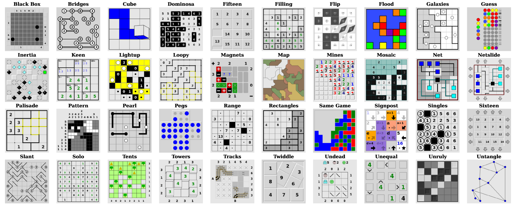</details> Figure 1: All puzzle classes of Simon Tatham’s Portable Puzzle Collection. In this paper, we introduce PUZZLES, a comprehensive RL benchmark specifically designed to evaluate RL agents’ algorithmic reasoning and problem-solving abilities in the realm of logical and algorithmic reasoning. Simon Tatham’s Puzzle Collection [35], curated by the renowned computer programmer and puzzle enthusiast Simon Tatham, serves as the foundation of PUZZLES. This collection includes a set of 40 logic puzzles, shown in Figure 1, each of which presents distinct challenges with various dimensions of adjustable complexity. They range from more well-known puzzles, such as Solo or Mines (commonly known as Sudoku and Minesweeper, respectively) to lesser-known puzzles such as Cube or Slant. PUZZLES includes all 40 puzzles in a standardized environment, each playable with a visual or discrete input and a discrete action space. Contributions. We propose PUZZLES, an RL environment based on Simon Tatham’s Puzzle Collection, comprising a collection of 40 diverse logic puzzles. To ensure compatibility, we have extended the original C source code to adhere to the standards of the Pygame library. Subsequently, we have integrated PUZZLES into the Gymnasium framework API, providing a straightforward, standardized, and widely-used interface for RL applications. PUZZLES allows the user to arbitrarily scale the size and difficulty of logic puzzles, providing detailed information on the strengths and generalization capabilities of RL agents. Furthermore, we have evaluated various RL algorithms on PUZZLES, providing baseline comparisons and demonstrating the potential for future research. 1 Related Work RL benchmarks. Various benchmarks have been proposed in RL. Bellemare et al. [24] introduced the influential Atari-2600 benchmark, on which Mnih et al. [11] trained RL agents to play the games directly from pixel inputs. This benchmark demonstrated the potential of RL in complex, high-dimensional environments. PUZZLES allows the use of a similar approach where only pixel inputs are provided to the agent. Todorov et al. [23] presented MuJoCo which provides a diverse set of continuous control tasks based on a physics engine for robotic systems. Another control benchmark is the DeepMind Control Suite by Duan et al. [26], featuring continuous actions spaces and complex control problems. The work by Côté et al. [28] emphasized the importance of natural language understanding in RL and proposed a benchmark for evaluating RL methods in text-based domains. Lanctot et al. [29] introduced OpenSpiel, encompassing a wide range of games, enabling researchers to evaluate and compare RL algorithms’ performance in game-playing scenarios. These benchmarks and frameworks have contributed significantly to the development and evaluation of RL algorithms. OpenAI Gym by Brockman et al. [25], and its successor Gymnasium by the Farama Foundation [36] helped by providing a standardized interface for many benchmarks. As such, Gym and Gymnasium have played an important role in facilitating reproducibility and benchmarking in reinforcement learning research. Therefore, we provide PUZZLES as a Gymnasium environment to enable ease of use. Logical and algorithmic reasoning within RL. Notable research in RL on logical reasoning includes automated theorem proving using deep RL [16] or RL-based logic synthesis [37]. Dasgupta et al. [38] find that RL agents can perform a certain degree of causal reasoning in a meta-reinforcement learning setting. The work by Jiang and Luo [30] introduces Neural Logic RL, which improves interpretability and generalization of learned policies. Eppe et al. [39] provide steps to advance problem-solving as part of hierarchical RL. Fawzi et al. [31] and Mankowitz et al. [32] demonstrate that RL can be used to discover novel and more efficient algorithms for well-known problems such as matrix multiplication and sorting. Neural algorithmic reasoning has also been used as a method to improve low-data performance in classical RL control environments [40, 41]. Logical reasoning might be required to compete in certain types of games such as chess, shogi and Go [33, 34, 42, 13], Poker [43, 44, 45, 46] or board games [47, 48, 49, 50]. However, these are usually multi-agent games, with some also featuring imperfect information and stochasticity. Reasoning benchmarks. Various benchmarks have been introduced to assess different types of reasoning capabilities, although only in the realm of classical ML. IsarStep, proposed by Li et al. [8], specifically designed to evaluate high-level mathematical reasoning necessary for proof-writing tasks. Another significant benchmark in the field of reasoning is the CLRS Algorithmic Reasoning Benchmark, introduced by Veličković et al. [9]. This benchmark emphasizes the importance of algorithmic reasoning in machine learning research. It consists of 30 different types of algorithms sourced from the renowned textbook “Introduction to Algorithms” by Cormen et al. [51]. The CLRS benchmark serves as a means to evaluate models’ understanding and proficiency in learning various algorithms. In the domain of large language models (LLMs), BIG-bench has been introduced by Srivastava et al. [10]. BIG-bench incorporates tasks that assess the reasoning capabilities of LLMs, including logical reasoning. Despite these valuable contributions, a suitable and unified benchmark for evaluating logical and algorithmic reasoning abilities in single-agent perfect-information RL has yet to be established. Recognizing this gap, we propose PUZZLES as a relevant and necessary benchmark with the potential to drive advancements and provide a standardized evaluation platform for RL methods that enable agents to acquire algorithmic and logical reasoning abilities. 2 The PUZZLES Environment In the following section we give an overview of the PUZZLES environment. The puzzles are available to play online at https://www.chiark.greenend.org.uk/~sgtatham/puzzles/; excellent standalone apps for Android and iOS exist as well. The environment is written in both Python and C. For a detailed explanation of all features of the environment as well as their implementation, please see Appendices B and C. Gymnasium RL Code puzzle_env.py puzzle.py pygame.c Puzzle C Sources Pygame Library puzzle Module rlp Package Python C Figure 2: Code and library landscape around the PUZZLES Environment, made up of the rlp Package and the puzzle Module . The figure shows how the puzzle Module presented in this paper fits within Tathams’s Puzzle Collection footnotemark: code, the Pygame package, and a user’s Gymnasium reinforcement learning code . The different parts are also categorized as Python language and C language. 2.1 Environment Overview Within the PUZZLES environment, we encapsulate the tasks presented by each logic puzzle by defining consistent state, action, and observation spaces. It is also important to note that the large majority of the logic puzzles are designed so that they can be solved without requiring any guesswork. By default, we provide the option of two observation spaces, one is a representation of the discrete internal game state of the puzzle, the other is a visual representation of the game interface. These observation spaces can easily be wrapped in order to enable PUZZLES to be used with more advanced neural architectures such as graph neural networks (GNNs) or Transformers. All puzzles provide a discrete action space which only differs in cardinality. To accommodate the inherent difficulty and the need for proper algorithmic reasoning in solving these puzzles, the environment allows users to implement their own reward structures, facilitating the training of successful RL agents. All puzzles are played in a two-dimensional play area with deterministic state transitions, where a transition only occurs after a valid user input. Most of the puzzles in PUZZLES do not have an upper bound on the number of steps, they can only be completed by successfully solving the puzzle. An agent with a bad policy is likely never going to reach a terminal state. For this reason, we provide the option for early episode termination based on state repetitions. As we show in Section 3.4, this is an effective method to facilitate learning. 2.2 Difficulty Progression and Generalization The PUZZLES environment places a strong emphasis on giving users control over the difficulty exhibited by the environment. For each puzzle, the problem size and difficulty can be adjusted individually. The difficulty affects the complexity of strategies that an agent needs to learn to solve a puzzle. As an example, Sudoku has tangible difficulty options: harder difficulties may require the use of new strategies such as forcing chains Forcing chains works by following linked cells to evaluate possible candidates, usually starting with a two-candidate cell. to find a solution, whereas easy difficulties only need the single position strategy. The single position strategy involves identifying cells which have only a single possible value. The scalability of the puzzles in our environment offers a unique opportunity to design increasingly complex puzzle configurations, presenting a challenging landscape for RL agents to navigate. This dynamic nature of the benchmark serves two important purposes. Firstly, the scalability of the puzzles facilitates the evaluation of an agent’s generalization capabilities. In the PUZZLES environment, it is possible to train an agent in an easy puzzle setting and subsequently evaluate its performance in progressively harder puzzle configurations. For most puzzles, the cardinality of the action space is independent of puzzle size. It is therefore also possible to train an agent only on small instances of a puzzle and then evaluate it on larger sizes. This approach allows us to assess whether an agent has learned the correct underlying algorithm and generalizes to out-of-distribution scenarios. Secondly, it enables the benchmark to remain adaptable to the continuous advancements in RL methodologies. As RL algorithms evolve and become more capable, the puzzle configurations can be adjusted accordingly to maintain the desired level of difficulty. This ensures that the benchmark continues to effectively assess the capabilities of the latest RL methods. 3 Empirical Evaluation We evaluate the baseline performance of numerous commonly used RL algorithms on our PUZZLES environment. Additionally, we also analyze the impact of certain design decisions of the environment and the training setup. Our metric of interest is the average number of steps required by a policy to successfully complete a puzzle, where lower is better. We refer to the term successful episode to denote the successful completion of a single puzzle instance. We also look at the success rate, i.e. what percentage of the puzzles was completed successfully. To provide an understanding of the puzzle’s complexity and to contextualize the agents’ performance, we include an upper-bound estimate of the optimal number of steps required to solve the puzzle correctly. This estimate is a combination of both the steps required to solve the puzzle using an optimal strategy, and an upper bound on the environment steps required to achieve this solution, such as moving the cursor to the correct position. The upper bound is denoted as Optimal. Please refer to LABEL:tab:parameters for details on how this upper bound is calculated for each puzzle. We run experiments based on all the RL algorithms presented in Table 8. We include both popular traditional algorithms such as PPO, as well as algorithms designed more specifically for the kinds of tasks presented in PUZZLES. Where possible, we used the implementations available in the RL library Stable Baselines 3 [52], using the default hyper-parameters. For MuZero and DreamerV3, we used the code available at [53] and [54], respectively. We provide a summary of all algorithms in Appendix Table 8. In total, our experiments required approximately 10’000 GPU hours. All selected algorithms are compatible with the discrete action space required by our environment. This circumstance prohibits the use of certain other common RL algorithms such as Soft-Actor Critic (SAC) [55] or Twin Delayed Deep Deterministic Policy Gradients (TD3) [56]. 3.1 Baseline Experiments For the general baseline experiments, we trained all agents on all puzzles and evaluate their performance. Due to the challenging nature of our puzzles, we have selected an easy difficulty and small size of the puzzle where possible. Every agent was trained on the discrete internal state observation using five different random seeds. We trained all agents by providing rewards only at the end of each episode upon successful completion or failure. For computational reasons, we truncated all episodes during training and testing at 10,000 steps. For such a termination, reward was kept at 0. We evaluate the effect of this episode truncation in Section 3.4 We provide all experimental parameters, including the exact parameters supplied for each puzzle in Section E.3. <details> <summary>x2.png Details</summary>  ### Visual Description ## Bar Chart: Average Episode Length Comparison ### Overview The image is a bar chart comparing the average episode length of different reinforcement learning algorithms. The chart displays the average episode length on the y-axis and the algorithm names on the x-axis. Error bars are included on each bar to indicate the variability or uncertainty in the average episode length. ### Components/Axes * **Y-axis:** "Average Episode Length", with a numerical scale from 0 to 4000, incrementing by 1000. * **X-axis:** Categorical axis listing the reinforcement learning algorithms: A2C, DQN, DreamerV3, MuZero, PPO, QRDQN, RecurrentPPO, TRPO, and Optimal. * **Bars:** Each bar represents the average episode length for a specific algorithm. The bars are light blue. * **Error Bars:** Black vertical lines extending above and below each bar, indicating the standard deviation or confidence interval. ### Detailed Analysis Here's a breakdown of the approximate average episode lengths and error bar ranges for each algorithm: * **A2C:** Average episode length is approximately 2750. Error bar extends from approximately 1750 to 3750. * **DQN:** Average episode length is approximately 2000. Error bar extends from approximately 1000 to 2400. * **DreamerV3:** Average episode length is approximately 1400. Error bar extends from approximately 500 to 2300. * **MuZero:** Average episode length is approximately 1800. Error bar extends from approximately 800 to 2800. * **PPO:** Average episode length is approximately 1600. Error bar extends from approximately 700 to 2500. * **QRDQN:** Average episode length is approximately 2750. Error bar extends from approximately 1750 to 4300. * **RecurrentPPO:** Average episode length is approximately 2350. Error bar extends from approximately 1350 to 3350. * **TRPO:** Average episode length is approximately 1750. Error bar extends from approximately 750 to 2400. * **Optimal:** Average episode length is approximately 200. Error bar is not visible, suggesting very low variance. ### Key Observations * QRDQN and A2C have the highest average episode lengths, both around 2750. * Optimal has the lowest average episode length, significantly lower than all other algorithms, at approximately 200. * QRDQN has the largest error bar, indicating high variability in episode length. * Optimal has a very small error bar, indicating low variability in episode length. ### Interpretation The bar chart provides a comparison of the performance of different reinforcement learning algorithms based on the average episode length. A lower average episode length generally indicates better performance, as the agent is able to achieve its goal in fewer steps. The "Optimal" algorithm has the lowest average episode length, suggesting it is the most efficient in this context. The error bars indicate the consistency of the performance of each algorithm. Algorithms with larger error bars, like QRDQN, have more variable performance, while algorithms with smaller error bars, like Optimal, have more consistent performance. 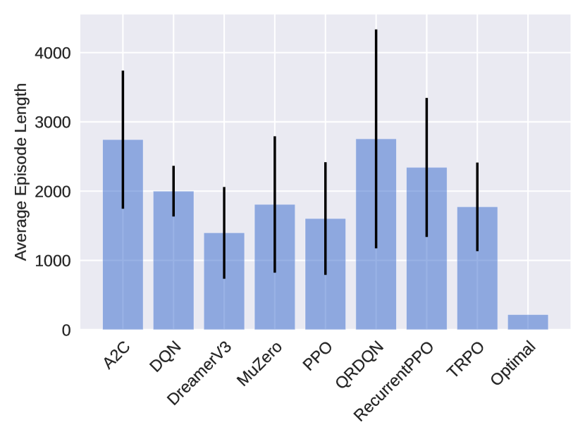</details> Figure 3: Average episode length of successful episodes for all evaluated algorithms on all puzzles in the easiest setting (lower is better). Some puzzles, namely Loopy, Pearl, Pegs, Solo, and Unruly, were intractable for all algorithms and were therefore excluded in this aggregation. The standard deviation is computed with respect to the performance over all evaluated instances for all trained seeds, aggregated for the total number of puzzles. Optimal refers the upper bound of the performance of an optimal policy, it therefore does not include a standard deviation. We see that DreamerV3 performs the best with an average episode length of 1334. However, this is still worse than the optimal upper bound at an average of 217 steps. To track an agent’s progress, we use episode lengths, i.e., how many actions an agent needs to solve a puzzle. A lower number of actions indicates a stronger policy that is closer to the optimal solution. To obtain the final evaluation, we run each policy on 1000 random episodes of the respective puzzle, again with a maximum step size of 10,000 steps. All experiments were conducted on NVIDIA 3090 GPUs. The training time for a single agent with 2 million PPO steps varied depending on the puzzle and ranged from approximately 1.75 to 3 hours. The training for DreamerV3 and MuZero was more demanding and training time ranged from approximately 10 to 20 hours. Figure 3 shows the average successful episode length for all algorithms. It can be seen that DreamerV3 performs best while PPO also achieves good performance, closely followed by TRPO and MuZero. This is especially interesting since PPO and TRPO follow much simpler training routines than DreamerV3 and MuZero. It seems that the implicit world models learned by DreamerV3 struggle to appropriately capture some puzzles. The high variance of MuZero may indicate some instability during training or the need for puzzle-specific hyperparamater tuning. Upon closer inspection of the detailed results, presented in Appendix Table 9 and 10, DreamerV3 manages to solve 62.7% of all puzzle instances. In 14 out of the 40 puzzles, it has found a policy that solves the puzzles within the Optimal upper bound. PPO and TRPO managed to solve an average of 61.6% and 70.8% of the puzzle instances, however only 8 and 11 of the puzzles have consistently solved within the Optimal upper bound. The algorithms A2C, RecurrentPPO, DQN and QRDQN perform worse than a pure random policy. Overall, it seems that some of the environments in PUZZLES are quite challenging and well suited to show the difference in performance between algorithms. It is also important to note that all the logic puzzles are designed so that they can be solved without requiring any guesswork. 3.2 Difficulty We further evaluate the performance of a subset of the puzzles on the easiest preset difficulty level for humans. We selected all puzzles where a random policy was able to solve them with a probability of at least 10%, which are Netslide, Same Game and Untangle. By using this selection, we estimate that the reward density should be relatively high, ideally allowing the agent to learn a good policy. Again, we train all algorithms listed in Table 8. We provide results for the two strongest algorithms, PPO and DreamerV3 in Table 1, with complete results available in Appendix Table 9. Note that as part of Section 3.4, we also perform ablations using DreamerV3 on more puzzles on the easiest preset difficulty level for humans. Table 1: Comparison of how many steps agents trained with PPO and DreamerV3 need on average to solve puzzles of two difficulty levels. In brackets, the percentage of successful episodes is reported. The difficulty levels correspond to the overall easiest and the easiest-for-humans settings. We also give the upper bound of optimal steps needed for each configuration. | Netslide | 2x3b1 | $35.3± 0.7$ (100.0%) | $12.0± 0.4$ (100.0%) | 48 | | --- | --- | --- | --- | --- | | 3x3b1 | $4742.1± 2960.1$ (9.2%) | $3586.5± 676.9$ (22.4%) | 90 | | | Same Game | 2x3c3s2 | $11.5± 0.1$ (100.0%) | $7.3± 0.2$ (100.0%) | 42 | | 5x5c3s2 | $1009.3± 1089.4$ (30.5%) | $527.0± 162.0$ (30.2%) | 300 | | | Untangle | 4 | $34.9± 10.8$ (100.0%) | $6.3± 0.4$ (100.0%) | 80 | | 6 | $2294.7± 2121.2$ (96.2%) | $1683.3± 73.7$ (82.0%) | 150 | | We can see that for both PPO and DreamerV3, the percentage of successful episodes decreases, with a large increase in steps required. DreamerV3 performs clearly stronger than PPO, requiring consistently fewer steps, but still more than the optimal policy. Our results indicate that puzzles with relatively high reward density at human difficulty levels remain challenging. We propose to use the easiest human difficulty level as a first measure to evaluate future algorithms. The details of the easiest human difficulty setting can be found in Appendix Table 7. If this level is achieved, difficulty can be further scaled up by increasing the size of the puzzles. Some puzzles also allow for an increase in difficulty with fixed size. 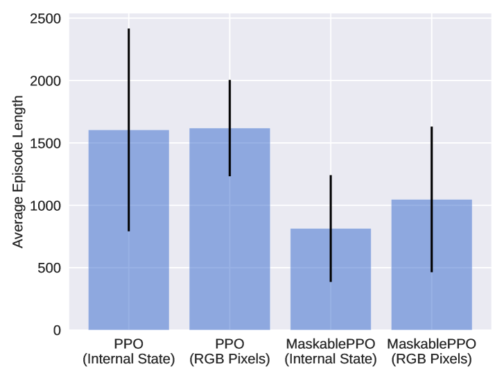3.3 Effect of Action Masking and Observation Representation We evaluate the effect of action masking, as well as observation type, on training performance. Firstly, we analyze whether action masking, as described in paragraph “Action Masking” in Section B.4, can positively affect training performance. Secondly, we want to see if agents are still capable of solving puzzles while relying on pixel observations. Pixel observations allow for the exact same input representation to be used for all puzzles, thus achieving a setting that is very similar to the Atari benchmark. We compare MaskablePPO to the default PPO without action masking on both types of observations. We summarize the results in Figure 4. Detailed results for masked RL agents on the pixel observations are provided in Appendix Table 11. <details> <summary>x3.png Details</summary>  ### Visual Description ## Bar Chart: Average Episode Length Comparison ### Overview The image is a bar chart comparing the average episode length of two reinforcement learning algorithms, PPO and MaskablePPO, under two different input conditions: "Internal State" and "RGB Pixels". The chart displays the average episode length as the height of the bars, with error bars indicating the variability or standard deviation. ### Components/Axes * **Y-axis:** "Average Episode Length", with a numerical scale from 0 to 2500 in increments of 500. * **X-axis:** Categorical axis representing the different algorithm and input combinations: * PPO (Internal State) * PPO (RGB Pixels) * MaskablePPO (Internal State) * MaskablePPO (RGB Pixels) * **Bars:** Light blue bars represent the average episode length for each category. * **Error Bars:** Black vertical lines extending above and below each bar, indicating the range of variability. ### Detailed Analysis The chart presents four distinct data points, each representing a different configuration of the reinforcement learning algorithm. * **PPO (Internal State):** The average episode length is approximately 1600. The error bar extends from approximately 700 to 2500. * **PPO (RGB Pixels):** The average episode length is approximately 1600. The error bar extends from approximately 1250 to 2000. * **MaskablePPO (Internal State):** The average episode length is approximately 800. The error bar extends from approximately 300 to 1250. * **MaskablePPO (RGB Pixels):** The average episode length is approximately 1050. The error bar extends from approximately 450 to 1650. ### Key Observations * PPO has a higher average episode length than MaskablePPO, regardless of the input type (Internal State or RGB Pixels). * The error bars for PPO (Internal State) and MaskablePPO (RGB Pixels) are larger, indicating greater variability in episode length. * The error bars for PPO (RGB Pixels) and MaskablePPO (Internal State) are smaller, indicating less variability in episode length. ### Interpretation The data suggests that the PPO algorithm generally results in longer episodes compared to MaskablePPO. This could indicate that PPO is more effective at exploring the environment or achieving a more stable policy. The use of "Internal State" versus "RGB Pixels" as input seems to have a less consistent impact, with the variability being more pronounced in some cases than others. The large error bars suggest that the performance of these algorithms can vary significantly from episode to episode, especially for PPO with internal state and MaskablePPO with RGB pixels. Further investigation would be needed to understand the factors contributing to this variability and to determine the statistical significance of the observed differences. </details> <details> <summary>x4.png Details</summary>  ### Visual Description ## Chart: Timesteps per Episode vs. Training Timesteps ### Overview The image is a line graph comparing the performance of different reinforcement learning algorithms (PPO and MaskablePPO) using different observation types (RGB Pixels and Internal State). The graph plots "Timesteps per Episode" on a logarithmic scale against "Training Timesteps" on a linear scale. ### Components/Axes * **Title:** None * **X-axis:** * Label: "Training Timesteps" * Scale: Linear, from 0.00 to 2.00, with increments of 0.25. Multiplied by 10^6. * Markers: 0.00, 0.25, 0.50, 0.75, 1.00, 1.25, 1.50, 1.75, 2.00 * **Y-axis:** * Label: "Timesteps per Episode" * Scale: Logarithmic (base 10), from 10^0 to 10^4 * Markers: 10^0, 10^1, 10^2, 10^3, 10^4 * **Legend:** Located at the bottom of the chart. * **Magenta:** PPO (RGB Pixels) * **Orange:** PPO (Internal State) * **Blue:** MaskablePPO (RGB Pixels) * **Green:** MaskablePPO (Internal State) ### Detailed Analysis * **Magenta Line: PPO (RGB Pixels)** * Trend: Initially increases rapidly, reaching approximately 10^3 timesteps per episode around 0.5 x 10^6 training timesteps. It then fluctuates significantly, with some drops and rises, before stabilizing around 10^2 timesteps per episode after 1.5 x 10^6 training timesteps. * Data Points: Starts around 10^1, peaks around 10^3, stabilizes around 10^2. * **Orange Line: PPO (Internal State)** * Trend: Starts high, around 10^2 timesteps per episode, and decreases slightly before fluctuating around 10^1 to 10^2 timesteps per episode throughout the training process. * Data Points: Starts around 10^2, fluctuates between 10^1 and 10^2. * **Blue Line: MaskablePPO (RGB Pixels)** * Trend: Starts around 10^2 timesteps per episode, decreases slightly, and then fluctuates around 10^1 timesteps per episode throughout the training process. There are some spikes to higher values. * Data Points: Starts around 10^2, fluctuates around 10^1. * **Green Line: MaskablePPO (Internal State)** * Trend: Starts around 10^2 timesteps per episode, decreases rapidly to around 10^1 timesteps per episode, and remains relatively stable at that level throughout the training process. * Data Points: Starts around 10^2, stabilizes around 10^1. ### Key Observations * PPO (RGB Pixels) shows the most significant initial improvement but also the most instability. * MaskablePPO (Internal State) converges quickly to a stable, low number of timesteps per episode. * Using Internal State generally results in lower timesteps per episode compared to using RGB Pixels. * MaskablePPO algorithms appear more stable than PPO algorithms. ### Interpretation The graph illustrates the learning curves of different reinforcement learning algorithms under different observation conditions. The PPO algorithm, when using RGB pixels as input, initially learns faster but exhibits more instability during training. The MaskablePPO algorithm, especially when using the internal state, demonstrates more stable learning and converges to a lower number of timesteps per episode, suggesting more efficient learning. The choice of observation type (RGB Pixels vs. Internal State) significantly impacts the performance and stability of the algorithms. Using the internal state generally leads to more stable and efficient learning, likely because it provides a more direct and less noisy representation of the environment's state. 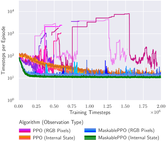</details> Figure 4: (left) We demonstrate the effect of action masking in both RGB observation and internal game state. By masking moves that do not change the current state, the agent requires fewer actions to explore, and therefore, on average solves a puzzle using fewer steps. (right) Moving average episode length during training for the Flood puzzle. Lower episode length is better, as the episode gets terminated as soon as the agent has solved a puzzle. Different colors describe different algorithms, where different shades of a color indicate different random seeds. Sparse dots indicate that an agent only occasionally managed to find a policy that solves a puzzle. It can be seen that both the use of discrete internal state observations and action masking have a positive effect on the training, leading to faster convergence and a stronger overall performance. As we can observe in Figure 4, action masking has a strongly positive effect on training performance. This benefit is observed both in the discrete internal game state observations and on the pixel observations. We hypothesize that this is due to the more efficient exploration, as actions without effect are not allowed. As a result, the reward density during training is increased, and agents are able to learn a better policy. Particularly noteworthy are the outcomes related to Pegs. They show that an agent with action masking can effectively learn a successful policy, while a random policy without action masking consistently fails to solve any instance. As expected, training RL agents on pixel observations increases the difficulty of the task at hand. The agent must first understand how the pixel observation relates to the internal state of the game before it is able to solve the puzzle. Nevertheless, in combination with action masking, the agents manage to solve a large percentage of all puzzle instances, with 10 of the puzzles consistently solved within the optimal upper bound. Furthermore, Figure 4 shows the individual training performance on the puzzle Flood. It can be seen that RL agents using action masking and the discrete internal game state observation converge significantly faster and to better policies compared to the baselines. The agents using pixel observations and no action masking struggle to converge to any reasonable policy. 3.4 Effect of Episode Length and Early Termination We evaluate whether the cutoff episode length or early termination have an effect on training performance of the agents. For computational reasons, we perform these experiments on a selected subset of the puzzles on human level difficulty and only for DreamerV3 (see Section E.5 for details). As we can see in Table 2, increasing the maximum episode length during training from 10,000 to 100,000 does not improve performance. Only when episodes get terminated after visiting the exact same state more than 10 times, the agent is able to solve more puzzle instances on average (31.5% vs. 25.2%). Given the sparse reward structure, terminating episodes early seems to provide a better trade-off between allowing long trajectories to successfully complete and avoiding wasting resources on unsuccessful trajectories. Table 2: Comparison of the effect of the maximum episode length (# Steps) and early termination (ET) on final performance. For each setting, we report average success episode length with standard deviation with respect to the random seed, all averaged over all selected puzzles. In brackets, the percentage of successful episodes is reported. | $1e5$ | 10 | $2950.9± 1260.2$ (31.6%) | | --- | --- | --- | | - | $2975.4± 1503.5$ (25.2%) | | | $1e4$ | 10 | $3193.9± 1044.2$ (26.1%) | | - | $2892.4± 908.3$ (26.8%) | | 3.5 Generalization PUZZLES is explicitly designed to facilitate the testing of generalization capabilities of agents with respect to different puzzle sizes or puzzle difficulties. For our experiments, we select puzzles with the highest reward density. We utilize a a custom observation wrapper and transformer-based encoder in order for the agent to be able to work with different input sizes, see Sections A.3 and A.4 for details. We call this approach PPO (Transformer) Table 3: We test generalization capabilities of agents by evaluating them on puzzle sizes larger than their training environment. We report the average number of steps an agent needs to solve a puzzle, and the percentage of successful episodes in brackets. The difficulty levels correspond to the overall easiest and the easiest-for-humans settings. For PPO (Transformer), we selected the best checkpoint during training according to the performance in the training environment. For PPO (Transformer) †, we selected the best checkpoint during training according to the performance in the generalization environment. | Netslide | 2x3b1 | ✓ | $244.1± 313.7$ (100.0%) | $242.0± 379.3$ (100.0%) | | --- | --- | --- | --- | --- | | 3x3b1 | ✗ | $9014.6± 2410.6$ (18.6%) | $9002.8± 2454.9$ (18.0%) | | | Same Game | 2x3c3s2 | ✓ | $9.3± 10.9$ (99.8%) | $26.2± 52.9$ (99.7%) | | 5x5c3s2 | ✗ | $379.0± 261.6$ (9.4%) | $880.1± 675.4$ (18.1%) | | | Untangle | 4 | ✓ | $38.6± 58.2$ (99.8%) | $69.8± 66.4$ (100.0%) | | 6 | ✗ | $3340.0± 3101.2$ (87.3%) | $2985.8± 2774.7$ (93.7%) | | The results presented in Table 3 indicate that while it is possible to learn a policy that generalizes it remains a challenging problem. Furthermore, it can be observed that selecting the best model during training according to the performance on the generalization environment yields a performance benefit in that setting. This suggests that agents may learn a policy that generalizes better during the training process, but then overfit on the environment they are training on. It is also evident that generalization performance varies substantially across different random seeds. For Netslide, the best agent is capable of solving 23.3% of the puzzles in the generalization environment whereas the worst agent is only able to solve 11.2% of the puzzles, similar to a random policy. Our findings suggest that agents are generally capable of generalizing to more complex puzzles. However, further research is necessary to identify the appropriate inductive biases that allow for consistent generalization without a significant decline in performance. 4 Discussion The experimental evaluation demonstrates varying degrees of success among different algorithms. For instance, puzzles such as Tracks, Map or Flip were not solvable by any of the evaluated RL agents, or only with performance similar to a random policy. This points towards the potential of intermediate rewards, better game rule-specific action masking, or model-based approaches. To encourage exploration in the state space, a mechanism that explicitly promotes it may be beneficial. On the other hand, the fact that some algorithms managed to solve a substantial amount of puzzles with presumably optimal performance demonstrates the advances in the field of RL. In light of the promising results of DreamerV3, the improvement of agents that have certain reasoning capabilities and an implicit world model by design stay an important direction for future research. Experimental Results. The experimental results presented in Section 3.1 and Section 3.3 underscore the positive impact of action masking and the correct observation type on performance. While a pixel representation would lead to a uniform observation for all puzzles, it currently increases complexity too much compared the discrete internal game state. Our findings indicate that incorporating action masking significantly improves the training efficiency of reinforcement learning algorithms. This enhancement was observed in both discrete internal game state observations and pixel observations. The mechanism for this improvement can be attributed to enhanced exploration, resulting in agents being able to learn more robust and effective policies. This was especially evident in puzzles where unmasked agents had considerable difficulty, thus showcasing the tangible advantages of implementing action masking for these puzzles. Limitations. While the PUZZLES framework provides the ability to gain comprehensive insights into the performance of various RL algorithms on logic puzzles, it is crucial to recognize certain limitations when interpreting results. The sparse rewards used in this baseline evaluation add to the complexity of the task. Moreover, all algorithms were evaluated with their default hyper-parameters. Additionally, the constraint of discrete action spaces excludes the application of certain RL algorithms. In summary, the different challenges posed by the logic-requiring nature of these puzzles necessitates a good reward system, strong guidance of agents, and an agent design more focused on logical reasoning capabilities. It will be interesting to see how alternative architectures such as graph neural networks (GNNs) perform. GNNs are designed to align more closely with the algorithmic solution of many puzzles. While the notion that “reward is enough” [57, 58] might hold true, our results indicate that not just any form of correct reward will suffice, and that advanced architectures might be necessary to learn an optimal solution. 5 Conclusion In this work, we have proposed PUZZLES, a benchmark that bridges the gap between algorithmic reasoning and RL. In addition to containing a rich diversity of logic puzzles, PUZZLES also offers an adjustable difficulty progression for each puzzle, making it a useful tool for benchmarking, evaluating and improving RL algorithms. Our empirical evaluation shows that while RL algorithms exhibit varying degrees of success, challenges persist, particularly in puzzles with higher complexity or those requiring nuanced logical reasoning. We are excited to share PUZZLES with the broader research community and hope that PUZZLES will foster further research for improving the algorithmic reasoning abilities of RL algorithms. Broader Impact This paper aims to contribute to the advancement of the field of Machine Learning (ML). Given the current challenges in ML related to algorithmic reasoning, we believe that our newly proposed benchmark will facilitate significant progress in this area, potentially elevating the capabilities of ML systems. Progress in algorithmic reasoning can contribute to the development of more transparent, explainable, and fair ML systems. This can further help address issues related to bias and discrimination in automated decision-making processes, promoting fairness and accountability. References - Serafini and Garcez [2016] Luciano Serafini and Artur d’Avila Garcez. Logic tensor networks: Deep learning and logical reasoning from data and knowledge. arXiv preprint arXiv:1606.04422, 2016. - Dai et al. [2019] Wang-Zhou Dai, Qiuling Xu, Yang Yu, and Zhi-Hua Zhou. Bridging machine learning and logical reasoning by abductive learning. Advances in Neural Information Processing Systems, 32, 2019. - Li et al. [2020] Yujia Li, Felix Gimeno, Pushmeet Kohli, and Oriol Vinyals. Strong generalization and efficiency in neural programs. arXiv preprint arXiv:2007.03629, 2020. - Veličković and Blundell [2021] Petar Veličković and Charles Blundell. Neural algorithmic reasoning. Patterns, 2(7), 2021. - Masry et al. [2022] Ahmed Masry, Do Long, Jia Qing Tan, Shafiq Joty, and Enamul Hoque. Chartqa: A benchmark for question answering about charts with visual and logical reasoning. In Findings of the Association for Computational Linguistics: ACL 2022, pages 2263–2279, 2022. - Jiao et al. [2022] Fangkai Jiao, Yangyang Guo, Xuemeng Song, and Liqiang Nie. Merit: Meta-path guided contrastive learning for logical reasoning. In Findings of the Association for Computational Linguistics: ACL 2022, pages 3496–3509, 2022. - Bardin et al. [2023] Sébastien Bardin, Somesh Jha, and Vijay Ganesh. Machine learning and logical reasoning: The new frontier (dagstuhl seminar 22291). In Dagstuhl Reports, volume 12. Schloss Dagstuhl-Leibniz-Zentrum für Informatik, 2023. - Li et al. [2021] Wenda Li, Lei Yu, Yuhuai Wu, and Lawrence C Paulson. Isarstep: a benchmark for high-level mathematical reasoning. In International Conference on Learning Representations, 2021. - Veličković et al. [2022] Petar Veličković, Adrià Puigdomènech Badia, David Budden, Razvan Pascanu, Andrea Banino, Misha Dashevskiy, Raia Hadsell, and Charles Blundell. The CLRS algorithmic reasoning benchmark. In Kamalika Chaudhuri, Stefanie Jegelka, Le Song, Csaba Szepesvari, Gang Niu, and Sivan Sabato, editors, Proceedings of the 39th International Conference on Machine Learning, volume 162 of Proceedings of Machine Learning Research, pages 22084–22102. PMLR, 17–23 Jul 2022. URL https://proceedings.mlr.press/v162/velickovic22a.html. - Srivastava et al. [2022] Aarohi Srivastava, Abhinav Rastogi, Abhishek Rao, Abu Awal Md Shoeb, Abubakar Abid, Adam Fisch, Adam R Brown, Adam Santoro, Aditya Gupta, Adrià Garriga-Alonso, et al. Beyond the imitation game: Quantifying and extrapolating the capabilities of language models. arXiv preprint arXiv:2206.04615, 2022. - Mnih et al. [2013] Volodymyr Mnih, Koray Kavukcuoglu, David Silver, Alex Graves, Ioannis Antonoglou, Daan Wierstra, and Martin A. Riedmiller. Playing Atari with Deep Reinforcement Learning. CoRR, abs/1312.5602, 2013. URL http://arxiv.org/abs/1312.5602. - Tang et al. [2017] Haoran Tang, Rein Houthooft, Davis Foote, Adam Stooke, OpenAI Xi Chen, Yan Duan, John Schulman, Filip DeTurck, and Pieter Abbeel. # exploration: A study of count-based exploration for deep reinforcement learning. Advances in neural information processing systems, 30, 2017. - Silver et al. [2018] David Silver, Thomas Hubert, Julian Schrittwieser, Ioannis Antonoglou, Matthew Lai, Arthur Guez, Marc Lanctot, Laurent Sifre, Dharshan Kumaran, Thore Graepel, et al. A general reinforcement learning algorithm that masters chess, shogi, and go through self-play. Science, 362(6419):1140–1144, 2018. - Badia et al. [2020] Adrià Puigdomènech Badia, Bilal Piot, Steven Kapturowski, Pablo Sprechmann, Alex Vitvitskyi, Zhaohan Daniel Guo, and Charles Blundell. Agent57: Outperforming the atari human benchmark. In International conference on machine learning, pages 507–517. PMLR, 2020. - Wurman et al. [2022] Peter R Wurman, Samuel Barrett, Kenta Kawamoto, James MacGlashan, Kaushik Subramanian, Thomas J Walsh, Roberto Capobianco, Alisa Devlic, Franziska Eckert, Florian Fuchs, et al. Outracing champion gran turismo drivers with deep reinforcement learning. Nature, 602(7896):223–228, 2022. - Kalashnikov et al. [2018] Dmitry Kalashnikov, Alex Irpan, Peter Pastor, Julian Ibarz, Alexander Herzog, Eric Jang, Deirdre Quillen, Ethan Holly, Mrinal Kalakrishnan, Vincent Vanhoucke, et al. Scalable deep reinforcement learning for vision-based robotic manipulation. In Conference on Robot Learning, pages 651–673. PMLR, 2018. - Kiran et al. [2021] B Ravi Kiran, Ibrahim Sobh, Victor Talpaert, Patrick Mannion, Ahmad A Al Sallab, Senthil Yogamani, and Patrick Pérez. Deep reinforcement learning for autonomous driving: A survey. IEEE Transactions on Intelligent Transportation Systems, 23(6):4909–4926, 2021. - Rudin et al. [2022] Nikita Rudin, David Hoeller, Philipp Reist, and Marco Hutter. Learning to walk in minutes using massively parallel deep reinforcement learning. In Conference on Robot Learning, pages 91–100. PMLR, 2022. - Rana et al. [2023] Krishan Rana, Ming Xu, Brendan Tidd, Michael Milford, and Niko Sünderhauf. Residual skill policies: Learning an adaptable skill-based action space for reinforcement learning for robotics. In Conference on Robot Learning, pages 2095–2104. PMLR, 2023. - Wang and Hong [2020] Zhe Wang and Tianzhen Hong. Reinforcement learning for building controls: The opportunities and challenges. Applied Energy, 269:115036, 2020. - Wu et al. [2022] Di Wu, Yin Lei, Maoen He, Chunjiong Zhang, and Li Ji. Deep reinforcement learning-based path control and optimization for unmanned ships. Wireless Communications and Mobile Computing, 2022:1–8, 2022. - Brunke et al. [2022] Lukas Brunke, Melissa Greeff, Adam W Hall, Zhaocong Yuan, Siqi Zhou, Jacopo Panerati, and Angela P Schoellig. Safe learning in robotics: From learning-based control to safe reinforcement learning. Annual Review of Control, Robotics, and Autonomous Systems, 5:411–444, 2022. - Todorov et al. [2012] Emanuel Todorov, Tom Erez, and Yuval Tassa. Mujoco: A physics engine for model-based control. In 2012 IEEE/RSJ international conference on intelligent robots and systems, pages 5026–5033. IEEE, 2012. - Bellemare et al. [2013] Marc G Bellemare, Yavar Naddaf, Joel Veness, and Michael Bowling. The arcade learning environment: An evaluation platform for general agents. Journal of Artificial Intelligence Research, 47:253–279, 2013. - Brockman et al. [2016] Greg Brockman, Vicki Cheung, Ludwig Pettersson, Jonas Schneider, John Schulman, Jie Tang, and Wojciech Zaremba. Openai gym. arXiv preprint arXiv:1606.01540, 2016. - Duan et al. [2016] Yan Duan, Xi Chen, Rein Houthooft, John Schulman, and Pieter Abbeel. Benchmarking deep reinforcement learning for continuous control. In International conference on machine learning, pages 1329–1338. PMLR, 2016. - Tassa et al. [2018] Yuval Tassa, Yotam Doron, Alistair Muldal, Tom Erez, Yazhe Li, Diego de Las Casas, David Budden, Abbas Abdolmaleki, Josh Merel, Andrew Lefrancq, et al. Deepmind control suite. arXiv preprint arXiv:1801.00690, 2018. - Côté et al. [2018] Marc-Alexandre Côté, Ákos Kádár, Xingdi Yuan, Ben Kybartas, Tavian Barnes, Emery Fine, James Moore, Ruo Yu Tao, Matthew Hausknecht, Layla El Asri, Mahmoud Adada, Wendy Tay, and Adam Trischler. Textworld: A learning environment for text-based games. CoRR, abs/1806.11532, 2018. - Lanctot et al. [2019] Marc Lanctot, Edward Lockhart, Jean-Baptiste Lespiau, Vinicius Zambaldi, Satyaki Upadhyay, Julien Pérolat, Sriram Srinivasan, Finbarr Timbers, Karl Tuyls, Shayegan Omidshafiei, Daniel Hennes, Dustin Morrill, Paul Muller, Timo Ewalds, Ryan Faulkner, János Kramár, Bart De Vylder, Brennan Saeta, James Bradbury, David Ding, Sebastian Borgeaud, Matthew Lai, Julian Schrittwieser, Thomas Anthony, Edward Hughes, Ivo Danihelka, and Jonah Ryan-Davis. OpenSpiel: A framework for reinforcement learning in games. CoRR, abs/1908.09453, 2019. URL http://arxiv.org/abs/1908.09453. - Jiang and Luo [2019] Zhengyao Jiang and Shan Luo. Neural logic reinforcement learning. In International conference on machine learning, pages 3110–3119. PMLR, 2019. - Fawzi et al. [2022] Alhussein Fawzi, Matej Balog, Aja Huang, Thomas Hubert, Bernardino Romera-Paredes, Mohammadamin Barekatain, Alexander Novikov, Francisco J R Ruiz, Julian Schrittwieser, Grzegorz Swirszcz, et al. Discovering faster matrix multiplication algorithms with reinforcement learning. Nature, 610(7930):47–53, 2022. - Mankowitz et al. [2023] Daniel J Mankowitz, Andrea Michi, Anton Zhernov, Marco Gelmi, Marco Selvi, Cosmin Paduraru, Edouard Leurent, Shariq Iqbal, Jean-Baptiste Lespiau, Alex Ahern, et al. Faster sorting algorithms discovered using deep reinforcement learning. Nature, 618(7964):257–263, 2023. - Lai [2015] Matthew Lai. Giraffe: Using deep reinforcement learning to play chess. arXiv preprint arXiv:1509.01549, 2015. - Silver et al. [2016] David Silver, Aja Huang, Chris J. Maddison, Arthur Guez, Laurent Sifre, George van den Driessche, Julian Schrittwieser, Ioannis Antonoglou, Veda Panneershelvam, Marc Lanctot, Sander Dieleman, Dominik Grewe, John Nham, Nal Kalchbrenner, Ilya Sutskever, Timothy Lillicrap, Madeleine Leach, Koray Kavukcuoglu, Thore Graepel, and Demis Hassabis. Mastering the game of go with deep neural networks and tree search. Nature, 529:484–489, 2016. URL https://doi.org/10.1038/nature16961. - Tatham [2004a] Simon Tatham. Simon tatham’s portable puzzle collection, 2004a. URL https://www.chiark.greenend.org.uk/~sgtatham/puzzles/. Accessed: 2023-05-16. - Foundation [2022] Farama Foundation. Gymnasium website, 2022. URL https://gymnasium.farama.org/. Accessed: 2023-05-12. - Wang et al. [2022] Chao Wang, Chen Chen, Dong Li, and Bin Wang. Rethinking reinforcement learning based logic synthesis. arXiv preprint arXiv:2205.07614, 2022. - Dasgupta et al. [2019] Ishita Dasgupta, Jane Wang, Silvia Chiappa, Jovana Mitrovic, Pedro Ortega, David Raposo, Edward Hughes, Peter Battaglia, Matthew Botvinick, and Zeb Kurth-Nelson. Causal reasoning from meta-reinforcement learning. arXiv preprint arXiv:1901.08162, 2019. - Eppe et al. [2022] Manfred Eppe, Christian Gumbsch, Matthias Kerzel, Phuong DH Nguyen, Martin V Butz, and Stefan Wermter. Intelligent problem-solving as integrated hierarchical reinforcement learning. Nature Machine Intelligence, 4(1):11–20, 2022. - Deac et al. [2021] Andreea-Ioana Deac, Petar Veličković, Ognjen Milinkovic, Pierre-Luc Bacon, Jian Tang, and Mladen Nikolic. Neural algorithmic reasoners are implicit planners. Advances in Neural Information Processing Systems, 34:15529–15542, 2021. - He et al. [2022] Yu He, Petar Veličković, Pietro Liò, and Andreea Deac. Continuous neural algorithmic planners. In Learning on Graphs Conference, pages 54–1. PMLR, 2022. - Silver et al. [2017] David Silver, Thomas Hubert, Julian Schrittwieser, Ioannis Antonoglou, Matthew Lai, Arthur Guez, Marc Lanctot, Laurent Sifre, Dharshan Kumaran, Thore Graepel, et al. Mastering chess and shogi by self-play with a general reinforcement learning algorithm. arXiv preprint arXiv:1712.01815, 2017. - Dahl [2001] Fredrik A Dahl. A reinforcement learning algorithm applied to simplified two-player texas hold’em poker. In European Conference on Machine Learning, pages 85–96. Springer, 2001. - Heinrich and Silver [2016] Johannes Heinrich and David Silver. Deep reinforcement learning from self-play in imperfect-information games. arXiv preprint arXiv:1603.01121, 2016. - Steinberger [2019] Eric Steinberger. Pokerrl. https://github.com/TinkeringCode/PokerRL, 2019. - Zhao et al. [2022] Enmin Zhao, Renye Yan, Jinqiu Li, Kai Li, and Junliang Xing. Alphaholdem: High-performance artificial intelligence for heads-up no-limit poker via end-to-end reinforcement learning. In Proceedings of the AAAI Conference on Artificial Intelligence, volume 36, pages 4689–4697, 2022. - Ghory [2004] Imran Ghory. Reinforcement learning in board games. 2004. - Szita [2012] István Szita. Reinforcement learning in games. In Reinforcement Learning: State-of-the-art, pages 539–577. Springer, 2012. - Xenou et al. [2019] Konstantia Xenou, Georgios Chalkiadakis, and Stergos Afantenos. Deep reinforcement learning in strategic board game environments. In Multi-Agent Systems: 16th European Conference, EUMAS 2018, Bergen, Norway, December 6–7, 2018, Revised Selected Papers 16, pages 233–248. Springer, 2019. - Perolat et al. [2022] Julien Perolat, Bart De Vylder, Daniel Hennes, Eugene Tarassov, Florian Strub, Vincent de Boer, Paul Muller, Jerome T Connor, Neil Burch, Thomas Anthony, et al. Mastering the game of stratego with model-free multiagent reinforcement learning. Science, 378(6623):990–996, 2022. - Cormen et al. [2022] Thomas H. Cormen, Charles Eric Leiserson, Ronald L. Rivest, and Clifford Stein. Introduction to Algorithms. The MIT Press, 4th edition, 2022. - Raffin et al. [2021] Antonin Raffin, Ashley Hill, Adam Gleave, Anssi Kanervisto, Maximilian Ernestus, and Noah Dormann. Stable-baselines3: Reliable reinforcement learning implementations. Journal of Machine Learning Research, 22(268):1–8, 2021. URL http://jmlr.org/papers/v22/20-1364.html. - Werner Duvaud [2019] Aurèle Hainaut Werner Duvaud. Muzero general: Open reimplementation of muzero. https://github.com/werner-duvaud/muzero-general, 2019. - Hafner et al. [2023a] Danijar Hafner, Jurgis Pasukonis, Jimmy Ba, and Timothy Lillicrap. Mastering diverse domains through world models. https://github.com/danijar/dreamerv3, 2023a. - Haarnoja et al. [2018] Tuomas Haarnoja, Aurick Zhou, Pieter Abbeel, and Sergey Levine. Soft actor-critic: Off-policy maximum entropy deep reinforcement learning with a stochastic actor. In International conference on machine learning, pages 1861–1870. PMLR, 2018. - Fujimoto et al. [2018] Scott Fujimoto, Herke Hoof, and David Meger. Addressing function approximation error in actor-critic methods. In International conference on machine learning, pages 1587–1596. PMLR, 2018. - Silver et al. [2021] David Silver, Satinder Singh, Doina Precup, and Richard S Sutton. Reward is enough. Artificial Intelligence, 299:103535, 2021. - Vamplew et al. [2022] Peter Vamplew, Benjamin J Smith, Johan Källström, Gabriel Ramos, Roxana Rădulescu, Diederik M Roijers, Conor F Hayes, Fredrik Heintz, Patrick Mannion, Pieter JK Libin, et al. Scalar reward is not enough: A response to silver, singh, precup and sutton (2021). Autonomous Agents and Multi-Agent Systems, 36(2):41, 2022. - Community [2000] Pygame Community. Pygame github repository, 2000. URL https://github.com/pygame/pygame/. Accessed: 2023-05-12. - Tatham [2004b] Simon Tatham. Developer documentation for simon tatham’s puzzle collection, 2004b. URL https://www.chiark.greenend.org.uk/~sgtatham/puzzles/devel/. Accessed: 2023-05-23. - Schulman et al. [2017] John Schulman, Filip Wolski, Prafulla Dhariwal, Alec Radford, and Oleg Klimov. Proximal policy optimization algorithms, 2017. URL http://arxiv.org/abs/1707.06347. - Huang et al. [2022] Shengyi Huang, Rousslan Fernand Julien Dossa, Antonin Raffin, Anssi Kanervisto, and Weixun Wang. The 37 implementation details of proximal policy optimization. In ICLR Blog Track, 2022. URL https://iclr-blog-track.github.io/2022/03/25/ppo-implementation-details/. https://iclr-blog-track.github.io/2022/03/25/ppo-implementation-details/. - Mnih et al. [2016] Volodymyr Mnih, Adrià Puigdomènech Badia, Mehdi Mirza, Alex Graves, Timothy P. Lillicrap, Tim Harley, David Silver, and Koray Kavukcuoglu. Asynchronous methods for deep reinforcement learning. CoRR, abs/1602.01783, 2016. URL http://arxiv.org/abs/1602.01783. - Schulman et al. [2015] John Schulman, Sergey Levine, Pieter Abbeel, Michael Jordan, and Philipp Moritz. Trust region policy optimization. In Francis Bach and David Blei, editors, Proceedings of the 32nd International Conference on Machine Learning, volume 37 of Proceedings of Machine Learning Research, pages 1889–1897, Lille, France, 07–09 Jul 2015. PMLR. URL https://proceedings.mlr.press/v37/schulman15.html. - Dabney et al. [2017] Will Dabney, Mark Rowland, Marc G. Bellemare, and Rémi Munos. Distributional reinforcement learning with quantile regression. CoRR, abs/1710.10044, 2017. URL http://arxiv.org/abs/1710.10044. - Schrittwieser et al. [2020] Julian Schrittwieser, Ioannis Antonoglou, Thomas Hubert, Karen Simonyan, Laurent Sifre, Simon Schmitt, Arthur Guez, Edward Lockhart, Demis Hassabis, Thore Graepel, et al. Mastering atari, go, chess and shogi by planning with a learned model. Nature, 588(7839):604–609, 2020. - Hafner et al. [2023b] Danijar Hafner, Jurgis Pasukonis, Jimmy Ba, and Timothy Lillicrap. Mastering diverse domains through world models. arXiv preprint arXiv:2301.04104, 2023b. Appendix A PUZZLES Environment Usage Guide A.1 General Usage A Python code example for using the PUZZLES environment is provided in LABEL:code:init-and-play-episode. All puzzles support seeding the initialization, by adding #{seed} after the parameters, where {seed} is an int. The allowed parameters are displayed in LABEL:tab:parameters. A full custom initialization argument would be as follows: {parameters}#{seed}. ⬇ 1 import gymnasium as gym 2 import rlp 3 4 # init an agent suitable for Gymnasium environments 5 agent = Agent. create () 6 7 # init the environment 8 env = gym. make (’rlp/Puzzle-v0’, puzzle = "bridges", 9 render_mode = "rgb_array", params = "4x4#42") 10 observation, info = env. reset () 11 12 # complete an episode 13 terminated = False 14 while not terminated: 15 action = agent. choose (env) # the agent chooses the next action 16 observation, reward, terminated, truncated, info = env. step (action) 17 env. close () Listing 1: Code example of how to initialize an environment and have an agent complete one episode. The PUZZLES environment is designed to be compatible with the Gymnasium API. The choice of Agent is up to the user, it can be a trained agent or random policy. A.2 Custom Reward A Python code example for implementing a custom reward system is provided in LABEL:code:custom-reward-wrapper. To this end, the environment’s step() function provides the puzzle’s internal state inside the info Python dict. ⬇ 1 import gymnasium as gym 2 class PuzzleRewardWrapper (gym. Wrapper): 3 def step (self, action): 4 obs, reward, terminated, truncated, info = self. env. step (action) 5 # Modify the reward by using members of info["puzzle_state"] 6 return obs, reward, terminated, truncated, info Listing 2: Code example of a custom reward implementation using Gymnasium’s Wrapper class. A user can use the game state information provided in info["puzzle_state"] to modify the rewards received by the agent after performing an action. A.3 Custom Observation A Python code example for implementing a custom observation structure that is compatible with an agent using a transformer encoder. Here, we provide the example for Netslide, please refer to our GitHub for more examples. ⬇ 1 import gymnasium as gym 2 import numpy as np 3 class NetslideTransformerWrapper (gym. ObservationWrapper): 4 def __init__ (self, env): 5 super (NetslideTransformerWrapper, self). __init__ (env) 6 self. original_space = env. observation_space 7 8 self. max_length = 512 9 self. embedding_dim = 16 + 4 10 self. observation_space = gym. spaces. Box ( 11 low =-1, high =1, shape =(self. max_length, self. embedding_dim,), dtype = np. float32 12 ) 13 14 self. observation_space = gym. spaces. Dict ( 15 {’obs’: self. observation_space, 16 ’len’: gym. spaces. Box (low =0, high = self. max_length, shape =(1,), 17 dtype = np. int32)} 18 ) 19 20 def observation (self, obs): 21 # The original observation is an ordereddict with the keys [’barriers’, ’cursor_pos’, ’height’, 22 # ’last_move_col’, ’last_move_dir’, ’last_move_row’, ’move_count’, ’movetarget’, ’tiles’, ’width’, ’wrapping’] 23 # We are only interested in ’barriers’, ’tiles’, ’cursor_pos’, ’height’ and ’width’ 24 barriers = obs [’barriers’] 25 # each element of barriers is an uint16, signifying different elements 26 barriers = np. unpackbits (barriers. view (np. uint8)). reshape (-1, 16) 27 # add some positional embedding to the barriers 28 embedded_barriers = np. concatenate ( 29 [barriers, self. pos_embedding (np. arange (barriers. shape [0]), obs [’width’], obs [’height’])], axis =1) 30 31 tiles = obs [’tiles’] 32 # each element of tiles is an uint16, signifying different elements 33 tiles = np. unpackbits (tiles. view (np. uint8)). reshape (-1, 16) 34 # add some positional embedding to the tiles 35 embedded_tiles = np. concatenate ( 36 [tiles, self. pos_embedding (np. arange (tiles. shape [0]), obs [’width’], obs [’height’])], axis =1) 37 cursor_pos = obs [’cursor_pos’] 38 39 embedded_cursor_pos = np. concatenate ( 40 [np. ones ((1, 16)), self. pos_embedding_cursor (cursor_pos, obs [’width’], obs [’height’])], axis =1) 41 42 embedded_obs = np. concatenate ([embedded_barriers, embedded_tiles, embedded_cursor_pos], axis =0) 43 44 current_length = embedded_obs. shape [0] 45 # pad with zeros to accomodate different sizes 46 if current_length < self. max_length: 47 embedded_obs = np. concatenate ( 48 [embedded_obs, np. zeros ((self. max_length - current_length, self. embedding_dim))], axis =0) 49 return {’obs’: embedded_obs, ’len’: np. array ([current_length])} 50 51 @staticmethod 52 def pos_embedding (pos, width, height): 53 # pos is an array of integers from 0 to width*height 54 # width and height are integers 55 # return a 2D array with the positional embedding, using sin and cos 56 x, y = pos % width, pos // width 57 # x and y are integers from 0 to width-1 and height-1 58 pos_embed = np. zeros ((len (pos), 4)) 59 pos_embed [:, 0] = np. sin (2 * np. pi * x / width) 60 pos_embed [:, 1] = np. cos (2 * np. pi * x / width) 61 pos_embed [:, 2] = np. sin (2 * np. pi * y / height) 62 pos_embed [:, 3] = np. cos (2 * np. pi * y / height) 63 return pos_embed 64 65 @staticmethod 66 def pos_embedding_cursor (pos, width, height): 67 # cursor pos goes from -1 to width or height 68 x, y = pos 69 x += 1 70 y += 1 71 width += 1 72 height += 1 73 pos_embed = np. zeros ((1, 4)) 74 pos_embed [0, 0] = np. sin (2 * np. pi * x / width) 75 pos_embed [0, 1] = np. cos (2 * np. pi * x / width) 76 pos_embed [0, 2] = np. sin (2 * np. pi * y / height) 77 pos_embed [0, 3] = np. cos (2 * np. pi * y / height) 78 return pos_embed Listing 3: Code example of a custom observation implementation using Gymnasium’s Wrapper class. A user can use the all elements of rpovided in the obs dict to create a custom observation. In this code example, the resulting observation is suitable for a transformer-based encoder. A.4 Generalization Example In LABEL:code:transformer-encoder, we show how a transformer-based features extractor can be built for Stable Baseline 3’s PPO MultiInputPolicy. Together with the observations from LABEL:code:custom-observation-wrapper, this feature extractor can work with variable-length inputs. This allows for easy evaluation in environments of different sizes than the environment the agent was originally trained in. ⬇ 1 import gymnasium as gym 2 import numpy as np 3 from stable_baselines3. common. torch_layers import BaseFeaturesExtractor 4 from stable_baselines3 import PPO 5 import torch 6 import torch. nn as nn 7 from torch. nn import TransformerEncoder, TransformerEncoderLayer 8 9 class TransformerFeaturesExtractor (BaseFeaturesExtractor): 10 def __init__ (self, observation_space, data_dim, embedding_dim, nhead, num_layers, dim_feedforward, dropout =0.1): 11 super (TransformerFeaturesExtractor, self). __init__ (observation_space, embedding_dim) 12 self. transformer = Transformer (embedding_dim = embedding_dim, 13 data_dim = data_dim, 14 nhead = nhead, 15 num_layers = num_layers, 16 dim_feedforward = dim_feedforward, 17 dropout = dropout) 18 19 def forward (self, observations: gym. spaces. Dict) -> torch. Tensor: 20 # Extract the ’obs’ key from the dict 21 obs = observations [’obs’] 22 length = observations [’len’] 23 # all elements of length should be the same (we can’t train on different puzzle sizes at the same time) 24 length = int (length [0]) 25 obs = obs [:, : length] 26 # Return the embedding of the cursor token (which is last) 27 return self. transformer (obs)[:, -1, :] 28 29 30 class Transformer (nn. Module): 31 def __init__ (self, embedding_dim, data_dim, nhead, num_layers, dim_feedforward, dropout =0.1): 32 super (Transformer, self). __init__ () 33 self. embedding_dim = embedding_dim 34 self. data_dim = data_dim 35 36 self. lin = nn. Linear (data_dim, embedding_dim) 37 38 encoder_layers = TransformerEncoderLayer ( 39 d_model = self. embedding_dim, 40 nhead = nhead, 41 dim_feedforward = dim_feedforward, 42 dropout = dropout, 43 batch_first = True 44 ) 45 46 self. transformer_encoder = TransformerEncoder (encoder_layers, num_layers) 47 48 def forward (self, x): 49 # x is of shape (batch_size, seq_length, embedding_dim) 50 x = self. lin (x) 51 transformed = self. transformer_encoder (x) 52 return transformed 53 54 if __name__ == "__main__": 55 policy_kwargs = dict ( 56 features_extractor_class = TransformerFeaturesExtractor, 57 features_extractor_kwargs = dict (embedding_dim = args. transformer_embedding_dim, 58 nhead = args. transformer_nhead, 59 num_layers = args. transformer_layers, 60 dim_feedforward = args. transformer_ff_dim, 61 dropout = args. transformer_dropout, 62 data_dim = data_dims [args. puzzle]) 63 ) 64 65 model = PPO ("MultiInputPolicy", 66 env, 67 policy_kwargs = policy_kwargs, 68 ) Listing 4: Code example of a transformer-based feature extractor written in PyTorch, compatible with Stable Baselines 3’s PPO. This encoder design allows for variable-length inputs, enabling generalization to previously unseen puzzle sizes. Appendix B Environment Features B.1 Episode Definition An episode is played with the intention of solving a given puzzle. The episode begins with a newly generated puzzle and terminates in one of two states. To achieve a reward, the puzzle is either solved completely or the agent has failed irreversibly. The latter state is unlikely to occur, as only a few games, for example pegs or minesweeper, are able to terminate in a failed state. Alternatively, the episode can be terminated early. Starting a new episode generates a new puzzle of the same kind, with the same parameters such as size or grid type. However, if the random seed is not fixed, the puzzle is likely to have a different layout from the puzzle in the previous episode. B.2 Observation Space There are two kinds of observations which can be used by the agent. The first observation type is a representation of the discrete internal game state of the puzzle, consisting of a combination of arrays and scalars. This observation is provided by the underlying code of Tathams’s puzzle collection. The composition and shape of the internal game state is different for each puzzle, which, in turn, requires the agent architecture to be adapted. The second type of observation is a representation of the pixel screen, given as an integer matrix of shape (3 $×$ width $×$ height). The environment deals with different aspect ratios by adding padding. The advantage of the pixel representation is a consistent representation for all puzzles, similar to the Atari RL Benchmark [11]. It could even allow for a single agent to be trained on different puzzles. On the other hand, it forces the agent to learn to solve the puzzles only based on the visual representation of the puzzles, analogous to human players. This might increase difficulty as the agent has to learn the task representation implicitly. B.3 Action Space Natively, the puzzles support two types of input, mouse and keyboard. Agents in PUZZLES play the puzzles only through keyboard input. This is due to our decision to provide the discrete internal game state of the puzzle as an observation, for which mouse input would not be useful. The action space for each puzzle is restricted to actions that can actively contribute to changing the logical state of a puzzle. This excludes “memory aides” such as markers that signify the absence of a certain connection in Bridges or adding candidate digits in cells in Sudoku. The action space also includes possibly rule-breaking actions, as long as the game can represent the effect of the action correctly. The largest action space has a cardinality of 14, but most puzzles only have five to six valid actions which the agent can choose from. Generally, an action is in one of two categories: selector movement or game state change. Selector movement is a mechanism that allows the agent to select game objects during play. This includes for example grid cells, edges, or screen regions. The selector can be moved to the next object by four discrete directional inputs and as such represents an alternative to continuous mouse input. A game state change action ideally follows a selector movement action. The game state change action will then be applied to the selected object. The environment responds by updating the game state, for example by entering a digit or inserting a grid edge at the current selector position. B.4 Action Masking The fixed-size action space allows an agent to execute actions that may not result in any change in game state. For example, the action of moving the selector to the right if the selector is already placed at the right border. The PUZZLES environment provides an action mask that marks all actions that change the state of the game. Such an action mask can be used to improve performance of model-based and even some model-free RL approaches. The action masking provided by PUZZLES does not ensure adherence to game rules, rule-breaking actions can most often still be represented as a change in the game state. B.5 Reward Structure In the default implementation, the agent only receives a reward for completing an episode. Rewards consist of a fixed positive value for successful completion and a fixed negative value otherwise. This reward structure encourages an agent to solve a given puzzle in the least amount of steps possible. The PUZZLES environment provides the option to define intermediate rewards tailored to specific puzzles, which could help improve training progress. This could be, for example, a negative reward if the agent breaks the rules of the game, or a positive reward if the agent correctly achieves a part of the final solution. B.6 Early Episode Termination Most of the puzzles in PUZZLES do not have an upper bound on the number of steps, where the only natural end can be reached via successfully solving the puzzle. The PUZZLES environment also provides the option for early episode termination based on state repetitions. If an agent reaches the exact same game state multiple times, the episode can be terminated in order to prevent wasteful continuation of episodes that no longer contribute to learning or are bound to fail. Appendix C PUZZLES Implementation Details In the following, a brief overview of PUZZLES ’s code implementation is given. The environment is written in both Python and C, in order to interface with Gymnasium [36] as the RL toolkit and the C source code of the original puzzle collection. The original puzzle collection source code is available under the MIT License. The source code and license are available at https://www.chiark.greenend.org.uk/~sgtatham/puzzles/. In maintext Figure 2, an overview of the environment and how it fits with external libraries is presented. The modular design in both PUZZLES and the Puzzle Collection’s original code allows users to build and integrate new puzzles into the environment. Environment Class The reinforcement learning environment is implemented in the Python class PuzzleEnv in the rlp package. It is designed to be compatible with the Gymnasium-style API for RL environments to facilitate easy adoption. As such, it provides the two important functions needed for progressing an environment, reset() and step(). Upon initializing a PuzzleEnv, a 2D surface displaying the environment is created. This surface and all changes to it are handled by the Pygame [59] graphics library. PUZZLES uses various functions provided in the library, such as shape drawing, or partial surface saving and loading. The reset() function changes the environment state to the beginning of a new episode, usually by generating a new puzzle with the given parameters. An agent solving the puzzle is also reset to a new state. reset() also returns two variables, observation and info, where observation is a Python dict containing a NumPy 3D array called pixels of size (3 $×$ surface_width $×$ surface_height). This NumPy array contains the RGB pixel data of the Pygame surface, as explained in Section B.2. The info dict contains a dict called puzzle_state, representing a copy of the current internal data structures containing the logical game state, allowing the user to create custom rewards. The step() function increments the time in the environment by one step, while performing an action chosen from the action space. Upon returning, step() provides the user with five variables, listed in Table 4. Table 4: Return values of the environment’s step() function. This information can then be used by an RL framework to train an agent. | Variable observation reward | Description 3D NumPy array containing RGB pixel data The cumulative reward gained throughout all steps of the episode | | --- | --- | | terminated | A bool stating whether an episode was completed by the agent | | truncated | A bool stating whether an episode was ended early, for example by reaching | | the maximum allowed steps for an episode | | | info | A dict containing a copy of the internal game state | Intermediate Rewards The environment encourages the use of Gymnasium’s Wrapper interface to implement custom reward structures for a given puzzle. Such custom reward structures can provide an easier game setting, compared to the sparse reward only provided when finishing a puzzle. Puzzle Module The PuzzleEnv object creates an instance of the class Puzzle. A Puzzle is essentially the glue between all Pygame surface tasks and the C back-end that contains the puzzle logic. To this end, it initializes a Pygame window, on which shapes and text are drawn. The Puzzle instance also loads the previously compiled shared library containing the C back-end code for the relevant puzzle. The PuzzleEnv also converts and forwards keyboard inputs (which are for example given by an RL agent’s action) into the format the C back-end understands. Compiled C Code The C part of the environment sits on top of the highly-optimized original puzzle collection source code as a custom front-end, as detailed in the collection’s developer documentation [60]. Similar to other front-end types, it represents the bridge between the graphics library that is used to display the puzzles and the game logic back-end. Specifically, this is done using Python API calls to Pygame’s drawing facilities. Appendix D Puzzle Descriptions We provide short descriptions of each puzzle from www.chiark.greenend.org.uk/ sgtatham/puzzles/. 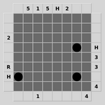For detailed instructions for each puzzle, please visit the docs available at www.chiark.greenend.org.uk/ sgtatham/puzzles/doc/index.html <details> <summary>extracted/5699650/img/puzzles/blackbox.png Details</summary>  ### Visual Description ## Diagram: Grid with Markers ### Overview The image shows a grid, possibly representing a game board or a puzzle, with numbers and letters along the edges and filled circles within the grid. ### Components/Axes * **Grid:** An 8x8 grid of squares. * **Edge Labels (Top):** 5, 1, 5, H, 2 * **Edge Labels (Left):** 2, H, R, H * **Edge Labels (Right):** H, 3, 3, 4 * **Edge Labels (Bottom):** 1, 4 * **Markers:** Three filled black circles located within the grid. ### Detailed Analysis * **Marker 1:** Located at row 6, column 2 (counting from top-left, starting at 1). * **Marker 2:** Located at row 3, column 6. * **Marker 3:** Located at row 6, column 6. ### Key Observations The grid has a sparse distribution of markers. The edge labels consist of numbers and the letter "H" and "R". ### Interpretation The image likely represents a puzzle or game board. The markers could indicate specific locations or pieces. The edge labels might represent coordinates, rules, or constraints of the game. Without further context, the exact purpose and rules of the game or puzzle are unclear. </details> Figure 5: Black Box: Find the hidden balls in the box by bouncing laser beams off them. 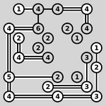<details> <summary>extracted/5699650/img/puzzles/bridges.png Details</summary>  ### Visual Description ## Diagram: Network of Numbered Nodes ### Overview The image depicts a network of interconnected nodes, each containing a number. The nodes are connected by lines, some of which are doubled. The background is a light gray. ### Components/Axes * **Nodes:** Circular shapes containing numbers. The numbers range from 1 to 6. Some nodes are shaded gray. * **Connections:** Lines connecting the nodes. Some connections are doubled, indicating a stronger or different type of relationship. * **Background:** Light gray. ### Detailed Analysis The diagram consists of nodes with the following values: 1, 2, 3, 4, 5, and 6. The nodes are arranged in a somewhat irregular pattern. * **Top Row:** From left to right: Node "1", Node "4", Node "4", Node "4". * **Second Row:** Node "4", Node "6", Node "2", Node "2", Node "1", Node "4". * **Third Row:** Node "4", Node "2", Node "2", Node "4". * **Fourth Row:** Node "5", Node "2", Node "1", Node "3". * **Fifth Row:** Node "4", Node "4", Node "3". * **Sixth Row:** Node "1", Node "3", Node "2". The connections between the nodes are as follows: * Node "1" (top-left) is connected to Node "4". * Node "4" (top-left) is connected to Node "1", Node "4", and Node "6". * Node "4" (top-middle) is connected to Node "4". * Node "4" (top-right) is connected to Node "4". * Node "4" (left-side) is connected to Node "6", Node "2", Node "4", and Node "5". * Node "6" is connected to Node "4". * Node "5" is connected to Node "4", Node "2". * Node "4" (bottom-left) is connected to Node "5", Node "4". * Node "4" (bottom-middle) is connected to Node "4", Node "3". * Node "3" (bottom-right) is connected to Node "4", Node "3". * Node "3" (right-side) is connected to Node "3", Node "2", Node "1". ### Key Observations * The number "4" appears most frequently as a node value. * Some connections are doubled, suggesting a different type of relationship or a stronger connection. * The nodes are not arranged in a regular grid or pattern. ### Interpretation The diagram likely represents a network or system where the nodes represent entities or states, and the numbers represent some attribute or value associated with those entities. The connections represent relationships or interactions between the entities. The doubled connections could indicate stronger or more frequent interactions. Without further context, it's difficult to determine the specific meaning of the numbers and connections. The diagram could be used to model various systems, such as social networks, transportation networks, or computer networks. </details> Figure 6: Bridges: Connect all the islands with a network of bridges. 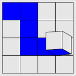<details> <summary>extracted/5699650/img/puzzles/cube.png Details</summary>  ### Visual Description ## Diagram: 2D Grid with 3D Cube ### Overview The image depicts a 5x5 grid, with some cells filled in blue and a single 3D cube placed on the grid. The grid provides a 2D space, while the cube introduces a 3D element. ### Components/Axes * **Grid:** A 5x5 grid with cells colored either white or blue. * **Cube:** A single white 3D cube positioned on the grid. ### Detailed Analysis * **Grid Cells:** * The grid is composed of 25 cells arranged in 5 rows and 5 columns. * Some cells are filled with blue color, while others remain white. * The blue cells form an "L" shape. * **Cube Placement:** * The 3D cube is placed on the grid, partially overlapping the blue cells. * The cube appears to be floating slightly above the grid surface, indicated by the shadow. ### Key Observations * The blue cells form a distinct "L" shape within the grid. * The 3D cube adds depth and perspective to the 2D grid. ### Interpretation The image combines 2D and 3D elements to create a visual representation of spatial relationships. The "L" shape formed by the blue cells could represent a specific area or region within the grid. The placement of the 3D cube on the grid suggests an interaction or relationship between the cube and the underlying grid structure. The image could be used to illustrate concepts such as spatial awareness, geometric shapes, or the integration of 2D and 3D elements. </details> Figure 7: Cube: Pick up all the blue squares by rolling the cube over them. 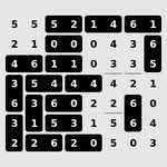<details> <summary>extracted/5699650/img/puzzles/dominosa.png Details</summary>  ### Visual Description ## Number Grid ### Overview The image shows a grid of numbers, with some numbers enclosed in black rectangles. The grid appears to be 8x8, although the rectangles obscure some of the numbers. ### Components/Axes * The grid consists of numbers ranging from 0 to 6. * Some numbers are enclosed in black rectangles. * There are two horizontal lines between numbers. ### Detailed Analysis or ### Content Details Here's the reconstructed grid with approximate values, accounting for the obscured numbers: | | | | | | | | | | :---- | :---- | :---- | :---- | :---- | :---- | :---- | :---- | | 5 | 5 | 5 | 2 | 1 | 4 | 6 | 1 | | 2 | 1 | 0 | 0 | 0 | 4 | 3 | 6 | | 4 | 6 | 1 | 1 | 0 | 3 | 3 | 5 | | 3 | 5 | 4 | 4 | 4 | 4 | 2 | 1 | | 6 | 3 | 6 | 0 | 2 | 2 | 6 | 0 | | 3 | 1 | 5 | 3 | 1 | 5 | 6 | 4 | | 2 | 2 | 6 | 2 | 0 | 5 | 0 | 3 | ### Key Observations * The numbers are single digits. * The black rectangles seem to group certain numbers together. * The horizontal lines are located between the third and fourth rows, and the fifth and sixth rows. ### Interpretation The image presents a numerical grid with some elements highlighted by black rectangles. Without further context, it's difficult to determine the purpose or meaning of the grid and the rectangles. It could be a puzzle, a game board, or a representation of some data where the rectangles indicate specific groupings or relationships between the numbers. The horizontal lines may indicate a separation of data. </details> Figure 8: Dominosa: Tile the rectangle with a full set of dominoes. 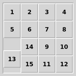<details> <summary>extracted/5699650/img/puzzles/fifteen.png Details</summary>  ### Visual Description \n ## Puzzle: Numbered Grid ### Overview The image shows a 4x4 grid with numbered tiles, except for one missing tile. The tiles are arranged in a non-sequential order, creating a sliding puzzle. ### Components/Axes * **Tiles:** 15 numbered tiles, labeled 1 through 15. * **Grid:** A 4x4 grid structure. * **Missing Tile:** One empty space in the grid. ### Detailed Analysis The tiles are arranged as follows: * **Row 1:** 1, 2, 3, 4 * **Row 2:** 5, 6, 7, 8 * **Row 3:** Empty, 14, 9, 10 * **Row 4:** 13, 15, 11, 12 ### Key Observations * The numbers are not in sequential order. * The empty space is in the third row, first column. ### Interpretation The image represents a classic sliding puzzle, where the goal is to arrange the tiles in sequential order by sliding them into the empty space. The current arrangement is a scrambled state of the puzzle. </details> Figure 9: Fifteen: Slide the tiles around to arrange them into order. 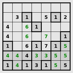<details> <summary>extracted/5699650/img/puzzles/filling.png Details</summary>  ### Visual Description ## Sudoku Puzzle: Partially Filled Grid ### Overview The image shows a partially filled Sudoku puzzle grid. The grid is 9x9, but only some cells contain numbers. Some numbers are black, while others are green, and some cells are shaded gray. ### Components/Axes * **Grid:** A 9x9 grid of cells. * **Numbers:** Digits from 1 to 7 are present in the grid. * **Colors:** Numbers are either black or green. Cells are either white or gray. ### Detailed Analysis or ### Content Details The grid contains the following numbers: * **Row 1:** Empty, 3, 1 (gray), Empty, 5, 1 (gray), 2 * **Row 2:** 4, Empty, 6 (green), 1 (gray), Empty, Empty, Empty * **Row 3:** 4, Empty, 6 (green), Empty, 7 (green), Empty, 1 * **Row 4:** 1, Empty, 6 (green), 1 (gray), 7 (green), 1 (gray), 5 (green) * **Row 5:** 4 (gray, green), 4 (gray, green), 4 (gray, green), 3 (gray, green), 3 (gray, green), 5 (gray, green), 5 (gray, green) * **Row 6:** 1 (gray), 4 (green), 1 (gray), 3 (gray), 1 (gray), 5 (gray, green), 5 (gray, green) ### Key Observations * The grid is not fully populated. * Some numbers are green, suggesting they might be user-entered or part of a solution process. * Some cells are gray, possibly indicating pre-filled values or constraints. * The numbers range from 1 to 7, which is unusual for a standard Sudoku puzzle (which typically uses 1 to 9). ### Interpretation The image represents a Sudoku puzzle in progress. The green numbers likely represent the player's attempts to solve the puzzle, while the black numbers and gray cells may represent the initial state of the puzzle. The puzzle uses a smaller range of numbers (1-7) than a standard Sudoku. The goal is to fill the remaining cells with numbers such that each row, column, and 3x3 subgrid contains each number exactly once. </details> Figure 10: Filling: Mark every square with the area of its containing region. 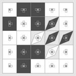<details> <summary>extracted/5699650/img/puzzles/flip.png Details</summary>  ### Visual Description ## Checkerboard Pattern: Abstract Tile Arrangement ### Overview The image presents a 5x5 grid filled with tiles of varying designs and shades of gray. The tiles are arranged in a non-uniform pattern, with some tiles featuring cross-like designs, others diamond-like designs, and some being plain shades of gray. ### Components/Axes * **Grid:** A 5x5 grid structure. * **Tiles:** Individual squares within the grid, each containing a specific design and shade. * **Designs:** * Cross-like design (appears in white, gray, and dark gray) * Diamond-like design (appears in white, gray, and dark gray) * Plain (white, gray, and dark gray) * **Shades:** White, light gray, dark gray. ### Detailed Analysis The grid is composed of 25 tiles. The arrangement of the tiles is as follows: * **Row 1:** White tile with cross, dark gray tile with cross, gray tile with cross, white tile with cross, white tile with cross. * **Row 2:** Dark gray tile with cross, white tile with cross, white tile with cross, gray tile with diamond, white tile with diamond. * **Row 3:** White tile with cross, white tile with cross, gray tile with cross, white tile with diamond, dark gray tile with diamond. * **Row 4:** White tile with cross, dark gray tile with cross, white tile with cross, gray tile with cross, white tile with diamond. * **Row 5:** Dark gray tile with cross, white tile with cross, white tile with cross, white tile with cross, white tile with cross. ### Key Observations * The pattern is not a simple checkerboard, as the tile designs and shades vary irregularly. * The diamond-like designs are concentrated in the upper-right quadrant of the grid. * The cross-like designs are more evenly distributed throughout the grid. * There are no plain tiles. ### Interpretation The image appears to be an abstract arrangement of tiles, possibly representing a game board or a design pattern. The non-uniform distribution of designs and shades suggests a deliberate composition rather than a random arrangement. The concentration of diamond-like designs in the upper-right quadrant could indicate a specific area of interest or a strategic element within the design. The image lacks a clear legend or key, making it difficult to determine the intended meaning or purpose of the arrangement. </details> Figure 11: Flip: Flip groups of squares to light them all up at once. 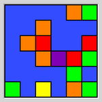<details> <summary>extracted/5699650/img/puzzles/flood.png Details</summary>  ### Visual Description ## Heatmap: Color Distribution ### Overview The image is a heatmap-like grid with various colored squares against a blue background. The colors include red, orange, yellow, green, and purple. The squares are arranged seemingly randomly, creating a visual pattern. ### Components/Axes * **Background Color:** Blue * **Square Colors:** Red, Orange, Yellow, Green, Purple * **Grid Structure:** The image is composed of a grid of squares. ### Detailed Analysis or ### Content Details * **Blue Squares:** The majority of the grid is filled with blue squares, forming the background. * **Red Squares:** Red squares are clustered in the upper-middle and right-middle sections of the grid. * **Orange Squares:** Orange squares are scattered throughout the grid, primarily in the upper and middle sections. * **Yellow Squares:** A single yellow square is located in the bottom-left quadrant. * **Green Squares:** Green squares are concentrated in the bottom-right quadrant. * **Purple Squares:** A single purple square is located in the middle of the grid. ### Key Observations * The distribution of colors is uneven, with blue being the dominant color. * Certain colors tend to cluster in specific regions of the grid. * The yellow and purple squares are isolated. ### Interpretation The image appears to be a visual representation of a categorical distribution. The colors could represent different categories, and their distribution across the grid might indicate their relative frequency or spatial relationships. Without additional context, it's difficult to determine the specific meaning of the colors or the grid structure. The clustering of certain colors suggests potential correlations or dependencies between the categories they represent. The isolated yellow and purple squares could be outliers or rare events. </details> Figure 12: Flood: Turn the grid the same colour in as few flood fills as possible. 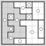<details> <summary>extracted/5699650/img/puzzles/galaxies.png Details</summary>  ### Visual Description ## Diagram: Nurikabe Puzzle ### Overview The image shows a completed Nurikabe puzzle on a grid. The grid is divided into regions, some of which are shaded gray (representing the "wall"), while others are white (representing the "islands"). Each white region contains a single circle with a number inside (not visible in this image), indicating the size of the island. The goal of Nurikabe is to shade cells to form a connected "wall" that does not create 2x2 blocks, and to ensure that the unshaded regions form islands of the correct size. ### Components/Axes * **Grid:** A square grid, approximately 10x10 cells. * **Wall (Gray Regions):** Shaded cells forming a connected network. * **Islands (White Regions):** Unshaded regions, each containing a circle. * **Circles:** Located within each island, representing the number of cells the island must contain. (The numbers themselves are not visible in this image.) ### Detailed Analysis The image shows a solved Nurikabe puzzle. The gray "wall" is connected and does not form any 2x2 blocks. The white "islands" are separated by the wall. The circles within each island are not visible, so it is impossible to verify if the size of each island matches the number in the circle. ### Key Observations * The gray wall is contiguous and covers a significant portion of the grid. * The white islands are distinct and separated by the wall. * The puzzle appears to be correctly solved, based on the rules of Nurikabe. ### Interpretation The image demonstrates the solution to a Nurikabe puzzle. The puzzle involves logical deduction to determine which cells should be shaded to form a connected wall and which cells should remain unshaded to form islands of specific sizes. The solution adheres to the rules of Nurikabe, indicating a valid puzzle solution. </details> Figure 13: Galaxies: Divide the grid into rotationally symmetric regions each centred on a dot. 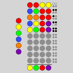<details> <summary>extracted/5699650/img/puzzles/guess.png Details</summary>  ### Visual Description ## Diagram: Color Pattern ### Overview The image shows a diagram with a pattern of colored circles arranged in columns and rows. The colors include red, orange, yellow, green, blue, and purple, along with gray and white/black combinations. The arrangement seems to represent a visual pattern or code. ### Components/Axes * **Colors:** Red, Orange, Yellow, Green, Blue, Purple, Gray, White/Black * **Arrangement:** Circles are arranged in columns and rows. ### Detailed Analysis The diagram consists of several distinct sections: 1. **Left Column:** A vertical column of colored circles in the order: Red, Green, Blue, Orange, Purple. 2. **Main Grid:** A grid of colored circles. The columns from left to right are: * Column 1: Red, Orange, Yellow, Gray, Gray, Gray, Gray, Gray * Column 2: Orange, Yellow, Green, Gray, Gray, Gray, Gray, Gray * Column 3: Yellow, Red, Gray, Gray, Gray, Gray, Gray * Column 4: Red, Green, Gray, Gray, Gray, Gray, Gray * Column 5: Purple, Gray, Gray, Gray, Gray, Gray 3. **Right Column:** A column of paired circles, alternating between white and black, then gray. 4. **Bottom Row:** A horizontal row of colored circles: Yellow, Green, Purple. ### Key Observations * The left column contains a sequence of colors. * The main grid has a pattern of colors in the top rows, with the remaining rows filled with gray. * The right column has a distinct pattern of paired circles. * The bottom row has a sequence of colors. ### Interpretation The diagram appears to represent a visual code or pattern. The arrangement of colors and the distinct sections suggest a structured system. Without additional context, it is difficult to determine the exact meaning or purpose of this pattern. The use of specific colors and their arrangement likely holds significance within the context it was designed for. </details> Figure 14: Guess: Guess the hidden combination of colours. 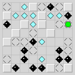<details> <summary>extracted/5699650/img/puzzles/inertia.png Details</summary>  ### Visual Description ## Image Analysis: Grid-Based Puzzle ### Overview The image depicts a grid-based puzzle, possibly a game board, with various symbols and colors distributed across the grid. The grid consists of square cells, some of which contain symbols like diamonds (light blue), circles (white with dashed outline), and solid black shapes resembling stylized bombs or mines. One cell contains a solid green circle. ### Components/Axes * **Grid:** A 10x10 grid of square cells. * **Symbols:** * Light Blue Diamonds: Scattered throughout the grid. * White Circles (with dashed outline): Scattered throughout the grid. * Solid Black Shapes: Resembling bombs or mines, scattered throughout the grid. * Solid Green Circle: Located near the top-right corner of the grid. ### Detailed Analysis or ### Content Details The grid is populated with a mix of empty cells (gray), cells containing light blue diamonds, cells containing white circles with dashed outlines, and cells containing solid black shapes. The green circle is a distinct element, likely indicating a target or goal. * **Light Blue Diamonds:** These are distributed somewhat randomly, with a higher concentration in the upper portion of the grid. * **White Circles (with dashed outline):** These are also scattered randomly, with no clear pattern. * **Solid Black Shapes:** These are concentrated more towards the bottom of the grid, with a few scattered in the upper and middle sections. * **Solid Green Circle:** Located at row 2, column 9. ### Key Observations * The distribution of the black shapes suggests a potential hazard zone in the lower part of the grid. * The green circle stands out as a target or goal. * The diamonds and circles appear to be obstacles or neutral elements. ### Interpretation The image likely represents a puzzle or game where the objective is to navigate from a starting point (not explicitly shown) to the green circle while avoiding the black shapes. The diamonds and circles may represent obstacles or elements that affect the gameplay in some way. The concentration of black shapes in the lower portion of the grid suggests that this area is more dangerous or challenging to navigate. </details> Figure 15: Inertia: Collect all the gems without running into any of the mines. 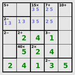<details> <summary>extracted/5699650/img/puzzles/keen.png Details</summary>  ### Visual Description ## KenKen Puzzle: Example ### Overview The image shows a completed KenKen puzzle, a mathematical and logical puzzle similar to Sudoku. The grid is 5x5, and each cage (group of cells) is marked with a target number and an operation. The goal is to fill the grid with numbers 1-5 such that each row and column contains each number exactly once, and the numbers within each cage combine to produce the target number using the specified operation. ### Components/Axes * **Grid:** 5x5 grid of cells. * **Cages:** Groups of cells marked with a target number and an operation (+, -, x, /). * **Numbers:** Each cell contains a number from 1 to 5. * **Operations:** Addition (+), Subtraction (-), Multiplication (x), Division (/). ### Detailed Analysis The grid is filled with numbers 1 through 5. Each row and column contains each number exactly once. The cages are as follows: * **Top-left:** "5+" cage, consisting of two cells with values 2 and 3. 2 + 3 = 5. * **Top-middle:** "15x" cage, consisting of two cells with values 3 and 5. 3 x 5 = 15. * **Top-right:** "7+" cage, consisting of two cells with values 2 and 5. 2 + 5 = 7. * **Top-right:** "10+" cage, consisting of one cell. * **Second row, left:** "2-" cage, consisting of two cells with values 1 and 3. |1 - 3| = 2. * **Third row, left:** "2-" cage, consisting of two cells. * **Third row, middle:** "2+" cage, consisting of two cells with values 2 and 4. 2 + 4 = 6. * **Third row, right:** "3-" cage, consisting of two cells with values 1 and 4. |1 - 4| = 3. * **Fourth row, left:** "40x" cage, consisting of two cells with values 5 and 2. 5 x 2 = 10. * **Fourth row, middle:** "2x" cage, consisting of two cells with values 2 and 4. 2 x 4 = 8. * **Bottom row, right:** "2-" cage, consisting of two cells with values 3 and 5. |3 - 5| = 2. The specific values in each cell are: | | Col 1 | Col 2 | Col 3 | Col 4 | Col 5 | | :---- | :---- | :---- | :---- | :---- | :---- | | Row 1 | 2 | 3 | 3 | 5 | 2 | | Row 2 | 1 | 3 | 5 | 2 | 5 | | Row 3 | 2 | 2 | 4 | 1 | 4 | | Row 4 | 5 | 5 | 2 | 4 | 1 | | Row 5 | 2 | 4 | 1 | 3 | 5 | ### Key Observations * Each row and column contains the numbers 1 through 5 exactly once. * The numbers within each cage satisfy the target number and operation. ### Interpretation The image demonstrates a correctly solved KenKen puzzle. The solution adheres to the rules of the puzzle, ensuring that each row and column contains unique numbers and that the cage constraints are satisfied. This puzzle showcases a combination of logical deduction and arithmetic skills. </details> Figure 16: Keen: Complete the latin square in accordance with the arithmetic clues. 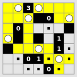<details> <summary>extracted/5699650/img/puzzles/lightup.png Details</summary>  ### Visual Description ## Diagram: Nurikabe Puzzle ### Overview The image shows a partially solved Nurikabe puzzle on a 9x9 grid. The grid contains white circles with numbers inside, black squares, and yellow squares. The remaining squares are gray. The goal of Nurikabe is to shade in squares to create a single connected "wall" (black squares) that does not form any 2x2 squares, while the numbered white circles represent "islands" of connected white squares, with the number indicating the size of the island. ### Components/Axes * **Grid:** 9x9 grid of squares. * **White Circles:** Represent islands, with numbers indicating their size. * **Black Squares:** Represent the "wall". * **Yellow Squares:** Represent squares that are part of an island. * **Gray Squares:** Represent squares that are part of the wall. ### Detailed Analysis The grid contains the following elements: * **Top Row:** * Column 3: White circle with the number "3" inside. * Column 5: White circle. * Column 8: White circle. * **Second Row:** * Column 1: "0" * **Third Row:** * Column 1: White circle. * **Fifth Row:** * Column 4: White circle. * **Sixth Row:** * Column 7: "1" * Column 7: "1" * **Seventh Row:** * Column 3: "0" * Column 4: "1" * **Eighth Row:** * Column 5: White circle. * **Ninth Row:** * Column 5: "0" The black squares are scattered throughout the grid, forming parts of the wall. The yellow squares are adjacent to the white circles, indicating they are part of the islands. ### Key Observations * The puzzle is partially solved, with some islands and wall segments already defined. * The numbers in the white circles indicate the size of the islands that need to be formed. * The black squares must form a single connected wall that does not create any 2x2 squares. ### Interpretation The image presents a snapshot of a Nurikabe puzzle in progress. The solver needs to strategically fill in the remaining squares to satisfy the rules of the game. The placement of the numbered islands and existing wall segments provides constraints that guide the solution. The solver must ensure that the islands are the correct size and that the wall is connected and does not form any 2x2 squares. </details> Figure 17: Light Up: Place bulbs to light up all the squares. 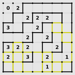<details> <summary>extracted/5699650/img/puzzles/loopy.png Details</summary>  ### Visual Description ## Diagram: Grid with Labeled Regions ### Overview The image shows a grid, approximately 9x9, with some cells outlined in black and others in yellow. Numbers are placed within some of the outlined regions. The grid appears to represent a spatial arrangement of different zones or areas, each labeled with a numerical value. ### Components/Axes * **Grid:** A square grid structure, approximately 9 rows and 9 columns. * **Black Outlines:** Black lines enclose certain areas within the grid. * **Yellow Outlines:** Yellow lines enclose other areas within the grid. * **Numerical Labels:** Numbers (0, 1, 2, 3) are placed inside some of the outlined regions. ### Detailed Analysis Here's a breakdown of the numerical labels and their approximate locations: * **Top-Left:** A region in the top-left corner contains the number "0". Adjacent to it, a region contains the number "2". * **Upper-Center:** A cluster of regions in the upper-center area are labeled with "2". * **Left-Center:** A region in the left-center area is labeled with "3". * **Center:** Several regions in the center are labeled with "2". * **Bottom-Left:** Regions in the bottom-left corner are labeled with "3" and "2". * **Bottom-Center:** Regions in the bottom-center are labeled with "3", "2", and "1". * **Right-Center:** Regions in the right-center are labeled with "2" and "1". ### Key Observations * The grid is divided into distinct regions, each enclosed by either black or yellow lines. * The numerical labels seem to indicate a property or value associated with each region. * The distribution of black and yellow outlines is not uniform, suggesting different categories or types of regions. ### Interpretation The diagram likely represents a spatial model or map where different areas are categorized and labeled. The numbers could represent a value, a count, or an index associated with each region. The black and yellow outlines might indicate different types of zones or areas. Without further context, it's difficult to determine the exact meaning of the diagram, but it appears to be a visual representation of spatially distributed data. </details> Figure 18: Loopy: Draw a single closed loop, given clues about number of adjacent edges. 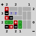<details> <summary>extracted/5699650/img/puzzles/magnets.png Details</summary>  ### Visual Description ## Puzzle Diagram: Grid with Symbols ### Overview The image is a diagram of a grid-based puzzle. The grid is 4x4, with some cells containing symbols (+, -, X) and numbers. Some cells are filled with gray rectangles, and two cells contain question marks. The grid is surrounded by numbers and symbols that likely represent constraints or rules for solving the puzzle. ### Components/Axes * **Grid:** A 4x4 grid. * **Symbols:** +, -, X * **Numbers:** 0, 1, 2, 3 * **Question Marks:** Two question marks in the top-left quadrant of the grid. * **Colors:** Red, Black, Green, Gray, Blue ### Detailed Analysis Here's a breakdown of the grid's contents: * **Row 1:** * Column 1: + (red) * Column 2: Empty (gray rectangle) * Column 3: Empty (gray rectangle) * Column 4: 1 * **Row 2:** * Column 1: - (black) * Column 2: ?? (blue) * Column 3: Empty (gray rectangle) * Column 4: 2 * **Row 3:** * Column 1: + (red), - (black) * Column 2: - (black) * Column 3: Empty (gray rectangle) * Column 4: 0 * **Row 4:** * Column 1: X (green), X (green) * Column 2: + (red) * Column 3: X (green) * Column 4: - The surrounding numbers and symbols are: * **Top Row:** + 2, 2, 1 * **Left Column:** 3, 2 * **Bottom Row:** 2, 2, 1, - * **Right Column:** 2, 0, - ### Key Observations * The puzzle uses a combination of symbols and numbers. * The question marks indicate unknown values that need to be determined. * The surrounding numbers and symbols likely represent constraints or rules for solving the puzzle. * The colors red, black, and green are associated with the symbols +, -, and X, respectively. ### Interpretation The image represents a logic puzzle where the goal is to fill in the missing values (represented by the question marks) based on the given symbols, numbers, and constraints. The surrounding numbers and symbols likely represent the sum or count of specific symbols in each row or column. The colors might indicate different types of elements or operations within the puzzle. Solving the puzzle would involve deductive reasoning and pattern recognition to determine the correct values for the question marks. </details> Figure 19: Magnets: Place magnets to satisfy the clues and avoid like poles touching. 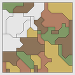<details> <summary>extracted/5699650/img/puzzles/map.png Details</summary>  ### Visual Description ## Diagram: Abstract Color Block Pattern ### Overview The image presents an abstract pattern composed of interconnected color blocks. The pattern resembles a stylized map or circuit board, with various colors filling irregular shapes. There is no clear data or quantitative information presented. ### Components/Axes The diagram consists of the following components: * **Color Blocks:** Irregularly shaped blocks filled with different colors. The colors observed are white, light brown, dark brown, light green, and yellow. * **Connecting Lines:** Thin white lines that connect the color blocks, creating a network-like structure. * **Overall Shape:** The entire pattern is contained within a square frame. ### Detailed Analysis or ### Content Details The color blocks are arranged in a seemingly random manner, with no discernible pattern or order. The white blocks are concentrated in the top-left corner, while the other colors are distributed throughout the rest of the area. The connecting lines create a sense of interconnectedness between the blocks. ### Key Observations * The pattern is abstract and does not represent any specific object or scene. * The color palette is limited to earthy tones and white. * The connecting lines add a sense of complexity and structure to the pattern. ### Interpretation The image is likely an artistic representation or a design element. The abstract nature of the pattern allows for multiple interpretations, depending on the viewer's perspective. The use of earthy tones may suggest a connection to nature or the environment. The interconnectedness of the blocks could symbolize relationships or networks. Without additional context, the exact meaning or purpose of the image remains open to interpretation. </details> Figure 20: Map: Colour the map so that adjacent regions are never the same colour. <details> <summary>extracted/5699650/img/puzzles/mines.png Details</summary>  ### Visual Description ## Minesweeper Game State: Partial Solution ### Overview The image shows a partially solved Minesweeper game board. Some cells are revealed, displaying numbers indicating the number of adjacent mines. Other cells are marked with flags, presumably indicating the location of mines. Some cells are still unrevealed. ### Components/Axes * **Cells:** The game board is a grid of cells. * **Numbers:** Revealed cells display numbers from 1 to 8, indicating the number of adjacent mines. * **Flags:** Cells marked with a red flag indicate a suspected mine location. * **Unrevealed Cells:** Blank cells that have not yet been clicked. ### Detailed Analysis The board is a grid. The visible cells contain the following information: * **Row 1:** 1, 2, 2, 2, 3, 1, 1, 1, 1 * **Row 2:** 2, 3, 1, 1, 4, 1, Flag, 5, 1, 4 * **Row 3:** Flag, 1, 7, 1, 5, 2, 3, 2, 1 * **Row 4:** 1, 1, 1, 5, 1, Flag, 1, 1, 1 * **Row 5:** 1, Flag, 1, 4, 2 * **Row 6:** 1, Flag, 2, 2, 1 * **Row 7:** 3, 3, 1, 4, 1 * **Row 8:** 3, 2, 4, 1, Flag, 1 The remaining rows are unrevealed. ### Key Observations * The numbers indicate the density of mines in the surrounding area. * Flags are used to mark suspected mine locations. * The player has successfully identified some mine locations and revealed some safe cells. ### Interpretation The image represents a snapshot of a Minesweeper game in progress. The player is using the numbers to deduce the location of mines and reveal safe cells. The presence of flags suggests that the player is strategically marking potential mine locations to avoid clicking on them. The game is not yet complete, as there are still unrevealed cells. </details> Figure 21: Mines: Find all the mines without treading on any of them. <details> <summary>extracted/5699650/img/puzzles/mosaic.png Details</summary>  ### Visual Description ## Kakuro Puzzle: Unsolved Grid ### Overview The image presents an unsolved Kakuro puzzle grid. The grid consists of white and black cells. The white cells are where numbers 1-9 are to be placed, and the black cells contain clues in the form of sums. The goal is to fill the white cells with numbers such that the sum of the numbers in each horizontal or vertical block equals the clue in the corresponding black cell. No number can be repeated within a block. ### Components/Axes * **Grid:** A 9x9 grid of cells. * **Black Cells:** Cells containing clues (sums). * **White Cells:** Cells to be filled with numbers. * **Clues:** Numbers in the black cells indicating the sum of the adjacent white cells in a row or column. ### Detailed Analysis The grid contains the following clues: * **Row 1:** 2 (column 3), 3 (column 9) * **Row 2:** 4 (column 2), 2 (column 4), 5 (column 6) * **Row 3:** 6 (column 2), 3 (column 9) * **Row 4:** 5 5 (columns 1 and 2), 6 (column 7) * **Row 5:** 5 (column 1), 4 (column 3), 2 (column 4), 4 (column 6), 4 (column 7) * **Row 6:** 0 (column 4), 3 (column 9) * **Row 7:** 6 (column 2), 4 (column 3), 4 (column 9) * **Row 8:** 4 (column 3), 2 (column 4), 3 (column 5), 2 (column 6) ### Key Observations * The puzzle is partially filled, with some clues already provided. * The size of the grid is 9x9. * The clues are located in the black cells, and the white cells are to be filled with numbers. ### Interpretation The image represents a standard Kakuro puzzle in an unsolved state. The clues provided in the black cells are essential for solving the puzzle. The solver must use logic and deduction to fill the white cells with numbers 1-9, ensuring that the sum of each block matches the corresponding clue and that no number is repeated within a block. The puzzle's difficulty depends on the number and placement of the clues. </details> Figure 22: Mosaic: Fill in the grid given clues about number of nearby black squares. <details> <summary>extracted/5699650/img/puzzles/net.png Details</summary>  ### Visual Description ## Diagram: Network Connection ### Overview The image is a diagram representing a network connection between two groups of nodes. The top group consists of blue nodes connected by black lines, while the bottom group consists of cyan nodes connected by cyan lines. A central black node acts as an intermediary between the two groups. The diagram is set against a grid background. ### Components/Axes * **Nodes:** Represented by squares. Blue nodes are in the top section, cyan nodes in the bottom, and a black node in the center. * **Connections:** Represented by lines. Black lines connect the blue nodes, and cyan lines connect the cyan nodes. * **Grid:** A light gray grid provides spatial context. * **Border:** A dark red border surrounds the entire diagram. ### Detailed Analysis * **Top Group (Blue Nodes):** There are three blue nodes in the top row and one blue node in the middle row. The top-left blue node is connected to the middle-row blue node. The top-middle and top-right blue nodes are connected to each other. All three are connected to the central black node. * **Bottom Group (Cyan Nodes):** There are two cyan nodes on the left and two on the right. The two left cyan nodes are connected to each other and to the central black node. The two right cyan nodes are connected to each other and to the central black node. * **Central Node:** A black node connects the top and bottom groups. ### Key Observations * The diagram illustrates a network where two distinct groups of nodes are interconnected via a central node. * The connections within each group are relatively simple, with direct links between nodes. * The central node acts as a bridge, facilitating communication between the two groups. ### Interpretation The diagram likely represents a simplified network architecture, where the blue and cyan nodes could represent different subnetworks or devices. The central black node could be a router or switch that manages traffic between these subnetworks. The diagram highlights the importance of the central node in enabling communication between the two groups. The simplicity of the connections within each group suggests a relatively straightforward network topology. </details> Figure 23: Net: Rotate each tile to reassemble the network. <details> <summary>extracted/5699650/img/puzzles/netslide.png Details</summary>  ### Visual Description ## Diagram: Network Topology ### Overview The image presents a diagram of a network topology, showing interconnected nodes and pathways within a grid-like structure. The diagram is enclosed within a red-brown border, and arrows around the perimeter suggest data flow or connectivity to external networks. ### Components/Axes * **Nodes:** Represented by colored squares (blue, cyan, and black). * **Connections:** Represented by black and teal lines indicating pathways between nodes. * **Grid:** A light gray grid provides spatial organization. * **Border:** A red-brown border encloses the network. * **Arrows:** Gray arrows around the border indicate external connectivity or data flow. ### Detailed Analysis * **Blue Nodes:** Three blue nodes are located on the left side of the grid, vertically aligned and connected by a black line. * **Cyan Nodes:** Three cyan nodes are located on the right side of the grid, vertically aligned and connected to the central black node by teal lines. * **Black Node:** A single black node is located in the center of the grid, acting as a central hub. * **Connections:** The black lines connect the blue nodes to each other. The teal lines connect the black node to each of the cyan nodes. * **External Connectivity:** Gray arrows point inward and outward from all sides of the red-brown border, suggesting bidirectional data flow or connections to external networks. ### Key Observations * The network appears to have a centralized architecture, with the black node acting as a central hub. * The blue nodes on the left seem to be input nodes, while the cyan nodes on the right seem to be output nodes. * The arrows around the border suggest that the network is connected to other networks or systems. ### Interpretation The diagram illustrates a basic network topology with a central hub connecting input and output nodes. The arrows indicate that this network is part of a larger system or network. The specific function of each node is not clear from the diagram, but the arrangement suggests a data processing or distribution system. The diagram could represent a simplified model of a computer network, a sensor network, or any other system where data flows between interconnected nodes. </details> Figure 24: Netslide: Slide a row at a time to reassemble the network. <details> <summary>extracted/5699650/img/puzzles/palisade.png Details</summary>  ### Visual Description ## Diagram: Grid Puzzle ### Overview The image shows a grid puzzle with numbers indicating the size of connected regions. Some regions are outlined in black, and some cells are highlighted in yellow. The puzzle appears to be partially solved. ### Components/Axes * The grid is a 6x6 square. * Numbers are placed in some of the cells, indicating the size of the connected region that cell belongs to. The numbers are: 2, 2, 3, 3, 3, 2, 1, 2. * Some regions are outlined in black. * Some cells are highlighted in yellow. ### Detailed Analysis * **Top-left corner:** A "2" is present. * **Second row, first column:** A "2" is present. * **Second row, second column:** A "3" is present. * **Third row, first column:** A "3" is present. * **Third row, second column:** A "3" is present. * **Fourth row, third column:** A "2" is present. * **Fifth row, second column:** A "1" is present. * **Sixth row, sixth column:** A "2" is present. * **Yellow Highlighted Region:** A 3x3 region in the top-right corner is highlighted in yellow. ### Key Observations * The puzzle involves identifying connected regions of cells based on the numbers provided. * The black outlines indicate completed regions. * The yellow highlighted region may be a clue or a partially completed region. ### Interpretation The image represents a logic puzzle where the goal is to divide the grid into regions of specific sizes, as indicated by the numbers within the grid. The black outlines likely represent completed regions, while the yellow highlighted area may be a region in progress or a clue to solving the puzzle. The puzzle requires spatial reasoning and logical deduction to correctly partition the grid. </details> Figure 25: Palisade: Divide the grid into equal-sized areas in accordance with the clues. <details> <summary>extracted/5699650/img/puzzles/pattern.png Details</summary>  ### Visual Description ## Pixel Art Puzzle ### Overview The image presents a pixel art puzzle, likely a nonogram or similar logic puzzle. It consists of a grid of colored squares (black, white, and gray) with numerical clues along the top and left edges. These clues indicate the lengths of consecutive runs of colored squares in each row and column. ### Components/Axes * **Grid:** A 10x10 grid of colored squares. * **Row Clues:** Numerical clues are positioned to the left of each row. * **Column Clues:** Numerical clues are positioned above each column. * **Colors:** The squares are colored black, white, or gray. ### Detailed Analysis or ### Content Details **Row Clues (Left Side):** * Row 1: 5 (all black) * Row 2: 5 (all black) * Row 3: 1 1 (white, white) * Row 4: 4 (all black) * Row 5: 5 (all white) * Row 6: 6 (all white) * Row 7: 2 3 (black, gray) * Row 8: 3 3 (gray, gray) * Row 9: 1 1 3 (black, black, gray) * Row 10: 1 1 4 (black, black, gray) **Column Clues (Top Side):** * Column 1: 2, 3, 4 * Column 2: 3, 2 * Column 3: 2, 4, 1 * Column 4: 4, 2, 3 * Column 5: 2, 3, 2 * Column 6: 3, 4 * Column 7: 3, 6 * Column 8: 3, 6 * Column 9: 3, 1 * Column 10: 3, 1 **Grid Colors:** * Row 1: Black, Black, Black, Black, Black, Gray, Gray, Gray, Gray, Gray * Row 2: Black, Black, Black, Black, Black, Gray, Gray, Gray, Gray, Gray * Row 3: White, Black, Gray, Gray, Gray, Gray, Gray, Gray, White, Gray * Row 4: Black, Black, Black, Black, Gray, Gray, Gray, Gray, Gray, Gray * Row 5: Gray, White, White, White, White, White, Black, Gray, Gray, Gray * Row 6: Gray, White, White, White, White, White, Black, Gray, Gray, Gray * Row 7: Black, Black, Gray, Gray, Gray, Black, Black, Black, Gray, Gray * Row 8: Gray, Gray, Gray, Gray, Gray, Black, Black, Black, Gray, Gray * Row 9: Black, Black, Gray, Gray, Gray, Gray, Gray, Gray, Gray, Gray * Row 10: Black, Black, Gray, Gray, Gray, Gray, Gray, Gray, Gray, Gray ### Key Observations * The puzzle uses three colors: black, white, and gray. * The clues indicate the lengths of consecutive runs of the same color in each row and column. * The grid is partially filled, suggesting it is in the process of being solved. ### Interpretation The image presents a logic puzzle where the goal is to fill in the grid completely based on the numerical clues. The clues represent the lengths of consecutive runs of each color in each row and column. By carefully analyzing the clues and the existing colored squares, one can deduce the colors of the remaining squares to complete the puzzle. The presence of three colors adds complexity compared to a standard black-and-white nonogram. The solution to this puzzle would reveal a pixel art image. </details> Figure 26: Pattern: Fill in the pattern in the grid, given only the lengths of runs of black squares. <details> <summary>extracted/5699650/img/puzzles/pearl.png Details</summary>  ### Visual Description ## Diagram: Grid Puzzle ### Overview The image shows a grid-based puzzle. The grid is 8x8, with a thick black line forming a path through the grid. There are black and white circles placed at various intersections of the grid lines. ### Components/Axes * **Grid:** An 8x8 grid with gray lines. * **Path:** A thick black line that traverses the grid, connecting various intersections. * **Black Circles:** Solid black circles located at specific intersections. * **White Circles:** Hollow white circles located at specific intersections. ### Detailed Analysis or Content Details The path starts at the top-left corner and meanders through the grid. The path's route is as follows: 1. Starts at the top-left corner (black circle). 2. Moves right, then down, then right again, then down. 3. Moves right, then up, then right again. 4. Moves down, then left, then down. 5. Moves left, then up, then left again (black circle). 6. Moves right (black circle). 7. Moves right again (black circle). 8. Moves up, then right, then up again. 9. Moves right, then down, then right again (white circle). 10. Moves up, then left, then up again. 11. Moves left, then down, then left again (white circle). 12. Moves down, then left. The positions of the circles are as follows: * **Black Circles:** * Top-left corner. * Middle-left, two rows down. * Middle-left, two rows down, one column to the right. * **White Circles:** * Two rows down, three columns to the right. * Four rows down, two columns to the left. * Six rows down, one column to the right. * Bottom-right corner. ### Key Observations The path does not cross itself. The black and white circles are placed at specific points along the path or near it. ### Interpretation The image likely represents a puzzle where the goal is to complete the path according to certain rules, possibly related to the placement of the black and white circles. The circles may indicate specific constraints or conditions that the path must satisfy. Without further context or instructions, the exact nature of the puzzle remains unclear. </details> Figure 27: Pearl: Draw a single closed loop, given clues about corner and straight squares. <details> <summary>extracted/5699650/img/puzzles/pegs.png Details</summary>  ### Visual Description ## Dot Pattern: Cross-Shaped Dot Arrangement ### Overview The image presents a cross-shaped arrangement of dots on a gray background. The dots are either blue or gray, forming a distinct pattern. The overall shape resembles a plus sign or a cross. ### Components/Axes * **Background:** Gray * **Dots:** Blue and Gray * **Shape:** Cross or Plus Sign ### Detailed Analysis or ### Content Details The cross shape is composed of five rectangular sections. The central rectangle contains a 4x4 grid of dots, mostly blue with some gray dots. The four arms of the cross extend from the sides of the central rectangle. Each arm contains a 2x2 grid of dots, with the majority being blue and some gray. Specifically: * **Central Rectangle:** 4x4 grid. Predominantly blue dots, with gray dots in the top-right and bottom-right corners. * **Top Arm:** 2x2 grid. Contains 1 blue dot and 3 gray dots. * **Bottom Arm:** 2x2 grid. All dots are blue. * **Left Arm:** 2x2 grid. All dots are blue. * **Right Arm:** 2x2 grid. Contains 1 blue dot and 3 gray dots. ### Key Observations * The central rectangle and the bottom and left arms are primarily blue. * The top and right arms have a mix of blue and gray dots. * The pattern is symmetrical along the vertical axis. ### Interpretation The image presents a simple visual pattern. The arrangement of blue and gray dots within the cross shape could represent a binary code or a visual representation of data. The asymmetry in the distribution of gray dots in the top and right arms suggests a deliberate design choice, possibly encoding specific information. Without further context, the exact meaning of the pattern remains unclear. </details> Figure 28: Pegs: Jump pegs over each other to remove all but one. 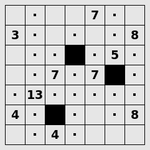<details> <summary>extracted/5699650/img/puzzles/range.png Details</summary>  ### Visual Description ## Grid Puzzle: Number Placement ### Overview The image presents a grid-based number puzzle. The grid is 7x7, with some cells containing numbers and others containing dots. There are also two black squares. The goal is likely to fill the remaining cells with numbers following certain rules, which are not explicitly stated in the image. ### Components/Axes * **Grid:** 7 rows and 7 columns. * **Numbers:** 3, 4, 5, 7, 8, 13 * **Empty Cells:** Represented by dots ('.'). * **Blocked Cells:** Represented by black squares. ### Detailed Analysis The grid contains the following numbers at these locations: * Row 1, Column 5: 7 * Row 2, Column 1: 3 * Row 2, Column 7: 8 * Row 3, Column 5: 5 * Row 4, Column 3: 7 * Row 4, Column 5: 7 * Row 5, Column 1: 13 * Row 6, Column 1: 4 * Row 6, Column 7: 8 * Row 7, Column 3: 4 There are two black squares: * Row 3, Column 4 * Row 4, Column 6 * Row 6, Column 3 The remaining cells are marked with dots, indicating they need to be filled. ### Key Observations * The puzzle involves placing numbers in a grid. * Some cells are pre-filled with numbers, while others are blocked. * The rules of the puzzle are not provided in the image. ### Interpretation The image represents a partially completed number puzzle. Without knowing the rules of the puzzle (e.g., Sudoku, Kakuro, etc.), it's impossible to determine the solution. The provided numbers and blocked cells serve as constraints for solving the puzzle. The puzzle likely requires logical deduction and pattern recognition to fill the remaining cells correctly. </details> Figure 29: Range: Place black squares to limit the visible distance from each numbered cell. <details> <summary>extracted/5699650/img/puzzles/rect.png Details</summary>  ### Visual Description ## Diagram: Nonogram Puzzle ### Overview The image shows a partially completed nonogram puzzle. The puzzle grid is 7x7, with some cells filled in gray and some cells containing numbers. The numbers likely represent the lengths of consecutive filled cells in the corresponding row or column. ### Components/Axes * **Grid:** A 7x7 grid of cells. * **Filled Cells:** Some cells are filled in gray. * **Numbers:** Some cells contain numbers, presumably clues for the puzzle. The numbers present are 2, 3, 4, 8. ### Detailed Analysis Here's a breakdown of the numbers and filled cells in each row and column: * **Row 1:** Contains the number 3. The last two cells are filled. * **Row 2:** Contains the numbers 2 and 3 and 2. * **Row 3:** Contains the numbers 4 and 8. * **Row 4:** Contains the numbers 2 and 3. * **Row 5:** Contains the numbers 4 and 2. * **Row 6:** Contains the numbers 2 and 3 and 3. The first cell is filled. * **Row 7:** Contains the number 3 and 3. The first two cells are filled. * **Column 1:** Contains the numbers 3, 4, 2, 3. * **Column 2:** Contains the number 8. * **Column 3:** Contains the numbers 2, 4, 3, 3. * **Column 4:** Contains the numbers 3, 2, 2, 3. * **Column 5:** Contains the numbers 3, 2, 3, 3. * **Column 6:** Contains the numbers 2, 3, 3. * **Column 7:** Contains the numbers 2, 3, 3. ### Key Observations * The puzzle is partially solved, with some cells already filled in. * The numbers provide clues about the lengths of consecutive filled cells in each row and column. * The goal is to fill in the remaining cells based on the clues. ### Interpretation The image represents a nonogram puzzle, a logic puzzle where cells in a grid must be colored or left blank according to numbers at the side of the grid to reveal a hidden picture. The numbers indicate the lengths of consecutive blocks of filled cells in each row or column, separated by one or more empty cells. The partially filled grid suggests that someone has started solving the puzzle, using the numbers as clues to deduce which cells should be filled. </details> Figure 30: Rectangles: Divide the grid into rectangles with areas equal to the numbers. <details> <summary>extracted/5699650/img/puzzles/samegame.png Details</summary>  ### Visual Description ## Puzzle: Colored Block Arrangement ### Overview The image shows a completed puzzle consisting of various colored blocks (red, green, and blue) arranged within a square grid. The blocks are of different shapes and sizes, fitting together to fill the grid. The top-left portion of the grid is empty (gray). ### Components/Axes * **Colors:** Red, Green, Blue, Gray (empty space) * **Grid:** Square grid containing the colored blocks. ### Detailed Analysis The puzzle is a square grid filled with red, green, and blue blocks of various shapes. The top-left corner of the grid is empty, represented by a gray color. The blocks are arranged to fit together without overlapping, creating a complete puzzle. * **Red Blocks:** Scattered throughout the puzzle, primarily concentrated in the top-right and center-right areas. * **Green Blocks:** Located in the center and bottom-left areas. * **Blue Blocks:** Primarily located in the bottom-left area. * **Empty Space (Gray):** Located in the top-left corner. ### Key Observations * The puzzle is complete, with all blocks fitting together without gaps or overlaps. * The colors are distributed throughout the puzzle, with no single color dominating any particular area. * The empty space in the top-left corner adds an element of asymmetry to the puzzle. ### Interpretation The image represents a completed puzzle, showcasing the arrangement of different colored blocks within a grid. The puzzle demonstrates spatial reasoning and problem-solving skills, as the blocks must be carefully arranged to fit together without gaps or overlaps. The empty space in the top-left corner adds an element of visual interest and asymmetry to the puzzle. The distribution of colors throughout the puzzle creates a visually appealing and balanced composition. </details> Figure 31: Same Game: Clear the grid by removing touching groups of the same colour squares. <details> <summary>extracted/5699650/img/puzzles/signpost.png Details</summary>  ### Visual Description ## Diagram: Grid with Values and Arrows ### Overview The image is a 4x4 grid diagram containing numbers, letters, and directional arrows. The grid cells are colored in shades of white, light gray, orange, and purple. Each cell contains a combination of text and arrows, indicating values and directions. ### Components/Axes * **Grid:** A 4x4 matrix representing the diagram's structure. * **Cells:** Individual squares within the grid, each containing data. * **Values:** Letters and numbers within the cells (e.g., "1", "e+1", "a", "d+4"). * **Arrows:** Directional indicators within the cells, pointing up, down, left, right, or diagonally. * **Colors:** White, light gray, orange, and purple, used to differentiate cells. ### Detailed Analysis Here's a breakdown of the grid's content, row by row: * **Row 1:** * Cell 1 (Top-Left): "1" (blue), downward gray arrow. * Cell 2: "3", rightward gray arrow. * Cell 3: "e+1" (orange), downward black arrow. * Cell 4: "4", downward-right gray arrow. * **Row 2:** * Cell 1: "2", rightward gray arrow. * Cell 2: "d+1" (purple), downward gray arrow. * Cell 3: "a" (orange), rightward brown arrow, dot below "a". * Cell 4: "a+1" (light orange), downward-left black arrow. * **Row 3:** * Cell 1: "e" (orange), rightward brown arrow, dot below "e". * Cell 2: "d+3" (purple), downward gray arrow. * Cell 3: "d" (purple), dot below "d". * Cell 4: "5", leftward black arrow. * **Row 4:** * Cell 1: "d+4" (purple), rightward black arrow. * Cell 2: "d+2" (purple), upward gray arrow. * Cell 3: Light gray, upward black arrow, dot below arrow. * Cell 4: "16" (blue), star symbol. ### Key Observations * The grid uses a combination of numerical and alphabetical values, often with additions (e.g., "e+1", "d+1"). * Directional arrows indicate movement or flow within the grid. * Cell colors may represent different categories or states. * The bottom-right cell contains a numerical value ("16") and a star symbol. ### Interpretation The diagram appears to represent a game board, puzzle, or a system with interconnected elements. The values and arrows likely indicate rules, states, or transitions within the system. The colors could represent different types of cells or conditions. The star symbol in the bottom-right cell might indicate a goal or completion point. The "d" and "e" values could be variables that change based on the arrows. </details> Figure 32: Signpost: Connect the squares into a path following the arrows. 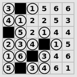<details> <summary>extracted/5699650/img/puzzles/singles.png Details</summary>  ### Visual Description ## Grid Puzzle ### Overview The image shows a grid puzzle, likely a variation of Sudoku or a similar number placement game. The grid is 6x6, with some cells containing numbers and others containing black squares or numbers enclosed in circles. The objective is likely to fill the remaining cells with numbers following specific rules. ### Components/Axes * **Grid:** A 6x6 grid. * **Numbers:** Integers from 1 to 6 are present in some cells. * **Circles:** Some numbers are enclosed in circles. * **Black Squares:** Some cells are filled with black squares. ### Detailed Analysis The grid contains the following numbers and arrangements: * **Row 1:** (3), Black Square, (1), 5, 6, 6 * **Row 2:** (4), (1), 2, 2, 5, 3 * **Row 3:** Black Square, (5), 2, (1), 4, 4 * **Row 4:** (2), (3), (4), Black Square, (1), 5 * **Row 5:** (1), (6), Black Square, (3), 4, 6 * **Row 6:** (5), Black Square, (3), (4), 6, 1 ### Key Observations * The numbers 1 through 6 appear in the grid. * Some numbers are enclosed in circles, which might indicate a constraint or rule related to those numbers. * Black squares likely represent cells that cannot be filled with numbers. ### Interpretation The image presents a partially completed number puzzle. The presence of circled numbers and black squares suggests specific rules or constraints that govern how the remaining cells should be filled. Without knowing the exact rules of the puzzle, it's impossible to determine the correct solution. The puzzle likely involves placing numbers 1-6 in each row, column, and possibly other defined regions, without repetition, while adhering to the constraints imposed by the circled numbers and black squares. </details> Figure 33: Singles: Black out the right set of duplicate numbers. 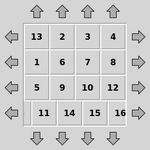<details> <summary>extracted/5699650/img/puzzles/sixteen.png Details</summary>  ### Visual Description ## Diagram: Grid with Numbered Cells and Arrows ### Overview The image is a diagram of a 4x4 grid, with each cell containing a number from 1 to 16. Arrows surround the grid, pointing inwards towards the grid's edges. ### Components/Axes * **Grid:** A 4x4 grid structure. * **Cells:** Each cell contains a unique number from 1 to 16. * **Arrows:** Arrows are positioned around the perimeter of the grid, pointing inwards. ### Detailed Analysis The grid is composed of 16 cells arranged in 4 rows and 4 columns. Each cell contains a number. The numbers are arranged as follows: * **Row 1:** 13, 2, 3, 4 * **Row 2:** 1, 6, 7, 8 * **Row 3:** 5, 9, 10, 12 * **Row 4:** 11, 14, 15, 16 Arrows are placed around the grid, indicating a direction towards the grid. There are four arrows on each side of the grid, centered on each edge. ### Key Observations The numbers within the grid are not in sequential order. The arrows suggest an inward direction or influence on the grid. ### Interpretation The diagram likely represents a system or process where elements (represented by numbers) are arranged in a grid-like structure, and external forces (represented by arrows) influence the grid. The non-sequential arrangement of numbers could indicate a specific order or relationship between the elements within the grid. The arrows could represent inputs, constraints, or forces acting upon the elements in the grid. Without additional context, the exact meaning of the diagram is speculative. </details> Figure 34: Sixteen: Slide a row at a time to arrange the tiles into order. 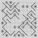<details> <summary>extracted/5699650/img/puzzles/slant.png Details</summary>  ### Visual Description ## Diagram: Grid with Numbered Nodes and Connecting Lines ### Overview The image is a diagram featuring a grid with nodes placed at the intersections. Each node is labeled with a number, and lines connect some of these nodes. The diagram appears to represent a network or a flow of some kind. ### Components/Axes * **Grid:** A square grid provides the underlying structure. * **Nodes:** Circles containing numbers are placed at grid intersections. The numbers range from 0 to 3. * **Lines:** Straight lines connect some of the nodes, forming a network. * **Node Labels:** The numbers inside the circles are node labels. The labels are integers from 0 to 3. ### Detailed Analysis The diagram consists of a grid with nodes and connecting lines. The nodes are labeled with numbers, and the lines connect some of these nodes. * **Top Row:** * Node (1) at the top-left. * Node (0) next to it. * Node (3) further to the right. * Node (3) and Node (2) in the top-right. * Node (0) at the top-right corner. * **Middle Rows:** * Nodes labeled (2), (3), (2), (2), (3), (2), (3), (2), (1), (2), (1), and (0) are present in the middle rows. * **Bottom Row:** * Nodes labeled (0), (0), (1), (0), (1), and (0) are present in the bottom row. The lines connect the nodes in a seemingly arbitrary manner, forming a network. ### Key Observations * The numbers on the nodes range from 0 to 3. * The lines connect nodes in various directions. * The diagram appears to represent a network or a flow of some kind. ### Interpretation The diagram likely represents a network or a flow of some kind, where the nodes represent locations or states, and the lines represent connections or transitions between them. The numbers on the nodes could represent some property of the location or state, such as its capacity or its priority. The diagram could be used to model a variety of systems, such as a transportation network, a communication network, or a manufacturing process. </details> Figure 35: Slant: Draw a maze of slanting lines that matches the clues. 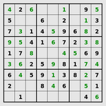<details> <summary>extracted/5699650/img/puzzles/solo.png Details</summary>  ### Visual Description ## Sudoku Puzzle: Solved Grid ### Overview The image shows a solved Sudoku puzzle. The grid is 9x9, divided into nine 3x3 subgrids. The numbers 1-9 appear in each row, column, and subgrid without repetition. The green numbers indicate the solution, while the black numbers were likely given at the start of the puzzle. ### Components/Axes * **Grid:** 9x9 cells * **Subgrids:** Nine 3x3 blocks * **Numbers:** Digits 1 through 9 * **Color Coding:** Green numbers represent the solution, black numbers represent the initial state. ### Detailed Analysis or ### Content Details Here's the Sudoku grid with the numbers extracted. Green numbers are the solution, and black numbers are the initial state. Row 1: 4, 2, 6, 3, 8, 1, 7, 9, 5 Row 2: 5, 8, 9, 6, 7, 2, 4, 1, 3 Row 3: 7, 3, 1, 4, 5, 9, 6, 8, 2 Row 4: 9, 5, 4, 1, 6, 7, 2, 3, 8 Row 5: 1, 7, 8, 2, 3, 4, 5, 6, 9 Row 6: 3, 6, 2, 5, 9, 8, 1, 7, 4 Row 7: 6, 4, 5, 9, 1, 3, 8, 2, 7 Row 8: 2, 9, 3, 8, 4, 6, 7, 5, 1 Row 9: 8, 1, 7, 3, 2, 5, 4, 6 ### Key Observations * The puzzle is solved correctly, with each row, column, and 3x3 subgrid containing the numbers 1-9 without repetition. * The green numbers are distributed throughout the grid, indicating that the puzzle required solving in multiple locations. ### Interpretation The image presents a solved Sudoku puzzle, demonstrating a successful application of logical deduction and problem-solving skills. The distribution of green numbers suggests that the puzzle was not trivial and required a significant amount of reasoning to complete. The initial state (represented by the black numbers) provided a starting point, and the solver was able to fill in the missing numbers while adhering to the rules of Sudoku. </details> Figure 36: Solo: Fill in the grid so that each row, column and square block contains one of every digit. 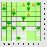<details> <summary>extracted/5699650/img/puzzles/tents.png Details</summary>  ### Visual Description ## Diagram: Grid with Trees and Triangles ### Overview The image shows a grid with trees and triangles scattered across it. Numbers are present along the right and bottom edges of the grid. ### Components/Axes * **Grid:** An 8x8 grid with alternating light green and white cells. * **Trees:** Green tree icons are placed in some of the cells. * **Triangles:** Yellow triangle icons are placed in some of the cells. * **Right Edge Numbers:** Numbers 3, 1, 1, 1, 1, 1, 3, 1 are listed vertically along the right edge of the grid. * **Bottom Edge Numbers:** Numbers 3, 0, 2, 1, 2, 2, 1, 1 are listed horizontally along the bottom edge of the grid. ### Detailed Analysis The grid contains a mix of trees and triangles. The numbers along the right and bottom edges likely represent some kind of constraint or count related to the trees and triangles within the grid. * **Row 1:** Contains 2 triangles and 2 trees. The number on the right is 3. * **Row 2:** Contains 1 tree. The number on the right is 1. * **Row 3:** Contains 1 tree and 1 triangle. The number on the right is 1. * **Row 4:** Contains 1 tree. The number on the right is 1. * **Row 5:** Contains 1 tree. The number on the right is 1. * **Row 6:** Contains 2 trees. The number on the right is 1. * **Row 7:** Contains 1 tree. The number on the right is 3. * **Row 8:** Contains 1 tree. The number on the right is 1. * **Column 1:** Contains 2 trees. The number on the bottom is 3. * **Column 2:** Contains 0 trees or triangles. The number on the bottom is 0. * **Column 3:** Contains 2 trees. The number on the bottom is 2. * **Column 4:** Contains 1 tree. The number on the bottom is 1. * **Column 5:** Contains 2 trees. The number on the bottom is 2. * **Column 6:** Contains 1 triangle and 1 tree. The number on the bottom is 2. * **Column 7:** Contains 1 tree. The number on the bottom is 1. * **Column 8:** Contains 1 tree. The number on the bottom is 1. ### Key Observations The numbers along the edges do not directly correspond to the number of trees in each row or column. The numbers may represent a more complex rule or constraint. ### Interpretation The image likely represents a puzzle or game where the goal is to place trees and triangles in the grid according to certain rules, possibly related to the numbers along the edges. The numbers could represent the total number of trees and triangles, or some other constraint. Without further context, the exact rules of the puzzle are unclear. </details> Figure 37: Tents: Place a tent next to each tree. 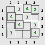<details> <summary>extracted/5699650/img/puzzles/towers.png Details</summary>  ### Visual Description ## 3D Grid Diagram: Numerical Distribution ### Overview The image is a 3D grid diagram representing a 4x4 matrix. Each cell in the grid is represented by a stack of cubes, with the height of the stack indicated by a green number on the top cube. The diagram also includes numerical labels along the top, bottom, left, and right edges, indicating row and column indices or potentially some other associated value. ### Components/Axes * **Grid:** A 4x4 grid structure formed by stacked cubes. * **Cell Values:** Green numbers (3, 4, 2) displayed on the top cube of each stack, representing the height or value associated with that cell. * **Edge Labels:** Numerical labels (1, 2, 3) along the top, bottom, left, and right edges of the grid. ### Detailed Analysis The grid contains the following values in each cell: * **Row 1:** 3, 4, 2 * **Row 2:** 4, 3 * **Row 3:** 4, 3 * **Row 4:** 3, 4 The edge labels are as follows: * **Top:** 2, 2, 1, 3 * **Bottom:** 2, 2, 3, 1 * **Left:** 3, 1, 2, 2 * **Right:** 2, 3, 2, 1 ### Key Observations * The cell values range from 2 to 4. * The edge labels range from 1 to 3. * There is no clear pattern in the distribution of cell values or edge labels. ### Interpretation The diagram represents a numerical distribution across a 4x4 grid. The cell values could represent various metrics, such as frequency, intensity, or magnitude. The edge labels could represent row and column indices, coordinates, or other associated attributes. Without additional context, it is difficult to determine the specific meaning of the values and labels. The diagram could be used to visualize data, represent a mathematical matrix, or illustrate a spatial distribution of values. </details> Figure 38: Towers: Complete the latin square of towers in accordance with the clues. 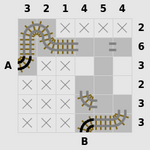<details> <summary>extracted/5699650/img/puzzles/tracks.png Details</summary>  ### Visual Description ## Grid Diagram: Rail Puzzle ### Overview The image is a grid-based puzzle featuring rail tracks. The grid is 6x6, with some cells containing rail segments, 'X' marks, or empty spaces. The goal appears to be connecting point A to point B with a continuous rail line. Numbers are present along the top and right edges of the grid, possibly indicating constraints or counts. ### Components/Axes * **Grid:** 6x6 grid of cells. * **Rails:** Curved and straight rail segments. * **Start/End Points:** Points labeled 'A' (top-left) and 'B' (bottom-center). * **X Marks:** 'X' symbols in some cells, likely indicating invalid paths. * **Numbers:** Numbers 3, 2, 1, 4, 5, 4 along the top edge and 2, 6, 3, 2, 3, 3 along the right edge. * **Equal Sign:** An equal sign is present in the second row, fifth column. ### Detailed Analysis * **Top Row:** * Column 1: 3 * Column 2: 2 * Column 3: 1 * Column 4: 4 * Column 5: 5 * Column 6: 4 * **Left Column:** A is located at the start of the rail track. * **Right Column:** * Row 1: 2 * Row 2: 6 * Row 3: 3 * Row 4: 2 * Row 5: 3 * Row 6: 3 * **Bottom Row:** B is located at the start of the rail track. * **Rail Placement:** * A curved rail segment starts at point A in the top-left corner. * A straight rail segment extends from the curved segment. * Another curved rail segment is near point B in the bottom-center. * **X Marks:** The 'X' marks are scattered throughout the grid, indicating blocked or invalid cells. * **Equal Sign:** The equal sign is in the second row, fifth column. ### Key Observations * The puzzle involves connecting points A and B with a continuous rail line, avoiding cells marked with 'X'. * The numbers along the top and right edges likely represent constraints or counts related to the rail placement. * The equal sign may indicate a specific condition or requirement for the puzzle. ### Interpretation The image presents a logic puzzle where the objective is to connect two points with a rail line, adhering to certain constraints. The numbers along the edges likely represent the number of rail segments or other elements that must be present in each row or column. The 'X' marks indicate invalid paths, and the equal sign may represent a specific condition that must be met for the puzzle to be solved. The puzzle requires spatial reasoning and problem-solving skills to determine the correct placement of rail segments to create a continuous path from A to B while satisfying all constraints. </details> Figure 39: Tracks: Fill in the railway track according to the clues. 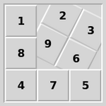<details> <summary>extracted/5699650/img/puzzles/twiddle.png Details</summary>  ### Visual Description ## Diagram: Numbered Grid with Overlapping Tiles ### Overview The image shows a 3x3 grid with numbers 1 through 9. Some of the grid cells are partially covered by overlapping tiles. ### Components/Axes * **Grid:** A 3x3 grid structure. * **Numbers:** The numbers 1 through 9 are placed within the grid cells. * **Overlapping Tiles:** Several tiles overlap the grid, partially obscuring some of the numbered cells. ### Detailed Analysis * **Cell 1:** Contains the number "1". * **Cell 2:** Contains the number "2". Partially covered by a tile. * **Cell 3:** Contains the number "3". Partially covered by a tile. * **Cell 4:** Contains the number "4". * **Cell 5:** Contains the number "5". * **Cell 6:** Contains the number "6". Partially covered by a tile. * **Cell 7:** Contains the number "7". * **Cell 8:** Contains the number "8". * **Cell 9:** Contains the number "9". Partially covered by a tile. ### Key Observations * The tiles overlap cells 2, 3, 6, and 9. * The numbers are arranged sequentially from 1 to 9. * The grid is a standard 3x3 arrangement. ### Interpretation The image appears to be a visual puzzle or a representation of a spatial arrangement where some elements are obscured by others. The overlapping tiles introduce a layer of complexity, potentially requiring the viewer to mentally reconstruct the complete grid. The image does not provide any specific data or facts, but rather presents a visual arrangement. </details> Figure 40: Twiddle: Rotate the tiles around themselves to arrange them into order. 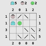<details> <summary>extracted/5699650/img/puzzles/undead.png Details</summary>  ### Visual Description ## Grid Puzzle: Character Placement ### Overview The image shows a grid puzzle with character counts above and to the side. The goal appears to be to place characters in the grid such that the number of characters in each row and column matches the numbers provided. The characters are a ghost, a vampire, and a smiley face. Diagonal lines are present in some cells. ### Components/Axes * **Characters:** Ghost (blue), Vampire (dark red), Smiley Face (green) * **Grid:** 4x4 grid * **Row Labels:** 1, 1, 3, 1 (left side) and 1, 1, 2, 5 (right side) * **Column Labels:** 2, 0, 1, 2 (top) and 2, 0, 0, 0 (bottom) * **Character Counts:** Ghost: 5, Vampire: 2, Smiley Face: 2 ### Detailed Analysis The grid is a 4x4 matrix. The numbers around the grid indicate the number of characters that should be present in each row and column. The diagonal lines in some cells might indicate restrictions on character placement. * **Row 1:** Labelled '1' on both sides. Contains a vampire in the first cell. * **Row 2:** Labelled '1' on both sides. Contains a ghost in the first cell and a smiley face in the second cell. * **Row 3:** Labelled '3' on the left and '2' on the right. * **Row 4:** Labelled '1' on the left and '5' on the right. * **Column 1:** Labelled '2' on top and '2' on the bottom. * **Column 2:** Labelled '0' on top and '0' on the bottom. * **Column 3:** Labelled '1' on top and '0' on the bottom. * **Column 4:** Labelled '2' on top and '0' on the bottom. ### Key Observations * Column 2 must be empty. * The total number of characters required in the rows (1+1+3+1 = 6 or 1+1+2+5 = 9) does not match the total number of characters required in the columns (2+0+1+2 = 5 or 2+0+0+0 = 2). This suggests there might be an error in the labels or that the numbers on the left/top are different from the numbers on the right/bottom. * The total number of characters to place is 5 ghosts + 2 vampires + 2 smiley faces = 9 characters. ### Interpretation The image presents a logic puzzle where the goal is to place characters into a grid based on row and column constraints. The diagonal lines likely represent restrictions on where characters can be placed. The inconsistency in row and column totals suggests a potential error in the puzzle's setup or that the numbers on the left/top are different from the numbers on the right/bottom. The puzzle requires careful planning to ensure all constraints are met. </details> Figure 41: Undead: Place ghosts, vampires and zombies so that the right numbers of them can be seen in mirrors. <details> <summary>extracted/5699650/img/puzzles/unequal.png Details</summary>  ### Visual Description ## Diagram: Grid Puzzle ### Overview The image shows a 4x4 grid puzzle with some cells containing numbers (1 or 4) and arrows indicating movement directions. The grid appears to be part of a logic or number puzzle. ### Components/Axes * **Grid:** A 4x4 grid of square cells. * **Numbers:** Some cells contain the number 1 or 4, displayed in green. * **Arrows:** Arrows indicate movement directions between cells. ### Detailed Analysis or ### Content Details Here's a breakdown of the grid's contents: * **Row 1:** * Cell 1: 4 (green) * Cell 2: Empty * Cell 3: Empty, with an arrow pointing left from Cell 3 to Cell 2. * Cell 4: Empty * **Row 2:** * Cell 1: Empty, with an arrow pointing down from Cell 1 in Row 1. * Cell 2: Empty * Cell 3: 4 (green) * Cell 4: Empty * **Row 3:** * Cell 1: Empty * Cell 2: 4 (green), with an arrow pointing up to Cell 2 in Row 2. * Cell 3: Empty * Cell 4: 1 (green), with an arrow pointing right from Cell 3 to Cell 4. * **Row 4:** * Cell 1: Empty, with an arrow pointing down from Cell 1 in Row 3. * Cell 2: Empty * Cell 3: 1 (green) * Cell 4: 4 (black) ### Key Observations * The numbers 1 and 4 are present in the grid. * Arrows indicate movement or relationships between cells. * The number 4 appears in green and black, while the number 1 appears only in green. ### Interpretation The image likely represents a puzzle where the goal is to fill the empty cells based on the numbers and arrow directions. The different colors of the number 4 might indicate different states or conditions within the puzzle. The arrows likely indicate the direction of a mathematical operation or a logical constraint. The puzzle's rules are not explicitly stated, but the arrangement of numbers and arrows suggests a logical or numerical challenge. </details> Figure 42: Unequal: Complete the latin square in accordance with the > signs. <details> <summary>extracted/5699650/img/puzzles/unruly.png Details</summary>  ### Visual Description ## Image Analysis: Abstract Grid Pattern ### Overview The image presents an abstract grid pattern composed of square tiles in varying shades of gray, black, and white. The tiles are arranged in a grid format, with some tiles appearing to be recessed or elevated, creating a three-dimensional effect. The pattern lacks any immediately discernible representational meaning and appears to be an artistic or abstract composition. ### Components/Axes * **Grid Structure:** The image is organized as a grid, with tiles arranged in rows and columns. The grid appears to be approximately 7x7. * **Tile Colors:** The tiles are colored in shades of gray, black, and white. * **Tile Elevation:** Some tiles appear to be recessed or elevated, adding a three-dimensional element to the pattern. ### Detailed Analysis The grid consists of 49 tiles. The distribution of colors appears random, with no immediately obvious pattern. The recessed or elevated tiles are also distributed seemingly randomly. ### Key Observations * The image is an abstract composition with no clear representational meaning. * The use of varying shades of gray, black, and white creates visual interest. * The recessed or elevated tiles add a three-dimensional element to the pattern. ### Interpretation The image is likely intended as an artistic or abstract composition. The lack of a clear representational meaning allows for individual interpretation. The use of varying shades of gray, black, and white, along with the recessed or elevated tiles, creates visual interest and adds depth to the pattern. The image could be interpreted as a representation of chaos, order, or a combination of both. </details> Figure 43: Unruly: Fill in the black and white grid to avoid runs of three. <details> <summary>extracted/5699650/img/puzzles/untangle.png Details</summary>  ### Visual Description ## Diagram: Network Graph ### Overview The image depicts a network graph consisting of nodes (represented by blue circles) connected by edges (represented by black lines). The graph appears to be undirected and unweighted. The nodes are arranged in a somewhat irregular pattern. ### Components/Axes * **Nodes:** Represented by blue circles. * **Edges:** Represented by black lines connecting the nodes. * **Background:** Light gray. ### Detailed Analysis The graph consists of 12 nodes. The connectivity between the nodes varies. Some nodes have a high degree (connected to many other nodes), while others have a low degree. * **Node 1 (bottom-left):** Connected to 2 other nodes. * **Node 2 (below Node 1):** Connected to 2 other nodes. * **Node 3 (left of Node 1):** Connected to 3 other nodes. * **Node 4 (above Node 3):** Connected to 2 other nodes. * **Node 5 (center):** Connected to 4 other nodes. * **Node 6 (top-left):** Connected to 3 other nodes. * **Node 7 (top):** Connected to 3 other nodes. * **Node 8 (top-right):** Connected to 3 other nodes. * **Node 9 (right of Node 7):** Connected to 2 other nodes. * **Node 10 (bottom-right):** Connected to 2 other nodes. * **Node 11 (above Node 5):** Connected to 2 other nodes. * **Node 12 (above Node 6):** Connected to 2 other nodes. ### Key Observations * The graph is not fully connected, meaning there are nodes that cannot be reached from other nodes without traversing multiple edges. * The node in the center (Node 5) appears to be a central hub, connecting to several other nodes. * There is a cluster of nodes in the bottom-left corner (Nodes 1, 2, and 3) that are highly interconnected. ### Interpretation The network graph visually represents relationships or connections between different entities. The specific meaning of the nodes and edges depends on the context in which the graph is used. For example, the nodes could represent people, and the edges could represent friendships. Or, the nodes could represent computers, and the edges could represent network connections. The structure of the graph reveals patterns of connectivity and influence within the network. The central hub (Node 5) could represent a key influencer or a critical infrastructure component. The clustered nodes in the bottom-left corner could represent a close-knit group or a highly integrated system. </details> Figure 44: Untangle: Reposition the points so that the lines do not cross. Appendix E Puzzle-specific Metadata E.1 Action Space We display the action spaces for all supported puzzles in Table 5. The action spaces vary in size and in the types of actions they contain. As a result, an agent must learn the meaning of each action independently for each puzzle. Table 5: The action spaces for each puzzle are listed, along with their cardinalities. The actions are listed with their name in the original Puzzle Collection C code. | Black Box | 5 | UP, DOWN, LEFT, RIGHT, SELECT | | --- | --- | --- | | Bridges | 5 | UP, DOWN, LEFT, RIGHT, SELECT | | Cube | 4 | UP, DOWN, LEFT, RIGHT | | Dominosa | 5 | UP, DOWN, LEFT, RIGHT, SELECT | | Fifteen | 4 | UP, DOWN, LEFT, RIGHT | | Filling | 13 | UP, DOWN, LEFT, RIGHT, 1, 2, 3, 4, 5, 6, 7, 8, 9 | | Flip | 5 | UP, DOWN, LEFT, RIGHT, SELECT | | Flood | 5 | UP, DOWN, LEFT, RIGHT, SELECT | | Galaxies | 5 | UP, DOWN, LEFT, RIGHT, SELECT | | Guess | 5 | UP, DOWN, LEFT, RIGHT, SELECT | | Inertia | 9 | 1, 2, 3, 4, 6, 7, 8, 9, UNDO | | Keen | 14 | UP, DOWN, LEFT, RIGHT, SELECT2, 1, 2, 3, 4, 5, 6, 7, 8, 9 | | Light Up | 5 | UP, DOWN, LEFT, RIGHT, SELECT | | Loopy | 6 | UP, DOWN, LEFT, RIGHT, SELECT, SELECT2 | | Magnets | 6 | UP, DOWN, LEFT, RIGHT, SELECT, SELECT2 | | Map | 5 | UP, DOWN, LEFT, RIGHT, SELECT | | Mines | 7 | UP, DOWN, LEFT, RIGHT, SELECT, SELECT2, UNDO | | Mosaic | 6 | UP, DOWN, LEFT, RIGHT, SELECT, SELECT2 | | Net | 5 | UP, DOWN, LEFT, RIGHT, SELECT | | Netslide | 5 | UP, DOWN, LEFT, RIGHT, SELECT | | Palisade | 5 | UP, DOWN, LEFT, RIGHT, CTRL | | Pattern | 6 | UP, DOWN, LEFT, RIGHT, SELECT, SELECT2 | | Pearl | 5 | UP, DOWN, LEFT, RIGHT, SELECT | | Pegs | 6 | UP, DOWN, LEFT, RIGHT, SELECT, UNDO | | Range | 5 | UP, DOWN, LEFT, RIGHT, SELECT | | Rectangles | 5 | UP, DOWN, LEFT, RIGHT, SELECT | | Same Game | 6 | UP, DOWN, LEFT, RIGHT, SELECT, UNDO | | Signpost | 6 | UP, DOWN, LEFT, RIGHT, SELECT, SELECT2 | | Singles | 6 | UP, DOWN, LEFT, RIGHT, SELECT, SELECT2 | | Sixteen | 6 | UP, DOWN, LEFT, RIGHT, SELECT, SELECT2 | | Slant | 6 | UP, DOWN, LEFT, RIGHT, SELECT, SELECT2 | | Solo | 13 | UP, DOWN, LEFT, RIGHT, 1, 2, 3, 4, 5, 6, 7, 8, 9 | | Tents | 6 | UP, DOWN, LEFT, RIGHT, SELECT, SELECT2 | | Towers | 14 | UP, DOWN, LEFT, RIGHT, SELECT2, 1, 2, 3, 4, 5, 6, 7, 8, 9 | | Tracks | 5 | UP, DOWN, LEFT, RIGHT, SELECT | | Twiddle | 6 | UP, DOWN, LEFT, RIGHT, SELECT, SELECT2 | | Undead | 8 | UP, DOWN, LEFT, RIGHT, SELECT2, 1, 2, 3 | | Unequal | 13 | UP, DOWN, LEFT, RIGHT, 1, 2, 3, 4, 5, 6, 7, 8, 9 | | Unruly | 6 | UP, DOWN, LEFT, RIGHT, SELECT, SELECT2 | | Untangle | 5 | UP, DOWN, LEFT, RIGHT, SELECT | E.2 Optional Parameters We display the optional parameters for all supported puzzles in LABEL:tab:parameters. If none are supplied upon initialization, a set of default parameters gets used for the puzzle generation process. Table 6: For each puzzle, all optional parameters a user may supply are shown and described. We also give the required data type of variable, where applicable (e.g., int or char). For parameters that accept one of a few choices (such as difficulty), the accepted values and corresponding explanation are given in braces. As as example: a difficulty parameter is listed as d{int} with allowed values {0 = easy, 1 = medium, 2 = hard}. In this case, choosing medium difficulty would correspond to d1. | Black Box | w8h8m5M5 | w{int} | grid width | (w $·$ h + w + h + 1) | | --- | --- | --- | --- | --- | | h{int} | grid height | $·$ (w + 2) $·$ (h + 2) | | | | m{int} | minimum number of balls | | | | | M{int} | maximum number of balls | | | | | Bridges | 7x7i5e2m2d0 | {int}x{int} | grid width $×$ grid height | 3 $·$ w $·$ $·$ (w + h + 8) | | i{int} | percentage of island squares | | | | | e{int} | expansion factor | | | | | m{int} | max bridges per direction | | | | | d{int} | difficulty {0 = easy, 1 = medium, 2 = hard} | | | | | Cube | c4x4 | {char} | type {c = cube, t = tetrahedron, | w $·$ $·$ F | | o = octahedron, i = icosahedron} | F = number of the body’s faces | | | | | {int}x{int} | grid width $×$ grid height | | | | | Dominosa | 6db | {int} | maximum number of dominoes | $\frac{1}{2}\left(\text{w}^{2}\text{ + 3w + 2}\right)$ | | d{char} | difficulty {t = trivial, b = basic, h = hard, | $·(\text{4}\sqrt{\text{w}^{2}\text{ + 3w + 2}}\text{ + 1})$ | | | | e = extreme, a = ambiguous} | | | | | | Fifteen | 4x4 | {int}x{int} | grid width $×$ grid height | $(w· h)^{4}$ | | Filling | 13x9 | {int}x{int} | grid width $×$ grid height | $(w· h)·(w+h+1)$ | | Flip | 5x5c | {int}x{int} | grid width $×$ grid height | $(w· h)·(w+h+1)$ | | {char} | type {c = crosses, r = random} | | | | | Flood | 12x12c6m5 | {int}x{int} | grid width $×$ grid height | $(w· h)·(w+h+1)$ | | c{int} | number of colors | | | | | m{int} | extra moves permitted (above the | | | | | solver’s minimum) | | | | | | Galaxies | 7x7dn | {int}x{int} | grid width $×$ grid height | $(2· w· h-w-h)$ | | d{char} | difficulty {n = normal, u = unreasonable} | $·(2· w+2· h+1)$ | | | | Guess | c6p4g10Bm | c{int} | number of colors | $(p+1)· g·(c+p)$ | | p{int} | pegs per guess | | | | | g{int} | maximum number of guesses | | | | | {char} | allow blanks {B = no, b = yes} | | | | | {char} | allow duplicates {M = no, m = yes} | | | | | Inertia | 10x8 | {int}x{int} | grid width $×$ grid height | $0.2· w^{2}· h^{2}$ | | Keen | 6dn | {int} | grid size | $(2· w+1)· w^{2}$ | | d{char} | difficulty {e = easy, n = normal, h = hard, | | | | | x = extreme, u = unreasonable} | | | | | | {char} | (Optional) multiplication only {m = yes} | | | | | Light Up | 7x7b20s4d0 | {int}x{int} | grid width $×$ grid height | $\frac{1}{2}·(w+h+1)$ | | b{int} | percentage of black squares | $·(w· h+1)$ | | | | s{int} | symmetry {0 = none, 1 = 2-way mirror, | | | | | 2 = 2-way rotational, 3 = 4-way mirror, | | | | | | 4 = 4-way rotational} | | | | | | d{int} | difficulty {0 = easy, 1 = tricky, 2 = hard} | | | | | Loopy | 10x10t12dh | {int}x{int} | grid width $×$ grid height | $(2· w· h+1)· 3·(w· h)^{2}$ | | t{int} | type {0 = squares, 1 = triangular, | | | | | 2 = honeycomb, 3 = snub-square, | | | | | | 4 = cairo, 5 = great-hexagonal, | | | | | | 6 = octagonal, 7 = kites, | | | | | | 8 = floret, 9 = dodecagonal, | | | | | | 10 = great-dodecagonal, | | | | | | 11 = Penrose (kite/dart), | | | | | | 12 = Penrose (rhombs), | | | | | | 13 = great-great-dodecagonal, | | | | | | 14 = kagome, 15 = compass-dodecagonal, | | | | | | 16 = hats} | | | | | | d{char} | difficulty {e = easy, n = normal, | | | | | t = tricky, h = hard} | | | | | | Magnets | 6x5dtS | {int}x{int} | grid width $×$ grid height | $w· h·(w+h+2)$ | | d{char} | difficulty {e = easy, t = tricky | | | | | {char} | (Optional) strip clues {S = yes} | | | | | Map | 20x15n30dn | {int}x{int} | grid width $×$ grid height | $2· n·(1+w+h)$ | | n{int} | number of regions | | | | | d{char} | difficulty {e = easy, n = normal, h = hard, | | | | | u = unreasonable} | | | | | | Mines | 9x9n10 | {int}x{int} | grid width $×$ grid height | $w· h·(w+h+1)$ | | n{int} | number of mines | | | | | p{char} | (Optional) ensure solubility {a = no} | | | | | Mosaic | 10x10h0 | {int}x{int} | grid width $×$ grid height | $w· h·(w+h+1)$ | | {str} | (Optional) aggressive generation {h0 = no} | | | | | Net | 5x5wb0.5 | {int}x{int} | grid width $×$ grid height | $w· h·(w+h+3)$ | | {char} | (Optional) walls wrap around {w = yes} | | | | | b{float} | barrier probability, interval: [0, 1] | | | | | {char} | (Optional) ensure unique solution {a = no} | | | | | Netslide | 4x4wb1m2 | {int}x{int} | grid width $×$ grid height | $2· w· h·(w+h-1)$ | | {char} | (Optional) walls wrap around {w = yes} | | | | | b{float} | barrier probability, interval: [0, 1] | | | | | m{int} | (Optional) number of shuffling moves | | | | | Palisade | 5x5n5 | {int}x{int} | grid width $×$ grid height | $(2· w· h-w-h)$ | | n{int} | region size | $·(w+h+3)$ | | | | Pattern | 15x15 | {int}x{int} | grid width $×$ grid height | $w· h(w+h+1)$ | | Pearl | 8x8dtn | {int}x{int} | grid width $×$ grid height | $w· h·(w+h+2)$ | | d{char} | difficulty {e = easy, t = tricky} | | | | | {char} | allow unsoluble {n = yes} | | | | | Pegs | 7x7cross | {int}x{int} | grid width $×$ grid height | $w· h·(w+h+2)$ | | {str} | type {cross, octagon, random} | | | | | Range | 9x6 | {int}x{int} | grid width $×$ grid height | $w· h·(w+h+1)$ | | Rectangles | 7x7e4 | {int}x{int} | grid width $×$ grid height | $2· w· h·(w+h+1)$ | | e{int} | expansion factor | | | | | {char} | ensure unique solution {a = no} | | | | | Same Game | 5x5c3s2 | {int}x{int} | grid width $×$ grid height | $w· h·(w+h+2)$ | | c{int} | number of colors | | | | | s{int} | scoring system {1 = $(n-1)^{2}$ , | | | | | 2 = $(n-2)^{2}$ } | | | | | | {char} | (Optional) ensure solubility {r = no} | | | | | Signpost | 4x4c | {int}x{int} | grid width $×$ grid height | $2· w· h·(w+h+1)$ | | {char} | (Optional) start and end in corners | | | | | {c = yes} | | | | | | Singles | 5x5de | {int}x{int} | grid width $×$ grid height | $w· h·(w+h+1)$ | | d{char} | difficulty {e = easy, k = tricky} | | | | | Sixteen | 5x5m2 | {int}x{int} | grid width $×$ grid height | $w· h·(w+h+3)$ | | m{int} | (Optional) number of shuffling moves | | | | | Slant | 8x8de | {int}x{int} | grid width $×$ grid height | $w· h·(w+h+1)$ | | d{char} | difficulty {e = easy, h = hard} | | | | | Solo | 3x3 | {int}x{int} | rows of sub-blocks $×$ cols of sub-blocks | $(w· h)^{2}*(2· w· h+1)$ | | {char} | (Optional) require every digit on each | | | | | main diagonal {x = yes} | | | | | | * | | {char} | (Optional) jigsaw (irregularly shaped | | | sub-blocks) main diagonal {j = yes} | | | | | | * | | {char} | (Optional) killer (digit sums) {k = yes} | | | * | | {str} | (Optional) symmetry. If not set, | | | it is 2-way rotation. {a = None, | | | | | | m2 = 2-way mirror, m4 = 4-way mirror, | | | | | | r4 = 4-way rotation, m8 = 8-way mirror, | | | | | | md2 = 2-way diagonal mirror, | | | | | | md4 = 4-way diagonal mirror} | | | | | | d{char} | difficulty {t = trivial, b = basic, | | | | | i = intermediate, a = advanced, | | | | | | e = extreme, u = unreasonable} | | | | | | Tents | 8x8de | {int}x{int} | grid width $×$ grid height | $\frac{1}{4}·(w+1)·(h+1)$ | | d{char} | difficulty {e = easy, t = tricky} | $·(w+h+1)$ | | | | Towers | 5de | {int} | grid size | $2·(w+1)· w^{2}$ | | d{char} | difficulty {e = easy, h = hard | | | | | x = extreme, u = unreasonable} | | | | | | Tracks | 8x8dto | {int}x{int} | grid width $×$ grid height | $w· h(2·(w+h)+1)$ | | d{char} | difficulty {e = easy, t = tricky, h = hard} | | | | | {char} | (Optional) disallow consecutive 1 clues | | | | | {o = no} | | | | | | Twiddle | 3x3n2 | {int}x{int} | grid width $×$ grid height | $(2· w· h· n^{2}+1)$ | | n{int} | rotating block size | $·(w+h-2· n+1)$ | | | | {char} | (Optional) one number per row {r = yes} | | | | | {char} | (Optional) orientation matters {o = yes} | | | | | m{int} | (Optional) number of shuffling moves | | | | | Undead | 4x4dn | {int}x{int} | grid width $×$ grid height | $w· h·(w+h+1)$ | | d{char} | difficulty {e = easy, n = normal, t = tricky} | | | | | Unequal | 4adk | {int} | grid size | $w^{2}·(2· w+1)$ | | {char} | (Optional) adjacent mode {a = yes} | | | | | d{char} | difficulty {t = trivial, e = easy, k = tricky, | | | | | x = extreme, r = recursive} | | | | | | Unruly | 8x8dt | {int} | grid size | $w· h·(w+h+1)$ | | {char} | (Optional) unique rows and cols {u = yes} | | | | | d{char} | difficulty {t = trivial, e = easy, n = normal} | | | | | Untangle | 25 | {int} | number of points | $n·(n+\sqrt{3n}· 4+2)$ | E.3 Baseline Parameters In Table 7, the parameters used for training the agents used for the comparisons in Section 3 is shown. Table 7: Listed below are the generation parameters supplied to each puzzle instance before training an agent, as well as some puzzle-specific notes. We propose the easiest preset difficulty setting as a first challenge for RL algorithms to reach human-level performance. | Black Box | w2h2m2M2 | w5h5m3M3 | | | --- | --- | --- | --- | | Bridges | 3x3 | 7x7i30e10m2d0 | | | Cube | c3x3 | c4x4 | | | Dominosa | 1dt | 3dt | | | Fifteen | 2x2 | 4x4 | | | Filling | 2x3 | 9x7 | | | Flip | 3x3c | 3x3c | | | Flood | 3x3c6m5 | 12x12c6m5 | | | Galaxies | 3x3de | 7x7dn | | | Guess | c2p3g10Bm | c6p4g10Bm | Episodes were terminated and negatively rewarded | | after the maximum number of guesses was made | | | | | without finding the correct solution. | | | | | Inertia | 4x4 | 10x8 | | | Keen | 3dem | 4de | Even the minimum allowed problem size | | proved to be infeasible for a random agent | | | | | Light Up | 3x3b20s0d0 | 7x7b20s4d0 | | | Loopy | 3x3t0de | 3x3t0de | | | Magnets | 3x3deS | 6x5de | | | Map | 3x3n5de | 20x15n30de | | | Mines | 4x4n2 | 9x9n10 | | | Mosaic | 3x3 | 3x3 | | | Net | 2x2 | 5x5 | | | Netslide | 2x3b1 | 3x3b1 | | | Palisade | 2x3n3 | 5x5n5 | | | Pattern | 3x2 | 10x10 | | | Pearl | 5x5de | 6x6de | | | Pegs | 4x4random | 5x7cross | | | Range | 3x3 | 9x6 | | | Rectangles | 3x2 | 7x7 | | | Same Game | 2x3c3s2 | 5x5c3s2 | | | Signpost | 2x3 | 4x4c | | | Singles | 2x3de | 5x5de | | | Sixteen | 2x3 | 3x3 | | | Slant | 2x2de | 5x5de | | | Solo | 2x2 | 2x2 | | | Tents | 4x4de | 8x8de | | | Towers | 3de | 4de | | | Tracks | 4x4de | 8x8de | | | Twiddle | 2x3n2 | 3x3n2r | | | Undead | 3x3de | 4x4de | | | Unequal | 3de | 4de | | | Unruly | 6x6dt | 8x8dt | Even the minimum allowed problem size | | proved to be infeasible for a random agent | | | | | Untangle | 4 | 6 | | E.4 Detailed Baseline Results We summarize all evaluated algorithms in Table 8. Table 8: Summary of all evaluated RL algorithms. | Proximal Policy Optimization (PPO) [61] Recurrent PPO [62] Advantage Actor Critic (A2C) [63] | On-Policy On-Policy On-Policy | No No No | | --- | --- | --- | | Asynchronous Advantage Actor Critic (A3C) [63] | On-Policy | No | | Trust Region Policy Optimization (TRPO) [64] | On-Policy | No | | Deep Q-Network (DQN) [11] | Off-Policy | No | | Quantile Regression DQN (QRDQN) [65] | Off-Policy | No | | MuZero [66] | Off-Policy | Yes | | DreamerV3 [67] | Off-Policy | No | As we limited the agents to a single final reward upon completion, where possible, we chose puzzle parameters that allowed random policies to successfully find a solution. Note that if a random policy fails to find a solution, an RL algorithm without guidance (such as intermediate rewards) will also be affected by this. If an agent has never accumulated a reward with the initial (random) policy, it will be unable to improve its performance at all. The chosen parameters roughly corresponded to the smallest and easiest puzzles, as more complex puzzles were found to be intractable. This fact is highlighted for example in Solo/Sudoku, where the reasoning needed to find a valid solution is already rather complex, even for a grid with 2 $×$ 2 sub-blocks. A few puzzles were still intractable due to the minimum complexity permitted by Tathams’s puzzle-specific problem generators, such as with Unruly. For the RGB pixel observations, the window size chosen for these small problems was set at 128 $×$ 128 pixels. Table 9: Listed below are the detailed results for all evaluated algorithms. Results show the average number of steps required for all successful episodes and standard deviation with respect to the random seeds. In brackets, we show the overall percentage of successful episodes. In the summary row, the last number in brackets denotes the total number of puzzles where a solution below the upper bound of optimal steps was found. Entries without values mean that no successful policy was found among all random seeds. This Table is continued in Table 10. Puzzle Supplied Parameters Optimal Random PPO TRPO DreamerV3 MuZero Blackbox w2h2m2M2 $144$ $2206$ $(99.2\%)$ $1773± 472$ $(59.5\%)$ $1744± 454$ $(96.3\%)$ $\mathbf{32± 5}$ $(100.0\%)$ $\mathbf{46± 0}$ $(0.1\%)$ Bridges 3x3 $378$ $547$ $(100.0\%)$ $682± 197$ $(85.1\%)$ $546± 13$ $(100.0\%)$ $\mathbf{9± 0}$ $(100.0\%)$ $397± 181$ $(86.7\%)$ Cube c3x3 $54$ $4181$ $(66.9\%)$ $744± 1610$ $(77.5\%)$ $433± 917$ $(99.8\%)$ $5068± 657$ $(22.5\%)$ - Dominosa 1dt $32$ $1980$ $(99.2\%)$ $457± 954$ $(70.0\%)$ $\mathbf{12± 1}$ $(100.0\%)$ $\mathbf{11± 1}$ $(100.0\%)$ $3659± 0$ $(0.0\%)$ Fifteen 2x2 $256$ $54$ $(100.0\%)$ $\mathbf{3± 0}$ $(100.0\%)$ $\mathbf{3± 0}$ $(100.0\%)$ $\mathbf{4± 0}$ $(100.0\%)$ $\mathbf{5± 1}$ $(100.0\%)$ Filling 2x3 $36$ $820$ $(100.0\%)$ $290± 249$ $(97.5\%)$ $\mathbf{9± 2}$ $(100.0\%)$ $443± 56$ $(83.4\%)$ $1099± 626$ $(15.0\%)$ Flip 3x3c $63$ $3138$ $(88.9\%)$ $3008± 837$ $(40.1\%)$ $2951± 564$ $(90.8\%)$ $1762± 568$ $(8.0\%)$ $1207± 1305$ $(3.1\%)$ Flood 3x3c6m5 $63$ $134$ $(97.4\%)$ $\mathbf{12± 0}$ $(99.9\%)$ $\mathbf{21± 4}$ $(99.6\%)$ $\mathbf{14± 1}$ $(100.0\%)$ $994± 472$ $(14.4\%)$ Galaxies 3x3de $156$ $4306$ $(33.9\%)$ $3860± 1778$ $(8.3\%)$ $4755± 527$ $(24.8\%)$ $3367± 1585$ $(11.0\%)$ $6046± 2722$ $(8.2\%)$ Guess c2p3g10Bm $200$ $358$ $(73.4\%)$ - $316± 52$ $(72.0\%)$ $268± 226$ $(77.0\%)$ $\mathbf{24± 0}$ $(0.8\%)$ Inertia 4x4 $51$ $13$ $(6.5\%)$ $\mathbf{22± 9}$ $(6.3\%)$ $635± 1373$ $(5.7\%)$ $926± 217$ $(5.7\%)$ $104± 73$ $(3.1\%)$ Keen 3dem $63$ $3152$ $(0.5\%)$ $3817± 0$ $(0.2\%)$ $5887± 1526$ $(0.4\%)$ $4350± 1163$ $(1.3\%)$ - Lightup 3x3b20s0d0 $35$ $2237$ $(98.1\%)$ $1522± 1115$ $(82.7\%)$ $2127± 168$ $(95.8\%)$ $438± 247$ $(72.0\%)$ $1178± 1109$ $(2.1\%)$ Loopy 3x3t0de $4617$ - - - - - Magnets 3x3deS $72$ $1895$ $(99.1\%)$ $1366± 1090$ $(90.2\%)$ $1912± 60$ $(99.1\%)$ $574± 56$ $(78.5\%)$ $1491± 0$ $(0.7\%)$ Map 3x3n5de $70$ $903$ $(99.9\%)$ $1172± 297$ $(75.7\%)$ $950± 34$ $(99.9\%)$ $1680± 197$ $(64.9\%)$ $467± 328$ $(0.9\%)$ Mines 4x4n2 $144$ $87$ $(18.1\%)$ $2478± 2424$ $(9.9\%)$ $\mathbf{123± 66}$ $(18.8\%)$ $272± 246$ $(50.1\%)$ $\mathbf{19± 22}$ $(4.6\%)$ Mosaic 3x3 $63$ $4996$ $(9.8\%)$ $4928± 438$ $(2.5\%)$ $5233± 615$ $(5.0\%)$ $4469± 387$ $(15.9\%)$ $5586± 0$ $(0.2\%)$ Net 2x2 $28$ $1279$ $(100.0\%)$ $\mathbf{9± 0}$ $(100.0\%)$ $\mathbf{9± 0}$ $(100.0\%)$ $\mathbf{10± 0}$ $(100.0\%)$ $339± 448$ $(8.2\%)$ Netslide 2x3b1 $48$ $766$ $(100.0\%)$ $1612± 1229$ $(41.6\%)$ $635± 145$ $(100.0\%)$ $\mathbf{12± 0}$ $(100.0\%)$ $683± 810$ $(25.0\%)$ Netslide 3x3b1 $90$ $4671$ $(11.0\%)$ $4671± 498$ $(9.2\%)$ $4008± 1214$ $(8.9\%)$ $3586± 677$ $(22.4\%)$ $3721± 1461$ $(13.2\%)$ Palisade 2x3n3 $56$ $1428$ $(100.0\%)$ $939± 604$ $(87.0\%)$ $1377± 35$ $(99.9\%)$ $\mathbf{39± 56}$ $(100.0\%)$ $86± 0$ $(0.0\%)$ Pattern 3x2 $36$ $3247$ $(92.9\%)$ $1542± 1262$ $(71.9\%)$ $2908± 355$ $(90.2\%)$ $820± 516$ $(58.0\%)$ $4063± 1696$ $(1.9\%)$ Pearl 5x5de $300$ - - - - - Pegs 4x4Random $160$ - - - - - Range 3x3 $63$ $535$ $(100.0\%)$ $780± 305$ $(65.8\%)$ $661± 198$ $(99.9\%)$ $888± 238$ $(55.6\%)$ $91± 76$ $(5.1\%)$ Rect 3x2 $72$ $723$ $(100.0\%)$ $\mathbf{27± 44}$ $(99.8\%)$ $\mathbf{9± 4}$ $(100.0\%)$ $\mathbf{8± 1}$ $(100.0\%)$ - Samegame 2x3c3s2 $42$ $76$ $(100.0\%)$ $123± 197$ $(98.8\%)$ $\mathbf{7± 0}$ $(100.0\%)$ $\mathbf{7± 0}$ $(100.0\%)$ $1444± 541$ $(28.7\%)$ Samegame 5x5c3s2 $300$ $571$ $(32.1\%)$ $1003± 827$ $(30.5\%)$ $672± 160$ $(30.8\%)$ $527± 162$ $(30.2\%)$ $\mathbf{184± 107}$ $(4.9\%)$ Signpost 2x3 $72$ $776$ $(96.1\%)$ $838± 53$ $(97.2\%)$ $799± 13$ $(97.0\%)$ $859± 304$ $(91.3\%)$ $4883± 1285$ $(5.9\%)$ Singles 2x3de $36$ $353$ $(100.0\%)$ $\mathbf{7± 3}$ $(100.0\%)$ $\mathbf{7± 4}$ $(100.0\%)$ $\mathbf{11± 8}$ $(99.9\%)$ $733± 551$ $(28.4\%)$ Sixteen 2x3 $48$ $2908$ $(94.1\%)$ $2371± 1226$ $(55.7\%)$ $2968± 181$ $(92.8\%)$ $\mathbf{17± 1}$ $(100.0\%)$ $3281± 472$ $(68.7\%)$ Slant 2x2de $20$ $447$ $(100.0\%)$ $333± 190$ $(80.4\%)$ $21± 2$ $(99.9\%)$ $596± 163$ $(100.0\%)$ $1005± 665$ $(7.4\%)$ Solo 2x2 $144$ - - - - - Tents 4x4de $56$ $4442$ $(44.3\%)$ $4781± 86$ $(10.3\%)$ $4828± 752$ $(31.0\%)$ $3137± 581$ $(12.1\%)$ $4556± 3259$ $(0.6\%)$ Towers 3de $72$ $4876$ $(1.0\%)$ - $3789± 1288$ $(0.5\%)$ $3746± 1861$ $(0.5\%)$ - Tracks 4x4de $272$ $5213$ $(0.5\%)$ $4129± nan$ $(0.1\%)$ $5499± 2268$ $(0.3\%)$ $4483± 1513$ $(0.3\%)$ - Twiddle 2x3n2 $98$ $851$ $(100.0\%)$ $\mathbf{8± 1}$ $(99.9\%)$ $\mathbf{11± 7}$ $(100.0\%)$ $\mathbf{8± 0}$ $(100.0\%)$ $761± 860$ $(37.6\%)$ Undead 3x3de $63$ $4390$ $(40.1\%)$ $4542± 292$ $(5.7\%)$ $4179± 299$ $(31.0\%)$ $4088± 297$ $(35.8\%)$ $3677± 342$ $(9.0\%)$ Unequal 3de $63$ $4540$ $(6.7\%)$ - $5105± 193$ $(3.6\%)$ $2468± 2025$ $(4.8\%)$ $4944± 368$ $(7.2\%)$ Unruly 6x6dt $468$ - - - - - Untangle 4 $150$ $141$ $(100.0\%)$ $\mathbf{13± 1}$ $(100.0\%)$ $\mathbf{11± 0}$ $(100.0\%)$ $\mathbf{6± 0}$ $(100.0\%)$ $499± 636$ $(26.5\%)$ Untangle 6 $79$ $2165$ $(96.9\%)$ $2295± 66$ $(96.2\%)$ $2228± 126$ $(96.5\%)$ $1683± 74$ $(82.0\%)$ $2380± 0$ $(11.2\%)$ Summary - $217$ $1984$ $(71.2\%)$ $1604± 801$ $(61.6\%)(8)$ $1773± 639$ $(70.8\%)(11)$ $1334± 654$ $(62.7\%)(14)$ $1808± 983$ $(16.0\%)(5)$ Table 10: Continuation from Table 9. Listed below are the detailed results for all evaluated algorithms. Results show the average number of steps required for all successful episodes and standard deviation with respect to the random seeds. In brackets, we show the overall percentage of successful episodes. In the summary row, the last number in brackets denotes the total number of puzzles where a solution below the upper bound of optimal steps was found. Entries without values mean that no successful policy was found among all random seeds. Puzzle Supplied Parameters Optimal Random A2C RecurrentPPO DQN QRDQN Blackbox w2h2m2M2 $144$ $2206$ $(99.2\%)$ $2524± 1193$ $(85.2\%)$ $2009± 427$ $(98.7\%)$ $2063± 70$ $(99.0\%)$ $2984± 1584$ $(76.8\%)$ Bridges 3x3 $378$ $547$ $(100.0\%)$ $540± 69$ $(100.0\%)$ $653± 165$ $(100.0\%)$ $549± 20$ $(100.0\%)$ $1504± 2037$ $(83.4\%)$ Cube c3x3 $54$ $4181$ $(66.9\%)$ $4516± 954$ $(17.5\%)$ $4943± 620$ $(16.2\%)$ $4407± 414$ $(43.4\%)$ $4241± 283$ $(26.4\%)$ Dominosa 1dt $32$ $1980$ $(99.2\%)$ $6408± nan$ $(0.2\%)$ $3009± 988$ $(80.6\%)$ $\mathbf{15± 6}$ $(100.0\%)$ $4457± 2183$ $(50.0\%)$ Fifteen 2x2 $256$ $54$ $(100.0\%)$ $\mathbf{4± 1}$ $(100.0\%)$ $\mathbf{3± 0}$ $(100.0\%)$ $\mathbf{3± 0}$ $(100.0\%)$ $\mathbf{3± 0}$ $(100.0\%)$ Filling 2x3 $36$ $820$ $(100.0\%)$ $777± 310$ $(99.3\%)$ $764± 106$ $(100.0\%)$ $761± 109$ $(99.7\%)$ $2828± 2769$ $(63.2\%)$ Flip 3x3c $63$ $3138$ $(88.9\%)$ $4345± 1928$ $(29.4\%)$ $3356± 1412$ $(46.9\%)$ $3493± 129$ $(87.1\%)$ $3741± 353$ $(56.8\%)$ Flood 3x3c6m5 $63$ $134$ $(97.4\%)$ $406± 623$ $(93.4\%)$ $120± 17$ $(97.7\%)$ $128± 12$ $(90.8\%)$ $1954± 2309$ $(65.2\%)$ Galaxies 3x3de $156$ $4306$ $(33.9\%)$ $4586± 980$ $(10.8\%)$ $3939± 1438$ $(0.4\%)$ $4657± 147$ $(26.1\%)$ - Guess c2p3g10Bm $200$ $358$ $(73.4\%)$ - $323± 52$ $(44.6\%)$ $550± 248$ $(71.9\%)$ $3260± 2614$ $(34.4\%)$ Inertia 4x4 $51$ $13$ $(6.5\%)$ $105± 197$ $(6.1\%)$ $1198± 1482$ $(5.6\%)$ $179± 156$ $(7.1\%)$ $1330± 296$ $(5.8\%)$ Keen 3dem $63$ $3152$ $(0.5\%)$ - - $6774± 1046$ $(0.4\%)$ - Lightup 3x3b20s0d0 $35$ $2237$ $(98.1\%)$ $3034± 793$ $(62.7\%)$ $3493± 929$ $(66.5\%)$ $2429± 214$ $(97.5\%)$ $3440± 945$ $(57.8\%)$ Loopy 3x3t0de $4617$ - - - - - Magnets 3x3deS $72$ $1895$ $(99.1\%)$ $3057± 1114$ $(47.9\%)$ $1874± 222$ $(99.2\%)$ $2112± 331$ $(98.1\%)$ $5182± 3878$ $(33.8\%)$ Map 3x3n5de $70$ $903$ $(99.9\%)$ $2552± 1223$ $(52.5\%)$ $2608± 1808$ $(59.4\%)$ $949± 30$ $(99.9\%)$ $1753± 769$ $(78.1\%)$ Mines 4x4n2 $144$ $87$ $(18.1\%)$ $\mathbf{120± 41}$ $(14.7\%)$ $1189± 1341$ $(12.1\%)$ $207± 146$ $(17.6\%)$ $1576± 1051$ $(13.2\%)$ Mosaic 3x3 $63$ $4996$ $(9.8\%)$ $4937± 424$ $(8.4\%)$ $4907± 219$ $(8.3\%)$ $5279± 564$ $(7.0\%)$ $9490± 155$ $(0.0\%)$ Net 2x2 $28$ $1279$ $(100.0\%)$ $149± 288$ $(100.0\%)$ $1232± 92$ $(100.0\%)$ $\mathbf{9± 0}$ $(100.0\%)$ $1793± 1663$ $(81.3\%)$ Netslide 2x3b1 $48$ $766$ $(100.0\%)$ $976± 584$ $(100.0\%)$ $2079± 1989$ $(64.7\%)$ $779± 37$ $(100.0\%)$ $1023± 206$ $(80.9\%)$ Netslide 3x3b1 $90$ $4671$ $(11.0\%)$ $4324± 657$ $(8.1\%)$ $2737± 1457$ $(1.7\%)$ $4099± 846$ $(5.1\%)$ $2025± 1475$ $(0.4\%)$ Palisade 2x3n3 $56$ $1428$ $(100.0\%)$ $1666± 198$ $(99.4\%)$ $1981± 1053$ $(92.5\%)$ $1445± 96$ $(99.9\%)$ $1519± 142$ $(99.8\%)$ Pattern 3x2 $36$ $3247$ $(92.9\%)$ $3445± 635$ $(82.9\%)$ $3733± 513$ $(79.7\%)$ $2809± 733$ $(89.7\%)$ $3406± 384$ $(51.1\%)$ Pearl 5x5de $300$ - - - - - Pegs 4x4Random $160$ - - - - - Range 3x3 $63$ $535$ $(100.0\%)$ $1438± 782$ $(81.4\%)$ $730± 172$ $(99.9\%)$ $594± 28$ $(100.0\%)$ - Rect 3x2 $72$ $723$ $(100.0\%)$ $3470± 2521$ $(17.6\%)$ $916± 420$ $(99.6\%)$ $511± 193$ $(97.4\%)$ $1560± 1553$ $(81.8\%)$ Samegame 2x3c3s2 $42$ $76$ $(100.0\%)$ $\mathbf{8± 1}$ $(100.0\%)$ $1777± 1643$ $(43.5\%)$ $\mathbf{8± 0}$ $(100.0\%)$ $\mathbf{14± 9}$ $(100.0\%)$ Samegame 5x5c3s2 $300$ $571$ $(32.1\%)$ $609± 155$ $(29.9\%)$ $1321± 1170$ $(30.3\%)$ $850± 546$ $(29.2\%)$ $5577± 1211$ $(12.8\%)$ Signpost 2x3 $72$ $776$ $(96.1\%)$ $2259± 1394$ $(85.9\%)$ $1000± 266$ $(77.9\%)$ $793± 17$ $(97.0\%)$ $2298± 2845$ $(78.0\%)$ Singles 2x3de $36$ $353$ $(100.0\%)$ $372± 47$ $(100.0\%)$ $331± 66$ $(100.0\%)$ $361± 47$ $(99.1\%)$ $392± 29$ $(100.0\%)$ Sixteen 2x3 $48$ $2908$ $(94.1\%)$ $3903± 479$ $(71.7\%)$ $3409± 574$ $(67.6\%)$ $2970± 107$ $(93.2\%)$ $4550± 848$ $(21.9\%)$ Slant 2x2de $20$ $447$ $(100.0\%)$ $984± 470$ $(99.8\%)$ $465± 34$ $(100.0\%)$ $496± 97$ $(100.0\%)$ $1398± 2097$ $(87.1\%)$ Solo 2x2 $144$ - - - - - Tents 4x4de $56$ $4442$ $(44.3\%)$ $6157± 1961$ $(2.1\%)$ $4980± 397$ $(12.8\%)$ $4515± 59$ $(38.1\%)$ $5295± 688$ $(7.8\%)$ Towers 3de $72$ $4876$ $(1.0\%)$ $9850± nan$ $(0.0\%)$ $8549± nan$ $(0.0\%)$ $5836± 776$ $(0.5\%)$ - Tracks 4x4de $272$ $5213$ $(0.5\%)$ $4501± nan$ $(0.0\%)$ - $5809± 661$ $(0.3\%)$ - Twiddle 2x3n2 $98$ $851$ $(100.0\%)$ $1248± 430$ $(99.6\%)$ $827± 71$ $(100.0\%)$ $\mathbf{83± 149}$ $(100.0\%)$ $3170± 1479$ $(33.4\%)$ Undead 3x3de $63$ $4390$ $(40.1\%)$ $5818± 154$ $(0.9\%)$ $5060± 2381$ $(0.5\%)$ - - Unequal 3de $63$ $4540$ $(6.7\%)$ $5067± 1600$ $(1.0\%)$ $5929± 1741$ $(1.1\%)$ $5057± 582$ $(5.6\%)$ - Unruly 6x6dt $468$ - - - - - Untangle 4 $150$ $141$ $(100.0\%)$ $1270± 1745$ $(90.4\%)$ $\mathbf{135± 18}$ $(100.0\%)$ $170± 29$ $(100.0\%)$ $871± 837$ $(99.0\%)$ Untangle 6 $79$ $2165$ $(96.9\%)$ $3324± 1165$ $(72.5\%)$ $2739± 588$ $(91.7\%)$ $2219± 84$ $(95.9\%)$ - Summary - $217$ $1984$ $(71.2\%)$ $2743± 954$ $(54.8\%)(3)$ $2342± 989$ $(61.1\%)(2)$ $1999± 365$ $(70.2\%)(5)$ $2754± 1579$ $(56.0\%)(2)$ Table 11: We list the detailed results for all the experiments of action masking and input representation. Results show the average number of steps required for all successful episodes and standard deviation with respect to the random seeds. In brackets, we show the overall percentage of successful episodes. In the summary row, the last number in brackets denotes the total number of puzzles where a solution below the upper bound of optimal steps was found. Entries without values mean that no successful policy was found among all random seeds. Puzzle Supplied Parameters Optimal Random PPO (Internal State) PPO (RGB Pixels) MaskablePPO (Internal State) MaskablePPO (RGB Pixels) Blackbox w2h2m2M2 $144$ $2206$ $(99.2\%)$ $1773± 472$ $(59.5\%)$ $1509± 792$ $(97.9\%)$ $\mathbf{9± 0}$ $(99.7\%)$ $\mathbf{30± 1}$ $(99.2\%)$ Bridges 3x3 $378$ $547$ $(100.0\%)$ $682± 197$ $(85.1\%)$ $\mathbf{89± 176}$ $(99.1\%)$ $\mathbf{25± 0}$ $(99.4\%)$ $\mathbf{9± 0}$ $(99.6\%)$ Cube c3x3 $54$ $4181$ $(66.9\%)$ $744± 1610$ $(77.5\%)$ $3977± 442$ $(67.7\%)$ $\mathbf{16± 1}$ $(81.2\%)$ $410± 157$ $(75.1\%)$ Dominosa 1dt $32$ $1980$ $(99.2\%)$ $457± 954$ $(70.0\%)$ $539± 581$ $(100.0\%)$ $\mathbf{12± 0}$ $(100.0\%)$ $\mathbf{19± 2}$ $(100.0\%)$ Fifteen 2x2 $256$ $54$ $(100.0\%)$ $\mathbf{3± 0}$ $(100.0\%)$ $\mathbf{37± 26}$ $(100.0\%)$ $\mathbf{4± 0}$ $(100.0\%)$ $\mathbf{3± 0}$ $(100.0\%)$ Filling 2x3 $36$ $820$ $(100.0\%)$ $290± 249$ $(97.5\%)$ $373± 175$ $(99.9\%)$ $\mathbf{7± 0}$ $(100.0\%)$ $\mathbf{34± 3}$ $(99.9\%)$ Flip 3x3c $63$ $3138$ $(88.9\%)$ $3008± 837$ $(40.1\%)$ $3616± 395$ $(78.3\%)$ $2174± 1423$ $(70.3\%)$ $319± 128$ $(81.3\%)$ Flood 3x3c6m5 $63$ $134$ $(97.4\%)$ $\mathbf{12± 0}$ $(99.9\%)$ $\mathbf{28± 12}$ $(99.7\%)$ $\mathbf{12± 0}$ $(99.9\%)$ $\mathbf{14± 0}$ $(99.9\%)$ Galaxies 3x3de $156$ $4306$ $(33.9\%)$ $3860± 1778$ $(8.3\%)$ $4439± 224$ $(29.1\%)$ $3640± 928$ $(40.2\%)$ $3372± 430$ $(40.5\%)$ Guess c2p3g10Bm $200$ $358$ $(73.4\%)$ - $344± 35$ $(72.0\%)$ $\mathbf{145± 19}$ $(75.4\%)$ - Inertia 4x4 $51$ $13$ $(6.5\%)$ $\mathbf{22± 9}$ $(6.3\%)$ $237± 10$ $(99.7\%)$ $\mathbf{41± 19}$ $(79.0\%)$ $169± 233$ $(69.8\%)$ Keen 3dem $63$ $3152$ $(0.5\%)$ $3817± 0$ $(0.2\%)$ - - - Lightup 3x3b20s0d0 $35$ $2237$ $(98.1\%)$ $1522± 1115$ $(82.7\%)$ $2401± 148$ $(97.5\%)$ $\mathbf{25± 8}$ $(99.1\%)$ $1608± 1144$ $(90.1\%)$ Loopy 3x3t0de $4617$ - - - - - Magnets 3x3deS $72$ $1895$ $(99.1\%)$ $1366± 1090$ $(90.2\%)$ $1794± 109$ $(98.7\%)$ $222± 33$ $(98.8\%)$ $425± 68$ $(99.2\%)$ Map 3x3n5de $70$ $903$ $(99.9\%)$ $1172± 297$ $(75.7\%)$ $958± 33$ $(99.9\%)$ $321± 33$ $(99.9\%)$ $467± 69$ $(99.1\%)$ Mines 4x4n2 $144$ $87$ $(18.1\%)$ $2478± 2424$ $(9.9\%)$ $2406± 296$ $(44.7\%)$ $412± 268$ $(43.3\%)$ $653± 396$ $(43.1\%)$ Mosaic 3x3 $63$ $4996$ $(9.8\%)$ $4928± 438$ $(2.5\%)$ $5673± 1547$ $(6.7\%)$ $3381± 906$ $(29.4\%)$ $3158± 247$ $(28.5\%)$ Net 2x2 $28$ $1279$ $(100.0\%)$ $\mathbf{9± 0}$ $(100.0\%)$ $180± 44$ $(100.0\%)$ $\mathbf{9± 0}$ $(100.0\%)$ - Netslide 2x3b1 $48$ $766$ $(100.0\%)$ $1612± 1229$ $(41.6\%)$ $\mathbf{35± 18}$ $(100.0\%)$ $\mathbf{13± 0}$ $(100.0\%)$ $96± 7$ $(100.0\%)$ Netslide 3x3b1 $90$ $4671$ $(11.0\%)$ $4671± 498$ $(9.2\%)$ - - - Palisade 2x3n3 $56$ $1428$ $(100.0\%)$ $939± 604$ $(87.0\%)$ $1412± 23$ $(99.9\%)$ $90± 55$ $(99.9\%)$ $347± 26$ $(99.8\%)$ Pattern 3x2 $36$ $3247$ $(92.9\%)$ $1542± 1262$ $(71.9\%)$ $2983± 173$ $(92.5\%)$ $\mathbf{14± 0}$ $(96.9\%)$ $1201± 1021$ $(88.7\%)$ Pearl 5x5de $300$ - - - - - Pegs 4x4Random $160$ - - - $1730± 579$ $(34.9\%)$ $1482± 687$ $(37.3\%)$ Range 3x3 $63$ $535$ $(100.0\%)$ $780± 305$ $(65.8\%)$ $613± 25$ $(100.0\%)$ $\mathbf{50± 69}$ $(100.0\%)$ $209± 26$ $(100.0\%)$ Rect 3x2 $72$ $723$ $(100.0\%)$ $\mathbf{27± 44}$ $(99.8\%)$ $300± 387$ $(100.0\%)$ $\mathbf{8± 0}$ $(100.0\%)$ $\mathbf{38± 9}$ $(100.0\%)$ Samegame 2x3c3s2 $42$ $76$ $(100.0\%)$ $123± 197$ $(98.8\%)$ $\mathbf{11± 8}$ $(100.0\%)$ $\mathbf{8± 0}$ $(100.0\%)$ $\mathbf{9± 0}$ $(100.0\%)$ Samegame 5x5c3s2 $300$ $571$ $(32.1\%)$ $1003± 827$ $(30.5\%)$ - - - Signpost 2x3 $72$ $776$ $(96.1\%)$ $838± 53$ $(97.2\%)$ $779± 50$ $(97.0\%)$ $567± 149$ $(97.7\%)$ $454± 50$ $(97.5\%)$ Singles 2x3de $36$ $353$ $(100.0\%)$ $\mathbf{7± 3}$ $(100.0\%)$ $306± 57$ $(100.0\%)$ $\mathbf{5± 1}$ $(100.0\%)$ $218± 17$ $(100.0\%)$ Sixteen 2x3 $48$ $2908$ $(94.1\%)$ $2371± 1226$ $(55.7\%)$ $3211± 450$ $(89.6\%)$ $\mathbf{19± 2}$ $(94.3\%)$ $3650± 190$ $(68.5\%)$ Slant 2x2de $20$ $447$ $(100.0\%)$ $333± 190$ $(80.4\%)$ $325± 119$ $(100.0\%)$ $\mathbf{12± 0}$ $(100.0\%)$ $89± 21$ $(100.0\%)$ Solo 2x2 $144$ - - - - - Tents 4x4de $56$ $4442$ $(44.3\%)$ $4781± 86$ $(10.3\%)$ $4493± 155$ $(37.5\%)$ $3485± 63$ $(39.9\%)$ $3485± 456$ $(45.0\%)$ Towers 3de $72$ $4876$ $(1.0\%)$ - - - - Tracks 4x4de $272$ $5213$ $(0.5\%)$ $4129± nan$ $(0.1\%)$ $4217± nan$ $(1.6\%)$ $5461± 976$ $(0.3\%)$ $5019± 2297$ $(0.4\%)$ Twiddle 2x3n2 $98$ $851$ $(100.0\%)$ $\mathbf{8± 1}$ $(99.9\%)$ $348± 466$ $(100.0\%)$ $\mathbf{7± 0}$ $(100.0\%)$ $\mathbf{12± 1}$ $(100.0\%)$ Undead 3x3de $63$ $4390$ $(40.1\%)$ $4542± 292$ $(5.7\%)$ $4129± 139$ $(40.0\%)$ $3415± 379$ $(42.8\%)$ $3482± 406$ $(46.1\%)$ Unequal 3de $63$ $4540$ $(6.7\%)$ - - $2322± 988$ $(38.7\%)$ $3021± 1368$ $(26.5\%)$ Unruly 6x6dt $468$ - - - - - Untangle 4 $150$ $141$ $(100.0\%)$ $\mathbf{13± 1}$ $(100.0\%)$ $\mathbf{35± 58}$ $(100.0\%)$ $\mathbf{12± 0}$ $(100.0\%)$ $\mathbf{7± 0}$ $(100.0\%)$ Untangle 6 $79$ $2165$ $(96.9\%)$ $2295± 66$ $(96.2\%)$ - - - Summary - $217$ $1984$ $(71.2\%)$ $1604± 801$ $(61.6\%)(8)$ $1619± 380$ $(82.8\%)(6)$ $814± 428$ $(81.2\%)(21)$ $1047± 583$ $(79.2\%)(10)$ E.5 Episode Length and Early Termination Parameters In Table 12, the puzzles and parameters used for training the agents for the ablation in Section 3.4 are shown in combination with the results. Due to limited computational budget, we included only a subset of all puzzles at the easy human difficulty preset for DreamerV3. Namely, we have selected all puzzles where a random policy was able to complete at least a single episode successfully within 10,000 steps in 1000 evaluations. It contains a subset of the more challenging puzzles, as can be seen by the performance of many algorithms in Table 9. For some puzzles, e.g. Netslide, Samegame, Sixteen and Untangle, terminating episodes early brings a benefit in final evaluation performance when using a large maximal episode length during training. For the smaller maximal episode length, the difference is not always as pronounced. Table 12: Listed below are the puzzles and their corresponding supplied parameters. For each setting, we report average success episode length with standard deviation with respect to the random seed, all averaged over all selected puzzles. In brackets, the percentage of successful episodes is reported. | Bridges | 7x7i30e10m2d0 | $1e4$ | 10 | $4183.0± 2140.5$ (0.2%) | | --- | --- | --- | --- | --- | | - | - | | | | | $1e5$ | 10 | $4017.9± 1390.1$ (0.3%) | | | | - | $4396.2± 2517.2$ (0.3%) | | | | | Cube | c4x4 | $1e4$ | 10 | $21.9± 1.4$ (100.0%) | | - | $21.4± 0.9$ (100.0%) | | | | | $1e5$ | 10 | $22.6± 2.0$ (100.0%) | | | | - | $21.3± 1.2$ (100.0%) | | | | | Flood | 12x12c6m5 | $1e4$ | 10 | - | | - | - | | | | | $1e5$ | 10 | - | | | | - | - | | | | | Guess | c6p4g10Bm | $1e4$ | 10 | - | | - | $1060.4± 851.3$ (0.6%) | | | | | $1e5$ | 10 | $2405.5± 2476.4$ (0.5%) | | | | - | $3165.2± 1386.8$ (0.6%) | | | | | Netslide | 3x3b1 | $1e4$ | 10 | $3820.3± 681.0$ (18.4%) | | - | $3181.3± 485.5$ (21.1%) | | | | | $1e5$ | 10 | $3624.9± 746.5$ (23.0%) | | | | - | $4050.6± 505.5$ (10.6%) | | | | | Samegame | 5x5c3s2 | $1e4$ | 10 | $53.8± 7.5$ (38.3%) | | - | $717.4± 309.0$ (29.1%) | | | | | $1e5$ | 10 | $47.3± 6.6$ (36.7%) | | | | - | $1542.9± 824.0$ (26.4%) | | | | | Signpost | 4x4c | $1e4$ | 10 | $6848.9± 677.7$ (1.1%) | | - | $6861.8± 301.8$ (1.5%) | | | | | $1e5$ | 10 | $6983.7± 392.4$ (1.6%) | | | | - | - | | | | | Sixteen | 3x3 | $1e4$ | 10 | $4770.5± 890.5$ (2.9%) | | - | $4480.5± 2259.3$ (25.5%) | | | | | $1e5$ | 10 | $3193.3± 2262.0$ (57.0%) | | | | - | $3517.1± 1846.7$ (23.5%) | | | | | Undead | 4x4de | $1e4$ | 10 | $5378.0± 1552.7$ (0.5%) | | - | $5324.4± 557.9$ (0.6%) | | | | | $1e5$ | 10 | $5666.2± 553.3$ (0.5%) | | | | - | $5771.3± 2323.6$ (0.4%) | | | | | Untangle | 6 | $1e4$ | 10 | $474.7± 117.6$ (99.1%) | | - | $1491.9± 193.8$ (89.3%) | | | | | $1e5$ | 10 | $597.0± 305.5$ (96.3%) | | | | - | $1338.4± 283.6$ (88.7%) | | | |