2407.01178v1

# Memory3: Language Modeling with Explicit Memory **Authors**: Hongkang Yang, Zehao Lin, Wenjin Wang, Hao Wu, Zhiyu Li, Bo Tang, Wenqiang Wei, Jinbo Wang, Zeyun Tang, Shichao Song, Chenyang Xi, Yu Yu, Kai Chen, Feiyu Xiong, Linpeng Tang, Weinan E > Center for LLM, Institute for Advanced Algorithms Research, Shanghai > Moqi Inc > Also at School of Mathematical Sciences, Peking University and AI for Science Institute Corresponding authors: Center for Machine Learning Research, Peking University Center for LLM, Institute for Advanced Algorithms Research, Shanghai (July 1, 2024) ## Abstract The training and inference of large language models (LLMs) are together a costly process that transports knowledge from raw data to meaningful computation. Inspired by the memory hierarchy of the human brain, we reduce this cost by equipping LLMs with explicit memory, a memory format cheaper than model parameters and text retrieval-augmented generation (RAG). Conceptually, with most of its knowledge externalized to explicit memories, the LLM can enjoy a smaller parameter size, training cost, and inference cost, all proportional to the amount of remaining “abstract knowledge”. As a preliminary proof of concept, we train from scratch a 2.4B LLM, which achieves better performance than much larger LLMs as well as RAG models, and maintains higher decoding speed than RAG. The model is named Memory 3, since explicit memory is the third form of memory in LLMs after implicit memory (model parameters) and working memory (context key-values). We introduce a memory circuitry theory to support the externalization of knowledge, and present novel techniques including a memory sparsification mechanism that makes storage tractable and a two-stage pretraining scheme that facilitates memory formation. <details> <summary>extracted/5700921/Figures/key_figure/m3mory_opening.png Details</summary>  ### Visual Description ## Diagram: Transformer LLM with Explicit Memory Architecture ### Overview This image is a technical system architecture diagram illustrating a proposed design for a Large Language Model (LLM) that incorporates an explicit, brain-inspired memory system. The diagram shows the flow of information between a core Transformer LLM, a memory bank, an explicit memory module, and an external knowledge base. The central concept is augmenting a standard Transformer with mechanisms to "write" (encode) and "read" (recall) information from a structured memory store, mimicking aspects of human long-term memory. ### Components/Axes The diagram is composed of several interconnected components, labeled as follows: 1. **Transformer LLM (Top Right):** A large, red-outlined box representing the core language model. 2. **Memory Bank (Top Left):** A vertical stack of light blue rectangles labeled `Memory 0`, `Memory 1`, `Memory 2`, `Memory ...`, and `Memory m`. 3. **Explicit Memory (Center):** A blue-outlined box labeled `Explicit memory (sparse attention key-values)`. Inside, it contains horizontal bars representing attention heads: `Head h₁`, `Head h₂`, `Head ...`, and `Head hₘ`. Each bar has a pattern of light blue blocks, indicating sparse activation. 4. **Knowledge Base (Bottom):** Three overlapping card-like elements labeled: * `Reference N` * `Reference N+1` * `Reference N+2` 5. **Text Snippets:** * A green box on the left: `<s>Reference:` * A green box on the right: `<s>... will benefit from brain-inspired designs. LLM equipped with explicit memory can __` * Text within the Knowledge Base cards (see Detailed Analysis). ### Detailed Analysis **Data Flow and Processes:** The diagram defines three primary data flows, indicated by large, light orange arrows: 1. **Read (self-attention):** An arrow points from the `Memory bank` to the `Transformer LLM`. This indicates the LLM can access and attend to the stored memories during its operation. 2. **Write (encode) in advance:** An arrow points from a second `Transformer LLM` box (bottom left) up to the `Explicit memory` module. This suggests a pre-processing or training phase where the model encodes information into the sparse key-value format. 3. **Memory recall:** A curved arrow originates from the right-hand text snippet (`<s>... will benefit from brain-inspired designs...`) and points to a specific memory slot (`Memory m`) in the bank. This illustrates the process of retrieving a relevant memory based on a context or query. **Content of Knowledge Base References:** The text on the reference cards is partially visible: * **Reference N:** "Explicit memory is one of the two main types of long-term human memory, the other of which ..." * **Reference N+1:** "Hippocampal cells are activated depending on what information one is exposed to, while ..." * **Reference N+2:** "The hippocampus plays an important role in the formation of new memories about ..." **Spatial Grounding:** * The `Memory bank` is positioned in the top-left quadrant. * The primary `Transformer LLM` is in the top-right quadrant. * The `Explicit memory` module is centrally located, acting as a bridge. * The `Knowledge base` occupies the bottom third of the diagram. * The `Write` process originates from the lower-left, while the `Read` process is at the top. ### Key Observations 1. **Dual-Phase Operation:** The architecture separates the "write/encode" phase (bottom) from the "read/recall" phase (top), suggesting memory is populated before or during a separate training/inference step. 2. **Sparse Memory Representation:** The `Explicit memory` is visualized as sparse patterns across multiple attention heads (`h₁` to `hₘ`), implying an efficient, distributed storage mechanism rather than a dense buffer. 3. **Brain-Inspired Analogy:** The text in the knowledge base references (`Reference N`, `N+1`, `N+2`) explicitly link the design to neuroscience concepts like human long-term memory, hippocampal function, and memory formation, providing the conceptual motivation for the architecture. 4. **Context-Driven Recall:** The `memory recall` arrow shows retrieval is triggered by a specific input sequence (the text snippet), indicating a content-addressable memory system. ### Interpretation This diagram proposes a significant augmentation to the standard Transformer LLM paradigm. It addresses a key limitation—the model's static, parametric knowledge—by introducing a dynamic, external **explicit memory** system. * **How it works:** The system functions in two stages. First, a **write/encode** process uses the LLM to transform information from a `Knowledge base` into a structured, sparse format stored in the `Explicit memory` module. This memory is then organized into a searchable `Memory bank`. During normal operation, the LLM can perform a **read** operation via self-attention to access this bank. Crucially, **memory recall** is context-sensitive; a given input prompt can trigger the retrieval of specific, relevant memories (like `Memory m`), which are then fed back into the LLM's context. * **Why it matters:** This design aims to create an LLM that can continuously learn and access a vast, updatable repository of knowledge without retraining its core parameters. It mimics the human ability to form new long-term memories (hippocampal function) and recall them when relevant. The sparse attention key-value representation suggests a focus on computational efficiency. The overall goal is to move beyond the fixed "knowledge cutoff" of traditional LLMs toward a more flexible, lifelong learning system that can integrate new information and recall it with precision, much like a human expert consulting their memory and notes. 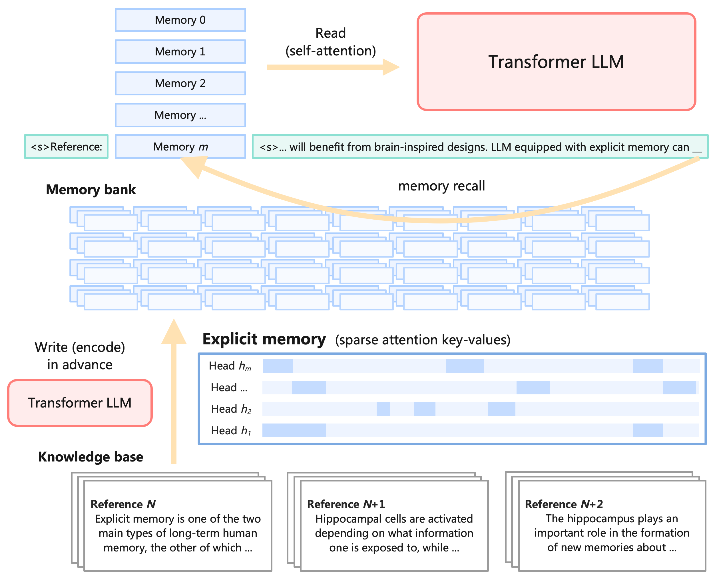</details> Figure 1: The Memory 3 model converts texts to explicit memories, and then recalls these memories during inference. The explicit memories can be seen as retrievable model parameters, externalized knowledge, or sparsely-activated neural circuits. <details> <summary>extracted/5700921/Figures/Result/memory3_benchmark_vs_size_small.png Details</summary>  ### Visual Description ## Scatter Plot: Language Model Benchmark Performance vs. Parameter Size ### Overview This image is a scatter plot comparing various large language models (LLMs) based on two metrics: their non-embedding parameter size (in billions) and their average benchmark evaluation score. The plot visually demonstrates the relationship between model scale and performance, highlighting one specific model in red for emphasis. ### Components/Axes * **Chart Type:** Scatter Plot * **X-Axis:** "Non-embedding parameter size (billion)". The scale is logarithmic, with major tick marks at 1, 2, 4, 8, 16, and 32 billion parameters. * **Y-Axis:** "Benchmark performance (avg eval score)". The scale is linear, ranging from approximately 35 to 67, with major tick marks every 5 units from 40 to 65. * **Data Points:** Each point represents a specific language model, labeled with its name. The points are colored either blue or red. * **Legend/Key:** There is no separate legend box. The color coding is implicit: one model is red, all others are blue. The red point is explicitly labeled "Memory³-2B-SFT". ### Detailed Analysis The plot contains 15 labeled data points. Below is a list of each model with its approximate coordinates (Parameter Size, Performance Score). Values are estimated based on the logarithmic x-axis and linear y-axis. **Models (Blue Points):** 1. **Gemma-2B-it:** (~2B, ~37) 2. **Qwen1.5-1.8B-Chat:** (~1.8B, ~50) 3. **MiniCPM-2B-SFT:** (~2B, ~54.5) 4. **Phi-2:** (~2.7B, ~55.5) 5. **Qwen1.5-4B-Chat:** (~4B, ~58) 6. **Llama2-7B-Chat:** (~7B, ~47) 7. **ChatGLM3-6B:** (~6B, ~54.5) 8. **Baichuan2-7B-Chat:** (~7B, ~55) 9. **Gemma-7B-it:** (~8B, ~47.5) 10. **Mistral-7B-v0.1:** (~7B, ~59) 11. **Qwen1.5-7B-Chat:** (~7.5B, ~65) 12. **Llama3-8B-it:** (~8B, ~66) 13. **Vicuna-13B-v1.5:** (~13B, ~52) 14. **Llama2-13B-Chat:** (~13B, ~51.5) 15. **Falcon-40B:** (~40B, ~55.5) **Model (Red Point):** 16. **Memory³-2B-SFT:** (~2.5B, ~63.5) - This point is located in the upper-left quadrant of the plot, significantly higher on the y-axis than other models of similar or larger size. ### Key Observations * **Performance Range:** Benchmark scores range from a low of ~37 (Gemma-2B-it) to a high of ~66 (Llama3-8B-it). * **Parameter Size Range:** Models span from ~1.8B to ~40B non-embedding parameters. * **General Trend:** There is a loose positive correlation; models with more parameters generally achieve higher benchmark scores. However, there is significant variance. For example, models around 7-8B parameters have scores ranging from ~47 (Llama2-7B-Chat) to ~66 (Llama3-8B-it). * **Notable Outlier:** The red-highlighted model, **Memory³-2B-SFT**, is a major outlier. With only ~2.5B parameters, it achieves a score of ~63.5, outperforming many models that are 3 to 16 times larger in size (e.g., outperforming Falcon-40B, Vicuna-13B, and all 7B-class models except Llama3-8B-it and Qwen1.5-7B-Chat). * **Cluster of 7B Models:** A dense cluster of models exists between 6B and 8B parameters, showing a wide performance spread of over 18 points (from ~47 to ~66). ### Interpretation This chart is designed to showcase the exceptional efficiency of the **Memory³-2B-SFT** model. The core message is that this specific 2.5B-parameter model achieves benchmark performance rivaling or exceeding that of models 4 to 16 times its size. The data suggests that raw parameter count is not the sole determinant of benchmark performance. Architectural innovations, training data quality, and training methodology (like the "Memory³" technique implied by the name) can lead to dramatic improvements in efficiency. The plot argues for the value of developing smaller, more efficient models that can deliver high performance without the computational cost of massive models. The wide scatter among similarly sized models (especially the 7B class) further emphasizes that factors beyond scale are critical. The outlier status of Memory³-2B-SFT positions it as a significant advancement in the pursuit of high-performance, compact language models. </details> (a) <details> <summary>extracted/5700921/Figures/Result/memory3_profession_vs_throughput.png Details</summary>  ### Visual Description ## Scatter Plot: Language Model Performance vs. Decoding Speed ### Overview This image is a scatter plot comparing seven different language models based on two metrics: their decoding speed with retrieval (x-axis) and their average score on professional tasks with retrieval (y-axis). The plot visualizes the trade-off between inference speed and task performance for these models. ### Components/Axes * **X-Axis:** "Decoding speed with retrieval (token/sec)". The scale is logarithmic, with major tick marks labeled at `4 × 10²` (400), `6 × 10²` (600), and `10³` (1000). The axis spans from approximately 350 to 1500 tokens/sec. * **Y-Axis:** "Professional tasks with retrieval (avg score)". The scale is linear, ranging from 35.0 to 55.0, with major tick marks every 2.5 units (35.0, 37.5, 40.0, etc.). * **Data Points:** Seven labeled points represent different models. Six are blue circles, and one is a red circle, indicating it is the primary subject of comparison. * **Labels:** Each data point is directly labeled with the model name. There is no separate legend box; the color (blue vs. red) is the only distinguishing visual cue beyond the labels themselves. ### Detailed Analysis The plot contains the following data points, listed from left (slower) to right (faster) along the x-axis: | Model | Color | Approx. Decoding Speed (tokens/sec) | Approx. Avg. Score | | :--- | :--- | :--- | :--- | | Llama2-7B-Chat | Blue | 380 | 36.2 | | Qwen1.5-4B-Chat | Blue | 450 | 55.5 | | MiniCPM-2B-SFT | Blue | 520 | 45.5 | | Phi-2 | Blue | 620 | 35.3 | | Memory³-2B-SFT | Red | 700 | 47.8 | | Qwen1.5-1.8B-Chat | Blue | 900 | 48.2 | | Gemma-2B-it | Blue | 1400 | 40.3 | ### Key Observations * **Performance-Speed Trade-off:** There is a general, but not strict, inverse relationship. The model with the highest performance (Qwen1.5-4B-Chat) is among the slowest, while the fastest model (Gemma-2B-it) has a lower average score. * **Highlighted Model:** The red point, **Memory³-2B-SFT**, occupies a central position. It achieves a relatively high performance score (47.8) while maintaining a moderate decoding speed (700 tokens/sec), suggesting a balance between the two metrics. * **Outliers:** * **Qwen1.5-4B-Chat** is a clear outlier in performance, scoring significantly higher than all other models despite its slower speed. * **Phi-2** has the lowest performance score but is not the fastest model. * **Clustering:** The models MiniCPM-2B-SFT, Memory³-2B-SFT, and Qwen1.5-1.8B-Chat form a cluster in the middle of the performance range (scores ~45-48) with varying speeds. ### Interpretation This chart is designed to benchmark the **Memory³-2B-SFT** model against other small-to-medium language models. The data suggests that Memory³-2B-SFT offers a compelling compromise: it delivers professional task performance comparable to the larger Qwen1.5-1.8B-Chat model while being slower, but it significantly outperforms similarly fast or faster models like Phi-2 and Gemma-2B-it. The plot implies that for applications requiring both reasonable speed and competent performance on professional tasks, Memory³-2B-SFT presents a favorable option. The extreme performance of Qwen1.5-4B-Chat indicates that larger model size (4B parameters) can yield substantial accuracy gains, but at a notable cost to inference speed. The chart effectively argues for the value proposition of the Memory³ architecture in balancing these competing demands. 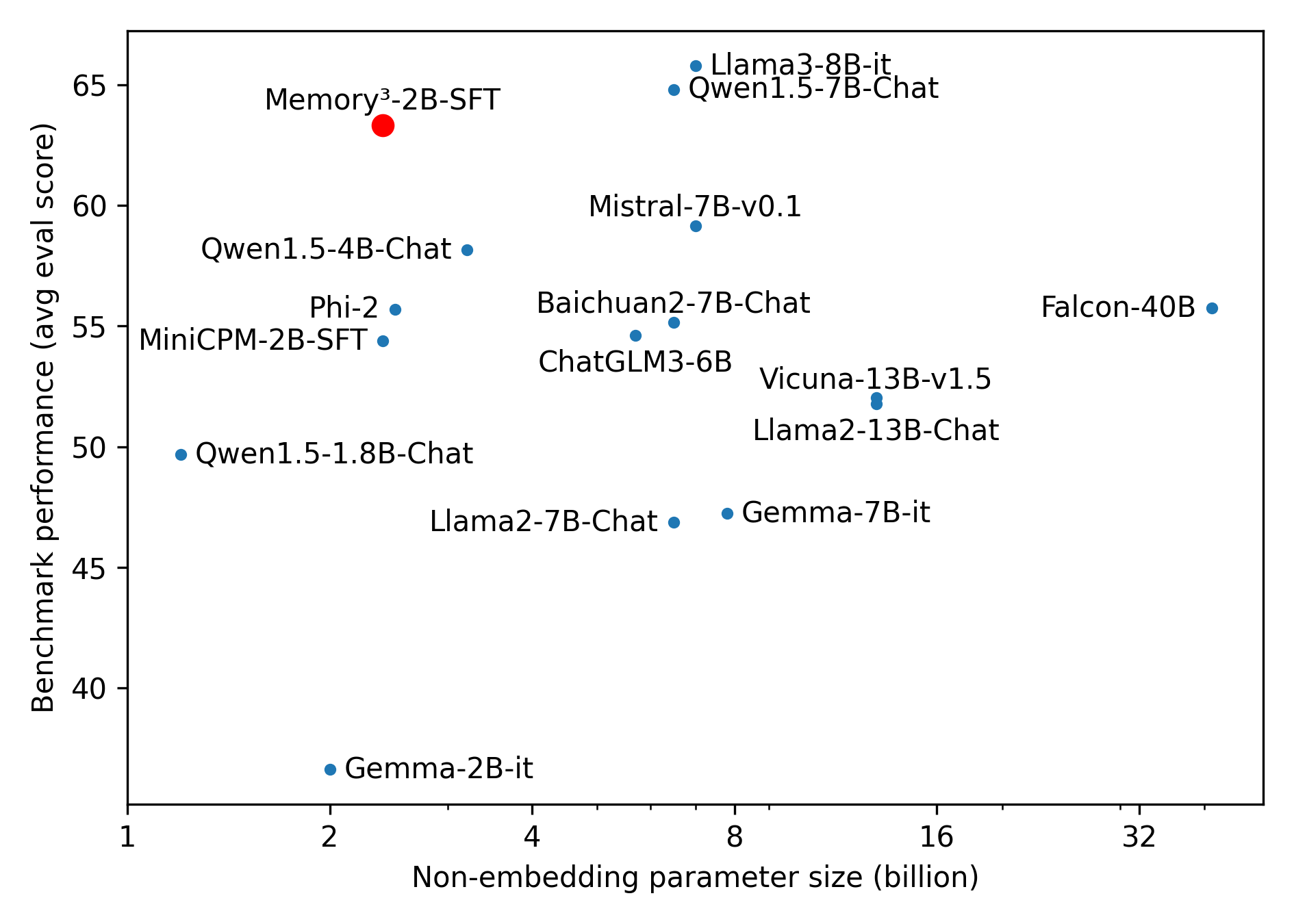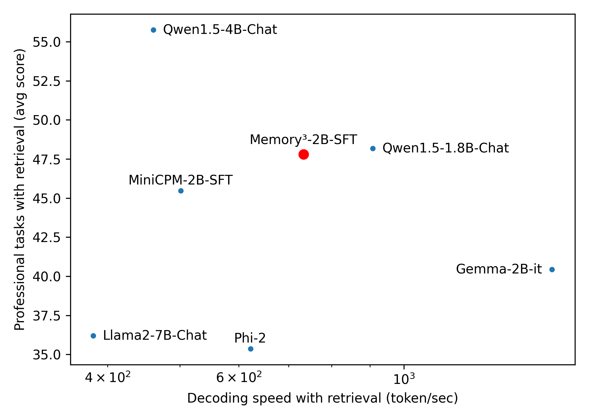</details> (b) Figure 2: Left: Performance on benchmarks, with respect to model size (top-left is better). Right: Retrieval-augmented performance on professional tasks, versus decoding speed with retrieval (top-right is better). The left plot is based on Table 16. The right plot is based on Tables 20 and 21. Memory 3 uses high frequency retrieval of explicit memories, while the RAG models use a fixed amount of 5 references. This is a preliminary experiment and we have not optimized the quality of our pretraining data as well as the efficiency of our inference pipeline, so the results may not be comparable to those of the SOTA models. ## 1 | Introduction Large language models (LLMs) have enjoyed unprecedented popularity in recent years thanks to their extraordinary performance [5, 9, 110, 11, 126, 4, 56, 54]. The prospect of scaling laws [60, 53, 99] and emergent abilities [119, 105] constantly drives for substantially larger models, resulting in the rapid increase in the cost of LLM training and inference. People have been trying to reduce this cost through optimizations in various aspects, including architecture [40, 6, 30, 75, 89, 109], data quality [104, 58, 48, 66], operator [32, 63], parallelization [95, 103, 62, 91], optimizer [71, 124, 117], scaling laws [53, 127], generalization theory [132, 55], hardware [33], etc. We introduce the novel approach of optimizing knowledge storage. The combined cost of LLM training and inference can be seen as the cost of encoding the knowledge from text data into various memory formats, plus the cost of reading from these memories during inference: $$ \sum_{\text{knowledge }k}\min_{\text{format }m}\text{cost}_{\text{write}}(k,m) +n_{k}\cdot\text{cost}_{\text{read}}(k,m) \tag{1} $$ where $\text{cost}_{\text{write}}$ is the cost of encoding a piece of knowledge $k$ into memory format $m$ , $\text{cost}_{\text{read}}$ is the cost of integrating $k$ from format $m$ into inference, and $n_{k}$ is the expected usage count of this knowledge during the lifespan of this LLM (e.g. a few months for each version of ChatGPT [86, 102]). The definitions of knowledge and memory in the context of LLMs are provided in Section 2, and this paper uses knowledge as a countable noun. Typical memory formats include model parameters and plain text for retrieval-augmented generative models (RAG); their write functions and read functions are listed in Table 3, and their $\text{cost}_{\text{write}}$ and $\text{cost}_{\text{read}}$ are provided in Figure 4. We introduce a new memory format, explicit memory, characterized by moderately low write cost and read cost. As depicted in Figure 1, our model first converts a knowledge base (or any text dataset) into explicit memories, implemented as sparse attention key-values, and then during inference, recalls these memories and integrates them into the self-attention layers. Our design is simple so that most of the existing Transformer-based LLMs should be able to accommodate explicit memories with a little finetuning, and thus it is a general-purpose “model amplifier”. Eventually, it should reduce the cost of pretraining LLMs, since there will be much less knowledge that must be stored in parameters, and thus less training data and smaller model size. The new memory format enables us to define a memory hierarchy for LLMs: plain text (RAG) $\to$ explicit memory $\to$ model parameter such that by going up the hierarchy, $\text{cost}_{\text{write}}$ increases while $\text{cost}_{\text{read}}$ decreases. To minimize the cost (1), one should store each piece of knowledge that is very frequently/rarely used in the top/bottom of this hierarchy, and everything in between as explicit memory. As illustrated in Table 3, the memory hierarchy of LLMs closely resembles that of humans. For humans, the explicit/implicit memories are the long-term memories that are acquired and used consciously/unconsciously [59]. | Memory format of humans | Example | Memory format of LLMs | Write | Read | | --- | --- | --- | --- | --- | | Implicit memory | common expressions | model parameters | training | matrix multiplication | | Explicit memory | books read | this work | memory encoding | self-attention | | External information | open-book exam | plain text (RAG) | none | encode from scratch | Table 3: Analogy of the memory hierarchies of humans and LLMs. As a remark, one can compare the plain LLMs to patients with impaired explicit memory, e.g. due to injury to the medial temporal lobe. These patients are largely unable to learn semantic knowledge (usually stored as explicit memory), but can acquire sensorimotor skills through repetitive priming (stored as implicit memories) [42, 26, 12]. Thus, one may hypothesize that due to the lack of explicit memory, the training of plain LLMs is as inefficient as repetitive priming, and thus has ample room for improvement. In analogy with humans, for instance, it is easy to recall and talk about a book we just read, but to recite it as unconsciously as tying shoe laces requires an enormous effort to force this knowledge into our muscle memory. From this perspective, it is not surprising that LLM training consumes so much data and energy [121, 77]. We want to rescue LLMs from this poor condition by equipping it with an explicit memory mechanism as efficient as that of humans. <details> <summary>extracted/5700921/Figures/Theory/total_cost_2B_chunk.png Details</summary>  ### Visual Description ## Line Chart: Cost Comparison of Memory Architectures vs. Usage Frequency ### Overview This is a technical line chart comparing the computational cost (in Tflops) of three different memory or knowledge retrieval approaches as a function of their expected usage frequency. The chart uses a semi-logarithmic scale (logarithmic x-axis, linear y-axis) to visualize performance across several orders of magnitude of usage. ### Components/Axes * **Chart Type:** Semi-log line chart with shaded regions under each curve. * **X-Axis:** * **Label:** `Expected usage count (n_k)` * **Scale:** Logarithmic (base 10). * **Range & Ticks:** Spans from `10^-2` (0.01) to `10^5` (100,000). Major ticks are at each power of 10: `10^-2`, `10^-1`, `10^0`, `10^1`, `10^2`, `10^3`, `10^4`, `10^5`. * **Y-Axis:** * **Label:** `Cost of write + read (Tflops)` * **Scale:** Linear. * **Range & Ticks:** Spans from `0.0` to approximately `2.7`. Major ticks are at intervals of `0.5`: `0.0`, `0.5`, `1.0`, `1.5`, `2.0`, `2.5`. * **Legend:** Located in the top-left corner of the plot area. * **Red Line:** `RAG` * **Green Line:** `Explicit memory` * **Blue Line:** `Model parameter` * **Shaded Regions:** Each line has a semi-transparent shaded area beneath it, colored to match its line (red, green, blue). ### Detailed Analysis **1. Data Series Trends & Approximate Values:** * **RAG (Red Line):** * **Trend:** Starts at near-zero cost for very low usage (`n_k < 10^-1`). The cost increases exponentially (appears as a steep, near-vertical line on this semi-log plot) as usage approaches and surpasses `n_k = 10^0` (1). The line exits the top of the chart (cost > 2.7 Tflops) shortly after `n_k = 10^0`. * **Key Point:** The cost becomes prohibitively high very quickly with increased usage. It intersects the `Explicit memory` line at approximately `n_k = 0.5` (midway between `10^-1` and `10^0` on the log scale) at a cost of ~0.3 Tflops. * **Explicit Memory (Green Line):** * **Trend:** Maintains a constant, low baseline cost (~0.3 Tflops) across a wide range of low-to-moderate usage frequencies, from `n_k = 10^-2` up to approximately `n_k = 10^2` (100). After this point, the cost begins to rise, increasing sharply (exponentially) as usage approaches `n_k = 10^4` (10,000). The line exits the top of the chart (cost > 2.7 Tflops) just after `n_k = 10^4`. * **Key Point:** This method is cost-effective for a broad middle range of usage frequencies. It intersects the `Model parameter` line at approximately `n_k = 1.5 x 10^4` (15,000) at a cost of ~2.25 Tflops. * **Model Parameter (Blue Line):** * **Trend:** A perfectly horizontal line, indicating a fixed cost independent of the usage count `n_k`. * **Value:** The constant cost is approximately **2.25 Tflops** (visually estimated as halfway between the 2.0 and 2.5 tick marks). **2. Spatial Grounding of Shaded Regions:** * The **red shaded region** (RAG) is a small, triangular area in the bottom-left, bounded by the red line, the x-axis, and the vertical line at its intersection with the green line (~`n_k=0.5`). * The **green shaded region** (Explicit memory) is the largest area, spanning from the y-axis to the vertical line at its intersection with the blue line (~`n_k=1.5x10^4`). It is bounded above by the green curve. * The **blue shaded region** (Model parameter) is a rectangular area on the far right, from the vertical line at ~`n_k=1.5x10^4` to the right edge of the chart (`n_k=10^5`), bounded above by the horizontal blue line. ### Key Observations 1. **Cost Regimes:** The chart defines three distinct cost regimes based on usage frequency (`n_k`): * **Low Usage (`n_k < ~0.5`):** RAG is the cheapest option. * **Moderate Usage (`0.5 < n_k < ~15,000`):** Explicit Memory is the cheapest option. * **High Usage (`n_k > ~15,000`):** Model Parameter (fixed cost) becomes the cheapest option. 2. **Scaling Behavior:** RAG scales extremely poorly with usage. Explicit Memory scales well until a very high usage threshold. Model Parameter cost does not scale with usage at all. 3. **Intersection Points:** The two critical crossover points (RAG/Explicit Memory at ~0.5, Explicit Memory/Model Parameter at ~15,000) define the boundaries of the optimal usage ranges for each method. ### Interpretation This chart illustrates a fundamental trade-off in system design between **initial setup cost** and **marginal operational cost**. * **RAG (Retrieval-Augmented Generation)** has near-zero setup cost but a very high marginal cost per usage, making it suitable only for information accessed very infrequently. * **Explicit Memory** represents a system with a moderate, fixed setup cost (the flat ~0.3 Tflops) and a low marginal cost up to a point. Once the volume of data or accesses exceeds a certain threshold (`n_k ~100-1000`), managing this explicit memory becomes increasingly expensive, likely due to search, indexing, or bandwidth constraints. * **Model Parameter** (e.g., baking knowledge directly into a neural network's weights) has a very high, fixed setup cost (training: ~2.25 Tflops) but zero marginal cost for retrieval. This makes it the most economical choice for knowledge that is accessed extremely frequently, as the high initial investment is amortized over countless uses. The chart argues that the "best" architecture is not universal but is dictated by the expected access pattern (`n_k`). It provides a quantitative framework for deciding when to use a database-like retrieval system (RAG), a dedicated memory module, or to invest in training the knowledge directly into a model. The shaded regions visually emphasize the total cost of ownership for each approach within its optimal domain. 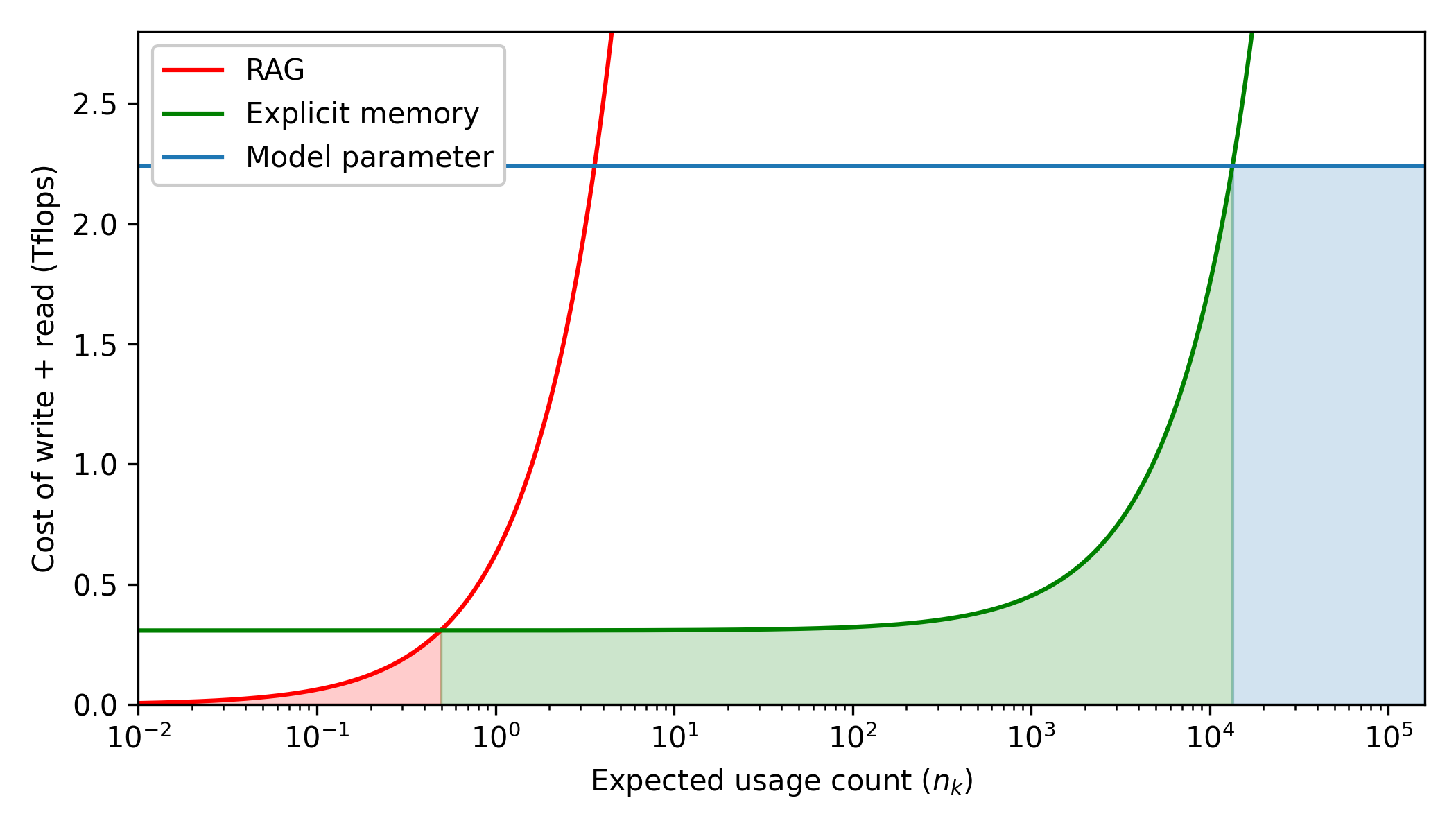</details> Figure 4: The total cost (TFlops) of writing and reading a piece of knowledge by our 2.4B model with respect to its expected usage count. The curves represent the cost of different memory formats, and the shaded area represents the minimum cost given the optimal format. The plot indicates that $(0.494,13400)$ is the advantage interval for explicit memory. The calculations are provided in Appendix A. (The blue curve is only a lower bound on the cost of model parameters.) A quantitative illustration of the cost (1) is given by Figure 4, where we characterize $\text{cost}_{\text{write}}$ and $\text{cost}_{\text{read}}$ by the amount of compute (TFlops). The plot indicates that if a piece of knowledge has an expected usage count $\in(0.494,13400)$ , then it is optimal to be stored as an explicit memory. Moreover, the introduction of explicit memory helps to externalize the knowledge stored in model parameters and thus allow us to use a lighter backbone, which ultimately reduces all the costs in Figure 4. The second motivation for explicit memory is to alleviate the issue of knowledge traversal. Knowledge traversal happens when the LLM wastefully invokes all its parameters (and thus all its knowledge) each time it generates a token. As an analogy, it is unreasonable for humans to recall everything they learned whenever they write a word. Let us define the knowledge efficiency of an LLM as the ratio of the minimum amount of knowledge sufficient for one decoding step to the amount of knowledge actually used. An optimistic estimation of knowledge efficiency for a 10B LLM is $10^{-5}$ : On one hand, it is unlikely that generating one token would require more than $10^{4}$ bits of knowledge (roughly equivalent to a thousand-token long passage, sufficient for enumerating all necessary knowledge); on the other hand, each parameter is involved in the computation and each stores at least 0.1 bit of knowledge [7, Result 10] (this density could be much higher if the LLM is trained on cleaner data), thus using $10^{9}$ bits in total. A novel architecture is needed to boost the knowledge efficiency of LLMs from $10^{-5}$ to $1$ , whereas current designs are far from this goal. Consider the mixture-of-experts architecture (MoE) for instance, which uses multiple MLP layers (experts) in each Transformer block and process each token with only a few MLPs. The boost of MoE, namely the ratio of the total amount of parameters to the amount of active parameters, is usually bounded by $4\sim 32$ [40, 56, 98]. Similarly, neither the mixture-of-depth architecture [37, 94] nor sparsified MLP neurons and attention heads [75] can bring greater gains. RAG appears very sparse if we compare the amount of retrieved texts with the size of the text database; nevertheless, RAG is usually built upon a plain LLM as backbone, which provides most of the knowledge used in inference, and thus offers little assistance in addressing the knowledge traversal problem. An ideal solution is to retrieve only the needed parameters for each token. This is naturally achieved by explicit memories if we compare memory recall to parameter retrieval. The third motivation is that, as a human-like design, explicit memory enables LLMs to develop more human-like capabilities. To name a few, - Infinitely long context: LLMs have the difficulty of processing long texts since their working memory (context key-values) costs too much GPU memory and compute. Meanwhile, despite that humans have very limited working memory capacity [27, 28], they can manage to read and write long texts by converting working memories to explicit memories (thus saving space) and retrieving only the needed explicit memories for inference (thus saving compute). Similarly, by saving explicit memories on drives and doing frequent and constant-size retrieval, LLMs can handle arbitrarily long contexts with time complexity $O(l\log l)$ instead of $\Theta(l^{2})$ , where $l$ is the context length. - Memory consolidation: Instead of writing a piece of knowledge directly into implicit memory, i.e. training model parameters, LLM can first convert it to explicit memory through plain encoding, and then convert this explicit memory to implicit memory through a low-cost step such as compression and finetuning, thus reducing the overall cost. - Factuality and interpretability: Encoding texts as explicit memories is less susceptible to information loss compared to dissolving them in model parameters. With more factual details provided by explicit memories, the LLMs would have less tendency to hallucinate. Meanwhile, the correspondence of explicit memories to readable texts makes the inference more transparent to humans, and also allows the LLM to consciously examine its own thought process. We demonstrate the improved factuality in the experiments section, and leave the rest to future work. In this work, we introduce a novel architecture and training scheme for LLM based on explicit memory. The architecture is called Memory 3, as explicit memory is the third form of memory in LLM after working memory (context key-values) and implicit memory (model parameters). - Memory 3 utilizes explicit memories during inference, alleviating the burden of model parameters to memorize specific knowledge. - The explicit memories are encoded from our knowledge base, and our sparse memory format maintains a realistic storage size. - We trained from scratch a Memory 3 model with 2.4B non-embedding parameters, and its performance surpasses SOTA models with greater sizes. It also enjoys better performance and faster inference than RAG. - Furthermore, Memory 3 boosts factuality and alleviates hallucination, and it enables fast adaptation to professional tasks. This paper is structured as follows: Section 2 lays the theoretical foundation for Memory 3, in particular our definitions of knowledge and memory. Section 3 discusses the basic design of Memory 3, including its architecture and training scheme. Sections 4, 5, and 6 describes the training of Memory 3. Section 7 evaluates the performance of Memory 3 on general benchmarks and professional tasks. Finally, Section 8 concludes this paper and discusses future works. ### 1.1 | Related work #### 1.1.1 | Retrieval-augmented Training Several language models have incorporated text retrieval from the pretraining stage. REALM [49] augments a BERT model with one retrieval step to solve QA tasks. Retro [16] enhances auto-regressive decoding with multiple rounds of retrieval, once per 64 tokens. The retrieved texts are injected through a two-layer encoder and then several cross-attention layers in the decoder. Retro++ [113] explores the scalability of Retro by reproducing Retro up to 9.5B parameters. Meanwhile, several models are adapted to retrieval in the finetuning stage. WebGPT [83] learns to use search engine through imitation learning in a text-based web-browsing environment. Toolformer [100] performs decoding with multiple tools including search engine, and the finetuning data is labeled by the LM iself. The closest model to ours is Retro. Unlike explicit memory, Retro needs to encode the retrieved texts in real-time during inference. To alleviate the cost of encoding these references, it chooses to use a separate, shallow encoder and also retrieve few references. Intuitively, this compromise greatly reduces the amount of knowledge that can be extracted and supplied to inference. Another line of research utilizes retrieval to aid long-context modeling. Memorizing Transformer [123] extends the context of language models by an approximate kNN lookup into a non-differentiable cache of past key-value pairs. LongLlama [112] enhances the discernability of context key-value pairs by a finetuning process inspired by contrastive learning. LONGMEM [118] designs a decoupled architecture to avoid the memory staleness issue when training the Memorizing Transformer. These methods are not directly applicable to large knowledge bases since the resulting key-value caches will occupy enormous space. Our method overcomes this difficulty through a more intense memory sparsification method. #### 1.1.2 | Sparse Computation To combat the aforementioned knowledge traversal problem and improve knowledge efficiency, ongoing works seek novel architectures that process each token with a minimum and adaptive subset of model parameters. This adaptive sparsity is also known as contextual sparsity [75]. The Mixture-of-Experts (MoE) use sparse routing to assign Transformer submodules to tokens, scaling model capacity without large increases in training or inference costs. The most common MoE design [40] hosts multiple MLP layers in each Transformer block and routes each token to a few MLPs with the highest allocation score predicted by a linear classifier. Furthermore, variants based on compression such as QMoE [41] are introduced to alleviate the memory burden of MoE. Despite the sparse routing, the boost in parameter efficiency is usually bounded by $4\sim 32$ . For instance, the Arctic model [98], one of the sparsest MoE LLM in recent years, has an active parameter ratio of about $3.5\$ . Similarly, the Mixture of Depth architecture processes each token with an adaptive subset of the model layers. The implementations can be based on early exit [37] or top- $k$ routing [94], reducing the amount of compute to $12.5\sim 50\$ . More fine-grained approaches can perform sparsification at the level of individual MLP neurons and attention heads. The model Deja Vu [75] trains a low-cost network for each MLP/attention layer that predicts the relevance of each neuron/head at this layer to each token. Then, during inference, Deja Vu keeps the top $5\sim 15\$ MLP neurons and $20\sim 50\$ attention heads for each token. #### 1.1.3 | Parameter as memory Several works have portrayed model parameters as implicit memory, in accordance with our philosophy. [46] demonstrates that the neurons in the MLP layers of GPTs behave like key-value pairs. Specifically, with the MLP layer written as $\sigma(XK^{T})V$ , each row of the first layer weight $K_{i}$ functions like a key vector, with the corresponding row in the second layer weight $V_{i}$ being the value vector. [46] observes that for most of the MLP neurons, the $K_{i}$ is activated by context texts that obey some human interpretable pattern, and the $V_{i}$ activates the column of the output matrix that corresponds to the most probable next token of the pattern (e.g. $n$ -gram). Based on this observation, [108] designs a GPT variant that consists of only attention layers, with performance matching that of the usual GPTs. The MLP layers are incorporated into the attention layers in the form of key-value vector pairs, which are called persistent memories. Similarly, using sensitivity analysis, [29] discovers that factual knowledge learned by BERT is often localized at one or few MLP neurons. These neurons are called “knowledge neurons”, and by manipulating them, [29] manages to update single pieces of knowledge of BERT. Meanwhile, [38] studies an interesting phenomenon known as superposition or polysemanticity, that a neural network can store many unrelated concepts into a single neuron. ## 2 | Memory Circuitry Theory This section introduces our memory circuitry theory, which defines knowledge and memory in the context of LLM. We will see that this theory helps to determine which knowledge can be stored as explicit memory, and what kind of model architecture is suitable for reading and writing explicit memories. For readers interested primarily in the results, it may suffice to review Claim 1 and Remark 1 before proceeding to the subsequent sections. The concepts to be discussed are illustrated in Figure 5. <details> <summary>extracted/5700921/Figures/Theory/memory_circuitry_theory.png Details</summary>  ### Visual Description ## Diagram: Transformer Circuits Knowledge Decomposition ### Overview This image is a hierarchical flowchart illustrating the decomposition of knowledge within "Transformer circuits." It maps how different types of knowledge and memory relate to the foundational "Model parameters." The diagram uses color-coded boxes and directional arrows to show relationships and flow. ### Components/Axes The diagram is structured as a top-down flowchart with the following labeled components, grouped by colored containers: 1. **Top-Level Component (Blue Box, Top Center):** * Label: `Transformer circuits` 2. **First-Level Decomposition (Light Blue Container, Middle):** * This container is labeled on its right side as `Separable knowledge`. * It contains two primary boxes: * Left Box: `Abstract knowledge` * Right Box: `Specific knowledge` 3. **Second-Level Decomposition (Light Green Container, Lower Middle):** * This container is labeled on its right side as `Memory hierarchy`. * It contains three boxes, all stemming from "Specific knowledge": * Left Box: `Implicit memory` * Center Box: `Explicit memory` * Right Box: `External information` 4. **Foundational Component (Red Box, Bottom Center):** * Label: `Model parameters` ### Detailed Analysis **Flow and Connections (Arrows):** * A solid black arrow originates from `Transformer circuits` and splits, pointing to both `Abstract knowledge` and `Specific knowledge`. * A solid black arrow flows directly from `Abstract knowledge` down to `Model parameters`. * A solid black arrow flows from `Specific knowledge` down to the `Memory hierarchy` container, where it splits into three arrows pointing to `Implicit memory`, `Explicit memory`, and `External information`. * A solid black arrow flows from `Implicit memory` down to `Model parameters`. * A **dashed** black arrow flows from `Explicit memory` down to `Model parameters`. This dashed line likely indicates a different, weaker, or more indirect relationship compared to the solid lines. **Spatial Grounding & Color Coding:** * The `Separable knowledge` container (light blue) is positioned in the upper-middle section, encompassing the two knowledge types. * The `Memory hierarchy` container (light green) is positioned directly below the `Specific knowledge` box, in the lower-middle section. * The `Model parameters` box (light red/pink) is the terminal point at the bottom center of the diagram. * All primary component boxes (`Abstract knowledge`, `Specific knowledge`, `Implicit memory`, `Explicit memory`, `External information`, `Model parameters`) have a darker blue or green border matching their container's theme, except for `Model parameters` which has a red border. ### Key Observations 1. **Hierarchical Decomposition:** The diagram presents a clear hierarchy: Transformer circuits are broken down into separable knowledge types, one of which (Specific knowledge) is further broken down into a memory hierarchy. 2. **Direct vs. Indirect Pathways:** `Abstract knowledge` has a direct, single-step connection to `Model parameters`. In contrast, `Specific knowledge` influences `Model parameters` indirectly through the three components of the `Memory hierarchy`. 3. **Dashed Line Significance:** The dashed arrow from `Explicit memory` to `Model parameters` is a notable visual distinction, suggesting this pathway may be less permanent, more computational, or functionally different from the solid-line pathways (e.g., from `Implicit memory`). 4. **Grouping Semantics:** The labels `Separable knowledge` and `Memory hierarchy` are not boxes themselves but annotations that define the conceptual grouping of the components they are placed next to. ### Interpretation This diagram provides a conceptual model for understanding how a transformer-based AI system might organize information. It suggests that: * **Knowledge is not monolithic.** It can be separated into abstract rules/patterns (`Abstract knowledge`) and concrete facts/data (`Specific knowledge`). * **Specific knowledge is managed through a memory system.** This system includes `Implicit memory` (likely encoded in weights), `Explicit memory` (perhaps like key-value caches or retrieval), and access to `External information` (like tools or databases). * **All pathways ultimately affect the model's core.** Both abstract understanding and specific memories, whether implicit or explicit, converge to influence or be stored within the foundational `Model parameters`. The dashed line for `Explicit memory` might imply that this type of memory is more transient or requires different processing to become a permanent part of the model's parameters. The Peircean investigative reading would focus on the **signs** (the boxes and arrows) to infer the **system's logic**. The diagram acts as an *icon* (a likeness of the system's structure) and a *symbol* (using conventional arrows to represent flow/influence). The key insight is the proposed architecture: a transformer's "circuits" implement a separable knowledge system where specific facts are managed by a distinct memory hierarchy before affecting the core model. This has implications for interpretability (we can study these components separately) and capability (understanding how abstract vs. specific knowledge is leveraged). </details> Figure 5: Categorization of knowledge and memory formats. The explicit memories, extracted from model activations, lie half-way between raw data and model parameters, so we use a dotted line to indicate that they may or may not be regarded as parameters. ### 2.1 | Preliminaries The objective is to decompose the computations of a LLM into smaller, recurring parts, and analyze which parts can be separated from the LLM. These small parts will be defined as the “knowledge” of the LLM, and this characterization helps to identify what knowledge can be externalized as explicit memory, enabling both the memory hierarchy and a lightweight backbone. One behaviorist approach is to define the smaller parts as input-output relations between small subsequences, such that if the input text contains a subsequence belonging to some pattern, then the output text of the LLM contains a subsequence that belongs to some corresponding pattern. - One specific input-output relation is that if the immediate context contains “China” and “capital”, then output the token “Beijing”. - One abstract input-output relation is that if the immediate context is some arithmetic expression (e.g. “ $123\times 456=$ ”) then output the answer (e.g. “ $56088$ ”). - One abstract relation that will be mentioned frequently is the “search, copy and paste” [85], such that if the context has the form “…[a][b]…[a]” then output “[b]”, where [a] and [b] are arbitrary tokens. A decomposition into these relations seems natural since autoregressive LLMs can be seen as upgraded versions of $n$ -grams, with the fixed input/output segments generalized to flexible patterns and with the plain lookup table generalized to multi-step computations. Nevertheless, a behaviorist approach is insufficient since an input-output relation alone cannot uniquely pin down a piece of knowledge: a LLM may answer correctly to arithmetic questions based on either the actual knowledge of arithmetic or memorization (hosting a lookup table for all expressions such as “ $123\times 456=56088$ ”). Therefore, we take a white-box approach that includes in the definition the internal computations of the LLM that convert these inputs to the related outputs. Here are two preliminary examples of internal computations. **Example 1** *Several works have studied the underlying mechanisms when LLMs answer to the prompt “The capital of China is” with “Beijing”, as well as other factual questions [29, 46, 79, 22]. At least two mechanisms are involved, and the LLM may use their superposition [79]. One mechanism is to use general-purpose attention heads (called “mover heads”) to move “capital” and “China” to the last token “is”, and then use the MLP layers to map the feature of the last token to “Beijing” [79]. Often, only one or a few MLP neurons are causally relevant, and they are called “knowledge neurons” [29]. This mechanism is illustrated in Figure 6 (left). Another mechanism involves attention heads $h$ whose value-to-output matrices $W^{h}_{V}W^{h}_{O}$ function like bigrams, e.g. mapping “captial” to {“Paris”, “Beijing”, …} and “China” to {“panda”, “Beijing”, …} , which sum up to produce “Beijing” [22, 46, 79]. This mechanism is illustrated in Figure 6 (middle).* **Example 2** *The ability of LLMs to perform “search, copy and paste”, namely answering to the context “…[a][b]…[a]” with “[b]”, is based on two attention heads, together called induction heads [85]. The first head copies the feature of the previous token, enabling [b] to “dress like” its previous token [a]. The second head searches for similar features, enabling the second [a] to attend to [b], which now has the appearance of [a]. Thereby, the last token [a] manages to retrieve the feature of [b] and to output [b]. This mechanism is illustrated in Figure 6 (right). A similar mechanism is found for in-context learning [116].* <details> <summary>extracted/5700921/Figures/Theory/classical_circuits_demo.png Details</summary>  ### Visual Description ## Diagram: Neural Network Attention Mechanism Illustration ### Overview The image displays three separate computational graphs (left, center, right) illustrating how a neural network, likely a transformer-based model, processes sequential text input to produce an output. The diagrams visualize the flow of information through layers (denoted by `l`) and time steps (denoted by `t`), highlighting different types of connections ("Attention edge" and "FFN edge") and the semantic relationships they encode. ### Components/Axes The diagrams are not charts with axes but are structured graphs. Key components include: - **Nodes (Circles):** Represent hidden states or activations at specific layers and time steps. They are labeled with mathematical notation (e.g., `X_t^{l+1}`). - **Input/Output Boxes (Rectangles):** At the bottom, they show the input token sequence. At the top, they show the predicted output token. - **Edges (Arrows):** Represent computational connections between nodes. They are color-coded and labeled with their type and associated parameters. - **Green Arrows:** Labeled "Attention edge". - **Red Arrow:** Labeled "FFN edge" (only in the left diagram). - **Edge Annotations:** Text placed near each edge describes its function using parameters `qk` (query-key) and `o` (output/value). ### Detailed Analysis **1. Left Diagram:** - **Input Sequence (Bottom):** Three boxes labeled `capital`, `China`, `is`. - **Initial Layer Nodes:** Three circles above the input: `X_{t-3}^l`, `X_{t-1}^l`, `X_t^l`. - **Attention Edges (Green):** - From `X_{t-3}^l` to `X_t^{l+1}`: Labeled `Attention edge e_{t-3,t}^{l,h}`. Annotation: `qk: relation`, `o: capital`. - From `X_{t-1}^l` to `X_t^{l+1}`: Labeled `Attention edge e_{t-1,t}^{l,k}`. Annotation: `qk: topic`, `o: China`. - **Intermediate Node:** `X_t^{l+1}` receives the two attention edges. - **FFN Edge (Red):** From `X_t^{l+1}` to `X_t^{l+2}`. Labeled `FFN edge e_t^{l+1,m}`. Annotation: `qk: (China, capital)`, `o: Beijing`. - **Output (Top):** A box labeled `Beijing` is connected to the final node `X_t^{l+2}`. **2. Center Diagram:** - **Input Sequence (Bottom):** Identical to the left: `capital`, `China`, `is`. - **Initial Layer Nodes:** Identical: `X_{t-3}^l`, `X_{t-1}^l`, `X_t^l`. - **First Attention Edge (Green):** From `X_{t-3}^l` to `X_t^{l+1}`. Labeled `Attention edge e_{t-3,t}^{l,h}`. Annotation: `qk: relation`, `o: Paris, Beijing`. - **Intermediate Node:** `X_t^{l+1}`. - **Second Attention Edge (Green):** From `X_{t-1}^{l+2}` to `X_t^{l+3}`. Labeled `Attention edge e_{t-1,t}^{l+2,k}`. Annotation: `qk: country`, `o: panda, Beijing`. - **Output (Top):** A box labeled `Beijing` is connected to the final node `X_t^{l+3}`. **3. Right Diagram (Generalized/Abstract):** - **Input Sequence (Bottom):** Uses placeholders: `[a]`, `[b]`, `[a]`. - **Initial Layer Nodes:** `X_{s-1}^l`, `X_s^l`, `X_t^l`. - **First Attention Edge (Green):** From `X_{s-1}^l` to `X_s^{l+1}`. Labeled `Attention edge e_{s-1,s}^{l,h}`. Annotation: `q: previous position`, `k: current position`, `o: [a]`. - **Intermediate Nodes:** `X_s^{l+1}` and `X_s^{l+2}`. - **Second Attention Edge (Green):** From `X_s^{l+2}` to `X_t^{l+3}`. Labeled `Attention edge e_{s,t}^{l+2,k}`. Annotation: `qk: [a]`, `o: [b]`. - **Output (Top):** A box labeled `[b]` is connected to the final node `X_t^{l+3}`. ### Key Observations 1. **Flow Direction:** Information flows upward from input tokens at the bottom, through intermediate processing nodes, to a final output token at the top. 2. **Edge Type Differentiation:** The left diagram explicitly shows two distinct processing steps: an **Attention** step (green) that gathers information from relevant past tokens (`capital`, `China`), followed by a **Feed-Forward Network (FFN)** step (red) that performs a final transformation to produce the output `Beijing`. 3. **Semantic Role Labeling:** The annotations (`qk`, `o`) explicitly label the semantic roles the network is attending to (e.g., `relation`, `topic`, `country`) and the information being retrieved or output (e.g., `capital`, `China`, `Beijing`). 4. **Generalization:** The right diagram abstracts the specific example into a general pattern using placeholders `[a]` and `[b]`, suggesting a reusable computational motif for retrieving an output `[b]` based on a query `[a]` and positional information. 5. **Parameter Notation:** The edge labels use detailed subscript/superscript notation (`e_{t-3,t}^{l,h}`) to specify the source and destination time steps (`t-3`, `t`), the layer (`l`), and likely the attention head (`h`, `k`, `m`). ### Interpretation This diagram is a pedagogical or technical illustration explaining the **mechanistic internals of a transformer model** performing a factual recall task ("capital of China is Beijing"). - **What it demonstrates:** It breaks down the inference process into discrete, interpretable steps. The model first uses **attention** to identify and gather relevant concepts (`relation: capital`, `topic: China`) from the input context. It then processes this gathered information, possibly through an **FFN layer**, to perform a knowledge lookup or computation, resulting in the specific fact (`Beijing`). - **Relationship between elements:** The diagrams show a hierarchy. The lower-level attention edges perform information aggregation based on semantic roles. The higher-level FFN edge (in the left diagram) acts upon this aggregated representation to generate the final answer. The center diagram may illustrate an alternative or extended pathway where attention operates across different layers (`l` and `l+2`). - **Notable patterns/anomalies:** The most significant pattern is the clear separation of **information retrieval** (attention) from **information transformation/output generation** (FFN). The use of explicit semantic labels (`qk: country`) suggests the model has learned to organize its internal representations around human-interpretable concepts. The right diagram's abstraction implies this is a fundamental, reusable pattern within the network's architecture for solving such queries. </details> Figure 6: Illustration of three subgraphs. Left: A subgraph that inputs “the capital of China is” and outputs “Beijing”. The knowledge neuron is marked in red and the mover heads in green. Middle: Another subgraph with similar function using task-specific heads. Right: The induction-heads subgraph that inputs “[a][b]…[a]” and outputs [b], where [a], [b] are arbitrary tokens. The notations are introduced in Section 2.2. The locations of these attention heads and MLP neurons may be variable. We will address the internal mechanism for an input-output relation as a circuit, and will define a piece of knowledge as an input-output relation plus its circuit. By manipulating these circuits, one can separate many pieces of knowledge from a LLM while keeping its function intact. Recent works on circuit discovery demonstrate that some knowledge and skills possessed by Transformer LLMs can be identified with patterns in their computation graphs [85, 116, 106, 45, 115, 24, 29, 46], but there has not been a universally accepted definition of circuit. Different from works on Boolean circuits [50, 80] and circuits with Transformer submodules as their nodes [24, 129], we characterize a circuit as a “spatial-temporal” phenomenon, whose causal structure is localized at the right places (MLP neurons and attention heads) and right times (tokens). Thus, we define a computation graph as a directed acyclic graph, whose nodes are the hidden features of all tokens at all all MLP and attention layers, and whose edges correspond to all activations inside these layers. In particular, the computation graph hosts one copy of the Transformer architecture at each time step. To transcend this phenomenological characterization, we define a circuit as an equivalence class of similar subgraphs across multiple computation graphs. As a remark, it is conceptually feasible to identify a circuit with the minimal subset of Transformer parameters that causes this circuit. The benefit is that such definition of knowledge seems more intrinsic to the LLM. Nevertheless, with the current definition, it is easier to perform surgery on the circuits and derive constructive proofs. Besides, it is known that Transformer submodules exhibit superposition or polysemanticity, such that one MLP neuron or attention head may serve multiple distinct functions [38, 79], making the identification of parameter subsets a challenge task. ### 2.2 | Knowledge We begin with the definition of the knowledge of LLMs. For now, it suffices to adopt heuristic definitions instead of fully rigorous ones. Throughout this section, by LLM we mean autoregressive Transformer LLM that has at least been pretrained. Let $L$ be the number of Transformer blocks and $H$ be the number of attention heads at each attention layer, and the blocks and heads are numbered by $l=0,\dots L-1$ and $h=0,\dots H-1$ . There are in total $2L$ layers (MLP layers and attention layers), and the input features to these layers are numbered by $0,\dots 2L-1$ . **Definition 1** *Given an LLM and a text $\mathbf{t}=(t_{0},\dots t_{n})$ , the computation graph $G$ on input $(t_{0},\dots t_{n-1})$ and target $(t_{1},\dots t_{n})$ is a directed graph with weighted edges such that - Its nodes consist of the hidden vectors $\mathbf{x}_{i}^{2l}$ before all attention layers, the hidden vectors $\mathbf{x}_{i}^{2l+1}$ before all MLP layers, and the output vectors $\mathbf{x}_{i}^{2L}$ , for all blocks $l=0,\dots L-1$ and positions $i=0,\dots n-1$ . - Its directed edges consist of each attention edge $e^{l,h}_{i,j}$ that goes from $\mathbf{x}_{i}^{2l}$ to $\mathbf{x}_{j}^{2l+1}$ at the $h$ -th head of the $l$ -th attention layer for all $l,h$ and $i\leq j$ , as well as each MLP edge $e^{l,m}_{i}$ that goes from $\mathbf{x}_{i}^{2l+1}$ to $\mathbf{x}_{i}^{2l+2}$ through the $m$ -th neuron of the $l$ -th MLP layer for all $l,m,i$ . - The weight of each attention edge $e^{l,h}_{i,j}$ , which measures the influence of the attention score $a^{l,h}_{i,j}$ on the LLM output, is defined by $$ \mathcal{L}-\mathcal{L}\big{|}_{a^{l,h}_{i,j}=0}\quad\text{or}\quad\frac{ \partial\mathcal{L}}{\partial a^{l,h}_{i,j}} $$ where $\mathcal{L}$ is the log-likelihood of the target $(t_{1},\dots t_{n})$ , with $\mathcal{L}|_{a=0}$ obtained by setting $a=0$ (i.e. causal intervention). Similarly, the weight of each MLP edge $e^{l,m}_{i}$ , which measures the influence of the neuron activation $a^{l,m}_{i}$ on the LLM output, is defined likewise. - Given any subgraph $S\subseteq G$ , define the associated input of $S$ as a subsequence $\mathbf{t}_{\text{in}}(S)\subseteq(t_{0},\dots t_{n-1})$ such that a token $t_{i}$ belongs to $\mathbf{t}_{\text{in}}(S)$ if and only if $\big{\|}\nabla_{\mathbf{x}_{i}^{0}}a\big{\|}$ is large for some attention edge (or MLP edge) in $S$ with attention score (or activation) $a$ . - Similarly, define the associated output of the subgraph $S$ as a subsequence $\mathbf{t}_{\text{out}}(S)\subseteq(t_{1},\dots t_{n})$ such that a token $t_{i}$ belongs to $\mathbf{t}_{\text{out}}(S)$ if and only if $$ \mathcal{L}_{i}-\mathcal{L}_{i}\big{|}_{a=0}\quad\text{or}\quad\frac{\partial \mathcal{L}_{i}}{\partial a} $$ is large for some attention edge (or MLP edge) in $S$ with attention score (or activation) $a$ . Here $\mathcal{L}_{i}$ is the log-likelihood of $t_{i}$ with respect to the LLM output.* <details> <summary>extracted/5700921/Figures/Theory/LLM_computation_graph.png Details</summary>  ### Visual Description ## Diagram: Neural Network Layer Connectivity Pattern ### Overview The image displays a technical diagram illustrating a connectivity pattern within a neural network architecture, likely depicting a specific layer or block. It shows three parallel processing units (columns) across three sequential layers or time steps. The diagram emphasizes both vertical (within-column) and horizontal (cross-column) connections, with distinct labeling for nodes and edges. ### Components/Axes The diagram is organized into three vertical columns and three horizontal layers (rows). There are no traditional axes, but the structure implies a flow from bottom to top. **Nodes (Circles):** * **Bottom Row (Layer 2l):** Three nodes labeled from left to right: * `x_i^{2l}` * `x_{i+1}^{2l}` * `x_{i+2}^{2l}` * **Middle Row (Layer 2l+1):** Three nodes labeled from left to right: * `x_i^{2l+1}` * `x_{i+1}^{2l+1}` * `x_{i+2}^{2l+1}` * **Top Row (Layer 2l+2):** Three nodes labeled from left to right: * `x_i^{2l+2}` * `x_{i+1}^{2l+2}` * `x_{i+2}^{2l+2}` **Edges (Connections):** * **Vertical Connections (Solid Blue Arrows):** Each node in the bottom row connects directly upward to the node directly above it in the middle row. Similarly, each node in the middle row connects directly upward to the node directly above it in the top row. * **Horizontal/Skip Connections (Light Blue, Dashed Arrows):** These originate from the bottom row nodes and connect to middle row nodes in *different* columns. * From `x_i^{2l}` (bottom-left): Arrows point to `x_{i+1}^{2l+1}` (middle-center) and `x_{i+2}^{2l+1}` (middle-right). * From `x_{i+1}^{2l}` (bottom-center): An arrow points to `x_{i+2}^{2l+1}` (middle-right). * From `x_{i+2}^{2l}` (bottom-right): No outgoing horizontal connections are shown. * **Loopback/Oval Connections (Solid Blue Ovals):** Each node in the middle row is enclosed within a vertical oval that connects back to itself, suggesting a recurrent or self-attention mechanism. This oval is labeled `e_i^{l,m}` for the leftmost column. * **Edge Labels:** * The horizontal/skip connections are collectively labeled `e_{i,i}^{l,h}` near the bottom-left of the diagram. * The oval connection in the first column is labeled `e_i^{l,m}`. ### Detailed Analysis **Spatial Grounding & Component Isolation:** * **Header/Top Region (Layer 2l+2):** Contains the three output nodes (`x_i^{2l+2}`, `x_{i+1}^{2l+2}`, `x_{i+2}^{2l+2}`). Each receives a single vertical input from the node below it. * **Main Chart/Middle Region (Layer 2l+1):** Contains the three intermediate nodes (`x_i^{2l+1}`, `x_{i+1}^{2l+1}`, `x_{i+2}^{2l+1}`). Each node has: 1. One vertical input from below. 2. Multiple horizontal/skip inputs from the bottom row (for the center and right nodes). 3. A self-looping oval connection. * **Footer/Bottom Region (Layer 2l):** Contains the three input nodes (`x_i^{2l}`, `x_{i+1}^{2l}`, `x_{i+2}^{2l}`). Each node serves as a source for: 1. One vertical connection to the node above. 2. Multiple horizontal/skip connections to nodes in the middle row of subsequent columns (for the left and center nodes). **Flow and Relationships:** The primary data flow is vertical, from layer `2l` to `2l+1` to `2l+2`. The horizontal connections (`e_{i,i}^{l,h}`) introduce cross-talk or information sharing between columns at the `2l` to `2l+1` transition. The ovals (`e_i^{l,m}`) indicate a separate, likely recurrent or intra-column, processing step applied at the `2l+1` layer before passing information to `2l+2`. ### Key Observations 1. **Asymmetric Horizontal Connectivity:** The skip connections are not all-to-all. Information flows forward (from lower index `i` to higher indices `i+1`, `i+2`), but not backward. The rightmost column (`i+2`) receives horizontal inputs but does not send any. 2. **Dual Processing at Middle Layer:** Nodes at layer `2l+1` are subject to two distinct operations: integration of vertical and horizontal inputs, followed by a self-looping operation (`e_i^{l,m}`). 3. **Consistent Labeling Scheme:** The superscripts (`2l`, `2l+1`, `2l+2`) clearly denote sequential layers. Subscripts (`i`, `i+1`, `i+2`) denote column or feature index. The edge labels use `l` for layer context, `h` for horizontal, and `m` for the middle-layer operation. ### Interpretation This diagram represents a **neural network building block with mixed connectivity**. It combines: * **Standard Feedforward Pathways:** The vertical connections. * **Cross-Column Gating or Mixing:** The forward-directed horizontal connections (`e_{i,i}^{l,h}`) allow information from earlier positions to influence later positions in the subsequent layer, akin to mechanisms in convolutional or transformer models. * **Intra-Column Recurrence or Refinement:** The self-looping ovals (`e_i^{l,m}`) suggest that each intermediate node undergoes an iterative update or self-attention process before its output is finalized. The structure is reminiscent of architectures designed for sequence processing (like Temporal Convolutional Networks or certain Transformer variants) or graph neural networks where nodes aggregate information from neighbors. The asymmetry in horizontal connections implies a causal or directional constraint, preventing information from future positions (`i+2`) from affecting past ones (`i`, `i+1`) at this specific stage. The diagram meticulously details how information is routed, transformed, and shared across both depth (layers) and width (columns/features). </details> (a) <details> <summary>extracted/5700921/Figures/Theory/LLM_subgraph_homomorphism.png Details</summary>  ### Visual Description ## Diagram: Neural Network or Information Flow Architecture ### Overview The image displays a schematic diagram of a network structure, likely representing a neural network, information processing system, or a conceptual model of connectivity. It consists of multiple nodes (represented as circles) arranged in a grid-like pattern, connected by three distinct types of directional arrows. Below the diagram, there is a line of text in two languages. ### Components/Axes * **Nodes:** The fundamental components are hollow circles with a dark blue outline. They are arranged in four horizontal rows. The exact number of nodes per row is not uniform, creating an irregular grid. * **Connections (Arrows):** Three types of directional connections are shown: 1. **Solid Black Arrows:** These represent primary or direct pathways. They connect nodes both horizontally (left to right) and vertically (upwards). 2. **Dashed Red Arrows:** These represent a secondary type of connection, possibly inhibitory, modulatory, or feedback pathways. They primarily flow from left to right, with some connections spanning multiple columns. 3. **Dashed Blue Arrows:** These represent a third type of connection, possibly excitatory, feedforward, or a different modulatory signal. They also flow predominantly from left to right. * **Text Element:** A single line of text is positioned at the very bottom of the image, spanning its width. It contains a mix of English and Chinese text. ### Detailed Analysis **Network Topology and Flow:** * The overall flow of information is from left to right, as indicated by the majority of arrow directions. * **Solid Black Arrows:** These create a backbone of connections. For example: * In the bottom-left, a node connects upward to the node above it. * A node in the second row from the bottom, second column from the left, connects diagonally upward to a node in the top row. * Multiple nodes in the right half of the diagram connect upward to nodes in the top row. * **Dashed Red Arrows:** These connections are more numerous and often span longer distances. They frequently originate from nodes in the left or central columns and terminate at nodes in the rightmost columns. Some red arrows also connect nodes within the same vertical column. * **Dashed Blue Arrows:** These follow a similar left-to-right pattern as the red arrows but are distinct in color and line style. They often run parallel to or interlace with the red dashed arrows, suggesting two parallel or interacting systems of modulation. **Text Transcription and Translation:** The text at the bottom is a single line containing both English and Chinese. The English words are in a standard font, while the Chinese characters are in a different, likely sans-serif font. * **Original Text (as visible):** `Vicent van Gogh was born on ... later Vicent van ... known as dentate gyrus. The dentate gyrus ... neurons in dentate` `梵高 出生于 ... 后来 梵高 ... 被称为 齿状回。 齿状回 ... 齿状回中的 神经元` * **English Transcription:** "Vicent van Gogh was born on ... later Vicent van ... known as dentate gyrus. The dentate gyrus ... neurons in dentate" * *Note: "Vicent" appears to be a misspelling of "Vincent". The ellipses (...) indicate omitted or fragmented text.* * **Chinese Transcription:** "梵高 出生于 ... 后来 梵高 ... 被称为 齿状回。 齿状回 ... 齿状回中的 神经元" * **English Translation of Chinese Text:** "Van Gogh was born in ... later Van Gogh ... is called the dentate gyrus. The dentate gyrus ... neurons in the dentate gyrus" ### Key Observations 1. **Dual-Language Caption:** The text is not a direct translation. The English mentions "Vicent van Gogh" and "dentate gyrus" in a seemingly disjointed sentence. The Chinese text also mentions "梵高" (Van Gogh) and "齿状回" (dentate gyrus), but the phrasing is slightly different. This suggests the text may be an example, a placeholder, or a caption from a different context (e.g., a presentation slide about memory or neuroscience where Van Gogh is used as an example). 2. **Complex Connectivity:** The diagram shows a high degree of interconnectivity, with nodes receiving multiple inputs (from black, red, and blue arrows) and sending multiple outputs. This is characteristic of neural network models. 3. **Lack of Explicit Labels:** The nodes themselves are not labeled (e.g., as "Input Layer," "Hidden Layer," "Neuron A"). The meaning of the three arrow types is not defined within the image. 4. **Spatial Layout:** The legend (if the arrow types are considered a legend) is not in a separate box but is embedded in the diagram's visual language. The text is grounded at the bottom margin. ### Interpretation This diagram visually represents a complex, directed graph structure. The three arrow types suggest a system with at least three distinct modes or pathways of interaction between components (nodes). In a technical context, this could model: * A **recurrent neural network (RNN)** or **long short-term memory (LSTM)** network, where the different arrow types could represent cell state, hidden state, and input/output gates. * A **biological neural circuit**, where solid arrows are axons, and dashed arrows represent different types of synaptic modulation (e.g., excitatory vs. inhibitory). * An **information flow diagram** in a software system or cognitive architecture, where different line styles denote different data or control signals. The text at the bottom is anomalous. The mention of "Van Gogh" and "dentate gyrus" (a brain region critical for memory formation) strongly implies the diagram is being used in a **neuroscience or memory research context**. It might be illustrating how information (like facts about an artist) is processed, stored, or retrieved in a brain-inspired model. The fragmented nature of the text suggests it could be a caption from a slide where the speaker was connecting an example (Van Gogh's biography) to the underlying neural mechanism (the dentate gyrus), with the diagram showing the hypothetical circuit involved. The diagram itself, however, is a generic connectivity schema and does not contain specific data or labeled functions. </details> (b) Figure 7: Left: Illustration of the computation graph over one Transformer block, showing only three tokens, one attention head and three MLP neurons. The edge weights are not shown. Right: The subgraphs $S_{1},S_{2}$ , namely the induced subgraphs of the attention edges (black arrows), belong to the circuit of the induction head. The red arrows denote a homomorphism from $S_{1}$ to $S_{2}$ , and the blue arrows denote a homomorphism from $S_{2}$ to $S_{1}$ . **Definition 2** *Given two computation graphs $G_{1},G_{2}$ of an LLM and their subgraphs $S_{1},S_{2}$ , a mapping $f$ from the nodes of $S_{1}$ to the nodes of $S_{2}$ (not necessarily injective) is a homomorphism if - every node at depth $l\in\{0,\dots 2L\}$ is mapped to depth $l$ , - if two nodes are on the same position $i$ , then they are mapped onto the same position, - if two nodes share an edge on attention head $h$ or MLP neuron $m$ , then their images also share an edge on head $h$ or neuron $m$ . If such a homomorphism exists, then we say that $S_{1}$ is homomorphic to $S_{2}$ .* It may be more convenient to define the mapping to be between the input tokens of two sentences, but we adopt the current formulation as it is applicable to more general settings without an obvious correspondence between the tokens and the hidden features at each layer. **Definition 3** *Given an LLM and a distribution of texts, a circuit is an equivalence class $\mathcal{K}$ of subgraphs from computation graphs on random texts, such that - The computation graph on a random text contains some subgraph $S\in\mathcal{K}$ with positive probability. - All subgraphs $S\in\mathcal{K}$ are homomorphic to each other. - All edges of all $S\in\mathcal{K}$ have non-negligible weights. - The pairs $(\mathbf{t}_{\text{in}}(S),\mathbf{t}_{\text{out}}(S))$ share some interpretable meaning across all $S\in\mathcal{K}$ .* **Definition 4** *Given an LLM and a distribution of texts, we call each circuit a knowledge. Furthermore, a circuit $\mathcal{K}$ is called a - specific knowledge, if the associated inputs $t_{\text{in}}(S)$ for all subgraphs $S\in\mathcal{K}$ share some interpretable meaning, and the associated outputs $t_{\text{out}}(S)$ for all $S\in\mathcal{K}$ are the same or differ by at most a small fraction of tokens. - abstract knowledge, else.* From now on, we use knowledge as a countable noun since the circuits are countable. Note that the criterion in Definition 4 is stronger than the last criterion in Definition 3, e.g. consider the circuit that always copy-and-pastes the previous token. We will see that the rigidity of specific knowledges makes them easier to externalize. Here are some well-known examples of knowledge. **Example 3** *Recall the knowledge neuron from Example 1 that helps to answer “The capital of China is Beijing”. Such neurons can be activated by a variety of contexts that involve the subject-relation pair (“China”, “capital”) [29]. Its circuit can be simply defined as the equivalence class of subgraphs induced by edges $e^{l,m}_{i}$ , where $(l,m)$ is the fixed location of the knowledge neuron and $i$ is the variable position of the last token of the context. The associated inputs are “China” and “capital”, and the associated outputs are always “Beijing”. By definition, this circuit is a specific knowledge, since its associated output is fixed and its associated inputs share a clear pattern (fixed tokens with variable positions).* Similarly, by straightforward construction, one can show that each $n$ -gram can be expressed as a specific knowledge. **Example 4** *Recall the induction heads [85] from Example 2 that complete “[a][b] …[a]” with “[b]”. Let $(l,h),(l+1,h^{\prime})$ be the locations of these two heads, and denote the variable positions of the two token [a]’s by $i,j$ . Its circuit is the equivalence class of subgraphs induced by the two edges $e^{l,h}_{i,i+1},e^{l+1,h^{\prime}}_{i+1,j}$ . Although the associated input-output pairs “[a][b]…[a][b]” have a clear pattern, the associated outputs “[b]” alone can be arbitrary, so the induction head is an abstract knowledge.* More sophisticated abstract knowledges have been identified for in-context learning [116] and indirect object identification [115]. **Definition 5** *Given a LLM and a knowledge $\mathcal{K}$ , a text $\mathbf{t}=(t_{0},\dots t_{n})$ is called a realization of $\mathcal{K}$ , if the computation graph on $\mathbf{t}$ has a subgraph that belongs to $\mathcal{K}$ .* For instance, any text of the form [a][b]…[a][b] can be a realization of the abstract knowledge of induction head. Our definition of knowledge is extrinsic, depending on a specific LLM, instead of intrinsic, depending only on texts. From this perspective, Problem (1) can be interpreted as relocating the knowledges from an all-encompassing LLM to more efficient models equipped with memory hierarchy. For concreteness, one can fix this reference LLM to be the latest version of ChatGPT or Claude [5, 9], or some infinitely large model from a properly defined limit that has learned from infinite data. **Assumption 1 (Completeness)** *Fix a reference LLM and a distribution of texts, let $G$ be the computation graph of a random text. Assume that there exists a set $\mathfrak{K}$ of knowledges such that, with probability 1 over the random text, the subgraph of $G$ induced by edges with non-negligible weights can be expressed as a union of subgraphs $\{S_{i}\in\mathcal{K}_{i}\}$ from $\{\mathcal{K}_{i}\}\subseteq\mathfrak{K}$ .* Essentially, Assumption 1 posits that all computations in the LLM can be fully decomposed into circuits, so that the LLM is nothing more than a collection of specific and abstract knowledges. This viewpoint underscores that the efficiency of LLMs is ultimately about the effective organization of these knowledges, an objective partially addressed by Problem (1). ### 2.3 | Memory Now the question is what knowledge can be separated from the model parameters and moved to the lower levels of the memory hierarchy. **Definition 6** *A knowledge $\mathcal{K}$ of the reference LLM is separable if there exists another LLM $M$ such that - $M$ does not possess this knowledge, such that for any realization $\mathbf{t}$ of $\mathcal{K}$ , the model $M$ cannot generate each token of the associated output $\mathbf{t}_{\text{out}}$ with high probability, e.g. $\mathbb{P}_{M}(t_{i}|t_{0}\dots t_{i-1})\leq 1/2$ for some $t_{i}\in\mathbf{t}_{\text{out}}$ . - There exists a text $\mathbf{t}_{*}$ such that for any realization $\mathbf{t}$ of $\mathcal{K}$ , the model $M$ using $\mathbf{t}_{*}$ as prefix can generate each token of the associated output $\mathbf{t}_{\text{out}}$ with high probability, e.g. $\mathbb{P}_{M}(t_{i}|\mathbf{t}_{*}t_{0}\dots t_{i-1})\geq 0.9$ for every $t_{i}\in\mathbf{t}_{\text{out}}$ . If among the realizations of $\mathcal{K}$ , the same associated input $\mathbf{t}_{\text{in}}$ can correspond to multiple associated outputs $\mathbf{t}_{\text{out}}$ , then the above probabilities are summed over all branches if position $i$ is a branching point.* **Definition 7** *A separable knowledge $\mathcal{K}$ of the reference LLM is imitable if any realization $\mathbf{t}^{\prime}$ of $\mathcal{K}$ can be used as the prefix $\mathbf{t}_{*}$ in Definition 6, e.g. for any realizations $\mathbf{t},\mathbf{t}^{\prime}$ of $\mathcal{K}$ , we have $\mathbb{P}_{M}(t_{i}|\mathbf{t}^{\prime}t_{0}\dots t_{i-1})\geq 0.9$ for every $t_{i}\in\mathbf{t}_{\text{out}}$ .* Basically, imitability means that LLMs can achieve the same effect as possessing this knowledge by retrieving example texts that demonstrate this knowledge. Few-shot prompting can be seen as a special case of providing realizations. Separability is a more general property than imitability. For instance, one can set the prefix $\mathbf{t}_{*}$ to be an abstract description of $\mathcal{K}$ instead of its realization, and this is reminiscent of instruction prompting. Nevertheless, it is not obvious whether the set of separable knowledges is strictly larger than the set of imitable knowledges. **Claim 1** *Every specific knowledge $\mathcal{K}$ is imitable and thus is separable.* * Proof (informal)* Without loss of generality, we can assume that for any realization $\mathbf{t}$ of $\mathcal{K}$ , all tokens of the associated input $\mathbf{t}_{\text{in}}$ precede all tokens of the associated output $\mathbf{t}_{\text{out}}$ . Otherwise, we can split $\mathbf{t}_{\text{in}}$ into two halves $\mathbf{t}_{1},\mathbf{t}_{2}$ that precedes/does not precede $\mathbf{t}_{\text{out}}$ , and split the corresponding subgraph $S\in\mathcal{K}$ into two halves $S_{1},S_{2}$ that have high weights with respect to $\mathbf{t}_{1},\mathbf{t}_{2}$ . Using monotonicity arguments once Definition 3 is fully formalized, one can try to show that this splitting is invariant across $S\in\mathcal{K}$ and therefore the sets of $S_{1},S_{2}$ are two specific knowledges. Consider sequences of the form [a][b]…[a’][b’], where [a], [a’] (or [b], [b’]) could be the associated inputs (or outputs) of any subgraphs $S,S^{\prime}\in\mathcal{K}$ . By Definition 4, [a] and [a’] always share some interpretable meaning, while [b] and [b’] are approximately the same sequence. One can construct an abstract knowledge that completes [a][b]…[a’] with [b’]: the first part of this circuit detects the common feature of the [a]’s (possibly overlapping with the subgraphs of $\mathcal{K}$ ), the second part is an induction head (analogous to Example 4, it provides [b] with the common feature of the [a]’s and lets [a’] to attend to [b]), and the third part generates [b’] based on [b] with possible slight modifications. This circuit is an abstract knowledge since it can be applied to other specific knowledges as long as their associated inputs share the same meaning with the [a]’s, no matter how their associated outputs could vary. Meanwhile, construct the model $M$ by letting the reference model forget $\mathcal{K}$ (e.g. by finetuning on a modified data distribution such that the associated input of $\mathcal{K}$ is never followed by the associated output, while the rest of the distribution remains the same). Combining this circuit with $M$ completes the proof. ∎ Claim 1 indicates that a lot of knowledges can be externalized from the model parameters. The converse of Claim 1 may not hold, since it is imaginable that some abstract knowledges can also be substituted with their realizations. **Remark 1** *There are three details in the proof of Claim 1 that will be useful later 1. The circuit we construct has only one attention head that attends to the reference text $\mathbf{t}^{\prime}$ from the present text $\mathbf{t}$ , while all other computations are confined within either $\mathbf{t}$ or $\mathbf{t^{\prime}}$ . 1. Moreover, in this attention head, the circuit only needs the edges from [b] to [a’]. Thus, in general this head only needs to attend to very few tokens in the reference. 1. It suffices for the reference $\mathbf{t}^{\prime}$ to attend only to itself. These properties will guide our architecture design.* To finish the set-up of Problem (1), we define the memory formats. The definition should subsume the aforementioned formats of model parameters, explicit memories and plain texts for RAG, and also allow for new memory formats of future LLMs. **Definition 8** *Let $\mathfrak{K}$ be the complete set of knowledges from Assumption 1 and consider the subset of separable knowledges. Let $\mathfrak{T}$ be a set that contains one or several realizations $\mathbf{t}$ for each separable knowledge. Let $f_{1},\dots f_{m}$ be any functions over $\mathfrak{T}$ . Abstractly speaking, a memory-augmented LLM $M$ is some mapping from prefixes to token distributions with additional inputs $$ M:\big{(}(t_{0}\dots t_{i-1}),\{\mathcal{K}_{1},\dots\mathcal{K}_{N}\},X_{1}, \dots X_{m}\big{)}\mapsto\mathbb{P}(\cdot|t_{0}\dots t_{i-1}) \tag{2} $$ where the set $\{\mathcal{K}_{1},\dots\mathcal{K}_{N}\}$ consists of non-separable knowledges of $M$ that are invoked at this step, and the sets $X_{j}$ consist of encoded texts $$ X_{j}=\big{\{}f_{j}(\mathbf{t}_{j,k})\big{\}} \tag{3} $$ for some $\mathbf{t}_{j,k}\in\mathfrak{T}$ . Each $j=1,\dots m$ represents a memory format and $f_{j}$ is called the write function of this format. If some realization of a separable knowledge $\mathcal{K}$ participates in the mapping $M$ , then we say that $\mathcal{K}$ is written in format $j$ and read by $M$ .* Analogous to Assumption 1, we are decomposing each step of LLM inference into the invoked circuits, but the decomposition here also involves reference texts that are written in various memory formats. Table 3 demonstrates that the write functions could be diverse, and the list is probably far from conclusive. Nevertheless, some heuristics still apply. The write function $f_{j}$ and the read process in $M$ for each format $j$ should be non-trivial such that, for any separable knowledge $\mathcal{K}$ not contained in $M$ and any realization $\mathbf{t}$ of $\mathcal{K}$ , if $\mathcal{K}$ enters in $M$ through format $j$ , then $M$ should be able to generate each token of the associated output of $\mathcal{K}$ in $\mathbf{t}$ with higher probability as in Definition 6. Thus, informally speaking, the total cost of writing and reading $\mathcal{K}$ must be bounded from 0, since some minimum computation is necessary for reducing the uncertainty in generating the correct tokens. It follows that the write cost and read cost are complementary, i.e. cheaper writing must be accompanied by more expensive reading. We define this inverse relationship between the write cost and read cost as the memory hierarchy. This relationship is in accordance with our experience regarding the three examples of human memories in Table 3, e.g. we can utter the common expressions almost immediately while it may take a few seconds to recall a book we read, but the former skill is acquired through years of language speaking. For the LLM memories in Table 3, the inverse relationship is illustrated Figure 4 and established by the calculations in Appendix A. 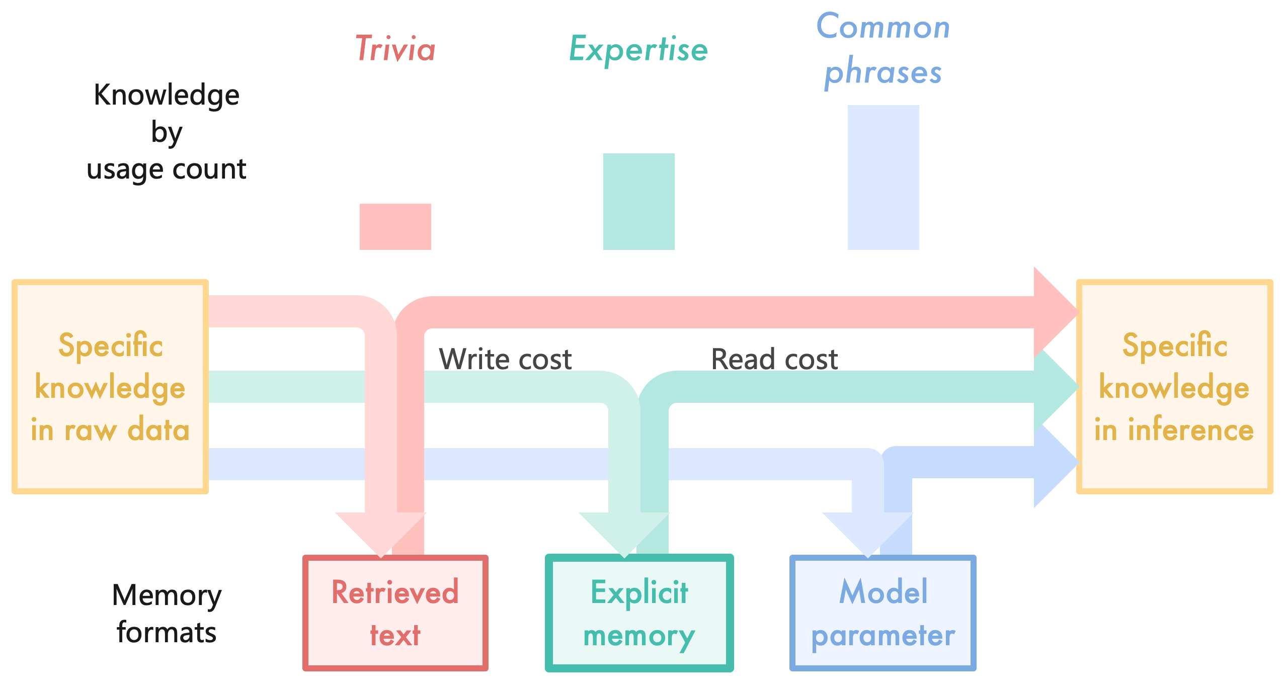<details> <summary>extracted/5700921/Figures/Theory/knowledge_distribution.png Details</summary>  ### Visual Description ## Diagram: Knowledge Processing Pathways in AI Systems ### Overview This image is a conceptual diagram illustrating how different types of knowledge ("Trivia," "Expertise," "Common phrases") are processed and stored in an AI system. It maps the flow from raw data to inference-ready knowledge, highlighting the associated computational costs and the memory formats used for storage. The diagram combines a simple bar chart with a flowchart to show relationships and pathways. ### Components/Axes **Top Section - Bar Chart:** * **Title/Label:** "Knowledge by usage count" (positioned top-left). * **Categories (X-axis):** Three distinct knowledge types, each with a corresponding colored bar. 1. **Trivia** (Label: Pink text, top-left). Bar: A short, solid pink rectangle. 2. **Expertise** (Label: Teal text, top-center). Bar: A medium-height, solid teal rectangle. 3. **Common phrases** (Label: Light blue text, top-right). Bar: The tallest, solid light blue rectangle. * **Y-axis:** Implied to represent "usage count" or frequency, with bar height indicating relative magnitude. No numerical scale is provided. **Middle Section - Flow Diagram:** * **Source Node (Left):** A yellow-bordered box labeled "Specific knowledge in raw data" (text in gold). * **Destination Node (Right):** A yellow-bordered box labeled "Specific knowledge in inference" (text in gold). * **Flow Paths:** Three colored, semi-transparent arrows flow from the source to the destination, each splitting to also feed into a corresponding memory format box below. 1. **Pink Path:** Associated with "Trivia." It has a label "Write cost" positioned above its initial segment. 2. **Teal Path:** Associated with "Expertise." It has a label "Read cost" positioned above its initial segment. 3. **Light Blue Path:** Associated with "Common phrases." No specific cost label is attached to this path segment. **Bottom Section - Memory Formats:** * **Label:** "Memory formats" (positioned bottom-left). * **Three storage boxes,** each receiving an arrow from the flow paths above: 1. **Retrieved text** (Red-bordered box, pink text). Receives the pink arrow. 2. **Explicit memory** (Teal-bordered box, teal text). Receives the teal arrow. 3. **Model parameter** (Blue-bordered box, light blue text). Receives the light blue arrow. ### Detailed Analysis The diagram establishes a clear mapping between knowledge types, memory formats, and processing costs: * **Trivia** is characterized by low usage count (shortest bar). It is processed via a pathway with a noted "Write cost" and is stored in the "Retrieved text" memory format. * **Expertise** has medium usage count (medium bar). Its pathway is associated with a "Read cost" and it is stored as "Explicit memory." * **Common phrases** have the highest usage count (tallest bar). They flow through a pathway without a specific cost label in this diagram and are stored directly as "Model parameter." The flow indicates that "Specific knowledge in raw data" is transformed into "Specific knowledge in inference" through these three parallel channels, each utilizing a different storage mechanism with different implied computational trade-offs (write vs. read cost). ### Key Observations 1. **Usage vs. Storage Complexity:** There is an inverse relationship suggested between usage frequency and the apparent complexity of the storage format. The most frequently used knowledge ("Common phrases") is stored in the most integrated format ("Model parameter"), while the least used ("Trivia") is stored in a more external format ("Retrieved text"). 2. **Cost Attribution:** "Write cost" is explicitly linked to the Trivia/Retrieved text pathway, implying that storing this information has a significant initial overhead. "Read cost" is linked to the Expertise/Explicit memory pathway, suggesting that accessing this structured knowledge has a recurring computational cost. 3. **Color-Coded Consistency:** The diagram uses a strict color-coding scheme (pink, teal, light blue) to visually link each knowledge type (top), its flow path (middle), and its final memory format (bottom), ensuring clear traceability. ### Interpretation This diagram presents a model for understanding how an AI system, likely a large language model, allocates different types of information across its architecture. It argues that not all knowledge is stored equally. * **"Trivia" (low-frequency facts)** is treated like an external reference. It's costly to index ("Write cost") but can be looked up when needed ("Retrieved text"), similar to a database or retrieval-augmented generation (RAG) system. * **"Expertise" (structured, mid-frequency knowledge)** is stored in a more accessible but still distinct format ("Explicit memory"), akin to a knowledge graph or curated fact base. The "Read cost" suggests querying this system is non-trivial. * **"Common phrases" (high-frequency linguistic patterns)** are the most efficiently utilized. They are compressed and internalized directly into the model's weights ("Model parameter"), making them instantly available during inference with minimal access latency. The overarching insight is that efficient AI systems employ a **hybrid memory architecture**. They balance the high capacity but slow access of external retrieval (for trivia) with the fast, integrated access of model parameters (for common patterns), using intermediate explicit memory for structured expertise. The diagram visually argues that the "cost" of knowledge (in compute terms) is a function of both its usage frequency and the chosen storage format. </details> Figure 8: Different memory formats with different balances of write cost and read cost. The specific knowledges with high to low usage counts are exemplified by common expressions, expertise and trivia, and are assigned to implicit memory, explicit memory and external information. The imbalanced use of knowledges leads to a heterogeneous distribution of knowledges across the memory hierarchy. To minimize the total cost (1), the separable knowledges that are used more often should be assigned to memory formats with high write cost and low read cost, whereas the rarely used knowledges should be assigned to formats with low write cost and high read cost. Also, adding a new memory format $m+1$ is always beneficial as it expands the search space and decreases the minimum cost whenever the usage count of some knowledge $\mathcal{K}$ lies in the interval $$ [n^{-}_{m+1},n^{+}_{m+1}]=\big{\{}n\in[0,\infty)~{}\big{|}~{}\text{argmin}_{j} ~{}\text{cost}_{\text{write}}(\mathcal{K},j)+n\cdot\text{cost}_{\text{read}}( \mathcal{K},j)=m+1\big{\}} $$ Examples of these intervals are displayed in Figure 4. For concreteness, Figure 8 depicts a reasonable distribution of the specific knowledges for humans, and we expect a similar distribution to hold for LLMs equipped with explicit memory. ## 3 | Design This section describes the architecture and training scheme of Memory 3. Regarding architecture, the goal is to design an explicit memory mechanism for Transformer LLMs with moderately low write cost and read cost. In addition, we want to limit the modification to the Transformer architecture to be as little as possible, adding no new trainable parameters, so that most of the existing Transformer LLMs can be converted to Memory 3 models with little finetuning. Thus, we arrive at a simple design: - Write cost: Before inference, the LLM writes each reference to an explicit memory, saved on drives. The memory is selected from the key-value vectors of the self-attention layers, so the write process involves no training. Each reference is processed independently, avoiding the cost of long-context attention. - Read cost: During inference, explicit memories are retrieved from drives and read by self-attention alongside the usual context key-values. Each memory consists of very few key-values from a small amount of attention heads, thus greatly reducing the extra compute, GPU storage, drive storage and loading time. It allows the LLM to retrieve many references frequently with limited influence on decoding speed. Regarding training, the goal is to reduce the cost of pretraining with a more efficient distribution of knowledge. Based on the discussion in Section 2.3, we want to encourage the LLM to learn only abstract knowledges, with the specific knowledges mostly externalized to the explicit memory bank. Ideally, the pretraining cost should be reduced to be proportional to the small amount of knowledge stored in the model parameters, thereby taking a step closer to the learning efficiency of humans. ### 3.1 | Inference Process From now on, we refer to the realizations of separable knowledges (Definitions 5 and 6) as references. Our knowledge base (or reference dataset) consists of $1.1\times 10^{8}$ text chunks with length bounded by 128 tokens. Its composition is described in Section 4.4. Each reference can be converted to an explicit memory, which is a tensor with shape (memory layers, 2, key-value heads, sparse tokens, head dimension) = $(22,2,8,8,80)$ The 2 stands for the key and value, while the other numbers are introduced later. Before inference, the Memory 3 model converts all references to explicit memories and save them on drives or non-volatile storage devices. Then, at inference time, whenever (the id of) a reference is retrieved, its explicit memory is loaded from drives and sent to GPU to be integrated into the computation of Memory 3. By Remark 1, a reference during encoding does not need to attend to any other texts (e.g. other references or query texts), so it is fine to encode each reference independently prior to inference. Such isolation also helps to reduce the compute of attention. One can also employ a “cold start” approach to bypass preparation time: each reference is converted to explicit memory upon its initial retrieval, rather than prior to inference. Subsequent retrievals will then access this stored memory. The aforementioned inference with precomputed explicit memories will be called “warm start”. 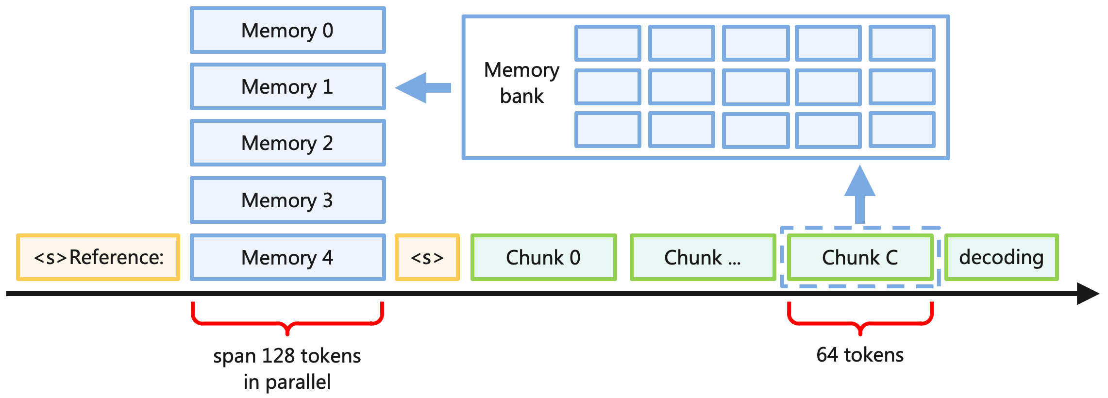<details> <summary>extracted/5700921/Figures/key_figure/m3mory_inference.png Details</summary>  ### Visual Description ## System Architecture Diagram: Memory-Augmented Parallel Processing Pipeline ### Overview The image is a technical system architecture diagram illustrating a memory-augmented processing pipeline. It depicts a flow where a "Reference" input is processed in parallel against multiple memory slots, followed by a sequential, chunk-based decoding stage that interacts with a larger "Memory bank." The diagram uses color-coding and spatial arrangement to distinguish between parallel and sequential processing phases. ### Components/Axes The diagram is organized into three main spatial regions: 1. **Top Region (Memory Bank & Slots):** * **Memory bank:** A large, light-blue rectangular container positioned in the top-right quadrant. It contains a 3x5 grid of 15 smaller, empty, light-blue rectangular slots. * **Memory Slots:** A vertical stack of five light-blue rectangles on the top-left, labeled from top to bottom: * `Memory 0` * `Memory 1` * `Memory 2` * `Memory 3` * `Memory 4` * **Relationship Arrow:** A solid blue arrow points from the `Memory bank` leftwards to the `Memory 1` slot, indicating a data flow or retrieval operation. 2. **Bottom Region (Processing Timeline):** * A thick black horizontal arrow runs across the bottom, representing a timeline or processing sequence from left to right. * **Reference Input (Left):** A yellow-outlined box labeled `<s>Reference:` is positioned at the start of the timeline. * **Parallel Processing Span:** A red curly brace underneath the timeline spans from the `Reference` box to the `Memory 4` slot. The annotation below it reads: `span 128 tokens in parallel`. * **Chunk Sequence (Right):** Following the parallel span, a series of green-outlined boxes are placed sequentially on the timeline: * `<s>` (A yellow-outlined box, similar to the reference marker) * `Chunk 0` * `Chunk ...` * `Chunk C` (This box is highlighted with a dashed blue outline) * `decoding` * **Chunk Interaction:** A solid blue arrow points upwards from the `Chunk C` box to the `Memory bank`, indicating that this specific chunk interacts with or retrieves data from the memory bank. * **Chunk Size Annotation:** A second red curly brace underneath the timeline spans the `Chunk C` and `decoding` boxes. The annotation below it reads: `64 tokens`. ### Detailed Analysis * **Color Coding:** * **Light Blue:** Used for all memory-related components (`Memory bank`, `Memory 0-4` slots). * **Yellow:** Used for sequence start markers (`<s>Reference:`, `<s>`). * **Green:** Used for data chunks in the sequential processing phase (`Chunk 0`, `Chunk ...`, `Chunk C`, `decoding`). * **Red:** Used for annotations describing token spans. * **Black:** Used for the main timeline arrow. * **Spatial Flow:** The process flows from left to right along the timeline. The initial `Reference` and the five `Memory` slots are processed in parallel (as indicated by the brace). The process then shifts to a sequential, chunk-by-chunk phase (`Chunk 0` to `decoding`). * **Key Relationships:** 1. The `Memory bank` feeds data into the parallel processing stage (arrow to `Memory 1`). 2. The sequential processing stage, specifically `Chunk C`, feeds back into or queries the `Memory bank` (arrow from `Chunk C`). 3. The parallel phase handles a larger context window (`128 tokens`) compared to the focused interaction in the sequential phase (`64 tokens` for the final chunk/decoding step). ### Key Observations 1. **Hybrid Processing Model:** The system combines parallel processing of a reference against multiple memory slots with a subsequent sequential, chunk-based decoding process. 2. **Asymmetric Memory Interaction:** The `Memory bank` has a bidirectional relationship with the pipeline: it provides data to the parallel stage and receives input from the sequential stage (`Chunk C`). 3. **Token Span Discrepancy:** The parallel phase operates on a 128-token span, while the annotated sequential phase (specifically the final chunk and decoding) is associated with a 64-token span, suggesting a reduction in context window or a more focused operation during decoding. 4. **Highlighted Element:** `Chunk C` is uniquely emphasized with a dashed outline, marking it as a critical component that bridges the sequential processing and the memory bank. ### Interpretation This diagram illustrates a sophisticated memory-augmented neural network architecture, likely for tasks like language modeling or machine translation. The design suggests a two-stage process: 1. **Contextualization Stage (Parallel):** A source "Reference" (e.g., a sentence to translate) is compared or attended against a set of memory slots (`Memory 0-4`) in parallel. This could represent retrieving relevant context or information from a fixed-size memory. The 128-token span indicates this stage handles a relatively broad context. 2. **Generation/Decoding Stage (Sequential):** The system then generates output sequentially in chunks. The interaction between `Chunk C` and the `Memory bank` implies that during generation, the model can dynamically access a larger, external memory store (`Memory bank`) to inform its predictions, moving beyond the limited slots used in the first stage. The 64-token annotation may indicate the size of the generation window or the granularity at which memory is accessed during decoding. The architecture aims to balance efficient parallel processing of input with the flexible, memory-aware generation of output, addressing the challenge of maintaining coherent long-range dependencies in sequence-to-sequence tasks. The separation of a small, fast memory (slots 0-4) from a larger bank is a common pattern for optimizing memory access latency. </details> Figure 9: The decoding process of Memory 3 with memory recall. Each chunk is a fixed-length interval of tokens, which may belong to either the prompt or generated text. During inference, as illustrated in Figure 9, whenever the LLM generates 64 tokens, it discards the current memories, uses these 64 tokens as query text to retrieve 5 new memories, and continues decoding with these memories. Similarly, when processing the prompt, the LLM retrieves 5 memories for each chunk of 64 tokens. Each chunk attends to its own memories, and the memories could be different across chunks. We leave it to future work to optimize these hyperparameters. The retrieval is performed with plain vector search with cosine similarity. The references as well as the query chunks are embedded by BGE-M3, a multilingual BERT model [17]. The query and key vectors for retrieval are both obtained from the output feature of the $\langle\text{cls}\rangle$ token. The vector index is built with FAISS [35]. To further save time, we maintain a fixed-size cache in RAM to store the most recently used explicit memories. It’s been observed that adjacent chunks often retrieve some of the same references. So the cache reduces the cost of loading explicit memories from drives. **Remark 2** *It would be ideal to perform retrieval using the hidden features from the LLM itself, since conceptually the LLM should know its needs better than any external module, and such internalized retrieval appears more anthropomorphic. Moreover, retrieving with the hidden features from different layers, different heads and different keywords can help to obtain more diverse results. One simple implementation is to use the sparsified attention queries of the query text to directly search for the explicit memories. Since the explicit memories are the attention key-values, such retrieval can work without the need to finetune the LLM. Specifically, this multi-vector retrieval can follow the routine of [61] with the additional constraint that a query from attention head $h$ can only search for keys from $h$ , while the sparse attention queries can be obtain using the same selection mechanism for explicit memories described later.* **Remark 3** *One shortcoming of RAG is that the references are usually text chunks instead of whole documents, and thus during inference the references are encoded without their contexts, making them less comprehensible. This shortcoming can be easily overcome for explicit memories. One solution is to encode each document as one sequence, then chunk the attention key-values into 128-token chunks and sparsify them into explicit memories. This procedure allows the key-values to attend to all their contexts.* ### 3.2 | Writing and Reading Memory Each explicit memory is a subset of the attention key-values from a subset of attention heads when encoding a reference. Thus, during inference, the LLM can directly read the retrieved explicit memories through its self-attention layers by concatenating them with the usual context key-values (Figure 9). Specially, for each attention head $h$ at layer $l$ , if it is chosen as a memory head, then its output $Y^{l,h}$ changes from the usual $$ Y^{l,h}_{i}=\text{softmax}\Big{(}\frac{X^{l,h}_{i}W^{l,h}_{Q}\big{(}X^{l,h}_{[ :i]}W^{l,h}_{K}\big{)}^{T}}{\sqrt{d_{h}}}\Big{)}X^{l,h}_{[:i]}W^{l,h}_{V}W^{l, h}_{O} $$ where $X_{[:i]}$ denotes all tokens before or at position $i$ and $d_{h}$ denotes the head dimension, to $$ Y^{l,h}_{i}=\text{softmax}\Big{(}\frac{X^{l,h}_{i}W^{l,h}_{Q}\cdot\text{concat }\big{(}K^{l,h}_{0},\dots K^{l,h}_{4},X^{l,h}_{[:i]}W^{l,h}_{K}\big{)}^{T}}{ \sqrt{d_{h}}}\Big{)}\text{concat}\big{(}V^{l,h}_{0},\dots V^{l,h}_{4},X^{l,h}_ {[:i]}W^{l,h}_{V}\big{)}W^{l,h}_{O} \tag{4} $$ where each $(K_{j},V_{j})$ denotes the keys and values of an explicit memory. While the context BOS token is $\langle\text{s}\rangle$ as usual, when encoding each reference we modify the BOS to “ $\langle\text{s}\rangle$ Reference:” to help the LLM distinguish between encoding normal texts and encoding references. This modified BOS is also prepended to the context during inference, as illustrated in Figure 9, while the context BOS token now serves as a separator between the references and context. Unlike the explicit memories which only appear at a subset of attention heads, this modified BOS is placed at every head at every layer. The motivation is that since the context BOS can attend to the references, its feature is no longer constant, so the LLM needs the modified BOS to serve as the new constant for all attention heads. Furthermore, we adopt parallel position encoding for all explicit memories, namely the positions of all their keys lie in the same interval of length 128, as depicted in Figure 9. We use the rotary position encoding (RoPE) [107]. The token sparsification is applied after RoPE processes the attention keys, so the selected tokens retain their relative positions in the references. Besides flexibility, one motivation for parallel position is to avoid the “lost in the middle” phenomenon [72], such that if the references are positioned serially, then the ones in the middle are likely to be ignored. Similarly, token sparsification also helps to alleviate this issue by making the attention more focused on the important tokens. We note that designs analogous to the parallel position have been used to improve in-context learning [96] and long-context modeling [15]. ### 3.3 | Memory Sparsification and Storage One of the greatest challenges for explicit memories is that the attention key-values occupy too much space. They not only demand more disk space, which could be costly, but also occupy GPU memory during inference, which could harm the batch size and thus the throughput of LLM generation. An intense compression is needed to save space. The full attention key tensor (or value tensor) for each reference has shape (layers, key-value heads, tokens, head dimension), so we compress all four dimensions. Regard layers, we only set the first half of the attention layers to be memory layers, i.e. layers that produce and attend to explicit memories (4), while the second half remain as the usual attention layers. Note that Remark 1 suggests that it is usually the attention heads in the middle of the LLM that attend to the references. So it seems that appointing the middle attention layers (e.g. the ones within the $25\$ to $75\$ depth range) to be memory layers is a more sensible choice. This heuristic is supported by the observations in [122, 39] that the attention to the distant context usually takes place in the middle layers. Regarding heads, we set all key-value heads at each memory layer to be memory heads. We reduce their amount by grouped query attention (GQA) [6], letting each key-value head be shared by multiple query heads, and obtain 20% sparsity (8 versus 40 heads). It is worth mentioning that, besides GQA and memory layers, another approach is to select a small subset of heads that are most helpful for reading memories, and this selection does not have to be uniform across layer. We describe several methods for selecting memory heads in Remark 4. Regarding tokens, we select 8 tokens out of 128 for each key-value head. We choose a high level of sparsity, since Remark 1 indicates that the attention from the context to the references are expected to be concentrated on very few tokens. Note that the selected tokens are in general different among heads, so in principle their union could cover a lot of tokens. For each head $h$ at layer $l$ , the selection uses top-8 over the attention weight $$ w^{l,h}_{j}=\sum_{i=0}^{127}\tilde{a}^{l,h}_{i,j},\quad\tilde{a}^{l,h}_{i,j}= \text{softmax}_{j}\Big{(}\frac{X^{l,h}_{i}W^{l,h}_{Q}(X^{l,h}_{j}W^{l,h}_{K})^ {T}}{\sqrt{d_{h}}}\Big{)} $$ which measures the importance of a token by the attention received from all tokens. The BOS tokens and paddings do not participate in the the computation of the weights. These attention weights $\tilde{a}$ are different from the usual ones, such that there is no causal mask or position encoding involved. The consideration is that since the explicit memories are prepared before any inference, the selection can only depend on the reference itself instead of any context texts. The removal of causal mask and position encoding ensures that tokens at any position has an equal chance to receive attention from others. To speed up computation, we adopt the following approximate weights in our implementation, although in retrospect this speedup is not necessary. $$ w^{l,h}_{j}=\sum_{i=0}^{127}\exp\Big{(}\frac{X^{l,h}_{i}W^{l,h}_{Q}(X^{l,h}_{j }W^{l,h}_{K})^{T}}{\sqrt{d_{h}}}\Big{)} $$ Similar designs that sparsify tokens based on attention weights have been adopted in long-context modeling to save space [74, 131]. Regarding head dimension, we optionally use a vector quantizer to compress each of the key and value vectors using residual quantizations [18] built with FAISS [35]. The compression rate is $80/7\approx 11.4$ . During inference, the retrieved memories are first loaded from drives, and then decompressed by the vector quantizer before being sent to GPU. The evaluations in Section 7.1 indicate that this compression has negligible influence on the performance of Memory 3. More details can be found in Appendix B. Hence, the total sparsity is 160 or 1830 (without or with vector compression). Originally, the explicit memory bank would have an enormous size of 7.17PB or equivalently 7340TB (given the model shape described in Section 3.4 and saved in bfloat16). Our compression brings it down to 45.9TB or 4.02TB (without or with vector compression), both acceptable for the drive storage of a GPU cluster. To deploy the Memory 3 model on end-side devices such as smart phones and laptops, one can place the explicit memory bank and the vector index on a cloud server, while the devices only need to store the model parameters and the decoder of the vector quantizer. During inference, to perform retrieval, the model on the end-side device sends the query vector to the cloud server, which then searches the index and returns the compressed memories. The speed test of this deployment is recorded in Section 7.5. **Remark 4** *If one wants to finetune a pretrained LLM into a Memory 3 model, there are several ways to select a small but effective subset of attention heads (among all heads at all layers) for memory heads (4). Methods such as [122, 39] are proposed to identify the heads that contribute the most to long-context modeling by retrieving useful information from distant tokens, and usually these special heads account for only $<10\$ of the total heads. Here we also propose a simple method for selecting memory heads: Given the validation subsets of a representative collection of evaluation tasks, one can measure the average performance $s_{h}$ for a modified version of the LLM for each attention head $h$ . The modification masks the distant tokens for head $h$ so it can only see the preceding 100 tokens and the BOS token. Then, it is reasonable to expect that $s_{h}$ would be markedly low for a small subset of heads $h$ , indicating that they are specialized for long-range attention.* **Remark 5** *Actually, Remark 1 suggests that each reference only needs to be attended to by just one attention head, although in general this special head may be different among the references. Thus, it seems a promising approach to apply adaptive sparsity not only to token selection, but also to the memory heads, namely each reference is routed to one or two heads (analogously to MoE), and its explicit memory is produced and read by these heads. Such design if feasible can further boost the sparsity of explicit memory and save much more space.* ### 3.4 | Model Shape As discussed in Section 2.3, the specific knowledges can be externalized to explicit memories, and thus to minimize the total cost (1), the model parameters (or implicit memory) only need to store abstract knowledges and the subset of specific knowledges that are frequently used. The shape of our model, i.e. (the number of Transformer blocks $L$ , heads $H$ , head dimension $d_{h}$ , width of the MLP layers $W$ ), is chosen to accommodate this desired knowledge distribution. Informally speaking, given a fixed parameter size $P$ , the shape maximizes the following objective $$ \max_{L,H,d_{h},W}\Big{\{}\frac{\text{capacity for abstract knowledge}}{\text{ capacity for specific knowledge}}~{}\Big{|}~{}\text{size}(L,H,d_{h},W)\approx P \Big{\}} \tag{5} $$ Here we set $P$ to be 2.4 billion. Some recent works suggest that the capacities for learning specific knowledges and abstract knowledges are subject to different constraints. On one hand, [29] observes that the amount of bits of trivia information (such as a person’s name, date of birth and job title) that a LLM can store depends only on its parameter size. Regardless of $L$ and $H$ , the max capacity is always around 2 bits per parameter. On the other hand, [120] trains Transformers to learn simple algorithms such as reversing a list and counting the occurrence of each letter. It is observed that for several such tasks, there exists a minimum $L_{0}$ and $H_{0}$ such that a Transformer with $L\geq L_{0}$ and $H\geq H_{0}$ can learn the task with perfect accuracy, whereas the accuracy drops significantly for Transformers with either $L=L_{0}-1$ or $H=H_{0}-1$ (given that either $L_{0}$ or $H_{0}\geq 2$ ). This sharp transition supports the view that the layers and heads of Transformer LLMs can be compared to algorithmic steps, and tasks with a certain level of complexity require at least a certain amount of steps. It is worth mentioning that the emergent phenomenon [119, 105] of LLMs can also be explained by this view and thus adds support to it, although it may not be the only explanation. By Definition 4, the abstract knowledges are expected to be circuits with greater complexity than specific knowledges, since their associated inputs and outputs exhibit greater variability and thus express more complex patterns. It follows that, in the context of the aforementioned works, the separation of specific and abstract knowledges should be positively correlated with the distinction between trivia information and algorithmic procedures. Hence, it is reasonable to adopt the approximation that the capacity of an LLM for specific knowledges only depends on its parameter size, whereas the capacity for abstract knowledges depends only on $L$ and $H$ . The informal problem (5) reduces to the maximization of $L$ and $H$ given a fixed parameter size. However, we are left with two ambiguities: first, this formulation does not specify the ratio between $L$ and $H$ , and second the head dimension $d_{h}$ and MLP width $W$ cannot be too small as the training may become unstable. Regarding the second point, our experiments indicate that pretraining becomes more unstable with increased spikes if $d_{h}\leq 64$ , so we set $d_{h}=80$ (though it needs to be pointed out that the loss spikes may not be solely attributed to the choice of $d_{h}$ , and high-quality data for instance may stabilize training and allow us to choose a smaller $d_{h}$ ). Also, the MLP width $W$ is set to be equal to the hidden dimension $d=Hd_{h}$ . Regarding the first point, controlled experiments (Figure 10) indicate that the loss decreases slightly more rapidly with $L:H\approx 1$ than with other ratios, so we adopt this ratio. 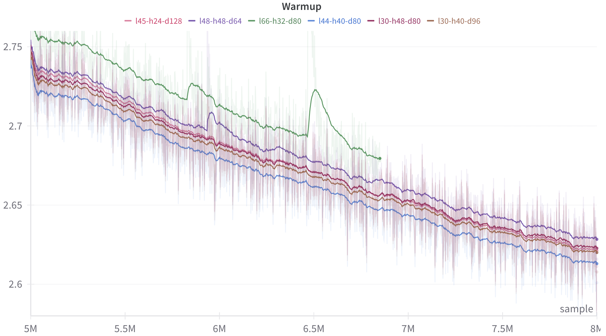<details> <summary>extracted/5700921/Figures/key_figure/optimize_2B_shape_warmup.png Details</summary>  ### Visual Description ## Line Chart: Warmup Performance of Model Configurations ### Overview The image displays a line chart titled "Warmup," plotting the performance (likely a loss metric) of six different model configurations over a training period measured in samples. The chart shows a general downward trend for all configurations, indicating improvement (reduction in loss) as training progresses. Each line is accompanied by a shaded region, likely representing variance or confidence intervals. ### Components/Axes * **Title:** "Warmup" (centered at the top). * **Legend:** Positioned at the top, below the title. It contains six entries, each with a colored line segment and a label: * Pink line: `l45-h24-d128` * Purple line: `l48-h48-d64` * Green line: `l66-h32-d80` * Blue line: `l44-h40-d80` * Dark Red line: `l30-h48-d80` * Brown line: `l30-h40-d96` * **X-Axis:** Labeled "sample" (bottom right). The axis has major tick marks at 5M, 5.5M, 6M, 6.5M, 7M, 7.5M, and 8M (where "M" denotes million). * **Y-Axis:** Unlabeled, but displays numerical values. Major tick marks are at 2.6, 2.65, 2.7, and 2.75. The scale is linear. ### Detailed Analysis The chart tracks six distinct data series, each corresponding to a model configuration denoted by a label (e.g., `l45-h24-d128`). The labels likely encode architectural parameters (e.g., layers, heads, dimensions). **Trend Verification & Data Points (Approximate):** All series exhibit a general downward slope from left (5M samples) to right (8M samples), indicating decreasing loss over time. The lines are noisy, with frequent small fluctuations. 1. **Green Line (`l66-h32-d80`):** * **Trend:** Starts as the highest line, decreases, but exhibits a significant, sharp upward spike (anomaly) centered around 6.5M samples before resuming its decline. * **Approximate Values:** Starts near 2.75 at 5M. After the spike, it ends near 2.68 at 8M. It remains the highest line for most of the chart's duration. 2. **Blue Line (`l44-h40-d80`):** * **Trend:** Consistently the lowest line throughout the plotted range, showing a steady decline. * **Approximate Values:** Starts near 2.72 at 5M. Ends near 2.61 at 8M. 3. **Purple Line (`l48-h48-d64`):** * **Trend:** Generally the second-highest line, following a similar path to the green line but without the major spike. * **Approximate Values:** Starts near 2.74 at 5M. Ends near 2.63 at 8M. 4. **Pink Line (`l45-h24-d128`), Dark Red Line (`l30-h48-d80`), Brown Line (`l30-h40-d96`):** * **Trend:** These three lines are tightly clustered in the middle of the pack, following very similar downward trajectories. They are often intertwined. * **Approximate Values:** All start between 2.73 and 2.74 at 5M. They end in a tight cluster between approximately 2.62 and 2.63 at 8M. **Spatial Grounding:** The legend is centered horizontally at the top. The green line's anomalous spike is a prominent feature in the center of the chart. The blue line occupies the bottom edge of the data cluster. The shaded variance regions are most expansive for the green line, especially around its spike. ### Key Observations 1. **Performance Hierarchy:** A clear, persistent hierarchy exists: `l66-h32-d80` (green) > `l48-h48-d64` (purple) > {`l45-h24-d128`, `l30-h48-d80`, `l30-h40-d96`} (cluster) > `l44-h40-d80` (blue). Lower y-values indicate better performance (lower loss). 2. **Anomaly:** The `l66-h32-d80` (green) configuration experiences a major, temporary performance degradation (loss spike) around 6.5M samples. 3. **Convergence:** By 8M samples, the performance gap between the middle three configurations and the best (green) has narrowed, but the blue configuration maintains a distinct advantage. 4. **Variance:** The shaded regions suggest that the `l66-h32-d80` (green) configuration also exhibits higher variance or instability, particularly around the anomaly. ### Interpretation This chart visualizes the "warmup" phase of training for different neural network architectures. The y-axis almost certainly represents a loss function (e.g., cross-entropy), where lower is better. The x-axis tracks the number of training samples processed. The data suggests that architectural choices (encoded in the labels) significantly impact both the final performance and the stability of training. The `l44-h40-d80` (blue) configuration appears to be the most efficient and stable learner within this sample range. The `l66-h32-d80` (green) configuration, while ultimately performing well, suffers from a notable instability event, which could be due to factors like learning rate sensitivity, gradient issues, or data batch characteristics. The tight clustering of the pink, dark red, and brown lines indicates that their respective architectural differences lead to very similar training dynamics and outcomes in this warmup phase. The chart is crucial for diagnosing training behavior, comparing model variants, and identifying potential instabilities that need to be addressed (e.g., via learning rate scheduling or architectural tweaks). The absence of a y-axis label is a minor omission for a technical document; it should be explicitly stated (e.g., "Validation Loss"). </details> Figure 10: Comparison of the training losses of models with different shapes, whose parameter sizes range in $2.1\sim 2.4$ B. The legend l44h40d80 denotes $L=44,H=40,d_{h}=80$ , and the $x$ -axis denotes the amount of training samples. Nevertheless, this comparison is not definite, since this is only the warmup stage of our training scheme (Section 3.6) and the ranking may change in the continual train stage when explicit memory is introduced. In addition, as discussed in Section 3.3, our model uses grouped query attention (GQA), so the number of key-value heads $H_{kv}$ is set to be $8$ , which is the usual choice for GQA. The MLP layers are gated two-layer networks without bias, which are the default choice in recent years [110, 11, 21, 8]. Finally, the model shape is set to be $L=44,H=40,H_{kv}=8,d_{h}=80,W=3200$ , with the total non-embedding parameter size being $2.4$ B. ### 3.5 | Training Designs Similar to our architecture design, the design of our training scheme focuses on learning abstract knowledges. The goal is to reduce the training compute, as the LLM no longer needs to memorize many of the specific knowledges. This shift in learning objective implies that all the default settings for pretraining LLMs may need to be redesigned, as they were optimized for the classical scenario when the LLMs learn both abstract and specific knowledges. 1. Data: Ideally, the pretraining data should have a high concentration of abstract knowledges and minimum amount of specific knowledges. It is known that LLM pretraining is very sensitive to the presence of specific knowledges. For instance, [55] observes that a small model can master arithmetic (e.g. addition of large numbers) if trained on clean data. However, if the training data is mixed with trivial information (e.g. random numbers), then the test accuracy stays at zero unless the model size is increased by a factor of 1500. It suggests that training on specific knowledges significantly inhibits the learning of abstract knowledges, and may explain why emergent abilities [119] are absent from small models. Notably, the Phi-3 model [4] is pretrained with a data composition that closely matches our desired composition. Although the technical details are not revealed, it is stated that they filter data based on two criteria: the data should encourage reasoning, and should not contain information that is too specific. 1. Initialization: [132] observes that initializing Transformer parameters with a smaller standard deviation ( $d^{c}$ with $c<-1/2$ instead of the usual $\Theta(d^{-1/2})$ [47, 52]) can encourage the model to learn compositional inference instead of memorization. Specially, an arithmetic dataset is designed with a train set and an out-of-distribution test set, which admits two possible answers. One answer relies on memorizing more rules during training, while the other requires an understanding of the compositional structure underlying these rules. The proposed mechanism is that training with smaller initialization belongs to the condensed regime that encourages sparse solutions, contrary to training with large initialization that belongs to the kernel regime or critical regime [78, 19]. 1. Weight decay: [90, 88] observe that using a larger weight decay coefficient (i.e. greater than the usual range of $0.001\sim 0.1$ ) can guide LLMs to favor generalization over memorization, and accelerate the learning of generalizable solutions. They consider settings that exhibit grokking [90] such that training would transit from perfect train accuracy and zero test accuracy to perfect test accuracy, and generalization ability is measured by how quickly this transition occurs. Moreover, theoretically speaking, it is expected that training generative models needs stronger regularization than training regression models, in order to prevent the generated distributions from collapsing onto the training data and become trivial [128]. In summary, it is recommendable to pretrain the Memory 3 model with a data composition that emphasizes abstract knowledges and minimizes specific information, a smaller initialization for parameters, and a larger weight decay coefficient. Since this work is only a preliminary version of Memory 3, we decide to stick with the conventional setting for training and have not experimented with any of these ideas. We look forward to incorporating these designs in future versions of the Memory 3 model. ### 3.6 | Two-stage Pretrain The Memory 3 model learns to write and read explicit memories during pretraining. The training data is prepended with retrieved references; the model encodes these references into explicit memories in real time, and integrates them into the self-attention computation of the training data. Unexpectedly, our pretraining consists of two stages, which we name as warmup and continual train. Only the continual train stage involves explicit memories, while the warmup stage uses the same format as ordinary pretraining. Our motivation is depicted in Figure 11. We observe that pretraining with explicit memories from the beginning would render the memories useless, as there appears to be no gain in training loss compared to ordinary pretraining. Meanwhile, given a checkpoint from ordinary pretraining, continual training with explicit memory exhibits a visible decrease in training loss. This comparison implies that a memory-less warmup stage might be necessary for pretraining a Memory 3 model. One possible explanation for this phenomenon is that in the beginning of pretraining, the model is too weak to understand and leverage the explicit memories it generates. Then, to reduce distraction, the self-attention layers might learn to always ignore these memories, thus hindering indefinitely the development of explicit memory. 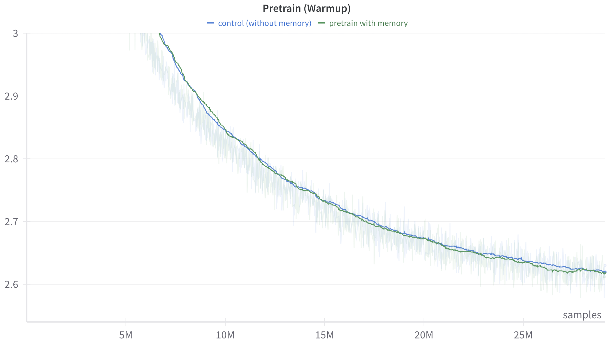<details> <summary>extracted/5700921/Figures/key_figure/warmup_l40-h32-d64-ml20_smooth95.png Details</summary>  ### Visual Description \n ## Line Chart: Pretrain (Warmup) Loss Curves ### Overview The image displays a line chart comparing the training loss (y-axis) over the number of training samples (x-axis) for two different pretraining configurations during a "warmup" phase. The chart shows a clear downward trend for both configurations, indicating that the model's performance (as measured by loss) improves with more training data. ### Components/Axes * **Chart Title:** "Pretrain (Warmup)" * **X-Axis:** * **Label:** "samples" * **Scale:** Linear scale with major tick marks at 5M, 10M, 15M, 20M, and 25M (where "M" denotes millions). * **Y-Axis:** * **Label:** Not explicitly labeled. Based on context, it represents a loss metric (e.g., cross-entropy loss). * **Scale:** Linear scale with major tick marks at 2.6, 2.7, 2.8, 2.9, and 3.0. * **Legend:** Located at the top center of the chart. * **Blue Line:** "control (without memory)" * **Green Line:** "pretrain with memory" * **Data Series:** Two primary lines with associated shaded regions. * **Blue Line (Control):** Represents the training loss for the baseline model without a memory component. * **Green Line (With Memory):** Represents the training loss for the model incorporating a memory mechanism. * **Shaded Regions:** Light blue and light green shaded areas around their respective lines, likely indicating variance, standard deviation, or a confidence interval across multiple runs. ### Detailed Analysis **Trend Verification:** * **Control (Blue Line):** The line exhibits a steep downward slope from the start (left) until approximately 10M samples, after which the rate of decrease slows, forming a convex curve that gradually flattens. * **Pretrain with Memory (Green Line):** Follows a nearly identical trajectory to the control line. It also shows a steep initial decline followed by a gradual flattening. **Data Point Extraction (Approximate Values):** * **At ~5M samples:** * Control (Blue): Loss ≈ 3.0 * With Memory (Green): Loss ≈ 2.99 (slightly below the blue line) * **At 10M samples:** * Control (Blue): Loss ≈ 2.85 * With Memory (Green): Loss ≈ 2.84 * **At 15M samples:** * Control (Blue): Loss ≈ 2.73 * With Memory (Green): Loss ≈ 2.72 * **At 20M samples:** * Control (Blue): Loss ≈ 2.67 * With Memory (Green): Loss ≈ 2.66 * **At 25M samples (end of chart):** * Control (Blue): Loss ≈ 2.62 * With Memory (Green): Loss ≈ 2.62 (The lines appear to converge at this point). **Spatial Grounding & Comparison:** The green line ("with memory") is consistently positioned slightly below the blue line ("control") throughout the entire visible range from 5M to 25M samples. The vertical gap between them is very small but persistent. The shaded variance regions for both lines overlap significantly, suggesting the difference in mean loss may not be statistically large relative to the run-to-run variability. ### Key Observations 1. **Dominant Trend:** Both configurations show a strong, monotonic decrease in loss as training samples increase, which is the expected behavior for a successful training process. 2. **Diminishing Returns:** The rate of loss improvement slows dramatically after the first 10M samples. The curve from 10M to 25M samples is much flatter than from 5M to 10M. 3. **Minimal Performance Gap:** The "pretrain with memory" configuration maintains a very slight but consistent advantage (lower loss) over the "control" configuration across the entire warmup phase shown. 4. **Convergence:** By 25M samples, the two lines are nearly indistinguishable, suggesting the performance benefit of memory may diminish or stabilize with sufficient training data in this warmup phase. 5. **High Variance:** The wide shaded regions indicate substantial noise or variability in the loss measurement at each point, which is common in early training stages. ### Interpretation This chart demonstrates the efficacy of the pretraining process, as loss decreases with more data. The core finding is that **incorporating a memory mechanism provides a marginal but consistent improvement in training efficiency (lower loss) during the warmup phase** compared to a control model without memory. The data suggests the memory component helps the model learn slightly faster or more effectively from the same amount of data, particularly in the earlier stages (5M-15M samples). However, the benefit is small in magnitude. The convergence of the lines at 25M samples could imply that: * The memory's advantage is most critical early on. * Given enough data, the control model eventually catches up in performance for this specific metric and phase. * The warmup phase's objectives might be largely met by both models after 25M samples, setting the stage for subsequent training phases. The high variance (shaded areas) is a critical context; the observed difference between the two methods, while consistent, is small relative to the noise. A rigorous analysis would require statistical testing to confirm if the gap is significant. Overall, the chart supports the hypothesis that memory-augmented pretraining is beneficial, but the effect size during warmup appears to be modest. 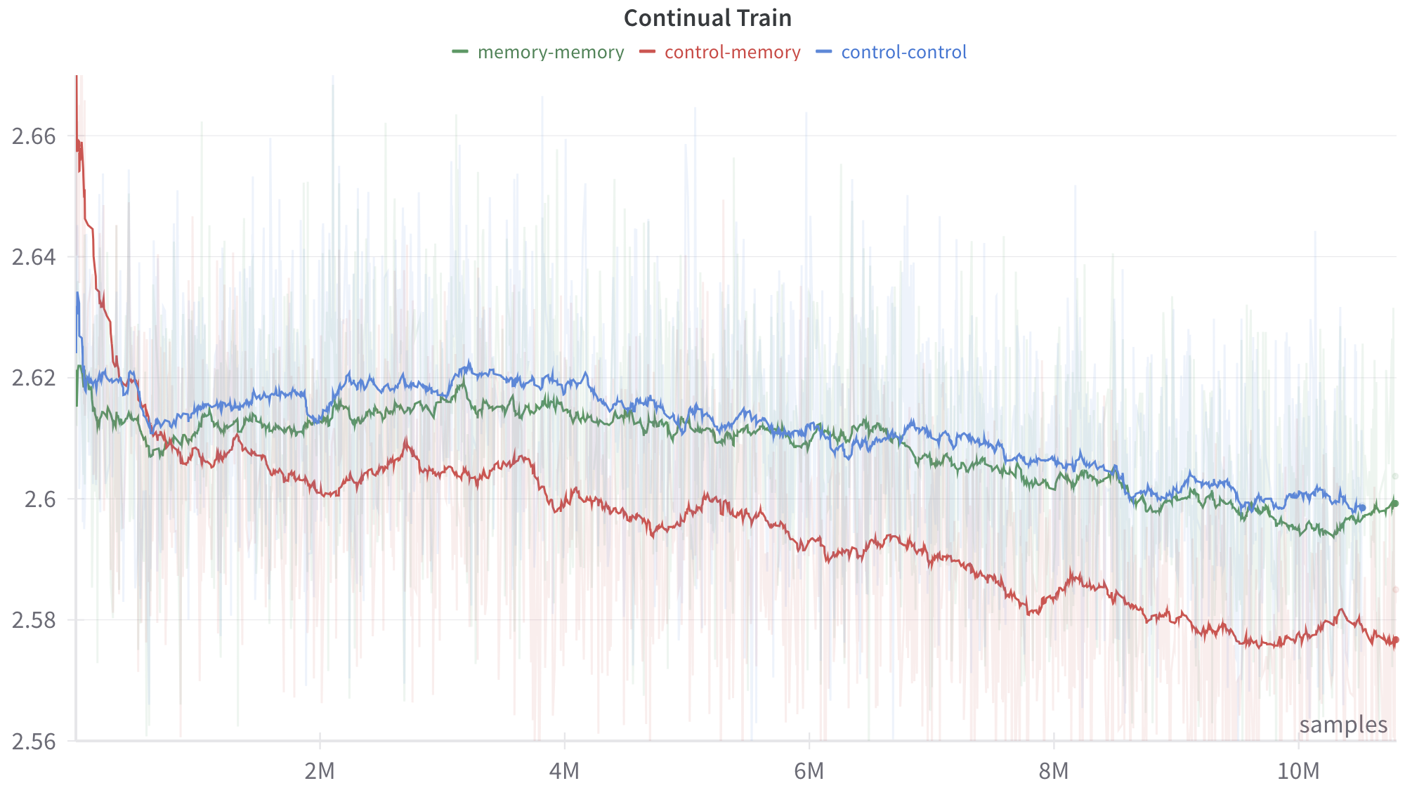</details> (a) <details> <summary>extracted/5700921/Figures/key_figure/continual_l40-h32-d64-ml20_smooth95.png Details</summary>  ### Visual Description ## Line Chart: Continual Train ### Overview The image displays a line chart titled "Continual Train," plotting a metric (y-axis) against the number of training samples (x-axis). It compares the performance of three distinct experimental conditions or model configurations over the course of a training process. The chart includes smoothed trend lines overlaid on top of noisier, raw data traces (shown as faint, semi-transparent lines in the background). ### Components/Axes * **Title:** "Continual Train" (top center). * **Legend:** Positioned at the top center, below the title. It defines three data series: * `memory-memory` (green line) * `control-memory` (red line) * `control-control` (blue line) * **X-Axis:** * **Label:** "samples" (bottom right corner). * **Scale:** Linear scale from 0 to over 10 million (10M) samples. * **Major Tick Marks:** Labeled at 2M, 4M, 6M, 8M, and 10M. * **Y-Axis:** * **Scale:** Linear scale from approximately 2.56 to 2.67. * **Major Tick Marks:** Labeled at 2.56, 2.58, 2.60, 2.62, 2.64, and 2.66. * **Interpretation:** The metric is unitless but likely represents a loss function (where lower is better) or a similar performance measure. ### Detailed Analysis **Trend Verification & Data Points (Approximate):** 1. **`control-memory` (Red Line):** * **Trend:** Shows a strong, consistent downward slope throughout the training period. It starts as the highest value and ends as the lowest. * **Key Points:** * Start (~0 samples): ~2.665 * At 2M samples: ~2.605 * At 4M samples: ~2.595 * At 6M samples: ~2.585 * At 8M samples: ~2.580 * End (~10.5M samples): ~2.575 2. **`memory-memory` (Green Line):** * **Trend:** Shows a gradual, slight downward trend. It starts in the middle, dips below the blue line around 1M samples, and remains generally between the red and blue lines for the remainder of the chart. * **Key Points:** * Start (~0 samples): ~2.620 * At 2M samples: ~2.610 * At 4M samples: ~2.615 * At 6M samples: ~2.610 * At 8M samples: ~2.605 * End (~10.5M samples): ~2.600 3. **`control-control` (Blue Line):** * **Trend:** Shows a very gradual, slight downward trend, nearly flat for long periods. It starts as the middle value, rises above the green line after ~1M samples, and remains the highest of the three for most of the training after the initial phase. * **Key Points:** * Start (~0 samples): ~2.635 * At 2M samples: ~2.615 * At 4M samples: ~2.620 * At 6M samples: ~2.615 * At 8M samples: ~2.605 * End (~10.5M samples): ~2.600 **Spatial Grounding & Component Isolation:** * **Header Region:** Contains the title and legend. The legend is horizontally aligned, with color-coded dashes preceding each label. * **Main Chart Region:** Contains the three primary trend lines and their associated shaded variance bands. The faint background lines show high-frequency noise in the raw data. * **Footer Region:** Contains the x-axis label ("samples") and tick marks. * **Cross-Reference:** The red line (`control-memory`) is consistently the lowest after the initial ~1M samples. The blue (`control-control`) and green (`memory-memory`) lines converge closely towards the end of the chart, both hovering near 2.600. ### Key Observations 1. **Diverging Performance:** The `control-memory` condition (red) demonstrates significantly better (lower) final performance compared to the other two conditions, with a clear and sustained improvement trajectory. 2. **Initial Volatility:** All three lines show high initial volatility within the first ~500k samples before settling into more stable trends. 3. **Convergence of Baselines:** The `memory-memory` (green) and `control-control` (blue) conditions, while following slightly different paths, end at nearly identical performance levels (~2.600) after 10M+ samples. 4. **Noise Level:** The raw data (faint background lines) exhibits substantial noise across all conditions, but the smoothed trends reveal clear underlying patterns. ### Interpretation This chart likely visualizes the results of an experiment in machine learning, specifically comparing different strategies for "continual training" or learning over a long sequence of data samples. The y-axis metric is probably a loss value, where a decrease indicates improved model performance. * **What the data suggests:** The `control-memory` strategy is the most effective for minimizing the loss metric over time. The `control-control` and `memory-memory` strategies are less effective and perform similarly to each other in the long run. * **Relationship between elements:** The naming convention (`control-memory`, etc.) implies a comparison between models that have access to some form of memory (`memory`) versus those that do not (`control`), and how they are trained (continually on new data vs. a fixed control set). The superior performance of `control-memory` suggests that combining a control mechanism with memory access yields the best continual learning outcome in this setup. * **Notable Anomalies:** The most striking feature is the consistent and substantial gap between the red line and the other two. This indicates a fundamental difference in the effectiveness of the `control-memory` approach. The near-identical endpoint for the green and blue lines is also notable, suggesting that, despite different intermediate behaviors, the `memory-memory` and `control-control` approaches have equivalent asymptotic performance for this task and metric. </details> (b) Figure 11: Left: Comparison of the warmup stage (training from scratch) with and without explicit memory. The blue and green curves are trained without and with explicit memories, respectively. Right: Comparison of the continual train stage. The blue and green curves are continual trained from their warmup checkpoints, and the red curve is initialized with the warmup checkpoint of the blue curve and continual trained with explicit memory. These plots indicate that pretraining a Memory 3 model requires a memory-less warmup stage. These experiments use a smaller model with 0.92B non-embedding parameters $(L=40,H=32,d_{h}=64)$ . The warmup stage uses 60B data and the continual train stage uses 22B. Another modification is to reduce the cost of continual train. Recall from Section 3.1 that during inference, each 64-token chunk attends to five explicit memories, or equivalently five 128-token references if using cold start, increasing the amount of input tokens by 10 times. The inference process avoids the cost of memory encoding by precomputation or warm start, but for the continual train, the references need to be encoded in real time. Our solution is to let the chunks share their references during training to reduce the total number of references in a batch. Specifically, each chunk of a training sequence retrieves only one reference, and in compensation, attends to the references of the previous four chunks, besides its own reference. Each train sequence has length 2048 and thus 32 chunks, so it is equipped with $32\times 128=4096$ reference tokens. The hidden features of these reference tokens are discarded once passing the last memory layer, since after that they no longer participate in the update of the hidden feature of the train tokens. Hence, each continual train step takes slightly more than twice the amount of time of a warmup step. It is necessary to avoid information leakage when equipping the training data with references (i.e. the train sequence and its retrieved references could be the same text), for otherwise training becomes too easy and the model would not learn much. Previously, Retro [16] requires that no train sequence can retrieve a reference from the same document, but this criterion may be insufficient since near-identical paragraphs may appear in multiple documents. Thus, we require that no train sequence can be accompanied by a reference sequence that has $>90\$ overlap with it. The overlap is measured by the length of their longest common subsequence divided by the length of the reference length. Specially, given any train sequence $\mathbf{t}$ and reference $\mathbf{r}$ , define their overlap by $$ \displaystyle\begin{split}\text{overlap}(\mathbf{t},\mathbf{r}):=\frac{1}{| \mathbf{r}|}\max\big{\{}N&~{}\big{|}~{}\exists 1\leq i_{1}<\dots<i_{N}\leq| \mathbf{t}|~{}\text{and}~{}\exists 1\leq j_{1}<\dots<j_{N}\leq|\mathbf{r}|\\ &~{}\text{and}~{}|i_{N}-i_{1}|\leq 2|\mathbf{r}|,~{}\text{such that}~{}\mathbf {t}_{i_{k}}=\mathbf{r}_{j_{k}}~{}\text{for}~{}k=1,\dots N\big{\}}\end{split} \tag{6} $$ The constraint $|i_{N}-i_{1}|\leq 2|\mathbf{r}|$ ensures that the overlap is not over-estimated as $|\mathbf{t}|\to\infty$ . ## 4 | Pretraining Data This section describes the procedures for collecting and filtering our pretraining dataset and knowledge base (or reference dataset). ### 4.1 | Data Collection The pretrain data is gathered from English and Chinese text datasets, mostly publicly available collections of webpages and books. We also include code, SFT data (supervised finetuning), and synthetic data. Specially, the English data mainly consists of RedPajamaV2 [23], SlimPajama [104] and the Piles [43], in total 200TB prior to filtering. The Chinese data mainly comes from Wanjuan [51], Wenshu [2], and MNBVC [81], in total 500TB prior to filtering. The code data mainly comes from Github, and we take the subset with the highest repository stars. The SFT data is included since these samples generally have higher quality than the webpages. We use the same data as in SFT training (Section 6.1), except that these samples are treated as ordinary texts during pretraining, i.e. all tokens participate in the loss computation, not just the answer tokens. ### 4.2 | Filtering The raw data is filtered with three steps: deduplication, rule-based filtering, and model-based filtering. First, deduplication is performed with MinHash for most of the datasets. One exception is RedPajamaV2, which already comes with deduplication labels. Second, we devise heuristic, rule-based filters analogous to the ones from [76, 92, 25]. The purpose is to eliminate texts that are ostensibly unsuitable for training, such as ones that only contain webpage source codes, random numbers, or incomprehensible shards. Our filters remove documents with less than 50 words, documents whose mean word lengths exceed 10 characters, documents with 70% of context being non-alphabetic characters, documents whose fractions of unique words are disproportionately high, documents whose entropy of unigrams is excessively low, and so on. Finally, we select the subset of data with highest “quality”, a score produced by a finetuned BERT model. Specially, we sample ten thousand documents and grade them by the XinYu-70B model [65, 68] with prompt-guided generation. The prompt asks the model to determine whether the input text is informative and produce a score between $0 0$ and $5$ . Then, these scores are used to finetune the Tiny-BERT model [57], which has only 14M parameters. The hyperparameters of this finetuning are optimized with respect to a held-out validation set. After that, we use this lightweight BERT to grade the entire dataset. **Remark 6** *Recall from Section 3.5 that the pretraining data of Memory 3 should emphasize abstract knowledges and minimize specific knowledges. The purpose is to not only obtain a lightweight LLM with an ideal distribution of knowledges in accordance with the memory hierarchy (Figure 8), but also prevent the specific knowledges from hindering the learning process of the model. The focus of our prompt on “informativeness” might be contradictory to this goal, since the selected texts that are rich in information content may contain too many specific knowledges. 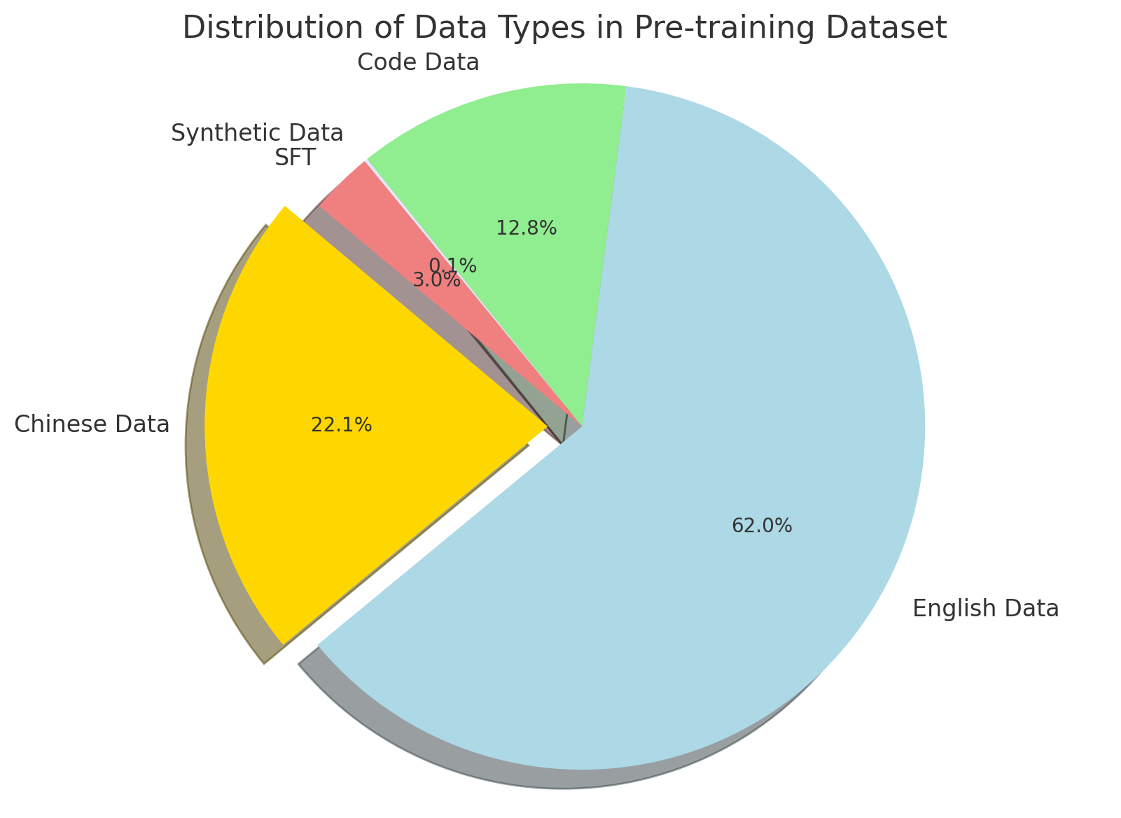For future versions of Memory 3, we will switch to a model-based filter favoring texts that exhibit more reasoning and less specifics.* <details> <summary>extracted/5700921/Figures/Data/pretrain_data_distribution.png Details</summary>  ### Visual Description ## Pie Chart: Distribution of Data Types in Pre-training Dataset ### Overview The image is a pie chart illustrating the proportional composition of different data types within a pre-training dataset. The chart is titled "Distribution of Data Types in Pre-training Dataset." It displays five distinct segments, each representing a category of data with its corresponding percentage of the total. ### Components/Axes * **Title:** "Distribution of Data Types in Pre-training Dataset" (centered at the top). * **Chart Type:** Pie chart with an exploded (separated) slice. * **Segments & Labels:** The chart contains five labeled segments. The labels are placed outside the pie, adjacent to their respective slices. * **Legend:** There is no separate legend box; labels are directly associated with slices. * **Spatial Layout:** * The largest slice ("English Data") occupies the right and bottom-right portion of the chart. * The second-largest slice ("Chinese Data") is on the left side and is exploded (pulled out) from the main pie. * The "Code Data" slice is at the top. * The "Synthetic Data SFT" slice is a small wedge between "Code Data" and "Chinese Data." * A very thin, unlabeled slice (0.1%) is visible between "Synthetic Data SFT" and "Chinese Data." ### Detailed Analysis The following table details each segment, its color, percentage, and spatial position within the pie chart (proceeding clockwise from the top): | Segment Label | Color (Approximate) | Percentage | Spatial Position & Notes | | :--- | :--- | :--- | :--- | | **Code Data** | Light green | 12.8% | Top segment. | | **Synthetic Data SFT** | Salmon pink / light red | 3.0% | Small wedge to the left of "Code Data." | | *(Unlabeled Segment)* | Grey | 0.1% | Extremely thin slice between "Synthetic Data SFT" and "Chinese Data." No external label is provided for this segment. | | **Chinese Data** | Bright yellow | 22.1% | Large slice on the left, exploded outward from the pie. | | **English Data** | Light blue | 62.0% | The dominant slice, occupying the entire right side and bottom of the chart. | **Trend Verification:** The visual trend is one of clear dominance by a single category ("English Data"), followed by a significant secondary category ("Chinese Data"). The remaining categories ("Code Data," "Synthetic Data SFT," and the unlabeled 0.1% slice) constitute a much smaller minority of the total dataset. ### Key Observations 1. **Dominance of English Data:** The "English Data" segment is the overwhelming majority, comprising 62.0% of the total dataset. 2. **Significant Chinese Component:** "Chinese Data" represents a substantial portion at 22.1%, indicating a strong multilingual focus, particularly between English and Chinese. 3. **Minority Categories:** "Code Data" (12.8%) and "Synthetic Data SFT" (3.0%) are minor components. The "Synthetic Data SFT" slice is notably small. 4. **Unlabeled Anomaly:** There is a very thin, grey slice labeled with "0.1%" inside the pie but with no corresponding external category label. This represents a data type that is either unnamed or considered negligible. 5. **Visual Emphasis:** The "Chinese Data" slice is exploded (separated) from the pie, a design choice that visually emphasizes this specific segment despite it not being the largest. ### Interpretation This pie chart provides a clear breakdown of the data sources used to pre-train an AI model. The composition suggests a model with a strong foundation in English-language data, balanced with a significant amount of Chinese-language data, pointing towards a bilingual or cross-lingual training objective. The inclusion of "Code Data" (12.8%) indicates the model is also being trained on programming languages to develop technical or reasoning capabilities. The very small "Synthetic Data SFT" (Supervised Fine-Tuning) slice (3.0%) suggests that artificially generated data plays a minimal role in the initial pre-training phase, possibly being reserved for later fine-tuning stages. The presence of the tiny, unlabeled 0.1% segment is an interesting anomaly; it could represent miscellaneous data, corrupted entries, or a category deemed too small to warrant a label. Overall, the dataset is heavily skewed towards natural language (English and Chinese), with code and synthetic data forming important but secondary pillars of the training corpus. </details> Figure 12: Composition of our pretraining dataset. The filtered dataset consists of around four trillion tokens, and its composition is illustrated in Figure 12. ### 4.3 | Tokenizer Similar to our dataset, our tokenizer mainly consists of Chinese and English tokens. The English vocabulary comes from the 32000 tokens of the LLaMA2 tokenizer. We include roughly the same amount of Chinese tokens produced from byte-pair encoding (BPE). The BPE is trained on a 20GB Chinese corpus that consists of Chinese news and e-books. After deduplication, the final vocabulary has 60299 tokens. ### 4.4 | Knowledge Base The knowledge base (or reference dataset) is used during training and inference as the source of explicit memories, as depicted in Figure 1. It consists of reference texts that are split into token sequences with length $\leq 128$ , as described in Section 3.1. Heuristically, a larger knowledge base is always better, as long as it does not contain misinformation, so it is not surprising that the reference dataset of Retro contains its entire pretrain dataset [16]. Nevertheless, the storage of explicit memories is more costly than plain texts despite our sparsification (Section 3.3), and thus to save storage space, we select a small subset of our pretrain dataset as the knowledge base. With a focus on high quality data, we include for references the English Wikipedia, WikiHow, the Chinese baike dataset, the subset of English and Chinese books whose titles appear academic, Chinese news, synthetic data and high quality codes. These texts are tokenized and split into chunks of 128 tokens, resulting in $1.1\times 10^{8}$ references in total. One may be curious whether our knowledge base may contain some of the evaluation questions, rendering our evaluation results (Section 7.1) less credible. To prevent such leakage, we include in our evaluation code a filtering step, such that for each evaluation question, if a retrieved reference has an overlap with the question that exceeds a threshold, then it is discarded. This deduplication is analogous to the one used when preparing for continual train (Section 3.6), with the overlap measured by (6). The threshold $2/3$ is chosen since we observe that typically a reference that contains a question would have an overlap $\geq 80\$ , while a relevant but distinct reference would have an overlap $\leq 40\$ . **Remark 7** *Currently, the compilation of the knowledge base is based on human preference. For future versions of Memory 3, we plan to take a model-oriented approach and measure the fitness of a candidate reference by its actual utility, e.g. the expected decrease in the validation loss of the LLM conditioned on this reference being retrieved by a random validation sample.* ## 5 | Pretrain This section describes the details of the pretraining process. The two-stage pretrain and memory-augmented data follow the designs introduced in Section 3.6. As an interpretation, the Memory 3 model during the warmup stage develops its reading comprehension, which is necessary during the continual train stage for initiating memory formation. ### 5.1 | Set-up Training is conducted with the Megatron-DeepSpeed package [3] and uses mixed-precision training with bfloat16 model parameters, bfloat16 activations, and float32 AdamW states. The batch size is around 4 million training tokens with sequence length 2048, not including the reference tokens. The weight decay is the common choice of 0.1. We adopt the “warmup-stable-decay” learning rate schedule of MiniCPM [54], which is reportedly better than the usual cosine schedule in term of training loss reduction. The learning rate linearly increases to the maximum value, then stays there for the majority of training steps, and finally in the last 10% steps decays rapidly to near zero. Our short-term experiments confirm the better performance of this schedule. Nevertheless, frequent loss spikes and loss divergences are encountered during the official pretraining, so we have to deviate from this schedule and manually decrease the learning rate to stabilize training. Originally, it is planned that both the warmup and continual train stages go through the entire 4T token pretrain dataset (Section 4). Due to the irremediable loss divergences, both stages have to be terminated earlier. 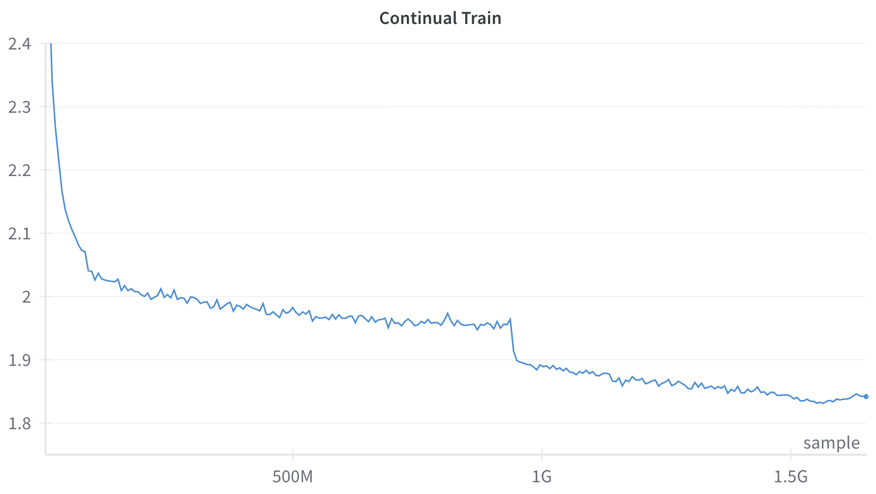### 5.2 | Warmup Stage <details> <summary>extracted/5700921/Figures/key_figure/warmup_loss.png Details</summary>  ### Visual Description \n ## Line Chart: Continual Train ### Overview The image displays a line chart titled "Continual Train," plotting a single data series over a large number of samples. The chart shows a generally decreasing trend with distinct phases of rapid decline, gradual descent with noise, and a sharp step-down. ### Components/Axes * **Title:** "Continual Train" (centered at the top). * **X-Axis:** * **Label:** "sample" (positioned at the bottom-right corner). * **Scale:** Linear scale with major tick marks labeled at "500M" (500 million), "1G" (1 billion), and "1.5G" (1.5 billion). The axis extends from approximately 0 to just beyond 1.5G samples. * **Y-Axis:** * **Label:** None present. * **Scale:** Linear scale with major tick marks labeled at 1.8, 1.9, 2, 2.1, 2.2, 2.3, and 2.4. The axis spans from 1.8 to 2.4. * **Data Series:** A single, continuous blue line. * **Legend:** None present. ### Detailed Analysis The blue line exhibits the following approximate behavior: 1. **Initial Steep Decline (0 to ~100M samples):** The line begins at the top-left corner, at a value of approximately 2.4. It drops very steeply, reaching a value of ~2.05 by the 100M sample mark. 2. **Gradual Descent with Noise (~100M to ~950M samples):** Following the initial drop, the line continues a slower, noisy descent. It fluctuates between approximately 2.05 and 1.95, trending gently downward. The noise appears as small, frequent up-and-down spikes. 3. **Sharp Step-Down (~950M to ~1G samples):** Just before the 1G sample mark, the line experiences a sharp, near-vertical drop from approximately 1.96 to about 1.90. 4. **Final Gradual Descent (~1G to ~1.6G samples):** After the step-down, the line resumes a gradual, noisy decline. It trends from ~1.90 down to a final value of approximately 1.84 at the far right of the chart (around 1.6G samples). The noise level appears slightly reduced compared to the second phase. ### Key Observations * **Overall Trend:** The primary trend is a consistent decrease in the y-axis value as the number of samples (x-axis) increases. * **Phased Behavior:** The training process shows distinct phases: rapid initial improvement, a long period of noisy refinement, a sudden discrete improvement event, and a final phase of slower refinement. * **Sharp Discontinuity:** The most notable feature is the sharp, step-like drop just before 1G samples. This is not a gradual trend but a sudden change. * **Noise Profile:** The line is not smooth; it contains high-frequency noise throughout, which is typical of stochastic processes like training loss curves. ### Interpretation This chart almost certainly represents a **training loss curve** from a machine learning model undergoing continual training. The y-axis, though unlabeled, is inferred to be a loss metric (e.g., cross-entropy loss), where lower values indicate better model performance. * **What it demonstrates:** The model is successfully learning, as evidenced by the overall downward trend in loss. The initial steep drop represents rapid early learning. The long, noisy plateau suggests the model is refining its parameters on the data, with the noise reflecting batch-to-batch variation. * **The Sharp Drop:** The sudden step-down at ~1G samples is highly significant. It likely corresponds to a deliberate intervention in the training process, such as: * A scheduled decrease in the learning rate. * The introduction of a new, more relevant dataset. * A change in model architecture or optimization algorithm. * **Notable Anomaly:** The absence of a y-axis title is a minor documentation flaw. The lack of a legend is acceptable for a single-series chart but would be problematic if multiple runs were plotted. * **Conclusion:** The data suggests a successful, large-scale training run (over 1.5 billion samples) where the model's performance improved substantially. The key event for investigation is the intervention at 1G samples, which provided a clear, discrete boost to performance. The continued decline after this point indicates the model had not yet fully converged by the end of the plotted data. 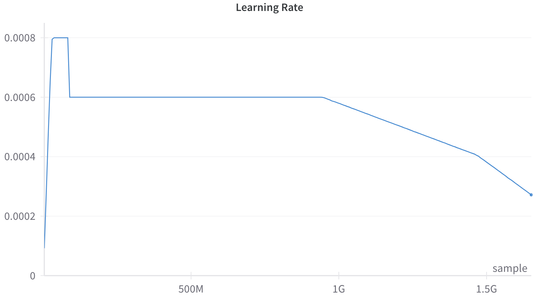</details> (a) <details> <summary>extracted/5700921/Figures/key_figure/warmup_lr.png Details</summary>  ### Visual Description ## Line Graph: Learning Rate Schedule ### Overview The image displays a line graph titled "Learning Rate," plotting the learning rate value against the number of training samples processed. The graph illustrates a common learning rate schedule used in machine learning model training, featuring distinct phases: a warm-up, a constant period, and a linear decay. ### Components/Axes * **Title:** "Learning Rate" (centered at the top). * **Y-Axis (Vertical):** Represents the learning rate value. It is a linear scale with labeled tick marks at: * 0 * 0.0002 * 0.0004 * 0.0006 * 0.0008 * **X-Axis (Horizontal):** Represents the number of training samples processed. It is labeled "sample" at the bottom-right. The axis has labeled tick marks at: * 500M (500 million) * 1G (1 billion) * 1.5G (1.5 billion) * **Data Series:** A single blue line traces the learning rate value over the sample count. There is no legend, as only one series is present. * **Visual Style:** The graph has a clean, minimal design with a white background. Horizontal grid lines are present only at the labeled y-axis ticks. ### Detailed Analysis The learning rate schedule follows a three-phase pattern: 1. **Warm-up Phase (Approx. 0 to ~50M samples):** The line starts at a value near 0 (approximately 0.0001) and rises very steeply to a peak of **0.0008**. It holds at this peak for a very short, flat segment. 2. **Constant Phase (Approx. ~50M to ~1G samples):** The learning rate drops sharply from 0.0008 to **0.0006**. It then remains perfectly constant at 0.0006 for the majority of the training run, from roughly 50 million samples until just before the 1 billion sample mark. 3. **Decay Phase (Approx. ~1G to 1.5G+ samples):** Beginning at approximately 1 billion samples, the learning rate begins a steady, linear decline. The slope is constant. By the 1.5G sample mark, the learning rate has decreased to approximately **0.0004**. The line continues decaying past this point, ending at a final data point (marked with a small dot) at approximately **0.00027**. **Trend Verification:** The visual trend is clear: a rapid initial increase, a long plateau, and then a consistent downward slope. The extracted numerical values align with this visual progression. ### Key Observations * **Scale of Training:** The x-axis scale (in billions of samples) indicates this schedule is for an extremely large-scale model training run. * **Abrupt Transitions:** The transitions between phases (warm-up to constant, constant to decay) are sharp and immediate, not gradual. * **Final Value:** The learning rate does not decay to zero within the visible graph; it ends at a non-zero value (~0.00027), suggesting training may continue or this is the final scheduled rate. * **Minimalist Design:** The graph contains only the essential elements (axes, labels, line) without additional annotations, markers, or a legend. ### Interpretation This graph depicts a **"warmup + constant + linear decay"** learning rate schedule, a standard technique in training deep neural networks, particularly large language models. * **Purpose of Phases:** * **Warm-up:** The initial rapid increase helps stabilize training early on when model weights are random, preventing large, destabilizing gradient updates. * **Constant Phase:** The long plateau at 0.0006 allows the model to learn steadily and efficiently over the bulk of the training process. * **Linear Decay:** The final decay phase fine-tunes the model. Gradually reducing the learning rate helps the model settle into a good minimum in the loss landscape, improving final performance and generalization. * **Underlying Logic:** The schedule balances exploration (higher learning rates early on) with exploitation (lower learning rates later for precise convergence). The specific values (peak of 0.0008, plateau at 0.0006) and the timing of transitions (at ~1G samples) are critical hyperparameters tuned for this specific model and dataset. * **Scale Context:** The use of "G" (billions) for samples underscores the massive computational scale of modern AI training. This single graph represents a training run that likely required thousands of GPU/TPU hours. </details> (b) Figure 13: The warmup stage without explicit memory. Left: Training loss. Right: Learning rate schedule. The training loss and learning rate schedule are plotted in Figure 13. Whenever severe loss divergence occurs, we restart from the last checkpoint before the divergence with a smaller learning rate, and thus the divergences are not shown in the figure. Eventually, the training terminates at around 3.1T tokens, when reducing the learning rate can no longer avoid loss divergence. 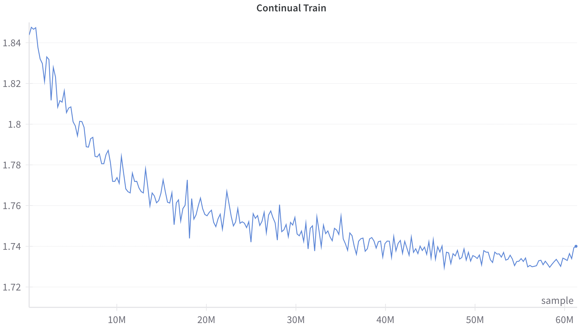### 5.3 | Continual Train Stage <details> <summary>extracted/5700921/Figures/key_figure/2B_continual_train_loss.png Details</summary>  ### Visual Description \n ## Line Chart: Continual Train ### Overview The image displays a line chart titled "Continual Train," plotting a single data series over a large number of samples. The chart shows a generally decreasing trend with significant high-frequency noise or volatility throughout the entire range. The visual suggests a metric (likely a loss or error rate) being tracked during a prolonged training process. ### Components/Axes * **Chart Title:** "Continual Train" (centered at the top). * **X-Axis:** * **Label:** "sample" (positioned at the bottom-right corner of the axis). * **Scale:** Linear scale from 0 to 60 million (60M) samples. * **Major Tick Marks:** Labeled at 10M, 20M, 30M, 40M, 50M, and 60M. * **Y-Axis:** * **Label:** No explicit axis title is present. * **Scale:** Linear scale ranging from approximately 1.72 to 1.85. * **Major Tick Marks:** Labeled at 1.72, 1.74, 1.76, 1.78, 1.80, 1.82, and 1.84. * **Data Series:** A single, continuous blue line. There is no legend, as only one series is plotted. ### Detailed Analysis **Trend Verification:** The blue line exhibits a clear, overall downward slope from left to right, indicating a decreasing value over the sample count. The trend is not smooth; it is characterized by constant, sharp fluctuations (noise) superimposed on the primary downward trajectory. **Data Point Extraction (Approximate):** * **Start (≈0 samples):** The line begins at its highest point, approximately **1.85**. * **10M Samples:** The value has dropped significantly to approximately **1.78**. The descent is steepest in this initial segment. * **20M Samples:** The value is approximately **1.76**. The rate of decrease has slowed compared to the first 10M samples. * **30M Samples:** The value is approximately **1.745**. The trend continues to flatten. * **40M Samples:** The value is approximately **1.735**. The line begins to show signs of plateauing. * **50M Samples:** The value is approximately **1.73**. The trend is largely flat with continued noise. * **60M Samples (End):** The line ends at a point slightly above the 1.74 grid line, approximately **1.74**. There is a very slight upward tick in the final few data points. **Noise Characterization:** The volatility is present across the entire x-axis. The amplitude of the fluctuations appears relatively consistent, spanning roughly ±0.01 to ±0.015 units on the y-axis, even as the mean value decreases. ### Key Observations 1. **Two-Phase Descent:** The chart shows a rapid initial improvement (steep negative slope) for the first ~15-20M samples, followed by a phase of diminishing returns where the improvement slows considerably. 2. **Convergence/Plateau:** After approximately 40M samples, the metric appears to stabilize or converge, oscillating within a narrow band between ~1.73 and ~1.74. 3. **Persistent Noise:** The training process exhibits significant and persistent variance at every stage, never producing a smooth curve. This suggests inherent noise in the optimization process or the data itself. 4. **Final Uptick:** There is a minor but noticeable upward movement in the very last segment of the line (approaching 60M samples), which could indicate the beginning of overfitting or simply noise at the end of the recorded data. ### Interpretation This chart almost certainly visualizes a **training loss curve** from a machine learning model undergoing continual or extended training. The y-axis, though unlabeled, represents a loss value (e.g., cross-entropy loss) that the model is minimizing. * **What it demonstrates:** The model is successfully learning, as evidenced by the consistent reduction in loss over 60 million training samples. The steep initial drop shows rapid early learning, while the later plateau indicates the model is approaching its performance limit on the given task/data. * **Relationship between elements:** The x-axis (samples) is the measure of training effort or exposure to data. The y-axis (loss) is the measure of model error. The downward trend confirms the training process is effective. * **Notable anomalies:** The persistent high-frequency noise is the most striking feature. In a typical training curve, one might expect a smoother line after smoothing or averaging. The raw, noisy plot suggests this is an unfiltered, per-batch or per-step loss value. The slight uptick at 60M samples warrants monitoring; if it continues, it could signal that further training is becoming detrimental. * **Underlying message:** The process requires a vast amount of data (60M samples) for convergence, and the final performance gain after the first 20M samples is relatively marginal. This highlights the computational cost of achieving the last few percentage points of improvement in model training. </details> (a) <details> <summary>extracted/5700921/Figures/key_figure/2B_continual_lr_schedule.png Details</summary>  ### Visual Description ## Line Graph: Learning Rate Schedule ### Overview The image displays a line graph titled "Learning Rate," plotting the learning rate value against the number of training samples processed. The graph illustrates a common learning rate schedule used in machine learning model training, characterized by an initial warm-up phase, a prolonged plateau, a gradual decay, and finally, sharp step-wise reductions. ### Components/Axes * **Title:** "Learning Rate" (centered at the top). * **Y-Axis (Vertical):** Represents the learning rate value. The axis is labeled with scientific notation markers: * 0 * 1e-5 (0.00001) * 2e-5 (0.00002) * 3e-5 (0.00003) * 4e-5 (0.00004) * 5e-5 (0.00005) * **X-Axis (Horizontal):** Represents the number of training samples. The axis is labeled with markers in millions (M): * 10M * 20M * 30M * 40M * 50M * 60M * The axis title "sample" is positioned at the bottom-right corner. * **Data Series:** A single line, colored dark magenta/burgundy, traces the learning rate value across the sample count. There is no separate legend, as only one data series is present. ### Detailed Analysis The learning rate schedule follows a distinct, multi-phase pattern: 1. **Warm-up Phase (Approx. 0 to 2M samples):** The line begins at or near 0 and rises almost vertically to its maximum value of 5e-5. This steep, near-instantaneous ascent suggests a very short warm-up period. 2. **Plateau Phase (Approx. 2M to 45M samples):** The learning rate remains constant at its peak value of **5e-5**. This forms a long, flat plateau spanning the majority of the training process shown. 3. **Gradual Decay Phase (Approx. 45M to 53M samples):** Starting around the 45M sample mark, the line begins a smooth, concave-downward curve. It decays from 5e-5 to approximately **4.5e-5** by the 53M sample point. 4. **First Step Decay (At ~53M samples):** There is a sharp, vertical drop in the learning rate. The value falls from ~4.5e-5 to approximately **2.8e-5**. 5. **Short Plateau (Approx. 53M to 56M samples):** The learning rate holds steady at ~2.8e-5 for a brief period of about 3 million samples. 6. **Second Step Decay (At ~56M samples):** Another sharp, vertical drop occurs. The learning rate falls from ~2.8e-5 to approximately **0.9e-5**. 7. **Final Phase (56M to 60M+ samples):** The line continues at this lower level, showing a very slight downward trend, ending at a value just below **0.9e-5** at the 60M sample mark. ### Key Observations * **Dominant Plateau:** Over 70% of the displayed training duration (from ~2M to ~45M samples) occurs at the maximum learning rate. * **Hybrid Schedule:** The schedule combines a continuous cosine-like decay (from 45M to 53M) with discrete step decays (at 53M and 56M). * **Aggressive Final Reduction:** The final learning rate is less than 20% of the peak value, indicating a significant fine-tuning phase at the end of training. * **Noisy Endpoint:** The line at the far right (60M) shows a slight downward jitter, which could be an artifact of the plotting or represent minor fluctuations. ### Interpretation This graph depicts a sophisticated learning rate schedule designed to optimize the training of a machine learning model, likely a large neural network. * **Purpose of Phases:** The initial warm-up stabilizes training early on. The long plateau allows the model to make substantial progress with a high learning rate. The subsequent decay phases (both gradual and step-wise) help the model converge to a finer solution by taking smaller steps as it approaches a potential minimum in the loss landscape. * **Strategic Design:** The combination of a long plateau followed by decay suggests the trainer expects most learning to happen early, with the later stages dedicated to refinement. The two sharp step drops are likely scheduled at predetermined points (e.g., after a certain number of epochs or when a validation metric plateaus) to force the model into a more precise convergence. * **Contextual Inference:** Such schedules are common in training large language models or other deep learning systems where balancing training stability, speed, and final performance is critical. The specific sample counts (in tens of millions) imply a large-scale training run. The absence of a loss or accuracy curve means we cannot judge the *effectiveness* of this schedule, only its structure. </details> (b) Figure 14: The continual train stage with explicit memory. Left: Training loss. Right: Learning rate schedule. The explicit memories enter into the Memory 3 model at this stage. The training steps are slower since the model needs to encode the references retrieved for the pretrain data to explicit memories in real time, and each step takes a bit more than twice the time of a warmup step. The training loss and learning rate schedule are plotted in Figure 14. The loss divergence soon becomes irremediable at around 120B training tokens, much shorter than the planned 4T tokens, and training has to stop there. One possible cause is that the continual train is initialized from the latest warmup checkpoint, which is located immediately before the break down of the warmup stage, and thus is already at the brink of divergence. The smaller learning rate of continual train delays the onset of divergence but not for long. ## 6 | Fine-tuning and Alignment This section describes our model finetuning, specifically supervised finetuning (SFT) and direct preference optimization (DPO). ### 6.1 | Supervised Finetuning Analogous to the StableLM model [14], our Memory 3 model is finetuned on a diverse collection of SFT datasets. We use the following datasets, which are publicly accessible on the Hugging Face Hub: UltraChat [34], WizardLM [125], SlimOrca [67], ShareGPT [114], Capybara [31], Deita [73], and MetaMathQA [130]. We also include synthetic data with emphasis on multi-round chat, mathematics, commonsense and knowledge. Each training sample consists of one or more rounds of question and answer pairs. We remove any sample with more than eight rounds. The final composition is listed in Table 15. | Dataset | Source | Number of Samples | | --- | --- | --- | | UltraChat | HuggingFaceH4/ultrachat_200k | 194409 | | WizardLM | WizardLM/WizardLM_evol_instruct_V2_196k | 80662 | | SlimOrca | Open-Orca/SlimOrca-Dedup | 143789 | | ShareGPT | openchat/openchat_sharegpt4_dataset | 3509 | | Capybara | LDJnr/Capybara | 7291 | | Deita | hkust-nlp/deita-10k-v0 | 2860 | | MetaMathQA | meta-math/MetaMathQA | 394418 | | Multi-round Chat | synthetic | 20000 | | Mathematics | synthetic | 20000 | | Commonsense | synthetic | 150000 | | Knowledge | synthetic | 270000 | Table 15: Composition of SFT dataset. The training process uses the cosine learning rate schedule with a max learning rate of $5\times 10^{-5}$ and a $10\$ linear warmup phase. The weight decay is 0.1, batch size is 512, and max sequence length is 2048 tokens. Finetuning is performed for 3 epochs. ### 6.2 | Direct Preference Optimization The Memory 3 model is further finetuned by DPO [93], to align with human preference and improve its conversation skills. The DPO dataset consists of general conversations (UltraFeedback Binarized [111]), math questions (Distilabel Math [10]) and codes questions (Synth Code [36]). The training uses the cosine learning rate schedule with max lr $4\times 10^{-6}$ . The inverse temperature $\beta$ of the DPO loss is set to $0.01$ . The improvement from DPO is displayed in Section 7.2. ## 7 | Evaluation We evaluate the general abilities (benchmark tasks), conversation skills, professional abilities (law and medicine), and facutality & hallucination of the Memory 3 model. We also measure its decoding speed. Our model is compared with SOTA LLMs of similar and larger sizes, as well as RAG models. ### 7.1 | General Abilities To evaluate the general abilities of Memory 3, we adopt all tasks from the Huggingface leaderboard and also include two Chinese tasks. Most of the results are displayed in Table 16, while TruthfulQA is listed in Table 19. All results are obtained in bfloat16 format, using the lm-evaluation-harness package [44] and the configuration of HuggingFace Open LLM leaderboard [13], i.e. the number of few-shot examples and grading methods. As described in Section 4.4, to prevent cheating, a filtering step is included in the retrieval process so that the model cannot copy from references that resemble the evaluation questions. | | | | English | Chinese | | | | | | | --- | --- | --- | --- | --- | --- | --- | --- | --- | --- | | LLM | Size | Avg. | ARC-C | HellaSwag | MMLU | Winogrande | GSM8k | CEVAL | CMMLU | | Falcon-40B | 41B | 55.75 | 61.86 | 85.28 | 56.89 | 81.29 | 21.46 | 41.38 | 42.07 | | Llama2-7B-Chat | 6.5B | 46.87 | 52.90 | 78.55 | 48.32 | 71.74 | 7.35 | 34.84 | 34.40 | | Llama2-13B-Chat | 13B | 51.78 | 59.04 | 81.94 | 54.64 | 74.51 | 15.24 | 38.63 | 38.43 | | Llama3-8B-it | 7.0B | 65.77 | 62.03 | 78.89 | 65.69 | 75.77 | 75.82 | 50.52 | 51.70 | | Vicuna-13B-v1.5 | 13B | 52.02 | 57.08 | 81.24 | 56.67 | 74.66 | 11.30 | 41.68 | 41.53 | | Mistral-7B-v0.1 | 7.0B | 59.15 | 59.98 | 83.31 | 64.16 | 78.37 | 37.83 | 45.91 | 44.49 | | Gemma-2B-it | 2.0B | 36.64 | 38.02 | 40.36 | 55.74 | 35.29 | 55.88 | 8.26 | 29.94 | | Gemma-7B-it | 7.8B | 47.23 | 51.45 | 71.96 | 53.52 | 67.96 | 32.22 | 27.93 | 25.70 | | MiniCPM-2B-SFT | 2.4B | 54.37 | 47.53 | 71.95 | 51.32 | 67.72 | 45.26 | 48.07 | 48.76 | | Phi-2 | 2.5B | 55.70 | 61.09 | 75.11 | 58.11 | 74.35 | 54.81 | 34.40 | 32.04 | | ChatGLM3-6B | 5.7B | 54.62 | 41.38 | 66.98 | 50.54 | 64.25 | 51.25 | 54.01 | 53.91 | | Baichuan2-7B-Chat | 6.5B | 55.16 | 52.73 | 74.06 | 52.77 | 69.77 | 28.28 | 53.12 | 55.38 | | Qwen1.5-1.8B-Chat | 1.2B | 49.67 | 38.74 | 60.02 | 45.87 | 59.67 | 33.59 | 55.57 | 54.22 | | Qwen1.5-4B-Chat | 3.2B | 58.15 | 43.26 | 69.73 | 55.55 | 64.96 | 52.24 | 61.89 | 59.39 | | Qwen1.5-7B-Chat | 6.5B | 64.80 | 56.48 | 79.02 | 60.52 | 66.38 | 54.36 | 68.20 | 68.67 | | Memory 3 -SFT | 2.4B | 63.31 | 58.11 | 80.51 | 59.68 | 74.51 | 52.84 | 59.29 | 58.24 | | with vector compression | 2.4B | 63.33 | 57.94 | 80.65 | 59.66 | 75.14 | 52.24 | 59.66 | 58.05 | | without memory | 2.4B | 60.80 | 57.42 | 73.14 | 57.29 | 74.35 | 51.33 | 56.32 | 55.72 | Table 16: Few-shot evaluation of general abilities. The model sizes only include non-embedding parameters. The results of our model without using explicit memory is included, which indicates that explicit memory boosts the average score by $2.51\$ . In comparison, the score difference between Llama2-7B and 13B is $4.91\$ while the latter has twice the amount of non-embedding parameters. Thus, it reasonable to say that explicit memory can increase the “effective model size” by $2.51/4.91\approx 51.1\$ . (Also, the score difference between Qwen-1.8B and 4B is $8.48\$ while the latter has $167\$ more non-embedding parameters. With respect to this scale, explicit memory increases the “effective model size” by $1.2.51/8.48\times 1.67\approx 49.4\$ .) We also include the results of Memory 3 with vector compression (Section 3.3). Even though the key-value vectors of the explicit memories are compressed to $8.75\$ of their original sizes, the performance of our model does not show any degradation. Other supplementary evaluations can be found in Appendix C. Next, we compare with a LLM that is pretrained with text retrieval. Specially, we consider the largest version of the Retro++ model [113], Retro++ XXL with 9.5B parameters. All tasks from Table 6 of [113] are taken, except for HANS, which is not available on lm-eval-harness, and all tasks are zero-shot. Similar to Table 16, Memory 3 is tested with a filtering threshold of 2/3. The results are listed in Table 17, where Memory 3 outperforms the model with much larger parameter size and reference dataset size. | LLM | Param size | Avg. | HellaSwag | BoolQ | Lambada | RACE | | --- | --- | --- | --- | --- | --- | --- | | Retro++ XXL | 9.1B | 61.0 | 70.6 | 70.7 | 72.7 | 43.2 | | Memory 3 -SFT | 2.4B | 64.7 | 83.3 | 80.4 | 57.9 | 45.3 | | Reference size | | PiQA | Winogrand | ANLI-R2 | WiC | | | 330B | | 77.4 | 65.8 | 35.5 | 52.4 | | | 14.3B | | 76.6 | 75.8 | 41.6 | 56.9 | | Table 17: Zero-shot comparison of LLMs pretrained with retrieval. The scores of Retro++ are taken from [113]. The size of a reference dataset is its number of tokens. The non-embedding parameter size of Retro++ is inferred from its vocabulary size. ### 7.2 | Conversation Skill Next we evaluate the conversation skills of Memory 3. We use MT-Bench (the Multi-turn Benchmark) [133] that consists of multi-round and open-ended questions. The results are listed in Table 18, including the Memory 3 model finetuned by DPO introduced in Section 6.2. | LLM | Size | MT-Bench Score | | --- | --- | --- | | Phi-3 | 3.6B | 8.38 | | Mistral-7B-Instruct-v0.2 | 7.0B | 7.60 | | Qwen1.5-7B-Chat | 6.5B | 7.60 | | Zephyr-7B-beta | 7.0B | 7.34 | | MiniCPM-2B-DPO | 2.4B | 6.89 | | Llama-2-70B-Chat | 68B | 6.86 | | Mistral-7B-Instruct-v0.1 | 7.0B | 6.84 | | Llama-2-13B-Chat | 13B | 6.65 | | Llama-2-7B-Chat | 6.5B | 6.57 | | MPT-30B-Chat | 30B | 6.39 | | ChatGLM2-6B | 6.1B | 4.96 | | Falcon-40B-Instruct | 41B | 4.07 | | Vicuna-7B | 6.5B | 3.26 | | Memory 3 -SFT | 2.4B | 5.31 | | Memory 3 -DPO | 2.4B | 5.80 | Table 18: MT-Bench scores. The model sizes only include non-embedding parameters. We obtain all these scores using GPT-4-0613 as grader, following the single answer grading mode of MT-Bench. Our model outperforms Vicuna-7B, Falcon-40B-Instruct, and ChatGLM2-6B with fewer parameters. ### 7.3 | Hallucination and Factuality Despite considerable progress, LLMs still face issues with hallucination, leading to outputs that often stray from factual accuracy [97]. Conceptually, Memory 3 should be less vulnerable to hallucination, since its explicit memories directly correspond to reference texts, whereas compressing texts into the model parameters might incur information loss. To evaluate hallucination, we select two English datasets, TruthfulQA [70] and HaluEval, and one Chinese dataset [64], HalluQA [20]. TruthfulQA is implemented with lm-evaluation-harness [44], while HaluEval and HalluQA are implemented with UHGEval [69]. The results are shown in Table 19, with Memory 3 achieving the highest scores on most tasks. | | | | English | Chinese | | | | | --- | --- | --- | --- | --- | --- | --- | --- | | LLM | Size | Avg. | HaluE-QA | HaluE-Dialogue | TruQA-MC1 | TruQA-MC2 | HalluQA | | Falcon-40B | 41B | 35.37 | 46.84 | 40.80 | 27.29 | 41.71 | 20.18 | | Llama2-13B | 13B | 28.01 | 23.34 | 31.05 | 25.95 | 36.89 | 22.81 | | Vicuna-13B-v1.5 | 13B | 37.07 | 24.93 | 37.35 | 35.13 | 50.88 | N/A | | Baichuan2-13B | 13B | 37.64 | 46.02 | 45.45 | 26.81 | 39.79 | 30.12 | | Gemma-7B | 7.8B | 37.03 | 50.91 | 48.19 | 20.69 | 46.65 | 18.71 | | Mistral-7B-v0.1 | 7.0B | 34.18 | 40.68 | 37.64 | 28.03 | 42.60 | 21.93 | | Llama2-7B | 6.5B | 36.80 | 52.46 | 51.93 | 25.09 | 38.94 | 15.59 | | Baichuan2-7B | 6.5B | 38.63 | 62.33 | 47.84 | 23.01 | 37.46 | 22.51 | | ChatGLM3-6B | 5.7B | 40.96 | 43.38 | 50.03 | 33.17 | 49.87 | 28.36 | | Qwen1.5-4B-Chat | 3.2B | 33.30 | 24.64 | 37.72 | 29.38 | 44.74 | 30.00 | | Phi-2 | 2.5B | 38.31 | 50.71 | 39.55 | 31.09 | 44.32 | 25.89 | | MiniCPM-SFT | 2.4B | 36.47 | 49.24 | 47.80 | 24.11 | 37.51 | 23.71 | | Gemma-2B | 2.0B | 38.04 | 53.41 | 52.22 | 24.60 | 39.78 | 20.18 | | Qwen1.5-1.8B-Chat | 1.2B | 37.52 | 47.18 | 52.11 | 26.68 | 40.57 | 21.05 | | Memory 3 -SFT | 2.4B | 48.60 | 56.61 | 53.91 | 38.80 | 57.72 | 35.96 | Table 19: Evaluation of hallucination. HaluE and TruQA denote HaluEval and TruthfulQA, respectively. Bolded numbers are the best results. The model sizes only include non-embedding parameters. Vicuna-13B-v1.5 gets one N/A since that entry is near zero and seems abnormal. ### 7.4 | Professional Tasks One benefit of using explicit memory is that the LLM can easily adapt to new fields and tasks by updating its knowledge base. One can simply import task-related references into the knowledge base of Memory 3, and optionally, convert them to explicit memories in the case of warm start. Then, the model can perform inference with this new knowledge, skipping the more costly and possibly lossy process of finetuning, and running faster than RAG. This cost reduction has been demonstrated in Figure 4 and Appendix A, and could facilitate the rapid deployment of LLMs across various industries. Besides cost reduction, we need to demonstrate that Memory 3 can perform no worse than RAG. We consider two professional tasks in law and medicine. The legal task consists of multiple-choice questions from the Chinese National Judicial Examination (JEC-QA) dataset [134]. The field-specific references are legal documents from the Chinese national laws and regulations database [1]. These references are merged with our general-purpose knowledge base (Section 4.4) for inference. The medical task consists of the medicine-related questions of C-Eval, MMLU and CMMLU, specifically from the following subsets: - C-Eval: clinical medicine, basic medicine - MMLU: clinical knowledge, anatomy, college medicine, college biology, nutrition, virology, medical genetics, professional medicine - CMMLU: anatomy, clinical knowledge, college medicine, genetics, nutrition, traditional Chinese medicine, virology Our knowledge base is supplemented with medical texts from the open-source medical books dataset [101]. | | JEC-QA | MED | | | | | | --- | --- | --- | --- | --- | --- | --- | | LLM | 3 refs | 5 refs | 7 refs | 3 refs | 5 refs | 7 refs | | Memory 3 -2B-SFT | 39.38 | 56.22 | | | | | | MiniCPM-2B-SFT | 38.83 | 37.65 | 37.94 | 53.73 | 53.29 | 52.84 | | Gemma-2B | 28.16 | 28.06 | 25.29 | 42.04 | 42.49 | 42.96 | | Gemma-2B-it | 30.04 | 31.13 | 29.34 | 41.70 | 43.24 | 42.66 | | Llama-2-7B | 28.06 | 24.70 | 24.90 | 45.14 | 44.43 | 37.96 | | Llama-2-7B-Chat | 26.18 | 25.10 | 25.20 | 48.18 | 47.29 | 39.39 | | Phi-2 | 25.00 | 25.30 | 23.32 | 50.05 | 45.42 | 45.59 | | Qwen1.5-1.8B-Chat | 42.98 | 43.87 | 41.50 | 52.16 | 52.50 | 52.16 | | Qwen1.5-4B-Chat | 51.98 | 50.49 | 50.99 | 61.19 | 61.02 | 61.06 | Table 20: Comparison with RAG on professional tasks. The results are shown in Table 20, and Memory 3 achieves better performance than most of the models. All evaluations use 5-shot prompting. The RAG models retrieve from the same knowledge bases and FAISS indices, except that they receive text references instead of explicit memories. They only retrieve once for each question, using only the question text for query, so the 5-shot examples do not distract the retrieval. Since the optimal number of references is not known for these RAG models, we test them for 3, 5, and 7 references per question, and it seems that $3\sim 5$ references are optimal. The usual formatting for RAG is used, i.e. header 1 + reference 1 + reference 2 + reference 3 + header 2 + few-shot examples + question, all separated by line breaks. The performance plotted in Figure 2 (right) is the average of the scores of the two tasks in Table 20 with five references. ### 7.5 | Inference Speed Finally, we evaluate the decoding speed or throughput of Memory 3, measured by generated tokens per second. The results are compared to those of RAG models, to quantify the speedup of explicit memory over text retrieval. A direct comparison of speeds is uninformative: The memory hierarchy (Figure 8) implies that the Memory 3 model is more reliant on retrieval to supply knowledge, and naturally Memory 3 performs retrieval with higher frequency ( $5$ references per 64 tokens, possibly higher in future versions). Therefore, it is necessary to jointly compare performance and speed. The speed measured in this section is plotted against the retrieval-augmented test accuracy from Section 7.4, resulting in Figure 2 (right). We measure decoding speed on a A800 GPU, and run all models with Flash Attention [32]. All models receive an input of batch size 32 and length 128 tokens, and generate an output with length 128 tokens. The throughput is computed by $32\times 128$ divided by the time spent. We test each model 9 times, remove the first record, and take the average of the rest. Memory 3 performs $2\times 128/64-1=3$ retrievals (the $-1$ means that the first decoded chunk inherits the explicit memories retrieved by the last input chunk). Each retrieval uses 32 queries to get $32\times 5$ explicit memories. We consider the warm start scenario, with the explicit memories precomputed and saved to drives. We implement the worst case scenario, such that the reference ids are reset to be unique after vector search and the memory cache on RAM is disabled, forcing Memory 3 to load $32\times 5$ memories from drives. Meanwhile, each RAG model performs one retrieval with query length 64 tokens, receives 5 references for each sample, and inserts them at the beginning of the sample, similar to the setup for Table 20. The results are listed in Table 21 (local server). The throughput of these models without retrieval is also provided. | | | Local server | End-side device | | | | --- | --- | --- | --- | --- | --- | | LLM | Size | with retrieval | w/o retrieval | with retrieval | w/o retrieval | | Memory 3 -2B | 2.4B | 733.0 | 1131 | 27.6 | 44.36 | | MiniCPM-2B | 2.4B | 501.5 | 974.0 | 21.7 | 51.79 | | Gemma-2B-it | 2.0B | 1581 | 2056 | 22.0 | 29.23 | | Gemma-7B-it | 7.8B | 395.6 | 1008 | 9.5 | 18.61 | | Mistral-7B-Instruct-v0.1 | 7.0B | 392.9 | 894.5 | 11.1 | 28.7 | | Llama-2-7B-Chat | 6.5B | 382.8 | 1005 | 10.0 | 23.19 | | Llama-2-13B-Chat | 13B | 241.1 | 632.5 | 2.5 | 5.44 | | Qwen1.5-1.8B-Chat | 1.2B | 908.2 | 1770 | - | - | | Qwen1.5-4B-Chat | 3.2B | 460.7 | 1002 | 22.3 | 53.39 | | Qwen1.5-7B-Chat | 6.5B | 365.8 | 894.5 | - | - | | Phi-2 | 2.5B | 622.2 | 1544 | - | - | Table 21: Inference throughput, measured by tokens per second. In addition, we study the throughput of these models when they are hosted on an end-side device and retrieve from a knowledge base on a remote server. Specifically, we use Jetson AGX Orin, and the server uses the vector engine MyScale [82]. The models are run with plain attention, with batch size 1. To simulate real-world use cases, the input is a fixed text prompt, with approximately 128 tokens, while the exact length can vary among different tokenizers. The output length is fixed to be 128 tokens. The results are listed in Table 21 (end-side device), and the Memory 3 model . **Remark 8** *Table 21 indicates that our Memory 3 -2B model is $1-733/1131\approx 35.2\$ slower than the same model without using memory. This is peculiar considering that reading explicit memories accounts for only a tiny fraction of the total compute: $$ \frac{2.884\times 10^{-3}~{}\text{TFlops}}{1.264~{}\text{TFlops}}\approx 0.228\ $$ (The calculations are based on Appendix A.) Controlled experiments indicate that the time consumption is mainly due to two sources: - Loading the memory key-values from drives to GPU: This overhead becomes prominent as Memory 3 retrieves with higher frequency. - Python implementation of chunkwise attention: When encoding a prompt, since each chunk attends to a different set of explicit memories, we use a for loop over the chunks to compute their attentions. They dominate other sources such as computing query vectors by the embedding model and searching the vector index. We will try to optimize our code to reduce these overheads to be as close as possible to $0.228\$ of the total inference time, e.g. implement the chunkwise attention with a CUDA kernel.* ## 8 | Conclusion The goal of this work is to reduce the cost of LLM training and inference, or equivalently, to construct a more efficient LLM that matches the performance of larger and slower LLMs. We analyze LLMs from the new perspective of knowledge manipulation, characterizing the cost of LLMs as the transport cost of “knowledges” in and out of various memory formats. Two causes of inefficiency are identified, namely the suboptimal placement of knowledges and the knowledge traversal problem. We solve both problems with explicit memory, a novel memory format, along with a new training scheme and architecture. Our preliminary experiment, the Memory 3 -2B model, exhibits stronger abilities and higher speed than many SOTA models with greater sizes as well as RAG models. For future work, we plan to explore the following directions: 1. Efficient training with abstract knowledges: Ideally, the training cost of Memory 3 model should be proportional to the small amount of non-separable knowledges, approaching the learning efficiency of humans. One approach is to filter the training data to maximize abstract knowledges and minimize specific knowledges (cf. Section 3.5 and Remark 6), and preferably the LLM should assess the quality of its own training data and ignore the unhelpful tokens. 1. Human-like capabilities: As described in the introduction, the explicit memory allows for interesting cognitive functions such as handling infinite contexts (conversion of working memory to explicit memory), memory consolidation (conversion of explicit memory to implicit memory), and conscious reasoning (reflection on the memory recall process). These designs may further improve the efficiency and reasoning ability of Memory 3. 1. Compact representation of explicit memory: The explicit memory of humans can be subdivided into episodic memory, which involve particular experiences, and semantic memory, which involve general truths [59]. This classification is analogous to our definition of specific and abstract knowledges. Our current implementation of explicit memory is closer to the episodic memory of humans, as each memory directly corresponds to a reference text. To improve its reasoning ability, one can try to equip Memory 3 with semantic memories, e.g. obtained from induction on the episodic memories. Besides these broad topics, there are also plenty of engineering works that can be done. For instance, an internalized retrieval process that matches sparse attention queries with memory keys (Remark 2), sparser memory heads with routing (Remark 5), memory extraction that fully preserves contexts (Remark 3), compilation of the knowledge base based on machine preference (Remark 7), reduction of the time consumption of explicit memory to be proportional to its compute overhead (Remark 8), and so on. ## Acknowledgement This work is supported by the NSFC Major Research Plan - Interpretable and General Purpose Next-generation Artificial Intelligence of China (No. 92270001). We thank Prof. Zhiqin Xu, Prof. Zhouhan Lin, Fangrui Liu, Liangkai Hang, Ziyang Tao, Xiaoxing Wang, Mingze Wang, Yongqi Jin, Haotian He, Guanhua Huang, Yirong Hu for helpful discussions. ## References - [1] The Chinese National Laws and Regulations Database. https://flk.npc.gov.cn/. [Accessed 20-03-2024]. - [2] Wenshu. https://wenshu.court.gov.cn/. [Accessed 20-03-2024]. - [3] Megatron-DeepSpeed. https://github.com/microsoft/Megatron-DeepSpeed, 2022. - [4] Marah Abdin, Sam Ade Jacobs, Ammar Ahmad Awan, Jyoti Aneja, Ahmed Awadallah, Hany Awadalla, Nguyen Bach, Amit Bahree, Arash Bakhtiari, Harkirat Behl, Alon Benhaim, Misha Bilenko, Johan Bjorck, Sébastien Bubeck, and et al. Phi-3 technical report: A highly capable language model locally on your phone, 2024. - [5] Josh Achiam, Steven Adler, Sandhini Agarwal, Lama Ahmad, Ilge Akkaya, Florencia Leoni Aleman, Diogo Almeida, Janko Altenschmidt, Sam Altman, Shyamal Anadkat, et al. GPT-4 technical report. arXiv preprint arXiv:2303.08774, 2023. - [6] Joshua Ainslie, James Lee-Thorp, Michiel de Jong, Yury Zemlyanskiy, Federico Lebrón, and Sumit Sanghai. GQA: Training generalized multi-query transformer models from multi-head checkpoints, 2023. - [7] Zeyuan Allen-Zhu and Yuanzhi Li. Physics of language models: Part 3.3, knowledge capacity scaling laws, 2024. - [8] Ebtesam Almazrouei, Hamza Alobeidli, Abdulaziz Alshamsi, Alessandro Cappelli, Ruxandra Cojocaru, Mérouane Debbah, Étienne Goffinet, Daniel Hesslow, Julien Launay, Quentin Malartic, Daniele Mazzotta, Badreddine Noune, Baptiste Pannier, and Guilherme Penedo. The falcon series of open language models, 2023. - [9] AI Anthropic. The Claude 3 model family: Opus, Sonnet, Haiku. Claude-3 Model Card, 2024. - [10] Argilla. Distilabel Math Preference DPO. https://huggingface.co/datasets/argilla/distilabel-math-preference-dpo, 2023. - [11] Jinze Bai, Shuai Bai, Yunfei Chu, Zeyu Cui, Kai Dang, Xiaodong Deng, Yang Fan, Wenbin Ge, Yu Han, Fei Huang, Binyuan Hui, Luo Ji, Mei Li, Junyang Lin, Runji Lin, Dayiheng Liu, Gao Liu, et al. Qwen technical report, 2023. - [12] Peter J Bayley and Larry R Squire. Failure to acquire new semantic knowledge in patients with large medial temporal lobe lesions. Hippocampus, 15(2):273–280, 2005. - [13] Edward Beeching, Clémentine Fourrier, Nathan Habib, Sheon Han, Nathan Lambert, Nazneen Rajani, Omar Sanseviero, Lewis Tunstall, and Thomas Wolf. Open LLM leaderboard. https://huggingface.co/spaces/HuggingFaceH4/open_llm_leaderboard, 2023. - [14] Marco Bellagente, Jonathan Tow, Dakota Mahan, Duy Phung, Maksym Zhuravinskyi, Reshinth Adithyan, James Baicoianu, Ben Brooks, Nathan Cooper, Ashish Datta, et al. Stable lm 2 1.6 b technical report. arXiv preprint arXiv:2402.17834, 2024. - [15] Amanda Bertsch, Uri Alon, Graham Neubig, and Matthew Gormley. Unlimiformer: Long-range transformers with unlimited length input. Advances in Neural Information Processing Systems, 36, 2024. - [16] Sebastian Borgeaud, Arthur Mensch, Jordan Hoffmann, Trevor Cai, Eliza Rutherford, Katie Millican, George Bm Van Den Driessche, Jean-Baptiste Lespiau, Bogdan Damoc, Aidan Clark, et al. Improving language models by retrieving from trillions of tokens. In International conference on machine learning, pages 2206–2240. PMLR, 2022. - [17] Jianlv Chen, Shitao Xiao, Peitian Zhang, Kun Luo, Defu Lian, and Zheng Liu. BGE M3-embedding: Multi-lingual, multi-functionality, multi-granularity text embeddings through self-knowledge distillation. arXiv preprint arXiv:2402.03216, 2024. - [18] Yongjian Chen, Tao Guan, and Cheng Wang. Approximate nearest neighbor search by residual vector quantization. Sensors, 10(12):11259–11273, 2010. - [19] Zheng Chen, Yuqing Li, Tao Luo, Zhaoguang Zhou, and Zhi-Qin John Xu. Phase diagram of initial condensation for two-layer neural networks. ArXiv, abs/2303.06561, 2023. - [20] Qinyuan Cheng, Tianxiang Sun, Wenwei Zhang, Siyin Wang, Xiangyang Liu, Mozhi Zhang, Junliang He, Mianqiu Huang, Zhangyue Yin, Kai Chen, and Xipeng Qiu. Evaluating hallucinations in chinese large language models, 2023. - [21] Aakanksha Chowdhery, Sharan Narang, Jacob Devlin, Maarten Bosma, Gaurav Mishra, Adam Roberts, Paul Barham, Hyung Won Chung, Charles Sutton, et al. Palm: Scaling language modeling with pathways, 2022. - [22] Bilal Chughtai, Alan Cooney, and Neel Nanda. Summing up the facts: Additive mechanisms behind factual recall in llms. arXiv preprint arXiv:2402.07321, 2024. - [23] Together Computer. Redpajama: an open dataset for training large language models, October 2023. - [24] Arthur Conmy, Augustine Mavor-Parker, Aengus Lynch, Stefan Heimersheim, and Adrià Garriga-Alonso. Towards automated circuit discovery for mechanistic interpretability. Advances in Neural Information Processing Systems, 36:16318–16352, 2023. - [25] Alexis Conneau, Kartikay Khandelwal, Naman Goyal, Vishrav Chaudhary, Guillaume Wenzek, Francisco Guzmán, Edouard Grave, Myle Ott, Luke Zettlemoyer, and Veselin Stoyanov. Unsupervised cross-lingual representation learning at scale. arXiv preprint arXiv:1911.02116, 2019. - [26] Suzanne Corkin. What’s new with the amnesic patient H.M.? Nature reviews neuroscience, 3(2):153–160, 2002. - [27] Nelson Cowan. The magical number 4 in short-term memory: A reconsideration of mental storage capacity. Behavioral and Brain Sciences, 24(1):87–114, 2001. - [28] Nelson Cowan. Working memory capacity: Classic Edition. Routledge, 2016. - [29] Damai Dai, Li Dong, Yaru Hao, Zhifang Sui, Baobao Chang, and Furu Wei. Knowledge neurons in pretrained transformers. arXiv preprint arXiv:2104.08696, 2021. - [30] Zihang Dai, Zhilin Yang, Yiming Yang, Jaime Carbonell, Quoc V. Le, and Ruslan Salakhutdinov. Transformer-xl: Attentive language models beyond a fixed-length context, 2019. - [31] Luigi Daniele and Suphavadeeprasit. Amplify-instruct: Synthetically generated diverse multi-turn conversations for effecient llm training. arXiv preprint arXiv:(coming soon), 2023. - [32] Tri Dao, Dan Fu, Stefano Ermon, Atri Rudra, and Christopher Ré. Flashattention: Fast and memory-efficient exact attention with io-awareness. Advances in Neural Information Processing Systems, 35:16344–16359, 2022. - [33] Nolan Dey, Gurpreet Gosal, Zhiming, Chen, Hemant Khachane, William Marshall, Ribhu Pathria, Marvin Tom, and Joel Hestness. Cerebras-gpt: Open compute-optimal language models trained on the cerebras wafer-scale cluster, 2023. - [34] Ning Ding, Yulin Chen, Bokai Xu, Yujia Qin, Zhi Zheng, Shengding Hu, Zhiyuan Liu, Maosong Sun, and Bowen Zhou. Enhancing chat language models by scaling high-quality instructional conversations, 2023. - [35] Matthijs Douze, Alexandr Guzhva, Chengqi Deng, Jeff Johnson, Gergely Szilvasy, Pierre-Emmanuel Mazaré, Maria Lomeli, Lucas Hosseini, and Hervé Jégou. The faiss library, 2024. - [36] Phung Van Duy. synth_code_preference_4k. https://huggingface.co/datasets/pvduy/synth_code_preference_4k, 2023. - [37] Maha Elbayad, Jiatao Gu, Edouard Grave, and Michael Auli. Depth-adaptive transformer, 2020. - [38] Nelson Elhage, Tristan Hume, Catherine Olsson, Nicholas Schiefer, Tom Henighan, Shauna Kravec, Zac Hatfield-Dodds, Robert Lasenby, Dawn Drain, Carol Chen, Roger Grosse, Sam McCandlish, Jared Kaplan, Dario Amodei, Martin Wattenberg, and Christopher Olah. Toy models of superposition. Transformer Circuits Thread, 2022. https://transformer-circuits.pub/2022/toy_model/index.html. - [39] Junjie Fang, Likai Tang, Hongzhe Bi, Yujia Qin, Si Sun, Zhenyu Li, Haolun Li, Yongjian Li, Xin Cong, Yukun Yan, Xiaodong Shi, Sen Song, Yankai Lin, Zhiyuan Liu, and Maosong Sun. UniMem: Towards a unified view of long-context large language models, 2024. - [40] William Fedus, Barret Zoph, and Noam Shazeer. Switch transformers: Scaling to trillion parameter models with simple and efficient sparsity. J. Mach. Learn. Res., 23:120:1–120:39, 2022. - [41] Elias Frantar and Dan Alistarh. Qmoe: Practical sub-1-bit compression of trillion-parameter models. CoRR, abs/2310.16795, 2023. - [42] John DE Gabrieli, Neal J Cohen, and Suzanne Corkin. The impaired learning of semantic knowledge following bilateral medial temporal-lobe resection. Brain and cognition, 7(2):157–177, 1988. - [43] Leo Gao, Stella Biderman, Sid Black, Laurence Golding, Travis Hoppe, Charles Foster, Jason Phang, Horace He, Anish Thite, Noa Nabeshima, Shawn Presser, and Connor Leahy. The pile: An 800gb dataset of diverse text for language modeling. CoRR, abs/2101.00027, 2021. - [44] Leo Gao, Jonathan Tow, Baber Abbasi, Stella Biderman, Sid Black, Anthony DiPofi, Charles Foster, Laurence Golding, Jeffrey Hsu, Alain Le Noac’h, Haonan Li, Kyle McDonell, Niklas Muennighoff, Chris Ociepa, Jason Phang, Laria Reynolds, Hailey Schoelkopf, Aviya Skowron, Lintang Sutawika, Eric Tang, Anish Thite, Ben Wang, Kevin Wang, and Andy Zou. A framework for few-shot language model evaluation, 12 2023. - [45] Mor Geva, Jasmijn Bastings, Katja Filippova, and Amir Globerson. Dissecting recall of factual associations in auto-regressive language models. arXiv preprint arXiv:2304.14767, 2023. - [46] Mor Geva, Roei Schuster, Jonathan Berant, and Omer Levy. Transformer feed-forward layers are key-value memories, 2021. - [47] Xavier Glorot and Yoshua Bengio. Understanding the difficulty of training deep feedforward neural networks. In Proceedings of the thirteenth international conference on artificial intelligence and statistics, pages 249–256. JMLR Workshop and Conference Proceedings, 2010. - [48] Suriya Gunasekar, Yi Zhang, Jyoti Aneja, Caio César Teodoro Mendes, Allie Del Giorno, Sivakanth Gopi, Mojan Javaheripi, Piero Kauffmann, Gustavo de Rosa, Olli Saarikivi, Adil Salim, Shital Shah, Harkirat Singh Behl, Xin Wang, Sébastien Bubeck, Ronen Eldan, Adam Tauman Kalai, Yin Tat Lee, and Yuanzhi Li. Textbooks are all you need, 2023. - [49] Kelvin Guu, Kenton Lee, Zora Tung, Panupong Pasupat, and Mingwei Chang. Retrieval augmented language model pre-training. In International conference on machine learning, pages 3929–3938. PMLR, 2020. - [50] Yiding Hao, Dana Angluin, and Robert Frank. Formal language recognition by hard attention transformers: Perspectives from circuit complexity. Transactions of the Association for Computational Linguistics, 10:800–810, 2022. - [51] Conghui He, Zhenjiang Jin, Chao Xu, Jiantao Qiu, Bin Wang, Wei Li, Hang Yan, Jiaqi Wang, and Dahua Lin. Wanjuan: A comprehensive multimodal dataset for advancing english and chinese large models. CoRR, abs/2308.10755, 2023. - [52] Kaiming He, Xiangyu Zhang, Shaoqing Ren, and Jian Sun. Delving deep into rectifiers: Surpassing human-level performance on imagenet classification. In Proceedings of the IEEE international conference on computer vision, pages 1026–1034, 2015. - [53] Jordan Hoffmann, Sebastian Borgeaud, Arthur Mensch, Elena Buchatskaya, Trevor Cai, Eliza Rutherford, Diego de Las Casas, Lisa Anne Hendricks, Johannes Welbl, Aidan Clark, et al. Training compute-optimal large language models. arXiv preprint arXiv:2203.15556, 2022. - [54] Shengding Hu, Yuge Tu, Xu Han, Chaoqun He, Ganqu Cui, Xiang Long, Zhi Zheng, Yewei Fang, Yuxiang Huang, Weilin Zhao, Xinrong Zhang, Zheng Leng Thai, Kaihuo Zhang, Chongyi Wang, Yuan Yao, Chenyang Zhao, Jie Zhou, Jie Cai, Zhongwu Zhai, Ning Ding, Chao Jia, Guoyang Zeng, Dahai Li, Zhiyuan Liu, and Maosong Sun. Minicpm: Unveiling the potential of small language models with scalable training strategies, 2024. - [55] Yufei Huang, Shengding Hu, Xu Han, Zhiyuan Liu, and Maosong Sun. Unified view of grokking, double descent and emergent abilities: A perspective from circuits competition. arXiv preprint arXiv:2402.15175, 2024. - [56] Albert Q. Jiang, Alexandre Sablayrolles, Arthur Mensch, Chris Bamford, Devendra Singh Chaplot, Diego de las Casas, Florian Bressand, Gianna Lengyel, Guillaume Lample, Lucile Saulnier, Lélio Renard Lavaud, Marie-Anne Lachaux, Pierre Stock, Teven Le Scao, Thibaut Lavril, Thomas Wang, Timothée Lacroix, and William El Sayed. Mistral 7b, 2023. - [57] Xiaoqi Jiao, Yichun Yin, Lifeng Shang, Xin Jiang, Xiao Chen, Linlin Li, Fang Wang, and Qun Liu. Tinybert: Distilling bert for natural language understanding, 2020. - [58] Jean Kaddour. The minipile challenge for data-efficient language models, 2023. - [59] E.R. Kandel, J.D. Koester, S.H. Mack, and S.A. Siegelbaum. Principles of Neural Science, Sixth Edition. McGraw Hill LLC, 2021. - [60] Jared Kaplan, Sam McCandlish, Tom Henighan, Tom B. Brown, Benjamin Chess, Rewon Child, Scott Gray, Alec Radford, Jeffrey Wu, and Dario Amodei. Scaling laws for neural language models, 2020. - [61] Omar Khattab and Matei Zaharia. Colbert: Efficient and effective passage search via contextualized late interaction over bert, 2020. - [62] Vijay Korthikanti, Jared Casper, Sangkug Lym, Lawrence McAfee, Michael Andersch, Mohammad Shoeybi, and Bryan Catanzaro. Reducing activation recomputation in large transformer models, 2022. - [63] Woosuk Kwon, Zhuohan Li, Siyuan Zhuang, Ying Sheng, Lianmin Zheng, Cody Hao Yu, Joseph E. Gonzalez, Hao Zhang, and Ion Stoica. Efficient memory management for large language model serving with pagedattention, 2023. - [64] Junyi Li, Xiaoxue Cheng, Xin Zhao, Jian-Yun Nie, and Ji-Rong Wen. Halueval: A large-scale hallucination evaluation benchmark for large language models. In The 2023 Conference on Empirical Methods in Natural Language Processing, 2023. - [65] Miao Li, Ming-Bin Chen, Bo Tang, Shengbin Hou, Pengyu Wang, Haiying Deng, Zhiyu Li, Feiyu Xiong, Keming Mao, Peng Cheng, and Yi Luo. Newsbench: A systematic evaluation framework for assessing editorial capabilities of large language models in chinese journalism, 2024. - [66] Yuanzhi Li, Sébastien Bubeck, Ronen Eldan, Allie Del Giorno, Suriya Gunasekar, and Yin Tat Lee. Textbooks are all you need ii: phi-1.5 technical report, 2023. - [67] Wing Lian, Guan Wang, Bleys Goodson, Eugene Pentland, Austin Cook, Chanvichet Vong, and ”Teknium”. Slimorca: An open dataset of gpt-4 augmented flan reasoning traces, with verification, 2023. - [68] Xun Liang, Shichao Song, Simin Niu, Zhiyu Li, Feiyu Xiong, Bo Tang, Yezhaohui Wang, Dawei He, Peng Cheng, Zhonghao Wang, and Haiying Deng. Uhgeval: Benchmarking the hallucination of chinese large language models via unconstrained generation, 2024. - [69] Xun Liang, Shichao Song, Simin Niu, Zhiyu Li, Feiyu Xiong, Bo Tang, Zhaohui Wy, Dawei He, Peng Cheng, Zhonghao Wang, and Haiying Deng. UHGEval: Benchmarking the hallucination of chinese large language models via unconstrained generation. arXiv preprint arXiv:2311.15296, 2023. - [70] Stephanie Lin, Jacob Hilton, and Owain Evans. TruthfulQA: Measuring how models mimic human falsehoods. In Smaranda Muresan, Preslav Nakov, and Aline Villavicencio, editors, Proceedings of the 60th Annual Meeting of the Association for Computational Linguistics (Volume 1: Long Papers), pages 3214–3252, Dublin, Ireland, May 2022. Association for Computational Linguistics. - [71] Hong Liu, Zhiyuan Li, David Hall, Percy Liang, and Tengyu Ma. Sophia: A scalable stochastic second-order optimizer for language model pre-training, 2024. - [72] Nelson F. Liu, Kevin Lin, John Hewitt, Ashwin Paranjape, Michele Bevilacqua, Fabio Petroni, and Percy Liang. Lost in the middle: How language models use long contexts, 2023. - [73] Wei Liu, Weihao Zeng, Keqing He, Yong Jiang, and Junxian He. What makes good data for alignment? a comprehensive study of automatic data selection in instruction tuning, 2023. - [74] Zichang Liu, Aditya Desai, Fangshuo Liao, Weitao Wang, Victor Xie, Zhaozhuo Xu, Anastasios Kyrillidis, and Anshumali Shrivastava. Scissorhands: Exploiting the persistence of importance hypothesis for llm kv cache compression at test time, 2023. - [75] Zichang Liu, Jue Wang, Tri Dao, Tianyi Zhou, Binhang Yuan, Zhao Song, Anshumali Shrivastava, Ce Zhang, Yuandong Tian, Christopher Ré, and Beidi Chen. Deja vu: Contextual sparsity for efficient llms at inference time. In Andreas Krause, Emma Brunskill, Kyunghyun Cho, Barbara Engelhardt, Sivan Sabato, and Jonathan Scarlett, editors, International Conference on Machine Learning, ICML 2023, 23-29 July 2023, Honolulu, Hawaii, USA, volume 202 of Proceedings of Machine Learning Research, pages 22137–22176. PMLR, 2023. - [76] Shayne Longpre, Gregory Yauney, Emily Reif, Katherine Lee, Adam Roberts, Barret Zoph, Denny Zhou, Jason Wei, Kevin Robinson, David Mimno, et al. A pretrainer’s guide to training data: Measuring the effects of data age, domain coverage, quality, & toxicity. arXiv preprint arXiv:2305.13169, 2023. - [77] Alexandra Sasha Luccioni, Sylvain Viguier, and Anne-Laure Ligozat. Estimating the carbon footprint of bloom, a 176b parameter language model, 2022. - [78] Tao Luo, Zhi-Qin John Xu, Zheng Ma, and Yaoyu Zhang. Phase diagram for two-layer relu neural networks at infinite-width limit. Journal of Machine Learning Research, 22(71):1–47, 2021. - [79] Ang Lv, Yuhan Chen, Kaiyi Zhang, Yulong Wang, Lifeng Liu, Ji-Rong Wen, Jian Xie, and Rui Yan. Interpreting key mechanisms of factual recall in transformer-based language models, 2024. - [80] William Merrill and Ashish Sabharwal. A logic for expressing log-precision transformers, 2023. - [81] MOP-LIWU Community and MNBVC Team. Mnbvc: Massive never-ending bt vast chinese corpus. https://github.com/esbatmop/MNBVC, 2023. - [82] MyScale. MyScaleDB. https://github.com/myscale/MyScaleDB. [Accessed 20-03-2024]. - [83] Reiichiro Nakano, Jacob Hilton, Suchir Balaji, Jeff Wu, Long Ouyang, Christina Kim, Christopher Hesse, Shantanu Jain, Vineet Kosaraju, William Saunders, et al. Webgpt: Browser-assisted question-answering with human feedback. arXiv preprint arXiv:2112.09332, 2021. - [84] Deepak Narayanan, Mohammad Shoeybi, Jared Casper, Patrick LeGresley, Mostofa Patwary, Vijay Anand Korthikanti, Dmitri Vainbrand, Prethvi Kashinkunti, Julie Bernauer, Bryan Catanzaro, Amar Phanishayee, and Matei Zaharia. Efficient large-scale language model training on gpu clusters using megatron-lm, 2021. - [85] Catherine Olsson, Nelson Elhage, Neel Nanda, Nicholas Joseph, Nova DasSarma, Tom Henighan, Ben Mann, Amanda Askell, Yuntao Bai, Anna Chen, Tom Conerly, Dawn Drain, Deep Ganguli, Zac Hatfield-Dodds, Danny Hernandez, Scott Johnston, Andy Jones, Jackson Kernion, Liane Lovitt, Kamal Ndousse, Dario Amodei, Tom Brown, Jack Clark, Jared Kaplan, Sam McCandlish, and Chris Olah. In-context learning and induction heads, 2022. - [86] OpenAI. GPT-4 turbo and GPT-4. https://platform.openai.com/docs/models/gpt-4-turbo-and-gpt-4, 2024. [Accessed 22-05-2024]. - [87] Long Ouyang, Jeffrey Wu, Xu Jiang, Diogo Almeida, Carroll Wainwright, Pamela Mishkin, Chong Zhang, Sandhini Agarwal, Katarina Slama, Alex Ray, et al. Training language models to follow instructions with human feedback. Advances in neural information processing systems, 35:27730–27744, 2022. - [88] Adam Pearce, Asma Ghandeharioun, Nada Hussein, Nithum Thain, Martin Wattenberg, and Lucas Dixon. Do machine learning models memorize or generalize? People+ AI Research, 2023. - [89] Bo Peng, Eric Alcaide, Quentin Anthony, Alon Albalak, Samuel Arcadinho, Stella Biderman, Huanqi Cao, Xin Cheng, Michael Chung, Matteo Grella, et al. Rwkv: Reinventing rnns for the transformer era, 2023. - [90] Alethea Power, Yuri Burda, Harri Edwards, Igor Babuschkin, and Vedant Misra. Grokking: Generalization beyond overfitting on small algorithmic datasets, 2022. - [91] Penghui Qi, Xinyi Wan, Guangxing Huang, and Min Lin. Zero bubble pipeline parallelism, 2023. - [92] Jack W Rae, Sebastian Borgeaud, Trevor Cai, Katie Millican, Jordan Hoffmann, Francis Song, John Aslanides, Sarah Henderson, Roman Ring, Susannah Young, et al. Scaling language models: Methods, analysis & insights from training gopher. arXiv preprint arXiv:2112.11446, 2021. - [93] Rafael Rafailov, Archit Sharma, Eric Mitchell, Christopher D Manning, Stefano Ermon, and Chelsea Finn. Direct preference optimization: Your language model is secretly a reward model. Advances in Neural Information Processing Systems, 36, 2024. - [94] David Raposo, Sam Ritter, Blake Richards, Timothy Lillicrap, Peter Conway Humphreys, and Adam Santoro. Mixture-of-depths: Dynamically allocating compute in transformer-based language models, 2024. - [95] Jeff Rasley, Samyam Rajbhandari, Olatunji Ruwase, and Yuxiong He. Deepspeed: System optimizations enable training deep learning models with over 100 billion parameters. In Proceedings of the 26th ACM SIGKDD International Conference on Knowledge Discovery & Data Mining, pages 3505–3506, 2020. - [96] Nir Ratner, Yoav Levine, Yonatan Belinkov, Ori Ram, Inbal Magar, Omri Abend, Ehud Karpas, Amnon Shashua, Kevin Leyton-Brown, and Yoav Shoham. Parallel context windows for large language models. arXiv preprint arXiv:2212.10947, 2022. - [97] Vipula Rawte, Swagata Chakraborty, Agnibh Pathak, Anubhav Sarkar, S.M Towhidul Islam Tonmoy, Aman Chadha, Amit Sheth, and Amitava Das. The troubling emergence of hallucination in large language models - an extensive definition, quantification, and prescriptive remediations. In Houda Bouamor, Juan Pino, and Kalika Bali, editors, Proceedings of the 2023 Conference on Empirical Methods in Natural Language Processing, pages 2541–2573, Singapore, December 2023. Association for Computational Linguistics. - [98] Snowflake AI Research. Snowflake arctic: The best LLM for enterprise AI — efficiently intelligent, truly open, Apr 2024. Accessed: 2024-05-15. - [99] Yangjun Ruan, Chris J. Maddison, and Tatsunori Hashimoto. Observational scaling laws and the predictability of language model performance, 2024. - [100] Timo Schick, Jane Dwivedi-Yu, Roberto Dessì, Roberta Raileanu, Maria Lomeli, Eric Hambro, Luke Zettlemoyer, Nicola Cancedda, and Thomas Scialom. Toolformer: Language models can teach themselves to use tools. Advances in Neural Information Processing Systems, 36, 2024. - [101] Scienceasdf. Medical books. https://github.com/scienceasdf/medical-books. [Accessed 20-03-2024]. - [102] Azure AI Services. GPT-4 and GPT-4 turbo models. https://learn.microsoft.com/en-us/azure/ai-services/openai/concepts/models#gpt-4-and-gpt-4-turbo-models, 2024. [Accessed 22-05-2024]. - [103] Mohammad Shoeybi, Mostofa Patwary, Raul Puri, Patrick LeGresley, Jared Casper, and Bryan Catanzaro. Megatron-lm: Training multi-billion parameter language models using model parallelism, 2020. - [104] Daria Soboleva, Faisal Al-Khateeb, Robert Myers, Jacob R Steeves, Joel Hestness, and Nolan Dey. SlimPajama: A 627B token cleaned and deduplicated version of RedPajama. https://www.cerebras.net/blog/slimpajama-a-627b-token-cleaned-and-deduplicated-version-of-redpajama, June 2023. - [105] Aarohi Srivastava, Abhinav Rastogi, Abhishek Rao, Abu Awal Md Shoeb, Abubakar Abid, Adam Fisch, Adam R. Brown, Adam Santoro, Aditya Gupta, Adrià Garriga-Alonso, Agnieszka Kluska, Aitor Lewkowycz, Akshat Agarwal, Alethea Power, Alex Ray, Alex Warstadt, Alexander W. Kocurek, Ali Safaya, Ali Tazarv, Alice Xiang, and et al. Beyond the imitation game: Quantifying and extrapolating the capabilities of language models, 2023. - [106] Alessandro Stolfo, Yonatan Belinkov, and Mrinmaya Sachan. A mechanistic interpretation of arithmetic reasoning in language models using causal mediation analysis. In Proceedings of the 2023 Conference on Empirical Methods in Natural Language Processing, pages 7035–7052, 2023. - [107] Jianlin Su, Murtadha Ahmed, Yu Lu, Shengfeng Pan, Wen Bo, and Yunfeng Liu. Roformer: Enhanced transformer with rotary position embedding. Neurocomputing, 568:127063, 2024. - [108] Sainbayar Sukhbaatar, Edouard Grave, Guillaume Lample, Herve Jegou, and Armand Joulin. Augmenting self-attention with persistent memory, 2019. - [109] Yutao Sun, Li Dong, Yi Zhu, Shaohan Huang, Wenhui Wang, Shuming Ma, Quanlu Zhang, Jianyong Wang, and Furu Wei. You only cache once: Decoder-decoder architectures for language models. arXiv preprint arXiv:2405.05254, 2024. - [110] Hugo Touvron, Louis Martin, Kevin Stone, Peter Albert, Amjad Almahairi, Yasmine Babaei, Nikolay Bashlykov, Soumya Batra, Prajjwal Bhargava, Shruti Bhosale, et al. Llama 2: Open foundation and fine-tuned chat models. arXiv preprint arXiv:2307.09288, 2023. - [111] Lewis Tunstall, Edward Beeching, Nathan Lambert, Nazneen Rajani, Kashif Rasul, Younes Belkada, Shengyi Huang, Leandro von Werra, Clémentine Fourrier, Nathan Habib, Nathan Sarrazin, Omar Sanseviero, Alexander M. Rush, and Thomas Wolf. Zephyr: Direct distillation of lm alignment, 2023. - [112] Szymon Tworkowski, Konrad Staniszewski, Mikołaj Pacek, Yuhuai Wu, Henryk Michalewski, and Piotr Miłoś. Focused transformer: Contrastive training for context scaling. Advances in Neural Information Processing Systems, 36, 2024. - [113] Boxin Wang, Wei Ping, Peng Xu, Lawrence McAfee, Zihan Liu, Mohammad Shoeybi, Yi Dong, Oleksii Kuchaiev, Bo Li, Chaowei Xiao, Anima Anandkumar, and Bryan Catanzaro. Shall we pretrain autoregressive language models with retrieval? A comprehensive study. In Houda Bouamor, Juan Pino, and Kalika Bali, editors, Proceedings of the 2023 Conference on Empirical Methods in Natural Language Processing, pages 7763–7786, Singapore, December 2023. Association for Computational Linguistics. - [114] Guan Wang, Sijie Cheng, Xianyuan Zhan, Xiangang Li, Sen Song, and Yang Liu. Openchat: Advancing open-source language models with mixed-quality data, 2023. - [115] Kevin Wang, Alexandre Variengien, Arthur Conmy, Buck Shlegeris, and Jacob Steinhardt. Interpretability in the wild: a circuit for indirect object identification in gpt-2 small. arXiv preprint arXiv:2211.00593, 2022. - [116] Lean Wang, Lei Li, Damai Dai, Deli Chen, Hao Zhou, Fandong Meng, Jie Zhou, and Xu Sun. Label words are anchors: An information flow perspective for understanding in-context learning. arXiv preprint arXiv:2305.14160, 2023. - [117] Mingze Wang, Haotian He, Jinbo Wang, Zilin Wang, Guanhua Huang, Feiyu Xiong, Zhiyu Li, Weinan E, and Lei Wu. Improving generalization and convergence by enhancing implicit regularization, 2024. - [118] Weizhi Wang, Li Dong, Hao Cheng, Xiaodong Liu, Xifeng Yan, Jianfeng Gao, and Furu Wei. Augmenting language models with long-term memory. Advances in Neural Information Processing Systems, 36, 2024. - [119] Jason Wei, Yi Tay, Rishi Bommasani, Colin Raffel, Barret Zoph, Sebastian Borgeaud, Dani Yogatama, Maarten Bosma, Denny Zhou, Donald Metzler, Ed H. Chi, Tatsunori Hashimoto, Oriol Vinyals, Percy Liang, Jeff Dean, and William Fedus. Emergent abilities of large language models, 2022. - [120] Gail Weiss, Yoav Goldberg, and Eran Yahav. Thinking like transformers, 2021. - [121] Carole-Jean Wu, Ramya Raghavendra, Udit Gupta, Bilge Acun, Newsha Ardalani, Kiwan Maeng, Gloria Chang, Fiona Aga Behram, James Huang, Charles Bai, Michael Gschwind, Anurag Gupta, Myle Ott, Anastasia Melnikov, Salvatore Candido, David Brooks, Geeta Chauhan, Benjamin Lee, Hsien-Hsin S. Lee, Bugra Akyildiz, Maximilian Balandat, Joe Spisak, Ravi Jain, Mike Rabbat, and Kim Hazelwood. Sustainable ai: Environmental implications, challenges and opportunities, 2022. - [122] Wenhao Wu, Yizhong Wang, Guangxuan Xiao, Hao Peng, and Yao Fu. Retrieval head mechanistically explains long-context factuality, 2024. - [123] Yuhuai Wu, Markus Norman Rabe, DeLesley Hutchins, and Christian Szegedy. Memorizing transformers. In International Conference on Learning Representations, 2021. - [124] Xingyu Xie, Pan Zhou, Huan Li, Zhouchen Lin, and Shuicheng Yan. Adan: Adaptive nesterov momentum algorithm for faster optimizing deep models, 2023. - [125] Can Xu, Qingfeng Sun, Kai Zheng, Xiubo Geng, Pu Zhao, Jiazhan Feng, Chongyang Tao, and Daxin Jiang. Wizardlm: Empowering large language models to follow complex instructions. arXiv preprint arXiv:2304.12244, 2023. - [126] Aiyuan Yang, Bin Xiao, Bingning Wang, Borong Zhang, Ce Bian, Chao Yin, Chenxu Lv, Da Pan, Dian Wang, Dong Yan, Fan Yang, Fei Deng, Feng Wang, Feng Liu, Guangwei Ai, Guosheng Dong, Haizhou Zhao, et al. Baichuan 2: Open large-scale language models, 2023. - [127] Greg Yang, Edward J Hu, Igor Babuschkin, Szymon Sidor, Xiaodong Liu, David Farhi, Nick Ryder, Jakub Pachocki, Weizhu Chen, and Jianfeng Gao. Tensor programs v: Tuning large neural networks via zero-shot hyperparameter transfer. arXiv preprint arXiv:2203.03466, 2022. - [128] Hongkang Yang. A mathematical framework for learning probability distributions. Journal of Machine Learning, 1(4):373–431, 2022. - [129] Yunzhi Yao, Ningyu Zhang, Zekun Xi, Mengru Wang, Ziwen Xu, Shumin Deng, and Huajun Chen. Knowledge circuits in pretrained transformers, 2024. - [130] Longhui Yu, Weisen Jiang, Han Shi, Jincheng Yu, Zhengying Liu, Yu Zhang, James T Kwok, Zhenguo Li, Adrian Weller, and Weiyang Liu. Metamath: Bootstrap your own mathematical questions for large language models. arXiv preprint arXiv:2309.12284, 2023. - [131] Zhenyu Zhang, Ying Sheng, Tianyi Zhou, Tianlong Chen, Lianmin Zheng, Ruisi Cai, Zhao Song, Yuandong Tian, Christopher Ré, Clark Barrett, et al. H2o: Heavy-hitter oracle for efficient generative inference of large language models. Advances in Neural Information Processing Systems, 36, 2024. - [132] Zhongwang Zhang, Pengxiao Lin, Zhiwei Wang, Yaoyu Zhang, and Zhi-Qin John Xu. Initialization is critical to whether transformers fit composite functions by inference or memorizing, 2024. - [133] Lianmin Zheng, Wei-Lin Chiang, Ying Sheng, Siyuan Zhuang, Zhanghao Wu, Yonghao Zhuang, Zi Lin, Zhuohan Li, Dacheng Li, Eric Xing, et al. Judging llm-as-a-judge with mt-bench and chatbot arena. Advances in Neural Information Processing Systems, 36, 2024. - [134] Haoxi Zhong, Chaojun Xiao, Cunchao Tu, Tianyang Zhang, Zhiyuan Liu, and Maosong Sun. Jec-qa: A legal-domain question answering dataset. Proceedings of the AAAI Conference on Artificial Intelligence, 34(05):9701–9708, Apr. 2020. ## Appendix A Cost Estimation This section provides the calculations for Figure 4, and we equate cost with the amount of compute measured in Tflops. Our 2.4B Memory 3 model is adopted as the backbone. Recall from Section 3.4 that this model has shape - Transformer blocks $L=44$ - Query heads $H=40$ and key-value heads $H_{kv}=8$ - Head dimension $d_{h}=80$ and hidden dimension $d=Hd_{h}=3200$ - MLP width $W=d$ - Vocabulary size as well as LM head size $n_{\text{vocab}}=60416$ - memory layers $L_{\text{mem}}=22$ , which is also the depth of the deepest memory layer. Fix a separable knowledge $\mathcal{K}$ , and represent it by one of its realizations $\mathbf{t}$ (Definition 5), and assume that $\mathbf{t}$ has length $l_{\text{ref}}=128$ tokens, following the setup of our reference dataset (Section 4.4). Recall from Section 3.3 that each memory has $l_{\text{mem}}=8$ tokens per memory head, and it is read by a chunk of length $l_{\text{chunk}}=64$ . Since we want to show that explicit memory is cheaper than implicit memory and RAG, it suffices to use coarse lower bounds on their costs. ### A.1 | Implicit Memory The write cost of implicit memory or model parameters is the training compute with $\mathbf{t}$ as input. Usually the training data of Transformer LLMs have length $2048\sim 8192$ , so we assume that $\mathbf{t}$ is a subsequence of a train sample $\mathbf{t}_{\text{train}}$ with length $l_{\text{train}}=2048$ . By [84], the training compute of one step with one sample is approximately $$ 3\cdot 2\cdot\big{[}L\big{(}l_{\text{train}}(2d^{2}+2dd_{h}H_{kv}+3dW)+2\frac{ l_{\text{train}}^{2}}{2}d\big{)}+l_{\text{train}}n_{\text{vocab}}d\big{]} $$ where $3$ means that the backward step costs twice as the forward step (and thus 3 times in total), the first $2$ means that the compute of matrix multiplication involves same amount of additions and multiplications. The five terms in the bracket come from QO embedding, KV embedding, MLP, attention, and LM head, respectively. The lower order terms, such as layer normalizations, are omitted. The fraction of the compute attributable to $\mathbf{t}$ is given by $$ 3\cdot 2\cdot\big{[}L\big{(}l_{\text{ref}}(2d^{2}+2dd_{h}H_{kv}+3dW)+2l_{\text {ref}}\frac{l_{\text{train}}}{2}d\big{)}+l_{\text{ref}}n_{\text{vocab}}d\big{]} $$ Assume that one training step is sufficient for storing knowledge $\mathcal{K}$ into model parameters. Then, the write cost is equal to the above term, and we obtain $$ \text{cost}_{\text{write}}\approx 2.24~{}\text{TFlops} $$ Meanwhile, we lower bound the read cost by zero. $$ \text{cost}_{\text{read}}\geq 0~{}\text{TFlops} $$ This lower bound is obviously correct and suits our comparison, since it makes implicit memory appear more competitive. The difficulty in estimating the cost is that the correspondence between knowledges and parameters is not fully understood. Nevertheless, we describe a possible way to obtain a reasonable bound. Recall from Section 1 that the model parameters suffer from the issue of knowledge traversal such that each parameter (and thus each implicit memory) is invoked during each call of the LLM. So the read cost of each implicit memory does not depend on its usage count $n_{k}$ , but instead on the total amount of model calls during the lifespan of this LLM. Dividing the total amount of inference compute used by this LLM by the amount of knowledges it possesses gives an estimation of the average read cost of a knowledge. The amount of knowledges in the LLM can be upper bounded based on the knowledge capacities measured by [7]. ### A.2 | Explicit Memory The write cost of an each explicit memory mainly comes from $L_{\text{mem}}$ self-attention layers, $L_{\text{mem}}-1$ MLP layers, and $L_{\text{mem}}$ token sparsification operations (computing the full attention matrix): | | $\displaystyle\text{cost}_{\text{write}}$ | $\displaystyle=2\cdot\big{[}L_{\text{mem}}\big{(}l_{\text{ref}}(2d^{2}+2dd_{h}H _{kv})+2\frac{l_{\text{ref}}^{2}}{2}d\big{)}+(L_{\text{mem}}-1)(l_{\text{ref}} \cdot 3dW)+L_{\text{mem}}(l_{\text{ref}}^{2}d)\big{]}$ | | | --- | --- | --- | --- | The read cost consists of the attention to the sparse tokens of an explicit memory from the chunk that retrieves this memory: $$ \text{cost}_{\text{read}}=2L_{\text{mem}}\cdot 2l_{\text{chunk}}l_{\text{mem}} d\approx 1.44\times 10^{-4}~{}\text{TFlops} $$ ### A.3 | External Information The write cost of text retrieval-augmented generation (RAG) is set to be zero, since the reference is stored as plain text. $$ \text{cost}_{\text{write}}=0~{}\text{TFlops} $$ The read cost is the additional compute brought by the retrieved references that are inserted in the prompt. To make RAG appear more competitive, we assume that only a chunk of the prompt or decoded text with length $l_{\text{chunk}}$ can attend to the references, and each reference can only attend to itself, which in general is not true. Then, | | $\displaystyle\text{cost}_{\text{write}}$ | $\displaystyle\geq 2\cdot\big{[}L\big{(}l_{\text{ref}}(2d^{2}+2dd_{h}H_{kv})+2l _{\text{ref}}\big{(}\frac{l_{\text{ref}}}{2}+l_{\text{chunk}}\big{)}d\big{)}+( L-1)(l_{\text{ref}}\cdot 3dW)\big{]}$ | | | --- | --- | --- | --- | In summary, the total cost (TFlops) of writing and reading each separable knowledge in terms of its expected usage count $n$ is given by $$ \begin{cases}c_{\text{implicit}}(n)\geq 2.24\\ c_{\text{explicit}}(n)=0.308+0.000144n\\ c_{\text{external}}(n)\geq 0.624n\end{cases} $$ These curves are plotted in Figure 4. Hence, if $n\in(0.494,13400)$ , then it is optimal to store the knowledge as an explicit memory. **Remark 9 (Knowledge retention)** *One aspect not covered by Problem (1) is the retention of knowledges in the model if its parameters are updated, e.g. due to finetuning. Both implicit memory and explicit memory are vulnerable to parameter change. Usually, model finetuning would include some amount of pretrain data to prevent catastrophic forgetting [87]. Similarly, if some explicit memories have already been produced, then they need to be rebuilt in order to remain readable by the updated model. It is an interesting research direction to design a more efficient architecture such that the implicit and explicit memories are robust with respect to model updates.* ## Appendix B Vector Compression Regarding the vector quantizer discussed in Sections 3.3 and 7.1, we use the composite index of FAISS with index type OPQ20x80-Residual2x14-PQ8x10. It can encode a 80-dimensional bfloat16 vector into a 14-dimensional uint8 vector, and thus its compression rate is $\frac{80\times 2}{14\times 1}\approx 11.4$ . To train this quantizer, we sample references from our knowledge base, encode them into explicit memories by our Memory 3 -2B-SFT model, and feed these key-value vectors to the quantizer. The references are sampled uniformly and independently, so the training is not biased towards the references that are retrieved by any specific evaluation task. ## Appendix C Supplementary Evaluation Results First, Table 22 records the growth of the test scores (Table 16) over the three training stages: warmup, continual train, and SFT. We believe that for future versions of Memory 3, fixing the loss divergence during the warmup stage can allow the continual train stage to proceed much further (cf. Section 5.3), and thus increase the performance boost of this stage. | | | English | Chinese | | | | | | | --- | --- | --- | --- | --- | --- | --- | --- | --- | | LLM | Avg. | ARC-C | HellaSwag | MMLU | Winogrande | GSM8k | CEVAL | CMMLU | | Warmup | 42.13 | 40.27 | 64.57 | 41.62 | 61.96 | 5.23 | 40.12 | 41.17 | | Continual train | 45.12 | 42.66 | 79.21 | 41.81 | 59.43 | 6.29 | 42.20 | 44.21 | | - without memory | 42.89 | 42.15 | 66.98 | 39.79 | 61.80 | 6.44 | 39.97 | 43.13 | | SFT | 63.31 | 58.11 | 80.51 | 59.68 | 74.51 | 52.84 | 59.29 | 58.24 | | - without memory | 60.80 | 57.42 | 73.14 | 57.29 | 74.35 | 51.33 | 56.32 | 55.72 | Table 22: Performance of Memory 3 -2B at different stages of training. The setup of the evaluation tasks is the same as in Table 16. Next, recall that for the evaluations in Section 7.1, a filter is included in the retrieval process to prevent copying, which removes references that overlap too much with the evaluation question. The filtering threshold should lie between $100\$ and the usual level of overlap between two related but distinct texts, and we set it to $2/3$ in Table 16. Table 23 records the impact of the filtering threshold on the test scores. The scores are stable for most tasks, indicating that their questions do not appear in our knowledge basis. | Threshold | Avg. | ARC-C | HellaSwag | MMLU | Winogrande | GSM8k | CEVAL | CMMLU | | --- | --- | --- | --- | --- | --- | --- | --- | --- | | no filter | 63.71 | 58.11 | 83.37 | 59.65 | 74.51 | 52.84 | 59.29 | 58.22 | | 80% | 63.62 | 58.11 | 82.69 | 59.65 | 74.51 | 52.84 | 59.29 | 58.24 | | 2/3 | 63.31 | 58.11 | 80.51 | 59.68 | 74.51 | 52.84 | 59.29 | 58.24 | | without memory | 60.80 | 57.42 | 73.14 | 57.29 | 74.35 | 51.33 | 56.32 | 55.72 | Table 23: Influence of the filtering threshold on the test scores in Table 16. Finally, Table 24 studies the influence of the few-shot prompts on the benchmark tasks. Recall that the number of few-shot examples for each task is ARC-C (25), HellaSwag (10), MMLU (5), Winogrande (5), GSM8k (5) as in HuggingFace OpenLLM Leaderboard [13], and we also adopt CEVAL (5), CMMLU (5). Interestingly, the boost from explicit memory increases from $2.51\$ to $3.70\$ as we switch to 0-shot. | Mode | Avg. | ARC-C | HellaSwag | MMLU | Winogrande | GSM8k | CEVAL | CMMLU | | --- | --- | --- | --- | --- | --- | --- | --- | --- | | Few-shot | 63.31 | 58.11 | 80.51 | 59.68 | 74.51 | 52.84 | 59.29 | 58.24 | | - without memory | 60.80 | 57.42 | 73.14 | 57.29 | 74.35 | 51.33 | 56.32 | 55.72 | | 0-shot | 58.23 | 58.79 | 83.29 | 60.53 | 75.85 | 13.50 | 57.95 | 57.74 | | - without memory | 54.54 | 57.34 | 73.15 | 58.59 | 74.98 | 10.46 | 54.53 | 54.26 | Table 24: Few-shot versus 0-shot for the benchmark tasks in Table 16.