# FlashAttention-3: Fast and Accurate Attention with Asynchrony and Low-precision
**Authors**: Jay Shah, Ganesh Bikshandi††footnotemark:, Ying Zhang, Vijay Thakkar, Pradeep Ramani, Tri Dao
> Equal contribution
Abstract
Attention, as a core layer of the ubiquitous Transformer architecture, is the bottleneck for large language models and long-context applications. FlashAttention elaborated an approach to speed up attention on GPUs through minimizing memory reads/writes. However, it has yet to take advantage of new capabilities present in recent hardware, with FlashAttention-2 achieving only 35% utilization on the H100 GPU. We develop three main techniques to speed up attention on Hopper GPUs: exploiting asynchrony of the Tensor Cores and TMA to (1) overlap overall computation and data movement via warp-specialization and (2) interleave block-wise matmul and softmax operations, and (3) block quantization and incoherent processing that leverages hardware support for FP8 low-precision. We demonstrate that our method, FlashAttention-3, achieves speedup on H100 GPUs by 1.5-2.0 $×$ with FP16 reaching up to 740 TFLOPs/s (75% utilization), and with FP8 reaching close to 1.2 PFLOPs/s. We validate that FP8 FlashAttention-3 achieves 2.6 $×$ lower numerical error than a baseline FP8 attention.
1 Introduction
For the Transformer architecture [59], the attention mechanism constitutes the primary computational bottleneck, since computing the self-attention scores of queries and keys has quadratic scaling in the sequence length. Scaling attention to longer context will unlock new capabilities (modeling and reasoning over multiple long documents [24, 50, 43] and files in large codebases [48, 30]), new modalities (high-resolution images [11], audio [23], video [25]), and new applications (user interaction with long history [53], agent workflow with long horizon [62]). This has generated significant interest in making attention faster in the long-context regime, including by approximation [27, 14, 56] and software optimization ([45, 17, 29]), or even alternative architectures [42, 55, 22].
In this work, we build on the work of Dao et al. [17] on developing exact-attention algorithms that integrate knowledge of the GPU’s execution model and hardware characteristics into their high-level design. In [17], Dao et al. introduced FlashAttention, a novel tiling strategy for parallelizing attention that eliminates intermediate reads/writes to slow global memory through fusing all of the attention operations into a single GPU kernel. Dao [15] restructured the algorithm as FlashAttention-2 to also parallelize over the sequence length dimension and perform the inner loop of the forward pass over blocks of the key and value matrices, thus improving the occupancy and distribution of work on the GPU. However, we observe that FlashAttention-2 nonetheless achieves poor utilization on newer GPUs relative to optimized matrix-multiplication (GEMM) kernels, such as 35% vs. 80-90% on the Hopper H100 GPU. Partially, this may be attributed to implementation-level differences, such as not using Hopper-specific instructions in place of Ampere ones when targeting the Tensor Cores. Several work such as ThunkerKitten [52] and cuDNN 9 [39] has shown that with Hopper-specific instructions and tile-based abstractions, one can speedup attention computation and simplify the implementation.
More fundamentally, FlashAttention-2 ’s algorithm adheres to a simplified synchronous model and makes no explicit use of asynchrony and low-precision in its design. Asynchrony is a result of hardware specialization to accelerate the most important operations in a ML workload: specific hardware units performing matrix multiplication (Tensor Cores) or memory loading (Tensor Memory Accelerator – TMA), separate from the rest of the CUDA cores performing logic, integer, and floating point computation. Low precision such as FP8 in Hopper and FP4 in Blackwell, continuing the trend of FP16 (Pascal in 2017) and BF16 (Ampere in 2020), is a proven technique to get double or quadruple throughput for the same power and chip area. We review the capabilities afforded by Hopper in these directions in § 2.2. The technical challenge is to redesign FlashAttention-2 to make use of these hardware features: asynchrony requires overlapping computation between matmul and softmax even though one depends on the output of the other, and low-precision requires care to minimize quantization error, especially in the case of outlier features in LLMs [20, 54].
To this end, we propose FlashAttention-3, which contributes and synthesizes three new ideas to further improve performance on newer GPU architectures: We describe our results in the context of NVIDIA’s Hopper architecture. However, our algorithm is operative for any GPU architecture with sufficiently robust asynchronous execution and low-precision capabilities.
1. Producer-Consumer asynchrony: We define a warp-specialized software pipelining scheme that exploits the asynchronous execution of data movement and Tensor Cores by splitting producers and consumers of data into separate warps, thereby extending the algorithm’s ability to hide memory and instruction issue latencies.
1. Hiding softmax under asynchronous block-wise GEMMs: We overlap the comparatively low-throughput non-GEMM operations involved in softmax, such as floating point multiply-add and exponential, with the asynchronous WGMMA instructions for GEMM. As part of this, we rework the FlashAttention-2 algorithm to circumvent certain sequential dependencies between softmax and the GEMMs. For example, in the 2-stage version of our algorithm, while softmax executes on one block of the scores matrix, WGMMA executes in the asynchronous proxy to compute the next block.
1. Hardware-accelerated low-precision GEMM: We adapt the forward pass algorithm to allow for targeting the FP8 Tensor Cores for GEMM, nearly doubling the measured TFLOPs/s. This requires bridging the different layout conformance requirements of WGMMA in terms of how blocks of FP32 accumulator and FP8 operand matrices are assumed to be laid out in memory. We use the techniques of block quantization and incoherent processing to mitigate the loss of accuracy that results from moving to FP8 precision.
To validate our method empirically, we benchmark FlashAttention-3 on the H100 SXM5 GPU over a range of parameters and show that (1) FP16 achieves 1.5-2.0 $×$ speedup over FlashAttention-2 in the forward pass (reaching up to 740 TFLOPs/s) and 1.5-1.75 $×$ in the backward pass, (2) FP8 achieves close to 1.2 PFLOPs/s, and (3) for large sequence length, FP16 outperforms and FP8 is competitive More precisely, for head dimension 64 FlashAttention-3 FP8 is ahead, while for head dimensions 128 and 256 it is at par for those cases without causal masking and behind with causal masking. with a state-of-the-art implementation of attention from NVIDIA’s cuDNN library. We also validate that FP16 FlashAttention-3 yields the same numerical error as FlashAttention-2 and is better than the standard attention implementation as intermediate results (e.g., softmax rescaling) are kept in FP32. Moreover, FP8 FlashAttention-3 with block quantization and incoherent processing is 2.6 $×$ more accurate than standard attention with per-tensor quantization in cases with outlier features.
We open-source FlashAttention-3 with a permissive license FlashAttention-3 is available at https://github.com/Dao-AILab/flash-attention and plan to integrate it with PyTorch and Hugging Face libraries to benefit the largest number of researchers and developers.
2 Background: Multi-Head Attention and GPU Characteristics
2.1 Multi-Head Attention
Let $\mathbf{Q},\mathbf{K},\mathbf{V}∈\mathbb{R}^{N× d}$ be the query, key and value input sequences associated to a single head, where $N$ is the sequence length and $d$ is the head dimension. Then the attention output $\mathbf{O}$ is computed as:
$$
\mathbf{S}=\alpha\mathbf{Q}\mathbf{K}^{\top}\in\mathbb{R}^{N\times N},\quad%
\mathbf{P}=\mathrm{softmax}(\mathbf{S})\in\mathbb{R}^{N\times N},\quad\mathbf{%
O}=\mathbf{P}\mathbf{V}\in\mathbb{R}^{N\times d},
$$
where $\mathrm{softmax}$ is applied row-wise and one typically sets $\alpha=1/\sqrt{d}$ as the scaling factor. In practice, we subtract $\mathrm{rowmax}(\mathbf{S})$ from $\mathbf{S}$ to prevent numerical instability with the exponential function. For multi-head attention (MHA), each head has its own set of query, key and value projections, and this computation parallelizes across multiple heads and batches to produce the full output tensor.
Now let $\phi$ be a scalar loss function and let $\mathbf{d}(-)=∂\phi/∂(-)$ be notation for the gradient. Given the output gradient $\mathbf{dO}∈\mathbb{R}^{N× d}$ , we compute $\mathbf{dQ}$ , $\mathbf{dK}$ , and $\mathbf{dV}$ according to the chain rule as follows:
| | $\displaystyle\mathbf{dV}$ | $\displaystyle=\mathbf{P}^{→p}\mathbf{dO}∈\mathbb{R}^{N× d}$ | |
| --- | --- | --- | --- |
Here, we have that $\mathbf{d}s=(\mathrm{diag}(p)-pp^{→p})\mathbf{d}p$ for $p=\mathrm{softmax}(s)$ as a function of a vector $s$ , and we write $\mathrm{dsoftmax}(\mathbf{dP})$ for this formula applied row-wise. Finally, this computation again parallelizes across the number of heads and batches for the backward pass of MHA.
2.2 GPU hardware characteristics and execution model
We describe the aspects of the GPU’s execution model relevant for FlashAttention-3, with a focus on the NVIDIA Hopper architecture as a concrete instantiation of this model.
Memory hierarchy:
The GPU’s memories are organized as a hierarchy of data locales, with capacity inversely related to bandwidth (Table 1) Luo et al. [34] reports shared memory bandwidth of 128 bytes per clock cycle per SM, and we multiply that by 132 SMs and the boost clock of 1830 MHz.. Global memory (GMEM), also known as HBM, is the off-chip DRAM accessible to all streaming multiprocessors (SMs). Data from GMEM gets transparently cached into an on-chip L2 cache. Next, each SM contains a small on-chip, programmer-managed highly banked cache called shared memory (SMEM). Lastly, there is the register file within each SM.
Thread hierarchy:
The GPU’s programming model is organized around logical groupings of execution units called threads. From the finest to coarsest level, the thread hierarchy is comprised of threads, warps (32 threads), warpgroups (4 contiguous warps), threadblocks (i.e., cooperative thread arrays or CTAs), threadblock clusters (in Hopper), and grids.
These two hierarchies are closely interlinked. Threads in the same CTA are co-scheduled on the same SM, and CTAs in the same cluster are co-scheduled on the same GPC. SMEM is directly addressable by all threads within a CTA, whereas each thread has at most 256 registers (RMEM) private to itself.
Table 1: Thread-Memory hierarchy for the NVIDIA Hopper H100 SXM5 GPU.
| Chip GPC SM | Grid Threadblock Clusters Threadblock (CTA) | GMEM L2 SMEM | 80 GiB @ 3.35 TB/s 50 MiB @ 12 TB/s 228 KiB per SM, 31TB/s per GPU |
| --- | --- | --- | --- |
| Thread | Thread | RMEM | 256 KiB per SM |
Asynchrony and warp-specialization:
GPUs are throughput processors that rely on concurrency and asynchrony to hide memory and execution latencies. For async memory copy between GMEM and SMEM, Hopper has the Tensor Memory Accelerator (TMA) as a dedicated hardware unit [38, §7.29]. Furthermore, unlike prior architectures such as Ampere, the Tensor Core of Hopper, exposed via the warpgroup-wide WGMMA instruction [40, §9.7.14], is also asynchronous and can source its inputs directly from shared memory.
Hardware support for asynchrony allows for warp-specialized kernels, where the warps of a CTA are divided into producer or consumer roles that only ever issue either data movement or computation. Generically, this improves the compiler’s ability to generate optimal instruction schedules [4]. In addition, Hopper supports the dynamic reallocation of registers between warpgroups via setmaxnreg [40, §9.7.17.1], so those warps doing MMAs can obtain a larger share of RMEM than those just issuing TMA (for which only a single thread is needed).
Low-precision number formats:
Modern GPUs have specialized hardware units for accelerating low-precision computation. For example, the WGMMA instruction can target the FP8 Tensor Cores on Hopper to deliver 2x the throughput per SM when compared to FP16 or BF16.
However, correctly invoking FP8 WGMMA entails understanding the layout constraints on its operands. Given a GEMM call to multiply $A× B^{→p}$ for an $M× K$ -matrix $A$ and an $N× K$ -matrix $B$ , we say that the $A$ or $B$ operand is mn-major if it is contiguous in the outer $M$ or $N$ dimension, and k-major if is instead contiguous in the inner $K$ -dimension. Then for FP16 WGMMA, both mn-major and k-major input operands are accepted for operands in SMEM, but for FP8 WGMMA, only the k-major format is supported. Moreover, in situations such as attention where one wants to fuse back-to-back GEMMs in a single kernel, clashing FP32 accumulator and FP8 operand layouts pose an obstacle to invoking dependent FP8 WGMMAs.
In the context of attention, these layout restrictions entail certain modifications to the design of an FP8 algorithm, which we describe in § 3.3.
2.3 Standard Attention and Flash Attention
Following Dao et al. [17], we let standard attention denote an implementation of attention on the GPU that materializes the intermediate matrices $\mathbf{S}$ and $\mathbf{P}$ to HBM. The main idea of FlashAttention was to leverage a local version of the softmax reduction to avoid these expensive intermediate reads/writes and fuse attention into a single kernel. Local softmax corresponds to lines 18 - 19 of the consumer mainloop in Algorithm 1 together with the rescalings of blocks of $\mathbf{O}$ . The simple derivation that this procedure indeed computes $\mathbf{O}$ can be found in [15, §2.3.1].
3 FlashAttention-3: Algorithm
In this section, we describe the FlashAttention-3 algorithm. For simplicity, we focus on the forward pass, with the backward pass algorithm described in § B.1. We first indicate how to integrate warp-specialization with a circular SMEM buffer into the base algorithm of FlashAttention-2. We then explain how to exploit asynchrony of WGMMA to define an overlapped GEMM-softmax 2-stage pipeline. Finally, we describe the modifications needed for FP8, both in terms of layout conformance and accuracy via block quantization and incoherent processing.
3.1 Producer-Consumer asynchrony through warp-specialization and pingpong scheduling
Warp-specialization
As with FlashAttention-2, the forward pass of FlashAttention-3 is embarrassingly parallel in the batch size, number of heads, and query sequence length. Thus, it will suffice to give a CTA-level view of the algorithm, which operates on a tile $\mathbf{Q}_{i}$ of the query matrix to compute the corresponding tile $\mathbf{O}_{i}$ of the output. To simplify the description, we first give the warp-specialization scheme with a circular SMEM buffer that does not have in addition the GEMM-softmax overlapping. Let $d$ be the head dimension, $N$ the sequence length, and fix a query block size $B_{r}$ to divide $\mathbf{Q}$ into $T_{r}=\lceil\frac{N}{B_{r}}\rceil$ blocks $\mathbf{Q}_{1},..,\mathbf{Q}_{T_{r}}$ .
Algorithm 1 FlashAttention-3 forward pass without intra-consumer overlapping – CTA view
0: Matrices $\mathbf{Q}_{i}∈\mathbb{R}^{B_{r}× d}$ and $\mathbf{K},\mathbf{V}∈\mathbb{R}^{N× d}$ in HBM, key block size $B_{c}$ with $T_{c}=\lceil\frac{N}{B_{c}}\rceil$ .
1: Initialize pipeline object to manage barrier synchronization with $s$ -stage circular SMEM buffer.
2: if in producer warpgroup then
3: Deallocate predetermined number of registers.
4: Issue load $\mathbf{Q}_{i}$ from HBM to shared memory.
5: Upon completion, commit to notify consumer of the load of $\mathbf{Q}_{i}$ .
6: for $0≤ j<T_{c}$ do
7: Wait for the $(j\,\%\,s)$ th stage of the buffer to be consumed.
8: Issue loads of $\mathbf{K}_{j},\mathbf{V}_{j}$ from HBM to shared memory at the $(j\,\%\,s)$ th stage of the buffer.
9: Upon completion, commit to notify consumers of the loads of $\mathbf{K}_{j},\mathbf{V}_{j}$ .
10: end for
11: else
12: Reallocate predetermined number of registers as function of number of consumer warps.
13: On-chip, initialize $\mathbf{O}_{i}=(0)∈\mathbb{R}^{B_{r}× d}$ and $\ell_{i},m_{i}=(0),(-∞)∈\mathbb{R}^{B_{r}}$ .
14: Wait for $\mathbf{Q}_{i}$ to be loaded in shared memory.
15: for $0≤ j<T_{c}$ do
16: Wait for $\mathbf{K}_{j}$ to be loaded in shared memory.
17: Compute $\mathbf{S}_{i}^{(j)}=\mathbf{Q}_{i}\mathbf{K}_{j}^{T}$ (SS-GEMM). Commit and wait.
18: Store $m_{i}^{\mathrm{old}}=m_{i}$ and compute $m_{i}=\mathrm{max}(m_{i}^{\mathrm{old}},\mathrm{rowmax}(\mathbf{S}_{i}^{(j)}))$ .
19: Compute $\widetilde{\mathbf{P}}_{i}^{(j)}=\mathrm{exp}(\mathbf{S}_{i}^{(j)}-m_{i})$ and $\ell_{i}=\mathrm{exp}(m_{i}^{\mathrm{old}}-m_{i})\ell_{i}+\mathrm{rowsum}(%
\widetilde{\mathbf{P}}_{i}^{(j)})$ .
20: Wait for $\mathbf{V}_{j}$ to be loaded in shared memory.
21: Compute $\mathbf{O}_{i}=\mathrm{diag}(\mathrm{exp}(m_{i}^{\mathrm{old}}-m_{i}))^{-1}%
\mathbf{O}_{i}+\widetilde{\mathbf{P}}_{i}^{(j)}\mathbf{V}_{j}$ (RS-GEMM). Commit and wait.
22: Release the $(j\,\%\,s)$ th stage of the buffer for the producer.
23: end for
24: Compute $\mathbf{O}_{i}=\mathrm{diag}(\ell_{i})^{-1}\mathbf{O}_{i}$ and $L_{i}=m_{i}+\log(\ell_{i})$ .
25: Write $\mathbf{O}_{i}$ and $L_{i}$ to HBM as the $i$ th block of $\mathbf{O}$ and $L$ .
26: end if
For our implementation of Algorithm 1 on Hopper, we use setmaxnreg for (de)allocations, TMA for loads of $\mathbf{Q}_{i}$ and $\{\mathbf{K}_{j},\mathbf{V}_{j}\}_{0≤ j<T_{c}}$ , and WGMMA to execute the GEMMs in the consumer mainloop, with the SS or RS prefix indicating whether the first operand is sourced from shared memory or register file. For interpreting the execution flow of Algorithm 1, note that issuing TMA loads does not stall on the completion of other loads due to asynchrony. Moreover, in the producer mainloop, no waits will be issued for the first $s$ iterations as the buffer gets filled.
Pingpong scheduling
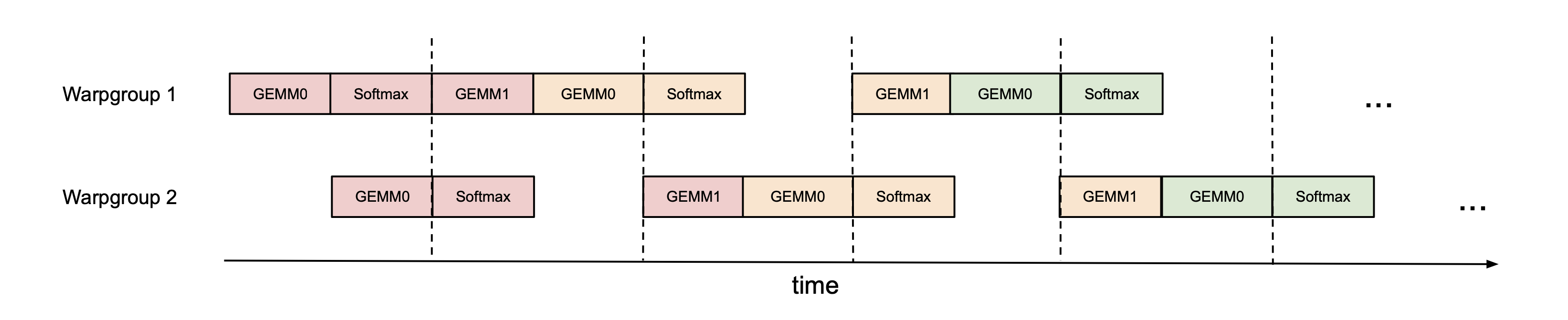
The asynchronous nature of WGMMA and TMA, along with warp-specialization, opens up the opportunity to overlap the softmax computation of one warpgroup with the GEMM of another warpgroup. To motivate this, notice that non-matmul operations have much lower throughput than matmul operations on modern hardware accelerators. As an example, the H100 SXM5 GPU has 989 TFLOPS of FP16 matmul but only 3.9 TFLOPS of special functions such as exponential The CUDA programming guide specifies that 16 operations of special functions can be performed per streaming multiprocessor (SM) per clock cycle. We multiply 16 by 132 SMs and 1830 MHz clock speed to get 3.9 TFLOPS of special functions. (necessary for softmax). For the attention forward pass in FP16 with head dimension 128, there are 512x more matmul FLOPS compared to exponential operations, but the exponential has 256x lower throughput, so exponential can take 50% of the cycle compared to matmul. The situation is even worse with FP8, where the matmul throughput doubles but the exponential throughput stays the same.
Since the exponential is performed by a separate hardware unit (the multi-function unit), ideally we’d want the exponential calculation to be scheduled when the Tensor Cores are performing the matmul. To do so, we use synchronization barriers (bar.sync instructions) to force the GEMMs (GEMM1 – $\mathbf{P}\mathbf{V}$ of one iteration, and GEMM0 – $\mathbf{Q}\mathbf{K}^{→p}$ of the next iteration) of warpgroup 1 to be scheduled before the GEMMs of warpgroup 2. As a result, the softmax of warpgroup 1 will be scheduled while warpgroup 2 is performing its GEMMs. Then the roles swap, with warpgroup 2 doing softmax while warpgroup 1 doing GEMMs (hence, “pingpong” scheduling). This is illustrated in Fig. 1. Though in practice the pingpong scheduling is not as clean as depicted in the figure, we generally find this to improve performance (e.g., from 570 TFLOPS to 620-640 TFLOPS for FP16 forward with head dimension 128 and sequence length 8192).
<details>
<summary>extracted/5728672/figs/pingpong_pipelining.png Details</summary>
### Visual Description
# Technical Document Extraction: Warpgroup Execution Timeline
## 1. Document Overview
This image is a technical timing diagram (Gantt-style chart) illustrating the parallel execution of computational tasks across two processing units, identified as **Warpgroup 1** and **Warpgroup 2**. The diagram visualizes how General Matrix Multiplication (GEMM) and Softmax operations are pipelined and synchronized over time.
## 2. Axis and Labels
* **Y-Axis (Vertical Categories):**
* **Warpgroup 1**: The top horizontal track of execution.
* **Warpgroup 2**: The bottom horizontal track of execution.
* **X-Axis (Horizontal Dimension):**
* Labeled as **"time"** with a right-pointing arrow indicating chronological progression.
* **Synchronization Markers:** Five vertical dashed lines intersect both warpgroup tracks, indicating synchronization points or stage boundaries.
## 3. Component Analysis (Task Blocks)
The diagram uses color-coded blocks to represent specific operations. There are three primary operation types: **GEMM0**, **GEMM1**, and **Softmax**.
### Color Coding and Grouping
The blocks are grouped by color, likely representing different stages or iterations of a pipeline:
1. **Pink Blocks:** Initial stage operations.
2. **Orange/Tan Blocks:** Intermediate stage operations.
3. **Green Blocks:** Final visible stage operations.
## 4. Execution Flow and Sequence
The diagram shows a staggered, pipelined execution where Warpgroup 2 starts its operations after Warpgroup 1 has completed its first task.
### Warpgroup 1 Sequence
1. **Stage 1 (Pink):** `GEMM0` $\rightarrow$ `Softmax` $\rightarrow$ `GEMM1` (Crosses first sync line).
2. **Stage 2 (Orange):** `GEMM0` $\rightarrow$ `Softmax` (Crosses second sync line).
3. **Stage 3 (Orange/Tan):** `GEMM1` (Starts after a gap following the third sync line).
4. **Stage 4 (Green):** `GEMM0` $\rightarrow$ `Softmax` (Crosses fourth sync line).
5. **Continuation:** Ellipsis (`...`) indicates the pattern continues.
### Warpgroup 2 Sequence
1. **Stage 1 (Pink):** Starts later than WG1. `GEMM0` $\rightarrow$ `Softmax` (Crosses first sync line).
2. **Stage 2 (Pink/Orange):** `GEMM1` (Pink) $\rightarrow$ `GEMM0` (Orange) $\rightarrow$ `Softmax` (Orange) (Crosses second and third sync lines).
3. **Stage 3 (Orange/Green):** `GEMM1` (Orange) $\rightarrow$ `GEMM0` (Green) $\rightarrow$ `Softmax` (Green) (Crosses fourth and fifth sync lines).
4. **Continuation:** Ellipsis (`...`) indicates the pattern continues.
## 5. Data Table Reconstruction
The following table maps the operations to the intervals defined by the vertical dashed synchronization lines (S1 through S5).
| Warpgroup | Pre-S1 | S1 to S2 | S2 to S3 | S3 to S4 | S4 to S5 | Post-S5 |
| :--- | :--- | :--- | :--- | :--- | :--- | :--- |
| **Warpgroup 1** | GEMM0 (P), Softmax (P) | GEMM1 (P), GEMM0 (O) | Softmax (O) | (Idle Gap) | GEMM1 (O), GEMM0 (G) | Softmax (G), ... |
| **Warpgroup 2** | (Idle), GEMM0 (P) | Softmax (P), GEMM1 (P) | GEMM0 (O), Softmax (O) | (Idle Gap) | GEMM1 (O), GEMM0 (G) | Softmax (G), ... |
*(Legend: P = Pink, O = Orange/Tan, G = Green)*
## 6. Technical Observations
* **Pipelining:** The diagram demonstrates a software pipeline. While Warpgroup 1 is working on the `GEMM0` of a new stage (Orange), Warpgroup 2 is finishing the `Softmax` of the previous stage (Pink).
* **Dependency/Stall:** There is a notable gap (idle time) for both warpgroups between the third and fourth synchronization lines, followed by the resumption of `GEMM1`.
* **Symmetry:** After the initial startup phase, the execution patterns of Warpgroup 1 and Warpgroup 2 become synchronized in terms of the types of operations performed between the dashed lines, though they remain offset by one operation block.
</details>
Figure 1: Pingpong scheduling for 2 warpgroups to overlap softmax and GEMMs: the softmax of one warpgroup should be scheduled when the GEMMs of another warpgroup are running. The same color denotes the same iteration.
Attention variants
For multi-query attention [51] and grouped query attention [3], we follow the approach in FlashAttention-2 and adjust the tensor indexing to avoid duplicating $\mathbf{K}$ and $\mathbf{V}$ in HBM.
3.2 Intra-warpgroup overlapping GEMMs and softmax
Even within one warpgroup, we can overlap some instructions in the softmax with some instructions in the GEMMs. We describe one technique to do so.
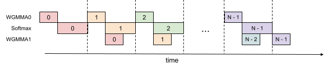
In the attention algorithm, operations within the inner loop (main loop) have sequential dependencies that impede parallelization within a single iteration. For example, (local) softmax (lines 18 to 19) relies on the output $\mathbf{S}_{i}^{(j)}$ of the first GEMM, while the second GEMM takes its result $\widetilde{\mathbf{P}}_{i}^{(j)}$ as an operand. Indeed, the wait statements in lines 17 and 21 of Algorithm 1 serialize the execution of softmax and GEMMs. However, we can break these dependencies by pipelining across iterations through additional buffers in registers. Pursuing this idea, we propose the following two-stage Note that the number of stages of the overlapping scheme is bounded by, but need not equal, the number $s$ of stages in the circular SMEM buffer. GEMM-softmax pipelining algorithm:
<details>
<summary>extracted/5728672/figs/2_stage_pipelining.png Details</summary>
### Visual Description
# Technical Document Extraction: Pipeline Execution Diagram
## 1. Overview
This image is a technical timing diagram illustrating a pipelined execution flow of three distinct computational tasks over time. The diagram uses a horizontal axis to represent time and a vertical axis to categorize the types of operations. It demonstrates a multi-stage pipeline where different operations (WGMMA0, Softmax, and WGMMA1) are interleaved to maximize hardware utilization.
## 2. Component Isolation
### 2.1 Axis and Labels
* **X-Axis:** A horizontal arrow pointing to the right, labeled **"time"** at the bottom center.
* **Y-Axis Labels:** Three categories are listed on the left side:
1. **WGMMA0** (Top row)
2. **Softmax** (Middle row)
3. **WGMMA1** (Bottom row)
* **Temporal Markers:** Vertical dashed lines divide the timeline into discrete execution stages or cycles.
### 2.2 Data Series (Operations)
The diagram uses color-coded blocks to represent specific iterations of a task. Each block contains a numerical identifier (0, 1, 2, ..., N-2, N-1).
| Color | Iteration Index | Description |
| :--- | :--- | :--- |
| **Light Red/Pink** | 0 | The first set of operations in the pipeline. |
| **Light Orange** | 1 | The second set of operations. |
| **Light Green** | 2 | The third set of operations. |
| **Light Purple** | N-1 | The final set of operations in the sequence. |
| **Light Blue** | N-2 | The penultimate operation for WGMMA1. |
---
## 3. Execution Flow and Logic
### 3.1 Sequential Dependency (Intra-iteration)
For any single iteration index (e.g., "0"), the tasks follow a staggered downward staircase pattern:
1. **WGMMA0** starts first.
2. **Softmax** starts immediately after WGMMA0 finishes.
3. **WGMMA1** starts immediately after Softmax finishes.
### 3.2 Pipelining Trend (Inter-iteration)
The diagram shows that while one iteration is performing a later stage, the next iteration begins its early stage.
* **Trend Observation:** The blocks slope downward and to the right for a single index, but the start of a new index (e.g., Index 1) aligns vertically with the start of the Softmax stage of the previous index (Index 0).
---
## 4. Detailed Step-by-Step Pipeline Transcription
| Time Interval (Defined by Dashed Lines) | WGMMA0 (Top) | Softmax (Middle) | WGMMA1 (Bottom) |
| :--- | :--- | :--- | :--- |
| **Interval 1** | Task 0 | (Idle) | (Idle) |
| **Interval 2** | (Idle) | Task 0 | (Idle) |
| **Interval 3** | Task 1 | Task 1 (Partial) | Task 0 |
| **Interval 4** | Task 2 | Task 2 (Partial) | Task 1 |
| **... (Ellipsis)** | ... | ... | ... |
| **Interval N** | Task N-1 | (Idle) | (Idle) |
| **Interval N+1** | (Idle) | Task N-1 | Task N-2 |
| **Interval N+2** | (Idle) | (Idle) | Task N-1 |
*Note: The diagram shows a specific overlap where the start of WGMMA0 for iteration `i+1` coincides with the start of the Softmax for iteration `i`. However, WGMMA1 for iteration `i` starts only after Softmax for iteration `i` is complete.*
## 5. Summary of Data Points
* **Total Stages:** 3 (WGMMA0 -> Softmax -> WGMMA1).
* **Concurrency:** At peak execution (middle of the diagram), three different iterations are active simultaneously across the three functional units.
* **Total Iterations:** Represented as $0$ through $N-1$.
</details>
Figure 2: 2-stage WGMMA-softmax pipelining
Algorithm 2 FlashAttention-3 consumer warpgroup forward pass
0: Matrices $\mathbf{Q}_{i}∈\mathbb{R}^{B_{r}× d}$ and $\mathbf{K},\mathbf{V}∈\mathbb{R}^{N× d}$ in HBM, key block size $B_{c}$ with $T_{c}=\lceil\frac{N}{B_{c}}\rceil$ .
1: Reallocate predetermined number of registers as function of number of consumer warps.
2: On-chip, initialize $\mathbf{O}_{i}=(0)∈\mathbb{R}^{B_{r}× d}$ and $\ell_{i},m_{i}=(0),(-∞)∈\mathbb{R}^{B_{r}}$ .
3: Wait for $\mathbf{Q}_{i}$ and $\mathbf{K}_{0}$ to be loaded in shared memory.
4: Compute $\mathbf{S}_{\mathrm{cur}}=\mathbf{Q}_{i}\mathbf{K}_{0}^{T}$ using WGMMA. Commit and wait.
5: Release the $0 0$ th stage of the buffer for $\mathbf{K}$ .
6: Compute $m_{i}$ , $\tilde{\mathbf{P}}_{\mathrm{cur}}$ and $\ell_{i}$ based on $\mathbf{S}_{\mathrm{cur}}$ , and rescale $\mathbf{O}_{i}$ .
7: for $1≤ j<T_{c}-1$ do
8: Wait for $\mathbf{K}_{j}$ to be loaded in shared memory.
9: Compute $\mathbf{S}_{\mathrm{next}}=\mathbf{Q}_{i}\mathbf{K}_{j}^{T}$ using WGMMA. Commit but do not wait.
10: Wait for $\mathbf{V}_{j-1}$ to be loaded in shared memory.
11: Compute $\mathbf{O}_{i}=\mathbf{O}_{i}+\tilde{\mathbf{P}}_{\mathrm{cur}}\mathbf{V}_{j-1}$ using WGMMA. Commit but do not wait.
12: Wait for the WGMMA $\mathbf{Q}_{i}\mathbf{K}_{j}^{T}$ .
13: Compute $m_{i}$ , $\tilde{\mathbf{P}}_{\mathrm{next}}$ and $\ell_{i}$ based on $\mathbf{S}_{\mathrm{next}}$ .
14: Wait for the WGMMA $\tilde{\mathbf{P}}_{\mathrm{cur}}\mathbf{V}_{j-1}$ and then rescale $\mathbf{O}_{i}$
15: Release the $(j\,\%\,s)$ th, resp. $(j-1\,\%\,s)$ th stage of the buffer for $\mathbf{K}$ , resp. $\mathbf{V}$ .
16: Copy $\mathbf{S}_{\mathrm{next}}$ to $\mathbf{S}_{\mathrm{cur}}$ .
17: end for
18: Wait for $\mathbf{V}_{T_{c}-1}$ to be loaded in shared memory.
19: Compute $\mathbf{O}_{i}=\mathbf{O}_{i}+\tilde{\mathbf{P}}_{\mathrm{last}}\mathbf{V}_{T_%
{c}-1}$ using WGMMA. Commit and wait.
20: Epilogue: Rescale $\mathbf{O}_{i}$ based on $m_{i}$ . Compute $L_{i}$ based on $m_{i}$ and $\ell_{i}$ . Write $\mathbf{O}_{i}$ and $L_{i}$ to HBM as the $i$ -th block of $\mathbf{O}$ and $L$ .
Algorithm 2 functions as a replacement for the consumer path of Algorithm 1 to comprise the complete FlashAttention-3 algorithm for FP16 precision. At a high-level, we use WGMMA as a metonym for asynchronous GEMM. Within the mainloop (lines 8 to 16), the second WGMMA operation of iteration $j$ (line 11) is overlapped with softmax operations from iteration $j+1$ (line 13).
While the pipelined structure illustrated above offers theoretical performance gains, there are several practical aspects to consider:
Compiler reordering
The pseudocode represents an idealized execution order but the compiler (NVCC) often rearranges instructions for optimization. This can disrupt the carefully crafted WGMMA and non-WGMMA operation pipelining sequence, potentially leading to unexpected behavior or diminished performance gains. An analysis of the SASS code shows that the compiler generates overlapped code as expected (Section B.2).
Register pressure
To maintain optimal performance, register spilling should be minimized. However, the 2-stage pipeline requires additional registers to store intermediate results and maintain context between stages. Specifically, an extra $\mathbf{S}_{\mathrm{next}}$ must be kept in registers, leading to extra register usage of size $B_{r}× B_{c}×\text{sizeof}(\text{float})$ per threadblock. This increased register demand may conflict with using larger block sizes (another common optimization), which is also register-hungry. In practice, trade-offs should be made based on profiling results.
3-stage pipelining
Extending the 2-stage algorithm described above, we propose a 3-stage variant that would further overlap the second WGMMA with softmax. While this approach offers the potential for even higher Tensor Core utilization, it requires even more registers due to an additional stage in the pipeline, making the trade-off between tile size and pipeline depth more difficult to balance. A detailed description of the 3-stage algorithm and its evaluation results can be found in § B.3.
3.3 Low-precision with FP8 T0 {d0, d1} T1 {d0, d1} T0 {d4, d5} T1 {d4, d5} T2 {d0, d1} T3 {d0, d1} T2 {d4, d5} T3 {d4, d5} T0 {d2, d3} T1 {d2, d3} T0 {d6, d7} T1 {d6, d7} T2 {d2, d3} T3 {d2, d3} T2 {d6, d7} T3 {d6, d7}
Figure 3: FP32 accumulator register WGMMA layout – rows 0 and 8, threads 0-3, entries 0-7. T0 {a0, a1} T0 {a2, a3} T1 {a0, a1} T1 {a2, a3} T2 {a0, a1} T2 {a2, a3} T3 {a0, a1} T3 {a2, a3} T0 {a4, a5} T0 {a6, a7} T1 {a4, a5} T1 {a6, a7} T2 {a4, a5} T2 {a6, a7} T3 {a4, a5} T3 {a6, a7}
Figure 4: FP8 operand A register WGMMA layout – rows 0 and 8, threads 0-3, entries 0-7.
Efficiency: layout transformations. Computing the forward pass of FlashAttention-3 in FP8 precision poses additional challenges not encountered for FP16 in terms of layout conformance.
First, we note that the input tensors $\mathbf{Q}$ , $\mathbf{K}$ , and $\mathbf{V}$ are typically given as contiguous in the head dimension, while to satisfy the k-major constraint on FP8 WGMMA for the second GEMM we need $\mathbf{V}$ , or rather the tiles of $\mathbf{V}$ loaded into SMEM, to be contiguous in the sequence length dimension. Since the TMA load itself cannot change the contiguous dimension, we then need to either (1) transpose $\mathbf{V}$ in GMEM as a pre-processing step, or (2) do an in-kernel transpose of tiles of $\mathbf{V}$ after loading them into SMEM. To implement option (1), we can either (1a) fuse the transpose to the epilogue of a preceding step such as the rotary embedding, or (1b) call a standalone pre-processing transpose kernel An optimized transpose kernel will achieve speed near the bandwidth of the device [46]. to exchange the strides of the sequence length and head dimensions. However, (1a) is difficult to integrate into a standard library, and (1b) is too wasteful in a memory-bound situation such as inference.
Instead, for FP8 FlashAttention-3 we opt for option (2). For the in-kernel transpose, we take advantage of the LDSM (ldmatrix) and STSM (stmatrix) instructions, which involve a warp of threads collectively loading SMEM to RMEM and storing RMEM to SMEM at a granularity of 128 bytes. In the PTX documentation, LDSM/STSM are described as copying $8× 8$ matrices with 16-bit entries [40, §9.7.13.4.15-16], but we can pack 8-bit entries two at a time to use LDSM/STSM in the context of FP8 precision. However, the transpose versions of LDSM/STSM cannot split packed 8-bit entries, which necessitates certain register movements in between LDSM and STSM to actually perform a tile-wise transpose; we omit the details. The LDSM/STSM instructions are both register efficient, allowing us to execute them in the producer warpgroup, and capable of transposing layouts when doing memory copy. Moreover, after the first iteration we can arrange for the transpose of the next $\mathbf{V}$ tile to be executed in the shadow of the two WGMMAs that involve the preceding $\mathbf{V}$ and current $\mathbf{K}$ tile.
Second, we observe that unlike with FP16, the memory layout of the FP32 accumulator of an FP8 WGMMA is different from that assumed for its operand A when held in registers. We depict fragments of these two layouts in Fig. 3 and Fig. 4, where the entries are held in registers per thread in the listed order. By using byte permute instructions, we can then transform the first WGMMA’s accumulator into a format suitable for the second WGMMA, and compatibly with the layout of the $\mathbf{V}$ tile produced by the in-kernel transpose. Specifically, with reference to Fig. 3, we change the order in sequence to
$$
\{\verb|d0 d1 d4 d5 d2 d3 d6 d7|\},
$$
and this register permutation is then replicated over every 8 bytes. In terms of the logical shape of the $\mathbf{P}$ tile, this manuever permutes its columns (e.g., columns $0189$ now become the first four columns). For WGMMA to then compute the correct output tile, we can correspondingly arrange for the in-kernel transpose to write out a matching row permutation of the $\mathbf{V}$ tile. This additional freedom afforded by doing the in-kernel transpose eliminates having to use shuffle instructions to change register ownership across threads, which we previously described in [7].
Accuracy: block quantization and incoherent processing. With FP8 (e4m3) format, one only uses 3 bits to store the mantissa and 4 bits for the exponent. This results in higher numerical error than FP16/BF16. Moreover, large models typically have outlier values [20, 54] that are much larger in magnitude than most other values, making quantization difficult. One typically use per-tensor scaling [37] by keeping one scalar per tensor (e.g., one for $\mathbf{Q}$ , for $\mathbf{K}$ , and for $\mathbf{V}$ ). To reduce the numerical error of attention in FP8, we employ two techniques:
1. Block quantization: we keep one scalar per block, so that for each of $\mathbf{Q}$ , $\mathbf{K}$ , $\mathbf{V}$ we split the tensor into blocks of size $B_{r}× d$ or $B_{c}× d$ and quantize them separately. This quantization can be fused with an operation right before attention (e.g., rotary embedding) with no additional slow down (since rotary embedding is memory-bandwidth bound). As the FlashAttention-3 algorithm naturally operates on blocks, we can scale each block of $\mathbf{S}$ to account for this block quantization at no computation cost.
1. Incoherent processing: to even out outliers, we multiply $\mathbf{Q}$ and $\mathbf{K}$ with a random orthogonal matrix $\mathbf{M}$ before quantizing to FP8. Since $\mathbf{M}$ is orthogonal, $\mathbf{M}\mathbf{M}^{→p}=I$ and so $(\mathbf{Q}\mathbf{M})(\mathbf{K}\mathbf{M})^{→p}=\mathbf{Q}\mathbf{K}^{→p}$ , i.e., multiplying both $\mathbf{Q}$ and $\mathbf{K}$ with $\mathbf{M}$ does not change the attention output. This serves to “spread out” the outliers since each entry of $\mathbf{Q}\mathbf{M}$ or $\mathbf{K}\mathbf{M}$ is a random sum of entries of $\mathbf{Q}$ or $\mathbf{K}$ , thus reducing quantization error. In practice, we follow Chee et al. [9] and Tseng et al. [58] and choose $\mathbf{M}$ to be the product of random diagonal matrices of $± 1$ and a Hadamard matrix, which can be multiplied in $O(d\log d)$ instead of $O(d^{2})$ , and can also be fused with the rotary embedding at no extra computation cost.
We validate that these two techniques reduces numerical error by up to 2.6 $×$ in § 4.3.
4 Empirical Validation
We use the primitives from CUTLASS [57] such as WGMMA and TMA abstractions to implement FlashAttention-3 and evaluate its efficiency and accuracy.
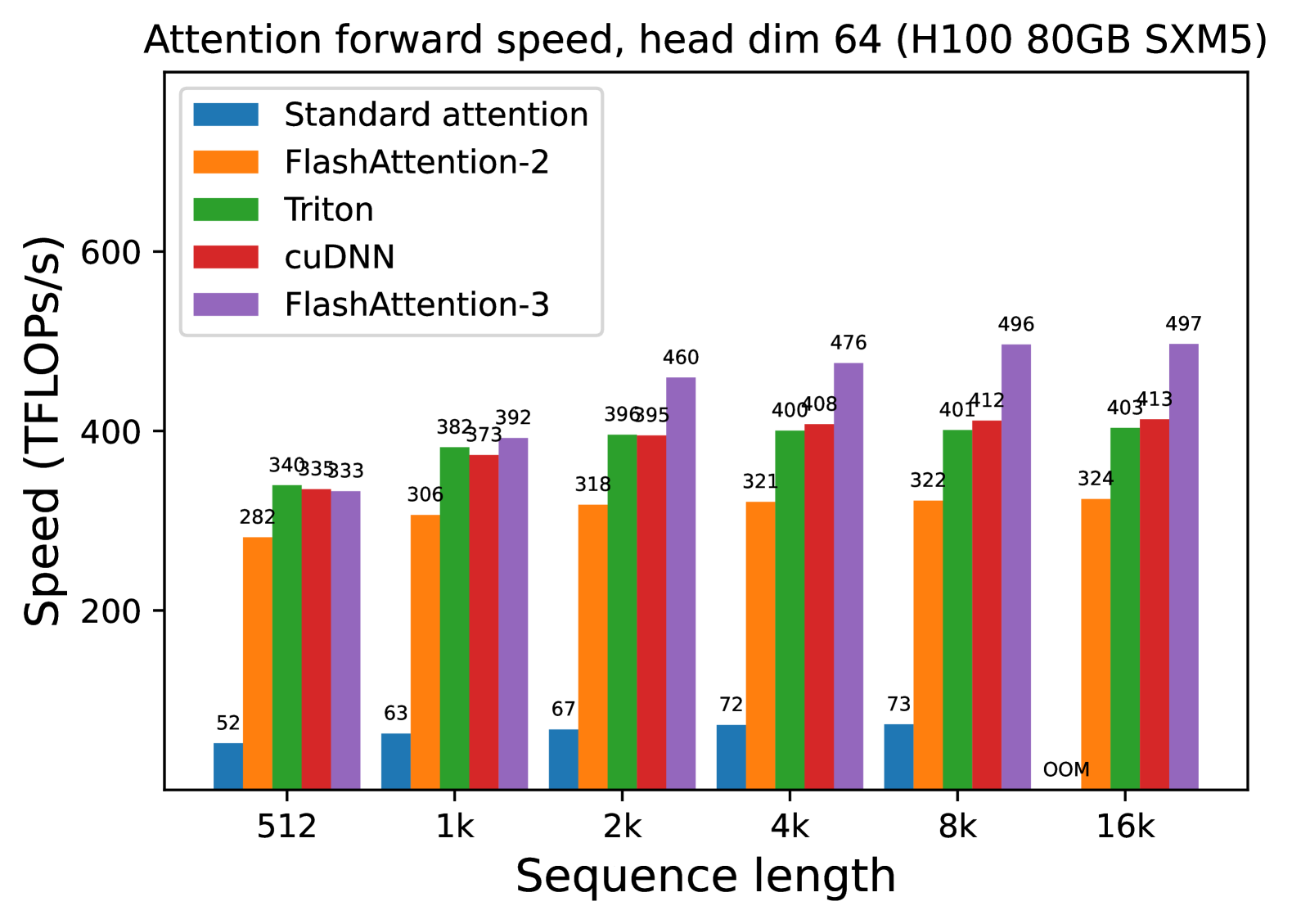
- Benchmarking attention. We measure the runtime of FlashAttention-3 across different sequence lengths and compare it to a standard implementation in PyTorch, FlashAttention-2, FlashAttention-2 in Triton (which uses H100-specific instructions), as well as a vendor’s implementation of FlashAttention-2 optimized for H100 GPUs from cuDNN. We confirm that FlashAttention-3 is up to 2.0 $×$ faster than FlashAttention-2 and 1.5 $×$ faster than FlashAttention-2 in Triton. FlashAttention-3 reaches up to 740 TFLOPs/s, 75% of the theoretical maximum TFLOPs/s on H100 GPUs.
- Ablation study. We confirm that our algorithmic improvements with warp-specialization and GEMM-softmax pipelining contribute to the speedup of FlashAttention-3.
- Accuracy of FP8 attention. We validate that block quantization and incoherent processing reduces the numerical error of FP8 FlashAttention-3 by 2.6 $×$ .
4.1 Benchmarking Attention
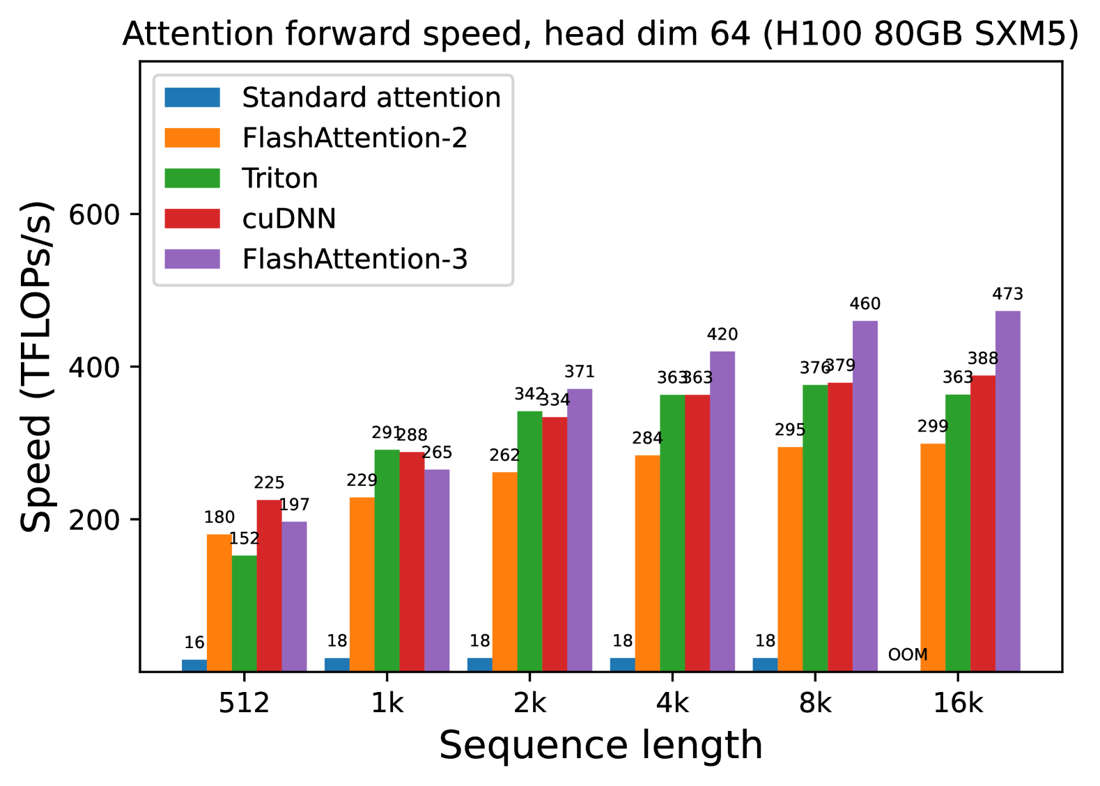
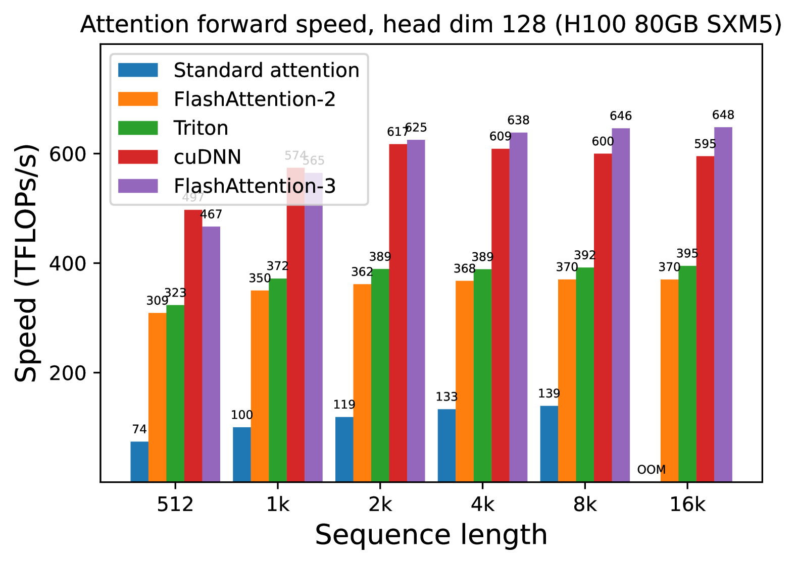
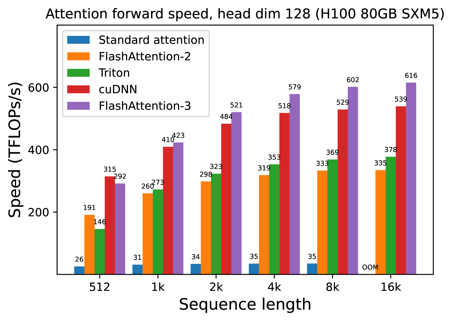
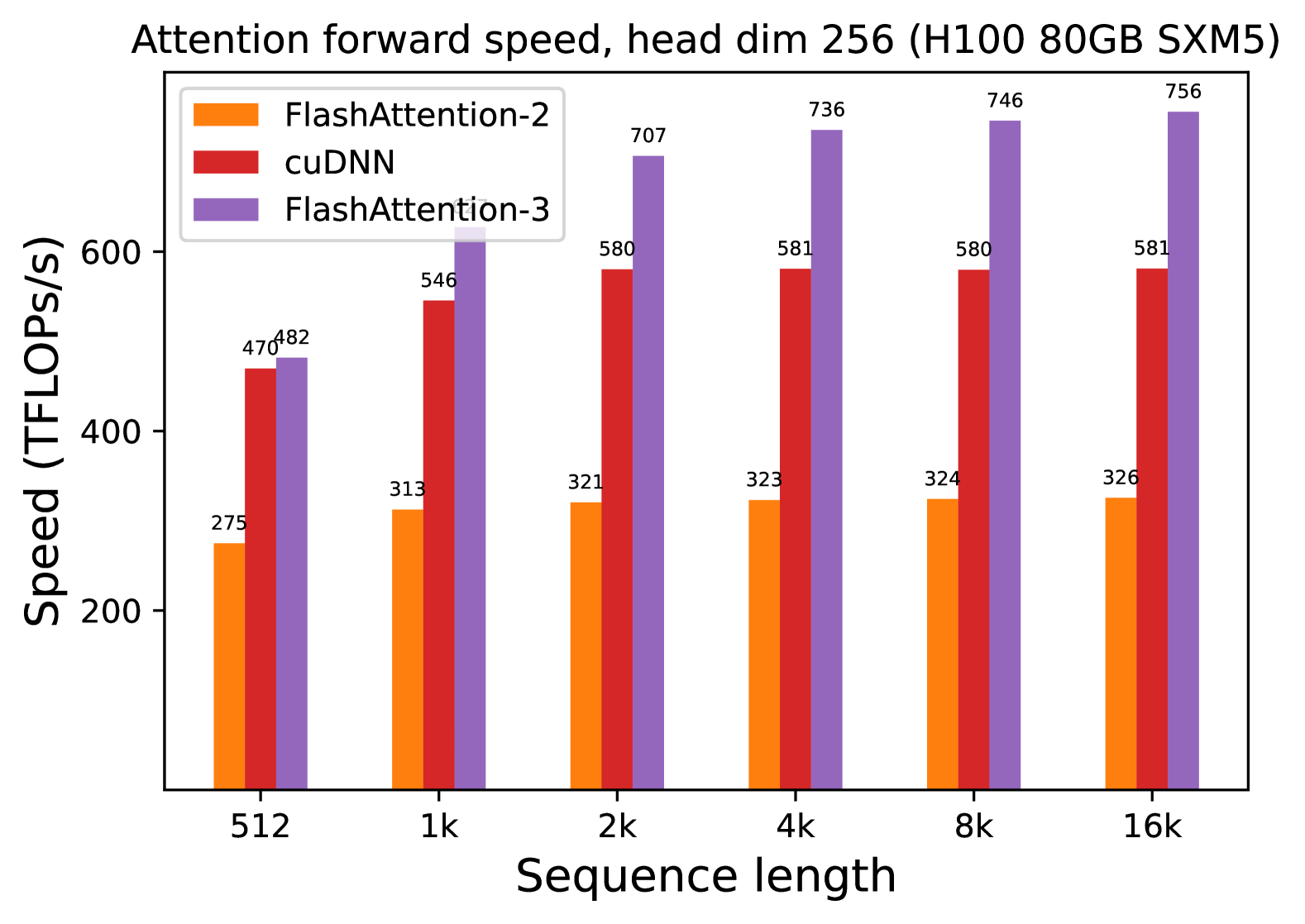
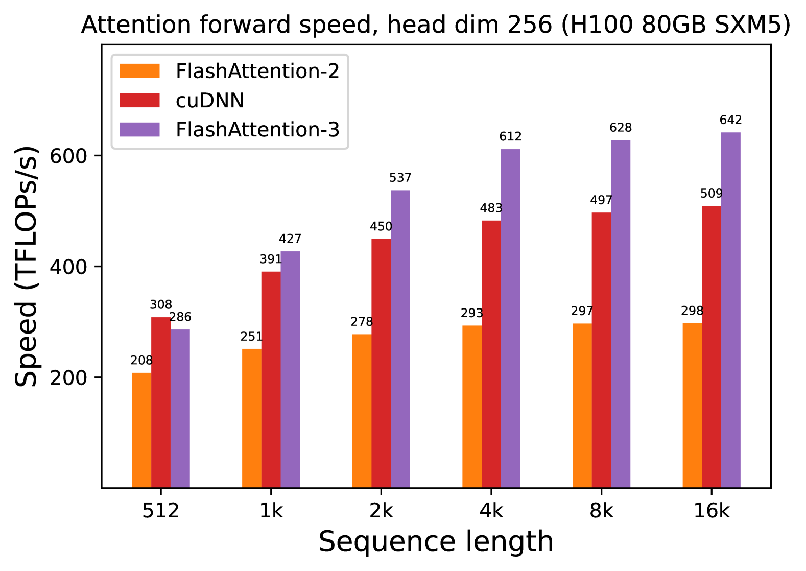
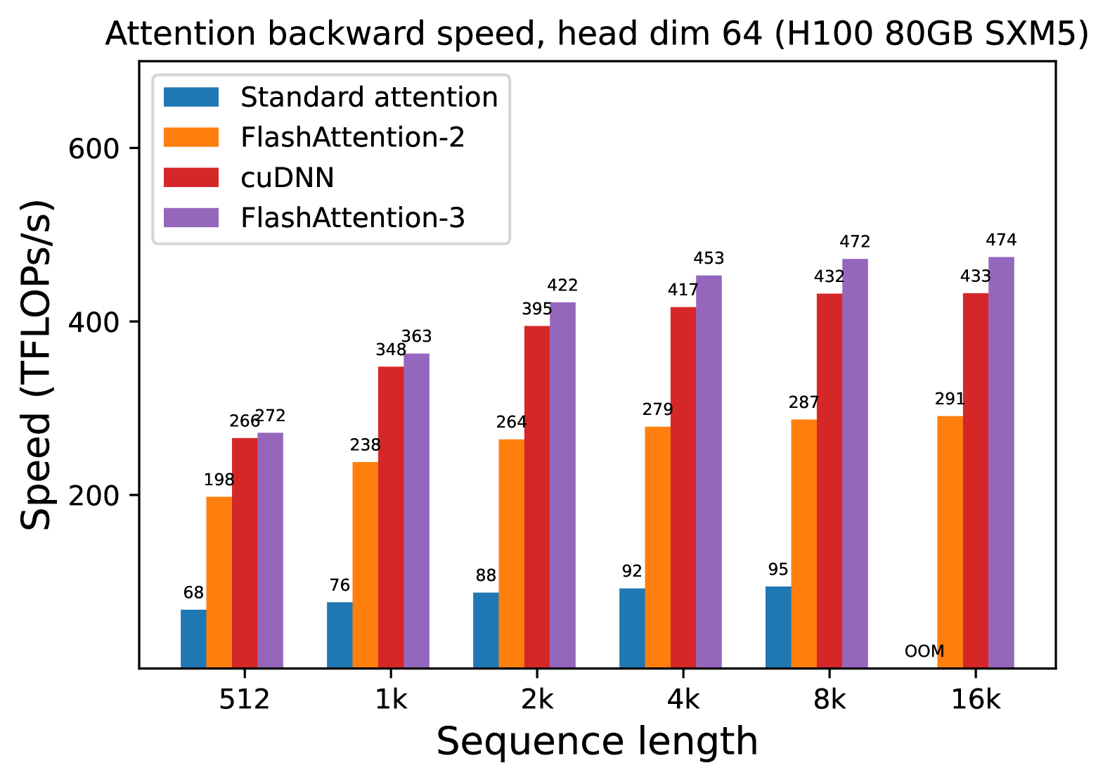
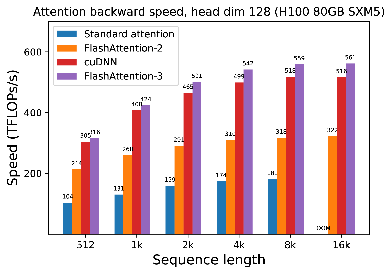
We measure the runtime of different attention methods on an H100 80GB SXM5 GPU for different settings (without / with causal mask, head dimension 64 or 128) for FP16 inputs. We report the results in Fig. 5 and Fig. 6, showing that FlashAttention-3 is around 1.5-2.0 $×$ faster than FlashAttention-2 in the forward pass and 1.5-1.75 $×$ faster in the backward pass. Compared to a standard attention implementation, FlashAttention-3 can be up to 3-16 $×$ faster. For medium and long sequences (1k and above), FlashAttention-3 even surpasses the speed of a vendor’s library (cuDNN – closed source) that has been optimized for H100 GPUs.
Benchmark settings:
We vary the sequence length as 512, 1k, …, 16k, and set batch size so that the total number of tokens is 16k. We set the hidden dimension to 2048, and head dimension to be either 64, 128, or 256 (i.e., 32 heads, 16 heads, or 8 heads). To calculate the FLOPs of the forward pass, we use:
$$
4\cdot\text{seqlen}^{2}\cdot\text{head dimension}\cdot\text{number of heads}.
$$
With causal masking, we divide this number by 2 to account for the fact that approximately only half of the entries are calculated. To get the FLOPs of the backward pass, we multiply the forward pass FLOPs by 2.5 (since there are 2 matmuls in the forward pass and 5 matmuls in the backward pass, due to recomputation).
<details>
<summary>x1.png Details</summary>
### Visual Description
# Technical Document Extraction: Attention Forward Speed Benchmark
## 1. Header Information
* **Title:** Attention forward speed, head dim 64 (H100 80GB SXM5)
* **Hardware Context:** NVIDIA H100 80GB SXM5 GPU.
* **Parameter Context:** Head dimension is fixed at 64.
## 2. Chart Structure and Metadata
* **Chart Type:** Grouped Bar Chart.
* **Y-Axis Label:** Speed (TFLOPS/s)
* **Y-Axis Scale:** Linear, ranging from 0 to 600+ (markers at 200, 400, 600).
* **X-Axis Label:** Sequence length
* **X-Axis Categories:** 512, 1k, 2k, 4k, 8k, 16k.
* **Legend Placement:** Top-left [x≈0.15, y≈0.85].
### Legend / Data Series Identification
| Color | Label | Trend Description |
| :--- | :--- | :--- |
| **Blue** | Standard attention | Low performance; slight upward trend as sequence length increases, then terminates. |
| **Orange** | FlashAttention-2 | Moderate performance; steady upward trend, plateauing around 324 TFLOPS/s. |
| **Green** | Triton | High performance; rapid initial growth, plateauing around 400-403 TFLOPS/s. |
| **Red** | cuDNN | High performance; steady upward trend, consistently outperforming Triton at higher sequence lengths. |
| **Purple** | FlashAttention-3 | Highest performance; aggressive upward trend, significantly outperforming all other methods as sequence length increases. |
## 3. Data Table Extraction
The following table reconstructs the numerical values (TFLOPS/s) displayed above each bar in the chart.
| Sequence Length | Standard attention (Blue) | FlashAttention-2 (Orange) | Triton (Green) | cuDNN (Red) | FlashAttention-3 (Purple) |
| :--- | :---: | :---: | :---: | :---: | :---: |
| **512** | 52 | 282 | 340 | 335 | 333 |
| **1k** | 63 | 306 | 382 | 373 | 392 |
| **2k** | 67 | 318 | 396 | 395 | 460 |
| **4k** | 72 | 321 | 400 | 408 | 476 |
| **8k** | 73 | 322 | 401 | 412 | 496 |
| **16k** | **OOM*** | 324 | 403 | 413 | 497 |
*\*OOM: Out of Memory*
## 4. Key Observations and Trends
### Performance Hierarchy
1. **FlashAttention-3 (Purple):** The clear leader in throughput. It shows the most significant scaling, reaching nearly 500 TFLOPS/s at a 16k sequence length. It is approximately 1.5x faster than FlashAttention-2 at large scales.
2. **cuDNN (Red) & Triton (Green):** These two implementations perform similarly. Triton is slightly faster at the smallest sequence length (512), but cuDNN overtakes it starting at the 4k sequence length and maintains a slight lead thereafter.
3. **FlashAttention-2 (Orange):** Maintains a consistent performance level between 282 and 324 TFLOPS/s, significantly faster than standard attention but trailing the newer optimizations.
4. **Standard Attention (Blue):** Performs poorly across all tests, never exceeding 73 TFLOPS/s.
### Scalability and Memory
* **Memory Limit:** "Standard attention" fails at the 16k sequence length due to an **OOM (Out of Memory)** error, whereas all optimized kernels (FlashAttention variants, Triton, and cuDNN) successfully process the 16k sequence.
* **Efficiency Gains:** The performance gap between optimized kernels and standard attention widens as sequence length increases. At 8k, FlashAttention-3 is roughly **6.8x faster** than standard attention.
</details>
(a) Forward, without causal mask, head dim 64
<details>
<summary>x2.png Details</summary>
### Visual Description
# Technical Document Extraction: Attention Forward Speed Benchmark
## 1. Header Information
* **Title:** Attention forward speed, head dim 64 (H100 80GB SXM5)
* **Hardware Context:** NVIDIA H100 80GB SXM5 GPU.
* **Parameter Configuration:** Head dimension is fixed at 64.
## 2. Chart Metadata
* **Type:** Grouped Bar Chart.
* **X-Axis Label:** Sequence length
* **X-Axis Categories:** 512, 1k, 2k, 4k, 8k, 16k.
* **Y-Axis Label:** Speed (TFLOPS/s)
* **Y-Axis Scale:** 0 to 600 (increments of 200 labeled).
* **Legend Location:** Top-left [x: ~0.15, y: ~0.85].
## 3. Legend and Series Identification
The chart compares five different attention implementations, color-coded as follows:
1. **Standard attention** (Blue): Represents the baseline implementation.
2. **FlashAttention-2** (Orange): An optimized attention mechanism.
3. **Triton** (Green): Implementation using the Triton language/compiler.
4. **cuDNN** (Red): NVIDIA's deep neural network library implementation.
5. **FlashAttention-3** (Purple): The latest iteration of the FlashAttention algorithm.
## 4. Data Table Reconstruction
The following table transcribes the numerical values (TFLOPS/s) displayed above each bar in the chart.
| Sequence Length | Standard attention (Blue) | FlashAttention-2 (Orange) | Triton (Green) | cuDNN (Red) | FlashAttention-3 (Purple) |
| :--- | :---: | :---: | :---: | :---: | :---: |
| **512** | 16 | 180 | 152 | 225 | 197 |
| **1k** | 18 | 229 | 291 | 288 | 265 |
| **2k** | 18 | 262 | 342 | 334 | 371 |
| **4k** | 18 | 284 | 363 | 363 | 420 |
| **8k** | 18 | 295 | 376 | 379 | 460 |
| **16k** | OOM* | 299 | 363 | 388 | 473 |
*\*OOM: Out of Memory*
## 5. Trend Analysis and Component Observations
### Standard attention (Blue)
* **Trend:** Extremely low and flat performance.
* **Observation:** Maintains a near-constant speed of 16-18 TFLOPS/s until it fails at 16k sequence length due to memory constraints (OOM).
### FlashAttention-2 (Orange)
* **Trend:** Steady upward slope that plateaus as sequence length increases.
* **Observation:** Performance grows from 180 to 299 TFLOPS/s, showing significant improvement over standard attention but trailing behind the other optimized methods at higher sequence lengths.
### Triton (Green)
* **Trend:** Rapid initial growth, leveling off after 4k.
* **Observation:** Performance jumps significantly between 512 (152 TFLOPS/s) and 2k (342 TFLOPS/s), eventually stabilizing around 363-376 TFLOPS/s.
### cuDNN (Red)
* **Trend:** Consistent upward slope.
* **Observation:** Starts as the fastest method at the shortest sequence length (225 TFLOPS/s at 512). It maintains a very similar performance profile to Triton from 1k to 8k, ending slightly higher at 388 TFLOPS/s for 16k.
### FlashAttention-3 (Purple)
* **Trend:** Strong, continuous upward slope with the highest ceiling.
* **Observation:** While it starts in the middle of the pack at 512 (197 TFLOPS/s), it scales the best of all tested methods. It becomes the clear leader at sequence lengths of 2k and above, reaching a peak of 473 TFLOPS/s at 16k.
## 6. Summary of Findings
FlashAttention-3 demonstrates superior scaling for long sequences on H100 hardware, outperforming FlashAttention-2 by approximately 58% and cuDNN by approximately 22% at a sequence length of 16k. Standard attention is non-viable for these workloads due to both extremely low throughput and memory inefficiency.
</details>
(b) Forward, with causal mask, head dim 64
<details>
<summary>x3.png Details</summary>
### Visual Description
# Technical Document Extraction: Attention Forward Speed Benchmark
## 1. Header Information
* **Title:** Attention forward speed, head dim 128 (H100 80GB SXM5)
* **Hardware Context:** NVIDIA H100 80GB SXM5 GPU.
* **Parameter Context:** Head dimension is fixed at 128.
## 2. Chart Structure and Metadata
* **Chart Type:** Grouped Bar Chart.
* **X-Axis (Independent Variable):** Sequence length.
* **Categories:** 512, 1k, 2k, 4k, 8k, 16k.
* **Y-Axis (Dependent Variable):** Speed (TFLOPS/s).
* **Scale:** Linear, ranging from 0 to 600+ (markers at 200, 400, 600).
* **Legend:**
1. **Standard attention** (Blue)
2. **FlashAttention-2** (Orange)
3. **Triton** (Green)
4. **cuDNN** (Red)
5. **FlashAttention-3** (Purple)
## 3. Data Table Reconstruction
The following table extracts the numerical values (TFLOPS/s) labeled above each bar in the chart.
| Sequence Length | Standard attention (Blue) | FlashAttention-2 (Orange) | Triton (Green) | cuDNN (Red) | FlashAttention-3 (Purple) |
| :--- | :---: | :---: | :---: | :---: | :---: |
| **512** | 74 | 309 | 323 | 497 | 467 |
| **1k** | 100 | 350 | 372 | 574 | 565 |
| **2k** | 119 | 362 | 389 | 617 | 625 |
| **4k** | 133 | 368 | 389 | 609 | 638 |
| **8k** | 139 | 370 | 392 | 600 | 646 |
| **16k** | OOM* | 370 | 395 | 595 | 648 |
*\*OOM: Out of Memory*
## 4. Trend Analysis and Component Isolation
### Series Trends
* **Standard attention (Blue):** Shows a slow upward slope from 74 to 139 TFLOPS/s as sequence length increases, but fails at 16k due to memory constraints (OOM). It is consistently the lowest performing method.
* **FlashAttention-2 (Orange):** Slopes upward initially and plateaus quickly around 370 TFLOPS/s from 8k onwards.
* **Triton (Green):** Follows a similar trend to FlashAttention-2 but maintains a consistent lead of ~20-25 TFLOPS/s over it, plateauing near 395 TFLOPS/s.
* **cuDNN (Red):** Shows a sharp upward trend, peaking at 2k (617 TFLOPS/s), then exhibits a slight downward trend as sequence length increases to 16k (595 TFLOPS/s).
* **FlashAttention-3 (Purple):** Shows the strongest scaling performance. While it starts slightly behind cuDNN at 512 and 1k, it overtakes all other methods at 2k and continues to slope upward, reaching the highest recorded value of 648 TFLOPS/s at 16k.
### Comparative Observations
* **Efficiency Gap:** There is a massive performance gap between "Standard attention" and all optimized kernels. At 8k, FlashAttention-3 is approximately 4.6x faster than Standard attention.
* **Crossover Point:** FlashAttention-3 overtakes cuDNN as the fastest implementation at the 2k sequence length mark.
* **Scalability:** FlashAttention-3 is the only implementation that shows continuous (albeit slowing) growth in TFLOPS/s across the entire tested range without regressing at higher sequence lengths.
</details>
(c) Forward, without causal mask, head dim 128
<details>
<summary>x4.png Details</summary>
### Visual Description
# Technical Data Extraction: Attention Forward Speed Benchmark
## 1. Document Header
* **Title:** Attention forward speed, head dim 128 (H100 80GB SXM5)
* **Hardware Context:** NVIDIA H100 80GB SXM5 GPU.
* **Parameter Context:** Head dimension is fixed at 128.
## 2. Chart Metadata
* **Type:** Grouped Bar Chart.
* **Y-Axis Label:** Speed (TFLOPS/s)
* **Y-Axis Scale:** 0 to 600+ (increments of 200 marked).
* **X-Axis Label:** Sequence length
* **X-Axis Categories:** 512, 1k, 2k, 4k, 8k, 16k.
* **Legend Location:** Top-left [x≈0.15, y≈0.85].
## 3. Legend and Series Identification
The chart compares five different implementations of the attention mechanism:
1. **Standard attention** (Blue): Represents the baseline performance.
2. **FlashAttention-2** (Orange): An optimized attention implementation.
3. **Triton** (Green): Implementation using the Triton language/compiler.
4. **cuDNN** (Red): NVIDIA's Deep Neural Network library implementation.
5. **FlashAttention-3** (Purple): The latest iteration of the FlashAttention algorithm.
---
## 4. Data Table Reconstruction
The following table transcribes the numerical values (TFLOPS/s) displayed above each bar in the chart.
| Sequence Length | Standard attention (Blue) | FlashAttention-2 (Orange) | Triton (Green) | cuDNN (Red) | FlashAttention-3 (Purple) |
| :--- | :---: | :---: | :---: | :---: | :---: |
| **512** | 26 | 191 | 146 | 315 | 292 |
| **1k** | 31 | 260 | 273 | 410 | 423 |
| **2k** | 34 | 298 | 323 | 484 | 521 |
| **4k** | 35 | 319 | 353 | 518 | 579 |
| **8k** | 35 | 333 | 369 | 529 | 602 |
| **16k** | OOM* | 335 | 378 | 539 | 616 |
*\*OOM: Out of Memory*
---
## 5. Trend Analysis and Component Isolation
### Standard attention (Blue)
* **Trend:** Extremely low and relatively flat performance.
* **Observation:** Performance crawls from 26 to 35 TFLOPS/s before failing at 16k sequence length due to memory constraints (OOM).
### FlashAttention-2 (Orange)
* **Trend:** Rapid initial growth, tapering off to a plateau.
* **Observation:** Shows a significant jump from 512 (191) to 1k (260), then stabilizes around 335 TFLOPS/s at higher sequence lengths.
### Triton (Green)
* **Trend:** Consistent upward slope across all sequence lengths.
* **Observation:** Starts lower than FlashAttention-2 at 512 (146 vs 191) but overtakes it at 1k and maintains a higher growth trajectory, reaching 378 TFLOPS/s at 16k.
### cuDNN (Red)
* **Trend:** High performance with steady gains, plateauing after 4k.
* **Observation:** Significantly outperforms the previous three methods. It is the fastest method at the shortest sequence length (512) with 315 TFLOPS/s.
### FlashAttention-3 (Purple)
* **Trend:** Strongest upward slope and highest peak performance.
* **Observation:** While slightly slower than cuDNN at 512 (292 vs 315), it scales better than all other methods. It becomes the performance leader starting at the 1k mark and reaches a peak of 616 TFLOPS/s at 16k, nearly doubling the performance of FlashAttention-2.
## 6. Summary of Findings
The data demonstrates that **FlashAttention-3** provides the best scaling and highest throughput for large sequence lengths on H100 hardware, specifically when the head dimension is 128. **Standard attention** is non-viable for large sequences due to its $O(n^2)$ memory requirements, resulting in an "OOM" state at 16k. **cuDNN** remains highly competitive, particularly at shorter sequence lengths (512).
</details>
(d) Forward, with causal mask, head dim 128
<details>
<summary>x5.png Details</summary>
### Visual Description
# Technical Document Extraction: Attention Forward Speed Benchmark
## 1. Document Metadata
* **Title:** Attention forward speed, head dim 256 (H100 80GB SXM5)
* **Image Type:** Grouped Bar Chart
* **Primary Language:** English
## 2. Component Isolation
### Header
* **Main Title:** "Attention forward speed, head dim 256 (H100 80GB SXM5)"
* **Context:** This chart benchmarks the performance of different attention mechanisms on an NVIDIA H100 80GB SXM5 GPU, specifically for a head dimension of 256.
### Main Chart Area
* **Y-Axis Label:** Speed (TFLOPs/s)
* **Y-Axis Scale:** Linear, ranging from 200 to 600+ (markers at 200, 400, 600).
* **X-Axis Label:** Sequence length
* **X-Axis Categories:** 512, 1k, 2k, 4k, 8k, 16k.
* **Legend (Top-Left):**
* **Orange:** FlashAttention-2
* **Red:** cuDNN
* **Purple:** FlashAttention-3
### Footer
* No footer text present.
## 3. Data Extraction and Trend Analysis
### Trend Verification
1. **FlashAttention-2 (Orange):** Shows a slight upward trend from 512 to 2k, then plateaus/stabilizes between 321 and 326 TFLOPs/s for higher sequence lengths.
2. **cuDNN (Red):** Shows a significant jump from 512 to 2k, then plateaus almost perfectly at 580-581 TFLOPs/s from 2k through 16k.
3. **FlashAttention-3 (Purple):** Shows the most aggressive upward trend, starting slightly above cuDNN at 512 and scaling significantly until it plateaus/stabilizes around 736-756 TFLOPs/s at higher sequence lengths.
### Data Table (Reconstructed)
The following table represents the precise numerical values labeled above each bar in the chart.
| Sequence Length | FlashAttention-2 (Orange) | cuDNN (Red) | FlashAttention-3 (Purple) |
| :--- | :--- | :--- | :--- |
| **512** | 275 | 470 | 482 |
| **1k** | 313 | 546 | 639 |
| **2k** | 321 | 580 | 707 |
| **4k** | 323 | 581 | 736 |
| **8k** | 324 | 580 | 746 |
| **16k** | 326 | 581 | 756 |
## 4. Technical Summary
The chart demonstrates a clear performance hierarchy for attention forward passes on H100 hardware with a head dimension of 256.
* **FlashAttention-3** is the highest-performing implementation, reaching a peak of **756 TFLOPs/s** at a 16k sequence length. It significantly outperforms both cuDNN and FlashAttention-2 across all tested sequence lengths.
* **cuDNN** maintains a middle-ground performance, stabilizing at approximately **581 TFLOPs/s**.
* **FlashAttention-2** is the slowest of the three in this specific configuration, stabilizing at approximately **326 TFLOPs/s**.
* **Scaling:** All three methods show performance gains as sequence length increases from 512 to 2k, after which performance gains become marginal (plateauing), suggesting the GPU reaches maximum utilization for these kernels at these sequence lengths.
</details>
(e) Forward, without causal mask, head dim 256
<details>
<summary>x6.png Details</summary>
### Visual Description
# Technical Document Extraction: Attention Forward Speed Benchmark
## 1. Header Information
* **Title:** Attention forward speed, head dim 256 (H100 80GB SXM5)
* **Hardware Context:** NVIDIA H100 80GB SXM5 GPU.
* **Parameter Context:** Head dimension is fixed at 256.
## 2. Chart Component Analysis
### Spatial Grounding & Legend
* **Legend Location:** Top-left corner of the plot area.
* **Data Series Identification:**
* **Orange Bar:** FlashAttention-2
* **Red Bar:** cuDNN
* **Purple Bar:** FlashAttention-3
### Axis Definitions
* **Y-Axis (Vertical):** Speed (TFLOPS/s). Scale ranges from 200 to 600+ with major tick marks every 200 units.
* **X-Axis (Horizontal):** Sequence length. Categorical values: 512, 1k, 2k, 4k, 8k, 16k.
## 3. Trend Verification
* **FlashAttention-2 (Orange):** Shows a steady but slow upward trend, starting at 208 TFLOPS/s and plateauing near 298 TFLOPS/s as sequence length increases.
* **cuDNN (Red):** Shows a significant upward trend from 512 to 4k, then begins to taper off, reaching a peak of 509 TFLOPS/s at the 16k sequence length.
* **FlashAttention-3 (Purple):** Shows the most aggressive upward trend. While it starts lower than cuDNN at the 512 length, it quickly overtakes both other methods and continues to scale significantly, reaching the highest recorded value of 642 TFLOPS/s.
## 4. Data Table Reconstruction
The following table represents the precise numerical values labeled above each bar in the chart.
| Sequence Length | FlashAttention-2 (Orange) [TFLOPS/s] | cuDNN (Red) [TFLOPS/s] | FlashAttention-3 (Purple) [TFLOPS/s] |
| :--- | :--- | :--- | :--- |
| **512** | 208 | 308 | 286 |
| **1k** | 251 | 391 | 427 |
| **2k** | 278 | 450 | 537 |
| **4k** | 293 | 483 | 612 |
| **8k** | 297 | 497 | 628 |
| **16k** | 298 | 509 | 642 |
## 5. Key Observations
* **Performance Leadership:** FlashAttention-3 is the fastest method for all sequence lengths of 1k and above.
* **Scaling Efficiency:** FlashAttention-3 demonstrates superior scaling with sequence length compared to FlashAttention-2 and cuDNN. At 16k sequence length, FlashAttention-3 is approximately 2.15x faster than FlashAttention-2 and 1.26x faster than cuDNN.
* **Small Sequence Exception:** At the smallest measured sequence length (512), cuDNN (308 TFLOPS/s) outperforms FlashAttention-3 (286 TFLOPS/s).
</details>
(f) Forward, with causal mask, head dim 256
Figure 5: Attention forward speed (FP16/BF16) on H100 GPU
<details>
<summary>x7.png Details</summary>
### Visual Description
# Technical Document Extraction: Attention Backward Speed Benchmark
## 1. Header Information
* **Title:** Attention backward speed, head dim 64 (H100 80GB SXM5)
* **Hardware Context:** NVIDIA H100 80GB SXM5 GPU.
* **Operation:** Backward pass of the Attention mechanism.
* **Parameter:** Head dimension fixed at 64.
## 2. Chart Metadata
* **Chart Type:** Grouped Bar Chart.
* **Y-Axis Label:** Speed (TFLOPs/s)
* **Y-Axis Scale:** 0 to 600 (increments of 200 labeled).
* **X-Axis Label:** Sequence length
* **X-Axis Categories:** 512, 1k, 2k, 4k, 8k, 16k.
* **Legend Location:** Top-left [x: ~0.15, y: ~0.85].
## 3. Legend and Series Identification
The chart compares four different implementations of the attention mechanism:
1. **Standard attention** (Blue): Represents the baseline implementation.
2. **FlashAttention-2** (Orange): An optimized attention algorithm.
3. **cuDNN** (Red): NVIDIA's Deep Neural Network library implementation.
4. **FlashAttention-3** (Purple): The latest iteration of the FlashAttention algorithm.
## 4. Data Extraction and Trend Analysis
### Trend Verification
* **Standard attention (Blue):** Shows very slow growth, plateauing early. It fails to scale with sequence length and results in an "OOM" (Out of Memory) error at the largest sequence length.
* **FlashAttention-2 (Orange):** Shows steady growth from 512 to 8k, then plateaus between 8k and 16k.
* **cuDNN (Red):** Shows significant performance gains as sequence length increases, consistently outperforming FlashAttention-2.
* **FlashAttention-3 (Purple):** The highest performing series across all sequence lengths. It shows a strong upward trend that begins to taper slightly at 16k but remains the leader.
### Data Table (TFLOPs/s)
| Sequence Length | Standard attention (Blue) | FlashAttention-2 (Orange) | cuDNN (Red) | FlashAttention-3 (Purple) |
| :--- | :--- | :--- | :--- | :--- |
| **512** | 68 | 198 | 266 | 272 |
| **1k** | 76 | 238 | 348 | 363 |
| **2k** | 88 | 264 | 395 | 422 |
| **4k** | 92 | 279 | 417 | 453 |
| **8k** | 95 | 287 | 432 | 472 |
| **16k** | OOM* | 291 | 433 | 474 |
*\*OOM = Out of Memory*
## 5. Key Observations
* **Performance Leadership:** FlashAttention-3 is the fastest implementation across all tested sequence lengths, reaching a peak of 474 TFLOPs/s at a 16k sequence length.
* **Memory Efficiency:** Standard attention is the only method that fails (OOM) at the 16k sequence length, highlighting the memory efficiency of the other three optimized kernels.
* **Scaling:** The performance gap between optimized kernels (FlashAttention-3, cuDNN) and the baseline (Standard attention) widens significantly as sequence length increases. At 8k, FlashAttention-3 is approximately 4.9x faster than Standard attention.
* **Comparison:** FlashAttention-3 consistently maintains a performance lead over the cuDNN implementation, with the gap being most pronounced at sequence lengths between 2k and 8k.
</details>
(a) Backward, without causal mask, head dim 64
<details>
<summary>x8.png Details</summary>
### Visual Description
# Technical Data Extraction: Attention Backward Speed Benchmark
## 1. Document Header
* **Title:** Attention backward speed, head dim 128 (H100 80GB SXM5)
* **Subject:** Performance benchmarking of different attention mechanisms on NVIDIA H100 GPU hardware.
## 2. Chart Metadata and Structure
* **Chart Type:** Grouped Bar Chart.
* **Y-Axis Label:** Speed (TFLOPS/s)
* **Y-Axis Scale:** Linear, ranging from 0 to 600 with major markers at [200, 400, 600].
* **X-Axis Label:** Sequence length
* **X-Axis Categories:** 512, 1k, 2k, 4k, 8k, 16k.
* **Legend Location:** Top-left [x: ~0.15, y: ~0.85].
## 3. Legend and Series Identification
The chart compares four distinct implementations, color-coded as follows:
1. **Standard attention** (Blue): Represents the baseline implementation.
2. **FlashAttention-2** (Orange): An optimized attention algorithm.
3. **cuDNN** (Red): NVIDIA's Deep Neural Network library implementation.
4. **FlashAttention-3** (Purple): The latest iteration of the FlashAttention algorithm.
## 4. Data Table Reconstruction
The following table transcribes the numerical values (TFLOPS/s) displayed above each bar in the chart.
| Sequence Length | Standard attention (Blue) | FlashAttention-2 (Orange) | cuDNN (Red) | FlashAttention-3 (Purple) |
| :--- | :--- | :--- | :--- | :--- |
| **512** | 104 | 214 | 305 | 316 |
| **1k** | 131 | 260 | 408 | 424 |
| **2k** | 159 | 291 | 465 | 501 |
| **4k** | 174 | 310 | 499 | 542 |
| **8k** | 181 | 318 | 518 | 559 |
| **16k** | OOM* | 322 | 516 | 561 |
*\*OOM: Out of Memory*
## 5. Trend Analysis and Observations
### Component Isolation: Performance Trends
* **Standard attention (Blue):** Shows a slow upward slope from 104 to 181 TFLOPS/s as sequence length increases, but fails at 16k due to memory constraints (OOM). It is consistently the lowest-performing method.
* **FlashAttention-2 (Orange):** Shows a steady upward slope, roughly doubling the performance of standard attention across all sequence lengths, peaking at 322 TFLOPS/s.
* **cuDNN (Red):** Shows a sharp upward slope between 512 and 2k, then plateaus/levels off between 4k and 16k, maintaining a high performance around 516-518 TFLOPS/s.
* **FlashAttention-3 (Purple):** Shows the steepest and highest upward slope. It consistently outperforms all other methods. It continues to scale effectively even at 16k, reaching the highest recorded value of 561 TFLOPS/s.
### Key Findings
* **Scaling:** All methods show improved TFLOPS/s as sequence length increases, indicating better hardware utilization at higher workloads.
* **Efficiency:** FlashAttention-3 provides a significant performance boost over FlashAttention-2 (approx. 1.5x to 1.7x improvement depending on sequence length).
* **Stability:** While cuDNN is highly competitive, FlashAttention-3 maintains a lead of approximately 7-8% at the highest sequence lengths (8k-16k).
* **Memory Management:** Only the "Standard attention" implementation encountered an Out of Memory (OOM) error at the 16k sequence length, highlighting the memory efficiency of the other three optimized kernels.
</details>
(b) Backward, without causal mask, head dim 128
Figure 6: Attention backward speed (FP16/BF16) on H100 GPU
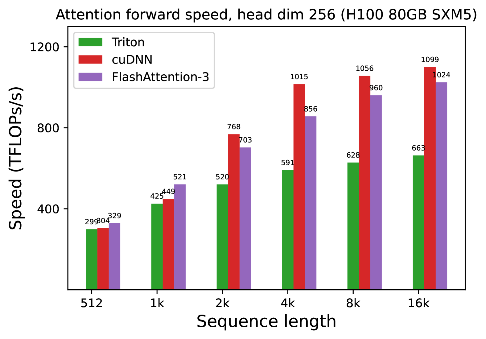
We also measure the runtime for FP8 for the forward pass under similar settings. We report the results for headdim 256 in Fig. 7 and give the full results in § C.2.
<details>
<summary>x9.png Details</summary>

### Visual Description
# Technical Document Extraction: Attention Forward Speed Benchmark
## 1. Metadata and Header Information
* **Title:** Attention forward speed, head dim 256 (H100 80GB SXM5)
* **Hardware Context:** NVIDIA H100 80GB SXM5 GPU.
* **Metric:** Speed measured in TFLOPS/s (Tera Floating Point Operations Per Second).
* **Primary Variable:** Sequence length (x-axis).
## 2. Component Isolation
### A. Legend
The legend identifies three distinct software implementations:
* **Green Bar:** Triton
* **Red Bar:** cuDNN
* **Purple Bar:** FlashAttention-3
### B. Axis Definitions
* **Y-Axis (Vertical):** Speed (TFLOPS/s). Scale ranges from 400 to 1200 with major tick marks at 400, 800, and 1200.
* **X-Axis (Horizontal):** Sequence length. Categories are: 512, 1k, 2k, 4k, 8k, 16k.
## 3. Data Extraction and Trend Analysis
### Trend Verification
* **Triton (Green):** Shows a consistent upward slope as sequence length increases, beginning to plateau between 8k and 16k.
* **cuDNN (Red):** Shows a strong upward slope, peaking at 8k and maintaining high performance at 16k. It is the fastest implementation for sequence lengths between 512 and 4k.
* **FlashAttention-3 (Purple):** Shows the steepest growth curve. While it starts as the slowest at 512, it overtakes Triton at 2k and overtakes cuDNN at 8k, becoming the fastest implementation for the longest sequence lengths (8k-16k).
### Data Table (Reconstructed)
| Sequence Length | Triton (Green) | cuDNN (Red) | FlashAttention-3 (Purple) |
| :--- | :--- | :--- | :--- |
| **512** | 529 | 686 | 510 |
| **1k** | 664 | 878 | 744 |
| **2k** | 766 | 1001 | 931 |
| **4k** | 854 | 1087 | 966 |
| **8k** | 897 | 1122 | 1151 |
| **16k** | 903 | 1139 | 1171 |
## 4. Key Findings and Observations
* **Peak Performance:** The highest recorded value is **1171 TFLOPS/s**, achieved by **FlashAttention-3** at a sequence length of 16k.
* **Crossover Point:** FlashAttention-3 demonstrates superior scaling. It surpasses cuDNN's performance once the sequence length reaches 8k.
* **Efficiency:** All three methods show significant performance gains as sequence length increases from 512 to 4k, likely due to better hardware utilization on the H100 GPU at larger scales.
* **Relative Performance:** At the smallest sequence length (512), cuDNN is ~34% faster than FlashAttention-3. At the largest sequence length (16k), FlashAttention-3 is ~2.8% faster than cuDNN and ~29.6% faster than Triton.
</details>
(a) Forward, without causal mask, head dim 256
<details>
<summary>x10.png Details</summary>
### Visual Description
# Technical Document Extraction: Attention Forward Speed Benchmark
## 1. Document Header
* **Title:** Attention forward speed, head dim 256 (H100 80GB SXM5)
* **Hardware Context:** NVIDIA H100 80GB SXM5 GPU.
* **Operation:** Attention forward pass with a head dimension of 256.
## 2. Chart Metadata and Structure
* **Chart Type:** Grouped Bar Chart.
* **X-Axis Label:** Sequence length
* **X-Axis Categories:** 512, 1k, 2k, 4k, 8k, 16k.
* **Y-Axis Label:** Speed (TFLOPS/s)
* **Y-Axis Scale:** Linear, ranging from 0 to 1200 with major ticks at 400, 800, and 1200.
* **Legend Categories:**
* **Triton:** Green bar
* **cuDNN:** Red bar
* **FlashAttention-3:** Purple bar
## 3. Data Extraction and Trend Analysis
### Trend Verification
* **Triton (Green):** Shows a consistent upward slope as sequence length increases, starting at ~300 TFLOPS/s and reaching ~660 TFLOPS/s. It is consistently the lowest performing of the three across all sequence lengths.
* **cuDNN (Red):** Shows a steep upward slope, particularly between 1k and 4k. It becomes the dominant performer starting at the 2k sequence length and maintains the highest TFLOPS/s through 16k.
* **FlashAttention-3 (Purple):** Shows a strong upward slope. It is the fastest at the smallest sequence length (512) and the second fastest from 2k to 16k.
### Data Table (Reconstructed)
| Sequence Length | Triton (Green) | cuDNN (Red) | FlashAttention-3 (Purple) |
| :--- | :--- | :--- | :--- |
| **512** | 299 | 304 | 329 |
| **1k** | 425 | 449 | 521 |
| **2k** | 520 | 768 | 703 |
| **4k** | 591 | 1015 | 856 |
| **8k** | 628 | 1056 | 960 |
| **16k** | 663 | 1099 | 1024 |
## 4. Component Analysis
* **Header Region:** Contains the descriptive title specifying the operation, head dimension, and specific GPU hardware.
* **Main Chart Region:** Contains the grouped bars. Each group corresponds to a sequence length. Data labels are placed directly above each bar for precision.
* **Legend Region:** Clearly distinguishes the three software implementations (Triton, cuDNN, FlashAttention-3) using color coding.
* **Footer/Axis Region:** Defines the independent variable (Sequence length) and the dependent variable (Speed in TFLOPS/s).
## 5. Summary of Findings
The benchmark indicates that for an H100 GPU with a head dimension of 256:
1. **FlashAttention-3** is the most efficient for very short sequences (512 to 1k).
2. **cuDNN** scales most effectively for medium to long sequences (2k to 16k), peaking at **1099 TFLOPS/s**.
3. **Triton** provides the lowest throughput of the three tested methods across the entire range of sequence lengths.
4. All methods show improved TFLOPS/s utilization as the sequence length increases, suggesting better hardware saturation at higher scales.
</details>
(b) Forward, with causal mask, head dim 256
Figure 7: Attention forward speed (FP8) on H100 GPU
4.2 Ablation Study: 2-Stage Pipelining Experiments
We ablate both the 2-stage WGMMA-softmax pipelining and warp-specialization for non-causal FP16 FlashAttention-3 with fixed parameters $\{\text{batch},\text{seqlen},\text{nheads},\text{hdim}\}=\{4,8448,16,128\}$ . The result in Table 2 confirms that our algorithmic improvements (asynchrony with warp-specialization and overlapping between GEMM and softmax) lead to significant speedup, from 570 to 661 TFLOPs.
Table 2: Pipelining ablation measurements
| FlashAttention-3 | 3.538 ms | 661 |
| --- | --- | --- |
| No GEMM-Softmax Pipelining, Warp-Specialization | 4.021 ms | 582 |
| GEMM-Softmax Pipelining, No Warp-Specialization | 4.105 ms | 570 |
4.3 Numerical Error Validation
As there has been interest in the numerical error [21] of FlashAttention, we compare FlashAttention-2, FlashAttention-3, and a standard implementation of attention against a reference implementation in FP64. To simulate outlier features and activations in LLMs [20, 54], we generate the entries of $\mathbf{Q},\mathbf{K},\mathbf{V}$ with the following distribution:
$$
\mathcal{N}(0,1)+\mathcal{N}(0,100)\cdot\mathrm{Bernoulli}(0.001).
$$
That is, each entry is normally distributed with zero mean and standard deviation 1, but for 0.1% of entries we add an independent term that’s normally distributed with standard deviation 10. We then measure the root mean squared error (RMSE) in Table 3. In FP16, both FlashAttention-2 and FlashAttention-3 achieves 1.7 $×$ lower RMSE compared to the standard implementation since intermediate results (softmax) are kept in FP32. The baseline attention in FP8 uses per-tensor scaling, with matmul accumulator in FP32 and intermediate softmax results kept in FP16. Thanks to block quantization and incoherent processing, FlashAttention-3 in FP8 is 2.6 $×$ more accurate than this baseline.
Table 3: Numerical error comparisons in FP16 and FP8 (e4m3).
| RMSE | 3.2e-4 | 1.9e-4 | 1.9e-4 |
| --- | --- | --- | --- |
| RMSE | 2.4e-2 | 9.1e-3 | 9.3e-3 | 2.4e-2 |
| --- | --- | --- | --- | --- |
5 Dicussion, Limitations, Conclusion
With FlashAttention-3, we have demonstrated that new programming techniques and hardware features such as asynchrony and low-precision can have a dramatic impact on the efficiency and accuracy of attention. We are able to speed up attention by 1.5-2.0 $×$ times compared to FlashAttention-2, and reduce FP8 numerical error by 2.6 $×$ compared to standard per-tensor quantization. Some limitations of our work that we hope to address in the future include: optimizing for LLM inference, integrating a persistent kernel design into the FP8 kernel, For our benchmarks, FP16 FlashAttention-3 has a persistent kernel and load balancing strategy, while FP8 FlashAttention-3 does not. This partly explains why FP8 FlashAttention-3 does not perform as well for small sequence length and causal masking compared to the FP8 cuDNN kernels. and understanding the effects of low-precision attention in large-scale training. Though we have focused on Hopper GPUs in this work, we expect that the techniques developed here will apply to other hardware accelerators. We hope that a faster and more accurate primitive such as attention will unlock new applications in long-context tasks.
Acknowledgments
We are grateful to the NVIDIA CUTLASS team (especially Haicheng Wu, Aniket Shivam, and Cris Cecka) for helping us understand Hopper’s programming model and for their library, which provides clean and powerful building blocks for the implementation of FlashAttention-3. We thank the cuDNN team for the idea of in-kernel transpose for FP8. The idea of overlapping GEMMs and softmax was inspired by insightful conversations with Christopher Ré, Benjamin Spector, Aniket Shivam, and Markus Hoehnerbach. The pingpong scheduling is adapted from the warp-specialized pingpong GEMM implementation in CUTLASS. We appreciate Driss Guessous for integrating FlashAttention to PyTorch. FlashAttention-3 has benefited from helpful discussions with Horace He on different attention variants, with Hao Liu and Phil Wang on distributed attention, and with Daniel Haziza and Chris De Sa on quantization. We thank Meta, Together AI, and Princeton Language and Intelligence (PLI) for compute support.
References
- Abdelfattah et al. [2016] Ahmad Abdelfattah, Azzam Haidar, Stanimire Tomov, and Jack Dongarra. Performance, design, and autotuning of batched gemm for gpus. pages 21–38, 06 2016. ISBN 978-3-319-41320-4. doi: 10.1007/978-3-319-41321-1_2.
- AI21 [2024] AI21. Introducing jamba: Ai21’s groundbreaking ssm-transformer model. AI21 blog, 2024.
- Ainslie et al. [2023] Joshua Ainslie, James Lee-Thorp, Michiel de Jong, Yury Zemlyanskiy, Federico Lebrón, and Sumit Sanghai. Gqa: Training generalized multi-query transformer models from multi-head checkpoints. arXiv preprint arXiv:2305.13245, 2023.
- Bauer et al. [2011] Michael Bauer, Henry Cook, and Brucek Khailany. CudaDMA: Optimizing GPU Memory Bandwidth via Warp Specialization. In Proceedings of 2011 International Conference for High Performance Computing, Networking, Storage and Analysis, SC ’11, New York, NY, USA, 2011. Association for Computing Machinery. ISBN 9781450307710. doi: 10.1145/2063384.2063400. URL https://doi.org/10.1145/2063384.2063400.
- Beck et al. [2024] Maximilian Beck, Korbinian Pöppel, Markus Spanring, Andreas Auer, Oleksandra Prudnikova, Michael Kopp, Günter Klambauer, Johannes Brandstetter, and Sepp Hochreiter. xlstm: Extended long short-term memory. arXiv preprint arXiv:2405.04517, 2024.
- Beltagy et al. [2020] Iz Beltagy, Matthew E Peters, and Arman Cohan. Longformer: The long-document transformer. arXiv preprint arXiv:2004.05150, 2020.
- Bikshandi and Shah [2024] Ganesh Bikshandi and Jay Shah. Delivering 1 PFLOP/s of Performance with FP8 FlashAttention-2, 2024. URL https://research.colfax-intl.com/adding-fp8-to-flashattention/.
- Brandon et al. [2023] William Brandon, Aniruddha Nrusimha, Kevin Qian, Zachary Ankner, Tian Jin, Zhiye Song, and Jonathan Ragan-Kelley. Striped attention: Faster ring attention for causal transformers. arXiv preprint arXiv:2311.09431, 2023.
- Chee et al. [2024] Jerry Chee, Yaohui Cai, Volodymyr Kuleshov, and Christopher M De Sa. Quip: 2-bit quantization of large language models with guarantees. Advances in Neural Information Processing Systems, 36, 2024.
- Chen et al. [2021] Beidi Chen, Tri Dao, Eric Winsor, Zhao Song, Atri Rudra, and Christopher Ré. Scatterbrain: Unifying sparse and low-rank attention. In Advances in Neural Information Processing Systems (NeurIPS), 2021.
- Chen et al. [2022] Richard J Chen, Chengkuan Chen, Yicong Li, Tiffany Y Chen, Andrew D Trister, Rahul G Krishnan, and Faisal Mahmood. Scaling vision transformers to gigapixel images via hierarchical self-supervised learning. In Proceedings of the IEEE/CVF Conference on Computer Vision and Pattern Recognition, pages 16144–16155, 2022.
- Child et al. [2019] Rewon Child, Scott Gray, Alec Radford, and Ilya Sutskever. Generating long sequences with sparse transformers. arXiv preprint arXiv:1904.10509, 2019.
- Choromanski et al. [2021] Krzysztof Choromanski, Valerii Likhosherstov, David Dohan, Xingyou Song, Andreea Gane, Tamas Sarlos, Peter Hawkins, Jared Davis, Afroz Mohiuddin, Lukasz Kaiser, et al. Rethinking attention with performers. In The International Conference on Learning Representations (ICLR), 2021.
- Choromanski et al. [2020] Krzysztof Marcin Choromanski, Valerii Likhosherstov, David Dohan, Xingyou Song, Andreea Gane, Tamas Sarlos, Peter Hawkins, Jared Quincy Davis, Afroz Mohiuddin, Lukasz Kaiser, et al. Rethinking attention with performers. In International Conference on Learning Representations (ICLR), 2020.
- Dao [2023] Tri Dao. FlashAttention-2: Faster Attention with Better Parallelism and Work Partitioning, 2023. URL https://arxiv.org/abs/2307.08691.
- Dao and Gu [2024] Tri Dao and Albert Gu. Transformers are SSMs: Generalized models and efficient algorithms with structured state space duality. In International Conference on Machine Learning (ICML), 2024.
- Dao et al. [2022] Tri Dao, Daniel Y. Fu, Stefano Ermon, Atri Rudra, and Christopher Ré. FlashAttention: Fast and memory-efficient exact attention with IO-awareness. In Advances in Neural Information Processing Systems, 2022.
- Dao et al. [2023] Tri Dao, Daniel Y Fu, Khaled K Saab, Armin W Thomas, Atri Rudra, and Christopher Ré. Hungry hungry hippos: Towards language modeling with state space models. In The International Conference on Learning Representations (ICLR), 2023.
- DeepSeek-AI [2024] DeepSeek-AI. Deepseek-v2: A strong, economical, and efficient mixture-of-experts language model. arXiv preprint arXiv:2405.04434, 2024.
- Dettmers et al. [2022] Tim Dettmers, Mike Lewis, Younes Belkada, and Luke Zettlemoyer. Llm. int8 (): 8-bit matrix multiplication for transformers at scale. CoRR abs/2208.07339, 2022.
- Golden et al. [2024] Alicia Golden, Samuel Hsia, Fei Sun, Bilge Acun, Basil Hosmer, Yejin Lee, Zachary DeVito, Jeff Johnson, Gu-Yeon Wei, David Brooks, et al. Is flash attention stable? arXiv preprint arXiv:2405.02803, 2024.
- Gu and Dao [2023] Albert Gu and Tri Dao. Mamba: Linear-time sequence modeling with selective state spaces. 2023.
- Gulati et al. [2020] Anmol Gulati, James Qin, Chung-Cheng Chiu, Niki Parmar, Yu Zhang, Jiahui Yu, Wei Han, Shibo Wang, Zhengdong Zhang, Yonghui Wu, et al. Conformer: Convolution-augmented transformer for speech recognition. arXiv preprint arXiv:2005.08100, 2020.
- Guo et al. [2021] Mandy Guo, Joshua Ainslie, David Uthus, Santiago Ontanon, Jianmo Ni, Yun-Hsuan Sung, and Yinfei Yang. Longt5: Efficient text-to-text transformer for long sequences. arXiv preprint arXiv:2112.07916, 2021.
- Ho et al. [2022] Jonathan Ho, Tim Salimans, Alexey Gritsenko, William Chan, Mohammad Norouzi, and David J Fleet. Video diffusion models. Advances in Neural Information Processing Systems, 35:8633–8646, 2022.
- Hooper et al. [2024] Coleman Hooper, Sehoon Kim, Hiva Mohammadzadeh, Michael W Mahoney, Yakun Sophia Shao, Kurt Keutzer, and Amir Gholami. Kvquant: Towards 10 million context length llm inference with kv cache quantization. arXiv preprint arXiv:2401.18079, 2024.
- Katharopoulos et al. [2020] Angelos Katharopoulos, Apoorv Vyas, Nikolaos Pappas, and François Fleuret. Transformers are RNNs: Fast autoregressive transformers with linear attention. In International Conference on Machine Learning, pages 5156–5165. PMLR, 2020.
- Kitaev et al. [2020] Nikita Kitaev, Łukasz Kaiser, and Anselm Levskaya. Reformer: The efficient transformer. In The International Conference on Machine Learning (ICML), 2020.
- Kwon et al. [2023] Woosuk Kwon, Zhuohan Li, Siyuan Zhuang, Ying Sheng, Lianmin Zheng, Cody Hao Yu, Joseph Gonzalez, Hao Zhang, and Ion Stoica. Efficient memory management for large language model serving with pagedattention. In Proceedings of the 29th Symposium on Operating Systems Principles, pages 611–626, 2023.
- Li et al. [2023] Raymond Li, Loubna Ben Allal, Yangtian Zi, Niklas Muennighoff, Denis Kocetkov, Chenghao Mou, Marc Marone, Christopher Akiki, Jia Li, Jenny Chim, et al. Starcoder: may the source be with you! arXiv preprint arXiv:2305.06161, 2023.
- Liu et al. [2023] Hao Liu, Matei Zaharia, and Pieter Abbeel. Ring attention with blockwise transformers for near-infinite context. arXiv preprint arXiv:2310.01889, 2023.
- Liu et al. [2024a] Hao Liu, Wilson Yan, Matei Zaharia, and Pieter Abbeel. World model on million-length video and language with ringattention. arXiv preprint arXiv:2402.08268, 2024a.
- Liu et al. [2024b] Zirui Liu, Jiayi Yuan, Hongye Jin, Shaochen Zhong, Zhaozhuo Xu, Vladimir Braverman, Beidi Chen, and Xia Hu. Kivi: A tuning-free asymmetric 2bit quantization for kv cache. arXiv preprint arXiv:2402.02750, 2024b.
- Luo et al. [2024] Weile Luo, Ruibo Fan, Zeyu Li, Dayou Du, Qiang Wang, and Xiaowen Chu. Benchmarking and Dissecting the Nvidia Hopper GPU Architecture, 2024. URL https://arxiv.org/abs/2402.13499.
- Ma et al. [2023] Xuezhe Ma, Chunting Zhou, Xiang Kong, Junxian He, Liangke Gui, Graham Neubig, Jonathan May, and Luke Zettlemoyer. Mega: Moving average equipped gated attention. In The International Conference on Learning Representations (ICLR), 2023.
- Ma et al. [2024] Xuezhe Ma, Xiaomeng Yang, Wenhan Xiong, Beidi Chen, Lili Yu, Hao Zhang, Jonathan May, Luke Zettlemoyer, Omer Levy, and Chunting Zhou. Megalodon: Efficient llm pretraining and inference with unlimited context length. arXiv preprint arXiv:2404.08801, 2024.
- Micikevicius et al. [2022] Paulius Micikevicius, Dusan Stosic, Neil Burgess, Marius Cornea, Pradeep Dubey, Richard Grisenthwaite, Sangwon Ha, Alexander Heinecke, Patrick Judd, John Kamalu, et al. Fp8 formats for deep learning. arXiv preprint arXiv:2209.05433, 2022.
- NVIDIA [2024] NVIDIA. CUDA Programming Guide Version 12.4, 2024. URL https://docs.nvidia.com/cuda/cuda-c-programming-guide/index.html.
- Nvidia [2024] Nvidia. Accelerating transformers with nvidia cudnn 9. Nvidia blog, 2024. URL https://developer.nvidia.com/blog/accelerating-transformers-with-nvidia-cudnn-9/.
- NVIDIA [2024] NVIDIA. Parallel Thread Execution ISA Version 8.4, 2024. URL https://docs.nvidia.com/cuda/pdf/ptx_isa_8.4.pdf.
- Osama et al. [2023] Muhammad Osama, Duane Merrill, Cris Cecka, Michael Garland, and John D. Owens. Stream-k: Work-centric parallel decomposition for dense matrix-matrix multiplication on the gpu. In Proceedings of the 28th ACM SIGPLAN Annual Symposium on Principles and Practice of Parallel Programming, PPoPP ’23, pages 429–431, New York, NY, USA, 2023. Association for Computing Machinery. ISBN 9798400700156. doi: 10.1145/3572848.3577479. URL https://doi.org/10.1145/3572848.3577479.
- Peng et al. [2023a] Bo Peng, Eric Alcaide, Quentin Anthony, Alon Albalak, Samuel Arcadinho, Huanqi Cao, Xin Cheng, Michael Chung, Matteo Grella, Kranthi Kiran GV, et al. RWKV: Reinventing RNNs for the Transformer era. arXiv preprint arXiv:2305.13048, 2023a.
- Peng et al. [2023b] Bowen Peng, Jeffrey Quesnelle, Honglu Fan, and Enrico Shippole. Yarn: Efficient context window extension of large language models. arXiv preprint arXiv:2309.00071, 2023b.
- Peng et al. [2021] Hao Peng, Nikolaos Pappas, Dani Yogatama, Roy Schwartz, Noah A Smith, and Lingpeng Kong. Random feature attention. In The International Conference on Learning Representations (ICLR), 2021.
- Rabe and Staats [2021] Markus N Rabe and Charles Staats. Self-attention does not need ${O}(n^{2})$ memory. arXiv preprint arXiv:2112.05682, 2021.
- Research [2024] Colfax Research. Tutorial: Matrix Transpose in CUTLASS, 2024. URL https://research.colfax-intl.com/tutorial-matrix-transpose-in-cutlass/.
- Roy et al. [2020] Aurko Roy, Mohammad Saffar, Ashish Vaswani, and David Grangier. Efficient content-based sparse attention with routing Transformers. arXiv preprint arXiv:2003.05997, 2020.
- Roziere et al. [2023] Baptiste Roziere, Jonas Gehring, Fabian Gloeckle, Sten Sootla, Itai Gat, Xiaoqing Ellen Tan, Yossi Adi, Jingyu Liu, Tal Remez, Jérémy Rapin, et al. Code llama: Open foundation models for code. arXiv preprint arXiv:2308.12950, 2023.
- Sanovar et al. [2024] Rya Sanovar, Srikant Bharadwaj, Renee St. Amant, Victor Rühle, and Saravan Rajmohan. Lean attention: Hardware-aware scalable attention mechanism for the decode-phase of transformers. 2024.
- Shaham et al. [2022] Uri Shaham, Elad Segal, Maor Ivgi, Avia Efrat, Ori Yoran, Adi Haviv, Ankit Gupta, Wenhan Xiong, Mor Geva, Jonathan Berant, et al. Scrolls: Standardized comparison over long language sequences. arXiv preprint arXiv:2201.03533, 2022.
- Shazeer [2019] Noam Shazeer. Fast transformer decoding: One write-head is all you need. arXiv preprint arXiv:1911.02150, 2019.
- Spector et al. [2024] Benjamin Spector, Aaryan Singhal, Simran Arora, and Christopher Ré, 2024. URL https://github.com/HazyResearch/ThunderKittens.
- Sun et al. [2019] Fei Sun, Jun Liu, Jian Wu, Changhua Pei, Xiao Lin, Wenwu Ou, and Peng Jiang. Bert4rec: Sequential recommendation with bidirectional encoder representations from transformer. In Proceedings of the 28th ACM international conference on information and knowledge management, pages 1441–1450, 2019.
- Sun et al. [2024] Mingjie Sun, Xinlei Chen, J Zico Kolter, and Zhuang Liu. Massive activations in large language models. arXiv preprint arXiv:2402.17762, 2024.
- Sun et al. [2023] Yutao Sun, Li Dong, Shaohan Huang, Shuming Ma, Yuqing Xia, Jilong Xue, Jianyong Wang, and Furu Wei. Retentive network: A successor to transformer for large language models. arXiv preprint arXiv:2307.08621, 2023.
- Tay et al. [2020] Yi Tay, Mostafa Dehghani, Dara Bahri, and Donald Metzler. Efficient transformers: A survey. arXiv preprint arXiv:2009.06732, 2020.
- Thakkar et al. [2023] Vijay Thakkar, Pradeep Ramani, Cris Cecka, Aniket Shivam, Honghao Lu, Ethan Yan, Jack Kosaian, Mark Hoemmen, Haicheng Wu, Andrew Kerr, Matt Nicely, Duane Merrill, Dustyn Blasig, Fengqi Qiao, Piotr Majcher, Paul Springer, Markus Hohnerbach, Jin Wang, and Manish Gupta. CUTLASS, January 2023. URL https://github.com/NVIDIA/cutlass.
- Tseng et al. [2024] Albert Tseng, Jerry Chee, Qingyao Sun, Volodymyr Kuleshov, and Christopher De Sa. Quip#: Even better llm quantization with hadamard incoherence and lattice codebooks. arXiv preprint arXiv:2402.04396, 2024.
- Vaswani et al. [2017] Ashish Vaswani, Noam Shazeer, Niki Parmar, Jakob Uszkoreit, Llion Jones, Aidan N Gomez, Łukasz Kaiser, and Illia Polosukhin. Attention is all you need. Advances in neural information processing systems, 30, 2017.
- Waleffe et al. [2024] Roger Waleffe, Wonmin Byeon, Duncan Riach, Brandon Norick, Vijay Korthikanti, Tri Dao, Albert Gu, Ali Hatamizadeh, Sudhakar Singh, Deepak Narayanan, et al. An empirical study of mamba-based language models. arXiv preprint arXiv:2406.07887, 2024.
- Xiong et al. [2021] Yunyang Xiong, Zhanpeng Zeng, Rudrasis Chakraborty, Mingxing Tan, Glenn Fung, Yin Li, and Vikas Singh. Nyströmformer: A nystöm-based algorithm for approximating self-attention. In Proceedings of the AAAI Conference on Artificial Intelligence. AAAI Conference on Artificial Intelligence, volume 35, page 14138, 2021.
- Yao et al. [2022] Shunyu Yao, Jeffrey Zhao, Dian Yu, Nan Du, Izhak Shafran, Karthik Narasimhan, and Yuan Cao. React: Synergizing reasoning and acting in language models. arXiv preprint arXiv:2210.03629, 2022.
- Zaheer et al. [2020] Manzil Zaheer, Guru Guruganesh, Kumar Avinava Dubey, Joshua Ainslie, Chris Alberti, Santiago Ontanon, Philip Pham, Anirudh Ravula, Qifan Wang, Li Yang, et al. Big bird: Transformers for longer sequences. Advances in Neural Information Processing Systems, 33, 2020.
- Zyphra [2024] Zyphra. Zyphra unveils zamba: A compact 7b ssm hybrid model. Zyphra blog, 2024.
Appendix A Related Work
Attention variants and distributed attention
Ever since attention became popular with the Transformer architecture [59], there has been a large body of work on approximating attention to scale it to longer sequences. These approximation methods can generally be categorized into two classes: sparse and low-rank. Sparse attention only computes some entries of the attention matrix ( $\mathrm{softmax}(\mathbf{Q}\mathbf{K}^{T})$ ) and assumes that other entries are zero. Different methods have different ways of choosing which entries should be zero, either with a fixed pattern [12], with a sliding window [6], or with a dynamic pattern through hashing [28] or routing [47]. The low-rank approach instead assumes that the attention matrix has a low-rank structure, and apply a pointwise nonlinearity to the query and key [27] with random projection [13, 44, 61]. One can also combine the sparse and low-rank approximation for better quality [63, 10]. However, these approximation methods typically do not offer the same model quality as standard attention [56], and so most large-scale models do not employ these techniques.
There are other variants of attention aimed at reducing the size of the KV cache to improve inference efficiency. Multi-query attention [51] and grouped query attention [3] tie different heads of $\mathbf{K}$ and $\mathbf{V}$ , and multiple query heads interact with the same key and value head. Multi-head latent attention [19] parameterizes the $\mathbf{K}$ and $\mathbf{V}$ as low-rank projections of a shared matrix to further reduce the KV cache size. However, all of these approaches do not change the core computation $\mathrm{softmax}(\mathbf{Q}\mathbf{K}^{T})\mathbf{V}$ during training and simply change how $\mathbf{Q},\mathbf{K},\mathbf{V}$ are obtained. As a result, any efficiency or accuracy improvement to the standard attention computation benefits these methods.
To extend to even longer context, attention computation can be distributed across multiple GPUs. Methods such as Ring attention [31, 32] and variants [8] can reach a context length of up to 1 million. They use FlashAttention (or FlashAttention-2) as a primitive, and so the improvement from FlashAttention-3 would benefit these distributed attention methods as well.
Alternative architectures
Motivated by the limitations of attention, a variety of alternative architectures have been proposed. They build on the connection between linear attention [27] and recurrent neural networks (RNNs). RWKV [42], H3 [18], MEGA [35], Retnet [55] enhance the expressivity of the simple cumulative sum in linear attention with more sophisticated recurrences. Mamba [22] and xLSTM [5] use learnable weighting for the recurrence and can match the quality of Transformers in language modeling at small or medium scale. These approaches can be connected to generalizations of linear attention through the lens of the structure of the token-mixing matrix [16]. These models have started to see some traction, seeing usage in some medium to large-scale models such as Jamba [2], Zamba [64], Megalodon [36], and Mamba2-hybrid [60]. For the highest quality, these SSM- and RNN-based models still employ many layers of attention. We expect that techniques to speed up attention presented in this work will be useful to speedup these alternative architectures.
Low-precision attention
Quantization is a promising approach to speed up attention, but they have mostly focused on reducing the space for KV cache for inference efficiency. QuIP [9] and QuIP# [58] use incoherent processing to reduce the quantization, and we adapted this technique for FP8 FlashAttention-3. Recent work suggests that for inference the KV cache is highly compressible down to 4-, 3-, or even 2-bits [26, 33]. However, quantization during training is still challenging as higher precision is typically required for stable training.
Hardware-aware Algorithms
Our work presented in this paper focuses on the micro-architecture specific tuning to leverage new instruction sets and adopt a natively asynchronous programming model. There are other orthogonal axes for hardware-aware algorithm co-design being explored. A recent example of this is LeanAttention [49], which recognizes the poor GPU occupancy and high memory bandwidth requirements of the sequential token generation phase as primary bottlenecks for inference and optimizes it via a smarter load balancing strategy similar to Stream-K load balancing [41] to achieve nearly peak occupancy. There is a large literature on optimizing GEMM for specific hardware that employs many of the same techniques. As an example, Abdelfattah et al. [1] presents a high performance batched GEMM kernel on K40c Graphics Processing Units (GPU) for both fixed and variable sizes, proposing specialized GEMM designs and a comprehensive autotuning process to deliver state-of-the-art performance.
Appendix B Addition Details on Algorithms
B.1 Asynchrony Through Warp Specialization for the Backward Pass
Similar to the forward pass § 3.1, we use warp specialization to handle asynchrony. Instead of just a simple producer-consumer pattern in the forward pass, we add one extra role of a $\mathbf{dQ}$ writer, since we need to accumulate the value of $\mathbf{dQ}$ produced by each thread block to the global value of $\mathbf{dQ}$ . This $\mathbf{dQ}$ accumulation introduces memory contention (many thread blocks writing to the same location) so having a separate warp to handle this (along with asynchrony) will avoid blocking the rest of the warps in the thread block to perform the next computation (matmul).
We include the backward pass with warp specialization in Algorithm 3.
Algorithm 3 FlashAttention-3 backward pass with warp specialization
0: Matrices $\mathbf{Q},\mathbf{K},\mathbf{V},\mathbf{O},\mathbf{dO}∈\mathbb{R}^{N× d}$ in HBM, logsumexp vector $L∈\mathbb{R}^{N}$ in HBM, block sizes $B_{c}$ , $B_{r}$ .
1: In a preprocessing kernel, compute $D=\mathrm{rowsum}(\mathbf{dO}\circ\mathbf{O})∈\mathbb{R}^{d}$ (pointwise multiply), write $D$ to HBM and divide it into $T_{r}$ blocks $D_{1},...,D_{T_{r}}$ of size $B_{r}$ each.
2: Divide $\mathbf{Q}$ into $T_{r}=\left\lceil\frac{N}{B_{r}}\right\rceil$ blocks $\mathbf{Q}_{1},...,\mathbf{Q}_{T_{r}}$ of size $B_{r}× d$ each, and divide $\mathbf{K},\mathbf{V}$ in to $T_{c}=\left\lceil\frac{N}{B_{c}}\right\rceil$ blocks $\mathbf{K}_{1},...,\mathbf{K}_{T_{c}}$ and $\mathbf{V}_{1},...,\mathbf{V}_{T_{c}}$ , of size $B_{c}× d$ each.
3: Divide $\mathbf{dO}$ into $T_{r}$ blocks $\mathbf{dO}_{i},...,\mathbf{dO}_{T_{r}}$ of size $B_{r}× d$ each, and divide $L$ into $T_{r}$ blocks $L_{i},...,L_{T_{r}}$ of size $B_{r}$ each.
4: Initialize pipeline object to manage barrier synchronization with $s$ -stage circular SMEM buffer.
5: if in producer warpgroup then
6: Deallocate predetermined number of registers.
7: Issue load $\mathbf{K}_{j}$ and $\mathbf{V}_{j}$ from HBM to shared memory.
8: Upon completion, commit to notify consumer of the load of $\mathbf{K}_{j}$ and $\mathbf{V}_{j}$ .
9: for $1≤ i≤ T_{r}$ do
10: Wait for the $(i\,\%\,s)$ th stage of the buffer to be consumed.
11: Issue loads of $\mathbf{Q}_{i},\mathbf{dO}_{i}$ from HBM to shared memory at the $(i\,\%\,s)$ th stage of the buffer.
12: Upon completion, commit to notify consumers of the loads of $\mathbf{Q}_{i},\mathbf{dO}_{i}$ .
13: end for
14: else if in consumer warpgroups then
15: Reallocate predetermined number of registers as function of number of consumer warps.
16: On-chip, Initialize $\mathbf{dK}_{j}=(0)_{B_{c}× d},\mathbf{dV}_{j}=(0)_{B_{c}× d}$ .
17: Wait for $\mathbf{K}_{j}$ and $\mathbf{V}_{j}$ to be loaded in shared memory.
18: for $1≤ i≤ T_{r}$ do
19: Wait for $\mathbf{Q}_{i}$ to be loaded in shared memory.
20: Load $L_{i},D_{i}$ from HBM to on-chip SRAM.
21: On chip, compute $\mathbf{S}_{i}^{(j)}=\mathbf{Q}_{i}\mathbf{K}_{j}^{T}∈\mathbb{R}^{B_{r}%
× B_{c}}$ (SS-GEMM). Commit.
22: Wait for $\mathbf{dO}_{i}$ to be loaded in shared memory.
23: On chip, compute $\mathbf{dP}_{i}^{(j)}=\mathbf{dO}_{i}\mathbf{V}_{j}^{→p}∈\mathbb{R}^{B_{r}%
× B_{c}}$ (SS-GEMM). Commit.
24: On chip, wait for $\mathbf{S}_{i}^{(j)}$ , then compute $\mathbf{P}_{i}^{(j)}=\mathrm{exp}(\mathbf{S}_{ij}-L_{i})∈\mathbb{R}^{B_{r}%
× B_{c}}$ .
25: On chip, wait for $\mathbf{dP}_{i}^{(j)}$ , then compute $\mathbf{dS}_{i}^{(j)}=\mathbf{P}_{i}^{(j)}\circ(\mathbf{dP}_{i}^{(j)}-D_{i})%
∈\mathbb{R}^{B_{r}× B_{c}}$ .
26: On chip, compute $\mathbf{dV}_{j}←\mathbf{dV}_{j}+(\mathbf{P}_{i}^{(j)})^{→p}\mathbf{%
dO}_{i}∈\mathbb{R}^{B_{c}× d}$ (RS-GEMM). Commit.
27: On chip, compute $\mathbf{dK}_{j}←\mathbf{dK}_{j}+{\mathbf{dS}_{i}^{(j)}}^{→p}\mathbf%
{Q}_{i}∈\mathbb{R}^{B_{c}× d}$ (RS-GEMM). Commit and wait for both $\mathbf{dV}_{j}$ and $\mathbf{dK}_{j}$ .
28: On chip, compute $\mathbf{dQ}_{i}^{(\mathrm{local})}=\mathbf{dS}_{i}^{(j)}\mathbf{K}_{j}∈%
\mathbb{R}^{B_{r}× d}$ (SS-GEMM), and write $\mathbf{dQ}_{i}^{(\mathrm{local})}$ to smem. Notify the $\mathbf{dQ}$ -writer.
29: end for
30: else if in $\mathbf{dQ}$ -writer warp then
31: for $1≤ i≤ T_{r}$ do
32: Wait for $\mathbf{dQ}_{i}^{(\mathrm{local})}$ to be ready in smem.
33: Using a semaphore, atomically add $\mathbf{dQ}_{i}^{(\mathrm{local})}$ to $\mathbf{dQ}_{i}$ in global memory.
34: end for
35: end if
B.2 2-Stage Pipelining SASS Analysis
We give simplified SASS code for the inside of the consumer warpgroup mainloop. // Compute row_max FMNMX.FTZ R0, R24, R6, !PT ; SHFL.BFLY PT, R185, R2, 0x2, 0x1f ; FMNMX and SHFL.BFLY // Apply exp2 and row_sum. Rescale O. FMUL.FTZ R2, R4, UR9 ; MUFU.EX2 R185, R184 ; FFMA.FTZ R24, R24, UR9, -R6.reuse ; FADD.FTZ R24, R211, R24 ; FMUL, FFMA, FMUL, MUFU.EX2, FADD // FP32 -> FP16 conversion are interleaved with exp2, row_sum and O rescaling. F2FP.F16.F32.PACK_AB R231, R25, R231 ; F2FP, FMUL, MUFU, FFMA, FADD ... // Start the first WGMMA. Broken down into 8 HGMMAs. // The first 7 HGMMAs are packed together. WARPGROUP.ARRIVE ; HGMMA.64x192x16.F32 R24, gdesc[UR44], RZ, !UPT ; ... HGMMA x 6 ... // FP32->FP16, exp2, row_sum, O rescaling are interleaved with HGMMA. F2FP.F16.F32.PACK_AB R214, R214, R187 ; MUFU.EX2 R234, R5 ; FADD.FTZ R237, R187, R2 ; F2FP, MUFU, FADD // The last HGMMA is issued here. No need to wait. HGMMA.64x192x16.F32 R24, gdesc[UR44], R24, gsb0 ; // Start the second WGMMA. Broken down into 12 HGMMAs. // All 12 HGMMAs are packed together. Not interleaved with other instructions. WARPGROUP.ARRIVE ; HGMMA.64x128x16.F32 R120, R228, gdesc[UR8].tnspB, R120 ; ... HGMMA x 10 ... HGMMA.64x128x16.F32 R120, R184, gdesc[UR8].tnspB, R120, gsb0 ; // wgmma.wait_group at the end. WARPGROUP.DEPBAR.LE gsb0, 0x0 ;
We make the following observations:
1. Softmax is reordered to the very beginning, even before the first WGMMA.
1. The first WGMMA is interleaved with softmax and FP32 $→$ FP16 datatype conversion of $\mathbf{S}$ . This indicates that WGMMA and non-WGMMAs are executed in parallel.
1. exp2, row\_sum, O rescaling and FP32 $→$ FP16 conversions are interleaved together.
1. The second WGMMA is not overlapped with other instructions, as expected.
Overall, SASS shows that the 2-stage pipelining idea works as expected.
B.3 3-Stage Pipelining Algorithm
We experiment with a 3-stage pipelining algorithm to parallelize the first WGMMA from iteration $j+2$ , softmax from iteration $j+1$ , and the second WGMMA from iteration $j$ . We describe this algorithm in Algorithm 4. This algorithm behaves worse than the 2-stage pipelining algorithm due to the reasons below:
<details>
<summary>extracted/5728672/figs/3_stage_pipelining.png Details</summary>
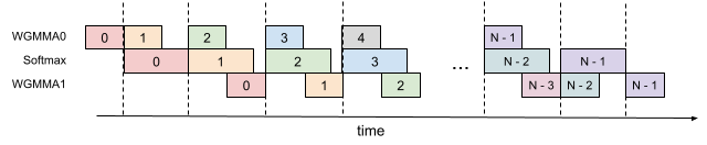
### Visual Description
# Technical Document Extraction: Pipeline Execution Diagram
## 1. Overview
This image is a technical timing diagram illustrating a pipelined execution flow across three distinct processing units or stages. It demonstrates how tasks are staggered over time to maximize hardware utilization. The diagram uses a horizontal "time" axis and vertical labels for the execution units.
## 2. Component Isolation
### Header/Labels (Left Side)
The vertical axis identifies three processing stages:
1. **WGMMA0**: Likely referring to a "Warpgroup Matrix Multiply-Accumulate" unit 0.
2. **Softmax**: A specialized stage for calculating the Softmax activation function.
3. **WGMMA1**: Likely referring to a "Warpgroup Matrix Multiply-Accumulate" unit 1.
### Main Chart Area (Center)
The chart uses colored blocks to represent discrete work units (iterations or batches). Each block contains a numerical index (0, 1, 2, 3, 4, ..., N-3, N-2, N-1).
* **Vertical Dashed Lines**: These represent synchronization points or clock cycle boundaries.
* **Horizontal Arrow**: Labeled **"time"**, indicating the progression of execution from left to right.
## 3. Data Flow and Pipelining Logic
The diagram illustrates a **three-stage pipeline**. A single task (e.g., Task 0) must pass through WGMMA0, then Softmax, then WGMMA1.
### Trend Verification
* **Staggered Start**: Each subsequent stage starts exactly one time-step after the previous stage begins.
* **Parallelism**: Once the pipeline is full (at the third time-step), all three units are working simultaneously on different data indices.
* **Dependency**: Softmax index $i$ cannot start until WGMMA0 index $i$ is complete. WGMMA1 index $i$ cannot start until Softmax index $i$ is complete.
### Execution Sequence Table
The following table reconstructs the spatial placement of the blocks relative to the time-steps (columns):
| Stage | T1 | T2 | T3 | T4 | T5 | ... | Tn-2 | Tn-1 | Tn | Tn+1 |
| :--- | :---: | :---: | :---: | :---: | :---: | :---: | :---: | :---: | :---: | :---: |
| **WGMMA0** | 0 | 1 | 2 | 3 | 4 | ... | N-1 | | | |
| **Softmax** | | 0 | 1 | 2 | 3 | ... | N-2 | N-1 | | |
| **WGMMA1** | | | 0 | 1 | 2 | ... | N-3 | N-2 | N-1 | |
## 4. Color Coding and Indexing
The blocks are color-coded to track specific data indices across the stages:
* **Index 0 (Pink/Red)**: Starts in WGMMA0 at T1, moves to Softmax at T2, moves to WGMMA1 at T3.
* **Index 1 (Orange/Tan)**: Starts in WGMMA0 at T2, moves to Softmax at T3, moves to WGMMA1 at T4.
* **Index 2 (Green)**: Starts in WGMMA0 at T3, moves to Softmax at T4, moves to WGMMA1 at T5.
* **Index 3 (Blue)**: Starts in WGMMA0 at T4, moves to Softmax at T5.
* **Index 4 (Grey)**: Starts in WGMMA0 at T5.
* **Index N-1 (Purple)**: The final index, shown completing the sequence at the end of the timeline.
## 5. Summary of Information
* **Total Stages**: 3
* **Total Tasks**: N (from 0 to N-1)
* **Concurrency**: High. After the initial ramp-up, the hardware achieves 100% utilization across these three units.
* **Latency**: Each individual task takes 3 time units to complete, but the throughput is 1 task per time unit.
</details>
Figure 8: 3-Stage Pipelining
Algorithm 4 FlashAttention 3-stage pipelining consumer warpgroup forward pass
0: Matrices $\mathbf{Q},\mathbf{K},\mathbf{V}∈\mathbb{R}^{N× d}$ in HBM, block sizes $B_{c}$ , $B_{r}$ . Each warpgroup reads 1 block Qi of size $B_{r}× d$ , $T_{c}=\left\lceil\frac{N}{B_{c}}\right\rceil$ blocks $\mathbf{K}_{1},...,\mathbf{K}_{T_{c}}$ and $\mathbf{V}_{1},...,\mathbf{V}_{T_{c}}$ of size $B_{c}× d$ . Each warpgroup writes 1 output block $\mathbf{O}_{i}$ of size $B_{r}× d$ , and 1 logsumexp block $L_{i}$ of size $B_{r}$ .
1: Initialization. Load $\mathbf{Q}_{i}$ from HBM to on-chip SRAM. Initialize $\mathbf{O}_{i},\ell_{i},m_{i},scale\_o$ .
2: Wait for the producer warpgroup loading $\mathbf{K}_{0}$ from HBM to on-chip SRAM.
3: Compute $\mathbf{S}=\mathbf{Q}_{i}\mathbf{K}_{0}^{T}$ using WGMMA. Commit and wait.
4: Compute $m_{i}$ , $\tilde{\mathbf{P}}_{i}$ , $\ell_{i}$ , $scale\_o$ based on $\mathbf{S}$ .
5: Wait for the producer warpgroup loading $\mathbf{K}_{1}$ from HBM to on-chip SRAM.
6: Compute $\mathbf{S}=\mathbf{Q}_{i}\mathbf{K}_{1}^{T}$ using WGMMA. Commit and wait.
7: for $2≤ j<T_{c}-2$ do
8: Wait for the producer warpgroup loading $\mathbf{K}_{j}$ from HBM to on-chip SRAM.
9: Compute $\mathbf{S}\_next=\mathbf{Q}_{i}\mathbf{K}_{j}^{T}$ using WGMMA. Commit but do not wait.
10: Wait for the producer warpgroup loading $\mathbf{V}_{j-2}$ from HBM to on-chip SRAM.
11: Rescale $\mathbf{O}_{i}$ based on $scale\_o$ .
12: Compute $\mathbf{O}_{i}=\mathbf{O}_{i}+\tilde{\mathbf{P}}_{i}\mathbf{V}_{j-2}$ using WGMMA. Commit but do not wait.
13: Compute $m_{i}$ , $\tilde{\mathbf{P}}_{i}\_next$ , $\ell_{i}$ , $scale\_o$ based on $\mathbf{S}$ .
14: Wait for all previous WGMMAs.
15: Copy $\mathbf{S}\_next$ to $\mathbf{S}$ .
16: Copy $\tilde{\mathbf{P}}_{i}\_next$ to $\tilde{\mathbf{P}}_{i}$ .
17: end for
18: Wait for the producer warpgroup loading $\mathbf{V}_{T_{c}-2}$ from HBM to on-chip SRAM.
19: Rescale $\mathbf{O}_{i}$ based on $scale\_o$ .
20: Compute $\mathbf{O}_{i}=\mathbf{O}_{i}+\tilde{\mathbf{P}}_{i}\mathbf{V}_{T_{c}-2}$ using WGMMA. Commit and wait.
21: Compute $m_{i}$ , $\tilde{\mathbf{P}}_{i}$ , $\ell_{i}$ , $scale\_o$ based on $\mathbf{S}$ .
22: Wait for the producer warpgroup loading $\mathbf{V}_{T_{c}-1}$ from HBM to on-chip SRAM.
23: Rescale $\mathbf{O}_{i}$ based on $scale\_o$ .
24: Compute $\mathbf{O}_{i}=\mathbf{O}_{i}+\tilde{\mathbf{P}}_{i}\mathbf{V}_{T_{c}-1}$ using WGMMA. Commit and wait.
25: Epilogue. Rescale $\mathbf{O}_{i}$ based on $\ell_{i}$ . Compute $L_{i}$ based on $\ell_{i}$ and $m_{i}$ . Write $\mathbf{O}_{i}$ and $L_{i}$ to HBM as the $i$ -th block of $\mathbf{O}$ and $L$ .
Overlapping.
We expected that softmax can be overlapped with (the first WGMMA + the second WGMMA). However, the compiler doesn’t cooperate in this way. SASS code shows that only the first WGMMA is overlapped with softmax, while the second WGMMA is not. It’s not clear why the compiler chooses to reorder instructions in this way.
Register pressure.
This algorithm requires more registers compared to the 2-stage pipelining algorithm. In theory, it needs to store an extra $\tilde{\mathbf{P}}_{i}$ and $scale\_o$ , which is of size $B_{r}× B_{c}×\text{sizeof}(\text{input\_data\_type})+B_{r}×%
\text{sizeof}(\text{float})$ . As a result, a smaller block size needs to be chosen.
Appendix C Addition Details on Experiments and Benchmarking
C.1 System and libraries
We benchmark the speed on an H100 80GB SXM5 (700W). We generally use the latest versions of the libraries, at the time of writing (May 2024). Specifically, we use:
- CUDA 12.3
- cuDNN 9.1.1.17
- CUTLASS 3.5
- FlashAttention 2.5.8
- Triton nightly 3.0.0.post20240424212437
- PyTorch 2.3.0
To reduce variability, we fix the GPU clock speed to 1830MHz (clock speed used to calculate the 989 TFLOPS FP16 theoretical max throughput). We repeat the benchmarks 100 times and take the average timing.
C.2 FP8 Attention Full Results
We use following sequence lengths: 512, 1024, 2048, 4224, 8448, 16896. When sequence length $≥$ 4k, we make it also divisible by 132 (number of SMs in H100 SXM5) to avoid wave quantization.
<details>
<summary>x11.png Details</summary>
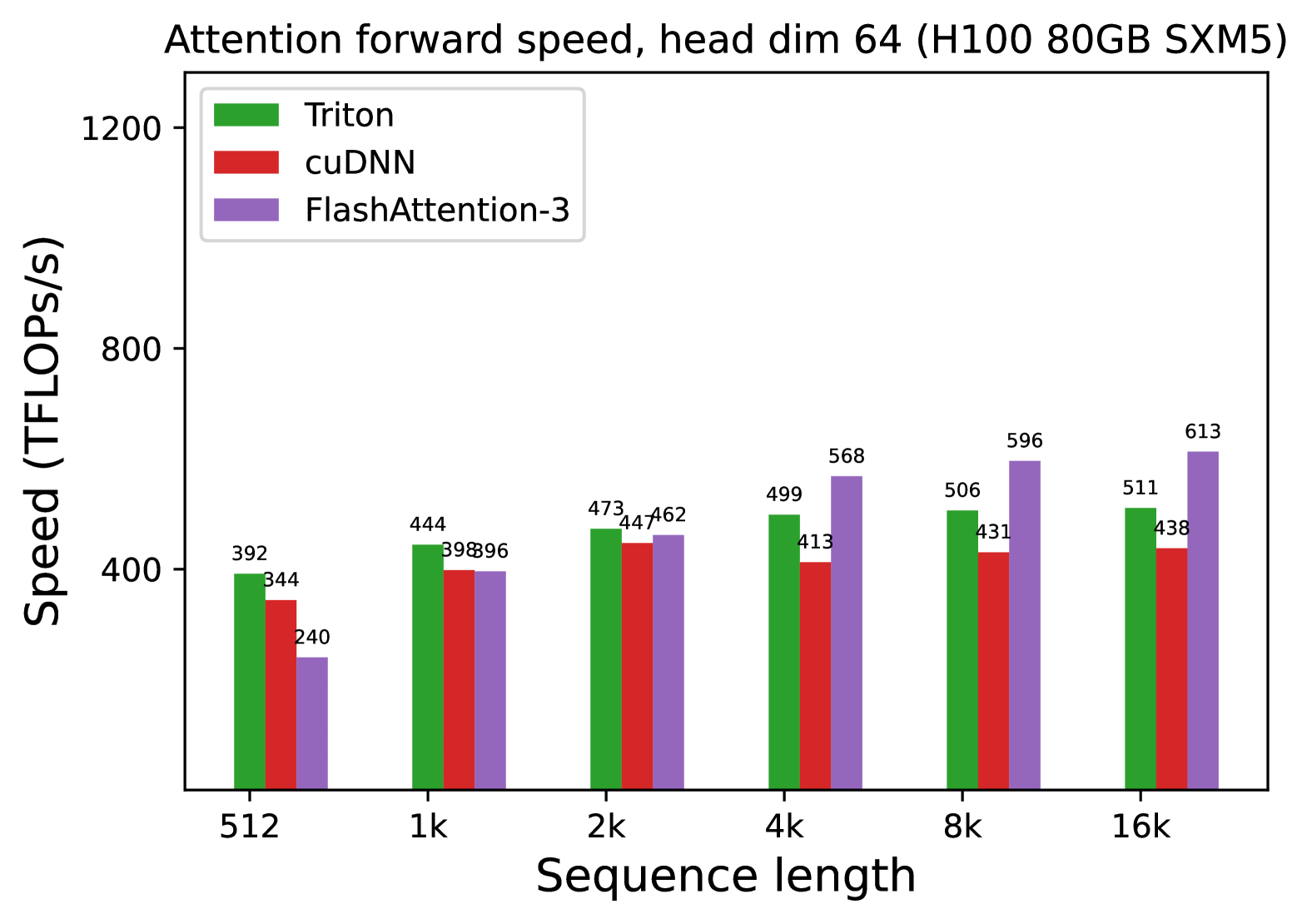
### Visual Description
# Technical Document Extraction: Attention Forward Speed Benchmark
## 1. Document Header & Metadata
* **Title:** Attention forward speed, head dim 64 (H100 80GB SXM5)
* **Hardware Context:** NVIDIA H100 80GB SXM5 GPU.
* **Parameter Specification:** Head dimension is fixed at 64.
## 2. Chart Structure
* **Type:** Grouped Bar Chart.
* **X-Axis (Independent Variable):** Sequence length.
* **Categories:** 512, 1k, 2k, 4k, 8k, 16k.
* **Y-Axis (Dependent Variable):** Speed (TFLOPs/s).
* **Scale:** Linear, ranging from 0 to 1200, with major ticks at 400, 800, and 1200.
* **Legend:**
* **Green Bar:** Triton
* **Red Bar:** cuDNN
* **Purple Bar:** FlashAttention-3
## 3. Data Extraction & Trend Analysis
### Trend Verification
* **Triton (Green):** Shows a steady, slight upward trend as sequence length increases, plateauing around 500 TFLOPs/s.
* **cuDNN (Red):** Shows an initial increase from 512 to 2k, followed by a slight decline and stabilization between 413 and 447 TFLOPs/s.
* **FlashAttention-3 (Purple):** Shows the most significant upward trend. It starts as the slowest at 512 but scales aggressively, becoming the fastest implementation from the 4k sequence length mark onwards.
### Data Table (Reconstructed)
Values are extracted from the labels positioned above each individual bar.
| Sequence Length | Triton (Green) | cuDNN (Red) | FlashAttention-3 (Purple) |
| :--- | :--- | :--- | :--- |
| **512** | 392 | 344 | 240 |
| **1k** | 444 | 398 | 396 |
| **2k** | 473 | 447 | 462 |
| **4k** | 499 | 413 | 568 |
| **8k** | 506 | 431 | 596 |
| **16k** | 511 | 438 | 613 |
## 4. Component Analysis
* **Header Region:** Contains the descriptive title defining the operation (Attention forward), the specific architectural constraint (head dim 64), and the hardware used (H100).
* **Main Chart Region:** Contains the grouped bars. Note that at sequence length **1k**, Triton is the clear leader, while cuDNN and FlashAttention-3 are nearly identical (398 vs 396).
* **Performance Crossover:** A critical observation is the performance crossover between 2k and 4k. At 2k, Triton is still the fastest (473), but by 4k, FlashAttention-3 (568) significantly outperforms both Triton (499) and cuDNN (413).
* **Scaling Efficiency:** FlashAttention-3 demonstrates superior scaling for long sequences, reaching a peak of 613 TFLOPs/s at 16k, which is approximately 2.5x its performance at 512. In contrast, Triton and cuDNN show much flatter scaling curves.
</details>
(a) Forward, without causal mask, head dim 64
<details>
<summary>x12.png Details</summary>
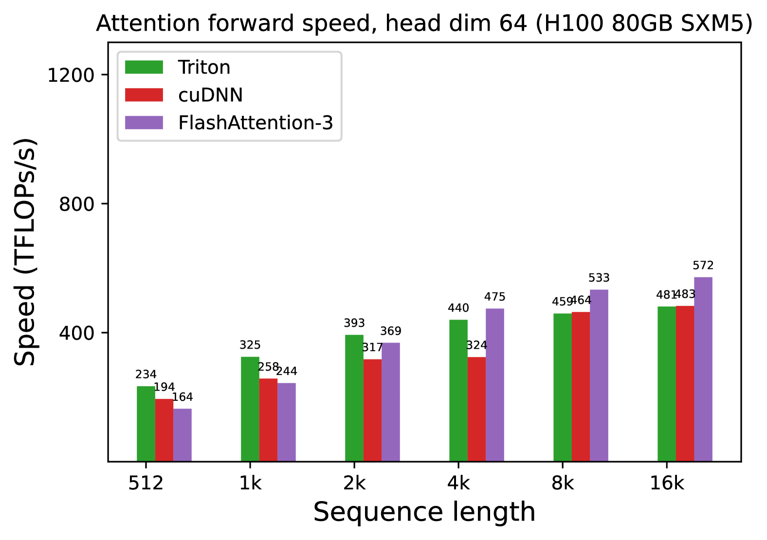
### Visual Description
# Technical Document Extraction: Attention Forward Speed Benchmark
## 1. Header Information
* **Title:** Attention forward speed, head dim 64 (H100 80GB SXM5)
* **Hardware Context:** NVIDIA H100 80GB SXM5 GPU.
* **Parameter Context:** Head dimension is fixed at 64.
## 2. Chart Metadata and Structure
* **Chart Type:** Grouped Bar Chart.
* **X-Axis (Independent Variable):** Sequence length.
* **Scale:** Categorical/Logarithmic progression (512, 1k, 2k, 4k, 8k, 16k).
* **Y-Axis (Dependent Variable):** Speed (TFLOPs/s).
* **Scale:** Linear, ranging from 0 to 1200, with major ticks at intervals of 400.
* **Legend:**
* **Green Bar:** Triton
* **Red Bar:** cuDNN
* **Purple Bar:** FlashAttention-3
## 3. Component Analysis and Trend Verification
### Triton (Green Bars)
* **Visual Trend:** Shows a consistent upward slope as sequence length increases, beginning to plateau slightly between 8k and 16k.
* **Performance:** It is the fastest implementation at the shortest sequence length (512) but is overtaken by FlashAttention-3 as the sequence length grows.
### cuDNN (Red Bars)
* **Visual Trend:** Shows a steady upward slope. It consistently performs lower than Triton across most sequence lengths but matches Triton's performance at the 16k mark.
* **Performance:** Generally the slowest or second-slowest implementation depending on the sequence length.
### FlashAttention-3 (Purple Bars)
* **Visual Trend:** Shows the steepest upward slope. While it starts as the slowest implementation at 512, it scales the most efficiently, overtaking cuDNN at 2k and Triton at 4k.
* **Performance:** Becomes the dominant implementation for long sequences (4k and above).
## 4. Data Table Reconstruction
The following table transcribes the numerical values labeled above each bar in the chart.
| Sequence Length | Triton (Green) [TFLOPs/s] | cuDNN (Red) [TFLOPs/s] | FlashAttention-3 (Purple) [TFLOPs/s] |
| :--- | :--- | :--- | :--- |
| **512** | 234 | 194 | 164 |
| **1k** | 325 | 258 | 244 |
| **2k** | 393 | 317 | 369 |
| **4k** | 440 | 324 | 475 |
| **8k** | 459 | 464 | 533 |
| **16k** | 481 | 483 | 572 |
## 5. Summary of Findings
The benchmark demonstrates that while **Triton** is optimized for shorter sequence lengths (under 1k), **FlashAttention-3** exhibits superior scaling properties on H100 hardware. By the 16k sequence length, FlashAttention-3 reaches **572 TFLOPs/s**, outperforming Triton (481 TFLOPs/s) and cuDNN (483 TFLOPs/s) by approximately 18-19%.
</details>
(b) Forward, with causal mask, head dim 64
<details>
<summary>x13.png Details</summary>
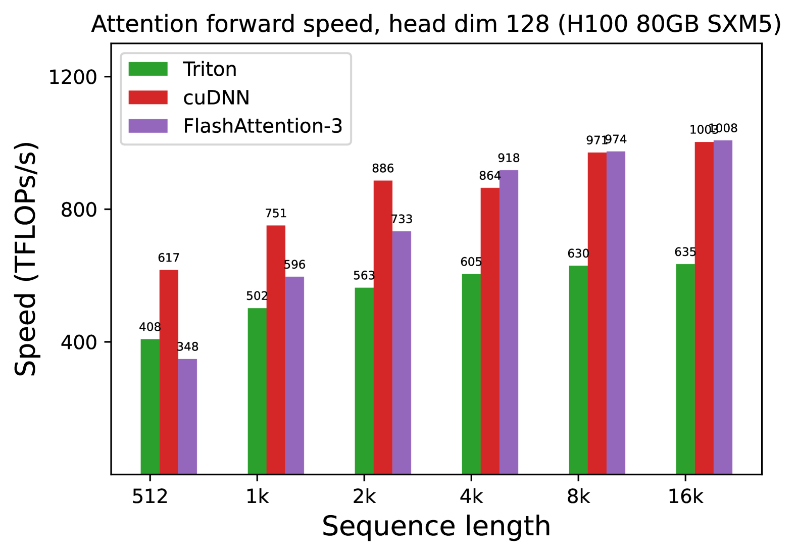
### Visual Description
# Technical Document Extraction: Attention Forward Speed Benchmark
## 1. Header Information
* **Title:** Attention forward speed, head dim 128 (H100 80GB SXM5)
* **Hardware Context:** NVIDIA H100 80GB SXM5 GPU.
* **Operation:** Attention forward pass with a head dimension of 128.
## 2. Chart Structure and Metadata
* **Chart Type:** Grouped Bar Chart.
* **Y-Axis Label:** Speed (TFLOPS/s)
* **Y-Axis Scale:** 0 to 1200, with major markers at 400, 800, and 1200.
* **X-Axis Label:** Sequence length
* **X-Axis Categories:** 512, 1k, 2k, 4k, 8k, 16k.
* **Legend Placement:** Top-left.
* **Legend Categories:**
* **Triton:** Green bar
* **cuDNN:** Red bar
* **FlashAttention-3:** Purple bar
## 3. Data Extraction and Trend Analysis
### Trend Verification
* **Triton (Green):** Shows a steady, monotonic upward trend as sequence length increases, starting at 408 and plateauing around 630-635 TFLOPS/s at higher sequence lengths.
* **cuDNN (Red):** Shows a sharp upward trend from 512 to 8k sequence lengths, significantly outperforming Triton at all points. It appears to reach a near-saturation point at 16k.
* **FlashAttention-3 (Purple):** Shows the most aggressive growth curve. It starts as the slowest performer at sequence length 512 but surpasses Triton at 2k and matches/slightly exceeds cuDNN at 8k and 16k.
### Data Table (Reconstructed)
Values are extracted from the labels positioned above each individual bar.
| Sequence Length | Triton (Green) | cuDNN (Red) | FlashAttention-3 (Purple) |
| :--- | :--- | :--- | :--- |
| **512** | 408 | 617 | 348 |
| **1k** | 502 | 751 | 596 |
| **2k** | 563 | 886 | 733 |
| **4k** | 605 | 864 | 918 |
| **8k** | 630 | 971 | 974 |
| **16k** | 635 | 1005 | 1008 |
## 4. Component Analysis & Key Findings
* **Performance Scaling:** All three implementations benefit from longer sequence lengths, which likely allows for better GPU utilization and occupancy.
* **Crossover Points:**
* FlashAttention-3 is less efficient than cuDNN and Triton at very short sequences (512).
* FlashAttention-3 overtakes Triton between 512 and 1k.
* FlashAttention-3 overtakes cuDNN between 2k and 4k.
* **Peak Performance:** FlashAttention-3 achieves the highest recorded throughput in this set at **1008 TFLOPS/s** at a sequence length of 16k, closely followed by cuDNN at **1005 TFLOPS/s**.
* **Efficiency Gap:** At the 16k sequence length, FlashAttention-3 and cuDNN are approximately **58% faster** than the Triton implementation.
</details>
(c) Forward, without causal mask, head dim 128
<details>
<summary>x14.png Details</summary>
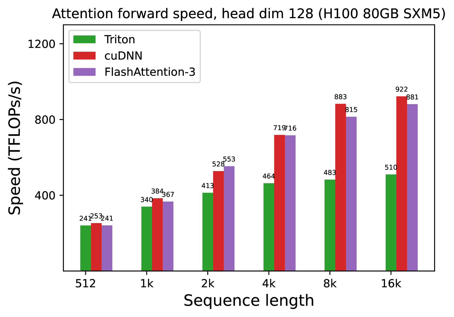
### Visual Description
# Technical Document Extraction: Attention Forward Speed Benchmark
## 1. Header Information
* **Title:** Attention forward speed, head dim 128 (H100 80GB SXM5)
* **Hardware Context:** NVIDIA H100 80GB SXM5 GPU.
* **Operation:** Attention forward pass.
* **Parameter:** Head dimension fixed at 128.
## 2. Chart Metadata
* **Type:** Grouped Bar Chart.
* **X-Axis Label:** Sequence length (Categorical/Logarithmic scale: 512 to 16k).
* **Y-Axis Label:** Speed (TFLOPS/s).
* **Y-Axis Scale:** 0 to 1200, with major ticks at 400, 800, and 1200.
* **Legend Placement:** Top-left [x ≈ 0.05, y ≈ 0.95].
## 3. Legend and Series Identification
The chart compares three software implementations/kernels:
1. **Triton** (Green): Represented by the leftmost bar in each group.
2. **cuDNN** (Red): Represented by the middle bar in each group.
3. **FlashAttention-3** (Purple): Represented by the rightmost bar in each group.
## 4. Data Table Extraction
The following table reconstructs the numerical values displayed above each bar in the chart.
| Sequence Length | Triton (Green) | cuDNN (Red) | FlashAttention-3 (Purple) |
| :--- | :---: | :---: | :---: |
| **512** | 241 | 253 | 241 |
| **1k** | 340 | 384 | 367 |
| **2k** | 413 | 528 | 553 |
| **4k** | 464 | 719 | 716 |
| **8k** | 483 | 883 | 815 |
| **16k** | 510 | 922 | 881 |
## 5. Trend Analysis and Observations
### Component Isolation: Trend Verification
* **Triton (Green):** Shows a steady, linear-like upward slope. It starts as the lowest performer at 512 (tied with FlashAttention-3) and remains the slowest implementation as sequence length increases, plateauing significantly compared to the others at higher sequence lengths.
* **cuDNN (Red):** Shows a strong upward slope. It is the fastest implementation at the smallest scale (512) and the largest scales (8k and 16k). It exhibits the highest peak performance at 922 TFLOPS/s.
* **FlashAttention-3 (Purple):** Shows a strong upward slope, closely tracking cuDNN. It surpasses cuDNN briefly at the 2k sequence length mark but falls slightly behind cuDNN at the 8k and 16k marks.
### Key Findings
* **Scaling:** All three methods show improved TFLOPS/s as sequence length increases, indicating better hardware utilization at larger scales.
* **Performance Leaders:** At sequence lengths of 4k and above, cuDNN and FlashAttention-3 significantly outperform Triton, achieving nearly double the throughput at 16k (922 and 881 TFLOPS/s vs. 510 TFLOPS/s).
* **Peak Performance:** The maximum recorded speed is **922 TFLOPS/s** achieved by **cuDNN** at a sequence length of 16k.
</details>
(d) Forward, with causal mask, head dim 128
<details>
<summary>x15.png Details</summary>
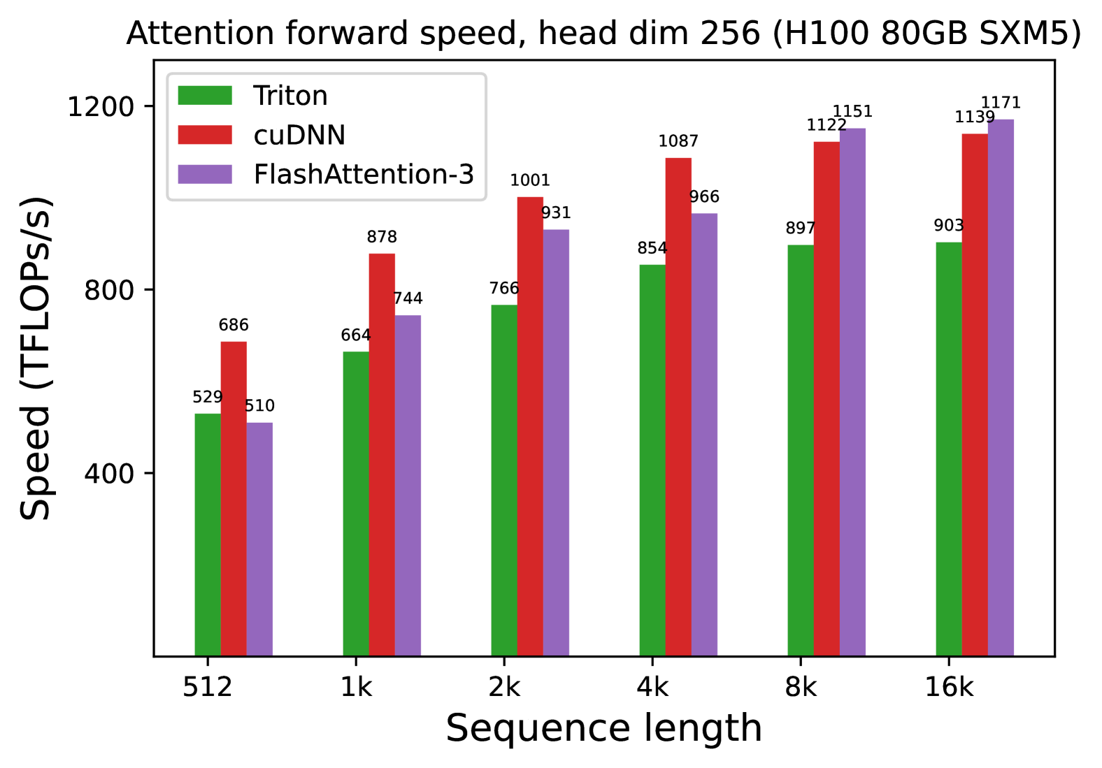
### Visual Description
# Technical Document Extraction: Attention Forward Speed Benchmark
## 1. Header Information
* **Title:** Attention forward speed, head dim 256 (H100 80GB SXM5)
* **Subject:** Performance benchmarking of different attention implementations on NVIDIA H100 GPU hardware.
## 2. Chart Metadata
* **Chart Type:** Grouped Bar Chart.
* **Y-Axis Label:** Speed (TFLOPS/s)
* **Y-Axis Scale:** Linear, ranging from 400 to 1200 with major ticks at 400, 800, and 1200.
* **X-Axis Label:** Sequence length
* **X-Axis Categories:** 512, 1k, 2k, 4k, 8k, 16k.
* **Legend Location:** Top-left
* **Legend Categories:**
* **Triton:** Green bar
* **cuDNN:** Red bar
* **FlashAttention-3:** Purple bar
## 3. Component Isolation & Data Extraction
### Trend Verification
* **Triton (Green):** Shows a consistent upward trend as sequence length increases, starting at 529 and plateauing around 900 TFLOPS/s.
* **cuDNN (Red):** Shows a strong upward trend, consistently outperforming Triton. It peaks at 1139 TFLOPS/s at the 16k sequence length.
* **FlashAttention-3 (Purple):** Shows the most significant growth curve. While it starts as the slowest at 512, it scales better than the others, eventually overtaking cuDNN at the 8k and 16k marks to become the fastest implementation.
### Data Table Reconstruction
The following table represents the precise numerical values labeled above each bar in the chart.
| Sequence Length | Triton (Green) | cuDNN (Red) | FlashAttention-3 (Purple) |
| :--- | :--- | :--- | :--- |
| **512** | 529 | 686 | 510 |
| **1k** | 664 | 878 | 744 |
| **2k** | 766 | 1001 | 931 |
| **4k** | 854 | 1087 | 966 |
| **8k** | 897 | 1122 | 1151 |
| **16k** | 903 | 1139 | 1171 |
## 4. Technical Observations
* **Scaling Efficiency:** FlashAttention-3 demonstrates superior scaling for long sequences (8k+). At 16k, it reaches the highest recorded throughput of **1171 TFLOPS/s**.
* **Small Sequence Performance:** For shorter sequences (512 to 4k), cuDNN maintains a performance lead over both Triton and FlashAttention-3.
* **Hardware Context:** These benchmarks are specific to the **H100 80GB SXM5** architecture with a **head dimension of 256**. Performance characteristics may vary on different hardware or with different head dimensions.
</details>
(e) Forward, without causal mask, head dim 256
<details>
<summary>x16.png Details</summary>

### Visual Description
# Technical Document Extraction: Attention Forward Speed Benchmark
## 1. Document Header
* **Title:** Attention forward speed, head dim 256 (H100 80GB SXM5)
* **Hardware Context:** NVIDIA H100 80GB SXM5 GPU.
* **Operation:** Attention forward pass with a head dimension of 256.
## 2. Chart Metadata
* **Chart Type:** Grouped Bar Chart.
* **X-Axis Label:** Sequence length
* **X-Axis Categories:** 512, 1k, 2k, 4k, 8k, 16k.
* **Y-Axis Label:** Speed (TFLOPS/s)
* **Y-Axis Scale:** Linear, ranging from 0 to 1200 with major ticks at 400, 800, and 1200.
* **Legend Categories:**
* **Triton:** Green bar
* **cuDNN:** Red bar
* **FlashAttention-3:** Purple bar
## 3. Component Isolation & Trend Analysis
### Region: Main Chart Area
The chart compares three software implementations (Triton, cuDNN, and FlashAttention-3) across increasing sequence lengths.
* **Triton (Green):** Shows a steady upward trend as sequence length increases, starting at 299 TFLOPS/s and reaching 663 TFLOPS/s. It is consistently the lowest performing of the three across all sequence lengths.
* **cuDNN (Red):** Shows a sharp upward trend, particularly between 1k and 4k sequence lengths. It overtakes FlashAttention-3 at the 2k mark and remains the highest-performing implementation for all subsequent sequence lengths, peaking at 1099 TFLOPS/s.
* **FlashAttention-3 (Purple):** Shows a strong upward trend. It is the fastest implementation at the smallest sequence lengths (512 and 1k). While its performance continues to grow to 1024 TFLOPS/s, it is surpassed by cuDNN from sequence length 2k onwards.
## 4. Data Table Reconstruction
| Sequence Length | Triton (Green) [TFLOPS/s] | cuDNN (Red) [TFLOPS/s] | FlashAttention-3 (Purple) [TFLOPS/s] |
| :--- | :--- | :--- | :--- |
| **512** | 299 | 304 | 329 |
| **1k** | 425 | 449 | 521 |
| **2k** | 520 | 768 | 703 |
| **4k** | 591 | 1015 | 856 |
| **8k** | 628 | 1056 | 960 |
| **16k** | 663 | 1099 | 1024 |
## 5. Key Findings
* **Maximum Performance:** cuDNN achieves the highest recorded throughput of **1099 TFLOPS/s** at a sequence length of 16k.
* **Crossover Point:** FlashAttention-3 is superior for short sequences (up to 1k). At sequence length 2k and above, cuDNN becomes the most efficient implementation.
* **Scaling:** All three methods benefit from larger sequence lengths, though Triton's scaling is more linear and shallow compared to the significant jumps seen in cuDNN and FlashAttention-3.
</details>
(f) Forward, with causal mask, head dim 256
Figure 9: Attention forward speed (FP8) on H100 GPU