2407.12861

# CiteME: Can Language Models Accurately Cite Scientific Claims? **Authors**: Ori Press, Andreas Hochlehnert, Ameya Prabhu, Vishaal Udandarao, Ofir Press, Matthias Bethge > Tübingen AI Center, University of Tübingen Open- 𝚿 𝚿 \mathbf{\Psi} bold_Ψ (Open-Sci) Collective > Tübingen AI Center, University of Tübingen University of Cambridge Open- 𝚿 𝚿 \mathbf{\Psi} bold_Ψ (Open-Sci) Collective > Princeton Language and Intelligence, Princeton University vskip=-.0leftmargin=0.025rightmargin=0.075font=small,itshape ## Abstract Thousands of new scientific papers are published each month. Such information overload complicates researcher efforts to stay current with the state-of-the-art as well as to verify and correctly attribute claims. We pose the following research question: Given a text excerpt referencing a paper, could an LM act as a research assistant to correctly identify the referenced paper? We advance efforts to answer this question by building a benchmark that evaluates the abilities of LMs in citation attribution. Our benchmark, CiteME, consists of text excerpts from recent machine learning papers, each referencing a single other paper. CiteME use reveals a large gap between frontier LMs and human performance, with LMs achieving only 4.2-18.5% accuracy and humans 69.7%. We close this gap by introducing CiteAgent, an autonomous system built on the GPT-4o LM that can also search and read papers, which achieves an accuracy of 35.3% on CiteME. Overall, CiteME serves as a challenging testbed for open-ended claim attribution, driving the research community towards a future where any claim made by an LM can be automatically verified and discarded if found to be incorrect. ## 1 Introduction <details> <summary>extracted/5974968/figures/fig1.png Details</summary>  ### Visual Description \n ## Diagram: Citation Retrieval Process Flowchart ### Overview The image is a three-part flowchart illustrating a process where an AI system identifies a cited academic paper from a given text snippet. The flow moves from left to right, indicated by black arrows connecting the components. ### Components/Axes The diagram consists of three distinct visual elements arranged horizontally: 1. **Left Component (Input Box):** A rounded rectangle with a light blue fill and a dark blue border. It contains the input task. 2. **Central Component (Processing Illustration):** A stylized, monochromatic (dark blue and white) illustration of a robot sitting at a desk, typing on a computer keyboard. The robot has a simple, friendly face with two dot eyes. A computer monitor is visible on the desk. 3. **Right Component (Output Box):** A rounded rectangle identical in style to the left box (light blue fill, dark blue border). It contains the system's output. Two solid black arrows, one pointing right from the left box to the central illustration, and another pointing right from the central illustration to the right box, indicate the direction of the process flow. ### Detailed Analysis **Left Box (Input):** * **Heading:** "Find the paper cited in this text:" * **Content (Transcribed Text):** "ESIM is another high performing model for sentence-pair classification tasks, particularly when used with ELMo embeddings [CITATION]" * **Language:** English. * **Note:** The placeholder `[CITATION]` is highlighted in a distinct blue color, different from the surrounding black text. **Central Illustration:** * This is a visual metaphor for an AI or computational agent performing a search or analysis task. It contains no textual information. **Right Box (Output):** * **Heading:** "After searching, I think the cited paper is:" * **Content (Transcribed Text):** "Deep contextualized word representations" * **Language:** English. ### Key Observations 1. **Process Flow:** The diagram explicitly models a three-stage pipeline: **Input (Query) -> Processing (Search/Analysis) -> Output (Result)**. 2. **Placeholder Identification:** The key trigger for the process is the `[CITATION]` placeholder within the input text. The system's task is to resolve this placeholder into a specific paper title. 3. **Output Specificity:** The output is a direct quote of a paper title, suggesting the system is designed to return exact bibliographic references rather than paraphrased information. 4. **Spatial Grounding:** The legend (the process flow) is embedded in the structure itself. The left box is the source, the central robot is the processing agent, and the right box is the destination/result. The arrows are the connectors. ### Interpretation This diagram serves as a high-level, conceptual model for an automated citation retrieval or academic search system. It demonstrates a common task in natural language processing and information retrieval: **entity linking** or **knowledge base grounding**, where a generic placeholder (like `[CITATION]`) is mapped to a specific, real-world entity (a paper title). The choice of a friendly robot at a computer anthropomorphizes the AI agent, making the technical process more relatable. The flow emphasizes a clear input-output transformation. The specific example used—resolving a citation about the ESIM model and ELMo embeddings—grounds the abstract process in a concrete, relevant NLP context. The output, "Deep contextualized word representations," is, in fact, the title of the seminal paper introducing ELMo (Embeddings from Language Models), indicating the system in the example has correctly identified the foundational work referenced in the input text. The diagram thus illustrates a successful instance of the system's intended function. 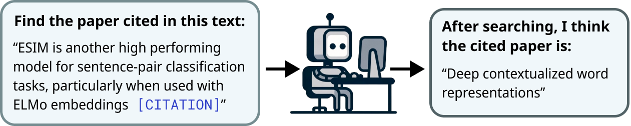</details> Figure 1: Example of a CiteME instance. The input (left) is an excerpt from a published paper with an anonymized citation; the target answer (right) is the title of the cited paper. */ $‡$ shared first/last authorship Code: github.com/bethgelab/CiteME, Dataset: huggingface.co/datasets/bethgelab/CiteME Correspondence to {ori.press, andreas.hochlehnert}@bethgelab.org Scientific discoveries are advancing at an ever-growing rate, with tens of thousands of new papers added just to arXiv every month [4]. This rapid progress has led to information overload within communities, making it nearly impossible for scientists to read all relevant papers. However, it remains a critical scholarship responsibility to check new claims and attribute credit to prior work accurately. Language models (LMs) have shown impressive abilities as assistants across tasks [25], which leads us to explore the following task in this paper: Can language models act as research assistants to help scientists deal with information overload? We make progress towards answering this question by evaluating the abilities of LMs in citation attribution [27, 59]. Given a text excerpt referencing a scientific claim, citation attribution is the task in which a system is asked to fetch the title of a referenced paper, as illustrated in Figure 1. Current benchmarks are collected automatically, which leads to the dominance of ambiguous or unattributable text excerpts that make overly broad claims or are not used as evidence for any specific claim, as shown in Table 1. Furthermore, these benchmarks typically frame citation attribution as a retrieval task from a small set of pre-selected papers where only paper titles and abstracts can be viewed, not the full paper’s content important for citation attribution [22, 50]. Table 1: Percentage of reasonable, ambiguous, unattributable, and trivial excerpts across 4 citation datasets, as labeled by human experts. For a detailed breakdown of every analyzed sample, see Appendix A. | FullTextPeerRead [42] ACL-200 [9, 58] RefSeer [40, 58] | 24 26 24 | 26 42 28 | 34 18 32 | 16 14 16 | | --- | --- | --- | --- | --- | | arXiv [33] | 10 | 50 | 30 | 10 | | Average | 21 | 36.5 | 28.5 | 14 | To address these issues, we introduce CiteME (Citation for Model Evaluation), the first manually curated citation attribution benchmark with text excerpts that unambiguously reference a single paper. CiteMe’s use of only unambiguous text excerpts eliminates the subjectivity that characterizes other benchmarks. To evaluate CiteMe, we conduct benchmark tests that focus on open-ended citation attribution. Human evaluators confirm the lack of ambiguity, achieving 69.7% accuracy while taking just 38.2 seconds on average to find the referenced papers. The current state-of-the-art system, SPECTER2 [77], experiences 0% accuracy on CiteME, highlighting the real-world difficulties of LM-based citation attribution. Similarly, current frontier LMs achieve performance of 4.2-18.5%, substantially beneath human performance. We conclude that current LMs cannot reliably link scientific claims to their sources. To bridge this gap, we introduce CiteAgent, an autonomous system built on top of the GPT-4o [1] LM and the Semantic Scholar search engine [46]. CiteAgent can search for and read papers repeatedly until it finds the referenced paper, mirroring how scientists perform this scholarship task to find targeted papers. CiteAgent correctly finds the right paper 35.3% of the time when evaluated on CiteME. In summary, our main contributions are: - CiteME, a challenging and human-curated benchmark of recent machine learning publications that evaluates the abilities of LMs to correctly attribute scientific claims. CiteME is both natural and challenging, even for SoTA LMs. - CiteAgent, an LM-based agent that uses the Internet to attribute scientific claims. Our agent uses an existing LM without requiring additional training. It also uses a search engine, which makes it applicable to real-world settings and differentiates it from systems that can search only within a predetermined corpus of papers. Future work that improves the accuracy of CiteME may lead to systems that can verify all claims an LM makes, not just those in the ML research domain. This could reduce the hallucination rate [92] and increase factuality [6] of LM-generated text. ## 2 The CiteME Benchmark We now present the CiteME benchmark, which we differentiate from other citation prediction benchmarks that are automatically curated, i.e., curated without human supervision or feedback in selecting text excerpts [32, 31, 9, 40, 72, 44, 42, 33]. For comparison, we study the quality of excerpts across four popular citation prediction benchmarks (FullTextPeerRead, [42], ACL-200 [9, 58], RefSeer [40, 58], and arXiv [33]). Specifically, we sample 50 excerpts from each dataset and categorize them using the following criteria: (1) Attributable vs Unattributable. The cited paper should provide evidence for the statement in the text excerpt, i.e., be an attribution as opposed to a statement that does not clearly refer to supporting evidence. Excerpts that do not follow this criterion are termed unattributable, as in the example: For all of our experiments, we use the hyperparameters from [CITATION]. (2) Unambiguous vs Ambiguous. The cited text excerpt should not be overly broad. The ground truth cited papers should clearly be the only possible reference for the claim in the text excerpt. Excerpts that do not follow this criterion are termed ambiguous, as in the example: [CITATION1, CITATION2] explored paper recommendation using deep networks. (3) Non-Trivial vs Trivial. The text excerpt should not include author names or title acronyms, which simply tests LM memorization and retrieval. Excerpts that do not follow this criterion are termed trivial, as in the example: SciBERT [CITATION] is a BERT-model pretrained on scientific texts. (4) Reasonable vs Unreasonable. The text excerpt should be attributable, unambiguous and non-trivial. We term excerpts that do not follow this criterion unreasonable, but we categorize them according to the underlying issue (e.g., unattributable, ambiguous, or trivial). An example of a reasonable excerpt is: We use the ICLR 2018–2022 database assembled by [CITATION], which includes 10,297 papers. In Table 1 (left), we demonstrate that most samples from all four datasets lack sufficient information for humans to identify the cited paper and are often labeled as ambiguous or unattributable. Additionally, an average of 17.5% of the samples are tagged as trivial because they include the title of the paper or its authors directly in the excerpt. Excerpts also frequently have formatting errors, making some nearly unreadable (see examples in Appendix A). Past work also notes similar artifacts [33, 42, 58], further supporting our claims. This analysis leads us to contend that performance on existing citation benchmarks might not reflect real-world performance of LM research assistants. In response to these deficiencies, we created CiteME, a new benchmark with human expert curation for unambiguous citation references. CiteME contains carefully selected text excerpts, each containing a single, clear citation to ensure easy and accurate evaluation. Curation. A team of 4 machine learning graduate students, henceforth referred to as “experts”, were responsible for collecting text excerpts. The experts were instructed to find samples that (1) referenced a single paper and (2) provided sufficient context to find the cited paper with scant background knowledge. Each sample was checked for reasonableness; only those deemed reasonable by two or more experts were retained. Some excerpts were slightly modified to make them reasonable. <details> <summary>extracted/5974968/figures/paper_tags.png Details</summary>  ### Visual Description \n ## Horizontal Bar Chart: CiteME Paper Tags ### Overview This image is a horizontal bar chart titled "CiteME Paper Tags." It displays the frequency of ten distinct research topic tags associated with papers in the "CiteME" dataset or system. The chart uses a single color for all bars, indicating a simple frequency count without sub-grouping. ### Components/Axes * **Title:** "CiteME Paper Tags" (centered at the top). * **Y-Axis (Vertical):** Lists the ten paper tag categories. From top to bottom: 1. Image Classification 2. Adversarial Machine Learning 3. Deep Learning Architectures 4. Vision-Language Models 5. Contrastive Learning 6. Multi-modal Learning 7. Representation Learning 8. Image Processing 9. Machine Learning Efficiency 10. Machine Learning Evaluation * **X-Axis (Horizontal):** Labeled "Tag Frequency." It has numerical markers at 2, 4, and 6. The axis line extends from 0 to just beyond 6. * **Legend:** There is no separate legend. All bars are rendered in the same light blue/teal color with a black outline. * **Data Representation:** Ten horizontal bars, each corresponding to a tag on the Y-axis. The length of each bar indicates its frequency. ### Detailed Analysis The chart presents a ranked list of tag frequencies. The bars are ordered from highest frequency at the top to lowest at the bottom. * **Top Tier (Frequency = 6):** * `Image Classification`: Bar extends to the '6' marker. * `Adversarial Machine Learning`: Bar extends to the '6' marker. * **Middle Tier (Frequency = 5):** * `Deep Learning Architectures`: Bar ends approximately halfway between the '4' and '6' markers. * `Vision-Language Models`: Bar ends approximately halfway between the '4' and '6' markers. * `Contrastive Learning`: Bar ends approximately halfway between the '4' and '6' markers. * `Multi-modal Learning`: Bar ends approximately halfway between the '4' and '6' markers. * `Representation Learning`: Bar ends approximately halfway between the '4' and '6' markers. * **Lower Tier (Frequency = 4):** * `Image Processing`: Bar extends to the '4' marker. * `Machine Learning Efficiency`: Bar extends to the '4' marker. * `Machine Learning Evaluation`: Bar extends to the '4' marker. **Trend Verification:** The visual trend is a clear step-down pattern. The top two bars are the longest and equal. The next five bars are of equal, slightly shorter length. The final three bars are the shortest and equal. This creates three distinct frequency clusters. ### Key Observations 1. **Dominant Topics:** "Image Classification" and "Adversarial Machine Learning" are the most frequently tagged topics, tied for the highest frequency. 2. **Core Research Cluster:** A large middle group of five topics (Deep Learning Architectures, Vision-Language Models, Contrastive Learning, Multi-modal Learning, Representation Learning) all share the same, slightly lower frequency. This suggests these are all core, well-represented areas within the dataset. 3. **Foundational/Supporting Topics:** The three least frequent tags ("Image Processing," "Machine Learning Efficiency," "Machine Learning Evaluation") are all at the same level. These may represent more foundational, methodological, or evaluation-focused aspects of the research. 4. **Visual Design:** The chart uses a minimalist design with a single color, focusing attention purely on the rank and magnitude of the frequencies. The lack of a legend is appropriate as there is only one data series. ### Interpretation The data suggests the "CiteME" paper collection is heavily focused on computer vision and robustness in machine learning. The top tag, "Image Classification," is a classic, central task in computer vision. Its tie with "Adversarial Machine Learning" indicates a strong concurrent emphasis on the security, robustness, and vulnerability of these models. The large middle cluster represents the modern toolkit and paradigms of the field: building new architectures (`Deep Learning Architectures`), learning from multiple data types (`Vision-Language Models`, `Multi-modal Learning`), and developing advanced training objectives (`Contrastive Learning`, `Representation Learning`). Their equal frequency implies a balanced representation of these interconnected research directions. The lower frequency of tags like "Image Processing" (a more traditional field) and "Machine Learning Efficiency"/"Evaluation" suggests that while these are necessary components, the primary research energy in this dataset is directed towards developing new models, tasks, and learning paradigms rather than low-level processing or optimization/assessment techniques. The chart effectively maps the landscape of a research community or corpus, highlighting its primary interests and the relative weight given to different sub-disciplines. </details> <details> <summary>extracted/5974968/figures/citeme_hist.png Details</summary>  ### Visual Description ## Bar Chart: CiteME Papers by Year Published ### Overview This is a vertical bar chart titled "CiteME Papers by Year Published." It displays the distribution of papers within the "CiteME" dataset or system by their publication year, expressed as a percentage of the total papers. The chart shows a non-uniform distribution with notable peaks at the beginning and end of the timeline. ### Components/Axes * **Title:** "CiteME Papers by Year Published" (centered at the top). * **Y-Axis:** Labeled "Percent of Papers." The scale runs from 0 to 25, with major tick marks at intervals of 5 (0, 5, 10, 15, 20, 25). * **X-Axis:** Represents publication years. The labels are, from left to right: "Pre '11", "'11", "'12", "'13", "'14", "'15", "'16", "'17", "'18", "'19", "'20", "'21", "'22", "'23", "'24". The labels are rotated approximately 45 degrees. * **Data Series:** A single series represented by light blue bars with black outlines. There is no legend, as there is only one data category. ### Detailed Analysis The following table reconstructs the approximate percentage values for each year, based on visual estimation against the y-axis scale. Values are approximate due to the visual nature of the extraction. | Year Label | Approximate Percent of Papers | Visual Trend Note | | :--- | :--- | :--- | | Pre '11 | 20% | A tall bar, the second highest on the chart. | | '11 | ~1% | The lowest bar on the chart. | | '12 | ~3% | | | '13 | ~3% | Similar height to '12. | | '14 | ~2% | Slightly lower than '12/'13. | | '15 | 5% | Aligns with the 5% grid line. | | '16 | ~4% | Slightly lower than '15. | | '17 | 5% | Similar height to '15. | | '18 | ~7% | | | '19 | ~11% | The first bar to exceed 10%. | | '20 | ~3% | A significant drop from '19. | | '21 | ~16% | A sharp increase. | | '22 | ~23% | The second tallest bar. | | '23 | ~24% | The tallest bar on the chart. | | '24 | ~2% | A sharp drop from the peak in '23. | **Trend Verification:** The data series shows a bimodal-like distribution. It starts high (Pre '11), drops to a low plateau from '11 to '14, begins a gradual climb from '15 to '19, dips in '20, then surges dramatically from '21 to a peak in '23, before falling sharply again in '24. ### Key Observations 1. **Peaks:** The two most significant concentrations of papers are from before 2011 (~20%) and the years 2022-2023 (~23% and ~24%). 2. **Troughs:** The years 2011 (~1%) and 2024 (~2%) represent the lowest points. The year 2020 (~3%) is also notably low compared to the years immediately before and after it. 3. **Recent Surge:** There is a pronounced and rapid increase in the percentage of papers from 2021 through 2023, suggesting a major growth phase or change in the CiteME system's usage or indexing during this period. 4. **2024 Drop:** The sharp decline in 2024 could indicate incomplete data for the year (if the chart was created mid-year), a change in policy, or a significant reduction in activity. ### Interpretation The chart suggests that the "CiteME" entity (likely a citation database, a research tool, or a specific collection) has a complex history. The high percentage of "Pre '11" papers indicates it either has a strong foundation of older literature or performed a bulk import of historical data. The low activity in the early 2010s ('11-'14) might reflect a period of low adoption or development. The most critical insight is the explosive growth from 2021 to 2023. This could correlate with increased academic output, the tool gaining popularity, a successful marketing effort, or integration with other platforms. The anomaly in 2020 (a dip) might be related to global disruptions affecting research output or priorities. The steep drop in 2024 is the most ambiguous point; without temporal context for when this chart was generated, it's unclear if this represents a full-year decline, a mid-year snapshot, or the beginning of a new trend. Overall, the data paints a picture of a system that was established with older content, experienced a quiet period, and then underwent a dramatic resurgence in recent years. 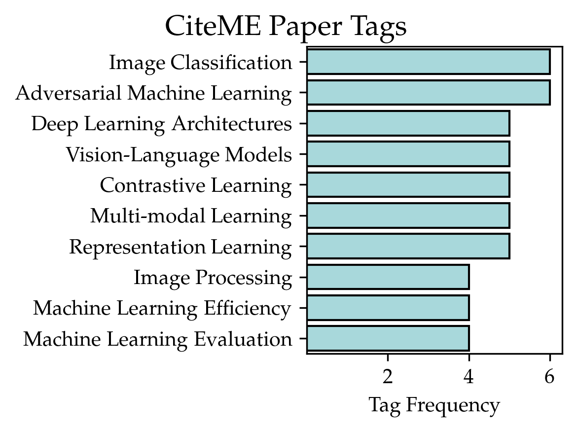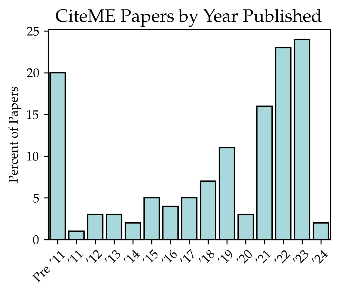</details> Figure 2: (Left) The top 10 most frequent labels of papers in CiteME, as identified by GPT-4. Overly broad tags like "Machine Learning" or "Deep Networks" were excluded (see Appendix D for details). (Right) Most excerpts in CiteME are from recent papers. Filtering Out the Easy Instances. To ensure that CiteMe is a challenging and robust dataset, we remove all dataset instances that GPT-4o can correctly answer. Filtering datasets by removing the samples that a strong model can correctly answer was previously done in Bamboogle [71] and the Graduate-Level Google-Proof Q&A Benchmark [73]. In our filtering process, GPT-4o was used with no Internet access or any other external tools. Therefore, it could answer only correctly specified papers that it memorized from its training process. We ran each sample through GPT-4o five times to cover its different outcomes. In the end, we filtered out 124 samples, leaving 130 samples in total. Human Evaluation. To ensure that our benchmark instances are not unsolvable, we evaluate human performance on them. Using a random subset of 100 samples, we asked a group of 20 experts, who were not part of benchmark construction, to perform the task of finding the referenced papers given only the excerpt, with each expert given 5 random samples from CiteME and a maximum of two minutes to solve each instance (similar to [47]). We observe that the experts found the correct citation 69.7% of the time, spending an average of only 38.2 seconds to do so. Note that this accuracy number does not represent the maximum-possible human performance since our annotators were limited to two minutes per question for budget reasons. Human accuracy may rise even higher given more time per instance. To check the experts’ consistency, five more experts were asked to solve the same instances previously answered by the original experts. In 71% of the cases, both experts agreed on the answer, and at least one expert got to the right answer in 93% of cases. Are 130 questions sufficient to evaluate LMs? Though traditional machine learning benchmarks usually contain thousands or even millions of test samples, recent work [17, 71, 74, 86] shows that LM benchmarks can include only 100-200 samples and remain insightful. HumanEval [17], for example, which consists of 164 programming problems, is among the most influential LM datasets today, appearing in virtually every SoTA LM paper recently published [66, 1, 81, 19]. Similarly, Bamboogle [71] contains 125 questions, DrawBench [74] contains 200 instances, and Plot2Code [86] contains 132 questions. This is in line with [70, 69], who show that benchmarks with many samples can be reduced to around 100 samples without sacrificing their utility. In addition, smaller benchmarks are advantageous because they are both cheaper to evaluate and impose a less significant environmental impact [76]. ## 3 CiteAgent We now describe CiteAgent, an LM-based system that we built to mimic researcher performance of open-ended citation attribution. A researcher seeking the correct attribution for a claim might use a search engine, read several papers, refine the search query, and repeat until successful. To allow CiteAgent to perform these actions, we built it to use Semantic Scholar to search for and read papers. Unless specified otherwise, we refer to CiteAgent with the GPT-4o backbone simply as CiteAgent throughout this paper. 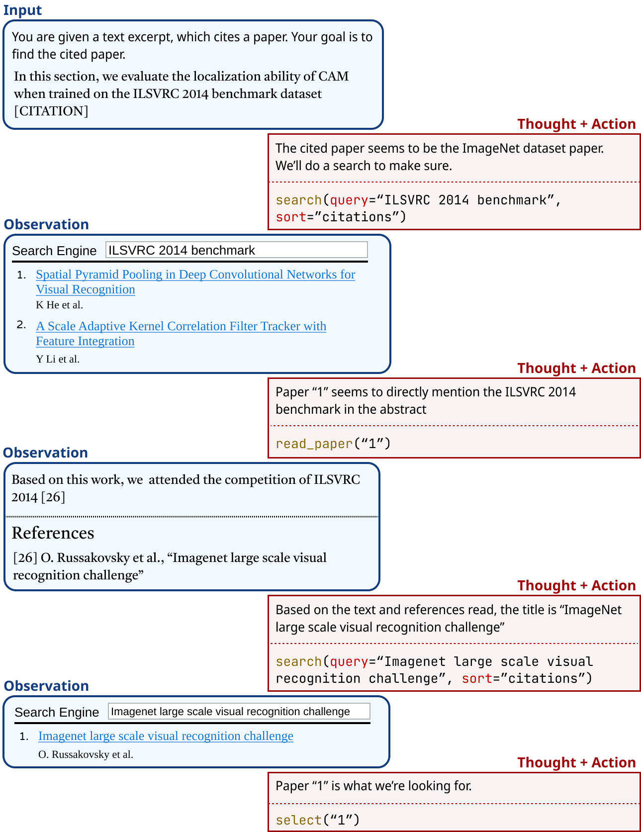Given a text excerpt, we prompt CiteAgent to perform one of a fixed set of custom commands and provide the output that the given command generated. CiteAgent then gives its rationale before performing another action, following [90, 88]. Figure 3 shows this process. We now describe the starting prompt and custom agent commands. Prompt. Our prompt includes the task description, descriptions of available commands, and a demonstration trajectory, i.e., the series of actions that the system executes while solving an instance [90, 88]. The trajectory includes searching, reading a paper, and searching again (see Figure 4). We model our prompt on the SWE-Agent prompt [88]. Table 2: Commands available to the model using our system. | search(query, sort) read(ID) select(ID) | Searches for a query; sorts results by relevance or by citation count; returns a list of papers, where each item consists of the paper ID, title, number of citations, and abstract. Returns the full text of a paper, including title, author list, abstract, and the paper itself. Selects a paper from the search results as the answer. | | --- | --- | Agent Commands. CiteAgent can respond to three custom commands (see Table 2). It always begins by executing the search command (sorting by relevance or citation count), which searches Semantic Scholar for a query and returns top results in a sorted order. After searching, CiteAgent can either search again, read one of the listed papers, or select a paper can perform up to 15 actions for every sample. Once a select action is taken, the session ends, and the selected paper is recorded. Search. CiteAgent initiates a search command by querying Semantic Scholar [46]. We chose the Selenium API [63] over the Semantic Scholar API due to the former’s significantly better re-ranked queries and its ability to provide a uniform interface for both our model and human trajectory annotators. Selenium also lets us access features such as sorting search results by relevance and citation count, which our human trajectory annotators found particularly valuable. To ensure correctness, we filter out search results published after the excerpt’s source paper, and the source paper itself. We then give CiteAgent the top 10 search results, which include paper id, title, abstract, and citation count. <details> <summary>extracted/5974968/figures/trajectory.png Details</summary>  ### Visual Description \n ## Diagram: Iterative Paper Citation Retrieval Process ### Overview The image is a vertical flowchart illustrating a step-by-step process for identifying and retrieving a specific academic paper cited within a text excerpt. The process involves iterative cycles of reasoning ("Thought + Action") and information retrieval ("Observation"), ultimately leading to the selection of the target paper. The diagram uses a consistent visual language with color-coded boxes and directional arrows to denote the flow of operations. ### Components/Axes The diagram is structured as a top-to-bottom sequence of interconnected blocks. There are three primary component types: 1. **Input Box (Blue Border):** Contains the initial problem statement. 2. **Thought + Action Box (Red Border):** Contains the system's reasoning and the specific action command it executes. 3. **Observation Box (Blue Border):** Displays the output or result returned from the executed action. Arrows connect these boxes to show the sequential flow of the process. ### Detailed Analysis The process unfolds as follows, with all text transcribed verbatim: **1. Input Stage (Top-Left)** * **Text:** "You are given a text excerpt, which cites a paper. Your goal is to find the cited paper. In this section, we evaluate the localization ability of CAM when trained on the ILSVRC 2014 benchmark dataset [CITATION]" **2. First Thought + Action Cycle** * **Thought:** "The cited paper seems to be the ImageNet dataset paper. We'll do a search to make sure." * **Action Command:** `search(query="ILSVRC 2014 benchmark", sort="citations")` **3. First Observation** * **Header:** "Search Engine | ILSVRC 2014 benchmark" * **Result 1:** "1. Spatial Pyramid Pooling in Deep Convolutional Networks for Visual Recognition" (Hyperlinked in blue) * Author: "K He et al." * **Result 2:** "2. A Scale Adaptive Kernel Correlation Filter Tracker with Feature Integration" (Hyperlinked in blue) * Author: "Y Li et al." **4. Second Thought + Action Cycle** * **Thought:** "Paper "1" seems to directly mention the ILSVRC 2014 benchmark in the abstract" * **Action Command:** `read_paper("1")` **5. Second Observation** * **Content Snippet:** "Based on this work, we attended the competition of ILSVRC 2014 [26]" * **References Section:** * "[26] O. Russakovsky et al., “Imagenet large scale visual recognition challenge”" **6. Third Thought + Action Cycle** * **Thought:** "Based on the text and references read, the title is "ImageNet large scale visual recognition challenge"" * **Action Command:** `search(query="Imagenet large scale visual recognition challenge", sort="citations")` **7. Third Observation** * **Header:** "Search Engine | Imagenet large scale visual recognition challenge" * **Result 1:** "1. Imagenet large scale visual recognition challenge" (Hyperlinked in blue) * Author: "O. Russakovsky et al." **8. Final Thought + Action (Bottom-Right)** * **Thought:** "Paper "1" is what we're looking for." * **Action Command:** `select("1")` ### Key Observations * **Process Logic:** The workflow demonstrates a refinement strategy. An initial broad search ("ILSVRC 2014 benchmark") yields multiple results. The system then reads a promising paper, extracts a precise reference title from it, and performs a new, more targeted search to find the exact cited work. * **Visual Coding:** The diagram uses color consistently: blue for data/input-output states and red for active reasoning/processing steps. * **Spatial Flow:** The process flows strictly from top to bottom, with "Thought + Action" boxes positioned to the right of the main vertical flow, indicating they are the driving engine for each step. * **Data Extraction:** The system successfully extracts key metadata: the paper title ("Imagenet large scale visual recognition challenge") and the primary author ("O. Russakovsky et al.") from the reference list. ### Interpretation This diagram models an **investigative agent's workflow** for resolving academic citations. It demonstrates a Peircean abductive reasoning pattern: starting with an incomplete clue (a citation placeholder), forming a hypothesis (it's the ImageNet paper), testing it (searching and reading), gathering new evidence (finding a specific reference), and finally converging on the most plausible conclusion (selecting the exact paper). The process highlights the importance of **contextual cross-referencing**. The initial search term was a benchmark name, but the definitive answer was found by reading a related paper and extracting its reference. This shows that citation retrieval often requires navigating a network of related documents rather than a single direct lookup. The final `select("1")` action signifies the successful completion of the information-seeking task, having moved from a vague citation marker to a specific, verifiable bibliographic entry. </details> Figure 3: The demonstration trajectory we gave CiteAgent in the prompt. Read. Read command execution causes CiteAgent to retrieve the open-access PDF corresponding to the selected paper from Semantic Scholar. Using the PyPDF2 library [29], our system extracts the text from the PDF, excluding visual figures. It then presents the text to CiteAgent, which generates a thought and a new command. If an open-access PDF link is unavailable, CiteAgent returns a message to that effect. We note that due to the limited context length of 8K tokens in the LLaMA-3 LM, we excluded the read action when using that model. Select. Select command execution causes CiteAgent to choose a paper to attribute to the input text excerpt, which ends the run. If the number of actions reaches 14, CiteAgent is prompted to make a selection, forcefully concluding the run. This design choice ensures that all runs complete within a finite time and budget. ## 4 Experiment Setup Below, we provide detailed implementation information for the baseline models and the various CiteAgent configurations we used for our evaluations. SPECTER Models. We present the results of SPECTER [21] and SPECTER2 [77] on CiteME as our baselines. SPECTER [21] encodes robust document-level representations for scientific texts, achieving high performance on citation prediction tasks without the need for fine-tuning. We use the Semantic Scholar SPECTER API https://github.com/allenai/paper-embedding-public-apis to embed the input text excerpts and the Semantic Scholar Datasets API https://api.semanticscholar.org/api-docs/datasets to embed all papers on Semantic Scholar, using these embeddings as our retrieval set. SPECTER2 models [77] introduce task-specific representations, each tailored to different tasks. For our experiments, we use the base customization of SPECTER2 from Hugging Face https://huggingface.co/allenai/specter2 to embed text excerpts and the Semantic Scholar Datasets API to similarly embed all papers on Semantic Scholar, forming our retrieval set. We apply an exact kNN [53] match to identify the closest embedding, computing the cosine similarity between the embeddings of text excerpt and all available papers (title and abstract). Using exact kNN matches ensures no approximations/errors are introduced while matching queries. We embed the query text excerpt as title only and both title and abstract, but that did not change the performance of the SPECTER models. CiteAgent. We run the CiteAgent system with three SoTA LMs as backbones: GPT-4o [1], Claude 3 Opus [3], and LLaMa-3-70B [81]. We additionally ablate over three classes of commands (Table 2): 1. Search and Read. The model can perform both search and read commands. 1. Search Only. The model is not allowed to read papers but can perform searches. 1. No Commands. The model operates with no access to the interface for actions like searching and reading. Each class of actions is evaluated with and without demonstrations trajectories in the prompt, resulting in six configurations per LM. With three LMs, two action classes, and the option to include or exclude demonstrations, we present a total of 12 CiteAgent ablations. We exclude LLaMa with both Search and Read because its context length is limited to 8k tokens. For all experiments, we use a temperature of 0.95, following Yang et al. [88], and provide our detailed prompts in Appendix E. ## 5 Results Table 3: Performance of LMs (using our system) and retrieval methods on CiteME, summarized. | | GPT-4o | LLaMA-3-70B | Claude 3 Opus | SPECTER2 | SPECTER1 | | --- | --- | --- | --- | --- | --- | | Accuracy [%] | 35.3 | 21.0 | 27.7 | 0 | 0 | We present the evaluation results of the CiteME benchmark in Table 3. Our best model, CiteAgent (GPT-4o, search and read commands, and a demonstration in the prompt) achieves 35.3% accuracy, while the previous state-of-the-art models, SPECTER2 and SPECTER, achieve 0%. Human performance on the same task is 69.7% accuracy, with less than a minute of search time, indicating that a significant 34.4% gap remains. Table 4: Accuracy (in %) of LMs and retrieval methods on CiteME. We test how the available commands and prompt demonstrations affect CiteME performance. LLaMA’s context window is too small and therefore incompatible with the read command. | | Method | | | | | | | | --- | --- | --- | --- | --- | --- | --- | --- | | GPT-4o | LLaMA-3-70B | Claude 3 Opus | SPECTER2 | SPECTER | | | | | Commands | No Commands | w/o Demo | 0 | 4.2 | 15.1 | 0 | 0 | | w/ Demo | 7.6 | 5.9 | 18.5 | – | – | | | | Search Only | w/o Demo | 26.1 | 21.0 | 26.1 | – | – | | | w/ Demo | 29.4 | 2.5 | 27.7 | – | – | | | | Search and Read | w/o Demo | 22.7 | N/A | 27.7 | – | – | | | w/ Demo | 35.3 | N/A | 26.1 | – | – | | | 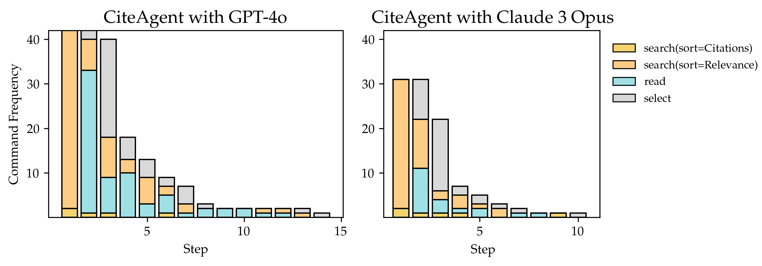Performance across Language Models. Comparing the performance of LMs across columns in Table 4, GPT-4o demonstrates the highest accuracy when it has access to both read and search commands, outperforming other LMs by a wide margin. This finding aligns with previous research [88], which shows that GPT-4 powered agents excel in solving software issues. Notably, GPT-4o achieves high performance across settings even though CiteME consists exclusively of samples that GPT-4o cannot predict correctly without commands; its 0% performance without commands and demonstration trajectory is by design. However, LMs outperforming the SPECTER models purely by autoregressive generation provides evidence that LMs act as implicit knowledge bases with sufficient capacity [68]. Peformance across Demonstrations. Comparing the performance between w/o Demo and w/ Demo rows in Table 4, we observe that LLaMA and Claude surprisingly perform worse when provided with a demonstration trajectory in the prompt. This may be due to the increased prompt length, which complicates the detection of important information [52]. LLaMA-3-70b incurs a performance drop to 2.5% due to combined history extending beyond its context length, resulting in errors. However, GPT-4o effectively utilizes demonstrations, which improves its accuracy. Performance across Commands. GPT-4o is the only LM whose accuracy improves with access to more commands, allowing it to read full papers. CiteAgent with GPT-4o creatively uses its commands across test samples, demonstrating command behaviors not shown in the demonstration trajectory (see Figure 4). It frequently refines its searches based on previous results and occasionally reads multiple papers before making a selection. In contrast, Claude 3 Opus is less effective in utilizing additional commands, likely due to difficulties in detecting important information [52]. <details> <summary>extracted/5974968/figures/trajectory_analysis.png Details</summary>  ### Visual Description ## Diagram: Search Strategy Workflow Sequences ### Overview The image displays a technical diagram illustrating five distinct sequences or workflows for a search-and-select process. Each sequence is presented as a vertical column of action blocks, grouped by colored dashed borders. The diagram visually compares different strategies for conducting searches (sorted by "Citations" or "Relevance"), reading results, and making a final selection. ### Components/Axes * **Structure:** Five vertical columns, each representing a discrete workflow sequence. * **Column Borders (Grouping):** * Column 1 (Far Left): Gray dashed border. * Columns 2 & 3: Green dashed borders. * Columns 4 & 5: Red dashed borders. * **Action Blocks (Color-Coded):** * **Yellow:** `search sort=Citations` * **Orange:** `search sort=Relevance` * **Light Blue:** `read` * **Gray:** `select` * **Layout:** Blocks are stacked vertically within each column, indicating a top-to-bottom sequence of actions. ### Detailed Analysis **Column 1 (Gray Border):** 1. `search sort=Citations` (Yellow) 2. `read` (Light Blue) 3. `search sort=Citations` (Yellow) 4. `select` (Gray) **Column 2 (Green Border):** 1. `search sort=Citations` (Yellow) 2. `search sort=Relevance` (Orange) 3. `read` (Light Blue) 4. `select` (Gray) **Column 3 (Green Border):** 1. `search sort=Relevance` (Orange) 2. `read` (Light Blue) 3. `search sort=Relevance` (Orange) 4. `read` (Light Blue) 5. `search sort=Relevance` (Orange) 6. `search sort=Relevance` (Orange) 7. `select` (Gray) **Column 4 (Red Border):** 1. `search sort=Relevance` (Orange) 2. `search sort=Relevance` (Orange) 3. `search sort=Relevance` (Orange) 4. `read` (Light Blue) 5. `select` (Gray) **Column 5 (Red Border):** 1. `search sort=Citations` (Yellow) 2. `search sort=Citations` (Yellow) 3. `search sort=Citations` (Yellow) 4. `read` (Light Blue) 5. `select` (Gray) ### Key Observations 1. **Action Repetition:** The number of search actions before the final "read" and "select" varies significantly between sequences, from a minimum of two to a maximum of five. 2. **Strategy Specialization:** The red-bordered columns (4 & 5) show highly specialized strategies. Column 4 uses only `sort=Relevance` searches, while Column 5 uses only `sort=Citations` searches. 3. **Mixed Strategy:** The green-bordered columns (2 & 3) employ mixed search strategies. Column 2 mixes one Citations and one Relevance search. Column 3 is the most complex, featuring five Relevance searches interspersed with two read actions. 4. **Baseline/Control:** The gray-bordered Column 1 appears to be a simpler or baseline strategy, using two Citations searches with a single read action in between. 5. **Common Termination:** All five sequences conclude with a single `read` action followed immediately by a `select` action. ### Interpretation This diagram models and compares different algorithmic or user-driven approaches to an information retrieval task. The core question it addresses is: **What is the optimal sequence and mix of search strategies (sorted by citation count vs. relevance) to efficiently find and select relevant information?** * **Efficiency vs. Thoroughness:** The sequences represent a spectrum. Column 1 is lean and fast. Column 3 is exhaustive and iterative, suggesting a thorough, possibly academic, research process. Columns 4 and 5 represent committed, single-metric strategies. * **The Role of "Read":** The `read` action is a critical evaluation step. Its placement varies—sometimes after every search (Column 3), sometimes only once at the end (Columns 4 & 5). This suggests a trade-off between continuous evaluation and batch processing. * **Grouping Significance:** The border colors likely denote categories of strategies. Green may indicate "balanced" or "adaptive" approaches, red indicates "specialized" or "extreme" approaches, and gray may indicate a "standard" or "control" method. * **Underlying Process:** The workflow implies a system where an agent (human or AI) performs searches, evaluates results through reading, and iterates based on findings before making a final selection. The diagram is a tool for analyzing the cost (in steps) and potential effectiveness of each procedural recipe. 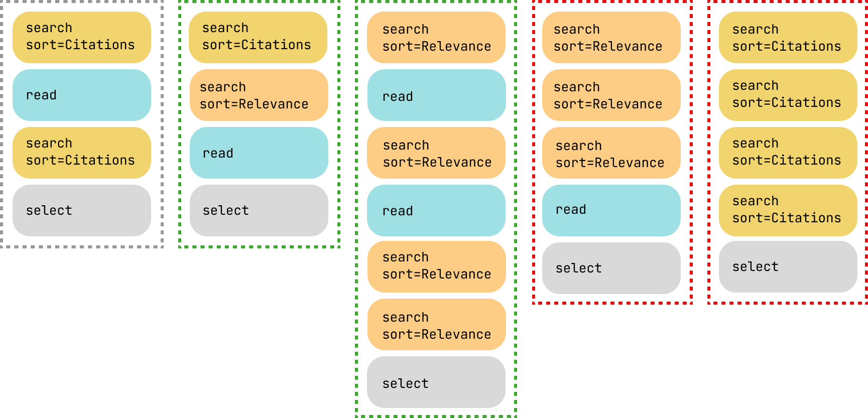</details> Figure 4: Five CiteAgent trajectories on five different samples. CiteAgent often exhibits behavior not shown in the demonstration given in the prompt, for example: searching by citation count and then by relevance, and searching multiple times in a row. Gray dotted box: prompt demonstration; green dotted boxes: CiteAgent succeeds; red dotted boxes: CiteAgent fails. ### 5.1 Error Analysis To better identify CiteAgent’s shortcomings, we analyze 50 randomly chosen CiteME samples from the best performing CiteAgent (using the GPT-4o backbone, with demonstrations, Search and Read commands) failed to solve correctly. We classify each error into three types based on CiteAgent’s searches, its predicted paper and the justification provided: Error Type 1: Misunderstands the Excerpt. This category accounts for 50% of the errors. It occurs when CiteAgent focuses on irrelevant parts of the excerpt or omits critical details. For example, in the following excerpt: The pioneering work of Reed et al. [37] approached text-guided image generation by training a conditional GAN [CITATION], conditioned by text embeddings obtained from a pretrained encoder. CiteAgent searches for "Reed text-guided image generation conditional GAN" instead of "conditional GAN". It mistakes "Reed" as relevant to the current citation although it pertains to the previous one. Error Type 2: Understands the Excerpt but Stops Prematurely. In 32% of cases, CiteAgent searches for the correct term, but it stops at a roughly matching paper instead of the exact match. For example, in the following excerpt: Using Gaussian noise and blur, [CITATION] demonstrate the superior robustness of human vision to convolutional networks, even after networks are fine-tuned on Gaussian noise or blur. CiteAgent found a paper comparing human and machine robustness but missed that it did not cover fine-tuned networks. Notably, this paper referenced the correct target paper, meaning CiteAgent could have found the right answer with just one more step if it had properly understood the paper it was reading. Moreover, in 12.5% of such cases, the correct paper appeared in the search results but was not chosen by CiteAgent. Error Type 3: Finds the Correct Citation but Stops Prematurely. The last 18% of errors occur when CiteAgent reads an abstract or paper and finds the correct citation; however, instead of doing another search, it selects the paper that cites the correct citation and stops searching. For example, in the following excerpt: [CITATION] investigates transformers’ theoretical expressiveness, showing that transformers cannot robustly model noncounter-free regular languages even when allowing infinite precision. CiteAgent finds a paper discussing the target paper and reports it, but it stops at the citing paper instead of searching for the correct target paper. For instance, it reports: ".. specifically mentioning Hahn’s work on transformers’ classification decisions becoming ineffective over longer input strings. This fits well with the description in the excerpt.." but it selects the citing paper instead of finding Hahn’s work, which is the correct target paper. Technical Errors. Aside from comprehension errors that stem from a lack of understanding an excerpt, 5.8% of runs encountered technical issues. Occasionally, the LM formats responses incorrectly, making them unparseable by the system. Additionally, the Semantic Scholar API has inconsistencies, such as not providing open access PDF links when available or linking to non-existent web pages. Further details on these technical errors are provided in Appendix F. <details> <summary>extracted/5974968/figures/4o_claude.png Details</summary>  ### Visual Description ## Stacked Bar Charts: CiteAgent Command Frequency by Step ### Overview The image displays two side-by-side stacked bar charts comparing the frequency of different commands used by an agent called "CiteAgent" when powered by two different large language models: GPT-4o (left chart) and Claude 3 Opus (right chart). The charts track command usage across sequential steps of a task. ### Components/Axes * **Chart Titles:** * Left Chart: "CiteAgent with GPT-4o" * Right Chart: "CiteAgent with Claude 3 Opus" * **Y-Axis (Both Charts):** Labeled "Command Frequency". The axis has major tick marks at 10, 20, 30, and 40. * **X-Axis (Both Charts):** Labeled "Step". The axis has major tick marks at 5, 10, and 15. The bars are plotted for each integer step from 1 onward. * **Legend (Located to the right of the second chart):** Defines four command types with associated colors: * `search(sort=Citations)`: Yellow/Gold color. * `search(sort=Relevance)`: Light Orange/Peach color. * `read`: Light Blue/Cyan color. * `select`: Light Gray color. ### Detailed Analysis **Data Extraction (Approximate Values):** The values below are estimated from the visual height of each colored segment within the stacked bars. **Chart 1: CiteAgent with GPT-4o** * **Step 1:** Total ~42. `search(sort=Citations)` ~2, `search(sort=Relevance)` ~40. * **Step 2:** Total ~40. `search(sort=Citations)` ~1, `search(sort=Relevance)` ~6, `read` ~33. * **Step 3:** Total ~40. `search(sort=Citations)` ~1, `search(sort=Relevance)` ~8, `read` ~9, `select` ~22. * **Step 4:** Total ~18. `search(sort=Relevance)` ~10, `read` ~8. * **Step 5:** Total ~13. `search(sort=Relevance)` ~3, `read` ~10. * **Step 6:** Total ~9. `search(sort=Relevance)` ~5, `read` ~4. * **Step 7:** Total ~7. `search(sort=Relevance)` ~2, `read` ~5. * **Step 8:** Total ~3. `search(sort=Relevance)` ~1, `read` ~2. * **Step 9:** Total ~2. `read` ~2. * **Step 10:** Total ~2. `read` ~2. * **Step 11:** Total ~2. `search(sort=Relevance)` ~1, `read` ~1. * **Step 12:** Total ~2. `search(sort=Relevance)` ~1, `read` ~1. * **Step 13:** Total ~2. `search(sort=Relevance)` ~1, `read` ~1. * **Step 14:** Total ~1. `select` ~1. * **Step 15:** Total ~1. `select` ~1. **Chart 2: CiteAgent with Claude 3 Opus** * **Step 1:** Total ~31. `search(sort=Citations)` ~2, `search(sort=Relevance)` ~29. * **Step 2:** Total ~31. `search(sort=Citations)` ~1, `search(sort=Relevance)` ~10, `read` ~11, `select` ~9. * **Step 3:** Total ~22. `search(sort=Relevance)` ~2, `read` ~4, `select` ~16. * **Step 4:** Total ~7. `search(sort=Relevance)` ~3, `read` ~2, `select` ~2. * **Step 5:** Total ~5. `search(sort=Relevance)` ~1, `read` ~2, `select` ~2. * **Step 6:** Total ~3. `search(sort=Relevance)` ~2, `read` ~1. * **Step 7:** Total ~2. `search(sort=Relevance)` ~1, `read` ~1. * **Step 8:** Total ~1. `read` ~1. * **Step 9:** Total ~1. `search(sort=Relevance)` ~1. * **Step 10:** Total ~1. `select` ~1. **Trend Verification:** * **`search(sort=Citations)` (Yellow):** Appears only in the first step for both models, with a very low frequency (~2). * **`search(sort=Relevance)` (Orange):** Dominates the first step for both models. Its frequency declines sharply after step 1 for GPT-4o and after step 2 for Claude 3 Opus, becoming minimal or absent in later steps. * **`read` (Blue):** Shows a significant peak in the early steps (Step 2 for GPT-4o, Step 2 for Claude 3 Opus). Its usage then declines steadily, persisting slightly longer than other commands in the GPT-4o sequence. * **`select` (Gray):** Has a major peak in Step 3 for both models. It appears sporadically in later steps for GPT-4o and has a smaller presence in early steps for Claude 3 Opus. ### Key Observations 1. **Step Count:** The GPT-4o agent runs for 15 steps, while the Claude 3 Opus agent concludes after 10 steps. 2. **Initial Command Distribution:** Both models start with a heavy emphasis on `search(sort=Relevance)`. GPT-4o's first step is almost exclusively this command, while Claude 3 Opus's first step includes a small amount of `search(sort=Citations)`. 3. **Peak of `read` and `select`:** Both models exhibit a clear pattern where the `read` command peaks at Step 2, followed by the `select` command peaking at Step 3. This suggests a common workflow: search, then read results, then select relevant items. 4. **Decay Pattern:** Command frequency for all types decays as steps increase. The decay appears more gradual for GPT-4o, which sustains low-level activity (mainly `read` and `search(sort=Relevance)`) through step 13. Claude 3 Opus's activity drops off more sharply after step 5. 5. **Late-Stage Activity:** In the GPT-4o chart, the final two steps (14, 15) consist solely of the `select` command, suggesting a final filtering or decision phase. ### Interpretation The data suggests a multi-stage research or citation-finding workflow executed by the CiteAgent. The consistent early peak of `search(sort=Relevance)` indicates an initial broad information gathering phase. The subsequent peaks of `read` and then `select` imply a logical progression: after retrieving search results, the agent reads them in detail and then selects the most pertinent ones. The difference in total steps and decay rate may indicate that the underlying model influences the agent's efficiency or thoroughness. The GPT-4o-powered agent engages in a longer, more drawn-out process with sustained low-level activity, potentially indicating more iterative refinement or a longer "tail" of processing. The Claude 3 Opus-powered agent completes its task in fewer steps with a sharper decline, which could suggest a more focused or decisive execution pattern. The exclusive use of `search(sort=Citations)` only at the very start for both models is notable; it may be used for an initial high-impact search before switching to relevance-based sorting for the remainder of the task. </details> Figure 5: CiteAgent trajectories on samples that were correctly predicted reveals differences in model behavior. GPT-4o reads more frequently than Claude 3 Opus and can correctly predict papers even after performing many actions. ### 5.2 Analyzing the Succesful Runs Manually examining the instances that were correctly predicted by GPT-4o and Claude 3 Opus (Figure 5) provides insights into how the LMs use commands they were given. First, we confirm the results presented in Table 4: GPT-4o frequently reads papers before it correctly predicts a citation. Second, when both LMs correctly predict a paper, they usually take just 5 steps or fewer to do so. This could stem from LMs loss of important details when given a long context window [52]. CiteAgent’s trajectories on CiteME enable us to analyze the shortcomings of GPT-4o and other SoTA LMs. These range from understanding fine details in text (Type 1 and Type 2 Errors), to not completely understanding the task (Type 3 Errors), to being unable to use commands (Technical Errors). Correcting these errors could improve the utility of LMs on CiteME and for other related tasks. ### 5.3 Benchmarking Reasoning Capability Improvements with Latest Models Table 5: Accuracy (in %) of newly released LMs on CiteME. | Commands | Method No Commands | w/o Demo | Claude-3.5-Sonnet 8.4 | LLaMa-3.1-70B 3.4 | o1-mini 16.0 | o1-preview 38.7 | | --- | --- | --- | --- | --- | --- | --- | | w/ Demo | 9.2 | 8.4 | 10.9 | – | | | | Search Only | w/o Demo | 36.1 | 29.4 | 25.2 | – | | | w/ Demo | 43.7 | 29.4 | 32.8 | – | | | | Search and Read | w/o Demo | 37.0 | 22.7 | 26.9 | – | | | w/ Demo | 40.3 | 27.7 | 34.5 | 61.3 | | | We compare the latest LLMs on the CiteME benchmark (Table 5) and find that Claude 3.5 Sonnet outperforms the previous best, Claude 3 Opus. This improvement stems from better generalization, as Sonnet achieves 9.2% without internet access, compared to Opus’ 18.5%. Similarly, LLaMa-3.1-70B shows significant gains of 8% over LLaMa-3.0-70B, highlighting enhanced reasoning capabilities. However, GPT-o1, while performing well on CiteME, appears to have memorized 38.7% of the dataset, making its 61.3% benchmark performance less clear in terms of true improvement compared to GPT-4o. ## 6 Related Work Recent work has made substantial progress in developing methods and datasets to assist researchers in paper writing and literature review [8, 12, 87] or act as tutors [18]. Early work [48, 56] showed that researchers automatically retrieved topics and papers considered highly relevant to their work. Other studies included methods that assist researchers in finding new ideas [34], understanding certain topics [62], provide expert answers backed up by evidence [55] or clarifying a paper’s related work by supplementing it with more information and focus [15, 67]. Closer to our line of research, prior studies developed methods for substantiating specific claims using evidence from published papers [75, 83, 85, 84, 91, 24, 39, 45]. Retrieval-augmented LMs [49, 11, 30] are also popularly used to ground claims with real-world evidence (see [60] for a survey). Chen et al. [16] built a web-based retrieval-augmented pipeline for fact verification; this contrasts with methods that use a static dataset for claim retrieval and verification [36, 5]. Concurrent to this work, Ajith et al. [2] build a retrieval benchmark consisting of questions about discoveries shown in specific machine learning papers. Paper discovery is a crucial component of systems that automate scientific research as shown in [10, 47, 54, 61, 78]. CiteME plays an important role in developing better tools for paper discovery, and provides a way to effectively measure their efficiency. Currently, these systems are tested as a whole, without isolating the tools responsible for scientific discovery. CiteME allows us to evaluate components within them independently – and we discover that current LM Agents are not yet ready for automated paper discovery, leading to serious gaps in end-to-end automated research pipelines. In addition, most existing LM benchmarks are saturated, with most LMs scoring 80-95% on them [43, 38, 20]. There is a need in the AI community to show what properties LMs currently lack, to show LM developers what aspects they should work on. On CiteME, the best LMs get less than 40%, clearly indicating to developers an important task that they could improve LMs on, while also providing an indicator they can use to track progress. Context-aware Recommendation. Relevant to our research focus, [57, 64, 37] take as input documents or parts thereof and recommend papers that are likely to be cited, often referred to as context-aware citation recommendation [51, 26, 89, 28, 42, 65, 33]. The text inputs we use in CiteME resemble those used in [42, 65, 80], which contain a few sentences with a masked out citation. However, CiteME differs because it uses excerpts containing only one unambiguous citation, making the context sufficient to identify the cited paper. Furthermore, our work explores agents with access to real-time paper information through tools like Semantic Scholar. This is crucial for real-time use since thousands of new papers are indexed by arXiv monthly (e.g., 8,895 papers in March 2024 under the cs category) [4]. Most previous approaches would be impractical due to the need for retraining with every new paper issuance. Citation Attribution Datasets. A variety of datasets contain text excerpts from scientific papers and corresponding citations [32, 31, 9, 40, 72, 44, 42, 33]. There are many crucial distinctions between the aforementioned datasets and CiteME, with the main one being that CiteME is composed of manually selected excerpts that clearly reference a paper. To our best knowledge, CiteME is the only dataset that reports human accuracy on the benchmark. Additionally, the excerpts in CiteME are mostly taken from papers published in the last few years (see Figure 2), whereas other datasets contain older papers. For example, the arXiv dataset [33] includes papers from 1991-2020, and FullTextPaperRead [42] contains papers from 2007-2017. This currency is particularly relevant in rapidly evolving fields like machine learning. The key distinction between the dataset and methods we present compared to previous works is their real life applicability. Our agent is based on SoTA LMs, needs no extra training, and can use a search engine, all of which make it easily applicable to real-world settings. ## 7 Conclusion This work introduces a citation attribution benchmark containing manually curated text excerpts that unambiguously refer to a single other paper. We posit that methods that succeed on CiteME are likely to be highly useful in assisting researchers with real-world ML-specific attribution tasks but also generally useful in finding sources for generic claims. Further, our CiteAgent autonomous system can search the Internet for and read papers, which we show to significantly enhance the abilities of LMs on CiteME. We anticipate that this work will lead to LMs that are more accurate research assistants in the vital scholarship tasks of attribution. ## Author Contributions The project was initiated by Andreas Hochlehnert and Ori Press, with feedback from Ameya Prabhu, Ofir Press, and Matthias Bethge. The dataset was created by Ori Press and Ameya Prabhu, with help from Vishaal Udandarao and Ofir Press. Experiments were carried out by Andreas Hochlehnert, with help from Ameya Prabhu. All authors contributed to the final manuscript. ## Acknowledgements The authors thank the International Max Planck Research School for Intelligent Systems (IMPRS-IS) for supporting Ori Press, Andreas Hochlehnert, and Vishaal Udandarao. Andreas Hochlehnert is supported by the Carl Zeiss Foundation through the project “Certification and Foundations of Safe ML Systems”. Matthias Bethge acknowledges financial support via the Open Philanthropy Foundation funded by the Good Ventures Foundation. Vishaal Udandarao was supported by a Google PhD Fellowship in Machine Intelligence. Matthias Bethge is a member of the Machine Learning Cluster of Excellence, funded by the Deutsche Forschungsgemeinschaft (DFG, German Research Foundation) under Germany’s Excellence Strategy – EXC number 2064/1 – Project number 390727645 and acknowledges support by the German Research Foundation (DFG): SFB 1233, Robust Vision: Inference Principles and Neural Mechanisms, TP 4, Project No: 276693517. This work was supported by the Tübingen AI Center. The authors declare no conflicts of interests. ## References - Achiam et al. [2023] Josh Achiam, Steven Adler, Sandhini Agarwal, Lama Ahmad, Ilge Akkaya, Florencia Leoni Aleman, Diogo Almeida, Janko Altenschmidt, Sam Altman, Shyamal Anadkat, et al. Gpt-4 technical report. arXiv preprint arXiv:2303.08774, 2023. - Ajith et al. [2024] Anirudh Ajith, Mengzhou Xia, Alexis Chevalier, Tanya Goyal, Danqi Chen, and Tianyu Gao. Litsearch: A retrieval benchmark for scientific literature search. arXiv preprint arXiv:2407.18940, 2024. - Anthropic [2024] Anthropic. Introducing the next generation of claude, 2024. URL https://www.anthropic.com/news/claude-3-family. - arXiv [2024] arXiv. arxiv monthly submission statistics, 2024. URL https://arxiv.org/stats/monthly_submissions. Accessed: 2024-05-27. - Atanasova [2024] Pepa Atanasova. Generating fact checking explanations. In Accountable and Explainable Methods for Complex Reasoning over Text, pages 83–103. Springer, 2024. - Augenstein et al. [2023] Isabelle Augenstein, Timothy Baldwin, Meeyoung Cha, Tanmoy Chakraborty, Giovanni Luca Ciampaglia, David Corney, Renee DiResta, Emilio Ferrara, Scott Hale, Alon Halevy, et al. Factuality challenges in the era of large language models. arXiv preprint arXiv:2310.05189, 2023. - Bengio [2013] Yoshua Bengio. Deep learning of representations: Looking forward. In International conference on statistical language and speech processing, pages 1–37. Springer, 2013. - Bhagavatula et al. [2018] Chandra Bhagavatula, Sergey Feldman, Russell Power, and Waleed Ammar. Content-based citation recommendation. arXiv preprint arXiv:1802.08301, 2018. - Bird et al. [2008] Steven Bird, Robert Dale, Bonnie Dorr, Bryan Gibson, Mark Joseph, Min-Yen Kan, Dongwon Lee, Brett Powley, Dragomir Radev, and Yee Fan Tan. The ACL Anthology reference corpus: A reference dataset for bibliographic research in computational linguistics. In Nicoletta Calzolari, Khalid Choukri, Bente Maegaard, Joseph Mariani, Jan Odijk, Stelios Piperidis, and Daniel Tapias, editors, Proceedings of the Sixth International Conference on Language Resources and Evaluation (LREC’08), Marrakech, Morocco, May 2008. European Language Resources Association (ELRA). URL http://www.lrec-conf.org/proceedings/lrec2008/pdf/445_paper.pdf. - Boiko et al. [2023] Daniil A Boiko, Robert MacKnight, Ben Kline, and Gabe Gomes. Autonomous chemical research with large language models. Nature, 624(7992):570–578, 2023. - Borgeaud et al. [2022] Sebastian Borgeaud, Arthur Mensch, Jordan Hoffmann, Trevor Cai, Eliza Rutherford, Katie Millican, George Bm Van Den Driessche, Jean-Baptiste Lespiau, Bogdan Damoc, Aidan Clark, et al. Improving language models by retrieving from trillions of tokens. In International conference on machine learning, pages 2206–2240. PMLR, 2022. - Boyko et al. [2023] James Boyko, Joseph Cohen, Nathan Fox, Maria Han Veiga, Jennifer I Li, Jing Liu, Bernardo Modenesi, Andreas H Rauch, Kenneth N Reid, Soumi Tribedi, et al. An interdisciplinary outlook on large language models for scientific research. arXiv preprint arXiv:2311.04929, 2023. - Bui et al. [2016] Thang Bui, Daniel Hernández-Lobato, Jose Hernandez-Lobato, Yingzhen Li, and Richard Turner. Deep gaussian processes for regression using approximate expectation propagation. In International conference on machine learning, pages 1472–1481. PMLR, 2016. - Burt et al. [2020] David R Burt, Carl Edward Rasmussen, and Mark Van Der Wilk. Convergence of sparse variational inference in gaussian processes regression. Journal of Machine Learning Research, 21(131):1–63, 2020. - Chang et al. [2023] Joseph Chee Chang, Amy X Zhang, Jonathan Bragg, Andrew Head, Kyle Lo, Doug Downey, and Daniel S Weld. Citesee: Augmenting citations in scientific papers with persistent and personalized historical context. In Proceedings of the 2023 CHI Conference on Human Factors in Computing Systems, pages 1–15, 2023. - Chen et al. [2023] Jifan Chen, Grace Kim, Aniruddh Sriram, Greg Durrett, and Eunsol Choi. Complex claim verification with evidence retrieved in the wild. arXiv preprint arXiv:2305.11859, 2023. - Chen et al. [2021] Mark Chen, Jerry Tworek, Heewoo Jun, Qiming Yuan, Henrique Ponde de Oliveira Pinto, Jared Kaplan, Harri Edwards, Yuri Burda, Nicholas Joseph, Greg Brockman, et al. Evaluating large language models trained on code. arXiv preprint arXiv:2107.03374, 2021. - Chevalier et al. [2024] Alexis Chevalier, Jiayi Geng, Alexander Wettig, Howard Chen, Sebastian Mizera, Toni Annala, Max Jameson Aragon, Arturo Rodríguez Fanlo, Simon Frieder, Simon Machado, et al. Language models as science tutors. arXiv preprint arXiv:2402.11111, 2024. - Chowdhery et al. [2023] Aakanksha Chowdhery, Sharan Narang, Jacob Devlin, Maarten Bosma, Gaurav Mishra, Adam Roberts, Paul Barham, Hyung Won Chung, Charles Sutton, Sebastian Gehrmann, et al. Palm: Scaling language modeling with pathways. Journal of Machine Learning Research, 24(240):1–113, 2023. - Cobbe et al. [2021] Karl Cobbe, Vineet Kosaraju, Mohammad Bavarian, Mark Chen, Heewoo Jun, Lukasz Kaiser, Matthias Plappert, Jerry Tworek, Jacob Hilton, Reiichiro Nakano, et al. Training verifiers to solve math word problems. arXiv preprint arXiv:2110.14168, 2021. - Cohan et al. [2020] Arman Cohan, Sergey Feldman, Iz Beltagy, Doug Downey, and Daniel S Weld. Specter: Document-level representation learning using citation-informed transformers. arXiv preprint arXiv:2004.07180, 2020. - Cohen et al. [2010] K Bretonnel Cohen, Helen L Johnson, Karin Verspoor, Christophe Roeder, and Lawrence E Hunter. The structural and content aspects of abstracts versus bodies of full text journal articles are different. BMC bioinformatics, 11:1–10, 2010. - Cox [1958] David R Cox. The regression analysis of binary sequences. Journal of the Royal Statistical Society Series B: Statistical Methodology, 20(2):215–232, 1958. - [24] Sam Cox, Michael Hammerling, Jakub Lála, Jon Laurent, Sam Rodriques, Matt Rubashkin, and Andrew White. Wikicrow: Automating synthesis of human scientific knowledge. - Dakhel et al. [2023] Arghavan Moradi Dakhel, Vahid Majdinasab, Amin Nikanjam, Foutse Khomh, Michel C Desmarais, and Zhen Ming Jack Jiang. Github copilot ai pair programmer: Asset or liability? Journal of Systems and Software, 203:111734, 2023. - Ebesu and Fang [2017] Travis Ebesu and Yi Fang. Neural citation network for context-aware citation recommendation. In Proceedings of the 40th international ACM SIGIR conference on research and development in information retrieval, pages 1093–1096, 2017. - Färber and Jatowt [2020] Michael Färber and Adam Jatowt. Citation recommendation: approaches and datasets. International Journal on Digital Libraries, 21(4):375–405, 2020. - Färber and Sampath [2020] Michael Färber and Ashwath Sampath. Hybridcite: A hybrid model for context-aware citation recommendation. In Proceedings of the ACM/IEEE joint conference on digital libraries in 2020, pages 117–126, 2020. - Fenniak et al. [2024] Mathieu Fenniak, Matthew Stamy, pubpub zz, Martin Thoma, Matthew Peveler, exiledkingcc, and pypdf Contributors. The pypdf library, 2024. URL https://pypi.org/project/pypdf/. See https://pypdf.readthedocs.io/en/latest/meta/CONTRIBUTORS.html for all contributors. - Gao et al. [2023] Tianyu Gao, Howard Yen, Jiatong Yu, and Danqi Chen. Enabling large language models to generate text with citations. arXiv preprint arXiv:2305.14627, 2023. - Gehrke et al. [2003] Johannes Gehrke, Paul Ginsparg, and Jon Kleinberg. Overview of the 2003 kdd cup. Acm Sigkdd Explorations Newsletter, 5(2):149–151, 2003. - Giles et al. [1998] C Lee Giles, Kurt D Bollacker, and Steve Lawrence. Citeseer: An automatic citation indexing system. In Proceedings of the third ACM conference on Digital libraries, pages 89–98, 1998. - Gu et al. [2022] Nianlong Gu, Yingqiang Gao, and Richard HR Hahnloser. Local citation recommendation with hierarchical-attention text encoder and scibert-based reranking. In European conference on information retrieval, pages 274–288. Springer, 2022. - Gu and Krenn [2024] Xuemei Gu and Mario Krenn. Generation and human-expert evaluation of interesting research ideas using knowledge graphs and large language models. arXiv preprint arXiv:2405.17044, 2024. - Guu et al. [2015] Kelvin Guu, John Miller, and Percy Liang. Traversing knowledge graphs in vector space. arXiv preprint arXiv:1506.01094, 2015. - Hanselowski et al. [2019] Andreas Hanselowski, Christian Stab, Claudia Schulz, Zile Li, and Iryna Gurevych. A richly annotated corpus for different tasks in automated fact-checking. arXiv preprint arXiv:1911.01214, 2019. - He et al. [2010] Qi He, Jian Pei, Daniel Kifer, Prasenjit Mitra, and Lee Giles. Context-aware citation recommendation. In Proceedings of the 19th international conference on World wide web, pages 421–430, 2010. - Hendrycks et al. [2021] Dan Hendrycks, Collin Burns, Saurav Kadavath, Akul Arora, Steven Basart, Eric Tang, Dawn Song, and Jacob Steinhardt. Measuring mathematical problem solving with the math dataset. arXiv preprint arXiv:2103.03874, 2021. - Huang et al. [2024] Chengyu Huang, Zeqiu Wu, Yushi Hu, and Wenya Wang. Training language models to generate text with citations via fine-grained rewards. arXiv preprint arXiv:2402.04315, 2024. - Huang et al. [2014] Wenyi Huang, Zhaohui Wu, Prasenjit Mitra, and C Lee Giles. Refseer: A citation recommendation system. In IEEE/ACM joint conference on digital libraries, pages 371–374. IEEE, 2014. - Iyyer et al. [2014] Mohit Iyyer, Jordan Boyd-Graber, Leonardo Claudino, Richard Socher, and Hal Daumé III. A neural network for factoid question answering over paragraphs. In Proceedings of the 2014 conference on empirical methods in natural language processing (EMNLP), pages 633–644, 2014. - Jeong et al. [2020] Chanwoo Jeong, Sion Jang, Eunjeong Park, and Sungchul Choi. A context-aware citation recommendation model with bert and graph convolutional networks. Scientometrics, 124:1907–1922, 2020. - Joshi et al. [2017] Mandar Joshi, Eunsol Choi, Daniel S Weld, and Luke Zettlemoyer. Triviaqa: A large scale distantly supervised challenge dataset for reading comprehension. arXiv preprint arXiv:1705.03551, 2017. - Kang et al. [2018] Dongyeop Kang, Waleed Ammar, Bhavana Dalvi, Madeleine Van Zuylen, Sebastian Kohlmeier, Eduard Hovy, and Roy Schwartz. A dataset of peer reviews (peerread): Collection, insights and nlp applications. arXiv preprint arXiv:1804.09635, 2018. - Khalifa et al. [2024] Muhammad Khalifa, David Wadden, Emma Strubell, Honglak Lee, Lu Wang, Iz Beltagy, and Hao Peng. Source-aware training enables knowledge attribution in language models. arXiv preprint arXiv:2404.01019, 2024. - Kinney et al. [2023] Rodney Kinney, Chloe Anastasiades, Russell Authur, Iz Beltagy, Jonathan Bragg, Alexandra Buraczynski, Isabel Cachola, Stefan Candra, Yoganand Chandrasekhar, Arman Cohan, et al. The semantic scholar open data platform. arXiv preprint arXiv:2301.10140, 2023. - Lála et al. [2023] Jakub Lála, Odhran O’Donoghue, Aleksandar Shtedritski, Sam Cox, Samuel G Rodriques, and Andrew D White. Paperqa: Retrieval-augmented generative agent for scientific research. arXiv preprint arXiv:2312.07559, 2023. - Learning [2011] Machine Learning. Apolo: Making sense of large network data by combining. 2011. - Lewis et al. [2020] Patrick Lewis, Ethan Perez, Aleksandra Piktus, Fabio Petroni, Vladimir Karpukhin, Naman Goyal, Heinrich Küttler, Mike Lewis, Wen-tau Yih, Tim Rocktäschel, et al. Retrieval-augmented generation for knowledge-intensive nlp tasks. Advances in Neural Information Processing Systems, 33:9459–9474, 2020. - Lin [2009] Jimmy Lin. Is searching full text more effective than searching abstracts? BMC bioinformatics, 10:1–15, 2009. - Liu et al. [2015] Haifeng Liu, Xiangjie Kong, Xiaomei Bai, Wei Wang, Teshome Megersa Bekele, and Feng Xia. Context-based collaborative filtering for citation recommendation. Ieee Access, 3:1695–1703, 2015. - Liu et al. [2024] Nelson F Liu, Kevin Lin, John Hewitt, Ashwin Paranjape, Michele Bevilacqua, Fabio Petroni, and Percy Liang. Lost in the middle: How language models use long contexts. Transactions of the Association for Computational Linguistics, 12:157–173, 2024. - Lloyd [1982] Stuart Lloyd. Least squares quantization in pcm. IEEE transactions on information theory, 28(2):129–137, 1982. - M. Bran et al. [2024] Andres M. Bran, Sam Cox, Oliver Schilter, Carlo Baldassari, Andrew D White, and Philippe Schwaller. Augmenting large language models with chemistry tools. Nature Machine Intelligence, pages 1–11, 2024. - Malaviya et al. [2023] Chaitanya Malaviya, Subin Lee, Sihao Chen, Elizabeth Sieber, Mark Yatskar, and Dan Roth. Expertqa: Expert-curated questions and attributed answers. arXiv preprint arXiv:2309.07852, 2023. - Mayr [2014] Philipp Mayr. Are topic-specific search term, journal name and author name recommendations relevant for researchers? arXiv preprint arXiv:1408.4440, 2014. - McNee et al. [2002] Sean M McNee, Istvan Albert, Dan Cosley, Prateep Gopalkrishnan, Shyong K Lam, Al Mamunur Rashid, Joseph A Konstan, and John Riedl. On the recommending of citations for research papers. In Proceedings of the 2002 ACM conference on Computer supported cooperative work, pages 116–125, 2002. - Medić and Šnajder [2020] Zoran Medić and Jan Šnajder. Improved local citation recommendation based on context enhanced with global information. In Proceedings of the first workshop on scholarly document processing, pages 97–103, 2020. - Metzler et al. [2021] Donald Metzler, Yi Tay, Dara Bahri, and Marc Najork. Rethinking search: making domain experts out of dilettantes. In Acm sigir forum, volume 55, pages 1–27. ACM New York, NY, USA, 2021. - Mialon et al. [2023] Grégoire Mialon, Roberto Dessì, Maria Lomeli, Christoforos Nalmpantis, Ram Pasunuru, Roberta Raileanu, Baptiste Rozière, Timo Schick, Jane Dwivedi-Yu, Asli Celikyilmaz, et al. Augmented language models: a survey. arXiv preprint arXiv:2302.07842, 2023. - Miret and Krishnan [2024] Santiago Miret and NM Krishnan. Are llms ready for real-world materials discovery? arXiv preprint arXiv:2402.05200, 2024. - Murthy et al. [2022] Sonia K Murthy, Kyle Lo, Daniel King, Chandra Bhagavatula, Bailey Kuehl, Sophie Johnson, Jonathan Borchardt, Daniel S Weld, Tom Hope, and Doug Downey. Accord: A multi-document approach to generating diverse descriptions of scientific concepts. arXiv preprint arXiv:2205.06982, 2022. - Muthukadan [2011] Baiju Muthukadan. Selenium with python. https://selenium-python.readthedocs.io/, 2011. - Nallapati et al. [2008] Ramesh M Nallapati, Amr Ahmed, Eric P Xing, and William W Cohen. Joint latent topic models for text and citations. In Proceedings of the 14th ACM SIGKDD international conference on Knowledge discovery and data mining, pages 542–550, 2008. - Ohagi and Aizawa [2022] Masaya Ohagi and Akiko Aizawa. Pre-trained transformer-based citation context-aware citation network embeddings. In Proceedings of the 22nd ACM/IEEE Joint Conference on Digital Libraries, pages 1–5, 2022. - Ouyang et al. [2022] Long Ouyang, Jeffrey Wu, Xu Jiang, Diogo Almeida, Carroll Wainwright, Pamela Mishkin, Chong Zhang, Sandhini Agarwal, Katarina Slama, Alex Ray, et al. Training language models to follow instructions with human feedback. Advances in neural information processing systems, 35:27730–27744, 2022. - Palani et al. [2023] Srishti Palani, Aakanksha Naik, Doug Downey, Amy X Zhang, Jonathan Bragg, and Joseph Chee Chang. Relatedly: Scaffolding literature reviews with existing related work sections. In Proceedings of the 2023 CHI Conference on Human Factors in Computing Systems, pages 1–20, 2023. - Petroni et al. [2019] Fabio Petroni, Tim Rocktäschel, Patrick Lewis, Anton Bakhtin, Yuxiang Wu, Alexander H Miller, and Sebastian Riedel. Language models as knowledge bases? arXiv preprint arXiv:1909.01066, 2019. - Polo et al. [2024] Felipe Maia Polo, Lucas Weber, Leshem Choshen, Yuekai Sun, Gongjun Xu, and Mikhail Yurochkin. tinybenchmarks: evaluating llms with fewer examples. arXiv preprint arXiv:2402.14992, 2024. - Prabhu et al. [2024] Ameya Prabhu, Vishaal Udandarao, Philip Torr, Matthias Bethge, Adel Bibi, and Samuel Albanie. Lifelong benchmarks: Efficient model evaluation in an era of rapid progress. arXiv preprint arXiv:2402.19472, 2024. - Press et al. [2022] Ofir Press, Muru Zhang, Sewon Min, Ludwig Schmidt, Noah A Smith, and Mike Lewis. Measuring and narrowing the compositionality gap in language models. arXiv preprint arXiv:2210.03350, 2022. - Radev et al. [2013] Dragomir R Radev, Pradeep Muthukrishnan, Vahed Qazvinian, and Amjad Abu-Jbara. The acl anthology network corpus. Language Resources and Evaluation, 47:919–944, 2013. - Rein et al. [2023] David Rein, Betty Li Hou, Asa Cooper Stickland, Jackson Petty, Richard Yuanzhe Pang, Julien Dirani, Julian Michael, and Samuel R Bowman. Gpqa: A graduate-level google-proof q&a benchmark. arXiv preprint arXiv:2311.12022, 2023. - Saharia et al. [2022] Chitwan Saharia, William Chan, Saurabh Saxena, Lala Li, Jay Whang, Emily L Denton, Kamyar Ghasemipour, Raphael Gontijo Lopes, Burcu Karagol Ayan, Tim Salimans, et al. Photorealistic text-to-image diffusion models with deep language understanding. Advances in neural information processing systems, 35:36479–36494, 2022. - Schuster et al. [2021] Tal Schuster, Adam Fisch, and Regina Barzilay. Get your vitamin c! robust fact verification with contrastive evidence. arXiv preprint arXiv:2103.08541, 2021. - Schwartz et al. [2020] Roy Schwartz, Jesse Dodge, Noah A Smith, and Oren Etzioni. Green ai. Communications of the ACM, 63(12):54–63, 2020. - Singh et al. [2022] Amanpreet Singh, Mike D’Arcy, Arman Cohan, Doug Downey, and Sergey Feldman. Scirepeval: A multi-format benchmark for scientific document representations. In Conference on Empirical Methods in Natural Language Processing, 2022. URL https://api.semanticscholar.org/CorpusID:254018137. - Skarlinski et al. [2024] Michael D Skarlinski, Sam Cox, Jon M Laurent, James D Braza, Michaela Hinks, Michael J Hammerling, Manvitha Ponnapati, Samuel G Rodriques, and Andrew D White. Language agents achieve superhuman synthesis of scientific knowledge. arXiv preprint arXiv:2409.13740, 2024. - Tang et al. [2019] Jianheng Tang, Tiancheng Zhao, Chenyan Xiong, Xiaodan Liang, Eric P Xing, and Zhiting Hu. Target-guided open-domain conversation. arXiv preprint arXiv:1905.11553, 2019. - Tang et al. [2023] Michael Tang, Shunyu Yao, John Yang, and Karthik Narasimhan. Referral augmentation for zero-shot information retrieval. arXiv preprint arXiv:2305.15098, 2023. - Touvron et al. [2023] Hugo Touvron, Thibaut Lavril, Gautier Izacard, Xavier Martinet, Marie-Anne Lachaux, Timothée Lacroix, Baptiste Rozière, Naman Goyal, Eric Hambro, Faisal Azhar, et al. Llama: Open and efficient foundation language models. arXiv preprint arXiv:2302.13971, 2023. - Vinyals and Le [2015] Oriol Vinyals and Quoc Le. A neural conversational model. arXiv preprint arXiv:1506.05869, 2015. - Wadden et al. [2021] David Wadden, Kyle Lo, Lucy Lu Wang, Arman Cohan, Iz Beltagy, and Hannaneh Hajishirzi. Multivers: Improving scientific claim verification with weak supervision and full-document context. arXiv preprint arXiv:2112.01640, 2021. - Wadden et al. [2022] David Wadden, Kyle Lo, Bailey Kuehl, Arman Cohan, Iz Beltagy, Lucy Lu Wang, and Hannaneh Hajishirzi. Scifact-open: Towards open-domain scientific claim verification. arXiv preprint arXiv:2210.13777, 2022. - Wright et al. [2022] Dustin Wright, David Wadden, Kyle Lo, Bailey Kuehl, Arman Cohan, Isabelle Augenstein, and Lucy Lu Wang. Generating scientific claims for zero-shot scientific fact checking. arXiv preprint arXiv:2203.12990, 2022. - Wu et al. [2024a] Chengyue Wu, Yixiao Ge, Qiushan Guo, Jiahao Wang, Zhixuan Liang, Zeyu Lu, Ying Shan, and Ping Luo. Plot2code: A comprehensive benchmark for evaluating multi-modal large language models in code generation from scientific plots. 2024a. URL https://api.semanticscholar.org/CorpusID:269757000. - Wu et al. [2024b] John F. Wu, Alina Hyk, Kiera McCormick, Christine Ye, Simone Astarita, Elina Baral, Jo Ciuca, Jesse Cranney, Anjalie Field, Kartheik G. Iyer, Philipp Koehn, Jenn Kotler, Sandor J. Kruk, Michelle Ntampaka, Charlie O’Neill, Josh Peek, Sanjib Sharma, and Mikaeel Yunus. Designing an evaluation framework for large language models in astronomy research. 2024b. URL https://api.semanticscholar.org/CorpusID:270199896. - Yang et al. [2024] John Yang, Carlos E. Jimenez, Alexander Wettig, Kilian Lieret, Shunyu Yao, Karthik Narasimhan, and Ofir Press. Swe-agent: Agent computer interfaces enable software engineering language models, 2024. - Yang et al. [2018] Libin Yang, Yu Zheng, Xiaoyan Cai, Hang Dai, Dejun Mu, Lantian Guo, and Tao Dai. A lstm based model for personalized context-aware citation recommendation. IEEE access, 6:59618–59627, 2018. - Yao et al. [2022] Shunyu Yao, Jeffrey Zhao, Dian Yu, Nan Du, Izhak Shafran, Karthik Narasimhan, and Yuan Cao. React: Synergizing reasoning and acting in language models. arXiv preprint arXiv:2210.03629, 2022. - Ye et al. [2023] Xi Ye, Ruoxi Sun, Sercan Ö Arik, and Tomas Pfister. Effective large language model adaptation for improved grounding. arXiv preprint arXiv:2311.09533, 2023. - Zhang et al. [2023] Muru Zhang, Ofir Press, William Merrill, Alisa Liu, and Noah A Smith. How language model hallucinations can snowball. arXiv preprint arXiv:2305.13534, 2023. ## Appendix A Excerpts from Citation Datasets To demonstrate the problematic nature of automatically sourced text excerpts, we randomly choose 10 excerpts from FullTextPeerRead, ACL-200, RefSeer, and arXiv. We tag each sample chosen with one of 4 tags, as summarised in Table 1 in the main paper. We show each sample as it appears verbatim, using the datasets that appear in the official repository https://github.com/nianlonggu/Local-Citation-Recommendation of Gu et al. [33]. #### ACL-200 [9, 58] - m which the data was extracted (original). We used a combination of automatic (e.g. BLEU–4 (OTHERCIT), METEOR (OTHERCIT)) and human metrics (using crowdsourcing) to evaluate the output (see generally, TARGETCIT . However, in the interest of space, we will restrict the discussion to a human judgment task on output preferences. We found this evaluation task to be most informative for system improvement. The ta Unattributable - n Section 2 that it is more difficult to extract keyphrases correctly from longer documents. Second, recent unsupervised approaches have rivaled their supervised counterparts in performance (OTHERCIT; TARGETCIT b). For example, KP-Miner (OTHERCIT), an unsupervised system, ranked third in the SemEval-2010 shared task with an F-score of 25.2, which is comparable to the best supervised system scoring 27.5. 5 An Ambiguous: The citation is ambiguous by definition, as the excerpt cites more than one paper. - rams include unigrams for all feature definitions and bigrams for selected ones. Figure 3b shows a sample of the actual extended set. We use two datasets, one prepared for the CoNLL 2000 shared task ( TARGETCIT and another prepared for the BioNLP/NLPBA 2004 shared task (OTHERCIT). They represent two different tagging tasks, chunking and named entity recognition, respectively. The CoNLL 2000 chunking dataset Trivial - ipts were from meetings, seminars and interviews. Some authors have also referred to this phenomenon as Ellipsis because of the elliptical form of the NSU [OTHERCIT, Fern´andez et al., 2004, OTHERCIT, TARGETCIT , OTHERCIT]. While the statistical approaches 336 have been investigated for the purpose of ellipsis detection [Fern´andez et al., 2004, OTHERCIT], it has been a common practice to use rules – syntact Ambiguous: The citation is ambiguous by definition, as the excerpt cites more than one paper. - e source language is morphologically poor, such as English, and the target language is morphologically rich, such as Russian, i.e., language pairs with a high degree of surface realization ambiguity ( TARGETCIT . To address this problem we propose a general approach based on bilingual neural networks (BNN) exploiting source-side contextual information. This paper makes a number of contributions: Unlike previ Reasonable - n our approach and the one described in (OTHERCIT). Such a similarity is calculated by using the WordNet::Similarity tool (OTHERCIT), and, concretely, the Wu-Palmer measure, as defined in Equation 1 ( TARGETCIT . 2N3 Sim(C1, C2) ? (1) N1 + N2 + 2N3 where C1 and C2 are the synsets whose similarity we want to calculate, C3 is their least common superconcept, N1 is the number of nodes on the path from C1 to C3, Reasonable - ch detected image object a visual attribute and a spatial relationship to the other objects in the image. The spatial relationships are translated into selected prepositions in the resulting captions. TARGETCIT used manually segmented and labeled images and introduced visual dependency representations (VDRs) that describe spatial relationships between the image objects. The captions are generated using templ Reasonable - ous open source machine translation systems. The widely used Moses system (OTHERCIT) implements the standard phrase-based translation model. Parsingbased translation models are implemented by Joshua ( TARGETCIT , SAMT (OTHERCIT), and cdec (OTHERCIT). Cunei (OTHERCIT) implements statistical example-based translation. OTHERCIT and OTHERCIT respectively provide additional open-source implementations of phrase-b Trivial - and test set, we had about 1000 sentences each with 10 reference translations taken from the NIST 2002 MT evaluation. All Chinese data was re-segmented with the CRF-based Stanford Chinese segmenter ( TARGETCIT that is trained on the segmentation of the Chinese Treebank for consistency. The parser used in Section 3 was used to parse the training data so that null elements could be recovered from the trees. Trivial - rdering between nodes), their means of creation, and the scoring method used to extract the best consensus output from the lattice (OTHERCIT). In speech processing, phoneme or word lattices (OTHERCIT; TARGETCIT are used as an interface between speech recognition and understanding. Lat1318 Proceedings of the 48th Annual Meeting of the Association for Computational Linguistics, pages 1318–1327, Uppsala, Sweden Ambiguous: The citation is ambiguous by definition, as the excerpt cites more than one paper. #### RefSeer [40, 58] - . Their experiments suggested that view independence does indeed affect the performance of co-training; but that CT, when compared to other algorithms that use labeled and unlabeled data, such as EM ( TARGETCIT ; OTHERCIT), may still prove e#ective even when an explicit feature split is unknown, provided that there is enough implicit redundancy in the data. In contrast to previous investigations of Ambiguous: The citation is ambiguous by definition, as the excerpt cites more than one paper. - eeded is NP-hard. On the other hand, if the permutation $π$ avoids the pattern 1-2-3, no shuffles are needed if k $≥$ 5 (this is the result that every triangle free circle graph is 5-colorable, see again TARGETCIT ). It becomes clear once more why circle graphs “frustrated mathematicians for some years” OTHERCIT, and still continue to do so. 5 Stacking Constraints We finally consider the generalization in which ite Reasonable - a small number of details they have many things in common, especially the process of motion compensation and the DCT. Due to similar motion compensation the motion vector (MV) can be reused very well TARGETCIT . Furthermore, the equivalent usage of the DCT of block size ? ? makes a transcoder implementation within the DCT-domain possible OTHERCIT. With the standardization of H.264 the task of heterogeneous trans Reasonable - tioned Transactions ? Lingxiang Xiang Michael L. Scott Department of Computer Science, University of Rochester lxiang, scott@cs.rochester.edu 1. Introduction Twenty years after the initial proposal TARGETCIT , hardware transactional memory is becoming commonplace. All commercial versions to date—and all that are likely to emerge in the near future—are best effort implementations: a transaction may abort a Reasonable - local values generating a cluster are uniformly distributed in the range of [ $μ_ij$ - $σ_ij$ $×$ 0.01, $μ_ij$ + $σ_ij$ $×$ 0.01]. ? Irrelevant feature f ? j $∈$ $S_i$ : We uniformly generate values in the entire range TARGETCIT . We then synthetically generate co-occurrence scores. While the co-occurrence score can be arbitrarily generated, it is non-trivial to decide the ground-truth clusters when featurebased and co-occurr Unattributable - for visualizing the messagesow between objects in terms of method invocations. The scenario diagrams are generated from event traces and linked to other sources of information. Jerding and colleagues TARGETCIT , OTHERCIT focus on the interactions between program components at runtime. They observed that recurring interaction pattern can be used in the abstraction process for program understanding. The authors d Trivial: Though the cited excerpt cites more than one paper, that author name is given. - Many multimedia services, such as audio-video conferencing or video playback, have associated with them performance requirements that must be met to guarantee acceptable service to the users. TARGETCIT describes the requirements that some typical applications place on networks. The Tenet Real-Time Protocol Suite [Ferrari92 ] is one approach to providing these real-time performance guarantees in pac Unattributable - y of the controlled system is jeopardized. Several scheduling paradigms have been developed to support the analysis of a task set and determine if a schedule is feasible, e.g., rate-monotone analysis TARGETCIT . These scheduling paradigms rely on the assumption that the worst-case execution time (WCET) of hard real-time tasks be known a-priori. If the WCET of all tasks is known, it can be determined if a sc Reasonable - Recommended for acceptance by L. Quan. For information on obtaining reprints of this article, please send e-mail to: tpami@computer.org, and reference IEEECS Log Number TPAMI-0308-1003. æ recovered TARGETCIT , OTHERCIT. Note that these calibration techniques can be used for both central and noncentral catadioptric cameras. 2. Self-calibration. This kind of calibration techniques uses only point correspo Ambiguous: The citation is ambiguous by definition, as the excerpt cites more than one paper. - ic controller in which a single action is associated with each node, and an observation results in a deterministic transition to a successor node (OTHERCIT; Hansen 1998; TARGETCIT a). In other cases, it is a stochastic controller in which actions are selected based on a probability distribution associated with each node, and an observation results in a probabilistic transition Ambiguous: The citation is ambiguous by definition, as the excerpt cites more than one paper. #### arXiv [33] - In this study we parallelized the computation of gradients to improve the efficiency, and for large datasets further improvements can be obtained by using random minibatches to perform the inversion TARGETCIT . Such a strategy can be applied to any variational inference method (e.g. also ADVI) since variational methods solve an optimization rather than a stochastic sampling problem. In comparison, this st Unattributable - e been shown to provide superior generative quality, but VAEs have a number of advantages which include outlier robustness, improved training stability and interpretable, disentangled representations TARGETCIT . Disentangled representations are generally conceived to be representations in which each element relates to an independent (and usually semantically meaningful) generative factor OTHERCIT OTHERCIT . Achieving a di Reasonable - tion (NTF) OTHERCIT . For example, NMF/NTF-based ML methods have been successfully used for analysis of Monte Carlo simulated fission chamber’s output signals OTHERCIT , for compression of scientific simulation data TARGETCIT , and for a variety of other applications OTHERCIT . To avoid confusion, we should emphasize that in this paper the term tensor is used to define two different types of mathematical objects. We use tensors t Unattributable - insight about the generalization to the multipartite scenario, but also since the recovery problem for a tripartite probability distribution given all the three possible bipartite marginals is open OTHERCIT TARGETCIT OTHERCIT . Moreover, moving to the quantum scenario, also the compatibility problem for just a couple of overlapping marginals is open OTHERCIT OTHERCIT . We are then going to assume the set of the two given marginal densit Ambiguous: The citation is ambiguous by definition, as the excerpt cites more than one paper. - seen that the proxy-SU(3) symmetry suggests N = 116 as the point of the prolate-to-oblate shape/phase transition, in agreement with existing exprerimental evidence OTHERCIT OTHERCIT OTHERCIT OTHERCIT OTHERCIT and microscopic calculations OTHERCIT OTHERCIT TARGETCIT OTHERCIT . Table 1 . Comparison between SU(3) irreps for U(6), U(10), U(15), and U(21), obtained by the code UNTOU3 OTHERCIT , contained in the relevant U(n) irrep for M valence protons or M valence neutrons. Above Ambiguous: The citation is ambiguous by definition, as the excerpt cites more than one paper. - h cannot be explained by the traditional expected utility theory. In the context of decision-theoretic systems, Nadendla et al. have presented detection rules employed by prospect theoretic agents in TARGETCIT under different scenarios based on decision costs. In particular, the authors have focused on two types of prospect theoretic agents, namely optimists and pessimists, and have shown that the prospect Trivial: The name of the author of the referenced paper appears in the excerpt. - .) (3) $ψ$ ( $∧$ S ) does depend on the isotopy class of the collection. Its image in the space A( $⋆$ k 1 ,… ,kµ ) , however, does not. These issues, and the above proof, are discussed in full detail in TARGETCIT . We remark that, in the form presented, this theorem does not depend on the two pieces of heavy machinery employed by OTHERCIT -it depends on neither the adapted Kirby-Fenn-Rourke theorem nor the OTHERCIT calculati Unattributable - ed to follows an addition rule 2ND 2 = analogous to that found for frequency conversion. A series of recent experiments demonstrated a more complex transfer of OAM in the generation of Raman sideband TARGETCIT OTHERCIT OTHERCIT . This process was found to follow a now wellestablished OAM-algebra for Stokes and anti-Stokes orders and was definitively verified through phase measurements in a simultaneous Young double slit e Ambiguous: The citation is ambiguous by definition, as the excerpt cites more than one paper. - BMD. An important tool to assess the performance of decoding metrics is the generalized mutual information (GMI) OTHERCIT Sec. 2.4 ]. An interpretation of uniform BMD and bit-shaped BMD as a GMI are given in TARGETCIT and OTHERCIT , respectively. In OTHERCIT Sec. 4.2.4 ], the GMI is evaluated for a bit-metric. It is observed that the GMI increases when the bits are dependent. We call this approach shaped GMI. Besides the GMI, oth Ambiguous: The citation is ambiguous by definition, as the excerpt cites more than one paper. - cay products dilute faster than matter, the expansion rate can be reduced around z $∼$ 2.3. However, the simplest such model, a dark matter component decaying into dark radiation with constant lifetime TARGETCIT OTHERCIT , is in conflict with observations of the late integrated SachsWolfe effect and lensing power spectrum OTHERCIT OTHERCIT . Moreover, we find $Ω$ ExDE becomes positive again at z < 1.5. Thus any decaying component mus Ambiguous: The citation is ambiguous by definition, as the excerpt cites more than one paper. #### FullTextPeerRead [42] - tion function: r=g.The typical training criterion for autoencoders is minimizing the reconstruction error, $Σ$ x $∈$ XL with respect to some loss L, typically either squared error or the binary cross-entropy TARGETCIT .Denoising autoencoders are an extension of autoencoders trained to reconstruct a clean version of an input from its corrupted version . The denoising task requires the network to learn representatio Ambiguous: Although [7] is cited, it could be argued that the original paper that used cross entropy as a loss [23] should be used. - al matrices of parameters, and show that it outperforms the random counterpart when applied to the problem of replacing one of the fully connected layers of a convolutional neural network for ImageNet TARGETCIT . Interestingly, while the random variant is competitive in simple applications , the adaptive variant has a considerable advantage in more demanding applications .The adaptive SELLs, including Adapti Trivial - eneous information networks. Recently, u peek_meaning:NTF . peek_catcode:NTF a . . published a question answering algorithm that converts a given question into a vector space model to find the answer TARGETCIT , but, like neural network based models 2013 , the learned model is generally uninterpretable. peek_meaning:NTF . peek_catcode:NTF a . . proposed T-verifier, a search engine based fact checker 2011 Ambiguous: The cited paper is [35], while [41] also fits the description given. - he graph’s main component correctly. The state-of-the-art described in gives a lowest value at 58, with the best algorithms around 60, while algorithms regularized spectral methods such as the one in TARGETCIT obtain about 80 errors.The current result should also extend directly to a slowly growing number of communities . It would be interesting to extend the current approach to smaller sized communities or Unattributable - amming approach that was used in all other structural tractability results that were known before, and as we have seen this is no coincidence. Instead, $B$ -acyclic #SAT lies outside the STV-framework of TARGETCIT that explains all old results in a uniform way.We close this paper with several open problems that we feel should be explored in the future. First, our algorithm for #SAT is specifically designed for Unattributable - our method on a fully-connected network , we compare our method with on this dataset. CIFAR and SVHN dataset, we evaluate our method on three popular network architectures: VGGNet, Net and DenseNet TARGETCIT . The VGGNet is originally designed for ImageNet classification. For our experiment a variation of the original VGGNet for CIFAR dataset is taken from . For Net, a 164-layer pre-activation Net with bo Trivial - ars, various probabilistic extensions of description logics have been investigated, see, for instance,.The one that is closest to our approach is the type 1 extension of ALC proposed in the appendixof TARGETCIT . Briefly, This difference is the main reason why the ExpTime algorithm proposed by tz and Schrödercannot be transferred to our setting. It does not suffice to consider the satisfiable types independ Unattributable - h we compute through current input and the previous hidden state. The final output of hidden state would be calculated based on memory cell and forget gate.In our experiment we used model discussed in TARGETCIT .t x is feature vector for tth word in a sentence and hl is previous hidden state then computation of hidden and output layer of LSTM would be.Where $σ$ is sigmoid activation function, $⋆$ is a element Unattributable - e use of conditional LSTMs in the generation component of neural network -based dialogue systems which depend on multiple conditioning sources and optimising multiple metrics.ral conversational agents TARGETCIT are direct extensions of the sequence-to-sequence model in which a conversation is cast as a source to target transduction problem.wever, these models are still far from real world applications becau Ambigiuous: The cited paper is [82], though [79] also fits the description given. - onsistent with previous findings.As a comparison we also include test performances of a BNN with a Gaussian approximation , a BNN with HMC, and a sparse Gaussian process model with 50 inducing points TARGETCIT . In test-LL metric our best dropout model out-performs the Gaussian approximation method on almost all datasets, and for some datasets is on par with HMC which is the current gold standard for yesian Ambiguous: The cited paper is [13], while [14] also fits the description given. ### A.1 Automatic Ambiguity Analysis In addition to the manual analysis above, we conducted an automated analysis of the ambiguous category. Specifically, we identified excerpts that cited multiple papers simultaneously (e.g., \cite{paper1, paper2, paper3}) where one of the cited papers is the target. This analysis allowed us to establish a lower bound on ambiguous excerpts across all benchmarks (Table 6). These excerpts can not serve well as questions since they have multiple different correct answers, whereas the respective benchmarks only include one correct target answer (as in CiteME). Table 6: Dataset ambiguity percentages from an automatic analysis. We note that this is just a lower bound estimate, as the automatic parsing is only able to detect a subset of the ambiguous excerpts. Still, these findings are consistent with our previous results, and show that previous benchmarks contain vast quantities of ambiguous excerpts. | arXiv | 54.96 | | --- | --- | | ACL | 27.20 | | RefSeer | 12.61 | FulllTextPeerRead automatically deletes all other citations, so this was not possible to do in their case. We have updated Table 1 in the revised draft with the results with the expanded 50-sample sets and included the automatic evaluation data. ## Appendix B Additional Comparison to Existing Benchmarks We additionally compare CiteME to previous benchmarks based on information found in [33]. Importatnly, CiteME differs from previous work in that the query set, from which the answers come from, is by far the largest with 218 million papers. Additionally, CiteME makes the entire paper available to the model, and not just a snippet. These two factors make CiteME able to mimic the experience a research would have when looking for papers. Table 7: Comparison of previous benchmarks and CiteME based on query set size, availability of full paper text, and date range. | FullTextPeerRead [42] | 5K | ✗ | ’07-’17 | | --- | --- | --- | --- | | ACL-200 [9, 58] | 20K | ✗ | ’09-’15 | | RefSeer [40, 58] | 625K | ✗ | Unk - ’14 | | arXiv [33] | 1.7M | ✗ | ’91-’20 | | CiteME (Ours) | 218M | ✓ | ’08-’24 | ## Appendix C CiteAgent Results By Year Language models may perform better on papers they encountered during training, with a drop in performance on newer papers, leading to better performance from more recently released models. To test this, we compare the results of our CiteAgent on excerpts from papers published before 2024 versus on excerpts from papers published in 2024. We note that the cutoff dates for Claude 3 Opus, Claude 3.5 Sonnet and GPT-4o are August 2023, August 2023 and October 2023 respectively. The results, shown in Table 8, show that this is indeed true for the LMs analyzed in this paper. Table 8: Accuracy of CiteAgent models (in %) on questions where the target papers were published either before 2024 and during 2024 | CiteAgent + GPT-4 | 36.99% | 32.61% | | --- | --- | --- | | CiteAgent + Claude 3 Opus | 28.77% | 21.74% | | CiteAgent + Claude 3.5 Sonnet | 42.47% | 36.96% | ## Appendix D Verifying GPT-4 Paper Tags We asked GPT-4 to generate 3 general tags that describe every paper in CiteME. We manually verify that the tags automatically generated by GPT-4 are overwhelmingly correct. Here, we give a few examples of papers, and their matching tags: - Paper Name: PaLI: A Jointly-Scaled Multilingual Language-Image Model Tags: Multimodal AI Models, Vision-Language Integration, Scalable Machine Learning - Paper Name: Grokking: Generalization Beyond Overfitting on Small Algorithmic Datasets Tags: Neural Network Generalization, Deep Learning Optimization, Algorithmic Data Analysis - Paper Name: Minimally distorted Adversarial Examples with a Fast Adaptive Boundary Attack Tags: Adversarial Machine Learning, Neural Network Security, Robustness Evaluation] - Paper Name: Mamba-R: Vision Mamba ALSO Needs Registers Tags: Computer Vision Models, Image Processing Techniques, Neural Network Architectures - Mass-Editing Memory in a Transformer Tags: Language Model Updating, Natural Language Processing, Machine Learning Techniques ## Appendix E Example Trajectory Please note that the abstracts retrieved in the paper search have been redacted, and only the first two of the ten results are displayed to condense the text. Additionally, the content retrieved by the paper reading action has been abbreviated. The system prompt is omitted for brevity. Complete and exact prompts are available in the published code. User: You are now given an excerpt. Find me the paper cited in the excerpt, using the tools described above. Please make sure that the paper you select really corresponds to the excerpt: there will be details mentioned in the excerpt that should appear in the paper. If you read an abstract and it seems like it could be the paper we’re looking for, read the paper to make sure. Also: sometimes you’ll read a paper that cites the paper we’re looking for. In such cases, please go to the references in order to find the full name of the paper we’re looking for, and search for it, and then select it. Our implementation for ImageNet follows the practice in [21, 41]. The image is resized with its shorter side randomly sampled in [256, 480] for scale augmentation [41]. A 224×224 crop is randomly sampled from an image or its horizontal flip, with the per-pixel mean subtracted [21]. The standard color augmentation in [21] is used. We adopt batch normalization (BN) [CITATION] right after each convolution and before activation. Assistant: { "reason": "The excerpt mentions batch normalization (BN) and places it right after each convolution and before activation. I’ll search for ’batch normalization’ to find the appropriate citation.", "action": { "name": "search_relevance", "query": "batch normalization" } } User: - Paper ID: 995c5f5e62614fcb4d2796ad2faab969da51713e Title: Batch Normalization: Accelerating Deep Network Training by Reducing Internal Covariate Shift Abstract: <redacted> Citation Count: 39617 - Paper ID: 713bbd21bd4780fc92a69645a8bee2a005cc90dd Title: Comparison of normalization algorithms for cross-batch color segmentation of histopathological images Abstract: <redacted> Citation Count: 18 <Remaining 8 Results> Assistant: { "reason": "The paper with ID 995c5f5e62614fcb4d2796ad2faab969da51713e titled ’Batch Normalization: Accelerating Deep Network Training by Reducing Internal Covariate Shift’ is explicitly about batch normalization and aligns perfectly with the mention of batch normalization in the given excerpt.", "action": { "name": "read", "paper_id": "995c5f5e62614fcb4d2796ad2faab969da51713e" } } User: arXiv:1502.03167v3 [cs.LG] 2 Mar 2015BatchNormalization: AcceleratingDeepNetworkTrainingb y ReducingInternalCovariateShift Sergey Ioffe GoogleInc., sioffe@google.comChristianSzegedy GoogleInc., szegedy@google.com Abstract TrainingDeepNeuralNetworksiscomplicatedbythefact that the distributionofeach layer’sinputschangesduring training, as the parametersof the previouslayers change. This slows down the training by requiringlower learning <Remaining Content of the Paper> Assistant: { "reason": "The paper Batch Normalization: Accelerating Deep Network Training by Reducing Internal Covariate Shift by Sergey Ioffe and Christian Szegedy precisely matches the description in the excerpt given. It details the application of batch normalization, placing it right after each convolution and before activation.", "action": { "name": "select", "paper_id": "995c5f5e62614fcb4d2796ad2faab969da51713e" } } ## Appendix F Technical Errors In this section, we break down the types of technical errors that can occur when running CiteAgent with a GPT-4o or Claude 3 Opus backbone. 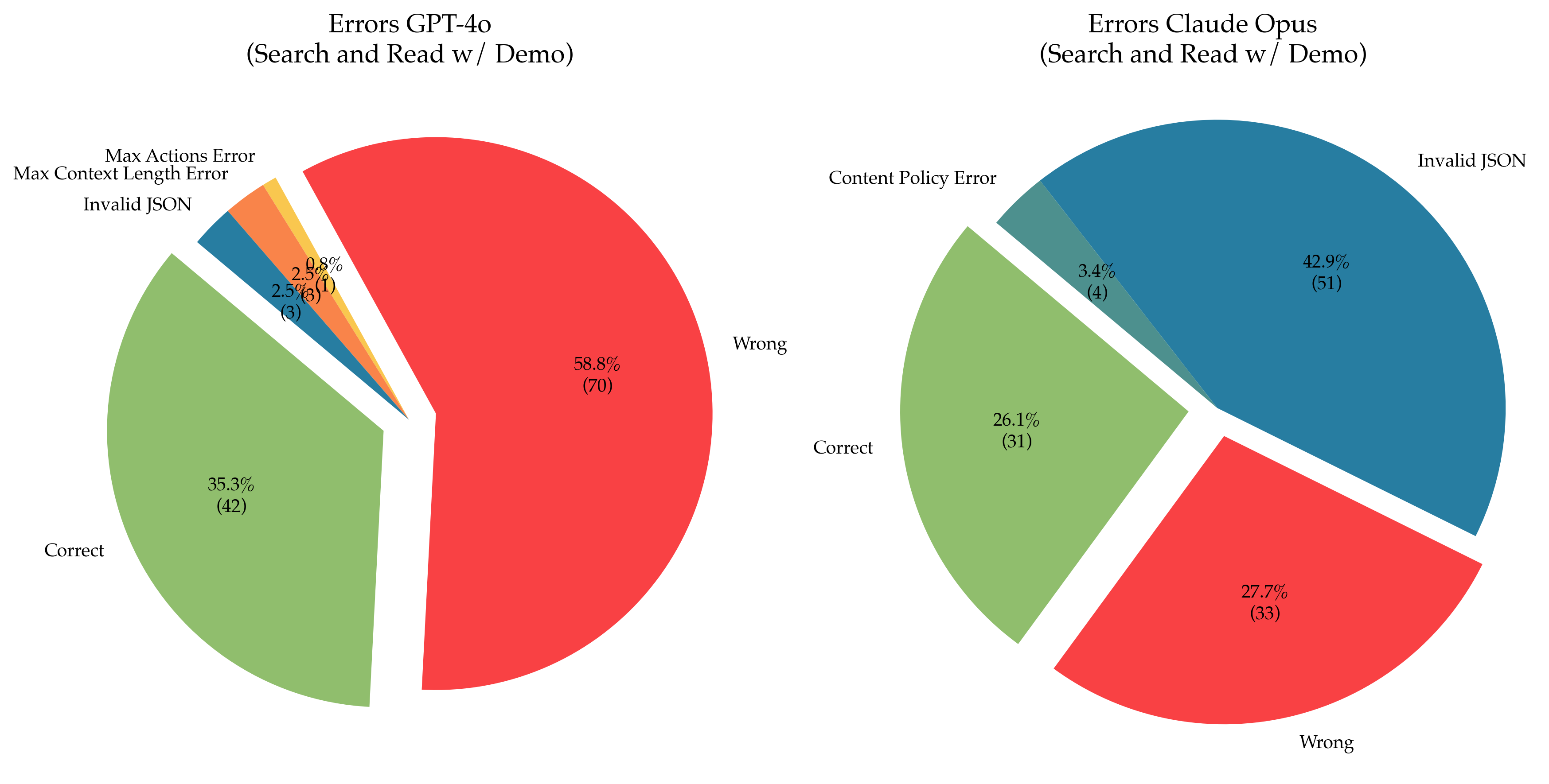<details> <summary>extracted/5974968/figures/technical_errors/error_final_prompt.png Details</summary>  ### Visual Description \n ## Comparative Error Analysis: GPT-4o vs. Claude Opus ### Overview The image displays two pie charts side-by-side, comparing the error distributions of two AI models, GPT-4o and Claude Opus, on a "Search and Read w/ Demo" task. Each chart breaks down the outcomes into categories of correct responses and various error types, showing both percentage and absolute count (in parentheses). ### Components/Axes * **Chart Type:** Two exploded pie charts. * **Titles:** * Left Chart: "Errors GPT-4o (Search and Read w/ Demo)" * Right Chart: "Errors Claude Opus (Search and Read w/ Demo)" * **Data Series (Categories):** The categories are consistent across both charts, represented by distinct colors: * **Correct** (Light Green) * **Wrong** (Red) * **Invalid JSON** (Blue) * **Max Context Length Error** (Orange) - *Only present in GPT-4o chart.* * **Max Actions Error** (Yellow) - *Only present in GPT-4o chart.* * **Content Policy Error** (Teal) - *Only present in Claude Opus chart.* * **Spatial Layout:** The two charts are positioned horizontally. The legend is integrated directly as labels pointing to their respective slices. Slices are "exploded" (separated from the center) for emphasis. ### Detailed Analysis #### **Chart 1: Errors GPT-4o (Left)** * **Wrong (Red):** This is the dominant slice, occupying the right half of the pie. It represents **58.8%** of outcomes, corresponding to **70** instances. * **Correct (Light Green):** The second-largest slice, located on the left side. It accounts for **35.3%** of outcomes, or **42** instances. * **Invalid JSON (Blue):** A small slice in the upper-left quadrant. It represents **2.5%** of outcomes, or **3** instances. * **Max Context Length Error (Orange):** A small slice adjacent to the Invalid JSON slice. It also represents **2.5%** of outcomes, or **3** instances. * **Max Actions Error (Yellow):** The smallest slice, a thin wedge next to the orange slice. It represents **0.8%** of outcomes, or **1** instance. * **Total Count (GPT-4o):** 70 + 42 + 3 + 3 + 1 = **119** total trials. #### **Chart 2: Errors Claude Opus (Right)** * **Invalid JSON (Blue):** This is the largest slice, occupying the top-right quadrant. It represents **42.9%** of outcomes, corresponding to **51** instances. * **Wrong (Red):** The second-largest slice, located in the bottom-right quadrant. It accounts for **27.7%** of outcomes, or **33** instances. * **Correct (Light Green):** The third-largest slice, on the left side. It represents **26.1%** of outcomes, or **31** instances. * **Content Policy Error (Teal):** A small slice in the upper-left quadrant. It represents **3.4%** of outcomes, or **4** instances. * **Total Count (Claude Opus):** 51 + 33 + 31 + 4 = **119** total trials. ### Key Observations 1. **Dominant Error Type Differs:** The primary failure mode for GPT-4o is providing a "Wrong" answer (58.8%). For Claude Opus, the primary failure is generating "Invalid JSON" (42.9%). 2. **Accuracy Comparison:** GPT-4o has a higher "Correct" rate (35.3% vs. 26.1%). 3. **Error Diversity:** GPT-4o exhibits a wider variety of error types (5 categories) compared to Claude Opus (4 categories). GPT-4o shows specific technical errors ("Max Context Length," "Max Actions") not seen in the Claude Opus chart. 4. **"Wrong" Answer Rate:** While "Wrong" is the top error for GPT-4o, it is the second-most common outcome for Claude Opus, at a significantly lower rate (27.7%). 5. **Total Trials:** Both models were evaluated on the same number of trials (119), allowing for direct comparison of counts. ### Interpretation This data suggests a fundamental difference in the failure profiles of the two models on this specific task. GPT-4o is more likely to produce a semantically incorrect but structurally valid response ("Wrong"). In contrast, Claude Opus struggles more with structural output formatting, as evidenced by its high rate of "Invalid JSON" errors. The presence of "Max Context Length" and "Max Actions" errors exclusively for GPT-4o may indicate it is more prone to hitting operational limits during this task. Conversely, Claude Opus encounters "Content Policy" errors, a category not observed for GPT-4o in this dataset. Despite GPT-4o's higher accuracy, its error distribution is more skewed towards a single, dominant category ("Wrong"). Claude Opus's errors are more evenly distributed between structural ("Invalid JSON") and semantic ("Wrong") issues. This analysis implies that debugging efforts for each model would need to target different root causes: improving answer correctness for GPT-4o versus improving output formatting and adherence to structural constraints for Claude Opus. </details> Figure 6: Different technical errors for the CiteAgent with Search and Read command with Demo comparing the GPT-4o and Claude Opus backbone. Claude Opus has a significantly higher error rate. It struggles to adhere to the expected JSON fromat and in four cases the content filter was triggered. 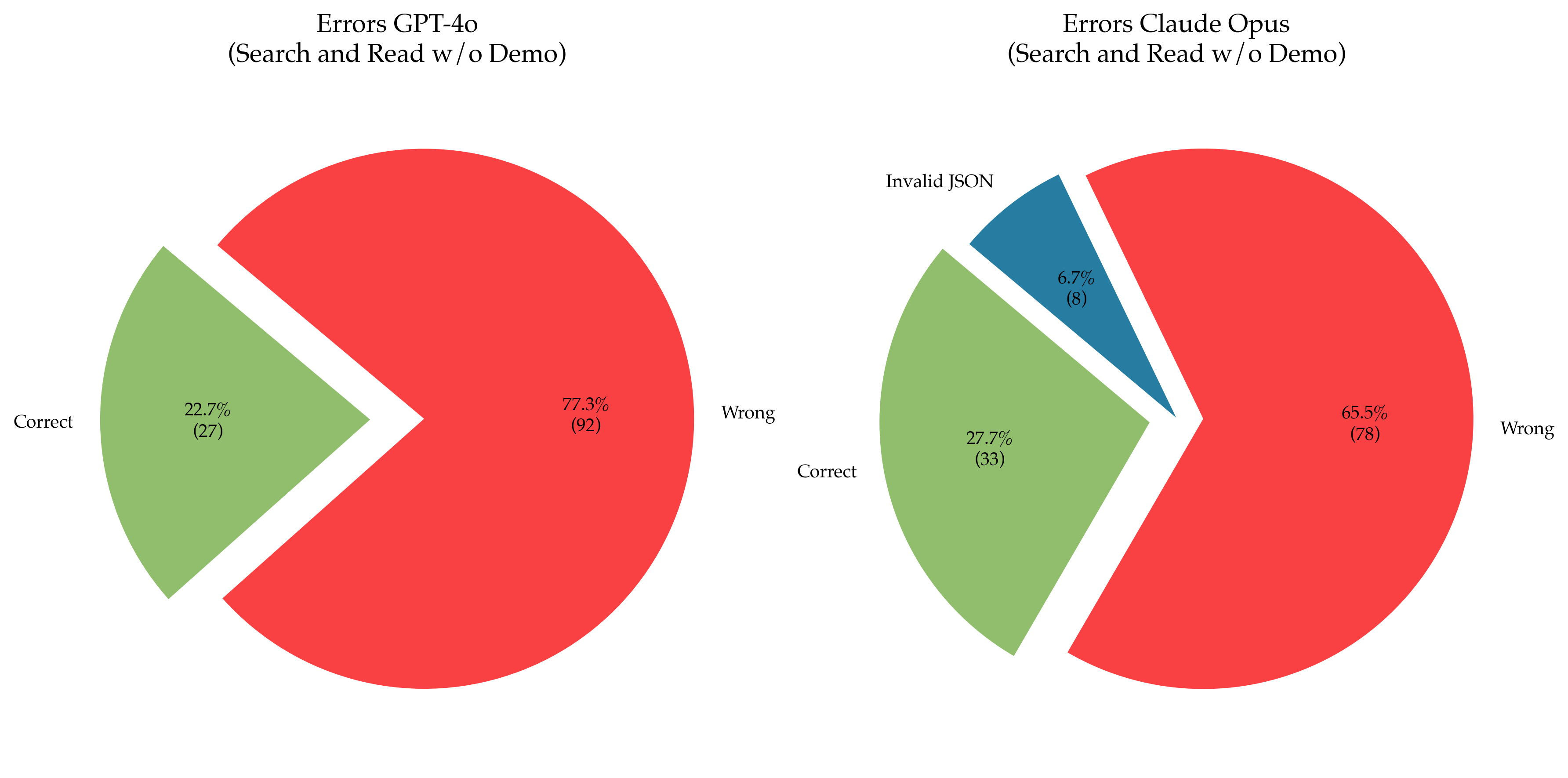<details> <summary>extracted/5974968/figures/technical_errors/error_zero_shot_search.png Details</summary>  ### Visual Description ## Comparative Pie Charts: Error Distributions for Two AI Models ### Overview The image displays two pie charts side-by-side, comparing the error distributions of two AI models, "GPT-4o" and "Claude Opus," on a task labeled "Search and Read w/o Demo." The charts visualize the proportion of "Correct," "Wrong," and (for Claude Opus) "Invalid JSON" outcomes. The language present in the image is English. ### Components/Axes * **Chart Type:** Two exploded pie charts. * **Titles:** * Left Chart: "Errors GPT-4o (Search and Read w/o Demo)" * Right Chart: "Errors Claude Opus (Search and Read w/o Demo)" * **Categories & Legend (Color Mapping):** * **Green Segment:** Labeled "Correct". * **Red Segment:** Labeled "Wrong". * **Blue Segment (Right Chart only):** Labeled "Invalid JSON". * **Data Labels:** Each segment contains a percentage and an absolute count in parentheses. * **Spatial Layout:** The two charts are positioned horizontally. In each chart, one segment is "exploded" (pulled away from the center) for emphasis. ### Detailed Analysis **Left Chart: Errors GPT-4o** * **Correct (Green):** Positioned on the left side of the pie, exploded outward. Represents **22.7%** of outcomes, with an absolute count of **(27)**. * **Wrong (Red):** Positioned on the right side of the pie. Represents **77.3%** of outcomes, with an absolute count of **(92)**. * **Total Count:** 27 + 92 = 119. **Right Chart: Errors Claude Opus** * **Correct (Green):** Positioned on the left side of the pie. Represents **27.7%** of outcomes, with an absolute count of **(33)**. * **Invalid JSON (Blue):** Positioned at the top of the pie, exploded outward. Represents **6.7%** of outcomes, with an absolute count of **(8)**. * **Wrong (Red):** Positioned on the right side of the pie. Represents **65.5%** of outcomes, with an absolute count of **(78)**. * **Total Count:** 33 + 8 + 78 = 119. ### Key Observations 1. **Primary Error Type:** For both models, the "Wrong" category (red) constitutes the majority of outcomes, indicating that incorrect responses are the most common failure mode. 2. **Model Comparison:** * GPT-4o has a higher percentage of "Wrong" outcomes (77.3%) compared to Claude Opus (65.5%). * Claude Opus has a slightly higher percentage of "Correct" outcomes (27.7%) compared to GPT-4o (22.7%). * Claude Opus exhibits a distinct error category, "Invalid JSON" (6.7%), which is not present in the GPT-4o chart. 3. **Visual Emphasis:** The "Correct" segment is exploded in the GPT-4o chart, while the "Invalid JSON" segment is exploded in the Claude Opus chart. This may draw attention to the positive outcome for the first model and a specific, novel error type for the second. ### Interpretation The data suggests a comparative performance analysis on a specific task ("Search and Read w/o Demo"). The high prevalence of "Wrong" answers for both models indicates this task is challenging, with error rates exceeding 65% in both cases. The key differentiator is the *type* of error. GPT-4o's errors are binary (correct vs. wrong), whereas Claude Opus introduces a third category: structural failure in output formatting ("Invalid JSON"). This implies that while Claude Opus may have a marginally better raw accuracy rate, it is susceptible to a specific technical failure mode not observed with GPT-4o in this test. Conversely, GPT-4o appears more consistent in its output format, even when the content is incorrect. The total sample size (119 trials per model) is identical, allowing for a direct comparison of proportions. The results highlight that model evaluation should consider not only the rate of correct answers but also the taxonomy and nature of failures, as different models may exhibit distinct error profiles. The "Invalid JSON" error for Claude Opus could be critical in applications requiring strict structured data output. </details> Figure 7: Different technical errors for the CiteAgent with Search and Read command without Demo comparing the GPT-4o and Claude Opus backbone. Because there is no demo the system prompt is much shorter just containing the task description and the format instructions. One can see that the JSON error rate for Claude Opus is now drastically reduced. GPT-4o also exhibits a smaller error rate but its performance is degraded. 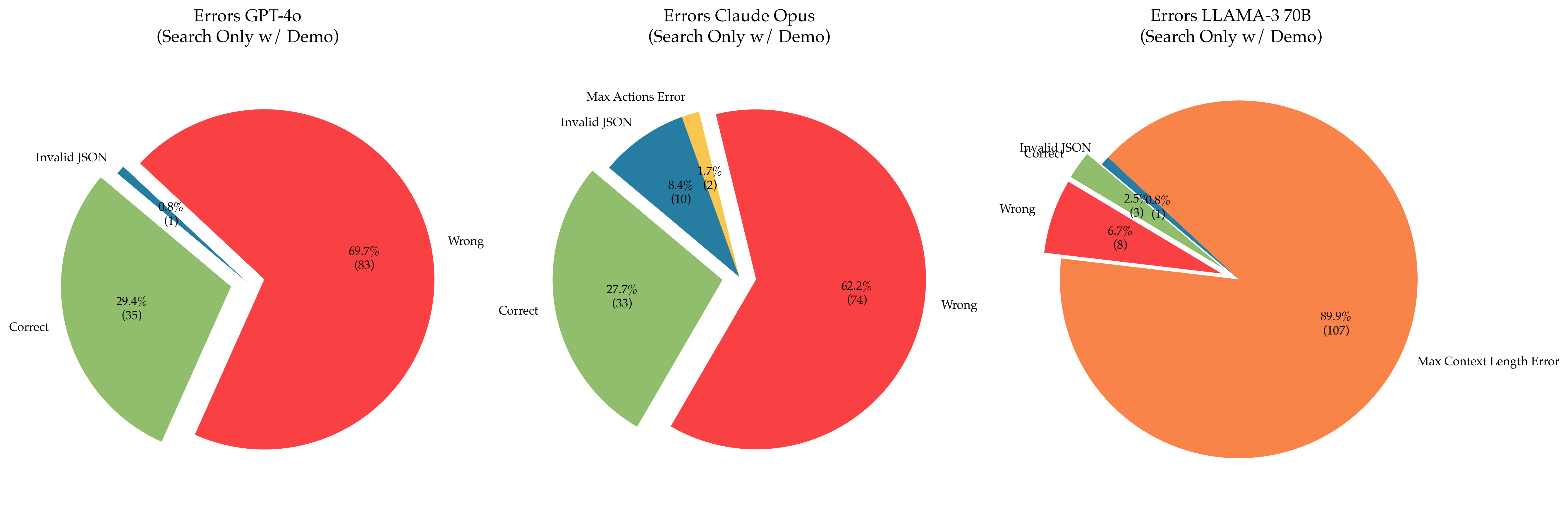<details> <summary>extracted/5974968/figures/technical_errors/error_search_only_demo.png Details</summary>  ### Visual Description ## [Pie Charts]: Error Distribution Comparison for Three AI Models in a "Search Only w/ Demo" Task ### Overview The image displays three pie charts arranged horizontally, each illustrating the distribution of outcomes (errors and correct responses) for a different large language model (LLM) performing a "Search Only w/ Demo" task. The charts compare GPT-4o, Claude Opus, and LLAMA-3 70B. The primary insight is the stark difference in the dominant failure mode for the LLAMA-3 70B model compared to the other two. ### Components/Axes * **Chart Titles (Top Center of each chart):** * Left: `Errors GPT-4o (Search Only w/ Demo)` * Center: `Errors Claude Opus (Search Only w/ Demo)` * Right: `Errors LLAMA-3 70B (Search Only w/ Demo)` * **Chart Type:** Pie charts (exploded slices for emphasis). * **Data Categories (Legend/Labels):** The categories are labeled directly on or adjacent to their respective pie slices. The consistent color coding across charts is: * **Red:** `Wrong` * **Green:** `Correct` * **Blue:** `Invalid JSON` * **Yellow:** `Max Actions Error` (Only present in the Claude Opus chart) * **Orange:** `Max Context Length Error` (Only present in the LLAMA-3 70B chart) * **Data Format:** Each slice is labeled with a percentage and, in parentheses, the absolute count of instances for that category. ### Detailed Analysis **1. GPT-4o (Left Chart)** * **Wrong (Red):** The largest slice, positioned on the right side of the pie. **69.7% (83 instances)**. * **Correct (Green):** The second-largest slice, positioned on the left side. **29.4% (35 instances)**. * **Invalid JSON (Blue):** A very thin slice between the Wrong and Correct slices. **0.8% (1 instance)**. * **Total Instances:** 83 + 35 + 1 = 119. **2. Claude Opus (Center Chart)** * **Wrong (Red):** The largest slice, positioned on the right. **62.2% (74 instances)**. * **Correct (Green):** The second-largest slice, positioned on the left. **27.7% (33 instances)**. * **Invalid JSON (Blue):** A moderate slice between Correct and Wrong. **8.4% (10 instances)**. * **Max Actions Error (Yellow):** A small slice adjacent to the Invalid JSON slice. **1.7% (2 instances)**. * **Total Instances:** 74 + 33 + 10 + 2 = 119. **3. LLAMA-3 70B (Right Chart)** * **Max Context Length Error (Orange):** The overwhelmingly dominant slice, occupying almost the entire chart. **89.9% (107 instances)**. * **Wrong (Red):** A small slice on the left side. **6.7% (8 instances)**. * **Correct (Green):** A very small slice adjacent to the Wrong slice. **2.5% (3 instances)**. * **Invalid JSON (Blue):** A very thin slice adjacent to the Correct slice. **0.8% (1 instance)**. * **Total Instances:** 107 + 8 + 3 + 1 = 119. ### Key Observations 1. **Consistent Sample Size:** All three models were evaluated on the same number of instances (119), allowing for direct comparison. 2. **Dominant Failure Modes Differ:** * For **GPT-4o** and **Claude Opus**, the primary failure is providing a `Wrong` answer (69.7% and 62.2% respectively). * For **LLAMA-3 70B**, the primary failure is a technical `Max Context Length Error` (89.9%), which is a different category of failure altogether. 3. **Correctness Rate:** GPT-4o (29.4%) and Claude Opus (27.7%) have similar, modest correctness rates. LLAMA-3 70B's correctness rate is drastically lower (2.5%). 4. **Error Diversity:** Claude Opus exhibits the widest variety of error types (4 categories), including the unique `Max Actions Error`. GPT-4o shows only two error types, while LLAMA-3 70B's errors are almost entirely of one type. 5. **Invalid JSON:** This error is present in all models but is most frequent in Claude Opus (8.4%). ### Interpretation This data suggests a fundamental difference in how these models handle the "Search Only w/ Demo" task, likely related to their architecture, context window management, or training. * **GPT-4o and Claude Opus** appear to be operating within their technical limits (rarely hitting action or context limits) but struggle with the *substantive correctness* of their outputs. Their performance is limited by reasoning or knowledge accuracy. * **LLAMA-3 70B**, however, is failing for a *procedural/technical* reason before it can even attempt the task correctly. The `Max Context Length Error` indicates the model's input or generated output exceeded its maximum allowed context window. This suggests the task's demonstrations or search results are too lengthy for this model's configuration, making it an unsuitable choice for this specific workflow without modification (e.g., chunking, summarization). * The comparison highlights that model evaluation must consider both **substantive accuracy** (Wrong vs. Correct) and **operational reliability** (technical errors like context length). A model might be conceptually capable but practically unusable for a given task due to technical constraints. The choice of model for this "Search Only w/ Demo" task would depend on whether the priority is minimizing wrong answers (favoring GPT-4o/Claude Opus) or ensuring the task runs to completion without technical failure (which none do perfectly, but LLAMA-3 70B fails at this spectacularly). </details> Figure 8: Different technical errors for the CiteAgent with Search Only command with Demo comparing the GPT-4o, Claude Opus and LLaMA-3 70B backbone. The system prompt containing the Demo takes up a considerable amount of LLaMA-3’s context length therefore just a few actions lead to the model running out of context. 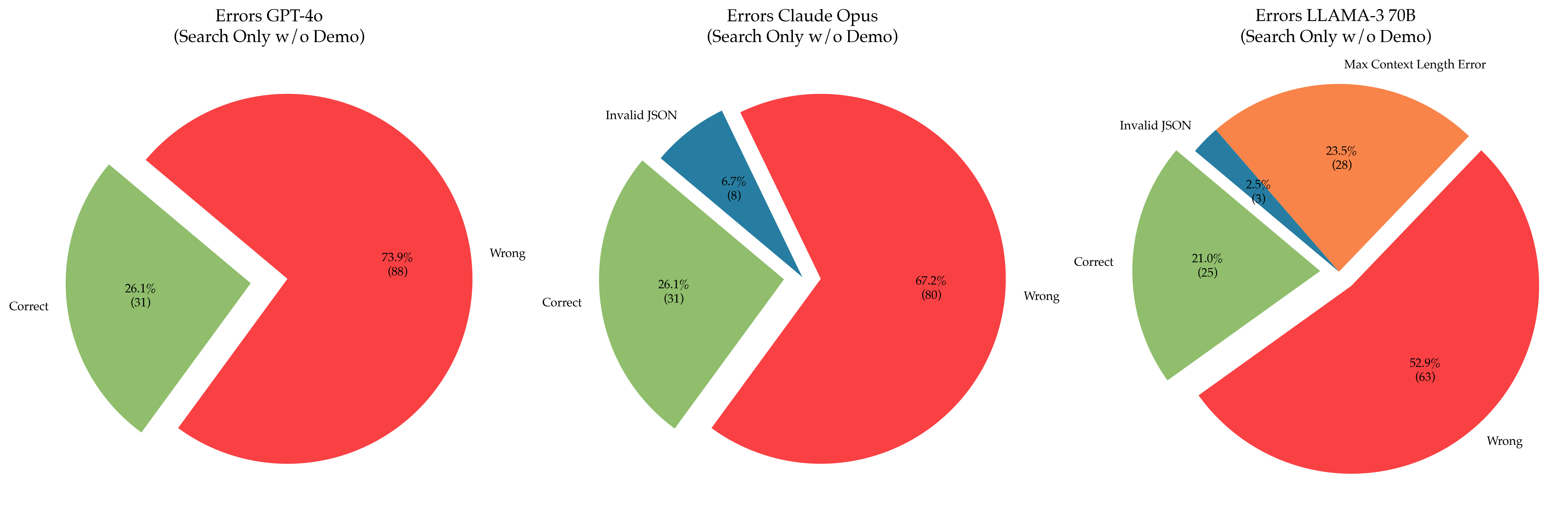<details> <summary>extracted/5974968/figures/technical_errors/error_search_only_no_demo.png Details</summary>  ### Visual Description ## Comparative Error Analysis: Three AI Models (Search Only w/o Demo) ### Overview The image displays three horizontally arranged pie charts, each analyzing the error distribution of a different large language model (LLM) under a "Search Only w/o Demo" testing condition. The charts compare the performance of GPT-4o, Claude Opus, and LLAMA-3 70B. Each chart breaks down results into categories of correctness and specific error types. ### Components/Axes * **Chart Titles (Top-Center of each chart):** * Left: `Errors GPT-4o (Search Only w/o Demo)` * Center: `Errors Claude Opus (Search Only w/o Demo)` * Right: `Errors LLAMA-3 70B (Search Only w/o Demo)` * **Chart Type:** Pie charts with exploded (pulled-out) segments for emphasis. * **Legend/Color Key (Inferred from segment labels):** * **Red:** `Wrong` * **Green:** `Correct` * **Blue:** `Invalid JSON` * **Orange:** `Max Context Length Error` * **Data Labels:** Each segment contains a percentage and a raw count in parentheses (e.g., `73.9% (88)`). ### Detailed Analysis **1. GPT-4o (Left Chart)** * **Segments:** * **Wrong (Red, dominant segment):** 73.9% (88 instances). This is the largest segment and is not exploded. * **Correct (Green, exploded segment):** 26.1% (31 instances). This segment is pulled out from the main pie. * **Total Instances:** 119 (88 + 31). **2. Claude Opus (Center Chart)** * **Segments:** * **Wrong (Red, dominant segment):** 67.2% (80 instances). Largest segment, not exploded. * **Correct (Green, exploded segment):** 26.1% (31 instances). Pulled out. * **Invalid JSON (Blue, exploded segment):** 6.7% (8 instances). Pulled out. * **Total Instances:** 119 (80 + 31 + 8). **3. LLAMA-3 70B (Right Chart)** * **Segments:** * **Wrong (Red, largest segment):** 52.9% (63 instances). Largest segment, not exploded. * **Max Context Length Error (Orange, exploded segment):** 23.5% (28 instances). Pulled out. * **Correct (Green, exploded segment):** 21.0% (25 instances). Pulled out. * **Invalid JSON (Blue, exploded segment):** 2.5% (3 instances). Pulled out. * **Total Instances:** 119 (63 + 28 + 25 + 3). ### Key Observations 1. **Consistent Sample Size:** All three models were evaluated on the same number of total instances (119), allowing for direct comparison. 2. **Primary Error Type:** The `Wrong` category (red) is the largest error type for all models, though its proportion decreases from GPT-4o (73.9%) to Claude Opus (67.2%) to LLAMA-3 70B (52.9%). 3. **Model-Specific Errors:** * GPT-4o's errors are binary: only `Correct` or `Wrong`. * Claude Opus introduces a formatting error (`Invalid JSON`). * LLAMA-3 70B exhibits a unique, significant error type: `Max Context Length Error` (23.5%), which is the second-largest segment for that model. 4. **Correctness Rate:** The `Correct` rate is similar for GPT-4o and Claude Opus (both 26.1%) but lower for LLAMA-3 70B (21.0%). 5. **Visual Emphasis:** In the Claude Opus and LLAMA-3 70B charts, all non-"Wrong" segments are exploded, visually highlighting the composition of correct answers and specific error subtypes. ### Interpretation This data suggests a performance and failure mode hierarchy among the tested models for the "Search Only w/o Demo" task. * **GPT-4o** demonstrates a straightforward failure pattern, with a high rate of substantive errors (`Wrong`) and no observed technical or formatting failures. Its correctness rate is tied for the highest. * **Claude Opus** shows a slight improvement in the primary `Wrong` error rate compared to GPT-4o and introduces a small percentage of output formatting errors (`Invalid JSON`). Its correctness rate is identical to GPT-4o. * **LLAMA-3 70B** has the lowest rate of primary `Wrong` errors but also the lowest correctness rate. This is because a substantial portion of its failures (nearly a quarter) are due to a technical limitation—exceeding the maximum context length. This indicates a potential architectural or configuration constraint specific to this model under the test conditions, rather than a pure reasoning failure. **Conclusion:** While LLAMA-3 70B appears to make fewer "wrong" answers, its overall utility is significantly hampered by context length errors. Claude Opus and GPT-4o have similar correctness, but Claude Opus shows a minor tendency toward formatting issues. The choice of model for this task may depend on whether avoiding context length errors (favoring GPT-4o/Claude Opus) or minimizing outright wrong answers (favoring Claude Opus/LLAMA-3 70B) is the higher priority. </details> Figure 9: Different technical errors for the CiteAgent with Search Only command without Demo comparing the GPT-4o, Claude Opus and LLaMA-3 70B backbone. 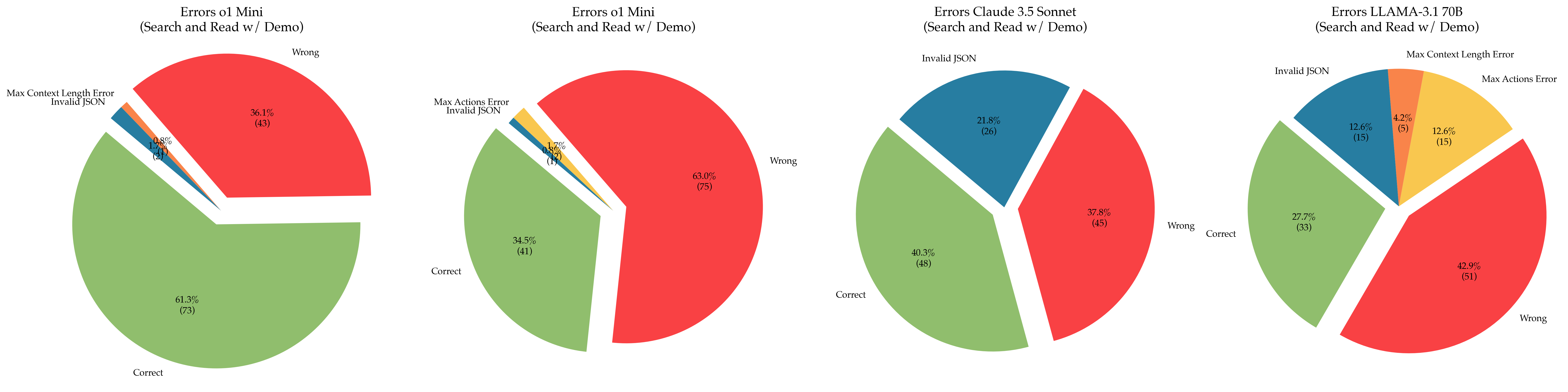<details> <summary>extracted/5974968/figures/technical_errors/error_final_prompt2.png Details</summary>  ### Visual Description \n ## Pie Charts: Comparative Error Analysis of AI Models on a "Search and Read" Task ### Overview The image displays four pie charts arranged horizontally, each illustrating the distribution of outcomes (correct answers and various error types) for a specific AI model performing a "Search and Read w/ Demo" task. The charts compare the performance of two instances of "o1 Mini", "Claude 3.5 Sonnet", and "LLAMA-3.1 70B". Each chart is titled with the model name and task. ### Components/Axes * **Chart Titles (Top-Center of each pie):** 1. `Errors o1 Mini (Search and Read w/ Demo)` 2. `Errors o1 Mini (Search and Read w/ Demo)` 3. `Errors Claude 3.5 Sonnet (Search and Read w/ Demo)` 4. `Errors LLAMA-3.1 70B (Search and Read w/ Demo)` * **Data Categories (Legend/Labels within slices):** The same five categories are used across all charts, color-coded as follows: * **Correct** (Green slice) * **Wrong** (Red slice) * **Invalid JSON** (Blue slice) * **Max Context Length Error** (Orange slice) * **Max Actions Error** (Yellow slice) * **Data Presentation:** Each slice is labeled with its category name, a percentage, and a raw count in parentheses (e.g., `61.3% (73)`). Slices are slightly separated ("exploded") for clarity. ### Detailed Analysis **Chart 1: Errors o1 Mini (First Instance)** * **Correct (Green, bottom-left):** 61.3% (73). This is the largest segment. * **Wrong (Red, top-right):** 36.1% (43). The second-largest segment. * **Invalid JSON (Blue, thin slice top-left):** 1.7% (2). * **Max Context Length Error (Orange, very thin slice top-left):** 0.8% (1). * **Max Actions Error (Yellow, not visibly present):** 0.0% (0). This category is listed in the legend but has no corresponding slice, indicating zero occurrences. **Chart 2: Errors o1 Mini (Second Instance)** * **Wrong (Red, right):** 63.0% (75). This is the dominant segment. * **Correct (Green, left):** 34.5% (41). The second-largest segment. * **Invalid JSON (Blue, thin slice top-left):** 1.7% (2). * **Max Actions Error (Yellow, thin slice top-left):** 0.8% (1). * **Max Context Length Error (Orange, not visibly present):** 0.0% (0). This category is listed but has no slice. **Chart 3: Errors Claude 3.5 Sonnet** * **Correct (Green, bottom-left):** 40.3% (48). The largest segment. * **Wrong (Red, right):** 37.8% (45). Slightly smaller than the "Correct" segment. * **Invalid JSON (Blue, top):** 21.8% (26). A substantial segment. * **Max Context Length Error (Orange, not visibly present):** 0.0% (0). * **Max Actions Error (Yellow, not visibly present):** 0.0% (0). **Chart 4: Errors LLAMA-3.1 70B** * **Wrong (Red, bottom-right):** 42.9% (51). The largest segment. * **Correct (Green, bottom-left):** 27.7% (33). The second-largest segment. * **Invalid JSON (Blue, top-left):** 12.6% (15). * **Max Actions Error (Yellow, top-right):** 12.6% (15). Equal in size to the "Invalid JSON" segment. * **Max Context Length Error (Orange, top-center):** 4.2% (5). ### Key Observations 1. **High Variability in o1 Mini:** The two charts for "o1 Mini" show dramatically different results. The first instance has a majority "Correct" rate (61.3%), while the second has a majority "Wrong" rate (63.0%). This suggests significant inconsistency in the model's performance or possibly different test conditions between runs. 2. **Model-Specific Error Profiles:** * **Claude 3.5 Sonnet** has a balanced split between "Correct" and "Wrong" but is notable for a high rate of "Invalid JSON" errors (21.8%), which is its primary failure mode. * **LLAMA-3.1 70B** has the highest "Wrong" rate (42.9%) and is the only model to exhibit all five error categories, including a significant "Max Actions Error" rate (12.6%). 3. **Error Type Prevalence:** "Invalid JSON" is a common error across three models (o1 Mini, Claude, LLAMA). "Max Context Length Error" and "Max Actions Error" are less frequent overall but are most prominent in the LLAMA model. ### Interpretation These charts provide a comparative diagnostic view of how different large language models fail on a specific, likely tool-augmented, task ("Search and Read w/ Demo"). The data suggests: * **Task Suitability & Reliability:** The stark contrast between the two o1 Mini runs indicates potential reliability issues or high sensitivity to prompt/task variations. Claude 3.5 Sonnet shows more consistent, though not superior, performance with a clear weakness in output formatting (JSON). * **Error Nature as a Model Fingerprint:** The distribution of error types acts as a fingerprint for each model's limitations. Claude's errors are primarily syntactic ("Invalid JSON"), while LLAMA's errors are more diverse, including both syntactic and resource-limit errors ("Max Actions", "Max Context Length"). This could inform debugging or prompt engineering strategies specific to each model. * **Performance Benchmarking:** For this specific task, no model achieves a "Correct" rate above ~61%. The highest "Wrong" rate is 63%, indicating the task is challenging for all evaluated models. The presence of system-level errors (Max Context/Actions) in LLAMA suggests it may be less optimized for multi-step, agentic workflows compared to the others. **Note on Language:** All text in the image is in English. </details> Figure 10: Different technical errors for the CiteAgent with Search and Read command with Demo comparing the o1-Preview, o1-Mini, Claude 3.5 Sonnet and LLaMA-3.1 70B backbone. 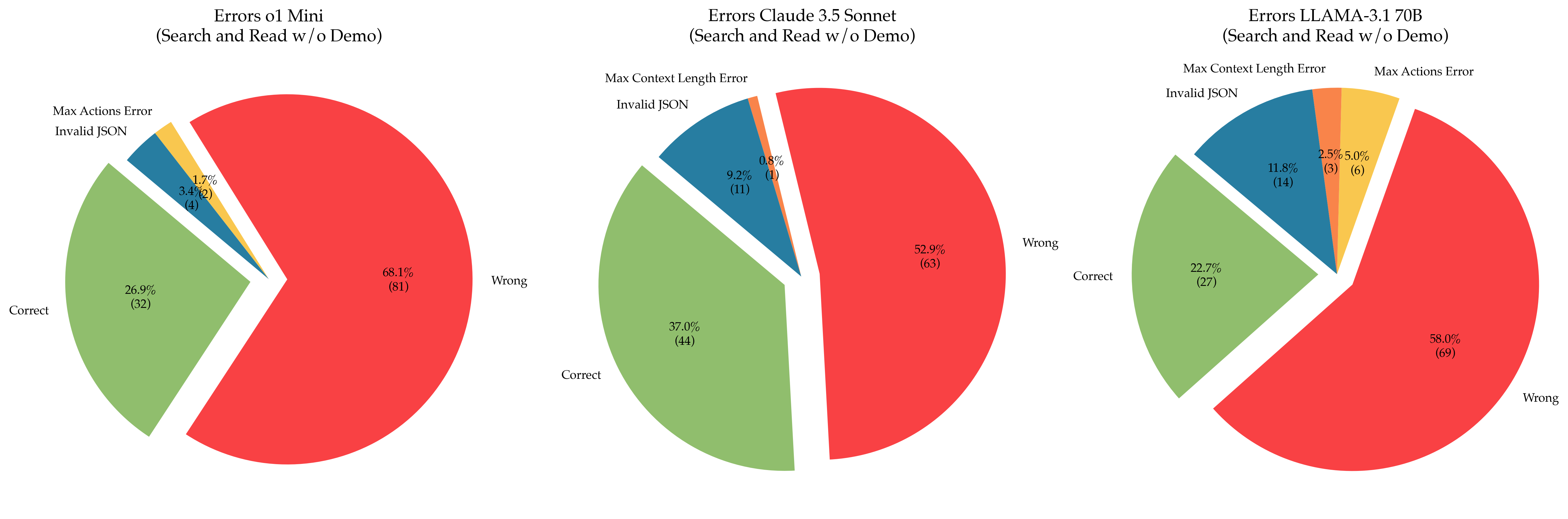<details> <summary>extracted/5974968/figures/technical_errors/error_search_and_read_no_demo.png Details</summary>  ### Visual Description ## Pie Charts: Error Distribution Comparison for Three AI Models ### Overview The image displays three pie charts arranged horizontally, each illustrating the error distribution for a different AI model when performing a "Search and Read" task without a demonstration ("w/o Demo"). The charts compare the performance of "o1 Mini," "Claude 3.5 Sonnet," and "LLAMA-3.1 70B." Each chart breaks down outcomes into "Correct," "Wrong," and specific error types. ### Components/Axes * **Chart Titles (Top Center of each chart):** * Left: `Errors o1 Mini (Search and Read w/o Demo)` * Center: `Errors Claude 3.5 Sonnet (Search and Read w/o Demo)` * Right: `Errors LLAMA-3.1 70B (Search and Read w/o Demo)` * **Categories (Legend Labels):** The following categories are used across the charts, each associated with a specific color: * **Wrong** (Red) * **Correct** (Green) * **Invalid JSON** (Blue) * **Max Context Length Error** (Orange) * **Max Actions Error** (Yellow) * **Data Labels:** Each pie slice is labeled with its category name, a percentage, and a raw count in parentheses (e.g., `68.1% (81)`). ### Detailed Analysis **1. Errors o1 Mini (Left Chart)** * **Wrong (Red):** The largest slice, positioned on the right side. **68.1% (81)**. * **Correct (Green):** The second-largest slice, positioned on the left side. **26.9% (32)**. * **Invalid JSON (Blue):** A small slice adjacent to the "Correct" slice. **3.4% (4)**. * **Max Actions Error (Yellow):** A very small slice adjacent to the "Invalid JSON" slice. **1.7% (2)**. * **Max Context Length Error (Orange):** **Not present** in this chart. * **Total Count:** 81 + 32 + 4 + 2 = 119. **2. Errors Claude 3.5 Sonnet (Center Chart)** * **Wrong (Red):** The largest slice, positioned on the right side. **52.9% (63)**. * **Correct (Green):** The second-largest slice, positioned on the left side. **37.0% (44)**. * **Invalid JSON (Blue):** A moderate slice adjacent to the "Correct" slice. **9.2% (11)**. * **Max Context Length Error (Orange):** A very small slice adjacent to the "Invalid JSON" slice. **0.8% (1)**. * **Max Actions Error (Yellow):** **Not present** in this chart. * **Total Count:** 63 + 44 + 11 + 1 = 119. **3. Errors LLAMA-3.1 70B (Right Chart)** * **Wrong (Red):** The largest slice, positioned on the right side. **58.0% (69)**. * **Correct (Green):** The second-largest slice, positioned on the left side. **22.7% (27)**. * **Invalid JSON (Blue):** A moderate slice adjacent to the "Correct" slice. **11.8% (14)**. * **Max Actions Error (Yellow):** A small slice adjacent to the "Invalid JSON" slice. **5.0% (6)**. * **Max Context Length Error (Orange):** A small slice adjacent to the "Max Actions Error" slice. **2.5% (3)**. * **Total Count:** 69 + 27 + 14 + 6 + 3 = 119. ### Key Observations 1. **Dominance of "Wrong" Outcomes:** In all three models, the "Wrong" category constitutes the majority of outcomes, ranging from 52.9% to 68.1%. 2. **Model Performance Ranking (by Correct %):** Claude 3.5 Sonnet (37.0%) > o1 Mini (26.9%) > LLAMA-3.1 70B (22.7%). 3. **Error Profile Diversity:** LLAMA-3.1 70B is the only model that exhibits all five error categories. o1 Mini lacks "Max Context Length Error," and Claude 3.5 Sonnet lacks "Max Actions Error." 4. **"Invalid JSON" Prevalence:** This is the most common specific error type across all models, increasing from o1 Mini (3.4%) to Claude 3.5 Sonnet (9.2%) to LLAMA-3.1 70B (11.8%). 5. **Rare Errors:** "Max Context Length Error" and "Max Actions Error" are relatively rare, each occurring in only one or two of the models and never exceeding 5.0% in any single chart. ### Interpretation This comparative visualization suggests significant differences in how these AI models fail on a standardized "Search and Read" task. * **Claude 3.5 Sonnet** demonstrates the highest reliability, with the lowest "Wrong" rate and the highest "Correct" rate. Its error profile is also simpler, lacking "Max Actions Error." * **o1 Mini** has the highest outright failure rate ("Wrong") but a moderate "Correct" rate. Its errors are primarily concentrated in the "Invalid JSON" category, suggesting potential issues with output formatting or parsing. * **LLAMA-3.1 70B** has the lowest "Correct" rate and the most diverse error profile. The presence of all error types, including the highest rates of "Max Actions Error" and "Max Context Length Error," indicates it may struggle with task constraints (action limits, context windows) more than the other models, in addition to general correctness and formatting issues. The consistent total count of 119 across all charts implies a controlled experiment where each model was evaluated on the same number of tasks. The data highlights that model evaluation should look beyond a simple "correct/incorrect" binary, as the specific failure modes (e.g., JSON formatting vs. exceeding action limits) provide crucial insights for debugging and improvement. The absence of certain error types in some models could be due to model-specific safeguards, different underlying architectures, or simply chance given the sample size. </details> Figure 11: Different technical errors for the CiteAgent with Search and Read command without Demo comparing the o1-Mini, Claude 3.5 Sonnet and LLaMA-3.1 70B backbone. 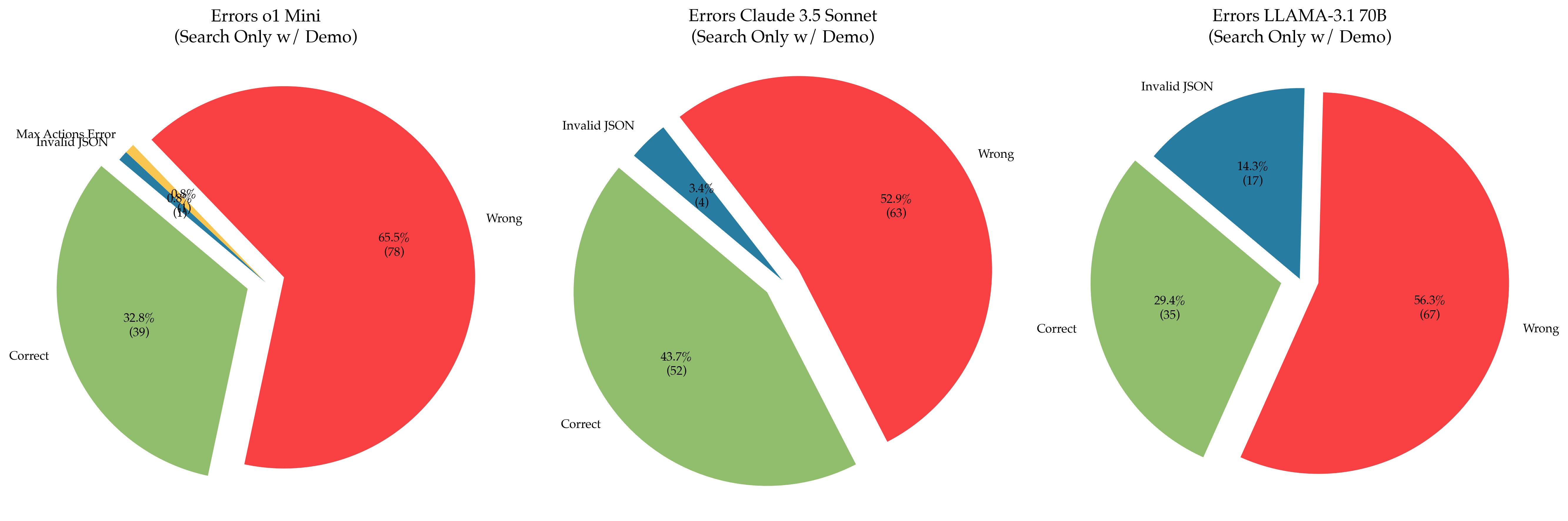<details> <summary>extracted/5974968/figures/technical_errors/error_search_only_demo2.png Details</summary>  ### Visual Description \n ## Pie Charts: Comparative Error Analysis of AI Models (Search Only w/ Demo) ### Overview The image displays three horizontally aligned pie charts, each illustrating the distribution of outcomes (Correct, Wrong, and specific error types) for a different large language model (LLM) under a "Search Only w/ Demo" testing condition. The charts compare the performance of "o1 Mini," "Claude 3.5 Sonnet," and "LLAMA-3.1 70B." ### Components/Axes * **Chart Titles (Top-Center of each pie):** 1. `Errors o1 Mini (Search Only w/ Demo)` 2. `Errors Claude 3.5 Sonnet (Search Only w/ Demo)` 3. `Errors LLAMA-3.1 70B (Search Only w/ Demo)` * **Categories (Labels within/next to pie slices):** * `Correct` (Green slice) * `Wrong` (Red slice) * `Invalid JSON` (Blue slice) * `Max Actions Error` (Yellow slice, present only in the first chart) * **Data Labels:** Each slice contains a percentage value and, in parentheses, the absolute count of instances for that category. * **Spatial Layout:** The three charts are arranged in a single row. The legend is integrated directly into each chart via labels placed adjacent to their corresponding slices. ### Detailed Analysis **Chart 1: Errors o1 Mini (Search Only w/ Demo)** * **Wrong (Red):** 65.5% (78 instances). This is the dominant slice, occupying nearly two-thirds of the pie. * **Correct (Green):** 32.8% (39 instances). This is the second-largest slice. * **Invalid JSON (Blue):** 0.8% (1 instance). A very thin slice. * **Max Actions Error (Yellow):** 0.8% (1 instance). A very thin slice, visually similar in size to the "Invalid JSON" slice. * **Total Instances:** 78 + 39 + 1 + 1 = 119. **Chart 2: Errors Claude 3.5 Sonnet (Search Only w/ Demo)** * **Wrong (Red):** 52.9% (63 instances). The largest slice, representing just over half of the outcomes. * **Correct (Green):** 43.7% (52 instances). A substantial slice, nearly matching the "Wrong" category in size. * **Invalid JSON (Blue):** 3.4% (4 instances). A small but clearly visible slice. * **Total Instances:** 63 + 52 + 4 = 119. **Chart 3: Errors LLAMA-3.1 70B (Search Only w/ Demo)** * **Wrong (Red):** 56.3% (67 instances). The largest slice. * **Correct (Green):** 29.4% (35 instances). The second-largest slice. * **Invalid JSON (Blue):** 14.3% (17 instances). A significant slice, notably larger than in the other two charts. * **Total Instances:** 67 + 35 + 17 = 119. ### Key Observations 1. **Consistent Sample Size:** All three models were evaluated on the same number of total instances (119), allowing for direct comparison of absolute counts. 2. **Performance Hierarchy:** In terms of the "Correct" rate, Claude 3.5 Sonnet (43.7%) > o1 Mini (32.8%) > LLAMA-3.1 70B (29.4%). 3. **Primary Failure Mode:** For all models, the "Wrong" category is the most common outcome, indicating that producing an incorrect answer is the primary failure mode, not system errors. 4. **Model-Specific Error Profiles:** * **o1 Mini** is the only model to exhibit a "Max Actions Error," though it is rare (1 instance). * **LLAMA-3.1 70B** has a markedly higher rate of "Invalid JSON" errors (14.3%) compared to Claude 3.5 Sonnet (3.4%) and o1 Mini (0.8%). This suggests a specific weakness in formatting output as valid JSON for this model under the test conditions. * **Claude 3.5 Sonnet** shows the most balanced profile between correct and wrong answers and has a low rate of JSON formatting errors. ### Interpretation This comparative analysis suggests that under the specific "Search Only w/ Demo" task, **Claude 3.5 Sonnet demonstrates the highest reliability**, with the highest correct rate and a low incidence of technical errors. **LLAMA-3.1 70B**, while having a "Wrong" rate comparable to the others, shows a significant vulnerability in generating syntactically correct JSON, which could be a critical failure point in applications requiring structured data output. **o1 Mini** has the highest outright error rate ("Wrong") but introduces a unique, albeit infrequent, "Max Actions Error." The data implies that model selection for this type of task should consider not just the raw accuracy ("Correct" rate) but also the *type* of failures. If the downstream system is intolerant of malformed JSON, LLAMA-3.1 70B would be a risky choice despite its otherwise similar "Wrong" rate. The consistent "Wrong" majority across all models indicates the task itself is challenging, with more than half of attempts resulting in incorrect answers for each model. </details> Figure 12: Different technical errors for the CiteAgent with Search Only command with Demo comparing the o1-Mini, Claude 3.5 Sonnet and LLaMA-3.1 70B backbone. 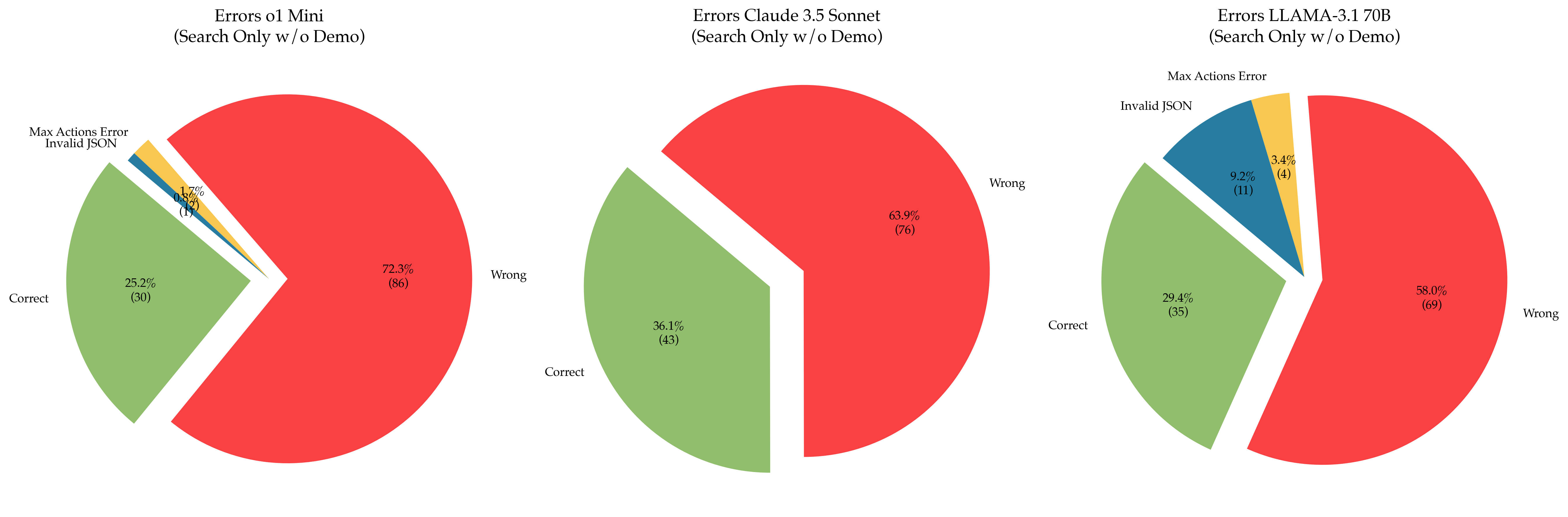<details> <summary>extracted/5974968/figures/technical_errors/error_search_only_no_demo2.png Details</summary>  ### Visual Description ## [Pie Charts]: Comparative Error Distributions for Three AI Models in Search-Only Tasks ### Overview The image displays three horizontally arranged pie charts, each illustrating the distribution of outcomes (Correct, Wrong, and specific error types) for a different large language model (LLM) when performing a "Search Only" task without a demonstration ("w/o Demo"). The charts compare the performance of "o1 Mini", "Claude 3.5 Sonnet", and "LLAMA-3.1 70B". ### Components/Axes * **Chart Titles (Top-Center of each chart):** * Left Chart: `Errors o1 Mini (Search Only w/o Demo)` * Center Chart: `Errors Claude 3.5 Sonnet (Search Only w/o Demo)` * Right Chart: `Errors LLAMA-3.1 70B (Search Only w/o Demo)` * **Legend / Segment Labels:** The labels are placed directly adjacent to their corresponding pie slices. The color coding is consistent across all charts: * **Green Slice:** `Correct` * **Red Slice:** `Wrong` * **Blue Slice:** `Invalid JSON` * **Yellow Slice:** `Max Actions Error` * **Data Labels:** Each slice contains two lines of text: the percentage of the total and, in parentheses, the absolute count of instances. ### Detailed Analysis **1. Errors o1 Mini (Left Chart)** * **Wrong (Red):** Dominates the chart. **72.3% (86 instances)**. This is the largest single segment across all three charts. * **Correct (Green):** The second-largest segment. **25.2% (30 instances)**. * **Max Actions Error (Yellow):** A very small slice. **1.7% (2 instances)**. * **Invalid JSON (Blue):** The smallest slice. **0.8% (1 instance)**. * *Spatial Note:* The "Correct" slice is exploded (pulled out) from the pie. The "Invalid JSON" and "Max Actions Error" slices are very thin and located between the "Correct" and "Wrong" slices. **2. Errors Claude 3.5 Sonnet (Center Chart)** * **Wrong (Red):** The largest segment. **63.9% (76 instances)**. * **Correct (Green):** A substantial segment. **36.1% (43 instances)**. * **Invalid JSON & Max Actions Error:** These slices are **not present** in this chart, indicating zero recorded instances of these specific error types for this model in this test. * *Spatial Note:* The "Correct" slice is exploded from the pie. The chart is simpler, containing only two segments. **3. Errors LLAMA-3.1 70B (Right Chart)** * **Wrong (Red):** The largest segment. **58.0% (69 instances)**. * **Correct (Green):** The second-largest segment. **29.4% (35 instances)**. * **Invalid JSON (Blue):** A notable segment. **9.2% (11 instances)**. * **Max Actions Error (Yellow):** A small segment. **3.4% (4 instances)**. * *Spatial Note:* The "Correct" slice is exploded from the pie. The "Invalid JSON" and "Max Actions Error" slices are clearly visible and located between the "Correct" and "Wrong" slices. ### Key Observations 1. **Performance Hierarchy:** In terms of the "Correct" rate, Claude 3.5 Sonnet (36.1%) > LLAMA-3.1 70B (29.4%) > o1 Mini (25.2%). 2. **Error Profile Variation:** The models exhibit distinct error profiles. * **o1 Mini** has the highest overall error rate (74.8%) and is the only model with a non-zero "Max Actions Error" rate below 2%. * **Claude 3.5 Sonnet** shows no instances of "Invalid JSON" or "Max Actions Error," suggesting its failures are purely in producing incorrect answers ("Wrong"). * **LLAMA-3.1 70B** has a significant "Invalid JSON" error rate (9.2%), which is an order of magnitude higher than o1 Mini's (0.8%). 3. **Dominant Failure Mode:** For all three models, the "Wrong" category is the largest segment, indicating that producing an incorrect answer is the most common failure mode, more common than technical errors like invalid JSON or hitting action limits. ### Interpretation This data suggests a trade-off between different types of reliability in LLM-based search agents. **Claude 3.5 Sonnet** demonstrates the highest raw accuracy and perfect technical reliability (no JSON/action errors) in this specific test setup, but its failures are absolute (the answer is simply wrong). **LLAMA-3.1 70B** has a lower accuracy than Claude but exhibits a more diverse error profile, with a notable propensity for structural output failures (Invalid JSON). **o1 Mini** performs the worst in terms of accuracy and has a small but present rate of action-limit errors. The absence of "Invalid JSON" and "Max Actions Error" for Claude 3.5 Sonnet could indicate superior instruction-following for output formatting and more efficient action planning. The high "Invalid JSON" rate for LLAMA-3.1 70B might point to challenges in consistently adhering to strict output schemas. The universal dominance of the "Wrong" category underscores that the core challenge in this task is generating correct information, not just formatting it correctly or managing the interaction loop. The "Search Only w/o Demo" condition likely removes helpful context, pushing models to rely purely on their parametric knowledge and search capabilities, which appears to be a significant point of failure for all three models tested. </details> Figure 13: Different technical errors for the CiteAgent with Search Only command without Demo comparing the o1-Mini, Claude 3.5 Sonnet and LLaMA-3.1 70B backbone. ## Appendix G Price and Duration Distribution In this section, we break down runtimes and costs associated with running CiteAgent with a GPT-4o or Claude 3 Opus backbone. 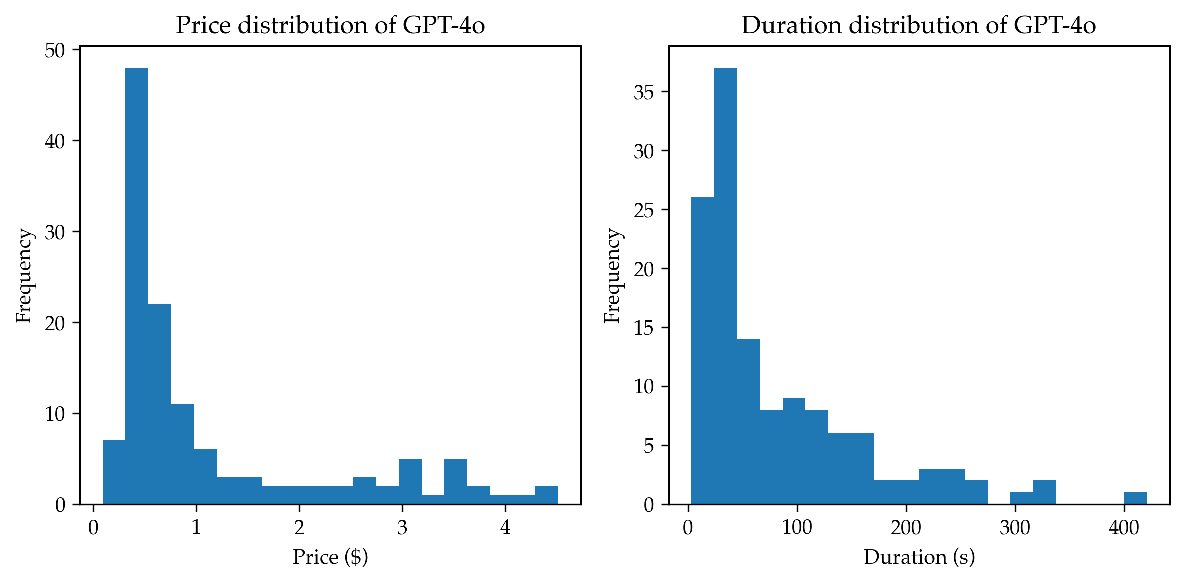<details> <summary>extracted/5974968/figures/price_gpt4o.png Details</summary>  ### Visual Description ## Histograms: Price and Duration Distributions of GPT-4o ### Overview The image displays two side-by-side histograms presenting statistical distributions for the GPT-4o model. The left histogram shows the distribution of price in US dollars ($), and the right histogram shows the distribution of duration in seconds (s). Both charts share a similar visual style with blue bars on a white background, using frequency as the vertical measure. ### Components/Axes **Left Histogram:** * **Title:** "Price distribution of GPT-4o" (centered at the top). * **X-axis:** Labeled "Price ($)". The axis has major tick marks and numerical labels at 0, 1, 2, 3, and 4. * **Y-axis:** Labeled "Frequency". The axis has major tick marks and numerical labels at 0, 10, 20, 30, 40, and 50. **Right Histogram:** * **Title:** "Duration distribution of GPT-4o" (centered at the top). * **X-axis:** Labeled "Duration (s)". The axis has major tick marks and numerical labels at 0, 100, 200, 300, and 400. * **Y-axis:** Labeled "Frequency". The axis has major tick marks and numerical labels at 0, 5, 10, 15, 20, 25, 30, and 35. **Spatial Layout:** The two histograms are positioned horizontally adjacent. The price histogram occupies the left half of the image, and the duration histogram occupies the right half. There is no shared legend, as each chart is a single data series. ### Detailed Analysis **Price Distribution (Left Chart):** The distribution is strongly right-skewed, with the vast majority of data points concentrated at the lower end of the price scale. * **Peak:** The highest frequency bar is located in the bin approximately between $0.4 and $0.6, with a frequency of approximately 48. * **Adjacent Bins:** The bin to the left (approx. $0.2-$0.4) has a frequency of ~7. The bin to the right (approx. $0.6-$0.8) has a frequency of ~22. * **Tail:** Frequencies drop sharply after $1.0. There is a long, sparse tail extending to $4.5, with small, intermittent bars (frequencies between ~1 and ~5) visible in the $2.5 to $4.5 range. **Duration Distribution (Right Chart):** This distribution is also right-skewed, with most durations clustered at the lower end. * **Peak:** The highest frequency bar is located in the bin approximately between 40 and 60 seconds, with a frequency of approximately 37. * **Adjacent Bins:** The bin to the left (approx. 20-40s) has a frequency of ~26. The bin to the right (approx. 60-80s) has a frequency of ~14. * **Tail:** Frequencies decline steadily after 80 seconds. A sparse tail extends to 420 seconds, with very low-frequency bars (frequencies of ~1-3) appearing intermittently beyond 200 seconds. ### Key Observations 1. **Strong Right Skew:** Both price and duration exhibit classic right-skewed (positive-skew) distributions. The mode (most common value) is at the low end for both metrics. 2. **Concentration of Data:** The bulk of the data (the "body" of the distribution) for price is below $1.0, and for duration is below 100 seconds. 3. **Presence of Outliers:** Both charts show a long tail, indicating the presence of outlier instances with significantly higher prices (up to ~$4.5) and longer durations (up to ~420 seconds), though these are rare. 4. **Similar Shape:** The two distributions share a nearly identical morphological shape, suggesting a potential correlation between the price and duration of GPT-4o tasks or queries in this dataset. ### Interpretation The data suggests that the cost (price) and processing time (duration) for GPT-4o are not normally distributed but follow a pattern common to many service-based metrics: most interactions are quick and inexpensive, while a small subset are significantly more resource-intensive. * **Operational Insight:** The high concentration of low-duration tasks implies the model is frequently used for relatively brief interactions. The corresponding concentration at low prices indicates these brief tasks are also low-cost. * **Correlation Implication:** The striking similarity in distribution shapes strongly hints that duration is a primary driver of price. Longer tasks likely consume more computational resources, leading to higher costs. The outliers represent the "heavy tail" of complex, time-consuming, and therefore expensive requests. * **Planning & Forecasting:** For users or system planners, this means budgeting and capacity planning can be based on the high-probability, low-value cluster, but must also account for the low-probability, high-impact outliers that can disproportionately affect total cost and latency. The distributions provide a quantitative basis for setting expectations and service-level agreements. </details> Figure 14: Price and duration distribution on CiteME with the Read and Search command with Demo for the GPT-4o backbone. The average price is $∼$ $ $1.2$ per run or $∼$ $ $150$ in total. The average duration is $82.9$ s per citation or $10772$ s in total. 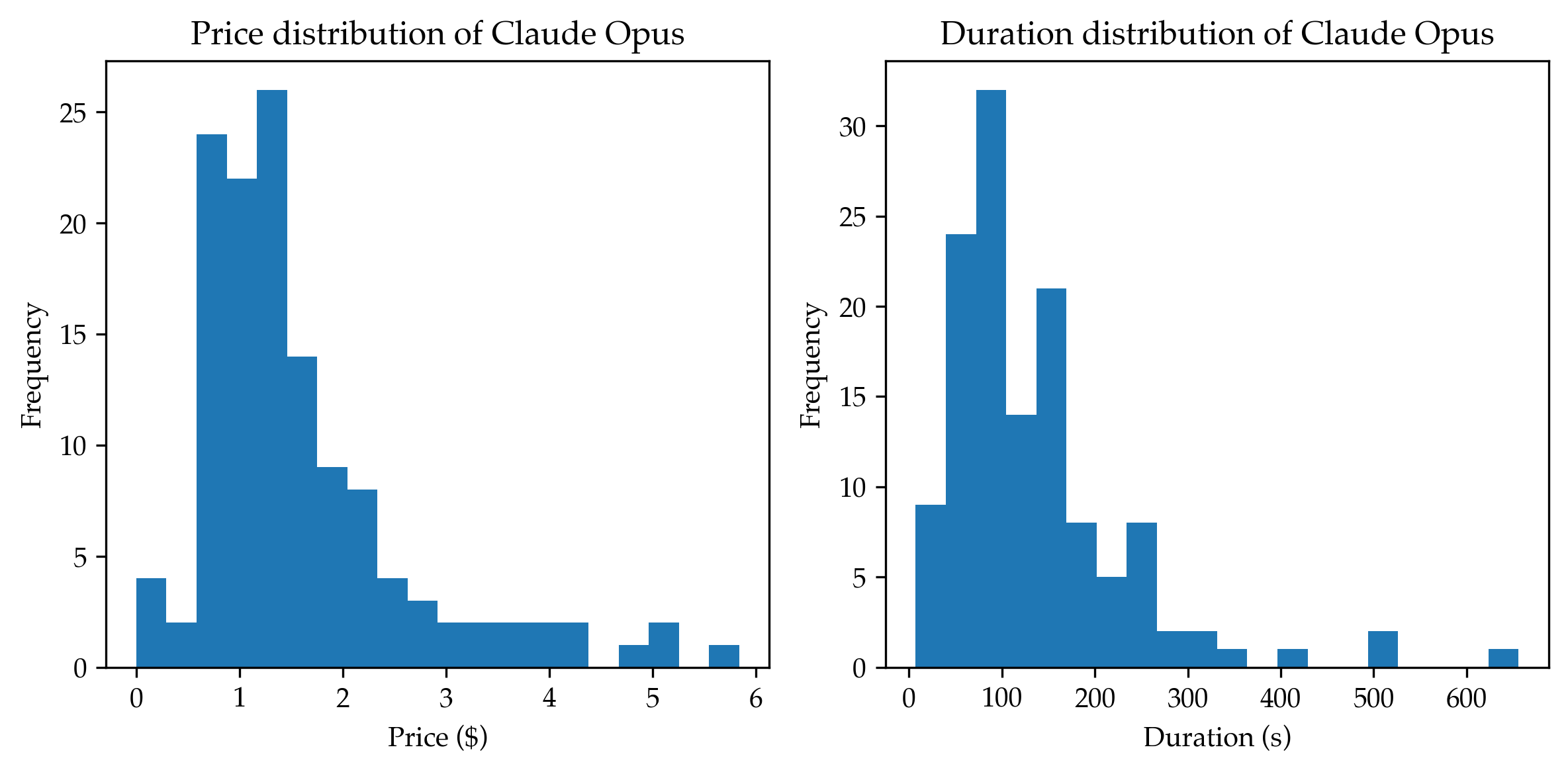<details> <summary>extracted/5974968/figures/price_claude.png Details</summary>  ### Visual Description ## Histograms: Price and Duration Distributions of Claude Opus ### Overview The image displays two side-by-side histograms visualizing the frequency distributions for two different metrics related to "Claude Opus": price in US dollars and duration in seconds. Both charts share a similar visual style with blue bars against a white background, using a standard histogram format to show the concentration of data points across value ranges. ### Components/Axes **Left Chart: Price Distribution** * **Title:** "Price distribution of Claude Opus" (Top center) * **X-axis:** Label is "Price ($)". The axis is marked with major ticks at 0, 1, 2, 3, 4, 5, and 6. The data appears to be binned in intervals of approximately $0.50. * **Y-axis:** Label is "Frequency". The axis is marked with major ticks at 0, 5, 10, 15, 20, and 25. The highest bar exceeds the 25 mark. **Right Chart: Duration Distribution** * **Title:** "Duration distribution of Claude Opus" (Top center) * **X-axis:** Label is "Duration (s)". The axis is marked with major ticks at 0, 100, 200, 300, 400, 500, and 600. The data appears to be binned in intervals of approximately 50 seconds. * **Y-axis:** Label is "Frequency". The axis is marked with major ticks at 0, 5, 10, 15, 20, 25, and 30. The highest bar exceeds the 30 mark. ### Detailed Analysis **Price Distribution (Left Chart):** * **Trend Verification:** The distribution is strongly right-skewed (positively skewed). The frequency rises sharply from the first bin, peaks early, and then gradually tapers off with a long tail extending to higher prices. * **Data Points (Approximate Frequencies per Bin):** * $0.00 - $0.50: ~4 * $0.50 - $1.00: ~24 * $1.00 - $1.50: ~22 * $1.50 - $2.00: ~26 (Peak) * $2.00 - $2.50: ~14 * $2.50 - $3.00: ~9 * $3.00 - $3.50: ~8 * $3.50 - $4.00: ~4 * $4.00 - $4.50: ~3 * $4.50 - $5.00: ~2 (Gap before next bar) * $5.00 - $5.50: ~1 * $5.50 - $6.00: ~2 * $6.00 - $6.50: ~1 **Duration Distribution (Right Chart):** * **Trend Verification:** This distribution is also right-skewed. It shows a very high concentration of short durations, with a sharp peak and a long tail of less frequent, longer durations. * **Data Points (Approximate Frequencies per Bin):** * 0 - 50 s: ~9 * 50 - 100 s: ~24 * 100 - 150 s: ~32 (Peak) * 150 - 200 s: ~14 * 200 - 250 s: ~21 * 250 - 300 s: ~8 * 300 - 350 s: ~5 * 350 - 400 s: ~8 * 400 - 450 s: ~2 * 450 - 500 s: ~1 (Gap before next bar) * 500 - 550 s: ~1 * 550 - 600 s: ~2 (Gap before next bar) * 600 - 650 s: ~1 ### Key Observations 1. **Concentration at Lower Values:** Both metrics show that the vast majority of instances are clustered at the lower end of their respective scales. Most prices are between $0.50 and $2.50, and most durations are between 50 and 250 seconds. 2. **Right-Skewed Nature:** The long tails to the right in both charts indicate the presence of outliers or less common instances that are significantly more expensive or longer in duration than the typical case. 3. **Peak Locations:** The modal (most frequent) price bin is approximately $1.50-$2.00. The modal duration bin is approximately 100-150 seconds. 4. **Data Gaps:** Both distributions show gaps in the tail (e.g., no price instances between ~$4.50-$5.00, no duration instances between ~450-500s), suggesting these higher values are sporadic. ### Interpretation The data suggests that the typical operation or task associated with "Claude Opus" is relatively low-cost and quick to complete. The strong right skew in both price and duration is characteristic of many service-based or computational processes, where most jobs are routine and efficient, but a small subset involves exceptional complexity, errors, or resource intensity, leading to disproportionate costs and time. The correlation between the two distributions is implied: longer tasks likely incur higher costs. The presence of outliers in both charts (e.g., tasks costing over $5 or lasting over 600 seconds) warrants investigation. These could represent edge cases, system errors, or particularly complex queries that may be of interest for optimization or understanding the limits of the system. The clear visualization allows for quick assessment of the central tendency and variability of these key operational metrics. </details> Figure 15: Price and duration distribution on CiteME with the Read and Search command with Demo for the Claude Opus backbone. The average price is $∼$ $ $1.6$ per run or $∼$ $ $206$ in total. The average duration is $136.0$ s per citation or $17675$ s in total. 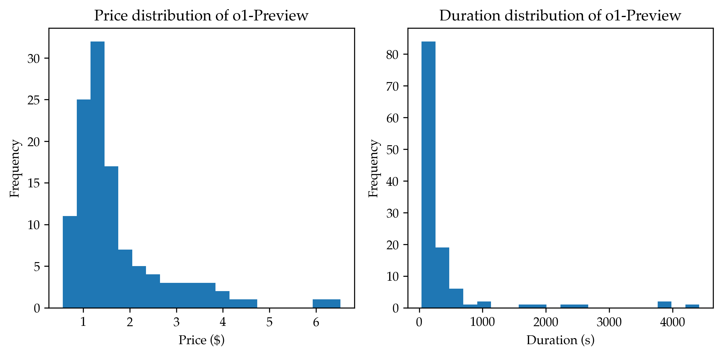<details> <summary>extracted/5974968/figures/price_o1_prewview.png Details</summary>  ### Visual Description ## Histograms: Price and Duration Distributions of o1-Preview ### Overview The image displays two side-by-side histograms visualizing the frequency distributions of two metrics for a subject labeled "o1-Preview": Price (in US Dollars) and Duration (in seconds). The charts are presented on a white background with black axes and titles. The data is represented by solid blue bars. ### Components/Axes **Left Chart: Price Distribution** * **Title:** "Price distribution of o1-Preview" (centered above the chart). * **Y-axis:** Label is "Frequency". The scale runs from 0 to 30, with major tick marks at intervals of 5 (0, 5, 10, 15, 20, 25, 30). * **X-axis:** Label is "Price ($)". The scale runs from approximately 0.5 to 6.5, with major tick marks labeled at 1, 2, 3, 4, 5, and 6. * **Legend:** None present. **Right Chart: Duration Distribution** * **Title:** "Duration distribution of o1-Preview" (centered above the chart). * **Y-axis:** Label is "Frequency". The scale runs from 0 to 80, with major tick marks at intervals of 10 (0, 10, 20, 30, 40, 50, 60, 70, 80). * **X-axis:** Label is "Duration (s)". The scale runs from 0 to approximately 4500, with major tick marks labeled at 0, 1000, 2000, 3000, and 4000. * **Legend:** None present. ### Detailed Analysis **Price Distribution (Left Chart):** * **Trend:** The distribution is strongly right-skewed (positively skewed). The highest frequency of occurrences is concentrated at the lower end of the price scale, with a long tail extending to higher prices. * **Data Points (Approximate Frequencies per Bin):** * Bin ~$0.50-$0.75: Frequency ≈ 11 * Bin ~$0.75-$1.00: Frequency ≈ 25 * **Peak Bin ~$1.00-$1.25: Frequency ≈ 32** (This is the mode of the distribution). * Bin ~$1.25-$1.50: Frequency ≈ 17 * Bin ~$1.50-$1.75: Frequency ≈ 7 * Bin ~$1.75-$2.00: Frequency ≈ 5 * Bin ~$2.00-$2.25: Frequency ≈ 4 * Bin ~$2.25-$2.50: Frequency ≈ 3 * Bin ~$2.50-$2.75: Frequency ≈ 3 * Bin ~$2.75-$3.00: Frequency ≈ 3 * Bin ~$3.00-$3.25: Frequency ≈ 3 * Bin ~$3.25-$3.50: Frequency ≈ 2 * Bin ~$3.50-$3.75: Frequency ≈ 1 * Bin ~$3.75-$4.00: Frequency ≈ 1 * Bin ~$6.00-$6.25: Frequency ≈ 1 (This is an isolated outlier far from the main cluster). **Duration Distribution (Right Chart):** * **Trend:** The distribution is extremely right-skewed. The vast majority of durations are very short, clustered near zero seconds, with an exceptionally long and sparse tail extending to over 4000 seconds. * **Data Points (Approximate Frequencies per Bin):** * **Peak Bin ~0-250s: Frequency ≈ 84** (This is the overwhelming mode). * Bin ~250-500s: Frequency ≈ 19 * Bin ~500-750s: Frequency ≈ 6 * Bin ~750-1000s: Frequency ≈ 1 * Bin ~1000-1250s: Frequency ≈ 2 * Bin ~1500-1750s: Frequency ≈ 1 * Bin ~2250-2500s: Frequency ≈ 1 * Bin ~3750-4000s: Frequency ≈ 2 * Bin ~4250-4500s: Frequency ≈ 1 ### Key Observations 1. **Dominant Low-Value Clusters:** Both distributions are dominated by low values. For price, the mode is between $1.00-$1.25. For duration, the mode is between 0-250 seconds. 2. **Extreme Skewness:** The duration distribution is far more skewed than the price distribution. While price has a tail extending to ~$6.25, duration has a tail extending to ~4500 seconds, which is orders of magnitude larger than the modal value. 3. **Presence of Outliers:** Both charts show outliers. The price chart has a single instance near $6.25, isolated from the main data. The duration chart has several sparse instances beyond 1500 seconds, with the furthest near 4500 seconds. 4. **Frequency Scales:** The y-axis scales differ significantly. The price chart's maximum frequency is ~32, while the duration chart's maximum frequency is ~84, indicating a higher concentration of data points in the lowest duration bin. ### Interpretation The data suggests that the "o1-Preview" entity (likely a model, service, or process) most commonly operates at a low cost (around $1) and completes its tasks very quickly (under 4 minutes). The strong right skew in both metrics indicates that while low-cost, fast operations are the norm, there is a non-trivial subset of instances that are significantly more expensive and/or time-consuming. The extreme skew in duration is particularly noteworthy. It implies that the process has a "long tail" behavior: most runs are brief, but a small fraction can become very lengthy, potentially indicating complex edge cases, system hangs, or tasks requiring extensive computation. The isolated high-price outlier suggests a rare, high-cost event that may be an anomaly or a specific, resource-intensive use case. From a business or operational perspective, this distribution pattern highlights that average cost and duration may be misleading metrics. The median would be a better measure of central tendency. Planning and resource allocation must account for the rare but impactful long-duration, high-cost instances to ensure system stability and accurate budgeting. </details> Figure 16: Price and duration distribution on CiteME with the Read and Search command with Demo for the o1-Preview backbone. The average price is $∼$ $ $1.7$ per run or $∼$ $ $205$ in total. The average duration is $369.8$ s per citation or $44006$ s in total. <details> <summary>extracted/5974968/figures/price_o1_mini.png Details</summary>  ### Visual Description \n ## Histograms: Price and Duration Distributions of o1-Mini ### Overview The image displays two side-by-side histograms presenting statistical distributions for a subject identified as "o1-Mini." The left chart shows the distribution of price in US dollars, and the right chart shows the distribution of duration in seconds. Both histograms are rendered in a standard blue color against a white background with black axes and labels. The data in both charts is heavily right-skewed. ### Components/Axes **Left Histogram:** * **Title:** "Price distribution of o1-Mini" (centered at the top). * **X-axis:** Labeled "Price ($)". The axis has major tick marks and numerical labels at 0.0, 0.5, 1.0, 1.5, 2.0, 2.5, and 3.0. * **Y-axis:** Labeled "Frequency". The axis has major tick marks and numerical labels at 0, 10, 20, 30, 40, 50, and 60. **Right Histogram:** * **Title:** "Duration distribution of o1-Mini" (centered at the top). * **X-axis:** Labeled "Duration (s)". The axis has major tick marks and numerical labels at 0, 100, 200, 300, 400, 500, and 600. * **Y-axis:** Labeled "Frequency". The axis has major tick marks and numerical labels at 0, 10, 20, 30, and 40. **Spatial Grounding:** Both charts are of equal size, placed horizontally adjacent. Titles are positioned directly above their respective plot areas. Axis labels are centered below the x-axes and rotated 90 degrees to the left of the y-axes. ### Detailed Analysis **Price Distribution (Left Chart):** * **Trend Verification:** The distribution is strongly right-skewed (positively skewed). The frequency is highest for the lowest price bin and decreases rapidly as price increases, with a long, sparse tail extending to the right. * **Data Points (Approximate Frequencies per Bin):** * Bin 0.0 - ~0.25: Frequency ≈ 65 (the mode). * Bin ~0.25 - 0.5: Frequency ≈ 22. * Bin 0.5 - ~0.75: Frequency ≈ 9. * Bin ~0.75 - 1.0: Frequency ≈ 7. * Bin 1.0 - ~1.25: Frequency ≈ 1. * Bin ~1.25 - 1.5: Frequency ≈ 2. * Bin 1.5 - ~1.75: Frequency ≈ 3. * Bin ~1.75 - 2.0: Frequency ≈ 4. * Bin 2.0 - ~2.25: Frequency ≈ 2. * Bin ~2.25 - 2.5: Frequency ≈ 1. * Bin 2.5 - ~2.75: Frequency ≈ 0. * Bin ~2.75 - 3.0: Frequency ≈ 1. * Bin >3.0: A single, very small bar is visible, suggesting a frequency of 1 for a price just above $3.00. **Duration Distribution (Right Chart):** * **Trend Verification:** This distribution is also right-skewed. The highest frequency occurs in the shortest duration bin. There is a sharp drop, followed by a secondary, smaller peak, and then a long tail of low-frequency events extending to 600 seconds. * **Data Points (Approximate Frequencies per Bin):** * Bin 0 - 50s: Frequency ≈ 45 (the mode). * Bin 50s - 100s: Frequency ≈ 20. * Bin 100s - 150s: Frequency ≈ 9. * Bin 150s - 200s: Frequency ≈ 15 (secondary peak). * Bin 200s - 250s: Frequency ≈ 3. * Bin 250s - 300s: Frequency ≈ 5. * Bin 300s - 350s: Frequency ≈ 1. * Bin 350s - 400s: Frequency ≈ 2. * Bin 400s - 450s: Frequency ≈ 1. * Bin 450s - 500s: Frequency ≈ 3. * Bin 500s - 550s: Frequency ≈ 1. * Bin 550s - 600s: Frequency ≈ 2. * Bin >600s: A single, very small bar is visible, suggesting a frequency of 1 for a duration just over 600 seconds. ### Key Observations 1. **Extreme Right Skew:** Both cost and time are dominated by a large number of low-value instances. The vast majority of "o1-Mini" instances cost less than $0.50 and take less than 100 seconds. 2. **Presence of Outliers:** Both distributions have long tails, indicating the existence of rare but significantly more expensive and time-consuming instances (e.g., prices near $3.00, durations over 600 seconds). 3. **Secondary Peak in Duration:** The duration histogram shows a notable secondary cluster of instances around the 150-200 second range, which is less pronounced in the price distribution. 4. **Data Sparsity in Tails:** The bins in the higher ranges (price >$1.50, duration >250s) have very low and sporadic frequencies, making precise estimation difficult. ### Interpretation The data suggests that "o1-Mini" is a process or service where the typical use case is both inexpensive and quick. The strong right skew is characteristic of many real-world phenomena like service costs or task completion times, where most operations are routine and efficient, but a small subset involves complex edge cases or problems that require disproportionate resources. The correlation between the two charts implies that longer durations generally lead to higher costs, which is logical if pricing is based on compute time or resource usage. The secondary peak in duration around 150-200 seconds, without a perfectly corresponding peak in price, might indicate a class of tasks that are moderately time-consuming but perhaps less computationally intensive, or it could be an artifact of the specific dataset sampled. From a business or operational perspective, this distribution highlights that while the median cost and time are low, budgeting and capacity planning must account for the high-impact outliers that consume a disproportionate share of resources. The sparsity in the tails also suggests that collecting more data on these high-value instances would be valuable for better understanding the upper limits of the system's requirements. </details> Figure 17: Price and duration distribution on CiteME with the Read and Search command with Demo for the 01-Mini backbone. The average price is $∼$ $ $0.4$ per run or $∼$ $ $50$ in total. The average duration is $125.1$ s per citation or $14886$ s in total. <details> <summary>extracted/5974968/figures/price_claude_3.5_sonnet.png Details</summary>  ### Visual Description ## Histograms: Price and Duration Distributions of Claude 3.5 Sonnet ### Overview The image displays two side-by-side histograms presenting statistical distributions for a service or model named "Claude 3.5 Sonnet." The left histogram shows the distribution of cost (Price in USD), and the right histogram shows the distribution of processing time (Duration in seconds). Both charts share a similar visual style with blue bars on a white background, using a standard frequency count on the vertical axis. ### Components/Axes **Left Histogram:** * **Title:** "Price distribution of Claude 3.5 Sonnet" * **X-axis Label:** "Price ($)" * **X-axis Scale:** Linear scale from 0.0 to 3.0, with major tick marks at 0.0, 0.5, 1.0, 1.5, 2.0, 2.5, and 3.0. * **Y-axis Label:** "Frequency" * **Y-axis Scale:** Linear scale from 0 to 35, with major tick marks at intervals of 5 (0, 5, 10, 15, 20, 25, 30, 35). **Right Histogram:** * **Title:** "Duration distribution of Claude 3.5 Sonnet" * **X-axis Label:** "Duration (s)" * **X-axis Scale:** Linear scale from 0 to 400, with major tick marks at 100, 200, 300, and 400. * **Y-axis Label:** "Frequency" * **Y-axis Scale:** Linear scale from 0 to 16, with major tick marks at intervals of 2 (0, 2, 4, 6, 8, 10, 12, 14, 16). **Spatial Layout:** The two histograms are positioned horizontally adjacent. The price distribution chart occupies the left half of the image, and the duration distribution chart occupies the right half. There is no shared legend, as each chart is a single data series. ### Detailed Analysis **Price Distribution (Left Chart):** * **Trend:** The distribution is strongly right-skewed (positively skewed). The frequency peaks sharply at the lower end of the price range and then decays rapidly, with a long tail extending towards higher prices. * **Data Points (Approximate Bin Frequencies):** * $0.0 - $0.25: ~18 * $0.25 - $0.50: ~34 (This is the modal bin, the highest peak) * $0.50 - $0.75: ~28 * $0.75 - $1.00: ~20 * $1.00 - $1.25: ~9 * $1.25 - $1.50: ~4 * $1.50 - $1.75: ~3 * $1.75 - $2.00: ~3 * $2.00 - $2.25: ~2 * $2.25 - $2.50: ~1 * $2.50 - $2.75: ~0 (No visible bar) * $2.75 - $3.00: ~2 * $3.00+: ~1 (A small bar appears just past the 3.0 mark) **Duration Distribution (Right Chart):** * **Trend:** The distribution is multimodal and right-skewed. It shows several local peaks, suggesting different common usage patterns or task complexities. The overall mass is concentrated between 0 and 250 seconds, with a tail extending to 400 seconds. * **Data Points (Approximate Bin Frequencies):** * 0 - 50s: ~11 * 50 - 100s: ~14 * 100 - 150s: ~8 * 150 - 200s: ~13 * 200 - 250s: ~11 (This appears to be the highest peak, the mode) * 250 - 300s: ~9 * 300 - 350s: ~8 * 350 - 400s: ~6 * 400 - 450s: ~2 * 450 - 500s: ~3 * 500 - 550s: ~1 * 550 - 600s: ~1 * 600s+: ~1 (A small bar appears at the far right) ### Key Observations 1. **Price Concentration:** The vast majority of interactions (over 80% based on visual estimation of the area) cost less than $1.00. The most common price point is between $0.25 and $0.50. 2. **Price Outliers:** There is a very small number of interactions costing between $2.75 and $3.00+, indicating rare, high-cost events. 3. **Duration Variability:** Duration shows much higher variability than price. While there is a concentration below 250 seconds, significant activity occurs across the entire range up to 400 seconds. 4. **Multimodal Duration:** The presence of multiple peaks (around 50-100s, 150-200s, and 200-250s) suggests distinct categories of tasks—perhaps short queries, medium-complexity tasks, and longer, more involved processes. 5. **Right Skew in Both:** Both metrics are right-skewed, meaning the mean is likely greater than the median for each. This is typical for cost and time data, where a majority of cases are low-value, but a few high-value cases pull the average up. ### Interpretation The data suggests that "Claude 3.5 Sonnet" is predominantly used for tasks that are low in cost and moderate in duration. The price distribution indicates a highly efficient or low-cost service for most applications, with the pricing model likely scaling with input/output tokens or computational complexity, resulting in the observed skew. The duration distribution is more revealing of usage patterns. The multimodality implies the model is being applied to a heterogeneous set of problems. The peaks could correspond to: * **Short tasks (~50-100s):** Simple Q&A, translation, or summarization. * **Medium tasks (~150-250s):** Code generation, detailed analysis, or multi-step reasoning. * **Long tasks (300s+):** Complex problem-solving, extensive document processing, or iterative creative work. The correlation between the two charts is implied but not shown: longer durations likely correlate with higher prices. The presence of outliers in both charts (very high price, very long duration) points to edge cases—either exceptionally complex user requests or potential system inefficiencies. For a business or user, this data highlights that while the typical interaction is quick and cheap, planning for occasional longer and more expensive tasks is necessary. The distributions provide a baseline for expected performance and cost, useful for budgeting and capacity planning. </details> Figure 18: Price and duration distribution on CiteME with the Read and Search command with Demo for the Claude 3.5 Sonnet backbone. The average price is $∼$ $ $0.6$ per run or $∼$ $ $80$ in total. The average duration is $143.7$ s per citation or $18686$ s in total.