2408.06003v1

# LUT Tensor Core: Lookup Table Enables Efficient Low-Bit LLM Inference Acceleration > ∗ Work is done during the internship at Microsoft Research. Shanghai Jiao Tong University 1 , Peking University 2 , University of Science and Technology of China 3 University of Washington 4 , Microsoft Research 5 ## Abstract As large language model (LLM) inference demands ever-greater resources, there is a rapid growing trend of using low-bit weights to shrink memory usage and boost inference efficiency. However, these low-bit LLMs introduce the need for mixed-precision matrix multiplication (mpGEMM), which is a crucial yet under-explored operation that involves multiplying lower-precision weights with higher-precision activations. Unfortunately, current hardware does not natively support mpGEMM, resulting in indirect and inefficient dequantization-based implementations. To address the mpGEMM requirements in low-bit LLMs, we explored the lookup table (LUT)-based approach for mpGEMM. However, a conventional LUT implementation falls short of its potential. To fully harness the power of LUT-based mpGEMM, we introduce LUT Tensor Core, a software-hardware co-design optimized for low-bit LLM inference. Specifically, we introduce software-based operator fusion and table symmetrization techniques to optimize table precompute and table storage, respectively. Then, LUT Tensor Core proposes the hardware design featuring an elongated tiling shape design to enhance table reuse and a bit-serial design to support various precision combinations in mpGEMM. Moreover, we design an end-to-end compilation stack with new instructions for LUT-based mpGEMM, enabling efficient LLM compilation and optimizations. The evaluation on low-bit LLMs (e.g., BitNet, LLAMA) shows that LUT Tensor Core achieves more than a magnitude of improvements on both compute density and energy efficiency. ## I Introduction The advent of Large Language Models (LLMs) offers disruptive opportunities in various AI applications [6, 4]. However, the deployment of LLMs requires substantial hardware resources. Recent studies suggest larger LLMs often exhibit better model accuracy [27, 57]. This incurs even higher deployment costs, thus posing a formidable barrier to the widespread adoption of LLM [20, 47, 46]. To reduce inference costs, low-bit LLMs have emerged as promising approaches [15, 29, 36, 10]. Among different solutions, weight quantization, i.e., quantizing LLMs with low-precision weights and high-precision activations, has become particularly attractive as it saves memory and computation costs while maintaining model accuracy [35, 14, 66, 72]. Weight quantization shifts the key computation pattern of LLM inference from conventional General Matrix Multiplication (GEMM) to mixed-precision GEMM (mpGEMM), where the weight matrix is in lower precision (e.g., INT4/2/1) and the activation matrix remains in higher precision (e.g., FP16/8, INT8). Currently, off-the-shelf hardware does not support mixed-precision operations natively. Consequently, most low-bit LLM inference systems have to utilize dequantization-based approaches for mpGEMM [35, 3, 1, 61]. Dequantization upscales low-bit representations to match the hardware-supported GEMM. Such extra operations can become a performance bottleneck in large batch scenarios and miss the opportunity of exploring the full advantages of low-bit LLMs. Lookup table (LUT) is another popular approach for low-bit computation and well suited for mpGEMM [25, 40, 45]. It replaces sophisticated computation by simple table lookup, thus requiring no dequantization. Despite its advantage, LUT-based mpGEMM GPU kernels often perform worse than dequantization-based kernels due to the inefficient LUT support in hardware, as illustrated in Figure 4. Moreover, a naïve hardware implementation for LUT, although straightforward, does not deliver the promised gain due to the fundamental challenges on extra table overheads, suboptimal hardware design choices, and non-negligible software stack integration efforts (Details in § II-C). LUT Tensor Core addresses these challenges through a holistic software and hardware co-design, accelerating low-bit LLM inference with a LUT-based mpGEMM solution. Specifically, LUT Tensor Core is unique in the following designs. Software optimization. To reduce the time to precompute a lookup table, LUT Tensor Core aggressively fuses table precomputation with the previous operator, leveraging the fact that table precomputation can always be decomposed into simple element-wise operations. Such fusions result in near zero overhead. To reduce storage overhead, LUT Tensor Core exposes and exploits the inherent symmetry of a lookup table for mpGEMM by reinterpreting $\{0,1\}$ as $\{-1,1\}$ , effectively cutting the table size in half. LUT Tensor Core also reduces the table width and supports various activation bit widths by appropriate table quantization, thus further improving efficiency. Hardware customization. LUT Tensor Core customizes the LUT-based Tensor Core design. The software optimizations simplify the implementation of each LUT hardware unit, enabling a reduction in the required registers and multiplexers. Meanwhile, LUT Tensor Core incorporates a concise and flexible bit-serial-like circuit to accommodate various combinations of mixed precision operations. This circuit enables temporal unfolding, unifying support for various weight bit widths and ensuring the hardware can handle diverse mpGEMM scenarios without excessive chip area. Unlike the conventional tensor core where a square-like tiling shape is preferred, LUT Tensor Core favors an elongated tiling shape for LUT-based mpGEMM. This elongated shape improves table reuse and aligns with the typical memory hierarchy in an accelerator, enhancing overall efficiency. New instruction and compilation support. LUT Tensor Core extends the traditional MMA instruction set to LMMA, an LUT-based MMA instruction set with necessary metadata designating the type and shape of the operands. This extension allows seamless integration of LUT-based operations into existing workflows. LUT Tensor Core adopts state-of-the-art tile-based deep learning compilers [7, 75, 54]. It leverages the shape information provided in LMMA to recompile LLM workloads. This low-overhead recompilation ensures an efficient and smooth integration of the proposed LUT Tensor Core into existing LLM ecosystem. Our LUT Tensor Core exhibits a 4 $×$ -6 $×$ reduction in power and area compared to the conventional Tensor Core. To validate the performance enhancement of mpGEMM, we integrate the design and instructions for LUT Tensor Core into Accel-Sim [28], a GPU hardware simulator. The results show that LUT Tensor Core uses only 16% of the area of a conventional Tensor Core while achieving even higher mpGEMM performance. In order to evaluate the end-to-end model inference speedup, we construct a tile-level cost model for LUT Tensor Core -equipped GPU. Results show that under nearly identical LLM accuracy, an accelerator equipped with LUT Tensor Core can achieve up to 6.93 $×$ inference speedup while only requiring 38.3% of the original Tensor Core’s area, i.e., 20.9 $×$ compute density and 11.2 $×$ energy efficiency improvements. Our contributions can be summarized as follows: - We propose LUT Tensor Core, a software-hardware co-design for LUT-based mpGEMM to boost the inference efficiency of low-bit LLMs. - Experiments show the proposed LUT Tensor Core achieves remarkable Power, Performance, and Area (PPA) gains. It exhibits substantial inference speedups for BitNet and quantized representative LLMs like LLAMA, OPT, and BLOOM, validating the efficacy of our approach. - Beyond efficiency, our design can accommodate a wide range of weight (e.g., INT4/2/1) and activation precisions (e.g., FP16/8, INT8). Moreover, LUT Tensor Core can smoothly integrates with existing inference hardware and software stacks with our extended LMMA instructions and compilation optimizations. ## II Background and Motivation ### II-A Low-Bit LLM Inference <details> <summary>x1.png Details</summary>  ### Visual Description ## Diagram: Transformer Block Architecture ### Overview The diagram illustrates a transformer block architecture with two primary components: 1. **Left Block**: Core transformer operations (Multi-Head Attention, Feed Forward, Add & Norm layers). 2. **Right Block**: Linear operations and projections (GEMM/mpGEMM, GeLU activation, output projections). ### Components/Axes - **Left Block**: - **Multi-Head Attention**: Processes input with parallel attention heads. - **Add & Norm**: Residual connections with layer normalization. - **Feed Forward**: Position-wise feed-forward network. - **N x**: Indicates repeated layers (N times). - **Right Block**: - **Linear: GEMM/mpGEMM**: General Matrix Multiply (GEMM) or multi-precision GEMM. - **GeLU**: Gaussian Error Linear Unit activation function. - **Output Projection**: Final linear projection for output. - **Self Attention: GEMM**: Matrix multiplication for self-attention. - **QKV Projection: mpGEMM**: Multi-precision GEMM for query-key-value projections. ### Detailed Analysis - **Left Block Flow**: 1. Input passes through **Multi-Head Attention** (parallel attention heads). 2. Output is added to the original input via **Add & Norm** (residual connection). 3. Result feeds into **Feed Forward** (position-wise transformations). 4. Another **Add & Norm** layer applies residual connection and normalization. - **Right Block Details**: - **GEMM/mpGEMM**: Optimized matrix multiplication for efficiency. - **GeLU**: Non-linear activation for hidden layers. - **Output Projection**: Final linear layer to produce output embeddings. - **Self Attention**: Uses GEMM for computing attention scores. - **QKV Projection**: Multi-precision GEMM for query, key, and value projections. ### Key Observations - **Residual Connections**: Both **Add & Norm** layers ensure gradient flow and mitigate vanishing gradients. - **Parallelism**: Multi-Head Attention enables parallel processing of different attention heads. - **Efficiency**: Use of **mpGEMM** suggests optimization for hardware acceleration (e.g., GPUs/TPUs). - **Activation**: GeLU introduces non-linearity, critical for learning complex patterns. ### Interpretation This architecture represents a standard transformer block used in models like BERT or GPT. The **Multi-Head Attention** captures contextual relationships, while **Feed Forward** layers model position-specific features. **Add & Norm** layers stabilize training via residual connections. The **Right Block** highlights hardware-optimized operations (GEMM/mpGEMM) for efficient computation, critical for large-scale models. The diagram emphasizes modularity, with each component (attention, feed-forward, projections) serving distinct roles in sequence modeling. 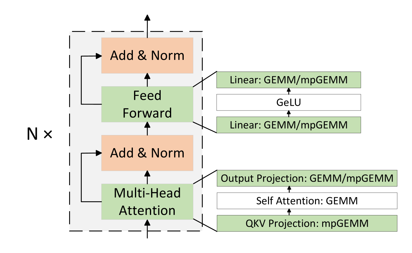</details> Figure 1: Decoder-only transformer blocks in LLMs. The primary computations are GEMM operations (or mpGEMM operations with weight quantization). Nowadays, LLMs mainly rely on the decoder-only transformer architecture shown as Fig. 1 to generate contextually cohesive output [58]. Specifically, LLMs are built with sequential transformer layers, where each transformer layer contains a multi-head attention block followed by a feed forward block. In both multi-head attention and feed forward block, the primary computations are GEMM operations or mpGEMM operations with weight quantization. The studies on scaling law [27, 20] suggest that LLMs will produce better results when scaling up transformer layers. Consequently, there is a rapid growth in the scale of models, which in turn requires significant hardware resources. For example, LLAMA-2-70B [57] consumes 140GB of memory for its model weights alone (in FP16), far exceeding the capacity of a modern GPU like NVIDIA A100 or H100. This imposes a considerable challenge for LLM deployment. To reduce inference costs in LLM deployment, low-bit quantization has become a popular approach [10, 12]. It reduces the precision of numerical representations of a model, thus decreasing memory footprint and computation time. Nowadays, it becomes a common practice to release LLMs with its low-bit versions [56, 67]. Quantization is known to degrade model accuracy. Among different choices, weight quantization is preferred over activation quantizations [35, 33]. This is because the values of model weights are known ahead of time and thus can be quantized offline. Weights can be quantized to 4-bit, 2-bit, and even 1-bit without impacting model accuracy significantly [56, 67, 14, 60, 39]. Conversely, activations are generated on-the-fly with a high variance, noticeably presented as dynamic outliers [10, 64, 17]. These outliers can lead to significant accuracy degradation. In some case, it is difficult to maintain model accuracy even with 8-bit activations. Although the trend is clear, finding the right bit-width for weight and activation is complex, as it needs to strike a delicate balance between model size, computational speed, and model accuracy per user demands. Different combinations of weight and activation bit-widths have been explored in different models and scenarios [10, 15, 18, 14, 60], suggesting that no universal solution that fits all scenarios. <details> <summary>x2.png Details</summary>  ### Visual Description ## Blank Image: No Content Detected ### Overview The image is entirely blank, consisting of a uniform gray square with no discernible elements, text, charts, diagrams, or visual data. No components, labels, or content are present. ### Components/Axes - **No axes, labels, or scales** are visible. - **No legends or color keys** are present. - **No text, annotations, or embedded content** exists in the image. ### Detailed Analysis - **No data points, numerical values, or categorical labels** can be identified. - **No diagrams, flowcharts, or UI elements** are detectable. - **No spatial grounding** (e.g., legend placement, axis alignment) is applicable due to the absence of elements. ### Key Observations - The image provides **no factual or technical information**. - No trends, outliers, or relationships can be inferred. ### Interpretation The image appears to be either: 1. A **technical error** (e.g., failed to load content). 2. A **placeholder** with no intended data. 3. A **deliberate blank slate** for illustrative purposes. Without additional context or content, no meaningful analysis or conclusions can be drawn. </details> Figure 2: (a) GEMM, (b) Indirect mpGEMM: mpGEMM to GEMM by dequantization, (c) Direct mpGEMM. ### II-B mpGEMM in Low-Bit LLM Inference The use of various bit-width for weights and activations leads to a unique requirement of mixed-precision General Matrix Multiplication (mpGEMM), where the weight matrix is in lower precision and the activation matrix remains in higher precision. Figure 2 shows an example of INT4/2/1 multiplied by FP16. Currently, commercial LLM inference hardware, such as GPU and TPU, does not support mpGEMM natively. They only focus on conventional GEMM where two inputs are with the same format and bit-width. Dequantization-based mpGEMM upscales low-precision weights to match the high-precision activations so that conventional GEMM is applicable [2, 61]. Although it can accommodate various combinations of precisions, dequantization requires extra operations and can become a performance bottleneck. Meanwhile, as the GEMM is still computed in high precision, dequantization-based mpGEMM cannot take the full advantage of low-precision computation. 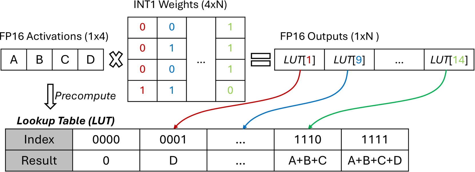LUT-based mpGEMM is an alternative approach that uses lookup tables (LUTs) to implement mpGEMM [45, 25, 40]. It precomutes dot products of high-precision activations with a limited set of low-precision weights and replaces the computation by simple lookups in the resulting table. LUT-based mpGEMM can eliminate most multiplications and reduce additions, thus presumably improving efficiency. Figure 3 illustrates a naive example of using LUT for FP16 activations multiplied by INT1 weights. In this case, the activation vector length is 4, resulting in a lookup table of size 16. This allows a table lookup to replace a dot product of 4-element vectors. For longer activations or higher-bit weights, a larger lookup table is required. <details> <summary>x3.png Details</summary>  ### Visual Description ## Diagram: Neural Network Layer with Lookup Table (LUT) Implementation ### Overview This diagram illustrates a computational process in a neural network layer, showing how input activations are transformed through matrix multiplication and a lookup table (LUT) to produce final outputs. The process involves precomputing possible activation sums and mapping them to LUT indices for efficient computation. ### Components/Axes 1. **FP16 Activations (1x4)**: Input vector with elements A, B, C, D. 2. **INT1 Weights (4xN)**: Weight matrix with binary values (0s and 1s). The first four columns are explicitly shown: ``` [0 0 ... 1] [0 1 ... 1] [0 0 ... 1] [1 1 ... 0] ``` 3. **FP16 Outputs (1xN)**: Result of matrix multiplication, connected to LUT via colored lines. 4. **Lookup Table (LUT)**: - **Index**: 4-bit binary values (0000 to 1111). - **Result**: Precomputed sums of activations (e.g., 0, D, A+B+C, A+B+C+D). 5. **Color-Coded Connections**: - **Red**: Links matrix row 1 (0 0 ... 1) to LUT[1]. - **Blue**: Links matrix row 2 (0 1 ... 1) to LUT[9]. - **Green**: Links matrix row 4 (1 1 ... 0) to LUT[14]. ### Detailed Analysis - **Matrix Multiplication**: The 4xN weight matrix multiplies the 1x4 activation vector, producing intermediate sums. For example: - Row 1 (0 0 ... 1) → Sum = D (activates only the last element). - Row 2 (0 1 ... 1) → Sum = A+B+C+D (activates all elements). - Row 4 (1 1 ... 0) → Sum = A+B+C (activates first three elements). - **LUT Mapping**: Intermediate sums are rounded to 4-bit indices (0-15) and mapped to precomputed results. For instance: - Index `0001` (1) → Result = D. - Index `1010` (10) → Result = A+B+C. - Index `1111` (15) → Result = A+B+C+D. ### Key Observations 1. **Sparse Weight Matrix**: Most weights are 0, reducing computational complexity. 2. **LUT Precomputation**: Avoids runtime summation by precomputing all possible activation combinations (16 entries for 4 inputs). 3. **Color-Coded Logic**: Each color represents a specific row in the weight matrix and its corresponding LUT index. ### Interpretation This diagram demonstrates a **quantized neural network layer** optimized for efficiency: - **Quantization**: Weights are binary (INT1), and activations are 16-bit floats (FP16), reducing memory and compute requirements. - **Lookup Table Optimization**: Precomputing activation sums (via LUT) eliminates repeated arithmetic operations during inference, critical for edge devices with limited resources. - **Sparse Connectivity**: The weight matrix’s sparsity (many 0s) suggests pruning or structured sparsity for further optimization. The process highlights a trade-off between precision (FP16 activations) and efficiency (INT1 weights + LUT), common in deployment scenarios where speed and memory are prioritized over absolute accuracy. </details> Figure 3: A naive LUT-based mpGEMM example of FP16 activations and INT1 weights. With the precomputed table, a table lookup can replace a dot product of 4-element vectors. 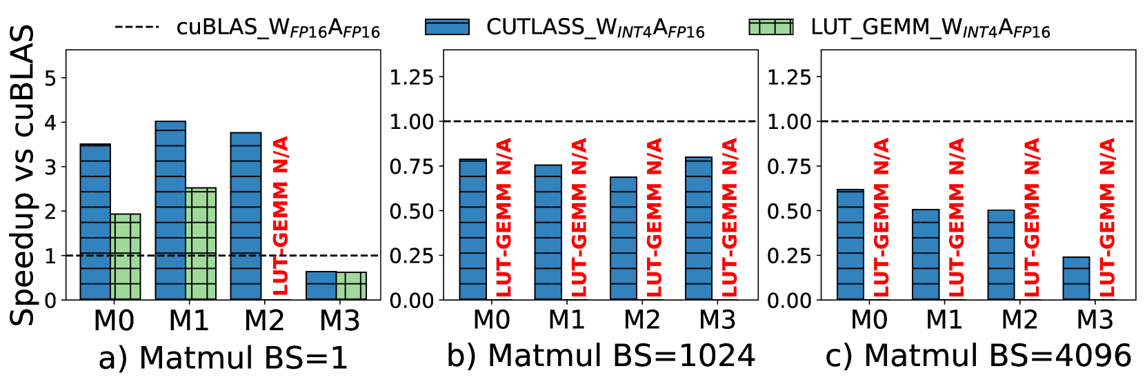Despite its theoretical advantage, LUT-based mpGEMM kernels are often less effective than dequantizaiton-based kernels on existing LLM inference hardware like GPUs, due to the limited LUT support. Figure 4 compares the performance of the LUT-based mpGEMM kernel in [45] to the dequantization-based mpGEMM kernel in CUTLASS [2] on A100 GPU. The results show that the dequantization-based kernel always outperforms the LUT-based kernel. When batch size is large, the LUT-based kernel performs several orders of magnitude worse because of the table access overhead. Thus we denote its performance as N/A in the figure. Moreover, the dequantization-based mpGEMM kernel performs worse than the FP16 $×$ FP16 GEMM cuBLAS kernel when batch size is large, due to the overhead of the additional dequantization operation. This motivates us to customize a LUT-base design for mpGEMM. <details> <summary>x4.png Details</summary>  ### Visual Description ## Bar Charts: Speedup vs cuBLAS for Matmul Configurations ### Overview The image contains three bar charts (a, b, c) comparing the speedup of three matrix multiplication (Matmul) implementations—**cuBLAS**, **CUTLASS**, and **LUT_GEMM**—relative to **cuBLAS** across different batch sizes (BS). Each chart corresponds to a specific BS value: - **a) Matmul BS=1** - **b) Matmul BS=1024** - **c) Matmul BS=4096** The y-axis represents **Speedup vs cuBLAS** (normalized to 1.0 for cuBLAS), and the x-axis lists four configurations: **M0, M1, M2, M3**. The charts use distinct colors for each method: - **Blue**: cuBLAS - **Green**: CUTLASS - **Red**: LUT_GEMM A dashed horizontal line at **1.0** indicates the baseline (cuBLAS performance). --- ### Components/Axes - **X-axis (Categories)**: - **M0, M1, M2, M3** (configurations). - **Y-axis (Values)**: - **Speedup vs cuBLAS** (0.0 to 5.0 for chart a), 0.0 to 1.25 for charts b and c). - **Legends**: - **cuBLAS** (blue bars) - **CUTLASS** (green bars) - **LUT_GEMM** (red bars) - **Annotations**: - "LUT-GEMM N/A" in red text (indicating missing data for LUT_GEMM in some cases). - Dashed line at **1.0** (baseline). --- ### Detailed Analysis #### Chart a) Matmul BS=1 - **cuBLAS**: - M0: ~3.5 (3.4–3.6) - M1: ~4.0 (3.9–4.1) - M2: ~3.8 (3.7–3.9) - M3: ~0.5 (0.4–0.6) - **CUTLASS**: - M0: ~2.0 (1.9–2.1) - M1: ~2.5 (2.4–2.6) - M2: ~2.3 (2.2–2.4) - M3: ~0.5 (0.4–0.6) - **LUT_GEMM**: - M0: ~1.0 (0.9–1.1) - M1: ~2.5 (2.4–2.6) - M2: ~3.0 (2.9–3.1) - M3: **N/A** (marked in red). #### Chart b) Matmul BS=1024 - **cuBLAS**: - M0: ~0.75 (0.73–0.77) - M1: ~0.70 (0.68–0.72) - M2: ~0.65 (0.63–0.67) - M3: ~0.75 (0.73–0.77) - **CUTLASS**: - M0: ~0.70 (0.68–0.72) - M1: ~0.65 (0.63–0.67) - M2: ~0.60 (0.58–0.62) - M3: ~0.70 (0.68–0.72) - **LUT_GEMM**: - M0: **N/A** - M1: **N/A** - M2: **N/A** - M3: **N/A** #### Chart c) Matmul BS=4096 - **cuBLAS**: - M0: ~0.50 (0.48–0.52) - M1: ~0.45 (0.43–0.47) - M2: ~0.40 (0.38–0.42) - M3: ~0.20 (0.18–0.22) - **CUTLASS**: - M0: ~0.50 (0.48–0.52) - M1: ~0.45 (0.43–0.47) - M2: ~0.40 (0.38–0.42) - M3: ~0.20 (0.18–0.22) - **LUT_GEMM**: - M0: **N/A** - M1: **N/A** - M2: **N/A** - M3: **N/A** --- ### Key Observations 1. **cuBLAS Dominates at Low BS (BS=1)**: - cuBLAS achieves the highest speedup (up to ~4.0) for M1, while CUTLASS and LUT_GEMM show significantly lower performance. - LUT_GEMM underperforms but matches cuBLAS at M3 (BS=1). 2. **Performance Degradation at Higher BS**: - For BS=1024 and BS=4096, all methods show speedup values **below 1.0**, indicating **slower performance than cuBLAS**. - LUT_GEMM is **not applicable (N/A)** for all configurations at BS=1024 and BS=4096, suggesting it may not be optimized for large batch sizes. 3. **Consistent Trends Across Configurations**: - cuBLAS and CUTLASS exhibit similar trends, with speedup decreasing as BS increases. - LUT_GEMM’s N/A values imply it is either untested or incompatible with these configurations. --- ### Interpretation - **cuBLAS as Baseline**: The dashed line at 1.0 confirms cuBLAS is the reference for speedup. - **CUTLASS vs. cuBLAS**: CUTLASS generally matches or slightly underperforms cuBLAS, suggesting it is a competitive alternative but not superior. - **LUT_GEMM Limitations**: The absence of data for LUT_GEMM at higher BS values (1024, 4096) indicates it may not scale well or is not implemented for these cases. - **BS Impact**: Speedup decreases with increasing BS, highlighting potential inefficiencies in handling large batch sizes. This data suggests that **cuBLAS remains the most efficient implementation** for the tested configurations, while **CUTLASS** offers comparable performance. **LUT_GEMM** appears limited in applicability, particularly for large batch sizes. </details> Figure 4: Dequantzation-based mpGEMM kernels (CUTLASS) vs. LUT-based mpGEMM kernels (LUT_GEMM) on A100 GPU. W INT4 A FP16 means weights in INT4 and activations in FP16, and so on so forth. The W FP16 A FP16 cuBLAS version serves as a baseline. Matrix shapes M0-M3 are extracted from the linear layers of the LLAMA2-70B model across batch sizes (BS) 1, 1024, and 4096. ### II-C Challenges of LUT-based mpGEMM Hardware At first glance, LUT-based hardware offers great simplicity, as it only requires register or memory for table storage and multiplexers for table lookup. However, our study suggests that a naïve LUT hardware design cannot deliver the promised gains. Numerous challenges and unexplored design aspects significantly affect system performance. This includes: Table precompute and storage. LUT-based approach requires precomputing the table, which can introduce area and latency overhead. The table can also occupy more storage space. This could diminish the efficiency gains. Bit-width flexibility. As discussed in § II-A, LUT-based mpGEMM needs to support different bit-width combinations, e.g., INT4/2/1 $×$ FP16/FP8/INT8, while handling each case separately may consume excessive chip area. Achieving efficiency and flexibility at the same time poses a new challenge. LUT tiling shape. The tiling of the LUT unit can significantly impact performance, as a suboptimal tiling shape increases storage costs and reduces opportunities for table reuse. Instruction and compilation. LUT-based mpGEMM requires a new instruction set. The conventional compilation stack optimized for standard GEMM hardware may not provide optimal mapping and scheduling plans for the mpGEMM instruction set with a different tiling shape. This increases the efforts to integrate the LLM inference software stack with the new LUT design. ## III LUT Tensor Core Design <details> <summary>x5.png Details</summary>  ### Visual Description ## Diagram: Neural Network Tensor Core Architecture ### Overview The image depicts a technical diagram of a neural network tensor core architecture, divided into two sections: 1. **Left**: A flowchart illustrating data flow and component interactions. 2. **Right**: A detailed LUT Tensor Core diagram showing memory structures, data paths, and processing units. --- ### Components/Axes #### Left Diagram (Flowchart): - **Ovals (Processes)**: - **Norm** (orange): Normalization step. - **Pre-Compute** (gray): Preprocessing for activation. - **LUT-mpGEMM** (green): Lookup Table-based General Matrix Multiply. - **Weight Reinterpretation** (gray): Conversion of low-bit weights. - **Arrows (Data Flow)**: - **Activation** (dashed line): Connects "Norm" to "Pre-Compute." - **Operator Fusion** (dashed line): Links "Pre-Compute" to "LUT-mpGEMM." - **LUT Table** (dashed line): Connects "LUT-mpGEMM" to "Reinterpreted Weight." - **Reinterpreted Weight** (dashed line): Feeds into "Compiled to LMMA." - **Text Labels**: - "Low-bit Weight" (left of "Weight Reinterpretation"). - "Compiled to LMMA" (bottom of flowchart). #### Right Diagram (LUT Tensor Core): - **LUT Table**: - A 8x4 grid of entries (e.g., `-A-B-C-D`, `-A-B-C+D`, etc.), representing signed combinations of 4-bit inputs. - Background: Light green. - **Low-bit Weight**: - A 4x1 column of orange blocks (representing 4-bit weights). - Background: Yellow. - **MUX (Multiplexer)**: - Two blue blocks labeled "MUX," with arrows indicating data flow from LUT Table and Low-bit Weight. - **Legend**: - **Orange**: Norm, Weight Reinterpretation. - **Gray**: Pre-Compute, Weight Reinterpretation. - **Green**: LUT-mpGEMM, LUT Table. - **Yellow**: Low-bit Weight. - **Blue**: MUX. --- ### Detailed Analysis #### Left Diagram: 1. **Norm → Pre-Compute**: - Normalized data is activated and precomputed for further processing. 2. **Operator Fusion**: - Combines operations (e.g., activation and LUT lookup) to optimize computation. 3. **LUT-mpGEMM**: - Uses a Lookup Table (LUT) to accelerate matrix multiplication (GEMM). 4. **Weight Reinterpretation**: - Converts low-bit weights (e.g., 4-bit) into a format compatible with the tensor core. 5. **Compiled to LMMA**: - Final stage where weights are compiled into a low-memory, high-throughput format. #### Right Diagram: 1. **LUT Table Structure**: - Entries like `-A-B-C-D` represent all possible 4-bit signed combinations (8 rows × 4 columns). - Designed for efficient address calculation in tensor operations. 2. **Low-bit Weight Integration**: - 4-bit weights are fed into the MUX alongside LUT outputs. 3. **MUX Functionality**: - Selects between LUT outputs and low-bit weights for processing. --- ### Key Observations 1. **Color Coding**: - Components are color-coded to distinguish between normalization (orange), preprocessing (gray), LUT-based operations (green), and memory structures (yellow/blue). 2. **Data Flow**: - The left diagram emphasizes computational steps, while the right diagram focuses on hardware implementation (LUTs, MUX). 3. **LUT-mpGEMM Role**: - Central to optimizing matrix operations by reducing memory access via lookup tables. --- ### Interpretation This architecture demonstrates a hybrid approach to neural network acceleration: - **Efficiency**: LUT-mpGEMM reduces computational complexity by precomputing common operations. - **Memory Optimization**: Low-bit weights (4-bit) and LMMA compilation minimize memory bandwidth requirements. - **Hardware-Software Co-Design**: The LUT Tensor Core integrates memory (LUT Table) and processing (MUX) to balance speed and resource usage. **Notable Trends**: - The use of LUTs suggests a focus on reducing dynamic computation in favor of static memory lookups. - Low-bit weight reinterpretation indicates quantization for energy-efficient inference. **Uncertainties**: - Exact bit-widths for weights (assumed 4-bit based on labels). - Specific activation functions or normalization methods (not explicitly stated). 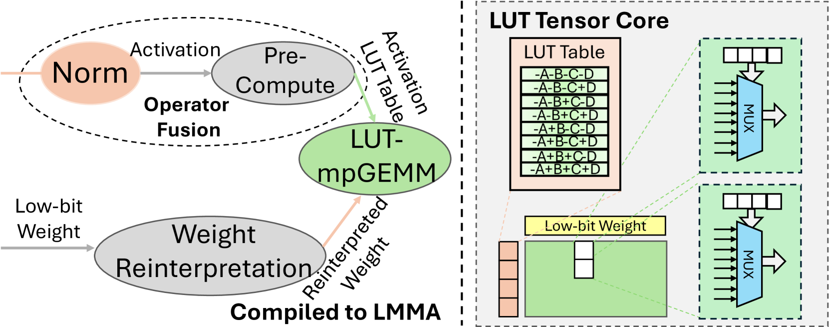</details> Figure 5: Workflow of LUT Tensor Core -accelerated low-bit LLMs. To unleash the full potential of LUT-based mpGEMM, we introduce LUT Tensor Core, a software-hardware co-design approach aimed at addressing the aforementioned efficiency, flexibility, and compatibility challenges (§ II-C). Fig. 5 illustrates the overview of LUT Tensor Core. Different from the conventional hardware-based solution for LUT table precompute and storage that may introduce significant hardware overheads, LUT Tensor Core designs software-based optimizations (§ III-A) to optimize the LUT table precompute and storage: precomputing the LUT table for the input activation tensor is performed by operator fusion, while the input weight tensor is reinterpreted to enable table storage optimizations. On the hardware side, LUT Tensor Core features a simplified microarchitecture (§ III-B), that enhances efficiency for mpGEMM processing and supports flexibility for various bit-width data types. To integrate LUT Tensor Core into existing deep learning ecosystem, we design the LUT-based Matrix Multiply-Accumulate (LMMA) instruction set to expose the LUT Tensor Core for programming mpGEMMs and implements the compilation stack to schedule the end-to-end LLM execution (§ III-C). ### III-A Software-based Table Optimization As introduced in § II, LUT-based mpGEMM needs additional table precomputing process and storage to store the precomputed results. Naively, the precomputed dot products of a length $K$ activation vector on the $W\_BIT$ weight require $(2^W\_BIT)^K$ entries for the table. For each activation element, multiplying it with the ${W\_BIT}$ weight has $2^W\_BIT$ possible results, constructing the precompute table for this activation element. Therefore, the precomputed table has $(2^W\_BIT)^K$ entries for a length $K$ activation vector. Fig. 3 shows the lookup table with $2^4$ entries for $K=4,{W\_BIT}=1$ . A commonly-used optimization is bit-serial [26] that represents a ${W\_BIT}$ integer as ${W}$ 1-bit integers and performs multiplication over 1-bit integers with bit shift. This paradigm can reuse the precompute table on 1-bit, and therefore reduces the table size to $2^K$ . However, this table size still has significant hardware overheads. To address these overheads, LUT Tensor Core proposes operator fusion to reduce the table precompute time, weight reinterpretation and table quantization to reduce the table size. #### III-A 1 Precomputing lookup table with operator fusion The LUT-based mpGEMM requires precomputing the dot production of high-precision activation and a set of low-precision weights as a table for the later lookup operations. A conventional hardware implementation is positioning the precompute unit adjacent to the LUT unit and performing the table precompute for each LUT unit on-the-fly. However, this implementation may significantly introduce hardware cost. Fortunately, the table precompute described above is an element-wise operation where each element is the production of an activation value and a combination $\{0,1\}$ of $K$ that can be processed by a general-purpose compute unit (e.g., CUDA Cores in GPU). Moreover, the precompute table can also be shared by LUT units instead of precomputing a table for each LUT unit to reduce the redundant precomputation. Therefore, we can enable a one-time precompute kernel for the input activation tensor and write back the precompute table to memory. Then the LUT units can load the precompute table to the register and perform table lookups. Furthermore, as introduced in Fig. 1, the preceding operator of a mpGEMM is normalization that is also an element-wise operator. The table precompute operation can be fused into the preceding operators for further optimizations, which will be detailed in § III-C 2. This helps to mitigate the table precompute overhead to almost zero as evaluated in § IV-E 1. #### III-A 2 Reinterpreting weight for table symmetrization <details> <summary>x6.png Details</summary>  ### Visual Description ## Diagram: Binary Value Reinterpretation with Sign Transformation ### Overview The diagram illustrates a binary-to-decimal reinterpretation process involving sign manipulation and offset transformation. It shows two parallel number lines: one representing original unsigned 4-bit binary values (0-15) and another showing reinterpreted values with negative ranges (-15 to 15). Mathematical equations and arrows demonstrate the transformation logic. ### Components/Axes 1. **Original Uint Section**: - Binary values: 0000 (0) to 1111 (15) - Decimal range: 0-15 - Labels: "Original Uint W3W2W1W0", "q ∈ {0,1,...,14,15}" 2. **Reinterpreted Section**: - Binary values: 0000 (-15) to 1111 (15) - Decimal range: -15 to 15 - Labels: "Reinterpreted W3'W2'W1'W0'", "q' ∈ {-15,-3,...,13,15}" 3. **Transformation Equations**: - r = S(q - z) - S' = 0.5, z' = -15 - S = 1, z = 0 4. **Legend**: - Original Uint: Gray color - Reinterpreted: Yellow color - Arrows: Dashed lines connecting original to reinterpreted values ### Detailed Analysis 1. **Binary Mapping**: - Original: 0000 (0) → 1111 (15) - Reinterpreted: 0000 (-15) → 1111 (15) - Midpoint shift: Original 7.5 → Reinterpreted -7.5 2. **Transformation Logic**: - Original values (q) are transformed using r = S(q - z) - When S=1 and z=0, r = q (identity transformation) - Reinterpreted values use S'=0.5 and z'=-15, creating a scaled and offset version 3. **Key Arrows**: - 0000 (0) → -15 (q'=-15) - 1111 (15) → 15 (q'=15) - 0111 (7) → 13 (q'=13) - 1000 (8) → -3 (q'=-3) ### Key Observations 1. **Range Expansion**: Reinterpreted values span -15 to 15 vs original 0-15 2. **Midpoint Shift**: Original midpoint (7.5) becomes -7.5 in reinterpreted 3. **Non-linear Mapping**: Values like 7→13 and 8→-3 show non-linear transformation 4. **Sign Bit Manipulation**: The reinterpretation appears to use the MSB (W3) as a sign bit ### Interpretation This diagram demonstrates a binary reinterpretation technique that: 1. **Expands Value Range**: By redefining the sign bit (W3), the system can represent both positive and negative values 2. **Applies Offset Transformation**: The z'=-15 offset suggests a two's complement-like system but with different scaling 3. **Uses Fractional Scaling**: S'=0.5 indicates a halving of the original value range 4. **Maintains Symmetry**: The reinterpreted range (-15 to 15) is symmetric around zero, unlike the original (0-15) The transformation appears to be a custom encoding scheme that allows representation of both positive and negative values while maintaining some relationship to the original unsigned values. The specific choice of S'=0.5 and z'=-15 suggests a deliberate design choice to balance positive/negative representation while preserving certain arithmetic properties. 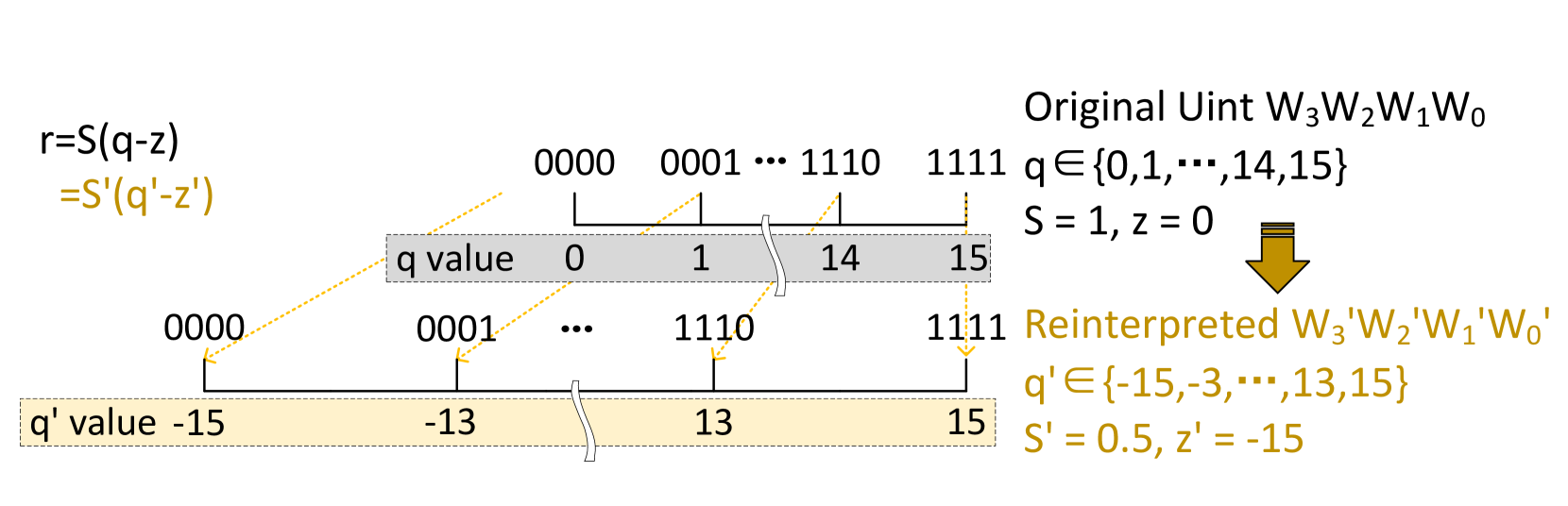</details> Figure 6: Reinterpreting 0,1 to -1,1 to enable symmetry, thereby cutting the table size by half. The $2^K$ table length of precomputing a length $K$ activation vector introduces cost in both table storage and table accesses. Fortunately, we observed the symmetrization property of integers that the integer representation can be symmetric around zero with a math-equivalent linear transformation. Assume $K$ weights $[W_K-1,...,W_2,W_1,W_0]$ are represented as a $K$ -bit integer: $$ r=s(q-z) \tag{1} $$ where $r$ is the real value, $s$ is the scale factor, $z$ is the bias, and $q$ is the integer representation to $K$ bits. To transform such representation to be symmetric around zero, we map $q$ to make it symmetric to zero and adjust $s$ and $z$ correspondingly: $$ q^\prime=2q-(2^K-1), s^\prime=s/2, z^\prime=2z+1-2^K \tag{2} $$ Fig. 6 shows the example of transforming the 4-bit unsigned integers. By calculating the $s^\prime$ and $z^\prime$ , $q^\prime$ is mapped from $\{0,1,...,14,15\}$ to $\{-15,-13,...,13,15\}$ , which is symmetric around zero. Let’s consider a dot product between the binary representation ${W_3W_2W_1W_0}={0100}$ and variables $A,B,C,D$ . Initially, the binary values {‘0’,‘1’} are interpreted as {0,1}. The calculation proceeds as follows: $$ r=s·(q-z)=1·(B-0)=B $$ After reinterpretation, the binary values {‘0’,‘1’} are redefined to mean {-1,1}, with the scale factor $s^\prime$ adjusted to 0.5 and the bias $z^\prime$ recalculated as $-(A+B+C+D)$ . The updated computation is: $$ r=s^\prime·(q^\prime-z^\prime)=0.5·((-A+B-C-D)+(A+B+C+D))=B $$ It’s clear that the two expressions remain mathematically equivalent. As the table entries are symmetric about zero, the lookup table exhibits properties similar to odd functions. Assuming the index is a 4-bit value $W_3W_2W_1W_0$ , a naive implementation of the lookup table (LUT) requires $2^4=16$ entries. However, it can be observed that the following property, akin to that of odd functions, holds: $$ LUT[W_3W_2W_1W_0]=-LUT[∼(W_3W_2W_1W_0)] \tag{3} $$ Therefore, the number of entries in the LUT can be reduced to half of the original, which is $2^4-1=8$ , and the equation becomes: $$ LUT[W_3W_2W_1W_0]=\begin{cases}-LUT[∼(W_2W_1W_0 )],&if W_3=1\\ LUT[W_2W_1W_0],&if W_3=0\end{cases} \tag{4} $$ Therefore, given a length $K$ activation vector, table symmetrization can reduce the table length to $2^K-1$ . The table size not only affects the computational operations required during the precompute stage, but also the multiplexers (MUX) size. Furthermore, each entry in the table also needs to be broadcast to $N$ PEs, typically 64 or 128, for dot product computations. Such an optimization significantly reduces the broadcasting overhead and the MUX selection overhead, thereby enhancing the energy efficiency and area efficiency of the circuit. Note that $W_3W_2W_1W_0$ in Equation 4 are all weights, which will not be modified in inference. So, the bit-level negation can be done by offline weight transformation and the equation can further be simplified to: $$ LUT[W_3^\primeW_2^\primeW_1^\primeW_0^\prime]=\begin{ cases}-LUT[W_2^\primeW_1^\primeW_0^\prime],&if W_3 ^\prime=1\\ LUT[W_2^\primeW_1^\primeW_0^\prime],&if W_3^ \prime=0\end{cases} \tag{5} $$ This simplification can eliminate the negation operation in circuit design, which will be introduce in § III-B. #### III-A 3 Table Quantization Table symmetrization can reduce the table size by half. Moreover, for high precision activations, such as FP32 or FP16, we utilize table quantization techniques to quantize the precomputed table elements to a lower, unified precision, such as INT8. This approach offers flexibility by supporting multiple activation precisions and efficiency by reducing storage requirements through lower precision table elements. Although table quantization might potentially affect model accuracy, it provides a significant advantage over conventional activation quantization. Traditional activation quantization cannot leverage dynamic, fine-grained quantization due to efficiency concerns. In contrast, table quantization allows for dynamic, fine-grained quantization during the precomputation phase. For instance, with a group size of 4 activation elements, we perform quantization for each generated table with 8 precomputed dot-products. This method is expected to maintain higher accuracy compared to conventional activation quantization. Our empirical experiments, as discussed in § IV-E 2, confirm this expectation. The results demonstrate that the impact on accuracy when using INT8 quantization for the table elements is minimal, thereby validating the effectiveness of our approach. 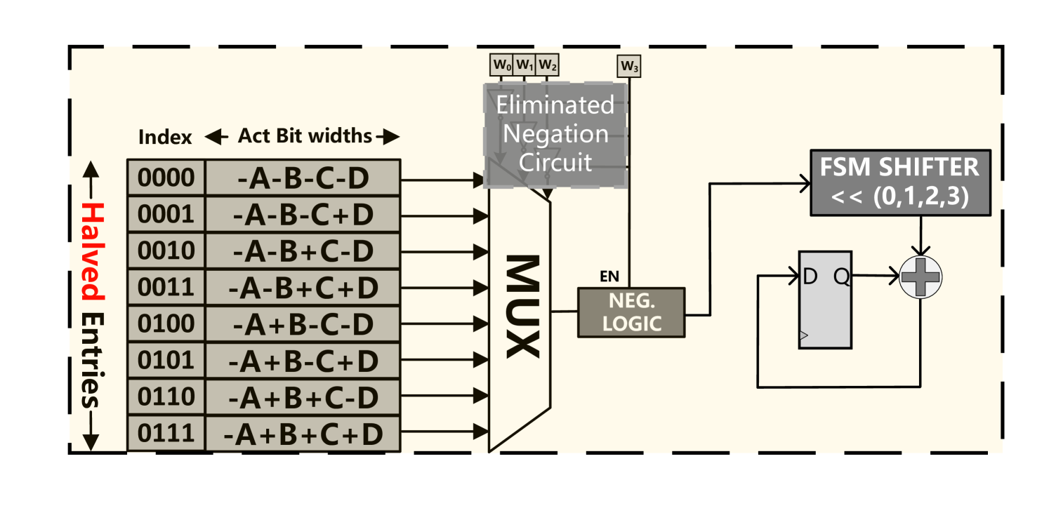### III-B LUT Tensor Core Microarchitecture #### III-B 1 Simplified LUT unit design with bit-serial By leveraging software-based precompute fusion and weight reinterpretation, the hardware cost for customizing each individual LUT unit is significantly reduced. Each LUT unit is simple and easy to scale out. Fig. 7 illustrates our LUT unit design. In comparison to a naive design, the registers needed to store the LUT can be halved, and the cost of the table broadcasting and MUX is also halved. Moreover, as depicted in equation 5, portion of the bit-level negation circuit can be eliminated from each LUT unit, resulting in lower area and power consumption in the hardware. To support flexible bit-widths for weights, we employ a bit-serial circuit architecture [26, 65]. This design unfolds the weight bit-width to W_BIT cycles, thereby enabling the processing of different bit-widths in a serialized manner. This bit-serial approach allows the hardware to adapt to various precision levels without the need for multiple distinct hardware implementations. <details> <summary>x7.png Details</summary>  ### Visual Description ## Block Diagram: Digital Signal Processing Circuit ### Overview The diagram illustrates a digital signal processing circuit with a multiplexer (MUX), negation logic, an FSM shifter, and a summation component. The left side features a table of "Halved Entries" with indexed combinations of variables A, B, C, D. The right side shows signal flow through negation logic, FSM shifter, and summation. ### Components/Axes - **Left Table**: - **Index**: Labeled "Index" with an arrow pointing right. - **Act Bit widths**: Labeled "Act Bit widths" with an arrow pointing right. - **Entries**: 8 rows labeled 0000 to 0111 (binary). Each row contains a combination of A, B, C, D with signs (e.g., "-A-B-C-D", "-A-B+C+D"). - **Label**: "Halved Entries" in red, with an arrow pointing down. - **Right Circuit**: - **MUX**: Labeled "MUX" with inputs from the left table. - **Negation Logic**: Labeled "NEG. LOGIC" with an "EN" (enable) signal. - **FSM Shifter**: Labeled "FSM SHIFTER << (0,1,2,3)>>" with a control signal. - **D Flip-Flop**: Labeled "D Q" with a "+" symbol for summation. - **Eliminated Negation Circuit**: A gray box labeled "Eliminated Negation Circuit" above the MUX. ### Detailed Analysis - **Left Table**: - 8 rows represent binary indices (0000 to 0111). - Each row combines A, B, C, D with alternating signs (e.g., "-A-B-C-D", "-A-B+C+D"). - No numerical values; entries are symbolic expressions. - **Right Circuit**: - **MUX**: Selects one of the 8 entries based on the index. - **Negation Logic**: Inverts the selected signal (EN controls enable). - **FSM Shifter**: Shifts the negated signal by 0–3 positions (control signal << (0,1,2,3)>>). - **D Flip-Flop**: Stores the shifted value (D Q). - **Summation**: Combines the shifted value with another input (symbolized by "+"). ### Key Observations - The "Eliminated Negation Circuit" suggests optimization to avoid redundant negation steps. - The FSM Shifter’s control signal allows dynamic shifting, critical for timing or positional adjustments. - The summation at the end implies the circuit aggregates processed signals. ### Interpretation This circuit processes binary data by selecting, negating, shifting, and summing signals. The MUX and FSM Shifter enable flexible configuration, while the negation logic ensures polarity control. The "Eliminated Negation Circuit" hints at efficiency improvements, possibly reducing power consumption or latency. The summation component suggests the circuit is part of a larger system requiring combined outputs (e.g., arithmetic operations or signal synthesis). ## Additional Notes - **Language**: All text is in English. - **No numerical data**: The diagram focuses on symbolic logic and component relationships rather than quantitative values. - **Flow Direction**: Signals move left-to-right, with feedback loops (e.g., D flip-flop output). </details> Figure 7: Optimized LUT unit with bit-serial. 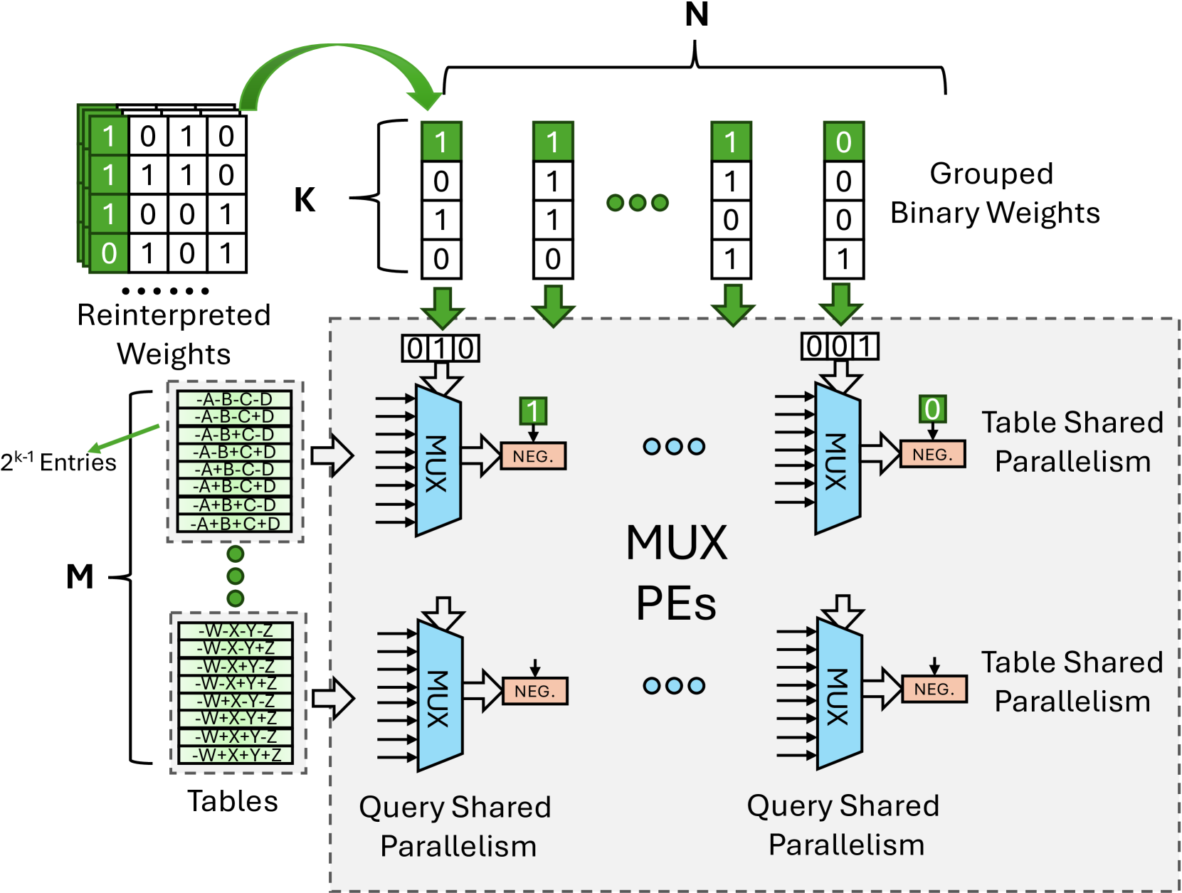#### III-B 2 Elongated LUT tiling The selection of dimensions $M$ , $N$ , and $K$ is crucial for the performance of LUT Tensor Core, with traditional choices for MAC-based Tensor Cores potentially leading to suboptimal performance in this context. As illustrated in Fig. 8, a $MNK$ Tile’s LUT Array comprises $M$ tables, $N$ sets of weights, and $M*N$ MUX-based units. Each table contains $M× 2^K-1$ entries, with each entry needing to be broadcast to $N$ MUX units; each set of Grouped Binary Weights includes $K$ bits, which must be broadcast to $M$ MUX units to act as select signals for the MUX. The total table size is given by the equation: $$ Total Table Size=M× 2^K-1×LUT\_BIT \tag{6} $$ and the size for grouped binary weights is given by: $$ Grouped Binary Weights Size=K× N×W\_BIT \tag{7} $$ where LUT_BIT is the bit width of the LUT entries, and W_BIT is the bit width of the weights. LUT Tensor Core prefers elongated tiling shape. With large $K$ , the size of table entries explodes exponentially, whereas $N$ represents the potential reuse of each table entry across multiple MUX units. Intuitively, we need to find a balance with a suitably sized $K$ , a larger $N$ , and a smaller $M$ —a configuration that diverges from the typical demands of conventional GPU Tensor Cores. Furthermore, we must consider the impact of this shape on tiling, as a more square-like tiling configuration can lead to lower I/O traffic. Therefore, we also strive to balance the size of the LUT and weight within a tile as closely as possible. In § IV-B 2, we conduct extensive and comprehensive experiments to explore the design space for $MNK$ tiling, verifing elongated tiling shapes achieve better efficiency. <details> <summary>x8.png Details</summary>  ### Visual Description ## Diagram: Binary Weight Processing Architecture ### Overview The diagram illustrates a technical architecture for processing binary weights in a computational system. It includes components for reinterpreting weights, grouping binary weights, and parallel processing via MUX PEs (Multiplexer Processing Elements). The flow involves reinterpreting weights, grouping them, and distributing them across query and table shared parallelism units. ### Components/Axes 1. **Reinterpreted Weights**: - A matrix with green and white blocks labeled "1" and "0". - Contains 2^(k-1) entries, with examples like "-A-B-C-D" and "-W-X-Y-Z". 2. **Grouped Binary Weights**: - A matrix with 1s and 0s, labeled "Grouped Binary Weights". - Arrows point from "Reinterpreted Weights" to this section. 3. **Tables**: - Contains entries like "-W-X-Y-Z" with variations (e.g., "+", "-"). - Arrows point from "Tables" to "Query Shared Parallelism" and "Table Shared Parallelism". 4. **MUX PEs**: - Central processing units labeled "MUX" with arrows from "Grouped Binary Weights". - Connected to "NEG." (negation) blocks. 5. **Parallelism Sections**: - **Query Shared Parallelism**: Arrows from MUX PEs to this section. - **Table Shared Parallelism**: Arrows from MUX PEs to this section. 6. **NEG. Blocks**: - Labeled "NEG." with arrows from MUX PEs. ### Detailed Analysis - **Reinterpreted Weights**: - A 4x4 matrix with green (1) and white (0) blocks. - Example entries: "1 0 1 0", "1 1 1 0", "1 0 0 1", "0 1 0 1". - **Grouped Binary Weights**: - A 4x4 matrix with 1s and 0s. - Example entries: "1 1 1 0", "1 1 0 0", "1 0 1 0", "0 1 0 1". - **Tables**: - Contains 2^(k-1) entries with variable combinations (e.g., "-W-X-Y-Z", "-W+X-Y+Z"). - Example entries: "-W-X-Y-Z", "-W-X+Y+Z", "-W+X-Y-Z", "-W+X+Y+Z". - **MUX PEs**: - Blue rectangular blocks labeled "MUX". - Arrows from "Grouped Binary Weights" to MUX PEs. - **Parallelism Sections**: - **Query Shared Parallelism**: Arrows from MUX PEs to this section. - **Table Shared Parallelism**: Arrows from MUX PEs to this section. - **NEG. Blocks**: - Pink rectangular blocks labeled "NEG.". - Arrows from MUX PEs to these blocks. ### Key Observations - The architecture emphasizes **parallelism** through MUX PEs and shared processing units. - **Binary weights** are grouped and distributed to both query and table shared parallelism. - **Negation** is applied after MUX processing, suggesting a step for sign handling. - The "2^(k-1) Entries" in tables imply exponential scaling with variable k. ### Interpretation This diagram represents a hardware or algorithmic framework for optimizing binary weight processing, likely in a neural network or machine learning context. The **reinterpreted weights** are transformed into grouped binary weights, which are then processed in parallel via MUX PEs. The **query and table shared parallelism** suggest a design for efficient data handling, where shared resources (e.g., memory or computation units) are utilized to reduce redundancy. The **negation blocks** indicate a step to handle signed weights, ensuring correct sign propagation. The use of **2^(k-1) Entries** implies a scalable system where the number of entries grows exponentially with the number of variables (k), enabling complex weight combinations. The flow from "Reinterpreted Weights" to "Grouped Binary Weights" to MUX PEs and then to parallelism sections highlights a pipeline for efficient computation. This architecture likely aims to balance computational efficiency with flexibility in handling diverse weight configurations. </details> Figure 8: Elongated $MNK$ tiling of LUT Tensor Core. LUT Tensor Core requires a larger $N$ (e.g., 64/128) to maximize table reuse, along with a suitably sized $K$ (e.g., 4) for a cost-efficient table size. ### III-C Instruction and Compilation To effectively integrate LUT Tensor Core into the existing GPU architecture and ecosystem, we propose a new set of instructions and have developed a compilation stack based on state-of-the-art DNN compilers [7, 75, 54]. Our compilation stack has been enhanced with specialized intrinsics and optimizations, specifically designed to leverage the unique capabilities of LUT Tensor Core. #### III-C 1 LUT-based MMA instructions To enable programming with LUT Tensor Core, we define a set of LMMA (LUT-based MMA) instructions as an extension of the MMA instruction set in GPU. lmma.{M}{N}{K}.{ $A_dtype$ }{ $W_dtype$ }{ $Accum_dtype$ }{ $O_dtype$ } The above formula shows the format of LMMA instructions, which is similar to MMA. Specifically, the $M$ , $N$ , and $K$ indicates the shape of the LUT Tensor Core. $A_dtype$ , $W_dtype$ , $Accum_dtype$ and $O_dtype$ indicate the data type of the inputs, accumulation and the output, respectively. Similar to MMA instructions, each LMMA instruction is scheduled to a warp of threads for execution. This warp of threads will calculate the formula $O_dtype[M,N]$ = $A_dtype[M,K]$ $×$ $W_dtype[N,K]$ + $Accum_dtype[M,N]$ .The LMMA instructions are similar to MMA instructions, while have different shapes and data types. <details> <summary>x9.png Details</summary>  ### Visual Description ## Diagram: Comparison of Conventional Matrix Operations vs. LUT Tensor Core Optimization ### Overview The diagram illustrates two approaches to matrix operations: a conventional method and an optimized LUT Tensor Core approach. It highlights differences in computational steps, memory usage, and instruction-level optimizations. The lower section details the LUT-based implementation with LMMA (Load Multiply Accumulate) instructions. --- ### Components/Axes #### Conventional Method 1. **Low-bit LLM DFG** → **Mul** → **GEMM** → **Low-bit LLM DFG** - Arrows labeled: "+ DFG Trans., Weight Reint." 2. **Low-bit LLM DFG** → **Mul** → **Precompute** → **LUT-mpGEMM** → **Low-bit LLM DFG** - Arrows labeled: "+ Operator Fusion" #### LUT Tensor Core - **Fused (Mul+ Precompute)** and **LUT-mpGEMM** blocks connected to **Low-bit LLM DFG**. #### LUT-based mpGEMM with LMMA - **Blocked GEMM** (Global Memory) → **Thread Block Tile** (Shared Memory) → **Warp Tile** (Register File) → **LMMA Instruction** (LUT Tensor Core) - Color-coded components: - **Yellow**: Blocked GEMM - **Blue**: Thread Block Tile - **Green**: Warp Tile - **Orange**: LMMA Instruction --- ### Detailed Analysis #### Conventional Method - **Flow**: Data flows through separate **Mul** and **GEMM** stages with intermediate data format conversions (DFG Trans.) and weight reintroduction. - **Inefficiencies**: Explicit steps for data movement and operator separation increase latency. #### LUT Tensor Core - **Fused Operations**: Combines **Mul** and **Precompute** into a single stage, reducing intermediate steps. - **LUT-mpGEMM**: Specialized instruction for matrix operations, optimized for low-bit precision. #### LUT-based mpGEMM with LMMA - **Memory Hierarchy**: - **Global Memory** (Blocked GEMM) → **Shared Memory** (Thread Block Tile) → **Register File** (Warp Tile) → **LUT Tensor Core** (LMMA). - **Optimization**: LMMA instructions enable in-place accumulation, minimizing register file usage and memory bandwidth. --- ### Key Observations 1. **Operator Fusion**: The LUT Tensor Core merges **Mul** and **Precompute** stages, eliminating redundant data transfers. 2. **Memory Efficiency**: The LUT-based approach reduces reliance on shared memory by leveraging the LUT Tensor Core for accumulation. 3. **Precision Handling**: Both methods use low-bit LLM DFG, but the LUT Tensor Core optimizes for low-bit precision via LMMA. --- ### Interpretation The diagram demonstrates how the LUT Tensor Core architecture streamlines matrix operations by: - **Fusing operations** to reduce computational overhead. - **Optimizing memory access** through hierarchical data movement (Global → Shared → Register → LUT Core). - **Leveraging LMMA instructions** for efficient accumulation, critical for low-bit precision workloads. This contrasts with the conventional method, which suffers from fragmented operations and higher latency due to explicit data format conversions and weight reintroduction. The LUT-based approach is particularly advantageous for AI/ML workloads requiring frequent matrix multiplications with low-bit quantization. 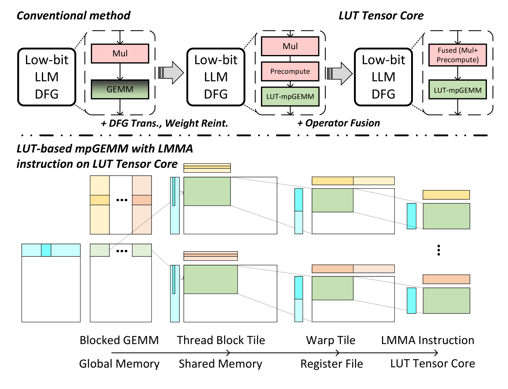</details> Figure 9: Compilation for LUT-based mpGEMM. Elongated tile for enhancing data reuse in mpGEMM. #### III-C 2 Compilation support and optimizations We implemented the LUT-based mpGEMM kernel generation and end-to-end LLM compilation with LUT Tensor Core on top of TVM [7], Roller [75] and Welder [54]. Specifically, the compilation stack encompasses the following key aspects and Fig. 9 shows an example of compilation on the LLAMA model: - DFG Transformation. Given the model represented in data-flow graph (DFG), we transform the mix-precision GEMM operator to a precompute operator and the LUT-based mpGEMM operator. This transformation is implemented as a graph optimization pass in Welder. - Operator Fusion. Operator fusion is a widely-used compiler technique to optimize the end-to-end model execution by reducing memory traffic and runtime overhead. We registered the precompute and the LUT-based mpGEMM operator and represented the required tile-based representation in Welder, enabling reusing Welder to do operator fusion. As shown in Fig. 9, the element-wise precompute operator is fused with the element-wise Norm operator prior to the GEMM operator in LLAMA, which further reduces the table precompute overhead. - LUT-based mpGEMM Scheduling. Similar to GEMM, scheduling LUT-based mpGEMM operator requires careful considering tiling on the memory hierarchy for performance. As shown in Figure 9, GPUs have a memory hierarchy of global memory, shared memory, registers, and tiling on the memory hierarchy can significantly improve the data reuse on on-chip memory to improve performance. Conventional tiling strategies [7, 73, 75] for GEMM assume the same data type on both activation and weight and focus on adjusting the tiling shape on memory hierarchy. However, mpGEMM has different data types on activation and weight, resulting in different memory behaviors for tensors of different data types. We observed the influence of different data types on memory hierarchy is the actual memory transactions. Therefore, we represent the tiling with the actual memory size instead of tiling shape, and register the shape of LMMA instructions and this tiling calculation in Roller’s rTile interfaces to schedule the proper tiling configurations. - Code Generation. With the finalized scheduling plans, code generation is performed using TVM. Specifically, the LMMA instructions are registered as intrinsics in TVM, and TVM can follow the scheduling to generate the kernel code with LMMA instructions. ## IV Evaluation In this section, we conduct a comprehensive and systematic evaluation of LUT Tensor Core to validate its efficiency in accelerating low-bit LLM inference. Initially, we assess the hardware efficiency gains of LUT Tensor Core via detailed PPA benchmarking (§ IV-B). Then, kernel-level experiments are conducted to illustrate the acceleration of mpGEMM (§ IV-C). Following this, we perform end-to-end inference evaluation on commonly-used LLMs to demonstrate the practical performance improvements (§ IV-D). We then delve into the effectiveness of our software optimizations on table precompute fusion and table quantization (§ IV-E). Finally, we provide a holistic comparison of model accuracy and efficiency with previous accelerator designs (§ IV-F). ### IV-A Experimental Setup and Methodology #### IV-A 1 Hardware PPA benchmarks We compare LUT Tensor Core approach with two baselines: Multiply-Accumulate (MAC)-based Tensor Core and Addition (ADD)-based Tensor Core. MAC represents the typical design in current GPUs which needs dequantization to support mpGEMM. ADD adopts the bit-serial computing proposed in [26] to support mpGEMM, where every bit of weights needs one addition. We implement LUT Tensor Core and baselines in Verilog and use Synopsys’s Design Compiler [55] and the TSMC 28nm process library for synthesizing circuits and generating PPA data. We apply DC’s medium effort level targeting 1GHz to ensure a fair comparison across all designs. #### IV-A 2 Kernel-level evaluation Considering that GPUs are the most widely-used hardware for LLM inference today and are equipped with MAC-based Tensor Cores, they provide an ideal platform for comparison and comprehensive evaluation. For mpGEMM kernel-level evaluation, we set the NVIDIA A100 GPU as the baseline. We employ Accel-Sim [28], an open-source state-of-the-art simulator, to run these experiments. Necessary modifications to the configuration and trace files in Accel-Sim allow us to simulate both the original A100 and the LUT Tensor Core -equipped A100. #### IV-A 3 Model end-to-end evaluation and analysis To extend our evaluation to real LLMs, we utilize four widely-used open-source LLMs: LLAMA-2 [57], OPT [71], BLOOM [32], and BitNet [60]. As Accel-Sim becomes infeasible for end-to-end LLM experiments due to its extremely slow simulation speed for large trace file size, we develop a tile-based simulator to support end to end inference evaluations, which will be detailed in § IV-D. <details> <summary>x10.png Details</summary>  ### Visual Description ## Line Graph: Compute Density (TFLOPs/mm²) vs. K ### Overview The graph depicts four data series representing compute density (TFLOPs/mm²) across values of K (2–8). Each series corresponds to a combination of weight precision (INT1) and activation precision (FP16, FP8, INT16, INT8). The y-axis ranges from 0 to 100, while the x-axis spans K=2 to K=8. ### Components/Axes - **X-axis (K)**: Integer values 2–8, labeled "K". - **Y-axis (Compute Density)**: TFLOPs/mm², labeled "Compute Density (TFLOPs/mm²)". - **Legend**: Positioned in the top-right corner, mapping colors to data series: - **Green dashed**: `W_INT1A_FP16` - **Blue dashed**: `W_INT1A_FP8` - **Solid green**: `W_INT1A_INT16` - **Solid blue**: `W_INT1A_INT8` ### Detailed Analysis 1. **W_INT1A_FP16 (Green dashed)**: - Starts at ~10 TFLOPs/mm² at K=2. - Peaks at ~20 TFLOPs/mm² at K=5. - Declines to ~15 TFLOPs/mm² at K=8. - Trend: Gradual increase until K=5, then gradual decline. 2. **W_INT1A_FP8 (Blue dashed)**: - Starts at ~30 TFLOPs/mm² at K=2. - Peaks at ~50 TFLOPs/mm² at K=5. - Declines to ~40 TFLOPs/mm² at K=8. - Trend: Sharp rise until K=5, then gradual decline. 3. **W_INT1A_INT16 (Solid green)**: - Starts at ~20 TFLOPs/mm² at K=2. - Peaks at ~50 TFLOPs/mm² at K=4. - Declines to ~30 TFLOPs/mm² at K=8. - Trend: Sharp rise until K=4, then gradual decline. 4. **W_INT1A_INT8 (Solid blue)**: - Starts at ~70 TFLOPs/mm² at K=2. - Peaks at ~100 TFLOPs/mm² at K=4. - Declines to ~50 TFLOPs/mm² at K=8. - Trend: Sharp rise until K=4, then steep decline. ### Key Observations - **Highest Peak**: `W_INT1A_INT8` (solid blue) achieves the maximum compute density (~100 TFLOPs/mm²) at K=4. - **Lowest Values**: `W_INT1A_FP16` (green dashed) consistently has the lowest compute density across all K values. - **Divergence at K=4**: All series peak at K=4 except `W_INT1A_FP16`, which peaks later at K=5. - **Steep Declines**: `W_INT1A_INT8` and `W_INT1A_INT16` show the sharpest declines post-K=4. ### Interpretation The data suggests that higher precision (INT8/INT16) correlates with greater compute density at lower K values, but performance degrades sharply as K increases. Lower precision (FP16/FP8) maintains more stable but lower compute densities. The peak at K=4 for INT8/INT16 may indicate an optimal configuration for this metric, while FP16/FP8 configurations lag significantly. The divergence in trends highlights trade-offs between precision and scalability across K values. 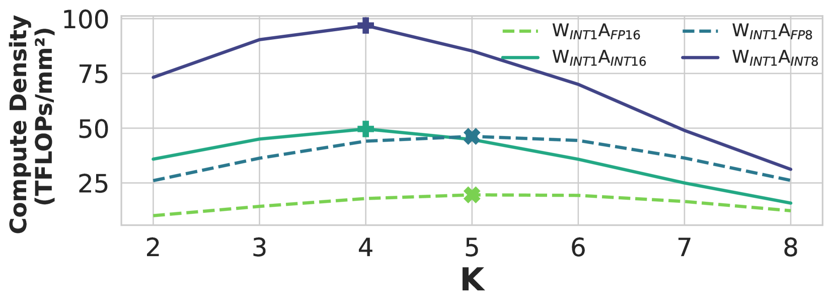</details> Figure 10: K-axis design space exploration for LUT Tensor Core ’s dot product unit. K = 4 is the optimal in general. ### IV-B Hardware PPA Benchmarks #### IV-B 1 Dot Product unit microbenchmark As discussed in § III-B 2, the parameter $K$ in LUT tiling is crucial for compute efficiency. In the hardware experiments, we fixed $M$ and $N$ to 1 and varied $K$ (i.e., a dot product unit of $K$ -element vectors) to explore its impact on compute density. Excessively large $K$ could potentially lead to an exponential growth in lookup table entries, thereby increasing area without proportional gains in efficiency. Conversely, smaller $K$ may lead to an inefficient dominance of computations being handled by adders, which could reduce compute density. As shown in Fig. 10, we found INT operations achieve optimal density at $K=4$ , while floating-point operations peak at $K=5$ but perform similarly well at $K=4$ . Therefore, we adopt $K=4$ for all subsequent LUT-based designs. <details> <summary>x11.png Details</summary>  ### Visual Description ## Line Chart: DP4 Unit Compute Density and Power @ TSMC 28nm (No Psum) ### Overview The chart compares compute density (TFLOPs/mm²) and power consumption (mW) across six DP4 unit configurations at TSMC 28nm process node. Two y-axes are used: left for compute density (0–150 TFLOPs/mm²) and right for power consumption (0–2.0 mW). The x-axis categorizes units by operation type (MAC, ADD, LUT) and precision (FP16/FP8). ### Components/Axes - **X-axis**: Unit configurations: - W_FP16A_FP16 MAC - W_INT1A_FP16 ADD - W_INT1A_FP16 LUT - W_FP8A_FP8 MAC - W_INT1A_FP8 ADD - W_INT1A_FP8 LUT - **Left Y-axis**: Compute Density (TFLOPs/mm²) [0–150] - **Right Y-axis**: Power Consumption (mW) [0–2.0] - **Legend**: - Red line/dots: Power Consumption - Gray bars: Compute Density - **Spatial Grounding**: Legend positioned top-right; red line connects power consumption points across x-axis. ### Detailed Analysis 1. **Compute Density (Gray Bars)**: - **W_FP16A_FP16 MAC**: ~3 TFLOPs/mm² - **W_INT1A_FP16 ADD**: ~8 TFLOPs/mm² - **W_INT1A_FP16 LUT**: ~65 TFLOPs/mm² - **W_FP8A_FP8 MAC**: ~10 TFLOPs/mm² - **W_INT1A_FP8 ADD**: ~20 TFLOPs/mm² - **W_INT1A_FP8 LUT**: ~130 TFLOPs/mm² - *Trend*: Compute density increases significantly for LUT operations, peaking at 130 TFLOPs/mm² for W_INT1A_FP8 LUT. 2. **Power Consumption (Red Line/Dots)**: - **W_FP16A_FP16 MAC**: ~1.8 mW - **W_INT1A_FP16 ADD**: ~0.6 mW - **W_INT1A_FP16 LUT**: ~0.1 mW - **W_FP8A_FP8 MAC**: ~0.5 mW - **W_INT1A_FP8 ADD**: ~0.3 mW - **W_INT1A_FP8 LUT**: ~0.05 mW - *Trend*: Power consumption decreases monotonically from MAC (~1.8 mW) to LUT (~0.05 mW). ### Key Observations - **Compute Density Outlier**: W_INT1A_FP8 LUT achieves the highest compute density (130 TFLOPs/mm²), 26× higher than W_FP16A_FP16 MAC. - **Power Efficiency**: LUT operations consume 36× less power than MAC operations (0.05 mW vs. 1.8 mW). - **Precision Impact**: FP8 configurations (W_FP8A_FP8 MAC) show 50% lower compute density than FP16 LUT but 10× lower power consumption. ### Interpretation The data demonstrates a trade-off between compute density and power efficiency: - **LUT Operations**: Maximize compute density while minimizing power, suggesting architectural optimizations for LUT-heavy workloads. - **FP8 vs. FP16**: FP8 reduces power consumption by 70–90% compared to FP16 but sacrifices compute density. This aligns with TSMC 28nm’s voltage scaling benefits for lower-precision operations. - **Anomaly**: W_INT1A_FP8 LUT’s power consumption (0.05 mW) is 20× lower than W_INT1A_FP16 LUT (0.1 mW), indicating precision-dependent power scaling. The chart highlights the importance of precision and operation type in optimizing compute density and power efficiency for DP4 units. 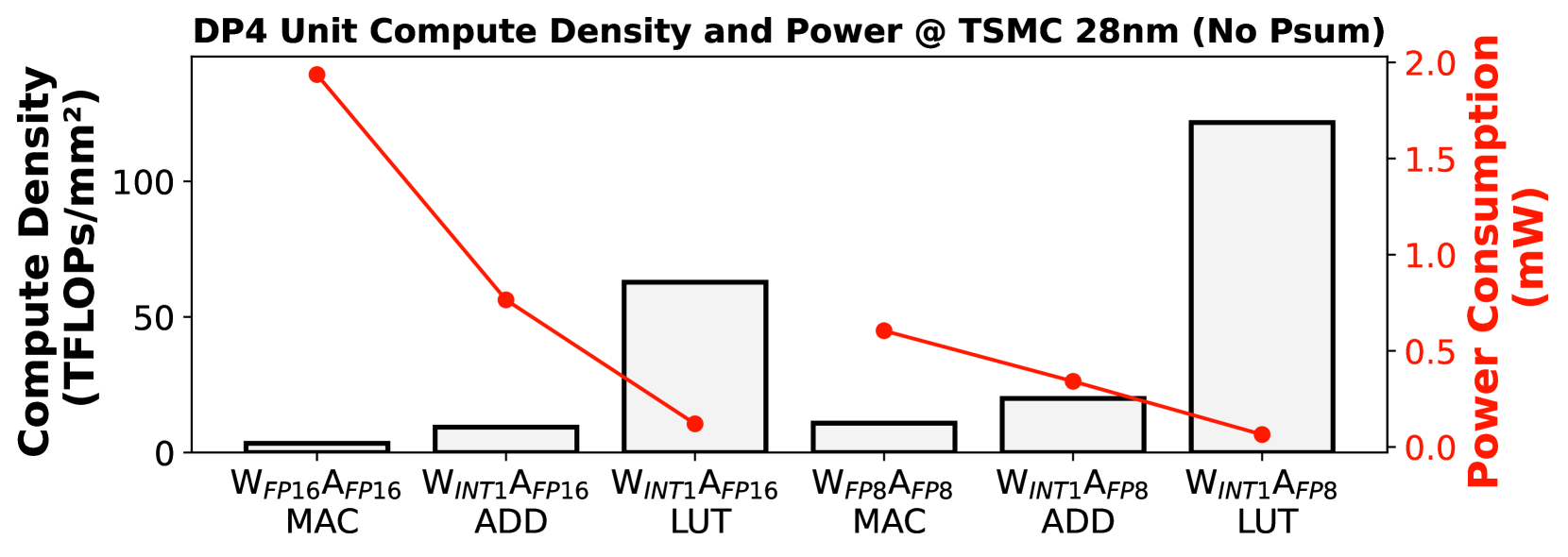</details> Figure 11: PPA comparison across MAC-based Tensor Core, ADD-based Tensor Core, and LUT Tensor Core ’s DP4 implementations. LUT Tensor Core ’s DP4 unit has significant compute density and power advantages. Following $K=4$ , we conduct benchmarks on dot product implementations using MAC-based, ADD-based, and LUT Tensor Core approach across various data formats. The configurations assessed include conventional symmetric precision with MAC ( $W_FP16A_FP16$ , $W_FP8A_FP8$ ) and mixed precision ( $W_INT1A_FP16$ , $W_INT1A_FP8$ ) using both ADD and LUT approaches. As depicted in Fig. 11, the LUT-based approach achieved the highest compute density, reaching 61.55 TFLOPs/mm 2 with $W_INT1A_FP16$ , substantially surpassing the conventional MAC configuration which registered only 3.39 TFLOPs/mm 2 with $W_FP16A_FP16$ . The behaviour of power efficiency exhibits similar performance. Specifically, under the $A_FP16$ format, the LUT Tensor Core approach delivered an 18.13 $×$ increase in compute density and reduced power consumption by 15.45 $×$ compared to MAC methods. 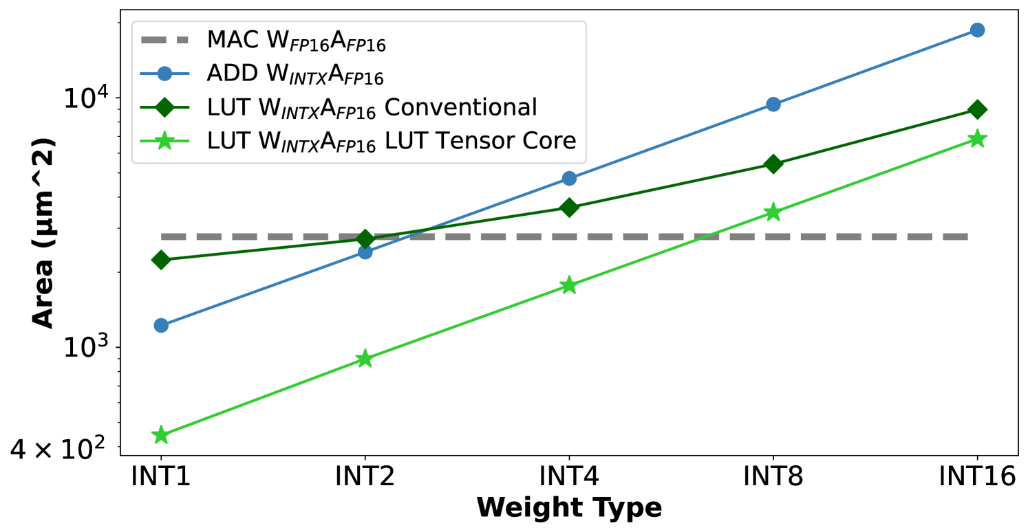Furthermore, we conduct weight-bit scaling experiments on the $W_INTX× A_FP16$ DP4 units for MAC-based, ADD-based , and LUT-based(LUT Tensor Core) implementations. The experiments are configured with the tensor core’s N dimension set to 4 to match the A100’s configuration. As shown in Fig. 12, the conventional LUT-based implementation does not have area advantages compared to the MAC baseline when the weight is more than 2-bit. The main area efficiency bottleneck is the table precompute and storage overheads. ADD-based implementations also only surpass the MAC baseline in the 1-bit and 2-bit cases. By optimizing the table storage overhead and the precompute overhead with symmetry-based table reduction and compilation optimizations, our LUT Tensor Core implementation outperforms all the baselines up to a weight bit-width of 6 and delivers much better area efficiency compared to the conventional LUT implementation. <details> <summary>x12.png Details</summary>  ### Visual Description ## Line Chart: Area vs. Weight Type for Different Weight Configurations ### Overview The chart compares the area (in μm²) required for different weight configurations (INT1, INT2, INT4, INT8, INT16) across four weight types: MAC W_FP16A_FP16, ADD W_INTXA_FP16, LUT W_INTXA_FP16 Conventional, and LUT W_INTXA_FP16 LUT Tensor Core. The y-axis uses a logarithmic scale (10³ to 10⁴), while the x-axis lists weight types in increasing order. --- ### Components/Axes - **X-axis (Weight Type)**: Categories labeled as INT1, INT2, INT4, INT8, INT16 (left to right). - **Y-axis (Area)**: Logarithmic scale from 4×10² to 10⁴ μm². - **Legend**: Located in the top-right corner, with four entries: 1. **MAC W_FP16A_FP16**: Dashed gray line. 2. **ADD W_INTXA_FP16**: Solid blue line with circle markers. 3. **LUT W_INTXA_FP16 Conventional**: Solid green line with diamond markers. 4. **LUT W_INTXA_FP16 LUT Tensor Core**: Solid green line with star markers. --- ### Detailed Analysis 1. **MAC W_FP16A_FP16** (Dashed Gray Line): - Constant area of ~10³ μm² across all weight types. - No variation observed. 2. **ADD W_INTXA_FP16** (Blue Line with Circles): - Starts at ~10³ μm² (INT1) and increases linearly to ~10⁴ μm² (INT16). - Data points: - INT1: ~10³ - INT2: ~1.5×10³ - INT4: ~3×10³ - INT8: ~7×10³ - INT16: ~10⁴ 3. **LUT W_INTXA_FP16 Conventional** (Green Line with Diamonds): - Starts at ~10³.5 μm² (INT1) and increases to ~10⁴.5 μm² (INT16). - Data points: - INT1: ~3×10³ - INT2: ~5×10³ - INT4: ~8×10³ - INT8: ~1.2×10⁴ - INT16: ~3×10⁴ 4. **LUT W_INTXA_FP16 LUT Tensor Core** (Green Line with Stars): - Starts at ~4×10² μm² (INT1) and increases to ~10⁴ μm² (INT16). - Data points: - INT1: ~4×10² - INT2: ~1×10³ - INT4: ~2×10³ - INT8: ~5×10³ - INT16: ~1×10⁴ --- ### Key Observations - **MAC** remains constant, suggesting fixed-area optimization for FP16 precision. - **ADD** and **Conventional LUT** show parallel growth, but Conventional LUT requires ~2–3× more area than ADD at higher weight types. - **LUT Tensor Core** starts with significantly lower area (INT1: 4×10² vs. ADD: 10³) but converges with ADD at INT16 (~10⁴ μm²). - All lines except MAC exhibit exponential growth with increasing weight type. --- ### Interpretation The data suggests that: 1. **Precision Trade-offs**: MAC’s fixed area implies hardware optimization for FP16 operations, while ADD and LUT configurations scale with weight type complexity. 2. **Efficiency Gains**: The LUT Tensor Core reduces area by ~50% compared to Conventional LUT at INT1 but matches ADD’s area at INT16, indicating diminishing returns at higher precision. 3. **Scalability**: ADD and LUT Tensor Core configurations scale more efficiently than Conventional LUT, which may impact design choices for high-precision applications. The logarithmic y-axis emphasizes exponential growth trends, highlighting the importance of weight type selection in area-constrained systems. </details> Figure 12: Area comparison of MAC-based Tensor Core, ADD-based Tensor Core, and LUT Tensor Core ’s DP4 units across weight bit-widths in $W_INTX× A_FP16$ . Conventional LUT implementation does not have area advantages. #### IV-B 2 Tensor Core benchmark <details> <summary>x13.png Details</summary>  ### Visual Description ## Chart/Diagram Type: Performance Trade-off Analysis of Tensor Core Architectures ### Overview The image contains 12 comparative graphs arranged in a 3x4 grid, analyzing the relationship between **power consumption (mW)** and **area efficiency (Area/1000 µm²)** for three tensor core architectures: **LUT Tensor Core** (green triangles), **ADD-based Tensor Core** (blue squares), and **MAC-based Tensor Core** (red circles). Each graph corresponds to a specific configuration (e.g., "W_INT1A_FP16", "W_INT2A_FP8") and includes dashed reference lines in green, blue, and red. ### Components/Axes - **X-axis**: Power/mW (ranges from 0 to 300, 400, 600, or 250 mW depending on the graph). - **Y-axis**: Area/1000 µm² (ranges from 0 to 200, 400, 500, or 200 µm² depending on the graph). - **Legends**: - Green triangles: LUT Tensor Core - Blue squares: ADD-based Tensor Core - Red circles: MAC-based Tensor Core - **Dashed Lines**: - Green: Likely represents an optimal or theoretical efficiency curve for LUT cores. - Blue: Likely represents an optimal or theoretical efficiency curve for ADD-based cores. - Red: Likely represents an optimal or theoretical efficiency curve for MAC-based cores. ### Detailed Analysis #### Graph 1: W_INT1A_FP16 Tensor Core - **Power Range**: 0–300 mW - **Area Range**: 0–200 µm² - **Data Points**: - LUT (green): 10–50 mW, 10–50 µm² - ADD-based (blue): 50–200 mW, 50–150 µm² - MAC-based (red): 200–300 mW, 150–200 µm² - **Trends**: - LUT cores show the lowest power-area trade-off. - MAC-based cores require significantly higher power and area. - Dashed lines suggest theoretical efficiency thresholds. #### Graph 2: W_INT1A_FP8 Tensor Core - **Power Range**: 0–120 mW - **Area Range**: 0–100 µm² - **Data Points**: - LUT (green): 10–30 mW, 10–30 µm² - ADD-based (blue): 30–100 mW, 30–80 µm² - MAC-based (red): 80–120 mW, 70–100 µm² - **Trends**: - LUT cores dominate in efficiency. - MAC-based cores cluster near the upper-right corner. #### Graph 3: W_INT4A_FP16 Tensor Core - **Power Range**: 0–600 mW - **Area Range**: 0–500 µm² - **Data Points**: - LUT (green): 50–200 mW, 50–200 µm² - ADD-based (blue): 200–400 mW, 200–400 µm² - MAC-based (red): 400–600 mW, 400–500 µm² - **Trends**: - MAC-based cores occupy the highest power-area quadrant. - Dashed lines indicate diminishing returns at higher power levels. #### Graph 4: W_INT4A_FP8 Tensor Core - **Power Range**: 0–250 mW - **Area Range**: 0–200 µm² - **Data Points**: - LUT (green): 20–100 mW, 20–100 µm² - ADD-based (blue): 100–250 mW, 100–200 µm² - MAC-based (red): 200–250 mW, 180–200 µm² - **Trends**: - LUT cores maintain a linear efficiency curve. - MAC-based cores show minimal improvement beyond 200 mW. #### Graph 5: W_INT2A_FP16 Tensor Core - **Power Range**: 0–400 mW - **Area Range**: 0–400 µm² - **Data Points**: - LUT (green): 50–200 mW, 50–200 µm² - ADD-based (blue): 200–400 mW, 200–400 µm² - MAC-based (red): 300–400 mW, 300–400 µm² - **Trends**: - MAC-based cores align closely with the red dashed line. - ADD-based cores show a steeper power-area slope. #### Graph 6: W_INT2A_FP8 Tensor Core - **Power Range**: 0–150 mW - **Area Range**: 0–200 µm² - **Data Points**: - LUT (green): 10–60 mW, 10–60 µm² - ADD-based (blue): 60–150 mW, 60–150 µm² - MAC-based (red): 120–150 mW, 120–150 µm² - **Trends**: - LUT cores remain the most efficient. - MAC-based cores cluster near the upper boundary. #### Graph 7: W_INT1A_FP16 (Repeated) - **Power Range**: 0–200 mW - **Area Range**: 0–200 µm² - **Data Points**: - LUT (green): 10–50 mW, 10–50 µm² - ADD-based (blue): 50–150 mW, 50–150 µm² - MAC-based (red): 150–200 mW, 150–200 µm² - **Trends**: - Similar to Graph 1 but with a narrower power range. #### Graph 8: W_INT1A_FP8 (Repeated) - **Power Range**: 0–60 mW - **Area Range**: 0–40 µm² - **Data Points**: - LUT (green): 5–20 mW, 5–20 µm² - ADD-based (blue): 20–60 mW, 20–40 µm² - MAC-based (red): 40–60 mW, 30–40 µm² - **Trends**: - LUT cores dominate at low power. - MAC-based cores show minimal area growth. #### Graph 9: W_INT4A_FP16 (Repeated) - **Power Range**: 0–500 mW - **Area Range**: 0–200 µm² - **Data Points**: - LUT (green): 50–200 mW, 50–200 µm² - ADD-based (blue): 200–400 mW, 200–400 µm² - MAC-based (red): 400–500 mW, 180–200 µm² - **Trends**: - MAC-based cores deviate from the red dashed line at higher power. #### Graph 10: W_INT4A_FP8 (Repeated) - **Power Range**: 0–250 mW - **Area Range**: 0–100 µm² - **Data Points**: - LUT (green): 20–100 mW, 20–100 µm² - ADD-based (blue): 100–250 mW, 100–200 µm² - MAC-based (red): 200–250 mW, 90–100 µm² - **Trends**: - MAC-based cores show a plateau in area growth. #### Graph 11: W_INT2A_FP16 (Repeated) - **Power Range**: 0–250 mW - **Area Range**: 0–200 µm² - **Data Points**: - LUT (green): 50–150 mW, 50–150 µm² - ADD-based (blue): 150–250 mW, 150–200 µm² - MAC-based (red): 200–250 mW, 180–200 µm² - **Trends**: - MAC-based cores exceed the red dashed line at 200 mW. #### Graph 12: W_INT2A_FP8 (Repeated) - **Power Range**: 0–120 mW - **Area Range**: 0–50 µm² - **Data Points**: - LUT (green): 10–50 mW, 10–50 µm² - ADD-based (blue): 50–120 mW, 50–50 µm² - MAC-based (red): 100–120 mW, 40–50 µm² - **Trends**: - LUT cores maintain a linear efficiency curve. - MAC-based cores cluster near the upper boundary. ### Key Observations 1. **LUT Tensor Cores** consistently demonstrate the lowest power-area trade-off across all configurations. 2. **MAC-based Tensor Cores** require significantly higher power and area, often clustering near the upper-right quadrant of the graphs. 3. **ADD-based Tensor Cores** fall between LUT and MAC-based cores in efficiency, with steeper power-area slopes. 4. **Dashed Lines** likely represent theoretical efficiency thresholds, with actual data points often exceeding these values. 5. **Configuration Variability**: Higher-precision configurations (e.g., FP16) generally require more power and area than lower-precision ones (e.g., FP8). ### Interpretation The data suggests that **LUT Tensor Cores** are the most area-efficient, making them ideal for applications with strict power or area constraints. **MAC-based Tensor Cores**, while less efficient, may offer higher computational throughput, justifying their trade-offs in performance-critical scenarios. The **ADD-based Tensor Cores** represent a middle ground, balancing efficiency and performance. The dashed lines imply that current implementations may not yet achieve theoretical optimal efficiency, highlighting opportunities for architectural improvements. Notably, MAC-based cores in high-power configurations (e.g., W_INT4A_FP16) deviate from their reference lines, suggesting potential inefficiencies at scale. This analysis underscores the importance of selecting tensor core architectures based on application-specific requirements, balancing power, area, and performance trade-offs. </details> Figure 13: PPA across LUT Tensor Core, ADD-based Tensor Core, and MAC-based Tensor Core implementations for mpGEMM. In previous experiments, we confirm the superiority of the LUT-based design within the basic DP units. In this section, we scale our investigation to the Tensor Core level, incorporating a design space exploration to identify optimal MNK configurations. We align the computational capabilities with those of the A100 INT8 Tensor Core, which delivers 1024 operations per cycle per Tensor Core, setting $M× N× K=512$ for extensive design space exploration. Our data types range from $A_FP16$ to $A_INT8$ and include various weight bit-widths. We compare our LUT Tensor Core approach against MAC- and ADD-based approaches. To make a fair comparison across difference activation data types, we don’t enable table quantization for this benchmark. As shown in Fig. 13, the dashed lines represent the contours where the minimum Area*Power point for each design methodology lies among all data points. Our results demonstrate that across 12 sets of experiments with different activation data formats and weight bit-widths, the LUT Tensor Core method achieves the smallest area and lowest power consumption, except in the $W_INT8A_INT4$ case. Notably, with 1-bit weights, the LUT Tensor Core approach exhibits a 4 $×$ -6 $×$ reduction in power and area compared to the MAC-based Tensor Core design. After our design space exploration, we identify the optimal MNK configuration for the LUT Tensor Core as $M2N64K4$ . <details> <summary>x14.png Details</summary>  ### Visual Description ## Bar Chart: Performance Comparison of LUT A_FP16 Configurations ### Overview The chart compares the performance (TFLOPs) and area (µm²) of different LUT A_FP16 implementations across three scenarios: `W_INT1A_FP16`, `W_INT2A_FP16`, and `W_INT4A_FP16`. It evaluates configurations including an "Ideal" baseline, real GPU hardware (A100), and simulated LUT-based implementations with varying regularization and scaling factors (1X, 2X, 4X, 8X). --- ### Components/Axes - **X-Axis**: Configurations grouped by scenario (`W_INT1A_FP16`, `W_INT2A_FP16`, `W_INT4A_FP16`) and scaling factor (1X, 2X, 4X, 8X). - **Y-Axis (Left)**: TFLOPs (logarithmic scale, 0–2000). - **Secondary Y-Axis (Right)**: Area (µm², linear scale, 0–200). - **Legend**: - Blue: Ideal - Purple: A100 Real GPU - Orange: Sim A100-LUT - Green: Sim A100-LUT with regularization (8X, 4X, 2X Reg) - Dashed Orange Line: Area (µm²) --- ### Detailed Analysis #### W_INT1A_FP16 - **Ideal**: Tallest bar (~2000 TFLOPs), lowest area (~100 µm²). - **A100 Real GPU**: ~1500 TFLOPs, ~150 µm². - **Sim A100-LUT**: ~1000 TFLOPs, ~120 µm². - **Sim A100-LUT 8X Reg**: ~800 TFLOPs, ~180 µm². - **Trend**: TFLOPs decrease with increasing regularization; area increases. #### W_INT2A_FP16 - **Ideal**: ~1800 TFLOPs, ~110 µm². - **A100 Real GPU**: ~1300 TFLOPs, ~140 µm². - **Sim A100-LUT**: ~900 TFLOPs, ~130 µm². - **Sim A100-LUT 4X Reg**: ~700 TFLOPs, ~160 µm². - **Trend**: Similar trade-off between TFLOPs and area as in W_INT1. #### W_INT4A_FP16 - **Ideal**: ~1600 TFLOPs, ~120 µm². - **A100 Real GPU**: ~1100 TFLOPs, ~150 µm². - **Sim A100-LUT**: ~800 TFLOPs, ~140 µm². - **Sim A100-LUT 2X Reg**: ~600 TFLOPs, ~170 µm². - **Trend**: Larger configurations show diminishing returns in TFLOPs with regularization. --- ### Key Observations 1. **Ideal vs. Real Hardware**: The "Ideal" configuration consistently outperforms the A100 Real GPU in TFLOPs but has lower area. 2. **Regularization Impact**: Higher regularization (e.g., 8X Reg) reduces TFLOPs but increases area, suggesting a performance-area trade-off. 3. **Scaling Factor**: Larger scaling factors (8X) generally improve TFLOPs but require more area, except in regularized cases. 4. **Area Trends**: The dashed orange line shows area increases with scaling factor, peaking at 8X Reg (~200 µm²). --- ### Interpretation The data highlights a critical trade-off between computational performance (TFLOPs) and hardware area. While the "Ideal" configuration offers the best performance, real-world implementations (A100 Real GPU) and simulated LUT-based approaches (Sim A100-LUT) balance these metrics differently. Regularization (e.g., 8X Reg) appears to prioritize area efficiency at the cost of performance, which may be beneficial for power-constrained systems. The A100 Real GPU serves as a practical middle ground, though it lags behind the Ideal baseline. The chart underscores the need for optimization strategies that align with specific application requirements (e.g., power vs. speed). </details> <details> <summary>x15.png Details</summary>  ### Visual Description ## Bar Charts: TFLOPs and Area Efficiency Across Scaling Factors ### Overview The image contains three side-by-side bar charts comparing computational performance (TFLOPs) and area efficiency (μm²/1000 TFLOPs) for different hardware configurations. Each chart represents a distinct scaling factor (W_INT8, W_INT2, W_INT4) and includes four configurations: cuBLAS, LUT A_INT8 1X, LUT A_INT8 2X, and LUT A_INT8 4X. The charts use color-coded bars with crosshatch patterns to differentiate configurations. ### Components/Axes - **X-Axes**: - Labels: `cuBLAS`, `LUT A_INT8 1X`, `LUT A_INT8 2X`, `LUT A_INT8 4X` - Position: Bottom of each chart - **Y-Axes**: - Left: `TFLOPs` (0–2500 in W_INT8, 0–600 in W_INT4) - Right: `Area /1000 TFLOPs` (0–40 in W_INT8, 0–40 in W_INT2, 0–40 in W_INT4) - **Legend**: - Colors: Blue (cuBLAS), Orange (LUT 1X), Green (LUT 2X), Purple (LUT 4X) - Position: Right of all charts - **Additional Elements**: - Orange dotted line connecting `LUT A_INT8 1X` points across charts ### Detailed Analysis #### W_INT8A_INT8 Chart - **TFLOPs**: - cuBLAS: ~500 (blue) - 1X: ~300 (orange) - 2X: ~600 (green) - 4X: ~1000 (purple) - **Area Efficiency**: - cuBLAS: ~40k μm²/1000 TFLOPs - 1X: ~20k - 2X: ~30k - 4X: ~50k #### W_INT2A_INT8 Chart - **TFLOPs**: - cuBLAS: ~1200 - 1X: ~600 - 2X: ~1000 - 4X: ~1800 - **Area Efficiency**: - cuBLAS: ~30k - 1X: ~15k - 2X: ~25k - 4X: ~40k #### W_INT4A_INT8 Chart - **TFLOPs**: - cuBLAS: ~400 - 1X: ~200 - 2X: ~300 - 4X: ~500 - **Area Efficiency**: - cuBLAS: ~20k - 1X: ~10k - 2X: ~15k - 4X: ~30k ### Key Observations 1. **Scaling Trends**: - Higher scaling factors (4X) consistently show higher TFLOPs but lower area efficiency compared to 1X configurations. - The orange dotted line demonstrates a downward trend in area efficiency as scaling increases from W_INT8 to W_INT4. 2. **Configuration Performance**: - cuBLAS dominates TFLOPs in W_INT8 and W_INT2 but underperforms in W_INT4. - LUT 4X configurations show the highest TFLOPs in W_INT4 despite lower area efficiency. 3. **Anomalies**: - W_INT4A_INT8 has the lowest TFLOPs overall, suggesting architectural limitations at higher scaling factors. - Area efficiency for LUT 2X configurations remains relatively stable across charts (~25–30k). ### Interpretation The data reveals a trade-off between computational performance and resource utilization. While higher scaling factors (4X) improve TFLOPs, they require disproportionately more area, reducing efficiency. The 1X configurations (orange bars) emerge as the most area-efficient across all scaling factors, though their TFLOPs remain lower than cuBLAS in W_INT8 and W_INT2. The orange dotted line underscores that 1X configurations maintain better area efficiency even as scaling increases, suggesting they are optimized for resource-constrained environments. The decline in cuBLAS performance in W_INT4 may indicate hardware-specific bottlenecks at extreme scaling. </details> Figure 14: Accel-Sim runtime and area across $A_FP16$ and $A_INT8$ LUT Tensor Core designs. ### IV-C Kernel-level Evaluation Building on the PPA superiority of the LUT Tensor Core, we employ Accel-Sim, a SOTA GPU simulator, to validate not only the robust computational power of LUT Tensor Core in mpGEMM operations but also their compatibility with existing GPU architectures. The mpGEMM benchmarks leverage the configuration used in the LLAMA2-13B model, with $M=2048$ , $N=27648$ , and $K=5120$ . The dataflow of mpGEMM is designed to be cutlass-like and output-stationary, with tiling shapes optimized by Roller [75] for efficient data reuse. For instance, a good candidate for $W_INT1A_INT8$ tiling sets the Thread Block tile to [128, 512, 32] and the Warp tile to [64, 256, 32]. As illustrated in Fig. 14, each subplot presents results where the leftmost bar represents actual measurements, followed by three simulated results: ideal peak performance, simulated measured performance, and performance after applying several times the baseline’s register capacity. The latter adjustment addresses bottlenecks caused by insufficient register capacity, which limit large tiling and systemically bind performance to memory constraints. This modification ensures that speedups are not mistakenly attributed to improved memory bandwidth. Experimental results confirm that LUT Tensor Core significantly outperforms traditional MAC-based Tensor Core in mpGEMM operations under equivalent area constraints. For instance, using $W_INT1A_FP16$ , the LUT Tensor Core approach achieves slightly higher mpGEMM performance while occupying only 14.3% the area of a MAC-based Tensor Core. With a modest 31.6% increase in area, incorporating more registers, the LUT configuration achieves a 6.9 $×$ acceleration in mpGEMM operations. ### IV-D Model End-to-End Evaluation While Accel-Sim offers detailed architectural emulation, it suffers from a slowdown of approximately five million times, transforming a ten-second task on an A100 GPU into a simulation period of up to 579 days, and generating trace files over 79TB in size. These limitations hinder comprehensive end-to-end assessments. To overcome these obstacles, we have developed a end-to-end simulator designed for rapid and accurate emulation with tile-level granularity. Our insight is that the behavior of highly optimized, large GPU kernels with minimal stalling can be treated as accelerators, particularly in LLM scenarios. This viewpoint is corroborated by findings from NVIDIA in NVAS [59], which suggests viewing GPU simulation philosophically as “dynamically interacting roofline components”, rather than as a “cycle-by-cycle progression”. Accordingly, we leverage analytical methods from established accelerator modeling practices, such as Timeloop [44], Maestro [30], and Tileflow [74], to develop a tile-based GPU simulator. This tool enables detailed and accurate assessments of dataflow, memory bandwidth, computational resources, and operator fusion. We plan to open-source this simulator in future work. 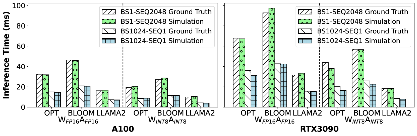<details> <summary>x16.png Details</summary>  ### Visual Description ## Bar Chart: Inference Time Comparison for Language Models on A100 and RTX3090 ### Overview The image is a grouped bar chart comparing inference times (in milliseconds) for three language models (OPT, BLOOM, LLaMA2) across two hardware platforms (A100, RTX3090). Each model is evaluated under two weight configurations (FP16 and INT8) and two data types (Ground Truth vs. Simulation). The chart highlights performance differences between hardware and model configurations. ### Components/Axes - **X-Axis**: - Models: OPT, BLOOM, LLaMA2 - Weight Configurations: - `W_FP16A_FP16` (FP16 precision) - `W_INT8A_INT8` (INT8 precision) - Data Types: Ground Truth (solid patterns) and Simulation (hatched patterns) - **Y-Axis**: Inference Time (ms), scaled from 0 to 100. - **Legend**: - Top-right corner, with four entries: 1. **BS1-SEQ2048 Ground Truth** (striped) 2. **BS1-SEQ2048 Simulation** (dotted) 3. **BS1024-SEQ1 Ground Truth** (solid) 4. **BS1024-SEQ1 Simulation** (checkered) - **Spatial Layout**: - Two main sections (A100 and RTX3090) side-by-side. - Each section contains grouped bars for models, weight configurations, and data types. ### Detailed Analysis #### A100 Hardware - **OPT**: - `W_FP16A_FP16`: - Ground Truth: ~30 ms (solid) - Simulation: ~35 ms (striped) - `W_INT8A_INT8`: - Ground Truth: ~15 ms (solid) - Simulation: ~10 ms (striped) - **BLOOM**: - `W_FP16A_FP16`: - Ground Truth: ~45 ms (solid) - Simulation: ~40 ms (striped) - `W_INT8A_INT8`: - Ground Truth: ~20 ms (solid) - Simulation: ~12 ms (striped) - **LLaMA2**: - `W_FP16A_FP16`: - Ground Truth: ~25 ms (solid) - Simulation: ~22 ms (striped) - `W_INT8A_INT8`: - Ground Truth: ~10 ms (solid) - Simulation: ~8 ms (striped) #### RTX3090 Hardware - **OPT**: - `W_FP16A_FP16`: - Ground Truth: ~70 ms (solid) - Simulation: ~75 ms (striped) - `W_INT8A_INT8`: - Ground Truth: ~40 ms (solid) - Simulation: ~35 ms (striped) - **BLOOM**: - `W_FP16A_FP16`: - Ground Truth: ~95 ms (solid) - Simulation: ~90 ms (striped) - `W_INT8A_INT8`: - Ground Truth: ~55 ms (solid) - Simulation: ~50 ms (striped) - **LLaMA2**: - `W_FP16A_FP16`: - Ground Truth: ~60 ms (solid) - Simulation: ~58 ms (striped) - `W_INT8A_INT8`: - Ground Truth: ~30 ms (solid) - Simulation: ~28 ms (striped) ### Key Observations 1. **Simulation vs. Ground Truth**: - Simulation times are consistently higher than ground truth across all models and hardware (e.g., OPT on A100: 35 ms vs. 30 ms). - Exceptions: LLaMA2 `W_INT8A_INT8` on A100 shows simulation slightly lower than ground truth (~8 ms vs. ~10 ms). 2. **Hardware Performance**: - RTX3090 inference times are significantly higher than A100 (e.g., BLOOM `W_FP16A_FP16` on RTX3090: 95 ms vs. A100: 45 ms). 3. **Weight Precision**: - INT8 configurations generally reduce inference times compared to FP16 (e.g., BLOOM on A100: 20 ms vs. 45 ms for FP16). 4. **Model Efficiency**: - LLaMA2 has the lowest inference times across both hardware and weight configurations. ### Interpretation - **Simulation Overhead**: The consistent increase in simulation times suggests computational overhead in simulated environments, possibly due to additional validation or emulation layers. - **Hardware Impact**: A100 outperforms RTX3090 by ~30-50% in inference times, indicating better optimization for these models. - **INT8 Advantage**: Lower precision (INT8) reduces inference times but may introduce accuracy trade-offs, as simulations sometimes negate this benefit. - **Model-Specific Trends**: LLaMA2’s efficiency across configurations suggests architectural optimizations, while BLOOM’s higher RTX3090 times may reflect larger model size or memory constraints. This analysis underscores the importance of hardware selection and weight precision in deploying language models, with simulations often reflecting real-world performance gaps. </details> Figure 15: Evaluation of end-to-end simulator accuracy. 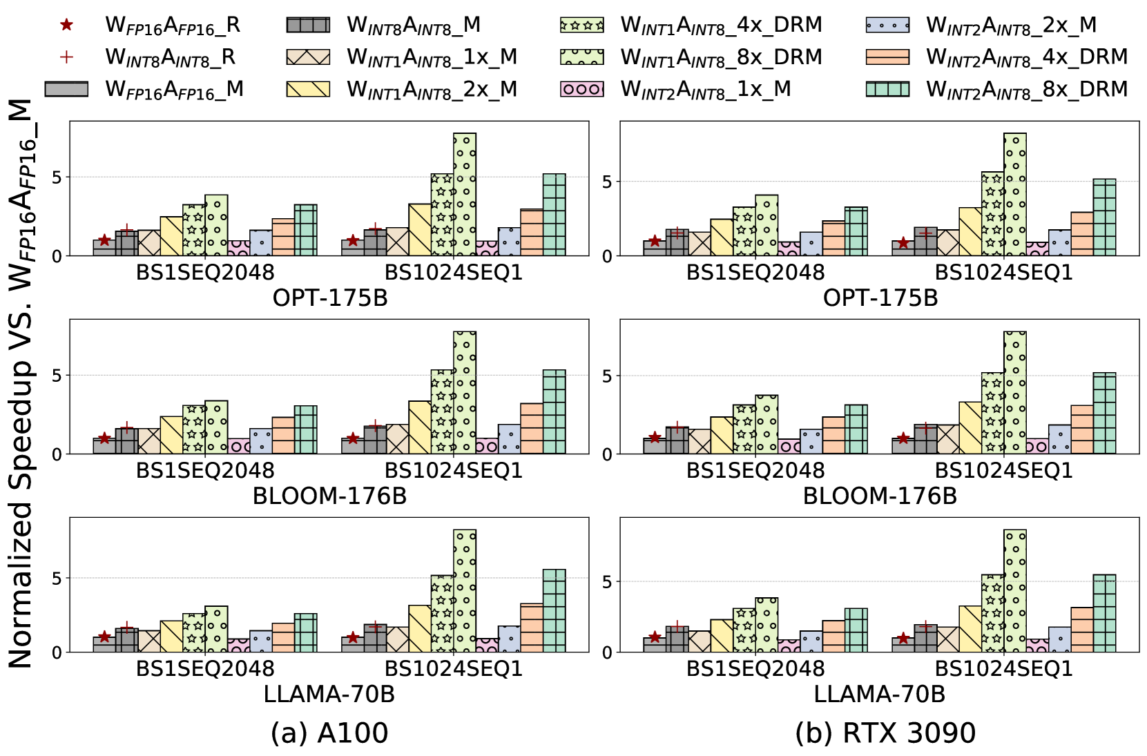<details> <summary>x17.png Details</summary>  ### Visual Description ## Bar Chart: Normalized Speedup vs. W_FP16A_FP16_M ### Overview The image presents a grouped bar chart comparing normalized speedup values across different hardware configurations (A100 and RTX 3090 GPUs) for three language models (OPT-175B, BLOOM-176B, LLAMA-70B) and two datasets (BS1SEQ2048, BS1024SEQ1). The chart uses patterned bars to represent distinct computational configurations, with speedup values normalized against a baseline (W_FP16A_FP16_M). ### Components/Axes - **X-axis**: Model/Dataset combinations (e.g., "BS1SEQ2048", "BS1024SEQ1") grouped by model (OPT-175B, BLOOM-176B, LLAMA-70B). - **Y-axis**: Normalized speedup (0–5 scale). - **Legend**: Located at the top, mapping 10 configurations to colors/patterns: - **Red star**: W_FP16A_FP16_R - **Gray cross**: W_INT8A_INT8_M - **Green stars**: W_INT1A_INT8_4x_DRM - **Blue dots**: W_INT2A_INT8_2x_M - **Yellow diagonal**: W_INT1A_INT8_1x_M - **Pink circles**: W_INT2A_INT8_1x_M - **Gray solid**: W_FP16A_FP16_M - **Yellow cross**: W_INT1A_INT8_2x_M - **Green checkered**: W_INT1A_INT8_8x_DRM - **Blue striped**: W_INT2A_INT8_4x_DRM - **Orange striped**: W_INT2A_INT8_8x_DRM ### Detailed Analysis #### A100 GPU Results - **OPT-175B**: - BS1SEQ2048: W_INT1A_INT8_8x_DRM (green checkered) shows highest speedup (~4.8). - BS1024SEQ1: W_INT2A_INT8_8x_DRM (orange striped) peaks at ~4.2. - **BLOOM-176B**: - BS1SEQ2048: W_INT1A_INT8_8x_DRM reaches ~4.5. - BS1024SEQ1: W_INT2A_INT8_8x_DRM achieves ~3.9. - **LLAMA-70B**: - BS1SEQ2048: W_INT1A_INT8_8x_DRM at ~4.0. - BS1024SEQ1: W_INT2A_INT8_8x_DRM at ~3.5. #### RTX 3090 GPU Results - **OPT-175B**: - BS1SEQ2048: W_INT1A_INT8_8x_DRM peaks at ~4.6. - BS1024SEQ1: W_INT2A_INT8_8x_DRM at ~4.0. - **BLOOM-176B**: - BS1SEQ2048: W_INT1A_INT8_8x_DRM at ~4.3. - BS1024SEQ1: W_INT2A_INT8_8x_DRM at ~3.8. - **LLAMA-70B**: - BS1SEQ2048: W_INT1A_INT8_8x_DRM at ~4.1. - BS1024SEQ1: W_INT2A_INT8_8x_DRM at ~3.6. ### Key Observations 1. **DRM Configurations Dominate**: All 8x_DRM variants (green checkered/orange striped) consistently show the highest speedups across models and datasets. 2. **Hardware Impact**: RTX 3090 generally outperforms A100, with speedups 10–15% higher for equivalent configurations. 3. **Dataset Sensitivity**: BS1024SEQ1 (larger context) shows reduced speedup gains compared to BS1SEQ2048. 4. **INT8 vs FP16**: INT8-based configurations (e.g., W_INT8A_INT8_M) underperform FP16 baselines in most cases. ### Interpretation The data suggests that 8x_DRM configurations (likely involving distributed memory optimizations) provide the most significant performance improvements, particularly on RTX 3090 hardware. The diminishing returns for larger datasets (BS1024SEQ1) imply memory bandwidth or computational overhead limitations. The consistent underperformance of INT8-only configurations (W_INT8A_INT8_M) highlights the importance of mixed-precision strategies (e.g., 4x/8x_DRM) for maximizing speedup. These findings could guide hardware-software co-design for large language model inference. </details> Figure 16: End-to-end simulation results on LLMs (A100 and 3090). R: Real GPU, M: Modeling, DR: Double Reg #### IV-D 1 Simulator accuracy evaluation In Fig. 15, we validate our end-to-end simulator using three representative LLMs: OPT-175B [71], BLOOM-176B [32], and LLAMA2-70B [57], across various configurations on a single layer on both the A100 and RTX 3090 GPUs. Our simulator achieves a mean absolute percentage error of only 5.21% against real GPU performance, while significantly faster than Accel-Sim in simulation speed. #### IV-D 2 End-to-End inference simulation results Following validation, Fig. 16 presents the benchmark results for the OPT, BLOOM, and LLAMA models. Our experiments reveal that, although many operators are not accelerated by Tensor Cores, the $W_INT1A_INT8$ LUT Tensor Core achieve theoretical peak compute performance up to 16 $×$ higher than traditional $W_FP16A_FP16$ Tensor Cores, while occupying only 38% of the area. Despite the theoretical improvement, the actual end-to-end performance improvement is up to 8.2 $×$ . This demonstrates that, as GEMM operations dominate in the encoding phases of LLMs and in large batch decoding, accelerated GEMM can often translate into significant end-to-end speedups in many scenarios. ### IV-E Software Optimization Analysis #### IV-E 1 Table precompute fusion analysis TABLE I: Comparison of seperated table precompute and fused table precompute. With operator fusion, the table precompute overhead is negligible. | Model | Config | Welder | Welder +precompute | Welder +Fused precompute | | --- | --- | --- | --- | --- | | OPT-175B | BS1SEQ2048 | 32.38 ms | 38.77 ms | 33.63 ms | | OPT-175B | BS1024SEQ1 | 14.99 ms | 17.43 ms | 15.50 ms | | BLOOM-176B | BS1SEQ4096 | 107.11 ms | 129.85 ms | 108.38 ms | | BLOOM-176B | BS1024SEQ1 | 20.99 ms | 26.05 ms | 21.31 ms | | LLAMA2-70B | BS1SEQ4096 | 34.68 ms | 37.60 ms | 35.65 ms | | LLAMA2-70B | BS1024SEQ1 | 11.45 ms | 15.21 ms | 11.75 ms | Table I demonstrates the impact of incorporating precomputation with the DNN compiler Welder [54], designed to enhance inference performance by optimizing operator fusion. This evaluation was conducted on a single layer of the OPT-175B, BLOOM-176B, and LLAMA2-70B models in both batch prefill and decoding configurations. Initially, precomputation on CUDA Cores led to average overheads of 16.47% and 24.41%. However, by delegating precomputation as an independent operator within Welder’s search space, overheads reduced dramatically to 2.62% and 2.52%, thus becoming negligible in the overall execution time. #### IV-E 2 Table quantization analysis To evaluate the impact of table quantization as introduced in Section III-A 3, we conduct a comparative experiments on a LLAMA2-7B model with 2-bit quantized weights. The 2-bit model is derived from BitDistiller [14], which is an open-source state-of-the-art model. The original configuration comprised INT2 weights and FP16 activations. Building upon the open-sourced code of BitDistiller, we further implemented INT8 table quantization with LUT-based mpGEMM. The evaluation metrics, align with BitDistiller, included perplexity on the WikiText-2 dataset [41], 5-shot accuracy on MMLU [19], and zero-shot accuracy across several tasks [70, 9, 43, 5, 51]. The results of this empirical study are summarized in Table II. Notably, the INT8 table quantization does not compromise model accuracy, with a negligible degradation in perplexity and a very slight increase in task accuracy, which may be attributed to the regularizing effect of quantization. TABLE II: Table quantization analysis on LLAMA2-7B. | # Bits | WikiText2 PPL $↓$ | MMLU 5s $↑$ | Zero-shot Accuracy $↑$ | | | | | | | --- | --- | --- | --- | --- | --- | --- | --- | --- | | HS | BQ | OQ | PQ | WGe | Avg. | | | | | $W_INT2A_FP16$ | 7.68 | 30.45 | 49.19 | 70.24 | 25.80 | 73.78 | 63.06 | 56.41 | | $W_INT2A_LUT\_INT8$ | 7.69 | 30.61 | 49.17 | 70.00 | 26.20 | 73.67 | 63.54 | 56.52 | TABLE III: Overall comparison of full-precision LLM on A100 and low-bit LLM on LUT Tensor Core -equipped A100. | A100 | LLAMA 3B $(W_FP16A_FP16)$ | 49.7% | 119.70ms | 51.75ms | 312 TFLOPs | 0.975mm 2 | 2.96TFLOPs/mm 2 | 2.98 TFLOPs/W | | --- | --- | --- | --- | --- | --- | --- | --- | --- | | A100-LUT-4X ∗ | BitNet b1.58 3B $(W_INT2A_INT8)$ | 49.4% | 42.49ms | 11.41ms | 1248 TOPs | 0.187mm 2 | 61.84TOPs/mm 2 | 33.32 TOPs/W | | A100-LUT-8X ∗ | BitNet b1.58 3B $(W_INT2A_INT8)$ | 49.4% | 38.02ms | 7.47ms | 2496 TOPs | 0.373mm 2 | 61.95TOPs/mm 2 | 33.65 TOPs/W | | Col1 | | --- | | Note: Given the absence of public data on the A100 Tensor Core area, and the fact that the A100 utilizes a 7nm process while our study is based on a 28nm process, the above data represent a fair comparison. These data have been optimized to the best of our ability, based on the 28nm process, targeting 1.41GHz to align with the A100’s frequency. A100-LUT ∗ represents LUT Tensor Core -equipped A100 DRM (Double Register Modeling). TC. represents Tensor Core. | TABLE IV: Comparison of related works. | | UNPU [34] | Ant [18] | Mokey [69] | FIGNA [24] | LUT Tensor Core | | --- | --- | --- | --- | --- | --- | | Act. Format | INT16 | flint4 | FP16/32, INT4 | FP16/32, BF16 | FP/INT8, FP/INT16 | | Wgt. Format | INT1 $∼$ INT16 | flint4 | INT3/4 | INT4/8 | INT1 $∼$ INT4 | | Compute Engine | LUT | flint-flint MAC | Multi Counter | Pre-aligned INT MAC | LUT | | Process | 65nm | 28nm | 65nm | 28nm | 28nm | | PE Energy Eff. | 27TOPs/W @0.9V ( $W_INT1A_INT16$ ) | N/A | N/A | 2.19X FP16-FP16 ( $W_INT4A_FP16$ ) | 63.78TOPs/W @0.9V DC ( $W_INT1A_INT8$ ) | | Compiler Stack | ✗ | ✗ | ✗ | ✗ | ✓ | | Evaluated Models | VGG-16, AlexNet | ResNet-18, BERT | BERT, Ro/DeBERTa | BERT, BLOOM, OPT | LLAMA, BitNet, BLOOM, OPT | ### IV-F Comparisons #### IV-F 1 Overall comparison To provide a comprehensive assessment of the LLM model’s accuracy, inference throughput, and PE area under mpGEMM, Table III presents an extensive evaluation. With nearly identical accuracy, the A100 equipped with LUT + BitNet achieves up to a 6.93 $×$ acceleration in inference speed while utilizing only 38.3% of the original Tensor Core’s area. This results in an increase of up to 20.9 $×$ in compute density and an 11.2 $×$ improvement in energy efficiency, thanks to the quantized LUT table and highly optimized LUT circuit through software-hardware co-design. These improvements maintain comparable LLM accuracy while significantly enhancing performance and efficiency. #### IV-F 2 Compared to prior works In comparison to prior works [34, 18, 69, 24] in hardware acceleration based on quantization, diverse computational engines, such as LUTs and MACs, have been employed. Each methodology entails distinct choices regarding weight and activation quantization formats, reflecting varied implementation strategies. While direct performance metrics like energy efficiency (TOPS/W) and area efficiency (TOPS/mm 2) are not explicitly provided in the literature due to differences in benchmarking setups and target backends, the orthogonal nature of these methodologies presents intriguing opportunities. ## V Discussion and Limitation Low-Bit Training and Finetuning. LUT Tensor Core primarily focuses on the inference acceleration for low-bit LLMs. Recent trends show an increasing interest in low-bit training and fine-tuning for LLMs [63, 11]. While LUT Tensor Core ’s approach for mpGEMM is applicable during the forward pass of low-bit training, the complexity and stability of the training process still demand more high precision computation in the backward pass. This involves tensors and calculations such as gradients and optimizer states, which are not yet fully compatible with low-bit formats at present. Further, the efficiency of training is impacted by a broad spectrum of factors such as memory efficiency and communication efficiency, beyond the just GEMM performance. Consequently, optimizing the low-bit training process requires a comprehensive strategy, possibly entailing new training algorithms that can embrace lower precision and hardware innovations to support the intricate requirements of training workflows. We identify these as potential future directions for extending LUT Tensor Core to the training domain. Long Context Attention and KV Cache Quantization. Addressing long contexts is an important frontier for LLM capabilities [48, 13]. In long context scenarios, the attention mechanism often becomes the computational bottleneck. Current research and practice indicate that during the prefilling stage, quantizing attention computation to FP8 does not significantly compromise model accuracy [52]. However, the implications of reducing precision to ultra-low bit levels for model accuracy remain unexplored. During the decoding phase, several studies have shown that quantizing the KV cache to 4-bit or even 2-bit has a negligible impact on model performance [21, 37]. Given that the Q matrix remains in high precision, the computation aligns with mpGEMM. Exploring LUT Tensor Core ’s potential in long context scenarios stands out as a promising future direction. ## VI Related work Low-Bit DNN Accelerators. As deep learning models, particularly LLMs, grow in size, there is an increasing need for low-bit quantization techniques to reduce model size and computational requirements. This has naturally led to the development of hardware accelerators to meet the requirements of lower bit-width data types for efficient quantized model inference. NVIDIA’s GPU architecture advancements reflect the shift towards supporting lower precision operations. Starting with the Fermi architecture’s support for FP32 and FP64, subsequent architectures have progressively included lower bit-width formats such as FP16 in Pascal, INT4 and INT8 in Turing, and BF16 in Ampere. In the era of LLMs, Hopper has introduced FP8 [42] and Blackwell has advanced to FP4 [49]. Beyond GPUs, recent studies propose customized accelerators that specifically target low-bit quantized DNNs [18, 68, 38, 50, 69, 31]. These advances demonstrate significant progress, they predominantly focus on GEMM operations where both inputs (weights and activations) share the same datatype and bit-width. FIGNA [24] customizes an $W_INT4A_FP16$ arithmetic unit for enhanced low-bit LLM inference. However, supporting a wide range of precision combinations in hardware necessitates a more complex design and increased chip area. LUT Tensor Core improves the efficiency of mpGEMM with LUT-based computing paradigm, and offers the flexibility to support diverse precision combinations without the need for complex hardware redesigns. Sparse DNN Accelerators. In conjunction with low-bit quantization, sparsity is another popular strategy to reduce model size and accelerate DNN inference. Sparsity leverages the inherent zero-valued elements within DNN weight matrices or activations, omitting them from computation and storage to improve efficiency. With the advent of the NVIDIA A100 GPU, Sparse Tensor Cores have been introduced, offering native support for sparsity by facilitating 2:4 structured sparsity [8]. Beyond commercial GPUs, there has been a surge in customized sparse DNN accelerators. These designs are tailored to exploit sparsity to varying degrees, often employing techniques such as pruning, zero-skipping, and sparse matrix formats to optimize both storage and computation [76, 62, 22, 16, 53, 23, 65]. Sparsity is also prevalent in low-bit LLMs. When combined with quantization, sparsity has the potential to yield even more substantial efficiency gains. However, effectively integrating both quantization and sparsity presents a significant challenges in maintaining model accuracy and customizing microarchitectures. The integration of sparsity into LUT Tensor Core represents a promising research direction, which we leave as future exploration. ## VII conclusion This paper presents the LUT Tensor Core, a software-hardware co-design with LUT-based computing paradigm to enable efficient mixed-precision GEMM operations for low-bit LLM acceleration. LUT Tensor Core can significantly boost computational performance, provide extensive flexibility for various precision combinations, and smoothly integrate with existing accelerator architecture and software ecosystems. ## References - [1] “llama.cpp,” https://github.com/ggerganov/llama.cpp. - [2] “NVIDIA CUTLASS,” https://github.com/NVIDIA/cutlass. - [3] “NVIDIA TensorRT-LLM,” https://github.com/NVIDIA/TensorRT-LLM. - [4] J. Achiam, S. Adler, S. Agarwal, L. Ahmad, I. Akkaya, F. L. Aleman, D. Almeida, J. Altenschmidt, S. Altman, S. Anadkat et al., “Gpt-4 technical report,” arXiv preprint arXiv:2303.08774, 2023. - [5] Y. Bisk, R. Zellers, R. L. Bras, J. Gao, and Y. Choi, “Piqa: Reasoning about physical commonsense in natural language,” 2019. - [6] T. Brown, B. Mann, N. Ryder, M. Subbiah, J. D. Kaplan, P. Dhariwal, A. Neelakantan, P. Shyam, G. Sastry, A. Askell et al., “Language models are few-shot learners,” Advances in neural information processing systems, vol. 33, pp. 1877–1901, 2020. - [7] T. Chen, T. Moreau, Z. Jiang, H. Shen, E. Q. Yan, L. Wang, Y. Hu, L. Ceze, C. Guestrin, and A. Krishnamurthy, “Tvm: end-to-end optimization stack for deep learning,” arXiv preprint arXiv:1802.04799, vol. 11, no. 20, 2018. - [8] J. Choquette, W. Gandhi, O. Giroux, N. Stam, and R. Krashinsky, “Nvidia a100 tensor core gpu: Performance and innovation,” IEEE Micro, vol. 41, no. 2, pp. 29–35, 2021. - [9] C. Clark, K. Lee, M.-W. Chang, T. Kwiatkowski, M. Collins, and K. Toutanova, “Boolq: Exploring the surprising difficulty of natural yes/no questions,” 2019. - [10] T. Dettmers, M. Lewis, Y. Belkada, and L. Zettlemoyer, “Gpt3. int8 (): 8-bit matrix multiplication for transformers at scale,” Advances in Neural Information Processing Systems, vol. 35, pp. 30 318–30 332, 2022. - [11] T. Dettmers, A. Pagnoni, A. Holtzman, and L. Zettlemoyer, “Qlora: Efficient finetuning of quantized llms,” Advances in Neural Information Processing Systems, vol. 36, 2024. - [12] T. Dettmers and L. Zettlemoyer, “The case for 4-bit precision: k-bit inference scaling laws,” in International Conference on Machine Learning. PMLR, 2023, pp. 7750–7774. - [13] Y. Ding, L. L. Zhang, C. Zhang, Y. Xu, N. Shang, J. Xu, F. Yang, and M. Yang, “Longrope: Extending llm context window beyond 2 million tokens,” arXiv preprint arXiv:2402.13753, 2024. - [14] D. Du, Y. Zhang, S. Cao, J. Guo, T. Cao, X. Chu, and N. Xu, “Bitdistiller: Unleashing the potential of sub-4-bit llms via self-distillation,” arXiv preprint arXiv:2402.10631, 2024. - [15] E. Frantar, S. Ashkboos, T. Hoefler, and D. Alistarh, “Gptq: Accurate post-training quantization for generative pre-trained transformers,” arXiv preprint arXiv:2210.17323, 2022. - [16] A. Gondimalla, M. Thottethodi, and T. Vijaykumar, “Eureka: Efficient tensor cores for one-sided unstructured sparsity in dnn inference,” in Proceedings of the 56th Annual IEEE/ACM International Symposium on Microarchitecture, 2023, pp. 324–337. - [17] C. Guo, J. Tang, W. Hu, J. Leng, C. Zhang, F. Yang, Y. Liu, M. Guo, and Y. Zhu, “Olive: Accelerating large language models via hardware-friendly outlier-victim pair quantization,” in Proceedings of the 50th Annual International Symposium on Computer Architecture, 2023, pp. 1–15. - [18] C. Guo, C. Zhang, J. Leng, Z. Liu, F. Yang, Y. Liu, M. Guo, and Y. Zhu, “Ant: Exploiting adaptive numerical data type for low-bit deep neural network quantization,” in 2022 55th IEEE/ACM International Symposium on Microarchitecture (MICRO). IEEE, 2022, pp. 1414–1433. - [19] D. Hendrycks, C. Burns, S. Basart, A. Zou, M. Mazeika, D. Song, and J. Steinhardt, “Measuring massive multitask language understanding,” 2021. - [20] J. Hoffmann, S. Borgeaud, A. Mensch, E. Buchatskaya, T. Cai, E. Rutherford, D. d. L. Casas, L. A. Hendricks, J. Welbl, A. Clark et al., “Training compute-optimal large language models,” arXiv preprint arXiv:2203.15556, 2022. - [21] C. Hooper, S. Kim, H. Mohammadzadeh, M. W. Mahoney, Y. S. Shao, K. Keutzer, and A. Gholami, “Kvquant: Towards 10 million context length llm inference with kv cache quantization,” arXiv preprint arXiv:2401.18079, 2024. - [22] G. Huang, Z. Wang, P.-A. Tsai, C. Zhang, Y. Ding, and Y. Xie, “Rm-stc: Row-merge dataflow inspired gpu sparse tensor core for energy-efficient sparse acceleration,” in Proceedings of the 56th Annual IEEE/ACM International Symposium on Microarchitecture, 2023, pp. 338–352. - [23] D. Im and H.-J. Yoo, “Lutein: Dense-sparse bit-slice architecture with radix-4 lut-based slice-tensor processing units,” in 2024 IEEE International Symposium on High-Performance Computer Architecture (HPCA). IEEE, 2024, pp. 747–759. - [24] J. Jang, Y. Kim, J. Lee, and J.-J. Kim, “Figna: Integer unit-based accelerator design for fp-int gemm preserving numerical accuracy,” in 2024 IEEE International Symposium on High-Performance Computer Architecture (HPCA). IEEE, 2024, pp. 760–773. - [25] Y. Jeon, B. Park, S. J. Kwon, B. Kim, J. Yun, and D. Lee, “Biqgemm: matrix multiplication with lookup table for binary-coding-based quantized dnns,” in SC20: International Conference for High Performance Computing, Networking, Storage and Analysis. IEEE, 2020, pp. 1–14. - [26] P. Judd, J. Albericio, T. Hetherington, T. M. Aamodt, and A. Moshovos, “Stripes: Bit-serial deep neural network computing,” in 2016 49th Annual IEEE/ACM International Symposium on Microarchitecture (MICRO). IEEE, 2016, pp. 1–12. - [27] J. Kaplan, S. McCandlish, T. Henighan, T. B. Brown, B. Chess, R. Child, S. Gray, A. Radford, J. Wu, and D. Amodei, “Scaling laws for neural language models,” arXiv preprint arXiv:2001.08361, 2020. - [28] M. Khairy, Z. Shen, T. M. Aamodt, and T. G. Rogers, “Accel-sim: An extensible simulation framework for validated gpu modeling,” in 2020 ACM/IEEE 47th Annual International Symposium on Computer Architecture (ISCA). IEEE, 2020, pp. 473–486. - [29] S. Kim, C. Hooper, A. Gholami, Z. Dong, X. Li, S. Shen, M. W. Mahoney, and K. Keutzer, “Squeezellm: Dense-and-sparse quantization,” arXiv preprint arXiv:2306.07629, 2023. - [30] H. Kwon, P. Chatarasi, V. Sarkar, T. Krishna, M. Pellauer, and A. Parashar, “Maestro: A data-centric approach to understand reuse, performance, and hardware cost of dnn mappings,” IEEE micro, vol. 40, no. 3, pp. 20–29, 2020. - [31] A. D. Lascorz, M. Mahmoud, A. H. Zadeh, M. Nikolic, K. Ibrahim, C. Giannoula, A. Abdelhadi, and A. Moshovos, “Atalanta: A bit is worth a “thousand” tensor values,” in Proceedings of the 29th ACM International Conference on Architectural Support for Programming Languages and Operating Systems, Volume 2, 2024, pp. 85–102. - [32] T. Le Scao, A. Fan, C. Akiki, E. Pavlick, S. Ilić, D. Hesslow, R. Castagné, A. S. Luccioni, F. Yvon, M. Gallé et al., “Bloom: A 176b-parameter open-access multilingual language model,” 2023. - [33] C. Lee, J. Jin, T. Kim, H. Kim, and E. Park, “Owq: Lessons learned from activation outliers for weight quantization in large language models,” arXiv preprint arXiv:2306.02272, 2023. - [34] J. Lee, C. Kim, S. Kang, D. Shin, S. Kim, and H.-J. Yoo, “Unpu: An energy-efficient deep neural network accelerator with fully variable weight bit precision,” IEEE Journal of Solid-State Circuits, vol. 54, no. 1, pp. 173–185, 2019. - [35] J. Lin, J. Tang, H. Tang, S. Yang, X. Dang, and S. Han, “Awq: Activation-aware weight quantization for llm compression and acceleration,” arXiv preprint arXiv:2306.00978, 2023. - [36] J. Liu, R. Gong, X. Wei, Z. Dong, J. Cai, and B. Zhuang, “Qllm: Accurate and efficient low-bitwidth quantization for large language models,” 2024. - [37] Z. Liu, J. Yuan, H. Jin, S. Zhong, Z. Xu, V. Braverman, B. Chen, and X. Hu, “Kivi: A tuning-free asymmetric 2bit quantization for kv cache,” arXiv preprint arXiv:2402.02750, 2024. - [38] Y.-C. Lo and R.-S. Liu, “Bucket getter: A bucket-based processing engine for low-bit block floating point (bfp) dnns,” in Proceedings of the 56th Annual IEEE/ACM International Symposium on Microarchitecture, ser. MICRO ’23. New York, NY, USA: Association for Computing Machinery, 2023, p. 1002–1015. [Online]. Available: https://doi.org/10.1145/3613424.3614249 - [39] S. Ma, H. Wang, L. Ma, L. Wang, W. Wang, S. Huang, L. Dong, R. Wang, J. Xue, and F. Wei, “The era of 1-bit llms: All large language models are in 1.58 bits,” arXiv preprint arXiv:2402.17764, 2024. - [40] S. Maleki, “Look-up mai gemm: Increasing ai gemms performance by nearly 2.5 x via msgemm,” arXiv preprint arXiv:2310.06178, 2023. - [41] S. Merity, C. Xiong, J. Bradbury, and R. Socher, “Pointer sentinel mixture models,” 2016. - [42] P. Micikevicius, D. Stosic, N. Burgess, M. Cornea, P. Dubey, R. Grisenthwaite, S. Ha, A. Heinecke, P. Judd, J. Kamalu et al., “Fp8 formats for deep learning,” arXiv preprint arXiv:2209.05433, 2022. - [43] T. Mihaylov, P. Clark, T. Khot, and A. Sabharwal, “Can a suit of armor conduct electricity? a new dataset for open book question answering,” 2018. - [44] A. Parashar, P. Raina, Y. S. Shao, Y.-H. Chen, V. A. Ying, A. Mukkara, R. Venkatesan, B. Khailany, S. W. Keckler, and J. Emer, “Timeloop: A systematic approach to dnn accelerator evaluation,” in 2019 IEEE international symposium on performance analysis of systems and software (ISPASS). IEEE, 2019, pp. 304–315. - [45] G. Park, B. Park, M. Kim, S. Lee, J. Kim, B. Kwon, S. J. Kwon, B. Kim, Y. Lee, and D. Lee, “Lut-gemm: Quantized matrix multiplication based on luts for efficient inference in large-scale generative language models,” arXiv preprint arXiv:2206.09557, 2023. - [46] P. Patel, E. Choukse, C. Zhang, A. Shah, Í. Goiri, S. Maleki, and R. Bianchini, “Splitwise: Efficient generative llm inference using phase splitting,” Power, vol. 400, no. 700W, pp. 1–75, 2023. - [47] D. Patterson, J. Gonzalez, U. Hölzle, Q. Le, C. Liang, L.-M. Munguia, D. Rothchild, D. R. So, M. Texier, and J. Dean, “The carbon footprint of machine learning training will plateau, then shrink,” Computer, vol. 55, no. 7, pp. 18–28, 2022. - [48] B. Peng, J. Quesnelle, H. Fan, and E. Shippole, “Yarn: Efficient context window extension of large language models,” arXiv preprint arXiv:2309.00071, 2023. - [49] B. D. Rouhani, R. Zhao, A. More, M. Hall, A. Khodamoradi, S. Deng, D. Choudhary, M. Cornea, E. Dellinger, K. Denolf et al., “Microscaling data formats for deep learning,” arXiv preprint arXiv:2310.10537, 2023. - [50] S. Ryu, H. Kim, W. Yi, E. Kim, Y. Kim, T. Kim, and J.-J. Kim, “Bitblade: Energy-efficient variable bit-precision hardware accelerator for quantized neural networks,” IEEE Journal of Solid-State Circuits, vol. 57, no. 6, pp. 1924–1935, 2022. - [51] K. Sakaguchi, R. L. Bras, C. Bhagavatula, and Y. Choi, “Winogrande: An adversarial winograd schema challenge at scale,” 2019. - [52] J. Shah, G. Bikshandi, Y. Zhang, V. Thakkar, P. Ramani, and T. Dao, “Flashattention-3: Fast and accurate attention with asynchrony and low-precision,” arXiv preprint arXiv:2407.08608, 2024. - [53] M. Shi, V. Jain, A. Joseph, M. Meijer, and M. Verhelst, “Bitwave: Exploiting column-based bit-level sparsity for deep learning acceleration,” in 2024 IEEE International Symposium on High-Performance Computer Architecture (HPCA). IEEE, 2024, pp. 732–746. - [54] Y. Shi, Z. Yang, J. Xue, L. Ma, Y. Xia, Z. Miao, Y. Guo, F. Yang, and L. Zhou, “Welder: Scheduling deep learning memory access via tile-graph,” in 17th USENIX Symposium on Operating Systems Design and Implementation (OSDI 23), 2023, pp. 701–718. - [55] Synopsys Inc., Design Compiler User Guide, 2018. - [56] G. Team, R. Anil, S. Borgeaud, Y. Wu, J.-B. Alayrac, J. Yu, R. Soricut, J. Schalkwyk, A. M. Dai, A. Hauth et al., “Gemini: a family of highly capable multimodal models,” arXiv preprint arXiv:2312.11805, 2023. - [57] H. Touvron, L. Martin, K. Stone, P. Albert, A. Almahairi, Y. Babaei, N. Bashlykov, S. Batra, P. Bhargava, S. Bhosale et al., “Llama 2: Open foundation and fine-tuned chat models,” arXiv preprint arXiv:2307.09288, 2023. - [58] A. Vaswani, N. Shazeer, N. Parmar, J. Uszkoreit, L. Jones, A. N. Gomez, Ł. Kaiser, and I. Polosukhin, “Attention is all you need,” Advances in neural information processing systems, vol. 30, 2017. - [59] O. Villa, D. Lustig, Z. Yan, E. Bolotin, Y. Fu, N. Chatterjee, N. Jiang, and D. Nellans, “Need for speed: Experiences building a trustworthy system-level gpu simulator,” in 2021 IEEE International Symposium on High-Performance Computer Architecture (HPCA). IEEE, 2021, pp. 868–880. - [60] H. Wang, S. Ma, L. Dong, S. Huang, H. Wang, L. Ma, F. Yang, R. Wang, Y. Wu, and F. Wei, “Bitnet: Scaling 1-bit transformers for large language models,” arXiv preprint arXiv:2310.11453, 2023. - [61] L. Wang, L. Ma, S. Cao, Q. Zhang, J. Xue, Y. Shi, N. Zheng, Z. Miao, F. Yang, T. Cao et al., “Ladder: Enabling efficient $\{$ Low-Precision $\}$ deep learning computing through hardware-aware tensor transformation,” in 18th USENIX Symposium on Operating Systems Design and Implementation (OSDI 24), 2024, pp. 307–323. - [62] Y. Wang, C. Zhang, Z. Xie, C. Guo, Y. Liu, and J. Leng, “Dual-side sparse tensor core,” in 2021 ACM/IEEE 48th Annual International Symposium on Computer Architecture (ISCA). IEEE, 2021, pp. 1083–1095. - [63] H. Xi, C. Li, J. Chen, and J. Zhu, “Training transformers with 4-bit integers,” Advances in Neural Information Processing Systems, vol. 36, pp. 49 146–49 168, 2023. - [64] G. Xiao, J. Lin, M. Seznec, H. Wu, J. Demouth, and S. Han, “Smoothquant: Accurate and efficient post-training quantization for large language models,” in International Conference on Machine Learning. PMLR, 2023, pp. 38 087–38 099. - [65] J. Yang, Z. Zhang, Z. Liu, J. Zhou, L. Liu, S. Wei, and S. Yin, “Fusekna: Fused kernel convolution based accelerator for deep neural networks,” in 2021 IEEE International Symposium on High-Performance Computer Architecture (HPCA). IEEE, 2021, pp. 894–907. - [66] Z. Yao, R. Yazdani Aminabadi, M. Zhang, X. Wu, C. Li, and Y. He, “Zeroquant: Efficient and affordable post-training quantization for large-scale transformers,” Advances in Neural Information Processing Systems, vol. 35, pp. 27 168–27 183, 2022. - [67] A. Young, B. Chen, C. Li, C. Huang, G. Zhang, G. Zhang, H. Li, J. Zhu, J. Chen, J. Chang et al., “Yi: Open foundation models by 01. ai,” arXiv preprint arXiv:2403.04652, 2024. - [68] A. H. Zadeh, I. Edo, O. M. Awad, and A. Moshovos, “Gobo: Quantizing attention-based nlp models for low latency and energy efficient inference,” in 2020 53rd Annual IEEE/ACM International Symposium on Microarchitecture (MICRO). IEEE, Oct. 2020. [Online]. Available: http://dx.doi.org/10.1109/MICRO50266.2020.00071 - [69] A. H. Zadeh, M. Mahmoud, A. Abdelhadi, and A. Moshovos, “Mokey: enabling narrow fixed-point inference for out-of-the-box floating-point transformer models,” in Proceedings of the 49th Annual International Symposium on Computer Architecture, ser. ISCA ’22. ACM, Jun. 2022. [Online]. Available: http://dx.doi.org/10.1145/3470496.3527438 - [70] R. Zellers, A. Holtzman, Y. Bisk, A. Farhadi, and Y. Choi, “Hellaswag: Can a machine really finish your sentence?” 2019. - [71] S. Zhang, S. Roller, N. Goyal, M. Artetxe, M. Chen, S. Chen, C. Dewan, M. Diab, X. Li, X. V. Lin et al., “Opt: Open pre-trained transformer language models,” arXiv preprint arXiv:2205.01068, 2022. - [72] Y. Zhang, L. Zhao, S. Cao, W. Wang, T. Cao, F. Yang, M. Yang, S. Zhang, and N. Xu, “Integer or floating point? new outlooks for low-bit quantization on large language models,” arXiv preprint arXiv:2305.12356, 2023. - [73] L. Zheng, C. Jia, M. Sun, Z. Wu, C. H. Yu, A. Haj-Ali, Y. Wang, J. Yang, D. Zhuo, K. Sen, J. E. Gonzalez, and I. Stoica, “Ansor: Generating High-Performance tensor programs for deep learning,” in 14th USENIX Symposium on Operating Systems Design and Implementation (OSDI 20). USENIX Association, Nov. 2020, pp. 863–879. [Online]. Available: https://www.usenix.org/conference/osdi20/presentation/zheng - [74] S. Zheng, S. Chen, S. Gao, L. Jia, G. Sun, R. Wang, and Y. Liang, “Tileflow: A framework for modeling fusion dataflow via tree-based analysis,” in Proceedings of the 56th Annual IEEE/ACM International Symposium on Microarchitecture, 2023, pp. 1271–1288. - [75] H. Zhu, R. Wu, Y. Diao, S. Ke, H. Li, C. Zhang, J. Xue, L. Ma, Y. Xia, W. Cui et al., “ $\{$ ROLLER $\}$ : Fast and efficient tensor compilation for deep learning,” in 16th USENIX Symposium on Operating Systems Design and Implementation (OSDI 22), 2022, pp. 233–248. - [76] M. Zhu, T. Zhang, Z. Gu, and Y. Xie, “Sparse tensor core: Algorithm and hardware co-design for vector-wise sparse neural networks on modern gpus,” in Proceedings of the 52nd Annual IEEE/ACM International Symposium on Microarchitecture, 2019, pp. 359–371.