2408.11042v1

# GraphFSA: A Finite State Automaton Framework for Algorithmic Learning on Graphs **Authors**: Florian Grötschla111Equal contribution., Joël Mathys, Christoffer Raun, Roger Wattenhofer > ETH Zurich ## Abstract Many graph algorithms can be viewed as sets of rules that are iteratively applied, with the number of iterations dependent on the size and complexity of the input graph. Existing machine learning architectures often struggle to represent these algorithmic decisions as discrete state transitions. Therefore, we propose a novel framework: GraphFSA (Graph Finite State Automaton). GraphFSA is designed to learn a finite state automaton that runs on each node of a given graph. We test GraphFSA on cellular automata problems, showcasing its abilities in a straightforward algorithmic setting. For a comprehensive empirical evaluation of our framework, we create a diverse range of synthetic problems. As our main application, we then focus on learning more elaborate graph algorithms. Our findings suggest that GraphFSA exhibits strong generalization and extrapolation abilities, presenting an alternative approach to represent these algorithms. 2307 ## 1 Introduction While machine learning has made tremendous progress, machines still have trouble generalizing concepts and extrapolating to unseen inputs. Large language models can write spectacular poems about traffic lights, but they still fail at multiplying two large numbers. They do not quite understand the multiplication algorithm since they do not have a good representation of algorithms. We want to teach machines some level of “algorithmic thinking.” Given some unknown process, can the machine distill what is going on and then apply the same algorithm in another situation? This paper concentrates on one of the simplest processes: finite state automata (FSA). An FSA is a basic automaton that jumps from one state to another according to a recipe. FSAs are the simplest, interesting version of an algorithm. However, if we assemble many FSAs in a network, the result is remarkably powerful regarding computation. Indeed, the simple Game of Life is already Turing-complete. Building on the work of Grattarola et al. [6] and Marr and Hütt [17], this paper presents GraphFSA (Graph Finite State Automaton), a novel framework designed to learn a finite state automata on graphs. GraphFSA extracts interpretable solutions and provides a framework to extrapolate to bigger graphs, effectively addressing the inherent challenges associated with conventional methods. To better understand the capabilities of GraphFSA, we evaluate the framework on various cellular automata problems. In this controllable setting, we can test the model’s abilities to extrapolate and verify that GraphFSA learns the correct rules. In addition, we introduce a novel dataset generator to create problem instances with known ground truth for the evaluation of GraphFSA models. Subsequently, we consider more elaborate graph algorithms to evaluate GraphFSA performance on more complex graph problems. Our paper makes the following key contributions: - We introduce GraphFSA, an execution framework designed for algorithmic learning on graphs, addressing the limitations of existing models in representing algorithmic decisions as discrete state transitions and extracting explainable solutions. - We present GRAB: The GR aph A utomaton B enchmark, a versatile dataset generator to facilitate the systematic benchmarking of GraphFSA models across different graph sizes and distributions. The code is available at https://github.com/ETH-DISCO/graph-fsa. - We present Diff-FSA, one specific approach to train models for the GraphFSA framework and use GRAB to compare its performance to a variety of baselines, showcasing that our model offers strong generalization capabilities. - We provide a discussion and visualization of GraphFSA’s functionalities and model variations. We provide insights into its explainability, limitations, and potential avenues for future work, positioning it as an alternative in learning graph algorithms. ## 2 Related work Finite state automaton. A Finite State Automaton (FSA), also known as a Finite State Machine (FSM), is a computational model used to describe the behavior of systems that operates on a finite number of states. It consists of a set of states, a set of transitions between these states triggered by input symbols from a finite alphabet, and an initial state. FSAs are widely employed in various fields, including computer science, linguistics, and electrical engineering, for tasks such as pattern recognition [16], parsing, and protocol specification due to their simplicity and versatility in modeling sequential processes. Additionaly, there is a growing interest in combining FSA with neural networks to enhance performance and generalization, a notion supported by studies by de Balle Pigem [1] on learning FSAs. Additional research by Mordvintsev [18] shows how a differentiable FSA can be learned. <details> <summary>x1.png Details</summary>  ### Visual Description \n ## Diagram: Finite State Automaton (FSA) Illustration ### Overview The image depicts a diagram illustrating a Finite State Automaton (FSA) and its state transitions over time. It shows three stages: a state at time 't', the FSA transition process, and the resulting state at time 't+1'. The diagram uses colored circles to represent states and arrows to represent transitions. Each state is annotated with a set of symbols ('O', 'X', '✓'). ### Components/Axes The diagram consists of three main sections: 1. **Left:** Initial state at time 't'. Contains three states (purple, light blue, and light blue) each with a set of symbols. 2. **Center:** The FSA transition diagram, labeled "FSA". This section shows the connections between states and the symbols that trigger transitions. 3. **Right:** Resulting state at time 't+1'. Contains three states (light blue, light blue, and green) each with a set of symbols. The symbols used within the states are 'O', 'X', and '✓'. The FSA diagram itself contains states represented by circles in purple, red, light blue, and green. Arrows indicate transitions between these states. A rectangular box with "OO" inside is also present. ### Detailed Analysis / Content Details **Time t (Left):** * **Purple State:** Contains approximately 6 symbols: 2 'O', 3 'X', and 1 '✓'. * **Light Blue State (Top):** Contains approximately 6 symbols: 2 'O', 3 'X', and 1 '✓'. * **Light Blue State (Bottom):** Contains approximately 6 symbols: 3 'O', 2 'X', and 1 '✓'. **FSA Transition (Center):** * **Purple State (Top-Left):** Has two outgoing arrows, one to a red state and one to a light blue state. Each arrow is associated with two 'O' symbols. * **Red State (Top-Center):** Has two outgoing arrows, both to light blue states. Each arrow is associated with one 'O' symbol. * **Light Blue State (Top-Right):** Has one outgoing arrow to a red state, associated with one 'O' symbol. * **Purple State (Bottom-Left):** Has one outgoing arrow to a red state, associated with one 'O' symbol. * **Red State (Bottom-Center):** Has two outgoing arrows: one to a light blue state and one to a green state. The arrow to the light blue state is associated with one 'O' symbol. The arrow to the green state is associated with two 'O' symbols and is contained within a dashed box. * **Light Blue State (Bottom-Right):** Has one outgoing arrow to a green state, associated with one 'O' symbol. * **Rectangular Box:** Contains "OO" and is connected to the red state. **Time t+1 (Right):** * **Light Blue State (Top):** Contains approximately 6 symbols: 2 'O', 3 'X', and 1 '✓'. * **Light Blue State (Bottom):** Contains approximately 6 symbols: 2 'O', 3 'X', and 1 '✓'. * **Green State:** Contains approximately 6 symbols: 3 'O', 2 'X', and 1 '✓'. ### Key Observations * The symbols 'O', 'X', and '✓' appear to represent input or state characteristics. * The FSA transitions are triggered by the 'O' symbol. * The number of symbols within each state remains relatively constant across time steps. * The diagram illustrates a deterministic FSA, as each state has a defined transition for each input symbol. ### Interpretation The diagram demonstrates the operation of a Finite State Automaton. The FSA takes input (represented by 'O') and transitions between states based on this input. The symbols 'X' and '✓' likely represent internal state information or conditions. The diagram shows how the FSA evolves from an initial state at time 't' to a new state at time 't+1' through a series of transitions. The dashed box around the transition to the green state suggests a special or significant transition. The FSA is a mathematical model of computation used to design and analyze systems with a finite number of states and transitions. The diagram provides a visual representation of this concept, illustrating how the FSA processes input and changes its state accordingly. The consistent number of symbols within each state suggests that the FSA is not accumulating or losing information during the transitions; it is simply rearranging its internal state. 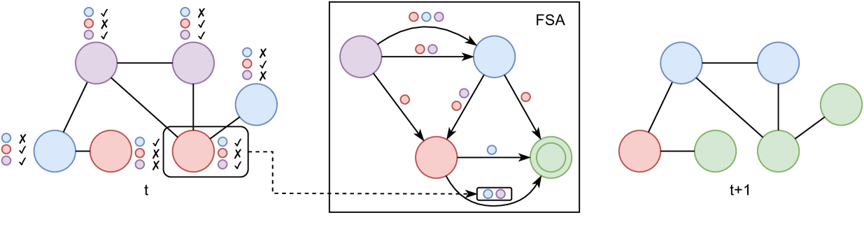</details> Figure 1: Illustration of the GraphFSA framework: Each node has its own state, represented by its color. Furthermore, each node runs the same Finite State Automaton, determining its next state depending on the neighborhood information. On the left, an example graph is shown with the aggregation next to it. In this example, the aggregator can distinguish if there is a node of a certain color/state in the neighborhood. In general, the aggregator can be any function that maps a state multiset to a finite set of values. State transitions are determined by the FSA depicted in the middle, which chooses chooses the next state based on the states appearing in the neighborhood and the old state. An example of the transition that is taken by the red node on the bottom right of the graph is shown. Note that the green state is final and does not have any outgoing transitions. Cellular automaton. Cellular Automata (CA) are discrete computational models introduced by John von Neumann in 1967 von Neumann and Burks [29]. They consist of a grid of cells, where each cell is in a discrete state and evolves following transition rules based on the states of neighboring cells. In our context, learning these transition functions from data and modeling the appropriate domain is of particular interest. Notably, recent work by Wulff and Hertz [31] trains a Neural Network (NN) to learn 1D and 2D CAs, while further advancements are made with Neural Cellular Automata (NCA) introduced by Mordvintsev et al. [19], and the Graph Cellular Automata (GCA) proposed by Marr and Hütt [17], operating on graph structures with diverse neighborhood transition rules. Additionally, Grattarola et al. [6] introduce Graph Neural Cellular Automata (GNCA), focusing on learning a GCA with continuous state spaces. GNCA mainly differs from our work in that it uses continuous instead of discrete state spaces and only learns a single transition step at a time, while we can extract rules from observations over multiple steps. Lastly, the study by Johnson et al. [11] investigates relationships defined by paths on a graph accepted by a finite-state automaton. Notably, this execution mechanism differs significantly from our methodology, serving the distinct purpose of adding edges on accepted paths. Unlike the synchronous execution of multiple finite-state automata in GraphFSA, here, the single automaton functions more like an agent traversing the graph. Consequently, the tasks the authors tackle, such as identifying additional edges in grid-world environments and abstract syntax trees (ASTs), differ from ours. It is crucial to highlight that this model only augments edges and does not predict node values. Graph neural networks. Graph Neural Networks (GNNs) were introduced by Scarselli et al. [23] and have gained significant attention. Various GNN architectures, such as Graph Convolutional Networks [14] and Graph Attention Networks [28], have been developed. A crucial area of GNN research is understanding their theoretical capabilities, which is linked to the WL color refinement algorithm that limits the conventional GNNs’ expressiveness [30, 32, 21]. The WL algorithm proceeds in rounds where node colors are relabeled based on their own color and the colors of nodes in the neighborhood. To achieve optimal expressiveness, message-passing GNNs must run the layers an adequate number of rounds to match the computational prowess of WL. The necessity of augmenting the number of rounds has been emphasized for algorithmic graph problems [15]. However, failing to adhere to the minimum rounds required may cause a GNN to fall short of solving or approximating specific problems, as shown by Sato et al. [22]. Furthermore, enhancing the interpretability and visualization of GNNs has become an essential part of GNN research. The development of GNNExplainer [33] marked a significant stride in generating explanations for Graph Neural Networks. Similarly, Hohman et al. [8] delved into visual analytics in deep learning, providing an interrogative survey for future developments in this domain. Another approach towards explainability is understanding specific examples proposed by Huang et al. [9]. Moreover, the GraphChef architecture introduced by Müller et al. [20], offers a comprehensive understanding of GNN decisions by replacing layers in the message-passing framework with decision trees. GraphChef uses the gumbelized softmax from Johnson et al. [12] to learn a discrete state space, enabling the extraction of decision trees. Algorithmic learning. Algorithm learning aims to learn an underlying algorithmic principle that allows generalization to unseen and larger instances. As such, one of the primary goals is to achieve extrapolation. Various models have been investigated for extrapolation, including RNNs capable of generalizing to inputs of varying lengths [5]. Specifically, in our work, we want to learn graph algorithms. For extrapolation, we want our learned models to scale to graphs that are more complex and larger than those used during training. Graph Neural Networks (GNNs) have been extensively applied to solve these algorithmic challenges [24, 27, 13]. Recent studies by Tang et al. [25], Veličković et al. [26], and Ibarz et al. [10] have emphasized improving extrapolation to larger graphs in algorithmic reasoning problems. However, most of the work focuses only on slightly larger graphs than those in the training set. Scaling to much larger graphs, as studied by Grötschla et al. [7] remains challenging. ## 3 The GraphFSA framework We present GraphFSA, a computational framework designed for executing Finite State Automata (FSA) on graph-structured data. Drawing inspiration from Graph Cellular Automata and Graph Neural Networks, GraphFSA defines an FSA at each node within the graph. This FSA remains the same across all nodes and encompasses a predetermined set of states and transition values. While all nodes abide by the rules of the same automaton, the nodes are usually in different states. As is customary for FSAs, a transition value and the current state jointly determine the subsequent state transition. In our approach, transition values are computed through the aggregation of neighboring node states. As the FSA can only handle a finite number of possible aggregations, we impose according limitations on the aggregation function. For the execution of the framework, nodes are first initialized with a state that represents their input features. The FSA is then executed synchronously on all nodes for a fixed number of steps. Each step involves determining transition values and executing transitions for each node to change their state. Upon completion, each node reaches an output state, facilitating node classification into a predetermined set of categorical values. A visual representation of the GraphFSA model is depicted in Figure 1. ### 3.1 Formal definition More formally, the GraphFSA $\mathcal{F}$ consists of a tuple $(\mathcal{M},\mathcal{Z},\mathcal{A},\mathcal{T})$ . $\mathcal{F}$ is applied to a graph $G=(V,E)$ and consists of a set of states $\mathcal{M}$ , an aggregation $\mathcal{A}$ and a transition function $\mathcal{T}$ . At time $t$ , each node $v\in V$ is in state $s_{v,t}\in\mathcal{M}$ . In its most general form, the aggregation $\mathcal{A}$ maps the multiset of neighboring states to an aggregated value $a\in\mathcal{Z}$ of a finite domain. $$ \displaystyle a_{v,t}=\mathcal{A}(\{\!\{s_{u,t}\mid u\in N(v)\}\!\}) \tag{1} $$ Here $\{\!\{\}\!\}$ denotes the multiset and $N(v)$ the neighbors of $v$ in $G$ . At each timestep $t$ , the transition function $\mathcal{T}:\mathcal{M}\times\mathcal{Z}\to\mathcal{M}$ takes the state of a node $s_{v,t}$ and its corresponding aggregated value $a_{v,t}$ and computes the state for the next timestep. $$ \displaystyle s_{v,t+1}=\mathcal{T}(s_{v,t},a_{v,t}) \tag{2} $$ For notational convenience, we also define the transition matrix $T$ of size $\left|\mathcal{M}\right|\times\left|\mathcal{Z}\right|$ where $T_{m,a}$ stores $\mathcal{T}(m,a)$ . Moreover, we introduce the notion of a state vector $s_{v}^{t}$ for each node $v\in V$ at time $t$ , which is a one-hot encoding of size $\left|\mathcal{M}\right|$ of the node’s current state. Aggregation functions. The transition value $a$ for node $v$ at time $t$ is directly determined by aggregating the multi-set of states from all neighboring nodes at time $t$ . The aggregation $\mathcal{A}$ specifies how the aggregated value is computed from this neighborhood information. Note that this formulation of the aggregation $\mathcal{A}$ allows for a general framework in which many different design choices can be made for a concrete class of GraphFSAs. Throughout this work, we will focus on the counting aggregation and briefly touch upon the positional aggregation. Counting aggregation: The aggregation aims to count the occurrence of each state in the immediate neighborhood. However, we want the domain $\mathcal{Z}$ to remain finite. Note that due to the general graph topology of $G$ , the naive count could lead to $\mathcal{Z}$ growing with $n$ the number of nodes. Instead, we take inspiration from the distributed computing literature, specifically the Stone Age Computing Model by Emek and Wattenhofer [3]. Here, the aggregation is performed according to the one-two-many principle, where each neighbor can only distinguish if a certain state appears once, twice, or more than twice in the immediate neighborhood. Formally, we can generalize this principle using a bounding parameter $b$ , which defines up to what threshold we can exactly count the neighbor states. The simplest mode would use $b=1$ , i.e., where we can distinguish if a state is part of the neighborhood or not. Note that this is equivalent to forcing the aggregation to use a set instead of a multi-set. For the general bounding parameter $b$ , we introduce the threshold function $\sigma$ , which counts the occurrences of a state in a multi-set. $$ \displaystyle\sigma(m,S)=\min(b,\left|\{\!\{s\mid s=m,s\in S\}\!\}\right|) \tag{3} $$ Therefore, the aggregated value $a_{v,t}$ will be an $\left|\mathcal{M}\right|$ dimensional vector of the following form, where the $m$ -th dimension corresponds to the number of occurrences of state $m$ . $$ \displaystyle(a_{v,t})_{m}=\sigma(m,\{\!\{s_{u,t}\mid u\in N(v)\}\!\}) \tag{4} $$ Note that there is a tradeoff between expressiveness and model size when choosing a higher bounding parameter $b$ . For a model with $|\mathcal{M}|$ number of states there are ${(b+1)}^{|\mathcal{M}|}$ many transition values for each state $m\in\mathcal{M}$ . Positional aggregation: This aggregation function takes into account the spatial relationship between nodes in the graph. If the underlying graph has a direction associated with each neighbor, i.e., in a grid, we assign each neighbor to a distinct slot within a transition value vector $a_{v,t}$ . This generalizes to graphs of maximum degree $d$ , where each of the d entries in $a_{v,t}$ corresponds to a state of a neighboring node. Average threshold-based aggregation An alternative aggregation operator utilizes the average value, which allows us to detect whether a specific threshold $t$ of neighbors is in a particular state. We compute the value to threshold by dividing the state sum by the neighborhood size of a node v. That, for example, allows us to detect whether the majority (e.g., 0.5) of neighbors are in a specific state. Starting and final states. We use starting states $S\subseteq\mathcal{M}$ of the FSA to encode the discrete set of inputs to the graph problem. These could be the starting states of a cellular automaton or the input to an algorithm (e.g., for BFS, the source node starts in a different state from the other nodes). Final states $F\subseteq\mathcal{M}$ are used to represent the output of a problem. In node prediction tasks, we choose one final state per class. Opposed to other states, it is not possible to transition away from a final state, meaning that once such a state is reached, it will never change. <details> <summary>x2.png Details</summary>  ### Visual Description \n ## Diagram: Network Evolution ### Overview The image presents a series of three network diagrams, illustrating a potential evolution of a network structure over time or under different conditions. Each diagram depicts a network composed of nodes (circles) connected by edges (lines). The diagrams are arranged horizontally, from left to right, suggesting a progression. The color of the nodes changes across the diagrams, potentially indicating different states or roles of the nodes. ### Components/Axes The diagrams do not have explicit axes or labels. The components are: * **Nodes:** Represented by circles. * **Edges:** Represented by lines connecting the nodes. * **Colors:** Used to differentiate nodes within each diagram and across diagrams. The colors present are: * White/Black (Diagram 1) * Lavender/Purple (Diagram 2) * Blue (Diagram 2 & 3) * Green (Diagram 3) * Red/Salmon (Diagram 3) ### Detailed Analysis or Content Details **Diagram 1 (Leftmost):** * The network consists of 7 nodes. * The nodes are connected in a linear chain-like structure. * All nodes are white with black outlines. * The network has a length of approximately 6 node-to-node connections. **Diagram 2 (Center):** * The network consists of 8 nodes. * The network has a more branched structure than Diagram 1. * There are 4 lavender/purple nodes and 4 blue nodes. * The network appears to have a central blue node connected to three lavender nodes and one other blue node. * The lavender nodes are connected to each other in a chain-like structure. **Diagram 3 (Rightmost):** * The network consists of 8 nodes. * The network has a branched structure, similar to Diagram 2, but with different colors. * There are 4 lavender/purple nodes, 2 blue nodes, 1 red/salmon node, and 2 green nodes. * The network appears to have a central blue node connected to two lavender nodes and one red/salmon node. * The red/salmon node is connected to two green nodes. * The lavender nodes are connected to each other in a chain-like structure. ### Key Observations * The network complexity increases from Diagram 1 to Diagram 2 and remains similar in Diagram 3. * The color scheme changes significantly across the diagrams, potentially indicating changes in node states or roles. * Diagram 3 introduces a new color (red/salmon and green), suggesting the emergence of new node types or functionalities. * The central node (blue) appears to maintain a consistent role across Diagrams 2 and 3, acting as a hub. ### Interpretation The diagrams likely represent the evolution of a network over time or under different conditions. The change in node colors could signify changes in node status, function, or importance. The increasing complexity from Diagram 1 to Diagram 2 suggests network growth or development. The introduction of new colors in Diagram 3 indicates the emergence of new elements or functionalities within the network. The consistent presence of the central blue node in Diagrams 2 and 3 suggests that this node plays a critical role in the network's structure and function, potentially acting as a central controller or hub. The branching structure in Diagrams 2 and 3 indicates a more distributed network architecture compared to the linear structure in Diagram 1. Without additional context, it is difficult to determine the specific meaning of the network evolution. However, the diagrams suggest a dynamic system undergoing changes in structure, function, and complexity. The diagrams could represent a variety of systems, such as social networks, biological networks, or computer networks. The change in colors could represent different states of nodes, such as active/inactive, healthy/infected, or online/offline. 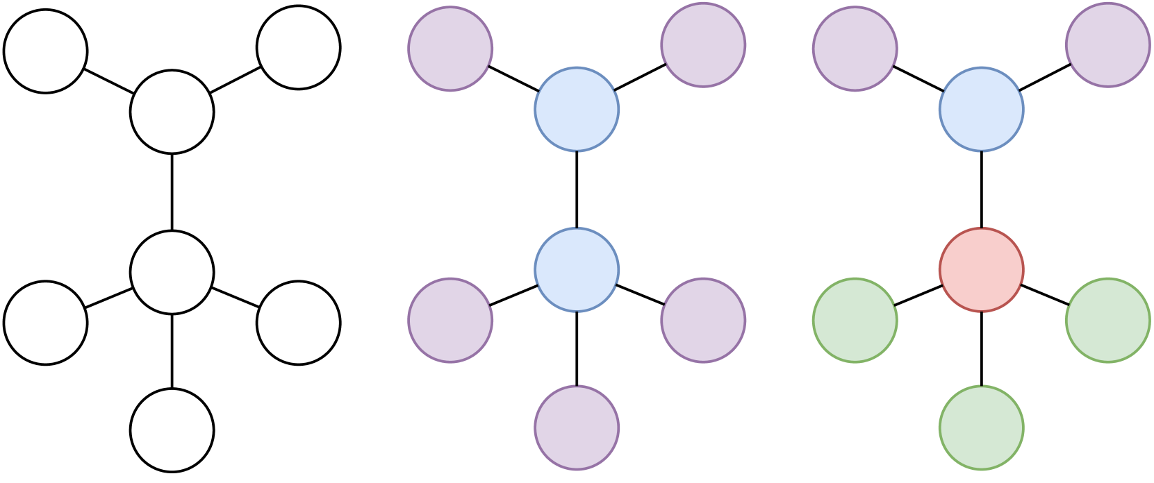</details> Figure 2: Original topology (left), nodes that GraphFSA can distinguish with 2+ aggregation (i.e., distinguish neighbors as 0, 1 or more than 2) (middle) and 1-WL color classes (right). More specifically, for GraphFSA, nodes cannot differentiate if they have 2 or 3 neighbors of a kind. In contrast, 1-WL can further distinguish the two nodes. Scalability. Scalability can be analyzed along two primary dimensions: the size of the graphs on which the cellular automata (CA) are executed, and the number of states that the learned CA can possess. Our approach demonstrates good scalability for larger graphs as it operates in linear time relative to the number of nodes and edges. However, scalability concerning the number of states is influenced by the chosen aggregation method. Specifically, with the counting aggregation, the number of possible aggregations becomes exponential in the number of states. It is, therefore, crucial to choose aggregations that lead to a smaller expansion when dealing with more states. <details> <summary>x3.png Details</summary>  ### Visual Description \n ## Diagram: State Transition Diagram ### Overview The image depicts a state transition diagram with two states: 's1' and 'f0'. Arrows indicate transitions between these states, labeled with numerical vectors. The diagram appears to represent a finite state machine or a similar system where the state changes based on input or events. ### Components/Axes The diagram consists of: * **States:** 's1' (left) and 'f0' (right). * **Transitions:** Two labeled arrows. * **Labels:** Numerical vectors associated with each transition. ### Detailed Analysis or Content Details * **State 's1':** A circular node labeled "s1". It has a self-looping transition. * **Self-loop Transition:** Labeled with the vector "[0, 0, 1, 0]". This indicates that when in state 's1', a transition back to 's1' occurs with the specified input. * **State 'f0':** A circular node labeled "f0". It has a self-looping transition. * **Self-loop Transition:** The state 'f0' has a self-looping transition. * **Transition from 's1' to 'f0':** An arrow pointing from 's1' to 'f0', labeled with the vector "[0, 1, 0, 0]". This indicates a transition from state 's1' to state 'f0' occurs with the specified input. ### Key Observations The diagram shows a system that can be in either state 's1' or 'f0'. State 's1' can return to itself, and can also transition to 'f0'. State 'f0' can only return to itself. The vectors associated with the transitions likely represent input conditions or events that trigger the state changes. ### Interpretation This diagram likely represents a simple finite state machine. The states 's1' and 'f0' could represent different modes of operation or stages in a process. The vectors "[0, 0, 1, 0]", "[0, 1, 0, 0]" represent the conditions that cause the transitions between states. The self-loop on 'f0' suggests that once the system enters state 'f0', it remains there unless a different, unrepresented input causes a transition. The diagram is a concise way to visualize the possible states and transitions of a system, making it useful for design, analysis, and documentation. The vectors suggest a 4-dimensional input space, where each element of the vector represents a binary condition (0 or 1). </details> <details> <summary>x4.png Details</summary>  ### Visual Description \n ## Diagram: State Transition Diagram ### Overview The image depicts a state transition diagram with four states: ~!, s0, s1, and !!. Arrows connect these states, each labeled with a numerical vector enclosed in square brackets. The diagram illustrates possible transitions between states based on the input represented by these vectors. ### Components/Axes The diagram consists of four circular nodes representing states. The nodes are labeled as follows: * **~!** (leftmost node) * **s0** (center-left node) * **s1** (center-right node) * **!!** (bottom-center node) Arrows with numerical vectors indicate transitions between states. The vectors are: * [0, 0, 0, 1] * [1, 1, 0, 0] * [0, 0, 1, 1] * [1, 0, 0, 0] * [0, 1, 1, 0] * [1, 1, 1, 0] ### Detailed Analysis The diagram shows the following transitions: 1. **~! to s0:** Labeled with [0, 0, 0, 1]. 2. **~! to !!:** Labeled with [0, 1, 1, 0]. 3. **s0 to s1:** Two transitions: * Labeled with [0, 0, 1, 1]. * Labeled with [1, 1, 0, 0]. 4. **s0 to !!:** Labeled with [1, 0, 0, 0]. 5. **!! to s0:** Labeled with [1, 1, 1, 0]. ### Key Observations The diagram represents a finite state machine. The transitions are defined by the input vectors. The state !! appears to be a "sink" state, as there are no outgoing transitions from it. The state s0 has multiple outgoing transitions, indicating branching behavior. ### Interpretation This diagram likely represents a simplified model of a system with discrete states and inputs. The input vectors could represent different events or conditions that trigger transitions between states. The diagram could be used to analyze the behavior of the system, identify potential deadlocks, or verify its correctness. The specific meaning of the states and input vectors would depend on the context of the system being modeled. The diagram suggests a system that can move from an initial state (~!) to either s0 or !!, and from s0 to either s1 or !!. The transition from !! back to s0 suggests a possible recovery or reset mechanism. The numerical vectors likely represent a binary input or a set of conditions that must be met for the transition to occur. 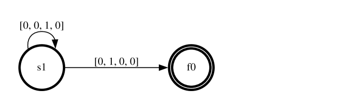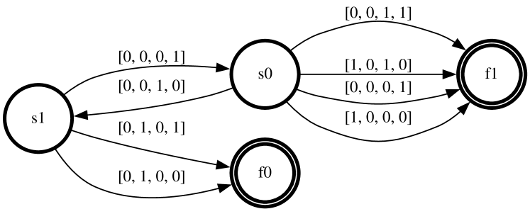</details> Figure 3: Partial Visualization of a learned GraphFSA model for the Distance problem. The root node starts in state $s_{1}$ (left), whereas all other nodes start in state $s_{0}$ (right). The final states $f_{0},f_{1}$ represent even and odd distances to the root, respectively. Aggregation values are presented as $[f_{0},f_{1},s_{0},s_{1}]$ where we apply the counting aggregation with bounding parameter $b=1$ . We can verify on the right that the nodes wait until they observe a final state in their neighborhood and then transition to the other final state. A full visualization of the same automaton can be found in the Appendix. ### 3.2 Expressiveness While the execution of GraphFSA may bear resemblance to one round of the Weisfeiler-Lehman test, this does not hold in general. In the example Figure 1, they are the same because the chosen GraphFSA-instantiation is powerful enough to distinguish all occurrences of states appearing in the neighborhoods. More specifically, nodes can distinguish if they have 0 or more than one neighbor in a certain state (“1+ aggregation”), which is sufficient for the given graph. In general, the aggregation function $\mathcal{A}$ distinguishes GraphFSA from the standard WL-refinement notion as it restricts the observation of the neighborhood from the usual multiset observations (as these cannot be bounded in size). Consequently, GraphFSA is strictly less expressive than 1-WL, resulting in a tradeoff between using a more expressive aggregator and maintaining the simplicity or explainability of the resulting model, particularly as the state space grows exponentially. Figure 2 presents an example comparing GraphFSA’s execution with a 2+ aggregator to WL refinement. Here, we can observe that GraphFSA is less expressive than 1-WL. However, for a large enough $b$ , GraphFSA can match 1-WL on restricted graph classes of bounded degree. In conclusion, while the finite number of possible aggregations restricts GraphFSA, it also keeps the mechanism simple. Our evaluation demonstrates that this can improve generalization performance for a learned GraphFSA. ### 3.3 Visualization and interpretability The GraphFSA framework offers inherent interpretability, facilitating visualization akin to a Finite State Automaton (FSA). This visualization approach allows us to easily explore the learned state transitions and the influence of neighboring nodes on state evolution. We outline two primary visualization techniques for GraphFSA: Complete FSA visualization. 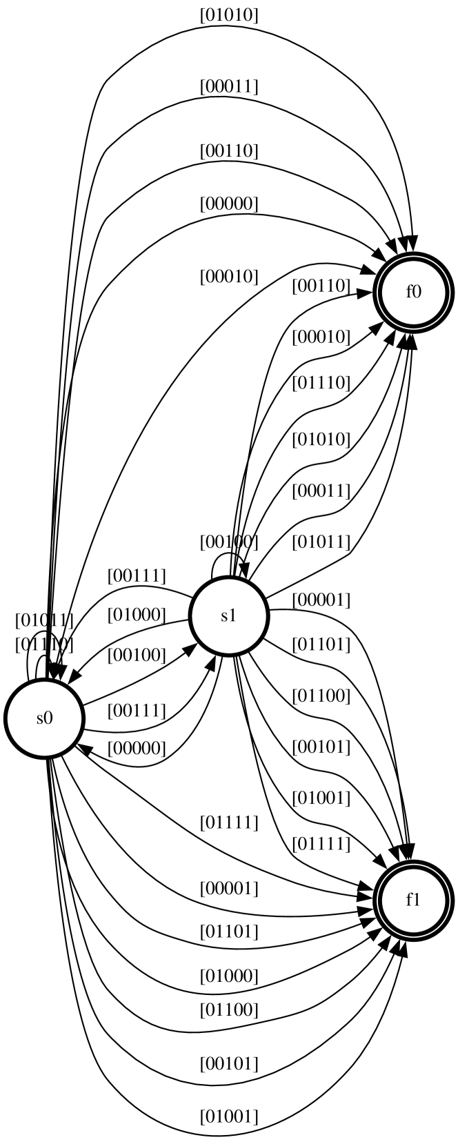This method provides a comprehensive depiction of the entire FSA representation within the GraphFSA model, encompassing all states and transitions. Each node in the graph corresponds to a distinct state, while directed edges represent transitions between states based on transition values. An example is visualized in Figure 5. Partial FSA visualization. Tailored for targeted analysis of the GraphFSA model’s behavior, this approach proves especially useful when dealing with large state spaces or focusing on specific behaviors. This method visualizes a selected starting state by evaluating the model across multiple problem instances and tracking all transitions that occur. Then, the visualization is constructed by exclusively displaying the states and transitions that have been used from the specified starting state. Figure 3 illustrates the partial visualization of a learned automaton. The transitions in the diagram are determined by aggregating the information of the neighboring states. The structure of the transition value is $[f_{0},f_{1},s_{0},s_{1}]$ . For instance, the state vector $[0,0,1,0]$ indicates that the node in the graph has one or more neighbors in state $s_{0}$ while having no neighbors in other states. <details> <summary>extracted/5781695/graphics/experiments/ca/hexagonial_input.png Details</summary>  ### Visual Description \n ## Hexagonal Grid: Color Distribution ### Overview The image depicts a hexagonal grid filled with alternating shades of gray and black. There are no axes, labels, or legends present. The arrangement appears to be a repeating pattern, but lacks any explicit data or quantitative information. ### Components/Axes There are no axes, labels, or legends. The image consists solely of a grid of hexagonal cells, colored either black or light gray. ### Detailed Analysis or Content Details The grid is approximately 7 hexagons wide and 6 hexagons tall. The hexagons are arranged in a honeycomb pattern. The color distribution appears to be roughly alternating, but not perfectly regular. * **Black Hexagons:** Approximately 13 hexagons are colored black. * **Gray Hexagons:** Approximately 28 hexagons are colored light gray. There is no clear trend or pattern beyond the alternating colors. The arrangement doesn't seem to represent any specific data set. ### Key Observations The number of gray hexagons is more than double the number of black hexagons. The arrangement is visually balanced, with the colors distributed throughout the grid. There is no obvious clustering of either color. ### Interpretation The image appears to be a visual representation of a simple pattern or a texture. Without any accompanying data or context, it's difficult to determine its purpose. It could be a stylized representation of a cellular structure, a visual metaphor for duality, or simply an abstract design. The lack of labels or axes suggests that the image is not intended to convey specific quantitative information, but rather to present a visual arrangement. It is possible that the image is a simplified representation of a more complex system, but without further information, this is speculative. The image does not provide any facts or data, and is purely descriptive. </details> <details> <summary>extracted/5781695/graphics/experiments/ca/hexagonial_output.png Details</summary>  ### Visual Description \n ## Hexagonal Grid: Pattern Visualization ### Overview The image displays a hexagonal grid filled with alternating black and light gray hexagons. There are no axes, labels, or legends present. The arrangement appears to be a repeating pattern. The image does not contain any factual data, but rather a visual representation of a pattern. ### Components/Axes There are no axes, labels, or legends. The image consists solely of a grid of hexagons. ### Detailed Analysis or Content Details The grid is approximately 7 hexagons wide and 6 hexagons tall. The hexagons are arranged in a honeycomb-like structure. * **Black Hexagons:** There are approximately 12 black hexagons. They are distributed in a checkerboard-like pattern. * **Light Gray Hexagons:** There are approximately 22 light gray hexagons. They are also distributed in a checkerboard-like pattern, alternating with the black hexagons. The pattern appears to be centered, with a black hexagon at the approximate center of the grid. The arrangement is symmetrical. ### Key Observations The most notable observation is the alternating pattern of black and light gray hexagons. The pattern is consistent throughout the grid, suggesting a deliberate design. There are no obvious outliers or anomalies. ### Interpretation The image likely represents a visual pattern or a simple demonstration of a tiling structure. The alternating colors could symbolize different states, categories, or values, but without additional context, the specific meaning is unclear. The hexagonal grid itself is a common structure in various fields, including chemistry (representing molecular structures), materials science (representing crystal lattices), and game design (representing game boards). The image could be used to illustrate concepts related to these fields, or simply as an abstract visual element. The lack of labels or data suggests the image is intended for illustrative purposes rather than conveying specific quantitative information. It is a visual representation of a repeating pattern, and its meaning is dependent on the context in which it is presented. </details> <details> <summary>x5.png Details</summary>  ### Visual Description \n ## Diagram: Cellular Automata Evolution ### Overview The image depicts the evolution of a one-dimensional cellular automaton over four discrete time steps: 0, 3, 6, and 9. The automaton consists of a linear array of cells, with each cell existing in one of three states: black, yellow, red, or blue. The diagram illustrates how the state of each cell changes based on the states of its neighboring cells according to a specific rule. ### Components/Axes The diagram is organized into four panels, each representing a time step. Each panel shows two rows of cells. The horizontal axis represents the cell position along the linear array. There are no explicit axes labels, but the time step is indicated above each panel ("Step 0", "Step 3", "Step 6", "Step 9"). The cells are represented as colored squares. The colors represent the cell states: * **Yellow:** Represents the background or default state. * **Black:** Represents an active or 'on' state. * **Red:** Represents a transient state. * **Blue:** Represents a transient state. ### Detailed Analysis **Step 0:** * Two black cells are present, each surrounded by yellow cells. * A blue segment is present on the left side of the top row. * A red segment is present on the right side of the top row. * A blue segment is present on the left side of the bottom row. * A red segment is present on the right side of the bottom row. **Step 3:** * The black cells have remained in the same positions. * The blue segments have moved one cell to the right. * The red segments have moved one cell to the left. **Step 6:** * The black cells have remained in the same positions. * The blue segments have merged into a single two-cell block. * The red segments have merged into a single two-cell block. * The blue and red blocks are positioned adjacent to the black cells. **Step 9:** * The black cells have remained in the same positions. * The blue segments have moved one cell to the right. * The red segments have moved one cell to the left. * The blue and red segments are now positioned in the same locations as in Step 0. ### Key Observations * The black cells remain stationary throughout the simulation. * The red and blue segments move in opposite directions, with red moving left and blue moving right. * The pattern repeats every three steps, suggesting a periodic behavior. * The red and blue segments appear to 'orbit' the black cells. ### Interpretation This diagram illustrates a simple one-dimensional cellular automaton. The automaton's behavior is governed by a set of rules that determine how the state of each cell changes based on the states of its neighbors. The observed periodic behavior suggests that the automaton is operating in a stable regime. The movement of the red and blue segments around the black cells could represent the propagation of information or energy within the system. The automaton's simplicity allows for easy visualization and analysis of complex emergent behaviors. The diagram demonstrates how simple rules can lead to complex patterns and dynamics. The repeating pattern suggests a conserved quantity within the system, possibly related to the number of red and blue cells. The black cells act as fixed points or attractors, influencing the movement of the other cell states. 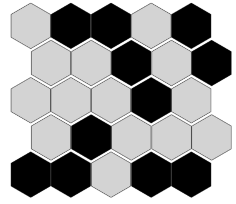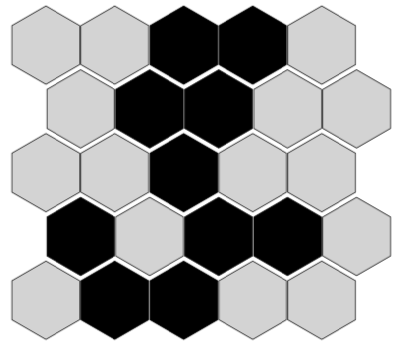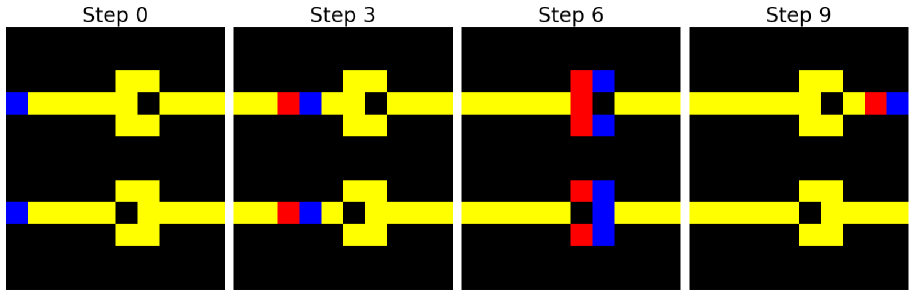</details> Figure 4: We study learning cellular automata as the simplest form of algorithmic behavior, which can lead to complex and intricate behavior patterns when assembled in a network. The left shows Conway’s Game of Life, which we can learn on general topologies such as the hexagonal grid due to the graph representation. A WireWorld automata is depicted on the right, which can be used to simulate transistors and electrical circuits. It shows the electron head (blue) and tail (red) transitioning through different wires (yellow). ### 3.4 GRAB: The GraphFSA dataset generator Accompanying the GraphFSA execution framework, which outlines the general interface and underlying principles shared amongst instances of GraphFSA, we provide GRAB, a flexible dataset generator to evaluate learned state automatons. Note that the introduced framework specifies the model structure but allows for different training methodologies that can be used to train specific model instances. The discrete nature of state transitions makes training these models a challenging task. This work proposes one possible way to train such models using input and output pairs. For alternative approaches, we deem it crucial to provide a systematic tool that can be used to develop new training strategies and further provide a principled way of thoroughly assessing the effectiveness across training methods. Therefore, GRAB provides an evaluation framework for learning state automatons on graphs. GRAB generates the ground truth for a synthetic FSA, which can be used for learning and testing on various graphs. In particular, GRAB provides out-of-the-box support for several graph sizes and supports testing on multiple graph distributions. In the dataset construction process, we first define the characteristics of the ground truth GraphFSA, specifying the number of states and configuring the number of initial and final states. Next, we generate a random Finite State Automaton (FSA) by selecting states for each transition value, adhering to the constraints of the final state set (final states cannot transition to other states). We then sample graphs from predefined distributions, offering testing on a diverse set of graph types such as trees, grids, fully connected graphs, regular graphs, and Erdos-Renyi graphs. The starting states for each node within these generated graphs are randomly initialized from the set $\mathcal{S}$ . Finally, we apply the GraphFSA model to these input graphs to compute the outputs according to the defined state transitions. For the dataset generation, we emphasize evaluating generalization, which we believe to be one of the essential abilities of the GraphFSA framework. Therefore, we establish an extrapolation dataset to assess the model’s capability beyond the graph sizes encountered during training. This dataset contains considerably larger graphs, representing a substantial deviation from the training data. However, if the correct automaton can be extracted during training, good generalization should be achievable despite the shift in the testing distribution. Input/output pairs for these larger graphs are produced by applying the same generated FSA to obtain the resulting states. ## 4 Empirical evaluation The GraphFSA framework is designed to extract state automaton representations with discrete states and transitions to learn to solve the task at hand through an algorithmic representation. Our evaluation consists of two key components to showcase this. In the first part, we focus on classic cellular automaton problems. These automatons serve as a foundational component of our study as they represent the simplest possible version of an algorithm. However, despite their simplicity, they can becomes increasingly powerful and exhibit complex behaviour when assembled together in a network. We successfully learn the underlying automaton rules, demonstrating the ability and advantage of the GraphFSA framework to capture simple algorithmic behaviour. In the second part of our empirical study, we evaluate our models using our proposed graph automaton benchmark and a set of more challenging graph algorithms. GRAB enables a comprehensive investigation of GraphFSA’s performance across a broad range of problems. We are particularly interested in the generalisation ability of the GraphFSA Framework. Therefore, we perform extrapolation experiments where we train on smaller graphs and subsequently test its performance on larger instances. Finally, we use the GraphFSA framework to learn a selection of elementary graph algorithms, demonstrating the framework’s capability and potential for algorithm learning. ### 4.1 Training We take inspiration from prior research on training differentiable finite state machines [18] and propose an adaption to train Diff-FSA, which follows the GraphFSA framework, on general graphs. To maintain differentiability, we relax the requirement for choosing a single next state for a transition in $\mathcal{T}$ during training and instead model it as a probability distribution over possible next states, resulting in a probabilistic automaton. We thus compute $P(X=m\ |\ \mathcal{M}\times\mathcal{Z})$ for $m\in\mathcal{M}$ and parameterize Diff-FSA with a matrix $T^{\prime}$ of size $\mathcal{M}\times\mathcal{Z}\times\mathcal{M}$ that holds the probabilities for all possible transitions and states. This means that the transition matrix $T^{\prime}$ contains the probabilities of transitioning from a state $m_{1}$ to a state $m_{2}$ given a specific transition value. To train the model with a given step number $t$ , we execute Diff-FSA for $t$ rounds and compute the loss based on the ground-truth output states of the graph automaton we want to learn when executing the same number of steps $t$ . For example, in the case of node classification problems, we aim to predict each node’s final state $f\in F$ . This makes it possible to backpropagate through the transition matrix $T^{\prime}$ . In addition, we apply an L2 loss to achieve the correct mapping between input and output states. Once the training of the probabilistic model is complete, we extract the decision matrix $T$ from $T^{\prime}$ by discretizing the distribution $P$ over the next states to the most likely one. Furthermore, we are interested in the model’s ability to produce consistent and correct outputs, even as the number of iterations changes. We refer to this as Iteration stability. The extrapolation capabilities of the GraphFSA model are achieved through the ability to adjust the number of iterations, representing the number of steps executed by the FSA. This flexibility is essential, especially for graphs with larger diameters, where information needs to propagate to all nodes. We can, therefore, train an FSA where we can choose a sufficiently large number of iterations to produce a correct output, and increasing this number of iterations still leads to a correct solution. We develop two approaches: Random iteration offset. During training, we introduce random adjustments to the number of iterations with a small offset factor. This randomization ensures that the model can effectively handle the problem with varying numbers of iterations. Final state loss. One approach to incentivize final states not to switch to other states is to incorporate an additional loss term that penalizes leaving a final state. We consider the learned transition matrix probabilities and penalize the model if the probability of switching from a final state $f\in F$ to any other state $m\in\mathcal{M},m\neq f$ is greater than 0 using an L1 loss. This approach encourages the model to stay in the final state, resulting in more stable predictions. Figure 3 provides an example of a state automata trained with this additional loss. Baseline models. The architecture that aligns most closely with our tasks is the Graph Neural Cellular Automata (GNCA) [6]. While GNCAs are designed to learn rules from single-step supervision, we apply several rounds when training with multiple steps. Besides GNCAs, we use recurrent message-passing GNNs. In contrast to GNCA, we follow the typical encode-process-decode [27], which means that the GNN keeps intermediate hidden embeddings that can be decoded to make predictions. We use the architecture proposed by Grötschla et al. [7], and observe that employing a GRU in the node update yields the best performance and generalization capabilities, in line with their results. This convolution is therefore used in all results in the paper. As the goal of a GraphFSA is to extract rules from the local neighborhood and update the node state purely based on this information, more advanced graph-learning architectures that go beyond this simple paradigm are not applicable in this setting. Our analysis mainly focuses on demonstrating the value of discrete state spaces, especially when generalizing to longer rollouts and larger graphs. ### 4.2 Classical cellular automata problems As a first step towards learning algorithms, we focus on cellular automata probelms. We consider a variety of different settings such as 1D and 2D automata, these include more well known instances such as Wireworld or Game of Life, which despite their simple rules are known to be Turing complete. For a more detailed explanation of the datasets, we refer to the Appendix. 1D-Cellular Automata The 1D-Cellular Automata dataset consists of one-dimensional cellular automata systems, each defined by one of the possible $2^{2^{3}}$ rules. Each rule corresponds to a distinct mapping of a cell’s state and its two neighbors to a new state. Game Of Life. The GameOfLife dataset follows the rules defined by Conway’s Game of Life [4]. A cell becomes alive if it has exactly 3 live neighbors. If a cell has less than 2 or more than 4 live neighbors, it dies, otherwise it persists. Furthermore, we consider a a variation where cells are hexagonal instead of the traditional square grid, which we refer to as the Hexagonal Game of Life. A visual representation is depicted in Figure 4. <details> <summary>x6.png Details</summary>  ### Visual Description ## State Diagram: Finite State Machine ### Overview The image depicts a state diagram representing a finite state machine (FSM). The diagram shows three states (s0, s1, f0, f1) and the transitions between them, labeled with binary strings. The diagram appears to model a sequential logic circuit or a stateful process. ### Components/Axes The diagram consists of: * **States:** Represented by circles labeled 's0', 's1', 'f0', and 'f1'. * **Transitions:** Represented by directed arrows connecting the states, labeled with 5-bit binary strings. * **Initial State:** 's0' is the initial state, indicated by the incoming arrow without a source state. ### Detailed Analysis or Content Details The diagram shows the following transitions: **From s0:** * To s1: labeled "[01011]", "[00111]", "[01000]", "[00101]", "[00010]", "[00001]", "[00100]", "[01101]", "[00000]", "[01111]", "[00110]", "[01001]" * To f0: labeled "[01010]" **From s1:** * To f0: labeled "[00111]", "[01000]", "[00101]", "[00010]", "[00001]", "[01101]", "[01011]", "[00000]", "[01111]", "[00110]", "[01001]" * To f1: labeled "[00100]", "[00000]", "[01111]", "[00110]", "[01001]" **From f0:** * To f1: labeled "[00110]", "[00101]", "[01110]", "[01010]", "[00011]", "[01011]", "[00001]", "[01101]", "[01100]", "[00101]", "[00101]", "[01001]" **From f1:** * To s0: labeled "[01111]", "[00111]", "[01101]", "[01001]", "[01100]", "[00101]", "[01001]", "[01001]", "[00101]", "[01001]" ### Key Observations * The state 's0' has the most incoming transitions, suggesting it's a common destination. * The state 'f1' has only outgoing transitions, leading back to 's0'. * The transitions are labeled with binary strings, which likely represent input values or conditions. * The diagram is fully connected, meaning every state can transition to every other state (or back to itself) given the appropriate input. ### Interpretation This state diagram likely represents a digital circuit or a control system. The binary strings on the transitions represent the input conditions that cause the system to move from one state to another. The diagram suggests a cyclical behavior, where the system transitions through the states 's0', 's1', 'f0', and 'f1' repeatedly based on the input sequence. The diagram could be a model for: * **A sequence detector:** The FSM might be designed to recognize a specific sequence of binary inputs. * **A counter:** The states could represent different count values, and the transitions could be triggered by clock pulses. * **A control logic:** The FSM could be part of a larger system that controls the behavior of other components. The fully connected nature of the diagram suggests a flexible system that can respond to a wide range of inputs. The specific meaning of the states and transitions would depend on the context in which the FSM is used. The diagram is a formal representation of a dynamic system, allowing for analysis and verification of its behavior. The diagram is a visual representation of a mathematical model, and can be used to simulate and understand the system's behavior. </details> Figure 5: Complete Visualization of a learned GraphFSA model for the Distance problem. The root node starts in state $s_{1}$ , whereas all other nodes start in state $s_{0}$ . The final states $f_{0},f_{1}$ represent even and odd distances to the root respectively. Aggregation values are presented as $[f_{0},f_{1},s_{0},s_{1}]$ where we apply the counting aggregation with bounding parameter $b=1$ . WireWorld. WireWorld [2] is an automaton designed to simulate the flow of an electron through a circuit. Cells can take one of four states: empty, electron head, electron tail, and conductor. Figure 4 shows an initial grid starting state and the evolution of WireWorld over multiple time steps. #### 4.2.1 Results For Cellular Automata problems, we generate training data for each problem by initializing a 4x4 input grid or path of length 4 (for 1D problems) with random initial states and apply the problem’s rules for a fixed number of steps to produce the corresponding output states. Our models are trained on these input-output pairs, using the same number of iterations as during dataset creation to ensure that we can extract the rule. Additionally, we test on an extrapolation dataset consisting of larger 10x10 grids. This dataset is used to evaluate the model’s ability to adapt to varying rule iterations with four different iteration numbers. 1D Cellular Automata. On this dataset, Diff-FSA uses the “positional neighbor-informed aggregation” aggregation technique. Notably, our model can successfully learn the rules for one-step training data (t=1). For the complete results, we refer to the Appendix. 2D Cellular Automata. 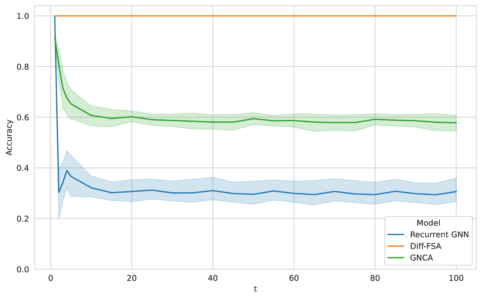For 2D Cellular Automata (CA) problems, Diff-FSA employs the counting aggregation. For Wireworld, we use a state space of four and a bounding parameter of three. We train all models to learn the one-step transition rules. During training, all models and baselines report high accuracy. We then investigate the generalization capabilities and especially the iteration stability of the learned models. We run the trained models on larger 10xs10 grids for more time steps t than during training. The results are depicted in Figure 6. Note that the recurrent GNN and GNCA both deteriorate outside the training distribution. However, Diff-FSA exhibits good iteration stability across the whole range of iterations. For the Game of Life variations, we provide a detailed comparison in the Appendix. <details> <summary>x7.png Details</summary>  ### Visual Description \n ## Line Chart: Model Accuracy Over Time ### Overview This image presents a line chart comparing the accuracy of three different models – Recurrent GNN, Diff-FSA, and GNCA – over time (represented by 't'). The chart displays the accuracy on the y-axis and time on the x-axis. Each model's performance is represented by a colored line, with shaded areas indicating the uncertainty or variance around the mean accuracy. ### Components/Axes * **X-axis:** Labeled "t", representing time. The scale ranges from approximately 0 to 100. * **Y-axis:** Labeled "Accuracy", representing the model's accuracy. The scale ranges from 0.0 to 1.0. * **Legend:** Located in the bottom-right corner, identifying the models: * "Recurrent GNN" (Blue) * "Diff-FSA" (Orange) * "GNCA" (Green) * **Data Series:** Three lines representing the accuracy of each model over time, with shaded regions representing uncertainty. * **Grid:** A light gray grid is present to aid in reading values. ### Detailed Analysis * **Recurrent GNN (Blue):** The line starts at approximately 0.35 at t=0, initially increases slightly to around 0.40 by t=5, then fluctuates around 0.30-0.35 with some oscillations until t=100. The shaded region indicates a significant amount of variance, particularly in the early stages. * **Diff-FSA (Orange):** This line starts at approximately 0.95 at t=0 and decreases rapidly to around 0.80 by t=5. It continues to decrease, leveling off around 0.60-0.65 from t=40 to t=100. The shaded region is relatively narrow, indicating lower variance compared to the Recurrent GNN. * **GNCA (Green):** The line begins at approximately 0.85 at t=0 and decreases steadily to around 0.60 by t=10. It then plateaus, remaining relatively stable between 0.55 and 0.65 from t=20 to t=100. The shaded region is moderate in width, suggesting a moderate level of variance. ### Key Observations * GNCA and Diff-FSA start with significantly higher accuracy than Recurrent GNN. * Recurrent GNN exhibits the highest variance in accuracy throughout the observed time period. * Diff-FSA shows the most rapid initial decrease in accuracy. * GNCA demonstrates the most stable accuracy over the longer term (t > 20). * All three models show a decreasing trend in accuracy over time, although GNCA and Diff-FSA stabilize after an initial drop. ### Interpretation The chart suggests that while GNCA and Diff-FSA initially outperform the Recurrent GNN, all models experience a decline in accuracy as time progresses. The Recurrent GNN's performance is less consistent, as indicated by the wider shaded region, suggesting it is more sensitive to variations in the data or training process. The stabilization of GNCA and Diff-FSA after the initial drop could indicate that they reach a point of diminishing returns or converge to a stable state. The initial high accuracy of Diff-FSA followed by a rapid decline might suggest a strong initial fit to the training data that doesn't generalize well over time. The consistent decline of the Recurrent GNN could be due to issues with vanishing gradients or difficulty in capturing long-range dependencies. The data suggests that GNCA might be the most robust model in the long run, given its relatively stable accuracy. Further investigation would be needed to understand the underlying reasons for these performance differences and to explore potential strategies for improving the accuracy and stability of each model. </details> Figure 6: Mean accuracies for Wireworld on a regular grid when trained on 1 step and applied for $t$ steps during inference (for 10 seeds each). All models report high accuracy for $t=1$ . However, performance deteriorates during inference when more steps are executed except for Diff-FSA. ### 4.3 Evaluation with GRAB Table 1: Evaluation of GraphFSA on synthetic data provided by GRAB. We report the accuracy and standard deviation over 10 runs. The underlying ground truth consists of an FSA using 4 states. We can test the in-distribution validation accuracy to see how well a model can fit the data. Moreover, we test extrapolation to larger graphs to verify that the rules for underlying automata were successfully learned. Our Diff-FSA models generally perform well across all scenarios. Note that the recurrent GNN performs well but lacks the interpretation and visualization of the learned mechanics as discrete state automata. | Model | Val Acc | n=10 | n=20 | n=50 | n=100 | | --- | --- | --- | --- | --- | --- | | GNCA | 0.38 $\pm$ 0.00 | 0.39 $\pm$ 0.00 | 0.40 $\pm$ 0.00 | 0.40 $\pm$ 0.00 | 0.39 $\pm$ 0.00 | | Recurrent GNN | 1.00 $\pm$ 0.00 | 0.91 $\pm$ 0.10 | 0.85 $\pm$ 0.13 | 0.82 $\pm$ 0.16 | 0.81 $\pm$ 0.16 | | Diff-FSA (4 states) | 0.99 $\pm$ 0.02 | 0.97 $\pm$ 0.02 | 0.96 $\pm$ 0.02 | 0.95 $\pm$ 0.03 | 0.94 $\pm$ 0.03 | | Diff-FSA (5 states) | 1.00 $\pm$ 0.01 | 0.98 $\pm$ 0.01 | 0.96 $\pm$ 0.02 | 0.95 $\pm$ 0.02 | 0.95 $\pm$ 0.02 | | Diff-FSA (6 states) | 0.99 $\pm$ 0.01 | 0.98 $\pm$ 0.01 | 0.95 $\pm$ 0.02 | 0.94 $\pm$ 0.02 | 0.94 $\pm$ 0.02 | We use GRAB to create diverse datasets to benchmark the different models. These datasets encompass different graph types and sizes and generate a synthetic state automaton to generate the ground truth. This allows us to precisely control the setup by adjusting the number of states of the ground truth automaton. For each specific dataset configuration, we train 10 different model instances. Extended results with more runs can be found in the Appendix. Table 1 shows the results for a dataset generated by GRAB. The dataset consists of tree graphs with a ground truth FSA consisting of 4 states. Generally, we can observe that both Diff-FSAinstances of the GraphFSA framework perform well, even if the number of states does not match exactly. The GNCA model performs poorly in this setting, as it struggles to learn the rules when they are applied for multiple steps. The recurrent GNN baseline performs well on in-distribution graphs, but struggles to generalize when the graph sizes are increased. Note that the recurrent GNN operates on continuous states, in contrast to the discrete states used by Diff-FSA. Moreover, the experiments were conducted with a varying number of states for Diff-FSA. While the ground-truth solution is modeled with 4 states, we want to investigate whether increasing this number for the learned automaton leads to different results. As we can observe, the accuracies are consistent for all sizes, indicating that more states can be used for training, which is especially useful when the underlying ground-truth automaton is not known beforehand. ### 4.4 Graph algorithms Table 2: Evaluation of learning graph algorithms on the Distance dataset. We report the accuracy and standard deviation over 10 runs. All models are trained on graphs of size at most 10 and then tested for extrapolation on larger graph sizes $n$ . Our Diff-FSA outperforms other discrete transition-based models while matching the recurrent GNN baseline. | GNCA | 0.50 $\pm$ 0.00 | 0.50 $\pm$ 0.00 | 0.51 $\pm$ 0.00 | 0.50 $\pm$ 0.00 | | --- | --- | --- | --- | --- | | Recurrent GNN | 1.00 $\pm$ 0.00 | 1.00 $\pm$ 0.00 | 1.00 $\pm$ 0.00 | 1.00 $\pm$ 0.00 | | Diff-FSA | 1.00 $\pm$ 0.00 | 1.00 $\pm$ 0.00 | 1.00 $\pm$ 0.00 | 1.00 $\pm$ 0.00 | To showcase the potential of the GraphFSA framework for algorithm learning, we further evaluate it on more challenging graph algorithm problems. We use the same graph algorithms as Grötschla et al. [7], which, among other setups, includes a simplified distance computation and path finding. Detailed descriptions of these datasets can be found in the Appendix. Similar to the data generated by GRAB, our training process incorporates a random number of iterations, with the sole condition that the number of steps is sufficiently large to ensure complete information propagation across the graph. For problems involving small training graphs, we train the Diff-FSA model with approximately ten iterations and apply the additive final state loss to ensure iteration stability and establish distinct starting and final states. The main aim is to validate that our proposed model is capable of learning more challenging algorithmic problems. It consistently performs better than GNCA. Compared to the recurrent GNN, it does not perform as well across all selected problems, but can learn correct solutions, as seen in the Distance task illustrated in Table 2. However, recall that Diff-FSAoperates on discrete states, making it much more challenging to learn. On the other hand, we can extract the learned solution and analyse the learned mechanics. A visualization of such a learned model is depicted in Figure 3 and Figure 5. This has the advantage over the recurrent baseline in that the learned mechanics can be interpreted, and the algorithmic behavior can be explained and verified. ## 5 Limitations and future work The main advantage of the GraphFSA framework is its use of discrete states. This allows us to interpret the learned mechanics through the lens of a state automaton. Moreover, it can perform well in scenarios where the underlying rules of a problem can be modeled with discrete transitions while requiring that inputs and outputs can be represented as discrete states. This is the case for several algorithmic settings but limits the model’s applicability to arbitrary graph learning tasks. To broaden the applicability of the GraphFSA framework, future work could investigate methods to map continuous input values to discrete states, potentially with a trainable module. Another aspect to investigate is the study of more finite aggregations for GraphFSA. These can heavily influence a model’s expressivity or align its execution to a specific task. Moreover, Diff-FSA only represents one possible approach to train models within the GraphFSA framework. Training models that yield discrete transitions remains challenging and could further improve performance and effectiveness. ## 6 Conclusion We present GraphFSA, an execution framework that extends finite state automata by leveraging discrete state spaces on graphs. Our research demonstrates the potential of GraphFSA for algorithm learning on graphs due to its ability to simulate discrete decision-making processes. Additionally, we introduce GRAB, a benchmark designed to test and compare methods compatible with the GraphFSA framework across a variety of graph distributions and sizes. Our evaluation shows that Diff-FSAcan effectively learn rules for classical cellular automata problems, such as the Game of Life, producing structured and interpretable representations in the form of finite state automata. While this approach is intentionally restrictive, it simplifies complexity and aligns the model with the task at hand. We further validate our methodology on a range of synthetic state automaton problems and complex algorithmic datasets. Notably, the discrete state space within GraphFSA enables Diff-FSAto exhibit robust generalization capabilities. ## References - de Balle Pigem [2013] B. de Balle Pigem. Learning finite-state machines: statistical and algorithmic aspects. TDX (Tesis Doctorals en Xarxa), 7 2013. URL http://www.tesisenred.net/handle/10803/129070. - Dewdney [1990] A. K. Dewdney. Computer recreations. Scientific American, 262(1):146–149, 1990. ISSN 00368733, 19467087. URL http://www.jstor.org/stable/24996654. - Emek and Wattenhofer [2013] Y. Emek and R. Wattenhofer. Stone age distributed computing. In Proceedings of the 2013 ACM Symposium on Principles of Distributed Computing, PODC ’13, page 137–146, New York, NY, USA, 2013. Association for Computing Machinery. ISBN 9781450320658. 10.1145/2484239.2484244. URL https://doi.org/10.1145/2484239.2484244. - Gardner [1970] M. Gardner. Mathematical games. Scientific American, 223(4):120–123, 1970. ISSN 00368733, 19467087. URL http://www.jstor.org/stable/24927642. - Gers and Schmidhuber [2001] F. Gers and E. Schmidhuber. Lstm recurrent networks learn simple context-free and context-sensitive languages. IEEE Transactions on Neural Networks, 12(6):1333–1340, 2001. 10.1109/72.963769. - Grattarola et al. [2024] D. Grattarola, L. Livi, and C. Alippi. Learning graph cellular automata. In Proceedings of the 35th International Conference on Neural Information Processing Systems, NIPS ’21, Red Hook, NY, USA, 2024. Curran Associates Inc. ISBN 9781713845393. - Grötschla et al. [2022] F. Grötschla, J. Mathys, and R. Wattenhofer. Learning graph algorithms with recurrent graph neural networks. 2022. URL https://arxiv.org/abs/2212.04934. - Hohman et al. [2019] F. Hohman, M. Kahng, R. Pienta, and D. H. Chau. Visual analytics in deep learning: An interrogative survey for the next frontiers. IEEE Transactions on Visualization and Computer Graphics, 25(8):2674–2693, 2019. 10.1109/TVCG.2018.2843369. - Huang et al. [2023] Q. Huang, M. Yamada, Y. Tian, D. Singh, and Y. Chang. Graphlime: Local interpretable model explanations for graph neural networks. IEEE Transactions on Knowledge and Data Engineering, 35(7):6968–6972, 2023. 10.1109/TKDE.2022.3187455. - Ibarz et al. [2022] B. Ibarz, V. Kurin, G. Papamakarios, K. Nikiforou, M. Bennani, R. Csordás, A. J. Dudzik, M. Bošnjak, A. Vitvitskyi, Y. Rubanova, A. Deac, B. Bevilacqua, Y. Ganin, C. Blundell, and P. Veličković. A generalist neural algorithmic learner. In B. Rieck and R. Pascanu, editors, Proceedings of the First Learning on Graphs Conference, volume 198 of Proceedings of Machine Learning Research, pages 2:1–2:23. PMLR, 09–12 Dec 2022. URL https://proceedings.mlr.press/v198/ibarz22a.html. - Johnson et al. [2020a] D. Johnson, H. Larochelle, and D. Tarlow. Learning graph structure with a finite-state automaton layer. Advances in Neural Information Processing Systems, 33:3082–3093, 2020a. - Johnson et al. [2020b] D. D. Johnson, H. Larochelle, and D. Tarlow. Learning graph structure with a finite-state automaton layer. In Proceedings of the 34th International Conference on Neural Information Processing Systems, NIPS ’20, Red Hook, NY, USA, 2020b. Curran Associates Inc. ISBN 9781713829546. - Joshi et al. [2021] C. K. Joshi, Q. Cappart, L.-M. Rousseau, and T. Laurent. Learning TSP Requires Rethinking Generalization. In L. D. Michel, editor, 27th International Conference on Principles and Practice of Constraint Programming (CP 2021), volume 210 of Leibniz International Proceedings in Informatics (LIPIcs), pages 33:1–33:21, Dagstuhl, Germany, 2021. Schloss Dagstuhl – Leibniz-Zentrum für Informatik. ISBN 978-3-95977-211-2. 10.4230/LIPIcs.CP.2021.33. URL https://drops.dagstuhl.de/entities/document/10.4230/LIPIcs.CP.2021.33. - Kipf and Welling [2017] T. N. Kipf and M. Welling. Semi-supervised classification with graph convolutional networks. In 5th International Conference on Learning Representations, ICLR 2017, Toulon, France, April 24-26, 2017, Conference Track Proceedings. OpenReview.net, 2017. URL https://openreview.net/forum?id=SJU4ayYgl. - Loukas [2020] A. Loukas. What graph neural networks cannot learn: depth vs width. In 8th International Conference on Learning Representations, ICLR 2020, Addis Ababa, Ethiopia, April 26-30, 2020. OpenReview.net, 2020. URL https://openreview.net/forum?id=B1l2bp4YwS. - Lucchesi and Kowaltowski [1993] C. L. Lucchesi and T. Kowaltowski. Applications of finite automata representing large vocabularies. Softw. Pract. Exper., 23(1):15–30, jan 1993. ISSN 0038-0644. 10.1002/spe.4380230103. URL https://doi.org/10.1002/spe.4380230103. - Marr and Hütt [2009] C. Marr and M.-T. Hütt. Outer-totalistic cellular automata on graphs. Physics Letters A, 373(5):546–549, jan 2009. 10.1016/j.physleta.2008.12.013. URL https://doi.org/10.1016%2Fj.physleta.2008.12.013. - Mordvintsev [2022] A. Mordvintsev. Differentiable finite state machines, 2022. URL https://google-research.github.io/self-organising-systems/2022/diff-fsm/. - Mordvintsev et al. [2020] A. Mordvintsev, E. Randazzo, E. Niklasson, and M. Levin. Growing neural cellular automata. Distill, 2020. URL https://distill.pub/2020/growing-ca/. - Müller et al. [2023] P. Müller, L. Faber, K. Martinkus, and R. Wattenhofer. Graphchef: Learning the recipe of your dataset. In ICML 3rd Workshop on Interpretable Machine Learning in Healthcare (IMLH), 2023. URL https://openreview.net/forum?id=ZgYZH5PFEg. - Papp and Wattenhofer [2022] P. A. Papp and R. Wattenhofer. A theoretical comparison of graph neural network extensions. In K. Chaudhuri, S. Jegelka, L. Song, C. Szepesvari, G. Niu, and S. Sabato, editors, Proceedings of the 39th International Conference on Machine Learning, volume 162 of Proceedings of Machine Learning Research, pages 17323–17345. PMLR, 17–23 Jul 2022. URL https://proceedings.mlr.press/v162/papp22a.html. - Sato et al. [2019] R. Sato, M. Yamada, and H. Kashima. Learning to sample hard instances for graph algorithms. In W. S. Lee and T. Suzuki, editors, Proceedings of The Eleventh Asian Conference on Machine Learning, volume 101 of Proceedings of Machine Learning Research, pages 503–518. PMLR, 17–19 Nov 2019. URL https://proceedings.mlr.press/v101/sato19a.html. - Scarselli et al. [2009] F. Scarselli, M. Gori, A. C. Tsoi, M. Hagenbuchner, and G. Monfardini. The graph neural network model. IEEE Transactions on Neural Networks, 20(1):61–80, 2009. 10.1109/TNN.2008.2005605. - Selsam et al. [2019] D. Selsam, M. Lamm, B. Bünz, P. Liang, L. de Moura, and D. L. Dill. Learning a SAT solver from single-bit supervision. In 7th International Conference on Learning Representations, ICLR 2019, New Orleans, LA, USA, May 6-9, 2019. OpenReview.net, 2019. URL https://openreview.net/forum?id=HJMC\_iA5tm. - Tang et al. [2020] H. Tang, Z. Huang, J. Gu, B.-L. Lu, and H. Su. Towards scale-invariant graph-related problem solving by iterative homogeneous gnns. In H. Larochelle, M. Ranzato, R. Hadsell, M. Balcan, and H. Lin, editors, Advances in Neural Information Processing Systems, volume 33, pages 15811–15822. Curran Associates, Inc., 2020. URL https://proceedings.neurips.cc/paper_files/paper/2020/file/b64a70760bb75e3ecfd1ad86d8f10c88-Paper.pdf. - Veličković et al. [2022] P. Veličković, A. P. Badia, D. Budden, R. Pascanu, A. Banino, M. Dashevskiy, R. Hadsell, and C. Blundell. The CLRS algorithmic reasoning benchmark. In K. Chaudhuri, S. Jegelka, L. Song, C. Szepesvari, G. Niu, and S. Sabato, editors, Proceedings of the 39th International Conference on Machine Learning, volume 162 of Proceedings of Machine Learning Research, pages 22084–22102. PMLR, 17–23 Jul 2022. URL https://proceedings.mlr.press/v162/velickovic22a.html. - Veličković and Blundell [2021] P. Veličković and C. Blundell. Neural algorithmic reasoning. Patterns, 2(7):100273, 2021. ISSN 2666-3899. https://doi.org/10.1016/j.patter.2021.100273. URL https://www.sciencedirect.com/science/article/pii/S2666389921000994. - Veličković et al. [2018] P. Veličković, G. Cucurull, A. Casanova, A. Romero, P. Liò, and Y. Bengio. Graph attention networks. In International Conference on Learning Representations, 2018. URL https://openreview.net/forum?id=rJXMpikCZ. - von Neumann and Burks [1967] J. von Neumann and A. W. Burks. Theory of self reproducing automata. 1967. URL https://api.semanticscholar.org/CorpusID:62696120. - Weisfeiler and Leman [1968] B. Weisfeiler and A. Leman. The reduction of a graph to canonical form and the algebra which appears therein. nti, Series, 2(9):12–16, 1968. - Wulff and Hertz [1992] N. H. Wulff and J. A. Hertz. Learning cellular automaton dynamics with neural networks. In Proceedings of the 5th International Conference on Neural Information Processing Systems, NIPS’92, page 631–638, San Francisco, CA, USA, 1992. Morgan Kaufmann Publishers Inc. ISBN 1558602747. - Xu et al. [2019] K. Xu, W. Hu, J. Leskovec, and S. Jegelka. How powerful are graph neural networks? In International Conference on Learning Representations, 2019. URL https://openreview.net/forum?id=ryGs6iA5Km. - Ying et al. [2019] Z. Ying, D. Bourgeois, J. You, M. Zitnik, and J. Leskovec. Gnnexplainer: Generating explanations for graph neural networks. In H. Wallach, H. Larochelle, A. Beygelzimer, F. d'Alché-Buc, E. Fox, and R. Garnett, editors, Advances in Neural Information Processing Systems, volume 32. Curran Associates, Inc., 2019. URL https://proceedings.neurips.cc/paper_files/paper/2019/file/d80b7040b773199015de6d3b4293c8ff-Paper.pdf. ## Appendix A Extended dataset descriptions ### A.1 Cellular Automata As a first interesting step towards learning algorithms, we focus on cellular automata probelms. We consider a variety of different settings such as 1D and 2D automata, these include more well known instances such as Wireworld or Game of Life, which despite its simple behaviour is known to be Turing complete. 1D-Cellular Automata The 1D-Cellular Automata dataset consists of one-dimensional cellular automata systems, each defined by one of the possible 256 rules. Each rule corresponds to a distinct mapping of a cell’s state and its two neighbors to a new state. Figure 7 provides a graphical illustration of one such automata. Note, that we need todistinguish between the left and right neighbors in order to capture all rules in GraphFSA. <details> <summary>x8.png Details</summary>  ### Visual Description Icon/Small Image (595x58) </details> Figure 7: Visualization of 1D CA rule 30 - top row shows different combinations (left neighbor state, current cell state, right neighbor state), bottom row center shows new state value for the cell Game Of Life The GameOfLife dataset captures the essence of Conway’s Game of Life that progresses based on its initial state and a set of simple rules. The progression of Conway’s Game of Life is dictated by a set of simple rules applied to each cell in the grid, considering its neighbors. Using the Moore neighborhood, which includes all eight surrounding cells, these rules are as follows: 1. Birth: A cell that is dead will become alive if it has exactly three living neighbors. 1. Survival: A cell that is alive will remain alive if it has two or three living neighbors. 1. Death: 1. Loneliness: A cell that is alive and has fewer than two living neighbors will die, mimicking underpopulation. 1. Overpopulation: A cell that is alive and has more than three living neighbors will die, representing overpopulation. Toroidal vs. non-toroidal For this dataset, we consider both toroidal and non-toroidal variations: 1. Toroidal: In the toroidal variation, the board’s edges wrap around, creating a continuous, closed surface. This means cells on the edge have neighbors on the opposite edge. 1. Non-Toroidal: In the standard, non-toroidal variation, cells on the board’s edge only consider neighbors within the boundary. Our dataset consists of input/output pairs where we randomly initialize the grid and then apply the Game of Life rules for a fixed number of steps. We represent this dataset through grid graphs and use the Moore neighborhood. Hexagonal Game Of Life The Hexagonal Game Of Life introduces a variation where cells are hexagonal as opposed to the traditional square grid. This change in cell structure offers a fresh set of neighbour cells, which can lead to distinct patterns and evolutions. A visual representation can be found in Figure 4. WireWorld The WireWorld dataset revolves around the cellular automaton ’WireWorld’ where cells can take one of four states: empty, electron head, electron tail, and conductor. It’s especially renowned for its capability to implement digital circuitry. In the dataset, we observe the evolution of a given cellular configuration over specified iterations. ### A.2 Graph algorithms Taking inspiration from the datasets utilized by Grötschla et al. [7], we create datasets for various classical graph problems. To ensure versatility and scalability, we generate new graphs for each problem instance and compute the corresponding ground truth during dataset creation. This approach enables us to construct datasets that not only encompass graphs of specific sizes but also facilitate evaluation on larger extrapolation datasets. We explore the following graph problems that helps us to explore different capabilities of our model. #### A.2.1 Distance The distance problem involves determining whether each node in the graph has an even or odd distance from the root node. To formulate this problem, we define input values for each problem instance, representing each node’s state in the graph. Among these nodes, one is designated as the root, while the others are marked as non-root inputs. The output is assigned a binary value (0 or 1) for each node based on $\text{distance}\mod 2$ from the root, where “distance” represents the length of the shortest path between the root and a node. #### A.2.2 RootValue In the root value problem, we want to propagate a value from the root throughout a path graph. One node in the graph is assigned a root label and a binary value (0,1). The objective is to propagate this binary value from the root across the entire graph. #### A.2.3 PathFinding The PathFinding problem determines whether a given node lies on the path between two marked nodes within a tree. The dataset comprises different trees, and two nodes are explicitly marked as relevant nodes within each tree. The objective is to predict whether a specific node in the tree, which is not one of the labeled nodes, lies on the path connecting these two marked nodes. #### A.2.4 PrefixSum The PrefixSum Dataset involves paths represented as sequences of nodes where each has an initial binary feature (either 1 or 0). The task is to predict the sum of all initial features to the right of each node in the path, considering modulo two arithmetic. ## Appendix B Additional model evaluation ### B.1 1D cellular automata We evaluate the models on 1D Cellular Automata evaluation for the different baselines and consider a larger graph during and multiple timesteps $t$ for our evaluation. We report the results in Table 3 for models that were trained on $t=1$ and in Table 4 for models trained on $t=2$ . Table 3: 1D Cellular Automata evaluation for the different baselines, we consider a path of size $10$ for the extrapolation data, and $t$ indicates the number of times the CA rule has been applied. We report accuracy and all models were trained for $t=1$ . | GNCA | 0.75 $\pm$ 0.00 | 0.66 $\pm$ 0.05 | 0.71 $\pm$ 0.08 | 0.79 $\pm$ 0.17 | 0.78 $\pm$ 0.17 | 0.77 $\pm$ 0.18 | 0.77 $\pm$ 0.18 | | --- | --- | --- | --- | --- | --- | --- | --- | | Recurrent GNN | 0.75 $\pm$ 0.00 | 0.50 $\pm$ 0.08 | 0.47 $\pm$ 0.17 | 0.47 $\pm$ 0.29 | 0.47 $\pm$ 0.30 | 0.47 $\pm$ 0.30 | 0.47 $\pm$ 0.30 | | Diff-FSA | 1.00 $\pm$ 0.00 | 1.00 $\pm$ 0.00 | 1.00 $\pm$ 0.00 | 1.00 $\pm$ 0.00 | 1.00 $\pm$ 0.00 | 1.00 $\pm$ 0.00 | 1.00 $\pm$ 0.00 | Table 4: 1D Cellular Automata evaluation for the different baselines, we consider a path of size $10$ for the extrapolation data, and $t$ indicates the number of times the CA rule has been applied. We report accuracy and all models were trained for $t=2$ . | GNCA | 0.49 $\pm$ 0.11 | 0.73 $\pm$ 0.03 | 0.70 $\pm$ 0.13 | 0.86 $\pm$ 0.16 | 0.86 $\pm$ 0.16 | 0.86 $\pm$ 0.16 | 0.86 $\pm$ 0.16 | | --- | --- | --- | --- | --- | --- | --- | --- | | Recurrent GNN | 0.64 $\pm$ 0.15 | 0.79 $\pm$ 0.00 | 0.58 $\pm$ 0.13 | 0.66 $\pm$ 0.26 | 0.67 $\pm$ 0.29 | 0.67 $\pm$ 0.30 | 0.68 $\pm$ 0.30 | | Diff-FSA | 1.00 $\pm$ 0.00 | 1.00 $\pm$ 0.00 | 1.00 $\pm$ 0.00 | 1.00 $\pm$ 0.00 | 1.00 $\pm$ 0.00 | 1.00 $\pm$ 0.00 | 1.00 $\pm$ 0.00 | ### B.2 2D cellular automata <details> <summary>x9.png Details</summary>  ### 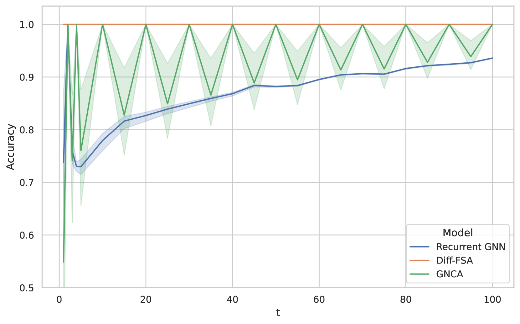Visual Description \n ## Line Chart: Accuracy vs. Time (t) ### Overview This image presents a line chart comparing the accuracy of three different models – Recurrent GNN, Diff-FSA, and GNCA – over time, represented by the variable 't'. The chart displays how the accuracy of each model evolves from t=0 to t=100. A shaded region surrounds the GNCA line, indicating a measure of variance or confidence interval. ### Components/Axes * **X-axis:** Labeled "t", representing time. The scale ranges from approximately 0 to 100. * **Y-axis:** Labeled "Accuracy", representing the accuracy score. The scale ranges from approximately 0.5 to 1.0. * **Legend:** Located in the top-right corner, identifying the three models: * Recurrent GNN (Blue line) * Diff-FSA (Orange line) * GNCA (Green line) with a shaded light green region. ### Detailed Analysis The chart shows three distinct accuracy curves. * **Recurrent GNN (Blue):** The line starts at approximately 0.73 at t=0, gradually increases, and appears to plateau around 0.92 between t=60 and t=100. The trend is generally upward, with a decreasing rate of increase over time. * t=0: ~0.73 * t=10: ~0.78 * t=20: ~0.82 * t=30: ~0.86 * t=40: ~0.88 * t=50: ~0.90 * t=60: ~0.91 * t=70: ~0.92 * t=80: ~0.92 * t=100: ~0.92 * **Diff-FSA (Orange):** The line begins at approximately 0.75 at t=0, quickly rises to approximately 0.98 around t=5, and then remains relatively stable, fluctuating slightly between approximately 0.97 and 1.0 for the remainder of the time period. * t=0: ~0.75 * t=5: ~0.98 * t=10: ~0.99 * t=20: ~0.98 * t=30: ~0.98 * t=40: ~0.98 * t=50: ~0.98 * t=60: ~0.98 * t=70: ~0.98 * t=80: ~0.98 * t=100: ~0.98 * **GNCA (Green):** The line starts at approximately 0.98 at t=0, exhibits significant oscillations throughout the time period, fluctuating between approximately 0.9 and 1.0. The shaded region indicates a substantial variance around this line. * t=0: ~0.98 * t=5: ~0.95 * t=10: ~1.0 * t=15: ~0.96 * t=20: ~0.92 * t=25: ~1.0 * t=30: ~0.94 * t=35: ~0.98 * t=40: ~0.92 * t=45: ~1.0 * t=50: ~0.95 * t=55: ~0.98 * t=60: ~0.93 * t=65: ~1.0 * t=70: ~0.96 * t=75: ~0.98 * t=80: ~0.94 * t=85: ~0.98 * t=90: ~0.96 * t=95: ~0.98 * t=100: ~0.97 ### Key Observations * Diff-FSA achieves the highest accuracy and maintains it consistently throughout the observed time period. * GNCA exhibits the highest variability in accuracy, with significant fluctuations. * Recurrent GNN shows a steady increase in accuracy, but ultimately reaches a lower plateau compared to Diff-FSA. * The initial accuracy of all three models is relatively similar, around 0.73-0.75. ### Interpretation The data suggests that Diff-FSA is the most robust and accurate model for the given task, consistently achieving high accuracy levels. GNCA, while starting with high accuracy, is prone to significant performance fluctuations, indicating potential instability or sensitivity to the input data. Recurrent GNN demonstrates a learning curve, improving its accuracy over time, but ultimately falls short of the performance of Diff-FSA. The shaded region around the GNCA line suggests that the model's performance is highly variable, and the reported accuracy may not be representative of all instances. The consistent high accuracy of Diff-FSA could be due to its architecture or training process, making it less susceptible to variations in the input data. The increasing accuracy of Recurrent GNN suggests that it benefits from continued exposure to data, but may require more time or data to reach optimal performance. </details> Figure 8: Mean accuracies for Game of Life on a regular grid when learned with 2 steps and applied for $t$ steps during inference (for 10 seeds each). All models report high accuracy for the training setup. However, performance deteriorates during inference when more steps are executed except for Diff-FSA. 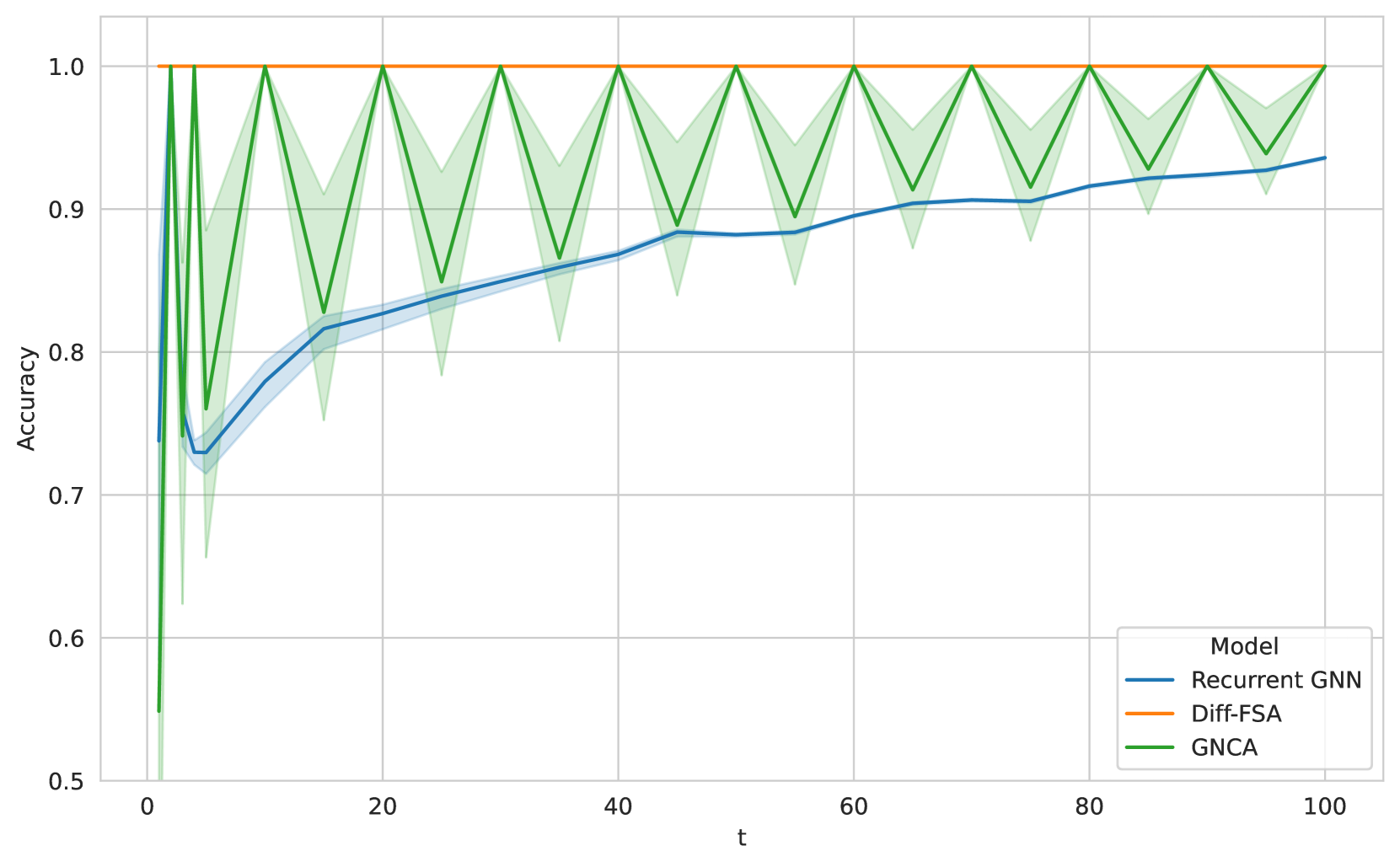<details> <summary>x10.png Details</summary>  ### Visual Description \n ## Line Chart: Model Accuracy Over Time ### Overview This line chart depicts the accuracy of three different models (Recurrent GNN, Diff-FSA, and GNCA) over time, represented by the variable 't'. The chart shows how the accuracy of each model changes as 't' increases from 0 to 100. A shaded region around each line indicates the variance or confidence interval of the accuracy measurements. ### Components/Axes * **X-axis:** Labeled "t", representing time or iterations. The scale ranges from approximately 0 to 100. * **Y-axis:** Labeled "Accuracy", representing the accuracy score. The scale ranges from approximately 0.5 to 1.0. * **Legend:** Located in the top-right corner, identifying the three models: * "Recurrent GNN" (Blue line) * "Diff-FSA" (Orange line) * "GNCA" (Green line) * **Data Series:** Three lines representing the accuracy of each model over time. Each line has a shaded region around it, indicating the variance. ### Detailed Analysis * **GNCA (Green Line):** Starts at approximately 0.5 at t=0, rapidly increases to 1.0 by t=5, and then oscillates between approximately 0.95 and 1.0 for the remainder of the chart. The shaded region around the line is relatively small, indicating low variance. * **Diff-FSA (Orange Line):** Starts at approximately 0.75 at t=0, increases steadily to approximately 0.85 by t=20, and then oscillates between approximately 0.8 and 0.95 for the remainder of the chart. The shaded region is larger than GNCA's, indicating higher variance. * **Recurrent GNN (Blue Line):** Starts at approximately 0.7 at t=0, increases steadily to approximately 0.88 by t=60, and then plateaus around 0.9. The shaded region is the largest of the three, indicating the highest variance. Here's a more detailed breakdown of approximate data points: | t | Recurrent GNN (Accuracy) | Diff-FSA (Accuracy) | GNCA (Accuracy) | | :---- | :----------------------- | :------------------ | :-------------- | | 0 | 0.7 | 0.75 | 0.5 | | 10 | 0.78 | 0.85 | 1.0 | | 20 | 0.83 | 0.85 | 1.0 | | 30 | 0.85 | 0.90 | 0.95 | | 40 | 0.86 | 0.90 | 1.0 | | 50 | 0.87 | 0.92 | 0.95 | | 60 | 0.88 | 0.92 | 1.0 | | 70 | 0.88 | 0.93 | 0.98 | | 80 | 0.89 | 0.94 | 1.0 | | 90 | 0.89 | 0.95 | 0.97 | | 100 | 0.9 | 0.95 | 0.95 | ### Key Observations * GNCA consistently exhibits the highest accuracy, remaining close to 1.0 for most of the time period. * Diff-FSA shows a moderate increase in accuracy, but with more variance than GNCA. * Recurrent GNN has the slowest increase in accuracy and the highest variance. * All three models demonstrate some level of oscillation in accuracy, particularly after the initial learning phase. ### Interpretation The chart suggests that GNCA is the most effective model for this task, achieving and maintaining high accuracy over time. Diff-FSA performs reasonably well, but with more fluctuations in accuracy. Recurrent GNN, while improving over time, lags behind the other two models in terms of both accuracy and stability. The oscillations observed in all models could indicate sensitivity to the data or the presence of noise. The shaded regions around each line highlight the uncertainty associated with each model's performance. The initial dip in accuracy for Recurrent GNN and the rapid increase for GNCA could represent the learning phase of each model, where they are adapting to the data. The consistent high accuracy of GNCA suggests it has effectively learned the underlying patterns in the data. </details> Figure 9: Mean accuracies for Game of Life on a hexagonal grid when learned with 2 steps and applied for $t$ steps during inference (for 10 seeds each). All models report high accuracy for the training setup. However, performance deteriorates during inference when more steps are executed except for Diff-FSA. Game of Life results. Specifically, we use a state space of two for Game of Life and a bounding parameter of five. We let all models execute 2 steps in order to learn the appropriate transition rules after two iterations for Game of Life. Further, we investigate the generalization capabilities and especially the iteration stability of the learned models. For this, we consider all models which achieve perfect training accuracy and let them run on larger 10 node paths for more timesteps t than during training. The results are depicted in Figure 8 for the regular Game of Life and in Figure 9 for the hexagonal variant. Note, that the recurrent GNN deteriorates outside the training distribution. Similarly, the GNCA baseline struggles to generalize as it has not learned the correct intermediate transitions for odd number of rules. The Diff-FSA on the other hand exhibits good iteration stability across the whole range of iterations. ### B.3 Dataset generator We perform further evaluations on more datasets generated by our dataset generator GRAB. The groudturth automaton consists of 4 states and we test multiple Diff-FSAwith 4, 5, and 6 states as well as the baselines over 10 runs. We report the achieved accuracies for the different experiments in Table 5. Table 5: Evaluation of GraphFSA on synthetic data provided by GRAB. We report the accuracy and standard deviation over 10 runs. The underlying ground truth consists of an FSA using 4 states. We can test the in-distribution validation accuracy to see how well a model can fit the data. Moreover, we test extrapolation to larger graphs to verify that the rules for underlying automata were successfully learned. Our Diff-FSA models generally perform well across all scenarios. Note that the recurrent GNN performs well but lacks the interpretation and visualization of the learned mechanics as discrete state automata. | Model | Val Acc | n=10 | n=20 | n=50 | n=100 | | --- | --- | --- | --- | --- | --- | | Experiment 1 | | | | | | | GNCA | 0.38 $\pm$ 0.00 | 0.39 $\pm$ 0.00 | 0.40 $\pm$ 0.00 | 0.40 $\pm$ 0.00 | 0.39 $\pm$ 0.00 | | Recurrent GNN | 1.00 $\pm$ 0.00 | 0.91 $\pm$ 0.10 | 0.85 $\pm$ 0.13 | 0.82 $\pm$ 0.16 | 0.81 $\pm$ 0.16 | | Diff-FSA (4 states) | 0.99 $\pm$ 0.02 | 0.97 $\pm$ 0.02 | 0.96 $\pm$ 0.02 | 0.95 $\pm$ 0.03 | 0.94 $\pm$ 0.03 | | Diff-FSA (5 states) | 1.00 $\pm$ 0.01 | 0.98 $\pm$ 0.01 | 0.96 $\pm$ 0.02 | 0.95 $\pm$ 0.02 | 0.95 $\pm$ 0.02 | | Diff-FSA (6 states) | 0.99 $\pm$ 0.01 | 0.98 $\pm$ 0.01 | 0.95 $\pm$ 0.02 | 0.94 $\pm$ 0.02 | 0.94 $\pm$ 0.02 | | Experiment 2 | | | | | | | GNCA | 0.66 $\pm$ 0.00 | 0.67 $\pm$ 0.00 | 0.66 $\pm$ 0.00 | 0.65 $\pm$ 0.00 | 0.65 $\pm$ 0.00 | | Recurrent GNN | 1.00 $\pm$ 0.00 | 0.84 $\pm$ 0.02 | 0.82 $\pm$ 0.02 | 0.81 $\pm$ 0.02 | 0.80 $\pm$ 0.02 | | Diff-FSA (4 states) | 1.00 $\pm$ 0.00 | 0.94 $\pm$ 0.01 | 0.93 $\pm$ 0.02 | 0.92 $\pm$ 0.02 | 0.91 $\pm$ 0.02 | | Diff-FSA (5 states) | 1.00 $\pm$ 0.00 | 0.93 $\pm$ 0.02 | 0.92 $\pm$ 0.02 | 0.91 $\pm$ 0.02 | 0.90 $\pm$ 0.02 | | Diff-FSA (6 states) | 1.00 $\pm$ 0.00 | 0.94 $\pm$ 0.02 | 0.93 $\pm$ 0.02 | 0.92 $\pm$ 0.02 | 0.91 $\pm$ 0.02 | | Experiment 3 | | | | | | | GNCA | 0.92 $\pm$ 0.00 | 0.95 $\pm$ 0.00 | 0.93 $\pm$ 0.00 | 0.93 $\pm$ 0.00 | 0.93 $\pm$ 0.00 | | Recurrent GNN | 0.98 $\pm$ 0.03 | 0.98 $\pm$ 0.02 | 0.96 $\pm$ 0.03 | 0.95 $\pm$ 0.03 | 0.95 $\pm$ 0.03 | | Diff-FSA (4 states) | 0.92 $\pm$ 0.00 | 0.95 $\pm$ 0.00 | 0.93 $\pm$ 0.00 | 0.93 $\pm$ 0.00 | 0.93 $\pm$ 0.00 | | Diff-FSA (5 states) | 0.91 $\pm$ 0.02 | 0.94 $\pm$ 0.03 | 0.92 $\pm$ 0.01 | 0.93 $\pm$ 0.01 | 0.93 $\pm$ 0.01 | | Diff-FSA (6 states) | 0.91 $\pm$ 0.02 | 0.94 $\pm$ 0.03 | 0.92 $\pm$ 0.01 | 0.93 $\pm$ 0.01 | 0.93 $\pm$ 0.01 | | Experiment 4 | | | | | | | GNCA | 0.56 $\pm$ 0.00 | 0.64 $\pm$ 0.00 | 0.63 $\pm$ 0.00 | 0.64 $\pm$ 0.00 | 0.63 $\pm$ 0.00 | | Recurrent GNN | 1.00 $\pm$ 0.00 | 0.98 $\pm$ 0.05 | 0.97 $\pm$ 0.05 | 0.97 $\pm$ 0.05 | 0.97 $\pm$ 0.05 | | Diff-FSA (4 states) | 1.00 $\pm$ 0.00 | 1.00 $\pm$ 0.00 | 1.00 $\pm$ 0.00 | 1.00 $\pm$ 0.00 | 1.00 $\pm$ 0.00 | | Diff-FSA (5 states) | 1.00 $\pm$ 0.00 | 1.00 $\pm$ 0.00 | 1.00 $\pm$ 0.00 | 1.00 $\pm$ 0.00 | 1.00 $\pm$ 0.00 | | Diff-FSA (6 states) | 1.00 $\pm$ 0.00 | 1.00 $\pm$ 0.00 | 1.00 $\pm$ 0.00 | 1.00 $\pm$ 0.00 | 1.00 $\pm$ 0.00 | | Experiment 5 | | | | | | | GNCA | 0.54 $\pm$ 0.00 | 0.54 $\pm$ 0.00 | 0.55 $\pm$ 0.00 | 0.54 $\pm$ 0.00 | 0.55 $\pm$ 0.00 | | Recurrent GNN | 1.00 $\pm$ 0.00 | 0.97 $\pm$ 0.03 | 0.94 $\pm$ 0.03 | 0.93 $\pm$ 0.03 | 0.93 $\pm$ 0.04 | | Diff-FSA (4 states) | 0.98 $\pm$ 0.00 | 0.96 $\pm$ 0.00 | 0.95 $\pm$ 0.00 | 0.93 $\pm$ 0.00 | 0.93 $\pm$ 0.00 | | Diff-FSA (5 states) | 0.98 $\pm$ 0.00 | 0.97 $\pm$ 0.00 | 0.95 $\pm$ 0.00 | 0.94 $\pm$ 0.00 | 0.94 $\pm$ 0.00 | | Diff-FSA (6 states) | 0.98 $\pm$ 0.00 | 0.96 $\pm$ 0.01 | 0.95 $\pm$ 0.01 | 0.94 $\pm$ 0.01 | 0.94 $\pm$ 0.00 | ### B.4 Algorithms We evaluate the GraphFSA framework and in particular our Diff-FSAand the baselines on more challenging algorithmic datasets. We evaluate on the four datasets Distance, PrefixSum, PathFinding and RootValue. The report the results in the tables: 6, 8 and 7. Table 6: Evaluation of learning graph algorithms on the RootValue dataset. We report the accuracy and standard deviation over 10 runs. All models are trained on graphs of size at most 10 and then tested for extrapolation on larger graph sizes $n$ . | GNCA | 0.50 $\pm$ 0.00 | 0.50 $\pm$ 0.00 | 0.50 $\pm$ 0.00 | 0.50 $\pm$ 0.00 | | --- | --- | --- | --- | --- | | Recurrent GNN | 1.00 $\pm$ 0.00 | 1.00 $\pm$ 0.00 | 0.92 $\pm$ 0.16 | 0.91 $\pm$ 0.16 | | Diff-FSA | 1.00 $\pm$ 0.02 | 0.99 $\pm$ 0.02 | 0.99 $\pm$ 0.03 | 0.99 $\pm$ 0.04 | Table 7: Evaluation of learning graph algorithms on the PathFinding dataset. We report the accuracy and standard deviation over 10 runs. All models are trained on graphs of size at most 10 and then tested for extrapolation on larger graph sizes $n$ . | GNCA | 0.58 $\pm$ 0.00 | 0.73 $\pm$ 0.00 | 0.83 $\pm$ 0.00 | 0.89 $\pm$ 0.00 | | --- | --- | --- | --- | --- | | Recurrent GNN | 0.97 $\pm$ 0.02 | 0.90 $\pm$ 0.03 | 0.88 $\pm$ 0.04 | 0.89 $\pm$ 0.09 | | Diff-FSA | 0.85 $\pm$ 0.00 | 0.85 $\pm$ 0.00 | 0.87 $\pm$ 0.00 | 0.91 $\pm$ 0.00 | Table 8: Evaluation of learning graph algorithms on the PrefixSum dataset. We report the accuracy and standard deviation over 10 runs. All models are trained on graphs of size at most 10 and then tested for extrapolation on larger graph sizes $n$ . | GNCA | 0.49 $\pm$ 0.00 | 0.50 $\pm$ 0.00 | 0.50 $\pm$ 0.00 | 0.50 $\pm$ 0.00 | | --- | --- | --- | --- | --- | | Recurrent GNN | 0.97 $\pm$ 0.04 | 0.95 $\pm$ 0.06 | 0.90 $\pm$ 0.13 | 0.84 $\pm$ 0.14 | | Diff-FSA | 0.74 $\pm$ 0.14 | 0.67 $\pm$ 0.17 | 0.63 $\pm$ 0.20 | 0.61 $\pm$ 0.20 |