# Towards Probabilistic Inductive Logic Programming with Neurosymbolic Inference and Relaxation
**Authors**: F. Hillerström and G.J. Burghouts
> TNO, The Netherlands
refs.bib
Hillerström and Burghouts
116 2024 10.1017/xxxxx
## Abstract
Many inductive logic programming (ILP) methods are incapable of learning programs from probabilistic background knowledge, e.g. coming from sensory data or neural networks with probabilities. We propose Propper, which handles flawed and probabilistic background knowledge by extending ILP with a combination of neurosymbolic inference, a continuous criterion for hypothesis selection (BCE) and a relaxation of the hypothesis constrainer (NoisyCombo). For relational patterns in noisy images, Propper can learn programs from as few as 8 examples. It outperforms binary ILP and statistical models such as a Graph Neural Network.
keywords: Inductive Logic Programming, Neurosymbolic inference, Probabilistic background knowledge, Relational patterns, Sensory data.
## 1 Introduction
Inductive logic programming (ILP) muggleton1995inverse learns a logic program from labeled examples and background knowledge (e.g. relations between entities). Due to the strong inductive bias imposed by the background knowledge, ILP methods can generalize from small numbers of examples cropper2022inductive. Other advantages are the ability to learn complex relations between the entities, the expressiveness of first-order logic, and the resulting program can be understood and transferred easily because it is in symbolic form cropper2022_30newintro. This makes ILP an attractive alternative methodology besides statistical learning methods.
For many real-world applications, dealing with noise is essential. Mislabeled samples are one source of noise. To learn from noisy labels, various ILP methods have been proposed to generalize a subset of the samples srinivasan2001aleph,ahlgren2013efficient,zeng2014quickfoil,raedt2015inducing. To advance methods to learn recursive programs and invent new predicates, Combo cropper2023learning was proposed, a method that searches for small programs that generalize subsets of the samples and combines them. MaxSynth hocquette2024learning extends Combo to allow for mislabeled samples, while trading off program complexity for training accuracy. These methods are dealing with noisy labels, but do not explicitly take into account errors in the background knowledge, nor are they designed to deal with probabilistic background knowledge.
Most ILP methods take as a starting point the inputs in symbolic declarative form cropper2021turning. Real-world data often does not come in such a form. A predicate $p(.)$ , detected in real-world data, is neither binary or perfect. The assessment of the predicate can be uncertain, resulting in a non-binary, probabilistic predicate. Or the assessment can be wrong, leading to imperfect predicates. Dealing with noisy and probabilistic background knowledge is relevant for learning from sources that exhibit uncertainties. A probabilistic source can be a human who needs to make judgements at an indicated level of confidence. A source can also be a sensor measurement with some confidence. For example, an image is described by the objects that are detected in it, by a deep learning model. Such a model predicts locations in the image where objects may be, at some level of confidence. Some objects are detected with a lower confidence than others, e.g. if the object is partially observable or lacks distinctive visual features. The deep learning model implements a probabilistic predicate that a particular image region may contain a particular object, e.g. 0.7 :: vehicle(x). Given that most object detection models are imperfect in practice, it is impossible to determine a threshold that distinguishes the correct and incorrect detections.
Two common ILP frameworks, Aleph srinivasan2001aleph and Popper learning_from_failures, typically fail to find the correct programs when dealing with predicted objects in images helff2023v; even with a state-of-the-art object detection model, and after advanced preprocessing of said detections. In the absence of an ideal binarization of probabilities, most ILP methods are not applicable to probabilistic sources cropper2021turning.
<details>
<summary>x1.png Details</summary>
### Visual Description
## Neurosymbolic Inference Diagram: Probabilistic Logic Cycle with Visual Examples
### Overview
This image is a technical diagram illustrating a neurosymbolic inference system that combines machine learning with logical reasoning. It depicts a cyclic process for generating and testing logical hypotheses against probabilistic visual data. The diagram is divided into two primary sections: a conceptual cycle on the left and a detailed panel on the right showing concrete examples of the inference process applied to aerial imagery.
### Components/Axes
The diagram contains no traditional chart axes. Its components are:
**Left Section - The Inference Cycle:**
* **Three Core Nodes:** "Generate", "Test", "Constrain" arranged in a clockwise cycle.
* **Connecting Arrows & Labels:**
* From "Generate" to "Test": Arrow labeled "logic program" with sub-label `is_on(vehicle, bridge)`.
* From "Test" to "Constrain": Arrow labeled "failure".
* From "Constrain" to "Generate": Arrow labeled "learned constraints".
* **Contributions (in blue italics):**
* `contribution #1`: Associated with "Neurosymbolic inference on Probabilistic background knowledge".
* `contribution #2`: Associated with "a continuous criterion for hypothesis selection (BCE)".
* `contribution #3`: Associated with "relaxation of the hypothesis constrainer (NoisyCombo)".
* **Additional Text:** "Predicates", "Constraints" at the top.
**Right Section - Example Panel:**
* **Title:** "Neurosymbolic inference on Probabilistic background knowledge"
* **Sub-sections:**
* **"Examples"**: Contains two green boxes listing probabilistic logical statements.
* **"positives"**: Shows two aerial images with yellow bounding boxes and labels.
* **"negatives"**: Shows two aerial images with yellow bounding boxes and labels.
* **Visual Connectors:** Yellow arrows link the logical statements in the "Examples" boxes to specific bounding boxes in the "positives" and "negatives" images.
### Detailed Analysis
**1. The Inference Cycle (Left Side):**
The process is iterative:
1. **Generate:** Creates a logic program (e.g., `is_on(vehicle, bridge)`) based on predicates, constraints, and learned constraints from previous cycles.
2. **Test:** Evaluates the logic program against data. Two example outcomes are shown in colored boxes:
* Green box: `0.21 :: is_on(vehicle, bridge)`
* Red box: `0.00 :: is_on(vehicle, bridge)`
The "failure" path is taken when the test yields a low probability (like 0.00).
3. **Constrain:** Uses the failure to relax or adjust the hypothesis constrainer (via "NoisyCombo", contribution #3), feeding back into the "Generate" step.
**2. Probabilistic Examples (Right Side - "Examples" box):**
* **Top Green Box (Positive Example):**
* `0.33 :: vehicle(A)`
* `0.68 :: bridge(B)`
* `0.92 :: is_close(A,B)`
* `0.95 :: is_on(A,B)`
* **Bottom Red Box (Negative Example):**
* `0.31 :: vehicle(A)`
* `0.42 :: bridge(B)`
* `0.29 :: is_close(A,B)`
* `0.00 :: is_on(A,B)`
**3. Visual Data with Bounding Boxes (Right Side - "positives"/"negatives"):**
Each image contains multiple detected objects with confidence scores. The yellow arrows map the logical variables `A` and `B` from the examples to specific visual detections.
* **Top-Left Positive Image:**
* `vehicle: 54.8%` (arrow from `vehicle(A)`)
* `bridge: 68.4%` (arrow from `bridge(B)`)
* `vehicle: 33.3%`
* **Top-Right Positive Image:**
* `bridge: 77.1%` (arrow from `bridge(B)`)
* `vehicle: 55.5%` (arrow from `vehicle(A)`)
* `vehicle: 50.4%`
* `vehicle: 64.2%`
* `vehicle: 18.5%`
* `vehicle: 85.1%`
* **Bottom-Left Negative Image:**
* `vehicle: 33.0%` (arrow from `vehicle(A)`)
* `bridge: 42.2%` (arrow from `bridge(B)`)
* **Bottom-Right Negative Image:**
* `vehicle: 48.4%` (arrow from `vehicle(A)`)
* `bridge: 79.1%` (arrow from `bridge(B)`)
* `vehicle: 56.2%`
* `vehicle: 66.8%`
* `vehicle: 57.0%`
* `vehicle: 39.3%`
* `vehicle: 43.5%`
### Key Observations
1. **Probabilistic Logic:** The system does not use binary true/false but assigns probabilities (0.00 to 0.95) to logical statements, reflecting uncertainty in perception and reasoning.
2. **Positive vs. Negative Correlation:** In the "positives" examples, the `is_on(A,B)` statement has high probability (0.95), correlating with visual detections where a vehicle and bridge are spatially related. In the "negatives" example, `is_on(A,B)` has 0.00 probability, even though a vehicle and bridge are detected (with lower confidence: 31% and 42%).
3. **Spatial Grounding:** The yellow arrows explicitly ground abstract logical variables (`A`, `B`) to concrete pixel regions in the images, demonstrating the neurosymbolic link.
4. **Cycle Logic:** The "failure" path from "Test" to "Constrain" is triggered by low-probability outcomes (like the 0.00 result), which then informs the generation of new constraints to improve future hypotheses.
### Interpretation
This diagram presents a framework for **robust visual reasoning under uncertainty**. It addresses a core challenge in AI: combining the pattern recognition strength of neural networks (which output probabilistic detections like `vehicle: 54.8%`) with the structured reasoning of symbolic logic (which can express relationships like `is_on`).
* **How it Works:** The system generates a logical hypothesis (e.g., "there is a vehicle on a bridge"). It tests this hypothesis by checking if the underlying visual detections (vehicle, bridge) and their spatial relationship (`is_close`) are supported by the neural network's output with sufficient confidence. If the combined probability is too low (a "failure"), the system learns to adjust its constraining rules, making future hypotheses more plausible or better aligned with the data.
* **Significance:** The "positives" and "negatives" show that the system isn't just checking for the presence of objects, but for a specific, complex relationship between them. The negative case is crucial—it shows a scenario where objects are detected but the critical relationship is not supported, leading to a logical rejection (`0.00 :: is_on`).
* **Contributions:** The three labeled contributions highlight the novel components: 1) The core neurosymbolic inference method itself, 2) A continuous (non-binary) criterion (BCE - likely Binary Cross-Entropy) for selecting the best hypothesis, and 3) A specific technique ("NoisyCombo") for relaxing logical constraints when faced with failure, enabling learning and adaptation.
In essence, the diagram illustrates a closed-loop system where visual perception informs logical reasoning, and logical failures guide the improvement of the reasoning process, all while quantitatively handling the inherent uncertainty of real-world data.
</details>
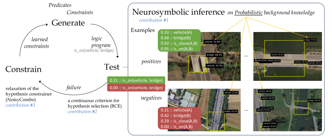
Figure 1: Our method Propper extends the ILP method Popper that learns from failures (left) with neurosymbolic inference to test logical programs on probabilistic background knowledge, e.g. objects detected in images with a certain probability (right).
We propose a method towards probabilistic ILP. At a high level, ILP methods typically induce a logical program that entails many positive and few negative samples, by searching the hypothesis space, and subsequently testing how well the current hypothesis fits the training samples cropper2022_30newintro. One such method is Popper, which learns from failures (LFF) learning_from_failures, in an iterative cycle of generating hypotheses, testing them and constraining the hypothesis search. Our proposal is to introduce a probabilistic extension to LFF at the level of hypothesis testing. For that purpose, we consider neurosymbolic AI hybrid_ai. Within neurosymbolic AI a neural network predicts the probability for a predicate. For example a neural network for object detection, which outputs a probability for a particular object being present in an image region, e.g., 0.7 :: vehicle(x). Neurosymbolic AI connects this neural network with knowledge represented in a symbolic form, to perform reasoning over the probabilistic predicates predicted by the neural network. With this combination of a neural network and symbolic reasoning, neurosymbolic AI can reason over unstructured inputs, such as images. We leverage neurosymbolic programming and connect it to the tester within the hypothesis search. One strength of neurosymbolic programming is that it can deal with uncertainty and imperfect information hybrid_ai,neuro_symbolic,scallop,scallop_foundationmodels, in our case the probablistic background knowledge.
We propose to use neurosymbolic inference as tester in the test-phase of the LFF cycle. Neurosymbolic reasoning calculates an output probability for a logical query being true, for every input sample. The input samples are the set of positive and negative examples, together with their probabilistic background knowledge. The logical query evaluated within the neurosymbolic reasoning is the hypothesis generated in the generate-phase of the LFF cycle, which is a first-order-logic program. With the predicted probability of the hypothesis being true per sample, it becomes possible to compute how well the hypothesis fits the training samples. That is used to continue the LFF cycle and generate new constraints based on the failures.
Our contribution is a step towards probabilistic ILP by proposing a method called Propper. It builds on an ILP framework that is already equipped to deal with noisy labels, Popper-MaxSynth learning_from_failures,hocquette2024learning, which we extend with neurosymbolic inference which is able to process probabilistic facts, i.e. uncertain and imperfect background knowledge. Our additional contributions are a continuous criterion for hypothesis selection, that can deal with probabilities, and a relaxed formulation for constraining the hypothesis space. Propper and the three contributions are outlined in Figure 1. We compare Popper and Propper with statistical ML models (SVM and Graph Neural Network) for the real-life task of finding relational patterns in satellite images based on objects predicted by an imperfect deep learning model. We validate the learning robustness and efficiency of the various models. We analyze the learned logical programs and discuss the cases which are hard to predict.
## 2 Related Work
For the interpretation of images based on imperfect object predictions, ILP methods such as Aleph srinivasan2001aleph and Popper learning_from_failures proved to be vulnerable and lead to incorrect programs or not returning a program at all helff2023v. Solutions to handle observational noise were proposed cropper2021beyondentailment for small binary images. With LogVis muggleton2018meta images are analyzed via physical properties. This method could estimate the direction of the light source or the position of a ball from images in very specific conditions or without clutter or distractors. $Meta_{Abd}$ dai2020abductive jointly learns a neural network with induction of recursive first-order logic theories with predicate invention. This was demonstrated on small binary images of digits. Real-life images are more complex and cluttered. We aim to extend these works to realistic samples, e.g. large color images that contain many objects under partial visiblity and in the midst of clutter, causing uncertainties. Contrary to $Meta_{Abd}$ , we take pretrained models as a starting point, as they are often already very good at their task of analyzing images. Our focus is on extending ILP to handle probabilistic background knowledge.
In statistical relational artificial intelligence (StarAI) raedt2016statistical the rationale is to directly integrate probabilities into logical models. StarAI addresses a different learning task than ILP: it learns the probabilistic parameters of a given program, whereas ILP learns the program cropper2021turning. Probabilities have been integrated into ILP previously. Aleph srinivasan2001aleph was used to find interesting clauses and then learn the corresponding weights huynh2008discriminative. ProbFOIL raedt2015inducing and SLIPCOVER bellodi2015structure search for programs with probabilities associated to the clauses, to deal with the probabilistic nature of the background knowledge. SLIPCOVER searches the space of probabilistic clauses using beam search. The clauses come from Progol muggleton1995inverse. Theories are searched using greedy search, where refinement is achieved by adding a clauses for a target predicate. As guidance the log likelihood of the data is considered. SLIPCOVER operates in a probabilistic manner on binary background knowledge, where our goal is to involve the probabilities associated explicitly the background knowledge.
How to combine these probabilistic methods with recent ILP frameworks is unclear. In our view, it is not trivial and possibly incompatible. Our work focuses on integrating a probabilistic method into a modern ILP framework, in a simple yet elegant manner. We replace the binary hypothesis tester of Popper learning_from_failures by a neurosymbolic program that can operate on probabilistic and imperfect background knowledge hybrid_ai,neuro_symbolic. Rather than advanced learning of both the knowledge and the program, e.g. NS-CL mao2019neuro, we take the current program as the starting point. Instead of learning parameters, e.g. Scallop scallop, we use the neurosymbolic program for inference given the program and probabilistic background knowledge. Real-life samples may convey large amounts of background knowledge, e.g. images with many objects and relations between them. Therefore, scalability is essential. Scallop scallop improved the scalability over earlier neurosymbolic frameworks such as DeepProbLog deepproblog,deepproblog_efficient. Scallop introduced a tunable parameter $k$ to restrain the validation of hypotheses by analyzing the top- $k$ proofs. They asymptotically reduced the computational cost while providing relative accuracy guarantees. This is beneficial for our purpose. By replacing only the hypothesis tester, the strengths of ILP (i.e. hypothesis search) are combined with the strengths of neurosymbolic inference (i.e. probabilistic hypothesis testing).
## 3 Propper Algorithm
To allow ILP on flawed and probabilistic background knowledge, we extend modern ILP (Section 3.1) with neurosymbolic inference (3.2) and coin our method Propper. The neurosymbolic inference requires program conversion by grammar functions (3.3), and we added a continuous criterion for hypothesis selection (3.4), and a relaxation of the hypothesis constrainer (3.5).
### 3.1 ILP: Popper
Popper represents the hypothesis space as a constraint satisfaction problem and generates constraints based on the performance of earlier tested hypotheses. It works by learning from failures (LFF) learning_from_failures. Given background knowledge $B$ , represented as a logic program, positive examples $E^{+}$ and negative examples $E^{-}$ , it searches for a hypothesis $H$ that is complete ( $\forall e\in E^{+},H\cup B\models e$ ) and consistent ( $\forall e\in E^{-},H\cup B\not\models e$ ). The algorithm consists of three main stages (see Figure 1, left). First a hypothesis in the form of a logical program is generated, given the known predicates and constraints on the hypothesis space. The Test stage tests the generated logical program against the provided background knowledge and examples, using Prolog for inference. It evaluates whether the examples are entailed by the logical program and background knowledge. From this information, failures that are made when applying the current hypothesis, can be identified. These failures are used to constrain the hypothesis space, by removing specializations or generalizations from the hypothesis space. In the original Popper implementation learning_from_failures, this cycle is repeated until an optimal solution is found; the smallest program that covers all positives and no negative examples See learning_from_failures for a formal definition.. Its extension Combo combines small programs that do not entail any negative example cropper2023learning. When no optimal solution is found, Combo returns the obtained best solution. The Popper variant MaxSynth does allow noise in the examples and generates constraints based on a minimum description length cost function, by comparing the length of a hypothesis with the possible gain in wrongly classified examples hocquette2024learning.
### 3.2 Neurosymbolic Inference: Scallop
Scallop is a language for neurosymbolic programming which integrates deep learning with logical reasoning scallop. Scallop reasons over continuous, probabilistic inputs and results in a probabilistic output confidence. It consists of two parts: a neural model that outputs the confidence for a specific concept occurring in the data and a reasoning model that evaluates the probability for the query of interest being true, given the input. It uses provenance frameworks kimmig2017algebraic to approximate exact probabilistic inference, where the AND operator is evaluated as a multiplication ( $AND(x,y)=x*y$ ), the OR as a minimization ( $OR(x,y)=min(1,x+y)$ ) and the NOT as a $1-x$ . Other, more advanced formulations are possible, e.g. $noisy$ - $OR(x,y)=1-(1-a)(1-b)$ for enhanced performance. For ease of integration, we considered this basic provenance. To improve the speed of the inference, only the most likely top-k hypotheses are processed, during the intermediate steps of computing the probabilities for the set of hypotheses.
### 3.3 Connecting ILP and Neurosymbolic Inference
Propper changes the Test stage of the Popper algorithm (see Figure 1): the binary Prolog reasoner is replaced by the neurosymbolic inference using Scallop, operating on probabilistic background knowledge (instead of binary), yielding a probability for each sample given the logical program. The background knowledge is extended with a probability value before each first-order-logic statement, e.g. 0.7 :: vehicle(x).
The Generate step yields a logic program in Prolog syntax. The program can cover multiple clauses, that can be understood as OR as one needs to be satisfied. Each clause is a function of predicates, with input arguments. The predicate arguments can differ between the clauses within the logic program. This is different from Scallop, where every clause in the logic program is assumed to be a function of the same set of arguments. As a consequence, the Prolog program requires syntax rewriting to arrive at an equivalent Scallop program. This rewriting involves three steps by consecutive grammar functions, which we illustrate with an example. Take the Prolog program:
$$
\displaystyle\begin{split}\texttt{f(A)}={}&\texttt{has\_object(A, B), vehicle(
B)}\\
\texttt{f(A)}={}&\texttt{has\_object(A, B), bridge(C), is\_on(B, C)}\end{split} \tag{1}
$$
The bodies of f(A) are extracted by: $b(\texttt{f})$ = {[has_object(A, B), vehicle(B)], [has_object(A, B), bridge(C), is_on(B, C)]}. The sets of arguments of f(A) are extracted by: $v(\texttt{f})=\{\{\texttt{A, B}\},\{\texttt{C, A, B}\}\}$ .
For a Scallop program, the clauses in the logic program need to be functions of the same argument set. Currently the sets are not the same: {A, B} vs. {C, A, B}. Function $e(\cdot)$ adds a dummy predicate for all non-used arguments, i.e. C in the first clause, such that all clauses operate on the same set, i.e. {C, A, B}:
$$
\displaystyle\begin{split}e([\texttt{has\_object(A, B)},{}&\texttt{vehicle(B)}
],\{\texttt{C, A, B}\})=\\
&\texttt{has\_object(A, B), vehicle(B), always\_true(C)}\end{split} \tag{2}
$$
After applying grammar functions $b(\cdot)$ , $v(\cdot)$ and $e(\cdot)$ , the Prolog program f(A) becomes the equivalent Scallop program g(C, A, B):
$$
\displaystyle\begin{split}\texttt{g\textsubscript{0}(C, A, B)}={}&\texttt{has
\_object(A, B), vehicle(B), always\_true(C)}\\
\texttt{g\textsubscript{1}(C, A, B)}={}&\texttt{has\_object(A, B), bridge(C),
is\_on(B, C)}\\
\texttt{g(C, A, B)}={}&\texttt{g\textsubscript{0}(C, A, B) or g\textsubscript{
1}(C, A, B)}\end{split} \tag{3}
$$
### 3.4 Selecting the Best Hypothesis
MaxSynth uses a minimum-description-length (MDL) cost hocquette2024learning to select the best solution:
$$
MDL_{B,E}=size(h)+fn_{B,E}(h)+fp_{B,E}(h) \tag{4}
$$
The MDL cost compares the number of correctly classified examples with the number of literals in the program. This makes the cost dependent on the dataset size and requires binary predictions in order to determine the number of correctly classified examples. Furthermore, it is doubtful whether the number of correctly classified examples can be compared directly with the rule size, since it makes the selection of the rule size dependent on the dataset size again.
Propper uses the Binary Cross Entropy (BCE) loss to compare the performance of hypotheses, as it is a more continuous measure than MDL. The neurosymbolic inference predicts an output confidence for an example being entailed by the hypothesis. The BCE-cost compares this predicted confidence with the groundtruth (one or zero). For $y_{i}$ being the groundtruth label and $p_{i}$ the confidence predicted via neurosymbolic inference for example $i$ , the BCE cost for $N$ examples becomes:
$$
BCE=\frac{1}{N}\sum_{i=1}^{N}(y_{i}*log(p_{i})+(1-y_{i})*log(1-p_{i})). \tag{5}
$$
Scallop reasoning automatically avoids overfitting, by punishing the size of the program, because when adding more or longer clauses the probability becomes lower by design. The more ANDs in the program, the lower the output confidence of the Scallop reasoning, due to the multiplication of the probabilities. Therefore, making a program more specific will result in a higher BCE-cost, unless the specification is beneficial to remove FPs. Making the program more generic will cover more samples (due to the addition operator for the OR). However the confidences for the negative samples will increase as well, which will increase the BCE-cost again. The BCE-cost is purely calculated on the predictions itself, and thereby removes the dependency on the dataset size and the comparison between number of samples and program length.
### 3.5 Constraining on Inferred Probabilities
Whereas Combo cropper2023learning and MaxSynth hocquette2024learning yield optimal programs given perfect background knowledge, with imperfect and probabilistic background knowledge no such guarantees can be provided. The probabilistic outputs of Scallop are converted into positives and negatives before constraining. The optimal threshold is chosen by testing 15 threshold values, evenly spaced between 0 and 1 and selecting the threshold resulting in the most highest true positives plus true negatives on the training samples.
MaxSynth generates constraints based on the MDL loss hocquette2024learning, making the constraints dependent on the size of the dataset. To avoid this dependency, we introduce the NoisyCombo constrainer. Combo generates constraints once a false positive (FP) or negative (FN) is detected. $\exists e\in E^{-},H\cup B\models e$ : prune generalisations. $\exists e\in E^{+},H\cup B\not\models e$ or $\forall e\in E^{-},H\cup B\not\models e$ : prune specialisations. NoisyCombo relaxes this condition and allows a few FPs and FNs to exist, depending on an expected noise level, inspired by LogVis muggleton2018meta. This parameter defines a percentage of the examples that could be imperfect, from which the allowed number of FPs and FNs is calculated. $\sum(e\in E^{-},H\cup B\models e)>noise\_level*N_{negatives}$ : prune generalisations. $\forall e\in E^{-},H\cup B\not\models e$ : prune specialisations. The positives are not thresholded by the noise level, since programs that cover at least one positive sample are added to the combiner.
## 4 Analyses
We validate Propper on a real-life task of finding relational patterns in satellite images, based on flawed and probabilistic background knowledge about the objects in the images, which are predicted by an imperfect deep learning model. We analyze the learning robustness under various degrees of flaws in the background knowledge. We do this for various models, including Popper (on which Propper is based) and statistical ML models. In addition, we establish the learning efficiency for very low amounts of training data, as ILP is expected to provide an advantage because it has the inductive bias of background knowledge. We analyze the learned logical programs, to compare them qualitatively against the target program. Finally, we discuss the cases that are hard to predict.
### 4.1 First Dataset
The DOTA dataset xia2018dota contains many satellite images. This dataset is very challenging, because the objects are small, and therefore visual details are lacking. Moreover, some images are very cluttered by sometimes more than 100 objects.
<details>
<summary>extracted/5868417/result_figs/pos_full.jpg Details</summary>
### Visual Description
## Annotated Aerial Image: Object Detection Results
### Overview
This is a top-down aerial or satellite photograph of a coastal or riverside area, overlaid with the results of an object detection algorithm. The image shows a body of water (dark green/brown), landmasses with vegetation, roads, buildings, and parking areas. Yellow bounding boxes with black text labels have been drawn around detected objects, indicating the object class ("vehicle" or "bridge") and the model's confidence score as a percentage.
### Components/Axes
* **Base Image:** Aerial photograph showing geographical features.
* **Annotations:** Yellow rectangular bounding boxes.
* **Labels:** Black text boxes with white text, positioned at the top-left corner of each bounding box. The format is `[class]: [confidence]%`.
* **Detected Classes:**
* `vehicle`
* `bridge`
* **Spatial Layout:** The image is divided into two primary areas:
1. **Upper Right:** A landmass with buildings, parking lots, and a road leading to a bridge.
2. **Lower Half:** A long, horizontal causeway or bridge structure spanning the water, with a road and vegetation on either side.
### Detailed Analysis
**List of All Detected Objects and Confidence Scores:**
*Upper Right Landmass & Bridge Area (from top to bottom):*
1. `vehicle: 43.9%` (Top-right corner, near edge of frame)
2. `vehicle: 51.5% ..0%` (Note: Label contains "..0%", likely an annotation error or artifact)
3. `vehicle: 39.9%` (On a building roof or parking area)
4. `vehicle: 30.3% %` (Note: Label contains an extra "%" symbol)
5. `vehicle: 41.8%` (On a road near the bridge approach)
6. `bridge: 86.4%` (Large box encompassing the bridge structure connecting to the upper landmass)
*Lower Horizontal Causeway/Bridge (from left to right):*
7. `vehicle: 37.0% e: 58.0%` (Note: Label contains "e: 58.0%", possibly an error or secondary data)
8. `vehicle: 30.1%`
9. `vehicle: 46.9%`
10. `vehicle: 50.4%`
11. `vehicle: 64.2%`
12. `vehicle: 55.5%` (Positioned above the main cluster on the road)
13. `bridge: 77.1%` (Large box encompassing the central section of the causeway over water)
14. `vehicle: 38.5%`
15. `vehicle: 49.1%`
16. `vehicle: 55.1%`
17. `vehicle: 63.2%`
18. `vehicle: 60.5%`
19. `vehicle: 75.5%`
20. `vehicle: 69.5%`
21. `vehicle: 48.7%`
22. `vehicle: 33.5%` (Far right end of the causeway)
### Key Observations
1. **Detection Distribution:** Vehicles are densely clustered along the horizontal causeway/bridge in the lower half of the image, suggesting active traffic flow. A smaller cluster exists in the parking areas on the upper landmass.
2. **Confidence Variability:** Confidence scores for vehicles range widely from ~30% to ~75%. The highest confidence detections (`75.5%`, `69.5%`, `64.2%`) are on the lower causeway. Bridge detections have relatively high confidence (`86.4%`, `77.1%`).
3. **Label Anomalies:** Several labels contain extraneous text (`..0%`, `%`, `e: 58.0%`), which may indicate errors in the annotation overlay process or the presence of additional, non-standard data fields.
4. **Spatial Grounding:** The two `bridge` labels correctly correspond to the two major bridge/causeway structures visible in the image. The `vehicle` labels are all placed on or adjacent to road surfaces and parking areas.
### Interpretation
This image represents the output of a computer vision model performing object detection on aerial imagery. The primary purpose is likely surveillance, traffic monitoring, or infrastructure assessment.
* **What the data suggests:** The model is successfully identifying key infrastructure (bridges) and mobile assets (vehicles). The high confidence on bridges indicates they are distinct, large features the model finds easy to classify. The variable confidence on vehicles may be due to factors like size, occlusion, shadow, or orientation relative to the sensor.
* **How elements relate:** The annotations are directly tied to the visual features in the base photograph. The clustering of vehicle detections on the causeway provides a snapshot of traffic density at the time the image was captured. The two bridges serve as critical choke points or connectors between landmasses.
* **Notable patterns/anomalies:** The most notable pattern is the heavy traffic on the lower causeway versus the lighter activity on the upper landmass roads. The label anomalies (e.g., `e: 58.0%`) are technical artifacts that do not correspond to visible features and should be disregarded as data errors unless their source is understood. The absence of detections on the water (except for a small, unlabelled white object that may be a boat) suggests the model is specifically tuned for land-based objects or that the watercraft did not meet the confidence threshold.
</details>
(a) Positive image
<details>
<summary>extracted/5868417/result_figs/neg_full.jpg Details</summary>
### Visual Description
\n
## Annotated Aerial Photograph: Object Detection Overlay
### Overview
This image is a high-resolution aerial or satellite photograph of an industrial and transportation area, overlaid with the results of an object detection algorithm. The algorithm has placed yellow bounding boxes around identified objects, each accompanied by a black label with white text stating the object class and a confidence percentage. The scene includes large industrial buildings, parking lots, a multi-lane highway, a river or canal, and forested areas.
### Components/Axes
* **Image Type:** Annotated aerial photograph.
* **Annotation System:**
* **Bounding Boxes:** Yellow rectangles outlining detected objects.
* **Labels:** Black rectangular tags with white text, positioned near their corresponding bounding box.
* **Data Format:** `[object class]: [confidence score]%`
* **Detected Object Classes:**
1. `vehicle`
2. `bridge`
* **Scene Layout (Spatial Grounding):**
* **Top-Left Quadrant:** Large industrial complex with multiple buildings, loading docks, and a dense parking lot filled with detected vehicles.
* **Center-Left:** More industrial buildings and parking areas.
* **Center-Right:** A multi-lane highway running vertically, with vehicles detected in the lanes.
* **Right Side:** A river or canal running parallel to the highway, crossed by a detected bridge. The far right is densely forested.
* **Bottom:** Continuation of the industrial area and highway.
### Detailed Analysis
**1. Vehicle Detections:**
Vehicles are detected in three primary clusters with varying confidence levels.
* **Cluster 1: Industrial Parking Lot (Top-Left)**
* **Density:** Very high. Dozens of vehicles are packed closely together.
* **Confidence Range:** Approximately 30% to 78%.
* **Sample Values (from top, moving down and right):**
* `vehicle: 34.3%`, `vehicle: 31.1%`, `vehicle: 30.4%`, `vehicle: 32.4%`
* `vehicle: 43.4%`, `vehicle: 34.2%`
* `vehicle: 78.3%` (Notably high confidence in this cluster)
* `vehicle: 36.7%`, `vehicle: 32.0%`, `vehicle: 44.3%`, `vehicle: 36.4%`, `vehicle: 43.4%`
* `vehicle: 31.7%`, `vehicle: 32.4%`, `vehicle: 35.3%`
* `vehicle: 58.6%`, `vehicle: 52.4%`, `vehicle: 40.6%`, `vehicle: 33.2%`, `vehicle: 42.1%`, `vehicle: 65.6%`
* `vehicle: 46.3%`, `vehicle: 39.7%`, `vehicle: 37.2%`, `vehicle: 70.1%`
* `vehicle: 53.3%`, `vehicle: 36.9%`
* `vehicle: 64.8%` (On a building roof, possibly a parked truck)
* **Cluster 2: Highway (Center-Right)**
* **Density:** Moderate. Vehicles are spaced apart in travel lanes.
* **Confidence Range:** Approximately 43% to 70%.
* **Sample Values (from top to bottom along the highway):**
* `vehicle: 60.5%`, `vehicle: 70.0%`
* `vehicle: 55.6%`, `vehicle: 58.3%`, `vehicle: 65.9%`
* `vehicle: 62.0%`, `vehicle: 65.5%`
* `vehicle: 53.1%`, `vehicle: 48.4%`, `vehicle: 56.2%`
* `vehicle: 57.0%`, `vehicle: 64.6%`
* `vehicle: 49.5%`, `vehicle: 43.5%`
* `vehicle: 65.1%`, `vehicle: 58.1%`
* `vehicle: 55.5%`, `vehicle: 57.6%`
* `vehicle: 68.4%`, `vehicle: 55.9%`, `vehicle: 50.6%`, `vehicle: 52.5%`
* **Cluster 3: Scattered/Other Areas**
* A few isolated detections, such as `vehicle: 36.5%` and `vehicle: 47.3%` near the top-left edge.
**2. Bridge Detection:**
* **Location:** Center-right, spanning the river/canal.
* **Detection:** `bridge: 79.1%`
* **Note:** This is the only non-vehicle object detected and has one of the highest confidence scores in the entire image.
### Key Observations
1. **Confidence Disparity:** There is a clear trend in confidence scores based on location. Vehicles on the open highway (Cluster 2) generally have higher confidence scores (mostly 50-70%) compared to those in the densely packed parking lot (Cluster 1), where scores are often in the 30-40% range. This suggests the model performs better on isolated, clearly defined objects against a simple background (asphalt road) than on clustered, partially occluded objects.
2. **High-Confidence Outliers:** Two detections stand out with ~78-79% confidence: one `vehicle` in the parking lot and the `bridge`. The bridge's high score indicates the model is very certain about this large, structurally distinct object.
3. **Detection Density:** The highest density of detections is in the industrial parking area, indicating significant vehicle storage or activity. The highway shows steady, moderate traffic flow.
4. **False Positive/Negative Potential:** The image does not show the original source, so it's impossible to confirm if all vehicles are detected (false negatives) or if any boxes are incorrect (false positives). However, the `vehicle: 64.8%` detection on a building roof could be a potential false positive if that object is not a vehicle.
### Interpretation
This image demonstrates the output of a computer vision model trained for object detection in aerial imagery. The data suggests the following:
* **Model Performance Context:** The model's confidence is context-dependent. It excels at identifying clear, singular infrastructure objects (the bridge) and vehicles on roads. Its performance degrades in complex, cluttered scenes like a packed parking lot, where object boundaries are less distinct.
* **Scene Activity:** The area is an active industrial/logistics zone with substantial vehicle storage and through-traffic on a major highway. The bridge is a key piece of infrastructure connecting the two sides of the waterway.
* **Utility:** Such data could be used for automated traffic monitoring, parking lot occupancy estimation, infrastructure mapping, or training data for improving AI models. The confidence scores are crucial for filtering results; a user might only trust detections above a certain threshold (e.g., 50%) for reliable analysis.
* **Investigative Reading (Peircean):** The pattern of detections forms an *index* of the scene's function. The cluster of low-confidence vehicles points to a storage yard. The line of medium-confidence vehicles points to a transit corridor. The single high-confidence bridge points to a critical choke point. Together, they paint a picture of a transportation and industrial hub. The variance in confidence is itself data, revealing the model's "uncertainty landscape" across different terrains.
</details>
(b) Negative image
<details>
<summary>extracted/5868417/result_figs/pos_crop.jpg Details</summary>
### Visual Description
## Object Detection Screenshot: Aerial Bridge View with Confidence Scores
### Overview
This image is a screenshot of an object detection system's output, overlaid on an aerial or satellite photograph. The system has identified and drawn bounding boxes around objects it classifies as a "bridge" and multiple "vehicles." Each detection is accompanied by a confidence score expressed as a percentage. The scene depicts a bridge spanning a body of water, with land and vegetation visible on either side.
### Components/Axes
* **Primary Image:** An aerial photograph showing a concrete bridge structure crossing dark water. The bridge runs horizontally across the frame. Green, vegetated landmasses are visible on the left and right banks.
* **Detection Overlays:** Yellow bounding boxes and associated text labels are superimposed on the image.
* **Text Labels:** All text is in English. Each label follows the format `[Object Class]: [Confidence Score]%`.
### Detailed Analysis
The following objects have been detected, listed with their approximate spatial position and confidence score:
1. **Bridge Detection:**
* **Label:** `bridge: 77.1%`
* **Position:** A large yellow bounding box encompasses the majority of the visible bridge structure. The label is positioned at the **top-right corner** of this box.
* **Trend/Verification:** This is the largest bounding box, correctly framing the primary subject of the image. The confidence score of 77.1% is the highest among all detections.
2. **Vehicle Detections:**
Five smaller yellow bounding boxes, each labeled as a vehicle, are distributed along the bridge deck. Their confidence scores vary significantly.
* **Vehicle 1:**
* **Label:** `vehicle: 55.5%`
* **Position:** Located on the bridge deck, slightly left of the center. The label is positioned **above** its bounding box.
* **Vehicle 2:**
* **Label:** `vehicle: 50.4%`
* **Position:** Located on the far left side of the bridge deck. The label is positioned **above** its bounding box.
* **Vehicle 3:**
* **Label:** `vehicle: 64.2%`
* **Position:** Located on the bridge deck, to the right of Vehicle 2. The label is positioned **above** its bounding box. This has the highest confidence score among the vehicle detections.
* **Vehicle 4:**
* **Label:** `vehicle: 38.5%`
* **Position:** Located on the bridge deck, right of center. The label is positioned **above** its bounding box. This has the lowest confidence score among all detections.
* **Vehicle 5:**
* **Label:** `vehicle: 49.1%`
* **Position:** Located on the far right side of the bridge deck. The label is positioned **above** its bounding box.
### Key Observations
* **Confidence Disparity:** There is a notable range in confidence scores for the "vehicle" class, from a low of 38.5% to a high of 64.2%. The "bridge" detection has a moderately high confidence of 77.1%.
* **Spatial Distribution:** The vehicle detections are spread across the length of the bridge, with two on the left, one center-left, one center-right, and one on the far right.
* **Visual Consistency:** All bounding boxes and text labels use the same color scheme (yellow boxes, white text on a black background), indicating they are outputs from the same detection model or system.
* **Potential False Positives/Negatives:** The low confidence for "vehicle: 38.5%" suggests the model is uncertain about that classification. The image resolution makes it difficult to visually confirm if all five detected objects are indeed vehicles.
### Interpretation
This image demonstrates the output of a computer vision model performing object detection on aerial imagery. The data suggests the model is reasonably confident in identifying large, distinct infrastructure like a bridge. However, its performance on smaller objects like vehicles is less consistent, as evidenced by the wide spread of confidence scores.
The relationship between the elements is hierarchical: the bridge is the primary detected structure, and the vehicles are secondary objects located upon it. The varying confidence levels for vehicles could be due to factors like object size in the image, occlusion, angle, or similarity to other objects on the bridge surface.
A notable anomaly is the detection of five separate vehicles. Without higher resolution, it's impossible to verify if these are true positives or if the model is misclassifying other bridge features (like lane markings, shadows, or expansion joints) as vehicles. The 38.5% confidence score is a clear indicator of model uncertainty for that specific instance. This output would typically require human review or a higher-confidence threshold to be actionable for applications like traffic monitoring or infrastructure assessment.
</details>
(c) (zoom)
<details>
<summary>extracted/5868417/result_figs/neg_crop.jpg Details</summary>
### Visual Description
\n
## Object Detection Overlay: Aerial Scene with Vehicle and Bridge Annotations
### Overview
This image is an aerial or satellite photograph of a landscape featuring a road, grassy areas, a water body (likely a river or canal), and a bridge. Overlaid on the photograph are the results of an object detection algorithm, visualized as yellow bounding boxes with accompanying text labels. The labels indicate the detected object class and the model's confidence score for that detection.
### Components/Axes
* **Background Image:** A top-down view of a semi-rural or suburban area.
* **Left Side:** A multi-lane road running vertically.
* **Center/Right Side:** Green, grassy terrain with some trees and pathways.
* **Right Side:** A dark, linear water body running vertically.
* **Center-Right:** A bridge structure crossing the water body, connecting pathways on either side.
* **Annotation Layer:** Yellow rectangular bounding boxes with black text labels positioned adjacent to them.
* **Label Format:** `[object class]: [confidence score]%`
* **Detected Classes:** "vehicle" and "bridge".
* **Confidence Scores:** Percentage values indicating the model's certainty.
### Detailed Analysis
The following object detections are present, listed from top to bottom, left to right:
1. **Top-Left Corner:**
* **Object:** vehicle
* **Confidence:** 48.4%
* **Position:** A small yellow box on the road near the top edge of the image.
2. **Upper-Left Quadrant:**
* **Object:** vehicle
* **Confidence:** 56.2%
* **Position:** A yellow box on the road, below the first detection.
3. **Center-Left (Overlapping Detections):**
* **Detection A:**
* **Object:** vehicle
* **Confidence:** 64.6% (Note: The text is partially obscured but appears to read "64 6%").
* **Position:** A yellow box on the road.
* **Detection B:**
* **Object:** vehicle
* **Confidence:** 57.0%
* **Position:** A yellow box on the road, slightly below and to the left of Detection A. The label for this detection is fully visible.
4. **Bottom-Left Quadrant (Overlapping Detections):**
* **Detection A:**
* **Object:** vehicle
* **Confidence:** 49.5%
* **Position:** A yellow box on the road.
* **Detection B:**
* **Object:** vehicle
* **Confidence:** 43.5%
* **Position:** A yellow box on the road, directly below Detection A.
5. **Center-Right:**
* **Object:** bridge
* **Confidence:** 79.1%
* **Position:** A large yellow box encompassing the bridge structure over the water body. This is the largest and most prominent annotation.
### Key Observations
* **Vehicle Clustering:** All six vehicle detections are clustered on the road on the left side of the image, suggesting a line of traffic or parked cars.
* **Confidence Range:** Vehicle detection confidence scores range from 43.5% to 64.6%, indicating moderate to low certainty by the model. The bridge detection has a significantly higher confidence score of 79.1%.
* **Annotation Layout:** Labels are placed to the right or left of their bounding boxes to avoid obscuring the detected object. Overlapping detections (e.g., at center-left and bottom-left) have their labels stacked vertically.
* **Scene Composition:** The image is divided diagonally by the road (left) and the water/bridge (right), with green space in between.
### Interpretation
This image is a direct output from a computer vision object detection model applied to aerial imagery. The primary purpose is to automatically identify and locate specific objects of interest—in this case, vehicles and infrastructure (a bridge).
* **Data Demonstrated:** The model has successfully localized multiple vehicles on a roadway and a single bridge structure. The confidence scores provide a metric for the reliability of each detection.
* **Element Relationships:** The bounding boxes spatially ground the abstract class labels ("vehicle", "bridge") to specific pixels in the image. The higher confidence for the bridge suggests it is a more distinct or well-defined feature for the model compared to the smaller, potentially less distinct vehicles from this altitude.
* **Notable Anomalies/Patterns:**
* The overlapping vehicle detections at the bottom-left and center-left could indicate either multiple vehicles in close proximity or potential duplicate detections of the same object by the model.
* The absence of detections in the grassy areas or on the pathways suggests the model is either not trained to detect other objects (e.g., trees, pedestrians) or none were present with sufficient confidence.
* The variation in vehicle confidence scores (43.5% to 64.6%) may reflect differences in vehicle size, color contrast against the road, or partial occlusion.
**In summary, this is not a chart or diagram presenting analyzed data trends, but rather a visualization of raw model inference results. The "facts" are the model's predictions: the location and classification of objects with associated confidence metrics. The image serves as a technical record of an object detection algorithm's performance on a specific aerial scene.**
</details>
(d) (zoom)
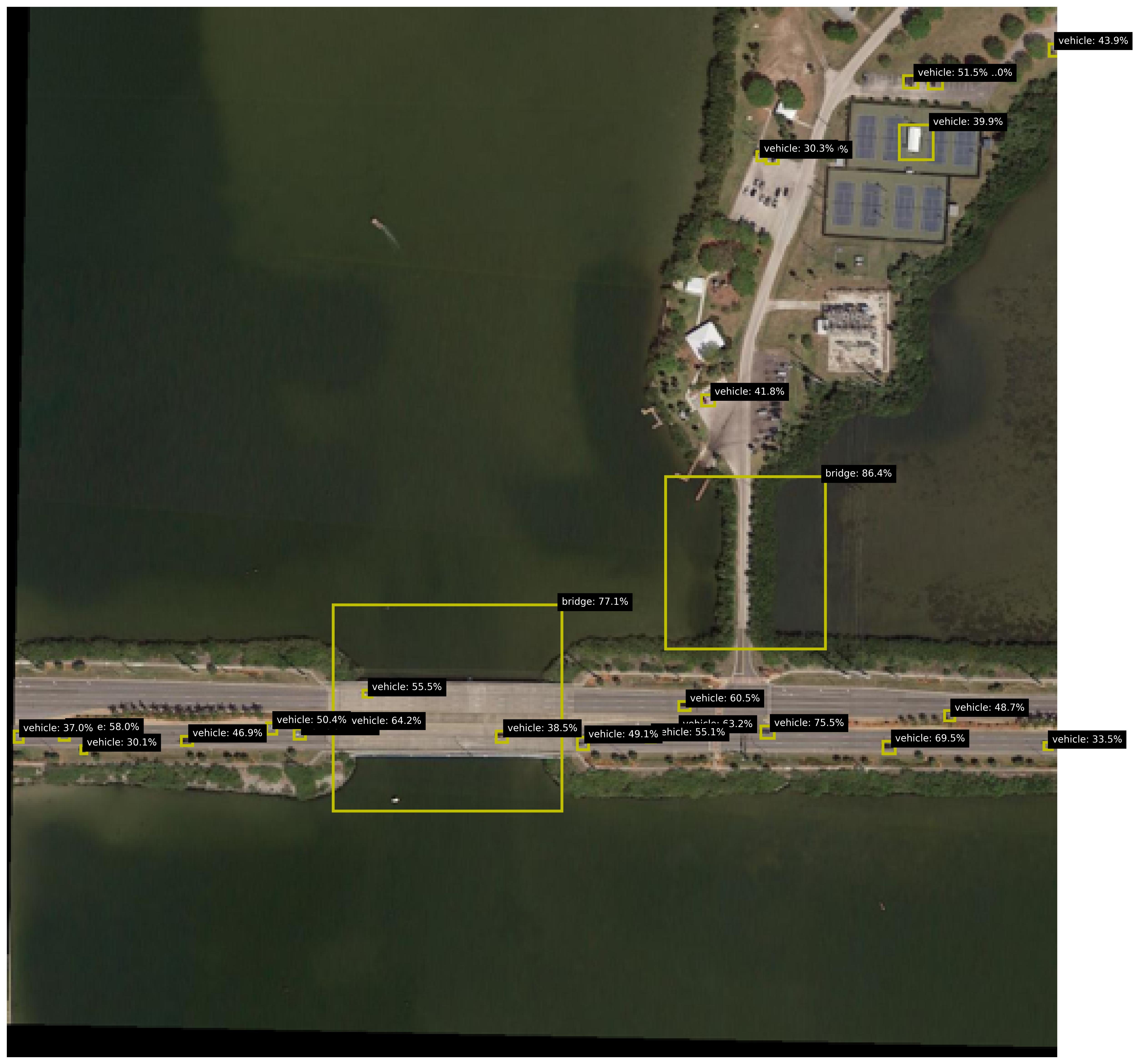
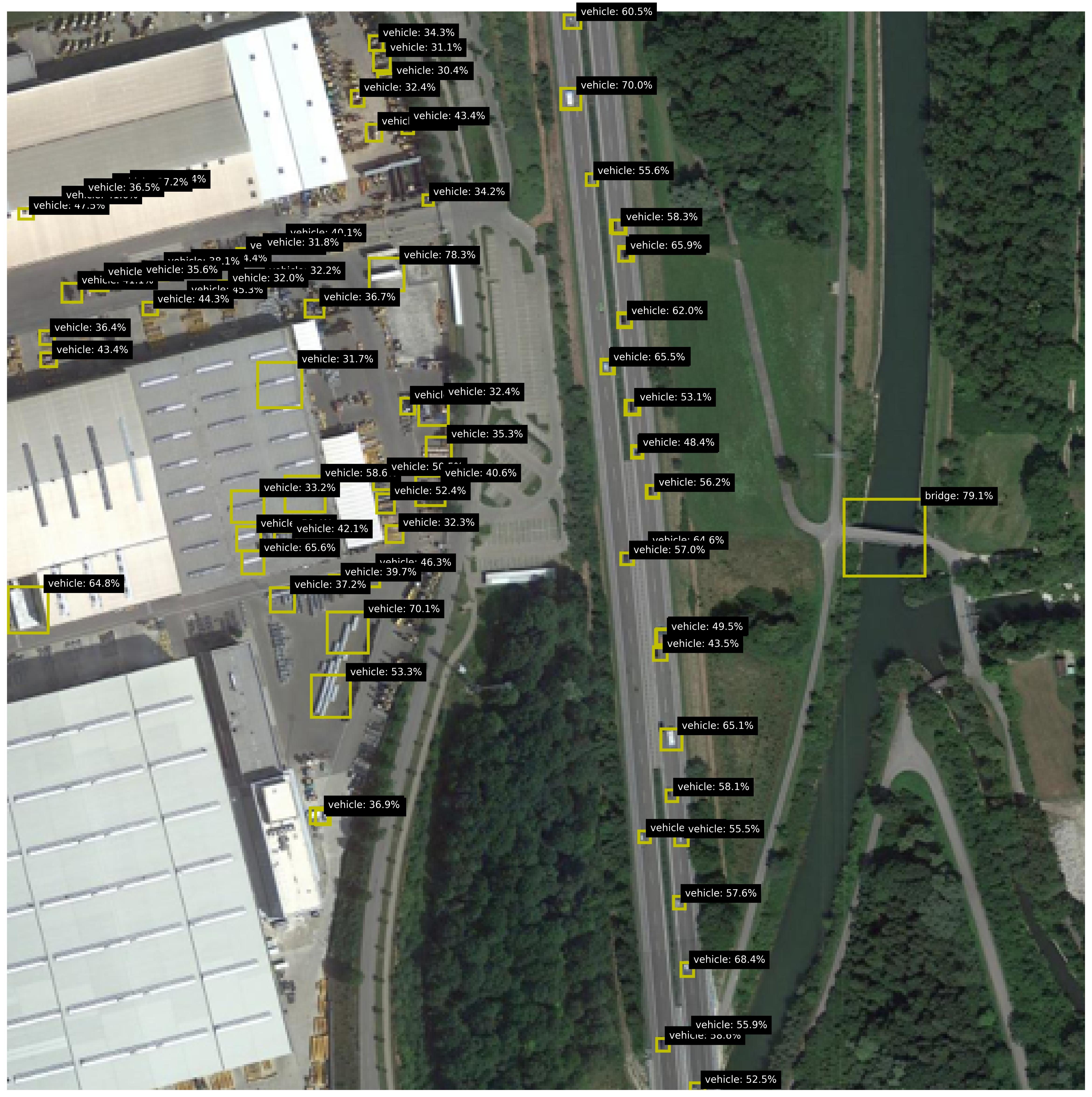
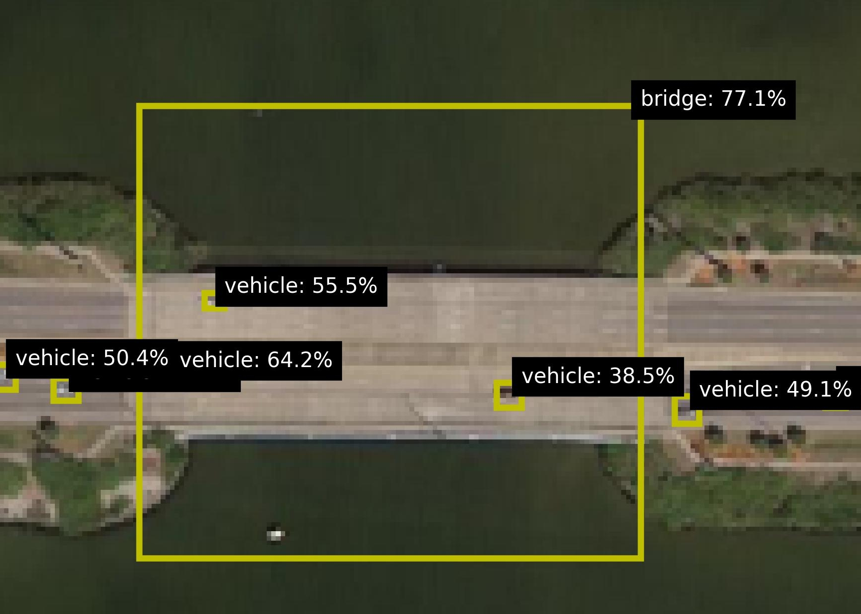
Figure 2: Examples of images with the detected objects and their probabilities.
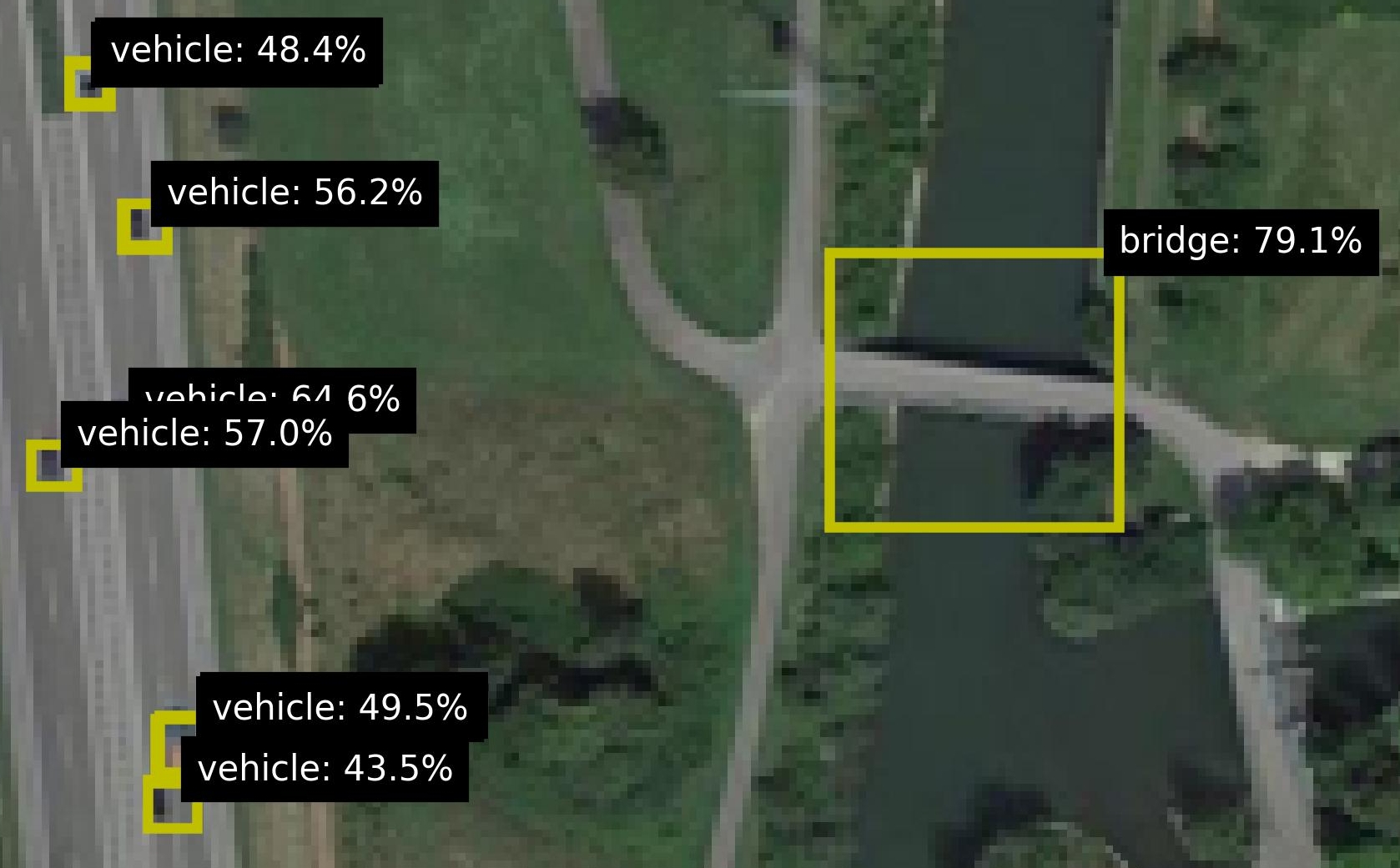
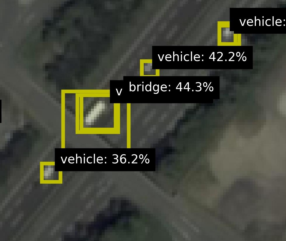
For the background knowledge, we leverage the pretrained DOTA Aerial Images Model dota_model to predict the objects in the images, with for each object a label, location (bounding box) and a probability (confidence value). For each image, the respective predictions are added to the background knowledge, as a predicate with a confidence, e.g. 0.7 :: vehicle(x). The locations of the objects are used to calculate a confidence for two relations: is_on and is_close. This information is added to the background knowledge as well. Figure 2 shows various images from the dataset, including zoomed versions to reveal some more details and to highlight the small size of the objects. Figure 2(b) shows an image with many objects. The relational patterns of interest is ‘vehicle on bridge’. For this pattern, there are 11 positive test images and 297 negative test images. Figure 2 shows both a positive (left) and negative image (right). To make the task realistic, both sets contain images with vehicles, bridges and roundabouts, so the model cannot distinguish the positives and negatives by purely finding the right sets of objects; the model really needs to find the right pattern between the right objects. Out of the negative images, 17 are designated as hard, due to incorrect groundtruths (2 images) and incorrect detections (15 images). These hard cases are shown in Figure 3.
<details>
<summary>extracted/5868417/result_figs/fp_crop_1.jpg Details</summary>
### Visual Description
## Annotated Aerial Image: Object Detection at Road Intersection
### Overview
This image is a low-resolution, pixelated aerial or satellite photograph of a road intersection, overlaid with the results of an object detection algorithm. The system has identified and placed bounding boxes around specific features, labeling them with a class name and a confidence percentage. The scene appears to be a multi-lane road crossing, with a prominent linear structure (likely a bridge or overpass) running diagonally from the upper left to the lower right.
### Components & Spatial Layout
The image is dominated by the photographic background. Overlaid on this are several graphical elements:
1. **Bounding Boxes:** Yellow rectangular boxes of varying sizes, outlining detected objects.
2. **Labels:** Black rectangular boxes with white text, attached to or near the bounding boxes. Each label contains an object class and a confidence score (e.g., "vehicle: 36.2%").
3. **Background:** A blurry, top-down view of a road network. A major road runs diagonally. The texture suggests asphalt and surrounding terrain or vegetation.
**Spatial Grounding of Detected Elements:**
* **Center-Left:** A large yellow bounding box surrounds a bright, elongated white object on the road. Its associated label, positioned below it, reads **"vehicle: 36.2%"**.
* **Center:** A smaller yellow bounding box is placed on the diagonal road structure. Its label, positioned to its right, reads **"bridge: 44.3%"**. A small letter "v" is visible just to the left of this label box.
* **Upper-Right Quadrant:** Two smaller yellow bounding boxes are present.
* The lower of these has a label to its right reading **"vehicle: 42.2%"**.
* The upper box has a label that is partially cut off by the top edge of the image. The visible text reads **"vehicle:"**. The confidence score is not visible.
* **Far Left Edge:** A small portion of another yellow bounding box is visible, but its label is completely outside the frame.
### Detailed Analysis: Detected Objects & Confidence Scores
The object detection system has output the following specific detections, listed with their approximate confidence scores and visual context:
1. **Object 1 (Center-Left):**
* **Class:** `vehicle`
* **Confidence:** `36.2%`
* **Visual Context:** The bounding box encloses a distinct, bright white, rectangular shape on the road surface, consistent with a vehicle seen from above. This is the largest detected vehicle.
2. **Object 2 (Center):**
* **Class:** `bridge`
* **Confidence:** `44.3%`
* **Visual Context:** The bounding box is placed directly on the prominent diagonal linear feature, which appears to be an overpass or bridge structure crossing over the road below. This is the detection with the highest visible confidence score.
3. **Object 3 (Upper-Right, Lower):**
* **Class:** `vehicle`
* **Confidence:** `42.2%`
* **Visual Context:** The bounding box surrounds a smaller, less distinct bright spot on the road, likely a smaller or more distant vehicle.
4. **Object 4 (Upper-Right, Upper - Partial):**
* **Class:** `vehicle`
* **Confidence:** `[Not visible - cut off]`
* **Visual Context:** Only the left portion of the bounding box and the class label are visible. The associated object is outside the image frame.
### Key Observations
* **Detection Confidence Hierarchy:** The "bridge" structure has the highest visible confidence (44.3%), followed by the two fully visible "vehicle" detections (42.2% and 36.2%). This may reflect the relative size, clarity, or distinctiveness of the objects in the low-resolution imagery.
* **Image Quality Limitation:** The source imagery is highly pixelated and blurry, which is a significant constraint for both human interpretation and automated detection accuracy.
* **Incomplete Data:** One detection label is truncated, and another bounding box on the far left has no visible label, indicating the analysis output is cropped or incomplete.
* **Scene Composition:** The detections cluster around the central intersection and the bridge structure, which are the most salient features in the scene.
### Interpretation
This image represents the output of a computer vision model, likely processing satellite or aerial surveillance imagery for infrastructure monitoring or traffic analysis.
* **What the Data Suggests:** The model is attempting to perform two distinct tasks: **vehicle detection** and **infrastructure (bridge) identification**. The varying confidence scores suggest the model finds the bridge feature more definitive than the vehicle features in this particular view, possibly due to the bridge's larger, more consistent geometric shape compared to the smaller, variable appearances of vehicles.
* **Relationship Between Elements:** The bounding boxes and labels are directly linked, providing a spatially-grounded audit trail for the AI's decisions. The placement of the "bridge" label on the central diagonal feature confirms the model's interpretation of that structure.
* **Anomalies & Uncertainty:** The primary anomaly is the **truncated label** for the fourth vehicle, which represents a loss of information. The **low confidence scores** (all below 50%) across the board indicate the model is uncertain about its classifications, which is consistent with the poor image quality. This output would typically require human verification or fusion with other data sources before being used for decision-making. The small "v" next to the bridge label might be a UI artifact or a partial class name from another detection layer.
</details>
<details>
<summary>extracted/5868417/result_figs/fp_crop_2.jpg Details</summary>
### Visual Description
## Object Detection Overlay: Aerial Road Intersection
### Overview
The image is a low-resolution aerial or satellite photograph of a road intersection, likely a roundabout or complex junction, overlaid with the output of an object detection algorithm. The algorithm has placed yellow bounding boxes around specific features and assigned them class labels with associated confidence percentages. The scene includes paved roads, grassy areas, and some indistinct structures.
### Components/Axes
* **Image Type:** Aerial/Satellite photograph with object detection overlay.
* **Primary Visual Elements:**
* **Road Network:** A multi-lane road runs diagonally from the top-left to the bottom-right. A curved road or ramp connects to it, forming a partial loop or roundabout in the upper-right quadrant.
* **Green Spaces:** Areas of grass or low vegetation are visible between the road segments.
* **Detection Overlays:** Four distinct yellow bounding boxes with black text labels are present.
* **Text Labels (Transcribed Exactly):**
1. `bridge: 46.3%` (Position: Upper-left quadrant, over a road segment)
2. `vehicle: 65.8%` (Position: Center-left, over a small object on the road)
3. `vehicle: 41.7%` (Position: Bottom-center, over a small object on the lower road)
4. `44.3% 9%` (Position: Bottom-left corner, partially cut off. The label format is atypical, showing two percentages without a clear class label.)
### Detailed Analysis
* **Detection 1 (bridge: 46.3%):**
* **Spatial Grounding:** A large yellow bounding box is positioned in the upper-left quadrant. It encloses a section of the main road where it appears to pass over another feature (possibly another road or a depression), consistent with a bridge or overpass structure.
* **Trend/Confidence:** The model expresses low-to-moderate confidence (46.3%) in this classification. The visual evidence for a bridge is ambiguous at this resolution.
* **Detection 2 (vehicle: 65.8%):**
* **Spatial Grounding:** A smaller yellow bounding box is located near the center-left of the image, directly on the main road surface. It surrounds a small, dark, rectangular object.
* **Trend/Confidence:** The model has moderate confidence (65.8%) that this object is a vehicle. The object's size and position on the roadway support this classification.
* **Detection 3 (vehicle: 41.7%):**
* **Spatial Grounding:** A small yellow bounding box is placed at the bottom-center of the image, on the lower section of the main road. It also surrounds a small, dark object.
* **Trend/Confidence:** The model has lower confidence (41.7%) in this vehicle detection compared to the other. The object may be smaller, less distinct, or partially obscured.
* **Detection 4 (44.3% 9%):**
* **Spatial Grounding:** This label is in the bottom-left corner and is partially cropped. No clear bounding box is associated with it in the visible frame.
* **Content:** The text `44.3% 9%` is anomalous. It may represent two separate confidence scores (e.g., for two closely spaced objects) or a formatting error in the overlay. No class label is visible.
* **Unlabeled Feature:**
* **Spatial Grounding:** A yellow bounding box is present at the top-center of the image, around a circular paved area (likely a roundabout center or a traffic circle).
* **Observation:** This box has no associated text label in the visible image, suggesting the detection may have been filtered out, or the label is outside the frame.
### Key Observations
1. **Variable Confidence:** The model's confidence varies significantly, from 41.7% to 65.8% for the "vehicle" class, and 46.3% for "bridge." This suggests challenges with the image resolution or the clarity of the objects.
2. **Incomplete Data:** One detection label is partially cut off, and one bounding box (around the circular feature) lacks a visible label, making the full detection set unclear.
3. **Object Scale:** The detected "vehicle" objects are very small relative to the image, comprising only a few pixels, which explains the moderate confidence scores.
4. **Scene Context:** The infrastructure (multi-lane roads, ramps) is consistent with an area where bridges and vehicles would be expected, providing contextual support for the model's classifications despite low confidence.
### Interpretation
This image demonstrates the output of a computer vision model performing object detection on aerial imagery. The primary purpose is likely automated feature extraction for mapping, traffic monitoring, or infrastructure assessment.
* **What the Data Suggests:** The model is attempting to identify and localize key transportation assets (vehicles, bridges) from a top-down view. The varying confidence scores highlight the difficulty of this task with low-resolution input; the model is "uncertain" about its identifications.
* **Relationship Between Elements:** The bounding boxes and labels are directly linked, with the text providing the model's interpretation of the visual data within each box. The spatial placement confirms the model is analyzing specific, localized regions of the larger scene.
* **Notable Anomalies:**
* The `44.3% 9%` label is a significant anomaly. It breaks the standard `[class]: [confidence]%` format, indicating a potential bug in the visualization code or an edge case in the detection pipeline (e.g., overlapping detections).
* The absence of a label for the circular feature's bounding box is also notable. It could mean the detection was below a confidence threshold for display, or the class name was not rendered.
* **Underlying Implications:** The image serves as a diagnostic view into an AI perception system. It reveals not just *what* the system sees, but *how sure* it is. For a technical user, this is more valuable than a perfect detection, as it exposes the system's limitations and areas for improvement (e.g., needing higher-resolution imagery or a model fine-tuned for small-object detection from aerial views). The scene itself is mundane, but the overlay transforms it into a report on algorithmic performance.
</details>
<details>
<summary>extracted/5868417/result_figs/fp_crop_3.jpg Details</summary>
### Visual Description
## Object Detection Overlay: Aerial Bridge Scene
### Overview
The image is a low-resolution aerial or satellite photograph, likely from a drone or overhead sensor, showing a bridge crossing a body of water. Overlaid on the photograph are the results of an object detection algorithm, presented as yellow bounding boxes with associated text labels and confidence scores. The scene is viewed from a high-angle, top-down perspective.
### Components/Axes
The image contains no traditional chart axes. The primary components are:
1. **Base Image:** A photographic scene.
2. **Detection Overlays:** Three yellow rectangular bounding boxes of varying sizes.
3. **Text Labels:** Black rectangular boxes with white text, positioned adjacent to their corresponding bounding boxes.
**Detected Objects and Labels:**
* **Object 1:** A large bounding box encompassing the main bridge structure.
* **Label:** `bridge: 57.7%`
* **Spatial Position:** The bounding box originates in the upper-left quadrant and extends diagonally towards the center-right. The label is positioned at the top-right corner of this box.
* **Object 2:** A small bounding box on the bridge deck.
* **Label:** `vehicle: 51.0%`
* **Spatial Position:** Located near the center of the image, slightly to the right. The label is positioned to the right of the box.
* **Object 3:** A small bounding box on the bridge deck, south of Object 2.
* **Label:** `vehicle: 31.8%`
* **Spatial Position:** Located in the lower-central part of the image. The label is positioned to the right of the box.
### Detailed Analysis
**Visual Scene Description:**
* **Bridge:** A grey, linear structure runs diagonally from the top-left to the bottom-right of the frame. It appears to be a multi-lane road bridge.
* **Water:** A dark, greenish body of water (likely a river or canal) flows beneath the bridge, visible on the left side and partially on the right.
* **Vegetation:** Dense, dark green foliage (trees and bushes) surrounds the water and the bridge approaches on both sides.
* **Image Quality:** The base photograph is pixelated and lacks fine detail, suggesting it is either a crop from a larger image or taken from a significant distance.
**Detection Data:**
The object detection system has identified three entities with the following confidence scores:
1. **Bridge:** Confidence = 57.7% (Moderate confidence)
2. **Vehicle (Upper):** Confidence = 51.0% (Moderate confidence)
3. **Vehicle (Lower):** Confidence = 31.8% (Low confidence)
### Key Observations
1. **Confidence Gradient:** There is a clear hierarchy in detection confidence. The largest object (the bridge) has the highest confidence, followed by one vehicle, with the second vehicle having notably lower confidence.
2. **Object Size vs. Confidence:** The two "vehicle" detections are of similar visual size in the image, yet their confidence scores differ significantly (51.0% vs. 31.8%). This suggests factors beyond simple size, such as contrast with the road surface, shape clarity, or contextual placement, influenced the model's certainty.
3. **Spatial Relationship:** The two vehicle detections are located on the bridge deck, consistent with the expected location for vehicles. The lower-confidence vehicle is positioned closer to the edge of the bridge structure.
4. **Bounding Box Precision:** The large "bridge" bounding box is not tightly fitted to the visible bridge structure; it includes a significant portion of the water and vegetation to the left. This may indicate the model's region proposal for the "bridge" class is broad or that the bridge's full extent is partially occluded or ambiguous in this view.
### Interpretation
This image represents the output of a computer vision model performing object detection on aerial imagery. The primary purpose is likely automated infrastructure monitoring or traffic analysis.
* **What the data suggests:** The model is moderately successful at identifying the primary infrastructure (the bridge) and is attempting to detect smaller objects (vehicles) upon it. The varying confidence scores indicate the model's uncertainty, which is crucial for downstream decision-making. A confidence of 31.8% for a vehicle is typically below standard deployment thresholds and would likely be filtered out in a practical system.
* **How elements relate:** The detections are contextually logical—vehicles are found on the bridge. The low resolution of the base image is a key limiting factor for detection accuracy, explaining the moderate-to-low confidence scores. The model is performing "detection," not "segmentation," as evidenced by the rectangular boxes rather than precise outlines.
* **Notable anomalies/outliers:** The most significant observation is the large discrepancy in confidence between the two visually similar vehicle detections. This warrants investigation: is the lower-confidence object actually a vehicle, or is it a different object (e.g., a road sign, a patch of discoloration) that the model misclassified? The imprecise bounding box for the bridge also suggests the model may struggle with defining the exact boundaries of large, linear infrastructure in overhead views.
* **Peircean Investigation:** The image is an *index* of an algorithmic process—it points directly to the operation of a detection model. The signs (the labels and boxes) are *icons* representing the model's hypothesized objects. The low confidence scores are *arguments* about the reliability of those hypotheses. To validate, one would need the original, high-resolution imagery and ground truth data. The image itself argues that automated analysis of such imagery is possible but fraught with uncertainty, requiring careful calibration and validation.
</details>
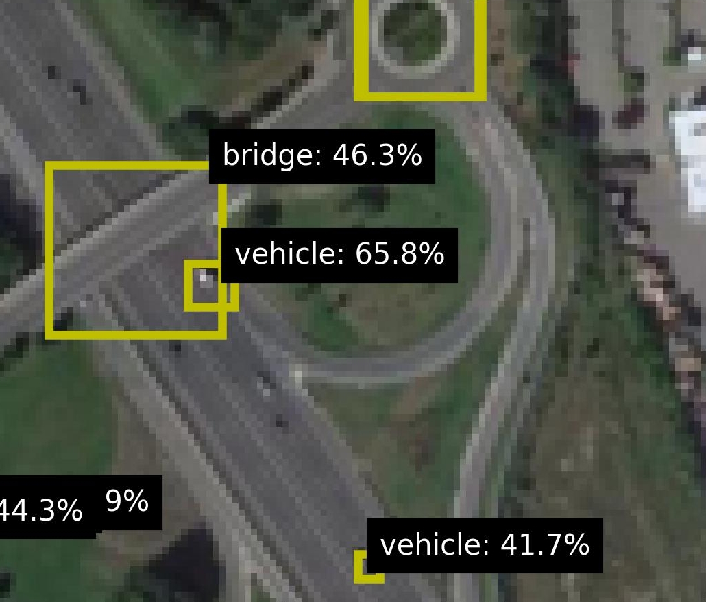
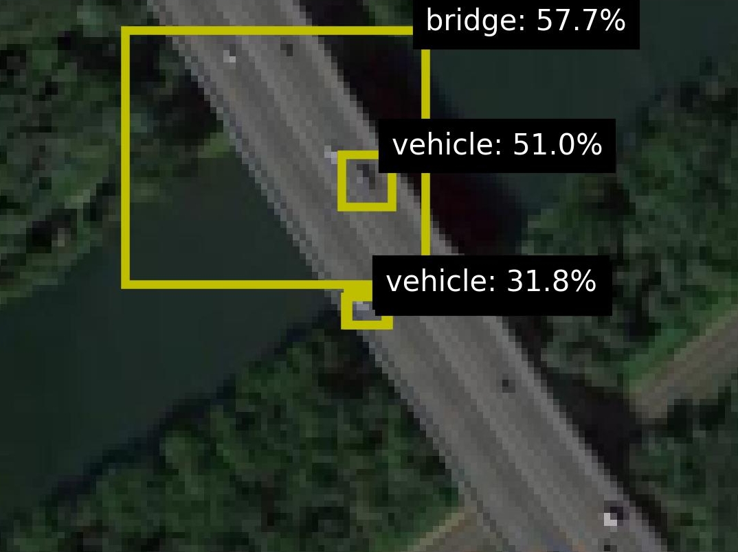
Figure 3: Hard cases due to incorrect groundtruths (right) or incorrect detections (others).
### 4.2 Experimental Setup
The dataset is categorized into three subsets that are increasingly harder in terms of flaws in the background knowledge. Easy: This smallest subset excludes the incorrect groundtruths, a manual check that most object predictions are reasonable, i.e. images with many predicted objects are withheld (this includes images with many false positives). Intermediate: This subset excludes the incorrect groundtruths. Compared to Easy, this subset adds all images with many object predictions. Hard: This is the full set, which includes all images, also the ones with incorrect groundtruths. We are curious whether ILP methods can indeed generalize from small numbers of examples, as is hypothesized cropper2022inductive. Many datasets used in ILP are using training data with tens to hundreds (sometimes thousands) of labeled samples hocquette2024learning,bellodi2015structure. We investigate the performance for as few as {1, 2, 4, 8} labels for respectively the positive and negative set, as this is common in practical settings. Moreover, common ILP datasets are about binary background knowledge, without associated probabilities hocquette2024learning,bellodi2015structure. In contrast, we consider probabilistic background knowledge. From the Easy subset we construct an Easy-1.0 set by thresholding the background knowledge with a manually chosen optimal threshold, which results in an almost noiseless dataset and shows the complexity of the logical rule to learn. All experiments are repeated 5 times, randomly selecting the training samples from the dataset and using the rest of the data set as test set.
### 4.3 Model Variants and Baselines
We compare Propper with Popper (on which it builds), to validate the merit of integrating the neurosymbolic inference and the continuous cost function BCE. Moreover, we compare these ILP models with statistical ML models: the Support Vector Machine cortes1995support (SVM) because it is used so often in practice; a Graph Neural Network wu2020comprehensive (GNN) because it is also relational by design which makes it a reasonable candidate for the task at hand i.e. finding a relational pattern between objects. All methods except the SVM are relational and permutation invariant. The objects are unordered and the models should therefore represent them in an orderless manner. The SVM is not permutation invariant, as objects and their features have some arbitrary but designated position in its feature vectors. All methods except Popper are probabilistic. All methods except the most basic Popper variant, can handle some degree of noise. The expected noise level for NoisyCombo is set at 0.15. The tested models are characterized in Table 1.
Table 1: The tested model variants and their properties.
| Tester Cost function | Cortes 1995 - - | Wu 2020 - - | Cropper 2021 Prolog MDL | Hoguette 2024 Prolog MDL | (ours) Constrainer Scallop BCE Type | - Stat. | - Stat. | Combo Logic | MaxSynth Logic | Noisy-Combo Logic |
| --- | --- | --- | --- | --- | --- | --- | --- | --- | --- | --- |
| Label noise | Yes | Yes | No | Yes | Yes | | | | | |
| Background noise | Yes | Yes | No | Some | Yes | | | | | |
| Relational | No | Yes | Yes | Yes | Yes | | | | | |
| Permutation inv. | No | Yes | Yes | Yes | Yes | | | | | |
| Probabilistic | Yes | Yes | No | No | Yes | | | | | |
For a valid comparison, we increase the SVM’s robustness against arbitrary object order. With prior knowledge about the relevant objects for the pattern at hand, these objects can be placed in front of the feature vector. This preprocessing step makes the SVM model less dependent on the arbitrary order of objects. In the remainder of the analyses, we call this variant ‘SVM ordered’. To binarize the probabilistic background knowledge as input for Popper, the detections are thresholded with the general value of 0.5.
### 4.4 Increasing Noise in Background Knowledge
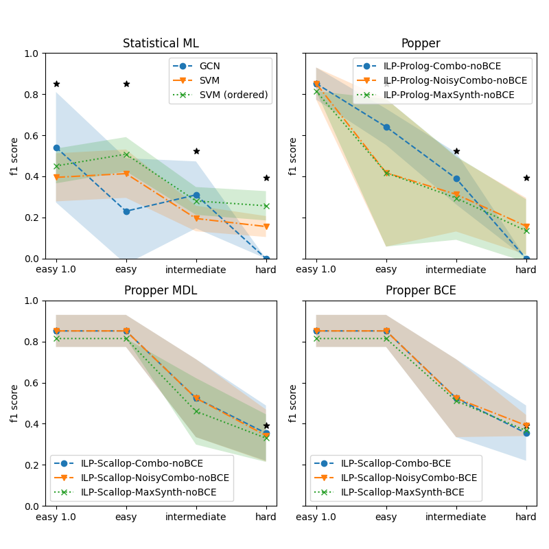
We are interested in how the robustness of model learning for increasing difficulty of the dataset. Here we investigate the performance on the three subsets from Section 4.2: Easy, Intermediate and Hard. Figure 4 shows the performance for various models for increasing difficulty. The four subplots show the various types of models. For a reference, the best performing model is indicated by an asterisk (*) in all subplots. It is clear that for increasing difficulty, all models struggle. The statistical ML models struggle the most: the performance of the GNN drops to zero on the Hard set. The SVMs are a bit more robust but the performance on the Hard set is very low. The most basic variant of Popper also drops to zero. The noise-tolerant Popper variants (Noisy-Combo and MaxSynth) perform similarly to the SVMs. Propper outperforms all models. This finding holds for all Propper variants (Combo, Noisy-Combo and MaxSynth). Using BCE as a cost function yields a small but negligible advantage over MDL.
<details>
<summary>extracted/5868417/result_propper_figures/increasing_test_hardness/n_train_avg_4_8.png Details</summary>
### Visual Description
\n
## [Chart Type]: Multi-Panel Line Chart with Confidence Intervals
### Overview
The image displays a 2x2 grid of four line charts, each comparing the performance (F1 score) of different machine learning or logic programming methods across four difficulty levels. The charts include shaded regions representing confidence intervals or variance. Black star markers appear at specific data points in each plot.
### Components/Axes
* **Overall Structure:** Four subplots arranged in a 2x2 grid.
* **Common Axes:**
* **X-axis (All plots):** Categorical labels representing task difficulty. From left to right: `easy 1.0`, `easy`, `intermediate`, `hard`.
* **Y-axis (All plots):** Labeled `f1 score`. Scale ranges from 0.0 to 1.0, with major ticks at 0.0, 0.2, 0.4, 0.6, 0.8, 1.0.
* **Subplot Titles (Top Center):**
1. Top-Left: `Statistical ML`
2. Top-Right: `Popper`
3. Bottom-Left: `Propper MDL`
4. Bottom-Right: `Propper BCE`
* **Legends:** Each subplot contains a legend box.
* **Statistical ML (Top-Left):** Legend is in the top-left corner. Contains:
* Blue circle with dashed line: `GCN`
* Orange triangle (down) with dash-dot line: `SVM`
* Green 'x' with dotted line: `SVM (ordered)`
* **Popper (Top-Right):** Legend is in the top-right corner. Contains:
* Blue circle with dashed line: `ILP-Prolog-Combo-noBCE`
* Orange triangle (down) with dash-dot line: `ILP-Prolog-NoisyCombo-noBCE`
* Green 'x' with dotted line: `ILP-Prolog-MaxSynth-noBCE`
* **Propper MDL (Bottom-Left):** Legend is in the bottom-left corner. Contains:
* Blue circle with dashed line: `ILP-Scallop-Combo-noBCE`
* Orange triangle (down) with dash-dot line: `ILP-Scallop-NoisyCombo-noBCE`
* Green 'x' with dotted line: `ILP-Scallop-MaxSynth-noBCE`
* **Propper BCE (Bottom-Right):** Legend is in the bottom-right corner. Contains:
* Blue circle with dashed line: `ILP-Scallop-Combo-BCE`
* Orange triangle (down) with dash-dot line: `ILP-Scallop-NoisyCombo-BCE`
* Green 'x' with dotted line: `ILP-Scallop-MaxSynth-BCE`
* **Other Visual Elements:**
* **Shaded Regions:** Each line has a semi-transparent shaded area of the same color, indicating confidence intervals or standard deviation.
* **Black Star Markers:** A black star (`★`) is plotted at specific (x, y) coordinates in each subplot, seemingly independent of the line series.
### Detailed Analysis
**1. Statistical ML (Top-Left)**
* **Trend Verification:** All three methods show a general downward trend in F1 score as difficulty increases from `easy 1.0` to `hard`.
* **Data Points (Approximate):**
* **GCN (Blue):** `easy 1.0`: ~0.55, `easy`: ~0.23, `intermediate`: ~0.31, `hard`: 0.0.
* **SVM (Orange):** `easy 1.0`: ~0.40, `easy`: ~0.41, `intermediate`: ~0.20, `hard`: ~0.16.
* **SVM (ordered) (Green):** `easy 1.0`: ~0.44, `easy`: ~0.50, `intermediate`: ~0.28, `hard`: ~0.25.
* **Black Stars:** Located at approximately (`easy 1.0`, 0.85), (`easy`, 0.85), (`intermediate`, 0.52), (`hard`, 0.40).
**2. Popper (Top-Right)**
* **Trend Verification:** All three ILP-Prolog methods start with high F1 scores at `easy 1.0` and show a steep, consistent decline as difficulty increases.
* **Data Points (Approximate):**
* **ILP-Prolog-Combo-noBCE (Blue):** `easy 1.0`: ~0.85, `easy`: ~0.64, `intermediate`: ~0.38, `hard`: 0.0.
* **ILP-Prolog-NoisyCombo-noBCE (Orange):** `easy 1.0`: ~0.85, `easy`: ~0.41, `intermediate`: ~0.31, `hard`: ~0.18.
* **ILP-Prolog-MaxSynth-noBCE (Green):** `easy 1.0`: ~0.80, `easy`: ~0.41, `intermediate`: ~0.29, `hard`: ~0.14.
* **Black Stars:** Located at approximately (`easy 1.0`, 0.85), (`intermediate`, 0.52), (`hard`, 0.40). No star at `easy`.
**3. Propper MDL (Bottom-Left)**
* **Trend Verification:** All three ILP-Scallop (noBCE) methods maintain high, stable performance for `easy 1.0` and `easy`, then decline sharply for `intermediate` and `hard`.
* **Data Points (Approximate):**
* **ILP-Scallop-Combo-noBCE (Blue):** `easy 1.0`: ~0.86, `easy`: ~0.86, `intermediate`: ~0.52, `hard`: ~0.36.
* **ILP-Scallop-NoisyCombo-noBCE (Orange):** `easy 1.0`: ~0.86, `easy`: ~0.86, `intermediate`: ~0.52, `hard`: ~0.38.
* **ILP-Scallop-MaxSynth-noBCE (Green):** `easy 1.0`: ~0.82, `easy`: ~0.82, `intermediate`: ~0.46, `hard`: ~0.34.
* **Black Stars:** Located at approximately (`hard`, 0.40). No stars at other difficulty levels.
**4. Propper BCE (Bottom-Right)**
* **Trend Verification:** Identical pattern to Propper MDL: stable high performance for easy tasks, then a decline.
* **Data Points (Approximate):**
* **ILP-Scallop-Combo-BCE (Blue):** `easy 1.0`: ~0.86, `easy`: ~0.86, `intermediate`: ~0.52, `hard`: ~0.36.
* **ILP-Scallop-NoisyCombo-BCE (Orange):** `easy 1.0`: ~0.86, `easy`: ~0.86, `intermediate`: ~0.52, `hard`: ~0.39.
* **ILP-Scallop-MaxSynth-BCE (Green):** `easy 1.0`: ~0.82, `easy`: ~0.82, `intermediate`: ~0.52, `hard`: ~0.38.
* **Black Stars:** None visible in this subplot.
### Key Observations
1. **Performance Degradation:** All methods across all subplots show decreasing F1 scores as task difficulty increases.
2. **Method Grouping:** The `Propper MDL` and `Propper BCE` (ILP-Scallop) methods exhibit a distinct "plateau-then-drop" pattern, maintaining near-peak performance from `easy 1.0` to `easy`, unlike the more linear decline in `Statistical ML` and `Popper`.
3. **BCE vs. noBCE:** Comparing the bottom two plots (`Propper MDL` vs. `Propper BCE`), the performance curves and final `hard` scores are very similar, suggesting the BCE (Binary Cross-Entropy) condition has minimal impact on the final outcome for these Scallop methods in this experiment.
4. **Black Star Pattern:** The black stars appear at consistent y-values across plots (e.g., ~0.85 at easy levels, ~0.52 at intermediate, ~0.40 at hard), but their presence varies by subplot. They likely represent a baseline, human performance, or an optimal benchmark for each difficulty level.
5. **Variance:** The shaded confidence intervals are widest for the `Statistical ML` methods, particularly GCN, indicating higher variance or less consistent performance. The `Propper` methods show tighter intervals.
### Interpretation
This set of charts evaluates the robustness of different algorithmic paradigms (Statistical ML, Inductive Logic Programming via Popper and Propper) on tasks of increasing difficulty.
* **Core Finding:** The task difficulty metric is a strong predictor of performance degradation for all tested methods. The "hard" category presents a significant challenge, reducing F1 scores to between 0.0 and 0.4.
* **Paradigm Comparison:** The `Propper` (ILP-Scallop) methods demonstrate superior robustness on easier tasks (`easy 1.0` and `easy`), maintaining F1 scores above 0.8, whereas `Statistical ML` and `Popper` methods begin degrading immediately. This suggests the Propper framework is better at leveraging the structure of simpler problems.
* **The "Hard" Problem:** The convergence of many methods towards low scores (0.0-0.4) at the `hard` level, alongside the consistent placement of the black star benchmark at ~0.40, implies this difficulty tier may represent a fundamental limit or a qualitatively different problem class that is challenging for all presented approaches.
* **Investigative Insight (Peircean):** The black stars act as an *index* pointing to a ground truth or reference performance. Their consistent y-values across plots suggest a standardized benchmark. Their absence in the `Propper BCE` plot and partial presence in others could indicate experimental design choices—perhaps that benchmark was not measured or is not applicable for all method comparisons. The near-identical results of `Propper MDL` and `Propper BCE` is a *sign* that the model's loss function (MDL vs. BCE) is not the critical factor for performance on these tasks; the underlying Scallop architecture or the data structure itself is the dominant cause.
</details>
Figure 4: Performance of the models on finding a relational pattern in satellite images, for increasing hardness of image sets. The best performer is Propper BCE, indicated in each graph by * for comparison. Our probabilistic ILP outperforms binary ILP and statistical ML.
### 4.5 Learning Efficiency with Few Labels
We are curious how the models perform with as few as {1, 2, 4, 8} labels for respectively the positive and negative set. The performance is measured on the Hard set. Figure 5 shows the performance for various models for increasing training set size. The four subplots show the various types of models. Again, for reference, the best performing model is indicated by an asterisk (*) in all subplots. The upper left shows the statistical ML models. They do perform better with more training samples, but the performance is inferior to the ILP model variants. The Propper variant with Scallop and Noisy-Combo and BCE is the best performer. BCE does not improve significantly over MDL. MaxSynth has an optimization criterion that cannot operate with less than three training samples. The main improvement by Propper is observed when switching from Combo to Noisy-Combo and switching from Prolog to Scallop (i.e. neurosymbolic inference).
<details>
<summary>extracted/5868417/result_propper_figures/increasing_train_samples/all_test_cases_avg.png Details</summary>
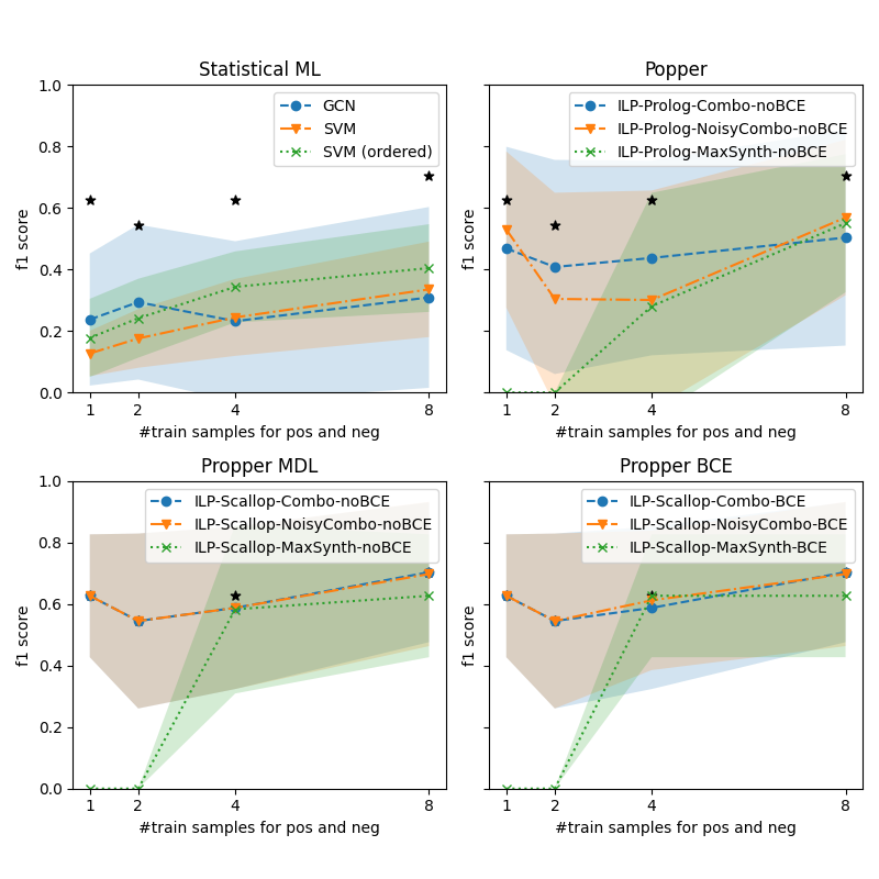
### Visual Description
## [Multi-Panel Line Chart]: Performance of Various ML/ILP Methods vs. Training Sample Size
### Overview
The image contains four separate line charts arranged in a 2x2 grid. Each chart plots the F1 score (y-axis) against the number of training samples for positive and negative classes (x-axis) for different machine learning or Inductive Logic Programming (ILP) methods. The charts compare the performance trends of these methods as the training set size increases from 1 to 8 samples. Shaded regions around each line likely represent confidence intervals or standard deviation. Black star markers appear at specific data points across all charts.
### Components/Axes
* **Common Elements (All Charts):**
* **X-axis:** Label: `#train samples for pos and neg`. Ticks/Values: `1`, `2`, `4`, `8`.
* **Y-axis:** Label: `f1 score`. Scale: `0.0` to `1.0` with increments of `0.2`.
* **Legend:** Positioned in the top-right corner of each subplot. Contains three data series with distinct markers and line styles.
* **Black Stars:** Five-pointed star markers (`★`) are plotted at specific (x, y) coordinates in each chart, seemingly independent of the main data series.
* **Chart-Specific Titles & Legends:**
1. **Top-Left Chart:** Title: `Statistical ML`. Legend:
* `GCN` (Blue circle marker, dashed line)
* `SVM` (Orange downward triangle marker, dashed line)
* `SVM (ordered)` (Green 'x' marker, dotted line)
2. **Top-Right Chart:** Title: `Popper`. Legend:
* `ILP-Prolog-Combo-noBCE` (Blue circle marker, dashed line)
* `ILP-Prolog-NoisyCombo-noBCE` (Orange downward triangle marker, dashed line)
* `ILP-Prolog-MaxSynth-noBCE` (Green 'x' marker, dotted line)
3. **Bottom-Left Chart:** Title: `Propper MDL`. Legend:
* `ILP-Scallop-Combo-noBCE` (Blue circle marker, dashed line)
* `ILP-Scallop-NoisyCombo-noBCE` (Orange downward triangle marker, dashed line)
* `ILP-Scallop-MaxSynth-noBCE` (Green 'x' marker, dotted line)
4. **Bottom-Right Chart:** Title: `Propper BCE`. Legend:
* `ILP-Scallop-Combo-BCE` (Blue circle marker, dashed line)
* `ILP-Scallop-NoisyCombo-BCE` (Orange downward triangle marker, dashed line)
* `ILP-Scallop-MaxSynth-BCE` (Green 'x' marker, dotted line)
### Detailed Analysis
**1. Statistical ML (Top-Left):**
* **Trend Verification:**
* **GCN (Blue):** Slopes gently upward. Starts low, increases slightly.
* **SVM (Orange):** Slopes upward. Starts lowest, shows steady improvement.
* **SVM (ordered) (Green):** Slopes upward. Starts higher than SVM, maintains a lead.
* **Data Points (Approximate F1 scores):**
* **x=1:** GCN ~0.23, SVM ~0.13, SVM (ordered) ~0.18. Black Star at ~0.62.
* **x=2:** GCN ~0.29, SVM ~0.18, SVM (ordered) ~0.24. Black Star at ~0.55.
* **x=4:** GCN ~0.23, SVM ~0.24, SVM (ordered) ~0.35. Black Star at ~0.62.
* **x=8:** GCN ~0.30, SVM ~0.34, SVM (ordered) ~0.40. Black Star at ~0.70.
**2. Popper (Top-Right):**
* **Trend Verification:**
* **ILP-Prolog-Combo-noBCE (Blue):** Dips at x=2, then slopes upward.
* **ILP-Prolog-NoisyCombo-noBCE (Orange):** Dips sharply at x=2, then slopes upward.
* **ILP-Prolog-MaxSynth-noBCE (Green):** Starts at 0, slopes steeply upward.
* **Data Points (Approximate F1 scores):**
* **x=1:** Combo ~0.47, NoisyCombo ~0.55, MaxSynth ~0.00. Black Star at ~0.62.
* **x=2:** Combo ~0.40, NoisyCombo ~0.31, MaxSynth ~0.00. Black Star at ~0.55.
* **x=4:** Combo ~0.43, NoisyCombo ~0.31, MaxSynth ~0.30. Black Star at ~0.62.
* **x=8:** Combo ~0.50, NoisyCombo ~0.57, MaxSynth ~0.58. Black Star at ~0.70.
**3. Propper MDL (Bottom-Left):**
* **Trend Verification:**
* **ILP-Scallop-Combo-noBCE (Blue):** Dips at x=2, then slopes upward.
* **ILP-Scallop-NoisyCombo-noBCE (Orange):** Dips at x=2, then slopes upward.
* **ILP-Scallop-MaxSynth-noBCE (Green):** Starts at 0, slopes steeply upward.
* **Data Points (Approximate F1 scores):**
* **x=1:** Combo ~0.63, NoisyCombo ~0.63, MaxSynth ~0.00.
* **x=2:** Combo ~0.55, NoisyCombo ~0.55, MaxSynth ~0.00.
* **x=4:** Combo ~0.59, NoisyCombo ~0.59, MaxSynth ~0.59. Black Star at ~0.62.
* **x=8:** Combo ~0.70, NoisyCombo ~0.70, MaxSynth ~0.62.
**4. Propper BCE (Bottom-Right):**
* **Trend Verification:**
* **ILP-Scallop-Combo-BCE (Blue):** Dips at x=2, then slopes upward.
* **ILP-Scallop-NoisyCombo-BCE (Orange):** Dips at x=2, then slopes upward.
* **ILP-Scallop-MaxSynth-BCE (Green):** Starts at 0, slopes steeply upward.
* **Data Points (Approximate F1 scores):**
* **x=1:** Combo ~0.63, NoisyCombo ~0.63, MaxSynth ~0.00.
* **x=2:** Combo ~0.55, NoisyCombo ~0.55, MaxSynth ~0.00.
* **x=4:** Combo ~0.59, NoisyCombo ~0.59, MaxSynth ~0.63. Black Star at ~0.62.
* **x=8:** Combo ~0.70, NoisyCombo ~0.70, MaxSynth ~0.62.
### Key Observations
1. **Performance Ceiling:** The black stars, which are consistent across all four charts at approximately (1, 0.62), (2, 0.55), (4, 0.62), and (8, 0.70), likely represent a benchmark, oracle, or upper-bound performance level for the task.
2. **Sample Size Sensitivity:** All methods show a general trend of improved F1 score with more training samples (from 1 to 8), though the rate of improvement varies significantly.
3. **Method Comparison:**
* In the "Statistical ML" chart, `SVM (ordered)` consistently outperforms standard `SVM` and `GCN`.
* The "Popper" (Prolog-based ILP) methods show high variance, with `MaxSynth` starting at zero but catching up dramatically.
* The "Propper" (Scallop-based ILP) methods, both MDL and BCE variants, start with much higher F1 scores (~0.63) at x=1 compared to other methods, suggesting better few-shot learning capability. Their `Combo` and `NoisyCombo` variants perform nearly identically.
4. **Zero-Start Phenomenon:** The `MaxSynth` variants in the ILP charts (Popper, Propper MDL, Propper BCE) all start at an F1 score of 0.0 for 1 and 2 training samples before improving, indicating a possible failure mode or initialization requirement with very small data.
### Interpretation
This set of charts provides a comparative analysis of learning efficiency across different algorithmic paradigms (Statistical ML vs. ILP) and specific implementations (GCN, SVM, Popper/Prolog, Propper/Scallop) on a task measured by F1 score.
The data suggests that for this specific task:
1. **Inductive Logic Programming (ILP) approaches, particularly those using the Scallop framework ("Propper"), demonstrate superior few-shot learning performance.** They achieve high F1 scores (~0.63) with just one training sample, whereas statistical methods start below 0.25. This implies the ILP methods are better at leveraging structural or logical constraints inherent in the problem when data is extremely scarce.
2. **The benefit of additional training samples is non-linear and method-dependent.** While all methods improve, the ILP methods show a "catch-up" dynamic, especially the `MaxSynth` strategy, which is ineffective with 1-2 samples but becomes competitive with 4-8 samples. This could indicate a threshold of data required for certain synthesis strategies to activate.
3. **The "Combo" and "NoisyCombo" strategies within the Scallop framework are robust and perform similarly,** suggesting that the core learning mechanism is stable regardless of the specific combination or noise-handling variant in this context.
4. **The consistent black stars serve as a crucial reference point,** showing that with 8 samples, several methods (notably Scallop-based ones and Popper's MaxSynth) approach or match this benchmark performance, while statistical methods remain significantly below it. This highlights the data efficiency of the logic-based approaches for this particular problem domain.
In summary, the visualization argues for the effectiveness of ILP, especially the Scallop-based "Propper" methods, in scenarios where training data is severely limited, outperforming traditional statistical ML models in sample efficiency.
</details>
Figure 5: Performance of the models on finding a relational pattern in satellite images, for increasing training sets. The best performer is Propper BCE, indicated in each graph by * for comparison. Our probabilistic ILP outperforms binary ILP and statistical ML.
### 4.6 Second Dataset
We are interested how the methods perform on a different dataset. The MS-COCO dataset lin2014microsoft contains a broad variety of images of everyday scenes. This dataset is challenging, because there are many different objects in a wide range of settings. Similar to the previous experiment, the background knowledge is acquired by the predictions of a pretrained model, GroundingDINO liu2023groundingDINO, which are used to extract the same two relations. Figure 6 shows some examples.
<details>
<summary>extracted/5868417/coco/2.jpg Details</summary>
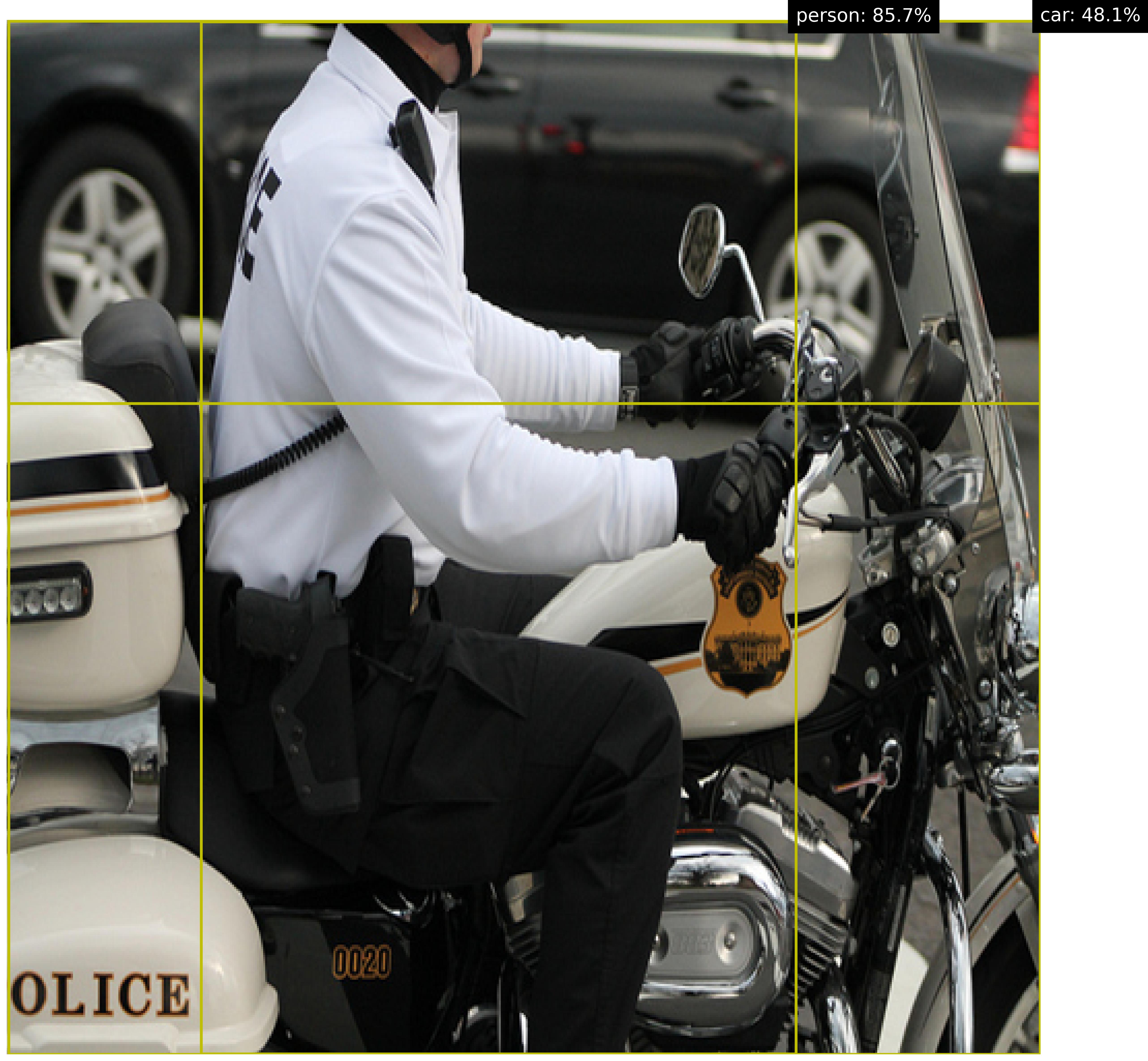
### Visual Description
## Object Detection Annotation: Police Officer on Motorcycle
### Overview
This image is a photograph of a police officer seated on a white police motorcycle, overlaid with bounding boxes and labels from an object detection system. The scene appears to be taken outdoors during the day, with a dark-colored car visible in the background. The primary focus is the officer and the motorcycle, which are highlighted by the detection system's annotations.
### Components/Axes
The image contains the following annotated components from an object detection model:
1. **Bounding Boxes & Labels:**
* **Person Detection:** A yellow bounding box encompasses the police officer. The associated label, located in the top-right corner of the image, reads: `person: 85.7%`.
* **Car Detection:** A second yellow bounding box outlines the dark car in the background. Its label, positioned to the right of the person label, reads: `car: 48.1%`.
2. **Visible Text in the Scene:**
* **Motorcycle Side Case (Bottom-Left):** The word `POLICE` is printed in large, black, serif-style capital letters on the white storage case.
* **Motorcycle Lower Fairing (Bottom-Center):** The number `0020` is displayed in a gold or orange color on a black panel.
* **Officer's Uniform:** A badge is visible on the officer's chest, but the text on it is not legible at this resolution.
* **Motorcycle Fuel Tank:** A shield-shaped emblem is present, but its specific text or insignia is not decipherable.
### Detailed Analysis
* **Spatial Grounding:**
* The `person: 85.7%` label is positioned in the extreme top-right corner of the image frame.
* The `car: 48.1%` label is positioned to the immediate right of the person label, at the same vertical level.
* The yellow bounding box for the person starts near the top edge of the image, extends down to cover the officer's torso and legs, and spans from the left side of the motorcycle's rear case to the right side of the windshield.
* The yellow bounding box for the car is located in the upper portion of the image, behind the officer, covering the visible portion of the vehicle's side and rear wheel.
* **Object Details:**
* **Person (Officer):** The officer is wearing a white long-sleeve shirt, black pants, black gloves, and a black face mask. A coiled radio wire is visible on their back. They are seated on the motorcycle with hands on the handlebars.
* **Vehicle (Motorcycle):** It is a large, white police-style motorcycle with chrome accents, a tall clear windshield, and hard storage cases. The number `0020` and the word `POLICE` are key identifying marks.
* **Vehicle (Car):** A dark-colored (likely black or dark grey) sedan is partially visible in the background, out of focus. Only the rear passenger side, including the wheel and door, is within the detection box.
### Key Observations
1. **Detection Confidence Disparity:** The model shows significantly higher confidence in identifying the person (85.7%) compared to the car (48.1%). This is likely because the officer is the central, in-focus subject, while the car is partially occluded, blurred, and in the background.
2. **Annotation Layout:** The detection labels are placed outside the main image content in the top-right margin, ensuring they do not obscure the visual data. The bounding boxes are drawn directly onto the image.
3. **Legible Text:** Only two text elements are clearly readable: "POLICE" and "0020". All other text on badges or emblems is too small or indistinct to transcribe.
### Interpretation
This image is not a data chart but a demonstration of computer vision output. The core information it conveys is the result of an object detection algorithm processing a real-world scene.
* **What the data suggests:** The algorithm has successfully localized two primary objects of interest: a human (specifically, a police officer) and a vehicle (a car). The confidence scores provide a quantitative measure of the model's certainty for each detection.
* **How elements relate:** The bounding boxes define the spatial relationship between the detected objects. The officer on the motorcycle is the foreground subject, while the car is a background element. The annotations are metadata layered on top of the photographic content.
* **Notable patterns/anomalies:** The lower confidence for the car is a common pattern in object detection when objects are partially visible or not the primary focus. The clear labeling of "POLICE" and "0020" provides specific identifying information about the motorcycle unit, which could be relevant for contextual analysis beyond simple object detection.
**In essence, this image serves as a technical record showing how an AI system perceives and labels a specific scene, highlighting its ability to identify and classify objects with associated confidence metrics.**
</details>
<details>
<summary>extracted/5868417/coco/3.jpg Details</summary>
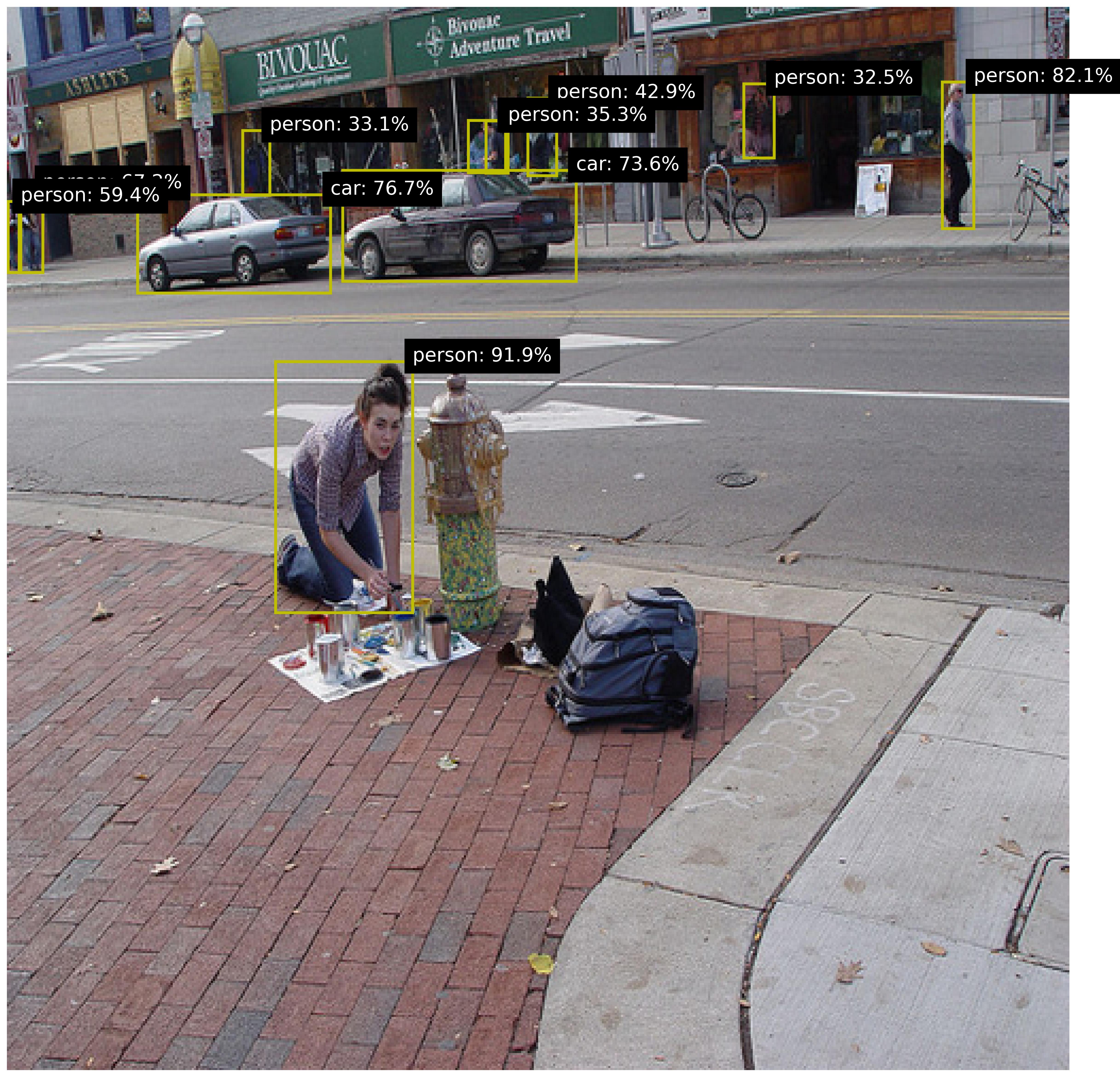
### Visual Description
## Object Detection Analysis: Street Scene with Confidence Scores
### Overview
This image is a photograph of an urban street scene overlaid with the results of an object detection algorithm. The algorithm has identified and placed bounding boxes around instances of "person" and "car," each accompanied by a confidence score percentage. The scene depicts a woman kneeling on a brick sidewalk in the foreground, with a street, parked cars, and storefronts in the background.
### Components/Axes
The image does not contain traditional chart axes. The primary informational components are the **object detection bounding boxes and labels**.
* **Bounding Box Style:** Yellow rectangular outlines.
* **Label Format:** Black text box with white text, formatted as `[class]: [confidence]%`.
* **Detected Classes:** `person`, `car`.
* **Background Text (Storefronts):** Visible English text includes "ASHLEY'S", "BIVOUAC", and "Bivouac Adventure Travel".
### Detailed Analysis
The detection results are spatially distributed across the image. Below is a list of all detected objects, ordered from the foreground (bottom of image) to the background (top of image), and from left to right within each depth plane.
**Foreground (Sidewalk):**
1. **person: 91.9%** - A woman kneeling on the brick sidewalk, interacting with paint cans and a decorated fire hydrant. This is the largest and most central detection.
**Background (Street & Storefronts):**
*Left Side:*
2. **person: 59.4%** - A person standing on the far-left sidewalk, partially cut off by the image frame.
3. **person: 67.2%** - A person standing near the left edge, behind the first car.
4. **car: 76.7%** - A silver sedan parked at the curb.
5. **person: 33.1%** - A person standing on the sidewalk behind the silver car.
*Center:*
6. **car: 73.6%** - A dark-colored sedan parked behind the silver car.
7. **person: 35.3%** - A person standing on the sidewalk, partially obscured by the dark car.
8. **person: 42.9%** - A person standing further back on the sidewalk, near a bicycle rack.
*Right Side:*
9. **person: 32.5%** - A person standing in the doorway of a store.
10. **person: 82.1%** - A person standing on the far-right sidewalk, near a bicycle.
### Key Observations
1. **Confidence vs. Proximity/Occlusion:** The highest confidence score (91.9%) is assigned to the most prominent, unobstructed subject in the foreground. Confidence scores generally decrease for objects that are smaller, further away, or partially occluded (e.g., persons at 33.1%, 35.3%, 32.5%).
2. **Class Distribution:** The model detected 8 instances of `person` and 2 instances of `car`.
3. **Spatial Grounding:** All bounding boxes are accurately placed around the visual extent of the objects they label. The labels are positioned directly above or adjacent to their corresponding boxes.
4. **Scene Context:** The detections are overlaid on a coherent street scene containing storefronts ("Bivouac Adventure Travel"), a crosswalk, a decorated fire hydrant, and personal items (backpack, paint supplies).
### Interpretation
This image serves as a visualization of an object detection model's output on a real-world scene. The data suggests the following:
* **Model Performance:** The model successfully localizes multiple instances of two common object classes (`person`, `car`) across varying scales and levels of occlusion. The high confidence on the foreground subject indicates strong feature recognition for clear, large examples.
* **Scene Understanding:** The distribution of detections provides a quantitative snapshot of the scene's composition: a primary human subject engaged in an activity, with background pedestrian and vehicular traffic typical of an urban commercial area.
* **Potential Limitations:** The lower confidence scores for some background persons may indicate challenges with scale, partial visibility, or less distinctive features at a distance. The model did not detect other present objects such as bicycles, the fire hydrant, or backpack, which defines the current scope of its trained classes.
* **Investigative Value:** For a technical document, this output demonstrates the model's capability and provides concrete examples of its precision (accurate bounding boxes) and confidence calibration across different object instances within a single complex image. The variance in confidence scores is a key metric for evaluating model reliability in practical applications.
</details>
Figure 6: Examples of the MS-COCO dataset with images of everyday scenes.
The pattern of interest is ‘person next to a car’. We consider all images that have a maximum of two persons and two cars, yielding 1728 images. We use random 8 positive and 8 negative images for training, which is repeated 5 times. We test both ILP variants, Popper and Propper, for the MaxSynth constrainer, because the Combo constrainer regularly did not return a solution. We validate Popper with various thresholds to be included as background knowledge. Propper does not need such a threshold beforehand, as all background knowledge is considered in a probabilistic manner. The results are shown in Table 2. Propper is the best performer, achieving f1 = 0.947. This is significantly better than the alternatives: SVM achieves f1 = 0.668 (-0.279) and Popper achieves f1 = 0.596 (-0.351). Adding probabilistic behavior to ILP is helpful for challenging datasets.
Table 2: Model variants and performance on MS-COCO.
| ILP | Propper (ours) | MaxSynth | probabilistic | BCE | - | 0.754 |
| --- | --- | --- | --- | --- | --- | --- |
| Statistical ML | SVM | - | - | - | - | 0.668 |
| Statistical ML | SVM (ordered) | - | - | - | - | 0.652 |
| ILP | Popper | MaxSynth | Prolog | MDL | 0.3 | 0.596 |
| ILP | Popper | MaxSynth | Prolog | MDL | 0.5 | 0.466 |
| ILP | Popper | MaxSynth | Prolog | MDL | 0.4 | 0.320 |
Table 3 shows the learned programs, how often each program was predicted across the experimental repetitions, and the respective resulting f1 scores. The best program is that there is a person on a car. Popper yields the same program, however, with a lower f1-score, since the background knowledge is thresholded before learning the program, removing important data from the background knowledge. This confirms that in practice it is intractable to set a perfect threshold on the background knowledge. It is beneficial to use Propper which avoids such prior thresholding.
Table 3: Learned programs, prevalence and performance on MS-COCO.
| Popper Popper Popper | 0.72 0.72 0 | 20 40 20 | f(A) :- has_object(A,C), is_on(B,C), person(B). f(A) :- person(C), is_on(C,B), has_object(A,C), car(B). No program learned. |
| --- | --- | --- | --- |
## 5 Discussion and Conclusions
We proposed Propper, which handles flawed and probabilistic background knowledge by extending ILP with a combination of neurosymbolic inference, a continuous criterion for hypothesis selection (BCE), and a relaxation of the hypothesis constrainer (NoisyCombo). Neurosymbolic inference has a significant impact on the results. Its advantage is that it does not need prior thresholding on the probabilistic background knowledge (BK), which is needed for binary ILP and is always imperfect. NoisyCombo has a small yet positive effect. It provides a parameter for the level of noise in BK, which can be tailored to the dataset at hand. The BCE has little impact. Propper is able to learn a logic program about a relational pattern that distinguishes between two sets of images, even if the background knowledge is provided by an imperfect neural network that predicts concepts in the images with some confidence. With as few as a handful of examples, Propper learns effective programs and outperforms statistical ML methods such as a GNN.
Although we evaluated Propper on two common datasets with different recording conditions, a broader evaluation of Propper across various domains and datasets to confirm its generalizability and robustness for various (especially non-image) use cases, is interesting. The proposed framework of integrated components allows for an easy setup of the system and simple adaptation to new developments/algorithms within the separate components. However, the integration as is performed now could be non-optimal in terms of computational efficiency. For example the output of the hypothesis generation is an answer set, which in Popper is converted to Prolog syntax. Propper converts this Prolog syntax to Scallop syntax. Developing a direct conversion from the answer sets to the Scallop syntax is recommended. We favored modularization over full integration and computational efficiency, in order to facilitate the methodological configuration and comparison of the various components. It is interesting to investigate whether a redesign of the whole system with the components integrated will lead to a better system. To make the step to fully probabilistic ILP, the allowance of probabilistic rules should be added to the system as well, for example by integration of StarAI methods raedt2016statistical.