2408.11367v2

# Towards Probabilistic Inductive Logic Programming with Neurosymbolic Inference and Relaxation **Authors**: F. Hillerström and G.J. Burghouts > TNO, The Netherlands refs.bib Hillerström and Burghouts 116 2024 10.1017/xxxxx ## Abstract Many inductive logic programming (ILP) methods are incapable of learning programs from probabilistic background knowledge, e.g. coming from sensory data or neural networks with probabilities. We propose Propper, which handles flawed and probabilistic background knowledge by extending ILP with a combination of neurosymbolic inference, a continuous criterion for hypothesis selection (BCE) and a relaxation of the hypothesis constrainer (NoisyCombo). For relational patterns in noisy images, Propper can learn programs from as few as 8 examples. It outperforms binary ILP and statistical models such as a Graph Neural Network. keywords: Inductive Logic Programming, Neurosymbolic inference, Probabilistic background knowledge, Relational patterns, Sensory data. ## 1 Introduction Inductive logic programming (ILP) muggleton1995inverse learns a logic program from labeled examples and background knowledge (e.g. relations between entities). Due to the strong inductive bias imposed by the background knowledge, ILP methods can generalize from small numbers of examples cropper2022inductive. Other advantages are the ability to learn complex relations between the entities, the expressiveness of first-order logic, and the resulting program can be understood and transferred easily because it is in symbolic form cropper2022_30newintro. This makes ILP an attractive alternative methodology besides statistical learning methods. For many real-world applications, dealing with noise is essential. Mislabeled samples are one source of noise. To learn from noisy labels, various ILP methods have been proposed to generalize a subset of the samples srinivasan2001aleph,ahlgren2013efficient,zeng2014quickfoil,raedt2015inducing. To advance methods to learn recursive programs and invent new predicates, Combo cropper2023learning was proposed, a method that searches for small programs that generalize subsets of the samples and combines them. MaxSynth hocquette2024learning extends Combo to allow for mislabeled samples, while trading off program complexity for training accuracy. These methods are dealing with noisy labels, but do not explicitly take into account errors in the background knowledge, nor are they designed to deal with probabilistic background knowledge. Most ILP methods take as a starting point the inputs in symbolic declarative form cropper2021turning. Real-world data often does not come in such a form. A predicate $p(.)$ , detected in real-world data, is neither binary or perfect. The assessment of the predicate can be uncertain, resulting in a non-binary, probabilistic predicate. Or the assessment can be wrong, leading to imperfect predicates. Dealing with noisy and probabilistic background knowledge is relevant for learning from sources that exhibit uncertainties. A probabilistic source can be a human who needs to make judgements at an indicated level of confidence. A source can also be a sensor measurement with some confidence. For example, an image is described by the objects that are detected in it, by a deep learning model. Such a model predicts locations in the image where objects may be, at some level of confidence. Some objects are detected with a lower confidence than others, e.g. if the object is partially observable or lacks distinctive visual features. The deep learning model implements a probabilistic predicate that a particular image region may contain a particular object, e.g. 0.7 :: vehicle(x). Given that most object detection models are imperfect in practice, it is impossible to determine a threshold that distinguishes the correct and incorrect detections. Two common ILP frameworks, Aleph srinivasan2001aleph and Popper learning_from_failures, typically fail to find the correct programs when dealing with predicted objects in images helff2023v; even with a state-of-the-art object detection model, and after advanced preprocessing of said detections. In the absence of an ideal binarization of probabilities, most ILP methods are not applicable to probabilistic sources cropper2021turning. <details> <summary>x1.png Details</summary>  ### Visual Description ## Diagram: Neurosymbolic Inference System with Probabilistic Background Knowledge ### Overview The image depicts a hybrid neurosymbolic inference system combining logic programming with probabilistic reasoning. It features a cyclical process for hypothesis generation and testing, alongside visual examples of object detection in aerial imagery. The system uses probabilistic background knowledge to constrain hypothesis selection and iteratively refines constraints based on test failures. ### Components/Axes **Left Section (Flowchart):** - **Nodes:** - `Predicates` (top-left) - `Constraints` (top-center) - `Generate` (center) - `Test` (right-center) - `failure` (bottom-center) - **Arrows:** - `learned constraints` (from Constraints to Generate) - `logic program` (from Generate to Test) - `is_on(vehicle, bridge)` (example predicate) - `relaxation of the hypothesis constrainer (NoisyCombo)` (from failure back to Constraints) - **Labels:** - `contribution #1` (near "Neurosymbolic inference") - `contribution #2` (near "BCE") - `contribution #3` (near "NoisyCombo") **Right Section (Image Grid):** - **Images:** Four aerial photographs showing roads, bridges, and vehicles. - **Annotations:** - **Green boxes (positives):** - `0.33 :: vehicle(A)` - `0.68 :: bridge(B)` - `0.92 :: is_close(A,B)` - `0.95 :: is_on(A,B)` - **Red boxes (negatives):** - `0.21 :: is_on(vehicle, bridge)` - `0.00 :: is_on(vehicle, bridge)` - `0.31 :: vehicle(A)` - `0.42 :: bridge(B)` - `0.29 :: is_close(A,B)` - `0.00 :: is_on(A,B)` - **Legend:** - Green = positives - Red = negatives ### Detailed Analysis **Flowchart Process:** 1. **Hypothesis Generation:** Combines predicates (e.g., `is_on(vehicle, bridge)`) with learned constraints to produce logic programs. 2. **Testing:** Evaluates hypotheses against real-world data (aerial images). 3. **Failure Handling:** Relaxes constraints (via NoisyCombo) when tests fail, enabling iterative refinement. **Image Annotations:** - **Positive Examples (Green):** High-confidence detections (e.g., 0.95 for `is_on(A,B)`). - **Negative Examples (Red):** Low-confidence or incorrect predictions (e.g., 0.00 for `is_on(vehicle, bridge)`). - **Probabilistic Scores:** Percentages in bounding boxes (e.g., "vehicle: 54.8%") likely represent model confidence in detections. ### Key Observations 1. **Iterative Refinement:** The flowchart's cyclical nature suggests adaptive learning from failures. 2. **Confidence Thresholding:** Negative examples with 0.00 scores indicate strict filtering of low-confidence predictions. 3. **Spatial Relationships:** The `is_close` and `is_on` predicates highlight the system's ability to reason about object proximity and positioning. 4. **Probabilistic Grounding:** Percentages in images (e.g., "bridge: 77.1%") demonstrate integration of probabilistic background knowledge. ### Interpretation This system bridges symbolic logic (e.g., `is_on(vehicle, bridge)`) with probabilistic reasoning, enabling robust object detection in complex aerial imagery. The iterative constraint relaxation (NoisyCombo) addresses noisy real-world data, while the BCE (Binary Cross-Entropy) criterion ensures only high-confidence hypotheses are retained. The visual examples show the system's ability to detect vehicles and bridges with varying confidence, though some cases (e.g., 0.00 scores) reveal limitations in handling ambiguous scenarios. The integration of learned constraints with probabilistic background knowledge suggests a framework for improving generalization in uncertain environments. 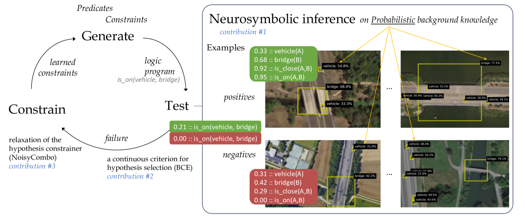</details> Figure 1: Our method Propper extends the ILP method Popper that learns from failures (left) with neurosymbolic inference to test logical programs on probabilistic background knowledge, e.g. objects detected in images with a certain probability (right). We propose a method towards probabilistic ILP. At a high level, ILP methods typically induce a logical program that entails many positive and few negative samples, by searching the hypothesis space, and subsequently testing how well the current hypothesis fits the training samples cropper2022_30newintro. One such method is Popper, which learns from failures (LFF) learning_from_failures, in an iterative cycle of generating hypotheses, testing them and constraining the hypothesis search. Our proposal is to introduce a probabilistic extension to LFF at the level of hypothesis testing. For that purpose, we consider neurosymbolic AI hybrid_ai. Within neurosymbolic AI a neural network predicts the probability for a predicate. For example a neural network for object detection, which outputs a probability for a particular object being present in an image region, e.g., 0.7 :: vehicle(x). Neurosymbolic AI connects this neural network with knowledge represented in a symbolic form, to perform reasoning over the probabilistic predicates predicted by the neural network. With this combination of a neural network and symbolic reasoning, neurosymbolic AI can reason over unstructured inputs, such as images. We leverage neurosymbolic programming and connect it to the tester within the hypothesis search. One strength of neurosymbolic programming is that it can deal with uncertainty and imperfect information hybrid_ai,neuro_symbolic,scallop,scallop_foundationmodels, in our case the probablistic background knowledge. We propose to use neurosymbolic inference as tester in the test-phase of the LFF cycle. Neurosymbolic reasoning calculates an output probability for a logical query being true, for every input sample. The input samples are the set of positive and negative examples, together with their probabilistic background knowledge. The logical query evaluated within the neurosymbolic reasoning is the hypothesis generated in the generate-phase of the LFF cycle, which is a first-order-logic program. With the predicted probability of the hypothesis being true per sample, it becomes possible to compute how well the hypothesis fits the training samples. That is used to continue the LFF cycle and generate new constraints based on the failures. Our contribution is a step towards probabilistic ILP by proposing a method called Propper. It builds on an ILP framework that is already equipped to deal with noisy labels, Popper-MaxSynth learning_from_failures,hocquette2024learning, which we extend with neurosymbolic inference which is able to process probabilistic facts, i.e. uncertain and imperfect background knowledge. Our additional contributions are a continuous criterion for hypothesis selection, that can deal with probabilities, and a relaxed formulation for constraining the hypothesis space. Propper and the three contributions are outlined in Figure 1. We compare Popper and Propper with statistical ML models (SVM and Graph Neural Network) for the real-life task of finding relational patterns in satellite images based on objects predicted by an imperfect deep learning model. We validate the learning robustness and efficiency of the various models. We analyze the learned logical programs and discuss the cases which are hard to predict. ## 2 Related Work For the interpretation of images based on imperfect object predictions, ILP methods such as Aleph srinivasan2001aleph and Popper learning_from_failures proved to be vulnerable and lead to incorrect programs or not returning a program at all helff2023v. Solutions to handle observational noise were proposed cropper2021beyondentailment for small binary images. With LogVis muggleton2018meta images are analyzed via physical properties. This method could estimate the direction of the light source or the position of a ball from images in very specific conditions or without clutter or distractors. $Meta_{Abd}$ dai2020abductive jointly learns a neural network with induction of recursive first-order logic theories with predicate invention. This was demonstrated on small binary images of digits. Real-life images are more complex and cluttered. We aim to extend these works to realistic samples, e.g. large color images that contain many objects under partial visiblity and in the midst of clutter, causing uncertainties. Contrary to $Meta_{Abd}$ , we take pretrained models as a starting point, as they are often already very good at their task of analyzing images. Our focus is on extending ILP to handle probabilistic background knowledge. In statistical relational artificial intelligence (StarAI) raedt2016statistical the rationale is to directly integrate probabilities into logical models. StarAI addresses a different learning task than ILP: it learns the probabilistic parameters of a given program, whereas ILP learns the program cropper2021turning. Probabilities have been integrated into ILP previously. Aleph srinivasan2001aleph was used to find interesting clauses and then learn the corresponding weights huynh2008discriminative. ProbFOIL raedt2015inducing and SLIPCOVER bellodi2015structure search for programs with probabilities associated to the clauses, to deal with the probabilistic nature of the background knowledge. SLIPCOVER searches the space of probabilistic clauses using beam search. The clauses come from Progol muggleton1995inverse. Theories are searched using greedy search, where refinement is achieved by adding a clauses for a target predicate. As guidance the log likelihood of the data is considered. SLIPCOVER operates in a probabilistic manner on binary background knowledge, where our goal is to involve the probabilities associated explicitly the background knowledge. How to combine these probabilistic methods with recent ILP frameworks is unclear. In our view, it is not trivial and possibly incompatible. Our work focuses on integrating a probabilistic method into a modern ILP framework, in a simple yet elegant manner. We replace the binary hypothesis tester of Popper learning_from_failures by a neurosymbolic program that can operate on probabilistic and imperfect background knowledge hybrid_ai,neuro_symbolic. Rather than advanced learning of both the knowledge and the program, e.g. NS-CL mao2019neuro, we take the current program as the starting point. Instead of learning parameters, e.g. Scallop scallop, we use the neurosymbolic program for inference given the program and probabilistic background knowledge. Real-life samples may convey large amounts of background knowledge, e.g. images with many objects and relations between them. Therefore, scalability is essential. Scallop scallop improved the scalability over earlier neurosymbolic frameworks such as DeepProbLog deepproblog,deepproblog_efficient. Scallop introduced a tunable parameter $k$ to restrain the validation of hypotheses by analyzing the top- $k$ proofs. They asymptotically reduced the computational cost while providing relative accuracy guarantees. This is beneficial for our purpose. By replacing only the hypothesis tester, the strengths of ILP (i.e. hypothesis search) are combined with the strengths of neurosymbolic inference (i.e. probabilistic hypothesis testing). ## 3 Propper Algorithm To allow ILP on flawed and probabilistic background knowledge, we extend modern ILP (Section 3.1) with neurosymbolic inference (3.2) and coin our method Propper. The neurosymbolic inference requires program conversion by grammar functions (3.3), and we added a continuous criterion for hypothesis selection (3.4), and a relaxation of the hypothesis constrainer (3.5). ### 3.1 ILP: Popper Popper represents the hypothesis space as a constraint satisfaction problem and generates constraints based on the performance of earlier tested hypotheses. It works by learning from failures (LFF) learning_from_failures. Given background knowledge $B$ , represented as a logic program, positive examples $E^{+}$ and negative examples $E^{-}$ , it searches for a hypothesis $H$ that is complete ( $\forall e\in E^{+},H\cup B\models e$ ) and consistent ( $\forall e\in E^{-},H\cup B\not\models e$ ). The algorithm consists of three main stages (see Figure 1, left). First a hypothesis in the form of a logical program is generated, given the known predicates and constraints on the hypothesis space. The Test stage tests the generated logical program against the provided background knowledge and examples, using Prolog for inference. It evaluates whether the examples are entailed by the logical program and background knowledge. From this information, failures that are made when applying the current hypothesis, can be identified. These failures are used to constrain the hypothesis space, by removing specializations or generalizations from the hypothesis space. In the original Popper implementation learning_from_failures, this cycle is repeated until an optimal solution is found; the smallest program that covers all positives and no negative examples See learning_from_failures for a formal definition.. Its extension Combo combines small programs that do not entail any negative example cropper2023learning. When no optimal solution is found, Combo returns the obtained best solution. The Popper variant MaxSynth does allow noise in the examples and generates constraints based on a minimum description length cost function, by comparing the length of a hypothesis with the possible gain in wrongly classified examples hocquette2024learning. ### 3.2 Neurosymbolic Inference: Scallop Scallop is a language for neurosymbolic programming which integrates deep learning with logical reasoning scallop. Scallop reasons over continuous, probabilistic inputs and results in a probabilistic output confidence. It consists of two parts: a neural model that outputs the confidence for a specific concept occurring in the data and a reasoning model that evaluates the probability for the query of interest being true, given the input. It uses provenance frameworks kimmig2017algebraic to approximate exact probabilistic inference, where the AND operator is evaluated as a multiplication ( $AND(x,y)=x*y$ ), the OR as a minimization ( $OR(x,y)=min(1,x+y)$ ) and the NOT as a $1-x$ . Other, more advanced formulations are possible, e.g. $noisy$ - $OR(x,y)=1-(1-a)(1-b)$ for enhanced performance. For ease of integration, we considered this basic provenance. To improve the speed of the inference, only the most likely top-k hypotheses are processed, during the intermediate steps of computing the probabilities for the set of hypotheses. ### 3.3 Connecting ILP and Neurosymbolic Inference Propper changes the Test stage of the Popper algorithm (see Figure 1): the binary Prolog reasoner is replaced by the neurosymbolic inference using Scallop, operating on probabilistic background knowledge (instead of binary), yielding a probability for each sample given the logical program. The background knowledge is extended with a probability value before each first-order-logic statement, e.g. 0.7 :: vehicle(x). The Generate step yields a logic program in Prolog syntax. The program can cover multiple clauses, that can be understood as OR as one needs to be satisfied. Each clause is a function of predicates, with input arguments. The predicate arguments can differ between the clauses within the logic program. This is different from Scallop, where every clause in the logic program is assumed to be a function of the same set of arguments. As a consequence, the Prolog program requires syntax rewriting to arrive at an equivalent Scallop program. This rewriting involves three steps by consecutive grammar functions, which we illustrate with an example. Take the Prolog program: $$ \displaystyle\begin{split}\texttt{f(A)}={}&\texttt{has\_object(A, B), vehicle( B)}\\ \texttt{f(A)}={}&\texttt{has\_object(A, B), bridge(C), is\_on(B, C)}\end{split} \tag{1} $$ The bodies of f(A) are extracted by: $b(\texttt{f})$ = {[has_object(A, B), vehicle(B)], [has_object(A, B), bridge(C), is_on(B, C)]}. The sets of arguments of f(A) are extracted by: $v(\texttt{f})=\{\{\texttt{A, B}\},\{\texttt{C, A, B}\}\}$ . For a Scallop program, the clauses in the logic program need to be functions of the same argument set. Currently the sets are not the same: {A, B} vs. {C, A, B}. Function $e(\cdot)$ adds a dummy predicate for all non-used arguments, i.e. C in the first clause, such that all clauses operate on the same set, i.e. {C, A, B}: $$ \displaystyle\begin{split}e([\texttt{has\_object(A, B)},{}&\texttt{vehicle(B)} ],\{\texttt{C, A, B}\})=\\ &\texttt{has\_object(A, B), vehicle(B), always\_true(C)}\end{split} \tag{2} $$ After applying grammar functions $b(\cdot)$ , $v(\cdot)$ and $e(\cdot)$ , the Prolog program f(A) becomes the equivalent Scallop program g(C, A, B): $$ \displaystyle\begin{split}\texttt{g\textsubscript{0}(C, A, B)}={}&\texttt{has \_object(A, B), vehicle(B), always\_true(C)}\\ \texttt{g\textsubscript{1}(C, A, B)}={}&\texttt{has\_object(A, B), bridge(C), is\_on(B, C)}\\ \texttt{g(C, A, B)}={}&\texttt{g\textsubscript{0}(C, A, B) or g\textsubscript{ 1}(C, A, B)}\end{split} \tag{3} $$ ### 3.4 Selecting the Best Hypothesis MaxSynth uses a minimum-description-length (MDL) cost hocquette2024learning to select the best solution: $$ MDL_{B,E}=size(h)+fn_{B,E}(h)+fp_{B,E}(h) \tag{4} $$ The MDL cost compares the number of correctly classified examples with the number of literals in the program. This makes the cost dependent on the dataset size and requires binary predictions in order to determine the number of correctly classified examples. Furthermore, it is doubtful whether the number of correctly classified examples can be compared directly with the rule size, since it makes the selection of the rule size dependent on the dataset size again. Propper uses the Binary Cross Entropy (BCE) loss to compare the performance of hypotheses, as it is a more continuous measure than MDL. The neurosymbolic inference predicts an output confidence for an example being entailed by the hypothesis. The BCE-cost compares this predicted confidence with the groundtruth (one or zero). For $y_{i}$ being the groundtruth label and $p_{i}$ the confidence predicted via neurosymbolic inference for example $i$ , the BCE cost for $N$ examples becomes: $$ BCE=\frac{1}{N}\sum_{i=1}^{N}(y_{i}*log(p_{i})+(1-y_{i})*log(1-p_{i})). \tag{5} $$ Scallop reasoning automatically avoids overfitting, by punishing the size of the program, because when adding more or longer clauses the probability becomes lower by design. The more ANDs in the program, the lower the output confidence of the Scallop reasoning, due to the multiplication of the probabilities. Therefore, making a program more specific will result in a higher BCE-cost, unless the specification is beneficial to remove FPs. Making the program more generic will cover more samples (due to the addition operator for the OR). However the confidences for the negative samples will increase as well, which will increase the BCE-cost again. The BCE-cost is purely calculated on the predictions itself, and thereby removes the dependency on the dataset size and the comparison between number of samples and program length. ### 3.5 Constraining on Inferred Probabilities Whereas Combo cropper2023learning and MaxSynth hocquette2024learning yield optimal programs given perfect background knowledge, with imperfect and probabilistic background knowledge no such guarantees can be provided. The probabilistic outputs of Scallop are converted into positives and negatives before constraining. The optimal threshold is chosen by testing 15 threshold values, evenly spaced between 0 and 1 and selecting the threshold resulting in the most highest true positives plus true negatives on the training samples. MaxSynth generates constraints based on the MDL loss hocquette2024learning, making the constraints dependent on the size of the dataset. To avoid this dependency, we introduce the NoisyCombo constrainer. Combo generates constraints once a false positive (FP) or negative (FN) is detected. $\exists e\in E^{-},H\cup B\models e$ : prune generalisations. $\exists e\in E^{+},H\cup B\not\models e$ or $\forall e\in E^{-},H\cup B\not\models e$ : prune specialisations. NoisyCombo relaxes this condition and allows a few FPs and FNs to exist, depending on an expected noise level, inspired by LogVis muggleton2018meta. This parameter defines a percentage of the examples that could be imperfect, from which the allowed number of FPs and FNs is calculated. $\sum(e\in E^{-},H\cup B\models e)>noise\_level*N_{negatives}$ : prune generalisations. $\forall e\in E^{-},H\cup B\not\models e$ : prune specialisations. The positives are not thresholded by the noise level, since programs that cover at least one positive sample are added to the combiner. ## 4 Analyses We validate Propper on a real-life task of finding relational patterns in satellite images, based on flawed and probabilistic background knowledge about the objects in the images, which are predicted by an imperfect deep learning model. We analyze the learning robustness under various degrees of flaws in the background knowledge. We do this for various models, including Popper (on which Propper is based) and statistical ML models. In addition, we establish the learning efficiency for very low amounts of training data, as ILP is expected to provide an advantage because it has the inductive bias of background knowledge. We analyze the learned logical programs, to compare them qualitatively against the target program. Finally, we discuss the cases that are hard to predict. ### 4.1 First Dataset The DOTA dataset xia2018dota contains many satellite images. This dataset is very challenging, because the objects are small, and therefore visual details are lacking. Moreover, some images are very cluttered by sometimes more than 100 objects. <details> <summary>extracted/5868417/result_figs/pos_full.jpg Details</summary>  ### Visual Description ## Aerial Image with Object Detection Annotations: Bridge and Vehicle Analysis ### Overview The image is an aerial view of a bridge spanning a body of water, with roads on either side. Vehicles are annotated along the roads and bridge with yellow bounding boxes and percentage labels. The bridge and vehicles are labeled with confidence scores (e.g., "bridge: 77.1%", "vehicle: 55.5%"). The water appears dark green, and the surrounding area includes vegetation, buildings, and infrastructure. --- ### Components/Axes 1. **Bridge**: - Labeled with two confidence scores: **77.1%** and **86.4%**. - Positioned centrally over the water, connecting two landmasses. 2. **Vehicles**: - Annotated along roads on both sides of the bridge and on the bridge itself. - Confidence scores range from **30.1%** to **75.5%**. - Some annotations include secondary values (e.g., "vehicle: 37.0%: e: 58.0%"). 3. **Roads**: - Two parallel roads flank the bridge, with vehicles distributed along their lengths. 4. **Annotations**: - Black text boxes with yellow outlines contain labels like "vehicle" or "bridge" followed by percentages. - Positioned near detected objects (e.g., vehicles on roads, bridge structure). --- ### Detailed Analysis - **Bridge**: - Confidence scores: **77.1%** (lower-left annotation) and **86.4%** (upper-right annotation). - Likely represents detection confidence for the bridge structure, with higher scores near the bridge's midpoint. - **Vehicles**: - **Left Road**: - Scores: **37.0%**, **58.0%**, **30.1%**, **46.9%**, **50.4%**, **64.2%**. - Vehicles clustered near the bridge's base. - **Right Road**: - Scores: **38.5%**, **49.1%**, **55.1%**, **69.5%**, **48.7%**, **33.5%**. - Higher scores (e.g., **69.5%**) near the bridge's far end. - **Bridge Surface**: - Scores: **41.8%**, **55.5%**, **60.5%**, **75.5%**. - Vehicles on the bridge show increasing confidence toward the far end. - **Secondary Values**: - Some annotations include additional metrics (e.g., "e: 58.0%"), possibly indicating error margins or secondary classifications. --- ### Key Observations 1. **Bridge Confidence**: - The bridge's confidence scores (**77.1%**, **86.4%**) are consistently higher than most vehicle scores, suggesting the detection system prioritizes infrastructure over smaller objects. 2. **Vehicle Confidence Trends**: - Vehicles near the bridge's base have lower scores (e.g., **30.1%**, **33.5%**), while those farther away show higher scores (e.g., **69.5%**, **75.5%**). - Secondary values (e.g., "e: 58.0%") may reflect uncertainty in object classification or environmental factors. 3. **Spatial Distribution**: - Vehicles are denser near the bridge, with fewer annotations on open road segments. - The bridge's annotations are concentrated along its length, with higher scores toward the far end. --- ### Interpretation 1. **Object Detection System**: - The annotations likely represent output from a computer vision model (e.g., YOLO, Faster R-CNN) analyzing traffic or infrastructure. - Confidence scores indicate the model's certainty in detecting bridges and vehicles. 2. **Performance Insights**: - The bridge's high confidence scores suggest robust detection of large, static structures. - Vehicle scores vary, possibly due to factors like occlusion, distance, or lighting conditions. 3. **Anomalies**: - The secondary values (e.g., "e: 58.0%") lack clear context but may represent error rates or alternative classifications (e.g., vehicle type). 4. **Practical Implications**: - This data could be used for traffic monitoring, infrastructure assessment, or autonomous vehicle navigation systems. --- ### Spatial Grounding - **Bridge Annotations**: Centered over the bridge structure, with labels near the midpoint and far end. - **Vehicle Annotations**: - Left Road: Bottom-left quadrant. - Right Road: Bottom-right quadrant. - Bridge Surface: Along the bridge's length, with higher scores toward the far end. - **Legend**: No explicit legend, but annotations act as de facto labels with confidence scores. --- ### Trend Verification - **Bridge**: Confidence increases from **77.1%** to **86.4%** along its length. - **Vehicles**: Scores generally rise from lower (near bridge base) to higher (farther from bridge), with outliers like **30.1%** and **33.5%**. - **Secondary Metrics**: Inconsistent presence (e.g., "e: 58.0%") suggests optional or conditional annotations. --- ### Conclusion The image demonstrates an object detection system's performance in identifying bridges and vehicles from an aerial perspective. The bridge's high confidence scores contrast with variable vehicle detection accuracy, highlighting challenges in detecting smaller or dynamically positioned objects. Secondary metrics and spatial trends suggest opportunities for model refinement, such as improving low-confidence detections near infrastructure or clarifying ambiguous annotations. </details> (a) Positive image <details> <summary>extracted/5868417/result_figs/neg_full.jpg Details</summary>  ### Visual Description ## Aerial Photograph with Vehicle and Bridge Annotations ### Overview The image is an aerial view of an industrial complex, highway, river, and surrounding greenery. Yellow bounding boxes with percentage labels (e.g., "vehicle: 36.5%", "bridge: 79.1%") are overlaid on specific objects. The annotations appear to represent confidence scores or detection metrics, though no legend or context is provided. ### Components/Axes - **Primary Elements**: - Industrial complex (left side, large white/gray buildings). - Highway (vertical road, center-right). - River (dark blue, right side). - Green spaces (trees, grass, bottom-right). - **Annotations**: - Yellow bounding boxes with black text (e.g., "vehicle: X.X%"). - One box labeled "bridge: 79.1%". - **No explicit legend, axes, or scales**. ### Detailed Analysis - **Vehicle Annotations**: - Percentages range from **7.2% to 78.3%**, with most clustered between **30% and 60%**. - Examples: - Top-left industrial area: "vehicle: 36.5%", "vehicle: 47.3%". - Highway: "vehicle: 60.5%", "vehicle: 70.0%". - Bottom-right: "vehicle: 52.5%", "vehicle: 68.4%". - Some labels are partially cut off (e.g., "vehicle: 36.5%" at the top-left edge). - **Bridge Annotation**: - Located on the right side, spanning the river. - Label: "bridge: 79.1%". ### Key Observations 1. **Highest Confidence**: The bridge has the highest percentage (79.1%), suggesting it may be a focal point or larger object. 2. **Vehicle Density**: The industrial complex and highway have the most vehicle annotations, indicating higher activity or detection focus. 3. **Spatial Distribution**: - Vehicles are annotated predominantly on paved surfaces (highway, parking lots). - Fewer annotations in green areas (riverbanks, forests). 4. **Ambiguity**: No clear explanation for the percentages (e.g., detection confidence, object size, or classification accuracy). ### Interpretation - The annotations likely represent a computer vision model’s confidence scores for object detection (e.g., vehicles, bridges). - The bridge’s high score (79.1%) may reflect its size or structural distinctiveness compared to smaller vehicles. - The industrial complex and highway show varied vehicle percentages, possibly due to differences in object density, size, or model performance in complex scenes. - The lack of a legend or contextual metadata limits interpretation of the percentages’ exact meaning. ## Notes - All text is in English. - No data tables, charts, or diagrams present. - Percentages are approximate and lack uncertainty ranges. - Spatial grounding confirms annotations align with physical objects (e.g., bridge spans the river). </details> (b) Negative image <details> <summary>extracted/5868417/result_figs/pos_crop.jpg Details</summary>  ### Visual Description ## Screenshot: Aerial View of Bridge with Object Detection Annotations ### Overview The image is an aerial photograph of a bridge spanning a body of water, annotated with object detection confidence scores. Yellow bounding boxes highlight vehicles on the bridge, each labeled with a percentage indicating detection confidence. A larger yellow box encloses the entire bridge, labeled "bridge: 77.1%". The water appears dark green, while the bridge and surrounding land are lighter in tone. ### Components/Axes - **Textual Annotations**: - "bridge: 77.1%" (top-right corner, black text on yellow box). - "vehicle: 55.5%" (center-left, small yellow box). - "vehicle: 50.4%" (bottom-left, overlapping with another vehicle). - "vehicle: 64.2%" (bottom-left, overlapping with "vehicle: 50.4%"). - "vehicle: 38.5%" (center-right, small yellow box). - "vehicle: 49.1%" (bottom-right, small yellow box). - **Visual Elements**: - Bridge: Horizontal structure spanning the image, with a textured surface. - Water: Dark green areas on both sides of the bridge. - Land: Light-colored areas with vegetation (trees, shrubs) flanking the bridge. - Vehicles: Small, indistinct shapes within yellow boxes (no explicit labels beyond confidence scores). ### Detailed Analysis - **Bridge Detection**: - Confidence: 77.1% (highest in the image). - Position: Central horizontal structure, spanning the entire width of the image. - **Vehicle Detections**: - Confidence scores range from **38.5% to 64.2%**, with no clear spatial pattern. - Positions: - 55.5%: Center-left of the bridge. - 50.4% and 64.2%: Overlapping near the bottom-left of the bridge. - 38.5%: Center-right of the bridge. - 49.1%: Bottom-right of the bridge. - Vehicle shapes are pixelated and lack distinct features (e.g., color, size). ### Key Observations 1. **Bridge Confidence Dominance**: The bridge is detected with significantly higher confidence (77.1%) than any individual vehicle. 2. **Vehicle Confidence Variability**: Vehicle confidence scores are inconsistent, suggesting potential challenges in detecting smaller or occluded objects. 3. **Overlapping Annotations**: Two vehicles (50.4% and 64.2%) share a bounding box, indicating possible model uncertainty in distinguishing closely spaced objects. 4. **Unlabeled Object**: A small white object in the water below the bridge lacks annotation, possibly an outlier or irrelevant to the detection task. ### Interpretation - **Model Performance**: The high confidence in bridge detection (77.1%) suggests the model effectively identifies large, continuous structures. However, lower vehicle confidence scores (38.5–64.2%) highlight limitations in detecting smaller or overlapping objects, which may require improved feature extraction or training data. - **Spatial Relationships**: The bridge’s uniform detection contrasts with the scattered, lower-confidence vehicle annotations, emphasizing the model’s reliance on object size and continuity. - **Anomalies**: The unlabeled white object in the water raises questions about the model’s focus—was it intentionally excluded, or is it a false negative? This analysis underscores the trade-offs in object detection systems: high accuracy for prominent objects versus challenges in resolving fine-grained details like individual vehicles. </details> (c) (zoom) <details> <summary>extracted/5868417/result_figs/neg_crop.jpg Details</summary>  ### Visual Description ## Screenshot: Aerial View with Object Detection Annotations ### Overview The image is an aerial view of a landscape featuring a river, roads, greenery, and infrastructure. Key elements include a bridge spanning a river, a road network, and multiple vehicles annotated with confidence percentages. The annotations are overlaid as black text boxes with white text, accompanied by yellow bounding boxes highlighting detected objects. ### Components/Axes - **Annotations**: - **Bridge**: Labeled "bridge: 79.1%" in the top-right quadrant, positioned above a yellow rectangular bounding box encompassing the bridge structure. 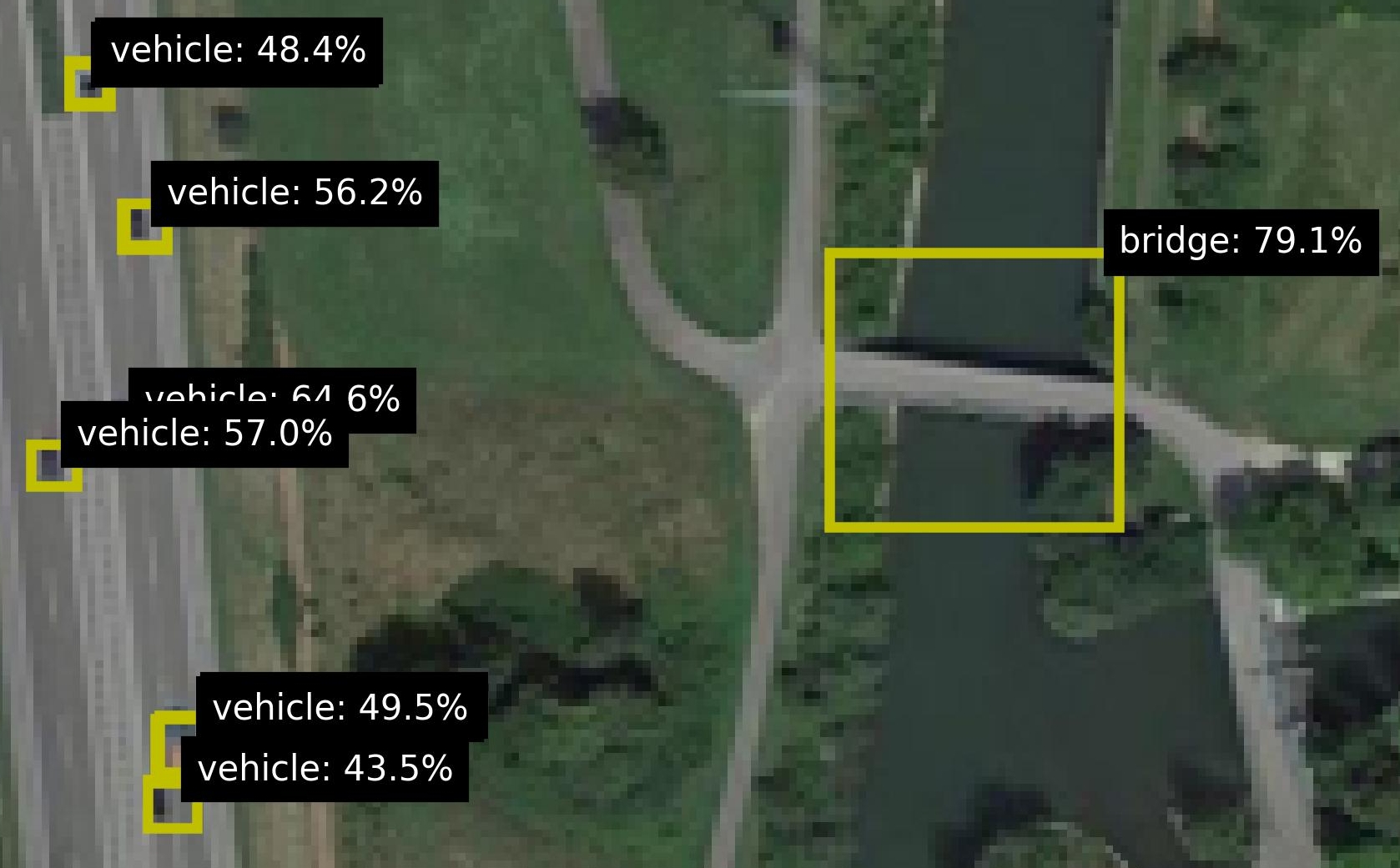- **Vehicles**: Six annotations labeled "vehicle: [percentage]" (48.4%, 56.2%, 64.6%, 57.0%, 49.5%, 43.5%) clustered along the left side of the image, aligned with yellow bounding boxes indicating vehicle positions on the road. - **Spatial Layout**: - **River**: Dark green watercourse running diagonally from top-right to bottom-left. - **Roads**: Gray pathways intersecting near the bridge, with one road curving leftward and another extending rightward. - **Greenery**: Light green fields and trees flanking the river and roads. ### Detailed Analysis - **Bridge**: - Confidence: 79.1% (highest among all annotations). - Position: Central-right, spanning the river. - Bounding Box: Yellow rectangle tightly aligned with the bridge's structure. - **Vehicles**: - Confidence scores range from 43.5% (lowest) to 64.6% (highest). - Positions: Left side of the image, distributed along the road parallel to the river. - Bounding Boxes: Yellow squares varying in size, correlating with vehicle dimensions and distances from the camera. - **Unlabeled Elements**: - River, roads, and greenery lack explicit annotations but are visually distinct. ### Key Observations 1. **Confidence Discrepancies**: Vehicle confidence scores vary significantly (43.5%–64.6%), suggesting differences in detection reliability, possibly due to occlusion, distance, or model uncertainty. 2. **Bridge Prominence**: The bridge's high confidence score (79.1%) indicates it is a dominant feature in the model's analysis, likely due to its size and structural clarity. 3. **Spatial Correlation**: Vehicles are concentrated on the left road, while the bridge dominates the right, reflecting a divided focus in the scene. ### Interpretation This image appears to be output from an object detection system analyzing infrastructure and traffic. The bridge's high confidence score highlights its importance as a critical infrastructure element, while the varying vehicle percentages may reflect challenges in detecting smaller or partially obscured objects. The absence of annotations for the river and roads suggests the model prioritizes man-made structures over natural features. The spatial distribution of annotations implies the system is tracking traffic flow on the left road and monitoring the bridge's presence, potentially for applications like traffic management or infrastructure monitoring. The lack of a legend or color-coded key limits direct correlation between bounding box colors and confidence levels, but the yellow boxes consistently highlight detected objects. 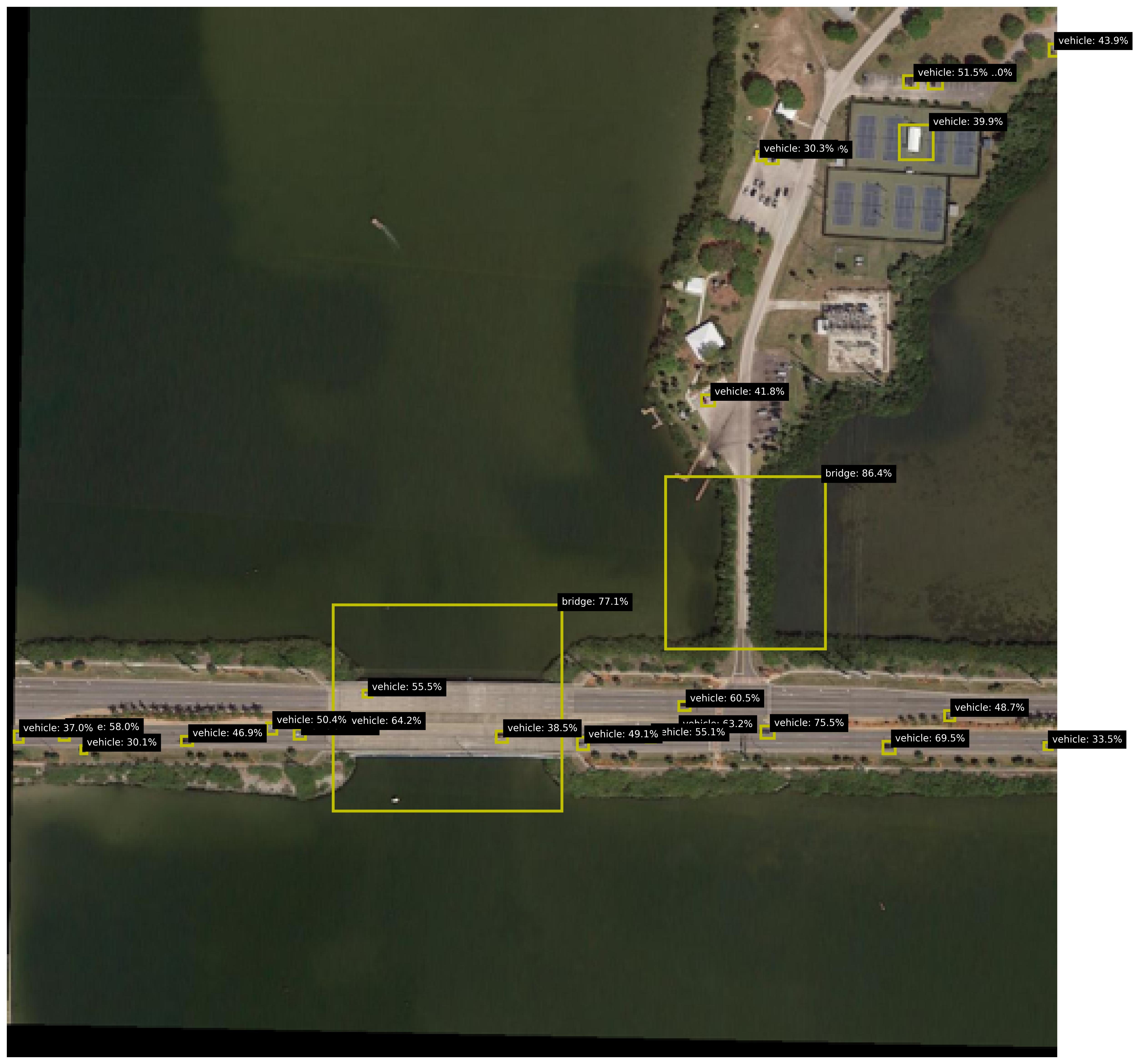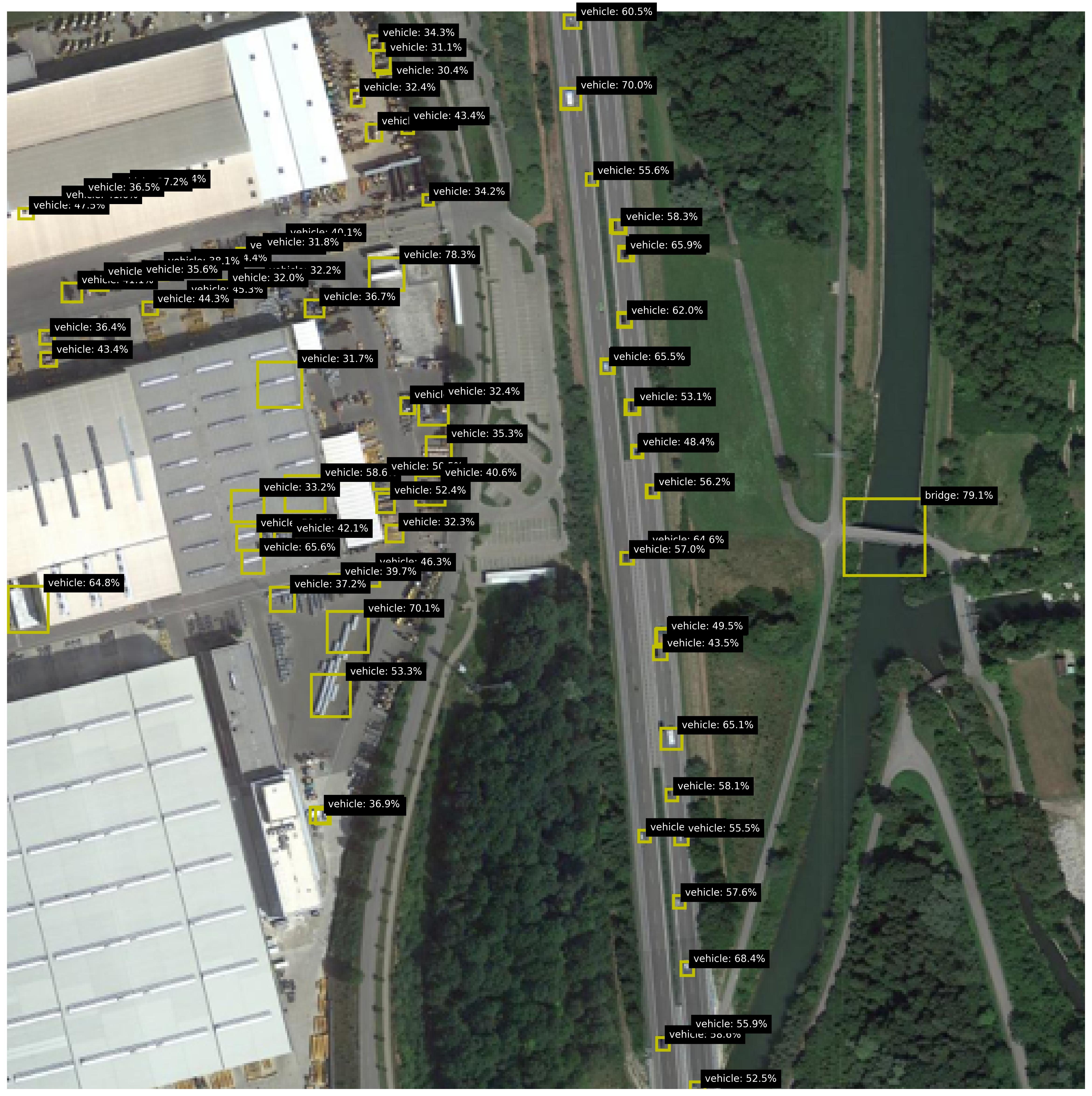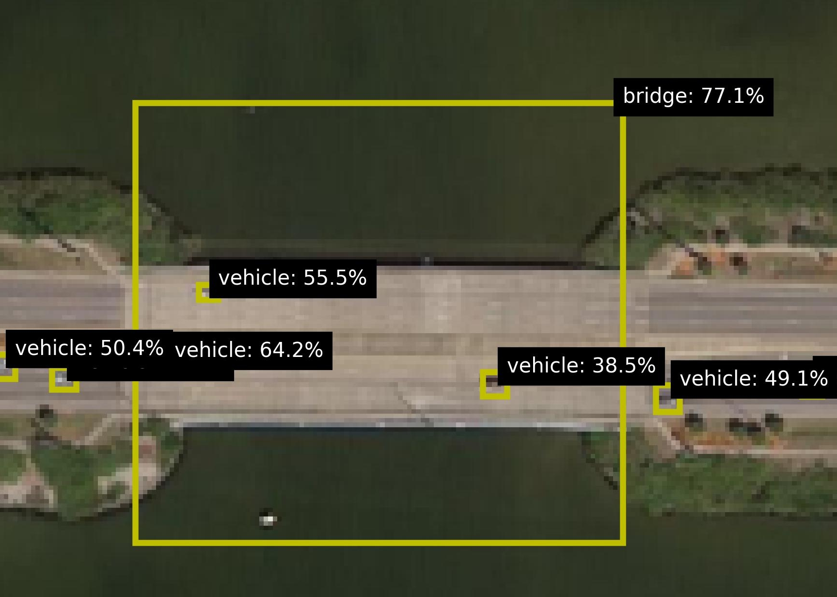</details> (d) (zoom) Figure 2: Examples of images with the detected objects and their probabilities. 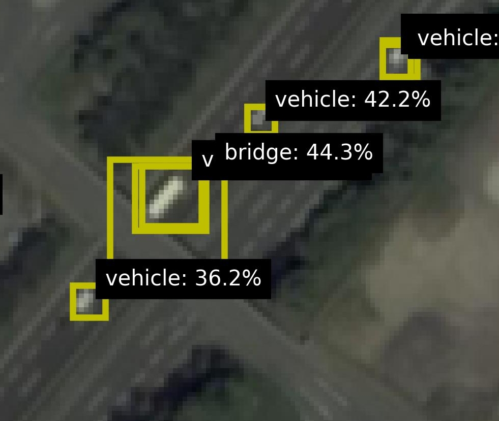For the background knowledge, we leverage the pretrained DOTA Aerial Images Model dota_model to predict the objects in the images, with for each object a label, location (bounding box) and a probability (confidence value). For each image, the respective predictions are added to the background knowledge, as a predicate with a confidence, e.g. 0.7 :: vehicle(x). The locations of the objects are used to calculate a confidence for two relations: is_on and is_close. This information is added to the background knowledge as well. Figure 2 shows various images from the dataset, including zoomed versions to reveal some more details and to highlight the small size of the objects. Figure 2(b) shows an image with many objects. The relational patterns of interest is ‘vehicle on bridge’. For this pattern, there are 11 positive test images and 297 negative test images. Figure 2 shows both a positive (left) and negative image (right). To make the task realistic, both sets contain images with vehicles, bridges and roundabouts, so the model cannot distinguish the positives and negatives by purely finding the right sets of objects; the model really needs to find the right pattern between the right objects. Out of the negative images, 17 are designated as hard, due to incorrect groundtruths (2 images) and incorrect detections (15 images). These hard cases are shown in Figure 3. <details> <summary>extracted/5868417/result_figs/fp_crop_1.jpg Details</summary>  ### Visual Description ## Screenshot: Object Detection Interface ### Overview The image is a pixelated aerial view of a roadway with three yellow bounding boxes highlighting vehicles. Each box is annotated with a label indicating "vehicle" or "bridge" and a percentage value. The interface appears to be from a computer vision system, likely used for object detection or classification. ### Components/Axes - **Labels**: - "vehicle: 36.2%" (bottom-left box) - "v bridge: 44.3%" (middle box) - "vehicle: 42.2%" (top-right box) - **Visual Elements**: - Yellow bounding boxes of varying sizes. - Pixelated roadway with greenery and infrastructure. - **Text**: All labels are in white font on black rectangular backgrounds. ### Detailed Analysis 1. **Bottom-Left Box**: - Label: "vehicle: 36.2%" - Size: Largest bounding box. - Position: Bottom-left quadrant of the image. 2. **Middle Box**: - Label: "v bridge: 44.3%" - Size: Medium-sized box. - Position: Center-right, overlapping the roadway. 3. **Top-Right Box**: - Label: "vehicle: 42.2%" - Size: Smallest box. - Position: Top-right corner. ### Key Observations - The "bridge" label (44.3%) has the highest percentage, suggesting higher confidence in bridge detection compared to vehicles. - The largest vehicle (36.2%) has the lowest confidence, while smaller vehicles have higher confidence (42.2% and 44.3%). - No legend is visible to confirm color-coding, but yellow boxes are consistently used for annotations. ### Interpretation - **Confidence Scores**: The percentages likely represent confidence scores from an object detection model. Higher scores (e.g., 44.3%) indicate stronger model certainty, while lower scores (36.2%) suggest uncertainty, possibly due to occlusion, size, or environmental factors. - **Bridge vs. Vehicle Detection**: The system prioritizes bridge detection (44.3%) over vehicles, which may reflect training data biases or feature prominence. - **Size-Confidence Paradox**: Larger vehicles have lower confidence, which could indicate challenges in detecting larger objects (e.g., due to resolution limits or algorithmic focus on smaller features). - **Pixelation**: The low-resolution image may reduce detection accuracy, particularly for smaller or distant objects. This data highlights potential limitations in the object detection system, such as size-dependent confidence and environmental interference. Further analysis could explore model adjustments to improve detection of larger vehicles or low-resolution inputs. </details> <details> <summary>extracted/5868417/result_figs/fp_crop_2.jpg Details</summary>  ### Visual Description ## Satellite Image with Annotated Landmarks and Vehicle Detection ### Overview The image depicts a satellite view of a highway interchange with annotated landmarks and vehicle detection results. Key elements include: - A curved highway interchange with multiple lanes - Two yellow bounding boxes highlighting specific areas - Text annotations with percentages indicating detection confidence scores - A circular roadway feature in the upper-right quadrant ### Components/Axes **Annotations:** 1. **Bridge**: Labeled "bridge: 46.3%" in a black box with white text, positioned above a yellow bounding box covering a bridge structure. 2. **Vehicle 1**: Labeled "vehicle: 65.8%" in a black box, located near the bridge annotation. 3. **Vehicle 2**: Labeled "vehicle: 41.7%" in a black box, positioned in the bottom-right quadrant. 4. **Unlabeled Percentages**: "44.3%" and "9%" in black boxes at the bottom-left, with no direct visual reference. **Visual Elements:** - **Highway**: Gray asphalt roads with white lane markings - **Vegetation**: Green areas indicating grass/trees - **Buildings**: Light-colored structures in the upper-right - **Bounding Boxes**: Yellow rectangles highlighting the bridge and two vehicles ### Detailed Analysis **Bridge Annotation (46.3%)** - Positioned at the top-left intersection of the interchange - Yellow bounding box covers a concrete bridge structure - Confidence score suggests moderate detection certainty **Vehicle 1 (65.8%)** - Located near the bridge, slightly downstream on the highway - Small yellow box highlights a single vehicle - Highest confidence score among annotations **Vehicle 2 (41.7%)** - Positioned in the bottom-right quadrant - Yellow box covers a vehicle near the interchange exit - Lower confidence than Vehicle 1 but higher than the bridge **Unlabeled Percentages (44.3% and 9%)** - Located in the bottom-left quadrant - No direct visual correlation to specific objects - May represent background detection scores or partial annotations ### Key Observations 1. **Confidence Score Variance**: Vehicle detections show higher confidence (65.8% and 41.7%) compared to the bridge (46.3%). 2. **Spatial Distribution**: High-confidence detections cluster near the bridge, suggesting possible model bias toward infrastructure features. 3. **Ambiguous Annotations**: The 9% value lacks a clear visual reference, potentially indicating a false positive or partial detection. 4. **Bridge Detection Challenge**: The bridge's 46.3% score may reflect difficulties in detecting large, static structures compared to moving vehicles. ### Interpretation This image demonstrates a computer vision system's performance in detecting highway infrastructure and vehicles. The higher confidence scores for vehicles (65.8% and 41.7%) suggest the model performs better at identifying dynamic objects than static structures like bridges. The bridge's 46.3% score might indicate challenges in distinguishing complex infrastructure features from surrounding terrain. The 9% unlabeled percentage could represent either a low-confidence detection or an annotation error. The spatial clustering of high-confidence detections near the bridge may reflect training data biases or model focus on specific features. These results highlight the importance of context-aware object detection in transportation monitoring systems, where both infrastructure and vehicle tracking are critical for safety and traffic management. </details> <details> <summary>extracted/5868417/result_figs/fp_crop_3.jpg Details</summary>  ### Visual Description ## Screenshot: Object Detection Annotations ### Overview The image is a pixelated aerial view of a bridge with two vehicles. A yellow bounding box highlights the bridge and vehicles, with text annotations indicating object detection confidence scores. The scene includes greenery (trees) flanking the bridge and road. ### Components/Axes - **Objects**: - Bridge (top-left, large yellow bounding box) - Vehicle 1 (center, smaller yellow bounding box) - Vehicle 2 (bottom, smallest yellow bounding box) - **Annotations**: - "bridge: 57.7%" (top-right of bridge box, black background, white text) - "vehicle: 51.0%" (center-right of Vehicle 1 box, black background, white text) - "vehicle: 31.8%" (bottom-right of Vehicle 2 box, black background, white text) ### Detailed Analysis - **Bridge**: - Confidence: 57.7% (highest among objects) - Position: Top-left, spanning the width of the image - **Vehicle 1**: - Confidence: 51.0% - Position: Center, partially overlapping the bridge - **Vehicle 2**: - Confidence: 31.8% (lowest among objects) - Position: Bottom, near the edge of the image ### Key Observations 1. The bridge has the highest detection confidence (57.7%), likely due to its size and structural clarity. 2. Vehicle 1 (51.0%) is more confidently detected than Vehicle 2 (31.8%), possibly due to better visibility or positioning. 3. Confidence scores decrease from bridge → Vehicle 1 → Vehicle 2, suggesting potential challenges in detecting smaller or more distant objects. ### Interpretation The annotations reflect a computer vision model's performance in identifying objects in an aerial scene. The bridge's higher confidence score aligns with its prominence in the image, while the vehicles' lower scores highlight challenges in detecting smaller or occluded objects. The disparity between Vehicle 1 (51.0%) and Vehicle 2 (31.8%) may indicate issues with perspective, motion blur, or algorithmic bias toward larger objects. These results underscore the importance of context-aware training for object detection systems in complex environments. 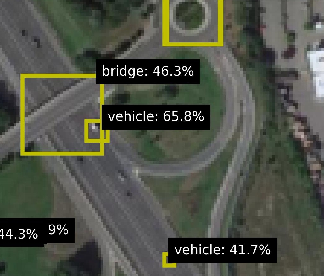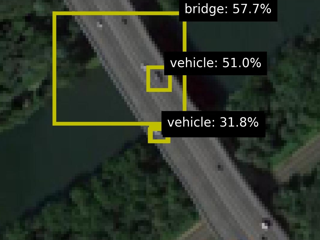</details> Figure 3: Hard cases due to incorrect groundtruths (right) or incorrect detections (others). ### 4.2 Experimental Setup The dataset is categorized into three subsets that are increasingly harder in terms of flaws in the background knowledge. Easy: This smallest subset excludes the incorrect groundtruths, a manual check that most object predictions are reasonable, i.e. images with many predicted objects are withheld (this includes images with many false positives). Intermediate: This subset excludes the incorrect groundtruths. Compared to Easy, this subset adds all images with many object predictions. Hard: This is the full set, which includes all images, also the ones with incorrect groundtruths. We are curious whether ILP methods can indeed generalize from small numbers of examples, as is hypothesized cropper2022inductive. Many datasets used in ILP are using training data with tens to hundreds (sometimes thousands) of labeled samples hocquette2024learning,bellodi2015structure. We investigate the performance for as few as {1, 2, 4, 8} labels for respectively the positive and negative set, as this is common in practical settings. Moreover, common ILP datasets are about binary background knowledge, without associated probabilities hocquette2024learning,bellodi2015structure. In contrast, we consider probabilistic background knowledge. From the Easy subset we construct an Easy-1.0 set by thresholding the background knowledge with a manually chosen optimal threshold, which results in an almost noiseless dataset and shows the complexity of the logical rule to learn. All experiments are repeated 5 times, randomly selecting the training samples from the dataset and using the rest of the data set as test set. ### 4.3 Model Variants and Baselines We compare Propper with Popper (on which it builds), to validate the merit of integrating the neurosymbolic inference and the continuous cost function BCE. Moreover, we compare these ILP models with statistical ML models: the Support Vector Machine cortes1995support (SVM) because it is used so often in practice; a Graph Neural Network wu2020comprehensive (GNN) because it is also relational by design which makes it a reasonable candidate for the task at hand i.e. finding a relational pattern between objects. All methods except the SVM are relational and permutation invariant. The objects are unordered and the models should therefore represent them in an orderless manner. The SVM is not permutation invariant, as objects and their features have some arbitrary but designated position in its feature vectors. All methods except Popper are probabilistic. All methods except the most basic Popper variant, can handle some degree of noise. The expected noise level for NoisyCombo is set at 0.15. The tested models are characterized in Table 1. Table 1: The tested model variants and their properties. | Tester Cost function | Cortes 1995 - - | Wu 2020 - - | Cropper 2021 Prolog MDL | Hoguette 2024 Prolog MDL | (ours) Constrainer Scallop BCE Type | - Stat. | - Stat. | Combo Logic | MaxSynth Logic | Noisy-Combo Logic | | --- | --- | --- | --- | --- | --- | --- | --- | --- | --- | --- | | Label noise | Yes | Yes | No | Yes | Yes | | | | | | | Background noise | Yes | Yes | No | Some | Yes | | | | | | | Relational | No | Yes | Yes | Yes | Yes | | | | | | | Permutation inv. | No | Yes | Yes | Yes | Yes | | | | | | | Probabilistic | Yes | Yes | No | No | Yes | | | | | | For a valid comparison, we increase the SVM’s robustness against arbitrary object order. With prior knowledge about the relevant objects for the pattern at hand, these objects can be placed in front of the feature vector. This preprocessing step makes the SVM model less dependent on the arbitrary order of objects. In the remainder of the analyses, we call this variant ‘SVM ordered’. To binarize the probabilistic background knowledge as input for Popper, the detections are thresholded with the general value of 0.5. 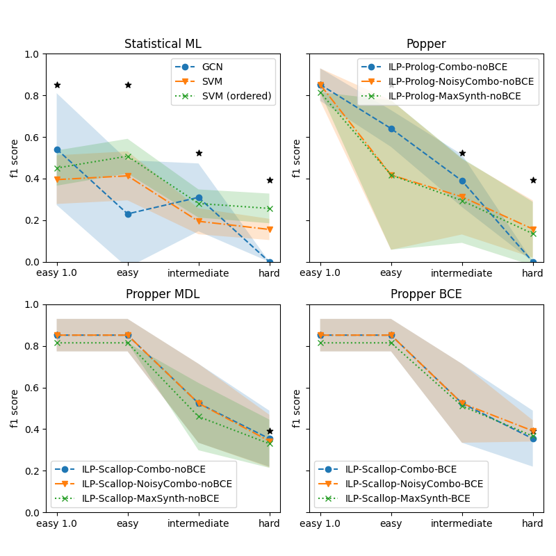### 4.4 Increasing Noise in Background Knowledge We are interested in how the robustness of model learning for increasing difficulty of the dataset. Here we investigate the performance on the three subsets from Section 4.2: Easy, Intermediate and Hard. Figure 4 shows the performance for various models for increasing difficulty. The four subplots show the various types of models. For a reference, the best performing model is indicated by an asterisk (*) in all subplots. It is clear that for increasing difficulty, all models struggle. The statistical ML models struggle the most: the performance of the GNN drops to zero on the Hard set. The SVMs are a bit more robust but the performance on the Hard set is very low. The most basic variant of Popper also drops to zero. The noise-tolerant Popper variants (Noisy-Combo and MaxSynth) perform similarly to the SVMs. Propper outperforms all models. This finding holds for all Propper variants (Combo, Noisy-Combo and MaxSynth). Using BCE as a cost function yields a small but negligible advantage over MDL. <details> <summary>extracted/5868417/result_propper_figures/increasing_test_hardness/n_train_avg_4_8.png Details</summary>  ### Visual Description ## Chart/Diagram Type: Grid of Line Charts ### Overview The image contains four line charts arranged in a 2x2 grid, each comparing model performance across task difficulty levels (easy 1.0, easy, intermediate, hard) using the f1 score metric. Each chart represents a different framework (Statistical ML, Popper, Popper MDL, Popper BCE) with distinct model variants. ### Components/Axes - **X-axis**: Task difficulty levels labeled as "easy 1.0", "easy", "intermediate", "hard". - **Y-axis**: f1 score ranging from 0.0 to 1.0. - **Legends**: - **Statistical ML**: GCN (blue solid line), SVM (orange dashed line), SVM (ordered) (green dotted line). - **Popper**: ILP-Prolog-Combo-noBCE (blue solid), ILP-Prolog-NoisyCombo-noBCE (orange dashed), ILP-Prolog-MaxSynth-noBCE (green dotted). - **Popper MDL**: ILP-Scallop-Combo-noBCE (blue solid), ILP-Scallop-NoisyCombo-noBCE (orange dashed), ILP-Scallop-MaxSynth-noBCE (green dotted). - **Popper BCE**: ILP-Scallop-Combo-BCE (blue solid), ILP-Scallop-NoisyCombo-BCE (orange dashed), ILP-Scallop-MaxSynth-BCE (green dotted). - **Shading**: Confidence intervals or variability bands around lines in Popper, Popper MDL, and Popper BCE charts. ### Detailed Analysis #### Statistical ML - **GCN (blue)**: Starts at ~0.55 (easy 1.0), drops to ~0.2 (easy), ~0.3 (intermediate), and ~0.0 (hard). - **SVM (orange)**: Starts at ~0.4 (easy 1.0), remains stable at ~0.4 (easy), drops to ~0.2 (intermediate), and ~0.1 (hard). - **SVM (ordered) (green)**: Starts at ~0.45 (easy 1.0), drops to ~0.3 (easy), ~0.25 (intermediate), and ~0.1 (hard). - **Stars**: Two outliers at ~0.8 (easy 1.0) and ~0.6 (intermediate). #### Popper - **ILP-Prolog-Combo-noBCE (blue)**: Starts at ~0.8 (easy 1.0), drops to ~0.4 (easy), ~0.3 (intermediate), and ~0.2 (hard). - **ILP-Prolog-NoisyCombo-noBCE (orange)**: Starts at ~0.6 (easy 1.0), drops to ~0.3 (easy), ~0.2 (intermediate), and ~0.1 (hard). - **ILP-Prolog-MaxSynth-noBCE (green)**: Starts at ~0.7 (easy 1.0), drops to ~0.4 (easy), ~0.3 (intermediate), and ~0.2 (hard). #### Popper MDL - **ILP-Scallop-Combo-noBCE (blue)**: Starts at ~0.8 (easy 1.0), drops to ~0.6 (easy), ~0.5 (intermediate), and ~0.4 (hard). - **ILP-Scallop-NoisyCombo-noBCE (orange)**: Starts at ~0.8 (easy 1.0), drops to ~0.5 (easy), ~0.4 (intermediate), and ~0.3 (hard). - **ILP-Scallop-MaxSynth-noBCE (green)**: Starts at ~0.8 (easy 1.0), drops to ~0.5 (easy), ~0.4 (intermediate), and ~0.3 (hard). #### Popper BCE - **ILP-Scallop-Combo-BCE (blue)**: Starts at ~0.8 (easy 1.0), drops to ~0.6 (easy), ~0.5 (intermediate), and ~0.4 (hard). - **ILP-Scallop-NoisyCombo-BCE (orange)**: Starts at ~0.8 (easy 1.0), drops to ~0.5 (easy), ~0.4 (intermediate), and ~0.3 (hard). - **ILP-Scallop-MaxSynth-BCE (green)**: Starts at ~0.8 (easy 1.0), drops to ~0.5 (easy), ~0.4 (intermediate), and ~0.3 (hard). ### Key Observations 1. **Downward Trend**: All models show a consistent decline in f1 score as task difficulty increases. 2. **Model Variability**: - **Statistical ML**: GCN performs worst at higher difficulties, while SVM (ordered) maintains slightly better stability. - **Popper**: ILP-Prolog-Combo-noBCE starts strongest but declines sharply. - **Popper MDL/BCE**: ILP-Scallop models maintain higher scores across difficulties compared to Popper variants. 3. **Confidence Intervals**: Shaded regions in Popper, Popper MDL, and Popper BCE charts suggest higher variability in performance for some models (e.g., ILP-Prolog-NoisyCombo-noBCE). 4. **Outliers**: Two stars in Statistical ML at easy 1.0 (~0.8) and intermediate (~0.6) may indicate exceptional or anomalous results. ### Interpretation - **Performance Degradation**: All models struggle with harder tasks, but the rate of decline varies. ILP-Prolog-Combo-noBCE (Popper) and GCN (Statistical ML) show the steepest drops. - **Robustness**: ILP-Scallop models (Popper MDL/BCE) exhibit greater resilience to difficulty increases, maintaining higher f1 scores. - **Ordered SVM**: In Statistical ML, the "ordered" variant underperforms the standard SVM, suggesting ordering constraints may harm generalization. - **NoBCE vs. BCE**: Models with "noBCE" (no background context) in Popper frameworks perform slightly worse than their BCE counterparts, indicating background context may aid generalization. - **Anomalies**: The stars in Statistical ML at easy 1.0 and intermediate could represent overfitting or data leakage, warranting further investigation. This analysis highlights trade-offs between model complexity, task difficulty, and generalization, with ILP-Scallop models emerging as the most robust across frameworks. </details> Figure 4: Performance of the models on finding a relational pattern in satellite images, for increasing hardness of image sets. The best performer is Propper BCE, indicated in each graph by * for comparison. Our probabilistic ILP outperforms binary ILP and statistical ML. 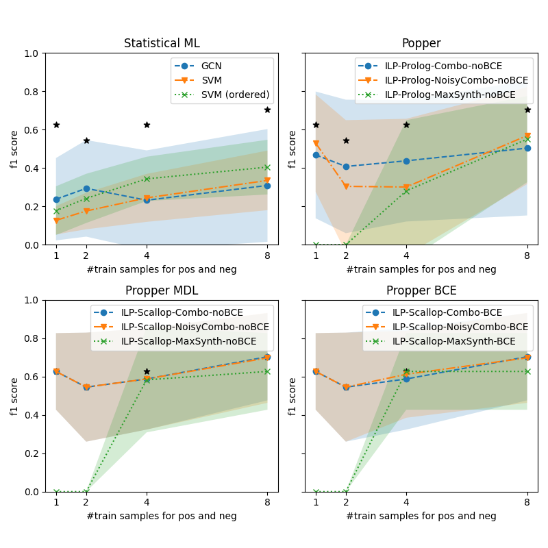### 4.5 Learning Efficiency with Few Labels We are curious how the models perform with as few as {1, 2, 4, 8} labels for respectively the positive and negative set. The performance is measured on the Hard set. Figure 5 shows the performance for various models for increasing training set size. The four subplots show the various types of models. Again, for reference, the best performing model is indicated by an asterisk (*) in all subplots. The upper left shows the statistical ML models. They do perform better with more training samples, but the performance is inferior to the ILP model variants. The Propper variant with Scallop and Noisy-Combo and BCE is the best performer. BCE does not improve significantly over MDL. MaxSynth has an optimization criterion that cannot operate with less than three training samples. The main improvement by Propper is observed when switching from Combo to Noisy-Combo and switching from Prolog to Scallop (i.e. neurosymbolic inference). <details> <summary>extracted/5868417/result_propper_figures/increasing_train_samples/all_test_cases_avg.png Details</summary>  ### Visual Description ## Chart Type: 2x2 Grid of Line Charts with Confidence Intervals ### Overview The image contains four line charts arranged in a 2x2 grid, each comparing the performance of different machine learning models across varying numbers of training samples. The charts are labeled: 1. **Statistical ML** 2. **Popper** 3. **Propper MDL** 4. **Propper BCE** Each chart plots the **F1 score** (y-axis) against the **number of training samples for positive and negative examples** (x-axis, ranging from 1 to 8). Confidence intervals are shaded around the lines, and black stars denote specific data points. --- ### Components/Axes #### Common Elements Across All Charts: - **X-axis**: `#train samples for pos and neg` (1, 2, 4, 8) - **Y-axis**: `f1 score` (0.0 to 1.0) - **Legends**: Model-specific labels with color-coded lines and markers. - **Shaded Areas**: Confidence intervals (e.g., ±0.1–0.2 around the mean F1 score). #### Chart-Specific Legends: 1. **Statistical ML**: - GCN (blue line) - SVM (orange line) - SVM (ordered) (green dotted line) 2. **Popper**: - ILP-Prolog-Combo-noBCE (blue line) - ILP-Prolog-NoisyCombo-noBCE (orange line) - ILP-Prolog-MaxSynth-noBCE (green dotted line) 3. **Propper MDL**: - ILP-Scallop-Combo-noBCE (blue line) - ILP-Scallop-NoisyCombo-noBCE (orange line) - ILP-Scallop-MaxSynth-noBCE (green dotted line) 4. **Propper BCE**: - ILP-Scallop-Combo-BCE (blue line) - ILP-Scallop-NoisyCombo-BCE (orange line) - ILP-Scallop-MaxSynth-BCE (green dotted line) --- ### Detailed Analysis #### 1. **Statistical ML** - **GCN (blue)**: - Starts at ~0.2 (1 sample), peaks at ~0.6 (4 samples), then drops to ~0.3 (8 samples). - Confidence interval widens significantly at 8 samples. - **SVM (orange)**: - Starts at ~0.1 (1 sample), rises to ~0.3 (4 samples), then plateaus at ~0.4 (8 samples). - **SVM (ordered) (green)**: - Starts at ~0.2 (1 sample), increases to ~0.4 (4 samples), then ~0.5 (8 samples). - **Black Stars**: - Located at (1, 0.6), (4, 0.5), and (8, 0.7), suggesting experimental benchmarks. #### 2. **Popper** - **ILP-Prolog-Combo-noBCE (blue)**: - Starts at ~0.4 (1 sample), dips to ~0.3 (2 samples), then rises to ~0.5 (4 samples) and ~0.6 (8 samples). - **ILP-Prolog-NoisyCombo-noBCE (orange)**: - Starts at ~0.2 (1 sample), rises to ~0.3 (2 samples), then ~0.4 (4 samples) and ~0.5 (8 samples). - **ILP-Prolog-MaxSynth-noBCE (green)**: - Starts at ~0.0 (1 sample), jumps to ~0.4 (4 samples), then ~0.5 (8 samples). - **Black Stars**: - Located at (1, 0.6), (4, 0.5), and (8, 0.7), mirroring the Statistical ML chart. #### 3. **Propper MDL** - **ILP-Scallop-Combo-noBCE (blue)**: - Starts at ~0.6 (1 sample), dips to ~0.5 (2 samples), then rises to ~0.7 (4 samples) and ~0.8 (8 samples). - **ILP-Scallop-NoisyCombo-noBCE (orange)**: - Starts at ~0.5 (1 sample), rises to ~0.6 (2 samples), then ~0.7 (4 samples) and ~0.8 (8 samples). - **ILP-Scallop-MaxSynth-noBCE (green)**: - Starts at ~0.0 (1 sample), jumps to ~0.6 (4 samples), then ~0.7 (8 samples). #### 4. **Propper BCE** - **ILP-Scallop-Combo-BCE (blue)**: - Starts at ~0.6 (1 sample), dips to ~0.5 (2 samples), then rises to ~0.7 (4 samples) and ~0.8 (8 samples). - **ILP-Scallop-NoisyCombo-BCE (orange)**: - Starts at ~0.5 (1 sample), rises to ~0.6 (2 samples), then ~0.7 (4 samples) and ~0.8 (8 samples). - **ILP-Scallop-MaxSynth-BCE (green)**: - Starts at ~0.0 (1 sample), jumps to ~0.6 (4 samples), then ~0.7 (8 samples). --- ### Key Observations 1. **Performance Trends**: - All models improve F1 scores as training samples increase, but the rate varies. - **MaxSynth models** (green dotted lines) show a sharp performance jump at 4 samples, suggesting a threshold effect. - **NoBCE models** (e.g., Popper, Propper MDL) generally outperform **BCE models** (e.g., Propper BCE) in later stages. 2. **Confidence Intervals**: - Wider intervals (e.g., GCN in Statistical ML) indicate higher variability in performance. - MaxSynth models (green) have narrower intervals, implying more consistent results. 3. **Anomalies**: - The **green dotted line** (MaxSynth) in Popper and Propper charts starts at 0.0 for 1 sample, then jumps sharply at 4 samples. This suggests synthetic data generation (MaxSynth) is ineffective with minimal training but becomes powerful at scale. - **Black stars** in Statistical ML and Popper align with high F1 scores at 1 and 8 samples, possibly representing idealized or benchmark results. --- ### Interpretation 1. **Model Behavior**: - **GCN** (Statistical ML) shows overfitting at 8 samples, as its F1 score drops despite more data. - **SVM (ordered)** outperforms regular SVM, indicating that data ordering improves generalization. - **MaxSynth models** (green) in Popper and Propper charts demonstrate that synthetic data generation (e.g., MaxSynth) can drastically boost performance when sufficient training samples are available, but it underperforms with minimal data. 2. **BCE vs. noBCE**: - The **Propper BCE** chart shows similar trends to **Propper MDL**, but the **noBCE** variants (e.g., ILP-Prolog-NoisyCombo-noBCE) achieve higher F1 scores, suggesting that avoiding BCE (e.g., using alternative loss functions) improves robustness. 3. **Practical Implications**: - For small datasets (<4 samples), simpler models like SVM or ordered SVM may be more reliable. - For larger datasets (≥4 samples), MaxSynth models and noBCE variants outperform others, highlighting the importance of synthetic data and loss function design. 4. **Uncertainties**: - The exact meaning of the **black stars** is unclear—they may represent external benchmarks or experimental constraints. - The **confidence intervals** suggest that some models (e.g., GCN) are more sensitive to training data variability. </details> Figure 5: Performance of the models on finding a relational pattern in satellite images, for increasing training sets. The best performer is Propper BCE, indicated in each graph by * for comparison. Our probabilistic ILP outperforms binary ILP and statistical ML. 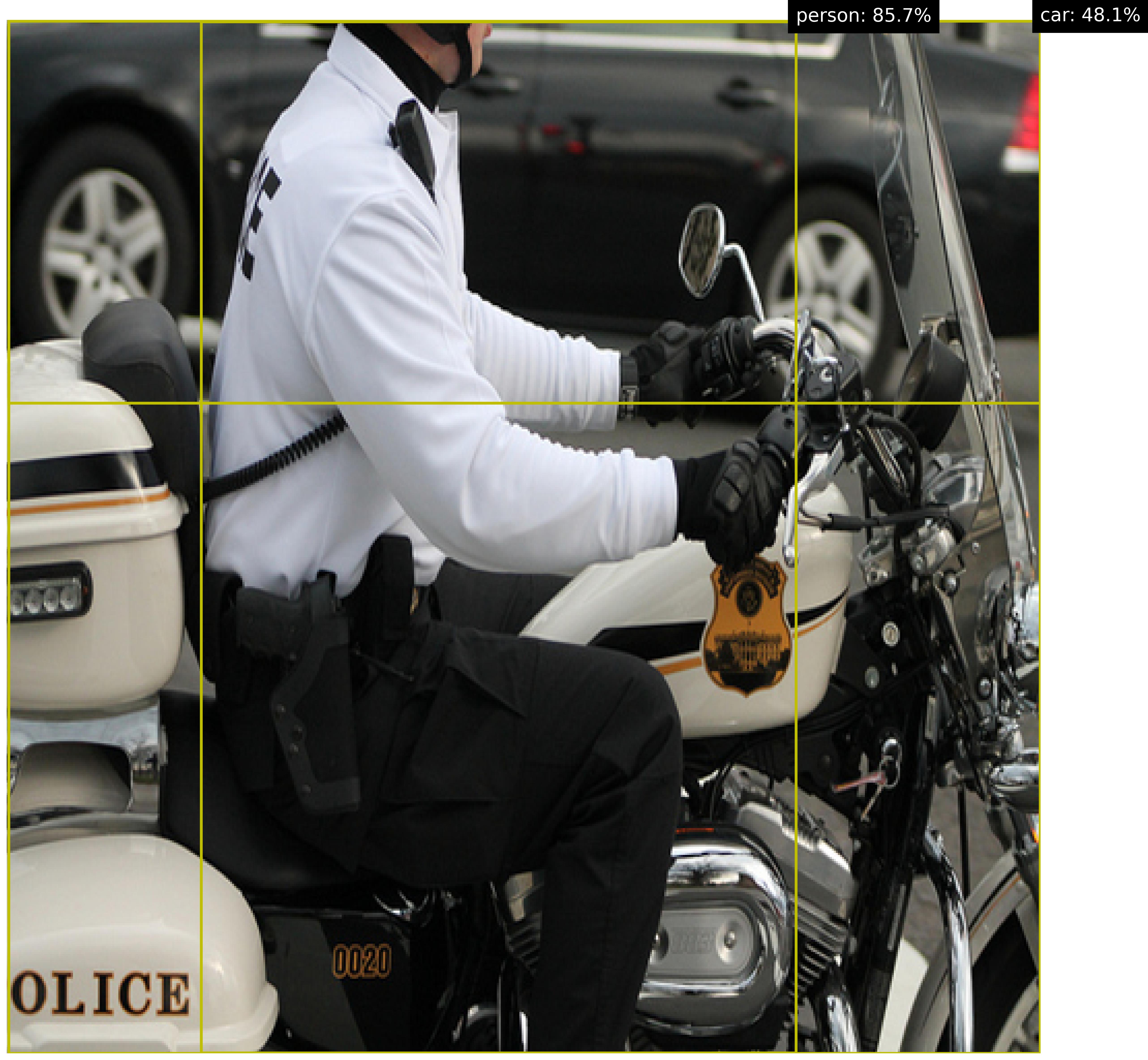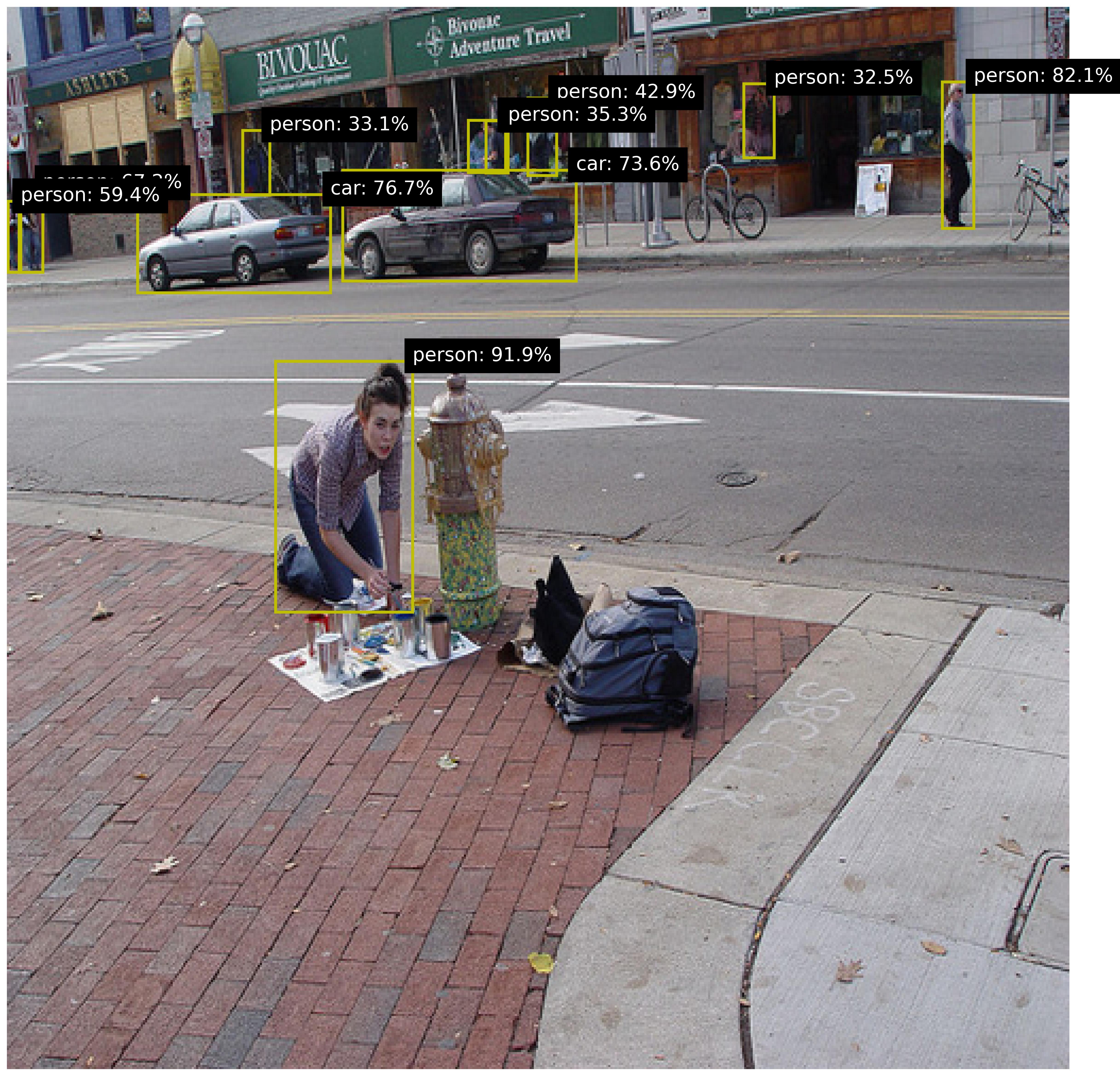### 4.6 Second Dataset We are interested how the methods perform on a different dataset. The MS-COCO dataset lin2014microsoft contains a broad variety of images of everyday scenes. This dataset is challenging, because there are many different objects in a wide range of settings. Similar to the previous experiment, the background knowledge is acquired by the predictions of a pretrained model, GroundingDINO liu2023groundingDINO, which are used to extract the same two relations. Figure 6 shows some examples. <details> <summary>extracted/5868417/coco/2.jpg Details</summary>  ### Visual Description ## Photograph: Police Officer on Motorcycle with Object Detection Overlay ### Overview The image depicts a police officer seated on a white motorcycle with black and orange accents. The officer wears a white long-sleeve uniform with "POLICE" printed on the back, black gloves, and a black helmet. The motorcycle features a badge with "POLICE" and a shield emblem on the fuel tank. A black sedan is partially visible in the background. Yellow grid lines overlay the image, with confidence percentages labeled for detected objects: "person: 85.7%" and "car: 48.1%". ### Components/Axes - **Primary Subjects**: - Police officer (centered, seated on motorcycle). - Motorcycle (white with black/orange stripes, model number "0020" on the side). - Black sedan (background, partially obscured). - **Overlay Elements**: - Yellow grid lines dividing the image into quadrants. - Text annotations in the top-right corner: - "person: 85.7%" (bounding box confidence for the officer). - "car: 48.1%" (bounding box confidence for the sedan). ### Detailed Analysis - **Textual Elements**: - "POLICE" in bold black letters on the motorcycle’s side panel. - "POLICE" in uppercase on the officer’s uniform back. - Badge on the motorcycle’s fuel tank: "POLICE" in black text with a gold shield emblem. - Model number "0020" in orange on the motorcycle’s side. - **Confidence Scores**: - Person detection confidence: 85.7% (high certainty, likely due to clear visibility of the officer). - Car detection confidence: 48.1% (lower certainty, possibly due to partial occlusion or motion blur). ### Key Observations 1. The grid lines and confidence scores suggest this image is from an object detection system (e.g., computer vision model). 2. The officer’s posture and uniform indicate readiness for duty. 3. The motorcycle’s design (white with black/orange) aligns with standard police vehicle aesthetics. 4. The sedan’s lower confidence score may reflect challenges in detection (e.g., partial visibility, background clutter). ### Interpretation This image demonstrates the application of object detection technology in real-world scenarios, such as traffic monitoring or law enforcement operations. The high confidence score for the person (85.7%) confirms the system’s reliability in identifying human subjects, while the lower score for the car highlights potential limitations in detecting vehicles under suboptimal conditions. The presence of "POLICE" branding on both the officer and motorcycle reinforces the context of official authority. The grid overlay provides spatial grounding for the detected objects, enabling precise localization for further analysis (e.g., tracking movement or identifying interactions). </details> <details> <summary>extracted/5868417/coco/3.jpg Details</summary>  ### Visual Description ## Photograph: Urban Scene with Object Detection Annotations ### Overview The image depicts a street scene with a person painting on a brick sidewalk, annotated with object detection labels. The scene includes pedestrians, vehicles, storefronts, and urban infrastructure. Yellow bounding boxes with confidence percentages are overlaid on detected objects. ### Components/Axes - **Foreground**: A person painting (labeled "person: 91.9%") kneeling on a brick sidewalk. - **Midground**: - A fire hydrant with a floral pattern. - A backpack and painting supplies (paint cans, brushes). - **Background**: - Two cars (labeled "car: 76.7%" and "car: 73.6%"). - Pedestrians (labeled "person: 33.1%", "person: 42.9%", "person: 35.3%", "person: 32.5%", "person: 82.1%"). - Storefronts: "BIVOUAC" (green sign), "Bivonic Adventure Travel" (green sign), and "ASHLEY'S" (yellow sign). - Bicycles parked near the sidewalk. ### Detailed Analysis - **Foreground Person**: - Positioned centrally on the brick sidewalk. - Confidence: 91.9% (highest in the image). - **Cars**: - Left car: 76.7% confidence. - Right car: 73.6% confidence. - **Pedestrians**: - Person near "Bivonic Adventure Travel": 42.9% confidence. - Person near "ASHLEY'S": 32.5% confidence (lowest). - Person near fire hydrant: 35.3% confidence. - Person on the far right: 82.1% confidence. - **Annotations**: - All labels use black text on yellow boxes. - Percentages likely represent model confidence scores. ### Key Observations 1. **Confidence Variance**: - Foreground objects (painter, fire hydrant) have higher confidence (91.9%, 82.1%). - Background objects (pedestrians, cars) show lower confidence (32.5%–76.7%). 2. **Occlusion/Visibility**: - The person near "ASHLEY'S" (32.5%) is partially obscured by a bicycle. - The fire hydrant’s floral pattern may reduce detection accuracy. 3. **Spatial Distribution**: - Annotations cluster near the center and right side of the image. ### Interpretation The annotations suggest this image was processed by an object detection model (e.g., YOLO, Faster R-CNN) to identify pedestrians and vehicles. The confidence scores indicate: - **Foreground Dominance**: Objects closer to the camera (painter, fire hydrant) are detected with higher certainty. - **Background Challenges**: Distant or occluded objects (e.g., pedestrian near "ASHLEY'S") have lower confidence, highlighting limitations in handling depth and occlusion. - **Model Bias**: The high confidence for the painter (91.9%) may reflect clear, unobstructed features, while lower scores for background pedestrians suggest difficulty in distinguishing individuals in cluttered environments. This analysis underscores the importance of spatial context and object visibility in computer vision tasks, with implications for applications like autonomous driving or surveillance systems. </details> Figure 6: Examples of the MS-COCO dataset with images of everyday scenes. The pattern of interest is ‘person next to a car’. We consider all images that have a maximum of two persons and two cars, yielding 1728 images. We use random 8 positive and 8 negative images for training, which is repeated 5 times. We test both ILP variants, Popper and Propper, for the MaxSynth constrainer, because the Combo constrainer regularly did not return a solution. We validate Popper with various thresholds to be included as background knowledge. Propper does not need such a threshold beforehand, as all background knowledge is considered in a probabilistic manner. The results are shown in Table 2. Propper is the best performer, achieving f1 = 0.947. This is significantly better than the alternatives: SVM achieves f1 = 0.668 (-0.279) and Popper achieves f1 = 0.596 (-0.351). Adding probabilistic behavior to ILP is helpful for challenging datasets. Table 2: Model variants and performance on MS-COCO. | ILP | Propper (ours) | MaxSynth | probabilistic | BCE | - | 0.754 | | --- | --- | --- | --- | --- | --- | --- | | Statistical ML | SVM | - | - | - | - | 0.668 | | Statistical ML | SVM (ordered) | - | - | - | - | 0.652 | | ILP | Popper | MaxSynth | Prolog | MDL | 0.3 | 0.596 | | ILP | Popper | MaxSynth | Prolog | MDL | 0.5 | 0.466 | | ILP | Popper | MaxSynth | Prolog | MDL | 0.4 | 0.320 | Table 3 shows the learned programs, how often each program was predicted across the experimental repetitions, and the respective resulting f1 scores. The best program is that there is a person on a car. Popper yields the same program, however, with a lower f1-score, since the background knowledge is thresholded before learning the program, removing important data from the background knowledge. This confirms that in practice it is intractable to set a perfect threshold on the background knowledge. It is beneficial to use Propper which avoids such prior thresholding. Table 3: Learned programs, prevalence and performance on MS-COCO. | Popper Popper Popper | 0.72 0.72 0 | 20 40 20 | f(A) :- has_object(A,C), is_on(B,C), person(B). f(A) :- person(C), is_on(C,B), has_object(A,C), car(B). No program learned. | | --- | --- | --- | --- | ## 5 Discussion and Conclusions We proposed Propper, which handles flawed and probabilistic background knowledge by extending ILP with a combination of neurosymbolic inference, a continuous criterion for hypothesis selection (BCE), and a relaxation of the hypothesis constrainer (NoisyCombo). Neurosymbolic inference has a significant impact on the results. Its advantage is that it does not need prior thresholding on the probabilistic background knowledge (BK), which is needed for binary ILP and is always imperfect. NoisyCombo has a small yet positive effect. It provides a parameter for the level of noise in BK, which can be tailored to the dataset at hand. The BCE has little impact. Propper is able to learn a logic program about a relational pattern that distinguishes between two sets of images, even if the background knowledge is provided by an imperfect neural network that predicts concepts in the images with some confidence. With as few as a handful of examples, Propper learns effective programs and outperforms statistical ML methods such as a GNN. Although we evaluated Propper on two common datasets with different recording conditions, a broader evaluation of Propper across various domains and datasets to confirm its generalizability and robustness for various (especially non-image) use cases, is interesting. The proposed framework of integrated components allows for an easy setup of the system and simple adaptation to new developments/algorithms within the separate components. However, the integration as is performed now could be non-optimal in terms of computational efficiency. For example the output of the hypothesis generation is an answer set, which in Popper is converted to Prolog syntax. Propper converts this Prolog syntax to Scallop syntax. Developing a direct conversion from the answer sets to the Scallop syntax is recommended. We favored modularization over full integration and computational efficiency, in order to facilitate the methodological configuration and comparison of the various components. It is interesting to investigate whether a redesign of the whole system with the components integrated will lead to a better system. To make the step to fully probabilistic ILP, the allowance of probabilistic rules should be added to the system as well, for example by integration of StarAI methods raedt2016statistical.