2408.12894v2

# FLoD: Integrating Flexible Level of Detail into 3D Gaussian Splatting for Customizable Rendering **Authors**: Yunji Seo, Young Sun Choi, HyunSeung Son, Youngjung Uh > 0009-0004-9941-3610 Yonsei University South Korea > 0009-0001-9836-4245 Yonsei University South Korea > 0009-0009-1239-0492 Yonsei University South Korea > 0000-0001-8173-3334 Yonsei University South Korea by-nc-nd <details> <summary>x1.png Details</summary>  ### Visual Description ## Technical Diagram: FLoD-3DGS Multi-Level Rendering Comparison ### Overview This image is a technical comparison diagram illustrating the performance and memory efficiency of two 3D rendering methods: **3D Gaussian Splatting** and **FLoD-3DGS** (likely "Flexible Level-of-Detail 3D Gaussian Splatting"). The diagram contrasts their ability to render a complex outdoor scene (a garden with a wooden table and chairs) on two different GPU hardware configurations with vastly different memory capacities. It also explains the multi-level rendering mechanism of FLoD-3DGS. ### Components/Axes The diagram is organized into three main vertical sections: 1. **Left Section (Hardware & Method Comparison):** * **Top Row:** Represents a high-end GPU: **RTX A5000 (24GB VRAM)**. * **Bottom Row:** Represents a low-end GPU: **GeForce MX250 (2GB VRAM)**. * **Vertical Labels:** The leftmost column labels the two rows of images as belonging to the methods **"3D Gaussian Splatting"** (top) and **"FLoD-3DGS"** (bottom). * **Performance Metric:** Each rendered image includes a **PSNR** (Peak Signal-to-Noise Ratio) value, a common metric for image quality. 2. **Center-Right Section (FLoD-3DGS Mechanism):** * **Title:** **"FLoD-3DGS levels"**. * **Levels:** Five distinct levels are shown, numbered **1** through **5**. Each level is visualized as a cluster of colored Gaussian splats: * Level 1: Yellow/Orange * Level 2: Red * Level 3: Magenta/Pink * Level 4: Blue * Level 5: Green * **Annotations:** * A **pink box** surrounds levels 3 and 4, with an arrow pointing left labeled **"selective rendering"**. * A **green box** surrounds level 5, with an arrow pointing left labeled **"single level rendering"**. 3. **Far-Right Section (Level Detail):** * **Title:** **"Single level renderings"**. * **Content:** Five small rendered images, each labeled **"level 1"** through **"level 5"**, showing the visual output when only that specific level's data is used for rendering. ### Detailed Analysis **Hardware Performance Comparison:** * **On RTX A5000 (24GB VRAM):** * **3D Gaussian Splatting:** Successfully renders the scene. **PSNR: 27.1**. * **FLoD-3DGS:** Successfully renders the scene with slightly higher quality. **PSNR: 27.6**. * **On GeForce MX250 (2GB VRAM):** * **3D Gaussian Splatting:** **Fails completely**. The output is a black box with the error message: **"CUDA out of memory."** * **FLoD-3DGS:** **Succeeds** in rendering the scene. **PSNR: 27.3**. This demonstrates its ability to operate within severe memory constraints. **FLoD-3DGS Level Mechanism:** * The system decomposes the 3D scene into five hierarchical levels of detail (LoD). * **Level 1** renderings are extremely blurry, capturing only the coarsest shapes and colors. * Detail increases progressively with each level. **Level 5** renderings are sharp and contain the finest details (e.g., individual leaves, wood grain). * The diagram indicates two operational modes: 1. **Selective Rendering:** Uses a combination of levels (e.g., levels 3 & 4) to balance quality and performance. 2. **Single Level Rendering:** Uses only one level (e.g., level 5) for rendering, which is the mode used to achieve the result on the low-memory MX250 GPU. ### Key Observations 1. **Memory Efficiency is Critical:** The most striking observation is the binary outcome on the low-memory GPU. The traditional method fails catastrophically, while FLoD-3DGS succeeds. 2. **Quality Preservation:** Despite using a "single level rendering" mode on the MX250, FLoD-3DGS achieves a PSNR (27.3) that is very close to its own performance on the high-end card (27.6) and even surpasses the traditional method on that card (27.1). This suggests the selected level (likely level 5) retains most of the perceptual quality. 3. **Visual Degradation is Gradual:** The "Single level renderings" column clearly shows that reducing the level of detail results in a predictable, gradual loss of sharpness and high-frequency detail, not a sudden collapse. ### Interpretation This diagram serves as a compelling technical argument for the **FLoD-3DGS** method. It demonstrates a solution to a fundamental problem in real-time 3D graphics: **high-quality rendering on hardware with limited memory**. * **The Problem:** State-of-the-art methods like 3D Gaussian Splatting require large amounts of VRAM to store all scene data, making them inaccessible on consumer or older hardware (exemplified by the MX250 failure). * **The Solution:** FLoD-3DGS introduces a **level-of-detail (LoD) hierarchy**. By organizing scene data into levels, the renderer can make intelligent trade-offs. On powerful hardware, it can use more levels for maximum quality. On constrained hardware, it can fall back to a single, optimized level. * **The Implication:** This technology could democratize access to high-quality 3D rendering, enabling complex scenes to run on a wider range of devices, from high-end workstations to laptops and potentially mobile devices. The "selective rendering" hint suggests further optimization potential, where the system could dynamically choose which levels to use based on what part of the scene is in view or the current performance budget. 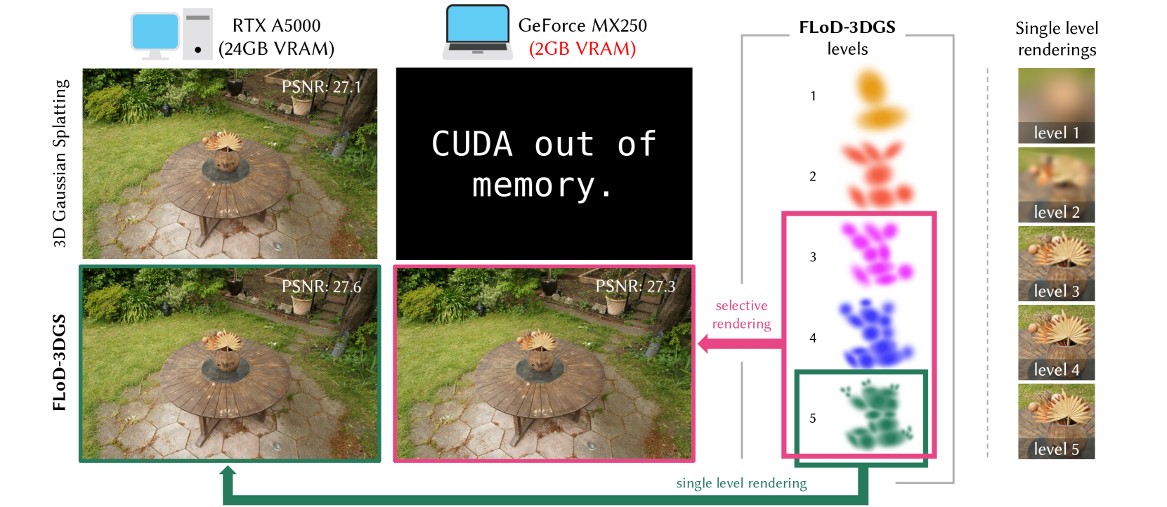**In essence, the image argues that FLoD-3DGS is not just an incremental improvement in quality, but a fundamental advancement in making advanced 3D rendering more robust, scalable, and accessible.** </details> Figure 1. We introduce Level of Detail (LoD) mechanism in 3D Gaussian Splatting (3DGS) through multi-level representations. These representations enable flexible rendering by selecting individual levels or subsets of levels. The green box illustrates max-level rendering on a high-end server, while the pink box shows subset-level rendering for a low-cost laptop, where traditional 3DGS fails to render. Thus, FLoD-3DGS can flexibly adapt to diverse hardware settings. ## Abstract 3D Gaussian Splatting (3DGS) has significantly advanced computer graphics by enabling high-quality 3D reconstruction and fast rendering speeds, inspiring numerous follow-up studies. However, 3DGS and its subsequent works are restricted to specific hardware setups, either on only low-cost or on only high-end configurations. Approaches aimed at reducing 3DGS memory usage enable rendering on low-cost GPU but compromise rendering quality, which fails to leverage the hardware capabilities in the case of higher-end GPU. Conversely, methods that enhance rendering quality require high-end GPU with large VRAM, making such methods impractical for lower-end devices with limited memory capacity. Consequently, 3DGS-based works generally assume a single hardware setup and lack the flexibility to adapt to varying hardware constraints. To overcome this limitation, we propose Flexible Level of Detail (FLoD) for 3DGS. FLoD constructs a multi-level 3DGS representation through level-specific 3D scale constraints, where each level independently reconstructs the entire scene with varying detail and GPU memory usage. A level-by-level training strategy is introduced to ensure structural consistency across levels. Furthermore, the multi-level structure of FLoD allows selective rendering of image regions at different detail levels, providing additional memory-efficient rendering options. To our knowledge, among prior works which incorporate the concept of Level of Detail (LoD) with 3DGS, FLoD is the first to follow the core principle of LoD by offering adjustable options for a broad range of GPU settings. Experiments demonstrate that FLoD provides various rendering options with trade-offs between quality and memory usage, enabling real-time rendering under diverse memory constraints. Furthermore, we show that FLoD generalizes to different 3DGS frameworks, indicating its potential for integration into future state-of-the-art developments. 3D Gaussian Splatting, Level-of-Detail, Novel View Synthesis submissionid: 1344 journal: TOG journalyear: 2025 journalvolume: 44 journalnumber: 4 publicationmonth: 8 copyright: cc price: doi: 10.1145/3731430 ccs: Computing methodologies Reconstruction ccs: Computing methodologies Point-based models ccs: Computing methodologies Rasterization ## 1. Introduction Recent advances in 3D reconstruction have led to significant improvements in the fidelity and rendering speed of novel view synthesis. In particular, 3D Gaussian Splatting (3DGS) (Kerbl et al., 2023) has demonstrated photo-realistic quality at exceptionally fast rendering rates. However, its reliance on numerous Gaussian primitives makes it impractical for rendering on devices with limited GPU memory. Similarly, methods such as AbsGS (Ye et al., 2024), FreGS (Zhang et al., 2024), and Mip-Splatting (Yu et al., 2024), which further enhance rendering quality, remain constrained to higher-end devices due to their dependence on a comparable or even greater number of Gaussians for scene reconstruction. Conversely, LightGaussian (Fan et al., 2023) and CompactGS (Lee et al., 2024) address memory limitations by removing redundant Gaussians, which helps reduce rendering memory demands as well as reducing storage size. However, the reduction in memory usage comes at the expense of rendering quality. Consequently, existing approaches are developed based on either high-end or low-cost devices. As a result, they lack the flexibility to adapt and produce optimal renderings across various GPU memory capacities. Motivated by the need for greater flexibility, we integrate the concept of Level of Detail (LoD) within the 3DGS framework. LoD is a concept in graphics and 3D modeling that provides different levels of detail, allowing model complexity to be adjusted for optimal performance on varying devices. At lower levels, models possess reduced geometric and textural detail, which decreases memory and computational demands. Conversely, at higher levels, models have increased detail, leading to higher memory and computational demands. This approach enables graphical applications to operate effectively on systems with varying GPU settings, avoiding processing delays for low-end devices while maximizing visual quality for high-end setups. Additionally, it enables the selective application of different levels, using higher levels where necessary and lower levels in less critical regions, to enhance resource efficiency while maintaining a high perceptual image. Recent methods that integrate LoD with 3DGS (Ren et al., 2024; Kerbl et al., 2024; Liu et al., 2024) develop multi-level representations to achieve consistent and high-quality renderings, rather than the adaptability to diverse GPU memory settings. While these methods excel at creating detailed high-level representations, rendering with only lower-level representations to accommodate middle or low-cost GPU settings causes significant scene content loss and distortions. This highlights the lack of flexibility in existing methods to adapt and optimize rendering quality across different hardware setups. <details> <summary>x2.png Details</summary>  ### Visual Description ## Diagram: FLoD-3DGS Pipeline and Components ### Overview The image is a technical diagram illustrating the pipeline and key components of a method called **FLoD-3DGS**. It depicts a multi-level training and rendering process for 3D Gaussian Splatting, starting from Structure-from-Motion (SfM) points. The diagram is divided into a main process flow at the top and four detailed explanatory sub-diagrams at the bottom, labeled (a), (b), (c), and (d). ### Components/Axes The diagram is organized into two primary regions: 1. **Main Pipeline (Top Region):** A horizontal flowchart showing the iterative training process. 2. **Detailed Sub-diagrams (Bottom Region):** Four panels explaining specific steps within the pipeline. **Textual Elements and Labels:** * **Main Pipeline Labels:** "SfM points", "Initialization (l = 1)", "Apply 3D scale constraint", "Large overlap" (red annotation), "Level training", "Save", "Level up if l < L_max (l ← l + 1)", "FLoD-3DGS", "Choose level(s)". * **Sub-diagram (a) Title:** "(a) 3D scale constraint". * **Sub-diagram (b) Title:** "(b) Overlap pruning". * **Sub-diagram (c) Title:** "(c) Single level rendering". * **Sub-diagram (d) Title:** "(d) Selective rendering". * **Additional Text in Sub-diagrams:** "No upper size limit", "Level l minimum size", "Level l+1 minimum size", "Level L_max no minimum size", "Large overlap", "Level 1", "Level 2", "Level L_max". ### Detailed Analysis #### Main Pipeline Flow The process begins on the far left with a cluster of black dots labeled **"SfM points"**. 1. **Initialization (l = 1):** An arrow points to a cluster of large, diffuse orange Gaussian ellipsoids, representing the initial 3D Gaussians at level 1. 2. **Apply 3D scale constraint:** The next step shows the Gaussians with a red dashed box highlighting an area of **"Large overlap"**. 3. **Level training:** The Gaussians are shown after training, appearing slightly more refined. 4. **Save:** The trained Gaussians for the current level are saved. 5. **Level up if l < L_max (l ← l + 1):** A feedback loop arrow returns to the "Apply 3D scale constraint" step, indicating the process repeats for the next level (l+1). This continues until the maximum level, L_max, is reached. 6. **Output - FLoD-3DGS:** The final output is a set of saved Gaussian models for each level, displayed in a row: **Level 1** (orange), **Level 2** (red), ..., **Level L_max** (green). These are enclosed in a blue bracket labeled **"FLoD-3DGS"**. 7. **Choose level(s):** A blue arrow points downward from the saved levels to the rendering sub-diagrams, indicating the user can select which level(s) to use for rendering. #### Sub-diagram (a): 3D scale constraint This panel explains how the minimum size of Gaussians changes across levels. * **Left (Level l):** A large circle with a radius labeled **"s_min^(l)"** and the annotation **"No upper size limit"**. The caption reads **"Level l minimum size"**. * **Middle (Level l+1):** A smaller circle with a radius labeled **"s_min^(l+1)"**. The caption reads **"Level l+1 minimum size"**. * **Right (Level L_max):** A very small, dense green Gaussian with a dot at its center. The caption reads **"Level L_max no minimum size"**. * **Flow:** Arrows connect the stages, showing a progression from larger minimum sizes at lower levels to no minimum size at the highest level (L_max). #### Sub-diagram (b): Overlap pruning This panel details the process of reducing overlap between Gaussians. * **Left:** A cluster of orange Gaussians inside a red dashed box labeled **"Large overlap"**. A red scissors icon is shown cutting one Gaussian. * **Right:** The same cluster after pruning, with the Gaussians now having less overlap and more distinct boundaries. #### Sub-diagrams (c) & (d): Rendering Modes These two panels, side-by-side, illustrate different rendering strategies using a camera frustum (inverted pyramid) as a visual metaphor. * **(c) Single level rendering:** The frustum is filled uniformly with green Gaussians from **"Level L_max"**. This represents rendering using only the highest-detail level. * **(d) Selective rendering:** The frustum is stratified. The top (closest to camera) contains orange Gaussians from **"Level 1"**, the middle contains red Gaussians from **"Level 2"**, and the bottom (farthest) contains green Gaussians from **"Level L_max"**. This represents a multi-scale rendering approach where different levels are used for different depth ranges or regions. ### Key Observations 1. **Iterative, Multi-Level Process:** The core of FLoD-3DGS is an iterative loop that trains and saves Gaussian models at progressively finer levels (from l=1 to L_max). 2. **Constraint Evolution:** The 3D scale constraint (sub-diagram a) becomes less restrictive with each level, allowing for smaller and more detailed Gaussians as the process advances. 3. **Overlap Management:** Explicit overlap pruning (sub-diagram b) is a key step to maintain quality and prevent redundancy in the Gaussian representation. 4. **Flexible Rendering:** The method supports two distinct rendering paradigms: using a single high-detail level or a selective, multi-level approach (sub-diagrams c & d). ### Interpretation The FLoD-3DGS pipeline describes a method for creating a **hierarchical representation of a 3D scene** using Gaussian Splatting. The process starts with a coarse model (Level 1) and iteratively refines it by adding levels with smaller, more precise Gaussians. The "3D scale constraint" ensures that each new level can represent finer details than the previous one. "Overlap pruning" is a critical optimization step to ensure the representation remains efficient and visually coherent. The final output is not a single model, but a **library of models at different scales** (Level 1 to L_max). This enables the **"Selective rendering"** strategy, which is the key innovation suggested by the diagram. Instead of rendering the entire scene with the most computationally expensive, high-detail model (Level L_max), the system can intelligently choose which level to use for different parts of the scene—likely using coarser levels for distant or simple regions and finer levels for close-up or complex areas. This approach aims to achieve an optimal balance between rendering quality and computational efficiency, adapting the level of detail dynamically based on the viewer's perspective or scene requirements. The diagram effectively communicates that FLoD-3DGS is a framework for building and utilizing multi-scale 3D Gaussian representations. 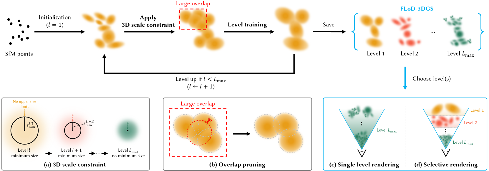</details> Figure 2. Method overview. Training begins at level 1, initialized from SfM points. During the training of each level, (a) a level-specific 3D scale constraint $s_min^(l)$ is imposed on the Gaussians as a lower bound, and (b) overlap pruning is performed to mitigate Gaussian overlap. At the end of each level’s training, the Gaussians are cloned and saved as the final representation for level $l$ . This level-by-level training continues until the max level ( $L_max$ ), resulting in a multi-level 3D Gaussian representation referred to as FLoD-3DGS. FLoD-3DGS supports (c) single-level rendering and (d) selective rendering using multiple levels. To address the hardware adaptability challenges, we propose Flexible Level of Detail (FLoD). FLoD constructs a multi-level 3D Gaussian Splatting (3DGS) representation that provides varying levels of detail and memory requirements, with each level independently capable of reconstructing the full scene. Our method applies a level-specific 3D scale constraint, which increases each successive level, to limit the amount of detail reconstructed and the rendering memory demand. Furthermore, we introduce a level-by-level training method to maintain a consistent 3D structure across all levels. Our trained FLoD representation provides the flexibility to choose any single level based on the available GPU memory or desired rendering rates. Furthermore, the independent and multi-level structure of our method allows different parts of an image to be rendered with different levels of detail, which we refer to as selective rendering. Depending on the scene type or the object of interest, higher-level Gaussians can be used to rasterize important regions, while lower levels can be assigned to less critical areas, resulting in more efficient rendering. As a result, FLoD provides the versatility of adapting to diverse GPU settings and rendering contexts. We empirically validate the effectiveness of FLoD in offering flexible rendering options, tested on both a high-end server and a low-cost laptop. We conduct experiments not only on the Tanks and Temples (Knapitsch et al., 2017) and Mip-Nerf360 (Barron et al., 2022) datasets, which are commonly used in 3DGS and its variants but also on the DL3DV-10K (Ling et al., 2023) dataset, which contains distant background elements that can be effectively represented through LoD. Furthermore, we demonstrate that FLoD can be easily integrated into existing 3DGS variants, while also enhancing the rendering quality. ## 2. Related Work ### 2.1. 3D Gaussian Splatting 3D Gaussian Splatting (3DGS) (Kerbl et al., 2023) has attained popularity for its fast rendering speed in comparison to other novel view synthesis literature such as NeRF (Mildenhall et al., 2020). Subsequent works, such as FreGS (Zhang et al., 2024) and AbsGS (Ye et al., 2024), improve rendering quality by modifying the loss function and the Gaussian density control strategy, respectively. However, these methods, including 3DGS, demand high rendering memory because they rely on a large number of Gaussians, making them unsuitable for low-cost devices with limited GPU memory. To address these memory challenges, various works have proposed compression methods for 3DGS. LightGaussian (Fan et al., 2023) and Compact3D (Lee et al., 2024) use pruning techniques, while EAGLES (Girish et al., 2024) employs quantized embeddings. However, their rendering quality falls short compared to 3DGS. RadSplat (Niemeyer et al., 2024) and Scaffold-GS (Lu et al., 2024) maintain rendering quality while reducing memory usage with neural radiance field prior and neural Gaussians. Despite these advancements, existing 3DGS methods lack the flexibility to provide multiple rendering options for optimizing performance across various GPU settings. In contrast, we propose a multi-level 3DGS that increases rendering flexibility by enabling rendering across various GPU settings, ranging from server GPUs with 24GB VRAM to laptop GPUs with 2GB VRAM. ### 2.2. Multi-Scale Representation There have been various attempts to improve the rendering quality of novel view synthesis through multi-scale representations. In the field of Neural Radiance Fields (NeRF), approaches such as Mip-NeRF (Barron et al., 2021) and Zip-NeRF (Barron et al., 2023) adopt multi-scale representations to improve rendering fidelity. Similarly, in 3D Gaussian Splatting (3DGS), Mip-Splatting (Yu et al., 2024) uses a multi-scale filtering mechanism, and MS-GS (Yan et al., 2024) applies a multi-scale aggregation strategy. However, these methods primarily focus on addressing the aliasing problem and do not consider the flexibility to adapt to different GPU settings. In contrast, our proposed method generates a multi-level representation that not only provides flexible rendering across various GPU settings but also enhances reconstruction accuracy. ### 2.3. Level of Detail Level of Detail (LoD) in computer graphics traditionally uses multiple representations of varying complexity, allowing the selection of detail levels according to computational resources. In NeRF literature, NGLOD (Takikawa et al., 2021) and Variable Bitrate Neural Fields (Takikawa et al., 2022) create LoD structures based on grid-based NeRFs. In 3D Gaussian Splatting (3DGS), methods such as Octree-GS (Ren et al., 2024) and Hierarchical-3DGS (Kerbl et al., 2024) integrate the concept of LoD and create multi-level 3DGS representation for efficient and high-detail rendering. However, these methods primarily target efficient rendering on high-end GPUs, such as A6000 or A100 GPUs with 48GB or 80GB VRAM. Moreover, these methods render using Gaussians from the entire range of levels, not solely from individual levels. Rendering with individual levels, particularly the lower ones, leads to a loss of image quality. Therefore, theses methods cannot provide rendering options with lower memory demands. While CityGaussian (Liu et al., 2024) can render individual levels using its multi-level representations created with various compression rates, it also does not address the challenges of rendering on lower-cost GPU. In contrast, our method allows for rendering using either individual or multiple levels, as all levels independently reconstruct the scene. Additionally, as each level has an appropriate degree of detail and corresponding rendering computational demand, our method offers rendering options that can be optimized for diverse GPU setups. ## 3. Preliminary 3D Gaussian Splatting (3DGS) (Kerbl et al., 2023) introduces a method to represent a 3D scene using a set of 3D Gaussian primitives. Each 3D Gaussian is characterized by attributes: position $\boldsymbol{μ}$ , opacity $o$ , covariance matrix $\boldsymbol{Σ}$ , and spherical harmonic coefficients. The covariance matrix $Σ$ is factorized into a scaling matrix $S$ and a rotation matrix $R$ : $$ \boldsymbol{Σ}=RSS^⊤R^⊤. \tag{1} $$ To facilitate the independent optimization of both components, the scaling matrix $S$ is optimized through the vector $s_opt$ , and the rotation matrix $R$ is optimized via the quaternion $q$ . These 3D Gaussians are projected to 2D screenspace and the opacity contribution of a Gaussian at a pixel $(x,y)$ is computed as follows: $$ α(x,y)=o· e^-\frac{1{2}≤ft(([x,y]^T-\boldsymbol{μ}^\prime)^ {T}\boldsymbol{Σ}^\prime-1([x,y]^T-\boldsymbol{μ}^\prime)\right)}, \tag{2} $$ where $\boldsymbol{μ}^\prime$ and $\boldsymbol{Σ}^\prime$ are the 2D projected mean and covariance matrix of the 3D Gaussians. The image is rendered by alpha blending the projected Gaussians in depth order. ## 4. Method: Flexible Level of Detail Our method reconstructs a scene as a $L_max$ -level 3D Gaussian representation, using 3D Gaussians of varying sizes from level 1 to $L_max$ (Section 4.1). Through our level-by-level training process (Section 4.2), each level independently captures the overall scene structure while optimizing for render quality appropriate to its respective level. This process results yields a novel LoD structure of 3D Gaussians, which we refer to as FLoD-3DGS. The lower levels in FLoD-3DGS reconstruct the coarse structures of the scene using fewer and larger Gaussians, while higher levels capture fine details using more and smaller Gaussians. Additionally, we introduce overlap pruning to eliminate artifacts caused by excessive Gaussian overlap (Section 4.3) and demonstrate our method’s easy integration with different 3DGS-based method (Section 4.4). ### 4.1. 3D Scale Constraint For each level $l$ where $l∈[1,L_max]$ , we impose a 3D scale constraint $s_min^(l)$ as the lower bound on 3D Gaussians. The 3D scale constraint $s_min^(l)$ is defined as follows: $$ s_min^(l)=\begin{cases}λ×ρ^1-l&for 1≤ l<L _max\\ 0&for l=L_max.\end{cases} \tag{3} $$ $λ$ is the initial 3D scale constraint, and $ρ$ is the scale factor by which the 3D scale constraint is reduced for each subsequent level. The 3D scale constraint is 0 at $L_max$ to allow reconstruction of the finest details without constraints at this stage. Then, we define 3D Gaussians’ scale at level $l$ as follows: $$ s^(l)=e^s_opt+s_min^(l). \tag{4} $$ where $s_opt$ is the learnable parameter for scale, while the 3D scale constraint $s_min^(l)$ is fixed. We note that $s^(l)>=s_min^(l)$ because $e^s_opt>0$ . On the other hand, there is no upper bound on Gaussian size at any level. This allows for flexible modeling, where scene contents with simple shapes and appearances can be modeled with fewer and larger Gaussians, avoiding the redundancy of using many small Gaussians at high levels. ### 4.2. Level-by-level Training We design a coarse-to-fine training process, where the next-level Gaussians are initialized by the fully-trained previous-level Gaussians. Similar to 3DGS, the 3D Gaussians at level 1 are initialized from SFM points. Then, the training process begins. Note that training of subsequent levels are nearly identical. The training process consists of periodic densification and pruning of Gaussians over a set number of iterations. This is then followed by the optimization of Gaussian attributes without any further densification or pruning for an additional set of iterations. Throughout the entire training process for level $l$ , the 3D scale of the Gaussian is constrained to be larger or equal to $s_min^(l)$ by definition. After completing training at level $l$ , this stage is saved as a checkpoint. At this point, the Gaussians are cloned and saved as the final Gaussians for level $l$ . Then, the checkpoint Gaussians are used to initialize Gaussians of the next level $l+1$ . For initialized Gaussians at the next level $l+1$ , we set $$ s_opt=\textnormal{log}(s^(l)-s_min^(l+1 )), \tag{5} $$ such that $s^(l+1)=s^(l)$ . It prevents abrupt initial loss by eliminating the gap $s^(l+1)-s^(l)=\cancel{e^s_opt^\text{ prev}}+s_min^(l+1)-(\cancel{e^s_opt^\text{ prev}}+s_min^(l))$ . Note that $s_opt^\text{prev}$ represents the learnable parameter for scale at level $l$ . ### 4.3. Overlap Pruning To prevent rendering artifacts, we remove Gaussians with large overlaps. Specifically, Gaussians whose average distance of its three nearest neighbors falls below a pre-defined distance threshold $d_OP^(l)$ are eliminated. Equation for $d_avg^(l)$ is given as: $$ d_avg^(i)=\frac{1}{3}∑_j=1^3d_ij \tag{6} $$ $d_OP^(l)$ is set as half of the 3D scale constraint $s_min^(l)$ for training level $l$ . This method also reduces the overall memory footprint. ### 4.4. Compatibility to Different Backbone The simplicity of our method, stemming from the straightforward design of the 3D scale constraints and the level-by-level training pipeline, makes it easy to integrate with other 3DGS-based techniques. We integrate our approach into Scaffold-GS (Lu et al., 2024), a variant of 3DGS that leverages anchor-based neural Gaussians. We generate a multi-level set of Scaffold-GS by applying progressively decreasing 3D scale constraints on the neural Gaussians, optimized through our level-by-level training method. ## 5. Rendering Methods FLoD’s $L_max$ -level 3D Gaussian representation provides a broad range of rendering options. Users can select a single level to render the scene (Section 5.1), or multiple levels to increase rendering efficiency through selective rendering (Section 5.2). Levels and rendering methods can be adjusted to achieve the desired rendering rates or to fit within available GPU memory limits. ### 5.1. Single-level Rendering From our multi-level set of 3D Gaussians $\{G^(l)\mid l=1,…,L_max\}$ , users can choose any single level for rendering to match their GPU memory capabilities. This approach is similar to how games or streaming services let users adjust quality settings to optimize performance for their devices. Rendering any single level independently is possible because each level is designed to fully reconstruct the scene. High-end hardware can handle the smaller and more numerous Gaussians of level $L_max$ , achieving high-quality rendering. However, rendering a large number of Gaussians may exceed the memory limits of commodity devices. In such cases, lower levels can be chosen to match the memory constraints. ### 5.2. Selective Rendering <details> <summary>x3.png Details</summary>  ### Visual Description ## Diagram: Multi-Level Projection Frustum with Screen-Space Constraints ### Overview This image is a technical diagram illustrating a multi-level projection or level-of-detail (LOD) scheme, likely used in computer graphics or rendering. It depicts how a viewing frustum is segmented into different regions (Levels 3, 4, and 5) based on distance from the camera, with associated minimum screen-space size constraints ($s_{\text{min}}$) for each level. The diagram establishes a relationship between world-space distance ($d_{\text{proj}}$), the image plane, and the projected size of objects. ### Components/Axes **1. Primary Axis (Horizontal):** * A horizontal black arrow at the bottom represents the primary distance axis, pointing to the right. * **Key Markers:** * $-f$: Located at the far left, aligned with the image plane. This likely represents the camera's focal length or near plane position in a negative coordinate system. * $o$: A red dot on the axis, representing the origin or camera center. * $d_{\text{proj}}^{(l=4)}$: A blue dashed vertical line marking the projection distance for Level 4. * $d_{\text{proj}}^{(L_{\text{start}}=3)}$: A magenta dashed vertical line marking the projection distance for the start of Level 3. **2. Image Plane & Projection Geometry (Left Side):** * **Image Plane:** A vertical black line on the left, labeled "image plane". * **Screensize Indicator:** A small red rectangle on the image plane, labeled "screensize ($\gamma = 1$)". This defines a reference screen-space size. * **Projection Lines:** Two cyan lines originate from the top and bottom of the "screensize" rectangle, converge at the red dot (origin $o$), and then diverge to form the boundaries of the viewing frustum extending to the right. **3. Frustum Levels & Regions (Main Area):** The diverging cyan lines define a frustum divided into three colored, sequential regions: * **Level 5 $L_{\text{end}}$ (Gaussians region):** The leftmost region, shaded in green. It is bounded on the right by the blue dashed line at $d_{\text{proj}}^{(l=4)}$. The label indicates this is the end of Level 5 and is associated with a "Gaussians region," suggesting a specific rendering technique (e.g., Gaussian splatting). * **Level 4:** The middle region, shaded in blue. It spans from the blue dashed line ($d_{\text{proj}}^{(l=4)}$) to the magenta dashed line ($d_{\text{proj}}^{(L_{\text{start}}=3)}$). * **Level 3 $L_{\text{start}}$:** The rightmost region, shaded in magenta. It begins at the magenta dashed line and extends to the right, fading out. The label indicates this is the start of Level 3. **4. Minimum Screen-Size Constraints:** Vertical double-headed arrows within each region define the minimum projected size ($s_{\text{min}}$) an object must have at that distance to be rendered at that level. * **For Level 4:** A blue arrow labeled $s_{\text{min}}^{(l=4)}$ spans the height of the blue frustum region at distance $d_{\text{proj}}^{(l=4)}$. * **For Level 3:** A magenta arrow labeled $s_{\text{min}}^{(L_{\text{start}}=3)}$ spans the height of the magenta frustum region at distance $d_{\text{proj}}^{(L_{\text{start}}=3)}$. ### Detailed Analysis The diagram defines a precise geometric and parametric relationship: 1. **Reference Setup:** A screen-space pixel or reference size ("screensize", $\gamma=1$) is defined on the image plane. Its projection through the camera center ($o$) creates the viewing frustum. 2. **Level Segmentation:** The frustum is partitioned along the depth axis into discrete levels (5, 4, 3). The partitioning is not arbitrary but is tied to specific projection distances ($d_{\text{proj}}$). 3. **Screen-Space Constraint:** For each level $l$, there is a minimum screen-space size $s_{\text{min}}^{(l)}$. This is visualized as the height of the frustum at the level's starting distance. An object at distance $d_{\text{proj}}^{(l)}$ must project to at least this size to be considered for rendering at level $l$. 4. **Direction of Progression:** The level numbers decrease (5 -> 4 -> 3) as distance from the camera increases. This is a common pattern in LOD systems where lower detail levels are used for farther objects. 5. **Color Coding:** The diagram uses a consistent color scheme for clarity: * **Green:** Level 5 / Gaussians region. * **Blue:** Level 4 and its associated parameters ($s_{\text{min}}^{(l=4)}$, $d_{\text{proj}}^{(l=4)}$). * **Magenta:** Level 3 and its associated parameters ($s_{\text{min}}^{(L_{\text{start}}=3)}$, $d_{\text{proj}}^{(L_{\text{start}}=3)}$). ### Key Observations * **Hierarchical Structure:** The diagram implies a hierarchical or multi-resolution rendering pipeline where scene elements are assigned to different levels based on their projected size. * **Gaussians Region:** The specific mention of "Gaussians region" for Level 5 strongly suggests this diagram is from a paper or system involving **3D Gaussian Splatting** or a similar point-based/splatting rendering technique. Level 5 may represent the highest-detail level where individual Gaussian primitives are used. * **Inverse Relationship:** The geometry shows that $s_{\text{min}}$ increases with distance ($s_{\text{min}}^{(L_{\text{start}}=3)} > s_{\text{min}}^{(l=4)}$). This is because the frustum expands; a constant angular size corresponds to a larger linear size at greater distances. * **Parameter Notation:** The use of $(l=4)$ and $(L_{\text{start}}=3)$ in the subscripts indicates these are level-specific parameters. $L_{\text{start}}$ may denote the first distance at which Level 3 becomes active. ### Interpretation This diagram is a **conceptual model for a level-of-detail selection mechanism in a rendering engine, likely one using Gaussian Splatting**. Its purpose is to define the rules for when to switch between different representation levels of a 3D scene. * **What it demonstrates:** It visually formalizes the core LOD criterion: an object's importance (and thus the detail level at which it is rendered) is a function of its **screen-space projected size**. Objects that project smaller than $s_{\text{min}}^{(l)}$ at distance $d_{\text{proj}}^{(l)}$ are either not rendered at level $l$ or are aggregated into a simpler representation (e.g., from Level 5 Gaussians to a lower-detail mesh or impostor in Level 4/3). * **Relationship between elements:** The image plane and screensize define the camera's view. The projection lines translate this into a 3D frustum. The $d_{\text{proj}}$ markers slice this frustum into zones. The $s_{\text{min}}$ arrows are the critical thresholds that link the 3D world (distance) back to the 2D image (screen size), creating a closed-loop system for LOD management. * **Significance:** This is a fundamental optimization strategy in real-time graphics. By rendering distant or small objects with less detail (Levels 4, 3), the system saves computational resources (memory, processing power) while maintaining visual quality for important, close-up objects (Level 5). The "Gaussians region" label points to a modern, neural rendering context where this LOD scheme might be applied to manage the complexity of a scene represented by millions of Gaussian primitives. The diagram provides the mathematical and geometric foundation for implementing such an LOD policy. 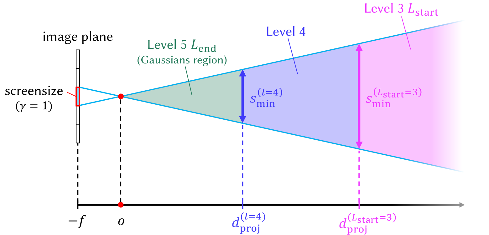</details> Figure 3. Visualization of the selective rendering process that shows how $d_proj^(l)$ determines the appropriate Gaussian level for specific regions. This example visualizes the case where level 3 is used as $L_start$ and level 5 as $L_end$ . Although a single level can be simply selected to match GPU memory capabilities, utilizing multiple levels can further enhance visual quality while keeping memory demands manageable. Distant objects or background regions do not need to be rendered with high-level Gaussians, which capture small and intricate details. This is because the perceptual difference between high-level and low-level Gaussian reconstructions becomes less noticeable as the distance from the viewpoint increases. In such scenarios, lower levels can be employed for distant regions while higher levels are used for closer areas. This arrangement of multiple level Gaussians can achieve perceptual quality comparable to using only high-level Gaussians but at a reduced memory cost. Therefore, we propose a faster and more memory-efficient rendering method by leveraging our multi-level set of 3D Gaussians $\{G^(l)\mid l=1,…,L_max\}$ . We create the set of Gaussians $G_sel$ for selective rendering by sampling Gaussians from a desired level range, $L_start$ to $L_end$ : $$ G_sel=\bigcup_l=L_{start}^L_end≤ft\{G^ {(l)}∈G^(l)\mid d_proj^(l-1)>d_G^(l)≥ d_ proj^(l)\right\}, \tag{7} $$ where $d_proj^(l)$ decides the inclusion of a Gaussian $G^(l)$ whose distance from the camera is $d_G^(l)$ . We define $d_proj^(l)$ as: $$ d_proj^(l)=\frac{s_min^(l)}{γ}×{f}, \tag{8} $$ by solving a proportional equation $s_min^(l):γ=d_proj^(l):f$ . Hence, the distance $d_proj^(l)$ is where the level-specific Gaussian 3D scale constraint $s_min^(l)$ becomes equal to the screen size threshold $γ$ on the image plane. $f$ is the focal length of the camera. We set $d_proj^(L_end)=0$ and $d_proj^(L_start-1)=∞$ to ensure that the scene is fully covered with Gaussians from the level range $L_start$ to $L_end$ . The Gaussian set $G_sel$ is created using the 3D scale constraint $s_min^(l)$ because $s_min^(l)$ represents the smallest 3D dimension that Gaussians at level $l$ can be trained to represent. Therefore, the distance $d_proj^(l)$ can be used to determine which level of Gaussians should be selected for different regions, as demonstrated in Figure 3. Since $s_min^(l)$ is fixed for each level, $d_proj^(l)$ is also fixed. Thus, constructing the Gaussian set $G_sel$ only requires calculating the distance of each Gaussian from the camera, $d_G^(l)$ . This method is computationally more efficient than the alternative, which requires calculating each Gaussian’s 2D projection and comparing it with the screen size threshold $γ$ at every level. The threshold $γ$ and the level range [ $L_start$ , $L_end$ ] can be adjusted to accommodate specific memory limitations or desired rendering rates. A smaller threshold and a high-level range prioritize fine details over memory and speed, while a larger threshold and a low-level range reduce memory use and speed up rendering at the cost of fine details. Predetermined Gaussian Set <details> <summary>x4.png Details</summary>  ### Visual Description ## Technical Diagram: Level-of-Detail (LOD) Management Strategies ### Overview The image is a technical diagram comparing two strategies for managing levels of detail (LOD) in a rendering or simulation system, likely related to 3D graphics or Gaussian splatting. It consists of two side-by-side sub-figures labeled **(a) predetermined** and **(b) per-view**. The diagram uses concentric regions and colored frustums to illustrate how different detail levels are assigned relative to a viewpoint or region of interest. ### Components/Axes The diagram is not a chart with axes but a conceptual illustration. Its key components are: **Labels and Text:** * **(a) predetermined**: Label for the left sub-figure. * **(b) per-view**: Label for the right sub-figure. * **Level 3 L_start (Gaussians region)**: A label in pink text, pointing to the outermost pink-shaded region in both sub-figures. * **Level 4**: A label in blue text, pointing to the middle blue-shaded ring/region. * **Level 5 L_end**: A label in green text, pointing to the innermost green-shaded circle/region. * **view frustum**: A label in cyan text, pointing to the cone-shaped viewing volumes in sub-figure (b). **Visual Elements & Spatial Grounding:** * **Sub-figure (a) - Predetermined:** * **Structure:** Three concentric circular regions centered in the frame. * **Innermost (Center):** A solid green circle labeled **Level 5 L_end**. * **Middle Ring:** A blue annular region surrounding the green circle, labeled **Level 4**. * **Outermost Region:** A diffuse pink glow extending from the blue ring to a dashed black circular boundary, labeled **Level 3 L_start (Gaussians region)**. * **Viewpoints:** Three stylized eye icons (▼) are placed within the green circle. Cyan lines (representing view rays or frustum edges) emanate from these eyes, passing through the blue and pink regions. The lines are straight and radiate outward, suggesting fixed viewing directions from predetermined positions. * **Sub-figure (b) - Per-view:** * **Structure:** The concentric circles are replaced by three distinct, wedge-shaped **view frustums** (cyan outlines) originating from a common central point (where the eye icons are clustered). * **Frustum Composition:** Each frustum is segmented into three colored zones corresponding to the levels: * The tip (closest to the center) is **green** (Level 5). * The middle segment is **blue** (Level 4). * The outer segment is a diffuse **pink** glow (Level 3). * **Arrangement:** The three frustums are oriented at different angles, covering a wider angular field than the straight lines in (a). They are contained within a dashed black circular boundary. * **Legend/Label Placement:** The labels **Level 3 L_start**, **Level 4**, and **Level 5 L_end** are positioned between the two sub-figures, with leader lines pointing to the corresponding colored regions in *both* (a) and (b), confirming the color-to-level mapping is consistent. ### Detailed Analysis The diagram contrasts two LOD assignment philosophies: 1. **Predetermined (a):** Detail levels are assigned based on **absolute distance** from a central point or region. The green (highest detail, Level 5) is at the core, surrounded by medium (blue, Level 4) and low-detail (pink, Level 3) zones. The view rays are straight and radial, implying the LOD is fixed regardless of the specific viewing angle. 2. **Per-view (b):** Detail levels are assigned **relative to each specific view frustum**. The LOD zones (green, blue, pink) are not concentric circles but are instead mapped directly onto the volume of each individual view frustum. The highest detail (green) is always at the frustum's near plane, with detail decreasing (blue, then pink) as distance from the camera increases along the view direction. This means the LOD is dynamically calculated for each viewpoint. ### Key Observations * **Color Consistency:** The color coding (Green=Level 5/High, Blue=Level 4/Medium, Pink=Level 3/Low) is maintained across both strategies and explicitly linked by the central labels. * **Spatial Reorganization:** The core difference is the transformation of LOD zones from **concentric shells** (distance-based) in (a) to **view-aligned volumes** (camera-based) in (b). * **Terminology:** The use of "L_start" and "L_end" suggests these levels define the start and end of a detail gradient or a specific range of interest (the "Gaussians region"). * **Boundary:** The dashed black circle in both figures likely represents the maximum extent or bounding volume of the system being managed. ### Interpretation This diagram illustrates a fundamental optimization concept in real-time rendering, such as for Gaussian Splatting or large-scale scene visualization. * **What it demonstrates:** It contrasts a **static, world-centric LOD system** (a) with a **dynamic, view-centric LOD system** (b). The predetermined method is simpler but may waste resources rendering high detail in areas not currently viewed. The per-view method is more complex but potentially more efficient, as it concentrates the highest detail (Level 5) precisely where the camera is looking, adapting the detail gradient to the view frustum's orientation. * **Relationship between elements:** The eye icons represent the camera(s). The colored regions represent different tiers of computational or geometric detail. The transition from (a) to (b) shows a shift in strategy from "where things are in the world" to "what the camera sees." * **Implication:** The "per-view" approach is likely proposed as an improvement for performance or quality, ensuring that the limited budget for high-detail processing (Level 5) is always applied to the most visually critical part of the scene—the area immediately in front of the viewer. The "Gaussians region" label hints this may be specific to a technique that uses Gaussian primitives for rendering. 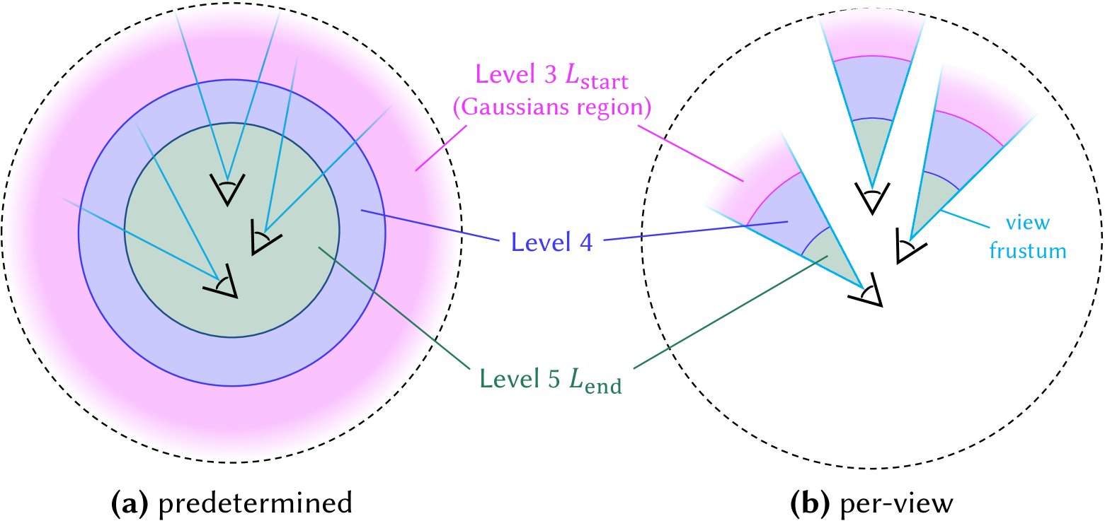</details> Figure 4. Comparison of predetermined Gaussian set $G_sel$ and per-view Gaussian set $G_sel$ creation methods. In the predetermined version, the Gaussian set is fixed, whereas the per-view version updates the Gaussian set dynamically whenever the camera position changes. This example illustrates the case where level 3 is used as $L_start$ and level 5 as $L_end$ . For scenes where important objects are centrally located or the camera trajectory is confined to a small region, higher-level Gaussians can be assigned in the central areas, while lower-level Gaussians are allocated to the background. This strategy enables high-quality rendering while reducing rendering memory and storage overhead. To achieve this, we calculate the Gaussian distance $d_G^(l)$ from the average position of all training view cameras before rendering and use it to predetermine the Gaussian subset $G_sel$ , as illustrated in Figure 4 (a). Since $G_sel$ is predetermined, it remains fixed during the rendering, eliminating the need to recalculate $d_G^(l)$ whenever the camera view changes. This predetermined approach allows for non-sampled Gaussians to be excluded, significantly reducing memory consumption during rendering. Furthermore, The sampled $G_sel$ can be stored for future use, requiring less storage compared to maintaining all level Gaussians. As a result, this method is especially beneficial for low-cost devices with limited GPU memory and storage capacity. <details> <summary>x5.png Details</summary>  ### Visual Description ## [Comparison Chart]: FLoD-3DGS vs. FLoD-Scaffold Detail Levels and Memory Usage ### Overview The image is a technical comparison chart displaying the visual quality and memory consumption of two different methods, labeled "FLoD-3DGS" and "FLoD-Scaffold," across five progressive levels of detail (LOD). The chart is structured as a 2x5 grid. The top row shows results for FLoD-3DGS, and the bottom row for FLoD-Scaffold. Each column corresponds to a detail level, from "level 1" (lowest detail) to "level 5 (Max)" (highest detail). For each method and level, a representative rendered image is shown, with the associated memory usage (in GB) annotated in the bottom-right corner of the image. ### Components/Axes * **Row Labels (Left Side):** Two methods are compared, listed vertically on the far left. * Top Row: `FLoD-3DGS` * Bottom Row: `FLoD-Scaffold` * **Column Headers (Top):** Five levels of detail are defined across the top. * Column 1: `level 1` * Column 2: `level 2` * Column 3: `level 3` * Column 4: `level 4` * Column 5: `level 5 (Max)` * **Data Annotations (Within each cell):** Each of the 10 image cells contains a memory usage value in the bottom-right corner, formatted as `memory: X.XXGB`. ### Detailed Analysis **Visual Quality Trend:** For both methods, moving from left (level 1) to right (level 5) shows a clear and significant increase in image sharpness, detail, and visual fidelity. Level 1 images are heavily blurred, while level 5 images are sharp and clear. **Memory Usage Data Points:** * **FLoD-3DGS (Top Row):** * Level 1: `memory: 0.25GB` * Level 2: `memory: 0.31GB` * Level 3: `memory: 0.75GB` * Level 4: `memory: 1.27GB` * Level 5 (Max): `memory: 2.06GB` * **Trend:** Memory usage increases monotonically and non-linearly with detail level. The jump from level 4 to 5 is the largest absolute increase (+0.79GB). * **FLoD-Scaffold (Bottom Row):** * Level 1: `memory: 0.24GB` * Level 2: `memory: 0.24GB` * Level 3: `memory: 0.43GB` * Level 4: `memory: 0.68GB` * Level 5 (Max): `memory: 0.98GB` * **Trend:** Memory usage also increases with detail level, but the growth is more gradual. Notably, levels 1 and 2 have identical memory usage (0.24GB). The increase from level 4 to 5 (+0.30GB) is smaller than for FLoD-3DGS. ### Key Observations 1. **Efficiency Divergence:** While both methods start at similar memory footprints at level 1 (~0.24-0.25GB), their memory consumption diverges significantly at higher detail levels. At level 5 (Max), FLoD-3DGS (2.06GB) uses more than double the memory of FLoD-Scaffold (0.98GB). 2. **Visual Quality vs. Memory Trade-off:** The chart visually demonstrates the trade-off between rendering quality and resource cost. Achieving the maximum visual fidelity (level 5) comes at a substantial memory cost, especially for the FLoD-3DGS method. 3. **Plateau in Scaffold:** The FLoD-Scaffold method shows no increase in memory between level 1 and level 2, suggesting a potential optimization or a different scaling behavior at the lowest detail tiers. ### Interpretation This chart is likely from a research paper or technical report on Level-of-Detail (LOD) management for 3D rendering, possibly in the context of Neural Radiance Fields (NeRF) or Gaussian Splatting, given the "3DGS" acronym. It serves to **benchmark and compare the memory efficiency** of two proposed techniques (FLoD-3DGS and FLoD-Scaffold) as they scale visual quality. The data suggests that **FLoD-Scaffold is a more memory-efficient method for achieving high-detail rendering**. For applications where memory is a constrained resource (e.g., mobile devices, real-time applications with many assets), FLoD-Scaffold would be the preferable choice to reach higher visual fidelity without the steep memory penalty seen in FLoD-3DGS. The chart effectively argues for the superiority of the Scaffold approach in terms of resource scaling. The identical memory usage for Scaffold at levels 1 and 2 might indicate a fixed overhead or a different strategy for handling the coarsest levels of detail. 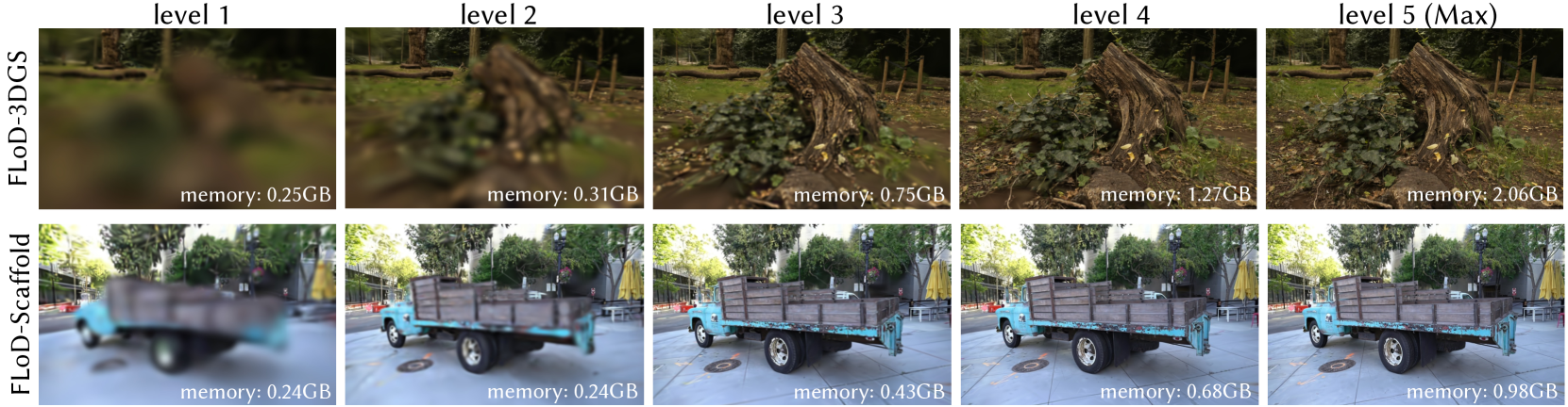</details> Figure 5. Renderings of each level in FLoD-3DGS and FLoD-Scaffold. FLoD can be integrated with both 3DGS and Scaffold-GS, with each level offering varying levels of detail and memory usage. Per-view Gaussian Set In large-scale scenes with camera trajectories that span broad regions, resampling the Gaussian set $G_sel$ based on the camera’s new position is necessary. This is because the camera may move and enter regions where lower level Gaussians have been assigned, leading to a noticeable decline in rendering quality. Therefore, in such cases, we define the Gaussian distance $d_G^(l)$ as the distance between a Gaussian $G^(l)$ and the current camera position. Consequently, whenever the camera position changes, $d_G^(l)$ is recalculated to resample the Gaussian set $G_sel$ as illustrated in Figure 4 (b). To maintain fast rendering rates, all Gaussians within the level range [ $L_start$ , $L_end$ ] are kept in GPU memory. Therefore, with the cost of increased rendering memory, selective rendering with per-view $G_sel$ effectively maintains consistent rendering quality over long camera trajectories. ## 6. Experiment ### 6.1. Experiment Settings #### 6.1.1. Datasets We conduct our experiments on a total of 15 real-world scenes. Two scenes are from Tanks&Temples (Knapitsch et al., 2017) and seven scenes are from Mip-NeRF360 (Barron et al., 2022), encompassing both bounded and unbounded environments. These datasets are commonly used in existing 3DGS research. In addition, we incorporate six unbounded scenes from DL3DV-10K (Ling et al., 2023), which include various urban and natural landscapes. We choose to include DL3DV-10K because it contains more objects located in distant backgrounds, providing a better demonstration of the diversity in real-world scenes. Further details on the datasets can be found in Appendix A. #### 6.1.2. Evaluation Metrics We measure PSNR, structural similarity SSIM (Wang et al., 2004), and perceptual similarity LPIPS (Zhang et al., 2018) for a comprehensive evaluation. Additionally, we assess the number of Gaussians used for rendering the scenes, the GPU memory usage, and the rendering rates (FPS) to evaluate resource efficiency. #### 6.1.3. Baselines We compare FLoD-3DGS against several models, including 3DGS (Kerbl et al., 2023), Scaffold-GS (Lu et al., 2024), Mip-Splatting (Yu et al., 2024), Octree-GS (Ren et al., 2024) and Hierarchical-3DGS (Kerbl et al., 2024). Among these, the main competitors are Octree-GS and Hierarchical-3DGS, as they share the LoD concept with FLoD. However, these two competitors define individual level representation differently from ours. In FLoD, each level representation independently reconstructs the scene. In contrast, Octree-GS defines levels by aggregating the representations from the first level up to the specified level, meaning that individual levels do not exist independently. On the other hand, Hierarchical-3DGS does not have the concept of rendering using a specific level’s representation, unlike FLoD and Octree-GS. Instead, it employs a hierarchical structure with multiple levels, where Gaussians from different levels are selected based on the target granularity $τ$ setting for each camera view during rendering. Additionally, like FLoD, Octree-GS is adaptable to both 3DGS and Scaffold-GS. We will refer to the 3DGS based Octree-GS as Octree-3DGS and the Scaffold-GS based Octree-GS as Octree-Scaffold. <details> <summary>x6.png Details</summary>  ### Visual Description ## Comparison Chart: Octree-3DGS vs. FLoD-3DGS Reconstruction Quality ### Overview The image is a technical comparison chart demonstrating the progressive reconstruction quality of two 3D Gaussian Splatting (3DGS) methods—**Octree-3DGS** (top row) and **FLoD-3DGS** (bottom row)—across five increasing levels of detail (Level 1 to Level 5). Each panel shows a rendered view of the same scene: a traditional Chinese architectural gate (paifang) with modern buildings in the background. Below each image are quantitative metrics for the number of Gaussians (#G's) and the Structural Similarity Index Measure (SSIM). ### Components/Axes * **Rows (Methods):** * **Top Row:** Labeled vertically on the left as "Octree-3DGS". * **Bottom Row:** Labeled vertically on the left as "FLoD-3DGS". * **Columns (Levels):** Five columns, each labeled at the top: "level 1", "level 2", "level 3", "level 4", "level 5 (Max)". * **Metrics per Panel:** Each of the 10 panels contains two lines of text below the image: 1. **#G's:** The number of Gaussian primitives used, followed by a percentage in parentheses (likely relative to the maximum for that method). 2. **SSIM:** The Structural Similarity Index Measure, a metric for image quality (1.0 = perfect match to reference). ### Detailed Analysis **Row 1: Octree-3DGS** * **Level 1:** Image is extremely blurry and distorted. Text: `#G's: 25K(9%) SSIM: 0.40` * **Level 2:** Image is less blurry, major structures are discernible but lack detail. Text: `#G's: 119K(17%) SSIM: 0.56` * **Level 3:** Image is clearer, details on the gate and background buildings are emerging. Text: `#G's: 276K(39%) SSIM: 0.68` * **Level 4:** Image is quite clear, with good detail on the gate's roof and pillars. Text: `#G's: 560K(78%) SSIM: 0.83` * **Level 5 (Max):** Image is sharp and detailed. Text: `#G's: 713K(100%) SSIM: 0.92` **Row 2: FLoD-3DGS** * **Level 1:** Image is blurry but shows more coherent structure than Octree-3DGS at the same level. Text: `#G's: 7K(0.7%) SSIM: 0.56` * **Level 2:** Image is significantly clearer than Octree-3DGS Level 2. Text: `#G's: 18K(2%) SSIM: 0.70` * **Level 3:** Image is already very clear, comparable to Octree-3DGS Level 4. Text: `#G's: 223K(22%) SSIM: 0.88` * **Level 4:** Image is very sharp. Text: `#G's: 475K(47%) SSIM: 0.93` * **Level 5 (Max):** Image is extremely sharp and detailed. Text: `#G's: 1015K(100%) SSIM: 0.96` **Embedded Text in Images:** The gate itself has a plaque with Chinese characters. The characters are partially legible in the higher-quality reconstructions (e.g., FLoD-3DGS Level 5). They appear to read "XX區" (the first two characters are less clear, possibly "XX District" or a name). ### Key Observations 1. **Efficiency vs. Quality Trade-off:** FLoD-3DGS achieves significantly higher SSIM scores at every corresponding level while using a vastly lower percentage of its total Gaussians. For example, at Level 3, FLoD uses 22% of its Gaussians for an SSIM of 0.88, while Octree uses 39% for an SSIM of 0.68. 2. **Visual Quality Progression:** Both methods show a clear trend of improving visual fidelity (less blur, more detail) as the level increases. However, FLoD-3DGS starts at a much higher baseline quality (SSIM 0.56 at Level 1 vs. Octree's 0.40). 3. **Resource Allocation:** The maximum resource usage (#G's at 100%) differs greatly: Octree-3DGS uses 713K Gaussians, while FLoD-3DGS uses 1015K. This suggests FLoD may have a higher ceiling for detail but is far more efficient in reaching acceptable quality earlier. 4. **Anomaly/Notable Point:** The SSIM for FLoD-3DGS at Level 1 (0.56) is equal to Octree-3DGS at Level 2, indicating FLoD's coarsest representation is as structurally similar to the reference as Octree's second-coarsest. ### Interpretation This chart is a performance benchmark for novel view synthesis techniques. It demonstrates that the **FLoD-3DGS method is substantially more efficient than Octree-3DGS** in terms of the quality-to-resource ratio. The data suggests FLoD employs a more effective level-of-detail (LoD) strategy, allocating Gaussian primitives in a way that captures essential scene structure much earlier in the refinement process. The **Peircean investigative reading** reveals the underlying claim: FLoD-3DGS is not just incrementally better, but represents a qualitative leap in efficiency. The steep SSIM improvement curve for FLoD (0.56 → 0.96) compared to Octree (0.40 → 0.92) indicates its progressive refinement is better aligned with human visual perception and structural fidelity. The fact that FLoD's Level 3 (22% resources) nearly matches Octree's Level 5 (100% resources) in SSIM (0.88 vs. 0.92) is a powerful argument for its practical utility in applications where computational resources or bandwidth are constrained, such as real-time rendering or streaming 3D content. The chart effectively argues that FLoD-3DGS provides a better user experience (higher quality) at lower cost (fewer Gaussians needed for a given quality target). 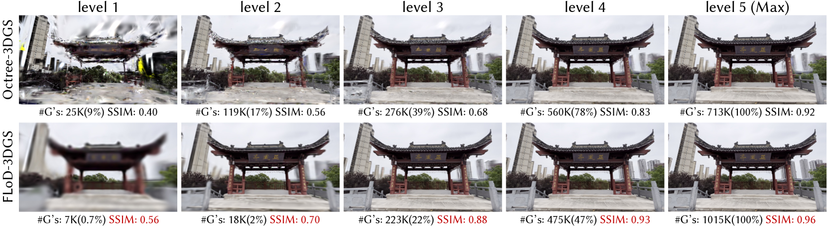</details> Figure 6. Comparison of the renderings at each level between FLoD-3DGS and Octree-3DGS on the DL3DV-10K dataset. ”#G’s” refers to the number of Gaussians, and the percentages (%) next to these values indicate the proportion of Gaussians used relative to the max level (level 5). <details> <summary>x7.png Details</summary>  ### Visual Description ## Comparative Visual Chart: Hierarchical-3DGS vs. FloD-3DGS Performance ### Overview The image is a 2x4 grid comparing the visual quality and resource usage of two 3D Gaussian Splatting (3DGS) methods: **Hierarchical-3DGS** (top row) and **FloD-3DGS** (bottom row). Each row shows four progressive levels of detail or quality settings for the same 3D scene (a garden patio with a wooden table and a decorative object). Below each sub-image, quantitative metrics for memory usage and Peak Signal-to-Noise Ratio (PSNR) are provided. ### Components/Axes * **Structure:** A grid with two rows and four columns. * **Row Labels (Left Side):** * Top Row: `Hierarchical-3DGS` (written vertically). * Bottom Row: `FloD-3DGS` (written vertically). * **Column/Parameter Labels (Top-Right of each sub-image):** * **Top Row (Hierarchical-3DGS):** Parameters are denoted by `τ` (tau). From left to right: `τ=120`, `τ=30`, `τ=15`, `τ=0 (Max)`. * **Bottom Row (FloD-3DGS):** Parameters are denoted by `level` sets. From left to right: `level{3,2,1}`, `level{4,3,2}`, `level{5,4,3}`, `level5 (Max)`. * **Data Labels (Below each sub-image):** Each contains two metrics: 1. `memory: X.XXGB (YY%)` - Memory usage in Gigabytes and as a percentage of the maximum. 2. `PSNR: XX.XX` - Peak Signal-to-Noise Ratio, a measure of image reconstruction quality. ### Detailed Analysis **Row 1: Hierarchical-3DGS** * **Trend:** As `τ` decreases (moving left to right), visual clarity improves, memory usage increases, and PSNR increases. * **Data Points:** 1. **τ=120 (Top-Left):** Image is very blurry. `memory:3.53GB(79%) PSNR: 20.98` 2. **τ=30:** Image is less blurry, details emerge. `memory:3.72GB(83%) PSNR: 23.47` 3. **τ=15:** Image is clear. `memory:4.19GB(93%) PSNR: 24.71` 4. **τ=0 (Max) (Top-Right):** Image is sharpest. `memory:4.46GB(100%) PSNR: 26.03` **Row 2: FloD-3DGS** * **Trend:** As the level set expands (moving left to right), visual clarity improves, memory usage increases, and PSNR increases. The memory percentages are highlighted in **red**. * **Data Points:** 1. **level{3,2,1} (Bottom-Left):** Image is reasonably clear. `memory:0.73GB(**29%**) PSNR: 24.02` 2. **level{4,3,2}:** Image is clearer. `memory:1.29GB(**52%**) PSNR: 26.23` 3. **level{5,4,3}:** Image is very clear. `memory:1.40GB(**57%**) PSNR: 26.71` 4. **level5 (Max) (Bottom-Right):** Image is sharpest. `memory:2.45GB(100%) PSNR: 27.64` ### Key Observations 1. **Efficiency Disparity:** FloD-3DGS achieves significantly higher PSNR values at much lower memory footprints compared to Hierarchical-3DGS. For example, FloD-3DGS at `level{4,3,2}` (PSNR 26.23, 1.29GB) surpasses the quality of Hierarchical-3DGS at its maximum setting (PSNR 26.03, 4.46GB) while using less than 30% of the memory. 2. **Visual Quality Correlation:** The visual improvement in the images directly correlates with the increasing PSNR values for both methods. 3. **Memory Scaling:** The maximum memory usage for FloD-3DGS (2.45GB) is approximately 55% of the maximum memory used by Hierarchical-3DGS (4.46GB). 4. **Parameter Notation:** The methods use different parameterization schemes (`τ` vs. `level` sets) to control the quality-memory trade-off. ### Interpretation This chart demonstrates a clear performance advantage for the **FloD-3DGS** method over **Hierarchical-3DGS** in the context of this specific 3D scene reconstruction task. The data suggests that FloD-3DGS employs a more efficient underlying representation or compression technique, allowing it to deliver superior visual fidelity (higher PSNR) while consuming substantially less GPU memory. The progressive improvement in both rows indicates that both methods support scalable quality settings. However, FloD-3DGS provides a much more favorable trade-off curve: a small increase in memory yields a large gain in PSNR, especially in the lower memory regimes. The red highlighting of the memory percentages for FloD-3DGS likely emphasizes its efficiency as a key selling point. From a technical standpoint, the `level` set parameterization in FloD-3DGS might correspond to a multi-resolution or hierarchical structure where more levels (e.g., `level5`) enable finer detail reconstruction. The chart effectively argues that FloD-3DGS is a more practical choice for applications where memory bandwidth or capacity is a constraint, such as real-time rendering on consumer hardware or processing large-scale scenes. 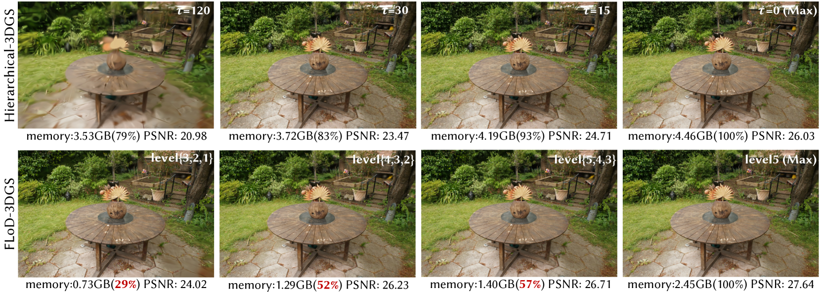</details> Figure 7. Comparison of the trade-off between visual quality and memory usage for FLoD-3DGS and Hierarchical-3DGS. The percentages (%) shown next to the memory values indicate how much memory each rendering setting consumes relative to the memory required by the ”Max” setting for maximum rendering quality. #### 6.1.4. Implementation FLoD-3DGS is implemented on the 3DGS framework. Experiments are mainly conducted on a single NVIDIA RTX A5000 24GB GPU. Following the common practice for LoD in graphics applications, we train our FLoD representation up to level $L_max=5$ . Note that $L_max$ is adjustable for specific objectives and settings with minimal impact on render quality. For FLoD-3DGS training with $L_max=5$ levels, we set the training iterations for levels 1, 2, 3, 4, and 5 to 10,000, 15,000, 20,000, 25,000, and 30,000, respectively. The number of training iterations for the max level matches that of the backbone, while the lower levels have fewer iterations due to their faster convergence. Gaussian density control techniques (densification, pruning, overlap pruning, opacity reset) are applied during the initial 5,000, 6,000, 8,000, 10,000, and 15,000 iterations for levels 1, 2, 3, 4, and 5, respectively. The Gaussian density control techniques run for the same duration as the backbone at the max level, but for shorter durations at the lower levels, as fewer Gaussians need to be optimized. Additionally, the intervals for densification are set to 2,000, 1,000, 500, 500, and 200 iterations for levels 1, 2, 3, 4, and 5, respectively. We use longer intervals compared to the backbone, which sets the interval to 100, as to allow more time for Gaussians to be optimized before new Gaussians are added or existing Gaussians are removed. These settings were selected based on empirical observations. Overlap pruning runs every 1000 iterations at all levels except the max level, where it is not applied. We set the initial 3D scale constraint $λ$ to 0.2 and the scale factor $ρ$ to 4. This configuration effectively distinguishes the level of detail across $L_max$ levels in most of the scenes we handle, enabling LoD representations that adapt to various memory capacities. For smaller scenes or when higher detail is required at lower levels, the initial 3D scale constraint $λ$ can be further reduced. Unlike the original 3DGS approach, we do not periodically remove large Gaussians or those with large projected sizes during training as we do not impose an upper bound on the Gaussian scale. All other training settings not mentioned follow those of the backbone model. For loss, we adopt L1 and SSIM losses across all levels, consistent with the backbone model. For selective rendering, we default to using the predetermined Gaussian set unless stated otherwise. The screen size threshold $γ$ is set as 1.0. This selects Gaussians of level $l$ from distances where the image projection of the level-specific 3D scale constraint $s_min^(l)$ becomes equal or smaller than 1.0 pixel length. ### 6.2. Flexible Rendering In this section, we show that each level representation from FLoD can be used independently. Based on this, we demonstrate the extensive range of rendering options that FLoD offers, through both single and selective rendering. <details> <summary>x8.png Details</summary>  ### Visual Description ## Visual Comparison Chart: Progressive Level Rendering Performance ### Overview The image displays a horizontal sequence of six panels, each showing the same 3D-rendered scene of a mossy, fallen log in a forest. The panels are labeled with increasing "level" identifiers, suggesting a progression in rendering quality or detail. Below each image, quantitative performance metrics are provided for two different GPU hardware configurations (A5000 and MX250). The chart demonstrates the trade-off between visual quality (measured by PSNR) and computational cost (memory usage and frame rate). ### Components/Axes * **Panel Structure:** Six vertical panels arranged left to right. * **Panel Headers (Top of each panel):** 1. `level {3,2,1}` 2. `level 3` 3. `level {4,3,2}` 4. `level 4` 5. `level {5,4,3}` 6. `level 5` * **Metrics Footer (Bottom of each panel):** Each panel contains three lines of text: * **Line 1:** `PSNR: [Value]` (Peak Signal-to-Noise Ratio, a quality metric). * **Line 2:** `memory: [Value]GB` (GPU memory consumption). * **Line 3:** `FPS: [Value](A5000) [Value](MX250)` (Frames Per Second on two different GPUs). * **Legend/Key:** Implicitly defined in the FPS line. `A5000` and `MX250` are the two hardware series being compared across all levels. ### Detailed Analysis **Data Series & Values (Left to Right):** 1. **Panel 1: `level {3,2,1}`** * **Visual:** The scene appears slightly softer or less detailed compared to later panels. * **PSNR:** 22.9 * **Memory:** 0.61GB * **FPS:** 304 (A5000), 28.7 (MX250) 2. **Panel 2: `level 3`** * **Visual:** Very similar to Panel 1, with minimal perceptible change. * **PSNR:** 23.0 * **Memory:** 0.76GB * **FPS:** 274 (A5000), 17.9 (MX250) 3. **Panel 3: `level {4,3,2}`** * **Visual:** A noticeable increase in sharpness and detail, particularly in the foliage and bark texture. * **PSNR:** 25.5 * **Memory:** 0.81GB * **FPS:** 218 (A5000), 13.2 (MX250) 4. **Panel 4: `level 4`** * **Visual:** Appears very similar to Panel 3, perhaps marginally sharper. * **PSNR:** 25.8 * **Memory:** 1.27GB * **FPS:** 178 (A5000), 10.6 (MX250) 5. **Panel 5: `level {5,4,3}`** * **Visual:** Further refinement in detail, though the incremental visual gain from the previous panel is subtle. * **PSNR:** 26.4 * **Memory:** 1.21GB * **FPS:** 150 (A5000), 8.4 (MX250) 6. **Panel 6: `level 5`** * **Visual:** The highest fidelity image in the sequence. * **PSNR:** 26.9 * **Memory:** 2.06GB * **FPS:** 113 (A5000), **OOM** (MX250). "OOM" likely stands for "Out Of Memory," indicating the MX250 GPU could not execute this rendering level. ### Key Observations 1. **Quality vs. Cost Trend:** There is a clear positive correlation between the "level" and PSNR (quality), and a clear negative correlation between "level" and FPS (performance). Memory usage generally increases with level. 2. **Hardware Disparity:** The A5000 GPU consistently delivers 10-15x higher frame rates than the MX250 across all executable levels, highlighting a massive performance gap between professional and mobile/workstation GPUs. 3. **Critical Failure Point:** The MX250 GPU hits a hard limit at `level 5`, failing with an Out-Of-Memory error, while the A5000 continues to function, albeit at a reduced frame rate. 4. **Non-Linear Memory Increase:** Memory usage does not scale perfectly linearly. The jump from `level {4,3,2}` (0.81GB) to `level 4` (1.27GB) is significant (+57%), as is the jump to `level 5` (2.06GB, +62% from level 4). 5. **Diminishing Returns:** The visual improvement between consecutive panels becomes less pronounced at higher levels, while the performance cost (drop in FPS, increase in memory) remains substantial. ### Interpretation This chart is a technical benchmark likely from a computer graphics or rendering engine study. It investigates the performance impact of increasing a multi-resolution or level-of-detail (LOD) system. * **What it demonstrates:** The data quantitatively proves that higher rendering levels (presumably involving more complex geometry, higher-resolution textures, or more advanced shading) produce higher-fidelity images (higher PSNR) but at a severe cost to performance (lower FPS) and resource consumption (higher memory). * **Relationship between elements:** The "level" labels are the independent variable. PSNR is the primary dependent variable measuring output quality. Memory and FPS are dependent variables measuring system cost. The two GPU series act as a controlled variable to show how hardware capability mediates this trade-off. * **Notable implications:** * **Optimization Insight:** For real-time applications (like games or simulations), a developer might choose `level {4,3,2}` as a "sweet spot," offering a large quality jump (PSNR +2.5 from base) for a moderate performance cost on the A5000, while remaining barely runnable on the MX250. * **Hardware Limitation:** The OOM error for the MX250 at `level 5` is a critical finding. It defines the absolute upper bound of that hardware's capability for this specific workload, information vital for setting minimum system requirements. * **Efficiency Analysis:** The non-linear memory growth suggests that the highest levels may be using disproportionately large assets or buffers, indicating a potential area for optimization in the rendering pipeline. 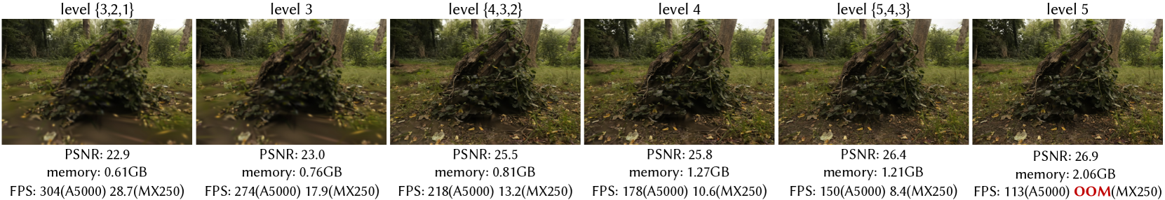**In essence, this image provides a clear, data-driven narrative about the cost of visual fidelity in real-time rendering, emphasizing that quality improvements are not free and are heavily constrained by available hardware resources.** </details> Figure 8. Various rendering options of FLoD-3DGS are evaluated on a server with an A5000 GPU and a laptop equipped with a 2GB VRAM MX250 GPU. The flexibility of FLoD-3DGS provides rendering options that prevent out-of-memory (OOM) errors and allow near real-time rendering on the laptop setting. #### 6.2.1. LoD Representation As shown in Figure 5, FLoD follows the LoD concept by offering independent representations at each level. Each level captures the scene with varying levels of detail and corresponding memory requirements. This enables users to select an appropriate level for rendering based on the desired visual quality and available memory. A key observation is that even at lower levels (e.g., levels 1, 2, and 3), FLoD-3DGS achieves high perceptual visual quality for the background. This is because, even with the large size of Gaussians at lower levels, the perceived detail in distant regions is similar to that achieved using the smaller Gaussians at higher levels. To further demonstrate the effectiveness of FLoD’s level representations, we compare renderings of each level from FLoD-3DGS with those from Octree-3DGS, as shown in Figure 6. At lower levels (e.g., levels 1, 2, and 3), Octree-3DGS shows broken structures, such as a pavilion, and the sharp artifacts created by very thin and elongated Gaussians. In contrast, FLoD-3DGS preserves the overall structure with appropriate detail for each level. Notably, it achieves this while using fewer Gaussians than Octree-3DGS, showing our method’s superiority in efficiently creating lower-level representations that better capture the scene structure. At higher levels (e.g., level 5), FLoD-3DGS uses more Gaussians to achieve higher visual quality and accurately reconstruct complex scene structures. This shows that our method can handle detailed scenes effectively through the higher level representations. In summary, the level representations of FLoD-3DGS outperform those of Octree-3DGS in reconstructing scene structures, as evidenced by its higher SSIM values across all levels. Furthermore, FLoD-3DGS uses significantly fewer Gaussians at lower levels, requiring only 0.7%, 2%, and 22% of the Gaussians of the max level for levels 1, 2, and 3, respectively. These results demonstrate that FLoD-3DGS can create level representations with a wide range of memory requirements. Note that we exclude Hierarchical-3DGS from this comparison because it was not designed for rendering with specific levels. For render results of Hierarchical-3DGS and Octree-3DGS that use Gaussians from single levels individually, please refer to Appendix C. 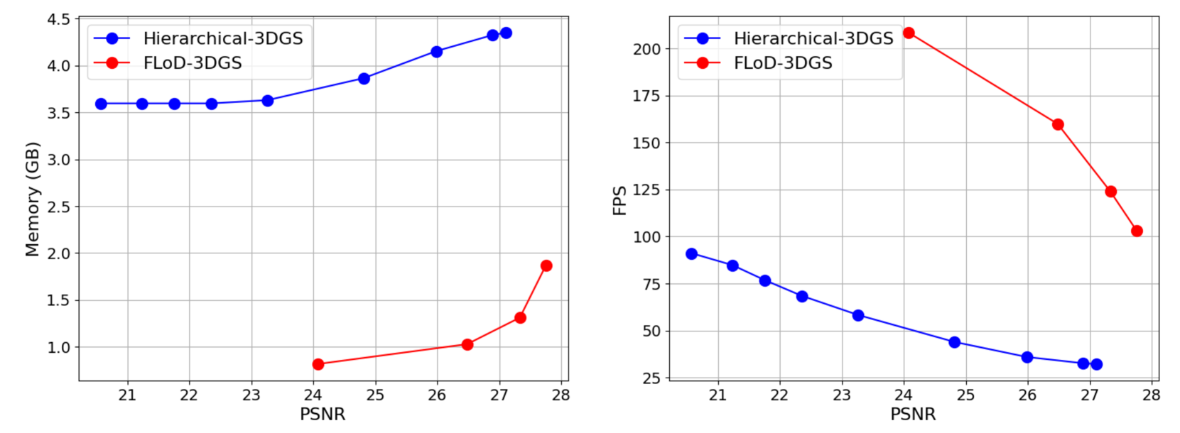<details> <summary>x9.png Details</summary>  ### Visual Description ## Line Charts: Performance Comparison of Hierarchical-3DGS vs. FLoD-3DGS ### Overview The image contains two side-by-side line charts comparing the performance of two 3D Gaussian Splatting (3DGS) methods: **Hierarchical-3DGS** (blue line with circular markers) and **FLoD-3DGS** (red line with circular markers). The charts plot two different performance metrics (Memory and FPS) against image quality (PSNR). ### Components/Axes **Left Chart:** * **Chart Type:** Line chart with markers. * **Y-Axis:** Label: `Memory (GB)`. Scale: Linear, ranging from approximately 0.5 to 4.5 GB. Major ticks at 1.0, 1.5, 2.0, 2.5, 3.0, 3.5, 4.0, 4.5. * **X-Axis:** Label: `PSNR`. Scale: Linear, ranging from approximately 20.5 to 28. Major ticks at 21, 22, 23, 24, 25, 26, 27, 28. * **Legend:** Located in the top-left corner. Contains two entries: * Blue line with circle marker: `Hierarchical-3DGS` * Red line with circle marker: `FLoD-3DGS` **Right Chart:** * **Chart Type:** Line chart with markers. * **Y-Axis:** Label: `FPS`. Scale: Linear, ranging from approximately 25 to 210. Major ticks at 25, 50, 75, 100, 125, 150, 175, 200. * **X-Axis:** Label: `PSNR`. Scale: Linear, identical to the left chart (20.5 to 28). * **Legend:** Located in the top-left corner. Identical to the left chart. ### Detailed Analysis **Left Chart (Memory vs. PSNR):** * **Trend - Hierarchical-3DGS (Blue):** The line shows a gradual, monotonic upward trend. Memory usage increases as PSNR (quality) increases. * Data Points (Approximate): * PSNR ~20.7: Memory ~3.6 GB * PSNR ~21.2: Memory ~3.6 GB * PSNR ~21.7: Memory ~3.6 GB * PSNR ~22.2: Memory ~3.6 GB * PSNR ~23.2: Memory ~3.65 GB * PSNR ~24.8: Memory ~3.9 GB * PSNR ~26.0: Memory ~4.15 GB * PSNR ~27.0: Memory ~4.35 GB * PSNR ~27.3: Memory ~4.4 GB * **Trend - FLoD-3DGS (Red):** The line shows a steep, accelerating upward trend, particularly after PSNR ~26. Memory usage increases sharply with quality. * Data Points (Approximate): * PSNR ~24.1: Memory ~0.8 GB * PSNR ~26.5: Memory ~1.05 GB * PSNR ~27.3: Memory ~1.35 GB * PSNR ~27.8: Memory ~1.9 GB **Right Chart (FPS vs. PSNR):** * **Trend - Hierarchical-3DGS (Blue):** The line shows a steady, monotonic downward trend. FPS (performance) decreases as PSNR (quality) increases. * Data Points (Approximate): * PSNR ~20.7: FPS ~90 * PSNR ~21.2: FPS ~85 * PSNR ~21.7: FPS ~77 * PSNR ~22.2: FPS ~70 * PSNR ~23.2: FPS ~60 * PSNR ~24.8: FPS ~45 * PSNR ~26.0: FPS ~37 * PSNR ~27.0: FPS ~33 * PSNR ~27.3: FPS ~33 * **Trend - FLoD-3DGS (Red):** The line shows a very steep, accelerating downward trend. FPS drops dramatically as quality increases. * Data Points (Approximate): * PSNR ~24.1: FPS ~210 * PSNR ~26.5: FPS ~160 * PSNR ~27.3: FPS ~125 * PSNR ~27.8: FPS ~103 ### Key Observations 1. **Memory Efficiency:** FLoD-3DGS consistently uses significantly less memory than Hierarchical-3DGS across all comparable PSNR values. At PSNR ~27.3, FLoD uses ~1.35 GB vs. Hierarchical's ~4.4 GB. 2. **Performance (FPS) at Low Quality:** At lower quality (PSNR ~24.1), FLoD-3DGS achieves a much higher FPS (~210) compared to Hierarchical-3DGS at a similar PSNR (~45 FPS at PSNR 24.8). 3. **Performance Degradation:** Both methods show a performance (FPS) trade-off for higher quality. However, the degradation is far more severe for FLoD-3DGS, with FPS dropping by over 50% from its peak as PSNR increases from ~24 to ~28. 4. **Quality Ceiling:** The data suggests FLoD-3DGS is being evaluated at a higher PSNR range (starting ~24) compared to Hierarchical-3DGS (starting ~20.7). The highest quality point shown is for FLoD-3DGS at PSNR ~27.8. ### Interpretation These charts illustrate a classic engineering trade-off between resource consumption (memory), performance (speed/FPS), and output quality (PSNR) in 3D Gaussian Splatting rendering. * **Hierarchical-3DGS** appears to be a more **stable and predictable** method. It has a higher baseline memory cost but scales more gracefully. Its performance (FPS) declines steadily with quality, suggesting a consistent computational load per quality increment. * **FLoD-3DGS** demonstrates a **highly efficient but volatile** profile. It achieves remarkable memory savings and very high frame rates at moderate quality levels. However, its costs (both memory and, especially, frame time) explode as one pushes for higher fidelity. This suggests its optimization strategy (likely involving level-of-detail or dynamic resource allocation) becomes increasingly expensive to manage at finer detail levels. **Conclusion:** The choice between methods depends on the application's priorities. For memory-constrained systems or applications targeting moderate quality with high frame rates, FLoD-3DGS is compelling. For applications requiring consistently high quality or where predictable performance scaling is critical, Hierarchical-3DGS may be preferable despite its higher memory footprint. The data implies FLoD-3DGS hits a "quality wall" where further improvements incur disproportionate performance costs. </details> Figure 9. Comparison of the trade-offs in selective rendering for FLoD-3DGS and Hierarchical-3DGS on Mip-NeRF360 scenes: visual quality(PSNR) versus memory usage, and visual quality versus rendering speed(FPS). #### 6.2.2. Selective Rendering FLoD provides not only single-level rendering but also selective rendering. Selective rendering enables more efficient rendering by selectively using Gaussians from multiple levels. To evaluate the efficiency of FLoD’s selective rendering, we compare rendering quality and memory usage for different selective rendering configurations against Hierarchical-3DGS. We compare with Hierarchical-3DGS because its rendering method, involving the selection of Gaussians from its hierarchy based on target granularity $τ$ , is similar to our selective rendering which selects Gaussians across level ranges based on the screen size threshold $γ$ . As shown in Figure 7, FLoD-3DGS effectively reduces memory usage through selective rendering. For example, selectively using levels 5, 4, and 3 reduces memory usage by about half compared to using only level 5, while the PSNR decreases by less than 1. Similarly, selective rendering with levels 3, 2, and 1 reduce memory usage to approximately 30%, with PSNR drop of about 3.6. In contrast, Hierarchical-3DGS does not reduce memory usage as effectively as FLoD-3DGS and also suffers from a greater decrease in rendering quality. Even when the target granularity $τ$ is set to 120, occupied GPU memory remains high, consuming approximately 79% of the memory used for the maximum rendering quality setting ( $τ=0$ ). Moreover, for this rendering setting, the PSNR drops significantly by more than 5. These results demonstrate that FLoD-3DGS’s selective rendering provides a wider range of rendering options, achieving a better balance between visual quality and memory usage compared to Hierarchical-3DGS. We further compare the memory usage to PSNR curve, and FPS to PSNR curve on the Mip-NeRF360 scenes in Figure 9. For FLoD-3DGS, we evaluate rendering performance using only level 5, as well as selectively using levels 5, 4, 3; levels 4, 3, 2; and levels 3, 2, 1. For Hierarchical-3DGS, we measure rendering performance with target granularity $τ$ set to 0, 6, 15, 30, 60, 90, 120, 160, and 200. The results show that FLoD-3DGS consistently uses less memory and achieves higher fps than Hierarchical-3DGS when compared at the same PSNR levels. Notably, as PSNR decreases, FLoD-3DGS shows a sharper reduction in memory usage, and a greater increase in fps. Note that for a fair comparison, we train Hierarchical-3DGS with a maximum $τ$ of 200 during the hierarchy optimization stage to enhance its rendering quality for larger $τ$ beyond its default settings. For renderings of Hierarchicial-3DGS using its default training settings, please refer to Appendix D. Table 1. Quantitative comparison of FLoD-3DGS to baselines across three real-world datasets (Mip-NeRF360, DL3DV-10K, Tanks&Temples). For FLoD-3DGS and Hierarchical-3DGS, we use the rendering setting that produces the best image quality. The best results are highlighted in bold. | 3DGS Mip-Splatting Octree-3DGS | 27.36 27.59 27.29 | 0.812 0.831 0.815 | 0.217 0.181 0.214 | 28.00 28.64 29.14 | 0.908 0.917 0.915 | 0.142 0.125 0.128 | 23.58 23.62 24.19 | 0.848 0.855 0.865 | 0.177 0.157 0.154 | | --- | --- | --- | --- | --- | --- | --- | --- | --- | --- | | Hierarchical-3DGS | 27.10 | 0.797 | 0.219 | 30.45 | 0.922 | 0.115 | 24.03 | 0.861 | 0.152 | | FLoD-3DGS | 27.75 | 0.815 | 0.224 | 31.99 | 0.937 | 0.107 | 24.41 | 0.850 | 0.186 | Table 2. Trade-offs between visual quality, rendering speed, and the number of Gaussians achieved in FLoD-3DGS through single-level and selective rendering in the Mip-NeRF360 dataset. | ✓ | 27.75 | 0.815 | 0.224 | 103 | 2189K | | --- | --- | --- | --- | --- | --- | | ✓- ✓- ✓ | 27.33 | 0.801 | 0.245 | 124 | 1210K | | ✓ $-\checkmark$ | 26.67 | 0.764 | 0.292 | 150 | 1049K | | ✓- ✓- ✓ | 26.48 | 0.759 | 0.298 | 160 | 856K | | ✓ | 24.11 | 0.634 | 0.440 | 202 | 443K | | ✓- ✓- ✓ | 24.07 | 0.632 | 0.442 | 208 | 414K | #### 6.2.3. Various Rendering Options FLoD supports both single-level rendering and selective rendering, offering a wide range of rendering options with varying visual quality and memory requirements. As shown in Table 2, FLoD enables flexible adjustment of the number of Gaussians. Reducing the number of Gaussians increases rendering speed while also reducing memory usage, allowing FLoD to adapt efficiently to hardware environments with varying memory constraints. To evaluate the flexibility of FLoD, we conduct experiments on a server with an A5000 GPU and a low-cost laptop equipped with a 2GB VRAM MX250 GPU. As shown in Figure 8, rendering with only level 4 or selective rendering using levels 5, 4, and 3 achieves visual quality comparable to rendering with only level 5, while reducing memory usage by approximately 40%. This reduction prevents out-of-memory (OOM) errors that occur on low-cost GPUs, such as the MX250, when rendering with only level 5. Furthermore, using lower levels for single-level rendering or selective rendering increases fps, enabling near real-time rendering even on low-cost devices. Hence, FLoD offers considerable flexibility by providing various rendering options through single and selective rendering, ensuring effective performance across devices with different memory capacities. For additional evaluations of rendering flexibility on the MX250 GPU in Mip-NeRF360 scenes, please refer to the Appendix G. ### 6.3. Max Level Rendering We have demonstrated that FLoD provides various rendering options following the LoD concept. However, in this section, we show that using only the max level for single-level rendering provides rendering quality comparable to those of existing models. Moreover, FLoD provides rendering quality comparable to those of existing models when using the maximum level for single-level rendering. Table 1 compares FLoD-3DGS with baselines across three real-world datasets. Table 1 compares max-level (level 5) of FLoD-3DGS with baselines across three real-world datasets. FLoD-3DGS performs competitively on the Mip-NeRF360 and Tanks&Temples datasets, which are commonly used in baseline evaluations, and outperforms all baselines across all reconstruction metrics on the DL3DV-10K dataset. This demonstrates that FLoD achieves high-quality rendering, which users can select from among the various rendering options FLoD provides. For qualitative comparisons, please refer to Appendix F. 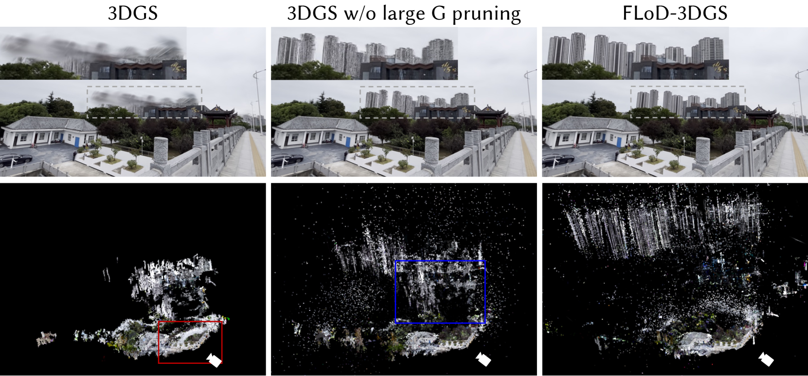<details> <summary>x10.png Details</summary>  ### Visual Description ## Diagram: Comparison of 3D Gaussian Splatting (3DGS) Methods ### Overview This image is a technical comparison figure, likely from a research paper or presentation, demonstrating the visual and structural differences between three variants of a 3D Gaussian Splatting (3DGS) reconstruction method. The figure is organized into a 3x2 grid. The top row shows rendered views of a 3D scene from a specific viewpoint. The bottom row shows the corresponding underlying 3D point cloud or Gaussian representation for each method against a black background. ### Components/Axes The image is divided into three vertical columns, each labeled with a method name at the top: 1. **Left Column:** `3DGS` 2. **Middle Column:** `3DGS w/o large G pruning` 3. **Right Column:** `FLoD-3DGS` Each column contains two vertically stacked panels: * **Top Panel:** A photorealistic rendered image of an outdoor scene. * **Bottom Panel:** A visualization of the 3D data structure (point cloud/Gaussians) used to generate the render above. **Scene Elements (Visible in all top-row renders):** * A traditional Chinese-style building with a grey tiled roof and white walls in the foreground left. * A stone balustrade and walkway leading towards the right. * A dense cluster of modern high-rise apartment buildings in the background. * Trees and greenery. * A black car parked near the traditional building. * A dashed white rectangular box is overlaid on the background buildings in each render, indicating a region of interest for comparison. * **Text within the scene:** On the dark grey building behind the traditional structure, there are gold-colored Chinese characters: `华` (Huá) and `侨` (Qiáo), which together form `华侨` (Huáqiáo), meaning "Overseas Chinese." **Data Visualization Elements (Bottom-row panels):** * The visualizations show white/colored points or splats on a black background, representing the 3D reconstruction. * **Left (`3DGS`):** A red rectangular box highlights a dense, somewhat noisy cluster of points in the lower-right quadrant. * **Middle (`3DGS w/o large G pruning`):** A blue rectangular box highlights a region in the center-right, showing a denser, more vertically oriented structure compared to the left panel. * **Right (`FLoD-3DGS`):** No colored box is present. The point cloud appears the most structured and dense, particularly in the upper region corresponding to the background buildings. * A small white arrow icon (likely indicating camera viewpoint or orientation) is present in the bottom-right corner of each bottom panel. ### Detailed Analysis **Top Row - Rendered Scene Quality:** * **`3DGS` (Left):** The render is significantly degraded. The background high-rise buildings are extremely blurry and lack any fine detail, appearing as smudged grey shapes. The foreground elements (traditional building, walkway) are somewhat clearer but still soft. * **`3DGS w/o large G pruning` (Middle):** A dramatic improvement over the left panel. The background buildings are now clearly resolved, showing individual windows and structural lines. The overall scene is much sharper. * **`FLoD-3DGS` (Right):** Visually very similar to the middle panel. The background buildings are sharp and detailed. The difference in render quality between the middle and right panels is subtle to the naked eye in this static image. **Bottom Row - 3D Data Structure:** * **`3DGS` (Left):** The point cloud is sparse and fragmented. The red box highlights a concentrated but messy cluster of points, likely corresponding to the poorly reconstructed background area. The overall structure lacks clear definition of the large buildings. * **`3DGS w/o large G pruning` (Middle):** The point cloud is much denser and more widespread. The blue box highlights a region where points form distinct vertical columns, clearly representing the high-rise buildings. There is a significant amount of "noise" or stray points scattered throughout the volume. * **`FLoD-3DGS` (Right):** This point cloud appears the most organized and dense. The vertical structures of the background buildings are very well-defined and prominent in the upper half of the visualization. The distribution of points seems more efficient and less noisy than the middle panel, with a clearer separation between the building structures and the surrounding space. ### Key Observations 1. **Progressive Improvement:** There is a clear visual progression from left to right. The standard `3DGS` fails to reconstruct distant/background geometry (the high-rises). Removing the "large G pruning" (`3DGS w/o large G pruning`) dramatically improves the reconstruction of these structures. `FLoD-3DGS` appears to refine this further, potentially with better point distribution or efficiency. 2. **Correlation Between Data and Render:** The quality of the rendered image (top row) is directly correlated with the density and organization of the underlying 3D data (bottom row). Sparse, noisy data leads to blurry renders; dense, structured data leads to sharp renders. 3. **Highlighted Regions:** The colored boxes (red and blue) are used to draw attention to specific areas in the 3D data that explain the differences in the rendered output. The red box in the left column shows the problematic, under-reconstructed area. The blue box in the middle column shows the successfully reconstructed building geometry. 4. **Text Language:** The embedded text in the scene (`华侨`) is in **Chinese (Simplified)**. It translates to **"Overseas Chinese"** in English. ### Interpretation This figure serves as a qualitative ablation study and comparison for a 3DGS-based method. It demonstrates that a specific algorithmic component—referred to as "large G pruning"—is detrimental to the reconstruction of large, distant structures like the background skyscrapers. By disabling this pruning (`w/o large G pruning`), the method retains more Gaussian primitives (the "G"s), allowing for a much more complete and accurate 3D model, which in turn produces a high-fidelity render. The `FLoD-3DGS` method is presented as the proposed or superior approach. While its rendered output is similar to the middle panel, its underlying data structure (bottom-right) suggests it achieves comparable or better visual quality potentially with a more optimized, less noisy, or more efficient representation of the 3D scene. The figure argues that `FLoD-3DGS` successfully balances detail preservation (like the middle method) with a cleaner geometric representation. **In essence, the image communicates:** "Our method (FLoD-3DGS) fixes a flaw in standard 3DGS that caused background details to be lost, and it does so with a high-quality 3D representation, as evidenced by these side-by-side comparisons of both the final pictures and the underlying 3D data." </details> Figure 10. Comparison of 3DGS and FLoD-3DGS on the DL3DV-10K dataset. The upper row shows rendering with zoom-in of the gray dashed box. The bottom row shows point visualization of the Gaussian centers. The red box shows distortions caused by large Gaussian pruning, and the blue box illustrates geometry inaccuracies that occur without the 3D scale constraint. FLoD’s 3D scale constraint ensures accurate Gaussian placement and improved rendering. Discussion on rendering quality improvement FLoD-3DGS particularly excels at rendering high-quality distant regions. This results in high PSNR on the DL3DV-10K dataset, which contains many distant objects. Two key differences from vanilla 3DGS drive this improvement: removing large Gaussian pruning and introducing a 3D scale constraint. Vanilla 3DGS prunes large Gaussians during training. This pruning causes distant backgrounds, such as the sky and buildings, to be incorrectly rendered with small Gaussians near the camera, as shown in the red box in Figure 10. This distortion disrupts the structure of the scene. Simply removing this pruning alleviates the problem and improves the rendering quality. However, removing large Gaussian pruning alone does not guarantee accurate Gaussian placement. As shown in the blue box in Figure 10, buildings are rendered with Gaussians of varying sizes at different depths, resulting in inaccurate geometry in the rendered image. FLoD’s 3D scale constraint solves this issue. It initially constrains Gaussians to be large, applying greater loss to mispositioned Gaussians to correct or prune them. During training, densification adds new Gaussians near existing ones, preserving accurate geometry as training progresses. This approach allows FLoD to reconstruct scene structures more precisely and in the correct positions. ### 6.4. Backbone Compatibility Table 3. Level-wise comparison of visual quality and memory usage (GB) for FLoD-3DGS, alongside Scaffold-GS and Octree-GS on Mip-NeRF360(Mip), DL3DV-10K(DL3DV) and Tanks&Temples(T&T) datasets. | FLoD-Scaffold(lv1) | Mip PSNR 20.1 | DL3DV mem. 0.5 | T&T PSNR 22.2 | mem. 0.3 | PSNR 17.1 | mem. 0.2 | | --- | --- | --- | --- | --- | --- | --- | | FLoD-Scaffold(lv2) | 22.1 | 0.5 | 25.2 | 0.3 | 19.3 | 0.3 | | FLoD-Scaffold(lv3) | 24.7 | 0.6 | 28.5 | 0.4 | 21.8 | 0.4 | | FLoD-Scaffold(lv4) | 26.6 | 0.8 | 30.1 | 0.6 | 23.6 | 0.7 | | FLoD-Scaffold(lv5) | 27.4 | 1.0 | 31.1 | 0.7 | 24.1 | 1.0 | | Scaffold-GS | 27.4 | 1.3 | 30.5 | 0.8 | 24.1 | 0.7 | | Octree-Scaffold | 27.2 | 1.0 | 30.9 | 0.6 | 24.6 | 0.8 | Our method, FLoD, integrates seamlessly with 3DGS and its variants. To demonstrate this, we apply FLoD not only to 3DGS (FLoD-3DGS) but also to Scaffold-GS that uses anchor-based neural Gaussians (FLoD-Scaffold). As shown in Figure 5, FLoD-Scaffold also generates representations with appropriate levels of detail and memory for each level. To further illustrate how FLoD-Scaffold provides suitable representations for each level across different datasets, we measure the PSNR and rendering memory usage for each level on three datasets. As shown in Table 3, FLoD-Scaffold provides various rendering options that balance visual quality and memory usage across all three datasets. In contrast, Octree-Scaffold, which also uses Scaffold-GS as its backbone model, has limitations in providing multiple rendering options due to its restricted representation capabilities for middle and low levels, similar to Octree-3DGS. Furthermore, FLoD-Scaffold also shows high visual quality when rendering with only the max level (level 5). As shown in Table 3, FLoD-Scaffold outperforms Scaffold-GS and achieves competitive results with Octree-Scaffold across all datasets. Consequently, FLoD can seamlessly integrate into existing 3DGS-based models, providing LoD functionality without degrading rendering quality. Furthermore, we expect FLoD to be compatible with future 3DGS-based models as well. ### 6.5. Urban Scene We further evaluate our method on Small City scene (Kerbl et al., 2024), which is a scene collected in Hierachcial-3DGS for evaluation. In urban scenes, where cameras cover extensive areas, selective rendering with a predetermined Gaussian set $G_sel$ can result in noticeable decline in rendering detail. This problem arises because the predetermined Gaussian set allocates higher level Gaussians around the average training camera position and lower levels for more distant areas. Consequently, as the camera moves into these peripheral areas, the rendering quality drops as lower level Gaussians are rasterized near the camera. Figure 11 (left) shows that predetermined Gaussian set $G_sel$ cannot maintain rendering quality when the camera moves far from this central position. 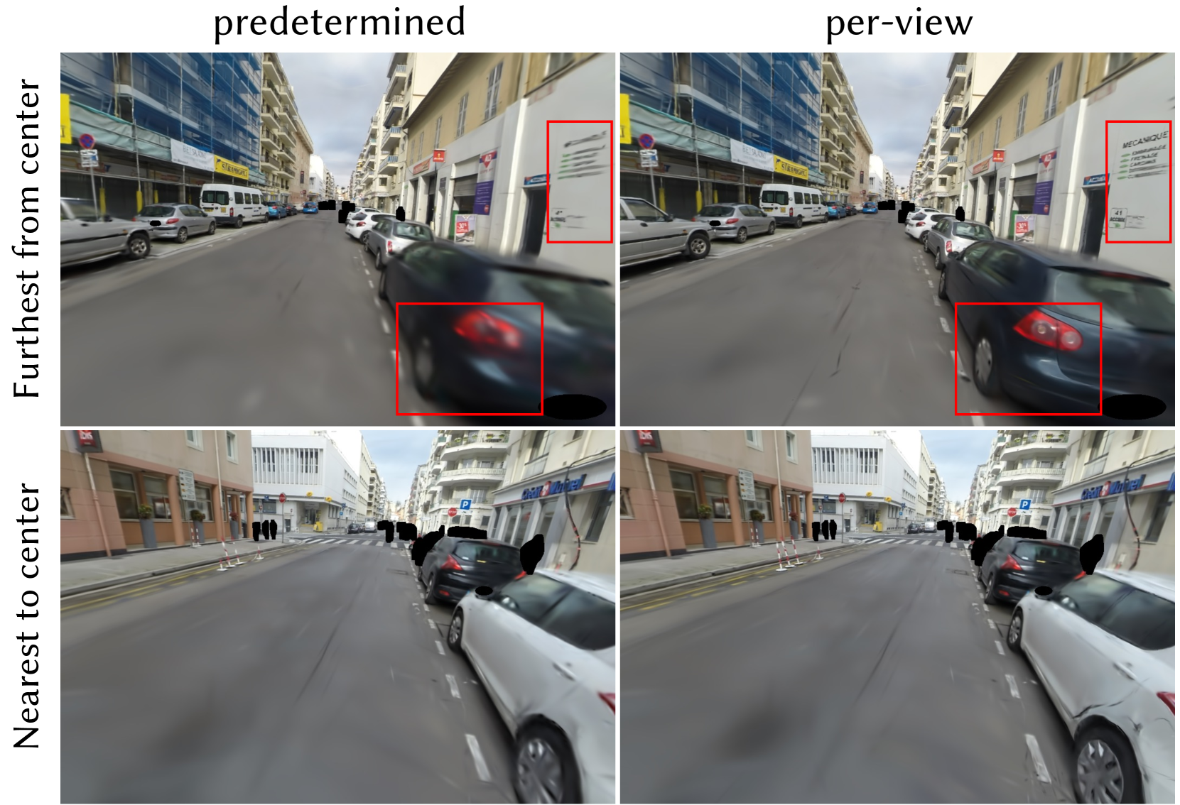<details> <summary>x11.png Details</summary>  ### Visual Description ## [Image Comparison]: Predetermined vs. Per-View Image Processing ### Overview The image is a 2x2 grid comparing two image processing or rendering methods, labeled "predetermined" and "per-view," applied to two different street scene captures. The comparison focuses on the clarity and detail of specific regions within the images, highlighted by red bounding boxes. The overall purpose appears to be a qualitative assessment of how each method handles image fidelity, particularly in areas away from the image center. ### Components/Axes * **Layout:** A 2x2 grid. * **Column Headers (Top):** * Left Column: `predetermined` * Right Column: `per-view` * **Row Labels (Left Side, Rotated 90°):** * Top Row: `Furthest from center` * Bottom Row: `Nearest to center` * **Visual Elements:** Each of the four panels contains a photographic street scene. Red rectangular bounding boxes are used to isolate and draw attention to specific regions within each image for comparison. ### Detailed Analysis The analysis is segmented by row and column, focusing on the content within the red bounding boxes. | Row / Column | `predetermined` | `per-view` | | :--- | :--- | :--- | | **Top Row: "Furthest from center" Scene** <br> *Scene Description:* A narrow urban street with parked cars on both sides. Buildings with shops line the street. A dark-colored car is prominent in the right foreground. | **Red Box 1 (Upper Right):** Highlights a white sign on a building facade. The text is significantly blurred and illegible. Only vague horizontal lines suggesting text are visible.<br>**Red Box 2 (Lower Center):** Highlights the rear taillight and bumper area of the dark car. The image is motion-blurred, making the taillight shape indistinct and the bumper details smeared. | **Red Box 1 (Upper Right):** Highlights the same white sign. The text is now legible. The sign reads:<br>* **Primary Text (Large, Bold):** `MECANIQUE`<br>* **Secondary Text (List below):**<br> * `ENTRETIEN`<br> * `REPARATION`<br> * `CARROSSERIE`<br> * `DEPANNAGE`<br>* **Additional Detail:** The number `41` is visible at the bottom left of the sign.<br>**Red Box 2 (Lower Center):** Highlights the same car taillight and bumper. The image is sharp. The taillight's internal structure and red color are clear, and the bumper's contour and reflection are well-defined. | | **Bottom Row: "Nearest to center" Scene** <br> *Scene Description:* A wider street intersection or plaza. Several parked cars are visible on the right. A crosswalk and traffic signs are present. Buildings, including one with a "Banque Populaire" sign, are in the background. | **Red Box 1 (Center):** Highlights a section of the road surface and the lower part of a parked car. The road markings and texture are somewhat soft.<br>**Red Box 2 (Right):** Highlights a building facade and a sign. The text on the sign is partially visible but blurry. | **Red Box 1 (Center):** Highlights the same road section. The asphalt texture and road markings appear slightly sharper and more defined compared to the "predetermined" version.<br>**Red Box 2 (Right):** Highlights the same building sign. The text clarity is marginally improved, but it remains difficult to read completely. The overall edge definition of the building appears slightly enhanced. | ### Key Observations 1. **Clarity Disparity:** The most significant difference is in the top row ("Furthest from center"). The "per-view" method dramatically improves the legibility of text and the sharpness of object details (car taillight) in these peripheral regions compared to the heavily blurred "predetermined" output. 2. **Spatial Dependency:** The improvement offered by the "per-view" method is most pronounced for elements located far from the image center, as indicated by the row label. The difference in the "Nearest to center" row is more subtle. 3. **Text Extraction:** The only fully legible text extracted from the highlighted regions is from the sign in the top-right panel: `MECANIQUE`, `ENTRETIEN`, `REPARATION`, `CARROSSERIE`, `DEPANNAGE`, and `41`. 4. **Other Visible Text (Not Highlighted):** Other signs in the scenes include `STEERWELL` (yellow sign, top row) and `Banque Populaire` (blue sign, bottom row). ### Interpretation This comparison likely evaluates a view-dependent or foveated rendering/processing technique against a uniform ("predetermined") one. The data suggests: * **The "per-view" method is superior for preserving high-frequency detail (text, edges) in peripheral areas of the image.** This is critical for applications like autonomous driving, surveillance, or virtual reality, where information at the edges of the field of view can be just as important as the center. * The "predetermined" method appears to apply a uniform level of processing or compression that disproportionately degrades quality away from the center, resulting in significant blur. * The **"Nearest to center"** comparison shows less dramatic improvement, implying that the baseline "predetermined" method may already allocate more resources or higher fidelity to the central region, leaving less room for improvement by the "per-view" technique. * The **outlier** is the extreme blur in the top-left panel's highlighted regions, which serves as a strong visual argument for the necessity of the "per-view" approach when peripheral detail is a requirement. **Conclusion:** The image provides visual evidence that a "per-view" processing strategy effectively mitigates the loss of detail in non-central image regions, which is a clear weakness of the "predetermined" approach shown. The primary informational gain is the restoration of legible text and sharp object boundaries in the periphery. </details> Figure 11. Comparison between the predetermined method and the per-view method in selective rendering using levels 5, 4, and 3 on the Small City scene. As shown in the red boxed areas, the per-view method maintains superior rendering quality even when far from the center of the scene, whereas the predetermined method shows a decline in rendering quality. Table 4. Quantitative comparison of FLoD-3DGS to Hierarchical-3DGS in Small City scene. The upper section compares FLoD-3DGS’s selective rendering methods and Hierarchical-3DGS ( $τ=30$ ), where all methods use a similar number of Gaussians. Note that #G’s for our per-view method and Hierarchical-3DGS is based on the view using the most number of Gaussians as this number varies across different views. The lower section lists the maximum quality renderings for both FLoD-3DGS and Hierarchical-3DGS for comparison. | FLoD-3DGS (per-view) | 25.49 | 221 | 1.03 GB | 601K | | --- | --- | --- | --- | --- | | FLoD-3DGS (predetermined) | 24.69 | 286 | 0.41 GB | 589K | | Hierarchcial-3DGS ( $τ=30$ ) | 24.69 | 55 | 5.36 GB | 610K | | FLoD-3DGS (max level) | 26.37 | 181 | 0.86 GB | 1308K | | Hierarchcial-3DGS ( $τ=0$ ) | 26.69 | 17 | 7.81 GB | 4892K | To maintain rendering quality across varying camera positions in urban environments, it is necessary to dynamically adapt the Gaussian set $G_sel$ . As shown in Figure 11 (right), selective rendering with per-view Gaussian set $G_sel$ maintains consistent rendering quality. Compared to using the predetermined $G_sel$ , per-view $G_sel$ increases PSNR by 0.8, but with a slower rendering speed and more rendering memory demands (Table 4). The slowdown occurs because the rendering of each view has an additional process of creating $G_sel$ . To mitigate the reduction in rendering speed, all Gaussians within the level range [ $L_start$ , $L_end$ ] are kept in GPU memory, which accounts for the increased memory usage. Despite the drawbacks, the trade-off for per-view $G_sel$ selective rendering is considered reasonable as the rendering quality becomes consistent, and it offers a faster rendering option compared to max level rendering. Table 4 also shows that our selective rendering (per-view) method not only achieves better PSNR with a comparable number of Gaussians but also outperforms Hierarchical-3DGS ( $τ=30$ ) in efficiency. Although both methods create the Gaussians set $G_sel$ for every individual view, our method achieves faster FPS and uses less rendering memory. ### 6.6. Ablation Study #### 6.6.1. 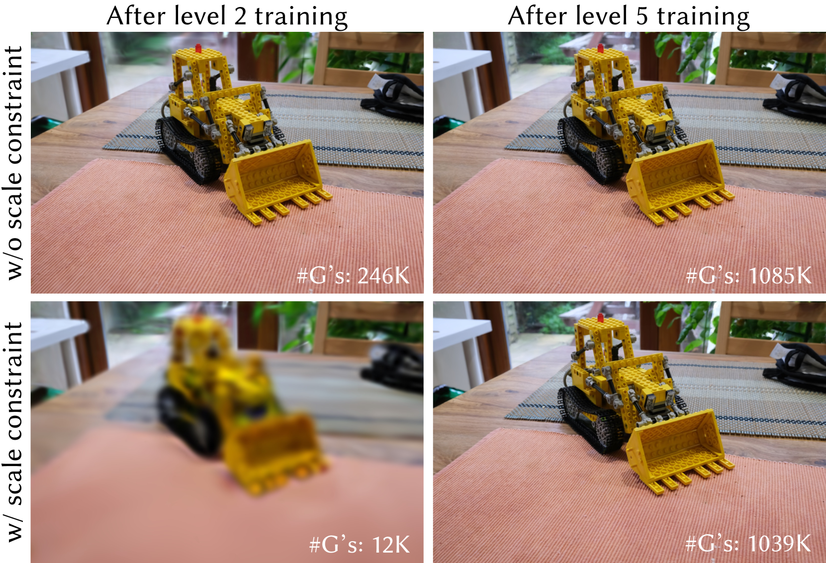3D Scale Constraint <details> <summary>x12.png Details</summary>  ### Visual Description ## Comparative Image Grid: Training Progress with and without Scale Constraint ### Overview The image is a 2x2 comparative grid of four photographs. Each photograph shows the same subject: a yellow LEGO Technic bulldozer model placed on a wooden table with placemats. The grid compares the visual results of a training process under two different conditions ("w/o scale constraint" and "w/ scale constraint") at two different training stages ("After level 2 training" and "After level 5 training"). A numerical metric labeled "#G's:" is provided in the bottom-right corner of each individual photo. ### Components/Axes The image is organized as a matrix with the following labels and structure: * **Row Labels (Vertical, Left Side):** * Top Row: `w/o scale constraint` * Bottom Row: `w/ scale constraint` * **Column Labels (Horizontal, Top):** * Left Column: `After level 2 training` * Right Column: `After level 5 training` * **Data Metric (Embedded in each photo, bottom-right):** * Label: `#G's:` (Likely an abbreviation for "Gradients" or a similar training iteration/step count). * Values: `246K`, `1085K`, `12K`, `1039K`. ### Detailed Analysis The grid presents four distinct states: 1. **Top-Left (w/o scale constraint, After level 2 training):** * **Visual:** The LEGO bulldozer is in sharp focus. Details like individual studs, the tread pattern, and the bucket teeth are clearly visible. The background (window, plants) is also reasonably clear. * **Data:** `#G's: 246K` 2. **Top-Right (w/o scale constraint, After level 5 training):** * **Visual:** The image remains sharp and clear, visually identical in quality to the top-left image. The bulldozer and background are well-defined. * **Data:** `#G's: 1085K` 3. **Bottom-Left (w/ scale constraint, After level 2 training):** * **Visual:** The image is severely blurred. The bulldozer is recognizable only by its general shape and color. No fine details are discernible. The background is a soft, indistinct blur. * **Data:** `#G's: 12K` 4. **Bottom-Right (w/ scale constraint, After level 5 training):** * **Visual:** The image has recovered to a sharp, clear state, comparable in quality to the two images in the top row. All details of the model and setting are visible again. * **Data:** `#G's: 1039K` ### Key Observations * **Clarity vs. Constraint:** The presence of the "scale constraint" has a dramatic negative impact on visual clarity at the earlier training stage (level 2), resulting in a completely blurred image. This constraint does not appear to affect the final clarity at level 5. * **Training Progression:** For both conditions, the `#G's` metric increases significantly from level 2 to level 5 (246K → 1085K without constraint; 12K → 1039K with constraint), indicating more training steps or computations were performed. * **Metric Discrepancy at Level 2:** There is a massive difference in the `#G's` count at level 2 between the two conditions (246K vs. 12K). The constrained process has performed far fewer gradient updates at this stage. * **Convergence at Level 5:** By level 5, the `#G's` counts for both conditions are much closer in magnitude (1085K vs. 1039K), and the visual results are similarly high-quality. ### Interpretation This image likely illustrates a concept from machine learning or optimization, specifically the effect of a "scale constraint" (which could relate to learning rate, gradient scaling, or parameter normalization) on the training dynamics of a model, possibly a generative model tasked with reconstructing or rendering this image. * **What the data suggests:** The scale constraint appears to severely hinder or slow down the initial phase of training (level 2), as evidenced by both the extremely low `#G's` count and the resulting poor-quality, blurred output. It acts as a significant bottleneck early on. * **How elements relate:** The comparison shows that this early bottleneck is not permanent. Given sufficient training (to level 5), the constrained process "catches up," achieving a high `#G's` count and producing a final result that is visually indistinguishable from the unconstrained process. The unconstrained process, meanwhile, proceeds smoothly from the start. * **Notable patterns/anomalies:** The most striking anomaly is the 20x difference in `#G's` at level 2 (246K vs. 12K). This suggests the constraint might cause the optimization to take many fewer, or much smaller, steps initially. The fact that both converge to a similar high-quality result by level 5 implies the constraint may enforce a more cautious or regularized optimization path that is slower to start but ultimately effective. The image serves as a visual proof that the constraint's primary effect is on training efficiency and trajectory, not necessarily on the final achievable quality. </details> Figure 12. Comparison of the renderings and number of Gaussians with and without the 3D scale constraint after level 2 and level 5 training on the Mip-NeRF360 dataset. We compare cases with and without the 3D scale constraint. For the case without the 3D scale constraint, Gaussians are optimized without any size limit. Additionally, we did not apply overlap pruning for this case, as the threshold for overlap pruning $d_OP^(l)$ is adjusted proportionally to the 3D scale constraint. Therefore, the case without the 3D scale constraint only applies level-by-level training method from our full method. As shown in Figure 12, without the 3D scale constraint, the amount of detail reconstructed after level 2 is comparable to that after the max level. In contrast, applying the 3D scale constraint results in a clear difference in detail between the two levels. Moreover, the case with the 3D scale constraint uses approximately 98.6% fewer Gaussians compared to the case without the 3D scale constraint. Therefore, the 3D scale constraint is crucial for ensuring varied detail across levels and enabling each level to maintain a different memory footprint. 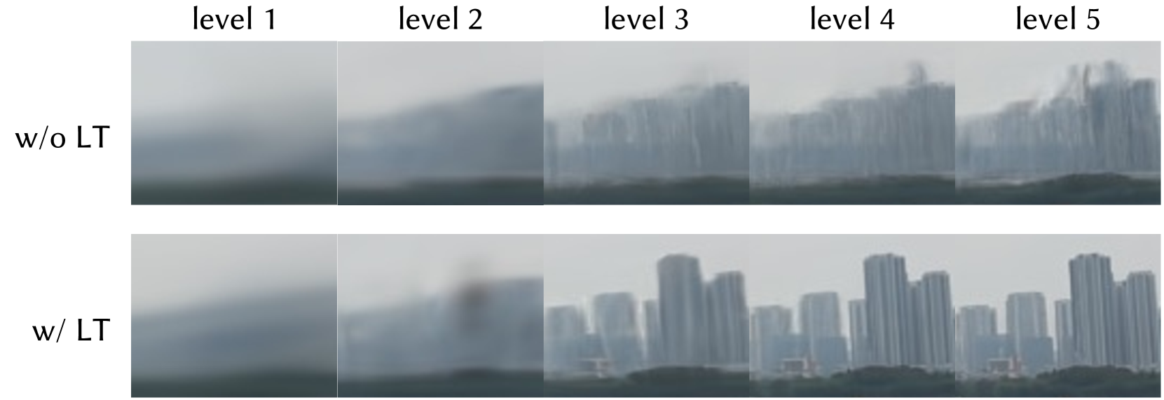<details> <summary>x13.png Details</summary>  ### Visual Description ## Comparative Image Clarity Chart: Effect of "LT" Across Five Levels ### Overview The image is a comparative chart displaying two rows of five sequential images each, illustrating the progressive visual clarity of a cityscape scene under two different conditions. The chart is structured as a 2x5 grid with clear row and column headers. The primary comparison is between a process or technique labeled "LT" (present or absent) across five incremental "levels." ### Components/Axes * **Row Labels (Left Side):** * Top Row: `w/o LT` (without LT) * Bottom Row: `w/ LT` (with LT) * **Column Headers (Top):** * `level 1`, `level 2`, `level 3`, `level 4`, `level 5` * **Image Content:** Each cell contains a rectangular image depicting a hazy, overcast cityscape with a skyline of tall buildings and a darker foreground (likely water or land). The visual quality changes progressively from left to right within each row. ### Detailed Analysis **Row 1: "w/o LT" (Without LT)** * **Trend:** Shows very gradual, minimal improvement in clarity from level 1 to level 5. * **Level 1:** Extremely blurry and hazy. No distinct building shapes are discernible; only vague, dark vertical forms against a grey sky. * **Level 2:** Slightly less hazy than level 1. The silhouette of a building mass begins to emerge, but details are completely absent. * **Level 3:** The skyline becomes more defined as a continuous, jagged shape. Individual buildings are still not clearly separable. * **Level 4:** Marginal improvement. The separation between some taller buildings becomes faintly visible, but the image remains very soft and lacks sharp edges. * **Level 5:** The clearest in this row, but still significantly blurred. The general shapes of several prominent high-rise buildings can be identified, though all fine detail and texture are lost in haze. **Row 2: "w/ LT" (With LT)** * **Trend:** Shows a dramatic, non-linear improvement in clarity, with a significant leap between levels 2 and 3. * **Level 1:** Similar to the "w/o LT" level 1—very blurry and hazy. * **Level 2:** Remains quite blurry, but a distinct dark, blurry spot appears in the center-left of the image, which is not present in the corresponding "w/o LT" image. This may be an artifact or a specific feature being highlighted. * **Level 3:** **Major improvement.** The image sharpens considerably. Individual buildings are now clearly distinguishable, with visible windows and structural edges. The haze is greatly reduced. * **Level 4:** Further refinement. Buildings appear sharper and more detailed than in level 3. The contrast between the buildings and the sky is higher. * **Level 5:** The clearest image in the entire chart. The cityscape is sharp, with well-defined buildings, clear window patterns, and minimal haze. The foreground details are also more distinct. ### Key Observations 1. **Differential Impact:** The "LT" technique has a profound effect, transforming an unusable, blurry image (level 3, w/o LT) into a clear, detailed one (level 3, w/ LT). 2. **Threshold Effect:** The most significant visual improvement for the "w/ LT" condition occurs between level 2 and level 3. Levels 1 and 2 remain poor, while levels 3, 4, and 5 show high-quality results. 3. **Anomaly:** The "w/ LT" level 2 image contains a unique dark, blurry artifact not seen in any other cell, suggesting a potential intermediate processing stage or error at that specific level. 4. **Baseline Progression:** Without LT, the scene improves only marginally across all five levels, suggesting that the underlying data or process has inherent limitations that LT overcomes. ### Interpretation This chart demonstrates the efficacy of a technique abbreviated as "LT" (likely a form of "Learning Transform," "Latent Transform," or similar image restoration/enhancement algorithm) for dehazing or super-resolving images of a cityscape. The data suggests that "LT" is not merely an incremental filter but a transformative process that unlocks latent detail. The stark contrast at level 3 implies that the technique requires a minimum threshold of input quality (or a specific parameter setting at level 3) to activate its full restorative capability. The progression from level 3 to 5 with LT shows continued refinement, indicating the method scales well with increased levels (which could represent more processing iterations, higher model capacity, or better input data). The anomaly at "w/ LT" level 2 is critical for investigation. It may represent a failure mode, a visualization of an internal model state, or a byproduct of the algorithm when operating below its effective threshold. For a technical document, this highlights the importance of operating the LT process at or above level 3 for reliable, high-quality output. The chart effectively argues that employing "LT" is essential for obtaining interpretable, detailed visual data from this specific imaging scenario. </details> Figure 13. Comparison of background region on the rendered images with and without level-by-level training across all levels on the DL3DV-10K dataset. The images are zoomed-in and cropped to highlight differences in the background regions. #### 6.6.2. Level-by-level Training Table 5. Quantitative comparison of image quality for each level with and without level-by-level training on DL3DV-10K dataset. LT denotes level-by-level training. | 5 4 | w/o LT w/ LT w/o LT | 31.20 31.97 29.05 | 0.930 0.936 0.896 | 0.158 0.105 0.161 | | --- | --- | --- | --- | --- | | w/ LT | 30.73 | 0.917 | 0.133 | | | 3 | w/o LT | 27.05 | 0.850 | 0.224 | | w/ LT | 28.29 | 0.869 | 0.200 | | | 2 | w/o LT | 23.41 | 0.734 | 0.376 | | w/ LT | 24.01 | 0.750 | 0.355 | | | 1 | w/o LT | 20.41 | 0.637 | 0.485 | | w/ LT | 20.81 | 0.646 | 0.475 | | <details> <summary>x14.png Details</summary>  ### 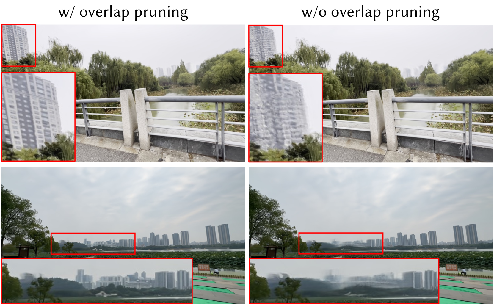Visual Description ## [Image Comparison]: Effect of Overlap Pruning on Image Reconstruction Quality ### Overview This image presents a side-by-side visual comparison demonstrating the impact of an "overlap pruning" technique on the quality of reconstructed or processed images. It consists of two columns and two rows. The left column is labeled "w/ overlap pruning" (with overlap pruning), and the right column is labeled "w/o overlap pruning" (without overlap pruning). Each of the two rows displays a different scene, with red bounding boxes highlighting specific regions of interest. Below each main image, a zoomed-in inset corresponding to the red box is provided to allow for detailed comparison of reconstruction artifacts. ### Components/Axes * **Text Labels:** * Top-left header: "w/ overlap pruning" * Top-right header: "w/o overlap pruning" * **Image Layout:** A 2x2 grid. * **Top Row:** A scene featuring a bridge railing in the foreground, trees, and a tall building in the background. * **Bottom Row:** A panoramic lakeside cityscape with a skyline of numerous high-rise buildings. * **Highlighting Elements:** * Red rectangular bounding boxes are placed on the main images to indicate regions that are magnified in the insets below. * **Top Row:** The red box is placed on the upper-left portion of the image, focusing on the tall building. * **Bottom Row:** The red box is placed on the central-left portion of the image, focusing on a segment of the distant city skyline. * **Insets:** Each main image has a corresponding zoomed-in inset placed directly below it, showing the content within the red bounding box at a larger scale. ### Detailed Analysis **Top Row Scene (Bridge and Building):** * **"w/ overlap pruning" (Left):** The zoomed-in inset of the building shows relatively clear and distinct window patterns and architectural edges. The lines of the building are sharp, and individual windows are discernible. * **"w/o overlap pruning" (Right):** The corresponding inset of the same building exhibits significant blurring and loss of high-frequency detail. The window patterns are smudged, edges are soft, and the building's texture appears washed out and indistinct. There is a noticeable "ghosting" or blending artifact. **Bottom Row Scene (City Skyline):** * **"w/ overlap pruning" (Left):** The zoomed-in inset of the city skyline shows buildings with defined shapes and edges. While atmospheric haze is present, the structures of individual buildings in the mid-ground are reasonably clear. * **"w/o overlap pruning" (Right):** The inset for this condition shows severe degradation. The buildings in the highlighted region are heavily blurred, with their forms blending into one another and into the background. Details are almost completely lost, resulting in a smudged, low-fidelity representation. ### Key Observations 1. **Consistent Quality Difference:** In both example scenes, the images processed "with overlap pruning" demonstrate substantially higher visual fidelity and detail preservation compared to those processed "without overlap pruning." 2. **Nature of Artifacts:** The primary artifact in the "w/o overlap pruning" images is a spatial blurring or smearing, particularly noticeable on structured, high-contrast details like building edges and windows. This suggests a failure to properly align or merge image data in overlapping regions. 3. **Spatial Grounding of Comparison:** The comparison is made direct and unambiguous by using identical red bounding boxes on the same scene content, with side-by-side insets. The legend (the text headers) is positioned clearly at the top of each column, and the color of the bounding boxes (red) is consistent across all comparisons. ### Interpretation This visual comparison serves as strong qualitative evidence for the efficacy of the "overlap pruning" technique in an image processing pipeline, likely related to tasks such as image stitching, super-resolution, or neural rendering (e.g., NeRFs). * **What the Data Suggests:** The technique successfully mitigates artifacts that occur when processing overlapping image regions. Without it, the system likely averages or incorrectly blends information from multiple views or patches, leading to the observed blurring and loss of detail. "Overlap pruning" appears to selectively use or weight data to preserve sharpness. * **How Elements Relate:** The layout is designed for immediate visual contrast. The headers define the experimental condition, the main images provide context, and the red-boxed insets act as a "magnifying glass" to prove the point at a granular level. The relationship is causal: the presence or absence of the technique (independent variable) directly causes the difference in image quality (dependent variable). * **Notable Implications:** The improvement is not subtle; it is the difference between a usable, detailed reconstruction and a severely degraded one. This indicates that overlap pruning is not merely an optimization but a critical component for achieving high-quality results in this specific application. The artifacts shown ("w/o" condition) are characteristic of problems in multi-view synthesis, confirming the likely technical domain of the underlying method. </details> Figure 14. Comparison between rendered images at level 5 trained with and without overlap pruning on the DL3DV-10K dataset. Zoomed-in images emphasize key differences. We compare cases with and without the level-by-level training approach. In the case without level-by-level training, the set of iterations for exclusive Gaussian optimization of each level is replaced with iterations that include additional densification and pruning. As shown in Figure 13, the absence of level-by-level training causes inaccuracies in the reconstructed structure at the intermediate level, which is carried on to the higher levels. In contrast, the case with our level-by-level training approach reconstructs the scene structure more accurately at level 3, resulting in improved reconstruction quality at levels 4 and 5. As demonstrated in Table 5, the case with level-by-level training outperforms the case without it in terms of PSNR, SSIM, and LPIPS across all levels. Hence, level-by level training is important for enhancing reconstruction quality across all levels. #### 6.6.3. Overlap Pruning We compare the result of training with and without overlap pruning across all levels. As shown in Figure 14, removing overlap pruning deteriorates the structure of the scene, degrading rendering quality. This issue is particularly noticeable in scenes with distant objects. We believe that overlap pruning mitigates the potential for artifacts by preventing the overlap of large Gaussians at distant locations. Furthermore, we compare the number of Gaussians at each level with and without overlap pruning. Table 6 illustrates that overlap pruning decreases the number of Gaussians, particularly at lower levels, with reductions of 90%, 34%, and 10% at levels 1, 2, and 3, respectively. This reduction is particularly important for minimizing memory usage for rendering on low-cost and low-memory devices that utilize low level representations. Table 6. Comparison of the number of Gaussians per level when trained with and without overlap pruning on the Mip-NeRF360 dataset. OP denotes overlap pruning. | w/o OP-w/ OP | 38K 10K | 49K 31K | 439K 390K | 1001K 970K | 2058K 2048K | | --- | --- | --- | --- | --- | --- | ## 7. Conclusion In this work, we propose Flexible Level of Detail (FLoD), a method that integrates LoD into 3DGS. FLoD reconstructs the scene in different degrees of detail while maintaining a consistent scene structure. Therefore, our method enables customizable rendering with a single or subset of levels, allowing the model to operate on devices ranging from high-end servers to low-cost laptops. Furthermore, FLoD easily integrates with 3DGS-based models implying its applicability to future 3DGS-based methods. ## 8. Limitation In scenes with long camera trajectories, using per-view Gaussian set is necessary to maintain consistent rendering quality during selective rendering. However, this method has the limitation that all Gaussians within the level range for selective rendering need to be kept on GPU memory to maintain fast rendering rates, as discussed in Section 6.5. Therefore, this method requires more memory capacity compared to single level rendering with only the highest level, $L_end$ , picked from the level range [ $L_start$ , $L_end$ ] used for selective rendering. Future research could explore the strategic planning and execution of transferring Gaussians from the CPU to the GPU, to reduce the memory burden while also keeping the advantage of selective rendering. Acknowledgements. This work was supported by the National Research Foundation of Korea (NRF, RS-2023-00223062) and an IITP grant (RS-2020-II201361, Artificial Intelligence Graduate School Program (Yonsei University)) funded by the Korean government (MSIT) . ## References - (1) - Barron et al. (2021) Jonathan T. Barron, Ben Mildenhall, Matthew Tancik, Peter Hedman, Ricardo Martin-Brualla, and Pratul P. Srinivasan. 2021. Mip-NeRF: A Multiscale Representation for Anti-Aliasing Neural Radiance Fields. ICCV (2021). - Barron et al. (2022) Jonathan T. Barron, Ben Mildenhall, Dor Verbin, Pratul P. Srinivasan, and Peter Hedman. 2022. Mip-NeRF 360: Unbounded Anti-Aliased Neural Radiance Fields. CVPR (2022). - Barron et al. (2023) Jonathan T. Barron, Ben Mildenhall, Dor Verbin, Pratul P. Srinivasan, and Peter Hedman. 2023. Zip-NeRF: Anti-Aliased Grid-Based Neural Radiance Fields. ICCV (2023). - Fan et al. (2023) Zhiwen Fan, Kevin Wang, Kairun Wen, Zehao Zhu, Dejia Xu, and Zhangyang Wang. 2023. LightGaussian: Unbounded 3D Gaussian Compression with 15x Reduction and 200+ FPS. arXiv:2311.17245 [cs.CV] - Girish et al. (2024) Sharath Girish, Kamal Gupta, and Abhinav Shrivastava. 2024. EAGLES: Efficient Accelerated 3D Gaussians with Lightweight EncodingS. arXiv:2312.04564 [cs.CV] https://arxiv.org/abs/2312.04564 - Kerbl et al. (2023) Bernhard Kerbl, Georgios Kopanas, Thomas Leimkühler, and George Drettakis. 2023. 3D Gaussian Splatting for Real-Time Radiance Field Rendering. ACM Transactions on Graphics 42, 4 (July 2023). https://repo-sam.inria.fr/fungraph/3d-gaussian-splatting/ - Kerbl et al. (2024) Bernhard Kerbl, Andreas Meuleman, Georgios Kopanas, Michael Wimmer, Alexandre Lanvin, and George Drettakis. 2024. A Hierarchical 3D Gaussian Representation for Real-Time Rendering of Very Large Datasets. ACM Transactions on Graphics 43, 4 (July 2024). https://repo-sam.inria.fr/fungraph/hierarchical-3d-gaussians/ - Knapitsch et al. (2017) Arno Knapitsch, Jaesik Park, Qian-Yi Zhou, and Vladlen Koltun. 2017. Tanks and Temples: Benchmarking Large-Scale Scene Reconstruction. ACM Transactions on Graphics 36, 4 (2017). - Lee et al. (2024) Joo Chan Lee, Daniel Rho, Xiangyu Sun, Jong Hwan Ko, and Eunbyung Park. 2024. Compact 3D Gaussian Representation for Radiance Field. In Proceedings of the IEEE/CVF Conference on Computer Vision and Pattern Recognition (CVPR). - Ling et al. (2023) Lu Ling, Yichen Sheng, Zhi Tu, Wentian Zhao, Cheng Xin, Kun Wan, Lantao Yu, Qianyu Guo, Zixun Yu, Yawen Lu, Xuanmao Li, Xingpeng Sun, Rohan Ashok, Aniruddha Mukherjee, Hao Kang, Xiangrui Kong, Gang Hua, Tianyi Zhang, Bedrich Benes, and Aniket Bera. 2023. DL3DV-10K: A Large-Scale Scene Dataset for Deep Learning-based 3D Vision. arXiv:2312.16256 [cs.CV] - Liu et al. (2024) Yang Liu, He Guan, Chuanchen Luo, Lue Fan, Junran Peng, and Zhaoxiang Zhang. 2024. CityGaussian: Real-time High-quality Large-Scale Scene Rendering with Gaussians. In ECCV. - Lu et al. (2024) Tao Lu, Mulin Yu, Linning Xu, Yuanbo Xiangli, Limin Wang, Dahua Lin, and Bo Dai. 2024. Scaffold-gs: Structured 3d gaussians for view-adaptive rendering. In Proceedings of the IEEE/CVF Conference on Computer Vision and Pattern Recognition. 20654–20664. - Mildenhall et al. (2020) Ben Mildenhall, Pratul P. Srinivasan, Matthew Tancik, Jonathan T. Barron, Ravi Ramamoorthi, and Ren Ng. 2020. NeRF: Representing Scenes as Neural Radiance Fields for View Synthesis. In ECCV. - Niemeyer et al. (2024) Michael Niemeyer, Fabian Manhardt, Marie-Julie Rakotosaona, Michael Oechsle, Daniel Duckworth, Rama Gosula, Keisuke Tateno, John Bates, Dominik Kaeser, and Federico Tombari. 2024. RadSplat: Radiance Field-Informed Gaussian Splatting for Robust Real-Time Rendering with 900+ FPS. arXiv.org (2024). - Ren et al. (2024) Kerui Ren, Lihan Jiang, Tao Lu, Mulin Yu, Linning Xu, Zhangkai Ni, and Bo Dai. 2024. Octree-GS: Towards Consistent Real-time Rendering with LOD-Structured 3D Gaussians. arXiv:2403.17898 [cs.CV] - Schönberger and Frahm (2016) Johannes Lutz Schönberger and Jan-Michael Frahm. 2016. Structure-from-Motion Revisited. In Conference on Computer Vision and Pattern Recognition (CVPR). - Takikawa et al. (2022) Towaki Takikawa, Alex Evans, Jonathan Tremblay, Thomas Müller, Morgan McGuire, Alec Jacobson, and Sanja Fidler. 2022. Variable Bitrate Neural Fields. In ACM SIGGRAPH 2022 Conference Proceedings (Vancouver, BC, Canada) (SIGGRAPH ’22). Association for Computing Machinery, New York, NY, USA, Article 41, 9 pages. https://doi.org/10.1145/3528233.3530727 - Takikawa et al. (2021) Towaki Takikawa, Joey Litalien, Kangxue Yin, Karsten Kreis, Charles Loop, Derek Nowrouzezahrai, Alec Jacobson, Morgan McGuire, and Sanja Fidler. 2021. Neural Geometric Level of Detail: Real-time Rendering with Implicit 3D Shapes. In Proceedings of the IEEE/CVF Conference on Computer Vision and Pattern Recognition (CVPR). - Wang et al. (2004) Zhou Wang, A.C. Bovik, H.R. Sheikh, and E.P. Simoncelli. 2004. Image quality assessment: from error visibility to structural similarity. IEEE Transactions on Image Processing 13, 4 (2004), 600–612. https://doi.org/10.1109/TIP.2003.819861 - Yan et al. (2024) Zhiwen Yan, Weng Fei Low, Yu Chen, and Gim Hee Lee. 2024. Multi-Scale 3D Gaussian Splatting for Anti-Aliased Rendering. In Proceedings of the IEEE/CVF Conference on Computer Vision and Pattern Recognition (CVPR). - Ye et al. (2024) Zongxin Ye, Wenyu Li, Sidun Liu, Peng Qiao, and Yong Dou. 2024. AbsGS: Recovering Fine Details for 3D Gaussian Splatting. arXiv:2404.10484 [cs.CV] - Yu et al. (2024) Zehao Yu, Anpei Chen, Binbin Huang, Torsten Sattler, and Andreas Geiger. 2024. Mip-Splatting: Alias-free 3D Gaussian Splatting. In Proceedings of the IEEE/CVF Conference on Computer Vision and Pattern Recognition (CVPR). 19447–19456. - Zhang et al. (2024) Jiahui Zhang, Fangneng Zhan, Muyu Xu, Shijian Lu, and Eric Xing. 2024. FreGS: 3D Gaussian Splatting with Progressive Frequency Regularization. arXiv:2403.06908 [cs.CV] https://arxiv.org/abs/2403.06908 - Zhang et al. (2018) Richard Zhang, Phillip Isola, Alexei A Efros, Eli Shechtman, and Oliver Wang. 2018. The Unreasonable Effectiveness of Deep Features as a Perceptual Metric. In CVPR. ## Appendix A Dataset Details We conduct experiments on the Tanks&Temples dataset (Knapitsch et al., 2017) and the Mip-NeRF360 dataset (Barron et al., 2022) as the two datasets were used for evaluation in our baselines: Octree-GS (Ren et al., 2024), 3DGS (Kerbl et al., 2023), Scaffold-GS (Lu et al., 2024) and Mip-Splatting (Yu et al., 2024). Additionally, we conduct experiments on the relatively recently released DL3DV-10K dataset (Ling et al., 2023) for a more comprehensive evaluation across diverse scenes. Camera parameters and initial points for all datasets are obtained using COLMAP (Schönberger and Frahm, 2016). We subsample every 8th image of each scene for testing, following the train/test splitting methodology presented in Mip-NeRF360. ### A.1. Tanks&Temples The Tanks&Temples dataset includes high-resolution multi-view images of various complex scenes, including both indoor and outdoor settings. Following our baselines, we conduct experiments on two unbounded scenes featuring large central objects: train and truck. For both scenes, we reduce the image resolution to $980× 545$ pixels, downscaling it to 25% of their original size. ### A.2. Mip-NeRF360 The Mip-NeRF360 dataset (Barron et al., 2022) consists of a diverse set of real-world 360-degree scenes, encompassing both bounded and unbounded environments. The images in the dataset were captured under controlled conditions to minimize lighting variations and avoid transient objects. For our experiments, we use the nine publicly available scenes: bicycle, bonsai, counter, garden, kitchen, room, stump, treehill and flowers. We reduce the original image’s width and height to one-fourth for the outdoor scenes, and to one-half for the indoor scenes. Specifically, the outdoor scenes are resized to approximately $1250× 830$ pixels, while the indoor scenes are resized to about $1558× 1039$ pixels. ### A.3. DL3DV-10K The DL3DV-10K dataset (Ling et al., 2023) expands the range of real-world scenes available for 3D representation learning by providing a vast number of indoor and outdoor real-world scenes. For our experiments, we select six outdoor scenes from DL3DV-10K for a more comprehensive evaluation on unbounded real-world environments. We use images with a reduced resolution of $960× 540$ pixels, following the resolution used in the DL3DV-10K paper. The first 10 characters of the hash codes for our selected scenes are aeb33502d5, 58e78d9c82, df87dfc4c, ce06045bca, 2bfcf4b343, and 9f518d2669. 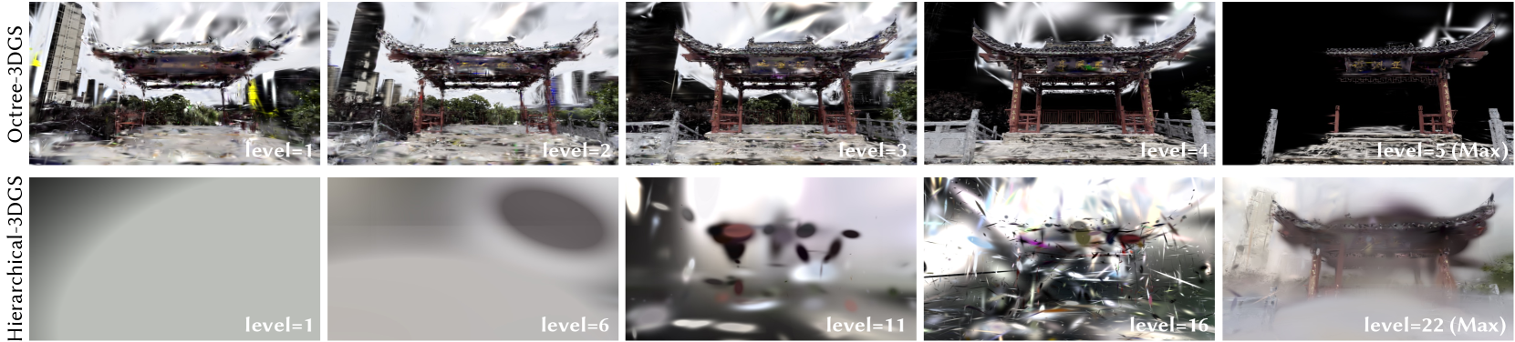<details> <summary>x15.png Details</summary>  ### Visual Description ## Comparison Chart: Octree-3DGS vs. Hierarchical-3DGS Reconstruction Levels ### Overview The image is a technical comparison chart displaying the progressive reconstruction quality of two different 3D Gaussian Splatting (3DGS) methods—Octree-3DGS and Hierarchical-3DGS—across increasing computational or detail levels. It consists of two horizontal rows, each containing five sequential images showing the same scene (a traditional Chinese archway or *paifang*) at different stages of reconstruction fidelity. ### Components/Axes * **Row Labels (Vertical Text, Left Side):** * Top Row: `Octree-3DGS` * Bottom Row: `Hierarchical-3DGS` * **Image Grid:** A 2x5 grid of images. * **Level Indicators (Text, Bottom-Right of each image):** * Top Row (Octree-3DGS): `level=1`, `level=2`, `level=3`, `level=4`, `level=5 (Max)` * Bottom Row (Hierarchical-3DGS): `level=1`, `level=6`, `level=11`, `level=16`, `level=22 (Max)` * **Scene Content:** Each image depicts a 3D reconstruction of an ornate, traditional Chinese archway with a curved roof, set in an urban environment with modern buildings in the background. The archway has a central plaque with Chinese characters. ### Detailed Analysis **Row 1: Octree-3DGS** * **Trend:** Shows a rapid and clear convergence towards a high-fidelity reconstruction. * **Level 1 (Top-Left):** The scene is recognizable but heavily distorted with blurry, smeared artifacts, especially in the sky and background. The archway structure is visible but lacks fine detail. * **Level 2 (Top-Center-Left):** Significant improvement. Distortion reduces, the archway's structure becomes sharper, and background buildings gain definition. * **Level 3 (Top-Center):** Further refinement. Details on the archway's roof and pillars become clearer. The scene appears more stable. * **Level 4 (Top-Center-Right):** Very close to the final output. Minor artifacts remain, but the overall scene is coherent and detailed. * **Level 5 (Max) (Top-Right):** The final, high-quality reconstruction. The archway is sharp, with clear textures and colors. The background is clean, and the Chinese characters on the plaque are legible (though not transcribed as data). The image has a black background, suggesting the reconstruction is isolated or the rendering mode changed. **Row 2: Hierarchical-3DGS** * **Trend:** Shows a much slower, more abstract convergence process, requiring significantly more levels (22 vs. 5) to achieve a recognizable result. * **Level 1 (Bottom-Left):** Almost entirely abstract. The image is a smooth, gray gradient with no recognizable scene elements. * **Level 6 (Bottom-Center-Left):** Still highly abstract. Shows large, soft, blob-like shapes in gray and dark tones. No scene structure is discernible. * **Level 11 (Bottom-Center):** The first hints of scene structure appear. Abstract shapes begin to coalesce into forms that suggest the archway's silhouette and some color patches, but it remains very blurry and impressionistic. * **Level 16 (Bottom-Center-Right):** A dramatic shift. The scene becomes recognizable, though filled with high-frequency, chaotic noise and artifacts. The archway and background are visible but severely degraded by visual "static." * **Level 22 (Max) (Bottom-Right):** The final reconstruction. The scene is coherent and detailed, comparable in quality to Octree-3DGS Level 4 or 5. Some softness or minor artifacts may remain compared to the Octree result. ### Key Observations 1. **Convergence Speed:** Octree-3DGS achieves a high-quality, stable reconstruction in just 5 levels. Hierarchical-3DGS requires 22 levels to reach a similar endpoint, with the intermediate stages (levels 1-16) being vastly more abstract and less informative. 2. **Intermediate Representation:** The two methods produce fundamentally different intermediate representations. Octree-3DGS maintains a recognizable, if distorted, scene from the first level. Hierarchical-3DGS passes through a prolonged phase of abstract, non-representational forms before abruptly resolving into a noisy scene. 3. **Final Quality:** Both methods appear to converge to a similar high-fidelity final output for this scene, as seen in their respective "(Max)" level images. 4. **Text in Scene:** The Chinese characters on the archway's plaque are part of the visual scene being reconstructed. They are not extracted as standalone textual data but are a visual feature that becomes legible at higher reconstruction levels. ### Interpretation This chart visually demonstrates a core trade-off in hierarchical or progressive 3D reconstruction algorithms. **Octree-3DGS** appears to use a method that preserves coarse scene structure from the outset, refining it efficiently. This is beneficial for applications requiring early, recognizable previews. **Hierarchical-3DGS** seems to employ a more bottom-up approach, possibly optimizing fundamental visual elements (like color blobs or wavelets) before assembling them into a coherent scene. This results in a long "abstract phase" but may offer advantages in handling complex geometry or lighting that are not apparent in this single example. The key takeaway is not just the difference in final quality (which is similar), but the stark difference in the *path* to that quality. The choice between these methods would depend on whether intermediate visual plausibility (favoring Octree) or other potential backend advantages of the hierarchical approach (like memory efficiency or handling of unstructured data) are more critical for a given application. The chart effectively argues that for this specific scene, Octree-3DGS provides a more immediately useful and interpretable progression. </details> Figure 15. Rendered images using only the Gaussians corresponding to a specific level in Octree-3DGS and Hierarchical-3DGS. $M←SfM Points$ $\triangleright$ Positions $S,R,C,A←InitAttributes()$ $\triangleright$ Scales, Rotations, Colors, Opacities for $l=1$ … $L_max$ do if $l<L_max$ then $s_min^(l)←λ×ρ^1-l$ $\triangleright$ 3D Scale constraint for current level else $s_min^(l)← 0$ $\triangleright$ No constraint at maximum level end if $i← 0$ $\triangleright$ Iteration count while not converged do $S^(l)←ApplyScaleConstraint(S_opt,s_min^(l ))$ $\triangleright$ Eq.4 $I←Rasterize(M,S^(l),R,C,A)$ $L←Loss(I,\hat{I})$ $M,S_opt,R,C,A←Adam(∇ L)$ $\triangleright$ Backpropagation if $i<\textnormal{DensificationIteration}$ then if $\textnormal{RefinementIteration}(i,l)$ then $\textnormal{Densification}()$ $\textnormal{Pruning}()$ $\textnormal{OverlapPruning}()$ $\triangleright$ Overlap pruning step end if end if $i← i+1$ end while $SaveClone(l,M,S^(l),R,C,A)$ $\triangleright$ Save clones for level $l$ if $l≠ L_max$ then $S_opt←AdjustScale(S^(l))$ $\triangleright$ Adjust scales for level $l+1$ end if end for $L_max$ : maximum level $λ,ρ$ : 3D scale constraint at level 1, scale factor ALGORITHM 1 Overall Training Algorithm for FLoD-3DGS $L_max$ : maximum level $λ,ρ$ : 3D scale constraint at level 1, scale factor ## Appendix B Method Details ### B.1. Training Algorithm The overall training process for FLoD-3DGS is summarized in Algorithm 1. ### B.2. 3D vs 2D Scale Constraint It is essential to impose the Gaussian scale constraint in 3D rather than on the 2D projected Gaussians. Although applying scale constraints to 2D projections is theoretically possible, it increases geometrical ambiguities in modeling 3D scenes. This is because the scale of the 2D projected Gaussians varies depending on their distance from the camera. Consequently, imposing a constant scale constraint on a 2D projected Gaussian from different camera positions sends inconsistent training signals, leading to Gaussian receiving training signals that misrepresent their true shape and position in 3D space. In contrast, applying 3D scale constraint to 3D Gaussians ensures consistent enlargement regardless of the camera’s position, thereby enabling stable optimization of the Gaussians’ 3D scale and position. 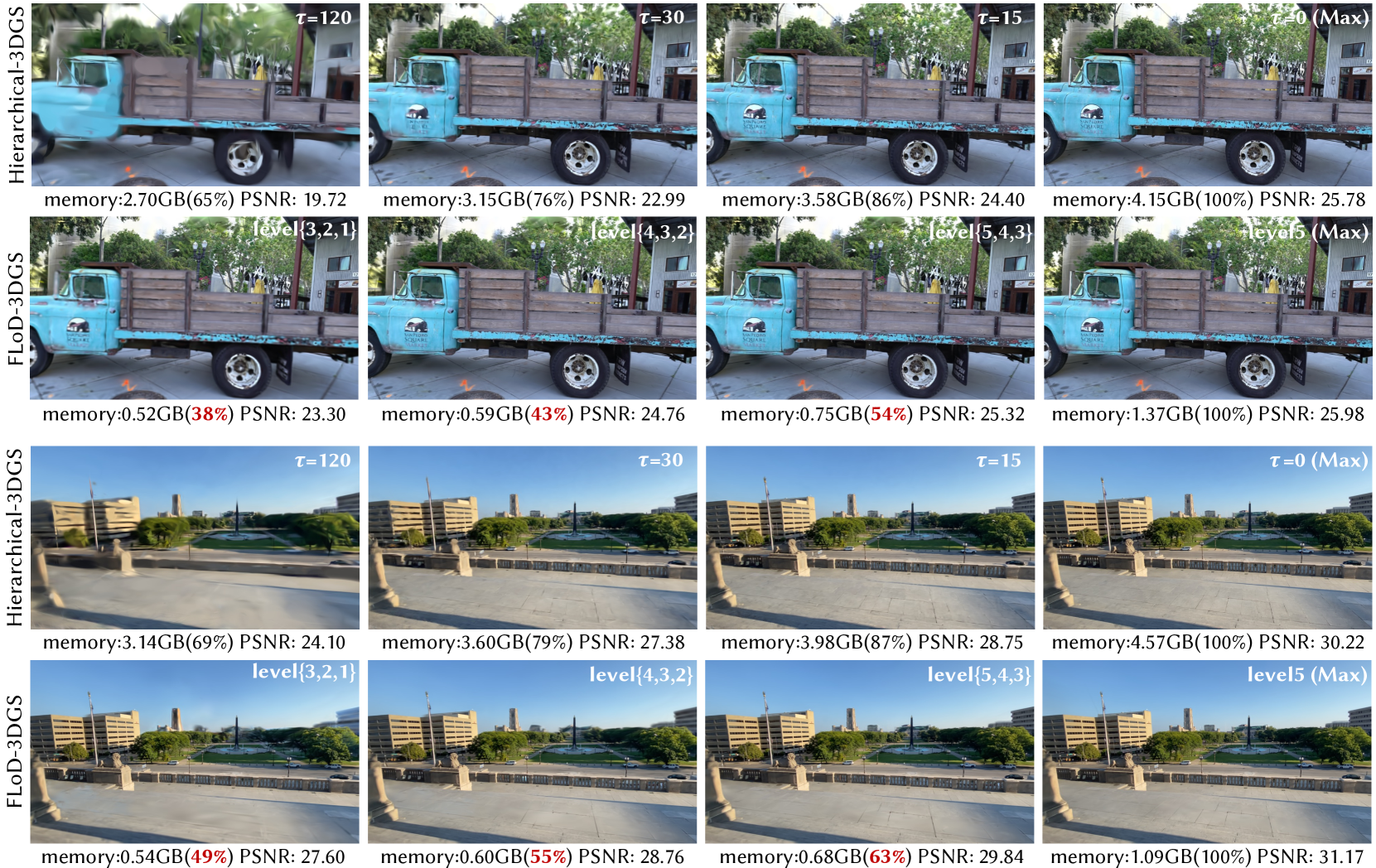<details> <summary>x16.png Details</summary>  ### Visual Description ## Comparative Analysis: Hierarchical-3DGS vs. FLoD-3DGS Rendering Quality and Memory Usage ### Overview The image presents a side-by-side visual and quantitative comparison of two 3D Gaussian Splatting (3DGS) rendering methods: **Hierarchical-3DGS** and **FLoD-3DGS**. The comparison is conducted across two distinct scenes: a close-up of a vintage blue truck and a wider shot of a building plaza. For each method and scene, four progressive quality levels are shown, with corresponding metrics for memory consumption and image quality (PSNR). ### Components/Axes The image is organized into a 4x4 grid, segmented into four primary horizontal rows. * **Row 1 (Top):** **Hierarchical-3DGS** applied to the **Truck Scene**. * **Parameter:** `τ` (tau), with values decreasing from left to right: `τ=120`, `τ=30`, `τ=15`, `τ=0 (Max)`. * **Metrics per panel:** Memory usage in GB and as a percentage of maximum, and Peak Signal-to-Noise Ratio (PSNR). * **Row 2:** **FLoD-3DGS** applied to the **Truck Scene**. * **Parameter:** Level sets, with complexity increasing from left to right: `level{3,2,1}`, `level{4,3,2}`, `level{5,4,3}`, `level5 (Max)`. * **Metrics per panel:** Memory usage in GB and as a percentage of maximum, and PSNR. * **Row 3:** **Hierarchical-3DGS** applied to the **Building Scene**. * **Parameter:** Same `τ` progression as Row 1. * **Metrics per panel:** Memory usage in GB and as a percentage of maximum, and PSNR. * **Row 4 (Bottom):** **FLoD-3DGS** applied to the **Building Scene**. * **Parameter:** Same level set progression as Row 2. * **Metrics per panel:** Memory usage in GB and as a percentage of maximum, and PSNR. **Visual Elements:** Each panel contains a rendered image of the scene. The visual quality (sharpness, detail) improves from left to right within each row. The memory percentage and PSNR values are overlaid as text at the bottom of each panel. ### Detailed Analysis #### Truck Scene Data **Hierarchical-3DGS (Row 1):** * **Trend:** As `τ` decreases (120 → 0), memory usage increases, and PSNR improves. * **Data Points:** * `τ=120`: Memory: 2.70GB (65%), PSNR: 19.72 * `τ=30`: Memory: 3.15GB (76%), PSNR: 22.99 * `τ=15`: Memory: 3.58GB (86%), PSNR: 24.40 * `τ=0 (Max)`: Memory: 4.15GB (100%), PSNR: 25.78 **FLoD-3DGS (Row 2):** * **Trend:** As the level set complexity increases, memory usage increases, and PSNR improves. * **Data Points:** * `level{3,2,1}`: Memory: 0.52GB (38%), PSNR: 23.30 * `level{4,3,2}`: Memory: 0.59GB (43%), PSNR: 24.76 * `level{5,4,3}`: Memory: 0.75GB (54%), PSNR: 25.32 * `level5 (Max)`: Memory: 1.37GB (100%), PSNR: 25.98 #### Building Scene Data **Hierarchical-3DGS (Row 3):** * **Trend:** As `τ` decreases (120 → 0), memory usage increases, and PSNR improves. * **Data Points:** * `τ=120`: Memory: 3.14GB (69%), PSNR: 24.10 * `τ=30`: Memory: 3.60GB (79%), PSNR: 27.38 * `τ=15`: Memory: 3.98GB (87%), PSNR: 28.75 * `τ=0 (Max)`: Memory: 4.57GB (100%), PSNR: 30.22 **FLoD-3DGS (Row 4):** * **Trend:** As the level set complexity increases, memory usage increases, and PSNR improves. * **Data Points:** * `level{3,2,1}`: Memory: 0.54GB (49%), PSNR: 27.60 * `level{4,3,2}`: Memory: 0.60GB (55%), PSNR: 28.76 * `level{5,4,3}`: Memory: 0.68GB (63%), PSNR: 29.84 * `level5 (Max)`: Memory: 1.09GB (100%), PSNR: 31.17 ### Key Observations 1. **Memory Efficiency:** FLoD-3DGS is dramatically more memory-efficient than Hierarchical-3DGS at comparable or even superior quality levels. For example, in the truck scene, FLoD-3DGS at its *lowest* quality (0.52GB, PSNR 23.30) uses less than 1/5th the memory of Hierarchical-3DGS at its *highest* quality (4.15GB, PSNR 25.78) while achieving a PSNR only 2.48 dB lower. 2. **Quality Ceiling:** In both scenes, the maximum quality (PSNR) achieved by FLoD-3DGS (`level5 (Max)`) is slightly higher than that of Hierarchical-3DGS (`τ=0 (Max)`). Truck: 25.98 vs. 25.78. Building: 31.17 vs. 30.22. 3. **Visual Fidelity:** The visual improvement from left to right is clear in both methods, with textures (wood grain on the truck, building facades) becoming sharper and less blurry. The visual difference between the highest quality settings of the two methods is minimal to the naked eye. 4. **Scene Dependency:** The absolute PSNR values are higher for the building scene than the truck scene for both methods, suggesting the building scene may be inherently easier to reconstruct or render. ### Interpretation This comparison demonstrates a significant advancement in efficiency for 3D Gaussian Splatting rendering. The **FLoD-3DGS** method achieves a superior **quality-to-memory ratio**. * **What the data suggests:** FLoD-3DGS likely employs a more sophisticated level-of-detail (LoD) or culling mechanism, allowing it to allocate memory resources more intelligently. It can produce high-fidelity results using a fraction of the memory required by the Hierarchical approach. The fact that its maximum quality is slightly higher also suggests its representation may be more effective or complete when fully deployed. * **Relationship between elements:** The core relationship shown is the trade-off between resource consumption (memory) and output quality (PSNR). Both methods follow the expected curve where more resources yield better quality, but FLoD-3DGS's curve is shifted dramatically to the left (more efficient). * **Notable implications:** For real-time applications, mobile deployment, or scenes with strict memory budgets, FLoD-3DGS presents a compelling advantage. It enables high-quality 3D rendering on hardware that could not support the memory demands of the Hierarchical method at similar fidelity. The data strongly argues for the adoption of more efficient, level-based splatting techniques over purely hierarchical ones. </details> Figure 16. Comparison of the trade-off between memory usage and visual quality in the selective rendering methods of FLoD-3DGS and Hierarchical-3DGS on the Tanks&Temples and DL3DV-10K datasets. The percentages (%) next to the memory values indicate how much memory each rendering setting uses compared to the memory required by the setting labeled as ”Max” for achieving maximum rendering quality. ### B.3. Gaussian Scale Constraint vs Count Constraint FLoD controls the level of detail and corresponding memory usage by training Gaussians with explicit 3D scale constraints. Adjusting the 3D scale constraint provides multiple rendering options with different memory requirements, as larger 3D scale constraints result in fewer Gaussians needed for scene reconstruction. An alternative method is to create multi-level 3DGS representations by directly limiting the Gaussian count. However, limiting the Gaussian count without enforcing scale constraints cannot reconstruct each level’s representation with the level of detail controlled. With only the rendering loss guiding Gaussian optimization and population control, certain local regions may achieve higher detail than others. This regional variation makes visually consistent rendering infeasible when multiple levels are combined for selective rendering, making such rendering option unviable. In contrast, FLoD’s 3D scale constraints ensure uniform detail within each level. Such uniformity enables visually consistent selective rendering and allows efficient calculation, as $G_sel$ can be constructed simply by computing the distance $d_G^(l)$ of each Gaussian from the camera, as discussed in Section 5.2. Furthermore, as discussed in Section 6.3, the 3D scale constraints also help preserve scene structure—especially in distant regions. Therefore, limiting the Gaussian count without scale constraints would degrade reconstruction quality. 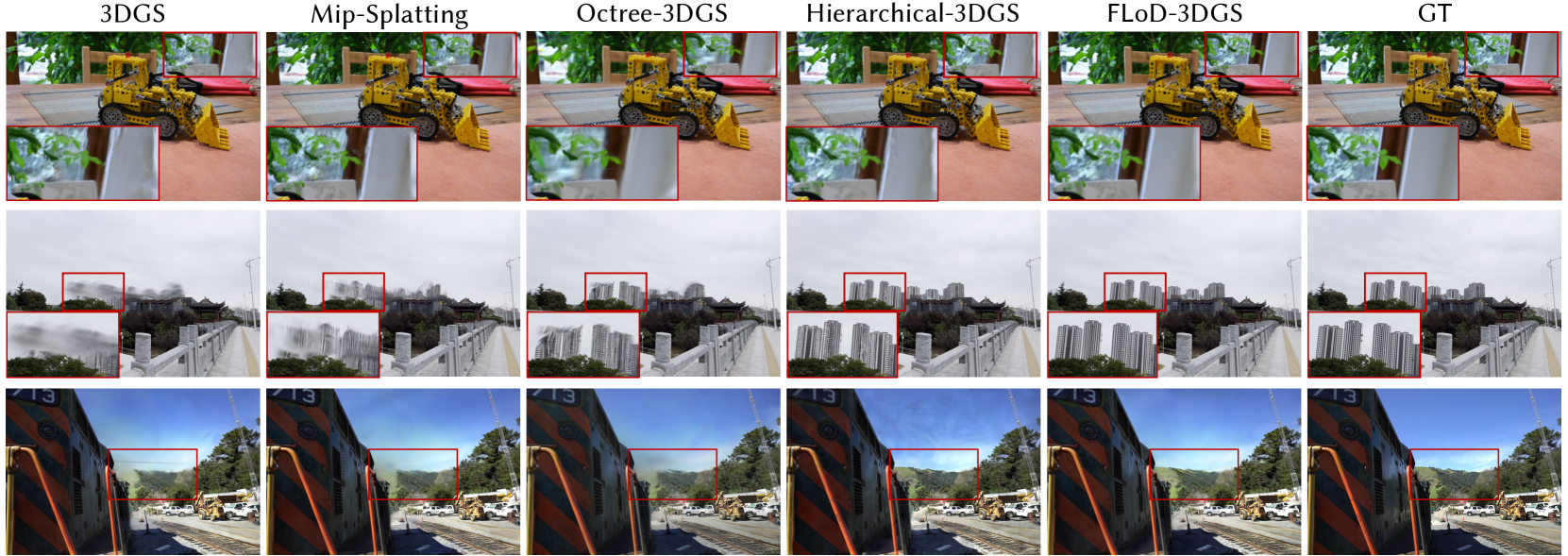<details> <summary>x17.png Details</summary>  ### Visual Description ## Comparative Visualization: 3D Gaussian Splatting (3DGS) Method Reconstruction Quality ### Overview The image is a comparative visualization grid from a technical paper or report, evaluating the visual output quality of five different 3D Gaussian Splatting (3DGS) reconstruction methods against a Ground Truth (GT) reference. It displays three distinct scenes (rows) rendered by each method (columns). Red bounding boxes highlight specific regions of interest, with corresponding zoomed-in insets provided in the bottom-left corner of each image panel for detailed comparison. ### Components/Axes * **Structure:** A 3-row by 6-column grid. * **Column Headers (Top Labels):** The six columns are labeled from left to right as: 1. `3DGS` 2. `Mip-Splatting` 3. `Octree-3DGS` 4. `Hierarchical-3DGS` 5. `FLoD-3DGS` 6. `GT` (Ground Truth) * **Row Content (Scenes):** * **Row 1:** An indoor scene featuring a yellow toy bulldozer on a wooden surface with a red object in the background. * **Row 2:** An outdoor cityscape view from a bridge or walkway, showing traditional Chinese-style rooftops in the mid-ground and modern high-rise buildings in the background under an overcast sky. * **Row 3:** A close-up view of the side of a train car (marked with "13") on a track, with trees, a road, and construction vehicles visible in the background. * **Visual Annotations:** * **Red Bounding Boxes:** Each image panel contains a red rectangular box outlining a specific region for detailed comparison. * **Zoomed Insets:** A smaller, magnified view of the area inside the red box is overlaid in the bottom-left corner of each panel. ### Detailed Analysis **Scene 1 (Toy Bulldozer):** * **Trend:** All methods reconstruct the main subject (bulldozer) recognizably. The key differentiator is the clarity of fine details and textures in the background and on surfaces. * **Data Points (Visual Quality in Inset):** * `3DGS`: Shows significant blurring and loss of detail in the zoomed region (appears to be foliage/texture). * `Mip-Splatting`: Slightly improved over 3DGS but still blurry. * `Octree-3DGS`: Noticeably sharper than the previous two. * `Hierarchical-3DGS`: Similar sharpness to Octree-3DGS. * `FLoD-3DGS`: Appears very sharp, with clear definition of edges and textures. * `GT`: The reference image, showing the highest level of detail and clarity. **Scene 2 (Cityscape):** * **Trend:** The primary challenge is the accurate reconstruction of distant, complex geometry (building facades) and handling atmospheric haze. * **Data Points (Visual Quality in Inset):** * `3DGS`: The buildings in the inset are extremely blurry and lack any structural definition. * `Mip-Splatting`: Shows some structural hints but remains very blurry and "smudged." * `Octree-3DGS`: Buildings are recognizable with defined edges, but textures are somewhat noisy or incomplete. * `Hierarchical-3DGS`: Similar to Octree-3DGS, with perhaps slightly better structural coherence. * `FLoD-3DGS`: Renders the buildings with high clarity, sharp edges, and clear window patterns, closely matching the GT. * `GT`: The reference, showing crisp, detailed buildings. **Scene 3 (Train):** * **Trend:** This scene tests the reconstruction of large, planar surfaces with text/numbers (the train side) and complex background elements. * **Data Points (Visual Quality in Inset):** * `3DGS`: The background area in the inset (trees/sky) is very blurry and lacks detail. * `Mip-Splatting`: Marginally better than 3DGS but still heavily blurred. * `Octree-3DGS`: Background details become more discernible. * `Hierarchical-3DGS`: Good clarity in the background. * `FLoD-3DGS`: Very clear reconstruction of both the train's edge and the background scenery. * `GT`: The reference image. ### Key Observations 1. **Performance Gradient:** There is a clear visual progression in reconstruction quality from left to right across the methods. `3DGS` and `Mip-Splatting` consistently produce the blurriest results, especially in detailed or distant regions. `Octree-3DGS` and `Hierarchical-3DGS` show significant improvement. `FLoD-3DGS` consistently produces results that are visually closest to the `GT` reference. 2. **Failure Modes:** The baseline `3DGS` method exhibits severe high-frequency detail loss, appearing as pervasive blurring. `Mip-Splatting` mitigates this slightly but does not resolve it. 3. **Strength of FLoD-3DGS:** The `FLoD-3DGS` method demonstrates a notable ability to preserve sharp edges (building outlines, train edges) and fine textures (building windows, foliage) that other methods smooth out. 4. **Consistency:** The relative performance ranking of the methods is consistent across all three diverse scenes (indoor object, outdoor cityscape, vehicle close-up), suggesting the observed advantages are robust. ### Interpretation This image serves as qualitative evidence in a research context, likely from a paper introducing or evaluating the `FLoD-3DGS` method. The visual comparison is designed to demonstrate that `FLoD-3DGS` achieves superior rendering fidelity compared to prior 3DGS variants. * **What the Data Suggests:** The data (visual results) suggests that the `FLoD-3DGS` algorithm incorporates improvements that better preserve high-frequency spatial information and geometric detail. This could be due to more efficient data structures, improved splatting primitives, or better optimization strategies that prevent over-smoothing. * **Relationship Between Elements:** The columns represent a chronological or complexity-based evolution of techniques, with `GT` as the ideal target. The rows prove the methods' generalizability. The red boxes and insets are critical, directing the viewer's attention to the exact regions where algorithmic differences are most pronounced, preventing assessment based on easy-to-reconstruct areas. * **Notable Anomalies/Outliers:** The most striking "outlier" is the dramatic failure of the baseline `3DGS` in the cityscape scene (Row 2), where distant buildings become unrecognizable blurs. This starkly highlights the problem the other methods aim to solve. Conversely, `FLoD-3DGS` is an outlier in the positive direction, consistently matching `GT` quality. * **Underlying Message:** The investigation implied by this chart is: "How can we improve 3D Gaussian Splatting to avoid detail loss?" The presented evidence argues that `FLoD-3DGS` is a successful answer, offering a significant leap in visual quality that brings synthetic reconstructions to a level nearly indistinguishable from ground truth photography in these examples. This has implications for applications requiring high-fidelity 3D capture, such as virtual reality, digital twins, and visual effects. </details> Figure 17. Qualitative comparison between FLoD-3DGS and baselines on three real-world datasets. The red boxes emphasize the key differences. Please zoom in for a more detailed view. 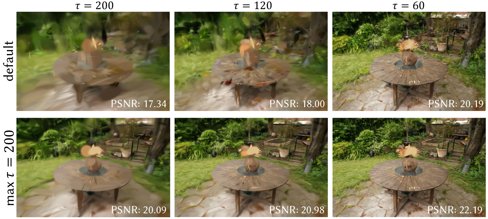<details> <summary>x18.png Details</summary>  ### Visual Description ## Comparative Image Reconstruction Chart: Effect of τ Parameter on Visual Quality and PSNR ### Overview The image is a 2x3 comparative grid displaying the results of an image reconstruction or rendering algorithm under different parameter settings. It visually and quantitatively demonstrates how two variables—the row condition ("default" vs. "max τ = 200") and the column parameter (τ = 200, 120, 60)—affect the clarity and fidelity of a reconstructed scene featuring a wooden table with a plant in an outdoor garden setting. ### Components/Axes * **Row Labels (Y-Axis):** Located vertically on the far left. * Top Row: `default` * Bottom Row: `max τ = 200` * **Column Headers (X-Axis):** Located horizontally at the top of each column. * Left Column: `τ = 200` * Middle Column: `τ = 120` * Right Column: `τ = 60` * **Data Metric:** Peak Signal-to-Noise Ratio (PSNR) is displayed as white text in the bottom-right corner of each sub-image. PSNR is a standard metric for measuring image reconstruction quality, where higher values indicate better fidelity to a reference image. * **Visual Content:** Each of the six panels shows the same core scene: a round, slatted wooden table on a stone patio, with a potted plant (resembling a small palm or cycad) on top, surrounded by lush green foliage and garden elements. ### Detailed Analysis The grid allows for a direct comparison across two dimensions: the algorithm variant (row) and the τ parameter (column). **Row 1: "default" method** * **τ = 200 (Top-Left):** The image is severely blurred and distorted. Details of the table, plant, and background are smeared and lack definition. **PSNR: 17.34** * **τ = 120 (Top-Middle):** Significant improvement in clarity over τ=200. The table's shape and the plant are more recognizable, but substantial blurring and artifacts remain, especially in the foliage. **PSNR: 18.00** * **τ = 60 (Top-Right):** The image is much sharper. The table's wood grain, the plant's leaves, and background details like a fence and other pots are clearly visible. Some minor softness remains. **PSNR: 20.19** **Row 2: "max τ = 200" method** * **τ = 200 (Bottom-Left):** This image is dramatically clearer than its "default" counterpart in the same column. The table and plant are well-defined, though the background foliage is still somewhat soft. **PSNR: 20.09** * **τ = 120 (Bottom-Middle):** Shows a slight but consistent improvement in sharpness and detail over the τ=200 result in this row. **PSNR: 20.98** * **τ = 60 (Bottom-Right):** This is the sharpest and highest-fidelity image in the entire grid. Fine details in the wood, stone, and individual leaves are crisp. **PSNR: 22.19** **Visual Trend Verification:** * **Across Columns (Left to Right):** For both rows, as τ decreases from 200 to 60, the visual clarity improves monotonically. The images transition from heavily blurred to sharp. This trend is confirmed by the PSNR values, which increase steadily from left to right in each row. * **Across Rows (Top to Bottom):** For every given τ value, the "max τ = 200" method produces a significantly clearer image with fewer artifacts than the "default" method. This is also confirmed by the PSNR values, which are substantially higher in the bottom row for each corresponding column. ### Key Observations 1. **Parameter Sensitivity:** The quality of the "default" method is highly sensitive to the τ parameter. A high τ (200) yields unusable results, while a lower τ (60) produces acceptable quality. 2. **Method Superiority:** The "max τ = 200" method is robust and superior across all tested τ values. Even at the highest τ (200), it outperforms the "default" method at its best setting (τ=60) in terms of PSNR (20.09 vs. 20.19, nearly equal) and visually appears comparable or better. 3. **Diminishing Returns:** The improvement in PSNR when moving from τ=120 to τ=60 is smaller than the jump from τ=200 to τ=120, especially for the "max τ = 200" row (ΔPSNR: ~1.2 vs. ~0.9). This suggests a potential point of diminishing returns for lowering τ further. 4. **PSNR-Visual Correlation:** There is a strong, direct correlation between the quantitative PSNR metric and the qualitative visual assessment in this chart. Higher PSNR consistently corresponds to a sharper, more detailed image. ### Interpretation This chart is likely from a research paper or technical report on neural rendering, view synthesis, or image reconstruction (e.g., NeRF, 3D Gaussian Splatting). The parameter **τ** (tau) probably controls a key aspect of the algorithm, such as the number of optimization iterations, a sampling rate, or a threshold for density/opacity pruning. The data demonstrates two key findings: 1. **The "max τ = 200" variant is a more effective algorithm.** It achieves high-quality results even with a parameter setting (τ=200) that causes the default method to fail. This suggests it has a better underlying model or optimization strategy that is less prone to the artifacts (like blurring and distortion) seen in the default method at high τ. 2. **Lower τ values improve quality for both methods, but with a cost.** While not stated in the image, in such algorithms, a lower τ (e.g., fewer iterations or more aggressive pruning) typically correlates with **faster computation or lower memory usage**. Therefore, the chart illustrates a critical trade-off: the "max τ = 200" method allows one to achieve high visual quality (high PSNR) **without** needing to lower τ to its minimum, potentially saving computational resources. It provides a better quality-speed Pareto frontier. **In summary, the chart provides evidence that the proposed "max τ = 200" method is more robust and efficient, delivering higher fidelity reconstructions across a range of operational parameters compared to the default approach.** </details> Figure 18. Comparison of Hierarchical-3DGS trained with the default max granularity ( $τ$ ) and a max $τ$ of 200. Results show that training with a larger max $τ$ improves rendering quality for large $τ$ values. ## Appendix C Single Level Comparison with Competitors Each level in FLoD has its own independent representation, unlike Octree-GS, where levels are not independent but rather dependent on previous levels. To ensure a fair comparison with Octree-GS in Section 6.2.1, we respect this dependency. To address any concerns that we may have presented the Octree-GS in a manner advantageous to our approach, we also render results using only the representation of each individual Octree-GS level. These results are shown in the upper row of Figure 15. As illustrated, Octree-GS automatically assigns higher levels to regions closer to training views and lower levels to more distant regions. This characteristic limits its flexibility compared to FLoD-3DGS, as it cannot render using various subsets of levels. In contrast, Hierarchical-3DGS automatically renders using nodes across multiple levels based on the target granularity $τ$ . It does not support rendering with nodes from a single level, unlike FLoD-3DGS and Octree-GS. For this reason, we do not conduct single-level comparisons for Hierarchical-3DGS in Section 6.2.1. However, to offer additional clarity, we render using only nodes from five selected levels (1, 6, 11, 16, and 22) out of its 22 levels. These results are shown in the lower row of Figure 15. ## Appendix D Selective Rendering Comparison In Section 6.2.2, we compare the memory efficiency of selective rendering between FLoD-3DGS and Hierarchical-3DGS. Since the default setting of Hierarchical-3DGS is intended for a maximum target granularity of 15, we extend the maximum target granularity $τ_max$ to 200 during its hierarchy optimization stage. This adjustment ensures a fair comparison with Hierarchical-3DGS across a broader range of rendering settings. As shown in Figure 18, its default setting results in significantly worse rendering quality for large $τ$ compared to when the hierarchy optimization stage has been adjusted. Section 6.2.2 presents results for the garden scene from the Mip-NeRF360 dataset. To demonstrate that FLoD-3DGS achieves superior memory efficiency across diverse scenes, we include additional results for the Tanks&Temples and DL3DV-10K datasets in Figure 16. In Hierarchical-3DGS, increasing the target granularity $τ$ does not significantly reduce memory usage, even though fewer Gaussians are used for rendering at larger $τ$ values. This occurs because all Gaussians, across every hierarchy level, are loaded onto the GPU according to the release code for evaluation. Consequently, the potential for memory reduction at higher $τ$ values is limited. The results in Figure 16 confirm that FLoD-3DGS effectively balances memory usage and visual quality trade-offs through selective rendering across various datasets. 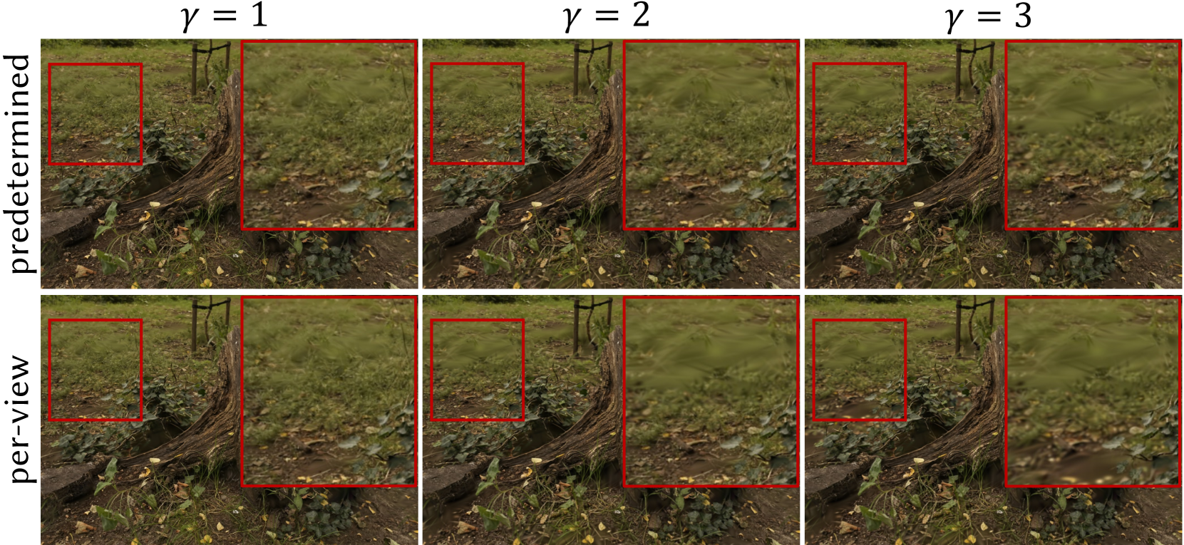## Appendix E Inconsistency in Selective Rendering <details> <summary>x19.png Details</summary>  ### Visual Description ## Visual Comparison Chart: Gamma Correction Effects on Image Processing Methods ### Overview This image is a technical comparison chart, likely from a research paper or technical report in computer vision or image processing. It visually demonstrates the effects of varying a gamma parameter (γ) on two different image processing or rendering methods, labeled "predetermined" and "per-view." The chart is organized as a 2x3 grid of image panels. ### Components/Axes * **Grid Structure:** The chart is a matrix with two rows and three columns. * **Row Labels (Left Side):** * Top Row: `predetermined` (written vertically, reading from bottom to top). * Bottom Row: `per-view` (written vertically, reading from bottom to top). * **Column Labels (Top):** * Left Column: `γ = 1` * Middle Column: `γ = 2` * Right Column: `γ = 3` * **Image Content:** Each of the six panels displays the same base scene: a close-up view of a garden or forest floor with soil, green plants, fallen leaves, and a curved, textured wooden log or root structure in the foreground. * **Annotations:** Each panel contains two red rectangular boxes, highlighting specific regions of interest within the scene for comparison. * **Box 1 (Left):** A smaller square box positioned in the upper-left quadrant of the image, focusing on a patch of ground and low-lying vegetation. * **Box 2 (Right):** A larger square box positioned in the right half of the image, focusing on the area where the wooden structure meets the ground and surrounding plants. ### Detailed Analysis The chart compares visual output across two methods and three gamma settings. The primary variable is the gamma value (γ), which typically controls luminance or color intensity in image processing. **Row 1: "predetermined" Method** * **γ = 1 (Top-Left Panel):** The image appears with natural, balanced contrast. Details in both the shadowed soil (highlighted by the left red box) and the textured wood/plants (highlighted by the right red box) are clearly visible. * **γ = 2 (Top-Middle Panel):** The image shows increased contrast and saturation. The greens in the vegetation appear more vivid, and the shadows in the soil patch (left box) become slightly darker. The texture on the wood (right box) appears more pronounced. * **γ = 3 (Top-Right Panel):** The effect is intensified. Contrast is high, with very dark shadows and bright highlights. The soil area (left box) is quite dark, potentially losing some detail. The vegetation and wood textures (right box) appear overly sharp and saturated, with a slight yellowish/greenish color cast. **Row 2: "per-view" Method** * **γ = 1 (Bottom-Left Panel):** The image is noticeably darker and has lower contrast compared to the "predetermined" γ=1 image. The soil patch (left box) is very dark, and overall scene illumination appears reduced. * **γ = 2 (Bottom-Middle Panel):** The image brightens significantly compared to its γ=1 counterpart. Contrast increases, revealing more detail in the soil (left box) and making the vegetation appear more vibrant. It visually resembles the "predetermined" γ=1 image more than its own γ=1 state. * **γ = 3 (Bottom-Right Panel):** The image becomes very bright, with high contrast and strong saturation. The soil area (left box) is now well-lit but may appear washed out. The vegetation and wood (right box) are highly saturated, with a strong yellow-green tint, similar to but potentially brighter than the "predetermined" γ=3 image. ### Key Observations 1. **Gamma Impact:** For both methods, increasing the gamma value (γ) from 1 to 3 systematically increases image contrast, brightness, and color saturation. 2. **Method Divergence:** The two methods respond differently to the same gamma value. * At **γ=1**, the "predetermined" method produces a well-exposed image, while the "per-view" method produces a significantly underexposed (dark) image. * At **γ=2**, the "per-view" method's output visually converges toward the "predetermined" method's output at γ=1. * At **γ=3**, both methods produce highly saturated, high-contrast images, though the "per-view" version may be slightly brighter. 3. **Visual Trend:** The "per-view" method shows a more dramatic *relative change* in appearance across the gamma range, starting very dark and becoming very bright. The "predetermined" method shows a more consistent, progressive enhancement from a balanced starting point. ### Interpretation This chart likely illustrates a core finding from a technical study on image-based rendering, view synthesis, or neural radiance fields (NeRFs). The parameter `γ` is probably a control within a rendering equation or a tone-mapping function. * **What the Data Suggests:** The "predetermined" method appears to have a more robust or pre-calibrated response to gamma, producing acceptable results at the baseline (γ=1). The "per-view" method seems to require gamma adjustment (specifically, a value around 2) to achieve a comparable visual quality to the baseline "predetermined" output. This implies the "per-view" method may have an inherent bias or different internal scaling that necessitates this correction. * **Relationship Between Elements:** The direct visual comparison across the grid allows researchers to quickly assess the perceptual impact of the gamma parameter and to identify the optimal setting for each method. The red boxes focus attention on challenging regions (dark soil, complex textures) where differences in exposure and detail preservation are most critical. * **Notable Anomalies/Patterns:** The most striking pattern is the inversion of relative brightness between the two methods at γ=1 versus γ=3. This suggests the gamma parameter interacts fundamentally differently with the underlying algorithms of each method. The chart effectively argues that a "one-size-fits-all" gamma setting is inappropriate and that the parameter must be tuned per method. </details> Figure 19. Rendering results of selective rendering using levels 5,4 and 3 with screen size thresholds $γ$ = 1, 2, and 3 for both predetermined and per-view Gaussian set $G_sel$ creation methods on the Mip-NeRF360 dataset. Red boxes emphasize the region where inconsistency is visible for larger $γ$ settings. Table 7. Rendering FPS results of FLoD-3DGS on a laptop with MX250 2GB GPU for 7 scenes from the Mip-NeRF360 dataset. A ”✓” on a single level indicates single-level rendering, while a ”✓” on multiple levels indicates selective rendering. ”✗” represents an OOM error, indicating that rendering FPS could not be measured. | ✓ | ✗ | 6.52 | ✗ | ✗ | 5.77 | 5.54 | 6.00 | 3.99 | 7.48 | | --- | --- | --- | --- | --- | --- | --- | --- | --- | --- | | ✓- ✓- ✓ | 5.10 | 8.81 | 6.92 | 8.48 | 8.33 | 6.27 | 6.58 | 4.20 | 8.69 | | ✓ $/\checkmark$ | 7.71 | 10.25 | 7.27 | 10.41 | 9.87 | 8.35 | 8.71 | 5.67 | 9.16 | | ✓- ✓- ✓ | 8.53 | 11.38 | 7.98 | 13.20 | 11.39 | 8.42 | 8.79 | 5.73 | 9.31 | | ✓ | 9.21 | 15.00 | 13.54 | 18.19 | 12.97 | 9.67 | 11.65 | 10.44 | 11.68 | | ✓- ✓- ✓ | 9.34 | 15.60 | 13.98 | 20.92 | 13.77 | 9.72 | 11.73 | 10.49 | 11.85 | Table 8. Comparison of visual quality and memory usage (GB) for FLoD-3DGS, alongside LightGS and CompactGS on Mip-NeRF360(Mip), DL3DV-10K(DL3DV) and Tanks&Temples(T&T) datasets. | FLoD-3DGS(lv5) | Mip PSNR 27.8 | DL3DV mem. 1.8 | T&T PSNR 31.9 | mem. 1.0 | PSNR 24.4 | mem. 1.1 | | --- | --- | --- | --- | --- | --- | --- | | FLoD-3DGS(lv4) | 26.6 | 1.2 | 30.7 | 0.6 | 23.8 | 0.6 | | FLoD-3DGS(lv3) | 24.1 | 0.8 | 28.3 | 0.5 | 21.7 | 0.5 | | LightGS | 26.6 | 1.2 | 27.2 | 0.7 | 23.3 | 0.6 | | CompactGS | 26.8 | 1.1 | 27.8 | 0.5 | 22.8 | 0.8 | In our selective rendering approach, the transition to a lower level occurs at the distance where the 2D projected 3D scaling constraint for the lower level becomes 1 pixel length, on the default screen size threshold $γ=1$ . While lower-level Gaussians can be trained to have large 3D scales - resulting in larger 2D splats - this generally happens when the larger splat aligns well with the training images. In such cases, these Gaussians do not receive training signals to shrink or split, and thus retain their large 3D scales. Therefore, inconsistency due to level transitions in selective rendering is unlikely, which is why we did not implement interpolation between successive levels. On the other hand, increasing the screen size threshold $γ$ beyond 1 can introduce visible inconsistencies in the rendering, as shown in Figure 19. ## Appendix F Qualitative Results of Max-level Rendering Section 6.3 quantitatively demonstrates that FLoD achieves rendering quality comparable to existing models. Figure 17 qualitatively shows that FLoD-3DGS reconstructs thin details and distant objects more accurately, or at least comparably, to the baselines. While Hierarchical-3DGS also handles distant objects well, it receives depth information from an external model. In contrast, FLoD-3DGS is trained without extra supervision. ## Appendix G Rendering on Low-cost Device FLoD offers wide range of rendering options through single-level and selective rendering, allowing users to adapt to a wide range of hardware capabilities. To demonstrate its effectiveness on low-cost devices, we measure FPS for Mip-NeRF360 scenes on the laptop equipped with an MX250 GPU (2GB VRAM). As shown in Table 7, single-level rendering at level 5 causes out-of-memory (OOM) errors in some scenes (e.g., stump). However, using selective rendering with levels 5, 4, and 3, or switching to a lower single level, resolves these errors. Additionally, in some cases (e.g., bonsai), FLoD enables real-time rendering. Thus, FLoD can provide adaptable rendering options even for low-cost devices. ## Appendix H Comparison with compression methods LightGaussian (Fan et al., 2023) and CompactGS (Lee et al., 2024) also address memory-related issues, but their primary focus is on creating a single compressed 3DGS with small storage size. In contrast, FLoD constructs multi-level LoD representations to accommodate varying GPU memory capacities during rendering. Due to this difference in purpose, a direct comparison with FLoD was not included in the main paper. To demonstrate the efficiency of FLoD-3DGS in GPU memory usage during rendering, we compare PSNR and GPU memory consumption across levels 5, 4, and 3 of FLoD-3DGS and the two baselines. As shown in Table 8, FLoD-3DGS achieves higher PSNR with comparable GPU memory usage. Furthermore, unlike LightGaussian and CompactGS, FLoD-3DGS supports multiple memory usage settings, indicating its adaptability across a range of GPU settings. Table 9. Comparison of Level 5 single-level rendering between FLoD-3DGS and FLoD-3DGS with the LightGaussian compression method applied (denoted as ’+LightGS’) on the Mip-NeRF360 dataset. | FLoD-3DGS FLoD-3DGS+LightGS | 103 144 | 518 31.7 | 27.8 27.1 | 0.815 0.799 | 0.224 0.250 | | --- | --- | --- | --- | --- | --- | ## Appendix I LightGaussian Compression on FLoD-3DGS FLoD-3DGS can store and render specific levels as needed. However, keeping the option of rendering with all levels requires significant storage disk space to accommodate them. To address this, we integrate LightGaussian’s (Fan et al., 2023) compression method into FLoD-3DGS to reduce storage disk usage. As shown in Table 9, compressing FLoD-3DGS reduces storage disk usage by 93% and enhances rendering speed. This compression, however, results in a reduction in reconstruction quality metrics compared to the original FLoD-3DGS, similar to how LightGaussian shows lower reconstruction quality than its baseline model, 3DGS. Despite this, we demonstrate that FLoD-3DGS can be further optimized to suit devices with constrained storage by incorporating compression techniques.