# Physics-Informed Machine Learning For Sound Field Estimation Invited paper for the IEEE SPM Special Issue on Model-based Data-Driven Audio Signal Processing
**Authors**: Shoichi Koyama, Juliano G. C. Ribeiro, Tomohiko Nakamura, Natsuki Ueno, and Mirco Pezzoli
> This work was supported by JST FOREST Program, Grant Number JPMJFR216M, JSPS KAKENHI, Grant Number 23K24864, and the European Union under the Italian National Recovery and Resilience Plan (NRRP) of NextGenerationEU, partnership on “Telecommunications of the Future” (PE00000001—program “RESTART”).Manuscript received April xx, 20xx; revised August xx, 20xx.
## Abstract
The area of study concerning the estimation of spatial sound, i.e., the distribution of a physical quantity of sound such as acoustic pressure, is called sound field estimation, which is the basis for various applied technologies related to spatial audio processing. The sound field estimation problem is formulated as a function interpolation problem in machine learning in a simplified scenario. However, high estimation performance cannot be expected by simply applying general interpolation techniques that rely only on data. The physical properties of sound fields are useful a priori information, and it is considered extremely important to incorporate them into the estimation. In this article, we introduce the fundamentals of physics-informed machine learning (PIML) for sound field estimation and overview current PIML-based sound field estimation methods.
Index Terms: Sound field estimation, kernel methods, physics-informed machine learning, physics-informed neural networks publicationid: pubid: 0000–0000/00$00.00 © 2024 IEEE
## I Introduction
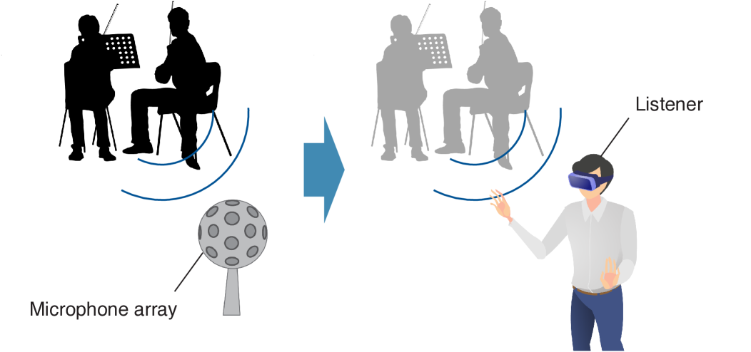
Sound field estimation, which is also referred to as sound field reconstruction, capturing, and interpolation, is a fundamental problem in acoustic signal processing, which is aimed at reconstructing a spatial acoustic field from a discrete set of microphone measurements. This essential technology has a wide variety of applications, such as room acoustic analysis, the visualization/auralization of an acoustic field, spatial audio reproduction using a loudspeaker array or headphones, and active noise cancellation in a spatial region. In particular, virtual/augmented reality (VR/AR) audio would be one of the most remarkable recent applications of this technology, as it requires capturing a sound field in a large region by multiple microphones (see Fig. 1). The spatial reconstruction of room impulse responses (RIRs) or acoustic transfer functions (ATFs), which is a special case of sound field estimation, can be applied to the estimation of steering vectors for beamforming and also head-related transfer functions (HRTFs) for binaural reproduction.
<details>
<summary>x1.png Details</summary>
### Visual Description
\n
## Diagram: Spatial Audio Capture and Reproduction
### Overview
The image depicts a diagram illustrating a system for capturing spatial audio from a source (two speakers) and reproducing it to a listener using a virtual reality (VR) headset. The diagram shows a transition from a captured audio scene to a reproduced audio experience.
### Components/Axes
The diagram consists of three main components:
1. **Source Scene:** Two figures, presumably speakers, are shown in silhouette on the left side of the image.
2. **Capture System:** A "Microphone array" is positioned below the source scene.
3. **Reproduction System:** A "Listener" wearing a VR headset is shown on the right side of the image.
An arrow indicates the flow of information from the source scene, through the microphone array, to the listener. Curved blue lines represent sound waves emanating from the speakers and reaching both the microphone array and the listener.
### Detailed Analysis or Content Details
* **Source Scene:** Two figures are depicted, one slightly in front of the other. Both figures are wearing headsets with microphones. The figure in the front is darker in color, appearing as a silhouette.
* **Microphone Array:** The microphone array is represented as a parabolic dish with multiple circular elements representing individual microphones. It is positioned centrally at the bottom of the diagram.
* **Listener:** The listener is a person wearing a VR headset. They are depicted with their right arm extended, as if interacting with a virtual environment.
* **Arrow:** A blue arrow points from the source scene towards the listener, indicating the direction of audio processing and reproduction.
* **Sound Waves:** Curved blue lines emanate from each speaker in the source scene. These lines represent the propagation of sound waves. They curve towards both the microphone array and the listener.
### Key Observations
The diagram illustrates a process of spatial audio capture and reproduction. The microphone array captures the sound field from the source scene, and this information is then used to recreate the audio experience for the listener through the VR headset. The curved lines suggest that the system is designed to capture and reproduce the directionality of sound.
### Interpretation
This diagram demonstrates a system for creating immersive audio experiences. The use of a microphone array suggests that the system is capable of capturing spatial information about the sound source, such as its location and direction. This information is then used to recreate the audio experience for the listener in a way that accurately reflects the original sound field. The VR headset is crucial for providing the visual context necessary for a truly immersive experience. The diagram highlights the importance of capturing and reproducing spatial audio for applications such as virtual reality, augmented reality, and teleconferencing. The transition from silhouette to grayscale suggests a transformation of the audio signal from raw capture to processed reproduction.
</details>
Figure 1: Sound field recording for VR audio. The sound field captured by a microphone array is reproduced by loudspeakers or headphones. The estimated sound field should account for listener movement and rotation within large regions.
Sound field estimation has been studied for a number of years. Estimating a sound field in the inverse direction of wave propagation based on wave domain (or spatial frequency domain) processing, i.e., the basis expansion of a sound field into plane wave or spherical wave functions, has been particularly applied to acoustic imaging tasks [1]. This technique has been introduced in the signal-processing field in recent decades. In particular, spherical harmonic domain processing using a spherical microphone array has been intensively investigated because its isotropic nature is suitable for spatial sound processing [2]. Wave domain processing has been applied to, for instance, spatial audio recording, source localization, source separation, and spatial active noise control.
The theoretical foundation of wave domain processing is derived from expansion representations by the solutions of the governing partial differential equations (PDEs) of acoustic fields, i.e., the wave equation in the time domain and the Helmholtz equation in the frequency domain. Since the basis functions used in wave domain processing, such as plane wave and spherical wave functions, are solutions of these PDEs in a region not including sound sources or scattering objects, the estimate is guaranteed to satisfy the wave and Helmholtz equations.
Although the classical methods are solely based on physics, advanced signal processing and machine learning techniques have also been applied to the sound field estimation problem. In particular, sparse optimization techniques have been investigated to improve the estimation accuracy while preserving the physical constraints for the estimate [3, 4, 5]. The physical constraints are usually imposed by the expansion representation of the sound field as used in the classical methods.
On the basis of great successes in various fields, (deep) neural networks [6] have also been incorporated into sound field estimation techniques in recent years to exploit their high representational power. The network weights are optimized to predict the sound field by using a set of training data. Basically, this approach is purely data-driven; that is, prior information on physical properties is not taken into account, as opposed to the methods mentioned above. To induce the estimate to satisfy the governing PDEs, the loss function for evaluating the deviation from the governing PDEs has been incorporated, and such a technique is referred to as the physics-informed neural networks (PINNs) [7, 8], which have been applied to various forward and inverse problems for physical fields, such as flow field [9], seismic field [10], and acoustic field [11]. PINNs help prevent unnatural distortions in the estimate, which are unlikely to occur in practical acoustic fields, particularly when the number of observations is small. Currently, there exist various methods using PINNs or other neural networks for sound field estimation as described in detail in the later sections [12, 13, 14, 15].
Physical properties are useful prior information in sound field estimation and methods based on physical properties have many advantages over purely data-driven approaches. Although sound field estimation methods have historically used physical constraints explicitly, with the recent development of machine learning techniques, physics-informed machine learning (PIML) in sound field estimation continues to grow significantly, especially after the advent of PINN [16, 17, 18, 19]. We describe how to embed physical properties for various machine learning techniques, such as linear regression, kernel regression, and neural networks, in the sound field estimation problem and summarize the current PIML-based methods for sound field estimation. Furthermore, current limitations and future outlooks are also discussed.
## II Sound field estimation problem
<details>
<summary>x2.png Details</summary>
### Visual Description
\n
## Diagram: Sound Wave Interference Pattern
### Overview
The image depicts a visual representation of sound wave interference, likely illustrating the principle of constructive and destructive interference. It shows a region (Ω) with alternating bands of color (red and blue/purple) representing areas of high and low sound pressure, respectively. Several microphone symbols are placed within this region.
### Components/Axes
* **Ω:** Label indicating the region of sound wave interference. Positioned in the top-right corner.
* **Microphone:** Label pointing to a microphone symbol. Positioned in the top-left corner.
* **Color Bands:** Alternating red and blue/purple bands representing areas of constructive (red) and destructive (blue/purple) interference.
* **Microphone Symbols:** Small circles with a line through them, representing microphone placements. Distributed throughout the region Ω.
### Detailed Analysis or Content Details
The diagram shows a roughly oval-shaped region (Ω) filled with alternating bands of red and blue/purple. The bands are not perfectly straight but are curved and wave-like. There are approximately 11 microphone symbols distributed within the region.
* **Microphone 1:** Located in the top-left, within a red band.
* **Microphone 2:** Located slightly below and to the right of Microphone 1, within a blue/purple band.
* **Microphone 3:** Located in the top-right, within a red band.
* **Microphone 4:** Located below Microphone 3, within a blue/purple band.
* **Microphone 5:** Located in the center-left, within a blue/purple band.
* **Microphone 6:** Located in the center, within a red band.
* **Microphone 7:** Located below Microphone 6, within a blue/purple band.
* **Microphone 8:** Located in the bottom-left, within a blue/purple band.
* **Microphone 9:** Located to the right of Microphone 8, within a red band.
* **Microphone 10:** Located in the bottom-right, within a blue/purple band.
* **Microphone 11:** Located slightly above Microphone 10, within a red band.
The region Ω is outlined with a dashed line. The color bands appear to be roughly parallel to each other, though with some curvature.
### Key Observations
The microphones are strategically placed within both the red and blue/purple bands, suggesting an investigation into the sound pressure levels at different points within the interference pattern. The alternating color bands clearly demonstrate the spatial variation of sound intensity due to interference.
### Interpretation
This diagram illustrates the concept of sound wave interference. The red bands represent areas where sound waves constructively interfere, resulting in higher sound pressure (louder sound). The blue/purple bands represent areas where sound waves destructively interfere, resulting in lower sound pressure (quieter sound). The placement of the microphones suggests an experiment or simulation to measure the sound pressure levels at various points within this interference pattern. The dashed outline (Ω) defines the area where the interference pattern is being observed. The diagram is a qualitative representation and does not provide specific numerical data about sound pressure levels or frequencies. It serves to visually explain the phenomenon of interference.
</details>
(a) Interior problem
<details>
<summary>x3.png Details</summary>
### Visual Description
\n
## Diagram: Microphone and Sound Wave Interaction
### Overview
The image depicts a diagram illustrating the interaction between a microphone and surrounding sound waves. Concentric waves, alternating between red and blue hues, emanate outwards. A microphone is positioned centrally, partially obscuring the wave pattern. A dotted line outlines a region labeled "Ω" around the microphone. Small circular icons with arrows pointing outwards are distributed around the microphone, seemingly representing sound sources or wave propagation.
### Components/Axes
* **Microphone:** Central component, white in color.
* **Sound Waves:** Concentric, alternating red and blue waves.
* **Region Ω:** Dotted line outlining an area around the microphone.
* **Sound Source Icons:** Small circles with outward-pointing arrows, positioned around the microphone.
* **Arrow:** A black arrow points from the microphone towards one of the sound source icons.
### Detailed Analysis or Content Details
The diagram shows a microphone positioned within a field of sound waves. The waves are represented as concentric circles, alternating between red and blue. The red waves appear to be more concentrated at the bottom of the microphone, while the blue waves are more prominent at the top. The dotted line labeled "Ω" encloses a region around the microphone, suggesting a defined area of interaction or influence. The small circular icons with arrows are distributed around the microphone, indicating potential sources of sound or directions of wave propagation. The arrow originating from the microphone points towards one of these icons, possibly indicating a transmission or detection pathway.
There are approximately 12 sound source icons distributed around the microphone. The icons are evenly spaced around the microphone.
### Key Observations
* The alternating red and blue waves suggest different phases or intensities of the sound waves.
* The concentration of red waves at the bottom of the microphone might indicate a specific frequency or characteristic of the sound.
* The region "Ω" highlights the area where the microphone interacts with the sound field.
* The arrow suggests a directional relationship between the microphone and the sound sources.
### Interpretation
This diagram likely illustrates the principle of sound detection by a microphone. The concentric waves represent sound pressure variations, and the microphone is designed to convert these variations into an electrical signal. The region "Ω" could represent the effective capture area of the microphone, where sound waves are most strongly detected. The alternating colors of the waves might represent constructive and destructive interference, influencing the signal received by the microphone. The arrow suggests that the microphone can both receive sound from sources and potentially transmit signals. The diagram is a simplified representation of a complex physical phenomenon, focusing on the fundamental interaction between a microphone and its acoustic environment. It does not provide quantitative data, but rather a conceptual visualization of the process.
</details>
(b) Exterior problem
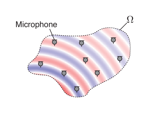
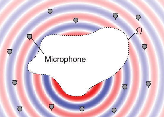
Figure 2: Sound field estimation of interior and exterior regions. In the interior problem, the sound field in the source-free interior region $\Omega$ is estimated. In contrast, the sound field in the source-free exterior region $\mathbb{R}^{3}\backslash\Omega$ is estimated in the exterior problem.
First, we formulate the sound field estimation problem. In this article, we mainly focus on an interior problem, that is, estimating a sound field inside a source-free region of the target with multiple microphones (see Fig. 2). Several methods introduced in this article are also applicable to the exterior or radiation problem.
The target region in the three-dimensional space is denoted as $\Omega\subset\mathbb{R}^{3}$ . The pressure distribution in $\Omega$ is represented by $U:\Omega\times\mathbb{R}\rightarrow\mathbb{R}$ in the time domain and $u:\Omega\times\mathbb{R}\rightarrow\mathbb{C}$ in the frequency domain, which is generated by sound waves propagating from one or more sound sources outside $\Omega$ and also by reverberation. Here, $U$ and $u$ are continuous functions of the position $\bm{r}\in\Omega$ and the time $t\in\mathbb{R}$ or the angular frequency $\omega\in\mathbb{R}$ . $M$ microphones are placed at arbitrary positions inside $\Omega$ . The objective of the sound field estimation problem is to reconstruct $U$ or $u$ from microphone observations.
In the frequency domain, the estimation can be performed at each frequency assuming signal independence between frequencies. If the estimator of $u$ is linear in the frequency domain, a finite-impulse-response (FIR) filter for estimating a sound field generated by usual sounds, such as speech and music, can be designed. Otherwise, the estimation is performed in the time–frequency domain, for example, by the short-time Fourier transform (STFT), or in the time domain. Particularly when the estimator is adapted to the environment, the direct estimation in the time domain is generally more challenging because the estimator for $U$ may have a large dimension of spatiotemporal functions. When the source signal is an impulse signal, which means that $U$ is a spatiotemporal function of an RIR, the problem can be relatively tractable because the time samples to be estimated are reduced to the length of RIRs at most and the estimation is generally performed offline.
For simplicity, the microphones are assumed to be omnidirectional, i.e., pressure microphones. In this scenario, the sound field estimation problem is equivalent to the general interpolation problem because the observations are spatial (or spatiotemporal) samples of the multivariate scalar function to be estimated. Specifically, when the microphone observations in the frequency domain are denoted by $\bm{s}(\omega)=[s_{1}(\omega),\ldots,s_{M}(\omega)]^{\mathsf{T}}\in\mathbb{C}^ {M}$ ( $(\cdot)^{\mathsf{T}}$ is the transpose) obtained by the pressure microphones at $\{\bm{r}_{m}\}_{m=1}^{M}$ , the observed values of $\{s_{m}(\omega)\}_{m=1}^{M}$ can be regarded as $\{u(\bm{r}_{m},\omega)\}_{m=1}^{M}$ contaminated by some noise. In the time domain, the sound field should be estimated from the observations of $M$ microphones and $T$ time samples. Most methods introduced in this article can be generalized to the case of directional microphones because the measurement process can be assumed to be a linear operation. It is also possible for most methods to be generalized to estimate expansion coefficients of spherical wave functions of the sound field at a predetermined expansion center, which is particularly useful for spatial audio applications such as ambisonics [20].
We start with techniques of embedding physical properties in general interpolation techniques. Then, current studies of sound field estimation based on PIML are introduced.
## III Embedding physical properties in interpolation techniques
In general interpolation techniques, the estimation of the continuous function $f:\mathbb{R}^{P}\to\mathbb{K}$ ( $\mathbb{K}$ is $\mathbb{R}$ or $\mathbb{C}$ , i.e., $f$ is $U$ or $u$ ) from a discrete set of observations $\bm{y}\in\mathbb{K}^{I}$ at the sampling points $\{\bm{x}_{i}\}_{i=1}^{I}$ is achieved by representing $f$ with some model parameters $\bm{\theta}$ and solving the following optimization problem:
$$
\displaystyle\operatorname*{minimize}_{\bm{\theta}}\mathcal{L}\left(\bm{y},\bm
{f}(\{\bm{x}_{i}\}_{i=1}^{I};\bm{\theta})\right)+\mathcal{R}(\bm{\theta}), \tag{1}
$$
where $\bm{f}(\{\bm{x}_{i}\}_{i=1}^{I};\bm{\theta})=[f(\bm{x}_{1};\bm{\theta}),\ldots ,f(\bm{x}_{I};\bm{\theta})]^{\mathsf{T}}\in\mathbb{K}^{I}$ is the vector of the discretized function $f$ represented by $\bm{\theta}$ , $\mathcal{L}$ is the loss function for evaluating the distance between $\bm{y}$ and $f$ at $\{\bm{x}_{i}\}_{i=1}^{I}$ , and $\mathcal{R}$ is the regularization term for $\bm{\theta}$ to prevent overfitting. A typical loss function is the squared error between $\bm{y}$ and $\bm{f}$ , which is written as
$$
\displaystyle\mathcal{L}\left(\bm{y},\bm{f}(\{\bm{x}_{i}\}_{i=1}^{I};\bm{
\theta})\right)=\|\bm{y}-\bm{f}(\{\bm{x}_{i}\}_{i=1}^{I};\bm{\theta})\|^{2}. \tag{2}
$$
One of the simplest regularization terms is the squared $\ell_{2}$ -norm penalty (Tikhonov regularization) for $\bm{\theta}$ defined as
$$
\displaystyle\mathcal{R}(\bm{\theta})=\lambda\|\bm{\theta}\|^{2}, \tag{3}
$$
where $\lambda$ is the positive constant parameter. By using the solution of (1), which is denoted as $\hat{\bm{\theta}}$ , we can estimate the function $f$ as $f(\bm{x};\hat{\bm{\theta}})$ .
The general interpolation techniques described above highly depend on data. Prior information on the function to be estimated is basically useful for preventing overfitting, whose simplest example is the squared $\ell_{2}$ -norm penalty (3). In the context of sound field estimation, one of the most beneficial lines of information will be the physical properties of the sound field. In particular, a governing PDE of the sound field, i.e., the wave equation in the time domain or the Helmholtz equation in the frequency domain, is an informative property because the function to be estimated should satisfy the governing PDE. The homogeneous wave and Helmholtz equations are respectively written as
$$
\displaystyle\left(\nabla_{\bm{r}}^{2}-\frac{1}{c^{2}}\frac{\partial^{2}}{
\partial t^{2}}\right)U(\bm{r},t)=0 \tag{4}
$$
and
$$
\displaystyle\left(\nabla_{\bm{r}}^{2}+k^{2}\right)u(\bm{r},\omega)=0, \tag{5}
$$
where $c$ is the sound speed and $k=\omega/c$ is the wave number. We introduce several techniques to embed these physical properties in the interpolation.
### III-A Regression with basis expansion into element solutions of governing PDEs
A widely used model for $f$ is a linear combination of a finite number of basis functions. We define the basis functions and their weights as $\{\varphi_{l}(\bm{x})\}_{l=1}^{L}$ and $\{\gamma_{l}\}_{l=1}^{L}$ , respectively, with $\varphi_{l}:\mathbb{R}^{P}\to\mathbb{K}$ and $\gamma_{l}\in\mathbb{K}$ . Then, $f$ is expressed as
$$
\displaystyle f(\bm{x};\bm{\gamma}) \displaystyle=\sum_{l=1}^{L}\gamma_{l}\varphi_{l}(\bm{x}) \displaystyle=\bm{\varphi}(\bm{x})^{\mathsf{T}}\bm{\gamma}, \tag{6}
$$
where $\bm{\varphi}(\bm{x})=[\varphi_{1},\ldots,\varphi_{L}]^{\mathsf{T}}\in\mathbb{K }^{L}$ and $\bm{\gamma}=[\gamma_{1},\ldots,\gamma_{L}]^{\mathsf{T}}\in\mathbb{K}^{L}$ . Thus, $f$ is interpolated by estimating $\bm{\gamma}$ from $\bm{y}$ .
A well-established technique used to constrain the estimate $f$ to the governing PDEs is the expansion into the element solutions of PDEs, which is particularly investigated in the frequency domain to constrain the estimate to satisfy the Helmholtz equation. Several expansion representations for the Helmholtz equation have been applied to the sound field estimation problem. When considering the interior problem, the following representations are frequently used [21]:
- Plane wave expansion (or Herglotz wave function)
$$
\displaystyle u(\bm{r},\omega)=\int_{\mathbb{S}_{2}}\tilde{u}(\bm{\eta},\omega
)\mathrm{e}^{-\mathrm{j}k\langle\bm{\eta},\bm{r}\rangle}\mathrm{d}\bm{\eta}, \tag{7}
$$
where $\tilde{u}$ is the complex amplitude of plane waves arriving from the direction $\bm{\eta}\in\mathbb{S}_{2}$ ( $\mathbb{S}_{2}$ is the unit sphere). Although the plane wave function is usually defined by using the propagation direction $\tilde{\bm{\eta}}=-\bm{\eta}$ , (7) is defined by using the arrival direction $\bm{\eta}$ for simplicity in the later formulations.
- Spherical wave function expansion
$$
\displaystyle u(\bm{r},\omega)=\sum_{\nu=0}^{\infty}\sum_{\mu=-\nu}^{\nu}
\mathring{u}_{\nu,\mu}(\bm{r}_{\mathrm{o}},\omega)j_{\nu}(k\|\bm{r}-\bm{r}_{
\mathrm{o}}\|)Y_{\nu,\mu}\left(\frac{\bm{r}-\bm{r}_{\mathrm{o}}}{\|\bm{r}-\bm{
r}_{\mathrm{o}}\|}\right), \tag{8}
$$
where $\mathring{u}_{\nu,\mu}$ is the expansion coefficient of the order $\nu$ and degree $\mu$ , $\bm{r}_{\mathrm{o}}$ is the expansion center, $j_{\nu}$ is the $\nu$ th-order spherical Bessel function, and $Y_{\nu,\mu}$ is the spherical harmonic function of the order $\nu$ and degree $\mu$ , accepting as arguments the azimuth and zenith angles of the unit vector $(\bm{r}-\bm{r}_{\mathrm{o}})/\|\bm{r}-\bm{r}_{\mathrm{o}}\|$ .
- Equivalent source distribution (or single-layer potential)
$$
\displaystyle u(\bm{r},\omega)=\int_{\partial\Omega}\breve{u}(\bm{r}^{\prime},
\omega)\frac{\mathrm{e}^{\mathrm{j}k(\bm{r}-\bm{r}^{\prime})}}{4\pi\|\bm{r}-
\bm{r}^{\prime}\|}\mathrm{d}\bm{r}^{\prime}, \tag{9}
$$
where $\breve{u}$ is the weight of the equivalent source, i.e., the point source, and $\partial\Omega$ is the boundary of $\Omega$ . The boundary surface of the equivalent source is not necessarily identical to $\partial\Omega$ if it encloses the region $\Omega$ .
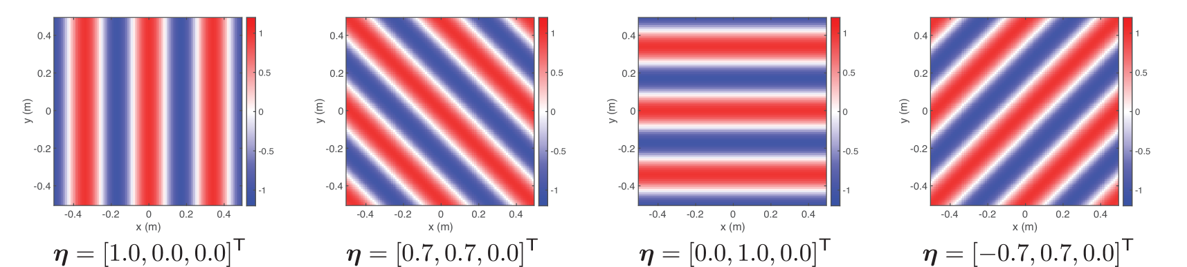
Examples of the element solutions are plotted in Fig. 3. By discretizing the integration operation in (7) and (9) or truncating the infinite-dimensional series expansion in (8), and setting the element solutions as $\{\varphi_{l}(\bm{x})\}_{l=1}^{L}$ and their weights as $\{\gamma_{l}\}_{l=1}^{L}$ , we can approximate the above representations as the finite-dimensional basis expansions in (6).
When the squared error loss function (2) and $\ell_{2}$ -norm penalty (3) are used, (6) becomes a simple least squares problem (or linear ridge regression). The closed-form solution of $\bm{\gamma}$ is obtained as
$$
\displaystyle\hat{\bm{\gamma}} \displaystyle=\operatorname*{arg\,min}_{\bm{\gamma}\in\mathbb{C}^{L}}\|\bm{y}-
\bm{\Phi}\bm{\gamma}\|^{2}+\lambda\|\bm{\gamma}\|^{2} \displaystyle=\left(\bm{\Phi}^{\mathsf{H}}\bm{\Phi}+\lambda\bm{I}\right)^{-1}
\bm{\Phi}^{\mathsf{H}}\bm{y}, \tag{10}
$$
where $\bm{\Phi}=[\bm{\varphi}(\bm{x}_{1}),\ldots,\bm{\varphi}(\bm{x}_{I})]^{\mathsf{ T}}\in\mathbb{K}^{I\times L}$ , $\bm{I}$ is the identity matrix, and $(\cdot)^{\mathsf{H}}$ is the conjugate transpose (equivalent to the transpose $(\cdot)^{\mathsf{T}}$ for a real-valued matrix). Then, $f$ is estimated using $\hat{\bm{\gamma}}$ as in (6) under the constraint that $f$ satisfies the governing PDE.
Various regularization terms for $\mathcal{R}$ other than the $\ell_{2}$ -norm penalty have been investigated to incorporate prior knowledge on the structure of $\bm{\gamma}$ . For example, the $\ell_{1}$ -norm penalty is widely used to promote sparsity on $\bm{\gamma}$ when $L\gg I$ in the context of sparse optimization and compressed sensing [22]. However, iterative algorithms, such as the fast iterative shrinkage thresholding algorithm and iteratively reweighted least squares, must be used to obtain the solution [23].
When applying the linear ridge regression, how to decide the number of basis functions $L$ , i.e., the number of plane waves (7) or point sources (9) and truncation order in (8), is not a trivial task. For the spherical wave function expansion, using the $\Omega$ radius $R$ , $\lceil kR\rceil$ and $\lceil\mathrm{e}kR/2\rceil$ are empirically known to be an appropriate truncation order when the target region $\Omega$ is a sphere. The sparsity-promoting regularization can help find an admissible number of basis functions using a dictionary matrix ( $\bm{\Phi}$ in (10)) constructed using a large number of basis functions [3, 4, 5].
<details>
<summary>x4.png Details</summary>
### Visual Description
\n
## Heatmaps: Parameter Variation Study
### Overview
The image presents four heatmaps, arranged horizontally. Each heatmap visualizes a two-dimensional distribution, likely representing a function's value across a coordinate plane. The heatmaps appear to be illustrating the effect of varying a parameter vector 'η' on the distribution. The x and y axes are labeled in meters (m). Each heatmap is labeled with a specific value for the parameter vector η.
### Components/Axes
Each heatmap shares the following components:
* **X-axis:** Labeled "x (m)", ranging from approximately -0.4 to 0.4 meters.
* **Y-axis:** Labeled "y (m)", ranging from approximately -0.4 to 0.4 meters.
* **Color Scale:** A continuous color scale ranging from approximately -1 (blue) to 1 (red), with 0 represented by white. The scale is positioned to the right of each heatmap.
* **Parameter Label:** Below each heatmap, a label indicates the value of the parameter vector η.
### Detailed Analysis or Content Details
**Heatmap 1:** η = [1.0, 0.0, 0.0]<sup>T</sup>
The heatmap displays vertical stripes. The color transitions from red to blue and back to red as you move from left to right. The stripes are approximately 0.1 meters wide. The values appear to oscillate between approximately 1 and -1.
**Heatmap 2:** η = [0.7, 0.7, 0.0]<sup>T</sup>
This heatmap shows diagonal stripes, running from the bottom-left to the top-right. The color transitions along these diagonals, alternating between red and blue. The stripes are approximately 0.15 meters wide. The values oscillate between approximately 1 and -1.
**Heatmap 3:** η = [0.0, 1.0, 0.0]<sup>T</sup>
This heatmap displays horizontal stripes. The color transitions from red to blue and back to red as you move from top to bottom. The stripes are approximately 0.1 meters wide. The values appear to oscillate between approximately 1 and -1.
**Heatmap 4:** η = [-0.7, 0.7, 0.0]<sup>T</sup>
This heatmap shows diagonal stripes, running from the top-left to the bottom-right. The color transitions along these diagonals, alternating between red and blue. The stripes are approximately 0.15 meters wide. The values oscillate between approximately 1 and -1.
### Key Observations
* The parameter vector η significantly alters the orientation of the stripes in the heatmaps.
* When the first element of η is non-zero, the stripes are vertical.
* When the second element of η is non-zero, the stripes are horizontal.
* When the first and second elements of η are both non-zero, the stripes are diagonal.
* The magnitude of the elements in η appears to influence the width of the stripes.
* The color scale consistently represents values between -1 and 1 across all heatmaps.
### Interpretation
The data suggests that the parameter vector η controls the directionality of a periodic pattern. The heatmaps likely represent a solution to a partial differential equation or a wave phenomenon where the parameter η influences the wave's propagation direction. The different components of η seem to correspond to different spatial frequencies or wave vectors.
The consistent color scale indicates that the underlying function's range remains constant, while the parameter η modulates its spatial distribution. The change in stripe orientation with different η values suggests a linear relationship between the parameter components and the pattern's direction. The observed patterns could represent interference phenomena or the behavior of a system under varying external forces. The fact that the values oscillate between -1 and 1 suggests a normalized or bounded quantity, potentially a correlation coefficient or a normalized amplitude.
</details>
(a) Plane wave functions
<details>
<summary>x5.png Details</summary>
### Visual Description
\n
## Heatmaps: Spatial Distribution of a Function
### Overview
The image presents four heatmaps, arranged horizontally. Each heatmap visualizes a two-dimensional function over a spatial domain defined by x and y coordinates, ranging from -0.4 to 0.4 meters. The color gradient represents the function's value, with red indicating higher values and blue indicating lower values. Each heatmap is labeled with a parameter pair (ν, μ).
### Components/Axes
Each heatmap shares the following components:
* **X-axis:** Labeled "x (m)", ranging from -0.4 to 0.4 with increments of approximately 0.1.
* **Y-axis:** Labeled "y (m)", ranging from -0.4 to 0.4 with increments of approximately 0.1.
* **Colorbar:** Located to the right of each heatmap, ranging from -0.1 to 0.1. The colorbar indicates the function's value corresponding to each color.
* **Labels:** Below each heatmap, the parameter pair (ν, μ) is specified.
### Detailed Analysis or Content Details
**Heatmap 1: (ν, μ) = (0, 0)**
* The heatmap displays a circular pattern.
* The center of the circle is at approximately (0, 0).
* The function values are highest (red) at the center and decrease radially outwards.
* There are alternating rings of positive (red) and negative (blue) values.
* Maximum value: approximately 0.1
* Minimum value: approximately -0.1
**Heatmap 2: (ν, μ) = (1, 1)**
* The heatmap displays a circular pattern, but the center is shifted.
* The center of the circle is at approximately (0.2, 0.2).
* The function values are highest (red) at the center and decrease radially outwards.
* There are alternating rings of positive (red) and negative (blue) values.
* Maximum value: approximately 0.1
* Minimum value: approximately -0.1
**Heatmap 3: (ν, μ) = (1, -1)**
* The heatmap displays a circular pattern, but the center is shifted.
* The center of the circle is at approximately (-0.2, 0.2).
* The function values are highest (red) at the center and decrease radially outwards.
* There are alternating rings of positive (red) and negative (blue) values.
* Maximum value: approximately 0.1
* Minimum value: approximately -0.1
**Heatmap 4: (ν, μ) = (2, 2)**
* The heatmap displays a circular pattern, but the center is shifted.
* The center of the circle is at approximately (0.2, -0.2).
* The function values are highest (red) at the center and decrease radially outwards.
* There are alternating rings of positive (red) and negative (blue) values.
* Maximum value: approximately 0.1
* Minimum value: approximately -0.1
### Key Observations
* All four heatmaps exhibit a circular pattern with alternating rings of positive and negative values.
* The parameter pair (ν, μ) determines the center of the circular pattern.
* The function values range consistently between approximately -0.1 and 0.1 across all heatmaps.
* The colorbar scale is identical for all four heatmaps.
### Interpretation
The data suggests that the heatmaps represent the spatial distribution of a function that exhibits circular symmetry. The parameters ν and μ control the center of this circular distribution. The alternating rings of positive and negative values indicate an oscillatory behavior within the circular pattern, potentially representing interference or wave-like phenomena. The consistent range of function values across all heatmaps suggests that the amplitude of the oscillation is constant, while the parameters ν and μ only affect the spatial location of the pattern. This could represent a wave function or a similar mathematical construct where the parameters define the phase or position of the wave. The function appears to be radially symmetric around the center defined by (ν, μ).
</details>
(b) Spherical wave functions
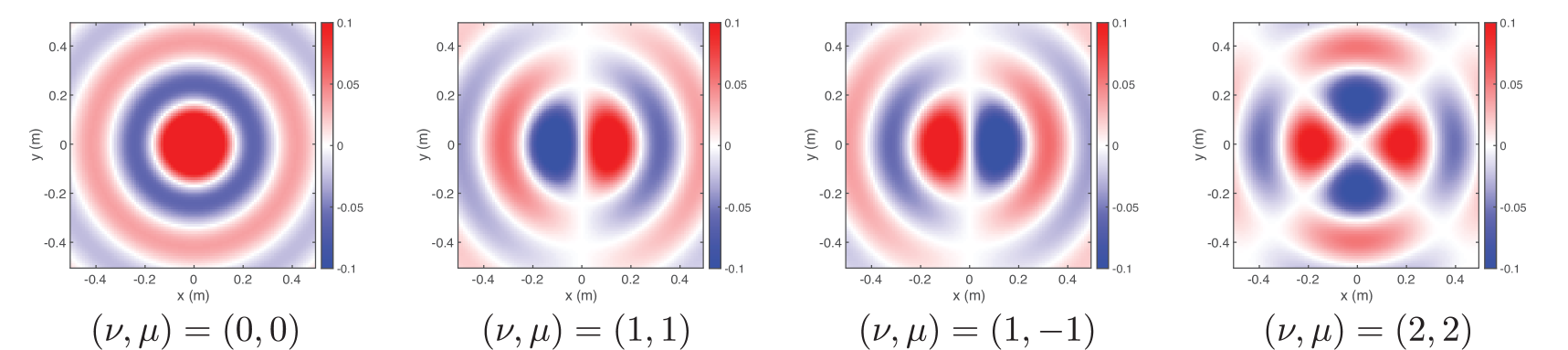
Figure 3: Basis functions used to constrain the solution to satisfy the Helmholtz equation on the $x$ – $y$ plane at the frequency of $1000~{}\mathrm{Hz}$ . (a) Plane wave functions. (b) Spherical wave functions. Real parts of the functions are plotted.
The finite-dimensional expansion into the element solutions of the governing PDE is a powerful and flexible technique to embed the physical properties, which has also been applied to the estimation of the exterior field and region including sources or scattering objects. This technique is also generalized to the cases of using directional microphones and estimating expansion coefficients of spherical wave functions [24, 25].
### III-B Kernel regression using reproducing kernel Hilbert space for governing PDE
Kernel regression is classified as a nonparametric regression technique. The kernel function $\kappa:\mathbb{R}^{P}\times\mathbb{R}^{P}\to\mathbb{K}$ should be defined as a similarity function expressed as an inner product defined on some functional space $\mathscr{H}$ , $\kappa(\bm{x},\bm{x}^{\prime})=\langle\bm{\varphi}(\bm{x}),\bm{\varphi}(\bm{x} ^{\prime})\rangle_{\mathscr{H}}$ . Thus, $\bm{\varphi}$ can be infinite-dimensional, which is one of the major differences from the basis expansion described in Section III-A. On the basis of the representer theorem [26], $f$ is represented by the weighted sum of $\kappa$ at the sampling points as
$$
\displaystyle f(\bm{x};\bm{\alpha}) \displaystyle=\sum_{i=1}^{I}\alpha_{i}\kappa(\bm{x},\bm{x}_{i}) \displaystyle=\bm{\kappa}(\bm{x})^{\mathsf{T}}\bm{\alpha}, \tag{11}
$$
where $\bm{\alpha}=[\alpha_{1},\ldots,\alpha_{I}]^{\mathsf{T}}\in\mathbb{K}^{I}$ are the weight coefficients and $\bm{\kappa}(\bm{x})=[\kappa(\bm{x},\bm{x}_{1}),\ldots,\kappa(\bm{x},\bm{x}_{I} )]^{\mathsf{T}}$ is the vector of kernel functions. In the kernel ridge regression [26], $\bm{\alpha}$ is obtained as
$$
\displaystyle\hat{\bm{\alpha}}=(\bm{K}+\lambda\bm{I})^{-1}\bm{y}, \tag{12}
$$
with the Gram matrix $\bm{K}\in\mathbb{K}^{I\times I}$ defined as
$$
\displaystyle\bm{K}=\begin{bmatrix}\kappa(\bm{x}_{1},\bm{x}_{1})&\cdots&\kappa
(\bm{x}_{1},\bm{x}_{I})\\
\vdots&\ddots&\vdots\\
\kappa(\bm{x}_{I},\bm{x}_{1})&\cdots&\kappa(\bm{x}_{I},\bm{x}_{I})\end{bmatrix}. \tag{13}
$$
Then, $f$ is interpolated by substituting $\hat{\bm{\alpha}}$ into (11).
In the kernel regression, the reproducing kernel Hilbert space to seek a solution must be properly defined, which also defines the reproducing kernel function $\kappa$ . In general machine learning, some assumptions for the data structure are imposed to define $\kappa$ . For example, the Gaussian kernel function [26] is frequently used to induce the smoothness of the function to be interpolated. The reproducing kernel Hilbert space $\mathscr{H}$ , as well as the kernel function $\kappa$ , can be defined to constrain the solution to satisfy the Helmholtz equation [27]. The solution space of the homogeneous Helmholtz equation is defined by the plane wave expansion (7) or spherical wave function expansion (8) with square-integrable or square-summable expansion coefficients. We here define the inner product over $\mathscr{H}$ using the plane wave expansion with positive directional weighting $w:\mathbb{S}_{2}\to\mathbb{R}_{\geq 0}$ as [28]
$$
\displaystyle\langle u_{1},u_{2}\rangle_{\mathscr{H}}=\frac{1}{4\pi}\int_{
\mathbb{S}_{2}}\frac{1}{w(\bm{\eta})}\tilde{u}_{1}(\bm{\eta})^{\ast}\tilde{u}_
{2}(\bm{\eta})\mathrm{d}\bm{\eta}. \tag{14}
$$
The directional weighting function $w$ is designed to incorporate prior knowledge of the directivity pattern of the target sound field by setting $\bm{\xi}$ in the approximate directions of sources or early reflections. We represent $w$ as a unimodal function using the von Mises–Fisher distribution [29] defined by
$$
\displaystyle w(\bm{\eta})=\frac{1}{C(\beta)}\mathrm{e}^{\beta\langle\bm{\eta}
,\bm{\xi}\rangle}, \tag{15}
$$
where $\bm{\xi}\in\mathbb{S}_{2}$ is the peak direction, $\beta$ is the parameter for controlling the sharpness of $w$ , and $C(\beta)$ is the normalization factor
$$
\displaystyle C(\beta)=\begin{cases}1,&\beta=0\\
\frac{\mathrm{sinh}(\beta)}{\beta},&\text{otherwise}\end{cases}. \tag{16}
$$
Then, the kernel function is analytically expressed as
$$
\displaystyle\kappa(\bm{r},\bm{r}^{\prime})=\frac{1}{C(\beta)}j_{0}\left(\sqrt
{\left(k(\bm{r}-\bm{r}^{\prime})-\mathrm{j}\beta\bm{\xi}\right)^{\mathsf{T}}
\left(k(\bm{r}-\bm{r}^{\prime})-\mathrm{j}\beta\bm{\xi}\right)}\right). \tag{17}
$$
When the directional weighting $w$ is uniform, i.e., no prior information on the directivity, $w$ is set as $1$ , and the kernel function is simplified as
$$
\displaystyle\kappa(\bm{r},\bm{r}^{\prime})=j_{0}\left(k\|\bm{r}-\bm{r}^{
\prime}\|\right). \tag{18}
$$
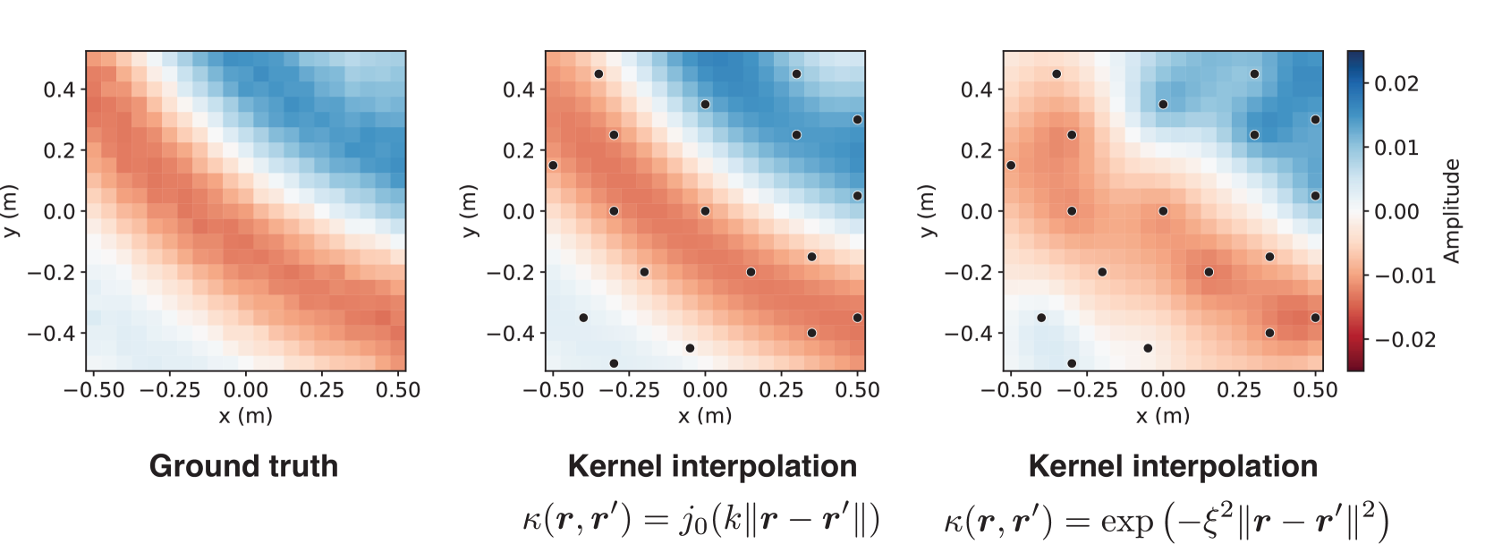
This function is equivalent to the spatial covariance function of diffused sound fields. Thus, the kernel ridge regression with the constraint of the Helmholtz equation is achieved by using the kernel function defined in (17) or (18). Figure 4 is an example of the experimental comparison of the physics-constrained kernel function (18) and the Gaussian kernel function.
The kernel regression described above is applied to interpolate the pressure distribution from discrete pressure measurements. This technique can be generalized to the cases of using directional microphones and estimating expansion coefficients of spherical wave functions [28], which is regarded as an infinite-dimensional generalization of the finite-dimensional basis expansion method [24].
<details>
<summary>x6.png Details</summary>
### Visual Description
\n
## Heatmaps: Kernel Interpolation Comparison
### Overview
The image presents three heatmaps side-by-side, comparing a "Ground truth" to two different "Kernel interpolation" methods. Each heatmap visualizes a two-dimensional distribution of "Amplitude" over a spatial area defined by x and y coordinates. The interpolation methods are differentiated by their kernel functions, displayed as equations below the respective heatmaps. Black dots are overlaid on the Kernel Interpolation heatmaps, presumably representing sample points.
### Components/Axes
Each heatmap shares the following components:
* **X-axis:** Labeled "x (m)", ranging from approximately -0.50 to 0.50 meters.
* **Y-axis:** Labeled "y (m)", ranging from approximately -0.40 to 0.40 meters.
* **Color Scale:** A vertical color bar on the right side represents "Amplitude", ranging from -0.02 to 0.02. The color gradient transitions from blue (negative amplitude) through white (zero amplitude) to red (positive amplitude).
* **Titles:** Each heatmap has a title indicating its content: "Ground truth", "Kernel interpolation" (with the first kernel equation), and "Kernel interpolation" (with the second kernel equation).
* **Kernel Equations:** Below the "Kernel interpolation" heatmaps are equations defining the kernel functions used:
* κ(r, r') = j₀(k||r - r'||)
* κ(r, r') = exp(-ξ²||r - r'||²)
### Detailed Analysis or Content Details
**1. Ground Truth Heatmap:**
* The heatmap displays a roughly elliptical pattern.
* The highest amplitude (red) is centered around x = 0.0 m and y = 0.0 m.
* Amplitude decreases radially from the center, transitioning through white to blue.
* The maximum positive amplitude appears to be around +0.015.
* The maximum negative amplitude appears to be around -0.015.
**2. Kernel Interpolation (j₀(k||r - r'||)) Heatmap:**
* This heatmap shows a similar elliptical pattern to the "Ground truth", but with more pronounced discrete features.
* Six black dots are overlaid on the heatmap. Their approximate coordinates are:
* (-0.25, -0.25)
* (-0.25, 0.25)
* (0.0, -0.25)
* (0.0, 0.25)
* (0.25, -0.25)
* (0.25, 0.25)
* The amplitude values at the dot locations appear to be positive, with the color ranging from light blue to red.
* The maximum positive amplitude appears to be around +0.02.
* The maximum negative amplitude appears to be around -0.01.
**3. Kernel Interpolation (exp(-ξ²||r - r'||²)) Heatmap:**
* This heatmap also displays an elliptical pattern, but it appears smoother than the previous interpolation.
* Six black dots are overlaid on the heatmap, at the same approximate coordinates as the previous heatmap.
* The amplitude values at the dot locations appear to be positive, with the color ranging from light blue to red.
* The maximum positive amplitude appears to be around +0.018.
* The maximum negative amplitude appears to be around -0.01.
### Key Observations
* Both kernel interpolation methods attempt to reconstruct the "Ground truth" distribution.
* The first kernel interpolation (j₀) produces a more discrete, less smooth result, with sharper transitions in amplitude.
* The second kernel interpolation (exp) produces a smoother, more continuous result.
* The black dots in the interpolation heatmaps likely represent the data points used for interpolation.
* The amplitude scale is slightly different between the "Ground truth" and the interpolation heatmaps, with the interpolation methods reaching slightly higher positive amplitudes.
### Interpretation
The image demonstrates a comparison of different kernel interpolation methods for reconstructing a two-dimensional field from a set of discrete sample points. The "Ground truth" represents the original, continuous field. The two kernel interpolation methods aim to approximate this field based on the sampled data (represented by the black dots).
The choice of kernel function significantly impacts the quality of the interpolation. The Bessel function (j₀) results in a more localized interpolation, potentially capturing finer details but also introducing artifacts. The exponential function (exp) provides a smoother interpolation, potentially sacrificing some detail but reducing artifacts.
The slight differences in the amplitude scale suggest that the interpolation methods may introduce some bias or scaling effects. The overall goal is to find an interpolation method that accurately reconstructs the "Ground truth" field with minimal error and artifacts. The visual comparison suggests that the exponential kernel provides a more visually appealing and potentially more accurate reconstruction in this case, but a quantitative analysis would be needed to confirm this.
</details>
Figure 4: Pressure distribution on the two-dimensional plane estimated by the kernel method using MeshRIR dataset [30]. Black dots indicate the microphone positions ( $M=18$ ). The kernel function of the spherical Bessel function (18) and Gaussian kernel ( $\xi=1.0k$ ) are compared. The source is an ordinary loudspeaker, and the source signal is the pulse signal lowpass-filtered up to $500~{}\mathrm{Hz}$ . The use of the physics-constrained kernel function improved the reconstruction accuracy. The figure is taken from [30], with an additional comparison with Gaussian kernel.
### III-C Regression by neural networks incorporating governing PDEs
<details>
<summary>x7.png Details</summary>
### Visual Description
\n
## Diagram: Neural Network Architecture
### Overview
The image depicts a neural network architecture, specifically a multi-layer perceptron (MLP). It illustrates the flow of information from an input layer, through hidden layers, to an output layer. The input and output are represented as grid-like structures, likely representing image data or feature maps. The network consists of multiple nodes connected by weighted edges.
### Components/Axes
The diagram is segmented into three main sections: "Input", a hidden network structure, and "Output".
* **Input:** A grid of approximately 8x8 cells, with varying shades of gray and red. Each cell contains a symbol resembling a stylized "Q".
* **Hidden Layers:** Two hidden layers are visible. The first layer has 'M' nodes labeled as s<sub>1</sub>(ω) through s<sub>M</sub>(ω). The second hidden layer has an unspecified number of nodes.
* **Output:** A grid of approximately 8x8 cells, similar in appearance to the input, with varying shades of gray and red, and containing the same "Q" symbol.
* **Nodes:** Represented as circles.
* **Connections:** Represented as lines connecting nodes between layers.
* **Labels:**
* "Input" - Top-left corner.
* "Output" - Top-right corner.
* s<sub>1</sub>(ω) to s<sub>M</sub>(ω) - Labels for the input nodes of the first hidden layer.
* u(r<sub>1</sub>, ω) to u(r<sub>J</sub>, ω) - Labels for the output nodes.
* ω - Appears in all node labels, likely representing a parameter or weight.
* r<sub>1</sub> to r<sub>J</sub> - Indices for the output nodes.
### Detailed Analysis or Content Details
The diagram shows a fully connected neural network. Each node in the first hidden layer (s<sub>i</sub>(ω)) is connected to every node in the second hidden layer. Similarly, each node in the second hidden layer is connected to every node in the output layer (u(r<sub>j</sub>, ω)).
* **Input Layer:** The input is a grid of 8x8 cells. The color variations and the "Q" symbol within each cell suggest that each cell represents a feature or a pixel value.
* **Hidden Layers:** The first hidden layer has 'M' nodes, where 'M' is not explicitly defined but appears to be approximately 8 based on the visual arrangement. The second hidden layer has 'J' nodes, where 'J' is not explicitly defined but appears to be approximately 4 based on the visual arrangement.
* **Output Layer:** The output is also a grid of 8x8 cells, mirroring the input structure. The color variations and "Q" symbol suggest a transformed representation of the input.
* **Connections:** The connections between layers are dense, indicating a fully connected network. The lines connecting the nodes are not weighted, so the strength of the connections is not visually represented.
* **Node Labels:** The labels s<sub>i</sub>(ω) and u(r<sub>j</sub>, ω) suggest that the nodes represent activations or outputs of the network, parameterized by ω. The 'i' and 'j' indices likely represent the position of the node within its respective layer.
### Key Observations
* The network architecture is symmetrical in terms of input and output dimensions (8x8).
* The use of the symbol "Q" within each cell of the input and output grids is consistent.
* The diagram does not provide any information about the activation functions used in the network.
* The diagram does not show any bias terms.
* The diagram does not show the number of hidden layers.
### Interpretation
The diagram illustrates a basic neural network designed to transform an input grid into an output grid. The network learns a mapping between the input and output through the adjustment of weights (represented by ω) during training. The "Q" symbol within each cell could represent a specific feature or pattern that the network is designed to recognize or manipulate. The color variations in the input and output grids suggest that the network is performing some form of feature extraction or transformation. The network could be used for tasks such as image recognition, image reconstruction, or pattern classification. The absence of specific details about the network's parameters and training process limits the ability to draw more specific conclusions. The diagram is a conceptual representation of a neural network architecture and does not provide any quantitative data about its performance.
</details>
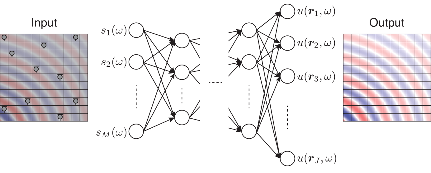
Figure 5: Feedforward neural network for sound field estimation in the frequency domain. The input is the observation $\bm{s}$ and the target output is the discretized value of $u$ . The network weights are optimized by using a pair of datasets.
When applying neural networks to regression problems, the target output is typically a discretized value, which is denoted as $\bm{t}\in\mathbb{R}^{J}$ , considering the real-valued function $f$ . In a simple manner, $\bm{t}$ is defined as a discretization of the domain into $\{\bm{x}_{j}\}_{j=1}^{J}$ with $J$ ( $>I$ ) sampling points, i.e., $t_{j}=f(\bm{x}_{j})$ . The neural network with input $\bm{y}\in\mathbb{R}^{I}$ and output $\bm{g}(\bm{y})\in\mathbb{R}^{J}$ , as shown in Fig. 5, is trained using a pair of datasets for various sampling points and function values $\{(\bm{y}_{d},\bm{t}_{d})\}_{d=1}^{D}$ , where the subscript $d$ is the index of the data and $D$ is the number of training data. There are various possibilities of the network architecture, but its parameters are collectively denoted as $\bm{\theta}_{\mathrm{NN}}$ . The loss function used to train the network, i.e., to obtain $\bm{\theta}_{\mathrm{NN}}$ , is, for example, the squared error written as
$$
\displaystyle\mathcal{J}(\bm{\theta}_{\mathrm{NN}})=\sum_{d=1}^{D}\|\bm{t}_{d}
-\bm{g}(\bm{y}_{d};\bm{\theta}_{\mathrm{NN}})\|^{2}. \tag{19}
$$
The parameters $\bm{\theta}_{\mathrm{NN}}$ are optimized basically by minimizing $\mathcal{J}$ using steepest-descent-based algorithms [6]. In the inference, the output for the unknown observation $\bm{y}$ , i.e., $\bm{g}(\bm{y})$ , is computed by forward propagation, which is regarded as a discretized estimate of $f$ . When estimating complex-valued functions, a simple strategy is to treat real and imaginary values separately. Other techniques are, for example, separating the complex values into magnitudes and phases and using complex-valued neural networks [31].
It is not straightforward to incorporate physical properties into the neural-network-based regression because the output is a discretized value. One of the techniques to constrain the estimate to satisfy the Helmholtz equation is to set the expansion coefficients of element solutions introduced in Section III-A to the target output [18, 32]. By using a pair of datasets $\{(\bm{y}_{d},\bm{\gamma}_{d})\}_{d=1}^{D}$ , we can train the network for predicting expansion coefficients. By using the estimated $\bm{\gamma}$ , we can obtain the continuous function $f$ satisfying the Helmholtz equation. This technique is referred to as the physics-constrained neural networks (PCNNs).
### III-D PINNs based on implicit neural representation
<details>
<summary>x8.png Details</summary>
### Visual Description
\n
## Diagram: Physics-Informed Neural Network (PINN) Architecture
### Overview
This diagram illustrates the architecture of a Physics-Informed Neural Network (PINN). It depicts the flow of information from an input field, through a neural network, to an output field, incorporating a physics-based loss function. The diagram highlights the data-driven and physics-constrained aspects of the PINN approach.
### Components/Axes
The diagram consists of three main sections: Input, Neural Network, and Output.
* **Input:** Labeled "{s<sub>m</sub>(ω)}<sup>M</sup><sub>m=1</sub>", representing a set of data points. The input is visualized as a circular field with concentric wave-like patterns, colored in shades of red and blue.
* **Neural Network:** A multi-layered neural network with input nodes labeled 'x', 'y', and 'z', and an output node labeled 'u'. The network has hidden layers represented by interconnected circles.
* **Output:** Visualized as a circular field with concentric wave-like patterns, similar to the input, colored in shades of red and blue.
* **Loss Functions:** Two loss functions are indicated: "J<sub>data</sub>" connected to the input and "J<sub>PDE</sub>" connected to the output.
* **Physics Constraint:** A box containing the equation "∇<sup>2</sup><sub>r</sub>∇<sup>2</sup><sub>r</sub> + k<sup>2</sup>" represents the physics-based constraint incorporated into the loss function.
### Detailed Analysis or Content Details
The input field shows a distribution of data points, represented by small circular markers. These points are likely samples from a physical system. The neural network takes these data points as input and learns to map them to the output field. The output field represents the predicted solution to the underlying physical problem.
The physics constraint, ∇<sup>2</sup><sub>r</sub>∇<sup>2</sup><sub>r</sub> + k<sup>2</sup>, is used to enforce the governing equations of the physical system. This constraint is incorporated into the loss function (J<sub>PDE</sub>), which penalizes deviations from the physics-based model.
The neural network architecture appears to be a fully connected feedforward network. The number of layers and nodes in each layer is not explicitly specified, but the diagram shows at least one hidden layer.
### Key Observations
* The diagram emphasizes the integration of data and physics in the learning process.
* The use of a physics-based loss function allows the PINN to learn solutions that are consistent with the underlying physical laws.
* The input and output fields share a similar structure, suggesting that the PINN is learning to reconstruct or extrapolate the input field based on the physics constraint.
* The equation within the box is a second-order differential operator, likely representing a wave equation or similar physical model.
### Interpretation
This diagram illustrates a powerful approach to solving physical problems using machine learning. PINNs combine the strengths of data-driven modeling and physics-based modeling. By incorporating physical constraints into the learning process, PINNs can achieve higher accuracy and generalization performance than traditional machine learning methods.
The diagram suggests that the PINN is being used to solve a problem involving wave propagation or a similar phenomenon described by the given differential equation. The input data likely represents measurements of the physical system, and the output data represents the predicted solution. The physics-based loss function ensures that the predicted solution satisfies the governing equations of the physical system.
The use of concentric wave-like patterns in the input and output fields suggests that the problem involves a radially symmetric solution. The parameter 'k' in the physics constraint likely represents a wave number or frequency.
The diagram provides a high-level overview of the PINN architecture. Further details about the specific implementation, such as the network architecture, loss function weights, and training procedure, would be needed to fully understand the model.
</details>
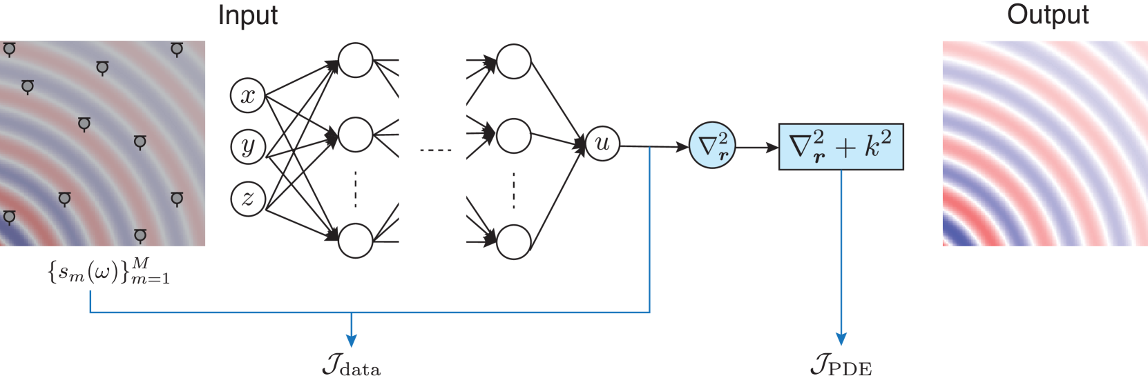
Figure 6: PINN using implicit neural representation for sound field estimation in the frequency domain. The input is the positional coordinates $\bm{r}=(x,y,z)$ and the target output is $u(\bm{r})$ . The network weights are optimized by using the observation $\bm{y}$ . In PINNs, the loss function is composed of the data loss $\mathcal{J}_{\mathrm{data}}$ and PDE loss $\mathcal{J}_{\mathrm{PDE}}$ to penalize the deviation from the governing PDE.
PINNs were first proposed to solve forward and inverse problems containing PDEs by using the implicit neural representation [8, 7]. In the implicit neural representation, neural networks (typically, multilayer perceptions) are used to implicitly represent a continuous function $f$ . The input and output of a neural network are the argument of $f$ , i.e., $\bm{x}\in\mathbb{R}^{P}$ , and the scalar function value $g(\bm{x};\bm{\theta}_{\mathrm{NN}})\in\mathbb{R}$ approximating $f(\bm{x})$ , respectively (see Fig. 6). The training data in this scenario are the pair of sampling points and function values $\{(\bm{x}_{i},y_{i})\}_{i=1}^{I}$ . The cost function is, for example, the squared error written as
$$
\displaystyle\mathcal{J}_{\mathrm{INR}}(\bm{\theta}_{\mathrm{NN}})=\sum_{i=1}^
{I}|y_{i}-g(\bm{x}_{i};\bm{\theta}_{\mathrm{NN}})|^{2}. \tag{20}
$$
Therefore, it is unnecessary to discretize the target output or prepare a pair of datasets because the observation data are regarded as the training data in this context.
A benefit of the implicit neural representation is that some constraints on $g$ including its (partial) derivatives can be included in the loss function:
$$
\displaystyle\mathcal{J}_{\mathrm{INR}}(\bm{\theta}_{\mathrm{NN}})=\sum_{i=1}^
{I}|y_{i}-g(\bm{x}_{i};\bm{\theta}_{\mathrm{NN}})|^{2}+\epsilon\sum_{n=1}^{N}
\left|H\left(g(\bm{x}_{n}),\nabla_{\bm{x}}g(\bm{x}_{n}),\nabla_{\bm{x}}^{2}g(
\bm{x}_{n}),\ldots\right)\right|^{2} \tag{21}
$$
with the positive constant $\epsilon$ and given constraints at $\{\bm{x}_{n}\}_{n=1}^{N}$
$$
\displaystyle H\left(g(\bm{x}_{n}),\nabla_{\bm{x}}g(\bm{x}_{n}),\nabla_{\bm{x}
}^{2}g(\bm{x}_{n}),\ldots\right)=0. \tag{22}
$$
Here, $\nabla_{\bm{x}}$ represents the gradient with respect to $\bm{x}$ . The evaluation points of the constraints $\{\bm{x}_{n}\}_{n=1}^{N}$ can be determined independently from the sampling points $\{\bm{x}_{i}\}_{i=1}^{I}$ . The loss function including derivatives is usually calculated using automatic differentiation [33].
Therefore, the physical properties represented by a PDE can be embedded into the loss function to infer the function approximately satisfying the governing PDE. When considering the sound field estimation in the frequency domain, as shown in Fig. 6, the loss function to train the neural network $g$ with the input $\bm{r}\in\Omega$ is expressed as
$$
\displaystyle\mathcal{J}_{\mathrm{PINN}}(\bm{\theta}_{\mathrm{NN}})=\mathcal{J
}_{\mathrm{data}}+\epsilon\mathcal{J}_{\mathrm{PDE}}, \tag{23}
$$
where
$$
\displaystyle\mathcal{J}_{\mathrm{data}}=\sum_{m=1}^{M}|s_{m}(\omega)-g(\bm{r}
_{m};\bm{\theta}_{\mathrm{NN}})|^{2}, \displaystyle\mathcal{J}_{\mathrm{PDE}}=\sum_{n=1}^{N}|(\nabla_{\bm{r}}^{2}+k^
{2})g(\bm{r}_{n};\bm{\theta}_{\mathrm{NN}})|^{2}. \tag{24}
$$
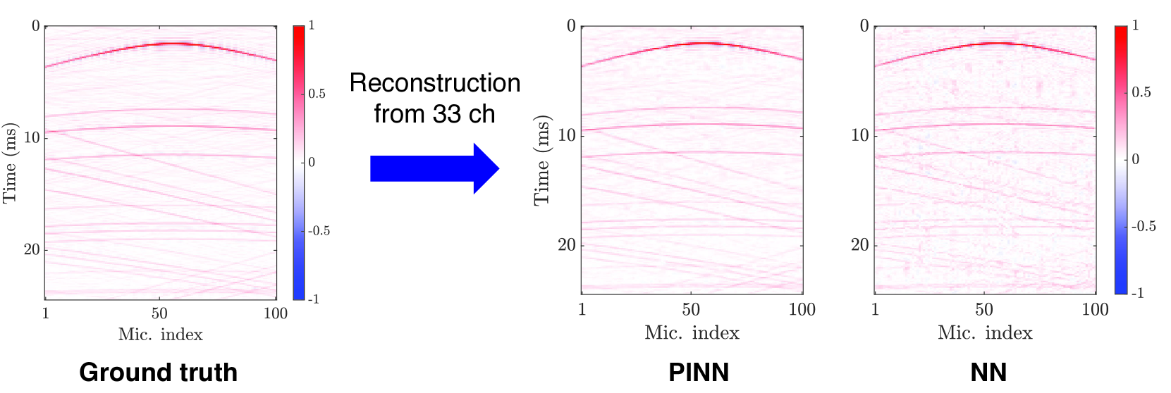
Thus, $g$ is trained to minimize the deviation from the Helmholtz equation as well as the observations at the sampling points $\{\bm{r}_{m}\}_{m=1}^{M}$ . Since this technique is based on an implicit neural representation, the observed signal $\{s_{m}(\omega)\}_{m=1}^{M}$ corresponds to the training data for the neural network. In this sense, PINNs can be classified as an unsupervised approach. Figure 7 shows an experimental example of RIR reconstruction using a neural network and the same architecture trained using the PINN loss (23). It can be seen in Fig. 7 that the neural network can estimate the RIRs, although they contain noise and incoherent wavefronts in the missing channels. In contrast, the result of the PINN is more accurate with reduced noise and coherent wavefronts owing to the adoption of the PDE loss.
To extract the properties of an acoustic environment by using a set of training data, i.e., supervised learning for sound field estimation, the general neural networks in Section III-C can be applied [34, 35, 36, 37]. Since the output of the neural network is a discretized value, the evaluation of the deviation from the governing PDE is not straightforward. A simple approach is difference approximation by finely discretizing the domain to compute the PDE loss [38]. Another strategy is the use of general interpolation techniques to obtain a continuous function from the output of the neural networks [17]; thus, the PDE loss is computed by using the interpolated function.
<details>
<summary>x9.png Details</summary>
### Visual Description
\n
## Heatmap: Reconstruction of Signals from Microphone Arrays
### Overview
The image presents three heatmaps comparing signal reconstruction quality using different methods: Ground Truth, Physics-Informed Neural Network (PINN), and a standard Neural Network (NN). Each heatmap visualizes the reconstructed signal over time for a 100-microphone array, with the color representing the signal amplitude. A blue arrow indicates the data flow from Ground Truth to PINN.
### Components/Axes
Each heatmap shares the following components:
* **X-axis:** "Mic. index" (Microphone Index), ranging from approximately 1 to 100.
* **Y-axis:** "Time (ms)" (Time in milliseconds), ranging from approximately 0 to 25.
* **Colorbar:** A color scale ranging from -1 to 1, representing the signal amplitude. Red indicates positive values close to 1, blue indicates negative values close to -1, and white/light colors represent values near 0.
* **Labels:** Each heatmap is labeled with the reconstruction method used: "Ground truth", "PINN", and "NN".
### Detailed Analysis
**1. Ground Truth:**
* The heatmap shows a clear, structured pattern of red lines (positive signal) concentrated in the upper portion of the plot. The lines are relatively straight and parallel, indicating a consistent signal across microphones and time.
* The signal amplitude appears to be consistently high (close to 1) across most microphones and time points.
* There is a slight gradient in the signal amplitude, with the upper lines being more intense red.
**2. PINN:**
* The PINN heatmap exhibits a similar pattern to the Ground Truth, but with significantly more noise and distortion. The lines are less defined and more scattered.
* The signal amplitude is less consistent, with more areas showing white/light colors (values near 0).
* The red lines are still present, but they are less concentrated and more diffuse.
* There is a noticeable amount of blue (negative signal) scattered throughout the heatmap, indicating reconstruction errors.
**3. NN:**
* The NN heatmap shows the most significant distortion and noise compared to the Ground Truth and PINN. The lines are highly scattered and fragmented.
* The signal amplitude is highly variable, with large areas of white/light colors and significant amounts of both red and blue.
* The overall structure of the signal is barely discernible, indicating a poor reconstruction quality.
### Key Observations
* The Ground Truth provides a clean and well-defined signal reconstruction.
* PINN demonstrates a reasonable reconstruction, but with noticeable noise and distortion.
* NN exhibits the poorest reconstruction quality, with significant noise and a lack of structure.
* The colorbar consistently ranges from -1 to 1 across all three heatmaps, allowing for a direct comparison of signal amplitudes.
### Interpretation
The data suggests that PINN offers a more accurate signal reconstruction compared to a standard Neural Network when reconstructing signals from a microphone array. While PINN introduces some noise and distortion, it preserves the overall structure of the signal better than the NN. The Ground Truth serves as a benchmark, demonstrating the ideal reconstruction quality. The increased noise in PINN and especially NN indicates that these methods struggle to accurately capture the underlying physics of the signal propagation, leading to reconstruction errors. The presence of blue in the PINN and NN heatmaps suggests that these methods sometimes reconstruct signals with incorrect polarity. The visual comparison highlights the benefits of incorporating physics-based knowledge (as in PINN) into neural network models for signal processing applications. The arrow indicates a process of attempting to approximate the Ground Truth using the PINN method.
</details>
Figure 7: RIRs (simulated shoebox-shaped room of $T_{60}=500~{}\mathrm{ms}$ ) measured by a uniform linear array of $100$ microphones are reconstructed using only $33$ randomly selected channels. PINN [14] and a plain neural network (NN) are compared. The addition of the physics loss improved the reconstruction accuracy of RIRs. Figures are taken from [39] in which the method proposed in [14] has initially appeared, and further details of the experimental setting are presented.
## IV Current studies of sound field estimation based on PIML
Current sound field estimation methods based on PIML are essentially based on the techniques introduced in Section III. The linear ridge regression based on finite-dimensional expansion into basis functions has been thoroughly investigated in the literature. In particular, the spherical wave function expansion has been used in spatial audio applications because of its compatibility with spherical microphone arrays [25, 2]. The kernel ridge regression (or infinite-dimensional expansion) with the constraint of the Helmholtz equation can be regarded as a generalization of linear-ridge-regression-based methods. Since it is applicable to the estimation in a region of an arbitrary shape with arbitrarily placed microphones and the number of parameters to be manually tuned can be reduced, kernel-ridge-regression-based methods are generally simpler and more useful than the linear-ridge-regression-based methods. One of the advantages of these methods is a linear estimator in the frequency domain, which means that the estimation is performed by the convolution of an FIR filter in the time domain. This property is highly important in real-time applications such as active noise control.
Sparsity-based methods have also been intensively investigated over the past ten or more years both in the frequency and time domains [3, 4, 5]. Sparsity is usually imposed on expansion coefficients of plane waves (7) and equivalent sources (9). Since the sound field is represented by a linear combination of sparse plane waves or equivalent sources, it is guaranteed that the interpolated function satisfies the Helmholtz equation. These techniques are effective when the sound field to be estimated fits the sparsity assumption, such as a less reverberant sound field. However, iterative algorithms are required to obtain a solution; thus, the estimator is nonlinear, and STFT-based processing is necessary in practice. The sparse plane wave model is also used in hierarchical-Bayesian-based Gaussian process regression, which can be regarded as a generalization of the kernel ridge regression [40]. Then, the inference process becomes a linear operation.
Neural-network-based sound field estimation methods have gained interest in recent years, which makes the inference more adaptive to the environment owing to the high representational power of neural networks [34, 35, 41, 36, 42, 37]. Physical properties have recently been incorporated into neural networks to mitigate physically unnatural distortions even with a small number of microphones. PINNs for the sound field estimation problem are investigated both in the frequency [43, 12, 13] and time domains [14, 15]. A major difference from the methods based on basis expansions and kernels is that the estimated function does not strictly satisfy the governing PDEs, i.e., the Helmholtz and wave equations, because its constraint is imposed by the loss function $\mathcal{J}_{\mathrm{PDE}}$ as in (23). The governing PDEs are strictly satisfied by using PCNN, i.e., setting the target output as expansion coefficients of the basis expansions [18, 32]; however, this approach can sacrifice the high representational power of neural networks by strongly restricting the solution space. Whereas the methods based on implicit neural representation are regarded as unsupervised learning, supervised-learning-based methods may have the capability to capture properties of acoustic environments and high accuracy even when the number of available microphones is particularly small. In the physics-informed convolutional neural network [17], the PDE loss is computed by using bicubic spline interpolation. In [16], a loss function based on the boundary integral equation of the Helmholtz equation, called the Kirchhoff–Helmholtz integral equation [1], is proposed in the context of acoustic imaging using a planar microphone array, which is also regarded as a supervised-learning approach.
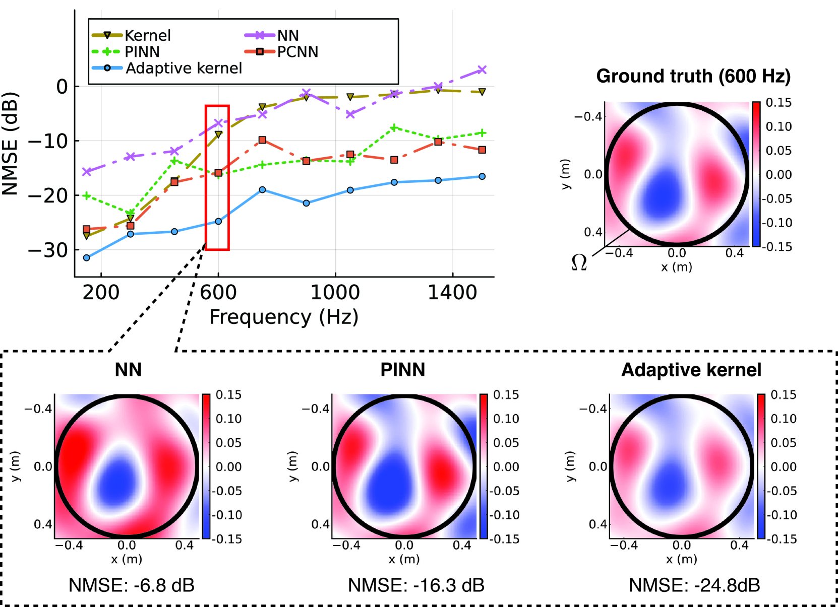
The inference process of neural networks involves multiple linear and nonlinear transformations; therefore, if a network is designed in the frequency domain, it cannot be implemented as an FIR filter in the time domain. The kernel-ridge-regression-based method using the kernel function adapted to acoustic environments using neural networks enables the linear operation of inference while preserving the constraint of the Helmholtz equation and the high flexibility of neural networks. In [19, 43], the directional weight $w$ in (14) is separated into the directed and residual components. The directed component is modeled by a weighted sum of von Mises–Fisher distributions (15) and the residual component is represented by a neural network to separately represent highly directive sparse sound waves and spatially complex late reverberation. The parameters of these components are jointly optimized by a steepest-descent-based algorithm. Experimental results in the frequency domain are demonstrated in Fig. 8, where the kernel method using (18), a plain neural network, PINN, PCNN with plane wave decomposition, and the adaptive kernel method proposed in [19, 43] are compared by numerical simulation. It can be observed that the adaptive kernel method performs well over the investigated frequency range.
As described above, various attempts have been made to incorporate physical properties into function interpolation and regression techniques for sound field estimation. The expansion representation introduced in Section III-A leads to the closed-form linear estimator in the frequency domain based on the linear and kernel ridge regression techniques. In exchange for their simple implementation and small computational cost, these techniques do not have sufficient adaptability to the acoustic environment because of their fixed estimator. Methods for adaptive estimators, e.g., using sparse optimization and kernel learning techniques, have also been studied. Recent neural-network-based methods having both high flexibility and physical validity have been investigated for both supervised- and unsupervised-learning approaches. Many of them make the estimator nonlinear; thus, the inference process for each time or time–frequency data becomes the forward propagation of the neural network for the supervised methods and both the training and inference of the neural network for the unsupervised methods; this process requires a high computational load. However, several methods integrating the expansion representation and neural networks enable estimators to be linear, which will be suitable for real-time applications. The current PIML-based sound field estimation methods using neural networks are compared in Table I.
<details>
<summary>x10.png Details</summary>
### Visual Description
\n
## Chart: NMSE vs. Frequency for Different Methods
### Overview
The image presents a chart comparing the Normalized Mean Squared Error (NMSE) in decibels (dB) across different frequencies (Hz) for four different methods: Kernel, Neural Network (NN), Physics-Informed Neural Network (PINN), and Probabilistic Convolutional Neural Network (PCNN). Below the main chart are visualizations of the ground truth and the results from each method at a specific frequency (600 Hz), represented as heatmaps.
### Components/Axes
* **X-axis:** Frequency (Hz), ranging from approximately 150 Hz to 1500 Hz. Marked at 200, 600, 1000, and 1400 Hz.
* **Y-axis:** NMSE (dB), ranging from approximately -30 dB to 0 dB. Marked at -30, -20, -10, 0, 10.
* **Legend:** Located in the top-left corner, identifying the data series:
* Kernel (Red, triangle markers)
* NN (Magenta, cross markers)
* PINN (Green, plus markers)
* PCNN (Blue, circle markers)
* **Ground Truth Heatmap:** Top-right corner, labeled "Ground truth (600 Hz)". X-axis labeled "x (m)", ranging from -0.15 to 0.4. Y-axis labeled "y (m)", ranging from -0.4 to 0.4.
* **Method Heatmaps:** Bottom row, labeled "NN", "PINN", and "Adaptive kernel" respectively. Each heatmap has the same x and y axis scales as the ground truth.
* **NMSE Values:** Below each method heatmap, the NMSE value in dB is displayed.
### Detailed Analysis or Content Details
**Main Chart (NMSE vs. Frequency):**
* **Kernel:** Starts at approximately -25 dB at 200 Hz, increases to around -10 dB at 600 Hz, then decreases to approximately -15 dB at 1400 Hz.
* **NN:** Starts at approximately 10 dB at 200 Hz, increases to around 15 dB at 600 Hz, then decreases to approximately 5 dB at 1400 Hz.
* **PINN:** Starts at approximately -20 dB at 200 Hz, increases to around -5 dB at 600 Hz, then remains relatively stable at around -10 dB at 1400 Hz.
* **PCNN:** Starts at approximately -5 dB at 200 Hz, remains relatively stable around -10 dB to -15 dB between 200 Hz and 1000 Hz, then increases to approximately -5 dB at 1400 Hz.
**Heatmaps (600 Hz):**
* **Ground Truth:** Shows a bipolar pattern with a positive lobe in the top-right and a negative lobe in the bottom-left. The color scale ranges from approximately -0.10 (dark red) to 0.15 (dark blue).
* **NN:** Similar bipolar pattern to the ground truth, but with less distinct lobes and a slightly shifted center. NMSE: -6.8 dB.
* **PINN:** Shows a more diffused pattern compared to the ground truth, with less clear separation between the positive and negative lobes. NMSE: -16.3 dB.
* **Adaptive Kernel:** Displays a pattern closest to the ground truth, with well-defined lobes and a similar shape. NMSE: -24.8 dB.
### Key Observations
* The Adaptive Kernel method consistently exhibits the lowest NMSE values across all frequencies, indicating the best performance.
* The NN method generally has the highest NMSE values, suggesting the poorest performance.
* The NMSE values for all methods tend to increase around 600 Hz, indicating a potential challenge in accurately modeling the system at that frequency.
* The heatmaps visually demonstrate the accuracy of each method in reproducing the ground truth pattern at 600 Hz. The Adaptive Kernel heatmap is the most similar to the ground truth.
### Interpretation
The data suggests that the Adaptive Kernel method is the most effective for modeling the system under investigation, as evidenced by its consistently low NMSE values. The NN method performs the worst, indicating that a simple neural network may not be sufficient to capture the underlying physics or complexity of the system. The PINN method shows moderate performance, potentially benefiting from the incorporation of physics-based information, but still falling short of the Adaptive Kernel.
The increase in NMSE around 600 Hz for all methods could indicate a resonance frequency or a region of increased sensitivity in the system. The heatmaps provide a visual representation of the errors, showing how each method deviates from the ground truth. The Adaptive Kernel's heatmap closely resembles the ground truth, confirming its superior performance.
The comparison of these methods highlights the importance of choosing an appropriate modeling technique based on the specific characteristics of the system being studied. The Adaptive Kernel's success suggests that a more sophisticated approach, potentially incorporating adaptive techniques, is crucial for achieving high accuracy.
</details>
Figure 8: Normalized mean square error (NMSE) and reconstructed pressure distribution inside a sphere of the target region in the frequency domain. A single point source was located outside the target region, and RIRs in a shoebox-shaped room were simulated by the image source method so that the reverberation time $T_{60}$ becomes $400~{}\mathrm{ms}$ . $M=41$ microphones were placed on two spherical surfaces with radii of $0.50$ and $0.49~{}\mathrm{m}$ . The kernel method using (18), the neural network without any physics (NN), PINN, PCNN with plane wave decomposition, and the adaptive kernel method proposed in [19, 43] are compared. The number of evaluation points of the PDE loss in PINN was $N=56$ . The architectures of NN, PINN, PCNN, and the adaptive kernel are basically the same (fully connected layers with 3 entries for input, 3 hidden layers with 8 neurons for the first, 8 neurons for neural ordinary differential equation (NODE) layer [44], and 5 neurons for the third hidden layer, and 1 output neuron. The rowdy activation function [45] is used for the first three layers and ReLU for the last layer on PCNN and adaptive kernel to guarantee nonnegativity.). Further details of the experimental setting are presented in [43].
TABLE I: Comparison of current sound field estimation methods based on PIML using neural networks with training data required or not required, linear or nonlinear estimator, time or frequency domain, and penalized or constrained physical property.
| Shigemi et al. 2022 [17] Karakonstantis et al. 2023 [18] and Lobato et al. 2024 [32] Chen et al. 2023 [12] and Ma et al. [13] | Supervised Supervised Unsupervised | Nonlinear Linear Nonlinear | Frequency Frequency Frequency | Penalized Constrained Penalized |
| --- | --- | --- | --- | --- |
| Olivieri et al. 2024 [14] and Karakonstantis et al. 2024 [15] | Unsupervised | Nonlinear | Time | Penalized |
| Ribeiro et al. 2023 [19, 43] | Unsupervised | Linear | Frequency | Constrained |
## V Outlook
PIML for sound field estimation is a rapidly growing research field and has successfully been applied to some application scenarios. However, the current methods still have some limitations. In particular, the major problems that should be resolved are 1) the preparation of training data, 2) the mismatch between training and test data, and 3) the neural network architecture design.
The methods using only the observation data, i.e., unsupervised methods, are useful when the acoustic environment to be measured is unpredictable. Supervised methods have the potential to extract properties of an acoustic environment by using a set of training data and to improve estimation accuracy when the number of microphones is particularly small. However, the training data should be a set of sound field data with high spatial (or spatiotemporal) resolution. Since the acoustic environment can have large variations of, e.g., source positions, directivity, and reflections, the first problem is how to prepare the training data, even though physical properties could help prevent overfitting in the case of a small number of training data. Currently, it is considered impractical to collect all the variations of sound field data by actual measurements. Therefore, it will be necessary to integrate multiple training datasets measured in different environments and also include some simulated data. Thus, the second problem of the mismatch between training and test data arises. The measurement systems for acoustic fields could have some variations. Even for the wave-based acoustic simulation techniques requiring a high computational load, there are some deviations between real and simulated data. Furthermore, the governing PDEs still include given model parameters, e.g., sound speed, which can be different from those in the training data. It is still unclear how these deviations can affect the estimation performance and how to mitigate those effects. The third problem is generally common to neural-network-based techniques, but there is currently no clear methodology for architectural design. Therefore, at present, architectures must be designed by trial and error depending on the task and data.
In addition to the problems listed above, there are several other unsolved issues. First, the target region of estimation is usually assumed not to include any sound sources or scattering objects. This assumption allows us to represent the interior sound field by basis functions introduced in Section III-A. However, in some applications, the target region is not necessarily source-free; thus, the governing PDE of the sound field to be estimated can become inhomogeneous. Several methods have been proposed for estimating a sound field including sound sources or scatterers. Furthermore, the methods using the PDE loss, such as PINN, can also be applied in this setting. However, further investigations of these methods in practical applications are still necessary.
Second, the estimation accuracy of the sound field estimation methods is highly dependent on the number of microphones and their placement. It is often necessary to cover the entire target region with the smallest possible number of microphones. On the basis of boundary integral equations, such as Kirchhoff–Helmholtz integrals, a sound field inside a source-free interior region can be predicted by using pressure and its normal derivative on its surface. However, the interior sound field cannot be uniquely determined at some frequencies solely from the pressure measurements on the boundary surface, which is called the forbidden frequency problem [1]. Although it is necessary to place microphones inside the target region, its optimal placement is not straightforward, especially for broadband measurements. Several techniques for the optimal placement of microphones for sound field estimation have been proposed; however, their effectiveness has not been sufficiently evaluated in practical applications. It may also be possible to incorporate auditory properties and/or multimodal information to reduce the number of microphones.
The PIML-based sound field estimation techniques, particularly linear-ridge-regression and kernel-ridge-regression-based methods, have already been applied to various applications, e.g., the spatial audio recording for binaural reproduction [46, 47], spatial interpolation of HRTFs [48], and spatial active noise control [49, 50], owing to their simple implementation and small computational cost. In binaural reproduction, the signals reaching both ears, when a listener is present in the target region, are reproduced by estimating the expansion coefficients of the sound field at the listening position. The HRTFs are also required in the binaural reproduction, but measuring them for each listener is costly. The interpolation of HRTFs can be formulated as an exterior sound field estimation problem based on reciprocity. Active noise control in a spatial region requires estimating a sound field of primary noise using microphones in a target region and synthesizing an anti-noise sound field using loudspeakers in real time. On the other hand, applications of neural-network-based methods are still limited to offline applications, e.g., acoustic imaging, owing to the above-mentioned challenges as well as the issue of relatively high computational cost. It is expected that these methods will also be applied to various applications in the future because of their high flexibility and interpolation capability.
## VI Conclusion
PIML-based sound field estimation methods are overviewed. Our focus was the interior problem, but several techniques can also be applied to the exterior problem and estimation in a region containing some sources or scattering objects. There exist several techniques that can be used to embed physical properties in interpolation techniques. In particular, the governing PDE of the sound field is considered useful prior information. Neural-network-based methods, which have been successfully applied in various domains, are expected to perform well for sound field estimation owing to their high expressive power. How to integrate physical prior knowledge with the high expressive power of neural networks will continue to be one of the most important topics in sound field estimation and its applications. Although there are still many unresolved issues, such as the preparation of training data, we expect further development of sound field estimation methods and their applications in various applied technologies in the future.
## References
- [1] E. G. Williams, Fourier Acoustics: Sound Radiation and Nearfield Acoustical Holography. Academic Press, 1999.
- [2] B. Rafaely, Fundamentals of Spherical Array Processing. Springer, 2015.
- [3] N. Bertin, L. Daudet, V. Emiya, and R. Gribonval, “Compressive sensing in acoustic imaging,” in Compressed Sensing and its Applications, H. Boche, R. Calderbank, G. Kutyniok, and J. Vybiral, Eds. Springer, 2015.
- [4] N. Antonello, E. De Sena, M. Moonen, P. A. Naylor, and T. van Waterschoot, “Room impulse response interpolation using a sparse spatio-temporal representation of the sound field,” IEEE/ACM Trans. Audio, Speech, Lang. Process., vol. 25, no. 10, pp. 1929–1941, 2017.
- [5] N. Murata, S. Koyama, N. Takamune, and H. Saruwatari, “Sparse representation using multidimensional mixed-norm penalty with application to sound field decomposition,” IEEE Trans. Signal Process., vol. 66, no. 12, pp. 3327–3338, 2018.
- [6] I. Goodfellow, Y. Bengio, and A. Courville, Deep Learning. MIT Press, 2016.
- [7] G. E. Karniadakis, I. G. Kevrekidis, L. Lu, P. Perdikari, S. Wang, and L. Yang, “Physics-informed machine learning,” Nat. Rev. Phys., vol. 3, p. 422â440, 2021.
- [8] M. Raissi, P. Perdikaris, and G. Karniadakis, “Physics-informed neural networks: A deep learning framework for solving forward and inverse problems involving nonlinear partial differential equations,” J. Comput. Phys., vol. 378, pp. 686–707, 2019.
- [9] S. Cuomo, V. S. D. Cola, F. Giampaolo, G. Rozza, M. Raissi, and F. Piccialli, “Scientific machine learning through physicsâinformed neural networks: Where we are and what’s next,” J. Sci. Comput., vol. 92, 2022.
- [10] Y. Lin, J. Theiler, and B. Wohlberg, “Physics-guided data-driven seismic inversion: Recent progress and future opportunities in full-waveform inversion,” IEEE Signal Process. Mag., vol. 40, no. 1, pp. 115–133, 2023.
- [11] N. Borrel-Jensen, S. Goswami, A. P. Engsig-Karup, G. E. Karniadakis, and C.-H. Jeong, “Sound propagation in realistic interactive 3d scenes with parameterized sources using deep neural operators,” Proc. National Academy of Sciences, vol. 121, no. 2, p. e2312159120, 2024.
- [12] X. Chen, F. Ma, A. Bastine, P. Samarasinghe, and H. Sun, “Sound field estimation around a rigid sphere with physics-informed neural network,” in Proc. Asia-Pacific Signal Inf. Process. Assoc. Annu. Summit Conf. (APSIPA ASC), 2023, pp. 1984–1989.
- [13] F. Ma, S. Zhao, and I. S. Burnett, “Sound field reconstruction using a compact acoustics-informed neural network,” arXiv:2402.08904, 2024.
- [14] M. Olivieri, X. Karakonstantis, M. Pezzoli, F. Antonacci, A. Sarti, and E. Fernandez-Grande, “Physics-informed neural network for volumetric sound field reconstruction of speech signals,” EURASIP J. Audio, Speech, Music Process., 2024, (in press).
- [15] X. Karakonstantis, D. Caviedes-Nozal, A. Richard, and E. Fernandez-Grande, “Room impulse response reconstruction with physics-informed deep learning,” J. Acoust. Soc. Amer., vol. 155, no. 2, p. 1048â1059, 2024.
- [16] M. Olivieri, M. Pezzoli, F. Antonacci, and A. Sarti, “A physics-informed neural network approach for nearfield acoustic holography,” Sensors, vol. 21, no. 23, 2021.
- [17] K. Shigemi, S. Koyama, T. Nakamura, and H. Saruwatari, “Physics-informed convolutional neural network with bicubic spline interpolation for sound field estimation,” in Proc. Int. Workshop Acoust. Signal Enhancement (IWAENC), Sep. 2022.
- [18] X. Karakonstantis and E. Fernandez-Grande, “Generative adversarial networks with physical sound field priors,” J. Acoust. Soc. Amer., vol. 154, no. 2, pp. 1226–1238, 2023.
- [19] J. G. C. Ribeiro, S. Koyama, and H. Saruwatari, “Kernel interpolation of acoustic transfer functions with adaptive kernel for directed and residual reverberations,” in Proc. IEEE Int. Conf. Acoust., Speech, Signal Process. (ICASSP), Rhodes island, Greece, Jun. 2023.
- [20] F. Zotter and M. Frank, Ambisonics: A Practical 3D Audio Theory for Recording, Studio Production, Sound Reinforcement, and Virtual Reality. Springer, 2019.
- [21] D. Colton and R. Kress, Inverse Acoustic and Electromagnetic Scattering Theory. Springer, 2013.
- [22] D. L. Donoho, “Compressed sensing,” IEEE Trans. Inf. Theory, vol. 52, no. 4, pp. 1289–1306, 2006.
- [23] M. Elad, Sparse and Redundant Representations: From Theory to Applications in Signal and Image Processing. Springer, 2010.
- [24] A. Laborie, R. Bruno, and S. Montoya, “A new comprehensive approach of surround sound recording,” in Proc. 114th AES Conv., Amsterdam, Netherlands, 2003.
- [25] M. A. Poletti, “Three-dimensional surround sound systems based on spherical harmonics,” J. Audio Eng. Soc., vol. 53, no. 11, pp. 1004–1025, 2005.
- [26] K. P. Murphy, Machine Learning: A Probabilistic Perspective. MIT Press, 2012.
- [27] N. Ueno, S. Koyama, and H. Saruwatari, “Sound field recording using distributed microphones based on harmonic analysis of infinite order,” IEEE Signal Process. Lett., vol. 25, no. 1, pp. 135–139, 2018.
- [28] ——, “Directionally weighted wave field estimation exploiting prior information on source direction,” IEEE Trans. Signal Process., vol. 69, pp. 2383–2395, 2021.
- [29] K. V. Mardia and P. E. Jupp, Directional Statistics. John Wiley & Sons, 2009.
- [30] S. Koyama, T. Nishida, K. Kimura, T. Abe, N. Ueno, and J. Brunnström, “MeshRIR: A dataset of room impulse responses on meshed grid points for evaluating sound field analysis and synthesis methods,” in Proc. IEEE Int. Workshop Appl. Signal Process. Audio Acoust. (WASPAA), Oct. 2021, pp. 151–155.
- [31] A. Hirose, Complex-Valued Neural Networks. Springer-Verlag, 2012.
- [32] T. Lobato, R. Sottek, and M. Vorländer, “Using learned priors to regularize the Helmholtz equation least-squares method,” J. Acoust. Soc. Amer., vol. 155, no. 2, p. 971â983, 2024.
- [33] A. G. Baydin, B. A. Pearlmutter, A. A. Radul, and J. M. Siskind, “Automatic differentiation in machine learning: a survey,” J. Mach. Learn. Res., pp. 1–43, 2018.
- [34] F. LluÃs, P. MartÃnez-Nuevo, M. B. Møller, and S. E. Shepstone, “Sound field reconstruction in rooms: Inpainting meets super-resolution,” J. Acoust. Soc. Amer., vol. 148, no. 2, 2020.
- [35] M. Pezzoli, D. Perini, A. Bernardini, F. Borra, F. Antonacci, and A. Sarti, “Deep prior approach for room impulse response reconstruction,” Sensors, vol. 22, no. 7, 2022.
- [36] E. Fernandez-Grande, X. Karakonstantis, D. Caviedes-Nozal, and P. Gerstoft, “Generative models for sound field reconstruction,” J. Acoust. Soc. Amer., vol. 153, no. 2, p. 1179â1190, 2023.
- [37] F. Miotello, L. Comanducci, M. Pezzoli, A. Bernardini, F. Antonacci, and A. Sarti, “Reconstruction of sound field through diffusion models,” in Proc. IEEE Int. Conf. Acoust., Speech, Signal Process. (ICASSP), Seoul, Republic of Korea, Apr. 2024.
- [38] X. Zhao, Z. Gong, Y. Zhang, W. Yao, and X. Chen, “Physics-informed convolutional neural networks for temperature field prediction of heat source layout without labeled data,” Eng. Appl. Artif. Intell., vol. 117, p. 105516, 2023.
- [39] M. Pezzoli, F. Antonacci, and A. Sarti, “Implicit neural representation with physics-informed neural networks for the reconstruction of the early part of room impulse responses,” in Proc. Forum Acusticum, Sep. 2023.
- [40] D. Caviedes-Nozal, N. A. B. Riis, F. M. Heuchel, J. Brunskog, P. Gerstoft, and E. Fernandez-Grande, “Gaussian processes for sound field reconstruction,” J. Acoust. Soc. Amer., vol. 149, no. 2, 2021.
- [41] A. Luo, Y. Du, M. J. Tarr, J. B. Tenenbaum, A. Torralba, and C. Gan, “Learning neural acoustic fields,” in Proc. Adv. Neural Inf. Process. Syst. (NeurIPS), 2022.
- [42] Z. Liang, W. Zhang, and T. D. Abhayapala, “Sound field reconstruction using neural processes with dynamic kernels,” EURASIP J. Audio, Speech, Music Process., vol. 13, 2024.
- [43] J. G. C. Ribeiro, S. Koyama, and H. Saruwatari, “Sound field estimation based on physics-constrained kernel interpolation adapted to environment,” TechRxiv, 2023.
- [44] R. T. Q. Chen, Y. Rubanova, J. Bettencourt, and D. Duvenaud, “Neural ordinary differential equations,” in Proc. Adv. Neural Inf. Process. Syst. (NeurIPS), 2018.
- [45] A. D. Jagtap, Y. Shin, K. Kawaguchi, and G. E. Karniadakis, “Deep kronecker neural networks: A general framework for neural networks with adaptive activation functions,” Neurocomputing, vol. 468, pp. 165–180, 2022.
- [46] N. Iijima, S. Koyama, and H. Saruwatari, “Binaural rendering from microphone array signals of arbitrary geometry,” J. Acoust. Soc. Amer., vol. 150, no. 4, pp. 2479–2491, 2021.
- [47] L. Birnie, T. Abhayapala, V. Tourbabin, and P. Samarasinghe, “Mixed source sound field translation for virtual binaural application with perceptual validation,” IEEE/ACM Trans. Audio, Speech, Lang. Process., vol. 29, pp. 1188–1203, 2021.
- [48] R. Duraiswami, D. N. Zotkin, and N. A. Gumerov, “Interpolation and range extrapolation of hrtfs [head related transfer functions],” in Proc. IEEE Int. Conf. Acoust., Speech, Signal Process. (ICASSP), 2004, pp. IV, 45–48.
- [49] J. Zhang, T. D. Abhayapala, W. Zhang, P. N. Samarasinghe, and S. Jiang, “Active noise control over space: A wave domain approach,” IEEE/ACM Trans. Audio, Speech, Lang. Process., vol. 26, no. 4, pp. 774–786, 2018.
- [50] S. Koyama, J. Brunnström, H. Ito, N. Ueno, and H. Saruwatari, “Spatial active noise control based on kernel interpolation of sound field,” IEEE/ACM Trans. Audio, Speech, Lang. Process., vol. 29, pp. 3052–3063, 2021.
| Col1 |
| --- |
| Shoichi Koyama (koyama.shoichi@ieee.org) received the B.E., M.S, and Ph.D. degrees from the University of Tokyo, Tokyo, Japan, in 2007, 2009, and 2014, respectively. He is currently an Associate Professor at the National Institute of Informatics (NII), Tokyo, Japan. Prior to joining NII, he was a Researcher at Nippon Telegraph and Telephone Corporation (2009–2014), and Research Associate (2014–2018) and Lecturer (2018–2023) at the University of Tokyo, Tokyo, Japan. He was also a Visiting Researcher at Paris Diderot University (Paris 7), Institut Langevin, Paris, France (2016–2018), and a Visiting Associate Professor at Research Institute of Electrical Communication, Tohoku University, Miyagi, Japan (2020–2023). His research interests include audio signal processing/machine learning, acoustic inverse problems, and spatial audio. |
| Col1 |
| --- |
| Juliano G. C. Ribeiro Juliano G. C. Ribeiro received his B.E. degree in electronic engineering from the Instituto Militar de Engenharia (IME), Rio de Janeiro, Brazil, in 2017, and the M.S. and Ph.D. degrees in information science and technology from the University of Tokyo, Tokyo, Japan, in 2021 and 2024, respectively. Currently a Research Engineer with Yamaha corporation. His research interests include spatial audio, acoustic signal processing and physics-informed machine learning. |
| Col1 |
| --- |
| Tomohiko Nakamura (tomohiko.nakamura.jp@ieee.org) received B.S., M.S., and Ph.D. degrees from the University of Tokyo, Japan, in 2011, 2013, and 2016, respectively. He joined SECOM Intelligent Systems Laboratory as a researcher in 2016 and moved to the University of Tokyo as Project Research Associate in 2019. He is currently a Senior Researcher with the National Institute of Advanced Industrial Science and Technology (AIST). His research interests include signal-processing-inspired deep learning, audio signal processing, and music signal processing. |
| Col1 |
| --- |
| Natsuki Ueno (natsuki.ueno@ieee.org) received the B.E. degree in engineering from Kyoto University, Kyoto, Japan, in 2016, and the M.S. and Ph.D. degrees in information science and technology from the University of Tokyo, Tokyo, Japan, in 2018 and 2021, respectively. He is currently an Associate professor at Kumamoto University, Kumamoto, Japan. His research interests include spatial audio and acoustic signal processing. |
| Col1 |
| --- |
| Mirco Pezzoli (mirco.pezzoli@polimi.it) received the M.S. degree (cum laude), in 2017, in computer engineering from the Politecnico di Milano, Italy. In 2021 he received the Ph.D. degree in information engineering at Politecnico di Milano. After two years as a Postdoctoral Researcher, he joined the Department of Electronics, Information and Bioengineering of the Politecnico di Milano as Junior Assistant Professor. His main research interests are multichannel audio signal processing, sound field reconstruction and musical acoustics. |