# Planning to avoid ambiguous states through Gaussian approximations to non-linear sensors in active inference agents
**Authors**: Wouter M. Kouw
> 0000-0002-0547-4817
institutetext: Bayesian Intelligent Autonomous Systems laboratory TU Eindhoven, Eindhoven, Netherlands email: w.m.kouw@tue.nl
## Abstract
In nature, active inference agents must learn how observations of the world represent the state of the agent. In engineering, the physics behind sensors is often known reasonably accurately and measurement functions can be incorporated into generative models. When a measurement function is non-linear, the transformed variable is typically approximated with a Gaussian distribution to ensure tractable inference. We show that Gaussian approximations that are sensitive to the curvature of the measurement function, such as a second-order Taylor approximation, produce a state-dependent ambiguity term. This induces a preference over states, based on how accurately the state can be inferred from the observation. We demonstrate this preference with a robot navigation experiment where agents plan trajectories.
Keywords: Active inference Free energy minimization Bayesian filtering Non-linear sensing Control systems Planning Navigation
## 1 Introduction
In nature, intelligent agents build a model to infer the causes of their sensations [2]. In engineering, we are able to utilize knowledge of the relevant physics to structure such a model. In particular, we often know how sensors measure states of the world. For example, we know how radar measures relative velocity and distance [19]. Measurement functions that are non-linear transformations of state variables pose challenges to state estimation, which are often dealt with using Gaussian approximations of the transformed variables [8, 14]. We show that for certain Gaussian approximations, an active inference agent will prefer to avoid states because it already knows that state estimation will be difficult.
Active inference agents are based on free energy functionals that rank policies on explorative and goal-directed behaviour [5, 7, 6, 16]. The expected free energy functional can be understood through its decomposition into a cross-entropy term between states and observations given action ("ambiguity"), and a Kullback-Leibler divergence between the posterior predictive and a goal prior distribution ("risk") [7, 18, 4]. We show that Gaussian approximations of a non-linear observation function that are itself linear in the covariance matrix, e.g., first-order Taylor and the unscented transform [9], lead to ambiguity terms that are constant over states. This echoes an earlier finding that agents with a linear Gaussian state-space model exhibit a constant ambiguity term [10]. However, utilizing a second-order Taylor approximation induces a non-constant ambiguity term. Under this model, the agent will avoid states where the non-linear measurement function curves strongly. Our contributions are:
- Analysis of ambiguity in expected free energy functions under three different Gaussian approximations.
- An experiment where a robot must plan a trajectory and navigate to a goal prior distribution, testing the effect of the ambiguity term.
## 2 Problem statement
We want to plan a trajectory for a robot across a plane. The robot’s state at time $k$ is its planar position and time derivatives, $x_k∈ℝ^D_x$ . The robot does not sense position directly, but has to infer it from noisy measurements $y_k∈ℝ^D_y$ , produced by a sensor through a non-linear mapping $g:ℝ^D_x→ℝ^D_y$ and measurement noise $v_k∈R^D_y$ . It accepts control inputs $u_k∈ℝ^D_u$ and moves according to linear dynamics with a transition matrix $A∈ℝ^D_x× D_x$ , control matrix $B∈ℝ^D_x× D_u$ and process noise $e_k∈ℝ^D_x$ . Overall, we consider robot systems described with discrete-time state-space models of the form:
$$
\displaystyle x_k \displaystyle=Ax_k-1+Bu_k+e_k , \displaystyle e_k∼N(0,Q) , \displaystyle y_k \displaystyle=g(x_k)+v_k , \displaystyle v_k∼N(0,R) , \tag{1}
$$
where $Q,R$ are noise covariance matrices.
The goal is to find a sequence of $T$ controls $\bar{u}_k=u_k+1,\dots u_k+T$ that produces future states close to a desired state $x_*$ . Agents must plan every time-step. The challenge is that errors in state estimation may cause drastic changes in the planned trajectory, which can lead an agent astray.
#### 2.0.1 Example
Consider a robot with position and velocity states that must move from position $x_0=(0,-1)$ to $x_*=(0,1)$ . Its state transition, control and process noise covariance matrices are given by:
$$
\displaystyle A=\begin{bmatrix}1&0&Δ t&0\\
0&1&0&Δ t\\
0&0&1&0\\
0&0&0&1\end{bmatrix}, B=\begin{bmatrix}0&0\\
0&0\\
Δ t&0\\
0&Δ t\end{bmatrix}, Q=\begin{bmatrix}σ^2_1\frac{Δ t^3
}{3}&0&σ^2_1\frac{Δ t^2}{2}&0\\
0&σ^2_2\frac{Δ t^3}{3}&0&σ^2_2\frac{Δ t^2}{2}
\\
σ^2_1\frac{Δ t^2}{2}&0&σ^2_1Δ t&0\\
0&σ^2_2\frac{Δ t^2}{2}&0&σ^2_2Δ t\end{bmatrix}, \tag{3}
$$
for $Δ t=0.5$ , $σ_1=σ_2=0.1$ . Measurements are produced by a sensor station at $(0,0)$ that reports relative angle $φ_k∈[-π π]$ and relative distance $d_k∈[0,∞)$ . The mapping and measurement noise covariance matrix are:
$$
\displaystyle g(x_k)=\begin{bmatrix}φ_k\\
d_k\end{bmatrix}=\begin{bmatrix}√{x_1k^2+x_2k^2}\\
\arctan(x_1k,x_2k)\end{bmatrix} , R=\begin{bmatrix}ρ^2_1&0\\
0&ρ^2_2\end{bmatrix} , \tag{4}
$$
where $ρ_1=ρ_2=0.001$ . Suppose it uses an extended Kalman filter (first-order Taylor approximation) for state estimation and a finite-horizon model-predictive control objective of the form:
$$
\displaystyle J_k(\bar{u}_k)=∑_t=k+1^k+T\big{(}(A\hat{x}_t-1+
Bu_t)-x_*\big{)}^∫ercalC\big{(}(A\hat{x}_t-1+Bu_t)-x_*\big{
)}+η u_t^2 , \tag{5}
$$
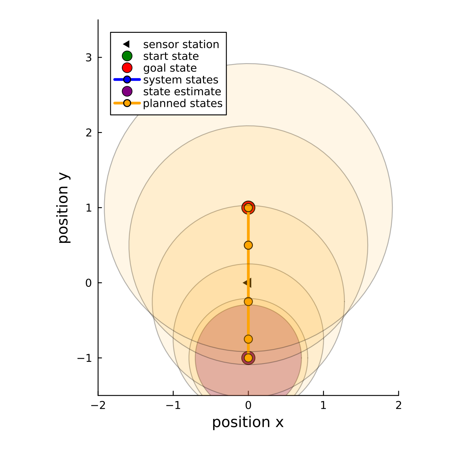
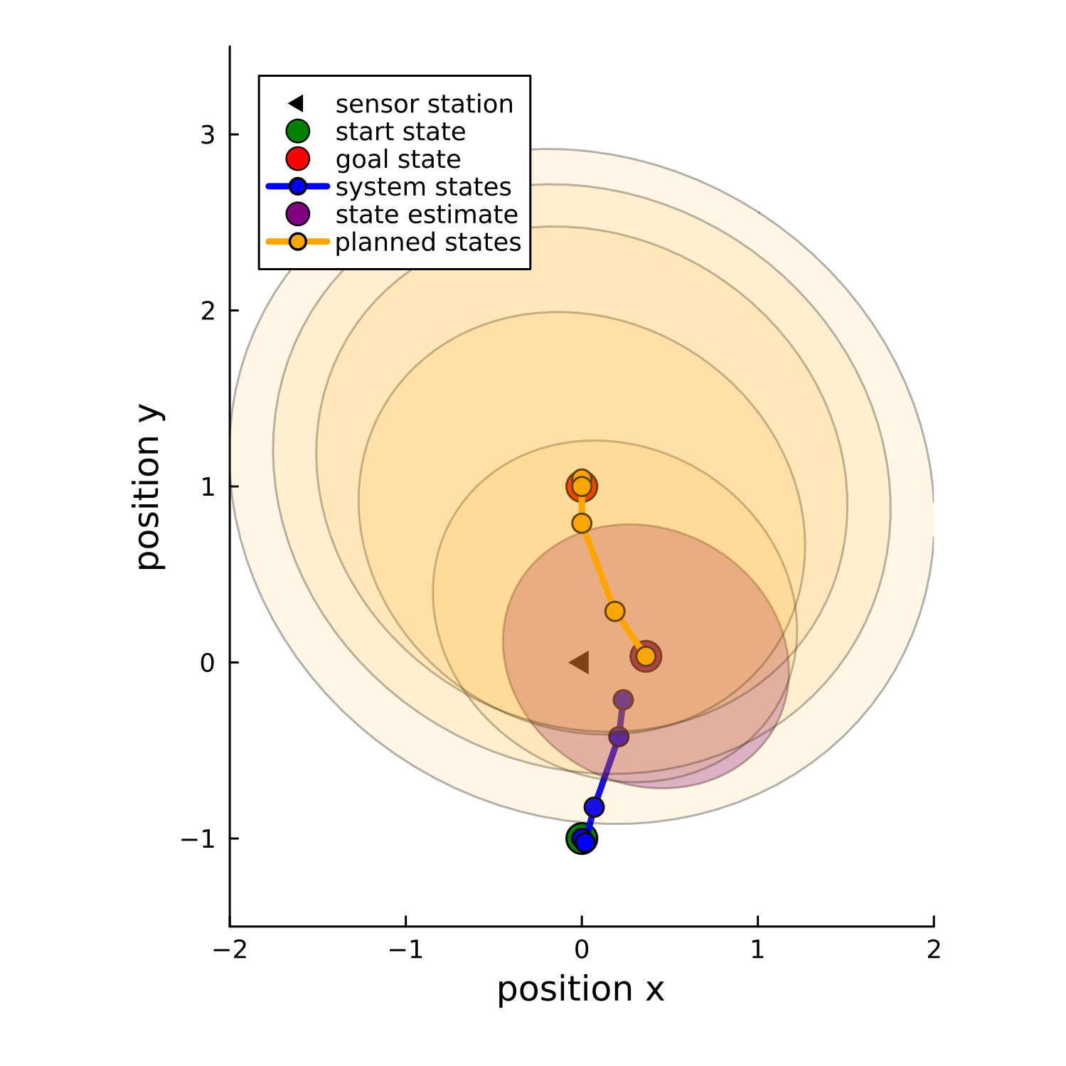
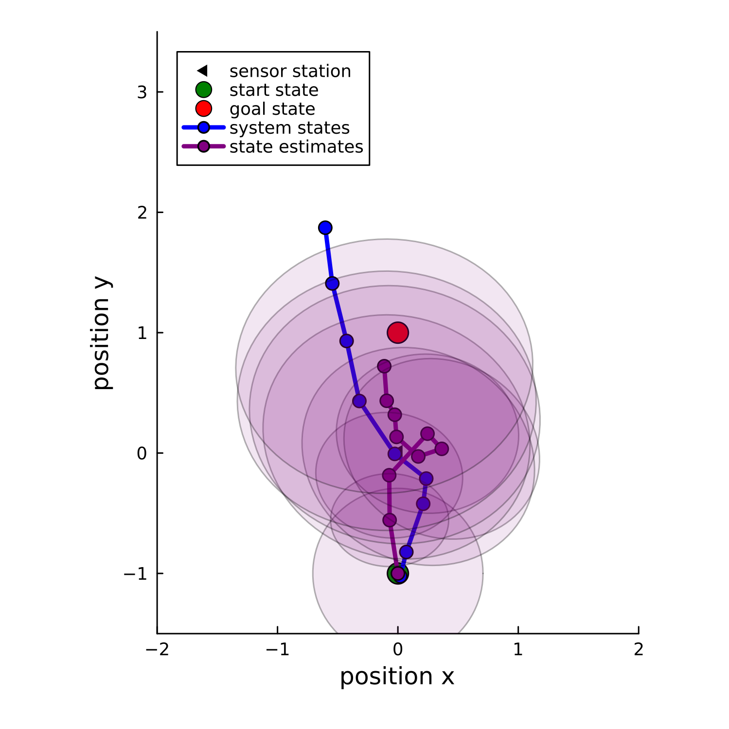
where $\hat{x}$ is the mean state, $\hat{x}_t=A\hat{x}_t-1+Bu_t$ , $C$ is a cost matrix (ones for position, zeros for velocity) and $η$ a regularization parameter. Minimizing this objective every time-step produces the control sequence $\bar{u}_k^MPC=\arg\min J_k(\bar{u}_k)$ . Such an agent will first plan a trajectory moving directly forward, as described in Figure 1 (left). However, as it approaches the sensor station, its state estimate become progressively more inaccurate and it makes increasingly more drastic adjustments to the control plan (see $k=5$ in Figure 1 middle). Figure 1 (right) shows the executed trajectory over a trial of 10 steps, demonstrating that the agent lost track of the robot’s state and did not successfully reach the target.
<details>
<summary>extracted/5864169/figures/cart2polar-mpc-trajectory-k1.png Details</summary>
### Visual Description
## Diagram: Path Planning and State Estimation in 2D Space
### Overview
The diagram illustrates a 2D coordinate system (x, y) with labeled axes ranging from -2 to 2 (x-axis) and -1 to 3 (y-axis). It includes concentric circles, colored points, and a legend explaining symbols and colors. The diagram appears to model a robotic or autonomous system's path planning, state estimation, and goal navigation.
### Components/Axes
- **Axes**:
- X-axis: "position x" (range: -2 to 2)
- Y-axis: "position y" (range: -1 to 3)
- **Legend** (top-left corner):
- `▲`: Sensor station
- `●` (green): Start state
- `●` (red): Goal state
- `●` (blue): System states
- `●` (purple): State estimate
- `●` (orange): Planned states
- **Circles**: Concentric shaded regions (lightest to darkest) centered at (0, 0), likely representing uncertainty or coverage areas.
### Detailed Analysis
1. **Sensor Station**:
- Located at (0, 0) (origin), marked with a black triangle (`▲`).
2. **Start State**:
- Green circle at (0, -1), labeled as the initial position.
3. **Goal State**:
- Red circle at (0, 1), marked as the target.
4. **System States**:
- Blue circles along the y-axis at approximate positions:
- (0, -0.5)
- (0, 0)
- (0, 0.5)
- (0, 1)
- These likely represent intermediate positions during navigation.
5. **State Estimate**:
- Purple circle at (0, -0.5), indicating the system's estimated position.
6. **Planned States**:
- Orange circles along the y-axis at:
- (0, -1.5)
- (0, -0.5)
- (0, 0.5)
- (0, 1.5)
- These may represent precomputed waypoints or trajectory points.
### Key Observations
- The system states and planned states are aligned vertically along the y-axis, suggesting a linear path from start to goal.
- The state estimate (purple) is offset from the system states (blue), indicating potential discrepancies between planned and actual positions.
- The concentric circles around the origin (sensor station) imply a radial coverage or uncertainty zone, with darker shades possibly representing higher confidence or smaller regions.
- The goal state (red) is positioned symmetrically above the start state (green) relative to the origin.
### Interpretation
This diagram likely models a robotic system's navigation process:
1. **Path Planning**: The orange "planned states" define a trajectory from the start state (0, -1) to the goal state (0, 1), with intermediate waypoints.
2. **State Estimation**: The purple "state estimate" at (0, -0.5) suggests the system's current position, which may differ from the planned path due to sensor noise or dynamic obstacles.
3. **System States**: The blue circles represent the actual positions recorded during execution, showing progression toward the goal.
4. **Sensor Coverage**: The concentric circles around the origin (sensor station) could represent the robot's sensor range or uncertainty in position estimation. The darkest circle (innermost) might indicate the highest confidence region.
The diagram emphasizes the relationship between planned trajectories, real-time state estimation, and sensor limitations. The offset between planned and estimated states highlights challenges in achieving precise navigation, while the linear alignment of system states suggests a simplified or constrained environment.
</details>
<details>
<summary>extracted/5864169/figures/cart2polar-mpc-trajectory-k5.png Details</summary>
### Visual Description
## Diagram: Control System State Representation
### Overview
The diagram illustrates a 2D coordinate system representing a control system's state space. It includes multiple elements: sensor station, start/goal states, system states, state estimates, and planned states. The visualization uses concentric circles, colored markers, and connecting lines to depict relationships between system components.
### Components/Axes
- **Axes**:
- X-axis: "position x" (range: -2 to 2)
- Y-axis: "position y" (range: -2 to 2)
- **Legend** (top-left corner):
- `▲`: Sensor station (black)
- `●`: Start state (green)
- `●`: Goal state (red)
- `●`: System states (blue)
- `●`: State estimate (purple)
- `●`: Planned states (orange)
- **Key Elements**:
- Concentric orange circles centered at (0,1) (goal state)
- Black triangle at (-1,0) (sensor station)
- Green circle at (0,-1) (start state)
- Red circle at (0,1) (goal state)
- Blue dots along a path from start to goal (system states)
- Purple dots along the same path (state estimates)
- Orange dots along the path (planned states)
### Detailed Analysis
1. **Path Representation**:
- A straight line connects start (0,-1) to goal (0,1)
- Blue dots (system states) are spaced at approximately:
- (-0.5, -0.5)
- (0, -0.5)
- (0.5, 0)
- (0.5, 0.5)
- (0.5, 1)
- Purple dots (state estimates) align with system states but show slight deviations:
- (-0.4, -0.6)
- (0, -0.4)
- (0.4, 0.1)
- (0.4, 0.6)
- (0.4, 1.1)
- Orange dots (planned states) follow the same trajectory but with increasing spacing:
- (-0.3, -0.7)
- (0, -0.3)
- (0.3, 0.2)
- (0.3, 0.8)
- (0.3, 1.2)
2. **Sensor Station**:
- Positioned at (-1,0) with a black triangle marker
- Located outside the main trajectory path
3. **State Space**:
- Concentric orange circles centered at goal state (0,1) with radii:
- 0.5, 1.0, 1.5, 2.0 units
- These circles represent planned states expanding from the goal
### Key Observations
1. The system trajectory follows a straight vertical path from start to goal
2. State estimates (purple) show consistent deviation from actual system states (blue)
3. Planned states (orange) expand outward from the goal, suggesting predictive modeling
4. Sensor station position creates a 90° angle with the trajectory path
5. All state markers maintain x-coordinates between -0.5 and 0.5 except the sensor station
### Interpretation
This diagram represents a robotic navigation system with:
- **Sensor Fusion**: The sensor station (-1,0) likely provides environmental data
- **Path Planning**: The orange circles indicate potential future states expanding from the goal
- **State Estimation**: Purple dots show the system's uncertainty in position tracking
- **Control Dynamics**: The blue dots represent actual system states following a planned trajectory
The spatial relationship between sensor station and trajectory suggests the system uses lateral sensing for obstacle avoidance while maintaining a straight path to the goal. The deviation between system states and state estimates indicates potential sensor noise or processing delays in the control loop.
</details>
<details>
<summary>extracted/5864169/figures/cart2polar-mpc-trajectory-trial.png Details</summary>
### Visual Description
##Scatter Plot: System State Trajectory with Uncertainty Ellipses
### Overview
The image depicts a 2D coordinate system (x: -2 to 2, y: -1 to 3) showing a system's trajectory from a start state to a goal state. Key elements include sensor station markers, state estimates, and uncertainty ellipses. The plot combines discrete data points with probabilistic representations of system states.
### Components/Axes
- **Axes**:
- X-axis: "position x" (-2 to 2)
- Y-axis: "position y" (-1 to 3)
- **Legend** (top-left):
- △: Sensor station
- ● (green): Start state
- ● (red): Goal state
- ● (blue): System states
- ● (purple): State estimates
- **Ellipses**: Gray contour lines representing uncertainty regions
### Detailed Analysis
1. **Sensor Station**:
- Position: (-1, -1) (green triangle)
- Spatial relationship: Located southwest of the trajectory path
2. **Start State**:
- Position: (0, -1) (green circle)
- Uncertainty: Smallest ellipse (radius ~0.2 units)
3. **Goal State**:
- Position: (1, 1) (red circle)
- Uncertainty: Medium ellipse (radius ~0.3 units)
4. **System States**:
- Trajectory: Blue line connecting start (0,-1) to goal (1,1)
- Intermediate points:
- (0.5, 0.5)
- (0.75, 0.75)
- Path characteristics: Linear progression with consistent slope (Δy/Δx = 1)
5. **State Estimates**:
- Distribution:
- Clustered around start (0,-1) and goal (1,1)
- 3 points along trajectory path (0.25,0.25), (0.5,0.5), (0.75,0.75)
- 2 outliers near (0.5,0.25) and (0.75,0.75)
- Uncertainty:
- Largest ellipses (~0.5 units radius) near start/goal
- Smaller ellipses (~0.2 units) along trajectory
### Key Observations
1. **Trajectory Certainty**:
- System states follow a straight path (y=x-1) between start and goal
- State estimates align with this path but show minor deviations
2. **Uncertainty Patterns**:
- Highest uncertainty at start/goal states (larger ellipses)
- Reduced uncertainty along the trajectory path
3. **Sensor Station Role**:
- Positioned outside the trajectory path
- May serve as reference point for state estimation
### Interpretation
This visualization represents a probabilistic path planning scenario where:
- The system moves from start (0,-1) to goal (1,1) along y=x-1
- State estimates (purple points) show both planned trajectory points and potential deviations
- Uncertainty ellipses suggest:
- Measurement noise in position tracking
- Potential for path deviation near start/goal
- Higher confidence in mid-trajectory positions
- The sensor station's position (-1,-1) may indicate:
- A fixed reference point for state estimation
- Potential obstacle or environmental feature
The plot demonstrates a trade-off between trajectory accuracy (linear path) and positional uncertainty (ellipse sizes), with the system showing greatest confidence in its mid-path positions.
</details>
Figure 1: (Left) Planned trajectory at $k=1$ , from start to goal directly over the sensor station. (Middle) Planned trajectory at $k=5$ showing a mismatch between true and estimated state resulting in a strong adjustment to the planned trajectory. (Right) Executed trajectory over a trial of $10$ steps demonstrates the agent losing track of the robot when it approaches the sensor station.
## 3 Agent specification
### 3.1 Probabilistic Model
The agent’s model will have Gaussian prior distributions over states and controls,
$$
\displaystyle p(x_0)=N(x_0\>|\>m_0,S_0) , N(
u_k\>|\>0,η^-1I) , \tag{6}
$$
with mean $m_0$ , covariance matrix $S_0$ , precision $η$ and identity matrix $I$ . The agent’s state transition will also be expressed as a Gaussian distribution:
$$
p(x_k\>|\>x_k-1,u_k)=N(x_k\>|\>Ax_k-1+Bu_k,Q) . \tag{7}
$$
Let the marginal state $x_k$ be Gaussian distributed, i.e., $p(x_k)=N(x_k\>|\>m_k,S_k)$ . We restrict our attention to approximations of the nonlinear sensor $g(x_k)$ that produce Gaussian joint distributions over states and observations [14], i.e.,
$$
\displaystyle p(y_k,x_k)≈N\Big{(}\begin{bmatrix}x_k\\
y_k\end{bmatrix}\>|\>\begin{bmatrix}m_k\\
μ_k\end{bmatrix},\begin{bmatrix}S_k&Γ_k\\
Γ_k^∫ercal&Σ_k\end{bmatrix}\Big{)} . \tag{8}
$$
From the joint, we obtain a conditional distribution of observations given states:
$$
\displaystyle p(y_k\>|\>x_k)≈N\big{(}y_k\>|\>μ_k+
Γ_k^∫ercalS_k^-1(x_k-m_k),Σ_k-Γ_kS_k^-1
Γ_k^∫ercal\big{)} . \tag{9}
$$
This distribution is linear in $x_k$ , and will allow for exact Bayesian filtering. But note that the parameters $μ_k$ , $Γ_k$ and $Σ_k$ may be nonlinear functions of $x_k$ , depending on the type of Gaussian approximation (specifics treated in Section 4), and may thus capture more of the effect of $g(x_k)$ .
### 3.2 Inferring states
We assume that, when inferring states, the agent has observed the system output $y_k=\hat{y}_k$ and input $u_k=\hat{u}_k$ . Let $D_k\triangleq\{\hat{y}_i,\hat{u}_i\}_i=1^k$ refer to data observed thus far. Given the known executed control, state estimation follows the general Bayesian filtering equations [14]. Firstly, the prior predictive distribution is given by:
$$
\displaystyle p(x_k| \hat{u}_k,D_k-1)=∫ p(x_k|x_
k-1,\hat{u}_k) p(x_k-1|D_k-1)
dx_k-1=N(x_k| \bar{m}_k,\bar{S}_k) . \tag{10}
$$
with $\bar{m}_k\triangleq Am_k-1+B\hat{u}_k$ and $\bar{S}_k\triangleq AS_k-1A^∫ercal+Q$ . This prediction is corrected by the observation through Bayes’ rule [14],
$$
\displaystyle p(x_k\>|\>D_k)=\frac{p(\hat{y}_k\>|\>x_k)}{p(
\hat{y}_k\>|\>D_k-1)}p(x_k\>|\>\hat{u}_k,D_k-1)=N(x_k\>|\>m_k,S_k) , \tag{11}
$$
with $m_k=\bar{m}_k+Γ_kΣ_k^-1(\hat{y}_k-μ_k)$ and $S_k=\bar{S}_k-Γ_kΣ_k^-1Γ_k$ .
### 3.3 Inferring controls
We will discuss the inference procedure first for a single step into the future, and then generalize to a finite horizon of length $T$ . Predictions for the future state and observation are made by unrolling the generative model to $t=k+1$ :
$$
\displaystyle p(y_t,x_t,u_t\>|\>D_k)=p(y_t\>|\>x_t)p(x_
t\>|\>u_t;D_k)p(u_t) . \tag{12}
$$
We will use an expected free energy functional to infer a posterior distribution over the control $u_t$ [13]:
$$
\displaystyleF_k[q]=∫ q(y_t\>|\>x_t)∫ q(x_t,u_t)\ln
\frac{q(x_t,u_t)}{p(y_t,x_t,u_t\>|\>D_k)}d(u_t
,x_t)dy_t . \tag{13}
$$
The variational model is specified to be:
$$
\displaystyle q(y_t\>|\>x_t)\triangleq p(y_t\>|\>x_t) , q(x_t,
u_t)\triangleq p(x_t\>|\>u_t;D_k)q(u_t) . \tag{14}
$$
Constraining $q(y_t\>|\>x_t)$ to the Gaussian approximation defined in Eq. 9 allows us to study deterministic approximations in an expected free energy minimization context. Given this variational model, Eq. 13 may be re-arranged to:
$$
\displaystyleF_k[q] \displaystyle=∫ p(y_t\>|\>x_t)∫ p(x_t\>|\>u_t;D_k)q(
u_t)\ln\frac{p(x_t\>|\>u_t;D_k)q(u_t)}{p(y_t,x_t,u_t
;D_k)}d(x_t,u_t)dy_t \displaystyle=∫q(u_t)\big{(}∫ p(y_t,x_t\>|\>u_t;D
_k)\ln\frac{p(x_t\>|\>u_t;D_k)q(u_t)}{p(y_t,x_t\>|\>u
_t;D_k)p(u_t)}d(y_t,x_t)\big{)}du_t \displaystyle=∫q(u_t)\big{(}\ln\frac{q(u_t)}{p(u_t)}+
\underbrace{∫p(y_t,x_t|u_t;D_k)\ln\frac{p(x_t\>|\>u
_t;D_k)}{p(y_t,x_t|u_t;D_k)}d(y_t,x
_t)}_J_k(u_t)\big{)}du_t. \tag{15}
$$
We refer to $J_k(u_t)$ as the expected free energy function as it depends on the value of $u_t$ not on its distribution. Under $J_k(u_t)=\ln(1/\exp(-J_k(u_t)))$ , the expected free energy functional can be concisely expressed as:
$$
\displaystyleF_k[q] \displaystyle=∫ q(u_t)\ln\frac{q(u_t)}{p(u_t)\exp≤ft(-J_
k(u_t)\right)}du_t . \tag{18}
$$
The above is a Kullback-Leibler divergence, which is minimal when
$$
\displaystyle q^*(u_t)∝ p(u_t)\exp≤ft(-J_k(u_t)
\right) . \tag{19}
$$
The proportionality is due to the implicit constraint A more rigorous treatment would define a Lagrangian with normalization and marginalization constraints [17]. However, such a treatment is inconsequential when resorting to MAP estimation, as will be pursued later in the paper. that $q^*(u_t)$ should integrate to $1$ . To work out the expectation in Eq. 17, we first decompose the joint over states and observations into
$$
\displaystyle p(y_t,x_t\>|\>u_t;D_k)=p(x_t\>|\>y_t,u_t
;D_k)p(y_t) , \tag{20}
$$
and then intervene on the marginal distribution over $y_t$ with a distribution reflecting desired future observations (a.k.a. goal prior) [11]:
$$
\displaystyle p(y_t)→ p(y_t\>|\>y_*)=N(y_t\>|\>μ
_*,Σ_*) . \tag{21}
$$
The next step involves applying Bayes’ rule in the inverse direction:
$$
\displaystyle\frac{1}{p(x_t\>|\>y_t,u_t;D_k)}=\frac{p(y_t
\>|\>u_t;D_k)}{p(y_t\>|\>x_t)p(x_t\>|\>u_t;D_
k)} , \tag{22}
$$
where the marginal prediction for the future observation is:
$$
\displaystyle p(y_t\>|\>u_t;D_k) \displaystyle=∫ p(y_t\>|\>x_t) p(x_t\>|\>u_t;D_k)
dx_t \displaystyle=∫N(\begin{bmatrix}x_t\\
y_t\end{bmatrix}\>|\>\begin{bmatrix}\bar{m}_t\\
μ_t\end{bmatrix},\begin{bmatrix}\bar{S_t}&Γ_t\\
Γ_t^∫ercal&Σ_t\end{bmatrix})dx_t=N(y_
t\>|\>μ_t,Σ_t) . \tag{23}
$$
Note that $μ_t$ and $Σ_t$ depend on $u_t$ through $\bar{m}_t$ . Plugging Eqs. 21 and 22 into Eq. 20 yields:
$$
\displaystyleJ_k(u_t) \displaystyle=∫p(y_t,x_t|u_t;D_k)\ln\frac{p(x_t|u_
t;D_k)}{p(y_t\>|\>y_*)}\frac{p(y_t\>|\>u_t;D_k
)}{p(y_t\>|\>x_t)p(x_t\>|\>u_t;D_k)} d(y_t,x_t) \displaystyle=\underbrace{∫p(y_t,x_t\>|\>u_t;D_k)\Big
{[}-\ln\frac{p(y_t,x_t\>|\>u_t;D_k)}{p(x_t\>|\>u_t;
D_k)}\Big{]}d(y_t,x_t)}_ambiguity \displaystyle +\underbrace{∫\Big{[}∫ p(y_t,x_t\>|\>u_t;
D_k)dx_t\Big{]}\ln\frac{p(y_t\>|\>u_t;D_
k)}{p(y_t\>|\>y_*)} dy_t}_risk. \tag{25}
$$
"Risk" refers to the Kullback-Leibler (KL) divergence between predicted and desired future observations. The inner integral in the risk term leads to a Gaussian distribution (Eq. 24) and the KL divergence between Gaussians is [3]:
$$
\displaystyleE_p(y_{t\>|\>u_t;D_k)}\Big{[}\ln\frac{p(
y_t\>|\>u_t;D_k)}{p(y_t\>|\>y_*)}\Big{]}=\frac{1}{2}\Big{(
}\ln\frac{|Σ_*|}{|Σ_t|}-D_y+tr\big{(}Σ_*^-1(
Σ_t+Ψ_*)\big{)}\Big{)} . \tag{27}
$$
where $Ψ_*\triangleq(μ_*-μ_t\big{)}\big{(}μ_*-μ_t)^∫ercal$ . "Ambiguity" refers to the conditional entropy of the future observations given the future states.
**Lemma 1**
*Ambiguity, as defined in Eq. 26, for a generative model described in Eq. 12 and a variational distribution described in Eq. 14, is:
$$
\displaystyleE_p(y_{t,x_t|u_t;D_k)}\big{[}-\ln
\frac{p(y_t,x_t|u_t;D_k)}{p(x_t|u_t;D_k)}
\big{]}=\frac{D_y}{2}\ln(2π\textit{e})+\frac{1}{2}\ln|Σ_t-Γ^
∫ercal_t\bar{S}_t^-1Γ_t|. \tag{28}
$$*
The proof is in Appendix 0.A. Note that the first term does not depend on the state $x_t$ . Plugging Eqs. 27 and 28 into the expected free energy function (Eq. 26) produces:
$$
\displaystyleJ_k(u_t)=\frac{1}{2}\Big{(}\ln\frac{|Σ_*
|}{|Σ_t|}+D_y\ln(2π)+tr\big{(}Σ_*^-1(Σ
_t+Ψ_*)\big{)}+\ln\big{|}Σ_t-Γ^∫ercal_t
\bar{S}_t^-1Γ_t\big{|}\Big{)} . \tag{29}
$$
Note that $Γ_t$ , $Σ_t$ and $Ψ_*$ depend on $u_t$ . The above steps can be generalized to a longer time horizon $t=k+1,\dots k+T$ . Because the prior is independent over time, $p(\bar{u})=∏_t=1^Tp(u_t)$ (see Eq. 6), the function $J_k(\bar{u})$ factorizes to a sum of recursive expected free energy functions $∑_t=1^TJ_k(u_t)$ .
We are interested in the most probable value under the approximate control posterior, i.e., the MAP estimate:
$$
\displaystyle\hat{u} \displaystyle=\underset{\bar{u}∈U}{\arg\max} q^*(\bar{u})=
\underset{\bar{u}∈U}{\arg\min}∑_t=k+1^k+TJ_t(u_t)-\ln p(u_t) , \tag{30}
$$
where $U⊂ℝ^T$ is the space of affordable controls over $T$ steps. Constraints such as motor force limits can be imposed during optimization.
## 4 Gaussian approximations
We discuss the three most popular Gaussian approximations to non-linear transformations of Gaussian random variables: the first and second-order Taylor series approximations (used in extended Kalman filters) and the unscented transform (used in the unscented Kalman filter) [9, 8] [14, Ch. 5].
The first-order Taylor series approximation effectively linearizes the non-linear observation function $g(x_t)$ . Since ambiguity is known to be constant over states under a linear observation function [10], it is no surprise that the first-order Taylor also leads to an ambiguity term that is constant over states.
**Theorem 4.1**
*Let $G_x(\bar{m}_t)$ be the Jacobian of $g$ with respect to $x_t$ , evaluated at $\bar{m}_t$ . Under a first -order Taylor approximation, the parameters $Σ_t,Γ_t$ are:
$$
\displaystyleΣ_t=G_x(\bar{m}_t)\bar{S}_tG_x(\bar{m}_t)^
∫ercal+R , Γ_t=\bar{S}_tG_x(\bar{m}_t)^∫ercal . \tag{31}
$$
With these parameters, the ambiguity term does not depend on the state $x_t$ :
$$
\displaystyleE_p(y_{t,x_t\>|\>u_t;D_k)}\big{[}-\ln
\frac{p(y_t,x_t\>|\>u_t;D_k)}{p(x_t\>|\>u_t;D_k)}\big{]}=\frac{D_y}{2}\ln(2π\textit{e})+\frac{1}{2}\ln|R| . \tag{32}
$$*
The proof is in Appendix 0.B. Perhaps surprisingly, under the second-order Taylor approximation, the ambiguity term varies as a function of the state $x_t$ .
**Theorem 4.2**
*Let $G_xx^(i)(\bar{m}_t)$ be the Hessian of the $i$ -th element of the non-linear observation function evaluated at $\bar{m}_t$ and $e_i$ be a canonical basis vector. The parameters $Σ_t,Γ_t$ computed through a second -order Taylor approximation are:
$$
\displaystyleΣ_t \displaystyle=G_x(\bar{m}_t)\bar{S}_tG_x(\bar{m}_t)^∫ercal+
\frac{1}{2}∑_i=1^D_y∑_j=1^D_ye_ie_j^∫ercaltr
\big{(}G_xx^(i)(\bar{m}_t)\bar{S}_tG_xx^(j)(\bar{m}_t)\bar{S}_t
\big{)}+R \displaystyleΓ_t \displaystyle=\bar{S}_tG_x(\bar{m}_t)^∫ercal . \tag{33}
$$
With these parameters, the ambiguity term depends on $x_t$ through:
$$
\displaystyleE_p(y_{t,x_t\>|\>u_t;D_k)}\big{[}-\ln
\frac{p(y_t,x_t\>|\>u_t;D_k)}{p(x_t\>|\>u_t;D_k)}\big{]}= \displaystyle \frac{D_y}{2}\ln(2π\textit{e})+\frac{1}{2}\ln\Big{|}
\frac{1}{2}∑_i=1^D_y∑_j=1^D_ye_ie_j^∫ercaltr
\big{(}G_xx^(i)(\bar{m}_t)\bar{S}_tG_xx^(j)(\bar{m}_t)\bar{S}_t
\big{)}+R \Big{|} . \tag{34}
$$*
The proof is in Appendix 0.C.
Interestingly, the ambiguity is also constant for the unscented transform.
**Theorem 4.3**
*Define $2D_x+1$ sigma points as:
$$
\displaystyleχ_0\triangleq\bar{m}_t, χ_i\triangleq\bar{m}_t
+√{D_x+λ}\big{[}√{\bar{S}_t}\big{]}_i, χ_D_{x+i}
\triangleq\bar{m}_t-√{D_x+λ}\big{[}√{\bar{S}_t}\big{]}
_i, \tag{35}
$$
where $i=1,\dots D_x$ , $[·]_i$ denotes the $i$ -th column of a matrix, and $√{S}$ denotes the matrix square root such that $√{S}√{S}=S$ . The parameter $λ\triangleqα^2(D_x+κ)-D_x$ depends on free parameters $α$ and $κ$ . Define $2D_x+1$ weights as:
$$
\displaystyle w_0\triangleq\frac{λ}{D_x+λ}+(1-α^2+β
) , w_i\triangleq\frac{1}{D_x+λ} , \tag{36}
$$
for $i=1,\dots 2D_x$ and $β$ as an additional free parameter. Under these sigma points and weights, the parameters $μ_t$ , $Σ_t$ , $Γ_t$ are [14, Eq. 5.89]:
$$
\displaystyleμ_t \displaystyle=\frac{λ}{D_x+λ}g(χ_0)+∑_i=1^2D_x
\frac{1}{2(D_x+λ)}g(χ_i) , Γ_t=∑_i=0^2D_x
w_i(χ_i-\bar{m}_t)(g(χ_i)-μ_t)^∫ercal , \displaystyle Σ_t=∑_i=0^2D_xw_i(g(χ_i)-μ_t)(g(
χ_i)-μ_t)^∫ercal+R . \tag{37}
$$
Then, the ambiguity is independent of the state:
$$
\displaystyleE_p(y_{t,x_t\>|\>u_t;D_k)} \displaystyle\big{[}-\ln\frac{p(y_t,x_t\>|\>u_t;D_k)}{p(x_t
\>|\>u_t;D_k)}\big{]}=\frac{D_y}{2}\ln(2π\textit{e})+\frac{
1}{2}\ln|R| . \tag{38}
$$*
The proof can be found in the Appendix 0.D. This result is conjectured to hold for other Gaussian approximations that are linear in their estimate of the covariance matrix, for example the Gauss-Hermite approximation [14, Ch. 6].
## 5 Experiments
Our experiment is as described in Section 2.0.1, with the nonlinear observation function $g(·)$ measuring relative angle and distance to a base station. Examples of sensors include Hall effect and ultrasound sensors. The robot starts at $x_0=[0 -1 0 0]$ and must reach $x_*=[0 1 0 0]$ . The agent’s state prior distribution’s parameters were $m_0=[0 -1 0 0]$ and $S_0=0.5I$ . Its control prior precision was set to a tiny value, $η=1.0· 10^-8$ , so as to best study the effects of ambiguity and risk. It was given a goal prior of $m_*=g(x_*)$ and $S_*=0.5I$ .
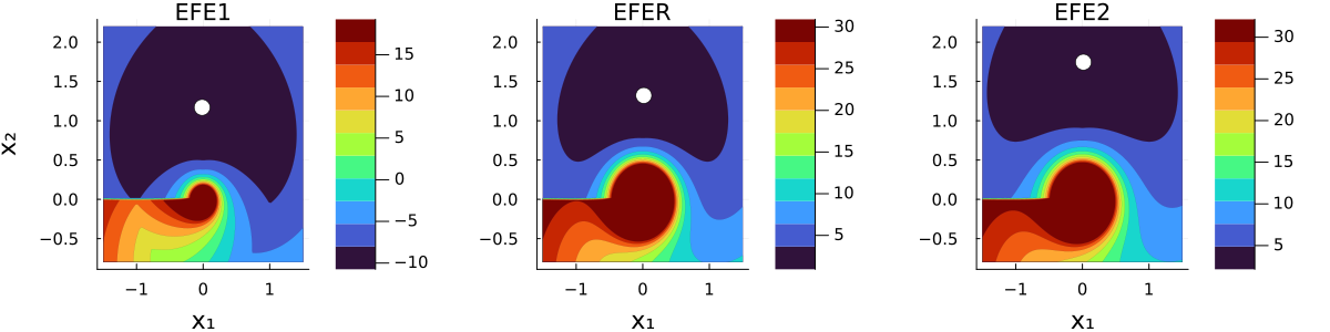
We will compare three agents Details and code at: https://github.com/biaslab/IWAI2024-ambiguity: firstly, an agent that uses the first-order Taylor approximation, referred to as EFE1. Secondly, an agent with a second-order Taylor approximation, referred to as EFE2. Thirdly, an agent with a second-order Taylor approximation but with only the risk term included, referred to as EFER. The difference between EFER and EFE2 reflects the effect of the ambiguity term, while the difference between EFE1 and EFE2 reflects the effect of the second-order Gaussian approximation. Figure 2 plots the value of the control objective function at every position in state-space, under a state covariance matrix of $S_t=I$ . States close to the sensor station are red and will lead to high values under the control objective. Note that the area around the sensor station increases from EFE1 to EFER due to the curvature of the relative distance sensor. The white markers are the approximate minimizers for this choice of $S_t$ matrix. Comparing EFER and EFE2, we can see that ambiguity increases the cost of being close to the sensor station.
<details>
<summary>extracted/5864169/figures/cart2polar-ambiguity-contourf.png Details</summary>
### Visual Description
## Heatmap Visualization: EFE1, EFER, EFE2
### Overview
The image contains three side-by-side heatmaps labeled **EFE1**, **EFER**, and **EFE2**, each depicting a 2D spatial distribution of values across axes **X1** (horizontal, -1 to 1) and **X2** (vertical, -0.5 to 2.0). All heatmaps share a consistent coordinate system but differ in color intensity ranges and spatial patterns. A white dot is consistently positioned at **(X1=0, X2=1)** across all plots.
---
### Components/Axes
- **Axes**:
- **X1**: Horizontal axis, labeled with values **-1, 0, 1**.
- **X2**: Vertical axis, labeled with values **-0.5, 0, 0.5, 1, 1.5, 2.0**.
- **Color Scales**:
- **EFE1**: Ranges from **-10 (dark blue)** to **15 (dark red)**.
- **EFER**: Ranges from **-10 (dark blue)** to **30 (dark red)**.
- **EFE2**: Ranges from **5 (light blue)** to **30 (dark red)**.
- **Legend**: Positioned on the right of each heatmap, with a vertical gradient from dark blue (low values) to dark red (high values). No explicit legend labels beyond the colorbar.
- **White Dot**: Located at **(X1=0, X2=1)** in all heatmaps, likely a reference point.
---
### Detailed Analysis
#### EFE1
- **Color Distribution**:
- Dominant **dark purple/blue** in the upper-left quadrant (X1 < 0, X2 > 0.5), indicating values near **-10**.
- A **gradient from red to blue** in the lower-left quadrant (X1 < 0, X2 < 0.5), transitioning from **15 to -10**.
- A **small white dot** at **(0,1)** stands out against the dark background.
- **Key Features**:
- A **circular red region** centered at **(X1=0, X2=1)** with a radius of ~0.5 units.
- A **funnel-like gradient** in the lower-left corner, transitioning from red (high values) to blue (low values).
#### EFER
- **Color Distribution**:
- Similar **dark purple/blue** upper-left quadrant as EFE1.
- A **larger red region** in the lower-left quadrant (X1 < 0, X2 < 0.5), extending to **X1=-0.5**, with values up to **30**.
- The white dot at **(0,1)** is surrounded by a **darker red halo** compared to EFE1.
- **Key Features**:
- The red region in the lower-left is **more extensive** than in EFE1, suggesting higher values in this area.
- The gradient near **(X1=0, X2=0.5)** transitions sharply from red to blue.
#### EFE2
- **Color Distribution**:
- **Dark purple/blue** upper-left quadrant, but with a **smaller red region** near **(X1=0, X2=1)** compared to EFER.
- A **broad red-to-blue gradient** in the lower-left quadrant, with values peaking at **30** near **(X1=-0.5, X2=0)**.
- The white dot at **(0,1)** is surrounded by a **moderate red halo**.
- **Key Features**:
- The red region in the lower-left is **less concentrated** than in EFER but covers a wider area.
- A **distinct gradient** from red (high values) to blue (low values) along the X1=0 axis.
---
### Key Observations
1. **Consistent Reference Point**: The white dot at **(0,1)** is present in all heatmaps, possibly indicating a critical threshold or anomaly.
2. **Color Scale Variability**:
- EFE1 has the **narrowest range** (-10 to 15), while EFER and EFE2 extend to **30**.
- EFE2’s scale starts at **5**, excluding negative values.
3. **Spatial Patterns**:
- All heatmaps show a **concentration of high values (red)** near **(X1=0, X2=1)**.
- EFER exhibits the **strongest gradient** in the lower-left quadrant, while EFE2 has a **wider but less intense red region**.
4. **Anomalies**:
- The white dot’s position remains unexplained by the color gradients, suggesting it may represent an outlier or predefined value.
---
### Interpretation
- **EFE1** likely represents a baseline scenario with moderate value ranges, where the white dot’s significance is unclear.
- **EFER** shows amplified values in the lower-left quadrant, possibly indicating a localized phenomenon (e.g., a shockwave or energy concentration).
- **EFE2** suggests a broader distribution of high values, with the white dot acting as a focal point for moderate-intensity effects.
- The **white dot’s consistent placement** across all heatmaps implies it is a **fixed reference** (e.g., a sensor location or theoretical origin point). Its lack of alignment with the red regions in EFE2 may indicate a decoupling between the reference and high-value zones in this scenario.
The heatmaps collectively demonstrate how spatial distributions of values (possibly energy, pressure, or error metrics) evolve across different conditions or parameters, with the white dot serving as a critical anchor for analysis.
</details>
Figure 2: Value under three EFE functions over a plane: EFE1 is risk and ambiguity under a first-order Taylor approximation, EFER is risk only under a second-order Taylor approximation and EFE2 is both risk and ambiguity under a second-order Taylor approximation. White markers indicate minimizers. Note that each EFE function induces a different preference over states.
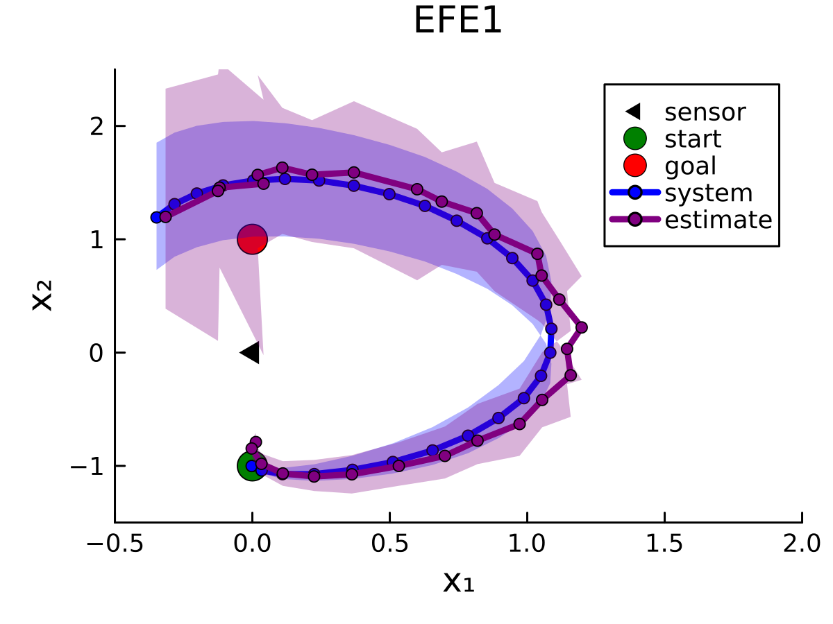
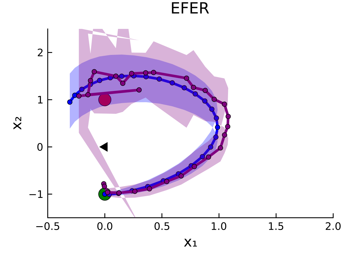
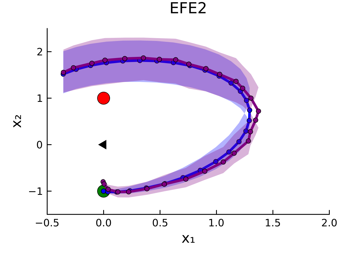
We ran 100 Monte Carlo experiments. Figure 3 plots the average trajectory of $T=30$ steps taken by the EFE1, EFER and EFE2 agents. Ribbons indicate the standard error of the mean at every time-point. Note that all agents avoid the sensor station, with EFE2 taking the widest curve (EFE1 and EFER turn at $x_1=1.0$ while EFE2 turns at $x_1=1.5$ ). EFE1 and EFER lose track of the robot in a number of experiments (like the model predictive controller in Sec. 2.0.1), leading to a more volatile average trajectory. EFE2 has the smoothest average trajectory, indicating that the ambiguity term helps planning.
<details>
<summary>extracted/5864169/figures/botnav-cart2polar-EFE1.png Details</summary>
### Visual Description
## Line Chart: EFE1 Trajectory Analysis
### Overview
The chart visualizes a dynamic system's trajectory estimation and sensor data in a 2D space (X1, X2). It compares actual system behavior (blue line) with predictive estimates (purple line), highlighting key reference points (start, goal, sensor) and uncertainty regions.
### Components/Axes
- **Axes**:
- X-axis (X1): -0.5 to 2.0 in increments of 0.5
- Y-axis (X2): -1 to 2 in increments of 1
- **Legend** (top-right):
- `sensor`: Black triangle (▲)
- `start`: Green circle (●)
- `goal`: Red circle (●)
- `system`: Blue line with circles (●)
- `estimate`: Purple line with dots (●)
- **Shaded Regions**:
- Light purple: Uncertainty around the estimate line
- Light blue: Uncertainty around the system line
### Detailed Analysis
1. **System Path (Blue Line)**:
- Starts at `start` (0, -1)
- Loops counterclockwise, passing near `sensor` (-0.5, 0)
- Ends near `goal` (0.5, 1) at X1=1.5, X2=0.2
- Uncertainty region: ±0.15 around the line
2. **Estimate Path (Purple Line)**:
- Mirrors system path but with slight deviations
- Peaks at X1=1.0, X2=1.8 (vs system's X2=1.5)
- Uncertainty region: ±0.2 around the line
3. **Reference Points**:
- `sensor` (▲): Fixed at (-0.5, 0)
- `start` (●): Green circle at (0, -1)
- `goal` (●): Red circle at (0.5, 1)
### Key Observations
- **Divergence**: Estimate path overshoots system path at X1=1.0 (X2=1.8 vs 1.5)
- **Uncertainty**: Estimate uncertainty (±0.2) exceeds system uncertainty (±0.15)
- **Sensor Positioning**: Located outside the main trajectory loop, suggesting external reference
- **Goal Proximity**: System path approaches goal within 0.3 units at final X1=1.5
### Interpretation
This chart demonstrates a control system's trajectory prediction vs actual behavior. The estimate path's divergence suggests potential model inaccuracies, particularly in the final loop. The sensor's position outside the trajectory implies it may serve as a calibration reference rather than a direct measurement point. The shaded uncertainty regions indicate the estimate's lower reliability compared to the system's observed path. The goal's placement within the system's final loop confirms successful path completion, though the estimate's overshoot highlights prediction challenges in dynamic environments.
</details>
<details>
<summary>extracted/5864169/figures/botnav-cart2polar-EFER.png Details</summary>
### Visual Description
## Scatter Plot with Confidence Intervals: EFER Analysis
### Overview
The image depicts a 2D scatter plot with two overlaid data series (blue and purple) and shaded confidence intervals. The plot is titled "EFER" and includes axis labels (X₁, X₂), a legend, and annotations. The data points form curved trajectories, with one series showing greater variability than the other.
### Components/Axes
- **Axes**:
- X-axis (X₁): Ranges from -0.5 to 2.0 in increments of 0.5.
- Y-axis (X₂): Ranges from -1 to 2 in increments of 1.
- **Legend**:
- **Series 1**: Blue line with light blue shading (confidence interval).
- **Series 2**: Purple line with light purple shading (confidence interval).
- **Annotations**:
- Black triangle pointing to a data point on Series 1 near (X₁=0.2, X₂=1.2).
- Green circle highlighting the origin (X₁=0, X₂=0).
### Detailed Analysis
1. **Series 1 (Blue)**:
- Starts at the origin (X₁=0, X₂=0).
- Curves upward, peaking near (X₁=0.5, X₂=1.5).
- Declines slightly after X₁=0.5, ending near (X₁=1.5, X₂=0.5).
- Confidence interval (shaded area) is narrowest near the origin and widens slightly toward the peak.
2. **Series 2 (Purple)**:
- Begins below Series 1 at (X₁=0, X₂=-1).
- Rises steeply, surpassing Series 1 near (X₁=0.3, X₂=0.5).
- Peaks at (X₁=1.0, X₂=1.8), then declines sharply.
- Confidence interval is consistently wider than Series 1, indicating higher variability.
3. **Data Points**:
- Both series include marked data points (circles) along their trajectories.
- Series 1 has a larger circle at (X₁=0.2, X₂=1.2), annotated by the black triangle.
- Series 2 has a larger circle at its peak (X₁=1.0, X₂=1.8).
### Key Observations
- **Divergence**: Series 2 overtakes Series 1 after X₁=0.3, suggesting a shift in behavior or interaction between the two variables.
- **Annotation Significance**: The black triangle highlights a local maximum for Series 1, potentially indicating a critical threshold or inflection point.
- **Variability**: Series 2’s wider confidence intervals suggest greater uncertainty or noise in its measurements compared to Series 1.
### Interpretation
The plot likely represents two competing or complementary processes (e.g., biological pathways, economic models) over a variable X₁. The divergence between Series 1 and 2 after X₁=0.3 implies a qualitative change in their relationship, such as one process dominating the other. The annotated point on Series 1 may represent a key observation (e.g., maximum efficiency, critical failure). The wider confidence intervals for Series 2 could reflect measurement challenges or inherent system complexity. The green circle at the origin might denote a baseline or reference state for both series.
</details>
<details>
<summary>extracted/5864169/figures/botnav-cart2polar-EFE2.png Details</summary>
### Visual Description
## Scatter Plot: EFE2 Model with Data Series and Outliers
### Overview
The image depicts a scatter plot titled "EFE2," showing two primary data series: a curved blue line with purple shading and a red circular outlier. A green circular data point and a black triangular marker are also present. The plot explores the relationship between variables **X1** (horizontal axis) and **X2** (vertical axis), with the blue line representing a modeled trend and the red point indicating an outlier.
---
### Components/Axes
- **Axes Labels**:
- **X1**: Horizontal axis, ranging from **-0.5 to 2.0**.
- **X2**: Vertical axis, ranging from **-1 to 2**.
- **Legend**:
- **Top-left corner**:
- **Blue line with purple shading**: Labeled "EFE2" (model trend).
- **Red circle**: Labeled "Outlier."
- **Data Points**:
- **Green circle**: Located at **(0, -1)**.
- **Red circle**: Located at **(0, 1)**.
- **Black triangle**: Positioned near **(0, -0.5)**.
---
### Detailed Analysis
1. **Blue Line (EFE2 Model)**:
- The blue line forms a **U-shaped curve** starting near **(-0.5, -1)**, peaking at approximately **(1.5, 1.5)**, and ending at **(2.0, 0)**.
- The **purple shading** around the line suggests a confidence interval or variability in the model's predictions.
- Data points along the line are evenly spaced, with **X1** values increasing from **-0.5 to 2.0** and **X2** values following the curve.
2. **Red Outlier**:
- A single red circular data point is located at **(0, 1)**, far above the blue line’s trajectory at **X1 = 0**.
- This point deviates significantly from the modeled trend, confirming its classification as an outlier.
3. **Green Data Point**:
- A green circle is positioned at **(0, -1)**, aligning with the lower end of the blue line’s curve.
4. **Black Triangle**:
- A black triangular marker is placed near **(0, -0.5)**, slightly above the green point. Its purpose is unclear but may indicate a directional trend or additional category.
---
### Key Observations
- The **U-shaped blue line** suggests a non-linear relationship between **X1** and **X2**, with a minimum at **X1 ≈ -0.5** and a maximum at **X1 ≈ 1.5**.
- The **red outlier** at **(0, 1)** is the only point outside the blue line’s shaded confidence interval, indicating potential anomalies or measurement errors.
- The **green point** at **(0, -1)** aligns with the model’s lower boundary, possibly serving as a reference or boundary condition.
- The **black triangle** near **(0, -0.5)** introduces ambiguity, as it is not labeled or explained in the legend.
---
### Interpretation
- The **EFE2 model** (blue line) demonstrates a parabolic relationship between **X1** and **X2**, with the shaded region highlighting uncertainty or variability in predictions.
- The **red outlier** at **(0, 1)** challenges the model’s accuracy at this specific **X1** value, suggesting either an exceptional case or a need for model refinement.
- The **green point** at **(0, -1)** may represent a boundary condition or starting point for the model’s behavior.
- The **black triangle**’s placement near **(0, -0.5)** could imply a directional trend (e.g., movement toward the origin) or an unclassified data category.
This visualization emphasizes the importance of contextualizing outliers and validating model assumptions in non-linear systems. The EFE2 model’s U-shape suggests diminishing returns or thresholds in the relationship between **X1** and **X2**, while the outlier underscores the need for robust error handling in predictive frameworks.
</details>
Figure 3: Trajectories of agents under three EFE functions, averaged over 100 Monte Carlo samples (ribbon is standard deviation of the mean). The robot starts at the green marker and must reach the red goal marker. All agents avoid the sensor station, with EFE2 taking the widest curve and having the smoothest average trajectory.
## 6 Discussion
One could argue that our analysis is more about model selection than inference, as each Gaussian approximation essentially constitutes a different generative model. In that sense, the experiments only indicate that richer approximations of nonlinear functions lead to better performance, which is not surprising. However, the result is more subtle than that since the unscented transform is richer than the first-order Taylor (produces a more accurate mean estimate [8]) but apparently still leads to constant ambiguity. No, the approximation must be sensitive to how the covariance matrix of the joint distribution over states and observations changes as a function of $g$ ’s curvature. It would be interesting to extend this work with parameter estimation, such as inferring the process noise covariance matrix using a Wishart distribution [15], or the state transition matrix with a Matrix-Normal distribution [1, 12].
## 7 Conclusion
We examined active inference agents with linear Gaussian distributed dynamics and a non-linear measurement function. We found that the first-order Taylor series and unscented transform approximations to the non-linearly transformed states lead to expected free energy functions with ambiguity terms that are constant over states. A second-order Taylor approximation leads to a state-dependent ambiguity term, inducing a preference over states.
#### 7.0.1 Acknowledgements
The author gratefully acknowledges financial support from the Eindhoven Artificial Intelligence Systems Institute (EAISI) at TU Eindhoven.
#### 7.0.2
The authors have no competing interests to declare that are relevant to the content of this article.
## Appendix 0.A Appendix: proof of Lemma 1
**Proof**
*The cross-entropy is split into two entropies that simplify according to:
$$
\displaystyleE_p(y_{t,x_t\>|\>u_t;D_k)}\big{[}-\ln
\frac{p(y_t,x_t\>|\>u_t;D_k)}{p(x_t\>|\>u_t;D_k)}\big{]} \displaystyle=-∫N\big{(}\begin{bmatrix}x_t\\
y_t\end{bmatrix}\>|\>\begin{bmatrix}\bar{m}_t\\
μ_t\end{bmatrix},\begin{bmatrix}\bar{S_t}&Γ_t\\
Γ_t^∫ercal&Σ_t\end{bmatrix}\big{)}\lnN\big{(}
\begin{bmatrix}x_t\\
y_t\end{bmatrix}\>|\>\begin{bmatrix}\bar{m}_t\\
μ_t\end{bmatrix},\begin{bmatrix}\bar{S_t}&Γ_t\\
Γ_t^∫ercal&Σ_t\end{bmatrix}\big{)} d(y_t,x_t) \displaystyle +∫N(x_t\>|\>\bar{m}_t,\bar{S}_t)\ln
N(x_t\>|\>\bar{m}_t,\bar{S}_t)dx_t \displaystyle=\frac{D_x+D_y}{2}\ln(2π\textit{e})+\frac{1}{2}\ln\big{|}
\begin{bmatrix}\bar{S_t}&Γ_t\\
Γ^∫ercal_t&Σ_t\end{bmatrix}\big{|}-\Big{(}\frac{D_x}{2}
\ln(2π\textit{e})+\frac{1}{2}\ln|\bar{S}_t|\Big{)} \displaystyle=\frac{D_y}{2}\ln(2π\textit{e})+\frac{1}{2}\ln\big{(}|\bar{S_t}|·|Σ_t-Γ^∫ercal_t\bar{S}^-1_tΓ_t|\big{)}
-\frac{1}{2}\ln|\bar{S}_t| \displaystyle=\frac{D_y}{2}\ln(2π\textit{e})+\frac{1}{2}\ln|Σ_t-
Γ^∫ercal_t\bar{S}_t^-1Γ_t| . \tag{39}
$$*
## Appendix 0.B Appendix: proof of Theorem 1
**Proof**
*Plugging $Σ_t$ , $Γ_t$ from (31) into the result from Lemma 1, yields:
$$
\displaystyle\frac{D_y}{2}\ln(2π\textit{e})+\frac{1}{2}\ln|Σ_t-
Γ_t^∫ercal\bar{S}_t^-1Γ| \displaystyle =\frac{D_y}{2}\ln(2π\textit{e})+\frac{1}{2}\ln|G_x(
\bar{m}_t)\bar{S}_tG_x(\bar{m}_t)^∫ercal+R-G_x(\bar{m}_t)\bar
{S}_t^∫ercal\bar{S}_t^-1\bar{S}_tG_x(\bar{m}_t)^∫ercal| \displaystyle =\frac{D_y}{2}\ln(2π\textit{e})+\frac{1}{2}\ln|R| . \tag{43}
$$
The cancellation is due to $\bar{S}_t$ being symmetric, i.e., $\bar{S}_t^∫ercal\bar{S}_t^-1=\bar{S}_t\bar{S}_t^-1=I$ .*
## Appendix 0.C Appendix: proof of Theorem 2
**Proof**
*Plugging $Σ_t$ , $Γ_t$ from (33) into the result from Lemma 1, yields:
$$
\displaystyle\frac{D_y}{2}\ln(2π\textit{e})+\frac{1}{2}\ln\Big{|}
Σ_t-Γ_t^∫ercal\bar{S}_t^-1Γ \Big{|}=\frac{D
_y}{2}\ln(2π\textit{e})+\frac{1}{2}\ln\Big{|} G_x(\bar{m}_t)\bar{
S}_tG_x(\bar{m}_t)^∫ercal \displaystyle +\frac{1}{2}∑_i=1^D_y∑_j=1^D_ye_ie_j^
∫ercaltr\big{(}G_xx^(i)(\bar{m}_t)\bar{S}_tG_xx^(j)(
\bar{m}_t)\bar{S}_t\big{)}+R-G_x(\bar{m}_t)\bar{S}_t^∫ercal\bar
{S}_t^-1\bar{S}_tG_x(\bar{m}_t)^∫ercal\Big{|} \displaystyle =\frac{D_y}{2}\ln(2π\textit{e})+\frac{1}{2}\ln\Big{|}
\frac{1}{2}∑_i=1^D_y∑_j=1^D_ye_ie_j^∫ercaltr
\big{(}G_xx^(i)(\bar{m}_t)\bar{S}_tG_xx^(j)(\bar{m}_t)\bar{S}_t
\big{)}+R \Big{|} . \tag{45}
$$
The covariance matrix $\bar{S}_t$ is symmetric, i.e., $\bar{S}_t^∫ercal\bar{S}_t^-1=\bar{S}_t\bar{S}_t^-1=I$ . Note that the Hessian $G_xx^(i)(\bar{m}_t)$ depends on the inferred mean of the predicted state $\bar{m}_t$ , meaning that ambiguity is not constant over state-space.*
## Appendix 0.D Appendix: proof of Theorem 3
**Proof**
*Plugging $μ_t$ , $Σ_t$ , $Γ_t$ from (4.3) into the log-determinant term from the result in Lemma 1, gives:
$$
\displaystyle\frac{1}{2}\ln\big{|}Σ_t-Γ_t^∫ercal\bar{S}_t
^-1Γ\big{|}=\frac{1}{2}\ln\Big{|}∑_i^\prime=0^2D_xw_i^
\prime(g(χ_i^\prime)-μ_t)(g(χ_i^\prime)-μ_t)^
∫ercal+R \displaystyle-\Big{(}∑_i=0^2D_xw_i(χ_i-\bar{m}_t)(g(χ
_i)-μ_t)^∫ercal\Big{)}^∫ercal\bar{S}_t^-1\Big{(}∑_
j=0^2D_xw_j(χ_j-\bar{m}_t)(g(χ_j)-μ_t)^
∫ercal\Big{)}\Big{|} . \tag{47}
$$*
The second term can be re-arranged to:
$$
\displaystyle\Big{(}∑_i=0^2D_xw_i(χ_i-\bar{m}_t)(g(χ_i)-μ_t)^∫ercal\Big{)}^∫ercal\bar{S}_t^-1\Big{(}∑_j
=0^2D_xw_j(χ_j-\bar{m}_t)(g(χ_j)-μ_t)^
∫ercal\Big{)} \displaystyle=∑_i=0^2D_x∑_j=0^2D_xw_i(g(χ_i)-μ_t)(χ_i-\bar{m}_t)^∫ercal\bar{S}_t^-1w_j(χ_j-
\bar{m}_t)(g(χ_j)-μ_t)^∫ercal . \tag{48}
$$
Note that for $j=0$ , $(χ_j-\bar{m}_t)=(\bar{m}_t-\bar{m}_t)=0$ . Let $D_λ=D_x+λ$ . For $j≥ 1$ :
$$
\displaystyle(χ_i-\bar{m}_t)^∫ercal\bar{S}_t^-1w_j(χ_j-\bar{m}_t) \displaystyle =(\bar{m}_t+(-1)^i√{D_λ}\big{[}√{\bar{S
}_t}\big{]}_i-\bar{m}_t)^∫ercal\bar{S}_t^-1\frac{1}{D_
λ}(\bar{m}_t+(-1)^j√{D_λ}\big{[}√{\bar{S}_t}
\big{]}_j-\bar{m}_t) \displaystyle =\frac{1}{D_λ}(√{D_λ})^2(-1)^i+j\big{[}
√{\bar{S}_t}\big{]}_i^∫ercal\bar{S}_t^-1\big{[}√{\bar{S}_t}\big{]}_j \displaystyle =(-1)^i+j\big{[}√{\bar{S}_t}\big{]}_i^∫ercal\bar
{S}_t^-1\big{[}√{\bar{S}_t}\big{]}_j . \tag{49}
$$
Furthermore, note that column selection $\big{[}·\big{]}_i$ is equivalent to right-multiplication with a canonical basis vector $e_i$ ;
$$
\displaystyle\big{[}√{\bar{S}_t}\big{]}_i^∫ercal\bar{S}_t^-1
\big{[}√{\bar{S}_t}\big{]}_j=\big{(}√{\bar{S}_t}e_i\big{)}^
∫ercal\bar{S}_t^-1\big{(}√{\bar{S}_t}e_j\big{)}=e_i^
∫ercal√{\bar{S}_t}^∫ercal\bar{S}_t^-1√{\bar{S}_t}e_j
. \tag{52}
$$
Since $\bar{S}_t$ is a normal matrix, the eigendecomposition $\bar{S}_t=VΩ V^-1$ generates an orthonormal eigenvector matrix $V$ , implying $V^-1=V^⊤$ , and a diagonal matrix of eigenvalues $Ω$ . This means that $√{\bar{S}_t}=VΩ^1/2V^-1$ , and that:
$$
\displaystyle√{\bar{S}_t}^∫ercal\bar{S}_t^-1√{\bar{S}_t} \displaystyle=\big{(}VΩ^1/2V^-1\big{)}^∫ercalVΩ^-1V^-1
\big{(}VΩ^1/2V^-1\big{)} \displaystyle=VΩ^1/2V^-1VΩ^-1V^-1VΩ^1/2V^-1 \displaystyle=VV^-1=I. \tag{53}
$$
Therefore, $e_i^∫ercalIe_j$ will be $1$ for all $i=j$ and $0 0$ for $i≠ j$ . We can thus identify two cases in the double sum in (48), one of which is always $0 0$ :
$$
\displaystyle∑_i=0^2D_x∑_j=0^2D_x \displaystyle w_i(g(χ_i)-μ_t)(χ_i-\bar{m}_t)^
∫ercal\bar{S}_t^-1w_j(χ_j-\bar{m}_t)(g(χ_j)-μ_t)^∫ercal \displaystyle=∑_i=0^2D_x∑_j=iw_i(g(χ_i)-μ_t)(-1)^(i+j) 1 (g(χ_j)-μ_t)^∫ercal \displaystyle +∑_i=0^2D_x∑_j≠ iw_i(g(χ_i)-μ
_t)(-1)^(i+j) 0 (g(χ_j)-μ_t)^∫ercal \displaystyle=∑_i=0^2D_xw_i(g(χ_i)-μ_t)(g(χ_i)-
μ_t)^∫ercal , \tag{56}
$$
where the $(-1)^(i+j)$ drops out because for $i=j$ , $i+j$ will always be even. One may now recognize that (0.D) has two terms that cancel each other:
$$
\displaystyle\frac{1}{2}\ln|∑_i^\prime=0^2D_xw_i^\prime(g(χ_i^\prime)-μ_t)(g(χ_i^\prime)-μ_t)^∫ercal+R
-∑_i=0^2D_xw_i \displaystyle(g(χ_i)-μ_t)(g(χ_i)-μ_t)^∫ercal| \displaystyle=\frac{1}{2}\ln|R| . \tag{59}
$$
Using this result and Lemma 1, we have proven Theorem 3.
## References
- [1] Barber, D., Chiappa, S.: Unified inference for variational Bayesian linear Gaussian state-space models. Advances in Neural Information Processing Systems 19 (2006)
- [2] Conant, R.C., Ross Ashby, W.: Every good regulator of a system must be a model of that system. International Journal of Systems Science 1 (2), 89–97 (1970)
- [3] Cover, T.M.: Elements of information theory. John Wiley & Sons (1999)
- [4] Da Costa, L., Parr, T., Sajid, N., Veselic, S., Neacsu, V., Friston, K.: Active inference on discrete state-spaces: A synthesis. Journal of Mathematical Psychology 99, 102447 (2020)
- [5] Friston, K.: The free-energy principle: a unified brain theory? Nature Reviews Neuroscience 11 (2), 127–138 (2010)
- [6] Friston, K., FitzGerald, T., Rigoli, F., Schwartenbeck, P., Pezzulo, G.: Active inference: a process theory. Neural Computation 29 (1), 1–49 (2017)
- [7] Friston, K., Rigoli, F., Ognibene, D., Mathys, C., Fitzgerald, T., Pezzulo, G.: Active inference and epistemic value. Cognitive Neuroscience 6 (4), 187–214 (2015)
- [8] Gustafsson, F., Hendeby, G.: Some relations between extended and unscented Kalman filters. IEEE Transactions on Signal Processing 60 (2), 545–555 (2011)
- [9] Julier, S.J., Uhlmann, J.K.: Unscented filtering and nonlinear estimation. Proceedings of the IEEE 92 (3), 401–422 (2004)
- [10] Koudahl, M.T., Kouw, W.M., de Vries, B.: On epistemics in expected free energy for linear Gaussian state space models. Entropy 23 (12), 1565 (2021)
- [11] van de Laar, T., Koudahl, M., van Erp, B., de Vries, B.: Active inference and epistemic value in graphical models. Frontiers in Robotics and AI 9, 794464 (2022)
- [12] Luttinen, J.: Fast variational Bayesian linear state-space model. In: European Conference on Machine Learning. pp. 305–320. Springer (2013)
- [13] Millidge, B., Tschantz, A., Buckley, C.L.: Whence the expected free energy? Neural Computation 33 (2), 447–482 (2021)
- [14] Särkkä, S.: Bayesian filtering and smoothing, vol. 3. Cambridge University Press (2013)
- [15] Sarkka, S., Nummenmaa, A.: Recursive noise adaptive Kalman filtering by variational Bayesian approximations. IEEE Transactions on Automatic Control 54 (3), 596–600 (2009)
- [16] Schwartenbeck, P., Passecker, J., Hauser, T.U., FitzGerald, T.H., Kronbichler, M., Friston, K.J.: Computational mechanisms of curiosity and goal-directed exploration. eLife 8, e41703 (2019)
- [17] Şenöz, İ., van de Laar, T., Bagaev, D., de Vries, B.: Variational message passing and local constraint manipulation in factor graphs. Entropy 23 (7), 807 (2021)
- [18] Tschantz, A., Seth, A.K., Buckley, C.L.: Learning action-oriented models through active inference. PLOS Computational Biology 16 (4), e1007805 (2020)
- [19] Zamiri-Jafarian, Y., Plataniotis, K.N.: A Bayesian surprise approach in designing cognitive radar for autonomous driving. Entropy 24 (5), 672 (2022)