2409.07661v1

# <details> <summary>x1.png Details</summary>  ### Visual Description ## Blank Image: No Content Detected ### Overview The provided image is a long, narrow rectangle with a uniform white background. No textual information, charts, diagrams, photographs, icons, or any other visual elements are present. The image appears to be entirely blank or a placeholder. ### Components/Axes * **Labels, Scales, Legends:** None present. * **Axis Titles/Markers:** None present. * **UI Elements/Annotations:** None present. ### Detailed Analysis * **Text Content:** No text of any kind is visible. * **Data Points/Trends:** No data is presented. * **Colors/Textures:** The entire image consists of a single, uniform white color (approximately hex #FFFFFF). * **Spatial Composition:** No elements exist to describe positioning or layout. ### Key Observations 1. The image contains zero extractable information. 2. It is a monochromatic, featureless field. 3. There are no discernible regions, borders, or artifacts. ### Interpretation This image does not provide any facts, data, or visual information to analyze. It is functionally equivalent to a blank page. The absence of content means no trends, relationships, or anomalies can be identified. If this image was intended to contain a chart, diagram, or document, it may be a rendering error, a placeholder, or an incorrect file upload. To proceed with analysis, a new image containing the intended content would be required. </details> <details> <summary>x2.png Details</summary>  ### Visual Description ## Image Type: Blank/Black Image ### Overview The provided image is a uniformly black, rectangular graphic with no visible content, text, charts, diagrams, or discernible features. It appears to be a solid black field. ### Components/Axes * **Visible Elements:** None. * **Labels, Scales, Legends:** None present. * **Text:** None present. ### Detailed Analysis / Content Details * **Visual Content:** The entire image area is filled with a consistent black color (approximately hex #000000). There are no gradients, textures, shapes, or variations in tone. * **Data Points:** No data points, lines, bars, or other graphical elements are present. * **Text Transcription:** No text of any kind is visible for transcription. ### Key Observations * The image contains zero extractable textual or graphical information. * There is no variation in the visual field to suggest hidden content, compression artifacts, or low-contrast elements. ### Interpretation The image, as presented, conveys no factual data, information, or visual subject matter. Its primary characteristic is the complete absence of content. * **Possible Contexts:** This could be a placeholder image, an error in file upload/rendering, a deliberately blank slate, or a test image for a pure black display. * **Implication for Analysis:** No technical document extraction, trend analysis, or component explanation is possible. The only verifiable fact is the image's monochromatic black appearance. * **Recommendation:** If this image was intended to contain information, it is recommended to verify the source file and re-upload a correct version. </details> <details> <summary>x3.png Details</summary>  ### Visual Description ## Text Header/Label: "ARTICLE TYPE" ### Overview The image displays a simple, rectangular header or label element. It consists of a solid-colored background with a single line of text. There are no charts, diagrams, data points, or complex visual elements present. The image serves as a categorical label or section header. ### Components/Axes * **Background:** A solid, muted blue-gray color (approximately hex #8E9AAF). * **Text:** The words "ARTICLE TYPE" are displayed. * **Text Style:** The text is in a clean, sans-serif font. It is rendered in all capital letters. The text color is white. * **Layout & Positioning:** The text is left-aligned within the rectangular banner. There is visible padding between the text and the left edge of the banner. The banner itself spans the full width of the image. ### Detailed Analysis * **Text Content:** The exact text is: `ARTICLE TYPE` * **Text Formatting:** All letters are uppercase. The font weight appears to be regular or medium, not bold or light. * **Color Values (Approximate):** * Background: A desaturated, medium-light blue-gray. * Text: Pure white or very near white. * **Data/Facts:** The image contains no numerical data, trends, axes, legends, or quantitative information. It is purely a textual label. ### Key Observations * **Simplicity:** The design is minimal and functional, focusing solely on presenting the categorical text. * **Contrast:** The white text on the muted blue-gray background provides clear, readable contrast. * **Context:** This element is likely a header or title for a section within a larger document, form, or user interface, intended to categorize or label the content that follows it. ### Interpretation This image is a **UI component or document header**. Its sole purpose is to present the categorical label "ARTICLE TYPE" to the viewer. It acts as a signpost, indicating that the information below or associated with this header pertains to the classification or type of an article (e.g., research article, review, editorial, case study). The clean, unadorned design suggests it is part of a professional or technical interface where clarity and quick recognition of section headings are prioritized. The lack of any interactive elements or data confirms its role as a static label. </details> | <details> <summary>x4.png Details</summary>  ### Visual Description Icon/Small Image (327x28) </details> | Curvature induces and enhances transport of spinning colloids through narrow channels † | | --- | --- | | Eric Cereceda-López, a,b Marco De Corato, c Ignacio Pagonabarraga, a,d Fanlong Meng, e,f,g Pietro Tierno, ∗,a,b,d and Antonio Ortiz-Ambriz, ∗,h | | | <details> <summary>x5.png Details</summary>  ### Visual Description \n ## Text Block: Publication Metadata ### Overview The image displays a simple, text-only block containing three lines of metadata typically associated with an academic or technical publication. The text is presented in a plain, sans-serif font against a white background. ### Content Details The image contains the following lines of text, transcribed exactly as they appear: 1. **Received Date** 2. **Accepted Date** 3. **DOI: 00.0000/xxxxxxxxxx** **Language Declaration:** All text in the image is in English. ### Key Observations * The first two lines ("Received Date" and "Accepted Date") are labels only, with no corresponding date values provided next to them. * The third line provides a Digital Object Identifier (DOI), but it is clearly a placeholder or template. The format `00.0000/xxxxxxxxxx` is not a valid DOI structure. A valid DOI typically follows the pattern `10.xxxx/...` where `10` is the directory indicator and `xxxx` is a four-digit registrant code. * The layout is minimal, with each line of text left-aligned and stacked vertically with standard line spacing. ### Interpretation This image represents a template or a placeholder for publication metadata. In a completed document, this section would provide critical tracking information: * **Received Date:** The date the manuscript was submitted to a journal or conference. * **Accepted Date:** The date the manuscript was formally accepted for publication after peer review. * **DOI:** A permanent, unique identifier used to locate the published article online. The placeholder here indicates that a real DOI has not yet been assigned or is meant to be filled in later. The absence of actual dates and the use of a placeholder DOI suggest this image is from a draft, a style guide, or a template for authors or publishers to complete. It highlights the standard metadata fields required for scholarly record-keeping and digital preservation. </details> | The effect of curvature and how it induces and enhances the transport of colloidal particles driven through narrow channels represent an unexplored research avenue. Here we combine experiments and simulations to investigate the dynamics of magnetically driven colloidal particles confined through a narrow, circular channel. We use an external precessing magnetic field to induce a net torque and spin the particles at a defined angular velocity. Due to the spinning, the particle propulsion emerges from the different hydrodynamic coupling with the inner and outer walls and strongly depends on the curvature. The experimental findings are combined with finite element numerical simulations that predict a positive rotation translation coupling in the mobility matrix. Further, we explore the collective transport of many particles across the curved geometry, making an experimental realization of a driven single file system. With our finding, we elucidate the effect of curvature on the transport of microscopic particles which could be important to understand the complex, yet rich, dynamics of particle systems driven through curved microfluidic channels. | footnotetext: a Departament de Física de la Matèria Condensada, Universitat de Barcelona, 08028, Spain. E-mail: ptierno@ub.edu footnotetext: b Institut de Nanociència i Nanotecnologia, Universitat de Barcelona (IN2UB), 08028, Barcelona, Spain. footnotetext: c Aragon Institute of Engineering Research (I3A), University of Zaragoza, Zaragoza, Spain. footnotetext: d University of Barcelona Institute of Complex Systems (UBICS), 08028, Barcelona, Spain footnotetext: e Chinese Academy of Sciences, CAS Key Laboratory for Theoretical Physics, Institute of Theoretical Physics, Beijing 100190, China footnotetext: f University of Chinese Academy of Sciences, School of Physical Sciences, Beijing 100049, China footnotetext: g University of Chinese Academy of Sciences, Wenzhou Institute, Wenzhou 325000, China footnotetext: h Tecnologico de Monterrey, School of Science and Engineering, 64849, Monterrey, Mexico. E-mail: aortiza@tec.mx footnotetext: † Electronic Supplementary Information (ESI) available: Two videos illustrating the single and collective particle dynamics within the ring. See DOI: 00.0000/00000000. ## 1 Introduction In viscous fluids the Reynold ( $Re$ ) number (the ratio between inertial and viscous forces) is relatively low and the Navier-Stokes equations become effectively time-reversible. 1 Under such conditions, inducing the transport of microscale objects may become problematic since any reciprocal motion, namely a series of body/shape deformations that are identical when reversed, do not produce a net movement. 2 However, many artificial prototypes are often powered by external fields, such as magnetic ones, which indeed induce periodic deformation or translations. Thus, at low $Re$ these systems require a subtle strategy to overcome the time-reversibility and propel, such as the presence of flexibility, 3, 4, 5, 6 non linearity of the dispersing medium, 7, 8 or the interaction between different parts. 9, 10, 11 The problem of propulsion at low $Re$ becomes even more complex when the active object, either a microswimmer or a synthetic self-propelled particle, is confined within a narrow channel. 12 The presence of confining walls can affect the microswimmer dynamics in many ways. In particular, planar surface can attract swimming bacteria due to hydrodynamic interactions, 13, 14 induce circular trajectories, 15, 16 or curved posts can be used as reflecting barriers or traps. 17 Moreover, it has been recently found that the curvature of the fallopian tubes guides the locomotion of sperm cells to promote fertilization, 18 and similar situations are not limited to bacteria or sperm cells, but extend to other types of situations. 19, 20, 21, 22 On the other hand, confinement can be used to rectify the random motion of microswimmers using patterned channels and other ratcheting methods. 23, 24, 25, 26, 27, 28, 29, 30, 31 At low $Re$ , the close proximity of a flat wall can break the spatial symmetry of the flow field and induce propulsion in simpler artificial systems, such as rotating magnetic particles, 32, 33, 34, 35 doublets 36 or elongated structures. 37, 38 Here we show that the geometry of the channel can be used to induce translation of a driven particle by breaking the rotational symmetry of the hydrodynamic interactions. We confine spinning magnetic colloids within narrow circular channels characterized by a width close to the particle diameter. We find that curvature can rectify the particle rotational motion inducing a net translational one. Moreover, these surface rotors are able to translate along the ring at a velocity that depends on the curvature of the channel. We explain this experimental observation using numerical simulations which elucidate the mechanism of motion based on the difference between the hydrodynamic coupling with the two confining walls, where the largest coupling is with the wall characterized by the largest curvature. Further, we investigate the collective propulsion of many driven rotors, and show that within the circular ring the magnetic particles behave as a driven single-file, with an initial diffusive regime followed by a ballistic one at a large time scale. <details> <summary>x6.png Details</summary>  ### Visual Description \n ## Diagram: Microscale Rotational System ### Overview The image consists of two panels, labeled **a** and **b**, which together illustrate a physical system involving a particle in a circular micro-trap. Panel **a** is a top-down microscopy image showing concentric circular patterns and overlaid coordinate axes and motion indicators. Panel **b** is a 3D schematic diagram explaining the system's geometry, forces, and a cross-sectional profile of the trapping potential. ### Components/Axes **Panel a (Microscopy Image):** * **Image Type:** Grayscale microscopy image (likely optical or electron). * **Overlaid Graphics:** * **Coordinate System:** A standard Cartesian coordinate system with axes labeled **x** (horizontal, pointing right) and **y** (vertical, pointing up). The origin is at the center of the concentric circles. * **Angle:** An angle **φ** (phi) is marked between the positive x-axis and a radial line extending into the fourth quadrant. * **Motion Indicators:** * A **red curved arrow** near the top of the inner circles indicates a clockwise rotation around the y-axis. * A **blue curved arrow** on the left side indicates a larger, counter-clockwise circular path or flow. * **Scale Bar:** A solid black horizontal bar is present in the bottom-right corner. **No numerical scale value is provided.** **Panel b (3D Schematic):** * **Main Diagram:** * **Central Structure:** A translucent, light-blue cylinder or post. * **Coordinate System:** A 3D Cartesian system with axes labeled **x**, **y**, and **z** (vertical). * **Vectors and Parameters:** * **H:** A blue arrow representing a magnetic field vector, pointing diagonally up and to the right from the cylinder's top. * **Ω (Omega):** A red curved arrow around the z-axis at the top of the cylinder, indicating an angular velocity or rotation of the field/structure. * **φ (phi):** The same angle as in panel **a**, shown between the x-axis and the projection of the **H** vector onto the xy-plane. * **ω (omega):** A red curved arrow around a spherical particle, indicating its orbital angular velocity. The particle is shown on a circular track or groove. * **Inset Graph (Bottom-Left of Panel b):** * **Type:** A 2D line plot showing a cross-sectional profile. * **Y-axis:** Labeled **h [µm]** (height in micrometers). Ticks are at **0** and **-4**. * **X-axis:** Labeled **ρ [µm]** (radial distance in micrometers). Ticks are at **3.5** and **6.5**. * **Data:** A blue line forms a U-shaped or well-shaped profile. A pink/red sphere is depicted sitting at the bottom of this well, centered between ρ = 3.5 µm and ρ = 6.5 µm. ### Detailed Analysis * **Panel a - Spatial Grounding:** The concentric circles suggest a fabricated micro-structure, like a circular channel or potential well. The red arrow (rotation) is positioned over the innermost bright ring. The blue arrow (orbit) is positioned over a darker, outer ring. The coordinate origin is precisely at the center of the pattern. * **Panel b - Component Isolation:** * **Header/Top:** Defines the driving forces: a rotating magnetic field (**H** with angular velocity **Ω**) applied to the system. * **Main Region:** Shows the physical layout: a central post, a circular track around it, and a spherical particle on that track. The particle's motion (**ω**) is coupled to the field's rotation. * **Footer/Inset:** Provides quantitative data on the trap geometry. The graph shows the particle is confined in a radial potential well. The well's bottom is at a height of approximately **h = -4 µm**. The particle's equilibrium position is at a radial distance **ρ ≈ 5.0 µm** (midpoint between 3.5 and 6.5 µm). The well width at the top (h=0) is approximately **3.0 µm** (from 3.5 to 6.5 µm). ### Key Observations 1. **Dual Representation:** The figure pairs an experimental observation (a) with a theoretical/model schematic (b) of the same phenomenon. 2. **Coordinate Consistency:** The angle **φ** and the x-y coordinate system are consistently defined in both panels, linking the experimental image to the model. 3. **Color-Coded Physics:** In panel **b**, **red** is used for angular velocities (**Ω**, **ω**), and **blue** is used for the magnetic field vector (**H**) and the potential well profile, creating a visual association between related concepts. 4. **Scale Discrepancy:** Panel **a** has a scale bar but no value. Panel **b**'s inset provides explicit micrometer-scale dimensions, suggesting the structures in **a** are on the order of 10s of micrometers in diameter. ### Interpretation This figure describes a **magnetically driven microrobotic or microfluidic system**. The data suggests the following mechanism: A spherical particle is trapped in a circular micro-groove (as quantified by the potential well in the inset of **b**). An external, rotating magnetic field (**H** with angular velocity **Ω**) is applied. This field exerts a torque on the particle (likely if it is magnetic or paramagnetic), causing it to orbit the central post with angular velocity **ω**. Panel **a** provides experimental evidence of such circular motion (blue arrow) within the fabricated concentric structure. The red arrow in **a** may indicate the direction of the driving field's rotation. The system demonstrates controlled, non-contact manipulation of a micro-particle using dynamic magnetic fields, with applications in micro-robotics, lab-on-a-chip devices, or studying active matter. The precise alignment of coordinates (**φ**) between experiment and model is crucial for quantitative analysis and control. 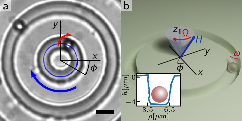</details> Fig. 1: (a) Optical microscope image of two circular channels in a PDMS mold each with a spinning paramagnetic colloidal particle. The red (blue) arrow in the image indicates the direction of the particle rotation (trajectory). Scale bar is $5\rm{μ m}$ , see also corresponding Movie S1†in the Supporting Information. (b) Schematic of a particle within the circular channel and of the applied precessing magnetic field $\bm{H}$ . The inset shows the transverse profile of the channel measured using confocal profilometry. ## 2 Methods ### 2.1 Experimental protocol The circular microchannels are realized in Polydimethylsiloxane (PDMS) with soft lithography. We first use commercial software (AUTOCAD) to design a sequence of lithographic channels with a width $w=3 \rm{μ m}$ , see Fig. 1 (a). The channels are placed concentrically so that they are always separated by a distance of $10\rm{μ m}$ . To sample the channels in 5 $\rm{μ m}$ intervals, the rings are separated in two sets, one starting at $5 \rm{μ m}$ and the other at $10 \rm{μ m}$ . The microchannels present a depth of $∼ 4\rm{μ m}$ thus, larger than the particle width, such that the particles are completely surrounded by solid walls, as shown by the confocal profile in Fig. 1 (b). We use the following procedure to realize the structures in PDMS. First, we fabricate reliefs in SU-8, an epoxy-based negative photoresist, on top of a silicon (Si) wafer. The latter was prepared by dehydrating it for $10$ minutes at $200^∘$ C on a hot plate and then plasma cleaned it for $1$ minute at a pressure of $1$ Torr. After that, a layer of SU-8 $3005$ is spin-coated on top of the Si wafer for $10$ s at $500$ revolution per minute (rpm), followed by spinning at $4000$ rpm for $120$ s, and later baked on a hot plate heated at a temperature of $95^∘$ C for $2$ minutes. The SU-8 is then polymerized by exposure to UV light through a Cromium (Cr) mask for $5.6$ s with a light intensity of $100 \rm{mJ cm^-2}$ (Mask aligner, i-line configuration with wavelength $λ$ =365nm). Then the exposed film is baked again for $1$ min at $65^∘$ C and for another $1$ min at $95^∘$ C, and developed for $30$ s in propylene glycol methyl ether acetate. We then transfer the obtained master to PDMS by first cleaning the SU-8 structure in a plasma cleaner, operating at a pressure of $1$ Torr for $1$ min, and then silanizing it in a vacuum chamber with a drop of silane (SiH 4) for one hour. After that, the PDMS is spin coated onto the Si wafer at $4000$ rpm during $1$ min and baked for $30$ min above a hot plate at a temperature of $95^∘$ C. The PDMS is then transferred to a cover glass by plasma cleaning both surfaces ( $1$ min at $1$ Torr), then joining the PDMS and the glass and finally peeling very carefully with a sharp blade the resulting PDMS film. Once the PDMS channels are fabricated, we realize a closed fluidic cell by first painting the PDMS patterned coverglass with two strips of silicon-based vacuum grease. After that, we deposit a drop containing the colloidal particles dispersed in water on top of it, we close it with another clean coverglass and then we seal the two open sides with more grease. The colloidal suspension is prepared by dispersing $1.5 \rm{μ l}$ from the stock solution of paramagnetic colloidal particles (Dynabeads M-270, $2.8\rm{μ m}$ in diameter) in $1 \rm{ml}$ of ultrapure water (MilliQ system, Millipore). The fluidic cell is placed on a custom-made inverted optical microscope equipped with optical tweezers that are controlled using two Acousto-Optic Deflectors (AA Optoelectronics DTSXY-400-1064) driven by a radio frequency wave generator (DDSPA2X-D431b-34). The optical tweezers ensure that the channels are filled with the desired number of particles. Since it is often necessary to push the deposited particles out of the channels, the tweezers have been set up to trap from below by driving the laser radiation (Manlight ML5-CW-P/TKS-OTS) through a high numerical aperture objective (Nikon $100×$ , Numerical aperture $1.3$ ). The trapping objective is also used for observation and a custom-made TV lens is mounted in the microscope setup to observe a wide enough field of view, $∼ 100 \rm{μ m^2}$ . The external magnetic fields used to spin the particles are applied using a set of five coils, all arranged around the sample. In particular, two coils have the main axis aligned along the $\hat{\bm{x}}$ direction, two for the $\hat{\bm{y}}$ direction and one for the $\hat{\bm{z}}$ direction which is perpendicular to the particle plane ( $\hat{\bm{x}},\hat{\bm{y}}$ ). The sample is placed directly above the coil oriented along the $\hat{\bm{z}}$ axis. The magnetic coils are connected to three power amplifiers (KEPCO BOP 20-10) which are driven by a digital-analog card (cDAQ NI-9269) and controlled with a custom-made LabVIEW program. ### 2.2 Numerical simulations To understand the mechanism of propulsion of the rotating particles in the channel, we perform finite element simulations. We consider a sphere suspended in a Newtonian liquid with viscosity $η$ and confined in a channel obtained from two concentric cylinders of height $h$ , as schematically depicted in Fig. 3 (a). The Reynolds number, estimated from the characteristic particle velocity in the ring, is vanishingly small and thus we neglect inertial effects. We consider a Cartesian reference frame with origin at the center of the channel (Fig. 1). We assume that the distance between the particle and the bottom wall, $z_p$ , is fixed due to the balance between gravitational forces and electrostatic repulsion. The ratio of the lateral size of the channel $w$ and the particle radius is fixed to ${w}/{a}=2.2$ which for our $a=1.4\rm{μ m}$ particles produces a channel $3.1\rm{μ m}$ wide, similar to that shown in the inset of 1 b). To model an open channel in the experimental system, we chose $h$ much larger than $w$ . The particle is placed near the bottom of the domain, and horizontally at the center, as depicted in Fig. 3 (a). The rotating magnetic field generates a constant torque $\bm{τ}_m$ along the $\hat{\bm{z}}$ axis, which leads to a constant angular velocity $ω_p$ along the same direction. As a result of the rotation, we expect the particle to translate along the direction that is tangential to the channel centerline, $\hat{\bm{φ}}$ , due to the hydrodynamic coupling with the channel walls (see Fig. 1 ). To investigate how the motion of the particle along the channel depends on the radius of curvature, we compute the mobility matrix of the particle. The mobility matrix, $\bm{M}$ , relates the translational ( $\bm{v}_p$ ) and angular velocity ( $\bm{ω}_p$ ) of the particle to external forces ( $\bm{F}$ ) and torques ( $\bm{τ}$ ): $$ \displaystyle\begin{bmatrix}\bm{v}_p\\ \bm{ω}_p\end{bmatrix}=\bm{M}\begin{bmatrix}\bm{F}\\ \bm{τ}\end{bmatrix} . \tag{1} $$ The mobility matrix, $\bm{M}$ , contains all the information about the hydrodynamic interactions between the particle and the surrounding boundaries. In this particular case, $\bm{M}$ depends on the radius of the channel $R$ . Here, we are interested in the coefficient that couples the magnetic torque, acting along the $\hat{\bm{z}}$ direction, to the translational velocity along the $\hat{\bm{φ}}$ direction. To obtain $\bm{M}$ , we first find the resistance matrix $\bm{R}$ , and then compute $\bm{M}$ as $\bm{M}=\bm{R}^-1$ . To do so, we solve the Stokes equation by imposing a single component of the velocity vector and then computing the resulting force and torque acting on the particle: $$ \displaystyle∇^2\bm{v}-∇ p=0 \displaystyle∇·\bm{v}=0 \tag{2} $$ where $\bm{v}$ is the velocity of the fluid and $\bm{p}$ is the pressure. We consider no-slip boundary condition on the walls of the domain $\bm{v}|_S=0$ , being $S$ the surface of the particle. On $S$ we fix the velocity or the angular velocity. The total forces and torques acting on the particle are computed using: $$ \displaystyle∫_S\bm{T}·\bm{n} dS=\bm{F} \displaystyle∫_S≤ft(\bm{r}-\bm{r_p}\right)×≤ft(\bm{T }·\bm{n}\right) dS=\bm{τ} \tag{4} $$ where $\bm{r}_p=(x_p,y_p,z_p)$ is the position vector of the particle center, $\bm{r}$ is the position of a point on the surface of the particle and $\bm{T}$ is the stress tensor defined as: $\bm{T}=η(∇ v+∇ v^T)-p\bm{I}$ , with $p$ the pressure. By repeating the simulation for all the six components of the velocity vector, we can construct the resistance matrix $\bm{R}$ which is the inverse of the mobility matrix, $\bm{M}=\bm{R}^-1$ . <details> <summary>x7.png Details</summary>  ### Visual Description ## Composite Figure: Particle Dynamics in a Channel ### Overview The image is a two-part scientific figure illustrating the motion of a spherical particle within a fluid-filled channel. Part (a) is a schematic diagram showing three different scenarios of particle rotation and translation. Part (b) is a quantitative data plot showing the relationship between the particle's rotational velocity and its radius, with an inset showing velocity as a function of phase angle. ### Components/Axes **Part (a) - Schematic Diagram:** * **Coordinate System:** A standard Cartesian coordinate system is shown in the bottom-left of the first panel, with the x-axis pointing right and the y-axis pointing up. * **Panels:** Three panels depict a pink sphere (particle) inside a light blue channel bounded by black walls. * **Left Panel:** The particle rotates clockwise (curved black arrows) and translates to the right (green arrow). Horizontal black lines below the particle indicate a shear flow profile. * **Middle Panel:** The particle rotates counter-clockwise (curved black arrows) and translates to the right (green arrow). Horizontal black lines above and below the particle indicate a different shear flow profile. * **Right Panel:** The particle rotates clockwise (curved black arrows) and translates to the right (green arrow). The channel walls are curved. A horizontal black arrow labeled with the Greek letter phi (φ) points to the right, indicating a phase or angular coordinate. **Part (b) - Data Plot:** * **Main Plot Axes:** * **X-axis:** Labeled `R [μm]` (Radius in micrometers). Major tick marks at 10, 20, 30, 40. * **Y-axis:** Labeled `v_φ [μm s⁻¹]` (Rotational velocity in micrometers per second). Major tick marks at 0.00, 0.05, 0.10, 0.15. * **Data Series:** A single data series represented by blue circular markers with vertical error bars. A solid blue line connects the markers, showing a fitted trend. * **Inset Plot:** Located in the top-right quadrant of the main plot. * **Title/Label:** `R = 5 μm` (indicating data for a particle of 5 micrometer radius). * **X-axis:** Labeled `φ [rad]` (Phase angle in radians). Major tick marks at -π, -π/2, 0, π/2, π. * **Y-axis:** Shares the same label and scale as the main plot's y-axis (`v_φ [μm s⁻¹]`). Major tick marks at 0.00, 0.25. * **Data:** Blue square markers with error bars, scattered around a horizontal blue line at approximately v_φ = 0.12 μm s⁻¹. ### Detailed Analysis **Main Plot (v_φ vs. R):** * **Trend Verification:** The data shows a clear, steeply decreasing trend. As the radius `R` increases, the rotational velocity `v_φ` decreases rapidly, approaching zero for larger radii. * **Data Points (Approximate):** * At R ≈ 5 μm, v_φ ≈ 0.14 μm s⁻¹ (highest point). * At R ≈ 10 μm, v_φ ≈ 0.05 μm s⁻¹. * At R ≈ 15 μm, v_φ ≈ 0.01 μm s⁻¹. * At R ≈ 20 μm, v_φ ≈ 0.00 μm s⁻¹ (within error bars). * At R ≈ 25 μm, v_φ ≈ 0.01 μm s⁻¹. * At R ≈ 30 μm, v_φ ≈ 0.02 μm s⁻¹. * At R ≈ 40 μm, v_φ ≈ 0.00 μm s⁻¹. * The solid blue line suggests an inverse relationship, possibly a power-law decay (e.g., v_φ ∝ 1/R or 1/R²). **Inset Plot (v_φ vs. φ for R=5μm):** * **Trend Verification:** The data points fluctuate around a constant positive value. There is no strong systematic trend with phase angle φ. * **Data Distribution:** The rotational velocity `v_φ` for the 5 μm particle is consistently positive, centered around a mean value of approximately 0.12 μm s⁻¹ (indicated by the horizontal blue line). The scatter and error bars show the variability of the measurement across different phase angles from -π to π radians. ### Key Observations 1. **Strong Size Dependence:** The rotational velocity `v_φ` is highly sensitive to particle size `R`, dropping dramatically as the particle gets larger. 2. **Asymptotic Behavior:** For particles with R ≥ 15 μm, the rotational velocity becomes very small, consistent with zero within the measurement uncertainty. 3. **Phase Independence (for small R):** For the smallest measured particle (R=5 μm), the rotational velocity does not show a strong dependence on the phase angle φ, suggesting its rotation is steady relative to the channel phase. 4. **Schematic Context:** The diagrams in (a) suggest the rotation and translation are coupled and influenced by the channel geometry (straight vs. curved walls) and the local fluid shear profile. ### Interpretation This figure investigates the dynamics of a particle (likely a vesicle or capsule) flowing through a microfluidic channel. The key finding is that **smaller particles rotate much faster** than larger ones under the same flow conditions. This is a classic signature of **tank-treading motion**, where the particle's membrane rotates while its shape remains steady, with the rotation rate inversely related to particle size. The schematic in (a) provides the physical context: the particle's motion (translation and rotation) is driven by the shear flow in the channel. The curved walls in the rightmost panel and the phase variable φ suggest the study may involve channels with periodic or curved geometries, where the particle's orientation (phase) could be important. The data in (b) quantitatively confirms the size-dependent rotation. The inset for R=5 μm shows that while the rotation is fast, it is relatively constant regardless of the particle's orientation (phase) within the channel. This implies that for small particles, the tank-treading frequency is set primarily by the global shear rate and particle size, not by its instantaneous position or orientation in a curved channel. The near-zero rotation for large particles (R > 15 μm) suggests a transition to a different motion regime, such as tumbling or steady orientation, where rotational velocity is minimal. 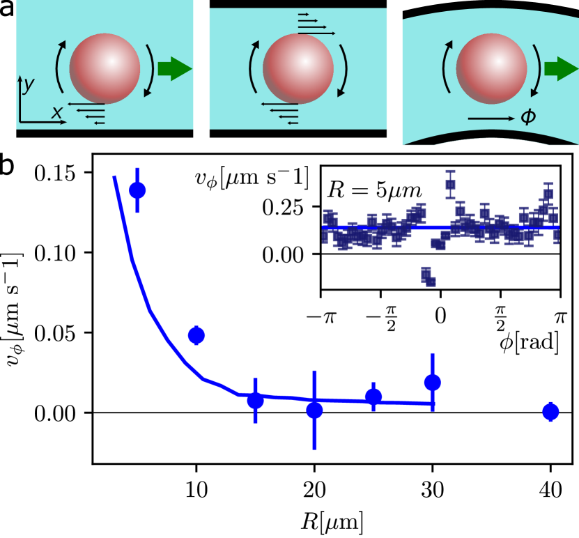</details> Fig. 2: (a) Schematic showing a spinning particle close to a single, flat wall (left), confined between two flat walls (center) and between two curved walls (right). All three images show the particles from the top view, i.e. the particle rotates in the ( $\hat{\bm{x}},\hat{\bm{y}}$ ) plane. The bottom wall, placed at $z=0$ , is not shown for clarity. (b) Tangential velocity $v_φ$ of the rotating magnetic particle inside the channels for different values of the central radius $R$ . The filled points are experimental measurements, and the continuous line is calculated from the numerical simulations using a magnetic torque equal to $τ_m=0.55 \rm{pN μ m}$ . The inset shows the mean velocity at each value of the angle for a ring with radius $R=5 \rm{μ m}$ . The angle $φ$ is measured with respect to the $\hat{\bm{x}}$ axis. <details> <summary>x8.png Details</summary>  ### Visual Description ## Composite Scientific Figure: Hemispherical Traction/Stress Analysis ### Overview The image is a four-panel composite figure (labeled a, b, c, d) from a technical or scientific publication. It presents a 3D schematic of a curved structure alongside three circular heatmap visualizations, likely representing some form of traction, stress, or force distribution across inner and outer hemispherical surfaces. The figure uses a consistent color scale (red to blue) to represent quantitative values. ### Components/Axes **Panel a (3D Schematic):** * **Type:** 3D diagram of a curved, cyan-colored structure. * **Labels & Dimensions:** * `R`: Radius of curvature (horizontal arrow at the top). * `w`: Width of the structure (horizontal arrow on the right face). * `h`: Height of the structure (vertical arrow on the right face). * **Annotations:** * A pink sphere is shown at the bottom right corner. * Two black arrows point to the sphere: one labeled `in` (pointing inward) and one labeled `out` (pointing outward). * Two small, bright white spots are visible on the inner curved surface. * **Coordinate System:** A small 3D axis indicator is present in the bottom left, showing the `ẑ` (z-hat) direction pointing upward. **Panels b, c, d (Circular Heatmaps):** * **Type:** Top-down view of circular (hemispherical projection) heatmaps. * **Common Elements:** * **Color Bar (Shared by b & c):** Located below panels b and c. * **Scale:** Linear, ranging from `-5` to `5`. * **Unit:** `N_φ` (Newton-phi, likely a component of force or traction). * **Color Gradient:** Dark red (negative) → White (zero) → Dark blue (positive). * **Coordinate System:** A small 2D axis indicator is present to the left of panel b, showing `ẑ` (vertical) and `φ̂` (phi-hat, horizontal). * **Panel b:** * **Title/Label:** `Outer hemisphere` (text at bottom left of the panel). * **Data Pattern:** A strong, concentrated dark red region at the center, fading to light orange/white towards the periphery. The distribution appears radially symmetric. * **Panel c:** * **Title/Label:** `Inner hemisphere` (text at bottom left of the panel). * **Data Pattern:** A strong, concentrated dark blue region at the center, fading to light blue/white towards the periphery. The distribution appears radially symmetric and is the inverse color pattern of panel b. * **Panel d:** * **Title/Label:** `Total traction` (text at bottom left of the panel). * **Color Bar (Specific):** Located directly below panel d. * **Scale:** Linear, ranging from `-2.5` to `2.5`. * **Unit:** `N_φ`. * **Color Gradient:** Same red-white-blue scheme as the shared bar. * **Data Pattern:** A complex, non-radially symmetric pattern. It features two prominent dark blue lobes on the left and right sides, a central vertical band of orange/red, and lighter blue/white regions elsewhere. Small, localized red and blue spots are visible near the top and bottom edges. ### Detailed Analysis * **Panel a (Schematic):** Defines the geometry of the system under study—a curved shell or channel with specified radius (`R`), width (`w`), and height (`h`). The `in`/`out` arrows and sphere suggest a point of interaction or force application. * **Panel b (Outer Hemisphere):** Shows a **negative** (`N_φ` < 0, red) traction/stress concentrated at the pole (center) of the outer surface. The magnitude is strongest at the center (approaching -5 N_φ) and diminishes radially outward. * **Panel c (Inner Hemisphere):** Shows a **positive** (`N_φ` > 0, blue) traction/stress concentrated at the pole of the inner surface. The magnitude is strongest at the center (approaching +5 N_φ) and diminishes radially outward. This is the direct opposite of the outer hemisphere pattern. * **Panel d (Total Traction):** Represents the net or combined effect. The color scale is half the range of the individual hemisphere plots (-2.5 to 2.5 N_φ). The pattern is no longer simple: * **Left/Right Lobes:** Large areas of positive (blue) traction. * **Central Vertical Band:** A region of negative (red/orange) traction. * **Edge Artifacts:** Small, high-magnitude spots at the top and bottom periphery may indicate boundary effects or numerical artifacts. ### Key Observations 1. **Symmetry & Inversion:** Panels b and c show perfect radial symmetry and are color inverses of each other, suggesting the inner and outer surfaces experience equal and opposite reactions at the central point. 2. **Pattern Transformation:** The simple, symmetric patterns of the individual hemispheres (b, c) combine to create a complex, asymmetric pattern in the total traction (d). This indicates the vector addition or interaction of the inner and outer forces is non-trivial. 3. **Magnitude Reduction:** The total traction scale (-2.5 to 2.5) is half that of the individual components (-5 to 5), implying significant cancellation occurs when combining the inner and outer surface tractions. 4. **Spatial Localization:** The strongest effects in all heatmaps are concentrated near the center (pole) of the hemispheres, corresponding to the likely point of force application suggested in panel a. ### Interpretation This figure likely illustrates the results of a simulation or experiment measuring mechanical traction (force per unit area) on a curved, shell-like structure. The data suggests that a point load or interaction (represented by the sphere in panel a) applied to the structure generates: * A compressive (negative, red) stress on the outer surface at the point of contact. * A tensile (positive, blue) stress on the inner surface at the same point. * A complex net traction field (panel d) when these effects are combined. The resulting pattern—with lateral blue lobes and a central red band—could indicate how the structure bends, twists, or distributes the load away from the immediate point of contact. The small edge spots in panel d warrant investigation as potential stress concentrations at the boundaries of the modeled domain. The figure effectively moves from a geometric definition (a) to component analysis (b, c) and finally to the synthesized result (d), providing a complete visual narrative of the mechanical response. 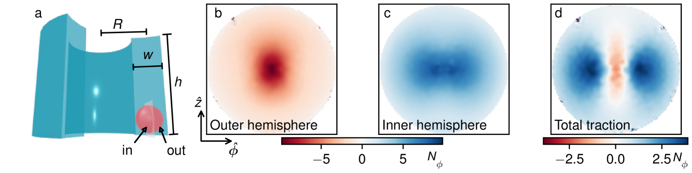</details> Fig. 3: (a) Schematic showing the simulation domain considered, which consists of the space between two concentric cylinders separated by a spacing $w$ , with height $h$ , and a central radius $R$ . (b,c) Surface traction in the outer (b) and inner (c) hemispheres of the particle, as defined in panel (a). (d) Total traction given by the sum of the functions shown in panels (b) and (c), which is positive, indicating a resulting force that pushes forward the particle. ## 3 Single particle motion We start by illustrating the dynamics of individual spinning particles dispersed within circular channels characterized by different radius $R$ . Fig. 1 (a) shows a microscope image of two channels with radii $R=5,15 \rm{μ m}$ and filled with one paramagnetic colloidal particle each, while the corresponding schematic of the experimental system is shown in Fig. 1 (b). The spinning is induced by the application of an external magnetic field that performs conical precession at a frequency $ω$ and an angle $θ$ around the $\hat{\bm{z}}$ axis: $$ \bm{H}≡ H_0[\cos{θ}\hat{\bm{z}}+\sin{θ}(\cos{(ω t)}\hat{ \bm{x}}+\sin{(ω t)}\hat{\bm{y}})] , \tag{6} $$ being $H_0$ the field amplitude. The precessing field has an in-plane component $\bm{H_xy}≡\sin{θ}(\cos{(ω t)}\hat{\bm{x}}+\sin{(ω t)} \hat{\bm{y}})$ which is used to spin the particles, and a static one perpendicular to the particle plane, $\bm{H}_z=H_0\cos{θ}\hat{\bm{z}}$ which is used to control the dipolar interactions when many particles are present. In particular, we keep constant the magnetic field values to $H_0=900 \rm{A m^-1}$ , the frequency $f=50$ Hz such that $ω=2π f=314.2 \rm{rad s^-1}$ and the cone angle at $θ=44.5^∘$ . For the single particle case, the precessing field at relative high frequency, is able to induce an average magnetic torque, $\bm{τ}_m=⟨\bm{m}×\bm{H}⟩$ , which sets the particles in rotational motion at an angular speed $ω_p$ close to the plane. This torque arises due to the finite relaxation time $t_r$ of the particle magnetization, as demonstrated in previous works. 39, 40 Note that here, for simplicity, we assume that the particles are characterized by a single relaxation time. For a paramagnetic colloid with radius $a=1.4 \rm{μ m}$ and magnetic volume susceptibility $χ∼ 0.4$ , the torque can be calculated as 41, 42, $$ \bm{τ}_m=\frac{4a^3πμ_0χ H_0^2\sin^2{(θ)}ω t_ r}{3(1+t_r^2ω^2)}\hat{\bm{z}} \tag{7} $$ being $μ_0=4π 10^-7 \rm{H m}$ the permeability of vacuum, similar to that of water. Assuming $t_r∼ 10^-3$ s we obtain $τ_m=0.32 \rm{pN μ m}$ . In the overdamped limit, the magnetic torque is balanced by the viscous torque $\bm{τ}_v$ arising from the rotation in water, $\bm{τ}_m+\bm{τ}_v=\bm{0}$ . Close to a planar wall, $\bm{τ}_v$ can be written as, $\bm{τ}_v=-8πη\bm{ω}_pa^3f_r(a/z_p)$ , where $η=10^-3 \rm{Pa· s}$ is the viscosity of water, and $f_r(a/z_p)$ is a correction term that accounts for the proximity of the bottom wall at a distance $z_p$ . 43 In particular, assuming the space between the particle and the wall $∼ 100$ nm, $f_r(a/h)=1.45$ . In the overdamped regime, the balance between both torques allows estimating the particle mean angular velocity: $⟨ω_p⟩=μ_0H_0^2\sin^2{θ}χτ_rω/[6 η(1+τ_r^2ω^2)]$ , which gives $ω_p=3.27\rm{rad s^-1}$ . Clearly, this estimate does not consider the presence of a top wall and how it reduces the particle angular rotation, as we will see later. Now let’s consider the general situation of a rotating free particle, far away from any surface. The rotational motion is reciprocal, and unable to induce any drift. However, if close to a solid wall, as shown in the left schematic in Fig. 2 (a), the rotational motion can be rectified into a net drift velocity due to the hydrodynamic interaction with the close substrate, 43 which breaks the spatial symmetry of the flow. The situation changes when the particle is squeezed between two flat channels, as in the middle of Fig. 2 (a). Now the asymmetric flow close to the bottom surface is balanced by the one at the top, and the spatial symmetry is restored. As a consequence, the particle is unable to propel unless small thermal fluctuations can displace the colloid from the central position making it closer to one of the two surfaces. However, even in this case, the rectification will be balanced on average. Here we show that, in contrast to previous cases, when the particle is confined between two curved walls, the effect of curvature breaks again the spatial symmetry, and induce a net particle motion, as shown in the last schematic in Fig. 2 (a). <details> <summary>x9.png Details</summary>  ### Visual Description ## Multi-Panel Scientific Figure: Droplet Dynamics in a Concentric Ring Trap ### Overview The image is a composite scientific figure consisting of three panels (a, b, c) presenting experimental data on the dynamics of droplets confined within a concentric ring structure. Panel (a) is a microscopy image showing the experimental setup. Panels (b) and (c) are quantitative plots analyzing particle motion and confinement as a function of a parameter labeled ρ_L. ### Components/Axes **Panel (a): Microscopy Image** * **Content:** A grayscale microscopy image showing a series of concentric, circular channels or rings. Numerous small, dark, spherical droplets are visible, primarily trapped within the grooves of the rings. A bright central spot is present. * **Labels:** The panel is labeled with a lowercase "a" in the top-left corner. * **Scale Bar:** A white horizontal scale bar is present in the bottom-right corner. Its exact length is not labeled in the image. **Panel (b): Mean Squared Displacement (MSD) Plots** * **Structure:** Two side-by-side log-log plots sharing a common color bar. * **X-Axis (Both Plots):** Label: `δt [s]` (time lag in seconds). Scale: Logarithmic, ranging from 10⁻¹ to 10³. * **Y-Axis (Both Plots):** Label: `⟨Δs²⟩ [μm²]` (mean squared displacement in square micrometers). Scale: Logarithmic, ranging from 10⁻² to 10⁴. * **Color Bar (Top Center):** Label: `ρ_L`. Scale: Linear, ranging from 0.01 (dark blue) to 0.30 (dark red). Ticks at: 0.01, 0.03, 0.06, 0.12, 0.14, 0.18, 0.20, 0.24, 0.28, 0.30. * **Legend (Left Plot):** Located in the top-left quadrant of the left plot. * Green dash-dot line: `~t` (indicating diffusive motion, MSD ∝ t). * Black dotted line: `~t²` (indicating ballistic motion, MSD ∝ t²). * **Data Series:** Multiple colored lines in each plot, with colors corresponding to the `ρ_L` color bar. **Panel (c): Confinement Metric Plot** * **Main Plot:** * **X-Axis:** Label: `ρ_L`. Scale: Linear, ranging from 0.10 to 0.30. * **Y-Axis:** Label: `⟨r²⟩`. Scale: Linear, ranging from 0.0 to 1.0. * **Data Points:** Two distinct series: * Red circles. * Blue squares. * **Inset Plot (Bottom-Right of Panel c):** * **X-Axis:** Label: `t (s)` (time in seconds). Scale: Linear, from 0 to 1000. * **Y-Axis:** Label: `r²`. Scale: Linear, from 0.4 to 1.0. * **Color Bar (Right of Inset):** Label: `ρ_L`. Scale: Linear, from 0.18 (light blue) to 0.30 (dark red). Ticks at: 0.18, 0.24, 0.30. * **Data Series:** Multiple noisy time-series lines, colored according to the inset's `ρ_L` color bar. ### Detailed Analysis **Panel (b) - Left Plot:** * **Trend Verification:** All colored MSD curves start near the `~t` (diffusive) reference line at short times (δt ~ 0.1-1 s). As time lag (δt) increases, the curves for lower `ρ_L` (bluer colors) bend upward, approaching the `~t²` (ballistic) reference line. The curves for higher `ρ_L` (redder colors) remain closer to the `~t` line for longer before showing a weaker upward bend. * **Data Points (Approximate):** * For `ρ_L` ≈ 0.01 (dark blue line): At δt = 100 s, ⟨Δs²⟩ ≈ 10² μm². At δt = 1000 s, ⟨Δs²⟩ ≈ 10⁴ μm². * For `ρ_L` ≈ 0.30 (dark red line): At δt = 100 s, ⟨Δs²⟩ ≈ 10¹ μm². At δt = 1000 s, ⟨Δs²⟩ ≈ 10² μm². **Panel (b) - Right Plot:** * **Trend Verification:** Similar overall trend to the left plot, but the curves appear more tightly grouped. The transition from diffusive to super-diffusive/ballistic motion is less pronounced for all `ρ_L` values compared to the left plot. * **Data Points (Approximate):** * For `ρ_L` ≈ 0.01 (dark blue line): At δt = 100 s, ⟨Δs²⟩ ≈ 10¹ μm². At δt = 1000 s, ⟨Δs²⟩ ≈ 10² μm². * For `ρ_L` ≈ 0.30 (dark red line): At δt = 100 s, ⟨Δs²⟩ ≈ 10⁰ μm². At δt = 1000 s, ⟨Δs²⟩ ≈ 10¹ μm². **Panel (c) - Main Plot:** * **Red Circles Series:** Shows a clear increasing trend. `⟨r²⟩` increases from ~0.25 at `ρ_L`=0.10 to ~0.95 at `ρ_L`=0.30. * **Blue Squares Series:** Shows a different, non-monotonic trend. `⟨r²⟩` is ~0.0 at `ρ_L`=0.12, rises to ~0.7 at `ρ_L`=0.20, and is ~0.8 at `ρ_L`=0.30. * **Spatial Grounding:** The red circle at `ρ_L`=0.30 is the highest point on the plot (top-right). The blue square at `ρ_L`=0.12 is the lowest point (bottom-left). **Panel (c) - Inset Plot:** * **Trend Verification:** The time series for `r²` shows fluctuations. Lines corresponding to higher `ρ_L` (redder colors) are consistently positioned higher on the y-axis (closer to 1.0) than lines for lower `ρ_L` (bluer colors), which are noisier and lower (closer to 0.5-0.7). * **Data Points (Approximate):** * For `ρ_L` ≈ 0.30 (dark red line): `r²` fluctuates between ~0.9 and 1.0. * For `ρ_L` ≈ 0.18 (light blue line): `r²` fluctuates between ~0.5 and 0.7. ### Key Observations 1. **Confinement Effect:** The parameter `ρ_L` strongly influences droplet dynamics. Higher `ρ_L` (redder colors) correlates with lower mean squared displacement (MSD) in panel (b) and a higher confinement metric `⟨r²⟩` in panel (c). 2. **Dynamic Transition:** The MSD plots in panel (b) show a crossover from short-time diffusive motion (~t scaling) to long-time super-diffusive or ballistic motion (~t² scaling). This transition is more pronounced at lower `ρ_L`. 3. **Two Metrics in Panel (c):** The red circles and blue squares in the main plot of panel (c) likely represent two different measurements or calculations of the confinement metric `⟨r²⟩`, showing distinct dependencies on `ρ_L`. 4. **Temporal Stability:** The inset in panel (c) demonstrates that the confinement metric `r²` is relatively stable over long timescales (1000 seconds) for a given `ρ_L`, though it exhibits significant fluctuations, especially at lower `ρ_L`. ### Interpretation This figure investigates the motion of droplets in a structured, concentric ring trap. The parameter `ρ_L` (likely a dimensionless density, loading fraction, or confinement strength) is the key control variable. * **What the data suggests:** The system exhibits a transition in dynamics. At low `ρ_L`, droplets are less confined and can undergo enhanced, super-diffusive motion over long times, possibly due to collective effects or interactions within the rings. At high `ρ_L`, droplets are strongly confined, leading to more restricted, diffusive motion and a higher localization metric (`⟨r²⟩`). * **How elements relate:** Panel (a) shows the physical system. Panel (b) quantifies the *nature* of the motion (diffusive vs. ballistic) as a function of time and `ρ_L`. Panel (c) quantifies the *degree* of confinement (`⟨r²⟩`) as a function of `ρ_L`, with the inset confirming the stability of this measure over time. * **Notable anomalies:** The non-monotonic behavior of the blue squares in panel (c) is intriguing. It suggests that the metric represented by the blue squares might be sensitive to a specific regime or interaction effect that peaks at intermediate `ρ_L` (~0.20). The clear separation between the two data series (red vs. blue) in panel (c) indicates they capture fundamentally different aspects of the droplets' spatial distribution or dynamics within the trap. **Language Declaration:** All text in the image is in English. No other languages are present. 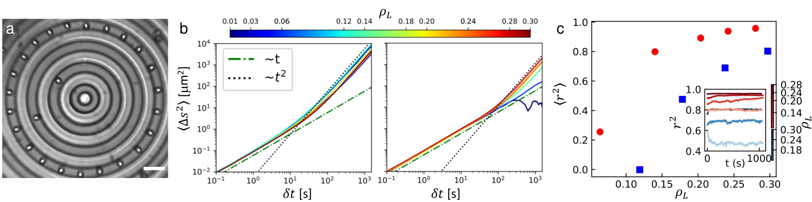</details> Fig. 4: (a) Optical microscope image of paramagnetic colloidal particles spinning inside a circular channel with radius $R=35 \rm{μ m}$ . The scale bar is 10 $μ m$ , see also Movie S2†in the Supporting Information. (b) Mean squared displacement of the circumference arc $⟨Δ s^2⟩$ as a function of the time intervals $δ t$ for different densities $ρ_L$ . Left (right) plot shows the experimental data for a channel with radius $R=15μ m$ ( $R=35μ m$ respectively). The dashed-dotted line indicate the normal diffusion ( $α=1$ ) while the dotted line shows the ballistic regime ( $α=2$ ). Colorbar, legend, and axes are common in both plots. (c) Average Kuramoto order parameter $⟨ r^2⟩$ (Eq. (10)) versus particle density $ρ_L$ . Blue squares (red disks) are experimental data for a channel with radius $R=15 \rm{μ m}$ ( $R=35 \rm{μ m}$ respectively). Inset shows the temporal evolution of $⟨ r^2⟩$ for different particle densities, identified by the color bar. The color code of the color bar is the same as in the main plot. To demonstrate this point, we perform a series of experiments by varying the channel radius $R∈[5,40] \rm{μ m}$ and measuring the tangential velocity of the particle $v_φ$ , Fig. 2 (b). We find that while for large rings ( $R>20 \rm{μ m}$ ) the particle does not display any net movement, $v_φ∼ 0$ , below $R∼ 10\rm{μ m}$ the effect of curvature becomes important and it can rectify the rotational motion of the particle. Indeed, for $R=5\rm{μ m}$ the particle circulates along the channel at a non-negligible speed of $v_φ≃ 0.14\rm{μ m s^-1}$ . The rectification process decreases by increasing $R$ , while the sense of rotation is equal to that of the precessing field, sign that the spinning particle is more strongly coupled to the bottom wall of the curved channel. This can be also appreciated from the Video S1†in the Supporting Information, where a driven particle in the small, $R=5 \rm{μ m}$ ring moves clockwise, even if the velocity is not uniform. Regarding this last point, we note that due to the resolution limit of the lithographic technique, our small channels may present imperfections such as deformations and non-uniform edges. These defects may pin a rotating particle during its motion for a longer time. This effect can be observed in the inset to Fig. 2, where we have discretized space and calculated the mean tangential velocity $v_φ$ for each slice of the circular trajectory. Here the time spent by the particle near $φ=0$ is larger, and at this point, the colloidal particle is trapped by a defect, taking a long time to be released by thermal motion. To avoid this problem, we have calculated the mean velocity directly from the binned series shown in the inset, giving equal weights to all the discrete slices. We can use the equation $$ \displaystyle v_φ=M_v_{φ,τ_z}τ_z \tag{8} $$ to calculate the tangential velocity, where the entry of the mobility matrix, $M_v_{φ,τ_z}$ , is calculated from finite element simulations. To match the experimental value we fit the value of $τ_z$ , which is constant for all values of the curvature $R$ . We have performed a non-linear regression of the experimental data and fit the velocity profile using the torque as a single, free parameter. The calculated off-axis component of the mobility matrix $\bm{M}$ is multiplied by a constant factor, which gives the continuous line shown in Fig. 2 (b). The data shows excellent agreement with the simulation for a torque of $τ$ = 0.55 pN $μ$ m, which is slightly lower than the calculated value of the magnetic torque, $τ_m=0.73 \rm{pN μ m}$ . We also performed simulations with the sphere center placed away from the channel centerline and closer to the inner or the outer wall. However, these simulations did not agree well with the experimental data. The small difference can be attributed to the different approximations used to calculate $τ_m$ , such as the presence of a single relaxation time or the value of the magnetic volume susceptibility of the particle which is a factor that can change from one batch to the other since it depends on the chemical synthesis used to produce these particles. To understand the origin of the propulsion, we have used the simulation to calculate the surface traction along a sphere rotating at a constant angular velocity. The traction is computed in each point on the particle surface from the stress tensor as $\bm{T}·\bm{n}$ , where $\bm{n}$ is the unit vector normal to the surface of the sphere. In Fig. 3 we are showing only the $\hat{\bm{φ}}-$ component of the traction vector, which points in the direction of the particle’s translational motion. In Figs. 3 (b) and (c), where we show the normalized traction force $N_φ$ calculated in the outer and inner hemispheres of the particle respectively, we find that the coupling of the particle surface to the outer wall pushes the particle back towards the negative $\hat{\bm{φ}}$ -direction, corresponding to a negative angular velocity. In contrast, the interaction between the inner hemisphere of the particle, and the inner wall pushes the particle along the forward direction. The last panel, Fig. 3 (d) shows the sum of both interactions, whose integral yields the total hydrodynamic force acting along the $\hat{\bm{φ}}$ direction. Even though there is a negative component in the center of the circle, which indicates a higher coupling to the outer wall, it is clear that the strongest contribution comes from the two positive lobes where the inner hemisphere coupling is stronger, and the total force along the $\hat{\bm{φ}}$ axis is positive. Thus, our finite element simulations confirm that the rectification process of a single rotating particle within a curved channel results only from the hydrodynamic interactions between the particle and the surfaces. ## 4 Driven magnetic single file We next explore the collective dynamics of an ensemble of interacting spinning colloids that are confined along the circular channel. Since the lateral width is $w∼ 2a$ the colloidal particles cannot pass each other, thus effectively forming a "single file" system. 44, 45. While the particle dynamics in a "passive" single file, driven only by thermal fluctuations, have been a matter of much interest in the past, 46, 47, 48 more scarce are realizations of "driven" single files 49, 50, where the particles undergo ballistic transport due to external force and collective interactions. 51, 52, 53, 54 In our case, a typical situation is shown in Fig. 4 (a), where $N=23$ particles move within a channel of radius $R=35\rm{μ m}$ (linear density $ρ_L=Na/(2π R)=0.15$ ), see also Video S2†in the Supporting Information. The applied precessing magnetic field apart from inducing the spinning motion within the particle is also used to reduce the magnetic dipolar interaction between them. In particular, in the point dipole approximation, we can consider that the interaction potential $U_dd$ between two equal moments $\bm{m}_i,j$ at relative position $r=|\bm{r}_i-\bm{r}_j|$ is given by: $U_dd=μ_0/4π\{(\bm{m}_i·\bm{m}_j/r^3)-[3(\bm{m}_i·\bm{r })(\bm{m}_j·\bm{r})/r^5]\}$ . Here the induced moment is given by, $m=Vχ H_0$ , being $V=(4π a^3)/3$ the particle volume. If we assume that the induced moments follow the precessing field with a cone angle $θ$ , these interactions can be time-averaged, and become: $$ ⟨ U_dd⟩=\frac{μ_0m^2}{4π r^3}P_2(\cos{θ}) , \tag{9} $$ where $P_2(\cos{θ})=(3\cos^2{θ}-1)/2$ is the second order Legendre polynomial. For the field parameters used, the dipolar interaction is small since $θ=44.5^∘$ which is close to the "magic angle" ( $θ=45.7^∘$ ) where $P_2(\cos{θ})∼ 0$ . From these values, we estimate that the pair repulsion is of the order of $U_dd=5k_BT$ being $T=293 \rm{K}$ the thermodynamic temperature and $k_B$ the Boltzmann constant. Thus, the magnetic interactions are slightly repulsive to avoid the particles attracting each other at high density. Indeed, for a purely rotating magnetic field ( $H_z=0$ , $θ=90^∘$ ) the spinning particles aggregate forming compact chains that induce clogging of the channel. In contrast, to obtain a strong repulsion we would require a smaller in-plane field component that would induce a smaller magnetic torque. Thus, we perform different experiments by varying both the particle linear density within the ring, $ρ_L$ , and the channel radius $R$ , while keeping fixed the applied field parameters, which are the same as in the single-particle case. From the particle positions, we measure the mean squared displacement (MSD) along the circumference arc $Δ s$ connecting a pair of particles within the ring. Here the MSD is calculated as $⟨Δ s^2(Δ t)⟩≡⟨(s(t)-s(t+δ t))^2⟩$ , being $δ t$ the lag time and $⟨…⟩$ a time average. We use the MSD to distinguish the dynamic regimes at the steady state. Here the MSD behaves as a power law $⟨Δ s^2(Δ t)⟩∼τ^α$ , with an exponent $α=1$ for standard diffusion and $α=2$ for ballistic transport, i.e. a single file of particles with constant speed. As shown in the left plot of Fig. 4 (b) for a small channel width, $R=15 \rm{μ m}$ , all MSDs behave similarly, showing an initial diffusive regime followed by a ballistic one at a longer time, and the transition between both dynamic regimes occurs at $∼ 10-20$ s. Increasing the particle density has a small effect in the ballistic regime, where the velocity is higher at a lower density. This effect indicates that the inter-particle interactions reduce the average speed of the single file. Since magnetic dipolar interactions are minimized by spinning the field at the "magic angle", this effect may arise from hydrodynamics. Indeed it was recently observed that these interactions may affect the circular motion of driven systems. 55, 56 In contrast, the situation changes for a larger channel, $R=35 \rm{μ m}$ and right plot in Fig. 4 (b). There, at low density $ρ_L$ the particle tangential speed vanishes, $v_φ=0$ (as shown in Fig. 2 (b)), and thus we recover a diffusive regime also at long time until the slope fluctuates due to lack of statistical averages. Increasing $ρ_L$ we recover the transition from the diffusive to the ballistic one, but occurring at a relatively longer time, $∼ 100$ s. The emergence of a ballistic regime results from the cooperative movement of the particles which generate hydrodynamic flow fields near the surface. Indeed, while single particles display negligible translational velocity in channel of radii $R=15\rm{μ m}$ and $35\rm{μ m}$ (Fig. 2(a)), we observed a ballistic regime in both cases at high density. As previously observed for a linear, one-dimensional chain of rotors 42, the spinning particles generate a cooperative flow close to a bounding wall which act as a “conveyor belt effect”. Here, the situation is similar, however the larger distance between the particles due to their repulsive interactions and the presence of two walls which screen the flow reduce the average speed of the single file and increase the time required for this cooperative effect to set in. We can estimate the transition time between both regimes for the single particle. We start by measuring the diffusion coefficient of the single particle within the channel from the MSD in the diffusive regime, $D=0.0379± 0.0002\rm{μ m^2 s^-1}$ . Thus, the motion of an individual magnetic particle will turn from the Brownian motion with $⟨Δ s^2⟩=2Dt$ to a ballistic one with $⟨Δ s^2⟩=(Rω_pt)^2$ after a characteristic time $τ_c=D/(Rω_p)^2$ . From the experimental data in Fig. 2 (b) we have that $ω_p=0.0073 \rm{rad s^-1}$ for $R=15 \rm{μ m}$ which gives $τ_c=3.1$ s, similar to the small channel in the left of Fig. 4 (b). We further analyze the relative particle displacement, and the presence of synchronized movement by measuring a Kuramoto-like 57, 58 order parameter, defined as: $$ ⟨ r^2(t)⟩=\frac{1}{N^2}∑_i,j=1^N\cos{(Δφ_ij (t))} \tag{10} $$ where $N$ is the number of particles, $Δφ_ij=φ_i-φ_j$ the difference between the angular position of two nearest particles $i,j$ and $φ_i,j$ is measured with respect to one axis ( $\hat{\bm{x}}$ ) located in the particle plane. This order parameter is normalized such that $⟨ r^2⟩∈[0,1]$ , where $1$ corresponds to the fully coordinated relative movement of all spinning particles. Fig. 4 (c) show the average value of $r^2$ at different density $ρ_L$ . In particular, we find that $r^2$ increases with $ρ_L$ since, for a large number of particles the repulsive particles start to interact with each other and their translation becomes more coordinated. On the other hand, we find that $⟨ r^2⟩$ decreases with the radius of curvature (data from red from blue) meaning that the curvature reduces the cooperative translation between the spinning particles. The cooperative movement revealed from the Kuramoto order parameter results from the repulsive magnetic dipolar interactions. Indeed, this parameter increases with density i.e. when the particles are closer to each other and experience stronger repulsive forces. However, the emergence of self-propulsion in our system is a pure hydrodynamic effect induced by the wall curvature. Indeed, the precessing field induces reciprocal magnetic dipolar interactions which could not give rise to any net motion of the spinning particles. ## Conclusions We have demonstrated that a circular channel can be used to induce and enhance the propulsion of spinning particles while the effect becomes absent for a flat one. The propulsion appears from the different hydrodynamic coupling to each of the two curved walls; even if the no-slip condition of each wall pushes the particle along an opposite direction, the two interactions are not symmetric due to the channel curvature. The dominating interaction is the one from the inner wall, which produces a rotation along the channel along the same direction as the angular velocity. We confirm this hypothesis both via experiments and finite element simulations. We note here that the realization of field-driven magnetic prototypes able to propel in viscous fluids is important for both fundamental and technological reasons. In the first case, the collection of self-propelled can be used as a model system to investigate fundamental aspects of non-equilibrium statistical physics. 59, 60, 61, 62, 63 On the other hand, it is expected that these prototypes can be used as controllable inclusions in microfluidic systems, 64, 65, 66, 67, 68 either to control or regulate the flow 69, 70, 71 or to transport microscopic biological or chemical cargoes. 38, 72, 73, 74, 75, 76, 77 The propulsion mechanism unveiled in this work could be used to move particles along a microfluidic device, either by designing it with a circular path, or by coupling many semicircles in a zig-zag to form a straight path. ## Data availability The data that support the findings of this study are available from the corresponding authors upon reasonable request. ## Conflicts of interest There are no conflicts to declare. ## Acknowledgements We thank Carolina Rodriguez-Gallo who shared the protocol for the sample preparation, and the MicroFabSpace and Microscopy Characterization Facility, Unit 7 of ICTS “NANBIOSIS” from CIBER-BBN at IBEC. This project has received funding from the European Research Council (ERC) under the European Union’s Horizon 2020 research and innovation program (grant agreement no. 811234). M.D.C. acknowledges funding from the Ramon y Cajal fellowship RYC2021-030948-I and the grant PID2022-139803NB-I00 funded by the MICIU/AEI/10.13039/501100011033 and by the EU under the NextGeneration EU/PRTR & FEDER programs. I. P. acknowledges support from MICINN and DURSI for financial support under Projects No. PID2021-126570NB-100 AEI/FEDER-EU and No. 2021SGR-673, respectively, and from Generalitat de Catalunya (ICREA Académia). P. T. acknowledges support from the Ministerio de Ciencia, Innovación y Universidades (grant no. PID2022- 137713NB-C21 AEI/FEDER-EU) and the Agència de Gestió d’Ajuts Universitaris i de Recerca (project 2021 SGR 00450) and the Generalitat de Catalunya (ICREA Académia). ## Notes and references - Happel and Brenner 2012 J. Happel and H. Brenner, Low Reynolds number hydrodynamics: with special applications to particulate media, Springer Science & Business Media, 2012, vol. 1. - Purcell 1977 E. M. Purcell, American Journal of Physics, 1977, 45, 3–11. - Dreyfus et al. 2005 R. Dreyfus, J. Baudry, M. L. Roper, M. Fermigier, H. A. Stone and J. Bibette, Nature, 2005, 437, 862–5. - Gao et al. 2010 W. Gao, S. Sattayasamitsathit, K. M. Manesh, D. Weihs and J. Wang, J. Am. Chem. Soc., 2010, 132, 14403–5. - Cebers and Erglis 2016 A. Cebers and K. Erglis, Adv. Funct. Mater., 2016, 26, 3783–3795. - Yang et al. 2020 T. Yang, B. Sprinkle, Y. Guo and N. Wu, Proc. Nat. Acad. Sci. USA, 2020, 117, 18186–18193. - Qiu et al. 2014 T. Qiu, T.-C. Lee, A. G. Mark, K. I. Morozov, R. Münster, O. Mierka, S. Turek, A. M. Leshansky and P. Fischeru, Nature Comm., 2014, 5, 5119. - Li et al. 2021 G. Li, E. Lauga and A. M. Ardekani, Journal of Non-Newtonian Fluid Mechanics, 2021, 297, 104655. - Snezhko and Aranson 2016 A. Snezhko and I. S. Aranson, Nat. Materials, 2016, 10, 698–703. - García-Torres et al. 2018 J. García-Torres, C. Calero, F. Sagués, I. Pagonabarraga and P. Tierno, Nature Comm., 2018, 9, 1663. - Steinbach et al. 2020 G. Steinbach, M. Schreiber, D. Nissen, M. Albrecht, S. Gemming and A. Erbe, Phys. Rev. Res., 2020, 2, 023092. - Bechinger et al. 2016 C. Bechinger, R. Di Leonardo, H. Löwen, C. Reichhardt, G. Volpe and G. Volpe, Rev. Mod. Phys., 2016, 88, 045006. - Frymier et al. 1995 P. D. Frymier, R. M. Ford, H. C. Berg and P. T. Cummings, Proc. Natl. Acad. Sci. U.S.A., 1995, 92, 6195–6199. - Berke et al. 2008 A. P. Berke, L. Turner, H. C. Berg and E. Lauga, Phys. Rev. Lett., 2008, 101, 038102. - Lauga et al. 2006 E. Lauga, W. R. DiLuzio, G. M. Whitesides and H. A. Stone, Biophysical Journal, 2006, 90, 400–412. - Di Leonardo et al. 2011 R. Di Leonardo, D. Dell’Arciprete, L. Angelani and V. Iebba, Phys. Rev. Lett., 2011, 106, 038101. - Spagnolie et al. 2015 S. E. Spagnolie, G. R. Moreno-Flores, D. Bartolo and E. Lauga, Soft Matter, 2015, 11, 3396–3411. - Raveshi et al. 2021 M. R. Raveshi, M. S. Abdul Halim, S. N. Agnihotri, M. K. O’Bryan, A. Neild and R. Nosrati, Nat Commun, 2021, 12, 3446. - Bianchi et al. 2020 S. Bianchi, V. Carmona Sosa, G. Vizsnyiczai and R. Di Leonardo, Sci Rep, 2020, 10, 4609. - Kuron et al. 2019 M. Kuron, P. Stärk, C. Holm and J. de Graaf, Soft Matter, 2019, 15, 5908–5920. - Volpe et al. 2011 G. Volpe, I. Buttinoni, D. Vogt, H.-J. Kümmerer and C. Bechinger, Soft Matter, 2011, 7, 8810. - Spagnolie and Lauga 2012 S. E. Spagnolie and E. Lauga, J. Fluid Mech., 2012, 700, 105–147. - Galajda et al. 2007 P. Galajda, J. Keymer, P. Chaikin and R. Austin, Journal of Bacteriology, 2007, 189, 8704–8707. - Wan et al. 2008 M. B. Wan, C. J. Olson Reichhardt, Z. Nussinov and C. Reichhardt, Phys. Rev. Lett., 2008, 101, 018102. - Ai and Wu 2014 B.-Q. Ai and J.-C. Wu, The Journal of Chemical Physics, 2014, 140, 094103. - Yariv and Schnitzer 2014 E. Yariv and O. Schnitzer, Phys. Rev. E, 2014, 90, 032115. - Koumakis et al. 2014 N. Koumakis, C. Maggi and R. Di Leonardo, Soft Matter, 2014, 10, 5695–5701. - Pototsky et al. 2013 A. Pototsky, A. M. Hahn and H. Stark, Phys. Rev. E, 2013, 87, 042124. - Ai et al. 2013 B.-q. Ai, Q.-y. Chen, Y.-f. He, F.-g. Li and W.-r. Zhong, Phys. Rev. E, 2013, 88, 062129. - Guidobaldi et al. 2014 A. Guidobaldi, Y. Jeyaram, I. Berdakin, V. V. Moshchalkov, C. A. Condat, V. I. Marconi, L. Giojalas and A. V. Silhanek, Phys. Rev. E, 2014, 89, 032720. - Kantsler et al. 2013 V. Kantsler, J. Dunkel, M. Polin and R. E. Goldstein, Proc. Natl. Acad. Sci. U.S.A., 2013, 110, 1187–1192. - Tierno et al. 2008 P. Tierno, R. Golestanian, I. Pagonabarraga and F. Sagués, Phys. Rev. Lett., 2008, 101, 218304. - Driscoll et al. 2017 M. Driscoll, B. Delmotte, M. Youssef, S. Sacanna, A. Donev and P. Chaikin, Nat. Physi., 2017, 13, 375–379. - Martinez-Pedrero et al. 2018 F. Martinez-Pedrero, E. Navarro-Argemí, A. Ortiz-Ambriz, I. Pagonabarraga and P. Tierno, Sci. Adv., 2018, 4, eaap9379. - Tierno and Snezhko 2021 P. Tierno and A. Snezhko, ChemNanoMat, 2021, 7, 881–893. - Morimoto et al. 2008 H. Morimoto, T. Ukai, Y. Nagaoka, N. Grobert and T. Maekawa, Phys. Rev. E, 2008, 78, 021403. - Sing et al. 2010 C. E. Sing, L. Schmid, M. F. Schneider, T. Franke and A. Alexander-Katz, Proc. Natl. Acad. Sci. U.S.A., 2010, 107, 535. - Zhang et al. 2010 L. Zhang, T. Petit, Y. Lu, B. E. Kratochvil, K. E. Peyer, R. Pei, J. Lou and B. J. Nelson, ACS Nano, 2010, 10, 6228–6234. - Tierno et al. 2007 P. Tierno, R. Muruganathan and T. M. Fischer, Phys. Rev. Lett., 2007, 98, 028301. - Janssen et al. 2009 X. J. A. Janssen, A. J. Schellekens, K. van Ommering, L. J. van Ijzendoorn and M. J. Prins, Biosens. Bioelectron., 2009, 24, 1937. - Cebers and Kalis 2011 A. Cebers and H. Kalis, Europ. Phys. J. E, 2011, 34, 1292. - Martinez-Pedrero et al. 2015 F. Martinez-Pedrero, A. Ortiz-Ambriz, I. Pagonabarraga and P. Tierno, Phys. Rev. Lett., 2015, 115, 138301. - Goldman et al. 1967 A. J. Goldman, R. G. Cox and H. Brenner, Chem. Eng. Sci., 1967, 22, 637. - Kärger and Ruthven 1992 Diffusion in zeolites and other microporous solids, ed. J. Kärger and D. Ruthven, Wiley, New York, 1992. - Kärger 1992 J. Kärger, Phys. Rev. A, 1992, 45, 4173–4174. - Wei et al. 2000 Q.-H. Wei, C. Bechinger and P. Leiderer, Science, 2000, 287, 625–627. - Lutz et al. 2004 C. Lutz, M. Kollmann and C. Bechinger, Phys. Rev. Lett., 2004, 93, 026001. - Lin et al. 2005 B. Lin, M. Meron, B. Cui, S. A. Rice and H. Diamant, Phys. Rev. Lett., 2005, 94, 216001. - Köppl et al. 2006 M. Köppl, P. Henseler, A. Erbe, P. Nielaba and P. Leiderer, Phys. Rev. Lett., 2006, 97, 208302. - Misiunas and Keyser 2019 K. Misiunas and U. F. Keyser, Phys. Rev. Lett., 2019, 122, 214501. - Taloni and Marchesoni 2006 A. Taloni and F. Marchesoni, Phys. Rev. Lett., 2006, 96, 020601. - Barkai and Silbey 2009 E. Barkai and R. Silbey, Phys. Rev. Lett., 2009, 102, 050602. - Illien et al. 2013 P. Illien, O. Bénichou, C. Mejía-Monasterio, G. Oshanin and R. Voituriez, Phys. Rev. Lett., 2013, 111, 038102. - Dolai et al. 2020 P. Dolai, A. Das, A. Kundu, C. Dasgupta, A. Dhar and K. V. Kumar, Soft Matter, 2020, 16, 7077. - Cereceda-López et al. 2021 E. Cereceda-López, D. Lips, A. Ortiz-Ambriz, A. Ryabov, P. Maass and P. Tierno, Phys. Rev. Lett., 2021, 127, 214501. - Lips et al. 2022 D. Lips, E. Cereceda-López, A. Ortiz-Ambriz, P. Tierno, A. Ryabov and P. Maass, Soft Matter, 2022, 96, 8983–8994. - Kuramoto and Nishikawa 1987 Y. Kuramoto and I. Nishikawa, Journal of Statistical Physics, 1987, 49, 569–605. - Strogatz 2000 S. H. Strogatz, Physica D: Nonlinear Phenomena, 2000, 143, 1–20. - Ramaswamy 2010 S. Ramaswamy, Annu. Rev. Condens. Matter Phys., 2010, 1, 323–345. - Marchetti et al. 2013 M. C. Marchetti, J. F. Joanny, S. Ramaswamy, T. B. Liverpool, J. Prost, M. Rao and R. A. Simha, Rev. Mod. Phys., 2013, 85, 1143–1189. - Fodor et al. 2016 E. Fodor, C. Nardini, M. E. Cates, J. Tailleur, P. Visco and F. van Wijland, Phys. Rev. Lett., 2016, 117, 038103. - Nardini et al. 2017 C. Nardini, E. Fodor, E. Tjhung, F. van Wijland, J. Tailleur and M. E. Cates, Phys. Rev. X, 2017, 7, 021007. - Palacios et al. 2021 L. S. Palacios, S. Tchoumakov, M. Guix, I. Pagonabarraga, S. Sánchez and A. G. Grushin, Nat Commun, 2021, 12, 4691. - Tierno et al. 2008 P. Tierno, R. Golestanian, I. Pagonabarraga and F. Sagués, J. Phys. Chem. B, 2008, 112, 16525. - Burdick et al. 2008 J. Burdick, R. Laocharoensuk, P. M. Wheat, J. D. Posner and J. Wang, J. Am. Chem. Soc., 2008, 26, 8164–8165. - Sundararajan et al. 2008 S. Sundararajan, P. E. Lammert, A. W. Zudans, V. H. Crespi and A. Sen, Nano Lett., 2008, 8, 1271–1276. - Sanchez et al. 2011 S. Sanchez, A. Solovev, S. Harazim and O. Schmidt, J. Am. Chem. Soc., 2011, 701, 133. - Sharan et al. 2021 P. Sharan, A. Nsamela, S. C. Lesher-Pérez and J. Simmchen, Small, 2021, 26, e2007403. - Terray et al. 2002 A. Terray, J. Oakey and D. W. M. Marr, Science, 2002, 296, 1841. - Sawetzki et al. 2008 T. Sawetzki, S. Rahmouni, C. Bechinger and D. W. M. Marr, Proc. Natl. Acad. Sci. U. S. A., 2008, 105, 20141. - Kavcic et al. 2009 B. Kavcic, D. Babic, N. Osterman, B. Podobnik and I. Poberaj, Appl. Phys. Lett., 2009, 95, 023504. - Palacci et al. 2013 J. Palacci, S. Sacanna, A. Vatchinsky, P. Chaikin and D. Pine, J. Am. Chem. Soc., 2013, 135, 15978. - Gao and Wang 2014 W. Gao and J. Wang, Nanoscale, 2014, 6, 10486–10494. - Martinez-Pedrero and Tierno 2015 F. Martinez-Pedrero and P. Tierno, Phys. Rev. Appl., 2015, 3, 051003. - Fernando Martinez-Pedrero 2017 P. T. Fernando Martinez-Pedrero, Helena Massana-Cid, Small, 2017, 13, 1603449. - Junot et al. 2023 G. Junot, C. Calero, J. García-Torres, I. Pagonabarraga and P. Tierno, Nano Lett., 2023, 23, 850–857. - Wang et al. 2023 X. Wang, B. Sprinkle, H. K. Bisoyi and Q. Li, Proc. Nat. Acad. Sci. USA, 2023, 120, e2304685120.