# CSKV: Training-Efficient Channel Shrinking for KV Cache in Long-Context Scenarios
## Abstract
Large Language Models (LLMs) have been widely adopted to process long-context tasks. However, the large memory overhead of the key-value (KV) cache poses significant challenges in long-context scenarios. Existing training-free KV cache compression methods typically focus on quantization and token pruning, which have compression limits, and excessive sparsity can lead to severe performance degradation. Other methods design new architectures with le ss KV overhead but require significant training overhead. To address the above two drawbacks, we further explore the redundancy in the channel dimension and apply an architecture-level design with minor training costs. Therefore, we introduce CSKV, a training-efficient C hannel S hrinking technique for KV cache compression: (1) We first analyze the singular value distribution of the KV cache, revealing significant redundancy and compression potential along the channel dimension. Based on this observation, we propose using low-rank decomposition for key and value layers and storing the low-dimension features. (2) To preserve model performance, we introduce a bi-branch KV cache, including a window-based full-precision KV cache and a low-precision compressed KV cache. (3) To reduce the training costs, we minimize the layer-wise reconstruction loss for the compressed KV cache instead of retraining the entire LLMs. Extensive experiments show that CSKV can reduce the memory overhead of the KV cache by 80% while maintaining the model’s long-context capability. Moreover, we show that our method can be seamlessly combined with quantization to further reduce the memory overhead, achieving a compression ratio of up to 95%. Code is available at https://github.com/wln20/CSKV.
## 1 Introduction
Large Language Models (LLMs) have been widely adopted in various natural language processing tasks, particularly those requiring long-context capabilities, such as document analysis and fact retrieval [6]. However, the key-value (KV) cache mechanism used in transformer-based LLMs poses significant efficiency challenges as its memory overhead grows linearly with the sequence length, often replacing the weights to be the memory bottleneck in long-context scenarios. For instance, processing a sequence with 200K tokens using LLaMA-2-7B [17] results in a KV cache occupying around 100GB, compared to 14GB required for model weights. Compressing the KV cache by over 10× is necessary to fit such a sequence on a single NVIDIA RTX 4090 GPU with 24GB of memory.
Existing KV cache compression methods, mainly training-free techniques like token pruning [22, 12, 18, 8] and quantization [10, 13, 11, 15], struggle to maintain model performance at high compression ratios, particularly in long-context tasks. Alternatively, training-required techniques, such as MLA [3] and cache sharing [16, 2], offer higher compression ratios but at the cost of significant retraining and are typically unable to be integrated with existing pre-trained models.
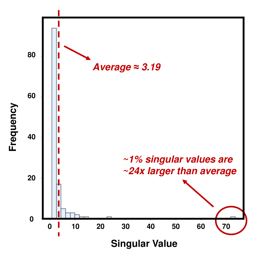
Inspired by MLA, we observe significant redundancy in the large channel dimensions of the KV cache, evidenced by the long-tailed distribution of singular values in the key and value caches (Details in Appendix). Experiments reveal that removing the smallest 50% of these singular values results in less than 1% average accuracy loss on the MMLU [5] benchmark (from 0.458 to 0.449).
Given this redundancy, we propose CSKV, a training-efficient C hannel S hrinking technique for the KV cache, designed to balances high compression ratios with low training costs. To sum up, we have the following contributions:
- To reduce the memory overhead of the KV cache while maintaining the performance, we design a bi-branch KV cache by preserving the recently used KV cache with original dimensions and reducing the dimension of the historical KV cache.
- To further improve the performance without significant training overhead, we propose an effective SVD-based initialization technique and train LLMs in a layer-wise manner by minimizing the reconstruction loss.
- Extensive experimental results demonstrate that our method can achieve an 80% KV cache compression ratio while maintaining the model’s long-context capability. We further demonstrate that our method can be seamlessly combined with 4-bit quantization, showcasing its power in achieving a total compression ratio of 95%.
## 2 Method
### 2.1 Inference with Bi-Branch KV Cache
To reduce the memory overhead, we design to reduce the memory overhead of the KV cache by using low-rank decomposition for both the Key and Value weight matrix. Without loss of generality, we will detail the workflow of compressing the key cache, as the process is identical to that of the value cache.
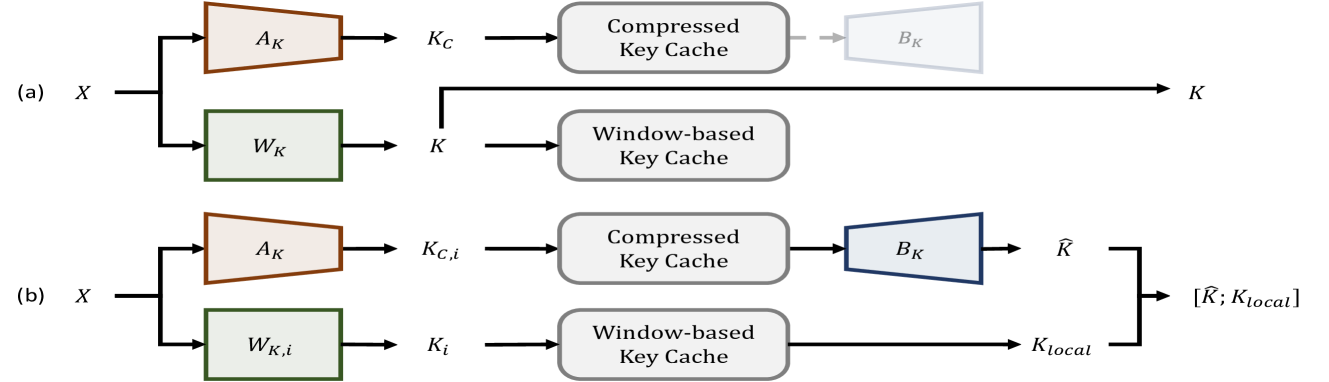
As shown in Figure 1, we use two matrices, $A_K∈ R^h_in× h_comp$ and $B_K∈ R^h_comp× h_out$ , to approximate the weight matrix of $W_K∈ R^h_in× h_out$ . Here the $h_in,h_out,h_comp$ are the input dimension of $W_K$ , the output dimension of $W_K$ , and the intermediate dimension of the low-rank decompression. Keeping the $h_comp$ smaller than $h_out$ and storing the intermediate features as the compressed Key cache, we can significantly save the memory overhead, especially in the long context scenario.
To maintain the high performance, we propose to follow the prior research by preserving the recently used tokens [1, 18] because they are crucial for accurate next-token prediction. To prevent the degradation of this local information during inference, we propose the bi-branch KV cache that preserves the recently used tokens effectively during both the prefilling and decoding stages. With a pre-defined window size $l_w$ , we compress the KV cache only after the tokens fill a complete window while retaining the residual tokens in their original hidden dimensions.
Specifically, for the prefilling stage, as shown in Figure 1 (a), given an input sequence with $n$ tokens, we first use the $A_K$ to generate the compressed Key matrix and store it in the Compressed Key Cache $K_C$ . In this case, the Compressed Key Cache contains all of the historical information of the given sentence. On the other branch, we use the original $W_K$ to generate the full-precision Key matrix $K$ for computation, which can guarantee that the computation results of the prefilling stage are the same as the original LLMs. Then, we only store the full-precision Key activation of the last $m$ tokens $K_local$ to preserve the local information for the decoding stage.
<details>
<summary>x1.png Details</summary>
### Visual Description
## Diagram: Key Caching System Architecture
### Overview
The image depicts two key caching architectures (labeled **a** and **b**) for processing input data **X**. Both architectures involve splitting **X** into components, processing through key caches, and producing outputs. The diagrams use color-coded blocks and arrows to represent data flow, transformations, and caching mechanisms.
### Components/Axes
1. **Input**:
- **X**: Primary input data source (positioned at the top-left of both sections).
2. **Processing Paths**:
- **Section (a)**:
- **A_K** (orange block): Transforms **X** into **K_c**.
- **W_K** (green block): Processes **X** directly into **K**.
- **Compressed Key Cache** (gray block): Stores **K_c** and outputs **B_K**.
- **Window-based Key Cache** (gray block): Stores **K** and outputs **K**.
- **Section (b)**:
- **A_K** (orange block): Transforms **X** into **K_c,i**.
- **W_K,i** (green block): Processes **X** into **K_i**.
- **Compressed Key Cache** (gray block): Stores **K_c,i** and outputs **B_K**.
- **Window-based Key Cache** (gray block): Stores **K_i** and outputs **K_local**.
3. **Outputs**:
- **K**: Final output in section (a).
- **K̂**: Refined output in section (b), derived from **B_K**.
- **[K̂; K_local]**: Combined output in section (b), merging **K̂** and **K_local**.
4. **Arrows**:
- Black arrows indicate data flow direction.
- Dashed arrows (e.g., from **Compressed Key Cache** to **B_K**) suggest optional or indirect pathways.
5. **Color Coding**:
- **Orange**: Key transformation blocks (**A_K**).
- **Green**: Window-based processing blocks (**W_K**, **W_K,i**).
- **Gray**: Key cache blocks (**Compressed Key Cache**, **Window-based Key Cache**).
- **Blue**: Refined output block (**B_K**).
### Detailed Analysis
- **Section (a)**:
- **A_K** and **W_K** process **X** independently.
- **K_c** (from **A_K**) is compressed and cached, then partially output as **B_K**.
- **K** (from **W_K**) bypasses compression and is directly cached and output.
- **Section (b)**:
- Introduces **W_K,i** and **K_i**, suggesting iterative or localized processing.
- **K_c,i** (from **A_K**) is compressed and cached, then refined into **B_K**.
- **K_i** (from **W_K,i**) is cached locally and combined with **K̂** for final output.
### Key Observations
1. **Evolution from (a) to (b)**:
- Section (b) adds granularity with **W_K,i** and **K_i**, implying localized or windowed processing.
- **K_local** in (b) suggests a focus on proximity-aware caching.
2. **Caching Strategies**:
- **Compressed Key Cache** reduces storage overhead for transformed keys (**K_c**, **K_c,i**).
- **Window-based Key Cache** retains raw keys (**K**, **K_i**) for direct use.
3. **Output Refinement**:
- **B_K** (blue block) acts as an intermediary for refining **K_c,i** into **K̂**.
- Final output **[K̂; K_local]** combines refined and localized keys, indicating a hybrid approach.
### Interpretation
The diagram illustrates a progression from a simple key caching system (section **a**) to a more sophisticated, multi-stage architecture (section **b**). Key insights include:
- **Efficiency vs. Accuracy**: Compressed caching reduces storage but may lose fidelity, while window-based caching preserves raw data for critical use cases.
- **Localization**: The introduction of **K_local** in (b) suggests optimization for proximity-sensitive applications (e.g., edge computing).
- **Hybrid Output**: Combining **K̂** (refined) and **K_local** (localized) implies a balance between global efficiency and local responsiveness.
This architecture could be applied to systems requiring adaptive caching, such as distributed databases, real-time analytics, or edge AI deployments. The use of color and block differentiation aids in visualizing the trade-offs between compression, caching, and output refinement.
</details>
Figure 1: The overview of the inference process. (a) The prefilling stage. (b) The decoding stage.
Moreover, during the decoding stage, as shown in Figure 1 (b), we only process one token during each forward pass. We take the process of the $(n+1)$ -th token as an example. For the cache update, we compute both the compressed Key activation $K_C$ and full-precision Key activation $K$ and update both Key caches with the new activations. In this case, the compressed Key cache has $(n+1)$ tokens, and the full-precision Key cache has $(m+1)$ tokens. To get the $(n+1)$ tokens’ Key matrix, we use the $(m+1)$ tokens from the full-precision Key cache as $K_local$ and use the $B_K$ to process the oldest $(n-m)$ tokens in the compressed Key cache as $\hat{K}$ . By concatenating the $\hat{K}$ and $K_local$ , we can get the target Key matrix for attention computation. Finally, we remove the oldest token from the full-precision Key cache to keep the window size as $m$ .
### 2.2 Efficient Fine-tuning by SVD-based Initialization
<details>
<summary>x2.png Details</summary>

### Visual Description
## Flowchart: Neural Network Architecture with Attention Mechanism and Loss Feedback
### Overview
The diagram illustrates a neural network architecture integrating attention mechanisms, loss calculation, and feedback loops. It depicts data flow from input (X) through multiple processing stages to final outputs (L_k and Z), with explicit feedback from loss to attention calculation.
### Components/Axes
1. **Input**:
- `X` (source node, splits into two branches)
2. **Processing Stages**:
- `A_K` (brown trapezoid): Likely attention-related component
- `W_K` (green rectangle): Weight matrix or transformation layer
- `K_C` (blue trapezoid): Key component in attention mechanism
- `B_K` (blue trapezoid): Value component in attention mechanism
3. **Loss & Feedback**:
- `MSELoss` (gray rectangle): Mean Squared Error loss function
- `L_k` (loss output)
- Feedback arrow from `MSELoss` to `Attention Calculation`
4. **Attention Mechanism**:
- `Attention Calculation` (gray rectangle): Processes key (K) to produce Z
5. **Outputs**:
- `L_k`: Loss value
- `Z`: Attention output
### Detailed Analysis
1. **Data Flow**:
- **Primary Path**:
`X → A_K → K_C → B_K → MSELoss → L_k`
- **Secondary Path**:
`X → W_K → K → Attention Calculation → Z`
- **Feedback Loop**:
`MSELoss → K` (modulates attention calculation)
2. **Component Relationships**:
- `A_K` and `B_K` form a key-value attention pair (K_C as key, B_K as value)
- `W_K` generates keys (K) for attention mechanism
- `MSELoss` provides gradient signals to refine attention weights (via K)
3. **Color Coding**:
- Brown: Input/initial processing (`A_K`)
- Green: Weight/transformation (`W_K`)
- Blue: Attention components (`K_C`, `B_K`)
- Gray: Loss/calculation (`MSELoss`, `Attention Calculation`)
### Key Observations
1. Dual-path architecture with parallel processing streams
2. Explicit feedback from loss to attention mechanism suggests adaptive weighting
3. Attention calculation receives both direct input (K) and loss-modulated input
4. Outputs L_k (loss) and Z (attention output) serve distinct purposes
### Interpretation
This architecture appears to implement a transformer-style model with:
1. **Attention Mechanism**: Standard key-value attention (A_K/K_C → B_K)
2. **Loss Integration**: MSELoss not only measures performance but actively shapes attention weights through feedback
3. **Adaptive Learning**: The feedback loop enables the model to dynamically adjust attention based on reconstruction error
4. **Dual Outputs**: Separates loss monitoring (L_k) from attention-derived representations (Z)
The design suggests a self-improving system where attention weights are continuously refined by both input data and error signals, potentially enhancing model robustness and interpretability.
</details>
Figure 2: The overview of the efficient layer-wise reconstruction fine-tuning.
Directly applying low-rank decomposed weight matrices for KV cache compression would result in the degradation of model performance when the compression ratio becomes high. To further enhance the model performance, we propose to introduce an efficient training process. We find that the initialization method to the proposed $A_K$ and $B_K$ is of great importance for convergence and final performance. In this case, we proposed to use the ASVD-based decomposition results for initialization. As shown in Figure 2, we train LLMs in a layer-wise manner by minimizing the layer-wise reconstruction loss for the compressed keys and values.
Specifically, for each layer, we can use the $W_K$ to generate the full-precision Key matrix $K=XW_K$ and use $A_K$ , $B_K$ to generate the lossy key matrix $\hat{K}=XA_KB_K$ . The local reconstruction loss of this layer could be defined as Equation 1:
$$
\displaystyle L_K=MSELoss(K,\hat{K}) \tag{1}
$$
where $L_K$ denotes the loss of keys in this layer, and $MSELoss(·,·)$ is the Mean Square Error (MSE) loss function. Finally, define the loss of keys and values in the $i$ -th layer as $L_K,i,L_V,i$ , the loss for the whole model is shown in Equantion 2:
$$
\displaystyleL_all=∑_j=0^n_l≤ft(L_K,j+L_V,j\right) \tag{2}
$$
where $L_all$ denotes the loss for the whole model, and $n_l$ denotes the number of layers.
## 3 Experiment
### 3.1 Experimental Setup
We evaluate our method on LongChat-7B-v1.5-32k [9] and Mistral-7B-Instruct-v0.2 [7]. We evaluate our method on three widely-used long-context benchmarks: LongEval [9], LongBench [21], and LVEval [19]. For comparison, we include results from StreamingLLM [18], H 2 O [22] Here we only compare the effect of H 2 O on Longchat-7b-v1.5-32k, as it only supports LLaMA architecture in its official implementation., and ASVD [20]. The first two are token pruning methods, while the latter is a SOTA channel-shrinking method. More details can be found in the Appendix.
### 3.2 Main Results
We apply compression ratios of 50% and 80% consistently for both keys and values. The results are presented in Table 1.
According to the evaluation results in table 1, the token pruning methods are especially not skilled in retrieval tasks like LongEval, even at a 50% compression ratio, when ASVD and CSKV only incur minor performance loss. As the compression ratio reaches 80%, all methods except for CSKV suffer great performance degradation on all three tasks. To dive deeper, we examine the failure cases of token pruning methods, and found that although the model could generate coherent sentences based on instructions, a great deal of the retrieved answers deviate from the ground truth by a small portion, like answering "4244" when the label is "42440", or give an irrelevant answer such as "1386". This might be caused by their token eviction mechanisms which inherently have to discard the information of some tokens completely, facing great risk of losing the ground truth information. In contrast, the abundant failure cases of ASVD at 80% compression are mainly caused by the loss of the model’s language modeling capabilities, like responding with dozens of tokens that could hardly form a sentence. Different from the aforementioned methods, CSKV consistently enables the model to generate instruction-following responses and give accurate answers on either retrieval tasks or QA tasks, showing its superior capability of keeping the model’s long-context abilities even at high compression ratios.
### 3.3 Ablation Studies
We conduct several ablation studies to further explore the potential of our method, and the main conclusions include: 1) The SVD-based initialization methods is crucial to the success of training; 2) The model performance is positively correlated with the window size, while the benefit would become less significant after it reaches a certain level; 3) In most cases, it would be better to compress the key cache more than the value cache given a certain budget; 4) CSKV could be seamlessly integrated with 4-bit QAT with very small performance loss. See Appendix for details.
Table 1: Performance of models with CSKV on long-context benchmarks.
| Model | C. Ratio | Method | LongEval $↑$ | LongBench $↑$ | LV-Eval $↑$ | | | | | |
| --- | --- | --- | --- | --- | --- | --- | --- | --- | --- | --- |
| 4k | 6k | 8k | 10k | 0-4k | 4-8k | 8k+ | 16k | | | |
| Longchat-7b-v1.5-32k | 0% | - | 1.00 | 1.00 | 0.98 | 0.98 | 0.46 | 0.43 | 0.46 | 0.13 |
| 50% | StreamingLLM | 0.12 | 0.16 | 0.06 | 0.20 | 0.37 | 0.39 | 0.40 | 0.09 | |
| H 2 O | 0.62 | 0.56 | 0.52 | 0.50 | 0.40 | 0.38 | 0.38 | 0.09 | | |
| ASVD | 0.92 | 0.96 | 0.92 | 0.94 | 0.44 | 0.41 | 0.43 | 0.11 | | |
| CSKV (Ours) | 0.98 | 0.94 | 0.96 | 0.94 | 0.46 | 0.42 | 0.45 | 0.12 | | |
| 80% | StreamingLLM | 0.06 | 0.06 | 0.02 | 0.02 | 0.31 | 0.35 | 0.39 | 0.06 | |
| H 2 O | 0.18 | 0.24 | 0.26 | 0.10 | 0.34 | 0.30 | 0.32 | 0.05 | | |
| ASVD | 0.26 | 0.12 | 0.06 | 0.04 | 0.36 | 0.31 | 0.32 | 0.04 | | |
| CSKV (Ours) | 0.92 | 0.94 | 0.94 | 0.90 | 0.43 | 0.40 | 0.41 | 0.10 | | |
| Mistral-7b-instruct-v0.2 | 0% | - | 1.00 | 1.00 | 0.98 | 0.94 | 0.50 | 0.47 | 0.45 | 0.20 |
| 50% | StreamingLLM | 0.06 | 0.12 | 0.04 | 0.14 | 0.39 | 0.38 | 0.37 | 0.12 | |
| ASVD | 1.00 | 0.98 | 0.92 | 0.94 | 0.49 | 0.45 | 0.44 | 0.17 | | |
| CSKV (Ours) | 1.00 | 1.00 | 0.96 | 0.94 | 0.50 | 0.47 | 0.47 | 0.20 | | |
| 80% | StreamingLLM | 0.06 | 0.04 | 0.00 | 0.04 | 0.34 | 0.34 | 0.33 | 0.06 | |
| ASVD | 0.04 | 0.00 | 0.04 | 0.00 | 0.33 | 0.29 | 0.29 | 0.05 | | |
| CSKV (Ours) | 0.98 | 0.96 | 0.90 | 0.92 | 0.45 | 0.42 | 0.41 | 0.17 | | |
## 4 Limitation and Future Directions
While demonstrating competitive performance, the proposed method’s compression ratio assignment is user-defined and might not be optimal, offering the potential to achieve higher compression ratios. Future work could explore the application of automated search algorithms to dynamically assign compression ratios to individual layers, accounting for their varying sensitivity to compression. Similarly, automated strategies could optimize memory budget allocation for keys and values, maximizing performance within a given constraint. We leave those directions for future works to explore.
## References
- [1] Iz Beltagy, Matthew E. Peters, and Arman Cohan. Longformer: The long-document transformer, 2020.
- [2] William Brandon, Mayank Mishra, Aniruddha Nrusimha, Rameswar Panda, and Jonathan Ragan Kelly. Reducing transformer key-value cache size with cross-layer attention, 2024.
- [3] DeepSeek-AI et al. Deepseek-v2: A strong, economical, and efficient mixture-of-experts language model, 2024.
- [4] Leo Gao, Stella Biderman, Sid Black, Laurence Golding, Travis Hoppe, Charles Foster, Jason Phang, Horace He, Anish Thite, Noa Nabeshima, et al. The pile: An 800gb dataset of diverse text for language modeling. arXiv preprint arXiv:2101.00027, 2020.
- [5] Dan Hendrycks, Collin Burns, Steven Basart, Andy Zou, Mantas Mazeika, Dawn Song, and Jacob Steinhardt. Measuring massive multitask language understanding. Proceedings of the International Conference on Learning Representations (ICLR), 2021.
- [6] Yunpeng Huang, Jingwei Xu, Junyu Lai, Zixu Jiang, Taolue Chen, Zenan Li, Yuan Yao, Xiaoxing Ma, Lijuan Yang, Hao Chen, Shupeng Li, and Penghao Zhao. Advancing transformer architecture in long-context large language models: A comprehensive survey, 2024.
- [7] Albert Q. Jiang, Alexandre Sablayrolles, Arthur Mensch, Chris Bamford, Devendra Singh Chaplot, Diego de las Casas, Florian Bressand, Gianna Lengyel, Guillaume Lample, Lucile Saulnier, Lélio Renard Lavaud, Marie-Anne Lachaux, Pierre Stock, Teven Le Scao, Thibaut Lavril, Thomas Wang, Timothée Lacroix, and William El Sayed. Mistral 7b, 2023.
- [8] Sehoon Kim, Sheng Shen, David Thorsley, Amir Gholami, Woosuk Kwon, Joseph Hassoun, and Kurt Keutzer. Learned token pruning for transformers. In Proceedings of the 28th ACM SIGKDD Conference on Knowledge Discovery and Data Mining, pages 784–794, 2022.
- [9] Dacheng Li*, Rulin Shao*, Anze Xie, Ying Sheng, Lianmin Zheng, Joseph E. Gonzalez, Ion Stoica, Xuezhe Ma, and Hao Zhang. How long can open-source llms truly promise on context length?, June 2023.
- [10] Shiyao Li, Xuefei Ning, Luning Wang, Tengxuan Liu, Xiangsheng Shi, Shengen Yan, Guohao Dai, Huazhong Yang, and Yu Wang. Evaluating quantized large language models, 2024.
- [11] Yujun Lin, Haotian Tang, Shang Yang, Zhekai Zhang, Guangxuan Xiao, Chuang Gan, and Song Han. Qserve: W4a8kv4 quantization and system co-design for efficient llm serving. arXiv preprint arXiv:2405.04532, 2024.
- [12] Zichang Liu, Aditya Desai, Fangshuo Liao, Weitao Wang, Victor Xie, Zhaozhuo Xu, Anastasios Kyrillidis, and Anshumali Shrivastava. Scissorhands: Exploiting the persistence of importance hypothesis for llm kv cache compression at test time, 2023.
- [13] Zirui Liu, Jiayi Yuan, Hongye Jin, Shaochen Zhong, Zhaozhuo Xu, Vladimir Braverman, Beidi Chen, and Xia Hu. Kivi: A tuning-free asymmetric 2bit quantization for kv cache. arXiv preprint arXiv:2402.02750, 2024.
- [14] Aleksandra Piktus. https://huggingface.co/datasets/ola13/small-the_pile, 2022.
- [15] Ying Sheng, Lianmin Zheng, Binhang Yuan, Zhuohan Li, Max Ryabinin, Beidi Chen, Percy Liang, Christopher Ré, Ion Stoica, and Ce Zhang. Flexgen: High-throughput generative inference of large language models with a single gpu. In International Conference on Machine Learning, pages 31094–31116. PMLR, 2023.
- [16] Yutao Sun, Li Dong, Yi Zhu, Shaohan Huang, Wenhui Wang, Shuming Ma, Quanlu Zhang, Jianyong Wang, and Furu Wei. You only cache once: Decoder-decoder architectures for language models, 2024.
- [17] Hugo Touvron et al. Llama 2: Open foundation and fine-tuned chat models, 2023.
- [18] Guangxuan Xiao, Yuandong Tian, Beidi Chen, Song Han, and Mike Lewis. Efficient streaming language models with attention sinks, 2024.
- [19] Tao Yuan, Xuefei Ning, Dong Zhou, Zhijie Yang, Shiyao Li, Minghui Zhuang, Zheyue Tan, Zhuyu Yao, Dahua Lin, Boxun Li, Guohao Dai, Shengen Yan, and Yu Wang. Lv-eval: A balanced long-context benchmark with 5 length levels up to 256k, 2024.
- [20] Zhihang Yuan, Yuzhang Shang, Yue Song, Qiang Wu, Yan Yan, and Guangyu Sun. Asvd: Activation-aware singular value decomposition for compressing large language models, 2024.
- [21] Bai Yushi, Lv Xin, Zhang Jiajie, Lyu Hongchang, Tang Jiankai, Huang Zhidian, Du Zhengxiao, Liu Xiao, Zeng Aohan, Hou Lei, Dong Yuxiao, Tang Jie, and Li Juanzi. Longbench: A bilingual, multitask benchmark for long context understanding. arXiv preprint arXiv:2308.14508, 2023.
- [22] Zhenyu Zhang, Ying Sheng, Tianyi Zhou, Tianlong Chen, Lianmin Zheng, Ruisi Cai, Zhao Song, Yuandong Tian, Christopher Ré, Clark Barrett, Zhangyang Wang, and Beidi Chen. H2o: Heavy-hitter oracle for efficient generative inference of large language models, 2023.
## Appendix
### A. Distribution of Singular Values of key cache
We visualize the distribution of singular values of key cache in the 14-th layer of LLaMA-2-7B-chat model, using data randomly sampled from the Pile [4] dataset. We find that the singular value of the key cache has a significant long-tailed distribution, and a similar phenomenon also appears in the value cache. In this case, only a tiny fraction of singular values have large magnitudes, while the vast majority are around zero, which can be removed without significant degradation of model performance.
<details>
<summary>x3.png Details</summary>
### Visual Description
## Bar Chart: Distribution of Singular Values
### Overview
The image is a bar chart displaying the frequency distribution of singular values. The x-axis represents "Singular Value," and the y-axis represents "Frequency." A vertical dashed red line indicates the average singular value (~3.19), while annotations highlight key observations about outliers.
---
### Components/Axes
- **X-axis (Singular Value)**: Ranges from 0 to 70, with discrete intervals.
- **Y-axis (Frequency)**: Ranges from 0 to 90, with discrete intervals.
- **Legend**: Not explicitly labeled, but visual elements (e.g., dashed line, annotations) are color-coded (red for emphasis).
- **Key Elements**:
- A vertical dashed red line at ~3.19 (average).
- Two bars:
- A tall bar at **Singular Value = 0** with frequency ~85.
- A short bar at **Singular Value = 70** with frequency ~1.
- Annotations:
- "Average ≈ 3.19" (red arrow pointing to the dashed line).
- "~1% singular values are ~24x larger than average" (red arrow pointing to the bar at 70).
---
### Detailed Analysis
- **Singular Value = 0**: Dominates the distribution with a frequency of ~85, indicating most data points cluster near zero.
- **Singular Value = 70**: A single outlier with frequency ~1, far from the average.
- **Average**: The dashed line at ~3.19 suggests the central tendency of the data.
- **Outlier Analysis**: The bar at 70 is explicitly noted as being ~24 times larger than the average (3.19 × 24 ≈ 76.56), though the actual value is 70. This discrepancy may reflect rounding or approximation in the annotation.
---
### Key Observations
1. **High Concentration at Zero**: ~85% of singular values are at 0, suggesting a sparse or degenerate structure in the underlying data.
2. **Extreme Outlier**: The singular value of 70 is an extreme outlier, far exceeding the average and other values.
3. **Annotation Inconsistency**: The claim that the outlier is "24x larger than average" (3.19 × 24 ≈ 76.56) does not align with the actual value of 70, indicating potential rounding or estimation in the annotation.
---
### Interpretation
The chart reveals a **highly skewed distribution** of singular values, with nearly all data points concentrated at zero and a single extreme outlier. This pattern is typical in scenarios where:
- The data matrix is **rank-deficient** (e.g., low-rank approximations in PCA or SVD).
- There is a **dominant feature** (e.g., a single dominant singular value) that overshadows others.
- The outlier at 70 may represent an **anomaly** or **special case** in the dataset, warranting further investigation.
The annotation about the outlier being "24x larger than average" highlights the **magnitude of deviation** from the norm, even if the exact value is slightly lower than the calculated 24× threshold. This suggests the data may contain **hidden structure** or **non-uniformity** that requires deeper analysis.
</details>
Figure 3: Distribution of of Singular Values of key cache.
### B. Details of Experimental Setup
We evaluate our method on widely used long-context models, including LongChat-7B-v1.5-32k [9] and Mistral-7B-Instruct-v0.2 [7]. For fine-tuning, we use a scaled-down version of the Pile [4] dataset [14] and is conducted with both the epoch and batch size set to 1, using the AdamW optimizer with an initial learning rate of 5e-5. The entire fine-tuning process for each 7B model is completed within 90 minutes on a single NVIDIA A100-80G GPU, resulting in minimal training costs. We initialize the model with ASVD [20], selecting 256 samples from the fine-tuning dataset as calibration data. We set $α=0.5$ and use the Absolute Mean Value method for configuring the scaling matrix $S$ .
The evaluation of our method is performed on three widely-used long-context benchmarks, including LongEval [9], LongBench [21] and LVEval [19]. Specifically, we choose the 200,300,400,500 lines subsets in LongEval (with an average length of 4k,6k,8k,10k), the qasper, hotpotqa, multifieldqa_en, gov_report, triviaqa subset of LongBench-E, along with the 16K subset of LVEval. To compare the results with other methods, we choose StreamingLLM [18], H 2 O [22] and ASVD [20], in which the first two are token pruning methods and the last one could be regarded as a channel shrinking method While the standard ASVD perform low-rank decomposition on all weights, here we merely decompose the $W_K,W_V$ in each layer.. We select compression ratios of 50% and 80% for the experiments, with the same compression ratios for keys and values.
### C. Ablation Study
Without loss of generality, we perform an ablation study on LongEval with the Longchat-7b-v1.5-32k model. The window size is set to 32 and the compression ratio is evenly distributed on keys and values by default. The "Avg.Acc" column in the following tables indicates the average accuracy on the four chosen subsets of LongEval.
#### C.1 Effect of Initialization Methods
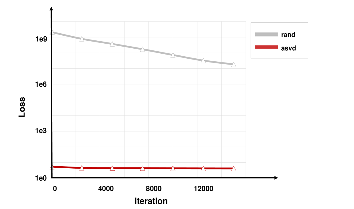
We test three initialization methods for the low-rank decomposed matrices: 1) random initialization, 2) standard SVD initialization, and 3) ASVD initialization. We keep their fine-tuning settings the same as mentioned in the Experimental Setups. The loss curves of 80% compression are shown in Figure 4, and the evaluation results for the trained models with a bi-branch strategy are shown in Table 2.
<details>
<summary>x4.png Details</summary>
### Visual Description
## Line Graph: Loss vs. Iteration
### Overview
The image depicts a line graph comparing two data series ("rand" and "asvd") across iterations. The y-axis represents "Loss" on a logarithmic scale (1e0 to 1e9), and the x-axis represents "Iteration" (0 to 14,000). The legend is positioned in the top-right corner, with "rand" in gray and "asvd" in red.
### Components/Axes
- **X-axis (Iteration)**: Labeled "Iteration," with ticks at 0, 4,000, 8,000, 12,000, and 14,000.
- **Y-axis (Loss)**: Labeled "Loss," with logarithmic ticks at 1e0, 1e3, 1e6, and 1e9.
- **Legend**: Located in the top-right corner, with:
- Gray line labeled "rand"
- Red line labeled "asvd"
### Detailed Analysis
1. **Gray Line ("rand")**:
- Starts at approximately **1e9** at iteration 0.
- Decreases monotonically, reaching **~1e7** by iteration 14,000.
- Data points are marked with white triangles (▲) along the line.
- Trend: Steady exponential decay.
2. **Red Line ("asvd")**:
- Remains nearly flat at **~1e0** across all iterations.
- Data points are marked with white triangles (▲) along the line.
- Trend: Constant value with no discernible change.
### Key Observations
- The "rand" series exhibits a significant downward trend, while "asvd" remains static.
- The logarithmic y-axis emphasizes the scale difference between the two series.
- Both lines use identical triangle markers (▲), but differ in color and trend.
### Interpretation
- **Efficiency Comparison**: The "asvd" method maintains a consistently low loss (~1e0), suggesting superior stability or optimization compared to "rand," which starts with a high loss (1e9) and gradually improves.
- **Logarithmic Scale Impact**: The y-axis compression highlights the disparity in loss magnitudes, making the "rand" trend appear more dramatic despite its gradual decline.
- **Potential Implications**: The "asvd" method may represent a more efficient algorithm or initialization strategy, as its loss does not degrade over iterations. The "rand" method’s decay could indicate a learning or optimization process, but its initial high loss suggests suboptimal starting conditions.
</details>
Figure 4: Loss curve with 80% compression ratio. "asvd" means initialize with ASVD, "rand" means random initialization. We drop the curve for standard SVD initialization as it almost overlaps with the ASVD one in the figure.
Table 2: Results of different initialization methods
| C. Ratio | Init. Method | Avg. Acc |
| --- | --- | --- |
| 0% | - | 0.99 |
| 50% | Random | 0.00 |
| SVD | 0.94 | |
| ASVD | 0.95 | |
| 60% | Random | 0.00 |
| SVD | 0.93 | |
| ASVD | 0.94 | |
| 70% | Random | 0.00 |
| SVD | 0.89 | |
| ASVD | 0.93 | |
| 80% | Random | 0.00 |
| SVD | 0.87 | |
| ASVD | 0.92 | |
It could be found that the loss of the random initialization method remains extremely high ( $∼$ 1e9) and is very hard to converge in a reasonable time, leading to the deterioration of model performance. This is quite intuitive as the information stored in the initial $W_K,W_V$ are completely destroyed and their information cannot be utilized. In contrast, the SVD-based initialization methods’ loss could converge quickly from approximately 5.5 to 4.0, leading to superior model performance. Therefore, the SVD-based initialization methods is crucial to the success of training. Specifically, the ASVD-initialized model performs slightly better than the SVD-initialized one after training, so we choose ASVD as the default initialization method.
#### C.2 Effect of Window Size
The window size determines how much local information could be preserved, which is of vital importance to the quality of generated content. We fix the compression ratio to 80% and evaluate the performance of the bi-branch trained model with multiple window size settings. The results are shown in Table 3.
Table 3: Results of different window sizes.
| 80% | 2 | 0.77 |
| --- | --- | --- |
| 4 | 0.83 | |
| 8 | 0.85 | |
| 16 | 0.88 | |
| 32 | 0.92 | |
| 64 | 0.93 | |
| 128 | 0.94 | |
| 256 | 0.94 | |
| 512 | 0.94 | |
| 1024 | 0.95 | |
| 2048 | 0.96 | |
| 4096 | 0.96 | |
The accuracy of the model shows a positive correlation with the window size, which is quite intuitive. Specifically, as the window size increases from 2 to 32, the accuracy improves relatively rapidly. However, when the window size exceeds 32, the rate of accuracy improvement notably decreases. This might indicate that a window size around 32 would be enough for local information preservation, while greater window sizes could not bring obvious improvement. Therefore, we may conclude that the model performance is positively correlated with the window size, while the benefit would become less significant after it reaches a certain level. Considering that an excessively large window size incurs non-negligible memory overhead, practitioners should carefully balance the trade-off between memory budget and accuracy when selecting the optimal window size for real-world applications.
#### C.3 Effect of Compression Ratio Allocation for KV
Different from the token pruning methods that have to keep or discard a certain token’s keys and values simultaneously, our channel shrinking method allows for the key cache and value cache to have different compression ratios. To investigate the impact of allocating a certain compression ratio to the key cache and value cache in different proportions, we conduct experiments by fixing the total compression rate at 50% and 75%, respectively. We then evaluate the model’s performance under various combinations of compression ratios for keys and values. The results are shown in Table 4.
Table 4: Results of different compression ratio assignments
| C. Ratio | KV C. Ratio | Avg. Acc |
| --- | --- | --- |
| 0% | - | 0.99 |
| 50% | K(87.5%) V(12.5%) | 0.97 |
| K(75.0%) V(25.0%) | 0.98 | |
| K(62.5%) V(37.5%) | 0.96 | |
| K(50.0%) V(50.0%) | 0.95 | |
| K(37.5%) V(62.5%) | 0.95 | |
| K(25.0%) V(75.0%) | 0.94 | |
| K(12.5%) V(87.5%) | 0.80 | |
| 75% | K(43.75%) V(6.25%) | 0.73 |
| K(37.50%) V(12.50%) | 0.89 | |
| K(31.25%) V(18.75%) | 0.95 | |
| K(25.00%) V(25.00%) | 0.93 | |
| K(18.75%) V(31.25%) | 0.88 | |
| K(12.59%) V(37.50%) | 0.80 | |
| K(6.25%) V(43.75%) | 0.43 | |
It could be found from the evaluation results that among the selected combinations, the optimal configuration consistently occurs when the compression ratio for the key cache exceeds that of the value cache, showing that it would be better to compress the key cache more than the value cache given a certain budget, in most cases. This potentially reveals that the sensitivity of keys towards compression is weaker than that of values, making the key cache much easier to compress.
#### C.4 Compatibility with Quantization
As the low-bit quantization methods are orthogonal with our method, we further demonstrate that quantization could be seamlessly combined with our method. Specifically, we apply KIVI [13] with 4-bit quantization on the compressed keys and values, using per-channel quantization for the former and per-token quantization for the latter. Both the window size and the residual size are set to 32. We separately perform the experiments with two quantization manners: PTQ (Post-Training Quantization) and QAT (Quantization-Aware Training). The results are shown in Table 5, where the "None" rows are the referenced results from the full-precision model.
Table 5: Results of integration with quantization
| C. Ratio (origin) | C. Ratio (4-bit) | Q. Mode | Avg. Acc |
| --- | --- | --- | --- |
| 0% | 0% | - | 0.99 |
| 50% | 87.5% | None | 0.95 |
| PTQ | 0.00 | | |
| QAT | 0.96 | | |
| 60% | 90.0% | None | 0.94 |
| PTQ | 0.00 | | |
| QAT | 0.94 | | |
| 70% | 92.5% | None | 0.93 |
| PTQ | 0.00 | | |
| QAT | 0.92 | | |
| 80% | 95.0% | None | 0.92 |
| PTQ | 0.00 | | |
| QAT | 0.90 | | |
According to the results in Table 5, directly applying PTQ would completely deteriorate the model’s performance, while the QAT results show minor degradation compared with their full-precision counterparts. The failure of PTQ might be a result of the significant density of the compressed representations, which are a lot more intact and difficult to directly quantize. In contrast, the QAT method includes the quantization loss during the optimization process and shows great compatibility with our channel shrinking method, where a total of 95% compression would still keep more than 90% of the model’s long-context capability. Therefore, it could be concluded that it would be better to compress the key cache more than the value cache given a certain budget, in most cases.