# Interpretable Contrastive Monte Carlo Tree Search Reasoning
\intervalconfig
soft open fences
Abstract
We propose (S) peculative (C) ontrastive MCTS ∗: a novel Monte Carlo Tree Search (MCTS) reasoning algorithm for Large Language Models (LLMs) which significantly improves both reasoning accuracy and speed. Our motivation comes from: 1. Previous MCTS LLM reasoning works often overlooked its biggest drawback—slower speed compared to CoT; 2. Previous research mainly used MCTS as a tool for LLM reasoning on various tasks with limited quantitative analysis or ablation studies of its components from reasoning interpretability perspective. 3. The reward model is the most crucial component in MCTS, however previous work has rarely conducted in-depth study or improvement of MCTS’s reward models. Thus, we conducted extensive ablation studies and quantitative analysis on components of MCTS, revealing the impact of each component on the MCTS reasoning performance of LLMs. Building on this, (i) we designed a highly interpretable reward model based on the principle of contrastive decoding and (ii) achieved an average speed improvement of 51.9% per node using speculative decoding. Additionally, (iii) we improved UCT node selection strategy and backpropagation used in previous works, resulting in significant performance improvement. We outperformed o1-mini by an average of 17.4% on the Blocksworld multi-step reasoning dataset using Llama-3.1-70B with SC-MCTS ∗. Our code is available at https://github.com/zitian-gao/SC-MCTS.
1 Introduction
With the remarkable development of Large Language Models (LLMs), models such as o1 (OpenAI, 2024a) have now gained a strong ability for multi-step reasoning across complex tasks and can solve problems that are more difficult than previous scientific, code, and mathematical problems. The reasoning task has long been considered challenging for LLMs. These tasks require converting a problem into a series of reasoning steps and then executing those steps to arrive at the correct answer. Recently, LLMs have shown great potential in addressing such problems. A key approach is using Chain of Thought (CoT) (Wei et al., 2024), where LLMs break down the solution into a series of reasoning steps before arriving at the final answer. Despite the impressive capabilities of CoT-based LLMs, they still face challenges when solving problems with an increasing number of reasoning steps due to the curse of autoregressive decoding (Sprague et al., 2024). Previous work has explored reasoning through the use of heuristic reasoning algorithms. For example, Yao et al. (2024) applied heuristic-based search, such as Depth-First Search (DFS) to derive better reasoning paths. Similarly, Hao et al. (2023) employed MCTS to iteratively enhance reasoning step by step toward the goal.
The tremendous success of AlphaGo (Silver et al., 2016) has demonstrated the effectiveness of the heuristic MCTS algorithm, showcasing its exceptional performance across various domains (Jumper et al., 2021; Silver et al., 2017). Building on this, MCTS has also made notable progress in the field of LLMs through multi-step heuristic reasoning. Previous work has highlighted the potential of heuristic MCTS to significantly enhance LLM reasoning capabilities. Despite these advancements, substantial challenges remain in fully realizing the benefits of heuristic MCTS in LLM reasoning.
<details>
<summary>extracted/6087579/fig/Fig1.png Details</summary>
### Visual Description
\n
## Diagram: BlocksWorld Task Decomposition
### Overview
This diagram illustrates the decomposition of a BlocksWorld task – placing the red block on top of the yellow block – into a sequence of actions. It compares the action choices (logits) of "Expert" and "Amateur" agents at different stages (S0, S1, S2) of the task, and visualizes the resulting action sequences (a0, a1). The diagram shows how the agents' preferences for different actions evolve as they approach the goal.
### Components/Axes
The diagram is structured into three main vertical sections representing stages S0, S1, and S2. Each stage has two sub-sections: "Expert Logits (SE)" and "Amateur Logits (SA)". Each of these sub-sections contains a small table with numerical values. To the right of stages S1 and S2 are "CD Logits (SCD)" blocks, which show the selected action with a checkmark. The rightmost portion of the diagram shows the state transitions resulting from the selected actions, visualized as block arrangements.
* **Stages (S0, S1, S2):** Represent the progression of the task.
* **Expert Logits (SE):** Numerical values indicating the preference of an expert agent for different actions.
* **Amateur Logits (SA):** Numerical values indicating the preference of an amateur agent for different actions.
* **CD Logits (SCD):** Shows the selected action at each stage, with a checkmark indicating the chosen action.
* **Block Arrangements:** Visual representation of the state of the blocks at different stages.
* **Goal:** "The red block is on top of the yellow block" (stated at the top of the diagram).
### Detailed Analysis or Content Details
**S0 (Initial State):**
* No logits are shown for S0. The initial state is simply defined by the goal.
**S1:**
* **Expert Logits (SE):** The table shows a single value of 8. This is associated with the action "unstack red". A second value of 1 is also present.
* **Amateur Logits (SA):** The table shows values of 6, 2, and 2. These are associated with the actions "unstack red", "pick up blue", and "pick up yellow" respectively.
* **CD Logits (SCD1):** The selected action is "unstack red" (marked with a checkmark). Other options listed are "pick up blue" and "pick up yellow".
* **Action Sequence (a0):** The diagram shows the action "unstack the red" leading to a new block arrangement.
**S2:**
* **Expert Logits (SE):** The table shows a single value of 7. A second value of 1 is also present.
* **Amateur Logits (SA):** The table shows values of 3, 2, 2, and 3. These are associated with the actions "stack on yellow", "stack on blue", "stack on green", and "put-down red" respectively.
* **CD Logits (SCD2):** The selected action is "stack on yellow" (marked with a checkmark). Other options listed are "stack on blue", "stack on green", and "put-down red".
* **Action Sequence (a1):** The diagram shows the action "stack on the yellow" leading to a new block arrangement.
**Legend:**
* **unstack red:** Represented by a light purple color.
* **pick up blue:** Represented by a light blue color.
* **pick up yellow:** Represented by a light yellow color.
* **stack on yellow:** Represented by a dark blue color.
* **stack on blue:** Represented by a dark green color.
* **stack on green:** Represented by a dark red color.
* **put-down red:** Represented by a light red color.
### Key Observations
* The expert agent consistently shows a much stronger preference for the correct action ("unstack red" in S1, "stack on yellow" in S2) compared to the amateur agent.
* The amateur agent's logits are more distributed across multiple actions, indicating greater uncertainty.
* The selected actions at each stage (indicated by the checkmarks) align with the goal of placing the red block on top of the yellow block.
* The block arrangements visually demonstrate the state transitions resulting from the selected actions.
### Interpretation
This diagram demonstrates a hierarchical task decomposition approach to solving the BlocksWorld problem. The expert agent exhibits a more focused and decisive action selection process, as evidenced by the higher logits for the correct actions. The amateur agent, on the other hand, explores a wider range of actions, suggesting a less efficient or less informed strategy. The diagram highlights the importance of having a clear understanding of the task and a strong preference for the correct actions in achieving the goal. The visualization of the block arrangements provides a concrete understanding of how the actions contribute to the overall task solution. The difference in logits between the expert and amateur agents suggests that the expert has a better internal model of the task and its requirements. The diagram could be used to analyze and compare different planning algorithms or agent architectures.
</details>
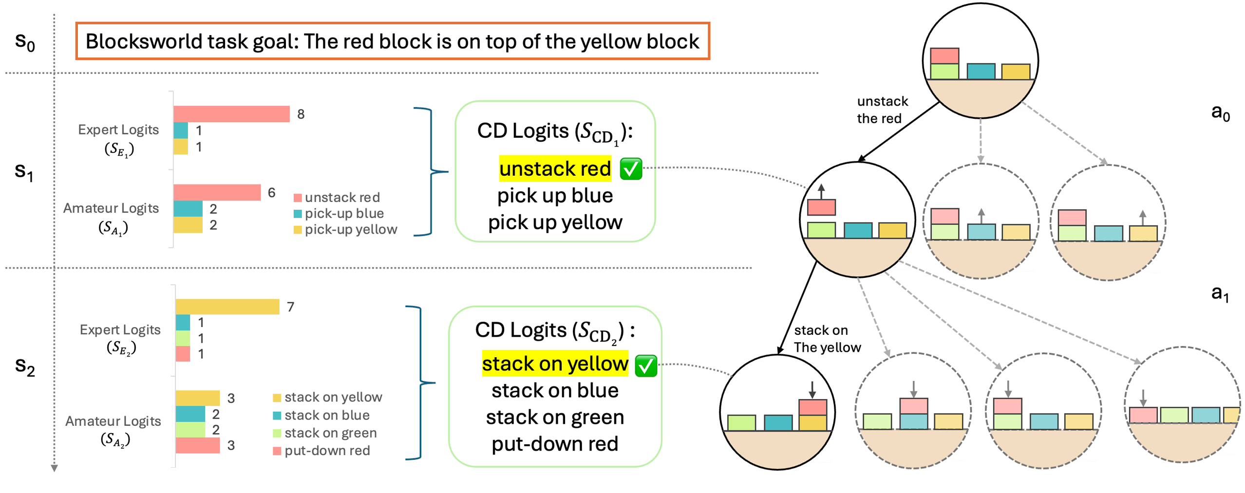
Figure 1: An overview of SC-MCTS ∗. We employ a novel reward model based on the principle of contrastive decoding to guide MCTS Reasoning on Blocksworld multi-step reasoning dataset.
The first key challenge is that MCTS’s general reasoning ability is almost entirely dependent on the reward model’s performance (as demonstrated by our ablation experiments in Section 5.5), making it highly challenging to design dense, general yet efficient rewards to guide MCTS reasoning. Previous works either require two or more LLMs (Tian et al., 2024) or training epochs (Zhang et al., 2024a), escalating the VRAM and computational demand, or they rely on domain-specific tools (Xin et al., 2024a; b) or datasets (Qi et al., 2024), making it difficult to generalize to other tasks or datasets.
The second key challenge is that MCTS is significantly slower than Chain of Thoughts (CoT). CoT only requires designing a prompt of multi-turn chats (Wei et al., 2024). In contrast, MCTS builds a reasoning tree with 2–10 layers depending on the difficulty of the task, where each node in the tree represents a chat round with LLM which may need to be visited one or multiple times. Moreover, to obtain better performance, we typically perform 2–10 MCTS iterations, which greatly increases the number of nodes, leading to much higher computational costs and slower reasoning speed.
To address the these challenges, we went beyond prior works that treated MCTS as a tool and focused on analyzing and improving its components especially reward model. Using contrastive decoding, we redesigned reward model by integrating interpretable reward signals, clustering their prior distributions, and normalizing the rewards using our proposed prior statistical method. To prevent distribution shift, we also incorporated an online incremental update algorithm. We found that the commonly used Upper Confidence Bound on Trees (UCT) strategy often underperformed due to sensitivity to the exploration constant, so we refined it and improved backpropagation to favor steadily improving paths. To address speed issues, we integrated speculative decoding as a "free lunch." All experiments were conducted using the Blocksworld dataset detailed in Section 5.1.
Our goal is to: (i) design novel and high-performance reward models and maximize the performance of reward model combinations, (ii) analyze and optimize the performance of various MCTS components, (iii) enhance the interpretability of MCTS reasoning, (iv) and accelerate MCTS reasoning. Our contributions are summarized as follows:
1. We went beyond previous works who primarily treated MCTS as an tool rather than analyzing and improving its components. Specifically, we found the UCT strategy in most previous works may failed to function from our experiment. We also refined the backpropagation of MCTS to prefer more steadily improving paths, boosting performance.
1. To fully study the interpretability of MCTS multi-step reasoning, we conducted extensive quantitative analysis and ablation studies on every component. We carried out numerous experiments from both the numerical and distributional perspectives of the reward models, as well as its own interpretability, providing better interpretability for MCTS multi-step reasoning.
1. We designed a novel, general action-level reward model based on the principle of contrastive decoding, which requires no external tools, training, or datasets. Additionally, we found that previous works often failed to effectively harness multiple reward models, thus we proposed a statistical linear combination method. At the same time, we introduced speculative decoding to speed up MCTS reasoning by an average of 52% as a "free lunch."
We demonstrated the effectiveness of our approach by outperforming OpenAI’s flagship o1-mini model by an average of 17.4% using Llama-3.1-70B on the Blocksworld multi-step reasoning dataset.
2 Related Work
Large Language Models Multi-Step Reasoning
One of the key focus areas for LLMs is understanding and enhancing their reasoning capabilities. Recent advancements in this area focused on developing methods that improve LLMs’ ability to handle complex tasks in domains like code generation and mathematical problem-solving. Chain-of-Thought (CoT) (Wei et al., 2024) reasoning has been instrumental in helping LLMs break down intricate problems into a sequence of manageable steps, making them more adept at handling tasks that require logical reasoning. Building upon this, Tree-of-Thought (ToT) (Yao et al., 2024) reasoning extends CoT by allowing models to explore multiple reasoning paths concurrently, thereby enhancing their ability to evaluate different solutions simultaneously. Complementing these approaches, Monte Carlo Tree Search (MCTS) has emerged as a powerful reasoning method for decision-making in LLMs. Originally successful in AlphaGo’s victory (Silver et al., 2016), MCTS has been adapted to guide model-based planning by balancing exploration and exploitation through tree-based search and random sampling, and later to large language model reasoning (Hao et al., 2023), showing great results. This adaptation has proven particularly effective in areas requiring strategic planning. Notable implementations like ReST-MCTS ∗ (Zhang et al., 2024a), rStar (Qi et al., 2024), MCTSr (Zhang et al., 2024b) and Xie et al. (2024) have shown that integrating MCTS with reinforced self-training, self-play mutual reasoning or Direct Preference Optimization (Rafailov et al., 2023) can significantly improve reasoning capabilities in LLMs. Furthermore, recent advancements such as Deepseek Prover (Xin et al., 2024a; b) demonstrates the potential of these models to understand complex instructions such as formal mathematical proof.
Decoding Strategies
Contrastive decoding and speculative decoding both require Smaller Language Models (SLMs), yet few have realized that these two clever decoding methods can be seamlessly combined without any additional cost. The only work that noticed this was Yuan et al. (2024a), but their proposed speculative contrastive decoding focused on token-level decoding. In contrast, we designed a new action-level contrastive decoding to guide MCTS reasoning, the distinction will be discussed further in Section 4.1. For more detailed related work please refer to Appendix B.
3 Preliminaries
3.1 Multi-Step Reasoning
A multi-step reasoning problem can be modeled as a Markov Decision Process (Bellman, 1957) $\mathcal{M}=(S,A,P,r,\gamma)$ . $S$ is the state space containing all possible states, $A$ the action space, $P(s^{\prime}|s,a)$ the state transition function, $r(s,a)$ the reward function, and $\gamma$ the discount factor. The goal is to learn and to use a policy $\pi$ to maximize the discounted cumulative reward $\mathbb{E}_{\tau\sim\pi}\left[\sum_{t=0}^{T}\gamma^{t}r_{t}\right]$ . For reasoning with LLMs, we are more focused on using an existing LLM to achieve the best reasoning.
3.2 Monte Carlo Tree Search
Monte Carlo Tree Search (MCTS) is a decision-making algorithm involving a search tree to simulate and evaluate actions. The algorithm operates in the following four phases:
Node Selection: The selection process begins at the root, selecting nodes hierarchically using strategies like UCT as the criterion to favor a child node based on its quality and novelty.
Expansion: New child nodes are added to the selected leaf node by sampling $d$ possible actions, predicting the next state. If the leaf node is fully explored or terminal, expansion is skipped.
Simulation: During simulation or “rollout”, the algorithm plays out the “game” randomly from that node to a terminal state using a default policy.
Backpropagation: Once a terminal state is reached, the reward is propagated up the tree, and each node visited during the selection phase updates its value based on the simulation result.
Through iterative application of its four phases, MCTS efficiently improves reasoning through trials and heuristics, converging on the optimal solution.
3.3 Contrastive Decoding
We discuss vanilla Contrastive Decoding (CD) from Li et al. (2023), which improves text generation in LLMs by reducing errors like repetition and self-contradiction. CD uses the differences between an expert model and an amateur model, enhancing the expert’s strengths and suppressing the amateur’s weaknesses. Consider a prompt of length $n$ , the CD objective is defined as:
$$
{\mathcal{L}}_{\text{CD}}(x_{\text{cont}},x_{\text{pre}})=\log p_{\text{EXP}}(%
x_{\text{cont}}|x_{\text{pre}})-\log p_{\text{AMA}}(x_{\text{cont}}|x_{\text{%
pre}})
$$
where $x_{\text{pre}}$ is the sequence of tokens $x_{1},...,x_{n}$ , the model generates continuations of length $m$ , $x_{\text{cont}}$ is the sequence of tokens $x_{n+1},...,x_{n+m}$ , and $p_{\text{EXP}}$ and $p_{\text{AMA}}$ are the expert and amateur probability distributions. To avoid penalizing correct behavior of the amateur or promoting implausible tokens, CD applies an adaptive plausibility constraint using an $\alpha$ -mask, which filters tokens by their logits against a threshold, the filtered vocabulary $V_{\text{valid}}$ is defined as:
$$
V_{\text{valid}}=\{i\mid s^{(i)}_{\text{EXP}}\geq\log\alpha+\max_{k}s^{(k)}_{%
\text{EXP}}\}
$$
where $s^{(i)}_{\text{EXP}}$ and $s^{(i)}_{\text{AMA}}$ are unnormalized logits assigned to token i by the expert and amateur models. Final logits are adjusted with a coefficient $(1+\beta)$ , modifying the contrastive effect on output scores (Liu et al., 2021):
$$
s^{(i)}_{\text{CD}}=(1+\beta)s^{(i)}_{\text{EXP}}-s^{(i)}_{\text{AMA}}
$$
However, our proposed CD is at action level, averaging over the whole action, instead of token level in vanilla CD. Our novel action-level CD reward more robustly captures the differences in confidence between the expert and amateur models in the generated answers compared to vanilla CD. The distinction will be illustrated in Section 4.1 and explained further in Appendix A.
3.4 Speculative Decoding as "free lunch"
Based on Speculative Decoding (Leviathan et al., 2023), the process can be summarized as follows: Let $M_{p}$ be the target model with the conditional distribution $p(x_{t}|x_{<t})$ , and $M_{q}$ be a smaller approximation model with $q(x_{t}|x_{<t})$ . The key idea is to generate $\gamma$ tokens using $M_{q}$ and filter them against $M_{p}$ ’s distribution, accepting tokens consistent with $M_{p}$ . Speculative decoding samples $\gamma$ tokens autoregressively from $M_{q}$ , keeping those where $q(x)≤ p(x)$ . If $q(x)>p(x)$ , the sample is rejected with probability $1-\frac{p(x)}{q(x)}$ , and a new sample is drawn from the adjusted distribution:
$$
p^{\prime}(x)=\text{norm}(\max(0,p(x)-q(x))).
$$
Since both contrastive and speculative decoding rely on the same smaller models, we can achieve the acceleration effect of speculative decoding as a "free lunch" (Yuan et al., 2024a).
4 Method
4.1 Multi-Reward Design
Our primary goal is to design novel and and high-performance reward models for MCTS reasoning and to maximize the performance of reward model combinations, as our ablation experiments in Section 5.5 demonstrate that MCTS performance is almost entirely determined by the reward model.
SC-MCTS ∗ is guided by three highly interpretable reward models: contrastive JS divergence, loglikelihood and self evaluation. Previous work such as (Hao et al., 2023) often directly adds reward functions with mismatched numerical magnitudes without any prior statistical analysis or linear combination. As a result, their combined reward models may fail to demonstrate full performance. Moreover, combining multiple rewards online presents numerous challenges such as distributional shifts in the values. Thus, we propose a statistically-informed reward combination method: Multi-RM method. Each reward model is normalized contextually by the fine-grained prior statistics of its empirical distribution. The pseudocode for reward model construction is shown in Algorithm 1. Please refer to Appendix D for a complete version of SC-MCTS ∗ that includes other improvements such as dealing with distribution shift when combining reward functions online.
Algorithm 1 SC-MCTS ∗, reward model construction
1: Expert LLM $\pi_{e}$ , Amateur SLM $\pi_{a}$ , Problem set $D$ ; $M$ selected problems for prior statistics, $N$ pre-generated solutions per problem, $K$ clusters
2: $\tilde{A}←\text{Sample-solutions}(\pi_{e},D,M,N)$ $\triangleright$ Pre-generate $M× N$ solutions
3: $p_{e},p_{a}←\text{Evaluate}(\pi_{e},\pi_{a},\tilde{A})$ $\triangleright$ Get policy distributions
4: for $r∈\{\text{JSD},\text{LL},\text{SE}\}$ do
5: $\bm{\mu}_{r},\bm{\sigma}_{r},\bm{b}_{r}←\text{Cluster-stats}(r(\tilde%
{A}),K)$ $\triangleright$ Prior statistics (Equation 1)
6: $R_{r}← x\mapsto(r(x)-\mu_{r}^{k^{*}})/\sigma_{r}^{k^{*}}$ $\triangleright$ Reward normalization (Equation 2)
7: end for
8: $R←\sum_{r∈\{\text{JSD},\text{LL},\text{SE}\}}w_{r}R_{r}$ $\triangleright$ Composite reward
9: $A_{D}←\text{MCTS-Reasoning}(\pi_{e},R,D,\pi_{a})$ $\triangleright$ Search solutions guided by $R$
10: $A_{D}$
Jensen-Shannon Divergence
The Jensen-Shannon divergence (JSD) is a symmetric and bounded measure of similarity between two probability distributions $P$ and $Q$ . It is defined as:
$$
\mathrm{JSD}(P\,\|\,Q)=\frac{1}{2}\mathrm{KL}(P\,\|\,M)+\frac{1}{2}\mathrm{KL}%
(Q\,\|\,M),\quad M=\frac{1}{2}(P+Q),
$$
where $\mathrm{KL}(P\,\|\,Q)$ is the Kullback-Leibler Divergence (KLD), and $M$ represents the midpoint distribution. The JSD is bounded between 0 and 1 for discrete distributions, making it better than KLD for online normalization of reward modeling.
Inspired by contrastive decoding, we propose our novel reward model: JSD between the expert model’s logits and the amateur model’s logits. Unlike vanilla token-level contrastive decoding (Li et al., 2023), our reward is computed at action-level, treating a sequence of action tokens as a whole:
$$
R_{\text{JSD}}=\frac{1}{n}\sum_{i=T_{\text{prefix}}+1}^{n}\left[\mathrm{JSD}(p%
_{\text{e}}(x_{i}|x_{<i})\,\|\,p_{\text{a}}(x_{i}|x_{<i})\right]
$$
where $n$ is the length of tokens, $T_{\text{prefix}}$ is the index of the last prefix token, $p_{\text{e}}$ and $p_{\text{a}}$ represent the softmax probabilities of the expert and amateur models, respectively. This approach ensures that the reward captures model behavior at the action level as the entire sequence of tokens is taken into account at once. This contrasts with vanilla token-level methods where each token is treated serially.
Loglikelihood
Inspired by Hao et al. (2023), we use a loglikelihood reward model to evaluate the quality of generated answers based on a given question prefix. The model computes logits for the full sequence (prefix + answer) and accumulates the log-probabilities over the answer part tokens.
Let the full sequence $x=(x_{1},x_{2},...,x_{T_{\text{total}}})$ consist of a prefix and a generated answer. The loglikelihood reward $R_{\text{LL}}$ is calculated over the answer portion:
$$
R_{\text{LL}}=\sum_{i=T_{\text{prefix}}+1}^{T_{\text{total}}}\log\left(\frac{%
\exp(z_{\theta}(x_{i}))}{\sum_{x^{\prime}\in V}\exp(z_{\theta}(x^{\prime}))}\right)
$$
where $z_{\theta}(x_{i})$ represents the unnormalized logit for token $x_{i}$ . After calculating logits for the entire sequence, we discard the prefix and focus on the answer tokens to form the loglikelihood reward.
Self Evaluation
Large language models’ token-level self evaluation can effectively quantify the model’s uncertainty, thereby improving the quality of selective generation (Ren et al., 2023). We instruct the LLM to perform self evaluation on its answers, using a action level evaluation method, including a self evaluation prompt to explicitly indicate the model’s uncertainty.
After generating the answer, we prompt the model to self-evaluate its response by asking "Is this answer correct/good?" This serves to capture the model’s confidence in its own output leading to more informed decision-making. The self evaluation prompt’s logits are then used to calculate a reward function. Similar to the loglikelihood reward model, we calculate the self evaluation reward $R_{\text{SE}}$ by summing the log-probabilities over the self-evaluation tokens.
Harnessing Multiple Reward Models
We collected prior distributions for the reward models and found some of them span multiple regions. Therefore, we compute the fine-grained prior statistics as mean and standard deviation of modes of the prior distribution ${\mathcal{R}}∈\{{\mathcal{R}}_{\text{JSD}},{\mathcal{R}}_{\text{LL}},{%
\mathcal{R}}_{\text{SE}}\}$ :
$$
\mu^{(k)}=\frac{1}{c_{k}}\sum_{R_{i}\in\rinterval{b_{1}}{b_{k+1}}}R_{i}\quad%
\text{and}\quad\sigma^{(k)}=\sqrt{\frac{1}{c_{k}}\sum_{R_{i}\in\rinterval{b_{1%
}}{b_{k+1}}}(R_{i}-\mu^{(k)})^{2}} \tag{1}
$$
where $b_{1}<b_{2}<...<b_{K+1}$ are the region boundaries in ${\mathcal{R}}$ , $R_{i}∈{\mathcal{R}}$ , and $c_{k}$ is the number of $R_{i}$ in $\rinterval{b_{1}}{b_{k+1}}$ . The region boundaries were defined during the prior statistical data collection phase 1.
After we computed the fine-grained prior statistics, the reward factors are normalized separately for each region (which degenerates to standard normalization if only a single region is found):
$$
R_{\text{norm}}(x)=(R(x)-\mu^{(k^{*})})/\sigma^{(k^{*})},~{}\text{where}~{}k^{%
*}=\operatorname*{arg\,max}\{k:b_{k}\leq R(x)\} \tag{2}
$$
This reward design, which we call Multi-RM method, has some caveats: first, to prevent distribution shift during reasoning, we update the mean and standard deviation of the reward functions online for each mode (see Appendix D for pseudocode); second, we focus only on cases with clearly distinct reward modes, leaving general cases for future work. For the correlation heatmap, see Appendix C.
4.2 Node Selection Strategy
Upper Confidence Bound applied on Trees Algorithm (UCT) (Coquelin & Munos, 2007) is crucial for the selection phase, balancing exploration and exploitation by choosing actions that maximize:
$$
UCT_{j}=\bar{X}_{j}+C\sqrt{\frac{\ln N}{N_{j}}}
$$
where $\bar{X}_{j}$ is the average reward of taking action $j$ , $N$ is the number of times the parent has been visited, and $N_{j}$ is the number of times node $j$ has been visited for simulation, $C$ is a constant to balance exploitation and exploration.
However, $C$ is a crucial part of UCT. Previous work (Hao et al., 2023; Zhang et al., 2024b) had limited thoroughly investigating its components, leading to potential failures of the UCT strategy. This is because they often used the default value of 1 from the original proposed UCT (Coquelin & Munos, 2007) without conducting sufficient quantitative experiments to find the optimal $C$ . This will be discussed in detail in Section 5.4.
4.3 Backpropagation
After each MCTS iteration, multiple paths from the root to terminal nodes are generated. By backpropagating along these paths, we update the value of each state-action pair. Previous MCTS approaches often use simple averaging during backpropagation, but this can overlook paths where the goal achieved metric $G(p)$ progresses smoothly (e.g., $G(p_{1})=0→ 0.25→ 0.5→ 0.75$ ). These paths just few step away from the final goal $G(p)=1$ , are often more valuable than less stable ones.
To improve value propagation, we propose an algorithm that better captures value progression along a path. Given a path $\mathbf{P}=\{p_{1},p_{2},...,p_{n}\}$ with $n$ nodes, where each $p_{i}$ represents the value at node $i$ , the total value is calculated by summing the increments between consecutive nodes with a length penalty. The increment between nodes $p_{i}$ and $p_{i-1}$ is $\Delta_{i}=p_{i}-p_{i-1}$ . Negative increments are clipped at $-0.1$ and downweighted by 0.5. The final path value $V_{\text{final}}$ is:
$$
V_{\text{final}}=\sum_{i=2}^{n}\left\{\begin{array}[]{ll}\Delta_{i},&\text{if %
}\Delta_{i}\geq 0\\
0.5\times\max(\Delta_{i},-0.1),&\text{if }\Delta_{i}<0\end{array}\right\}-%
\lambda\times n \tag{3}
$$
where $n$ is the number of nodes in the path and $\lambda=0.1$ is the penalty factor to discourage long paths.
5 Experiments
5.1 Dataset
Blocksworld (Valmeekam et al., 2024; 2023) is a classic domain in AI research for reasoning and planning, where the goal is to rearrange blocks into a specified configuration using actions like ’pick-up,’ ’put-down,’ ’stack,’ and ’unstack. Blocks can be moved only if no block on top, and only one block at a time. The reasoning process in Blocksworld is a MDP. At time step $t$ , the LLM agent selects an action $a_{t}\sim p(a\mid s_{t},c)$ , where $s_{t}$ is the current block configuration, $c$ is the prompt template. The state transition $s_{t+1}=P(s_{t},a_{t})$ is deterministic and is computed by rules. This forms a trajectory of interleaved states and actions $(s_{0},a_{0},s_{1},a_{1},...,s_{T})$ towards the goal state.
One key feature of Blocksworld is its built-in verifier, which tracks progress toward the goal at each step. This makes Blocksworld ideal for studying heuristic LLM multi-step reasoning. However, we deliberately avoid using the verifier as part of the reward model as it is task-specific. More details of Blocksworld can be found in Appendix F.
5.2 Main Results
To evaluate the SC-MCTS ∗ algorithm in LLM multi-step reasoning, we implemented CoT, RAP-MCTS, and SC-MCTS ∗ using Llama-3-70B and Llama-3.1-70B. For comparison, we used Llama-3.1-405B and GPT-4o for CoT, and applied 0 and 4 shot single turn for o1-mini, as OpenAI (2024b) suggests avoiding CoT prompting. The experiment was conducted on Blocksworld dataset across all steps and difficulties. For LLM settings, GPU and OpenAI API usage data, see Appendix E and H.
| Mode | Models | Method | Steps | | | | | | |
| --- | --- | --- | --- | --- | --- | --- | --- | --- | --- |
| Step 2 | Step 4 | Step 6 | Step 8 | Step 10 | Step 12 | Avg. | | | |
| Easy | Llama-3-70B ~Llama-3.2-1B | 4-shot CoT | 0.2973 | 0.4405 | 0.3882 | 0.2517 | 0.1696 | 0.1087 | 0.2929 |
| RAP-MCTS | 0.9459 | 0.9474 | 0.8138 | 0.4196 | 0.2136 | 0.1389 | 0.5778 | | |
| SC-MCTS* (Ours) | 0.9730 | 0.9737 | 0.8224 | 0.4336 | 0.2136 | 0.2222 | 0.5949 | | |
| Llama-3.1-70B ~Llama-3.2-1B | 4-shot CoT | 0.5405 | 0.4868 | 0.4069 | 0.2238 | 0.2913 | 0.2174 | 0.3441 | |
| RAP-MCTS | 1.0000 | 0.9605 | 0.8000 | 0.4336 | 0.2039 | 0.1111 | 0.5796 | | |
| SC-MCTS* (Ours) | 1.0000 | 0.9737 | 0.7724 | 0.4503 | 0.3010 | 0.1944 | 0.6026 | | |
| Llama-3.1-405B | 0-shot CoT | 0.8108 | 0.6579 | 0.5931 | 0.5105 | 0.4272 | 0.3611 | 0.5482 | |
| 4-shot CoT | 0.7838 | 0.8553 | 0.6483 | 0.4266 | 0.5049 | 0.4167 | 0.5852 | | |
| o1-mini | 0-shot | 0.9730 | 0.7368 | 0.5103 | 0.3846 | 0.3883 | 0.1944 | 0.4463 | |
| 4-shot | 0.9459 | 0.8026 | 0.6276 | 0.3497 | 0.3301 | 0.2222 | 0.5167 | | |
| GPT-4o | 0-shot CoT | 0.5405 | 0.4868 | 0.3241 | 0.1818 | 0.1165 | 0.0556 | 0.2666 | |
| 4-shot CoT | 0.5135 | 0.6579 | 0.6000 | 0.2797 | 0.3010 | 0.3611 | 0.4444 | | |
| Hard | Llama-3-70B ~Llama-3.2-1B | 4-shot CoT | 0.5556 | 0.4405 | 0.3882 | 0.2517 | 0.1696 | 0.1087 | 0.3102 |
| RAP-MCTS | 1.0000 | 0.8929 | 0.7368 | 0.4503 | 0.1696 | 0.1087 | 0.5491 | | |
| SC-MCTS* (Ours) | 0.9778 | 0.8929 | 0.7566 | 0.5298 | 0.2232 | 0.1304 | 0.5848 | | |
| Llama-3.1-70B ~Llama-3.2-1B | 4-shot CoT | 0.6222 | 0.2857 | 0.3421 | 0.1722 | 0.1875 | 0.2174 | 0.2729 | |
| RAP-MCTS | 0.9778 | 0.9048 | 0.7829 | 0.4702 | 0.1875 | 0.1087 | 0.5695 | | |
| SC-MCTS* (Ours) | 0.9778 | 0.9405 | 0.8092 | 0.4702 | 0.1696 | 0.2174 | 0.5864 | | |
| Llama-3.1-405B | 0-shot CoT | 0.7838 | 0.6667 | 0.6053 | 0.3684 | 0.2679 | 0.2609 | 0.4761 | |
| 4-shot CoT | 0.8889 | 0.6667 | 0.6579 | 0.4238 | 0.5804 | 0.5217 | 0.5915 | | |
| o1-mini | 0-shot | 0.6889 | 0.4286 | 0.1776 | 0.0993 | 0.0982 | 0.0000 | 0.2034 | |
| 4-shot | 0.9556 | 0.8452 | 0.5263 | 0.3907 | 0.2857 | 0.1739 | 0.4966 | | |
| GPT-4o | 0-shot CoT | 0.6222 | 0.3929 | 0.3026 | 0.1523 | 0.0714 | 0.0000 | 0.2339 | |
| 4-shot CoT | 0.6222 | 0.4167 | 0.5197 | 0.3642 | 0.3304 | 0.1739 | 0.4102 | | |
Table 1: Accuracy of various reasoning methods and models across steps and difficulty modes on the Blocksworld multi-step reasoning dataset.
From Table 1, it can be observed that SC-MCTS ∗ significantly outperforms RAP-MCTS and 4-shot CoT across both easy and hard modes, and in easy mode, Llama-3.1-70B model using SC-MCTS ∗ outperforms the 4-shot CoT Llama-3.1-405B model.
<details>
<summary>extracted/6087579/fig/acc.png Details</summary>
### Visual Description
\n
## Line Chart: Accuracy vs. Step for Different Models
### Overview
The image presents two line charts, side-by-side, comparing the accuracy of several language models (Llama-3.1-70B, Llama-3.1-405B, and ol-mini) across different steps (2, 4, 6, 8, 10, and 12). The accuracy is measured on the y-axis, ranging from 0.0 to 1.0, while the step number is on the x-axis. Each line represents a different model or configuration. The charts appear to be evaluating the performance of these models in a multi-step reasoning process.
### Components/Axes
* **Y-axis Label:** "Accuracy" (Scale: 0.0 to 1.0, increments of 0.2)
* **X-axis Label:** "Step" (Markers: 2, 4, 6, 8, 10, 12)
* **Legend (Top-Right of each chart):**
* Llama-3.1-70B: 4-shot CoT (Orange, dashed line)
* Llama-3.1-70B: RAP-MCTS (Yellow, dashed line)
* Llama-3.1-70B: SC-MCTS¹ (Ours) (Red, solid line)
* ol-mini: 4-shot (Pink, dashed line)
* Llama-3.1-405B: 4-shot CoT (Blue, dashed line)
### Detailed Analysis or Content Details
**Chart 1 (Left):**
* **Llama-3.1-70B: 4-shot CoT (Orange):** Starts at approximately 0.9 accuracy at Step 2, decreases steadily to approximately 0.15 at Step 12.
* **Llama-3.1-70B: RAP-MCTS (Yellow):** Starts at approximately 0.8 accuracy at Step 2, decreases to approximately 0.2 at Step 12.
* **Llama-3.1-70B: SC-MCTS¹ (Ours) (Red):** Starts at approximately 0.85 accuracy at Step 2, decreases rapidly to approximately 0.1 at Step 12.
* **ol-mini: 4-shot (Pink):** Starts at approximately 0.7 accuracy at Step 2, decreases sharply to approximately 0.1 at Step 12.
* **Llama-3.1-405B: 4-shot CoT (Blue):** Starts at approximately 0.95 accuracy at Step 2, decreases rapidly to approximately 0.15 at Step 12.
**Chart 2 (Right):**
* **Llama-3.1-70B: 4-shot CoT (Orange):** Starts at approximately 0.9 accuracy at Step 2, decreases steadily to approximately 0.15 at Step 12.
* **Llama-3.1-70B: RAP-MCTS (Yellow):** Starts at approximately 0.8 accuracy at Step 2, decreases to approximately 0.2 at Step 12.
* **Llama-3.1-70B: SC-MCTS¹ (Ours) (Red):** Starts at approximately 0.85 accuracy at Step 2, decreases rapidly to approximately 0.1 at Step 12.
* **ol-mini: 4-shot (Pink):** Starts at approximately 0.7 accuracy at Step 2, decreases sharply to approximately 0.1 at Step 12.
* **Llama-3.1-405B: 4-shot CoT (Blue):** Starts at approximately 0.95 accuracy at Step 2, decreases rapidly to approximately 0.15 at Step 12.
### Key Observations
* All models exhibit a significant decrease in accuracy as the step number increases. This suggests that the models struggle with maintaining performance over multiple reasoning steps.
* Llama-3.1-405B: 4-shot CoT consistently starts with the highest accuracy in both charts.
* The "SC-MCTS¹ (Ours)" model (red line) shows a relatively steep decline in accuracy compared to other models.
* The two charts are nearly identical, suggesting the results are consistent across different runs or datasets.
### Interpretation
The data suggests that while larger models (Llama-3.1-405B) may initially perform better, all models experience a substantial drop in accuracy as the number of reasoning steps increases. This indicates a limitation in the models' ability to maintain coherence and accuracy over extended reasoning chains. The rapid decline of the "SC-MCTS¹ (Ours)" model suggests that this particular approach may not scale well with increasing step numbers, despite potentially showing promise in initial steps. The consistent trend across both charts reinforces the robustness of the findings. The "1" superscript on "SC-MCTS¹" suggests a version or variant of the model, and further investigation would be needed to understand the specific differences. The consistent decline in accuracy across all models highlights the ongoing challenge of building language models capable of complex, multi-step reasoning.
</details>
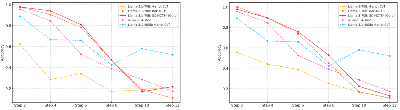
Figure 2: Accuracy comparison of various models and reasoning methods on the Blocksworld multi-step reasoning dataset across increasing reasoning steps.
From Figure 2, we observe that as the reasoning path lengthens, the performance advantage of two MCTS reasoning algorithms over themselves, GPT-4o, and Llama-3.1-405B’s CoT explicit multi-turn chats and o1-mini implicit multi-turn chats (OpenAI, 2024b) in terms of accuracy diminishes, becoming particularly evident after Step 6. The accuracy decline for CoT is more gradual as the reasoning path extends, whereas models employing MCTS reasoning exhibits a steeper decline. This trend could be due to the fixed iteration limit of 10 across different reasoning path lengths, which might be unfair to longer paths. Future work could explore dynamically adjusting the iteration limit based on reasoning path length. It may also be attributed to our use of a custom EOS token to ensure output format stability in the MCTS reasoning process, which operates in completion mode. As the number of steps and prompt prefix lengths increases, the limitations of completion mode may become more pronounced compared to the chat mode used in multi-turn chats. Additionally, we observe that Llama-3.1-405B benefits significantly from its huge parameter size, although underperforming at fewer steps, experiences the slowest accuracy decline as the reasoning path grows longer.
5.3 Reasoning Speed
<details>
<summary>extracted/6087579/fig/speed.png Details</summary>
### Visual Description
\n
## Bar Charts: Token Generation Speed Comparison
### Overview
The image presents two bar charts comparing the token generation speed (Tokens/s) of different models: Vanilla, SD-Llama-3.1-8B, and SD-Llama-3.2-1B. The first chart focuses on the Llama3.1-70B model, while the second focuses on the Llama-3.1-405B model. A horizontal dashed line at 60 Tokens/s is present in the first chart, and at 6 Tokens/s in the second chart, serving as a reference point. Each bar is labeled with a relative speed multiplier (e.g., 1.00x, 1.15x).
### Components/Axes
* **X-axis:** Model Name (Llama3.1-70B, Llama-3.1-405B)
* **Y-axis:** Token Generation Speed (Tokens/s). The scale ranges from 0 to 100 in the first chart and 0 to 14 in the second chart.
* **Legend (Top-Right of each chart):**
* Red: Vanilla
* Yellow: SD-Llama-3.1-8B
* Light Blue: SD-Llama-3.2-1B
* **Reference Line:** A horizontal dashed line is present in each chart. The first chart has a line at approximately 60 Tokens/s, and the second at approximately 6 Tokens/s.
* **Multiplier Labels:** Each bar is labeled with a multiplier relative to the "Vanilla" model.
### Detailed Analysis or Content Details
**Chart 1: Llama3.1-70B**
* **Vanilla:** The Vanilla model achieves a token generation speed of approximately 42 Tokens/s, labeled as 1.00x.
* **SD-Llama-3.1-8B:** This model achieves a token generation speed of approximately 58 Tokens/s, labeled as 1.15x.
* **SD-Llama-3.2-1B:** This model achieves a token generation speed of approximately 84 Tokens/s, labeled as 1.52x.
**Chart 2: Llama-3.1-405B**
* **Vanilla:** The Vanilla model achieves a token generation speed of approximately 5 Tokens/s, labeled as 1.00x.
* **SD-Llama-3.1-8B:** This model achieves a token generation speed of approximately 12 Tokens/s, labeled as 2.00x.
* **SD-Llama-3.2-1B:** This model achieves a token generation speed of approximately 3 Tokens/s, labeled as 0.55x.
### Key Observations
* For the Llama3.1-70B model, SD-Llama-3.2-1B significantly outperforms both Vanilla and SD-Llama-3.1-8B in terms of token generation speed.
* For the Llama-3.1-405B model, SD-Llama-3.1-8B significantly outperforms both Vanilla and SD-Llama-3.2-1B.
* The relative performance of the SD models varies depending on the base model (70B vs. 405B).
* The reference lines provide a clear visual indication of performance thresholds.
### Interpretation
The data suggests that the SD-Llama models can significantly improve token generation speed compared to the Vanilla models, but the extent of the improvement is dependent on the underlying Llama model size. For the 70B model, the 3.2-1B variant provides the largest speedup. However, for the 405B model, the 3.1-8B variant is superior. This indicates a complex interaction between the SD-Llama optimization and the base model architecture. The multipliers provide a convenient way to quantify the performance gains. The horizontal lines likely represent a target or baseline performance level. The difference in performance between the two charts suggests that the benefits of the SD-Llama optimization may scale differently with model size. Further investigation would be needed to understand the reasons for this difference and to optimize the SD-Llama models for different Llama model sizes.
</details>
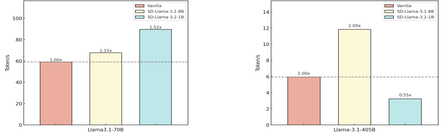
Figure 3: Speedup comparison of different model combinations. For speculative decoding, we use Llama-3.2-1B and Llama-3.1.8B as amateur models with Llama-3.1-70B and Llama-3.1-405B as expert models, based on average node-level reasoning speed in MCTS for Blocksworld multi-step reasoning dataset.
As shown in Figure 3, we can observe that the combination of Llama-3.1-405B with Llama-3.1-8B achieves the highest speedup, improving inference speed by approximately 100% compared to vanilla decoding. Similarly, pairing Llama-3.1-70B with Llama-3.2-1B results in a 51.9% increase in reasoning speed. These two combinations provide the most significant gains, demonstrating that speculative decoding with SLMs can substantially enhance node level reasoning speed. However, we can also observe from the combination of Llama-3.1-405B with Llama-3.2-1B that the parameters of SLMs in speculative decoding should not be too small, since the threshold for accepting draft tokens during the decoding process remains fixed to prevent speculative decoding from affecting performance (Leviathan et al., 2023), as overly small parameters may have a negative impact on decoding speed, which is consistent with the findings in Zhao et al. (2024); Chen et al. (2023).
5.4 Parameters
<details>
<summary>extracted/6087579/fig/uct.png Details</summary>
### Visual Description
\n
## Line Chart: Accuracy vs. C Parameter
### Overview
The image presents a line chart comparing the accuracy of three different methods – RAP-MCTS, SC-MCTS* (labeled as "Ours"), and a Negative Control (c=0) – as a function of the 'C' parameter. The chart visually demonstrates how accuracy changes with varying values of 'C'.
### Components/Axes
* **X-axis:** Labeled "C", ranging from approximately 0 to 400, with markers at 0, 50, 100, 150, 200, 250, 300, 350, and 400.
* **Y-axis:** Labeled "Accuracy", ranging from approximately 0.54 to 0.63, with markers at 0.54, 0.56, 0.58, 0.60, 0.62.
* **Legend:** Located in the top-right corner.
* RAP-MCTS: Represented by black triangles (▲).
* SC-MCTS* (Ours): Represented by black stars (★).
* Negative Control (c=0): Represented by black circles (●).
* **Gridlines:** Present to aid in reading values.
### Detailed Analysis
* **Negative Control (c=0):** The line starts at approximately 0.54 at C=0, increases sharply to around 0.58 at C=10, then plateaus around 0.58 until C=150. After C=150, the accuracy decreases steadily, reaching approximately 0.55 at C=400.
* **SC-MCTS* (Ours):** The line begins at approximately 0.61 at C=0, increases to a peak of around 0.63 at C=75, then fluctuates between approximately 0.62 and 0.63 until C=200. After C=200, the accuracy decreases to approximately 0.61 at C=400.
* **RAP-MCTS:** The line starts at approximately 0.55 at C=0, increases rapidly to a peak of around 0.63 at C=50, then decreases slightly to approximately 0.62 at C=100. It remains relatively stable around 0.62-0.63 until C=250, after which it declines to approximately 0.61 at C=400.
Here's a more detailed breakdown of approximate data points:
| C | Negative Control | SC-MCTS* (Ours) | RAP-MCTS |
| :---- | :--------------- | :-------------- | :------- |
| 0 | 0.54 | 0.61 | 0.55 |
| 10 | 0.58 | 0.62 | 0.62 |
| 50 | 0.58 | 0.63 | 0.63 |
| 75 | 0.58 | 0.63 | 0.62 |
| 100 | 0.58 | 0.62 | 0.62 |
| 150 | 0.58 | 0.62 | 0.62 |
| 200 | 0.57 | 0.62 | 0.62 |
| 250 | 0.56 | 0.62 | 0.62 |
| 300 | 0.55 | 0.61 | 0.61 |
| 350 | 0.55 | 0.61 | 0.61 |
| 400 | 0.55 | 0.61 | 0.61 |
### Key Observations
* SC-MCTS* (Ours) and RAP-MCTS achieve higher accuracy than the Negative Control across all values of 'C'.
* Both SC-MCTS* and RAP-MCTS exhibit an initial increase in accuracy with increasing 'C', followed by a plateau and eventual decline.
* The Negative Control shows a relatively stable accuracy until C=150, after which it decreases.
* The peak accuracy for SC-MCTS* and RAP-MCTS is around C=75 and C=50 respectively.
### Interpretation
The chart suggests that the 'C' parameter has a significant impact on the accuracy of the tested methods. Initially, increasing 'C' improves accuracy, likely due to increased exploration or exploitation in the search process. However, beyond a certain point, increasing 'C' leads to diminishing returns and eventually a decrease in accuracy, potentially due to overfitting or increased computational cost.
The consistently higher accuracy of SC-MCTS* (Ours) and RAP-MCTS compared to the Negative Control indicates that these methods are more effective at solving the underlying problem. The slight difference in peak accuracy and the rate of decline between SC-MCTS* and RAP-MCTS suggest that they have different strengths and weaknesses, and the optimal value of 'C' may vary depending on the specific method used. The negative control serves as a baseline, demonstrating the performance without the specific enhancements implemented in the other two methods. The decline in the negative control after C=150 could indicate a point where the baseline method begins to suffer from the increased complexity or noise introduced by higher 'C' values.
</details>
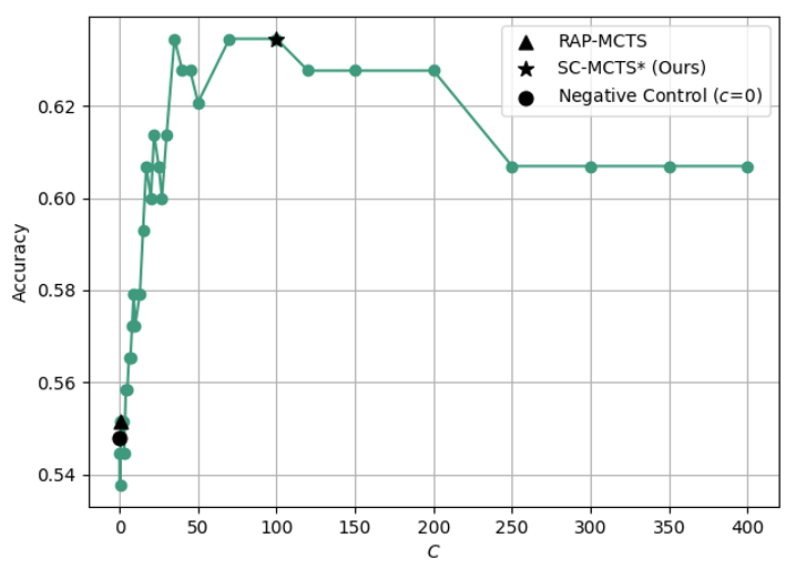
Figure 4: Accuracy comparison of different constant $C$ of UCT on Blocksworld multi-step reasoning dataset.
<details>
<summary>extracted/6087579/fig/iter.png Details</summary>
### Visual Description
\n
## Line Chart: Accuracy vs. Iteration for Different Modes
### Overview
This image presents a line chart illustrating the relationship between accuracy and iteration number for two different modes: "Easy Mode" and "Hard Mode". The chart displays how accuracy changes as the number of iterations increases.
### Components/Axes
* **X-axis:** Labeled "Iteration", ranging from 1 to 10. The axis is linearly scaled.
* **Y-axis:** Labeled "Accuracy", ranging from 0.35 to 0.65. The axis is linearly scaled.
* **Legend:** Located in the bottom-right corner.
* "Easy Mode" - Represented by a blue line with circle markers.
* "Hard Mode" - Represented by a red line with circle markers.
* **Gridlines:** Present to aid in reading values.
### Detailed Analysis
**Easy Mode (Blue Line):**
The blue line representing "Easy Mode" shows a generally upward trend, indicating increasing accuracy with each iteration.
* Iteration 1: Approximately 0.41
* Iteration 2: Approximately 0.42
* Iteration 3: Approximately 0.47
* Iteration 4: Approximately 0.50
* Iteration 5: Approximately 0.56
* Iteration 6: Approximately 0.60
* Iteration 7: Approximately 0.61
* Iteration 8: Approximately 0.62
* Iteration 9: Approximately 0.63
* Iteration 10: Approximately 0.63
**Hard Mode (Red Line):**
The red line representing "Hard Mode" also shows an upward trend, but it starts at a lower accuracy and increases more slowly than "Easy Mode".
* Iteration 1: Approximately 0.35
* Iteration 2: Approximately 0.35
* Iteration 3: Approximately 0.42
* Iteration 4: Approximately 0.48
* Iteration 5: Approximately 0.53
* Iteration 6: Approximately 0.57
* Iteration 7: Approximately 0.59
* Iteration 8: Approximately 0.60
* Iteration 9: Approximately 0.61
* Iteration 10: Approximately 0.61
### Key Observations
* "Easy Mode" consistently achieves higher accuracy than "Hard Mode" across all iterations.
* The rate of accuracy improvement decreases as the number of iterations increases for both modes. The curve flattens out.
* The initial accuracy for "Hard Mode" is significantly lower than for "Easy Mode".
* Both lines show a clear positive correlation between iteration number and accuracy.
### Interpretation
The data suggests that the algorithm or system being evaluated performs better in "Easy Mode" than in "Hard Mode", as evidenced by the consistently higher accuracy scores. The increasing accuracy with more iterations indicates that the system is learning or improving its performance over time. The flattening of the curves at higher iteration numbers suggests diminishing returns – further iterations yield smaller improvements in accuracy. The difference in initial accuracy between the two modes could indicate that "Hard Mode" presents a more challenging initial state or requires more iterations to reach a comparable level of performance. This could be due to a more complex problem space, a different set of constraints, or a more difficult learning landscape in "Hard Mode". The chart demonstrates the impact of mode difficulty on the learning process and the trade-off between iteration count and accuracy gain.
</details>
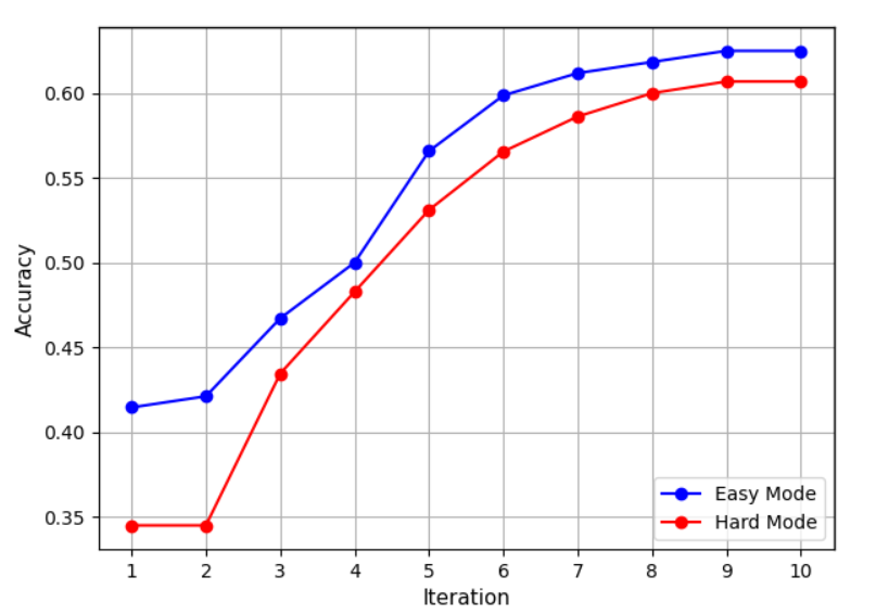
Figure 5: Accuracy comparison of different numbers of iteration on Blocksworld multi-step reasoning dataset.
As discussed in Section 4.2, the constant $C$ is a crucial part of UCT strategy, which completely determines whether the exploration term takes effect. Therefore, we conducted quantitative experiments on the constant $C$ , to eliminate interference from other factors, we only use MCTS base with the common reward model $R_{\text{LL}}$ for both RAP-MCTS and SC-MCTS ∗. From Figure 5 we can observe that the constant $C$ of RAP-MCTS is too small to function effectively, while the constant $C$ of SC-MCTS ∗ is the value most suited to the values of reward model derived from extensive experimental data. After introducing new datasets, this hyperparameter may need to be re-tuned.
From Figure 5, it can be observed that the accuracy of SC-MCTS ∗ on multi-step reasoning increases steadily with the number of iterations. During the first 1-7 iterations, the accuracy rises consistently. After the 7th iteration, the improvement in accuracy becomes relatively smaller, indicating that under the experimental setting with depth limitations, the exponentially growing exploration nodes in later iterations bring diminishing returns in accuracy.
5.5 Ablation Study
| Parts of SC-MCTS ∗ | Accuracy (%) | Improvement (%) |
| --- | --- | --- |
| MCTS base | 55.92 | — |
| + $R_{\text{JSD}}$ | 62.50 | +6.58 |
| + $R_{\text{LL}}$ | 67.76 | +5.26 |
| + $R_{\text{SE}}$ | 70.39 | +2.63 |
| + Multi-RM Method | 73.68 | +3.29 |
| + Improved $C$ of UCT | 78.95 | +5.27 |
| + BP Refinement | 80.92 | +1.97 |
| SC-MCTS ∗ | 80.92 | Overall +25.00 |
Table 2: Ablation Study on the Blocksworld dataset at Step 6 under difficult mode. For a more thorough ablation study, the reward model for the MCTS base was set to pseudo-random numbers.
As shown in Table 2, the results of the ablation study demonstrate that each component of SC-MCTS ∗ contributes significantly to performance improvements. Starting from a base MCTS accuracy of 55.92%, adding $R_{\text{JSD}}$ , $R_{\text{LL}}$ , and $R_{\text{SE}}$ yields a combined improvement of 14.47%. Multi-RM method further boosts performance by 3.29%, while optimizing the $C$ parameter in UCT adds 5.27%, and the backpropagation refinement increases accuracy by 1.97%. Overall, SC-MCTS ∗ achieves an accuracy of 80.92%, a 25% improvement over the base, demonstrating the effectiveness of these enhancements for complex reasoning tasks.
5.6 Interpretability Study
In the Blocksworld multi-step reasoning dataset, we utilize a built-in ground truth verifier to measure the percentage of progress toward achieving the goal at a given step, denoted as $P$ . The value of $P$ ranges between $[0,1]$ . For any arbitrary non-root node $N_{i}$ , the progress is defined as:
$$
P(N_{i})=\text{Verifier}(N_{i}).
$$
For instance, in a 10-step Blocksworld reasoning task, the initial node $A$ has $P(A)=0$ . After executing one correct action and transitioning to the next node $B$ , the progress becomes $P(B)=0.1$ .
Given a non-root node $N_{i}$ , transitioning to its parent node $\text{Parent}(N_{i})$ through a specific action $a$ , the contribution of $a$ toward the final goal state is defined as:
$$
\Delta_{a}=P(\text{Parent}(N_{i}))-P(N_{i}).
$$
Next, by analyzing the relationship between $\Delta_{a}$ and the reward value $R_{a}$ assigned by the reward model for action $a$ , we aim to reveal how our designed reward model provides highly interpretable reward signals for the selection of each node in MCTS. We also compare the performance of our reward model against a baseline reward model. Specifically, the alignment between $\Delta_{a}$ and $R_{a}$ demonstrates the interpretability of the reward model in guiding the reasoning process toward the goal state. Since Section 5.5 has already demonstrated that the reasoning performance of MCTS reasoning is almost entirely determined by the reward model, using interpretable reward models greatly enhances the interpretability of our algorithm SC-MCTS ∗.
<details>
<summary>extracted/6087579/fig/reward.png Details</summary>
### Visual Description
\n
## Histograms: Reward Distribution of Baseline (RAP-MCTS) and SC-MCTS*
### Overview
The image presents two histograms displaying reward distributions for two different algorithms: Baseline (RAP-MCTS) and SC-MCTS*. Both histograms are overlaid with a color gradient representing the proportion of positive A<sub>α</sub> values. Each histogram also includes Spearman and Pearson correlation coefficients with associated p-values.
### Components/Axes
* **X-axis (Left Histogram):** Reward values ranging approximately from -640 to -560.
* **X-axis (Right Histogram):** Reward values ranging approximately from -4 to 4.
* **Y-axis (Both Histograms):** Frequency, ranging from 0 to 2000+.
* **Color Gradient (Both Histograms):** Represents the proportion of positive A<sub>α</sub>, ranging from 0.0 (purple) to 0.6 (green). A legend is present in the top-right corner of the right histogram.
* **Title (Left Histogram):** "Reward Distribution of Baseline (RAP-MCTS)"
* **Title (Right Histogram):** "Reward Distribution of SC-MCTS*"
* **Correlation Statistics (Both Histograms):**
* Spearman: 0.01 (Left) / 0.32 (Right)
* Pearson: 0.01 (Left) / 0.32 (Right)
* P-value: 0.2624 (Left) / <0.0001 (Right)
### Detailed Analysis or Content Details
**Left Histogram (Baseline - RAP-MCTS):**
The histogram is approximately bell-shaped, but with a slight skew towards the left (negative reward values). The peak frequency is around 1900, occurring at a reward value of approximately -590. The distribution is relatively narrow, with most rewards falling between -630 and -560. The color gradient shows a predominantly purple hue, indicating a low proportion of positive A<sub>α</sub> values.
* **Approximate Data Points (Peak):** (-590, 1900)
* **Approximate Data Points (Left Tail):** (-640, 200), (-630, 300)
* **Approximate Data Points (Right Tail):** (-560, 250)
**Right Histogram (SC-MCTS*):**
This histogram is more symmetrical and centered around 0. The peak frequency is around 2200, occurring at a reward value of approximately 0. The distribution is wider than the baseline histogram, with rewards ranging from -4 to 4. The color gradient shows a mix of purple, blue, and green, indicating a higher proportion of positive A<sub>α</sub> values, particularly around the peak.
* **Approximate Data Points (Peak):** (0, 2200)
* **Approximate Data Points (Left Tail):** (-4, 300), (-2, 800)
* **Approximate Data Points (Right Tail):** (2, 800), (4, 300)
### Key Observations
* The Baseline (RAP-MCTS) histogram shows a distribution of predominantly negative rewards.
* The SC-MCTS* histogram shows a distribution centered around zero, with a more balanced representation of positive and negative rewards.
* The p-value for the SC-MCTS* correlation is significantly lower (<0.0001) than for the Baseline (0.2624), suggesting a stronger correlation.
* The Spearman and Pearson correlation coefficients are low for the Baseline (0.01) but higher for SC-MCTS* (0.32).
* The color gradient indicates that positive A<sub>α</sub> values are more prevalent in the SC-MCTS* distribution, particularly around the peak reward value.
### Interpretation
The data suggests that the SC-MCTS* algorithm performs better than the Baseline (RAP-MCTS) in terms of reward distribution. The SC-MCTS* algorithm generates a wider range of rewards, including a significant number of positive rewards, while the Baseline algorithm consistently produces negative rewards. The lower p-value and higher correlation coefficients for SC-MCTS* indicate a stronger relationship between the reward and the proportion of positive A<sub>α</sub> values. The color gradient visually reinforces this observation, showing a higher concentration of green (positive A<sub>α</sub>) around the peak reward value for SC-MCTS*.
The difference in reward distributions could be attributed to the specific mechanisms of each algorithm. The Baseline algorithm may be more prone to getting stuck in suboptimal solutions, resulting in consistently negative rewards. The SC-MCTS* algorithm, on the other hand, appears to be more effective at exploring the solution space and identifying rewarding actions. The A<sub>α</sub> values likely represent a measure of confidence or desirability, and the correlation suggests that the algorithm is more likely to select actions with higher A<sub>α</sub> values when it receives positive rewards.
</details>
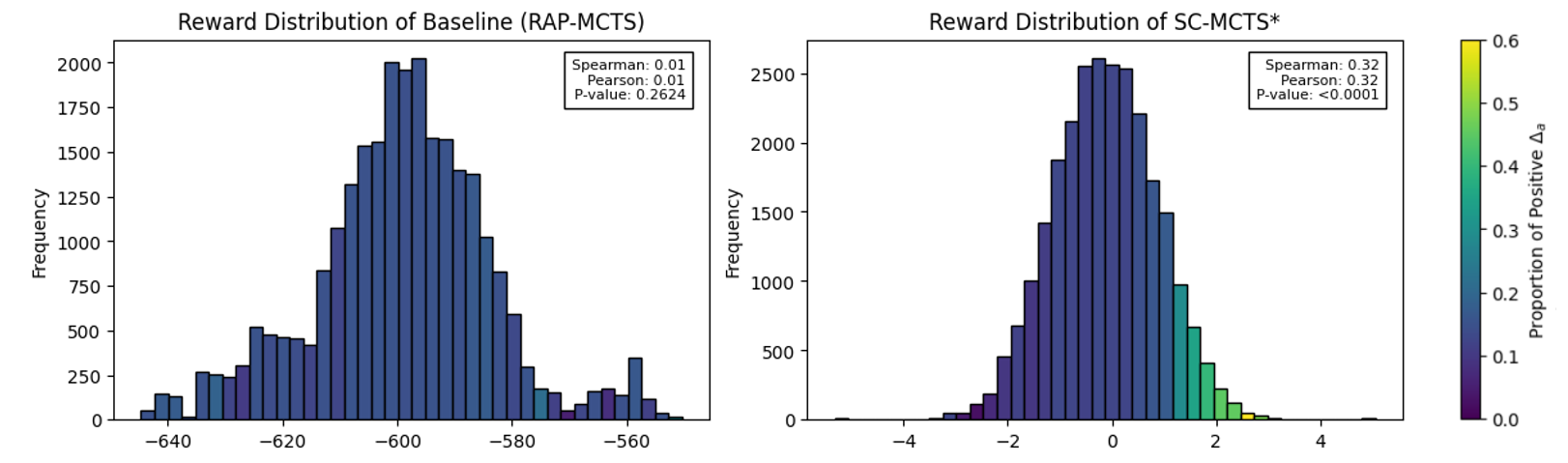
Figure 6: Reward distribution and interpretability analysis. The left histogram shows the baseline reward model (RAP-MCTS), while the right represents SC-MCTS ∗. Bin colors indicate the proportion of positive $\Delta_{a}$ (lighter colors means higher proportions). Spearman and Pearson correlations along with p-values are shown in the top right of each histogram.
From Figure 6, shows that SC-MCTS* reward values correlate significantly with $\Delta_{a}$ , as indicated by the high Spearman and Pearson coefficients. Additionally, the mapping between the reward value bins and the proportion of positive $\Delta_{a}$ (indicated by the color gradient from light to dark) is highly consistent and intuitive. This strong alignment suggests that our reward model effectively captures the progress toward the goal state, providing interpretable signals for action selection during reasoning.
These results highlight the exceptional interpretability of our designed reward model, which ensures that SC-MCTS* not only achieves superior reasoning performance but is also highly interpretable. This interpretability is crucial for understanding and improving the decision-making process in multi-step reasoning tasks, further validating transparency of our proposed algorithm.
6 Conclusion
In this paper, we present SC-MCTS ∗, a novel and effective algorithm to enhancing the reasoning capabilities of LLMs. With extensive improvements in reward modeling, node selection strategy and backpropagation, SC-MCTS ∗ boosts both accuracy and speed, outperforming OpenAI’s o1-mini model by 17.4% on average using Llama-3.1-70B on the Blocksworld dataset. Experiments demonstrate its strong performance, making it a promising approach for multi-step reasoning tasks. For future work please refer to Appendix J. The synthesis of interpretability, efficiency and generalizability positions SC-MCTS ∗ as a valuable contribution to advancing LLMs multi-step reasoning.
References
- Bellman (1957) Richard Bellman. A markovian decision process. Journal of Mathematics and Mechanics, 6(5):679–684, 1957. ISSN 00959057, 19435274. URL http://www.jstor.org/stable/24900506.
- Chen et al. (2023) Charlie Chen, Sebastian Borgeaud, Geoffrey Irving, Jean-Baptiste Lespiau, Laurent Sifre, and John Jumper. Accelerating large language model decoding with speculative sampling, 2023. URL https://arxiv.org/abs/2302.01318.
- Chen et al. (2024) Qiguang Chen, Libo Qin, Jiaqi Wang, Jinxuan Zhou, and Wanxiang Che. Unlocking the boundaries of thought: A reasoning granularity framework to quantify and optimize chain-of-thought, 2024. URL https://arxiv.org/abs/2410.05695.
- Coquelin & Munos (2007) Pierre-Arnaud Coquelin and Rémi Munos. Bandit algorithms for tree search. In Proceedings of the Twenty-Third Conference on Uncertainty in Artificial Intelligence, UAI’07, pp. 67–74, Arlington, Virginia, USA, 2007. AUAI Press. ISBN 0974903930.
- Frantar et al. (2022) Elias Frantar, Saleh Ashkboos, Torsten Hoefler, and Dan Alistarh. Gptq: Accurate post-training quantization for generative pre-trained transformers, 2022.
- Hao et al. (2023) Shibo Hao, Yi Gu, Haodi Ma, Joshua Hong, Zhen Wang, Daisy Wang, and Zhiting Hu. Reasoning with language model is planning with world model. In Houda Bouamor, Juan Pino, and Kalika Bali (eds.), Proceedings of the 2023 Conference on Empirical Methods in Natural Language Processing, pp. 8154–8173, Singapore, December 2023. Association for Computational Linguistics. doi: 10.18653/v1/2023.emnlp-main.507. URL https://aclanthology.org/2023.emnlp-main.507.
- Hao et al. (2024) Shibo Hao, Yi Gu, Haotian Luo, Tianyang Liu, Xiyan Shao, Xinyuan Wang, Shuhua Xie, Haodi Ma, Adithya Samavedhi, Qiyue Gao, Zhen Wang, and Zhiting Hu. LLM reasoners: New evaluation, library, and analysis of step-by-step reasoning with large language models. In ICLR 2024 Workshop on Large Language Model (LLM) Agents, 2024. URL https://openreview.net/forum?id=h1mvwbQiXR.
- Jumper et al. (2021) John Jumper, Richard Evans, Alexander Pritzel, Tim Green, Michael Figurnov, Olaf Ronneberger, Kathryn Tunyasuvunakool, Russ Bates, Augustin Žídek, Anna Potapenko, Alex Bridgland, Clemens Meyer, Simon A. A. Kohl, Andrew J. Ballard, Andrew Cowie, Bernardino Romera-Paredes, Stanislav Nikolov, Rishub Jain, Jonas Adler, and Trevor Back. Highly accurate protein structure prediction with alphafold. Nature, 596(7873):583–589, Jul 2021. doi: https://doi.org/10.1038/s41586-021-03819-2. URL https://www.nature.com/articles/s41586-021-03819-2.
- Leviathan et al. (2023) Yaniv Leviathan, Matan Kalman, and Yossi Matias. Fast inference from transformers via speculative decoding. In Proceedings of the 40th International Conference on Machine Learning, ICML’23. JMLR.org, 2023.
- Li et al. (2023) Xiang Lisa Li, Ari Holtzman, Daniel Fried, Percy Liang, Jason Eisner, Tatsunori Hashimoto, Luke Zettlemoyer, and Mike Lewis. Contrastive decoding: Open-ended text generation as optimization. In Anna Rogers, Jordan Boyd-Graber, and Naoaki Okazaki (eds.), Proceedings of the 61st Annual Meeting of the Association for Computational Linguistics (Volume 1: Long Papers), pp. 12286–12312, Toronto, Canada, July 2023. Association for Computational Linguistics. doi: 10.18653/v1/2023.acl-long.687. URL https://aclanthology.org/2023.acl-long.687.
- Liu et al. (2021) Alisa Liu, Maarten Sap, Ximing Lu, Swabha Swayamdipta, Chandra Bhagavatula, Noah A. Smith, and Yejin Choi. DExperts: Decoding-time controlled text generation with experts and anti-experts. In Proceedings of the 59th Annual Meeting of the Association for Computational Linguistics and the 11th International Joint Conference on Natural Language Processing (Volume 1: Long Papers), pp. 6691–6706, Online, August 2021. Association for Computational Linguistics. doi: 10.18653/v1/2021.acl-long.522. URL https://aclanthology.org/2021.acl-long.522.
- McAleese et al. (2024) Nat McAleese, Rai Michael Pokorny, Juan Felipe Ceron Uribe, Evgenia Nitishinskaya, Maja Trebacz, and Jan Leike. Llm critics help catch llm bugs, 2024.
- O’Brien & Lewis (2023) Sean O’Brien and Mike Lewis. Contrastive decoding improves reasoning in large language models, 2023. URL https://arxiv.org/abs/2309.09117.
- OpenAI (2024a) OpenAI. Introducing openai o1. https://openai.com/o1/, 2024a. Accessed: 2024-10-02.
- OpenAI (2024b) OpenAI. How reasoning works. https://platform.openai.com/docs/guides/reasoning/how-reasoning-works, 2024b. Accessed: 2024-10-02.
- Qi et al. (2024) Zhenting Qi, Mingyuan Ma, Jiahang Xu, Li Lyna Zhang, Fan Yang, and Mao Yang. Mutual reasoning makes smaller llms stronger problem-solvers, 2024. URL https://arxiv.org/abs/2408.06195.
- Rafailov et al. (2023) Rafael Rafailov, Archit Sharma, Eric Mitchell, Christopher D Manning, Stefano Ermon, and Chelsea Finn. Direct preference optimization: Your language model is secretly a reward model. In A. Oh, T. Naumann, A. Globerson, K. Saenko, M. Hardt, and S. Levine (eds.), Advances in Neural Information Processing Systems, volume 36, pp. 53728–53741. Curran Associates, Inc., 2023. URL https://proceedings.neurips.cc/paper_files/paper/2023/file/a85b405ed65c6477a4fe8302b5e06ce7-Paper-Conference.pdf.
- Ren et al. (2023) Jie Ren, Yao Zhao, Tu Vu, Peter J. Liu, and Balaji Lakshminarayanan. Self-evaluation improves selective generation in large language models. In Javier Antorán, Arno Blaas, Kelly Buchanan, Fan Feng, Vincent Fortuin, Sahra Ghalebikesabi, Andreas Kriegler, Ian Mason, David Rohde, Francisco J. R. Ruiz, Tobias Uelwer, Yubin Xie, and Rui Yang (eds.), Proceedings on "I Can’t Believe It’s Not Better: Failure Modes in the Age of Foundation Models" at NeurIPS 2023 Workshops, volume 239 of Proceedings of Machine Learning Research, pp. 49–64. PMLR, 16 Dec 2023. URL https://proceedings.mlr.press/v239/ren23a.html.
- Silver et al. (2016) David Silver, Aja Huang, Chris J. Maddison, Arthur Guez, Laurent Sifre, George van den Driessche, Julian Schrittwieser, Ioannis Antonoglou, Veda Panneershelvam, Marc Lanctot, Sander Dieleman, Dominik Grewe, John Nham, Nal Kalchbrenner, Ilya Sutskever, Timothy Lillicrap, Madeleine Leach, Koray Kavukcuoglu, Thore Graepel, and Demis Hassabis. Mastering the game of go with deep neural networks and tree search. Nature, 529(7587):484–489, Jan 2016. doi: https://doi.org/10.1038/nature16961.
- Silver et al. (2017) David Silver, Thomas Hubert, Julian Schrittwieser, Ioannis Antonoglou, Matthew Lai, Arthur Guez, Marc Lanctot, Laurent Sifre, Dharshan Kumaran, Thore Graepel, Timothy Lillicrap, Karen Simonyan, and Demis Hassabis. Mastering chess and shogi by self-play with a general reinforcement learning algorithm, 2017. URL https://arxiv.org/abs/1712.01815.
- Sprague et al. (2024) Zayne Sprague, Fangcong Yin, Juan Diego Rodriguez, Dongwei Jiang, Manya Wadhwa, Prasann Singhal, Xinyu Zhao, Xi Ye, Kyle Mahowald, and Greg Durrett. To cot or not to cot? chain-of-thought helps mainly on math and symbolic reasoning, 2024. URL https://arxiv.org/abs/2409.12183.
- Tian et al. (2024) Ye Tian, Baolin Peng, Linfeng Song, Lifeng Jin, Dian Yu, Haitao Mi, and Dong Yu. Toward self-improvement of llms via imagination, searching, and criticizing. ArXiv, abs/2404.12253, 2024. URL https://api.semanticscholar.org/CorpusID:269214525.
- Valmeekam et al. (2023) Karthik Valmeekam, Matthew Marquez, Sarath Sreedharan, and Subbarao Kambhampati. On the planning abilities of large language models - a critical investigation. In Thirty-seventh Conference on Neural Information Processing Systems, 2023. URL https://openreview.net/forum?id=X6dEqXIsEW.
- Valmeekam et al. (2024) Karthik Valmeekam, Matthew Marquez, Alberto Olmo, Sarath Sreedharan, and Subbarao Kambhampati. Planbench: an extensible benchmark for evaluating large language models on planning and reasoning about change. In Proceedings of the 37th International Conference on Neural Information Processing Systems, NIPS ’23, Red Hook, NY, USA, 2024. Curran Associates Inc.
- Wei et al. (2024) Jason Wei, Xuezhi Wang, Dale Schuurmans, Maarten Bosma, Brian Ichter, Fei Xia, Ed H. Chi, Quoc V. Le, and Denny Zhou. Chain-of-thought prompting elicits reasoning in large language models. In Proceedings of the 36th International Conference on Neural Information Processing Systems, NIPS ’22, Red Hook, NY, USA, 2024. Curran Associates Inc. ISBN 9781713871088.
- Xie et al. (2024) Yuxi Xie, Anirudh Goyal, Wenyue Zheng, Min-Yen Kan, Timothy P. Lillicrap, Kenji Kawaguchi, and Michael Shieh. Monte carlo tree search boosts reasoning via iterative preference learning, 2024. URL https://arxiv.org/abs/2405.00451.
- Xin et al. (2024a) Huajian Xin, Daya Guo, Zhihong Shao, Zhizhou Ren, Qihao Zhu, Bo Liu (Benjamin Liu), Chong Ruan, Wenda Li, and Xiaodan Liang. Deepseek-prover: Advancing theorem proving in llms through large-scale synthetic data. ArXiv, abs/2405.14333, 2024a. URL https://api.semanticscholar.org/CorpusID:269983755.
- Xin et al. (2024b) Huajian Xin, Z. Z. Ren, Junxiao Song, Zhihong Shao, Wanjia Zhao, Haocheng Wang, Bo Liu, Liyue Zhang, Xuan Lu, Qiushi Du, Wenjun Gao, Qihao Zhu, Dejian Yang, Zhibin Gou, Z. F. Wu, Fuli Luo, and Chong Ruan. Deepseek-prover-v1.5: Harnessing proof assistant feedback for reinforcement learning and monte-carlo tree search, 2024b. URL https://arxiv.org/abs/2408.08152.
- Xu (2023) Haotian Xu. No train still gain. unleash mathematical reasoning of large language models with monte carlo tree search guided by energy function, 2023. URL https://arxiv.org/abs/2309.03224.
- Yao et al. (2024) Shunyu Yao, Dian Yu, Jeffrey Zhao, Izhak Shafran, Thomas L. Griffiths, Yuan Cao, and Karthik Narasimhan. Tree of thoughts: deliberate problem solving with large language models. In Proceedings of the 37th International Conference on Neural Information Processing Systems, NIPS ’23, Red Hook, NY, USA, 2024. Curran Associates Inc.
- Yuan et al. (2024a) Hongyi Yuan, Keming Lu, Fei Huang, Zheng Yuan, and Chang Zhou. Speculative contrastive decoding. In Lun-Wei Ku, Andre Martins, and Vivek Srikumar (eds.), Proceedings of the 62nd Annual Meeting of the Association for Computational Linguistics (Volume 2: Short Papers), pp. 56–64, Bangkok, Thailand, August 2024a. Association for Computational Linguistics. URL https://aclanthology.org/2024.acl-short.5.
- Yuan et al. (2024b) Lifan Yuan, Ganqu Cui, Hanbin Wang, Ning Ding, Xingyao Wang, Jia Deng, Boji Shan, Huimin Chen, Ruobing Xie, Yankai Lin, Zhenghao Liu, Bowen Zhou, Hao Peng, Zhiyuan Liu, and Maosong Sun. Advancing llm reasoning generalists with preference trees, 2024b.
- Zhang et al. (2024a) Dan Zhang, Sining Zhoubian, Ziniu Hu, Yisong Yue, Yuxiao Dong, and Jie Tang. Rest-mcts*: Llm self-training via process reward guided tree search, 2024a. URL https://arxiv.org/abs/2406.03816.
- Zhang et al. (2024b) Di Zhang, Xiaoshui Huang, Dongzhan Zhou, Yuqiang Li, and Wanli Ouyang. Accessing gpt-4 level mathematical olympiad solutions via monte carlo tree self-refine with llama-3 8b, 2024b. URL https://arxiv.org/abs/2406.07394.
- Zhao et al. (2024) Weilin Zhao, Yuxiang Huang, Xu Han, Wang Xu, Chaojun Xiao, Xinrong Zhang, Yewei Fang, Kaihuo Zhang, Zhiyuan Liu, and Maosong Sun. Ouroboros: Generating longer drafts phrase by phrase for faster speculative decoding, 2024. URL https://arxiv.org/abs/2402.13720.
Appendix A Action-Level Contrastive Reward
We made the distinction between action-level variables and token-level variables: action-level (or step-level) variables are those that aggregate over all tokens in a reasoning step, and is typically utilized by the reasoning algorithm directly; token-level variables, by contrast, operates in a more microscopic and low-level environment, such as speculative decoding.
We found that the traditional contrastive decoding using the difference in logits, when aggregated over the sequence gives a unstable reward signal compared to JS divergence. We suspected this is due to the unbounded nature of logit difference, and the potential failure modes associated with it that needs extra care and more hyperparameter tuning.
Appendix B More Related Work
Large Language Models Multi-Step Reasoning
Deepseek Prover (Xin et al., 2024a; b) relied on Lean4 as an external verification tool to provide dense reward signals in the RL stage. ReST-MCTS ∗ (Zhang et al., 2024a) employed self-training to collect high-quality reasoning trajectories for iteratively improving the value model. AlphaLLM (Tian et al., 2024) used critic models initialized from the policy model as the MCTS reward model. rStar (Qi et al., 2024) utilized mutual consistency of SLMs and an additional math-specific action space. Xu (2023) proposed reconstructing fine-tuned LLMs into residual-based energy models to guide MCTS.
Speculative Decoding
Speculative decoding was first introduced in Leviathan et al. (2023), as a method to accelerate sampling from large autoregressive models by computing multiple tokens in parallel without retraining or changing the model structure. It enhances computational efficiency, especially in large-scale generation tasks, by recognizing that hard language-modeling tasks often include easier subtasks that can be approximated well by more efficient models. Similarly, DeepMind introduced speculative sampling (Chen et al., 2023), which expands on this idea by generating a short draft sequence using a faster draft model and then scoring this draft with a larger target model.
Contrastive Decoding
Contrastive decoding, as proposed by Li et al. (2023), is a simple, computationally light, and training-free method for text generation that can enhancethe quality and quantity by identifying strings that highlight potential differences between strong models and weak models. In this context, the weak models typically employ conventional greedy decoding techniques such as basic sampling methods, while the strong models are often well-trained large language models. This approach has demonstrated notable performance improvements in various inference tasks, including arithmetic reasoning and multiple-choice ranking tasks, thereby increasing the accuracy of language models. According to experiments conducted by O’Brien & Lewis (2023), applying contrastive decoding across various tasks has proven effective in enhancing the reasoning capabilities of LLMs.
Appendix C Reward Functions Correlation
<details>
<summary>extracted/6087579/fig/heatmap.png Details</summary>
### Visual Description
\n
## Heatmap: Correlation Heatmap of Reward Functions
### Overview
The image presents a correlation heatmap visualizing the relationships between three reward functions: R<sub>LL</sub>, R<sub>SE</sub>, and R<sub>SD</sub>. The heatmap uses a color gradient to represent correlation coefficients, ranging from -1.00 (blue) to 1.00 (red).
### Components/Axes
* **Title:** "Correlation Heatmap of Reward Functions" (top-center)
* **X-axis Labels:** R<sub>LL</sub>, R<sub>SE</sub>, R<sub>SD</sub> (bottom)
* **Y-axis Labels:** R<sub>LL</sub>, R<sub>SE</sub>, R<sub>SD</sub> (left)
* **Color Legend:** Located in the top-right corner, ranging from blue (-1.00) to red (1.00), with intermediate values marked at -0.75, -0.50, -0.25, 0.25, 0.50, 0.75.
### Detailed Analysis
The heatmap displays the correlation coefficients between each pair of reward functions.
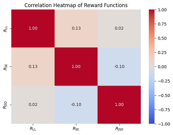
* **R<sub>LL</sub> vs. R<sub>LL</sub>:** 1.00 (dark red, top-left cell) - Perfect positive correlation.
* **R<sub>LL</sub> vs. R<sub>SE</sub>:** 0.13 (light red, top-middle cell) - Weak positive correlation.
* **R<sub>LL</sub> vs. R<sub>SD</sub>:** 0.02 (very light red, top-right cell) - Very weak positive correlation.
* **R<sub>SE</sub> vs. R<sub>LL</sub>:** 0.13 (light red, middle-left cell) - Weak positive correlation.
* **R<sub>SE</sub> vs. R<sub>SE</sub>:** 1.00 (dark red, middle-center cell) - Perfect positive correlation.
* **R<sub>SE</sub> vs. R<sub>SD</sub>:** -0.10 (light blue, middle-right cell) - Weak negative correlation.
* **R<sub>SD</sub> vs. R<sub>LL</sub>:** 0.02 (very light red, bottom-left cell) - Very weak positive correlation.
* **R<sub>SD</sub> vs. R<sub>SE</sub>:** -0.10 (light blue, bottom-middle cell) - Weak negative correlation.
* **R<sub>SD</sub> vs. R<sub>SD</sub>:** 1.00 (dark red, bottom-right cell) - Perfect positive correlation.
### Key Observations
* Each reward function has a perfect positive correlation with itself (diagonal cells are all 1.00).
* R<sub>LL</sub> and R<sub>SE</sub> exhibit a weak positive correlation.
* R<sub>SE</sub> and R<sub>SD</sub> show a weak negative correlation.
* The correlations between R<sub>LL</sub> and R<sub>SD</sub> are very close to zero, indicating almost no linear relationship.
### Interpretation
The heatmap reveals the degree of linear association between the three reward functions. The strong positive correlations along the diagonal are expected, as each function is perfectly correlated with itself. The weak positive correlation between R<sub>LL</sub> and R<sub>SE</sub> suggests that when R<sub>LL</sub> increases, R<sub>SE</sub> tends to increase slightly, but the relationship is not strong. The weak negative correlation between R<sub>SE</sub> and R<sub>SD</sub> indicates that as R<sub>SE</sub> increases, R<sub>SD</sub> tends to decrease slightly. The near-zero correlation between R<sub>LL</sub> and R<sub>SD</sub> suggests these two reward functions are largely independent of each other in a linear sense.
This information is valuable for understanding how these reward functions might interact when used in a reinforcement learning or optimization context. If the reward functions are highly correlated, they may provide redundant signals, while uncorrelated functions may offer more diverse information to the learning agent. The heatmap provides a concise visual summary of these relationships.
</details>
Figure 7: Reward Functions Correlation Heatmap.
It can be seen from Figure 7 that the correlations between the three reward functions are relatively low, absolute values all below 0.15. These low correlations of reward functions make them ideal for Multi-RM method.
Appendix D Algorithm Details of SC-MCTS ∗
The pseudocode inside MCTS reasoning of SC-MCTS ∗ is shown in Algorithm 2, based on Zhang et al. (2024a). The complete version of SC-MCTS ∗ is: first sample a subset of problems to obtain the prior data for reward values (Algorithm 1), then use it and two SLMs, one for providing contrastive reward signals, another for speculative decoding speedup, to perform MCTS reasoning. The changes of SC-MCTS ∗ compared to previous works are highlighted in teal.
Algorithm 2 SC-MCTS ∗, reasoning
1: expert LLM $\pi_{\text{e}}$ , amatuer SLM $\pi_{\text{a}}$ , speculative SLM $\pi_{\text{s}}$ , problem $q$ , reward model $R$ , reward factor statistics ${\mathcal{S}}$ , max iterations $T$ , threshold $l$ , branch $b$ , rollout steps $m$ , roll branch $d$ , weight parameter $\alpha$ , exploration constant $C$
2: $T_{q}←$ Initialize-tree $(q)$
3: for $i=1... T$ do
4: $n←$ Root $(T_{q})$
5: while $n$ is not leaf node do $\triangleright$ Node selection
6: $n←$ $\operatorname*{arg\,max}_{n^{\prime}∈\text{children}(n)}(v_{n^{\prime}}+C%
\sqrt{\frac{\ln{N_{n}}}{N_{n^{\prime}}}})$ $\triangleright$ Select child node based on UCT
7: end while
8: if $v_{n}≥ l$ then break $\triangleright$ Output solution
9: end if
10: if $n$ is not End of Inference then
11: for $j=1... b$ do $\triangleright$ Thought expansion
12: $n_{j}←$ Get-new-child $(A_{n},q,\pi_{\text{e}})$ $\triangleright$ Expand based on previous steps
13: $v_{n_{j}},{\mathcal{S}}←$ $R(A_{n_{j}},q,\pi_{\text{e}},\pi_{\text{a}},{\mathcal{S}})$ $\triangleright$ Evaluate contrastive reward and update reward factor statistics
14: end for
15: $n^{\prime}←$ $\operatorname*{arg\,max}_{n^{\prime}∈\text{children}(n)}(v_{n^{\prime}})$
16: $v_{\max}←$ 0
17: for $k=1... m$ do $\triangleright$ Greedy MC rollout
18: $A,v_{\max}←$ Get-next-step-with-best-value $(A,q,\pi_{\text{e}},\pi_{\text{s}},d)$ $\triangleright$ Sample new children using speculative decoding and record the best observed value
19: end for
20: $v_{n^{\prime}}←$ $\alpha v_{n^{\prime}}+(1-\alpha)v_{\max}$
21: $N_{n^{\prime}}←$ $N_{n^{\prime}}+1$ $\triangleright$ Update value and visit count of the rollout node
22: end if
23: Back-propagate $(n)$ $\triangleright$ Update value of parent nodes (Equation 3)
24: end for
25: $n←$ Get-best-node $(T_{q})$ $\triangleright$ Fetch the node with the highest value in the search tree
26: $A_{n}$
Although we sampled a small portion of the dataset as prior data for reward values, distribution shift may still occur when normalizing reward values during reasoning. Therefore, we use the following algorithm to incrementally update the mean and standard deviation of the online reward distribution:
Algorithm 3 Online incremental update of reward factor statistics
1: reward factors $\mathcal{R}(=\{\text{JSD},\text{LL},\text{SE}\})$ , statistics $\{\mu_{r}^{(k)},\sigma_{r}^{(k)},n_{r}^{(k)}\}_{r∈\mathcal{R},k∈\{1,...%
,K\}}$ , cluster assignment function $f$
2: for $r∈\mathcal{R}$ do
3: $k^{*}← f(x)$ $\triangleright$ Assign sample to cluster
4: $v_{r}← r(x)$ $\triangleright$ Compute reward factor value
5: $n_{r}^{(k^{*})}← n_{r}^{(k^{*})}+1$ $\triangleright$ Update sample count
6: $\delta← v_{r}-\mu_{r}^{(k^{*})}$ $\triangleright$ Compute difference from mean
7: $\mu_{r}^{(k^{*})}←\mu_{r}^{(k^{*})}+\delta/n_{r}^{(k^{*})}$ $\triangleright$ Update mean
8: $M_{2}←(n_{r}^{(k^{*})}-1)(\sigma_{r}^{(k^{*})})^{2}+\delta(v_{r}-\mu_%
{r}^{(k^{*})})$
9: $\sigma_{r}^{(k^{*})}←\sqrt{M_{2}/n_{r}^{(k^{*})}}$ $\triangleright$ Update standard deviation
10: end for
11: updated statistics $\{\mu_{r}^{(k)},\sigma_{r}^{(k)},n_{r}^{(k)}\}_{r∈\mathcal{R},k∈\{1,...%
,K\}}$
Appendix E Experimental Settings
For reproducibility, you can download the checkpoints from the Huggingface repository below and use the hyperparameters below. We utilized 4-bit quantized checkpoints in all experiments, as they only result in around 2% performance loss while providing several-fold reductions in memory usage and significantly improving inference speed (Frantar et al., 2022). For better output formatting to capture a single step and convert it into an MCTS node, we used the LLM’s completion mode so we set LLM to greedy sampling, and we don’t have to set an additional system prompt, simply apply prompts in Appendix F. Our experiments were all conducted on exllamav2 inference framework.
E.1 Checkpoints
| Usage | Models | Links |
| --- | --- | --- |
| Expert | Llama-3.1-405B | https://huggingface.co/hugging-quants/Meta-Llama-3.1-405B-Instruct-GPTQ-INT4 |
| Llama-3.1-70B | https://huggingface.co/hugging-quants/Meta-Llama-3.1-70B-Instruct-GPTQ-INT4 | |
| Llama-3-70B | https://huggingface.co/TechxGenus/Meta-Llama-3-70B-Instruct-GPTQ | |
| Amateur | Llama-3.1-8B | https://huggingface.co/hugging-quants/Meta-Llama-3.1-8B-Instruct-GPTQ-INT4 |
| Llama-3-8B | https://huggingface.co/astronomer/Llama-3-8B-Instruct-GPTQ-4-Bit | |
| Llama-3.2-1B | https://huggingface.co/meta-llama/Llama-3.2-1B | |
| OpenAI | GPT-4o | https://platform.openai.com/docs/models/gpt-4o |
| o1-mini | https://platform.openai.com/docs/models/o1 | |
Table 3: Checkpoints used in experiments and their links.
E.2 Hyperparameters
| Hyperparameter | Value |
| --- | --- |
| temperature | 1.0 |
| top-k | 1.0 |
| top-p | 1.0 |
| repetition_penalty | 1.0 |
| max_new_tokens | 200 |
| max_seq_len | 32768 |
| MCTS EOS: Llama-3 family | "\n[" |
| CoT EOS: Llama-3 family | "\n", "<|eot_id|>" |
Table 4: LLM Hyperparameters and EOS tokens used in experiments.
Appendix F Blocksworld Dataset
The Blocksworld dataset comprises 600 instances with varying block numbers and plan lengths. Simpler instances have 3-5 blocks, while more complex cases involve up to 25 blocks, introducing additional goals and obstacles. This setup covers a range of problem difficulties for evaluating planning algorithms.
F.1 Difficulty Settings
According to settings of LLM Reasoners (Hao et al., 2024), we divide the original 600 instances of Blocksworld (Valmeekam et al., 2024) into two parts, Easy and Hard settings.
In the Easy Blocksworld setting, we use more friendly demonstration cases. If a problem requires a specific minimum number of steps to solve, we select other problems that require the same number of steps as demonstration cases in the context. For example, if a problem requires at least 4 steps to solve, we use other 4-step problems as demonstration examples. For each group of problems, we randomly select 10 cases to create a pool of demonstration cases, while the remaining cases form the test set (a total of 540 cases). During inference, we randomly sample 4-shot demonstration cases from this pool to construct the prompts.
In the Hard Blocksworld setting, we randomly select 10 cases from the entire dataset to create the demonstration pool. These selected cases are then excluded from the test set, leaving a total of 590 cases for testing. During inference, we randomly sample 4-shot demonstration cases from this global pool, without considering the minimum number of actions required for the test case. For example, if a problem requires at least 4 steps to solve, we may still use demonstration cases that require a different number of steps, such as 2 or 12, as there is no restriction based on the number of actions.
| domain_intro: |
| --- |
| I am playing with a set of objects. Here are the actions I can do: |
| pick up a block |
| unstack a block from on top of another block |
| put down a block |
| stack a block on top of another block |
| I have the following restrictions on my actions: To perform the Pick Up action, the block must be clear, on the table, and my hand must be empty. Once the Pick Up action is performed, I am holding the block, and my hand is no longer empty. |
| To perform the Unstack action, the block must be clear, on top of another block, and my hand must be empty. Once the Unstack action is performed, I am holding the block, and my hand is no longer empty. |
| To perform the Put Down action, I must be holding a block. Once the Put Down action is performed, the block is on the table, my hand is empty, and the block becomes clear. |
| To perform the Stack action, I must be holding a block, and the block I want to stack it on must be clear. Once the Stack action is performed, the block is on top of another block, my hand is empty, and the block on top is no longer clear. |
Table 5: Normal Blocksworld Task Setting
F.2 Prompts Settings of Easy Blocksworld
Input Instructions: I am playing with a set of blocks where I need to arrange the blocks into stacks. Here are the actions I can do: 1.
Pick up a block 2.
Unstack a block from on top of another block 3.
Put down a block 4.
Stack a block on top of another block I have the following restrictions on my actions: 1.
I can only pick up or unstack one block at a time. 2.
I can only pick up or unstack a block if my hand is empty. 3.
I can only pick up a block if the block is on the table and the block is clear. A block is clear if the block has no other blocks on top of it and if the block is not picked up. 4.
I can only unstack a block from on top of another block if the block I am unstacking was really on top of the other block. 5.
I can only unstack a block from on top of another block if the block I am unstacking is clear. Once I pick up or unstack a block, I am holding the block. 1.
I can only put down a block that I am holding. 2.
I can only stack a block on top of another block if I am holding the block being stacked. 3.
I can only stack a block on top of another block if the block onto which I am stacking the block is clear. Once I put down or stack a block, my hand becomes empty. [STATEMENT] As initial conditions I have that, the red block is clear, the hand is empty, the blue block is on top of the orange block, the red block is on the table, the orange block is on the table and the yellow block is on the table. My goal is to have that the orange block is on top of the blue block. My plan is as follows: [End Of STATEMENT] [PLAN] unstack the blue block from on top of the orange block put down the blue block pick up the orange block stack the orange block on top of the blue block [PLAN END] [STATEMENT] As initial conditions I have that, the red block is clear, the yellow block is clear, the hand is empty, the red block is on top of the blue block, the yellow block is on top of the orange block, the blue block is on the table and the orange block is on the table. My goal is to have that the orange block is on top of the red block. My plan is as follows: [End Of STATEMENT] Output format: [PLAN] [LLM Completion] [PLAN_END]
Table 6: The Prompt Settings for Easy Blocksworld
F.3 Prompts Settings of Hard Blocksworld
| Input Instructions: |
| --- |
| I am playing with a set of blocks where I need to arrange the blocks into stacks. Here are the actions I can do: 1.
Pick up a block 2.
Unstack a block from on top of another block 3.
Put down a block 4.
Stack a block on top of another block I have the following restrictions on my actions: 1.
I can only pick up or unstack one block at a time. 2.
I can only pick up or unstack a block if my hand is empty. 3.
I can only pick up a block if the block is on the table and the block is clear. A block is clear if the block has no other blocks on top of it and if the block is not picked up. 4.
I can only unstack a block from on top of another block if the block I am unstacking was really on top of the other block. 5.
I can only unstack a block from on top of another block if the block I am unstacking is clear. Once I pick up or unstack a block, I am holding the block. 1.
I can only put down a block that I am holding. 2.
I can only stack a block on top of another block if I am holding the block being stacked. 3.
I can only stack a block on top of another block if the block onto which I am stacking the block is clear. Once I put down or stack a block, my hand becomes empty. |
| [STATEMENT] |
| As initial conditions I have that, the blue block is clear, the hand is empty, the blue block is on top of the red block, the red block is on the table, the orange block is on the table and the yellow block is on the table. |
| My goal is to have that the blue block is on top of the orange block. My plan is as follows: |
| [End Of STATEMENT] |
| [PLAN] |
| unstack the blue block from on top of the red block |
| stack the blue block on top of the orange block |
| [PLAN END] |
| [STATEMENT] |
| As initial conditions I have that, the red block is clear, the yellow block is clear, the hand is empty, the red block is on top of the blue block, the yellow block is on top of the orange block, the blue block is on the table and the orange block is on the table. |
| My goal is to have that the orange block is on top of the red block. My plan is as follows: |
| [End Of STATEMENT] |
| Output format: |
| [PLAN] |
| [LLM Completion] |
| [PLAN_END] |
Table 7: The Prompt Settings for Hard Blocksworld
Appendix G Example Trees of Different $c$ of UCT
<details>
<summary>extracted/6087579/fig/uct_2.png Details</summary>
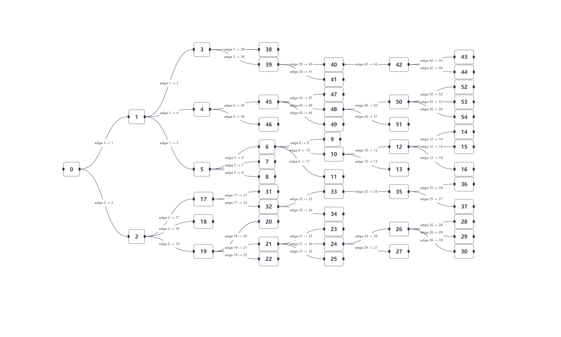
### Visual Description
\n
## Diagram: Directed Graph with Node and Edge Labels
### Overview
The image depicts a directed graph consisting of numbered nodes (0-54) connected by labeled edges. The graph appears to be a network or flow diagram, with arrows indicating the direction of relationships between nodes. The nodes are represented as black circles, and the edges are labeled with "edge X -> Y", indicating a connection from node X to node Y.
### Components/Axes
The diagram consists solely of nodes and edges. There are no explicit axes or scales. The nodes are numbered from 0 to 54. The edges are labeled with source and destination node numbers.
### Detailed Analysis or Content Details
The diagram contains 55 nodes (0-54) and numerous directed edges. Here's a breakdown of the connections, transcribed from the image:
* edge 0 -> 1
* edge 1 -> 3
* edge 1 -> 4
* edge 1 -> 5
* edge 2 -> 17
* edge 2 -> 18
* edge 2 -> 19
* edge 3 -> 38
* edge 3 -> 39
* edge 4 -> 45
* edge 4 -> 46
* edge 5 -> 7
* edge 5 -> 8
* edge 6 -> 9
* edge 6 -> 10
* edge 7 -> 11
* edge 8 -> 11
* edge 9 -> 12
* edge 10 -> 12
* edge 10 -> 13
* edge 11 -> 13
* edge 11 -> 14
* edge 12 -> 15
* edge 12 -> 16
* edge 13 -> 16
* edge 17 -> 31
* edge 17 -> 32
* edge 18 -> 20
* edge 18 -> 21
* edge 19 -> 22
* edge 19 -> 23
* edge 20 -> 23
* edge 20 -> 24
* edge 21 -> 24
* edge 21 -> 25
* edge 22 -> 24
* edge 22 -> 26
* edge 23 -> 26
* edge 23 -> 27
* edge 24 -> 27
* edge 24 -> 28
* edge 25 -> 28
* edge 25 -> 29
* edge 26 -> 28
* edge 26 -> 30
* edge 27 -> 30
* edge 27 -> 31
* edge 28 -> 31
* edge 28 -> 36
* edge 29 -> 36
* edge 29 -> 37
* edge 30 -> 37
* edge 31 -> 33
* edge 32 -> 33
* edge 32 -> 34
* edge 33 -> 35
* edge 34 -> 35
* edge 35 -> 36
* edge 35 -> 37
* edge 38 -> 40
* edge 39 -> 41
* edge 40 -> 42
* edge 41 -> 42
* edge 42 -> 43
* edge 42 -> 44
* edge 43 -> 44
* edge 44 -> 52
* edge 45 -> 47
* edge 45 -> 48
* edge 46 -> 48
* edge 46 -> 49
* edge 47 -> 50
* edge 48 -> 50
* edge 49 -> 51
* edge 50 -> 52
* edge 50 -> 53
* edge 51 -> 54
* edge 52 -> 54
* edge 53 -> 54
* edge 54 -> 14
### Key Observations
The graph is densely connected, particularly around nodes 1, 2, 6, 17, 20, 22, 23, 24, 26, 27, 28, 31, 32, 33, 35, 45, 46, 47, 48, 50, and 52. Node 1 appears to be a central hub, with connections to nodes 3, 4, and 5. Node 54 has incoming edges from 52, 53, and 51, and an outgoing edge to 14.
### Interpretation
This diagram likely represents a flow or dependency network. The nodes could represent tasks, states, or entities, and the edges represent the relationships or transitions between them. The labeling of edges as "edge X -> Y" suggests a directed flow from node X to node Y.
The density of connections around certain nodes indicates that those nodes are critical points in the network. For example, node 1 is a central hub, suggesting it controls or influences multiple downstream processes. The connections to node 54 suggest it is a final state or destination.
The diagram could be used to model a variety of systems, such as a workflow, a state machine, or a communication network. Without additional context, it is difficult to determine the specific meaning of the nodes and edges. The diagram appears to be a visualization of a complex system, and its purpose is to illustrate the relationships between its components. The presence of numbered edges suggests a possible ordering or prioritization of connections.
</details>
Figure 8: Monte Carlo Tree with origin parameter $c$ of UCT
<details>
<summary>extracted/6087579/fig/uct_1.png Details</summary>
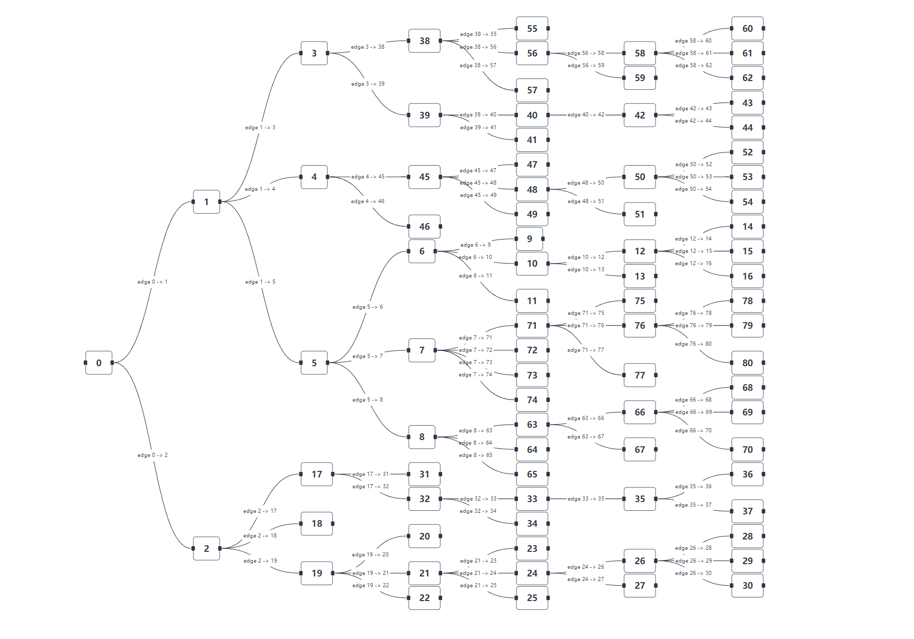
### Visual Description
\n
## Diagram: Network Graph
### Overview
The image depicts a network graph consisting of numbered nodes (1-94) connected by directed edges. Each edge is labeled with its source and destination node numbers. The graph appears to be a directed acyclic graph (DAG), meaning there are no cycles. The nodes are arranged in a roughly hierarchical structure, with nodes 1 and 2 at the bottom and branching upwards.
### Components/Axes
The diagram consists solely of nodes and directed edges. There are no axes or explicit scales. The nodes are numbered from 1 to 94. The edges are labeled with "edge X -> Y", indicating a directed connection from node X to node Y.
### Detailed Analysis or Content Details
The diagram contains 94 nodes and numerous edges. Here's a breakdown of the connections, organized by source node:
* **Node 1:** edges 1 -> 3, 1 -> 5
* **Node 2:** edges 2 -> 6, 2 -> 8
* **Node 3:** edges 3 -> 38, 3 -> 39
* **Node 4:** edges 4 -> 45, 4 -> 46
* **Node 5:** edges 5 -> 6, 5 -> 7
* **Node 6:** edges 6 -> 10, 6 -> 11
* **Node 7:** edges 7 -> 71, 7 -> 72
* **Node 8:** edges 8 -> 41, 8 -> 42
* **Node 9:** edges 9 -> 48, 9 -> 49
* **Node 10:** edges 10 -> 12, 10 -> 13
* **Node 11:** edges 11 -> 73, 11 -> 74
* **Node 12:** edges 12 -> 14, 12 -> 15
* **Node 13:** edges 13 -> 75, 13 -> 76
* **Node 14:** edges 14 -> 52, 14 -> 53
* **Node 15:** edges 15 -> 78, 15 -> 79
* **Node 16:** edges 16 -> 80, 16 -> 81
* **Node 17:** edges 17 -> 55, 17 -> 56
* **Node 18:** edges 18 -> 58, 18 -> 59
* **Node 19:** edges 19 -> 61, 19 -> 62
* **Node 20:** edges 20 -> 64, 20 -> 65
* **Node 21:** edges 21 -> 66, 21 -> 67
* **Node 22:** edges 22 -> 68, 22 -> 69
* **Node 23:** edges 23 -> 70, 23 -> 71
* **Node 24:** edges 24 -> 73, 24 -> 74
* **Node 25:** edges 25 -> 75, 25 -> 76
* **Node 26:** edges 26 -> 77, 26 -> 78
* **Node 27:** edges 27 -> 79, 27 -> 80
* **Node 28:** edges 28 -> 81, 28 -> 82
* **Node 29:** edges 29 -> 83, 29 -> 84
* **Node 30:** edges 30 -> 85, 30 -> 86
* **Node 31:** edges 31 -> 87, 31 -> 88
* **Node 32:** edges 32 -> 89, 32 -> 90
* **Node 33:** edges 33 -> 91, 33 -> 92
* **Node 34:** edges 34 -> 93, 34 -> 94
* **Node 35:** edges 35 -> 38, 35 -> 39
* **Node 36:** edges 36 -> 40, 36 -> 41
* **Node 37:** edges 37 -> 42, 37 -> 43
* **Node 38:** edges 38 -> 55, 38 -> 56
* **Node 39:** edges 39 -> 57, 39 -> 58
* **Node 40:** edges 40 -> 59, 40 -> 60
* **Node 41:** edges 41 -> 61, 41 -> 62
* **Node 42:** edges 42 -> 63, 42 -> 64
* **Node 43:** edges 43 -> 65, 43 -> 66
* **Node 44:** edges 44 -> 67, 44 -> 68
* **Node 45:** edges 45 -> 47, 45 -> 48
* **Node 46:** edges 46 -> 49, 46 -> 50
* **Node 47:** edges 47 -> 51, 47 -> 52
* **Node 48:** edges 48 -> 53, 48 -> 54
* **Node 49:** edges 49 -> 51, 49 -> 54
* **Node 50:** edges 50 -> 52, 50 -> 53
* **Node 51:** edges 51 -> 54, 51 -> 55
* **Node 52:** edges 52 -> 56, 52 -> 57
* **Node 53:** edges 53 -> 58, 53 -> 59
* **Node 54:** edges 54 -> 60, 54 -> 61
* **Node 55:** edges 55 -> 62, 55 -> 63
* **Node 56:** edges 56 -> 64, 56 -> 65
* **Node 57:** edges 57 -> 66, 57 -> 67
* **Node 58:** edges 58 -> 68, 58 -> 69
* **Node 59:** edges 59 -> 70, 59 -> 71
* **Node 60:** edges 60 -> 72, 60 -> 73
* **Node 61:** edges 61 -> 74, 61 -> 75
* **Node 62:** edges 62 -> 76, 62 -> 77
* **Node 63:** edges 63 -> 78, 63 -> 79
* **Node 64:** edges 64 -> 80, 64 -> 81
* **Node 65:** edges 65 -> 82, 65 -> 83
* **Node 66:** edges 66 -> 84, 66 -> 85
* **Node 67:** edges 67 -> 86, 67 -> 87
* **Node 68:** edges 68 -> 88, 68 -> 89
* **Node 69:** edges 69 -> 90, 69 -> 91
* **Node 70:** edges 70 -> 92, 70 -> 93
* **Node 71:** edges 71 -> 94, 71 -> 72
* **Node 72:** edges 72 -> 74, 72 -> 75
* **Node 73:** edges 73 -> 76, 73 -> 77
* **Node 74:** edges 74 -> 78, 74 -> 79
* **Node 75:** edges 75 -> 80, 75 -> 81
* **Node 76:** edges 76 -> 82, 76 -> 83
* **Node 77:** edges 77 -> 84, 77 -> 85
* **Node 78:** edges 78 -> 86, 78 -> 87
* **Node 79:** edges 79 -> 88, 79 -> 89
* **Node 80:** edges 80 -> 90, 80 -> 91
* **Node 81:** edges 81 -> 92, 81 -> 93
* **Node 82:** edges 82 -> 94, 82 -> 83
* **Node 83:** edges 83 -> 85, 83 -> 86
* **Node 84:** edges 84 -> 87, 84 -> 88
* **Node 85:** edges 85 -> 89, 85 -> 90
* **Node 86:** edges 86 -> 91, 86 -> 92
* **Node 87:** edges 87 -> 93, 87 -> 94
* **Node 88:** edges 88 -> 89, 88 -> 90
* **Node 89:** edges 89 -> 91, 89 -> 92
* **Node 90:** edges 90 -> 93, 90 -> 94
* **Node 91:** edges 91 -> 92, 91 -> 93
* **Node 92:** edges 92 -> 94, 92 -> 93
* **Node 93:** edges 93 -> 94
* **Node 94:** No outgoing edges.
### Key Observations
The graph is highly interconnected, with many nodes having multiple outgoing edges. Nodes 1 and 2 serve as root nodes, initiating the flow of connections. Node 94 is a terminal node, with no outgoing edges. The graph appears to be structured in layers, with nodes branching out from the initial roots.
### Interpretation
This diagram likely represents a workflow, decision tree, or dependency graph. The nodes could represent tasks, states, or entities, and the edges represent transitions, dependencies, or relationships. The hierarchical structure suggests a process that starts with a few initial steps (nodes 1 and 2) and branches out into a more complex network of interconnected actions. The terminal node (94) represents the final outcome or completion of the process. The multiple paths from the root nodes to the terminal node indicate that there are different ways to achieve the final outcome. The diagram could be used to visualize a complex system, identify critical paths, or analyze potential bottlenecks. The lack of cycles confirms that the process is deterministic and will eventually reach a conclusion.
</details>
Figure 9: Monte Carlo Tree with our optimized parameter $c$ of UCT
From Figure 8 and 9 we can observed that with our optimized parameter $c$ of UCT, MCTS algorithm in node selection decisions tends to prioritize exploring new nodes rather than repeatedly following old paths, which may often lead to dead ends.
Appendix H OpenAI API Data
| Difficulty | Model | USD per instance | Total Experiment Cost (USD) |
| --- | --- | --- | --- |
| Easy (0-shot) | GPT-4o | $0.0032 | $1.73 |
| o1-mini | $0.0136 | $7.34 | |
| Easy (4-shot) | GPT-4o | $0.0062 | $3.35 |
| o1-mini | $0.0171 | $9.23 | |
| Hard (0-shot) | GPT-4o | $0.0032 | $1.89 |
| o1-mini | $0.0177 | $10.44 | |
| Hard (4-shot) | GPT-4o | $0.0063 | $3.70 |
| o1-mini | $0.0172 | $10.15 | |
Table 8: OpenAI API cost of experiments on the Blocksworld dataset.
<details>
<summary>extracted/6087579/fig/Step_Length_vs_Reasoning_Tokens_for_Zero_Shot_Easy_Blocksworld.png Details</summary>
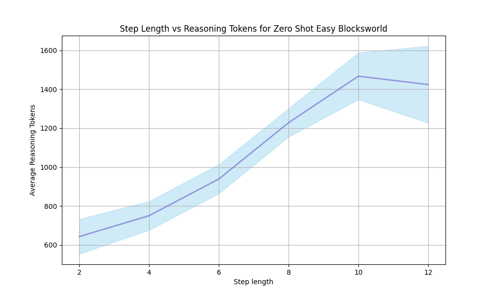
### Visual Description
\n
## Line Chart: Step Length vs Reasoning Tokens for Zero Shot Easy Blocksworld
### Overview
This image presents a line chart illustrating the relationship between "Step Length" and "Average Reasoning Tokens" in a "Zero Shot Easy Blocksworld" scenario. The chart displays a generally increasing trend, with some fluctuation, suggesting that as the step length increases, the average number of reasoning tokens also tends to increase. A shaded region around the line indicates the variance or confidence interval.
### Components/Axes
* **Title:** "Step Length vs Reasoning Tokens for Zero Shot Easy Blocksworld" - positioned at the top-center of the chart.
* **X-axis:** "Step length" - ranging from approximately 2 to 12, with tick marks at integer values.
* **Y-axis:** "Average Reasoning Tokens" - ranging from approximately 600 to 1600, with tick marks at intervals of 200.
* **Data Series:** A single blue line representing the relationship between step length and reasoning tokens. A light blue shaded region surrounds the line, representing the standard deviation or confidence interval.
### Detailed Analysis
The blue line representing the data series shows an overall upward trend. Let's break down the approximate values at specific step lengths:
* **Step Length = 2:** Average Reasoning Tokens ≈ 700
* **Step Length = 4:** Average Reasoning Tokens ≈ 800
* **Step Length = 6:** Average Reasoning Tokens ≈ 1000
* **Step Length = 8:** Average Reasoning Tokens ≈ 1300
* **Step Length = 10:** Average Reasoning Tokens ≈ 1500
* **Step Length = 12:** Average Reasoning Tokens ≈ 1400
The shaded region around the line indicates the variability in the data. The width of the shaded region appears to increase with step length, suggesting greater variance in the average reasoning tokens at higher step lengths. The shaded region at step length 12 is wider than at step length 2.
### Key Observations
* The relationship between step length and reasoning tokens is generally positive, but not strictly linear.
* There is a noticeable peak around step length 10, followed by a slight decrease at step length 12. This suggests that the increase in reasoning tokens may plateau or even decrease beyond a certain step length.
* The variance in reasoning tokens increases with step length.
### Interpretation
The chart suggests that as the complexity of the task (represented by step length) increases, the amount of reasoning required (measured in tokens) also increases. This is expected, as more steps likely require more complex planning and inference. The peak at step length 10 and subsequent decrease at step length 12 could indicate a point of diminishing returns, where further increasing the step length does not necessarily lead to a proportional increase in reasoning tokens. This could be due to the task becoming saturated with information or the model reaching a limit in its reasoning capacity. The increasing variance with step length suggests that the reasoning process becomes more unpredictable or diverse as the task becomes more complex. This data could be used to optimize the step length for a given task, balancing the need for sufficient reasoning with the cost of increased token usage. The "Zero Shot Easy Blocksworld" context implies that the model is performing this task without any prior training examples, making the observed relationship even more significant.
</details>
Figure 10: o1-mini Step Length vs Reasoning Tokens for Zero Shot in Easy Blocksworld
<details>
<summary>extracted/6087579/fig/Step_Length_vs_Reasoning_Tokens_for_Four_Shot_Easy_Blocksworld.png Details</summary>
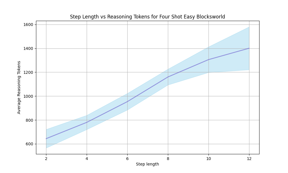
### Visual Description
\n
## Line Chart: Step Length vs Reasoning Tokens for Four Shot Easy Blocksworld
### Overview
This chart depicts the relationship between step length and the average number of reasoning tokens used in a "Four Shot Easy Blocksworld" environment. The chart uses a line graph with a shaded area representing the variance or confidence interval around the mean.
### Components/Axes
* **Title:** "Step Length vs Reasoning Tokens for Four Shot Easy Blocksworld" - positioned at the top-center of the chart.
* **X-axis:** "Step length" - ranging from approximately 2 to 12, with tick marks at integer values.
* **Y-axis:** "Average Reasoning Tokens" - ranging from approximately 600 to 1600, with tick marks at intervals of 200.
* **Data Series:** A single blue line representing the average reasoning tokens, with a light blue shaded area indicating the standard deviation or confidence interval.
* **Grid:** A light gray grid is present, aiding in the readability of the data points.
### Detailed Analysis
The blue line representing the average reasoning tokens exhibits a generally upward trend. As the step length increases, the average number of reasoning tokens also increases. The shaded area around the line indicates the variability in the data.
Here's an approximate extraction of data points, noting the inherent uncertainty in reading values from the chart:
* **Step Length = 2:** Average Reasoning Tokens ≈ 700
* **Step Length = 4:** Average Reasoning Tokens ≈ 850
* **Step Length = 6:** Average Reasoning Tokens ≈ 1000
* **Step Length = 8:** Average Reasoning Tokens ≈ 1150
* **Step Length = 10:** Average Reasoning Tokens ≈ 1350
* **Step Length = 12:** Average Reasoning Tokens ≈ 1550
The shaded area's width varies along the x-axis. It appears wider at lower step lengths (2-6) indicating greater variance in reasoning tokens at those points, and narrows as step length increases (8-12), suggesting more consistent reasoning token usage.
### Key Observations
* The relationship between step length and reasoning tokens is positive and appears roughly linear.
* The variance in reasoning token usage is higher at lower step lengths.
* There are no obvious outliers or anomalies in the data.
### Interpretation
The chart suggests that as the complexity of the task (represented by step length) increases, the model requires more reasoning tokens to solve it. This is a logical expectation, as more steps generally necessitate more complex thought processes. The decreasing variance at higher step lengths could indicate that the model becomes more consistent in its reasoning approach as the task becomes more challenging, or that the variance is simply being masked by the increasing average. The "Four Shot Easy Blocksworld" context suggests this is a relatively simple environment, and the linear relationship may not hold true for more complex scenarios. The data implies a direct correlation between the number of steps required to solve a problem and the computational resources (reasoning tokens) needed. This information is valuable for understanding the scalability and efficiency of the model in this specific environment.
</details>
Figure 11: o1-mini Step Length vs Reasoning Tokens for Four Shot in Easy Blocksworld
<details>
<summary>extracted/6087579/fig/Step_Length_vs_Reasoning_Tokens_for_Zero_Shot_Hard_Blocksworld.png Details</summary>
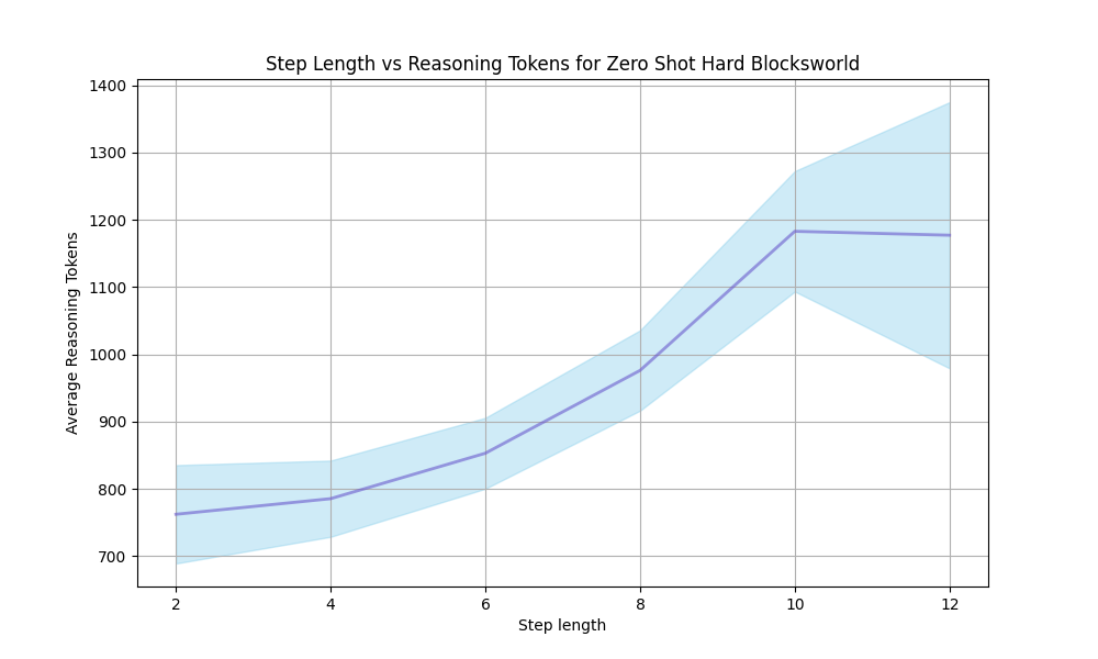
### Visual Description
\n
## Line Chart: Step Length vs Reasoning Tokens for Zero Shot Hard Blocksworld
### Overview
The image presents a line chart illustrating the relationship between "Step Length" and "Average Reasoning Tokens" for a "Zero Shot Hard Blocksworld" scenario. The chart displays a clear upward trend, indicating that as the step length increases, the average number of reasoning tokens also increases. A shaded region around the line represents the uncertainty or variance in the data.
### Components/Axes
* **Title:** "Step Length vs Reasoning Tokens for Zero Shot Hard Blocksworld" - positioned at the top-center of the chart.
* **X-axis:** "Step length" - ranging from approximately 2 to 12, with tick marks at integer values.
* **Y-axis:** "Average Reasoning Tokens" - ranging from approximately 700 to 1400, with tick marks at intervals of 100.
* **Data Series:** A single blue line representing the relationship between step length and reasoning tokens.
* **Confidence Interval:** A light blue shaded region surrounding the blue line, indicating the variance or confidence interval around the average reasoning tokens.
* **Gridlines:** Horizontal and vertical gridlines are present to aid in reading values.
### Detailed Analysis
The blue line representing the data series starts at approximately (2, 730) and ends at approximately (12, 1370).
Here's a breakdown of approximate data points, reading from left to right:
* (2, 730)
* (4, 770)
* (6, 850)
* (8, 1000)
* (10, 1250)
* (12, 1370)
The line exhibits a generally linear upward trend, but the slope appears to increase slightly as the step length increases. The shaded region around the line widens as the step length increases, suggesting greater variance in the average reasoning tokens at higher step lengths.
### Key Observations
* The relationship between step length and average reasoning tokens is positive and appears to be approximately linear.
* The variance in reasoning tokens increases with step length.
* There are no obvious outliers or anomalies in the data.
### Interpretation
The chart suggests that increasing the step length in the "Zero Shot Hard Blocksworld" scenario leads to a corresponding increase in the average number of reasoning tokens required. This could indicate that more complex reasoning is needed as the problem's step length increases. The widening confidence interval suggests that the reasoning process becomes more variable or less predictable at higher step lengths. This could be due to a greater number of possible solution paths or increased uncertainty in the reasoning process. The data implies that there is a cost associated with increasing step length in terms of computational resources (reasoning tokens). This information is valuable for optimizing the performance of the zero-shot learning system in this environment. The chart demonstrates a clear trade-off between step length and reasoning cost.
</details>
Figure 12: o1-mini Step Length vs Reasoning Tokens for Zero Shot in Hard Blocksworld
<details>
<summary>extracted/6087579/fig/Step_Length_vs_Reasoning_Tokens_for_Four_Shot_Hard_Blocksworld.png Details</summary>
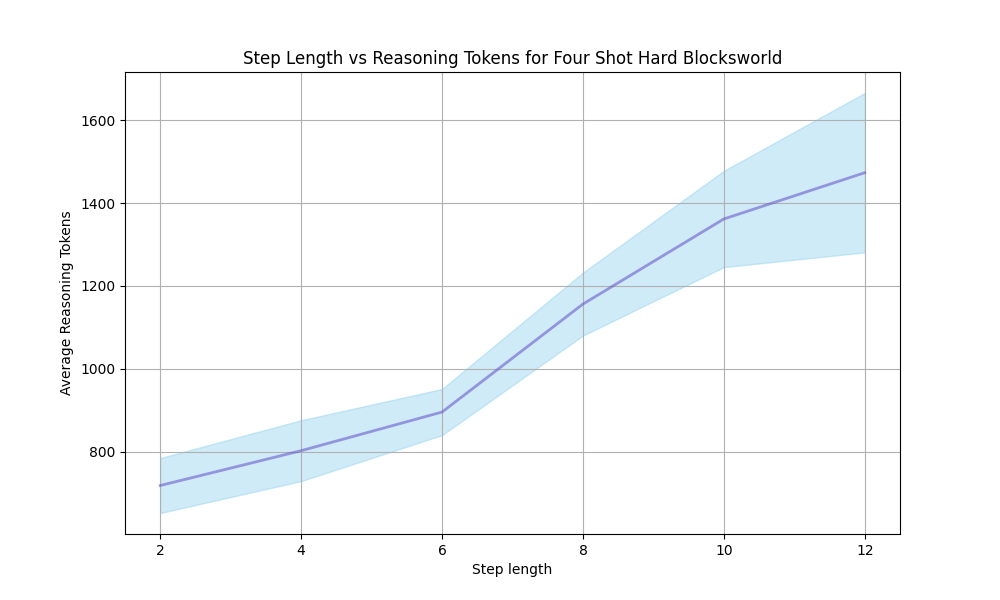
### Visual Description
## Line Chart: Step Length vs Reasoning Tokens for Four Shot Hard Blocksworld
### Overview
This chart depicts the relationship between step length and the average number of reasoning tokens used, specifically for the "Four Shot Hard Blocksworld" problem. The chart uses a line graph with a shaded confidence interval to illustrate the trend.
### Components/Axes
* **Title:** "Step Length vs Reasoning Tokens for Four Shot Hard Blocksworld" - positioned at the top-center of the chart.
* **X-axis:** "Step length" - ranging from approximately 2 to 12, with tick marks at integer values.
* **Y-axis:** "Average Reasoning Tokens" - ranging from approximately 600 to 1600, with tick marks at intervals of 200.
* **Data Series:** A single blue line representing the average reasoning tokens, with a light blue shaded area indicating a confidence interval.
### Detailed Analysis
The blue line representing the average reasoning tokens exhibits a clear upward trend as step length increases. The confidence interval widens as step length increases, indicating greater uncertainty in the average reasoning token count at larger step lengths.
Here's an approximate extraction of data points, acknowledging the inherent uncertainty in reading values from the graph:
* **Step Length = 2:** Average Reasoning Tokens ≈ 750
* **Step Length = 4:** Average Reasoning Tokens ≈ 850
* **Step Length = 6:** Average Reasoning Tokens ≈ 950
* **Step Length = 8:** Average Reasoning Tokens ≈ 1200
* **Step Length = 10:** Average Reasoning Tokens ≈ 1450
* **Step Length = 12:** Average Reasoning Tokens ≈ 1600
The shaded confidence interval appears to be approximately ±100-200 tokens around the blue line, but this varies with step length. At step length 2, the interval is narrower, while at step length 12, it is wider.
### Key Observations
* There is a strong positive correlation between step length and the average number of reasoning tokens.
* The uncertainty in the average reasoning token count increases with step length.
* The data suggests that longer step lengths require more reasoning tokens.
### Interpretation
The chart demonstrates that as the complexity of the problem-solving process (represented by step length) increases, the amount of reasoning required (measured in tokens) also increases. This is expected, as more steps generally necessitate more computational effort. The widening confidence interval at higher step lengths suggests that the relationship between step length and reasoning tokens may become more variable or less predictable as the problem becomes more complex. This could be due to factors such as increased branching in the search space or the emergence of more diverse solution strategies. The "Four Shot Hard Blocksworld" context implies this is a challenging problem, and the data reflects the increased cognitive load associated with solving it. The data suggests that there is a cost to increasing step length in terms of reasoning tokens, which could be relevant for optimizing the efficiency of problem-solving algorithms.
</details>
Figure 13: o1-mini Step Length vs Reasoning Tokens for Four Shot in Hard Blocksworld
Appendix I GPU Usage
In the main experiments, the total GPU usage (measured in GPU hours) for different models on NVIDIA H800 SXM5 80GB GPUs shows a clear progression with model size. For RAP-MCTS, Llama-3 70B requires approximately 420 GPU hours across all steps and difficulty modes, Llama-3.1 70B model requires approximately 450 GPU hours. For SC-MCTS ∗, Llama-3 70B requires approximately 280 GPU hours across all steps and difficulty modes and difficulty modes, Llama-3.1 70B model requires approximately 300 GPU hours. For CoT, Llama-3-70B and Llama-3.1-70B both takes approximately 7 GPU hours across all steps and difficulty modes, while Llama-3.1 405B model exhibits significantly higher GPU usage, amounting to approximately 75 GPU hours. In the parameter research and algorithm development phase before main experiments, we consumed a total of around 800 GPU hours on NVIDIA A100 SXM4 80GB GPUs.
Appendix J Future Work
In future work, we can explore utilizing more metrics-based reward models (such as the three reward models discussed in this paper) with LM-based reward models (such as Critic LLM (McAleese et al., 2024) and Eurus (Yuan et al., 2024b)). Additionally, there is potential to design more general methods for splitting steps in other tasks and datasets. Since step-splitting is the most challenging part of MCTS multi-step reasoning generalization, although we conducted extensive experiments on the Blocksworld multi-step reasoning dataset, which is the most suitable dataset for studying MCTS multi-step reasoning as far as we know. Some previous works have attempted to use datasets like GSM8K and MATH through extensive adaptation efforts on the datasets themselves, however, we aim to design a more general method from the perspective of step-splitting. We hope that MCTS multi-step reasoning will achieve the same level of generalization as CoT, which remains a fundamental area for future research. Future work can also attempt to combine this approach with the fine-grained compositional reasoning framework (Chen et al., 2024) to further explore the boundaries of MCTS multi-step reasoning capabilities.