2410.02707v4

# LLMs Know More Than They Show: On the Intrinsic Representation of LLM Hallucinations > Corresponding author; Work partially done during internship at Apple. ## Abstract Large language models (LLMs) often produce errors, including factual inaccuracies, biases, and reasoning failures, collectively referred to as “hallucinations”. Recent studies have demonstrated that LLMs’ internal states encode information regarding the truthfulness of their outputs, and that this information can be utilized to detect errors. In this work, we show that the internal representations of LLMs encode much more information about truthfulness than previously recognized. We first discover that the truthfulness information is concentrated in specific tokens, and leveraging this property significantly enhances error detection performance. Yet, we show that such error detectors fail to generalize across datasets, implying that—contrary to prior claims—truthfulness encoding is not universal but rather multifaceted. Next, we show that internal representations can also be used for predicting the types of errors the model is likely to make, facilitating the development of tailored mitigation strategies. Lastly, we reveal a discrepancy between LLMs’ internal encoding and external behavior: they may encode the correct answer, yet consistently generate an incorrect one. Taken together, these insights deepen our understanding of LLM errors from the model’s internal perspective, which can guide future research on enhancing error analysis and mitigation. Our code is available in https://github.com/technion-cs-nlp/LLMsKnow. ## 1 Introduction The ever-growing popularity of large language models (LLM) across many domains has brought a significant limitation to center stage: their tendency to “hallucinate” – which is often used to describe the generation of inaccurate information. But what are hallucinations, and what causes them? A considerable body of research has sought to define, taxonomize, and understand hallucinations through extrinsic, behavioral analysis, primarily examining how users perceive such errors (Bang et al., 2023; Ji et al., 2023; Huang et al., 2023a; Rawte et al., 2023). However, this approach does not adequately address how these errors are encoded within the LLMs. Alternatively, another line of work has explored the internal representations of LLMs, suggesting that LLMs encode signals of truthfulness (Kadavath et al., 2022; Li et al., 2024; Chen et al., 2024, inter alia). However, these analyses were typically restricted to detecting errors—determining whether a generated output contains inaccuracies—without delving deeper into how such signals are represented and could be leveraged to understand or mitigate hallucinations. In this work, we reveal that the internal representations of LLMs encode much more information about truthfulness than previously recognized. Through a series of experiments, we train classifiers on these internal representations to predict various features related to the truthfulness of generated outputs. Our findings reveal the patterns and types of information encoded in model representations, linking this intrinsic data to extrinsic LLM behavior. This enhances our ability to detect errors (while understanding the limitations of error detection), and may guide the development of more nuanced strategies based on error types and mitigation methods that make use of the model’s internal knowledge. Our experiments are designed to be general, covering a broad array of LLM limitations. While the term “hallucinations” is widely used, it lacks a universally accepted definition (Venkit et al., 2024). Our framework adopts a broad interpretation, considering hallucinations to encompass all errors produced by an LLM, including factual inaccuracies, biases, common-sense reasoning failures, and other real-world errors. This approach enables us to draw general conclusions about model errors from a broad perspective. Our first step is identifying where truthfulness signals are encoded in LLMs. Previous studies have suggested methods for detecting errors in LLM outputs using intermediate representations, logits, or probabilities, implying that LLMs may encode signals of truthfulness (Kadavath et al., 2022; Li et al., 2024; Chen et al., 2024). Focusing on long-form generations, which reflect real-world usage of LLMs, our analysis uncovers a key oversight: the choice of token used to extract these signals (Section 3). We find that truthfulness information is concentrated in the exact answer tokens – e.g., “Hartford” in “The capital of Connecticut is Hartford, an iconic city…”. Recognizing this nuance significantly improves error detection strategies across the board, revealing that truthfulness encoding is stronger than previously observed. From this point forward, we concentrate on our most effective strategy: a classifier trained on intermediate LLM representations within the exact answer tokens, referred to as ‘probing classifiers’ (Belinkov, 2021). This approach helps us explore what these representations reveal about LLMs. Our demonstration that a trained probing classifier can predict errors suggests that LLMs encode information related to their own truthfulness. However, we find that probing classifiers do not generalize across different tasks (Section 4). Generalization occurs only within tasks requiring similar skills (e.g., factual retrieval), indicating the truthfulness information is “skill-specific” and varies across different tasks. For tasks involving different skills, e.g., sentiment analysis, these classifiers are no better–or worse–than logit-based uncertainty predictors, challenging the idea of a “universal truthfulness” encoding proposed in previous work (Marks & Tegmark, 2023; Slobodkin et al., 2023). Instead, our results indicate that LLMs encode multiple, distinct notions of truth. Thus, deploying trainable error detectors in practical applications should be undertaken with caution. We next find evidence that LLMs encode not only error detection signals but also more nuanced information about error types. Delving deeper into errors within a single task, we taxonomize its errors based on responses across repeated samples (Section 5). For example, the same error being consistently generated is different from an error that is generated occasionally among many other distinct errors. Using a different set of probing classifiers, we find that error types are predictable from the LLM representations, drawing a connection between the models’s internal representations and its external behavior. This classification offers a more nuanced understanding of errors, enabling developers to predict error patterns and implement more targeted mitigation strategies. Finally, we find that the truthfulness signals encoded in LLMs can also differentiate between correct and incorrect answers for the same question (Section 6). Results highlight a significant misalignment between LLM’s internal representations and its external behavior in some cases. The model’s internal encoding may identify the correct answer–yet it frequently generates an incorrect response. This discrepancy reveals that the LLM’s external behavior may misrepresent its abilities, potentially pointing to new strategies for reducing errors by utilizing its existing strengths. Overall, our model-centric framework provides a deeper understanding of LLM errors, suggesting potential directions for improvements in error analysis and mitigation. ## 2 Background Defining and characterizing LLM errors. The term “hallucinations” is widely used across various subfields such as conversational AI (Liu et al., 2022), abstractive summarization (Zhang et al., 2019), and machine translation (Wang & Sennrich, 2020), each interpreting the term differently. Yet, no consensus exists on defining hallucinations: Venkit et al. (2024) identified 31 distinct frameworks for conceptualizing hallucinations, revealing the diversity of perspectives. Research efforts aim to define and taxonomize hallucinations, distinguishing them from other error types (Liu et al., 2022; Ji et al., 2023; Huang et al., 2023a; Rawte et al., 2023). On the other hand, recent scholarly conversations introduce terms like “confabulations” (Millidge, 2023) and “fabrications” (McGowan et al., 2023), attributing a possible “intention” to LLMs, although the notions of LLM “intention” and other human-like traits are still debated (Salles et al., 2020; Serapio-García et al., 2023; Harnad, 2024). These categorizations, however, adopt a human-centric view by focusing on the subjective interpretations of LLM hallucinations, which does not necessarily reflect how these errors are encoded within the models themselves. This gap limits our ability to address the root causes of hallucinations, or to reason about their nature. For example, it is unclear whether conclusions about hallucinations defined in one framework can be applied to another framework. Liang et al. (2024) defined hallucinations as inconsistencies with the training data. While this approach engage with the possible root causes of hallucinations, our study focuses on insights from the model itself, without requiring training data access. Instead, we adopt a broad interpretation of hallucinations. Here, we define hallucinations as any type of error generated by an LLM, including factual inaccuracies, biases, failures in common-sense reasoning, and others. Another line of research suggests that LLMs either encode information about their own errors (Kadavath et al., 2022; Azaria & Mitchell, 2023) or exhibit discrepancies between their outputs and internal representations (Liu et al., 2023; Gottesman & Geva, 2024), indicating the presence of underlying mechanisms not reflected in their final outputs. Moreover, Yona et al. (2024) found that current LLMs fail to effectively convey their uncertainty through their generated outputs. Hence, we propose shifting the focus from human-centric interpretations of hallucinations to a model-centric perspective, examining the model’s intermediate activations. Error detection in LLMs. Error detection is a longstanding task in NLP, crucial for maintaining high standards in various practical applications and for constructing more reliable systems that ensure user trust (Bommasani et al., 2021). Over the years, many studies have proposed task-specific solutions (see Section A.1). However, the recent shift towards general-purpose LLMs necessitates a holistic approach capable of addressing any error type, rather than focusing on specific ones, making it suitable for the diverse errors generated by these models. A line of work has addressed this challenge by leveraging external knowledge sources (Lewis et al., 2020; Gao et al., 2023) or an external LLM judge (Lin et al., 2021; Rawte et al., 2023) to identify erroneous outputs. On the other hand, our work focuses on detection methods that rely solely on the computations of the LLM—specifically, output logits, probabilities after softmax, and hidden states. Error detection in LLMs is also closely linked to uncertainty estimation, where low certainty signals potential inaccuracies and possible errors. Popular methods to derive calibrated confidence include inspecting the model logit output values (Varshney et al., 2023; Taubenfeld et al., 2025), agreement across multiple sampled answers (Kuhn et al., 2023; Manakul et al., 2023; Tian et al., 2023a), verbalized probability (Tian et al., 2023b), and direct prompting (Kadavath et al., 2022). Another line of work trains probing classifiers to discover and utilize truthfulness features. This approach has shown some success by probing the final token of an answer–either generated (Kadavath et al., 2022; Snyder et al., 2023; Yuksekgonul et al., 2023; Zou et al., 2023; Yin et al., 2024; Chen et al., 2024; Simhi et al., 2024; Gekhman et al., 2025) or not (Li et al., 2024; Marks & Tegmark, 2023; Burns et al., 2022; Azaria & Mitchell, 2023; Rateike et al., 2023). Others probe the final token of the prompt before the response is generated (Slobodkin et al., 2023; Snyder et al., 2023; Simhi et al., 2024; Gottesman & Geva, 2024). Many previous studies simplify the analysis by generating answers in a few-shot setting or limiting generation to a single token. In contrast, we simulate real-world usage of LLMs by allowing unrestricted answer generation. By probing exact answer tokens, we achieve significant improvements in error detection. ## 3 Better Error Detection This section presents our experiments on detecting LLM errors through their own computations, focusing on token selection’s impact and introducing a method that outperforms other approaches. ### 3.1 Task Definition Given an LLM $M$ , an input prompt $p$ and the LLM-generated response $\hat{y}$ , the task is to predict whether $\hat{y}$ is correct or wrong. We assume that there is access to the LLM’s internal states (i.e., white-box setting), but no access to any external resources (e.g., search engine or additional LLMs). We use a dataset $D=\{(q_{i},y_{i})\}_{i=1}^{N}$ , consisting of $N$ question-label pairs, where $\{q_{i}\}_{i=1}^{N}$ represents a series of questions (e.g., “What is the capital of Connecticut?”) and $\{y_{i}\}_{i=1}^{N}$ the corresponding ground-truth answers (“Hartford”). For each question $q_{i}$ , we prompt the model $M$ to generate a response $y_{i}$ , resulting in the set of predicted answers $\{\hat{y}_{i}\}_{i=1}^{N}$ (“The capital of Connecticut is Hartford…”). Next, to build our error-detection dataset, we evaluate the correctness of each generated response $\hat{y}_{i}$ by comparing it to the ground-truth label $y_{i}$ . This comparison yields a correctness label $z_{i}\in\{0,1\}$ ( $1$ correct, $0 0$ wrong). The comparison can be done either via automatic heuristics or with the assistance of an instruct-LLM. For most datasets, we use heuristics to predict correctness, except for one case. See Appendix A.2. Our error detection dataset is: $\{(q_{i},\hat{y}_{i},z_{i})\}_{i=1}^{N}$ . Note that this dataset is defined based on the analyzed LLM and its generated answers. Any instances where the LLM refuses to answer are excluded, as these can easily be classified as incorrect. ### 3.2 Experimental Setup Datasets and models. We perform all experiments on four LLMs: Mistral-7b (Jiang et al., 2023), Mistral-7b-instruct-v0.2 (denoted Mistral-7b-instruct), Llama3-8b (Touvron et al., 2023), and Llama3-8b-instruct. We consider 10 different datasets spanning various domains and tasks: TriviaQA (Joshi et al., 2017), HotpotQA with/without context (Yang et al., 2018), Natural Questions (Kwiatkowski et al., 2019), Winobias (Zhao et al., 2018), Winogrande (Sakaguchi et al., 2021), MNLI (Williams et al., 2018), Math (Sun et al., 2024), IMDB review sentiment analysis (Maas et al., 2011), and a dataset of movie roles (movies) that we curate. We allow unrestricted response generation to mimic real-world LLM usage, with answers decoded greedily. For more details on the datasets and the prompts used to generate answers, refer to Appendix A.3. Performance metric. We measure the area under the ROC curve to evaluate error detectors, providing a single metric that reflects their ability to distinguish between positive and negative cases across many thresholds, balancing sensitivity (true positive rate) and specificity (false positive rate). Error detection methods. We compare methods from both uncertainty and hallucinations literature. - Aggregated probabilities / logits: Previous studies (Guerreiro et al., 2023; Kadavath et al., 2022; Varshney et al., 2023; Huang et al., 2023b) aggregate output token probabilities or logits to score LLM confidence for error detection. We implement several methods from the literature, calculating the minimum, maximum, or mean of these values. The main paper reports results for the most common approach, Logits-mean, and the best-performing one, Logits-min, with additional baselines in Appendix B. - P(True): Kadavath et al. (2022) showed that LLMs are relatively calibrated when asked to evaluate the correctness of their generation via prompting. We implement this evaluation using the same prompt. - Probing: Probing classifiers involve training a small classifier on a model’s intermediate activations to predict features of processed text (Belinkov, 2021). Recent studies show their effectiveness for error detection in generated text (Kadavath et al., 2022, inter alia). An intermediate activation is a vector $h_{l,t}$ from a specific LLM layer $l$ and (either read or generated) token $t$ . Thus, each LLM generation produces multiple such activations. Following prior work, we use a linear probing classifier for error detection (Li et al., 2024, inter alia) on static tokens: the last generated token ( $h_{l,-1}$ ), the one before it ( $h_{l,-2}$ ), and the final prompt token ( $h_{l,k}$ ). The layer $l$ is selected per token based on validation set performance. For further details on the implementation of each method, refer to Appendix A.4. <details> <summary>x1.png Details</summary>  ### Visual Description \n ## Diagram: Prompt-Response Token Annotation ### Overview The image is a technical diagram illustrating the tokenization and annotation process for a prompt-response pair in a language model interaction. It visually maps specific tokens within a user's prompt and the model's generated response, highlighting key segments like the question, the exact answer, and end-of-sequence markers. ### Components/Axes The diagram consists of two primary rounded rectangular boxes connected by annotated arrows, set against a plain white background. 1. **Prompt Box (Top, Green Fill):** * **Label:** "Prompt" (written vertically on the left side). * **Content:** `<s> [INST] What is the capital of the U.S. state of Connecticut? [/INST]` * **Annotations:** * A green arrow labeled `last_q_token` points to the closing `[/INST]` tag. * The entire prompt text is enclosed in a green box. 2. **Response Box (Bottom, Blue Fill):** * **Label:** "Mistral" (written vertically on the left side). * **Content:** `The capital city of the U.S. state of Connecticut is Hartford. It's one of the oldest cities in the United States and was founded in 1635. Hartford is located in the central part of the state and is home to several cultural institutions, universities, and businesses.</s>` * **Annotations:** * A purple arrow labeled `first_exact_answer_token` points to the start of the word "Hartford". * A blue arrow labeled `last_exact_answer_token` points to the end of the word "Hartford". * The word "Hartford" is enclosed in a purple box. * The final token `</s>` is enclosed in an orange box. * Below the orange box, the numbers `-2` (in blue) and `-1` (in orange) are written, likely indicating token indices relative to the end of the sequence. ### Detailed Analysis The diagram explicitly maps the structure of a single instruction-following interaction: * **Prompt Structure:** The user prompt is formatted with special tokens: `<s>` (start of sequence), `[INST]` (instruction start), the question text, and `[/INST]` (instruction end). The annotation `last_q_token` identifies the final token of the question segment. * **Response Structure:** The model's response is a continuous block of text ending with the `</s>` (end of sequence) token. * **Answer Extraction:** The diagram isolates the core factual answer ("Hartford") within the longer response. It defines the "first_exact_answer_token" and "last_exact_answer_token" to precisely bracket this answer span. * **Token Indexing:** The numbers `-2` and `-1` beneath the `</s>` token suggest a reverse indexing scheme for the final tokens in the sequence, where `-1` is the last token (`</s>`) and `-2` is the token immediately preceding it (the period after "businesses"). ### Key Observations 1. **Instruction Format:** The prompt uses a clear `[INST]...[/INST]` delimiter format, common in models fine-tuned for instruction following. 2. **Answer Localization:** The model's response contains the exact answer ("Hartford") embedded within a longer, informative sentence. The annotation system is designed to locate this exact answer span automatically. 3. **End-of-Sequence Handling:** The diagram explicitly marks the model's stop token (`</s>`) and provides a mechanism (negative indexing) to reference tokens at the very end of the generated sequence. 4. **Visual Coding:** Color is used systematically: green for prompt elements, blue for response elements, purple for the answer span, and orange for the end token. ### Interpretation This diagram serves as a technical schematic for a **token-level evaluation or analysis pipeline**. It demonstrates a method for: * **Parsing Structured Prompts:** Identifying the boundaries of the user's instruction within a formatted input string. * **Extracting Model Answers:** Precisely locating the core answer within a verbose model generation, which is crucial for automated scoring (e.g., exact match, F1 score) against a ground truth. * **Understanding Model Output Structure:** Analyzing how a model like "Mistral" structures its responses, including its use of end-of-sequence tokens. The relationship shown is a **mapping from raw text to annotated token spans**. The "Prompt" is the input, the "Mistral" box is the output, and the arrows/boxes represent the metadata extracted by an analysis tool. This process is fundamental for benchmarking model performance, debugging generation issues, and training reward models for reinforcement learning from human feedback (RLHF). The inclusion of negative indices (`-2`, `-1`) is particularly insightful, as it reveals a common programming practice for handling sequences of variable length when focusing on the final elements. 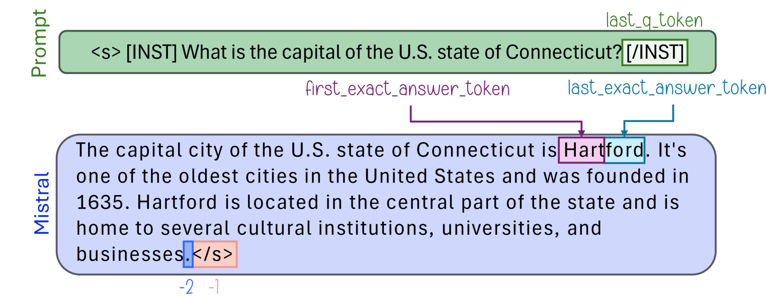</details> Figure 1: Example for the input and LLM output from the TriviaQA dataset, and the names of the tokens that can be probed. Exact Answer Tokens. Existing methods often overlook a critical nuance: the token selection for error detection, typically focusing on the last generated token or taking a mean. However, since LLMs typically generate long-form responses, this practice may miss crucial details (Brunner et al., 2020). Other approaches use the last token of the prompt (Slobodkin et al., 2023, inter alia), but this is inherently inaccurate due to LLMs’ unidirectional nature, failing to account for the generated response and missing cases where different sampled answers from the same model vary in correctness. We investigate a previously unexamined token location: the exact answer tokens, which represent the most meaningful parts of the generated response. We define exact answer tokens as those whose modification alters the answer’s correctness, disregarding subsequent generated content. In practice, we do not use this definition for extracting the exact answer, but rather an instruct model in a few-shot setting. Still, the definition is useful to manually verify that automatic extractions work as expected. Figure 1 illustrates the different token locations. In the following experiments, we implement each error detection method with an “exact answer” version, demonstrating that it often improves performance, especially in probing. Implementation details for detecting the exact answer token are given in Appendix A.2. ### 3.3 Results <details> <summary>extracted/6450693/figures/probing_heatmaps/mistral-7b-instruct/triviaqa_auc.png Details</summary>  ### Visual Description ## Heatmap: Layer vs. Token Activation/Attention ### Overview The image displays a heatmap visualizing a numerical value (likely attention weight, activation strength, or correlation) across two dimensions: **Layer** (vertical axis) and **Token** (horizontal axis). The data is represented by a color gradient from light blue (low value) to dark blue (high value). A prominent black rectangular outline highlights a specific region of interest within the heatmap. ### Components/Axes * **Y-Axis (Vertical):** Labeled **"Layer"**. The scale runs from **0** at the top to **30** at the bottom, with major tick marks at every even number (0, 2, 4, ..., 30). This likely represents layers in a neural network model. * **X-Axis (Horizontal):** Labeled **"Token"**. It contains a series of categorical and numerical labels. From left to right, the labels are: * `last_q` * `first_answer` * `second_answer` * `exact_answer_before_first` * `exact_answer_first` * `exact_answer_last` * `exact_answer_after_last` * `-8` * `-7` * `-6` * `-5` * `-4` * `-3` * `-2` * `-1` * **Color Scale/Legend:** Positioned on the right side of the chart. It is a vertical color bar labeled with numerical values. The scale ranges from **0.5** (lightest blue/white at the bottom) to **1.0** (darkest blue at the top), with intermediate markers at **0.6, 0.7, 0.8, and 0.9**. * **Highlighted Region:** A thick black rectangle is drawn around a vertical block of cells. This region spans horizontally from the token `exact_answer_before_first` to `exact_answer_after_last` (covering four token columns) and vertically across all layers (0 to 30). ### Detailed Analysis The heatmap shows a grid of colored cells, where each cell's color corresponds to a value between approximately 0.5 and 1.0. * **General Pattern:** The left side of the heatmap (tokens `last_q` through `exact_answer_after_last`) generally exhibits higher values (darker blue shades) compared to the right side (numerical tokens `-8` to `-1`), which are predominantly lighter. * **Within the Highlighted Region:** The four columns within the black rectangle (`exact_answer_before_first`, `exact_answer_first`, `exact_answer_last`, `exact_answer_after_last`) show the highest concentration of dark blue cells, indicating values consistently in the upper range of the scale (0.7 to 1.0). The intensity appears particularly strong in the middle layers (approximately layers 8 through 20). * **Layer Trends:** For the highlighted tokens, values seem to peak in the middle layers and are slightly lower in the very top (0-4) and bottom (26-30) layers. For the numerical tokens on the right, values are uniformly low across all layers, with only faint blue shading. * **Token Trends:** Moving from left to right across the x-axis, there is a clear gradient of decreasing value intensity. The `exact_answer_*` tokens have the highest values, followed by `second_answer` and `first_answer`, then `last_q`. The numerical tokens (`-8` to `-1`) have the lowest values. ### Key Observations 1. **Strongest Signal:** The model's layers show the strongest response (highest values) to tokens related to the "exact answer" (`exact_answer_before_first`, `exact_answer_first`, `exact_answer_last`, `exact_answer_after_last`). 2. **Spatial Focus:** The black rectangle explicitly draws attention to this "exact answer" token group, suggesting it is the primary subject of analysis. 3. **Clear Dichotomy:** There is a stark contrast between the high-value region on the left (semantic/answer tokens) and the low-value region on the right (numerical position tokens). 4. **Mid-Layer Peak:** Within the high-value region, the signal is not uniform across layers; it appears most intense in the network's middle layers. ### Interpretation This heatmap likely visualizes **attention weights** or **activation patterns** in a transformer-based language model during a question-answering task. The data suggests the following: * **Model Focus:** The model allocates significantly more "attention" or computational resources to tokens directly surrounding and comprising the exact answer compared to other parts of the input (like the question token `last_q` or positional markers `-8` to `-1`). * **Information Processing:** The concentration of high values in the middle layers aligns with common findings in neural network interpretability, where mid-level layers often process task-specific, semantic information. * **Functional Implication:** The pattern indicates the model has learned to identify and prioritize the span of text that constitutes the precise answer. The tokens `exact_answer_before_first` and `exact_answer_after_last` likely act as boundary markers, helping the model isolate the answer span. The low values for numerical tokens suggest they serve a minor, possibly structural, role that does not require strong activation. * **Anomaly/Outlier:** There are no major outliers; the gradient from high to low values across token types is smooth and consistent, indicating a robust and focused pattern of model behavior for this task. The black rectangle is an annotation, not a data feature, used to emphasize the key finding. </details> (a) TriviaQA <details> <summary>extracted/6450693/figures/probing_heatmaps/mistral-7b-instruct/winobias_auc.png Details</summary>  ### Visual Description ## Heatmap: Layer-wise Token Activation/Attention Pattern ### Overview The image is a heatmap visualization, likely representing activation strengths, attention weights, or some form of importance score across different layers of a neural network model for specific tokens in a sequence. The data is presented as a grid where color intensity corresponds to a numerical value. ### Components/Axes * **Chart Type:** Heatmap. * **Y-Axis (Vertical):** Labeled **"Layer"**. It represents the depth or layer index within a model, numbered from **0** at the top to **30** at the bottom, with tick marks at every even number (0, 2, 4, ..., 30). * **X-Axis (Horizontal):** Labeled **"Token"**. It lists specific token identifiers or categories. From left to right, the labels are: 1. `last_q` 2. `first_answer` 3. `second_answer` 4. `exact_answer_before_first` (Start of highlighted region) 5. `exact_answer_first` 6. `exact_answer_last` 7. `exact_answer_after_last` (End of highlighted region) 8. `-8` 9. `-7` 10. `-6` 11. `-5` 12. `-4` 13. `-3` 14. `-2` 15. `-1` * **Color Scale/Legend:** Located on the **right side** of the chart. It is a vertical color bar mapping color to a numerical value, ranging from **0.5** (lightest blue/white) at the bottom to **1.0** (darkest blue) at the top. The scale has major ticks at 0.5, 0.6, 0.7, 0.8, 0.9, and 1.0. * **Highlighted Region:** A thick black rectangular box is drawn around the four central token columns: `exact_answer_before_first`, `exact_answer_first`, `exact_answer_last`, and `exact_answer_after_last`. This box spans from the top (Layer 0) to the bottom (Layer 30) of the heatmap. ### Detailed Analysis The heatmap displays a matrix of values where each cell's color corresponds to the scale on the right. Darker blue indicates a higher value (closer to 1.0), while lighter blue/white indicates a lower value (closer to 0.5). **Trend Verification & Data Point Analysis:** 1. **Highlighted "exact_answer_*" Tokens (Center-Left):** * **Trend:** This group shows the **strongest and most consistent high values** across the majority of layers. * **Details:** From approximately **Layer 10 downwards**, these four columns are predominantly dark blue, indicating values consistently in the **0.85 - 1.0** range. The intensity appears highest in the middle layers (roughly 12-24). In the very top layers (0-6), the values are more moderate (light to medium blue, ~0.6-0.8). 2. **Initial Tokens (`last_q`, `first_answer`, `second_answer`) (Far Left):** * **Trend:** These show **moderate to high values**, but with more variability and generally less intensity than the highlighted group. * **Details:** `last_q` and `first_answer` have a mix of medium and dark blue cells, with values often in the **0.7 - 0.9** range, especially in the middle to lower layers. `second_answer` appears slightly lighter on average than the first two. 3. **Numerical Tokens (`-8` to `-1`) (Right Side):** * **Trend:** These tokens exhibit the **lowest values** on average, with a clear gradient. * **Details:** The leftmost numerical token (`-8`) is the lightest, with many cells in the **0.5 - 0.7** range. Moving right towards `-1`, the colors gradually darken, indicating a slight increase in value. The token `-1` has the highest values in this group, with some cells reaching medium blue (~0.8) in the lower layers. The top layers (0-8) for all numerical tokens are very light. 4. **Layer-wise Pattern (Vertical Trend):** * **Trend:** There is a general trend of **increasing values from top to bottom** (from Layer 0 to Layer 30) for most tokens. * **Details:** The top 8-10 layers are noticeably lighter across the entire chart. The middle and lower layers (10-30) contain the darkest blue cells, suggesting that the measured property (e.g., attention, activation) becomes more pronounced or focused in deeper parts of the model. ### Key Observations * **Primary Outlier Group:** The four tokens inside the black box (`exact_answer_*`) are clear outliers, demonstrating significantly higher and more sustained values across layers compared to all other tokens. * **Secondary Pattern:** The numerical tokens (`-8` to `-1`) form a distinct group with lower values, showing an internal gradient where tokens closer to `-1` have slightly higher values. * **Layer Depth Correlation:** Deeper layers (higher layer numbers) generally show stronger signals (darker colors) than shallower layers for the same token. * **Spatial Grounding:** The legend is positioned to the right of the main grid. The black highlight box is centered horizontally on the four "exact_answer" columns and spans the full vertical height of the plot area. ### Interpretation This heatmap likely visualizes the internal state of a transformer-based language model during a specific task, such as question-answering. The "Token" axis represents different positions or types of tokens in the input/output sequence. * **What the data suggests:** The model allocates significantly more "attention" or generates stronger activations for tokens directly related to the **exact answer** (`exact_answer_*` group). This indicates these tokens are critically important for the model's processing or output generation at most depths. * **Relationship between elements:** The contrast between the high-value `exact_answer_*` tokens and the lower-value numerical tokens (which may represent positional embeddings or less critical context) highlights a **focal point** in the model's computation. The model appears to "pay attention" most to the precise answer span. * **Notable trends:** The increase in value strength with layer depth is a common pattern in deep networks, where higher-level, more abstract features are built in deeper layers. The gradient within the numerical tokens (`-8` to `-1`) might reflect a positional bias, where tokens closer to the end of a sequence (or a reference point) are slightly more salient. * **Underlying mechanism:** The black box emphasizes that the analysis is specifically focused on how the model treats the exact answer span compared to other question (`last_q`) and answer (`first_answer`, `second_answer`) tokens, as well as generic positional markers. The data strongly supports the hypothesis that the model's internal representations are highly tuned to the exact answer location. </details> (b) Winobias <details> <summary>extracted/6450693/figures/probing_heatmaps/mistral-7b-instruct/answerable_math_auc.png Details</summary>  ### Visual Description ## Heatmap: Neural Network Layer-Token Activation Analysis ### Overview The image displays a heatmap visualizing numerical values (likely attention weights, activation strengths, or correlation scores) across different layers of a neural network (y-axis) and specific tokens or token positions (x-axis). A prominent vertical black rectangle highlights a specific region of interest on the x-axis. A color scale bar on the right indicates that values range from 0.5 (lightest blue/white) to 1.0 (darkest blue). ### Components/Axes * **Chart Type:** Heatmap. * **Y-Axis (Vertical):** * **Label:** "Layer" * **Scale:** Linear, numbered from 0 at the top to 30 at the bottom, with tick marks every 2 units (0, 2, 4, ..., 30). * **X-Axis (Horizontal):** * **Label:** "Token" * **Categories (from left to right):** 1. `last_q` 2. `first_answer` 3. `second_answer` 4. `exact_answer_before_first` (Start of highlighted region) 5. `exact_answer_first` 6. `exact_answer_last` 7. `exact_answer_after_last` (End of highlighted region) 8. `-8` 9. `-7` 10. `-6` 11. `-5` 12. `-4` 13. `-3` 14. `-2` 15. `-1` * **Color Scale (Legend):** * **Position:** Right side of the chart. * **Range:** 0.5 to 1.0. * **Gradient:** Continuous gradient from very light blue/white (0.5) to dark blue (1.0). * **Tick Marks:** Labeled at 0.5, 0.6, 0.7, 0.8, 0.9, 1.0. * **Highlighted Region:** * A thick black rectangle outlines a vertical band on the heatmap. * **Spatial Grounding:** This rectangle is positioned in the center-left of the chart, spanning from the x-axis category `exact_answer_before_first` to `exact_answer_after_last`. It covers all layers (0-30) vertically within this token range. ### Detailed Analysis * **General Pattern:** The heatmap shows a clear concentration of high values (dark blue) within the highlighted vertical band. Values outside this band are generally lower (lighter blue to white). * **Highlighted Band Analysis (Tokens: `exact_answer_before_first` to `exact_answer_after_last`):** * **Trend Verification:** This entire vertical strip exhibits consistently high values across nearly all layers (0-30). The color is predominantly dark blue, indicating values frequently in the 0.8-1.0 range. * **Sub-Patterns:** Within this band, the columns for `exact_answer_first` and `exact_answer_last` appear to have the most intense and consistent dark blue coloring, suggesting these tokens may have the highest values. The columns `exact_answer_before_first` and `exact_answer_after_last` are also dark but show slightly more variation, with some lighter blue cells, particularly in the middle layers (approx. layers 10-20). * **Non-Highlighted Regions Analysis:** * **Left Region (Tokens: `last_q`, `first_answer`, `second_answer`):** Values are generally low to moderate. The color is mostly light blue, corresponding to an approximate range of 0.5-0.7. There is no strong layer-wise trend; values are scattered. * **Right Region (Tokens: `-8` to `-1`):** Values are also generally low to moderate, similar to the left region. The color is predominantly light blue (0.5-0.7). There is a subtle pattern where the columns for `-2` and `-1` appear slightly darker (closer to 0.7-0.8) in the lower layers (approx. layers 20-30) compared to the upper layers. * **Layer-wise Trends:** * There is no single, strong trend that applies to all tokens across layers. The most significant pattern is the stability of high values within the highlighted token band across all layers. * In the non-highlighted regions, the distribution of moderate values appears somewhat random without a clear increasing or decreasing trend from layer 0 to layer 30. ### Key Observations 1. **Dominant Feature:** The most striking feature is the vertical band of high activation/values for the four tokens related to the "exact answer" (`exact_answer_before_first`, `exact_answer_first`, `exact_answer_last`, `exact_answer_after_last`). This is explicitly highlighted by the black rectangle. 2. **Token Specificity:** The tokens `exact_answer_first` and `exact_answer_last` within the highlighted band show the most consistently high values (darkest blue). 3. **Low Baseline:** Tokens outside the highlighted "exact answer" context (`last_q`, `first_answer`, `second_answer`, and the numbered tokens `-8` to `-1`) show significantly lower values, mostly in the lower half of the scale (0.5-0.7). 4. **Spatial Anomaly:** The numbered tokens on the far right (`-8` to `-1`) show a slight increase in value in the lower network layers (20-30), particularly for `-2` and `-1`. ### Interpretation This heatmap likely visualizes a metric like attention weight or hidden state activation strength within a transformer-based language model, analyzing how the model processes a specific question-answer pair. * **What the data suggests:** The model's internal representations (across all layers from 0 to 30) are strongly and consistently focused on the tokens immediately surrounding the "exact answer." The high values in the highlighted band indicate these tokens are critically important for the model's processing at every level of its hierarchy. * **How elements relate:** The stark contrast between the high-value "exact answer" band and the low-value surrounding tokens demonstrates a sharp contextual focus. The model appears to "lock onto" the precise answer span. The numbered tokens (`-8` to `-1`), which likely represent positions relative to the end of the sequence or a special token, show weaker and more diffuse activation, suggesting they play a less central role in this specific analysis. * **Notable outliers/trends:** The slight increase in value for tokens `-2` and `-1` in the deeper layers (20-30) is a subtle but interesting anomaly. This could indicate that the final layers of the model pay slightly more attention to the very end of the input sequence, perhaps for tasks like determining when to stop generating or for final answer normalization. * **Peircean investigative reading:** The heatmap is an indexical sign pointing to the model's internal focus. The highlighted rectangle is a direct index of the researcher's hypothesis—that the "exact answer" tokens are key. The data confirms this hypothesis strongly. The chart is also a symbolic representation of the model's computational state, allowing us to infer that the mechanism for answer extraction or verification is distributed across all layers but is highly localized to specific token positions. The lack of a strong layer-wise gradient suggests this focus is a fundamental, early-established property of the processing stream for this input, not something that emerges only in deep layers. 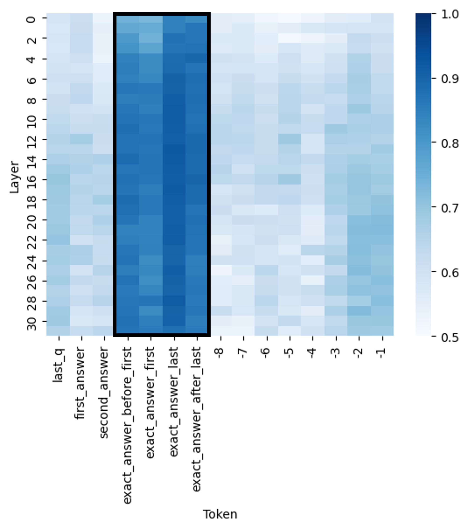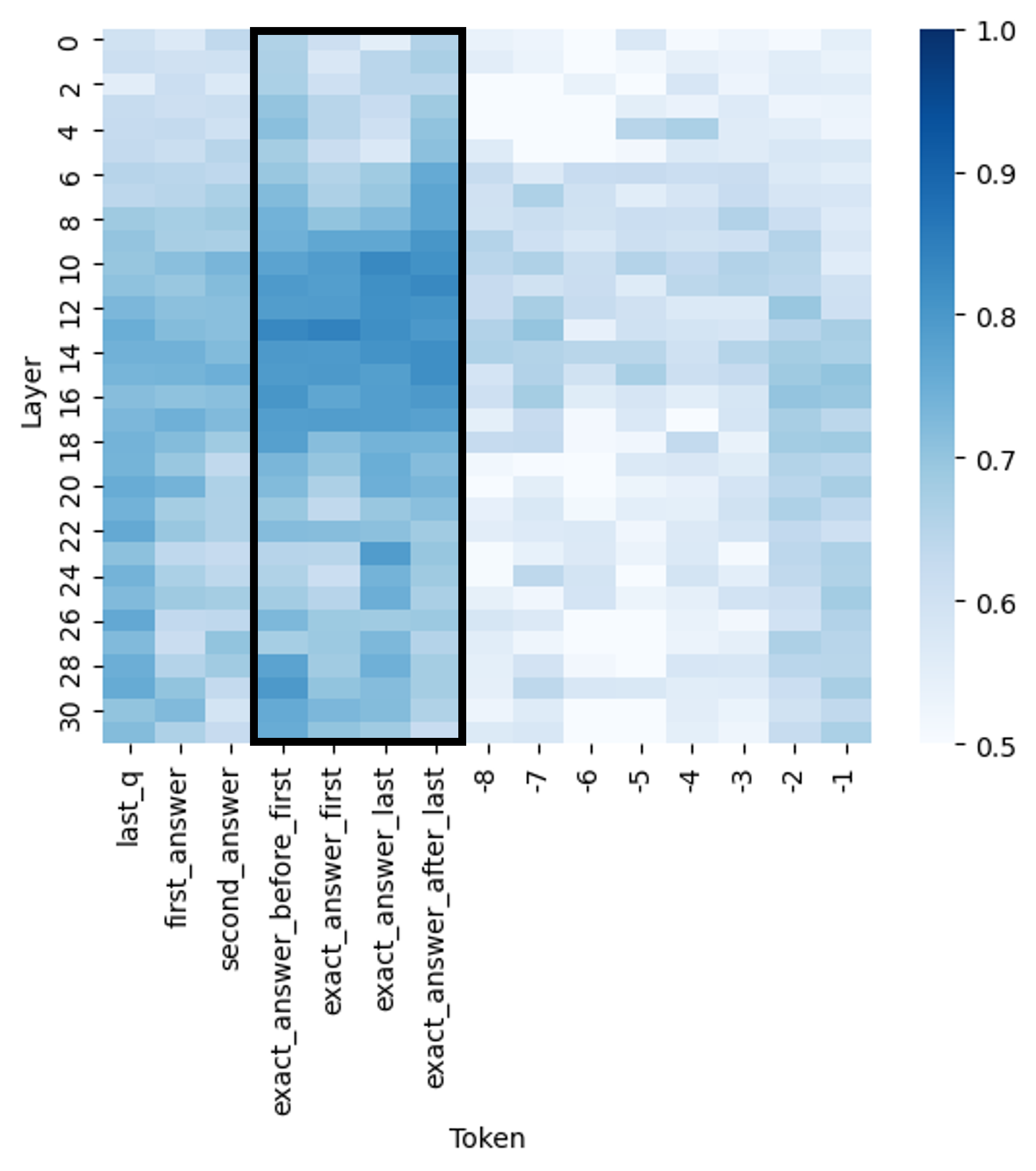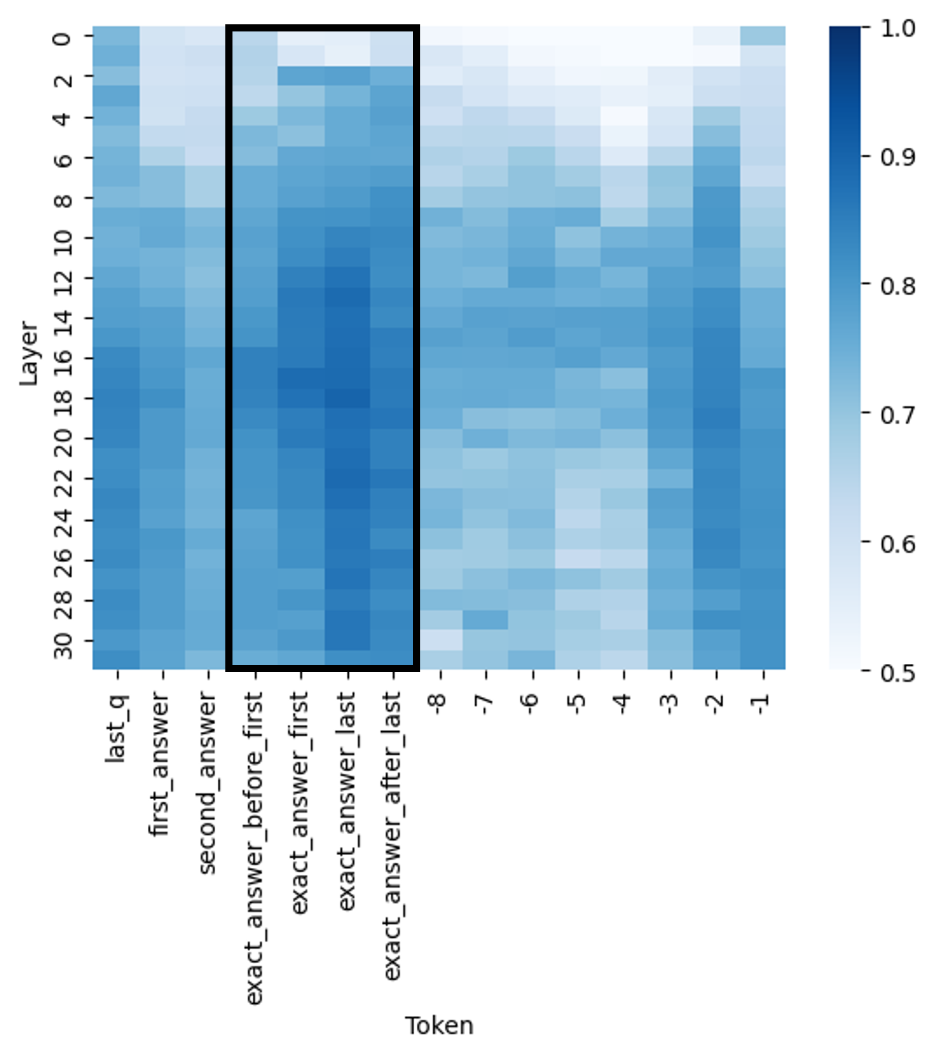</details> (c) Math Figure 2: AUC values of a probe error detector across layers and tokens, Mistral-7b-instruct. Generation proceeds from left to right, with detection performance peaking at the exact answer tokens. Patterns of truthfulness encoding. We first focus on probing classifiers to gain insights into the internal representations of LLMs. Specifically, we analyze the effects of layer and token selection on the error detection performance of these probing classifiers. By systematically probing all model layers, starting from the last question token to the final generated token, we observe consistent truthfulness encoding patterns. Figure 2 shows AUC metrics of probes across Mistral-7b-Instruct layers and tokens. Middle to later layers often yield the most effective probing results (see Appendix B for more datasets and models), aligning with previous studies on truthfulness encoding (Burns et al., 2022; CH-Wang et al., 2023) and transformer representations (nostalgebraist, 2020; Meng et al., 2022; Geva et al., 2023). Regarding tokens, a strong truthfulness signal appears immediately after the prompt, suggesting that this representation encodes information on the model’s general ability to answer the question correctly. This signal weakens as text generation progresses but peaks again at the exact answer tokens. Towards the end of the generation process, signal strength rises again, though it remains weaker than at the exact answer tokens. These patterns are consistent across nearly all datasets and models (see Appendix B), suggesting a general mechanism by which LLMs encode and process truthfulness during text generation. Error Detection Results. Table 1: Comparison of error detection techniques using AUC metric, across different models and datasets. The best-performing method is bolded. Using exact answer tokens is useful for many cases, especially probing. | | Mistral-7b-Instruct | Llama 3-8b-Instruct | | | | | | --- | --- | --- | --- | --- | --- | --- | | TriviaQA | Winobias | Math | TriviaQA | Winobias | Math | | | Logits-mean | $0.60$ $\pm 0.009$ | $0.56$ $\pm 0.017$ | $0.55$ $\pm 0.029$ | $0.66$ $\pm 0.005$ | $0.60$ $\pm 0.026$ | $0.75$ $\pm 0.018$ | | Logits-mean-exact | $0.68$ $\pm 0.007$ | $0.54$ $\pm 0.012$ | $0.51$ $\pm 0.005$ | $0.71$ $\pm 0.006$ | $0.55$ $\pm 0.019$ | $0.80$ $\pm 0.021$ | | Logits-min | $0.63$ $\pm 0.008$ | $0.59$ $\pm 0.012$ | $0.51$ $\pm 0.017$ | $0.74$ $\pm 0.007$ | $0.61$ $\pm 0.024$ | $0.75$ $\pm 0.016$ | | Logits-min-exact | $0.75$ $\pm 0.006$ | $0.53$ $\pm 0.013$ | $0.71$ $\pm 0.009$ | $0.79$ $\pm 0.006$ | $0.61$ $\pm 0.019$ | $0.89$ $\pm 0.018$ | | p(True) | $0.66$ $\pm 0.006$ | $0.45$ $\pm 0.021$ | $0.48$ $\pm 0.022$ | $0.73$ $\pm 0.008$ | $0.59$ $\pm 0.020$ | $0.62$ $\pm 0.017$ | | p(True)-exact | $0.74$ $\pm 0.003$ | $0.40$ $\pm 0.021$ | $0.60$ $\pm 0.025$ | $0.73$ $\pm 0.005$ | $0.63$ $\pm 0.014$ | $0.59$ $\pm 0.018$ | | Probe @ token | | | | | | | | Last generated [-1] | $0.71$ $\pm 0.006$ | $0.82$ $\pm 0.004$ | $0.74$ $\pm 0.008$ | $0.81$ $\pm 0.005$ | $0.86$ $\pm 0.007$ | $0.82$ $\pm 0.016$ | | Before last generated [-2] | $0.73$ $\pm 0.004$ | $0.85$ $\pm 0.004$ | $0.74$ $\pm 0.007$ | $0.75$ $\pm 0.005$ | $0.88$ $\pm 0.005$ | $0.79$ $\pm 0.020$ | | End of question | $0.76$ $\pm 0.008$ | $0.82$ $\pm 0.011$ | $0.72$ $\pm 0.007$ | $0.77$ $\pm 0.007$ | $0.80$ $\pm 0.018$ | $0.72$ $\pm 0.023$ | | Exact | 0.85 $\pm 0.004$ | 0.92 $\pm 0.005$ | 0.92 $\pm 0.008$ | 0.83 $\pm 0.002$ | 0.93 $\pm 0.004$ | 0.95 $\pm 0.027$ | Next, we evaluate various error detection methods by comparing their performance with and without the use of exact answer tokens. Table 1 compares the AUC across three representative datasets (additional datasets and models in Appendix B, showing consistent patterns). Here we present results for the last exact answer token, which outperformed both the first exact answer token and the one preceding it, while the token following the last performed similarly. Incorporating the exact answer token improves the different error detection methods in almost all datasets. Notably, our probing technique (bottom line) consistently outperforms all other baselines across the board. While we did not compare all existing error detection methods, the primary conclusion is that information about truthfulness is highly localized in specific generated tokens, and that focusing on exact answer tokens leads to significant improvements in error detection. ## 4 Generalization Between Tasks The effectiveness of a probing classifier in detecting errors suggests that LLMs encode information about the truthfulness of their outputs. This supports using probing classifiers for error detection in production, but their generalizability across tasks remains unclear. While some studies argue for a universal mechanism of truthfulness encoding in LLMs (Marks & Tegmark, 2023; Slobodkin et al., 2023), results on probe generalization across datasets are mixed (Kadavath et al., 2022; Marks & Tegmark, 2023; CH-Wang et al., 2023; Slobodkin et al., 2023; Levinstein & Herrmann, 2024) –observing a decline in performance, yet it remains significantly above random chance. Understanding this is essential for real-world applications, where the error detector may encounter examples that significantly differ from those it was trained on. Therefore, we explore whether a probe trained on one dataset can detect errors in others. Our generalization experiments are conducted between all of the ten datasets discussed in Section 3, covering a broader range of reaslistic task settings than previous work. This breadth of experiments has not been previously explored, and is crucial considering the mixed findings in previous work. We select the optimal token and layer combination for each dataset, train all probes using this combination on other datasets, and then test them on the original dataset. We evaluate generalization performance using the absolute AUC score, defined as $\max(\text{auc},1-\text{auc})$ , to also account for cases where the learned signal in one dataset is reversed in another. Results. <details> <summary>extracted/6450693/figures/generalization/mistral_instruct.png Details</summary>  ### Visual Description ## Heatmap: Cross-Dataset Performance ### Overview The image is a heatmap visualizing numerical performance scores (likely accuracy or a similar metric) for machine learning models. It compares models trained on one dataset (y-axis) and tested on another (x-axis). The values range from 0.0 to 1.0, with a color scale from blue (low) to red (high) indicating performance. ### Components/Axes * **Y-axis (Vertical):** Labeled "Train dataset". Lists 10 datasets used for training: 1. TriviaQA 2. HotpotQA 3. Movies 4. Winobias 5. Winogrande 6. NLI 7. IMDB 8. Math 9. HotpotQA_WC 10. NQ_WC * **X-axis (Horizontal):** Labeled "Test dataset". Lists the same 10 datasets used for testing, in the same order as the y-axis. * **Color Scale/Legend:** Positioned on the right side of the chart. It is a vertical bar showing a gradient from blue (labeled `0.0`) at the bottom to red (labeled `1.0`) at the top. The midpoint (white/light color) is labeled `0.6`. This scale maps the numerical values in the grid to colors. 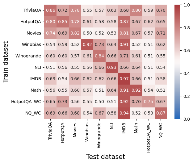### Detailed Analysis The heatmap is a 10x10 grid. Each cell contains a numerical value representing the performance score when the model trained on the row's dataset is tested on the column's dataset. The values are transcribed below in a table. | Train \ Test | TriviaQA | HotpotQA | Movies | Winobias | Winogrande | NLI | IMDB | Math | HotpotQA_WC | NQ_WC | |--------------|----------|----------|--------|----------|------------|-----|------|------|-------------|-------| | **TriviaQA** | 0.86 | 0.72 | 0.78 | 0.55 | 0.57 | 0.63| 0.68 | 0.80 | 0.59 | 0.70 | | **HotpotQA** | 0.80 | 0.85 | 0.78 | 0.61 | 0.58 | 0.58| 0.87 | 0.67 | 0.62 | 0.65 | | **Movies** | 0.74 | 0.69 | 0.82 | 0.50 | 0.52 | 0.53| 0.81 | 0.67 | 0.57 | 0.71 | | **Winobias** | 0.54 | 0.59 | 0.52 | 0.92 | 0.73 | 0.64| 0.91 | 0.52 | 0.51 | 0.62 | | **Winogrande**| 0.60 | 0.60 | 0.57 | 0.61 | 0.84 | 0.66| 0.71 | 0.61 | 0.51 | 0.55 | | **NLI** | 0.51 | 0.56 | 0.55 | 0.56 | 0.66 | 0.93| 0.66 | 0.64 | 0.51 | 0.54 | | **IMDB** | 0.63 | 0.54 | 0.66 | 0.62 | 0.62 | 0.66| 0.97 | 0.66 | 0.51 | 0.58 | | **Math** | 0.56 | 0.55 | 0.60 | 0.57 | 0.51 | 0.64| 0.91 | 0.92 | 0.54 | 0.51 | | **HotpotQA_WC**| 0.65 | 0.73 | 0.56 | 0.55 | 0.50 | 0.51| 0.92 | 0.70 | 0.75 | 0.67 | | **NQ_WC** | 0.69 | 0.66 | 0.68 | 0.54 | 0.67 | 0.58| 0.94 | 0.52 | 0.53 | 0.87 | ### Key Observations 1. **Diagonal Dominance:** The highest values in each row almost always occur on the main diagonal (where the Train and Test datasets are the same). This indicates models perform best when tested on the same dataset they were trained on. Examples: NLI→NLI (0.93), IMDB→IMDB (0.97), Math→Math (0.92). 2. **Strong Cross-Dataset Performance (IMDB Column):** The "Test IMDB" column shows consistently high scores (≥0.81) for models trained on many different datasets (TriviaQA, HotpotQA, Movies, Winobias, Winogrande, NLI, IMDB, Math, HotpotQA_WC, NQ_WC). This suggests the IMDB test set may be easier or that features learned from other datasets transfer well to it. 3. **Weak Cross-Dataset Performance:** Some train-test pairs show very low scores (<0.60), indicating poor transfer. For example, models trained on NLI, Math, or the "_WC" variants often score poorly on datasets like Winobias, Winogrande, HotpotQA_WC, and NQ_WC when not trained on them. 4. **"_WC" Dataset Behavior:** The "HotpotQA_WC" and "NQ_WC" datasets show moderate to high performance when tested on themselves (0.75 and 0.87 respectively) and on IMDB, but generally lower scores on other datasets. Their training rows also show lower scores on most other test sets. ### Interpretation This heatmap is a transfer learning or generalization matrix for AI models across 10 distinct question-answering or text classification datasets. The data suggests: * **Dataset Specificity:** Models are highly specialized. The strong diagonal indicates that knowledge learned from a specific dataset does not automatically generalize well to others, highlighting the challenge of creating broadly capable models. * **Asymmetric Transfer:** Transfer is not symmetric. For instance, a model trained on Movies scores 0.81 on IMDB, but a model trained on IMDB scores only 0.66 on Movies. This implies the datasets have different underlying structures or difficulty levels. * **The "Easy" Test Set:** The IMDB dataset appears to be a "universal" or easier target, as nearly all models perform well on it. This could be because it has distinctive features that are easily picked up by models trained on diverse data, or its evaluation metric is more lenient. * **Cluster of Related Tasks:** The high diagonal and near-diagonal values for datasets like TriviaQA, HotpotQA, and Movies suggest these tasks share more commonalities with each other than with tasks like Winobias or NLI. The "_WC" datasets (likely "Wrong Context" variants) form another cluster with distinct behavior. In essence, the chart maps the landscape of task relationships for these models. It visually answers: "If I train my model on task A, how well can I expect it to perform on task B?" The clear takeaway is that performance is highly dependent on the specific pair of tasks, with same-task performance being the most reliable. </details> (a) Raw AUC values. Values above $0.5$ indicate some generalization. <details> <summary>extracted/6450693/figures/generalization/mistral_instruct_reduced.png Details</summary>  ### Visual Description ## Heatmap: Cross-Dataset Performance Transfer Matrix ### Overview This image is a heatmap visualizing the performance transfer between different machine learning datasets. It shows how models trained on one dataset (rows) perform when tested on another dataset (columns). The values represent a performance metric (likely accuracy difference or transfer score), with positive values (red) indicating positive transfer and negative values (blue) indicating negative transfer or performance degradation. ### Components/Axes * **Chart Type:** Heatmap (Confusion Matrix style) * **Y-Axis (Vertical):** Labeled "Train dataset". Lists 10 datasets used for training models. * **X-Axis (Horizontal):** Labeled "Test dataset". Lists the same 10 datasets used for testing. * **Color Scale/Legend:** A vertical color bar is positioned on the **right side** of the chart. It maps numerical values to colors: * **Dark Red:** ~0.3 (Highest positive value) * **Light Red/Pink:** ~0.1 to 0.2 * **White/Very Light Gray:** ~0.0 * **Light Blue:** ~-0.1 * **Dark Blue:** ~-0.2 (Lowest negative value) * **Data Labels:** Each cell in the 10x10 grid contains a numerical value, printed in black text. ### Detailed Analysis **List of Train Datasets (Y-axis, top to bottom):** 1. TriviaQA 2. HotpotQA 3. Movies 4. Winobias 5. Winogrande 6. NLI 7. IMDB 8. Math 9. HotpotQA_WC 10. NQ_WC **List of Test Datasets (X-axis, left to right):** 1. TriviaQA 2. HotpotQA 3. Movies 4. Winobias 5. Winogrande 6. NLI 7. IMDB 8. Math 9. HotpotQA_WC 10. 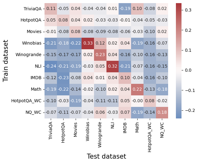NQ_WC **Complete Data Grid (Train Dataset -> Test Dataset: Value):** * **TriviaQA ->:** TriviaQA: 0.11, HotpotQA: -0.05, Movies: 0.04, Winobias: -0.04, Winogrande: -0.04, NLI: 0.01, IMDB: -0.19, Math: 0.10, HotpotQA_WC: -0.08, NQ_WC: 0.02 * **HotpotQA ->:** TriviaQA: -0.05, HotpotQA: 0.08, Movies: 0.04, Winobias: 0.02, Winogrande: -0.03, NLI: -0.03, IMDB: -0.01, Math: -0.04, HotpotQA_WC: -0.05, NQ_WC: -0.03 * **Movies ->:** TriviaQA: -0.01, HotpotQA: -0.08, Movies: 0.08, Winobias: -0.08, Winogrande: -0.09, NLI: -0.08, IMDB: -0.06, Math: -0.03, HotpotQA_WC: -0.10, NQ_WC: 0.02 * **Winobias ->:** TriviaQA: -0.21, HotpotQA: -0.18, Movies: -0.22, Winobias: 0.33, Winogrande: 0.12, NLI: 0.02, IMDB: 0.04, Math: -0.19, HotpotQA_WC: -0.16, NQ_WC: -0.07 * **Winogrande ->:** TriviaQA: -0.15, HotpotQA: -0.17, Movies: -0.17, Winobias: 0.02, Winogrande: 0.23, NLI: 0.04, IMDB: -0.16, Math: -0.10, HotpotQA_WC: -0.16, NQ_WC: -0.13 * **NLI ->:** TriviaQA: -0.24, HotpotQA: -0.21, Movies: -0.19, Winobias: -0.03, Winogrande: 0.05, NLI: 0.32, IMDB: -0.21, Math: -0.07, HotpotQA_WC: -0.16, NQ_WC: -0.15 * **IMDB ->:** TriviaQA: -0.12, HotpotQA: -0.23, Movies: -0.08, Winobias: 0.04, Winogrande: 0.01, NLI: 0.04, IMDB: 0.10, Math: -0.04, HotpotQA_WC: -0.16, NQ_WC: -0.10 * **Math ->:** TriviaQA: -0.19, HotpotQA: -0.22, Movies: -0.14, Winobias: -0.02, Winogrande: -0.10, NLI: 0.02, IMDB: 0.04, Math: 0.22, HotpotQA_WC: -0.13, NQ_WC: -0.18 * **HotpotQA_WC ->:** TriviaQA: -0.10, HotpotQA: -0.03, Movies: -0.19, Winobias: -0.04, Winogrande: -0.11, NLI: -0.11, IMDB: 0.05, Math: -0.00, HotpotQA_WC: 0.08, NQ_WC: -0.02 * **NQ_WC ->:** TriviaQA: -0.07, HotpotQA: -0.11, Movies: -0.07, Winobias: -0.04, Winogrande: 0.06, NLI: -0.03, IMDB: 0.07, Math: -0.19, HotpotQA_WC: -0.14, NQ_WC: 0.18 ### Key Observations 1. **Strong Diagonal Performance:** The highest values in the matrix are consistently found along the main diagonal (where Train dataset = Test dataset). This includes Winobias (0.33), NLI (0.32), Winogrande (0.23), Math (0.22), and TriviaQA (0.11). This indicates models perform best when tested on the same domain they were trained on. 2. **Significant Negative Transfer:** Many off-diagonal cells show strong negative values (dark blue), particularly when models trained on one dataset are tested on a seemingly unrelated one. For example: * NLI-trained model on TriviaQA test: -0.24 * IMDB-trained model on HotpotQA test: -0.23 * Math-trained model on HotpotQA test: -0.22 3. **Positive Transfer Clusters:** Some related datasets show positive off-diagonal transfer: * Winobias -> Winogrande: 0.12 (both are coreference resolution tasks). * Winogrande -> Winobias: 0.02 (weaker, but still positive). * NQ_WC -> NQ_WC (diagonal): 0.18, and it shows slight positive transfer to IMDB (0.07) and Winogrande (0.06). 4. **Neutral or Weak Transfer:** The "Movies" dataset row and column show mostly weak, slightly negative values, suggesting it neither benefits from nor strongly harms performance on other tasks, except for its own diagonal (0.08). ### Interpretation This heatmap provides a quantitative map of **task relatedness and negative transfer** in machine learning. The data suggests: 1. **Domain Specificity is Dominant:** The strong diagonal confirms that models are highly specialized. Training on a specific dataset (e.g., NLI for natural language inference) yields the best results on that exact task, but this expertise does not generalize well—and often hurts performance—on other tasks. 2. **Negative Transfer is a Major Challenge:** The prevalence of blue cells indicates that naively applying a model trained on one task to another can be actively detrimental. This is a critical consideration for real-world AI deployment, where a model might encounter out-of-domain data. 3. **Task Taxonomy Can Be Inferred:** The pattern of positive off-diagonal values helps cluster tasks. Winobias and Winogrande (both reasoning/commonsense tasks) show some mutual positive transfer. Question-answering datasets (TriviaQA, HotpotQA, NQ_WC) show mixed but generally weak relationships with each other. 4. **Outlier - NLI:** The NLI (Natural Language Inference) dataset shows the strongest diagonal (0.32) and the most severe negative transfer to other tasks (e.g., -0.24 to TriviaQA). This suggests NLI learning creates a very distinct, specialized model representation that is highly incompatible with other types of language understanding tasks. **In essence, the chart argues against the notion of a single, general-purpose language model trained on a mix of tasks. Instead, it visualizes the "balkanization" of model performance, where expertise in one area often comes at the cost of performance in another.** </details> (b) Performance (AUC) difference of the probe and the logit-based method. Values above $0 0$ indicate generalization beyond the logit-based method. Figure 3: Generalization between datasets, Mistral-7b-instruct. After subtracting the logit-based method’s performance, we observe that most datasets show limited or no meaningful generalization. Figure 3(a) shows the generalization results for Mistral-7b-instruct, with similar patterns observed for other LLMs in Appendix C. In this context, values above $0.5$ indicate successful generalization. At first glance, the results appear consistent with previous research: most heatmap values exceed $0.5$ , implying some degree of generalization across tasks. This observation supports the existence of a universal mechanism for decoding truthfulness, since the same linear directions—captured by the probe—encode truthfulness information across many datasets. However, upon closer inspection, it turns out that most of this performance can be achieved by logit-based truthfulness detection, which only observes the output logits. Figure 3(b) presents the same heatmap after subtracting results from our strongest logit-based baseline (Logit-min-exact). This adjusted heatmap reveals the probe’s generalization rarely exceeds what can be achieved by examining logits alone. This suggests that the observed generalization is not due to a universal internal encoding of truthfulness. Instead, it likely arises from information already available through external features, such as logits. Past evidence for generalization may therefore have been overstated. Nonetheless, we do observe some successful generalization in tasks requiring similar skills, such as parametric factual retrieval (TriviaQA, HotpotQA, Movies) and common-sense reasoning (Winobias, Wingrande, NLI). This suggests that, although the overall pattern of truthfulness signals across tokens appeared consistent across tasks (as observed in Section 3.3), LLMs have many “skill-specific” truthfulness mechanisms rather than universal ones. However, some patterns remain unexplained, such as the asymmetric generalization from TriviaQA to Math tasks. Overall, our findings indicate that models have a multifaceted representation of truthfulness. The internal mechanisms responsible for solving distinct problem are implemented as different mechanisms (e.g., circuits) within models (Elhage et al., 2021; Olah et al., 2023). Similarly, LLMs do not encode truthfulness through a single unified mechanism but rather through multiple mechanisms, each corresponding to different notions of truth. Further investigation is required to disentangle these mechanisms. ## 5 Investigating Error Types Having established the limitations of error detection, we now shift to error analysis. Previously, we explored types of LLM limitations across different tasks, noting both commonalities and distinctions in their error representations. In this section, we focus on the types of errors LLMs make in a specific task—TriviaQA—which represents factual errors, a commonly studied issue in LLMs (Kadavath et al., 2022; Snyder et al., 2023; Li et al., 2024; Chen et al., 2024; Simhi et al., 2024). 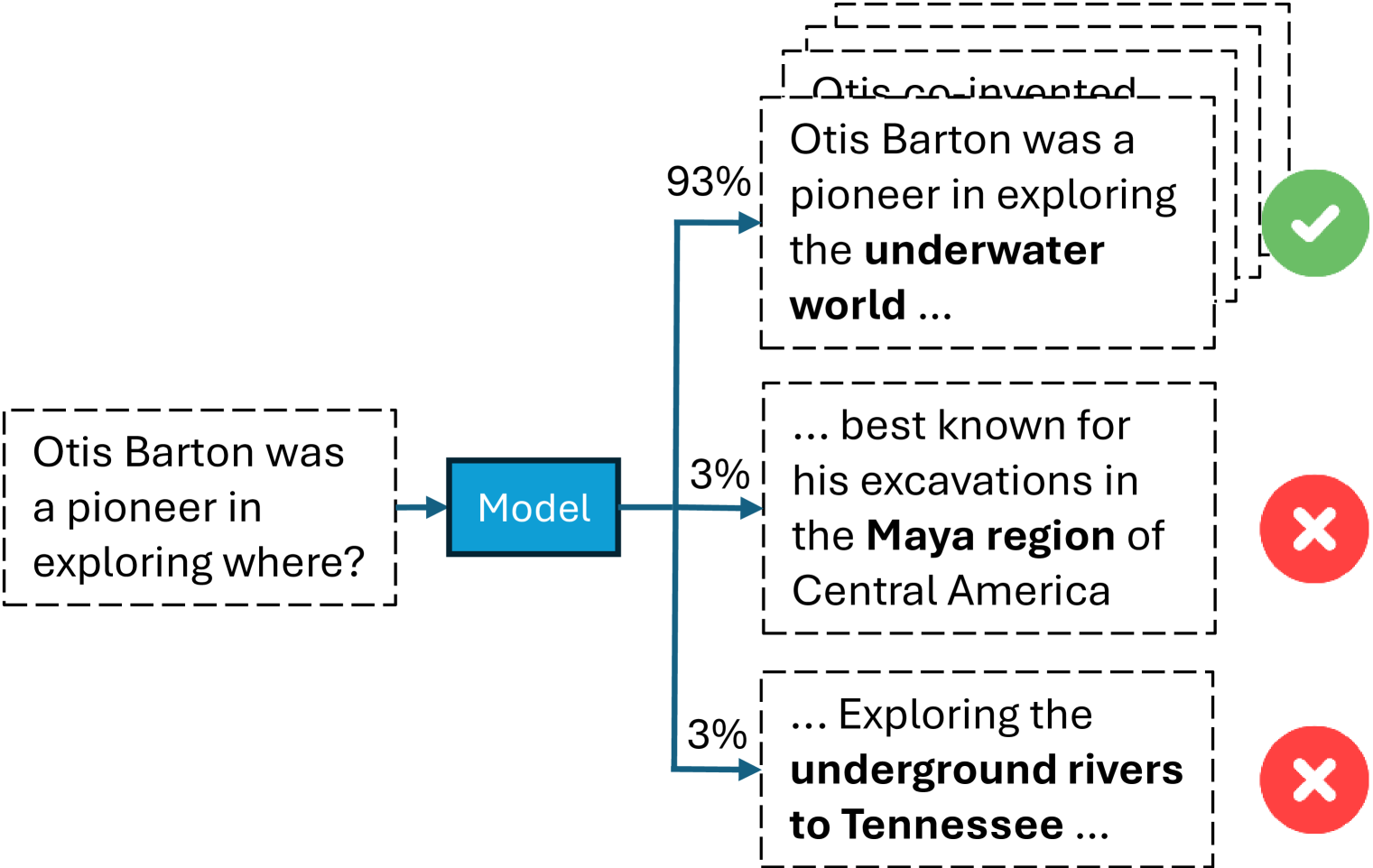### 5.1 Taxonomy of Errors Intuitively, not all mistakes are identical. In one case, an LLM may consistently generate an incorrect answer, considering it correct, while in another case, it could issue a best guess. To analyze errors from the LLM’s perspective, we sample $K=30$ responses at a temperature setting of $T=1$ We chose $K=30$ as the overall correctness seemed to plateau around this point; see Appendix D. We found that lower temperatures generally produced less truthful answers across repeated trials. for each example in the dataset and then analyze the resulting distribution of answers. <details> <summary>x2.png Details</summary>  ### Visual Description \n ## Diagram: Model Output for a Factual Question ### Overview The image is a flowchart or decision diagram illustrating how a machine learning model processes a factual question and generates multiple possible answers, each with an associated confidence score and a correctness indicator. The diagram visually separates the input, processing unit, and output options. ### Components/Axes The diagram is structured from left to right: 1. **Input (Left):** A dashed-line box containing the question. 2. **Processing (Center):** A solid blue rectangle labeled "Model". 3. **Outputs (Right):** Three dashed-line boxes stacked vertically, each containing a possible answer. Arrows connect the "Model" to each output box. 4. **Confidence Scores:** Percentage values are placed on the arrows leading to each output. 5. **Correctness Indicators:** Icons placed to the right of each output box. ### Detailed Analysis **1. Input Question:** * **Text:** "Otis Barton was a pioneer in exploring where?" * **Location:** Left side of the diagram, enclosed in a dashed-line box. **2. Model:** * **Label:** "Model" * **Location:** Center, represented by a solid blue rectangle. An arrow points from the input question to this box. **3. Outputs (from top to bottom):** * **Output 1 (Top):** * **Text:** "Otis Barton was a pioneer in exploring the **underwater world** ..." * **Confidence Score:** 93% (displayed on the arrow leading to this box). * **Correctness Indicator:** A green circle with a white checkmark (✓), positioned to the right of the text box. This indicates a correct answer. * **Spatial Note:** This is the topmost output box. The text "underwater world" is in bold. * **Output 2 (Middle):** * **Text:** "... best known for his excavations in the **Maya region** of Central America" * **Confidence Score:** 3% (displayed on the arrow leading to this box). * **Correctness Indicator:** A red circle with a white 'X', positioned to the right of the text box. This indicates an incorrect answer. * **Spatial Note:** This is the middle output box. The text "Maya region" is in bold. * **Output 3 (Bottom):** * **Text:** "... Exploring the **underground rivers to Tennessee** ..." * **Confidence Score:** 3% (displayed on the arrow leading to this box). * **Correctness Indicator:** A red circle with a white 'X', positioned to the right of the text box. This indicates an incorrect answer. * **Spatial Note:** This is the bottom output box. The text "underground rivers to Tennessee" is in bold. ### Key Observations 1. **Confidence Distribution:** The model assigns a very high confidence (93%) to one answer and very low, equal confidence (3% each) to the other two. This creates a stark contrast between the primary output and the alternatives. 2. **Correctness Correlation:** The answer with the highest confidence score (93%) is the only one marked as correct (green checkmark). The two low-confidence answers are both marked as incorrect (red X). 3. **Text Formatting:** Key phrases within the answers ("underwater world", "Maya region", "underground rivers to Tennessee") are bolded, likely to highlight the core subject of each proposed answer. 4. **Diagram Semantics:** The use of dashed-line boxes for inputs and outputs versus a solid box for the "Model" may visually distinguish between data and the processing unit. ### Interpretation This diagram serves as a clear visualization of a model's inference process for a factual query. It demonstrates a scenario where the model is highly confident in a single, correct answer and assigns minimal, equal probability to incorrect distractors. The data suggests the model has a strong, correct association for the entity "Otis Barton" with "underwater world" exploration. The incorrect answers reference plausible but wrong domains (archaeology in the Maya region, speleology in Tennessee), indicating the model's knowledge base correctly discriminates between these fields. The stark 93% vs. 3% confidence split implies the model's internal scoring mechanism is decisive in this case, leaving little ambiguity. This could reflect either a well-trained model with clear factual boundaries or a specific test case designed to showcase high-confidence correct retrieval. The diagram effectively communicates not just *what* the model answered, but also its *certainty* and the *validity* of that answer. </details> (a) The LLM mostly answers correctly, but sometimes hallucinates. <details> <summary>x3.png Details</summary>  ### Visual Description ## Diagram: Model Response Confidence and Accuracy ### Overview The image is a flowchart diagram illustrating a language model's response to a factual question. It shows the input question, the model processing it, and two possible output responses with associated confidence scores and correctness indicators. The diagram demonstrates a scenario where the model assigns high confidence to an incorrect answer and low confidence to the correct one. ### Components/Axes The diagram is structured horizontally from left to right with the following components: 1. **Input Question (Left):** A dashed-line box containing the text: "Which American state borders on only one other state?" 2. **Model (Center):** A solid blue rectangle labeled "Model". An arrow points from the input question to this box. 3. **Output Paths (Right):** Two arrows branch from the "Model" box, leading to two separate output boxes. * **Upper Path (Incorrect Answer):** * Confidence Score: "87%" is written above the arrow. * Output Box: A dashed-line box containing overlapping text. The primary visible text reads: "The only state to border ... is **Missouri** ..." with "Missouri" in bold. Partially visible text above reads: "**Missouri** is the". * Correctness Indicator: A red circle with a white "X" is positioned to the right of this box. * **Lower Path (Correct Answer):** * Confidence Score: "13%" is written below the arrow. * Output Box: A dashed-line box containing overlapping text. The primary visible text reads: "The US state that ... is **Maine**, which ..." with "Maine" in bold. Partially visible text above reads: "**Maine** is the". * Correctness Indicator: A green circle with a white checkmark is positioned to the right of this box. ### Detailed Analysis * **Flow:** Input Question → Model → Two concurrent output hypotheses. * **Confidence Distribution:** The model's confidence is heavily skewed. It assigns an 87% probability to the incorrect answer ("Missouri") and only a 13% probability to the correct answer ("Maine"). * **Textual Content:** The output boxes contain what appear to be the beginnings of generated text responses. The bolded state names ("Missouri", "Maine") are the key entities in the answers. The ellipses (...) indicate truncated or continuing text. * **Spatial Grounding:** The incorrect output (87%, Missouri) is placed above the correct output (13%, Maine). The correctness icons (X and checkmark) are aligned vertically on the far right, providing immediate visual feedback. ### Key Observations 1. **High-Confidence Error:** The most striking observation is the model's strong confidence (87%) in a factually incorrect statement. Missouri borders eight other states, not one. 2. **Low-Confidence Correctness:** The model correctly identifies Maine (which borders only New Hampshire) but assigns it a very low confidence score (13%). 3. **Output Presentation:** The overlapping text in the output boxes suggests these might be samples from a set of generated candidates or a visualization of the model's internal "thought" process considering multiple possibilities. ### Interpretation This diagram serves as a clear visual critique of a common failure mode in large language models: **confident hallucination**. It demonstrates that a model's assigned probability or confidence score is not a reliable indicator of factual accuracy. The model has learned a strong but incorrect association (perhaps due to biases in training data where "Missouri" is frequently discussed in geographical contexts) and prioritizes it over the correct, but less statistically prominent, fact. The relationship between the elements highlights the core challenge of AI alignment and reliability. The "Model" is a black box that transforms a clear question into a probabilistic distribution of answers, where the most likely output is wrong. This underscores the necessity for external verification, fact-checking mechanisms, and improved training techniques that better ground models in factual knowledge rather than just statistical patterns. The diagram is a succinct argument for why confidence scores alone should not be trusted for critical information retrieval. 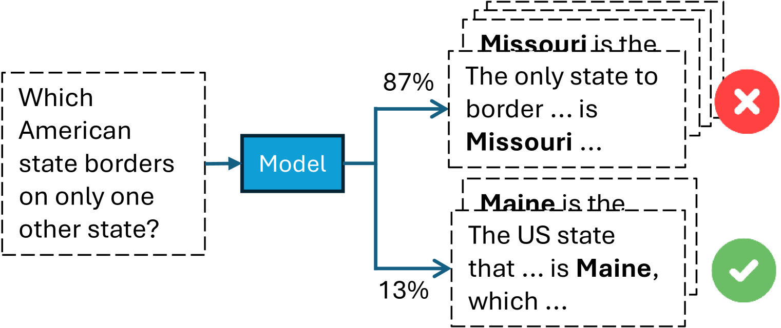</details> (b) The LLM mostly answers incorrectly, but seems to have some knowledge on the correct answer. <details> <summary>x4.png Details</summary>  ### Visual Description ## Diagram: Model Output for a Factual Question ### Overview This image is a flowchart or diagram illustrating the output of a machine learning model ("Model") when given a specific factual question. The diagram shows the input question, the model processing it, and three possible generated answers, each associated with a confidence percentage and a correctness indicator (correct or incorrect). ### Components/Axes The diagram is structured horizontally, flowing from left to right. 1. **Input (Left):** A dashed-line box containing the question text. 2. **Processing (Center):** A solid blue rectangle labeled "Model". 3. **Outputs (Right):** Three dashed-line boxes, each containing a partial answer text. Each output is connected to the model by a blue arrow. - **Output 1 (Top):** Arrow labeled "20%". Box contains text. To its right is a red circle with a white "X". - **Output 2 (Middle):** Arrow labeled "6%". Box contains text. To its right is a red circle with a white "X". - **Output 3 (Bottom):** Arrow labeled "6%". Box contains text. To its right is a green circle with a white checkmark. - Vertical ellipsis (`:`) between Output 2 and Output 3, suggesting additional, unshown outputs. ### Detailed Analysis **1. Input Question:** - **Text:** "Who became the first female to deliver football commentary on 'match of the day'?" - **Language:** English. **2. Model Outputs:** - **Output 1 (Top, 20% confidence):** - **Text:** "... In 2007, **Gabby Logan** ..." - **Correctness Indicator:** Red circle with white "X" (Incorrect). - **Output 2 (Middle, 6% confidence):** - **Text:** "The first ... is **Clare Balding**" - **Correctness Indicator:** Red circle with white "X" (Incorrect). - **Output 3 (Bottom, 6% confidence):** - **Text:** "**Jackie Oatley** is the first woman ..." - **Correctness Indicator:** Green circle with white checkmark (Correct). **3. Spatial Grounding & Visual Flow:** - The input question is positioned on the far left. - The "Model" box is centered vertically, acting as the processing node. - The three outputs are stacked vertically on the right. The highest confidence output (20%) is at the top, followed by the two lower confidence outputs (6% each). - The correctness indicators are placed immediately to the right of their respective answer boxes, providing a clear visual verdict. ### Key Observations 1. **Confidence vs. Accuracy Mismatch:** The model assigns its highest confidence (20%) to an incorrect answer (Gabby Logan). The correct answer (Jackie Oatley) is generated with a much lower confidence score (6%), equal to another incorrect answer (Clare Balding). 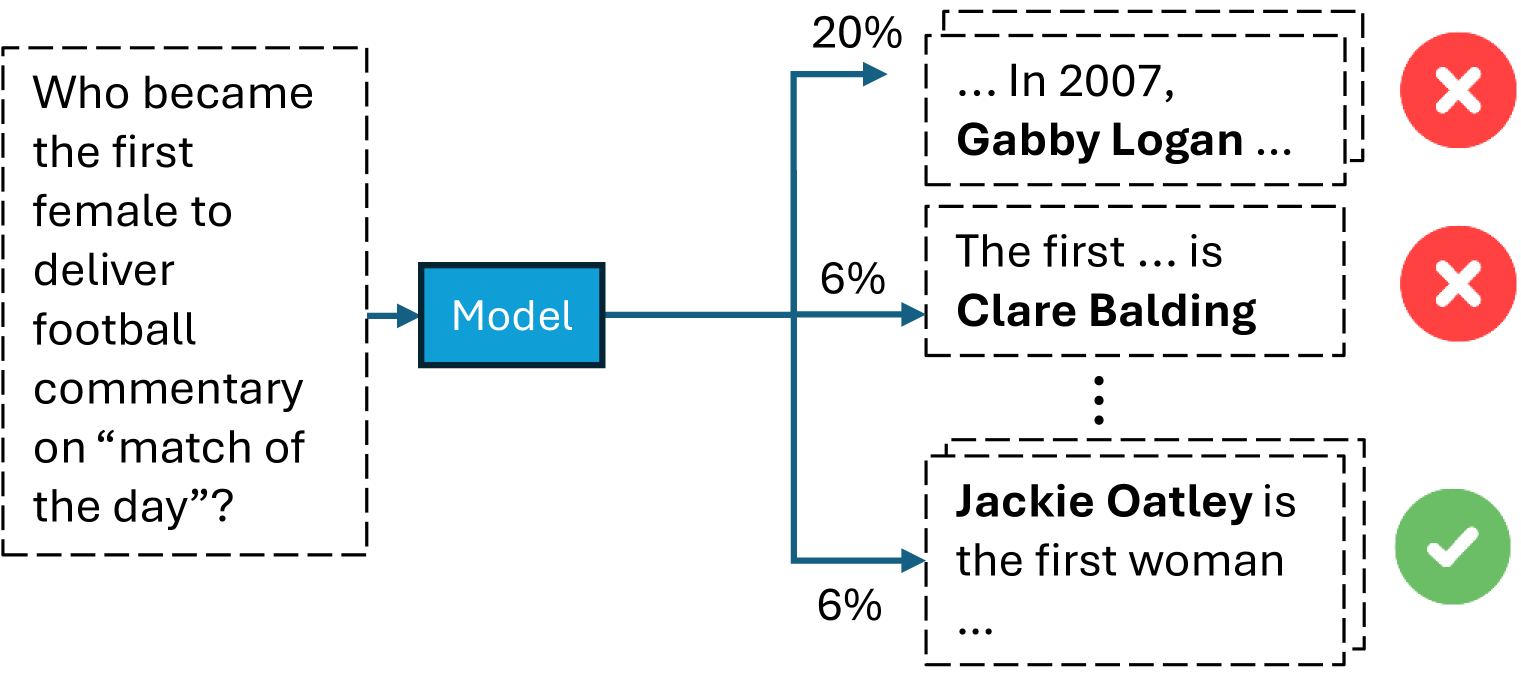2. **Output Distribution:** The diagram explicitly shows three outputs but uses a vertical ellipsis to imply the model generates a distribution over many possible answers, not just these three. 3. **Answer Specificity:** The correct answer identifies a specific individual, "Jackie Oatley." The incorrect answers also name specific individuals, suggesting the model is retrieving or generating plausible but factually wrong entities. 4. **Temporal Reference:** One incorrect answer includes a specific year ("2007"), which may be a confabulated detail associated with the wrong person. ### Interpretation This diagram serves as a clear visual critique of a common failure mode in language models: **poor calibration between confidence and factual accuracy.** It demonstrates that a model can be more confident in a wrong answer than in the correct one. The data suggests the model's internal probability distribution for this question is misaligned with ground truth. The high confidence in "Gabby Logan" might stem from her being a well-known sports presenter, creating a strong but incorrect association. The lower confidence for the correct answer, "Jackie Oatley," indicates the model has learned the fact but assigns it lower probability, possibly due to less frequent training data or competing associations. The inclusion of the ellipsis is crucial—it shows this is a snapshot of a larger output distribution, emphasizing that the model considers many possibilities, and the shown examples are just the top or most illustrative ones. This highlights the challenge of extracting reliable, single answers from probabilistic models without additional verification or confidence-thresholding mechanisms. The diagram effectively argues for the need to evaluate not just if a model can produce a correct answer, but how confidently it does so. </details> (c) The LLM generates many different answers, one of them is the correct one which is generated a small fraction of the resamples. Figure 4: Different error types in free-form generation, exposed when resampled many times. Figure 4 illustrates three representative error types. In one (Figure 4(a)), the model usually gives the correct answer but occasionally make an error, implying correct information is present but sampling may lead to mistakes. In another (Figure 4(b), the model often responds incorrectly, though it is capable of providing the right answer, indicating some retained knowledge despite consistently making the same error. In a third type (Figure 4(c)), the model generates a wide array of mostly incorrect answers, reflecting low confidence in any generated answer. More generally, we categorize the errors by logging three specific features for each example: (a) the number of different answers generated; (b) the frequency of the correct answer; and (c) the frequency of the most common incorrect answer. These features reveal the following error patterns: - (A) Refuses to answer: The model responds that it cannot answer the question in at least half the cases. - (B) Consistently correct: Answers correctly in at least half of the cases. This category is divided into: (B1) always correct; and (B2) mostly correct with occasional errors. - (C) Consistently incorrect: Consistently generates the same incorrect response in at least half of the cases. Similarly to type B, we subdivide this type into (C1) correct answer is never produced; and (C2) correct answer appears at least once. - (D) Two competing: Generates both correct and incorrect responses at similar rates–difference in rates is 5 or less, and each response is generated at least 5 times. - (E) Many answers: Generates over 10 distinct answers. Like types C and D, Subtypes include (E1) correct answer is never generated; and (E2) correct answer is generated at least once. This taxonomy covers 96% of the errors in TriviaQA for Mistral-7b-instruct. For more qualitative examples of each type of error, see Appendix D.3. Although some overlap exists between types, our goal is to identify general patterns and explore their connection to the models’s internal representations. For a discussion on the design choices of this taxonomy, refer to Appendix D.1. This taxonomy classifies LLM errors based on an extrinsic, behavior-based analysis. Similarly, previous work analyzed repeated samples to assess an LLM’s knowledge of the correct answer (Simhi et al., 2024; Gekhman et al., 2024). Our approach is distinct because it also examines the nature of errors that the LLM makes. Furthermore, as we discuss next, we analyze the connection between these behavioral patterns and the model’s internal encoding. ### 5.2 Predicting Error Types Our taxonomy offers an external, behavioral analysis of LLMs, which we complement by an intrinsic evaluation. We explore whether LLMs encode information on potential error types within their intermediate activations, offering a deeper insight into the underlying mechanisms. To investigate this, we train a probe in a one-to-many setting, where a single probe identifies a specific error type from all others. We use representations extracted from the answers produced via greedy decoding. Table 2 presents the results. Our findings show that error types can be predicted from the intermediate representations of the greedy decoding generations, suggesting that they may capture not only output correctness but also fine-grained information about potential errors. While detection performance varies between types, the predictability of each type is valuable on its own, as it opens the possibility of tailoring targeted interventions for specific error types. Additionally, although performance on error types C and D is lower, it remains well above random, providing meaningful insights. These results suggest that internal representations encode more than just binary correctness, revealing a nuanced taxonomy of error types and offering deeper insights into how these models process and encode knowledge. Table 2: AUC scores for error type classification (TriviaQA). Error types are predictable from the inner model representations, indicating the encoding of fine-grained information on errors. | Error type | Mistral-7b | Mistral-Instr-7b | Llama3-8b | Llama3-Instr-8b | | --- | --- | --- | --- | --- | | (A) Refuses to answer | $0.86\scriptscriptstyle{\pm 0.002}$ | $0.85\scriptscriptstyle{\pm 0.011}$ | $0.87\scriptscriptstyle{\pm 0.002}$ | $0.88\scriptscriptstyle{\pm 0.014}$ | | (B) Consistently correct | $0.88\scriptscriptstyle{\pm 0.001}$ | $0.82\scriptscriptstyle{\pm 0.008}$ | $0.86\scriptscriptstyle{\pm 0.001}$ | $0.81\scriptscriptstyle{\pm 0.002}$ | | (C) Consistently incorrect | $0.59\scriptscriptstyle{\pm 0.002}$ | $0.67\scriptscriptstyle{\pm 0.002}$ | $0.59\scriptscriptstyle{\pm 0.002}$ | $0.64\scriptscriptstyle{\pm 0.003}$ | | (D) Two competing | $0.63\scriptscriptstyle{\pm 0.002}$ | $0.68\scriptscriptstyle{\pm 0.006}$ | $0.61\scriptscriptstyle{\pm 0.001}$ | $0.65\scriptscriptstyle{\pm 0.004}$ | | (E) Many answers | $0.90\scriptscriptstyle{\pm 0.001}$ | $0.84\scriptscriptstyle{\pm 0.003}$ | $0.89\scriptscriptstyle{\pm 0.001}$ | $0.89\scriptscriptstyle{\pm 0.001}$ | ## 6 Detecting the Correct Answer After identifying that models encode diverse truthfulness-related information, we examine how this internal truthfulness aligns with their external behavior during response generation. To this end, we use our probe, We choose the best-performing probe for each task, which is trained on the last exact answer token. trained on error detection, to select an answer from a pool of 30 generated responses to the same question. We then measure the model’s accuracy based on the selected answers. A case where this accuracy does not significantly differ from traditional decoding methods (such as greedy decoding), suggests that the LLM’s internal representation of truthfulness is consistent with its external behavior. In simpler terms, that the model is generating answers that it also internally considers as correct. Conversely, a case where using the probe alters performance either way, would suggest a misalignment between the LLM’s internal representations and its actual behavior. Experimental Setup The experiments were conducted on TriviaQA, Winobias, and Math. We resample each model answer in the same strategy described in Section 5.1. The final chosen answer is the one with the highest correctness probability, as assessed by the probe. We compare to three baselines: (1) greedy decoding, (2) random selection from the $K=30$ answer candidates; and (3) majority vote wherein the most frequently generated answer is chosen. Results The results for Mistral-7b-instruct are summarized in Figure 5, with additional results for other LLMs and datasets as well as qualitative examples provided in Appendix E. We only present results on error types that appear 30 times or more in our test dataset. Overall, using the probe to select answers enhances the LLMs accuracy across all examined tasks. However, the extent of improvement varies by error type. For instance, in the TriviaQA dataset, there is minimal gain in the “mostly correct” category (B2). In contrast, substantial gains—ranging from 30 to 40 points in some cases—are observed in the “mostly incorrect” (C2), “two competing answers” (D), and “many answers” (E1) categories. Interestingly, and perhaps surprisingly, the probe is most effective in cases where the LLM lacks any (external) preference for the correct answer during generation. The fact that the probe can effectively identify the correct answer in these scenarios, points at a significant disconnect between the LLM’s internal encoding and its external behavior. These results suggest that even when the model encodes information of which answer is correct, it can still generate an incorrect answer in practice. While using the probe to select the answer proves effective, it is not proposed here as an error mitigation strategy but rather as a diagnostic tool. However, these findings indicate that further research in this area could leverage the existing knowledge within LLMs to significantly reduce errors. We recommend exploring this direction in future investigations. <details> <summary>extracted/6450693/figures/choose_answer/probe_choose_answer_triviaqa_mistral_instruct.png Details</summary>  ### Visual Description ## Grouped Bar Chart: Performance Comparison of Four Methods Across Various Answer Consistency Categories ### Overview The image displays a grouped bar chart comparing the performance (in percentage) of four different methods—greedy, random, majority, and probing—across nine distinct categories related to answer consistency and correctness. The chart is designed to evaluate how each method performs under different response scenarios. ### Components/Axes * **Chart Type:** Grouped Bar Chart. * **Y-Axis:** Represents a percentage scale from 0 to 100, with major gridlines at intervals of 25 (0, 25, 50, 75, 100). The axis is labeled with these numerical markers. * **X-Axis:** Lists nine categorical groups describing answer patterns. The labels are: 1. All 2. Refuses to answer 3. Consistently correct (All) 4. Consistently correct (Most) 5. Consistently incorrect (All) 6. Consistently incorrect (Most) 7. Two competing 8. Many answers (Non correct) 9. Many answers (Correct appears) * **Legend:** Positioned at the top center of the chart. It defines the four data series by color: * **greedy:** Green bar * **random:** Light blue bar * **majority:** Tan/Yellow bar * **probing:** Red/Mauve bar ### Detailed Analysis The performance values for each method within every category are as follows. The trend for each category is described first, followed by the extracted data points. 1. **Category: All** * *Trend:* All methods show moderate performance, with a slight upward trend from greedy to probing. * *Values:* greedy: 63, random: 64, majority: 67, probing: 71. 2. **Category: Refuses to answer** * *Trend:* Performance is very low for greedy and random, zero for majority, and notably higher for probing. * *Values:* greedy: 6, random: 6, majority: 0, probing: 28. 3. **Category: Consistently correct (All)** * *Trend:* All methods achieve perfect or near-perfect scores. * *Values:* greedy: 100, random: 100, majority: 100, probing: 100. 4. **Category: Consistently correct (Most)** * *Trend:* High performance across all methods, with majority scoring highest. * *Values:* greedy: 88, random: 83, majority: 99, probing: 89. 5. **Category: Consistently incorrect (All)** * *Trend:* All methods score zero, indicating complete failure in this scenario. * *Values:* greedy: 0, random: 0, majority: 0, probing: 0. 6. **Category: Consistently incorrect (Most)** * *Trend:* Low performance for greedy and random, zero for majority, and a significantly higher score for probing. * *Values:* greedy: 11, random: 15, majority: 0, probing: 53. 7. **Category: Two competing** * *Trend:* A clear upward trend from greedy to probing, with probing showing a substantial lead. * *Values:* greedy: 32, random: 45, majority: 50, probing: 78. 8. **Category: Many answers (Non correct)** * *Trend:* Extremely low performance, with only greedy registering a minimal score. * *Values:* greedy: 1, random: 0, majority: 0, probing: 0. 9. **Category: Many answers (Correct appears)** * *Trend:* A clear upward trend from greedy to probing, with probing again performing best. * *Values:* greedy: 23, random: 19, majority: 38, probing: 56. ### Key Observations * **Probing Dominance:** The probing method (red bar) is the top performer in 7 out of the 9 categories. Its advantage is most dramatic in challenging scenarios like "Refuses to answer" (+22 points over next best), "Consistently incorrect (Most)" (+38 points), and "Two competing" (+28 points). * **Method Failure Points:** All methods completely fail (score 0) in the "Consistently incorrect (All)" category. The majority method also scores 0 in "Refuses to answer" and "Consistently incorrect (Most)". * **Ceiling and Floor Effects:** The "Consistently correct (All)" category represents a ceiling effect where all methods max out at 100%. The "Consistently incorrect (All)" and "Many answers (Non correct)" categories represent floor effects where performance collapses. * **Majority Method Volatility:** The majority method shows extreme volatility, achieving perfect scores in some categories (100 in "Consistently correct (All)", 99 in "Consistently correct (Most)") but scoring zero in three others. ### Interpretation This chart evaluates the robustness of four answer-aggregation or selection strategies (greedy, random, majority, probing) under different conditions of answer correctness and consistency. The data suggests that the **probing** strategy is significantly more robust and effective across a wider range of difficult or ambiguous scenarios (e.g., when answers are refused, when there are competing answers, or when incorrect answers dominate). Its consistent superiority implies it is better at discerning or extracting correct information from noisy or unreliable outputs. The **majority** method, while highly effective when answers are consistently correct, is brittle and fails completely when faced with consistent incorrectness or answer refusal. This highlights a key weakness of simple majority voting: it can be confidently wrong if the majority of sources are wrong. The **greedy** and **random** methods generally underperform, serving as baselines. Their low scores in challenging categories confirm that more sophisticated methods like probing are necessary for reliable performance in real-world, imperfect conditions. The categories themselves outline a taxonomy of potential failure modes or response patterns in a question-answering or generation system. The chart effectively maps method performance to these specific failure modes, providing a diagnostic view of where each strategy succeeds or breaks down. The perfect scores in "Consistently correct (All)" validate that all methods work under ideal conditions, making the divergences in other categories more meaningful. 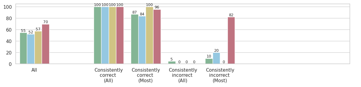</details> (a) TriviaQA <details> <summary>extracted/6450693/figures/choose_answer/probe_choose_answer_math_mistral_instruct.png Details</summary>  ### Visual Description \n ## Bar Chart: Performance Across Consistency Categories ### Overview The image displays a grouped bar chart comparing four distinct data series (represented by different colors) across five categories related to consistency of correctness. The vertical axis represents a numerical score or percentage, ranging from 0 to 100. The chart is designed to show how different groups perform across varying levels of consistency in their correctness. ### Components/Axes * **Vertical Axis (Y-axis):** Numerical scale from 0 to 100, with major gridlines at intervals of 20 (0, 20, 40, 60, 80, 100). The axis title is not explicitly shown but implies a performance metric (e.g., accuracy percentage). * **Horizontal Axis (X-axis):** Five categorical groups: 1. `All` 2. `Consistently correct (All)` 3. `Consistently correct (Most)` 4. `Consistently incorrect (All)` 5. `Consistently incorrect (Most)` * **Data Series (Legend Inferred from Bar Colors):** The legend is not visible in the image. The four data series are identified by their bar colors, listed here in the order they appear within each group from left to right: 1. **Green** (approximate hex: #8fbc8f) 2. **Light Blue** (approximate hex: #add8e6) 3. **Beige/Tan** (approximate hex: #d2b48c) 4. **Red/Mauve** (approximate hex: #bc8f8f) * **Data Labels:** The exact numerical value for each bar is displayed directly above it. ### Detailed Analysis **Group 1: `All`** * Green: 55 * Light Blue: 52 * Beige: 57 * Red: 70 * *Trend:* All series show moderate performance, with the Red series scoring notably higher than the others. **Group 2: `Consistently correct (All)`** * Green: 100 * Light Blue: 100 * Beige: 100 * Red: 100 * *Trend:* Perfect scores across all four data series. This represents the peak performance for every group. **Group 3: `Consistently correct (Most)`** * Green: 87 * Light Blue: 84 * Beige: 100 * Red: 96 * *Trend:* High performance, but with variation. Beige maintains a perfect score, Red is very high, while Green and Light Blue show a slight decrease from the perfect score in the previous category. **Group 4: `Consistently incorrect (All)`** * Green: 5 * Light Blue: 0 * Beige: 0 * Red: 0 * *Trend:* Extremely low performance. Only the Green series registers a minimal score (5); the other three series have a score of 0. **Group 5: `Consistently incorrect (Most)`** * Green: 10 * Light Blue: 20 * Beige: 0 * Red: 82 * *Trend:* Mixed and highly anomalous. Green and Light Blue show low but non-zero scores. Beige remains at 0. The Red series is a dramatic outlier with a very high score of 82. ### Key Observations 1. **Perfect Performance Ceiling:** All series achieve a score of 100 in the `Consistently correct (All)` category. 2. **The "Red" Series Anomaly:** The Red series exhibits a unique and counterintuitive pattern. It scores high in the `All` category (70), very high in `Consistently correct (Most)` (96), and then an extremely high 82 in `Consistently incorrect (Most)`. This suggests it performs well even when the underlying subjects are mostly incorrect. 3. **The "Beige" Series Consistency:** The Beige series shows a binary pattern: it scores either 100 (in the first three categories) or 0 (in the last two "incorrect" categories). 4. **Low Performance in Incorrect Categories:** As expected, scores plummet in the `Consistently incorrect` categories for Green, Light Blue, and Beige. The Green series shows a slight residual score (5 and 10), while Light Blue only shows a score in the `Most` incorrect category (20). ### Interpretation This chart likely visualizes the performance of four different models, algorithms, or methods (the color series) on a task, segmented by the consistency of the ground truth or the subjects' behavior. * **What the data suggests:** The `Consistently correct (All)` category represents an ideal scenario where all methods perform perfectly. The `Consistently correct (Most)` category introduces some noise or difficulty, causing performance to dip slightly for most methods, except Beige which remains robust. * **Relationship between elements:** The stark contrast between the `correct` and `incorrect` categories highlights the fundamental challenge. Most methods (Green, Light Blue, Beige) fail catastrophically when faced with consistently incorrect data, as their scores drop to near zero. This is an expected outcome for systems trained on correct patterns. * **Notable anomaly and its implication:** The Red series is the critical outlier. Its high score in `Consistently incorrect (Most)` (82) is paradoxical. This could indicate several possibilities: * **Overfitting to a Spurious Feature:** The Red method might be relying on a feature that correlates with the *label* in the training data but is actually irrelevant or misleading in this specific "incorrect" context. * **Different Objective:** The Red method might not be optimizing for correctness in the same way as the others. It could be designed to predict a different, correlated attribute that remains present even when the primary judgment is "incorrect." * **Data Leakage or Flaw:** There might be a flaw in the evaluation setup for this specific series and category, allowing it to achieve a high score inappropriately. * **Why it matters:** This chart moves beyond simple average performance. By segmenting results based on consistency, it reveals critical failure modes (the collapse in incorrect categories) and exposes potentially problematic behavior (the Red series' anomaly) that would be hidden in an aggregated metric. It prompts investigation into *why* the Red series behaves so differently, which is key to understanding the reliability and true capabilities of each method. </details> (b) Math Figure 5: Different answer choice strategies, Mistral-7B-Instruct. A notable improvement in accuracy by using the error-detection probe is observed for error types where the LLM shows no preference for the correct answer across repeated generations. ## 7 Discussion and Conclusions In this study, we analyzed LLM errors through their internal representations. Our approach depends on access to internal representations, restricting its use to open-source models. We focus on QA tasks with clear gold labels, which are key for benchmarking truthfulness detection and valued by the community. To ensure robustness, we tested 10 datasets across 4 model architectures. Open-ended tasks are left for future research, with our work laying the groundwork for broader applications. For instance, we found that truthfulness-related information is localized in specific tokens within long-responses, enabling practical improvements in error detection for production models. This insight could extend to tasks like summarization, by probing the most meaningful entities in an answer. Truthfulness features showed poor generalization across tasks and datasets, highlighting the need for caution when applying trained error detectors in varied settings. Some unexplained patterns suggest hidden links between unrelated tasks that warrant further research. Improving generalization could involve exploring the effects of layer-token combinations and training on diverse datasets, as demonstrated by Bürger et al. (2024). Deciphering task-specific truthfulness features and their overlaps across tasks might also enhance classifier design. Still, task-specific probes could be highly valuable in critical fields like medicine and law, where reliability matters. These probes can detect errors, predict error types, and guide response selection from resampled outputs, offering significant practical benefits. Guidelines for applying these probes are provided in Appendix F. Finally, we identified a significant discrepancy between the model’s external behavior and internal states, where it repeatedly outputs incorrect responses despite internally encoding the correct answer. It is possible that mechanisms favoring likelihood override those promoting truthfulness, as LLMs are trained to predicting likely tokens, which does not necessarily align with factual accuracy. Our findings imply that these models already encode valuable information that could possibly be harnessed to reduce errors. Work by Chuang et al. (2024) shows promising results in this area, while a subsequent work by Gekhman et al. (2025) focused exclusively on this “hidden knowledge” phenomenon, formally defining it and studying its extent. In conclusion, our findings suggest that LLMs’ internal representations provide useful insights into their errors, highlights the complex link between the internal processes of models and their external outputs, and hopefully paves the way for further improvements in error detection and mitigation. ## 8 Reproducibility Statement To ensure reproducibility of our work, we provide detailed instructions and necessary code. The source code, including scripts for generating model answers, probing, resampling, and error type analysis, is available in the supplementary material, where we also provide command examples and specific seeds used for experiment reproducibility. This repository includes documentation on how to set up the environment, download and preprocess datasets, and execute the experiments outlined in Sections 3–6 of the paper. Additionally, all datasets, models, and results generation steps are described in the Appendix A. #### Acknowledgments This research was supported by the Israel Science Foundation (grant No. 448/20), an Azrieli Foundation Early Career Faculty Fellowship, an AI Alignment grant from Open Philanthropy, and a Google gift. HO is supported by the Apple AIML PhD fellowship. This research was funded by the European Union (ERC, Control-LM, 101165402). Views and opinions expressed are however those of the author(s) only and do not necessarily reflect those of the European Union or the European Research Council Executive Agency. Neither the European Union nor the granting authority can be held responsible for them. ## References - Allauzen (2007) Alexandre Allauzen. Error detection in confusion network. In 8th Annual Conference of the International Speech Communication Association, INTERSPEECH 2007, Antwerp, Belgium, August 27-31, 2007, pp. 1749–1752. ISCA, 2007. doi: 10.21437/INTERSPEECH.2007-490. URL https://doi.org/10.21437/Interspeech.2007-490. - Azaria & Mitchell (2023) Amos Azaria and Tom Mitchell. The internal state of an llm knows when it’s lying. In Findings of the Association for Computational Linguistics: EMNLP 2023, pp. 967–976, 2023. - Bang et al. (2023) Yejin Bang, Samuel Cahyawijaya, Nayeon Lee, Wenliang Dai, Dan Su, Bryan Wilie, Holy Lovenia, Ziwei Ji, Tiezheng Yu, Willy Chung, et al. A multitask, multilingual, multimodal evaluation of chatgpt on reasoning, hallucination, and interactivity. arXiv preprint arXiv:2302.04023, 2023. - Belinkov (2021) Yonatan Belinkov. Probing classifiers: Promises, shortcomings, and advances, 2021. URL https://arxiv.org/abs/2102.12452. - Bell et al. (2019) Samuel J. Bell, Helen Yannakoudakis, and Marek Rei. Context is key: Grammatical error detection with contextual word representations. In Helen Yannakoudakis, Ekaterina Kochmar, Claudia Leacock, Nitin Madnani, Ildikó Pilán, and Torsten Zesch (eds.), Proceedings of the Fourteenth Workshop on Innovative Use of NLP for Building Educational Applications, BEA@ACL 2019, Florence, Italy, August 2, 2019, pp. 103–115. Association for Computational Linguistics, 2019. doi: 10.18653/V1/W19-4410. URL https://doi.org/10.18653/v1/w19-4410. - Bommasani et al. (2021) Rishi Bommasani, Drew A Hudson, Ehsan Adeli, Russ Altman, Simran Arora, Sydney von Arx, Michael S Bernstein, Jeannette Bohg, Antoine Bosselut, Emma Brunskill, et al. On the opportunities and risks of foundation models. arXiv preprint arXiv:2108.07258, 2021. - Brunner et al. (2020) Gino Brunner, Yang Liu, Damian Pascual, Oliver Richter, Massimiliano Ciaramita, and Roger Wattenhofer. On identifiability in transformers. In 8th International Conference on Learning Representations (ICLR 2020)(virtual). International Conference on Learning Representations, 2020. - Bürger et al. (2024) Lennart Bürger, Fred A Hamprecht, and Boaz Nadler. Truth is universal: Robust detection of lies in llms. arXiv preprint arXiv:2407.12831, 2024. - Burns et al. (2022) Collin Burns, Haotian Ye, Dan Klein, and Jacob Steinhardt. Discovering latent knowledge in language models without supervision. arXiv preprint arXiv:2212.03827, 2022. - Caines et al. (2020) Andrew Caines, Christian Bentz, Kate M. Knill, Marek Rei, and Paula Buttery. Grammatical error detection in transcriptions of spoken english. In Donia Scott, Núria Bel, and Chengqing Zong (eds.), Proceedings of the 28th International Conference on Computational Linguistics, COLING 2020, Barcelona, Spain (Online), December 8-13, 2020, pp. 2144–2162. International Committee on Computational Linguistics, 2020. doi: 10.18653/V1/2020.COLING-MAIN.195. URL https://doi.org/10.18653/v1/2020.coling-main.195. - CH-Wang et al. (2023) Sky CH-Wang, Benjamin Van Durme, Jason Eisner, and Chris Kedzie. Do androids know they’re only dreaming of electric sheep?, 2023. - Chen et al. (2024) Chao Chen, Kai Liu, Ze Chen, Yi Gu, Yue Wu, Mingyuan Tao, Zhihang Fu, and Jieping Ye. INSIDE: LLMs’ internal states retain the power of hallucination detection. In The Twelfth International Conference on Learning Representations, 2024. URL https://openreview.net/forum?id=Zj12nzlQbz. - Chen et al. (2013) Wei Chen, Sankaranarayanan Ananthakrishnan, Rohit Kumar, Rohit Prasad, and Prem Natarajan. ASR error detection in a conversational spoken language translation system. In IEEE International Conference on Acoustics, Speech and Signal Processing, ICASSP 2013, Vancouver, BC, Canada, May 26-31, 2013, pp. 7418–7422. IEEE, 2013. doi: 10.1109/ICASSP.2013.6639104. URL https://doi.org/10.1109/ICASSP.2013.6639104. - Cheng & Duan (2020) Yong Cheng and Mofan Duan. Chinese grammatical error detection based on BERT model. In Erhong YANG, Endong XUN, Baolin ZHANG, and Gaoqi RAO (eds.), Proceedings of the 6th Workshop on Natural Language Processing Techniques for Educational Applications, pp. 108–113, Suzhou, China, December 2020. Association for Computational Linguistics. URL https://aclanthology.org/2020.nlptea-1.15. - Chuang et al. (2024) Yung-Sung Chuang, Yujia Xie, Hongyin Luo, Yoon Kim, James R. Glass, and Pengcheng He. Dola: Decoding by contrasting layers improves factuality in large language models. In The Twelfth International Conference on Learning Representations, 2024. URL https://openreview.net/forum?id=Th6NyL07na. - Elhage et al. (2021) Nelson Elhage, Neel Nanda, Catherine Olsson, Tom Henighan, Nicholas Joseph, Ben Mann, Amanda Askell, Yuntao Bai, Anna Chen, Tom Conerly, et al. A mathematical framework for transformer circuits. Transformer Circuits Thread, 1(1):12, 2021. - Errattahi et al. (2015) Rahhal Errattahi, Asmaa El Hannani, and Hassan Ouahmane. Automatic speech recognition errors detection and correction: A review. In Mourad Abbas and Ahmed Abdelali (eds.), 1st International Conference on Natural Language and Speech Processing, ICNLSP 2015, Algiers, Algeria, October 18-19, 2015, volume 128 of Procedia Computer Science, pp. 32–37. Elsevier, 2015. doi: 10.1016/J.PROCS.2018.03.005. URL https://doi.org/10.1016/j.procs.2018.03.005. - Flickinger et al. (2016) Dan Flickinger, Michael Wayne Goodman, and Woodley Packard. Uw-stanford system description for AESW 2016 shared task on grammatical error detection. In Joel R. Tetreault, Jill Burstein, Claudia Leacock, and Helen Yannakoudakis (eds.), Proceedings of the 11th Workshop on Innovative Use of NLP for Building Educational Applications, BEA@NAACL-HLT 2016, June 16, 2016, San Diego, California, USA, pp. 105–111. The Association for Computer Linguistics, 2016. doi: 10.18653/V1/W16-0511. URL https://doi.org/10.18653/v1/w16-0511. - Gao et al. (2023) Luyu Gao, Zhuyun Dai, Panupong Pasupat, Anthony Chen, Arun Tejasvi Chaganty, Yicheng Fan, Vincent Zhao, Ni Lao, Hongrae Lee, Da-Cheng Juan, et al. Rarr: Researching and revising what language models say, using language models. In Proceedings of the 61st Annual Meeting of the Association for Computational Linguistics (Volume 1: Long Papers), pp. 16477–16508, 2023. - Gekhman et al. (2020) Zorik Gekhman, Roee Aharoni, Genady Beryozkin, Markus Freitag, and Wolfgang Macherey. KoBE: Knowledge-based machine translation evaluation. In Trevor Cohn, Yulan He, and Yang Liu (eds.), Findings of the Association for Computational Linguistics: EMNLP 2020, pp. 3200–3207, Online, November 2020. Association for Computational Linguistics. doi: 10.18653/v1/2020.findings-emnlp.287. URL https://aclanthology.org/2020.findings-emnlp.287. - Gekhman et al. (2022) Zorik Gekhman, Dina Zverinski, Jonathan Mallinson, and Genady Beryozkin. RED-ACE: Robust error detection for ASR using confidence embeddings. In Yoav Goldberg, Zornitsa Kozareva, and Yue Zhang (eds.), Proceedings of the 2022 Conference on Empirical Methods in Natural Language Processing, pp. 2800–2808, Abu Dhabi, United Arab Emirates, December 2022. Association for Computational Linguistics. doi: 10.18653/v1/2022.emnlp-main.180. URL https://aclanthology.org/2022.emnlp-main.180. - Gekhman et al. (2023) Zorik Gekhman, Jonathan Herzig, Roee Aharoni, Chen Elkind, and Idan Szpektor. TrueTeacher: Learning factual consistency evaluation with large language models. In Houda Bouamor, Juan Pino, and Kalika Bali (eds.), Proceedings of the 2023 Conference on Empirical Methods in Natural Language Processing, pp. 2053–2070, Singapore, December 2023. Association for Computational Linguistics. doi: 10.18653/v1/2023.emnlp-main.127. URL https://aclanthology.org/2023.emnlp-main.127. - Gekhman et al. (2024) Zorik Gekhman, Gal Yona, Roee Aharoni, Matan Eyal, Amir Feder, Roi Reichart, and Jonathan Herzig. Does fine-tuning llms on new knowledge encourage hallucinations?, 2024. - Gekhman et al. (2025) Zorik Gekhman, Eyal Ben David, Hadas Orgad, Eran Ofek, Yonatan Belinkov, Idan Szpector, Jonathan Herzig, and Roi Reichart. Inside-out: Hidden factual knowledge in llms. arXiv preprint arXiv:2503.15299, 2025. - Geva et al. (2023) Mor Geva, Jasmijn Bastings, Katja Filippova, and Amir Globerson. Dissecting recall of factual associations in auto-regressive language models. arXiv preprint arXiv:2304.14767, 2023. - Gottesman & Geva (2024) Daniela Gottesman and Mor Geva. Estimating knowledge in large language models without generating a single token. In Proceedings of the 2024 Conference on Empirical Methods in Natural Language Processing (EMNLP 2024), Miami, Florida, 2024. Association for Computational Linguistics. - Guerreiro et al. (2023) Nuno M Guerreiro, Elena Voita, and André FT Martins. Looking for a needle in a haystack: A comprehensive study of hallucinations in neural machine translation. In Proceedings of the 17th Conference of the European Chapter of the Association for Computational Linguistics, pp. 1059–1075, 2023. - Harnad (2024) Stevan Harnad. Language writ large: Llms, chatgpt, grounding, meaning and understanding. arXiv preprint arXiv:2402.02243, 2024. - Honovich et al. (2021) Or Honovich, Leshem Choshen, Roee Aharoni, Ella Neeman, Idan Szpektor, and Omri Abend. $q^{2}$ : Evaluating factual consistency in knowledge-grounded dialogues via question generation and question answering. In Marie-Francine Moens, Xuanjing Huang, Lucia Specia, and Scott Wen-tau Yih (eds.), Proceedings of the 2021 Conference on Empirical Methods in Natural Language Processing, pp. 7856–7870, Online and Punta Cana, Dominican Republic, November 2021. Association for Computational Linguistics. doi: 10.18653/v1/2021.emnlp-main.619. URL https://aclanthology.org/2021.emnlp-main.619. - Honovich et al. (2022) Or Honovich, Roee Aharoni, Jonathan Herzig, Hagai Taitelbaum, Doron Kukliansy, Vered Cohen, Thomas Scialom, Idan Szpektor, Avinatan Hassidim, and Yossi Matias. TRUE: Re-evaluating factual consistency evaluation. In Marine Carpuat, Marie-Catherine de Marneffe, and Ivan Vladimir Meza Ruiz (eds.), Proceedings of the 2022 Conference of the North American Chapter of the Association for Computational Linguistics: Human Language Technologies, pp. 3905–3920, Seattle, United States, July 2022. Association for Computational Linguistics. doi: 10.18653/v1/2022.naacl-main.287. URL https://aclanthology.org/2022.naacl-main.287. - Huang et al. (2023a) Lei Huang, Weijiang Yu, Weitao Ma, Weihong Zhong, Zhangyin Feng, Haotian Wang, Qianglong Chen, Weihua Peng, Xiaocheng Feng, Bing Qin, et al. A survey on hallucination in large language models: Principles, taxonomy, challenges, and open questions. arXiv preprint arXiv:2311.05232, 2023a. - Huang et al. (2023b) Yuheng Huang, Jiayang Song, Zhijie Wang, Huaming Chen, and Lei Ma. Look before you leap: An exploratory study of uncertainty measurement for large language models. arXiv preprint arXiv:2307.10236, 2023b. - Ji et al. (2023) Ziwei Ji, Nayeon Lee, Rita Frieske, Tiezheng Yu, Dan Su, Yan Xu, Etsuko Ishii, Ye Jin Bang, Andrea Madotto, and Pascale Fung. Survey of hallucination in natural language generation. ACM Computing Surveys, 55(12):1–38, 2023. - Jiang et al. (2023) Albert Q. Jiang, Alexandre Sablayrolles, Arthur Mensch, Chris Bamford, Devendra Singh Chaplot, Diego de las Casas, Florian Bressand, Gianna Lengyel, Guillaume Lample, Lucile Saulnier, Lélio Renard Lavaud, Marie-Anne Lachaux, Pierre Stock, Teven Le Scao, Thibaut Lavril, Thomas Wang, Timothée Lacroix, and William El Sayed. Mistral 7b, 2023. URL https://arxiv.org/abs/2310.06825. - Joshi et al. (2017) Mandar Joshi, Eunsol Choi, Daniel S Weld, and Luke Zettlemoyer. Triviaqa: A large scale distantly supervised challenge dataset for reading comprehension. In Proceedings of the 55th Annual Meeting of the Association for Computational Linguistics (Volume 1: Long Papers), pp. 1601–1611, 2017. - Kadavath et al. (2022) Saurav Kadavath, Tom Conerly, Amanda Askell, Tom Henighan, Dawn Drain, Ethan Perez, Nicholas Schiefer, Zac Hatfield-Dodds, Nova DasSarma, Eli Tran-Johnson, et al. Language models (mostly) know what they know. arXiv preprint arXiv:2207.05221, 2022. - Kasewa et al. (2018) Sudhanshu Kasewa, Pontus Stenetorp, and Sebastian Riedel. Wronging a right: Generating better errors to improve grammatical error detection. In Ellen Riloff, David Chiang, Julia Hockenmaier, and Jun’ichi Tsujii (eds.), Proceedings of the 2018 Conference on Empirical Methods in Natural Language Processing, Brussels, Belgium, October 31 - November 4, 2018, pp. 4977–4983. Association for Computational Linguistics, 2018. URL https://aclanthology.org/D18-1541/. - Kotek et al. (2023) Hadas Kotek, Rikker Dockum, and David Sun. Gender bias and stereotypes in large language models. In Proceedings of the ACM collective intelligence conference, pp. 12–24, 2023. - Kryscinski et al. (2020) Wojciech Kryscinski, Bryan McCann, Caiming Xiong, and Richard Socher. Evaluating the factual consistency of abstractive text summarization. In Bonnie Webber, Trevor Cohn, Yulan He, and Yang Liu (eds.), Proceedings of the 2020 Conference on Empirical Methods in Natural Language Processing (EMNLP), pp. 9332–9346, Online, November 2020. Association for Computational Linguistics. doi: 10.18653/v1/2020.emnlp-main.750. URL https://aclanthology.org/2020.emnlp-main.750. - Kuhn et al. (2023) Lorenz Kuhn, Yarin Gal, and Sebastian Farquhar. Semantic uncertainty: Linguistic invariances for uncertainty estimation in natural language generation. In The Eleventh International Conference on Learning Representations, 2023. URL https://openreview.net/forum?id=VD-AYtP0dve. - Kwiatkowski et al. (2019) Tom Kwiatkowski, Jennimaria Palomaki, Olivia Redfield, Michael Collins, Ankur Parikh, Chris Alberti, Danielle Epstein, Illia Polosukhin, Matthew Kelcey, Jacob Devlin, Kenton Lee, Kristina N. Toutanova, Llion Jones, Ming-Wei Chang, Andrew Dai, Jakob Uszkoreit, Quoc Le, and Slav Petrov. Natural questions: a benchmark for question answering research. Transactions of the Association of Computational Linguistics, 2019. - Laban et al. (2022) Philippe Laban, Tobias Schnabel, Paul N. Bennett, and Marti A. Hearst. SummaC: Re-visiting NLI-based models for inconsistency detection in summarization. Transactions of the Association for Computational Linguistics, 10:163–177, 2022. doi: 10.1162/tacl˙a˙00453. URL https://aclanthology.org/2022.tacl-1.10. - Levinstein & Herrmann (2024) Benjamin A Levinstein and Daniel A Herrmann. Still no lie detector for language models: Probing empirical and conceptual roadblocks. Philosophical Studies, pp. 1–27, 2024. - Lewis et al. (2020) Patrick Lewis, Ethan Perez, Aleksandra Piktus, Fabio Petroni, Vladimir Karpukhin, Naman Goyal, Heinrich Küttler, Mike Lewis, Wen-tau Yih, Tim Rocktäschel, et al. Retrieval-augmented generation for knowledge-intensive nlp tasks. Advances in Neural Information Processing Systems, 33:9459–9474, 2020. - Li et al. (2024) Kenneth Li, Oam Patel, Fernanda Viégas, Hanspeter Pfister, and Martin Wattenberg. Inference-time intervention: Eliciting truthful answers from a language model. Advances in Neural Information Processing Systems, 36, 2024. - Li & Wang (2024) Wei Li and Houfeng Wang. Detection-correction structure via general language model for grammatical error correction. In Lun-Wei Ku, Andre Martins, and Vivek Srikumar (eds.), Proceedings of the 62nd Annual Meeting of the Association for Computational Linguistics (Volume 1: Long Papers), ACL 2024, Bangkok, Thailand, August 11-16, 2024, pp. 1748–1763. Association for Computational Linguistics, 2024. URL https://aclanthology.org/2024.acl-long.96. - Liang et al. (2024) Xun Liang, Shichao Song, Zifan Zheng, Hanyu Wang, Qingchen Yu, Xunkai Li, Rong-Hua Li, Yi Wang, Zhonghao Wang, Feiyu Xiong, et al. Internal consistency and self-feedback in large language models: A survey. arXiv preprint arXiv:2407.14507, 2024. - Lin et al. (2021) Stephanie Lin, Jacob Hilton, and Owain Evans. Truthfulqa: Measuring how models mimic human falsehoods. arXiv preprint arXiv:2109.07958, 2021. - Liu et al. (2023) Kevin Liu, Stephen Casper, Dylan Hadfield-Menell, and Jacob Andreas. Cognitive dissonance: Why do language model outputs disagree with internal representations of truthfulness? In Houda Bouamor, Juan Pino, and Kalika Bali (eds.), Proceedings of the 2023 Conference on Empirical Methods in Natural Language Processing, pp. 4791–4797, Singapore, December 2023. Association for Computational Linguistics. doi: 10.18653/v1/2023.emnlp-main.291. URL https://aclanthology.org/2023.emnlp-main.291. - Liu et al. (2022) Tianyu Liu, Yizhe Zhang, Chris Brockett, Yi Mao, Zhifang Sui, Weizhu Chen, and Bill Dolan. A token-level reference-free hallucination detection benchmark for free-form text generation. In Smaranda Muresan, Preslav Nakov, and Aline Villavicencio (eds.), Proceedings of the 60th Annual Meeting of the Association for Computational Linguistics (Volume 1: Long Papers), pp. 6723–6737, Dublin, Ireland, May 2022. Association for Computational Linguistics. doi: 10.18653/v1/2022.acl-long.464. URL https://aclanthology.org/2022.acl-long.464. - Lo (2019) Chi-kiu Lo. YiSi - a unified semantic MT quality evaluation and estimation metric for languages with different levels of available resources. In Ondřej Bojar, Rajen Chatterjee, Christian Federmann, Mark Fishel, Yvette Graham, Barry Haddow, Matthias Huck, Antonio Jimeno Yepes, Philipp Koehn, André Martins, Christof Monz, Matteo Negri, Aurélie Névéol, Mariana Neves, Matt Post, Marco Turchi, and Karin Verspoor (eds.), Proceedings of the Fourth Conference on Machine Translation (Volume 2: Shared Task Papers, Day 1), pp. 507–513, Florence, Italy, August 2019. Association for Computational Linguistics. doi: 10.18653/v1/W19-5358. URL https://aclanthology.org/W19-5358. - Maas et al. (2011) Andrew L. Maas, Raymond E. Daly, Peter T. Pham, Dan Huang, Andrew Y. Ng, and Christopher Potts. Learning word vectors for sentiment analysis. In Proceedings of the 49th Annual Meeting of the Association for Computational Linguistics: Human Language Technologies, pp. 142–150, Portland, Oregon, USA, June 2011. Association for Computational Linguistics. URL http://www.aclweb.org/anthology/P11-1015. - Manakul et al. (2023) Potsawee Manakul, Adian Liusie, and Mark Gales. Selfcheckgpt: Zero-resource black-box hallucination detection for generative large language models. In Proceedings of the 2023 Conference on Empirical Methods in Natural Language Processing, pp. 9004–9017, 2023. - Marks & Tegmark (2023) Samuel Marks and Max Tegmark. The geometry of truth: Emergent linear structure in large language model representations of true/false datasets. arXiv preprint arXiv:2310.06824, 2023. - McGowan et al. (2023) Alessia McGowan, Yunlai Gui, Matthew Dobbs, Sophia Shuster, Matthew Cotter, Alexandria Selloni, Marianne Goodman, Agrima Srivastava, Guillermo A Cecchi, and Cheryl M Corcoran. Chatgpt and bard exhibit spontaneous citation fabrication during psychiatry literature search. Psychiatry Research, 326:115334, 2023. - Meng et al. (2022) Kevin Meng, David Bau, Alex Andonian, and Yonatan Belinkov. Locating and editing factual associations in GPT. Advances in Neural Information Processing Systems, 36, 2022. arXiv:2202.05262. - Millidge (2023) Beren Millidge. LLMs confabulate not hallucinate. Beren’s Blog, March 2023. URL https://www.beren.io/2023-03-19-LLMs-confabulate-not-hallucinate/. - Mishra & Kaur (2013) Ritika Mishra and Navjot Kaur. A survey of spelling error detection and correction techniques. International Journal of Computer Trends and Technology, 4(3):372–374, 2013. - nostalgebraist (2020) nostalgebraist. Interpreting gpt: The logit lens. LessWrong blog post, 2020. URL https://www.lesswrong.com/posts/AcKRB8wDpdaN6v6ru/interpreting-gpt-the-logit-lens. Accessed: 2024-11-18. - Olah et al. (2023) Chris Olah, Nelson Elhage, Neel Nanda, Catherine Schubert, Daniel Filan, et al. Towards monosemanticity: Decomposing language models with dictionary learning. Transformer Circuits Thread, 2023. URL https://transformer-circuits.pub/2023/monosemantic-features/index.html. - Pedregosa et al. (2011) F. Pedregosa, G. Varoquaux, A. Gramfort, V. Michel, B. Thirion, O. Grisel, M. Blondel, P. Prettenhofer, R. Weiss, V. Dubourg, J. Vanderplas, A. Passos, D. Cournapeau, M. Brucher, M. Perrot, and E. Duchesnay. Scikit-learn: Machine learning in Python. Journal of Machine Learning Research, 12:2825–2830, 2011. - Pellegrini & Trancoso (2009) Thomas Pellegrini and Isabel Trancoso. Error detection in broadcast news ASR using markov chains. In Zygmunt Vetulani (ed.), Human Language Technology. Challenges for Computer Science and Linguistics - 4th Language and Technology Conference, LTC 2009, Poznan, Poland, November 6-8, 2009, Revised Selected Papers, volume 6562 of Lecture Notes in Computer Science, pp. 59–69. Springer, 2009. doi: 10.1007/978-3-642-20095-3“˙6. URL https://doi.org/10.1007/978-3-642-20095-3_6. - Pu et al. (2021) Amy Pu, Hyung Won Chung, Ankur Parikh, Sebastian Gehrmann, and Thibault Sellam. Learning compact metrics for MT. In Marie-Francine Moens, Xuanjing Huang, Lucia Specia, and Scott Wen-tau Yih (eds.), Proceedings of the 2021 Conference on Empirical Methods in Natural Language Processing, pp. 751–762, Online and Punta Cana, Dominican Republic, November 2021. Association for Computational Linguistics. doi: 10.18653/v1/2021.emnlp-main.58. URL https://aclanthology.org/2021.emnlp-main.58. - Rao et al. (2020) Gaoqi Rao, Erhong Yang, and Baolin Zhang. Overview of NLPTEA-2020 shared task for Chinese grammatical error diagnosis. In Erhong YANG, Endong XUN, Baolin ZHANG, and Gaoqi RAO (eds.), Proceedings of the 6th Workshop on Natural Language Processing Techniques for Educational Applications, pp. 25–35, Suzhou, China, December 2020. Association for Computational Linguistics. URL https://aclanthology.org/2020.nlptea-1.4. - Rateike et al. (2023) Miriam Rateike, Celia Cintas, John Wamburu, Tanya Akumu, and Skyler Speakman. Weakly supervised detection of hallucinations in llm activations. arXiv preprint arXiv:2312.02798, 2023. - Rawte et al. (2023) Vipula Rawte, Swagata Chakraborty, Agnibh Pathak, Anubhav Sarkar, SM Tonmoy, Aman Chadha, Amit P Sheth, and Amitava Das. The troubling emergence of hallucination in large language models–an extensive definition, quantification, and prescriptive remediations. arXiv preprint arXiv:2310.04988, 2023. - Rei et al. (2020) Ricardo Rei, Craig Stewart, Ana C Farinha, and Alon Lavie. COMET: A neural framework for MT evaluation. In Bonnie Webber, Trevor Cohn, Yulan He, and Yang Liu (eds.), Proceedings of the 2020 Conference on Empirical Methods in Natural Language Processing (EMNLP), pp. 2685–2702, Online, November 2020. Association for Computational Linguistics. doi: 10.18653/v1/2020.emnlp-main.213. URL https://aclanthology.org/2020.emnlp-main.213. - Rei et al. (2022a) Ricardo Rei, José G. C. de Souza, Duarte Alves, Chrysoula Zerva, Ana C Farinha, Taisiya Glushkova, Alon Lavie, Luisa Coheur, and André F. T. Martins. COMET-22: Unbabel-IST 2022 submission for the metrics shared task. In Philipp Koehn, Loïc Barrault, Ondřej Bojar, Fethi Bougares, Rajen Chatterjee, Marta R. Costa-jussà, Christian Federmann, Mark Fishel, Alexander Fraser, Markus Freitag, Yvette Graham, Roman Grundkiewicz, Paco Guzman, Barry Haddow, Matthias Huck, Antonio Jimeno Yepes, Tom Kocmi, André Martins, Makoto Morishita, Christof Monz, Masaaki Nagata, Toshiaki Nakazawa, Matteo Negri, Aurélie Névéol, Mariana Neves, Martin Popel, Marco Turchi, and Marcos Zampieri (eds.), Proceedings of the Seventh Conference on Machine Translation (WMT), pp. 578–585, Abu Dhabi, United Arab Emirates (Hybrid), December 2022a. Association for Computational Linguistics. URL https://aclanthology.org/2022.wmt-1.52. - Rei et al. (2022b) Ricardo Rei, Marcos Treviso, Nuno M. Guerreiro, Chrysoula Zerva, Ana C Farinha, Christine Maroti, José G. C. de Souza, Taisiya Glushkova, Duarte Alves, Luisa Coheur, Alon Lavie, and André F. T. Martins. CometKiwi: IST-unbabel 2022 submission for the quality estimation shared task. In Philipp Koehn, Loïc Barrault, Ondřej Bojar, Fethi Bougares, Rajen Chatterjee, Marta R. Costa-jussà, Christian Federmann, Mark Fishel, Alexander Fraser, Markus Freitag, Yvette Graham, Roman Grundkiewicz, Paco Guzman, Barry Haddow, Matthias Huck, Antonio Jimeno Yepes, Tom Kocmi, André Martins, Makoto Morishita, Christof Monz, Masaaki Nagata, Toshiaki Nakazawa, Matteo Negri, Aurélie Névéol, Mariana Neves, Martin Popel, Marco Turchi, and Marcos Zampieri (eds.), Proceedings of the Seventh Conference on Machine Translation (WMT), pp. 634–645, Abu Dhabi, United Arab Emirates (Hybrid), December 2022b. Association for Computational Linguistics. URL https://aclanthology.org/2022.wmt-1.60. - Sakaguchi et al. (2021) Keisuke Sakaguchi, Ronan Le Bras, Chandra Bhagavatula, and Yejin Choi. Winogrande: An adversarial winograd schema challenge at scale. Communications of the ACM, 64(9):99–106, 2021. - Salles et al. (2020) Arleen Salles, Kathinka Evers, and Michele Farisco. Anthropomorphism in ai. AJOB neuroscience, 11(2):88–95, 2020. - Scialom et al. (2021) Thomas Scialom, Paul-Alexis Dray, Sylvain Lamprier, Benjamin Piwowarski, Jacopo Staiano, Alex Wang, and Patrick Gallinari. QuestEval: Summarization asks for fact-based evaluation. In Marie-Francine Moens, Xuanjing Huang, Lucia Specia, and Scott Wen-tau Yih (eds.), Proceedings of the 2021 Conference on Empirical Methods in Natural Language Processing, pp. 6594–6604, Online and Punta Cana, Dominican Republic, November 2021. Association for Computational Linguistics. doi: 10.18653/v1/2021.emnlp-main.529. URL https://aclanthology.org/2021.emnlp-main.529. - Sellam et al. (2020) Thibault Sellam, Dipanjan Das, and Ankur Parikh. BLEURT: Learning robust metrics for text generation. In Dan Jurafsky, Joyce Chai, Natalie Schluter, and Joel Tetreault (eds.), Proceedings of the 58th Annual Meeting of the Association for Computational Linguistics, pp. 7881–7892, Online, July 2020. Association for Computational Linguistics. doi: 10.18653/v1/2020.acl-main.704. URL https://aclanthology.org/2020.acl-main.704. - Serapio-García et al. (2023) Greg Serapio-García, Mustafa Safdari, Clément Crepy, Luning Sun, Stephen Fitz, Peter Romero, Marwa Abdulhai, Aleksandra Faust, and Maja Matarić. Personality traits in large language models. arXiv preprint arXiv:2307.00184, 2023. - Simhi et al. (2024) Adi Simhi, Jonathan Herzig, Idan Szpektor, and Yonatan Belinkov. Constructing benchmarks and interventions for combating hallucinations in llms, 2024. - Slobodkin et al. (2023) Aviv Slobodkin, Omer Goldman, Avi Caciularu, Ido Dagan, and Shauli Ravfogel. The curious case of hallucinatory (un)answerability: Finding truths in the hidden states of over-confident large language models. In Houda Bouamor, Juan Pino, and Kalika Bali (eds.), Proceedings of the 2023 Conference on Empirical Methods in Natural Language Processing, pp. 3607–3625, Singapore, December 2023. Association for Computational Linguistics. doi: 10.18653/v1/2023.emnlp-main.220. URL https://aclanthology.org/2023.emnlp-main.220. - Snyder et al. (2023) Ben Snyder, Marius Moisescu, and Muhammad Bilal Zafar. On early detection of hallucinations in factual question answering, 2023. URL https://arxiv.org/abs/2312.14183. - Sun et al. (2024) Yuhong Sun, Zhangyue Yin, Qipeng Guo, Jiawen Wu, Xipeng Qiu, and Hui Zhao. Benchmarking hallucination in large language models based on unanswerable math word problem. CoRR, 2024. - Taubenfeld et al. (2025) Amir Taubenfeld, Tom Sheffer, Eran Ofek, Amir Feder, Ariel Goldstein, Zorik Gekhman, and Gal Yona. Confidence improves self-consistency in llms. arXiv preprint arXiv:2502.06233, 2025. - Tian et al. (2023a) Katherine Tian, Eric Mitchell, Huaxiu Yao, Christopher D Manning, and Chelsea Finn. Fine-tuning language models for factuality. arXiv preprint arXiv:2311.08401, 2023a. - Tian et al. (2023b) Katherine Tian, Eric Mitchell, Allan Zhou, Archit Sharma, Rafael Rafailov, Huaxiu Yao, Chelsea Finn, and Christopher D Manning. Just ask for calibration: Strategies for eliciting calibrated confidence scores from language models fine-tuned with human feedback. arXiv preprint arXiv:2305.14975, 2023b. - Touvron et al. (2023) Hugo Touvron, Thibaut Lavril, Gautier Izacard, Xavier Martinet, Marie-Anne Lachaux, Timothée Lacroix, Baptiste Rozière, Naman Goyal, Eric Hambro, Faisal Azhar, et al. Llama: Open and efficient foundation language models. arXiv preprint arXiv:2302.13971, 2023. - Varshney et al. (2023) Neeraj Varshney, Wenlin Yao, Hongming Zhang, Jianshu Chen, and Dong Yu. A stitch in time saves nine: Detecting and mitigating hallucinations of llms by validating low-confidence generation, 2023. - Venkit et al. (2024) Pranav Narayanan Venkit, Tatiana Chakravorti, Vipul Gupta, Heidi Biggs, Mukund Srinath, Koustava Goswami, Sarah Rajtmajer, and Shomir Wilson. ” confidently nonsensical?”: A critical survey on the perspectives and challenges of’hallucinations’ in nlp. arXiv preprint arXiv:2404.07461, 2024. - Wang & Sennrich (2020) Chaojun Wang and Rico Sennrich. On exposure bias, hallucination and domain shift in neural machine translation. In Dan Jurafsky, Joyce Chai, Natalie Schluter, and Joel Tetreault (eds.), Proceedings of the 58th Annual Meeting of the Association for Computational Linguistics, pp. 3544–3552, Online, July 2020. Association for Computational Linguistics. doi: 10.18653/v1/2020.acl-main.326. URL https://aclanthology.org/2020.acl-main.326. - Wang & Tan (2020) Quanbin Wang and Ying Tan. Grammatical error detection with self attention by pairwise training. In 2020 International Joint Conference on Neural Networks, IJCNN 2020, Glasgow, United Kingdom, July 19-24, 2020, pp. 1–7. IEEE, 2020. doi: 10.1109/IJCNN48605.2020.9206715. URL https://doi.org/10.1109/IJCNN48605.2020.9206715. - Williams et al. (2018) Adina Williams, Nikita Nangia, and Samuel Bowman. A broad-coverage challenge corpus for sentence understanding through inference. In Proceedings of the 2018 Conference of the North American Chapter of the Association for Computational Linguistics: Human Language Technologies, Volume 1 (Long Papers), pp. 1112–1122. Association for Computational Linguistics, 2018. URL http://aclweb.org/anthology/N18-1101. - Yang et al. (2018) Zhilin Yang, Peng Qi, Saizheng Zhang, Yoshua Bengio, William Cohen, Ruslan Salakhutdinov, and Christopher D Manning. Hotpotqa: A dataset for diverse, explainable multi-hop question answering. In Proceedings of the 2018 Conference on Empirical Methods in Natural Language Processing, pp. 2369–2380, 2018. - Yin et al. (2024) Fan Yin, Jayanth Srinivasa, and Kai-Wei Chang. Characterizing truthfulness in large language model generations with local intrinsic dimension. In Proceedings of the 41st International Conference on Machine Learning, Vienna, Austria, 2024. - Yona et al. (2024) Gal Yona, Roee Aharoni, and Mor Geva. Can large language models faithfully express their intrinsic uncertainty in words?, 2024. URL https://arxiv.org/abs/2405.16908. - Yuksekgonul et al. (2023) Mert Yuksekgonul, Varun Chandrasekaran, Erik Jones, Suriya Gunasekar, Ranjita Naik, Hamid Palangi, Ece Kamar, and Besmira Nushi. Attention satisfies: A constraint-satisfaction lens on factual errors of language models. In The Twelfth International Conference on Learning Representations, 2023. - Zhang et al. (2019) Zhengyan Zhang, Xu Han, Zhiyuan Liu, Xin Jiang, Maosong Sun, and Qun Liu. ERNIE: Enhanced language representation with informative entities. In Anna Korhonen, David Traum, and Lluís Màrquez (eds.), Proceedings of the 57th Annual Meeting of the Association for Computational Linguistics, pp. 1441–1451, Florence, Italy, July 2019. Association for Computational Linguistics. doi: 10.18653/v1/P19-1139. URL https://aclanthology.org/P19-1139. - Zhao et al. (2018) Jieyu Zhao, Tianlu Wang, Mark Yatskar, Vicente Ordonez, and Kai-Wei Chang. Gender bias in coreference resolution: Evaluation and debiasing methods. arXiv preprint arXiv:1804.06876, 2018. - Zhou et al. (2005) Lina Zhou, Yongmei Shi, Jinjuan Feng, and Andrew Sears. Data mining for detecting errors in dictation speech recognition. IEEE Trans. Speech Audio Process., 13(5-1):681–688, 2005. doi: 10.1109/TSA.2005.851874. URL https://doi.org/10.1109/TSA.2005.851874. - Zou et al. (2023) Andy Zou, Long Phan, Sarah Chen, James Campbell, Phillip Guo, Richard Ren, Alexander Pan, Xuwang Yin, Mantas Mazeika, Ann-Kathrin Dombrowski, Shashwat Goel, Nathaniel Li, Michael J. Byun, Zifan Wang, Alex Mallen, Steven Basart, Sanmi Koyejo, Dawn Song, Matt Fredrikson, J. Zico Kolter, and Dan Hendrycks. Representation engineering: A top-down approach to ai transparency, 2023. URL https://arxiv.org/abs/2310.01405. ## Appendix A Implementation Details ### A.1 Task Specific Error Detection In this work, we specifically address errors produced by modern large language models (LLMs). Given the diverse range of tasks these models are applied to, our focus is on general error detection across all categories, rather than isolating specific types. Prior to the emergence of LLMs, much research targeted error detection for specific tasks, with common examples including grammatical errors (Kasewa et al., 2018; Bell et al., 2019; Cheng & Duan, 2020; Wang & Tan, 2020; Flickinger et al., 2016), spelling mistakes (Mishra & Kaur, 2013), machine translation inaccuracies (Lo, 2019; Pu et al., 2021; Sellam et al., 2020; Gekhman et al., 2020; Rei et al., 2020; 2022a; 2022b), speech recognition faults (Caines et al., 2020; Rao et al., 2020; Li & Wang, 2024; Zhou et al., 2005; Allauzen, 2007; Gekhman et al., 2022; Errattahi et al., 2015; Pellegrini & Trancoso, 2009; Chen et al., 2013), and factual consistency failures (Honovich et al., 2022; Laban et al., 2022; Honovich et al., 2021; Gekhman et al., 2023; Scialom et al., 2021; Kryscinski et al., 2020). ### A.2 Probing: Implementation Details We examine the intermediate representations of the exact answer tokens generated by a large language model (LLM) during the answer generation process. The intermediate representation selected for this analysis is derived from the output of the final multi-layer perceptron (MLP). This choice is based on preliminary experiments comparing the MLP output, the residual stream, and the attention heads, which showed no significant differences. We leave the in-depth analysis for future work. For the probing classifier, we employ a logistic regression model from the scikit-learn library (Pedregosa et al., 2011). We used the default hyperparameters, which include a norm penalty of L2 and an LBFGS solver. We initially experimented with other hyper-parameters and did not find a singnificant difference. For each random seed, the dataset was split to training and validation in a 80-20 ratio, and the test dataset was bootstrap sampled. Obtaining correctness label for the probing dataset. An answer is generally considered correct if it includes the correct answer label and appears before any alternative incorrect labels. We manually analyzed the results of this heuristic to confirm that it is accurate in almost all cases. However, one exception is the Natural Questions with Context (NQ_WC) dataset, where we identified false negatives and thus deployed a more precise validation using an instruct LLM, as demonstrated below: [backgroundcolor=blue!5, skipabove=0.5] Evaluate the following answers to questions. For each question you would be given an LLM answer and the correct answer. You would have to determine if the LLM answer is correct or not. If the LLM answer is correct, write ’1’ and if it is not correct, write ’0’. For example: Question: [Question 1] Ground Truth: [Gold label 1] LLM Answer: [LLM long answer 1] Correctness: 0 Question: [Question 2] Ground Truth: [Gold label 2] LLM Answer: [LLM long answer 2] Correctness: 1 Question: [Question] Ground Truth: [Label] LLM Answer: [LLM long answer] Correctness: Detecting and using exact answer tokens. Exact answers are identified from a lengthy generated answer using an external algorithm, which processes the question and the LLM’s response, $A(q_{i},\hat{y_{i}})$ , to extract the exact answer. After extraction, we identify the exact answer tokens via a simple search process, focusing on four key tokens: the one before the first exact answer token, the first and last exact answer tokens, and the one after the last. For the implementation of $A$ that detects the exact locations of answer tokens, we use a combination of heuristic methods and an instruction-tuned LLM. Specifically, when the set of possible answers is finite, we rely on heuristics. For more open-ended scenarios, such as factual questions, we automatically locate the answer if it matches the gold label. Otherwise, we prompt an instruction-tuned LLM, specifically Mistral-7b-Instruct (Jiang et al., 2023), to identify and extract the exact answer substring using the following prompt: [backgroundcolor=blue!5, skipabove=0.5] Extract from the following long answer the short answer, only the relevant tokens. If the long answer does not answer the question, output NO ANSWER. Q: [Question 1] A: [LLM long answer 1] Exact answer: [Short exact answer 1] Q: [Question 2] A: [LLM long answer that does not answer the question] Exact answer: NO ANSWER Q: [Question] A: [LLM long answer] Exact answer: To extract a valid exact answer from a long response, we prompt the instruct LLM up to five times. This process involves verifying that the exact answer is a substring of the long answer unless the instruct LLM indicates that there is no answer. To avoid bias in our probing task, we only retain questions for which a valid exact answer was successfully extracted. This ensures there is no unfair correlation between invalid answers and incorrect answers in the experiments. We note the following: (a) While it is possible to use an instruct LLM to extract every answer regardless of its correctness, we chose the aforementioned strategy to improve the efficiency of our experiments; (b) This is just one possible implementation. For each LLM, one could use the same LLM to extract its own exact answer token, as demonstrated in a proof-of-concept over 1000 samples of TriviaQA in Table 3. Alternatively, it may be more effective to train a smaller system specifically designed for detecting exact answer tokens, which would be more suitable for real-world scenarios. We choose to keep the extraction process as abstract as possible, as our primary focus is not on the specific implementation, but on analyzing the potential gains from probing these locations. Additionally, if the exact answer token is not among the first generated tokens, we examine the token immediately preceding it (“before exact answer token”). If the exact answer token is not the last one, we also examine the following token. When the exact answer spans multiple tokens, the first and last exact answer tokens are probed separately. Table 3: Success rate of extracting exact answer from a long model answer. Each model is used to extract answers from its own output. | Mistral-7b | Mistral-Instruct-7b | Llama3-8b | Llama3-Instruct-8b | | --- | --- | --- | --- | | 0.99 | 0.96 | 0.99 | 0.95 | ### A.3 Datasets We outline here all ten datasets that we investigate in our work. In our analysis, we aimed at covering a wide range of tasks, skills required to solve the tasks, diversity of datasets and as a result also different LLM limitations such as factual inaccuracies (often referred to as “hallucinations”), biases, arithmetic mistakes, and more. For each dataset, we explain how it covers something different from all the previous datasets. For all datasets, we present the LLM with non or a short instruct, a context (if exists for the task), and let it generate a free text. We follow this paradigm as it better mimics real-world usage of LLMs by humans, as opposed to using few-shot to force a short answer that is generated on the first token (Yuksekgonul et al., 2023; Chen et al., 2024; Simhi et al., 2024). One exception to this is a the sentiment analysis (IMDB) for which we apply 1-shot for the LLM to use the allowed labels, as it did not follow the instruction alone and we could not identify if the answer is correct or not even with manual analysis. Additionally, we implemented a different prompting strategy to the instruct and non-instruct LLMs. To see the exact formats we used to prompt each dataset and LLM, refer to our code implementation at https://github.com/technion-cs-nlp/LLMsKnow. For each dataset we used a split of 10K training samples and 10K test samples, unless the dataset is too small, in which case we mention the size. - TriviaQA (Joshi et al., 2017): a collection of trivia question-answer pairs. The questions are presented to the LLM without any context, allowing it to generate responses based solely on its internal, parametric knowledge. The dataset includes various acceptable variations of the correct answer, which are used to automatically evaluate the accuracy of the generated res. - HotpotQA (Yang et al., 2018): a dataset designed for diverse multi-hop question answering. Each entry includes Wikipedia documents that help answering the questions. We use two different settings: (1) without context, where questions are asked directly, which covers slightly different skills from TriviaQA as it requires reasoning in addition to factual knowledge; and (2) with context (HotpotQA_WC), where the additional context is provided, emphasizing the ability to adhere to and utilize contextual information to solve the task. - Movies: to further investigate generalization, we focused on a case of classic “hallucinations”, involving factual knowledge, within a non-diverse dataset. This approach allowed us to test whether generalization to other types of errors is influenced by the type of error (factual versus others) or by the dataset’s diversity. For this purpose, we created the movies dataset consisting of prompts in the form: “Who acted as [figure name] in the movie [movie name]?” The figures, movies, and correct answers were sourced from “The Movies Dataset” in Kaggle: https://www.kaggle.com/datasets/rounakbanik/the-movies-dataset, which is based on the MovieLens website. - Winogrande (Sakaguchi et al., 2021): we use this dataset to explore errors in common-sense reasoning. It consists of Winograd-style coreference challenges, where each example presents a sentence containing two entities and a pronoun. The objective is to determine which entity the pronoun refers to, relying on common-sense reasoning. For example, in the sentence: “The trophy doesn’t fit into the suitcase because it’s too large,” the pronoun “it” refers to the trophy, not the suitcase. - Winobias (Zhao et al., 2018): this benchmark focuses on coreference resolution in the context of gender bias, revealing a different type of limitation in LLMs. Each example consists of two professions: one stereotypically male and one stereotypically female, along with a gendered pronoun. The task requires the LLM to determine which profession the pronoun refers to. The sentences are unambiguous, with one correct answer. In some cases, the correct answer aligns with the stereotype, while in others, it is anti-stereotypical. For example, in the sentence “The developer argued with the designer because she did not like the design,” “she” refers to the developer, which is an anti-stereotypical case since “developer” is considered a stereotypically male profession. Research has shown that LLMs often perform poorly on anti-stereotypical sentences (Zhao et al., 2018) and tend to base their decisions on stereotypes rather than on common-sense reasoning or linguistic rules (Kotek et al., 2023). Each split contains around 1500 samples. - NLI (Natural Language Inference): NLI involves determining whether a given “hypothesis” is true (entailment), false (contradiction), or undetermined (neutral) based on a provided “premise.” For this purpose, we use the MNLI dataset (Williams et al., 2018). NLI tasks address a distinct aspect of common-sense reasoning and are generally considered complex. This complexity allows us to investigate whether a model’s generalization ability is related to the difficulty of the task it was trained on, or to other factors, such as the limited diversity of labels (NLI has only three valid labels) or the type of task. - Math (Sun et al., 2024): this dataset includes both unanswerable and answerable math problems. In our study, we focus exclusively on the answerable problems, as our aim is to assess the correctness of the LLM’s outputs, which requires a known correct answer (gold standard). This task introduces an additional, previously unexplored skill of arithmetic reasoning. The train-test split consists of approximately 2,000 and 650 samples, respectively. - IMDB (Maas et al., 2011): contains movie reviews used for the task of sentiment classification. - Natural Questions With Context (Kwiatkowski et al., 2019): the Natural Questions (NQ) dataset is designed to evaluate and train automatic question-answering systems. It consists of real, anonymized queries submitted by users to Google, with answers extracted from Wikipedia, as well as the relevant Wikipedia pages which can be given in context. We included this dataset to introduce an additional challenge that requires adherence to context, complementing the HotpotQA with context dataset. ### A.4 Baselines: Implementation Details Aggregated probabilities / logits. Inspired by prior work (Kadavath et al., 2022; Guerreiro et al., 2023), we compute an aggregated score using the log-probabilities or raw probabilities of the generated text tokens $y_{1},y_{2},\ldots,y_{N}$ produced by the generative large language model (LLM). For instance, the following formulation is used to compute the Logits-mean baseline on the entire generated answer: $$ \centering\frac{1}{N}\sum_{i=1}^{N}\mathbb{P}(y_{i}|Q,y_{1},...,y_{i-1})\@add@centering \tag{1} $$ We also explore aggregation strategies that focus solely on the exact answer tokens (PE-Exact). Following Varshney et al. (2023), we also experiment with aggregating the minimum and maximum values (PE-[Min—Max]-[Exact]), alongside the mean aggregation described in Equation 1. P(True): We follow Kadavath et al. (2022) and prompt the LLM to judge whether its answer is correct. Our prompt followed the following template, from Kadavath et al. (2022): [backgroundcolor=blue!5, skipabove=0.5] Question: [Question] Proposed Answer: [LLM long answer] Is the proposed answer: (A) True (B) False The proposed answer is: ## Appendix B Full Error Detection Results Figure 6 presents the AUC values of a traind probe across layers and token for Mistral-7b-instruct, showing a similar pattern across all datasets. We also observe similar patterns across other models. See our repo https://github.com/technion-cs-nlp/LLMsKnow for the figures. 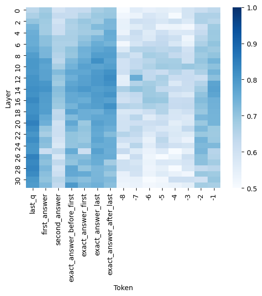<details> <summary>extracted/6450693/figures/probing_heatmaps/mistral-7b-instruct/hotpotqa_auc.png Details</summary>  ### Visual Description ## Heatmap: Layer-Token Activation Heatmap ### Overview The image is a heatmap visualizing numerical activation values across two dimensions: neural network layers (vertical axis) and specific tokens (horizontal axis). The color intensity represents the magnitude of the value, with a scale provided on the right. The data appears to relate to the internal activations of a language model during a question-answering task, focusing on specific token positions. ### Components/Axes * **Y-Axis (Vertical):** Labeled **"Layer"**. It is a linear scale with major tick marks labeled from **0** at the top to **30** at the bottom, in increments of 2 (0, 2, 4, ..., 30). This represents the depth or layer number within a neural network. * **X-Axis (Horizontal):** Labeled **"Token"**. It contains categorical labels for specific token positions. From left to right, the labels are: * `last_q` * `first_answer` * `second_answer` * `exact_answer_before_first` * `exact_answer_first` * `exact_answer_last` * `exact_answer_after_last` * `-8` * `-7` * `-6` * `-5` * `-4` * `-3` * `-2` * `-1` * **Color Bar (Legend):** Positioned on the far right of the chart. It is a vertical gradient bar mapping color to numerical value. * **Scale:** Linear, ranging from **0.5** (bottom, lightest blue/white) to **1.0** (top, darkest blue). * **Labels:** The bar is labeled at intervals: **0.5, 0.6, 0.7, 0.8, 0.9, 1.0**. * **Color Mapping:** Lighter shades (approaching white) correspond to lower values (~0.5-0.6). Medium blue shades correspond to mid-range values (~0.7-0.8). Dark blue shades correspond to high values (~0.9-1.0). ### Detailed Analysis The heatmap displays a grid of colored cells, where each cell's color corresponds to a value between 0.5 and 1.0 for a specific Layer-Token pair. **Trend Verification & Data Point Extraction (Approximate):** * **Column `last_q`:** This column shows consistently high activation (dark blue) across nearly all layers. Values appear to be in the **0.85 - 1.0** range from Layer 0 to Layer 30, with some of the darkest cells (closest to 1.0) appearing in the middle layers (approx. Layers 8-20). * **Columns `first_answer` to `exact_answer_after_last`:** These columns show moderate to high activation, but with more variation than `last_q`. * `first_answer`: Shows medium-dark blue in upper layers (0-10), becoming slightly lighter in lower layers. Approximate range: **0.7 - 0.9**. * `second_answer`: Similar pattern to `first_answer`, perhaps slightly lighter on average. Approximate range: **0.65 - 0.85**. * `exact_answer_before_first`, `exact_answer_first`, `exact_answer_last`, `exact_answer_after_last`: These four columns exhibit a similar pattern. They show relatively high activation (medium to dark blue) in the upper half of the layers (0-15), which then becomes notably lighter (lower values) in the lower layers (16-30). Approximate range across all: **0.6 - 0.9**, with the lower layers dipping towards **0.6**. * **Columns `-8` to `-1`:** These columns, representing negative token indices (likely positions relative to the end of a sequence), show the lowest activations overall. * They are predominantly light blue to white, indicating values clustered near the bottom of the scale. * The approximate range for most cells in these columns is **0.5 - 0.7**. * There is a slight trend where columns `-8` to `-5` are marginally darker (higher value) than columns `-4` to `-1`, which are the lightest in the entire heatmap. **Spatial Grounding:** * The **highest value cells** (darkest blue, ~1.0) are located in the **center-left** region of the heatmap, specifically in the `last_q` column across the middle layers. * The **lowest value cells** (lightest blue/white, ~0.5) are located in the **bottom-right** region, specifically in the `-4` to `-1` columns across the lower layers (20-30). * The legend is placed **outside the main plot area, to its right**. ### Key Observations 1. **Dominance of `last_q`:** The token labeled `last_q` (likely the last token of the question) exhibits the strongest and most consistent high activation across the entire network depth. This is the most salient feature of the heatmap. 2. **Layer-Dependent Activation for Answer Tokens:** Tokens related to the answer (`first_answer`, `exact_answer_*`) show a clear pattern of higher activation in the upper/middle layers, which diminishes in the deepest layers (20-30). 3. **Low Activation for Late Sequence Tokens:** Tokens with negative indices (`-8` to `-1`), which may represent padding or tokens far from the answer span, show uniformly low activation, especially the very last positions (`-4` to `-1`). 4. **Vertical Banding:** There is a visible vertical banding pattern, where entire columns share similar color profiles, indicating that the token position is a stronger determinant of activation level than the specific layer, except for the answer-related tokens which show a layer-dependent gradient. ### Interpretation This heatmap likely visualizes the **attention or activation patterns** within a transformer-based language model during a question-answering inference step. The data suggests the following: * **Model Focus:** The model's internal representations are most strongly and consistently engaged with the **last token of the question (`last_q`)** throughout its processing layers. This implies the question's final context is a critical anchor for the model's reasoning process. * **Information Processing Flow:** For answer-specific tokens, the model appears to process them most intensely in its **middle layers**. The fading activation in the deepest layers could indicate that by that stage, the information from these tokens has been integrated into a more abstract representation, or that the final layers are performing a different function (like output projection) where these specific token activations are less pronounced. * **Noise vs. Signal:** The very low activation for the final negative-index tokens suggests the model effectively **ignores or down-weights** these positions, treating them as irrelevant padding or non-informative context. This demonstrates the model's ability to filter out noise. * **Architectural Insight:** The clear separation between the high-activation "question" zone, the medium-activation "answer" zone with its layer gradient, and the low-activation "padding" zone provides a visual map of how the model allocates its computational resources across different types of input tokens. This is valuable for interpretability, showing where the model "looks" to perform its task. 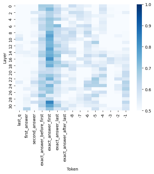</details> (a) HotpotQA <details> <summary>extracted/6450693/figures/probing_heatmaps/mistral-7b-instruct/hotpotqa_with_context_auc.png Details</summary>  ### Visual Description ## Heatmap: Layer-Token Activation Pattern ### Overview The image is a heatmap visualization depicting numerical values (likely activation strengths, attention scores, or correlation coefficients) across a grid defined by neural network layers (Y-axis) and specific tokens (X-axis). The color intensity represents the magnitude of the value, with a scale provided on the right. ### Components/Axes * **Y-Axis (Vertical):** Labeled **"Layer"**. It is a linear scale with major tick marks at intervals of 2, ranging from **0 at the top to 30 at the bottom**. The layers are numbered sequentially: 0, 2, 4, 6, 8, 10, 12, 14, 16, 18, 20, 22, 24, 26, 28, 30. * **X-Axis (Horizontal):** Labeled **"Token"**. It contains categorical labels for specific tokens or token positions. Reading from left to right, the labels are: 1. `last_q` 2. `first_answer` 3. `second_answer` 4. `exact_answer_before_first` 5. `exact_answer_first` 6. `exact_answer_last` 7. `exact_answer_after_last` 8. `-8` 9. `-7` 10. `-6` 11. `-5` 12. `-4` 13. `-3` 14. `-2` 15. `-1` * **Color Bar (Legend):** Positioned vertically on the **right side** of the chart. It provides a scale for interpreting the cell colors. * **Label:** None explicit, but the scale implies a value range. * **Range:** **0.5 (lightest blue/white) to 1.0 (darkest blue)**. * **Gradient:** A continuous blue gradient, where darker blue corresponds to higher values. ### Detailed Analysis The heatmap is a 16 (Layers) x 15 (Tokens) grid. Each cell's color corresponds to a value between approximately 0.5 and 1.0. **Trend Verification & Spatial Analysis:** * **General Pattern:** The highest values (darkest blue cells, ~0.9-1.0) are not uniformly distributed. They form a distinct vertical band in the middle-left section of the chart. * **High-Value Columns:** The columns for tokens **`exact_answer_before_first`** and **`exact_answer_first`** show the most intense and consistent dark blue coloring, particularly from **Layer 8 down to Layer 16**. This indicates these tokens have very high associated values in the mid-layers of the network. * **High-Value Rows:** The layers showing the most intense activity are concentrated between **Layer 8 and Layer 16**. Within this band, the darkest cells are in the `exact_answer_first` column. * **Lower-Value Areas:** The top rows (Layers 0-6) and bottom rows (Layers 20-30) generally show lighter colors (values closer to 0.5-0.7), with some exceptions. The rightmost columns (tokens `-8` through `-1`) also show predominantly lighter colors, indicating lower values for these positional tokens. * **Specific Observations:** * The token **`exact_answer_first`** at **Layer 14** appears to be one of the darkest cells in the entire map, suggesting a peak value near 1.0. * The token **`last_q`** shows moderate values (medium blue) in the early layers (0-4) but fades to lighter shades in deeper layers. * The token **`exact_answer_after_last`** shows a notable pocket of medium-high values (medium blue) around **Layers 22-26**. ### Key Observations 1. **Mid-Layer Focus:** The network's processing, as measured by this metric, is most intense in the middle layers (8-16) for specific answer-related tokens. 2. **Token Specificity:** There is a strong differentiation between token types. Tokens directly referencing the "exact answer" (`exact_answer_before_first`, `exact_answer_first`) elicit much stronger responses than general positional tokens (`-8` to `-1`) or question/other answer tokens (`last_q`, `first_answer`). 3. **Spatial Clustering:** High values are not random; they cluster in a specific region of the layer-token space, suggesting a localized computational focus. ### Interpretation This heatmap likely visualizes the internal state (e.g., attention weights or neuron activations) of a language model during a task involving question answering and answer extraction. The data suggests the model's "focus" or processing strength is not evenly distributed. * **What it demonstrates:** The model appears to dedicate significant computational resources in its middle layers to precisely locating and processing the beginning of the exact answer span (`exact_answer_before_first`, `exact_answer_first`). This is a critical step for tasks like extractive question answering. * **Relationship between elements:** The Y-axis (Layer) represents depth of processing, and the X-axis (Token) represents the input sequence. The pattern shows that deep, mid-level processing is specialized for answer-critical tokens, while shallower and deeper layers, as well as non-critical tokens, are less engaged by this particular metric. * **Notable patterns/anomalies:** The sharp drop-off in value for tokens `-8` to `-1` is notable. These likely represent tokens at negative positions relative to some anchor (e.g., the end of the answer). Their low values suggest the model's mechanism being measured here is not strongly engaged by these trailing positional markers. The secondary cluster for `exact_answer_after_last` in layers 22-26 might indicate a separate, later-stage process for verifying or contextualizing the answer's end. 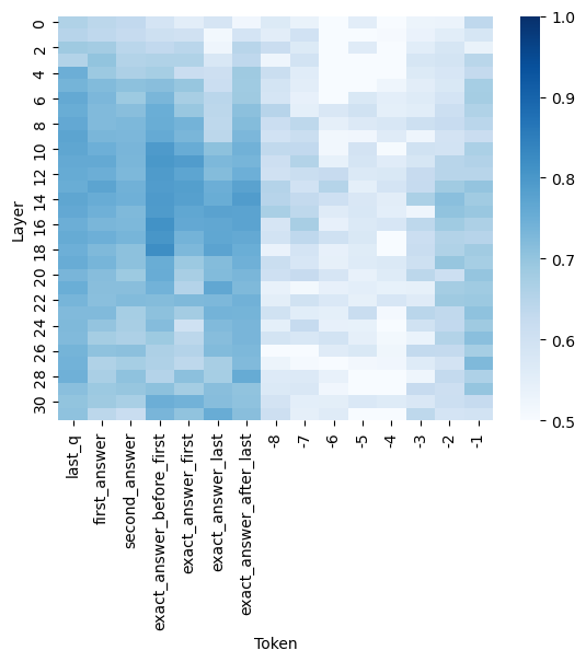</details> (b) HotpotQA with context <details> <summary>extracted/6450693/figures/probing_heatmaps/mistral-7b-instruct/movies_auc.png Details</summary>  ### Visual Description ## Heatmap: Layer vs. Token Activation/Attention Pattern ### Overview The image is a heatmap visualization, likely representing activation strengths, attention weights, or some form of normalized score (ranging from 0.5 to 1.0) across different layers of a neural network model and specific token positions. The chart shows how a particular metric varies for different tokens at each layer depth. ### Components/Axes * **Chart Type:** Heatmap. * **Y-Axis (Vertical):** Labeled **"Layer"**. It represents the depth within a model, with tick marks and labels at intervals of 2, starting from **0** at the top and descending to **30** at the bottom. * **X-Axis (Horizontal):** Labeled **"Token"**. It lists specific token identifiers or positions. The labels are rotated 90 degrees for readability. From left to right, the tokens are: 1. `last_q` 2. `first_answer` 3. `second_answer` 4. `exact_answer_before_first` 5. `exact_answer_first` 6. `exact_answer_last` 7. `exact_answer_after_last` 8. `-8` 9. `-7` 10. `-6` 11. `-5` 12. `-4` 13. `-3` 14. `-2` 15. `-1` * **Color Bar/Legend:** Positioned on the **right side** of the chart. It is a vertical gradient bar mapping color intensity to numerical values. * **Scale:** Linear, from **0.5** (lightest blue/white) at the bottom to **1.0** (darkest blue) at the top. * **Labels:** Major ticks are labeled at **0.5, 0.6, 0.7, 0.8, 0.9, and 1.0**. ### Detailed Analysis The heatmap displays a grid where each cell's color corresponds to a value between 0.5 and 1.0 for a specific Layer-Token pair. **General Trend Verification:** * **Vertical Trend (Per Token):** For most tokens, the value (color intensity) is not constant across layers. There is significant variation from top (Layer 0) to bottom (Layer 30). * **Horizontal Trend (Per Layer):** Within a single layer row, the value varies considerably across different tokens. No single layer shows a uniform color across all tokens. **Specific Observations by Token Group:** 1. **Named Tokens (Left 7 columns):** * `last_q`, `first_answer`, `second_answer`: Show moderate to high values (medium to dark blue) in the early-to-mid layers (approx. Layers 0-16). The intensity often peaks around Layers 4-12. * `exact_answer_before_first`, `exact_answer_first`, `exact_answer_last`: These three tokens exhibit a very strong, consistent pattern. They display the **highest values (darkest blue, ~0.9-1.0)** across a broad range of layers, particularly from Layer 4 down to approximately Layer 20. This forms a prominent dark vertical band in the center-left of the heatmap. * `exact_answer_after_last`: Shows a more moderate pattern, with higher values in early layers that fade in deeper layers. 2. **Numerical Tokens (Right 8 columns, `-8` to `-1`):** * These tokens generally show **lower values (lighter blue, ~0.5-0.7)** compared to the named "exact_answer" tokens. * There is a subtle gradient: tokens `-8` and `-7` tend to have slightly higher values in the very early layers (0-6) compared to tokens `-1` and `-2`. * The region for these tokens becomes very light (values near 0.5) in the middle layers (approx. Layers 10-22), indicating minimal activation or attention. **Spatial Grounding & Key Data Points:** * **Highest Values (~1.0):** Concentrated in the columns for `exact_answer_before_first`, `exact_answer_first`, and `exact_answer_last`, primarily between **Layers 8 and 16**. * **Lowest Values (~0.5):** Found in the columns for the numerical tokens (`-5` to `-1`) in the **middle layer range (Layers 12-20)**. * **Notable Anomaly:** The column for `exact_answer_after_last` shows a pocket of higher value (darker blue) around **Layer 26-28**, which is an outlier compared to its surrounding layers and the general trend of the numerical tokens to its right. ### Key Observations 1. **Strong Selective Activation:** The model's internal representations (as measured by this metric) are highly selective. Tokens related to the "exact answer" (especially `before_first`, `first`, and `last`) elicit a much stronger response across many layers than the question token (`last_q`) or other answer tokens. 2. **Layer-Specific Processing:** The processing focus shifts with depth. Early layers (0-10) show broad activation across many named tokens. Mid-layers (10-20) show extreme specialization for the core "exact answer" tokens. Deeper layers (20-30) show a more diffuse and generally weaker pattern. 3. **Positional Encoding for Numerical Tokens:** The numerical tokens (`-8` to `-1`), which likely represent relative positions (e.g., tokens before the answer), show a weak and fading signal, suggesting they are less critical for the measured metric in deeper processing stages. ### Interpretation This heatmap likely visualizes **attention weights** or **activation norms** from a transformer-based model during a question-answering task. The data suggests the model has learned to strongly focus on and process the tokens that constitute the "exact answer" throughout a significant portion of its network depth (Layers 4-20). This indicates these tokens are information-rich and central to the model's reasoning or output generation process. The weaker signal for the question token (`last_q`) and other answer tokens implies they may serve more as context, while the core answer tokens are the primary carriers of the required information. The fading signal for positional numerical tokens in mid-layers suggests that precise positional information becomes less important as the model integrates semantic meaning in deeper layers. The outlier high-value spot for `exact_answer_after_last` in deep layers could indicate a late-stage verification or formatting step related to the answer's boundary. In essence, the chart provides a "brain scan" of the model, revealing which parts of the input it deems most important and at what stage of processing. The clear, strong pattern for the exact answer tokens is a sign of a model that has successfully learned to identify and prioritize the key information for its task. 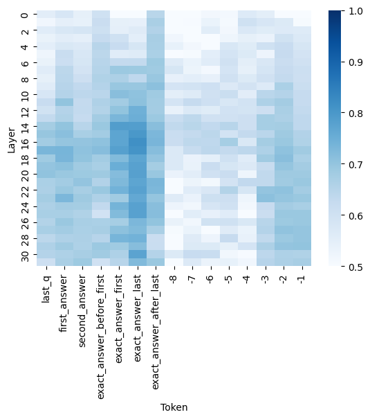</details> (c) Movies <details> <summary>extracted/6450693/figures/probing_heatmaps/mistral-7b-instruct/winogrande_auc.png Details</summary>  ### Visual Description ## Heatmap: Layer-wise Token Activation/Attention Intensity ### Overview The image is a heatmap visualization, likely representing the intensity of attention weights, activation values, or another saliency metric across different layers of a neural network model for specific tokens in a sequence. The chart shows how the importance or activation of certain tokens varies as information propagates through the model's layers. ### Components/Axes * **Chart Type:** Heatmap. * **Y-Axis (Vertical):** Labeled **"Layer"**. It represents the depth within the neural network, with values ranging from **0** at the top to **30** at the bottom, in increments of 2 (0, 2, 4, ..., 30). * **X-Axis (Horizontal):** Labeled **"Token"**. It lists specific tokens or positions in an input sequence. The labels, from left to right, are: 1. `last_q` 2. `first_answer` 3. `second_answer` 4. `exact_answer_before_first` 5. `exact_answer_first` 6. `exact_answer_last` 7. `exact_answer_after_last` 8. `-8` 9. `-7` 10. `-6` 11. `-5` 12. `-4` 13. `-3` 14. `-2` 15. `-1` * **Color Scale/Legend:** Positioned on the **right side** of the chart. It is a vertical color bar indicating the value mapped to each cell's color. The scale ranges from **0.5** (lightest blue/white) at the bottom to **1.0** (darkest blue) at the top. The gradient moves from white/light blue (low value) through medium blue to dark navy blue (high value). ### Detailed Analysis The heatmap is a grid where each cell's color corresponds to a value between 0.5 and 1.0 for a specific (Layer, Token) pair. **Spatial & Color Analysis:** * **High-Value Clusters (Dark Blue):** The most intense, dark blue cells (values approaching 1.0) are concentrated in two primary columns: * **`exact_answer_first` (Column 5):** Shows consistently high values (dark blue) from approximately **Layer 10 down to Layer 30**. The intensity appears strongest around **Layers 14-22**. * **`exact_answer_last` (Column 6):** Also exhibits very high values, particularly from **Layer 12 to Layer 30**, with a peak intensity similar to `exact_answer_first`. * **Moderate-Value Regions (Medium Blue):** * The columns for `exact_answer_before_first` (Column 4) and `exact_answer_after_last` (Column 7) show medium blue shades, indicating moderate values (approx. 0.7-0.85), especially in the middle to lower layers (10-30). * The column for `last_q` (Column 1) displays a patchy pattern of medium blue, with some higher values in the very early layers (0-6) and again in the mid-layers. * **Low-Value Regions (Light Blue/White):** * The columns labeled with negative numbers (`-8` to `-1`, Columns 8-15) are predominantly light blue or white, indicating values closer to the lower end of the scale (0.5-0.65). This suggests these positional tokens have relatively low saliency/activation across all layers. * The tokens `first_answer` (Column 2) and `second_answer` (Column 3) also show generally low to moderate values, lighter than the "exact_answer" columns. **Trend Verification:** * **Vertical Trend (Across Layers):** For the high-value tokens (`exact_answer_first`, `exact_answer_last`), the trend is not linear. Values start low in the initial layers (0-8), increase sharply in the middle layers (10-20), and remain high through the final layers (22-30). This suggests these tokens become critically important in the model's intermediate processing stages. * **Horizontal Trend (Across Tokens):** There is a clear hierarchy of token importance. The "exact answer" boundary tokens (`first`, `last`) are the most salient, followed by their immediate context (`before_first`, `after_last`), then the question token (`last_q`), and finally the generic answer tokens and positional indices, which are the least salient. ### Key Observations 1. **Token Specificity Matters:** The model pays dramatically more attention to tokens explicitly marking the boundaries of the "exact answer" (`exact_answer_first`, `exact_answer_last`) compared to generic answer tokens (`first_answer`, `second_answer`) or positional indices. 2. **Mid-Layer Focus:** The peak activation for critical tokens occurs in the middle to late layers (10-30), not in the earliest embedding layers. This aligns with the understanding that deeper layers in transformers often handle more abstract, task-specific reasoning. 3. **Positional Token Noise:** The low, uniform values for the numbered positional tokens (`-8` to `-1`) suggest they serve as background or structural elements without carrying significant task-specific information in this context. 4. **Symmetry around Answer:** The columns `exact_answer_before_first` and `exact_answer_after_last` show similar, moderate intensity patterns, indicating the model attends to the context immediately surrounding the answer span. ### Interpretation This heatmap provides a technical window into the internal mechanics of a language model, likely during a question-answering task. The data suggests the model has learned to **precisely localize the answer span** by assigning high importance to the tokens that demarcate its start (`exact_answer_first`) and end (`exact_answer_last`). This focus intensifies as the signal propagates through the network's layers, peaking in the mid-to-deep layers where complex feature integration occurs. The stark contrast between the high-value "exact answer" columns and the low-value positional columns indicates the model is not merely relying on token position but is performing **content-based attention**. It successfully identifies and prioritizes the semantically crucial tokens for the task. The moderate attention to the immediate context (`before_first`, `after_last`) may reflect the model verifying the answer's coherence with its surrounding text. **Notable Anomaly:** The token `last_q` (presumably the last token of the question) shows some early-layer activation, which is logical as the question is processed first. However, its importance does not peak as dramatically as the answer-boundary tokens in deeper layers, suggesting the model's focus shifts decisively from question understanding to answer extraction as processing depth increases. In summary, this visualization demonstrates a model that has developed an efficient internal strategy: it uses specific, learned boundary markers to isolate the answer span, dedicating its computational resources (attention/activation) most heavily to these critical points during deep processing. 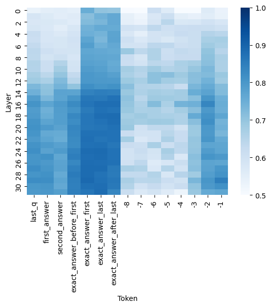</details> (d) Winogrande <details> <summary>extracted/6450693/figures/probing_heatmaps/mistral-7b-instruct/mnli_auc.png Details</summary>  ### Visual Description ## Heatmap: Token Activation Across Neural Network Layers ### Overview The image is a heatmap visualizing the intensity of a metric (likely attention weight, activation strength, or probability) for specific tokens across the layers of a neural network model. The heatmap uses a blue color gradient to represent values, with darker blue indicating higher values. The data suggests an analysis of how a model processes or attends to different parts of a question-answer sequence. ### Components/Axes * **Y-Axis (Vertical):** Labeled "Layer". It represents the depth within the neural network, with layers numbered from 0 at the top to 30 at the bottom. The axis has tick marks at intervals of 2 (0, 2, 4, ..., 30). * **X-Axis (Horizontal):** Labeled "Token". It lists specific tokens or positions in a text sequence. From left to right, the tokens are: 1. `last_q` 2. `first_answer` 3. `second_answer` 4. `exact_answer_before_first` 5. `exact_answer_first` 6. `exact_answer_last` 7. `exact_answer_after_last` 8. `-8` 9. `-7` 10. `-6` 11. `-5` 12. `-4` 13. `-3` 14. `-2` 15. `-1` * **Color Bar (Legend):** Located on the right side of the chart. It provides a scale for interpreting the cell colors. * **Label:** None explicit, but the scale implies a normalized value (e.g., attention score, probability). * **Range:** 0.5 (lightest blue/white) to 1.0 (darkest blue). * **Ticks:** Marked at 0.5, 0.6, 0.7, 0.8, 0.9, and 1.0. ### Detailed Analysis The heatmap shows a 31 (Layers 0-30) by 15 (Tokens) grid of colored cells. The color intensity represents the value for each (Layer, Token) pair. **Trend Verification & Spatial Grounding:** * **Left Token Group (`last_q` to `exact_answer_after_last`):** This group generally shows higher values (darker blue) compared to the right group. * `exact_answer_first` and `exact_answer_last` exhibit the highest and most consistent values across the middle to lower layers (approximately layers 8-28), appearing as a dark blue vertical band. Their values are estimated to be between 0.85 and 1.0 in this region. * `exact_answer_before_first` and `exact_answer_after_last` also show high values, but slightly less intense and consistent than the central two. * `last_q`, `first_answer`, and `second_answer` have more moderate and variable values. They show lighter blue (values ~0.6-0.75) in the top layers (0-10), becoming darker (values ~0.75-0.9) in the middle and lower layers. * **Right Token Group (`-8` to `-1`):** This group, likely representing positional tokens or tokens preceding the answer, shows significantly lower values overall. * The cells are predominantly light blue to white, indicating values between 0.5 and 0.7. * There is a subtle pattern where tokens closer to `-1` (e.g., `-2`, `-1`) have slightly darker blue patches in some middle layers (e.g., around layers 14-22) compared to tokens like `-8` or `-7`, but the values remain low (estimated ≤0.75). * **Layer-wise Trend:** For most tokens, values tend to be lower (lighter) in the very top layers (0-4) and increase (darken) in the middle layers (8-24), before sometimes slightly decreasing again in the final layers (26-30). This is most pronounced for the answer-related tokens. ### Key Observations 1. **Strong Focus on Exact Answer Tokens:** The model's highest activations are concentrated on the tokens `exact_answer_first` and `exact_answer_last`, particularly in the middle layers. This suggests these positions are critically important for the model's internal processing related to the task. 2. **Clear Differentiation Between Answer and Context:** There is a stark contrast in activation levels between the semantic answer tokens (left group) and the positional/preceding tokens (right group). The model clearly distinguishes their importance. 3. **Mid-Layer Processing Peak:** The core processing, as indicated by peak activation values, appears to occur in the network's middle layers (roughly 8-24), not at the very beginning or end. 4. **Gradual Information Flow:** The increasing activation from top layers to middle layers for answer tokens suggests information is being progressively integrated and refined as it moves through the network. ### Interpretation This heatmap likely visualizes **attention weights** or **hidden state activations** from a transformer-based model (like BERT or GPT) during a question-answering task. The "Token" axis represents specific positions in the input sequence fed to the model. * **What the data suggests:** The model pays the most "attention" or assigns the highest importance to the exact span of the answer (`exact_answer_first` to `exact_answer_last`). The tokens immediately before and after this span are also highly relevant, forming a context window around the answer. The question token (`last_q`) and other answer candidates (`first_answer`, `second_answer`) are moderately important. The model largely ignores the tokens far before the answer (represented by `-8` to `-4`). * **How elements relate:** The layer-wise progression shows how information flows. Early layers may perform basic token embedding, middle layers perform complex reasoning and attention focusing on the answer span, and final layers may prepare the output. The clear separation between answer and non-answer tokens indicates the model has successfully learned to identify the critical part of the input for its task. * **Notable Anomalies/Patterns:** The near-perfect vertical band of high activation for `exact_answer_first` and `exact_answer_last` is striking. It implies these two positions are almost always the focal point, regardless of layer depth after the initial few. This could be a signature of a model fine-tuned for extractive QA, where pinpointing the exact answer boundaries is the primary objective. The lower values for `-1` and `-2` compared to other negative tokens might indicate a slight "edge effect" where the model pays a tiny bit more attention to tokens immediately preceding the answer block. 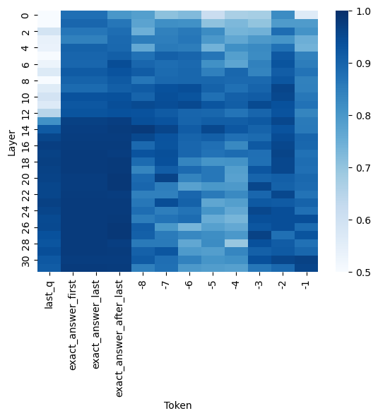</details> (e) NLI <details> <summary>extracted/6450693/figures/probing_heatmaps/mistral-7b-instruct/imdb_auc.png Details</summary>  ### Visual Description ## Heatmap: Layer-Token Correlation Matrix ### Overview This image is a heatmap visualizing the correlation strength between different "Tokens" (X-axis) across various neural network "Layers" (Y-axis). The color intensity represents the correlation value, with a scale provided on the right. The chart appears to analyze the internal representations of specific tokens within a language model's processing layers. ### Components/Axes * **Chart Type:** Heatmap (2D grid of colored cells). * **Y-Axis (Vertical):** Labeled **"Layer"**. It has numerical markers from **0 to 30** in increments of 2 (0, 2, 4, ..., 30). This represents the depth or layer number within a neural network. * **X-Axis (Horizontal):** Labeled **"Token"**. It contains 12 categorical labels. From left to right: 1. `last_q` 2. `exact_answer_first` 3. `exact_answer_last` 4. `exact_answer_after_last` 5. `-8` 6. `-7` 7. `-6` 8. `-5` 9. `-4` 10. `-3` 11. `-2` 12. `-1` * **Legend/Color Scale:** Positioned vertically on the **right side** of the chart. It is a gradient bar labeled from **0.5** (bottom, lightest blue/white) to **1.0** (top, darkest blue). The scale indicates the correlation value, where darker blue signifies a higher correlation (closer to 1.0) and lighter blue/white signifies a lower correlation (closer to 0.5). ### Detailed Analysis The heatmap displays a grid of 31 rows (Layers 0-30) by 12 columns (Tokens). Each cell's color corresponds to a correlation value based on the legend. **Trend Verification & Data Point Analysis:** 1. **First Four Tokens (`last_q`, `exact_answer_first`, `exact_answer_last`, `exact_answer_after_last`):** * **Visual Trend:** These columns form a distinct, dark blue block, especially from Layer 12 downward. The correlation is consistently high. * **Data Points:** The cells for these tokens are predominantly dark blue, indicating correlation values **approximately between 0.85 and 1.0** across most layers. The highest correlations (darkest blue, ~0.95-1.0) are concentrated in the lower half of the network (Layers ~12-30). Layers 0-10 show slightly lighter shades, suggesting correlations in the **~0.75-0.90** range for these tokens. 2. **Numbered Tokens (`-8` to `-1`):** * **Visual Trend:** These columns show more variability. There is a general pattern where correlation is higher in the middle layers (approx. Layers 8-20) and lower in the very early (0-6) and very late (24-30) layers. The columns for `-4`, `-3`, `-2`, and `-1` appear slightly darker on average than `-8` through `-5`. * **Data Points:** * **Mid-Layer Peak:** For tokens `-8` to `-1`, the darkest cells (highest correlation, **~0.80-0.90**) are found roughly between **Layers 8 and 20**. * **Early/Late Layer Troughs:** The lightest cells (lowest correlation, **~0.50-0.70**) for these tokens are in **Layers 0-6** and **Layers 24-30**. * **Token Variation:** Tokens `-4`, `-3`, `-2`, `-1` maintain slightly higher correlations in the later layers (20-30) compared to tokens `-8`, `-7`, `-6`, `-5`. ### Key Observations 1. **Bimodal Pattern:** The heatmap reveals two distinct behavioral groups: the "answer-related" tokens (`last_q`, `exact_answer_*`) and the "positional" tokens (`-8` to `-1`). 2. **Layer-Dependent Correlation:** Correlation strength is not uniform across the network. For the positional tokens, it follows an inverted-U shape, peaking in the middle layers. For the answer tokens, it generally increases with depth. 3. **High Answer Token Consistency:** The first four tokens maintain very high inter-correlation throughout the network, suggesting their representations are strongly aligned, especially in deeper layers. 4. **Spatial Grounding:** The legend is on the right. The darkest region of the entire chart is the lower-left quadrant (Layers 12-30, Tokens 1-4). The lightest regions are the top rows (Layers 0-4) across all tokens, and the bottom rows for the numbered tokens. ### Interpretation This heatmap likely visualizes the **cosine similarity or correlation of token embeddings** across the layers of a transformer-based language model. The "Token" labels suggest an analysis of how the model processes a question (`last_q`) and its answer (`exact_answer_*`), alongside relative positional markers (`-8` to `-1`, likely representing tokens preceding the answer). * **What the data suggests:** The strong, deep-layer correlation among the answer-related tokens indicates that the model's internal representation of the question and the precise answer span becomes highly unified and stable as information is processed through the network. This is crucial for accurate answer extraction. * **How elements relate:** The middle-layer peak for positional tokens aligns with the known function of middle transformer layers in building contextual understanding. The drop in correlation for these tokens in final layers might indicate they are being "used up" or transformed into the final answer representation. * **Notable Anomaly/Insight:** The stark contrast between the two token groups is the key finding. It visually demonstrates that the model treats "semantic" tokens (question/answer) fundamentally differently from "structural" or positional tokens, maintaining a much stronger and more consistent representation for the former throughout its depth. This could be a signature of effective information flow for question-answering tasks. </details> (f) IMDB Figure 6: AUC values of a probe error detector across layers and tokens, Mistral-7b-instruct. The detection performance spikes at the exact answer tokens. Tables 4, 5, 6, and 7 present the full error detection results across all baselines and datasets, which are consistent with the main paper results. Table 4: Comparison of error detection performance (AUC) on Mistral-7B. | | Mistral-7B | | | | | | --- | --- | --- | --- | --- | --- | | TriviaQA | Winobias | Math | Movies | IMDB | | | Logits-mean | $0.67$ $\pm 0.004$ | $0.49$ $\pm 0.010$ | $0.41$ $\pm 0.015$ | $0.67$ $\pm 0.007$ | $0.88$ $\pm 0.064$ | | Logits-mean-exact | $0.67$ $\pm 0.004$ | $0.50$ $\pm 0.010$ | $0.56$ $\pm 0.026$ | $0.68$ $\pm 0.008$ | $0.57$ $\pm 0.080$ | | Logits-min | $0.80$ $\pm 0.003$ | $0.45$ $\pm 0.014$ | $0.48$ $\pm 0.021$ | $0.73$ $\pm 0.006$ | $0.78$ $\pm 0.056$ | | Logits-min-exact | $0.80$ $\pm 0.005$ | $0.53$ $\pm 0.014$ | $0.78$ $\pm 0.032$ | $0.72$ $\pm 0.005$ | $0.57$ $\pm 0.080$ | | Logits-max | $0.53$ $\pm 0.008$ | $0.49$ $\pm 0.010$ | $0.42$ $\pm 0.023$ | $0.54$ $\pm 0.005$ | $0.83$ $\pm 0.076$ | | Logits-max-exact | $0.54$ $\pm 0.009$ | $0.50$ $\pm 0.010$ | $0.40$ $\pm 0.024$ | $0.58$ $\pm 0.007$ | $0.57$ $\pm 0.080$ | | Probas-mean | $0.76$ $\pm 0.003$ | $0.53$ $\pm 0.018$ | $0.66$ $\pm 0.016$ | $0.72$ $\pm 0.007$ | $0.87$ $\pm 0.041$ | | Probas-mean-exact | $0.78$ $\pm 0.002$ | $0.55$ $\pm 0.014$ | $0.62$ $\pm 0.016$ | $0.74$ $\pm 0.007$ | $0.83$ $\pm 0.057$ | | Probas-min | $0.82$ $\pm 0.003$ | $0.52$ $\pm 0.013$ | $0.82$ $\pm 0.020$ | $0.73$ $\pm 0.006$ | $0.86$ $\pm 0.032$ | | Probas-min-exact | 0.85 $\pm 0.003$ | $0.58$ $\pm 0.011$ | $0.84$ $\pm 0.015$ | $0.74$ $\pm 0.006$ | $0.83$ $\pm 0.057$ | | Probas-max | $0.53$ $\pm 0.008$ | $0.50$ $\pm 0.016$ | $0.43$ $\pm 0.025$ | $0.55$ $\pm 0.008$ | $0.80$ $\pm 0.074$ | | Probas-max-exact | $0.55$ $\pm 0.009$ | $0.51$ $\pm 0.013$ | $0.39$ $\pm 0.019$ | $0.59$ $\pm 0.009$ | $0.83$ $\pm 0.057$ | | p(True) | $0.57$ $\pm 0.007$ | $0.53$ $\pm 0.019$ | $0.56$ $\pm 0.027$ | $0.51$ $\pm 0.003$ | $0.65$ $\pm 0.004$ | | p(True)-exact | $0.56$ $\pm 0.006$ | $0.55$ $\pm 0.026$ | $0.57$ $\pm 0.036$ | $0.52$ $\pm 0.003$ | $0.65$ $\pm 0.003$ | | Probe @ token | | | | | | | Last generated [-1] | $0.83$ $\pm 0.002$ | $0.65$ $\pm 0.008$ | $0.82$ $\pm 0.023$ | $0.79$ $\pm 0.002$ | $0.85$ $\pm 0.007$ | | Before last generated [-2] | $0.82$ $\pm 0.003$ | $0.84$ $\pm 0.012$ | $0.83$ $\pm 0.019$ | $0.78$ $\pm 0.003$ | $0.95$ $\pm 0.004$ | | End of question | $0.74$ $\pm 0.005$ | $0.78$ $\pm 0.012$ | $0.83$ $\pm 0.016$ | $0.77$ $\pm 0.002$ | $0.81$ $\pm 0.009$ | | Exact answer last | $0.84$ $\pm 0.005$ | 0.89 $\pm 0.007$ | 0.96 $\pm 0.008$ | $0.78$ $\pm 0.003$ | 0.95 $\pm 0.004$ | | Exact answer last+1 | $0.84$ $\pm 0.004$ | $0.84$ $\pm 0.012$ | $0.95$ $\pm 0.010$ | 0.80 $\pm 0.002$ | $0.85$ $\pm 0.007$ | | HotpotQA | HotpotQA-WC | Winogrande | NLI | NQ-WC | | | Logits-mean | $0.63$ $\pm 0.005$ | $0.52$ $\pm 0.009$ | $0.49$ $\pm 0.004$ | $0.51$ $\pm 0.004$ | $0.69$ $\pm 0.006$ | | Logits-mean-exact | $0.57$ $\pm 0.008$ | $0.52$ $\pm 0.007$ | $0.50$ $\pm 0.003$ | 0.93 $\pm 0.004$ | $0.72$ $\pm 0.005$ | | Logits-min | $0.72$ $\pm 0.008$ | $0.59$ $\pm 0.006$ | $0.50$ $\pm 0.007$ | $0.53$ $\pm 0.005$ | $0.65$ $\pm 0.009$ | | Logits-min-exact | $0.72$ $\pm 0.007$ | $0.65$ $\pm 0.004$ | $0.51$ $\pm 0.007$ | $0.49$ $\pm 0.006$ | $0.70$ $\pm 0.005$ | | Logits-max | $0.54$ $\pm 0.007$ | $0.49$ $\pm 0.010$ | $0.48$ $\pm 0.005$ | $0.48$ $\pm 0.005$ | $0.59$ $\pm 0.012$ | | Logits-max-exact | $0.48$ $\pm 0.010$ | $0.44$ $\pm 0.007$ | $0.50$ $\pm 0.003$ | $0.48$ $\pm 0.005$ | $0.58$ $\pm 0.009$ | | Probas-mean | $0.65$ $\pm 0.004$ | $0.55$ $\pm 0.006$ | $0.51$ $\pm 0.007$ | $0.49$ $\pm 0.003$ | $0.63$ $\pm 0.008$ | | Probas-mean-exact | $0.62$ $\pm 0.006$ | $0.56$ $\pm 0.007$ | $0.51$ $\pm 0.005$ | $0.02$ $\pm 0.001$ | $0.66$ $\pm 0.007$ | | Probas-min | $0.73$ $\pm 0.005$ | $0.58$ $\pm 0.007$ | $0.52$ $\pm 0.009$ | $0.53$ $\pm 0.004$ | $0.63$ $\pm 0.011$ | | Probas-min-exact | $0.78$ $\pm 0.005$ | $0.66$ $\pm 0.004$ | $0.52$ $\pm 0.008$ | $0.49$ $\pm 0.005$ | $0.69$ $\pm 0.006$ | | Probas-max | $0.54$ $\pm 0.008$ | $0.49$ $\pm 0.007$ | $0.50$ $\pm 0.005$ | $0.47$ $\pm 0.004$ | $0.52$ $\pm 0.004$ | | Probas-max-exact | $0.48$ $\pm 0.010$ | $0.44$ $\pm 0.005$ | $0.50$ $\pm 0.004$ | $0.48$ $\pm 0.003$ | $0.53$ $\pm 0.012$ | | p(True) | $0.55$ $\pm 0.007$ | $0.54$ $\pm 0.006$ | $0.51$ $\pm 0.005$ | $0.51$ $\pm 0.003$ | $0.52$ $\pm 0.008$ | | p(True)-exact | $0.61$ $\pm 0.005$ | $0.54$ $\pm 0.006$ | $0.61$ $\pm 0.006$ | $0.51$ $\pm 0.006$ | $0.53$ $\pm 0.014$ | | Probe @ token | | | | | | | Last generated [-1] | $0.78$ $\pm 0.006$ | $0.67$ $\pm 0.004$ | $0.51$ $\pm 0.007$ | $0.77$ $\pm 0.004$ | $0.78$ $\pm 0.003$ | | Before last generated [-2] | $0.79$ $\pm 0.007$ | $0.69$ $\pm 0.007$ | $0.66$ $\pm 0.004$ | $0.81$ $\pm 0.002$ | $0.75$ $\pm 0.006$ | | End of question | $0.72$ $\pm 0.007$ | $0.56$ $\pm 0.003$ | $0.51$ $\pm 0.007$ | $0.88$ $\pm 0.004$ | $0.70$ $\pm 0.005$ | | Exact answer last | $0.80$ $\pm 0.008$ | 0.74 $\pm 0.007$ | 0.69 $\pm 0.006$ | $0.84$ $\pm 0.004$ | $0.81$ $\pm 0.009$ | | Exact answer last+1 | 0.81 $\pm 0.008$ | $0.72$ $\pm 0.005$ | $0.59$ $\pm 0.005$ | $0.75$ $\pm 0.006$ | 0.84 $\pm 0.007$ | Table 5: Comparison of error detection performance (AUC) on Mistral-7B-Instruct. | | Mistral-7B-Instruct | | | | | | --- | --- | --- | --- | --- | --- | | TriviaQA | Winobias | Math | Movies | IMDB | | | Logits-mean | $0.60$ $\pm 0.009$ | $0.56$ $\pm 0.017$ | $0.55$ $\pm 0.029$ | $0.63$ $\pm 0.005$ | $0.57$ $\pm 0.006$ | | Logits-mean-exact | $0.68$ $\pm 0.007$ | $0.54$ $\pm 0.012$ | $0.51$ $\pm 0.005$ | $0.70$ $\pm 0.004$ | $0.87$ $\pm 0.007$ | | Logits-min | $0.63$ $\pm 0.008$ | $0.59$ $\pm 0.012$ | $0.51$ $\pm 0.017$ | $0.66$ $\pm 0.008$ | $0.52$ $\pm 0.007$ | | Logits-min-exact | $0.75$ $\pm 0.006$ | $0.53$ $\pm 0.013$ | $0.71$ $\pm 0.009$ | $0.74$ $\pm 0.005$ | $0.87$ $\pm 0.007$ | | Logits-max | $0.54$ $\pm 0.005$ | $0.53$ $\pm 0.012$ | $0.54$ $\pm 0.039$ | $0.54$ $\pm 0.004$ | $0.47$ $\pm 0.004$ | | Logits-max-exact | $0.55$ $\pm 0.004$ | $0.54$ $\pm 0.011$ | $0.32$ $\pm 0.015$ | $0.61$ $\pm 0.006$ | $0.87$ $\pm 0.007$ | | Probas-mean | $0.60$ $\pm 0.007$ | $0.58$ $\pm 0.018$ | $0.56$ $\pm 0.028$ | $0.61$ $\pm 0.002$ | $0.54$ $\pm 0.008$ | | Probas-mean-exact | $0.71$ $\pm 0.003$ | $0.57$ $\pm 0.015$ | $0.71$ $\pm 0.014$ | $0.74$ $\pm 0.006$ | $0.84$ $\pm 0.007$ | | Probas-min | $0.59$ $\pm 0.008$ | $0.58$ $\pm 0.014$ | $0.50$ $\pm 0.025$ | $0.60$ $\pm 0.008$ | $0.51$ $\pm 0.010$ | | Probas-min-exact | $0.74$ $\pm 0.004$ | $0.57$ $\pm 0.016$ | $0.75$ $\pm 0.011$ | $0.73$ $\pm 0.006$ | $0.84$ $\pm 0.007$ | | Probas-max | $0.50$ $\pm 0.006$ | $0.41$ $\pm 0.010$ | $0.53$ $\pm 0.009$ | $0.51$ $\pm 0.005$ | $0.48$ $\pm 0.004$ | | Probas-max-exact | $0.51$ $\pm 0.007$ | $0.54$ $\pm 0.010$ | $0.45$ $\pm 0.015$ | $0.60$ $\pm 0.003$ | $0.84$ $\pm 0.007$ | | p(True) | $0.68$ $\pm 0.005$ | $0.45$ $\pm 0.021$ | $0.48$ $\pm 0.026$ | $0.62$ $\pm 0.005$ | $0.62$ $\pm 0.009$ | | p(True)-exact | $0.74$ $\pm 0.003$ | $0.40$ $\pm 0.021$ | $0.60$ $\pm 0.025$ | $0.69$ $\pm 0.008$ | $0.60$ $\pm 0.009$ | | Probe @ token | | | | | | | Last generated [-1] | $0.71$ $\pm 0.006$ | $0.82$ $\pm 0.004$ | $0.74$ $\pm 0.008$ | $0.72$ $\pm 0.005$ | $0.92$ $\pm 0.010$ | | Before last generated [-2] | $0.73$ $\pm 0.004$ | $0.85$ $\pm 0.004$ | $0.74$ $\pm 0.007$ | $0.72$ $\pm 0.006$ | $0.94$ $\pm 0.006$ | | End of question | $0.76$ $\pm 0.008$ | $0.82$ $\pm 0.011$ | $0.72$ $\pm 0.007$ | $0.74$ $\pm 0.003$ | $0.96$ $\pm 0.006$ | | Exact answer last | $0.85$ $\pm 0.004$ | 0.92 $\pm 0.005$ | 0.92 $\pm 0.008$ | $0.81$ $\pm 0.003$ | 0.97 $\pm 0.005$ | | Exact answer last+1 | 0.86 $\pm 0.006$ | $0.88$ $\pm 0.006$ | $0.90$ $\pm 0.010$ | 0.82 $\pm 0.003$ | $0.96$ $\pm 0.006$ | | HotpotQA | HotpotQA-WC | Winogrande | NLI | NQ-WC | | | Logits-mean | $0.61$ $\pm 0.002$ | $0.55$ $\pm 0.009$ | $0.59$ $\pm 0.004$ | $0.64$ $\pm 0.006$ | $0.71$ $\pm 0.008$ | | Logits-mean-exact | $0.66$ $\pm 0.009$ | $0.55$ $\pm 0.004$ | $0.49$ $\pm 0.004$ | $0.57$ $\pm 0.004$ | $0.69$ $\pm 0.009$ | | Logits-min | $0.61$ $\pm 0.003$ | $0.53$ $\pm 0.013$ | $0.61$ $\pm 0.003$ | $0.62$ $\pm 0.002$ | $0.67$ $\pm 0.008$ | | Logits-min-exact | $0.77$ $\pm 0.004$ | $0.67$ $\pm 0.013$ | $0.48$ $\pm 0.004$ | $0.54$ $\pm 0.005$ | $0.69$ $\pm 0.006$ | | Logits-max | $0.53$ $\pm 0.008$ | $0.51$ $\pm 0.011$ | $0.52$ $\pm 0.006$ | $0.59$ $\pm 0.008$ | $0.63$ $\pm 0.011$ | | Logits-max-exact | $0.51$ $\pm 0.011$ | $0.41$ $\pm 0.010$ | $0.49$ $\pm 0.007$ | $0.64$ $\pm 0.003$ | $0.63$ $\pm 0.013$ | | Probas-mean | $0.63$ $\pm 0.003$ | $0.56$ $\pm 0.010$ | $0.58$ $\pm 0.005$ | $0.62$ $\pm 0.005$ | $0.68$ $\pm 0.010$ | | Probas-mean-exact | $0.72$ $\pm 0.006$ | $0.66$ $\pm 0.010$ | $0.46$ $\pm 0.004$ | $0.57$ $\pm 0.003$ | $0.65$ $\pm 0.008$ | | Probas-min | $0.58$ $\pm 0.003$ | $0.52$ $\pm 0.008$ | $0.59$ $\pm 0.002$ | $0.58$ $\pm 0.008$ | $0.65$ $\pm 0.014$ | | Probas-min-exact | $0.76$ $\pm 0.004$ | $0.68$ $\pm 0.010$ | $0.46$ $\pm 0.005$ | $0.57$ $\pm 0.003$ | $0.66$ $\pm 0.008$ | | Probas-max | $0.50$ $\pm 0.005$ | $0.53$ $\pm 0.003$ | $0.48$ $\pm 0.007$ | $0.52$ $\pm 0.007$ | $0.51$ $\pm 0.005$ | | Probas-max-exact | $0.46$ $\pm 0.010$ | $0.46$ $\pm 0.010$ | $0.48$ $\pm 0.004$ | $0.53$ $\pm 0.004$ | $0.52$ $\pm 0.018$ | | p(True) | $0.54$ $\pm 0.006$ | $0.54$ $\pm 0.004$ | $0.53$ $\pm 0.003$ | $0.58$ $\pm 0.003$ | $0.57$ $\pm 0.006$ | | p(True)-exact | $0.60$ $\pm 0.008$ | $0.48$ $\pm 0.005$ | $0.57$ $\pm 0.011$ | $0.65$ $\pm 0.004$ | $0.57$ $\pm 0.009$ | | Probe @ token | | | | | | | Last generated [-1] | $0.72$ $\pm 0.005$ | $0.64$ $\pm 0.005$ | $0.74$ $\pm 0.005$ | $0.85$ $\pm 0.004$ | $0.82$ $\pm 0.006$ | | Before last generated [-2] | $0.73$ $\pm 0.006$ | $0.64$ $\pm 0.004$ | $0.76$ $\pm 0.004$ | $0.87$ $\pm 0.002$ | $0.84$ $\pm 0.009$ | | End of question | $0.80$ $\pm 0.003$ | $0.63$ $\pm 0.003$ | $0.71$ $\pm 0.007$ | $0.79$ $\pm 0.004$ | $0.85$ $\pm 0.010$ | | Exact answer last | $0.85$ $\pm 0.003$ | $0.75$ $\pm 0.006$ | 0.84 $\pm 0.005$ | 0.93 $\pm 0.003$ | $0.86$ $\pm 0.003$ | | Exact answer last+1 | 0.85 $\pm 0.002$ | 0.76 $\pm 0.004$ | $0.80$ $\pm 0.004$ | $0.92$ $\pm 0.004$ | 0.87 $\pm 0.006$ | Table 6: Comparison of error detection performance (AUC) on Llama-8b. | | Llama-8b | | | | | | --- | --- | --- | --- | --- | --- | | TriviaQA | Winobias | Math | Movies | IMDB | | | Logits-mean | $0.58$ $\pm 0.006$ | $0.44$ $\pm 0.015$ | $0.43$ $\pm 0.026$ | $0.64$ $\pm 0.008$ | $0.77$ $\pm 0.007$ | | Logits-mean-exact | $0.63$ $\pm 0.007$ | $0.50$ $\pm 0.015$ | $0.50$ $\pm 0.028$ | $0.64$ $\pm 0.008$ | $0.77$ $\pm 0.007$ | | Logits-min | $0.75$ $\pm 0.007$ | $0.50$ $\pm 0.022$ | $0.45$ $\pm 0.042$ | $0.73$ $\pm 0.005$ | $0.73$ $\pm 0.007$ | | Logits-min-exact | $0.76$ $\pm 0.003$ | $0.53$ $\pm 0.009$ | $0.75$ $\pm 0.022$ | $0.73$ $\pm 0.005$ | $0.77$ $\pm 0.007$ | | Logits-max | $0.48$ $\pm 0.006$ | $0.48$ $\pm 0.009$ | $0.42$ $\pm 0.027$ | $0.53$ $\pm 0.005$ | $0.72$ $\pm 0.007$ | | Logits-max-exact | $0.52$ $\pm 0.007$ | $0.49$ $\pm 0.014$ | $0.35$ $\pm 0.026$ | $0.53$ $\pm 0.005$ | $0.77$ $\pm 0.007$ | | Probas-mean | $0.64$ $\pm 0.006$ | $0.41$ $\pm 0.008$ | $0.61$ $\pm 0.029$ | $0.71$ $\pm 0.007$ | $0.70$ $\pm 0.008$ | | Probas-mean-exact | $0.72$ $\pm 0.005$ | $0.50$ $\pm 0.018$ | $0.54$ $\pm 0.026$ | $0.72$ $\pm 0.006$ | $0.88$ $\pm 0.003$ | | Probas-min | $0.79$ $\pm 0.008$ | $0.43$ $\pm 0.004$ | $0.75$ $\pm 0.044$ | $0.74$ $\pm 0.005$ | $0.68$ $\pm 0.005$ | | Probas-min-exact | $0.82$ $\pm 0.003$ | $0.53$ $\pm 0.014$ | $0.78$ $\pm 0.022$ | $0.74$ $\pm 0.005$ | $0.88$ $\pm 0.003$ | | Probas-max | $0.49$ $\pm 0.006$ | $0.50$ $\pm 0.009$ | $0.46$ $\pm 0.032$ | $0.53$ $\pm 0.007$ | $0.60$ $\pm 0.009$ | | Probas-max-exact | $0.53$ $\pm 0.008$ | $0.50$ $\pm 0.018$ | $0.36$ $\pm 0.032$ | $0.54$ $\pm 0.007$ | $0.88$ $\pm 0.003$ | | p(True) | $0.62$ $\pm 0.005$ | $0.48$ $\pm 0.011$ | $0.53$ $\pm 0.027$ | $0.61$ $\pm 0.005$ | $0.51$ $\pm 0.010$ | | p(True)-exact | $0.67$ $\pm 0.002$ | $0.53$ $\pm 0.017$ | $0.63$ $\pm 0.028$ | $0.58$ $\pm 0.005$ | $0.52$ $\pm 0.008$ | | Probe @ token | | | | | | | Last generated [-1] | $0.77$ $\pm 0.005$ | $0.59$ $\pm 0.024$ | $0.83$ $\pm 0.013$ | $0.82$ $\pm 0.005$ | $0.94$ $\pm 0.002$ | | Before last generated [-2] | $0.76$ $\pm 0.012$ | $0.58$ $\pm 0.021$ | $0.82$ $\pm 0.032$ | $0.79$ $\pm 0.004$ | $0.96$ $\pm 0.002$ | | End of question | $0.73$ $\pm 0.005$ | $0.77$ $\pm 0.012$ | $0.80$ $\pm 0.027$ | $0.78$ $\pm 0.005$ | $0.68$ $\pm 0.009$ | | Exact answer last | 0.82 $\pm 0.006$ | 0.91 $\pm 0.007$ | 0.96 $\pm 0.010$ | $0.80$ $\pm 0.005$ | 0.97 $\pm 0.001$ | | Exact answer last+1 | $0.82$ $\pm 0.006$ | $0.86$ $\pm 0.008$ | $0.95$ $\pm 0.007$ | 0.82 $\pm 0.006$ | $0.95$ $\pm 0.003$ | | HotpotQA | HotpotQA-WC | Winogrande | NLI | NQ-WC | | | Logits-mean | $0.65$ $\pm 0.004$ | $0.62$ $\pm 0.006$ | $0.48$ $\pm 0.003$ | $0.47$ $\pm 0.002$ | $0.53$ $\pm 0.010$ | | Logits-mean-exact | $0.55$ $\pm 0.003$ | $0.54$ $\pm 0.006$ | $0.49$ $\pm 0.004$ | $0.48$ $\pm 0.002$ | $0.58$ $\pm 0.009$ | | Logits-min | $0.57$ $\pm 0.004$ | $0.49$ $\pm 0.003$ | $0.48$ $\pm 0.003$ | $0.48$ $\pm 0.007$ | $0.58$ $\pm 0.009$ | | Logits-min-exact | $0.69$ $\pm 0.002$ | $0.68$ $\pm 0.006$ | $0.49$ $\pm 0.003$ | $0.48$ $\pm 0.007$ | $0.61$ $\pm 0.010$ | | Logits-max | $0.61$ $\pm 0.005$ | $0.60$ $\pm 0.004$ | $0.48$ $\pm 0.003$ | $0.52$ $\pm 0.003$ | $0.51$ $\pm 0.008$ | | Logits-max-exact | $0.47$ $\pm 0.003$ | $0.46$ $\pm 0.005$ | $0.49$ $\pm 0.004$ | $0.51$ $\pm 0.002$ | $0.54$ $\pm 0.005$ | | Probas-mean | $0.67$ $\pm 0.002$ | $0.62$ $\pm 0.006$ | $0.49$ $\pm 0.002$ | $0.48$ $\pm 0.004$ | $0.57$ $\pm 0.003$ | | Probas-mean-exact | $0.62$ $\pm 0.005$ | $0.56$ $\pm 0.005$ | $0.51$ $\pm 0.002$ | $0.46$ $\pm 0.006$ | $0.64$ $\pm 0.007$ | | Probas-min | $0.62$ $\pm 0.006$ | $0.51$ $\pm 0.002$ | $0.49$ $\pm 0.003$ | $0.50$ $\pm 0.010$ | $0.62$ $\pm 0.005$ | | Probas-min-exact | $0.76$ $\pm 0.005$ | $0.67$ $\pm 0.004$ | $0.51$ $\pm 0.002$ | $0.50$ $\pm 0.010$ | $0.69$ $\pm 0.008$ | | Probas-max | $0.61$ $\pm 0.004$ | $0.58$ $\pm 0.004$ | $0.48$ $\pm 0.002$ | $0.48$ $\pm 0.003$ | $0.51$ $\pm 0.012$ | | Probas-max-exact | $0.49$ $\pm 0.003$ | $0.44$ $\pm 0.004$ | $0.51$ $\pm 0.003$ | $0.47$ $\pm 0.002$ | $0.56$ $\pm 0.005$ | | p(True) | $0.52$ $\pm 0.007$ | $0.45$ $\pm 0.005$ | $0.54$ $\pm 0.004$ | $0.54$ $\pm 0.007$ | $0.56$ $\pm 0.006$ | | p(True)-exact | $0.58$ $\pm 0.005$ | $0.50$ $\pm 0.007$ | $0.64$ $\pm 0.004$ | $0.62$ $\pm 0.005$ | $0.61$ $\pm 0.002$ | | Probe @ token | | | | | | | Last generated [-1] | $0.76$ $\pm 0.007$ | $0.57$ $\pm 0.006$ | $0.59$ $\pm 0.006$ | $0.89$ $\pm 0.002$ | $0.66$ $\pm 0.010$ | | Before last generated [-2] | $0.74$ $\pm 0.007$ | $0.58$ $\pm 0.005$ | $0.59$ $\pm 0.005$ | $0.94$ $\pm 0.002$ | $0.63$ $\pm 0.008$ | | End of question | $0.71$ $\pm 0.006$ | $0.53$ $\pm 0.004$ | $0.48$ $\pm 0.003$ | $0.91$ $\pm 0.001$ | $0.66$ $\pm 0.004$ | | Exact answer last | $0.81$ $\pm 0.006$ | $0.77$ $\pm 0.004$ | 0.65 $\pm 0.004$ | 0.94 $\pm 0.002$ | 0.75 $\pm 0.008$ | | Exact answer last+1 | 0.82 $\pm 0.004$ | 0.79 $\pm 0.001$ | $0.57$ $\pm 0.004$ | $0.90$ $\pm 0.002$ | $0.75$ $\pm 0.007$ | Table 7: Comparison of error detection performance (AUC) on Llama-8b-Instruct. | | Llama-8b-Instruct | | | | | | --- | --- | --- | --- | --- | --- | | TriviaQA | Winobias | Math | Movies | IMDB | | | Logits-mean | $0.66$ $\pm 0.005$ | $0.60$ $\pm 0.026$ | $0.75$ $\pm 0.018$ | $0.75$ $\pm 0.005$ | $0.59$ $\pm 0.017$ | | Logits-mean-exact | $0.71$ $\pm 0.006$ | $0.55$ $\pm 0.019$ | $0.80$ $\pm 0.021$ | $0.72$ $\pm 0.004$ | $0.88$ $\pm 0.012$ | | Logits-min | $0.74$ $\pm 0.007$ | $0.61$ $\pm 0.024$ | $0.75$ $\pm 0.016$ | $0.71$ $\pm 0.005$ | $0.55$ $\pm 0.016$ | | Logits-min-exact | $0.79$ $\pm 0.006$ | $0.61$ $\pm 0.019$ | $0.89$ $\pm 0.018$ | $0.77$ $\pm 0.006$ | $0.88$ $\pm 0.012$ | | Logits-max | $0.54$ $\pm 0.007$ | $0.55$ $\pm 0.013$ | $0.73$ $\pm 0.027$ | $0.67$ $\pm 0.003$ | $0.51$ $\pm 0.009$ | | Logits-max-exact | $0.58$ $\pm 0.005$ | $0.54$ $\pm 0.019$ | $0.64$ $\pm 0.014$ | $0.61$ $\pm 0.003$ | $0.88$ $\pm 0.012$ | | Probas-mean | $0.67$ $\pm 0.006$ | $0.63$ $\pm 0.024$ | $0.66$ $\pm 0.033$ | $0.73$ $\pm 0.006$ | $0.73$ $\pm 0.015$ | | Probas-mean-exact | $0.75$ $\pm 0.009$ | $0.61$ $\pm 0.014$ | $0.83$ $\pm 0.022$ | $0.74$ $\pm 0.005$ | $0.74$ $\pm 0.021$ | | Probas-min | $0.67$ $\pm 0.009$ | $0.65$ $\pm 0.019$ | $0.64$ $\pm 0.036$ | $0.65$ $\pm 0.004$ | $0.57$ $\pm 0.016$ | | Probas-min-exact | $0.79$ $\pm 0.008$ | $0.62$ $\pm 0.014$ | $0.86$ $\pm 0.024$ | $0.74$ $\pm 0.005$ | $0.74$ $\pm 0.021$ | | Probas-max | $0.54$ $\pm 0.003$ | $0.49$ $\pm 0.020$ | $0.57$ $\pm 0.022$ | $0.64$ $\pm 0.006$ | $0.49$ $\pm 0.008$ | | Probas-max-exact | $0.56$ $\pm 0.007$ | $0.55$ $\pm 0.016$ | $0.57$ $\pm 0.018$ | $0.61$ $\pm 0.003$ | $0.74$ $\pm 0.021$ | | p(True) | $0.73$ $\pm 0.008$ | $0.59$ $\pm 0.020$ | $0.62$ $\pm 0.017$ | $0.66$ $\pm 0.004$ | $0.60$ $\pm 0.006$ | | p(True)-exact | $0.73$ $\pm 0.005$ | $0.63$ $\pm 0.014$ | $0.59$ $\pm 0.018$ | $0.63$ $\pm 0.006$ | $0.76$ $\pm 0.004$ | | Probe @ token | | | | | | | Last generated [-1] | $0.81$ $\pm 0.005$ | $0.86$ $\pm 0.007$ | $0.82$ $\pm 0.016$ | $0.78$ $\pm 0.004$ | $0.81$ $\pm 0.014$ | | Before last generated [-2] | $0.75$ $\pm 0.005$ | $0.88$ $\pm 0.005$ | $0.79$ $\pm 0.020$ | $0.82$ $\pm 0.005$ | $0.83$ $\pm 0.006$ | | End of question | $0.77$ $\pm 0.007$ | $0.80$ $\pm 0.018$ | $0.72$ $\pm 0.023$ | $0.76$ $\pm 0.005$ | $0.87$ $\pm 0.006$ | | Exact answer last | 0.83 $\pm 0.002$ | 0.93 $\pm 0.004$ | 0.95 $\pm 0.027$ | $0.85$ $\pm 0.005$ | 0.96 $\pm 0.003$ | | Exact answer last+1 | $0.83$ $\pm 0.006$ | $0.90$ $\pm 0.005$ | $0.94$ $\pm 0.023$ | 0.86 $\pm 0.004$ | $0.95$ $\pm 0.004$ | | HotpotQA | HotpotQA-WC | Winogrande | NLI | NQ-WC | | | Logits-mean | $0.65$ $\pm 0.002$ | $0.56$ $\pm 0.004$ | $0.58$ $\pm 0.007$ | $0.59$ $\pm 0.009$ | $0.65$ $\pm 0.006$ | | Logits-mean-exact | $0.66$ $\pm 0.008$ | $0.57$ $\pm 0.005$ | $0.48$ $\pm 0.003$ | $0.49$ $\pm 0.010$ | $0.67$ $\pm 0.005$ | | Logits-min | $0.67$ $\pm 0.008$ | $0.55$ $\pm 0.007$ | $0.60$ $\pm 0.008$ | $0.53$ $\pm 0.009$ | $0.68$ $\pm 0.004$ | | Logits-min-exact | $0.76$ $\pm 0.010$ | $0.65$ $\pm 0.010$ | $0.48$ $\pm 0.004$ | $0.50$ $\pm 0.009$ | $0.68$ $\pm 0.004$ | | Logits-max | $0.59$ $\pm 0.005$ | $0.56$ $\pm 0.005$ | $0.46$ $\pm 0.004$ | $0.55$ $\pm 0.013$ | $0.56$ $\pm 0.006$ | | Logits-max-exact | $0.52$ $\pm 0.006$ | $0.48$ $\pm 0.002$ | $0.48$ $\pm 0.003$ | $0.49$ $\pm 0.009$ | $0.63$ $\pm 0.008$ | | Probas-mean | $0.61$ $\pm 0.002$ | $0.56$ $\pm 0.010$ | $0.57$ $\pm 0.007$ | $0.58$ $\pm 0.007$ | $0.65$ $\pm 0.007$ | | Probas-mean-exact | $0.68$ $\pm 0.008$ | $0.65$ $\pm 0.006$ | $0.51$ $\pm 0.006$ | $0.57$ $\pm 0.009$ | $0.67$ $\pm 0.003$ | | Probas-min | $0.60$ $\pm 0.004$ | $0.51$ $\pm 0.007$ | $0.59$ $\pm 0.007$ | $0.55$ $\pm 0.005$ | $0.64$ $\pm 0.008$ | | Probas-min-exact | $0.74$ $\pm 0.007$ | $0.67$ $\pm 0.007$ | $0.51$ $\pm 0.006$ | $0.59$ $\pm 0.008$ | $0.66$ $\pm 0.004$ | | Probas-max | $0.56$ $\pm 0.005$ | $0.53$ $\pm 0.005$ | $0.46$ $\pm 0.003$ | $0.51$ $\pm 0.004$ | $0.55$ $\pm 0.004$ | | Probas-max-exact | $0.49$ $\pm 0.007$ | $0.47$ $\pm 0.002$ | $0.51$ $\pm 0.005$ | $0.50$ $\pm 0.009$ | $0.62$ $\pm 0.006$ | | p(True) | $0.55$ $\pm 0.005$ | $0.55$ $\pm 0.008$ | $0.47$ $\pm 0.002$ | $0.54$ $\pm 0.006$ | $0.71$ $\pm 0.003$ | | p(True)-exact | $0.55$ $\pm 0.004$ | $0.50$ $\pm 0.005$ | $0.50$ $\pm 0.008$ | $0.50$ $\pm 0.003$ | $0.67$ $\pm 0.007$ | | Probe @ token | | | | | | | Last generated [-1] | $0.77$ $\pm 0.005$ | $0.68$ $\pm 0.006$ | $0.69$ $\pm 0.006$ | $0.78$ $\pm 0.005$ | $0.77$ $\pm 0.009$ | | Before last generated [-2] | $0.76$ $\pm 0.002$ | $0.69$ $\pm 0.005$ | $0.67$ $\pm 0.008$ | $0.79$ $\pm 0.004$ | $0.75$ $\pm 0.007$ | | End of question | $0.78$ $\pm 0.004$ | $0.60$ $\pm 0.003$ | $0.65$ $\pm 0.004$ | $0.74$ $\pm 0.002$ | $0.75$ $\pm 0.011$ | | Exact answer last | 0.83 $\pm 0.005$ | 0.76 $\pm 0.003$ | 0.78 $\pm 0.007$ | 0.91 $\pm 0.005$ | 0.78 $\pm 0.006$ | | Exact answer last+1 | $0.83$ $\pm 0.002$ | $0.76$ $\pm 0.006$ | $0.70$ $\pm 0.006$ | $0.90$ $\pm 0.004$ | $0.78$ $\pm 0.007$ | ## Appendix C Full Generalization Results Figures 7, 8 and 9 present the generalization results for the remaining models. While these results exhibit similar high-level patterns to those found in the main paper on Mistral-7b-instruct, notable differences suggest that these models may possess different mechanisms for encoding truthfulness. 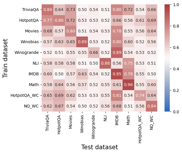<details> <summary>extracted/6450693/figures/generalization/mistral.png Details</summary>  ### Visual Description ## Heatmap: Cross-Dataset Performance Matrix ### Overview The image is a heatmap visualization displaying numerical performance scores (likely accuracy or a similar metric) for various machine learning models or systems. The matrix compares performance when a model is trained on one dataset (rows) and tested on another (columns). The values range from 0.0 to 1.0, with a color gradient from blue (low) to red (high) indicating the score. ### Components/Axes * **Y-Axis (Vertical):** Labeled **"Train dataset"**. It lists 10 distinct training datasets: * TriviaQA * HotpotQA * Movies * Winobias * Winogrande * NLI * IMDB * Math * HotpotQA_WC * NQ_WC * **X-Axis (Horizontal):** Labeled **"Test dataset"**. It lists the same 10 datasets in the same order as the y-axis, creating a square matrix. * **Color Bar/Legend:** Positioned vertically on the **right side** of the chart. It provides a scale from **0.0 (blue)** to **1.0 (dark red)**, with intermediate markers at 0.2, 0.4, 0.6, and 0.8. This legend is used to interpret the color intensity of each cell in the heatmap. * **Data Cells:** A 10x10 grid where each cell contains a numerical value and is colored according to the scale. The value represents the performance score for the corresponding Train-Test dataset pair. ### Detailed Analysis The following table reconstructs the heatmap's data. Rows represent the **Train dataset**, and columns represent the **Test dataset**. Values are transcribed directly from the image. | Train \ Test | TriviaQA | HotpotQA | Movies | Winobias | Winogrande | NLI | IMDB | Math | HotpotQA_WC | NQ_WC | | :--- | :---: | :---: | :---: | :---: | :---: | :---: | :---: | :---: | :---: | :---: | | **TriviaQA** | 0.84 | 0.64 | 0.73 | 0.50 | 0.54 | 0.51 | 0.80 | 0.72 | 0.54 | 0.66 | | **HotpotQA** | 0.77 | 0.80 | 0.72 | 0.53 | 0.53 | 0.52 | 0.66 | 0.56 | 0.61 | 0.69 | | **Movies** | 0.68 | 0.57 | 0.80 | 0.51 | 0.54 | 0.53 | 0.78 | 0.55 | 0.56 | 0.64 | | **Winobias** | 0.57 | 0.63 | 0.65 | **0.89** | 0.53 | 0.52 | 0.80 | 0.60 | 0.52 | 0.56 | | **Winogrande** | 0.52 | 0.51 | 0.55 | 0.55 | **0.66** | 0.52 | 0.89 | 0.54 | 0.53 | 0.52 | | **NLI** | 0.58 | 0.58 | 0.58 | 0.51 | 0.50 | **0.88** | 0.56 | 0.75 | 0.53 | 0.51 | | **IMDB** | 0.60 | 0.50 | 0.57 | 0.63 | 0.54 | 0.52 | **0.95** | 0.78 | 0.55 | 0.50 | | **Math** | 0.58 | 0.64 | 0.56 | 0.57 | 0.52 | 0.55 | 0.61 | **0.96** | 0.55 | 0.60 | | **HotpotQA_WC** | 0.65 | 0.69 | 0.62 | 0.53 | 0.53 | 0.55 | 0.81 | 0.54 | **0.74** | 0.64 | | **NQ_WC** | 0.62 | 0.67 | 0.54 | 0.50 | 0.52 | 0.56 | 0.68 | 0.51 | 0.56 | **0.84** | **Trend Verification by Row (Train Dataset):** * **TriviaQA:** Shows high performance on itself (0.84) and IMDB (0.80), moderate on Movies (0.73) and Math (0.72), and lower on others. * **HotpotQA:** Strong on itself (0.80) and TriviaQA (0.77), moderate on NQ_WC (0.69), and lower elsewhere. * **Movies:** Peaks on itself (0.80) and IMDB (0.78), moderate on TriviaQA (0.68), and lower on others. * **Winobias:** Has a very high score on itself (0.89) and a high score on IMDB (0.80), with other scores being moderate to low. * **Winogrande:** Shows a very high score on IMDB (0.89) and a moderate score on itself (0.66), with other scores generally low. * **NLI:** Peaks sharply on itself (0.88) and has a relatively high score on Math (0.75), with other scores low. * **IMDB:** Has an extremely high score on itself (0.95) and a high score on Math (0.78), with other scores moderate to low. * **Math:** Has the highest score in the entire matrix on itself (0.96), with other scores generally low to moderate. * **HotpotQA_WC:** Performs best on itself (0.74) and IMDB (0.81), with moderate scores on its non-WC counterpart (0.69) and TriviaQA (0.65). * **NQ_WC:** Peaks on itself (0.84) and shows moderate performance on HotpotQA (0.67) and IMDB (0.68). ### Key Observations 1. **Diagonal Dominance:** The highest value in each row is almost always on the main diagonal (where Train and Test datasets are the same). This indicates models perform best when tested on the same domain they were trained on. 2. **Strong Cross-Domain Pairs:** Several train-test pairs show notably high performance despite being different datasets: * **IMDB as a Test Set:** It yields high scores (≥0.78) for models trained on Winobias, Winogrande, Movies, IMDB, and HotpotQA_WC. * **Math as a Test Set:** It yields high scores for models trained on NLI (0.75) and IMDB (0.78). * **TriviaQA & HotpotQA:** These show moderate to high mutual performance. 3. **Weak Cross-Domain Pairs:** Performance is generally low (<0.60) when models trained on reasoning-heavy datasets (Winobias, Winogrande, NLI, Math) are tested on QA datasets (TriviaQA, HotpotQA, NQ_WC), and vice-versa. 4. **WC Variant Behavior:** The "_WC" (likely "Without Context") datasets show interesting patterns. HotpotQA_WC performs better on IMDB than its standard counterpart. NQ_WC performs better on HotpotQA than the standard NQ model likely would. ### Interpretation This heatmap provides a detailed map of **domain generalization** and **transfer learning** capabilities across a suite of NLP benchmarks. * **What it demonstrates:** The data strongly suggests that the underlying models or systems are highly specialized. The pronounced diagonal indicates that knowledge learned from a specific dataset does not transfer perfectly to others, highlighting the challenge of creating general-purpose models. The high scores on the diagonal represent "in-domain" performance, while off-diagonal scores represent "out-of-domain" generalization. * **Relationships between elements:** The matrix reveals clusters of related tasks. For example, the QA datasets (TriviaQA, HotpotQA, NQ_WC) form a loose cluster with moderate mutual transfer. Similarly, the coreference/reasoning datasets (Winobias, Winogrande) show some transfer to each other and to IMDB. The IMDB dataset acts as a surprisingly good general test set for several model types, suggesting its sentiment analysis task may share underlying features with other tasks. * **Notable anomalies and insights:** * The **Math** dataset is an outlier in its self-performance (0.96) but shows poor generalization to most other tasks, suggesting it requires highly specialized knowledge. * The **IMDB** dataset's role as a strong transfer target is a key finding. It may be a simpler or more fundamental task that benefits many models. * The **NLI** model's strong performance on **Math** (0.75) is intriguing and may indicate that natural language inference skills are beneficial for mathematical reasoning tasks. * The **"_WC"** variants show that removing context alters generalization patterns, sometimes improving transfer to certain domains (e.g., HotpotQA_WC to IMDB). In essence, this matrix is a diagnostic tool for understanding the strengths, weaknesses, and interconnectedness of different NLP tasks and the models trained on them. It underscores that achieving robust, general AI requires moving beyond high diagonal scores to improve the off-diagonal generalization. </details> (a) Raw AUC values. Values above $0.5$ indicate some generalization. 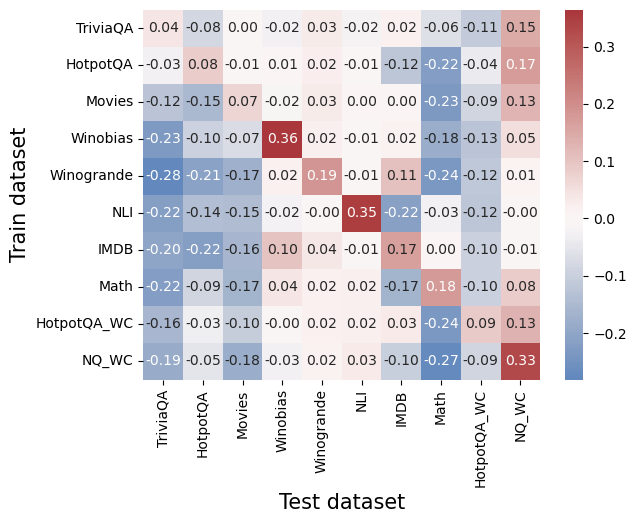<details> <summary>extracted/6450693/figures/generalization/mistral_reduced.png Details</summary>  ### Visual Description ## Heatmap: Cross-Dataset Performance Comparison ### Overview The image is a heatmap visualizing numerical performance scores (likely correlation coefficients, transfer learning gains, or similar metrics) between various training datasets (y-axis) and test datasets (x-axis). The values range from approximately -0.28 to +0.36, with a color scale from blue (negative) to red (positive). The chart compares 10 distinct datasets on both axes. ### Components/Axes * **Y-Axis (Vertical):** Labeled "Train dataset". Contains 10 categorical labels, from top to bottom: 1. TriviaQA 2. HotpotQA 3. Movies 4. Winobias 5. Winogrande 6. NLI 7. IMDB 8. Math 9. HotpotQA_WC 10. NQ_WC * **X-Axis (Horizontal):** Labeled "Test dataset". Contains the same 10 categorical labels, from left to right: 1. TriviaQA 2. HotpotQA 3. Movies 4. Winobias 5. Winogrande 6. NLI 7. IMDB 8. Math 9. HotpotQA_WC 10. NQ_WC * **Legend/Color Bar:** Positioned on the right side of the chart. It is a vertical gradient bar mapping color to numerical value. * **Scale:** Linear. * **Range:** Approximately -0.2 (dark blue) to +0.3 (dark red). * **Key Markers:** -0.2, -0.1, 0.0, 0.1, 0.2, 0.3. * **Interpretation:** Blue shades indicate negative values, white/light shades indicate values near zero, and red shades indicate positive values. ### Detailed Analysis The heatmap is a 10x10 grid. Each cell contains a numerical value and is colored according to the legend. Below is the reconstructed data table, with Train dataset as rows and Test dataset as columns. | Train \ Test | TriviaQA | HotpotQA | Movies | Winobias | Winogrande | NLI | IMDB | Math | HotpotQA_WC | NQ_WC | | :--- | :--- | :--- | :--- | :--- | :--- | :--- | :--- | :--- | :--- | :--- | | **TriviaQA** | 0.04 | -0.08 | 0.00 | -0.02 | 0.03 | -0.02 | 0.02 | -0.06 | -0.11 | 0.15 | | **HotpotQA** | -0.03 | 0.08 | -0.01 | 0.01 | 0.02 | -0.01 | -0.12 | -0.22 | -0.04 | 0.17 | | **Movies** | -0.12 | -0.15 | 0.07 | -0.02 | 0.03 | 0.00 | 0.00 | -0.23 | -0.09 | 0.13 | | **Winobias** | -0.23 | -0.10 | -0.07 | **0.36** | 0.02 | -0.01 | 0.02 | -0.18 | -0.13 | 0.05 | | **Winogrande** | -0.28 | -0.21 | -0.17 | 0.02 | **0.19** | -0.01 | 0.11 | -0.24 | -0.12 | 0.01 | | **NLI** | -0.22 | -0.14 | -0.15 | -0.02 | 0.00 | **0.35** | -0.22 | -0.03 | -0.12 | -0.00 | | **IMDB** | -0.20 | -0.22 | -0.16 | 0.10 | 0.04 | -0.01 | **0.17** | 0.00 | -0.10 | -0.01 | | **Math** | -0.22 | -0.09 | -0.17 | 0.04 | 0.02 | 0.02 | -0.17 | **0.18** | -0.10 | 0.08 | | **HotpotQA_WC** | -0.16 | -0.03 | -0.10 | -0.00 | 0.02 | 0.02 | 0.03 | -0.24 | **0.09** | 0.13 | | **NQ_WC** | -0.19 | -0.05 | -0.18 | -0.03 | 0.02 | 0.03 | -0.10 | -0.27 | -0.09 | **0.33** | **Trend Verification by Row (Train Dataset):** * **TriviaQA:** Mostly neutral to slightly negative values, with a positive spike (0.15) on NQ_WC. * **HotpotQA:** Mixed, with a notable negative value on Math (-0.22) and a positive value on NQ_WC (0.17). * **Movies:** Generally negative or near-zero, except for its own test (0.07) and NQ_WC (0.13). * **Winobias:** Strong positive on its own test (0.36, the highest value in the chart), otherwise mostly negative. * **Winogrande:** Strong negative values across most tests, except for a positive on its own test (0.19) and a mild positive on IMDB (0.11). * **NLI:** Strong positive on its own test (0.35), otherwise strongly negative, especially on IMDB (-0.22). * **IMDB:** Negative across most, with positives on Winobias (0.10) and its own test (0.17). * **Math:** Mostly negative, with a positive on its own test (0.18) and a mild positive on NQ_WC (0.08). * **HotpotQA_WC:** Mostly negative, with positives on its own test (0.09) and NQ_WC (0.13). * **NQ_WC:** Strong positive on its own test (0.33), otherwise mostly negative, with a strong negative on Math (-0.27). ### Key Observations 1. **Diagonal Dominance:** The highest values for each row almost always occur on the diagonal (where Train and Test datasets are the same). This suggests models perform best when tested on the same domain they were trained on. 2. **Highest Positive Values:** The strongest positive scores are **Winobias→Winobias (0.36)**, **NLI→NLI (0.35)**, and **NQ_WC→NQ_WC (0.33)**. 3. **Strongest Negative Values:** The most negative scores are **Winogrande→TriviaQA (-0.28)**, **NQ_WC→Math (-0.27)**, and **Winogrande→Math (-0.24)**. 4. **NQ_WC as a Test Set:** The NQ_WC column (far right) shows a consistent pattern of positive values for almost all training sets, suggesting it may be an "easier" or more generalizable test benchmark. 5. **Math as a Test Set:** The Math column shows consistently negative values for all training sets except its own, indicating it is a difficult, specialized domain that does not transfer well from other datasets. ### Interpretation This heatmap likely illustrates **transfer learning performance** or **cross-domain generalization** between different natural language processing (NLP) and reasoning datasets. The data suggests: * **Strong Domain Specificity:** The prominent diagonal indicates that knowledge or skills learned from a specific dataset (e.g., Winobias for bias detection, NLI for natural language inference) do not transfer effectively to other domains. This is a common challenge in AI, highlighting the lack of robust, generalizable understanding. * **Asymmetric Relationships:** The transfer is not symmetric. For example, training on Winobias and testing on Winogrande yields 0.02, but training on Winogrande and testing on Winobias yields 0.02 as well in this case, but other pairs show more asymmetry. This implies the datasets capture different, sometimes non-overlapping, skills. * **Nature of Benchmarks:** The consistent positivity of the NQ_WC test column might indicate it is a broader, more factual recall-based benchmark that benefits from many types of training data. Conversely, the consistent negativity of the Math test column underscores its unique, formal reasoning requirements that are not addressed by general language datasets. * **Outliers and Anomalies:** The strong negative values (e.g., -0.28) are as informative as the positives. They suggest that training on certain datasets (like Winogrande) might actively *hurt* performance on others (like TriviaQA), possibly due to conflicting objectives or overfitting to specific patterns that are misleading in a new context. In essence, the chart maps the "knowledge landscape" of these AI benchmarks, showing islands of specialized competence (the diagonal) surrounded by seas of negative or neutral transfer, with a few bridges (like NQ_WC) that connect to multiple training sources. </details> (b) Performance (AUC) difference of the probe and the logit-based method. Values above $0 0$ indicate generalization beyond the logit-based method. Figure 7: Generalization between datasets, Mistral-7b. 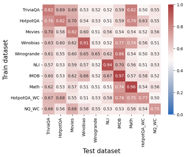<details> <summary>extracted/6450693/figures/generalization/llama.png Details</summary>  ### Visual Description \n ## Heatmap: Cross-Dataset Performance ### Overview The image is a heatmap visualizing a matrix of numerical performance scores (likely accuracy, F1, or a similar metric) between different "Train datasets" (rows) and "Test datasets" (columns). The values range from 0.0 to 1.0, with a color gradient from blue (low) to red (high) indicating the score. The chart is designed to show how well a model trained on one dataset generalizes to another. ### Components/Axes * **Y-Axis (Vertical):** Labeled **"Train dataset"**. It lists 10 datasets used for training: 1. TriviaQA 2. HotpotQA 3. Movies 4. Winobias 5. Winogrande 6. NLI 7. IMDB 8. Math 9. HotpotQA_WC 10. NQ_WC * **X-Axis (Horizontal):** Labeled **"Test dataset"**. It lists the same 10 datasets used for testing, in the same order as the Y-axis. * **Color Scale/Legend:** Located on the right side of the chart. It is a vertical bar showing the mapping of color to numerical value. * **Range:** 0.0 (bottom, blue) to 1.0 (top, red). * **Key Markers:** 0.0, 0.2, 0.4, 0.6, 0.8, 1.0. * **Data Grid:** A 10x10 grid of colored cells. Each cell contains a numerical value (to two decimal places) representing the performance score for the corresponding Train-Test dataset pair. ### Detailed Analysis The following table reconstructs the entire data matrix. Values are transcribed directly from the image. Rows represent the "Train dataset" and columns represent the "Test dataset". | Train \ Test | TriviaQA | HotpotQA | Movies | Winobias | Winogrande | NLI | IMDB | Math | HotpotQA_WC | NQ_WC | | :--- | :---: | :---: | :---: | :---: | :---: | :---: | :---: | :---: | :---: | :---: | | **TriviaQA** | **0.82** | 0.69 | 0.69 | 0.53 | 0.52 | 0.52 | 0.59 | 0.82 | 0.50 | 0.55 | | **HotpotQA** | 0.76 | **0.82** | 0.70 | 0.54 | 0.53 | 0.51 | 0.59 | 0.79 | 0.63 | 0.55 | | **Movies** | 0.70 | 0.58 | **0.82** | 0.60 | 0.51 | 0.56 | 0.54 | 0.54 | 0.52 | 0.56 | | **Winobias** | 0.63 | 0.60 | 0.62 | **0.91** | 0.53 | 0.52 | 0.77 | 0.74 | 0.56 | 0.51 | | **Winogrande** | 0.61 | 0.55 | 0.60 | 0.65 | **0.65** | 0.62 | 0.86 | 0.54 | 0.50 | 0.53 | | **NLI** | 0.57 | 0.53 | 0.59 | 0.57 | 0.52 | **0.94** | 0.70 | 0.56 | 0.51 | 0.53 | | **IMDB** | 0.60 | 0.53 | 0.62 | 0.66 | 0.52 | 0.67 | **0.97** | 0.57 | 0.58 | 0.52 | | **Math** | 0.62 | 0.53 | 0.57 | 0.51 | 0.51 | 0.51 | 0.74 | **0.96** | 0.54 | 0.56 | | **HotpotQA_WC** | 0.67 | 0.68 | 0.55 | 0.51 | 0.53 | 0.58 | 0.78 | 0.75 | **0.77** | 0.50 | | **NQ_WC** | 0.66 | 0.56 | 0.68 | 0.58 | 0.55 | 0.53 | 0.53 | 0.56 | 0.54 | **0.75** | **Trend Verification & Spatial Grounding:** * **Diagonal Trend:** The cells where the Train and Test dataset are the same (the main diagonal from top-left to bottom-right) are consistently the highest values in their respective rows and are colored dark red. This indicates strong within-dataset performance. * **High Off-Diagonal Values:** Notable high scores exist between related datasets. For example: * Train: **Winobias** (0.91) -> Test: **Winobias** (dark red). * Train: **IMDB** (0.97) -> Test: **IMDB** (darkest red on the chart). * Train: **NLI** (0.94) -> Test: **NLI** (dark red). * Train: **Winogrande** (0.86) -> Test: **IMDB** (medium red). * Train: **TriviaQA** (0.82) -> Test: **Math** (medium red). * **Low Values:** The lowest scores (lightest colors, near 0.5) are often found in the lower-right quadrant of the matrix, particularly when training on QA datasets (TriviaQA, HotpotQA) and testing on others, or vice-versa. ### Key Observations 1. **Strongest Performance:** The single highest score is **0.97** for the **IMDB** train/test pair. 2. **Weakest Performance:** The lowest scores appear to be around **0.50-0.51**. Examples include: * Train: **TriviaQA** -> Test: **HotpotQA_WC** (0.50) * Train: **HotpotQA_WC** -> Test: **NQ_WC** (0.50) * Train: **Winobias** -> Test: **NQ_WC** (0.51) * Train: **NLI** -> Test: **HotpotQA_WC** (0.51) 3. **Dataset Clusters:** Some datasets show stronger cross-performance: * **IMDB** and **Winogrande** have a high mutual score (Train Winogrande -> Test IMDB = 0.86). * **TriviaQA** and **Math** show a surprisingly high transfer (Train TriviaQA -> Test Math = 0.82). * **HotpotQA** and **HotpotQA_WC** show moderate transfer (0.63 and 0.68 in respective directions). 4. **Asymmetry:** Performance is not always symmetric. For example: * Train on **Winobias**, Test on **IMDB**: **0.77** * Train on **IMDB**, Test on **Winobias**: **0.66** ### Interpretation This heatmap provides a diagnostic view of model generalization across diverse NLP tasks (Question Answering, Commonsense Reasoning, Sentiment Analysis, Natural Language Inference, etc.). * **What it demonstrates:** The high diagonal values confirm that models perform best when tested on the same distribution they were trained on. The off-diagonal values reveal the **transfer learning potential** between datasets. High off-diagonal scores suggest the datasets share underlying features or task structures that a model can leverage. * **Relationships between elements:** The matrix acts as a similarity map. Datasets that are "close" in this map (high mutual scores, like IMDB and Winogrande) are likely more similar in the skills they require or the data patterns they contain. Datasets with low mutual scores are more distinct. * **Notable anomalies/patterns:** * The very high transfer from **TriviaQA to Math** (0.82) is intriguing and suggests the reasoning or retrieval skills from TriviaQA might be highly applicable to the Math dataset used here. * The **IMDB** dataset appears to be both very easy to master (0.97 self-score) and a good source for training models that perform well on other tasks (e.g., 0.86 on Winogrande, 0.78 on HotpotQA_WC). This could indicate it's a strong, general-purpose sentiment or text feature dataset. * The **QA datasets (TriviaQA, HotpotQA, NQ_WC)** generally show lower cross-performance with other dataset types, suggesting their specific QA format or knowledge requirements are less transferable to tasks like sentiment analysis (IMDB) or natural language inference (NLI). * The **"WC" variants** (HotpotQA_WC, NQ_WC) likely stand for "Without Context" or a similar modification. Their generally lower scores compared to their parent datasets suggest the context is a crucial component for performance on those tasks. In essence, this chart is a tool for understanding task relatedness and predicting how a model trained for one purpose might fare in another, guiding decisions about multi-task learning, data selection, and model robustness. </details> (a) Raw AUC values. Values above $0.5$ indicate some generalization. 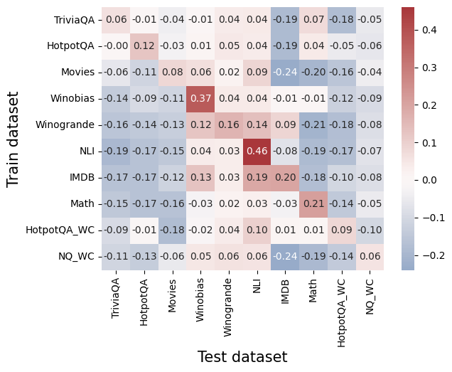<details> <summary>extracted/6450693/figures/generalization/llama_reduced.png Details</summary>  ### Visual Description ## Heatmap: Cross-Dataset Correlation Analysis ### Overview The image is a heatmap visualizing the correlation coefficients between machine learning models trained on various datasets (y-axis) and evaluated on different test datasets (x-axis). The chart uses a diverging color scale to represent the strength and direction of correlation, with red indicating positive correlation, blue indicating negative correlation, and white/light colors indicating values near zero. ### Components/Axes * **Y-Axis (Vertical):** Labeled "Train dataset". It lists 10 training datasets from top to bottom: 1. TriviaQA 2. HotpotQA 3. Movies 4. Winobias 5. Winogrande 6. NLI 7. IMDB 8. Math 9. HotpotQA_WC 10. NQ_WC * **X-Axis (Horizontal):** Labeled "Test dataset". It lists 10 test datasets from left to right, in the same order as the y-axis: 1. TriviaQA 2. HotpotQA 3. Movies 4. Winobias 5. Winogrande 6. NLI 7. IMDB 8. Math 9. HotpotQA_WC 10. NQ_WC * **Color Bar/Legend:** Positioned on the right side of the chart. It is a vertical gradient bar mapping color to correlation values. * **Scale:** Ranges from approximately -0.2 (dark blue) to +0.4 (dark red). * **Key Markers:** -0.2, -0.1, 0.0, 0.1, 0.2, 0.3, 0.4. * **Data Grid:** A 10x10 grid of colored cells. Each cell contains a numerical correlation value printed in black text. The cell's color corresponds to the value according to the color bar. ### Detailed Analysis The following table reconstructs the correlation matrix. Values are transcribed directly from the cells. The diagonal (where Train dataset = Test dataset) is highlighted in **bold** as it represents the in-domain performance correlation. | Train \ Test | TriviaQA | HotpotQA | Movies | Winobias | Winogrande | NLI | IMDB | Math | HotpotQA_WC | NQ_WC | | :--- | :--- | :--- | :--- | :--- | :--- | :--- | :--- | :--- | :--- | :--- | | **TriviaQA** | **0.06** | -0.01 | -0.04 | -0.01 | 0.04 | 0.04 | -0.19 | 0.07 | -0.18 | -0.05 | | **HotpotQA** | -0.00 | **0.12** | -0.03 | 0.01 | 0.05 | 0.04 | -0.19 | 0.04 | -0.05 | -0.06 | | **Movies** | -0.06 | -0.11 | **0.08** | 0.06 | 0.02 | 0.09 | -0.24 | -0.20 | -0.16 | -0.04 | | **Winobias** | -0.14 | -0.09 | -0.11 | **0.37** | 0.04 | 0.04 | -0.01 | -0.01 | -0.12 | -0.09 | | **Winogrande** | -0.16 | -0.14 | -0.13 | 0.12 | **0.16** | 0.14 | 0.09 | -0.21 | -0.18 | -0.08 | | **NLI** | -0.19 | -0.17 | -0.15 | 0.04 | 0.03 | **0.46** | -0.08 | -0.19 | -0.17 | -0.07 | | **IMDB** | -0.17 | -0.17 | -0.12 | 0.13 | 0.03 | 0.19 | **0.20** | -0.18 | -0.10 | -0.08 | | **Math** | -0.15 | -0.17 | -0.16 | -0.03 | 0.02 | 0.03 | -0.03 | **0.21** | -0.14 | -0.05 | | **HotpotQA_WC** | -0.09 | -0.01 | -0.18 | -0.02 | 0.04 | 0.10 | 0.01 | 0.01 | **0.09** | -0.10 | | **NQ_WC** | -0.11 | -0.13 | -0.06 | 0.05 | 0.06 | 0.06 | -0.24 | -0.19 | -0.14 | **0.06** | **Trend Verification by Row (Train Dataset):** * **TriviaQA:** Mostly weak negative correlations with other test sets, strongest negative with IMDB (-0.19). * **HotpotQA:** Weak correlations overall, slightly positive with itself (0.12). * **Movies:** Strong negative correlation with IMDB (-0.24) and Math (-0.20). * **Winobias:** Shows a strong positive correlation with itself (0.37). Weak to moderate positive with a few others (e.g., Winogrande 0.12). * **Winogrande:** Positive correlation with itself (0.16) and NLI (0.14). Negative with Math (-0.21). * **NLI:** Shows the strongest single correlation in the chart with itself (0.46). Generally weak negative or near-zero correlations elsewhere. * **IMDB:** Positive correlation with itself (0.20) and NLI (0.19). Negative with Movies (-0.12) and others. * **Math:** Strong positive correlation with itself (0.21). Generally negative correlations with other datasets. * **HotpotQA_WC:** Weak correlations overall, slightly positive with itself (0.09) and NLI (0.10). * **NQ_WC:** Weak correlations, slightly positive with itself (0.06) and Winobias (0.05). Strong negative with IMDB (-0.24). ### Key Observations 1. **Diagonal Dominance:** The highest correlation for most rows is on the diagonal (same train and test dataset), indicating models perform best when tested on data from the same distribution they were trained on. The exceptions are TriviaQA and HotpotQA_WC, where their diagonal values are not the highest in their row. 2. **Strongest Positive Correlation:** The cell at the intersection of **Train: NLI** and **Test: NLI** has the highest value in the entire chart: **0.46**. 3. **Strongest Negative Correlation:** The cell at **Train: Movies** and **Test: IMDB** has the most negative value: **-0.24**. The cell at **Train: NQ_WC** and **Test: IMDB** also shows -0.24. 4. **Dataset Clusters:** * **NLI & Winobias/Winogrande:** Models trained on NLI show a mild positive correlation with Winobias (0.04) and Winogrande (0.03) test sets. Conversely, Winobias-trained models show a mild positive correlation with the NLI test set (0.04). * **IMDB & Movies:** There is a notable negative relationship. Models trained on Movies perform poorly on IMDB tests (-0.24), and models trained on IMDB perform poorly on Movies tests (-0.12). 5. **General Trend:** Most off-diagonal correlations are weak (between -0.2 and +0.2), suggesting that performance on one dataset is not a strong predictor of performance on a different dataset for most pairs. ### Interpretation This heatmap provides a diagnostic view of **transfer learning** or **cross-domain generalization** between different natural language processing and reasoning tasks. * **What it demonstrates:** The data suggests that most of these datasets represent distinct tasks or distributions. A model's proficiency in one area (e.g., NLI) does not reliably translate to proficiency in another (e.g., Math or Movies). The strong diagonal values confirm that models are highly specialized to their training distribution. * **Relationships between elements:** The chart reveals hidden relationships. For instance, the positive correlation between NLI and Winogrande/Winobias might indicate that these tasks share underlying skills like commonsense reasoning or linguistic understanding. The negative correlation between Movies and IMDB is surprising, as both are text classification tasks related to sentiment; it might suggest that the features or biases learned from one movie review dataset are actively detrimental to performance on the other, possibly due to differing domains (e.g., product reviews vs. movie reviews) or label definitions. * **Notable Anomalies:** The fact that `TriviaQA` and `HotpotQA_WC` do not have their highest correlation on the diagonal is an anomaly. For `TriviaQA`, the highest value in its row is 0.07 (with Math test set). For `HotpotQA_WC`, the highest is 0.10 (with NLI test set). This could indicate noise in the data, a measurement artifact, or that these models generalize in unexpected ways. * **Peircean Investigation:** The chart is an **index** of model performance relationships. It points directly to the fact that task similarity is not always intuitive. It is a **symbol** of the challenge in creating general-purpose AI, as expertise is often compartmentalized. The pattern invites further **abductive reasoning**: Why do NLI models transfer somewhat to Winogrande? Why do Movies and IMDB models negatively transfer? The answers likely lie in the underlying linguistic and semantic structures of the datasets themselves. </details> (b) Performance (AUC) difference of the probe and the logit-based method. Values above $0 0$ indicate generalization beyond the logit-based method. Figure 8: Generalization between datasets, Llama-3-8b. 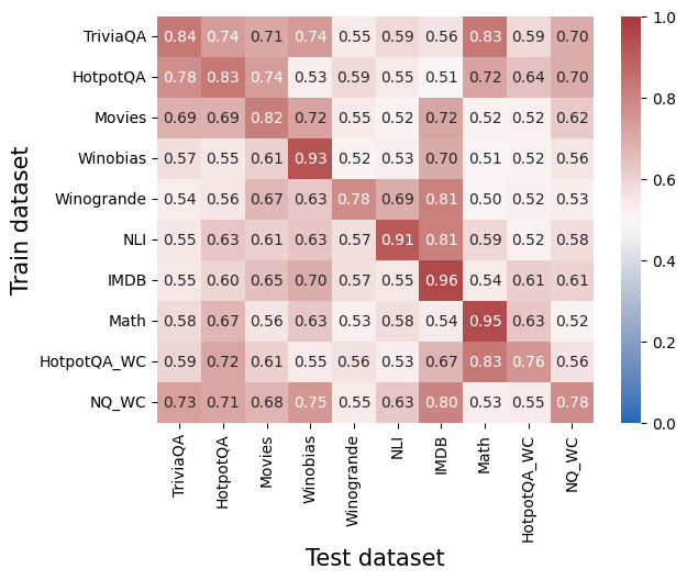<details> <summary>extracted/6450693/figures/generalization/llama_instruct.png Details</summary>  ### Visual Description ## Heatmap: Cross-Dataset Performance Matrix ### Overview The image is a heatmap visualizing a square matrix of numerical values, likely representing performance scores (e.g., accuracy, F1, or transferability metric) between different machine learning datasets. The matrix compares models trained on one dataset (y-axis) and tested on another (x-axis). All values are between 0.50 and 0.96, indicated by a color gradient from light pink/beige (lower values) to dark red (higher values). The color bar legend on the right confirms the scale ranges from 0.0 (blue) to 1.0 (dark red), though no blue values appear in this specific matrix. ### Components/Axes * **Chart Type:** Heatmap (Confusion Matrix style). * **Y-Axis (Vertical):** Labeled **"Train dataset"**. Categories from top to bottom: 1. TriviaQA 2. HotpotQA 3. Movies 4. Winobias 5. Winogrande 6. NLI 7. IMDB 8. Math 9. HotpotQA_WC 10. NQ_WC * **X-Axis (Horizontal):** Labeled **"Test dataset"**. Categories from left to right (identical to y-axis): 1. TriviaQA 2. HotpotQA 3. Movies 4. Winobias 5. Winogrande 6. NLI 7. IMDB 8. Math 9. HotpotQA_WC 10. NQ_WC * **Legend/Color Bar:** Positioned vertically on the **right side** of the chart. It maps color intensity to numerical values, with a scale from **0.0 (blue)** at the bottom to **1.0 (dark red)** at the top. Tick marks are at 0.0, 0.2, 0.4, 0.6, 0.8, and 1.0. * **Data Cells:** A 10x10 grid. Each cell contains a numerical value (to two decimal places) and is colored according to the legend. ### Detailed Analysis The following table reconstructs the matrix. Values are read as the score for the model trained on the **Row Dataset** and tested on the **Column Dataset**. | Train \ Test | TriviaQA | HotpotQA | Movies | Winobias | Winogrande | NLI | IMDB | Math | HotpotQA_WC | NQ_WC | | :--- | :---: | :---: | :---: | :---: | :---: | :---: | :---: | :---: | :---: | :---: | | **TriviaQA** | **0.84** | 0.74 | 0.71 | 0.74 | 0.55 | 0.59 | 0.56 | 0.83 | 0.59 | 0.70 | | **HotpotQA** | 0.78 | **0.83** | 0.74 | 0.53 | 0.59 | 0.55 | 0.51 | 0.72 | 0.64 | 0.70 | | **Movies** | 0.69 | 0.69 | **0.82** | 0.72 | 0.55 | 0.52 | 0.72 | 0.52 | 0.52 | 0.62 | | **Winobias** | 0.57 | 0.55 | 0.61 | **0.93** | 0.52 | 0.53 | 0.70 | 0.51 | 0.52 | 0.56 | | **Winogrande** | 0.54 | 0.56 | 0.67 | 0.63 | **0.78** | 0.69 | 0.81 | 0.50 | 0.52 | 0.53 | | **NLI** | 0.55 | 0.63 | 0.61 | 0.63 | 0.57 | **0.91** | 0.81 | 0.59 | 0.52 | 0.58 | | **IMDB** | 0.55 | 0.60 | 0.65 | 0.70 | 0.57 | 0.55 | **0.96** | 0.54 | 0.61 | 0.61 | | **Math** | 0.58 | 0.67 | 0.56 | 0.63 | 0.53 | 0.58 | 0.54 | **0.95** | 0.63 | 0.52 | | **HotpotQA_WC** | 0.59 | 0.72 | 0.61 | 0.55 | 0.56 | 0.53 | 0.67 | **0.83** | **0.76** | 0.56 | | **NQ_WC** | 0.73 | 0.71 | 0.68 | 0.75 | 0.55 | 0.63 | 0.80 | 0.53 | 0.55 | **0.78** | **Trend Verification:** * **Diagonal Trend:** The cells where the train and test dataset are identical (the main diagonal from top-left to bottom-right) consistently show the highest values in their respective rows, forming a dark red diagonal line. This indicates models perform best when evaluated on the same dataset they were trained on. * **Off-Diagonal Trends:** Performance generally drops for cross-dataset evaluation, but significant variation exists. Some dataset pairs show relatively high transfer (e.g., NLI→IMDB: 0.81, HotpotQA_WC→Math: 0.83), while others show low transfer (e.g., Winogrande→Math: 0.50, Winobias→Math: 0.51). ### Key Observations 1. **Highest Performance:** The single highest value in the matrix is **0.96**, for a model trained and tested on **IMDB**. The next highest are **0.95** (Math→Math) and **0.93** (Winobias→Winobias). 2. **Strongest Cross-Dataset Transfer:** Notable high off-diagonal values include: * **NLI → IMDB:** 0.81 * **HotpotQA_WC → Math:** 0.83 * **TriviaQA → Math:** 0.83 * **NQ_WC → IMDB:** 0.80 3. **Weakest Cross-Dataset Transfer:** The lowest values (around 0.50-0.53) often involve the **Math** and **Winogrande** datasets as either train or test targets, suggesting these domains are less transferable to or from others. 4. **Dataset Clusters:** Some datasets show similar performance profiles. For example, **TriviaQA** and **HotpotQA** (and their _WC variants) have moderately high scores with each other, suggesting they share similar task characteristics. **NLI** and **IMDB** also show a strong mutual transfer (0.81 and 0.55, respectively). ### Interpretation This heatmap provides a quantitative map of **transfer learning effectiveness** or **domain similarity** across ten distinct NLP datasets. The data suggests: * **Domain Specificity is Dominant:** The strong diagonal confirms that models are highly specialized to the data distribution and task format of their training set. This is the primary factor in performance. * **Underlying Task Similarity:** High off-diagonal values reveal latent relationships between datasets. For instance, the strong transfer between **NLI** (Natural Language Inference) and **IMDB** (sentiment analysis) might indicate that the logical reasoning skills learned for NLI are beneficial for discerning sentiment in movie reviews. Similarly, the transfer between **TriviaQA** and **Math** could suggest shared skills in information retrieval and structured problem-solving. * **The "_WC" Suffix:** The datasets `HotpotQA_WC` and `NQ_WC` likely represent variants of their parent datasets (HotpotQA and Natural Questions) with a specific modification (e.g., "Without Context" or "Web Content"). Their performance patterns are similar to but distinct from their parent datasets, showing how data preprocessing or format changes impact transferability. * **Practical Implication:** For a practitioner, this matrix is a guide for model selection and data strategy. If you have a model trained on `NLI`, it may perform reasonably well on `IMDB` without fine-tuning. Conversely, a model trained on `Winogrande` would likely require significant adaptation to perform well on `Math`. The matrix helps identify which source datasets might be good proxies for pre-training when target domain data is scarce. **In summary, the image is not just a performance report but a diagnostic tool revealing the landscape of task relationships and knowledge transfer within this set of NLP benchmarks.** </details> (a) Raw AUC values. Values above $0.5$ indicate some generalization. 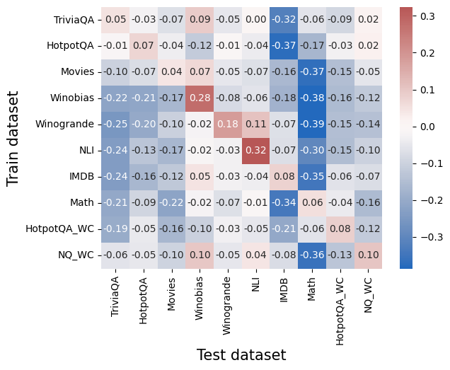<details> <summary>extracted/6450693/figures/generalization/llama_instruct_reduced.png Details</summary>  ### Visual Description ## Heatmap: Cross-Dataset Performance Correlations ### Overview The image is a heatmap visualization showing the correlation or performance transfer values between various training datasets (y-axis) and test datasets (x-axis). The chart uses a diverging color scale from blue (negative values) to red (positive values) to represent the numerical relationships. Each cell contains a specific numerical value. ### Components/Axes * **Y-Axis (Vertical):** Labeled "Train dataset". The categories from top to bottom are: 1. TriviaQA 2. HotpotQA 3. Movies 4. Winobias 5. Winogrande 6. NLI 7. IMDB 8. Math 9. HotpotQA_WC 10. NQ_WC * **X-Axis (Horizontal):** Labeled "Test dataset". The categories from left to right are: 1. TriviaQA 2. HotpotQA 3. Movies 4. Winobias 5. Winogrande 6. NLI 7. IMDB 8. Math 9. HotpotQA_WC 10. NQ_WC * **Color Bar/Legend:** Positioned on the right side of the chart. It is a vertical gradient bar. * **Range:** Approximately -0.3 (dark blue) to +0.3 (dark red). * **Midpoint:** 0.0 is represented by a very light, almost white color. * **Scale:** The bar has labeled ticks at -0.3, -0.2, -0.1, 0.0, 0.1, 0.2, 0.3. ### Detailed Analysis The following table reconstructs the heatmap data. Values are read directly from the cells. The color intensity corresponds to the magnitude and sign (red=positive, blue=negative). | Train \ Test | TriviaQA | HotpotQA | Movies | Winobias | Winogrande | NLI | IMDB | Math | HotpotQA_WC | NQ_WC | | :--- | :--- | :--- | :--- | :--- | :--- | :--- | :--- | :--- | :--- | :--- | | **TriviaQA** | 0.05 | -0.03 | -0.07 | 0.09 | -0.05 | 0.00 | **-0.32** | -0.06 | -0.09 | 0.02 | | **HotpotQA** | -0.01 | 0.07 | -0.04 | -0.12 | -0.01 | -0.04 | **-0.37** | 0.17 | -0.03 | 0.02 | | **Movies** | -0.10 | -0.07 | 0.04 | 0.07 | -0.05 | -0.07 | -0.16 | **-0.37** | -0.15 | -0.05 | | **Winobias** | -0.22 | -0.21 | -0.17 | **0.28** | -0.08 | -0.06 | -0.18 | **-0.38** | -0.16 | -0.12 | | **Winogrande** | -0.25 | -0.20 | -0.10 | -0.02 | **0.18** | 0.11 | -0.07 | **-0.39** | -0.15 | -0.14 | | **NLI** | -0.24 | -0.13 | -0.17 | -0.02 | -0.03 | **0.32** | -0.07 | -0.30 | -0.15 | -0.10 | | **IMDB** | -0.24 | -0.16 | -0.12 | 0.05 | -0.03 | -0.04 | **0.08** | **-0.35** | -0.06 | -0.07 | | **Math** | -0.21 | -0.09 | -0.22 | -0.02 | -0.07 | -0.01 | **-0.34** | 0.06 | -0.04 | -0.16 | | **HotpotQA_WC** | -0.19 | -0.05 | -0.16 | -0.10 | -0.03 | -0.05 | -0.21 | -0.06 | **0.08** | -0.12 | | **NQ_WC** | -0.06 | -0.05 | -0.10 | 0.10 | -0.05 | 0.04 | -0.08 | **0.36** | -0.13 | **0.10** | **Note on Color-Value Cross-Reference:** The strongest positive values (dark red) are 0.32 (NLI train on NLI test), 0.28 (Winobias train on Winobias test), and 0.36 (NQ_WC train on Math test). The strongest negative values (dark blue) are -0.39 (Winogrande train on Math test), -0.38 (Winobias train on Math test), and -0.37 (HotpotQA train on IMDB test). ### Key Observations 1. **Strong Diagonal Positivity:** Most datasets show a positive correlation when the training and testing dataset are the same (the diagonal from top-left to bottom-right). Notable exceptions are `IMDB` (0.08) and `Math` (0.06), which show weak positive self-correlation. 2. **Pervasive Negative Correlation with Math:** The "Math" test column is predominantly dark blue, indicating strong negative values for nearly all training datasets, especially `Winogrande` (-0.39), `Winobias` (-0.38), `TriviaQA` (-0.32), and `IMDB` (-0.35). 3. **Strong Negative Correlation with IMDB:** The "IMDB" test column also shows strong negative values for several training sets, most notably `HotpotQA` (-0.37) and `TriviaQA` (-0.32). 4. **Positive Transfer Anomalies:** There are a few instances of positive correlation between different datasets: * `NQ_WC` (train) shows a strong positive correlation with `Math` (test) at 0.36. * `HotpotQA` (train) shows a moderate positive correlation with `Math` (test) at 0.17. * `NLI` (train) shows a moderate positive correlation with `Winogrande` (test) at 0.11. 5. **Cluster of Negative Values:** The top-left quadrant (e.g., `TriviaQA`, `HotpotQA`, `Movies` training on `TriviaQA`, `HotpotQA`, `Movies` testing) contains many small negative values, suggesting weak negative transfer or interference among these QA and text classification tasks. ### Interpretation This heatmap likely illustrates **transfer learning performance or interference** between different machine learning datasets. The values could represent differences in model accuracy, loss, or another performance metric when a model trained on one dataset is evaluated on another, compared to a baseline. * **Diagonal Values:** The generally positive diagonal suggests that models perform best when tested on the same domain they were trained on, which is expected. The weak diagonal for `IMDB` and `Math` might indicate these datasets are either very distinct or that models trained on them generalize poorly even to themselves under the evaluation metric used. * **Negative Values (Blue):** The widespread negative values, especially for the `Math` and `IMDB` test columns, indicate **negative transfer**. Training on most other datasets hurts performance on these specific test sets. This suggests `Math` and `IMDB` require specialized knowledge or reasoning skills that are not learned, and are perhaps even disrupted, by training on general QA (`TriviaQA`, `HotpotQA`) or other text datasets (`Movies`, `NLI`). * **Positive Off-Diagonal Values:** The strong positive value for `NQ_WC` → `Math` (0.36) is a critical anomaly. It suggests that the `NQ_WC` (likely "Natural Questions - Wrong Context") dataset contains features or patterns that are highly beneficial for the `Math` task, more so than training on `Math` itself. This could point to a shared underlying reasoning skill (e.g., handling numerical data or multi-step logic) between these seemingly disparate tasks. * **Overall Pattern:** The chart reveals a complex landscape of task relationships. It shows that most general language tasks interfere with specialized tasks like math reasoning (`Math`) and sentiment/domain classification (`IMDB`). However, it also uncovers a specific, beneficial transfer path (`NQ_WC` to `Math`) that could be exploited for model improvement. The data argues against the notion of a single, universally beneficial pre-training dataset and highlights the importance of task-specific or carefully curated training data. </details> (b) Performance (AUC) difference of the probe and the logit-based method. Values above $0 0$ indicate generalization beyond the logit-based method. Figure 9: Generalization between datasets, Llama-3-8b-instruct. 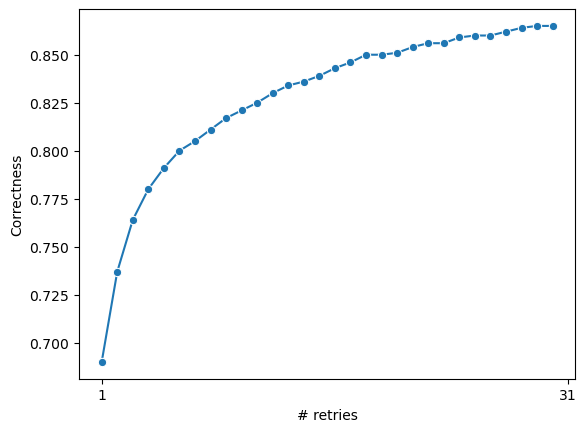## Appendix D Taxonomy of Errors <details> <summary>extracted/6450693/figures/correctness_across_resamples.png Details</summary>  ### Visual Description \n ## Line Chart: Correctness vs. Number of Retries ### Overview The image displays a 2D line chart plotting a metric called "Correctness" against the "# retries". The chart shows a single data series represented by a blue line with circular markers at each data point. The relationship is non-linear, demonstrating a rapid initial increase in correctness that gradually plateaus as the number of retries increases. ### Components/Axes * **Chart Type:** Line chart with data point markers. * **X-Axis (Horizontal):** * **Label:** "# retries" * **Scale:** Linear scale. * **Visible Tick Markers:** The axis is explicitly labeled at the start (`1`) and the end (`31`). The intermediate tick marks are present but not numerically labeled. * **Y-Axis (Vertical):** * **Label:** "Correctness" * **Scale:** Linear scale. * **Visible Tick Markers:** Labeled at intervals of 0.025, starting from `0.700` at the bottom to `0.850` at the top. The specific labeled values are: `0.700`, `0.725`, `0.750`, `0.775`, `0.800`, `0.825`, `0.850`. * **Data Series:** * **Color:** Medium blue (approximately hex #1f77b4). * **Marker Style:** Solid circular dots. * **Line Style:** Solid line connecting the markers. * **Legend:** No legend is present, as there is only one data series. * **Title:** No chart title is visible within the image frame. ### Detailed Analysis **Trend Verification:** The blue line exhibits a clear logarithmic or asymptotic growth trend. It starts with a very steep positive slope at low retry counts, which progressively flattens as the number of retries increases, indicating diminishing returns. **Data Point Extraction (Approximate Values):** The following table reconstructs the approximate data points by reading the chart. Values are estimated based on the position of the blue markers relative to the axis scales. Uncertainty is inherent in visual estimation from a static image. | # Retries (X) | Correctness (Y) | Approximate Coordinates (X, Y) | | :--- | :--- | :--- | | 1 | ~0.690 | (1, 0.690) | | 2 | ~0.738 | (2, 0.738) | | 3 | ~0.765 | (3, 0.765) | | 4 | ~0.782 | (4, 0.782) | | 5 | ~0.792 | (5, 0.792) | | 6 | ~0.800 | (6, 0.800) | | 7 | ~0.805 | (7, 0.805) | | 8 | ~0.810 | (8, 0.810) | | 9 | ~0.815 | (9, 0.815) | | 10 | ~0.820 | (10, 0.820) | | 11 | ~0.825 | (11, 0.825) | | 12 | ~0.828 | (12, 0.828) | | 13 | ~0.832 | (13, 0.832) | | 14 | ~0.835 | (14, 0.835) | | 15 | ~0.838 | (15, 0.838) | | 16 | ~0.840 | (16, 0.840) | | 17 | ~0.842 | (17, 0.842) | | 18 | ~0.845 | (18, 0.845) | | 19 | ~0.847 | (19, 0.847) | | 20 | ~0.849 | (20, 0.849) | | 21 | ~0.850 | (21, 0.850) | | 22 | ~0.852 | (22, 0.852) | | 23 | ~0.854 | (23, 0.854) | | 24 | ~0.856 | (24, 0.856) | | 25 | ~0.857 | (25, 0.857) | | 26 | ~0.858 | (26, 0.858) | | 27 | ~0.859 | (27, 0.859) | | 28 | ~0.860 | (28, 0.860) | | 29 | ~0.861 | (29, 0.861) | | 30 | ~0.862 | (30, 0.862) | | 31 | ~0.863 | (31, 0.863) | ### Key Observations 1. **Diminishing Returns:** The most significant gains in correctness occur within the first 5-7 retries. After approximately 10 retries, the curve's slope becomes very shallow. 2. **Asymptotic Behavior:** The correctness value appears to approach an asymptote just above 0.860. The increase from retry 20 to 31 is minimal (~0.014) compared to the increase from retry 1 to 12 (~0.138). 3. **No Plateau within Range:** While the curve flattens, it does not become perfectly horizontal within the displayed range (1 to 31 retries). There is still a very slight positive slope at the end of the chart. 4. **Consistent Monotonic Increase:** The correctness metric never decreases with additional retries; it is a monotonically increasing function. ### Interpretation This chart demonstrates a classic pattern of **convergent improvement with diminishing marginal returns**. In a technical context, this likely models a process where repeated attempts ("retries") improve the probability or quality of a successful outcome ("Correctness"). * **What it suggests:** The system or algorithm being measured benefits greatly from a small number of retries, quickly reaching a high level of correctness (e.g., ~0.800 by 6 retries). However, achieving near-maximum performance requires a substantially larger number of attempts. * **Relationship between elements:** The independent variable (# retries) directly drives the dependent variable (Correctness), but the relationship is non-linear. The "cost" (in time, computation, or resources) of each additional retry yields progressively less "benefit" in correctness. * **Practical Implication:** This data is crucial for optimization. It helps answer: "How many retries are enough?" The "knee" of the curve (around 5-10 retries) represents a potential sweet spot balancing performance and efficiency. Pushing beyond 20-25 retries may be computationally expensive for negligible gain, unless the application demands absolute maximum correctness regardless of cost. * **Underlying Mechanism:** The shape suggests the process may be overcoming initial, easily-solvable errors quickly, while later retries tackle rarer, more stubborn failure modes. It could model scenarios like: a machine learning model's accuracy improving with more training epochs, a network packet successfully transmitting after multiple attempts, or a heuristic algorithm refining its solution over iterations. </details> Figure 10: The percentage of answers for which at least one generated answer was correct. The first step is greedy decoding. Figure 10 presents, for each amount of resamples, the amount percentage of answers for which at least one generated answer was correct. The experiment was done on Mistral-7b-instruct with the TriviaQA dataset. For many answers that the greedy decoding fails to correctly provide an answer, the LLM is still able to generate the correct answer in at least one resample. The plot plateues around 30 resamples. ### D.1 Error Taxonomy Design Choices The error taxonomy proposed in this paper is intentionally non-orthogonal, as some errors may simultaneously belong to multiple categories. For instance, an error might fall under both “consistently incorrect” (e.g., the same incorrect answer appears at least 15 times) and “many different answers” (e.g., the remaining answers show over 10 distinct variants). Our taxonomy is designed to capture such nuanced cases, as restricting classification to a single category would hinder the generalizability of insights. Instead, we aim to learn general properties across different error types, providing LLM providers with actionable insights into questions exhibiting overlapping error patterns. To support this non-orthogonal framework, our probes function as one-to-many classifiers, enabling precise error analysis and tailored solutions. ### D.2 Results on Additional Datasets Table 8 presents the results of error type classification on the Winobias dataset and Table 9 on the Math dataset. Table 8: AUC scores for error type classification (Winobias). | Error type | Mistral-7b | Mistral-Instr-7b | Llama3-8b | Llama3-Instr-8b | | --- | --- | --- | --- | --- | | (A) Refuses to answer | - | - | - | - | | (B) Consistently correct | $0.83\scriptscriptstyle{\pm 0.004}$ | $0.88\scriptscriptstyle{\pm 0.002}$ | $0.84\scriptscriptstyle{\pm 0.003}$ | $0.89\scriptscriptstyle{\pm 0.003}$ | | (C) Consistently incorrect | $0.83\scriptscriptstyle{\pm 0.004}$ | $0.88\scriptscriptstyle{\pm 0.002}$ | $0.79\scriptscriptstyle{\pm 0.004}$ | $0.90\scriptscriptstyle{\pm 0.003}$ | | (D) Two competing | $0.68\scriptscriptstyle{\pm 0.004}$ | $0.58\scriptscriptstyle{\pm 0.015}$ | $0.74\scriptscriptstyle{\pm 0.005}$ | $0.88\scriptscriptstyle{\pm 0.004}$ | | (E) Many answers | - | - | - | - | Table 9: AUC scores for error type classification (Math). Error types are predictable from the inner model representations, indicating the encoding of fine-grained information on errors. | Error type | Mistral-7b | Mistral-Instr-7b | Llama3-8b | Llama3-Instr-8b | | --- | --- | --- | --- | --- | | (A) Refuses to answer | - | - | - | - | | (B) Consistently correct | $0.85\scriptscriptstyle{\pm 0.017}$ | $0.84\scriptscriptstyle{\pm 0.007}$ | $0.83\scriptscriptstyle{\pm 0.020}$ | $0.87\scriptscriptstyle{\pm 0.006}$ | | (C) Consistently incorrect | $0.85\scriptscriptstyle{\pm 0.026}$ | $0.85\scriptscriptstyle{\pm 0.003}$ | $0.69\scriptscriptstyle{\pm 0.032}$ | $0.91\scriptscriptstyle{\pm 0.007}$ | | (D) Two competing | - | $0.76\scriptscriptstyle{\pm 0.020}$ | $0.57\scriptscriptstyle{\pm 0.001}$ | $0.79\scriptscriptstyle{\pm 0.006}$ | | (E) Many answers | $0.74\scriptscriptstyle{\pm 0.010}$ | $0.79\scriptscriptstyle{\pm 0.015}$ | $0.69\scriptscriptstyle{\pm 0.041}$ | $0.90\scriptscriptstyle{\pm 0.008}$ | ### D.3 Qualitative Examples Tables 10 and 11 present qualitative examples of the error types in the TriviaQA and Math datasets. Table 10: Examples of error types in TriviaQA, Mistral-7B-Instruct. Correct answer is in bold. | Type of error | Question | Answers | | --- | --- | --- | | Consistently correct | What clothing-part metaphorically classifies workers/jobs according to white or blue? | “ collar ”: $30$ | | Consistently incorrect | Which town in southeast Wales became a UNESCO World Heritage Site in 2000? | “Blaenavon”: 1, “Caerleon”: 29 | | Many different answers | Published in 2013 who wrote the novel ’The Kill List’? | “ Frederick Forsyth ”: 1, “Jerry Patterson”: $1$ , “Edward Lee”: $1$ , “Barry Lancet”: $4$ “Jeremy Holiday”: $1$ , “Barry Lincoff”: $1$ , “Jim Marrs”: $1$ , “John Marrs”: $1$ , “Anthony Lacy”: $1$ , “Daniel Kraus”: $1$ , “Ron Bass”: $1$ , “David Martiniello”: $2$ , “Eric Lustbader”: $1$ , “Barbie Latza Nadeau”: $1$ , “James Swallow”: $1$ , “Mark Sullivan”: $1$ , “Alex Binotto”: $1$ , “David Baldacci”: $1$ , “Bill Cosores”: $1$ , “Frederic J. Brown”: $1$ , “Ron Capps and Tate Foley”: $1$ , “Barbie Wilde”: $1$ , “NO ANSWER”: $3$ | | Two competing answers | What is the only letter of the alphabet which does not appear in any of the names of the 50 American states? | “ The letter q ”: 15, “The letter X”: 15 | Table 11: Examples of error types in Math, Mistral-7B-Instruct. Correct answer is in bold. | Type of error | Question | Answers | | --- | --- | --- | | Consistently correct | If John travels 15 miles on a bike ride, and Jill travels 5 miles less, how many miles does Jim travel if he travels only 20% as far as Jill? | “ 2 ”: $30$ | | Consistently incorrect | Joy has 30 pencils, and Colleen has 50 pencils. If they bought the pencils at $4 each at the store, how much more money did Colleen pay than Joy for her pencils? | “ 80$ ”: 1, “16$”: $29$ (correct) | | Many different answers | If the first skyscraper was built 100 years ago, how many years in the future will it be 5 years before its 200th anniversary of being built? | “ 95 ”: $14$ , “91”: $1$ , “87”: $1$ , “15”: $2$ , “96”: $1$ , “Six”: $1$ , “202 ”: $1$ , “2035”: $1$ , “195”: $1$ , “49”: $1$ , “101”: $1$ , “199”: $1$ , “3 years before the 200th anniversary”: $1$ , “203 years after it was built”: $1$ , “196”: $1$ , “2043”: $1$ | | Two competing answers | David did 27 more push-ups but 7 less crunches than Zachary in gym class today. If Zachary did 5 push- ups and 17 crunches.How many more crunches than push-ups did Zachary do? | “ 12 ”:5, “1”: 5 $x$ | ## Appendix E Detecting the Correct Answer Full Results In Table 12 we present some qualitative samples from Mistral-7b-instruct, for the phenomenon we observe at error type (C2) Consistently incorrect but generates the correct answer at least one time. The samples in the table represent cases where the probe chose the correct answer. Table 13 compares different decoding mechanisms, including the choice via probe, on non-instruct models, and Table 14 compares on the instruct models. For all datasets and models, we observe similar conclusions to those in the main paper: significant improvement is observed for error types where the LLM shows no preference to the correct answer. Table 12: Examples of questions where Mistral-7b-Instruct consistently provided incorrect answers but occasionally generated the correct one. In these instances, the probe successfully identified the right answer. For each question, the model was sampled 30 times. Table 13: Various answer choice strategies, non-instruct models. | | Mistral-7b | | | | | | | | | | | | | --- | --- | --- | --- | --- | --- | --- | --- | --- | --- | --- | --- | --- | | TriviaQA | Math | Winobias | | | | | | | | | | | | Error type | Greedy | Random | Majority | Probing | Greedy | Random | Majority | Probing | Greedy | Random | Majority | Probing | | All | $0.63$ $\pm 0.003$ | $0.54$ $\pm 0.004$ | $0.65$ $\pm 0.002$ | $0.62$ $\pm 0.003$ | $0.25$ $\pm 0.018$ | $0.36$ $\pm 0.022$ | $0.49$ $\pm 0.019$ | $0.60$ $\pm 0.017$ | $0.69$ $\pm 0.016$ | $0.58$ $\pm 0.009$ | $0.62$ $\pm 0.009$ | $0.83$ $\pm 0.006$ | | (A) Refuses to answer | $0.08$ $\pm 0.015$ | $0.04$ $\pm 0.009$ | $0.00$ $\pm 0.000$ | $0.13$ $\pm 0.007$ | $0.01$ $\pm 0.009$ | $0.04$ $\pm 0.019$ | $0.00$ $\pm 0.000$ | $0.22$ $\pm 0.033$ | - | - | - | - | | (B1) All | $1.00$ $\pm 0.000$ | $1.00$ $\pm 0.000$ | $1.00$ $\pm 0.000$ | $1.00$ $\pm 0.000$ | - | - | - | - | - | - | - | - | | (B2) Most | $0.98$ $\pm 0.001$ | $0.84$ $\pm 0.009$ | $1.00$ $\pm 0.000$ | $0.91$ $\pm 0.002$ | $0.96$ $\pm 0.024$ | $0.84$ $\pm 0.031$ | $1.00$ $\pm 0.000$ | $0.86$ $\pm 0.041$ | $0.96$ $\pm 0.004$ | $0.73$ $\pm 0.009$ | $0.95$ $\pm 0.003$ | $0.91$ $\pm 0.009$ | | (C) Consistently incorrect | | | | | | | | | | | | | | (C1) All | $0.00$ $\pm 0.003$ | $0.00$ $\pm 0.000$ | $0.00$ $\pm 0.000$ | $0.00$ $\pm 0.000$ | - | - | - | - | - | - | - | - | | (C2) Most | $0.03$ $\pm 0.014$ | $0.20$ $\pm 0.008$ | $0.00$ $\pm 0.000$ | $0.27$ $\pm 0.036$ | - | - | - | - | $0.19$ $\pm 0.010$ | $0.30$ $\pm 0.026$ | $0.00$ $\pm 0.000$ | $0.70$ $\pm 0.007$ | | (D) Two competing | $0.48$ $\pm 0.006$ | $0.36$ $\pm 0.008$ | $0.52$ $\pm 0.015$ | $0.54$ $\pm 0.016$ | - | - | - | - | $0.73$ $\pm 0.018$ | $0.54$ $\pm 0.022$ | $0.47$ $\pm 0.030$ | $0.85$ $\pm 0.019$ | | (E) Many answers | | | | | | | | | | | | | | (E1) Non correct | $0.01$ $\pm 0.004$ | $0.00$ $\pm 0.000$ | $0.00$ $\pm 0.000$ | $0.00$ $\pm 0.000$ | $0.01$ $\pm 0.010$ | $0.00$ $\pm 0.000$ | $0.00$ $\pm 0.000$ | $0.00$ $\pm 0.000$ | - | - | - | - | | (E2) Correct appears | $0.38$ $\pm 0.009$ | $0.21$ $\pm 0.006$ | $0.42$ $\pm 0.015$ | $0.38$ $\pm 0.009$ | $0.09$ $\pm 0.010$ | $0.17$ $\pm 0.034$ | $0.36$ $\pm 0.020$ | $0.62$ $\pm 0.035$ | - | - | - | - | | Llama-8b | | | | | | | | | | | | | | TriviaQA | Math | Winobias | | | | | | | | | | | | Error type | Greedy | Sampling | Majority | Probing | Greedy | Sampling | Majority | Probing | Greedy | Sampling | Majority | Probing | | All | $0.66$ $\pm 0.002$ | $0.58$ $\pm 0.003$ | 0.68 $\pm 0.003$ | 0.68 $\pm 0.002$ | $0.30$ $\pm 0.023$ | $0.47$ $\pm 0.022$ | $0.62$ $\pm 0.014$ | $0.70$ $\pm 0.021$ | $0.73$ $\pm 0.011$ | $0.61$ $\pm 0.005$ | $0.66$ $\pm 0.016$ | 0.84 $\pm 0.006$ | | (A) Refuses to answer | $0.08$ $\pm 0.005$ | $0.07$ $\pm 0.011$ | $0.00$ $\pm 0.000$ | 0.16 $\pm 0.011$ | $0.00$ $\pm 0.007$ | $0.04$ $\pm 0.015$ | $0.00$ $\pm 0.000$ | $0.25$ $\pm 0.025$ | - | - | - | - | | (B) Consistently correct | | | | | | | | | | | | | | (B1) All | $1.00$ $\pm 0.000$ | $1.00$ $\pm 0.000$ | $1.00$ $\pm 0.000$ | $1.00$ $\pm 0.000$ | - | - | - | - | - | - | - | - | | (B2) Most | $0.98$ $\pm 0.001$ | $0.87$ $\pm 0.002$ | 1.00 $\pm 0.000$ | $0.95$ $\pm 0.002$ | $0.77$ $\pm 0.024$ | $0.88$ $\pm 0.025$ | $1.00$ $\pm 0.000$ | $0.97$ $\pm 0.014$ | $0.98$ $\pm 0.005$ | $0.75$ $\pm 0.004$ | 1.00 $\pm 0.000$ | $0.94$ $\pm 0.003$ | | (C) Consistently incorrect | | | | | | | | | | | | | | (C1) All | $0.00$ $\pm 0.000$ | $0.00$ $\pm 0.000$ | $0.00$ $\pm 0.000$ | $0.00$ $\pm 0.000$ | - | - | - | - | - | - | - | - | | (C2) Most | $0.06$ $\pm 0.013$ | $0.18$ $\pm 0.009$ | $0.00$ $\pm 0.000$ | 0.35 $\pm 0.043$ | - | - | - | - | $0.25$ $\pm 0.026$ | $0.29$ $\pm 0.023$ | $0.00$ $\pm 0.000$ | 0.65 $\pm 0.022$ | | (D) Two competing | $0.44$ $\pm 0.029$ | $0.42$ $\pm 0.035$ | $0.53$ $\pm 0.020$ | 0.66 $\pm 0.030$ | - | - | - | - | $0.73$ $\pm 0.025$ | $0.47$ $\pm 0.019$ | $0.41$ $\pm 0.037$ | 0.86 $\pm 0.014$ | | (E) Many answers | | | | | | | | | | | | | | (E1) Non correct | $0.00$ $\pm 0.000$ | $0.00$ $\pm 0.000$ | $0.00$ $\pm 0.000$ | $0.00$ $\pm 0.000$ | $0.00$ $\pm 0.000$ | $0.00$ $\pm 0.000$ | $0.00$ $\pm 0.000$ | $0.00$ $\pm 0.000$ | - | - | - | - | | (E2) Correct appears | $0.46$ $\pm 0.009$ | $0.34$ $\pm 0.009$ | $0.53$ $\pm 0.007$ | 0.54 $\pm 0.005$ | $0.14$ $\pm 0.015$ | $0.17$ $\pm 0.025$ | $0.44$ $\pm 0.047$ | $0.65$ $\pm 0.031$ | - | - | - | - | Table 14: Various answer choice strategies, instruct models. | | Mistral-7b-Instruct | | | | | | | | | | | | | --- | --- | --- | --- | --- | --- | --- | --- | --- | --- | --- | --- | --- | | TriviaQA | Math | Winobias | | | | | | | | | | | | Error type | Greedy | Random | Majority | Probing | Greedy | Random | Majority | Probing | Greedy | Random | Majority | Probing | | All | $0.63$ $\pm 0.003$ | $0.64$ $\pm 0.002$ | $0.67$ $\pm 0.004$ | $0.71$ $\pm 0.003$ | $0.55$ $\pm 0.021$ | $0.52$ $\pm 0.019$ | $0.57$ $\pm 0.025$ | $0.70$ $\pm 0.014$ | $0.77$ $\pm 0.012$ | $0.77$ $\pm 0.008$ | $0.77$ $\pm 0.010$ | $0.79$ $\pm 0.008$ | | (A) Refuses to answer | $0.06$ $\pm 0.005$ | $0.06$ $\pm 0.011$ | $0.00$ $\pm 0.000$ | $0.28$ $\pm 0.009$ | - | - | - | - | - | - | - | - | | (B1) All | $1.00$ $\pm 0.000$ | $1.00$ $\pm 0.000$ | $1.00$ $\pm 0.000$ | $1.00$ $\pm 0.000$ | $1.00$ $\pm 0.000$ | $1.00$ $\pm 0.000$ | $1.00$ $\pm 0.000$ | $1.00$ $\pm 0.000$ | $1.00$ $\pm 0.000$ | $1.00$ $\pm 0.000$ | $1.00$ $\pm 0.000$ | $1.00$ $\pm 0.000$ | | (B2) Most | $0.88$ $\pm 0.007$ | $0.83$ $\pm 0.009$ | $0.99$ $\pm 0.002$ | $0.89$ $\pm 0.010$ | $0.87$ $\pm 0.013$ | $0.84$ $\pm 0.024$ | $1.00$ $\pm 0.000$ | $0.96$ $\pm 0.007$ | $0.91$ $\pm 0.031$ | $0.87$ $\pm 0.029$ | $0.96$ $\pm 0.017$ | $0.89$ $\pm 0.032$ | | (C) Consistently incorrect | | | | | | | | | | | | | | (C1) All | $0.00$ $\pm 0.003$ | $0.00$ $\pm 0.000$ | $0.00$ $\pm 0.000$ | $0.00$ $\pm 0.000$ | $0.05$ $\pm 0.020$ | $0.00$ $\pm 0.000$ | $0.00$ $\pm 0.000$ | $0.00$ $\pm 0.000$ | $0.00$ $\pm 0.000$ | $0.00$ $\pm 0.000$ | $0.00$ $\pm 0.000$ | $0.00$ $\pm 0.000$ | | (C2) Most | $0.11$ $\pm 0.009$ | $0.15$ $\pm 0.012$ | $0.00$ $\pm 0.000$ | $0.53$ $\pm 0.005$ | $0.10$ $\pm 0.040$ | $0.20$ $\pm 0.050$ | $0.00$ $\pm 0.000$ | $0.82$ $\pm 0.037$ | $0.18$ $\pm 0.057$ | $0.20$ $\pm 0.039$ | $0.00$ $\pm 0.000$ | $0.54$ $\pm 0.067$ | | (D) Two competing | $0.32$ $\pm 0.010$ | $0.45$ $\pm 0.023$ | $0.50$ $\pm 0.024$ | $0.78$ $\pm 0.017$ | - | - | - | - | - | - | - | - | | (E) Many answers | | | | | | | | | | | | | | (E1) Non correct | $0.01$ $\pm 0.003$ | $0.00$ $\pm 0.000$ | $0.00$ $\pm 0.000$ | $0.00$ $\pm 0.000$ | - | - | - | - | - | - | - | - | | (E2) Correct appears | $0.23$ $\pm 0.020$ | $0.19$ $\pm 0.022$ | $0.38$ $\pm 0.009$ | $0.56$ $\pm 0.025$ | - | - | - | - | - | - | - | - | | Llama-8b-Instruct | | | | | | | | | | | | | | TriviaQA | Math | Winobias | | | | | | | | | | | | Error type | Greedy | Sampling | Majority | Probing | Greedy | Sampling | Majority | Probing | Greedy | Sampling | Majority | Probing | | All | $0.69$ $\pm 0.003$ | $0.67$ $\pm 0.001$ | $0.71$ $\pm 0.002$ | 0.73 $\pm 0.004$ | $0.89$ $\pm 0.010$ | $0.87$ $\pm 0.012$ | 0.91 $\pm 0.013$ | 0.91 $\pm 0.010$ | $0.75$ $\pm 0.009$ | $0.74$ $\pm 0.009$ | $0.76$ $\pm 0.012$ | 0.83 $\pm 0.009$ | | (A) Refuses to answer | $0.06$ $\pm 0.011$ | $0.05$ $\pm 0.011$ | $0.00$ $\pm 0.000$ | 0.27 $\pm 0.025$ | - | - | - | - | - | - | - | - | | (B) Consistently correct | | | | | | | | | | | | | | (B1) All | $1.00$ $\pm 0.000$ | $1.00$ $\pm 0.000$ | $1.00$ $\pm 0.000$ | $1.00$ $\pm 0.000$ | $1.00$ $\pm 0.000$ | $1.00$ $\pm 0.000$ | $1.00$ $\pm 0.000$ | $1.00$ $\pm 0.000$ | $1.00$ $\pm 0.000$ | $1.00$ $\pm 0.000$ | $1.00$ $\pm 0.000$ | $1.00$ $\pm 0.000$ | | (B2) Most | $0.93$ $\pm 0.002$ | $0.86$ $\pm 0.009$ | 1.00 $\pm 0.001$ | $0.92$ $\pm 0.004$ | $0.94$ $\pm 0.014$ | $0.92$ $\pm 0.014$ | 1.00 $\pm 0.000$ | $0.95$ $\pm 0.013$ | $0.94$ $\pm 0.006$ | $0.88$ $\pm 0.010$ | $1.00$ $\pm 0.000$ | $0.93$ $\pm 0.011$ | | (C) Consistently incorrect | | | | | | | | | | | | | | (C1) All | $0.00$ $\pm 0.001$ | $0.00$ $\pm 0.000$ | $0.00$ $\pm 0.000$ | $0.00$ $\pm 0.000$ | - | - | - | - | $0.00$ $\pm 0.000$ | $0.00$ $\pm 0.000$ | $0.00$ $\pm 0.000$ | $0.00$ $\pm 0.000$ | | (C2) Most | $0.12$ $\pm 0.018$ | $0.22$ $\pm 0.010$ | $0.00$ $\pm 0.000$ | 0.43 $\pm 0.010$ | - | - | - | - | $0.11$ $\pm 0.018$ | $0.15$ $\pm 0.025$ | $0.00$ $\pm 0.000$ | 0.67 $\pm 0.016$ | | (D) Two competing | $0.43$ $\pm 0.017$ | $0.42$ $\pm 0.014$ | $0.46$ $\pm 0.016$ | 0.60 $\pm 0.010$ | - | - | - | - | $0.39$ $\pm 0.068$ | $0.39$ $\pm 0.047$ | $0.38$ $\pm 0.042$ | 0.83 $\pm 0.050$ | | (E) Many answers | | | | | | | | | | | | | | (E1) Non correct | $0.00$ $\pm 0.002$ | $0.00$ $\pm 0.000$ | $0.00$ $\pm 0.000$ | $0.00$ $\pm 0.000$ | - | - | - | - | - | - | - | - | | (E2) Correct appears | $0.28$ $\pm 0.006$ | $0.28$ $\pm 0.008$ | $0.40$ $\pm 0.009$ | 0.52 $\pm 0.009$ | - | - | - | - | - | - | - | - | ## Appendix F Practical Guidance on Integrating Insights from this Paper into Model Development Workflows The findings of this study reveal critical insights into the internal mechanisms of Large Language Models (LLMs) and their implications for truthfulness and error handling. To effectively incorporate these insights into model development, consider the following strategies: Error Detection. Focus on representations of exact answer tokens to train the error detection probe. These tokens encode significant truthfulness signals and improve the reliability of error detection mechanisms. The trained probe should be integrated as part of the pipeline for specific task, e.g., math calculations. The probe provides a confidence score which can be used to warn the user for unreliable outputs, or to perform an intervention to fix the answer. Error-Specific Interventions. The taxonomy of errors outlined in this study can be utilized to classify and analyze the types of errors that an LLMs may produce. Identifying these error types is useful for customizing strategies for error mitigation. The probes for detecting error types can be deployed as part of the LLM pipeline and create interventions based on their predictions. For example, Retrieval Augmented Generation (RAG) (Lewis et al., 2020) can help for “consistently incorrect” errors, as well as resampling and choosing the answer ranked highest by the error detection probe, or weight-update, if possible, as a more consistent solution. For “consistently correct” error types, an intervention on the LLM’s internal representations can increase the confidence in generating a correct answer (Simhi et al., 2024). Cross-Task Generalization. Universal generalization of probing classifiers across unrelated tasks should be approached with caution. The results in this work show that probes are mainly useful for task-specific error detection.