# Inference Scaling for Long-Context Retrieval Augmented Generation
**Authors**: Zhenrui Yue, Honglei Zhuang, Aijun Bai, Kai Hui, Rolf Jagerman, Hansi Zeng, Zhen Qin, Dong Wang, Xuanhui Wang, Michael Bendersky
> University of Illinois Urbana-Champaign
> Equal contributionGoogle DeepMind
> Google DeepMind
> Work done while at Google DeepMindUniversity of Massachusetts Amherst
Corresponding author:
zhenrui3@illinois.edu, hlz@google.com
Abstract
The scaling of inference computation has unlocked the potential of long-context large language models (LLMs) across diverse settings. For knowledge-intensive tasks, the increased compute is often allocated to incorporate more external knowledge. However, without effectively utilizing such knowledge, solely expanding context does not always enhance performance. In this work, we investigate inference scaling for retrieval augmented generation (RAG), exploring the combination of multiple strategies beyond simply increasing the quantity of knowledge, including in-context learning and iterative prompting. These strategies provide additional flexibility to scale test-time computation (e.g., by increasing retrieved documents or generation steps), thereby enhancing LLMs’ ability to effectively acquire and utilize contextual information. We address two key questions: (1) How does RAG performance benefit from the scaling of inference computation when optimally configured? (2) Can we predict the optimal test-time compute allocation for a given budget by modeling the relationship between RAG performance and inference parameters? Our observations reveal that increasing inference computation leads to nearly linear gains in RAG performance when optimally allocated, a relationship we describe as the inference scaling laws for RAG. Building on this, we further develop the computation allocation model to estimate RAG performance across different inference configurations. The model predicts optimal inference parameters under various computation constraints, which align closely with the experimental results. By applying these optimal configurations, we demonstrate that scaling inference compute on long-context LLMs achieves up to 58.9% gains on benchmark datasets compared to standard RAG.
keywords: Inference scaling, Retrieval augmented generation, Long-context LLMs
1 Introduction
Long-context large language models (LLMs) are designed to handle extended input sequences, enabling them to process and understand longer context (e.g., Gemini 1.5 Pro with up to 2M tokens) (Achiam et al., 2023; Team et al., 2023; Reid et al., 2024). Combined with increased inference computation, long-context LLMs demonstrate improved performance across various downstream tasks (Agarwal et al., ; Snell et al., 2024). For example, many-shot in-context learning (ICL) can match the performance of supervised fine-tuning by providing extensive in-context examples (Bertsch et al., 2024). Particularly for knowledge-intensive tasks that leverage retrieval augmented generation (RAG), increasing the quantity or size of retrieved documents up to a certain threshold consistently enhances the performance (Ram et al., 2023; Xu et al., 2024; Jiang et al., 2024).
<details>
<summary>extracted/6240196/figures/perf_vs_length_musique.png Details</summary>
### Visual Description
# Technical Data Extraction: Performance vs. Effective Context Length
This document provides a detailed technical extraction of the data presented in the provided image, which consists of two side-by-side line charts comparing different Retrieval-Augmented Generation (RAG) configurations.
## 1. General Layout and Metadata
* **Image Type:** Two comparative line charts with logarithmic x-axes.
* **Primary Language:** English.
* **Y-Axis (Common):** "Normalized Performance" (Linear scale, ranging from -3 to +3).
* **X-Axis (Common):** "Effective Context Length" (Logarithmic scale, ranging from $10^2$ to approximately $5 \times 10^6$).
* **Visual Elements:** Both charts feature a dashed grey trend line representing the upper bound of performance and red circular markers indicating the "Optimal Config" at various context lengths.
---
## 2. Left Chart: RAG Performance
### Component Isolation: Left Panel
* **Legend Location:** Top-left [x: ~0.05, y: ~0.90].
* **Legend Items:**
* **RAG:** Light purple line with triangle markers ($\triangle$).
* **Optimal Config:** Red circular markers ($\bullet$).
### Data Series Analysis
* **Trend Verification (RAG):** Multiple light purple lines represent different RAG configurations. They show an upward trend from $10^2$ to $10^3$, followed by a plateau or slight decline between $10^4$ and $10^5$, and a final peak near $10^5$ before tapering off.
* **Trend Verification (Optimal Config):** The red dots follow the dashed "frontier" line, showing a steady logarithmic-like increase that plateaus at a Normalized Performance of approximately 0.0.
### Key Data Points (Approximate)
| Effective Context Length | Optimal Config (Red Dot) Performance |
| :--- | :--- |
| $10^2$ | -1.9 |
| $5 \times 10^2$ | -1.6 |
| $10^3$ | -1.2 |
| $2 \times 10^3$ | -0.7 |
| $7 \times 10^3$ | -0.3 |
| $5 \times 10^4$ | -0.2 |
| $1.2 \times 10^5$ | +0.1 |
---
## 3. Right Chart: DRAG and IterDRAG Performance
### Component Isolation: Right Panel
* **Legend Location:** Top-left [x: ~0.55, y: ~0.90].
* **Legend Items:**
* **DRAG:** Light blue line with triangle markers ($\triangle$).
* **IterDRAG:** Light green line with triangle markers ($\triangle$).
* **Optimal Config:** Red circular markers ($\bullet$).
### Data Series Analysis
* **Trend Verification (DRAG - Blue):** These lines generally track the lower-to-middle performance range. They show growth up to $10^5$ context length but generally saturate or decline after reaching a performance level of approximately 0.5.
* **Trend Verification (IterDRAG - Green):** These lines represent higher performance at longer context lengths. While some configurations start late (at $10^4$), they continue to climb as context length increases, reaching performance levels between 1.0 and 2.0.
* **Trend Verification (Optimal Config):** Unlike the left chart, the optimal configuration here does not plateau at 0. It continues a strong upward linear-log trend, reaching nearly 2.0 at $10^6$ context length.
### Key Data Points (Approximate)
| Effective Context Length | Optimal Config (Red Dot) Performance | Dominant Series |
| :--- | :--- | :--- |
| $10^2$ | -1.9 | DRAG |
| $10^3$ | -0.8 | DRAG |
| $10^4$ | +0.2 | DRAG / IterDRAG Transition |
| $10^5$ | +0.9 | IterDRAG |
| $5 \times 10^5$ | +1.9 | IterDRAG |
| $10^6$ | +1.9 | IterDRAG |
---
## 4. Comparative Summary
* **Scaling Limits:** The standard **RAG** (Left) appears to hit a performance ceiling at a Normalized Performance of ~0.0, regardless of increased context length beyond $10^5$.
* **Optimization:** The **DRAG** and **IterDRAG** methods (Right) allow for significantly higher performance scaling. **IterDRAG** specifically is responsible for the performance gains seen at the highest context lengths ($10^5$ to $10^6$), nearly doubling the peak performance of standard RAG.
* **Frontier Line:** The dashed grey line in the right chart has a much steeper slope than the one in the left chart, indicating that the DRAG/IterDRAG architectures utilize additional context much more effectively than standard RAG.
</details>
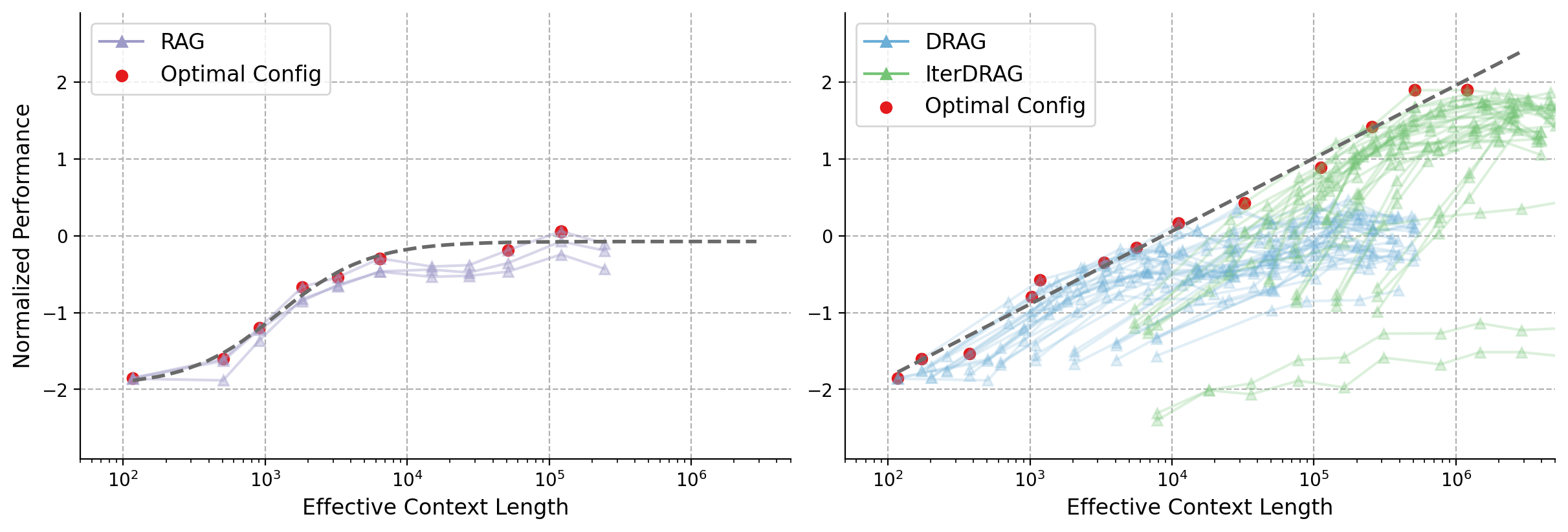
Figure 1: Normalized performance vs. effective context lengths on MuSiQue. Each line represents a fixed configuration, scaled by adjusting the number of documents. Red dots and dash lines represent the optimal configurations and their fitting results. Standard RAG plateaus early at $10^{4}$ tokens, in contrast, DRAG and IterDRAG show near-linear improvement as the effective context length grows.
Previous studies on inference scaling for RAG focus on expanding the retrieved knowledge by increasing the number or lengths of retrieved documents (Xu et al., 2024; Jiang et al., 2024; Shao et al., 2024). However, only emphasizing on the knowledge quantity without providing further guidance presents certain limitations. On one hand, current long-context LLMs still have limited ability to effectively locate relevant information in ultra-long sequences upon challenging tasks (Li et al., 2024; Kuratov et al., 2024). For instance, the optimal performance of long-context LLMs is often achieved without fully utilizing the maximum length (Agarwal et al., ). On the other hand, numerous studies show that retrieving over soft thresholds (e.g., top-10 documents) leads to a performance plateau and may even cause declines (Ram et al., 2023; Lee et al., 2024a; Kuratov et al., 2024). Such performance drops may be traced back to the increased noise within context, which causes distraction and adversely affects generation (Yoran et al., 2024; Zhang et al., 2024; Leng et al., 2024). As a result, inference scaling of long-context RAG remains challenging for existing methods.
In this work, we leverage a broader range of strategies to comprehensively explore how RAG benefits from the scaling of inference computation. A straightforward strategy is demonstration-based RAG (DRAG), where multiple RAG examples are provided as demonstrations to utilize the long-context capabilities of LLMs (Brown et al., 2020). DRAG allows models to learn (in-context) how to locate relevant information and apply it to response generation Different from in-context RAG that prepends documents / QA examples (Press et al., 2023; Ram et al., 2023), we leverage multiple examples comprising of documents, questions and answers to demonstrate the task.. Nevertheless, the quality of one-step retrieval varies across tasks and often fails to provide sufficient information. Inspired by iterative methods (Trivedi et al., 2023; Yoran et al., 2024), we develop iterative demonstration-based RAG (IterDRAG). IterDRAG learns to decompose input queries into simpler sub-queries and answer them using interleaved retrieval. By iteratively retrieving and generating upon sub-queries, LLMs construct reasoning chains that bridge the compositionality gap for multi-hop queries. Together, these strategies provide additional flexibility in scaling inference computation for RAG, allowing long-context LLMs to more effectively address complex knowledge-intensive queries.
Building on these strategies, we investigate multiple ways to scale up inference computation. Here, we measure computation by considering the total number of input tokens across all iterations, referred to as the effective context length. In DRAG, scaling the effective context length can be done by increasing two inference parameters: the number of retrieved documents and in-context examples. In IterDRAG, test-time compute can be further extended by introducing additional generation steps. Since different combinations of inference parameters result in varied allocations of computational resources, our goal is to establish the relationship between RAG performance, different scales and allocations of inference computation. Through extensive experiments on benchmark QA datasets, we demonstrate an almost linear relationship between RAG performance and the scale of effective context length by combining both RAG strategies, as shown in Figure 1 (right). Moreover, our RAG strategies exhibit improved performance than merely scaling the number of documents, achieving state-of-the-art performance with the compact Gemini 1.5 Flash (See evaluation in Figure 2).
Drawing from our observations, we examine the relationship between RAG performance and inference computation, which we quantify as the inference scaling laws for RAG. These observed inference scaling laws reveal that RAG performance consistently improves with the expansion of the effective context length under optimal configurations. Consequently, we take a deeper dive into modeling RAG performance with respect to various inference computation allocations. Our goal is to predict the optimal set of inference parameters that maximize the performance across different RAG tasks. To achieve this, we quantitatively model the relationship between RAG performance and varying inference configurations with the computation allocation model for RAG. Using the estimated computation allocation model, the optimal configurations can be empirically determined and generalize well for various scenarios, thereby maximizing the utilization of the computation budget. We summarize our contributions as follows:
- We systematically investigate inference scaling for long-context RAG, for which we introduce two scaling strategies, DRAG and IterDRAG, to effectively scale inference compute.
- We comprehensively evaluate DRAG and IterDRAG, where they not only achieve state-of-the-art performance, but also exhibit superior scaling properties compared to solely increasing the quantity of documents.
- Through extensive experiments on benchmark QA datasets, we demonstrate that when test-time compute is optimally allocated, long-context RAG performance can scale almost linearly with the increasing order of magnitude of the computation budget.
- We quantitatively model the relationship between RAG performance and different inference parameters, deriving the computation allocation model. This model aligns closely with our experimental results and generalize well across scenarios, providing practical guidance for optimal computation allocation in long-context RAG.
<details>
<summary>extracted/6240196/figures/intro_barchart.png Details</summary>
### Visual Description
# Technical Document Extraction: Performance Comparison of QA Models
## 1. Image Overview
This image is a grouped bar chart comparing the performance (Accuracy) of five different Question Answering (QA) methodologies across four specific datasets and an overall average. The chart uses a color-coded system to differentiate between the models.
## 2. Component Isolation
### A. Header / Legend
* **Location:** Top-center of the chart area.
* **Legend Items (Left to Right):**
* **Zero-shot QA:** Dark Gray bar
* **Many-shot QA:** Orange bar
* **RAG:** Light Purple bar
* **DRAG:** Light Blue bar
* **IterDRAG:** Light Green bar
### B. Main Chart Area (Axes)
* **Y-Axis (Vertical):** Labeled **"Accuracy"**. Scale ranges from 0 to 80, with major gridlines and markers at intervals of 20 (0, 20, 40, 60, 80).
* **X-Axis (Horizontal):** Categorical axis representing datasets and the summary metric.
* **Categories:** Bamboogle, HotpotQA, MuSiQue, 2WikiMultiHopQA, Average.
* **Grid:** Light gray horizontal and vertical gridlines are present to facilitate value estimation.
### C. Data Visualization
The chart consists of five groups of bars. Each group contains five bars corresponding to the models in the legend. Numerical values are printed directly above each bar for precision.
---
## 3. Data Table Reconstruction
The following table transcribes all numerical data points presented in the chart.
| Dataset / Category | Zero-shot QA (Gray) | Many-shot QA (Orange) | RAG (Purple) | DRAG (Blue) | IterDRAG (Green) |
| :--- | :---: | :---: | :---: | :---: | :---: |
| **Bamboogle** | 19.2 | 24.8 | 52.8 | 57.6 | 68.8 |
| **HotpotQA** | 25.2 | 26.2 | 50.9 | 52.2 | 56.4 |
| **MuSiQue** | 6.6 | 8.5 | 16.8 | 18.2 | 30.5 |
| **2WikiMultiHopQA** | 30.7 | 34.3 | 48.4 | 53.3 | 76.9 |
| **Average** | 20.4 | 23.5 | 42.2 | 45.4 | 58.2 |
---
## 4. Trend Analysis and Key Findings
### Trend Verification
For every category (Bamboogle, HotpotQA, MuSiQue, 2WikiMultiHopQA, and Average), the data series follows a consistent **upward slope**.
* **Zero-shot QA** is always the lowest performing.
* **Many-shot QA** shows a marginal improvement over Zero-shot.
* **RAG** shows a significant performance jump compared to Many-shot QA.
* **DRAG** consistently outperforms RAG.
* **IterDRAG** is consistently the highest-performing model across all datasets.
### Key Observations
1. **Superiority of IterDRAG:** IterDRAG achieves the highest accuracy in every single test case. Its most significant lead is in the **2WikiMultiHopQA** dataset, where it reaches **76.9%**, nearly 24 percentage points higher than the next best model (DRAG at 53.3%).
2. **Dataset Difficulty:** **MuSiQue** appears to be the most challenging dataset for all models, with the highest score (IterDRAG) only reaching **30.5%**, while other datasets see scores in the 50s, 60s, or 70s.
3. **RAG vs. Non-RAG:** There is a distinct "step-function" increase in accuracy when moving from Many-shot QA to RAG-based methods (RAG, DRAG, IterDRAG). For example, in Bamboogle, accuracy jumps from 24.8% (Many-shot) to 52.8% (RAG).
4. **Average Performance:** On average, IterDRAG (**58.2%**) outperforms the baseline Zero-shot QA (**20.4%**) by a factor of nearly 3x.
</details>
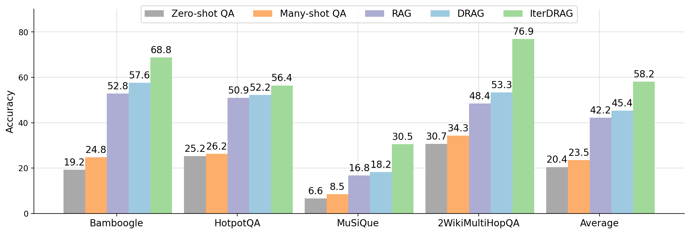
Figure 2: Evaluation accuracy of Gemini 1.5 Flash using different methods: zero-shot QA, many-shot QA, RAG (with an optimal number of documents), DRAG and IterDRAG on benchmark QA datasets. By scaling up inference compute (up to 5M tokens), DRAG consistently outperforms baselines, while IterDRAG improves upon DRAG through interleaving retrieval and iterative generation.
2 Related Work
2.1 Long-Context LLMs
Long-context large language models (LLMs) are designed to utilize extensive context and thereby improve their generative capabilities. Early works in extending context lengths involve sparse / low-rank kernels to reduce memory requirements (Kitaev et al., 2019; Beltagy et al., 2020; Zaheer et al., 2020; Choromanski et al., 2020). In addition, recurrent and state space models (SSMs) are proposed as efficient substitutes for transformer-based models (Gu et al., 2021; Gu and Dao, 2023; Peng et al., 2023a; Beck et al., 2024). For causal LLMs, extrapolation and interpolation methods have proven effective in expanding context window lengths (Press et al., 2021; Chen et al., 2023; Sun et al., 2023; Peng et al., 2023b). Recent advancements in efficient attention methods (Dao et al., 2022; Jacobs et al., 2023; Liu et al., 2023) further enable LLMs to train and infer upon input sequences comprising millions of tokens (Achiam et al., 2023; Team et al., 2023; Reid et al., 2024).
2.2 In-Context Learning
In-context learning (ICL) offers a computationally efficient approach to enhance model performance at inference time by conditioning on a few demonstrations of the task (Brown et al., 2020). To further improve ICL performance, existing works focuses on pretraining strategies that optimize the language models to learn in-context (Min et al., 2022; Wei et al., 2023; Gu et al., 2023). In addition, selective usage of few-shot examples are shown to be helpful for enhancing downstream task performance (Liu et al., 2022; Rubin et al., 2022; Wang et al., 2024). Notably, reformatting or finding optimal ordering of in-context examples also improves ICL performance effectiveness (Lu et al., 2022; Wu et al., 2023; Liu et al., 2024a). With the emergence of long-context LLMs (Achiam et al., 2023; Team et al., 2023; Reid et al., 2024), scaling the number of examples becomes possible in ICL (Li et al., 2023; Bertsch et al., 2024; Agarwal et al., ). For instance, Agarwal et al. show that many-shot ICL can mitigate pretraining biases within LLMs and thus improves ICL performance across various tasks.
2.3 Retrieval Augmented Generation
Retrieval augmented generation (RAG) improves language model performance by incorporating relevant knowledge from external sources (Lewis et al., 2020; Guu et al., 2020; Karpukhin et al., 2020). In contrast to naïve RAG, optimizing the retrieval stage can effectively enhance context relevance and improve generation performance (Ma et al., 2023; Trivedi et al., 2023; Jiang et al., 2023; Shi et al., 2024; Sarthi et al., 2024; Lin et al., 2024). An example is REPLUG, in which Shi et al. (2024) leverage LLM as supervision to learn a dense retriever model. In addition, encoding documents can increase knowledge retrieval and improve generation capabilities (Khandelwal et al., 2019; Izacard and Grave, 2021; Borgeaud et al., 2022; Izacard et al., 2023). For instance, Izacard and Grave (2021) leverages fusion-in-decoder architecture to encode multiple question-passage pairs while maintaining the model efficiency. Alternatively, selectively utilizing knowledge from the documents improves the robustness of LLMs against irrelevant context (Yu et al., 2023; Yoran et al., 2024; Yan et al., 2024; Yue et al., 2024; Zhang et al., 2024). For example, RAFT proposes to train language models with negative documents to improve generation quality and relevance (Zhang et al., 2024). Concurrent to our work, long-document retrieval and datastore scaling are proposed to optimize RAG performance (Jiang et al., 2024; Shao et al., 2024). Despite such progress, inference scaling remains under-explored for long-context RAG methods. As such, we investigate how variations in inference computation impact RAG performance, with the goal of optimizing test-time compute allocation.
3 Inference Scaling Strategies for RAG
3.1 Preliminaries
We measure inference computation with effective context length, defined as the total number of input tokens across all iterations before the LLM outputs the final answer. For most methods that only call the LLM once, the effective context length is equivalent to the number of input tokens in the prompt and is limited by the context window limit of the LLM. For methods that iteratively call the LLM, the effective context length can be extended indefinitely depending on the strategy. We exclude output tokens and retrieval costs from our analysis, as LLMs typically generate significantly fewer tokens (fewer than 10) in knowledge-intensive tasks. Additionally, retrieval is generally much less computationally expensive than LLM inference, especially with scalable matching methods (Sun et al., 2024). Our objective is to understand how RAG performance changes as we scale up inference computation. In demonstration-based RAG (DRAG), we achieve such scaling by incorporating both extensive documents and in-context examples. For further scaling, we increase generation steps through iterative demonstration-based RAG (IterDRAG). We introduce both strategies below.
3.2 Demonstration-Based RAG
Demonstration-based RAG (DRAG) leverages in-context learning to exploit the capabilities of long-context LLMs by directly generating answers from an extended input context. DRAG builds upon naïve RAG and integrates both documents and in-context examples into the input prompt. This expanded context allows the model to generate answers to the input query within a single inference request (See Figure 3 left). For both in-context examples and the test-time query, we employ a retrieval model to select the top- $k$ retrieved documents from a large corpus (e.g., Wikipedia). We reverse the order of the retrieved documents, placing higher-ranked documents closer to the query (Liu et al., 2024b). As we use instruction-tuned LLMs, we design a similar prompt template following Agarwal et al. and align the formatting with prefixes for retrieved documents, input and output (See Appendix H). Unlike previous works (Press et al., 2023; Trivedi et al., 2023), DRAG incorporates extensive retrieved documents within the demonstrations, enabling long-context LLMs to learn to extract relevant information and answer questions using a rich input context.
<details>
<summary>x1.png Details</summary>
### Visual Description
# Technical Document Extraction: Iterative Retrieval-Augmented Generation (IterDRAG) Workflow
This document provides a comprehensive technical extraction of the provided architectural diagram, which illustrates the workflows for standard Retrieval-Augmented Generation (RAG) and an iterative variant labeled "IterDRAG."
## 1. Component Isolation
The diagram is organized into three primary functional regions, delineated by dashed grey boundary lines:
* **Input/Standard RAG Region (Left):** Contains the primary data inputs and the direct path to a final answer.
* **DRAG Region (Bottom-Center):** Represents a single-step decomposition phase.
* **IterDRAG Region (Right):** Represents an iterative, multi-step decomposition and retrieval process.
---
## 2. Data Components and Labels
### Input Blocks (Left Column)
* **In-Context Examples:** Grey rectangle.
* **Documents:** Red rectangle.
* **Input Query:** Blue rectangle.
### Process Nodes (Main Flow)
* **Sub-Query 1:** Pink rectangle.
* **Intermediate Answer 1:** Pink rectangle.
* **Sub-Query 2:** Red rectangle.
* **Intermediate Answer 2:** Red rectangle.
* **Sub-Query n:** Purple rectangle.
* **Intermediate Answer n:** Purple rectangle.
* **Final Answer:** Green rectangle (appears twice: once for the direct path and once for the iterative path).
### Action Icons and Text
* **Robot Icon + "Generate":** Indicates a Large Language Model (LLM) generation step.
* **Magnifying Glass/Globe Icon + Robot Icon + "Retrieve & Generate":** Indicates a retrieval step followed by an LLM generation step.
* **Ellipsis (...):** Located between Intermediate Answer 2 and Sub-Query n, indicating an undefined number of iterative steps.
---
## 3. Workflow and Logic Flow
### Path A: Standard Direct Generation
1. The **Input Query** (Blue) flows downward.
2. An LLM performs a **Generate** action.
3. Produces a **Final Answer** (Green, bottom left).
### Path B: IterDRAG (Iterative Decomposition)
This path follows a sequential, dependency-based logic:
1. **Initialization:** The **Input Query** (Blue) is sent to the first decomposition stage.
2. **Step 1 (Pink):**
* The system performs a **Generate** action to create **Sub-Query 1**.
* A **Retrieve & Generate** action is performed on Sub-Query 1 to produce **Intermediate Answer 1**.
3. **Step 2 (Red):**
* **Intermediate Answer 1** feeds into the next stage to generate **Sub-Query 2**.
* A **Retrieve & Generate** action is performed on Sub-Query 2 to produce **Intermediate Answer 2**.
4. **Step n (Purple):**
* After an arbitrary number of iterations (...), the process reaches **Sub-Query n**.
* A **Retrieve & Generate** action produces **Intermediate Answer n**.
5. **Synthesis:**
* A green horizontal line aggregates the **Input Query** and all **Intermediate Answers (1, 2, ... n)**.
* A final **Generate** action is performed on this aggregated context.
* Produces the **Final Answer** (Green, bottom right).
---
## 4. Spatial Grounding and Visual Encoding
| Element | Color | Spatial Placement | Logic/Trend |
| :--- | :--- | :--- | :--- |
| **Input Query** | Blue | Left-center | The primary trigger for all subsequent processes. |
| **Sub-Queries** | Pink/Red/Purple | Top row, right of input | These move horizontally, representing the progression of the decomposition. |
| **Intermediate Answers** | Pink/Red/Purple | Middle row | These are positioned directly below their respective sub-queries, showing a 1:1 relationship. |
| **Final Answer** | Green | Bottom-left & Bottom-right | Represents the terminal state of the workflow. |
| **Aggregation Line** | Green | Bottom horizontal | Connects the original query and all intermediate results to the final generation step. |
---
## 5. Summary of System Logic
The diagram contrasts a simple "Query-to-Answer" model with an iterative "Decompose-Retrieve-Answer" model. The **IterDRAG** process is characterized by its sequential nature, where each subsequent sub-query is informed by the intermediate answer of the previous step. The final output is synthesized from the original query combined with the cumulative knowledge gathered across all $n$ iterations.
</details>
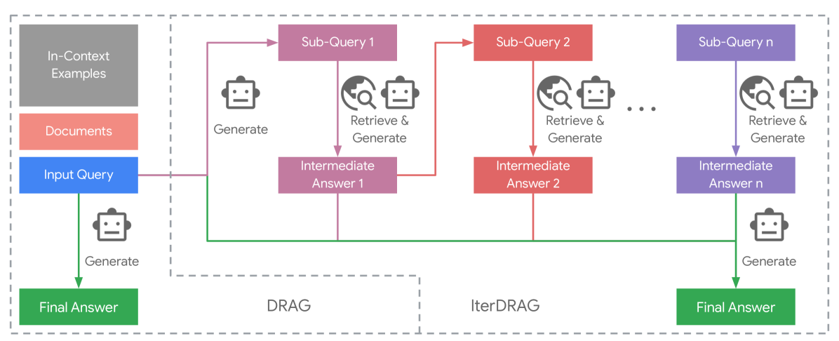
Figure 3: DRAG vs. IterDRAG. IterDRAG breaks down the input query into sub-queries and answer them to improve the accuracy of the final answer. In test-time, IterDRAG scales the computation through multiple inference steps to decompose complex queries and retrieve documents.
3.3 Iterative Demonstration-Based RAG
Despite access to external knowledge, complex multi-hop queries remain challenging due to the compositionality gap. To tackle this issue, we introduce iterative demonstration-based RAG (IterDRAG), which handles complex queries by decomposing the query into simpler sub-queries. For each sub-query, retrieval is performed to gather additional contextual information, which is then used to generate intermediate answers. After all sub-queries are resolved, the retrieved context, sub-queries, and their answers are combined to synthesize the final answer (See Figure 3 right).
While multiple existing datasets provide training data with queries and corresponding answers, sub-queries and intermediate answers are often absent. To generate in-context examples with sub-queries and intermediate answers, we prompt LLMs with constrained decoding to follow the Self-Ask format (Press et al., 2023; Koo et al., 2024). In each iteration, LLMs generate either a sub-query, an intermediate answer, or the final answer. If a sub-query is generated, additional documents are retrieved and interleaved into the prompt before producing the intermediate answer. IterDRAG continues until the final answer is generated or the number of maximum iterations is reached, at which point LLM is forced to generate the final answer. We retain examples with intermediate steps and correct final answers to construct in-context demonstrations. Each example should include the retrieved documents, sub-query and answer pairs, as well as the final answer.
During inference, in-context examples are prepended to the initial documents retrieved for the input query. Similarly, each inference request yields a sub-query, an intermediate answer, or the final answer. Upon sub-queries, additional documents are retrieved and merged with the initial ones to generate intermediate answers. In our implementation, we allow up to five iterations of query decomposition before generating the final answer. This iterative process effectively scales test-time computation, with the input tokens from all iterations summed to calculate the effective context length. IterDRAG facilitates a more granular approach by learning to: (1) decompose query into simple and manageable sub-queries; and (2) retrieve and locate relevant information to answer (sub)-queries. As such, the iterative retrieval and generation strategy helps narrowing the compositionality gap and improves knowledge extraction, thereby enhancing overall RAG performance.
4 RAG Performance and Inference Computation Scale
4.1 Fixed Budget Optimal Performance
For a given budget on inference computation, i.e., a maximum effective context length $L_{\text{max}}$ , there are multiple ways to optimize the use of computation resources through inference parameters. For example, in DRAG, we can adjust both the number of retrieved documents and in-context examples, while in the IterDRAG strategy, we additionally introduce the number of iterations for retrieval and generation. Henceforth, we use $\theta$ to denote all these inference parameters.
For each input query and its ground-truth answer $(x_{i},y_{i})∈\mathcal{X}$ , we can apply the RAG inference strategy $f$ parameterized by $\theta$ . We denote the effective input context length to the LLM as $l(x_{i};\theta)$ and the obtained prediction as $\hat{y}_{i}=f(x_{i};\theta)$ . A metric $P(y_{i},\hat{y}_{i})$ can then be calculated based on $y_{i}$ and $\hat{y}_{i}$ . To understand the relationship between RAG performance and inference computation, we sample a few different inference computation budgets. For each budget $L_{\text{max}}$ , we find the optimal average metric $P^{*}(L_{\text{max}})$ achievable within this budget by enumerating different $\theta∈\Theta$ :
$$
P^{*}(L_{\text{max}}):=\max_{\theta\in\Theta}\Big{\{}\frac{1}{|\mathcal{X}|}%
\sum_{i}P\big{(}y_{i},f(x_{i};\theta)\big{)}\Big{|}\forall i,l(x_{i};\theta)%
\leq L_{\text{max}}\Big{\}}. \tag{1}
$$
Our goal is to establish the relationship between the inference computation budget $L_{\text{max}}$ and the best possible performance within this budget $P^{*}(L_{\text{max}})$ , using any possible strategies and parameter configurations to allocate the inference computation resources. For simplicity, we also refer to $P^{*}(L_{\text{max}})$ as the optimal performance. We investigate the following factors within the inference parameter set $\theta$ : (1) the number of documents $k$ , which are retrieved from a large corpus (e.g., Wikipedia) based on the input query; (2) the number of in-context examples $m$ , where each of the examples consists of $k$ documents, an input query and its label; and (3) the number of generation iterations $n$ . In DRAG, an answer can be directly generated upon input context, so $n=1$ . In contrast, IterDRAG involves multiple steps of interleaved retrieval and generation, expanding both the effective context length and inference compute without needing longer context windows.
Table 1: Optimal performance of different methods with varying maximum effective context lengths $L_{\text{max}}$ (i.e., the total number of input tokens across all iterations). ZS QA and MS QA refers to zero-shot QA and many-shot QA respectively. Partial results are omitted for methods that do not further scale with increasing $L_{\text{max}}$ . For clarity, we mark the best results for each $L_{\text{max}}$ in bold.
| $L_{\text{max}}$ | Method | Bamboogle | HotpotQA | MuSiQue | 2WikiMultiHopQA | | | | | | | | |
| --- | --- | --- | --- | --- | --- | --- | --- | --- | --- | --- | --- | --- | --- |
| EM | F1 | Acc | EM | F1 | Acc | EM | F1 | Acc | EM | F1 | Acc | | |
| 16k | ZS QA | 16.8 | 25.9 | 19.2 | 22.7 | 32.0 | 25.2 | 5.0 | 13.2 | 6.6 | 28.3 | 33.5 | 30.7 |
| MS QA | 24.0 | 30.7 | 24.8 | 24.6 | 34.0 | 26.2 | 7.4 | 16.4 | 8.5 | 33.2 | 37.5 | 34.3 | |
| RAG | 44.0 | 54.5 | 45.6 | 44.2 | 57.9 | 49.2 | 12.3 | 21.5 | 15.3 | 42.3 | 49.3 | 46.5 | |
| DRAG | 44.0 | 55.2 | 45.6 | 45.5 | 58.5 | 50.2 | 14.5 | 24.6 | 16.9 | 45.2 | 53.5 | 50.5 | |
| IterDRAG | 46.4 | 56.2 | 51.2 | 36.0 | 47.4 | 44.4 | 8.1 | 17.5 | 12.2 | 33.2 | 38.8 | 43.8 | |
| 32k | RAG | 48.8 | 56.2 | 49.6 | 44.2 | 58.2 | 49.3 | 12.3 | 21.5 | 15.3 | 42.9 | 50.6 | 48.0 |
| DRAG | 48.8 | 59.2 | 50.4 | 46.9 | 60.3 | 52.0 | 15.4 | 26.0 | 17.3 | 45.9 | 53.7 | 51.4 | |
| IterDRAG | 46.4 | 56.2 | 52.0 | 38.3 | 49.8 | 44.4 | 12.5 | 23.1 | 19.7 | 44.3 | 54.6 | 56.8 | |
| 128k | RAG | 51.2 | 60.3 | 52.8 | 45.7 | 59.6 | 50.9 | 14.0 | 23.7 | 16.8 | 43.1 | 50.7 | 48.4 |
| DRAG | 52.8 | 62.3 | 54.4 | 47.4 | 61.3 | 52.2 | 15.4 | 26.0 | 17.9 | 47.5 | 55.3 | 53.1 | |
| IterDRAG | 63.2 | 74.8 | 68.8 | 44.8 | 59.4 | 52.8 | 17.3 | 28.0 | 24.5 | 62.3 | 73.8 | 74.6 | |
| 1M | DRAG | 56.0 | 62.9 | 57.6 | 47.4 | 61.3 | 52.2 | 15.9 | 26.0 | 18.2 | 48.2 | 55.7 | 53.3 |
| IterDRAG | 65.6 | 75.6 | 68.8 | 48.7 | 63.3 | 55.3 | 22.2 | 34.3 | 30.5 | 65.7 | 75.2 | 76.4 | |
| 5M | IterDRAG | 65.6 | 75.6 | 68.8 | 51.7 | 64.4 | 56.4 | 22.5 | 35.0 | 30.5 | 67.0 | 75.2 | 76.9 |
We evaluate the performance of Gemini 1.5 Flash with context length window up to 1M tokens on knowledge-intensive question answering, including multi-hop datasets Bamboogle, HotpotQA, MuSiQue and 2WikiMultiHopQA (Press et al., 2023; Yang et al., 2018; Trivedi et al., 2022; Ho et al., 2020). Additional results are provided in Appendix B and Appendix C. To manage the computational costs of extensive experiments, we follow Wu et al. (2024); Gutiérrez et al. (2024) and sample 1.2k examples from each dataset for evaluation. The evaluation metrics include exact match (EM), F1 score (F1) and accuracy (Acc), in which the accuracy metric assesses whether the ground truth is located within the prediction. We sample the inference computation budget $L_{\text{max}}$ as 16k, 32k, 128k, 1M and 5M tokens. For the parameter space $\Theta$ of DRAG, we consider the number of documents $k∈\{0,1,2,5,10,20,50,100,200,500,1000\}$ , and the number in-context examples $m$ ranging from $0 0$ , $2^{0}$ , $2^{1}$ , …, to $2^{8}$ . For IterDRAG, we further experiment with number of iterations $n$ up to 5. We compare to the following baselines: (1) zero-shot QA (QA), where the model does not leverage any retrieved documents or demonstrations; (2) many-shot QA (MS QA), where the model only uses varying number of demonstrations $m$ without any retrieved document; and (3) retrieval augmented generation (RAG), where the model only uses $k$ retrieved documents without demonstrations. We report the optimal performance of each method with different maximum effective context length budgets by examining their performance with different inference parameter configurations.
<details>
<summary>extracted/6240196/figures/perf_vs_length.png Details</summary>
### Visual Description
# Technical Data Extraction: Performance vs. Effective Context Length
## 1. Component Isolation
* **Header/Legend:** Located in the top-left quadrant. Contains three identifiers.
* **Main Chart Area:** A scatter/line plot with a logarithmic X-axis and linear Y-axis. It features a dense collection of semi-transparent lines and a series of highlighted red data points.
* **Axes:**
* **Y-Axis (Vertical):** Labeled "Normalized Performance". Range: -3 to 3.
* **X-Axis (Horizontal):** Labeled "Effective Context Length". Logarithmic scale ranging from $10^2$ to approximately $5 \times 10^6$.
## 2. Legend and Label Extraction
* **Legend Location:** [x=0.05, y=0.85] (Top-left corner).
* **DRAG (Blue Triangle):** Represented by light blue lines with triangular markers.
* **IterDRAG (Green Triangle):** Represented by light green lines with triangular markers.
* **Optimal Config (Red Circle):** Represented by solid red circular points.
* **Dashed Grey Line:** (Unlabeled in legend) Represents the upper frontier or trend line of the optimal configurations.
## 3. Data Series Analysis and Trend Verification
### Series 1: DRAG (Blue Lines)
* **Visual Trend:** These lines generally occupy the lower-left to middle-right section of the graph. They show a positive correlation between context length and performance, but they saturate or plateau earlier than the green series, generally staying below a Normalized Performance of 1.0.
* **Range:** Predominantly active between $10^2$ and $5 \times 10^5$ Effective Context Length.
### Series 2: IterDRAG (Green Lines)
* **Visual Trend:** These lines begin appearing prominently around $5 \times 10^3$ context length. They slope upward more aggressively than the blue series at higher context lengths, reaching higher Normalized Performance values (up to ~2.0).
* **Range:** Predominantly active between $5 \times 10^3$ and $5 \times 10^6$ Effective Context Length.
### Series 3: Optimal Config (Red Dots)
* **Visual Trend:** These points track the maximum performance achieved at various context lengths. They follow a logarithmic upward trajectory, closely tracked by a dashed grey trend line.
* **Key Data Points (Approximate):**
* $10^2$: ~ -1.4
* $5 \times 10^2$: ~ -1.1
* $10^3$: ~ -0.4
* $5 \times 10^3$: ~ +0.4
* $10^4$: ~ +0.5
* $10^5$: ~ +1.4
* $5 \times 10^5$: ~ +1.9
* $10^6$: ~ +1.9
## 4. Structural Data Representation
| Effective Context Length (X) | Approx. Max Normalized Performance (Y) | Dominant Method at Frontier |
| :--- | :--- | :--- |
| $10^2$ | -1.4 | DRAG (Blue) |
| $10^3$ | -0.4 | DRAG (Blue) |
| $10^4$ | +0.5 | Transition (Blue/Green) |
| $10^5$ | +1.4 | IterDRAG (Green) |
| $10^6$ | +1.9 | IterDRAG (Green) |
## 5. Technical Summary
The chart illustrates the scaling behavior of two methods, **DRAG** and **IterDRAG**, regarding **Normalized Performance** as **Effective Context Length** increases.
1. **Scaling:** There is a clear logarithmic scaling law, indicated by the dashed grey line, where performance increases as context length grows.
2. **Method Superiority:** DRAG (blue) is the primary contributor to performance at shorter context lengths ($< 10^4$). IterDRAG (green) becomes the superior method for high-context scenarios ($> 10^4$), achieving the highest overall performance scores.
3. **Saturation:** Performance appears to begin leveling off as it approaches $10^6$ context length, with the "Optimal Config" points clustering around a Normalized Performance value of 2.0.
</details>
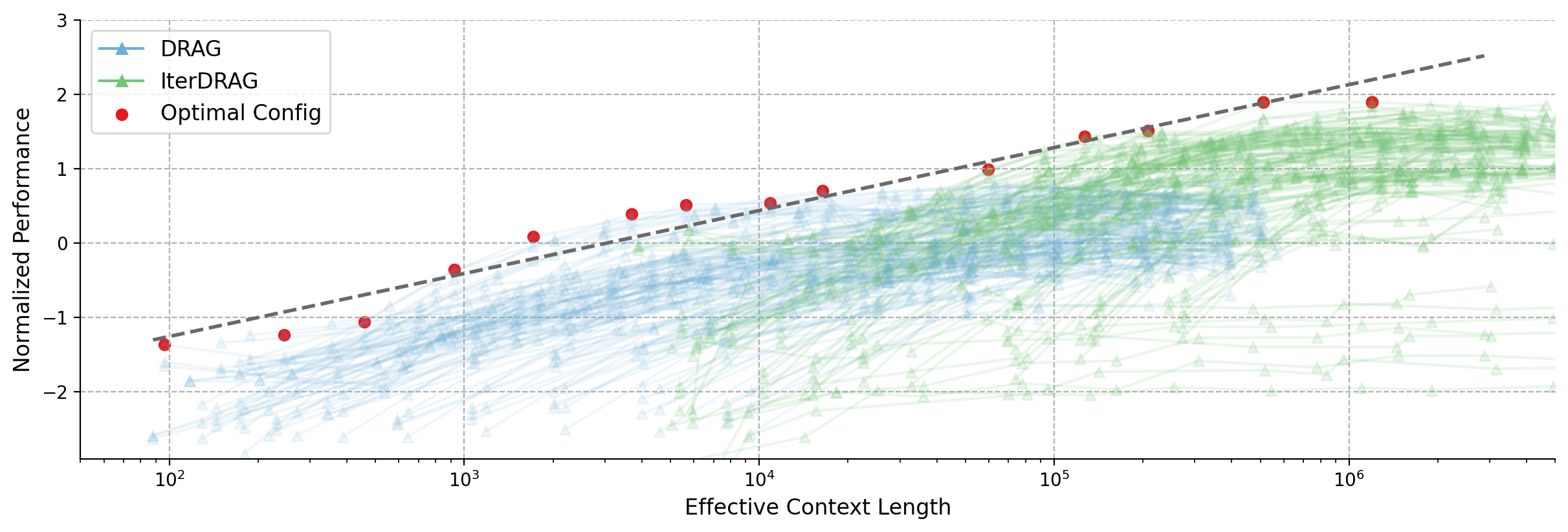
Figure 4: Normalized performance vs. effective context lengths across datasets. Each line represents a fixed configuration, scaled by varying the number of documents. Red dots indicate the optimal configurations, with the dashed line showing the fitting results. The observed optimal performance can be approximated by a linear relationship with the effective context lengths.
4.2 Overall Performance
We report the optimal performance $P^{*}(L_{\text{max}})$ for different inference strategies in Table 1, where we identify the optimal inference parameters for each computation budget $L_{\text{max}}$ . Some variants are omitted for certain $L_{\text{max}}$ because they do not scale to the corresponding context length. For example, the prompt for zero-shot QA cannot be increased, while the number of in-context examples for many-shot QA is capped at $2^{8}$ , so neither scales to $L_{\text{max}}=$ 32k. Similarly, RAG does not scale to $L_{\text{max}}$ larger than 128k, and DRAG is limited by the LLM’s context window limit of 1M.
Unlike QA and RAG baselines, the performance of DRAG and IterDRAG consistently increase as we expand the maximum effective context length. More specifically, we observe: (1) DRAG and IterDRAG scale better than baselines. Baselines like many-shot QA peak at 16k tokens, while RAG improves until 128k, after which performance plateaus. In comparison, DRAG and IterDRAG can find optimal configurations to more effectively utilize test-time compute, exhibiting superior performance and scaling properties. Performance of DRAG consistently improves until 1M tokens, while IterDRAG further enhances RAG performance with 5M tokens of computation budget by iteratively calling LLMs. (2) DRAG excels with shorter maximum lengths, while IterDRAG scales more effectively with longer effective context length. At 16k and 32k, DRAG typically delivers the best performance, while at 128k and beyond, IterDRAG achieves superior results overall, highlighting the effectiveness of iterative retrieval and generation. These results suggest that increasing $L_{\text{max}}$ is beneficial for RAG, with DRAG and IterDRAG strategies each excelling at different scales.
4.3 Inference Scaling Laws for RAG
To analyze RAG performance with different effective context lengths, we plot the performance of all configurations across datasets in Figure 4. Similar to Figure 1, we visualize DRAG and IterDRAG and highlight the optimal performance $P^{*}(L_{\text{max}})$ for different selections of $L_{\text{max}}$ . The fitting results are shown as grey dashed lines. We provide additional dataset-specific results in Appendix E.
The optimal performance exhibits consistent gains as the effective context length expands, demonstrating a strong linear correlation, which we term the inference scaling laws for RAG. Combined with dataset-specific results, our key observations are: (1) The optimal performance scales nearly linearly with the order of magnitude of the inference compute. Such linear relationship suggests that RAG performance can be improved by increasing computation, allowing for more accurate predictions of performance given available compute resources. (2) For $L_{\text{max}}$ above $10^{5}$ , IterDRAG continues to scale effectively with interleaving retrieval and iterative generation. This aligns with our results in Table 1, where IterDRAG better utilizes computation budgets for effective context lengths exceeding 128k. (3) Gains on optimal performance gradually diminish beyond an effective context length of 1M. Despite dataset variations, the performance follows similar trends up to 1M tokens. Beyond that, improvements from 1M to 5M are less substantial or plateau, potentially due to limitations in long-context modeling. In summary, while gains are smaller beyond 1M tokens, optimal RAG performance scales almost linearly with increasing inference compute through DRAG and IterDRAG.
<details>
<summary>x2.png Details</summary>
### Visual Description
# Technical Data Extraction: Performance Heatmaps
This document provides a comprehensive extraction of data from three performance heatmaps comparing model performance across two dimensions: the number of documents provided in the context (x-axis) and the number of few-shot examples provided (y-axis).
## 1. Document Overview
The image consists of three heatmaps arranged horizontally, representing different evaluation metrics:
* **Left Chart:** EM (Exact Match) Performance
* **Middle Chart:** F1 Performance
* **Right Chart:** Acc (Accuracy) Performance
### Common Axis Definitions
* **X-Axis (Top):** Number of Documents (`0-Doc`, `1-Doc`, `2-Doc`, `5-Doc`, `10-Doc`, `20-Doc`, `50-Doc`, `100-Doc`, `200-Doc`, `500-Doc`, `1000-Doc`).
* **Y-Axis (Left):** Number of Shots (`0-Shot`, $2^0$-Shot, $2^1$-Shot, $2^2$-Shot, $2^3$-Shot, $2^4$-Shot, $2^5$-Shot, $2^6$-Shot, $2^7$-Shot, $2^8$-Shot).
* **Color Gradient:** Blue (Lower performance) $\rightarrow$ White (Median) $\rightarrow$ Red (Higher performance).
---
## 2. Data Extraction: EM Performance (Left Chart)
**Trend Analysis:** Performance generally increases as both the number of documents and the number of shots increase. The highest performance is concentrated in the bottom-right of the populated area. Note that the matrix is triangular; data is not provided for high-shot/high-doc combinations in the bottom right corner.
| Shots \ Docs | 0-Doc | 1-Doc | 2-Doc | 5-Doc | 10-Doc | 20-Doc | 50-Doc | 100-Doc | 200-Doc | 500-Doc | 1000-Doc |
| :--- | :---: | :---: | :---: | :---: | :---: | :---: | :---: | :---: | :---: | :---: | :---: |
| **0-Shot** | 18.2 | 22.8 | 27.5 | 30.4 | 32.0 | 34.9 | 35.6 | 36.9 | 37.8 | 38.2 | 36.9 |
| **$2^0$-Shot** | 19.4 | 26.9 | 28.9 | 31.3 | 34.3 | 36.0 | 38.0 | 36.1 | 40.0 | 40.7 | 39.8 |
| **$2^1$-Shot** | 20.4 | 27.6 | 29.2 | 31.8 | 34.4 | 36.9 | 38.2 | 39.8 | 40.2 | 40.5 | - |
| **$2^2$-Shot** | 19.9 | 27.6 | 30.0 | 32.8 | 34.4 | 37.1 | 37.9 | 38.5 | 40.2 | 40.1 | - |
| **$2^3$-Shot** | 21.0 | 29.4 | 30.6 | 33.5 | 35.5 | 38.0 | 39.0 | 40.4 | 39.3 | - | - |
| **$2^4$-Shot** | 20.3 | 30.2 | 31.6 | 34.4 | 35.9 | 37.1 | 39.2 | 40.1 | 39.1 | - | - |
| **$2^5$-Shot** | 20.7 | 30.1 | 32.5 | 35.8 | 37.1 | 38.2 | 39.3 | 41.2 | - | - | - |
| **$2^6$-Shot** | 21.2 | 30.6 | 33.0 | 36.0 | 37.4 | 38.2 | 39.0 | - | - | - | - |
| **$2^7$-Shot** | 21.8 | 30.6 | 34.3 | 36.3 | 38.2 | 38.6 | - | - | - | - | - |
| **$2^8$-Shot** | 21.6 | 30.7 | 32.5 | 36.0 | 37.8 | - | - | - | - | - | - |
---
## 3. Data Extraction: F1 Performance (Middle Chart)
**Trend Analysis:** F1 scores are consistently higher than EM scores. The peak performance (50.8) occurs at $2^5$-Shot with 100-Doc. There is a clear "sweet spot" for performance as document count increases, with a slight drop-off at the extreme 1000-Doc edge for the 0-shot row.
| Shots \ Docs | 0-Doc | 1-Doc | 2-Doc | 5-Doc | 10-Doc | 20-Doc | 50-Doc | 100-Doc | 200-Doc | 500-Doc | 1000-Doc |
| :--- | :---: | :---: | :---: | :---: | :---: | :---: | :---: | :---: | :---: | :---: | :---: |
| **0-Shot** | 26.2 | 30.1 | 35.6 | 40.2 | 42.2 | 45.0 | 45.8 | 46.6 | 47.4 | 48.4 | 47.1 |
| **$2^0$-Shot** | 26.4 | 35.4 | 37.9 | 41.5 | 45.1 | 46.8 | 48.6 | 47.2 | 50.0 | 50.7 | 49.1 |
| **$2^1$-Shot** | 27.3 | 35.5 | 38.3 | 42.2 | 45.3 | 47.0 | 48.8 | 49.8 | 50.2 | 50.0 | - |
| **$2^2$-Shot** | 27.4 | 35.8 | 39.1 | 43.5 | 45.3 | 47.4 | 49.1 | 48.7 | 49.5 | 49.5 | - |
| **$2^3$-Shot** | 28.2 | 38.5 | 40.1 | 44.0 | 46.5 | 48.3 | 49.5 | 50.1 | 49.3 | - | - |
| **$2^4$-Shot** | 27.9 | 38.9 | 41.0 | 44.9 | 46.7 | 47.8 | 49.7 | 50.6 | 49.6 | - | - |
| **$2^5$-Shot** | 28.2 | 39.6 | 42.7 | 46.3 | 47.6 | 48.6 | 49.8 | 50.8 | - | - | - |
| **$2^6$-Shot** | 28.8 | 40.5 | 42.9 | 46.4 | 48.3 | 48.9 | 50.0 | - | - | - | - |
| **$2^7$-Shot** | 28.8 | 39.7 | 44.1 | 47.4 | 48.5 | 49.0 | - | - | - | - | - |
| **$2^8$-Shot** | 29.0 | 40.1 | 43.0 | 46.2 | 48.1 | - | - | - | - | - | - |
---
## 4. Data Extraction: Acc Performance (Right Chart)
**Trend Analysis:** Accuracy follows the same general trend as EM and F1. The highest recorded value is 44.8 at $2^5$-Shot and 100-Doc. The performance gain from 0-Doc to 1000-Doc is significant (roughly doubling the score).
| Shots \ Docs | 0-Doc | 1-Doc | 2-Doc | 5-Doc | 10-Doc | 20-Doc | 50-Doc | 100-Doc | 200-Doc | 500-Doc | 1000-Doc |
| :--- | :---: | :---: | :---: | :---: | :---: | :---: | :---: | :---: | :---: | :---: | :---: |
| **0-Shot** | 20.4 | 25.2 | 29.9 | 32.7 | 35.0 | 38.0 | 39.0 | 40.5 | 41.1 | 41.8 | 40.7 |
| **$2^0$-Shot** | 20.4 | 29.0 | 30.9 | 34.0 | 37.1 | 39.4 | 41.6 | 39.7 | 43.4 | 44.1 | 43.0 |
| **$2^1$-Shot** | 21.4 | 29.4 | 31.3 | 34.4 | 37.3 | 40.1 | 41.6 | 43.0 | 43.6 | 43.9 | - |
| **$2^2$-Shot** | 21.0 | 29.4 | 32.0 | 35.5 | 37.4 | 40.5 | 41.4 | 42.0 | 43.5 | 43.4 | - |
| **$2^3$-Shot** | 22.1 | 31.1 | 32.6 | 36.0 | 38.5 | 41.0 | 42.2 | 43.7 | 42.8 | - | - |
| **$2^4$-Shot** | 21.6 | 32.0 | 33.7 | 37.0 | 38.9 | 40.2 | 42.6 | 43.5 | 42.5 | - | - |
| **$2^5$-Shot** | 21.8 | 32.2 | 34.6 | 38.6 | 40.1 | 41.1 | 42.7 | 44.8 | - | - | - |
| **$2^6$-Shot** | 22.4 | 32.8 | 35.0 | 38.3 | 40.2 | 41.2 | 42.4 | - | - | - | - |
| **$2^7$-Shot** | 22.9 | 32.7 | 36.2 | 38.6 | 41.0 | 42.0 | - | - | - | - | - |
| **$2^8$-Shot** | 22.7 | 32.7 | 34.6 | 38.1 | 40.4 | - | - | - | - | - | - |
</details>
(a) Averaged DRAG performance heatmap for different metrics.
<details>
<summary>x3.png Details</summary>
### Visual Description
# Technical Data Extraction: Performance Comparison Chart
## 1. Component Isolation
* **Header/Legend:** Located in the top-left quadrant. Contains labels for two data series.
* **Main Chart Area:** A line graph with a logarithmic X-axis and linear Y-axis. It features two primary trend lines (thick dashed) superimposed over a high-density "spaghetti plot" of individual trials (thin translucent lines with triangular markers). Shaded regions represent the variance/confidence intervals for each series.
* **Axes:**
* **Y-Axis (Vertical):** Labeled "Normalized Performance". Range: -3 to 2.
* **X-Axis (Horizontal):** Labeled "Number of Documents". Logarithmic scale. Range: $10^0$ (0 on the plot) to $10^3$.
## 2. Legend and Spatial Grounding
* **Legend Location:** Top-left corner, approximately at [x: 0.1, y: 0.9] in relative coordinates.
* **Series 1: DRAG**
* **Color:** Blue (#377eb8 approx.)
* **Line Style:** Thick dashed line.
* **Associated Data:** Blue shaded region and blue translucent individual trial lines.
* **Series 2: IterDRAG**
* **Color:** Green (#4daf4a approx.)
* **Line Style:** Thick dashed line.
* **Associated Data:** Green shaded region and green translucent individual trial lines.
## 3. Trend Verification and Data Extraction
### Series: IterDRAG (Green)
* **Visual Trend:** The line starts at a higher baseline than DRAG. It shows a strong upward slope from 0 to 100 documents, reaching a peak performance. After 100 documents, it maintains a plateau until approximately 200, followed by a sharp decline toward 1000 documents.
* **Estimated Data Points (Mean):**
* **0 ($10^0$):** ~ -1.1
* **1 ($10^0$):** ~ -0.4
* **2:** ~ 0.1
* **5:** ~ 0.5
* **10 ($10^1$):** ~ 0.75
* **20:** ~ 0.85
* **50:** ~ 0.9
* **100 ($10^2$):** ~ 1.05 (Peak)
* **200:** ~ 0.95
* **500:** ~ 0.4
* **1000 ($10^3$):** ~ -0.7
### Series: DRAG (Blue)
* **Visual Trend:** Starts at a lower baseline (~ -2.0). It exhibits a steady, consistent upward slope throughout the majority of the document range. Unlike IterDRAG, it does not peak early; it continues to rise slowly until approximately 500 documents before showing a slight downward turn at the 1000 mark.
* **Estimated Data Points (Mean):**
* **0 ($10^0$):** ~ -1.95
* **1 ($10^0$):** ~ -1.05
* **2:** ~ -0.8
* **5:** ~ -0.45
* **10 ($10^1$):** ~ -0.25
* **20:** ~ 0.0
* **50:** ~ 0.1
* **100 ($10^2$):** ~ 0.15
* **200:** ~ 0.22
* **500:** ~ 0.28 (Peak)
* **1000 ($10^3$):** ~ 0.1
## 4. Statistical Observations
* **Variance:** Both methods show significant variance, as indicated by the wide shaded regions and the spread of individual trial lines (triangles).
* **Comparative Performance:** **IterDRAG** consistently outperforms **DRAG** in the range of 0 to ~400 documents.
* **Crossover/Convergence:** At the highest document count ($10^3$), the performance of IterDRAG drops significantly, while DRAG remains relatively stable, suggesting DRAG may be more robust at extreme scales, though both show a downward trend at the very end.
* **Peak Performance:** IterDRAG achieves its highest normalized performance (~1.0) at approximately 100 documents. DRAG achieves its highest performance (~0.3) at approximately 500 documents.
</details>
(b) Performance vs. number of documents.
<details>
<summary>x4.png Details</summary>
### Visual Description
# Technical Data Extraction: Performance Comparison Chart
## 1. Image Overview
This image is a line graph comparing the performance of two methods, **DRAG** and **IterDRAG**, across an increasing number of "shots." The chart includes thick dashed lines representing the mean performance and numerous faint lines with triangular markers representing individual trials or data subsets, indicating the variance and distribution of the results.
## 2. Component Isolation
### Header / Legend
- **Location:** Top-left corner (approx. [x=0.1, y=0.9] in normalized coordinates).
- **Legend Items:**
- **DRAG:** Represented by a thick dashed line and associated faint lines.
- **IterDRAG:** Represented by a thick dashed line and associated faint lines.
### Axes
- **X-Axis (Horizontal):** Labeled "shots". Values range from 0 to 10.
- **Y-Axis (Vertical):** Labeled "Performance" (or similar metric). Values range from 0.0 to 1.0.
## 3. Data Trends
- **DRAG:** Shows a steady increase in performance as the number of shots increases, starting near 0.4 and plateauing towards 0.8.
- **IterDRAG:** Exhibits a steeper initial improvement compared to DRAG, reaching higher performance levels (approaching 0.9) with fewer shots.
- **Variance:** Both methods show significant variance in individual trials, as indicated by the spread of the faint lines, though the mean (dashed line) provides a clear trend for each.
</details>
(c) Performance vs. number of shots.
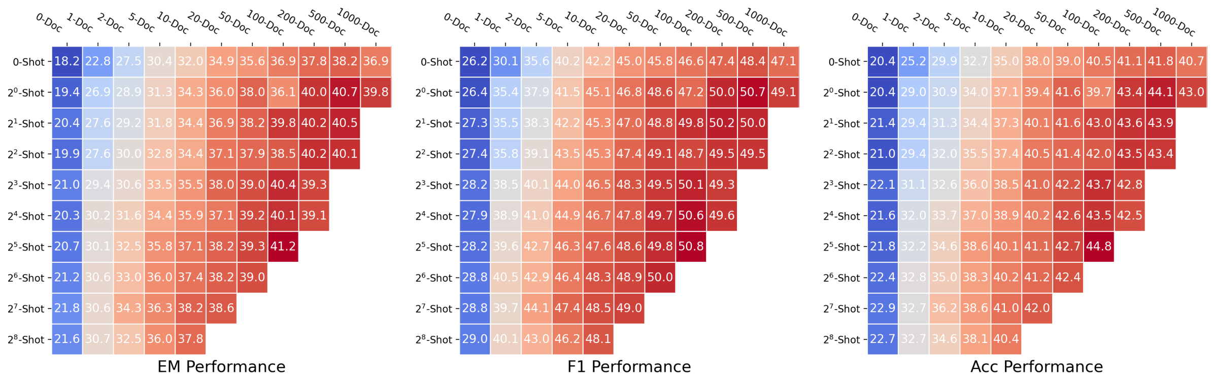
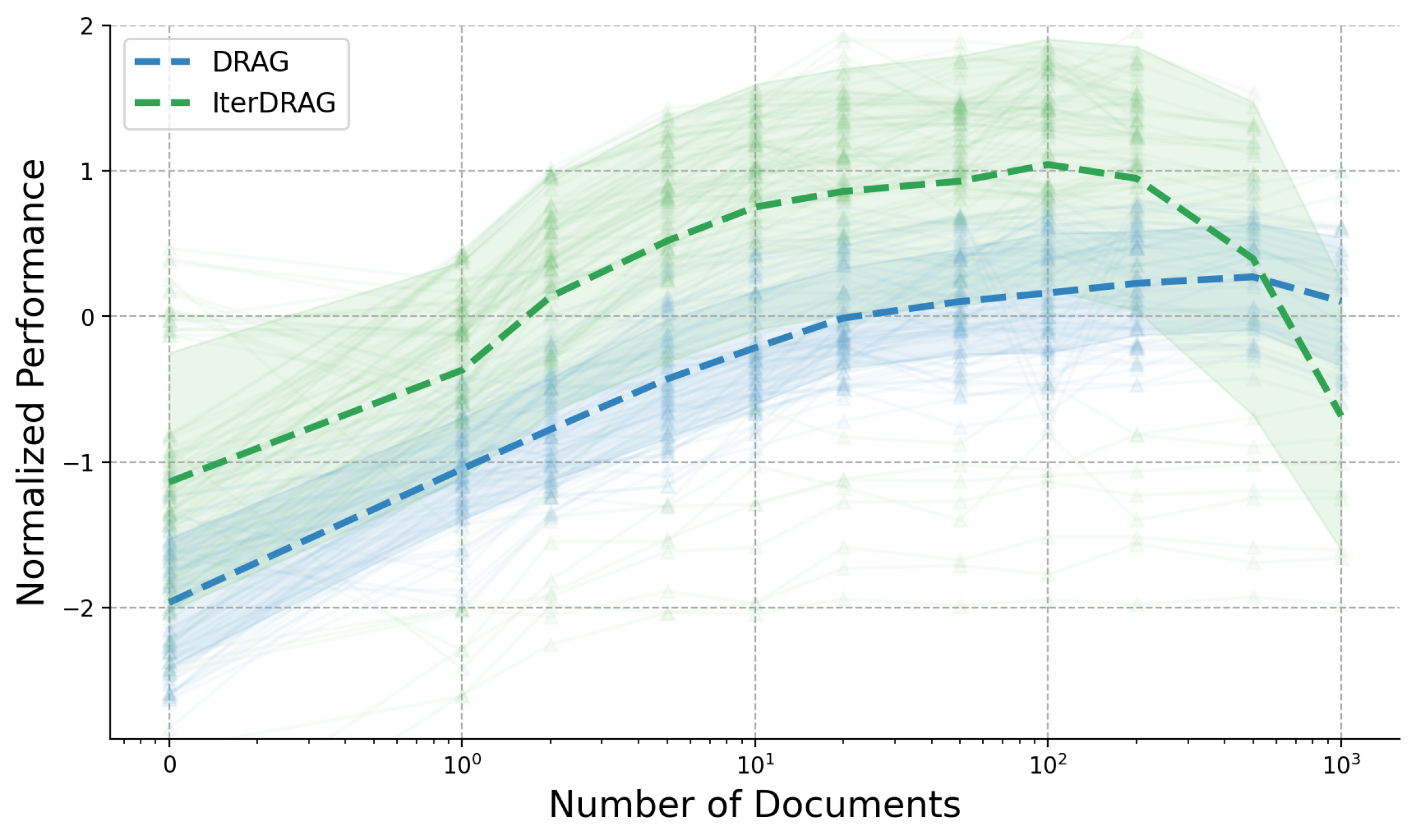
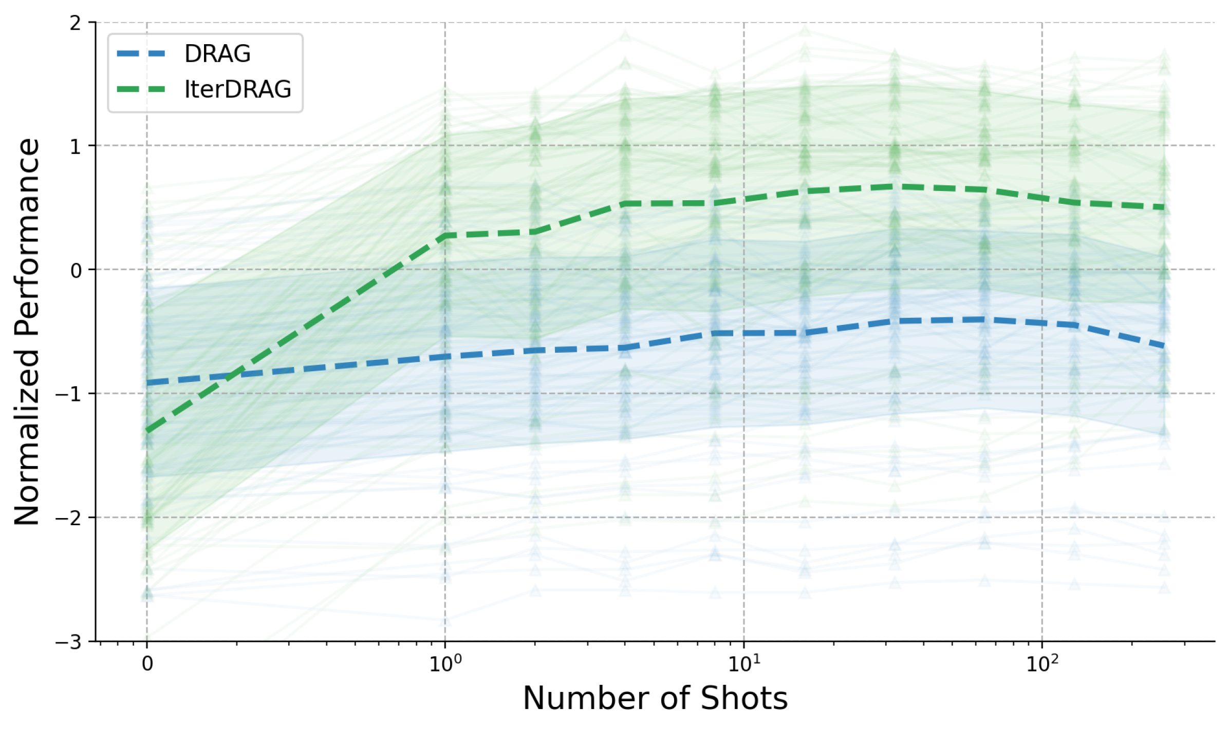
Figure 5: RAG performance changes with varying number of documents and in-context examples. 5(a) reports the averaged metric values across datasets, whereas in 5(b) and 5(c), each line represents the normalized performance of a consistent configuration with progressively increasing documents / shots.
4.4 Parameter-Specific Scaling
To gain further insights into the dynamics of DRAG and IterDRAG, we grid search over different combinations of $\theta$ and evaluate the performance. The results are presented in Figure 5, where we visualize DRAG performance using heatmaps (See IterDRAG heatmap in Appendix C). Additionally, we provide further results with varying numbers of documents ( $k$ ) and shots ( $m$ ). In summary, scaling retrieval, demonstrations and more generation steps leads to performance gains in most cases, yet such gains vary by effective context length and method. In particular, we note: (1) Documents and in-context examples are not equally helpful. For a fixed configuration, increasing the number of retrieved documents $k$ usually leads to more substantial performance gains, as evidenced by the differing slopes in Figure 5. (2) Increasing shots $m$ is more helpful for IterDRAG. For example, increase $m$ from 0 to 1 (rather than $k$ ) is more helpful for IterDRAG, possibly due to demonstrations that leads to improved in-context query decomposition and knowledge extraction. (3) Scaling saturates differently for DRAG and IterDRAG. An example can be found in the increase of $m$ from 0 to 1, which results in significant improvements for IterDRAG but shows little impact on DRAG. Beyond the soft thresholds, further increases in $k$ or $m$ yield marginal gains or even results in performance declines. (4) For a given $L_{\text{max}}$ , the optimal $\theta$ depends on the method, metric and dataset. As illustrated in Figure 5(a) and Figure 8, the optimal combinations are sensitive to the metrics and located differently, posing challenges for performance modeling w.r.t. $\theta$ . In conclusion, increasing documents, demonstrations and iterations can enhance RAG performance, but each contributes differently to the overall results. As such, identifying the optimal combination of hyperparameters remains challenging.
5 Inference Computation Allocation for Long-Context RAG
After examining the overall performance of different RAG strategies and the varying impacts of different inference parameters, we now quantify the relationship between performance and the hyperparameter set $\theta$ . We hypothesize that for long-context RAG, we can model such test-time scaling properties and term it computation allocation model for RAG. This model, in turn, can be used to guide the selection of $\theta$ based on the maximum effective context length $L_{\text{max}}$ .
5.1 Formulation and Estimation
With a slight abuse of notation, we redefine the average performance metric $P$ (e.g., accuracy) on dataset $\mathcal{X}$ as a function of $\theta$ . We consider the number of documents $k$ , demonstrations $m$ and maximum iterations $n$ within $\theta$ , namely $\theta:=(k,m,n)^{T}$ . To account for the variance across methods and tasks, we introduce $i:=(i_{\text{doc}},i_{\text{shot}},0)^{T}$ . $i_{\text{doc}}$ and $i_{\text{shot}}$ measure the informativeness of documents and in-context examples respectively. While technically we can also define an $i_{\text{iter}}$ to measure the informativeness of additional generation steps, applying $i_{\text{iter}}$ does not yield improved accuracy, so we leave it as 0 in our experiments. We formulate the computation allocation model as In our implementation, we shift the values within $\theta$ by a small $\epsilon$ to prevent numerical issues with $\log(0)$ .:
$$
\sigma^{-1}(P(\theta))\approx(a+b\odot i)^{T}\log(\theta)+c, \tag{2}
$$
where $\odot$ refers to element-wise product. $a,b∈\mathbb{R}^{3}$ and $c∈\mathbb{R}$ are parameters to be estimated, and $i$ can be computed base on the specific task. There are different ways to define $i$ ; we choose a definition to compute $i$ based on the performance difference between selected base configurations. In particular, for each strategy on each dataset, $i_{\text{doc}}$ is defined as the performance gain by only adding one document compared to zero-shot QA. Similarly, $i_{\text{shot}}$ is defined as the performance gain by adding only one in-context example compared to zero-shot QA. To account for the sub-linearity in extremely long contexts (above 1M), we apply an inverse sigmoidal mapping $\sigma^{-1}$ to scale the values of the metric $P$ . Further implementation details are reported in Appendix H.
<details>
<summary>x5.png Details</summary>
### Visual Description
# Technical Data Extraction: Normalized Performance vs. Number of Shots
## 1. Document Overview
This image contains four side-by-side scatter plots with regression trend lines and confidence intervals. The charts evaluate the "Normalized Performance" of a system across four different datasets (Bamboogle, HotpotQA, MuSiQue, and 2WikiMultiHopQA) based on the "Number of Shots" provided.
## 2. Global Metadata and Legend
* **Header Legend [Top Center]:**
* `-- 0-Doc` (Blue dashed line/points)
* `-- 1-Doc` (Orange dashed line/points)
* `-- 10-Doc` (Purple dashed line/points)
* `-- 100-Doc` (Grey dashed line/points)
* `-- 1000-Doc` (Light Salmon/Pink dashed line/points)
* **Y-Axis (Common):** "Normalized Performance" (Scale: -3 to 2, increments of 1).
* **X-Axis (Common):** "Number of Shots" (Logarithmic scale: $0, 10^0, 10^1, 10^2$). Note: The '0' shot is plotted on the far left before the log scale break.
---
## 3. Component Analysis by Dataset
### A. Bamboogle
* **Trend Analysis:** All series show a positive correlation between the number of shots and performance.
* **Data Series Details:**
* **0-Doc (Blue):** Lowest performance. Starts at approx. -2.4 (0 shots), rises steadily to approx. -2.0 at 256 shots.
* **1-Doc (Orange):** Starts at approx. -1.2 (0 shots), rises to approx. -0.4 at 256 shots.
* **10-Doc (Purple):** Starts at approx. -0.3 (0 shots), rises to approx. 0.5 at 256 shots.
* **100-Doc (Grey):** Starts at approx. 0.8 (0 shots), rises to approx. 1.5 at 32 shots (data ends early).
* **1000-Doc (Salmon):** Highest performance. Starts at approx. 1.1 (0 shots), rises to approx. 1.5 at 1 shot (data ends early).
### B. HotpotQA
* **Trend Analysis:** Similar upward trajectory across all series, though the slope for 0-Doc is flatter than in Bamboogle.
* **Data Series Details:**
* **0-Doc (Blue):** Starts at approx. -2.5, ends at approx. -2.3.
* **1-Doc (Orange):** Starts at approx. -1.2, ends at approx. -0.4.
* **10-Doc (Purple):** Starts at approx. 0.3, ends at approx. 0.7.
* **100-Doc (Grey):** Starts at approx. 0.5, ends at approx. 0.8 (at 32 shots).
* **1000-Doc (Salmon):** Starts at approx. 0.4, peaks near 0.7 (at 2 shots).
### C. MuSiQue
* **Trend Analysis:** Steeper improvement curves compared to the first two datasets, particularly for the 10-Doc (Purple) series.
* **Data Series Details:**
* **0-Doc (Blue):** Starts at approx. -2.5, ends at approx. -1.7.
* **1-Doc (Orange):** Starts at approx. -2.2 (significant outlier/low start), rises sharply to approx. -0.6.
* **10-Doc (Purple):** Starts at approx. -0.2, rises significantly to approx. 1.2.
* **100-Doc (Grey):** Starts at approx. 0.1, reaches approx. 0.9 (at 32 shots).
* **1000-Doc (Salmon):** Starts at approx. 0.5, reaches approx. 0.8 (at 1 shot).
### D. 2WikiMultiHopQA
* **Trend Analysis:** Shows the widest variance at 0 shots. All series exhibit strong upward trends.
* **Data Series Details:**
* **0-Doc (Blue):** Starts at approx. -2.1, ends at approx. -1.4.
* **1-Doc (Orange):** Starts very low at approx. -2.8, rises sharply to approx. -0.6.
* **10-Doc (Purple):** Starts at approx. -0.5, rises to approx. 1.0.
* **100-Doc (Grey):** Starts at approx. 0.4, reaches approx. 1.1 (at 32 shots).
* **1000-Doc (Salmon):** Starts at approx. 0.0, reaches approx. 0.5 (at 2 shots).
---
## 4. Key Observations & Patterns
1. **Document Count Impact:** There is a clear vertical stratification. Increasing the number of documents (from 0-Doc to 1000-Doc) consistently shifts the performance baseline upward across all datasets.
2. **Shot Scaling:** Performance generally improves as the "Number of Shots" increases from 0 to 256. The improvement is most pronounced in the 1-Doc and 10-Doc series.
3. **Data Density:** The 0-Doc, 1-Doc, and 10-Doc series contain data points up to 256 shots. The 100-Doc series terminates at 32 shots, and the 1000-Doc series terminates at 1 or 2 shots, likely due to context window limitations.
4. **Consistency:** The relative ordering of the document counts (0 < 1 < 10 < 100 < 1000) is maintained across all four benchmarks, indicating a robust correlation between retrieved document volume and model performance.
</details>
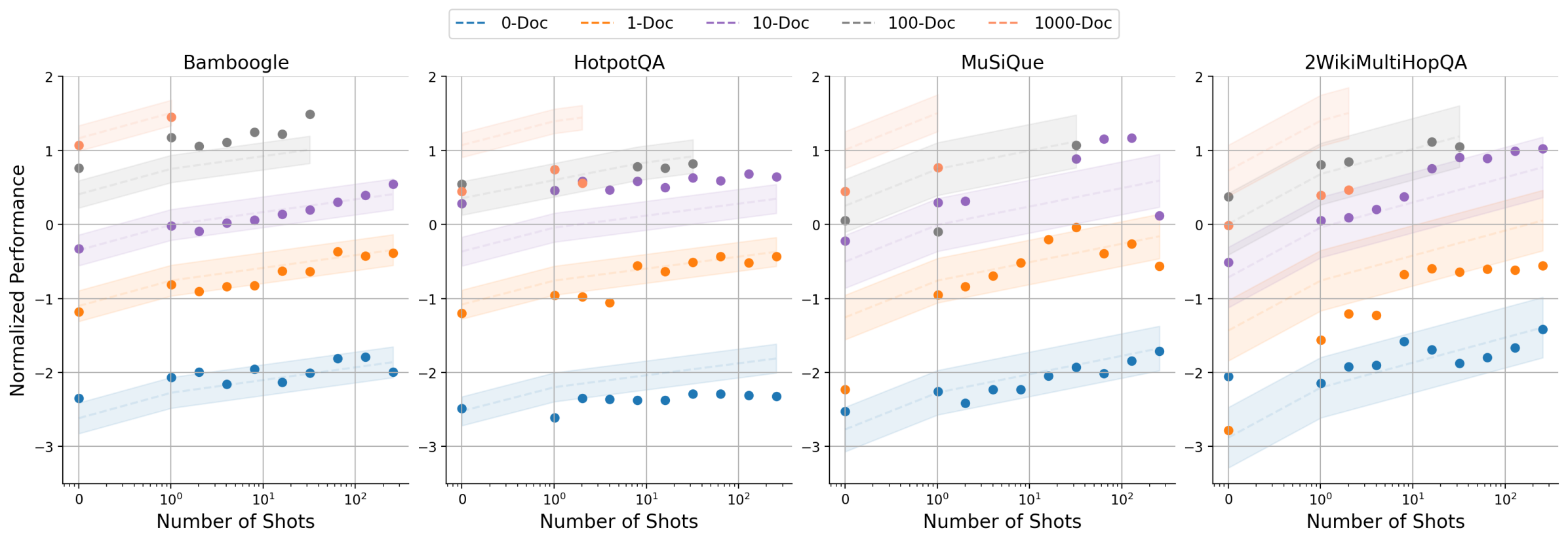
Figure 6: The estimated performance using the proposed observational scaling laws vs. actual metric values in DRAG. The subplots represent different datasets, where each line corresponds to a fixed number of documents, we scale the context length by increasing the number of shots.
In Equation 2, estimations on $a$ , $b$ and $c$ are specific to a certain model, reflecting how LLMs improve with varying number of documents and shots (i.e., in-context learning / zero-shot capabilities). In contrast, $i$ models the performance variations within the selected task (i.e., how external knowledge / demonstrations help responding to the query). Therefore, the computation allocation model can be estimated once and applied to various downstream tasks without requiring additional calibration. To estimate the parameters, varying combinations of $\theta$ are evaluated to perform ordinary least squares on $a$ , $b$ and $c$ . We report the parameters for Gemini 1.5 Flash in Appendix F.
5.2 Validating the Computation Allocation Model for RAG
We evaluate the computation allocation model for RAG by comparing the predicted metrics to the actual values, with normalized results for DRAG visualized in Figure 6. Here, each subplot represents a different dataset, and each line corresponds to a document setting ( $k$ ), we scale the context length by adjusting in-context examples ( $m$ ). As illustrated, the performance improves with the increase of $k$ and $m$ across datasets, displaying highly consistent trends between the predicted and actual metric values, despite some variations. Notably, each dataset exhibits different levels of consistency: Bamboogle exhibits the highest consistency, while HotpotQA generates more variable results. Our findings demonstrate how external knowledge and in-context learning can effectively enhance RAG performance with long-context capabilities, suggesting the effectiveness of the computation allocation model for RAG and how they may be used to predict benchmark results.
Table 2: Ablation study results of the computation allocation model for RAG.
| | Exclude $b$ | Quadratic $\theta$ | Linear $\sigma$ | Sigmoidal $\sigma$ | | | | |
| --- | --- | --- | --- | --- | --- | --- | --- | --- |
| $R^{2}$ | MSE | $R^{2}$ | MSE | $R^{2}$ | MSE | $R^{2}$ | MSE | |
| Values | 0.866 | 0.116 | 0.867 | 0.117 | 0.876 | 0.109 | 0.903 | 0.085 |
Ablation Study.
To verify the effectiveness of the computation allocation model, we perform ablation studies and evaluate the fitting performance of different variants. In particular, we assess: (1) estimation without $b$ and $i$ (i.e., Exclude $b$ ); (2) a quadratic form of input $\log(\theta)$ (Quadratic $\theta$ ); (3) linear scaling of $P$ (Linear $\sigma$ ); and (4) sigmoid scaling of $P$ (Sigmoidal $\sigma$ ). The $R^{2}$ and MSE values for these variants are reported in Table 2, in which (4) represents the complete design of our computation allocation model. The results indicate that incorporating the additional $b$ with $i$ enhances the relevance and reduces error across all tasks. Moreover, applying inverse sigmoid to $P$ significantly improves the estimation in comparison to quadratic $\theta$ or linear scaling.
Table 3: Domain generalization results of the computation allocation model for RAG.
| Baseline Predict Oracle | 49.6 64.0 65.6 | 58.8 75.6 75.6 | 51.2 68.0 68.8 | 46.3 47.8 48.7 | 60.2 63.3 63.3 | 51.4 55.3 55.3 | 14.9 19.3 22.2 | 24.7 32.5 34.3 | 16.9 29.3 30.5 | 46.5 60.8 65.7 | 53.7 72.4 75.2 | 51.6 74.9 76.4 |
| --- | --- | --- | --- | --- | --- | --- | --- | --- | --- | --- | --- | --- |
Domain Generalization.
We also examine the generalization of the computation allocation model for RAG for unseen domains. In other words, the parameters of Equation 2 are tested on the target domain but learnt from the remaining domains. For inference, only $i$ is derived from the target domain. We report the results for 1M effective context length in Table 3, where we compare to an 8-shot baseline configuration (scaled by increasing retrieved documents) and the optimum results (Oracle). In summary, the results show that computation allocation model significantly outperforms baseline and closely aligns with the oracle results (96.6% of the optimal performance). Notably, Bamboogle and HotpotQA exhibit highly similar target results, with the performance metrics varying by less than 2.5% from the oracle. These results suggest the potential of applying the computation allocation model for RAG to a wider range of knowledge-intensive tasks.
Table 4: Length extrapolation results of the computation allocation model for RAG.
| Baseline Predict Oracle | 37.4 37.4 39.2 | 47.6 48.2 49.8 | 40.4 41.0 42.7 | 39.0 41.2 46.9 | 49.5 52.0 59.0 | 42.2 45.4 55.1 | 39.3 48.0 50.5 | 49.3 60.9 62.1 | 42.8 56.9 57.7 | 44.5 47.9 51.7 | 55.4 59.8 62.6 | 49.8 55.2 58.1 |
| --- | --- | --- | --- | --- | --- | --- | --- | --- | --- | --- | --- | --- |
Length Extrapolation.
In addition to predictability on unseen domains, we explore the extrapolation of context length based on the computation allocation model. Here, we estimate the parameters of Equation 2 using experiments with shorter context lengths and assess their predictive accuracy on longer ones. We assess different extrapolation settings and present the predicted metric values in Table 4. Our observations are: (1) The predictions are accurate and consistently outperform the 8-shot baseline. For instance, the average difference between the predicted and oracle results from 128k to 1M tokens is just 2.8%. (2) Extrapolating from 32k to 128k is challenging. This is because DRAG performs best around 32k, while IterDRAG typically excels at a long context of 128k, as evidenced in Figure 4. Consequently, it creates a discrepancy between training and predicting performance distribution. (3) 5M context length is less predictable, with the average performance difference between predicted and oracle metrics observed at a substantial 5.6%. Overall, length extrapolation with computation allocation model is accurate and more effective for target lengths below 1M.
6 Discussion
Retrieval.
One critical factor in improving performance of RAG lies in the quality of the retrieved documents. To study how retrieval impacts final accuracy, we analyze retrieval performance and report the results across different document sizes in Appendix A. In all datasets, recall scores demonstrate improvements as the number of documents increases, approaching near-perfect scores with large document sets (e.g., $\sim$ 1k). Despite consistent gains in recall, the results show diminishing returns on discounted ranking metrics like NDCG, indicating increasing distraction within the context. This trend is also evident in in Figure 5(b), where RAG performance peaks between 100 and 500 documents. Our observations suggest the necessity of refining retrieval (e.g., through re-ranking) to further optimize the document relevance, particularly in cases of complex, multi-hop queries. However, how the inference scaling behavior discovered in this paper would change in the presence of such a refining component remains unknown. Alternatively, iterative retrieval, as seen in IterDRAG, improves recall performance by using simpler, straightforward sub-queries to collect additional context for each intermediate answer. In summary, retrieving more documents improves recall but does not necessarily lead to better generation quality if the documents are not effectively ranked or filtered. This highlights the need for retrieval methods that dynamically adjust to minimize irrelevant content.
Error Analysis.
Despite overall improvements, our error analysis in Appendix G reveals that certain errors persist, particularly in cases of compositional reasoning tasks where multiple hops of reasoning are required. The common errors fall into four categories: (1) inaccurate or outdated retrieval; (2) incorrect or lack of reasoning; (3) hallucination or unfaithful reasoning; and (4) evaluation issues or refusal to answer. The first category highlights the need for enhancing retrieval methods and maintaining a reliable & up-to-date knowledge base, specially for complex questions that rely on multiple supporting facts. In addition, incorrect or missing reasoning steps often result in errors or partially correct answers. In our experiments, we observe that both (1) and (2) are substantially improved with IterDRAG, suggesting the importance of interleaving retrieval and iterative generation for multi-hop queries. Moreover, developing faithful LLMs and strategies to mitigate hallucination could further enhance RAG performance. Finally, we note that existing metrics fail in certain cases (e.g., abbreviations), underscoring the need for more robust and reliable evaluation methods.
Long-Context Modeling.
We also discuss the impact of long-context modeling w.r.t. RAG performance. In summary, we find that retrieving more documents is generally beneficial for RAG performance, as demonstrated in Section 4. Nevertheless, naïvely extending the context length in each generation step does not always lead to better results. Specifically, DRAG performance peaks at around $10^{5}$ tokens, while IterDRAG achieves optimal performance at around $10^{6}$ tokens by leveraging multiple rounds of generation. For instance, as seen in the performance plateau in Figure 1 and Figure 11, LLMs struggle to effectively utilize very long contexts ( $≥ 10^{5}$ tokens) in each iteration, potentially due to inherent limitations of long-context modeling. Our observations suggest that: (1) the model’s ability to identify relevant information from extensive context remains to be improved, especially when presented with large quantity of “similar” documents; (2) the long-context modeling should be further refined to enhance in-context learning capabilities, where multiple lengthy demonstrations are provided.
Trade-Off Between Inference Compute and RAG Performance.
In our experiments, we observe consistent benefits of inference scaling using DRAG and IterDRAG, potentially changing the optimal trade-off between inference compute and RAG performance. Existing methods often exhibit diminishing returns when scaling inference compute beyond certain thresholds where RAG performance plateaus. As a result, the optimal trade-off between inference compute and RAG performance is unlikely to be found beyond these thresholds, as further investment in scaling inference compute becomes inefficient. In contrast, our findings demonstrate that long-context RAG performance can improve almost linearly with increased test-time compute when optimally allocated. Therefore, the optimal trade-off in our setting largely depends on the inference budget, with higher budgets consistently yielding steady gains. Combined with the computation allocation model for RAG, this approach enables the derivation of a (nearly) optimal solution for long-context RAG given computation constraints.
7 Conclusion
In this paper, we explore inference scaling in long-context RAG. By systematically studying the performance with different inference configurations, we demonstrate that RAG performance improves almost linearly with the increasing order of magnitude of the test-time compute under optimal inference parameters. Based on our observations, we derive inference scaling laws for RAG and the corresponding computation allocation model, designed to predict RAG performance on varying hyperparameters. Through extensive experiments, we show that optimal configurations can be accurately estimated and align closely with the experimental results. These insights provide a strong foundation for future research in optimizing inference strategies for long-context RAG.
References
- Achiam et al. (2023) J. Achiam, S. Adler, S. Agarwal, L. Ahmad, I. Akkaya, F. L. Aleman, D. Almeida, J. Altenschmidt, S. Altman, S. Anadkat, et al. GPT-4 technical report. arXiv preprint arXiv:2303.08774, 2023.
- (2) R. Agarwal, A. Singh, L. M. Zhang, B. Bohnet, L. Rosias, S. C. Chan, B. Zhang, A. Faust, and H. Larochelle. Many-shot in-context learning. In ICML 2024 Workshop on In-Context Learning.
- Beck et al. (2024) M. Beck, K. Pöppel, M. Spanring, A. Auer, O. Prudnikova, M. Kopp, G. Klambauer, J. Brandstetter, and S. Hochreiter. xLSTM: Extended long short-term memory. arXiv preprint arXiv:2405.04517, 2024.
- Beltagy et al. (2020) I. Beltagy, M. E. Peters, and A. Cohan. Longformer: The long-document transformer. arXiv preprint arXiv:2004.05150, 2020.
- Bertsch et al. (2024) A. Bertsch, M. Ivgi, U. Alon, J. Berant, M. R. Gormley, and G. Neubig. In-context learning with long-context models: An in-depth exploration. arXiv preprint arXiv:2405.00200, 2024.
- Borgeaud et al. (2022) S. Borgeaud, A. Mensch, J. Hoffmann, T. Cai, E. Rutherford, K. Millican, G. B. Van Den Driessche, J.-B. Lespiau, B. Damoc, A. Clark, et al. Improving language models by retrieving from trillions of tokens. In International conference on machine learning, pages 2206–2240. PMLR, 2022.
- Brown et al. (2020) T. Brown, B. Mann, N. Ryder, M. Subbiah, J. D. Kaplan, P. Dhariwal, A. Neelakantan, P. Shyam, G. Sastry, A. Askell, et al. Language models are few-shot learners. Advances in neural information processing systems, 33:1877–1901, 2020.
- Chen et al. (2023) S. Chen, S. Wong, L. Chen, and Y. Tian. Extending context window of large language models via positional interpolation. arXiv preprint arXiv:2306.15595, 2023.
- Choromanski et al. (2020) K. Choromanski, V. Likhosherstov, D. Dohan, X. Song, A. Gane, T. Sarlos, P. Hawkins, J. Davis, A. Mohiuddin, L. Kaiser, et al. Rethinking attention with performers. arXiv preprint arXiv:2009.14794, 2020.
- Dao et al. (2022) T. Dao, D. Fu, S. Ermon, A. Rudra, and C. Ré. Flashattention: Fast and memory-efficient exact attention with IO-awareness. Advances in Neural Information Processing Systems, 35:16344–16359, 2022.
- Geva et al. (2021) M. Geva, D. Khashabi, E. Segal, T. Khot, D. Roth, and J. Berant. Did Aristotle use a laptop? a question answering benchmark with implicit reasoning strategies. Transactions of the Association for Computational Linguistics, 9:346–361, 2021.
- Gu and Dao (2023) A. Gu and T. Dao. Mamba: Linear-time sequence modeling with selective state spaces. arXiv preprint arXiv:2312.00752, 2023.
- Gu et al. (2021) A. Gu, K. Goel, and C. Ré. Efficiently modeling long sequences with structured state spaces. arXiv preprint arXiv:2111.00396, 2021.
- Gu et al. (2023) Y. Gu, L. Dong, F. Wei, and M. Huang. Pre-training to learn in context. In Proceedings of the 61st Annual Meeting of the Association for Computational Linguistics (Volume 1: Long Papers), pages 4849–4870, 2023.
- Gutiérrez et al. (2024) B. J. Gutiérrez, Y. Shu, Y. Gu, M. Yasunaga, and Y. Su. HippoRAG: Neurobiologically inspired long-term memory for large language models. arXiv preprint arXiv:2405.14831, 2024.
- Guu et al. (2020) K. Guu, K. Lee, Z. Tung, P. Pasupat, and M. Chang. Retrieval augmented language model pre-training. In International conference on machine learning, pages 3929–3938. PMLR, 2020.
- Ho et al. (2020) X. Ho, A.-K. D. Nguyen, S. Sugawara, and A. Aizawa. Constructing a multi-hop QA dataset for comprehensive evaluation of reasoning steps. In Proceedings of the 28th International Conference on Computational Linguistics, pages 6609–6625, 2020.
- Izacard and Grave (2021) G. Izacard and É. Grave. Leveraging passage retrieval with generative models for open domain question answering. In Proceedings of the 16th Conference of the European Chapter of the Association for Computational Linguistics: Main Volume, pages 874–880, 2021.
- Izacard et al. (2023) G. Izacard, P. Lewis, M. Lomeli, L. Hosseini, F. Petroni, T. Schick, J. Dwivedi-Yu, A. Joulin, S. Riedel, and E. Grave. Atlas: Few-shot learning with retrieval augmented language models. Journal of Machine Learning Research, 24(251):1–43, 2023.
- Jacobs et al. (2023) S. A. Jacobs, M. Tanaka, C. Zhang, M. Zhang, L. Song, S. Rajbhandari, and Y. He. DeepSpeed Ulysses: System optimizations for enabling training of extreme long sequence transformer models. arXiv preprint arXiv:2309.14509, 2023.
- Jiang et al. (2023) Z. Jiang, F. F. Xu, L. Gao, Z. Sun, Q. Liu, J. Dwivedi-Yu, Y. Yang, J. Callan, and G. Neubig. Active retrieval augmented generation. In Proceedings of the 2023 Conference on Empirical Methods in Natural Language Processing, pages 7969–7992, 2023.
- Jiang et al. (2024) Z. Jiang, X. Ma, and W. Chen. LongRAG: Enhancing retrieval-augmented generation with long-context LLMs. arXiv preprint arXiv:2406.15319, 2024.
- Joshi et al. (2017) M. Joshi, E. Choi, D. S. Weld, and L. Zettlemoyer. TriviaQA: A large scale distantly supervised challenge dataset for reading comprehension. In Proceedings of the 55th Annual Meeting of the Association for Computational Linguistics (Volume 1: Long Papers), pages 1601–1611, 2017.
- Karpukhin et al. (2020) V. Karpukhin, B. Oguz, S. Min, P. Lewis, L. Wu, S. Edunov, D. Chen, and W.-t. Yih. Dense passage retrieval for open-domain question answering. In Proceedings of the 2020 Conference on Empirical Methods in Natural Language Processing (EMNLP), pages 6769–6781, 2020.
- Khandelwal et al. (2019) U. Khandelwal, O. Levy, D. Jurafsky, L. Zettlemoyer, and M. Lewis. Generalization through memorization: Nearest neighbor language models. In International Conference on Learning Representations, 2019.
- Kitaev et al. (2019) N. Kitaev, L. Kaiser, and A. Levskaya. Reformer: The efficient transformer. In International Conference on Learning Representations, 2019.
- Koo et al. (2024) T. Koo, F. Liu, and L. He. Automata-based constraints for language model decoding. arXiv preprint arXiv:2407.08103, 2024.
- Kuratov et al. (2024) Y. Kuratov, A. Bulatov, P. Anokhin, I. Rodkin, D. Sorokin, A. Sorokin, and M. Burtsev. BABILong: Testing the limits of LLMs with long context reasoning-in-a-haystack. arXiv preprint arXiv:2406.10149, 2024.
- Kwiatkowski et al. (2019) T. Kwiatkowski, J. Palomaki, O. Redfield, M. Collins, A. Parikh, C. Alberti, D. Epstein, I. Polosukhin, J. Devlin, K. Lee, et al. Natural questions: a benchmark for question answering research. Transactions of the Association for Computational Linguistics, 7:453–466, 2019.
- Lee et al. (2024a) J. Lee, A. Chen, Z. Dai, D. Dua, D. S. Sachan, M. Boratko, Y. Luan, S. M. Arnold, V. Perot, S. Dalmia, et al. Can long-context language models subsume retrieval, RAG, SQL, and more? arXiv preprint arXiv:2406.13121, 2024a.
- Lee et al. (2024b) J. Lee, Z. Dai, X. Ren, B. Chen, D. Cer, J. R. Cole, K. Hui, M. Boratko, R. Kapadia, W. Ding, et al. Gecko: Versatile text embeddings distilled from large language models. arXiv preprint arXiv:2403.20327, 2024b.
- Leng et al. (2024) Q. Leng, J. Portes, S. Havens, M. Zaharia, and M. Carbin. Long context rag performance of large language models. arXiv preprint arXiv:2411.03538, 2024.
- Lewis et al. (2020) P. Lewis, E. Perez, A. Piktus, F. Petroni, V. Karpukhin, N. Goyal, H. Küttler, M. Lewis, W.-t. Yih, T. Rocktäschel, et al. Retrieval-augmented generation for knowledge-intensive NLP tasks. Advances in Neural Information Processing Systems, 33:9459–9474, 2020.
- Li et al. (2023) M. Li, S. Gong, J. Feng, Y. Xu, J. Zhang, Z. Wu, and L. Kong. In-context learning with many demonstration examples. arXiv preprint arXiv:2302.04931, 2023.
- Li et al. (2024) T. Li, G. Zhang, Q. D. Do, X. Yue, and W. Chen. Long-context LLMs struggle with long in-context learning. arXiv preprint arXiv:2404.02060, 2024.
- Lin et al. (2024) X. V. Lin, X. Chen, M. Chen, W. Shi, M. Lomeli, R. James, P. Rodriguez, J. Kahn, G. Szilvasy, M. Lewis, et al. RA-DIT: Retrieval-augmented dual instruction tuning. In The Twelfth International Conference on Learning Representations, 2024.
- Liu et al. (2023) H. Liu, M. Zaharia, and P. Abbeel. Ring attention with blockwise transformers for near-infinite context. arXiv preprint arXiv:2310.01889, 2023.
- Liu et al. (2022) J. Liu, D. Shen, Y. Zhang, W. B. Dolan, L. Carin, and W. Chen. What makes good in-context examples for GPT-3? In Proceedings of Deep Learning Inside Out (DeeLIO 2022): The 3rd Workshop on Knowledge Extraction and Integration for Deep Learning Architectures, pages 100–114, 2022.
- Liu et al. (2024a) S. Liu, H. Ye, L. Xing, and J. Y. Zou. In-context vectors: Making in context learning more effective and controllable through latent space steering. In Forty-first International Conference on Machine Learning, 2024a.
- Liu et al. (2024b) Z. Liu, W. Ping, R. Roy, P. Xu, C. Lee, M. Shoeybi, and B. Catanzaro. ChatQA: Surpassing GPT-4 on conversational QA and RAG. arXiv preprint arXiv:2401.10225, 2024b.
- Lu et al. (2022) Y. Lu, M. Bartolo, A. Moore, S. Riedel, and P. Stenetorp. Fantastically ordered prompts and where to find them: Overcoming few-shot prompt order sensitivity. In Proceedings of the 60th Annual Meeting of the Association for Computational Linguistics (Volume 1: Long Papers), pages 8086–8098, 2022.
- Ma et al. (2023) X. Ma, Y. Gong, P. He, H. Zhao, and N. Duan. Query rewriting in retrieval-augmented large language models. In Proceedings of the 2023 Conference on Empirical Methods in Natural Language Processing, pages 5303–5315, 2023.
- Min et al. (2022) S. Min, M. Lewis, L. Zettlemoyer, and H. Hajishirzi. MetaICL: Learning to learn in context. In Proceedings of the 2022 Conference of the North American Chapter of the Association for Computational Linguistics: Human Language Technologies, pages 2791–2809, 2022.
- Ni et al. (2021) J. Ni, C. Qu, J. Lu, Z. Dai, G. H. Ábrego, J. Ma, V. Y. Zhao, Y. Luan, K. B. Hall, M.-W. Chang, et al. Large dual encoders are generalizable retrievers. arXiv preprint arXiv:2112.07899, 2021.
- Peng et al. (2023a) B. Peng, E. Alcaide, Q. Anthony, A. Albalak, S. Arcadinho, S. Biderman, H. Cao, X. Cheng, M. Chung, L. Derczynski, et al. RWKV: Reinventing rnns for the transformer era. In Findings of the Association for Computational Linguistics: EMNLP 2023, pages 14048–14077, 2023a.
- Peng et al. (2023b) B. Peng, J. Quesnelle, H. Fan, and E. Shippole. Yarn: Efficient context window extension of large language models. arXiv preprint arXiv:2309.00071, 2023b.
- Petroni et al. (2020) F. Petroni, A. Piktus, A. Fan, P. Lewis, M. Yazdani, N. De Cao, J. Thorne, Y. Jernite, V. Karpukhin, J. Maillard, et al. KILT: a benchmark for knowledge intensive language tasks. arXiv preprint arXiv:2009.02252, 2020.
- Press et al. (2021) O. Press, N. A. Smith, and M. Lewis. Train short, test long: Attention with linear biases enables input length extrapolation. arXiv preprint arXiv:2108.12409, 2021.
- Press et al. (2023) O. Press, M. Zhang, S. Min, L. Schmidt, N. A. Smith, and M. Lewis. Measuring and narrowing the compositionality gap in language models. In Findings of the Association for Computational Linguistics: EMNLP 2023, pages 5687–5711, 2023.
- Ram et al. (2023) O. Ram, Y. Levine, I. Dalmedigos, D. Muhlgay, A. Shashua, K. Leyton-Brown, and Y. Shoham. In-context retrieval-augmented language models. Transactions of the Association for Computational Linguistics, 11:1316–1331, 2023.
- Reid et al. (2024) M. Reid, N. Savinov, D. Teplyashin, D. Lepikhin, T. Lillicrap, J.-b. Alayrac, R. Soricut, A. Lazaridou, O. Firat, J. Schrittwieser, et al. Gemini 1.5: Unlocking multimodal understanding across millions of tokens of context. arXiv preprint arXiv:2403.05530, 2024.
- Rubin et al. (2022) O. Rubin, J. Herzig, and J. Berant. Learning to retrieve prompts for in-context learning. In Proceedings of the 2022 Conference of the North American Chapter of the Association for Computational Linguistics: Human Language Technologies, pages 2655–2671, 2022.
- Sarthi et al. (2024) P. Sarthi, S. Abdullah, A. Tuli, S. Khanna, A. Goldie, and C. D. Manning. RAPTOR: Recursive abstractive processing for tree-organized retrieval. In The Twelfth International Conference on Learning Representations, 2024.
- Shao et al. (2024) R. Shao, J. He, A. Asai, W. Shi, T. Dettmers, S. Min, L. Zettlemoyer, and P. W. Koh. Scaling retrieval-based language models with a trillion-token datastore. arXiv preprint arXiv:2407.12854, 2024.
- Shi et al. (2024) W. Shi, S. Min, M. Yasunaga, M. Seo, R. James, M. Lewis, L. Zettlemoyer, and W.-t. Yih. REPLUG: Retrieval-augmented black-box language models. In Proceedings of the 2024 Conference of the North American Chapter of the Association for Computational Linguistics: Human Language Technologies (Volume 1: Long Papers), pages 8364–8377, 2024.
- Snell et al. (2024) C. Snell, J. Lee, K. Xu, and A. Kumar. Scaling LLM test-time compute optimally can be more effective than scaling model parameters. arXiv preprint arXiv:2408.03314, 2024.
- Sun et al. (2024) P. Sun, D. Simcha, D. Dopson, R. Guo, and S. Kumar. SOAR: improved indexing for approximate nearest neighbor search. Advances in Neural Information Processing Systems, 36, 2024.
- Sun et al. (2023) Y. Sun, L. Dong, B. Patra, S. Ma, S. Huang, A. Benhaim, V. Chaudhary, X. Song, and F. Wei. A length-extrapolatable transformer. In Proceedings of the 61st Annual Meeting of the Association for Computational Linguistics (Volume 1: Long Papers), pages 14590–14604, 2023.
- Team et al. (2023) G. Team, R. Anil, S. Borgeaud, Y. Wu, J.-B. Alayrac, J. Yu, R. Soricut, J. Schalkwyk, A. M. Dai, A. Hauth, et al. Gemini: a family of highly capable multimodal models. arXiv preprint arXiv:2312.11805, 2023.
- Trivedi et al. (2022) H. Trivedi, N. Balasubramanian, T. Khot, and A. Sabharwal. MuSiQue: Multihop questions via single-hop question composition. Transactions of the Association for Computational Linguistics, 10:539–554, 2022.
- Trivedi et al. (2023) H. Trivedi, N. Balasubramanian, T. Khot, and A. Sabharwal. Interleaving retrieval with chain-of-thought reasoning for knowledge-intensive multi-step questions. In Proceedings of the 61st Annual Meeting of the Association for Computational Linguistics (Volume 1: Long Papers), pages 10014–10037, 2023.
- Wang et al. (2024) X. Wang, W. Zhu, M. Saxon, M. Steyvers, and W. Y. Wang. Large language models are latent variable models: Explaining and finding good demonstrations for in-context learning. Advances in Neural Information Processing Systems, 36, 2024.
- Wei et al. (2022) J. Wei, X. Wang, D. Schuurmans, M. Bosma, F. Xia, E. Chi, Q. V. Le, D. Zhou, et al. Chain-of-thought prompting elicits reasoning in large language models. Advances in neural information processing systems, 35:24824–24837, 2022.
- Wei et al. (2023) J. Wei, L. Hou, A. Lampinen, X. Chen, D. Huang, Y. Tay, X. Chen, Y. Lu, D. Zhou, T. Ma, et al. Symbol tuning improves in-context learning in language models. In Proceedings of the 2023 Conference on Empirical Methods in Natural Language Processing, pages 968–979, 2023.
- Wu et al. (2024) K. Wu, E. Wu, and J. Zou. How faithful are RAG models? quantifying the tug-of-war between RAG and LLMs’ internal prior. arXiv preprint arXiv:2404.10198, 2024.
- Wu et al. (2023) Z. Wu, Y. Wang, J. Ye, and L. Kong. Self-adaptive in-context learning: An information compression perspective for in-context example selection and ordering. In Proceedings of the 61st Annual Meeting of the Association for Computational Linguistics (Volume 1: Long Papers), pages 1423–1436, 2023.
- Xu et al. (2024) P. Xu, W. Ping, X. Wu, L. McAfee, C. Zhu, Z. Liu, S. Subramanian, E. Bakhturina, M. Shoeybi, and B. Catanzaro. Retrieval meets long context large language models. In The Twelfth International Conference on Learning Representations, 2024.
- Yan et al. (2024) S.-Q. Yan, J.-C. Gu, Y. Zhu, and Z.-H. Ling. Corrective retrieval augmented generation. arXiv preprint arXiv:2401.15884, 2024.
- Yang et al. (2018) Z. Yang, P. Qi, S. Zhang, Y. Bengio, W. Cohen, R. Salakhutdinov, and C. D. Manning. HotpotQA: A dataset for diverse, explainable multi-hop question answering. In Proceedings of the 2018 Conference on Empirical Methods in Natural Language Processing, pages 2369–2380, 2018.
- Yoran et al. (2024) O. Yoran, T. Wolfson, O. Ram, and J. Berant. Making retrieval-augmented language models robust to irrelevant context. In The Twelfth International Conference on Learning Representations, 2024.
- Yu et al. (2023) W. Yu, H. Zhang, X. Pan, K. Ma, H. Wang, and D. Yu. Chain-of-note: Enhancing robustness in retrieval-augmented language models. arXiv preprint arXiv:2311.09210, 2023.
- Yue et al. (2024) Z. Yue, H. Zeng, Y. Lu, L. Shang, Y. Zhang, and D. Wang. Evidence-driven retrieval augmented response generation for online misinformation. arXiv preprint arXiv:2403.14952, 2024.
- Zaheer et al. (2020) M. Zaheer, G. Guruganesh, K. A. Dubey, J. Ainslie, C. Alberti, S. Ontanon, P. Pham, A. Ravula, Q. Wang, L. Yang, et al. Big bird: Transformers for longer sequences. Advances in neural information processing systems, 33:17283–17297, 2020.
- Zhang et al. (2024) T. Zhang, S. G. Patil, N. Jain, S. Shen, M. Zaharia, I. Stoica, and J. E. Gonzalez. RAFT: Adapting language model to domain specific rag. arXiv preprint arXiv:2403.10131, 2024.
Appendix A Retrieval Quality
We assess the retrieval quality of DRAG and IterDRAG using the Gecko-1B model (Lee et al., 2024b) and evaluate their impact on final RAG performance. Specifically, we retrieve varying numbers of documents per input query and measure the retrieval quality using three metrics: Recall, NDCG, and MRR, with document counts ranging from 1 to 2k. The retrieval results of DRAG are shown in Figure 7. In addition, we evaluate the quality of iterative retrieval, where a maximum of five interleaving retrieval steps are performed. Here, we retrieve 50 documents at each step and use a 2-shot setting, with the results in comparison to DRAG in Table 5.
<details>
<summary>x6.png Details</summary>
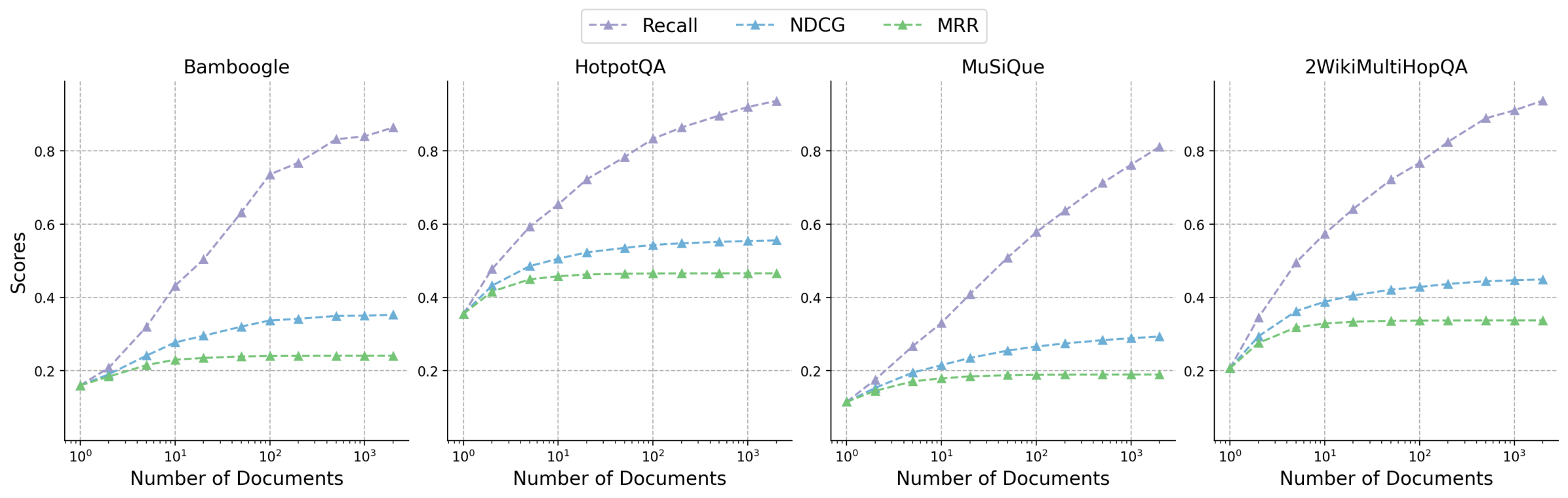
### Visual Description
# Technical Data Extraction: Retrieval Performance Metrics
This document provides a comprehensive extraction of the data and trends presented in the provided image, which consists of four line charts evaluating retrieval performance across different datasets.
## 1. Metadata and Global Components
* **Image Type:** Multi-panel line chart (4 subplots).
* **Primary Language:** English.
* **Global Legend:** Located at the top center of the image.
* **Recall:** Purple dashed line with triangle markers ($\triangle$).
* **NDCG:** Blue dashed line with triangle markers ($\triangle$).
* **MRR:** Green dashed line with triangle markers ($\triangle$).
* **X-Axis (All Subplots):** "Number of Documents". Logarithmic scale ranging from $10^0$ (1) to $2 \times 10^3$ (2000).
* **Y-Axis (All Subplots):** "Scores". Linear scale ranging from 0.2 to 0.8 (with some data points extending to ~0.1 and ~0.9).
* **Grid:** Light gray dashed grid lines for both major x-axis log intervals and y-axis increments of 0.2.
---
## 2. Subplot Analysis
### Subplot 1: Bamboogle
* **Trend Analysis:**
* **Recall (Purple):** Shows a strong, consistent upward slope. It starts as the lowest metric at $x=1$ and becomes the highest by a significant margin as the number of documents increases.
* **NDCG (Blue):** Slopes upward moderately, beginning to plateau around $x=100$.
* **MRR (Green):** Slopes upward slightly at first, then plateaus almost completely after $x=10$.
* **Data Points (Approximate):**
* **At $x=1$:** Recall $\approx$ 0.16, NDCG $\approx$ 0.16, MRR $\approx$ 0.16.
* **At $x=10$:** Recall $\approx$ 0.43, NDCG $\approx$ 0.28, MRR $\approx$ 0.23.
* **At $x=2000$:** Recall $\approx$ 0.86, NDCG $\approx$ 0.35, MRR $\approx$ 0.24.
### Subplot 2: HotpotQA
* **Trend Analysis:**
* **Recall (Purple):** Strong logarithmic growth, curving upward throughout the range.
* **NDCG (Blue):** Moderate growth, showing signs of saturation/plateau after $x=100$.
* **MRR (Green):** Rapid initial growth from $x=1$ to $x=10$, followed by a flat plateau.
* **Data Points (Approximate):**
* **At $x=1$:** All metrics converge at $\approx$ 0.35.
* **At $x=10$:** Recall $\approx$ 0.65, NDCG $\approx$ 0.50, MRR $\approx$ 0.45.
* **At $x=2000$:** Recall $\approx$ 0.94, NDCG $\approx$ 0.55, MRR $\approx$ 0.46.
### Subplot 3: MuSiQue
* **Trend Analysis:**
* **Recall (Purple):** Steady, nearly linear growth on the log scale.
* **NDCG (Blue):** Slow, steady growth, maintaining a significant gap below Recall.
* **MRR (Green):** Very slight initial growth, reaching a plateau very early (around $x=5$).
* **Data Points (Approximate):**
* **At $x=1$:** All metrics converge at $\approx$ 0.11.
* **At $x=10$:** Recall $\approx$ 0.33, NDCG $\approx$ 0.21, MRR $\approx$ 0.18.
* **At $x=2000$:** Recall $\approx$ 0.81, NDCG $\approx$ 0.29, MRR $\approx$ 0.19.
### Subplot 4: 2WikiMultiHopQA
* **Trend Analysis:**
* **Recall (Purple):** Strong upward trajectory, similar to HotpotQA.
* **NDCG (Blue):** Moderate growth, leveling off after $x=50$.
* **MRR (Green):** Initial growth until $x=10$, then remains perfectly flat.
* **Data Points (Approximate):**
* **At $x=1$:** All metrics converge at $\approx$ 0.21.
* **At $x=10$:** Recall $\approx$ 0.57, NDCG $\approx$ 0.38, MRR $\approx$ 0.33.
* **At $x=2000$:** Recall $\approx$ 0.93, NDCG $\approx$ 0.45, MRR $\approx$ 0.34.
---
## 3. Summary of Findings
| Dataset | Starting Score (x=1) | Final Recall (x=2000) | Final NDCG (x=2000) | Final MRR (x=2000) |
| :--- | :--- | :--- | :--- | :--- |
| **Bamboogle** | ~0.16 | ~0.86 | ~0.35 | ~0.24 |
| **HotpotQA** | ~0.35 | ~0.94 | ~0.55 | ~0.46 |
| **MuSiQue** | ~0.11 | ~0.81 | ~0.29 | ~0.19 |
| **2WikiMultiHopQA** | ~0.21 | ~0.93 | ~0.45 | ~0.34 |
**Key Observations:**
1. **Recall** is the most sensitive metric to the number of documents, showing continuous improvement as more documents are retrieved across all datasets.
2. **MRR (Mean Reciprocal Rank)** is the least sensitive, typically plateauing after only 10 documents are retrieved. This suggests that the "correct" answer is rarely found deeper in the results if it wasn't in the top 10.
3. **HotpotQA** shows the highest overall performance across all metrics, while **MuSiQue** shows the lowest.
4. In all cases, at $x=1$ (retrieving only one document), Recall, NDCG, and MRR are identical, which is mathematically expected for these metrics at $k=1$.
</details>
Figure 7: Retrieval performance of DRAG on different datasets.
In Figure 7, recall demonstrates consistent improvements as the number of documents increases, approaching near-perfect scores when large document sets (e.g., 1k) are retrieved. However, both NDCG and MRR metrics plateau early at around 100 documents, with diminishing gains as the document count further rises. This divergence suggests that while more documents lead to better recall, the relevance and ranking quality (captured by NDCG and MRR) do not improve proportionally, and even introduce extensive noise. Therefore, higher recall doesn’t necessarily translate into better final answer quality when the retrieved documents aren’t effectively ranked or filtered.
Table 5: Retrieval performance of DRAG and IterDRAG ( $k=50$ documents, $m=2$ shots).
| DRAG IterDRAG | 0.632 0.736 | 0.321 0.420 | 0.239 0.346 | 0.783 0.855 | 0.535 0.549 | 0.465 0.478 | 0.509 0.670 | 0.255 0.365 | 0.188 0.291 | 0.722 0.935 | 0.421 0.605 | 0.336 0.528 |
| --- | --- | --- | --- | --- | --- | --- | --- | --- | --- | --- | --- | --- |
Unlike the one-step retrieval in DRAG, iterative retrieval based on query decomposition often yields simpler sub-queries, facilitating more effective retrieval. In addition, merging the retrieved documents from different steps typically results in higher overall retrieval performance, as evidenced in Table 5. With IterDRAG, the performance gains are consistent and reach the average of 30.5%. Specifically, we observe higher gains for complex multi-hop queries (e.g., 2WikiMultiHopQA), where metric improvements can be as high as 57.1%. Moreover, the gains on ranking-discounted metrics (30.7% in NDCG and 39.9% MRR) show greater improvements compared to recall (21.7%). In summary, these findings highlight the superiority of iterative retrieval with query decomposition over one-step methods, which effectively contribute to the overall performance of IterDRAG.
Appendix B Chain-of-Thought vs. IterDRAG.
Table 6: Chain-of-thought (CoT) vs. IterDRAG results ( $k=5$ documents, $m=4$ shots).
| CoT IterDRAG | 40.2 44.8 | 51.3 59.4 | 45.6 52.8 | 8.9 17.9 | 16.1 30.1 | 10.8 25.9 | 33.0 57.5 | 37.9 69.9 | 36.7 72.3 |
| --- | --- | --- | --- | --- | --- | --- | --- | --- | --- |
To evaluate different iterative strategies, we compare the commonly used chain-of-thought (CoT) with IterDRAG (Wei et al., 2022). In particular, we generate the CoT examples following Trivedi et al. (2023) and adopt the 4-shot setting with 5 documents. The results on three larger datasets (HotpotQA, MuSiQue and 2WikiMultiHopQA), as reported in Table 6, highlight the performance differences between these strategies, in which IterDRAG consistently outperforms CoT with significant improvements. Such difference can be traced back to three key factors: (1) the retrieval quality of CoT is limited without interleaving retrieval as in IterDRAG; (2) Gemini 1.5 Flash is relatively small and may not perform well in free-form reasoning in comparison to larger LLMs; and (3) the generated CoT examples are less informative than handcrafted ones and underperform compared to constrained decoding with Self-Ask (Press et al., 2023; Koo et al., 2024). Consequently, IterDRAG demonstrates its effectiveness as a scalable method for knowledge-intensive tasks.
Appendix C Additional RAG Results
<details>
<summary>x7.png Details</summary>
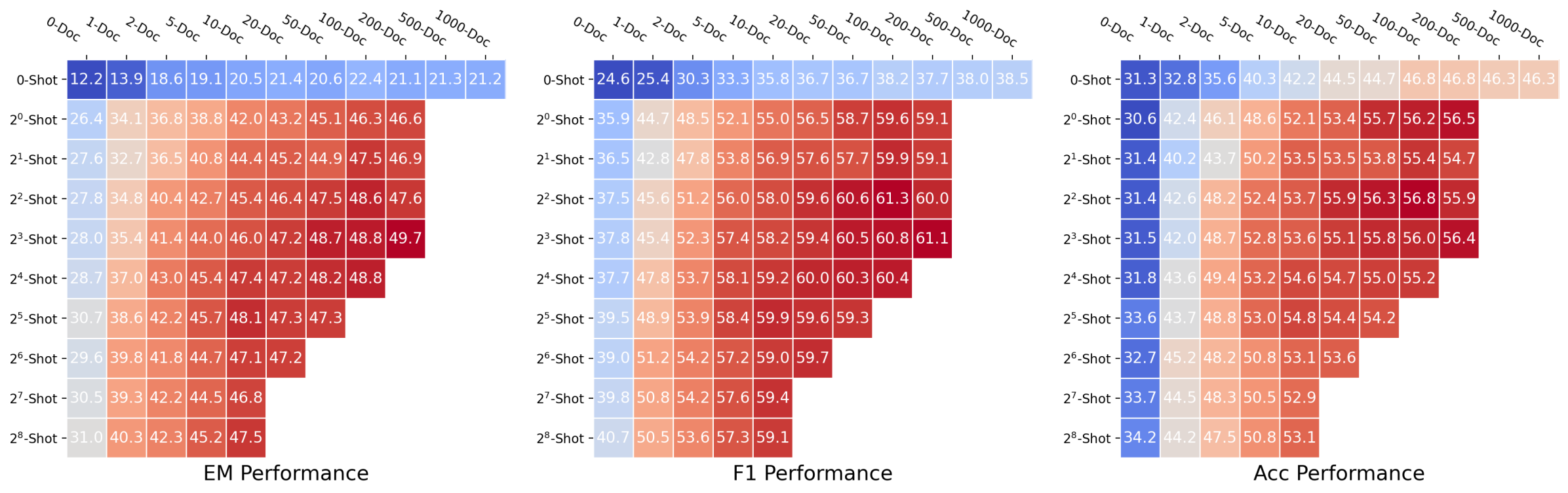
### Visual Description
# Technical Data Extraction: Performance Heatmaps
This document contains a detailed extraction of three heatmaps representing performance metrics for a machine learning model across different configurations of "Shot" (y-axis) and "Doc" (x-axis).
## 1. Document Overview
The image consists of three distinct heatmaps arranged horizontally. Each heatmap shares the same axes but represents a different performance metric:
* **Left:** EM Performance (Exact Match)
* **Center:** F1 Performance
* **Right:** Acc Performance (Accuracy)
### Shared Axis Definitions
* **X-Axis (Top):** Number of Documents ("Doc"). Values: 0-Doc, 1-Doc, 2-Doc, 5-Doc, 10-Doc, 20-Doc, 50-Doc, 100-Doc, 200-Doc, 500-Doc, 1000-Doc.
* **Y-Axis (Left):** Number of Shots. Values: 0-Shot, $2^0$-Shot, $2^1$-Shot, $2^2$-Shot, $2^3$-Shot, $2^4$-Shot, $2^5$-Shot, $2^6$-Shot, $2^7$-Shot, $2^8$-Shot.
* **Color Gradient:** Blue (Lower values) $\rightarrow$ White (Mid-range) $\rightarrow$ Red (Higher values).
---
## 2. Data Tables
### Table 1: EM Performance
**Trend Analysis:** Performance generally increases as both the number of documents and shots increase. The highest performance is concentrated in the bottom-right of the populated cells (around $2^3$-Shot and 200-Doc).
| Shot / Doc | 0-Doc | 1-Doc | 2-Doc | 5-Doc | 10-Doc | 20-Doc | 50-Doc | 100-Doc | 200-Doc | 500-Doc | 1000-Doc |
| :--- | :--- | :--- | :--- | :--- | :--- | :--- | :--- | :--- | :--- | :--- | :--- |
| **0-Shot** | 12.2 | 13.9 | 18.6 | 19.1 | 20.5 | 21.4 | 20.6 | 22.4 | 21.1 | - | - |
</details>
Figure 8: IterDRAG performance heatmap for different metrics averaged across datasets.
We report the IterDRAG results averaged across datasets in Figure 8, shown as heatmaps where the x-axis represents the number of documents and the y-axis represents the number of shots. Performance is color-coded, with blue indicating lower values and red indicating higher values. The best-performing combinations are located toward the bottom right of each heatmap, which corresponds to longer context lengths. In comparison to DRAG, as reported in Figure 5(a), the optimal number of in-context examples is higher at 32, which highlights the importance of in-context demonstrations in enabling better query decomposition and interleaved retrieval. Combined with multiple generation steps, IterDRAG further improves RAG performance over DRAG.
<details>
<summary>x8.png Details</summary>
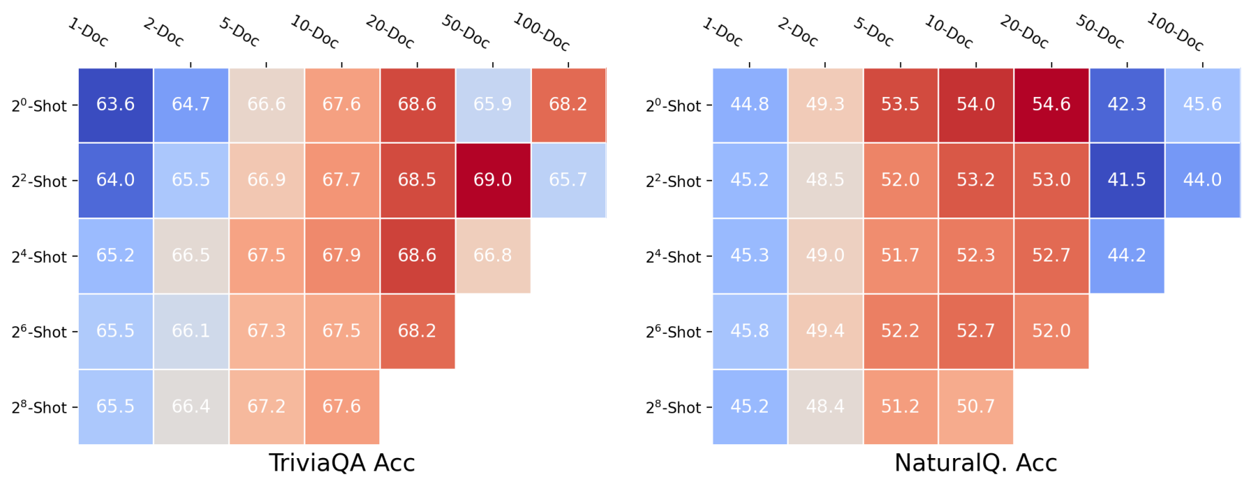
### Visual Description
# Technical Data Extraction: Performance Heatmaps for TriviaQA and Natural Questions
This document contains a detailed extraction of data from two side-by-side heatmaps illustrating model accuracy (Acc) across two different datasets: **TriviaQA** (left) and **Natural Questions (NaturalQ.)** (right).
## 1. Document Structure and Components
The image is divided into two main regions, each containing a heatmap with a shared coordinate system for the axes.
* **X-Axis (Top):** Represents the number of documents used, labeled as `1-Doc`, `2-Doc`, `5-Doc`, `10-Doc`, `20-Doc`, `50-Doc`, and `100-Doc`.
* **Y-Axis (Left):** Represents the number of "shots" (examples) provided, labeled in powers of 2: $2^0$-Shot, $2^2$-Shot, $2^4$-Shot, $2^6$-Shot, and $2^8$-Shot.
* **Color Gradient:** A diverging color scale is used where **Dark Red** indicates the highest accuracy values, **White/Beige** indicates median values, and **Dark Blue** indicates the lowest accuracy values.
---
## 2. Region 1: TriviaQA Acc (Left Chart)
### Trend Analysis
The TriviaQA heatmap shows a general trend where accuracy improves as the number of documents increases from 1 to 20. Performance peaks around the 20-Doc to 50-Doc range. Interestingly, performance appears relatively stable or slightly improves as the number of shots increases for low document counts, but the highest overall performance (69.0) is achieved at $2^2$-Shot with 50 documents.
### Data Table: TriviaQA Accuracy (%)
| Shots \ Docs | 1-Doc | 2-Doc | 5-Doc | 10-Doc | 20-Doc | 50-Doc | 100-Doc |
| :--- | :---: | :---: | :---: | :---: | :---: | :---: | :---: |
| **$2^0$-Shot** | 63.6 | 64.7 | 66.6 | 67.6 | 68.6 | 65.9 | 68.2 |
| **$2^2$-Shot** | 64.0 | 65.5 | 66.9 | 67.7 | 68.5 | 69.0 | 65.7 |
| **$2^4$-Shot** | 65.2 | 66.5 | 67.5 | 67.9 | 68.6 | 66.8 | [N/A] |
| **$2^6$-Shot** | 65.5 | 66.1 | 67.3 | 67.5 | 68.2 | [N/A] | [N/A] |
| **$2^8$-Shot** | 65.5 | 66.4 | 67.2 | 67.6 | [N/A] | [N/A] | [N/A] |
---
## 3. Region 2: NaturalQ. Acc (Right Chart)
### Trend Analysis
The Natural Questions heatmap displays a distinct "peak" performance zone. Accuracy increases significantly when moving from 1-Doc to 20-Doc, reaching a maximum of 54.6 at $2^0$-Shot/20-Doc. However, there is a sharp performance degradation (indicated by the shift to dark blue) when moving to 50-Doc and 100-Doc for the lower shot counts, suggesting a potential "distraction" or context window issue at those scales for this specific dataset.
### Data Table: Natural Questions Accuracy (%)
| Shots \ Docs | 1-Doc | 2-Doc | 5-Doc | 10-Doc | 20-Doc | 50-Doc | 100-Doc |
| :--- | :---: | :---: | :---: | :---: | :---: | :---: | :---: |
| **$2^0$-Shot** | 44.8 | 49.3 | 53.5 | 54.0 | 54.6 | 42.3 | 45.6 |
| **$2^2$-Shot** | 45.2 | 48.5 | 52.0 | 53.2 | 53.0 | 41.5 | 44.0 |
| **$2^4$-Shot** | 45.3 | 49.0 | 51.7 | 52.3 | 52.7 | 44.2 | [N/A] |
| **$2^6$-Shot** | 45.8 | 49.4 | 52.2 | 52.7 | 52.0 | [N/A] | [N/A] |
| **$2^8$-Shot** | 45.2 | 48.4 | 51.2 | 50.7 | [N/A] | [N/A] | [N/A] |
---
## 4. Summary of Observations
* **Dataset Difficulty:** TriviaQA shows higher absolute accuracy scores (ranging from 63.6 to 69.0) compared to Natural Questions (ranging from 41.5 to 54.6).
* **Optimal Document Count:** For both datasets, the 20-Doc column consistently shows high performance (deep orange/red).
* **Scaling Limitations:** Both charts contain empty cells (white space) in the bottom-right corners, indicating that data for high-shot/high-document combinations (e.g., $2^8$-Shot with 100-Doc) was either not collected or is not applicable, likely due to context length constraints of the model being tested.
* **Anomalies:** In the NaturalQ. chart, the performance drop at 50-Doc and 100-Doc for $2^0$ and $2^2$ shots is much more pronounced than in the TriviaQA chart.
</details>
Figure 9: Evaluation accuracy of DRAG on TriviaQA and Natural Questions (NaturalQ.).
In addition to multi-hop question answering datasets, we also report results on one-hop datasets, specifically TriviaQA and Natural Questions (Joshi et al., 2017; Kwiatkowski et al., 2019). The evaluations for one-hop datasets are performed with DRAG and presented in Figure 9, similar to Figure 8. For TriviaQA, increasing the number of documents generally leads to improved accuracy, where the highest accuracy of 69.0% is achieved with 50 documents. In Natural Questions, performance increases with the number of documents up to about 10 or 20 documents, but further increases in the document count lead to diminishing returns or even slight declines in accuracy. The highest accuracy of 54.6% is achieved with 20 documents in 1-shot, and performance drops slightly when more documents are included. In summary, the optimal number of shots falls between 1 and 4. While increasing the number of shots and documents leads to initial performance gains, these improvements plateau beyond certain thresholds. This trend, in contrast to multi-hop datasets, may be partially attributed to the nature of the one-hop questions and retrieval relevance.
Table 7: StrategyQA accuracy results.
| Acc | 61.1 | 74.7 | 74.7 | 79.0 | 83.4 |
| --- | --- | --- | --- | --- | --- |
| | StrategyQA | | | | |
| Zero-shot QA | Many-shot QA | RAG | DRAG | IterDRAG | |
We also include the multi-hop and binary StrategyQA dataset in our experiments, see Table 7 (Geva et al., 2021). Despite being binary questions, we observe similar trends to our main experiments. For example, DRAG consistently outperforms the baseline QA and RAG methods, with 29.3% accuracy improvement to for the baseline QA model. Furthermore, the performance is boosted with 83.4 accuracy using the iterative IterDRAG. These results demonstrate that even for binary, multi-hop tasks, iterative approaches provide substantial gains, confirming the effectiveness of both long-context and iterative strategies for inference scaling in RAG.
Appendix D Additional Results on Inference Scaling Laws with GTR Retriever
<details>
<summary>x9.png Details</summary>
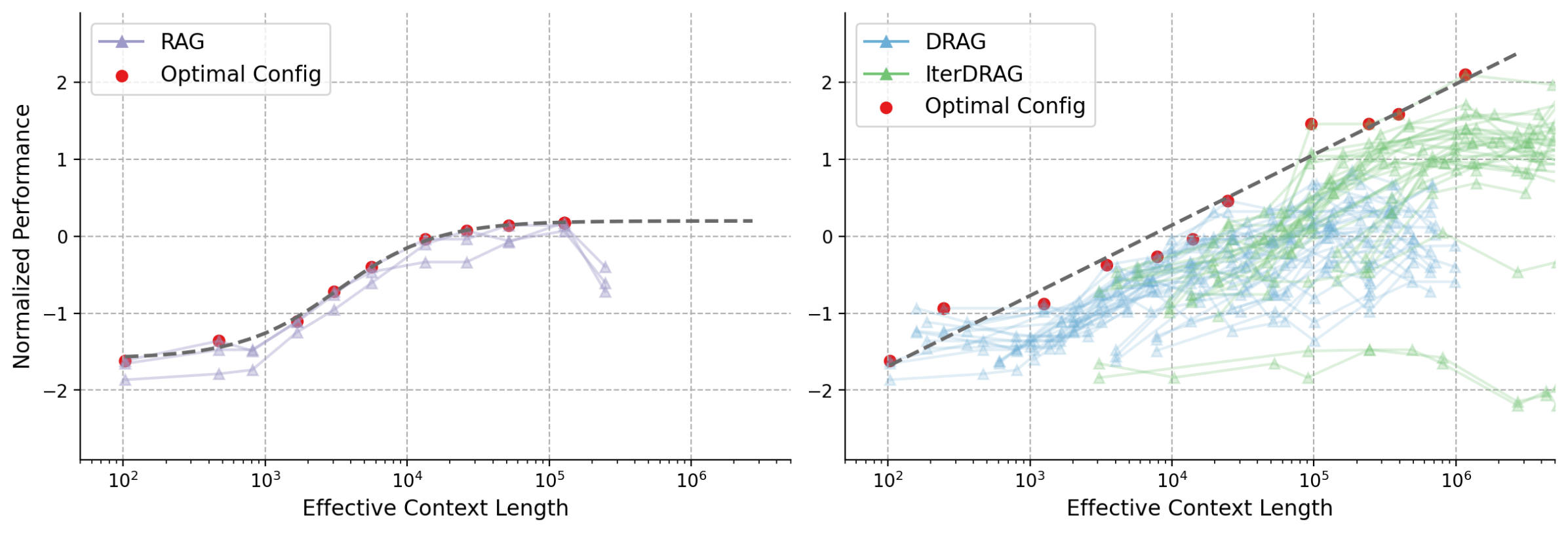
### Visual Description
# Technical Data Extraction: Performance vs. Effective Context Length
This document provides a comprehensive technical extraction of the data presented in the two-panel line chart comparing different retrieval and generation strategies.
## 1. General Metadata
* **Image Type:** Two-panel line chart with logarithmic x-axes.
* **Language:** English.
* **Common Y-Axis:** "Normalized Performance" (Linear scale from -2 to 2).
* **Common X-Axis:** "Effective Context Length" (Logarithmic scale from $10^2$ to $10^6$).
* **Common Visual Elements:**
* **Dashed Grey Line:** Represents the theoretical or empirical upper bound/frontier of performance.
* **Red Circles:** Labeled as "Optimal Config," these points sit on or define the dashed grey frontier line.
* **Grid:** Dashed grey grid lines for both axes.
---
## 2. Left Panel: RAG Performance
This panel focuses on the "RAG" (Retrieval-Augmented Generation) method.
### Component Isolation: Left Panel
* **Legend Location:** Top-left [x: ~0.05, y: ~0.90].
* **Legend Items:**
* Purple line with triangle markers: **RAG**
* Red circle: **Optimal Config**
### Data Trends and Points
* **Trend Analysis:** The RAG performance shows an initial upward slope as context length increases from $10^2$ to $10^5$. However, after reaching a peak near $10^5$, the performance plateaus and then shows a sharp decline (drop-off) as context length continues to increase toward $3 \times 10^5$.
* **Frontier (Dashed Line):** Starts at approx. -1.6 ($10^2$) and curves upward to plateau at approx. 0.2 ($10^5$ and beyond).
* **Optimal Config Points (Red):**
* $10^2$: ~ -1.6
* $5 \times 10^2$: ~ -1.4
* $10^3$: ~ -1.1
* $3 \times 10^3$: ~ -0.7
* $6 \times 10^3$: ~ -0.4
* $1.5 \times 10^4$: ~ 0.0
* $3 \times 10^4$: ~ 0.1
* $5 \times 10^4$: ~ 0.15
* $1.2 \times 10^5$: ~ 0.2
* **RAG Series (Purple):** Multiple faint lines indicate different trials or sub-configurations. They generally follow the frontier but fall below it, especially at the highest context lengths where they drop toward -0.8.
---
## 3. Right Panel: DRAG and IterDRAG Performance
This panel compares "DRAG" and "IterDRAG" methods, showing significantly higher scaling potential than standard RAG.
### Component Isolation: Right Panel
* **Legend Location:** Top-left [x: ~0.55, y: ~0.90].
* **Legend Items:**
* Blue line with triangle markers: **DRAG**
* Green line with triangle markers: **IterDRAG**
* Red circle: **Optimal Config**
### Data Trends and Points
* **Trend Analysis (DRAG - Blue):** These lines cluster in the $10^2$ to $10^5$ range. They show a steady upward trend but generally saturate or become noisier around a performance level of 0 to 0.5.
* **Trend Analysis (IterDRAG - Green):** These lines extend much further to the right (up to $5 \times 10^6$). They show a continued upward trajectory, maintaining performance gains at much higher context lengths than RAG or standard DRAG.
* **Frontier (Dashed Line):** Unlike the RAG chart, this frontier does not plateau. It maintains a steady positive linear slope on the log-linear plot, reaching a performance value of ~2.1 at $10^6$ context length.
* **Optimal Config Points (Red):**
* $10^2$: ~ -1.6
* $2.5 \times 10^2$: ~ -0.9
* $1.2 \times 10^3$: ~ -0.9
* $3.5 \times 10^3$: ~ -0.4
* $8 \times 10^3$: ~ -0.3
* $1.5 \times 10^4$: ~ 0.0
* $2.5 \times 10^4$: ~ 0.5
* $10^5$: ~ 1.5
* $2.5 \times 10^5$: ~ 1.5
* $4 \times 10^5$: ~ 1.6
* $1.1 \times 10^6$: ~ 2.1
---
## 4. Comparative Summary
| Feature | RAG (Left) | DRAG / IterDRAG (Right) |
| :--- | :--- | :--- |
| **Max Performance** | ~0.2 | ~2.1 |
| **Scaling Limit** | Plateaus/Drops after $10^5$ | Continues scaling past $10^6$ |
| **Frontier Shape** | Logarithmic/Saturating | Linear-Log (Constant growth) |
| **Stability** | High variance/drop at high context | IterDRAG (Green) maintains growth at extreme context |
**Conclusion:** The data indicates that while RAG performance saturates and eventually degrades with increased context length, the DRAG and specifically IterDRAG methods allow for continued performance improvements as the effective context length scales into the millions.
</details>
Figure 10: Normalized performance with increasing effective context lengths on MuSiQue, the results are obtained with GTR XXL retriever and Gemini 1.5 Flash.
To enhance the generalizability of our scaling observations and validate the findings with an alternative retriever model, we conduct additional experiments using the open-source GTR XXL retriever and Gemini 1.5 Flash (Ni et al., 2021). Figure 10 shows the results on MuSiQue, evaluated using 100 sampled examples from the dataset for computational efficiency. Different from the performance plateau in standard RAG, DRAG and IterDRAG yields consistent performance gains with increasing context length, especially with IterDRAG at longer context lengths. Overall, the results demonstrate consistent patterns in inference scaling even with a different retriever model, highlighting the potential of expanding text-time compute in long-context RAG for more generalized scenarios.
Appendix E Additional Results on Inference Scaling Laws for RAG
<details>
<summary>x10.png Details</summary>
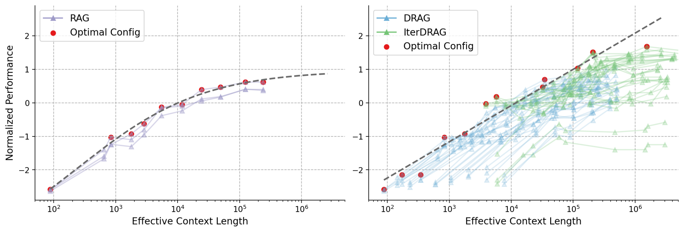
### Visual Description
# Technical Data Extraction: Performance vs. Effective Context Length
This document provides a detailed technical extraction of the data and trends presented in the provided image, which consists of two side-by-side line charts comparing different Retrieval-Augmented Generation (RAG) configurations.
## 1. General Chart Metadata
* **X-Axis (Common):** "Effective Context Length"
* **Scale:** Logarithmic ($10^2$ to $10^6$).
* **Major Tick Marks:** $10^2, 10^3, 10^4, 10^5, 10^6$.
* **Y-Axis (Common):** "Normalized Performance"
* **Scale:** Linear (from -2 to 2).
* **Major Tick Marks:** -2, -1, 0, 1, 2.
* **Visual Elements:** Both charts feature a dashed grey trend line representing the theoretical or empirical upper bound of performance as context length increases. Red circular dots represent the "Optimal Config" at specific context intervals.
---
## 2. Left Chart: RAG Performance
### Component Isolation: Left Panel
* **Legend Location:** Top-left $[x \approx 0.05, y \approx 0.90]$
* **Legend Items:**
* **RAG:** Light purple line with triangle markers ($\triangle$).
* **Optimal Config:** Red circular markers ($\bullet$).
### Trend Verification: RAG
The RAG data series consists of multiple faint purple lines representing different sub-configurations, with one primary line highlighted.
* **Visual Trend:** The performance starts at its lowest point at $10^2$ context length and follows a logarithmic growth curve. The slope is steepest between $10^2$ and $10^3$, then gradually flattens (plateaus) as it approaches $10^5$ and $10^6$.
* **Saturation:** Performance appears to saturate around a normalized value of $0.5$ to $0.8$ as context length exceeds $10^5$.
### Data Point Extraction (Approximate)
| Effective Context Length | Normalized Performance (Optimal Config - Red Dot) |
| :--- | :--- |
| $\approx 10^2$ | -2.6 |
| $\approx 8 \times 10^2$ | -1.0 |
| $\approx 2 \times 10^3$ | -0.9 |
| $\approx 3 \times 10^3$ | -0.6 |
| $\approx 6 \times 10^3$ | -0.1 |
| $\approx 10^4$ | 0.0 |
| $\approx 2 \times 10^4$ | 0.4 |
| $\approx 5 \times 10^4$ | 0.5 |
| $\approx 10^5$ | 0.6 |
| $\approx 2 \times 10^5$ | 0.6 |
---
## 3. Right Chart: DRAG and IterDRAG Performance
### Component Isolation: Right Panel
* **Legend Location:** Top-left $[x \approx 0.55, y \approx 0.90]$
* **Legend Items:**
* **DRAG:** Light blue line with triangle markers ($\triangle$).
* **IterDRAG:** Light green line with triangle markers ($\triangle$).
* **Optimal Config:** Red circular markers ($\bullet$).
### Trend Verification: DRAG & IterDRAG
* **DRAG (Blue):** Multiple blue lines show a similar upward trend to the standard RAG but extend further into the higher context lengths.
* **IterDRAG (Green):** These lines generally start at higher context lengths (beginning around $5 \times 10^3$). They show a higher performance ceiling than the standard RAG, continuing to climb past the $1.0$ normalized performance mark.
* **Overall Trend:** Unlike the left chart which plateaus, the right chart shows continued performance growth. The "Optimal Config" dots follow the dashed grey line much more closely and for a longer duration, reaching a peak performance near $1.8$ at context lengths exceeding $10^6$.
### Data Point Extraction (Approximate)
| Effective Context Length | Normalized Performance (Optimal Config - Red Dot) |
| :--- | :--- |
| $\approx 10^2$ | -2.6 |
| $\approx 2 \times 10^2$ | -2.2 |
| $\approx 4 \times 10^2$ | -2.2 |
| $\approx 9 \times 10^2$ | -1.1 |
| $\approx 2 \times 10^3$ | -0.9 |
| $\approx 4 \times 10^3$ | 0.0 |
| $\approx 6 \times 10^3$ | 0.2 |
| $\approx 3 \times 10^4$ | 0.5 |
| $\approx 4 \times 10^4$ | 0.7 |
| $\approx 10^5$ | 1.1 |
| $\approx 2 \times 10^5$ | 1.5 |
| $\approx 2 \times 10^6$ | 1.7 |
---
## 4. Comparative Summary
* **Performance Ceiling:** The standard RAG (Left) plateaus significantly earlier (around $10^5$ context length) with a maximum normalized performance below 1.0.
* **Scalability:** The DRAG and IterDRAG methods (Right) demonstrate superior scalability. They continue to improve performance as context length increases toward $10^6$, nearly doubling the peak performance of the standard RAG.
* **Optimal Configuration Alignment:** In the right chart, the "Optimal Config" points track the theoretical dashed line much more accurately at high context lengths compared to the left chart, where the optimal points begin to fall below the dashed line after $10^4$.
</details>
(a) Normalized performance vs. effective context lengths on Bamboogle.
<details>
<summary>x11.png Details</summary>
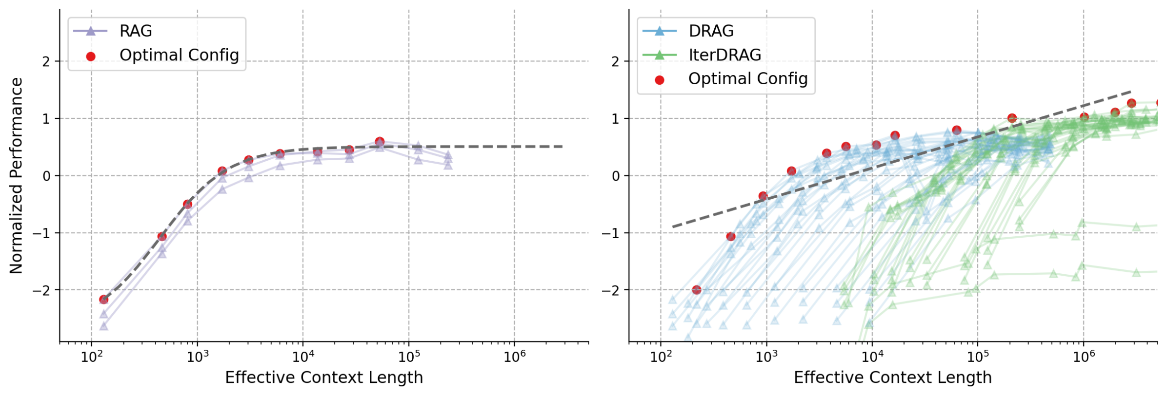
### Visual Description
# Technical Data Extraction: Performance vs. Effective Context Length
This document provides a detailed extraction of the data and trends presented in the two-panel line chart comparing different retrieval and generation configurations.
## 1. General Layout and Metadata
* **Image Type:** Two-panel line graph with logarithmic x-axis.
* **Y-Axis (Both Panels):** "Normalized Performance" (Linear scale from -3 to +3, with major gridlines at intervals of 1.0).
* **X-Axis (Both Panels):** "Effective Context Length" (Logarithmic scale from $10^2$ to $10^6+$).
* **Visual Elements:**
* **Dashed Grey Line:** Represents the theoretical or empirical "frontier" of optimal performance across context lengths.
* **Red Dots:** Labeled as "Optimal Config," these mark the peak performance points for specific context length intervals.
* **Faded Lines with Triangles:** Represent individual experimental runs/configurations.
---
## 2. Left Panel: RAG Performance
### Component Isolation: Left Chart
* **Legend Location:** Top-left $[x \approx 0.05, y \approx 0.9]$.
* **Series 1 (Purple Triangles):** **RAG**. Multiple faded purple lines showing various RAG configurations.
* **Series 2 (Red Circles):** **Optimal Config**. Points following the upper boundary of the RAG configurations.
### Trend Analysis: RAG
The RAG performance shows a steep logarithmic growth starting from approximately -2.5 at $10^2$ context length. The performance plateaus significantly after $10^4$ context length, reaching a maximum normalized performance of approximately 0.5.
### Data Points (Optimal Config - RAG)
| Effective Context Length (Approx.) | Normalized Performance (Approx.) | Trend Observation |
| :--- | :--- | :--- |
| $1.2 \times 10^2$ | -2.2 | Rapid ascent |
| $5 \times 10^2$ | -1.1 | Rapid ascent |
| $10^3$ | -0.5 | Decelerating growth |
| $2 \times 10^3$ | 0.1 | Approaching plateau |
| $6 \times 10^3$ | 0.4 | Plateau entry |
| $10^4$ to $10^5$ | 0.4 to 0.6 | Stable plateau |
---
## 3. Right Panel: DRAG and IterDRAG Performance
### Component Isolation: Right Chart
* **Legend Location:** Top-left $[x \approx 0.55, y \approx 0.9]$.
* **Series 1 (Blue Triangles):** **DRAG**. Faded blue lines representing various DRAG configurations.
* **Series 2 (Green Triangles):** **IterDRAG**. Faded green lines representing iterative DRAG configurations.
* **Series 3 (Red Circles):** **Optimal Config**. Points marking the highest performance achieved at various context lengths across both methods.
### Trend Analysis: DRAG vs. IterDRAG
* **DRAG (Blue):** Dominates the lower context lengths ($10^2$ to $10^4$). It shows a similar growth curve to RAG but maintains a higher trajectory, crossing the 0.0 performance mark around $3 \times 10^3$.
* **IterDRAG (Green):** Becomes relevant at higher context lengths ($>10^4$). While individual runs vary wildly, the "Optimal Config" points in the $10^5$ to $10^6$ range are driven by these configurations.
* **Overall Frontier (Dashed Line):** Unlike the RAG panel which plateaus, the DRAG/IterDRAG frontier continues to climb steadily, exceeding a normalized performance of 1.0 as context length approaches $10^6$.
### Data Points (Optimal Config - DRAG/IterDRAG)
| Effective Context Length (Approx.) | Normalized Performance (Approx.) | Series Source |
| :--- | :--- | :--- |
| $2 \times 10^2$ | -2.0 | DRAG |
| $4 \times 10^2$ | -1.1 | DRAG |
| $10^3$ | -0.4 | DRAG |
| $2 \times 10^3$ | 0.1 | DRAG |
| $5 \times 10^3$ | 0.5 | DRAG |
| $10^4$ | 0.6 | DRAG |
| $6 \times 10^4$ | 0.8 | DRAG/IterDRAG |
| $2 \times 10^5$ | 1.0 | IterDRAG |
| $10^6$ | 1.1 | IterDRAG |
| $3 \times 10^6$ | 1.3 | IterDRAG |
---
## 4. Comparative Summary
* **Scaling Ceiling:** RAG (Left) hits a performance ceiling of $\approx 0.5$ at $10^4$ context length. In contrast, DRAG/IterDRAG (Right) breaks this ceiling, reaching $>1.0$ performance as context length scales toward $10^6$.
* **Configuration Density:** The right panel shows a much higher density of experimental configurations (faded lines), particularly for IterDRAG at high context lengths, indicating a larger search space or higher sensitivity to parameters at scale.
* **Optimal Frontier:** The dashed grey line in the right panel has a positive slope throughout the entire x-axis range, whereas the left panel's frontier becomes horizontal (slope $\approx 0$) after $10^4$.
</details>
(b) Normalized performance vs. effective context lengths on HotpotQA.
<details>
<summary>x12.png Details</summary>
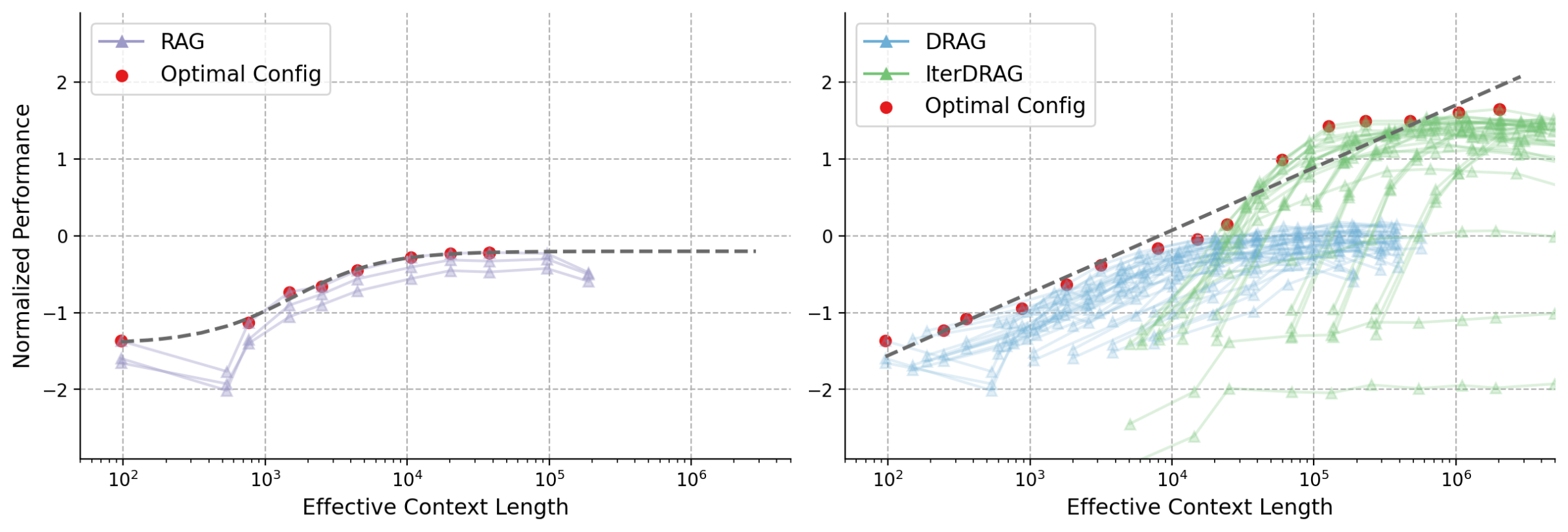
### Visual Description
# Technical Data Extraction: Performance vs. Effective Context Length
This document provides a detailed technical extraction of the provided image, which consists of two side-by-side line charts comparing different Retrieval-Augmented Generation (RAG) configurations.
## 1. Global Chart Metadata
* **Y-Axis Label:** Normalized Performance
* **Y-Axis Scale:** Linear, ranging from -2 to 2 (with major ticks at -2, -1, 0, 1, 2).
* **X-Axis Label:** Effective Context Length
* **X-Axis Scale:** Logarithmic ($10^2$ to $10^6$).
* **Visual Style:** White background with a grey dashed grid. A dark grey dashed line represents the "Pareto frontier" or the upper bound of performance across all configurations in both plots.
---
## 2. Left Plot: RAG Performance
This plot focuses on standard RAG configurations.
### Legend Information
* **Location:** Top-left [x: ~0.05, y: ~0.90]
* **Series 1:** `RAG` (Light purple line with triangle markers $\triangle$).
* **Series 2:** `Optimal Config` (Red solid circles $\bullet$).
### Component Analysis & Trends
* **Trend Verification:** The RAG data series (purple lines) show an initial dip between $10^2$ and $10^3$, followed by a steady upward slope as context length increases, eventually plateauing around $10^4$ to $10^5$.
* **Data Points (Approximate):**
* **Initial State ($10^2$):** Performance starts at approximately -1.4.
* **The Dip ($5 \times 10^2$):** Performance drops to its lowest point, approximately -2.0.
* **Recovery ($10^3$):** Performance rises sharply to approximately -1.0.
* **Plateau ($10^4$ - $10^5$):** Performance stabilizes between -0.5 and -0.2.
* **Optimal Config (Red Dots):** These track the highest-performing purple line at each context interval, following the dark grey dashed trend line.
---
## 3. Right Plot: DRAG and IterDRAG Performance
This plot introduces more complex configurations (DRAG and IterDRAG) and extends the context length further.
### Legend Information
* **Location:** Top-left [x: ~0.55, y: ~0.90]
* **Series 1:** `DRAG` (Light blue line with triangle markers $\triangle$).
* **Series 2:** `IterDRAG` (Light green line with triangle markers $\triangle$).
* **Series 3:** `Optimal Config` (Red solid circles $\bullet$).
### Component Analysis & Trends
* **Trend Verification (DRAG - Blue):** These lines follow a similar trajectory to the standard RAG in the left plot but are shifted slightly higher. They trend upward from $10^2$ and plateau around $10^4$ to $10^5$ at a performance level near 0.
* **Trend Verification (IterDRAG - Green):** These lines represent the highest scaling potential. While some configurations start low (below -2), the successful configurations slope steeply upward starting at $10^4$, surpassing both RAG and DRAG.
* **Trend Verification (Optimal Config - Red):** The red dots follow a strong, consistent upward linear-log trend (the dark grey dashed line), showing that as context length increases to $10^6$, performance continues to scale.
### Data Points (Approximate)
| Effective Context Length | Optimal Performance (Red Dots) | Dominant Series |
| :--- | :--- | :--- |
| $10^2$ | ~ -1.4 | DRAG |
| $10^3$ | ~ -0.9 | DRAG |
| $10^4$ | ~ -0.2 | DRAG / IterDRAG Transition |
| $10^5$ | ~ +1.0 | IterDRAG |
| $10^6$ | ~ +1.5 | IterDRAG |
| $2 \times 10^6$ | ~ +1.6 | IterDRAG |
---
## 4. Comparative Summary
* **Scaling:** Standard **RAG** (Left) plateaus early and does not benefit significantly from context lengths beyond $10^4$.
* **Advanced Methods:** **DRAG** (Blue) improves upon RAG but also reaches a ceiling.
* **Superiority of IterDRAG:** **IterDRAG** (Green) is the only method shown that continues to scale performance effectively into the "Long Context" regime ($10^5$ to $10^6$), defining the upper bound of the "Optimal Config" trend line in the high-context regions.
* **The Pareto Frontier:** The dark grey dashed line indicates a logarithmic relationship between effective context length and normalized performance, which is only achievable by switching from standard RAG to IterDRAG as context grows.
</details>
(c) Normalized performance vs. effective context lengths on 2WikiMultiHopQA.
Figure 11: Normalized performance with increasing effective context lengths on different datasets.
We present data-specific results on the relationship between the performance and the effective context length. Figure 11 presents the results on the other three datasets other than MuSiQue (See Figure 1 for visualized results on MuSiQue). We observe different behavior depending on the datasets. For instance, the gains are more linear and consistent on Bamboogle and MuSiQue, and almost linear on 2WikiMultiHopQA until 1M tokens. However, HotpotQA and 2WikiMultiHopQA with effective context length longer than 100k tokens exhibit more sigmoidal patterns, likely due to the difficulty of the datasets and the quality of the retrieved documents.
Appendix F Additional Results on Computation Allocation Model for RAG
<details>
<summary>x13.png Details</summary>
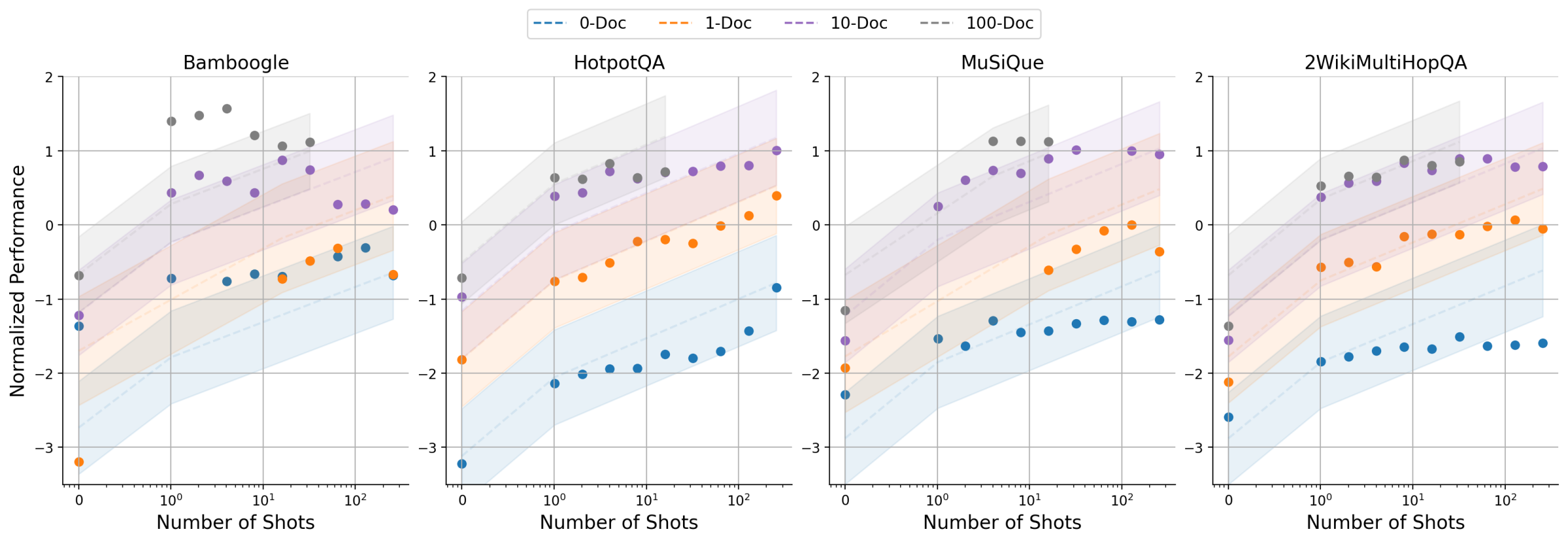
### Visual Description
# Technical Data Extraction: Normalized Performance vs. Number of Shots
## 1. Document Overview
This image contains four line/scatter plots arranged horizontally, comparing the "Normalized Performance" (y-axis) against the "Number of Shots" (x-axis) across four different datasets. Each plot includes data for four different document conditions (0-Doc, 1-Doc, 10-Doc, 100-Doc).
## 2. Global Metadata and Legend
* **Legend Location:** Top center of the image, above the charts.
* **Legend Categories:**
* **0-Doc:** Blue dashed line with blue circular markers.
* **1-Doc:** Orange dashed line with orange circular markers.
* **10-Doc:** Purple dashed line with purple circular markers.
* **100-Doc:** Grey dashed line with grey circular markers.
* **Common Y-Axis:** "Normalized Performance" (Range: -3 to 2, increments of 1).
* **Common X-Axis:** "Number of Shots" (Logarithmic scale: 0, $10^0$, $10^1$, $10^2$).
* **Visual Features:** Each data series includes a shaded confidence interval or variance band of the same color as the line.
---
## 3. Component Analysis by Dataset
### A. Bamboogle (First Plot)
* **Trend Analysis:** All series show an upward trend as the number of shots increases. The 100-Doc (Grey) series maintains the highest performance but plateaus/dips slightly after 10 shots. The 0-Doc (Blue) and 1-Doc (Orange) series start significantly lower (approx. -1.5 to -3.2) and converge toward -0.5 at higher shot counts.
* **Key Data Points (Approximate):**
* **0-Doc (Blue):** Starts at ~-1.4 (0 shots), rises to ~-0.3 (256 shots).
* **1-Doc (Orange):** Starts at ~-3.2 (0 shots), rises to ~-0.7 (256 shots).
* **10-Doc (Purple):** Starts at ~-1.2, rises to ~0.2 (256 shots).
* **100-Doc (Grey):** Starts at ~-0.7, peaks at ~1.6 (4 shots), ends at ~1.1 (32 shots).
### B. HotpotQA (Second Plot)
* **Trend Analysis:** Strong linear-log growth for all series. The performance gap between 0-Doc and 100-Doc is consistently wide (approx. 2 units of normalized performance).
* **Key Data Points (Approximate):**
* **0-Doc (Blue):** Starts at ~-3.2, rises to ~-0.8.
* **1-Doc (Orange):** Starts at ~-1.8, rises to ~0.4.
* **10-Doc (Purple):** Starts at ~-1.0, rises to ~1.0.
* **100-Doc (Grey):** Starts at ~-0.7, rises to ~0.7 (data ends at 16 shots).
### C. MuSiQue (Third Plot)
* **Trend Analysis:** Similar to HotpotQA, but the 0-Doc (Blue) series plateaus much earlier (around 1 shot) and remains relatively flat between -1.5 and -1.2.
* **Key Data Points (Approximate):**
* **0-Doc (Blue):** Starts at ~-2.3, plateaus around -1.3.
* **1-Doc (Orange):** Starts at ~-1.9, rises to ~-0.4.
* **10-Doc (Purple):** Starts at ~-1.6, rises to ~1.0.
* **100-Doc (Grey):** Starts at ~-1.2, rises to ~1.1 (data ends at 16 shots).
### D. 2WikiMultiHopQA (Fourth Plot)
* **Trend Analysis:** The 0-Doc (Blue) series shows a sharp initial increase from 0 to 1 shot, then remains flat. The 10-Doc (Purple) and 1-Doc (Orange) series show steady improvement.
* **Key Data Points (Approximate):**
* **0-Doc (Blue):** Starts at ~-2.6, rises to ~-1.8 at 1 shot, ends at ~-1.6.
* **1-Doc (Orange):** Starts at ~-2.1, rises to ~-0.1.
* **10-Doc (Purple):** Starts at ~-1.5, rises to ~0.8.
* **100-Doc (Grey):** Starts at ~-1.4, rises to ~0.9 (data ends at 32 shots).
---
## 4. Summary of Findings
1. **Document Count Impact:** There is a clear ordinal relationship where `100-Doc > 10-Doc > 1-Doc > 0-Doc` in terms of normalized performance across all datasets.
2. **Few-Shot Learning:** Increasing the "Number of Shots" generally improves performance for all document conditions, though the 0-Doc condition often plateaus earlier than conditions with more documents.
3. **Data Density:** The 100-Doc (Grey) series consistently has fewer data points on the x-axis (stopping between 16 and 32 shots) compared to the other series which extend to 256 shots.
4. **Starting Points:** At 0 shots, the performance varies wildly by dataset, with MuSiQue and 2WikiMultiHopQA showing much lower baseline performance for the 0-Doc condition compared to Bamboogle.
</details>
Figure 12: The estimated performance using the proposed computation allocation model vs. actual metric values in IterDRAG. The subplots represent different datasets, where each line corresponds to a fixed number of documents, we scale the context length by increasing the number of shots.
Table 8: Computation allocation mode of Gemini 1.5 Flash with $p$ -value, $R^{2}$ and MSE statistics.
| Value | 0.325 | 0.101 | 0.177 | -0.067 | -0.008 | 0 | -0.730 | 0.903 | 0.085 |
| --- | --- | --- | --- | --- | --- | --- | --- | --- | --- |
| $p$ -value | 0.000 | 0.000 | 0.000 | 0.000 | 0.092 | N/A | 0.000 | N/A | N/A |
We further explore the findings on the computation allocation model. In particular, we report the estimated parameters along with $p$ -values, $R^{2}$ , and MSE statistics in Table 8. In our implementation, we constrain the last element of $b$ , leaving six learnable parameters in total. Our analysis shows that all parameters are statistically significant, except for $b_{1}$ , which has a $p$ -value slightly above 0.05. Nonetheless, our experiments suggest that retaining $b_{1}$ improves generalization in many cases, such as IterDRAG on multi-hop datasets. For sigmoid scaling, we fit a custom function between the predicted $\hat{P}$ and ground truth $P$ values, defined as $\sigma(x)=\frac{3.30}{1+e^{-1.81(x+0.46)}}-2.18$ .
We also visualize the predictions on for IterDRAG across different datasets in Figure 12, where each subplot represents a dataset and each line corresponds to a document setting ( $k$ ). The inference compute is scaled by increasing the number of in-context examples ( $m$ ) and generation iterations ( $n$ ). Here, we find similar trends to those in Figure 6, although IterDRAG shows larger variations compared to DRAG. HotpotQA and 2WikiMultiHopQA show more consistent trends with the predictions, likely due to the predominance of multi-hop queries. In summary, our findings are consistent for both DRAG and IterDRAG, demonstrating that RAG performance can be accurately modeled by our computation allocation model for RAG. For Bamboogle, HotpotQA and 2WikiMultiHopQA, we provide the normalized performance with increasing effective context lengths in Figure 11, in which we observe similar trends to the results on MuSiQue (See Figure 1). We also illustrate the prediction surface for both DRAG and IterDRAG in Figure 13.
<details>
<summary>x14.png Details</summary>
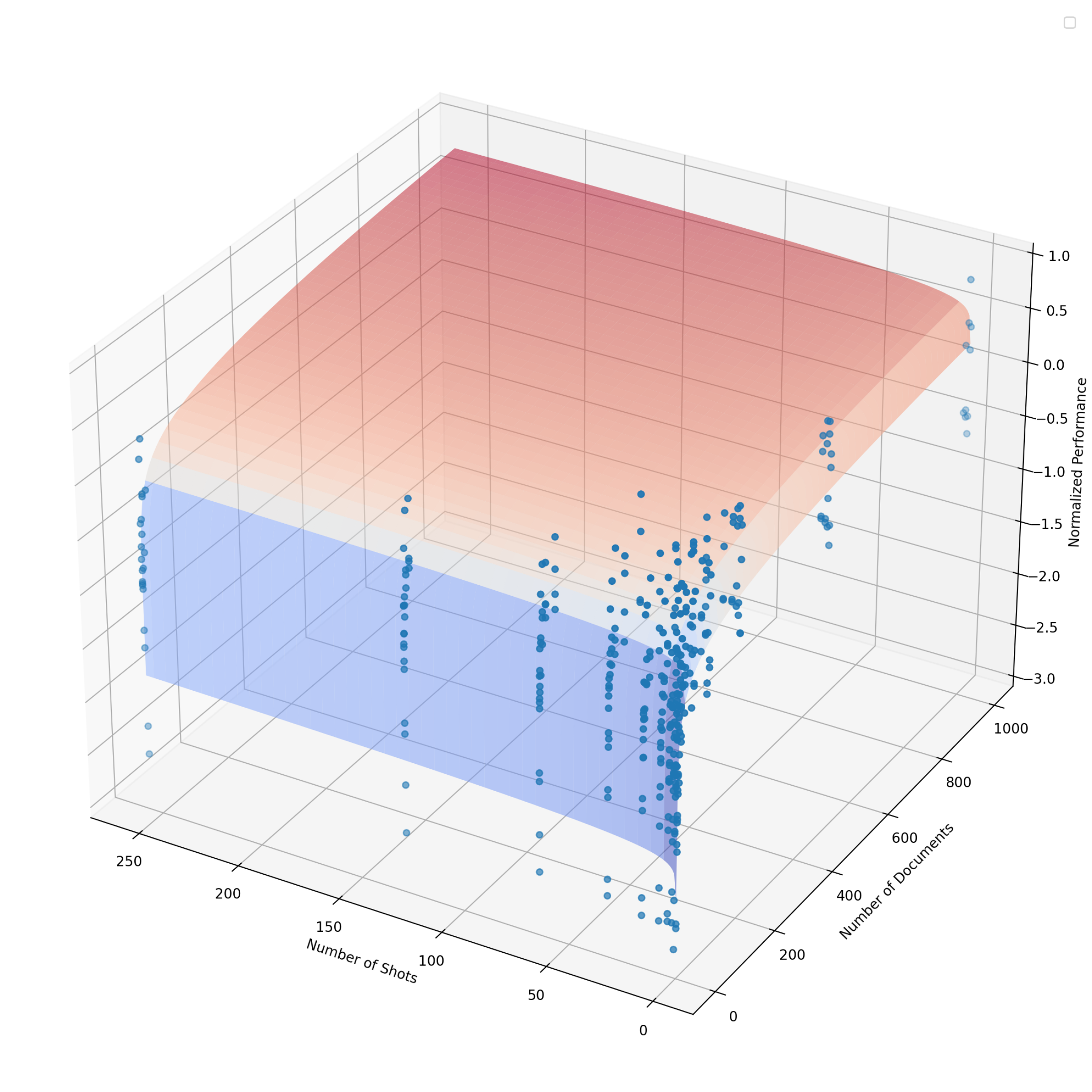
### Visual Description
# Technical Data Extraction: 3D Surface and Scatter Plot
## 1. Image Overview
This image is a three-dimensional (3D) visualization containing a fitted regression surface and a corresponding scatter plot of data points. It illustrates the relationship between two independent variables and one dependent variable.
## 2. Component Isolation
### A. Header/Legend Region
* **Location:** Top right corner.
* **Content:** An empty legend box is present, but it contains no text or labels.
### B. Main Chart Region (3D Space)
The chart uses a Cartesian coordinate system with three axes.
#### Axis Labels and Scales
| Axis | Label | Scale Range | Markers |
| :--- | :--- | :--- | :--- |
| **X-Axis (Bottom Left)** | Number of Shots | 250 to 0 (Decreasing) | 250, 200, 150, 100, 50, 0 |
| **Y-Axis (Bottom Right)** | Number of Documents | 0 to 1000 (Increasing) | 0, 200, 400, 600, 800, 1000 |
| **Z-Axis (Vertical)** | Normalized Performance | -3.0 to 1.0 | -3.0, -2.5, -2.0, -1.5, -1.0, -0.5, 0.0, 0.5, 1.0 |
### C. Data Series and Trends
#### 1. Fitted Surface (Regression Model)
* **Visual Description:** A semi-transparent, curved surface that spans the entire grid.
* **Color Gradient:** The surface uses a diverging color map.
* **Red/Salmon:** Represents higher "Normalized Performance" values (roughly > -0.5).
* **White/Light Grey:** Represents the transition zone (roughly at -1.0).
* **Blue/Lavender:** Represents lower "Normalized Performance" values (roughly < -1.5).
* **Trend Verification:**
* **Along "Number of Shots":** As the number of shots increases (moving toward 250), the performance generally increases and then plateaus.
* **Along "Number of Documents":** As the number of documents increases (moving toward 1000), the performance increases significantly.
* **Interaction:** The lowest performance is predicted at the [0 shots, 0 documents] corner, while the highest performance is predicted at the [250 shots, 1000 documents] corner.
#### 2. Scatter Plot (Observed Data Points)
* **Visual Description:** Small, blue, semi-transparent circular markers.
* **Spatial Distribution:**
* The data points are clustered at specific intervals along the "Number of Shots" axis (e.g., at 0, 50, 100, 150, 250).
* There is a high density of points near the 0-50 "Number of Shots" range and the 0-200 "Number of Documents" range.
* **Trend Verification:**
* The points generally follow the curvature of the surface but show significant variance (vertical spread) at each coordinate pair.
* At low "Number of Shots" and low "Number of Documents," several outliers drop significantly below the surface, reaching the -3.0 performance mark.
* At high "Number of Documents" (near 1000), the points are clustered tightly near the top of the Z-axis (0.5 to 1.0).
## 3. Key Data Insights
* **Primary Driver:** "Number of Documents" appears to have a stronger positive correlation with "Normalized Performance" than "Number of Shots," as evidenced by the steeper slope of the surface along the Y-axis.
* **Diminishing Returns:** The surface flattens out as "Number of Shots" exceeds 150, suggesting diminishing returns for increasing shots beyond that point.
* **Performance Floor:** The data indicates a "floor" or minimum performance around -3.0, which occurs primarily when both independent variables are at their lowest values.
</details>
(a) Performance vs. predicted surface for DRAG.
<details>
<summary>x15.png Details</summary>
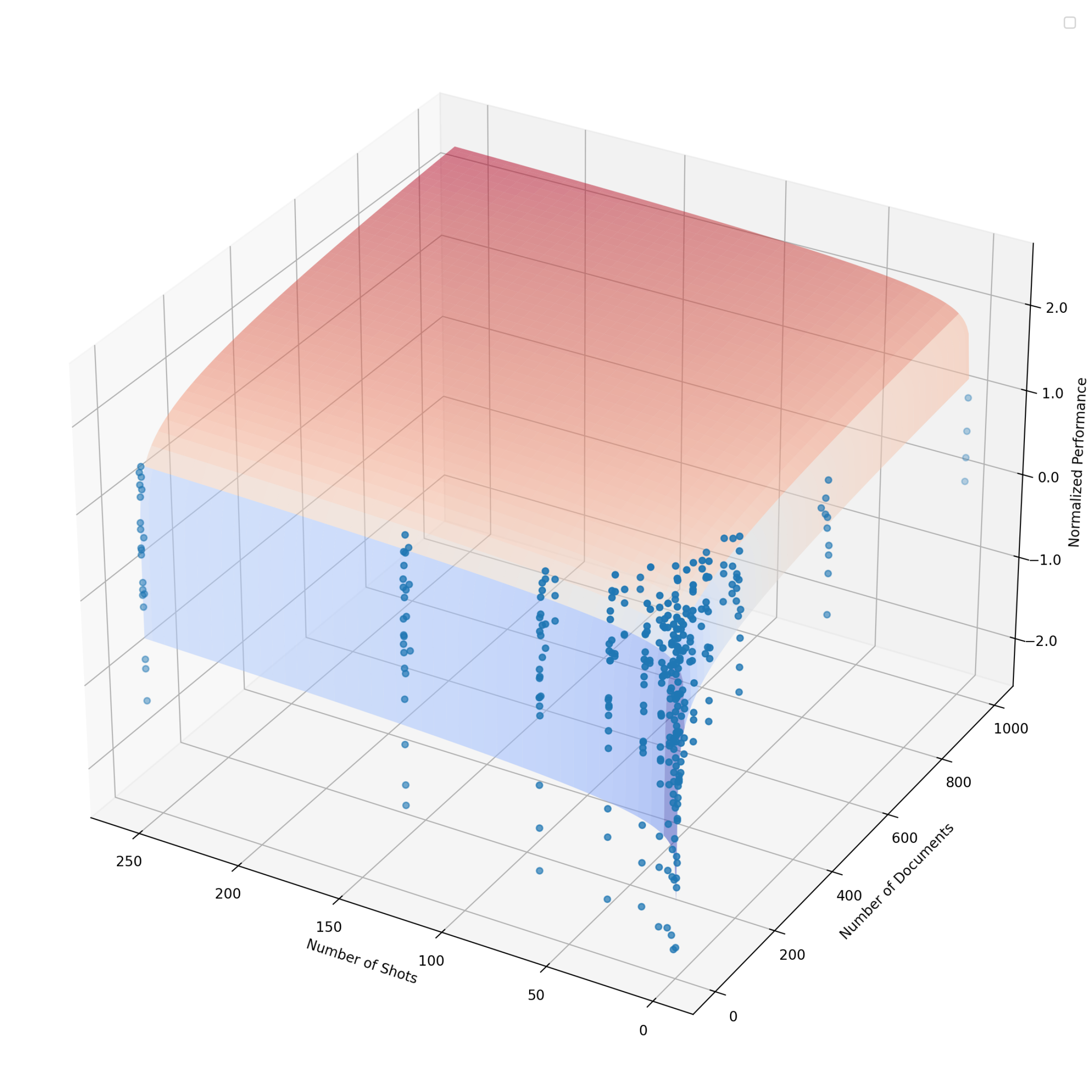
### Visual Description
# Technical Document Extraction: 3D Surface and Scatter Plot Analysis
## 1. Image Overview
This image is a three-dimensional (3D) visualization combining a scatter plot of discrete data points with a fitted regression surface. It illustrates the relationship between two independent variables—**Number of Shots** and **Number of Documents**—and a dependent variable, **Normalized Performance**.
## 2. Component Isolation
### A. Header/Legend Region
* **Location:** Top right corner [x: ~950, y: ~20].
* **Content:** A small, empty legend box is present, but it contains no text or labels.
### B. Axis Definitions
The chart uses a 3D Cartesian coordinate system with the following axes:
| Axis | Label | Scale Range | Orientation |
| :--- | :--- | :--- | :--- |
| **X-Axis** | **Number of Shots** | 0 to 250 (Decreasing left-to-right) | Horizontal (Depth) |
| **Y-Axis** | **Number of Documents** | 0 to 1000 | Horizontal (Width) |
| **Z-Axis** | **Normalized Performance** | -2.0 to 2.0 | Vertical (Height) |
**Axis Markers:**
* **Number of Shots:** 0, 50, 100, 150, 200, 250.
* **Number of Documents:** 0, 200, 400, 600, 800, 1000.
* **Normalized Performance:** -2.0, -1.0, 0.0, 1.0, 2.0.
### C. Main Data Visualization
The visualization consists of two primary layers:
#### 1. Scatter Plot (Discrete Data)
* **Color:** Blue circular markers.
* **Distribution:** The points are clustered primarily at low values of "Number of Shots" (near 0) and "Number of Documents" (near 0).
* **Trend Verification:** As the "Number of Shots" increases toward 250, the density of data points decreases significantly. There are distinct vertical "columns" of data points at specific intervals of "Number of Shots" (e.g., at approximately 0, 32, 64, 128, and 256), suggesting these were fixed experimental parameters.
* **Performance Variance:** At low shot/document counts, the "Normalized Performance" (Z-axis) shows high variance, ranging from approximately -2.5 to 0.5.
#### 2. Regression Surface (Fitted Model)
* **Color Gradient:** A smooth surface transitioning from **Light Blue** (lower performance values) to **Red/Salmon** (higher performance values).
* **Trend Verification:**
* The surface slopes upward as both "Number of Shots" and "Number of Documents" increase.
* The slope is steepest at low values (near the origin) and begins to plateau as it approaches the higher bounds of the axes.
* The surface reaches its maximum "Normalized Performance" (approaching 2.0) at the back corner where "Number of Shots" is 250 and "Number of Documents" is 1000.
* **Curvature:** The surface exhibits a logarithmic or sub-linear growth pattern along both horizontal axes, indicating diminishing returns in performance as more shots or documents are added.
## 3. Key Data Insights and Trends
* **Positive Correlation:** There is a clear positive correlation between the input variables (Shots/Documents) and the output (Normalized Performance).
* **Data Sparsity:** While the model (the surface) predicts high performance at high shot/document counts, the actual data points (scatter) are sparse in those regions, particularly at the [250, 1000] coordinate.
* **Performance Range:** The "Normalized Performance" appears centered around 0.0 for mid-range inputs, with the model predicting a peak near 2.0 and a floor near -1.5 to -2.0 for minimal inputs.
## 4. Language Declaration
* **Primary Language:** English.
* **Other Languages:** None detected.
</details>
(b) Performance vs. predicted surface for IterDRAG.
Figure 13: Normalized performance vs. predicted surface for DRAG and IterDRAG.
Inaccurate or outdated retrieval
Question: What is the lowest elevation of the longest railway tunnel? Prediction: 500 meters Annotation: 312 m Question: According to QS World University Rankings, where does the college that Ibrahim Shihata attended rank? Prediction: 3rd Annotation: 551-600 Question: Which battle occurred first, the Battle of Manila or the Battle of Guam? Prediction: Battle of Manila Annotation: Battle of Guam
(a) Example mistakes due to inaccurate or outdated retrieval.
Incorrect or lack of reasoning
Question: Which mountain, Masherbrum or Khunyang Chhish, is a taller mountain? Prediction: Masherbrum Annotation: Khunyang Chhish Question: What is the date of death of the director of film The Organization (Film)? Prediction: April 15, 2018 Annotation: December 12, 2012 Question: Who introduced a system of musical notation in the 14th century that is used in the area where most of the invasion of the eastern Roman Empire took place? Prediction: Philippe de Vitry Annotation: John Kukuzelis
(b) Example mistakes due to incorrect or lack of reasoning.
Hallucination or unfaithful reasoning
Question: Who was the last emperor of the dynasty that succeeded the Song dynasty? Prediction: Emperor Yuanzhen Annotation: Toghon Temür Question: What is another notable work by the illustrator of Sylvester and the Magic Pebble? Prediction: Shrek! Annotation: Doctor De Soto Question: In what movie did a Kenyan-Mexican actress, who graduated from Hampshire College, star in in 2015? Prediction: Queen of Katwe Annotation: Star Wars: The Force Awakens
(c) Example mistakes due to hallucination or unfaithful reasoning.
Evaluation issues or refusal to answer
Question: The most populous city in Punjab is how large (area wise)? Prediction: 310 sq. km Annotation: 310 square kilometers Question: Renáta Tomanová and Larisa Neiland are former professional athletes for what sport? Prediction: Tennis Annotation: Professional tennis
(d) Example mistakes due to evaluation issues or refusal to answer.
Figure 14: Example mistakes of DRAG and IterDRAG across datasets.
Appendix G Error Analysis
Despite the performance gains from scaling effective context length, RAG performance on challenging datasets like MuSiQue remain moderate, even for IterDRAG. To address this, we analyze the mistakes in both DRAG and IterDRAG to examine the limitations and errors inherent in these approaches. In the following, we explore common failure cases (See Figure 14) to understand where each method falls short and how they could be further improved.
We provide selected example mistakes from Figure 14(a) to Figure 14(d), with retrieved documents omitted for brevity. The reasons for common errors can be grouped into four categories: (1) inaccurate or outdated retrieval; (2) incorrect or lack of reasoning; (3) hallucination or unfaithful reasoning; and (4) evaluation issues or refusal to answer. We elaborate on these categories below:
- Inaccurate or outdated retrieval: A major source of RAG errors stems from the retrieval process, where relevant knowledge is not correctly retrieved. For example, in the first question of Figure 14(c), the top-50 retrieved documents do not contain the correct answer. A similar issue occurs in the second QA pair, where outdated retrieval results fail to provide useful information. In the third case, although both battles are retrieved, the initial documents overly focus on the Battle of Manila, leading to an incorrect response.
- Incorrect or lack of reasoning: Beyond retrieval issues, incorrect reasoning chains are another common source of errors. For example, in the first case in Figure 14(b), although the correct documents are retrieved, the reasoning process is incomplete (i.e., no explicit comparison of the mountain heights), leading to an incorrect answer in DRAG. Similarly, in the second and third cases, the reasoning is either absent (as in DRAG) or flawed. As a result, reasoning-related errors tend to occur more frequently in difficult questions and in the one-step DRAG approach.
- Hallucination or unfaithful reasoning: Other than retrieval and reasoning, hallucination and unfaithful reasoning also contribute to errors in knowledge-intensive tasks. In the first case, the prediction is incorrect and cannot be found in the retrieved documents. As for the rest cases, while the answers are related, certain steps in the reasoning chain are flawed and cause errors in the final answers. These highlight the persistent challenge of hallucination in LLMs, particularly in long-context generation tasks.
- Evaluation issues or refusal to answer: Finally, we observed several evaluation issues that may lead to inaccurate evaluation. For instance, the use of abbreviations or variations in date format can result in incorrect scoring across all metrics. Moreover, our experiments do not account for abstaining from answering, which could cause unfair scores.
<details>
<summary>x16.png Details</summary>
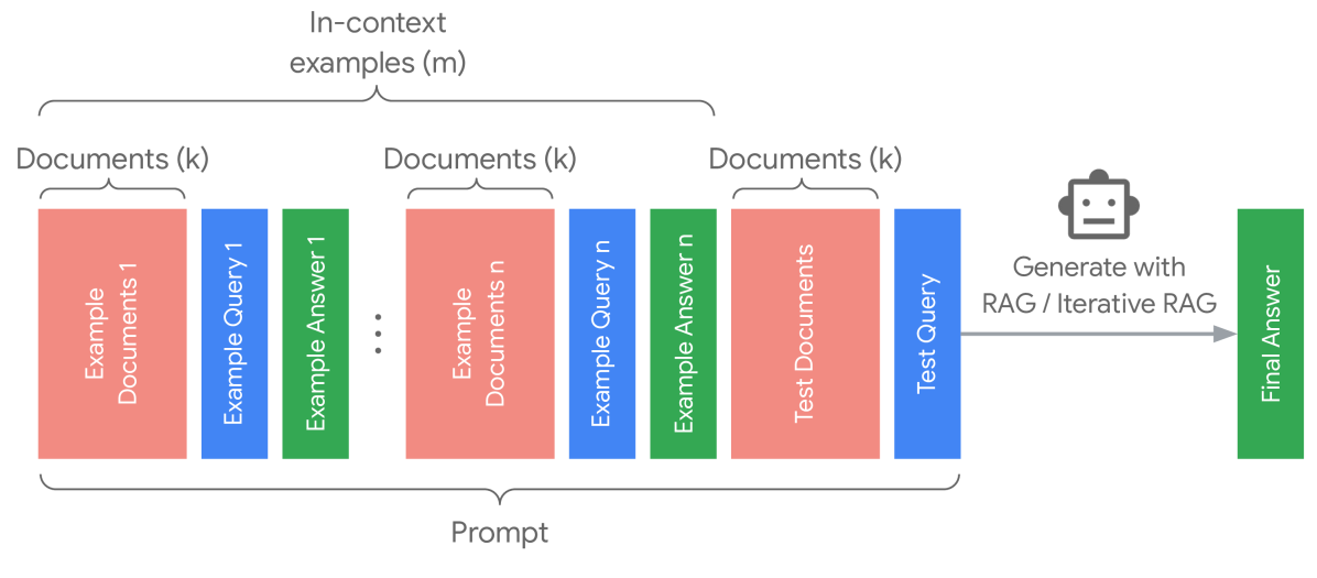
### Visual Description
# Technical Document Extraction: RAG / Iterative RAG Prompt Structure
## 1. Overview
This image is a technical diagram illustrating the architectural composition of a prompt used for Retrieval-Augmented Generation (RAG) or Iterative RAG. It demonstrates how multiple in-context examples and test data are sequenced to generate a final answer.
## 2. Component Isolation
### Region A: Header / Global Brackets
* **Top Bracket:** Spans the first two sets of examples. Label: `In-context examples (m)`.
* **Bottom Bracket:** Spans the entire sequence from the first example to the test query. Label: `Prompt`.
### Region B: Main Sequence (Input Data)
The input is composed of repeating blocks and a final test block, color-coded by function:
* **Red Blocks:** Represent source material. Label: `Documents (k)`.
* **Blue Blocks:** Represent queries.
* **Green Blocks:** Represent answers.
#### Sequence Breakdown:
1. **Example Set 1:**
* **Red Block:** `Example Documents 1` (Sub-labeled `Documents (k)`)
* **Blue Block:** `Example Query 1`
* **Green Block:** `Example Answer 1`
2. **Ellipsis (`...`):** Indicates a continuation of the pattern for $n$ examples.
3. **Example Set n:**
* **Red Block:** `Example Documents n` (Sub-labeled `Documents (k)`)
* **Blue Block:** `Example Query n`
* **Green Block:** `Example Answer n`
4. **Test Set:**
* **Red Block:** `Test Documents` (Sub-labeled `Documents (k)`)
* **Blue Block:** `Test Query`
### Region C: Processing and Output
* **Icon:** A stylized robot head representing an AI model/LLM.
* **Transition Arrow:** A grey arrow pointing from the `Prompt` sequence to the `Final Answer`.
* **Process Label:** `Generate with RAG / Iterative RAG`.
* **Output Block (Green):** `Final Answer`.
## 3. Data Structure and Logic
The diagram defines a specific mathematical and logical relationship for the prompt construction:
| Component | Variable | Description |
| :--- | :--- | :--- |
| **In-context examples** | $m$ | The total number of few-shot examples provided in the prompt. |
| **Documents** | $k$ | The number of retrieved documents provided for each specific query (both example and test). |
| **Prompt** | N/A | The concatenation of $m$ examples (Document + Query + Answer) followed by the Test Document and Test Query. |
## 4. Flow Description
1. **Contextualization:** The system retrieves $k$ documents for $m$ different examples. Each example consists of the documents, a query, and the correct answer.
2. **Test Input:** The system retrieves $k$ documents for the current `Test Query`.
3. **Prompt Assembly:** All $m$ examples and the current test data are bundled into a single `Prompt`.
4. **Generation:** The AI model processes the `Prompt` using a `RAG` or `Iterative RAG` methodology.
5. **Termination:** The process results in a single `Final Answer`.
## 5. Text Transcription (Precise)
* **Top Labels:** "In-context examples (m)", "Documents (k)" (repeated 3 times).
* **Internal Block Text (Vertical):**
* "Example Documents 1"
* "Example Query 1"
* "Example Answer 1"
* "Example Documents n"
* "Example Query n"
* "Example Answer n"
* "Test Documents"
* "Test Query"
* "Final Answer"
* **Action Text:** "Generate with RAG / Iterative RAG"
* **Bottom Label:** "Prompt"
</details>
Figure 15: Input prompt that comprises of $m$ in-context examples, the test documents and query, in which each document chunk consists of $k$ retrieved documents. For IterDRAG, the example answers additionally provide sub-queries and intermediate answers as demonstrations.
Appendix H Implementation
In our experiments, we utilize the Gecko-1B (en) embedding model to index both the documents and input queries (Lee et al., 2024b), using Wikipedia passages from the KILT benchmark as the document source (Petroni et al., 2020). In test-time, the input query is compared against all embeddings in the corpus, and the top- $k$ neighbors are selected for inference. Each document is then truncated on the right side to a maximum of 1024 tokens using whitespace tokenization. For each example, we arrange the elements in the following order: documents, query, and label, with the retrieved documents listed in reverse order, placing the higher-ranked documents closer to the query (Liu et al., 2024b). Consequently, the prompt comprises of multiple in-context examples, followed by the test documents and test query, as illustrated in Figure 15.
For generation, we utilize Gemini 1.5 Flash for more efficient experiments. In DRAG, inference scaling is achieved by increasing the context length through the combination of documents ( $k$ ) and in-context examples ( $m$ ). Then, the prompt (See Figure 16) is provided to the model for a one-time generation using the default generation parameters. For IterDRAG, the input prompt is constructed in a similar fashion, with the example answers consisting of assembled sub-queries, intermediate answers, and the final answer (See Figure 17). Here, we scale test-time compute by incorporating iterative retrieval and generation, along with the increase of documents and demonstrations. In each iteration, we restrict the generation to adhere to the Self-Ask format, in which the response should start with “Follow up: ”, “Intermediate answer: ” or “So the final answer is: ” (Koo et al., 2024). Each iteration begins with the generation of a sub-query and concludes with the production of an intermediate answer. If a sub-query is generated, additional documents are retrieved and appended to the initial set (i.e., Test Documents in Figure 15), after which the model generates an intermediate answer. We allow up to five iterations, after which the model is forced to produce the final answer.
To evaluate the estimated parameters within computation allocation model for RAG, we normalized the performance metrics by subtracting the mean and dividing by the standard deviation for each dataset and metric. For DRAG, the effective context length is calculated by counting the tokens in the prompt, while for IterDRAG, it is determined by summing the context tokens across all inference requests. We constrain the last parameter in $b$ and perform ordinary least squares to estimate rest six parameters in Equation 2. To prevent numerical instability, we shift the values in $\theta$ by a small constant $\epsilon$ of 0.01. When computing $R^{2}$ and MSE, we manage noisy data by excluding peak and valley outliers in our experiments. However, for domain generalization and length extrapolation, all data points are included in the evaluation. To predict downstream task performance, $i$ should be computed for each task. Specifically, in each strategy and task: $i_{\text{doc}}=P(k=1,m=0,n=1)-P(k=0,m=0,n=1)$ , $i_{\text{shot}}=P(k=0,m=1,n=1)-P(k=0,m=0,n=1)$ . For the predicted optimal hyperparameters, we present the actual metric values to validate the efficacy of computation allocation model for RAG.
Prompt for DRAG
You are an expert in question answering. I am going to give you one or more example triples of context, question and answer, in which the context may or may not be relevant to the question. The examples will be written. Context (which may or may not be relevant): <Retrieved documents> Question: What is the place of birth of the director of film Servant’S Entrance? Answer: Helsingfors <Further demonstrations> After the examples, I am going to provide another pair of context and question, in which the context may or may not be relevant to the question. I want you to answer the question. Give only the answer, and no extra commentary, formatting, or chattiness. Answer the question. Context (which may or may not be relevant): <Retrieved documents> Question: Who was born first out of Thomas Henry Holland and Jean-Mandé Sigogne? Answer:
Figure 16: Example prompt for DRAG. The prompt comprises of instructions and varying number of demonstrations, followed by a test example.
Prompt for IterDRAG
You are an expert in question answering. I am going to give you one or more example sets of context, question, potential follow up questions and their respective answers, in which the context may or may not be relevant to the questions. The examples will be written. Context: <Retrieved documents> Question: What nationality is the director of film Boggy Creek Ii: And The Legend Continues? Follow up: Who is the director of the film Boggy Creek II: And The Legend Continues? Intermediate answer: The director of the film Boggy Creek II: And The Legend Continues is Charles B. Pierce. Follow up: What is the nationality of Charles B. Pierce? Intermediate answer: The nationality of Charles B. Pierce is American. So the final answer is: American <Further demonstrations> After the examples, I am going to provide another pair of context and question, in which the context may or may not be relevant to the question. I want you to answer the question. When needed, generate follow up question(s) using the format ’Follow up: X’, where X is the follow up question. Then, answer each follow up question using ’Intermediate answer: X’ with X being the answer. Finally, answer to the main question with the format ’So the final answer is: X’, where X is the final answer. Context: <Retrieved documents (with interleaving retrieval)> Question: Where was the director of film Death Of A Friend born? Follow up: | Intermediate answer: | So the final answer is:
Figure 17: Example prompt for IterDRAG. The prompt comprises of instructions and varying number of demonstrations, followed by a test example. In each iteration, we control the generation to follow the Self-Ask format with constrained decoding.