# \scalerel* \method: On-the-Fly Self-Speculative Decoding for LLM Inference Acceleration
> Corresponding Author
Abstract
Speculative decoding (SD) has emerged as a widely used paradigm to accelerate LLM inference without compromising quality. It works by first employing a compact model to draft multiple tokens efficiently and then using the target LLM to verify them in parallel. While this technique has achieved notable speedups, most existing approaches necessitate either additional parameters or extensive training to construct effective draft models, thereby restricting their applicability across different LLMs and tasks. To address this limitation, we explore a novel plug-and-play SD solution with layer-skipping, which skips intermediate layers of the target LLM as the compact draft model. Our analysis reveals that LLMs exhibit great potential for self-acceleration through layer sparsity and the task-specific nature of this sparsity. Building on these insights, we introduce \method, an on-the-fly self-speculative decoding algorithm that adaptively selects intermediate layers of LLMs to skip during inference. \method does not require auxiliary models or additional training, making it a plug-and-play solution for accelerating LLM inference across diverse input data streams. Our extensive experiments across a wide range of models and downstream tasks demonstrate that \method can achieve over a $1.3×$ $\sim$ $1.6×$ speedup while preserving the original distribution of the generated text. We release our code in https://github.com/hemingkx/SWIFT.
1 Introduction
Large Language Models (LLMs) have exhibited outstanding capabilities in handling various downstream tasks (OpenAI, 2023; Touvron et al., 2023a; b; Dubey et al., 2024). However, their token-by-token generation necessitated by autoregressive decoding poses efficiency challenges, particularly as model sizes increase. To address this, speculative decoding (SD) has been proposed as a promising solution for lossless LLM inference acceleration (Xia et al., 2023; Leviathan et al., 2023; Chen et al., 2023). At each decoding step, SD first employs a compact draft model to efficiently predict multiple tokens as speculations for future decoding steps of the target LLM. These tokens are then validated by the target LLM in parallel, ensuring that the original output distribution remains unchanged.
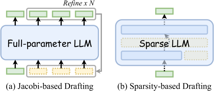
Recent advancements in SD have pushed the boundaries of the latency-accuracy trade-off by exploring various strategies (Xia et al., 2024), including incorporating lightweight draft modules into LLMs (Cai et al., 2024; Ankner et al., 2024; Li et al., 2024a; b), employing fine-tuning strategies to facilitate efficient LLM drafting (Kou et al., 2024; Yi et al., 2024; Elhoushi et al., 2024), and aligning draft models with the target LLM (Liu et al., 2023a; Zhou et al., 2024; Miao et al., 2024). Despite their promising efficacy, these approaches require additional modules or extensive training, which limits their broad applicability across different model types and causes significant inconvenience in practice. To tackle this issue, another line of research has proposed the Jacobi-based drafting (Santilli et al., 2023; Fu et al., 2024) to facilitate plug-and-play SD. As illustrated in Figure 1 (a), these methods append pseudo tokens to the input prompt, enabling the target LLM to generate multiple tokens as drafts in a single decoding step. However, the Jacobi-decoding paradigm misaligns with the autoregressive pretraining objective of LLMs, resulting in suboptimal acceleration effects.
<details>
<summary>x1.png Details</summary>
### Visual Description
## Diagram: LLM Drafting Methods
### Overview
The image presents two diagrams illustrating different drafting methods for Large Language Models (LLMs): Jacobi-based Drafting and Sparsity-based Drafting. Each diagram shows the flow of information and the interaction between different components.
### Components/Axes
**Diagram (a): Jacobi-based Drafting**
* **Main Component:** A rounded rectangle labeled "Full-parameter LLM" in the center. The rectangle has a light blue fill and a darker blue outline.
* **Input Blocks:** Three blocks at the bottom, each with a dotted yellow fill and a gray outline.
* **Output Blocks:** Three blocks at the top, each with a solid green fill and a gray outline.
* **Refinement Loop:** A gray rounded rectangle encompassing the top output blocks, labeled "Refine x N" at the top.
* **Arrows:** Black arrows indicate the flow of information. Arrows point upwards from the input blocks to the "Full-parameter LLM," and from the "Full-parameter LLM" to the output blocks. A gray arrow connects the rightmost output block back to the bottom input blocks.
* **Title:** "(a) Jacobi-based Drafting" is located below the diagram.
**Diagram (b): Sparsity-based Drafting**
* **Main Component:** A rounded rectangle containing three horizontal layers. The top and bottom layers have a solid light blue fill and a darker blue outline. The middle layer has a dotted yellow fill and a gray outline. The text "Sparse LLM" is written in the middle layer.
* **Input Block:** A block at the bottom with a solid green fill.
* **Output Block:** A block at the top with a solid green fill.
* **Arrows:** Dashed black arrows indicate the flow of information. An arrow points upwards from the input block to the bottom layer of the "Sparse LLM." An arrow points upwards from the middle layer to the top layer. An arrow points upwards from the top layer to the output block.
* **Title:** "(b) Sparsity-based Drafting" is located below the diagram.
### Detailed Analysis
**Diagram (a): Jacobi-based Drafting**
* The "Full-parameter LLM" receives input from three blocks at the bottom.
* The "Full-parameter LLM" generates output to three blocks at the top.
* The "Refine x N" loop suggests that the output is fed back into the system for refinement.
* The input blocks have a yellow fill, while the output blocks have a green fill.
**Diagram (b): Sparsity-based Drafting**
* The "Sparse LLM" has a layered structure.
* The input block feeds into the bottom layer of the "Sparse LLM."
* The middle layer of the "Sparse LLM" is dotted yellow, suggesting a sparse representation.
* The output block receives output from the top layer of the "Sparse LLM."
* The arrows are dashed, which may indicate a different type of information flow compared to the solid arrows in diagram (a).
### Key Observations
* Diagram (a) involves a "Full-parameter LLM" and a refinement loop.
* Diagram (b) involves a "Sparse LLM" with a layered structure.
* The diagrams use different arrow styles to indicate different types of information flow.
* The diagrams use different fill colors to distinguish between different types of blocks.
### Interpretation
The diagrams illustrate two different approaches to drafting LLMs. Jacobi-based Drafting uses a full-parameter model and refines the output through a feedback loop. Sparsity-based Drafting uses a sparse model with a layered structure. The choice of drafting method depends on the specific requirements of the application. The use of different arrow styles and fill colors helps to distinguish between the different components and information flows in each diagram. The "Refine x N" loop in the Jacobi-based Drafting suggests an iterative process, while the layered structure in the Sparsity-based Drafting suggests a hierarchical processing approach.
</details>
Figure 1: Illustration of prior solution and ours for plug-and-play SD. (a) Jacobi-based drafting appends multiple pseudo tokens to the input prompt, enabling the target LLM to generate multiple tokens as drafts in a single step. (b) \method adopts sparsity-based drafting, which exploits the inherent sparsity in LLMs to facilitate efficient drafting. This work is the first exploration of plug-and-play SD using sparsity-based drafting.
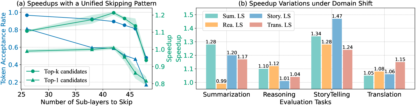
In this work, we introduce a novel research direction for plug-and-play SD: sparsity-based drafting, which leverages the inherent sparsity in LLMs to enable efficient drafting (see Figure 1 (b)). Specifically, we exploit a straightforward yet practical form of LLM sparsity – layer sparsity – to accelerate inference. Our approach is based on two key observations: 1) LLMs possess great potential for self-acceleration through layer sparsity. Contrary to the conventional belief that layer selection must be carefully optimized (Zhang et al., 2024), we surprisingly found that uniformly skipping layers to draft can still achieve a notable $1.2×$ speedup, providing a strong foundation for plug-and-play SD. 2) Layer sparsity is task-specific. We observed that each task requires its own optimal set of skipped layers, and applying the same layer configuration across different tasks would cause substantial performance degradation. For example, the speedup drops from $1.47×$ to $1.01×$ when transferring the configuration optimized for a storytelling task to a reasoning task.
Building on these observations, we introduce \method, the first on-the-fly self-speculative decoding algorithm that adaptively optimizes the set of skipped layers in the target LLM during inference, facilitating the lossless acceleration of LLMs across diverse input data streams. \method integrates two key innovations: (1) a context-based layer set optimization mechanism that leverages LLM-generated context to efficiently identify the optimal set of skipped layers corresponding to the current input stream, and (2) a confidence-aware inference acceleration strategy that maximizes the use of draft tokens, improving both speculation accuracy and verification efficiency. These innovations allow \method to strike an expected balance between the latency-accuracy trade-off in SD, providing a new plug-and-play solution for lossless LLM inference acceleration without the need for auxiliary models or additional training, as demonstrated in Table 1.
We conduct experiments using LLaMA-2 and CodeLLaMA models across multiple tasks, including summarization, code generation, mathematical reasoning, etc. \method achieves a $1.3×$ $\sim$ $1.6×$ wall-clock time speedup compared to conventional autoregressive decoding. Notably, in the greedy setting, \method consistently maintains a $98\%$ $\sim$ $100\%$ token acceptance rate across the LLaMA2 series, indicating the high alignment potential of this paradigm. Further analysis validated the effectiveness of \method across diverse data streams and its compatibility with various LLM backbones.
Our key contributions are:
1. We performed an empirical analysis of LLM acceleration on layer sparsity, revealing both the potential for LLM self-acceleration via layer sparsity and its task-specific nature, underscoring the necessity for adaptive self-speculative decoding during inference.
1. Building on these insights, we introduce \method, the first plug-and-play self-speculative decoding algorithm that optimizes the set of skipped layers in the target LLM on the fly, enabling lossless acceleration of LLM inference across diverse input data streams.
1. We conducted extensive experiments across various models and tasks, demonstrating that \method consistently achieves a $1.3×$ $\sim$ $1.6×$ speedup without any auxiliary model or training, while theoretically guaranteeing the preservation of the generated text’s distribution.
2 Related Work
Speculative Decoding (SD)
Due to the sequential nature of autoregressive decoding, LLM inference is constrained by memory-bound computations (Patterson, 2004; Shazeer, 2019), with the primary latency bottleneck arising not from arithmetic computations but from memory reads/writes of LLM parameters (Pope et al., 2023). To mitigate this issue, speculative decoding (SD) introduces utilizing a compact draft model to predict multiple decoding steps, with the target LLM then validating them in parallel (Xia et al., 2023; Leviathan et al., 2023; Chen et al., 2023). Recent SD variants have sought to enhance efficiency by incorporating additional modules (Kim et al., 2023; Sun et al., 2023; Du et al., 2024; Li et al., 2024a; b) or introducing new training objectives (Liu et al., 2023a; Kou et al., 2024; Zhou et al., 2024; Gloeckle et al., 2024). However, these approaches necessitate extra parameters or extensive training, limiting their applicability across different models. Another line of research has explored plug-and-play SD methods with Jacobi decoding (Santilli et al., 2023; Fu et al., 2024), which predict multiple steps in parallel by appending pseudo tokens to the input and refining them iteratively. As shown in Table 1, our work complements these efforts by investigating a novel plug-and-play SD method with layer-skipping, which exploits the inherent sparsity of LLM layers to accelerate inference. The most related approaches to ours include Self-SD (Zhang et al., 2024) and LayerSkip (Elhoushi et al., 2024), which also skip intermediate layers of LLMs to form the draft model. However, both methods require a time-consuming offline training process, making them neither plug-and-play nor easily generalizable across different models and tasks.
| Eagle (Li et al., 2024a; b) | Draft Heads | Yes | ✗ | ✓ | ✓ | ✓ | - |
| --- | --- | --- | --- | --- | --- | --- | --- |
| Rest (He et al., 2024) | Context Retrieval | Yes | ✗ | ✓ | ✓ | ✓ | - |
| Self-SD (Zhang et al., 2024) | Layer Skipping | No | ✗ | ✓ | ✓ | ✗ | - |
| \hdashline Parallel (Santilli et al., 2023) | Jacobi Decoding | No | ✓ | ✓ | ✗ | ✗ | $0.9×$ $\sim$ $1.0×$ |
| Lookahead (Fu et al., 2024) | Jacobi Decoding | No | ✓ | ✓ | ✓ | ✓ | $1.2×$ $\sim$ $1.4×$ |
| \method (Ours) | Layer Skipping | No | ✓ | ✓ | ✓ | ✓ | $1.3×$ $\sim$ $1.6×$ |
Table 1: Comparison of \method with existing SD methods. “ AM ” denotes whether the method requires auxiliary modules such as additional parameters or data stores. “ Greedy ”, “ Sampling ”, and “ Token Tree ” denote whether the method supports greedy decoding, multinomial sampling, and token tree verification, respectively. \method is the first plug-and-play layer-skipping SD method, which is orthogonal to those Jacobi-based methods such as Lookahead (Fu et al., 2024).
Efficient LLMs Utilizing Sparsity
LLMs are powerful but often over-parameterized (Hu et al., 2022). To address this issue, various methods have been proposed to accelerate inference by leveraging different forms of LLM sparsity. One promising research direction is model compression, which includes approaches such as quantization (Dettmers et al., 2022; Frantar et al., 2023; Ma et al., 2024), parameter pruning (Liu et al., 2019; Hoefler et al., 2021; Liu et al., 2023b), and knowledge distillation (Touvron et al., 2021; Hsieh et al., 2023; Gu et al., 2024). These approaches aim to reduce model sparsity by compressing LLMs into more compact forms, thereby decreasing memory usage and computational overhead during inference. Our proposed method, \method, focuses specifically on sparsity within LLM layer computations, providing a more streamlined approach to efficient LLM inference that builds upon recent advances in layer skipping (Corro et al., 2023; Zhu et al., 2024; Jaiswal et al., 2024; Liu et al., 2024). Unlike these existing layer-skipping methods that may lead to information loss and performance degradation, \method investigates the utilization of layer sparsity to enable lossless acceleration of LLM inference.
3 Preliminaries
3.1 Self-Speculative Decoding
Unlike most SD methods that require additional parameters, self-speculative decoding (Self-SD) first proposed utilizing parts of an LLM as a compact draft model (Zhang et al., 2024). In each decoding step, this approach skips intermediate layers of the LLM to efficiently generate draft tokens; these tokens are then validated in parallel by the full-parameter LLM to ensure that the output distribution of the target LLM remains unchanged. The primary challenge of Self-SD lies in determining which layers, and how many, should be skipped – referred to as the skipped layer set – during the drafting stage, which is formulated as an optimization problem. Formally, given the input data $\mathcal{X}$ and the target LLM $\mathscr{M}_{T}$ with $L$ layers (including both attention and MLP layers), Self-SD aims to identify the optimal skipped layer set $\bm{z}$ that minimizes the average inference time per token:
$$
\bm{z}^{*}=\underset{\bm{z}}{\arg\min}\frac{\sum_{\bm{x}\in\mathcal{X}}f\left(%
\bm{x}\mid\bm{z};\bm{\theta}_{\mathscr{M}_{T}}\right)}{\sum_{\bm{x}\in\mathcal%
{X}}|\bm{x}|},\quad\text{ s.t. }\bm{z}\in\{0,1\}^{L}, \tag{1}
$$
where $f(·)$ is a black-box function that returns the inference latency of sample $\bm{x}$ , $\bm{z}_{i}∈\{0,1\}$ denotes whether layer $i$ of the target LLM is skipped when drafting, and $|\bm{x}|$ represents the sample length. Self-SD addresses this problem through a Bayesian optimization process (Jones et al., 1998). Before inference, this process iteratively selects new inputs $\bm{z}$ based on a Gaussian process (Rasmussen & Williams, 2006) and evaluates Eq (1) on the training set of $\mathcal{X}$ . After a specified number of iterations, the best $\bm{z}$ is considered an approximation of $\bm{z}^{*}$ and is held fixed for inference.
While Self-SD has proven effective, its reliance on a time-intensive Bayesian optimization process poses certain limitations. For each task, Self-SD must sequentially evaluate all selected training samples during every iteration to optimize Eq (1); Moreover, the computational burden of Bayesian optimization escalates substantially with the number of iterations. As a result, processing just eight CNN/Daily Mail (Nallapati et al., 2016) samples for 1000 Bayesian iterations requires nearly 7.5 hours for LLaMA-2-13B and 20 hours for LLaMA-2-70B on an NVIDIA A6000 server. These computational demands restrict the generalizability of Self-SD across different models and tasks.
3.2 Experimental Observations
This subsection delves into Self-SD, exploring the plug-and-play potential of this layer-skipping SD paradigm for lossless LLM inference acceleration. Our key findings are detailed below.
<details>
<summary>x2.png Details</summary>
### Visual Description
## Combined Chart: Speedups and Domain Shift Variations
### Overview
The image presents two charts side-by-side. Chart (a) on the left shows the relationship between the number of sub-layers skipped and the token acceptance rate for Top-k and Top-1 candidates. Chart (b) on the right displays speedup variations under domain shift across different evaluation tasks (Summarization, Reasoning, StoryTelling, and Translation) for four different scenarios (Sum. LS, Story. LS, Rea. LS, and Trans. LS).
### Components/Axes
**Chart (a): Speedups with a Unified Skipping Pattern**
* **Title:** Speedups with a Unified Skipping Pattern
* **X-axis:** Number of Sub-layers to Skip (ranging from 25 to 45 in increments of 5)
* **Y-axis (left):** Token Acceptance Rate (ranging from 0.2 to 1.0 in increments of 0.2)
* **Y-axis (right):** Speedup (ranging from 0.8 to 1.2 in increments of 0.1)
* **Legend (bottom-left):**
* Blue line with circle markers: Top-k candidates
* Green line with triangle markers: Top-1 candidates
**Chart (b): Speedup Variations under Domain Shift**
* **Title:** Speedup Variations under Domain Shift
* **X-axis:** Evaluation Tasks (Summarization, Reasoning, StoryTelling, Translation)
* **Y-axis:** Speedup (ranging from 0.9 to 1.5 in increments of 0.1)
* **Legend (top-left):**
* Light Blue: Sum. LS
* Blue: Story. LS
* Orange: Rea. LS
* Light Red: Trans. LS
### Detailed Analysis
**Chart (a): Speedups with a Unified Skipping Pattern**
* **Top-k candidates (Blue line):**
* The line starts at approximately 0.97 at 25 sub-layers.
* It decreases to approximately 0.9 at 40 sub-layers.
* It then decreases sharply to approximately 0.9 at 45 sub-layers.
* **Top-1 candidates (Green line):**
* The line starts at approximately 0.8 at 25 sub-layers.
* It increases to approximately 0.98 at 40 sub-layers.
* It then decreases sharply to approximately 0.8 at 45 sub-layers.
**Chart (b): Speedup Variations under Domain Shift**
* **Summarization:**
* Sum. LS (Light Blue): 1.28
* Rea. LS (Orange): 0.99
* Story. LS (Blue): 1.20
* Trans. LS (Light Red): 1.17
* **Reasoning:**
* Sum. LS (Light Blue): 1.10
* Rea. LS (Orange): 1.12
* Story. LS (Blue): 1.01
* Trans. LS (Light Red): 1.04
* **StoryTelling:**
* Sum. LS (Light Blue): 1.34
* Rea. LS (Orange): 1.28
* Story. LS (Blue): 1.47
* Trans. LS (Light Red): 1.24
* **Translation:**
* Sum. LS (Light Blue): 1.05
* Rea. LS (Orange): 1.08
* Story. LS (Blue): 1.06
* Trans. LS (Light Red): 1.15
### Key Observations
* In Chart (a), the token acceptance rate for Top-k candidates generally decreases as the number of sub-layers skipped increases. The token acceptance rate for Top-1 candidates generally increases as the number of sub-layers skipped increases, then decreases sharply.
* In Chart (b), the speedup varies significantly across different evaluation tasks and scenarios. StoryTelling shows the highest speedup for Story. LS, while Reasoning shows the lowest speedup overall.
### Interpretation
Chart (a) suggests that skipping more sub-layers initially improves the token acceptance rate for Top-1 candidates, but eventually, skipping too many sub-layers degrades the performance for both Top-k and Top-1 candidates. Chart (b) indicates that the effectiveness of different strategies (Sum. LS, Story. LS, Rea. LS, Trans. LS) is highly dependent on the specific evaluation task. StoryTelling benefits most from the Story. LS strategy, while Reasoning shows relatively low speedups across all strategies. The domain shift significantly impacts the speedup achieved by each strategy.
</details>
Figure 2: (a) LLMs possess self-acceleration potential via layer sparsity. By utilizing drafts from the top- $k$ candidates, we found that uniformly skipping half of the layers during drafting yields a notable $1.2×$ speedup. (b) Layer sparsity is task-specific. Each task requires its own optimal set of skipped layers, and applying the skipped layer configuration from one task to another can lead to substantial performance degradation. “ X LS ” represents the skipped layer set optimized for task X.
3.2.1 LLMs Possess Self-Acceleration Potential via Layer Sparsity
We begin by investigating the potential of behavior alignment between the target LLM and its layer-skipping variant. Unlike previous work (Zhang et al., 2024) that focused solely on greedy draft predictions, we leverage potential draft candidates from top- $k$ predictions, as detailed in Section 4.2. We conducted experiments using LLaMA-2-13B across the CNN/Daily Mail (Nallapati et al., 2016), GSM8K (Cobbe et al., 2021), and TinyStories (Eldan & Li, 2023) datasets. We applied a uniform layer-skipping pattern with $k$ set to 10. The experimental results, illustrated in Figure 2 (a), demonstrate a $30\%$ average improvement in the token acceptance rate by leveraging top- $k$ predictions, with over $90\%$ of draft tokens accepted by the target LLM. Consequently, compared to Self-SD, which achieved a maximum speedup of $1.01×$ in this experimental setting, we revealed that the layer-skipping SD paradigm could yield an average wall-clock speedup of $1.22×$ over conventional autoregressive decoding with a uniform layer-skipping pattern. This finding challenges the prevailing belief that the selection of skipped layers must be meticulously curated, suggesting instead that LLMs possess greater potential for self-acceleration through inherent layer sparsity.
3.2.2 Layer Sparsity is Task-specific
We further explore the following research question: Is the skipped layer set optimized for one specific task applicable to other tasks? To address this, we conducted domain shift experiments using LLaMA-2-13B on the CNN/Daily Mail, GSM8K, TinyStories, and WMT16 DE-EN datasets. The experimental results, depicted in Figure 2 (b), reveal two critical findings: 1) Each task requires its own optimal skipped layer set. As illustrated in Figure 2 (b), the highest speedup performance is consistently achieved by the skipped layer configuration specifically optimized for each task. The detailed configuration of these layers is presented in Appendix A, demonstrating that the optimal configurations differ across tasks. 2) Applying the static skipped layer configuration across different tasks can lead to substantial efficiency degradation. For example, the speedup decreases from $1.47×$ to $1.01×$ when the optimized skipped layer set from a storytelling task is applied to a mathematical reasoning task, indicating that the optimized skipped layer set for one specific task does not generalize effectively to others.
These findings lay the groundwork for our plug-and-play solution within layer-skipping SD. Section 3.2.1 provides a strong foundation for real-time skipped layer selection, suggesting that additional optimization using training data may be unnecessary; Section 3.2.2 highlights the limitations of static layer-skipping patterns for dynamic input data streams across various tasks, underscoring the necessity for adaptive layer optimization during inference. Building on these insights, we present our on-the-fly self-speculative decoding method for efficient and adaptive layer set optimization.
4 SWIFT: On-the-Fly Self-Speculative Decoding
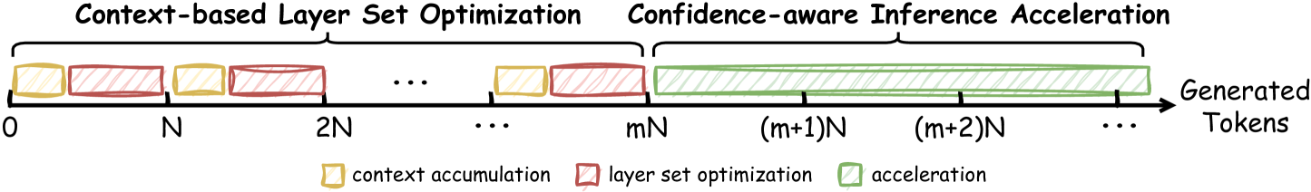
We introduce \method, the first plug-and-play self-speculative decoding approach that optimizes the skipped layer set of the target LLM on the fly, facilitating lossless LLM acceleration across diverse input data streams. As shown in Figure 3, \method divides LLM inference into two distinct phases: (1) context-based layer set optimization (§ 4.1), which aims to identify the optimal skipped layer set given the input stream, and (2) confidence-aware inference acceleration (§ 4.2), which employs the determined configuration to accelerate LLM inference.
<details>
<summary>x3.png Details</summary>
### Visual Description
## Diagram: Context-based and Confidence-aware Optimization
### Overview
The image is a diagram illustrating the process of context-based layer set optimization and confidence-aware inference acceleration in relation to generated tokens. It shows a timeline divided into sections representing context accumulation, layer set optimization, and acceleration.
### Components/Axes
* **Horizontal Axis:** Represents "Generated Tokens" with markers at 0, N, 2N, ..., mN, (m+1)N, (m+2)N, and so on. The arrow indicates the direction of token generation.
* **Legend (bottom-left):**
* Yellow box: "context accumulation"
* Red box: "layer set optimization"
* Green box: "acceleration"
* **Top Labels:**
* "Context-based Layer Set Optimization" spans from 0 to mN.
* "Confidence-aware Inference Acceleration" spans from mN to the end of the timeline.
### Detailed Analysis
* **Context-based Layer Set Optimization (0 to mN):**
* Alternating yellow (context accumulation) and red (layer set optimization) blocks.
* The blocks appear to be of roughly equal size.
* The pattern repeats several times, indicated by the ellipsis (...).
* **Confidence-aware Inference Acceleration (mN onwards):**
* Begins with a red (layer set optimization) block.
* Followed by a long series of green (acceleration) blocks, indicated by the ellipsis (...).
* The green blocks appear to increase in length as the number of generated tokens increases.
### Key Observations
* The process starts with context accumulation and layer set optimization.
* After 'mN' tokens, the process transitions to confidence-aware inference acceleration, primarily involving acceleration blocks.
* The acceleration blocks seem to grow in size as more tokens are generated.
### Interpretation
The diagram illustrates a multi-stage process for token generation, likely within a neural network or similar system. Initially, context is accumulated, and the layer set is optimized. As the system gains confidence (after 'mN' tokens), the focus shifts to acceleration, which becomes increasingly dominant as more tokens are generated. The increasing size of the acceleration blocks suggests that the system becomes more efficient or faster at generating tokens as it progresses. The diagram highlights the transition from initial setup and optimization to a phase of accelerated inference.
</details>
Figure 3: Timeline of \method inference. N denotes the maximum generation length per instance.
4.1 Context-based Layer Set Optimization
Layer set optimization is a critical challenge in self-speculative decoding, as it determines which layers of the target LLM should be skipped to form the draft model (see Section 3.1). Unlike prior methods that rely on time-intensive offline optimization, our work emphasizes on-the-fly layer set optimization, which poses a greater challenge to the latency-accuracy trade-off: the optimization must be efficient enough to avoid delays during inference while ensuring accurate drafting of subsequent decoding steps. To address this, we propose an adaptive optimization mechanism that balances efficiency with drafting accuracy. Our method minimizes overhead by performing only a single forward pass of the draft model per step to validate potential skipped layer set candidates. The core innovation is the use of LLM-generated tokens (i.e., prior context) as ground truth, allowing for simultaneous validation of the draft model’s accuracy in predicting future decoding steps.
In the following subsections, we illustrate the detailed process of this optimization phase for each input instance, which includes context accumulation (§ 4.1.1) and layer set optimization (§ 4.1.2).
4.1.1 Context Accumulation
Given an input instance in the optimization phase, the draft model is initialized by uniformly skipping layers in the target LLM. This initial layer-skipping pattern is maintained to accelerate inference until a specified number of LLM-generated tokens, referred to as the context window, has been accumulated. Upon reaching this window length, the inference transitions to layer set optimization.
<details>
<summary>x4.png Details</summary>
### Visual Description
## Diagram: Efficient Layer Set Suggestion and Parallel Candidate Evaluation
### Overview
The image presents a diagram illustrating a system for efficient layer set suggestion and parallel candidate evaluation in the context of Large Language Models (LLMs). It is divided into two main parts: (a) Efficient Layer Set Suggestion and (b) Parallel Candidate Evaluation. The diagram outlines the flow of data and processes involved in generating and evaluating different layer configurations for an LLM.
### Components/Axes
**Overall Structure:** The diagram is split into two sections, (a) and (b), enclosed in dashed-line boxes.
**Section (a) - Efficient Layer Set Suggestion:**
* **LLM Inputs:** Represented by a series of alternating tan and green blocks, indicating input tokens and LLM-generated tokens.
* **Random Search:** A tan rounded rectangle containing the text "Random Search" and the code snippet "np.random.choice()", accompanied by a dice icon.
* **Bayes Optimization:** A tan rounded rectangle containing the text "Bayes Optimization" and a line graph with several data points.
* **Layer Set:** A vertical stack of alternating tan blocks labeled "MLP" and "Attention", with binary values (0 or 1) to their right, enclosed in square brackets. The bottom value is labeled 'z'.
* **Target LLM Verification:** A blue rounded rectangle containing the text "Target LLM Verification" and an icon resembling a target with a checkmark.
* **Arrows:** Solid and dashed arrows indicate the flow of data and control between components.
**Section (b) - Parallel Candidate Evaluation:**
* **Original Outputs:** A series of alternating tan and green blocks, representing original outputs.
* **Draft Tokens:** A series of blue blocks, representing draft tokens.
* **Calculate Matchness:** Text label indicating the calculation of matchness between original outputs and draft tokens.
* **Gaussian Update:** A purple rounded rectangle containing the text "Gaussian Update".
* **Alter Skipped Layer Set:** A tan rounded rectangle containing the text "Alter Skipped Layer Set" and an icon of two squares with rotating arrows.
* **Compact Draft Model:** A green rounded rectangle containing the text "Compact Draft Model" and an icon of a document with a pencil.
* **Arrows:** Solid and dotted arrows indicate the flow of data and control between components.
**Legend (Bottom):**
* Tan: input tokens
* Green: LLM-generated tokens
* Blue: draft tokens
* Tan: accepted tokens
### Detailed Analysis
**Section (a) - Efficient Layer Set Suggestion:**
1. **LLM Inputs:** A sequence of 5 blocks, alternating between tan (input tokens) and green (LLM-generated tokens).
2. **Random Search:** The "Random Search" block suggests a method for randomly selecting layer configurations. The "np.random.choice()" code snippet indicates the use of a random choice function, likely from the NumPy library.
3. **Bayes Optimization:** The "Bayes Optimization" block suggests an alternative method for selecting layer configurations using Bayesian optimization techniques. The line graph within the block likely represents the optimization process.
4. **Layer Set:** The stack of "MLP" and "Attention" layers represents a possible layer configuration for the LLM. The binary values (0 or 1) next to each layer likely indicate whether that layer is included (1) or skipped (0) in the current configuration. The 'z' at the bottom is likely a variable representing the final binary value.
* From top to bottom, the layers are: MLP (0), Attention (1), MLP (0), Attention (0), MLP (1), Attention (0).
5. **Flow:**
* The "LLM Inputs" feed into both "Random Search" and "Bayes Optimization".
* Both "Random Search" and "Bayes Optimization" contribute to the "Layer Set" configuration.
* The "Layer Set" is then passed to "Parallel Candidate Evaluation".
* "Target LLM Verification" receives "Draft multiple steps" from "Compact Draft Model" and outputs "Accepted tokens" which updates "LLM Inputs".
**Section (b) - Parallel Candidate Evaluation:**
1. **Original Outputs:** A sequence of 5 blocks, alternating between tan and green, representing the original outputs of the LLM.
2. **Draft Tokens:** A sequence of 5 blue blocks, representing the draft tokens generated by the current layer configuration.
3. **Calculate Matchness:** The "Calculate Matchness" step compares the "Original Outputs" and "Draft Tokens" to assess the quality of the draft.
4. **Gaussian Update:** The "Gaussian Update" block suggests that a Gaussian process is used to update the model based on the matchness score.
5. **Alter Skipped Layer Set:** If the draft is not the best, the "Alter Skipped Layer Set" block indicates that the layer configuration is modified.
6. **Compact Draft Model:** The "Compact Draft Model" block represents the final, optimized draft model.
7. **Flow:**
* "Original Outputs" and "Draft Tokens" are compared in "Calculate Matchness".
* "Calculate Matchness" feeds into "Gaussian Update".
* If the draft is not the best, "Calculate Matchness" feeds into "Alter Skipped Layer Set".
* "Alter Skipped Layer Set" feeds back into the "Draft Tokens".
* The "Draft Tokens" are passed to "Compact Draft Model".
**Legend:** The legend at the bottom clarifies the color coding used for different types of tokens: input tokens (tan), LLM-generated tokens (green), draft tokens (blue), and accepted tokens (tan).
### Key Observations
* The diagram illustrates a closed-loop system for optimizing layer configurations in LLMs.
* Two methods, "Random Search" and "Bayes Optimization", are used to suggest layer configurations.
* Parallel candidate evaluation is performed to assess the quality of different layer configurations.
* The system incorporates a mechanism for updating the model based on the matchness score between original outputs and draft tokens.
### Interpretation
The diagram presents a method for efficiently exploring and optimizing the layer structure of Large Language Models. By using a combination of random search and Bayesian optimization, the system can generate a diverse set of layer configurations. The parallel candidate evaluation process allows for the simultaneous assessment of these configurations, enabling the system to quickly identify promising layer structures. The Gaussian update mechanism provides a means for refining the model based on the performance of different layer configurations. The closed-loop nature of the system allows for continuous improvement and adaptation of the LLM's layer structure. The use of draft tokens and the comparison with original outputs suggests a form of iterative refinement, where the model gradually improves its performance by exploring different layer configurations.
</details>
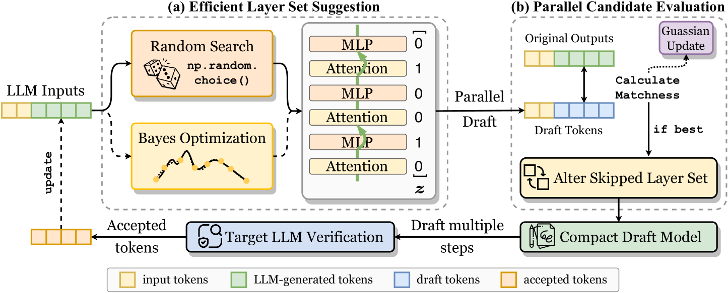
Figure 4: Layer set optimization process in \method. During the optimization stage, \method performs an optimization step prior to each LLM decoding step to adjust the skipped layer set, which involves: (a) Efficient layer set optimization. \method integrates random search with interval Bayesian optimization to propose layer set candidates; (b) Parallel candidate evaluation. \method uses LLM-generated tokens (i.e., prior context) as ground truth, enabling simultaneous validation of the proposed candidates. The best-performing layer set is selected to accelerate the current decoding step.
4.1.2 Layer Set Optimization
During this stage, as illustrated in Figure 4, we integrate an optimization step before each LLM decoding step to refine the skipped layer set, which comprises two substeps:
Efficient Layer Set Suggestion
This substep aims to suggest a potential layer set candidate. Formally, given a target LLM $\mathscr{M}_{T}$ with $L$ layers, our goal is to identify an optimal skipped layer set $\bm{z}∈\{0,1\}^{L}$ to form the compact draft model. Unlike Zhang et al. (2024), which relies entirely on a time-consuming Bayesian optimization process, we introduce an efficient strategy that combines random search with Bayesian optimization. In this approach, random sampling efficiently handles most of the exploration. Specifically, given a fixed skipping ratio $r$ , \method applies Bayesian optimization at regular intervals of $\beta$ optimization steps (e.g., $\beta=25$ ) to suggest the next layer set candidate, while random search is employed during other optimization steps.
$$
\bm{z}=\left\{\begin{array}[]{ll}\operatorname{Bayesian\_Optimization}(\bm{l})%
&\text{ if }o\text{ \% }\beta=0\\
\operatorname{Random\_Search}(\bm{l})&\text{ otherwise }\end{array},\right. \tag{2}
$$
where $1≤ o≤ S$ is the current optimization step; $S$ denotes the maximum number of optimization steps; $\bm{l}=\binom{L}{rL}$ denotes the input space, i.e., all possible combinations of layers that can be skipped.
Parallel Candidate Evaluation
\method
leverages LLM-generated context to simultaneously validate the candidate draft model’s performance in predicting future decoding steps. Formally, given an input sequence $\bm{x}$ and the previously generated tokens within the context window, denoted as $\bm{y}=\{y_{1},...,y_{\gamma}\}$ , the draft model $\mathscr{M}_{D}$ , which skips the designated layers $\bm{z}$ of the target LLM, is employed to predict these context tokens in parallel:
$$
y^{\prime}_{i}=\arg\max_{y}\log P\left(y\mid\bm{x},\bm{y}_{<i};\bm{\theta}_{%
\mathscr{M}_{D}}\right),1\leq i\leq\gamma, \tag{3}
$$
where $\gamma$ represents the context window. The cached key-value pairs in the target LLM $\mathscr{M}_{T}$ are reused by $\mathscr{M}_{D}$ , presumably aligning $\mathscr{M}_{D}$ ’s distribution with $\mathscr{M}_{T}$ and reducing the redundant computation. The matchness score is defined as the exact match ratio between $\bm{y}$ and $\bm{y}^{\prime}$ :
$$
\texttt{matchness}=\frac{\sum_{i}\mathbb{I}\left(y_{i}=y^{\prime}_{i}\right)}{%
\gamma},1\leq i\leq\gamma, \tag{4}
$$
where $\mathbb{I}(·)$ denotes the indicator function. This score serves as the optimization objective during optimization, reflecting $\mathscr{M}_{D}$ ’s accuracy in predicting future decoding steps. As shown in Figure 4, the matchness score at each step is integrated into the Gaussian process model to guide Bayesian optimization, with the highest-scoring layer set candidate being retained to form the draft model.
As illustrated in Figure 3, the process of context accumulation and layer set optimization alternates for each instance until a termination condition is met – either the maximum number of optimization steps is reached or the best candidate remains unchanged over multiple iterations. Once the optimization phase concludes, the inference process transitions to the confidence-aware inference acceleration phase, where the optimized draft model is employed to speed up LLM inference.
4.2 Confidence-aware Inference Acceleration
<details>
<summary>x5.png Details</summary>
### Visual Description
## Diagram: Early-Stopping Drafting and Dynamic Verification
### Overview
The image presents two diagrams illustrating "Early-stopping Drafting" and "Dynamic Verification" processes. The diagrams depict how attention mechanisms and probability thresholds influence the selection and verification of words in a sequence.
### Components/Axes
**Diagram (a): Early-stopping Drafting**
* **Title:** (a) Early-stopping Drafting
* **Top-Left Text:** Continue
* **Probability Condition:** p_is = 0.85 > ε
* **Input:** Attention (arrow pointing upwards to M_D)
* **Module:** M_D (green rounded rectangle)
* **Output Sequence (Blue):**
* "is" (solid blue rectangle)
* "will" (dashed blue rectangle)
* "that" (no rectangle)
* **Dashed Arrow:** A curved dashed arrow originates from the "is" rectangle and points downwards and rightwards towards the "is" input of diagram (b).
**Diagram (b): Dynamic Verification**
* **Title:** (b) Dynamic Verification
* **Top-Right Text:** Early Stop!
* **Probability Condition:** p_all = 0.65 < ε
* **Input:** is (arrow pointing upwards to M_D)
* **Module:** M_D (green rounded rectangle)
* **Output Sequence (Red):**
* "all" (solid red rectangle)
* "the" (dashed red rectangle)
* "best" (dashed red rectangle)
* **Arrow:** A right-pointing arrow connects the output sequence of diagram (a) to the attention matrix in diagram (b).
**Attention Matrix**
* A 6x6 grid representing an attention matrix.
* Rows correspond to the words "is", "all", "will", "the", "best".
* Columns correspond to the words "is", "all", "will", "the", "best".
* Cells are either yellow (indicating attention) or white (no attention).
**Attention Labels**
* **Vertical Attention Labels:** "Attention" written vertically.
* "is" (solid blue rectangle)
* "all" (solid red rectangle)
* "will" (dashed blue rectangle)
* "the" (dashed red rectangle)
* "best" (dashed red rectangle)
* **Horizontal Attention Labels:** "Attention" written horizontally.
* "is" (solid blue rectangle)
* "all" (solid red rectangle)
* "will" (dashed blue rectangle)
* "the" (dashed red rectangle)
* "best" (dashed red rectangle)
### Detailed Analysis
**Diagram (a): Early-stopping Drafting**
* The process starts with an "Attention" input to the module M_D.
* If the probability p_is for the word "is" is greater than a threshold ε (0.85 > ε), the process continues.
* The output sequence includes "is" (solid blue), "will" (dashed blue), and "that".
**Diagram (b): Dynamic Verification**
* The process starts with the word "is" as input to the module M_D.
* If the probability p_all for the word "all" is less than a threshold ε (0.65 < ε), the process stops early.
* The output sequence includes "all" (solid red), "the" (dashed red), and "best" (dashed red).
**Attention Matrix**
* The attention matrix shows the relationships between the words.
* The yellow cells indicate where attention is focused.
* Row 1 ("is"): Attends to column 1 ("is") and column 2 ("all").
* Row 2 ("all"): Attends to column 1 ("is") and column 2 ("all").
* Row 3 ("will"): Attends to column 3 ("will") and column 4 ("the").
* Row 4 ("the"): Attends to column 3 ("will") and column 4 ("the").
* Row 5 ("best"): Attends to column 5 ("best") and column 6 ("<end of sequence>").
### Key Observations
* The diagrams illustrate two different strategies for sequence generation: early-stopping and dynamic verification.
* Early-stopping is based on a probability threshold for a specific word ("is").
* Dynamic verification is based on a probability threshold for another word ("all").
* The attention matrix visualizes the relationships between the words in the sequence.
* Solid rectangles indicate words that are directly considered, while dashed rectangles indicate words that are potentially considered or predicted.
### Interpretation
The diagrams demonstrate how attention mechanisms and probability thresholds can be used to control the generation of sequences. Early-stopping allows the process to terminate if a certain condition is met, while dynamic verification allows the process to adapt based on the relationships between the words. The attention matrix provides a visual representation of these relationships, showing which words are most relevant to each other. The use of solid and dashed rectangles highlights the distinction between definite and potential word selections, adding a layer of nuance to the process. The probability thresholds (0.85 and 0.65) suggest a trade-off between accuracy and efficiency, where higher thresholds may lead to more accurate sequences but also require more computation.
</details>
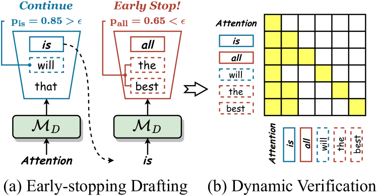
Figure 5: Confidence-aware inference process of \method. (a) The drafting terminates early if the confidence score drops below threshold $\epsilon$ . (b) Draft candidates are dynamically selected based on confidence and then verified in parallel by the target LLM.
During the acceleration phase, the optimization step is removed. \method applies the best-performed layer set to form the compact draft model and decodes following the draft-then-verify paradigm. Specifically, at each decoding step, given the input $\bm{x}$ and previous LLM outputs $\bm{y}$ , the draft model $\mathscr{M}_{D}$ predicts future LLM decoding steps in an autoregressive manner:
$$
y^{\prime}_{j}=\arg\max_{y}\log P\left(y\mid\bm{x},\bm{y},\bm{y}^{\prime}_{<j}%
;\bm{\theta}_{\mathscr{M}_{D}}\right), \tag{5}
$$
where $1≤ j≤ N_{D}$ is the current draft step, $N_{D}$ denotes the maximum draft length, $\bm{y}^{\prime}_{<j}$ represents previous draft tokens, and $P(·)$ denotes the probability distribution of the next draft token. The KV cache of the target LLM $\mathscr{M}_{T}$ and preceding draft tokens $\bm{y}^{\prime}_{<j}$ is reused to reduce the computational cost.
Let $p_{j}=\max P(·)$ denote the probability of the top-1 draft prediction $y^{\prime}_{j}$ , which can be regarded as a confidence score. Recent research (Li et al., 2024b; Du et al., 2024) shows that this score is highly correlated with the likelihood that the draft token $y^{\prime}_{j}$ will pass verification – higher confidence scores indicate a greater chance of acceptance. Therefore, following previous studies (Zhang et al., 2024; Du et al., 2024), we leverage the confidence score to prune unnecessary draft steps and select valuable draft candidates, improving both speculation accuracy and verification efficiency.
As shown in Figure 5, we integrate \method with two confidence-aware inference strategies These confidence-aware inference strategies are also applied during the optimization phase, where the current optimal layer set is used to form the draft model and accelerate the corresponding LLM decoding step.: 1) Early-stopping Drafting. The autoregressive drafting process halts if the confidence $p_{j}$ falls below a specified threshold $\epsilon$ , avoiding any waste of subsequant drafting computation. 2) Dynamic Verification. Each $y^{\prime}_{j}$ is dynamically extended with its top- $k$ draft predictions for parallel verification to enhance speculation accuracy, with $k$ determined by the confidence score $p_{j}$ . Concretely, $k$ is set to 10, 5, 3, and 1 for $p$ in the ranges of $(0,0.5]$ , $(0.5,0.8]$ , $(0.8,0.95]$ , and $(0.95,1]$ , respectively. All draft candidates are linearized into a single sequence and verified in parallel by the target LLM using a special causal attention mask (see Figure 5 (b)).
5 Experiments
5.1 Experimental Setup
Implementation Details
We mainly evaluate \method on LLaMA-2 (Touvron et al., 2023b) and CodeLLaMA series (Rozière et al., 2023) across various tasks, including summarization, mathematical reasoning, storytelling, and code generation. The evaluation datasets include CNN/Daily Mail (CNN/DM) (Nallapati et al., 2016), GSM8K (Cobbe et al., 2021), TinyStories (Eldan & Li, 2023), and HumanEval (Chen et al., 2021). The maximum generation lengths on CNN/DM, GSM8K, and TinyStories are set to 64, 64, and 128, respectively. We conduct 1-shot evaluation for CNN/DM and TinyStories, and 5-shot evaluation for GSM8K. We compare pass@1 and pass@10 for HumanEval. We randomly sample 1000 instances from the test set for each dataset except HumanEval. The maximum generation lengths for HumanEval and all analyses are set to 512. During optimization, we employ both random search and Bayesian optimization https://github.com/bayesian-optimization/BayesianOptimization to suggest skipped layer set candidates. Following prior work, we adopt speculative sampling (Leviathan et al., 2023) as our acceptance strategy with a batch size of 1. Detailed setups are provided in Appendix B.1 and B.2.
Baselines
In our main experiments, we compare \method to two existing plug-and-play methods: Parallel Decoding (Santilli et al., 2023) and Lookahead Decoding (Fu et al., 2024), both of which employ Jacobi decoding for efficient LLM drafting. It is important to note that \method, as a layer-skipping SD method, is orthogonal to these Jacobi-based SD methods, and integrating \method with them could further boost inference efficiency. We exclude other SD methods from our comparison as they necessitate additional modules or extensive training, which limits their generalizability.
Evaluation Metrics
We report two widely-used metrics for \method evaluation: mean generated length $M$ (Stern et al., 2018) and token acceptance rate $\alpha$ (Leviathan et al., 2023). Detailed descriptions of these metrics can be found in Appendix B.3. In addition to these metrics, we report the actual decoding speed (tokens/s) and wall-time speedup ratio compared with vanilla autoregressive decoding. The acceleration of \method theoretically guarantees the preservation of the target LLMs’ output distribution, making it unnecessary to evaluate the generation quality. However, to provide a point of reference, we present the evaluation scores for code generation tasks.
| LLaMA-2-13B Parallel Lookahead | Vanilla 1.04 1.38 | 1.00 0.95 $×$ 1.16 $×$ | 1.00 $×$ 1.11 1.50 | 1.00 0.99 $×$ 1.29 $×$ | 1.00 $×$ 1.06 1.62 | 1.00 0.97 $×$ 1.37 $×$ | 1.00 $×$ 19.49 25.46 | 20.10 0.97 $×$ 1.27 $×$ | 1.00 $×$ |
| --- | --- | --- | --- | --- | --- | --- | --- | --- | --- |
| \method | 4.34 | 1.37 $×$ † | 3.13 | 1.31 $×$ † | 8.21 | 1.53 $×$ † | 28.26 | 1.41 $×$ | |
| LLaMA-2-13B -Chat | Vanilla | 1.00 | 1.00 $×$ | 1.00 | 1.00 $×$ | 1.00 | 1.00 $×$ | 19.96 | 1.00 $×$ |
| Parallel | 1.06 | 0.96 $×$ | 1.08 | 0.97 $×$ | 1.10 | 0.98 $×$ | 19.26 | 0.97 $×$ | |
| Lookahead | 1.35 | 1.15 $×$ | 1.57 | 1.31 $×$ | 1.66 | 1.40 $×$ | 25.69 | 1.29 $×$ | |
| \method | 3.54 | 1.28 $×$ | 2.95 | 1.25 $×$ | 7.42 | 1.50 $×$ † | 26.80 | 1.34 $×$ | |
| LLaMA-2-70B | Vanilla | 1.00 | 1.00 $×$ | 1.00 | 1.00 $×$ | 1.00 | 1.00 $×$ | 4.32 | 1.00 $×$ |
| Parallel | 1.05 | 0.95 $×$ | 1.07 | 0.97 $×$ | 1.05 | 0.96 $×$ | 4.14 | 0.96 $×$ | |
| Lookahead | 1.36 | 1.15 $×$ | 1.54 | 1.30 $×$ | 1.59 | 1.35 $×$ | 5.45 | 1.26 $×$ | |
| \method | 3.85 | 1.43 $×$ † | 2.99 | 1.39 $×$ † | 6.17 | 1.62 $×$ † | 6.41 | 1.48 $×$ | |
Table 2: Comparison between \method and prior plug-and-play methods. We report the mean generated length M, speedup ratio, and average decoding speed (tokens/s) under greedy decoding. † indicates results with a token acceptance rate $\alpha$ above 0.98. More details are provided in Appendix C.1.
| HumanEval (pass@1) \method HumanEval (pass@10) | Vanilla 4.75 Vanilla | 1.00 0.98 1.00 | - 0.311 - | 0.311 1.40 $×$ 0.628 | 1.00 $×$ 3.79 1.00 $×$ | 1.00 0.88 1.00 | - 0.372 - | 0.372 1.46 $×$ 0.677 | 1.00 $×$ 1.00 $×$ |
| --- | --- | --- | --- | --- | --- | --- | --- | --- | --- |
| \method | 3.55 | 0.93 | 0.628 | 1.29 $×$ | 2.79 | 0.90 | 0.683 | 1.30 $×$ | |
Table 3: Experimental results of \method on code generation tasks. We report the mean generated length M, acceptance rate $\alpha$ , accuracy (Acc.), and speedup ratio for comparison. We use greedy decoding for pass@1 and random sampling with a temperature of 0.6 for pass@10.
5.2 Main Results
Table 2 presents the comparison between \method and previous plug-and-play methods on text generation tasks. The experimental results demonstrate the following findings: (1) \method shows superior efficiency over prior methods, achieving consistent speedups of $1.3×$ $\sim$ $1.6×$ over vanilla autoregressive decoding across various models and tasks. (2) The efficiency of \method is driven by the high behavior consistency between the target LLM and its layer-skipping draft variant. As shown in Table 2, \method produces a mean generated length M of 5.01, with a high token acceptance rate $\alpha$ ranging from $90\%$ to $100\%$ . Notably, for the LLaMA-2 series, this acceptance rate remains stable at $98\%$ $\sim$ $100\%$ , indicating that nearly all draft tokens are accepted by the target LLM. (3) Compared with 13B models, LLaMA-2-70B achieves higher speedups with a larger layer skip ratio ( $0.45$ $→$ $0.5$ ), suggesting that larger-scale LLMs exhibit greater layer sparsity. This underscores \method ’s potential to deliver even greater speedups as LLM scales continue to grow. A detailed analysis of this finding is presented in Section 5.3, while additional experimental results for LLaMA-70B models, including LLaMA-3-70B, are presented in Appendix C.2.
Table 3 shows the evaluation results of \method on code generation tasks. \method achieves speedups of $1.3×$ $\sim$ $1.5×$ over vanilla autoregressive decoding, demonstrating its effectiveness across both greedy decoding and random sampling settings. Additionally, speculative sampling theoretically guarantees that \method maintains the original output distribution of the target LLM. This is empirically validated by the task performance metrics in Table 3. Despite a slight variation in the pass@10 metric for CodeLLaMA-34B, \method achieves identical performance to autoregressive decoding.
5.3 In-depth Analysis
<details>
<summary>x6.png Details</summary>
### Visual Description
## Line Chart: Matchness and Speedup vs. Number of Instances
### Overview
The image presents a line chart showing the relationship between the number of instances and two metrics: Matchness (left y-axis) and Speedup (right y-axis). There are two speedup metrics: Overall Speedup and Instance Speedup. A vertical dashed line indicates an "Optimization Stop!" point. A table on the right provides a latency breakdown per token for different modules.
### Components/Axes
* **X-axis:** "# of Instances", ranging from 0 to 100 in increments of 10.
* **Left Y-axis:** "Matchness", ranging from 0.0 to 1.0 in increments of 0.2.
* **Right Y-axis:** "Speedup", ranging from 1.2 to 1.6 in increments of 0.1.
* **Legend (bottom-right):**
* Green line with circles: "Overall Speedup"
* Gray line with circles: "Instance Speedup"
* **Vertical dashed red line:** Labeled "Optimization Stop!" at approximately x=11.
* **Horizontal dashed black line:** Labeled "Average" at approximately y=1.55 (speedup).
* **Table (right side):** "Latency Breakdown per Token"
* Columns: "Modules", "Latency (ms)", "Ratio (%)"
* Rows: "Optimize", "Draft", "Verify", "Others", "Total"
### Detailed Analysis
**1. Matchness (Blue Line):**
* Trend: The Matchness line slopes sharply upward from approximately 0.1 to 0.9 within the first 10 instances, then plateaus around 1.0.
* Data Points:
* Instance 0: Matchness ≈ 0.1
* Instance 5: Matchness ≈ 0.7
* Instance 10: Matchness ≈ 0.9
* Instance 15-100: Matchness ≈ 1.0
**2. Overall Speedup (Green Line):**
* Trend: The Overall Speedup line slopes upward from approximately 1.2 to 1.5 within the first 70 instances, then plateaus around 1.5. A shaded green area represents the uncertainty.
* Data Points:
* Instance 0: Speedup ≈ 1.2
* Instance 10: Speedup ≈ 1.4
* Instance 40: Speedup ≈ 1.5
* Instance 70-100: Speedup ≈ 1.52
**3. Instance Speedup (Gray Line):**
* Trend: The Instance Speedup line fluctuates between 0.85 and 0.95 after the "Optimization Stop!".
* Data Points:
* Instance 0: Speedup ≈ 0.3
* Instance 10: Speedup ≈ 0.7
* Instance 40: Speedup ≈ 0.9
* Instance 70-100: Speedup ≈ 0.9
**4. Latency Breakdown Table:**
| Modules | Latency (ms) | Ratio (%) |
| -------- | ------------- | --------- |
| Optimize | 0.24 ± 0.02 | 0.8 |
| Draft | 19.93 ± 1.36 | 64.4 |
| Verify | 8.80 ± 2.21 | 28.4 |
| Others | 1.98 ± 0.13 | 6.4 |
| Total | 30.95 ± 2.84 | 100.0 |
### Key Observations
* Matchness increases rapidly in the initial instances and then stabilizes.
* Overall Speedup shows a gradual increase and then plateaus.
* Instance Speedup fluctuates around an average value after the optimization stop.
* The "Draft" module contributes the most to the total latency, accounting for 64.4% of the total latency.
### Interpretation
The chart suggests that the optimization process significantly improves Matchness in the early stages. The Overall Speedup also benefits from the optimization, showing a steady increase. The Instance Speedup, however, fluctuates, indicating variability in individual instances. The latency breakdown highlights that the "Draft" module is the most time-consuming, suggesting it could be a target for further optimization. The "Optimization Stop!" point likely indicates a point where the optimization process was halted, possibly due to diminishing returns or other constraints.
</details>
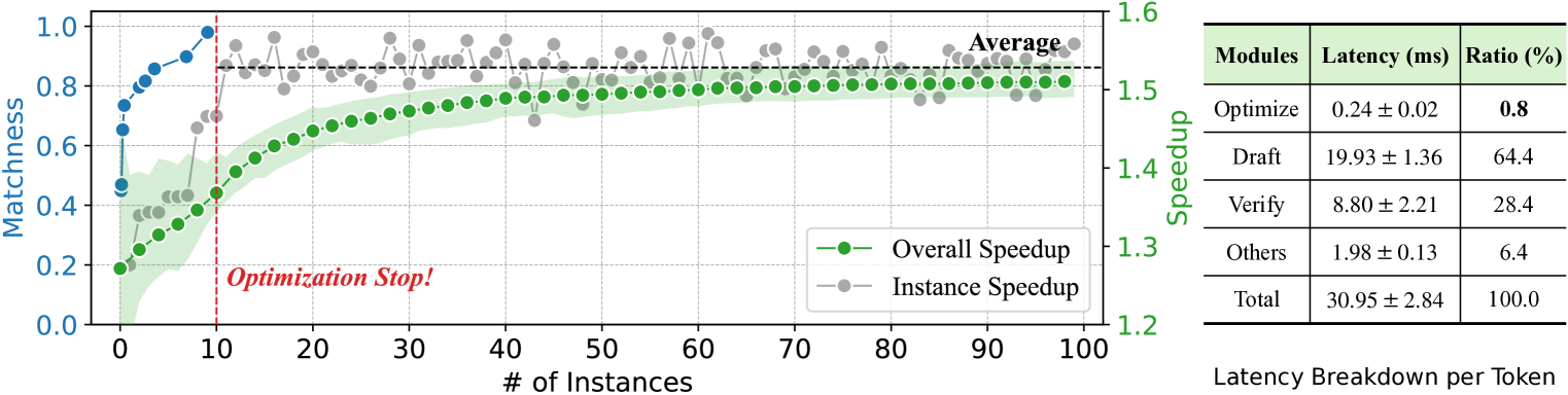
Figure 6: Illustration and latency breakdown of \method inference. As the left figure shows, after the context-based layer set optimization phase, the overall speedup of \method steadily increases, reaching the average instance speedup during the acceleration phase. The additional optimization steps account for only $\bf{0.8\%}$ of the total inference latency, as illustrated in the right figure.
Illustration of Inference
As described in Section 4, \method divides the LLM inference process into two distinct phases: optimization and acceleration. Figure 6 (left) illustrates the detailed acceleration effect of \method during LLM inference. Specifically, the optimization phase begins at the start of inference, where an optimization step is performed before each decoding step to adjust the skipped layer set forming the draft model. As shown in Figure 6, in this phase, the matchness score of the draft model rises sharply from 0.45 to 0.73 during the inference of the first instance. This score then gradually increases to 0.98, which triggers the termination of the optimization process. Subsequently, the inference transitions to the acceleration phase, during which the optimization step is removed, and the draft model remains fixed to accelerate LLM inference. As illustrated, the instance speedup increases with the matchness score, reaching an average of $1.53×$ in the acceleration phase. The overall speedup gradually rises as more tokens are generated, eventually approaching the average instance speedup. This dynamic reflects a key feature of \method: the efficiency of \method improves with increasing input length and the number of instances.
Breakdown of Computation
Figure 6 (right) presents the computation breakdown of different modules in \method with 1000 CNN/DM samples using LLaMA-2-13B. The results demonstrate that the optimization step only takes $\bf{0.8\%}$ of the overall inference process, indicating the efficiency of our strategy. Compared with Self-SD (Zhang et al., 2024) that requires a time-consuming optimization process (e.g., 7.5 hours for LLaMA-2-13B on CNN/DM), \method achieves a nearly 180 $×$ optimization time reduction, facilitating on-the-fly inference acceleration. Besides, the results show that the drafting stage of \method consumes the majority of inference latency. This is consistent with our results of mean generated length in Table 2 and 3, which shows that nearly $80\%$ output tokens are generated by the efficient draft model, demonstrating the effectiveness of our \method framework.
<details>
<summary>x7.png Details</summary>
### Visual Description
## Chart: Speedup and Token Acceptance Comparison
### Overview
The image is a combination bar and line chart comparing the performance of three systems (Vanilla, Self-SD, and SWIFT) across five tasks (Summarization, Reasoning, Instruction, Translation, and QA). The primary y-axis on the left represents "Speedup," measured by bars for each system and task. The secondary y-axis on the right represents "Token Acceptance," measured by lines for Self-SD and SWIFT.
### Components/Axes
* **X-axis:** Categorical axis representing the tasks: Summarization, Reasoning, Instruction, Translation, QA.
* **Left Y-axis:** "Speedup" ranging from 0.8 to 1.6 in increments of 0.2.
* **Right Y-axis:** "Token Acceptance" ranging from 0.5 to 1.0 in increments of 0.1.
* **Legend (Top):**
* Vanilla (Orange bar)
* Self-SD (Light Blue bar)
* SWIFT (Blue bar)
* SWIFT (Green line with circles)
* Self-SD (Gray dashed line with circles)
### Detailed Analysis
**Bar Chart (Speedup):**
* **Summarization:**
* Vanilla: 1.00x
* Self-SD: 1.28x
* SWIFT: 1.56x
* **Reasoning:**
* Vanilla: 1.00x
* Self-SD: 1.10x
* SWIFT: 1.45x
* **Instruction:**
* Vanilla: 1.00x
* Self-SD: 1.08x
* SWIFT: 1.47x
* **Translation:**
* Vanilla: 1.00x
* Self-SD: 1.05x
* SWIFT: 1.27x
* **QA:**
* Vanilla: 1.00x
* Self-SD: 1.02x
* SWIFT: 1.35x
**Line Chart (Token Acceptance):**
* **SWIFT (Green):** The line starts at approximately 0.98 for Summarization, remains relatively high, fluctuating between 0.9 and 1.0 across all tasks, ending at approximately 0.95 for QA.
* **Self-SD (Gray):** The line starts at approximately 0.93 for Summarization, decreases significantly for Reasoning (to approximately 0.7), fluctuates between 0.6 and 0.7 for Instruction and Translation, and ends at approximately 0.65 for QA.
### Key Observations
* SWIFT consistently outperforms Vanilla and Self-SD in terms of speedup across all tasks.
* Self-SD shows a modest speedup compared to Vanilla, but is significantly lower than SWIFT.
* Token acceptance for SWIFT is consistently higher than Self-SD across all tasks.
* Token acceptance for Self-SD drops significantly for Reasoning.
### Interpretation
The chart demonstrates that SWIFT provides a significant speedup compared to Vanilla and Self-SD across various natural language processing tasks. Additionally, SWIFT maintains a higher token acceptance rate than Self-SD, suggesting better overall performance and quality. The drop in token acceptance for Self-SD during the Reasoning task indicates a potential weakness in handling reasoning-related prompts. The consistent 1.00x speedup for Vanilla across all tasks suggests it serves as a baseline for comparison.
</details>
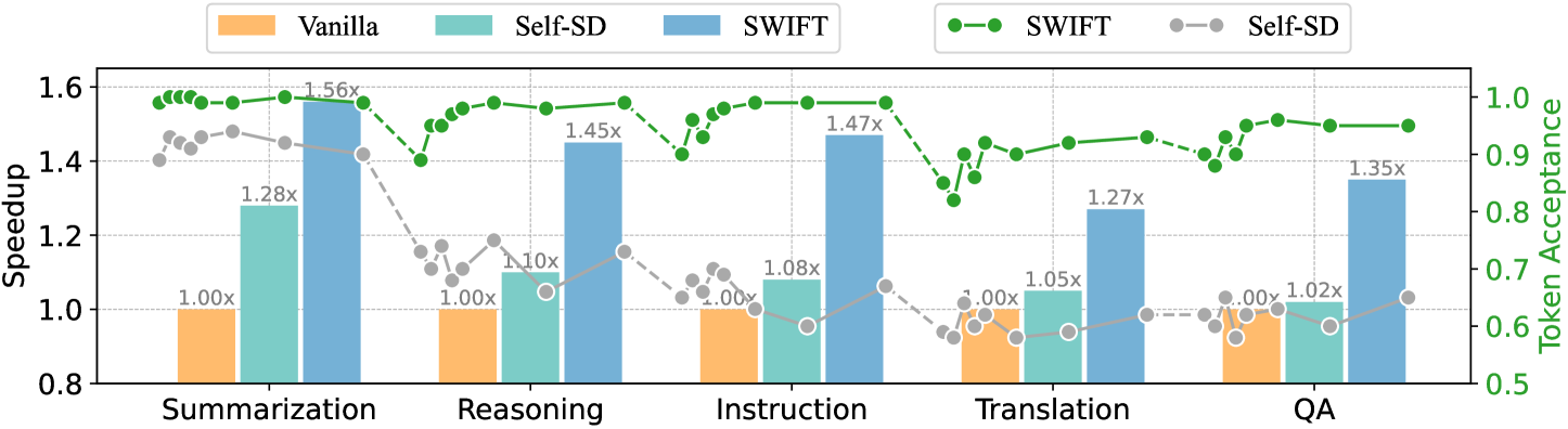
Figure 7: Comparison between \method and Self-SD in handling dynamic data input streams. Unlike Self-SD, which suffers from efficiency reduction during distribution shift, \method maintains stable acceleration performance with an acceptance rate exceeding 0.9.
Dynamic Input Data Streams
We further validate the effectiveness of \method in handling dynamic input data streams. We selected CNN/DM, GSM8K, Alpaca (Taori et al., 2023), WMT14 DE-EN, and Nature Questions (Kwiatkowski et al., 2019) for the evaluation on summarization, reasoning, instruction following, translation, and question answering tasks, respectively. For each task, we randomly sample 500 instances from the test set and concatenate them task-by-task to form the input stream. The experimental results are presented in Figure 7. As demonstrated, Self-SD is sensitive to domain shifts, with the average token acceptance rate dropping from $92\%$ to $68\%$ . Consequently, it suffers from severe speedup reduction from $1.33×$ to an average of $1.05×$ under domain shifts. In contrast, \method exhibits promising adaptation capability to different domains with an average token acceptance rate of $96\%$ , leading to a consistent $1.3×$ $\sim$ $1.6×$ speedup.
<details>
<summary>x8.png Details</summary>
### Visual Description
## Line Charts: Flexible Optimization Strategy and Scaling Law of SWIFT
### Overview
The image presents two line charts comparing the speedup achieved by different optimization strategies and scaling laws. Chart (a) explores the impact of varying the number of instances on speedup for a flexible optimization strategy, while chart (b) examines the scaling law of SWIFT with respect to the layer skip ratio.
### Components/Axes
**Chart (a): Flexible Optimization Strategy**
* **Title:** (a) Flexible Optimization Strategy
* **X-axis:** # of Instances, ranging from 0 to 50 in increments of 5.
* **Y-axis:** Speedup, ranging from 1.25 to 1.50 in increments of 0.05.
* **Legend (bottom-right):**
* Blue: S=1000, β=25
* Orange: S=500, β=25
* Green: S=1000, β=50
**Chart (b): Scaling Law of SWIFT**
* **Title:** (b) Scaling Law of SWIFT
* **X-axis:** Layer Skip Ratio r, ranging from 0.30 to 0.60 in increments of 0.05.
* **Y-axis:** Speedup, ranging from 1.2 to 1.6 in increments of 0.1.
* **Legend (bottom-left):**
* Blue: 7B
* Orange: 13B
* Green: 70B
### Detailed Analysis
**Chart (a): Flexible Optimization Strategy**
* **Blue Line (S=1000, β=25):** The speedup increases rapidly from approximately 1.28 at 0 instances to around 1.44 at 15 instances. It then continues to increase at a slower rate, reaching approximately 1.50 at 45 instances.
* (0, 1.28)
* (5, 1.35)
* (10, 1.40)
* (15, 1.44)
* (20, 1.46)
* (25, 1.47)
* (30, 1.48)
* (35, 1.49)
* (40, 1.495)
* (45, 1.50)
* **Orange Line (S=500, β=25):** The speedup increases from approximately 1.29 at 0 instances to around 1.42 at 15 instances. It then continues to increase at a slower rate, reaching approximately 1.47 at 45 instances.
* (0, 1.29)
* (5, 1.34)
* (10, 1.38)
* (15, 1.42)
* (20, 1.44)
* (25, 1.45)
* (30, 1.46)
* (35, 1.465)
* (40, 1.47)
* (45, 1.47)
* **Green Line (S=1000, β=50):** The speedup increases from approximately 1.29 at 0 instances to around 1.40 at 15 instances. It then continues to increase at a slower rate, reaching approximately 1.45 at 45 instances.
* (0, 1.29)
* (5, 1.33)
* (10, 1.36)
* (15, 1.40)
* (20, 1.42)
* (25, 1.43)
* (30, 1.44)
* (35, 1.445)
* (40, 1.45)
* (45, 1.45)
**Chart (b): Scaling Law of SWIFT**
* **Blue Line (7B):** The speedup increases from approximately 1.36 at a layer skip ratio of 0.30 to a peak of approximately 1.43 at 0.40. It then decreases to approximately 1.23 at 0.50.
* (0.30, 1.36)
* (0.35, 1.39)
* (0.40, 1.43)
* (0.45, 1.33)
* (0.50, 1.23)
* (0.55, N/A)
* (0.60, N/A)
* **Orange Line (13B):** The speedup increases from approximately 1.47 at a layer skip ratio of 0.30 to a peak of approximately 1.53 at 0.45. It then decreases to approximately 1.30 at 0.55.
* (0.30, 1.47)
* (0.35, 1.48)
* (0.40, 1.51)
* (0.45, 1.53)
* (0.50, 1.50)
* (0.55, 1.30)
* (0.60, N/A)
* **Green Line (70B):** The speedup increases from approximately 1.49 at a layer skip ratio of 0.30 to a peak of approximately 1.59 at 0.50. It then decreases to approximately 1.34 at 0.60.
* (0.30, 1.49)
* (0.35, 1.50)
* (0.40, 1.53)
* (0.45, 1.57)
* (0.50, 1.59)
* (0.55, 1.46)
* (0.60, 1.34)
### Key Observations
* **Chart (a):** Increasing the number of instances generally leads to higher speedup, but the rate of increase diminishes as the number of instances grows. The configuration with S=1000 and β=25 consistently achieves the highest speedup.
* **Chart (b):** The optimal layer skip ratio varies depending on the model size. The 70B model achieves the highest speedup at a layer skip ratio of 0.50, while the 13B model peaks at 0.45. The 7B model peaks at 0.40.
### Interpretation
The charts provide insights into optimizing performance through flexible optimization strategies and scaling laws. Chart (a) suggests that increasing the number of instances can improve speedup, but there are diminishing returns. Chart (b) highlights the importance of tuning the layer skip ratio based on the model size to maximize speedup. The data indicates that larger models (70B) benefit from higher layer skip ratios, while smaller models (7B, 13B) perform better with lower ratios. This information is valuable for researchers and practitioners seeking to optimize the performance of SWIFT models.
</details>
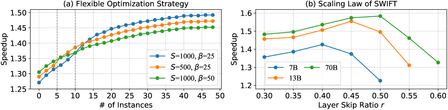
Figure 8: In-depth analysis of \method, which includes: (a) Flexible optimization strategy. The maximum optimization iteration $S$ and Bayesian interval $\beta$ can be flexibly adjusted to accommodate different input data types. (b) Scaling law. The speedup and optimal layer skip ratio of \method increase with larger model sizes, indicating that larger LLMs exhibit greater layer sparsity.
Flexible Optimization & Scaling Law
Figure 8 (a) presents the flexibility of \method in handling various input types by adjusting the maximum optimization step $S$ and Bayesian interval $\beta$ . For input with fewer instances, reducing $S$ enables an earlier transition to the acceleration phase while increasing $\beta$ reduces the overhead during the optimization phase, enhancing speedups during the initial stages of inference. In cases with sufficient input data, \method enables exploring more optimization paths, thereby enhancing the overall speedup. Figure 8 (b) illustrates the scaling law of \method: as the model size increases, both the optimal layer-skip ratio and overall speedup improve, indicating that larger LLMs exhibit more layer sparsity. This finding highlights the potential of \method for accelerating LLMs of larger sizes (e.g., 175B), which we leave for future investigation.
<details>
<summary>x9.png Details</summary>
### Visual Description
## Bar Chart: Speedup Comparison of Language Models
### Overview
The image is a bar chart comparing the speedup of two language models, Yi-34B and DeepSeek-Coder-33B, under three different configurations: Vanilla, Base, and Instruct. The chart displays the speedup achieved by each model and configuration relative to a baseline (Vanilla).
### Components/Axes
* **Title:** None explicitly provided in the image.
* **X-axis:** Categorical axis representing the language models: Yi-34B and DeepSeek-Coder-33B.
* **Y-axis:** Numerical axis labeled "Speedup," ranging from 1.0 to 1.6, with gridlines at intervals of 0.1.
* **Legend:** Located at the top of the chart, indicating the configurations:
* Vanilla (Orange)
* Base (Blue)
* Instruct (Teal)
### Detailed Analysis
**Yi-34B:**
* **Vanilla (Orange):** Speedup of 1.00.
* **Base (Blue):** Speedup of 1.31.
* **Instruct (Teal):** Speedup of 1.26.
**DeepSeek-Coder-33B:**
* **Vanilla (Orange):** Speedup of 1.00.
* **Base (Blue):** Speedup of 1.54.
* **Instruct (Teal):** Speedup of 1.39.
### Key Observations
* For both models, the Vanilla configuration has a speedup of 1.00, indicating it's the baseline.
* The Base configuration consistently provides a higher speedup than the Instruct configuration for both models.
* DeepSeek-Coder-33B achieves a higher speedup than Yi-34B in both the Base and Instruct configurations.
### Interpretation
The bar chart illustrates the performance gains (speedup) achieved by using the Base and Instruct configurations compared to the Vanilla configuration for two different language models. The data suggests that both models benefit from the Base and Instruct configurations, but DeepSeek-Coder-33B shows a more significant improvement, especially with the Base configuration. The Vanilla configuration serves as a control, showing no speedup (1.00) for both models, as expected. The Base configuration appears to be more effective than the Instruct configuration for both models, indicating that the specific optimizations or instructions used in the Base configuration are more beneficial for these models and tasks.
</details>
Figure 9: Speedups of \method on LLM backbones and their instruction-tuned variants.
Other LLM Backbones
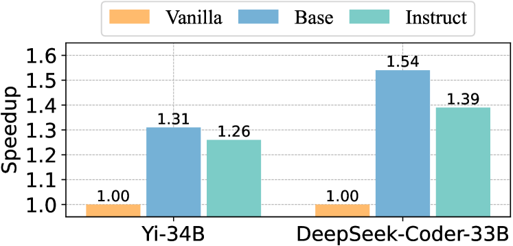
Beyond LLaMA, we assess the effectiveness of \method on additional LLM backbones. Specifically, we include Yi-34B (Young et al., 2024) and DeepSeek-Coder-33B (Guo et al., 2024) along with their instruction-tuned variants for text and code generation tasks, respectively. The speedup results of \method are illustrated in Figure 9, demonstrating that \method achieves efficiency improvements ranging from $26\%$ to $54\%$ on these LLM backbones. Further experimental details are provided in Appendix C.3.
6 Conclusion
In this work, we introduce \method, an on-the-fly self-speculative decoding algorithm that adaptively selects certain intermediate layers of LLMs to skip during inference. The proposed method does not require additional training or auxiliary models, making it a plug-and-play solution for accelerating LLM inference across diverse input data streams. Extensive experiments conducted across various LLMs and tasks demonstrate that \method achieves over a $1.3×$ $\sim$ $1.6×$ speedup while preserving the distribution of the generated text. Furthermore, our in-depth analysis highlights the effectiveness of \method in handling dynamic input data streams and its seamless integration with various LLM backbones, showcasing the great potential of this paradigm for practical LLM inference acceleration.
Ethics Statement
The datasets used in our experiments are publicly released and labeled through interaction with humans in English. In this process, user privacy is protected, and no personal information is contained in the dataset. The scientific artifacts that we used are available for research with permissive licenses. The use of these artifacts in this paper is consistent with their intended purpose.
Acknowledgements
We thank all anonymous reviewers for their valuable comments during the review process. The work described in this paper was supported by Research Grants Council of Hong Kong (PolyU/15207122, PolyU/15209724, PolyU/15207821, PolyU/15213323) and PolyU internal grants (BDWP).
Reproducibility Statement
All the results in this work are reproducible. We provide all the necessary code in the Supplementary Material to replicate our results. The repository includes environment configurations, scripts, and other relevant materials. We discuss the experimental settings in Section 5.1 and Appendix C, including implementation details such as models, datasets, inference setup, and evaluation metrics.
References
- Ankner et al. (2024) Zachary Ankner, Rishab Parthasarathy, Aniruddha Nrusimha, Christopher Rinard, Jonathan Ragan-Kelley, and William Brandon. Hydra: Sequentially-dependent draft heads for medusa decoding. CoRR, abs/2402.05109, 2024. doi: 10.48550/ARXIV.2402.05109. URL https://doi.org/10.48550/arXiv.2402.05109.
- Bae et al. (2023) Sangmin Bae, Jongwoo Ko, Hwanjun Song, and Se-Young Yun. Fast and robust early-exiting framework for autoregressive language models with synchronized parallel decoding. In Houda Bouamor, Juan Pino, and Kalika Bali (eds.), Proceedings of the 2023 Conference on Empirical Methods in Natural Language Processing, pp. 5910–5924, Singapore, December 2023. Association for Computational Linguistics. doi: 10.18653/v1/2023.emnlp-main.362. URL https://aclanthology.org/2023.emnlp-main.362.
- Cai et al. (2024) Tianle Cai, Yuhong Li, Zhengyang Geng, Hongwu Peng, Jason D. Lee, Deming Chen, and Tri Dao. Medusa: Simple LLM inference acceleration framework with multiple decoding heads. In Forty-first International Conference on Machine Learning, ICML 2024, Vienna, Austria, July 21-27, 2024. OpenReview.net, 2024. URL https://openreview.net/forum?id=PEpbUobfJv.
- Chen et al. (2023) Charlie Chen, Sebastian Borgeaud, Geoffrey Irving, Jean-Baptiste Lespiau, Laurent Sifre, and John Jumper. Accelerating large language model decoding with speculative sampling. CoRR, abs/2302.01318, 2023. doi: 10.48550/arXiv.2302.01318. URL https://doi.org/10.48550/arXiv.2302.01318.
- Chen et al. (2021) Mark Chen, Jerry Tworek, Heewoo Jun, Qiming Yuan, Henrique Pondé de Oliveira Pinto, Jared Kaplan, Harrison Edwards, et al. Evaluating large language models trained on code. CoRR, abs/2107.03374, 2021. URL https://arxiv.org/abs/2107.03374.
- Cobbe et al. (2021) Karl Cobbe, Vineet Kosaraju, Mohammad Bavarian, Mark Chen, Heewoo Jun, Lukasz Kaiser, Matthias Plappert, Jerry Tworek, Jacob Hilton, Reiichiro Nakano, Christopher Hesse, and John Schulman. Training verifiers to solve math word problems. CoRR, abs/2110.14168, 2021. URL https://arxiv.org/abs/2110.14168.
- Corro et al. (2023) Luciano Del Corro, Allie Del Giorno, Sahaj Agarwal, Bin Yu, Ahmed Awadallah, and Subhabrata Mukherjee. Skipdecode: Autoregressive skip decoding with batching and caching for efficient LLM inference. CoRR, abs/2307.02628, 2023. doi: 10.48550/ARXIV.2307.02628. URL https://doi.org/10.48550/arXiv.2307.02628.
- Dettmers et al. (2022) Tim Dettmers, Mike Lewis, Younes Belkada, and Luke Zettlemoyer. Gpt3.int8(): 8-bit matrix multiplication for transformers at scale. In Sanmi Koyejo, S. Mohamed, A. Agarwal, Danielle Belgrave, K. Cho, and A. Oh (eds.), Advances in Neural Information Processing Systems 35: Annual Conference on Neural Information Processing Systems 2022, NeurIPS 2022, New Orleans, LA, USA, November 28 - December 9, 2022, 2022. URL http://papers.nips.cc/paper_files/paper/2022/hash/c3ba4962c05c49636d4c6206a97e9c8a-Abstract-Conference.html.
- Du et al. (2024) Cunxiao Du, Jing Jiang, Yuanchen Xu, Jiawei Wu, Sicheng Yu, Yongqi Li, Shenggui Li, Kai Xu, Liqiang Nie, Zhaopeng Tu, and Yang You. Glide with a cape: A low-hassle method to accelerate speculative decoding. In Forty-first International Conference on Machine Learning, ICML 2024, Vienna, Austria, July 21-27, 2024. OpenReview.net, 2024. URL https://openreview.net/forum?id=mk8oRhox2l.
- Dubey et al. (2024) Abhimanyu Dubey, Abhinav Jauhri, Abhinav Pandey, Abhishek Kadian, Ahmad Al-Dahle, et al. The llama 3 herd of models, 2024. URL https://arxiv.org/abs/2407.21783.
- Eldan & Li (2023) Ronen Eldan and Yuanzhi Li. Tinystories: How small can language models be and still speak coherent english? CoRR, abs/2305.07759, 2023. doi: 10.48550/ARXIV.2305.07759. URL https://doi.org/10.48550/arXiv.2305.07759.
- Elhoushi et al. (2024) Mostafa Elhoushi, Akshat Shrivastava, Diana Liskovich, Basil Hosmer, Bram Wasti, Liangzhen Lai, Anas Mahmoud, Bilge Acun, Saurabh Agarwal, Ahmed Roman, Ahmed Aly, Beidi Chen, and Carole-Jean Wu. LayerSkip: Enabling early exit inference and self-speculative decoding. In Lun-Wei Ku, Andre Martins, and Vivek Srikumar (eds.), Proceedings of the 62nd Annual Meeting of the Association for Computational Linguistics (Volume 1: Long Papers), pp. 12622–12642, Bangkok, Thailand, August 2024. Association for Computational Linguistics. URL https://aclanthology.org/2024.acl-long.681.
- Frantar et al. (2023) Elias Frantar, Saleh Ashkboos, Torsten Hoefler, and Dan Alistarh. OPTQ: Accurate quantization for generative pre-trained transformers. In The Eleventh International Conference on Learning Representations, 2023. URL https://openreview.net/forum?id=tcbBPnfwxS.
- Fu et al. (2024) Yichao Fu, Peter Bailis, Ion Stoica, and Hao Zhang. Break the sequential dependency of LLM inference using lookahead decoding. In Forty-first International Conference on Machine Learning, ICML 2024, Vienna, Austria, July 21-27, 2024. OpenReview.net, 2024. URL https://openreview.net/forum?id=eDjvSFOkXw.
- Gloeckle et al. (2024) Fabian Gloeckle, Badr Youbi Idrissi, Baptiste Rozière, David Lopez-Paz, and Gabriel Synnaeve. Better & faster large language models via multi-token prediction. CoRR, abs/2404.19737, 2024. doi: 10.48550/ARXIV.2404.19737. URL https://doi.org/10.48550/arXiv.2404.19737.
- Gu et al. (2024) Yuxian Gu, Li Dong, Furu Wei, and Minlie Huang. MiniLLM: Knowledge distillation of large language models. In The Twelfth International Conference on Learning Representations, 2024. URL https://openreview.net/forum?id=5h0qf7IBZZ.
- Guo et al. (2024) Daya Guo, Qihao Zhu, Dejian Yang, Zhenda Xie, Kai Dong, Wentao Zhang, Guanting Chen, Xiao Bi, Y. Wu, Y. K. Li, Fuli Luo, Yingfei Xiong, and Wenfeng Liang. Deepseek-coder: When the large language model meets programming - the rise of code intelligence. CoRR, abs/2401.14196, 2024. doi: 10.48550/ARXIV.2401.14196. URL https://doi.org/10.48550/arXiv.2401.14196.
- He et al. (2024) Zhenyu He, Zexuan Zhong, Tianle Cai, Jason Lee, and Di He. REST: Retrieval-based speculative decoding. In Kevin Duh, Helena Gomez, and Steven Bethard (eds.), Proceedings of the 2024 Conference of the North American Chapter of the Association for Computational Linguistics: Human Language Technologies (Volume 1: Long Papers), pp. 1582–1595, Mexico City, Mexico, June 2024. Association for Computational Linguistics. URL https://aclanthology.org/2024.naacl-long.88.
- Hoefler et al. (2021) Torsten Hoefler, Dan Alistarh, Tal Ben-Nun, Nikoli Dryden, and Alexandra Peste. Sparsity in deep learning: Pruning and growth for efficient inference and training in neural networks. J. Mach. Learn. Res., 22(241):1–124, 2021.
- Hooper et al. (2023) Coleman Hooper, Sehoon Kim, Hiva Mohammadzadeh, Hasan Genc, Kurt Keutzer, Amir Gholami, and Yakun Sophia Shao. SPEED: speculative pipelined execution for efficient decoding. CoRR, abs/2310.12072, 2023. doi: 10.48550/ARXIV.2310.12072. URL https://doi.org/10.48550/arXiv.2310.12072.
- Hsieh et al. (2023) Cheng-Yu Hsieh, Chun-Liang Li, Chih-Kuan Yeh, Hootan Nakhost, Yasuhisa Fujii, Alex Ratner, Ranjay Krishna, Chen-Yu Lee, and Tomas Pfister. Distilling step-by-step! outperforming larger language models with less training data and smaller model sizes. In Anna Rogers, Jordan L. Boyd-Graber, and Naoaki Okazaki (eds.), Findings of the Association for Computational Linguistics: ACL 2023, Toronto, Canada, July 9-14, 2023, pp. 8003–8017. Association for Computational Linguistics, 2023. doi: 10.18653/V1/2023.FINDINGS-ACL.507. URL https://doi.org/10.18653/v1/2023.findings-acl.507.
- Hu et al. (2022) Edward J. Hu, Yelong Shen, Phillip Wallis, Zeyuan Allen-Zhu, Yuanzhi Li, Shean Wang, Lu Wang, and Weizhu Chen. Lora: Low-rank adaptation of large language models. In The Tenth International Conference on Learning Representations, ICLR 2022, Virtual Event, April 25-29, 2022. OpenReview.net, 2022. URL https://openreview.net/forum?id=nZeVKeeFYf9.
- Jaiswal et al. (2024) Ajay Jaiswal, Bodun Hu, Lu Yin, Yeonju Ro, Shiwei Liu, Tianlong Chen, and Aditya Akella. Ffn-skipllm: A hidden gem for autoregressive decoding with adaptive feed forward skipping. CoRR, abs/2404.03865, 2024. doi: 10.48550/ARXIV.2404.03865. URL https://doi.org/10.48550/arXiv.2404.03865.
- Jones et al. (1998) Donald R. Jones, Matthias Schonlau, and William J. Welch. Efficient global optimization of expensive black-box functions. J. Glob. Optim., 13(4):455–492, 1998. doi: 10.1023/A:1008306431147. URL https://doi.org/10.1023/A:1008306431147.
- Kim et al. (2023) Sehoon Kim, Karttikeya Mangalam, Suhong Moon, Jitendra Malik, Michael W. Mahoney, Amir Gholami, and Kurt Keutzer. Speculative decoding with big little decoder. In Alice Oh, Tristan Naumann, Amir Globerson, Kate Saenko, Moritz Hardt, and Sergey Levine (eds.), Advances in Neural Information Processing Systems 36: Annual Conference on Neural Information Processing Systems 2023, NeurIPS 2023, New Orleans, LA, USA, December 10 - 16, 2023, 2023. URL http://papers.nips.cc/paper_files/paper/2023/hash/7b97adeafa1c51cf65263459ca9d0d7c-Abstract-Conference.html.
- Kim et al. (2024) Taehyeon Kim, Ananda Theertha Suresh, Kishore A Papineni, Michael Riley, Sanjiv Kumar, and Adrian Benton. Accelerating blockwise parallel language models with draft refinement. In The Thirty-eighth Annual Conference on Neural Information Processing Systems, 2024. URL https://openreview.net/forum?id=KT6F5Sw0eg.
- Kou et al. (2024) Siqi Kou, Lanxiang Hu, Zhezhi He, Zhijie Deng, and Hao Zhang. Cllms: Consistency large language models. In Forty-first International Conference on Machine Learning, ICML 2024, Vienna, Austria, July 21-27, 2024. OpenReview.net, 2024. URL https://openreview.net/forum?id=8uzBOVmh8H.
- Kwiatkowski et al. (2019) Tom Kwiatkowski, Jennimaria Palomaki, Olivia Redfield, Michael Collins, Ankur Parikh, Chris Alberti, Danielle Epstein, Illia Polosukhin, Jacob Devlin, Kenton Lee, Kristina Toutanova, Llion Jones, Matthew Kelcey, Ming-Wei Chang, Andrew M. Dai, Jakob Uszkoreit, Quoc Le, and Slav Petrov. Natural questions: A benchmark for question answering research. Transactions of the Association for Computational Linguistics, 7:452–466, 2019. doi: 10.1162/tacl˙a˙00276. URL https://aclanthology.org/Q19-1026.
- Leviathan et al. (2023) Yaniv Leviathan, Matan Kalman, and Yossi Matias. Fast inference from transformers via speculative decoding. In Andreas Krause, Emma Brunskill, Kyunghyun Cho, Barbara Engelhardt, Sivan Sabato, and Jonathan Scarlett (eds.), International Conference on Machine Learning, ICML 2023, 23-29 July 2023, Honolulu, Hawaii, USA, volume 202 of Proceedings of Machine Learning Research, pp. 19274–19286. PMLR, 2023. URL https://proceedings.mlr.press/v202/leviathan23a.html.
- Li et al. (2024a) Yuhui Li, Fangyun Wei, Chao Zhang, and Hongyang Zhang. Eagle: Speculative sampling requires rethinking feature uncertainty, 2024a.
- Li et al. (2024b) Yuhui Li, Fangyun Wei, Chao Zhang, and Hongyang Zhang. EAGLE-2: faster inference of language models with dynamic draft trees. CoRR, abs/2406.16858, 2024b. doi: 10.48550/ARXIV.2406.16858. URL https://doi.org/10.48550/arXiv.2406.16858.
- Liu et al. (2023a) Xiaoxuan Liu, Lanxiang Hu, Peter Bailis, Ion Stoica, Zhijie Deng, Alvin Cheung, and Hao Zhang. Online speculative decoding. CoRR, abs/2310.07177, 2023a. doi: 10.48550/ARXIV.2310.07177. URL https://doi.org/10.48550/arXiv.2310.07177.
- Liu et al. (2024) Yijin Liu, Fandong Meng, and Jie Zhou. Accelerating inference in large language models with a unified layer skipping strategy. CoRR, abs/2404.06954, 2024. doi: 10.48550/ARXIV.2404.06954. URL https://doi.org/10.48550/arXiv.2404.06954.
- Liu et al. (2019) Zhuang Liu, Mingjie Sun, Tinghui Zhou, Gao Huang, and Trevor Darrell. Rethinking the value of network pruning. In 7th International Conference on Learning Representations, ICLR 2019, New Orleans, LA, USA, May 6-9, 2019. OpenReview.net, 2019. URL https://openreview.net/forum?id=rJlnB3C5Ym.
- Liu et al. (2023b) Zichang Liu, Jue Wang, Tri Dao, Tianyi Zhou, Binhang Yuan, Zhao Song, Anshumali Shrivastava, Ce Zhang, Yuandong Tian, Christopher Re, et al. Deja vu: Contextual sparsity for efficient llms at inference time. In International Conference on Machine Learning, pp. 22137–22176. PMLR, 2023b.
- Ma et al. (2024) Shuming Ma, Hongyu Wang, Lingxiao Ma, Lei Wang, Wenhui Wang, Shaohan Huang, Li Dong, Ruiping Wang, Jilong Xue, and Furu Wei. The era of 1-bit llms: All large language models are in 1.58 bits. CoRR, abs/2402.17764, 2024. doi: 10.48550/ARXIV.2402.17764. URL https://doi.org/10.48550/arXiv.2402.17764.
- Miao et al. (2024) Xupeng Miao, Gabriele Oliaro, Zhihao Zhang, Xinhao Cheng, Zeyu Wang, Zhengxin Zhang, Rae Ying Yee Wong, Alan Zhu, Lijie Yang, Xiaoxiang Shi, Chunan Shi, Zhuoming Chen, Daiyaan Arfeen, Reyna Abhyankar, and Zhihao Jia. Specinfer: Accelerating large language model serving with tree-based speculative inference and verification. In Proceedings of the 29th ACM International Conference on Architectural Support for Programming Languages and Operating Systems, Volume 3, ASPLOS ’24, pp. 932–949, New York, NY, USA, 2024. Association for Computing Machinery. ISBN 9798400703867. doi: 10.1145/3620666.3651335. URL https://doi.org/10.1145/3620666.3651335.
- Nallapati et al. (2016) Ramesh Nallapati, Bowen Zhou, Cícero Nogueira dos Santos, Çaglar Gülçehre, and Bing Xiang. Abstractive text summarization using sequence-to-sequence rnns and beyond. In Yoav Goldberg and Stefan Riezler (eds.), Proceedings of the 20th SIGNLL Conference on Computational Natural Language Learning, CoNLL 2016, Berlin, Germany, August 11-12, 2016, pp. 280–290. ACL, 2016. doi: 10.18653/V1/K16-1028. URL https://doi.org/10.18653/v1/k16-1028.
- OpenAI (2023) OpenAI. GPT-4 technical report. CoRR, abs/2303.08774, 2023. doi: 10.48550/ARXIV.2303.08774. URL https://doi.org/10.48550/arXiv.2303.08774.
- Patterson (2004) David A. Patterson. Latency lags bandwith. Commun. ACM, 47(10):71–75, 2004. doi: 10.1145/1022594.1022596. URL https://doi.org/10.1145/1022594.1022596.
- Pope et al. (2023) Reiner Pope, Sholto Douglas, Aakanksha Chowdhery, Jacob Devlin, James Bradbury, Jonathan Heek, Kefan Xiao, Shivani Agrawal, and Jeff Dean. Efficiently scaling transformer inference. In Dawn Song, Michael Carbin, and Tianqi Chen (eds.), Proceedings of the Sixth Conference on Machine Learning and Systems, MLSys 2023, Miami, FL, USA, June 4-8, 2023. mlsys.org, 2023. URL https://proceedings.mlsys.org/paper_files/paper/2023/hash/c4be71ab8d24cdfb45e3d06dbfca2780-Abstract-mlsys2023.html.
- Rasmussen & Williams (2006) Carl Edward Rasmussen and Christopher K. I. Williams. Gaussian processes for machine learning. Adaptive computation and machine learning. MIT Press, 2006. ISBN 026218253X. URL https://www.worldcat.org/oclc/61285753.
- Rozière et al. (2023) Baptiste Rozière, Jonas Gehring, Fabian Gloeckle, Sten Sootla, Itai Gat, Xiaoqing Ellen Tan, Yossi Adi, Jingyu Liu, Tal Remez, Jérémy Rapin, Artyom Kozhevnikov, Ivan Evtimov, Joanna Bitton, Manish Bhatt, Cristian Canton-Ferrer, Aaron Grattafiori, Wenhan Xiong, Alexandre Défossez, Jade Copet, Faisal Azhar, Hugo Touvron, Louis Martin, Nicolas Usunier, Thomas Scialom, and Gabriel Synnaeve. Code llama: Open foundation models for code. CoRR, abs/2308.12950, 2023. doi: 10.48550/ARXIV.2308.12950. URL https://doi.org/10.48550/arXiv.2308.12950.
- Santilli et al. (2023) Andrea Santilli, Silvio Severino, Emilian Postolache, Valentino Maiorca, Michele Mancusi, Riccardo Marin, and Emanuele Rodolà. Accelerating transformer inference for translation via parallel decoding. In Anna Rogers, Jordan L. Boyd-Graber, and Naoaki Okazaki (eds.), Proceedings of the 61st Annual Meeting of the Association for Computational Linguistics (Volume 1: Long Papers), ACL 2023, Toronto, Canada, July 9-14, 2023, pp. 12336–12355. Association for Computational Linguistics, 2023. doi: 10.18653/v1/2023.acl-long.689. URL https://doi.org/10.18653/v1/2023.acl-long.689.
- Shazeer (2019) Noam Shazeer. Fast transformer decoding: One write-head is all you need. CoRR, abs/1911.02150, 2019. URL http://arxiv.org/abs/1911.02150.
- Stern et al. (2018) Mitchell Stern, Noam Shazeer, and Jakob Uszkoreit. Blockwise parallel decoding for deep autoregressive models. In Samy Bengio, Hanna M. Wallach, Hugo Larochelle, Kristen Grauman, Nicolò Cesa-Bianchi, and Roman Garnett (eds.), Advances in Neural Information Processing Systems 31: Annual Conference on Neural Information Processing Systems 2018, NeurIPS 2018, December 3-8, 2018, Montréal, Canada, pp. 10107–10116, 2018. URL https://proceedings.neurips.cc/paper/2018/hash/c4127b9194fe8562c64dc0f5bf2c93bc-Abstract.html.
- Sun et al. (2023) Ziteng Sun, Ananda Theertha Suresh, Jae Hun Ro, Ahmad Beirami, Himanshu Jain, and Felix Yu. Spectr: Fast speculative decoding via optimal transport. In Thirty-seventh Conference on Neural Information Processing Systems, 2023. URL https://openreview.net/forum?id=SdYHLTCC5J.
- Taori et al. (2023) Rohan Taori, Ishaan Gulrajani, Tianyi Zhang, Yann Dubois, Xuechen Li, Carlos Guestrin, Percy Liang, and Tatsunori B. Hashimoto. Stanford alpaca: An instruction-following llama model. https://github.com/tatsu-lab/stanford_alpaca, 2023.
- Touvron et al. (2021) Hugo Touvron, Matthieu Cord, Matthijs Douze, Francisco Massa, Alexandre Sablayrolles, and Hervé Jégou. Training data-efficient image transformers & distillation through attention. In International Conference on Machine Learning, pp. 10347–10357. PMLR, 2021.
- Touvron et al. (2023a) Hugo Touvron, Thibaut Lavril, Gautier Izacard, Xavier Martinet, Marie-Anne Lachaux, Timothée Lacroix, Baptiste Rozière, Naman Goyal, Eric Hambro, Faisal Azhar, Aurélien Rodriguez, Armand Joulin, Edouard Grave, and Guillaume Lample. Llama: Open and efficient foundation language models. CoRR, abs/2302.13971, 2023a. doi: 10.48550/arXiv.2302.13971. URL https://doi.org/10.48550/arXiv.2302.13971.
- Touvron et al. (2023b) Hugo Touvron, Louis Martin, Kevin Stone, Peter Albert, Amjad Almahairi, Yasmine Babaei, et al. Llama 2: Open foundation and fine-tuned chat models. CoRR, abs/2307.09288, 2023b. doi: 10.48550/ARXIV.2307.09288. URL https://doi.org/10.48550/arXiv.2307.09288.
- Xia et al. (2023) Heming Xia, Tao Ge, Peiyi Wang, Si-Qing Chen, Furu Wei, and Zhifang Sui. Speculative decoding: Exploiting speculative execution for accelerating seq2seq generation. In Houda Bouamor, Juan Pino, and Kalika Bali (eds.), Findings of the Association for Computational Linguistics: EMNLP 2023, Singapore, December 6-10, 2023, pp. 3909–3925. Association for Computational Linguistics, 2023. doi: 10.18653/V1/2023.FINDINGS-EMNLP.257. URL https://doi.org/10.18653/v1/2023.findings-emnlp.257.
- Xia et al. (2024) Heming Xia, Zhe Yang, Qingxiu Dong, Peiyi Wang, Yongqi Li, Tao Ge, Tianyu Liu, Wenjie Li, and Zhifang Sui. Unlocking efficiency in large language model inference: A comprehensive survey of speculative decoding. In Lun-Wei Ku, Andre Martins, and Vivek Srikumar (eds.), Findings of the Association for Computational Linguistics ACL 2024, pp. 7655–7671, Bangkok, Thailand and virtual meeting, August 2024. Association for Computational Linguistics. URL https://aclanthology.org/2024.findings-acl.456.
- Yang et al. (2023) Seongjun Yang, Gibbeum Lee, Jaewoong Cho, Dimitris S. Papailiopoulos, and Kangwook Lee. Predictive pipelined decoding: A compute-latency trade-off for exact LLM decoding. CoRR, abs/2307.05908, 2023. doi: 10.48550/ARXIV.2307.05908. URL https://doi.org/10.48550/arXiv.2307.05908.
- Yi et al. (2024) Hanling Yi, Feng Lin, Hongbin Li, Ning Peiyang, Xiaotian Yu, and Rong Xiao. Generation meets verification: Accelerating large language model inference with smart parallel auto-correct decoding. In Lun-Wei Ku, Andre Martins, and Vivek Srikumar (eds.), Findings of the Association for Computational Linguistics ACL 2024, pp. 5285–5299, Bangkok, Thailand and virtual meeting, August 2024. Association for Computational Linguistics. URL https://aclanthology.org/2024.findings-acl.313.
- Young et al. (2024) Alex Young, Bei Chen, Chao Li, Chengen Huang, Ge Zhang, Guanwei Zhang, Heng Li, Jiangcheng Zhu, Jianqun Chen, Jing Chang, Kaidong Yu, Peng Liu, Qiang Liu, Shawn Yue, Senbin Yang, Shiming Yang, Tao Yu, Wen Xie, Wenhao Huang, Xiaohui Hu, Xiaoyi Ren, Xinyao Niu, Pengcheng Nie, Yuchi Xu, Yudong Liu, Yue Wang, Yuxuan Cai, Zhenyu Gu, Zhiyuan Liu, and Zonghong Dai. Yi: Open foundation models by 01.ai. CoRR, abs/2403.04652, 2024. doi: 10.48550/ARXIV.2403.04652. URL https://doi.org/10.48550/arXiv.2403.04652.
- Zhang et al. (2024) Jun Zhang, Jue Wang, Huan Li, Lidan Shou, Ke Chen, Gang Chen, and Sharad Mehrotra. Draft& verify: Lossless large language model acceleration via self-speculative decoding. In Lun-Wei Ku, Andre Martins, and Vivek Srikumar (eds.), Proceedings of the 62nd Annual Meeting of the Association for Computational Linguistics (Volume 1: Long Papers), pp. 11263–11282, Bangkok, Thailand, August 2024. Association for Computational Linguistics. URL https://aclanthology.org/2024.acl-long.607.
- Zhou et al. (2024) Yongchao Zhou, Kaifeng Lyu, Ankit Singh Rawat, Aditya Krishna Menon, Afshin Rostamizadeh, Sanjiv Kumar, Jean-François Kagy, and Rishabh Agarwal. Distillspec: Improving speculative decoding via knowledge distillation. In The Twelfth International Conference on Learning Representations, 2024. URL https://openreview.net/forum?id=rsY6J3ZaTF.
- Zhu et al. (2024) Yunqi Zhu, Xuebing Yang, Yuanyuan Wu, and Wensheng Zhang. Hierarchical skip decoding for efficient autoregressive text generation. CoRR, abs/2403.14919, 2024. doi: 10.48550/ARXIV.2403.14919. URL https://doi.org/10.48550/arXiv.2403.14919.
Appendix
Appendix A Preliminary Details
We present the detailed configuration of Self-SD across four task domains in Figure 10, demonstrating that the optimal skipped layer configurations vary depending on the specific task.
<details>
<summary>x10.png Details</summary>

### Visual Description
## Bar Chart: MLP vs ATT
### Overview
The image is a bar chart comparing two categories, MLP and ATT, across a range of numerical values from 1 to 80. The chart displays the presence or absence of data for each category at each numerical value using colored bars. Blue bars represent MLP, and red bars represent ATT.
### Components/Axes
* **Y-axis Labels:** MLP, ATT
* **X-axis:** Numerical values ranging from 1 to 80, incrementing by 2 for MLP and by 2 for ATT.
* **Bar Colors:** Blue for MLP, Red for ATT.
### Detailed Analysis
The chart shows the distribution of data points for MLP and ATT across the numerical range.
* **MLP (Blue):**
* Present at values: 2, 4, 16, 18, 20, 22, 24, 26, 28, 36, 44, 46, 48, 50, 52, 54, 56, 58, 60, 62, 64, 66, 68, 70, 72, 74, 76
* Absent at values: 6, 8, 10, 12, 14, 30, 32, 34, 38, 40, 42, 78, 80
* **ATT (Red):**
* Present at values: 1, 3, 5, 7, 9, 11, 13, 15, 17, 19, 21, 23, 25, 27, 29, 31, 33, 35, 37, 39, 41, 43, 45, 47, 49, 51, 53, 55, 57, 59, 61, 63, 65, 67, 69, 71, 73, 75, 77, 79
* Absent at values: None
### Key Observations
* ATT has data points for every odd number from 1 to 79.
* MLP has data points for a subset of even numbers from 2 to 76.
* There is no overlap in the numerical values where both MLP and ATT have data points.
### Interpretation
The chart visually represents the presence or absence of data for two categories, MLP and ATT, across a numerical range. The data suggests that ATT is present at every odd number, while MLP is present at a selection of even numbers. The lack of overlap indicates that the two categories are mutually exclusive in terms of the numerical values they represent. This could indicate different types of events, measurements, or classifications associated with these numerical values.
</details>
(a) Summarization - CNN/DM
<details>
<summary>x11.png Details</summary>

### Visual Description
## Data Representation: Paired Number Series
### Overview
The image presents two series of numbers, labeled "MLP" and "ATT", displayed as a sequence of numbers. Each number is associated with a colored block. The MLP series is associated with blue blocks, and the ATT series is associated with red blocks. The numbers appear to represent a sequence of values or identifiers.
### Components/Axes
* **Labels:**
* "MLP" (top row)
* "ATT" (bottom row)
* **Number Series:**
* MLP: 2, 4, 6, 8, 10, 12, 14, 16, 18, 20, 22, 24, 26, 28, 30, 32, 34, 36, 38, 40, 42, 44, 46, 48, 50, 52, 54, 56, 58, 60, 62, 64, 66, 68, 70, 72, 74, 76, 78, 80
* ATT: 1, 3, 5, 7, 9, 11, 13, 15, 17, 19, 21, 23, 25, 27, 29, 31, 33, 35, 37, 39, 41, 43, 45, 47, 49, 51, 53, 55, 57, 59, 61, 63, 65, 67, 69, 71, 73, 75, 77, 79
* **Color Coding:**
* MLP: Blue blocks
* ATT: Red blocks
### Detailed Analysis or ### Content Details
The image displays two rows of numbers, each associated with a specific color. The numbers in each row are consecutive odd or even integers.
* **MLP (Blue):** The numbers are even integers, starting from 2 and incrementing by 2 up to 80.
* **ATT (Red):** The numbers are odd integers, starting from 1 and incrementing by 2 up to 79.
### Key Observations
* The numbers in each row are sequential, with a constant difference of 2 between adjacent numbers.
* The colors (blue and red) visually distinguish the two series.
* The numbers are aligned horizontally, suggesting a sequence or series.
### Interpretation
The image likely represents a comparison or pairing of two numerical sequences. The "MLP" and "ATT" labels could refer to different categories, groups, or variables. The colored blocks serve to visually differentiate the two series, making it easy to track and compare the corresponding numbers. The consistent increment of 2 in each series suggests a linear progression or a systematic relationship between the numbers. Without further context, it's difficult to determine the specific meaning or purpose of these number series, but the visual representation indicates a structured and organized dataset.
</details>
(b) Reasoning - GSM8K
<details>
<summary>x12.png Details</summary>

### Visual Description
## Data Visualization: MLP vs ATT
### Overview
The image presents a visual comparison between two categories, "MLP" and "ATT", across a numerical range from 1 to 80. Each category is represented by a row of numbers, with some numbers highlighted in blue (for MLP) and red (for ATT). The highlighting indicates a specific attribute or status associated with that number for the respective category.
### Components/Axes
* **Rows:** Two rows labeled "MLP" (top) and "ATT" (bottom).
* **Numerical Range:** Numbers from 1 to 80 are displayed horizontally.
* **Highlighting:** Certain numbers are highlighted with blue (MLP) or red (ATT) blocks.
### Detailed Analysis
**MLP (Top Row):**
* Numbers 2, 4, 6, 8, 10, 12, 14, 16, 18, 20, 22, 24, 26, 28, 30, 32, 34, 36, 38, 40, 42, 44, 46, 48, 50, 52, 54, 56, 58, 60, 62, 64, 66, 68, 70, 72, 74, 76, 78, and 80 are highlighted in blue.
* All even numbers from 2 to 80 are highlighted.
**ATT (Bottom Row):**
* Numbers 1, 3, 5, 7, 9, 11, 13, 15, 17, 19, 21, 23, 25, 27, 29, 31, 33, 35, 37, 39, 41, 43, 45, 47, 49, 51, 53, 55, 57, 59, 61, 63, 65, 67, 69, 71, 73, 75, 77, and 79 are highlighted in red.
* All odd numbers from 1 to 79 are highlighted.
### Key Observations
* MLP highlights all even numbers from 2 to 80.
* ATT highlights all odd numbers from 1 to 79.
* There is no overlap in the highlighted numbers between MLP and ATT.
### Interpretation
The visualization clearly distinguishes between two categories, MLP and ATT, based on whether they are associated with even or odd numbers within the range of 1 to 80. This could represent a binary classification or a distinct characteristic associated with each category. The data suggests a clear and mutually exclusive relationship between MLP and even numbers, and ATT and odd numbers.
</details>
(c) Storytelling - TinyStories
<details>
<summary>x13.png Details</summary>

### Visual Description
## Data Visualization: MLP vs ATT
### Overview
The image presents a visualization comparing two categories, "MLP" and "ATT," across a numerical range from 1 to 80. Each category is represented by a series of numbers, with some numbers highlighted by colored blocks (blue for MLP, red for ATT). The visualization appears to indicate the presence or activation of each category at specific numerical values.
### Components/Axes
* **Y-Axis Labels:** "MLP" (top row), "ATT" (bottom row)
* **X-Axis:** Numerical range from 1 to 80, incrementing by 2 for MLP and by 2 for ATT.
* **Data Representation:** Blue blocks indicate the presence of "MLP" at specific numerical values. Red blocks indicate the presence of "ATT" at specific numerical values.
### Detailed Analysis
**MLP (Blue Blocks):**
The "MLP" category has blue blocks at the following values:
2, 4, 6, 8, 12, 14, 16, 18, 22, 28, 36, 38, 40, 50, 52, 58, 60, 62, 64, 68, 70, 72, 78
**ATT (Red Blocks):**
The "ATT" category has red blocks at the following values:
9, 13, 15, 17, 19, 21, 23, 25, 27, 29, 31, 33, 45, 47, 49, 51, 53, 55, 57, 59, 61, 63, 65, 67, 69, 71, 73, 75, 77
### Key Observations
* The "MLP" category has blocks concentrated at the beginning of the range (2-18) and then becomes sparse.
* The "ATT" category has blocks concentrated in the middle of the range (9-77) and is absent at the beginning.
* There is minimal overlap between the blocks of "MLP" and "ATT."
### Interpretation
The visualization likely represents the activation or presence of two different entities ("MLP" and "ATT") across a range of numerical values. The distribution of blocks suggests that "MLP" is more active at lower values, while "ATT" is more active at higher values. The lack of overlap indicates that these two entities are active in different regions of the numerical range. The specific meaning of the numerical values and the nature of "MLP" and "ATT" would require additional context.
</details>
(d) Translation - WMT16
Figure 10: Visualization of skipped layer set configurations of LLaMA-2-13B optimized by Self-SD (Zhang et al., 2024) on different task domains. Gray squares indicate retained layers, red squares denote skipped attention layers, and blue squares signify skipped MLP layers.
Appendix B Experimental Setups
B.1 Models and Datasets
Our experiments mainly evaluate the effectiveness of \method on LLaMA-2 (Touvron et al., 2023b) and CodeLLaMA series (Rozière et al., 2023). We provide empirical validation on a diverse range of generation tasks. For summarization, mathematical reasoning, storytelling, and code generation tasks, we chose the CNN/Daily Mail (CNN/DM) (Nallapati et al., 2016), GSM8K (Cobbe et al., 2021), TinyStories (Eldan & Li, 2023), and HumanEval (Chen et al., 2021) datasets, respectively. We perform 1-shot evaluation for CNN/DM and TinyStories, and 5-shot evaluation for GSM8K. The maximum generation lengths on CNN/DM, GSM8K, and TinyStories are set to 64, 64, and 128, respectively. We compare pass@1 and pass@10 for HumanEval. In our further analysis, we include three more datasets to validate the capability of \method in handling dynamic input data streams. Specifically, we select Alpaca (Taori et al., 2023), WMT14 DE-EN, and Nature Questions (Kwiatkowski et al., 2019) for the instruction following, translation, and question answering tasks, respectively. The maximum generation lengths for HumanEval and all analyses are set to 512. We randomly sample 1000 instances from the test set for each dataset except HumanEval.
B.2 Inference Setup
In the optimization phase, we employ both random search and Bayesian optimization to suggest potential skipped layer set candidates, striking a balance between optimization performance and efficiency. The context window $\gamma$ is set to 32. The maximum draft length $N_{D}$ is set to 25. For random sampling in code generation tasks, we apply a temperature of 0.6 and $top\_p=0.95$ . The maximum number of layer set optimization steps $S$ is set to 1000, with Bayesian optimization performed every $\beta=25$ steps. The optimization phase is set to be early stopped if the matchness score does not improve after 300 steps or exceeds 0.95. The layer skip ratio $r$ is fixed at 0.45 for the 13B model and 0.5 for the 34B and 70B models. All experiments were conducted using Pytorch 2.1.0 on 4 $×$ NVIDIA RTX A6000 GPU (40GB) with CUDA 12.1, and an Intel(R) Xeon(R) Platinum 8370C CPU with 32 cores. Inference for our method and all baselines was performed using the Huggingface transformers package. Following prior work, we adopt speculative sampling (Leviathan et al., 2023) as our acceptance strategy, and the batch size is set to 1.
B.3 Evaluation Metrics
This subsection provides a detailed illustration of our evaluation metrics, which are mean generated length $M$ and token acceptance rate $\alpha$ . Specifically, the mean generated length $M$ refers to the average number of output tokens produced per forward pass of the target LLM; the acceptance rate $\alpha$ is defined as the ratio of accepted tokens to the total number of draft steps. In other words, it represents the expected probability of the target LLM accepting a potential token from a forward pass of the draft model. These two metrics are independent of computational hardware and, therefore considered as more objective metrics. Given the mean generated length $M$ , acceptance rate $\alpha$ , and the layer skip ratio $r$ , the mathematical formula for the expected wall-time speedup during the acceleration phase is derived as follows:
$$
\mathbb{E}(\text{Spd.})=\frac{M}{(M-1)\times\frac{c}{\alpha}+1}=\frac{M\alpha}%
{(M-1)c+\alpha},\quad c=1-r, \tag{6}
$$
where $c$ is defined as the cost coefficient in Leviathan et al. (2023). It is calculated as the ratio between the single forward time of the draft model and that of the target LLM. In summary, the ideal speedup will be higher with the larger $M$ and $\alpha$ and smaller $c$ .
Appendix C Experimental Details
C.1 Details of Main Results
We present the detailed statistics of our main experimental results in Table 4. \method consistently achieves a token acceptance rate $\alpha$ exceeding $90\%$ across all evaluation settings, with the mean generated length M ranging from 2.99 to 8.21. These statistics indicate strong behavior alignment between the target LLM and its layer-skipping draft variant, as discussed in Section 5.2. Additionally, we report the expected speedup $\mathbb{E}(\text{Spd.})$ calculated using Eq (6), indicating that the current implementation of \method has significant potential for further optimization to boost its efficiency.
| LLaMA-2-13B \method LLaMA-2-13B -Chat | Vanilla 4.34 Vanilla | 1.00 0.99 1.00 | - 1.52 $×$ - | 1.00 $×$ 3.13 1.00 $×$ | 1.00 0.98 1.00 | - 1.43 $×$ - | 1.00 $×$ 8.21 1.00 $×$ | 1.00 1.00 1.00 | - 1.65 $×$ - | 1.00 $×$ 1.53 $×$ 1.00 $×$ | 1.00 $×$ 1.00 $×$ |
| --- | --- | --- | --- | --- | --- | --- | --- | --- | --- | --- | --- |
| \method | 3.54 | 0.90 | 1.39 $×$ | 2.95 | 0.92 | 1.36 $×$ | 7.42 | 0.99 | 1.62 $×$ | 1.46 $×$ | |
| LLaMA-2-70B | Vanilla | 1.00 | - | 1.00 $×$ | 1.00 | - | 1.00 $×$ | 1.00 | - | 1.00 $×$ | 1.00 $×$ |
| \method | 3.85 | 0.99 | 1.58 $×$ | 2.99 | 0.98 | 1.48 $×$ | 6.17 | 0.99 | 1.71 $×$ | 1.59 $×$ | |
Table 4: Detailed results of \method on text generation tasks using LLaMA-2 series. We report the mean generated length M, token acceptance rate $\alpha$ , and the expected speedup $\mathbb{E}(\text{Spd.})$ calculated by Eq (6) under the setting of greedy decoding with FP16 precision.
C.2 Additional Results on LLaMA-70B Models
In addition to the main results presented in Table 2, we provide further experimental evaluations of \method on LLaMA-70B models, including LLaMA-2-70B and LLaMA-3-70B, along with their instruction-tuned variants, under the same experimental settings. The results demonstrate that \method consistently achieves a $1.4×$ $\sim$ $1.5×$ wall-clock speedup across both the LLaMA-2 and LLaMA-3 series. Notably, \method achieves a token acceptance rate $\alpha$ exceeding $85\%$ across various evaluation settings, with the mean generated length M ranging from 3.43 to 7.80. Although differences in layer redundancy are observed between models (e.g., skip ratio $r$ for LLaMA-2-70B vs. LLaMA-3-70B During the optimization phase, the layer skip ratio $r$ for LLaMA-3-70B was automatically adjusted from 0.5 to 0.4 as the token acceptance rate $\alpha$ remained below the tolerance threshold of 0.7.), \method demonstrates robust adaptability, maintaining consistent acceleration performance regardless of model version.
| LLaMA-2-70B \method LLaMA-2-70B -Chat | Vanilla 3.85 Vanilla | 1.00 0.99 1.00 | - 1.43 $×$ - | 1.00 $×$ 2.99 1.00 $×$ | 1.00 0.98 1.00 | - 1.39 $×$ - | 1.00 $×$ 6.17 1.00 $×$ | 1.00 0.99 1.00 | - 1.62 $×$ - | 1.00 $×$ 1.48 $×$ 1.00 $×$ | 1.00 $×$ 1.00 $×$ |
| --- | --- | --- | --- | --- | --- | --- | --- | --- | --- | --- | --- |
| \method | 3.43 | 0.85 | 1.31 $×$ | 3.12 | 0.89 | 1.32 $×$ | 5.45 | 0.95 | 1.53 $×$ | 1.37 $×$ | |
| LLaMA-3-70B | Vanilla | 1.00 | - | 1.00 $×$ | 1.00 | - | 1.00 $×$ | 1.00 | - | 1.00 $×$ | 1.00 $×$ |
| \method | 5.43 | 0.99 | 1.41 $×$ | 4.11 | 0.99 | 1.37 $×$ | 7.80 | 0.99 | 1.51 $×$ | 1.43 $×$ | |
| LLaMA-3-70B -Instruct | Vanilla | 1.00 | - | 1.00 $×$ | 1.00 | - | 1.00 $×$ | 1.00 | - | 1.00 $×$ | 1.00 $×$ |
| \method | 3.76 | 0.95 | 1.33 $×$ | 3.92 | 0.93 | 1.31 $×$ | 5.87 | 0.97 | 1.43 $×$ | 1.36 $×$ | |
Table 5: Experimental results of \method on text generation tasks using the LLaMA-70B series. We report the mean generated length M, token acceptance rate $\alpha$ , and speedup ratio under the setting of greedy decoding. The skip ratio $r$ is set to 0.5 for LLaMA-2 models and 0.4 for LLaMA-3 models.
C.3 Detailed Results of LLM Backbones
To further validate the effectiveness of \method, we conducted experiments using additional LLM backbones beyond the LLaMA series. Specifically, we select two recently representative LLMs: Yi-34B for text generation and DeepSeek-Coder-33B for code generation tasks. The experimental results are illustrated in Table 6 and 7, demonstrating the efficacy of \method across these LLM backbones. \method achieves a consistent $1.2×$ $\sim$ $1.3×$ wall-clock speedup on the Yi-34B series and a $1.3×$ $\sim$ $1.5×$ on the DeepSeek-Coder-33B series. Notably, for the DeepSeek-Coder-33B series, \method attains a mean generate length M ranging from 3.16 to 4.17, alongside a token acceptance rate $\alpha$ exceeding $83\%$ . These findings substantiate the utility of \method as a general-purpose, plug-and-play SD method, offering promising inference acceleration across diverse LLM backbones.
| Yi-34B \method Yi-34B-Chat | Vanilla 2.74 Vanilla | 1.00 0.94 1.00 | - 1.30 $×$ - | 1.00 $×$ 2.65 1.00 $×$ | 1.00 0.97 1.00 | - 1.28 $×$ - | 1.00 $×$ 3.25 1.00 $×$ | 1.00 0.98 1.00 | - 1.34 $×$ - | 1.00 $×$ 1.31 $×$ 1.00 $×$ | 1.00 $×$ 1.00 $×$ |
| --- | --- | --- | --- | --- | --- | --- | --- | --- | --- | --- | --- |
| \method | 2.84 | 0.91 | 1.29 $×$ | 2.77 | 0.89 | 1.27 $×$ | 2.52 | 0.80 | 1.21 $×$ | 1.26 $×$ | |
Table 6: Experimental results of \method on text generation tasks using Yi-34B series. We report the mean generated length M, token acceptance rate $\alpha$ and speedup ratio under the setting of greedy decoding with FP16 precision. The skip ratio $r$ is set to 0.45.
Appendix D Further Analysis and Discussion
D.1 Ablation Study
Table 8 presents the ablation study of \method using LLaMA-2-13B on CNN/DM. The experimental results demonstrate that each component of \method contributes to its overall speedup of \method. Specifically, early-stopping drafting effectively reduces the number of ineffective draft steps, improving the token acceptance rate $\alpha$ by $55\%$ . Dynamic verification further enhances efficiency by selecting suitable draft candidates from the top- $k$ predictions based on their confidence scores; removing this component leads to a decrease in both the mean generated length (M) and the overall speedup ratio. Additionally, the optimization phase refines the set of skipped layers, improving speedup by $34\%$ compared to the initial uniform layer-skipping strategy. In summary, these results confirm the effectiveness of each proposed innovation in \method.
| HumanEval (pass@1) \method HumanEval (pass@10) | Vanilla 4.97 Vanilla | 1.00 0.99 1.00 | - 1.54 $×$ - | 1.00 $×$ 3.80 1.00 $×$ | 1.00 0.88 1.00 | - 1.39 $×$ - | 1.00 $×$ 1.00 $×$ |
| --- | --- | --- | --- | --- | --- | --- | --- |
| \method | 3.16 | 0.91 | 1.36 $×$ | 3.74 | 0.83 | 1.31 $×$ | |
Table 7: Experimental results of \method on code generation tasks using DeepSeek-Coder-33B series. The skip ratio $r$ is set to 0.5. We use greedy decoding for pass@1 and random sampling with a temperature of 0.6 for pass@10. “ DS ” denotes the abbreviation of DeepSeek.
| \method w/o early-stopping w/o dynamic ver. | 5.82 11.16 4.39 | 0.98 0.43 0.90 | 1.560 $×$ 0.896 $×$ 1.342 $×$ |
| --- | --- | --- | --- |
| w/o optimization | 2.15 | 0.90 | 1.224 $×$ |
Table 8: Ablation study of \method. “ ver. ” denotes the abbreviation of verification.
| 16 32 64 | 3.91 5.82 5.56 | 0.95 0.98 0.99 | 1.341 $×$ 1.560 $×$ 1.552 $×$ | 0.242ms 0.244ms 0.312ms |
| --- | --- | --- | --- | --- |
| 128 | 5.61 | 0.98 | 1.550 $×$ | 0.425ms |
Table 9: Speedups of \method across different context window $\gamma$ . The latency of the optimization step is reported to illustrate the associated overhead.
D.2 Context Window
In Table 9, we show a detailed analysis of context window $\gamma$ , which determines the number of LLM-generated tokens used in the layer set optimization process. A smaller $\gamma$ introduces greater randomness in the matchness score calculation, resulting in suboptimal performance, while a larger $\gamma$ increases the computational overhead of the optimization step. The results indicate that $\gamma=32$ provides an optimal balance between optimization performance and computational overhead.
D.3 Comparisons with Prior Layer-Skipping Methods
In this subsection, we compare \method with two representative layer-skipping speculative decoding (SD) methods: LayerSkip (Elhoushi et al., 2024) and Self-SD (Zhang et al., 2024). Specifically, LayerSkip (Elhoushi et al., 2024) introduces an innovative approach to self-speculative decoding by implementing early-exit drafting, where the LLM generates drafts using only its earlier layers. However, this method necessitates a time-consuming pretraining or finetuning process, which modifies the original output distribution of the target LLM. Such alterations may compromise the reliability of the generated outputs; Self-SD (Zhang et al., 2024) proposed to construct the compact draft model by skipping intermediate layers, using an extensive Bayesian Optimization process before inference to determine the optimal skipped layers within the target LLM. As illustrated in Section 3.1, while effective, Self-SD suffers from significant optimization latency (nearly 7.5 hours for LLaMA-2-13B and 20 hours for LLaMA-2-70B). This prolonged optimization process limits its practicality and generalizability across diverse models and tasks.
Tables 10 and 11 summarize the comparative results in terms of acceleration performance and training/optimization costs, respectively. Below, we detail the advantages of \method over these methods:
- Comparison with LayerSkip: LayerSkip achieves an aggressive skip ratio ( $r=0.8$ ), resulting in an average generated length of $2.42$ and a token acceptance rate of $0.64$ . However, its reliance on pretraining or finetuning alters the original distribution of the target LLM, potentially reducing reliability. In contrast, \method preserves the original distribution of the target LLM while delivering a comparable $1.56×$ speedup without requiring additional training.
- Comparison with Self-SD: Self-SD relies on a time-intensive Bayesian Optimization process, which incurs substantial latency before inference. \method eliminates this bottleneck through an on-the-fly optimization strategy, achieving an approximately $\mathbf{200×}$ reduction in optimization latency while maintaining the same $1.56×$ speedup. We further augmented Self-SD with our Confidence-aware Inference Acceleration strategy (Self-SD w/ dynamic ver.). Even compared to this augmented version, \method achieves competitive speedups.
These findings highlight the efficiency and practicality of \method over previous layer-skipping SD methods. As the first plug-and-play layer-skipping SD approach, we hope that \method could provide valuable insights and inspire further research in this area.
| LayerSkip | ✗ | ✗ | 0.80 | 2.42 | 0.64 | 1.64 $×$ |
| --- | --- | --- | --- | --- | --- | --- |
| \hdashline Self-SD | ✗ | ✓ | 0.43 | 4.02 | 0.85 | 1.29 $×$ |
| Self-SD w/ dynamic ver. | ✗ | ✓ | 0.43 | 5.69 | 0.98 | 1.52 $×$ |
| \method (Ours) | ✓ | ✓ | 0.45 | 5.82 | 0.98 | 1.56 $×$ |
Table 10: Comparison of \method and prior layer-skipping SD methods. We report the skip ratio $r$ , mean generated length M, token acceptance $\alpha$ , and speedup ratio under greedy decoding. The results are obtained with LLaMA-2-13B on CNN/DM. “ ver. ” denotes the abbreviation of verification.
| LayerSkip Self-SD \method (Ours) | $50× 10^{3}$ training steps with 64 A100 (80GB) 1000 Bayesian Optimization Iterations Before inference N/A | - $\sim$ $7.5$ hours $\sim$ $\mathbf{2}$ minutes |
| --- | --- | --- |
Table 11: Comparison of \method and prior layer-skipping SD methods in terms of training cost and optimization latency for LLaMA-2-13B. Training costs are sourced from the original papers, while optimization latency is measured from our re-implementation on an A6000 GPU. \method demonstrates a $\sim$ $\mathbf{200×}$ reduction in optimization latency compared to previous methods without requiring additional training, establishing it as an efficient plug-and-play SD method.
D.4 Detailed Comparisons with Self-SD
<details>
<summary>x14.png Details</summary>
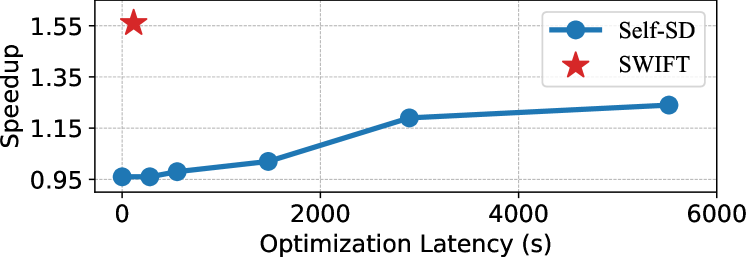
### Visual Description
## Line Chart: Speedup vs. Optimization Latency
### Overview
The image is a line chart comparing the speedup achieved by two methods, "Self-SD" and "SWIFT," against the optimization latency in seconds. The x-axis represents optimization latency, and the y-axis represents speedup. The chart shows the trend of speedup for "Self-SD" as optimization latency increases, and a single data point for "SWIFT."
### Components/Axes
* **X-axis:** Optimization Latency (s), ranging from 0 to 6000, with gridlines at intervals of 2000.
* **Y-axis:** Speedup, ranging from 0.95 to 1.55, with gridlines at intervals of 0.20.
* **Legend:** Located in the top-right corner.
* Blue line with circle markers: Self-SD
* Red star marker: SWIFT
### Detailed Analysis
* **Self-SD (Blue Line):** The speedup for Self-SD generally increases with optimization latency.
* At 0s latency, the speedup is approximately 0.96.
* At approximately 500s latency, the speedup is approximately 0.97.
* At approximately 1000s latency, the speedup is approximately 0.98.
* At approximately 2000s latency, the speedup is approximately 1.02.
* At approximately 3000s latency, the speedup is approximately 1.18.
* At approximately 5750s latency, the speedup is approximately 1.21.
* **SWIFT (Red Star):** The speedup for SWIFT is a single point at 0s latency, with a speedup of approximately 1.55.
### Key Observations
* SWIFT achieves a significantly higher speedup than Self-SD at 0s optimization latency.
* Self-SD's speedup increases with optimization latency, but it never reaches the speedup achieved by SWIFT.
* The rate of increase in speedup for Self-SD decreases as optimization latency increases.
### Interpretation
The chart suggests that SWIFT is more efficient than Self-SD when optimization latency is not a factor. However, as optimization latency increases, Self-SD's performance improves, although it never surpasses SWIFT's initial speedup. This could indicate that SWIFT is better suited for scenarios where quick results are needed, while Self-SD might be preferable when more time can be allocated for optimization. The diminishing returns of Self-SD's speedup with increasing latency suggest that there is a point beyond which further optimization provides minimal benefit.
</details>
Figure 11: Comparison of \method and Self-SD in terms of optimization latency and speedup. \method achieves a $1.56×$ speedup with an optimization latency of 116 seconds.
In this subsection, we provide a detailed comparison of \method and Self-SD (Zhang et al., 2024). Figure 11 presents the speedups of Self-SD across varying optimization latencies, reflecting the increase in Bayesian Optimization iterations. As shown, Self-SD achieves minimal speedup improvement – almost equivalent to unified skipping – with fewer than 50 Bayesian iterations, corresponding to an optimization latency below 1474 seconds. At 100 Bayesian iterations, Self-SD achieves a $1.19×$ speedup; however, its optimization latency is nearly 25 times longer than that of \method (2898s vs. 116s).
Table 12 compares \method and Self-SD (first two rows) under similar optimization latencies. The results highlight \method ’s superiority in both optimization efficiency (116s vs. 155s) and speedup ( $1.56×$ vs. $0.97×$ ). Even when compared to the augmented version of Self-SD (w/ dynamic verification), \method achieves a substantial $30\%$ relative improvement in speedup. Below, we analyze the factors contributing to this advantage (elaborated in Section 3.1):
- Optimization Objective Granularity: Self-SD calculates its optimization objective at a multi-sample level, requiring sequential decoding of all selected training samples (e.g., 8 samples with 32 tokens each) for every iteration to optimize Equation 1. In contrast, \method adopts a step-level optimization objective, optimizing the layer set dynamically at each decoding step.
- Bayesian Optimization Complexity: The computational complexity of Bayesian optimization increases significantly with the number of iterations. \method mitigates this burden by combining random search with interval Bayesian optimization, accelerating convergence of the optimization process while reducing computational overhead.
To further examine optimization trade-offs, we reduce Self-SD’s sequential optimization requirement to a single sample with 8 tokens, enabling more Bayesian Optimization iterations within a comparable latency. The corresponding results, denoted as Self-SD c (rows 3-4), are presented in Table 12. Even with these optimized settings, \method demonstrates substantial superior speedup and efficiency, highlighting the effectiveness of our proposed strategies.
| Self-SD | - | 5 | 155 | 0.50 | 1.80 | 0.57 | 0.97 $×$ |
| --- | --- | --- | --- | --- | --- | --- | --- |
| Self-SD w/ dynamic ver. | - | 5 | 155 | 0.50 | 2.07 | 0.86 | 1.17 $×$ |
| Self-SD c | - | 30 | 199 | 0.45 | 2.08 | 0.70 | 1.04 $×$ |
| Self-SD c w/ dynamic ver. | - | 30 | 199 | 0.45 | 2.44 | 0.93 | 1.22 $×$ |
| \method (Ours) | 552 | 23 | 116 | 0.45 | 5.82 | 0.98 | 1.56 $×$ |
Table 12: Comparison of \method and Self-SD at similar optimization latencies. We report the skip ratio $r$ , mean generated length M, token acceptance rate $\alpha$ , and speedup under greedy decoding. The results are obtained with LLaMA-2-13B on CNN/DM, with “ ver. ” indicating verification.
D.5 The Necessity of Plug-and-Play SD Methods
There has been a surge of recent interest in Speculative Decoding (SD), leading to the development of numerous promising strategies in the field, which can be broadly categorized into two directions:
- Training-required SD. These methods require additional pretraining or fine-tuning to improve speculative accuracy, often involving the integration of extra parameters. For instance, Medusa (Cai et al., 2024) and Eagle (Li et al., 2024a; b) incorporate lightweight draft heads into target LLMs and fine-tune them, achieving $3×$ $\sim$ $4×$ speedups.
- Plug-and-play SD. These approaches offer immediate acceleration of LLM inference without relying on auxiliary models or additional training. Notable examples include Parallel Decoding (Santilli et al., 2023) and Lookahead (Fu et al., 2024), which leverage Jacobi-based drafting, achieving $1.2×$ $\sim$ $1.4×$ speedups across various LLMs.
While training-required SD methods generally deliver higher speedups, their reliance on additional training and parameters limits both their generalizability and practicality. This has sparked debate within the academic community regarding the value of plug-and-play SD methods. To address these concerns, we present a detailed analysis below to highlight the necessity of plug-and-play SD approaches and underscore the contributions of our proposed \method:
1) Training costs of training-required SD methods are often prohibitive.
Training-required methods such as Medusa (Cai et al., 2024) and Eagle (Li et al., 2024a; b), while achieving higher speedups, incur substantial training costs. Despite efforts to reduce training overhead, these methods still require extensive computational resources (e.g., GPU time and datasets) to deliver valid acceleration performance. For example, Eagle requires 1–2 days of training with 8 RTX 3090 GPUs for LLaMA-33B or up to 2 days on 4 A100 (40G) GPUs for LLaMA-2-Chat-70B, using a dataset of 70k dialogues from ShareGPT. Such computational burdens introduce challenges in several scenarios:
- Users must train new draft models for unsupported target LLMs. For example, if the user’s target LLM is not among the released checkpoints or if the base model is updated (e.g., LLaMA-3.x), users are forced to train a new draft model, which may exceed their available GPU resources (e.g., GPU time).
- Users with small-scale acceleration needs face inefficiencies. For instance, a researcher needing to evaluate a small set of samples (e.g., 10 hours of evaluation) would find the 1–2 day training requirement disproportionate and hinder overall research efficiency.
2) Plug-and-play SD fills critical gaps unaddressed by training-required methods.
Plug-and-play SD methods, including \method, are model-agnostic and training-free, providing immediate acceleration without requiring additional computational overhead. These attributes are particularly critical for large models (70B–340B) and for use cases requiring rapid integration. The growing adoption of plug-and-play SD methods, such as Lookahead (Fu et al., 2024), further underscores their importance. These methods cater to scenarios where ease of use and computational efficiency are paramount, validating their research significance.
3) \method pioneers plug-and-play SD with layer-skipping drafting.
\method
represents the first plug-and-play SD method to incorporate layer-skipping drafting. It consistently achieves $1.3×$ $\sim$ $1.6×$ speedups over vanilla autoregressive decoding across diverse models and tasks. Additionally, it demonstrates $10\%$ $\sim$ $20\%$ higher efficiency compared to Lookahead (Fu et al., 2024). Despite its effectiveness, \method introduces a complementary research direction for existing plug-and-play SD. Its approach is orthogonal to Lookahead Decoding, and combining the two could further amplify their collective efficiency. We believe this study provides valuable insights and paves the way for future SD advancements, particularly for practical and cost-effective LLM acceleration.
To sum up, while training-required SD methods achieve higher speedups, their high computational costs and limited flexibility reduce practicality. Plug-and-play SD methods, like \method, offer training-free, model-agnostic acceleration, making them ideal for diverse scenarios. We hope this clarification fosters greater awareness and recognition of the value of plug-and-play SD research.
D.6 Additional Discussions with Related Work
In this work, we leverage the inherent layer sparsity of LLMs through layer skipping, which selectively bypasses intermediate layers within the target LLM to construct the compact draft model. In addition to layer skipping, there has been another research direction in SD that focuses on early exiting, where inference halts at earlier layers to improve computational efficiency (Yang et al., 2023; Hooper et al., 2023; Bae et al., 2023; Elhoushi et al., 2024). Particularly, LayerSkip (Elhoushi et al., 2024) explores early-exit drafting by generating drafts using only the earlier layers of the target LLM, followed by verification with the full-parameter model. This approach requires training involving layer dropout and early exit losses. Similarly, PPD (Yang et al., 2023) employs early exiting but trains individual classifiers for each layer instead of relying on a single final-layer classifier. Although effective, these methods rely on extensive fine-tuning to enable early-exiting capabilities, incurring substantial computational costs. Moreover, the training process alters the target LLM’s original output distribution, potentially compromising the reliability of generated outputs. In contrast, our proposed \method does not require auxiliary models or additional training, preserving the original output distribution of the target LLM while delivering comparable acceleration benefits.
There has been a parallel line of training-required SD research focusing on non-autoregressive drafting strategies (Stern et al., 2018; Cai et al., 2024; Gloeckle et al., 2024; Kim et al., 2024). These methods integrate multiple draft heads into the target LLM, enabling the parallel generation of draft tokens at each decoding step. Notably, Kim et al. (2024) builds on the Blockwise Parallel Decoding paradigm introduced in Stern et al. (2018), accelerating inference by refining block drafts with task-independent n-grams and lightweight rescorers using smaller LMs. While these approaches achieve notable acceleration, they also necessitate extensive training of draft models. \method complements these efforts by pioneering plug-and-play SD that eliminates the need for auxiliary models or additional training, offering a more flexible and practical solution for diverse use cases.
D.7 Optimization Steps
We present the detailed configuration of \method across various optimization steps in Figure 10. As the process continues, the skipped layer set is gradually refined toward the optimal configuration.
<details>
<summary>x15.png Details</summary>

### Visual Description
## Data Comparison: MLP vs. ATT
### Overview
The image presents a comparison of two data series, labeled "MLP" and "ATT," across a range of numerical values from 1 to 80. The data is visualized using colored blocks, with blue representing MLP and red representing ATT. Each block corresponds to a specific numerical value.
### Components/Axes
* **Y-Axis Labels:** "MLP" (top row), "ATT" (bottom row)
* **X-Axis Values:** Numerical values ranging from 1 to 80, incrementing by 2 for MLP and by 2 for ATT.
### Detailed Analysis
The data is presented in two rows, each representing a different category.
* **MLP (Blue):** The top row is labeled "MLP". The values associated with MLP are: 2, 4, 6, 8, 10, 12, 14, 16, 18, 20, 22, 24, 26, 28, 30, 32, 34, 36, 38, 40, 42, 44, 46, 48, 50, 52, 54, 56, 58, 60, 62, 64, 66, 68, 70, 72, 74, 76, 78, 80.
* **ATT (Red):** The bottom row is labeled "ATT". The values associated with ATT are: 1, 3, 5, 7, 9, 11, 13, 15, 17, 19, 21, 23, 25, 27, 29, 31, 33, 35, 37, 39, 41, 43, 45, 47, 49, 51, 53, 55, 57, 59, 61, 63, 65, 67, 69, 71, 73, 75, 77, 79.
### Key Observations
* The data series are presented as discrete values, with each value represented by a colored block.
* The values for MLP are all even numbers, while the values for ATT are all odd numbers.
* The values for ATT start at 1 and end at 79, while the values for MLP start at 2 and end at 80.
### Interpretation
The image provides a direct comparison between two distinct sets of numerical values, one consisting of even numbers (MLP) and the other consisting of odd numbers (ATT). The visualization clearly distinguishes between the two series, making it easy to identify the specific values associated with each category. The data suggests a simple, systematic difference between the two series, with MLP representing even numbers and ATT representing odd numbers within the specified range.
</details>
(a) Optimization Step 0
<details>
<summary>x16.png Details</summary>

### Visual Description
## Comparison Chart: MLP vs. ATT
### Overview
The image presents a comparison chart between two categories, "MLP" and "ATT," across a range of numerical values from 1 to 80. The chart uses colored blocks (blue for MLP and red for ATT) to indicate the presence of a value within each category.
### Components/Axes
* **Y-Axis Labels:** "MLP" (top row) and "ATT" (bottom row).
* **X-Axis:** Numerical values ranging from 1 to 80. Each number represents a distinct column.
* **Data Representation:** Blue blocks indicate the presence of a value for "MLP," and red blocks indicate the presence of a value for "ATT."
### Detailed Analysis
The chart displays the presence or absence of values for MLP and ATT across the numerical range.
* **MLP (Blue):**
* Values present: 2, 6, 18, 20, 22, 26, 32, 34, 40, 42, 50, 56, 60, 64, 70, 72, 78
* Values absent: 4, 8, 10, 12, 14, 16, 24, 28, 30, 36, 38, 44, 46, 48, 52, 54, 58, 62, 66, 68, 74, 76, 80
* **ATT (Red):**
* Values present: 11, 13, 23, 25, 31, 33, 37, 39, 41, 45, 49, 51, 55, 57, 59, 63, 65, 69
* Values absent: 1, 3, 5, 7, 9, 15, 17, 19, 21, 27, 29, 35, 43, 47, 53, 61, 67, 71, 73, 75, 77, 79
### Key Observations
* MLP has values concentrated in the lower and middle ranges, with gaps in between.
* ATT has values concentrated in the lower and middle ranges, with gaps in between.
* There is no overlap in the values present for MLP and ATT.
### Interpretation
The chart visually represents a comparison of the presence of specific values between two categories, MLP and ATT. The absence of overlap suggests that these categories might represent mutually exclusive sets of data or distinct characteristics across the numerical range. The clustering of values within certain ranges for each category could indicate patterns or trends specific to each category.
</details>
(b) Optimization Step 64
<details>
<summary>x17.png Details</summary>

### Visual Description
## Heatmap: MLP vs ATT
### Overview
The image is a heatmap comparing two categories, MLP and ATT, across a range of numerical values from 1 to 80. The heatmap uses blue and red to represent the presence of values for each category.
### Components/Axes
* **Rows:** Two rows labeled "MLP" and "ATT".
* **Columns:** Numerical values from 1 to 80, incrementing by 2 for MLP (2, 4, 6, ..., 80) and by 2 for ATT (1, 3, 5, ..., 79).
* **Color Coding:**
* Blue: Indicates the presence of a value for MLP.
* Red: Indicates the presence of a value for ATT.
### Detailed Analysis
The heatmap shows the distribution of values for MLP and ATT.
* **MLP:** Blue blocks are present for every even number from 2 to 80.
* **ATT:** Red blocks are present for every odd number from 1 to 79.
### Key Observations
* MLP has values only at even numbers.
* ATT has values only at odd numbers.
* There is no overlap in the values between MLP and ATT.
### Interpretation
The heatmap visually represents a clear distinction between the values associated with MLP and ATT. MLP is associated with even numbers, while ATT is associated with odd numbers. This suggests that the two categories are mutually exclusive in terms of their numerical values within the given range.
</details>
(c) Optimization Step 128
<details>
<summary>x18.png Details</summary>

### Visual Description
## Data Distribution Chart: MLP vs ATT
### Overview
The image presents a data distribution chart comparing two categories, MLP and ATT, across a numerical range from 1 to 80. The chart uses colored blocks to indicate the presence of data points for each category at specific numerical values. MLP is represented by blue blocks, while ATT is represented by red blocks.
### Components/Axes
* **Y-Axis Labels:** MLP (top row), ATT (bottom row)
* **X-Axis:** Numerical values ranging from 1 to 80, incrementing by 2 for MLP and by 2 for ATT.
### Detailed Analysis or ### Content Details
**MLP (Blue Blocks):**
* Data points are present at the following values: 16, 22, 26, 38, 40, 44, 46, 58, 60, 78.
* The distribution of data points for MLP is sparse and uneven across the numerical range.
**ATT (Red Blocks):**
* Data points are present at the following values: 1, 3, 5, 7, 9, 11, 13, 15, 17, 19, 21, 23, 25, 27, 29, 31, 33, 35, 37, 39, 41, 43, 45, 47, 49, 51, 53, 55, 57, 59, 61, 63, 65, 67, 69, 71, 73, 75, 77, 79.
* The distribution of data points for ATT is dense and relatively uniform across the numerical range.
### Key Observations
* ATT has a much higher density of data points compared to MLP.
* MLP's data points are clustered in certain regions of the numerical range, while ATT's are more evenly spread.
### Interpretation
The chart visually demonstrates a significant difference in the distribution of data points between MLP and ATT. ATT appears to have data points across almost the entire range, suggesting a more comprehensive or continuous presence. In contrast, MLP's data points are selective, indicating a more specific or limited presence within the same range. This could imply that ATT is more consistently active or relevant across the numerical values, while MLP is only active or relevant at certain specific points.
</details>
(d) Optimization Step 512
Figure 12: Visualization of skipped layer set configurations of LLaMA-2-13B optimized by \method on different optimization steps. Gray squares indicate retained layers, red squares denote skipped attention layers, and blue squares signify skipped MLP layers.
D.8 Case Study
We present examples from CNN/DM and Humaneval in Table 13 and 14, respectively, comparing token acceptance between \method and prior plug-and-play approach, Lookahead (Fu et al., 2024). The results demonstrate that \method accepts a higher number of drafts, which are uniformly distributed in the outputs, highlighting the effectiveness of our approach.
Table 13: CNN/DM example using LLaMA-2-13B; red tokens indicate accepted drafts.
| Lookahead \hdashline \method | A Canadian law student was greeted by a friendly note from a stranger when he returned to his car after leaving the head lights on all day . A Canadian law student was gre et ed by a friendly note from a stranger when he returned to his car after leaving the headlights on all day . |
| --- | --- |
Table 14: Humaneval example using CodeLLaMA-13B; red tokens indicate accepted drafts.
| Lookahead \hdashline \method | for i in range(len(numbers) - 1): if abs(numbers [i] - numbers [i + 1]) <= threshold: return True return False def has_close_elements_2(numbers: List[float], threshold: float) ->bool: ””” Check if in given list of numbers, are any two numbers closer to each other than given threshold. >>>has_close_elements_2-for i in range(len (numbers) - 1): if abs (numbers [i] - numbers[i + 1]) <= threshold: return True return False def has_close_elements_ 2(numbers: List[float], threshold: float) -> bool: ””” Check if in given list of numbers, are any two numbers closer to each other than given threshold. >>> has _close_elements_2 |
| --- | --- |