# Neural Normalized Compression Distance and the Disconnect Between Compression and Classification
**Authors**:
- John Hurwitz (University of Maryland, Baltimore County)
- Charles Nicholas (University of Maryland, Baltimore County)
- Edward Raff
- Booz Allen Hamilton (University of Maryland, Baltimore County)
## Abstract
It is generally well understood that predictive classification and compression are intrinsically related concepts in information theory. Indeed, many deep learning methods are explained as learning a kind of compression, and that better compression leads to better performance. We interrogate this hypothesis via the Normalized Compression Distance (NCD), which explicitly relies on compression as the means of measuring similarity between sequences and thus enables nearest-neighbor classification. By turning popular large language models (LLMs) into lossless compressors, we develop a Neural NCD and compare LLMs to classic general-purpose algorithms like gzip. In doing so, we find that classification accuracy is not predictable by compression rate alone, among other empirical aberrations not predicted by current understanding. Our results imply that our intuition on what it means for a neural network to “compress” and what is needed for effective classification are not yet well understood.
## 1 Introduction
The link between compression and prediction has been well-established (15). Predictors (such as machine learning models) can be turned into compressors when combined with an entropy coding technique such as arithmetic coding (27). Conversely, compressors can be used to make predictions via a compressor-based distance metric and a distance-based learning algorithm such as $k$ -nearest neighbors. A popular method for the latter approach is the Normalized Compression Distance (NCD) (14), which is theoretically optimal as a distance metric if given an optimal compressor. NCD has seen success in a variety of domains, including anomaly detection and clustering (10), text classification (9), and image classification (8). Here, the compressors used are primarily traditional compression algorithms such as gzip and lzma. While these traditional compression algorithms can compress data quickly and successfully in an impressively wide variety of domains, much better lossless compression performance is generally possible in any given specialized domain through learned neural network-based compressors (2; 12; 11). In the text domain, the leading compressors in terms of compression rate are neural-network based (16) and far surpass the performance of traditional compressors, at the cost of being more computationally expensive.
Given the superior compression ability of neural compressors, the natural question arises of whether their improved compression rates translate into improved predictive performance. Indeed, it has been hypothesized that compression algorithms with better compression rates should classify better on account of closer approximation to Kolmogorov complexity. We investigate NCD-based classification performance differences by replacing traditional compressors with LLM-based neural compressors in this paradigm, noting the effect of compression rate on test accuracy, and comparing NCD performance with Euclidean distance with a model’s latent representation. We find that counter to conventional wisdom, NCD-based classification accuracy is not predictable solely from compression rate. We exhibit cases where a neural compressor achieves consistent and superior compression rates across datasets but can either outperform or underperform traditional compressors depending on the dataset.
This paper is organized as follows. In section 2 we describe our novel approach to doing NCD-based text classification via pretrained LLMs as neural compressors in the few-shot text classification setting, and provide requisite background in the information-theoretic grounding of compression distance. In section 3 we highlight related work in neural compression, compression-distance-based machine learning, and the connection between compression rate and classification accuracy. In section 4 we describe our experimental results and three primary findings relating to the relationship between compression rate and accuracy, effects of varying the choice of LLM for neural compression, and a comparison to using the models’ latent representations with Euclidean distance. We then provide a brief conclusion in section 5.
## 2 Method: Neural Normalized Compression Distance
In this section we provide a brief description of Kolmogorov complexity and its connection to practical notions of compression distance, arithmetic coding and its usefulness in lossless compression schemes, and our novel approach to using pretrained LLMs as neural compressors in the few shot text classification setting.
### 2.1 Kolmogorov Complexity and Compression Distance
Given a sequence $x$ , the Kolmogorov Complexity $K(x)$ (13) is defined as the length of the shortest computer program that outputs $x$ . $K(x)$ can be interpreted as the output of the best possible lossless compressor given any input bitstring $x$ . The Conditional Kolmogorov Complexity function $K(x|y)$ is defined as the length of the shortest program that outputs $x$ given another sequence $y$ as input. Using the notion of Kolmogorov Complexity, Li et al. (14) define the Normalized Information Distance (NID).
$$
\textnormal{NID}(x,y)=\frac{\max\{K(x|y),K(y|x)\}}{\max\{K(x),K(y)\}} \tag{1}
$$
The NID is a metric The proof that NID is a metric includes negligible error terms for the identity axiom and triangle inequality (14). and has a range of $[0,1]$ . The lower the NID, the more shared information exists between $x$ and $y$ which gives an indication of similarity. It is well-known that $K$ is uncomputable. In practice, we can approximate $K$ by using any compression algorithm. Li et al. (14) define the Normalized Compression Distance such that, given a compression algorithm, and a function $C(x)$ which returns the length of the compressed output of sequence $x$ in bytes, gives us a practical approximation of the NID. $xy$ indicates the concatenation of sequences $x$ and $y$ .
$$
\textnormal{NCD}(x,y)=\frac{C(xy)-\min\{C(x),C(y)\}}{\max\{C(x),C(y)\}} \tag{2}
$$
### 2.2 NCD-Based Sequence Classification
By using any compressor to calculate pairwise NCDs, these NCDs can be used as the distance metric in the non-parametric classification algorithm $k$ nearest neighbors ( $k$ NN). There is an $O(n^2)$ complexity for the pairwise distance calculations between the train set and test set, each requiring the compression of a concatenated pair of samples. In current practice, this complexity is a limiting factor for choice of model size and dataset size. To use a compressor in this way only requires the compression phase; decompression is never needed.
### 2.3 Arithmetic Coding
In modern neural lossless compression paradigms, arithmetic coding (27) is one of the most popular schemes for entropy coding due to its near-optimality, and its ability to handle adaptive probabilistic models (25; 6; 3; 12; 2). Arithmetic coding is an entropy coding technique which, given a probability distribution as input, represents a sequence of symbols as a single arbitrary-precision floating-point number between 0 and 1. Symbols with high probability will be encoded with fewer bits than symbols with low probability. Arithmetic coding is compatible with an adaptive probabilistic model where the next-symbol probabilities can differ for each index in the sequence. Language models fit precisely this paradigm, where the prediction at each index of a sequence yields a probability distribution for the next symbol. By doing arithmetic coding on this probability distribution as input, we perform lossless compression. The resulting bitstream, with access to the same probabilistic model, can be used in a reverse process to reconstruct the original sequence.
### 2.4 Neural Normalized Compression Distance for Sequence Classification
We refer to the use of neural network-based compressors to calculate NCDs as Neural Normalized Compression Distance (Neural NCD). We extend previous work on compression-based sequence classification by using Neural NCD in the few-shot text classification setting. The neural compressor, which is a language model paired with arithmetic coding, is used to calculate NCDs that are then used as the distance metric for $k$ NN. There are two primary reasons why using pretrained LLMs as the probabilistic models in a lossless compression scheme is useful for studying the relationship between compression rate and accuracy of NCD-based classification. First, neural compressors can achieve much better compression rates than traditional compressors in specific domains, allowing us to investigate the effects of compression rate on classification accuracy when using neural compressors. Second, the model can be easily swapped out, allowing us to study similar effects when varying model architecture and size.
## 3 Related Work
Neural Compression: Neural networks have been successfully used to perform lossless compression on a variety of domains including text (3; 2; 12) and images (8). Large Language Models (LLMs) in particular have shown promise for lossless compression of text (25; 6) due to excellence in next-symbol prediction, with neural methods leading the Large Text Classification Benchmark (16) and achieving better compression rates than traditional compressors like gzip, at the cost of more computation. Other works that attempt alternative architectures inspired by compression algorithms are beyond the current scope of this article (24).
Compression Distance for Machine Learning: There is empirical evidence to show that compression distance is effective in anomaly detection, clustering, and classification of sequential data (10; 5). Li et al. (14), who proposed NID, also showed its effectiveness in text classification. Jiang et al. (9) show that NCD-based classification with the traditional compressor gzip performs competitively with neural methods such as BERT (7) on few-shot text classification tasks. A follow-up work (8) uses deep latent variable models for compression of images, outperforming supervised neural network methods for few-shot image classification. Others have relaxed the compression requirements and instead extracted feature-vectors from compression dictionaries/methods to obtain faster distance calculations (19; 21).
Compression Rate and Classification Accuracy: Jiang et al. (9) show a moderate linear correlation between compression rate and test accuracy among traditional compressors for few shot text classification, while noting the importance of the actual compression algorithm and finding cases where algorithms with better compression rates still under-perform ones with lower ratios. A follow-up work (8) also shows a similar correlation among mostly traditional compressors and one latent variable neural compressor on image classification datasets, and older work in malware analysis found a similar result (4). Notably, compression similarity has seen wide use in malware for its ability to handle hard-to-parse and large binary files (26; 23; 21; 22; 19; 20).
## 4 Experiments
Three key insights are derived from our study. First, accuracy of NCD-based classification methods is not predictable from compression rate alone when using neural compressors in the text classification domain. Second, by comparing different LLMs as neural compressors, we show that models of similar size but different architectures and pretraining have similar performance when compared to traditional compressors. Third, the extent to which Neural NCD improves or hinders performance over a Euclidean distance approach using the model’s latent representations is model-dependent; we show that Neural NCD performs better than latent representations for certain models and performs worse for others.
We investigate Neural NCD for non-parametric NCD-based text classification in a few-shot setting using the datasets AGNews, 20News, and DBpedia (though we only use AGNews and DBpedia in subsection 4.2 and subsection 4.3). We use Bellard’s ts_zip utility (3) to perform neural compression with the model RWKV 169M (17). We compare these results with the use of the traditional compressors gzip, zstandard (zstd), and lzma on the same task.
To investigate the few-shot setting, we draw $n=\{5,10,50,100\}$ labeled train samples from each class, obtain a subset of 100 test samples via stratified sampling across five trials for each $n$ , calculating the mean test accuracy, 95% confidence interval, and compression rate (compressed size / original size). The $O(n^2)$ computational complexity of pairwise NCD calculation for neural compression is a limiting factor in the computational cost of this method, scaling with LLM model size and size of training and test sets. For this reason we subsample only 100 test samples here for each of the five trials. See Appendix A for further experiment details.
### 4.1 Neural compressor has variable Neural NCD performance despite consistently superior compression rates.
It has been hypothesized that compressors that achieve better compression rates should improve the performance of NCD-based methods through a better approximation of Kolmogorov Complexity (9; 8). Through our text classification experiments with a neural compressor, we find that compression rate alone is not enough to predict the differences in NCD-based classification accuracy when using neural compressors across various datasets in the text domain. We note the compression rates (lower is better compression) for each compressor on each dataset in Table 1.
Table 1: Compression rates (lower is better compression) across compressors for the AGNews, 20News, and DBpedia datasets. For neural compressors, we use the raw compression rate which ignores the size of the neural network. The RWKV 169M model achieves the best compression rate across each dataset.
| gzip zstd lzma | 0.785 0.743 1.070 | 0.593 0.596 0.685 | 0.824 0.785 1.115 |
| --- | --- | --- | --- |
| RWKV 169M | 0.248 | 0.204 | 0.248 |
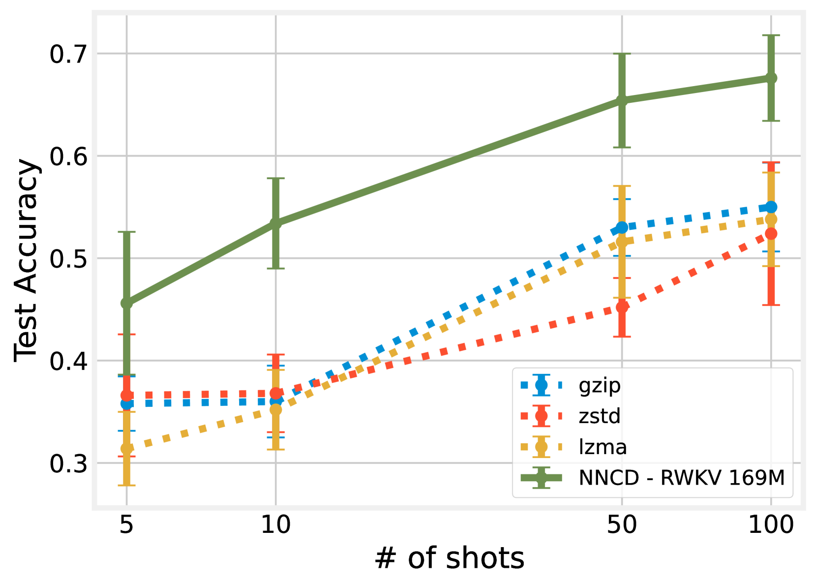
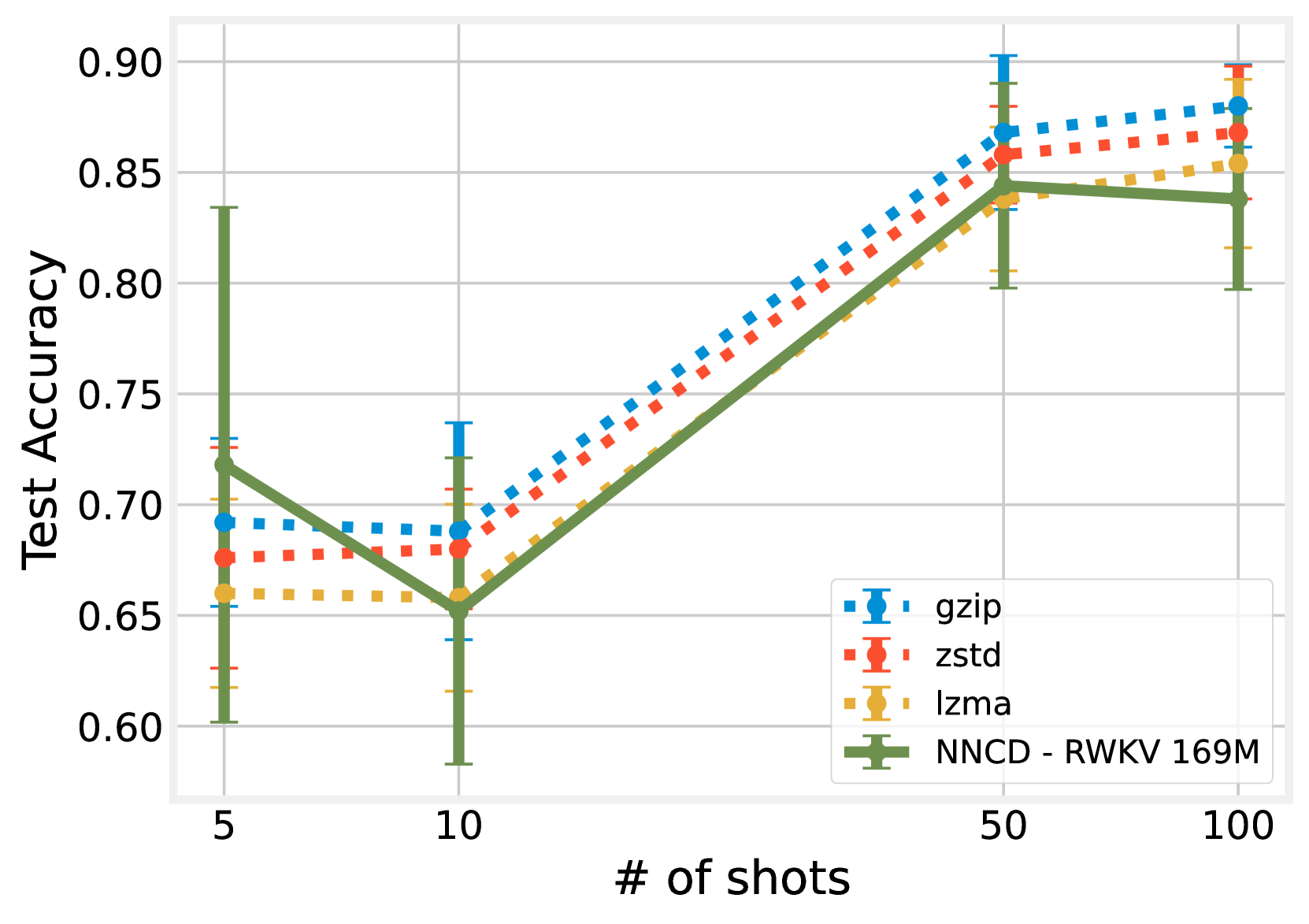
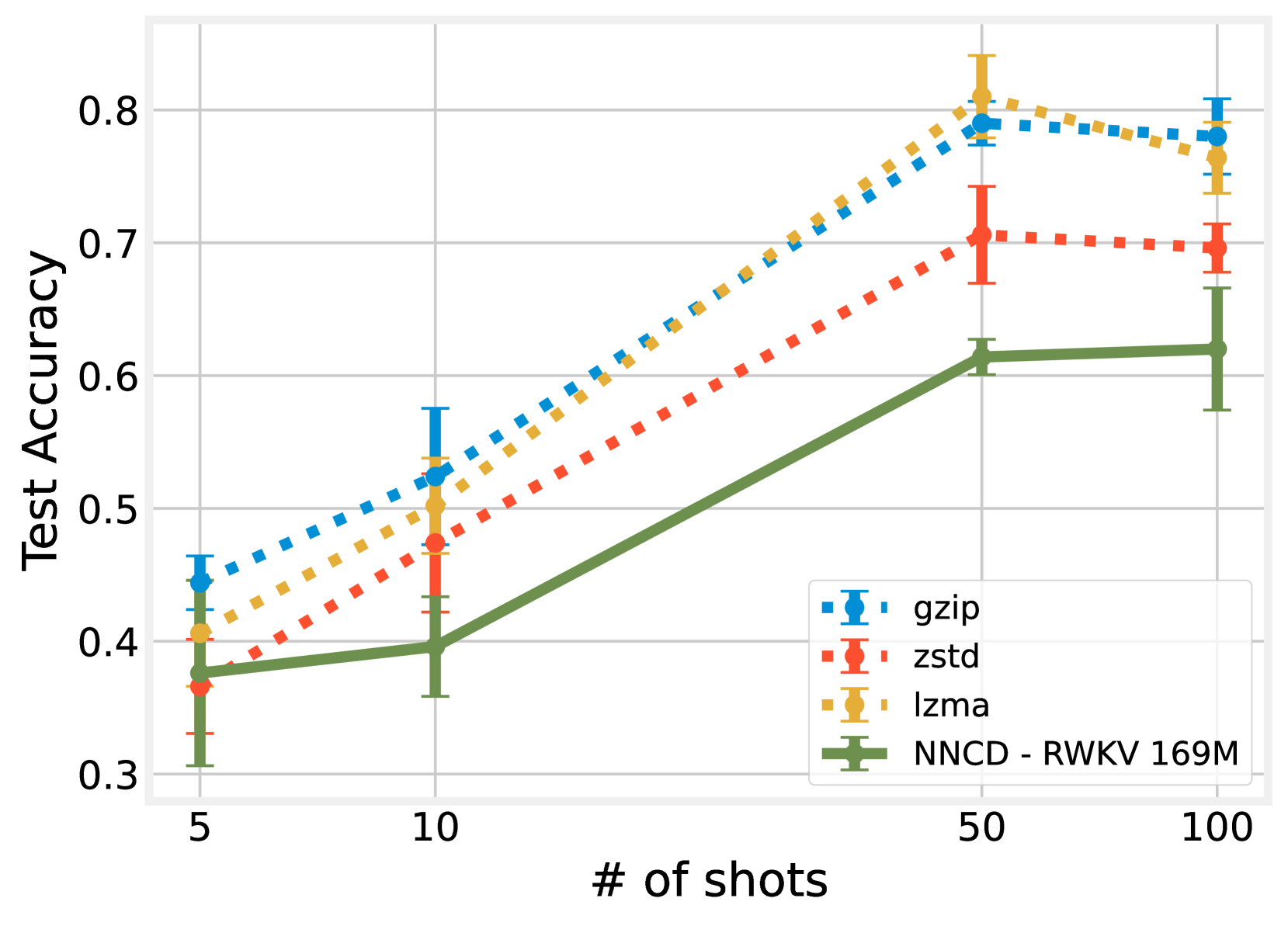
Ignoring the size of the language models, even a small, simple model such as RWKV 169M achieves significantly lower compression rates than traditional compressors. Despite the RWKV neural compressor achieving superior compression rates than traditional compressors on each dataset, Neural NCD yields varying relative performance when compared to using NCDs of traditional compressors, outperforming them on AGNews, performing on-par with them on 20News, and underperforming them on DBpedia (see Figure 1). Of particular note is that the RWKV compressor and gzip retain their compression rates across both AGNews and DBpedia, and yet neural compression outperforms gzip on the former and underperforms it on the latter.
(a) AGNews
<details>
<summary>x1.png Details</summary>
### Visual Description
## Line Chart: Test Accuracy vs. Number of Shots
### Overview
The chart compares the test accuracy of four models (gzip, zstd, lzma, and NNC-D - RWKV 169M) across different numbers of training shots (5, 10, 50, 100). Test accuracy increases with the number of shots for all models, with NNC-D consistently outperforming the others. Error bars indicate variability in accuracy measurements.
### Components/Axes
- **X-axis**: Number of shots (5, 10, 50, 100).
- **Y-axis**: Test accuracy (0.3 to 0.7).
- **Legend**:
- **Blue squares**: gzip
- **Red circles**: zstd
- **Orange diamonds**: lzma
- **Green crosses**: NNC-D - RWKV 169M
- **Error bars**: Vertical lines with caps, representing confidence intervals (e.g., ±0.03 to ±0.05).
### Detailed Analysis
1. **NNC-D - RWKV 169M (Green Crosses)**:
- **5 shots**: ~0.45 (±0.05, error range: 0.40–0.50).
- **10 shots**: ~0.53 (±0.06, error range: 0.47–0.59).
- **50 shots**: ~0.65 (±0.06, error range: 0.59–0.71).
- **100 shots**: ~0.68 (±0.05, error range: 0.63–0.73).
2. **gzip (Blue Squares)**:
- **5 shots**: ~0.37 (±0.03, error range: 0.34–0.40).
- **10 shots**: ~0.37 (±0.03, error range: 0.34–0.40).
- **50 shots**: ~0.53 (±0.04, error range: 0.49–0.57).
- **100 shots**: ~0.54 (±0.05, error range: 0.49–0.59).
3. **zstd (Red Circles)**:
- **5 shots**: ~0.38 (±0.03, error range: 0.35–0.41).
- **10 shots**: ~0.38 (±0.03, error range: 0.35–0.41).
- **50 shots**: ~0.46 (±0.04, error range: 0.42–0.50).
- **100 shots**: ~0.52 (±0.05, error range: 0.47–0.57).
4. **lzma (Orange Diamonds)**:
- **5 shots**: ~0.32 (±0.03, error range: 0.29–0.35).
- **10 shots**: ~0.35 (±0.03, error range: 0.32–0.38).
- **50 shots**: ~0.51 (±0.04, error range: 0.47–0.55).
- **100 shots**: ~0.53 (±0.05, error range: 0.48–0.58).
### Key Observations
- **NNC-D dominates**: It achieves the highest accuracy at all shot counts, with a steep upward trend.
- **Other models improve gradually**: gzip, zstd, and lzma show slower progress, with lzma outperforming zstd at higher shots.
- **Error variability**: NNC-D has larger error bars, suggesting higher variability in its performance.
- **Convergence gap**: At 100 shots, NNC-D’s accuracy (~0.68) exceeds others by ~0.15–0.16, but the gap narrows slightly compared to 50 shots.
### Interpretation
The data demonstrates that **NNC-D - RWKV 169M** is significantly more effective than traditional compression algorithms (gzip, zstd, lzma) in this context. Its performance scales strongly with data volume, suggesting it leverages larger datasets more efficiently. While error bars indicate higher variability for NNC-D, its mean accuracy remains superior, making it the optimal choice for high-stakes applications. The slower improvement of traditional models highlights their limitations in handling complex patterns, even with abundant data. This chart likely informs model selection in scenarios where data quantity and accuracy trade-offs are critical.
</details>
(b) 20News
<details>
<summary>x2.png Details</summary>
### Visual Description
## Line Chart: Test Accuracy vs. Number of Shots
### Overview
The chart compares the test accuracy of four algorithms (gzip, zstd, lzma, and NNCD - RWKV 169M) across varying numbers of shots (5, 10, 50, 100). Test accuracy is plotted on the y-axis (0.6–0.9), while the x-axis represents the number of shots. Each algorithm is represented by a distinct line style and color, with error bars indicating variability in accuracy measurements.
### Components/Axes
- **Y-Axis**: Test Accuracy (0.6–0.9, increments of 0.05).
- **X-Axis**: Number of Shots (5, 10, 50, 100).
- **Legend**: Located in the bottom-right corner, mapping colors to algorithms:
- **Blue (dashed)**: gzip
- **Red (dotted)**: zstd
- **Orange (dash-dot)**: lzma
- **Green (solid)**: NNCD - RWKV 169M
- **Markers**: Each data point is marked with a symbol (e.g., square, diamond) corresponding to its algorithm.
### Detailed Analysis
1. **gzip (Blue Dashed Line)**:
- **5 shots**: ~0.69 (±0.03 error).
- **10 shots**: ~0.68 (±0.04 error).
- **50 shots**: ~0.86 (±0.03 error).
- **100 shots**: ~0.88 (±0.02 error).
- **Trend**: Gradual improvement with more shots.
2. **zstd (Red Dotted Line)**:
- **5 shots**: ~0.67 (±0.04 error).
- **10 shots**: ~0.66 (±0.05 error).
- **50 shots**: ~0.85 (±0.03 error).
- **100 shots**: ~0.87 (±0.02 error).
- **Trend**: Steady upward trajectory.
3. **lzma (Orange Dash-Dot Line)**:
- **5 shots**: ~0.66 (±0.05 error).
- **10 shots**: ~0.65 (±0.06 error).
- **50 shots**: ~0.83 (±0.04 error).
- **100 shots**: ~0.85 (±0.03 error).
- **Trend**: Slow but consistent improvement.
4. **NNCD - RWKV 169M (Green Solid Line)**:
- **5 shots**: ~0.72 (±0.06 error).
- **10 shots**: ~0.65 (±0.05 error).
- **50 shots**: ~0.84 (±0.03 error).
- **100 shots**: ~0.84 (±0.02 error).
- **Trend**: Initial dip at 10 shots, then recovery and plateau.
### Key Observations
- **NNCD - RWKV 169M** exhibits the highest accuracy at 5 and 100 shots but shows a notable dip at 10 shots (~0.65), suggesting potential instability at intermediate shot counts.
- **gzip** and **zstd** demonstrate the most consistent improvement, with gzip achieving the highest accuracy at 100 shots (~0.88).
- **lzma** lags behind other algorithms across all shot counts but shows marginal gains at higher shot volumes.
- Error bars are largest at 5 shots (e.g., NNCD: ±0.06) and smallest at 100 shots (±0.02), indicating greater variability in low-shot scenarios.
### Interpretation
The data suggests that increasing the number of shots generally improves test accuracy for all algorithms, with diminishing returns at higher shot counts. NNCD - RWKV 169M’s performance is most erratic, with a significant drop at 10 shots that contradicts its strong performance at 5 and 100 shots. This could indicate sensitivity to specific data distributions or computational constraints at intermediate shot counts. gzip and zstd show robust scalability, while lzma’s slower improvement highlights potential inefficiencies in its compression strategy. The error bars underscore the importance of shot count in stabilizing accuracy measurements, particularly in low-data regimes.
</details>
(c) DBpedia
<details>
<summary>x3.png Details</summary>
### Visual Description
## Line Chart: Test Accuracy vs. Number of Shots
### Overview
The chart compares the test accuracy of four compression algorithms (gzip, zstd, lzma, and NNCD - RWKV 169M) across varying numbers of shots (5, 10, 50, 100). Test accuracy is plotted on the y-axis (0.3–0.8), while the x-axis represents the number of shots. Each algorithm is represented by a distinct line style and color, with error bars indicating variability in performance.
### Components/Axes
- **Y-axis**: Test Accuracy (0.3–0.8, increments of 0.1)
- **X-axis**: Number of Shots (5, 10, 50, 100)
- **Legend**: Located in the bottom-right corner, mapping:
- **Blue (dashed line + square markers)**: gzip
- **Red (dotted line + diamond markers)**: zstd
- **Yellow (solid line + circle markers)**: lzma
- **Green (solid line + cross markers)**: NNCD - RWKV 169M
- **Error Bars**: Vertical lines extending from data points, representing confidence intervals.
### Detailed Analysis
1. **gzip (Blue)**:
- Starts at ~0.45 (5 shots), rises to ~0.78 (50 shots), then slightly declines to ~0.77 (100 shots).
- Error bars are largest at 50 and 100 shots, indicating higher variability.
2. **zstd (Red)**:
- Begins at ~0.37 (5 shots), increases to ~0.70 (50 shots), then drops to ~0.69 (100 shots).
- Error bars are moderate, with the largest spread at 50 shots.
3. **lzma (Yellow)**:
- Starts at ~0.41 (5 shots), peaks at ~0.80 (50 shots), then decreases to ~0.76 (100 shots).
- Error bars are smallest, suggesting consistent performance.
4. **NNCD - RWKV 169M (Green)**:
- Begins at ~0.37 (5 shots), rises steadily to ~0.62 (50 shots), then plateaus at ~0.63 (100 shots).
- Error bars are moderate, with the largest spread at 50 shots.
### Key Observations
- **Performance Trends**:
- All algorithms improve accuracy with more shots, except for minor declines at 100 shots for gzip, zstd, and lzma.
- **lzma** achieves the highest accuracy at 50 shots (~0.80), while **NNCD** remains the lowest (~0.63).
- **Error Variability**:
- gzip and zstd show the most variability (larger error bars), particularly at higher shot counts.
- lzma demonstrates the most stable performance (smallest error bars).
- **Diminishing Returns**:
- Accuracy gains plateau or slightly regress at 100 shots for most algorithms.
### Interpretation
The data suggests that increasing the number of shots generally improves test accuracy, but the rate of improvement diminishes beyond 50 shots. **lzma** outperforms other algorithms, potentially due to its compression efficiency or model architecture. **NNCD - RWKV 169M** lags behind, possibly due to suboptimal hyperparameters or training dynamics. The variability in gzip and zstd indicates sensitivity to input data distribution or implementation specifics. Error bars highlight the importance of statistical robustness in algorithm evaluation.
</details>
Figure 1: Comparison of RWKV 169M neural compressor and traditional compressors using $k$ NN with NCD across the datasets AGNews, 20News, and DBpedia (NNCD = Neural NCD). Despite the neural compressor achieving superior compression rates, we find cases where Neural NCD outperforms, underperforms, and performs on-par with traditional compressors on the few shot sequence classification task. This calls into question the hypothesis that accuracy of NCD-based methods is predictable solely from compression rates.
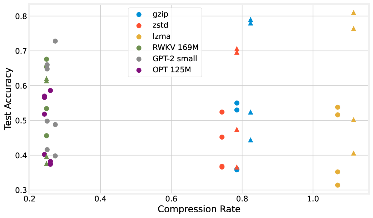
We see the same phenomenon strictly among the traditional compressors as well, where there is no big difference in performance despite varying compression rates Note that for short sequences, LZMA’s dictionary size outweighs the compression savings, leading to rates greater than 1. However, despite these poor compression rates LZMA is still able to do NCD-based sequence classification on-par with gzip and zstd.. We plot test accuracies across compression rates for AGNews and DBpedia across all few-shot settings in Figure 2. We can see that each compressor tends to have its own range of compression rates for these datasets, and despite drastically varying rates, the test accuracy spread is roughly the same, even with neural compressors with much lower compression rates.
<details>
<summary>x4.png Details</summary>
### Visual Description
## Scatter Plot: Test Accuracy vs. Compression Rate
### Overview
The image is a scatter plot comparing test accuracy (y-axis) against compression rate (x-axis) for six different compression models. Data points are color-coded by model, with a legend in the top-left corner. The plot reveals trade-offs between compression efficiency and performance accuracy across models.
### Components/Axes
- **X-axis (Compression Rate)**: Ranges from 0.2 to 1.2 in increments of 0.1.
- **Y-axis (Test Accuracy)**: Ranges from 0.3 to 0.8 in increments of 0.1.
- **Legend**: Located in the top-left corner, mapping colors to models:
- Blue circles: gzip
- Orange circles: zstd
- Yellow circles: lzma
- Green circles: RWKV 169M
- Gray circles: GPT-2 small
- Purple circles: OPT 125M
### Detailed Analysis
1. **gzip (Blue Circles)**:
- Test accuracy decreases from ~0.75 at 0.2 compression to ~0.55 at 0.8 compression.
- No data points beyond 0.8 compression.
2. **zstd (Orange Circles)**:
- Accuracy declines from ~0.65 at 0.2 compression to ~0.45 at 0.8 compression.
- No data points beyond 0.8 compression.
3. **lzma (Yellow Circles)**:
- Accuracy drops sharply from ~0.6 at 0.2 compression to ~0.3 at 1.2 compression.
- Highest compression rate (1.2) but lowest accuracy.
4. **RWKV 169M (Green Circles)**:
- Relatively stable accuracy (~0.55–0.65) across 0.2–0.6 compression.
- Slight decline to ~0.5 at 0.8 compression.
5. **GPT-2 small (Gray Circles)**:
- Accuracy fluctuates between ~0.4 and ~0.7 across 0.2–0.6 compression.
- No data points beyond 0.6 compression.
6. **OPT 125M (Purple Circles)**:
- Accuracy ranges from ~0.38 to ~0.6 across 0.2–0.6 compression.
- No data points beyond 0.6 compression.
### Key Observations
- **Trade-off Pattern**: Higher compression rates generally correlate with lower test accuracy for most models.
- **Outliers**:
- Lzma achieves the highest compression rate (1.2) but has the lowest accuracy (~0.3).
- RWKV 169M maintains higher accuracy than other models at lower compression rates.
- **Trends**:
- gzip and zstd show consistent declines in accuracy with increasing compression.
- RWKV 169M exhibits the most stable performance across compression rates.
### Interpretation
The data suggests a fundamental trade-off between compression efficiency and model performance. Models like RWKV 169M appear to balance these factors better, maintaining higher accuracy even at moderate compression rates. In contrast, lzma and gzip prioritize compression at the expense of accuracy, which may be unsuitable for applications requiring high fidelity. The absence of data beyond 0.6 compression for some models (e.g., GPT-2 small, OPT 125M) implies potential limitations in their compression capabilities or testing scope. This visualization highlights the need for context-specific model selection based on the priority between compression and accuracy.
</details>
Figure 2: Test accuracy plotted against compression rate (lower is better compression) for AGNews and DBpedia across different few shot settings. Different shapes indicate different datasets, and each compressor is its own color. If compression rate and predictive performance were correlated, we would expect a diagonal relationship to occur, but none exists.
The internal workings of each compression algorithm are important in determining NCD quality. For example, gzip searches for repeated byte sequences only within a 32 KB sliding window. Since the concatenation of two inputs is a crucial component to calculating the NCD, large sequence lengths will prevent gzip from exploiting far-reaching redundancies between the two. Differences in neural network architectures among neural compressors may yield different abilities to identify these long range similarities and thus varying NCD quality.
Table 2: Compression rates when using various pretrained language models for neural compression on the AGNews and DBpedia datasets. For neural compressors, we use the raw compression rate which ignores the size of the neural network.
| gzip RWKV 169M GPT-2 117M | 0.785 0.248 0.250 | 0.824 0.248 0.273 |
| --- | --- | --- |
| OPT 125M | 0.242 | 0.259 |
### 4.2 Using other models for neural compression
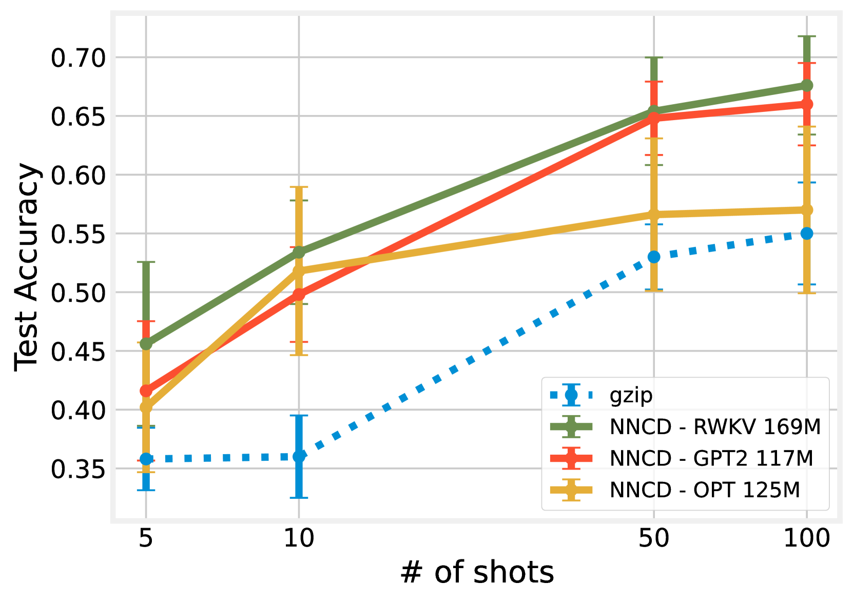
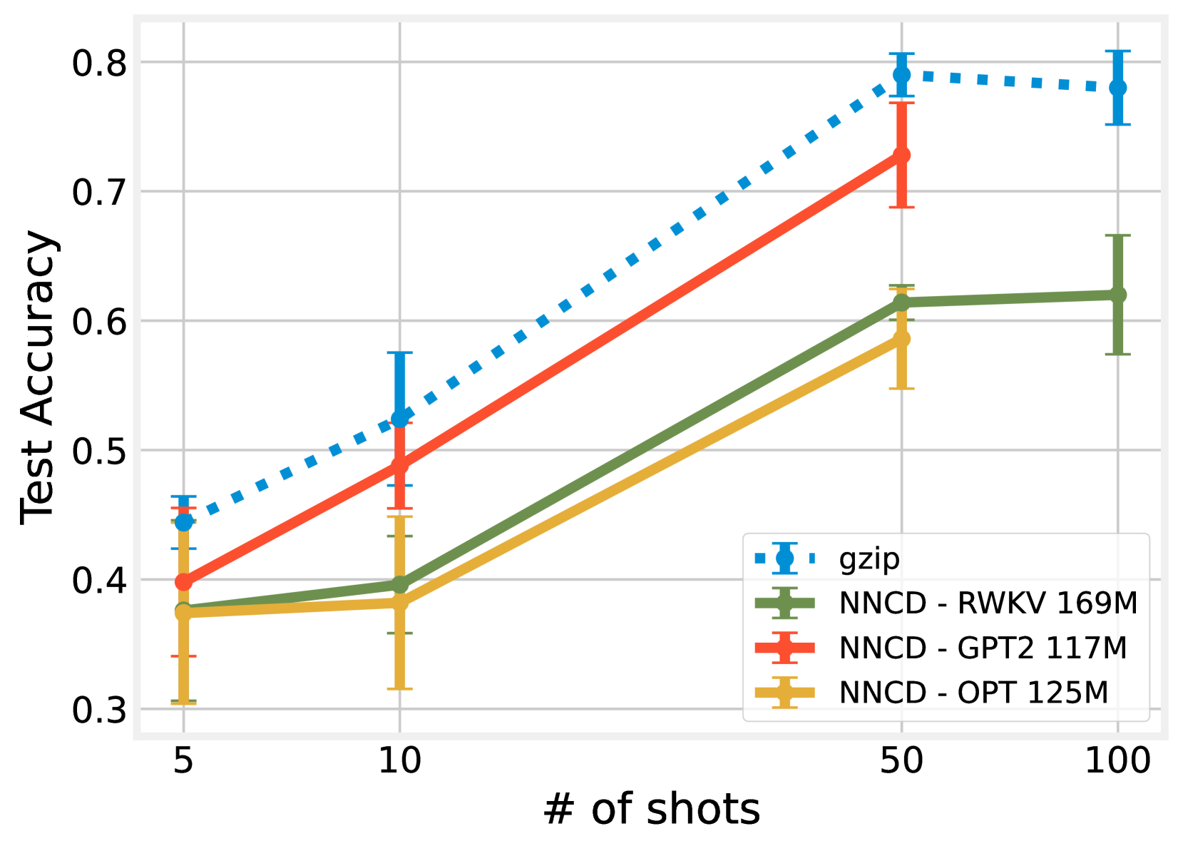
In order to investigate the effects of the particular choice of model and model architecture on Neural NCD performance, we run identical experiments as above, swapping out RWKV 169M for two other models: GPT-2 117M (GPT-2 small) (18) and OPT 125M (28), as shown in Figure 3. Here we only use the gzip results out of the traditional compressors since they perform comparably and to aid visual clarity. We can see that all neural models outperform gzip in the same way on AGNews, and underperform it in the same way on DBpedia. Compression rates across models are shown in Table 2.
(a) AGNews
<details>
<summary>x5.png Details</summary>
### Visual Description
## Line Chart: Test Accuracy vs. # of Shots
### Overview
The chart compares the test accuracy of four models (gzip, NNCD - RWKV 169M, NNCD - GPT2 117M, NNCD - OPT 125M) across varying numbers of training shots (5, 10, 50, 100). Test accuracy is plotted on the y-axis (0.35–0.70), while the x-axis represents the number of shots. Error bars indicate uncertainty in accuracy measurements.
### Components/Axes
- **X-axis**: "# of shots" (logarithmic scale: 5, 10, 50, 100).
- **Y-axis**: "Test Accuracy" (linear scale: 0.35–0.70).
- **Legend**: Located in the bottom-right corner, with four entries:
- Blue dashed line: gzip
- Green solid line: NNCD - RWKV 169M
- Red solid line: NNCD - GPT2 117M
- Yellow solid line: NNCD - OPT 125M
### Detailed Analysis
1. **gzip (Blue Dashed Line)**:
- Starts at ~0.36 accuracy at 5 shots, increasing to ~0.55 at 100 shots.
- Error bars: ±0.03 (5 shots), ±0.04 (10 shots), ±0.05 (50 shots), ±0.06 (100 shots).
2. **NNCD - RWKV 169M (Green Solid Line)**:
- Begins at ~0.45 accuracy at 5 shots, rising to ~0.68 at 100 shots.
- Error bars: ±0.05 (5 shots), ±0.06 (10 shots), ±0.07 (50 shots), ±0.08 (100 shots).
3. **NNCD - GPT2 117M (Red Solid Line)**:
- Starts at ~0.42 accuracy at 5 shots, reaching ~0.66 at 100 shots.
- Error bars: ±0.04 (5 shots), ±0.05 (10 shots), ±0.06 (50 shots), ±0.07 (100 shots).
4. **NNCD - OPT 125M (Yellow Solid Line)**:
- Begins at ~0.40 accuracy at 5 shots, increasing to ~0.57 at 100 shots.
- Error bars: ±0.05 (5 shots), ±0.06 (10 shots), ±0.07 (50 shots), ±0.08 (100 shots).
### Key Observations
- **Trend Verification**:
- All models show **increasing test accuracy** with more shots.
- RWKV 169M and GPT2 117M outperform OPT 125M and gzip consistently.
- At 100 shots, RWKV 169M achieves the highest accuracy (~0.68), followed by GPT2 117M (~0.66).
- **Error Bar Analysis**:
- Larger error bars at lower shot counts (e.g., ±0.08 for OPT 125M at 100 shots) suggest greater variability in performance.
- RWKV 169M and GPT2 117M exhibit smaller error bars at higher shot counts, indicating more stable performance.
### Interpretation
- **Model Performance**:
- The NNCD models (RWKV, GPT2, OPT) significantly outperform the baseline gzip, which is likely a non-machine learning compression algorithm. This suggests that neural network-based models (NNCD) are more effective for this task.
- RWKV 169M and GPT2 117M, with larger parameter counts (169M vs. 117M), demonstrate superior accuracy, highlighting the impact of model capacity.
- **Uncertainty and Variability**:
- Error bars indicate that performance stability improves with more shots. For example, RWKV 169M’s error bar at 100 shots (±0.08) is smaller than at 5 shots (±0.05), suggesting reduced variability as data increases.
- **Anomalies**:
- At 100 shots, RWKV 169M’s accuracy (~0.68) exceeds GPT2 117M’s (~0.66), despite GPT2’s smaller parameter count. This may reflect architectural efficiency or training dynamics.
- **Practical Implications**:
- For tasks requiring high accuracy with limited data, RWKV 169M and GPT2 117M are preferable to OPT 125M or gzip.
- The chart underscores the importance of model architecture and parameter count in few-shot learning scenarios.
</details>
(b) DBpedia
<details>
<summary>x6.png Details</summary>
### Visual Description
## Line Chart: Test Accuracy vs. Number of Shots
### Overview
The chart compares test accuracy across four models (gzip, NCCD-RWKV 169M, NCCD-GPT2 117M, NCCD-OPT 125M) as a function of the number of training shots (5, 10, 50, 100). Test accuracy is plotted on the y-axis (0.3–0.8), and the number of shots is on the x-axis. Data series are represented by distinct colors and markers, with error bars indicating uncertainty.
### Components/Axes
- **Y-axis**: Test Accuracy (0.3–0.8, increments of 0.1)
- **X-axis**: Number of Shots (5, 10, 50, 100)
- **Legend**: Located in the bottom-right corner, with four entries:
- **Blue (dashed line + circle markers)**: gzip
- **Green (solid line + cross markers)**: NCCD-RWKV 169M
- **Red (solid line + cross markers)**: NCCD-GPT2 117M
- **Yellow (solid line + cross markers)**: NCCD-OPT 125M
### Detailed Analysis
1. **gzip (Blue)**:
- Starts at ~0.44 (5 shots) with error bars spanning ~0.42–0.46.
- Increases to ~0.52 (10 shots, error ~0.48–0.56).
- Rises sharply to ~0.78 (50 shots, error ~0.75–0.81).
- Slightly declines to ~0.77 (100 shots, error ~0.75–0.81).
2. **NCCD-RWKV 169M (Green)**:
- Begins at ~0.38 (5 shots, error ~0.36–0.40).
- Increases to ~0.39 (10 shots, error ~0.37–0.41).
- Gains to ~0.61 (50 shots, error ~0.59–0.63).
- Stabilizes at ~0.62 (100 shots, error ~0.60–0.64).
3. **NCCD-GPT2 117M (Red)**:
- Starts at ~0.40 (5 shots, error ~0.38–0.42).
- Rises to ~0.49 (10 shots, error ~0.46–0.52).
- Jumps to ~0.73 (50 shots, error ~0.70–0.76).
- Peaks at ~0.74 (100 shots, error ~0.72–0.76).
4. **NCCD-OPT 125M (Yellow)**:
- Begins at ~0.38 (5 shots, error ~0.36–0.40).
- Increases to ~0.39 (10 shots, error ~0.37–0.41).
- Gains to ~0.59 (50 shots, error ~0.57–0.61).
- Reaches ~0.61 (100 shots, error ~0.59–0.63).
### Key Observations
- **gzip** consistently outperforms all NCCD models, especially at higher shot counts (50–100 shots).
- **NCCD-GPT2 117M** shows the steepest improvement, surpassing gzip at 50 shots (~0.73 vs. ~0.78) but with larger error margins.
- **NCCD-OPT 125M** has the lowest accuracy across all shot counts but demonstrates steady growth.
- Error bars are largest for gzip and GPT2, suggesting higher variability in their performance.
### Interpretation
The data suggests that **gzip** is the most robust model for this task, maintaining high accuracy even with limited shots. The NCCD models improve significantly with more data, but their performance depends on architecture size: GPT2 117M outperforms RWKV 169M and OPT 125M, likely due to its larger parameter count. The error bars highlight trade-offs between model complexity and stability. Notably, gzip’s decline at 100 shots may indicate overfitting or diminishing returns, while NCCD models show more linear scaling. This could inform decisions about model selection based on data availability and computational resources.
</details>
Figure 3: Comparison of RWKV 169M, GPT-2 117M, and OPT 125M, as the neural compressors used for Neural NCD. Neural compressors outperform gzip similarly on AGNews, and underperform it similarly on DBpedia.
### 4.3 Comparison with Euclidean distance between Latent Representations
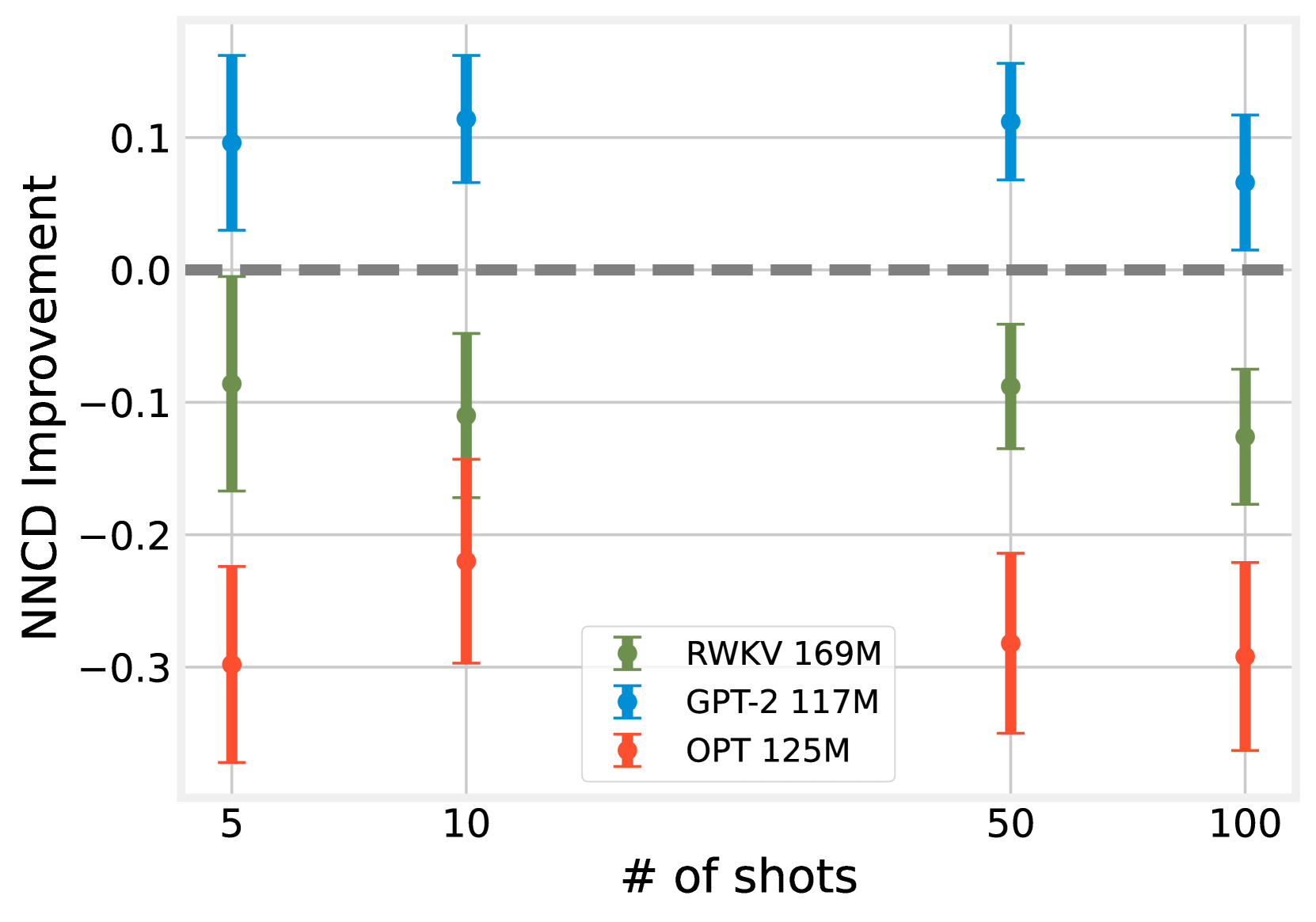
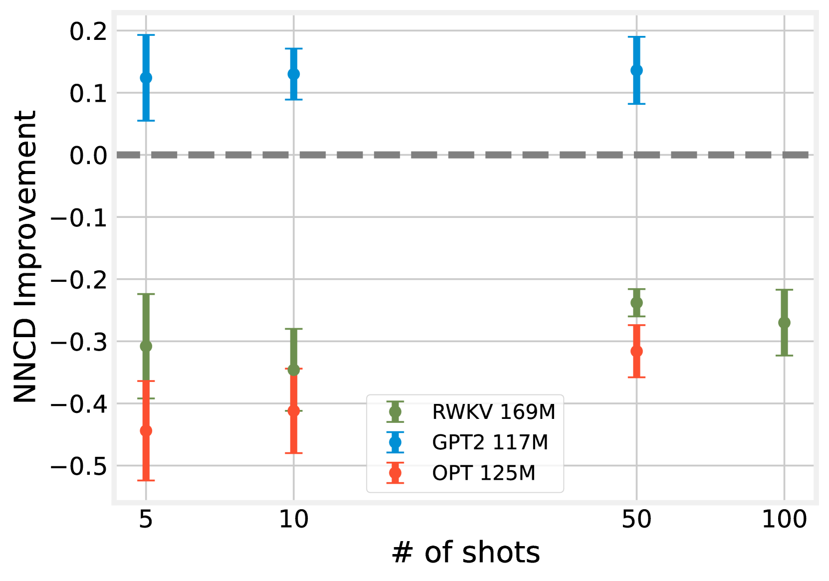
For each neural compressor we test, we perform identical experiments as previously mentioned using the model’s latent representation of a sequence and $k$ NN with Euclidean distance. The results are shown in Figure 4. We find that depending on the choice of neural network model used for neural compression, Neural NCD can either outperform or underperform the Euclidean distance-based approach on sequence latent representations. For example, a Neural NCD approach with GPT-2 small outperforms using the model’s latent representations, however with OPT 125M, latent representations drastically outperform a Neural NCD approach. This indicates that despite various LLMs providing similar compression ability, the usefulness of their latent representations for Euclidean distance-based approaches can differ.
(a) AGNews
<details>
<summary>x7.png Details</summary>
### Visual Description
## Line Chart: NNCD Improvement vs. Number of Shots
### Overview
The chart compares the performance improvement of three language models (RW KV 169M, GPT-2 117M, and OPT 125M) across different numbers of training shots (5, 10, 50, 100). The y-axis measures "NNCD Improvement" (ranging from -0.3 to 0.1), with positive values indicating improvement and negative values indicating degradation. Error bars represent uncertainty in measurements.
### Components/Axes
- **X-axis**: "# of shots" (logarithmic scale: 5, 10, 50, 100)
- **Y-axis**: "NNCD Improvement" (-0.3 to 0.1, with a dashed reference line at 0.0)
- **Legend**: Located at the bottom-right, mapping colors to models:
- Green: RW KV 169M
- Blue: GPT-2 117M
- Red: OPT 125M
- **Error Bars**: Vertical lines extending from each data point to indicate measurement uncertainty.
### Detailed Analysis
1. **RW KV 169M (Green)**:
- **Trend**: Slightly worsens as shots increase.
- **Values**:
- 5 shots: -0.11 (±0.05)
- 10 shots: -0.10 (±0.08)
- 50 shots: -0.12 (±0.06)
- 100 shots: -0.13 (±0.07)
- **Error Bars**: Largest uncertainty at 10 shots (±0.08).
2. **GPT-2 117M (Blue)**:
- **Trend**: Consistently improves with more shots.
- **Values**:
- 5 shots: 0.10 (±0.06)
- 10 shots: 0.12 (±0.05)
- 50 shots: 0.13 (±0.04)
- 100 shots: 0.08 (±0.07)
- **Error Bars**: Smallest uncertainty at 50 shots (±0.04).
3. **OPT 125M (Red)**:
- **Trend**: Degrades significantly with more shots.
- **Values**:
- 5 shots: -0.30 (±0.10)
- 10 shots: -0.20 (±0.12)
- 50 shots: -0.25 (±0.08)
- 100 shots: -0.28 (±0.11)
- **Error Bars**: Largest uncertainty at 10 shots (±0.12).
### Key Observations
- **GPT-2 117M** is the only model showing improvement (positive NNCD values), with peak performance at 50 shots (0.13).
- **RW KV 169M** and **OPT 125M** exhibit degradation as shots increase, with OPT 125M showing the most severe decline (-0.30 to -0.28).
- Error bars suggest GPT-2 has more consistent results, while OPT 125M has the highest variability.
### Interpretation
The data suggests that **GPT-2 117M** benefits from increased training data (shots), likely due to its architecture or training methodology. In contrast, **RW KV 169M** and **OPT 125M** may suffer from overfitting or inefficiencies in scaling, as their performance deteriorates with more data. The error bars highlight that GPT-2’s results are more reliable, while OPT 125M’s variability raises concerns about its robustness. This could inform model selection for tasks requiring data efficiency or scalability.
</details>
(b) DBpedia
<details>
<summary>x8.png Details</summary>
### Visual Description
## Line Chart: NNCD Improvement vs. Number of Shots
### Overview
The chart compares the NNCD (Normalized Negative Log-Likelihood Difference) improvement across three language models (RWKV 169M, GPT2 117M, OPT 125M) at varying numbers of training shots (5, 10, 50, 100). Error bars represent uncertainty in measurements.
### Components/Axes
- **X-axis**: Number of shots (5, 10, 50, 100)
- **Y-axis**: NNCD Improvement (range: -0.5 to 0.2)
- **Legend**: Located at bottom-right, mapping colors to models:
- Green: RWKV 169M
- Blue: GPT2 117M
- Red: OPT 125M
### Detailed Analysis
1. **RWKV 169M (Green)**
- **5 shots**: -0.30 (±0.10)
- **10 shots**: -0.35 (±0.12)
- **50 shots**: -0.25 (±0.08)
- **100 shots**: -0.28 (±0.07)
- **Trend**: Slight improvement with more shots, but remains negative. Error bars decrease with shot count.
2. **GPT2 117M (Blue)**
- **5 shots**: 0.12 (±0.08)
- **10 shots**: 0.13 (±0.07)
- **50 shots**: 0.14 (±0.06)
- **100 shots**: 0.15 (±0.05)
- **Trend**: Consistent upward trajectory. Error bars shrink slightly at higher shot counts.
3. **OPT 125M (Red)**
- **5 shots**: -0.45 (±0.15)
- **10 shots**: -0.40 (±0.12)
- **50 shots**: -0.35 (±0.09)
- **100 shots**: -0.30 (±0.08)
- **Trend**: Gradual improvement with more shots. Error bars decrease as shot count increases.
### Key Observations
- **GPT2 117M** consistently outperforms others, maintaining positive NNCD improvement across all shot counts.
- **RWKV 169M** and **OPT 125M** show negative improvement at low shot counts but improve marginally with more data.
- **Error bars** are largest at 5-10 shots, indicating higher uncertainty in small datasets.
- **GPT2's stability** (smallest error bars) suggests robustness to data scarcity.
### Interpretation
The data demonstrates that **GPT2 117M** achieves the highest NNCD improvement, likely due to its architecture or training methodology. All models benefit from increased shot counts, but **RWKV** and **OPT** require significantly more data to approach GPT2's performance. The error bars highlight the challenge of training with limited data, particularly for smaller models (e.g., OPT 125M at 5 shots shows ±0.15 uncertainty). This suggests that **data efficiency** is a critical factor in model performance, with GPT2's architecture potentially offering better generalization from limited examples.
</details>
Figure 4: Test accuracy difference when comparing Neural NCD to Euclidean distance on sequence latent representations with 95% confidence interval. Values above 0 indicate Neural NCD outperforming Euclidean distance. For RWKV, the representation is the final hidden state. For GPT2 and OPT, we average the latent representation of each token. Despite comparable compression rates of each model, the quality and usefulness of distance between latent representations is highly variable across models.
## 5 Conclusion
We have shown that compression rate alone does not reliably predict NCD-based classification accuracy when using neural compressors in the text domain. With a variety of neural network architectures with which the machine learning community trains language models and neural compressors, it is likely that these architectural differences will also yield varying ability to exploit compressible redundancies across concatenated sequences yielding varying NCD quality. We’ve shown that neural models with different architectures and pretraining details tend to overperform or underperform traditional compressors in similar ways on the same dataset. Finally, we compared Neural NCD with latent representations from the same model, showing that Neural NCD outperforms latent representations for some models and under-performs them for others.
## References
- (1)
- Bellard (2021) Fabrice Bellard. 2021. NNCP v2: Lossless Data Compression with Transformer. https://bellard.org/nncp/nncp_v2.1.pdf.
- Bellard (2024) Fabrice Bellard. 2024. ts_zip: Text Compression using Large Language Models. https://bellard.org/ts_zip/.
- Borbely (2015) Rebecca Schuller Borbely. 2015. On normalized compression distance and large malware: Towards a useful definition of normalized compression distance for the classification of large files. Journal of Computer Virology and Hacking Techniques 12, 4 (Dec. 2015), 235–242. https://doi.org/10.1007/s11416-015-0260-0
- Cebrián et al. (2005) Manuel Cebrián, Manuel Alfonseca, and Alfonso Ortega. 2005. Common pitfalls using the normalized compression distance: What to watch out for in a compressor. Communications in Information & Systems 5, 4 (2005), 367–384.
- Delétang et al. (2024) Grégoire Delétang, Anian Ruoss, Paul-Ambroise Duquenne, Elliot Catt, Tim Genewein, Christopher Mattern, Jordi Grau-Moya, Li Kevin Wenliang, Matthew Aitchison, Laurent Orseau, Marcus Hutter, and Joel Veness. 2024. Language Modeling Is Compression. arXiv:2309.10668 [cs.LG] https://arxiv.org/abs/2309.10668
- Devlin et al. (2019) Jacob Devlin, Ming-Wei Chang, Kenton Lee, and Kristina Toutanova. 2019. BERT: Pre-training of Deep Bidirectional Transformers for Language Understanding. In Proceedings of the 2019 Conference of the North American Chapter of the Association for Computational Linguistics: Human Language Technologies, Volume 1 (Long and Short Papers), Jill Burstein, Christy Doran, and Thamar Solorio (Eds.). Association for Computational Linguistics, Minneapolis, Minnesota, 4171–4186. https://doi.org/10.18653/v1/N19-1423
- Jiang et al. (2022) Zhiying Jiang, Yiqin Dai, Ji Xin, Ming Li, and Jimmy Lin. 2022. Few-Shot Non-Parametric Learning with Deep Latent Variable Model. In Advances in Neural Information Processing Systems, S. Koyejo, S. Mohamed, A. Agarwal, D. Belgrave, K. Cho, and A. Oh (Eds.), Vol. 35. Curran Associates, Inc., 26448–26461. https://proceedings.neurips.cc/paper_files/paper/2022/file/a92519f525c00085095fa41c5c46cdb5-Paper-Conference.pdf
- Jiang et al. (2023) Zhiying Jiang, Matthew Yang, Mikhail Tsirlin, Raphael Tang, Yiqin Dai, and Jimmy Lin. 2023. “Low-Resource” Text Classification: A Parameter-Free Classification Method with Compressors. In Findings of the Association for Computational Linguistics: ACL 2023, Anna Rogers, Jordan Boyd-Graber, and Naoaki Okazaki (Eds.). Association for Computational Linguistics, Toronto, Canada, 6810–6828. https://doi.org/10.18653/v1/2023.findings-acl.426
- Keogh et al. (2004) Eamonn Keogh, Stefano Lonardi, and Chotirat Ann Ratanamahatana. 2004. Towards parameter-free data mining. In Proceedings of the Tenth ACM SIGKDD International Conference on Knowledge Discovery and Data Mining (Seattle, WA, USA) (KDD ’04). Association for Computing Machinery, New York, NY, USA, 206–215. https://doi.org/10.1145/1014052.1014077
- Knoll (2022) Byron Knoll. 2022. tensorflow-compress. https://github.com/byronknoll/tensorflow-compress.
- Knoll (2024) Byron Knoll. 2024. CMIX version 21. http://www.byronknoll.com/cmix.html.
- Kolmogorov (1963) Andrei N. Kolmogorov. 1963. On tables of random numbers. In Proceedings of the Symposium on the Theory of Numbers. 369–376.
- Li et al. (2004) Ming Li, Xin Chen, Xin Li, Bin Ma, and Paul MB Vitányi. 2004. The similarity metric. IEEE Transactions on Information Theory 50, 12 (2004), 3250–3264.
- MacKay (2003) David J. C. MacKay. 2003. Information theory, inference, and learning algorithms. Cambridge University Press.
- Mahoney (2024) Matt Mahoney. 2024. Large Text Compression Benchmark. https://www.mattmahoney.net/dc/text.html.
- Peng et al. (2023) Bo Peng, Eric Alcaide, Quentin Anthony, Alon Albalak, Samuel Arcadinho, Stella Biderman, Huanqi Cao, Xin Cheng, Michael Chung, Matteo Grella, Kranthi Kiran GV, Xuzheng He, Haowen Hou, Jiaju Lin, Przemyslaw Kazienko, Jan Kocon, Jiaming Kong, Bartlomiej Koptyra, Hayden Lau, Krishna Sri Ipsit Mantri, Ferdinand Mom, Atsushi Saito, Guangyu Song, Xiangru Tang, Bolun Wang, Johan S. Wind, Stanislaw Wozniak, Ruichong Zhang, Zhenyuan Zhang, Qihang Zhao, Peng Zhou, Qinghua Zhou, Jian Zhu, and Rui-Jie Zhu. 2023. RWKV: Reinventing RNNs for the Transformer Era. arXiv:2305.13048 [cs.CL] https://arxiv.org/abs/2305.13048
- Radford et al. (2019) Alec Radford, Jeffrey Wu, Rewon Child, David Luan, Dario Amodei, Ilya Sutskever, et al. 2019. Language models are unsupervised multitask learners. OpenAI blog 1, 8 (2019), 9.
- Raff and Nicholas (2017a) Edward Raff and Charles Nicholas. 2017a. An Alternative to NCD for Large Sequences, Lempel-Ziv Jaccard Distance. In Proceedings of the 23rd ACM SIGKDD International Conference on Knowledge Discovery and Data Mining - KDD ’17. ACM Press, New York, New York, USA, 1007–1015. https://doi.org/10.1145/3097983.3098111
- Raff and Nicholas (2017b) Edward Raff and Charles Nicholas. 2017b. Malware Classification and Class Imbalance via Stochastic Hashed LZJD. In Proceedings of the 10th ACM Workshop on Artificial Intelligence and Security (AISec ’17). ACM, New York, NY, USA, 111–120. https://doi.org/10.1145/3128572.3140446
- Raff et al. (2020) Edward Raff, Charles Nicholas, and Mark McLean. 2020. A New Burrows Wheeler Transform Markov Distance. In The Thirty-Fourth AAAI Conference on Artificial Intelligence. 5444–5453. https://doi.org/10.1609/aaai.v34i04.5994 arXiv:1912.13046
- Raff and Nicholas (2018) Edward Raff and Charles K. Nicholas. 2018. Lempel-Ziv Jaccard Distance, an effective alternative to ssdeep and sdhash. Digital Investigation (feb 2018). https://doi.org/10.1016/j.diin.2017.12.004 arXiv:1708.03346
- S. Resende et al. (2019) João S. Resende, Rolando Martins, and Luís Antunes. 2019. A Survey on Using Kolmogorov Complexity in Cybersecurity. Entropy 21, 12 (Dec. 2019), 1196. https://doi.org/10.3390/e21121196
- Saul et al. (2023) Rebecca Saul, Mohammad Mahmudul Alam, John Hurwitz, Edward Raff, Tim Oates, and James Holt. 2023. Lempel-Ziv Networks. In Proceedings on "I Can’t Believe It’s Not Better! - Understanding Deep Learning Through Empirical Falsification" at NeurIPS 2022 Workshops (Proceedings of Machine Learning Research, Vol. 187). PMLR, 1–11. https://proceedings.mlr.press/v187/saul23a.html
- Valmeekam et al. (2023) Chandra Shekhara Kaushik Valmeekam, Krishna Narayanan, Dileep Kalathil, Jean-Francois Chamberland, and Srinivas Shakkottai. 2023. LLMZip: Lossless Text Compression using Large Language Models. arXiv:2306.04050 [cs.IT] https://arxiv.org/abs/2306.04050
- Wehner (2007) Stephanie Wehner. 2007. Analyzing worms and network traffic using compression. J. Comput. Secur. 15, 3 (Aug. 2007), 303–320.
- Witten et al. (1987) Ian H. Witten, Radford M. Neal, and John G. Cleary. 1987. Arithmetic coding for data compression. Commun. ACM 30, 6 (jun 1987), 520–540. https://doi.org/10.1145/214762.214771
- Zhang et al. (2022) Susan Zhang, Stephen Roller, Naman Goyal, Mikel Artetxe, Moya Chen, Shuohui Chen, Christopher Dewan, Mona Diab, Xian Li, Xi Victoria Lin, Todor Mihaylov, Myle Ott, Sam Shleifer, Kurt Shuster, Daniel Simig, Punit Singh Koura, Anjali Sridhar, Tianlu Wang, and Luke Zettlemoyer. 2022. OPT: Open Pre-trained Transformer Language Models. arXiv:2205.01068 [cs.CL] https://arxiv.org/abs/2205.01068
## Appendix A Experiment Details
We use the labeled datasets AGNews, 20News, and DBpedia. For AGNews and DBpedia, we use the original dataset and classification setting: four classes for AGNews and fourteen classes for DBpedia. For 20News, we reduce the number of classes to two using only alt.atheism and comp.graphics. For $k$ NN classification algorithm, we use $k=3$ for all experiments.