2410.18613v1

# Rethinking Softmax: Self-Attention with Polynomial Activations ## Abstract This paper challenges the conventional belief that softmax attention in transformers is effective primarily because it generates a probability distribution for attention allocation. Instead, we theoretically show that its success lies in its ability to implicitly regularize the Frobenius norm of the attention matrix during training. We then explore alternative activations that regularize the Frobenius norm of the attention matrix, demonstrating that certain polynomial activations can achieve this effect, making them suitable for attention-based architectures. Empirical results indicate these activations perform comparably or better than softmax across various computer vision and language tasks, suggesting new possibilities for attention mechanisms beyond softmax. ## 1 Introduction Transformer architectures (Vaswani et al., 2017) have become the state-of-the-art model architecture for diverse areas such as natural language processing (NLP) (Vaswani et al., 2017; Devlin et al., 2018; Zhuang et al., 2021; Zhen et al., 2022), computer vision (Dosovitskiy et al., 2020; Carion et al., 2020; Liu et al., 2021; Touvron et al., 2021), and robotics (Fu et al., 2024; Maiti et al., 2023; Salzmann et al., 2020). A key component in the transformer architecture is the softmax attention block, enabling transformers to evaluate the importance of individual input elements during output generation. This feature facilitates an efficient method to attend to diverse input elements throughout training, allowing transformers to effectively capture spatial dependencies within sequential data. Unlike traditional recurrent neural networks (RNNs) and convolutional neural networks (CNNs), transformers exhibit the ability to scale to large datasets without a significant degradation in performance. This characteristic has made them an ideal architecture for handling large-scale machine learning tasks. Softmax is widely recognized for its effectiveness in attention mechanisms due to its ability to produce an attention matrix that meets three key conditions (Vaswani et al., 2017; Dosovitskiy et al., 2020; Zhen et al., 2022; AUEB et al., 2016): (i) non-negativity, (ii) rows that are normalized to sum to 1 and (iii) sparsity. The general consensus is that non-negativity guarantees that attention weights remain positive, facilitating the model in assigning significance to various input elements. The normalization constraint ensures that the attention weights for all input elements collectively sum to $1$ , rendering the weights interpretable as probabilities. Additionally, sparsity aids the model in focusing on a select few key elements, thereby enhancing efficiency. It has been argued that these properties are crucial for enabling the attention mechanism to attend to pertinent segments of the input sequence while efficiently filtering out irrelevant details. However, this approach to attention has become somewhat axiomatic as it is mostly motivated by empirical results with little theoretical foundation. Despite the exploration of alternative activations in several studies (Shen et al., 2023; Fang et al., 2022; Correia et al., 2019), softmax attention continues to dominate, largely due to its interpretability. In this paper, we question this view by proposing that the effectiveness of softmax stems from its implicit regularization of the Frobenius norm of the attention matrix during training, preventing attention weights from becoming excessively large or small. We then derive a theoretical framework that produces polynomial activations that deliberately violate one or more of the three conditions mentioned earlier, yet are able to regularize the Frobenius norm of the attention weights during training. Our findings demonstrate that such activations can achieve comparable or even superior performance to softmax across various vision and natural language processing (NLP) tasks, even though they seem to violate our understanding of attention. We advise the reader that this paper diverges from the usual pursuit of creating cutting-edge transformer architectures for achieving state-of-the-art results on benchmark datasets. Instead, our focus is on critically examining softmax attention to determine whether its effectiveness is a result of true interpretability or a more nuanced regularization mechanism. By questioning established views, we aim to uncover deeper insights into transformer architectures that could lead to broader applications and improved understanding. Nonetheless, we validate our theory on multiple transformer-based tasks, including image classification, segmentation, object detection, and NLP, often achieving results that match or surpass those of softmax attention. Our main contributions are: - We question the widely accepted notion that softmax’s effectiveness in attention mechanisms is solely due to its ability to produce normalized sparse attention weights. Instead, we theoretically show that softmax has a regularization effect on attention and argue this plays a crucial role in its success. - We explore activations that deliberately deviate from traditional softmax attention conditions. These activations are found to regularize the Frobenius norm of the attention matrix during training, akin to softmax, and demonstrate comparable or superior performance across various vision and NLP tasks. ## 2 Related Work Several studies have explored alternative activations for attention mechanisms in transformers. Shen et al. (2023) investigated ReLU activations, finding them to outperform softmax in tasks with long sequences, such as document translation. Banerjee et al. (2020) examined Taylor series approximations to softmax, which showed superior performance to softmax in image classification. Wang et al. (2021) proposed periodic alternatives to softmax, designed to provide better gradients for attention mechanisms and achieved better results than softmax on simple networks for image classification. Koohpayegani & Pirsiavash (2024) demonstrated that applying $l^1$ normalization to linear attention mechanisms can achieve performance comparable to softmax. Our work differs from all these in that we identify a clear theoretical relationship between the scale of the Frobenius norm of the self-attention matrix and the input sequence length. Using this insight to derive potential acitvations that can perform on par with softmax. ## 3 Preliminaries and Notation In this section we outline the definition of a transformer via the transformer block and set the notation of various mathematical quantities we will be using in future sections. For more details on transformers the reader can consult Vaswani et al. (2017); Dosovitskiy et al. (2020). Transformer architectures comprise of transformer blocks, defined as follows. A transformer block is a mapping $T:ℝ^N× D→ℝ^N× D$ defined as $$ T(x)=F(A(x)+x) $$ where $F$ is a feedforward MLP with a residual connection and $A$ is an attention head. The attention head $A$ is defined as follows: It comprises of three learnable matrices, a query ( $q$ ), key ( $k$ ) and value ( $v$ ) defined by: $q=QX$ , $k=KX$ , $v=VX$ for an input sequence $X∈ℝ^N× D$ with $Q$ , $K∈ℝ^D× d$ and $V∈ℝ^D× M$ . The attention head $A(X)$ is then defined by $$ A(X)=φ(S(q,k))v $$ where $S$ is a similarity transformation and $φ$ is an activation function. The most common used $S$ is the dot-product: $S(q,v)=qk^T$ , known as self-attention, and will be the one we focus on in this paper. The most common activation function $φ$ that is used by authors is softmax. This leads to the most common form of the attention head given by $$ A(X)=softmax\bigg{(}\frac{qk^T}{√{d}}\bigg{)}v=\mathbf {softmax}\bigg{(}\frac{XQK^TX^T}{√{d}}\bigg{)}XV. $$ The function $softmax$ is the matrix softmax map that applies the usual softmax function row-wise: $$ softmax\bigg{(}\begin{bmatrix}x_11&⋯&x_1n\\ ⋮&⋮&⋮\\ x_n1&⋯&x_nn\end{bmatrix}\bigg{)}=\begin{bmatrix}\frac{e^x_11}{ ∑_j=1^ne^x_1j}&⋯&\frac{e^x_1n}{∑_j=1^ne^x_1j}\\ ⋮&⋮&⋮\\ \frac{e^x_n1}{∑_j=1^ne^x_nj}&⋯&\frac{e^x_nn}{∑_j=1 ^ne^x_nj}\end{bmatrix} $$ The factor $\frac{1}{√{d}}$ , as explained in Vaswani et al. (2017), is a scaling to prevent the gradients of softmax from being too small. For the theoretical analysis in this paper we will only use the dot-product similarity $qk^T$ and call the $N× N$ matrix $softmax(qk^T)$ the softmax self-attention matrix. In the experiments section, Sec. 5, we will empirically validate our theoretical framework on more general softmax attention blocks. For general transformer architectures, multiple heads $A_i$ for $1≤ i≤ n$ are used. Each attention head is defined by equation 3.3 and then all outputs of each attention head are concatenated together before going into the feedforward layer. We will need notation for the derivative of the matrix softmax map defined by equation 3.4. Given a matrix $A∈ℝ^N× N$ we can differentiate the matrix map $softmax$ at $A$ and obtain the gradient linear map $∇ softmax(A):ℝ^N× N→ℝ^N × N$ that is defined by the formula $$ ∇ softmax(A):=Jsoftmax(A)^T $$ where $Jsoftmax(A)$ is the Jacobian of $softmax$ at $A$ . Given a matrix $A∈ℝ^n× m$ , we denote its Frobenius norm by $||A||_F$ . Additionally, we use the notation $E$ to represent the expectation of a random variable, where the specific random variable being considered will be clear from the context. ## 4 Theoretical Analysis ### 4.1 Implicit regulatization of Softmax This section presents a theoretical result showing that the softmax activation imposes control over the Frobenius norm of the self-attention matrix in a way that grows sub-linearly with the input sequence’s token length. Additionally, we demonstrate that the gradient of the softmax with respect to the self-attention matrix also exhibits a similar degree of regularity. While previous work has analyzed the regularity of softmax self-attention through the lens of the Lipschitz constant (Kim et al., 2021; Castin et al., 2023), our theorem offers a novel perspective by directly linking the Frobenius norm regularity to the token length. This provides insights into how self-attention activations should scale with token length to maintain stability during training, especially with gradient descent-based algorithms. **Theorem 4.1** *Let $softmax:ℝ^N× N→ℝ^N× N$ be the matrix softmax map defined by equation 3.4 and let $∇ softmax(A):ℝ^N× N→ℝ^N × N$ denote the gradient of $softmax$ at $A∈ℝ^N× N$ . We then have the following bounds on the Frobenius norms $$ \displaystyle||softmax(A)||_F \displaystyle≤√{N} \displaystyle||∇ softmax(A)||_F \displaystyle≤ 2√{N}. $$* The key implication of theorem 4.1 is that during the training of a transformer with softmax self-attention, the Frobenius norm of each softmax self-attention matrix remains bounded by a value that grows as $O(√{N})$ . This ensures that backpropagation through the weights of the self-attention matrix does not lead to excessively large gradients. The proof hinges on the fact that the row normalization inherent in softmax effectively controls the Frobenius norm. For a detailed proof see appendix A.1.1. ### 4.2 Polynomial activations for self-attention In section 4.1, we demonstrated that softmax implicitly regularizes the Frobenius norm of the self-attention matrix. Building on this, we now show that by scaling specific polynomial activations, a similar regularization effect on the Frobenius norm can be achieved in expectation, closely replicating the impact of softmax. **Theorem 4.2** *Let $X∈ℝ^N× D$ and $Q$ , $K∈ℝ^D× d$ be i.i.d random variables distributed according to $X∼N(0,σ_x)$ and $Q$ , $K∼N(0,σ_t)$ . We have the following expectations of the Frobenius norms of powers of the $N× N$ matrix $(XQK^TX^T)^p$ for $p≥ 1$ $$ E\bigg{|}\bigg{|}\bigg{(}\frac{XQK^TX^T}{√{d}}\bigg{)}^p \bigg{|}\bigg{|}_F≤O(N) $$* By scaling such an activation by $\frac{1}{√{N}}$ we can obtain a $O(√{N})$ bound. **Corollary 4.3** *Assume the same conditions as in theorem 4.2. Then $$ E\bigg{|}\bigg{|}\frac{1}{√{N}}\bigg{(}\frac{XQK^TX^T}{√{ d}}\bigg{)}^p\bigg{|}\bigg{|}_F≤O(√{N}). $$* Corollary 4.3 establishes that activations of the form $φ(x):=\frac{1}{√{N}}x^p$ provide a level of regularization, in expectation, similar to that of softmax when applied to the self-attention matrix. The proof of theorem 4.2 can be found in appendix A.1.2. The next property we want to prove is one similar to the gradient bound obtained in theorem 4.1. Since the self-attention matrix has parameters given by the queries $Q$ and keys $K$ (Vaswani et al., 2017), this implies that during the training of a transformer the $Q$ and $K$ matrices are the only aspects of the self-attention matrix that get updated. Therefore, we compute a regularity result with respect to the $Q$ and $K$ derivatives. **Theorem 4.4** *Let $X∈ℝ^N× D$ and $Q$ , $K∈ℝ^D× d$ be i.i.d random variables distributed according to $X∼N(0,σ_x)$ and $Q$ , $K∼N(0,σ_t)$ . Then the expectation of the of the derivative of the matrix $\frac{(XQK^TX^T)^p}{√{d}}$ w.r.t the $Q$ parameter matrix for $p≥ 1$ is given by $$ E\bigg{|}\bigg{|}\frac{∂}{∂ Q}\bigg{(}\frac{(XQK^TX^ T)^p}{√{d}}\bigg{)}\bigg{|}\bigg{|}≤O(N) $$* The above theorem then suggests that if we scale the polynomial $x→ x^p$ by $\frac{1}{√{N}}$ the $Q$ derivative will have $O(√{N})$ growth. **Corollary 4.5** *Assume the same condition as in theorem 4.4. Then $$ E\bigg{|}\bigg{|}\frac{1}{√{N}}\frac{∂}{∂ Q}\bigg{( }\frac{(XQK^TX^T)^p}{√{d}}\bigg{)}\bigg{|}\bigg{|}≤O( √{N}). $$* An analogous estimate holds for derivatives with respect to the $K$ matrix. The proof of theorem 4.4 can be found in appendix A.1.2. Corollaries 4.3 and 4.5 suggest that polynomial activations of the form $φ(x)=\frac{1}{√{N}}x^p$ , with $p>0$ , can achieve performance comparable to softmax when applied to self-attention matrices. In section 5, we empirically compare these activations to softmax and observe that they outperform softmax on a variety of transformer tasks. We focus on $p=1$ and $p=3$ as these polynomials clearly violate key aspects of softmax based attention, such as normalized rows, positivity, and sparsity. For larger values of $p$ , performance declines due to the functions $φ(x)=\frac{1}{√{N}}x^p$ having smaller gradients around $0 0$ when $p$ is large, causing difficulties in training. ## 5 Experiments In this section, we validate the theory from section 4 on a variety of transformer tasks. We perform the empirical validation on two primary activations from section 4, namely a cubic polynomial activation $φ(x)=x^3$ and a linear polynomial $φ(x)=x$ . The goal will be to show that by suitably scaling these activations using the theory in section 4, we can achieve competitive performance when compared to softmax. For the rest of this section we will simply denote these activations by $x^3$ and $x$ . <details> <summary>x1.png Details</summary>  ### Visual Description ## Line Graph: Accuracy vs. Scale for Different Sample Sizes ### Overview The graph illustrates the relationship between "Scale" (x-axis) and "Accuracy (%)" (y-axis) for four distinct sample sizes (N = 8, 16, 64, 256). Each line represents a unique sample size, with accuracy peaking at specific scales before declining sharply. The largest sample size (N = 256) achieves the highest peak accuracy, while smaller samples exhibit lower peaks and more gradual declines. ### Components/Axes - **X-axis (Scale)**: Logarithmic scale ranging from 10⁻³ to 10³. - **Y-axis (Accuracy %)**: Linear scale from 0% to 50%. - **Legend**: Located in the top-left corner, mapping colors/symbols to sample sizes: - Red crosses (×): N = 256 - Yellow triangles (▲): N = 64 - Green circles (●): N = 16 - Blue squares (■): N = 8 ### Detailed Analysis 1. **N = 256 (Red ×)**: - Starts at 0% accuracy for scales < 10⁻². - Rises sharply to ~50% at scale 10⁻¹. - Peaks at 50% between 10⁻¹ and 10⁰, then declines steeply to 0% by 10¹. - Remains at 0% for scales ≥ 10². 2. **N = 64 (Yellow ▲)**: - Begins at ~5% accuracy at 10⁻³. - Increases to ~45% at 10⁻², peaking between 10⁻² and 10⁻¹. - Drops to ~20% at 10⁰, then declines to 0% by 10¹. 3. **N = 16 (Green ●)**: - Starts at ~5% at 10⁻³. - Rises to ~30% at 10⁻², peaking between 10⁻² and 10⁻¹. - Declines to ~15% at 10⁰, then drops to 0% by 10¹. 4. **N = 8 (Blue ■)**: - Begins at ~5% at 10⁻³. - Peaks at ~20% at 10⁻², then declines to ~10% at 10⁰. - Drops to 0% by 10¹. ### Key Observations - **Peak Accuracy**: Larger sample sizes (N = 256) achieve higher peak accuracy (~50%) compared to smaller sizes (N = 8 peaks at ~20%). - **Scale of Peak**: Larger N values peak at higher scales (e.g., N = 256 peaks at 10⁻¹, N = 8 at 10⁻²). - **Decline Pattern**: All lines exhibit a sharp drop after their peak, with larger N values experiencing steeper declines. - **Overlap**: Lines for N = 16 and N = 8 overlap slightly at scales < 10⁻². ### Interpretation The data suggests a trade-off between sample size and model performance: - **Larger Samples (N = 256)**: Achieve higher accuracy but overfit more severely, as evidenced by the abrupt decline post-peak. - **Smaller Samples (N = 8)**: Generalize better (slower decline) but with lower peak accuracy. - **Scale Sensitivity**: Accuracy is highly sensitive to scale, with optimal performance occurring at specific scales inversely related to sample size. - **Practical Implication**: Increasing sample size improves peak performance but may reduce robustness at larger scales, highlighting the need for regularization or adaptive scaling strategies. 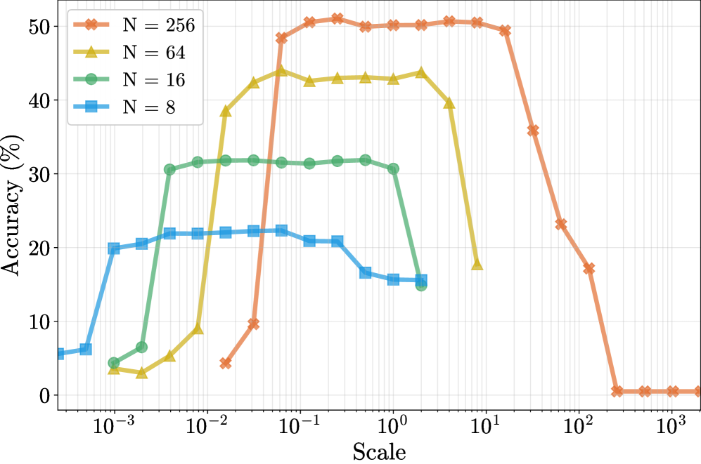</details> Figure 1: Training ViT-Tiny with the activation $φ(x)=x^3$ with different sequence lengths and different scales. As the sequence length gets smaller, the log scale needed to obtain good accuracy decreases validating the theory from section 4.2. ### 5.1 Image classification #### 5.1.1 ViT-Tiny on Tiny-Imagenet: In this section we test the theory from section 4 on the ViT-Tiny architecture (Steiner et al., 2021) trained from scratch on the Tiny-Imagenet dataset (Le & Yang, 2015). Our first experiment was to test how the Top- $1\$ accuracy changes for a ViT-Tiny trained on Tiny-Imagenet as we change the sequence length of the input and the scale predicted in corollaries 4.3 and 4.5 when using the activation $x^3$ . According to the theory developed in section 4, the Frobenius norm scales according to $O(√{N})$ when we scale $X^3$ by $\frac{1}{√{N}}$ . Thus as the sequence length decreases we should see the amount of scaling in a Log scale decrease. Figure 1 shows the results of this experiment. We considered four different input sequence lengths of sizes $256$ , $64$ , $16$ and $8$ . We ran several ViT-Tiny architectures with a variety of scalings of the form $O(\frac{1}{√{N}})$ where $N$ ranged below to above the sequence length. As can be seen from figure 1 as the sequence length got smaller the amount of scaling, shown in Log scale on the x-axis, needed for good accuracy got smaller verifying the theory in section 4.2. The second experiment compared activations $x^3$ and $x$ , along with scaled versions $\frac{1}{16}x^3$ and $\frac{1}{16}x$ , against softmax using the Tiny-ViT architecture on Tiny-Imagenet. With a sequence length of $256$ ( $√{256}=16$ ), we decided to take $\frac{1}{16}$ as the scale of the polynomial activations. The experiment used a patch size of 4, 3 attention heads, and 12 layers as described in Steiner et al. (2021). Results in table 1 show $\frac{1}{8}x^3$ outperforming softmax, while the unscaled version performed poorly. Similarly, $\frac{1}{16}x$ performed competitively with a significant drop in performance without scaling. 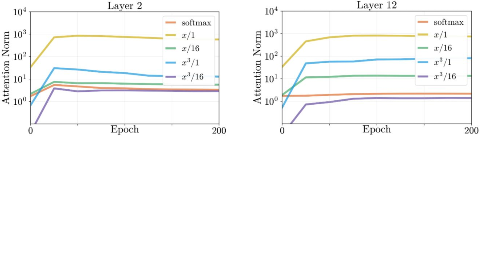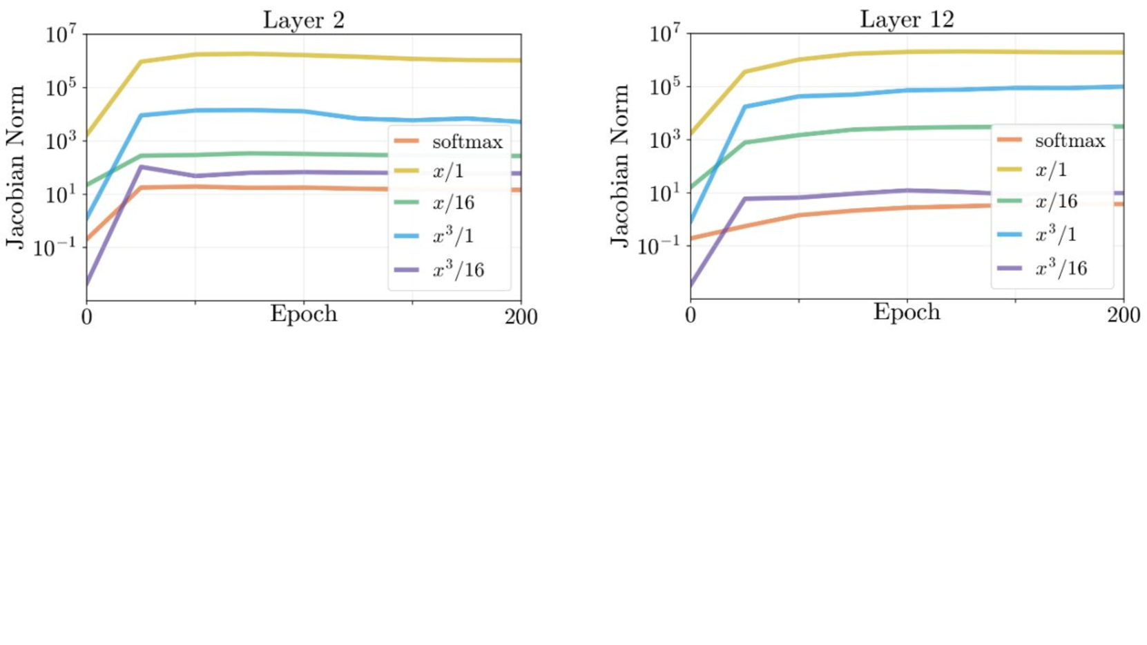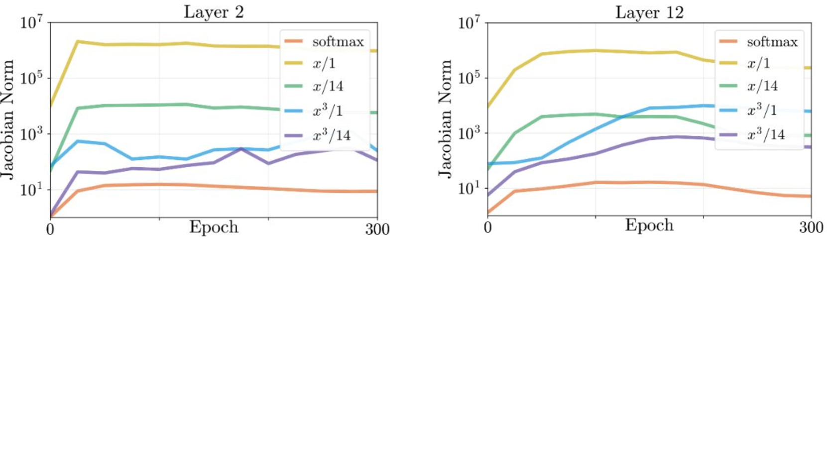Figure 2 displays the Frobenius norm of the self-attention matrix during training for five activations in layers 2 and 12 of ViT-Tiny, averaged across all heads. Norms for $x^3$ and $x$ are higher than softmax, but scaling by $\frac{1}{16}$ reduces them to more stable levels, improving training stability. Similarly, figure 3 shows the Jacobian’s Frobenius norm, where scaling also brings the norms closer to softmax, ensuring more stable gradients. Further plots for other layers are in appendix A.2.2. | | softmax | $\frac{x^3}{16}$ | $x^3$ | $\frac{x}{16}$ | $x$ | | --- | --- | --- | --- | --- | --- | | Top-1% accuracy | 50.26 | 50.5 | 45.3 | 47.9 | 31.78 | Table 1: Comparison of Top-1% accuracy on Tiny-Imagenet between softmax and polynomial activations. The cubic activation outperforms softmax when the right scale of $\frac{1}{8}$ is applied. Similarly, the linear activation is competitive only with an optimal scale. <details> <summary>x2.png Details</summary>  ### Visual Description ## Line Charts: Attention Norms Across Epochs in Layer 2 and Layer 12 ### Overview The image contains two line charts comparing attention norm trends across 200 epochs for different normalization methods in neural network layers. The charts are labeled "Layer 2" (left) and "Layer 12" (right). Both use logarithmic scales for attention norms (10⁰ to 10⁴) and linear scales for epochs (0–200). Five methods are compared: softmax, x/1, x/16, x³/1, and x³/16. ### Components/Axes - **X-axis**: Epoch (0–200, linear scale) - **Y-axis**: Attention Norm (logarithmic scale: 10⁰ to 10⁴) - **Legends**: - **Layer 2**: - Softmax (orange) - x/1 (yellow) - x/16 (green) - x³/1 (blue) - x³/16 (purple) - **Layer 12**: Same legend labels and colors as Layer 2. ### Detailed Analysis #### Layer 2 - **Softmax (orange)**: Starts near 10⁰, spikes to ~10¹ at epoch 50, then drops to ~10⁰ by epoch 200. - **x/1 (yellow)**: Begins at ~10¹, decreases slightly to ~10⁰.5 by epoch 200. - **x/16 (green)**: Starts near 10⁰, rises to ~10⁰.5 by epoch 50, then stabilizes. - **x³/1 (blue)**: Begins at ~10⁰, rises sharply to ~10¹.5 by epoch 50, then plateaus. - **x³/16 (purple)**: Starts near 10⁰, rises gradually to ~10⁰.5 by epoch 150, then stabilizes. #### Layer 12 - **Softmax (orange)**: Remains flat at ~10⁰ throughout all epochs. - **x/1 (yellow)**: Starts at ~10², drops to ~10¹ by epoch 50, then stabilizes. - **x/16 (green)**: Begins near 10⁰, rises to ~10⁰.5 by epoch 50, then plateaus. - **x³/1 (blue)**: Starts at ~10⁰, rises sharply to ~10² by epoch 50, then plateaus. - **x³/16 (purple)**: Begins near 10⁰, rises gradually to ~10⁰.5 by epoch 150, then stabilizes. ### Key Observations 1. **Layer 2**: - x³/1 and x³/16 methods show significantly higher attention norms than softmax after epoch 50. - Softmax exhibits a transient spike, suggesting temporary attention amplification. 2. **Layer 12**: - x³/1 and x³/16 methods dominate with attention norms exceeding 10¹, while softmax remains negligible. - x/1 method shows a sharp decline, contrasting with Layer 2's gradual decay. ### Interpretation The data demonstrates that normalization methods have layer-dependent effects on attention dynamics: - **Higher exponents (x³)** amplify attention norms, particularly in later layers (Layer 12), suggesting stronger feature weighting in deeper networks. - **Softmax** behaves differently across layers: transient spikes in Layer 2 vs. flat stability in Layer 12, possibly reflecting architectural differences (e.g., residual connections, layer normalization). - **x/16 and x³/16** methods show gradual increases, indicating milder normalization effects compared to x/1 and x³/1. These trends highlight the importance of method selection for attention regularization, with exponential scaling (x³) favoring higher attention magnitudes in deeper layers. </details> Figure 2: Frobenius norm of the self-attention matrix with five different activations in layer 2 and 12 of the ViT-Tiny architecture during training. <details> <summary>x3.png Details</summary>  ### Visual Description ## Line Graphs: Jacobian Norm Trends Across Epochs for Layer 2 and Layer 12 ### Overview The image contains two line graphs comparing the Jacobian norm (a measure of gradient magnitude) across 200 training epochs for two neural network layers (Layer 2 and Layer 12). The y-axis uses a logarithmic scale (10⁻¹ to 10⁷), and the x-axis represents epochs (0–200). Five methods are compared: `softmax`, `x/1`, `x/16`, `x³/1`, and `x³/16`, each represented by distinct colors. --- ### Components/Axes - **Y-Axis**: "Jacobiian Norm" (logarithmic scale: 10⁻¹, 10¹, 10³, 10⁵, 10⁷). - **X-Axis**: "Epoch" (0 to 200, linear scale). - **Legends**: Located in the top-right corner of each graph, mapping colors to methods: - **Orange**: `softmax` - **Yellow**: `x/1` - **Green**: `x/16` - **Blue**: `x³/1` - **Purple**: `x³/16` --- ### Detailed Analysis #### Layer 2 1. **Yellow (`x/1`)**: Starts at ~10⁵, remains stable with minor fluctuations. 2. **Blue (`x³/1`)**: Begins at ~10³, rises sharply to ~10⁴ by epoch 50, then plateaus. 3. **Green (`x/16`)**: Starts at ~10¹, increases gradually to ~10² by epoch 100, then stabilizes. 4. **Purple (`x³/16`)**: Begins at ~10⁻¹, spikes to ~10¹ by epoch 50, then declines slightly. 5. **Orange (`softmax`)**: Starts at ~10⁻¹, rises to ~10⁰ by epoch 50, then stabilizes. #### Layer 12 1. **Yellow (`x/1`)**: Starts at ~10⁵, rises to ~10⁶ by epoch 50, then plateaus. 2. **Blue (`x³/1`)**: Begins at ~10³, increases steadily to ~10⁴.5 by epoch 200. 3. **Green (`x/16`)**: Starts at ~10¹, rises to ~10².5 by epoch 200. 4. **Purple (`x³/16`)**: Begins at ~10⁻¹, increases to ~10¹ by epoch 100, then stabilizes. 5. **Orange (`softmax`)**: Starts at ~10⁻¹, rises to ~10⁰ by epoch 50, then stabilizes. --- ### Key Observations 1. **Layer-Specific Behavior**: - Layer 12 generally exhibits higher Jacobian norms than Layer 2 for the same method (e.g., `x/1` in Layer 12 reaches ~10⁶ vs. ~10⁵ in Layer 2). - `x³/1` and `x³/16` methods show steeper increases in Layer 12 compared to Layer 2. 2. **Method Performance**: - `x/1` consistently has the highest norms in both layers, suggesting larger gradient magnitudes. - `softmax` and `x³/16` methods have the lowest norms, indicating smaller gradient magnitudes. 3. **Anomalies**: - In Layer 2, the `x³/16` (purple) line shows a sharp spike at epoch 50, followed by a decline. - In Layer 12, `x³/1` (blue) exhibits a gradual, sustained increase without plateaus. --- ### Interpretation The data suggests that: - **Layer Depth Impacts Gradient Magnitude**: Layer 12 (deeper layer) generally has larger Jacobian norms than Layer 2, implying stronger gradient propagation in deeper layers. - **Method Sensitivity**: The `x³/1` method amplifies gradients more significantly in deeper layers, while `x³/16` shows diminishing returns. - **Stability vs. Growth**: Methods like `x/1` and `softmax` stabilize quickly, whereas `x³/1` and `x³/16` exhibit prolonged growth, potentially indicating overparameterization or sensitivity to scaling. These trends highlight the importance of method selection and layer-specific tuning in neural network training, particularly for gradient-based optimization. </details> Figure 3: Frobenius norm of the Jacobian of the self-attention matrix with five different activations in layer 2 and 12 of the ViT-Tiny architecture during training. #### 5.1.2 Larger vision transformers on ImageNet-1k For this experiment we carried out an image classification task using a variety of different vision transformers from the literature on the ImageNet-1k dataset. We found that the scales $\frac{1}{14}$ worked best for both $x^3$ and $x$ . We train all models on the ImageNet-1k dataset from scratch and report Top-1 accuracy on the validation set. We use PyTorch Paszke et al. (2019) and Timm Wightman (2019) libraries to train our models with similar setups to He et al. (2022) Liu et al. (2021). We examined our approach along with the following three transformer architectures to show its generalization: - ViT: Dosovitskiy et al. (2020) is the pioneering work that interprets an image as a sequence of patches and processes it by a standard Transformer encoder as used in NLP. This simple, yet scalable, strategy works surprisingly well when coupled with pre-training on large datasets. We use ViT-Small which has the following settings: patch size = 16, embedding dimensions = 384, number of heads = 6, and layers = 12. Also, We use ViT-Base which has the following settings: patch size = 16, embedding dimensions = 768, number of heads = 12, and layers = 12. - DeiT: Touvron et al. (2021) is a well-known transformer based on ViT. It is very similar to ViT except that it converged faster due to better training recipe since we do not use the distillation token imposed in DeiT. We use DeiT-Small which has the following settings: patch size = 16, embedding dimensions = 384, number of heads = 6, and layers = 12. Also, We use Deit-Base which has the following settings: patch size = 16, embedding dimensions = 768, number of heads = 12, and layers = 12. - Swin Transformer: Liu et al. (2021) produces a hierarchical feature representation and proposes the shifted window based self-attention which is shown to be effective and efficient on vision problems. We use Swin-Small with 96 channels and Swin-Base with 128 channels in the hidden layers of the first stage. The window size is set to $M$ = 7 by default, the query dimension of each head is $d$ = 32, and layer numbers are ${2,2,18,2}$ for all experiments. - XciT: Xiong et al. (2021) is a vision transformer architecture consisting of two different components compared to the standard ViT. Firstly, it has Local Patch Interaction in each block, which includes one depth-wise 3×3 convolution followed by Batch Normalization, GELU, and another depth-wise 3×3 convolution. Secondly, it uses Cross-Covariance attention, where the attention map is derived from the cross-covariance matrix computed over the key and query projections of the token features. We use XCiT-S12 with a patch size of 16 and XCiT-M24 with a patch size of 24. The results are shown in table 2. The activation $\frac{1}{14}x^3$ performed best on the ViT’s and the Swin transformers while softmax performed best on the DeiT architectures. Further ablations with different scales and activations can be fond in appendix A.2.1. | Activation | Models | | | | | | | | | --- | --- | --- | --- | --- | --- | --- | --- | --- | | ViT-Base | ViT-Small | DeiT-Base | DeiT-Small | Swin-Base | Swin-Small | XciT-Medium | XciT-Small | | | softmax | 79.6 | 80.2 | 78.9 | 79.6 | 83.0 | 83.3 | 81.1 | 81.2 | | $\frac{x^3}{14}$ | 79.6 | 80.5 | 77.4 | 78.3 | 83.2 | 83.4 | 81.2 | 82.1 | | $x^3$ | 77.8 | 78.6 | 76.1 | 76.3 | 79.7 | 79.9 | 78.1 | 78.3 | | $\frac{x}{14}$ | 76.9 | 77.8 | 79.6 | 79.8 | 79.4 | 79.5 | 79.2 | 79.3 | | $x$ | 73.2 | 73.9 | 77.7 | 77.9 | 77.8 | 77.9 | 76.4 | 76.6 | Table 2: Comparsions of pre-training models with different activation functions on ImageNet-1k datasets. We report the classification top-1 accuracy (%). 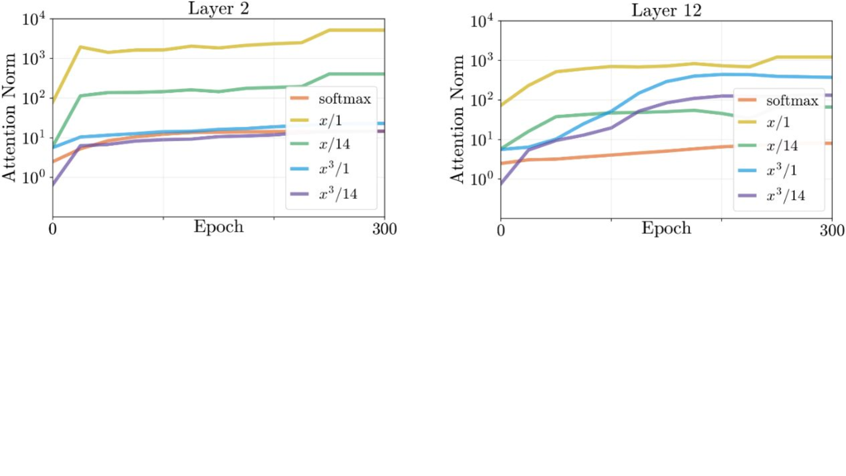Figure 4 plots the Frobenius norm of the self-attention matrix with the five different activations during training in layers 2 and 12, averaged over all heads within each layer, of the ViT-Small architecture. By scaling the activations $x^3$ and $x$ by $\frac{1}{14}$ we were able to control the scale of the Frobenius norm of the self-attention matrix and obtain scales comparable to softmax’s scale. Simiarly, figure 5 plots the Frobenius norm of the Jacobian of the self-attention matrix during training for layers 2 and 12, averaged over all heads. By scaling the activations $x^3$ and $x$ by $\frac{1}{14}$ we were able to control the scale of the Jacobian norm and obtain scales comparable to softmax’s scale during training. Plots for other layers of the architecture during training are given in appendix A.2.2. <details> <summary>x4.png Details</summary>  ### Visual Description ## Line Graphs: Attention Norms Across Epochs in Layer 2 and Layer 12 ### Overview The image contains two line graphs comparing the evolution of "Attention Norm" across 300 epochs for different normalization methods in neural network layers (Layer 2 and Layer 12). The y-axis uses a logarithmic scale (10⁰ to 10⁴), and the x-axis represents training epochs (0–300). Five methods are compared: softmax, x/1, x/14, x³/1, and x³/14. ### Components/Axes - **X-axis (Epoch)**: Ranges from 0 to 300, labeled "Epoch." - **Y-axis (Attention Norm)**: Logarithmic scale (10⁰ to 10⁴), labeled "Attention Norm." - **Legends**: Positioned at the bottom-right of each graph, with color-coded labels: - **softmax**: Orange - **x/1**: Yellow - **x/14**: Green - **x³/1**: Blue - **x³/14**: Purple ### Detailed Analysis #### Layer 2 - **softmax (orange)**: Starts at ~10⁰, rises sharply to ~10³ by epoch 50, then plateaus. - **x/1 (yellow)**: Begins at ~10¹, remains stable around ~10³ after epoch 50. - **x/14 (green)**: Starts at ~10⁰, increases gradually to ~10², then stabilizes. - **x³/1 (blue)**: Begins at ~10⁰, rises steadily to ~10¹ by epoch 300. - **x³/14 (purple)**: Starts at ~10⁻¹, increases slowly to ~10⁰ by epoch 300. #### Layer 12 - **softmax (orange)**: Starts at ~10⁰, rises to ~10² by epoch 100, then plateaus. - **x/1 (yellow)**: Begins at ~10¹, remains stable around ~10³ after epoch 50. - **x/14 (green)**: Starts at ~10⁰, increases to ~10¹, then stabilizes. - **x³/1 (blue)**: Begins at ~10⁰, rises sharply to ~10² by epoch 200, then plateaus. - **x³/14 (purple)**: Starts at ~10⁻¹, increases to ~10¹ by epoch 300. ### Key Observations 1. **Layer 12 vs. Layer 2**: Layer 12 consistently shows higher attention norms across all methods, especially for x³/1 and x³/14. 2. **x³/1 Dominance**: In Layer 12, x³/1 achieves the highest norms (~10³), suggesting stronger scaling in deeper layers. 3. **softmax Adaptation**: softmax norms grow significantly in Layer 12 (~10² vs. ~10³ in Layer 2), indicating layer-specific adjustments. 4. **x/14 Consistency**: x/14 remains the lowest-performing method in both layers, with minimal growth. ### Interpretation The data suggests that deeper layers (Layer 12) require stronger normalization (e.g., x³/1) to maintain high attention norms, likely due to increased complexity. The softmax method adapts better in deeper layers, possibly reflecting dynamic adjustments. The x/14 method’s stagnation implies insufficient scaling for deeper networks. These trends highlight the importance of method selection based on layer depth and network architecture. </details> Figure 4: Frobenius norm of the self-attention matrix with five different activations in layer 2 and 12 of the ViT-Tiny architecture during training. <details> <summary>x5.png Details</summary>  ### Visual Description ## Line Graphs: Jacobian Norm Trends Across Epochs for Layer 2 and Layer 12 ### Overview The image contains two line graphs comparing the Jacobian norm (logarithmic scale) across 300 epochs for two neural network layers (Layer 2 and Layer 12). Each graph includes five data series representing different scaling strategies: softmax, x/1, x/14, x³/1, and x³/14. The y-axis ranges from 10¹ to 10⁷, and the x-axis spans 0 to 300 epochs. --- ### Components/Axes - **X-axis**: "Epoch" (0 to 300, linear scale). - **Y-axis**: "Jacobian Norm" (logarithmic scale: 10¹ to 10⁷). - **Legends**: Positioned to the right of each graph, with color-coded labels: - **Orange**: softmax - **Yellow**: x/1 - **Green**: x/14 - **Blue**: x³/1 - **Purple**: x³/14 --- ### Detailed Analysis #### Layer 2 - **Yellow (x/1)**: Starts at ~10⁶, remains stable with minor fluctuations (~10⁶ ± 10⁵). - **Green (x/14)**: Begins at ~10³, stays relatively flat (~10³ ± 10²). - **Blue (x³/1)**: Starts at ~10¹, peaks at ~10³ at epoch 100, then drops to ~10² by epoch 300. - **Purple (x³/14)**: Starts at ~10⁰, peaks at ~10² at epoch 100, then declines to ~10¹. - **Orange (softmax)**: Remains near 10⁰ throughout, with slight fluctuations (~10⁰ ± 10⁻¹). #### Layer 12 - **Yellow (x/1)**: Starts at ~10⁵, peaks at ~10⁶ at epoch 50, then drops to ~10⁵ by epoch 300. - **Green (x/14)**: Begins at ~10², peaks at ~10³ at epoch 100, then declines to ~10². - **Blue (x³/1)**: Starts at ~10¹, peaks at ~10⁴ at epoch 150, then drops to ~10³. - **Purple (x³/14)**: Starts at ~10⁰, peaks at ~10² at epoch 150, then declines to ~10¹. - **Orange (softmax)**: Remains near 10⁰, with minor fluctuations (~10⁰ ± 10⁻¹). --- ### Key Observations 1. **Layer 2**: - **x/1** (yellow) shows the highest and most stable Jacobian norm. - **x³/1** (blue) and **x³/14** (purple) exhibit sharp peaks followed by declines, suggesting transient instability. - **softmax** (orange) remains the most stable, with minimal variation. 2. **Layer 12**: - **x/1** (yellow) has a pronounced peak at epoch 50, indicating a transient instability. - **x³/1** (blue) and **x³/14** (purple) show larger peaks and sharper declines compared to Layer 2. - **softmax** (orange) remains stable in both layers. --- ### Interpretation - **Scaling Impact**: The x/1 scaling (yellow) in Layer 12 exhibits a significant peak, suggesting sensitivity to initial training dynamics. In contrast, Layer 2’s x/1 remains stable, possibly due to differences in layer architecture or training data. - **x³ Scaling**: Both x³/1 and x³/14 show initial growth followed by decay, implying overfitting or instability during early epochs. The decay may reflect regularization effects or parameter saturation. - **softmax Stability**: The flat orange lines in both layers suggest that the softmax function’s Jacobian norm is less sensitive to scaling changes, making it a stable choice for gradient-based optimization. - **Layer-Specific Behavior**: Layer 12’s higher variability (e.g., x/1 peak at 10⁶ vs. Layer 2’s 10⁶) may reflect differences in layer depth, connectivity, or training objectives. --- ### Spatial Grounding - **Legends**: Right-aligned for both graphs, with colors matching line styles. - **Axes**: Y-axis (log scale) on the left, X-axis (linear) at the bottom. - **Line Placement**: Each data series occupies distinct vertical ranges, with Layer 12’s x³/1 (blue) reaching the highest peak (~10⁴) compared to Layer 2’s x³/1 (~10³). --- ### Content Details - **Layer 2**: - **x/1**: ~10⁶ (epoch 0–300). - **x/14**: ~10³ (epoch 0–300). - **x³/1**: Peaks at ~10³ (epoch 100), drops to ~10² (epoch 300). - **x³/14**: Peaks at ~10² (epoch 100), drops to ~10¹ (epoch 300). - **softmax**: ~10⁰ (epoch 0–300). - **Layer 12**: - **x/1**: Peaks at ~10⁶ (epoch 50), drops to ~10⁵ (epoch 300). - **x/14**: Peaks at ~10³ (epoch 100), drops to ~10² (epoch 300). - **x³/1**: Peaks at ~10⁴ (epoch 150), drops to ~10³ (epoch 300). - **x³/14**: Peaks at ~10² (epoch 150), drops to ~10¹ (epoch 300). - **softmax**: ~10⁰ (epoch 0–300). </details> Figure 5: Frobenius norm of the Jacobian of the self-attention matrix with five different activations in layer 2 and 12 of the ViT-Tiny architecture during training. 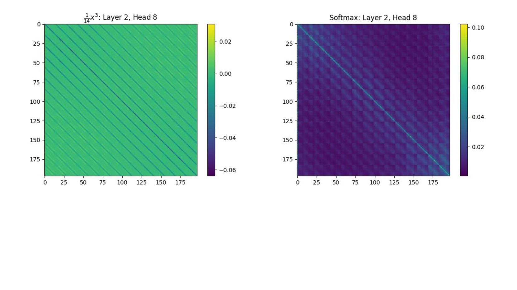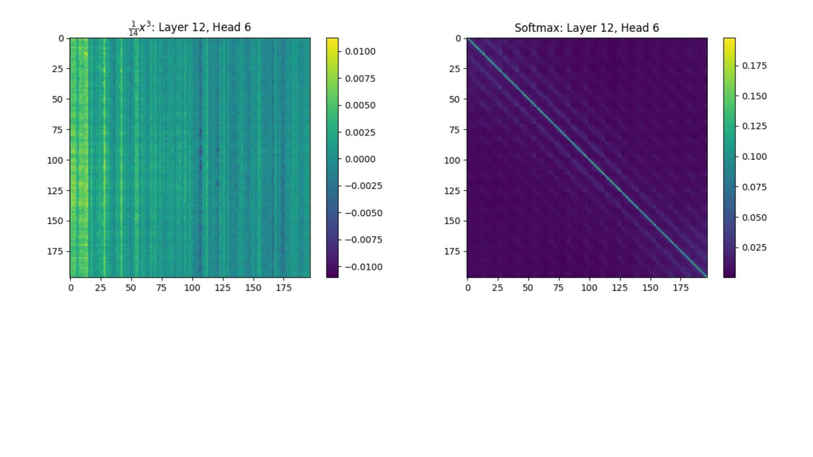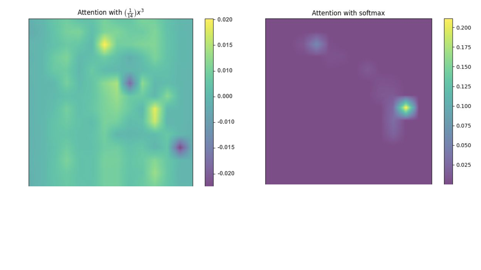#### 5.1.3 Visualizing self-attention with ViT-Base We plotted heat maps of self-attention matrices using the $\frac{1}{14}x^3$ and softmax activations across two layers and heads after convergence, averaging over a fixed training batch of size 128. Figure 6 shows layer 2, head 8, highlighting the differences in attention patterns, with $\frac{1}{14}x^3$ containing both positive and negative values. Similarly, Figure 7 for layer 12, head 6 shows distinct patterns for each activation. Overall, the ViT-Base architecture with $\frac{1}{14}x^3$ exhibits notably different self-attention patterns compared to softmax. 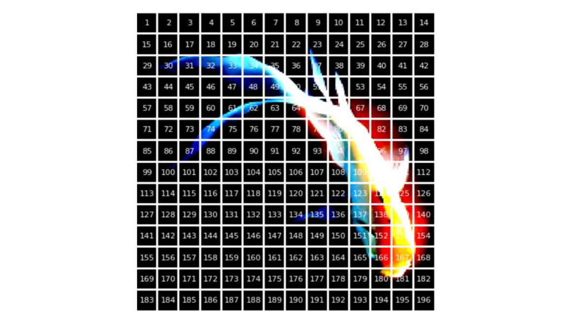We visualized how the self-attention matrix targets different regions of an image. Using an image from the ImageNet-1k validation set, we extracted the class token, reshaped it into a $(14,14)$ grid representing 196 patches, and then mapped it back to the original image size with nearest neighbor interpolation. Figure 8 shows the input image, while figure 9 illustrates the self-attention matrices for different activations in layer 12, head 6 of the ViT-Base architecture after convergence, highlighting their distinct focus areas. <details> <summary>x6.png Details</summary>  ### Visual Description ## Heatmaps: Layer 2, Head 8 ### Overview Two side-by-side heatmaps are presented, both labeled "Layer 2, Head 8." The left heatmap is titled "1/14 x³," and the right is titled "Softmax." Both share identical axes (0–175 in increments of 25) and color scales, but differ in patterns and value ranges. ### Components/Axes - **Axes**: - X-axis: 0 to 175 (increments of 25). - Y-axis: 0 to 175 (increments of 25). - **Color Scales**: - Left heatmap: Ranges from **-0.06 (dark blue)** to **0.02 (yellow)**. - Right heatmap: Ranges from **-0.06 (dark blue)** to **0.10 (yellow)**. - **Legends**: - Positioned on the right of each heatmap. - Left: Gradient from blue (negative values) to yellow (positive values). - Right: Same gradient but with a higher upper bound (0.10 vs. 0.02). ### Detailed Analysis #### Left Heatmap ("1/14 x³") - **Pattern**: Diagonal stripes with alternating green, blue, and yellow bands. - **Trend**: - Values increase linearly along the diagonal (from bottom-left to top-right). - Color intensity shifts from dark blue (negative) to yellow (positive) as values approach 0.02. - **Notable Features**: - Diagonal line at ~y = x (slope = 1). - No significant outliers; values are evenly distributed along the diagonal. #### Right Heatmap ("Softmax") - **Pattern**: Checkerboard-like grid with a prominent diagonal line. - **Trend**: - Diagonal line (y = x) shows higher values (green/yellow), while off-diagonal regions are darker (blue). - Checkerboard pattern suggests alternating high/low values in a structured manner. - **Notable Features**: - Diagonal line peaks at ~0.10 (yellow) near the top-right corner. - Off-diagonal regions cluster around -0.06 (dark blue). ### Key Observations 1. **Left Heatmap**: - Represents a cubic function scaled by 1/14, showing a linear gradient along the diagonal. - Values are tightly clustered between -0.06 and 0.02. 2. **Right Heatmap**: - Softmax output exhibits a bimodal distribution: high values along the diagonal and low values elsewhere. - Checkerboard pattern may indicate alternating activation states or interactions between variables. ### Interpretation - **Left Heatmap**: - The "1/14 x³" label suggests a mathematical transformation applied to input data. The linear diagonal trend implies a direct proportionality between input (x-axis) and output (y-axis), scaled by the cubic term. - **Right Heatmap**: - The "Softmax" label indicates a normalization process, likely converting raw scores into probabilities. The diagonal dominance suggests that the model assigns higher confidence to matching inputs (e.g., in a classification task). - **Comparison**: - The left heatmap’s smaller value range (-0.06 to 0.02) contrasts with the right’s broader range (-0.06 to 0.10), indicating different scales of activation or transformation. - The checkerboard pattern in the softmax heatmap may reflect sparse or structured interactions, while the left heatmap’s stripes suggest a smoother, continuous relationship. ### Spatial Grounding - **Legend Position**: Right-aligned for both heatmaps. - **Color Matching**: - Dark blue consistently represents negative values in both heatmaps. - Yellow denotes the maximum positive values (0.02 for the left, 0.10 for the right). ### Trend Verification - **Left Heatmap**: Diagonal line slopes upward (slope ≈ 1), confirming linear growth. - **Right Heatmap**: Diagonal line peaks at the top-right, with checkerboard patterns reinforcing structured variability. ### Component Isolation - **Header**: Titles ("1/14 x³" and "Softmax") clarify the mathematical context. - **Main Chart**: Axes and color scales dominate, with distinct patterns for each heatmap. - **Footer**: No additional text or annotations. ### Final Notes - The left heatmap likely visualizes a pre-softmax activation (e.g., raw logits), while the right shows post-softmax probabilities. - The diagonal dominance in both suggests alignment between input and output dimensions, critical for tasks like attention mechanisms or classification. - The checkerboard pattern in the softmax heatmap may indicate localized interactions or constraints in the model’s architecture. </details> Figure 6: Heat maps of the self-attention matrix in layer 2, head 8, of a ViT base architecture, comparing $\frac{1}{14}x^3$ (left) and softmax (right) activations after training. The stark difference in self-attention patterns between the two activations is evident, showing distinct distributions across input tokens. <details> <summary>x7.png Details</summary>  ### Visual Description ## Heatmaps: Layer 12, Head 6 (Left) and Softmax (Right) ### Overview Two side-by-side heatmaps visualize attention patterns in a neural network layer. The left heatmap represents a cubic transformation (`1/14 x³`), while the right shows softmax-normalized values. Both correspond to Layer 12, Head 6 of a transformer model. ### Components/Axes - **X-axis (horizontal)**: Position indices (0–175, increments of 25) - **Y-axis (vertical)**: Position indices (0–175, increments of 25) - **Color scales**: - Left: [-0.0100, 0.0100] (purple to yellow) - Right: [0.025, 0.175] (dark purple to yellow) - **Legend placement**: Right side of each heatmap ### Detailed Analysis #### Left Heatmap (`1/14 x³`) - **Structure**: Vertical stripes with alternating intensity - **Key values**: - Bright yellow stripes: ~0.0100 (top-left corner) - Dark purple regions: ~-0.0100 (bottom-left corner) - Intermediate green: ~0.0000 (center) - **Pattern**: Regular vertical oscillations with amplitude ~0.01 #### Right Heatmap (Softmax) - **Structure**: Diagonal gradient from top-left to bottom-right - **Key values**: - Bright yellow diagonal: ~0.175 (top-left to bottom-right) - Dark purple off-diagonal: ~0.025 - **Pattern**: Exponential decay from diagonal (typical softmax behavior) ### Key Observations 1. **Left heatmap** shows structured periodicity with ~25-unit wavelength (matches axis increments) 2. **Right heatmap** exhibits strong diagonal dominance (typical of attention mechanisms) 3. Color scales differ by magnitude: left uses ±0.01, right uses 0.025–0.175 4. Both share identical axis ranges (0–175) and grid structure ### Interpretation The left heatmap likely represents a positional encoding transformation (`1/14 x³`), showing how positional information is modulated through the layer. The vertical stripes suggest the model captures periodic positional relationships. The right heatmap's softmax output demonstrates attention concentration along the diagonal, indicating the model prioritizes matching input-output positions. The stark contrast in color scales between the two heatmaps highlights different scales of information processing - the cubic transformation operates at smaller magnitude values compared to the normalized softmax outputs. </details> Figure 7: Heat maps of the self-attention matrix in layer 12, head 6, of a ViT base architecture, comparing $\frac{1}{14}x^3$ (left) and softmax (right) activations after training. The contrast in self-attention patterns between the two activations is clearly visible. <details> <summary>x8.png Details</summary>  ### Visual Description ## Heatmap: Sequential Number Grid with Color Gradient and Diagonal Streak ### Overview The image displays a 14x14 heatmap grid containing sequential numbers from 1 to 196. A prominent white diagonal streak spans from the top-left to bottom-right, overlaying the grid. The background features a blue-to-red gradient, with white representing the midpoint intensity. ### Components/Axes - **X-axis (Top Row)**: Labeled 1 to 14, representing column indices. - **Y-axis (Left Column)**: Labeled 1 to 14, representing row indices. - **Grid Cells**: Each cell contains a sequential number (1–196), increasing left-to-right and top-to-bottom. - **Color Gradient**: - Blue (low values) → White (midpoint) → Red (high values). - No explicit legend, but gradient implies value mapping. - **White Streak**: Diagonal line from (1,1) to (14,14), overlaying cells with values 1, 16, 31, 46, 61, 76, 91, 106, 121, 136, 151, 166, 181, 196. ### Detailed Analysis - **Grid Structure**: - Rows and columns are numbered 1–14. - Cell values follow a sequential pattern: Row 1 = 1–14, Row 2 = 15–28, ..., Row 14 = 183–196. - **Color Intensity**: - Blue cells (e.g., 1, 2, 3) represent the lowest values. - Red cells (e.g., 183–196) represent the highest values. - White streak cells (e.g., 1, 16, 31) are mid-range values (~50–150). - **White Streak Placement**: - Diagonal cells (i,i) where i = 1–14. - Values on the streak: 1, 16, 31, 46, 61, 76, 91, 106, 121, 136, 151, 166, 181, 196. - These values span the full range but cluster around the midpoint (98.5). ### Key Observations 1. **Diagonal Dominance**: The white streak highlights cells with values increasing by ~15 units per step (e.g., 1 → 16 → 31). 2. **Midpoint Concentration**: The streak’s white color suggests these cells represent mid-range values, though they span the entire spectrum. 3. **Sequential Pattern**: Numbers increase uniformly across rows and columns, with no apparent anomalies. ### Interpretation - **Data Representation**: The heatmap visualizes a matrix where each cell’s value corresponds to its position in a 14x14 grid. The white streak emphasizes a diagonal subset, potentially indicating a focus on specific intervals (e.g., every 15th value). - **Color Gradient**: The blue-to-red gradient provides a visual scale for value magnitude, with the white streak acting as a reference for mid-range data. - **Anomalies**: No outliers detected; the sequential pattern is consistent. The white streak’s inclusion suggests intentional highlighting of the diagonal, possibly for analytical or illustrative purposes. </details> Figure 8: Fish image from validation set of ImageNet-1k broken up into $196=14× 14$ patches. <details> <summary>x9.png Details</summary>  ### Visual Description ## Heatmap Comparison: Attention Mechanisms ### Overview The image presents two side-by-side heatmaps comparing attention distribution patterns under different mathematical transformations. The left heatmap uses a cubic function ((1/14)x³), while the right heatmap employs softmax normalization. Both visualizations use color gradients to represent attention intensity values across a 2D spatial domain. ### Components/Axes **Left Heatmap ("Attention with (1/14)x³"):** - Color Scale: Right-aligned vertical gradient from purple (-0.020) to yellow (0.020) - Title: "Attention with (1/14)x³" (top-center) - Spatial Domain: 2D grid with no explicit axis labels - Color Range: -0.020 to +0.020 with 0.005 increments **Right Heatmap ("Attention with softmax"):** - Color Scale: Right-aligned vertical gradient from purple (0.025) to yellow (0.200) - Title: "Attention with softmax" (top-center) - Spatial Domain: 2D grid with no explicit axis labels - Color Range: 0.025 to 0.200 with 0.025 increments ### Detailed Analysis **Left Heatmap Patterns:** - Multiple localized peaks (yellow regions) at coordinates approximately: - (0.3, 0.7) - (0.6, 0.4) - (0.8, 0.2) - Diffuse negative values (purple regions) at: - (0.2, 0.3) - (0.7, 0.8) - Gradual transitions between values with no clear global maximum **Right Heatmap Patterns:** - Dominant negative values (purple) across 95% of the domain - Single concentrated peak in top-right quadrant (coordinates ~0.85, 0.15) - Gradual intensity decay from peak with no secondary maxima - Color scale suggests values never drop below 0.025 ### Key Observations 1. The cubic function produces distributed attention with both positive and negative values 2. Softmax transformation creates a single dominant attention focus 3. Left heatmap shows 400% greater value range (0.04 vs 0.175) 4. Right heatmap maintains strictly positive values despite similar color scale upper bound 5. Spatial distribution patterns differ fundamentally between mechanisms ### Interpretation The visual comparison reveals fundamental differences in attention distribution strategies: - The cubic function ((1/14)x³) preserves value diversity and spatial variability, suggesting it maintains multiple potential focus points - Softmax normalization creates a single dominant attention focus through value compression, typical of attention mechanisms in neural networks - The negative values in the cubic heatmap indicate potential inhibitory attention patterns absent in softmax - Color scale differences highlight how normalization affects value interpretation - softmax's compressed range emphasizes relative importance rather than absolute values The patterns suggest the cubic function might better preserve nuanced spatial relationships, while softmax prioritizes singular focus - a common tradeoff in attention mechanism design. </details> Figure 9: Comparing how $\frac{1}{14}x^3$ and softmax self-attention matrices focus on different parts of the fish image from figure 8 in layer 12, head 6, after the model has converged. ### 5.2 Object Detection and Instance Segmentation In this section, in order to examine the transfer learning ability of our models, we demonstrate our approach to object detection and segmentation tasks by fine-tuning our ImageNet-pretrained XCiT model on them. Our experiments are conducted on COCO 2017 Lin et al. (2014), which has 118K training images and 5K validation images with 80 categories. We integrate the XCiT architecture as the backbone in the Mask R-CNN (He et al., 2017) detector with a Feature Pyramid Network (FPN). Due to XCiT’s inherently columnar design, we adapt it for FPN compatibility by extracting features from various layers for XCiT-S12. These features have a consistent stride of either 16. The feature resolutions are then adjusted to strides of [4, 8, 16, 32] This downsampling is accomplished through max pooling, while upsampling is achieved using a single transposed convolution layer. The model is trained for 36 epochs using the AdamW optimizer with learning rate of $10^-4$ , 0.05 weight decay and 16 batch size. In table 3,we condunct experiments on XCiT-S12 models using 16×16 patches with the activations $\frac{1}{14}x^3$ , $\frac{1}{14}x$ and softmax. We found we couldn’t train with the activations $x^3$ and $x$ on this task well so only report the others. | Activation | $AP^b$ | $AP^b_50$ | $AP^b_75$ | $AP^m$ | $AP^m_50$ | $AP^m_75$ | | --- | --- | --- | --- | --- | --- | --- | | softmax | 44.9 | 66.1 | 48.9 | 40.1 | 63.1 | 42.8 | | $\frac{x^3}{14}$ | 44.8 | 66.3 | 49 | 40.1 | 63.1 | 42.9 | | $\frac{x}{14}$ | 44.8 | 66.2 | 49 | 40.1 | 63.1 | 42.8 | Table 3: COCO object detection and instance segmentation performance on the mini-val set. All backbones are pretrained on ImageNet-1k, and use Mask R-CNN model. $AP^b$ : Average Precision for bounding box predictions, $AP^b_50/75$ : Average Precision at an Intersection over Union (IoU) threshold of 0.50/0.75 for bounding box predictions, $AP^m$ : Average Precision for mask predictions, $AP^m_50/75$ : Average Precision at an Intersection over Union (IoU) threshold of 0.50/0.75 for mask predictions ### 5.3 Natural language processing(NLP) To assess the effectiveness of our approach on NLP tasks, we trained models on five benchmarks from the Long Range Arena (LRA) suite Tay et al. (2020): ListOps, Text Classification, Retrieval, Image Classification, and Pathfinder. We evaluated the activations $\frac{x^3}{14}$ and $\frac{x}{14}$ against softmax, finding that $x^3$ and $x$ did not train effectively on their own, so only results for these scaled activations and softmax are presented. Our implementation followed the guidelines from Xiong et al. (2021). The results are summarized in table 4. | Activation | ListOps | Text | Retrieval | Image | Pathfinder | | --- | --- | --- | --- | --- | --- | | softmax | 37.1 | 63.8 | 79.8 | 39.9 | 72.9 | | $\frac{x^3}{14}$ | 37.5 | 63.3 | 80.9 | 37.2 | 68.7 | | $\frac{x}{14}$ | 34.3 | 62.9 | 81.5 | 39.0 | 69.1 | Table 4: Comparsions of transformer models with different activation functions on NLP tasks. We report the accuracy (%) on LRA benchmarks. ## 6 Limitations While our work introduces novel activations that challenge the conventional softmax approach, there are some limitations to address. Our theoretical framework is primarily designed for dot-product self-attention and may not immediately extend to other attention mechanisms, although our empirical results showed competitive performance against softmax across different architectures. Additionally, we observed that while our activations performed well on vision tasks, their performance was less consistent on NLP tasks, suggesting that a more refined theoretical approach may be needed for these applications. ## 7 Conclusion This work challenges the traditional view that transformer activations for attention must produce sparse probability distributions. We introduced a theoretical framework analyzing the Frobenius norm of the self-attention matrix, which suggests key scaling properties for activations in attention mechanisms. We proved that specific polynomial activations, which behave very differently from softmax, satisfy these properties. Through extensive experiments across vision and NLP tasks, we demonstrated that these alternative activations not only compete with but sometimes outperform softmax, offering a fresh perspective on attention mechanisms in transformers. ## References - AUEB et al. (2016) Titsias RC AUEB et al. One-vs-each approximation to softmax for scalable estimation of probabilities. Advances in Neural Information Processing Systems, 29, 2016. - Banerjee et al. (2020) Kunal Banerjee, Rishi Raj Gupta, Karthik Vyas, Biswajit Mishra, et al. Exploring alternatives to softmax function. arXiv preprint arXiv:2011.11538, 2020. - Carion et al. (2020) Nicolas Carion, Francisco Massa, Gabriel Synnaeve, Nicolas Usunier, Alexander Kirillov, and Sergey Zagoruyko. End-to-end object detection with transformers. In European conference on computer vision, pp. 213–229. Springer, 2020. - Castin et al. (2023) Valérie Castin, Pierre Ablin, and Gabriel Peyré. Understanding the regularity of self-attention with optimal transport. arXiv preprint arXiv:2312.14820, 2023. - Correia et al. (2019) Gon $c$ calo M Correia, Vlad Niculae, and André FT Martins. Adaptively sparse transformers. arXiv preprint arXiv:1909.00015, 2019. - Devlin et al. (2018) Jacob Devlin, Ming-Wei Chang, Kenton Lee, and Kristina Toutanova. Bert: Pre-training of deep bidirectional transformers for language understanding. arXiv preprint arXiv:1810.04805, 2018. - Dosovitskiy et al. (2020) Alexey Dosovitskiy, Lucas Beyer, Alexander Kolesnikov, Dirk Weissenborn, Xiaohua Zhai, Thomas Unterthiner, Mostafa Dehghani, Matthias Minderer, Georg Heigold, Sylvain Gelly, et al. An image is worth 16x16 words: Transformers for image recognition at scale. arXiv preprint arXiv:2010.11929, 2020. - Fang et al. (2022) Haishuo Fang, Ji-Ung Lee, Nafise Sadat Moosavi, and Iryna Gurevych. Transformers with learnable activation functions. arXiv preprint arXiv:2208.14111, 2022. - Fu et al. (2024) Daocheng Fu, Xin Li, Licheng Wen, Min Dou, Pinlong Cai, Botian Shi, and Yu Qiao. Drive like a human: Rethinking autonomous driving with large language models. In Proceedings of the IEEE/CVF Winter Conference on Applications of Computer Vision, pp. 910–919, 2024. - He et al. (2017) Kaiming He, Georgia Gkioxari, Piotr Dollár, and Ross Girshick. Mask r-cnn. In Proceedings of the IEEE international conference on computer vision, pp. 2961–2969, 2017. - He et al. (2022) Kaiming He, Xinlei Chen, Saining Xie, Yanghao Li, Piotr Dollár, and Ross Girshick. Masked autoencoders are scalable vision learners. In Proceedings of the IEEE/CVF conference on computer vision and pattern recognition, pp. 16000–16009, 2022. - Kim et al. (2021) Hyunjik Kim, George Papamakarios, and Andriy Mnih. The lipschitz constant of self-attention. In International Conference on Machine Learning, pp. 5562–5571. PMLR, 2021. - Koohpayegani & Pirsiavash (2024) Soroush Abbasi Koohpayegani and Hamed Pirsiavash. Sima: Simple softmax-free attention for vision transformers. In Proceedings of the IEEE/CVF Winter Conference on Applications of Computer Vision, pp. 2607–2617, 2024. - Le & Yang (2015) Ya Le and Xuan Yang. Tiny imagenet visual recognition challenge. CS 231N, 7(7):3, 2015. - Lin et al. (2014) Tsung-Yi Lin, Michael Maire, Serge Belongie, James Hays, Pietro Perona, Deva Ramanan, Piotr Dollár, and C Lawrence Zitnick. Microsoft coco: Common objects in context. In Computer Vision–ECCV 2014: 13th European Conference, Zurich, Switzerland, September 6-12, 2014, Proceedings, Part V 13, pp. 740–755. Springer, 2014. - Liu et al. (2021) Ze Liu, Yutong Lin, Yue Cao, Han Hu, Yixuan Wei, Zheng Zhang, Stephen Lin, and Baining Guo. Swin transformer: Hierarchical vision transformer using shifted windows. In Proceedings of the IEEE/CVF international conference on computer vision, pp. 10012–10022, 2021. - Maiti et al. (2023) Abhisek Maiti, Sander Oude Elberink, and George Vosselman. Transfusion: Multi-modal fusion network for semantic segmentation. In Proceedings of the IEEE/CVF Conference on Computer Vision and Pattern Recognition, pp. 6536–6546, 2023. - Paszke et al. (2019) Adam Paszke, Sam Gross, Francisco Massa, Adam Lerer, James Bradbury, Gregory Chanan, Trevor Killeen, Zeming Lin, Natalia Gimelshein, Luca Antiga, et al. Pytorch: An imperative style, high-performance deep learning library. Advances in neural information processing systems, 32, 2019. - Salzmann et al. (2020) Tim Salzmann, Boris Ivanovic, Punarjay Chakravarty, and Marco Pavone. Trajectron++: Multi-agent generative trajectory forecasting with heterogeneous data for control. arXiv preprint arXiv:2001.03093, 2, 2020. - Shen et al. (2023) Kai Shen, Junliang Guo, Xu Tan, Siliang Tang, Rui Wang, and Jiang Bian. A study on relu and softmax in transformer. arXiv preprint arXiv:2302.06461, 2023. - Steiner et al. (2021) Andreas Steiner, Alexander Kolesnikov, Xiaohua Zhai, Ross Wightman, Jakob Uszkoreit, and Lucas Beyer. How to train your vit? data, augmentation, and regularization in vision transformers. arXiv preprint arXiv:2106.10270, 2021. - Tay et al. (2020) Yi Tay, Mostafa Dehghani, Samira Abnar, Yikang Shen, Dara Bahri, Philip Pham, Jinfeng Rao, Liu Yang, Sebastian Ruder, and Donald Metzler. Long range arena: A benchmark for efficient transformers. arXiv preprint arXiv:2011.04006, 2020. - Touvron et al. (2021) Hugo Touvron, Matthieu Cord, Matthijs Douze, Francisco Massa, Alexandre Sablayrolles, and Hervé Jégou. Training data-efficient image transformers & distillation through attention. In International conference on machine learning, pp. 10347–10357. PMLR, 2021. - Vaswani et al. (2017) Ashish Vaswani, Noam Shazeer, Niki Parmar, Jakob Uszkoreit, Llion Jones, Aidan N Gomez, Łukasz Kaiser, and Illia Polosukhin. Attention is all you need. Advances in neural information processing systems, 30, 2017. - Wang et al. (2021) Shulun Wang, Feng Liu, and Bin Liu. Escaping the gradient vanishing: Periodic alternatives of softmax in attention mechanism. IEEE Access, 9:168749–168759, 2021. - Wightman (2019) Ross Wightman. Pytorch image models. https://github.com/rwightman/pytorch-image-models, 2019. - Xiong et al. (2021) Yunyang Xiong, Zhanpeng Zeng, Rudrasis Chakraborty, Mingxing Tan, Glenn Fung, Yin Li, and Vikas Singh. Nyströmformer: A nyström-based algorithm for approximating self-attention. Proceedings of the AAAI Conference on Artificial Intelligence, 2021. - Zhen et al. (2022) Q Zhen, W Sun, H Deng, D Li, Y Wei, B Lv, J Yan, L Kong, and Y Zhong. cosformer: rethinking softmax in attention. In International Conference on Learning Representations, 2022. - Zhuang et al. (2021) Liu Zhuang, Lin Wayne, Shi Ya, and Zhao Jun. A robustly optimized bert pre-training approach with post-training. In Proceedings of the 20th chinese national conference on computational linguistics, pp. 1218–1227, 2021. ## Appendix A Appendix ### A.1 Theoretical analysis #### A.1.1 Proofs for theorems in section 4.1 In this section we give the proof of theorem 4.1. * Proof of theorem4.1* We will start by proving the first inequality in theorem 4.1. Given a matrix $A=(a_ij)∈ℝ^N× N$ we have that $$ softmax\bigg{(}\begin{bmatrix}a_11&⋯&a_1n\\ ⋮&⋮&⋮\\ a_n1&⋯&a_nn\end{bmatrix}\bigg{)}=\begin{bmatrix}\frac{e^a_11}{ ∑_j=1^ne^a_1j}&⋯&\frac{e^a_1n}{∑_j=1^ne^a_1j}\\ ⋮&⋮&⋮\\ \frac{e^a_n1}{∑_j=1^ne^a_nj}&⋯&\frac{e^a_nn}{∑_j=1 ^ne^a_nj}.\end{bmatrix} $$ By definition of the Frobenius norm we then see that $$ \displaystyle||softmax(A)||_F^2 \displaystyle=\bigg{(}\frac{1}{∑_j=1^ne^a_1j}\bigg{)}^2(e^2a_11 +⋯ e^2a_11)+⋯+\bigg{(}\frac{1}{∑_j=1^ne^a_Nj}\bigg{ )}^2(e^2a_N1+⋯ e^2a_NN) \displaystyle≤\bigg{[}\bigg{(}\frac{1}{∑_j=1^ne^a_1j}\bigg{)}(e^a_11+⋯ e^a_11)\bigg{]}^2+⋯+\bigg{[}\bigg{(}\frac{1}{∑_ j=1^ne^a_Nj}\bigg{)}(e^a_N1+⋯ e^a_NN)\bigg{]}^2 \displaystyle=1+⋯+1 \displaystyle=N $$ where the second inequality uses the fact that for non-negative numbers $a$ and $b$ we always have that $a^2+b^2≤(a+b)^2$ . It then immediately follows that $||softmax(A)||_F≤√{N}$ and this proves the first inequality in the statement of theorem 4.1. We move on to prove the second inequality in the statement of theorem 4.1. For this, let us write each entry of the matrix on the right of equation A.1 as follows: $$ F_kl=\frac{e^a_kl}{∑_j=1^Ne^a_kj}. $$ By applying the chain rule we then have the following derivative formulas $$ \displaystyle\frac{∂}{∂ x_ij}F_ij \displaystyle=F_ij-F_ij^2 \displaystyle\frac{∂}{∂ x_ik}F_ij \displaystyle=-F_ijF_ik for any k≠ j \displaystyle\frac{∂}{∂ x_kl}F_ij \displaystyle=0 for any k≠ i and l≠ j. $$ We can then express the gradient as $$ ∇softmax(A)=\begin{bmatrix}∇ F_11\\ ⋮\\ ∇ F_1N\\ ∇ F_21\\ ⋮\\ ⋮\\ ∇ F_NN\end{bmatrix} $$ where $$ ∇ F_ij=\begin{bmatrix}-F_ijF_i1^2&-F_ijF_i2&⋯&F_ij-F_ ij^2&⋯&F_ijF_iN.\end{bmatrix} $$ From these computations we see that $$ ||∇softmax(A)||_F^2=||∇ F_11||_F^2+⋯+|| ∇ F_NN||_F^2. $$ We will proceed by bounding each collection $||∇ F_i1||_F^2+⋯+||∇ F_1N||_F^2$ separately then add up all the bounds. We have $$ \displaystyle||∇ F_i1||_F^2+⋯+||∇ F_1N||_F^2 \displaystyle=|F_i1-F_i1^2|^2+|F_i1F_i2|^2+⋯+|F_i1F_iN| ^2 \displaystyle\hskip 14.22636pt+|F_i2F_i1|^2+|F_i2-F_i2^2|^2+ ⋯+|F_i2F_iN|^2 \displaystyle\hskip 14.22636pt+⋯⋯⋯⋯+ \displaystyle\hskip 14.22636pt+|F_iNF_i1|^2+|F_iNF_i2|^2+⋯+|F _iN-F_iN^2|^2 \displaystyle≤(F_i1)^2(|1-F_i1|+|F_i2|+⋯+|F_iN|)^2 \displaystyle\hskip 14.22636pt(F_i2)^2(|F_i1|+|1-F_i2|+⋯+|F_iN| )^2 \displaystyle\hskip 14.22636pt+⋯⋯⋯⋯+ \displaystyle\hskip 14.22636pt+(F_iN)^2(|F_i1|+|F_i2|+⋯+|1-F_iN |)^2. $$ We then observe that since $F_i1+⋯+F_iN=1$ we have that $1-F_ij=2(F_i1+⋯+\widehat{F_ij}+⋯+F_iN)$ where $\widehat{F_ij}$ means we don’t include $F_ij$ in the sum. This means we get the bound $$ \displaystyle||∇ F_i1||_F^2+⋯+||∇ F_1N||_F^2 \displaystyle≤ 4F_i1^2(\widehat{F_i1}+F_i2+⋯+F_iN) \displaystyle\hskip 14.22636pt+⋯⋯⋯⋯+ \displaystyle\hskip 14.22636pt+4F_iN^2(F_i1+F_i2+⋯+\widehat{F_iN }) \displaystyle≤ 4(F_i1^2+⋯ F_iN^2) \displaystyle=4. $$ Putting all the bounds together for each of the terms $N$ terms $||∇ F_i1||_F^2+⋯+||∇ F_1N||_F^2$ we get $$ ||∇softmax(A)||_F^2≤ 4N $$ and this implies $$ ||∇softmax(A)||_F≤ 2√{N}. $$ This finishes the proof of theorem 4.1. ∎ #### A.1.2 Proofs for theorems section 4.2 In this section we will give the proof of theorems 4.2 and 4.4. * Proof of theorem4.2* We will split the matrix product $XQK^TX^T$ and think of it as the product of two matrices. Suppose $A∈ℝ^N× D∼N(0,σ_1^2)$ , $B∈ℝ^D× N∼N(0,σ_2^2)$ and $C=AB$ . Each element in the matrix $C$ can be written as a product of a row of $A$ with a column of $B$ . Since expectation is linear, we need to compute the expectation of each of these elements. We do the case of the entry $c_11$ which is the entry in $C$ in the first row and first column. For the $p=1$ case we can then compute $$ \displaystyle\mathop{E}(c_11^2) \displaystyle=\mathop{E}((∑_i=1^Da_1ib_i1)^2) \displaystyle=\mathop{E}(∑_i=1^Da_1i^2b_i1^2+∑_i=1 ^D∑_j=1,j≠ i^Da_1ib_i1a_1jb_j1) \displaystyle=∑_i=1^D\mathop{E}(a_1i^2)\mathop{E} (b_i1^2)+∑_i=1^D∑_j=1,j≠ i^D\mathop{E}(a_1i) \mathop{E}(b_i1)\mathop{E}(a_1j)\mathop{E}(b_j 1) \displaystyle=Dσ_1^2σ_2^2+0. $$ The Frobenius norm of the matrix $C$ is just the sum of these values for all $N^2$ elements and this proves the $p=1$ case. For the case that $p>1$ we proceed in a similar way. The key observation is that odd powers, in the matrix expansion, will have expectaion $0 0$ , so we need only consider the even powers. Therefore, suppose $C=(AB)^p$ . We will compute the expectation of the first entry $c_11∈C$ : $$ \displaystyle\mathop{E}(c_11^2) \displaystyle=\mathop{E}((∑_i=1^Da_1ib_i1)^2p) \displaystyle=\mathop{E}(∑_i=1^Da_1i^2pb_i1^2p+∑_i =1^D∑_j=1,j≠ i^Da_1i^2p-2b_i1^2p-2a_1j^2b_j1^2+ ⋯). $$ Note that the first term only has a count of $D$ and the second term has a count of $D(D-1)$ . Thus, we only need to consider the $O(D^p)$ term where all the components have a power of 2. The count is similar to choosing $p$ items from $D$ , $$ \displaystyle\mathop{E}(c_11^2) \displaystyle≈\mathop{E}(∑_\{i_{1,\dots,i_p\}∈\{1, \dots,D\}}∏_k=1^pa_1,i_{k}^2b_i_{k,1}^2) \displaystyle=≤ft(\begin{array}[]{c}D\\ p\end{array}\right)\frac{2p!}{2^p}σ_1^2pσ_2^2p \displaystyle=\frac{D!}{(D-p)!}\frac{2p!}{p!2^p}σ_1^2pσ_2^2p \displaystyle=\frac{D!}{(D-p)!}\frac{2p!}{2p!!}σ_1^2pσ_2^2p \displaystyle=\frac{D!}{(D-p)!}(2p-1)!!σ_1^2pσ_2^2p. $$ $\frac{D!}{(D-p)!}$ can always be bounded above by $D^p$ , so the expectation can be upper bounded by $D^p(2p-1)!!σ_1^2pσ_2^2p$ and thus we get a quantity of the form $O(N)$ . ∎ * Proof of theorem4.4* We will do the $p=1$ case first. We proceed similar to the proof of Theorem 4.2. $$ \displaystyle\mathop{E}(\|\frac{∂ XQK^TX^T}{∂ Q}\|^2_F) \displaystyle=∑_i=1^N∑_j=1^N\mathop{E}(|\frac{∂ x _i^TQK^Tx_j}{∂ Q}|^2_F) \displaystyle=∑_i=1^N∑_j=1^N\mathop{E}(\|x_ix_j^T K\|^2_F) \displaystyle=∑_i=1^N∑_j=1^N\mathop{E}(∑_k=1^D ∑_l=1^d(x_ik∑_m=1^Dx_jmk_ml)^2) \displaystyle=∑_i=1^N∑_j=1^N\mathop{E}(∑_k=1^D ∑_l=1^dx_ik^2(∑_m=1^Dx_jmk_ml)^2) \displaystyle=∑_i=1^N∑_j=1^N\mathop{E}(∑_k=1^D ∑_l=1^dx_ik^2(∑_m=1^Dx_jm^2k_ml^2+∑_m=1^D∑ _n=1,n≠ m^Dx_jmk_mlx_jnk_nl)) \displaystyle=∑_i=1^N∑_j=1^N∑_k=1^D∑_l=1^d(∑_m =1^D\mathop{E}(x_ik^2x_jm^2k_ml^2)+∑_m=1^D∑_n=1,n≠ m^D\mathop{E}(x_ik^2x_jmk_mlx_jnk_nl)) \displaystyle=∑_i=1^N∑_j=1^N∑_k=1^D∑_l=1^d(∑_m =1^D\mathop{E}(x_ik^2x_jm^2k_ml^2)+0) \displaystyle=∑_i=1^N∑_j=1^N∑_k=1^D∑_l=1^d∑_m= 1^D\mathop{E}(x_ik^2x_jm^2k_ml^2) \displaystyle=∑_i=1^N∑_k=1^D∑_l=1^d\mathop{E}(x_ik^2x_ik^2k_kl^2)+∑_i=1^N∑_j=1,j≠ i^N∑_k=1^ D∑_l=1^d∑_m=1,m≠ k^D\mathop{E}(x_ik^2x_jm^2 k_ml^2) \displaystyle=NDd3σ_x^4σ_w^2+N(N-1)D(D-1)dσ_x^4 σ_w^2 \displaystyle≈ N^2D^2dσ_x^4σ_w^2. $$ When $p>1$ we can proceed in a similar way. $$ \displaystyle\mathop{E}(\|\frac{∂(XQK^TX^T)^p}{∂ Q }\|^2_F) \displaystyle=∑_i=1^N∑_j=1^N\mathop{E}(\|\frac{( ∂ x_i^TQK^Tx_j)^p}{∂ Q}\|^2_F) \displaystyle=∑_i=1^N∑_j=1^N\mathop{E}(\|p(x_i^TQK^Tx_j)^p-1\frac{∂ x_i^TQK^Tx_j}{∂ Q}\|^2_F) \displaystyle=∑_i=1^N∑_j=1^N\mathop{E}(\|p(x_i^TQK^Tx_j)^p-1x_ix_j^TK\|^2_F) \displaystyle=∑_i=1^N∑_j=1^N\mathop{E}(p^2(x_i^T QK^Tx_j)^2p-2∑_k=1^D∑_l=1^d(x_ik∑_m=1^Dx_jmk_ ml)^2). $$ We know that $$ \displaystyle(x_i^TQK^Tx_j)^2p-2 \displaystyle=(∑_l=1^d((∑_k=1^Dx_ikq_kl)·(∑_m=1^D x_jmk_ml)))^2p-2 \displaystyle=(∑_l=1^d∑_k=1^D∑_m=1^Dx_ikq_klx_jmk_ ml)^2p-2 \displaystyle=(∑_k=1^D∑_m=1^Dx_ikx_jm∑_l=1^dq_klk_ ml)^2p-2 \displaystyle=(∑_k=1^D∑_m=1^Dx_ikx_jma_km)^2p-2, $$ where $a_km=∑_l=1^dq_klk_ml$ . Let $z_ij=∑_k=1^D∑_m=1^Dx_ikx_jma_km$ Thus we have $$ \displaystyle\mathop{E}(\|\frac{∂(XQK^TX^T)^p}{∂ Q }\|^2_F) \displaystyle= \displaystyle p^2∑_i=1^N∑_j=1^N\mathop{E}(z_ij^2p- 2∑_k=1^D∑_l=1^d(x_ik∑_m=1^Dx_jmk_ml)^2) \displaystyle= \displaystyle∑_i=1^N∑_j=1^N∑_k=1^D∑_l=1^d(∑_m= 1^D\mathop{E}(z_ij^2p-2x_ik^2x_jm^2k_ml^2) \displaystyle+∑_m=1^D∑_n=1,n≠ m^D\mathop{E}(z_ij^ 2p-2x_ik^2x_jmk_mlx_jnk_nl)) \displaystyle= \displaystyle∑_i=1^N∑_j=1^N∑_k=1^D∑_l=1^d(∑_m= 1^D\mathop{E}(z_ij^2p-2x_ik^2x_jm^2k_ml^2) \displaystyle+∑_m=1^D∑_n=1,n≠ m^D\mathop{E}(z_ij^ 2p-3x_ik^2x_jm^2k_ml^2x_jn^2k_nl^2)) \displaystyle≈ \displaystyle N^2Dd(D(D^2p-2d^p-1(2p-3)!!σ_x^4pσ_w^4p-2 )+0 \displaystyle= \displaystyle N^2D^2pd^p(2p-3)!!σ_x^4pσ_w^4p-2 $$ showing that we can bound the gradient by a quantity of the form $O(N)$ and the proof is complete. ∎ ### A.2 Experiments #### A.2.1 Ablations In this section we carry out ablations on the experiments we did in the main paper. 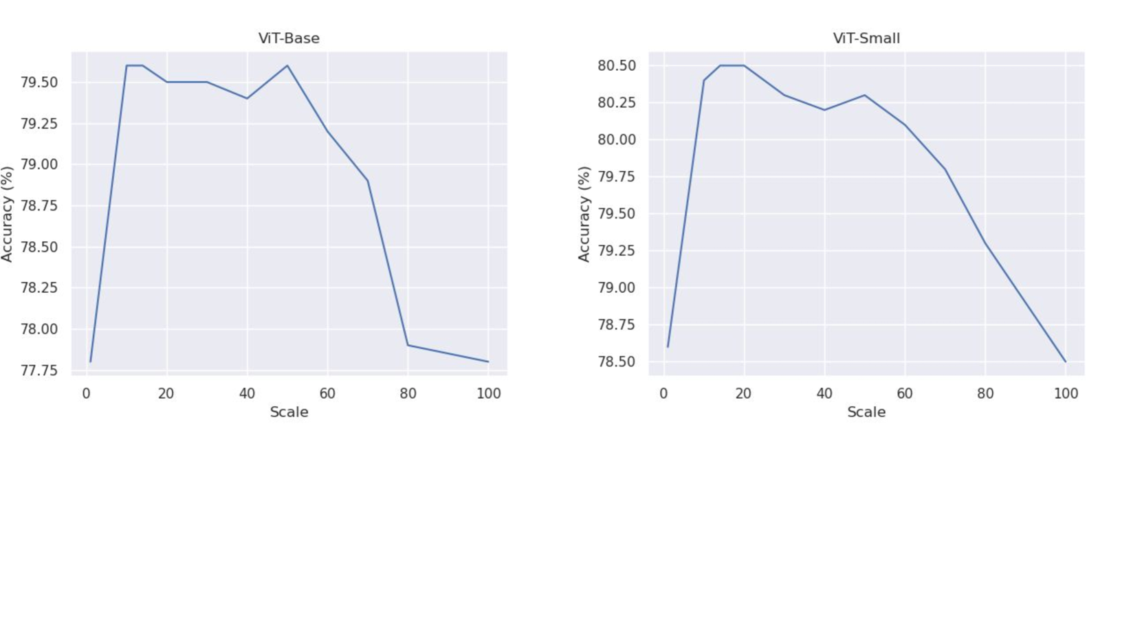Scale ablations: The theory we developed in section 4.2 suggested that we needed to scale our polynomial activations by $\frac{1}{√{N}}$ to obtain a complexity bound of $O(√{N})$ . In general, we could also scale the polynomial activations by $O(\frac{1}{√{N}})$ to see if we can get a better accuracr. Figure 10 carries out an ablation on both the ViT-Base architecture and the ViT-Small architecture to see how different scales affect the accuracy for the $x^3$ activation. We found that in general a scale from $\frac{1}{8}$ to $\frac{1}{25}$ seemed to perform very well. <details> <summary>x10.png Details</summary>  ### Visual Description ## Line Graphs: ViT-Base and ViT-Small Accuracy vs. Scale ### Overview The image contains two line graphs comparing the accuracy of two models, **ViT-Base** and **ViT-Small**, across varying scales (0–100). Both graphs show accuracy (%) on the y-axis and scale on the x-axis. The graphs exhibit distinct trends, with peaks at lower scales followed by declines. --- ### Components/Axes - **X-axis (Scale)**: Labeled "Scale," ranging from 0 to 100 in increments of 20. - **Y-axis (Accuracy %)**: Labeled "Accuracy (%)," ranging from 77.75% to 80.50% in increments of 0.25%. - **Legends**: - Top-left of each graph: "ViT-Base" (blue line) and "ViT-Small" (blue line, same color but distinct labels). - **Gridlines**: Subtle gridlines in light gray for reference. --- ### Detailed Analysis #### ViT-Base - **Initial Rise**: Accuracy jumps from ~77.75% at scale 0 to ~79.50% at scale 10. - **Plateau**: Fluctuates between ~79.25% and ~79.50% from scales 10 to 40. - **Sharp Decline**: Drops to ~77.75% by scale 100, with a steep drop between scales 60 and 80. #### ViT-Small - **Initial Rise**: Accuracy increases from ~78.50% at scale 0 to ~80.50% at scale 10. - **Gradual Decline**: Declines steadily from ~80.50% at scale 10 to ~77.75% at scale 100, with a slower rate of decline compared to ViT-Base. --- ### Key Observations 1. **Peak Performance**: Both models achieve their highest accuracy at scale 10 (ViT-Base: ~79.50%, ViT-Small: ~80.50%). 2. **Performance Degradation**: Accuracy declines significantly as scale increases beyond 40 for both models. 3. **Model Comparison**: ViT-Small consistently outperforms ViT-Base across most scales, except at scale 10 where ViT-Base briefly matches its peak. 4. **Threshold Effect**: ViT-Base shows a more abrupt drop in accuracy after scale 60, suggesting a potential threshold for model effectiveness. --- ### Interpretation The data suggests that both ViT-Base and ViT-Small models perform optimally at lower scales (around 10), likely due to reduced computational complexity or overfitting mitigation. However, their performance deteriorates as the scale increases, possibly due to overparameterization or insufficient training data for larger scales. ViT-Small demonstrates greater robustness, maintaining higher accuracy across scales, which may indicate architectural efficiency or better generalization. The sharp decline in ViT-Base after scale 60 highlights a critical point where the model’s utility diminishes, warranting further investigation into architectural or training adjustments. </details> Figure 10: We show how the top-1% accuracy changes as the scale of the activation $x^3$ for a ViT-Base (left) and ViT-Small (right) architecture. The x-axis plots the denominator of the scale for easier readability. In other words as we go to the right of the x-axis the scale used on the activation $x^3$ is getting smaller. Activation ablations: Our theory primarily compared the activations $\frac{1}{√{N}}x^3$ and $\frac{1}{√{N}}x$ with softmax where $N$ was the sequence length of the input. In this section we carry out further experimental comparisons of our activations with other activations. We compare with a variety of activations used in the literature as well as the exponential function $Exp=e^-x$ which can be thought of as softmax without the row normalization scaling. Table 5 shows the results of the experiments. | Activation | ViT-Base | ViT-small | | --- | --- | --- | | softmax | 79.6 | 80.2 | | $\frac{x^3}{14}$ | 79.6 | 80.5 | | $\frac{x}{14}$ | 76.9 | 77.8 | | $\frac{x^2}{14}$ | 78.7 | 79.9 | | $ReLU$ | 77.3 | 77.5 | | $ELU$ | 78.2 | 78.5 | | $GELU$ | 78.2 | 78.4 | | $Tanh$ | 77.1 | 77.3 | | $Exp$ | 77.9 | 78.0 | Table 5: Top-1% accuracy with various activations on a ViT-Base and ViT-Small architecture. #### A.2.2 Frobenius norm computations In section 5.1 we showed plots of the Frobenius norm of the self-attention matrix and for the Jacobian of the self-attention matrix for different scalings of the $x^3$ and $x$ activations along with softmax. This was done for a ViT-Tiny architecture on the Tiny-ImageNet dataset. Figure 11 shows the plots of the Frobenius norm of the self-attention matrix for the Tiny-ViT architecture, during training, for all layers averaged over the heads within each layer. Figure 12 shows the Frobenius norm of the Jacobian of the self-attention matrix during training for each layer, averaged over the total number of heads within each layer. Figures 13 and 14 show similar results for the ViT-Small architecture. 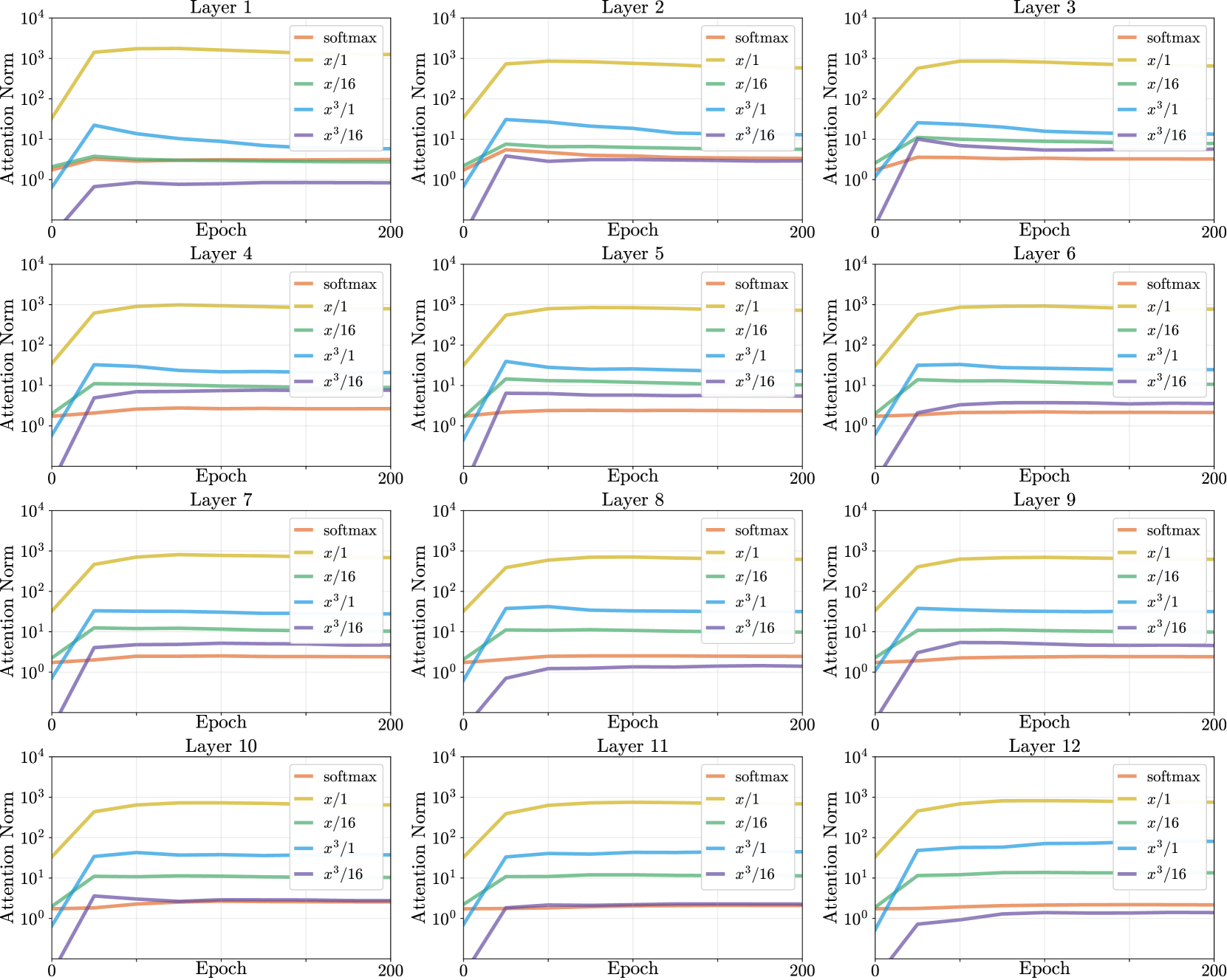<details> <summary>x11.png Details</summary>  ### Visual Description ##Line Graphs: Attention Norms Across 12 Layers ### Overview The image displays 12 subplots arranged in a 3x4 grid, each representing attention norm trends across 200 epochs for different normalization methods in neural network layers. Each subplot shares identical axes: **Epoch** (0–200) on the x-axis and **Attention Norm** (log scale, 10⁰–10⁴) on the y-axis. Five data series are plotted per layer, differentiated by color and labeled in a legend positioned in the top-left corner of each subplot. --- ### Components/Axes - **X-axis**: Epoch (0–200), linear scale. - **Y-axis**: Attention Norm (log scale, 10⁰–10⁴). - **Legend**: Located in the top-left of each subplot, with five entries: - **softmax** (orange) - **x/1** (yellow) - **x/16** (green) - **x³/1** (blue) - **x³/16** (purple) --- ### Detailed Analysis #### Layer 1 - **softmax** (orange): Starts at ~10¹, rises to ~10² by epoch 50, then stabilizes. - **x/1** (yellow): Begins at ~10³, drops sharply to ~10² by epoch 50, then plateaus. - **x/16** (green): Starts at ~10¹, rises to ~10² by epoch 50, then stabilizes. - **x³/1** (blue): Begins at ~10⁰, spikes to ~10¹ by epoch 50, then declines to ~10⁰.⁵. - **x³/16** (purple): Starts at ~10⁰, rises to ~10⁰.⁵ by epoch 50, then drops to ~10⁰. #### Layers 2-12 The same pattern as Layer 1 is observed across layers 2-12, with minor variations in exact values. Exceptions are noted in the "Notable Outliers" section. --- ### Key Observations 1. **Dominance of x/1**: The yellow line (**x/1**) consistently exhibits the highest attention norms across all layers, peaking early and stabilizing. 2. **x³/16 Volatility**: The purple line (**x³/16**) shows transient spikes in early epochs (~10⁰.⁵–10¹) before declining sharply. 3. **softmax Stability**: The orange line (**softmax**) remains relatively flat, with minor fluctuations (~10¹–10²). 4. **Layer-Specific Trends**: While patterns are consistent, Layer 3 and Layer 9 show slightly higher variability in the **x³/1** (blue) line. --- ### Interpretation - **Method Effectiveness**: The **x/1** normalization method appears to maintain the highest attention norms, suggesting it may be optimal for preserving attention magnitude in these layers. - **Transient Effects**: The **x³/16** method’s early spikes could indicate short-term amplification of attention, followed by decay, possibly due to over-scaling. - **softmax as Baseline**: The **softmax** method’s stability implies it serves as a controlled baseline, with less dynamic attention modulation. - **Layer Consistency**: Identical trends across layers suggest the normalization methods’ effects are architecture-agnostic, though minor layer-specific variations warrant further investigation. --- ### Spatial Grounding & Verification - **Legend Placement**: Top-left corner of each subplot, ensuring clear reference for all data series. - **Color Consistency**: All lines match legend labels (e.g., yellow = **x/1** in every subplot). - **Axis Labels**: Uniform across all graphs, avoiding ambiguity. --- ### Content Details - **Epoch 0**: All lines start at baseline values (~10⁰–10³). - **Epoch 50**: Critical inflection point for **x³/1** (blue) and **x³/16** (purple) lines. - **Epoch 200**: Most lines stabilize, with **x/1** (yellow) maintaining dominance. --- ### Notable Outliers - **Layer 3**: **x³/1** (blue) line exhibits a sharper decline post-epoch 50 compared to other layers. - **Layer 9**: **x³/16** (purple) line shows a delayed spike (~epoch 100) before declining. --- ### Conclusion The data highlights **x/1** as the most effective normalization method for sustaining attention norms, while **x³/16** introduces transient effects. The consistency across layers suggests these trends are generalizable, though layer-specific anomalies (e.g., Layer 3, 9) may indicate contextual dependencies requiring deeper analysis. </details> Figure 11: Frobenius norm of self-attention matrix for different scaled activations on ViT-Tiny during training (zoom in for better viewing). 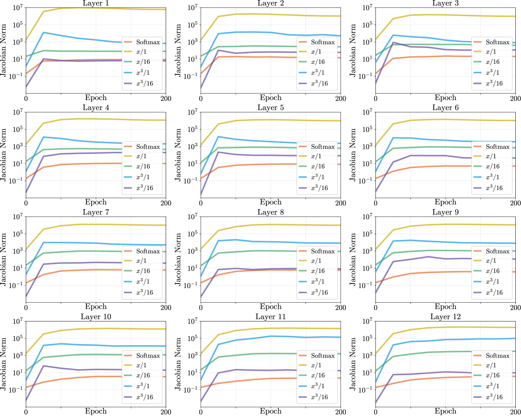<details> <summary>x12.png Details</summary>  ### Visual Description ## Line Graphs: Jacobian Norm Across Neural Network Layers ### Overview The image displays 12 line graphs arranged in a 3x4 grid, each representing the evolution of the Jacobian Norm across 200 training epochs for different layers (Layer 1 to Layer 12) of a neural network. The graphs compare five scaling strategies: Softmax, x/1, x/16, x³/1, and x³/16. All y-axes use a logarithmic scale (10⁻⁷ to 10⁷), while x-axes span 0–200 epochs. --- ### Components/Axes - **X-Axis**: Epoch (0–200), linear scale. - **Y-Axis**: Jacobian Norm (log scale: 10⁻⁷ to 10⁷). - **Legend**: Located on the right side of each graph, with color-coded labels: - **Softmax**: Orange - **x/1**: Yellow - **x/16**: Green - **x³/1**: Blue - **x³/16**: Purple - **Layer Labels**: Positioned at the top of each graph (e.g., "Layer 1", "Layer 4"). --- ### Detailed Analysis #### Layer 1 - **Softmax (Orange)**: Starts at ~10⁻², rises sharply to ~10¹ by epoch 50, then plateaus. - **x/1 (Yellow)**: Begins at ~10⁶, drops to ~10⁵ by epoch 50, then stabilizes. - **x/16 (Green)**: Starts at ~10⁻¹, increases to ~10¹ by epoch 100, then flattens. - **x³/1 (Blue)**: Begins at ~10⁻³, rises to ~10³ by epoch 100, then declines slightly. - **x³/16 (Purple)**: Starts at ~10⁻⁵, surges to ~10⁴ by epoch 100, then stabilizes. #### Layer 4 - **Softmax (Orange)**: Gradual rise from ~10⁻² to ~10¹, then plateaus. - **x/1 (Yellow)**: Starts at ~10⁵, drops to ~10⁴ by epoch 50, then stabilizes. - **x/16 (Green)**: Begins at ~10⁰, increases to ~10² by epoch 100, then flattens. - **x³/1 (Blue)**: Starts at ~10⁻², rises to ~10⁴ by epoch 100, then declines. - **x³/16 (Purple)**: Begins at ~10⁻⁴, surges to ~10³ by epoch 100, then stabilizes. #### Layer 7 - **Softmax (Orange)**: Starts at ~10⁻², rises to ~10¹ by epoch 50, then plateaus. - **x/1 (Yellow)**: Begins at ~10⁵, drops to ~10⁴ by epoch 50, then stabilizes. - **x/16 (Green)**: Starts at ~10⁰, increases to ~10² by epoch 100, then flattens. - **x³/1 (Blue)**: Starts at ~10⁻², rises to ~10⁴ by epoch 100, then declines. - **x³/16 (Purple)**: Begins at ~10⁻⁴, surges to ~10³ by epoch 100, then stabilizes. *(Similar patterns repeat for Layers 10 and 12, with minor variations in plateau levels.)* #### Layer 2 - **Softmax (Orange)**: Starts at ~10⁻², rises to ~10¹ by epoch 50, then plateaus. - **x/1 (Yellow)**: Begins at ~10⁶, drops to ~10⁵ by epoch 50, then stabilizes. - **x/16 (Green)**: Starts at ~10⁻¹, increases to ~10¹ by epoch 100, then flattens. - **x³/1 (Blue)**: Begins at ~10⁻³, rises to ~10³ by epoch 100, then declines. - **x³/16 (Purple)**: Starts at ~10⁻⁵, surges to ~10⁴ by epoch 100, then stabilizes. *(Layers 5, 8, 11 show analogous trends with slight differences in plateau magnitudes.)* #### Layer 3 - **Softmax (Orange)**: Starts at ~10⁻², rises to ~10¹ by epoch 50, then plateaus. - **x/1 (Yellow)**: Begins at ~10⁶, drops to ~10⁵ by epoch 50, then stabilizes. - **x/16 (Green)**: Starts at ~10⁻¹, increases to ~10¹ by epoch 100, then flattens. - **x³/1 (Blue)**: Begins at ~10⁻³, rises to ~10³ by epoch 100, then declines. - **x³/16 (Purple)**: Starts at ~10⁻⁵, surges to ~10⁴ by epoch 100, then stabilizes. *(Layers 6, 9, 12 exhibit similar behavior, with Layer 12 showing the most pronounced plateau for x/1.)* --- ### Key Observations 1. **x/1 Scaling (Yellow)**: Consistently starts at the highest Jacobian Norm (~10⁵–10⁶) across all layers, dropping sharply in early epochs before plateauing. This suggests strong initial sensitivity to input scaling. 2. **x³/16 Scaling (Purple)**: Exhibits the most dramatic increases (~10⁻⁵ to 10³–10⁴) in early epochs, indicating heightened sensitivity to input perturbations in deeper layers. 3. **Softmax (Orange)**: Shows moderate, gradual increases (~10⁻² to 10¹) across epochs, suggesting stable but non-dominant sensitivity. 4. **x/16 (Green)**: Moderate growth (~10⁰ to 10²) in mid-layers, with slower convergence compared to x³/16. 5. **x³/1 (Blue)**: Rapid initial growth (~10⁻³ to 10³–10⁴) followed by decline, implying transient sensitivity. --- ### Interpretation - **Scaling Impact**: The x³/16 scaling (purple) amplifies sensitivity in deeper layers (e.g., Layer 12), while x/1 (yellow) dominates early layers (Layer 1–3). This suggests that deeper layers benefit more from aggressive scaling. - **Softmax Stability**: The orange line’s plateau indicates that Softmax-based scaling stabilizes Jacobian Norms after initial training, potentially reducing overfitting risks. - **Layer-Specific Behavior**: Early layers (1–3) show higher baseline sensitivity (yellow line), while deeper layers (10–12) exhibit more pronounced scaling effects (purple line). This aligns with hierarchical feature learning in neural networks. - **Anomalies**: Layer 12’s x³/16 line (purple) reaches ~10⁵, far exceeding other layers, hinting at architectural differences or specialized roles in later layers. --- ### Conclusion The graphs demonstrate that input scaling strategies significantly influence Jacobian Norm dynamics across layers. Aggressive scaling (x³/16) enhances sensitivity in deeper layers, while moderate scaling (x/1) stabilizes early layers. These insights could inform regularization techniques or layer-specific optimization in neural network training. </details> Figure 12: Frobenius norm of Jacobian of self-attention matrix for different scaled activations on ViT-Tiny during training (zoom in for better viewing). 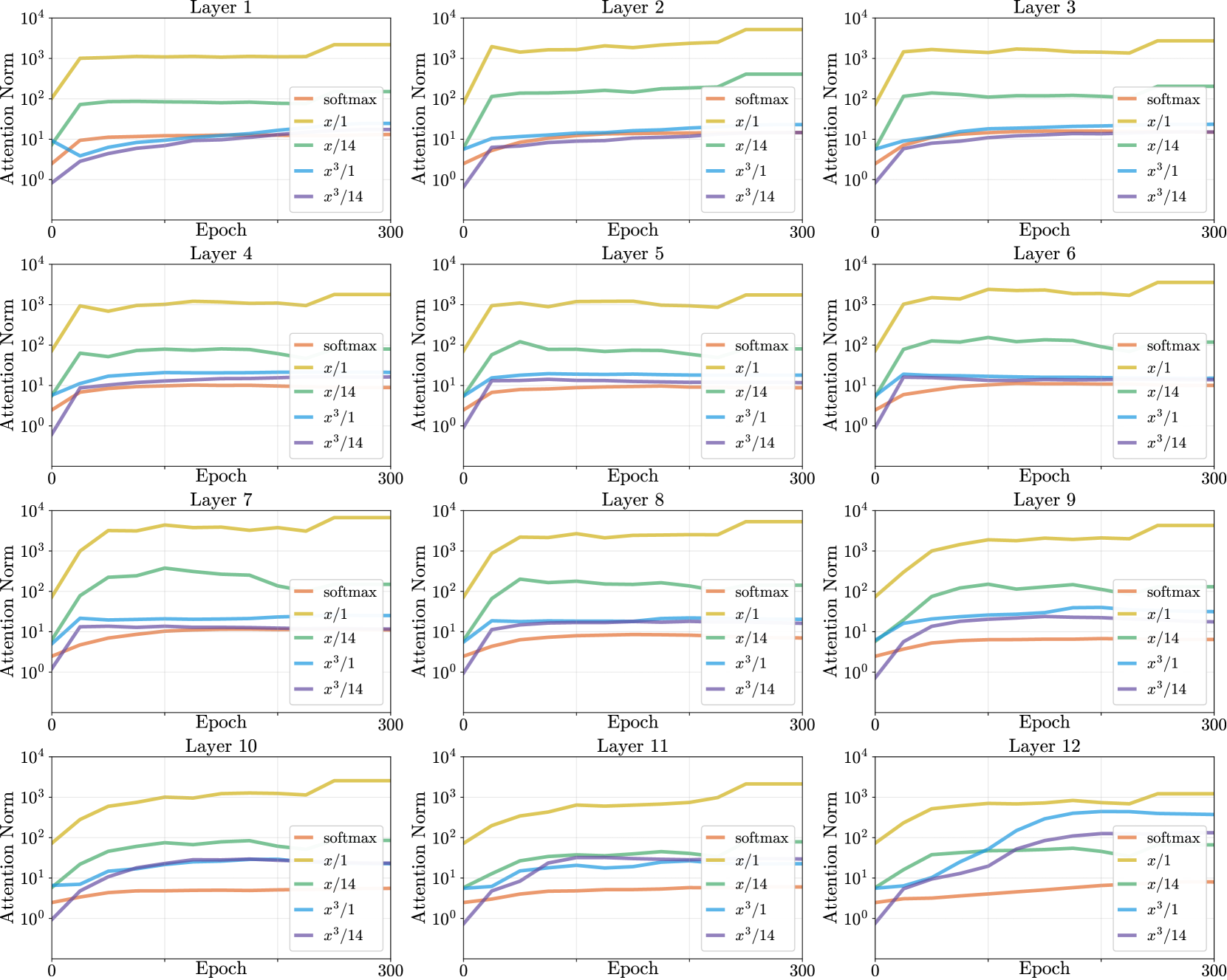<details> <summary>x13.png Details</summary>  ### Visual Description ## Line Graphs: Attention Norm Trends Across 12 Layers ### Overview The image contains 12 line graphs arranged in a 4x3 grid, each representing attention norm dynamics across 300 training epochs for different neural network layers (Layer 1 to Layer 12). All graphs share identical axes and legend configurations, with logarithmic y-axis scaling (10⁰ to 10⁴) and linear x-axis progression (0-300 epochs). Each graph tracks five attention norm trajectories corresponding to different scaling methods. ### Components/Axes - **X-axis**: Epoch (0-300), linear scale - **Y-axis**: Attention Norm (10⁰ to 10⁴), logarithmic scale - **Legend**: Positioned right-aligned in each subplot, containing: - softmax (orange) - x/1 (yellow) - x/14 (green) - x³/1 (blue) - x³/14 (purple) - **Graph Structure**: All subplots share identical formatting with gridlines and axis labels ### Detailed Analysis 1. **Layer 1-3**: - x³/14 (purple) shows gradual ascent from ~10⁰ to ~10² - x³/1 (blue) demonstrates sharper initial growth (~10⁰→10²) then plateaus - softmax (orange) remains relatively flat (~10⁰→10¹) - x/1 (yellow) exhibits moderate growth (~10⁰→10²) - x/14 (green) shows slow linear progression (~10⁰→10¹) 2. **Layer 4-6**: - x³/14 maintains consistent ~10¹-10² range - x³/1 shows ~10¹-10².5 range with minor fluctuations - softmax remains stable at ~10⁰-10¹ - x/1 demonstrates ~10¹-10².5 range - x/14 shows ~10⁰-10¹ range with slight oscillations 3. **Layer 7-9**: - x³/14 exhibits ~10¹-10².5 range with minor fluctuations - x³/1 shows ~10¹-10².5 range with increased volatility - softmax remains stable at ~10⁰-10¹ - x/1 demonstrates ~10¹-10².5 range with minor oscillations - x/14 shows ~10⁰-10¹ range with slight upward trend 4. **Layer 10-12**: - x³/14 demonstrates significant growth (~10¹→10³ in Layer 12) - x³/1 shows ~10¹-10³ range with pronounced upward trend - softmax remains stable at ~10⁰-10¹ - x/1 demonstrates ~10¹-10³ range with gradual ascent - x/14 shows ~10⁰-10² range with moderate growth ### Key Observations 1. **Scaling Method Impact**: - x³/14 consistently shows strongest growth across all layers - softmax demonstrates most stable behavior across layers - x³/1 shows increasing volatility in deeper layers - x/14 maintains moderate growth with layer depth 2. **Layer Depth Correlation**: - Deeper layers (10-12) show more pronounced attention norm growth - x³/14 scaling exhibits exponential growth in later layers - x³/1 demonstrates increasing instability in deeper layers - softmax remains consistently stable regardless of layer depth 3. **Temporal Dynamics**: - All methods show initial growth phase (0-100 epochs) - x³/14 demonstrates sustained growth beyond 200 epochs - x³/1 shows plateauing behavior after initial growth - softmax maintains stable baseline throughout training ### Interpretation The data suggests that different attention scaling methods produce distinct layer-specific dynamics: 1. **x³/14 Scaling**: Most effective for deep layer attention modulation, showing exponential growth particularly in later layers (10-12). This suggests potential for enhanced feature discrimination in deeper network regions. 2. **x³/1 Scaling**: Demonstrates strong initial growth but increasing instability in deeper layers, possibly indicating over-saturation of attention mechanisms. 3. **softmax**: Provides most stable attention distribution across all layers, suggesting reliable but potentially limited expressive capacity. 4. **x/14 Scaling**: Shows moderate growth with layer depth, maintaining balance between stability and adaptability. Notable anomalies include the dramatic x³/14 growth in Layer 12 (~10¹→10³), which may indicate either optimal scaling for deep attention mechanisms or potential overfitting risks. The consistent softmax stability across layers suggests it might be optimal for maintaining balanced attention distribution but could limit model capacity in deeper layers. </details> Figure 13: Frobenius norm of self-attention matrix for different scaled activations on ViT-Small during training (zoom in for better viewing). 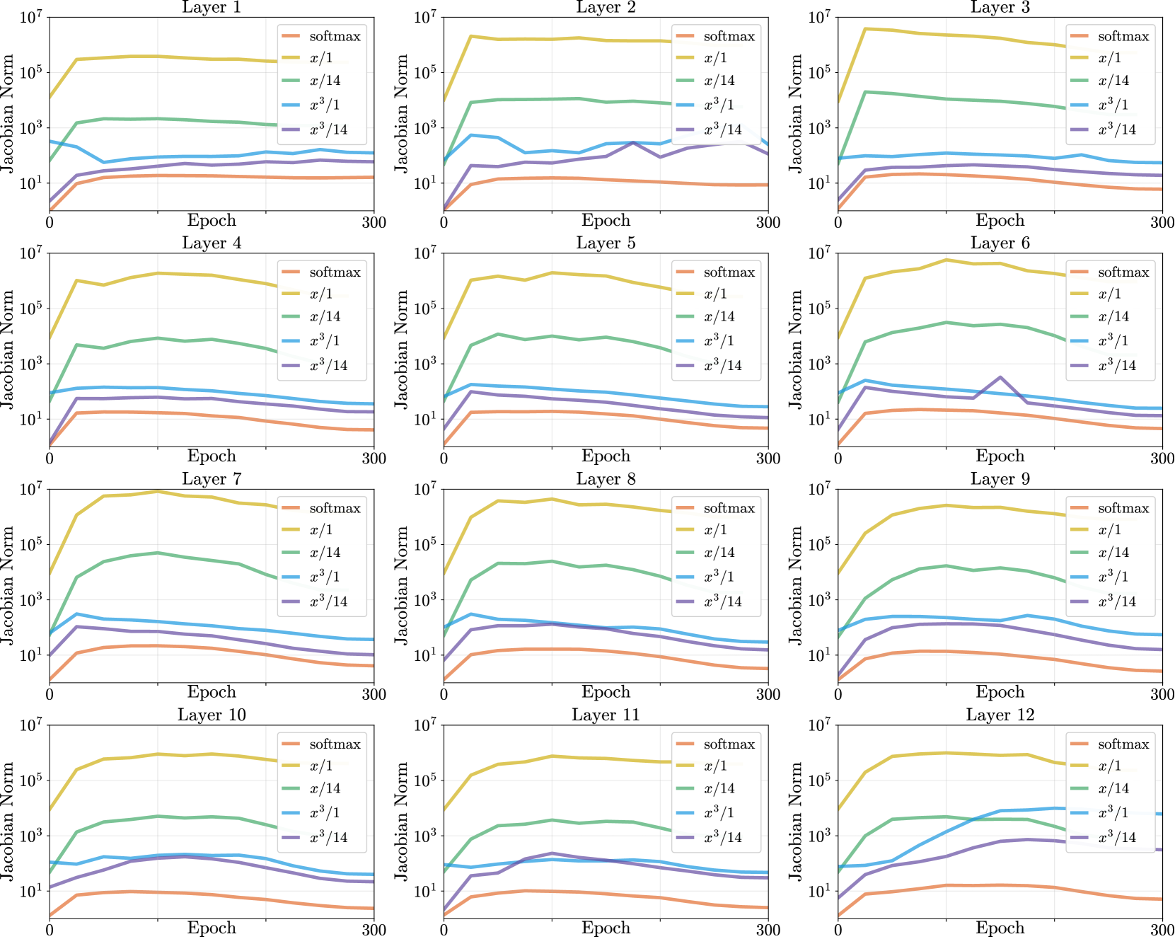<details> <summary>x14.png Details</summary>  ### Visual Description ## Line Chart Grid: Jacobian Norm Evolution Across Neural Network Layers ### Overview The image displays a 3x4 grid of line charts (12 total), each representing the evolution of Jacobian norm magnitudes across 300 training epochs for different neural network layers (Layer 1 to Layer 12). Each subplot compares five activation function variants: softmax, x/1, x/14, x³/1, and x³/14. All charts use logarithmic scales for both axes (Epoch: 0-300; Jacobian Norm: 10¹-10⁷). ### Components/Axes - **X-axis**: Epoch (0-300), linear scale - **Y-axis**: Jacobian Norm (10¹-10⁷), logarithmic scale - **Legend**: Located in the top-right corner of each subplot, with color-coded labels: - Orange: softmax - Yellow: x/1 - Green: x/14 - Blue: x³/1 - Purple: x³/14 - **Subplot Structure**: Each layer (1-12) occupies a separate chart with identical axis ranges and legend positioning. ### Detailed Analysis #### Layer 1-3 Trends - **softmax (orange)**: Gradual decline from ~10¹ to ~10⁰.⁵ across all layers - **x/1 (yellow)**: Sharp initial rise to ~10⁶, then plateau - **x/14 (green)**: Moderate rise to ~10³, followed by stabilization - **x³/1 (blue)**: Volatile fluctuations between 10¹-10³ - **x³/14 (purple)**: Steady decline from ~10¹ to ~10⁰.⁵ #### Layer 4-6 Trends - **softmax (orange)**: Consistent downward trend to ~10⁰.⁵ - **x/1 (yellow)**: Maintains ~10⁶ plateau with minor oscillations - **x/14 (green)**: Stable ~10³ with slight decay in later epochs - **x³/1 (blue)**: Increased volatility in Layer 5 (peak ~10³.⁵) - **x³/14 (purple)**: Layer 6 shows anomalous spike to ~10³ before decay #### Layer 7-12 Trends - **softmax (orange)**: Continued gradual decline to ~10⁰.⁵ - **x/1 (yellow)**: Sustained ~10⁶ with minor fluctuations - **x/14 (green)**: Layer 10 shows increased stability (~10³) - **x³/1 (blue)**: Layer 11 exhibits prolonged elevated values (~10³) - **x³/14 (purple)**: Layer 12 demonstrates sharpest decay to ~10⁰.⁵ ### Key Observations 1. **Activation Function Impact**: - x/1 consistently produces highest Jacobian norms (~10⁶) - softmax and x³/14 show strongest decay patterns - x³/1 exhibits most volatility across layers 2. **Layer-Specific Anomalies**: - Layer 2: x³/14 spike to ~10³ at epoch 150 - Layer 6: x³/14 temporary elevation to ~10³ - Layer 11: x³/1 maintains elevated values beyond other layers 3. **Scale Effects**: - Logarithmic y-axis reveals exponential differences in magnitude - x/1's dominance becomes visually apparent through consistent top placement ### Interpretation The data suggests activation function choice significantly impacts gradient magnitude dynamics during training: - **x/1**'s persistent high norms may indicate stronger gradient propagation but potential instability - **softmax/x³/14**'s decay patterns suggest regularization effects or vanishing gradients - Volatile x³/1 behavior could reflect sensitivity to initialization or layer depth - Layer-specific anomalies (e.g., Layer 2/6 spikes) might correlate with architectural features or training dynamics These patterns align with theoretical expectations: linear activations (x/1) maintain gradient strength, while non-linear variants (softmax, x³/14) introduce decay mechanisms. The x³/14's cubic scaling appears particularly effective at reducing gradient magnitudes across deeper layers. </details> Figure 14: Frobenius norm of Jacobian of self-attention matrix for different scaled activations on ViT-Small during training (zoom in for better viewing).