2411.08561

# LogLLM: Log-based Anomaly Detection Using Large Language Models **Authors**: Wei Guan, Jian Cao1, Shiyou Qian, Jianqi Gao, Chun Ouyang > 1Corresponding author.1Department of Computer Science and Engineering, SJTU, Shanghai, China2The School of Information Systems, QUT, Brisbane, Australia{guan-wei, cao-jian, qshiyou, 193139}@sjtu.edu.cn, c.ouyang@qut.edu.au Abstract Software systems often record important runtime information in logs to help with troubleshooting. Log-based anomaly detection has become a key research area that aims to identify system issues through log data, ultimately enhancing the reliability of software systems. Traditional deep learning methods often struggle to capture the semantic information embedded in log data, which is typically organized in natural language. In this paper, we propose LogLLM, a log-based anomaly detection framework that leverages large language models (LLMs). LogLLM employs BERT for extracting semantic vectors from log messages, while utilizing Llama, a transformer decoder-based model, for classifying log sequences. Additionally, we introduce a projector to align the vector representation spaces of BERT and Llama, ensuring a cohesive understanding of log semantics. Unlike conventional methods that require log parsers to extract templates, LogLLM preprocesses log messages with regular expressions, streamlining the entire process. Our framework is trained through a novel three-stage procedure designed to enhance performance and adaptability. Experimental results across four public datasets demonstrate that LogLLM outperforms state-of-the-art methods. Even when handling unstable logs, it effectively captures the semantic meaning of log messages and detects anomalies accurately. Index Terms: System log, anomaly detection, large language model, deep learning, log analysis I Introduction Ensuring high availability and reliability is crucial for large-scale software-intensive systems [1, 2]. As these systems become more complex and expansive, the occurrence of anomalies becomes unavoidable [3, 4]. Even a minor issue can lead to performance degradation, data integrity problems, and substantial losses in both customers and revenue. Therefore, anomaly detection is vital for maintaining the health and stability of complex software-intensive systems [5]. Software-intensive systems typically produce console logs that record system states and critical runtime events [6]. Engineers can utilize this log data to evaluate system health, identify anomalies, and trace the root causes of issues. However, due to the potentially vast volume of logs, manually analyzing them for anomalies can be both labor-intensive and prone to mistakes [7]. Consequently, log-based anomaly detection has emerged as a key area in automated log analysis, focusing on the automatic identification of system anomalies through log data. Numerous deep learning-based methods [8, 9, 10, 11, 12, 13, 14, 15, 16, 17, 18, 19, 20, 21, 22] for log-based anomaly detection have been proposed. These methods typically employ sequential deep learning models such as LSTM [23] and transformers [24]. These methods can be further divided into reconstruction-based methods [8, 9, 10, 11, 12, 13, 14, 15] and binary classification-based methods [16, 17, 18, 19, 20, 21, 22]. Reconstruction-based methods involve designing and training a deep neural network to reconstruct input log sequences, with anomalies detected based on reconstruction errors. The underlying principle is that anomalous samples cannot be accurately reconstructed. Binary classification-based methods, on the other hand, involve designing a binary classifier to classify samples as either normal or anomalous. These methods often require labeled anomalies for training purposes. It is recognized that system logs are documented in natural language and contain a significant amount of semantic information. Nevertheless, traditional deep learning-based methods struggle to effectively capture this information. In recent years, significant advancements have been achieved in LLMs, such as GPT-4 [25], Llama 3 [26], and ChatGLM [27]. These models are characterized by their vast parameter sizes and are pretrained on substantially larger datasets, ranging from several gigabytes to terabytes in size. This extensive pretraining equips them with remarkable language comprehension abilities, enabling superior performance in tasks such as summarization, paraphrasing, and instruction following even in zero-shot scenarios [28]. Existing methods that utilize LLMs for log-based anomaly detection can be categorized into prompt engineering-based [29, 7, 30, 31] and fine-tuning-based [32, 33, 34, 35, 3, 36, 37, 38, 39, 40] approaches. Prompt engineering-based methods leverage the zero/few-shot capabilities of LLMs to detect anomalies based solely on the models’ internal knowledge. However, these methods often struggle to customize solutions for specific datasets, leading to suboptimal detection performance. Fine-tuning-based methods integrate LLMs into deep neural networks and tailor them to user-specific datasets. Nevertheless, these methods encounter challenges such as limited semantic understanding, suboptimal LLM utilization (relying solely on LLMs for semantic information extraction), and insufficient consideration of input data format, which can lead to memory overflow. To tackle the aforementioned challenges, we propose LogLLM, a novel log-based anomaly detection framework that harnesses LLMs. Unlike traditional methods that rely on log parsers for template extraction, LogLLM preprocesses log messages using regular expressions, thereby streamlining the entire process. LogLLM, a fine-tuning-based method, utilizes BERT, a transformer encoder-based model, to extract semantic vectors from log messages. Additionally, it employs Llama, a transformer decoder-based model, to classify log sequences. To ensure coherence in log semantics, we introduce a projector that aligns the vector representation spaces of BERT and Llama. Our framework is trained using a novel three-stage procedure designed to enhance both performance and adaptability. As illustrated in Section V-G, LLMs frequently face out-of-memory challenges due to their extensive parameter sizes [41]. Directly inputting the entire log sequence (by concatenating log messages into a long string) into Llama can lead to out-of-memory issues and potentially confuse the LLM, making it difficult to focus on key points for distinguishing anomalies. By adopting BERT to summarize each log message, LogLLM effectively mitigates these problems. We conduct experiments across four public datasets, and the results demonstrate that LogLLM outperforms state-of-the-art methods. Even when handling unstable logs, where new log templates frequently emerge due to software evolution, it effectively captures the semantic meaning of log messages and detects anomalies accurately. The ablation study confirms the effectiveness of the three-stage training procedure. The main contributions of our work are as follows: - We introduce LogLLM, a novel log-based anomaly detection framework leveraging LLMs. This study marks the first attempt to simultaneously employ transformer encoder-based and decoder-based LLMs, specifically BERT and Llama, for log-based anomaly detection. - We propose a novel three-stage procedure to optimize the training and coordination of different components within the deep model, enhancing both performance and adaptability. - We conduct extensive experiments on four publicly available real-world datasets, demonstrating that LogLLM achieves exceptional performance. II Related Work In this section, we explore related work in the field of log-based anomaly detection, with a particular focus on deep learning-based methods. We give special attention to approaches that utilize pretrained LLMs. II-A Traditional Deep Learning for Log-based Anomaly Detection Many traditional deep learning-based methods for log-based anomaly detection have been proposed. These works can be grouped into two types based on the training paradigm: reconstruction-based methods and binary classification-based methods. Reconstruction-based methods [8, 9, 10, 11, 12, 13, 14, 15] involve designing and training a deep neural network to reconstruct input log sequences. Anomalies are detected based on reconstruction errors. Normal log sequences can be reconstructed with minimal errors, while anomalous log sequences cannot be effectively reconstructed, resulting in significantly higher reconstruction errors. These methods consistently train the deep model on normal data that is free of anomalies, which means they are semi-supervised. DeepLog [8] adopts LSTM to predict the next log template ID based on past log sequences. Similarly, LogAnomaly [9] predicts the next log template ID based on both sequential and quantitative patterns. Autoencoders (AEs) [10, 11, 12, 13] and generative adversarial networks (GANs) [14, 15] are widely used in reconstruction-based methods. For example, LogAttn [10] adopts an AE that incorporates a temporal convolutional network (TCN) to capture temporal semantic correlations and a deep neural network (DNN) to capture statistical correlations. Duan et al. [14] use a GAN, where an encoder-decoder framework based on LSTM serves as the generator. Convolutional neural networks (CNNs) are used as the discriminator. The reconstruction error is calculated based on the difference between the input and the output from the generator. Binary classification-based methods [16, 17, 18, 19, 20, 21, 22] often employ deep neural networks that output either one or two values. Typically, a single value represents the probability that a sample belongs to the anomalous class, and anomalies are detected by applying a threshold to convert this probability into a binary classification. When two values are output, they represent the probabilities of the sample belonging to the normal and anomalous classes, respectively. Most methods [16, 17, 18, 19, 20] typically train deep models in a supervised manner. For example, Zhang et al. [16] propose LayerLog, which integrates word, log, and logseq layers to extract semantic features from log sequences. CNNs are utilized in [17, 18] to develop a binary classifier. LogRobust [19] integrates a pre-trained Word2Vec model, specifically FastText [42], and combines it with TF-IDF weights to learn representation vectors of log templates. These vectors are then fed into an attention-based Bi-LSTM model for anomaly detection. LogGD [20] transforms log sequences into graphs and utilizes a graph transformer neural network that combines graph structure and node semantics for log-based anomaly detection. Some work [21, 22] involves training binary classifiers in a semi-supervised manner. For example, Trine [21] uses a transformer encoder [24] to encode normal log sequences into vector representations and a generator to produce random fake vector representations. The discriminator, which is composed of a transformer and a multi-layer perceptron (MLP), is trained to distinguish whether the given vector representations are normal log sequences and it is subsequently used to detect anomalies. PLELog [22] tackles the challenge of insufficient labeling by employing probabilistic label estimation and develops an attention-based GRU neural network for anomaly detection. It is acknowledged that system logs are recorded in natural language and contain a substantial amount of semantic information. However, traditional deep learning-based methods face challenges in capturing this information. II-B LLMs for Log-based Anomaly Detection Existing LLMs can be categorized into transformer encoder-based models, such as BERT [43], RoBERTa [44], and SpanBERT [45], and transformer decoder-based models, including GPT-4 [25], Llama 3 [26], and ChatGLM [27]. Two prevalent strategies for utilizing LLMs are prompt engineering and fine-tuning. Prompt engineering-based methods [29, 7, 30, 31] detect anomalies solely by relying on the internal knowledge of LLMs. These methods typically employ transformer decoder-based models. For instance, Qi et al. [7] employ ChatGPT for zero-shot and few-shot log-based anomaly detection, utilizing prompt templates that integrate the log sequence directly. However, this approach becomes impractical when using a large window size for grouping log messages. Egersdoerfer et al. [30] address this issue by maintaining a summary-based memory, which summarizes the previous log messages, eliminating the need to input the entire log sequence for anomaly detection. RAGLog [31] uses a retrieval augmented generative (RAG) framework [46] to analyze log entries by querying its store of samples of normal log entries. They design prompt templates for LLMs to determine whether a queried log entry is normal or abnormal. Prompt engineering-based methods often struggle to customize solutions for specific datasets, which can lead to suboptimal detection performance in particular datasets. <details> <summary>x1.png Details</summary>  ### Visual Description ### Technical Document Extraction: System Log Data Table This image displays a structured technical log, likely from a high-performance computing system (indicated by the "RAS KERNEL INFO" and hardware location strings). The image is segmented into two primary logical regions: **Header** (left, green border) and **Content** (right, blue border). --- #### 1. Component Isolation * **Header Region (Left):** Contains metadata including Unix timestamps, dates, hardware location identifiers, high-precision timestamps, and log source classification. * **Content Region (Right):** Contains the specific error messages or status updates associated with the corresponding header entry. * **Footer/Ellipses:** Both sections end with "..." indicating that this is a truncated sample of a larger dataset. --- #### 2. Data Table Reconstruction The following table reconstructs the textual information provided in the image. The data is organized into three distinct log entries. | Entry | Header Data (Metadata & Timestamps) | Content (Log Message) | | :--- | :--- | :--- | | **1** | 1117838978 2005.06.03 R02-M1-N0-C:J12-U11 2005-06-03-15.49.38.026704 R02-M1-N0-C:J12-U11 RAS KERNEL INFO | instruction cache parity error corrected | | **2** | 1117843015 2005.06.03 R21-M1-N6-C:J08-U11 2005-06-03-16.56.55.309974 R21-M1-N6-C:J08-U11 RAS KERNEL INFO | 141 double-hummer alignment exceptions | | **3** | 1117848119 2005.06.03 R16-M1-N2-C:J17-U01 2005-06-03-18.21.59.871925 R16-M1-N2-C:J17-U01 RAS KERNEL INFO | CE sym 2, at 0x0b85eee0, mask 0x05 | | **...** | ... | ... | --- #### 3. Detailed Content Analysis **Header Structure Breakdown:** Each line in the Header follows a consistent pattern: 1. **Unix Epoch Timestamp:** (e.g., `1117838978`) 2. **Date (YYYY.MM.DD):** (e.g., `2005.06.03`) 3. **Hardware Location ID:** A string identifying the Rack, Module, Node, and Component (e.g., `R02-M1-N0-C:J12-U11`). 4. **Full ISO Timestamp:** (e.g., `2005-06-03-15.49.38.026704`) 5. **Redundant Location ID:** Repeats the hardware location string. 6. **Log Source:** `RAS KERNEL INFO` (Reliability, Availability, and Serviceability kernel information). **Content/Message Analysis:** * **Entry 1:** Reports a corrected hardware error related to the instruction cache parity. * **Entry 2:** Reports a specific count (141) of "double-hummer alignment exceptions," which refers to a specific floating-point unit architecture (Double Hummer) used in IBM Blue Gene/L systems. * **Entry 3:** Reports a Correctable Error (CE) at a specific memory address (`0x0b85eee0`) with a bitmask (`0x05`). --- #### 4. Spatial and Trend Observations * **Spatial Placement:** The "Header" label is centered at the top of the green box. The "Content" label is centered at the top of the blue box. * **Temporal Trend:** The timestamps show a chronological progression throughout the day of June 3, 2005, starting at 15:49:38 and ending at 18:21:59. * **Hardware Variation:** Each log entry originates from a different hardware component (R02, R21, and R16), suggesting these are system-wide logs rather than logs from a single node. </details> Figure 1: An example of a system log. Fine-tuning-based methods [32, 33, 34, 35, 3, 36, 37, 38, 39, 40] incorporate LLMs into deep neural networks and customize them to the user’s own dataset. Some methods [32, 33, 34, 35], although adopting transformer encoder-based LLMs for anomaly detection, do not capture the semantic information within log sequences. For example, LogBERT [32] and LAnoBERT [33] utilize BERT to reconstruct the input sequence of log template IDs (IDs of log string templates) and detect anomalies based on reconstruction errors, disregarding the semantic information. Other methods [3, 36, 37, 38, 39] use transformer encoder-based LLMs solely for extracting semantic information from log messages and then employ either smaller models [3, 36, 37, 38] or distance-based comparison [39] for classification. For instance, NeuralLog [3] leverages BERT to extract semantic vectors from raw log messages, which are subsequently used to detect anomalies via a transformer-based classification model. Similarly, RAPID [39] utilizes transformer encoder-based models to extract semantic vectors and performs anomaly detection by comparing each query log sequence with its nearest document log sequence. Hadadi et al. [40] directly input template sequences parsed from log sequences, into GPT models and fine-tune it to accurately predict sequence labels. However, this approach faces two key challenges. First, the boundaries between templates within the sequences are unclear, making it difficult for the model to learn the sequential dependencies. Second, each template may be tokenized into multiple tokens by the LLM’s tokenizer, and a single sequence can contain numerous log templates. As a result, an excessive number of tokens may be generated, often exceeding the token (memory) limits of LLMs [41], thereby restricting the length of sequences that can be processed. These two challenges are further demonstrated in Section V-G. LogLLM is a fine-tuning-based method that utilizes BERT for extracting semantic vectors from log messages and Llama, a transformer decoder-based model, for log sequence classification. This method aligns the vector representation spaces of BERT and Llama using a projector. The use of BERT ensures clear boundaries between log messages, as each message is represented by a distinct embedding vector, thereby enhancing classification performance. Moreover, when memory and parameter size of Llama are held constant, this approach can handle longer sequences compared to directly tokenizing the entire log sequence using Llama’s tokenizer. III Preliminaries To establish the groundwork for subsequent sections, we introduce the system log, which records the system’s events and internal states during runtime. A system log contains a list of log messages in chronological order. 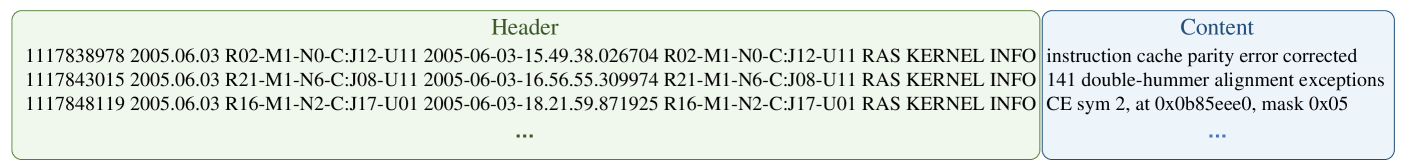Fig. 1 presents a snippet of a raw system log generated by the BGL (the BlueGene/L supercomputer system), with each log message ordered according to the recorded time. These raw log messages are semi-structured texts consisting of a header and content. The header, determined by the logging framework, includes information such as timestamp, verbosity level (e.g., WARN/INFO), and component [47]. The log content comprises a constant part (keywords that reveal the log template) and a variable part (parameters that carry dynamic runtime information). In this paper, we focus solely on the content of each log message. <details> <summary>x2.png Details</summary>  ### Visual Description # Technical Document Extraction: Log Session Windowing Diagram ## 1. Overview This image is a technical diagram illustrating the process of partitioning a continuous **System Log** into discrete **Log Sequences** based on specific identifiers (Block IDs) using a "Session window" mechanism. The diagram uses color-coding to track specific data blocks across different log views. --- ## 2. Component Isolation ### Region A: Source (System Log) Located on the left side of the diagram, this represents the raw, interleaved stream of log entries. **Table: System Log Content** | Line # | Log Entry Text | | :--- | :--- | | 1 | Receiving block <span style="color:red">blk_-5632101276183739500</span> src: /10.251.27.63:36433 dest: /10.251.27.63:50010 | | 2 | BLOCK* NameSystem.allocateBlock: /user/root/randtxt4/_temporary/task_200811101024/part-00999. <span style="color:red">blk_-5632101276183739500</span> | | 3 | Receiving block <span style="color:blue">blk_-4506306395053060141</span> src: /10.251.193.175:40709 dest: /10.251.193.175:50010 | | 4 | PacketResponder 0 for block <span style="color:red">blk_-5632101276183739500</span> terminating | | ... | ... | --- ### Region B: Process (Session Window) A central horizontal arrow points from the System Log to the Log Sequences. * **Label:** "Session window" * **Function:** This represents the logic that filters and groups the interleaved log entries into separate sequences based on the unique Block ID. --- ### Region C: Output (Log Sequences) Located on the right side, consisting of stacked windows representing filtered views of the original log. #### **Log Sequence #1 (For blk_-5632101276183739500)** This sequence extracts only the entries related to the red-colored Block ID. | Line # | Log Entry Text | | :--- | :--- | | 1 | Receiving block <span style="color:red">blk_-5632101276183739500</span> src: /10.251.27.63:36433 dest: /10.251.27.63:50010 | | 2 | BLOCK* NameSystem.allocateBlock: /user/root/randtxt4/_temporary/task_200811101024/part-00999. <span style="color:red">blk_-5632101276183739500</span> | | 3 | PacketResponder 0 for block <span style="color:red">blk_-5632101276183739500</span> terminating | | ... | ... | #### **Log Sequence #2 (For blk_-4506306395053060141)** This sequence (partially obscured in the background) extracts entries related to the blue-colored Block ID. | Line # | Log Entry Text | | :--- | :--- | | 1 | Receiving block <span style="color:blue">blk_-4506306395053060141</span> src: /10.251.193.175:40709 dest: /... | *Note: There is a vertical ellipsis (⋮) above the sequences, indicating that multiple such sequences are generated for different block IDs.* --- ## 3. Data Mapping & Trend Verification ### Color Coding Logic * **Red Text:** Refers to `blk_-5632101276183739500`. In the System Log, these appear at lines 1, 2, and 4. In Log Sequence #1, they are consolidated into a continuous sequence (lines 1, 2, and 3). * **Blue Text:** Refers to `blk_-4506306395053060141`. In the System Log, this appears at line 3. In the output, it is moved to the first line of Log Sequence #2. ### Flow Analysis 1. **Input:** A single stream where events for different processes (blocks) are mixed chronologically. 2. **Transformation:** The "Session window" identifies the unique identifier in each line. 3. **Output:** The stream is demultiplexed. Each unique identifier gets its own dedicated "Log Sequence" window, maintaining the relative chronological order of events for that specific identifier while removing unrelated noise. </details> (a) Session window <details> <summary>x3.png Details</summary>  ### Visual Description # Technical Document Extraction: Log Processing Diagram This image illustrates a data preprocessing workflow where a continuous **System Log** is partitioned into discrete **Log Sequences** using a sliding window mechanism. ## 1. Component Isolation The diagram is divided into three primary functional regions: * **Source (Left):** A table representing the raw "System Log". * **Transformation (Center):** Text and an arrow describing the logic applied to the source. * **Output (Right):** A stack of tables representing the resulting "Log Sequences". --- ## 2. Source Data: System Log The source is a structured table containing sequential log entries. | Line # | Log Content | | :--- | :--- | | 1 | iar 00106ba8 dear 0246dd1c | | 2 | 5052567 floating point alignment exceptions | | 3 | CE sym 25, at 0x10e1bce0, mask 0x40 | | 4 | invalid operation exception (software)...0 | | 5 | L3 ecc control register: 00000000 | | ... | ... | --- ## 3. Transformation Logic A horizontal arrow points from the System Log to the Log Sequences, indicating a data flow. The following parameters define the transformation: * **Mechanism:** Sliding window * **Window size:** 2 (Each output sequence contains 2 log entries) * **Step size:** 2 (The window moves forward by 2 entries for each new sequence, resulting in non-overlapping blocks in this specific example) --- ## 4. Output Data: Log Sequences The output consists of multiple overlapping tables (Log Sequence #1, #2, #3, etc.). Based on the "Step size: 2", the entries are grouped as follows: ### Log Sequence #1 | Line # | Log Content | | :--- | :--- | | 1 | iar 00106ba8 dear 0246dd1c | | 2 | 5052567 floating point alignment exceptions | ### Log Sequence #2 | Line # | Log Content | | :--- | :--- | | 1 | CE sym 25, at 0x10e1bce0, mask 0x40 | | (2)* | *[Implicitly: invalid operation exception (software)...0]* | *Note: The visual for Sequence #2 only explicitly shows the first line of its window (Source Line 3).* ### Log Sequence #3 | Line # | Log Content | | :--- | :--- | | 1 | L3 ecc control register: 00000000 | *Note: The visual for Sequence #3 shows the first line of its window (Source Line 5). The stack continues upward as indicated by the vertical ellipsis (⋮).* --- ## 5. Summary of Flow and Trends The diagram demonstrates a **fixed-window segmentation** of log data. Because the **Window size** and **Step size** are both equal to **2**, the system is performing a "tumbling window" or non-overlapping partition. * **Sequence #1** captures Source Lines 1-2. * **Sequence #2** captures Source Lines 3-4. * **Sequence #3** captures Source Lines 5-6. This process transforms a continuous stream of unstructured or semi-structured text into fixed-length packets suitable for machine learning input or batch analysis. </details> (b) Sliding window Figure 2: Illustrative examples of log message partitioning. 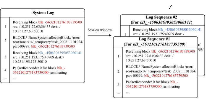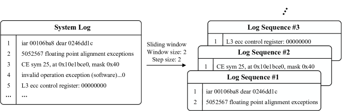The log messages can be grouped into log sequences (i.e., series of log messages that record specific execution flows) based on session or fixed/sliding windows [48]. Session window partitioning groups log messages according to their session IDs, thereby generating sequences that include the log messages within each session. For example, Fig. 2a illustrates the HDFS [49] logs undergoing the session window grouping process, where the block_id serves as the session ID. In contrast, fixed/sliding window partitioning groups log messages based on a fixed size (window size), which can be defined by either the time span or the number of log messages. This method creates sequences that capture snapshots of system log messages over time. For example, Fig. 2b illustrates the BGL [50] logs undergoing the sliding window grouping process, with a window size of 2 messages and a step size of 2 messages. The objective of log-based anomaly detection is to identify anomalous log sequences, facilitating the recognition of potential issues within the system’s operational behavior. 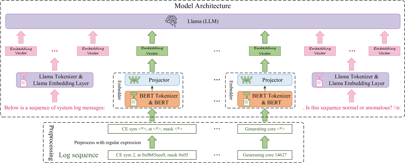IV Methodology In this section, we present our innovative anomaly detection framework, LogLLM. As illustrated in Fig. 3, the log sequence undergoes preprocessing using regular expressions before being fed into a deep neural network that integrates BERT [43], a projector, and Llama [26] for log sequence classification. In the following sections, we will provide detailed insights into log sequence preprocessing, the architecture of the deep model, and the model training procedure. <details> <summary>x4.png Details</summary>  ### Visual Description # Technical Document Extraction: Model Architecture for Log Analysis ## 1. Overview The image illustrates a technical architecture for a Large Language Model (LLM) based system designed to analyze system log sequences for anomaly detection. The architecture integrates a pre-trained LLM (Llama) with specialized embedders (BERT) to process both natural language prompts and structured log data. --- ## 2. Component Segmentation ### Region 1: Header / Core Model * **Main Container:** Labeled "Model Architecture" (dashed boundary). * **Central Processor:** A large purple horizontal block labeled **"Llama (LLM)"** with a brain icon. This serves as the primary reasoning engine. ### Region 2: Input Processing (Prompting) This region handles the natural language context surrounding the log data. * **Text Prompts:** * **Prefix (Left):** "Below is a sequence of logs..." * **Suffix (Right):** "Is this sequence anomalous?" * **Embedding Layer:** Both prefix and suffix are processed through a **BERT Embedder** (represented by blue blocks) to convert text into vector representations. ### Region 3: Log Sequence Processing This region handles the structured log data. * **Log Sequence:** A series of discrete log events (e.g., Log 1, Log 2, ..., Log N). * **Log Embedder:** Each log entry is passed through a dedicated **BERT Embedder**. * **Vector Representation:** The output is a sequence of vectors ($v_1, v_2, ..., v_n$). ### Region 4: Integration and Output * **Concatenation:** The embedded Prefix, Log Vectors, and Suffix are concatenated into a single input sequence for the Llama model. * **Output:** The model generates a classification or response based on the integrated context. </details> Figure 3: The framework of LogLLM. Notably, the model includes a single instance of BERT and the projector. IV-A Preprocessing Considering that the log message content includes variable parameters carrying dynamic runtime information, which is always irrelevant to the anomalies and complicates deep model training, as demonstrated in Section V-F, a technique is needed to identify these parameters and replace them with a constant token. Log parsers, such as Drain [51] and Spell [52], are widely adopted in log-based anomaly detection methods and appear to be a useful technique. However, as noted by Le et al. [3], existing log parsers do not always perform correctly on all log datasets and struggle to handle out-of-vocabulary (OOV) words in new log messages, resulting in a loss of semantic information. When logs are unstable, these parsers become increasingly ineffective over time, making it difficult to support subsequent anomaly detection. Thanks to the structured log generation process, the textual format of parameters representing specific objects can be easily identified using regular expressions [53]. Consequently, we replace each variable parameter, such as account, directory path, and IP address, with ‘<*>’. Despite its simplicity, this technique offers significant performance advantages. Compared with log parsers, this preprocessing technique is more effective and does not require training. IV-B Model Architecture As shown in Fig. 3, our deep model consists of three main components: BERT, a projector, and Llama. Both BERT and Llama are pretrained LLMs. BERT is utilized to extract vector representations of log messages, while Llama is employed to classify the log sequences. The projector serves as a bridge, aligning the vector representation spaces of BERT and Llama. It is important to note that our model incorporates only one instance of BERT and one projector. IV-B 1 BERT BERT generates a semantic vector by processing the semantic vector of the classification token ([CLS]) through a linear layer followed by a tanh activation function. Each log message, once preprocessed, is encoded into a semantic vector using the BERT tokenizer and BERT model. For a preprocessed log sequence, the output of BERT is a sequence of semantic vectors $C=(c_{1},c_{2},...,c_{N})∈\mathbb{R}^{N× d_{BERT}}$ , where $N$ represents the length of the log sequence (i.e., the number of log messages) and $d_{BERT}$ is the dimension of each semantic vector (i.e., hidden size). IV-B 2 Projector The projector is a linear layer that maps the semantic vectors $C∈\mathbb{R}^{N× d_{BERT}}$ to the token embedding vectors accepted by Llama, represented as $E=(e_{1},e_{2},...,e_{N})∈\mathbb{R}^{N× d_{Llama}}$ , where $d_{Llama}$ is the hidden size of Llama. The projector is designed to align the vector representation spaces of BERT and Llama. IV-B 3 Llama To conduct prompt tuning on Llama, the transformer decoder-based LLM, we generate corresponding textual queries based on embedded log sequences. Specifically, each query consists of three components. The first component introduces the log sequence, such as " Below is a sequence of system log messages: ". The second component comprises the token embeddings $E$ output by the projector. The third component queries whether the sequence is anomalous, asking, for instance, ". Is this sequence normal or anomalous? ". The first and third components are fed into the Llama tokenizer and Llama embedding layer sequentially, producing $E_{1}∈\mathbb{R}^{A× d_{Llama}}$ and $E_{3}∈\mathbb{R}^{Q× d_{Llama}}$ , where $A$ and $Q$ are the number of tokens produced by tokenizing the first and third components, respectively. Then, the token embeddings of the three components are concatenated, represented as $[E_{1}||E||E_{3}]∈\mathbb{R}^{(A+N+Q)× d_{Llama}}$ and fed into Llama. IV-C Training IV-C 1 Minority Class Oversampling LogLLM is a supervised anomaly detection method, which means it needs labeled normal and anomalous samples for training. However, supervised anomaly detection methods often face the challenge of data imbalance, which can lead to biased model training. In an anomaly detection task, there are only two classes: normal and anomalous, and the number of instances in each class is uncertain. To cope with data imbalance, we oversample the class with fewer samples, ensuring that the proportion of the minority class is no less than $\beta$ . Formally, let the proportion of the minority class be $\alpha$ and $\alpha<\beta$ , and the total number of samples be $Sample\_num$ . To achieve a proportion of $\beta$ for the minority class, it will be oversampled to the following quantity: $$ \frac{\beta(1-\alpha)}{1-\beta}\times Sample\_num \tag{1} $$ This adjustment will make the proportion of the minority class equal to $\beta$ . IV-C 2 Training Objective Our objective is to train the deep model to predict whether a given log sequence is normal or anomalous. We fine-tune the model to respond appropriately: if the sequence is anomalous, it outputs ‘ The sequence is anomalous. ’; if normal, it outputs ‘ The sequence is normal. ’. We utilize cross-entropy loss [54] as our loss function. IV-C 3 Training Procedure To train our deep model, we follow three main stages. Stage 1. Fine-tuning Llama to capture the answer template: The first stage involves fine-tuning Llama to capture the answer template. Specifically, we train Llama to respond to the prompt ‘ Is this sequence normal or anomalous? ’ with ‘ The sequence is anomalous/normal. ’. This stage requires only a few data samples. Stage 2. Training the embedder of log messages: The second stage involves training the embedder of log messages, specifically BERT and the projector. This stage aims to project each log message to the embedding of the most suitable token in Llama, enabling Llama to discern whether the given log sequence is normal or anomalous. Stage 3. Fine-tuning the entire model: Finally, we fine-tune the entire model to ensure cohesive and accurate performance across all components. IV-C 4 Efficient Fine-Tuning on LLMs To reduce the costs involved in fine-tuning LLMs (BERT and Llama) with a substantial number of parameters, we utilize QLoRA [55] to minimize memory usage. QLoRA accomplishes this by backpropagating gradients into a frozen 4-bit quantized model, while maintaining the performance levels achieved during the full 16-bit fine-tuning process. V Experiments In this section, we conduct extensive experiments on four real-life logs to investigate the following research questions (RQs): - RQ1: How effective is LogLLM in log-based anomaly detection? - RQ2: How do different preprocessing techniques impact the performance of LogLLM? - RQ3: How effective is the embedder for Llama? - RQ4: How does the size of the Llama model affect the performance of LogLLM? - RQ5: How does each stage of the three-stage training process influence the performance of LogLLM? - RQ6: How do different levels of minority class oversampling, determined by the hyperparameter $\beta$ , affect the performance of LogLLM? LogLLM is coded in Python, and the source code is available at https://github.com/guanwei49/LogLLM. V-A Benchmark Methods To verify the superiority of the proposed method, we compare LogLLM with five state-of-the-art semi-supervised methods: DeepLog [8], LogAnomaly [9], PLELog [22], FastLogAD [34], and LogBERT [32]. We also compare it with three supervised methods: LogRobust [19], CNN [18] and NeuralLog [3], and one method that does not require training a deep model but needs some normal samples for retrieval: RAPID [39]. Notably, FastLogAD, LogBERT, NeuralLog, and RAPID adopt LLMs for anomaly detection. V-B Experimental Settings We conduct all experiments on a server equipped with an Intel Xeon Gold 6330 CPU (38 cores), 256GB of memory, and an NVIDIA A40 GPU with 48 GB of memory. In our experiment, we utilize the BERT-base model https://huggingface.co/google-bert/bert-base-uncased and Llama-3-8B model https://huggingface.co/meta-llama/Meta-Llama-3-8B as backbones. The hyperparameter $\beta$ , which is described in Section IV-C 1, is set to 30%. We use the AdamW optimizer [56] to train the model with a mini-batch size of 16. Unless otherwise specified, the training procedure is configured as follows: In the first stage, only 1,000 samples are involved with a learning rate of 5e-4. The second and third stages each consist of two epochs with a learning rate of 5e-5. For a fair comparison, we configure the hyperparameters for all compared methods according to the values provided in their original articles. V-C Metrics We evaluate the performance of these methods using the widely adopted $Precision$ , $Recall$ and $F_{1}\!-\!score$ . These metrics are calculated as follows: $$ Precision=\frac{TP}{TP+FP} \tag{2} $$ $$ Recall=\frac{TP}{TP+FN} \tag{3} $$ $$ F_{1}\!-\!score=\frac{2*Precision*Recall}{Precision+Recall} \tag{4} $$ , where $TP$ , $FN$ , $FP$ represent true positives, false negatives and false positives respectively. Precision refers to the percentage of correctly detected anomalies among all anomalies identified by the model, while recall represents the percentage of anomalies that are correctly identified from all real anomalies. The F 1 -score combines these two metrics into a single measure, providing a balanced assessment of the model’s performance in detecting anomalies. V-D Dataset TABLE I: The statistics of datasets used in the experiments. | | # Log messages # Log sequences | # Log sequences # Anomalies | Training Data Anomaly ratio | Testing Data # Log sequences | # Anomalies | Anomaly ratio | | | | --- | --- | --- | --- | --- | --- | --- | --- | --- | | HDFS | 11,175,629 | 575,061 | 460,048 | 13,497 | 2.93% | 115,013 | 3,341 | 2.90% | | BGL | 4,747,963 | 47,135 | 37,708 | 4,009 | 10.63% | 9,427 | 817 | 8.67% | | Liberty | 5,000,000 | 50,000 | 40,000 | 34,144 | 85.36% | 10,000 | 651 | 6.51% | | Thunderbird | 10,000,000 | 99,997 | 79,997 | 837 | 1.05% | 20,000 | 29 | 0.15% | To evaluate our method for log-based anomaly detection, we selected four public datasets [57]: HDFS, BGL, Liberty, and Thunderbird. The details for each dataset are provided below: HDFS (Hadoop Distributed File System) dataset [49] is generated by running Hadoop-based mapreduce jobs on over 200 Amazon EC2 nodes and contains a total of 11,175,629 log messages. These log messages are grouped into different log windows based on their block_id, which reflect program executions in the HDFS, resulting in 575,061 blocks. Among these, 16,838 blocks (2.93%) indicate system anomalies. BGL (Blue Gene/L) dataset [50] is a supercomputing system log dataset collected from a BlueGene/L supercomputer system at lawrence livermore national labs (LLNL). The dataset contains 4,747,963 log messages, each of which has been manually labeled as either normal or anomalous. There are 348,460 log messages (7.34%) that are labeled as anomalous. Thunderbird dataset [50] is a publicly accessible collection of log data sourced from the Thunderbird supercomputer at sandia national laboratories (SNL). This dataset consists of both normal and anomalous messages, each of which has been manually categorized. Although the dataset contains over 200 million log messages, we focus on a subset of 10 million continuous log messages for computational efficiency. This subset includes 4,937 anomalous log messages, representing approximately 0.049% of the total. Liberty dataset [50] comprises system logs from the Liberty supercomputer at sandia national labs (SNL) in Albuquerque. This supercomputer features 512 processors and 944 GB of memory, and the dataset contains over 200 million log messages. For computational efficiency, we sample 5 million consecutive log messages, among which 1,600,525 are identified as anomalous, constituting approximately 32.01% of the total sampled messages. In the context of HDFS, we adopt a session window strategy, which involves grouping log messages into sequences based on the block_id present in each log message. Each session is labeled using ground truth. For other datasets, including BGL, Thunderbird, and Liberty, we utilize a sliding window strategy to group log messages, with a window size of 100 messages and a step size of 100 messages. A log sequence is deemed anomalous if it contains at least one anomalous log message according to the ground truth. Similar to existing work [19, 8, 9, 22, 39, 34], we split each dataset into a training set and a testing set with a ratio of 8:2 to evaluate the performance of a log-based anomaly detection approach. For the HDFS dataset, we randomly split the log sequences into training and testing data. In contrast, for the BGL, Thunderbird, and Liberty datasets, we adhere to a chronological split [6]. This strategy ensures that all log sequences in the training set precede those in the testing set, reflecting real-world conditions and mitigating potential data leakage from unstable log data. Table I summarizes the statistics of the datasets used in the experiments. V-E Performance Evaluation (RQ1) TABLE II: Experimental results on HDFS, BGL, Liberty, and Thunderbird datasets. The best results are highlighted in bold. | DeepLog LogAnomaly PLELog | $\usym{2714}$ $\usym{2714}$ $\usym{2714}$ | 0.835 0.886 0.893 | 0.994 0.893 0.979 | 0.908 0.966 0.934 | 0.166 0.176 0.595 | 0.988 0.985 0.880 | 0.285 0.299 0.710 | 0.751 0.684 0.795 | 0.855 0.876 0.874 | 0.800 0.768 0.832 | 0.017 0.025 0.808 | 0.966 0.966 0.724 | 0.033 0.050 0.764 | 0.506 0.521 0.810 | | --- | --- | --- | --- | --- | --- | --- | --- | --- | --- | --- | --- | --- | --- | --- | | FastLogAD | $\usym{2714}$ | 0.721 | 0.893 | 0.798 | 0.167 | 1.000 | 0.287 | 0.151 | 0.999 | 0.263 | 0.008 | 0.931 | 0.017 | 0.341 | | LogBERT | $\usym{2714}$ | 0.989 | 0.614 | 0.758 | 0.165 | 0.989 | 0.283 | 0.902 | 0.633 | 0.744 | 0.022 | 0.172 | 0.039 | 0.456 | | LogRobust | $\usym{2714}$ | 0.961 | 1.000 | 0.980 | 0.696 | 0.968 | 0.810 | 0.695 | 0.979 | 0.813 | 0.318 | 1.000 | 0.482 | 0.771 | | CNN | $\usym{2714}$ | 0.966 | 1.000 | 0.982 | 0.698 | 0.965 | 0.810 | 0.580 | 0.914 | 0.709 | 0.870 | 0.690 | 0.769 | 0.818 | | NeuralLog | $\usym{2717}$ | 0.971 | 0.988 | 0.979 | 0.792 | 0.884 | 0.835 | 0.875 | 0.926 | 0.900 | 0.794 | 0.931 | 0.857 | 0.893 | | RAPID | $\usym{2717}$ | 1.000 | 0.859 | 0.924 | 0.874 | 0.399 | 0.548 | 0.911 | 0.611 | 0.732 | 0.200 | 0.207 | 0.203 | 0.602 | | LogLLM | $\usym{2717}$ | 0.994 | 1.000 | 0.997 | 0.861 | 0.979 | 0.916 | 0.992 | 0.926 | 0.958 | 0.966 | 0.966 | 0.966 | 0.959 | Table II presents the experimental results of various log-based anomaly detection methods on the HDFS, BGL, Liberty, and Thunderbird datasets. The best results are highlighted in bold. We have the following observations: The proposed LogLLM achieves the highest F 1 -score across all datasets. On average, LogLLM’s F 1 -scores are 6.6% better than the best existing method, NeuralLog, demonstrating its effectiveness in log-based anomaly detection. Despite the adoption of LLMs in FastLogAD, LogBERT, NeuralLog, and RAPID for anomaly detection, their performance remains unsatisfactory. FastLogAD and LogBERT utilize BERT, a transformer encoder-based model, for detecting anomalies based on log sequence reconstruction errors. Their inputs consist of sequences of log template IDs (IDs of log string templates) extracted from log messages via log parsers, lacking semantic information. In contrast, NeuralLog and RAPID utilize transformer encoder-based models to extract semantic vectors from log messages. However, NeuralLog utilizes smaller models, whereas RAPID relies on distance-based comparison for anomaly sequence classification. LogLLM, on the other hand, leverages both BERT for extracting semantic vectors and Llama, a transformer decoder-based LLM, for anomaly detection. The representation spaces of BERT and Llama are aligned via a projector, fully harnessing the potential of LLMs for log-based anomaly detection. Moreover, LogLLM achieves a balance between precision and recall, indicating that it maintains low false alarm rates and minimizes missed reports. In contrast, methods like FastLogAD are excessively sensitive to anomalies, often resulting in numerous false alarms. For example, on the BGL dataset, despite FastLogAD having a recall of 1, it only achieves a precision of 0.167, making it impractical for real-world use. Similarly, methods such as DeepLog, LogAnomaly and LogBERT exhibit similar issues. On the other hand, RAPID is not sensitive enough to anomalies, leading to many undetected anomalies. For instance, on the BGL dataset, RAPID achieves a precision of 0.874 but a recall of only 0.399. Effect of labeled anomalies: As illustrated in Table II, in contrast to methods such as DeepLog, LogAnomaly, FastLogAD, LogBERT, and RAPID, which require clean datasets devoid of anomalies to build anomaly detection models, methods like PLELog, LogRobust, CNN, NeuralLog, and LogLLM demonstrate superior performance. These models are trained using not only normal samples but also labeled anomalies. For instance, these five methods achieve an average F 1 -score above 0.771 across four datasets, whereas others that do not utilize labeled anomalies perform poorly, with an average F 1 -score below 0.602 across four datasets. This demonstrates that incorporating labeled anomalies can provide a significant advantage to anomaly detection methods. TABLE III: Computational cost. | | Training time (Minutes) | Testing time (Minutes) | | --- | --- | --- | | DeepLog | 72.17 | 3.42 | | LogAnomaly | 156.16 | 7.25 | | PLELog | 315.47 | 33.59 | | LogRobust | 108.42 | 2.48 | | CNN | 98.16 | 2.16 | | FastLogAD | 254.17 | 0.29 | | LogBERT | 429.04 | 43.77 | | NeuralLog | 267.46 | 21.44 | | RAPID | 63.98 | 38.43 | | LogLLM | 1,065.15 | 64.48 | Computational cost: The time consumption of each method is presented in Table III. These results have been averaged across all the datasets. Although RAPID does not require training a deep model, the extraction and retrieval of vector representations remain time-consuming. In comparison to other methods, FastLogAD requires relatively high training time, but it has the shortest testing time because it uses only the discriminator of the model during testing. As anticipated, while our proposed LogLLM demonstrates the best performance, it also incurs the highest computational cost due to its large number of parameters. However, the testing time of LogLLM remains acceptable when compared to other methods that utilize LLMs, such as LogBERT, NeuralLog, and RAPID. V-F Different Preprocessing Techniques (RQ2) TABLE IV: Effects of different preprocessing techniques on HDFS, BGL, Liberty, and Thunderbird datasets. The best results are highlighted in bold. | | HDFS Prec. | BGL Rec. | Liberty F 1 | Thunderbird Prec. | Avg. F 1 Rec. | F 1 | Prec. | Rec. | F 1 | Prec. | Rec. | F 1 | | | --- | --- | --- | --- | --- | --- | --- | --- | --- | --- | --- | --- | --- | --- | | Raw | 0.994 | 0.991 | 0.993 | 0.943 | 0.767 | 0.846 | 0.911 | 0.908 | 0.909 | 0.806 | 0.862 | 0.833 | 0.895 | | Template ID | 0.995 | 0.945 | 0.969 | 0.775 | 0.286 | 0.418 | 0.994 | 0.270 | 0.425 | 1.000 | 0.379 | 0.550 | 0.591 | | Template | 0.991 | 1.000 | 0.995 | 0.861 | 0.919 | 0.889 | 0.968 | 0.931 | 0.949 | 0.950 | 0.655 | 0.776 | 0.902 | | RE (LogLLM) | 0.994 | 1.000 | 0.997 | 0.861 | 0.979 | 0.916 | 0.992 | 0.926 | 0.958 | 0.966 | 0.966 | 0.966 | 0.959 | TABLE V: Effects of the embedder (BERT & adapter) and LLaMA model size, where ‘Mem.’ indicates GPU memory usage (GB), and ‘Tim.’ indicates training time (Minutes). ‘-’ indicates an out-of-memory (OOM) error. | | HDFS Prec. | BGL Rec. | Liberty F 1 | Thunderbird Mem. | Tim. | Prec. | Rec. | F 1 | Mem. | Tim. | Prec. | Rec. | F 1 | Mem. | Tim. | Prec. | Rec. | F 1 | Mem. | Tim. | | --- | --- | --- | --- | --- | --- | --- | --- | --- | --- | --- | --- | --- | --- | --- | --- | --- | --- | --- | --- | --- | | L.-1B | 0.986 | 0.995 | 0.991 | 16.5 | 1022.1 | - | - | - | - | - | 0.960 | 0.699 | 0.809 | 42.6 | 443.2 | 1.000 | 0.724 | 0.840 | 44.5 | 1732.1 | | Emb. & L.-1B | 0.996 | 0.996 | 0.996 | 8.0 | 1412.2 | 0.734 | 0.944 | 0.825 | 32.4 | 187.1 | 0.950 | 0.905 | 0.927 | 29.3 | 173.2 | 0.875 | 0.966 | 0.918 | 32.4 | 715.1 | | L.-8B | 0.988 | 0.997 | 0.992 | 43.0 | 4712.1 | - | - | - | - | - | - | - | - | - | - | - | - | - | - | - | | Emb. & L.-8B | 0.994 | 1.000 | 0.997 | 16.6 | 2168.2 | 0.861 | 0.979 | 0.916 | 38.0 | 396.2 | 0.992 | 0.926 | 0.958 | 36.1 | 412.1 | 0.966 | 0.966 | 0.966 | 38.2 | 1284.2 | We evaluate the effectiveness of the different preprocessing techniques. The results are shown in Table IV. In this table, ‘ Raw ’ indicates that the content of log messages is not preprocessed and is directly input into the proposed deep model. ‘ Template ’ indicates that sequences of log templates produced by Drain [51], a log parser, are used as input for the proposed deep model. ‘ Template ID ’ signifies that the IDs of log templates, obtained by Drain, are simply encoded into numeric vectors using an embedding layer instead of BERT. The preprocessing technique ‘Template ID’ renders the model unable to capture the semantic information within log messages. Notably, the parser Drain is applied to the entire dataset, rather than only the training dataset, to avoid performance degradation due to the OOV problem. ‘ RE ’ indicates that regular expressions, as introduced in Section IV-A, are used for preprocessing log messages. As anticipated, the preprocessing technique ‘RE’ yields the highest F 1 -score across all datasets. Conversely, the preprocessing technique ‘Template ID’ consistently results in the lowest F 1 -score across all datasets, averaging 36.8% lower than that of ‘RE’. This can be attributed to the fact that ‘Template ID’ hinders the model’s ability to capture the semantic information within log messages, thereby impairing its capability to detect anomalies from a natural language perspective. The preprocessing techniques ‘Raw’ and ‘Template’ result in relatively good performance, but their F 1 -scores are still 6.4% and 5.7% lower than that of ‘RE’, respectively. For the preprocessing technique ‘Raw’, the variable parts (parameters that carry dynamic runtime information) within the content of each log message have little influence on anomaly detection. However, due to their high randomness, they can confuse the model, making it difficult to discern anomalies. For the preprocessing technique ‘Template’, the parser is not always reliable, sometimes incorrectly removing the constant parts or retaining the variable parts, which can lead to information loss or confusion for the model, making it difficult to discern anomalies. V-G Effect of the Embedder (RQ3) We investigate whether the embedder (BERT and adapter) is necessary for LogLLM. The results are presented in Table V. ‘L.-1B’ refers to directly inputting the log sequence (by concatenating log messages with semicolons (;) as separators into a long string) into the ‘Llama-3.2-1B’ model https://huggingface.co/meta-llama/Llama-3.2-1B. ‘Emb. & L.-1B’ represents LogLLM based on ‘Llama-3.2-1B’. As expected, with the assistance of the embedder, the model requires less GPU memory, thereby avoiding out-of-memory (OOM) errors. Additionally, it enhances model performance by clarifying the boundaries between messages within a sequence. This improved representation enables the LLM to capture sequential dependencies better. V-H Effect of the Llama Model Size (RQ4) As shown in Table V, larger LLaMA model sizes lead to better performance, at the cost of increased GPU memory usage and longer training times. On average, compared to using Llama-3.2-1B, adopting Llama-3-8B improves the F 1 -score by 4.3%, but increases GPU memory usage by 7.7 GB and extends training time by 443.2 minutes. V-I Ablation Study of the Training Procedure (RQ5) TABLE VI: Ablation study of the training procedure on HDFS, BGL, Liberty, and Thunderbird datasets. The best results are highlighted in bold. | | HDFS Prec. | BGL Rec. | Liberty F 1 | Thunderbird Prec. | Avg. F 1 Rec. | F 1 | Prec. | Rec. | F 1 | Prec. | Rec. | F 1 | | | --- | --- | --- | --- | --- | --- | --- | --- | --- | --- | --- | --- | --- | --- | | W/O Stage 1 | 0.991 | 1.000 | 0.995 | 0.578 | 0.971 | 0.725 | 0.685 | 0.290 | 0.408 | 0.381 | 0.828 | 0.522 | 0.662 | | W/O Stage 2 | 0.994 | 1.000 | 0.997 | 0.858 | 0.920 | 0.888 | 0.995 | 0.906 | 0.949 | 0.848 | 0.966 | 0.903 | 0.934 | | W/O Stage 1&2 | 0.992 | 1.000 | 0.996 | 0.853 | 0.882 | 0.868 | 0.995 | 0.906 | 0.949 | 0.897 | 0.897 | 0.897 | 0.927 | | W/O Stage 3 | 0.993 | 0.999 | 0.996 | 0.704 | 0.776 | 0.738 | 1.000 | 0.684 | 0.812 | 0.958 | 0.793 | 0.868 | 0.854 | | LogLLM | 0.994 | 1.000 | 0.997 | 0.861 | 0.979 | 0.916 | 0.992 | 0.926 | 0.958 | 0.966 | 0.966 | 0.966 | 0.959 | We investigate the effect of each training procedure through an ablation study. The results are presented in Table VI, where ‘ W/O ’ denotes ‘ without ’. We have the following observations: Skipping any training stage results in a decrease in the F 1 -score across all datasets, demonstrating the effectiveness of our three-stage training procedure. It is noteworthy that training without stage 1 leads to the worst performance, with the F 1 -score averaged across all datasets decreasing by as much as 29.7%. However, training without stages 1&2 (only adopting training stage 3: fine-tuning the entire model) yields acceptable performance, with only a 3.2% decrease in the average F 1 -score. This demonstrates that fine-tuning Llama to capture the answer template (Stage 1) is essential before training the embedder (BERT and projector) of log messages (Stage 2). Without stage 1 (i.e., directly training the embedder), the embedder may be misdirected, resulting in incorrect semantic capture of log messages and model failure. Training without stage 3 yields relatively poor performance, with an average F 1 -score decrease of 10.5%. This indicates that sequentially fine-tuning Llama and training the embedder alone is insufficient for the model to capture anomalous patterns; cohesive fine-tuning of the entire model is essential. Training without stages 2 and 1&2 also results in a performance decrease, with average F 1 -score reductions of 2.5% and 3.2%, respectively. This demonstrates that individually training the embedder before fine-tuning the entire model can also enhance performance. This stage allows the embedder to generate better semantic vectors of log messages for Llama to discern anomalies. In summary, our proposed three-stage training procedure is well-suited for our deep model in log-based anomaly detection. <details> <summary>x5.png Details</summary>  ### Visual Description # Technical Data Extraction: Precision vs. $\beta$ (%) Chart ## 1. Component Isolation * **Header:** None present. * **Main Chart Area:** A line graph plotted on a light gray background with a broken Y-axis. * **Legend:** Located in the bottom-right quadrant of the plot area. * **Axes:** * **Y-axis (Vertical):** Labeled "Precision". Range from 0.00 to 1.00, with a scale break between 0.00 and 0.75. * **X-axis (Horizontal):** Labeled "$\beta$ (%)". Range from 0 to 80. --- ## 2. Axis and Legend Extraction ### Axis Labels and Markers * **Y-axis (Precision):** * Major Ticks: 0.00, 0.75, 0.80, 0.85, 0.90, 0.95, 1.00. * Note: There is a visual break in the axis between 0.00 and 0.75. * **X-axis ($\beta$ (%)):** * Major Ticks: 0, 10, 20, 30, 40, 50, 60, 70, 80. ### Legend Details The legend is located at approximately $[x=0.75, y=0.25]$ relative to the chart area. * **Black line with Square markers ($\square$):** HDFS * **Blue line with Upward Triangle markers ($\triangle$):** Liberty * **Red line with Circle markers ($\circ$):** BGL * **Green line with Downward Triangle markers ($\nabla$):** Thunderbird --- ## 3. Trend Verification and Data Extraction ### Series 1: HDFS (Black, Square) * **Trend:** Extremely stable and high. The line remains nearly horizontal at the top of the chart. * **Data Points (Approximate):** * $\beta=0$ to $80$: Consistently maintains a precision of $\approx 0.99$ to $1.00$. ### Series 2: Liberty (Blue, Upward Triangle) * **Trend:** High and stable with a slight upward shift early on. * **Data Points (Approximate):** * $\beta=0$ to $10$: $\approx 0.98$ * $\beta=20$ to $80$: Increases slightly and plateaus at $\approx 0.99$. ### Series 3: Thunderbird (Green, Downward Triangle) * **Trend:** Sharp initial increase, followed by a stable plateau, and a significant decline after $\beta=50$. * **Data Points (Approximate):** * $\beta=0$: $0.00$ * $\beta=10$ to $50$: Plateaus at $\approx 0.96$. * $\beta=60$: Drops to $\approx 0.93$. * $\beta=70$: Drops to $\approx 0.87$. * $\beta=80$: Drops to $\approx 0.85$. ### Series 4: BGL (Red, Circle) * **Trend:** Moderate precision with a "hump" shape; it peaks at $\beta=40$ before declining. * **Data Points (Approximate):** * $\beta=0$ to $20$: $\approx 0.84$ * $\beta=30$: $\approx 0.86$ * $\beta=40$: Peaks at $\approx 0.88$. * $\beta=50$: $\approx 0.86$ * $\beta=60$: $\approx 0.85$ * $\beta=70$: $\approx 0.81$ * $\beta=80$: $\approx 0.79$ --- ## 4. Data Table Reconstruction | $\beta$ (%) | HDFS (Black $\square$) | Liberty (Blue $\triangle$) | Thunderbird (Green $\nabla$) | BGL (Red $\circ$) | | :--- | :--- | :--- | :--- | :--- | | **0** | ~0.99 | ~0.98 | 0.00 | ~0.84 | | **10** | ~0.99 | ~0.98 | ~0.96 | ~0.84 | | **20** | ~0.99 | ~0.99 | ~0.96 | ~0.84 | | **30** | ~0.99 | ~0.99 | ~0.96 | ~0.86 | | **40** | ~0.99 | ~0.99 | ~0.96 | ~0.88 | | **50** | ~0.99 | ~0.99 | ~0.96 | ~0.86 | | **60** | ~0.99 | ~0.99 | ~0.93 | ~0.85 | | **70** | ~0.99 | ~0.99 | ~0.87 | ~0.81 | | **80** | ~0.99 | ~0.99 | ~0.85 | ~0.79 | --- ## 5. Summary of Findings The chart evaluates the "Precision" of four different datasets (HDFS, Liberty, Thunderbird, and BGL) against a variable parameter $\beta$ expressed as a percentage. * **HDFS and Liberty** are the most robust, maintaining near-perfect precision across the entire range of $\beta$. * **Thunderbird** requires $\beta > 0$ to function (starting at 0 precision at $\beta=0$) but performs well until $\beta$ exceeds 50%, after which precision degrades. * **BGL** shows the lowest overall precision of the group, peaking at $\beta=40\%$ and showing sensitivity to higher values of $\beta$. </details> (a) Precision <details> <summary>x6.png Details</summary>  ### Visual Description # Technical Data Extraction: Recall vs. $\beta$ (%) Performance Chart ## 1. Component Isolation * **Header:** None present. * **Main Chart Area:** A line graph plotted on a Cartesian coordinate system. The Y-axis represents "Recall" and the X-axis represents "$\beta$ (%)". The Y-axis features a scale break between 0.00 and 0.90. * **Legend:** Located in the bottom-right quadrant of the plot area (approximate spatial grounding: [x=60-90%, y=15-30%]). * **Footer:** None present. --- ## 2. Axis and Scale Information * **Y-Axis (Vertical):** * **Label:** Recall * **Scale:** Non-linear due to a break. The lower segment is 0.00. The upper segment ranges from 0.90 to 1.00 with major tick intervals of 0.05. * **X-Axis (Horizontal):** * **Label:** $\beta$ (%) * **Scale:** Linear, ranging from 0 to 80 with major tick intervals of 10. --- ## 3. Legend and Data Series Identification The legend contains four distinct data series, each identified by a specific color and marker shape: 1. **HDFS:** Black line with open square markers ($\square$). 2. **BGL:** Red line with open circle markers ($\circ$). 3. **Liberty:** Blue line with open upward-pointing triangle markers ($\triangle$). 4. **Thunderbird:** Green line with open downward-pointing triangle markers ($\nabla$). --- ## 4. Trend Verification and Data Extraction ### Series 1: HDFS (Black, Square) * **Trend:** This series maintains the highest performance. It starts near 0.99 at $\beta=0$ and quickly plateaus at 1.00 for all values of $\beta \ge 20$. * **Data Points (Approximate):** * $\beta=0$: ~0.993 * $\beta=10$: ~0.996 * $\beta=20$ to $80$: 1.00 ### Series 2: BGL (Red, Circle) * **Trend:** Starts at a baseline of ~0.903, remains flat until $\beta=10$, then shows a sharp upward slope between $\beta=10$ and $\beta=30$. It continues a very gradual upward crawl from $\beta=30$ to $\beta=80$. * **Data Points (Approximate):** * $\beta=0$: 0.903 * $\beta=10$: 0.903 * $\beta=20$: ~0.930 * $\beta=30$: ~0.980 * $\beta=80$: ~0.985 ### Series 3: Liberty (Blue, Up-Triangle) * **Trend:** This is the only series showing a negative correlation. It starts at ~0.93 and exhibits a steady, slight downward slope as $\beta$ increases. * **Data Points (Approximate):** * $\beta=0$: 0.93 * $\beta=30$: ~0.927 * $\beta=80$: ~0.915 ### Series 4: Thunderbird (Green, Down-Triangle) * **Trend:** Shows the most dramatic initial change. It starts at 0.00 when $\beta=0$, slopes sharply upward to ~0.93 at $\beta=10$, remains flat until $\beta=20$, then jumps to a plateau of ~0.965 for all values $\beta \ge 30$. * **Data Points (Approximate):** * $\beta=0$: 0.00 * $\beta=10$: 0.93 * $\beta=20$: 0.93 * $\beta=30$ to $80$: ~0.965 --- ## 5. Reconstructed Data Table | $\beta$ (%) | HDFS (Black $\square$) | BGL (Red $\circ$) | Liberty (Blue $\triangle$) | Thunderbird (Green $\nabla$) | | :--- | :--- | :--- | :--- | :--- | | **0** | ~0.993 | ~0.903 | ~0.930 | 0.000 | | **10** | ~0.996 | ~0.903 | ~0.930 | ~0.930 | | **20** | 1.000 | ~0.930 | ~0.928 | ~0.930 | | **30** | 1.000 | ~0.980 | ~0.927 | ~0.965 | | **40** | 1.000 | ~0.982 | ~0.924 | ~0.965 | | **50** | 1.000 | ~0.983 | ~0.921 | ~0.965 | | **60** | 1.000 | ~0.984 | ~0.919 | ~0.965 | | **70** | 1.000 | ~0.984 | ~0.917 | ~0.965 | | **80** | 1.000 | ~0.985 | ~0.915 | ~0.965 | --- ## 6. Summary of Findings * **HDFS** is the most robust dataset, reaching perfect recall quickly. * **Thunderbird** requires a minimum $\beta$ of 10% to achieve usable recall, failing completely at 0%. * **Liberty** is the only dataset where increasing the $\beta$ parameter slightly degrades the Recall performance. * **BGL** and **Thunderbird** both show significant performance gains when $\beta$ is increased from 20% to 30%. </details> (b) Recall <details> <summary>x7.png Details</summary>  ### Visual Description # Technical Data Extraction: F1-score vs. $\beta$ (%) Performance Chart ## 1. Component Isolation * **Header:** None present. * **Main Chart Area:** A line graph plotted on a light gray background with a white border. It features a broken Y-axis to accommodate a wide range of values (0.00 to 1.00). * **Legend:** Located in the bottom-right quadrant of the plot area. * **Axes:** * **Y-axis (Vertical):** Labeled "$F_1$-score". Scale ranges from 0.00 to 1.00, with a break between 0.00 and 0.85. * **X-axis (Horizontal):** Labeled "$\beta$ (%)". Scale ranges from 0 to 80 in increments of 10. --- ## 2. Legend and Data Series Identification The legend is positioned at approximately $[x=0.6, y=0.2]$ relative to the chart area. It identifies four distinct data series: | Series Name | Color | Marker Shape | Trend Description | | :--- | :--- | :--- | :--- | | **HDFS** | Black | Square ($\square$) | Extremely stable; remains near 1.00 across all $\beta$ values. | | **Liberty** | Blue | Upward Triangle ($\triangle$) | Very stable; maintains a consistent value near 0.95. | | **BGL** | Red | Circle ($\circ$) | Bell-shaped curve; rises from 0 to 30%, then declines steadily. | | **Thunderbird** | Green | Downward Triangle ($\nabla$) | Sharp initial rise, plateau between 30-50%, then significant decline. | --- ## 3. Data Extraction and Trend Verification ### Series 1: HDFS (Black Line, Square Marker) * **Trend:** Horizontal line. The performance is unaffected by the change in $\beta$. * **Data Points:** * $\beta=0$ to $80$: Consistently stays at approximately **0.99 to 1.00**. ### Series 2: Liberty (Blue Line, Upward Triangle) * **Trend:** Horizontal line with negligible fluctuations. * **Data Points:** * $\beta=0$ to $80$: Consistently stays at approximately **0.95 to 0.96**. ### Series 3: BGL (Red Line, Circle Marker) * **Trend:** Starts at a baseline, peaks at $\beta=30\%$, and then degrades. * **Data Points (Approximate):** * $\beta=0$: 0.85 * $\beta=10$: 0.85 * $\beta=20$: 0.90 * $\beta=30$: **0.92 (Peak)** * $\beta=40$: 0.91 * $\beta=50$: 0.88 * $\beta=60$: 0.87 * $\beta=70$: 0.87 * $\beta=80$: 0.85 ### Series 4: Thunderbird (Green Line, Downward Triangle) * **Trend:** Rapid ascent from zero, a high-performance plateau, followed by a steep descent after $\beta=50\%$. * **Data Points (Approximate):** * $\beta=0$: 0.00 * $\beta=10$: 0.95 * $\beta=20$: 0.95 * $\beta=30$: **0.97 (Peak Plateau Start)** * $\beta=40$: 0.97 * $\beta=50$: 0.97 (Peak Plateau End) * $\beta=60$: 0.95 * $\beta=70$: 0.92 * $\beta=80$: 0.90 --- ## 4. Axis and Label Transcription * **Y-axis Title:** $F_1$-score * **Y-axis Markers:** 0.00, 0.85, 0.90, 0.95, 1.00 (Note: There is a visual break symbol "//" between 0.00 and 0.85). * **X-axis Title:** $\beta$ (%) * **X-axis Markers:** 0, 10, 20, 30, 40, 50, 60, 70, 80 * **Legend Text:** * HDFS * BGL * Liberty * Thunderbird --- ## 5. Summary of Findings The chart evaluates the sensitivity of the $F_1$-score to the parameter $\beta$ across four datasets. **HDFS** and **Liberty** are highly robust to changes in $\beta$. **Thunderbird** requires $\beta > 0$ to function but performs best between 30% and 50%. **BGL** shows a clear optimal performance point at $\beta=30\%$, with performance degrading as the parameter moves toward either extreme. </details> (c) F 1 -score <details> <summary>x8.png Details</summary>  ### Visual Description # Technical Data Extraction: Training Time vs. $\beta$ (%) ## 1. Component Isolation * **Header:** None present. * **Main Chart:** A line graph plotted on a Cartesian coordinate system with a light gray background. It contains four distinct data series represented by different colors and markers. * **Legend:** Located in the upper-middle section of the plot area (approximate spatial grounding: center-top, within the grid). * **Axes:** * **Y-axis (Vertical):** Represents "Training time (minutes)". * **X-axis (Horizontal):** Represents "$\beta$ (%)". --- ## 2. Axis and Label Extraction * **Y-Axis Title:** Training time (minutes) * **Y-Axis Scale:** 0 to 2500, with major tick marks every 500 units (0, 500, 1000, 1500, 2000, 2500). Minor tick marks are present between major intervals. * **X-Axis Title:** $\beta$ (%) * **X-Axis Scale:** 0 to 80, with major tick marks every 10 units (0, 10, 20, 30, 40, 50, 60, 70, 80). --- ## 3. Legend and Data Series Identification The legend is contained within a black-bordered box and identifies four datasets: | Series Name | Line Color | Marker Shape | Visual Trend Description | | :--- | :--- | :--- | :--- | | **HDFS** | Black | Open Square ($\square$) | Starts highest (~450); exhibits exponential growth, especially after $\beta=40\%$. | | **BGL** | Red | Open Circle ($\circ$) | Starts lowest (~100); remains relatively flat until $\beta=40\%$, then shows a slight upward curve. | | **Liberty** | Blue | Open Triangle ($\triangle$) | Overlaps with BGL initially; begins to diverge upward slightly more than BGL after $\beta=30\%$. | | **Thunderbird** | Green | Open Inverted Triangle ($\nabla$) | Starts at a moderate level (~250); shows steady growth, accelerating significantly after $\beta=50\%$. | --- ## 4. Data Point Extraction (Estimated Values) Based on the visual alignment with the grid and axis markers, the following values are extracted: | $\beta$ (%) | HDFS (Black $\square$) | Thunderbird (Green $\nabla$) | Liberty (Blue $\triangle$) | BGL (Red $\circ$) | | :--- | :--- | :--- | :--- | :--- | | **0** | ~440 | ~220 | ~80 | ~80 | | **10** | ~450 | ~240 | ~80 | ~80 | | **20** | ~490 | ~290 | ~90 | ~80 | | **30** | ~540 | ~330 | ~100 | ~100 | | **40** | ~700 | ~400 | ~150 | ~140 | | **50** | ~850 | ~500 | ~210 | ~180 | | **60** | ~1050 | ~610 | ~260 | ~220 | | **70** | ~1450 | ~900 | ~330 | ~280 | | **80** | ~2200 | ~1250 | ~430 | ~350 | --- ## 5. Key Trends and Observations 1. **Positive Correlation:** All four datasets show a positive correlation between the parameter $\beta$ (%) and the Training time (minutes). As $\beta$ increases, training time increases. 2. **Growth Rate:** The growth is non-linear for all series. The rate of increase (slope) accelerates as $\beta$ moves from 40% to 80%. 3. **Relative Performance:** * **HDFS** is consistently the most computationally expensive dataset to train, ending at over 2000 minutes. * **Thunderbird** represents the median complexity, ending at approximately 1250 minutes. * **Liberty and BGL** are the most efficient. While they track closely together for the first half of the scale, Liberty becomes slightly more time-consuming than BGL as $\beta$ exceeds 40%. 4. **Critical Threshold:** There is a visible "elbow" or inflection point around $\beta = 30\% - 40\%$ for all datasets, after which the training time begins to climb much more steeply. </details> (d) Training time Figure 4: Impact of minority class oversampling. 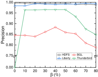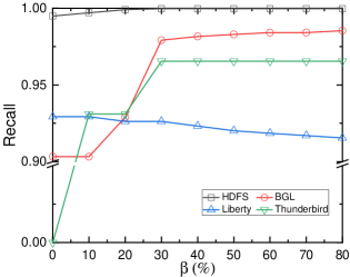V-J Impact of Minority Class Oversampling (RQ6) Note that normal and anomalous samples in the training dataset are imbalanced, as shown in Table I. For the HDFS, BGL, and Thunderbird datasets, normal samples outnumber anomalous samples. Conversely, in the Liberty dataset, anomalous samples exceed normal samples. As described in Section IV-C 1, the hyper-parameter $\beta$ controls the proportion of the minority class by oversampling to address the data imbalance problem. In this section, we investigate the impact of $\beta$ by varying its value. Fig. 4 illustrates the performance of LogLLM on the four datasets under different magnitudes of $\beta$ . When $\beta=0$ , the samples are not oversampled; instead, the original datasets are utilized directly for training. As illustrated in Fig. 4b, for the HDFS, BGL, and Thunderbird datasets, the recall always increases, while for the Liberty dataset, recall decreases as $\beta$ increases. This can be attributed to the fact that for the HDFS, BGL, and Thunderbird datasets, when $\beta$ increases, anomalies are oversampled, making the model more prone to identifying samples as anomalies. In contrast, for the Liberty dataset, when $\beta$ increases, normal samples are oversampled, making the model more prone to identifying samples as normal. 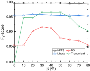As illustrated in Fig. 4c, the trend of the F 1 -score is basically the same across all datasets. The F 1 -score increases and then decreases as $\beta$ increases. However, the LogLLM seems not to be sensitive to $\beta$ ; when $\beta$ is between 10% and 80%, the variation in the F 1 -score is no more than 0.07. Thanks to the substantial semantic knowledge embedded in LLMs, a trained model can effectively learn anomalous patterns and detect anomalies, even when the minority class constitutes only 10% of the dataset. However, LogLLM appears unable to effectively handle extremely imbalanced scenarios. For instance, in the Thunderbird dataset, anomalies constitute only 1.05% of the samples, causing the trained model to be biased and classify all samples as normal. As a result, precision, recall, and F 1 -score are all equal to 0. Compared to the BGL and Thunderbird datasets, the precision, recall and F 1 -score for the HDFS and Liberty datasets exhibit minimal variation with respect to $\beta$ . This consistency arises from the more distinct patterns between abnormal and normal samples in the HDFS and Liberty datasets, allowing LogLLM to easily differentiate them, regardless of the ratio of normal and abnormal samples. 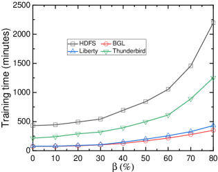As anticipated, as $\beta$ increases, the training time also increases, as shown in Fig. 4d. This relationship arises because a higher $\beta$ leads to more oversampled data samples, as indicated by equation (1), thereby enlarging the training dataset. To summarize, minority class oversampling is essential; however, the value of the hyperparameter $\beta$ does not significantly impact the performance of LogLLM, making careful selection unnecessary. Moreover, excessively large values of $\beta$ are undesirable, as they result in prolonged training times. Values between 30% and 50% are deemed acceptable. VI Conclusion In this paper, we propose LogLLM, a novel log-based anomaly detection framework that leverages LLMs. LogLLM employs both transformer encoder-based and decoder-based LLMs, specifically BERT and Llama, for log-based anomaly detection. BERT is utilized to extract semantic vectors from log messages, while Llama is used to classify log sequences. To ensure coherence in log semantics, we introduce a projector that aligns the vector representation spaces of BERT and Llama. LogLLM is trained using an innovative three-stage procedure designed to enhance both performance and adaptability. Extensive experiments conducted on four public real-world datasets demonstrate that LogLLM achieves remarkable performance. Subsequent ablation studies further confirm the effectiveness of our three-stage training procedure. References - [1] R. S. Kazemzadeh and H.-A. Jacobsen, “Reliable and highly available distributed publish/subscribe service,” in 2009 28th IEEE International Symposium on Reliable Distributed Systems. IEEE, 2009, pp. 41–50. - [2] E. Bauer and R. Adams, Reliability and availability of cloud computing. John Wiley & Sons, 2012. - [3] V.-H. Le and H. Zhang, “Log-based anomaly detection without log parsing,” in 2021 36th IEEE/ACM International Conference on Automated Software Engineering (ASE). IEEE, 2021, pp. 492–504. - [4] W. Guan, J. Cao, H. Zhao, Y. Gu, and S. Qian, “Survey and benchmark of anomaly detection in business processes,” IEEE Transactions on Knowledge and Data Engineering, pp. 1–23, 2024. - [5] S. Zhang, Y. Ji, J. Luan, X. Nie, Z. Chen, M. Ma, Y. Sun, and D. Pei, “End-to-end automl for unsupervised log anomaly detection,” Automated Software Engineering (ASE’24), 2024. - [6] V.-H. Le and H. Zhang, “Log-based anomaly detection with deep learning: How far are we?” in Proceedings of the 44th international conference on software engineering, 2022, pp. 1356–1367. - [7] J. Qi, S. Huang, Z. Luan, S. Yang, C. Fung, H. Yang, D. Qian, J. Shang, Z. Xiao, and Z. Wu, “Loggpt: Exploring chatgpt for log-based anomaly detection,” in 2023 IEEE International Conference on High Performance Computing & Communications, Data Science & Systems, Smart City & Dependability in Sensor, Cloud & Big Data Systems & Application (HPCC/DSS/SmartCity/DependSys). IEEE, 2023, pp. 273–280. - [8] M. Du, F. Li, G. Zheng, and V. Srikumar, “Deeplog: Anomaly detection and diagnosis from system logs through deep learning,” in Proceedings of the 2017 ACM SIGSAC conference on computer and communications security, 2017, pp. 1285–1298. - [9] W. Meng, Y. Liu, Y. Zhu, S. Zhang, D. Pei, Y. Liu, Y. Chen, R. Zhang, S. Tao, P. Sun et al., “Loganomaly: Unsupervised detection of sequential and quantitative anomalies in unstructured logs.” in IJCAI, vol. 19, no. 7, 2019, pp. 4739–4745. - [10] L. Zhang, W. Li, Z. Zhang, Q. Lu, C. Hou, P. Hu, T. Gui, and S. Lu, “Logattn: Unsupervised log anomaly detection with an autoencoder based attention mechanism,” in International conference on knowledge science, engineering and management. Springer, 2021, pp. 222–235. - [11] M. Catillo, A. Pecchia, and U. Villano, “Autolog: Anomaly detection by deep autoencoding of system logs,” Expert Systems with Applications, vol. 191, p. 116263, 2022. - [12] Y. Xie and K. Yang, “Log anomaly detection by adversarial autoencoders with graph feature fusion,” IEEE Transactions on Reliability, 2023. - [13] X. Zhang, X. Chai, M. Yu, and D. Qiu, “Anomaly detection model for log based on lstm network and variational autoencoder,” in 2023 4th International Conference on Information Science, Parallel and Distributed Systems (ISPDS). IEEE, 2023, pp. 239–244. - [14] X. Duan, S. Ying, W. Yuan, H. Cheng, and X. Yin, “A generative adversarial networks for log anomaly detection.” Comput. Syst. Sci. Eng., vol. 37, no. 1, pp. 135–148, 2021. - [15] Z. He, Y. Tang, K. Zhao, J. Liu, and W. Chen, “Graph-based log anomaly detection via adversarial training,” in International Symposium on Dependable Software Engineering: Theories, Tools, and Applications. Springer, 2023, pp. 55–71. - [16] C. Zhang, X. Wang, H. Zhang, J. Zhang, H. Zhang, C. Liu, and P. Han, “Layerlog: Log sequence anomaly detection based on hierarchical semantics,” Applied Soft Computing, vol. 132, p. 109860, 2023. - [17] S. Hashemi and M. Mäntylä, “Onelog: towards end-to-end software log anomaly detection,” Automated Software Engineering, vol. 31, no. 2, p. 37, 2024. - [18] S. Lu, X. Wei, Y. Li, and L. Wang, “Detecting anomaly in big data system logs using convolutional neural network,” in 2018 IEEE 16th Intl Conf on Dependable, Autonomic and Secure Computing, 16th Intl Conf on Pervasive Intelligence and Computing, 4th Intl Conf on Big Data Intelligence and Computing and Cyber Science and Technology Congress (DASC/PiCom/DataCom/CyberSciTech). IEEE, 2018, pp. 151–158. - [19] X. Zhang, Y. Xu, Q. Lin, B. Qiao, H. Zhang, Y. Dang, C. Xie, X. Yang, Q. Cheng, Z. Li et al., “Robust log-based anomaly detection on unstable log data,” in Proceedings of the 2019 27th ACM joint meeting on European software engineering conference and symposium on the foundations of software engineering, 2019, pp. 807–817. - [20] Y. Xie, H. Zhang, and M. A. Babar, “Loggd: Detecting anomalies from system logs with graph neural networks,” in 2022 IEEE 22nd International conference on software quality, reliability and security (QRS). IEEE, 2022, pp. 299–310. - [21] Z. Zhao, W. Niu, X. Zhang, R. Zhang, Z. Yu, and C. Huang, “Trine: Syslog anomaly detection with three transformer encoders in one generative adversarial network,” Applied Intelligence, vol. 52, no. 8, pp. 8810–8819, 2022. - [22] L. Yang, J. Chen, Z. Wang, W. Wang, J. Jiang, X. Dong, and W. Zhang, “Semi-supervised log-based anomaly detection via probabilistic label estimation,” in 2021 IEEE/ACM 43rd International Conference on Software Engineering (ICSE). IEEE, 2021, pp. 1448–1460. - [23] S. Hochreiter, “Long short-term memory,” Neural Computation MIT-Press, 1997. - [24] A. Vaswani, “Attention is all you need,” Advances in Neural Information Processing Systems, 2017. - [25] J. Achiam, S. Adler, S. Agarwal, L. Ahmad, I. Akkaya, F. L. Aleman, D. Almeida, J. Altenschmidt, S. Altman, S. Anadkat et al., “Gpt-4 technical report,” arXiv preprint arXiv:2303.08774, 2023. - [26] A. Dubey, A. Jauhri, A. Pandey, A. Kadian, A. Al-Dahle, A. Letman, A. Mathur, A. Schelten, A. Yang, A. Fan et al., “The llama 3 herd of models,” arXiv preprint arXiv:2407.21783, 2024. - [27] T. GLM, A. Zeng, B. Xu, B. Wang, C. Zhang, D. Yin, D. Rojas, G. Feng, H. Zhao, H. Lai et al., “Chatglm: A family of large language models from glm-130b to glm-4 all tools,” arXiv preprint arXiv:2406.12793, 2024. - [28] W. Guan, J. Cao, J. Gao, H. Zhao, and S. Qian, “Dabl: Detecting semantic anomalies in business processes using large language models,” arXiv preprint arXiv:2406.15781, 2024. - [29] Y. Liu, S. Tao, W. Meng, F. Yao, X. Zhao, and H. Yang, “Logprompt: Prompt engineering towards zero-shot and interpretable log analysis,” in Proceedings of the 2024 IEEE/ACM 46th International Conference on Software Engineering: Companion Proceedings, 2024, pp. 364–365. - [30] C. Egersdoerfer, D. Zhang, and D. Dai, “Early exploration of using chatgpt for log-based anomaly detection on parallel file systems logs,” in Proceedings of the 32nd International Symposium on High-Performance Parallel and Distributed Computing, 2023, pp. 315–316. - [31] J. Pan, W. S. Liang, and Y. Yidi, “Raglog: Log anomaly detection using retrieval augmented generation,” in 2024 IEEE World Forum on Public Safety Technology (WFPST). IEEE, 2024, pp. 169–174. - [32] H. Guo, S. Yuan, and X. Wu, “Logbert: Log anomaly detection via bert,” in 2021 international joint conference on neural networks (IJCNN). IEEE, 2021, pp. 1–8. - [33] Y. Lee, J. Kim, and P. Kang, “Lanobert: System log anomaly detection based on bert masked language model,” Applied Soft Computing, vol. 146, p. 110689, 2023. - [34] Y. Lin, H. Deng, and X. Li, “Fastlogad: Log anomaly detection with mask-guided pseudo anomaly generation and discrimination,” arXiv preprint arXiv:2404.08750, 2024. - [35] C. Almodovar, F. Sabrina, S. Karimi, and S. Azad, “Logfit: Log anomaly detection using fine-tuned language models,” IEEE Transactions on Network and Service Management, 2024. - [36] S. Chen and H. Liao, “Bert-log: Anomaly detection for system logs based on pre-trained language model,” Applied Artificial Intelligence, vol. 36, no. 1, p. 2145642, 2022. - [37] J. L. Adeba, D.-H. Kim, and J. Kwak, “Sarlog: Semantic-aware robust log anomaly detection via bert-augmented contrastive learning,” IEEE Internet of Things Journal, 2024. - [38] Y. Fu, K. Liang, and J. Xu, “Mlog: Mogrifier lstm-based log anomaly detection approach using semantic representation,” IEEE Transactions on Services Computing, vol. 16, no. 5, pp. 3537–3549, 2023. - [39] G. No, Y. Lee, H. Kang, and P. Kang, “Training-free retrieval-based log anomaly detection with pre-trained language model considering token-level information,” Engineering Applications of Artificial Intelligence, vol. 133, p. 108613, 2024. - [40] F. Hadadi, Q. Xu, D. Bianculli, and L. Briand, “Anomaly detection on unstable logs with gpt models,” arXiv preprint arXiv:2406.07467, 2024. - [41] M. Burtsev, M. Reeves, and A. Job, “The working limitations of large language models,” MIT Sloan Management Review, vol. 65, no. 2, pp. 8–10, 2024. - [42] A. Joulin, “Fasttext. zip: Compressing text classification models,” arXiv preprint arXiv:1612.03651, 2016. - [43] J. Devlin, “Bert: Pre-training of deep bidirectional transformers for language understanding,” arXiv preprint arXiv:1810.04805, 2018. - [44] Y. Liu, “Roberta: A robustly optimized bert pretraining approach,” arXiv preprint arXiv:1907.11692, 2019. - [45] M. Joshi, D. Chen, Y. Liu, D. S. Weld, L. Zettlemoyer, and O. Levy, “Spanbert: Improving pre-training by representing and predicting spans,” Transactions of the association for computational linguistics, vol. 8, pp. 64–77, 2020. - [46] P. Lewis, E. Perez, A. Piktus, F. Petroni, V. Karpukhin, N. Goyal, H. Küttler, M. Lewis, W.-t. Yih, T. Rocktäschel et al., “Retrieval-augmented generation for knowledge-intensive nlp tasks,” Advances in Neural Information Processing Systems, vol. 33, pp. 9459–9474, 2020. - [47] J. Zhu, S. He, J. Liu, P. He, Q. Xie, Z. Zheng, and M. R. Lyu, “Tools and benchmarks for automated log parsing,” in 2019 IEEE/ACM 41st International Conference on Software Engineering: Software Engineering in Practice (ICSE-SEIP). IEEE, 2019, pp. 121–130. - [48] P. He, J. Zhu, S. He, J. Li, and M. R. Lyu, “An evaluation study on log parsing and its use in log mining,” in 2016 46th annual IEEE/IFIP international conference on dependable systems and networks (DSN). IEEE, 2016, pp. 654–661. - [49] W. Xu, L. Huang, A. Fox, D. Patterson, and M. Jordan, “Online system problem detection by mining patterns of console logs,” in 2009 ninth IEEE international conference on data mining. IEEE, 2009, pp. 588–597. - [50] A. Oliner and J. Stearley, “What supercomputers say: A study of five system logs,” in 37th annual IEEE/IFIP international conference on dependable systems and networks (DSN’07). IEEE, 2007, pp. 575–584. - [51] P. He, J. Zhu, Z. Zheng, and M. R. Lyu, “Drain: An online log parsing approach with fixed depth tree,” in 2017 IEEE international conference on web services (ICWS). IEEE, 2017, pp. 33–40. - [52] M. Du and F. Li, “Spell: Streaming parsing of system event logs,” in 2016 IEEE 16th International Conference on Data Mining (ICDM). IEEE, 2016, pp. 859–864. - [53] V.-H. Le and H. Zhang, “Log parsing with prompt-based few-shot learning,” in 2023 IEEE/ACM 45th International Conference on Software Engineering (ICSE). IEEE, 2023, pp. 2438–2449. - [54] J. S. Bridle, “Probabilistic interpretation of feedforward classification network outputs, with relationships to statistical pattern recognition,” in Neurocomputing: Algorithms, architectures and applications. Springer, 1990, pp. 227–236. - [55] T. Dettmers, A. Pagnoni, A. Holtzman, and L. Zettlemoyer, “Qlora: Efficient finetuning of quantized llms,” Advances in Neural Information Processing Systems, vol. 36, 2024. - [56] I. Loshchilov, “Decoupled weight decay regularization,” arXiv preprint arXiv:1711.05101, 2017. - [57] J. Zhu, S. He, P. He, J. Liu, and M. R. Lyu, “Loghub: A large collection of system log datasets for ai-driven log analytics,” in 2023 IEEE 34th International Symposium on Software Reliability Engineering (ISSRE). IEEE, 2023, pp. 355–366.