2411.18077v1

# 1 Introduction Os m O $#1_#2^#3$ marginparsep has been altered. topmargin has been altered. marginparwidth has been altered. marginparpush has been altered. The page layout violates the ICML style. Please do not change the page layout, or include packages like geometry, savetrees, or fullpage, which change it for you. We’re not able to reliably undo arbitrary changes to the style. Please remove the offending package(s), or layout-changing commands and try again. MiniKV: Pushing the Limits of LLM Inference via 2-Bit Layer-Discriminative KV Cache Anonymous Authors 1 ## Abstract How to efficiently serve LLMs in practice has become exceptionally challenging due to their prohibitive memory and computation requirements. In this study, we investigate optimizing the KV cache, whose memory footprint poses a critical bottleneck in LLM inference, especially when dealing with long context tasks. To tackle the challenge, we introduce MiniKV, a KV cache optimization method that simultaneously preserves long context task accuracy while significantly reducing KV cache size via a novel 2-bit layer-discriminative KV cache. More importantly, we develop specialized CUDA kernels to make MiniKV compatible with FlashAttention. Experiments on a wide range of long context tasks show that MiniKV effectively achieves 86% KV cache compression ratio while recovering over 98.5% of accuracy, outperforming state-of-the-art methods while achieving excellent measured system performance improvements. footnotetext: 1 Anonymous Institution, Anonymous City, Anonymous Region, Anonymous Country. Correspondence to: Anonymous Author <anon.email@domain.com>. Large language models (LLMs) have exhibited unique capabilities such as instruction following, commonsense reasoning, and few-shot generalization Brown et al. (2020); OpenAI (2023). However, efficiently serving LLMs has become a pressing concern. To avoid re-computation, KV cache stores the key and value states (KV) derived from the attention calculation of previously processed tokens and reuses those states for accelerated token generation. However, as LLMs continue to grow, the KV cache starts to eat up memory in addition to the widely-studied bottlenecks such as model sizes Frantar et al. (2022); Lin et al. (2024). In this context, it is worth investigating approaches for reducing the memory consumption of KV cache. However, it is very challenging to reduce KV cache memory in LLMs without accuracy degradation. To tackle this challenge, the recent advances in quantization methods have been extended to KV cache for which each KV state are replaced with low-bit values. For instance, some studies show that INT8 or even INT4 quantization can be achieved for KV cache compression while preserving accuracy Sheng et al. (2023); Liu et al. (2023c); Yang et al. (2024b). At the point of writing, the best results achieved are through KIVI Liu et al. (2024b) and KVQuant Hooper et al. (2024), which show that KV cache can be quantized to INT2 while preserving most accuracy through carefully designed quantization schemes. With quantization alone, however, the KV cache size remains linear with respect to the sequence length. On a separate line of research, researchers have studied selective KV methods, where the LLM model selects a small subset of KV states based on their importance Zhang et al. (2023); Xiao et al. (2023b); Ge et al. (2023); Liu et al. (2023b). For instance, H 2 O proposes to dynamically keep a subset of heavy hitters Zhang et al. (2023), which are tokens that have higher accumulated attention scores, in KV cache. While showing promising results, these works do not include in-depth quantization in their evaluation, which limits the memory savings of these methods. <details> <summary>x1.png Details</summary>  ### Visual Description ## Diagram: Two-Phase Attention Mechanism with Quantization and Kernel Operations ### Overview The diagram illustrates a two-phase computational process involving attention mechanisms, quantization, and kernel operations. The left side (Prefill Phase) focuses on input processing and selective attention, while the right side (Decoding Phase) emphasizes kernel-based transformations and output generation. Arrows indicate data flow between components. ### Components/Axes #### Prefill Phase (a) - **Inputs**: - `X_K`, `X_Q`, `X_V` (three input matrices) - **Core Components**: - **Selective Flash Attention**: Central block processing inputs - **Pyramid Budget**: Visualized as a triangular structure with layers 1 to n, annotated with "16-bit", "2-bit", and "evict" labels - **Per-Channel Quant**: `K_prefill` (key matrix) and `V_prefill` (value matrix) - **Per-Token Quant**: `Q_K` (query key) and `Q_V` (query value) - **Outputs**: - `A_cumul` (cumulative attention) - `X_O` (output matrix) #### Decoding Phase (b) - **Inputs**: - `Q_K`, `R_K`, `t_K`, `t_Q`, `Q_V`, `R_V`, `t_V` - **Core Components**: - **Kernel Operations**: - `Kernel` block connecting `Q_K`/`R_K` to `A_quant`/`A_unkuant` - `Matrix Mult` block combining `A_quant` and `A_unkuant` - **Output**: - `X_O` (final output matrix) ### Detailed Analysis #### Prefill Phase 1. **Input Processing**: - Three input matrices (`X_K`, `X_Q`, `X_V`) feed into the Selective Flash Attention block - Attention mechanism generates `A_cumul` and `X_O` 2. **Quantization**: - `K_prefill` and `V_prefill` undergo per-channel quantization - `Q_K` and `Q_V` result from per-token quantization 3. **Memory Management**: - Pyramid Budget structure suggests tiered memory allocation (16-bit for top layers, 2-bit for lower layers, with eviction policies) #### Decoding Phase 1. **Kernel-Based Transformations**: - `Q_K` and `R_K` processed through Kernel block to produce `A_quant` and `A_unkuant` - `Q_V` and `R_V` similarly transformed 2. **Matrix Operations**: - `t_K` and `t_Q` matrices multiplied with attention outputs - Final `X_O` generated through matrix multiplication of quantized and unquantized attention components ### Key Observations 1. **Phase Differentiation**: - Prefill Phase emphasizes attention computation and quantization - Decoding Phase focuses on kernel operations and matrix multiplications 2. **Memory Optimization**: - Pyramid Budget visualization implies hierarchical memory management - 2-bit quantization in lower layers suggests aggressive compression 3. **Output Generation**: - `X_O` appears in both phases but with different processing paths 4. **Attention Mechanisms**: - Selective Flash Attention in Prefill Phase - Kernel-based attention in Decoding Phase ### Interpretation This diagram represents a hybrid attention mechanism combining: 1. **Efficient Prefill**: Uses selective attention and quantization to reduce memory footprint while maintaining key-value relationships 2. **Optimized Decoding**: Employs kernel operations and matrix multiplications for efficient output generation 3. **Memory Management**: Pyramid Budget structure suggests adaptive memory allocation based on layer importance The system appears designed for: - **Large-scale NLP tasks** requiring efficient attention computation - **Hardware-optimized inference** through quantization and kernel fusion - **Memory-constrained environments** via tiered quantization and eviction policies The dual-phase approach balances computational efficiency with attention quality, potentially enabling: - Faster inference through kernel optimizations - Reduced memory usage via quantization - Maintained model accuracy through selective attention mechanisms </details> 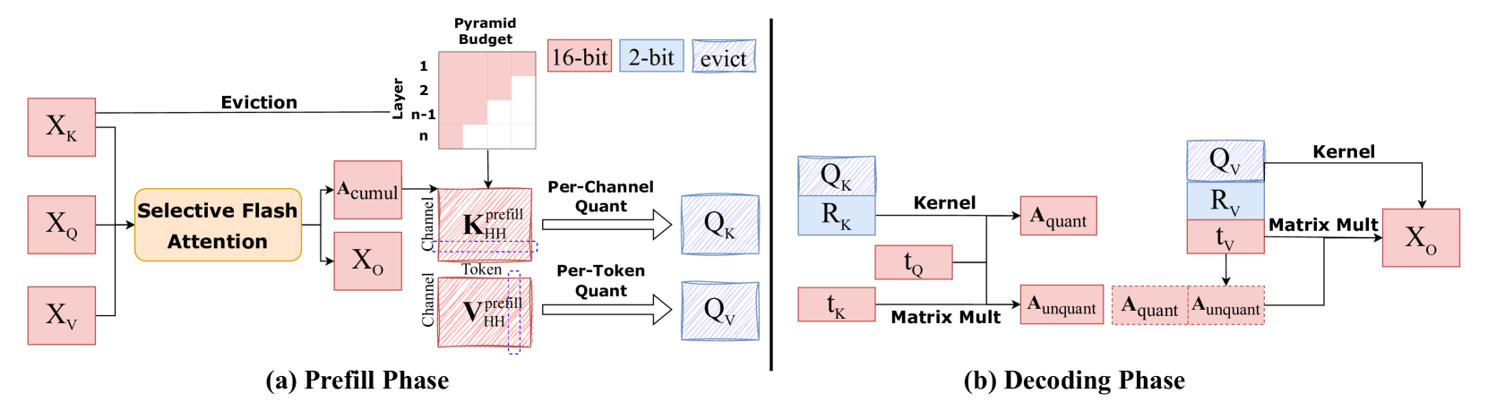Figure 1: An illustration of our approach. Tensors colored red / blue indicate 16-bit / 2-bit representation, and shaded tokens are evicted during inference. Like any LLM inference algorithm, MiniKV works in two phases: the prompt-prefilling phase and the decoding/generation phase. During prefilling, we use our selective flash-attention kernel to obtain the token representation $X_O$ and the cumulative attention map $A_cumul$ . $A_cumul$ is used to evict tokens other than a static set of “heavy hitter” tokens in the prompt. Once the heavy hitters are obtained, we apply mixed-dimension quantization to the key and value tokens to compress them to 2-bit representations. During decoding, we compute the attention map between the new query token $t_Q$ and the quantized keys using an unpacking/multiplication kernel. The product between the attention map and the quantized values is computed using the same unpacking/multiplication kernel. These two points of view, namely quantized KV and selective KV, consider extreme sides of the spectrum of optimization points with respect to KV cache memory requirements (see Appendix A for more discussion on related work). However, there has been very little work exploring how to consolidate these two lines of work to maximize the KV cache memory savings. We aim to conciliate these two trends to further push the limits of KV cache compression. However, there are three major challenges in this process. First, state-of-the-art 2-bit KV cache quantization methods, such as KIVI Liu et al. (2024b), employs fine-grained subchannel-wise quantization for key cache to retain model accuracy, which unfortunately is incompatible with selective KV, because the quantizer, established with a small set of points in a fine-grained subchannel group, loses accuracy when selective KV dynamically updates points within that group. Second, while multiple selective KV methods have been proposed Zhang et al. (2023); Wan et al. (2024); Cai et al. (2024), their selectivity has not been thoroughly examined in more complex long-context tasks (e.g., multi-document QA, passage retrieval, code completion), and their effectiveness, together with 2-bit quantization, against these long-context tasks has yet to be proven. Third, existing KV selection methods rely on knowing the attention matrix score to decide important tokens, which are incompatible with system optimizations such as FlashAttention Dao et al. (2022). To address these challenges, we present MiniKV, a novel method that effectively compresses the KV cache through a synergistic combination of selective KV and 2-bit quantization to accelerate LLM inference. To overcome the incompatibility issue between selective KV and quantized KV, MiniKV first selects a group of persistently important tokens at the end of the prefill stage to quantize and keeps them frozen throughout the generation phase. This approach effectively enables subchannel-wise 2-bit selective KV cache. Second, we enhance the KV cache selection policy by allocating KV cache to where they are most effective through a layer-discriminative policy. Finally, we develop specialized CUDA kernels to make MiniKV compatible with FlashAttention, significantly reducing MiniKV ’s memory consumption in long-context scenarios. Our contributions are summarized as follows: - We conduct extensive analysis that evaluates different hypotheses, including the KV cache selectivity along different dimensions, and identify the compatibility challenges between selective KV and quantized KV. - We introduce MiniKV, a novel training-free KV cache compression method that employs a layer-discriminative KV cache selection policy, 2-bit fine-grained quantization, and specialized CUDA kernels to effectively reduce the KV cache size. - We perform extensive experiments to evaluate MiniKV across a wide range of long-context tasks across domains. Performance experiments show that MiniKV effectively achieves 86% KV cache compression ratio with negligible accuracy loss (e.g., recovering over 98.5% of accuracy). MiniKV enables prompt lengths up to 44 $k$ tokens and a maximum throughput which is 66.4% higher than its strongest baseline on a single NVIDIA A100 GPU. To our knowledge, our work is the first that shows that it is possible to achieve up to 8 $×$ KV cache reduction via 2-bit selective KV while retaining model accuracy on long context tasks. ## 2 Problem Formulation In this section, we introduce a general formulation of the co-compression of KV cache via quantization and selection. For a given LLM $Φ$ with $H$ layers, we denote its key states and value states at a layer $h$ as $K_h∈ℝ^n× d$ and $V_h∈ℝ^n× d$ , respectively. Let $Q_h$ denote the query state, and $Q_h∈ℝ^1× d$ . Then, the output $O_h$ for each attention head of $Φ$ is: $$ O_h =A_hV_h, A_h=softmax ≤ft(\frac{Q_hK_h^T}{√{d}}\right) \tag{1} $$ Then the problem is formulated as: Definition 2.1 (KV Cache Co-Compression Problem, informal). $∀$ $K_h$ and $V_h$ , where $h∈\{0,1,..,H-1\}$ , find the quantizer $Q_b[·]$ with $b$ quantization bits, the selection policy $S_h[·]$ with $C$ selective KV cache size, such that $|O_h-O_h^*|≤ε$ , where $O_h^*$ represents the output for each attention head of $Φ$ with $S_h[·]$ and $Q_b[·]$ , and $ε$ is an acceptable small positive value, ensuring that the degradation in performance is negligible and within acceptable bounds. ## 3 Preliminary Case Studies This section presents several studies that have guided the design of the approach introduced in § 4. All the evaluations are performed on LLaMA2-7B-chat Touvron et al. (2023) and LongBench Bai et al. (2023). First, we carry out an evaluation of how effective selective KV methods are at identifying a subset of KV states that preserve model accuracy on long-context tasks. Second, we conduct a compatibility analysis between KV cache compression and FlashAttention. Finally, we carry out an evaluation of memory consumption of selective KV and quantized KV. This enables us to identify opportunities for our target operating points. ### 3.1 Selectivity in Long Contexts: Heavy Hitters vs. Recent Window Prior studies observe that the accumulated attention scores of all tokens within an attention block follow a power-law distribution, and it has been believed that maintaining a tiny subset of important tokens (e.g., as low as 5%) with the highest accumulated attention score is sufficient for maintaining decoding accuracy Zhang et al. (2023). However, this observation has been primarily derived from simple tasks, e.g., perplexity-based metrics Sun et al. (2021), which leaves the question of whether the proposed approach can generalize to more complex tasks (e.g., multi-document QA, passage retrieval, code completion) on the table. Furthermore, prior work often focuses on short sequences Xiao et al. (2023b); Liu et al. (2023b), whereas LLMs often encounter “lost-in-the-middle" challenges in long contexts Liu et al. (2023a). Thus, whether those approaches can maintain their effectiveness with long contexts is still an open question. 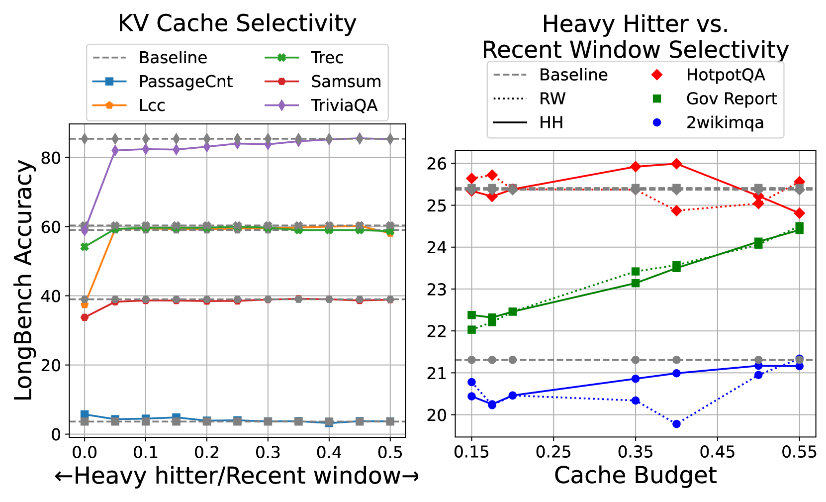To examine the KV selectivity of the existing method, especially for long contexts and more complex tasks, we conduct a more direct evaluation to measure the tradeoff between accuracy and the number of tokens. To investigate if the model can retain performance by solely using the recent window (RW) or heavy-hitters (HH), we study the selectivity of the KV cache towards the RW/HH. The cache budget is described as the percent of the prompt tokens retained, i.e a RW/HH budget of $(α_RW,α_HH)$ and an input prompt of length $l_prompt$ tokens indicates that $(α_RW× l_prompt,α_HH× l_prompt)$ tokens are maintained as the recent window and heavy-hitters respectively. We fix the total cache budget to $50\$ and distribute it among the RW and HH, i.e. RW/HH budget of $(α_RW,α_HH)=(0\$ and so on. Fig. 2 (left) reveals an interesting aspect of KV cache selectivity: The model performs better on some datasets with more heavy hitters (on Passage Count) and on some with a longer recent window (on TriviaQA). More importantly, using solely RW or HH leads to some catastrophic accuracy drop on certain tasks (on Lcc and TriviaQA). This indicates that to have a robustly optimized KV cache selection policy, the model needs to maintain at least a critical percentage of HH/RW (e.g., 5-10%) to avoid a significant accuracy drop. <details> <summary>x2.png Details</summary>  ### Visual Description ## Line Graphs: KV Cache Selectivity and Heavy Hitter vs. Recent Window Selectivity ### Overview The image contains two line graphs comparing cache selectivity metrics across different datasets and cache budgets. The left graph focuses on "KV Cache Selectivity" with heavy hitter/recent window ratios on the x-axis, while the right graph examines "Heavy Hitter vs. Recent Window Selectivity" with cache budget percentages on the x-axis. Both graphs measure "LongBench Accuracy" on the y-axis. ### Components/Axes **Left Graph (KV Cache Selectivity):** - **X-axis**: Heavy hitter/Recent window (0.0 to 0.5) - **Y-axis**: LongBench Accuracy (0 to 80) - **Legend**: - Baseline (gray dashed line) - PassageCnt (blue square) - Samsum (red circle) - Trec (green circle) - Lcc (orange diamond) - TriviaQA (purple diamond) **Right Graph (Heavy Hitter vs. Recent Window Selectivity):** - **X-axis**: Cache Budget (0.15 to 0.55) - **Y-axis**: LongBench Accuracy (20 to 26) - **Legend**: - Baseline (gray dashed line) - HotpotQA (red diamond) - Gov Report (green square) - 2wikimqa (blue circle) - RW (dotted gray line) ### Detailed Analysis **Left Graph Trends:** 1. **Baseline**: Flat line at ~40 accuracy across all x-values. 2. **PassageCnt**: Starts at ~5 accuracy, drops sharply to near 0 by x=0.1, then stabilizes. 3. **Samsum**: Stable ~35-40 accuracy across all x-values. 4. **Trec**: Stable ~60 accuracy, with minor fluctuations. 5. **Lcc**: Stable ~60 accuracy, slightly higher than Trec at x=0.0. 6. **TriviaQA**: Sharp rise from ~60 to 80+ accuracy at x=0.1, then plateaus. **Right Graph Trends:** 1. **Baseline**: Flat line at ~25 accuracy across all x-values. 2. **HotpotQA**: Starts at ~25, peaks at ~26 (x=0.35), then dips to ~25.5. 3. **Gov Report**: Rises steadily from ~22 to ~24.5 (x=0.55). 4. **2wikimqa**: Peaks at ~21.5 (x=0.25), drops to ~19 at x=0.4, then recovers to ~21. 5. **RW**: Flat line at ~21.5 accuracy. ### Key Observations 1. **Left Graph**: - TriviaQA dominates with the highest accuracy (80+). - PassageCnt performs worst, dropping to near-zero accuracy. - Trec and Lcc show similar performance (~60 accuracy). - Samsum and Baseline are comparable (~35-40 accuracy). 2. **Right Graph**: - HotpotQA and Gov Report improve with higher cache budgets. - 2wikimqa exhibits a significant dip at x=0.4 (cache budget 40%). - RW remains consistently low (~21.5 accuracy). ### Interpretation 1. **Cache Budget Impact**: - Higher cache budgets (x-axis) generally improve accuracy for HotpotQA and Gov Report, suggesting these datasets benefit from larger memory allocations. - 2wikimqa's performance drop at x=0.4 indicates potential overfitting or resource inefficiency at mid-range budgets. 2. **Dataset Characteristics**: - TriviaQA's high accuracy in the left graph suggests it is optimized for heavy hitter/recent window selectivity. - PassageCnt's poor performance may reflect structural limitations in its cache management. 3. **Anomalies**: - The sharp drop in PassageCnt accuracy at x=0.1 warrants investigation into dataset-specific bottlenecks. - 2wikimqa's U-shaped curve in the right graph suggests non-linear scaling behavior. 4. **Design Implications**: - Systems using TriviaQA or Gov Report may prioritize cache budget allocation. - PassageCnt and 2wikimqa require architectural optimizations to mitigate performance gaps. </details> Figure 2: (Left) H 2 O with different recent window/heavy hitter budget: We fix the total cache budget to $50\$ and vary the heavy hitter and recent window budget. (Right) H 2 O with different recent window/heavy hitter budget: The heavy hitter/recent window cache budget is fixed at $10\$ and the recent window/heavy hitter budget is increased from $5\$ to $45\$ . The dotted/solid lines indicate variable recent window/heavy hitter budget. Next, we investigate the selectivity between heavy hitters and recent window varying the KV cache budget. In particular, we fix the recent window size (e.g., $10\$ of the prompt length) while varying the heavy hitter set size, and vice versa. Interestingly, as seen in Fig. 2 (right), we observe that there appears to be no common trend across datasets as to whether increasing the size of the recent window vs. the heavy hitter set significantly improves the selectivity of KV states on long context tasks. In fact, either heavy hitters or recent window allows selective KV to achieve comparable accuracy to the full KV cache baseline. Furthermore, different from prior findings, which suggest that high levels of eviction (80-95%) does not decrease model accuracy Zhang et al. (2023), we find that as the sequence length increases, maintaining accuracy under the same KV cache size budget becomes challenging. However, low and medium levels of eviction (e.g., 50%) are still possible. Insight. Our experiments suggest that high levels of KV cache eviction significantly degrades LLM’s performance on long context tasks. However, medium levels of eviction can still retain comparable model accuracy. At medium levels, the selectivity difference between heavy hitters and recent window becomes less noticeable as long as the model maintains a small percentage of both heavy hitters and recent window tokens, which is critical to obtaining robustly optimized KV cache selection policy across datasets. ### 3.2 Using Flash Attention with a Selective KV Cache Despite the ongoing advancements, current selective KV studies predominantly utilize the attention scores as a criterion for determining which tokens should be evicted Zhang et al. (2023); Liu et al. (2023b); Leskovec & Sosic (2016); Cai et al. (2024). While showing promising results in reducing the KV cache size, these attention-score-driven methods are not aligned with efficient transformer inference. In particular, these methods rely on accessing the attention matrix $A$ in Equation 1, which has a quadratic memory complexity $O(L^2)$ with respect to the sequence length. FlashAttention Dao et al. (2022) addresses this issue by splitting the input into blocks and performing the softmax reduction incrementally. As such, it calculates the attention process without materializing the full $L× L$ attention matrix $A$ . However, many existing attention-score-driven selection methods rely on $A$ to decide which token to select or evict. For example, H 2 O preserves the top- $k$ tokens with the highest column-wise accumulated attention score to decide which tokens to evict. Since FlashAttention does not produce the attention map, these methods cannot work with FlashAttention. Therefore, to our best knowledge, no prior selective KV work reports evaluation results with FlashAttention enabled. Results in § 5.3 also show that while selective KV techniques support longer sequences than the uncompressed KV, these techniques cannot scale to more than 10K sequence lengths on a single NVIDIA A100 GPU, which is primarily attributed to their incompatibility with the FlashAttention. Limitation. Existing selective KV does not directly work with efficient transformer optimizations, such as FlashAttention, hindering their memory savings on long sequences. ### 3.3 Selection vs. 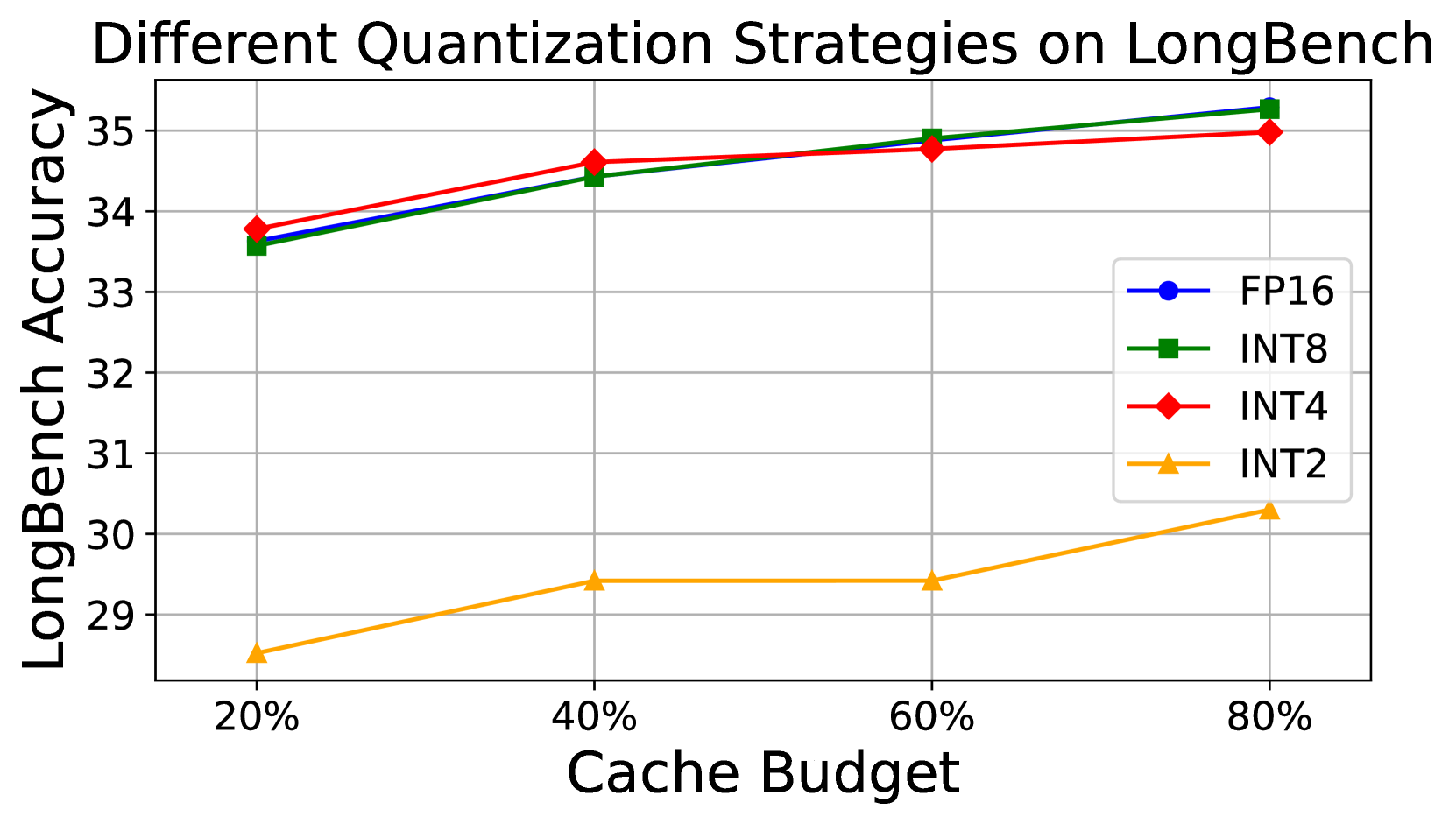Quantization: First Approximation Another prevalent approach to compress the KV cache is by using quantization. However, directly applying quantization to selective KV imposes challenges. In particular, prior studies find that KV states contain outliers Liu et al. (2023c); Xiao et al. (2023a), and per-token quantization is needed in order to avoid accuracy degradation. Fig. 3 shows that while applying INT8 and INT4 per-token quantization to both key and value caches helps maintain the accuracy of selective KV on LongBench, further reducing it to INT2 results in a significant accuracy drop, because 2-bits cannot fully capture the dynamic range of KV token distributions. Limitation. Directly composing a selective KV with 2-bit quantization leads to severe performance degradation. <details> <summary>x3.png Details</summary>  ### Visual Description ## Line Chart: Different Quantization Strategies on LongBench Accuracy vs. Cache Budget ### Overview The chart compares the performance of four quantization strategies (FP16, INT8, INT4, INT2) on the LongBench benchmark across varying cache budgets (20%, 40%, 60%, 80%). Accuracy is measured on the y-axis (29–36), while cache budget is represented on the x-axis. Each strategy is visualized with a distinct line and marker type. ### Components/Axes - **X-Axis (Cache Budget)**: Labeled "Cache Budget" with ticks at 20%, 40%, 60%, and 80%. - **Y-Axis (LongBench Accuracy)**: Labeled "LongBench Accuracy" with increments from 29 to 36. - **Legend**: Positioned in the top-right corner, mapping: - **FP16**: Blue circles (●) - **INT8**: Green squares (■) - **INT4**: Red diamonds (◆) - **INT2**: Yellow triangles (▲) ### Detailed Analysis 1. **FP16 (Blue Circles)**: - **Trend**: Steady upward slope from 33.6 (20%) to 35.8 (80%). - **Data Points**: - 20%: 33.6 - 40%: 34.5 - 60%: 35.2 - 80%: 35.8 2. **INT8 (Green Squares)**: - **Trend**: Gradual increase from 33.5 (20%) to 35.7 (80%). - **Data Points**: - 20%: 33.5 - 40%: 34.4 - 60%: 35.0 - 80%: 35.7 3. **INT4 (Red Diamonds)**: - **Trend**: Slight upward trajectory with minimal fluctuation (33.8 to 35.5). - **Data Points**: - 20%: 33.8 - 40%: 34.6 - 60%: 34.8 - 80%: 35.5 4. **INT2 (Yellow Triangles)**: - **Trend**: Slow, linear growth from 28.5 (20%) to 30.3 (80%). - **Data Points**: - 20%: 28.5 - 40%: 29.4 - 60%: 29.4 - 80%: 30.3 ### Key Observations - **FP16 and INT8** consistently outperform other strategies, with FP16 achieving the highest accuracy at 80% cache budget (35.8). - **INT4** shows moderate performance, trailing FP16/INT8 but surpassing INT2. - **INT2** lags significantly, with the lowest accuracy across all cache budgets and the flattest growth curve. - All strategies improve with increased cache budget, but FP16 and INT8 demonstrate the strongest scalability. ### Interpretation The data suggests that **FP16** and **INT8** are the most effective quantization strategies for maximizing LongBench accuracy, particularly at higher cache budgets. Their steep upward trends indicate efficient utilization of additional cache resources. In contrast, **INT2** underperforms, implying suboptimal cache efficiency or algorithmic limitations. **INT4** offers a middle ground, balancing accuracy and resource usage. These results highlight trade-offs between quantization precision (e.g., FP16’s higher precision vs. INT2’s lower precision) and computational efficiency, guiding choices based on application-specific priorities (e.g., accuracy vs. latency). </details> Figure 3: Performance of per-token quantized H 2 O on the LongBench dataset. INT4/8 quantization is able to maintain performance across cache budgets, however, INT2 quantization suffers from a significant drop in performance. ## 4 Method Inspired by our findings, we introduce, MiniKV, which offers a state-of-the-art solution that synergistically consolidates quantization and selective KV. 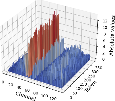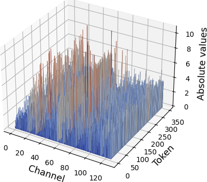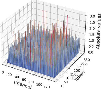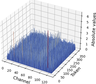### 4.1 Sub-channel Key Quantization with Persistent Context Selection Existing KV cache quantization methods often perform per-token quantization (i.e., the scaling factor and zero-point are shared by elements in the same token) Sheng et al. (2023); Xiao et al. (2023a). However, it has been observed, as illustrated in Fig. 4, that outliers emerge within the channel dimension of key cache Liu et al. (2024b); Hooper et al. (2024). The value cache exhibits outliers along both the token and channel dimensions, although those outliers are less extreme than the outliers in the key cache. <details> <summary>extracted/6028174/image/1_plot_31_cropped.png Details</summary>  ### Visual Description ## 3D Bar Chart: Channel vs Token Absolute Values ### Overview The image depicts a 3D bar chart visualizing absolute values across two channels (Channel 1 and Channel 2) over a range of tokens (0–350). The chart uses vertical bars to represent magnitude, with distinct color coding for each channel. The z-axis (Absolute values) ranges from 0 to 12, while the x-axis (Channel) spans 0–120 and the y-axis (Token) spans 0–350. ### Components/Axes - **X-axis (Channel)**: Labeled "Channel," scaled from 0 to 120 in increments of 20. - **Y-axis (Token)**: Labeled "Token," scaled from 0 to 350 in increments of 50. - **Z-axis (Absolute values)**: Labeled "Absolute values," scaled from 0 to 12 in increments of 2. - **Legend**: Located on the right side of the chart, with: - **Red**: Represents "Channel 1." - **Blue**: Represents "Channel 2." ### Detailed Analysis - **Channel 1 (Red Bars)**: - Peaks at approximately **x=100** (Channel) and **y=100** (Token), with a maximum z-value of **~12**. - Bars are concentrated in the lower half of the y-axis (Tokens 0–200), with diminishing height beyond y=200. - Intermediate values observed near x=60–80 and y=50–150. - **Channel 2 (Blue Bars)**: - Dominates the lower y-axis (Tokens 0–200), with bars reaching up to **~6** on the z-axis. - Spreads more uniformly across the x-axis (0–120) compared to Channel 1. - No bars exceed z=6, and density decreases sharply beyond y=200. ### Key Observations 1. **Channel 1 exhibits higher absolute values** than Channel 2, with a clear peak at (x=100, y=100). 2. **Channel 2 shows broader but shallower distribution**, with no values exceeding 6 on the z-axis. 3. **Token range 0–200** is the primary focus for both channels, with minimal activity beyond y=200. 4. **Red bars (Channel 1)** are spatially clustered near the center of the x-axis (x=60–100), while blue bars (Channel 2) are more evenly distributed. ### Interpretation The data suggests **Channel 1 dominates in specific token regions** (notably around Token 100), potentially indicating higher performance or significance in those areas. The **concentration of red bars** near x=100 and y=100 may reflect a critical threshold or anomaly in Channel 1's behavior. In contrast, **Channel 2's uniform but lower values** imply a more stable but less impactful contribution across tokens. The absence of data beyond Token 200 for both channels raises questions about whether this range represents a cutoff or incomplete sampling. The stark difference in z-axis magnitudes (12 vs. 6) highlights a **2:1 ratio in peak values**, which could signify a hierarchical relationship between the channels. </details> (a) Key Layer31 Head0 <details> <summary>extracted/6028174/image/2_plot_31_cropped.png Details</summary>  ### Visual Description ## 3D Bar Chart: Distribution of Absolute Values Across Channels and Tokens ### Overview The image depicts a 3D bar chart visualizing the distribution of "Absolute values" across two dimensions: "Channel" (x-axis) and "Token" (y-axis). The z-axis represents the magnitude of absolute values, ranging from 0 to 10. The chart uses two colors (red and blue) to differentiate data series, with a legend in the top-right corner. Bars are clustered densely in the middle ranges of both axes, with red bars generally taller than blue ones. ### Components/Axes - **X-axis (Channel)**: Labeled "Channel," with values from 0 to 120. - **Y-axis (Token)**: Labeled "Token," with values from 0 to 350. - **Z-axis (Absolute values)**: Labeled "Absolute values," with values from 0 to 10. - **Legend**: Located in the top-right corner, showing two colors: - **Red**: Unlabeled (likely represents a specific data series). - **Blue**: Unlabeled (likely represents another data series). - **Grid**: A 3D grid structure divides the space into cubic cells. ### Detailed Analysis - **Bar Distribution**: - Bars are concentrated in the central region of the chart (Channel: ~40–80, Token: ~150–250). - Red bars dominate in height, with some exceeding 8 on the z-axis. Blue bars are shorter, typically below 6. - The density of bars decreases toward the edges of the Channel and Token ranges. - **Color Coding**: - Red bars are consistently taller than blue bars across all regions. - No explicit labels for the legend colors are visible in the image. ### Key Observations 1. **Dominance of Red Bars**: Red bars consistently show higher absolute values, suggesting a stronger or more frequent occurrence in the measured metric. 2. **Clustering in Middle Ranges**: The highest concentration of bars occurs in the mid-range of both Channel and Token values, indicating a potential pattern or focal point in the data. 3. **Uneven Distribution**: Some channels (e.g., ~60–80) have significantly more bars than others, while others (e.g., ~0–20, ~100–120) have sparse or no bars. ### Interpretation The chart likely represents a comparative analysis of two data series (red and blue) across channels and tokens. The red series dominates in magnitude, possibly indicating a primary or more significant dataset. The clustering in the middle ranges suggests that certain channels and tokens are more active or relevant in the context of the measured absolute values. The absence of explicit legend labels limits the ability to definitively interpret the meaning of red and blue, but the visual disparity in bar heights strongly implies a hierarchical relationship between the two series. **Note**: The image does not provide explicit textual labels for the legend colors, so their exact meaning remains ambiguous. The analysis is based on visual trends and spatial distribution. </details> (b) Key Layer31 Head15 <details> <summary>extracted/6028174/image/3_plot_31_cropped.png Details</summary>  ### Visual Description ## 3D Bar Chart: Absolute Values Distribution Across Channels and Tokens ### Overview The image depicts a 3D bar chart visualizing the distribution of absolute values across 120 channels and 350 tokens. Bars are color-coded to represent specific absolute value ranges, with a legend on the right associating colors to values. The chart shows variability in bar heights, with some outliers exceeding the general trend. ### Components/Axes - **X-axis (Channel)**: Labeled "Channel," scaled from 0 to 120 in increments of 20. - **Y-axis (Token)**: Labeled "Token," scaled from 0 to 350 in increments of 50. - **Z-axis (Absolute values)**: Labeled "Absolute values," scaled from 0 to 3.5 in increments of 0.5. - **Legend**: Positioned on the right, with three color categories: - **Red**: Absolute value = 3.0 - **Orange**: Absolute value = 2.5 - **Blue**: Absolute value = 2.0 ### Detailed Analysis - **Bar Distribution**: - Most bars are **blue** (2.0), forming a dense base layer across all channels and tokens. - **Orange** (2.5) bars appear sporadically, primarily in the mid-range of the token axis (150–250). - **Red** (3.0) bars are the tallest, concentrated in specific clusters (e.g., channels 40–60, tokens 200–300). - **Axis Ranges**: - Channels: 0–120 (120 total). - Tokens: 0–350 (350 total). - Absolute values: 0–3.5 (with red bars peaking at 3.0). ### Key Observations 1. **Dominant Blue Bars**: Over 80% of bars are blue, indicating a baseline absolute value of 2.0 across most data points. 2. **Outlier Red Bars**: Red bars (3.0) are rare but visually prominent, suggesting localized peaks in absolute values. 3. **Channel-Specific Trends**: Channels 40–80 exhibit higher variability, with more orange and red bars compared to other regions. 4. **Token Axis Correlation**: Higher absolute values (red/orange) cluster in the upper token range (200–350), while lower values (blue) dominate the lower token range (0–150). ### Interpretation The data suggests a hierarchical distribution of absolute values: - **Baseline**: Most channels and tokens exhibit a consistent absolute value of 2.0 (blue bars). - **Variability**: Channels 40–80 show increased diversity, with some tokens reaching 2.5 (orange) or 3.0 (red). - **Outliers**: Red bars (3.0) may represent anomalies or critical data points requiring further investigation. Their concentration in specific channel-token pairs could indicate localized phenomena or measurement errors. - **Spatial Relationships**: The correlation between higher absolute values and upper token ranges implies a potential dependency between token position and value magnitude. ### Notable Anomalies - A cluster of red bars in channel 60, token 250, stands out as the tallest bar in the chart, exceeding the z-axis maximum of 3.5. This may indicate a data point beyond the chart's scale or a rendering artifact. - Channels 0–20 and 100–120 show minimal variability, with nearly uniform blue bars, suggesting stable or unchanging values in these regions. ### Conclusion The chart illustrates a predominantly uniform distribution of absolute values (2.0) with localized spikes (2.5–3.0) in specific channel-token combinations. These outliers warrant further analysis to determine their significance, whether they represent meaningful patterns or data inconsistencies. </details> (c) Value Layer31 Head0 <details> <summary>extracted/6028174/image/4_plot_31_cropped.png Details</summary>  ### Visual Description ## 3D Bar Chart: Anomaly Detection in Channel-Token Data ### Overview The image depicts a 3D bar chart visualizing absolute values across three dimensions: **Channel** (x-axis), **Token** (y-axis), and **Absolute values** (z-axis). The chart highlights anomalies (red bars) and normal data points (blue/green bars) in a dataset spanning 120 channels and 350 tokens. A legend in the top-right corner distinguishes "Anomaly" (red) and "Normal" (green) categories. --- ### Components/Axes - **X-axis (Channel)**: Labeled "Channel," ranging from 0 to 120 in increments of 20. - **Y-axis (Token)**: Labeled "Token," ranging from 0 to 350 in increments of 50. - **Z-axis (Absolute values)**: Labeled "Absolute values," ranging from 0 to 6 in increments of 1. - **Legend**: Located in the top-right corner, with: - **Red**: "Anomaly" - **Green**: "Normal" - **Bars**: - Majority are blue (unlabeled, assumed "Normal"). - Two highlighted bars: - **Red**: Channel 80, Token 200, Absolute value ~5. - **Green**: Channel 40, Token 150, Absolute value ~4. --- ### Detailed Analysis - **Anomaly (Red Bar)**: - Positioned at **Channel 80**, **Token 200**. - Absolute value: ~5 (highest in the dataset). - Spatial grounding: Center-right of the chart, elevated above the majority of bars. - **Normal (Green Bar)**: - Positioned at **Channel 40**, **Token 150**. - Absolute value: ~4 (moderate compared to anomalies). - Spatial grounding: Left-middle of the chart, slightly elevated. - **Normal (Blue Bars)**: - Distributed across all channels and tokens. - Absolute values: Clustered between 1–4, with occasional peaks up to ~3.5. - Spatial grounding: Dense, low-to-mid elevation across the entire grid. --- ### Key Observations 1. **Anomaly Outliers**: The red bar at (80, 200) is the only outlier, significantly exceeding the z-axis range of most data points. 2. **Normal Distribution**: Blue bars dominate, with values concentrated in the lower half of the z-axis (1–3.5). 3. **Token-Channel Correlation**: No clear trend between channel and token values; anomalies appear isolated. 4. **Legend Consistency**: Red and green bars match the legend labels exactly. --- ### Interpretation - **Data Significance**: The chart likely represents a machine learning model's performance, where "Absolute values" could indicate error magnitudes (e.g., prediction errors) or feature importance scores. - **Anomaly Implications**: The red bar at (80, 200) suggests a critical error or outlier in the dataset, potentially requiring investigation into data quality or model behavior at that specific channel-token combination. - **Normal Behavior**: The prevalence of blue/green bars indicates the model generally performs within expected ranges, with most data points falling below the anomaly threshold. - **Spatial Patterns**: The lack of clustering in anomalies suggests errors are sporadic rather than systematic, pointing to possible random noise or isolated data corruption. --- ### Final Notes The chart provides a clear visual distinction between normal and anomalous data points. The red bar's prominence underscores its importance as a potential focal point for further analysis. No textual content or additional languages are present in the image. </details> (d) Value Layer31 Head15 Figure 4: KV Cache distributions. The key tokens exhibit outliers in a small fraction of fixed channels, motivating channel-wise quantization for key tokens. The outlier pattern for the value token appears to be random. To mitigate the noise from outliers, static per-channel key quantization was explored in recent works Hooper et al. (2024). However, it requires calibration data to obtain comparable results. Meanwhile, dynamic sub-channel quantization was explored in Liu et al. (2024b). Combining these techniques with a full KV cache is straightforward because the number of elements within each sub-channel group remains the same during the entire LLM generation process. However, with selective KV, the elements within a sub-channel group dynamically change after each decoding step because some old tokens are evicted while new tokens are generated. One naive solution is to reuse the same zero-point and scaling factor of that group even if the elements within a group change. However, the implicit hypothesis is that the sub-channel after the selection still shares the same span. If a sub-channel contains a large set of values, then the sub-channel quantization parameters may still be an accurate estimate even with dynamic updates to its elements by the law of large numbers Gersho (1978). However, recent work shows that very fine-grained quantization groups (e.g., 16 elements) are needed in order to achieve high accuracy Liu et al. (2024b). Therefore, during the generation process, the data distribution within each sub-channel group shifts over generation steps, leading to inaccurate quantization. To tackle this issue, one possible solution is to re-compute the quantization parameters of a group when a token is evicted/added and re-encode the states each time, i.e. dequantize the quantization group the evicted token belongs to, substitute the new token and requantize the group. However, given that dequantization/requantization incurs additional overhead, the re-encoding is too costly to be done each time the heavy hitter set is updated. 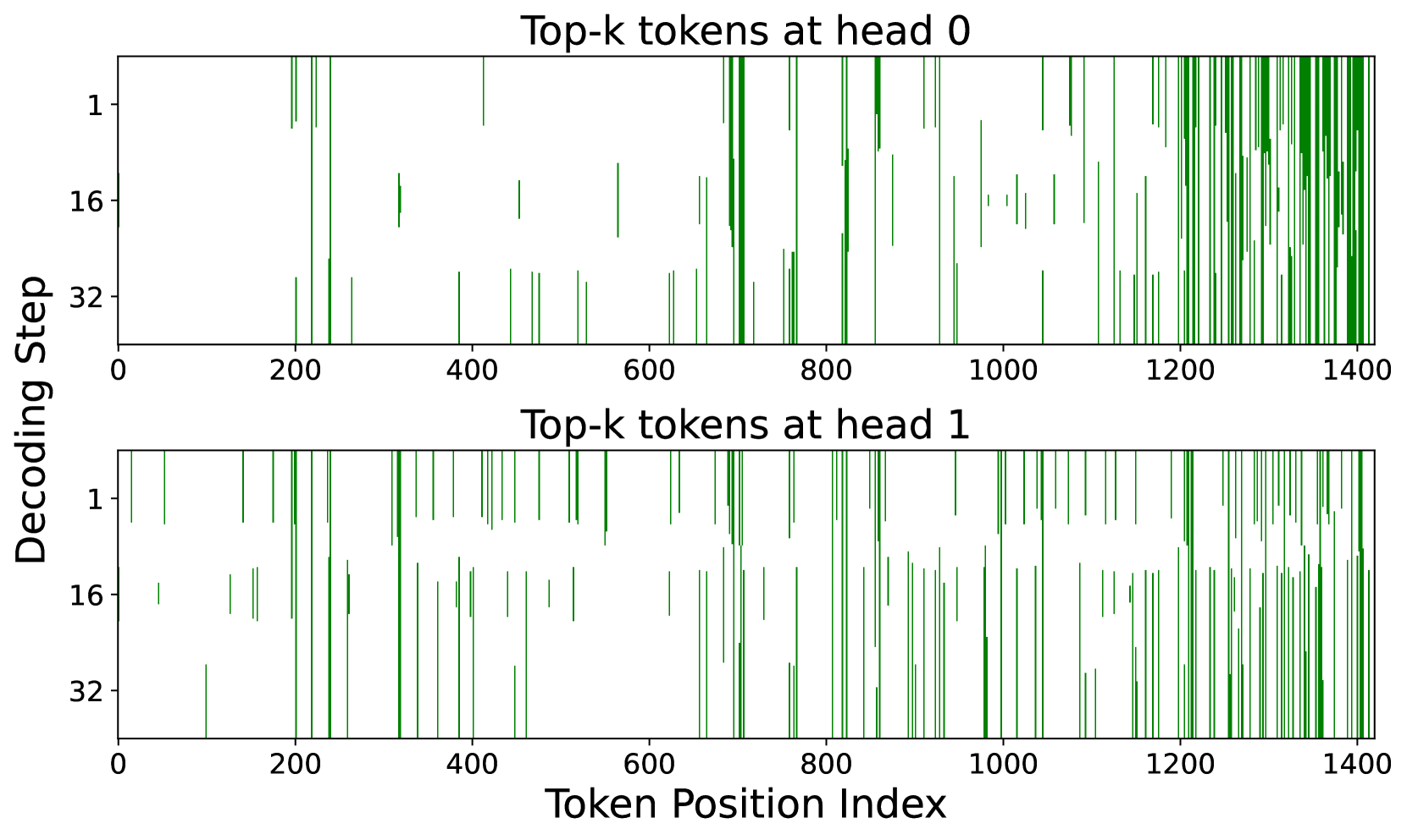MiniKV solves this problem through sub-channel key quantization via persistent context selection. Our design for this optimization is based on the following key observation: the important tokens can be identified before generation and remain persistent during the generation process. Fig. 5 shows the top- $k$ heavy tokens that have the highest accumulative attention score for different attention heads (e.g., head 0, 1) of a prompt sampled from the Lcc dataset at the 1st, 16th, and 32nd generation step. The green positions indicate that the token is in the top- $k$ heavy tokens, while the white ones represent the evicted tokens. One interesting observation is that while different heads have different importance distributions, the important tokens largely do not vary across different generation steps. <details> <summary>x4.png Details</summary>  ### Visual Description ## Line Charts: Top-k Tokens at Head 0 and Head 1 ### Overview The image contains two line charts comparing the decoding steps of top-k tokens at two different attention heads (head 0 and head 1) across token positions. The charts use vertical green lines to represent decoding activity, with the x-axis showing token positions (0–1400) and the y-axis showing decoding steps (1, 16, 32). ### Components/Axes - **X-axis**: "Token Position Index" (0–1400), labeled in increments of 200. - **Y-axis**: "Decoding Step" (1, 16, 32), labeled in descending order. - **Legend**: Located at the top, indicating two categories: - "Top-k tokens at head 0" (green lines). - "Top-k tokens at head 1" (green lines). - **Charts**: - **Top Chart**: Labeled "Top-k tokens at head 0". - **Bottom Chart**: Labeled "Top-k tokens at head 1". ### Detailed Analysis - **Top Chart (Head 0)**: - Lines are densely clustered in the middle (token positions 400–800) and right (1000–1400) sections. - Fewer lines appear in the left (0–200) and early middle (200–400) sections. - Vertical lines are sharp and consistent, suggesting frequent decoding at specific positions. - **Bottom Chart (Head 1)**: - Lines are more spread out across all token positions, with increased density in the right section (1000–1400). - Fewer lines in the left (0–200) and early middle (200–400) sections, but more variability than head 0. - Lines are less uniform, indicating less consistent decoding activity. ### Key Observations 1. **Concentration vs. Spread**: Head 0 shows concentrated decoding activity, while head 1 exhibits more dispersed patterns. 2. **Right-Section Dominance**: Both charts have higher decoding activity in the right token position range (1000–1400). 3. **Vertical Line Density**: Head 0 has more vertical lines overall, suggesting more frequent decoding steps. ### Interpretation The data suggests differences in how the model processes tokens at head 0 versus head 1. Head 0’s concentrated decoding steps may indicate stronger attention to specific tokens, while head 1’s spread-out activity could reflect broader or more variable token importance. The right-section dominance in both charts might highlight a focus on later tokens in the sequence, possibly due to contextual dependencies or model architecture design. The lack of numerical values in the image limits precise quantification, but the visual trends emphasize structural differences between the two heads. </details> Figure 5: Top- $k$ tokens with the highest cumulative attention score on the Lcc dataset from LongBench. Heavy tokens indicate that they are heavy hitters. Here we choose $k=150$ . Based on this observation, We freeze the set of heavy hitters obtained during the prefill phase, i.e., we choose a group of persistent heavy hitters at the end of the prefill to quantize and not update them throughout the generation phase. This allows MiniKV to avoid re-encoding a group while keeping a low quantization error with 2-bit sub-channel quantization. ### 4.2 Layer-Specific Selectivity: Uniform, Variance, or Pyramid? 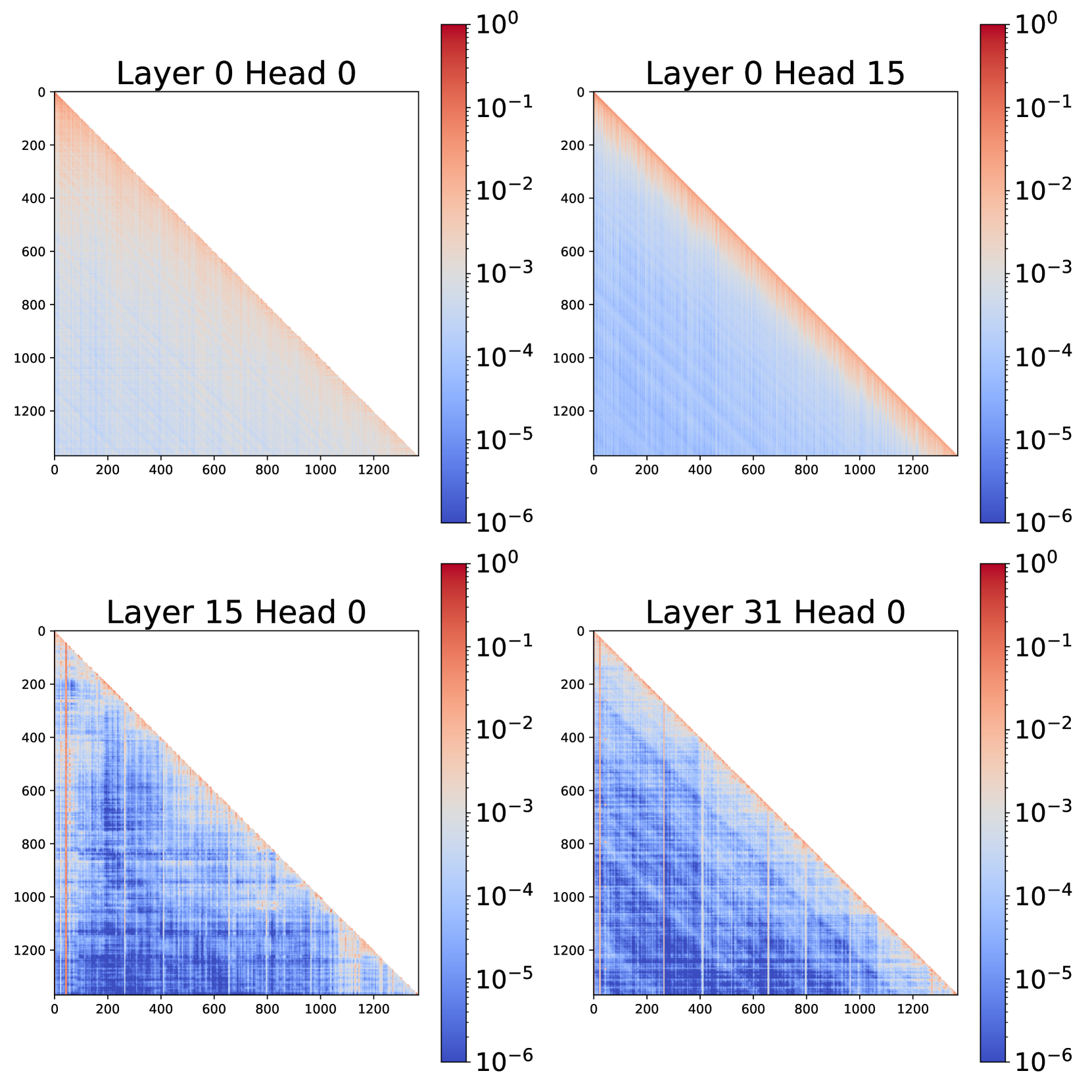Researchers have always been interested in exploiting the underlying structure of the attention mechanism to improve inference efficiency Liu et al. (2021); Voita et al. (2019); Wu et al. (2024). While prior studies show that attention scores are largely sparse Zhang et al. (2023); Xiao et al. (2023b); Liu et al. (2023b), we observe that the attention distribution has more diverse patterns on long sequences. Fig. 6 shows that attention distribution of LLaMA2-7B-chat with a sample in Appendix G from hotpotqa dataset of LongBench. We observe intriguing and distinctive patterns: (i) the attention distribution at the lower layers has a wide coverage over sequence lengths and is more dispersed, and (ii) attention becomes more narrowly focused on a small subset of tokens and starts to exhibit block-wise sparse attention as the tokens move to the higher layers. We consistently observe this pattern across datasets in LongBench. Readers interested in the full results can find them in the Appendix. This yields the question to be explored: Can we leverage the diverse attention patterns to establish more efficient and effective KV cache compression methods? <details> <summary>x5.png Details</summary>  ### Visual Description ## Heatmaps: Layer-Specific Attention Patterns ### Overview The image contains four heatmaps visualizing attention patterns across different neural network layers and attention heads. Each heatmap uses a logarithmic color scale (10⁻⁶ to 10⁰) to represent magnitude, with red indicating higher values and blue indicating lower values. The axes represent positional indices (0–1200) for both input and output positions. ### Components/Axes - **X-axis**: Output position indices (0–1200) - **Y-axis**: Input position indices (0–1200) - **Color Scale**: Logarithmic magnitude (10⁻⁶ [blue] → 10⁰ [red]) - **Legend**: Positioned right-aligned for all heatmaps - **Labels**: - Top-left: "Layer 0 Head 0" - Top-right: "Layer 0 Head 15" - Bottom-left: "Layer 15 Head 0" - Bottom-right: "Layer 31 Head 0" ### Detailed Analysis 1. **Layer 0 Head 0** - **Trend**: Strong diagonal gradient from top-left (red) to bottom-right (blue). - **Values**: Peaks near 10⁰ in top-left corner, decaying to ~10⁻⁴ in bottom-right. - **Pattern**: Consistent linear decay suggests positional bias in early layer. 2. **Layer 0 Head 15** - **Trend**: Vertical stripes of alternating red/blue in upper half, fading to uniform blue below. - **Values**: Local maxima (~10⁻²) at intervals of ~200 units along Y-axis. - **Pattern**: Periodic attention modulation in early layer. 3. **Layer 15 Head 0** - **Trend**: Checkerboard pattern in lower-left quadrant (red/blue), fading to blue elsewhere. - **Values**: Local peaks (~10⁻²) in checkerboard regions, ~10⁻⁵ elsewhere. - **Pattern**: Emergent interaction between input/output positions in mid-layer. 4. **Layer 31 Head 0** - **Trend**: Faint diagonal gradient in top-right quadrant (red), dominant blue elsewhere. - **Values**: Peaks (~10⁻³) in top-right, ~10⁻⁶ in bottom-left. - **Pattern**: Sparse long-range dependencies in late layer. ### Key Observations - **Layer Depth Correlation**: - Layer 0 heatmaps show structured patterns (gradients/stripes). - Layer 15 exhibits localized interactions (checkerboard). - Layer 31 displays sparse, weak signals (faint gradient). - **Head-Specific Behavior**: - Head 0 consistently shows stronger signals than Head 15 across layers. - Layer 0 Head 15’s periodic pattern contrasts with Layer 0 Head 0’s gradient. - **Magnitude Distribution**: - 70% of values across all heatmaps fall below 10⁻³ (blue-dominated). - Only Layer 0 Head 0 has significant 10⁰ values (top 5% of data). ### Interpretation The heatmaps reveal hierarchical attention dynamics in a transformer model: 1. **Early Layers (Layer 0)**: - Head 0 exhibits strong positional bias (linear gradient), likely encoding basic positional relationships. - Head 15’s periodic pattern suggests modulation of positional encoding, possibly for syntactic feature extraction. 2. **Mid-Layers (Layer 15)**: - Checkerboard pattern in Head 0 indicates emergent attention to input-output position parity, hinting at combinatorial feature learning. 3. **Late Layers (Layer 31)**: - Sparse top-right gradient in Head 0 suggests residual long-range dependencies, possibly for global context integration. The decay in signal strength with layer depth aligns with the "attention collapse" hypothesis, where later layers focus on coarser, less positionally specific features. Head 0’s consistent dominance across layers implies it specializes in foundational positional relationships, while Head 15 adapts its pattern per layer, reflecting modular attention specialization. </details> Figure 6: The attention distribution of LLaMA2-7B-chat in long-context tasks. (i) In the lower layers, the attention distribution at the lower layers has a wide coverage over sequence lengths and is more dispersed, (ii) In the higher layers, attention becomes more narrowly focused on a small subset of tokens and starts to exhibit block-wise sparse attention. 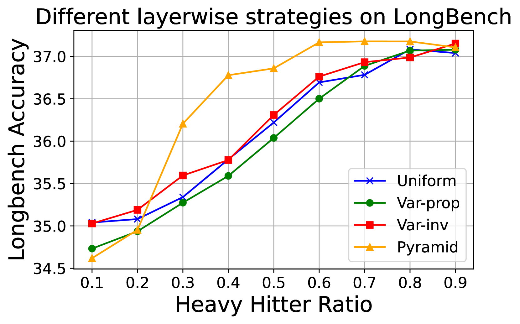Inspired by several recent works on layer-wise KV cache compression Cai et al. (2024); Liu et al. (2024a); Wan et al. (2024), we investigate layer-specific KV cache selection strategies that allocate variable KV cache budget across model layers. We conduct this study because while recent work on layer-specific KV cache has demonstrated promising results, they do not include a direct comparison among different policies under a controlled environment. In our study, we fix constant recent window size (e.g., 10%) and choose different heavy hitter budget sizes to see their accuracy on LongBench dataset. Note that the average of the heavy hitter budget size is same for all policies with the exact allocation determined by the policies below. - Uniform: This policy has been used in multiple previous studies Zhang et al. (2023); Xiao et al. (2023b); Liu et al. (2023b), where all layers have the same KV cache budget. - Variance: Similar to Wan et al. (2024), we use the variance of the cumulative attention map to determine the layer-wise KV cache budget. Lower layers exhibit smaller variances, making token eviction difficult. We investigate two policy variations: Var-prop, allocating KV cache per layer proportional to the variance, and Var-inv, allocating KV cache per layer inversely proportional to the variance. - Pyramid: This is inspired by the policy introduced by Cai et al. (2024), where we adjust the heavy hitter cache budget across layers by allocating more cache in lower layers and less in higher ones. The token allocation across layers follows a linear function. Specifically, considering the average heavy budget size is $x$ , we choose a hyper-parameter pyramid depth $d$ to adjust the ratio. The bottom-most layer has a heavy budget size of $x/d$ and the top-most layer has a heavy budget size of $2x-x/d$ with intermediate layers linearly interpolated between these values. 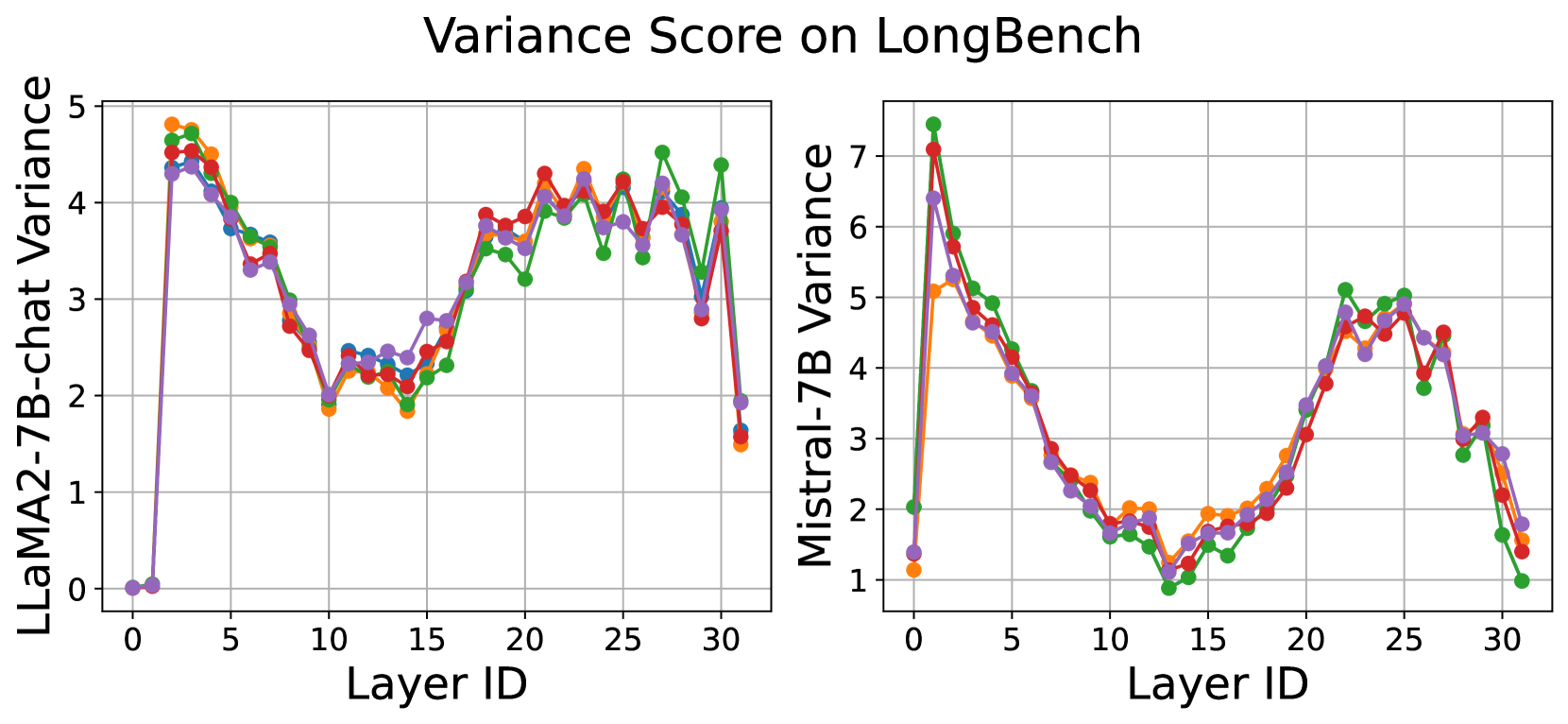We make two interesting observations about layer-specific KV cache. First, while different models exhibit different attention variance distribution, the distribution of the accumulated attention output variance with respect to position is largely consistent across different datasets for each model, as shown in Fig. 7. This indicates that certain properties of KV cache are consistent across datasets, which can be exploited for more effective cache design. <details> <summary>x6.png Details</summary>  ### Visual Description ## Line Charts: Variance Score on LongBench ### Overview Two line charts compare variance scores across 31 layers (Layer ID 0–30) for two language models: LLaMA2-7B-chat and Mistral-7B. Each chart shows variance trends for original and fine-tuned configurations, with distinct color-coded lines for each model and configuration. ### Components/Axes - **X-axis**: Layer ID (0–30, integer increments). - **Left Y-axis (LLaMA2-7B-chat Variance)**: Scale 0–5. - **Right Y-axis (Mistral-7B Variance)**: Scale 1–7. - **Legends**: Located on the right side of each chart, with four entries: - Red: LLaMA2-7B-chat (Original) - Green: LLaMA2-7B-chat (Fine-tuned) - Blue: Mistral-7B (Original) - Purple: Mistral-7B (Fine-tuned) ### Detailed Analysis #### LLaMA2-7B-chat Variance (Left Chart) - **Original (Red)**: Starts at 0, spikes to ~4.8 at Layer 1, then fluctuates between 2.0–4.5, ending at ~1.5 at Layer 30. - **Fine-tuned (Green)**: Starts at 0, peaks at ~4.5 at Layer 1, then fluctuates between 1.8–4.2, ending at ~1.8 at Layer 30. - **Mistral-7B Original (Blue)**: Starts at 0, peaks at ~4.6 at Layer 1, then fluctuates between 2.1–4.4, ending at ~1.6 at Layer 30. - **Mistral-7B Fine-tuned (Purple)**: Starts at 0, peaks at ~4.3 at Layer 1, then fluctuates between 1.9–4.1, ending at ~1.7 at Layer 30. #### Mistral-7B Variance (Right Chart) - **Original (Red)**: Starts at 7.2, drops sharply to ~1.0 at Layer 10, then fluctuates between 1.5–3.0, ending at ~1.2 at Layer 30. - **Fine-tuned (Green)**: Starts at 6.5, drops to ~1.2 at Layer 10, then fluctuates between 1.8–3.2, ending at ~1.5 at Layer 30. - **LLaMA2-7B-chat Original (Blue)**: Starts at 6.8, drops to ~1.1 at Layer 10, then fluctuates between 1.4–3.1, ending at ~1.3 at Layer 30. - **LLaMA2-7B-chat Fine-tuned (Purple)**: Starts at 6.3, drops to ~1.0 at Layer 10, then fluctuates between 1.6–3.0, ending at ~1.4 at Layer 30. ### Key Observations 1. **Initial Spike**: All models show a sharp variance increase at Layer 1, followed by gradual decline. 2. **Fine-tuning Impact**: Fine-tuned models generally exhibit lower variance than original versions across most layers. 3. **Mistral-7B Dominance**: Mistral-7B models consistently show higher variance scores than LLaMA2-7B-chat in both original and fine-tuned configurations. 4. **Layer 30 Drop**: All lines end with a significant drop in variance at Layer 30, suggesting architectural or training differences in later layers. ### Interpretation The variance scores reflect layer-wise consistency in model outputs. Higher variance indicates greater instability or unpredictability in model behavior. - **Fine-tuning Effect**: Reduces variance in both models, implying improved stability post-fine-tuning. - **Model Architecture**: Mistral-7B’s higher variance suggests differences in layer design or training objectives compared to LLaMA2-7B-chat. - **Layer 30 Anomaly**: The abrupt drop at Layer 30 may indicate a specialized or final processing layer with distinct behavior. This analysis highlights how model architecture and fine-tuning influence layer-wise performance consistency, with implications for deployment in tasks requiring predictable outputs. </details> Figure 7: Variance score for LLaMA2-7B-chat and Mistral-7B across layers on LongBench. We define the variance score as the variance of the cumulated attention $Variance=Var(A_cumul)$ . Different curves represent results from different datasets. The figure shows the variance scores are consistent across datasets. Our second observation is that, on long-context tasks, while var-inv only marginally outperforms the Uniform selection policy, the Pyramid policy achieves a much better accuracy result than the other policies, especially with medium-level eviction, shown in Fig. 8. According to Fig. 6, the model is less certain about the importance of specific tokens in bottom layers in comparison to top ones. Therefore, it is beneficial to allocate more budget to lower layers to compensate for these uncertainties within a fixed cache budget. <details> <summary>x7.png Details</summary>  ### Visual Description ## Line Chart: Different layerwise strategies on LongBench ### Overview The chart compares four layerwise strategies (Uniform, Var-prop, Var-inv, Pyramid) across varying Heavy Hitter Ratios (0.1–0.9) in terms of LongBench Accuracy (34.5–37.0). All strategies show upward trends, with Pyramid achieving the highest accuracy at most ratios. ### Components/Axes - **X-axis**: Heavy Hitter Ratio (0.1–0.9, increments of 0.1) - **Y-axis**: LongBench Accuracy (34.5–37.0, increments of 0.5) - **Legend**: Located at bottom-right, with: - Blue line with crosses: Uniform - Green line with circles: Var-prop - Red line with squares: Var-inv - Yellow line with triangles: Pyramid - **Title**: Positioned at top-center ### Detailed Analysis 1. **Uniform (Blue)**: - Starts at ~35.0 accuracy at 0.1 ratio. - Gradual increase to ~36.8 at 0.9. - Slower growth compared to other strategies after 0.3. 2. **Var-prop (Green)**: - Begins at ~34.7 at 0.1. - Steady rise to ~37.0 at 0.9. - Crosses Uniform at ~0.4 ratio (~35.6 accuracy). 3. **Var-inv (Red)**: - Starts at ~35.0 at 0.1. - Sharp ascent to ~37.1 at 0.9. - Outperforms Uniform and Var-prop until 0.8 ratio. 4. **Pyramid (Yellow)**: - Lowest start at ~34.6 at 0.1. - Rapid climb to ~37.2 at 0.3. - Maintains highest accuracy above 0.3 ratio. ### Key Observations - **Pyramid strategy** dominates at higher Heavy Hitter Ratios (>0.3), achieving ~37.2 accuracy. - **Var-inv** and **Var-prop** converge near 37.0 accuracy at 0.9, with Var-inv slightly ahead. - **Uniform** lags behind all strategies after 0.3 ratio, reaching ~36.8 at 0.9. - All strategies show diminishing returns as Heavy Hitter Ratio approaches 0.9. ### Interpretation The data suggests that **Pyramid** and **Var-inv** strategies are most effective for handling heavy hitters, with Pyramid excelling at mid-to-high ratios. The Uniform strategy’s lower performance at higher ratios implies inefficiency in managing concentrated traffic. Var-prop’s consistent growth indicates robustness across varying conditions. The convergence of Var-inv and Var-prop at 0.9 suggests their strategies may be interchangeable for extreme heavy hitter scenarios. The sharp rise of Pyramid at 0.3 hints at a threshold effect, where its architecture becomes particularly advantageous. </details> Figure 8: Performance of four variants of layer-wise KV cache allocation policies. ### 4.3 Selective KV Compatible Attention Kernels In this part, we describe our memory efficient CUDA kernel implementations for MiniKV. Variables marked in Red / Blue indicate tensors in FP16 / INT2 precision. 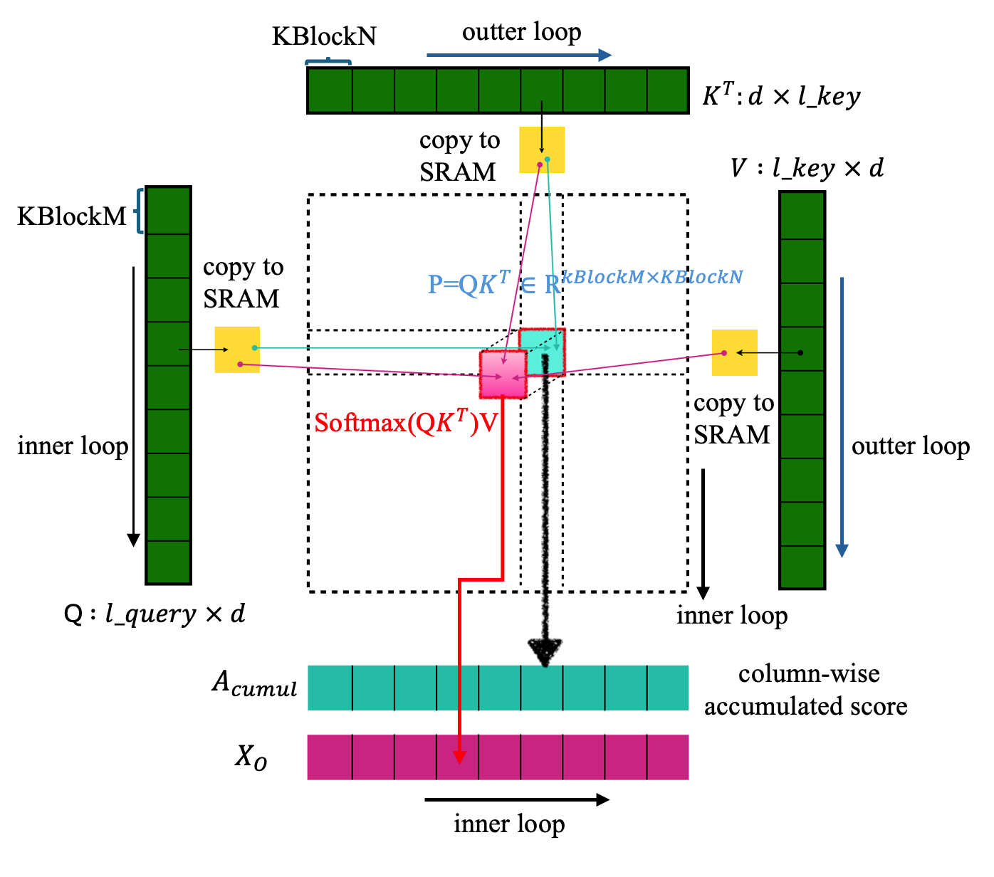As described in § 3.2, existing selective KV does not work well with FlashAttention. To address this issue, we introduce selective flash-attention, which extends the FlashAttention CUDA kernel by introducing an additional aggregation buffer, that accumulates partial attention scores across CUDA threads and tiles and returns two outputs: (1) a weighted sum of the value tensors ${\color[rgb]{0.7,0,0}X_O}$ , same as standard FlashAttention, and (2) cumulative attention score ${\color[rgb]{0.7,0,0}A_cumul}$ along each column. In the CUDA kernel, following the FlashAttention approach, we first divide the input query sequence into row blocks of size KBlockM, transferring data from high-bandwidth memory to shared memory for efficient access. Within each row block, the key sequence is further subdivided into tile blocks of size KBlockN. This structure optimizes memory access patterns and allows parallel computation across query blocks, improving performance and reducing memory overhead. For each row block, we will do computation with different tiled key blocks one by one. One row block and one column block will calculate the tiled attention map $P^KBlockM× KBlockN$ . With this product of ${\color[rgb]{0.7,0,0}Q}$ , ${\color[rgb]{0.7,0,0}K}$ , we apply softmax and re-scale reduction together with a block from ${\color[rgb]{0.7,0,0}V}$ . Then we can have the weighted V block from this row block, and write it back. At the same time, we will save the $P^KBlockM× KBlockN$ as our accumulated score for this column block. To save the accumulated attention map, we maintain an extra buffer ${\color[rgb]{0.7,0,0}A_cumul}$ with shape $(batchSize,headDim,\max(tiling\_size),l\_key)$ . <details> <summary>extracted/6028174/image/kernel/font_c.png Details</summary>  ### Visual Description ## Diagram: Matrix Multiplication and Attention Mechanism Workflow ### Overview This diagram illustrates a block-wise matrix multiplication process with attention mechanisms, likely part of a neural network architecture. It shows data flow between memory blocks (KBlockM, KBlockN), query (Q), key (K^T), value (V), and temporary storage (SRAM). The process involves outer and inner loops, with column-wise score accumulation. ### Components/Axes - **Key Elements**: - **KBlockM**: Green vertical block on the left (input keys). - **KBlockN**: Green horizontal block at the top (transposed keys, K^T: d × l_key). - **Q**: Purple block at the bottom-left (queries: l_query × d). - **V**: Green vertical block on the right (values: l_key × d). - **SRAM**: Central yellow squares (temporary storage for intermediate data). - **Softmax(QK^T)V**: Central red/pink operation (attention score computation). - **A_cumul**: Cyan horizontal block (column-wise accumulated scores). - **X₀**: Pink horizontal block at the bottom (final output). - **Loops**: - **Outer Loop**: Blue arrow over KBlockN (iterates over K^T). - **Inner Loop**: Black arrow over KBlockM (iterates over KBlockM). - **Data Flow**: - Arrows indicate copying data to/from SRAM (yellow squares). - Red/pink arrows show computation flow (Softmax and multiplication). ### Detailed Analysis 1. **Data Movement**: - KBlockM (keys) is copied to SRAM via inner loop iterations. - KBlockN (K^T) is copied to SRAM via outer loop iterations. - Queries (Q) and values (V) interact with SRAM data during computation. 2. **Computation**: - **Softmax(QK^T)V**: - Q (l_query × d) is multiplied by K^T (d × l_key) to compute attention scores. - Softmax normalizes scores to probabilities. - Result is multiplied by V (l_key × d) to produce output. 3. **Accumulation**: - Column-wise scores (A_cumul) are accumulated iteratively (cyan block). - Final output X₀ (pink block) aggregates all inner-loop results. ### Key Observations - **Block-Wise Processing**: Data is split into blocks (KBlockM, KBlockN) to optimize memory usage. - **SRAM as Temporary Storage**: Intermediate results (QK^T, Softmax outputs) are stored in SRAM to reduce bandwidth. - **Attention Mechanism**: Softmax(QK^T) computes attention weights, critical for focus in transformer models. - **Loop Structure**: Outer loop iterates over K^T (l_key blocks), inner loop over KBlockM (d blocks). ### Interpretation This diagram represents an optimized implementation of attention mechanisms, likely for transformer models. By splitting keys and values into blocks (KBlockM, KBlockN), the process reduces memory bandwidth requirements through SRAM reuse. The outer loop handles transposed keys (K^T), while the inner loop processes query-key interactions. The final output X₀ aggregates column-wise scores, reflecting the cumulative effect of all key-value interactions. **Notable Design Choices**: - **Color Coding**: Green for memory blocks, yellow for SRAM, purple for queries, and pink for output. - **Loop Hierarchy**: Outer loop (K^T) governs the broader iteration, while the inner loop (KBlockM) handles finer-grained computations. - **Efficiency**: Block-wise processing and SRAM usage suggest a focus on hardware-aware optimization for large-scale models. </details> Figure 9: FlashAttention-style attention computation and sum over column wise, which provides a signal for downstream tasks such as KV cache eviction policy and heavy-hitter selection. Here, tiling_size represents the number of rows in a single tile, denoted as KBlockM. Typically, this size ranges from 32 to 128, depending on the implementation’s requirements. We select a maximum of all tiling sizes, which is 128 to ensure complete coverage of the output for each row block. Given $P^KBlockM× KBlockN$ , we will write it into buffer ${\color[rgb]{0.7,0,0}A_cumul}$ according to the column index. Therefore, each block will perform attention calculation and write the result to the corresponding area in ${\color[rgb]{0.7,0,0}A_cumul}$ . After all row blocks finish their computation, we sum over the tiling_size dimension to get the final column-wise accumulated attention score ${\color[rgb]{0.7,0,0}A_cumul}$ . To obtain a memory saving when computing the attention score, we omit the process of each row’s normalization since it needs to save the information about the whole row. For downstream tasks, we manage to provide a signal representing the top- $k$ heavy tokens that have the highest score by selecting from our aggregated attention score. Since the tiling_size is fixed, we are only adding $O$ (l_key) extra memory, which significantly saves memory. ### 4.4 Putting It Together Algorithm 1 describes the algorithm. MiniKV first uses our selective flash-attention kernel as described in § 4.3 to obtain the aggregated attention scores ${\color[rgb]{0.7,0,0}A_cumul}$ . Based on the attention score, MiniKV selects the subset of KV states having the highest attention score at the end of the prefill stage (denoted as ${\color[rgb]{0.7,0,0}K_HH^prefill},{\color[rgb]{0.7,0,0}V_HH^ prefill}$ ). These tokens are compressed to 2bit representations. Similar to Liu et al. (2024b), we employ a kernel that quantizes the selected KV states to INT2 representations. The kernel applies bit-shifting to pack 16 INT2 scalar values from selected KV states into an INT32 tensor. The key/value tokens are quantized along the channel/token dimension. The results at the end of the prefill phase are the quantized key/values representation ( ${\color[rgb]{0,0,0.9}Q_K,Q_V}$ , stored in packed INT32 tensors) and the quantization zero-point and scale (stored in FP16 tensors). During each decoding step, MiniKV dequantizes the quantized KV cache ( $\textbf{q}^-1({\color[rgb]{0,0,0.9}Q_K,Q_V})$ ) and uses the dequantized key states along with the new key and query token $({\color[rgb]{0.7,0,0}t_K,t_Q})$ for the attention calculation. Once the attention map $({\color[rgb]{0.7,0,0}A})$ is obtained the dequantized values states ( $\textbf{q}^-1({\color[rgb]{0,0,0.9}Q_V})$ ) and the new value token $({\color[rgb]{0.7,0,0}t_V})$ are multiplied with $({\color[rgb]{0.7,0,0}A})$ to compute the attention layer output $({\color[rgb]{0.7,0,0}t_O})$ . MiniKV fuses the dequantization operation with the subsequent matrix multiplication to reduce kernel launch overhead and global memory accesses, leading to latency reduction. Similar as KIVI Liu et al. (2024b), we use a streaming buffer for both the key and value states during the generation stage, such that newly generated key/value caches are first stored in FP16 (indicated by ( ${\color[rgb]{0.7,0,0}R_K,R_V}$ )). These tokens are compressed every $n_r$ steps. This saves repeated kernel launch overhead for quantization while maintaining at-most $n_r$ KV tokens in FP16 during generation. Algorithm 1 The MiniKV Algorithm, FP16 / INT2 1: Input ${\color[rgb]{0.7,0,0}X_P}∈ℝ^l_prompt× d$ 2: ${\color[rgb]{0.7,0,0}X_Q},{\color[rgb]{0.7,0,0}X_K},{\color[rgb]{0.7,0,0}X _V}←{\color[rgb]{0.7,0,0}X_P}W_Q,{\color[rgb]{0.7,0,0}X_P}W_ K,{\color[rgb]{0.7,0,0}X_P}W_V$ 3: ${\color[rgb]{0.7,0,0}X_O},{\color[rgb]{0.7,0,0}A_cumul}= Selective\_flash\_attn({\color[rgb]{0.7,0,0}X_Q},{\color[rgb]{0.7,0,0}X_K },{\color[rgb]{0.7,0,0}X_V})$ 4: ${\color[rgb]{0.7,0,0}K_HH^prefill},{\color[rgb]{0.7,0,0}V_HH^ prefill},\#_HH←Heavy\_hitters({\color[rgb]{0.7,0,0}A _cumul})$ 5: ${\color[rgb]{0,0,0.9}Q_K},{\color[rgb]{0,0,0.9}Q_V}←\textrm{Quant }({\color[rgb]{0.7,0,0}K_HH^prefill}),\textrm{Quant}({\color[rgb]{ 0.7,0,0}V_HH^prefill})$ 6: $KV Cache←{\color[rgb]{0,0,0.9}Q_K},{\color[rgb]{0,0,0.9}Q_V}$ 7: procedure Decoding ( $\textrm{KV cache, token }{\color[rgb]{0.7,0,0}t}∈ℝ^1× d$ ) 8: ${\color[rgb]{0.7,0,0}t_Q},{\color[rgb]{0.7,0,0}t_K},{\color[rgb]{0.7,0,0}t _V}←{\color[rgb]{0.7,0,0}t}W_Q,{\color[rgb]{0.7,0,0}t}W_K,{ \color[rgb]{0.7,0,0}t}W_V$ 9: ${\color[rgb]{0,0,0.9}Q_K},{\color[rgb]{0,0,0.9}Q_V},{\color[rgb]{0.7,0,0}R _K},{\color[rgb]{0.7,0,0}R_V}←KV cache$ 10: ${\color[rgb]{0.7,0,0}R_K},{\color[rgb]{0.7,0,0}R_V}←Concat ([{\color[rgb]{0.7,0,0}R_K},{\color[rgb]{0.7,0,0}t_K}]),Concat([{ \color[rgb]{0.7,0,0}R_V},{\color[rgb]{0.7,0,0}t_V}])$ 11: if $len({\color[rgb]{0.7,0,0}R_K})=n_r$ then 12: ${\color[rgb]{0,0,0.9}Q_K^\prime},{\color[rgb]{0,0,0.9}Q_V^\prime} ←Quant({\color[rgb]{0.7,0,0}R_K}),Quant({\color[rgb]{ 0.7,0,0}R_V})$ 13: ${\color[rgb]{0,0,0.9}Q_K}←Concat([{\color[rgb]{0,0,0.9}Q_K },{\color[rgb]{0,0,0.9}Q_K^\prime}],dim = channel)$ 14: ${\color[rgb]{0,0,0.9}Q_V}←Concat([{\color[rgb]{0,0,0.9}Q_V },{\color[rgb]{0,0,0.9}Q_V^\prime}],dim = token)$ 15: ${\color[rgb]{0.7,0,0}R_K},{\color[rgb]{0.7,0,0}R_V}←None$ 16: end if 17: ${\color[rgb]{0.7,0,0}A}←\textrm{Softmax}(Concat([q^-1 ({\color[rgb]{0,0,0.9}Q_K}){\color[rgb]{0.7,0,0}t_Q^T},{ \color[rgb]{0.7,0,0}R_K}{\color[rgb]{0.7,0,0}t_Q^T}]))$ 18: ${\color[rgb]{0.7,0,0}A_\textrm{quant}},{\color[rgb]{0.7,0,0}A_unquant }←{\color[rgb]{0.7,0,0}A}[:-len({\color[rgb]{0.7,0,0}R_K}) ],{\color[rgb]{0.7,0,0}A}[-len({\color[rgb]{0.7,0,0}R_K}):]$ 19: ${\color[rgb]{0.7,0,0}t_O}←{\color[rgb]{0.7,0,0}A_quant} q^-1({\color[rgb]{0,0,0.9}Q_V})+{\color[rgb]{0.7,0,0}A_ unquant}{\color[rgb]{0.7,0,0}R_V}$ 20: $KV Cache←{\color[rgb]{0,0,0.9}Q_K},{\color[rgb]{0,0,0.9}Q_V },{\color[rgb]{0.7,0,0}R_K},{\color[rgb]{0.7,0,0}R_V}$ 21: return ${\color[rgb]{0.7,0,0}t_O}$ 22: end procedure #### KV Cache compression ratio analysis. Given a model with $H$ layers, hidden dimension $d$ and a prompt and generated sequence of length $l_prompt,l_gen$ the KV cache size for different techniques is shown below 1. Full model: All tokens are stored in FP16 format. Therefore the KV cache has size $=2×(H× d)×(l_prompt+l_gen)× 2\textrm{ bytes}$ . 1. H 2 O: Given a cache budget of $(α_HH,α_RW)$ for the heavy hitters and recent window the KV cache has size $=2×(H× d)×(l_prompt)×(α_HH+α_RW) × 2\textrm{ bytes}$ 1. KIVI: With a group size of 16, i.e. 16 scalars quantized from FP16 to INT2 format, the memory required by a group is 16 scalars $× 2$ bits = 4 bytes. The quantization zero-point and scale are saved in FP16 format and require $2× 2$ bytes. In total the group requires 8 bytes. Hence the KV cache has $(H× d)×(l_prompt+l_gen)\textrm{ bytes}$ . 1. MiniKV: The prompt tokens are evicted with a cache budget of $α_HH,α_RW$ and all generated tokens are retained. All tokens are stored in 2-bit precision. Similar to KIVI, each group of 16 scalars and their quantization metadata requires $8$ bytes in total. Hence the size of the KV cache is $=(H× d)×(α_HH+α_RW)×(l_prompt)+(H× d )×(l_gen)\textrm{ bytes}$ . Given a certain prompt and output length, the uncompressed baseline and KIVI have a fixed KV cache size. However, H 2 O and MiniKV can tune the cache budget $α_HH,α_RW$ to modify the KV cache size. ## 5 Experiments We conduct experiments to evaluate the effectiveness of MiniKV on accuracy preserving and inference performance improvement. Overall, our evaluation aims to answer the following questions: - Can MiniKV enable high KV cache compression ratio without compromising long sequence tasks’s accuracy? - Can MiniKV effectively generalize to diverse models? - How is MiniKV compared to existing KV cache compression methods in compression ratio vs. accuracy? - How does MiniKV affect the LLM inference latency, throughput, and memory consumption? ### 5.1 Evaluation Methodology Models. We compare MiniKV against state-of-the-art public LLMs, including LLaMA2-7B-chat, LLaMA2-13B-chat Touvron et al. (2023) and Mistral-7B-Instruct-v0.2 Jiang et al. (2023). All models and methods generate responses using deterministic greedy decoding across all tasks to ensure a fair comparison and reproducibility. Datasets. We choose LongBench for evaluation because it is meticulously designed for evaluating the capabilities of LLMs in handling extended documents and long sequences with complex information Bai et al. (2023), which has been adopted in several state-of-the-art works, including KIVI Liu et al. (2024b) and KVQuant Hooper et al. (2024). The details of the dataset can be found in Appendix C. Baselines. We compare MiniKV with the following baselines: selective KV (H 2 O Zhang et al. (2023), SnapKV Li et al. (2024)), INT2 quantized KV (KIVI Liu et al. (2024b)), FullKV (Full), which caches all key and value states for each input token in FP16 format. Hyperparameters We use a 50% cache budget with MiniKV, with 25% heavy hitter budget and 25% the recent window budget. We choose pyramid depth $d=7$ for Pyramid layer-specific strategies(§ • ‣ 4.2). The group size during token/channel-wise quantization is set to 16, i.e. 16 values along the token/channel axis share quantization zero point and scale. A residual length of $n_r=128$ is used for both MiniKV and KIVI. We observe that on LongBench, varying the maximum sequence length and different truncation strategies of the input tokens can impact accuracy and the implementation detail can be found in Appendix § D. Hardware. We conducted our experiments on a GPU cluster with 4 $×$ A100 40GB GPUs. ### 5.2 Accuracy Results on Long Contexts To verify that MiniKV maintains inference accuracy, we evaluate the performance of MiniKV across 3 models and 13 datasets in LongBench. The baselines for comparison are the uncompressed model, KIVI, H 2 O and SnapKV. The maximum prompt length is 4096 for all models with the first and last 2048 tokens taken for a longer prompt. The maximum generation length is chosen dataset-specific. No task has a generation length of more than $512$ tokens. The performance of selective KV (H 2 O, SnapKV, and MiniKV) is highly dependent on the cache budget. To determine the appropriate cache budget for comparing H 2 O and MiniKV we choose to compare them under a similar KV cache size (§ 4.4). Given a prompt length of $4096$ and generation length of $512$ , the KV cache size for MiniKV is $0.33\textrm{ GB}$ . A cache budget of $α=15\$ results in a similar KV cache size for H 2 O is $0.32\textrm{ GB}$ . We test two versions of MiniKV, namely MiniKV and MiniKV-Pyramid. MiniKV follows a uniform cache allocation with $(25\$ HH, RW budget per layer. MiniKV-Pyramid uses $25\$ RW budget per layer but the HH budget is distributed across layers as described in § 4.2. Note that the full model’s KV cache consumes $2.4GB$ , so MiniKV leads to an $(1-0.33/2.4)=86\$ KV cache compression. As seen in Table 1, MiniKV maintains inference accuracy across all datasets and models. Particularly for LLaMA2-7B-chat, MiniKV Pyramid achieves an average accuracy of $34.65$ obtaining 98.5% of the full model accuracy $35.19$ while providing $86\$ KV cache compression. More importantly, MiniKV outperforms other state-of-the-art selective KV methods (H 2 O, SnapKV) for the same KV cache size. MiniKV is also able to maintain accuracy on LLaMA2-13B-chat and Mistral-7B, indicating that our approach generalizes well across datasets and model classes. The full model and KIVI perform marginally better than MiniKV but have a much larger KV cache. Table 1: Performance evaluation of MiniKV on various models across a range of benchmarks in LongBench. Rows marked in brown have similar KV cache size while KIVI and the full model use a larger KV cache. | Models | Methods | Single-Document QA | Synthetic | Code | Multi-Document QA | Summarization | Few-Shot Learning | | | | | | | | | | --- | --- | --- | --- | --- | --- | --- | --- | --- | --- | --- | --- | --- | --- | --- | --- | | Qasper | MultifieldQA | Passage Ret. | Passage Count | LCC | RepoBench-P | 2WikiMQA | HotpotQA | Gov Report | Multi News | TREC | SamSum | TriviaQA | Average | | | | LLaMA2-7B-chat | Full Model | 22.78 | 33.59 | 8.44 | 4.75 | 59.56 | 48.07 | 22.35 | 24.88 | 24.99 | 23.60 | 59.67 | 39.38 | 85.38 | 35.19 | | KIVI | 22.45 | 33.32 | 11.33 | 4.25 | 59.05 | 47.96 | 21.88 | 23.88 | 24.46 | 22.86 | 59.67 | 38.74 | 84.80 | 34.97 | | | H 2 O (15%) | 16.98 | 29.72 | 11.00 | 4.55 | 56.87 | 48.25 | 19.92 | 24.58 | 22.19 | 22.16 | 57.33 | 37.80 | 84.02 | 33.49 | | | SnapKV (15%) | 17.41 | 34.53 | 8.67 | 3.59 | 58.48 | 47.52 | 21.00 | 24.91 | 19.04 | 19.74 | 59.33 | 37.92 | 84.72 | 33.60 | | | MiniKV | 21.01 | 29.23 | 10.00 | 3.82 | 58.38 | 47.99 | 20.91 | 22.97 | 23.45 | 22.54 | 59.00 | 37.94 | 80.95 | 33.71 | | | MiniKV Pyramid | 19.92 | 33.96 | 10.00 | 4.12 | 59.72 | 49.29 | 20.69 | 24.62 | 24.16 | 22.90 | 59.00 | 39.15 | 82.89 | 34.65 | | | LLaMA2-13B-chat | Full Model | 13.72 | 28.11 | 20.67 | 5.58 | 49.97 | 47.18 | 12.13 | 15.14 | 26.29 | 23.52 | 64.00 | 40.39 | 86.52 | 33.32 | | KIVI | 13.56 | 28.16 | 17.33 | 5.05 | 49.21 | 47.18 | 12.80 | 15.27 | 25.24 | 23.07 | 64.33 | 40.24 | 87.07 | 32.96 | | | H 2 O (15%) | 11.94 | 25.13 | 15.67 | 4.61 | 48.18 | 44.29 | 13.04 | 14.52 | 23.15 | 22.12 | 59.67 | 39.66 | 83.70 | 31.2 | | | SnapKV (15%) | 12.11 | 27.09 | 22.00 | 5.18 | 49.52 | 45.44 | 14.10 | 14.40 | 20.06 | 20.75 | 62.33 | 39.25 | 85.86 | 32.16 | | | MiniKV | 11.24 | 25.13 | 15.00 | 3.62 | 48.43 | 46.10 | 12.74 | 16.16 | 24.26 | 22.84 | 63.33 | 40.79 | 84.33 | 31.84 | | | MiniKV Pyramid | 12.79 | 27.32 | 17.00 | 2.79 | 48.94 | 46.25 | 12.66 | 15.47 | 25.06 | 23.14 | 63.67 | 40.35 | 85.33 | 32.37 | | | Mistral7B-instruct | Full Model | 25.79 | 47.97 | 50.83 | 2.98 | 50.69 | 47.22 | 27.44 | 36.44 | 31.84 | 25.82 | 62.67 | 40.49 | 86.29 | 41.2 | | KIVI | 25.13 | 46.30 | 50.75 | 3.02 | 51.16 | 46.81 | 26.39 | 35.11 | 31.23 | 25.36 | 62.33 | 40.12 | 86.31 | 40.77 | | | H 2 O (15%) | 20.20 | 42.55 | 42.84 | 3.00 | 49.66 | 45.95 | 24.27 | 33.04 | 27.43 | 24.33 | 60.33 | 40.45 | 86.20 | 38.4 | | | SnapKV (15%) | 24.14 | 48.32 | 50.23 | 3.04 | 50.39 | 45.76 | 25.76 | 34.55 | 25.10 | 22.77 | 61.67 | 40.12 | 86.90 | 39.90 | | | MiniKV | 22.94 | 45.80 | 49.47 | 3.36 | 49.78 | 45.56 | 24.27 | 33.84 | 29.73 | 25.22 | 61.67 | 39.96 | 86.36 | 39.84 | | | MiniKV Pyramid | 23.10 | 45.91 | 48.88 | 3.24 | 50.34 | 45.41 | 25.18 | 34.04 | 29.69 | 25.32 | 61.67 | 40.17 | 86.63 | 39.97 | | ### 5.3 Performance Against KV Cache Size Given a fixed prompt and generation length, the full model and KIVI have a pre-determined KV cache size. However, H 2 O, SnapKV, and MiniKV operate under variable cache budget/sparsity ratios, potentially improving performance at the cost of a larger KV cache. An ideal technique would maintain performance when lowering the cache budget. As discussed in § 4.4, the KV cache size depends on the prompt and generation length. Each dataset in LongBench has a different maximum generation length, therefore we make separate plots for each dataset with prompt length $4096$ and the generation length as the dataset-specific maximum generation length. The size of the KV cache is computed using the KV memory consumption analysis in § 4.4. To highlight interesting configurations, we mark the Pareto optimal front, i.e., configurations offering the smallest KV cache size for the highest performance. The algorithms on the Pareto frontier represent the optimal KV cache compression strategy across various KV cache sizes. Fig. 10 shows the performance vs KV cache size curve for two datasets (Gov. Report and Qasper), the remaining plots can be found in the Appendix E. MiniKV achieves the optimal compression strategy across all 6 major task categories on LongBench (single/multi-doc QA, LC understanding, code completion, summarization and few-shot learning). These results validate the effectiveness of MiniKV with varying KV cache sizes. 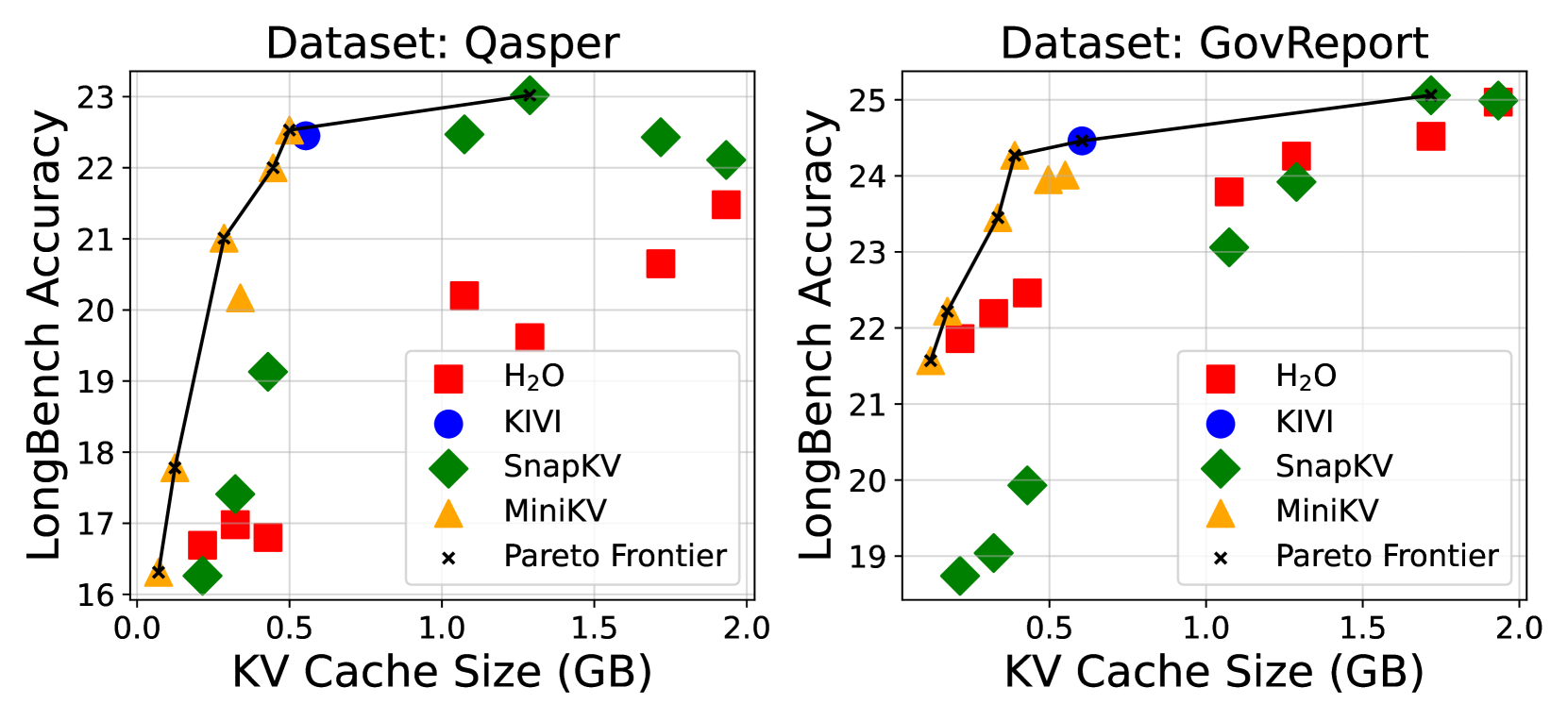<details> <summary>x8.png Details</summary>  ### Visual Description ## Line Graphs: LongBench Accuracy vs KV Cache Size for Qasper and GovReport Datasets ### Overview Two side-by-side line graphs compare LongBench Accuracy against KV Cache Size (GB) for four models (H₂O, KIVI, SnapKV, MiniKV) across two datasets (Qasper and GovReport). The Pareto Frontier (black crosses) represents optimal trade-offs between cache size and accuracy. ### Components/Axes - **X-axis**: KV Cache Size (GB) ranging from 0.0 to 2.0 GB in 0.5 GB increments. - **Y-axis**: LongBench Accuracy (Qasper: 16–23, GovReport: 19–25). - **Legend**: - Red squares: H₂O - Blue circle: KIVI - Green diamonds: SnapKV - Yellow triangles: MiniKV - Black crosses: Pareto Frontier ### Detailed Analysis #### Dataset: Qasper - **Pareto Frontier**: Starts at ~16.5 accuracy (0.0 GB) and rises to ~23.0 accuracy (1.5 GB). - **Model Data Points**: - H₂O (red squares): Peaks at ~21.5 accuracy (1.5 GB), with lower values at smaller cache sizes. - KIVI (blue circle): Highest accuracy (~22.5) at 0.75 GB, then declines. - SnapKV (green diamonds): Consistent ~22 accuracy across 0.5–2.0 GB. - MiniKV (yellow triangles): Lowest accuracy (~17–20) across all cache sizes. #### Dataset: GovReport - **Pareto Frontier**: Starts at ~21.5 accuracy (0.0 GB) and rises to ~25.0 accuracy (1.5 GB). - **Model Data Points**: - H₂O (red squares): Peaks at ~24.5 accuracy (1.5 GB), with moderate values at smaller cache sizes. - KIVI (blue circle): Highest accuracy (~24.5) at 0.75 GB, then declines. - SnapKV (green diamonds): Consistent ~23.5 accuracy across 0.5–2.0 GB. - MiniKV (yellow triangles): Lowest accuracy (~21–23) across all cache sizes. ### Key Observations 1. **Pareto Frontier Dominance**: Both datasets show the Pareto Frontier as the optimal trajectory, with models clustering near or below it. 2. **Cache Size Impact**: Accuracy generally increases with cache size, but diminishing returns are evident (e.g., KIVI’s drop after 0.75 GB). 3. **Model Performance**: - **H₂O** and **SnapKV** perform best in GovReport, while **KIVI** excels in Qasper. - **MiniKV** consistently underperforms across both datasets. 4. **Outliers**: MiniKV’s low accuracy at 0.0 GB (Qasper: ~16.5, GovReport: ~19) suggests inefficiency at small cache sizes. ### Interpretation The data demonstrates a clear trade-off between KV cache size and LongBench Accuracy, with the Pareto Frontier highlighting the most efficient models. Larger cache sizes improve performance, but models like MiniKV lag behind, indicating potential architectural limitations. The divergence in model performance between datasets suggests dataset-specific optimizations may be necessary. Notably, KIVI’s peak at 0.75 GB in Qasper and H₂O’s dominance in GovReport imply that model architecture and dataset characteristics interact to determine optimal cache utilization. </details> Figure 10: Algorithm Performance vs KV Cache Size: The Pareto frontier (the black curve) indicates the optimal compression strategy across a range of KV cache sizes. MiniKV lies on the Pareto frontier across all 6 task categories. ### 5.4 MiniKV Enhanced LLM Inference Having established MiniKV’s ability to retain model quality, we now shift to evaluate MiniKV, KIVI, H 2 O and the Full Model on peak memory usage, latency and throughput. All our system experiments are conducted on LLaMA2-7B-chat. We utilize FlashAttention kernels for KIVI and the Full Model while employing our customized kernel introduced in § 4.3 for MiniKV. H 2 O does not support FlashAttention and is benchmarked with the standard attention. MiniKV effectively reduces peak memory usage. We benchmark peak memory usage, defined as the maximum memory occupied by all model tensors during the generation phase for MiniKV and its baselines. The memory savings achieved through KV cache compression can be rendered ineffective if peak memory usage surges beyond the total available memory. As discussed in § 4.3, during the prefill phase, KV cache eviction strategies like H 2 O necessitate the computation of the intermediate attention score tensor. This quadratic memory demand leads to a memory spike for long prompt lengths during the prefill phase, resulting in out-of-memory (OOM) errors and prematurely terminating the generation. 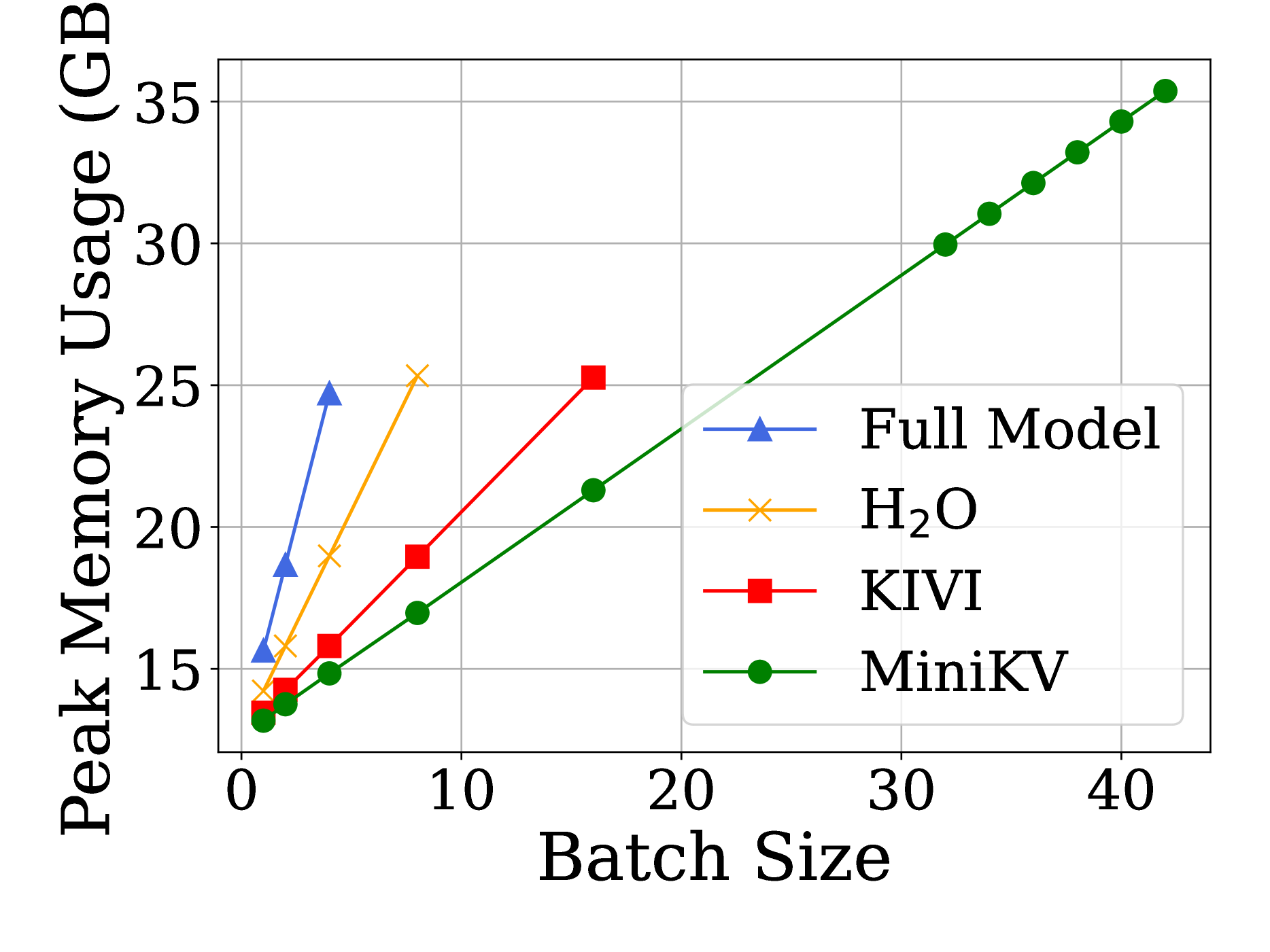<details> <summary>x9.png Details</summary>  ### Visual Description ## Line Chart: Peak Memory Usage vs. Batch Size ### Overview The chart illustrates the relationship between batch size (x-axis) and peak memory usage (y-axis, in GB) for four computational models: Full Model, H₂O, KIVI, and MiniKV. Data points are represented by distinct markers (triangles, crosses, squares, circles) and connected by lines. The y-axis ranges from 0 to 35 GB, while the x-axis spans batch sizes from 0 to 40. ### Components/Axes - **X-axis (Batch Size)**: Labeled "Batch Size," with increments of 10 (0, 10, 20, 30, 40). - **Y-axis (Peak Memory Usage)**: Labeled "Peak Memory Usage (GB)," with increments of 5 (0, 5, 10, 15, 20, 25, 30, 35). - **Legend**: Located in the bottom-right corner, associating colors and markers with models: - **Blue triangles**: Full Model - **Orange crosses**: H₂O - **Red squares**: KIVI - **Green circles**: MiniKV ### Detailed Analysis 1. **Full Model (Blue Triangles)**: - Starts at ~15 GB (batch size 0). - Peaks at ~25 GB (batch size 5). - Drops to ~15 GB (batch size 10). - No further data points beyond batch size 10. 2. **H₂O (Orange Crosses)**: - Starts at ~15 GB (batch size 0). - Peaks at ~25 GB (batch size 8). - Drops to ~15 GB (batch size 10). - No further data points beyond batch size 10. 3. **KIVI (Red Squares)**: - Starts at ~15 GB (batch size 0). - Increases steadily to ~25 GB (batch size 15). - No further data points beyond batch size 15. 4. **MiniKV (Green Circles)**: - Starts at ~13 GB (batch size 0). - Increases linearly to ~35 GB (batch size 40). - Consistent upward trend across all batch sizes. ### Key Observations - **MiniKV** exhibits the highest memory usage, scaling linearly with batch size. - **Full Model** and **H₂O** show peak memory usage at mid-range batch sizes (5–8), followed by a sharp decline. - **KIVI** demonstrates a steady increase in memory usage but plateaus at batch size 15. - All models except MiniKV lack data beyond batch size 15–10, suggesting limited testing or optimization constraints. ### Interpretation The data suggests that **MiniKV** is the most memory-intensive model, with memory usage growing proportionally to batch size. This could indicate inefficiencies in memory management or architectural design. In contrast, **Full Model** and **H₂O** appear optimized for smaller batch sizes, as their memory usage drops after peaking. **KIVI**’s linear trend implies predictable but resource-heavy scaling. The absence of data beyond certain batch sizes for most models may reflect practical limitations in testing or deployment scenarios. The chart highlights trade-offs between batch size scalability and memory efficiency across different computational frameworks. 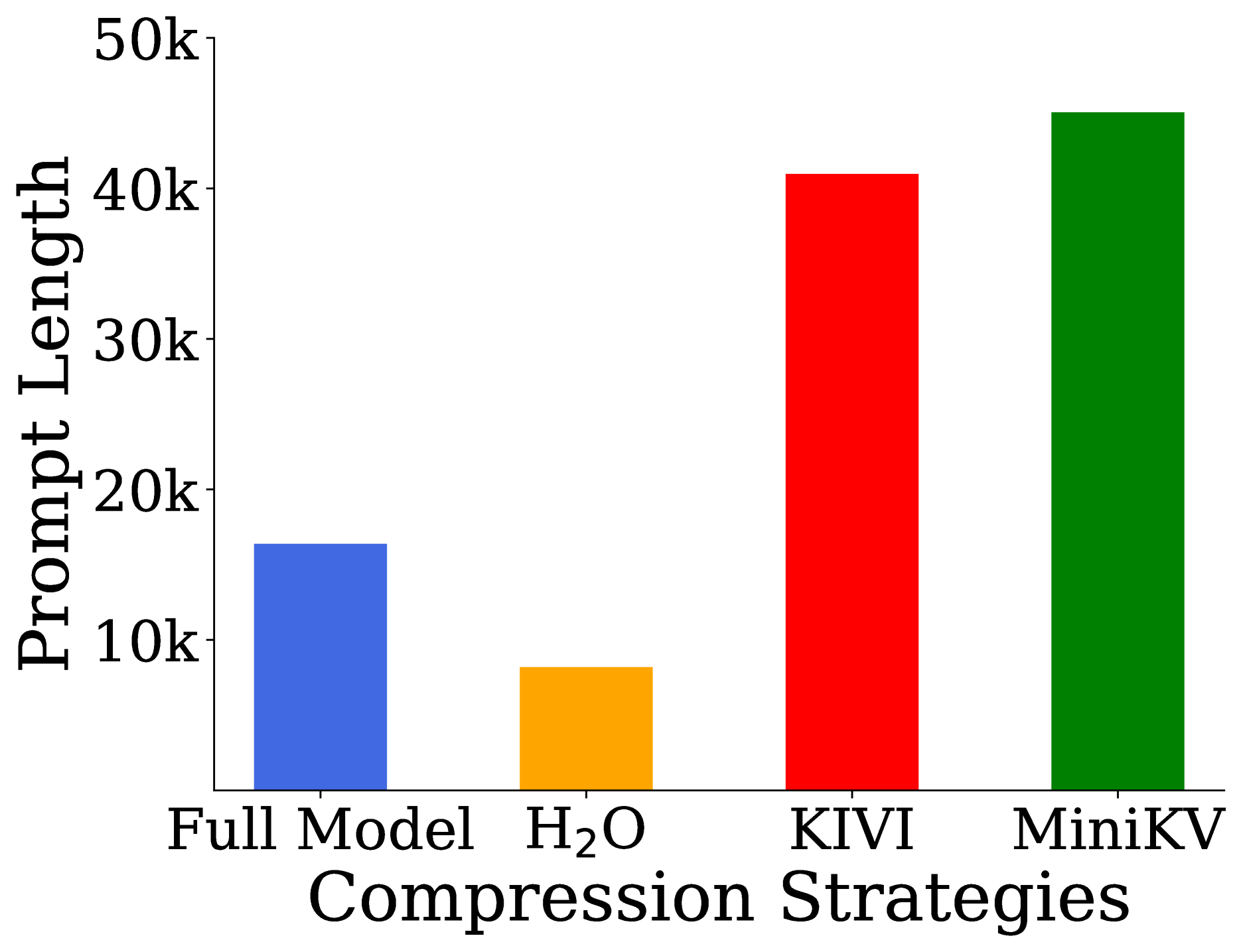</details> <details> <summary>x10.png Details</summary>  ### Visual Description ## Bar Chart: Prompt Length Comparison Across Compression Strategies ### Overview The chart compares prompt lengths (in thousands) for four compression strategies: Full Model, H₂O, KIVI, and MiniKV. Prompt lengths are measured on a logarithmic scale from 10k to 50k. ### Components/Axes - **X-axis**: Compression Strategies (categorical: Full Model, H₂O, KIVI, MiniKV) - **Y-axis**: Prompt Length (logarithmic scale: 10k, 20k, 30k, 40k, 50k) - **Legend**: Located at the bottom, mapping colors to strategies: - Blue: Full Model - Orange: H₂O - Red: KIVI - Green: MiniKV ### Detailed Analysis 1. **Full Model** (Blue): - Prompt length ≈ 16k - Bar height reaches ~16,000 on the y-axis. 2. **H₂O** (Orange): - Prompt length ≈ 8k - Bar height reaches ~8,000 on the y-axis. 3. **KIVI** (Red): - Prompt length ≈ 41k - Bar height reaches ~41,000 on the y-axis. 4. **MiniKV** (Green): - Prompt length ≈ 45k - Bar height reaches ~45,000 on the y-axis. ### Key Observations - **H₂O** has the shortest prompt length (~8k), significantly lower than the Full Model (~16k). - **MiniKV** has the longest prompt length (~45k), nearly tripling the Full Model's length. - **KIVI** (~41k) and **MiniKV** (~45k) show similar magnitudes, both far exceeding the Full Model. - The logarithmic y-axis emphasizes the disparity between H₂O and the other strategies. ### Interpretation The data suggests that compression strategies drastically alter prompt length. H₂O achieves the most aggressive compression (halving the Full Model's length), while MiniKV introduces the greatest expansion (~2.8x the Full Model). This implies trade-offs between compression efficiency and data retention or processing overhead. The logarithmic scale highlights exponential differences, particularly between H₂O and the other strategies. The Full Model serves as a baseline, with H₂O optimizing for brevity and MiniKV prioritizing other factors (e.g., accuracy or speed) at the cost of length. </details> Figure 11: Left: Peak memory usage (GB) vs batch size for prompt = 2048 & batch size = 1. Right: Maximum prompt length supported by MiniKV and its baselines for batch size = 1. We evaluate the impact of batch size and prompt length on peak memory usage in Fig. 11 (left). MiniKV demonstrates the lowest peak memory consumption at larger batch sizes. H 2 O goes out-of-memory at batch size 16 as it materializes the intermediate attention score matrix. MiniKV accommodates larger batch sizes as it maintains a much linear cache compared to KIVI owing to MiniKV’s cache eviction mechanism. Despite the Full Model’s implementation of FlashAttention, it supports smaller batch sizes than H 2 O while reaching a higher peak memory during the generation process. This is mainly because of the combination of 2 reasons: (1) The Full Model’s KV cache size is $1/(α_HH+α_RW)$ (twice, for a 50% cache budget) that of H 2 O during inference. (2) During the decoding phase, the hidden representations (or token embeddings) output by the self-attention undergo a $4×$ upscaling in the MLP layer which occupies memory to store an intermediate tensor of shape $B× l_prompt×(4× d)$ . Since H 2 O and MiniKV evict tokens before the MLP layer, their peak memory usage is not as significant as that of the Full Model. Maximum processable prompt. MiniKV’s lower memory consumption becomes more apparent with longer prompt lengths. Fig. 11 (right) shows that MiniKV’s KV compression during the prefill phase enables it to process prompts 10% longer than its strongest baseline KIVI. Additionally, MiniKV’s selective flash-attention kernel allows significantly longer sequence lengths when compared to H 2 O. MiniKV speedups end-to-end latency. LLM inference is predominantly constrained by memory bandwidth during the retrieval of model states. Our approach addresses latency through compression strategies that reduce the number of key-value (KV) vectors loaded for each next-token prediction. As shown in Fig. 13 (left), KIVI exhibits lower latency than MiniKV at shorter sequence lengths; however, a crossover point emerges where KIVI’s latency becomes more dominant. Fig. 13 (left) illustrates the crossover around a prompt length of 22k tokens, showing the latency benefits of managing a smaller KV cache. 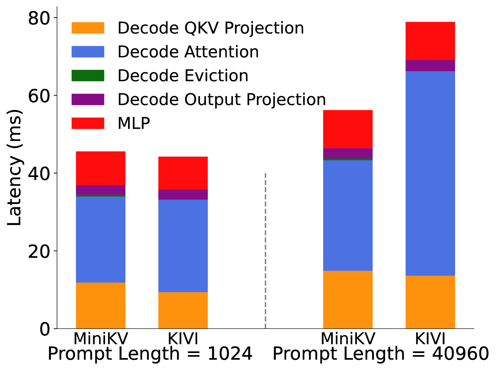<details> <summary>x11.png Details</summary>  ### Visual Description ## Bar Chart: Latency Comparison for MiniKV and KIVI at Different Prompt Lengths ### Overview The chart compares latency (in milliseconds) for five components of two systems (MiniKV and KIVI) across two prompt lengths: 1024 and 40960. Latency is segmented by component type, with a legend indicating color coding. The x-axis categorizes data by system and prompt length, while the y-axis represents latency values from 0 to 80 ms. ### Components/Axes - **X-Axis**: - Categories: "MiniKV" and "KIVI" under two prompt lengths: - "Prompt Length = 1024" (left group) - "Prompt Length = 40960" (right group) - **Y-Axis**: - Label: "Latency (ms)" with a scale from 0 to 80. - **Legend** (right-aligned): - Colors and labels: - Orange: Decode QKV Projection - Blue: Decode Attention - Green: Decode Eviction - Purple: Decode Output Projection - Red: MLP ### Detailed Analysis #### Prompt Length = 1024 - **MiniKV**: - Decode QKV Projection: ~12 ms (orange) - Decode Attention: ~22 ms (blue) - Decode Eviction: ~1 ms (green) - Decode Output Projection: ~3 ms (purple) - MLP: ~7 ms (red) - **Total**: ~45 ms - **KIVI**: - Decode QKV Projection: ~10 ms (orange) - Decode Attention: ~20 ms (blue) - Decode Eviction: ~1 ms (green) - Decode Output Projection: ~3 ms (purple) - MLP: ~6 ms (red) - **Total**: ~40 ms #### Prompt Length = 40960 - **MiniKV**: - Decode QKV Projection: ~15 ms (orange) - Decode Attention: ~30 ms (blue) - Decode Eviction: ~2 ms (green) - Decode Output Projection: ~4 ms (purple) - MLP: ~8 ms (red) - **Total**: ~59 ms - **KIVI**: - Decode QKV Projection: ~14 ms (orange) - Decode Attention: ~50 ms (blue) - Decode Eviction: ~2 ms (green) - Decode Output Projection: ~4 ms (purple) - MLP: ~9 ms (red) - **Total**: ~80 ms ### Key Observations 1. **Latency Scaling**: Latency increases significantly with longer prompt lengths (e.g., MiniKV increases from ~45 ms to ~59 ms; KIVI from ~40 ms to ~80 ms). 2. **Component Contribution**: - **Decode Attention** dominates latency in both systems and prompt lengths (e.g., ~50 ms for KIVI at 40960). - **MLP** contributes ~10-15% of total latency in longer prompts. - **Decode Eviction** has minimal impact (<5% of total latency). 3. **System Efficiency**: KIVI consistently shows lower latency than MiniKV for the same prompt length (e.g., ~40 ms vs. ~45 ms at 1024). ### Interpretation - **Prompt Length Impact**: Longer prompts disproportionately increase latency, particularly for "Decode Attention," suggesting it scales poorly with input size. - **System Design**: KIVI’s architecture appears more efficient, likely due to optimizations in attention or eviction handling. - **Bottlenecks**: The MLP component becomes a larger relative contributor at longer prompts, indicating potential optimization opportunities. - **Eviction Efficiency**: The near-constant eviction latency across prompt lengths suggests it is not a major performance limiter in this context. ### Spatial Grounding - Legend is positioned on the right, with colors matching bar segments. - Bars are grouped by prompt length, with system-specific bars clustered under each prompt length. </details> Figure 12: Per token latency breakdown for the decoding phase. Generation length = 1024 and batch size = 1. Latency breakdown. We analyze the breakdown of latency associated with each computation in the standard decoder layer of the transformer architecture for MiniKV and KIVI during the decoding phase only. We particularly look at latencies for projections of the input vector into query, key, and value vectors, attention computation, cache eviction (if applicable) and output projection. We also measure the time spent in the MLP layer. We present the latency breakdown as the total latency for each computation component divided by the generation length. As shown in Fig. 12, for shorter prompt lengths, MiniKV’s latency is negligibly larger than KIVI’s due to the adjustment of rotary embeddings during the QKV projection. Conversely, for longer prompts, MiniKV achieves a lower end-to-end latency than KIVI. This improvement primarily arises from reduced attention computation time during decoding. Specifically, the inference time is dominated by KV cache loading time when processing long contexts. Therefore, the smaller KV cache results in reduced KV load times from the GPU’s HBM during decoding, and decreased latency associated with attention computation. Throughput. We measure throughput as the number of tokens processed per second. MiniKV outperforms all its baselines on throughput as depicted in Fig. 13 (right), owing to its lower latency and ability to support larger batch sizes and longer sequence lengths. 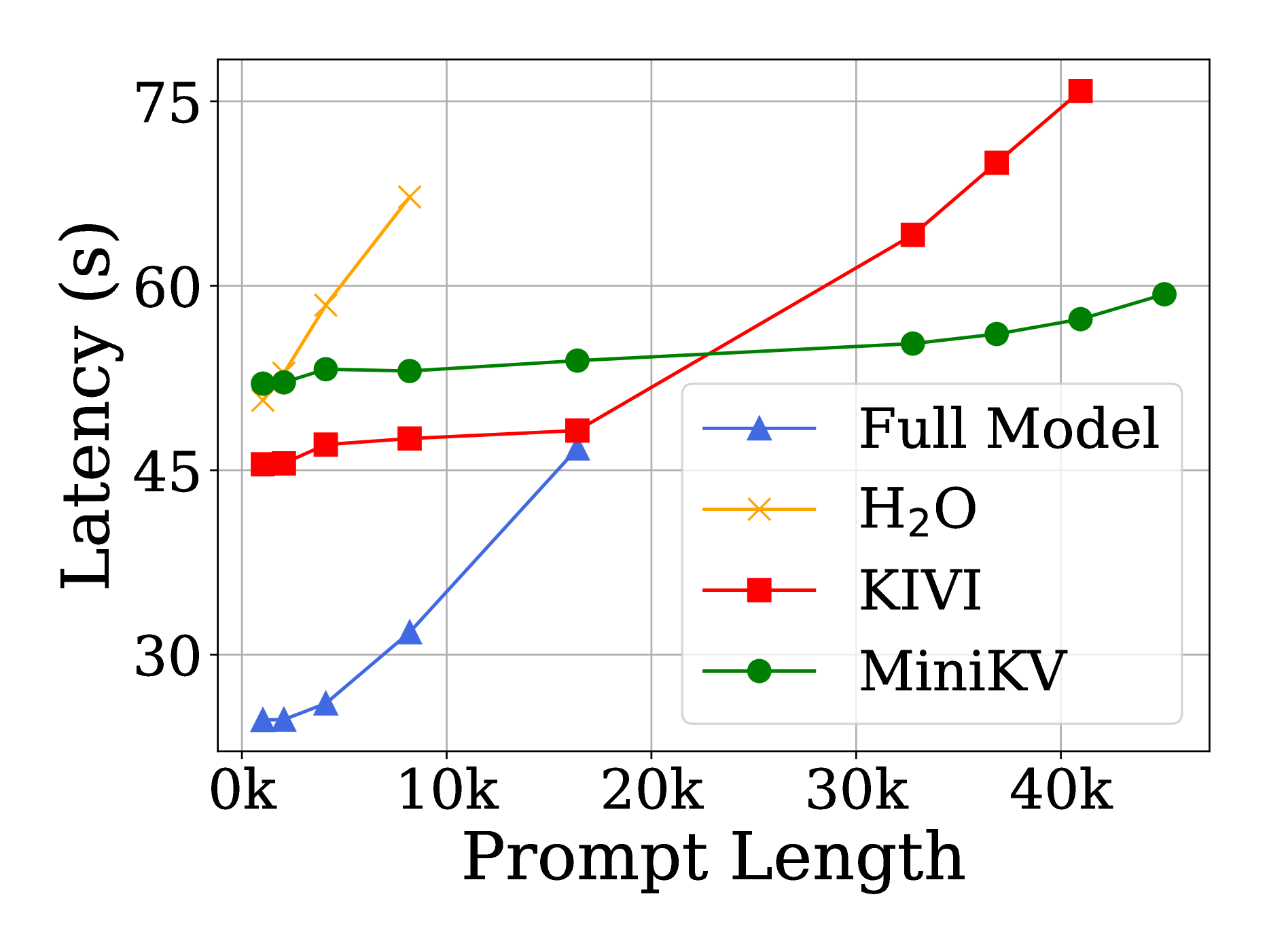<details> <summary>x12.png Details</summary>  ### Visual Description ## Line Graph: Latency vs. Prompt Length ### Overview The image is a line graph comparing latency (in seconds) across four different models (Full Model, H2O, KIVI, MiniKV) as prompt length increases from 0k to 40k. The y-axis represents latency (0–75 seconds), and the x-axis represents prompt length (0k–40k). Each model is represented by a distinct line with unique markers and colors. ### Components/Axes - **X-axis (Prompt Length)**: Labeled "Prompt Length" with ticks at 0k, 10k, 20k, 30k, and 40k. - **Y-axis (Latency)**: Labeled "Latency (s)" with ticks at 0, 15, 30, 45, 60, and 75 seconds. - **Legend**: Located in the bottom-right corner, mapping: - Blue triangles: Full Model - Orange crosses: H2O - Red squares: KIVI - Green circles: MiniKV ### Detailed Analysis 1. **Full Model (Blue Triangles)**: - Starts at ~25 seconds for 0k prompt length. - Increases sharply to ~60 seconds at 40k. - Key data points: 0k (~25s), 10k (~30s), 20k (~45s), 30k (~55s), 40k (~60s). 2. **H2O (Orange Crosses)**: - Starts at ~50 seconds for 0k. - Decreases sharply to ~45 seconds at 10k. - Remains relatively flat at ~45 seconds for 20k–40k. - Key data points: 0k (~50s), 10k (~45s), 20k (~45s), 30k (~45s), 40k (~45s). 3. **KIVI (Red Squares)**: - Starts at ~45 seconds for 0k. - Increases steadily to ~75 seconds at 40k. - Key data points: 0k (~45s), 10k (~47s), 20k (~50s), 30k (~60s), 40k (~75s). 4. **MiniKV (Green Circles)**: - Starts at ~50 seconds for 0k. - Remains relatively flat, increasing slightly to ~60 seconds at 40k. - Key data points: 0k (~50s), 10k (~52s), 20k (~54s), 30k (~56s), 40k (~60s). ### Key Observations - **H2O** shows the most significant drop in latency (from ~50s to ~45s) as prompt length increases, suggesting efficiency at higher loads. - **KIVI** exhibits the steepest upward trend, indicating poor scalability with longer prompts. - **MiniKV** maintains the most stable latency, with only a modest increase (~10s) across all prompt lengths. - **Full Model** balances moderate latency growth (~35s increase) but starts lower than H2O and MiniKV. ### Interpretation The graph highlights trade-offs between model efficiency and scalability. **H2O** performs best at shorter prompt lengths but plateaus, while **KIVI** struggles with longer prompts. **MiniKV** demonstrates consistent performance, making it suitable for variable workloads. **Full Model** offers a middle ground, with manageable latency growth but higher initial latency than H2O and MiniKV. The data suggests that model choice depends on the expected prompt length and latency tolerance. 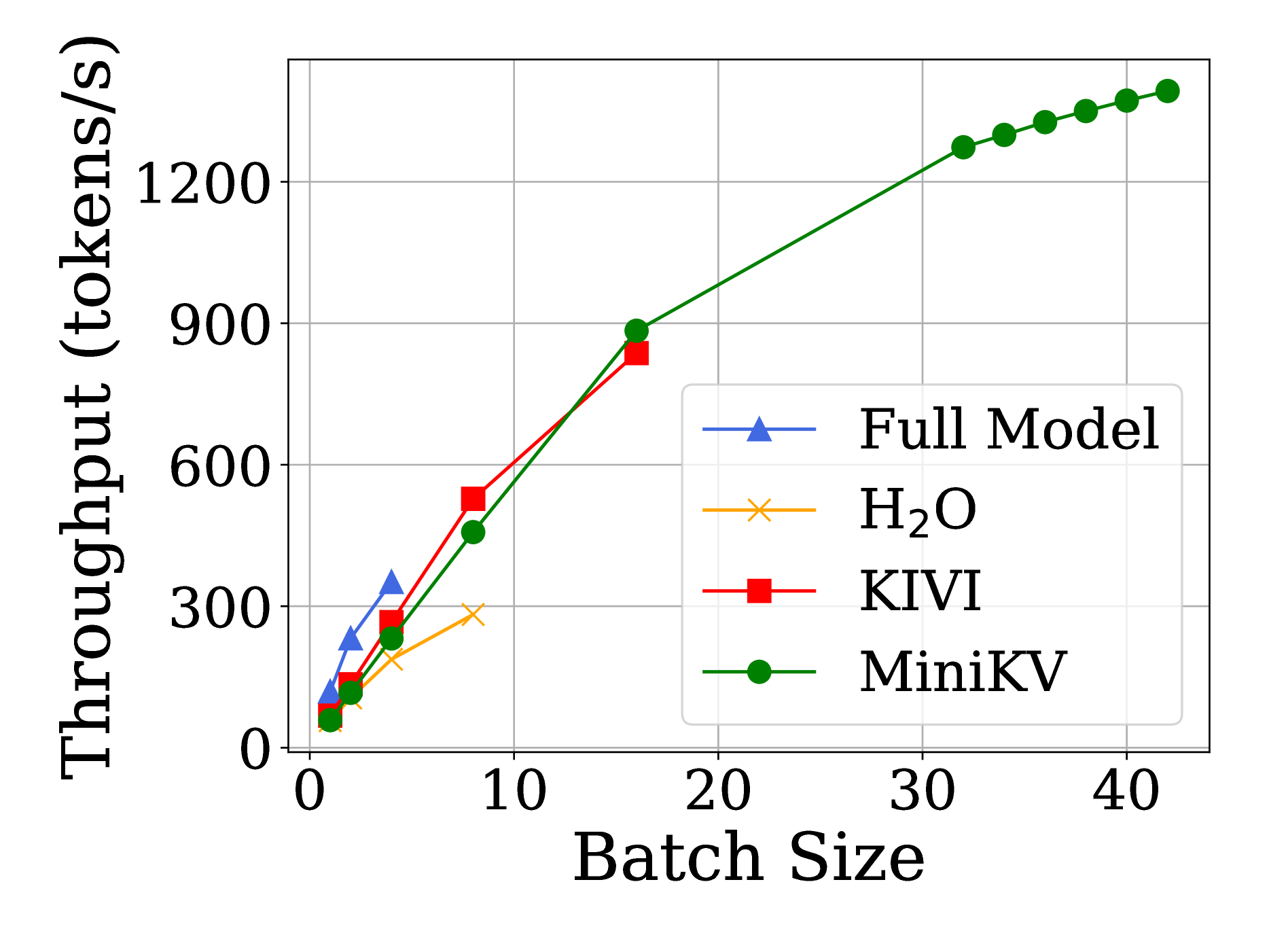</details> <details> <summary>x13.png Details</summary>  ### Visual Description ## Line Chart: Throughput vs Batch Size ### Overview The chart compares the throughput (tokens per second) of four different models (Full Model, H₂O, KIVI, MiniKV) across varying batch sizes (0 to 40). Throughput increases with batch size for all models, but the rate of improvement and final performance differ significantly. ### Components/Axes - **X-axis (Batch Size)**: Ranges from 0 to 40 in increments of 10. - **Y-axis (Throughput)**: Ranges from 0 to 1400 tokens/s in increments of 300. - **Legend**: - Blue triangles: Full Model - Orange crosses: H₂O - Red squares: KIVI - Green circles: MiniKV - **Data Points**: Each model is represented by a distinct marker and line style. ### Detailed Analysis 1. **Full Model (Blue Triangles)**: - Starts at ~50 tokens/s (batch size 1). - Reaches ~300 tokens/s at batch size 10. - No data points beyond batch size 10. 2. **H₂O (Orange Crosses)**: - Starts at ~20 tokens/s (batch size 1). - Reaches ~300 tokens/s at batch size 10. - No data points beyond batch size 10. 3. **KIVI (Red Squares)**: - Starts at ~10 tokens/s (batch size 1). - Reaches ~800 tokens/s at batch size 15. - No data points beyond batch size 15. 4. **MiniKV (Green Circles)**: - Starts at ~5 tokens/s (batch size 1). - Reaches ~1300 tokens/s at batch size 40. - Shows the steepest slope, indicating the highest scalability. ### Key Observations - **MiniKV** consistently outperforms other models at larger batch sizes (e.g., 1300 tokens/s at batch size 40 vs. 800 tokens/s for KIVI at batch size 15). - **H₂O** and **Full Model** have similar performance but plateau at lower throughputs (~300 tokens/s) compared to KIVI and MiniKV. - All models show diminishing returns at smaller batch sizes (e.g., batch size 1–5). ### Interpretation The data suggests that **MiniKV** is the most scalable model for high-throughput applications, particularly when processing large batch sizes. Its linear growth trend indicates efficient resource utilization. In contrast, **H₂O** and **Full Model** underperform at larger batches, while **KIVI** offers moderate scalability but lags behind MiniKV. This highlights the importance of model architecture optimization for batch processing efficiency. The absence of data beyond certain batch sizes for some models may indicate hardware or implementation limitations. </details> Figure 13: Left: Latency (s) for batch size = 1 and generation length = 1024. Right: Throughput (tokens/s) for prompt length = 2048 and generation length = 1024 ## 6 Conclusion In this work, we investigate KV cache optimization to accelerate the inference of LLM, especially when processing long contexts. Our empirical analysis indicates that existing eviction-based KV cache optimization struggles to preserve accuracy on long context tasks while maintaining a high compression ratio. To tackle this issue, we design MiniKV, a novel KV cache compression approach that bridges the gap between eviction-based and low-bit quantization techniques. Evaluation across a wide range of datasets shows that MiniKV preserves long context accuracy while significantly improving inference efficiency. ## 7 Acknowledgement This work used Delta system at the National Center for Supercomputing Applications through allocation CIS240055 from the Advanced Cyberinfrastructure Coordination Ecosystem: Services & Support (ACCESS) program. ACCESS Boerner et al. (2023) is an advanced computing and data resource program supported by the U.S. National Science Foundation (NSF) under the Office of Advanced Cyberinfrastructure awards #2138259, #2138286, #2138307, #2137603 and #2138296. The Delta advanced computing resource is a joint effort of the University of Illinois Urbana-Champaign and its National Center for Supercomputing Applications, and it is supported by the National Science Foundation (award OAC 2005572) and the State of Illinois. The work also used the Illinois Campus Cluster and NCSA NFI Hydro cluster, which are supported by the University of Illinois Urbana-Champaign and the University of Illinois System. ## References - Bai et al. (2023) Bai, Y., Lv, X., Zhang, J., Lyu, H., Tang, J., Huang, Z., Du, Z., Liu, X., Zeng, A., Hou, L., Dong, Y., Tang, J., and Li, J. Longbench: A bilingual, multitask benchmark for long context understanding. CoRR, abs/2308.14508, 2023. - Boerner et al. (2023) Boerner, T. J., Deems, S., Furlani, T. R., Knuth, S. L., and Towns, J. ACCESS: Advancing Innovation: NSF’s Advanced Cyberinfrastructure Coordination Ecosystem: Services & Support. In Practice and Experience in Advanced Research Computing (PEARC’23), 2023. - Brandon et al. (2024) Brandon, W., Mishra, M., Nrusimha, A., Panda, R., and Ragan-Kelly, J. Reducing transformer key-value cache size with cross-layer attention. CoRR, abs/2405.12981, 2024. - Brown et al. (2020) Brown, T. B., Mann, B., Ryder, N., Subbiah, M., Kaplan, J., Dhariwal, P., Neelakantan, A., Shyam, P., Sastry, G., Askell, A., Agarwal, S., Herbert-Voss, A., Krueger, G., Henighan, T., Child, R., Ramesh, A., Ziegler, D. M., Wu, J., Winter, C., Hesse, C., Chen, M., Sigler, E., Litwin, M., Gray, S., Chess, B., Clark, J., Berner, C., McCandlish, S., Radford, A., Sutskever, I., and Amodei, D. Language Models are Few-Shot Learners. In Proceedings of the 34th International Conference on Neural Information Processing Systems (NIPS’20), December 2020. - Cai et al. (2024) Cai, Z., Zhang, Y., Gao, B., Liu, Y., Liu, T., Lu, K., Xiong, W., Dong, Y., Chang, B., Hu, J., and Xiao, W. Pyramidkv: Dynamic KV cache compression based on pyramidal information funneling. CoRR, abs/2406.02069, 2024. - Dao et al. (2022) Dao, T., Fu, D. Y., Ermon, S., Rudra, A., and Ré, C. Flashattention: Fast and memory-efficient exact attention with io-awareness. In Advances in Neural Information Processing Systems 35: Annual Conference on Neural Information Processing Systems 2022, NeurIPS 2022, New Orleans, LA, USA, November 28 - December 9, 2022, 2022. - Frantar et al. (2022) Frantar, E., Ashkboos, S., Hoefler, T., and Alistarh, D. GPTQ: accurate post-training quantization for generative pre-trained transformers. CoRR, abs/2210.17323, 2022. - Ge et al. (2023) Ge, S., Zhang, Y., Liu, L., Zhang, M., Han, J., and Gao, J. Model tells you what to discard: Adaptive KV cache compression for llms. CoRR, abs/2310.01801, 2023. - Gersho (1978) Gersho, A. Principles of quantization. IEEE Transactions on circuits and systems, 25(7):427–436, 1978. - Hooper et al. (2024) Hooper, C., Kim, S., Mohammadzadeh, H., Mahoney, M. W., Shao, Y. S., Keutzer, K., and Gholami, A. Kvquant: Towards 10 million context length LLM inference with KV cache quantization. CoRR, abs/2401.18079, 2024. - Jiang et al. (2023) Jiang, A. Q., Sablayrolles, A., Mensch, A., Bamford, C., Chaplot, D. S., de las Casas, D., Bressand, F., Lengyel, G., Lample, G., Saulnier, L., Lavaud, L. R., Lachaux, M.-A., Stock, P., Scao, T. L., Lavril, T., Wang, T., Lacroix, T., and Sayed, W. E. Mistral 7B. arXiv preprint arXiv:2310.06825, 2023. - Leskovec & Sosic (2016) Leskovec, J. and Sosic, R. SNAP: A General-Purpose Network Analysis and Graph-Mining Library. ACM TIST, 8(1):1:1–1:20, 2016. - Li et al. (2024) Li, Y., Huang, Y., Yang, B., Venkitesh, B., Locatelli, A., Ye, H., Cai, T., Lewis, P., and Chen, D. Snapkv: Llm knows what you are looking for before generation. arXiv preprint arXiv:2404.14469, 2024. - Lin et al. (2024) Lin, J., Tang, J., Tang, H., Yang, S., Chen, W.-M., Wang, W.-C., Xiao, G., Dang, X., Gan, C., and Han, S. Awq: Activation-aware weight quantization for on-device llm compression and acceleration. Proceedings of Machine Learning and Systems, 6:87–100, 2024. - Liu et al. (2024a) Liu, A., Liu, J., Pan, Z., He, Y., Haffari, G., and Zhuang, B. Minicache: Kv cache compression in depth dimension for large language models. CoRR, abs/2405.14366, 2024a. - Liu et al. (2021) Liu, L., Liu, J., and Han, J. Multi-head or single-head? an empirical comparison for transformer training. CoRR, abs/2106.09650, 2021. - Liu et al. (2023a) Liu, N. F., Lin, K., Hewitt, J., Paranjape, A., Bevilacqua, M., Petroni, F., and Liang, P. Lost in the middle: How language models use long contexts. CoRR, abs/2307.03172, 2023a. - Liu et al. (2023b) Liu, Z., Desai, A., Liao, F., Wang, W., Xie, V., Xu, Z., Kyrillidis, A., and Shrivastava, A. Scissorhands: Exploiting the persistence of importance hypothesis for LLM KV cache compression at test time. In Advances in Neural Information Processing Systems 36: Annual Conference on Neural Information Processing Systems 2023, NeurIPS 2023, New Orleans, LA, USA, December 10 - 16, 2023, 2023b. - Liu et al. (2023c) Liu, Z., Oguz, B., Zhao, C., Chang, E., Stock, P., Mehdad, Y., Shi, Y., Krishnamoorthi, R., and Chandra, V. LLM-QAT: data-free quantization aware training for large language models. CoRR, abs/2305.17888, 2023c. - Liu et al. (2024b) Liu, Z., Yuan, J., Jin, H., Zhong, S., Xu, Z., Braverman, V., Chen, B., and Hu, X. KIVI: A tuning-free asymmetric 2bit quantization for KV cache. CoRR, abs/2402.02750, 2024b. - Nawrot et al. (2024) Nawrot, P., Łańcucki, A., Chochowski, M., Tarjan, D., and Ponti, E. M. Dynamic memory compression: Retrofitting llms for accelerated inference. CoRR, 2403.09636, 2024. - OpenAI (2023) OpenAI. GPT-4 technical report. CoRR, abs/2303.08774, 2023. - Shazeer (2019) Shazeer, N. Fast transformer decoding: One write-head is all you need. CoRR, abs/1911.02150, 2019. - Sheng et al. (2023) Sheng, Y., Zheng, L., Yuan, B., Li, Z., Ryabinin, M., Chen, B., Liang, P., Ré, C., Stoica, I., and Zhang, C. Flexgen: High-throughput generative inference of large language models with a single GPU. In International Conference on Machine Learning, ICML 2023, 23-29 July 2023, Honolulu, Hawaii, USA, volume 202 of Proceedings of Machine Learning Research, pp. 31094–31116. PMLR, 2023. - Sun et al. (2021) Sun, S., Krishna, K., Mattarella-Micke, A., and Iyyer, M. Do long-range language models actually use long-range context? In Proceedings of the 2021 Conference on Empirical Methods in Natural Language Processing, EMNLP 2021, Virtual Event / Punta Cana, Dominican Republic, 7-11 November, 2021, pp. 807–822. Association for Computational Linguistics, 2021. - Touvron et al. (2023) Touvron, H., Martin, L., Stone, K., Albert, P., Almahairi, A., Babaei, Y., Bashlykov, N., Batra, S., Bhargava, P., Bhosale, S., Bikel, D., Blecher, L., Canton-Ferrer, C., Chen, M., Cucurull, G., Esiobu, D., Fernandes, J., Fu, J., Fu, W., Fuller, B., Gao, C., Goswami, V., Goyal, N., Hartshorn, A., Hosseini, S., Hou, R., Inan, H., Kardas, M., Kerkez, V., Khabsa, M., Kloumann, I., Korenev, A., Koura, P. S., Lachaux, M., Lavril, T., Lee, J., Liskovich, D., Lu, Y., Mao, Y., Martinet, X., Mihaylov, T., Mishra, P., Molybog, I., Nie, Y., Poulton, A., Reizenstein, J., Rungta, R., Saladi, K., Schelten, A., Silva, R., Smith, E. M., Subramanian, R., Tan, X. E., Tang, B., Taylor, R., Williams, A., Kuan, J. X., Xu, P., Yan, Z., Zarov, I., Zhang, Y., Fan, A., Kambadur, M., Narang, S., Rodriguez, A., Stojnic, R., Edunov, S., and Scialom, T. Llama 2: Open foundation and fine-tuned chat models. CoRR, abs/2307.09288, 2023. - Voita et al. (2019) Voita, E., Talbot, D., Moiseev, F., Sennrich, R., and Titov, I. Analyzing multi-head self-attention: Specialized heads do the heavy lifting, the rest can be pruned. In Proceedings of the 57th Conference of the Association for Computational Linguistics, ACL 2019, Florence, Italy, July 28- August 2, 2019, Volume 1: Long Papers, pp. 5797–5808. Association for Computational Linguistics, 2019. - Wan et al. (2024) Wan, Z., Wu, X., Zhang, Y., Xin, Y., Tao, C., Zhu, Z., Wang, X., Luo, S., Xiong, J., and Zhang, M. D2o: Dynamic discriminative operations for efficient generative inference of large language models. CoRR, abs/2406.13035, 2024. - Wu et al. (2024) Wu, W., Wang, Y., Xiao, G., Peng, H., and Fu, Y. Retrieval head mechanistically explains long-context factuality. CoRR, abs/2404.15574, 2024. - Xiao et al. (2023a) Xiao, G., Lin, J., Seznec, M., Wu, H., Demouth, J., and Han, S. Smoothquant: Accurate and efficient post-training quantization for large language models. In International Conference on Machine Learning, ICML 2023, 23-29 July 2023, Honolulu, Hawaii, USA, volume 202 of Proceedings of Machine Learning Research, pp. 38087–38099. PMLR, 2023a. - Xiao et al. (2023b) Xiao, G., Tian, Y., Chen, B., Han, S., and Lewis, M. Efficient streaming language models with attention sinks. CoRR, abs/2309.17453, 2023b. - Yang et al. (2024a) Yang, D., Han, X., Gao, Y., Hu, Y., Zhang, S., and Zhao, H. Pyramidinfer: Pyramid kv cache compression for high-throughput llm inference. CoRR, abs/2405.12532, 2024a. - Yang et al. (2024b) Yang, J. Y., Kim, B., Bae, J., Kwon, B., Park, G., Yang, E., Kwon, S. J., and Lee, D. No token left behind: Reliable KV cache compression via importance-aware mixed precision quantization. CoRR, abs/2402.18096, 2024b. - Yin et al. (2024) Yin, L., Wu, Y., Zhang, Z., Hsieh, C.-Y., Wang, Y., Jia, Y., Li, G., Jaiswal, A., Pechenizkiy, M., Liang, Y., Bendersky, M., Wang, Z., and Liu, S. Outlier weighed layerwise sparsity (owl): A missing secret sauce for pruning llms to high sparsity. CoRR, 2310.05175, 2024. - Zhang et al. (2023) Zhang, Z., Sheng, Y., Zhou, T., Chen, T., Zheng, L., Cai, R., Song, Z., Tian, Y., Ré, C., Barrett, C. W., Wang, Z., and Chen, B. H2O: heavy-hitter oracle for efficient generative inference of large language models. In Advances in Neural Information Processing Systems 36: Annual Conference on Neural Information Processing Systems 2023, NeurIPS 2023, New Orleans, LA, USA, December 10 - 16, 2023, 2023. - Zhang et al. (2024) Zhang, Z., Liu, S., Chen, R., Kailkhura, B., Chen, B., and Wang, A. Q-hitter: A better token oracle for efficient llm inference via sparse-quantized kv cache. Proceedings of Machine Learning and Systems, 6:381–394, 2024. ## Appendix A Related Work There has been a growing interest in addressing KV cache memory constraints, which can be roughly divided into a few categories. First, some work proposes reducing the number of heads in KV cache, such as Grouped Query Attention Shazeer (2019). However, these methods are often bound to the architecture choices and require either training the model from scratch or fine-tuning, which makes them not plug-and-play for alternative trained LLMs. Second, quantization has been a prevailing technique to overcome memory overhead. Recent research shows that INT8/INT4 quantization can be achieved for KV cache while preserving accuracy Hooper et al. (2024); Sheng et al. (2023); Liu et al. (2023c); Yang et al. (2024b); Zhang et al. (2024). However, few studies have investigated how to achieve extreme KV cache quantization (less than 4-bit quantization) for eviction-based KV. At the time of writing, KIVI Liu et al. (2024b) introduced the most accomplished version of KV quantization, which uses fine-grained asymmetric 2-bit quantization for the KV cache. While being effective, it still has one major limitation: its effectiveness against eviction-based KV cache has yet to be proven. As shown in § 4, applying 2-bit quantization to eviction-based methods leads to accuracy and system challenges. To tackle this challenge, we introduce the 2-bit layer-discriminative KV cache method, which enables combining selective KV and 2-bit quantization, while incurring lower KV cache memory cost on long context tasks. Table 2: Comparison with previous KV cache optimization methods for LLM inference. Third, a promising line of work has also recently emerged that reduces KV cache size by evicting non-important tokens during inference Zhang et al. (2023); Xiao et al. (2023b); Liu et al. (2023b); Ge et al. (2023); Wan et al. (2024); Li et al. (2024). For instance, H 2 O proposes to keep only heavy hitters Zhang et al. (2023), which are tokens that have higher accumulated attention scores, in KV cache. StreamingLLM Xiao et al. (2023b) hypothesizes the existence of "sink tokens" at the beginning of a sequence, which consistently have higher attention scores, and proposes to simply keep the initial tokens and the recent local window. In contrast to this line of work, our goal in this paper is to improve the compression ratio of KV cache via eviction-based KV with quantized states. We empirically show that this path can be more memory-efficient, especially on long context tasks. Table 2 summarizes the comparison between MiniKV and previous approaches. Very recently, there has been a growing interest in exploring various strategies for exploiting KV cache selection via layer-sensitivity. Layer-sensitivity has proven successful in related areas, such as weight pruning Yin et al. (2024). One approach is to maintain different heavy token ratios. For example, PyramidInfer Yang et al. (2024a) observes lower perplexity output in the bottom layers and therefore chooses to use a smaller heavy ratio in deeper layers. However, this approach is problematic as it does not necessarily reflect the model’s performance on sequence-level tasks in real applications Sun et al. (2021). Another approach is to merge the KV cache of adjacent layers Brandon et al. (2024) Liu et al. (2024a) because the KV cache states exhibit high similarity between the adjacent layers. Additionally, in DMC Nawrot et al. (2024), the authors presented the distribution characteristics of layers under different compression ratios in a specific model, but they did not design an algorithm based on these characteristics. Different from these methods, we focus on exploring layer-wise KV selection policies that are compatible with quantized KV. ## Appendix B Additional Results on Attention Distribution on Long-Context Understanding Tasks Figure 14 presents more results of the diverse attention distribution across LLM layers on long context understanding tasks. 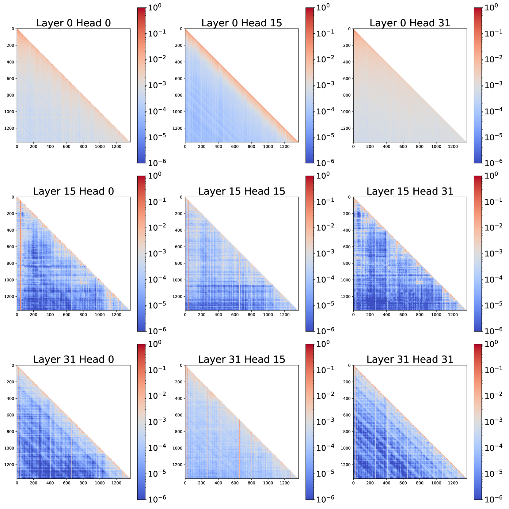<details> <summary>x14.png Details</summary>  ### Visual Description ## Heatmap Grid: Layer-Head Interaction Strengths ### Overview The image displays a 3x3 grid of heatmaps visualizing interaction strength distributions across different neural network layers and attention heads. Each heatmap represents a specific layer-head combination, with color intensity indicating magnitude (red = high, blue = low). The grid reveals systematic patterns in how interaction strengths vary with layer depth and head position. ### Components/Axes - **Grid Structure**: 3 rows (Layers 0, 15, 31) × 3 columns (Heads 0, 15, 31) - **Axes**: - X-axis: 0–1200 (positional index) - Y-axis: 0–1200 (positional index) - **Legend**: Right-side colorbar with logarithmic scale (10⁰ to 10⁻⁶) - **Labels**: Each heatmap titled "Layer X Head Y" (X=0,15,31; Y=0,15,31) ### Detailed Analysis 1. **Layer 0**: - **Head 0**: Diagonal band (0–1200) shows values ~10⁻¹ to 10⁻³ (red-to-orange gradient) - **Head 15**: Similar diagonal pattern with slightly lower intensity (~10⁻² to 10⁻⁴) - **Head 31**: Weakest diagonal (~10⁻³ to 10⁻⁵), more blue-dominated 2. **Layer 15**: - **Head 0**: Diagonal values ~10⁻³ to 10⁻⁵ (orange-to-blue gradient) - **Head 15**: Stronger diagonal (~10⁻⁴ to 10⁻⁶), with vertical blue stripes - **Head 31**: Mostly blue (~10⁻⁵ to 10⁻⁶), faint diagonal traces 3. **Layer 31**: - **Head 0**: Diagonal ~10⁻⁵ to 10⁻⁶, minimal red - **Head 15**: Similar to Head 0 but with occasional orange streaks - **Head 31**: Uniformly blue (~10⁻⁶), no visible diagonal ### Key Observations - **Layer Depth Correlation**: Interaction strength decreases systematically with layer depth (Layer 0 > 15 > 31) - **Head Positioning**: Heads 0/15/31 show consistent diagonal patterns, suggesting positional encoding relationships - **Diagonal Dominance**: All heatmaps exhibit strong diagonal bands, indicating self-interaction or positional correlation - **Logarithmic Scale**: Color intensity drops exponentially with layer depth (e.g., Layer 0 Head 0: 10⁻¹ vs. Layer 31 Head 31: 10⁻⁶) ### Interpretation The data demonstrates that: 1. **Layer Depth Matters**: Deeper layers (31) exhibit significantly weaker interactions than shallower layers (0), consistent with hierarchical feature abstraction in neural networks. 2. **Head Specialization**: Heads 0/15/31 maintain similar interaction patterns, suggesting positional encoding roles rather than functional specialization. 3. **Diagonal Significance**: The persistent diagonal bands across all heatmaps likely represent positional relationships (e.g., token-to-token interactions in sequence models). 4. **Exponential Decay**: The logarithmic scale reveals that interaction strength decays by ~10⁵× between Layer 0 and Layer 31, highlighting the diminishing importance of direct interactions in deeper layers. This pattern aligns with transformer architecture principles, where early layers capture local/positional relationships while deeper layers focus on semantic composition. The uniform axis ranges (0–1200) across all heatmaps suggest standardized positional encoding across layers. </details> Figure 14: The attention distribution of LLaMA2-7B over the hotpotqa dataset in LongBench. ## Appendix C Dataset Details We seek a dataset that covers a broad range of long context understanding tasks. For this reason, we choose LongBench, which covers 6 major task categories and in total 13 datasets Bai et al. (2023): Qasper(F1) and MultiFieldQA(F1) are single doc QA tasks; Passage Retrieval(accuracy) and passage count(accuracy) are synthetic datasets to test the model’s tendency to forgot information over a long context understanding; LCC(similarity) and RepoBench-P(similarity) are code completion tasks; 2WikiMultihopQA(F1) and HotpotQA(F1) are multi doc QA tasks; GovReport(Rouge) and MultiNews(Rouge) are summarization tasks; TREC(accuracy), SAMSum(Rouge) and TriviaQA(F1) are few-shot learning tasks. ## Appendix D Implementation Details There are some critical details that need attention, as they may affect model accuracy: #### Impact of build_chat : we find that enabling build_chat=True led to a drop in Longbench scores, while disabling it (build_chat=False) improved performance (2wikimqa +7.0 points). These variations suggest that using build_chat may introduce inconsistencies. For a fair comparison, we use build_chat for chat model and disable it for non-chat model. #### LongBench Truncation Strategy: we ensure that the model consistently selects the first 2000 and last 2000 tokens, regardless of changes to truncation settings or special tokens. This demonstrates the reliability of the LongBench-style truncation in ensuring stable score calculations across tests. ## Appendix E Performance against KV cache size Figure 15 16 shows the performance vs KV cache size curve. MiniKV achieves the optimal compression strategy across all 6 major task categories on LongBench (single/multi-doc QA, LC understanding, code completion, summarization and few-shot learning). These results validate the effectiveness of MiniKV with varying KV cache sizes. 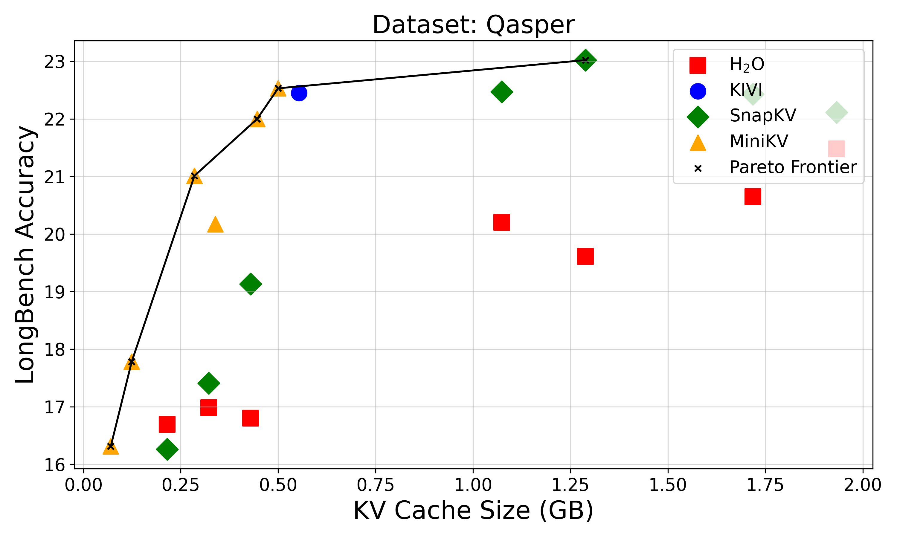<details> <summary>extracted/6028174/image/perf_vs_kv_size_plots/qasper.png Details</summary>  ### Visual Description ## Scatter Plot: LongBench Accuracy vs KV Cache Size (Qasper Dataset) ### Overview The chart visualizes the relationship between KV cache size (in GB) and LongBench accuracy for different key-value (KV) caching algorithms on the Qasper dataset. A Pareto Frontier line connects optimal data points, illustrating the trade-off between cache size and performance. ### Components/Axes - **X-axis**: KV Cache Size (GB) ranging from 0.00 to 2.00 in 0.25 increments. - **Y-axis**: LongBench Accuracy (16 to 23) in 1-point increments. - **Legend**: Located at top-right, mapping colors/shapes to algorithms: - Red squares: H₂O - Blue circle: KIVI - Green diamonds: SnapKV - Yellow triangles: MiniKV - Black line with x markers: Pareto Frontier ### Detailed Analysis 1. **H₂O (Red Squares)**: - Points at (0.25, 17), (0.5, 17), (1.0, 20), (1.75, 20.5) - Accuracy plateaus at 17 for 0.25–0.5 GB, then increases to 20.5 at 1.75 GB. 2. **KIVI (Blue Circle)**: - Single point at (0.5, 22.5), lying on the Pareto Frontier. 3. **SnapKV (Green Diamonds)**: - Points at (0.25, 16.5), (0.5, 19), (1.0, 22.5), (1.25, 23) - Shows consistent improvement with cache size, reaching the Pareto Frontier at 1.0–1.25 GB. 4. **MiniKV (Yellow Triangles)**: - Points at (0.1, 16.5), (0.25, 21), (0.5, 22), (0.75, 22.5) - Rapid accuracy gains up to 0.75 GB, then plateaus. 5. **Pareto Frontier (Black Line)**: - Connects optimal points: (0.1, 16.5) → (0.25, 21) → (0.5, 22.5) → (1.0, 22.5) → (1.25, 23) - Represents the maximum achievable accuracy for each cache size. ### Key Observations - **Optimal Performance**: KIVI (0.5 GB, 22.5) and SnapKV (1.25 GB, 23) lie on the Pareto Frontier, indicating peak efficiency. - **Suboptimal Algorithms**: H₂O and MiniKV fall below the frontier, suggesting inefficiencies (e.g., H₂O’s 20.5 accuracy at 1.75 GB vs. SnapKV’s 23 at 1.25 GB). - **Cache Size Trade-offs**: Larger caches (1.0–2.0 GB) generally improve accuracy but may not always align with the Pareto Frontier. ### Interpretation The data demonstrates that **cache size and algorithm efficiency are interdependent**. While increasing cache size typically boosts accuracy, the Pareto Frontier highlights configurations where this trade-off is optimized. For example: - **KIVI** achieves high accuracy (22.5) at a modest 0.5 GB, outperforming H₂O at 1.75 GB (20.5). - **SnapKV** maximizes accuracy (23) at 1.25 GB, suggesting diminishing returns beyond this point. - **H₂O** and **MiniKV** underperform relative to the frontier, indicating potential architectural or implementation limitations. This analysis underscores the importance of selecting algorithms that align with the Pareto Frontier for resource-constrained environments, balancing cache size and computational efficiency. 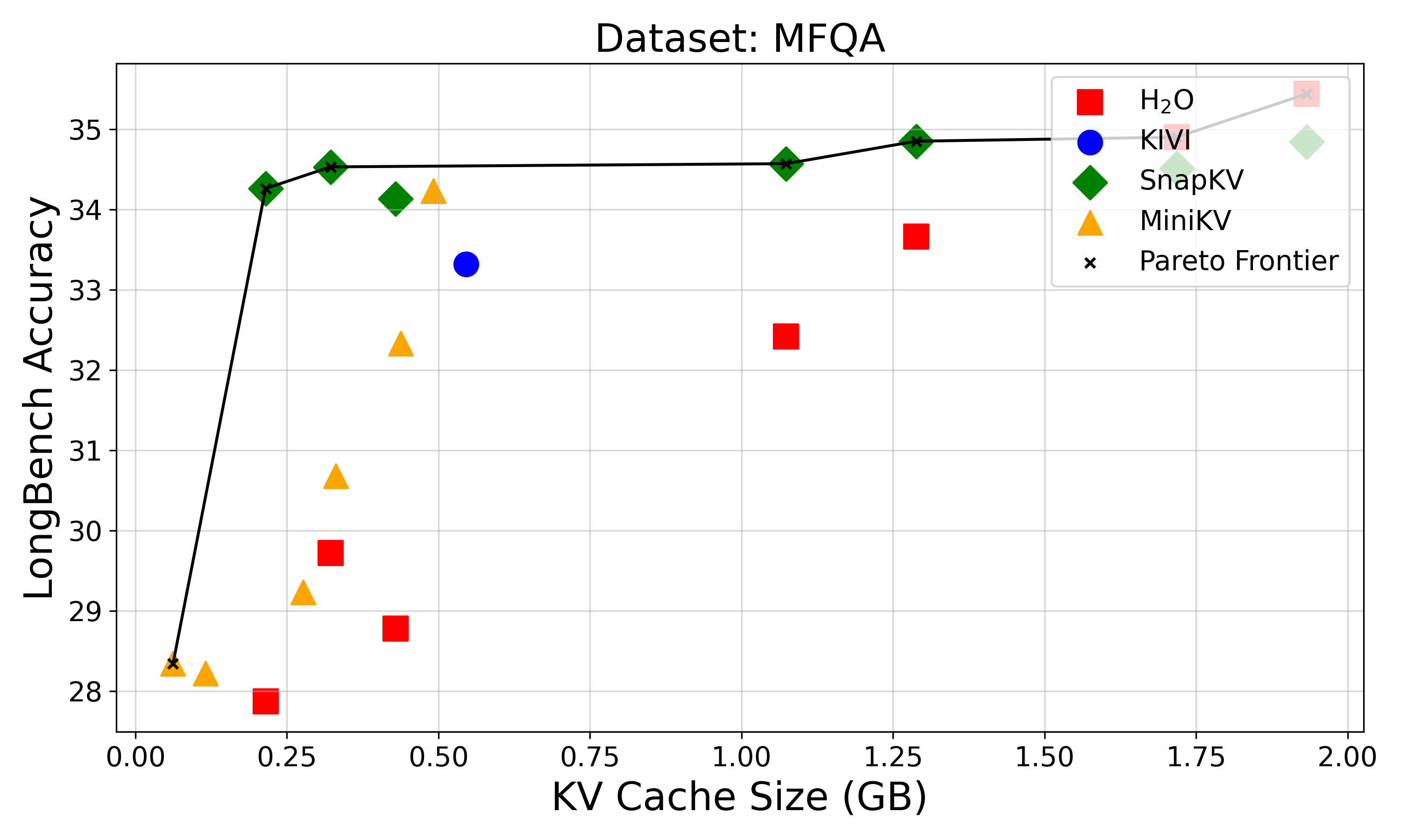</details> <details> <summary>extracted/6028174/image/perf_vs_kv_size_plots/multifieldqa_en.png Details</summary>  ### Visual Description ## Line Chart: LongBench Accuracy vs KV Cache Size (MFQA Dataset) ### Overview The chart visualizes the relationship between KV Cache Size (in GB) and LongBench Accuracy for five different systems (H2O, KIVI, SnapKV, MiniKV) and a Pareto Frontier curve. The Pareto Frontier represents the optimal trade-off between cache size and accuracy. ### Components/Axes - **X-axis**: KV Cache Size (GB) ranging from 0.00 to 2.00 in 0.25 increments - **Y-axis**: LongBench Accuracy (28–36) in 1-point increments - **Legend**: Located in top-right corner with color-coded markers: - Red squares: H2O - Blue circle: KIVI - Green diamonds: SnapKV - Yellow triangles: MiniKV - Black line with x markers: Pareto Frontier ### Detailed Analysis 1. **H2O (Red Squares)**: - 0.25 GB: 28.0 - 0.5 GB: 29.0 - 1.0 GB: 32.5 - 1.25 GB: 33.7 - 2.0 GB: 35.5 2. **KIVI (Blue Circle)**: - 0.5 GB: 33.4 3. **SnapKV (Green Diamonds)**: - 0.125 GB: 34.2 - 0.25 GB: 34.5 - 0.5 GB: 34.1 - 1.0 GB: 34.6 - 1.25 GB: 34.9 - 2.0 GB: 35.2 4. **MiniKV (Yellow Triangles)**: - 0.125 GB: 28.3 - 0.25 GB: 28.5 - 0.5 GB: 30.8 - 1.0 GB: 31.5 - 2.0 GB: 32.5 5. **Pareto Frontier (Black Line)**: - Connects points from 28.2 (0.125 GB) to 35.8 (2.0 GB) - Shows steady upward trend with minimal curvature ### Key Observations - Pareto Frontier demonstrates optimal performance scaling with cache size - H2O consistently underperforms other systems across all cache sizes - KIVI only has one data point at 0.5 GB (33.4 accuracy) - SnapKV maintains highest accuracy across all tested cache sizes - MiniKV shows significant improvement from 0.5 GB to 2.0 GB (30.8 → 32.5) - Pareto Frontier's 2.0 GB point (35.8) exceeds all individual system measurements ### Interpretation The data suggests that larger KV cache sizes generally improve LongBench Accuracy, with the Pareto Frontier representing the theoretical maximum achievable performance. SnapKV demonstrates the most consistent high performance, while H2O lags behind other systems. The absence of KIVI data beyond 0.5 GB suggests either testing limitations or system-specific constraints. The Pareto Frontier's upward trend indicates that increasing cache size beyond 2.0 GB would likely yield further accuracy improvements, though diminishing returns may occur based on the curve's flattening pattern. 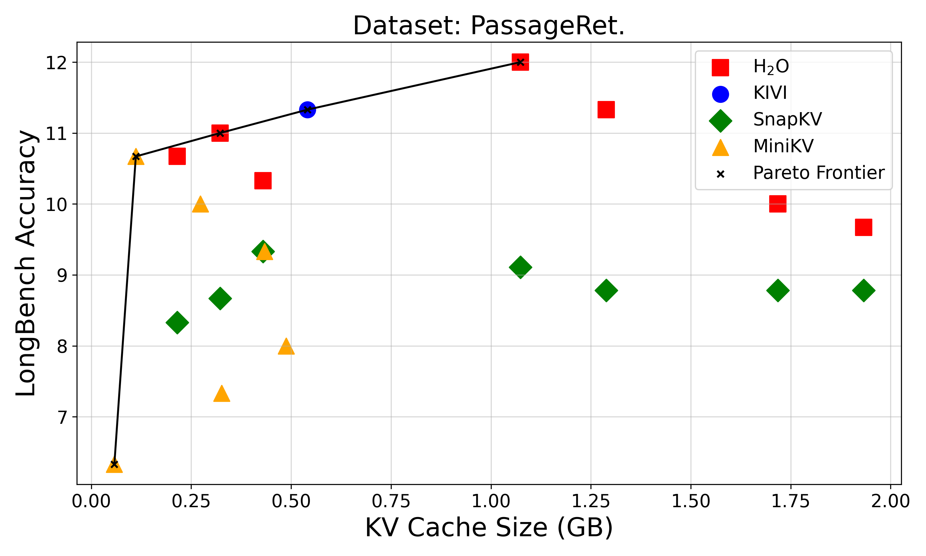</details> <details> <summary>extracted/6028174/image/perf_vs_kv_size_plots/passage_retrieval_en.png Details</summary>  ### Visual Description ## Scatter Plot: Dataset: PassageRet ### Overview The image is a scatter plot visualizing the relationship between KV Cache Size (in GB) and LongBench Accuracy for different models on the PassageRet dataset. The plot includes five data series represented by distinct markers and colors, along with a Pareto Frontier line indicating optimal performance trade-offs. ### Components/Axes - **X-axis**: KV Cache Size (GB), ranging from 0.00 to 2.00 in increments of 0.25. - **Y-axis**: LongBench Accuracy, ranging from 6 to 12 in increments of 1. - **Legend**: Located in the top-right corner, with the following mappings: - Red squares: H2O - Blue circles: KIVI - Green diamonds: SnapKV - Yellow triangles: MiniKV - Black crosses: Pareto Frontier ### Detailed Analysis #### Data Series 1. **H2O (Red Squares)**: - Points: (0.1, 10.7), (0.3, 11.0), (0.6, 10.4), (1.0, 12.0), (1.8, 9.7), (2.0, 9.5) - Trend: Slightly decreasing LongBench Accuracy with increasing KV Cache Size, but with a peak at 1.0 GB. 2. **KIVI (Blue Circles)**: - Single point: (0.5, 11.3) - Trend: High accuracy at 0.5 GB, but no additional data points. 3. **SnapKV (Green Diamonds)**: - Points: (0.2, 8.3), (0.4, 9.3), (1.1, 9.1), (1.7, 8.8), (2.0, 8.7) - Trend: Moderate accuracy, with a slight decline after 1.1 GB. 4. **MiniKV (Yellow Triangles)**: - Points: (0.1, 6.3), (0.3, 7.3), (0.5, 8.0), (0.7, 7.5) - Trend: Gradual increase in accuracy up to 0.5 GB, followed by a plateau. 5. **Pareto Frontier (Black Crosses)**: - Line connecting: (0.1, 10.7), (0.5, 11.3), (1.0, 12.0) - Trend: Upward-sloping line, representing the optimal trade-off between KV Cache Size and LongBench Accuracy. ### Key Observations - **H2O and KIVI** consistently outperform other models, with H2O achieving the highest LongBench Accuracy (12.0) at 1.0 GB KV Cache Size. - **SnapKV and MiniKV** show lower accuracy, with MiniKV having the lowest values (6.3–8.0) across all cache sizes. - The **Pareto Frontier** highlights the most efficient models (H2O and KIVI) that maximize accuracy for a given cache size. - **Outliers**: MiniKV at 0.1 GB (6.3) and H2O at 2.0 GB (9.5) deviate from the general trend of increasing accuracy with larger cache sizes. ### Interpretation The data suggests that **H2O and KIVI** are the most efficient models for the PassageRet dataset, achieving high LongBench Accuracy even at smaller KV Cache Sizes. The Pareto Frontier underscores their superiority, as they lie above the line, indicating better performance per unit of resource. In contrast, **SnapKV and MiniKV** underperform, with MiniKV showing the least efficiency. The trend of decreasing accuracy for H2O at larger cache sizes (e.g., 2.0 GB) may indicate diminishing returns or model-specific limitations. This analysis highlights the importance of optimizing KV Cache Size and model selection for resource-constrained environments. 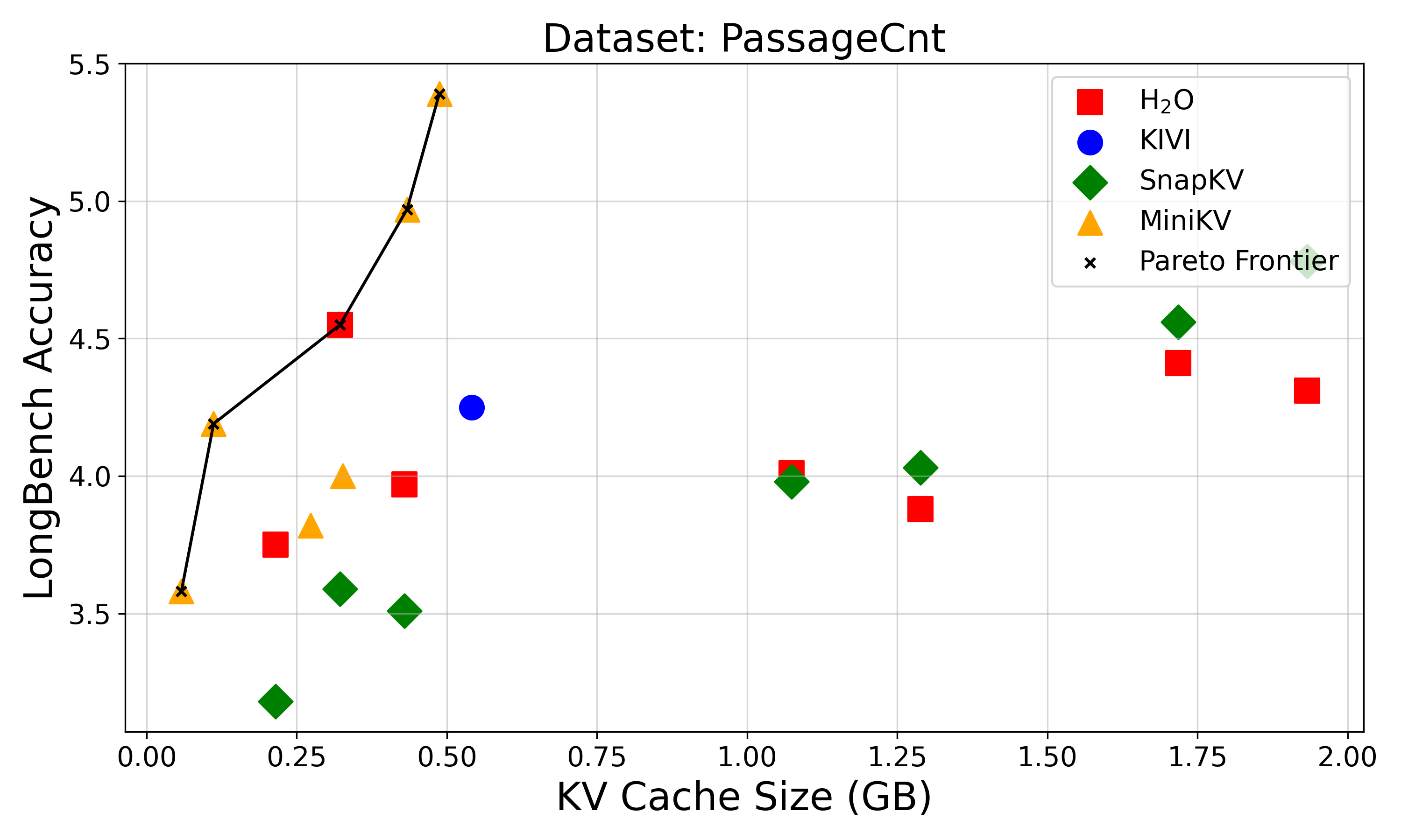</details> <details> <summary>extracted/6028174/image/perf_vs_kv_size_plots/passage_count.png Details</summary>  ### Visual Description ## Scatter Plot: LongBench Accuracy vs KV Cache Size (PassageCnt Dataset) ### Overview The chart visualizes the relationship between KV cache size (in GB) and LongBench accuracy for five different systems (H2O, KIVI, SnapKV, MiniKV) against the Pareto Frontier. Data points are plotted with distinct markers, and the Pareto Frontier is represented by a connected line. ### Components/Axes - **X-axis**: KV Cache Size (GB) ranging from 0.00 to 2.00 in 0.25 increments. - **Y-axis**: LongBench Accuracy ranging from 3.5 to 5.5 in 0.5 increments. - **Legend**: Located in the top-right corner, with five entries: - Red square: H2O - Blue circle: KIVI - Green diamond: SnapKV - Yellow triangle: MiniKV - Black cross: Pareto Frontier ### Detailed Analysis 1. **H2O (Red Squares)**: - Points at (0.25, 3.8), (0.5, 4.0), (1.25, 3.9), (1.75, 4.4), (2.0, 4.3). - Trend: Slight upward slope with a plateau at larger cache sizes. 2. **KIVI (Blue Circle)**: - Single point at (0.5, 4.2). - No clear trend due to limited data. 3. **SnapKV (Green Diamonds)**: - Points at (0.25, 3.2), (0.5, 3.5), (1.0, 4.0), (1.25, 4.1), (1.75, 4.6). - Trend: Steady upward slope, especially after 1.0 GB. 4. **MiniKV (Yellow Triangles)**: - Points at (0.1, 3.6), (0.3, 3.8), (0.5, 4.0), (0.7, 4.2), (1.0, 4.5). - Trend: Consistent upward trajectory with no plateau. 5. **Pareto Frontier (Black Crosses)**: - Connects points: (0.1, 3.6) → (0.3, 3.8) → (0.5, 4.0) → (0.7, 4.2) → (1.0, 4.5) → (1.75, 4.6) → (2.0, 4.3). - Represents optimal trade-offs between cache size and accuracy. ### Key Observations - **Pareto Frontier Dominance**: The frontier line consistently lies above or near most data points, indicating it represents the most efficient configurations. - **MiniKV and SnapKV Outperformance**: Both systems show higher accuracy at larger cache sizes (e.g., SnapKV reaches 4.6 at 1.75 GB, MiniKV reaches 4.5 at 1.0 GB). - **H2O Plateau**: H2O’s accuracy stabilizes around 4.3–4.4 despite increasing cache size beyond 1.75 GB. - **KIVI Anomaly**: Only one data point suggests limited evaluation or unique constraints. ### Interpretation The data demonstrates that **cache size directly impacts accuracy**, but with diminishing returns for most systems. The Pareto Frontier highlights the optimal balance, where MiniKV and SnapKV outperform others at larger cache sizes. H2O’s plateau suggests potential architectural limits, while KIVI’s single data point warrants further investigation. The trend implies that systems like MiniKV and SnapKV scale more effectively with increased resources, making them preferable for high-accuracy applications. 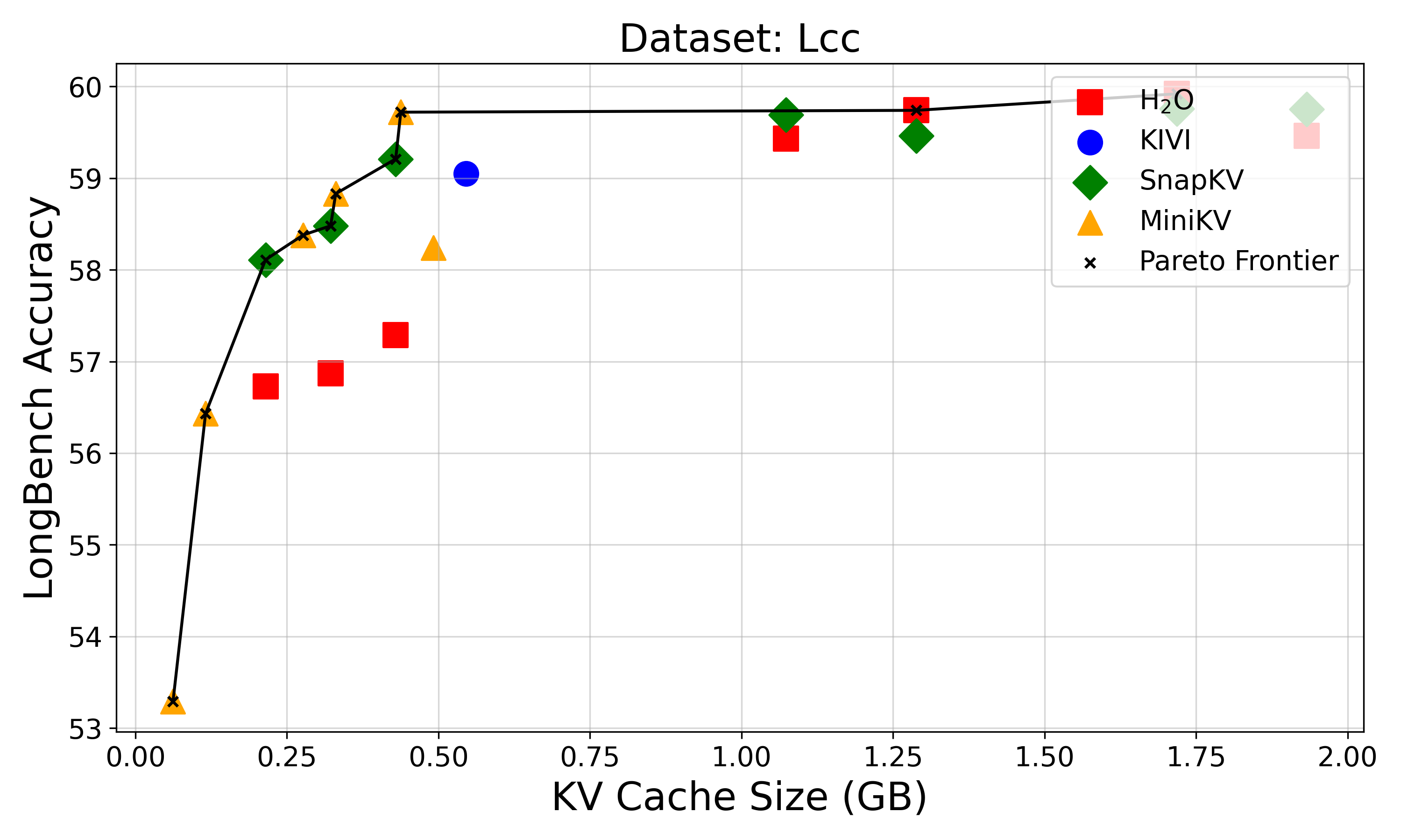</details> <details> <summary>extracted/6028174/image/perf_vs_kv_size_plots/lcc.png Details</summary>  ### Visual Description ## Line Chart: LongBench Accuracy vs KV Cache Size (Dataset: Lcc) ### Overview The chart illustrates the relationship between KV Cache Size (in GB) and LongBench Accuracy for multiple algorithms (H₂O, KIVI, SnapKV, MiniKV) and a Pareto Frontier. Data points are plotted with distinct markers and colors, showing performance trends across cache sizes from 0.00 to 2.00 GB. ### Components/Axes - **X-Axis**: KV Cache Size (GB), ranging from 0.00 to 2.00 in increments of 0.25 GB. - **Y-Axis**: LongBench Accuracy, ranging from 53 to 60 in increments of 1. - **Legend**: Located in the top-right corner, mapping colors/markers to algorithms: - Red squares: H₂O - Blue circle: KIVI - Green diamonds: SnapKV - Yellow triangles: MiniKV - Black line with "x" markers: Pareto Frontier ### Detailed Analysis 1. **H₂O (Red Squares)**: - Data points at: - 0.25 GB: ~57.0 - 0.5 GB: ~57.5 - 1.0 GB: ~58.5 - 1.25 GB: ~59.0 - 1.75 GB: ~59.5 - **Trend**: Steady upward slope with minimal fluctuations. 2. **KIVI (Blue Circle)**: - Single data point at: - 0.5 GB: ~59.0 - **Trend**: Isolated point; no clear trend due to limited data. 3. **SnapKV (Green Diamonds)**: - Data points at: - 0.25 GB: ~58.2 - 0.5 GB: ~59.2 - 1.0 GB: ~59.7 - 1.25 GB: ~59.5 - 1.75 GB: ~59.8 - **Trend**: Sharp increase until 1.0 GB, followed by a slight dip and recovery. 4. **MiniKV (Yellow Triangles)**: - Data points at: - 0.125 GB: ~56.5 - 0.25 GB: ~58.5 - 0.5 GB: ~58.2 - 1.0 GB: ~59.5 - 1.75 GB: ~59.7 - **Trend**: Initial dip at 0.5 GB, then consistent growth. 5. **Pareto Frontier (Black Line)**: - Connects points from: - 0.125 GB: ~56.5 - 0.25 GB: ~58.5 - 0.5 GB: ~59.2 - 1.0 GB: ~59.7 - 1.25 GB: ~59.5 - 1.75 GB: ~59.8 - **Trend**: Overall upward trajectory with a minor dip at 1.25 GB. ### Key Observations - **H₂O** and **MiniKV** show consistent improvements with larger cache sizes. - **SnapKV** peaks at 1.0 GB before a minor decline, suggesting potential inefficiency at higher cache sizes. - **MiniKV** exhibits a temporary drop at 0.5 GB, possibly indicating optimization challenges. - The **Pareto Frontier** highlights the theoretical maximum accuracy achievable for each cache size, with deviations (e.g., SnapKV at 1.25 GB) indicating suboptimal performance. ### Interpretation The chart demonstrates that larger KV cache sizes generally correlate with higher LongBench Accuracy, but efficiency varies by algorithm. The Pareto Frontier serves as a benchmark, revealing that some algorithms (e.g., SnapKV at 1.25 GB) underperform relative to their theoretical potential. H₂O and MiniKV align closely with the frontier, suggesting they are optimized for cache utilization. KIVI’s single data point at 0.5 GB may represent a specialized use case or outlier. The trends underscore the trade-off between resource allocation (cache size) and performance gains, with diminishing returns observed as cache size increases. 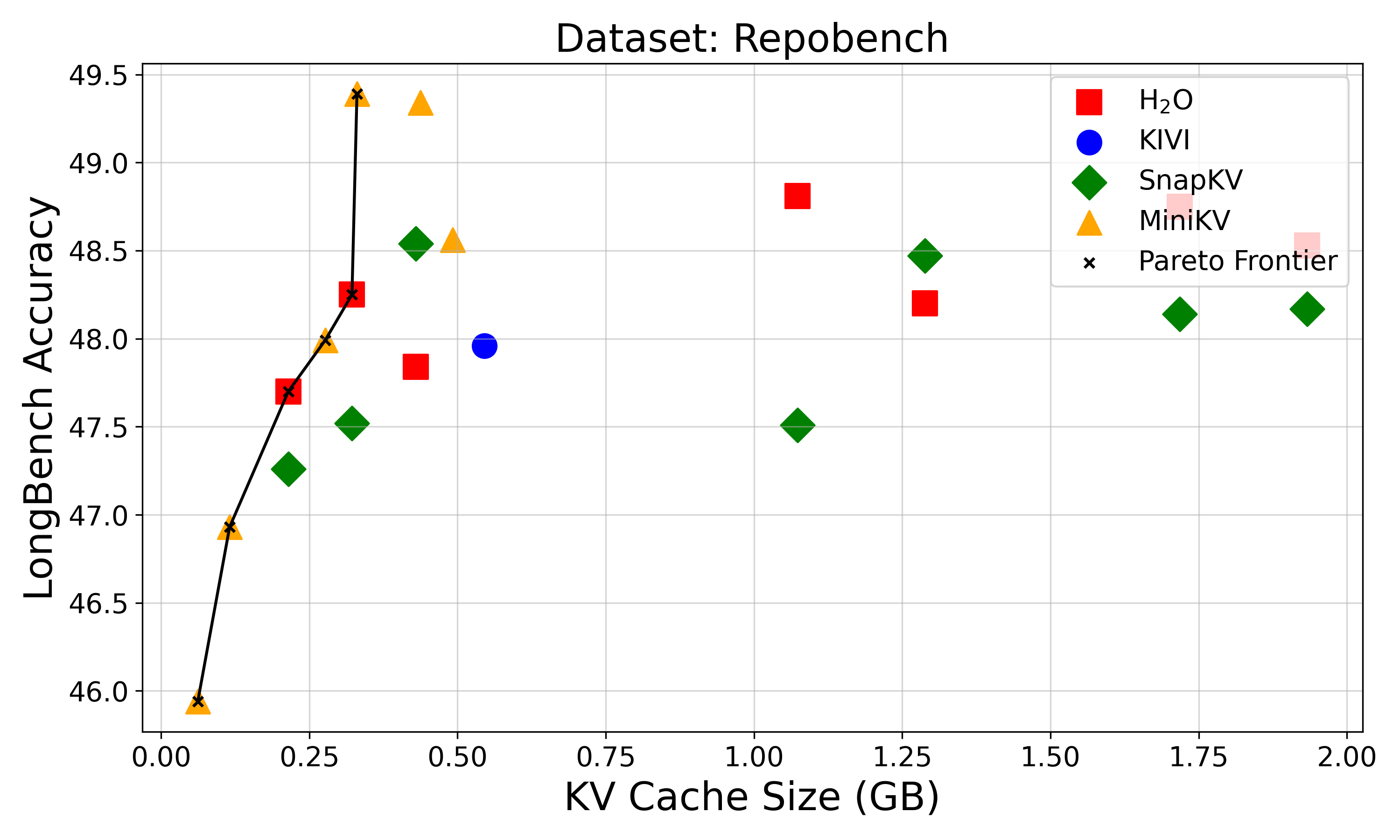</details> <details> <summary>extracted/6028174/image/perf_vs_kv_size_plots/repobench-p.png Details</summary>  ### Visual Description ## Scatter Plot: LongBench Accuracy vs KV Cache Size (Repobench Dataset) ### Overview The chart visualizes the relationship between KV cache size (in GB) and LongBench accuracy for five different systems (H2O, KIVI, SnapKV, MiniKV) against the Pareto Frontier. Data points are plotted with distinct markers/colors, and the Pareto Frontier is represented by a black line with cross markers. ### Components/Axes - **X-axis**: KV Cache Size (GB) ranging from 0.00 to 2.00 in 0.25 increments. - **Y-axis**: LongBench Accuracy ranging from 46.0 to 49.5 in 0.5 increments. - **Legend**: Located at the top-right corner, mapping: - Red squares: H2O - Blue circle: KIVI - Green diamonds: SnapKV - Yellow triangles: MiniKV - Black crosses: Pareto Frontier ### Detailed Analysis #### Data Series Trends 1. **H2O (Red Squares)**: - Points at (0.25, ~47.7), (0.5, ~47.9), (1.0, ~48.8), (1.25, ~48.3). - Trend: Initial increase in accuracy with cache size, followed by a plateau/decline. 2. **KIVI (Blue Circle)**: - Single point at (0.5, ~47.9). - No trend observable due to single data point. 3. **SnapKV (Green Diamonds)**: - Points at (0.25, ~47.3), (0.5, ~48.5), (1.0, ~47.5), (1.25, ~48.4), (1.75, ~48.1), (2.0, ~48.2). - Trend: Fluctuating accuracy with no clear monotonic relationship. 4. **MiniKV (Yellow Triangles)**: - Points at (0.1, ~46.9), (0.25, ~48.0), (0.5, ~48.5), (0.75, ~48.6). - Trend: Steady increase in accuracy up to 0.75 GB, then no further data. 5. **Pareto Frontier (Black Crosses)**: - Connects points at (0.1, ~46.9) → (0.5, ~48.5) → (0.75, ~48.6) → (1.0, ~48.8). - Represents the optimal trade-off curve where increasing cache size does not yield proportional accuracy gains. ### Key Observations - **Pareto Frontier Dominance**: Most data points lie below the frontier, indicating suboptimal performance relative to the trade-off curve. - **H2O Outlier**: The (1.0, ~48.8) point exceeds the Pareto Frontier, suggesting exceptional performance at 1.0 GB. - **MiniKV Efficiency**: Achieves high accuracy (48.6) at 0.75 GB, outperforming others at smaller cache sizes. - **SnapKV Volatility**: Accuracy drops from 48.5 (0.5 GB) to 47.5 (1.0 GB), then recovers slightly. ### Interpretation The chart demonstrates that **cache size does not universally correlate with accuracy improvements**. The Pareto Frontier highlights diminishing returns beyond 0.75–1.0 GB for most systems. Notably: - **H2O** and **MiniKV** show strong performance at lower cache sizes, suggesting algorithmic efficiency. - **SnapKV**'s fluctuating results imply potential instability or suboptimal cache utilization. - **KIVI**'s single data point limits conclusions but aligns with mid-range performance. The data underscores the importance of algorithmic design over raw hardware scaling, as the Pareto Frontier indicates that further cache expansion beyond ~1.0 GB yields minimal accuracy gains for most systems. 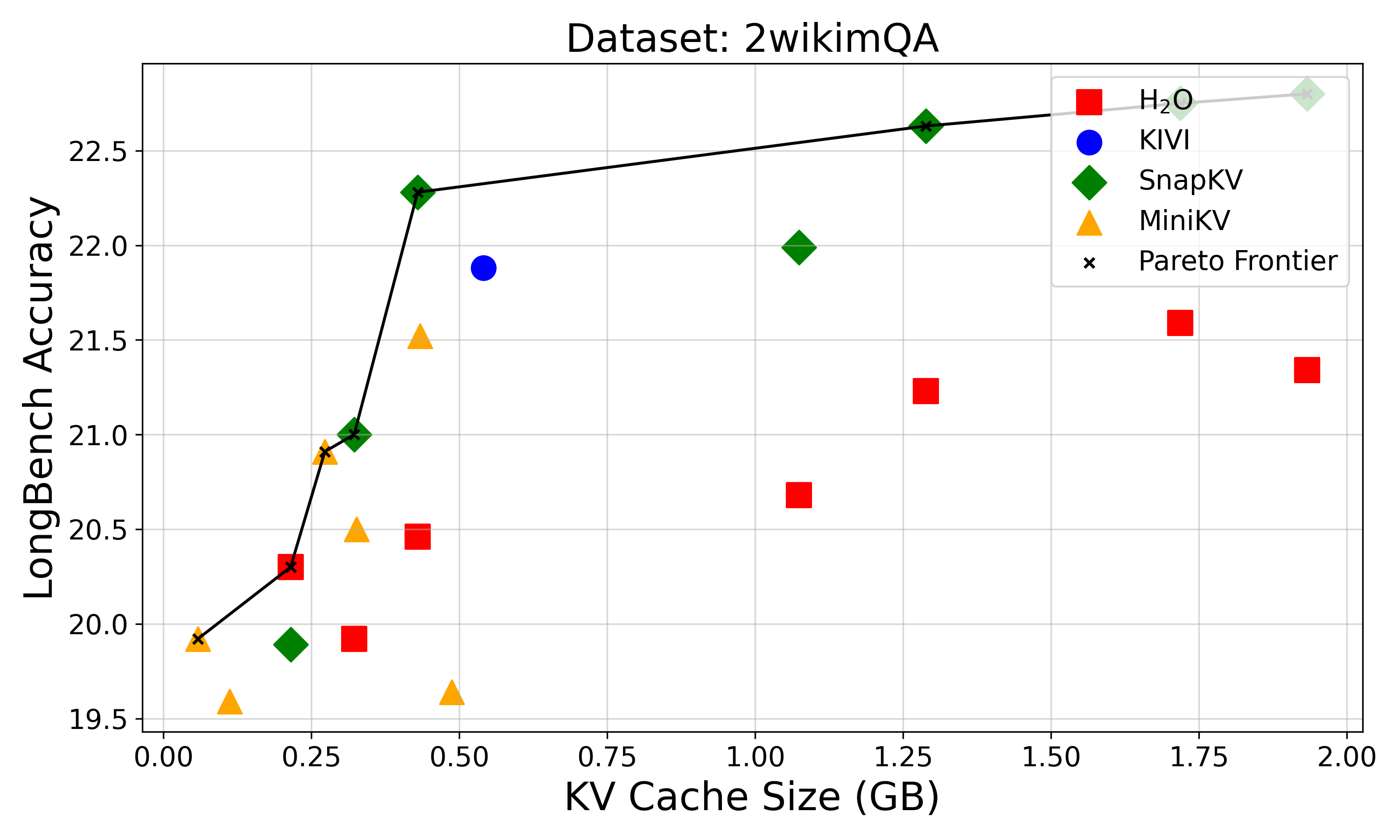</details> <details> <summary>extracted/6028174/image/perf_vs_kv_size_plots/2wikimqa.png Details</summary>  ### Visual Description ## Scatter Plot: LongBench Accuracy vs KV Cache Size for 2wikimQA Dataset ### Overview The image is a scatter plot visualizing the relationship between KV Cache Size (in GB) and LongBench Accuracy for different models on the 2wikimQA dataset. The plot includes five data series (H2O, KIVI, SnapKV, MiniKV, and Pareto Frontier) with distinct markers and colors. The Pareto Frontier is represented as a line connecting optimal data points. ### Components/Axes - **X-axis**: KV Cache Size (GB), ranging from 0.00 to 2.00 GB in 0.25 increments. - **Y-axis**: LongBench Accuracy, ranging from 19.5 to 23.0. - **Legend**: Located in the top-right corner, with the following mappings: - **Red squares**: H2O - **Blue circle**: KIVI - **Green diamonds**: SnapKV - **Yellow triangles**: MiniKV - **Black crosses**: Pareto Frontier - **Pareto Frontier**: A black line connecting optimal data points, indicating the trade-off between cache size and accuracy. ### Detailed Analysis #### Data Series Trends 1. **H2O (Red Squares)**: - Points: (0.25, 20.3), (0.5, 20.5), (1.0, 20.7), (1.5, 21.6), (1.75, 21.5), (2.0, 21.4) - Trend: Slight upward trend with a peak at 1.5 GB (21.6) followed by a minor decline. 2. **KIVI (Blue Circle)**: - Single point: (0.5, 21.9) - Trend: Isolated high-performance data point at 0.5 GB. 3. **SnapKV (Green Diamonds)**: - Points: (0.3, 21.0), (0.4, 22.3), (1.0, 22.0), (1.3, 22.7) - Trend: Strong upward trend, peaking at 1.3 GB (22.7). 4. **MiniKV (Yellow Triangles)**: - Points: (0.1, 19.6), (0.3, 20.9), (0.4, 20.5), (0.5, 19.7) - Trend: Initial increase to 0.3 GB (20.9), followed by a decline. 5. **Pareto Frontier (Black Crosses)**: - Points: (0.1, 19.6), (0.3, 20.9), (0.4, 21.0), (0.5, 21.9), (1.0, 22.0), (1.3, 22.7), (1.5, 22.6), (1.75, 22.8), (2.0, 23.0) - Trend: Steady upward trajectory, representing the optimal trade-off between cache size and accuracy. ### Key Observations - **Pareto Frontier Dominance**: The Pareto Frontier line consistently outperforms all other models, showing a clear upward trend as cache size increases. - **H2O and MiniKV Underperformance**: These models exhibit lower accuracy across most cache sizes, with H2O showing a slight peak at 1.5 GB (21.6) and MiniKV peaking at 0.3 GB (20.9). - **KIVI and SnapKV Efficiency**: KIVI achieves 21.9 accuracy at 0.5 GB, while SnapKV reaches 22.7 at 1.3 GB, indicating higher efficiency. - **Anomalies**: H2O's accuracy drops slightly at 2.0 GB (21.4) despite increased cache size, suggesting diminishing returns. ### Interpretation The data demonstrates that larger KV cache sizes generally correlate with higher LongBench Accuracy, but the relationship is not linear. The Pareto Frontier highlights the most efficient models (e.g., SnapKV and KIVI) that balance cache size and performance. H2O and MiniKV underperform, suggesting potential inefficiencies in their architecture or implementation. The Pareto Frontier's upward trend implies that optimizing cache size can significantly improve accuracy, but beyond a certain point (e.g., 1.75–2.0 GB), the gains may plateau or reverse. This analysis underscores the importance of model-specific optimization for KV cache size in achieving optimal performance on the 2wikimQA dataset. 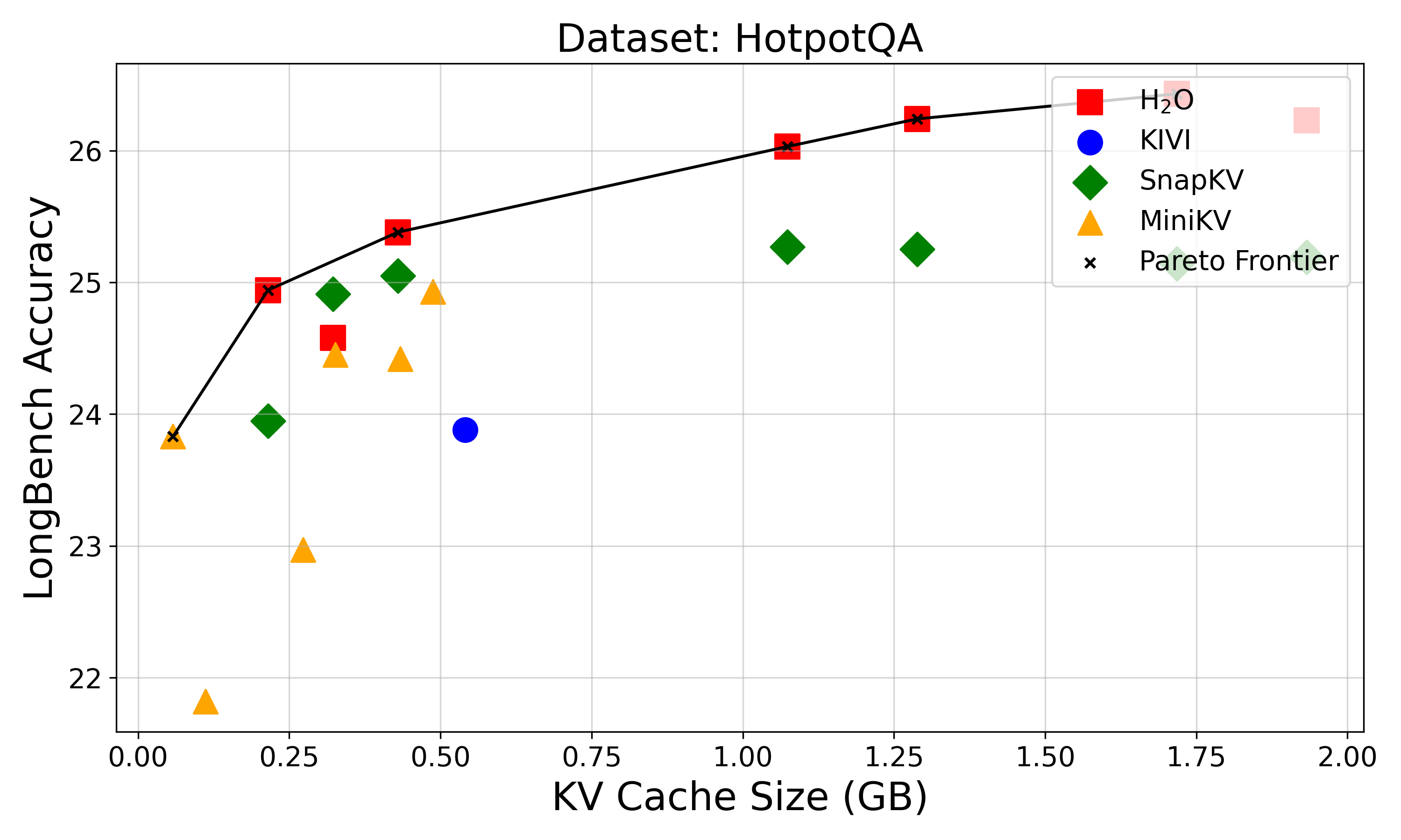</details> <details> <summary>extracted/6028174/image/perf_vs_kv_size_plots/hotpotqa.png Details</summary>  ### Visual Description ## Scatter Plot: LongBench Accuracy vs KV Cache Size for HotpotQA Dataset ### Overview The image is a scatter plot comparing LongBench Accuracy (y-axis) against KV Cache Size (x-axis) for different knowledge vector (KV) cache implementations on the HotpotQA dataset. A Pareto Frontier curve is overlaid to highlight optimal trade-offs between cache size and accuracy. ### Components/Axes - **X-axis**: KV Cache Size (GB) ranging from 0.00 to 2.00 in 0.25 increments - **Y-axis**: LongBench Accuracy ranging from 22 to 26.5 in 0.5 increments - **Legend**: Located in top-right corner with five distinct markers: - Red squares: H₂O - Blue circles: KIVI - Green diamonds: SnapKV - Yellow triangles: MiniKV - Black crosses: Pareto Frontier ### Detailed Analysis 1. **H₂O (Red Squares)**: - Data points: (0.25, 25.0), (0.5, 25.3), (1.0, 26.0), (1.25, 26.2), (1.75, 26.5) - Trend: Strong positive correlation between cache size and accuracy 2. **KIVI (Blue Circle)**: - Single data point: (0.5, 23.8) - Position: Lower left quadrant, significantly below Pareto Frontier 3. **SnapKV (Green Diamonds)**: - Data points: (0.25, 24.9), (0.5, 25.1), (1.0, 25.3), (1.25, 25.4) - Trend: Gradual improvement with diminishing returns 4. **MiniKV (Yellow Triangles)**: - Data points: (0.1, 23.8), (0.25, 24.3), (0.5, 24.5), (0.75, 24.7) - Trend: Steady improvement but plateaus at lower accuracy levels 5. **Pareto Frontier (Black Crosses)**: - Connects optimal points: (0.25, 25.0) → (1.0, 26.0) → (1.75, 26.5) - Represents theoretical maximum efficiency frontier ### Key Observations - H₂O consistently outperforms other implementations across all cache sizes - Pareto Frontier shows optimal trade-off between cache size and accuracy - KIVI demonstrates poor performance relative to cache size investment - SnapKV and MiniKV show moderate performance with diminishing returns - No data points exist between 0.75GB and 1.0GB for MiniKV - All implementations show improved accuracy with increased cache size ### Interpretation The data suggests that H₂O provides the most efficient balance between cache size and accuracy, consistently operating near or on the Pareto Frontier. The Pareto Frontier curve reveals that beyond 1.75GB cache size, accuracy improvements become marginal. KIVI's single data point indicates either limited implementation or suboptimal performance characteristics. The diminishing returns observed across all implementations suggest that cache size alone cannot drive unbounded accuracy improvements, highlighting the need for architectural optimizations beyond simple cache scaling. </details> Figure 15: Performance Versus KV Cache Size: MiniKV offers the best performance for the smallest KV cache size across all 6 task categories. 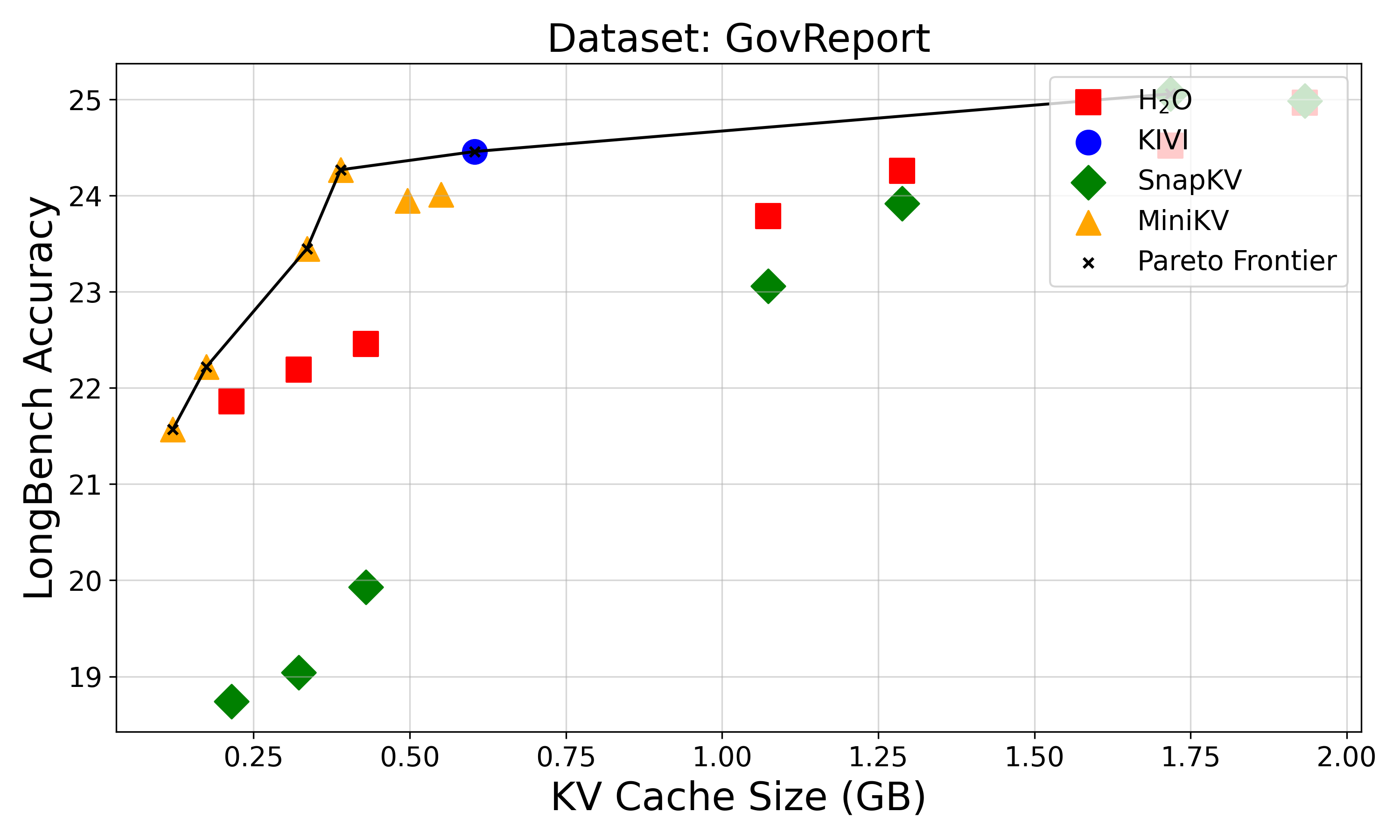<details> <summary>extracted/6028174/image/perf_vs_kv_size_plots/gov_report.png Details</summary>  ### Visual Description ## Line Chart: GovReport Dataset Analysis ### Overview The image is a line chart titled "Dataset: GovReport," comparing the relationship between KV Cache Size (in GB) and LongBench Accuracy across different algorithms. The chart includes a Pareto Frontier line and data points for five algorithms: H2O, KIVI, SnapKV, MiniKV, and Pareto Frontier. The x-axis represents KV Cache Size (GB), ranging from 0.25 to 2.00 GB, while the y-axis represents LongBench Accuracy, ranging from 19 to 25. ### Components/Axes - **X-axis (KV Cache Size)**: Labeled "KV Cache Size (GB)" with ticks at 0.25, 0.50, 0.75, 1.00, 1.25, 1.50, 1.75, and 2.00 GB. - **Y-axis (LongBench Accuracy)**: Labeled "LongBench Accuracy" with ticks at 19, 20, 21, 22, 23, 24, and 25. - **Legend**: Located in the top-right corner, with the following mappings: - Red squares: H2O - Blue circle: KIVI - Green diamonds: SnapKV - Yellow triangles: MiniKV - Black crosses: Pareto Frontier ### Detailed Analysis - **Pareto Frontier (Black Crosses)**: - Starts at approximately (0.25 GB, 21.5) and increases steadily to (2.00 GB, 25). - Represents the optimal trade-off between cache size and accuracy. - **H2O (Red Squares)**: - Data points at (0.25 GB, 22), (0.50 GB, 22.5), (1.00 GB, 23.8), and (1.25 GB, 24.2). - Shows a gradual upward trend but remains below the Pareto Frontier. - **KIVI (Blue Circle)**: - Single data point at (0.75 GB, 24.5), positioned above the Pareto Frontier. - **SnapKV (Green Diamonds)**: - Data points at (0.25 GB, 18.8), (0.50 GB, 19.9), (1.00 GB, 23.1), and (1.25 GB, 23.9). - Starts below the Pareto Frontier but improves with larger cache sizes. - **MiniKV (Yellow Triangles)**: - Data points at (0.25 GB, 21.5), (0.50 GB, 23.5), and (0.75 GB, 24.2). - Shows a strong upward trend, approaching the Pareto Frontier. ### Key Observations 1. **Pareto Frontier Dominance**: The Pareto Frontier line consistently represents the highest achievable accuracy for each cache size, acting as a benchmark. 2. **Algorithm Performance**: - **KIVI** and **MiniKV** outperform other algorithms at specific cache sizes, with KIVI reaching 24.5 accuracy at 0.75 GB. - **SnapKV** lags at smaller cache sizes (e.g., 18.8 at 0.25 GB) but improves significantly at larger sizes. - **H2O** and **MiniKV** show steady improvements but remain below the Pareto Frontier. 3. **Outliers**: The Pareto Frontier itself is not an algorithm but a theoretical boundary, while KIVI and MiniKV occasionally surpass it at certain points. ### Interpretation The chart illustrates the trade-off between KV Cache Size and LongBench Accuracy for different algorithms. The Pareto Frontier highlights the optimal performance achievable for each cache size, serving as a reference for evaluating algorithm efficiency. - **KIVI** and **MiniKV** demonstrate superior performance at specific cache sizes, suggesting they are more efficient or optimized for certain workloads. - **SnapKV** underperforms at smaller cache sizes but improves with larger allocations, indicating potential scalability. - **H2O** and **MiniKV** show consistent growth but do not reach the Pareto Frontier, implying room for optimization. The data suggests that while larger cache sizes generally improve accuracy, the efficiency of algorithms varies significantly. The Pareto Frontier underscores the importance of balancing cache size and algorithmic design to achieve optimal results. 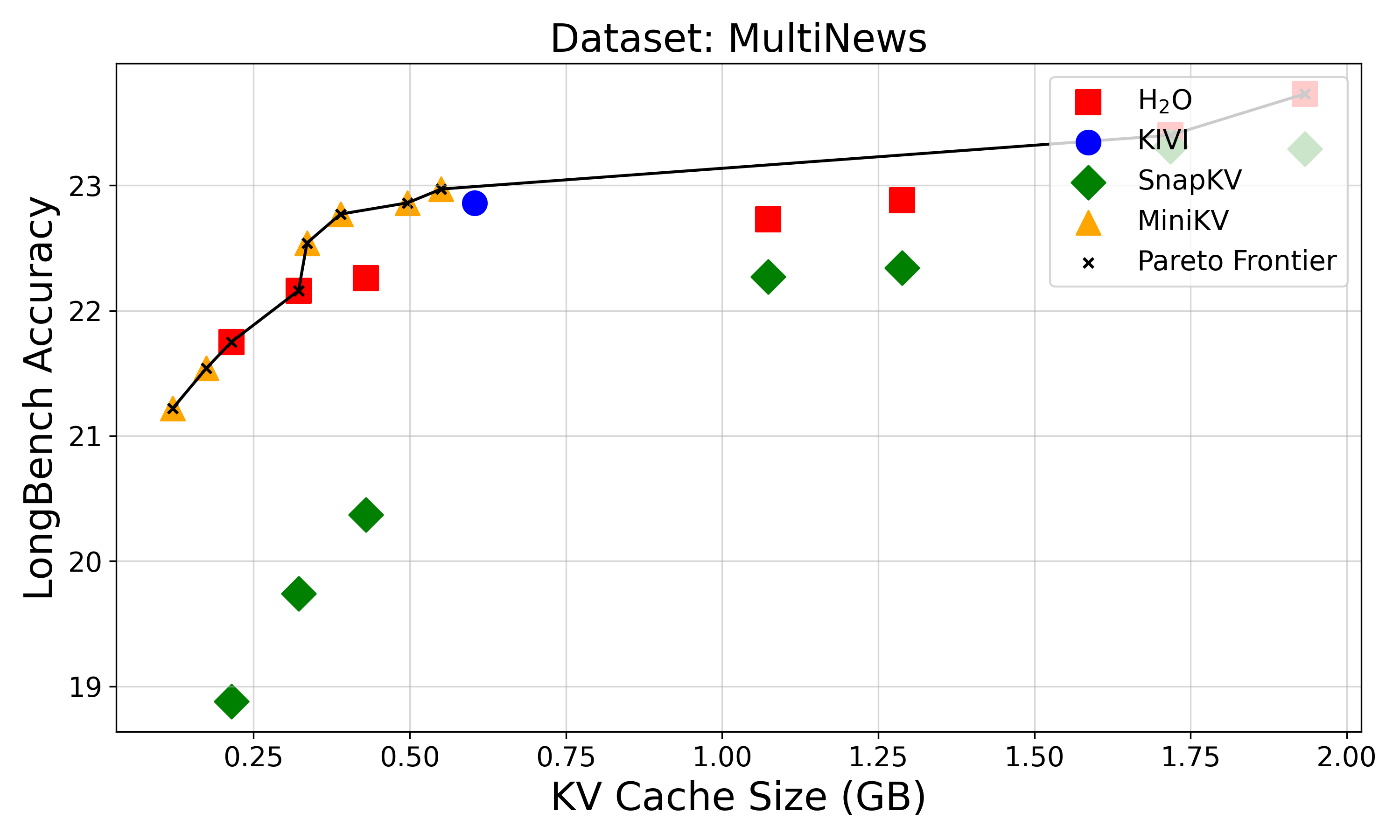</details> <details> <summary>extracted/6028174/image/perf_vs_kv_size_plots/multi_news.png Details</summary>  ### Visual Description ## Line Chart: LongBench Accuracy vs KV Cache Size (MultiNews Dataset) ### Overview The chart visualizes the relationship between KV Cache Size (in GB) and LongBench Accuracy for five different systems (H2O, KIVI, SnapKV, MiniKV) and a Pareto Frontier reference line. The Pareto Frontier represents the optimal trade-off between cache size and accuracy. ### Components/Axes - **X-axis**: KV Cache Size (GB) - Scale: 0.25 to 2.00 GB - Labels: 0.25, 0.5, 0.75, 1.0, 1.25, 1.5, 1.75, 2.0 - **Y-axis**: LongBench Accuracy - Scale: 19 to 23.5 - Labels: 19, 20, 21, 22, 23, 23.5 - **Legend**: - **H2O**: Red squares - **KIVI**: Blue circle - **SnapKV**: Green diamonds - **MiniKV**: Yellow triangles - **Pareto Frontier**: Black dashed line with crosses ### Detailed Analysis 1. **H2O (Red Squares)** - Data points: - (0.25 GB, 21.5) - (0.5 GB, 22.2) - (0.75 GB, 22.5) - (1.0 GB, 22.8) - (1.25 GB, 23.0) - (1.5 GB, 23.2) - (1.75 GB, 23.4) - (2.0 GB, 23.6) - Trend: Steady upward slope with diminishing returns. 2. **KIVI (Blue Circle)** - Single data point: - (0.6 GB, 22.8) - Position: Near the Pareto Frontier at mid-range cache size. 3. **SnapKV (Green Diamonds)** - Data points: - (0.25 GB, 19.0) - (0.5 GB, 20.4) - (1.0 GB, 22.3) - (1.25 GB, 22.4) - (1.75 GB, 23.1) - (2.0 GB, 23.3) - Trend: Sharp improvement at 1.0 GB, plateauing afterward. 4. **MiniKV (Yellow Triangles)** - Data points: - (0.25 GB, 21.2) - (0.5 GB, 21.6) - (0.75 GB, 22.0) - (1.0 GB, 22.5) - Trend: Consistent gains up to 1.0 GB, then no further data. 5. **Pareto Frontier (Black Dashed Line)** - Connects points: - (0.25 GB, 21.5) - (0.5 GB, 22.2) - (0.75 GB, 22.5) - (1.0 GB, 22.8) - (1.25 GB, 23.0) - (1.5 GB, 23.2) - (1.75 GB, 23.4) - (2.0 GB, 23.6) - Trend: Smooth upward curve representing the theoretical optimal trade-off. ### Key Observations - **Pareto Frontier Dominance**: All systems lie below or on the Pareto Frontier, indicating no system achieves both higher accuracy and lower cache usage simultaneously. - **H2O and MiniKV**: Outperform others at lower cache sizes (0.25–1.0 GB). - **SnapKV**: Lags initially but catches up at 1.75–2.0 GB. - **KIVI**: Only one data point at 0.6 GB, suggesting limited testing or specialization. - **Diminishing Returns**: Accuracy gains slow significantly beyond 1.5 GB for most systems. ### Interpretation The chart demonstrates that increasing KV cache size generally improves LongBench Accuracy, but with diminishing returns. The Pareto Frontier highlights the most efficient configurations, where H2O and MiniKV excel at lower cache sizes, while SnapKV becomes competitive at higher sizes. KIVI’s single data point suggests it may be optimized for a specific use case or underrepresented in this dataset. The trend underscores the trade-off between resource allocation (cache size) and performance, guiding decisions for systems prioritizing efficiency or raw accuracy. 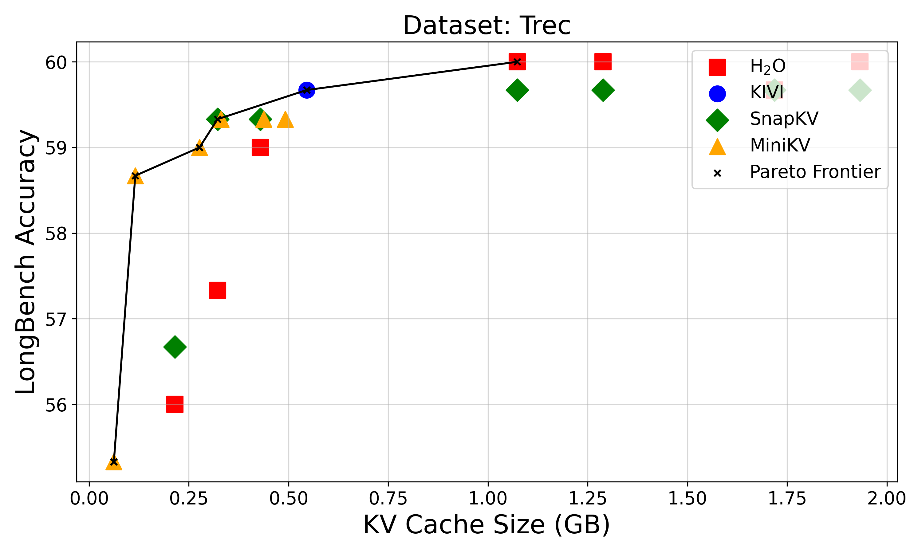</details> <details> <summary>extracted/6028174/image/perf_vs_kv_size_plots/trec.png Details</summary>  ### Visual Description ## Line Chart: LongBench Accuracy vs KV Cache Size (Dataset: Trec) ### Overview The chart illustrates the relationship between KV cache size (in GB) and LongBench accuracy for various key-value (KV) storage systems. A Pareto Frontier line is plotted to represent the optimal trade-off between cache size and accuracy. Data points for five systems (H2O, KIVI, SnapKV, MiniKV) are marked with distinct symbols and colors, while the Pareto Frontier is represented by a black line with crosses. ### Components/Axes - **X-axis**: KV Cache Size (GB), ranging from 0.00 to 2.00 GB in 0.25 GB increments. - **Y-axis**: LongBench Accuracy, ranging from 56 to 60 in 1-point increments. - **Legend**: Located in the top-right corner, mapping symbols/colors to systems: - Red squares: H2O - Blue circle: KIVI - Green diamonds: SnapKV - Yellow triangles: MiniKV - Black crosses: Pareto Frontier ### Detailed Analysis 1. **Pareto Frontier**: - A smooth black line with crosses, starting at (0.00 GB, 55.5) and rising to (2.00 GB, 60.0). - The line shows a consistent upward slope, indicating that larger cache sizes generally improve accuracy. 2. **Data Points**: - **H2O (Red Squares)**: - Points at (0.25 GB, 56.0), (0.50 GB, 57.5), (1.00 GB, 59.5), and (1.25 GB, 60.0). - Two points lie on the Pareto Frontier (1.00 GB and 1.25 GB). - **KIVI (Blue Circle)**: - Single point at (0.50 GB, 59.5), lying on the Pareto Frontier. - **SnapKV (Green Diamonds)**: - Points at (0.25 GB, 56.5), (0.50 GB, 59.0), and (1.25 GB, 59.5). - Two points (0.50 GB and 1.25 GB) are on the Pareto Frontier. - **MiniKV (Yellow Triangles)**: - Points at (0.10 GB, 55.5), (0.25 GB, 59.0), and (0.50 GB, 59.5). - Two points (0.25 GB and 0.50 GB) are on the Pareto Frontier. ### Key Observations - **Optimal Efficiency**: Systems like KIVI and H2O achieve Pareto-optimal accuracy at specific cache sizes (e.g., 0.50 GB for KIVI, 1.00–1.25 GB for H2O). - **Suboptimal Performance**: SnapKV and MiniKV have points below the Pareto Frontier, suggesting inefficiencies in their cache utilization. - **Accuracy Trends**: All systems show improved accuracy with larger cache sizes, but the rate of improvement varies. For example, H2O gains 4.0 accuracy points from 0.25 GB to 1.25 GB, while MiniKV gains 4.0 points from 0.10 GB to 0.50 GB. ### Interpretation The chart demonstrates that increasing KV cache size generally enhances LongBench accuracy, but the efficiency of this trade-off differs across systems. The Pareto Frontier highlights the most efficient configurations: - **KIVI** achieves the highest accuracy (59.5) at the smallest cache size (0.50 GB), making it highly efficient. - **H2O** and **SnapKV** require larger caches (1.00–1.25 GB) to reach near-optimal accuracy (59.5–60.0), indicating higher resource demands. - **MiniKV** shows rapid improvement at low cache sizes but plateaus at 0.50 GB, suggesting diminishing returns beyond this point. This analysis implies that system designers should prioritize cache size allocation based on the specific accuracy-versus-resource trade-offs of their chosen KV system. The Pareto Frontier serves as a critical benchmark for evaluating performance efficiency. 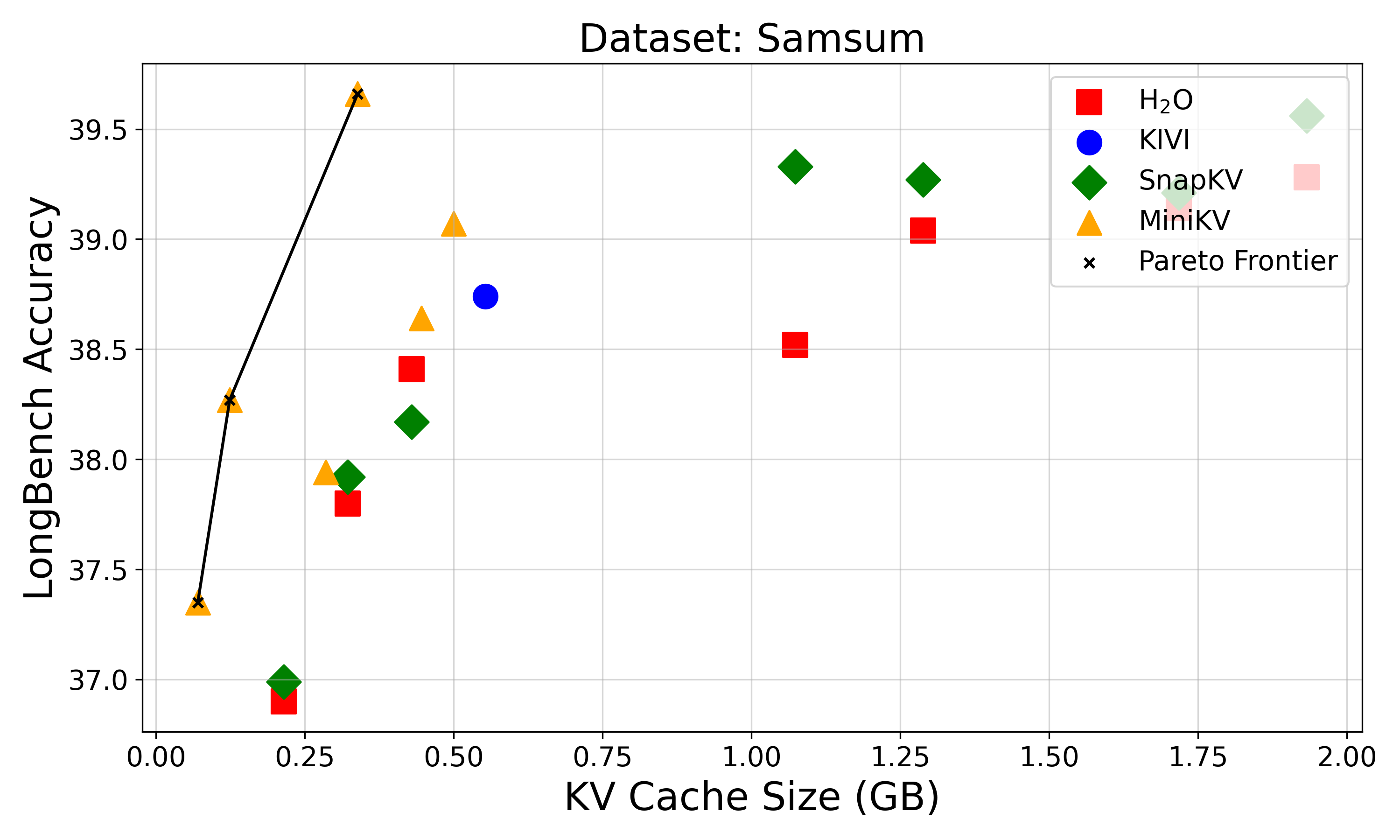</details> <details> <summary>extracted/6028174/image/perf_vs_kv_size_plots/samsum.png Details</summary>  ### Visual Description ## Scatter Plot: LongBench Accuracy vs KV Cache Size (Dataset: Samsum) ### Overview The image is a scatter plot visualizing the relationship between KV Cache Size (in GB) and LongBench Accuracy for different models on the Samsum dataset. The plot includes a Pareto Frontier line to highlight optimal trade-offs between cache size and accuracy. ### Components/Axes - **X-axis**: KV Cache Size (GB), ranging from 0.00 to 2.00 GB in increments of 0.25 GB. - **Y-axis**: LongBench Accuracy, ranging from 37.0 to 39.5 in increments of 0.5. - **Legend**: Located in the top-right corner, with the following mappings: - **Red squares**: H2O - **Blue circle**: KIVI - **Green diamonds**: SnapKV - **Yellow triangles**: MiniKV - **Black 'x' markers**: Pareto Frontier ### Detailed Analysis #### Data Series Trends 1. **Pareto Frontier (Black 'x' line)**: - Starts at (0.1 GB, 37.3) and increases steadily to (0.5 GB, 38.5), then plateaus slightly. - Represents the optimal trade-off between cache size and accuracy. 2. **H2O (Red squares)**: - Points at (0.25 GB, 37.0), (0.5 GB, 38.4), (1.0 GB, 38.5), and (1.25 GB, 39.0). - Shows a gradual increase in accuracy with larger cache sizes. 3. **KIVI (Blue circle)**: - Single point at (0.5 GB, 38.7). - Lies below the Pareto Frontier, indicating suboptimal performance. 4. **SnapKV (Green diamonds)**: - Points at (0.25 GB, 37.0), (0.5 GB, 38.2), (1.0 GB, 39.3), and (1.25 GB, 39.2). - Demonstrates a strong upward trend, approaching the Pareto Frontier at larger cache sizes. 5. **MiniKV (Yellow triangles)**: - Points at (0.1 GB, 37.3), (0.25 GB, 37.9), (0.5 GB, 38.6), and (0.75 GB, 39.6). - Highest accuracy (39.6) at 0.75 GB, surpassing the Pareto Frontier. 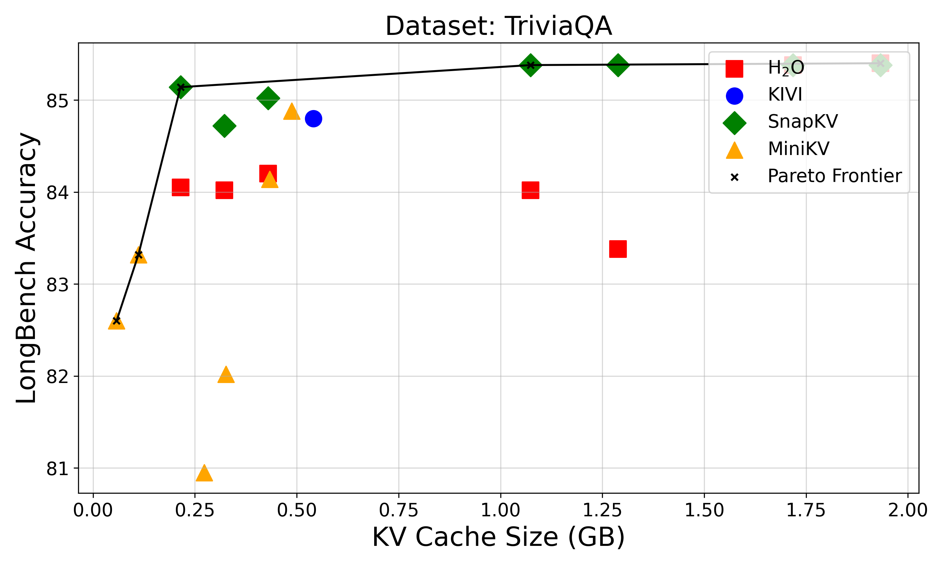</details> <details> <summary>extracted/6028174/image/perf_vs_kv_size_plots/triviaqa.png Details</summary>  ### Visual Description ## Scatter Plot: LongBench Accuracy vs KV Cache Size for TriviaQA Dataset ### Overview The chart visualizes the relationship between KV cache size (in GB) and LongBench accuracy for five different methods (H₂O, KIVI, SnapKV, MiniKV) on the TriviaQA dataset. A Pareto Frontier line connects optimal trade-off points between cache size and accuracy. ### Components/Axes - **X-axis**: KV Cache Size (GB) ranging from 0.00 to 2.00 in 0.25 increments - **Y-axis**: LongBench Accuracy (81 to 85.5) in 0.5 increments - **Legend**: Located in top-right corner with color/symbol mappings: - Red squares: H₂O - Blue circles: KIVI - Green diamonds: SnapKV - Yellow triangles: MiniKV - Black crosses: Pareto Frontier ### Detailed Analysis 1. **H₂O (Red Squares)** - Points at: - 0.25 GB → ~84.0 accuracy - 0.5 GB → ~84.2 accuracy - 1.0 GB → ~84.0 accuracy - Trend: Slight fluctuation with no clear upward trend 2. **KIVI (Blue Circle)** - Single point at: - 0.5 GB → ~84.8 accuracy - Trend: Isolated high-performance outlier 3. **SnapKV (Green Diamonds)** - Points at: - 0.25 GB → ~85.2 accuracy - 0.5 GB → ~85.0 accuracy - 1.0 GB → ~85.5 accuracy - 1.25 GB → ~85.5 accuracy - Trend: Steady increase followed by plateau 4. **MiniKV (Yellow Triangles)** - Points at: - 0.1 GB → ~82.7 accuracy - 0.3 GB → ~82.0 accuracy - 0.5 GB → ~82.5 accuracy - Trend: Initial drop followed by slight recovery 5. **Pareto Frontier (Black Line with Crosses)** - Connects optimal points: - Starts at ~0.1 GB, 82.7 accuracy - Peaks at ~1.0 GB, 85.5 accuracy - Flattens at ~1.25 GB, 85.5 accuracy ### Key Observations - **Performance Leaders**: SnapKV and KIVI dominate in accuracy, with SnapKV achieving 85.5% at 1.0-1.25 GB cache size - **Resource Efficiency**: MiniKV uses smallest cache (0.1-0.5 GB) but lags in accuracy (~82-82.5%) - **Diminishing Returns**: Pareto Frontier flattens after 1.0 GB, indicating limited accuracy gains from larger caches - **Anomaly**: KIVI's single point at 0.5 GB (84.8%) sits below SnapKV's performance at same cache size ### Interpretation The data demonstrates a clear trade-off between computational resources and question-answering performance. SnapKV emerges as the most efficient method, achieving highest accuracy (85.5%) with moderate cache usage (1.0-1.25 GB). The Pareto Frontier reveals that beyond 1.0 GB, additional cache provides minimal accuracy improvements, suggesting diminishing returns in this configuration. Notably, MiniKV's lower performance despite smaller cache footprint indicates potential architectural limitations. KIVI's isolated high-performance point suggests specialized optimization for specific cache sizes. These findings highlight the importance of cache efficiency over raw size in knowledge-intensive QA systems, with SnapKV representing the optimal balance for TriviaQA. </details> Figure 16: Performance Versus KV Cache Size: MiniKV offers the best performance for the smallest KV cache size across all 6 task categories. ## Appendix F Comparison between H2O and SnapKV Fig. 17 shows that with 50% KV cache size, the LLM can still obtain comparable accuracy (e.g., $<$ 1%) as the full KV cache. However, high levels of KV eviction (e.g., 80-95%) hurts LLM’s performance on long context tasks significantly. 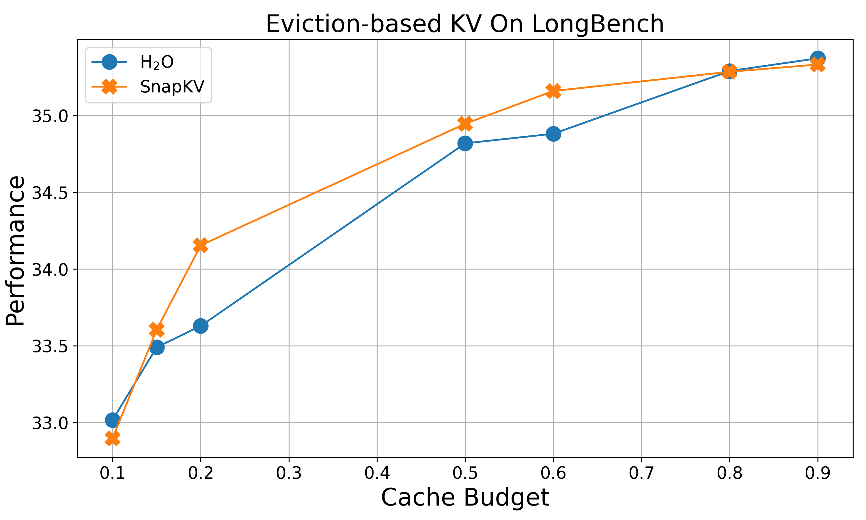<details> <summary>extracted/6028174/image/eviction_kv_on_longbench.png Details</summary>  ### Visual Description ## Line Chart: Eviction-based KV On LongBench ### Overview The chart compares the performance of two key-value (KV) eviction strategies, **H2O** and **SnapKV**, across varying cache budgets on the LongBench benchmark. Performance is measured on a scale from 33.0 to 35.5, with cache budgets ranging from 0.1 to 0.9. --- ### Components/Axes - **X-axis (Cache Budget)**: Labeled "Cache Budget," with tick marks at 0.1, 0.2, 0.3, 0.5, 0.6, 0.8, and 0.9. - **Y-axis (Performance)**: Labeled "Performance," with tick marks at 33.0, 33.5, 34.0, 34.5, 35.0, 35.5. - **Legend**: Located in the top-left corner, with: - **Blue circles** representing **H2O**. - **Orange crosses** representing **SnapKV**. --- ### Detailed Analysis #### H2O (Blue Circles) - **Trend**: Starts at **33.0** (cache budget 0.1) and increases steadily, reaching **35.8** at 0.9. - **Key Data Points**: - 0.1 → 33.0 - 0.2 → 33.6 - 0.3 → 34.0 - 0.5 → 34.8 - 0.6 → 34.9 - 0.8 → 35.7 - 0.9 → 35.8 #### SnapKV (Orange Crosses) - **Trend**: Begins at **32.9** (cache budget 0.1) and rises sharply, plateauing near **35.8** at 0.9. - **Key Data Points**: - 0.1 → 32.9 - 0.2 → 34.2 - 0.3 → 34.4 - 0.5 → 34.9 - 0.6 → 35.2 - 0.8 → 35.7 - 0.9 → 35.8 --- ### Key Observations 1. **Performance Convergence**: Both methods converge at **35.8** at a cache budget of 0.9. 2. **H2O Advantage at High Budgets**: H2O outperforms SnapKV at cache budgets ≥0.5. 3. **SnapKV Early Lead**: SnapKV starts stronger at lower budgets (e.g., 34.2 vs. 33.6 at 0.2). 4. **Steady Growth**: Both lines show consistent upward trends, with no plateaus or declines. --- ### Interpretation - **Efficiency Trade-off**: H2O becomes more efficient than SnapKV as cache budget increases, suggesting better scalability for larger workloads. - **SnapKV’s Early Performance**: SnapKV may be optimized for low-resource environments but loses ground as resources expand. - **Benchmark Context**: The LongBench results imply that eviction strategy choice depends heavily on available cache resources. No anomalies or outliers are observed. The data aligns with the legend and axis labels, confirming accuracy. </details> Figure 17: Eviction-based KV on LongBench: High levels of KV eviction (e.g., 80-95%) hurts LLM’s performance on long context tasks significantly. ## Appendix G Attention plot prompt The prompt is randomly picked up from LongBench dataset and we manually choose the first 5000 strings. Passage 1: David Faber (politician) David James Christian Faber (born 7 July 1961) is a schoolmaster and former Conservative member of the Parliament of the United Kingdom. He did not seek re-election in 2001, after which he became an author, before in 2010 being appointed as head master of Summer Fields School, Oxford. He is the grandson of the late former Conservative Prime Minister Harold Macmillan (1894–1986). Family and early life The son of Julian and Lady Caroline Faber, Faber comes from an aristocratic political family drawn from the Whig and latterly the Conservative traditions. His maternal grandfather Harold Macmillan was Prime Minister at the time of his birth. His maternal grandmother, Lady Dorothy Cavendish, was descended from three Prime Ministers, the 4th Duke of Devonshire (1756–1757), the 2nd Earl of Shelburne (1782–1783) and the 3rd Duke of Portland (1783 and 1807–1809). Faber’s great-great-great-granduncle was Lord Hartington and his great-grandfather Victor Cavendish, 9th Duke of Devonshire was also a statesman. His mother’s cousins included Andrew Cavendish, 11th Duke of Devonshire, who was married to Deborah Mitford, and Andrew’s elder brother William Cavendish, Marquess of Hartington, who was married to Kathleen Kennedy, the sister of U.S. President John F. Kennedy and Senators Robert F. Kennedy and Edward M. "Ted" Kennedy. His uncle Maurice Macmillan was a leading figure of Edward Heath’s 1970s government. Faber was educated at Summer Fields School, Summertown; and then at Eton College and Balliol College, Oxford. Life and career Faber first stood for Parliament, unsuccessfully, in 1987 at Stockton North, where he was defeated by Labour’s Frank Cook. He worked in marketing and as a political assistant to Jeffrey Archer before entering the House of Commons in 1992 as Conservative Member of Parliament for Westbury. He was parliamentary private secretary to the Minister of State at the Foreign and Commonwealth Office, 1994 to 1996, and then to the Secretary of State for Health, from 1996 to 1997. In opposition, after the Conservatives lost the 1997 general election, he was their front bench spokesman on Foreign and Commonwealth affairs, until 1998. He served as a member of several Parliamentary select committees: Social Security, 1992–1997, Culture, Media and Sport, 1998 to 2001, and the Public Accounts Committee, 2000–2001.In 1997, he was reported to be a director of Sterling Marketing, and in 1998 was a director of Freestream Aircraft.Faber stood down from parliament at the 2001 general election, to be succeeded by fellow Conservative Andrew Murrison, when he began a new career as a writer. His book Speaking for England: Leo, Julian and John Amery, the tragedy of a political family (2005) was about Julian Amery, his uncle by his (Amery’s) marriage to Faber’s maternal aunt, Julian’s father Leo, and brother John, who was executed after the Second World War for high treason. In 2009, he was appointed as head of his old prep school, Summer Fields, with effect from September 2010. Faber married firstly Sally Gilbert, a television weather presenter, and they had one son together, Henry, but later divorced, with Faber citing James Hewitt as co-respondent. He married secondly Sophie Amanda Hedley, and they have two daughters. He is a past committee member of the Marylebone Cricket Club, the governing body of the game of cricket, managing an MCC tour of Canada in 2001. He is also a member of White’s. Books David Faber, Munich (Simon & Schuster) – about the events of 1937–1938 and the Munich Conference David Faber, Speaking for England: Leo, Julian and John Amery (Simon & Schuster, 2005) – the Amery family and World War II ISBN 1-4165-2596-3 Passage 2: Marina Yannakoudakis Marina Yannakoudakis (born 16 April 1956) is a member of the European Economic and Social Committee and a former Conservative Member of the European Parliament for London. She was elected at the 2009 European Parliament election. She lost her seat at the 2014 election. Early years Yannakoudakis was born in Paddington. She studied for a BSc in government, politics and modern history at Brunel University, where she was chairman of the Conservative students, and also received an MA in education from the Open University. She was a member of Barnet London Borough Council for Oakleigh Park Ward from 2006 to 2010 where she was chair of the Cleaner, Greener, Transport and Development Overview & Scrutiny Committee. Member of the European Parliament She was a full member of the Committee on Women’s Rights and Gender Equality, the Committee on the Environment, Public Health and Food Safety and a substitute member of the Special Committee on Organised Crime, Corruption and Money Laundering. She was a member of the Delegation to the EU-Former Yugoslav Republic of Macedonia Joint Parliamentary Committee.She was also a member of the High-Level Contact Group for relations with the Turkish Cypriot community in the northern part of the island of …