2412.06769v1

# Training Large Language Models to Reason in a Continuous Latent Space **Authors**: Shibo Hao, Sainbayar Sukhbaatar, DiJia Su, Xian Li, Zhiting Hu, Jason Weston, Yuandong Tian 1]FAIR at Meta 2]UC San Diego \contribution [*]Work done at Meta (December 23, 2025) Abstract Large language models (LLMs) are restricted to reason in the “language space”, where they typically express the reasoning process with a chain-of-thought (CoT) to solve a complex reasoning problem. However, we argue that language space may not always be optimal for reasoning. For example, most word tokens are primarily for textual coherence and not essential for reasoning, while some critical tokens require complex planning and pose huge challenges to LLMs. To explore the potential of LLM reasoning in an unrestricted latent space instead of using natural language, we introduce a new paradigm Coconut (C hain o f Con tin u ous T hought). We utilize the last hidden state of the LLM as a representation of the reasoning state (termed “continuous thought”). Rather than decoding this into a word token, we feed it back to the LLM as the subsequent input embedding directly in the continuous space. Experiments show that Coconut can effectively augment the LLM on several reasoning tasks. This novel latent reasoning paradigm leads to emergent advanced reasoning patterns: the continuous thought can encode multiple alternative next reasoning steps, allowing the model to perform a breadth-first search (BFS) to solve the problem, rather than prematurely committing to a single deterministic path like CoT. Coconut outperforms CoT in certain logical reasoning tasks that require substantial backtracking during planning, with fewer thinking tokens during inference. These findings demonstrate the promise of latent reasoning and offer valuable insights for future research. 1 Introduction Large language models (LLMs) have demonstrated remarkable reasoning abilities, emerging from extensive pretraining on human languages (Dubey et al., 2024; Achiam et al., 2023). While next token prediction is an effective training objective, it imposes a fundamental constraint on the LLM as a reasoning machine: the explicit reasoning process of LLMs must be generated in word tokens. For example, a prevalent approach, known as chain-of-thought (CoT) reasoning (Wei et al., 2022), involves prompting or training LLMs to generate solutions step-by-step using natural language. However, this is in stark contrast to certain human cognition results. Neuroimaging studies have consistently shown that the language network – a set of brain regions responsible for language comprehension and production – remains largely inactive during various reasoning tasks (Amalric and Dehaene, 2019; Monti et al., 2012, 2007, 2009; Fedorenko et al., 2011). Further evidence indicates that human language is optimized for communication rather than reasoning (Fedorenko et al., 2024). A significant issue arises when LLMs use language for reasoning: the amount of reasoning required for each particular reasoning token varies greatly, yet current LLM architectures allocate nearly the same computing budget for predicting every token. Most tokens in a reasoning chain are generated solely for fluency, contributing little to the actual reasoning process. On the contrary, some critical tokens require complex planning and pose huge challenges to LLMs. While previous work has attempted to fix these problems by prompting LLMs to generate succinct reasoning chains (Madaan and Yazdanbakhsh, 2022), or performing additional reasoning before generating some critical tokens (Zelikman et al., 2024), these solutions remain constrained within the language space and do not solve the fundamental problems. On the contrary, it would be ideal for LLMs to have the freedom to reason without any language constraints, and then translate their findings into language only when necessary. <details> <summary>figures/figure_1_meta_3.png Details</summary>  ### Visual Description # Technical Document Extraction: Chain-of-Thought (CoT) and Chain of Continuous Thought (CoCoNUT) Diagrams ## Diagram Overview The image contains two side-by-side diagrams comparing **Chain-of-Thought (CoT)** and **Chain of Continuous Thought (CoCoNUT)** architectures in large language models. Both diagrams illustrate token processing flows and hidden state utilization. --- ### **Left Diagram: Chain-of-Thought (CoT)** #### Components and Flow 1. **Input Section**: - **Input Token**: `[Question]` (yellow square). - **Input Embedding**: Represented by a sequence of yellow squares labeled `x_i`, `x_i+1`, `x_i+2`, ..., `x_i+j`. 2. **Processing**: - **Large Language Model**: Central gray rectangle labeled "Large Language Model." - **Hidden States**: Purple squares labeled "last hidden state" (e.g., `x_i`, `x_i+1`, ..., `x_i+j`). 3. **Output Section**: - **Output Token (Sampling)**: Purple squares labeled `x_i`, `x_i+1`, ..., `x_i+j`. - **Final Output**: `[Answer]` (purple square). #### Legend and Spatial Grounding - **Legend**: Located on the right side of the diagram. - **Purple**: Last hidden states. - **Yellow**: Input embeddings. - **Spatial Flow**: Tokens flow left-to-right through the model, with hidden states feeding into output token sampling. --- ### **Right Diagram: Chain of Continuous Thought (CoCoNUT)** #### Components and Flow 1. **Input Section**: - **Input Token**: `[Question]` (yellow square). - **Special Tokens**: `<bot>` and `<eot>` (yellow squares). - **Input Embedding**: Represented by a sequence of yellow squares. 2. **Processing**: - **Large Language Model**: Central gray rectangle labeled "Large Language Model." - **Hidden States**: Orange squares labeled "last hidden states" (e.g., `x_i`, `x_i+1`, ..., `x_i+j`). - **Feedback Loop**: Hidden states are reused as input embeddings for subsequent steps (indicated by bidirectional arrows). 3. **Output Section**: - **Output Token (Sampling)**: Orange squares labeled `x_i`, `x_i+1`, ..., `x_i+j`. - **Final Output**: `[Answer]` (purple square). #### Legend and Spatial Grounding - **Legend**: Located on the right side of the diagram. - **Orange**: Last hidden states. - **Yellow**: Input embeddings. - **Spatial Flow**: Hidden states are recycled as input embeddings, creating a continuous loop within the model. --- ### Key Differences | Feature | CoT | CoCoNUT | |------------------------|------------------------------|------------------------------| | **Hidden State Use** | Linear progression | Recycled as input embeddings | | **Special Tokens** | None | `<bot>`, `<eot>` | | **Feedback Mechanism** | None | Explicit feedback loop | --- ### Notes - **No Numerical Data**: Both diagrams are conceptual and do not include numerical values or statistical trends. - **Color Consistency**: Legend colors (purple, yellow, orange) are strictly adhered to in both diagrams. - **Textual Labels**: All labels (e.g., `[Question]`, `[Answer]`, `<bot>`) are transcribed verbatim. This extraction provides a complete technical breakdown of the diagrams, ensuring no component or label is omitted. 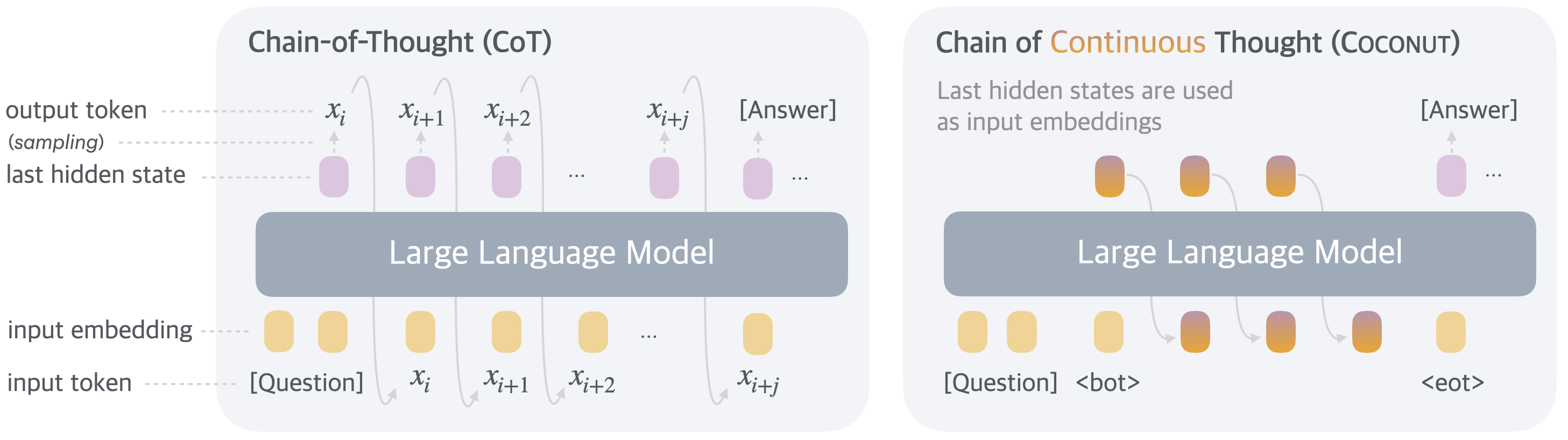</details> Figure 1: A comparison of Chain of Continuous Thought (Coconut) with Chain-of-Thought (CoT). In CoT, the model generates the reasoning process as a word token sequence (e.g., $[x_{i},x_{i+1},...,x_{i+j}]$ in the figure). Coconut regards the last hidden state as a representation of the reasoning state (termed “continuous thought”), and directly uses it as the next input embedding. This allows the LLM to reason in an unrestricted latent space instead of a language space. In this work we instead explore LLM reasoning in a latent space by introducing a novel paradigm, Coconut (Chain of Continuous Thought). It involves a simple modification to the traditional CoT process: instead of mapping between hidden states and language tokens using the language model head and embedding layer, Coconut directly feeds the last hidden state (a continuous thought) as the input embedding for the next token (Figure 1). This modification frees the reasoning from being within the language space, and the system can be optimized end-to-end by gradient descent, as continuous thoughts are fully differentiable. To enhance the training of latent reasoning, we employ a multi-stage training strategy inspired by Deng et al. (2024), which effectively utilizes language reasoning chains to guide the training process. Interestingly, our proposed paradigm leads to an efficient reasoning pattern. Unlike language-based reasoning, continuous thoughts in Coconut can encode multiple potential next steps simultaneously, allowing for a reasoning process akin to breadth-first search (BFS). While the model may not initially make the correct decision, it can maintain many possible options within the continuous thoughts and progressively eliminate incorrect paths through reasoning, guided by some implicit value functions. This advanced reasoning mechanism surpasses traditional CoT, even though the model is not explicitly trained or instructed to operate in this manner, as seen in previous works (Yao et al., 2023; Hao et al., 2023). Experimentally, Coconut successfully enhances the reasoning capabilities of LLMs. For math reasoning (GSM8k, Cobbe et al., 2021), using continuous thoughts is shown to be beneficial to reasoning accuracy, mirroring the effects of language reasoning chains. This indicates the potential to scale and solve increasingly challenging problems by chaining more continuous thoughts. On logical reasoning including ProntoQA (Saparov and He, 2022), and our newly proposed ProsQA (Section 4.1) which requires stronger planning ability, Coconut and some of its variants even surpasses language-based CoT methods, while generating significantly fewer tokens during inference. We believe that these findings underscore the potential of latent reasoning and could provide valuable insights for future research. 2 Related Work Chain-of-thought (CoT) reasoning. We use the term chain-of-thought broadly to refer to methods that generate an intermediate reasoning process in language before outputting the final answer. This includes prompting LLMs (Wei et al., 2022; Khot et al., 2022; Zhou et al., 2022), or training LLMs to generate reasoning chains, either with supervised finetuning (Yue et al., 2023; Yu et al., 2023) or reinforcement learning (Wang et al., 2024; Havrilla et al., 2024; Shao et al., 2024; Yu et al., 2024a). Madaan and Yazdanbakhsh (2022) classified the tokens in CoT into symbols, patterns, and text, and proposed to guide the LLM to generate concise CoT based on analysis of their roles. Recent theoretical analyses have demonstrated the usefulness of CoT from the perspective of model expressivity (Feng et al., 2023; Merrill and Sabharwal, 2023; Li et al., 2024). By employing CoT, the effective depth of the transformer increases because the generated outputs are looped back to the input (Feng et al., 2023). These analyses, combined with the established effectiveness of CoT, motivated our design that feeds the continuous thoughts back to the LLM as the next input embedding. While CoT has proven effective for certain tasks, its autoregressive generation nature makes it challenging to mimic human reasoning on more complex problems (LeCun, 2022; Hao et al., 2023), which typically require planning and search. There are works that equip LLMs with explicit tree search algorithms (Xie et al., 2023; Yao et al., 2023; Hao et al., 2024), or train the LLM on search dynamics and trajectories (Lehnert et al., 2024; Gandhi et al., 2024; Su et al., 2024). In our analysis, we find that after removing the constraint of a language space, a new reasoning pattern similar to BFS emerges, even though the model is not explicitly trained in this way. Latent reasoning in LLMs. Previous works mostly define latent reasoning in LLMs as the hidden computation in transformers (Yang et al., 2024; Biran et al., 2024). Yang et al. (2024) constructed a dataset of two-hop reasoning problems and discovered that it is possible to recover the intermediate variable from the hidden representations. Biran et al. (2024) further proposed to intervene the latent reasoning by “back-patching” the hidden representation. Shalev et al. (2024) discovered parallel latent reasoning paths in LLMs. Another line of work has discovered that, even if the model generates a CoT to reason, the model may actually utilize a different latent reasoning process. This phenomenon is known as the unfaithfulness of CoT reasoning (Wang et al., 2022; Turpin et al., 2024). To enhance the latent reasoning of LLM, previous research proposed to augment it with additional tokens. Goyal et al. (2023) pretrained the model by randomly inserting a learnable <pause> tokens to the training corpus. This improves LLM’s performance on a variety of tasks, especially when followed by supervised finetuning with <pause> tokens. On the other hand, Pfau et al. (2024) further explored the usage of filler tokens, e.g., “... ”, and concluded that they work well for highly parallelizable problems. However, Pfau et al. (2024) mentioned these methods do not extend the expressivity of the LLM like CoT; hence, they may not scale to more general and complex reasoning problems. Wang et al. (2023) proposed to predict a planning token as a discrete latent variable before generating the next reasoning step. Recently, it has also been found that one can “internalize” the CoT reasoning into latent reasoning in the transformer with knowledge distillation (Deng et al., 2023) or a special training curriculum which gradually shortens CoT (Deng et al., 2024). Yu et al. (2024b) also proposed to distill a model that can reason latently from data generated with complex reasoning algorithms. These training methods can be combined to our framework, and specifically, we find that breaking down the learning of continuous thoughts into multiple stages, inspired by iCoT (Deng et al., 2024), is very beneficial for the training. Recently, looped transformers (Giannou et al., 2023; Fan et al., 2024) have been proposed to solve algorithmic tasks, which have some similarities to the computing process of continuous thoughts, but we focus on common reasoning tasks and aim at investigating latent reasoning in comparison to language space. 3 Coconut: Chain of Continuous Thought In this section, we introduce our new paradigm Coconut (Chain of Continuous Thought) for reasoning in an unconstrained latent space. We begin by introducing the background and notation we use for language models. For an input sequence $x=(x_{1},...,x_{T})$ , the standard large language model $\mathcal{M}$ can be described as: $$ H_{t}=\text{Transformer}(E_{t}+P_{t}) $$ $$ \mathcal{M}(x_{t+1}\mid x_{\leq t})=\text{softmax}(Wh_{t}) $$ where $E_{t}=[e(x_{1}),e(x_{2}),...,e(x_{t})]$ is the sequence of token embeddings up to position $t$ ; $P_{t}=[p(1),p(2),...,p(t)]$ is the sequence of positional embeddings up to position $t$ ; $H_{t}∈\mathbb{R}^{t× d}$ is the matrix of the last hidden states for all tokens up to position $t$ ; $h_{t}$ is the last hidden state of position $t$ , i.e., $h_{t}=H_{t}[t,:]$ ; $e(·)$ is the token embedding function; $p(·)$ is the positional embedding function; $W$ is the parameter of the language model head. Method Overview. In the proposed Coconut method, the LLM switches between the “language mode” and “latent mode” (Figure 1). In language mode, the model operates as a standard language model, autoregressively generating the next token. In latent mode, it directly utilizes the last hidden state as the next input embedding. This last hidden state represents the current reasoning state, termed as a “continuous thought”. Special tokens <bot> and <eot> are employed to mark the beginning and end of the latent thought mode, respectively. As an example, we assume latent reasoning occurs between positions $i$ and $j$ , i.e., $x_{i}=$ <bot> and $x_{j}=$ <eot>. When the model is in the latent mode ( $i<t<j$ ), we use the last hidden state from the previous token to replace the input embedding, i.e., $E_{t}=[e(x_{1}),e(x_{2}),...,e(x_{i}),h_{i},h_{i+1},...,h_{t-1}]$ . After the latent mode finishes ( $t≥ j$ ), the input reverts to using the token embedding, i.e., $E_{t}=[e(x_{1}),e(x_{2}),...,e(x_{i}),h_{i},h_{i+1},...,h_{j-1},e(x_{j}),...,e(x_{t})]$ . It is noteworthy that $\mathcal{M}(x_{t+1}\mid x_{≤ t})$ is not defined when $i<t<j$ , since the latent thought is not intended to be mapped back to language space. However, $\mathrm{softmax}(Wh_{t})$ can still be calculated for probing purposes (see Section 4). 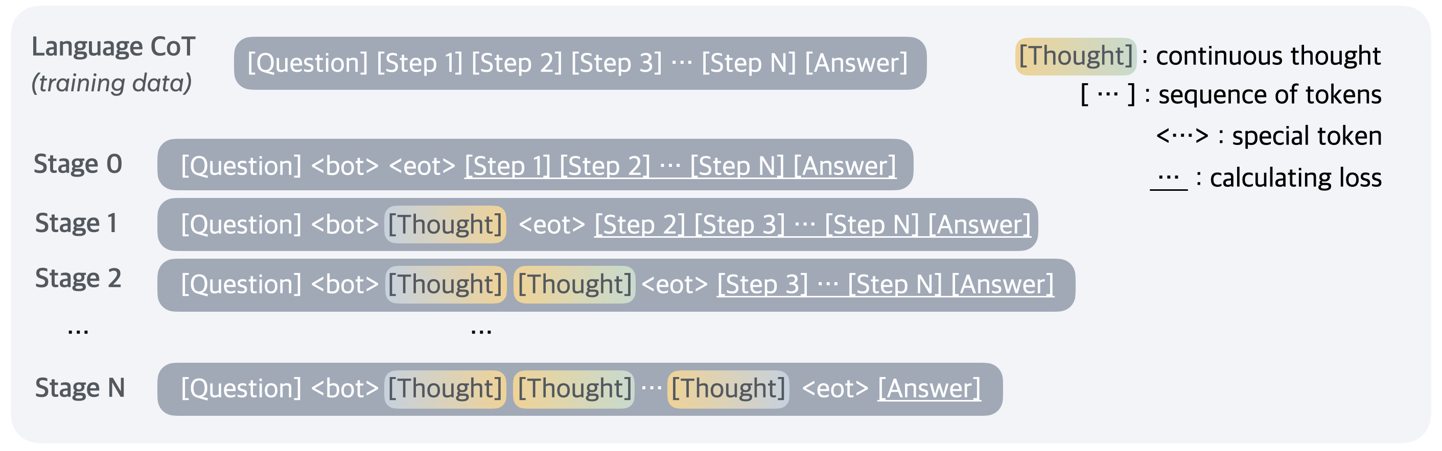Training Procedure. In this work, we focus on a problem-solving setting where the model receives a question as input and is expected to generate an answer through a reasoning process. We leverage language CoT data to supervise continuous thought by implementing a multi-stage training curriculum inspired by Deng et al. (2024). As shown in Figure 2, in the initial stage, the model is trained on regular CoT instances. In the subsequent stages, at the $k$ -th stage, the first $k$ reasoning steps in the CoT are replaced with $k× c$ continuous thoughts If a language reasoning chain is shorter than $k$ steps, then all the language thoughts will be removed., where $c$ is a hyperparameter controlling the number of latent thoughts replacing a single language reasoning step. Following Deng et al. (2024), we also reset the optimizer state when training stages switch. We insert <bot> and <eot> tokens to encapsulate the continuous thoughts. <details> <summary>figures/figure_2_meta_5.png Details</summary>  ### Visual Description # Technical Document Extraction: Language CoT Training Data Diagram ## Diagram Overview The image illustrates the structure of **Language Chain-of-Thought (CoT) training data** for a language model. It visualizes the progression of model reasoning stages, token sequences, and special token usage during training. --- ## Key Components ### 1. Header - **Title**: `Language CoT (training data)` - **Sequence Template**: </details> Figure 2: Training procedure of Chain of Continuous Thought (Coconut). Given training data with language reasoning steps, at each training stage we integrate $c$ additional continuous thoughts ( $c=1$ in this example), and remove one language reasoning step. The cross-entropy loss is then used on the remaining tokens after continuous thoughts. During the training process, we mask the loss on questions and latent thoughts. It is important to note that the objective does not encourage the continuous thought to compress the removed language thought, but rather to facilitate the prediction of future reasoning. Therefore, it’s possible for the LLM to learn more effective representations of reasoning steps compared to human language. Training Details. Our proposed continuous thoughts are fully differentiable and allow for back-propagation. We perform $n+1$ forward passes when $n$ latent thoughts are scheduled in the current training stage, computing a new latent thought with each pass and finally conducting an additional forward pass to obtain a loss on the remaining text sequence. While we can save any repetitive computing by using a KV cache, the sequential nature of the multiple forward passes poses challenges for parallelism. Further optimizing the training efficiency of Coconut remains an important direction for future research. Inference Process. The inference process for Coconut is analogous to standard language model decoding, except that in latent mode, we directly feed the last hidden state as the next input embedding. A challenge lies in determining when to switch between latent and language modes. As we focus on the problem-solving setting, we insert a <bot> token immediately following the question tokens. For <eot>, we consider two potential strategies: a) train a binary classifier on latent thoughts to enable the model to autonomously decide when to terminate the latent reasoning, or b) always pad the latent thoughts to a constant length. We found that both approaches work comparably well. Therefore, we use the second option in our experiment for simplicity, unless specified otherwise. 4 Experiments We validate the feasibility of LLM reasoning in a continuous latent space through experiments on three datasets. We mainly evaluate the accuracy by comparing the model-generated answers with the ground truth. The number of newly generated tokens per question is also analyzed, as a measure of reasoning efficiency. We report the clock-time comparison in Appendix 8. 4.1 Reasoning Tasks Math Reasoning. We use GSM8k (Cobbe et al., 2021) as the dataset for math reasoning. It consists of grade school-level math problems. Compared to the other datasets in our experiments, the problems are more diverse and open-domain, closely resembling real-world use cases. Through this task, we explore the potential of latent reasoning in practical applications. To train the model, we use a synthetic dataset generated by Deng et al. (2023). Logical Reasoning. Logical reasoning involves the proper application of known conditions to prove or disprove a conclusion using logical rules. This requires the model to choose from multiple possible reasoning paths, where the correct decision often relies on exploration and planning ahead. We use 5-hop ProntoQA (Saparov and He, 2022) questions, with fictional concept names. For each problem, a tree-structured ontology is randomly generated and described in natural language as a set of known conditions. The model is asked to judge whether a given statement is correct based on these conditions. This serves as a simplified simulation of more advanced reasoning tasks, such as automated theorem proving (Chen et al., 2023; DeepMind, 2024). We found that the generation process of ProntoQA could be more challenging, especially since the size of distracting branches in the ontology is always small, reducing the need for complex planning. To fix that, we apply a new dataset construction pipeline using randomly generated DAGs to structure the known conditions. The resulting dataset requires the model to perform substantial planning and searching over the graph to find the correct reasoning chain. We refer to this new dataset as ProsQA (Pro of with S earch Q uestion- A nswering). A visualized example is shown in Figure 7. More details of datasets can be found in Appendix 7. 4.2 Experimental Setup We use a pre-trained GPT-2 (Radford et al., 2019) as the base model for all experiments. The learning rate is set to $1× 10^{-4}$ while the effective batch size is 128. Following Deng et al. (2024), we also reset the optimizer when the training stages switch. Math Reasoning. By default, we use 2 latent thoughts (i.e., $c=2$ ) for each reasoning step. We analyze the correlation between performance and $c$ in Section 1. The model goes through 3 stages besides the initial stage. Then, we have an additional stage, where we still use $3× c$ continuous thoughts as in the penultimate stage, but remove all the remaining language reasoning chain. This handles the long-tail distribution of reasoning chains longer than 3 steps. We train the model for 6 epochs in the initial stage, and 3 epochs in each remaining stage. Logical Reasoning. We use one continuous thought for every reasoning step (i.e., $c=1$ ). The model goes through 6 training stages in addition to the initial stage, because the maximum number of reasoning steps is 6 in these two datasets. The model then fully reasons with continuous thoughts to solve the problems in the last stage. We train the model for 5 epochs per stage. For all datasets, after the standard schedule, the model stays in the final training stage, until the 50th epoch. We select the checkpoint based on the accuracy on the validation set. For inference, we manually set the number of continuous thoughts to be consistent with their final training stage. We use greedy decoding for all experiments. 4.3 Baselines and Variants of Coconut We consider the following baselines: (1) CoT: We use the complete reasoning chains to train the language model with supervised finetuning, and during inference, the model generates a reasoning chain before outputting an answer. (2) No-CoT: The LLM is trained to directly generate the answer without using a reasoning chain. (3) iCoT (Deng et al., 2024): The model is trained with language reasoning chains and follows a carefully designed schedule that “internalizes” CoT. As the training goes on, tokens at the beginning of the reasoning chain are gradually removed until only the answer remains. During inference, the model directly predicts the answer. (4) Pause token (Goyal et al., 2023): The model is trained using only the question and answer, without a reasoning chain. However, different from No-CoT, special <pause> tokens are inserted between the question and answer, which are believed to provide the model with additional computational capacity to derive the answer. For a fair comparison, the number of <pause> tokens is set the same as continuous thoughts in Coconut. We also evaluate some variants of our method: (1) w/o curriculum: Instead of the multi-stage training, we directly use the data from the last stage which only includes questions and answers to train Coconut. The model uses continuous thoughts to solve the whole problem. (2) w/o thought: We keep the multi-stage training which removes language reasoning steps gradually, but don’t use any continuous latent thoughts. While this is similar to iCoT in the high-level idea, the exact training schedule is set to be consistent with Coconut, instead of iCoT. This ensures a more strict comparison. (3) Pause as thought: We use special <pause> tokens to replace the continuous thoughts, and apply the same multi-stage training curriculum as Coconut. 4.4 Results and Discussion | Method | GSM8k | ProntoQA | ProsQA | | | | | --- | --- | --- | --- | --- | --- | --- | | Acc. (%) | # Tokens | Acc. (%) | # Tokens | Acc. (%) | # Tokens | | | CoT | 42.9 $\ ±$ 0.2 | 25.0 | 98.8 $\ ±$ 0.8 | 92.5 | 77.5 $\ ±$ 1.9 | 49.4 | | No-CoT | 16.5 $\ ±$ 0.5 | 2.2 | 93.8 $\ ±$ 0.7 | 3.0 | 76.7 $\ ±$ 1.0 | 8.2 | | iCoT | 30.0 ∗ | 2.2 | 99.8 $\ ±$ 0.3 | 3.0 | 98.2 $\ ±$ 0.3 | 8.2 | | Pause Token | 16.4 $\ ±$ 1.8 | 2.2 | 77.7 $\ ±$ 21.0 | 3.0 | 75.9 $\ ±$ 0.7 | 8.2 | | Coconut (Ours) | 34.1 $\ ±$ 1.5 | 8.2 | 99.8 $\ ±$ 0.2 | 9.0 | 97.0 $\ ±$ 0.3 | 14.2 | | - w/o curriculum | 14.4 $\ ±$ 0.8 | 8.2 | 52.4 $\ ±$ 0.4 | 9.0 | 76.1 $\ ±$ 0.2 | 14.2 | | - w/o thought | 21.6 $\ ±$ 0.5 | 2.3 | 99.9 $\ ±$ 0.1 | 3.0 | 95.5 $\ ±$ 1.1 | 8.2 | | - pause as thought | 24.1 $\ ±$ 0.7 | 2.2 | 100.0 $\ ±$ 0.1 | 3.0 | 96.6 $\ ±$ 0.8 | 8.2 | Table 1: Results on three datasets: GSM8l, ProntoQA and ProsQA. Higher accuracy indicates stronger reasoning ability, while generating fewer tokens indicates better efficiency. ∗ The result is from Deng et al. (2024). <details> <summary>x1.png Details</summary>  ### Visual Description # Technical Document Extraction: Line Chart Analysis ## Chart Overview The image depicts a **line chart** with a shaded gradient area, representing the relationship between the number of thoughts per step and accuracy percentage. The chart uses a **blue line** with a **light-to-dark blue gradient shading** to indicate uncertainty or confidence intervals. --- ### Axis Labels and Markers - **X-Axis**: - Title: `# Thoughts per step` - Values: `0`, `1`, `2` (discrete steps) - **Y-Axis**: - Title: `Accuracy (%)` - Range: `25%` to `36%` (increments of `2%`) --- ### Data Points and Trend 1. **Line Data**: - **Point 1**: `(0, 25.5%)` - **Point 2**: `(1, 31.0%)` - **Point 3**: `(2, 34.0%)` - **Trend**: The line exhibits a **steady upward slope**, increasing by approximately `5.5%` per step. 2. **Shaded Area**: - Represents a **confidence interval** or uncertainty range. - Gradient transitions from **light blue** (near the line) to **dark blue** (at the edges), suggesting diminishing confidence with distance from the central trend. --- ### Legend and Annotations - **Legend**: - Located in the **top-right corner** of the chart. - **No explicit label** is provided for the line or shaded area. - **Color Reference**: The line and shading are both blue, but no textual legend entry is visible. --- ### Spatial Grounding and Component Isolation - **Main Chart Region**: - Dominates the center of the image. - Shaded area spans the full width of the chart, anchored to the line. - **Footer/Background**: - No additional annotations or text outside the chart area. --- ### Key Observations 1. **Accuracy Correlation**: - Accuracy improves linearly as the number of thoughts per step increases. - From `25.5%` at `0` thoughts to `34.0%` at `2` thoughts. 2. **Uncertainty Representation**: - The shaded gradient implies higher confidence near the central trend line and lower confidence at the extremes. --- ### Missing Elements - **Legend Label**: No textual description of the line or shaded area is present. - **Secondary Axes/Annotations**: None observed. --- ### Conclusion The chart demonstrates a direct, positive correlation between the number of thoughts per step and accuracy. The shaded gradient provides a visual cue for uncertainty, though the absence of a legend label limits interpretability. 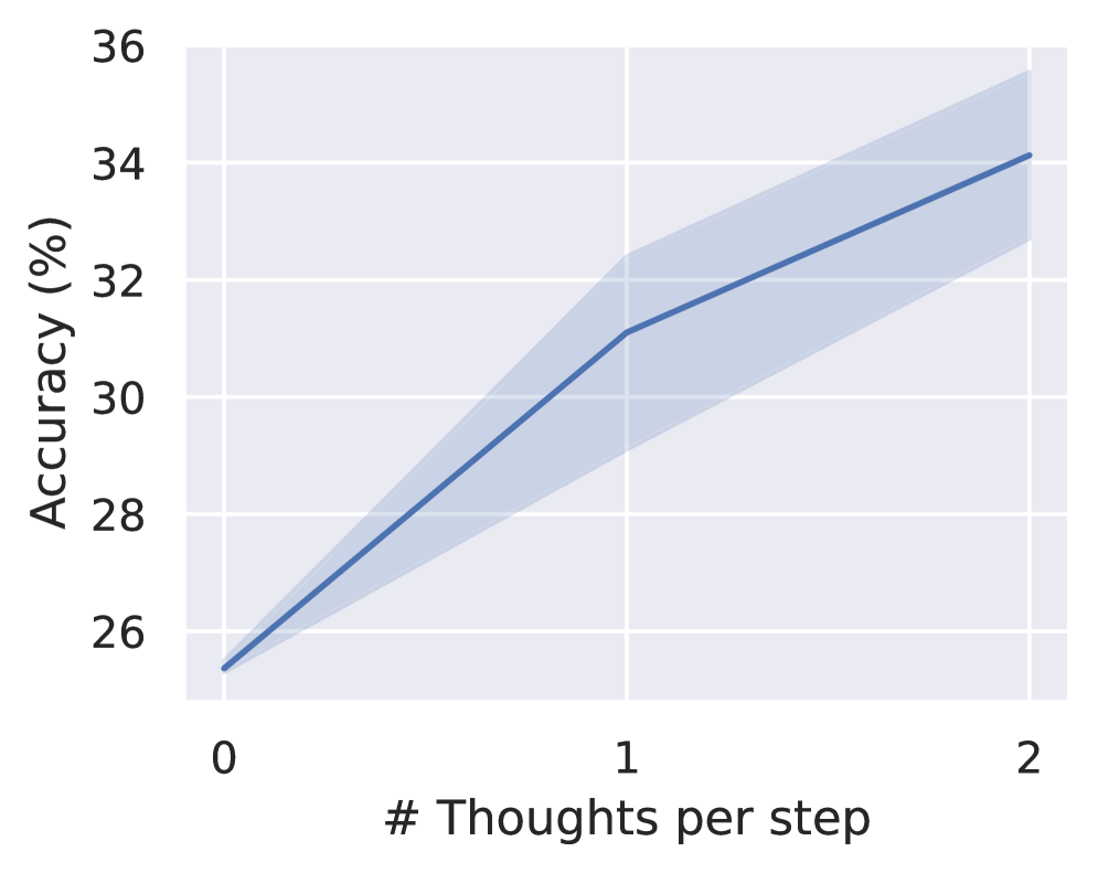</details> Figure 3: Accuracy on GSM8k with different number of continuous thoughts. We show the overall results on all datasets in Table 1. Continuous thoughts effectively enhance LLM reasoning, as shown by the consistent improvement over no-CoT. It even shows better performance than CoT on ProntoQA and ProsQA. We describe several key conclusions from the experiments as follows. “Chaining” continuous thoughts enhances reasoning. In conventional CoT, the output token serves as the next input, which proves to increase the effective depth of LLMs and enhance their expressiveness (Feng et al., 2023). We explore whether latent space reasoning retains this property, as it would suggest that this method could scale to solve increasingly complex problems by chaining multiple latent thoughts. In our experiments with GSM8k, we found that Coconut outperformed other architectures trained with similar strategies, particularly surpassing the latest baseline, iCoT (Deng et al., 2024). The performance is significantly better than Coconut (pause as thought) which also enables more computation in the LLMs. While Pfau et al. (2024) empirically shows that filler tokens, such as the special <pause> tokens, can benefit highly parallelizable problems, our results show that Coconut architecture is more effective for general problems, e.g., math word problems, where a reasoning step often heavily depends on previous steps. Additionally, we experimented with adjusting the hyperparameter $c$ , which controls the number of latent thoughts corresponding to one language reasoning step (Figure 3). As we increased $c$ from 0 to 1 to 2, the model’s performance steadily improved. We discuss the case of larger $c$ in Appendix 9. These results suggest that a chaining effect similar to CoT can be observed in the latent space. In two other synthetic tasks, we found that the variants of Coconut (w/o thoughts or pause as thought), and the iCoT baseline also achieve impressive accuracy. This indicates that the model’s computational capacity may not be the bottleneck in these tasks. In contrast, GSM8k, being an open-domain question-answering task, likely involves more complex contextual understanding and modeling, placing higher demands on computational capability. Latent reasoning outperforms language reasoning in planning-intensive tasks. Complex reasoning often requires the model to “look ahead” and evaluate the appropriateness of each step. Among our datasets, GSM8k and ProntoQA are relatively straightforward for next-step prediction, due to intuitive problem structures and limited branching. In contrast, ProsQA’s randomly generated DAG structure significantly challenges the model’s planning capabilities. As shown in Table 1, CoT does not offer notable improvement over No-CoT. However, Coconut, its variants, and iCoT substantially enhance reasoning on ProsQA, indicating that latent space reasoning provides a clear advantage in tasks demanding extensive planning. An in-depth analysis of this process is provided in Section 5. The LLM still needs guidance to learn latent reasoning. In the ideal case, the model should learn the most effective continuous thoughts automatically through gradient descent on questions and answers (i.e., Coconut w/o curriculum). However, from the experimental results, we found the models trained this way do not perform any better than no-CoT. <details> <summary>figures/figure_4_meta.png Details</summary>  ### Visual Description # Technical Document Extraction: Diagram Analysis ## Overview The image depicts a technical diagram illustrating components of a Large Language Model (LLM) system, including a bar chart visualization, a flow diagram of model components, and a textual math problem. The diagram uses color-coded elements to represent different data points and processes. --- ## 1. Bar Chart Component ### Structure - **X-Axis Labels**: `"180"`, `"180"`, `"9"` - **Y-Axis Values**: `0.22`, `0.20`, `0.13` - **Legend**: Located on the right side of the chart, with three orange bars corresponding to the X-axis labels. ### Data Points | X-Axis Label | Y-Axis Value | Color | |--------------|--------------|--------| | "180" | 0.22 | Orange | | "180" | 0.20 | Orange | | "9" | 0.13 | Orange | ### Trends - The bar chart shows a **decreasing trend** in Y-axis values as X-axis labels decrease from "180" to "9". --- ## 2. Large Language Model (LLM) Flow Diagram ### Components - **LM Head**: A central orange block labeled "LM head" with a dashed arrow pointing to the bar chart. - **Colored Ovals**: - **Purple**: Labeled `<bot>` (beginning of text) and `<eot>` (end of text). - **Orange**: Intermediate processing nodes. - **Yellow**: Additional nodes. - **Arrows**: Indicate directional flow between components (e.g., `<bot>` → orange ovals → `<eot>`). ### Spatial Grounding - **Legend**: Not explicitly labeled for ovals, but colors correspond to: - Purple: `<bot>` and `<eot>` - Orange: Intermediate nodes - Yellow: Additional nodes ### Textual Elements - **Embedded Text**: - `<bot>` (beginning of text) - `<eot>` (end of text) - Numerical value: `540` (possibly representing token count or processing steps). --- ## 3. Textual Math Problem ### Content > "James decides to run 3 sprints 3 times a week. He runs 60 meters each sprint. How many total meters does he run a week?" ### Analysis - **Problem Type**: Arithmetic calculation. 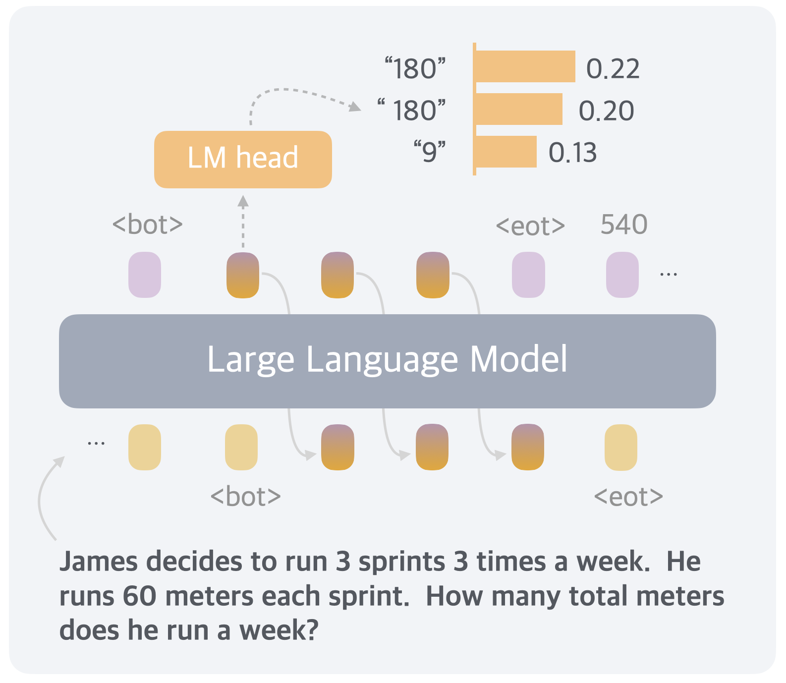- **Key Values**: - Sprints per session: `3` - Sessions per week: `3` - Meters per sprint: `60` - **Calculation**: </details> Figure 4: A case study where we decode the continuous thought into language tokens. With the multi-stage curriculum which decomposes the training into easier objectives, Coconut is able to achieve top performance across various tasks. The multi-stage training also integrates well with pause tokens (Coconut - pause as thought). Despite using the same architecture and similar multi-stage training objectives, we observed a small gap between the performance of iCoT and Coconut (w/o thoughts). The finer-grained removal schedule (token by token) and a few other tricks in iCoT may ease the training process. We leave combining iCoT and Coconut as future work. While the multi-stage training used for Coconut has proven effective, further research is definitely needed to develop better and more general strategies for learning reasoning in latent space, especially without the supervision from language reasoning chains. Continuous thoughts are efficient representations of reasoning. Though the continuous thoughts are not intended to be decoded to language tokens, we can still use it as an intuitive interpretation of the continuous thought. We show a case study in Figure 4 of a math word problem solved by Coconut ( $c=1$ ). The first continuous thought can be decoded into tokens like “180”, “ 180” (with a space), and “9”. Note that, the reasoning trace for this problem should be $3× 3× 60=9× 60=540$ , or $3× 3× 60=3× 180=540$ . The interpretations of the first thought happen to be the first intermediate variables in the calculation. Moreover, it encodes a distribution of different traces into the continuous thoughts. As shown in Section 5.3, this feature enables a more advanced reasoning pattern for planning-intense reasoning tasks. 5 Understanding the Latent Reasoning in Coconut In this section, we present an analysis of the latent reasoning process with a variant of Coconut. By leveraging its ability to switch between language and latent space reasoning, we are able to control the model to interpolate between fully latent reasoning and fully language reasoning and test their performance (Section 5.2). This also enables us to interpret the the latent reasoning process as tree search (Section 5.3). Based on this perspective, we explain why latent reasoning can make the decision easier for LLMs (Section 5.4). 5.1 Experimental Setup Methods. The design of Coconut allows us to control the number of latent thoughts by manually setting the position of the <eot> token during inference. When we enforce Coconut to use $k$ continuous thoughts, the model is expected to output the remaining reasoning chain in language, starting from the $k+1$ step. In our experiments, we test variants of Coconut on ProsQA with $k∈\{0,1,2,3,4,5,6\}$ . Note that all these variants only differ in inference time while sharing the same model weights. Besides, we report the performance of CoT and no-CoT as references. To address the issue of forgetting earlier training stages, we modify the original multi-stage training curriculum by always mixing data from other stages with a certain probability ( $p=0.3$ ). This updated training curriculum yields similar performance and enables effective control over the switch between latent and language reasoning. 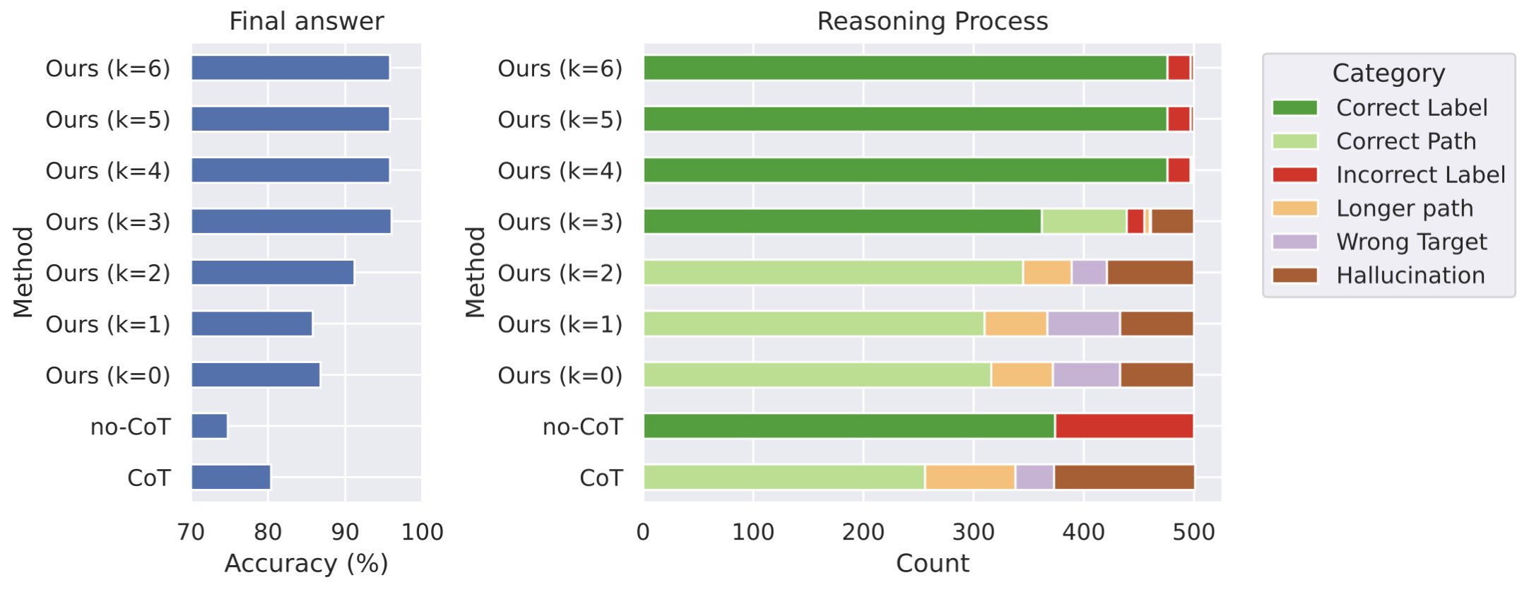Metrics. We apply two sets of evaluation metrics. One of them is based on the correctness of the final answer, regardless of the reasoning process. It is the metric used in the main experimental results above (Section 1). To enable fine-grained analysis, we define another metric on the reasoning process. Assuming we have a complete language reasoning chain which specifies a path in the graph, we can classify it into (1) Correct Path: The output is one of the shortest paths to the correct answer. (2) Longer Path: A valid path that correctly answers the question but is longer than the shortest path. (3) Hallucination: The path includes nonexistent edges or is disconnected. (4) Wrong Target: A valid path in the graph, but the destination node is not the one being asked. These four categories naturally apply to the output from Coconut ( $k=0$ ) and CoT, which generate the full path. For Coconut with $k>0$ that outputs only partial paths in language (with the initial steps in continuous reasoning), we classify the reasoning as a Correct Path if a valid explanation can complete it. Also, we define Longer Path and Wrong Target for partial paths similarly. If no valid explanation completes the path, it’s classified as hallucination. In no-CoT and Coconut with larger $k$ , the model may only output the final answer without any partial path, and it falls into (5) Correct Label or (6) Incorrect Label. These six categories cover all cases without overlap. <details> <summary>figures/figure_5_revised_1111.png Details</summary>  ### Visual Description # Technical Document Extraction: Bar Chart Analysis ## Image Description The image contains two horizontally aligned bar charts side-by-side, labeled **"Final answer"** (left) and **"Reasoning Process"** (right). Both charts use segmented bars with color-coded categories defined in a legend on the right. The y-axis lists methods, and the x-axis represents quantitative metrics. --- ### **Legend & Categories** The legend defines six categories with distinct colors: 1. **Correct Label** (Dark Green) 2. **Correct Path** (Light Green) 3. **Incorrect Label** (Red) 4. **Longer Path** (Orange) 5. **Wrong Target** (Purple) 6. **Hallucination** (Brown) --- ### **Left Chart: Final Answer** - **Y-Axis (Methods)**: - `Ours (k=6)` to `Ours (k=0)` (descending order) - `no-CoT` - `CoT` - **X-Axis (Accuracy %)**: - Range: 70% to 100% - Bars represent accuracy percentages for each method. #### **Key Trends**: 1. **Highest Accuracy**: - `Ours (k=6)`, `Ours (k=5)`, `Ours (k=4)`, and `Ours (k=3)` all achieve ~95% accuracy. 2. **Decline with Lower k**: - `Ours (k=2)` drops to ~90%, `Ours (k=1)` to ~85%, and `Ours (k=0)` to ~88%. 3. **Baseline Methods**: - `no-CoT` has the lowest accuracy (~75%). - `CoT` achieves ~80% accuracy. --- ### **Right Chart: Reasoning Process** - **Y-Axis (Methods)**: - Same methods as the left chart (`Ours (k=6)` to `CoT`). - **X-Axis (Count)**: - Range: 0 to 500 (total reasoning steps per method). - Bars are segmented by the legend categories. #### **Key Trends**: 1. **Dominant Category**: - **Correct Label** (Dark Green) dominates for all methods, especially `Ours (k=6)` (~480 counts). 2. **Error Categories**: - **Incorrect Label** (Red) and **Hallucination** (Brown) are minimal for high-k methods (`k=6` to `k=3`). - For lower-k methods (`k=2`, `k=1`, `k=0`), **Longer Path** (Orange) and **Wrong Target** (Purple) increase slightly. 3. **Baseline Methods**: - `no-CoT` has ~380 Correct Labels and ~120 Incorrect Labels. - `CoT` shows ~320 Correct Labels, ~80 Longer Path, and ~100 Hallucination. --- ### **Spatial Grounding & Color Verification** - **Legend Position**: Right side of both charts. - **Color Consistency**: - All segments in the right chart match the legend (e.g., Dark Green = Correct Label). - No mismatches observed between bar colors and legend labels. --- ### **Data Table Reconstruction** #### Left Chart (Accuracy %) | Method | Accuracy (%) | |--------------|--------------| | Ours (k=6) | ~95 | | Ours (k=5) | ~95 | | Ours (k=4) | ~95 | | Ours (k=3) | ~95 | | Ours (k=2) | ~90 | | Ours (k=1) | ~85 | | Ours (k=0) | ~88 | | no-CoT | ~75 | | CoT | ~80 | #### Right Chart (Reasoning Process Counts) | Method | Correct Label | Correct Path | Incorrect Label | Longer Path | Wrong Target | Hallucination | |--------------|---------------|--------------|-----------------|-------------|--------------|---------------| | Ours (k=6) | ~480 | ~20 | ~5 | 0 | 0 | 0 | | Ours (k=5) | ~480 | ~20 | ~5 | 0 | 0 | 0 | | Ours (k=4) | ~480 | ~20 | ~5 | 0 | 0 | 0 | | Ours (k=3) | ~350 | ~50 | ~5 | 0 | 0 | 10 | | Ours (k=2) | ~300 | ~50 | ~10 | 20 | 10 | 20 | | Ours (k=1) | ~300 | ~50 | ~15 | 25 | 15 | 25 | | Ours (k=0) | ~300 | ~50 | ~20 | 30 | 20 | 30 | | no-CoT | ~380 | 0 | ~120 | 0 | 0 | 0 | | CoT | ~320 | ~80 | 0 | 80 | 10 | 100 | --- ### **Final Notes** - The image does not provide exact numerical values; all data points are inferred from bar lengths. - Higher-k methods (`k=6` to `k=3`) consistently outperform lower-k and baseline methods in both accuracy and reasoning quality. - Errors (e.g., Incorrect Label, Hallucination) increase as k decreases, highlighting the trade-off between model complexity and performance. </details> Figure 5: The accuracy of final answer (left) and reasoning process (right) of multiple variants of Coconut and baselines on ProsQA. <details> <summary>figures/figure_6_meta_3.png Details</summary>  ### Visual Description # Technical Document Extraction ## Diagram Analysis ### Flowchart Structure - **Nodes**: - **Root Node**: "Alex" (Blue) - **Target Node**: "bompus" (Green) - **Distractive Nodes**: "gorpus", "rempus", "jelpus", "sam", "hilpus", "impus", "jompus", "brimpus", "scrompus", "yumpus", "lempus", "zhorpus", "gwompus", "gorpus", "yimpus", "lorpus", "jack" (Orange) - **Child of Root Node**: "sterpus", "grimpus" (Purple) - **Grandchild of Root Node**: "rorpus", "bompus", "boompus" (Orange) - **Arrows**: - Directed edges connect nodes to indicate hierarchical or relational relationships (e.g., "Alex → grimpus", "grimpus → rorpus", "rorpus → bompus"). ### Legend - **Color Coding**: - Blue: Root node - Green: Target node - Orange: Distractive node - Purple: Child of the root node - Orange (alternate): Grandchild of the root node ### Spatial Grounding - Legend located in the top-right quadrant of the image. - Node colors strictly adhere to legend definitions (e.g., "Alex" is blue, "bompus" is green). --- ## Textual Content ### Question Section **Question**: "Every grimpus is a yimpus. Every worpus is a jelpus. Every zhorpus is a sterpus. Alex is a grimpus. Every lumps is a yumpus. Question: Is Alex a gorpus or bompus?" ### Solutions #### Ground Truth Solution - **Statements**: 1. Alex is a grimpus. 2. Every grimpus is a rorpus. 3. Every rorpus is a bompus. 4. ### Alex is a bompus. #### CoT (Chain of Thought) - **CoT(k=1)**: - **Statements**: 1. Every lempus is a scrompus. 2. Every scrompus is a brimpus. 3. ### Alex is a brimpus ❌ (Wrong Target) - **Annotation**: (Wrong Target) - **CoT(k=2)**: - **Statements**: 1. Every rorpus is a bompus. 2. ### Alex is a bompus ✅ (Correct Path) - **Annotation**: (Correct Path) #### CoT (Hallucination) - **Statements**: 1. Every yumpus is a rempus. 2. Every rempus is a gorpus. 3. ### Alex is a gorpus ❌ (Hallucination) --- ## Key Trends and Data Points 1. **Flowchart Logic**: - Root node "Alex" branches into "grimpus" (child) and "rorpus" (grandchild). - "rorpus" directly connects to the target node "bompus". - Distractive nodes (e.g., "gorpus", "yumpus") form alternative paths but are not part of the correct solution. 2. **Solution Evaluation**: - **Correct Path**: CoT(k=2) aligns with the Ground Truth by following "grimpus → rorpus → bompus". - **Incorrect Paths**: - CoT(k=1) erroneously links "Alex" to "brimpus" via "lempus → scrompus". - CoT(k=2) hallucination incorrectly associates "Alex" with "gorpus" via "yumpus → rempus". --- ## Component Isolation ### Header - **Legend**: Defines node color semantics (Root, Target, Distractive, Child, Grandchild). ### Main Chart - **Flowchart**: Hierarchical relationships between nodes, with "Alex" as the root and "bompus" as the target. ### Footer - **Question and Solutions**: Logical reasoning steps and annotations for evaluation. --- ## Data Table Reconstruction | Node | Color | Relationship to Root | |------------|-----------|----------------------| | Alex | Blue | Root | | grimpus | Purple | Child | | rorpus | Orange | Grandchild | | bompus | Green | Target | | gorpus | Orange | Distractive | | yumpus | Orange | Distractive | --- ## Final Notes - All textual information extracted from the image is in English. - No non-English content detected. - Diagram and text are self-contained; no external context required. 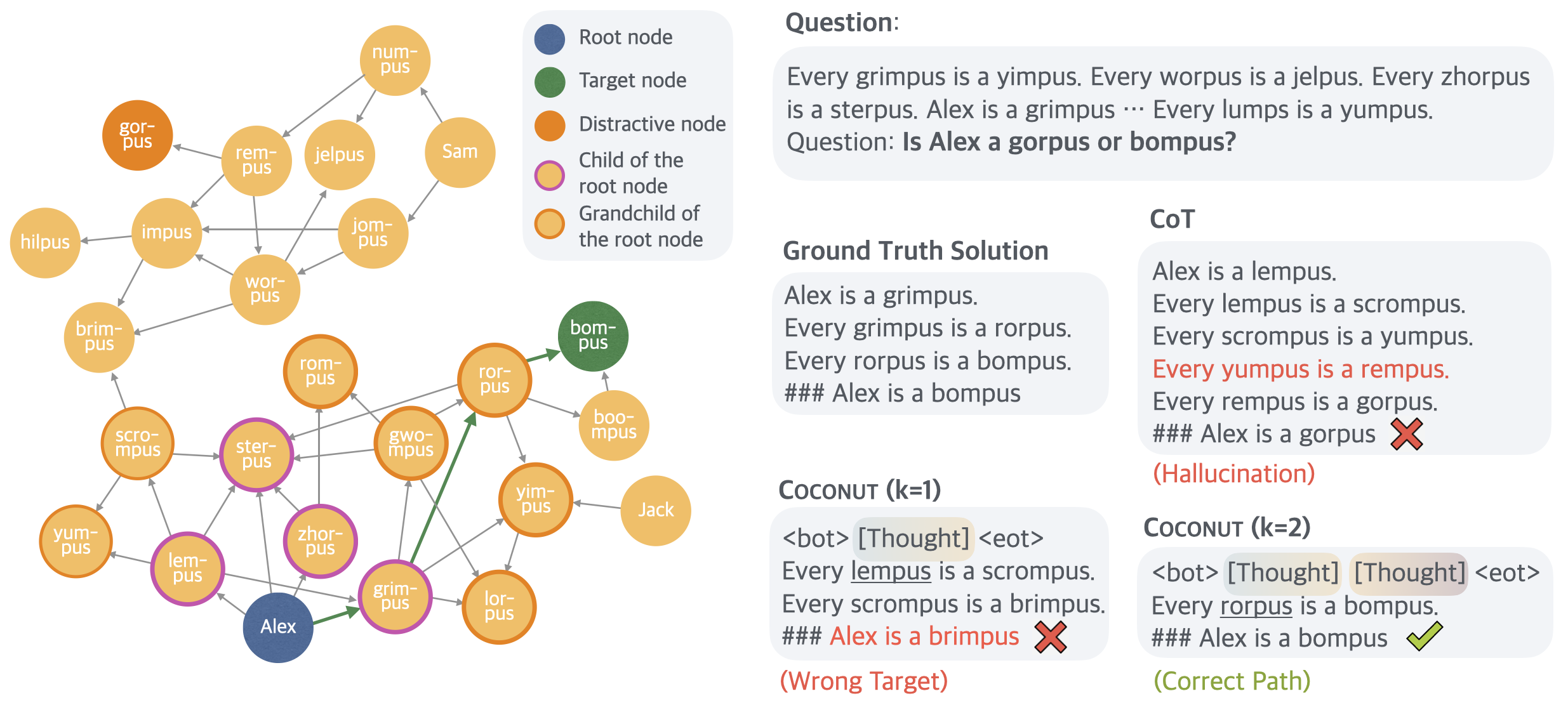</details> Figure 6: A case study of ProsQA. The model trained with CoT hallucinates an edge (Every yumpus is a rempus) after getting stuck in a dead end. Coconut (k=1) outputs a path that ends with an irrelevant node. Coconut (k=2) solves the problem correctly. <details> <summary>figures/figure_7_meta_4.png Details</summary>  ### Visual Description # Technical Document Analysis: "Coconut (k=1)" and "Coconut (k=2)" Processes ## Overview The image contains two comparative diagrams illustrating the "Coconut" process for two scenarios: **(k=1)** and **(k=2)**. Each diagram demonstrates probabilistic calculations for word decomposition, with connections between nodes and edge weights. Key elements include: - Central node labeled **"Alex"** - Colored nodes with labels (e.g., "sterpus," "lemplus," "rorpus") - Edge labels showing probabilities and heights (`h=0`, `h=1`, `h=2`) - Equations in gray boxes for calculating composite probabilities --- ## Diagram 1: **Coconut (k=1)** ### Structure - **Central Node**: "Alex" (blue) - **Connected Nodes**: - **Left Side**: - `sterpus` (purple): 0.01 (h=0) - `lemplus` (purple): 0.33 (h=2) - `zorpus` (purple): 0.16 (h=1) - `grimpus` (purple): 0.32 (h=2) - **Right Side**: - Equation in gray box: `p("lemplus") = p("le") * p("mp") * p("us") = 0.33` ### Key Observations 1. **Word Decomposition**: - "lemplus" is decomposed into substrings `le`, `mp`, and `us`, with probabilities multiplied to calculate the total (`0.33`). 2. **Edge Labels**: - Probabilities range from `0.01` (low confidence) to `0.33` (moderate confidence). 3. **Height Indicator**: - `h=0` to `h=2` likely represents hierarchical levels or confidence thresholds. --- ## Diagram 2: **Coconut (k=2)** ### Structure - **Central Node**: "Alex" (blue) - **Connected Nodes**: - **Left Side**: - `yimpus` (orange): 5e-5 (h=1) - `gwompus` (orange): 0.12 (h=1) - **Center**: - `grimpus` (orange): 0.12 (h=1) - **Right Side**: - `rorpus` (orange): 0.87 (h=1) - `scrompus` (orange): 2e-3 (h=1) - `rompus` (orange): 3e-3 (h=0) - `yumpus` (orange): 7e-4 (h=0) - Equation in gray box: `p("rorpus") = p("ro") * p("rp") * p("us") = 0.87` ### Key Observations 1. **Complex Decomposition**: - "rorpus" is decomposed into `ro`, `rp`, and `us`, yielding a high probability (`0.87`). 2. **Edge Labels**: - Probabilities span from `5e-5` (extremely low) to `0.87` (very high). 3. **Height Indicator**: - `h=0` and `h=1` suggest a simpler hierarchy compared to k=1. --- ## Cross-Diagram Comparison | Component | k=1 Diagram | k=2 Diagram | |----------------|----------------------|----------------------| | Central Node | Alex | Alex | | Primary Labels | sterpus, lemplus | rorpus, grimpus | | Highest Prob | 0.33 (lemplus) | 0.87 (rorpus) | | Edge Colors | Purple | Orange | | Equation Format| `p("word") = ...` | `p("word") = ...` | --- ## Critical Notes 1. **Color Coding**: - Purple in k=1 and orange in k=2 likely denote distinct word categories or confidence ranges. 2. **Mathematical Logic**: - Probabilities are calculated as products of substring probabilities (e.g., `p("lemplus") = p("le") * p("mp") * p("us")`). 3. **Spelling Variations**: - Words like "lemplus" and "rorpus" suggest intentional orthographic patterns for decomposition testing. --- ## Missing Information - No explicit axis titles, legends, or spatial legend coordinates (e.g., `[x, y]` for legend) are present. - No heatmap or chart-like visualization detected; diagrams rely on node-edge relationships and equations. --- ## Conclusion The diagrams model a probabilistic word decomposition system ("Coconut") where composite terms are broken into substrings, and their probabilities are combined multiplicatively. The two scenarios (k=1 vs. k=2) differ in complexity and color coding but share identical calculation logic. The system prioritizes high-probability decompositions (e.g., `rorpus` at 0.87 in k=2) while accounting for edge cases (e.g., `yumpus` at 7e-4). 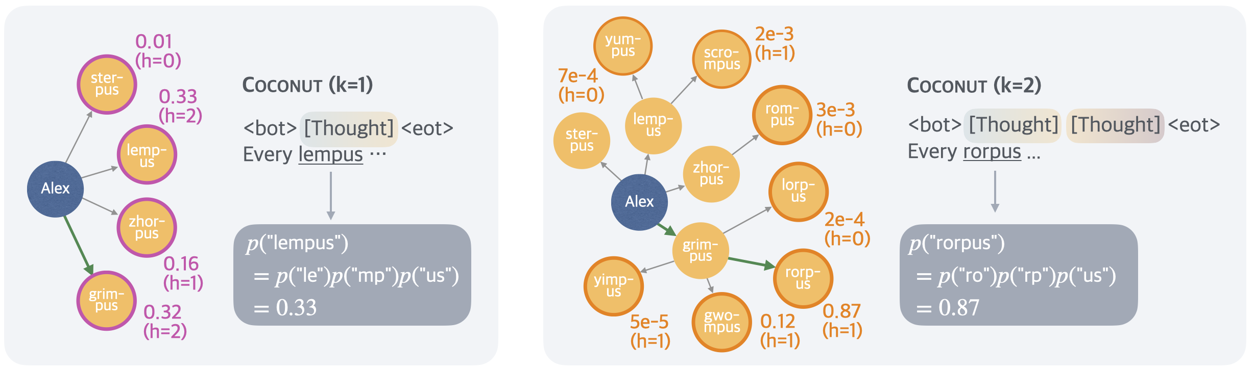</details> Figure 7: An illustration of the latent search trees. The example is the same test case as in Figure 7. The height of a node (denoted as $h$ in the figure) is defined as the longest distance to any leaf nodes in the graph. We show the probability of the first concept predicted by the model following latent thoughts (e.g., “lempus” in the left figure). It is calculated as the multiplication of the probability of all tokens within the concept conditioned on previous context (omitted in the figure for brevity). This metric can be interpreted as an implicit value function estimated by the model, assessing the potential of each node leading to the correct answer. 5.2 Interpolating between Latent and Language Reasoning Figure 5 shows a comparative analysis of different reasoning methods on ProsQA. As more reasoning is done with continuous thoughts (increasing $k$ ), both final answer accuracy (Figure 5, left) and the rate of correct reasoning processes (“Correct Label” and “Correct Path” in Figure 5, right) improve. Additionally, the rate of “Hallucination” and “Wrong Target” decrease, which typically occur when the model makes a wrong move earlier. This also indicates the better planning ability when more reasoning happens in the latent space. A case study is shown in Figure 7, where CoT hallucinates an nonexistent edge, Coconut ( $k=1$ ) leads to a wrong target, but Coconut ( $k=2$ ) successfully solves the problem. In this example, the model cannot accurately determine which edge to choose at the earlier step. However, as latent reasoning can avoid making a hard choice upfront, the model can progressively eliminate incorrect options in subsequent steps and achieves higher accuracy at the end of reasoning. We show more evidence and details of this reasoning process in Section 5.3. The comparison between CoT and Coconut ( $k=0$ ) reveals another interesting observation: even when Coconut is forced to generate a complete reasoning chain, the accuracy of the answers is still higher than CoT. The generated reasoning paths are also more accurate with less hallucination. From this, we can infer that the training method of mixing different stages improves the model’s ability to plan ahead. The training objective of CoT always concentrates on the generation of the immediate next step, making the model “shortsighted”. In later stages of Coconut training, the first few steps are hidden, allowing the model to focus more on future steps. This is related to the findings of Gloeckle et al. (2024), where they propose multi-token prediction as a new pretraining objective to improve the LLM’s ability to plan ahead. 5.3 Interpreting the Latent Search Tree Given the intuition that continuous thoughts can encode multiple potential next steps, the latent reasoning can be interpreted as a search tree, rather than merely a reasoning “chain”. Taking the case of Figure 7 as a concrete example, the first step could be selecting one of the children of Alex, i.e., {lempus, sterpus, zhorpus, grimpus}. We depict all possible branches in the left part of Figure 7. Similarly, in the second step, the frontier nodes will be the grandchildren of Alex (Figure 7, right). Unlike a standard breadth-first search (BFS), which explores all frontier nodes uniformly, the model demonstrates the ability to prioritize promising nodes while pruning less relevant ones. To uncover the model’s preferences, we analyze its subsequent outputs in language space. For instance, if the model is forced to switch back to language space after a single latent thought ( $k=1$ ), it predicts the next step in a structured format, such as “every [Concept A] is a [Concept B].” By examining the probability distribution over potential fillers for [Concept A], we can derive numeric values for the children of the root node Alex (Figure 7, left). Similarly, when $k=2$ , the prediction probabilities for all frontier nodes—the grandchildren of Alex —are obtained (Figure 7, right). <details> <summary>figures/percentile.png Details</summary>  ### Visual Description # Technical Document Extraction: Line Graph Analysis ## Image Overview The image contains **two side-by-side line graphs** titled "First thoughts" (left) and "Second thoughts" (right). Both graphs share identical axes and legend structures but differ in line curvature and data point distribution. --- ### **1. Axis Labels and Markers** - **X-axis**: - Title: `Percentile` - Range: `0.0` to `1.0` (increments of `0.2`) - Markers: Gridlines at every `0.2` interval - **Y-axis**: - Title: `Value` - Range: `0.0` to `1.0` (increments of `0.2`) - Markers: Gridlines at every `0.2` interval --- ### **2. Legend** - **Placement**: Bottom-left corner of each graph - **Labels and Colors**: - `Top 1`: Darkest blue (`#003f5c`) - `Top 2`: Medium blue (`#2f4b7c`) - `Top 3`: Lightest blue (`#665191`) - **Note**: Colors match the corresponding lines in both graphs. --- ### **3. Line Graph Components** #### **Left Graph: "First thoughts"** - **Lines**: - `Top 1`: Steepest upward curve, reaching ~0.95 at `Percentile = 1.0` - `Top 2`: Moderate upward curve, reaching ~0.85 at `Percentile = 1.0` - `Top 3`: Gentle upward curve, reaching ~0.75 at `Percentile = 1.0` - **Trend**: All lines originate at `(0, 0)` and ascend monotonically. `Top 1` dominates the upper region, while `Top 3` remains closest to the baseline. #### **Right Graph: "Second thoughts"** - **Lines**: - `Top 1`: Slightly less steep than left graph, reaching ~0.90 at `Percentile = 1.0` - `Top 2`: Similar to left graph, reaching ~0.80 at `Percentile = 1.0` - `Top 3`: Flatter curve, reaching ~0.65 at `Percentile = 1.0` - **Trend**: Lines exhibit reduced separation compared to the left graph. `Top 1` and `Top 2` converge more closely near `Percentile = 1.0`. --- ### **4. Key Observations** - **Consistency**: Both graphs share identical axis ranges and legend structure. - **Divergence**: - "Second thoughts" lines are generally lower in value than "First thoughts" at equivalent percentiles. - `Top 3` shows the most significant reduction in value between the two graphs. - **No Embedded Text**: No additional annotations or data tables are present. --- ### **5. Spatial Grounding** - **Legend Position**: `[x=0.05, y=0.05]` relative to each graph’s bottom-left corner. - **Line Placement**: - `Top 1` consistently occupies the uppermost region. - `Top 3` remains closest to the baseline across all percentiles. --- ### **6. Trend Verification** - **Left Graph ("First thoughts")**: - `Top 1`: Steep upward slope (highest value gain). - `Top 2`: Moderate upward slope. - `Top 3`: Gentle upward slope. - **Right Graph ("Second thoughts")**: - All lines exhibit reduced steepness compared to the left graph. - `Top 1` and `Top 2` converge near `Percentile = 1.0`. --- ### **7. Component Isolation** - **Header**: Titles "First thoughts" and "Second thoughts" in bold black text. - **Main Chart**: Dual-axis line graphs with gridlines and shaded regions. - **Footer**: Legend box with color-coded labels. --- ### **8. Data Extraction** No explicit numerical data points are labeled. Values are inferred from line positions relative to gridlines: - **Example (Left Graph)**: - At `Percentile = 0.5`: - `Top 1`: ~0.7 - `Top 2`: ~0.6 - `Top 3`: ~0.5 --- ### **9. Language and Translation** - **Primary Language**: English - **No Additional Languages Detected** --- ### **10. Final Notes** - The graphs likely represent cumulative distribution functions or percentile-based value rankings. - The shaded regions between lines suggest confidence intervals or value ranges, though this is not explicitly labeled. 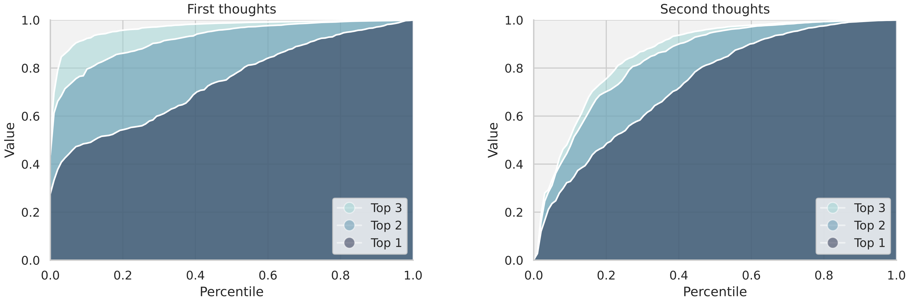</details> Figure 8: Analysis of parallelism in latent tree search. The left plot depicts the cumulative value of the top-1, top-2, and top-3 candidate nodes for the first thoughts, calculated across test cases and ranked by percentile. The significant gaps between the lines reflect the model’s ability to explore alternative latent thoughts in parallel. The right plot shows the corresponding analysis for the second thoughts, where the gaps between lines are narrower, indicating reduced parallelism and increased certainty in reasoning as the search tree develops. This shift highlights the model’s transition toward more focused exploration in later stages. The probability distribution can be viewed as the model’s implicit value function, estimating each node’s potential to reach the target. As shown in the figure, “lempus”, “zhorpus”, “grimpus”, and “sterpus” have a value of 0.33, 0.16, 0.32, and 0.01, respectively. This indicates that in the first continuous thought, the model has mostly ruled out “sterpus” as an option but remains uncertain about the correct choice among the other three. In the second thought, however, the model has mostly ruled out other options but focused on “rorpus”. Figure 8 presents an analysis of the parallelism in the model’s latent reasoning across the first and second thoughts. For the first thoughts (left panel), the cumulative values of the top-1, top-2, and top-3 candidate nodes are computed and plotted against their respective percentiles across the test set. The noticeable gaps between the three lines indicate that the model maintains significant diversity in its reasoning paths at this stage, suggesting a broad exploration of alternative possibilities. In contrast, the second thoughts (right panel) show a narrowing of these gaps. This trend suggests that the model transitions from parallel exploration to more focused reasoning in the second latent reasoning step, likely as it gains more certainty about the most promising paths. 5.4 Why is a Latent Space Better for Planning? <details> <summary>figures/value_stats_meta_2.png Details</summary>  ### Visual Description # Technical Document Extraction: Line Chart Analysis ## Chart Overview The image contains two line charts titled **"First thoughts"** (top) and **"Second thoughts"** (bottom). Both charts share identical axis labels and legend structure but differ in data trends. --- ### **First thoughts** Chart #### Components - **X-axis**: Labeled **"Height"**, with integer markers from 0 to 6. - **Y-axis**: Labeled **"Value"**, with decimal markers from 0.0 to 0.6 in increments of 0.1. - **Legend**: Located in the **top-left corner**, with two entries: - **Blue line**: "Correct" (solid line). - **Orange line**: "Incorrect" (dashed line). - **Shaded Regions**: Confidence intervals (light blue for "Correct," light orange for "Incorrect"). #### Data Trends 1. **Correct (Blue Line)**: - Starts at **0.5** when Height = 0. - Peaks at **0.55** at Height = 5. - Declines to **0.45** at Height = 6. - **Trend**: Initial rise, plateau, then gradual decline. 2. **Incorrect (Orange Line)**: - Starts at **0.0** when Height = 0. - Rises to **0.3** at Height = 5. - Declines to **0.25** at Height = 6. - **Trend**: Steady increase followed by a sharp drop. #### Spatial Grounding - Legend position: **[x=0.05, y=0.95]** (normalized coordinates). - Blue line consistently above orange line until Height = 5, where they intersect. --- ### **Second thoughts** Chart #### Components - **X-axis**: Labeled **"Height"**, with integer markers from 0 to 5. - **Y-axis**: Labeled **"Value"**, with decimal markers from 0.0 to 0.6 in increments of 0.1. - **Legend**: Located in the **top-left corner**, with two entries: - **Blue line**: "Correct" (solid line). - **Orange line**: "Incorrect" (dashed line). - **Shaded Regions**: Confidence intervals (light blue for "Correct," light orange for "Incorrect"). #### Data Trends 1. **Correct (Blue Line)**: - Starts at **0.5** when Height = 1. - Peaks at **0.55** at Height = 2. - Declines to **0.25** at Height = 5. - **Trend**: Early peak followed by a steep drop. 2. **Incorrect (Orange Line)**: - Starts at **0.0** when Height = 0. - Rises to **0.15** at Height = 4. - Declines to **0.1** at Height = 5. - **Trend**: Gradual increase followed by a decline. #### Spatial Grounding - Legend position: **[x=0.05, y=0.95]** (normalized coordinates). - Blue line dominates early, while orange line gains prominence after Height = 3. --- ### Key Observations 1. **First thoughts**: - "Correct" responses show higher initial confidence (Value ~0.5) but decline over time. - "Incorrect" responses gain traction (Value ~0.3) but drop sharply at Height = 6. 2. **Second thoughts**: - "Correct" responses peak early (Height = 2) and then plummet. - "Incorrect" responses show delayed growth (Height = 4) before declining. 3. **Confidence Intervals**: - Shaded regions indicate variability in responses, with wider intervals for "Correct" in the first chart and "Incorrect" in the second. --- ### Data Table Reconstruction #### First thoughts | Height | Correct Value | Incorrect Value | |--------|---------------|-----------------| | 0 | 0.5 | 0.0 | | 1 | 0.5 | 0.2 | | 2 | 0.52 | 0.25 | | 3 | 0.55 | 0.3 | | 4 | 0.55 | 0.35 | | 5 | 0.55 | 0.3 | | 6 | 0.45 | 0.25 | #### Second thoughts | Height | Correct Value | Incorrect Value | |--------|---------------|-----------------| | 0 | 0.0 | 0.0 | | 1 | 0.5 | 0.1 | | 2 | 0.55 | 0.12 | | 3 | 0.5 | 0.15 | | 4 | 0.45 | 0.18 | | 5 | 0.25 | 0.1 | --- ### Notes - All values are approximate, derived from visual inspection of line intersections with gridlines. - No textual data beyond axis labels, legend, and chart titles is present. - No non-English text detected. 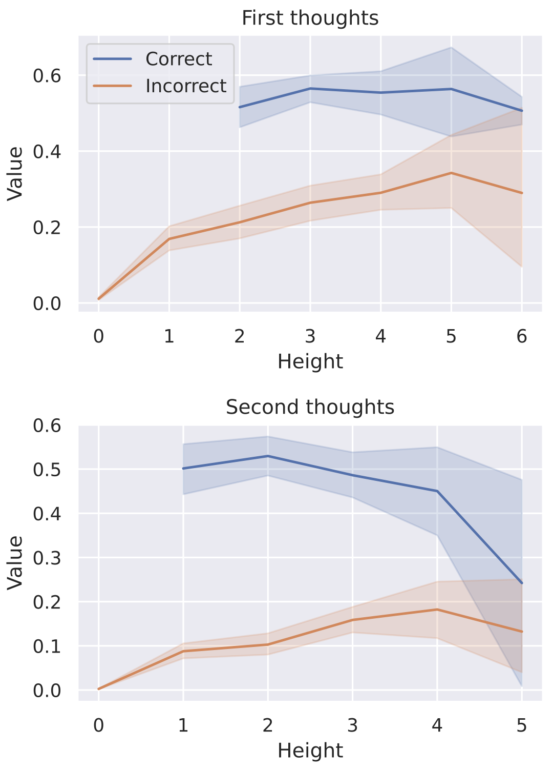</details> Figure 9: The correlation between prediction probability of concepts and their heights. In this section, we explore why latent reasoning is advantageous for planning, drawing on the search tree perspective and the value function defined earlier. Referring to our illustrative example, a key distinction between “sterpus” and the other three options lies in the structure of the search tree: “sterpus” is a leaf node (Figure 7). This makes it immediately identifiable as an incorrect choice, as it cannot lead to the target node “bompus”. In contrast, the other nodes have more descendants to explore, making their evaluation more challenging. To quantify a node’s exploratory potential, we measure its height in the tree, defined as the shortest distance to any leaf node. Based on this notion, we hypothesize that nodes with lower heights are easier to evaluate accurately, as their exploratory potential is limited. Consistent with this hypothesis, in our example, the model exhibits greater uncertainty between “grimpus” and “lempus”, both of which have a height of 2—higher than the other candidates. To test this hypothesis more rigorously, we analyze the correlation between the model’s prediction probabilities and node heights during the first and second latent reasoning steps across the test set. Figure 9 reveals a clear pattern: the model successfully assigns lower values to incorrect nodes and higher values to correct nodes when their heights are low. However, as node heights increase, this distinction becomes less pronounced, indicating greater difficulty in accurate evaluation. In conclusion, these findings highlight the benefits of leveraging latent space for planning. By delaying definite decisions and expanding the latent reasoning process, the model pushes its exploration closer to the search tree’s terminal states, making it easier to distinguish correct nodes from incorrect ones. 6 Conclusion In this paper, we presented Coconut, a novel paradigm for reasoning in continuous latent space. Through extensive experiments, we demonstrated that Coconut significantly enhances LLM reasoning capabilities. Notably, our detailed analysis highlighted how an unconstrained latent space allows the model to develop an effective reasoning pattern similar to BFS. Future work is needed to further refine and scale latent reasoning methods. One promising direction is pretraining LLMs with continuous thoughts, which may enable models to generalize more effectively across a wider range of reasoning scenarios. We anticipate that our findings will inspire further research into latent reasoning methods, ultimately contributing to the development of more advanced machine reasoning systems. Acknowledgement The authors express their sincere gratitude to Jihoon Tack for his valuable discussions throughout the course of this work. References - Achiam et al. (2023) Josh Achiam, Steven Adler, Sandhini Agarwal, Lama Ahmad, Ilge Akkaya, Florencia Leoni Aleman, Diogo Almeida, Janko Altenschmidt, Sam Altman, Shyamal Anadkat, et al. Gpt-4 technical report. arXiv preprint arXiv:2303.08774, 2023. - Amalric and Dehaene (2019) Marie Amalric and Stanislas Dehaene. A distinct cortical network for mathematical knowledge in the human brain. NeuroImage, 189:19–31, 2019. - Biran et al. (2024) Eden Biran, Daniela Gottesman, Sohee Yang, Mor Geva, and Amir Globerson. Hopping too late: Exploring the limitations of large language models on multi-hop queries. arXiv preprint arXiv:2406.12775, 2024. - Chen et al. (2023) Wenhu Chen, Ming Yin, Max Ku, Pan Lu, Yixin Wan, Xueguang Ma, Jianyu Xu, Xinyi Wang, and Tony Xia. Theoremqa: A theorem-driven question answering dataset. In Proceedings of the 2023 Conference on Empirical Methods in Natural Language Processing, pages 7889–7901, 2023. - Cobbe et al. (2021) Karl Cobbe, Vineet Kosaraju, Mohammad Bavarian, Mark Chen, Heewoo Jun, Lukasz Kaiser, Matthias Plappert, Jerry Tworek, Jacob Hilton, Reiichiro Nakano, et al. Training verifiers to solve math word problems. arXiv preprint arXiv:2110.14168, 2021. - DeepMind (2024) Google DeepMind. Ai achieves silver-medal standard solving international mathematical olympiad problems, 2024. https://deepmind.google/discover/blog/ai-solves-imo-problems-at-silver-medal-level/. - Deng et al. (2023) Yuntian Deng, Kiran Prasad, Roland Fernandez, Paul Smolensky, Vishrav Chaudhary, and Stuart Shieber. Implicit chain of thought reasoning via knowledge distillation. arXiv preprint arXiv:2311.01460, 2023. - Deng et al. (2024) Yuntian Deng, Yejin Choi, and Stuart Shieber. From explicit cot to implicit cot: Learning to internalize cot step by step. arXiv preprint arXiv:2405.14838, 2024. - Dubey et al. (2024) Abhimanyu Dubey, Abhinav Jauhri, Abhinav Pandey, Abhishek Kadian, Ahmad Al-Dahle, Aiesha Letman, Akhil Mathur, Alan Schelten, Amy Yang, Angela Fan, et al. The llama 3 herd of models. arXiv preprint arXiv:2407.21783, 2024. - Fan et al. (2024) Ying Fan, Yilun Du, Kannan Ramchandran, and Kangwook Lee. Looped transformers for length generalization. arXiv preprint arXiv:2409.15647, 2024. - Fedorenko et al. (2011) Evelina Fedorenko, Michael K Behr, and Nancy Kanwisher. Functional specificity for high-level linguistic processing in the human brain. Proceedings of the National Academy of Sciences, 108(39):16428–16433, 2011. - Fedorenko et al. (2024) Evelina Fedorenko, Steven T Piantadosi, and Edward AF Gibson. Language is primarily a tool for communication rather than thought. Nature, 630(8017):575–586, 2024. - Feng et al. (2023) Guhao Feng, Bohang Zhang, Yuntian Gu, Haotian Ye, Di He, and Liwei Wang. Towards revealing the mystery behind chain of thought: a theoretical perspective. Advances in Neural Information Processing Systems, 36, 2023. - Gandhi et al. (2024) Kanishk Gandhi, Denise Lee, Gabriel Grand, Muxin Liu, Winson Cheng, Archit Sharma, and Noah D Goodman. Stream of search (sos): Learning to search in language. arXiv preprint arXiv:2404.03683, 2024. - Giannou et al. (2023) Angeliki Giannou, Shashank Rajput, Jy-yong Sohn, Kangwook Lee, Jason D Lee, and Dimitris Papailiopoulos. Looped transformers as programmable computers. In International Conference on Machine Learning, pages 11398–11442. PMLR, 2023. - Gloeckle et al. (2024) Fabian Gloeckle, Badr Youbi Idrissi, Baptiste Rozière, David Lopez-Paz, and Gabriel Synnaeve. Better & faster large language models via multi-token prediction. arXiv preprint arXiv:2404.19737, 2024. - Goyal et al. (2023) Sachin Goyal, Ziwei Ji, Ankit Singh Rawat, Aditya Krishna Menon, Sanjiv Kumar, and Vaishnavh Nagarajan. Think before you speak: Training language models with pause tokens. arXiv preprint arXiv:2310.02226, 2023. - Hao et al. (2023) Shibo Hao, Yi Gu, Haodi Ma, Joshua Jiahua Hong, Zhen Wang, Daisy Zhe Wang, and Zhiting Hu. Reasoning with language model is planning with world model. arXiv preprint arXiv:2305.14992, 2023. - Hao et al. (2024) Shibo Hao, Yi Gu, Haotian Luo, Tianyang Liu, Xiyan Shao, Xinyuan Wang, Shuhua Xie, Haodi Ma, Adithya Samavedhi, Qiyue Gao, et al. Llm reasoners: New evaluation, library, and analysis of step-by-step reasoning with large language models. arXiv preprint arXiv:2404.05221, 2024. - Havrilla et al. (2024) Alex Havrilla, Yuqing Du, Sharath Chandra Raparthy, Christoforos Nalmpantis, Jane Dwivedi-Yu, Maksym Zhuravinskyi, Eric Hambro, Sainbayar Sukhbaatar, and Roberta Raileanu. Teaching large language models to reason with reinforcement learning. arXiv preprint arXiv:2403.04642, 2024. - Khot et al. (2022) Tushar Khot, Harsh Trivedi, Matthew Finlayson, Yao Fu, Kyle Richardson, Peter Clark, and Ashish Sabharwal. Decomposed prompting: A modular approach for solving complex tasks. arXiv preprint arXiv:2210.02406, 2022. - LeCun (2022) Yann LeCun. A path towards autonomous machine intelligence version 0.9. 2, 2022-06-27. Open Review, 62(1):1–62, 2022. - Lehnert et al. (2024) Lucas Lehnert, Sainbayar Sukhbaatar, Paul Mcvay, Michael Rabbat, and Yuandong Tian. Beyond a*: Better planning with transformers via search dynamics bootstrapping. arXiv preprint arXiv:2402.14083, 2024. - Li et al. (2024) Zhiyuan Li, Hong Liu, Denny Zhou, and Tengyu Ma. Chain of thought empowers transformers to solve inherently serial problems. arXiv preprint arXiv:2402.12875, 2024. - Madaan and Yazdanbakhsh (2022) Aman Madaan and Amir Yazdanbakhsh. Text and patterns: For effective chain of thought, it takes two to tango. arXiv preprint arXiv:2209.07686, 2022. - Merrill and Sabharwal (2023) William Merrill and Ashish Sabharwal. The expresssive power of transformers with chain of thought. arXiv preprint arXiv:2310.07923, 2023. - Monti et al. (2007) Martin M Monti, Daniel N Osherson, Michael J Martinez, and Lawrence M Parsons. Functional neuroanatomy of deductive inference: a language-independent distributed network. Neuroimage, 37(3):1005–1016, 2007. - Monti et al. (2009) Martin M Monti, Lawrence M Parsons, and Daniel N Osherson. The boundaries of language and thought in deductive inference. Proceedings of the National Academy of Sciences, 106(30):12554–12559, 2009. - Monti et al. (2012) Martin M Monti, Lawrence M Parsons, and Daniel N Osherson. Thought beyond language: neural dissociation of algebra and natural language. Psychological science, 23(8):914–922, 2012. - Pfau et al. (2024) Jacob Pfau, William Merrill, and Samuel R Bowman. Let’s think dot by dot: Hidden computation in transformer language models. arXiv preprint arXiv:2404.15758, 2024. - Radford et al. (2019) Alec Radford, Jeffrey Wu, Rewon Child, David Luan, Dario Amodei, Ilya Sutskever, et al. Language models are unsupervised multitask learners. OpenAI blog, 1(8):9, 2019. - Saparov and He (2022) Abulhair Saparov and He He. Language models are greedy reasoners: A systematic formal analysis of chain-of-thought. arXiv preprint arXiv:2210.01240, 2022. - Shalev et al. (2024) Yuval Shalev, Amir Feder, and Ariel Goldstein. Distributional reasoning in llms: Parallel reasoning processes in multi-hop reasoning. arXiv preprint arXiv:2406.13858, 2024. - Shao et al. (2024) Zhihong Shao, Peiyi Wang, Qihao Zhu, Runxin Xu, Junxiao Song, Mingchuan Zhang, YK Li, Yu Wu, and Daya Guo. Deepseekmath: Pushing the limits of mathematical reasoning in open language models. arXiv preprint arXiv:2402.03300, 2024. - Su et al. (2024) DiJia Su, Sainbayar Sukhbaatar, Michael Rabbat, Yuandong Tian, and Qinqing Zheng. Dualformer: Controllable fast and slow thinking by learning with randomized reasoning traces. arXiv preprint arXiv:2410.09918, 2024. - Turpin et al. (2024) Miles Turpin, Julian Michael, Ethan Perez, and Samuel Bowman. Language models don’t always say what they think: unfaithful explanations in chain-of-thought prompting. Advances in Neural Information Processing Systems, 36, 2024. - Wang et al. (2022) Boshi Wang, Sewon Min, Xiang Deng, Jiaming Shen, You Wu, Luke Zettlemoyer, and Huan Sun. Towards understanding chain-of-thought prompting: An empirical study of what matters. arXiv preprint arXiv:2212.10001, 2022. - Wang et al. (2024) Peiyi Wang, Lei Li, Zhihong Shao, Runxin Xu, Damai Dai, Yifei Li, Deli Chen, Yu Wu, and Zhifang Sui. Math-shepherd: Verify and reinforce llms step-by-step without human annotations. In Proceedings of the 62nd Annual Meeting of the Association for Computational Linguistics (Volume 1: Long Papers), pages 9426–9439, 2024. - Wang et al. (2023) Xinyi Wang, Lucas Caccia, Oleksiy Ostapenko, Xingdi Yuan, William Yang Wang, and Alessandro Sordoni. Guiding language model reasoning with planning tokens. arXiv preprint arXiv:2310.05707, 2023. - Wei et al. (2022) Jason Wei, Xuezhi Wang, Dale Schuurmans, Maarten Bosma, Fei Xia, Ed Chi, Quoc V Le, Denny Zhou, et al. Chain-of-thought prompting elicits reasoning in large language models. Advances in neural information processing systems, 35:24824–24837, 2022. - Xie et al. (2023) Yuxi Xie, Kenji Kawaguchi, Yiran Zhao, James Xu Zhao, Min-Yen Kan, Junxian He, and Michael Xie. Self-evaluation guided beam search for reasoning. Advances in Neural Information Processing Systems, 36, 2023. - Yang et al. (2024) Sohee Yang, Elena Gribovskaya, Nora Kassner, Mor Geva, and Sebastian Riedel. Do large language models latently perform multi-hop reasoning? arXiv preprint arXiv:2402.16837, 2024. - Yao et al. (2023) Shunyu Yao, Dian Yu, Jeffrey Zhao, Izhak Shafran, Tom Griffiths, Yuan Cao, and Karthik Narasimhan. Tree of thoughts: Deliberate problem solving with large language models. Advances in Neural Information Processing Systems, 36, 2023. - Yu et al. (2024a) Fangxu Yu, Lai Jiang, Haoqiang Kang, Shibo Hao, and Lianhui Qin. Flow of reasoning: Efficient training of llm policy with divergent thinking. arXiv preprint arXiv:2406.05673, 2024a. - Yu et al. (2023) Longhui Yu, Weisen Jiang, Han Shi, Jincheng Yu, Zhengying Liu, Yu Zhang, James T Kwok, Zhenguo Li, Adrian Weller, and Weiyang Liu. Metamath: Bootstrap your own mathematical questions for large language models. arXiv preprint arXiv:2309.12284, 2023. - Yu et al. (2024b) Ping Yu, Jing Xu, Jason Weston, and Ilia Kulikov. Distilling system 2 into system 1. arXiv preprint arXiv:2407.06023, 2024b. - Yue et al. (2023) Xiang Yue, Xingwei Qu, Ge Zhang, Yao Fu, Wenhao Huang, Huan Sun, Yu Su, and Wenhu Chen. Mammoth: Building math generalist models through hybrid instruction tuning. arXiv preprint arXiv:2309.05653, 2023. - Zelikman et al. (2024) Eric Zelikman, Georges Harik, Yijia Shao, Varuna Jayasiri, Nick Haber, and Noah D Goodman. Quiet-star: Language models can teach themselves to think before speaking. arXiv preprint arXiv:2403.09629, 2024. - Zhou et al. (2022) Denny Zhou, Nathanael Schärli, Le Hou, Jason Wei, Nathan Scales, Xuezhi Wang, Dale Schuurmans, Claire Cui, Olivier Bousquet, Quoc Le, et al. Least-to-most prompting enables complex reasoning in large language models. arXiv preprint arXiv:2205.10625, 2022. \beginappendix 7 Datasets 7.1 Examples We provide some examples of the questions and CoT solutions for the datasets used in our experiments. GSM8k Question = "John cuts his grass to 2 inches. It grows .5 inches per month. When it gets to 4 inches he cuts it back down to 2 inches. It cost $100 to get his grass cut. How much does he pay per year?" Steps = ["<<4-2=2>>", "<<2/.5=4>>", "<<12/4=3>>", "<<100*3=300>>"] Answer = "300" ProntoQA Question = "Brimpuses are not luminous. Shumpuses are amenable. Each yumpus is a lorpus. Gorpuses are shumpuses. Each zumpus is a grimpus. Gorpuses are rompuses. Dumpuses are not floral. Lempuses are cold. Brimpuses are impuses. Every lorpus is floral. Every rompus is transparent. Grimpuses are muffled. Rompuses are yumpuses. Rompuses are wumpuses. Zumpuses are fast. Wumpuses are bitter. Every sterpus is orange. Each lorpus is a vumpus. Yumpuses are feisty. Each yumpus is a lempus. Gorpuses are snowy. Zumpuses are gorpuses. Every lorpus is a sterpus. Stella is a brimpus. Stella is a zumpus. True or false: Stella is not floral." Steps = ["Stella is a zumpus. Zumpuses are gorpuses.", "Stella is a gorpus. Gorpuses are rompuses.", "Stella is a rompus. Rompuses are yumpuses.", "Stella is a yumpus. Each yumpus is a lorpus.", "Stella is a lorpus. Every lorpus is floral.", "Stella is floral."] Answer = "False" ProsQA Question = "Every shumpus is a rempus. Every shumpus is a yimpus. Every terpus is a fompus. Every terpus is a gerpus. Every gerpus is a brimpus. Alex is a rempus. Every rorpus is a scrompus. Every rorpus is a yimpus. Every terpus is a brimpus. Every brimpus is a lempus. Tom is a terpus. Every shumpus is a timpus. Every yimpus is a boompus. Davis is a shumpus. Every gerpus is a lorpus. Davis is a fompus. Every shumpus is a boompus. Every shumpus is a rorpus. Every terpus is a lorpus. Every boompus is a timpus. Every fompus is a yerpus. Tom is a dumpus. Every rempus is a rorpus. Is Tom a lempus or scrompus?" Steps = ["Tom is a terpus.", "Every terpus is a brimpus.", "Every brimpus is a lempus."] Answer = "Tom is a lempus." 7.2 Construction of ProsQA To construct the dataset, we first compile a set of typical entity names, such as “Alex” and “Jack,” along with fictional concept names like “lorpus” and “rorpus,” following the setting of ProntoQA (Saparov and He, 2022). Each problem is structured as a binary question: “Is [Entity] a [Concept A] or [Concept B]?” Assuming [Concept A] is the correct answer, we build a directed acyclic graph (DAG) where each node represents an entity or a concept. The graph is constructed such that a path exists from [Entity] to [Concept A] but not to [Concept B]. Algorithm 1 describes the graph construction process. The DAG is incrementally built by adding nodes and randomly connecting them with edges. To preserve the validity of the binary choice, with some probability, we enforce that the new node cannot simultaneously serve as a descendant to both node $0$ and $1$ . This separation maintains distinct families of nodes and balances their sizes to prevent model shortcuts. After the graph is constructed, nodes without parents are assigned entity names, while other nodes receive concept names. To formulate a question of the form “Is [Entity] a [Concept A] or [Concept B]?”, we designate node $0$ in the graph as [Entity], a leaf node labeled $1$ as [Concept A], and a leaf node labeled $2$ as [Concept B]. This setup ensures a path from [Entity] to [Concept A] without any connection to [Concept B], introducing a moderately complex reasoning path. Finally, to avoid positional biases, [Concept A] and [Concept B] are randomly permuted in each question. Algorithm 1 Graph Construction for ProsQA $edges←\{\}$ $nodes←\{0,1\}$ $labels←\{0:1,1:2\}$ $\triangleright$ Labels: 1 (descendant of node 0), 2 (descendant of node 1), 3 (both), 0 (neither). $groups←\{0:\{\},1:\{0\},2:\{1\},3:\{\}\}$ $idx← 2$ while $idx<N$ do $\triangleright$ For each new node, randomly add edges from existing nodes $n\_in\_nodes←\text{poisson}(1.5)$ $rand←\text{random}()$ if $rand≤ 0.35$ then $candidates← groups[0]\cup groups[1]$ $\triangleright$ Cannot be a descendant of node 1. else if $rand≤ 0.7$ then $candidates← groups[0]\cup groups[2]$ $\triangleright$ Cannot be a descendant of node 0. else $candidates← nodes$ end if $n\_in\_nodes←\min(\text{len}(candidates),n\_in\_nodes)$ $weights←[\text{depth\_to\_root}(c)· 1.5+1\;∀ c∈ candidates]$ $\triangleright$ Define sampling weights to prioritize deeper nodes. $\triangleright$ This way, the solution reasoning chain is expected to be longer. $in\_nodes←\text{random\_choice}(candidates,n\_in\_nodes,\text{prob}=weights/\text{sum}(weights))$ $cur\_label← 0$ for $in\_idx∈ in\_nodes$ do $cur\_label← cur\_label\mid labels[in\_idx]$ $\triangleright$ Update label using bitwise OR. $edges.\text{append}((in\_idx,idx))$ end for $groups[cur\_label].\text{append}(idx)$ $labels[idx]← cur\_label$ $nodes← nodes\cup\{idx\}$ $idx← idx+1$ end while | # Nodes | # Edges | Len. of Shortest Path | # Shortest Paths | | --- | --- | --- | --- | | 23.0 | 36.0 | 3.8 | 1.6 | Table 2: Statistics of the graph structure in ProsQA. 7.3 Statistics We show the size of all datasets in Table 3. | GSM8k ProntoQA ProsQA | 385,620 9,000 17,886 | 500 200 300 | 1319 800 500 | | --- | --- | --- | --- | Table 3: Statistics of the datasets. 8 Clock-Time Reasoning Efficiency Metric We present a clock-time comparison to evaluate reasoning efficiency. The reported values represent the average inference time per test case (in seconds), with a batch size of 1, measured on an Nvidia A100 GPU. For the no-CoT and CoT baselines, we employ the standard generate method from the transformers https://github.com/huggingface/transformers library. Our results show that clock time is generally proportional to the number of newly generated tokens, as detailed in Table 1. | No-CoT CoT Coconut | 0.03 0.26 0.09 | 0.03 0.85 0.11 | 0.08 0.47 0.15 | | --- | --- | --- | --- | Table 4: Inference time (in seconds) comparison across tasks and methods. 9 Using More Continuous Thoughts In Figure 3, we present the performance of Coconut on GSM8k using $c∈\{0,1,2\}$ . When experimenting with $c=3$ , we observe a slight performance drop accompanied by increased variance. Analysis of the training logs indicates that adding three continuous thoughts at once – particularly during the final stage transition – leads to a sharp spike in training loss, causing instability. Future work will explore finer-grained schedules, such as incrementally adding continuous thoughts one at a time while removing fewer language tokens, as in iCoT (Deng et al., 2024). Additionally, combining language and latent reasoning—e.g., generating the reasoning skeleton in language and completing the reasoning process in latent space—could provide a promising direction for improving performance and stability.