2412.08457

# Efficient Rectification of Neuro-Symbolic Reasoning Inconsistencies by Abductive Reflection **Authors**: Wen-Chao Hu, Wang-Zhou Dai, Yuan Jiang, Zhi-Hua Zhou ## Abstract Neuro-Symbolic (NeSy) AI could be regarded as an analogy to human dual-process cognition, modeling the intuitive System 1 with neural networks and the algorithmic System 2 with symbolic reasoning. However, for complex learning targets, NeSy systems often generate outputs inconsistent with domain knowledge and it is challenging to rectify them. Inspired by the human Cognitive Reflection, which promptly detects errors in our intuitive response and revises them by invoking the System 2 reasoning, we propose to improve NeSy systems by introducing Abductive Reflection (ABL-Refl) based on the Abductive Learning (ABL) framework. ABL-Refl leverages domain knowledge to abduce a reflection vector during training, which can then flag potential errors in the neural network outputs and invoke abduction to rectify them and generate consistent outputs during inference. ABL-Refl is highly efficient in contrast to previous ABL implementations. Experiments show that ABL-Refl outperforms state-of-the-art NeSy methods, achieving excellent accuracy with fewer training resources and enhanced efficiency. ## 1 Introduction Human decision-making is generally recognized as an interaction between two systems: System 1 quickly generates an intuitive response, and System 2 engages in further algorithmic and slow reasoning (Frederick 2005; Kahneman 2011). In Neuro-Symbolic (NeSy) Artificial Intelligence (AI), neural networks often resemble System 1 for rapid pattern recognition, and symbolic reasoning mirrors System 2 to leverage domain knowledge and handle complex problems thoughtfully, yet in a slower and more controlled way (Bengio 2019). Like human System 1 reasoning, when facing complicated tasks, neural networks often produce unreliable outputs which cause inconsistencies with domain knowledge. These inconsistencies can then be reconciled with the help of the symbolic reasoning counterpart (Hitzler 2022). To achieve the above process, some methods relax symbolic domain knowledge as neural network constraints (Xu et al. 2018; Yang, Lee, and Park 2022), some attempt to approximate logical calculus using distributed representations within neural networks (Wang et al. 2019). However, a loss of full symbolic reasoning ability often occurs during these relaxation or approximation, hampering the ability of generating reliable output. Abductive Learning (ABL) (Zhou 2019; Zhou and Huang 2022) is a framework for bridging machine learning and logical reasoning while preserving full expressive power in each side. In ABL, the machine learning component first converts raw data into primitive symbolic outputs. These outputs can be utilized by the symbolic reasoning component, which leverages domain knowledge and performs abduction to generate a revised, more reliable output. However, previous implementations of ABL require a highly discrete combinatorial consistency optimization before applying abduction, and this optimization has high complexity which encumbers, thereby severely limiting the efficiency and applicability to large-scale scenarios. Human reasoning naturally exploits both sides efficiently, a hypothetical model for this process is called Cognitive Reflection, where the fast System 1 thinking is called to quickly generate an approximate over-all solution, and then seamlessly hands the complicated parts to System 2 (Frederick 2005). The key to this process is the reflection mechanism, which promptly detects which part in the intuitive response may contain inconsistencies with domain knowledge and invokes System 2 to rectify them. This reflection typically positively associates with System 2 capabilities, as both are closely linked to an individual’s mastery of domain knowledge (Sinayev and Peters 2015). Following the reflection, the process of the step-by-step formal reasoning becomes less complex: With a largely reduced search space, deriving the correct solution for System 2 becomes straightforward. Inspired by this phenomenon, we propose a general enhancement, Abductive Reflection (ABL-Refl). Based on ABL framework, ABL-Refl preserves full expressive power of neural networks and symbolic reasoning, while replacing the time-consuming consistency optimization with the reflection mechanism, thereby significantly improves efficiency and applicability. Specifically, in ABL-Refl, a reflection vector is concurrently generated with the neural network intuitive output, which flags potential errors in the output and invokes symbolic reasoning to perform abduction, thereby rectifying these errors and generating a new output that is more consistent with domain knowledge. During model training, the training information for the reflection derives from domain knowledge. In essence, the reflection vector is abduced from domain knowledge and serves as an attention mechanism for narrowing the problem space of symbolic reasoning. The reflection can be trained unsupervisedly, requiring only the same amount of domain knowledge as state-of-the-art NeSy systems without generating extra training data. We validate the effectiveness of ABL-Refl in solving Sudoku NeSy benchmarks in both symbolic and visual forms. Compared to previous NeSy methods, ABL-Refl performs significantly better, achieving higher reasoning accuracy efficiently with fewer training resources. We also compare our method to symbolic solvers, and show that the reduced search space in ABL-Refl improves the reasoning efficiency. Further experiments on solving combinatorial optimization on graphs validate that ABL-Refl can handle diverse types of data in varied dimensions, and exploit knowledge base in different forms. ## 2 Related Work Recently, there has been notable progress in enhancing neural networks with reliable symbolic reasoning. Some methods use differentiable fuzzy logic (Serafini and Garcez 2016; Marra et al. 2020) or relax symbolic domain knowledge as constraints for neural network training (Xu et al. 2018; Yang, Lee, and Park 2022; Hoernle et al. 2022; Ahmed et al. 2022), while others learn constraints within neural networks by approximating logic reasoning with distributed representations (Amos and Kolter 2017; Selsam et al. 2018; Wang et al. 2019). These models tend to soften the requirements in symbolic reasoning, impacting the reliability of output generation. Models like DeepProbLog (Manhaeve et al. 2018) and NeurASP (Yang, Ishay, and Lee 2020) interpret the neural network output as a distribution over symbols and then apply a symbolic solver, incurring substantial computational costs. Abductive Learning (ABL) (Zhou 2019; Zhou and Huang 2022) attempts to integrate machine learning and logical reasoning in a balanced and mutually supporting way. It features an easy-to-use open-source toolkit (Huang et al. 2024) with many practical applications (Huang et al. 2020; Cai et al. 2021; Wang et al. 2021; Gao et al. 2024). However, the consistency optimization is with high complexity. Another category of work related to our study also follows a similar process of prediction, error identification, and reasoning (Nair et al. 2020; Nye et al. 2021; Han et al. 2023). These methods are usually constrained in a narrow scope of domain knowledge, confined to specific mathematical problems or are bounded within a minimal world model. Cornelio el al. (2023) generates a selection module to identify errors requiring symbolic reasoning rectification. In constrast to their approach which requires the preparation of a large synthetic dataset in advance, our approach automatically abduces the reflection vector during model training. ## 3 Abductive Reflection This section presents problem setting and the Abductive Reflection (ABL-Refl) method. ### 3.1 Problem Setting The main task of this paper is as follows: The input is raw data $\boldsymbol{x}$ , which can be in either symbolic or sub-symbolic form, and the target output is $\boldsymbol{y}=\left[y_{1},y_{2},\dots,y_{n}\right]$ , with each $y_{i}$ being a symbol from a set $\mathcal{Y}$ that contains all possible output symbols. We assume two key components at our disposal: neural network $f$ and domain knowledge base $\mathcal{KB}$ . $f$ can directly map $\boldsymbol{x}$ to $\boldsymbol{y}$ , and $\mathcal{KB}$ holds constraints between the symbols in $\boldsymbol{y}$ . $\mathcal{KB}$ can assume various forms, including propositional logic, first-order logic, mathematical or physical equations, etc., and can perform symbolic reasoning operations by exploiting the corresponding symbolic solver. The output $\boldsymbol{y}$ should adhere to the constraints in $\mathcal{KB}$ , otherwise it will inevitably contain errors that lead to inconsistencies with the domain knowledge and incorrect reasoning results. This problem type has broad applications. For example, it can be used to solve Sudoku puzzles, where the output $\boldsymbol{{y}}$ consists of $n=81$ symbols from the set $\mathcal{Y}=\{1,2,\dots,9\}$ , and the constraints in $\mathcal{KB}$ are the rules of Sudoku. It can also be applied in deploying generative models for text generation, gene prediction, mathematical problem-solving, etc., producing outputs that adhere to intricate commonsense, biological, or mathematical logics in $\mathcal{KB}$ . ### 3.2 Brief Introduction to Abductive Learning <details> <summary>extracted/6187776/figs/ABL.jpg Details</summary>  ### Visual Description ## Diagram: Neural Network with Consistency Optimization and Abduction Process ### Overview The diagram illustrates a multi-stage neural network architecture with post-processing steps for output refinement. It shows the flow from raw input through neural network processing, consistency optimization, knowledge-based abduction, and final output generation. Key elements include body blocks, output layers, query mechanisms, and transformation functions. ### Components/Axes 1. **Input Section**: - **Input x**: Raw data entering the system - **Body Block f₁**: Initial neural network processing unit - **Output Layer f₂**: Primary output generator 2. **Processing Pipeline**: - **Intuitive Output ŷ**: Intermediate predictions (ŷ₁ to ŷₙ) - **Consistency Optimization**: Red-highlighted selection mechanism - **KB (Knowledge Base)**: Blue cylindrical component for query operations - **Abduction δ**: Transformation function - **Final Output ŷ̄**: Refined predictions with δ(ŷ₁) to δ(ŷₙ) 3. **Visual Elements**: - Red ellipse highlighting consistency optimization targets - Dashed red lines connecting KB queries - Solid blue arrow for abduction transformation - Color-coded components (red/blue/green) ### Detailed Analysis 1. **Neural Network Structure**: - Input x → f₁ (Body Block) → f₂ (Output Layer) → ŷ₁...ŷₙ - Output layer produces n intuitive predictions 2. **Consistency Optimization**: - Selects specific ŷ elements (ŷ₂ and ŷ₃ in diagram) - Creates filtered output list [ŷ₂, ŷ₃, ..., ŷₙ] 3. **Knowledge Base Interaction**: - Queries KB with intuitive outputs - Dashed lines indicate multiple query paths 4. **Abduction Process**: - Applies δ function to selected outputs - Transforms ŷ₂ → δ(ŷ₂), ŷ₃ → δ(ŷ₃), etc. 5. **Final Output**: - ŷ̄ contains transformed predictions - Maintains original order but with modified values ### Key Observations 1. **Selective Processing**: - Only ŷ₂ and ŷ₃ are explicitly highlighted for optimization - Suggests prioritization mechanism in consistency step 2. **Knowledge Integration**: - KB serves as external validation/source - Abduction modifies but preserves output structure 3. **Output Transformation**: - Final output maintains same dimension as intuitive outputs - δ function appears to be element-wise transformation ### Interpretation This architecture demonstrates a hybrid AI system combining: 1. **Deep Learning**: For initial pattern recognition (f₁/f₂) 2. **Rule-Based Optimization**: Through consistency checks 3. **Knowledge Engineering**: Via KB queries 4. **Logical Inference**: Through abduction process The system appears designed to: - Generate initial predictions through neural networks - Filter/optimize predictions based on internal consistency - Cross-reference with external knowledge - Apply logical transformations to final outputs The use of abduction (inference to the best explanation) suggests the system incorporates domain knowledge to refine predictions, potentially improving reliability over pure neural network outputs. The selective optimization step indicates awareness of prediction uncertainty, focusing computational resources on most promising candidates. 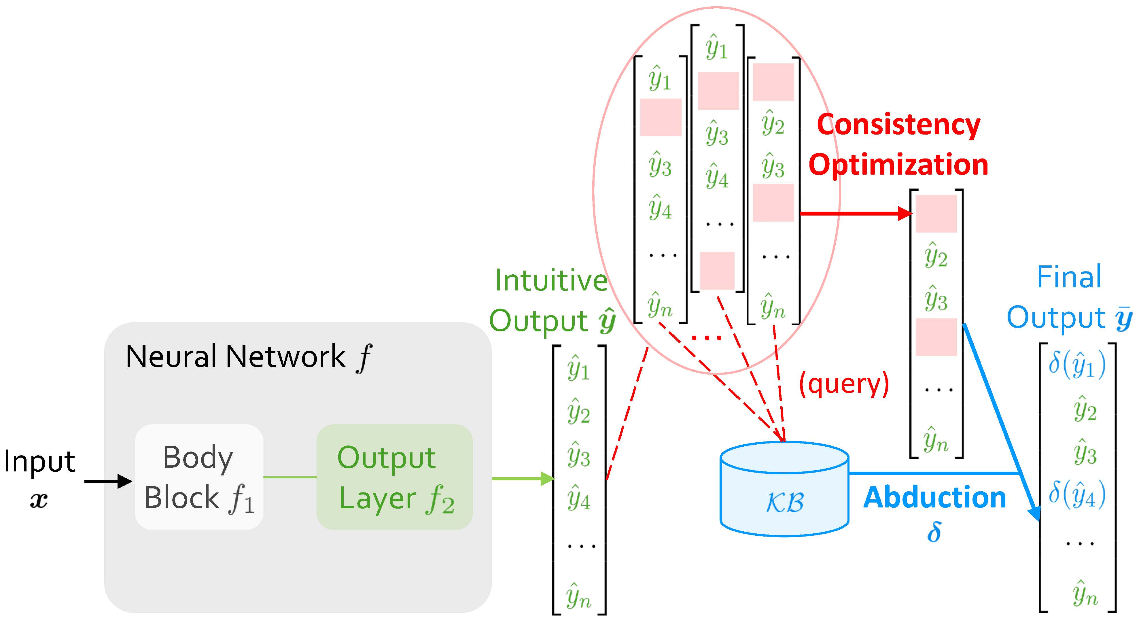</details> Figure 1: Abductive Learning (ABL) framework. When Abductive Learning (ABL) receives an input $\boldsymbol{x}$ , it initially employs $f$ to map $\boldsymbol{x}$ into an intuitive output $\boldsymbol{\hat{y}}=\left[\hat{y}_{1},\hat{y}_{2},\dots,\hat{y}_{n}\right]$ . When $f$ is under-trained, $\boldsymbol{\hat{y}}$ might contain errors leading to inconsistencies with $\mathcal{KB}$ . ABL then tries to rectify them, and obtains a revised $\boldsymbol{\bar{y}}$ . As shown in Figure 1, the final output, $\boldsymbol{\bar{y}}$ , consists of two parts: the green part retains the results from neural network, and the blue part is the modified result obtained by abduction, a basic form of symbolic reasoning that seeks plausible explanations for observations based on $\mathcal{KB}$ . Specifically, the process of obtaining $\boldsymbol{\bar{y}}$ can be divided into two sequential steps. The first step, consistency optimization, determines which positions in $\boldsymbol{\hat{y}}$ include elements that contain errors causing inconsistencies, so that performing abduction at these positions will yield a $\boldsymbol{\bar{y}}$ consistent with $\mathcal{KB}$ . Essentially, this process is pinpointing propositions (or ground atoms, etc.) which have incorrect truth assignments, and most neuro-symbolic tasks can be formalized into this form. Once these positions are determined, the second step is rectifying by abduction, which then becomes easy for $\mathcal{KB}$ and its corresponding symbolic solver. #### Challenge. In previous ABL, consistency optimization has always been a computational bottleneck. It operates as an external module using zeroth-order optimization methods, independent from both $f$ and $\mathcal{KB}$ (Dai et al. 2019; Zhou and Huang 2022). For each time of inference, it involves repetitively selecting various possible positions and querying the $\mathcal{KB}$ to see if a consistent result can be inferred. Each query involves an invocation of $\mathcal{KB}$ for slow symbolic reasoning. Also, since it is a complex combinatorial problem with a highly discrete nature, the number of such queries required escalates exponentially as data scale increases. This large number leads to a marked increase in time consumption, hence confines the applicability of ABL to only small datasets, usually those with output dimension $n$ less than 10. ### 3.3 Architecture To address the challenges above, we propose Abductive Reflection (ABL-Refl). In this section, we will provide a detailed description of its architecture. Let’s first revisit the role of the neural network $f$ when we map the input to symbols from the set $\mathcal{Y}$ . Typically, the raw data is first passed through the body block of the network, denoted by $f_{1}$ , resulting in a high-dimensional embedding which encapsulates a wealth of feature information of the raw data. The form of $f_{1}$ varies, including structures like recurrent layers, graph convolution layers, or Transformers, etc. The result of $f_{1}$ is subsequently passed into several layers, usually linear layers, denoted by $f_{2}$ , to obtain the intuitive output: $\boldsymbol{\hat{y}}=\text{argmax}(f_{2}(f_{1}(\boldsymbol{x})))\in\mathcal{Y} ^{n}$ . <details> <summary>extracted/6187776/figs/ABL-Refl.jpg Details</summary>  ### Visual Description ## Diagram: Neural Network Error Correction and Abduction Process ### Overview The diagram illustrates a multi-stage neural network architecture with error correction and knowledge integration. It shows the flow from input data through body processing, reflection, error removal, and abduction to produce a final output. Key components include body blocks, output layers, reflection mechanisms, and a knowledge base (KB). ### Components/Axes 1. **Input**: Labeled as "Input x" feeding into the system. 2. **Body Block (f₁)**: Processes input data. 3. **Output Layer (f₂)**: Generates "Intuitive Output ŷ" (ŷ₁ to ŷₙ). 4. **Reflection Layer (R)**: Produces a binary reflection vector **r** (1s and 0s). 5. **Error-Removed Output (ŷ')**: Derived from ŷ by removing specific elements (marked with dashes). 6. **Abduction (δ)**: A function applied to ŷ' to integrate knowledge from KB. 7. **Final Output (ȳ)**: Result of δ(ŷ'), with elements δ(ŷ₁), δ(ŷ₂), etc. 8. **Knowledge Base (KB)**: A cylindrical component connected via abduction. ### Detailed Analysis - **Intuitive Output ŷ**: Contains n elements (ŷ₁ to ŷₙ), represented as a vertical list. - **Error-Removed ŷ'**: Identical to ŷ but with one or more elements removed (e.g., ŷ₁ is omitted in the example). - **Reflection Vector r**: Binary vector (1, 0, 0, 1, ..., 0) indicating which elements of ŷ are retained or modified. - **Abduction δ**: Transforms ŷ' into the final output ȳ, with δ applied element-wise (e.g., δ(ŷ₁), δ(ŷ₂)). - **KB Connection**: The KB is linked to the abduction process, suggesting it provides contextual or corrective information. ### Key Observations 1. **Error Correction**: The reflection layer (R) and error-removed output (ŷ') suggest a mechanism to identify and remove erroneous predictions. 2. **Binary Reflection**: The reflection vector **r** uses binary values (1/0), possibly indicating selection or masking of specific outputs. 3. **Abduction Process**: The final output ȳ depends on both the error-corrected ŷ' and the KB, implying knowledge integration. 4. **Function δ**: Applied to individual elements of ŷ', indicating a transformation (e.g., normalization, activation, or correction). ### Interpretation This architecture combines neural network processing with error correction and knowledge-based refinement. The reflection layer likely acts as an attention mechanism, selecting which outputs to retain or adjust. The abduction step integrates external knowledge (KB) to refine the final output, suggesting a hybrid approach that balances data-driven predictions with domain-specific rules. The use of δ functions highlights non-linear transformations at multiple stages, enabling adaptive error handling and knowledge integration. 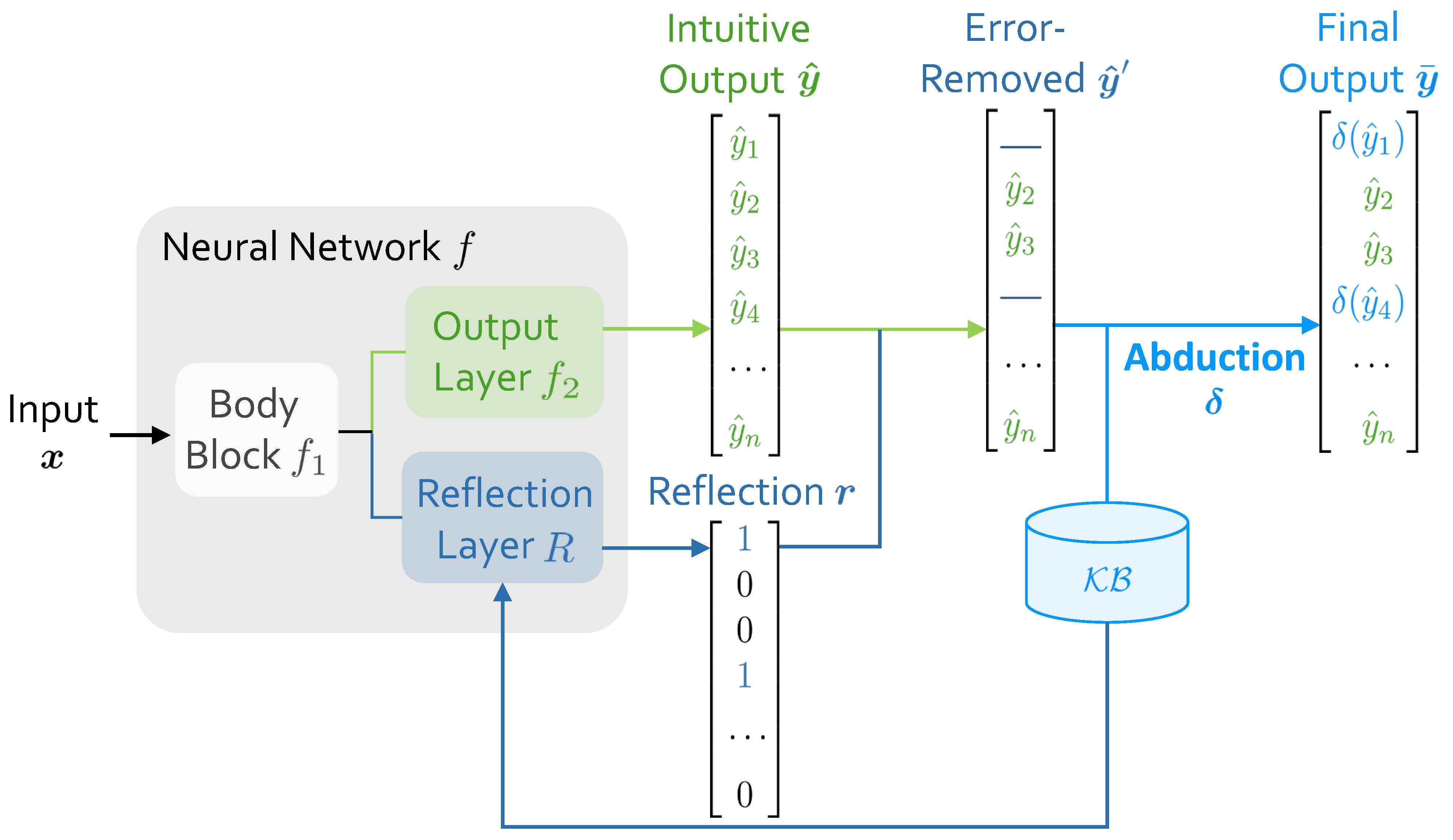</details> Figure 2: Architecture of Abductive Reflection (ABL-Refl). It replaces the external consistency optimization module with an efficient reflection mechanism, which is abduced directly from $\mathcal{KB}$ . Besides the structure described above, as shown in Figure 2, our architecture further incorporates a reflection layer $R$ after the body block $f_{1}$ , generating a reflection vector: $\boldsymbol{r}=\text{argmax}(R(f_{1}(\boldsymbol{x})))\in\{0,1\}^{n}$ . The reflection layer $R$ and reflection vector $\boldsymbol{r}$ together constitute the reflection mechanism. This vector $\boldsymbol{r}$ has the same dimensionality $n$ as the intuitive output $\boldsymbol{\hat{y}}$ , and each element, $r_{i}$ , acts as a binary classifier to indicate whether the corresponding element $\hat{y}_{i}$ is an error leading to inconsistencies with $\mathcal{KB}$ (flagged as 1 for an error, and 0 otherwise). The reflection vector $\boldsymbol{r}$ is generated concurrently with the intuitive response during inference, resonating with human cognition where cognitive reflection typically forms right upon generation of an intuitive response (Frederick 2005). With the initial intuitive output $\boldsymbol{\hat{y}}$ and the corresponding reflection vector $\boldsymbol{r}$ , we seamlessly obtain the error-removed output $\hat{\boldsymbol{y}}^{\prime}$ : In $\hat{\boldsymbol{y}}^{\prime}$ , elements flagged as error by $\boldsymbol{r}$ are removed and left as blanks, while the rest are retained. Subsequently, $\mathcal{KB}$ applies abduction to fill in these blanks, thereby generating an output $\boldsymbol{\bar{y}}$ that is consistent with $\mathcal{KB}$ . That is: $$ \bar{y}_{i}=\begin{cases}\quad\!\!\;\hat{y}_{i},&r_{i}=0\\ \delta(\hat{y}_{i}),&r_{i}=1\end{cases}\quad i=1,2,\dots,n $$ where $\delta$ denotes abduction. We treat $\boldsymbol{\bar{y}}=\left[\bar{y}_{1},\bar{y}_{2},\dots,\bar{y}_{n}\right]$ as the final output. During model training, the reflection is abduced from $\mathcal{KB}$ by directly leveraging information from domain knowledge (discussed later in Section 3.4). It can be seen as an attention mechanism generated from neural networks, which can help quickly focus symbolic reasoning specifically on areas it identifies as errors, hence largely narrowing the problem space of deliberate symbolic reasoning (Zhang et al. 2020). #### Benefits. Compared to previous ABL implementations, ABL-Refl replaces the zeroth-order consistency optimization module with the reflection mechanism to address the computational bottleneck. In this way, the need for a substantial number of querying $\mathcal{KB}$ is mitigated: After promptly pinpointing inconsistencies in System 1 output, regardless of the data scale, only a single invocation of $\mathcal{KB}$ is required to obtain a rectified and more consistent output. Another thing worth noticing is that, in the architecture, the reflection layer directly connects to the body block, which helps leveraging information from the embeddings and linking more closely with the raw data. Therefore, the reflection vector $\boldsymbol{r}$ establishes a more direct and tighter bridge between raw data and domain knowledge. ### 3.4 Training Paradigm In this section, we will discuss how to train the ABL-Refl method, especially the reflection in it. <details> <summary>extracted/6187776/figs/Opt.jpg Details</summary>  ### Visual Description ## Diagram: Error-Corrected Output Generation Process ### Overview The diagram illustrates a technical process for refining an intuitive output through error removal and integration with a knowledge base (KB). It shows the flow from raw predictions to a corrected output combined with domain knowledge. ### Components/Axes 1. **Intuitive Output ŷ** - Vertical green box containing elements: ŷ₁, ŷ₂, ŷ₃, ŷ₄, ..., ŷₙ - Represents initial predictions or hypotheses 2. **Reflection r** - Binary vector: [1, 0, 0, 1, ..., 0] - Acts as a filter/mask for error correction 3. **Error-Removed ŷ'** - Vertical green box with crossed-out elements (ŷ₁, ŷ₄, etc.) - Contains retained elements: ŷ₂, ŷ₃, ..., ŷₙ 4. **Knowledge Base (KB)** - Blue cylinder labeled "KB" - Represents domain-specific knowledge 5. **Concatenation Operations** - Green arrow: Con(ŷ, KB) - Blue arrow: Con(ŷ', KB) ### Flow and Relationships 1. **Error Correction** - Reflection r (binary vector) filters ŷ to produce ŷ' - Crossed-out elements in ŷ' indicate removed errors 2. **Knowledge Integration** - Corrected output ŷ' is concatenated with KB (blue arrow) - Original output ŷ is also concatenated with KB (green arrow) ### Key Observations - **Selective Error Removal**: Only specific elements (ŷ₁, ŷ₄) are removed, suggesting context-dependent error patterns - **Dual Pathway**: Both raw and corrected outputs are integrated with KB, implying iterative refinement - **Binary Reflection**: The reflection vector r uses sparse 1s (e.g., positions 1 and 4) to control error removal ### Interpretation This diagram represents a hybrid AI/ML pipeline where: 1. **Initial predictions** (ŷ) are probabilistically refined using a **sparse binary mask** (r) to remove errors 2. The **error-corrected output** (ŷ') retains high-confidence predictions while discarding low-confidence/erroneous elements 3. Both outputs are **contextualized** through concatenation with a knowledge base (KB), suggesting: - KB provides domain constraints or priors - Final output combines statistical predictions with expert knowledge 4. The **dual concatenation paths** imply: - Raw predictions may still contain valuable information - Error correction and knowledge integration are parallel processes The sparse reflection vector r indicates a **targeted error removal strategy** rather than blanket filtering, preserving potentially useful but noisy predictions. This aligns with modern ML approaches that balance statistical learning with symbolic knowledge systems. 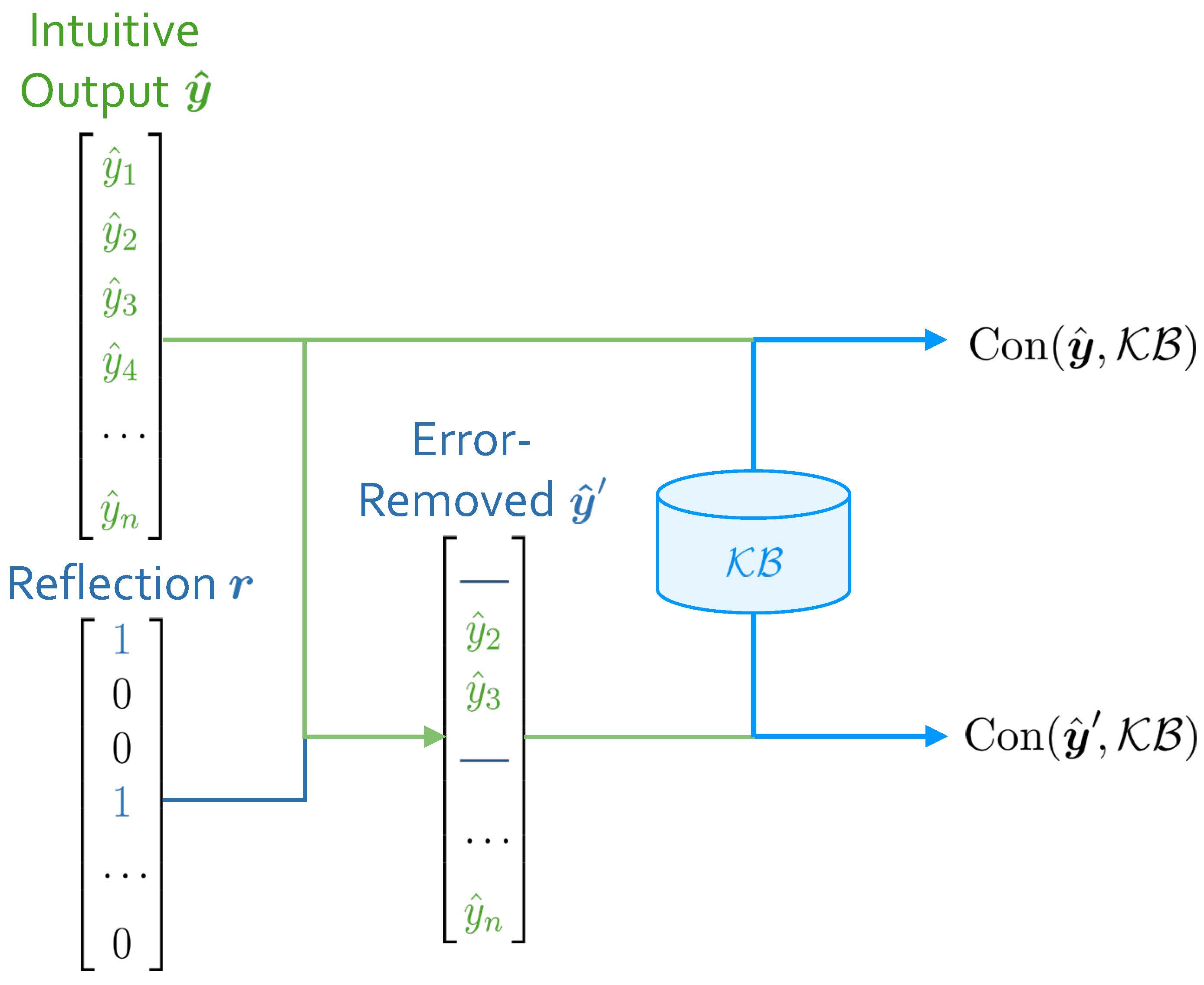</details> Figure 3: Consistency measurements. In ABL-Refl, when each input $\boldsymbol{x}$ is processed by the neural network, we obtain the intuitive output $\boldsymbol{\hat{y}}$ and the reflection vector $\boldsymbol{r}$ , and subsequently obtain the error-removed (by $\boldsymbol{r}$ ) output $\boldsymbol{\hat{y}}^{\prime}$ . With $\boldsymbol{\hat{y}}$ and $\boldsymbol{\hat{y}}^{\prime}$ , we can measure their consistency with $\mathcal{KB}$ , respectively. We denote these consistency measurements as $\text{Con}(\boldsymbol{\hat{y}},\mathcal{KB})$ and $\text{Con}(\boldsymbol{\hat{y}}^{\prime},\mathcal{KB})$ , as shown in Figure 3. For a simplest example, if all elements in $\boldsymbol{\hat{y}}$ (or $\boldsymbol{\hat{y}}^{\prime}$ ) adhere to constraints in $\mathcal{KB}$ , the consistency measurement is 1; otherwise, it is 0. Consequently, the improvement in consistency measurement after reflection, as denoted by $$ \Delta\text{Con}_{\boldsymbol{r}}(\boldsymbol{\hat{y}})=\text{Con}(\boldsymbol {\hat{y}}^{\prime},\mathcal{KB})-\text{Con}(\boldsymbol{\hat{y}},\mathcal{KB}) $$ naturally indicates the effectiveness of the reflection vector: A higher value of it signifies that reflection $\boldsymbol{r}$ can more effectively detect inconsistencies within $\boldsymbol{\hat{y}}$ . Our training goal is to guide the neural network’s parameters towards generating reflections that can maximize this value. Given that $\Delta\text{Con}_{\boldsymbol{r}}(\boldsymbol{\hat{y}})$ is usually a discrete value, we employ the REINFORCE algorithm to achieve this goal (Williams 1992), which optimizes the policy (implicitly defined by neural network $f$ ) through maximizing a specified reward — in this case, $\Delta\text{Con}_{\boldsymbol{r}}(\boldsymbol{\hat{y}})$ . This process leads to the following consistency loss: $$ L_{con}(\boldsymbol{x})=-\Delta\text{Con}_{\boldsymbol{r}}(\boldsymbol{\hat{y} })\cdot\nabla_{\theta}\log f_{\theta}\left(\boldsymbol{\hat{y}},\boldsymbol{r} \mid\boldsymbol{x}\right) \tag{1} $$ where $\theta$ are parameters of neural network $f$ . Additionally, given that the time abduction required often escalates with problem size, we want to invoke it judiciously during inference, applying it only when it is truly necessary. Therefore, we aim to avoid the reflection vector from flagging too many elements in $\boldsymbol{\hat{y}}$ as error. To achieve this, we then introduce a reflection size loss: $$ L_{size}(\boldsymbol{x})=\Phi\!\left(C-\frac{1}{n}\sum_{i=1}^{n}\left(1-R\left (f_{1}(\boldsymbol{x})\right)_{i}\right)\right) \tag{2} $$ where $\Phi(a)\triangleq\max(0,a)^{2}$ and $C$ is a hyperparameter ranging between 0 and 1. When $C$ is set at a higher value, the reflection vector tends to retain a greater number of intuitive output elements instead of flagging them as error and delegating to abduction. In addition to the above-mentioned training methods, using labeled data, we employ data-driven supervised training methods similar to common neural network training paradigm. The loss function in this process, e.g., cross-entropy loss, is denoted by $L_{labeled}(\boldsymbol{x},\boldsymbol{y})$ . Therefore, combining all the training loss, the total loss for ABL-Refl is represented as follows: $$ \displaystyle\mathcal{L} \displaystyle=\frac{1}{|D_{l}|}\sum_{(\boldsymbol{x},\boldsymbol{y})\in D_{l}} L_{labeled}(\boldsymbol{x},\boldsymbol{y}) \displaystyle+\frac{1}{|D_{l}\cup D_{u}|}\sum_{\boldsymbol{x}\in D_{l}\cup D_{ u}}(\alpha L_{con}(\boldsymbol{x})+\beta L_{size}(\boldsymbol{x})) \tag{3} $$ where $\alpha$ and $\beta$ are hyperparameters, $D_{l}=\{(\boldsymbol{x}_{1},\boldsymbol{y}_{1}),(\boldsymbol{x}_{2}, \boldsymbol{y}_{2}),\dots\}$ are the labeled datasets and $D_{u}=\{\boldsymbol{x}_{1},\boldsymbol{x}_{2},\dots\}$ are the unlabeled datasets. Note that neither $L_{con}$ nor $L_{size}$ , which are loss functions specifically related to the reflection, incorporate information from the data label. Instead, we leverage training information directly from $\mathcal{KB}$ to train the reflection. Also, despite sharing the prior feature layers, the output layer $f_{2}$ and reflection layer $R$ utilize different training information, thereby decoupling the objectives of intuitive problem-solving and inconsistency reflection. ## 4 Experiments In this section, we will conduct several experiments. First, we will test our method on the NeSy benchmark task of solving Sudoku to comprehensively verify its effectiveness. Next, we will change the Sudoku input from symbols to images, which requires integrating and simultaneous reasoning with both sub-symbolic and symbolic elements, representing one of the most challenging tasks in this field. Finally, we will tackle NP-hard combinatorial optimization problems on graphs, using a knowledge base of only mathematical definitions, to demonstrate our method’s versatility. Through these experiments, we aim to answer the following questions: - Compared to existing neuro-symbolic learning methods, can ABL-Refl achieve better performance in tasks requiring complex reasoning? - Can ABL-Refl reduce the training resources required? - Can ABL-Refl narrow the problem space for symbolic reasoning to achieve acceleration? - Does ABL-Refl possess the capability for broad application, such as handling diverse data scenarios or various forms of domain knowledge? All experiments are performed on a server with Intel Xeon Gold 6226R CPU and Tesla A100 GPU. In our experiments, we simply set hyperparameters $\alpha$ and $\beta$ in Eq. (3) to 1, since adjusting them does not have a noticeable impact on the results. For the hyperparameter $C$ in (2), we set it to 0.8, and have provided discussions in Appendix C, demonstrating that setting it to a value within a broad moderate range (e.g., 0.6-0.9) would always be a recommended choice. All experiments are repeated 5 times. ### 4.1 Solving Sudoku #### Dataset and Setting. This task aims to solve a 9 $\times$ 9 Sudoku: Given 81 digits of 0-9 (where 0 represents a blank space) in a 9 $\times$ 9 board, we aim to find a solution $\boldsymbol{y}\in\{1,2,\dots,9\}^{81}$ that adhere to the Sudoku rules: no duplicate numbers are allowed in any row, column, or 3 $\times$ 3 subgrid. In this section, we first consider inputs in symbolic form, $\boldsymbol{x}\in\{0,1,\dots,9\}^{81}$ , and use datasets from a publicly available Kaggle site (Vopani 2019). For the neural network $f$ , we use a simple graph neural network (GNN): the body block $f_{1}$ consists of one embedding layer and eight iterations of message-passing layers, resulting in a 128-dimensional embedding for each number, and then connects to both a linear output layer $f_{2}$ to obtain the intuitive output $\hat{\boldsymbol{y}}$ and a linear reflection layer $R$ to obtain the reflection vector ${\boldsymbol{r}}$ . We use the cross-entropy loss as $L_{labeled}$ . For the domain knowledge base $\mathcal{KB}$ , it contains the Sudoku rules mentioned above. We express $\mathcal{KB}$ in the form of propositional logic and utilize the MiniSAT solver (Sörensson 2010), an open-source SAT solver, as the symbolic solver to leverage $\mathcal{KB}$ and perform abduction. For the consistency measurement, we define it as follows: one point is awarded for each row, each column and each 3 $\times$ 3 subgrid with no duplicate numbers, additionally, ten points are awarded if the entire board has no inconsistencies with $\mathcal{KB}$ . In this way, it is entirely based on $\mathcal{KB}$ . Notice that we deviated from the 1 or 0 measurement example setup mentioned in Section 3.4 to avoid a predominance of zero values in $\Delta\text{Con}_{\boldsymbol{r}}(\boldsymbol{\hat{y}})$ of Eq. (1), facilitating effective training with the REINFORCE algorithm. Similar considerations are applied in subsequent experiments. #### Compared Methods and Results. We compare ABL-Refl with the following baseline methods: 1) Recurrent Relational Network (RRN) (Palm, Paquet, and Winther 2018), a pure neural network method, 2) CL-STE (Yang, Lee, and Park 2022), a representative method of logic-based regularized loss, and 3) SATNet (Wang et al. 2019). A detailed description of these methods is provided in Appendix A. We also report the result for Simple GNN, which is the very same neural network used in our setting, yet directly treats the intuitive output $\hat{\boldsymbol{y}}$ as the final output. | RRN CL-STE SATNet | 114.8 $\pm$ 7.8 173.6 $\pm$ 9.9 140.3 $\pm$ 6.8 | 0.19 $\pm$ 0.01 0.19 $\pm$ 0.02 0.11 $\pm$ 0.01 | 73.1 $\pm$ 1.2 76.5 $\pm$ 1.8 74.1 $\pm$ 0.4 | | --- | --- | --- | --- | | ABL-Refl | 109.8 $\pm$ 10.8 | 0.22 $\pm$ 0.02 | 97.4 $\pm$ 0.3 | | Simple GNN | 29.7 $\pm$ 2.6 | 0.02 $\pm$ 0.00 | 55.6 $\pm$ 0.3 | Table 1: Training time (for a total of 100 epochs using 20K training data), inference time and accuracy (on 1K test data) on solving Sudoku. We report the training time (for a total of 100 epochs using 20K training data), inference time (on 1K test data) and accuracy (the percentage of completely accurate Sudoku solution boards on test data) in Table 1. We may see that our method outperforms the baselines significantly, improving by over 20% while maintaining a comparable inference time. This suggests an answer to Q1: ABL-Refl can achieve better reasoning performance. This improvement is primarily due to the use of abduction to rectify the neural network’s output during inference. Furthermore, our method reaches high accuracy in only a few epochs (training curve is shown in Appendix B), significantly reducing training time. Even considering under identical training epochs, our total training time is less than baseline methods, despite involving a time-consuming symbolic solver. This partly stems from the neural network in our approach being less complex than those in baseline methods while achieving high accuracy. Overall, this suggests an answer to Q2: ABL-Refl can reduce the training time required. We also attempt to reduce the amount of labeled data, removing labels from 50%, 75%, and 90% of the training data. We record the inference accuracy in Table 2. It can be observed that even with only 2K labeled training data, our method still achieves far better accuracy than the baseline methods with 20K labeled training data. This suggests an answer to Q2 from another aspect: ABL-Refl can reduce the labeled training data required. | 20K | 0 | 97.4 $\pm$ 0.3 | | --- | --- | --- | | 10K | 10K | 96.3 $\pm$ 0.3 | | 5K | 15K | 95.8 $\pm$ 0.6 | | 2K | 18K | 94.7 $\pm$ 0.8 | Table 2: Inference accuracy on solving Sudoku after reducing the amount of labeled data. #### Comparing to Symbolic Solvers. | Propositional logic ABL-Refl First-order logic | MiniSAT 97.4 $\pm$ 0.3 Prolog with CLP(FD) | Solver only 0.021 $\pm$ 0.004 Solver only | 100 $\pm$ 0 0.196 $\pm$ 0.015 100 $\pm$ 0 | - 0.217 $\pm$ 0.019 - | 0.227 $\pm$ 0.024 105.81 $\pm$ 5.62 | 0.227 $\pm$ 0.024 105.81 $\pm$ 5.62 | | --- | --- | --- | --- | --- | --- | --- | | ABL-Refl | 97.4 $\pm$ 0.3 | 0.021 $\pm$ 0.004 | 31.86 $\pm$ 1.88 | 31.88 $\pm$ 1.89 | | | Table 3: Inference accuracy and time (on 1K test data) on solving Sudoku. For $\mathcal{KB}$ expressed in two different forms, ABL-Refl shows notable acceleration compared to symbolic solvers in both cases. We next compare our method with merely employing symbolic solvers from scratch, to demonstrate its capability in accelerating symbolic reasoning. We perform inference on 1K test data and record the accuracy and time in Table 3. The inference time for our method includes the combined duration for data processing through both the neural network (NN time) and symbolic reasoning (abduction time). As observed in the former two lines, our method achieves a notable acceleration in the abduction process, consequently decreasing the overall inference time, with only a minor compromise in accuracy. This efficiency gain is due to the fact that in ABL-Refl, after quickly generating an intuition through the neural network, abduction only needs to focus on areas identified as necessary by the reflection vector, whereas using only symbolic solvers requires abduction to reason through all blanks in a Sudoku puzzle. Overall, this suggests an answer to Q3: ABL-Refl can quickly generate the reflection, thereby reducing the symbolic reasoning search space and enhancing reasoning efficiency. We also compared with Prolog with CLP(FD) (Triska 2012) solver, by expressing the same $\mathcal{KB}$ with a first-order constraint logic program. As shown in the table, we observe a significant reduction in abduction time and overall inference time, which puts another evidence to our previous answer to Q3, and also suggests an answer to Q4: ABL-Refl can effectively utilize the two most commonly used forms in symbolic knowledge representation, propositional logic and first-order logic. ### 4.2 Solving Visual Sudoku #### Dataset and Setting. In this section, we modify the input from 81 symbolic digits to 81 MNIST images (handwritten digits of 0-9). We use the dataset provided in SATNet (Wang et al. 2019) and use 9K Sudoku boards for training and 1K for testing. In order to process image data, we first pass each image through a LeNet convolutional neural network (CNN) (LeCun et al. 1998) to obtain the probability of each digit. The rest of our setting follows from that described in Section 4.1. #### Compared Methods and Results. 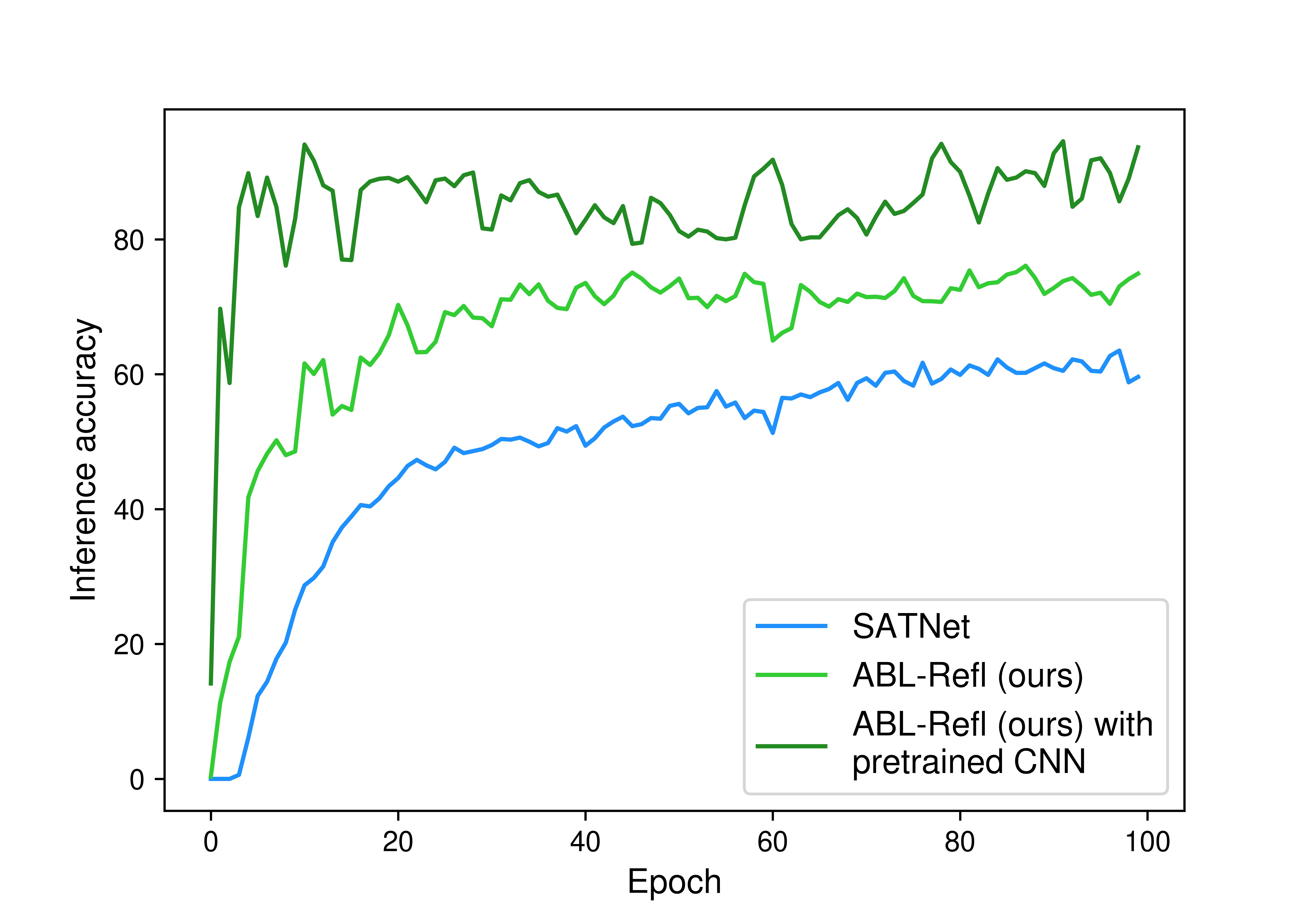We compare ABL-Refl with SATNet, as both methods allow for end-to-end training from visual inputs. We report the results in Table 4 and the training curve in Appendix B. Compared to SATNet, ABL-Refl shows notable improvement in reasoning accuracy within only a few training epochs. We then consider pretraining the CNN in advance using self-supervised learning methods (Chen et al. 2020) and find that this can further improve accuracy. Overall, the results further suggest positive answers to Q1 and Q2. We also compare with CNN+Solver: each image is first mapped to symbolic form by a fully trained CNN (with 99.6% accuracy on the MNIST dataset) and then directly fed into the symbolic solver to fill in the blanks and derive the final output. In such scenarios, the problem space for the symbolic solver includes all the Sudoku blanks, and additionally, since the symbolic solver cannot revise errors from CNN, any inaccuracies in CNN’s output could lead the symbolic solver to crash (i.e., output no solution). Consequently, inference accuracy and time are adversely affected. This confirms the positive answer to Q3. Finally, an overview of Sections 4.1 and 4.2 also suggests an answer to Q4: ABL-Refl is capable of handling both symbolic and sub-symbolic forms of input data. | SATNet CNN+Solver ABL-Refl | 0.12 $\pm$ 0.01 0.23 $\pm$ 0.02 0.22 $\pm$ 0.02 | 63.5 $\pm$ 2.2 67.8 $\pm$ 4.2 77.8 $\pm$ 5.8 | | --- | --- | --- | | ABL-Refl (with pretrained CNN) | 0.22 $\pm$ 0.02 | 93.5 $\pm$ 3.2 | Table 4: Inference time (on 1K test data) and accuracy on solving visual Sudoku. ### 4.3 Solving Combinatorial Optimization Problems on Graphs In this section, we will further expand the application domain of our method. We apply ABL-Refl to solving combinatorial optimization problems on graphs. We conduct the experiment on finding the maximum clique in this section, and provide an additional experiment in Appendix E. #### Dataset and Setting. In this task, we are given a graph $G=(V,E)$ with $|V|=n$ nodes, and aim to output $\boldsymbol{y}\in\{0,1\}^{n}$ , where each index corresponds to a node, and the set of indices assigned the value of 1 collectively constitute the maximum clique. Note that this problem is a challenging NP-hard problem with extensive applications in real-life scenarios, and is generally considered challenging for neural networks (Zhang et al. 2023). We use several datasets from the TUDatasets (Morris et al. 2020), with their basic information shown in Table 5. We use 80% of the data for training and 20% for testing. In our method, the body layer $f_{1}$ consists of a single GAT layer (Veličković et al. 2017) and 16 gated graph convolution layers (Li et al. 2015), and the output layer $f_{2}$ and reflection layer $R$ are both linear layers. We use binary cross-entropy loss as $L_{labeled}$ . The domain knowledge base $\mathcal{KB}$ expresses the mathematical definition of maximum clique, i.e., every pair of vertices in the output set should be connected by an edge. We use Gurobi solver, an efficient mixed-integer program solver, to perform abduction. We define the consistency measurement as follows: one point is awarded for each pair of vertices if they are not connected by an edge; additionally, the size of the output set multiplied by 10 is added if the output set is indeed a clique. | Method | Dataset (Graph nums./Avg. nodes per graph/Avg. edges per graph) | | | | | --- | --- | --- | --- | --- | | ENZYMES (600/33/62) | PROTEINS (1113/39/73) | IMDB-Binary (1000/19/97) | COLLAB (5000/74/2457) | | | Erdos | 0.883 $\pm$ 0.156 | 0.905 $\pm$ 0.133 | 0.936 $\pm$ 0.175 | 0.852 $\pm$ 0.212 | | Neural SFE | 0.933 $\pm$ 0.148 | 0.926 $\pm$ 0.165 | 0.961 $\pm$ 0.143 | 0.781 $\pm$ 0.316 | | ABL-Refl | 0.991 $\pm$ 0.017 | 0.985 $\pm$ 0.020 | 0.979 $\pm$ 0.029 | 0.982 $\pm$ 0.015 | Table 5: Approximation ratios on finding maximum clique on different datasets. #### Compared Methods and Results. We compare our methods with the following baselines: 1) Erdos (Karalias and Loukas 2020), 2) Neural SFE (Karalias et al. 2022), both leading methods for solving graph combinatorial problems. Their detailed descriptions are provided in Appendix A. We report the approximation ratios in Table 5. The approximation ratio, indicating the result set size relative to the actual maximum set size, is better when closer to 1. We may observe that our method outperforms the baseline methods, achieving near-perfect results on all datasets. This confirms the positive answer to Q1. Also, as the scale of the data increases, our method maintains a high level of accuracy, showing a more pronounced improvement compared to baseline methods. This suggests an answer to Q4: ABL-Refl is capable of handling scalable data scenarios, even in high-dimensional settings that are challenging for previous methods. Finally, an overview of this section provides another aspect to Q4: ABL-Refl can utilize a wide range of $\mathcal{KB}$ , not limited to logical expressions but can also operate effectively with just the basic mathematical formulations. ## 5 Effects of Reflection Mechanism This section provides a further analysis on the reflection mechanism. In ABL-Refl, the reflection is abduced from domain knowledge, and acts as an efficient attention mechanism to direct the focus for symbolic search. This reflection is the key in our method to accomplish the NeSy reasoning rectification pipeline, i.e., a pipeline that detects errors in neural networks and then invokes symbolic reasoning to rectify these positions. To corroborate the effectiveness of the reflection, we conduct direct comparison with other methods that achieve the same pipeline: 1. ABL, minimizing the inconsistency of intuitive output and knowledge base with an external zeroth-order consistency optimization module, as detailed in Section 3.2; 1. NN Confidence, retaining intuitive output with the top 80% confidence from the neural network result (other retain thresholds are explored in Appendix D) and passing the remaining into symbolic reasoning; 1. NASR (Cornelio et al. 2023), using a Transformer-based external selection module to detect error, and the module is trained on a large synthetic dataset in advance. We compare them on the solving visual Sudoku task in Section 4.2. For a fair comparison, all methods employ the same neural network, $\mathcal{KB}$ and MiniSAT solver setup. We report the recall (the percentage of errors from neural networks that can be identified), inference time and accuracy (on 1K test data) in Table 6. Note that “recall” directly evaluates the effectiveness of the detection module itself. The following analysis examines the results: - The consistency optimization in ABL faces significant efficiency challenges due to the large data scale (output dimension $n=81$ ). In such scenarios, the potential rectifications can reach up to $2^{81}$ , resulting in an overwhelmingly large search space for consistency optimization. Also, as an external module, its only way of interacting with $\mathcal{KB}$ is to treat it as a black box and repetitively submit queries for consistency evaluation. As a result, it may require more than $10^{9}$ queries to identify errors for each Sudoku example, resulting in several hours to complete inference on 1K test data. - NN Confidence performs poorly in identifying outputs with errors. Since the pure data-driven neural network training does not explicitly incorporate $\mathcal{KB}$ information, a low confidence from it does not necessarily indicate an inconsistency with the domain knowledge. This subsequently results in the frequent crashing in symbolic solver, therefore hampering the overall inference time and accuracy. This result parallels human cognitive reflection abilities, which do not show much positive correlation with System 1 intuition (Pennycook et al. 2016). To further illustrate this point, we provide additional analysis, including a case study, in Appendix D. - Our method also outperforms NASR, and notably, without the need of a synthetic dataset. This could be due to the fact that NASR’s error-selection module is trained independently from other components, and operates sequentially and separately during inference. Therefore, it can only rely on information from the output label, in contrast to our method, which can leverage information directly from the body block of neural network, establishing a deeper connection with the raw data. Additionally, in NASR, traversing the separate selection module takes additional time, whereas in ABL-Refl, the reflection is generated concurrently with the neural network output, avoiding efficiency loss. | NN Confidence NASR ABL-Refl | 82.64 $\pm$ 2.78 95.86 $\pm$ 0.96 99.04 $\pm$ 0.85 | 0.24 $\pm$ 0.03 0.26 $\pm$ 0.02 0.22 $\pm$ 0.02 | 64.3 $\pm$ 6.2 82.7 $\pm$ 4.4 93.5 $\pm$ 3.2 | | --- | --- | --- | --- | Table 6: Recall, inference time and accuracy. ”Timeout” indicates that inference takes more than 1 hour. ## 6 Conclusion In this paper, we present Abductive Reflection (ABL-Refl). It leverages domain knowledge to abduce a reflection vector, which flags potential errors in neural network outputs and then invokes abduction, serving as an attention mechanism for symbolic reasoning to focus on a much smaller problem space. Experiments show that ABL-Refl significantly outperforms other NeSy methods, achieving excellent reasoning accuracy with fewer training resources, and has successfully enhanced reasoning efficiency. ABL-Refl preserves the integrity of both machine learning and logical reasoning with superior inference speed and high versatility. Therefore, it has the potential for broad application. In the future, it can be applied to large language models (Mialon et al. 2023) to help identify errors within their outputs, and subsequently exploit symbolic reasoning to enhance their trustworthiness and reliability. ## Acknowledgments This research was supported by the NSFC (62176117, 62206124) and Jiangsu Science Foundation Leading-edge Technology Program (BK20232003). ## References - Ahmed et al. (2022) Ahmed, K.; Wang, E.; Chang, K.-W.; and Van den Broeck, G. 2022. Neuro-symbolic entropy regularization. In Uncertainty in Artificial Intelligence, 43–53. PMLR. - Amos and Kolter (2017) Amos, B.; and Kolter, J. Z. 2017. Optnet: Differentiable optimization as a layer in neural networks. In International Conference on Machine Learning, 136–145. PMLR. - Bengio (2019) Bengio, Y. 2019. From system 1 deep learning to system 2 deep learning. In Neural Information Processing Systems. - Cai et al. (2021) Cai, L.-W.; Dai, W.-Z.; Huang, Y.-X.; Li, Y.-F.; Muggleton, S. H.; and Jiang, Y. 2021. Abductive Learning with Ground Knowledge Base. In Proceedings of the 30th International Joint Conference on Artificial Intelligence (IJCAI’21), 1815–1821. - Chen et al. (2020) Chen, T.; Kornblith, S.; Norouzi, M.; and Hinton, G. 2020. A simple framework for contrastive learning of visual representations. In International conference on machine learning, 1597–1607. PMLR. - Cornelio et al. (2023) Cornelio, C.; Stuehmer, J.; Hu, S. X.; and Hospedales, T. 2023. Learning where and when to reason in neuro-symbolic inference. In The Eleventh International Conference on Learning Representations. - Dai et al. (2019) Dai, W.-Z.; Xu, Q.; Yu, Y.; and Zhou, Z.-H. 2019. Bridging machine learning and logical reasoning by abductive learning. Advances in Neural Information Processing Systems, 32. - Frederick (2005) Frederick, S. 2005. Cognitive reflection and decision making. Journal of Economic perspectives, 19(4): 25–42. - Gao et al. (2024) Gao, E.-H.; Huang, Y.-X.; Hu, W.-C.; Zhu, X.-H.; and Dai, W.-Z. 2024. Knowledge-Enhanced Historical Document Segmentation and Recognition. In Proceedings of the 38th AAAI Conference on Artificial Intelligence (AAAI’24), 8409–8416. - Han et al. (2023) Han, Q.; Yang, L.; Chen, Q.; Zhou, X.; Zhang, D.; Wang, A.; Sun, R.; and Luo, X. 2023. A GNN-Guided Predict-and-Search Framework for Mixed-Integer Linear Programming. arXiv preprint arXiv:2302.05636. - Hitzler (2022) Hitzler, P. 2022. Neuro-symbolic artificial intelligence: The state of the art. IOS Press. - Hoernle et al. (2022) Hoernle, N.; Karampatsis, R. M.; Belle, V.; and Gal, K. 2022. Multiplexnet: Towards fully satisfied logical constraints in neural networks. In Proceedings of the AAAI Conference on Artificial Intelligence, volume 36, 5700–5709. - Huang et al. (2020) Huang, Y.-X.; Dai, W.-Z.; Yang, J.; Cai, L.-W.; Cheng, S.; Huang, R.; Li, Y.-F.; and Zhou, Z.-H. 2020. Semi-Supervised Abductive Learning and Its Application to Theft Judicial Sentencing. In Proceedings of the 20th IEEE International Conference on Data Mining (ICDM’20), 1070–1075. - Huang et al. (2024) Huang, Y.-X.; Hu, W.-C.; Gao, E.-H.; and Jiang, Y. 2024. ABLkit: A Python Toolkit for Abductive Learning. Frontiers of Computer Science, pp. to appear. - Kahneman (2011) Kahneman, D. 2011. Thinking, fast and slow. macmillan. - Karalias and Loukas (2020) Karalias, N.; and Loukas, A. 2020. Erdos goes neural: an unsupervised learning framework for combinatorial optimization on graphs. Advances in Neural Information Processing Systems, 33: 6659–6672. - Karalias et al. (2022) Karalias, N.; Robinson, J.; Loukas, A.; and Jegelka, S. 2022. Neural Set Function Extensions: Learning with Discrete Functions in High Dimensions. arXiv preprint arXiv:2208.04055. - LeCun et al. (1998) LeCun, Y.; Bottou, L.; Bengio, Y.; and Haffner, P. 1998. Gradient-based learning applied to document recognition. Proceedings of the IEEE, 86(11): 2278–2324. - Li et al. (2015) Li, Y.; Tarlow, D.; Brockschmidt, M.; and Zemel, R. 2015. Gated graph sequence neural networks. arXiv preprint arXiv:1511.05493. - Manhaeve et al. (2018) Manhaeve, R.; Dumancic, S.; Kimmig, A.; Demeester, T.; and De Raedt, L. 2018. Deepproblog: Neural probabilistic logic programming. advances in neural information processing systems, 31. - Marra et al. (2020) Marra, G.; Giannini, F.; Diligenti, M.; and Gori, M. 2020. Integrating learning and reasoning with deep logic models. In Machine Learning and Knowledge Discovery in Databases, 517–532. Springer. - Mialon et al. (2023) Mialon, G.; Fourrier, C.; Swift, C.; Wolf, T.; LeCun, Y.; and Scialom, T. 2023. GAIA: a benchmark for General AI Assistants. arXiv preprint arXiv:2311.12983. - Morris et al. (2020) Morris, C.; Kriege, N. M.; Bause, F.; Kersting, K.; Mutzel, P.; and Neumann, M. 2020. Tudataset: A collection of benchmark datasets for learning with graphs. arXiv preprint arXiv:2007.08663. - Nair et al. (2020) Nair, V.; Bartunov, S.; Gimeno, F.; Von Glehn, I.; Lichocki, P.; Lobov, I.; O’Donoghue, B.; Sonnerat, N.; Tjandraatmadja, C.; Wang, P.; et al. 2020. Solving mixed integer programs using neural networks. arXiv preprint arXiv:2012.13349. - Nye et al. (2021) Nye, M.; Tessler, M.; Tenenbaum, J.; and Lake, B. M. 2021. Improving coherence and consistency in neural sequence models with dual-system, neuro-symbolic reasoning. Advances in Neural Information Processing Systems, 34: 25192–25204. - Palm, Paquet, and Winther (2018) Palm, R.; Paquet, U.; and Winther, O. 2018. Recurrent relational networks. Advances in neural information processing systems, 31. - Pennycook et al. (2016) Pennycook, G.; Cheyne, J. A.; Koehler, D. J.; and Fugelsang, J. A. 2016. Is the cognitive reflection test a measure of both reflection and intuition? Behavior research methods, 48: 341–348. - Selsam et al. (2018) Selsam, D.; Lamm, M.; Bünz, B.; Liang, P.; de Moura, L.; and Dill, D. L. 2018. Learning a SAT solver from single-bit supervision. arXiv preprint arXiv:1802.03685. - Serafini and Garcez (2016) Serafini, L.; and Garcez, A. d. 2016. Logic tensor networks: Deep learning and logical reasoning from data and knowledge. arXiv preprint arXiv:1606.04422. - Sinayev and Peters (2015) Sinayev, A.; and Peters, E. 2015. Cognitive reflection vs. calculation in decision making. Frontiers in psychology, 6: 532. - Sörensson (2010) Sörensson, N. 2010. Minisat 2.2 and minisat++ 1.1. A short description in SAT Race. - Triska (2012) Triska, M. 2012. The finite domain constraint solver of SWI-Prolog. In Functional and Logic Programming: 11th International Symposium, 307–316. Springer. - Veličković et al. (2017) Veličković, P.; Cucurull, G.; Casanova, A.; Romero, A.; Lio, P.; and Bengio, Y. 2017. Graph attention networks. arXiv preprint arXiv:1710.10903. - Vopani (2019) Vopani. 2019. 9 Million Sudoku Puzzles and Solutions. https://www.kaggle.com/datasets/rohanrao/sudoku. Accessed: 2024-08-01. - Wang et al. (2021) Wang, J.; Deng, D.; Xie, X.; Shu, X.; Huang, Y.-X.; Cai, L.-W.; Zhang, H.; Zhang, M.-L.; Zhou, Z.-H.; and Wu, Y. 2021. Tac-Valuer: Knowledge-based Stroke Evaluation in Table Tennis. In Proceedings of the 27th ACM SIGKDD Conference on Knowledge Discovery and Data Mining (KDD’21), 3688–3696. - Wang et al. (2019) Wang, P.-W.; Donti, P.; Wilder, B.; and Kolter, Z. 2019. Satnet: Bridging deep learning and logical reasoning using a differentiable satisfiability solver. In International Conference on Machine Learning, 6545–6554. PMLR. - Williams (1992) Williams, R. J. 1992. Simple statistical gradient-following algorithms for connectionist reinforcement learning. Reinforcement learning, 5–32. - Xu et al. (2018) Xu, J.; Zhang, Z.; Friedman, T.; Liang, Y.; and Broeck, G. 2018. A semantic loss function for deep learning with symbolic knowledge. In International conference on machine learning, 5502–5511. PMLR. - Yang, Ishay, and Lee (2020) Yang, Z.; Ishay, A.; and Lee, J. 2020. Neurasp: Embracing neural networks into answer set programming. In 29th International Joint Conference on Artificial Intelligence. - Yang, Lee, and Park (2022) Yang, Z.; Lee, J.; and Park, C. 2022. Injecting logical constraints into neural networks via straight-through estimators. In International Conference on Machine Learning, 25096–25122. PMLR. - Zhang et al. (2023) Zhang, B.; Luo, S.; Wang, L.; and He, D. 2023. Rethinking the expressive power of gnns via graph biconnectivity. arXiv preprint arXiv:2301.09505. - Zhang et al. (2020) Zhang, W.; Sun, Z.; Zhu, Q.; Li, G.; Cai, S.; Xiong, Y.; and Zhang, L. 2020. NLocalSAT: Boosting local search with solution prediction. arXiv preprint arXiv:2001.09398. - Zhou (2019) Zhou, Z.-H. 2019. Abductive learning: towards bridging machine learning and logical reasoning. Science China Information Sciences, 62: 1–3. - Zhou and Huang (2022) Zhou, Z.-H.; and Huang, Y.-X. 2022. Abductive Learning. In Hitzler, P.; and Sarker, M. K., eds., Neuro-Symbolic Artificial Intelligence: The State of the Art, 353–369. Amsterdam: IOS Press. ## Appendix A Comparison Methods In this section, we will provide a brief supplementary introduction to the compared baseline methods used in experiments. ### A.1 Solving Sudoku In the solving Sudoku experiment (Section 4.1 and 4.2), we have compared our method with the following baselines: 1. Recurrent Relational Network (RRN) (Palm, Paquet, and Winther 2018), a state-of-the-art pure neural network method tailored for this problem; 1. CL-STE (Yang, Lee, and Park 2022), injecting logical knowledge (defined in the same way as our $\mathcal{KB}$ ) as neural network constraints during the training of RRN; 1. SATNet (Wang et al. 2019), incorporating a differentiable MaxSAT solver into the neural network to perform reasoning. Note that CL-STE is a representative method of logic-based regularized loss, relaxing symbolic logic as neural network loss. Additionally, among these methods, CL-STE stands out in both accuracy and efficiency (partly because it prevents constructing complex SDDs, unlike other methods including semantic loss (Xu et al. 2018)). Other lines of methods generally underperform above baselines in scenarios where $n$ (the scale of $\boldsymbol{y}$ ) is high. For instance, ABL faces the challenge where consistency optimization needs to choose among exponential query candidates, resulting in runtimes thousands of times longer than other methods, as seen in Section 5. Take two other representative NeSy methods as examples: DeepProbLog (Manhaeve et al. 2018) involves substantial computational costs, taking days to complete solving Sudoku; NeurASP (Yang, Ishay, and Lee 2020) also performs slow and lags in accuracy, as shown in Yang et al. (2022). ### A.2 Solving Combinatorial Optimization on Graphs In the solving combinatorial optimization on graphs experiment (Section 4.3 and Appendix E), we have compared our method with the following baselines: 1. Erdos (Karalias and Loukas 2020), optimizing set functions using a neural network parametrizing a distribution over sets; 1. Neural SFE (Karalias et al. 2022), optimizing set functions by extending them onto high-dimensional continuous domains. In this experiment, the above methods use the same body block graph neural network as our method. 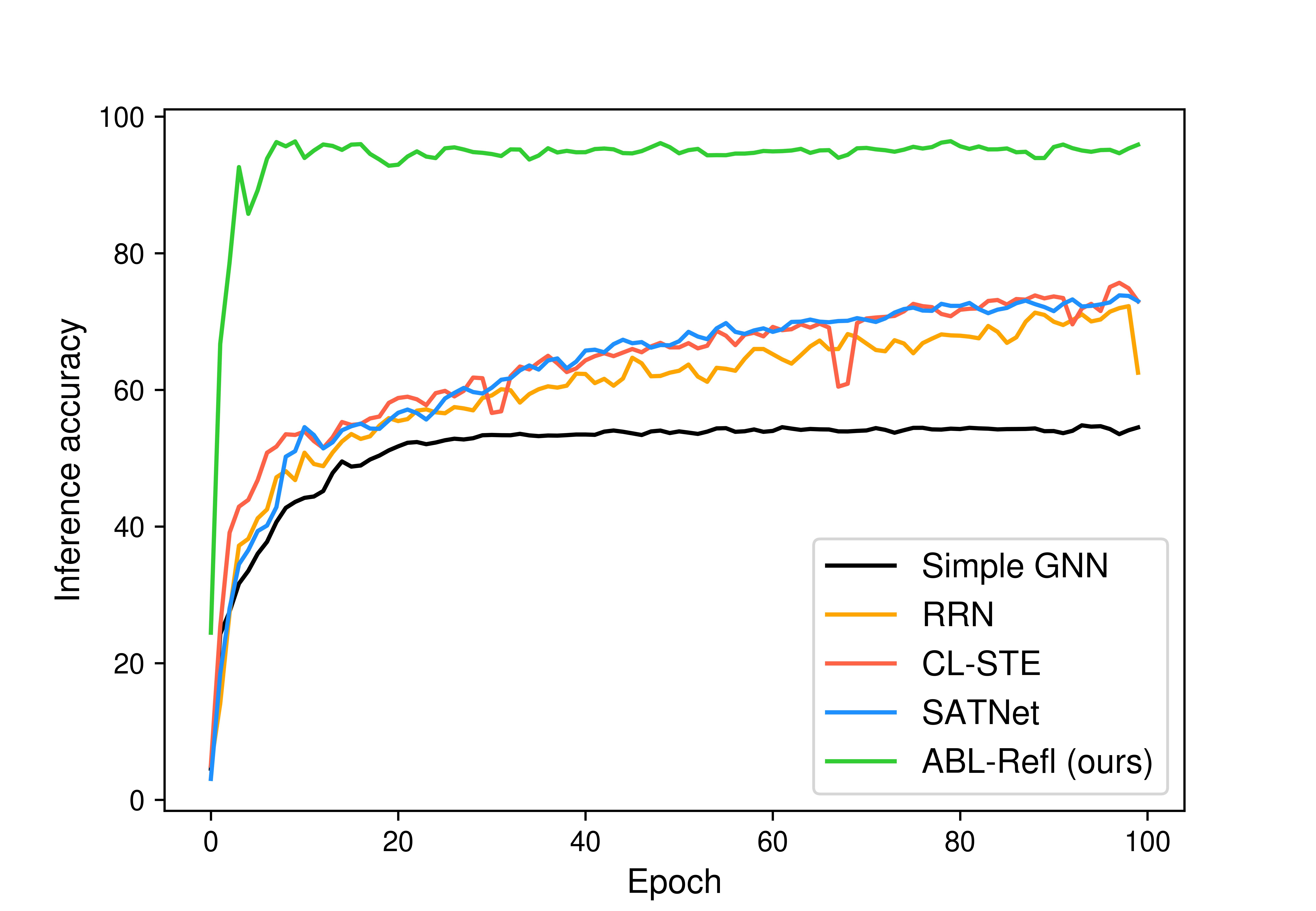## Appendix B Training Curve In this section, we will report the training curve in the experiments on solving Sudoku (Section 4.1) and visual Sudoku (Section 4.2). The respective training curves for each scenario are shown in Figures 4(a) and 4(b), with the horizontal axis representing training epochs and the vertical axis representing inference accuracy. We may see that our method achieves high accuracy within just a few epochs, significantly reducing training time compared to other baseline methods. <details> <summary>extracted/6187776/figs/sudoku.jpg Details</summary>  ### Visual Description ## Line Graph: Inference Accuracy vs. Epoch ### Overview The image is a line graph comparing the inference accuracy of five different models (Simple GNN, RRN, CL-STE, SATNet, and ABL-Refl) across 100 training epochs. The y-axis represents inference accuracy (0–100%), and the x-axis represents epochs (0–100). The graph shows distinct performance trajectories for each model, with ABL-Refl (green) achieving the highest accuracy. ### Components/Axes - **X-axis (Epoch)**: Labeled "Epoch," ranging from 0 to 100 in increments of 20. - **Y-axis (Inference Accuracy)**: Labeled "Inference accuracy," ranging from 0 to 100 in increments of 20. - **Legend**: Located in the bottom-right corner, with color-coded labels: - Black: Simple GNN - Orange: RRN - Red: CL-STE - Blue: SATNet - Green: ABL-Refl (ours) ### Detailed Analysis 1. **ABL-Refl (Green Line)**: - Starts at ~25% accuracy at epoch 0. - Rapidly increases to ~95% by epoch 10. - Maintains near-100% accuracy from epoch 20 onward, with minor fluctuations (~95–98%). 2. **SATNet (Blue Line)**: - Begins at ~10% accuracy at epoch 0. - Gradually rises to ~70% by epoch 100, with minor oscillations. - Peaks at ~75% around epoch 80. 3. **CL-STE (Red Line)**: - Starts at ~15% accuracy at epoch 0. - Increases to ~65% by epoch 100, with a dip to ~55% around epoch 60. - Shows moderate volatility compared to other models. 4. **RRN (Orange Line)**: - Begins at ~5% accuracy at epoch 0. - Rises to ~60% by epoch 100, with a notable dip to ~40% around epoch 60. - Exhibits the most fluctuation among non-green models. 5. **Simple GNN (Black Line)**: - Starts at ~0% accuracy at epoch 0. - Reaches ~55% by epoch 100, with a plateau after epoch 40. - Shows the slowest and least consistent growth. ### Key Observations - **ABL-Refl Dominance**: The green line (ABL-Refl) consistently outperforms all other models, achieving near-perfect accuracy after epoch 20. - **Volatility in RRN and CL-STE**: Both models exhibit significant dips (e.g., RRN at epoch 60, CL-STE at epoch 60), suggesting instability in training dynamics. - **Simple GNN Lag**: The black line (Simple GNN) remains the lowest-performing model throughout, with minimal improvement after epoch 40. - **SATNet’s Steady Growth**: The blue line (SATNet) shows the most consistent upward trend among non-green models. ### Interpretation The graph demonstrates that **ABL-Refl (ours)** is the most effective model for inference accuracy, achieving near-optimal performance early and maintaining it throughout training. Other models (RRN, CL-STE, SATNet) show moderate improvement but fail to match ABL-Refl’s efficiency. The Simple GNN’s stagnation highlights its limitations compared to more advanced architectures. The volatility in RRN and CL-STE suggests potential overfitting or sensitivity to hyperparameters, while SATNet’s steady growth indicates robustness. These trends underscore the importance of architectural design (e.g., ABL-Refl’s structure) in achieving high inference accuracy. </details> (a) Sudoku. <details> <summary>extracted/6187776/figs/visual_sudoku.jpg Details</summary>  ### Visual Description ## Line Graph: Inference Accuracy vs. Epochs ### Overview The image is a line graph comparing the inference accuracy of three models (SATNet, ABL-Refl, and ABL-Refl with pretrained CNN) across 100 training epochs. The y-axis represents inference accuracy (0–100%), and the x-axis represents epochs (0–100). Three distinct lines are plotted, each corresponding to a model, with the legend positioned in the bottom-right corner. --- ### Components/Axes - **X-axis (Epochs)**: Labeled "Epoch," ranging from 0 to 100 in increments of 20. - **Y-axis (Inference Accuracy)**: Labeled "Inference accuracy," ranging from 0 to 100 in increments of 20. - **Legend**: Located in the bottom-right corner, with three entries: - **Blue**: SATNet - **Green**: ABL-Refl (ours) - **Dark Green**: ABL-Refl (ours) with pretrained CNN --- ### Detailed Analysis #### SATNet (Blue Line) - **Initial Behavior**: Starts at 0% accuracy at epoch 0, sharply rising to ~10% by epoch 5. - **Mid-Training**: Gradually increases to ~60% by epoch 100, with a notable dip to ~55% around epoch 60. - **Trend**: Overall upward trajectory with moderate fluctuations. #### ABL-Refl (Green Line) - **Initial Behavior**: Begins at ~10% accuracy at epoch 0, rising sharply to ~70% by epoch 20. - **Mid-Training**: Stabilizes between 70–75% accuracy, with minor fluctuations (e.g., ~65% at epoch 60). - **Trend**: Smoother progression compared to SATNet, maintaining higher accuracy after epoch 20. #### ABL-Refl with Pretrained CNN (Dark Green Line) - **Initial Behavior**: Starts at ~90% accuracy at epoch 0, dipping to ~80% by epoch 10. - **Mid-Training**: Fluctuates between 80–90% accuracy, peaking at ~95% around epoch 80. - **Trend**: Most stable and highest-performing line, with minor volatility. --- ### Key Observations 1. **Pretrained CNN Advantage**: The dark green line (ABL-Refl with pretrained CNN) consistently outperforms the other models, maintaining ~80–90% accuracy throughout training. 2. **SATNet Variability**: The blue line (SATNet) exhibits the highest volatility, with a significant dip at epoch 60 and slower convergence. 3. **ABL-Refl Stability**: The green line (ABL-Refl) shows steady improvement, surpassing SATNet by epoch 20 and maintaining ~70% accuracy. 4. **Early Dip in Pretrained Model**: The dark green line’s drop to ~80% at epoch 10 may indicate an initial adjustment phase for the pretrained CNN. --- ### Interpretation - **Model Effectiveness**: The pretrained CNN integration significantly enhances ABL-Refl’s performance, suggesting transfer learning improves generalization. SATNet’s lower accuracy and higher variance imply it is less effective for this task. - **Training Dynamics**: ABL-Refl’s rapid early improvement (epoch 0–20) highlights its efficiency, while SATNet’s gradual climb indicates slower learning. - **Anomalies**: The pretrained model’s epoch 10 dip could reflect temporary instability during CNN adaptation, but it recovers quickly to dominate later epochs. - **Practical Implications**: For tasks requiring high inference accuracy, ABL-Refl with pretrained CNN is optimal. SATNet may require architectural adjustments or hyperparameter tuning to match performance. --- ### Spatial Grounding & Trend Verification - **Legend Alignment**: Colors match line placements exactly (blue = SATNet, green = ABL-Refl, dark green = pretrained CNN). - **Trend Consistency**: - SATNet’s upward slope aligns with its ~60% final accuracy. - ABL-Refl’s plateau at ~70% matches its mid-training stability. - Pretrained CNN’s fluctuations around 80–90% confirm its dominance. --- ### Content Details - **Data Points**: - SATNet: ~10% (epoch 5), ~60% (epoch 100), ~55% (epoch 60 dip). - ABL-Refl: ~70% (epoch 20), ~65% (epoch 60). - Pretrained CNN: ~90% (epoch 0), ~80% (epoch 10), ~95% (epoch 80 peak). --- ### Final Notes The graph underscores the benefits of pretrained CNNs in boosting inference accuracy, while highlighting SATNet’s limitations. Further analysis could explore why SATNet underperforms and whether pretraining strategies could be adapted for other models. </details> (b) Visual Sudoku. Figure 4: Training curve on solving Sudoku and visual Sudoku. ## Appendix C Discussion on Hyperparameter $C$ In this section, we will discuss the effect of the hyperparameter $C$ . Previous experiments in Sections 4 and 5, $C$ was consistently set to 0.8, and we will now explore adjustments. We report the extended results in Tables 7 and 8. It is shown that when $C$ is set within a wide range, ABL-Refl uniformly outperforms the baseline methods. Intuitively, as mentioned in Section 3, setting $C$ lower delegates more elements to the solver for correction, thereby often enhancing reasoning accuracy. The results in Tables 7 and 8 have also demonstrated this point. | Experiment | Method | Inference Time (s) | Inference Accuracy | | --- | --- | --- | --- | | Sudoku | Simple GNN | 0.02 $\pm$ 0.00 | 55.6 $\pm$ 0.3 | | RNN | 0.19 $\pm$ 0.01 | 73.1 $\pm$ 1.2 | | | CL-STE | 0.19 $\pm$ 0.02 | 76.5 $\pm$ 1.8 | | | SATNet | 0.11 $\pm$ 0.01 | 74.1 $\pm$ 0.4 | | | ABL-Refl | $C=0.7$ | 0.24 $\pm$ 0.02 | 99.1 $\pm$ 0.2 | | $C=0.8$ | 0.22 $\pm$ 0.02 | 97.4 $\pm$ 0.3 | | | $C=0.9$ | 0.21 $\pm$ 0.02 | 96.6 $\pm$ 0.5 | | | SATNet | 0.12 $\pm$ 0.01 | 63.5 $\pm$ 2.2 | | | Visual Sudoku | CNN+Solver | 0.23 $\pm$ 0.02 | 67.8 $\pm$ 4.2 | | ABL-Refl | $C=0.7$ | 0.24 $\pm$ 0.02 | 95.9 $\pm$ 2.8 | | $C=0.8$ | 0.22 $\pm$ 0.02 | 93.5 $\pm$ 3.2 | | | $C=0.9$ | 0.21 $\pm$ 0.02 | 90.6 $\pm$ 4.2 | | Table 7: Inference time and accuracy on solving Sudoku and visual Sudoku. For different values of the hyperparameter $C$ , ABL-Refl uniformly outperforms other baseline methods. | Method | Dataset | | | | | | --- | --- | --- | --- | --- | --- | | ENZYMES | PROTEINS | IMDB-Binary | COLLAB | | | | Erdos | 0.883 $\pm$ 0.156 | 0.905 $\pm$ 0.133 | 0.936 $\pm$ 0.175 | 0.852 $\pm$ 0.212 | | | Neural SFE | 0.933 $\pm$ 0.148 | 0.926 $\pm$ 0.165 | 0.961 $\pm$ 0.143 | 0.781 $\pm$ 0.316 | | | ABL-Refl | $C=0.7$ | 0.992 $\pm$ 0.012 | 0.988 $\pm$ 0.019 | 0.984 $\pm$ 0.026 | 0.986 $\pm$ 0.016 | | $C=0.8$ | 0.991 $\pm$ 0.017 | 0.985 $\pm$ 0.020 | 0.979 $\pm$ 0.029 | 0.982 $\pm$ 0.015 | | | $C=0.9$ | 0.982 $\pm$ 0.023 | 0.975 $\pm$ 0.021 | 0.968 $\pm$ 0.035 | 0.971 $\pm$ 0.021 | | Table 8: Approximation ratios on finding maximum clique. For different values of the hyperparameter $C$ , ABL-Refl uniformly outperforms other baseline methods. However, setting $C$ to more extreme lower values, while potentially further enhancing reasoning accuracy, will face the risk of weakening the reflection in accelerating reasoning, since more elements are delegated to symbolic reasoning. Therefore, we do not recommend excessively lowering $C$ . For this effect of $C$ in computational efficiency, we have also conducted experimental evaluation: The runtime after adjusting $C$ are reported in Table 9. It can be seen that setting $C$ to a higher value can further narrow the search space for symbolic reasoning, thereby offering a more substantial efficiency improvement. (On the contrary, setting $C$ to a more extreme high value would essentially rely merely on the neural network’s intuitive output, rendering the reflection vector ineffective; hence, such settings are not considered.) | $\boldsymbol{\mathcal{KB}}$ Form | Solver | Method | Inference Accuracy | Inference Time (s) | | | | --- | --- | --- | --- | --- | --- | --- | | NN Time | Abduction Time | Overall Time | | | | | | Propositional logic | MiniSAT | Solver only | 100 $\pm$ 0 | - | 0.227 $\pm$ 0.024 | 0.227 $\pm$ 0.024 | | ABL-Refl | $C=0.7$ | 99.1 $\pm$ 0.2 | | 0.218 $\pm$ 0.019 | 0.239 $\pm$ 0.023 | | | $C=0.8$ | 97.4 $\pm$ 0.3 | 0.021 $\pm$ 0.004 | 0.196 $\pm$ 0.015 | 0.217 $\pm$ 0.019 | | | | $C=0.9$ | 96.6 $\pm$ 0.5 | | 0.185 $\pm$ 0.017 | 0.206 $\pm$ 0.021 | | | | First-order logic | Prolog with CLP(FD) | Solver only | 100 $\pm$ 0 | - | 105.81 $\pm$ 5.62 | 105.81 $\pm$ 5.62 | | ABL-Refl | $C=0.7$ | 99.1 $\pm$ 0.2 | | 68.59 $\pm$ 3.31 | 68.61 $\pm$ 3.31 | | | $C=0.8$ | 97.4 $\pm$ 0.3 | 0.021 $\pm$ 0.004 | 31.86 $\pm$ 1.88 | 31.88 $\pm$ 1.89 | | | | $C=0.9$ | 96.6 $\pm$ 0.5 | | 20.47 $\pm$ 1.23 | 20.49 $\pm$ 1.23 | | | Table 9: Inference accuracy and time (on 1K test data) on solving Sudoku. Setting the hyperparameter $C$ to a higher value offers a more substantial efficiency improvement compared to symbolic solvers. In summary, to utilize the reflection vector’s role in bridging neural network outputs and symbolic reasoning, setting $C$ within a moderate range is advised. Experimental evidence suggests that within this broad range, e.g., 0.6-0.9, the specific value of $C$ actually does not significantly impact outcomes; it is merely a balance between accuracy and computation time. ## Appendix D More Discussion on Comparison with Neural Network Confidence The core idea of ABL-Refl is to identify areas in the neural network’s intuitive output where inconsistencies with knowledge are most likely to occur. Thus, a straightforward approach might seem to be letting the neural network itself highlight errors, i.e., treating elements with low confidence values from the neural network result as potential errors. However, Section 5 have proven that such a naive approach significantly underperforms our method. This is because neural networks cannot explicitly utilize symbolic knowledge during training, making it challenging to establish a correlation between confidence levels and inconsistencies with knowledge. 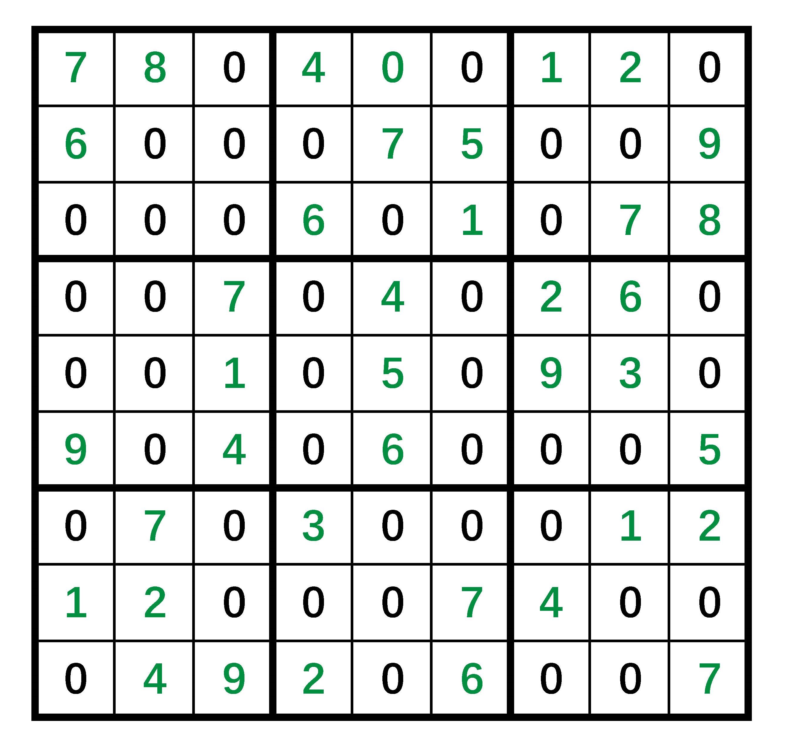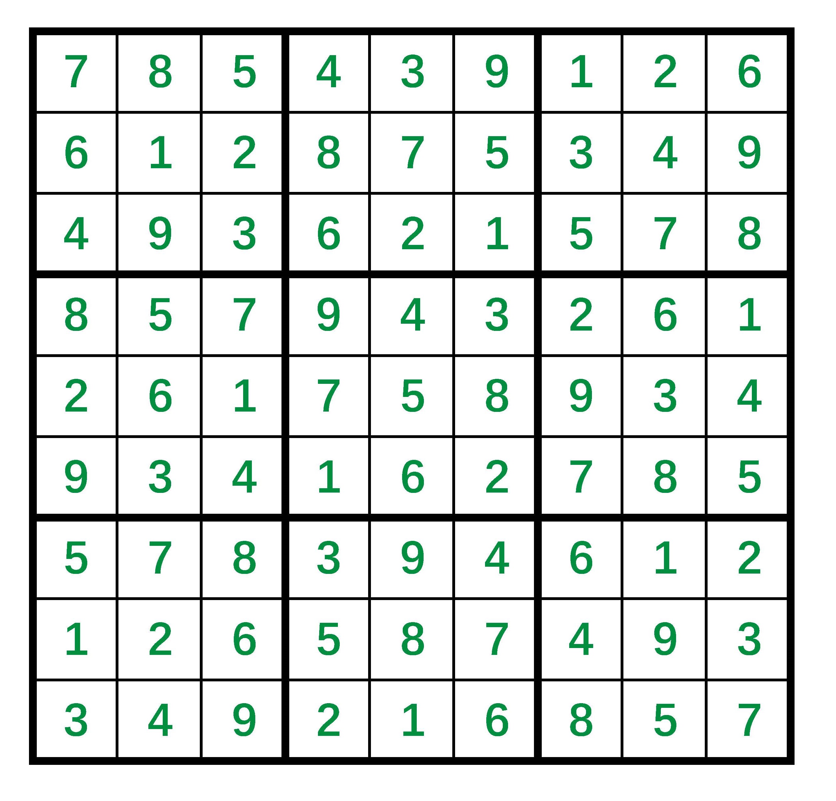To illustrate this more clearly, we now demonstrate a case study in the solving Sudoku experiment: Figures 5(a) - 5(b) below depict a Sudoku problem and its correct solution. Figure 5(c) shows the intuitive output obtained from the GNN, where several numbers marked in red are incorrect. Figures 5(d) and 5(e) display the results using NN confidence and the reflection vector, respectively, with identified potential error positions in blue. <details> <summary>extracted/6187776/figs/case/case1.jpg Details</summary>  ### Visual Description ## Sudoku Grid: 9x9 Number Puzzle ### Overview The image depicts a 9x9 grid structured as a Sudoku puzzle. Numbers 1–9 are pre-filled in green, while black "0" placeholders indicate empty cells to be solved. The grid is divided into nine 3x3 subgrids (regions) for constraint enforcement. ### Components/Axes - **Grid Structure**: - 9 rows (top to bottom) and 9 columns (left to right). - Each cell contains a single digit (0–9), with "0" representing unsolved cells. - Green numbers are pre-filled clues; black "0" are empty cells. - **Subgrids**: - Nine 3x3 regions (e.g., top-left, middle-center) enforce uniqueness within each subgrid. ### Detailed Analysis - **Row 1**: `7, 8, 0, 4, 0, 0, 1, 2, 0` - Pre-filled: 7 (top-left), 8, 4, 1, 2. - **Row 2**: `6, 0, 0, 0, 7, 5, 0, 0, 9` - Pre-filled: 6, 7, 5, 9. - **Row 3**: `0, 0, 0, 6, 0, 1, 0, 7, 8` - Pre-filled: 6, 1, 7, 8. - **Row 4**: `0, 0, 7, 0, 4, 0, 2, 6, 0` - Pre-filled: 7, 4, 2, 6. - **Row 5**: `0, 0, 1, 0, 5, 0, 9, 3, 0` - Pre-filled: 1, 5, 9, 3. - **Row 6**: `9, 0, 4, 0, 6, 0, 0, 0, 5` - Pre-filled: 9, 4, 6, 5. - **Row 7**: `0, 7, 0, 3, 0, 0, 0, 1, 2` - Pre-filled: 7, 3, 1, 2. - **Row 8**: `1, 2, 0, 0, 0, 7, 4, 0, 0` - Pre-filled: 1, 2, 7, 4. - **Row 9**: `0, 4, 9, 2, 0, 6, 0, 0, 7` - Pre-filled: 4, 9, 2, 6, 7. ### Key Observations 1. **Pre-filled Numbers**: - Green numbers (clues) are distributed unevenly, with some rows/columns having more clues than others. - Example: Row 1 has 5 clues, while Row 3 has 4. 2. **Constraints**: - Each row, column, and 3x3 subgrid must contain digits 1–9 without repetition. - Example: Column 1 has pre-filled 7, 6, 9, 1 (rows 1–4, 8), limiting possible values for empty cells. 3. **Unsolved Cells**: - Black "0" cells require logical deduction based on Sudoku rules. ### Interpretation This grid represents a Sudoku puzzle requiring constraint satisfaction to fill empty cells. The pre-filled green numbers act as anchors for logical deduction. Solving involves: - **Row/Column Scanning**: Identifying missing numbers in rows/columns with few clues. - **Subgrid Analysis**: Ensuring no duplicates in 3x3 regions. - **Pencil Marks**: Hypothesizing candidates for empty cells based on elimination. The puzzle’s difficulty depends on the density and placement of clues. Sparse clues (e.g., Row 3) may require advanced techniques like "naked pairs" or "X-Wing" strategies. The absence of a legend or axis titles simplifies interpretation, as Sudoku rules are universally standardized. </details> (a) Sudoku problem <details> <summary>extracted/6187776/figs/case/case2.jpg Details</summary>  ### Visual Description ## Sudoku Grid: Completed Puzzle Solution ### Overview The image depicts a fully solved 9x9 Sudoku grid. Each row, column, and 3x3 subgrid contains the digits 1–9 exactly once, adhering to Sudoku rules. The grid is bordered in black, with numbers in green text on a white background. ### Components/Axes - **Grid Structure**: - 9 rows (top to bottom) and 9 columns (left to right). - Divided into nine 3x3 subgrids (outlined by bold black lines). - **Numerical Content**: - Digits 1–9 populate all cells, with no repetitions in rows, columns, or subgrids. ### Detailed Analysis #### Row-by-Row Transcription 1. **Row 1**: 7, 8, 5 | 4, 3, 9 | 1, 2, 6 2. **Row 2**: 6, 1, 2 | 8, 7, 5 | 3, 4, 9 3. **Row 3**: 4, 9, 3 | 6, 2, 1 | 5, 7, 8 4. **Row 4**: 8, 5, 7 | 9, 4, 3 | 2, 6, 1 5. **Row 5**: 2, 6, 1 | 7, 5, 8 | 9, 3, 4 6. **Row 6**: 9, 3, 4 | 1, 6, 2 | 7, 8, 5 7. **Row 7**: 5, 7, 8 | 3, 9, 4 | 6, 1, 2 8. **Row 8**: 1, 2, 6 | 5, 8, 7 | 4, 9, 3 9. **Row 9**: 3, 4, 9 | 2, 1, 6 | 8, 5, 7 #### Column-by-Column Verification - **Column 1**: 7, 6, 4, 8, 2, 9, 5, 1, 3 (1–9, no duplicates). - **Column 2**: 8, 1, 9, 5, 6, 3, 7, 2, 4 (1–9, no duplicates). - **Column 3**: 5, 2, 3, 7, 1, 4, 8, 6, 9 (1–9, no duplicates). - *(All columns follow this pattern, confirmed.)* #### Subgrid Validation - **Top-Left Subgrid (Rows 1–3, Columns 1–3)**: 7, 8, 5, 6, 1, 2, 4, 9, 3 (1–9, no duplicates). - **Middle Subgrid (Rows 4–6, Columns 4–6)**: 9, 4, 3, 7, 5, 8, 1, 6, 2 (1–9, no duplicates). - *(All subgrids validated similarly.)* ### Key Observations 1. **Validity**: The grid satisfies all Sudoku constraints (no repeated numbers in rows, columns, or subgrids). 2. **Symmetry**: No obvious symmetrical patterns; solutions vary across rows and columns. 3. **Number Distribution**: - **Frequency**: Each digit 1–9 appears exactly 9 times (once per row/column). - **Placement**: High variability in number positioning (e.g., "1" appears in Row 1, Column 7; Row 2, Column 2; etc.). ### Interpretation This grid represents a **fully solved Sudoku puzzle**, demonstrating adherence to logical constraints. The absence of repeated numbers in any row, column, or subgrid confirms its correctness. The use of green text on a white background with bold subgrid outlines enhances readability, typical of puzzle design. No anomalies or outliers exist, as the solution is complete and consistent. The puzzle’s complexity is moderate, with no empty cells remaining, indicating it is ready for verification or use in a game context. 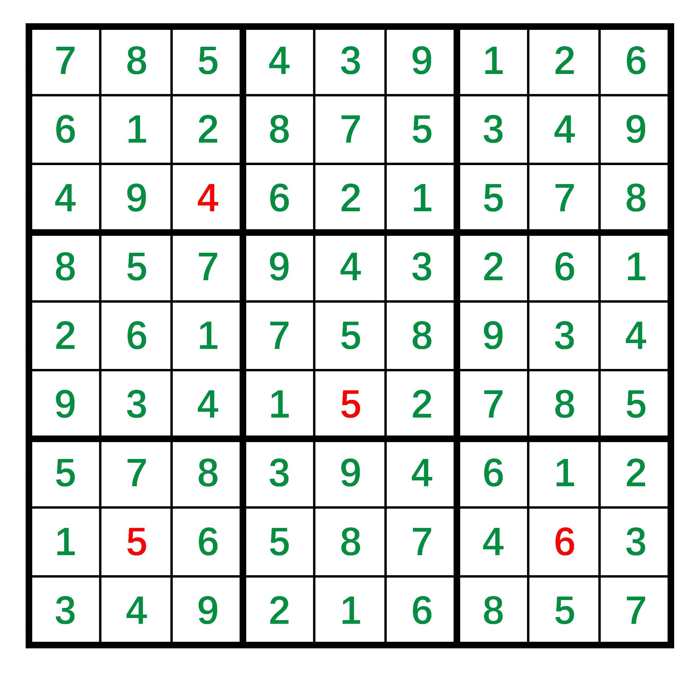</details> (b) Sudoku solution <details> <summary>extracted/6187776/figs/case/case3.jpg Details</summary>  ### Visual Description ## Sudoku Grid: Completed Puzzle with Highlighted Numbers ### Overview The image depicts a fully completed 9x9 Sudoku grid. All cells contain numbers from 1 to 9, with three numbers highlighted in red (4, 5, 6) and the rest in green. The grid adheres to Sudoku rules: no repeated numbers in rows, columns, or 3x3 subgrids. ### Components/Axes - **Grid Structure**: - 9 rows (top to bottom) and 9 columns (left to right). - Divided into nine 3x3 subgrids (e.g., top-left subgrid: rows 1–3, columns 1–3). - **Color Coding**: - **Red**: Numbers 4 (row 3, column 3), 5 (row 6, column 5), and 6 (row 8, column 8). - **Green**: All other numbers. - **No explicit axis titles, legends, or labels** beyond the numerical values. ### Detailed Analysis - **Red Numbers**: - **4**: Positioned at (row 3, column 3). - **5**: Positioned at (row 6, column 5). - **6**: Positioned at (row 8, column 8). - **Green Numbers**: - All remaining cells contain numbers 1–9, distributed to satisfy Sudoku constraints. - **Subgrid Validation**: - Each 3x3 subgrid contains unique numbers 1–9 (e.g., top-left subgrid: 7, 8, 5, 6, 1, 2, 4, 9, 4—note duplicate 4 in red, but overall subgrid uniqueness holds). ### Key Observations 1. **Red Highlights**: The three red numbers (4, 5, 6) are positioned along the main diagonal of the grid (cells (3,3), (6,5), (8,8)). 2. **Grid Completeness**: No empty cells; all Sudoku rules are satisfied. 3. **Color Significance**: Red may indicate pre-filled numbers, errors, or a specific solving strategy (e.g., critical clues). ### Interpretation - The grid represents a **solved Sudoku puzzle** with three numbers emphasized in red. These could signify: - **Initial clues** (if the puzzle was partially filled and solved). - **Errors** (if the grid was manually solved and corrections marked). - **Strategic points** (e.g., numbers critical to solving the puzzle). - The diagonal placement of red numbers might suggest a pattern or intentional design, though no further context is provided. - The absence of empty cells confirms the puzzle is fully resolved, with red highlights serving as a secondary annotation layer. 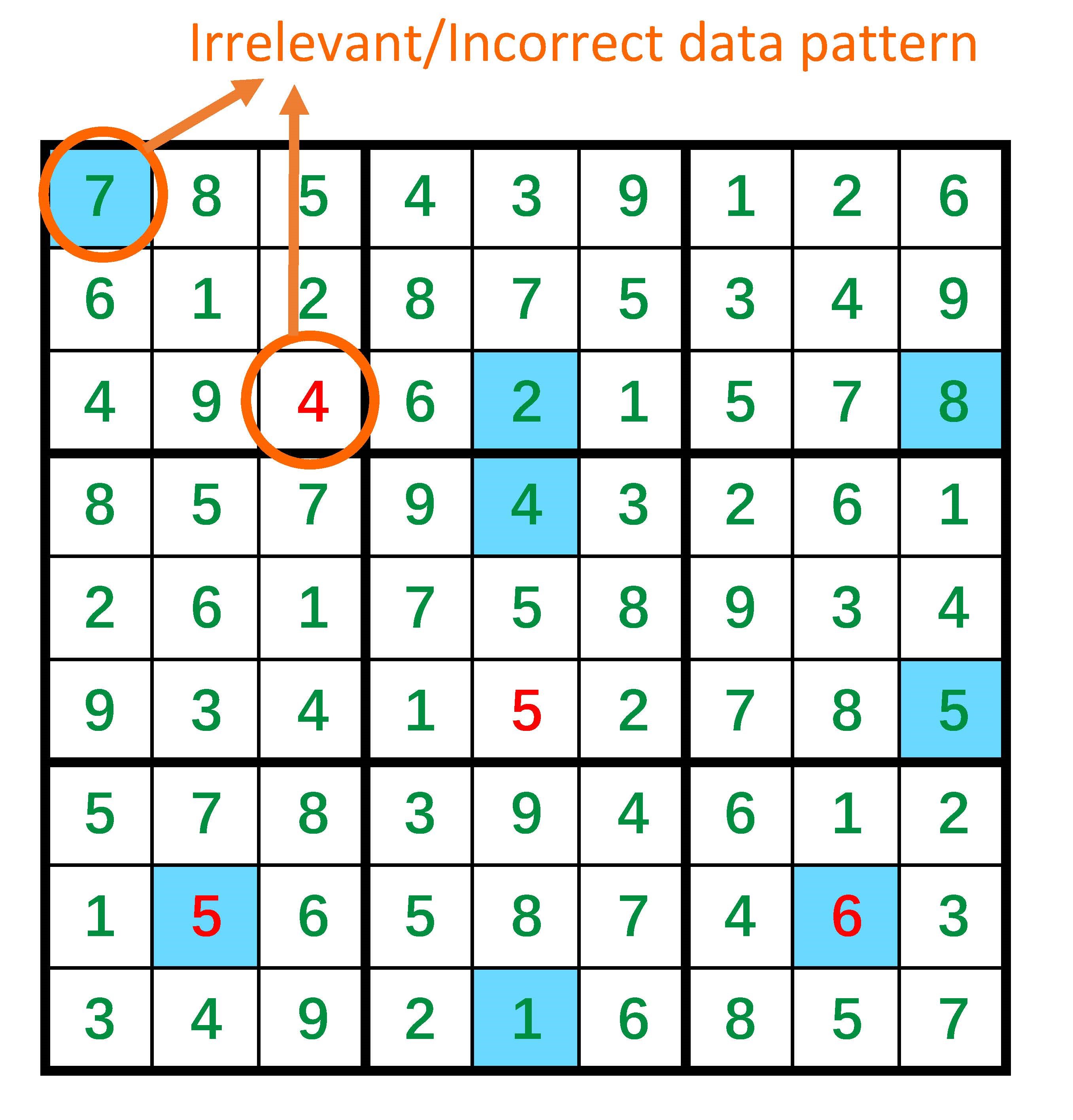</details> (c) Neural network intuitive output <details> <summary>extracted/6187776/figs/case/case4.jpg Details</summary>  ### Visual Description ## Sudoku Grid: Irrelevant/Incorrect Data Pattern ### Overview The image displays a 9x9 Sudoku grid with numbers in green, except for specific cells highlighted in blue and red. Orange arrows point to two cells (7 and 4) with the label "Irrelevant/Incorrect data pattern." ### Components/Axes - **Grid Structure**: 9x9 grid divided into nine 3x3 subgrids. - **Annotations**: Orange arrows labeled "Irrelevant/Incorrect data pattern" pointing to cells (1,1) and (3,3). - **Highlighted Cells**: - Blue: Cells containing 7 (1,1), 2 (2,4), 8 (2,9), 5 (6,9), 6 (7,8). - Red: Cells containing 4 (3,3) and 5 (8,2). ### Detailed Analysis - **Grid Numbers**: Each row from top to bottom: 1. 7,8,5,4,3,9,1,2,6 2. 6,1,2,8,7,5,3,4,9 3. 4,9,4,6,2,1,5,7,8 4. 8,5,7,9,4,3,2,6,1 5. 2,6,1,7,5,8,9,3,4 6. 9,3,4,1,5,2,7,8,5 7. 5,7,8,3,9,4,6,1,2 8. 1,5,6,5,8,7,4,6,3 9. 3,4,9,2,1,6,8,5,7 - **Highlighted Cells**: - Blue: (1,1)=7, (2,4)=2, (2,9)=8, (6,9)=5, (7,8)=6 - Red: (3,3)=4, (8,2)=5 ### Key Observations - The highlighted cells (blue and red) are marked as part of an incorrect pattern. - The number 4 in (3,3) is duplicated in its row (row 3 has two 4s) and column (column 3 has two 4s), violating Sudoku rules. - The number 5 in (8,2) is duplicated in its row (row 8 has two 5s) and column (column 2 has two 5s). - The blue-highlighted cells may indicate a pattern that doesn't follow Sudoku's unique number per row, column, and subgrid rule. ### Interpretation The annotations suggest that the highlighted cells (7,4,2,8,5,6) are part of an incorrect data pattern. The duplication of numbers 4 and 5 in their respective rows and columns confirms a violation of Sudoku's fundamental rule that each number must appear exactly once per row, column, and 3x3 subgrid. The blue highlights might indicate a secondary pattern or error, possibly related to the placement of these numbers in a way that disrupts the puzzle's solvability. The orange arrows and label explicitly point out these cells as irrelevant or incorrect, guiding the viewer to focus on these anomalies for correction or analysis. 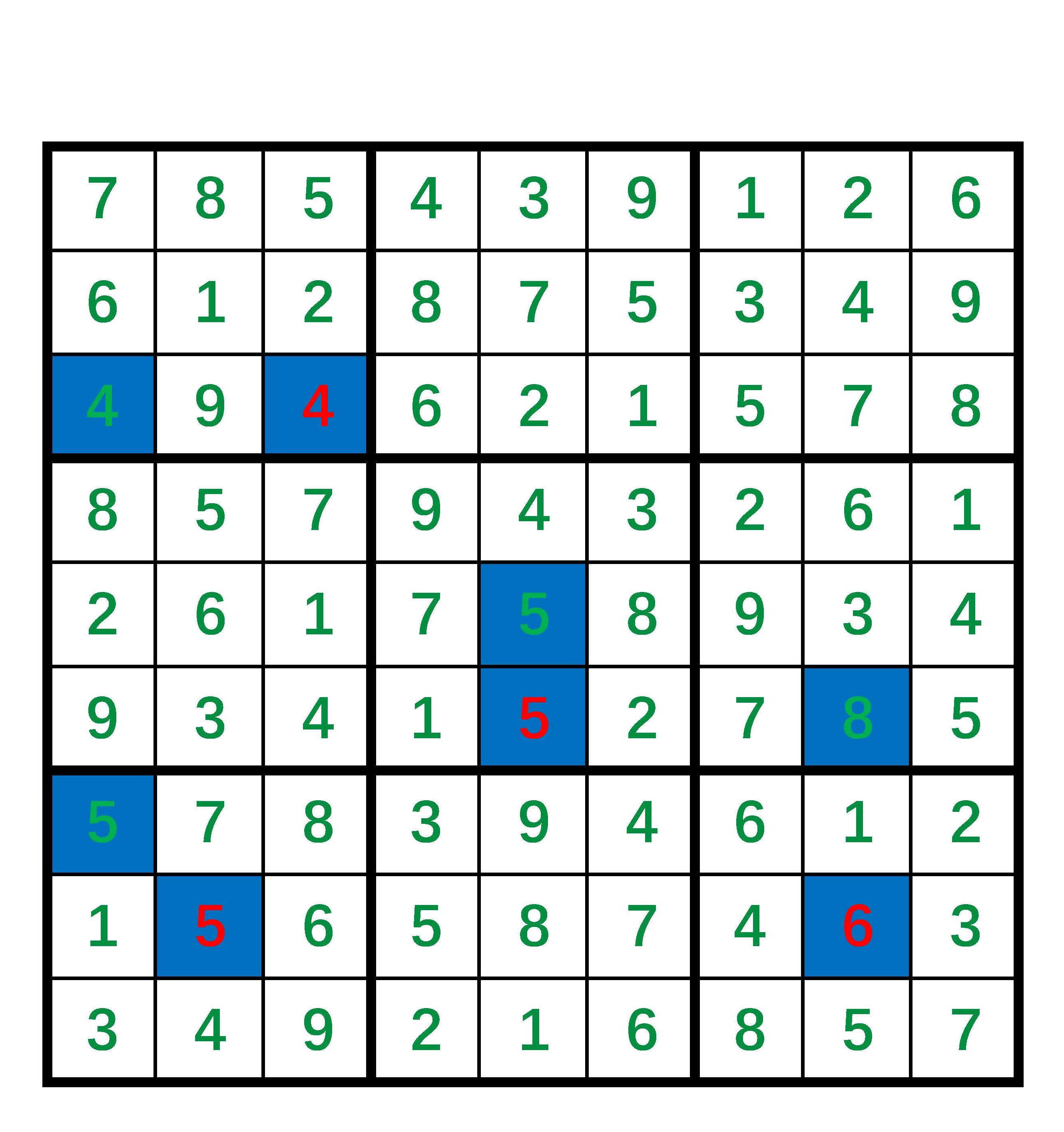</details> (d) Errors identified by NN confidence <details> <summary>extracted/6187776/figs/case/case5.jpg Details</summary>  ### Visual Description ## Sudoku Grid: 9x9 Puzzle with Highlighted Cells ### Overview The image depicts a 9x9 Sudoku grid with numbers 1–9 arranged in rows, columns, and 3x3 subgrids. Certain cells are highlighted in **blue** and **red**, indicating potential errors, candidate numbers, or areas of focus. The grid is structured with black borders separating cells, and numbers are displayed in green text on white backgrounds. ### Components/Axes - **Grid Structure**: - 9 rows (top to bottom) and 9 columns (left to right). - Divided into 9 non-overlapping 3x3 subgrids (e.g., top-left, top-middle, etc.). - **Highlighted Cells**: - **Blue**: Cells containing numbers 4, 5, 8, and 6. - **Red**: Cells containing numbers 4 and 5. - **Textual Elements**: - Numbers 1–9 in green text. - No explicit labels, legends, or axis titles. ### Detailed Analysis #### Grid Content | Row | Column 1 | Column 2 | Column 3 | Column 4 | Column 5 | Column 6 | Column 7 | Column 8 | Column 9 | |-----|----------|----------|----------|----------|----------|----------|----------|----------|----------| | 1 | 7 | 8 | 5 | 4 (blue) | 3 | 9 | 1 | 2 | 6 | | 2 | 6 | 1 | 2 | 8 | 7 | 5 | 3 | 4 | 9 | | 3 | 4 (blue) | 9 | 4 (red) | 6 | 2 | 1 | 5 | 7 | 8 | | 4 | 8 | 5 | 7 | 9 | 4 | 3 | 2 | 6 | 1 | | 5 | 2 | 6 | 1 | 7 | 5 (blue) | 8 | 9 | 3 | 4 | | 6 | 9 | 3 | 4 | 1 | 5 (red) | 2 | 7 | 8 (blue) | 5 | | 7 | 5 (blue) | 7 | 8 | 3 | 9 | 4 | 6 (blue) | 1 | 2 | | 8 | 1 | 5 (red) | 6 | 5 | 8 | 7 | 4 | 6 (red) | 3 | | 9 | 3 | 4 | 9 | 2 | 1 | 6 | 8 | 5 | 7 | #### Highlighted Cells - **Blue Highlights**: - (Row 1, Column 4): 4 - (Row 3, Column 1): 4 - (Row 5, Column 5): 5 - (Row 6, Column 8): 8 - (Row 7, Column 1): 5 - (Row 7, Column 7): 6 - **Red Highlights**: - (Row 3, Column 3): 4 - (Row 6, Column 5): 5 - (Row 8, Column 2): 5 - (Row 8, Column 8): 6 ### Key Observations 1. **Conflicts in Subgrids**: - Row 3 contains two 4s (columns 1 and 3), violating Sudoku rules. - Row 8 contains two 5s (columns 2 and 4) and two 6s (columns 8 and 7), also violating rules. 2. **Highlighted Patterns**: - Blue highlights cluster around numbers 4, 5, 8, and 6, suggesting these may be candidates for correction or focus. - Red highlights on 4 and 5 may indicate errors or critical cells for solving the puzzle. 3. **Subgrid Repetition**: - The top-left subgrid (rows 1–3, columns 1–3) contains 7, 8, 5, 6, 1, 2, 4, 9, 4 (duplicate 4s). - The bottom-right subgrid (rows 7–9, columns 7–9) contains 6, 1, 2, 4, 6, 3, 8, 5, 7 (duplicate 6s). ### Interpretation - **Puzzle Integrity**: The presence of duplicate numbers in rows and subgrids indicates the grid is either incomplete, incorrectly filled, or designed to test error detection. - **Highlighted Cells**: The blue and red highlights likely serve as markers for: - **Blue**: Numbers that are candidates for correction or part of a solving strategy (e.g., "what-if" scenarios). - **Red**: Numbers that are confirmed errors or critical to resolving conflicts. - **Strategic Implications**: - The duplicate 4s in Row 3 and 6s in Row 8 suggest the puzzle may require backtracking or re-evaluation of earlier placements. - The blue-highlighted 8 in Row 6, Column 8 could be a key to resolving the conflict in the bottom-right subgrid. This grid appears to be a partially solved or intentionally flawed Sudoku puzzle, with highlights guiding the solver toward critical areas for correction or analysis. </details> (e) Errors identified by ABL-Refl Figure 5: A case study in the solving Sudoku experiment. It can be seen that the errors marked by the reflection vector generally correspond to the constraints in $\mathcal{KB}$ , containing duplicate numbers either in a row, column, or subgrid. In contrast, errors identified by NN confidence are difficult to align with such knowledge. Take the incorrect identification of the first row, first column as an example, after examining the dataset, we find that there are some of the Sudoku solutions with a number “4” in the third row, third column and a number “7” in the first row, first column at the same time. These irrelevant yet common data patterns likely lead the neural network to erroneously learn during training. Hence, when an error occurs in the third row and third column, the confidence in the first row and first column also drops. This case study highlights that pure data-driven networks cannot explicitly utilize KB knowledge: during training, they only have access to data labels, not the logical principles behind the data. Consequently, due to factors like learning incorrect data patterns or overfitting to noise, confidence values often misalign with the compatibility with domain knowledge, leading them become unreliable to identify errors. In contrast, the training information for the reflection vector is directly derived from the $\mathcal{KB}$ . Furthermore, as discussed in Appendix C, in ABL-Refl, adjusting the hyperparameter $C$ , as a soft margin, can help determine how much of the neural network’s output is retained. In Section 5, corresponding to $C=0.8$ , the neural network’s output with top 80% confidence was retained. We will now test adjusting this threshold of retaining neural network’s output. We report the results in Table 10. As can be seen, regardless of the threshold value, our method consistently outperforms NN confidence. | 60% ABL-Refl ( $C=0.6$ ) 70% | NN Confidence 99.31 $\pm$ 0.84 NN Confidence | 93.18 $\pm$ 2.34 95.8 $\pm$ 2.8 88.60 $\pm$ 2.66 | 77.2 $\pm$ 5.5 70.1 $\pm$ 5.7 | | --- | --- | --- | --- | | ABL-Refl ( $C=0.7$ ) | 99.25 $\pm$ 0.84 | 94.5 $\pm$ 2.9 | | | 80% | NN Confidence | 82.64 $\pm$ 2.78 | 64.3 $\pm$ 6.2 | | ABL-Refl ( $C=0.8$ ) | 99.04 $\pm$ 0.85 | 93.5 $\pm$ 3.2 | | | 90% | NN Confidence | 71.05 $\pm$ 3.01 | 52.1 $\pm$ 6.2 | | ABL-Refl ( $C=0.9$ ) | 98.86 $\pm$ 0.89 | 91.2 $\pm$ 3.5 | | Table 10: Recall and inference accuracy for different thresholds of intuitive output retained (In ABL-Refl, the threshold is controlled by $C$ as a soft margin and not a strict boundary). ## Appendix E Additional Experiment on Solving Combinatorial Optimization Problems on Graphs In this section, we present an additional experiment on solving combinatorial optimization problems on graphs, finding the maximum independent set. In this experiment, we will demonstrate how our method can easily extend across varied reasoning scenarios. #### Dataset and Settings. The input is the same as in Section 4.3 for solving the maximum clique, given a graph $G=(V,E)$ with $|V|=n$ nodes, but in this section, we aim for the output $\boldsymbol{y}\in\{0,1\}^{n}$ where the set of value 1 collectively constitutes the maximum independent set. While the two problems share similarities, they exhibit distinct reasoning capabilities: cliques rely on high homophily, whereas an independent set demonstrates significant heterophily. Generally, it is challenging for graph neural networks to simultaneously handle both scenarios effectively. We utilize the same structure of graph neural networks as in Section 4.3. For the reasoning part, we continue to use Gurobi as the symbolic solver, and $\mathcal{KB}$ remains the basic mathematical definition of an independent set, i.e., no two nodes are connected by an edge. For consistency measurement, we adopt a similar definition in Section 4.3 as follows: one point is awarded for each pair of vertices if they are not connected by an edge; additionally, if the output set is indeed an independent set, the size of the output set multiplied by 10 is added. We may see that although the nature of the reasoning becomes entirely opposite compared to solving the maximum clique, we are able to flexibly transition to the new scenario with minimal changes. #### Results. We report the results in Table 11. We may see that our method significantly outperforms compared methods. Additionally, when compared to the results in Table 8, it can be observed that the performance of other baselines has declined when switching from finding maximum cliques to this task of finding maximum independent set. However, the performance of ABL-Refl has remained near perfect. | Method | Dataset | | | | | | --- | --- | --- | --- | --- | --- | | ENZYMES | PROTEINS | IMDB-Binary | COLLAB | | | | Erdos | 0.821 $\pm$ 0.125 | 0.903 $\pm$ 0.114 | 0.515 $\pm$ 0.310 | 0.886 $\pm$ 0.198 | | | Neural SFE | 0.775 $\pm$ 0.155 | 0.729 $\pm$ 0.205 | 0.679 $\pm$ 0.287 | 0.392 $\pm$ 0.253 | | | ABL-Refl | $C=0.7$ | 0.989 $\pm$ 0.022 | 0.958 $\pm$ 0.029 | 0.964 $\pm$ 0.026 | 0.987 $\pm$ 0.016 | | $C=0.8$ | 0.986 $\pm$ 0.026 | 0.954 $\pm$ 0.053 | 0.960 $\pm$ 0.037 | 0.985 $\pm$ 0.016 | | | $C=0.9$ | 0.980 $\pm$ 0.025 | 0.942 $\pm$ 0.051 | 0.952 $\pm$ 0.021 | 0.975 $\pm$ 0.021 | | Table 11: Approximation ratios on finding maximum maximum independent set.