# Aristotle: Mastering Logical Reasoning with A Logic-Complete Decompose-Search-Resolve Framework
> Corresponding author: Hao Fei
## Abstract
In the context of large language models (LLMs), current advanced reasoning methods have made impressive strides in various reasoning tasks. However, when it comes to logical reasoning tasks, major challenges remain in both efficacy and efficiency. This is rooted in the fact that these systems fail to fully leverage the inherent structure of logical tasks throughout the reasoning processes such as decomposition, search, and resolution. To address this, we propose a logic-complete reasoning framework, Aristotle, with three key components: Logical Decomposer, Logical Search Router, and Logical Resolver. In our framework, symbolic expressions and logical rules are comprehensively integrated into the entire reasoning process, significantly alleviating the bottlenecks of logical reasoning, i.e., reducing sub-task complexity, minimizing search errors, and resolving logical contradictions. The experimental results on several datasets demonstrate that Aristotle consistently outperforms state-of-the-art reasoning frameworks in both accuracy and efficiency, particularly excelling in complex logical reasoning scenarios. We will open-source all our code at http://llm-symbol.github.io/Aristotle.
## 1 Introduction
LLMs Patel et al. (2023); Chowdhery et al. (2023) have unlocked unprecedented potential in semantic understanding Zhao et al. (2023), sparking immense hope for realizing AGI. A fundamental requirement for true intelligence is the ability to perform human-level reasoning, such as commonsense reasoning Wang et al. (2024c), mathematical problem-solving Wang et al. (2024a), and geometric reasoning Eisner et al. (2024). To achieve this, researchers have drawn inspiration from human reasoning processes, proposing various methods and strategies for LLM-based reasoning. One of the most groundbreaking works is the Chain-of-Thought (CoT) Wei et al. (2022), which breaks down complex problems into smaller sub-problems, solving them step by step. The birth of CoT has elevated the reasoning capabilities of LLMs to new heights. Further research has built on this foundation by closely emulating human cognitive patterns, introducing more advanced approaches, such as Least-to-Most Zhou et al. (2023), Tree-of-Thought (ToT) Yao et al. (2023), Graph-of-Thought (GoT) Besta et al. (2024), and Plan-and-Solve Wang et al. (2023a), which have achieved progressively better results on reasoning benchmarks. In summary, successful LLM-based reasoning methods generally involve three key modules Huang and Chang (2023); Li et al. (2024): problem decomposition, path searching, and problem resolution.
<details>
<summary>x1.png Details</summary>
### Visual Description
## Bar Chart Comparison: Error Rate and Reasoning Steps
### Overview
The image displays a two-panel bar chart comparing the performance of two methods, labeled "ToT" (blue bars) and "Ours" (red bars). The left panel compares "Error Rate (%)" across two categories, "SE" and "RE." The right panel compares the number of "Reasoning Steps" for a single, unspecified category. The chart visually emphasizes the reduction in both error rate and reasoning steps achieved by the "Ours" method relative to "ToT."
### Components/Axes
* **Legend:** Positioned at the top center. Contains two entries:
* A blue rectangle labeled "ToT".
* A red rectangle labeled "Ours".
* **Left Chart (Error Rate):**
* **Y-axis:** Labeled "Error Rate (%)". Scale markers at 0, 10, 20, and 30.
* **X-axis:** Two categorical labels: "SE" and "RE".
* **Right Chart (Reasoning Steps):**
* **Y-axis:** Labeled "Reasoning Steps". Scale markers at 0, 10, 20, and 30.
* **X-axis:** No explicit label. Contains a single pair of bars.
* **Data Annotations:** Red downward-pointing arrows with numerical labels indicate the absolute reduction from the "ToT" value to the "Ours" value.
### Detailed Analysis
**Left Panel: Error Rate (%)**
* **Category SE:**
* **ToT (Blue Bar):** Value is explicitly labeled as **15.0**.
* **Ours (Red Bar):** The bar is significantly shorter. A red arrow points from the top of the ToT bar down to the top of the Ours bar, labeled **-11.1**. This indicates the "Ours" error rate is approximately 15.0 - 11.1 = **3.9%**.
* **Category RE:**
* **ToT (Blue Bar):** Value is explicitly labeled as **28.4**.
* **Ours (Red Bar):** The bar is very short, near the baseline. A red arrow points from the top of the ToT bar down to the top of the Ours bar, labeled **-28.0**. This indicates the "Ours" error rate is approximately 28.4 - 28.0 = **0.4%**.
**Right Panel: Reasoning Steps**
* **ToT (Blue Bar):** Value is explicitly labeled as **24.6**.
* **Ours (Red Bar):** The bar is shorter. A red arrow points from the top of the ToT bar down to the top of the Ours bar, labeled **-12.9**. This indicates the "Ours" method uses approximately 24.6 - 12.9 = **11.7** reasoning steps.
### Key Observations
1. **Consistent Superiority:** The "Ours" method outperforms "ToT" on all presented metrics, showing both lower error rates and fewer reasoning steps.
2. **Magnitude of Improvement:** The reduction is most dramatic in the "RE" error rate, where the error drops by 28.0 percentage points (a ~98.6% relative reduction). The reduction in reasoning steps is also substantial, cutting the count by more than half.
3. **Visual Design:** The use of red downward arrows directly on the chart provides an immediate, quantitative understanding of the improvement without requiring the viewer to calculate differences from the axis.
### Interpretation
This chart is designed to convincingly demonstrate the effectiveness of a proposed method ("Ours") against a baseline or alternative method ("ToT"). The data suggests that "Ours" is not only more accurate (lower error rates) but also more efficient (requires fewer reasoning steps). The near-elimination of error in the "RE" category is a particularly strong result.
The pairing of error rate and reasoning steps implies a relationship between efficiency and accuracy. The chart argues that the "Ours" method achieves better outcomes *while* using a simpler or more direct reasoning process, which is a highly desirable property in computational or AI systems. The clear, annotated presentation is typical of a research paper or technical report aiming to highlight a significant methodological advancement.
</details>
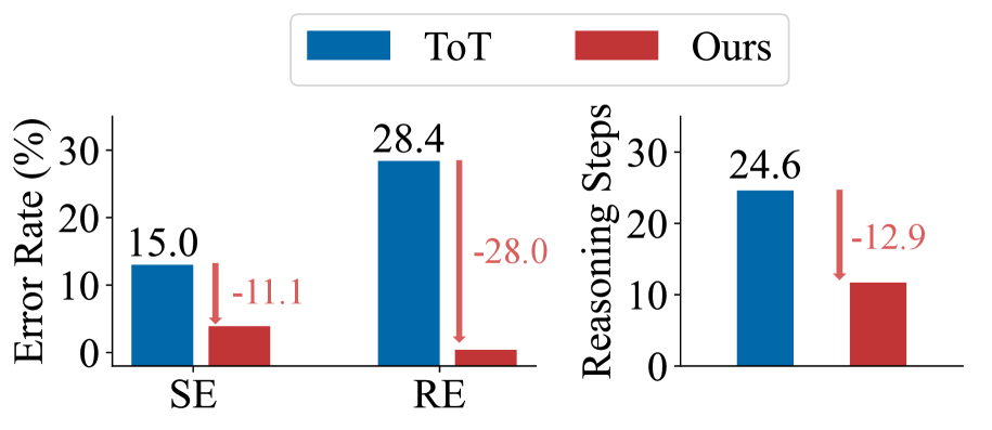
Figure 1: Our reasoning framework vs. the SoTA ToT: comparison in terms of Search Error (SE) and single-step Reasoning Error (RE), as well as in terms of average number of reasoning steps.
<details>
<summary>x2.png Details</summary>
### Visual Description
\n
## Logical Reasoning Flowchart: Automated Theorem Proving Process
### Overview
This image is a detailed flowchart illustrating a multi-step automated logical reasoning system designed to evaluate a given premise and question. The system decomposes natural language into formal logic, searches for contradictions through iterative resolution, and concludes whether a statement is true or false. The process is divided into three main phases: Search Initialization, Search and Resolve, and Conclude Answer.
### Components/Axes
The diagram is organized into three vertical columns corresponding to the three main steps. Key components include:
- **Raw Input**: Contains the initial natural language premise and question.
- **Translated and Decomposed**: Shows the logical formalization of the input.
- **Initialization**: Defines the starting logical clauses for the reasoning engine.
- **Search and Resolve**: The core processing loop containing a **Resolver**, **Search Router**, and mechanisms for checking **Current Clauses** against **Complementary Clauses**.
- **Reasoning Complete?**: A decision diamond that checks for contradictions.
- **Proof**: A box showing the logical proof structure.
- **Reasoning Trajectories**: A detailed side panel showing the step-by-step evolution of clauses across three reasoning rounds.
- **Final answer**: The concluding output.
**Visual Elements & Spatial Grounding:**
- **Colors**: Blue boxes represent resolved or current clauses. Pink boxes represent complementary clauses or contradiction states. Yellow boxes represent inputs, outputs, or key decisions. Green and purple boxes represent processing modules (Translator, Decomposer).
- **Arrows**: Gray arrows indicate the primary flow of data and control between steps. Dashed arrows indicate feedback loops or secondary data flow.
- **Layout**: The main process flows from top-left (Raw Input) down through the center column. The "Reasoning Trajectories" panel is positioned to the right of the main flow, providing a detailed audit trail.
### Detailed Analysis
#### Step 1: Search Initialization
* **Raw Input (Top-Left)**:
* **Premise (P):** "If people are nice, then they are nice. If people are smart, then they are patient. Dave is Smart."
* **Question (S):** "Dave is nice."
* **(True/False/Unknown/Self-Contradiction)**
* **Translated and Decomposed (Below Raw Input)**:
* The premise and question are processed by a **Translator** and **Decomposer**.
* **Premises (Pn):**
1. `Patient(x, False) ∨ Nice(x, True)`
2. `Patient(x, False) ∨ Patient(x, True)`
3. `Smart(x, False) ∨ Patient(x, True)`
* **Question (Sn):** `Nice(Dave, True)`
* **Initialization (Bottom-Left)**:
* **Sn:** `Nice(Dave, True)`
* **¬Sn:** `Nice(Dave, False)` (The negation of the question).
* The system initializes with the question and its negation, along with the list of premises (Pn) ①, ②, ③.
#### Step 2: Search and Resolve (Center Column)
This is an iterative loop.
1. **Search Router** selects a **Current Clause** (starting with `¬Sn: Nice(Dave, False)`) and the set of **Premises (Pn)**.
2. The **Resolver** attempts to find a **Complementary Clause** from the premises that can be resolved with the current clause.
3. The system checks for contradictions.
* **First Pass:** With `Current Clause: ¬Sn: Nice(Dave, False)`, it finds **Complementary Clause ①:** `Patient(x, False) ∨ Nice(x, True)`. The result is `Resolved Clause: Patient(Dave, False)` with the note "No Contradiction".
* The process loops back ("Reasoning Complete? -> No") with the new resolved clause as the current clause.
#### Step 3: Conclude Answer & Reasoning Trajectories (Right Panel)
The right panel details the three rounds of reasoning that occur within the "Search and Resolve" loop.
* **Start 2nd Round:**
* **Current Clause:** `¬Sn: Nice(Dave, False)` (This appears to be a reset or carry-over; the main flow had `Patient(Dave, False)`).
* **Complementary Clause ①:** `Patient(x, False) ∨ Nice(x, True)`
* **Resolved Clause:** `Patient(Dave, False)` (No contradiction).
* **Start 3rd Round:**
* **Current Clause:** `Patient(Dave, False)`
* **Complementary Clause ②:** `Smart(x, False) ∨ Patient(x, True)`
* **Resolved Clause:** `Smart(Dave, False)` (No contradiction).
* **Final Round (Implied):**
* **Current Clause:** `Smart(Dave, False)`
* **Complementary Clause ③:** `Smart(x, False) ∨ Patient(x, True)`
* **Resolved Clause:** `Contradiction!` (Resolving `Smart(Dave, False)` with `Smart(x, False) ∨ Patient(x, True)` yields `Patient(Dave, True)`, which contradicts the earlier derived `Patient(Dave, False)`).
* **Proof:** `D_Sn = Pn ⊢ Sn` and `D_¬Sn = Pn ⊢ ¬Sn`. The system has derived both the question (`Sn`) and its negation (`¬Sn`) from the premises, indicating a self-contradiction in the original premise set.
**Final Answer (Bottom Center):** "The answer is **True**." This is derived from the proof box `D_Sn = Pn ⊢ Sn`, meaning the premises logically entail the question `Sn: Nice(Dave, True)`.
### Key Observations
1. **Self-Contradictory Premises:** The logical decomposition reveals that the original natural language premise "If people are nice, then they are nice" is a tautology (always true) and adds no constraint. The core issue arises from the interaction of the other premises, which ultimately lead to a contradiction (`Patient(Dave, False)` and `Patient(Dave, True)`).
2. **Reasoning Path:** The system does not directly prove `Nice(Dave, True)`. Instead, it attempts to prove the negation (`Nice(Dave, False)`), fails by deriving a contradiction, and therefore concludes the original statement must be true (a form of proof by contradiction or reductio ad absurdum).
3. **Visual Audit Trail:** The "Reasoning Trajectories" panel is crucial for debugging and understanding the step-by-step logical inferences, showing exactly which clauses were combined at each stage.
### Interpretation
This flowchart demonstrates a **resolution-based theorem prover** applied to a logical puzzle. It showcases the core challenges in automated reasoning: translating ambiguous natural language into precise formal logic and navigating complex inference chains.
The process highlights that the initial premise set is **inconsistent**. The statement "Dave is nice" is deemed **True** not because it is directly supported, but because assuming its opposite (`Dave is not nice`) leads to a logical impossibility given the other premises. This is a classic example of how formal systems handle contradictions—they expose them rather than ignore them.
The diagram serves as a technical specification for such a system, detailing the data structures (clauses), control flow (search and resolve loop), and proof logging (trajectories). It emphasizes the importance of **clause management** and **contradiction detection** as the engine of logical deduction. The final answer "True" is a consequence of the system's design to return the original statement if its negation is unsatisfiable, even if the underlying premise set is flawed.
</details>
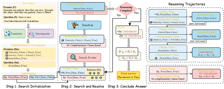
Figure 2: Our Aristotle logical reasoning framework (best viewed via zooming in). In step 1, the
<details>
<summary>figure/translation.png Details</summary>

### Visual Description
## Diagram: Language Translation/Exchange Icon
### Overview
The image is a stylized, flat-design icon or diagram representing a bidirectional language translation or communication process. It features two primary symbolic elements connected by curved arrows, suggesting a continuous cycle or exchange.
### Components/Axes
The diagram is composed of four main visual components arranged on a light gray background:
1. **Top-Left Element:** A light purple, rounded speech bubble shape. Inside it is a large, dark gray Chinese character: **文**.
2. **Bottom-Right Element:** A bright blue, rounded shape resembling a document or speech bubble. Inside it is a large, dark gray capital letter: **A**.
3. **Top-Right Arrow:** A dark gray, curved arrow originating from the blue "A" shape and pointing towards the purple "文" bubble.
4. **Bottom-Left Arrow:** A dark gray, curved arrow originating from the purple "文" bubble and pointing towards the blue "A" shape.
### Detailed Analysis
* **Textual Content:**
* **Chinese Character:** **文** (Pronounced: *wén*). This character means "text," "language," "writing," or "culture." It is rendered in a bold, sans-serif style.
* **Latin Letter:** **A**. This is a standard, bold, sans-serif capital "A." In this context, it most likely represents the Latin alphabet or the English language, potentially as an abbreviation for "Alpha" or simply as a symbol for Western languages.
* **Spatial Relationships & Flow:**
* The two main elements are placed diagonally opposite each other (top-left and bottom-right).
* The arrows create a clear, clockwise circular flow between the two elements. The top arrow indicates a process from "A" to "文," and the bottom arrow indicates a process from "文" to "A."
* The design uses a limited color palette: light purple (#E6E6FA approx.), bright blue (#00BFFF approx.), dark gray (#333333 approx.), and a light gray background (#F0F0F0 approx.).
### Key Observations
* The diagram is abstract and symbolic rather than literal. It does not depict actual translation software or a specific user interface.
* The use of a single Chinese character and a single Latin letter is a minimalist representation of two distinct language systems.
* The curved arrows are of equal weight and style, implying a balanced, reciprocal relationship between the two language systems.
* The shapes (speech bubble/document) are generic and could represent dialogue, text input, or documents.
### Interpretation
This diagram is a conceptual representation of **bidirectional translation or linguistic exchange**.
* **What it suggests:** The core idea is the conversion or communication between two different language domains, symbolized by Chinese (文) and a Latin-based language (A). The cyclic arrows emphasize that this is not a one-way translation but an ongoing, interactive process—like a conversation, real-time translation, or the work of a bilingual system.
* **How elements relate:** The "文" and "A" are the core subjects. The speech bubble shapes frame them as units of communication. The arrows define the relationship between them as dynamic and reciprocal.
* **Notable Anomalies/Inferences:** The choice of "A" is interesting. It could be a placeholder for any Latin-alphabet language, or it might specifically reference "Alpha," hinting at a project name or a first version (e.g., "Healer Alpha" from the system prompt). The diagram's simplicity makes it versatile for representing concepts like machine translation, cross-cultural communication, language learning, or API integration between systems using different languages. The lack of additional text or labels makes its meaning broad and open to interpretation within the context of language technology.
</details>
Translator and
<details>
<summary>figure/decomposer.png Details</summary>
### Visual Description
\n
## Diagram: Hierarchical Tree Structure
### Overview
The image displays a simple, three-level hierarchical tree diagram or organizational chart. It consists of colored, rounded rectangular boxes connected by solid blue lines, indicating a parent-child or branching relationship. The diagram is presented on a plain, light gray background. There is **no textual information** (labels, titles, or data) present within any of the boxes or elsewhere in the image.
### Components/Axes
* **Nodes:** Six rounded rectangular boxes, each with a distinct color and a subtle 3D effect created by a darker shade on the left and top edges.
* **Connections:** Solid, medium-blue lines that connect the boxes, forming the hierarchical structure. The lines branch at right angles.
* **Layout:** The diagram is structured in three distinct horizontal levels.
* **Level 1 (Top):** A single yellow box, centered horizontally.
* **Level 2 (Middle):** Two boxes. A red box is positioned to the left of the center line, and a green box is positioned to the right.
* **Level 3 (Bottom):** Three boxes. From left to right: a green box, a yellow box, and a blue box. They are evenly spaced across the width of the diagram.
### Detailed Analysis
* **Spatial Grounding & Structure:**
* The top (yellow) box is the root node. A single blue line descends from its bottom center.
* This line connects to a horizontal blue bar that spans the width between the two middle-level boxes.
* From this horizontal bar, two vertical lines descend to connect to the top centers of the red (left) and green (right) boxes.
* From the bottom center of the red box, a blue line descends to a second, wider horizontal bar.
* From the bottom center of the green box, a blue line also descends to connect to the same horizontal bar.
* From this second horizontal bar, three vertical lines descend to connect to the top centers of the three bottom-level boxes (green, yellow, blue).
* **Color Palette:**
* **Yellow:** Used for the top-level node and the center node of the bottom level.
* **Red:** Used for the left node of the middle level.
* **Green:** Used for the right node of the middle level and the left node of the bottom level.
* **Blue:** Used for the right node of the bottom level and for all connecting lines.
* **Trend Verification:** Not applicable, as this is a structural diagram, not a data chart. The "flow" is strictly top-down and branching.
### Key Observations
1. **Absence of Text:** The most significant observation is the complete lack of any textual labels, identifiers, or data within the diagram. Its meaning is entirely abstract.
2. **Color Repetition:** The colors yellow and green are each used twice, while red and blue are used once for a node. The blue color is exclusively used for the connecting lines and one final node.
3. **Symmetry and Asymmetry:** The structure is symmetrical at the first branching (one node to two), but becomes asymmetrical at the second branching, as the left parent (red) and right parent (green) both connect to all three child nodes, rather than each having their own distinct set.
4. **Visual Style:** The design is flat with minimal depth cues (the 3D shading on the boxes). It uses a simple, clean, and modern aesthetic suitable for presentations or conceptual illustrations.
### Interpretation
This diagram is a **template or abstract representation** of a hierarchical system. Its meaning is not defined by the image itself but would be provided by context or accompanying text.
* **What it demonstrates:** It visually models a one-to-many, multi-level relationship. The top node is the primary category or origin. It splits into two secondary categories. Both of these secondary categories then share or contribute to three tertiary items or outcomes at the bottom level.
* **How elements relate:** The blue lines explicitly define the relationships and flow of authority, dependency, or categorization. The shared connection from both middle nodes to all bottom nodes suggests a **matrix or combined influence** structure, rather than a strict, siloed tree. For example, the bottom three items could be projects that receive input from both departments (red and green).
* **Notable anomalies:** The key anomaly is the **lack of semantic content**. Without labels, the diagram is purely syntactic. The color choices appear arbitrary for meaning-coding but may be for visual distinction. The structure implies that the two middle-level entities have equal standing and identical relationships to the bottom level, which is a specific and notable organizational pattern.
**In summary, this is a blank structural template for a two-tiered hierarchy where two parent nodes jointly oversee three child nodes. To extract factual information, the boxes would need to be populated with text.**
</details>
Decomposer together transform $P$ and $S$ into $P_n$ and $S_n$ . Then, we initialize the $C_current$ using the decomposed $S_n$ and $¬ S_n$ . In step 2, the
<details>
<summary>x5.png Details</summary>

### Visual Description
Icon/Small Image (29x29)
</details>
Search Router uses the $C_current$ and $P_n$ to search for $C_complement$ . The
<details>
<summary>x6.png Details</summary>

### Visual Description
Icon/Small Image (29x29)
</details>
Resolver then resolves $C_current$ with $C_complement$ to produce $C_resolved$ . The reasoning complete if: (1) the $C_resolved$ determines whether a contradiction exists; (2) reach the maximum number of iterations $I_max$ . In step 3, Aristotle then concludes the Proof $D_S_{n}$ and $D_¬ S_{n}$ based on the Proof Determination. Using these proofs, Aristotle determines the final answer based on Eq. (1). Note that two distinct reasoning paths will be implemented: a solid box representing the path starting from $¬ S_n$ , and a dotted box representing the path starting from $S_n$ . The complete reasoning process for both two paths, including all iterations are shown in the right part “ Reasoning Trajectories ”.
Compared to other forms of general reasoning, logical reasoning Huang and Chang (2023) stands out as one of the most challenging tasks, as it demands the strictest evidence, arguments, and logical rigor to arrive at sound conclusions or judgments. Logical reasoning more closely mirrors human-level cognitive processes, making it crucial in high-stakes domains such as mathematical proof generation, legal analysis, and scientific discovery Cummins et al. (1991); Markovits and Vachon (1989). In recent years, numerous studies have investigated how to integrate LLMs into logical reasoning. For example, some methods Pan et al. (2023); Gao et al. (2023) use LLMs to translate textual problems into symbolic expressions, which are then addressed by external logic solvers. Subsequent work, such as SymbCoT Xu et al. (2024), suggests that LLMs themselves can handle both symbolic translation and logic resolution, thus avoiding potential information loss caused when using external solvers. While SymbCoT has achieved state-of-the-art (SoTA) performance, the inherent simplicity of CoT’s linear reasoning process leaves considerable room for further improvement in LLM-based logical reasoning.
In response, certain research Yao et al. (2023); Besta et al. (2024); Zhang et al. (2023) has applied sophisticated general-purpose reasoning methods (e.g., ToT, GoT) directly to logical reasoning tasks. Unfortunately, these approaches largely overlook the inherent structure of logical tasks and fail to effectively integrate logical rules into the decompose-search-resolve framework, leaving key issues unresolved in both reasoning efficacy and efficiency:
$\blacktriangleright$ From an efficacy perspective, first, when LLMs decompose logical problems, they often rely on the linguistic token relations rather than the underlying logical structure, leading to disconnected sub-problems and faulty reasoning. Specifically, when reasoning hinges on specific logical relationships, neglecting them can result in disjointed sub-problems, breaking the logical chain and ultimately leading to incorrect conclusions. Furthermore, during the search stage, current path search methods rely heavily on evaluators that may be unreliable, selecting nodes based on possibly flawed logic, causing error propagation through subsequent reasoning steps Chen et al. (2024); Wang et al. (2024b). For the resolving step, these methods guide LLMs to solve sub-questions with simple text prompts, which frequently contain logical errors, resulting in numerous faulty nodes in the search space Xu et al. (2024). These errors propagate through subsequent reasoning steps, causing entire paths to fail and leading to reasoning failure. Our preliminary experiments reveal that directly applying SoTA general-purpose reasoning methods with a search mechanism to logical tasks results in significant errors, with 28.4% for reasoning and 15.0% for search, as shown in Fig. 1.
$\blacktriangleright$ From an efficiency perspective, these approaches also lead to significant shortcomings. For example, generating large numbers of incorrect nodes wastes computational resources Ning et al. (2024). Moreover, relying on unreliable evaluators introduces bias into the search process, leading to unnecessary node and path explorations, ultimately reducing efficiency Chen et al. (2024). We note that inefficient logical reasoning systems can significantly undermine their value in practical application scenarios.
To address these challenges, we propose a novel reasoning framework, Aristotle, which effectively tackles the performance and the efficiency bottlenecks in existing logical reasoning tasks by completely integrating symbolic expressions and rules into each stage of the decomposition, search, and resolution. Fig. 2 illustrates the overall framework. Specifically, we first introduce a Logical Decomposer that breaks down the original problem into smaller and simpler components based on its logical structure, reducing the complexity of logical tasks. We then devise a Logical Search Router, which leverages proof by contradiction to directly search for logical inconsistencies, thereby reducing search errors from unreliable evaluators and minimizing the number of steps required by existing methods. Finally, we develop a Logical Resolver, which rigorously resolves logical contradictions at each reasoning step, guided by the Logical Search Router. Overall, Aristotle thoroughly considers the inherent logical structure of tasks, fully incorporating logical symbols into the entire decompose-search-resolve framework. This ensures a more logically coherent reasoning process, leading to more reliable final results.
We conducted experiments across multiple logical reasoning benchmarks, where our method surpasses the current SoTA baselines by 4.5% with GPT-4 and 5.4% with GPT-4o. Further analysis revealed that the decomposer, search router, and resolver modules each contributed to: (i) reducing task complexity during problem decomposition, leading to improved accuracy in subsequent search and reasoning phases; (ii) focusing search efforts on the most direct and relevant paths, which reduced errors and enhanced efficiency; (iii) achieving near-perfect logical reasoning accuracy. Moreover, we observe that Aristotle delivers even greater performance improvements in complex scenarios, such as those with more intricate logical structures or longer reasoning chains. Overall, this work marks the first successful complete integration of symbolic logic expressions into every stage of an LLM-based reasoning framework (decomposition, search, and resolution), demonstrating that LLMs can perform complete logical reasoning over symbolic structures.
## 2
<details>
<summary>figure/aristotle_icon.png Details</summary>

### Visual Description
## Icon: Stylized Male Figure
### Overview
The image is a simple, flat-design icon depicting the head and shoulders of a stylized male figure. It uses a limited color palette with bold black outlines, characteristic of icon sets used in user interfaces or digital illustrations. There is no embedded text, data, or complex diagrammatic flow.
### Components/Design Elements
The icon is composed of several distinct visual components:
1. **Head & Hair:** A rounded head shape with a gray area representing hair on top and a full gray beard and mustache. The hairline is defined by a curved black line.
2. **Face:** A peach-colored facial area containing:
* **Eyes:** Two simple, solid black oval dots.
* **Eyebrows:** Two short, curved black lines above the eyes.
* **Nose:** A small, curved black line.
* **Mouth:** A simple, horizontal black line within the beard area.
3. **Ears:** Two peach-colored, semi-circular shapes on either side of the head.
4. **Clothing/Shoulders:** A light blue-gray area below the head, suggesting a shirt or tunic. A single black diagonal line runs from the lower left towards the upper right, indicating a fold or seam in the fabric.
5. **Outline:** All elements are defined by consistent, medium-weight black outlines.
### Detailed Analysis
* **Color Palette:**
* **Primary Fill Colors:** Gray (hair/beard), Peach (skin), Light Blue-Gray (clothing).
* **Outline/Detail Color:** Black.
* **Background:** The icon is presented on a plain, light gray background.
* **Style:** The design is minimalist and symbolic, not realistic. It uses geometric shapes and clean lines. The figure has a neutral, perhaps slightly stern or thoughtful expression.
* **Spatial Composition:** The figure is centered within the image frame. The head occupies the upper two-thirds, with the shoulders forming the base. The elements are symmetrically arranged around the vertical axis of the face.
### Key Observations
* The icon contains **no textual information, labels, axes, legends, or numerical data**.
* It is a representational symbol, not a chart, graph, or technical diagram.
* The design is highly simplified, conveying the concept of "a man," possibly with connotations of age, wisdom, or a classical philosopher/sage due to the beard and simple attire.
### Interpretation
This image is a graphical asset, not a document containing factual data or information to be extracted. Its purpose is symbolic or representational.
* **What it represents:** The icon is a visual shorthand for concepts such as "male user," "person," "philosopher," "sage," "teacher," or "historical figure." The beard and simple clothing are key signifiers that steer the interpretation away from a generic person and towards an archetype associated with wisdom or antiquity.
* **How elements relate:** The components work together to create a recognizable human silhouette. The black outlines provide clear separation between the different color fields (hair, skin, clothing), ensuring the icon remains legible at small sizes.
* **Notable features:** The lack of detailed facial features (like pupils or a detailed mouth) is intentional, keeping the icon generic and universally understandable. The diagonal line on the clothing is the only element that breaks the perfect symmetry, adding a slight touch of detail or character.
**Conclusion for Technical Documentation:** This image contains no extractable textual or numerical data. It is a design element. A technical description for documentation purposes would focus on its visual attributes (colors, shapes, style) and its intended symbolic meaning within a user interface or document.
</details>
Aristotle Architecture
We first formally define the logical reasoning task. Given a set of premises $P=\{p_1,p_2,…,p_n\}$ , where each $p_i$ represents a logical statement, a reasoner should derive an answer $A$ regarding a given statement $S$ . The possible answer is true ( $T$ ), false ( $F$ ), unknown ( $U$ ), or self-contradictory ( $SD$ ). Self-contradictory means a statement can be proved true and false simultaneously. The formal definition of each answer can be found in Eq. (1).
As illustrated in Fig. 2, Aristotle has an architecture with four modules: Translator, Decomposer, Search Router, and Resolver.
####
<details>
<summary>figure/translation.png Details</summary>

### Visual Description
## Diagram: Language Translation/Exchange Icon
### Overview
The image is a stylized, flat-design icon or diagram representing a bidirectional language translation or communication process. It features two primary symbolic elements connected by curved arrows, suggesting a continuous cycle or exchange.
### Components/Axes
The diagram is composed of four main visual components arranged on a light gray background:
1. **Top-Left Element:** A light purple, rounded speech bubble shape. Inside it is a large, dark gray Chinese character: **文**.
2. **Bottom-Right Element:** A bright blue, rounded shape resembling a document or speech bubble. Inside it is a large, dark gray capital letter: **A**.
3. **Top-Right Arrow:** A dark gray, curved arrow originating from the blue "A" shape and pointing towards the purple "文" bubble.
4. **Bottom-Left Arrow:** A dark gray, curved arrow originating from the purple "文" bubble and pointing towards the blue "A" shape.
### Detailed Analysis
* **Textual Content:**
* **Chinese Character:** **文** (Pronounced: *wén*). This character means "text," "language," "writing," or "culture." It is rendered in a bold, sans-serif style.
* **Latin Letter:** **A**. This is a standard, bold, sans-serif capital "A." In this context, it most likely represents the Latin alphabet or the English language, potentially as an abbreviation for "Alpha" or simply as a symbol for Western languages.
* **Spatial Relationships & Flow:**
* The two main elements are placed diagonally opposite each other (top-left and bottom-right).
* The arrows create a clear, clockwise circular flow between the two elements. The top arrow indicates a process from "A" to "文," and the bottom arrow indicates a process from "文" to "A."
* The design uses a limited color palette: light purple (#E6E6FA approx.), bright blue (#00BFFF approx.), dark gray (#333333 approx.), and a light gray background (#F0F0F0 approx.).
### Key Observations
* The diagram is abstract and symbolic rather than literal. It does not depict actual translation software or a specific user interface.
* The use of a single Chinese character and a single Latin letter is a minimalist representation of two distinct language systems.
* The curved arrows are of equal weight and style, implying a balanced, reciprocal relationship between the two language systems.
* The shapes (speech bubble/document) are generic and could represent dialogue, text input, or documents.
### Interpretation
This diagram is a conceptual representation of **bidirectional translation or linguistic exchange**.
* **What it suggests:** The core idea is the conversion or communication between two different language domains, symbolized by Chinese (文) and a Latin-based language (A). The cyclic arrows emphasize that this is not a one-way translation but an ongoing, interactive process—like a conversation, real-time translation, or the work of a bilingual system.
* **How elements relate:** The "文" and "A" are the core subjects. The speech bubble shapes frame them as units of communication. The arrows define the relationship between them as dynamic and reciprocal.
* **Notable Anomalies/Inferences:** The choice of "A" is interesting. It could be a placeholder for any Latin-alphabet language, or it might specifically reference "Alpha," hinting at a project name or a first version (e.g., "Healer Alpha" from the system prompt). The diagram's simplicity makes it versatile for representing concepts like machine translation, cross-cultural communication, language learning, or API integration between systems using different languages. The lack of additional text or labels makes its meaning broad and open to interpretation within the context of language technology.
</details>
Translator.
We use the LLM itself to parse the given premises $P$ and question statement $S$ into a symbolic format, which aims to eliminate ambiguity and ensure precision in the logical statement. We specifically use Logic Programming (LP) language, adopting Prolog’s grammar Clocksin and Mellish (2003) to represent the problem as facts, rules, and queries. Facts and rules Baader et al. (2003) are derived from $P$ , while queries are formulated based on the $S$ . We denote the translated premises (facts and rules) as $P_t$ , and queries as $S_t$ . The details of the grammar can be found at A
####
<details>
<summary>figure/decomposer.png Details</summary>

### Visual Description
\n
## Diagram: Hierarchical Tree Structure
### Overview
The image displays a simple, three-level hierarchical tree diagram or organizational chart. It consists of colored, rounded rectangular boxes connected by solid blue lines, indicating a parent-child or branching relationship. The diagram is presented on a plain, light gray background. There is **no textual information** (labels, titles, or data) present within any of the boxes or elsewhere in the image.
### Components/Axes
* **Nodes:** Six rounded rectangular boxes, each with a distinct color and a subtle 3D effect created by a darker shade on the left and top edges.
* **Connections:** Solid, medium-blue lines that connect the boxes, forming the hierarchical structure. The lines branch at right angles.
* **Layout:** The diagram is structured in three distinct horizontal levels.
* **Level 1 (Top):** A single yellow box, centered horizontally.
* **Level 2 (Middle):** Two boxes. A red box is positioned to the left of the center line, and a green box is positioned to the right.
* **Level 3 (Bottom):** Three boxes. From left to right: a green box, a yellow box, and a blue box. They are evenly spaced across the width of the diagram.
### Detailed Analysis
* **Spatial Grounding & Structure:**
* The top (yellow) box is the root node. A single blue line descends from its bottom center.
* This line connects to a horizontal blue bar that spans the width between the two middle-level boxes.
* From this horizontal bar, two vertical lines descend to connect to the top centers of the red (left) and green (right) boxes.
* From the bottom center of the red box, a blue line descends to a second, wider horizontal bar.
* From the bottom center of the green box, a blue line also descends to connect to the same horizontal bar.
* From this second horizontal bar, three vertical lines descend to connect to the top centers of the three bottom-level boxes (green, yellow, blue).
* **Color Palette:**
* **Yellow:** Used for the top-level node and the center node of the bottom level.
* **Red:** Used for the left node of the middle level.
* **Green:** Used for the right node of the middle level and the left node of the bottom level.
* **Blue:** Used for the right node of the bottom level and for all connecting lines.
* **Trend Verification:** Not applicable, as this is a structural diagram, not a data chart. The "flow" is strictly top-down and branching.
### Key Observations
1. **Absence of Text:** The most significant observation is the complete lack of any textual labels, identifiers, or data within the diagram. Its meaning is entirely abstract.
2. **Color Repetition:** The colors yellow and green are each used twice, while red and blue are used once for a node. The blue color is exclusively used for the connecting lines and one final node.
3. **Symmetry and Asymmetry:** The structure is symmetrical at the first branching (one node to two), but becomes asymmetrical at the second branching, as the left parent (red) and right parent (green) both connect to all three child nodes, rather than each having their own distinct set.
4. **Visual Style:** The design is flat with minimal depth cues (the 3D shading on the boxes). It uses a simple, clean, and modern aesthetic suitable for presentations or conceptual illustrations.
### Interpretation
This diagram is a **template or abstract representation** of a hierarchical system. Its meaning is not defined by the image itself but would be provided by context or accompanying text.
* **What it demonstrates:** It visually models a one-to-many, multi-level relationship. The top node is the primary category or origin. It splits into two secondary categories. Both of these secondary categories then share or contribute to three tertiary items or outcomes at the bottom level.
* **How elements relate:** The blue lines explicitly define the relationships and flow of authority, dependency, or categorization. The shared connection from both middle nodes to all bottom nodes suggests a **matrix or combined influence** structure, rather than a strict, siloed tree. For example, the bottom three items could be projects that receive input from both departments (red and green).
* **Notable anomalies:** The key anomaly is the **lack of semantic content**. Without labels, the diagram is purely syntactic. The color choices appear arbitrary for meaning-coding but may be for visual distinction. The structure implies that the two middle-level entities have equal standing and identical relationships to the bottom level, which is a specific and notable organizational pattern.
**In summary, this is a blank structural template for a two-tiered hierarchy where two parent nodes jointly oversee three child nodes. To extract factual information, the boxes would need to be populated with text.**
</details>
Decomposer.
By breaking down the logical statement into a standardized logical form, we can simplify the reasoning process, making it easier to apply formal rules and perform efficient logical calculations. To achieve this, we use an LLM to transform the parsed premises $P_t$ , and queries $S_t$ into a standardized logical form through Normalization Davis and Putnam (1960) and Skolemization Nonnengart (1996), converting them into Conjunctive Normal Form (CNF) and eliminates quantifiers, denoted as $P_n$ and $S_n$ . For example, the logical rule $∀ x (P(x)→ Q(x))$ will be decomposed into $¬ P(x)∨ Q(x)$ .
####
<details>
<summary>x7.png Details</summary>

### Visual Description
Icon/Small Image (29x29)
</details>
Search Router.
We adopt the proof-by-contradiction Bishop (1967) approach because it allows us to straightforwardly search for complementary clauses. This method reduces search errors and directly targets logical conflicts, making the reasoning process faster and more efficient. We design a rule-based module to search for the clauses $C_complement∈ P_n$ such that $C_current$ and $C_complement$ contain complementary terms. Terms are complementary when they share the same predicate and argument, but have opposite polarity. For example, if the $C_current$ is $P(x,True)$ , clauses in the premises that contains $P(x,False)$ will be found by the Search Router as $C_complement$ , since they are complementary (same predicate $P$ and argument $x$ but opposite polarity (True vs. False)). We will explain how we define the $C_current$ in Section 3. We include more details about the search strategy in Appendix B and H.
####
<details>
<summary>x8.png Details</summary>

### Visual Description
Icon/Small Image (29x29)
</details>
Resolver.
To conduct effective step-wise reasoning during proof by contradiction, we adhere to the resolution principle Robinson (1965) as it provides clear and concise instructions to resolve logical conflicts, minimizing the likelihood of reasoning errors. Specifically, it works by canceling out the complementary terms identified by the Search Router and connecting the remaining terms, a process that will be implemented using an LLM. Specifically, given two clauses $C_current$ and $C_complement$ , where:
$$
C_current=P(x,True)∨ A
$$
$$
C_complement=P(x,False)∨ B
$$
Here, $P(x,True)$ and $P(x,False)$ are complementary terms. The Resolver cancels out them and connects the remaining terms. The resolved clause becomes:
$$
C_resolved=Resolve(C_current,C_complement)=A∨ B
$$
If the remaining clause is empty or contradiction ( $⊥$ ) E.g. Resolve $C_current=(A)$ and $C_complement=(¬ A)$ will get an empty clause $C_resolved=⊥$ . An empty clause is equivalent to a contradiction. , we can conclude the proof and determine the answer, which will be explained in detail in Section 3 at Step 2.
## 3 Logic-Complete Reasoning Processing
With Aristotle, we now demonstrate how each module comes into play to form the integrated dual-path reasoning process.
#### Step 1: Search Initialization.
As shown in the step 1 of Fig. 2, given the original premises $P$ and the question statement $S$ , we first translate them into symbolic format $P_t$ and $S_t$ , and then decompose them into $P_n$ and $S_n$ , respectively.
Translate and Decompose $\blacktriangleright$ Input: $P$ , $S$ $\blacktriangleright$ Output: $P_n$ , $S_n$ , $C_current$ = { $S_n$ , $¬ S_n$ }
To implement proof by contradiction, we initialize the current clause $C_current$ with both $S_n$ and its negation $¬ S_n$ , denoted as $C_current=S_n$ and $C_current=¬ S_n$ . Considering both $S_n$ and $¬ S_n$ is necessary because we need both proofs to scrupulously conclude an answer, which is marked in Eq. (1) and will be explained in detail later in Step 3.
#### Step 2: Search and Resolve.
At this stage, two reasoning paths are initiated: one from $C_current=S_n$ and the other from $C_current=¬ S_n$ , initialized in Step 1. We aim to reach a final answer using proof by contradiction for both paths, iteratively search for complementary clauses and resolve conflicts. This helps us systematically reach an accurate final answer more quickly. Specifically for each reasoning path, presented in the Step 2 of Fig. 2, the Search Router selects clauses $C_complement∈ P_n$ that are complementary to $C_current$ .
Search $\blacktriangleright$ Input: $P_n$ , $C_current$ $\blacktriangleright$ Output: $C_complement$
The Resolver module then applies the resolution rule Resolve( $C_current$ , $C_complement$ ) to produce a new clause $C_resolved$ .
Resolve $\blacktriangleright$ Input: $C_current$ , $C_complement$ $\blacktriangleright$ Output: $C_resolved$
If the $C_resolved$ indicates a contradiction or confirms the absence of a contradiction, we then terminate the reasoning process. If not, we then update $C_current$ = $C_resolved$ and repeat the Search and Resolve process. If the process reaches the maximum number of iterations $I_max$ and still does not find a contradiction, we conclude that there is no contradiction and terminate the reasoning process. Given the determination of whether contradiction exists, we then use the formula presented below to formally establish the proof $D_S_{n}$ (started from $C_current$ = $S_n$ ) and $D_¬ S_{n}$ (started from $C_current$ = $¬ S_n$ ) to determine whether $P_n$ entails either $S_n$ or $¬ S_n$ .
Proof Determination $D_S_{n}=\begin{cases}P_n\vdash¬ S_n&($C_\text{resolved$ = Contradiction)}\ P_n\not\vdash¬ S_n&($C_\text{resolved$ = No Contradiction)}\end{cases}$ $D_¬ S_{n}=\begin{cases}P_n\vdash S_n&($C_\text{resolved$ = Contradiction)}\ P_n\not\vdash S_n&($C_\text{resolved$ = No Contradiction)}\end{cases}$
#### Step 3: Conclude Answer.
This proof $D_S_{n}$ and $D_¬ S_{n}$ can then be used to conclude the truth value $A$ of $S$ based on Eq. (1). For example, consider a statement $S$ . If we get $D_S_{n}$ = $P\vdash¬ S$ and $D_¬ S_{n}$ = $P\not\vdash S$ , the combination of $P\vdash¬ S$ and $P\not\vdash S$ leads to the conclusion $A$ that $S$ is false according to Eq. (1).
Final Answer $\blacktriangleright$ Input: $D_S_{n}∈≤ft\{P_n\vdash¬ S_n,P_n\not\vdash¬ S_n\right\}$ $D_¬ S_{n}∈≤ft\{P_n\vdash S_n,P_n\not\vdash S_n\right\}$ $\blacktriangleright$ Output: $A∈\{True, False, Unknown, Self-Contradictory\}$
$$
A=≤ft\{\begin{array}[]{ll}True,&P_n\vdash S_n∧ P_n\not\vdash¬ S_n\\
False,&P_n\not\vdash S_n∧ P_n\vdash¬ S_n\\
Unknown,&P_n\not\vdash S_n∧ P_n\not\vdash¬ S_n\\
Self-Contradictory,&P_n\vdash S_n∧ P_n\vdash¬ S_n\\
\end{array}\right. \tag{1}
$$
The full algorithm and an example case can be found in Appendix H and I, respectively.
| | Method | GPT-4 | GPT-4o | | | | | | |
| --- | --- | --- | --- | --- | --- | --- | --- | --- | --- |
| ProntoQA | ProofWriter | LogicNLI | Avg | ProntoQA | ProofWriter | LogicNLI | Avg | | |
| LR | Naive | 77.4 | 53.1 | 49.0 | 59.8 | 89.6 | 48.7 | 53.0 | 63.8 |
| CoT | 98.9 | 68.1 | 51.0 | 72.6 | 98.0 | 77.2 | 61.0 | 78.7 | |
| AR | CoT-SC | 93.4 | 69.3 | 57.3 | 73.3 | 99.6 | 78.3 | 64.3 | 80.7 |
| CR | 98.2 | 71.7 | 62.0 | 77.3 | 99.6 | 82.2 | 61.0 | 80.9 | |
| DetermLR | 98.6 | 79.2 | 57.0 | 78.3 | 93.4 | 69.8 | 58.0 | 75.7 | |
| ToT | 97.6 | 70.3 | 52.7 | 73.5 | 98.6 | 69.0 | 56.7 | 74.8 | |
| SR | SymbCoT | 99.6 | 82.5 | 59.0 | 80.4 | 99.4 | 82.3 | 58.7 | 80.1 |
| Logic-LM | 83.2 | 79.7 | - | - | 83.2 | 72.0 | - | - | |
| Ours | 99.6 | 86.8 | 68.3 | 84.9 | 99.6 | 88.5 | 70.7 | 86.3 | |
| (+0.0) | (+4.3) | (+6.3) | (+4.5) | (+0.0) | (+6.2) | (+6.4) | (+5.4) | | |
Table 1: Performance on GPT-4 and GPT-4o. The second best score is underlined and bold one is the best. In the brackets are the corresponding improvements in between.
## 4 Experiments
We present the experiment settings, baselines and results in this Section.
| $\bullet$ Claude-3.5-Sonnet CoT-SC | ProntoQA 98.0 | ProofWriter 78.5 | LogicNLI 54.3 | Avg 77.0 |
| --- | --- | --- | --- | --- |
| CR | 88.8 | 57.8 | 57.7 | 68.1 |
| ToT | 92.0 | 69.5 | 46.7 | 69.4 |
| Ours | 99.0 | 86.5 | 61.3 | 82.3 |
| (+1.0) | (+8.0) | (+3.6) | (+5.3) | |
| $\bullet$ Llama-3.1-405b | | | | |
| CoT-SC | 84.0 | 69.5 | 60.3 | 71.3 |
| CR | 96.0 | 56.3 | 50.7 | 67.7 |
| ToT | 98.4 | 65.5 | 56.7 | 73.5 |
| Ours | 98.4 | 89.5 | 69.0 | 85.6 |
| (+0.0) | (+20.0) | (+8.7) | (+12.1) | |
Table 2: Performance by using Claude-3.5-Sonnet and Llama-3.1-405B LLMs.
### 4.1 Settings
#### LLMs.
We assess the baselines and our method using GPT-4 and GPT-4o. We also include Claude and LLaMA to verify whether our method can generalize to different LLMs other than GPT series.
#### Dataset.
We evaluated both the baselines and our method on three carefully selected logical reasoning datasets: ProntoQA Saparov and He (2023), ProofWriter Tafjord et al. (2021) and LogicNLI Tian et al. (2021). These datasets were chosen to reflect increasing levels of difficulty, with ProntoQA being the easiest, ProofWriter moderately complex, and LogicNLI the most challenging due to their intricate logical structures. ProntoQA focuses on basic deductive logical relationships, ProofWriter introduces more complex structures such as “and/or,” and LogicNLI presents the most intricate reasoning with constructs such as “either/or” and “if and only if”. This progression enables us to comprehensively evaluate the effectiveness of our method across varying levels of complexity in logical structure. The details of each dataset can be found in appendix D.
#### Baselines.
We compare with a wide range of established baselines. Those baselines can be classified into three main categories. (1) Linear Reasoning (LR) refers to approaches where the model arrives at an answer through a single-step process, using a straightforward response based on the initial prompt including: Naive Prompting and CoT Wei et al. (2022); (2) Aggregative Reasoning (AR) refers to methods where the model performs reasoning multiple times or aggregates the results to reach a final answer. This includes: CoT-SC Wang et al. (2023b); Cumulative Reasoning (CR; Zhang et al., 2023); DetermLR Sun et al. (2024); ToT Yao et al. (2023); (3) Symbolic Reasoning (SR), which engages symbolic expressions and rules in the reasoning framework including: SymbCoT Xu et al. (2024) and Logic-LM Pan et al. (2023). More details can be found in Appendix G.
### 4.2 Main Result
The main results are presented in Table 1, from which we can learn the following observations:
#### Our method consistently outperforms all baselines across the three datasets.
Specifically, we achieve average improvements over CoT-SC, ToT, CR, and SymbCoT of 11.6%, 11.4%, 7.6%, and 4.5% on GPT-4, and 5.6%, 11.5%, 5.4%, and 6.2% on GPT-4o, respectively. These results demonstrate the general advantage of our method over the existing baselines across different datasets.
#### Our method performs even more effectively in complex logical scenarios.
We notice in Table 1 that our approach does not yield an improvement on the ProntoQA dataset. This can be attributed to the relative simplicity of the dataset, where most baselines already achieve high accuracy, leaving limited room for further enhancement. However, our improvements are more pronounced on the challenging datasets. Specifically, we achieve a 4.3% and 6.2% improvement over the second-best baseline on ProofWriter with GPT-4 and GPT-4o, respectively. On the most challenging dataset, LogicNLI, we observe even greater improvements of 6.3% for GPT-4 and 6.4% for GPT-4o. These results highlight the advantages of our method in scenarios involving complex logical structures and increased difficulty.
#### Our method is generalizable across different models.
In Table 2, we present the results for two models (Claude and Llama) outside the GPT series. We compare our method with strong baselines that aggregate multiple reasoning paths. Our method demonstrates similar improvements over the selected strong baseline, highlighting its generalizability across different models.
<details>
<summary>x9.png Details</summary>
### Visual Description
\n
## Grouped Bar Chart: Model Ablation Study on ProofWriter and LogicNLI Datasets
### Overview
The image displays a grouped bar chart comparing the accuracy (in percentage) of a proposed model ("Ours") against three ablated versions on two distinct datasets: ProofWriter and LogicNLI. The chart visually demonstrates the performance impact of removing specific model components.
### Components/Axes
* **Chart Type:** Grouped bar chart.
* **Y-Axis:** Labeled "Accuracy (%)". The scale runs from 30 to 90, with major tick marks at 30, 50, 70, and 90.
* **X-Axis:** Contains two primary categorical groups: "ProofWriter" (left group) and "LogicNLI" (right group).
* **Legend:** Positioned at the bottom center of the chart. It defines four model variants by color:
* **Dark Red:** "Ours"
* **Medium Red:** "w/o Decomposer"
* **Light Red:** "w/o Search Router"
* **Very Light Pink:** "w/o Resolver"
* **Data Labels:** Each bar has its exact accuracy percentage value displayed directly above it.
### Detailed Analysis
**ProofWriter Dataset (Left Group):**
1. **Ours (Dark Red, leftmost bar):** 88.5% accuracy. This is the tallest bar in the entire chart.
2. **w/o Decomposer (Medium Red, second bar):** 62.0% accuracy.
3. **w/o Search Router (Light Red, third bar):** 37.7% accuracy. This is the shortest bar in the ProofWriter group.
4. **w/o Resolver (Very Light Pink, rightmost bar):** 47.1% accuracy.
**LogicNLI Dataset (Right Group):**
1. **Ours (Dark Red, leftmost bar):** 70.7% accuracy. This is the tallest bar in the LogicNLI group.
2. **w/o Decomposer (Medium Red, second bar):** 42.8% accuracy. This is the shortest bar in the LogicNLI group.
3. **w/o Search Router (Light Red, third bar):** 39.1% accuracy.
4. **w/o Resolver (Very Light Pink, rightmost bar):** 57.5% accuracy.
**Trend Verification:**
* In both datasets, the "Ours" model (dark red) shows a clear upward trend compared to all ablated versions, achieving the highest accuracy.
* The removal of any component leads to a significant performance drop. The magnitude of the drop varies by dataset and component.
* For ProofWriter, the performance order from highest to lowest is: Ours > w/o Decomposer > w/o Resolver > w/o Search Router.
* For LogicNLI, the performance order from highest to lowest is: Ours > w/o Resolver > w/o Decomposer > w/o Search Router.
### Key Observations
1. **Consistent Superiority:** The full model ("Ours") significantly outperforms all ablated variants on both tasks, indicating the combined value of all components.
2. **Component Criticality Varies by Task:**
* The **Search Router** appears to be the most critical component for the **ProofWriter** task, as its removal causes the largest accuracy drop (from 88.5% to 37.7%, a 50.8 percentage point decrease).
* The **Decomposer** appears to be the most critical component for the **LogicNLI** task, as its removal causes the largest drop (from 70.7% to 42.8%, a 27.9 percentage point decrease).
3. **Resolver's Role:** Removing the **Resolver** has the least severe impact among the ablations in both tasks, though the drop is still substantial. Interestingly, the model without the Resolver performs better on LogicNLI (57.5%) than the model without the Decomposer (42.8%), which is the opposite of the trend seen in ProofWriter.
4. **Overall Performance Gap:** The absolute performance gap between the full model and the best ablated version is larger for ProofWriter (88.5% vs. 62.0%, a 26.5-point gap) than for LogicNLI (70.7% vs. 57.5%, a 13.2-point gap).
### Interpretation
This ablation study provides strong evidence for the efficacy of the proposed model's architecture. The data suggests that the **Decomposer**, **Search Router**, and **Resolver** are not redundant; each contributes meaningfully to the model's overall reasoning capability, as measured by accuracy on these logical inference tasks.
The varying impact of component removal across datasets implies that the tasks (ProofWriter and LogicNLI) likely rely on different reasoning sub-skills. ProofWriter, which involves generating natural language proofs, seems heavily dependent on the **Search Router**—perhaps for navigating a knowledge base or proof space. LogicNLI, which involves classifying natural language inferences, seems more dependent on the **Decomposer**—likely for breaking down complex sentences into logical forms.
The fact that the full model achieves the highest score on both tasks demonstrates the robustness and generalizability of the integrated approach. The chart effectively argues that the proposed model's strength lies in the synergistic combination of its specialized components, and removing any one of them creates a significant bottleneck in performance.
</details>
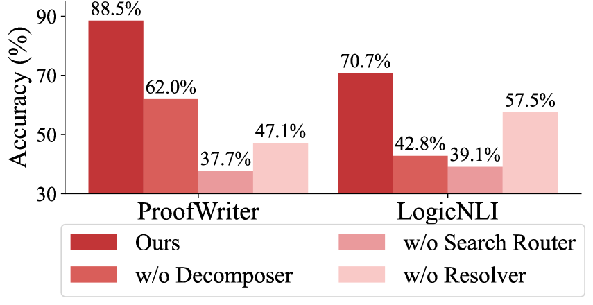
Figure 3: Ablation results (w/ GPT-4o).
### 4.3 Model Ablation
To evaluate the contribution of each module in our framework, we conducted an ablation study by replacing each module individually with simpler alternatives. Specifically, we substitute (1) the Decomposer by prompting the LLM for simple decomposition, (2) the Resolver by prompting the LLM to infer using the given premises, and (3) the Search Router by prompting the LLM to search for relevant premises.
The results, shown in Fig. 3, demonstrate that removing any module leads to a significant performance drop, highlighting the importance of each component. Notably, replacing the Search Router results in the largest performance decline (50.8% and 31.6% for ProofWriter and LogicNLI, respectively), emphasizing the benefits of searching complementary premises under the proof-by-contradiction strategy. Besides, the Decomposer has a greater impact than the Resolver on LogicNLI, whereas in ProofWriter, the Resolver plays a more significant role than the Decomposer. This is because LogicNLI includes more complex logical structures, such as “either…or…”, “vice versa”, and “if and only if”, while ProofWriter primarily involves simpler conjunctions such as “and”, “or”. As a result, LogicNLI relies more heavily on the Decomposer to break down complex logical statements into simpler forms for optimal performance.
## 5 Analysis and Discussion
We now take one step further, delving into the underlying working mechanisms of our system.
<details>
<summary>x10.png Details</summary>
### Visual Description
## Scatter Plot: Method Performance Comparison (Accuracy vs. Computational Steps)
### Overview
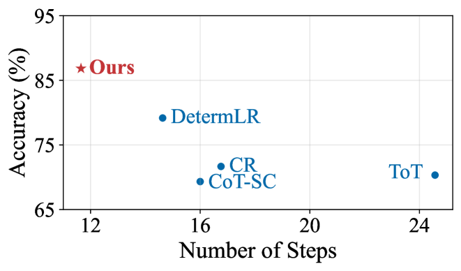
The image is a 2D scatter plot comparing the performance of five different methods or algorithms. The plot visualizes the trade-off between computational cost (measured in "Number of Steps") and performance (measured as "Accuracy (%)"). One method, labeled "Ours," is highlighted with a distinct red star, suggesting it is the proposed or primary method of the study from which this figure originates.
### Components/Axes
* **Chart Type:** Scatter Plot
* **X-Axis:**
* **Label:** "Number of Steps"
* **Scale:** Linear, ranging from approximately 11 to 25.
* **Major Ticks:** 12, 16, 20, 24.
* **Y-Axis:**
* **Label:** "Accuracy (%)"
* **Scale:** Linear, ranging from 65 to 95.
* **Major Ticks:** 65, 75, 85, 95.
* **Data Series & Legend:** The legend is embedded directly in the plot area, with labels placed adjacent to their corresponding data points.
* **"Ours":** Represented by a **red star (★)**. Positioned in the top-left quadrant.
* **"DetermLR":** Represented by a **blue circle (●)**. Positioned in the upper-middle area.
* **"CR":** Represented by a **blue circle (●)**. Positioned near the center, slightly below "DetermLR".
* **"CoT-SC":** Represented by a **blue circle (●)**. Positioned just below and slightly left of "CR".
* **"ToT":** Represented by a **blue circle (●)**. Positioned in the bottom-right quadrant.
### Detailed Analysis
The plot contains five distinct data points. Below is an analysis of each, including approximate coordinate extraction and trend description.
1. **"Ours" (Red Star)**
* **Spatial Position:** Top-left corner of the data cluster.
* **Approximate Coordinates:** (X ≈ 12, Y ≈ 88).
* **Trend Description:** This point represents the highest accuracy and the lowest number of steps among all plotted methods.
2. **"DetermLR" (Blue Circle)**
* **Spatial Position:** Upper-middle region, to the right and below "Ours".
* **Approximate Coordinates:** (X ≈ 15, Y ≈ 79).
* **Trend Description:** Shows a significant drop in accuracy (~9 percentage points) compared to "Ours" for a moderate increase in steps (~3 more steps).
3. **"CR" (Blue Circle)**
* **Spatial Position:** Near the center of the plot.
* **Approximate Coordinates:** (X ≈ 17, Y ≈ 72).
* **Trend Description:** Positioned below "DetermLR", indicating lower accuracy for a slightly higher step count.
4. **"CoT-SC" (Blue Circle)**
* **Spatial Position:** Just below and slightly left of "CR".
* **Approximate Coordinates:** (X ≈ 16, Y ≈ 69).
* **Trend Description:** Has the second-lowest accuracy and a step count similar to "CR".
5. **"ToT" (Blue Circle)**
* **Spatial Position:** Far right, bottom quadrant.
* **Approximate Coordinates:** (X ≈ 24.5, Y ≈ 70).
* **Trend Description:** This method requires the highest number of steps by a large margin but achieves an accuracy only marginally better than "CoT-SC" and worse than "CR".
### Key Observations
* **Dominant Performance:** The method labeled "Ours" is a clear outlier, achieving the highest accuracy (~88%) with the fewest computational steps (~12). This represents a Pareto-optimal point on the chart.
* **Inverse General Trend:** Among the four blue-circle methods, there is no clear positive correlation between steps and accuracy. In fact, the method with the most steps ("ToT") has one of the lowest accuracies.
* **Clustering:** "CR" and "CoT-SC" form a cluster with similar step counts (16-17) and relatively low accuracy (69-72%).
* **Efficiency Gap:** There is a substantial performance gap between the proposed method ("Ours") and all other compared methods in this visualization.
### Interpretation
This chart is designed to demonstrate the superior efficiency and effectiveness of the "Ours" method. The data suggests that "Ours" achieves a breakthrough in the accuracy-efficiency trade-off, delivering top-tier performance while being significantly less computationally expensive (requiring fewer steps) than alternatives like "DetermLR", "CR", "CoT-SC", and especially "ToT".
The poor performance of "ToT" (high steps, low accuracy) is particularly notable, indicating it may be an inefficient approach for the task measured here. The clustering of "CR" and "CoT-SC" suggests these methods may share similar underlying mechanisms or limitations.
The visual rhetoric—using a distinct red star for "Ours" placed in the coveted "high accuracy, low cost" top-left corner—is a powerful and intentional choice to highlight the proposed method's advantage. The chart effectively argues that "Ours" is not just incrementally better but represents a different class of performance compared to the other plotted techniques.
</details>
Figure 4: Accuracy vs. Efficiency on ProofWriter using GPT-4. Efficiency is measured as the average number of visited nodes/steps required to solve the problem. The upper-left corner is the optimal point, representing the best performance with the fewest visited nodes.
### 5.1 Accuracy vs. Efficiency
#### Our method achieves better reasoning accuracy with higher efficiency.
Here, we measure the average number of steps or nodes for solving problems in the ProofWriter dataset. As shown in Fig. 4, our method not only achieves the highest accuracy across all baselines but does so with the least number of visited nodes indicating both superior efficacy and efficiency. Specifically, our method achieves the highest accuracy among all baselines, while visiting only 11.65 nodes on average, reducing the number of nodes visited by 52.6%, 30.5%, and 20.4% compared to ToT, CR, and DetermLR, respectively. This demonstrates that our approach effectively balances accuracy and computational efficiency. By directly targeting contradictions, it significantly streamlines the reasoning process, making it both precise and efficient.
### 5.2 Step-wise Reasoning Accuracy
#### The
<details>
<summary>x11.png Details</summary>

### Visual Description
Icon/Small Image (29x29)
</details>
Resolver can achieve near-perfect accuracy in one-step logical inference.
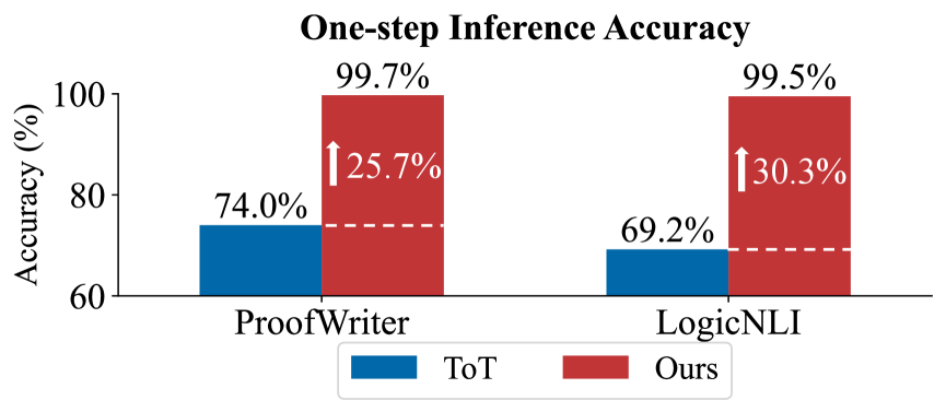
To understand why our framework is effective, we must also examine its one-step logical reasoning accuracy. Since the final answer is derived from these individual inferences (i.e., nodes in ToT and steps in Ours), their accuracy directly impacts the overall performance. We compare the one-step reasoning accuracy of our method with that of ToT shown in Fig. 5. We randomly sample 100 cases with manual evaluation. ToT demonstrated around 70% accuracy, which is consistent with prior research showing that LLMs can sometimes introduce logical errors. In contrast, our Aristotle achieved near-perfect accuracy in one-step inference, underscoring the effectiveness of the Resolver module’s use of the resolution principle. This is because the resolution principle provides a systematic and logically rigorous way to resolve contradictions, simplifying the reasoning process compared to methods that rely on LLMs to reason from previous steps and multiple premises.
<details>
<summary>x12.png Details</summary>
### Visual Description
## Bar Chart: One-step Inference Accuracy
### Overview
The image is a bar chart comparing the accuracy of two methods, labeled "ToT" and "Ours," on two different datasets or tasks: "ProofWriter" and "LogicNLI." The chart demonstrates a significant performance improvement of the "Ours" method over the "ToT" method for both tasks.
### Components/Axes
* **Chart Title:** "One-step Inference Accuracy" (centered at the top).
* **Y-axis:** Labeled "Accuracy (%)". The scale runs from 60 to 100, with major tick marks at 60, 80, and 100.
* **X-axis:** Contains two categorical labels: "ProofWriter" (left) and "LogicNLI" (right).
* **Legend:** Located at the bottom center of the chart.
* A blue rectangle is labeled "ToT".
* A red rectangle is labeled "Ours".
* **Data Series:** Two sets of paired bars, one for each x-axis category.
* **ProofWriter Set:** A blue bar (ToT) on the left, a red bar (Ours) on the right.
* **LogicNLI Set:** A blue bar (ToT) on the left, a red bar (Ours) on the right.
* **Annotations:**
* White text labels above each bar show the exact accuracy percentage.
* White upward-pointing arrows are placed between the paired bars, with text indicating the percentage point improvement of "Ours" over "ToT".
* A horizontal dashed white line extends from the top of each blue bar to the corresponding red bar, visually connecting the baseline to the improved result.
### Detailed Analysis
**1. ProofWriter Task:**
* **ToT (Blue Bar):** Accuracy is **74.0%**.
* **Ours (Red Bar):** Accuracy is **99.7%**.
* **Improvement:** An arrow indicates an increase of **25.7%** (percentage points) from the ToT baseline.
**2. LogicNLI Task:**
* **ToT (Blue Bar):** Accuracy is **69.2%**.
* **Ours (Red Bar):** Accuracy is **99.5%**.
* **Improvement:** An arrow indicates an increase of **30.3%** (percentage points) from the ToT baseline.
**Trend Verification:**
* For both tasks, the red bar ("Ours") is substantially taller than the blue bar ("ToT"), confirming a visual trend of superior performance.
* The improvement margin is larger for LogicNLI (30.3%) than for ProofWriter (25.7%).
### Key Observations
* **Near-Perfect Performance:** The "Ours" method achieves near-perfect accuracy (99.5% and 99.7%) on both tasks.
* **Significant Gains:** The improvements are very large, exceeding 25 percentage points in both cases.
* **Consistent Pattern:** The relationship between the methods is consistent across both tasks: "Ours" dramatically outperforms "ToT".
* **Baseline Performance:** The "ToT" method performs moderately on ProofWriter (74.0%) and slightly worse on LogicNLI (69.2%).
### Interpretation
The data presents a clear and compelling case for the superiority of the "Ours" method over the "ToT" method for one-step inference on the tested tasks. The near-ceiling performance of "Ours" suggests it has effectively solved these specific inference challenges under the given conditions. The larger improvement on LogicNLI might indicate that the "Ours" method is particularly adept at handling the type of reasoning required by that dataset compared to ProofWriter. The chart is designed to highlight this dramatic performance gap, using color contrast, direct numerical labels, and explicit improvement annotations to make the conclusion unambiguous for a technical audience. The primary message is one of substantial methodological advancement.
</details>
Figure 5: One-step reasoning accuracy using GPT-4o.
### 5.3 Search Error
#### Our method effectively reduces errors from the search strategy.
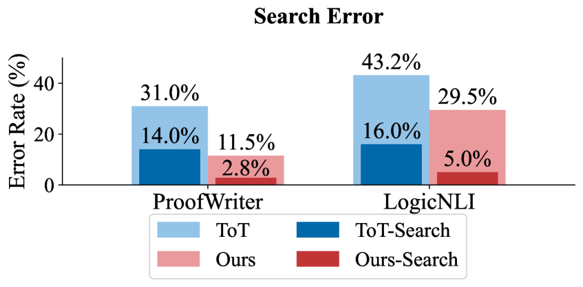
Apart from one-step logical inference, the search router also plays a crucial role. Previous research has shown that methods involving an evaluator to guide the search tend to underperform as the evaluator can be unreliable and may mislead the reasoning process, resulting in incorrect answers. We assess the search error In ToT, search errors occur when the evaluator selects a logically flawed node for expansion. In contrast, in our method, search errors arise when either the complementary clause is not found or a non-complementary clause is selected. The evaluation process is conducted manually., as shown in Fig. 6. Our search strategy significantly reduces errors, lowering them by 11.2% in ProofWriter and 9.0% in LogicNLI. This demonstrates that our logic-based search approach outperforms LLM self-evaluation, effectively addressing the limitations posed by unreliable evaluators in logical reasoning. An explanation is that our method simplifies the search process by focusing on identifying complementary clauses, a task with clear definitions and rules that an LLM can easily follow with a few examples. In contrast, having an LLM evaluate logical inferences, such as in ToT, requires complex judgments, making it more prone to errors Chen et al. (2024); Wang et al. (2024b).
<details>
<summary>x13.png Details</summary>
### Visual Description
## Bar Chart: Search Error Rate Comparison
### Overview
The image is a grouped bar chart titled "Search Error" that compares the error rates (in percentage) of four different methods across two datasets: "ProofWriter" and "LogicNLI". The chart visually demonstrates the performance impact of adding a search component to two base methods ("ToT" and "Ours").
### Components/Axes
* **Chart Title:** "Search Error" (centered at the top).
* **Y-Axis:** Labeled "Error Rate (%)". The axis has numerical markers at 0, 20, and 40.
* **X-Axis:** Contains two categorical labels: "ProofWriter" (left group) and "LogicNLI" (right group).
* **Legend:** Positioned at the bottom center of the chart. It defines four data series by color:
* Light Blue: "ToT"
* Dark Blue: "ToT-Search"
* Light Red/Pink: "Ours"
* Dark Red: "Ours-Search"
### Detailed Analysis
The chart presents data for two distinct datasets, each with four associated methods.
**1. ProofWriter Dataset (Left Group):**
* **ToT (Light Blue Bar):** The tallest bar in this group, with a labeled value of **31.0%**.
* **ToT-Search (Dark Blue Bar):** A significantly shorter bar, with a labeled value of **14.0%**.
* **Ours (Light Red Bar):** Slightly shorter than the ToT-Search bar, with a labeled value of **11.5%**.
* **Ours-Search (Dark Red Bar):** The shortest bar in the entire chart, with a labeled value of **2.8%**.
**2. LogicNLI Dataset (Right Group):**
* **ToT (Light Blue Bar):** The tallest bar in the entire chart, with a labeled value of **43.2%**.
* **ToT-Search (Dark Blue Bar):** A much shorter bar, with a labeled value of **16.0%**.
* **Ours (Light Red Bar):** The second-tallest bar in this group, with a labeled value of **29.5%**.
* **Ours-Search (Dark Red Bar):** The shortest bar in this group, with a labeled value of **5.0%**.
### Key Observations
* **Consistent Trend of Improvement with Search:** For both base methods ("ToT" and "Ours") and on both datasets, the addition of a search component ("-Search") results in a substantial reduction in error rate.
* **"Ours-Search" is the Top Performer:** The dark red "Ours-Search" method achieves the lowest error rate in both datasets (2.8% on ProofWriter, 5.0% on LogicNLI).
* **"ToT" Has the Highest Error Rates:** The light blue "ToT" method has the highest error rate in both datasets (31.0% and 43.2%).
* **Relative Performance:** The "Ours" method (light red) consistently outperforms the "ToT" method (light blue) without search. With search, "Ours-Search" (dark red) consistently outperforms "ToT-Search" (dark blue).
* **Dataset Difficulty:** Error rates are universally higher on the LogicNLI dataset compared to ProofWriter for all corresponding methods, suggesting LogicNLI may be a more challenging task.
### Interpretation
This chart provides strong empirical evidence for two key conclusions within the context of the research it represents:
1. **The Efficacy of Search:** The primary finding is that integrating a search mechanism dramatically improves performance (lowers error rates) for both the "ToT" and the proposed "Ours" methodology. The magnitude of improvement is significant, often reducing the error rate by more than half (e.g., ToT from 31.0% to 14.0% on ProofWriter).
2. **Superiority of the Proposed Method:** The data suggests that the authors' method ("Ours") is fundamentally more effective than the baseline "ToT" method. This is true in both its standalone form and, more importantly, when augmented with search. The "Ours-Search" combination is presented as the state-of-the-art result in this comparison, achieving near-negligible error rates on the ProofWriter task.
The chart is designed to persuade the viewer that the authors' approach ("Ours") is not only better than the existing method ("ToT") but that its advantage is amplified when both are enhanced with search capabilities. The consistent pattern across two different datasets strengthens the generalizability of this claim.
</details>
Figure 6: The outer bar shows the overall error rate. The inner bar represents the proportion of the error caused by the search strategy.
### 5.4 Complex Reasoning
#### Our method demonstrates a clear advantage in handling problems of increasing difficulty.
We evaluate accuracy across different reasoning difficulties in ProofWriter, as shown in Fig. 7. Our method consistently outperforms others at all depths, maintaining superior accuracy. It excels particularly at moderate and challenging depths, surpassing baselines like SymbCoT and Logic-LM. Even as other methods struggle at higher depths, our approach remains robust, demonstrating better scalability and resilience to problem difficulty. This effectiveness is due to two main factors: (1) using the resolution principle minimizes errors at each step and prevents them from compounding, and (2) streamlining the reasoning process reduces steps, lowering the likelihood of error accumulation.
<details>
<summary>x14.png Details</summary>
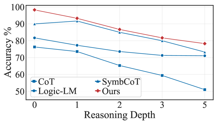
### Visual Description
\n
## Line Chart: Accuracy vs. Reasoning Depth
### Overview
The image displays a line chart comparing the performance of four different methods or models on a task requiring varying depths of reasoning. The chart plots "Accuracy %" against "Reasoning Depth," showing a general downward trend for all methods as reasoning complexity increases.
### Components/Axes
* **Chart Type:** Multi-series line chart with markers.
* **Y-Axis:** Labeled "Accuracy %". The scale runs from 50 to 100, with major gridlines at intervals of 10 (50, 60, 70, 80, 90, 100).
* **X-Axis:** Labeled "Reasoning Depth". The marked data points are at depths 0, 1, 2, 3, and 5. The value 4 is not plotted.
* **Legend:** Positioned in the bottom-left corner of the chart area. It contains four entries:
* `CoT`: Blue line with square markers (■).
* `SymbCoT`: Blue line with upward-pointing triangle markers (▲).
* `Logic-LM`: Blue line with circle markers (●).
* `Ours`: Red line with diamond markers (◆).
### Detailed Analysis
The chart tracks the accuracy of four methods across five reasoning depth levels. Below is an analysis of each series, including its visual trend and approximate data points.
**1. CoT (Blue line, square markers ■)**
* **Trend:** Shows the steepest and most consistent decline in accuracy as reasoning depth increases.
* **Data Points (Approximate):**
* Depth 0: ~76%
* Depth 1: ~74%
* Depth 2: ~66%
* Depth 3: ~60%
* Depth 5: ~51%
**2. SymbCoT (Blue line, triangle markers ▲)**
* **Trend:** Starts with high accuracy, peaks slightly at depth 1, then declines steadily. It maintains the second-highest performance throughout.
* **Data Points (Approximate):**
* Depth 0: ~90%
* Depth 1: ~92%
* Depth 2: ~85%
* Depth 3: ~80%
* Depth 5: ~74%
**3. Logic-LM (Blue line, circle markers ●)**
* **Trend:** Shows a moderate, relatively steady decline. Its performance is consistently between CoT and SymbCoT.
* **Data Points (Approximate):**
* Depth 0: ~82%
* Depth 1: ~78%
* Depth 2: ~74%
* Depth 3: ~72%
* Depth 5: ~71%
**4. Ours (Red line, diamond markers ◆)**
* **Trend:** Demonstrates the highest accuracy at every reasoning depth. It declines gradually but remains significantly above the other methods.
* **Data Points (Approximate):**
* Depth 0: ~98%
* Depth 1: ~94%
* Depth 2: ~87%
* Depth 3: ~82%
* Depth 5: ~78%
### Key Observations
1. **Universal Performance Degradation:** All four methods experience a decrease in accuracy as the reasoning depth increases from 0 to 5.
2. **Consistent Hierarchy:** The performance ranking (`Ours` > `SymbCoT` > `Logic-LM` > `CoT`) is maintained at every measured reasoning depth.
3. **Differential Resilience:** The method labeled "Ours" and "SymbCoT" show greater resilience to increased reasoning depth compared to "CoT" and "Logic-LM". The gap between the best (`Ours`) and worst (`CoT`) performer widens significantly at greater depths (from a ~22% gap at depth 0 to a ~27% gap at depth 5).
4. **Missing Data Point:** There is no data plotted for Reasoning Depth = 4.
### Interpretation
This chart presents a comparative evaluation of reasoning capabilities. The "Reasoning Depth" likely corresponds to the number of logical or computational steps required to solve a problem.
* **What the data suggests:** The proposed method ("Ours") demonstrates superior and more robust performance, maintaining high accuracy even as problems become more complex. This implies it has a more effective architecture or training for multi-step reasoning tasks compared to the baseline methods (CoT, SymbCoT, Logic-LM).
* **Relationship between elements:** The downward slope for all lines is the central relationship, quantifying the "cost" of complexity. The vertical separation between the lines at any given x-value represents the performance advantage of one method over another for a fixed problem difficulty.
* **Notable trends/anomalies:** The most notable trend is the diverging performance. While all methods degrade, the rate of degradation varies. "CoT" degrades rapidly, suggesting it struggles significantly with deeper reasoning chains. "Ours" degrades the slowest, indicating better generalization to complex problems. The absence of data at depth 4 is an anomaly in the experimental reporting but does not obscure the clear overall trend.
</details>
Figure 7: Studying the effect of reasoning depth with GPT-4 on ProofWriter.
#### The cost scaling is stable with increased reasoning depth.
To complement the performance analysis on different reasoning depth, we also address concerns about the scalability of our framework when applied to tasks requiring deeper reasoning involving greater reasoning depth. Specifically, we provide a detailed examination of the marginal computational costs and token usage associated with extended reasoning chains. Aristotle is designed to handle increased reasoning depth in an efficient and controlled manner.
Each reasoning step in our framework consists of two operations. First, a search operation is performed using a deterministic rule-based method, which introduces minimal computational overhead and does not contribute additional token usage as reasoning depth increases. Second, a resolve operation is executed by the resolver module, which processes one reasoning step at a time and is the only component contributing to token-based computational cost.
This modular design ensures that total token usage grows linearly with the number of reasoning steps, keeping the marginal cost per additional step low and predictable. To empirically validate the efficiency and stability of our approach, we analyzed token usage for individual reasoning steps across two benchmark datasets, ProofWriter and LogicNLI, as shown in Table 3. The statistics indicate that token usage per reasoning step is highly consistent, exhibiting low standard deviation and coefficient of variation. Moreover, the absolute token cost per step remains modest, ensuring that deeper reasoning does not impose a significant computational burden. Given the stable, linear scaling of token consumption and the low per-step cost, our framework maintains its efficiency even for tasks requiring extended reasoning chains.
| ProofWriter LogicNLI | 3076.8 2071.1 | 19.1 26.4 | 0.71% 0.85% |
| --- | --- | --- | --- |
Table 3: Token usage statistics per reasoning step. TU denotes Token Usage, Std. Dev. denotes Standard Deviation, and CV denotes Coefficient of Variation.
<details>
<summary>x15.png Details</summary>
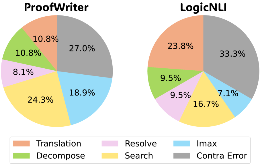
### Visual Description
\n
## Pie Charts: ProofWriter and LogicNLI Dataset Error Distributions
### Overview
The image displays two pie charts side-by-side, comparing the distribution of error types or reasoning steps across two different datasets or models named "ProofWriter" and "LogicNLI". A shared legend at the bottom defines six categories. The charts are presented on a plain white background.
### Components/Axes
* **Chart Titles:** "ProofWriter" (left chart), "LogicNLI" (right chart). Both are in bold, black, sans-serif font.
* **Legend:** Positioned at the bottom center of the image. It contains six colored squares with corresponding labels:
* Orange square: `Translation`
* Green square: `Decompose`
* Pink square: `Resolve`
* Yellow square: `Search`
* Blue square: `Imax`
* Gray square: `Contra Error`
* **Data Representation:** Each pie chart is divided into six colored segments, each labeled with a percentage value. The segments correspond to the categories in the legend.
### Detailed Analysis
**ProofWriter Chart (Left):**
* **Contra Error (Gray):** 27.0% - The largest segment, located in the top-right quadrant.
* **Search (Yellow):** 24.3% - The second-largest segment, located in the bottom-left quadrant.
* **Imax (Blue):** 18.9% - Located in the bottom-right quadrant.
* **Translation (Orange):** 10.8% - Located in the top-left quadrant.
* **Decompose (Green):** 10.8% - Located in the left-center, adjacent to Translation.
* **Resolve (Pink):** 8.1% - The smallest segment, located between Decompose and Search.
**LogicNLI Chart (Right):**
* **Contra Error (Gray):** 33.3% - The largest segment, located in the top-right quadrant.
* **Translation (Orange):** 23.8% - The second-largest segment, located in the top-left quadrant.
* **Search (Yellow):** 16.7% - Located in the bottom-left quadrant.
* **Decompose (Green):** 9.5% - Located in the left-center.
* **Resolve (Pink):** 9.5% - Located between Decompose and Search.
* **Imax (Blue):** 7.1% - The smallest segment, located in the bottom-right quadrant.
### Key Observations
1. **Dominant Category:** "Contra Error" is the largest category in both datasets, comprising over a quarter of the distribution in ProofWriter (27.0%) and a third in LogicNLI (33.3%).
2. **Significant Shifts:**
* The "Translation" category is more than twice as prevalent in LogicNLI (23.8%) compared to ProofWriter (10.8%).
* The "Imax" category shows the opposite trend, being significantly larger in ProofWriter (18.9%) than in LogicNLI (7.1%).
3. **Similar Proportions:** The "Decompose" and "Resolve" categories have similar, relatively small proportions in both charts (10.8%/8.1% in ProofWriter, 9.5%/9.5% in LogicNLI).
4. **Rank Order Change:** The order of the second and third largest categories differs between the charts. In ProofWriter, it is Search (24.3%) then Imax (18.9%). In LogicNLI, it is Translation (23.8%) then Search (16.7%).
### Interpretation
The data suggests a fundamental difference in the error or reasoning step profiles between the ProofWriter and LogicNLI datasets or the models evaluated on them.
* The consistently high proportion of **"Contra Error"** indicates that handling contradictions or counterfactual reasoning is a major challenge across both contexts.
* The stark contrast in **"Translation"** and **"Imax"** proportions is the most notable finding. This implies that the LogicNLI task involves significantly more challenges related to translating or interpreting natural language into a formal representation ("Translation"), while the ProofWriter task involves more challenges related to a process or metric labeled "Imax" (potentially related to maximization or inference depth).
* The relative stability of **"Decompose"** and **"Resolve"** suggests these reasoning steps are consistently minor components of the overall error profile for these tasks.
In summary, while both tasks share a common primary difficulty (Contra Error), their secondary challenges are distinctly different, pointing to variations in task structure, data complexity, or the reasoning skills they primarily test.
</details>
Figure 8: Error analysis on ProofWriter and LogicNLI with GPT-4o.
### 5.5 Error Analysis
To thoroughly understand the limitations of our framework, we conduct a manual error analysis on the ProofWriter and LogicNLI datasets using GPT-4o. The detailed error statistics are presented in Fig. F.
The majority of errors stem from the Contradiction Error, primarily due to flaws in dataset construction. The next most common source is the Search module, where complementary clauses exist but are not retrieved. This is often due to unexpected symbols (e.g., LaTeX code) in the LLM’s output that disrupt regular expression matching.
Translation and Decomposition errors are the third largest category. These occur when the LLM struggles to parse complex logical relationships or convert them into the correct symbolic form. Such errors are more prevalent in LogicNLI, which features more intricate constructs (e.g., "either…or…" and "if and only if") compared to the simpler logic in ProofWriter (e.g., "and," "or").
Another notable source of error is Insufficient Iterations, where the reasoning process terminates prematurely, often concluding "No contradiction" when further iterations might reveal one. While increasing the iteration threshold could mitigate this, it must be balanced against computational efficiency.
Finally, Resolution errors, often due to incorrect variable instantiations, are relatively infrequent. This is because logical statements have been reduced to a simple conjunctive normal form (CNF) by this point, making them easier to interpret, and the resolution principle offers clear guidance for resolving inconsistencies.
Potential improvements include incorporating more targeted in-context learning (ICL) examples to enhance translation and resolution. Besides, enhancing regular expression patterns to accommodate a wider range of syntactic variations could further reduce search errors. Additionally, tuning iteration limits would help achieve a better balance between accuracy and computational efficiency. More details of error analysis can be found at Appendix F.
## 6 Related Work
Enhancing the logical reasoning of LLMs to achieve human-like levels has been a key focus in recent research Huang and Chang (2023); Dunivin (2024). Existing approaches can be broadly categorized into the following:
#### Linear Reasoning.
These approaches involve prompting LLMs once to emulate human reasoning in a sequential manner. The representative is the CoT method Wei et al. (2022), which guides the model to generate reasoning steps linearly. Building upon CoT, SymbCoT Xu et al. (2024) incorporates symbolic expressions and rules into the linear reasoning process to achieve more rigorous logical reasoning. However, these methods lack any searching or backtracking mechanism to avoid flawed reasoning paths, leading to suboptimal performance. In this paper, we thus consider the searching-based reasoning framework.
#### Sampling Methods.
These methods obtain the final answer through samplings to enhance reasoning diversity and accuracy Wang et al. (2023b); Fu et al. (2023); Manakul et al. (2023). This involves running the reasoning process multiple times, with the increased diversity of reasoning paths contributing to better results. However, they do not resolve the underlying issue of flawed logical reasoning inherent to the LLM, which is resolved by the resolution principle Robinson (1965) in our framework.
#### Iterative Reasoning with Search.
These methods rely on an evaluator to search for different reasoning paths to avoid flawed nodes. Techniques such as ToT Yao et al. (2023), and its variances Xie et al. (2023); Zhang et al. (2023); Sun et al. (2024), generate multiple thoughts during the reasoning. An evaluator repetitively selects the most probable paths to expand to the next level until the final answer. However, the evaluator may not be reliable Chen et al. (2024); Wang et al. (2024b), potentially selecting incorrect nodes for expansion and propagating errors. This paper proposes a search mechanism that relies on matching symbolic logic, avoiding the use of an unreliable evaluator.
#### Reasoning Relying on External Tools.
Here LLMs often involve integrating well-developed rule-based reasoning engines, where LLMs act as mere translators, converting the natural language of reasoning questions into specific symbolic forms to be processed by external rule-based engines. Examples include Logic-LM Pan et al. (2023), LINC Olausson et al. (2023) and PAL Gao et al. (2023). The limitation of this approach lies in the strict formatting requirements of external logic resolver; LLMs inevitably introduce syntax errors during translation, leading to failures in the reasoning process. Fortunately, the success of SymbCoT Xu et al. (2024) preliminarily demonstrates that enabling LLMs to perform logical reasoning based on symbols is feasible and promising. In our paper, we further prove that symbolic logic expressions can be fully integrated into all processes of the reasoning framework, including decomposition, search, and inference, thereby demonstrating that LLMs themselves can completely achieve high-level symbolic logical reasoning.
## 7 Conclusion
We presented Aristotle, a logic-complete reasoning framework designed to tackle the challenges of logical reasoning, which comprehensively integrates symbolic expressions and logical rules into three core components: Logical Decomposer, Logical Search Router, and Logical Resolver. These modules streamline the reasoning process by reducing the task complexity, minimizing the search errors, and rigorously resolving logical contradictions. Our experiments show that our method consistently outperforms state-of-the-art frameworks in both accuracy and efficiency significantly.
## Acknowledgements
This work is supported by the Ministry of Education, Singapore, under its MOE AcRF TIER 3 Grant (MOE-MOET32022-0001).
## Potential Limitations
Our method faces two potential limitations. First, the reasoning process relies on the quality of translation and decomposition. However, even with a few-shot approach, LLMs cannot always guarantee that these processes are fully correct. Future work could consider more advanced methods to guarantee the quality of these processes, such as fine-tuning. Secondly, our reasoning approach requires that all necessary information is explicitly stated in the premises. If any implicit information or assumptions exist, our method may fail to capture them, leading to incorrect reasoning. A more detailed analysis of this limitation is provided in Appendix E. Nevertheless, there are existing methods that explore how to make implicit information explicit. Future work could integrate those methods into this framework to address this limitation.
## Ethics Statement
The datasets employed in our research were carefully selected from publicly available or ethically sourced materials, and we take deliberate steps to identify and reduce biases within these datasets to uphold fairness in our outcomes.
## References
- Baader et al. (2003) Franz Baader, Diego Calvanese, Deborah L. McGuinness, Daniele Nardi, and Peter F. Patel-Schneider, editors. 2003. The Description Logic Handbook: Theory, Implementation, and Applications. Cambridge University Press.
- Besta et al. (2024) Maciej Besta, Nils Blach, Ales Kubicek, Robert Gerstenberger, Michal Podstawski, Lukas Gianinazzi, Joanna Gajda, Tomasz Lehmann, Hubert Niewiadomski, Piotr Nyczyk, and Torsten Hoefler. 2024. Graph of thoughts: Solving elaborate problems with large language models. In Proceedings of the AAAI Conference on Artificial Intelligence, pages 17682–17690, Vancouver, Canada.
- Bishop (1967) Errett Bishop. 1967. Foundations of Constructive Analysis. Mcgraw-Hill.
- Chen et al. (2024) Ziru Chen, Michael White, Ray Mooney, Ali Payani, Yu Su, and Huan Sun. 2024. When is tree search useful for LLM planning? It depends on the discriminator. In Proceedings of the 62nd Annual Meeting of the Association for Computational Linguistics, pages 13659–13678, Bangkok, Thailand.
- Chowdhery et al. (2023) Aakanksha Chowdhery, Sharan Narang, Jacob Devlin, Maarten Bosma, Gaurav Mishra, Adam Roberts, Paul Barham, Hyung Won Chung, Charles Sutton, Sebastian Gehrmann, Parker Schuh, Kensen Shi, Sasha Tsvyashchenko, Joshua Maynez, Abhishek Rao, Parker Barnes, Yi Tay, Noam Shazeer, Vinodkumar Prabhakaran, Emily Reif, Nan Du, Ben Hutchinson, Reiner Pope, James Bradbury, Jacob Austin, Michael Isard, Guy Gur-Ari, Pengcheng Yin, Toju Duke, Anselm Levskaya, Sanjay Ghemawat, Sunipa Dev, Henryk Michalewski, Xavier Garcia, Vedant Misra, Kevin Robinson, Liam Fedus, Denny Zhou, Daphne Ippolito, David Luan, Hyeontaek Lim, Barret Zoph, Alexander Spiridonov, Ryan Sepassi, David Dohan, Shivani Agrawal, Mark Omernick, Andrew M. Dai, Thanumalayan Sankaranarayana Pillai, Marie Pellat, Aitor Lewkowycz, Erica Moreira, Rewon Child, Oleksandr Polozov, Katherine Lee, Zongwei Zhou, Xuezhi Wang, Brennan Saeta, Mark Diaz, Orhan Firat, Michele Catasta, Jason Wei, Kathy Meier-Hellstern, Douglas Eck, Jeff Dean, Slav Petrov, and Noah Fiedel. 2023. Palm: Scaling language modeling with pathways. Journal of Machine Learning Research, 24:240:1–240:113.
- Clocksin and Mellish (2003) William F Clocksin and Christopher S Mellish. 2003. Programming in Prolog. Springer Science & Business Media.
- Cummins et al. (1991) D.D. Cummins, T. Lubart, O. Alksnis, et al. 1991. Conditional reasoning and causation. Memory & Cognition, 19:274–282.
- Davis and Putnam (1960) Martin Davis and Hilary Putnam. 1960. A computing procedure for quantification theory. J. ACM, 7(3):201–215.
- Dunivin (2024) Zackary Okun Dunivin. 2024. Scalable qualitative coding with LLMs: Chain-of-Thought reasoning matches human performance in some hermeneutic tasks. ArXiv preprint, abs/2401.15170.
- Eisner et al. (2024) Ben Eisner, Yi Yang, Todor Davchev, Mel Vecerík, Jonathan Scholz, and David Held. 2024. Deep se(3)-equivariant geometric reasoning for precise placement tasks. In The Twelfth International Conference on Learning Representations, Vienna, Austria.
- Fu et al. (2023) Yao Fu, Hao Peng, Ashish Sabharwal, Peter Clark, and Tushar Khot. 2023. Complexity-based prompting for multi-step reasoning. In The Eleventh International Conference on Learning Representations, Kigali, Rwanda.
- Gao et al. (2023) Luyu Gao, Aman Madaan, Shuyan Zhou, Uri Alon, Pengfei Liu, Yiming Yang, Jamie Callan, and Graham Neubig. 2023. PAL: program-aided language models. In International Conference on Machine Learning, volume 202, pages 10764–10799, Honolulu, Hawaii, USA. PMLR.
- Han et al. (2022) Simeng Han, Hailey Schoelkopf, Yilun Zhao, Zhenting Qi, Martin Riddell, Luke Benson, Lucy Sun, Ekaterina Zubova, Yujie Qiao, Matthew Burtell, David Peng, Jonathan Fan, Yixin Liu, Brian Wong, Malcolm Sailor, Ansong Ni, Linyong Nan, Jungo Kasai, Tao Yu, Rui Zhang, Shafiq R. Joty, Alexander R. Fabbri, Wojciech Kryscinski, Xi Victoria Lin, Caiming Xiong, and Dragomir Radev. 2022. FOLIO: natural language reasoning with first-order logic. ArXiv preprint, abs/2209.00840.
- Huang and Chang (2023) Jie Huang and Kevin Chen-Chuan Chang. 2023. Towards reasoning in large language models: A survey. In Findings of the Association for Computational Linguistics: ACL 2023, pages 1049–1065, Toronto, Canada.
- Li et al. (2024) Haoming Li, Zhaoliang Chen, Jonathan Zhang, and Fei Liu. 2024. LASP: surveying the state-of-the-art in large language model-assisted AI planning. ArXiv preprint, abs/2409.01806.
- Liu et al. (2023) Hanmeng Liu, Ruoxi Ning, Zhiyang Teng, Jian Liu, Qiji Zhou, and Yue Zhang. 2023. Evaluating the logical reasoning ability of ChatGPT and GPT-4. ArXiv preprint, abs/2304.03439.
- Liu et al. (2020) Jian Liu, Leyang Cui, Hanmeng Liu, Dandan Huang, Yile Wang, and Yue Zhang. 2020. LogiQA: A challenge dataset for machine reading comprehension with logical reasoning. In Proceedings of the Twenty-Ninth International Joint Conference on Artificial Intelligence, pages 3622–3628.
- Manakul et al. (2023) Potsawee Manakul, Adian Liusie, and Mark Gales. 2023. SelfCheckGPT: Zero-resource black-box hallucination detection for generative large language models. In Proceedings of the 2023 Conference on Empirical Methods in Natural Language Processing, pages 9004–9017, Singapore.
- Markovits and Vachon (1989) Henry Markovits and Robert Vachon. 1989. Reasoning with contrary-to-fact propositions. Journal of Experimental Child Psychology, 47:398–412.
- Ning et al. (2024) Xuefei Ning, Zinan Lin, Zixuan Zhou, Zifu Wang, Huazhong Yang, and Yu Wang. 2024. Skeleton-of-Thought: Prompting llms for efficient parallel generation. In The Twelfth International Conference on Learning Representations, Vienna, Austria.
- Nonnengart (1996) Andreas Nonnengart. 1996. Strong skolemization.
- Olausson et al. (2023) Theo Olausson, Alex Gu, Ben Lipkin, Cedegao Zhang, Armando Solar-Lezama, Joshua Tenenbaum, and Roger Levy. 2023. LINC: A neurosymbolic approach for logical reasoning by combining language models with First-Order Logic provers. In Proceedings of the 2023 Conference on Empirical Methods in Natural Language Processing, pages 5153–5176, Singapore.
- Pan et al. (2023) Liangming Pan, Alon Albalak, Xinyi Wang, and William Wang. 2023. Logic-LM: Empowering large language models with symbolic solvers for faithful logical reasoning. In Findings of the Association for Computational Linguistics: EMNLP 2023, pages 3806–3824, Singapore.
- Parmar et al. (2024) Mihir Parmar, Nisarg Patel, Neeraj Varshney, Mutsumi Nakamura, Man Luo, Santosh Mashetty, Arindam Mitra, and Chitta Baral. 2024. LogicBench: Towards systematic evaluation of logical reasoning ability of large language models. In Proceedings of the 62nd Annual Meeting of the Association for Computational Linguistics, pages 13679–13707, Bangkok, Thailand.
- Patel et al. (2023) Ajay Patel, Bryan Li, Mohammad Sadegh Rasooli, Noah Constant, Colin Raffel, and Chris Callison-Burch. 2023. Bidirectional language models are also few-shot learners. In The Eleventh International Conference on Learning Representations, Kigali, Rwanda.
- Patel et al. (2024) Nisarg Patel, Mohith Kulkarni, Mihir Parmar, Aashna Budhiraja, Mutsumi Nakamura, Neeraj Varshney, and Chitta Baral. 2024. Multi-LogiEval: Towards evaluating multi-step logical reasoning ability of large language models. In Proceedings of the Annual Meeting of the Association for Computational Linguistics, pages 20856–20879, Bangkok, Thailand.
- Robinson (1965) John Alan Robinson. 1965. A machine-oriented logic based on the resolution principle. J. ACM, 12(1):23–41.
- Saparov and He (2023) Abulhair Saparov and He He. 2023. Language models are greedy reasoners: A systematic formal analysis of Chain-of-Thought. In The Eleventh International Conference on Learning Representations, Kigali, Rwanda.
- Sun et al. (2024) Hongda Sun, Weikai Xu, Wei Liu, Jian Luan, Bin Wang, Shuo Shang, Ji-Rong Wen, and Rui Yan. 2024. DetermLR: Augmenting LLM-based logical reasoning from indeterminacy to determinacy. In Proceedings of the 62nd Annual Meeting of the Association for Computational Linguistics (Volume 1: Long Papers), pages 9828–9862, Bangkok, Thailand.
- Tafjord et al. (2021) Oyvind Tafjord, Bhavana Dalvi, and Peter Clark. 2021. ProofWriter: Generating implications, proofs, and abductive statements over natural language. In Findings of the Association for Computational Linguistics: ACL-IJCNLP 2021, pages 3621–3634.
- Tian et al. (2021) Jidong Tian, Yitian Li, Wenqing Chen, Liqiang Xiao, Hao He, and Yaohui Jin. 2021. Diagnosing the first-order logical reasoning ability through LogicNLI. In Proceedings of the 2021 Conference on Empirical Methods in Natural Language Processing, pages 3738–3747, Online and Punta Cana, Dominican Republic.
- Tyagi et al. (2024) Nemika Tyagi, Mihir Parmar, Mohith Kulkarni, Aswin RRV, Nisarg Patel, Mutsumi Nakamura, Arindam Mitra, and Chitta Baral. 2024. Step-by-step reasoning to solve grid puzzles: Where do LLMs falter? ArXiv preprint, abs/2407.14790.
- Wang et al. (2024a) Ke Wang, Houxing Ren, Aojun Zhou, Zimu Lu, Sichun Luo, Weikang Shi, Renrui Zhang, Linqi Song, Mingjie Zhan, and Hongsheng Li. 2024a. Mathcoder: Seamless code integration in LLMs for enhanced mathematical reasoning. In The Twelfth International Conference on Learning Representations, ICLR 2024, Vienna, Austria, May 7-11, 2024.
- Wang et al. (2023a) Lei Wang, Wanyu Xu, Yihuai Lan, Zhiqiang Hu, Yunshi Lan, Roy Ka-Wei Lee, and Ee-Peng Lim. 2023a. Plan-and-Solve Prompting: Improving zero-shot Chain-of-Thought reasoning by large language models. In Proceedings of the 61st Annual Meeting of the Association for Computational Linguistics (Volume 1: Long Papers), pages 2609–2634, Toronto, Canada.
- Wang et al. (2024b) Peiyi Wang, Lei Li, Liang Chen, Zefan Cai, Dawei Zhu, Binghuai Lin, Yunbo Cao, Lingpeng Kong, Qi Liu, Tianyu Liu, and Zhifang Sui. 2024b. Large language models are not fair evaluators. In Proceedings of the 62nd Annual Meeting of the Association for Computational Linguistics, pages 9440–9450, Bangkok, Thailand.
- Wang et al. (2024c) Weiqi Wang, Tianqing Fang, Chunyang Li, Haochen Shi, Wenxuan Ding, Baixuan Xu, Zhaowei Wang, Jiaxin Bai, Xin Liu, Cheng Jiayang, Chunkit Chan, and Yangqiu Song. 2024c. CANDLE: Iterative conceptualization and instantiation distillation from large language models for commonsense reasoning. In Proceedings of the Annual Meeting of the Association for Computational Linguistics, pages 2351–2374, Bangkok, Thailand.
- Wang et al. (2023b) Xuezhi Wang, Jason Wei, Dale Schuurmans, Quoc V. Le, Ed H. Chi, Sharan Narang, Aakanksha Chowdhery, and Denny Zhou. 2023b. Self-consistency improves chain of thought reasoning in language models. In The Eleventh International Conference on Learning Representations, Kigali, Rwanda.
- Wei et al. (2022) Jason Wei, Xuezhi Wang, Dale Schuurmans, Maarten Bosma, Brian Ichter, Fei Xia, Ed H. Chi, Quoc V. Le, and Denny Zhou. 2022. Chain-of-Thought prompting elicits reasoning in large language models. In Advances in Neural Information Processing Systems 35: Annual Conference on Neural Information Processing Systems, New Orleans, LA, USA.
- Xie et al. (2023) Yuxi Xie, Kenji Kawaguchi, Yiran Zhao, James Xu Zhao, Min-Yen Kan, Junxian He, and Michael Qizhe Xie. 2023. Self-evaluation guided beam search for reasoning. In Proceedings of the Annual Conference on Neural Information Processing Systems, New Orleans, LA, USA.
- Xu et al. (2024) Jundong Xu, Hao Fei, Liangming Pan, Qian Liu, Mong-Li Lee, and Wynne Hsu. 2024. Faithful logical reasoning via Symbolic Chain-of-Thought. In Proceedings of the 62nd Annual Meeting of the Association for Computational Linguistics, pages 13326–13365, Bangkok, Thailand.
- Yao et al. (2023) Shunyu Yao, Dian Yu, Jeffrey Zhao, Izhak Shafran, Tom Griffiths, Yuan Cao, and Karthik Narasimhan. 2023. Tree of Thoughts: Deliberate problem solving with large language models. In Advances in Neural Information Processing Systems 36: Annual Conference on Neural Information Processing Systems, New Orleans, LA, USA.
- Yu et al. (2020) Weihao Yu, Zihang Jiang, Yanfei Dong, and Jiashi Feng. 2020. Reclor: A reading comprehension dataset requiring logical reasoning. In 8th International Conference on Learning Representations.
- Zhang et al. (2023) Yifan Zhang, Jingqin Yang, Yang Yuan, and Andrew Chi-Chih Yao. 2023. Cumulative reasoning with large language models. ArXiv preprint, abs/2308.04371.
- Zhao et al. (2023) Wayne Xin Zhao, Kun Zhou, Junyi Li, Tianyi Tang, Xiaolei Wang, Yupeng Hou, Yingqian Min, Beichen Zhang, Junjie Zhang, Zican Dong, Yifan Du, Chen Yang, Yushuo Chen, Zhipeng Chen, Jinhao Jiang, Ruiyang Ren, Yifan Li, Xinyu Tang, Zikang Liu, Peiyu Liu, Jian-Yun Nie, and Ji-Rong Wen. 2023. A survey of large language models. ArXiv preprint, abs/2303.18223.
- Zhou et al. (2023) Denny Zhou, Nathanael Schärli, Le Hou, Jason Wei, Nathan Scales, Xuezhi Wang, Dale Schuurmans, Claire Cui, Olivier Bousquet, Quoc V. Le, and Ed H. Chi. 2023. Least-to-Most prompting enables complex reasoning in large language models. In The Eleventh International Conference on Learning Representations, Kigali, Rwanda.
## Appendix A Logical Grammar
Facts: A fact is an assertion about specific individuals in the domain. It involves a predicate applied to constants (not variables) and states that a particular relationship holds between these individuals. For example, $Sees(Jack,Tom,True)$ asserts Jack sees Tom.
Rules: A rule delineates a logical relationship between predicates and forms an integral component of the domain’s terminological knowledge. These rules typically incorporate variables and are universally quantified, ensuring their applicability across all relevant instances within the domain. Rules can involve logical connectors such as "and" ( $∧$ ), "or" ( $∨$ ), "either…or…" (exclusive or, $⊕$ ), and "not" ( $¬$ ), appearing on both sides of the implication ( $→$ ) or biconditional ( $↔$ ) operators. For instance, the rule
$$
∀ x,y≤ft(Sees(x,y)→Knows(x,y)\right)
$$
asserts that for all individuals $x$ and $y$ , if $x$ sees $y$ , then $x$ knows $y$ .
Query: A query is a fact that needs to be proven based on the given facts and rules.
## Appendix B Three potential situations for searching complement
When searching for a complementary clause during the resolution process, three potential situations may arise.
- If exactly one complementary clause is found the resolution will be directly implemented.
- If multiple complementary clauses are identified, we prioritize the shorter clauses, while saving the remaining clauses as backup options. In cases where the current reasoning path cannot find any further complementary clauses before reaching the predefined maximum number of iterations, we will backtrack and attempt to use these backup clauses.
- If no complementary clause is found initially, we will backtrack to the backup list. Should the backup list also be exhausted, we will conclude the reasoning process by determining the result as "No contradiction found."
This approach ensures a structured and efficient search and resolution process, while also accounting for cases where multiple or no complementary clauses are found, improving overall search robustness.
## Appendix C Conjunctive Normal Form
Conjunctive Normal Form (CNF) is a standardized way of expressing logical statements in Boolean logic. In CNF, a formula is composed of a conjunction (AND, denoted as $∧$ ) of clauses, where each clause is a disjunction (OR, denoted as $∨$ ) of literals. A literal is either a variable or its negation. For example, the logical statement $(A∨¬ B)∧(C∨ D)$ is in CNF. Each group within the parentheses is a clause, and the entire expression is the conjunction of these clauses. The reason we need logical statements to be in CNF to conduct resolution is that resolution is a fundamental inference rule in automated theorem proving. It works by finding pairs of clauses where one contains a literal and the other contains its negation. These pairs can then be combined to eliminate the opposing literals, simplifying the overall logical expression. Since CNF breaks down complex statements into smaller, manageable components of ANDs and ORs, it allows the resolution rule to systematically and efficiently simplify or refute logical expressions, thus enabling automated reasoning systems to solve problems.
## Appendix D Dataset Specifications
ProntoQA is a synthetic dataset designed to assess models’ deductive reasoning abilities. For our evaluation, we use the most difficult 5-hop subset. Each question in this dataset requires verifying whether a given claim is "True" or "False" based on the provided premises. The dataset focuses on basic logical relationships. For instance, given "X is Y", "Y is Z", determining whether "X is Z".
ProofWriter is a popular dataset for logical deductive reasoning. The dataset has five subsets with different reasoning depths (from 1 to 5). We use the hardest depth-5 subset for evaluation. And the context in this dataset contains more challenging logical relationships such as the combination of "and" and "or".
LogicNLI is a challenging NLI-style dataset that effectively disentangles the target logical reasoning from commonsense inference. In addition to common logical relationships such as "and" and "or", it presents the most difficult relationships among the three datasets, such as "either…or…", "vice versa", and "if and only if".
The test sizes are 500 for ProntoQA, 600 for ProofWriter, and 300 for LogicNLI, respectively.
## Appendix E Evaluation on Real-world Dataset
| CoT Aristotle | 75.0 76.5 | 65.6 31.2 |
| --- | --- | --- |
Table 4: Performance on Real-world’s Benchmark
The ability to solve real-world problems is important, as it reflects a model’s applicability beyond synthetic or constrained settings. Numerous benchmarks Han et al. (2022); Patel et al. (2024); Liu et al. (2023); Parmar et al. (2024); Liu et al. (2020); Yu et al. (2020); Tyagi et al. (2024) have been introduced to evaluate this capability by incorporating tasks that require implicit reasoning, background knowledge, and commonsense understanding.
We include an evaluation on real-world datasets FOLIO Han et al. (2022) and LogiQA Liu et al. (2020), to provide a deeper understanding of Aristotle. As shown in Table 4, Aristotle’s performance is suboptimal. This is primarily due to its design: it operates on explicitly stated premises and deliberately avoids relying on unstated assumptions or external background knowledge. However, real-world scenarios frequently depend on such implicit information and commonsense reasoning, making these capabilities essential for robust performance.
While Aristotle promotes clarity and precision in logical inference, it may not fully capture the complexities inherent in real-world tasks—a limitation we have acknowledged in the main paper. Notably, Aristotle’s performance on LogiQA is significantly worse than on FOLIO. Our qualitative analysis reveals that this discrepancy stems from LogiQA’s greater reliance on commonsense knowledge and implicit assumptions, which makes it less compatible with Aristotle’s strictly premise-driven reasoning approach.
To address this, our plan is to incorporate external knowledge to better handle such scenarios in future work. For instance, information retrieval from the internet or commonsense knowledge graphs could supplement the explicit premises with the necessary implicit knowledge for reasoning. This integration would enable our method to leverage background information that is not explicitly provided, improving its applicability and performance in solving real-world tasks.
## Appendix F Error Analysis
Here, we present a more detailed error analysis.
### F.1 False Contradiction
False contradiction refers to when the method identifies a contradiction when none should exist, leading to an incorrect final answer. This issue often arises in cases where the ground truth of a problem is false. For example, when the ground truth is false, we should find a contradiction when reasoning from the negation of the statement and no contradiction when reasoning from the original statement, as outlined in the equation 1.
However, our method sometimes finds a contradiction even when reasoning from the original statement, altering the final answer and producing errors. This should be due to the way datasets are constructed. When the ground truth is false, for instance, the dataset may be built such that the false statement is provable, but the construction process might fail to ensure that the true statement is not provable. This oversight results in both the true and false values being provable, making the problem self-contradictory. This situation occurs more frequently when the ground truth is either true or false, suggesting that the dataset did not fully account for the exclusive relationship between proving one value and excluding the other.
In an ideal dataset construction where the ground truth is true or false, the premises should only allow for the ground truth to be provable, while any other possible answers should be logically excluded. That is, if a statement is provably true, it should be impossible to prove its negation, and vice versa. Ensuring this exclusivity is crucial for logical consistency.
That said, it’s important to note that these False Contradictions represent only a small portion of the overall dataset. While this issue can affect some instances, it doesn’t significantly undermine the dataset’s overall effectiveness for testing reasoning models.
### F.2 Resolver Instantiation Error
An instantiation error occurs when a resolver incorrectly substitutes a variable, leading to an inaccurate conclusion. For example, given two clauses: $Smart(Gary,False)$ and $Smart(Gary,True)∨ Nice(x,False)$ , the correct resolution would recognize that $Smart(Gary,False)$ directly complements $Smart(Gary,True)$ , resulting in the simplified clause $Nice(x,False)$ without needing to instantiate ‘x‘. However, if the resolver mistakenly instantiates "x" as "Gary," the clause changes to $Nice(Gary,False)$ , which is more specific than necessary.
This error restricts the generality of the conclusion, as the correct clause $Nice(x,False)$ is intended to apply to any individual, not just "Gary." Such improper instantiation can lead to faulty reasoning in subsequent steps, where conclusions might be incorrectly drawn because the reasoning process has been prematurely narrowed to a specific case. Ensuring that instantiation only occurs when necessary can help prevent these errors and maintain the validity of logical deductions.
## Appendix G Baselines
Here we illustrate the details of each baseline.
#### Naive Prompting
Naive Prompting refers to a basic prompting technique where a model is given a question or task without any complex instructions or intermediate steps. The model is expected to output a direct answer based on its existing knowledge. In this approach, the reasoning process is implicit, and the model simply leverages its pre-trained knowledge to respond without additional structured reasoning or step-by-step guidance.
#### Chain-of-Thought (CoT)
Chain-of-Thought (CoT) prompting is a more advanced prompting strategy that encourages the model to generate intermediate reasoning steps before arriving at a final answer. Instead of asking the model for an immediate response, the prompt guides the model to break down the reasoning process into smaller, logical steps. This allows the model to engage in more thoughtful problem-solving and often leads to better performance on tasks requiring multi-step reasoning Wei et al. (2022).
#### Chain-of-Thought with Self-Consistency (CoT-SC)
Chain-of-Thought with Self-Consistency (CoT-SC) improves upon the standard CoT method by running the chain-of-thought reasoning process multiple times independently. Instead of producing just one reasoning chain per query, the model generates multiple chains for the same task. After running these different reasoning processes, the final answer is determined by applying majority voting on the outputs. This ensures that the model selects the answer that is most consistent across multiple reasoning attempts, which helps reduce variability and errors caused by randomness or incorrect intermediate steps in any single chain Wang et al. (2023b).
#### Cumulative Reasoning (CR)
Cumulative Reasoning builds on the idea that reasoning can be improved over successive iterations. The model does not simply reach a conclusion in one step, but rather, the reasoning evolves across multiple stages or passes. In this process, intermediate results are used as building blocks for the final solution, allowing the model to accumulate information and refine its reasoning step by step Zhang et al. (2023).
#### DetermLR
DetermLR is a reasoning approach that rethinks the process as an evolution from indeterminacy to determinacy. It categorizes premises into determinate (clear) and indeterminate (uncertain) types, guiding models to convert indeterminate data into determinate insights. The approach uses quantitative methods to prioritize relevant premises and employs reasoning memory to store and retrieve historical reasoning paths. This helps streamline the reasoning process, progressively refining the model’s understanding to produce more determinate and accurate conclusions Sun et al. (2024).
#### Tree-of-Thought (ToT)
Tree-of-Thought (ToT) is a framework that uses a tree-like structure for reasoning. Instead of generating a single chain of thought, the model explores multiple reasoning pathways in parallel, branching out into different possible solutions. The tree structure allows the model to evaluate and prune different paths, keeping only the most promising routes to reach the correct solution. This approach is particularly useful for problems where multiple reasoning paths can lead to the answer, allowing for exploration and selection of the best path Yao et al. (2023).
#### SymbCoT
SymbCoT integrates symbolic expressions and rules into the chain-of-thought (CoT) process. It translates natural language input into symbolic representations, allowing the model to reason based on these symbolic expressions. The LLM then applies symbolic rules to process and analyze the information, enhancing its ability to handle tasks that require formal reasoning and structured problem-solving Xu et al. (2024).
#### Logic-LM
Logic-LM translates natural language input into a symbolic format and then applies a rule-based logical engine to perform reasoning. This approach leverages formal logic rules to process and analyze the symbolic representation, enabling more structured and precise reasoning, particularly for tasks that require strict logical inferences Pan et al. (2023).
## Appendix H Full Algorithm
Input: Premises $P$ , Question Statement $S$ , LLM $p_θ$ , Translator $T()$ , Decomposer $D()$ , Search Router $SR()$ , Resolver $R()$ , Search Round Limit $S$
$P_t,S_t← T(P,S)$ ;
// Translate the given premises and statement
$P_n,S_n← D(P_t,S_t)$ ;
// Decompose the translated premises and statement
$C_current\_list←[S_n,¬ S_n]$ ;
// Initiate search with $S_n$ and its negation
1 $Search\_round← 0$ ;
2
3 foreach $C_current$ in $C_current\_list$ do
4 while $Search\_round<S$ do
$C_searched\_list← SR(C_current,P_n)$ ;
// Search for complementary clause
5 $num\_searched\_C←len(C_searched\_list)$ ;
6
7 if $num\_searched\_C>=1$ then
8 $C_searched← C_searched\_list[0]$ ;
9
10 else
11 $C_searched← C_searched\_list.pop(0)$ ;
12
13 end if
14
$cache←\{P_n:C_searched\_list\}$ ;
// If more than one $C_current$ , save in $cache$
15
16 if $num\_searched\_C==0$ then
17 if $cache[C_current]$ is not empty then
$C_current←next(iter(cache))$ ;
// If no $C_current$ found, search from $cache$
18 $C_searched←cache[C_current].pop(0)$ ;
19
20 end if
21 else
22 if Start from $S_n$ then
$D_S_{n}← P\not\vdash¬ S$ ;
// If $cache$ is empty, make conclusion
23
24 end if
25 if Start from $¬ S_n$ then
26 $D_¬ S_{n}← P\not\vdash S$ ;
27
28 end if
29 break;
30
31 end if
32
33 end if
34
35 $C_resolved← R(C_current,C_searched)$ ;
36 if $C_resolved==`Contradiction'$ then
37 if Start from $S_n$ then
$D_S_{n}← P\vdash¬ S$ ;
// If contradiction is found, make conclusion
38 ;
39 end if
40 if Start from $¬ S_n$ then
41 $D_¬ S_{n}← P\vdash S$ ;
42
43 end if
44 break;
45
46 end if
47 else
$P_n← P_n∪\{C_resolved\}$ ;
// Append $C_resolved$ on $P_n$
48
49 end if
50 $C_current← C_resolved$ ;
51
52 end while
53 if Start from $S_n$ then
$D_S_{n}← P\not\vdash¬ S$ ;
// If no contradiction found and reach max iterations, make conclusion
54
55 end if
56 if Start from $¬ S_n$ then
57 $D_¬ S_{n}← P\not\vdash S$ ;
58
59 end if
60
61 end foreach
Algorithm 1 Methodology
## Appendix I Case Study
Given the premises, we need to determine whether the question statement $S$ "Dave is not nice" is true/false/unknown/self-contradictory. We first start the first reasoning path from $C_current$ = $S_n$ . $C_complement$ is the complementary clause found by the Search Router from $P_n$ .
Logical Resolution Steps
Translated and Decomposed Premises $P_n$ : 1.
If someone is green then they are nice ::: $∀ x≤ft(Green(x,False)∨Nice(x,True)\right)$ 2.
If someone is smart then they are green ::: $∀ x≤ft(Smart(x,False)∨Green(x,True)\right)$ 3.
Dave is smart ::: $Smart(Dave,True)$ Question Statement $S_n$ : Dave is not nice ::: Nice(Dave, False) $C_current: Nice(Dave,False)$ Resolution Steps: 1.
First Resolution:
$Resolve≤ft(C_current=Nice(Dave,False), C_complement=∀ x≤ft(Green(x,False)∨Nice(x,True)\right)\right)$
•
Instantiate $C_complement$ for $x=Dave$ :
$Green(Dave,False)∨Nice(Dave,True)$ •
Resolve with $C_current=Nice(Dave,False)$ :
$\displaystyleNice(Dave,False)$ and $\displaystyleGreen(Dave,False)∨Nice(Dave,True)$ •
Since $Nice(Dave,False)$ contradicts $Nice(Dave,True)$ , the new resolved clause is:
$C_resolved=Green(Dave,False)$ •
Update $C_current$ to $C_resolved$ :
$C_current=C_resolved=Green(Dave,False)$ 2.
Second Resolution:
$Resolve≤ft(C_current=Green(Dave,False), C_complement=∀ x≤ft(Smart(x,False)∨Green(x,True)\right)\right)$
•
Instantiate $C_complement$ for $x=Dave$ :
$Smart(Dave,False)∨Green(Dave,True)$ •
Resolve with $C_current=Green(Dave,False)$ :
$\displaystyleGreen(Dave,False)$ and $\displaystyleSmart(Dave,False)∨Green(Dave,True)$ •
Since $Green(Dave,False)$ contradicts $Green(Dave,True)$ , the new resolved clause is:
$C_resolved=Smart(Dave,False)$ •
Update $C_current$ to $C_resolved$ :
$C_current=C_resolved=Smart(Dave,False)$ 3.
Third Resolution:
$Resolve≤ft(C_current=Smart(Dave,False), C_complement=Smart(Dave,True)\right)$
•
Resolve $Smart(Dave,False)$ with $Smart(Dave,True)$ :
$\displaystyleSmart(Dave,False)$ and $\displaystyleSmart(Dave,True)$ •
Since $Smart(Dave,False)$ contradicts $Smart(Dave,True)$ , the final resolved clause is:
$C_resolved=Contradiction$
Conclusion: $D_S_{n}$ = $P\vdash¬ S$
We then start the second reasoning path from $C_current$ = $¬ S_n$ .
Logical Resolution Steps
Translated and Decomposed Premises $P_n$ : 1.
If someone is green then they are nice ::: $∀ x≤ft(Green(x,False)∨Nice(x,True)\right)$ 2.
If someone is smart then they are green ::: $∀ x≤ft(Smart(x,False)∨Green(x,True)\right)$ 3.
Dave is smart ::: $Smart(Dave,True)$ Question Statement $S_n$ : Dave is not nice ::: Nice(Dave, False) $C_current=¬ S_n=Nice(Dave,True)$ Resolution Steps: 1.
First Resolution:
No complementary clause was found from the given premises, thus we directly conclude "No contradiction found"
Conclusion: $D_¬ S_{n}$ = $P\not\vdash S$
Since we get: $D_S_{n}$ = $P\vdash¬ S$ and $D_¬ S_{n}$ = $P\not\vdash S$ from two reasoning paths correspondingly, according to Eq. (1), the final answer is False.
## Appendix J Full Prompting of Each Module
### J.1 ProntoQA
Translation
Task Description: You are given a problem description and a question. The task is to: 1.
Define all the predicates in the problem. 2.
Parse the problem into logic rules based on the defined predicates. 3.
Write all the facts mentioned in the problem. 4.
Parse the question into the logic form. Premises $P$ : •
Each jompus is fruity. Every jompus is a wumpus. Every wumpus is not transparent. Wumpuses are tumpuses. Tumpuses are mean. Tumpuses are vumpuses. Every vumpus is cold. Each vumpus is a yumpus. Yumpuses are orange. Yumpuses are numpuses. Numpuses are dull. Each numpus is a dumpus. Every dumpus is not shy. Impuses are shy. Dumpuses are rompuses. Each rompus is liquid. Rompuses are zumpuses. Alex is a tumpus. Statement $S$ : •
True or false: Alex is not shy. Facts (included in $P_t$ ): •
$Tumpuses(Alex)$ : Alex is a tumpus. •
(… more facts …) Rules (included in $P_t$ ): •
$Jompus(x)⇒ Fruity(x)$ : Each jompus is fruity. •
(… more rules …) Translated Query $S_t$ : •
$Shy(Alex,False)$ ::: Alex is not shy
Decomposition
Task Description: You are given a problem description and a question. The task is to: 1.
Given the premises and conjecture in logical form, decompose the logical statements using normalization and skolemization. 2.
Normalization: Convert each premise and conjecture into Prenex Normal Form (PNF), then into Conjunctive Normal Form (CNF). 3.
Skolemization: Eliminate existential quantifiers by introducing Skolem constants or functions. Premises $P_t$ : •
$Jompus(x,True)→ Shy(x,False)$ •
$Jompus(x,True)→ Yumpus(x,True)$ •
(…more premises… ) Query $S_t$ : •
$Sour(Max,True)$ Decomposed Premises $P_n$ : •
1. $¬ Jompus(x,True)∨ Shy(x,False)$ •
2. $(¬ Jompus(x,True)∨ Yumpus(x,True)$ •
(… additional decomposed premises …) Query $S_n$ : •
$Sour(Max,True)$
Resolve
Task Description: You are given a problem description and a question. The task is to: 1.
Check for Complementary/Contradictory Terms. Two terms are contradictory if they share the same predicate and arguments but differ in boolean value (True vs. False). 2.
If contradictory terms are found, apply the resolution rule: From $(P(x,True)∨ Q(x,True))$ and $(P(x,False)∨ M(x,True))$ , derive $Q(x,True)∨ M(x,True)$ . 3.
If the resolution leads to an empty clause or direct contradiction, then output "Contradiction". Otherwise output the new clause after resolution. Example: Given Clauses ( $C_current$ and $C_complement$ ) •
$Difficult(Bradley,True)∨ Known(x,False)$ •
$Difficult(x,False)∨ Embarrassed(x,True)∨ Colorful(x,False)$ Resolved $C_resolved$ : •
$Known(x,False)∨ Embarrassed(Bradley,True)∨ Colorful(Bradley,False)$ (…more examples…)
### J.2 ProofWriter
Translation
Task Description: You are given a problem description and a question. The task is to: 1.
Define all the predicates in the problem. 2.
Parse the problem into logic rules based on the defined predicates. 3.
Write all the facts mentioned in the problem. 4.
Parse the question into the logic form. Premises $P$ : •
Anne is quiet. Erin is furry. Erin is green. Fiona is furry. Fiona is quiet. Fiona is red. Fiona is rough. Fiona is white. Harry is furry. Harry is quiet. Harry is white. Young people are furry. If Anne is quiet then Anne is red. Young, green people are rough. If someone is green then they are white. If someone is furry and quiet then they are white. If someone is young and white then they are rough. All red people are young. Statement $S$ : •
Is the following statement true, false, or unknown? Anne is white. Facts (included in $P_t$ ): •
$Quite(Anne,True)$ : Anne is quiet. •
(… More facts …) Rules (included in $P_t$ ): •
$Young(x,True)⇒ Furry(x,True)$ : Young people are furry. •
(… More rules …) Query $S_t$ : •
White(Anne, True) ::: Anne is white.
Decomposition
Task Description: You are given a problem description and a question. The task is to: 1.
Given the premises and conjecture in logical form, decompose the logical statements using normalization and skolemization. 2.
Normalization: Convert each premise and conjecture into Prenex Normal Form (PNF), then into Conjunctive Normal Form (CNF). 3.
Skolemization: Eliminate existential quantifiers by introducing Skolem constants or functions. Premises $P_t$ : •
$Quite(Anne,True)$ : Anne is quiet. •
$Young(x,True)⇒ Furry(x,True)$ : Young people are furry. •
(…more premises… ) Query $S_t$ : •
White(Anne, True) ::: Anne is white. Decomposed Premises $P_n$ : •
1. $Quite(Anne,True)$ •
2. $Young(x,False)∨ Furry(x,True)$ •
(… additional decomposed premises …) Query $S_n$ : •
$White(Anne,True)$
Resolve
Task Description: You are given a problem description and a question. The task is to: 1.
Check for Complementary/Contradictory Terms. Two terms are contradictory if they share the same predicate and arguments but differ in boolean value (True vs. False). 2.
If contradictory terms are found, apply the resolution rule: From $(P(x,True)∨ Q(x,True))$ and $(P(x,False)∨ M(x,True))$ , derive $Q(x,True)∨ M(x,True)$ . 3.
If the resolution leads to an empty clause or direct contradiction, then output "Contradiction". Otherwise output the new clause after resolution. Example: Given Clauses ( $C_current$ and $C_complement$ ) •
$Difficult(Bradley,True)∨ Known(x,False)$ •
$Difficult(x,False)∨ Embarrassed(x,True)∨ Colorful(x,False)$ Resolved $C_resolved$ : •
$Known(x,False)∨ Embarrassed(Bradley,True)∨ Colorful(Bradley,False)$ (…more examples…)
### J.3 LogicNLI
Translation
Task Description: You are given a problem description and a question. The task is to: 1.
Define all the predicates in the problem. 2.
Parse the problem into logic rules based on the defined predicates. 3.
Write all the facts mentioned in the problem. 4.
Parse the question into the logic form. 5.
Please make sure to differentiate ’or’ and ’either…or…’. For ’or’, you should translate it with the inclusive ’or’ ( $∨$ ) operator. For ’either…or…’, you should translate it with the ’exclusive or’ ( $⊕$ ) operator. 6.
Please be careful when translating clauses with words "equivalent", "vice versa" and "if and only if". Make sure you use the biconditional " $↔$ " in those translations. Premises $P$ : •
Medwin is doubtful. Roberto is not bitter. Roberto is not grieving. If someone is not bitter, then he is not grieving. Medwin being not sociable implies that Medwin is not pure. If there is someone who is either not pure or not doubtful, then Lynda is not grieving. Statement $S$ : •
Bernard is not bitter. Facts (included in $P_t$ ): •
$Doubtful(Medwin,True)$ ::: Medwin is doubtful. •
(… More facts …) Rules (included in $P_t$ ): •
$Bitter(x,False)⇒ Grieving(x,False)$ : If someone is not bitter, then he is not grieving. •
(… More rules …) Query $S_t$ : •
Bitter(Bernard, False) ::: Bernard is not bitter.
Decomposition
Task Description: You are given a problem description and a question. The task is to: 1.
Given the premises and conjecture in logical form, decompose the logical statements using normalization and skolemization. 2.
Normalization: Convert each premise and conjecture into Prenex Normal Form (PNF), then into Conjunctive Normal Form (CNF). 3.
Skolemization: Eliminate existential quantifiers by introducing Skolem constants or functions. Premises $P_t$ : •
$Doubtful(Medwin,True)$ ::: Medwin is doubtful. •
$Bitter(x,False)⇒ Grieving(x,False)$ : If someone is not bitter, then he is not grieving. •
(…more premises… ) Query $S_t$ : •
$Bitter(Bernard,False)$ ::: Bernard is not bitter. Decomposed Premises $P_n$ : •
1. $Doubtful(Medwin,True)$ •
2. $Bitter(x,True)∨ Grieving(x,False)$ •
(… additional decomposed premises …) Query $S_n$ : •
$Bitter(Bernard,False)$
Resolve
Task Description: You are given a problem description and a question. The task is to: 1.
Check for Complementary/Contradictory Terms. Two terms are contradictory if they share the same predicate and arguments but differ in boolean value (True vs. False). 2.
If contradictory terms are found, apply the resolution rule: From $(P(x,True)∨ Q(x,True))$ and $(P(x,False)∨ M(x,True))$ , derive $Q(x,True)∨ M(x,True)$ . 3.
If the resolution leads to an empty clause or direct contradiction, then output "Contradiction". Otherwise output the new clause after resolution. Example: Given Clauses ( $C_current$ and $C_complement$ ) •
$Difficult(Bradley,True)∨ Known(x,False)$ •
$Difficult(x,False)∨ Embarrassed(x,True)∨ Colorful(x,False)$ Resolved $C_resolved$ : •
$Known(x,False)∨ Embarrassed(Bradley,True)∨ Colorful(Bradley,False)$ (…more examples…)