# DeepSeek-V3 Technical Report
**Report Number**: 001
Abstract
We present DeepSeek-V3, a strong Mixture-of-Experts (MoE) language model with 671B total parameters with 37B activated for each token. To achieve efficient inference and cost-effective training, DeepSeek-V3 adopts Multi-head Latent Attention (MLA) and DeepSeekMoE architectures, which were thoroughly validated in DeepSeek-V2. Furthermore, DeepSeek-V3 pioneers an auxiliary-loss-free strategy for load balancing and sets a multi-token prediction training objective for stronger performance. We pre-train DeepSeek-V3 on 14.8 trillion diverse and high-quality tokens, followed by Supervised Fine-Tuning and Reinforcement Learning stages to fully harness its capabilities. Comprehensive evaluations reveal that DeepSeek-V3 outperforms other open-source models and achieves performance comparable to leading closed-source models. Despite its excellent performance, DeepSeek-V3 requires only 2.788M H800 GPU hours for its full training. In addition, its training process is remarkably stable. Throughout the entire training process, we did not experience any irrecoverable loss spikes or perform any rollbacks. The model checkpoints are available at https://github.com/deepseek-ai/DeepSeek-V3.
{CJK*}
UTF8gbsn
<details>
<summary>x1.png Details</summary>
### Visual Description
# Technical Document Extraction: LLM Benchmark Performance Comparison
## 1. Component Isolation
* **Header/Legend:** Located at the top of the image, spanning the width. It contains six color-coded labels for the models being compared.
* **Main Chart:** A grouped bar chart showing performance across six different benchmarks.
* **Y-Axis:** Located on the left, representing "Accuracy / Percentile (%)".
* **X-Axis:** Located at the bottom, representing six specific benchmark categories with their respective metrics in parentheses.
---
## 2. Legend and Model Identification
The legend is positioned at the top of the chart. Each model is represented by a specific color and pattern:
| Model Name | Color/Pattern Description |
| :--- | :--- |
| **DeepSeek-V3** | Royal Blue with white diagonal stripes (hatching) |
| **DeepSeek-V2.5** | Light Blue (solid) |
| **Qwen2.5-72B-Inst** | Medium Grey (solid) |
| **Llama-3.1-405B-Inst** | Light Grey (solid) |
| **GPT-4o-0513** | Tan/Beige (solid) |
| **Claude-3.5-Sonnet-1022** | Cream/Off-white (solid) |
---
## 3. Data Table Reconstruction
The following table extracts the numerical data points displayed above each bar in the chart.
| Benchmark (Metric) | DeepSeek-V3 | DeepSeek-V2.5 | Qwen2.5-72B-Inst | Llama-3.1-405B-Inst | GPT-4o-0513 | Claude-3.5-Sonnet-1022 |
| :--- | :---: | :---: | :---: | :---: | :---: | :---: |
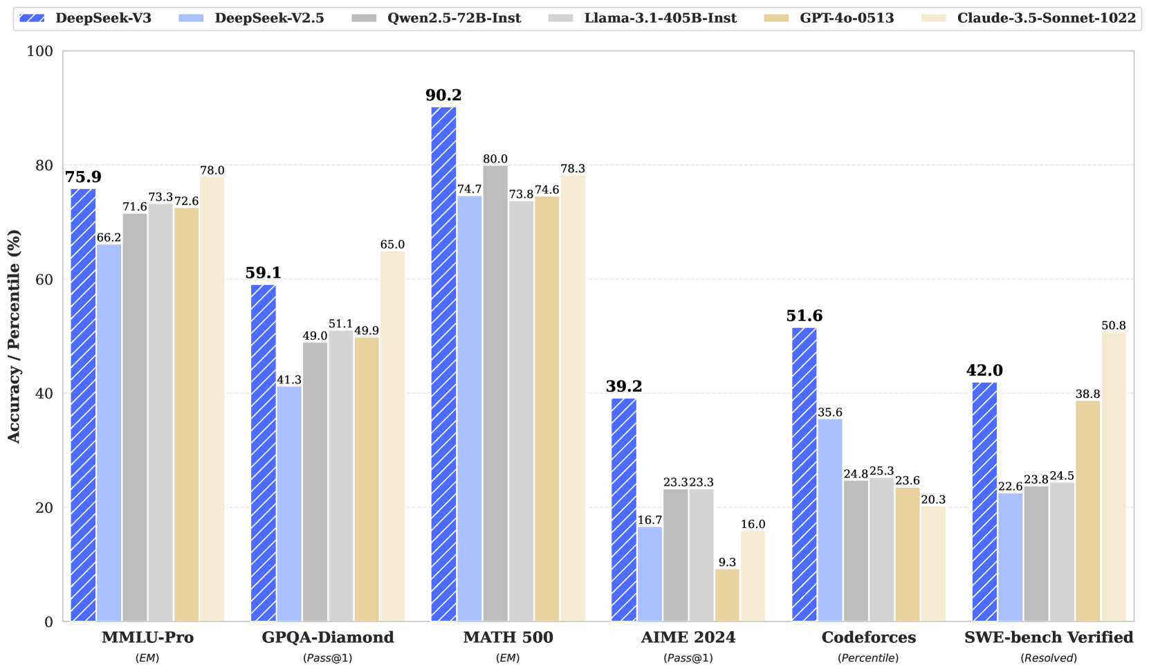
| **MMLU-Pro** *(EM)* | **75.9** | 66.2 | 71.6 | 73.3 | 72.6 | 78.0 |
| **GPQA-Diamond** *(Pass@1)* | **59.1** | 41.3 | 49.0 | 51.1 | 49.9 | 65.0 |
| **MATH 500** *(EM)* | **90.2** | 74.7 | 80.0 | 73.8 | 74.6 | 78.3 |
| **AIME 2024** *(Pass@1)* | **39.2** | 16.7 | 23.3 | 23.3 | 9.3 | 16.0 |
| **Codeforces** *(Percentile)* | **51.6** | 35.6 | 24.8 | 25.3 | 23.6 | 20.3 |
| **SWE-bench Verified** *(Resolved)* | **42.0** | 22.6 | 23.8 | 24.5 | 38.8 | 50.8 |
---
## 4. Trend Analysis and Key Observations
### General Trends
* **DeepSeek-V3 Performance:** In every category, the DeepSeek-V3 value is highlighted in a **bold font**, indicating it is the primary subject of the chart. It outperforms its predecessor (DeepSeek-V2.5) significantly across all benchmarks.
* **Competitive Standing:** DeepSeek-V3 holds the highest score in 4 out of the 6 benchmarks shown (MMLU-Pro and SWE-bench Verified being the exceptions where Claude-3.5-Sonnet-1022 leads).
### Category Specifics
1. **MMLU-Pro (EM):** Most models cluster between 71% and 78%. Claude-3.5-Sonnet-1022 leads this category at 78.0%, followed by DeepSeek-V3 at 75.9%.
2. **GPQA-Diamond (Pass@1):** Claude-3.5-Sonnet-1022 leads (65.0%), with DeepSeek-V3 following (59.1%). There is a significant drop-off to the other models which are near or below 50%.
3. **MATH 500 (EM):** DeepSeek-V3 shows a dominant lead at 90.2%, which is 10.2 percentage points higher than the next closest model (Qwen2.5-72B-Inst at 80.0%).
4. **AIME 2024 (Pass@1):** DeepSeek-V3 shows a very strong lead at 39.2%, more than double the performance of most other models in the set (e.g., DeepSeek-V2.5 at 16.7% and Claude at 16.0%).
5. **Codeforces (Percentile):** DeepSeek-V3 leads significantly at 51.6%. Interestingly, the "frontier" Western models (GPT-4o and Claude-3.5) perform the worst in this specific coding percentile metric (23.6% and 20.3% respectively).
6. **SWE-bench Verified (Resolved):** Claude-3.5-Sonnet-1022 leads at 50.8%. DeepSeek-V3 follows at 42.0%, showing a substantial improvement over DeepSeek-V2.5 (22.6%).
---
## 5. Axis and Scale Details
* **Y-Axis:** Ranges from 0 to 100 with major increments every 20 units (0, 20, 40, 60, 80, 100). Horizontal dashed grid lines are present at each 20-unit interval to facilitate visual alignment.
* **X-Axis:** Categorical, representing six distinct benchmarks. Each category contains a cluster of six bars corresponding to the models in the legend.
</details>
Figure 1: Benchmark performance of DeepSeek-V3 and its counterparts. Contents
1. 1 Introduction
1. 2 Architecture
1. 2.1 Basic Architecture
1. 2.1.1 Multi-Head Latent Attention
1. 2.1.2 DeepSeekMoE with Auxiliary-Loss-Free Load Balancing
1. 2.2 Multi-Token Prediction
1. 3 Infrastructures
1. 3.1 Compute Clusters
1. 3.2 Training Framework
1. 3.2.1 DualPipe and Computation-Communication Overlap
1. 3.2.2 Efficient Implementation of Cross-Node All-to-All Communication
1. 3.2.3 Extremely Memory Saving with Minimal Overhead
1. 3.3 FP8 Training
1. 3.3.1 Mixed Precision Framework
1. 3.3.2 Improved Precision from Quantization and Multiplication
1. 3.3.3 Low-Precision Storage and Communication
1. 3.4 Inference and Deployment
1. 3.4.1 Prefilling
1. 3.4.2 Decoding
1. 3.5 Suggestions on Hardware Design
1. 3.5.1 Communication Hardware
1. 3.5.2 Compute Hardware
1. 4 Pre-Training
1. 4.1 Data Construction
1. 4.2 Hyper-Parameters
1. 4.3 Long Context Extension
1. 4.4 Evaluations
1. 4.4.1 Evaluation Benchmarks
1. 4.4.2 Evaluation Results
1. 4.5 Discussion
1. 4.5.1 Ablation Studies for Multi-Token Prediction
1. 4.5.2 Ablation Studies for the Auxiliary-Loss-Free Balancing Strategy
1. 4.5.3 Batch-Wise Load Balance VS. Sequence-Wise Load Balance
1. 5 Post-Training
1. 5.1 Supervised Fine-Tuning
1. 5.2 Reinforcement Learning
1. 5.2.1 Reward Model
1. 5.2.2 Group Relative Policy Optimization
1. 5.3 Evaluations
1. 5.3.1 Evaluation Settings
1. 5.3.2 Standard Evaluation
1. 5.3.3 Open-Ended Evaluation
1. 5.3.4 DeepSeek-V3 as a Generative Reward Model
1. 5.4 Discussion
1. 5.4.1 Distillation from DeepSeek-R1
1. 5.4.2 Self-Rewarding
1. 5.4.3 Multi-Token Prediction Evaluation
1. 6 Conclusion, Limitations, and Future Directions
1. A Contributions and Acknowledgments
1. B Ablation Studies for Low-Precision Training
1. B.1 FP8 v.s. BF16 Training
1. B.2 Discussion About Block-Wise Quantization
1. C Expert Specialization Patterns of the 16B Aux-Loss-Based and Aux-Loss-Free Models
1 Introduction
In recent years, Large Language Models (LLMs) have been undergoing rapid iteration and evolution (OpenAI, 2024a; Anthropic, 2024; Google, 2024), progressively diminishing the gap towards Artificial General Intelligence (AGI). Beyond closed-source models, open-source models, including DeepSeek series (DeepSeek-AI, 2024b, c; Guo et al., 2024; DeepSeek-AI, 2024a), LLaMA series (Touvron et al., 2023a, b; AI@Meta, 2024a, b), Qwen series (Qwen, 2023, 2024a, 2024b), and Mistral series (Jiang et al., 2023; Mistral, 2024), are also making significant strides, endeavoring to close the gap with their closed-source counterparts. To further push the boundaries of open-source model capabilities, we scale up our models and introduce DeepSeek-V3, a large Mixture-of-Experts (MoE) model with 671B parameters, of which 37B are activated for each token.
With a forward-looking perspective, we consistently strive for strong model performance and economical costs. Therefore, in terms of architecture, DeepSeek-V3 still adopts Multi-head Latent Attention (MLA) (DeepSeek-AI, 2024c) for efficient inference and DeepSeekMoE (Dai et al., 2024) for cost-effective training. These two architectures have been validated in DeepSeek-V2 (DeepSeek-AI, 2024c), demonstrating their capability to maintain robust model performance while achieving efficient training and inference. Beyond the basic architecture, we implement two additional strategies to further enhance the model capabilities. Firstly, DeepSeek-V3 pioneers an auxiliary-loss-free strategy (Wang et al., 2024a) for load balancing, with the aim of minimizing the adverse impact on model performance that arises from the effort to encourage load balancing. Secondly, DeepSeek-V3 employs a multi-token prediction training objective, which we have observed to enhance the overall performance on evaluation benchmarks.
In order to achieve efficient training, we support the FP8 mixed precision training and implement comprehensive optimizations for the training framework. Low-precision training has emerged as a promising solution for efficient training (Kalamkar et al., 2019; Narang et al., 2017; Peng et al., 2023b; Dettmers et al., 2022), its evolution being closely tied to advancements in hardware capabilities (Micikevicius et al., 2022; Luo et al., 2024; Rouhani et al., 2023a). In this work, we introduce an FP8 mixed precision training framework and, for the first time, validate its effectiveness on an extremely large-scale model. Through the support for FP8 computation and storage, we achieve both accelerated training and reduced GPU memory usage. As for the training framework, we design the DualPipe algorithm for efficient pipeline parallelism, which has fewer pipeline bubbles and hides most of the communication during training through computation-communication overlap. This overlap ensures that, as the model further scales up, as long as we maintain a constant computation-to-communication ratio, we can still employ fine-grained experts across nodes while achieving a near-zero all-to-all communication overhead. In addition, we also develop efficient cross-node all-to-all communication kernels to fully utilize InfiniBand (IB) and NVLink bandwidths. Furthermore, we meticulously optimize the memory footprint, making it possible to train DeepSeek-V3 without using costly tensor parallelism. Combining these efforts, we achieve high training efficiency.
During pre-training, we train DeepSeek-V3 on 14.8T high-quality and diverse tokens. The pre-training process is remarkably stable. Throughout the entire training process, we did not encounter any irrecoverable loss spikes or have to roll back. Next, we conduct a two-stage context length extension for DeepSeek-V3. In the first stage, the maximum context length is extended to 32K, and in the second stage, it is further extended to 128K. Following this, we conduct post-training, including Supervised Fine-Tuning (SFT) and Reinforcement Learning (RL) on the base model of DeepSeek-V3, to align it with human preferences and further unlock its potential. During the post-training stage, we distill the reasoning capability from the DeepSeek-R1 series of models, and meanwhile carefully maintain the balance between model accuracy and generation length.
We evaluate DeepSeek-V3 on a comprehensive array of benchmarks. Despite its economical training costs, comprehensive evaluations reveal that DeepSeek-V3-Base has emerged as the strongest open-source base model currently available, especially in code and math. Its chat version also outperforms other open-source models and achieves performance comparable to leading closed-source models, including GPT-4o and Claude-3.5-Sonnet, on a series of standard and open-ended benchmarks.
| in H800 GPU Hours-in USD | 2664K $5.328M | 119K $0.238M | 5K $0.01M | 2788K $5.576M |
| --- | --- | --- | --- | --- |
Table 1: Training costs of DeepSeek-V3, assuming the rental price of H800 is $2 per GPU hour.
Lastly, we emphasize again the economical training costs of DeepSeek-V3, summarized in Table 1, achieved through our optimized co-design of algorithms, frameworks, and hardware. During the pre-training stage, training DeepSeek-V3 on each trillion tokens requires only 180K H800 GPU hours, i.e., 3.7 days on our cluster with 2048 H800 GPUs. Consequently, our pre-training stage is completed in less than two months and costs 2664K GPU hours. Combined with 119K GPU hours for the context length extension and 5K GPU hours for post-training, DeepSeek-V3 costs only 2.788M GPU hours for its full training. Assuming the rental price of the H800 GPU is $2 per GPU hour, our total training costs amount to only $5.576M. Note that the aforementioned costs include only the official training of DeepSeek-V3, excluding the costs associated with prior research and ablation experiments on architectures, algorithms, or data.
Our main contribution includes:
Architecture: Innovative Load Balancing Strategy and Training Objective
- On top of the efficient architecture of DeepSeek-V2, we pioneer an auxiliary-loss-free strategy for load balancing, which minimizes the performance degradation that arises from encouraging load balancing.
- We investigate a Multi-Token Prediction (MTP) objective and prove it beneficial to model performance. It can also be used for speculative decoding for inference acceleration.
Pre-Training: Towards Ultimate Training Efficiency
- We design an FP8 mixed precision training framework and, for the first time, validate the feasibility and effectiveness of FP8 training on an extremely large-scale model.
- Through the co-design of algorithms, frameworks, and hardware, we overcome the communication bottleneck in cross-node MoE training, achieving near-full computation-communication overlap. This significantly enhances our training efficiency and reduces the training costs, enabling us to further scale up the model size without additional overhead.
- At an economical cost of only 2.664M H800 GPU hours, we complete the pre-training of DeepSeek-V3 on 14.8T tokens, producing the currently strongest open-source base model. The subsequent training stages after pre-training require only 0.1M GPU hours.
Post-Training: Knowledge Distillation from DeepSeek-R1
- We introduce an innovative methodology to distill reasoning capabilities from the long-Chain-of-Thought (CoT) model, specifically from one of the DeepSeek R1 series models, into standard LLMs, particularly DeepSeek-V3. Our pipeline elegantly incorporates the verification and reflection patterns of R1 into DeepSeek-V3 and notably improves its reasoning performance. Meanwhile, we also maintain control over the output style and length of DeepSeek-V3.
Summary of Core Evaluation Results
- Knowledge: (1) On educational benchmarks such as MMLU, MMLU-Pro, and GPQA, DeepSeek-V3 outperforms all other open-source models, achieving 88.5 on MMLU, 75.9 on MMLU-Pro, and 59.1 on GPQA. Its performance is comparable to leading closed-source models like GPT-4o and Claude-Sonnet-3.5, narrowing the gap between open-source and closed-source models in this domain. (2) For factuality benchmarks, DeepSeek-V3 demonstrates superior performance among open-source models on both SimpleQA and Chinese SimpleQA. While it trails behind GPT-4o and Claude-Sonnet-3.5 in English factual knowledge (SimpleQA), it surpasses these models in Chinese factual knowledge (Chinese SimpleQA), highlighting its strength in Chinese factual knowledge.
- Code, Math, and Reasoning: (1) DeepSeek-V3 achieves state-of-the-art performance on math-related benchmarks among all non-long-CoT open-source and closed-source models. Notably, it even outperforms o1-preview on specific benchmarks, such as MATH-500, demonstrating its robust mathematical reasoning capabilities. (2) On coding-related tasks, DeepSeek-V3 emerges as the top-performing model for coding competition benchmarks, such as LiveCodeBench, solidifying its position as the leading model in this domain. For engineering-related tasks, while DeepSeek-V3 performs slightly below Claude-Sonnet-3.5, it still outpaces all other models by a significant margin, demonstrating its competitiveness across diverse technical benchmarks.
In the remainder of this paper, we first present a detailed exposition of our DeepSeek-V3 model architecture (Section 2). Subsequently, we introduce our infrastructures, encompassing our compute clusters, the training framework, the support for FP8 training, the inference deployment strategy, and our suggestions on future hardware design. Next, we describe our pre-training process, including the construction of training data, hyper-parameter settings, long-context extension techniques, the associated evaluations, as well as some discussions (Section 4). Thereafter, we discuss our efforts on post-training, which include Supervised Fine-Tuning (SFT), Reinforcement Learning (RL), the corresponding evaluations, and discussions (Section 5). Lastly, we conclude this work, discuss existing limitations of DeepSeek-V3, and propose potential directions for future research (Section 6).
2 Architecture
We first introduce the basic architecture of DeepSeek-V3, featured by Multi-head Latent Attention (MLA) (DeepSeek-AI, 2024c) for efficient inference and DeepSeekMoE (Dai et al., 2024) for economical training. Then, we present a Multi-Token Prediction (MTP) training objective, which we have observed to enhance the overall performance on evaluation benchmarks. For other minor details not explicitly mentioned, DeepSeek-V3 adheres to the settings of DeepSeek-V2 (DeepSeek-AI, 2024c).
<details>
<summary>x2.png Details</summary>
### Visual Description
# Technical Document Extraction: DeepSeek Architecture Overview
This document provides a comprehensive technical breakdown of the provided architectural diagram, which illustrates the components of a Transformer Block, specifically detailing the **DeepSeekMoE** and **Multi-Head Latent Attention (MLA)** mechanisms.
---
## 1. High-Level Structure: Transformer Block $\times L$
The left side of the image depicts the standard macro-architecture of a Transformer layer, which is repeated $L$ times.
### Components and Flow:
* **Input Path:** Data enters from the bottom.
* **Sub-layer 1 (Attention):**
* **RMSNorm:** The input first passes through Root Mean Square Normalization.
* **Attention:** The normalized signal enters the Attention block (detailed in the MLA section).
* **Residual Connection:** The original input is added to the output of the Attention block via an element-wise addition operator ($\oplus$).
* **Sub-layer 2 (Feed-Forward):**
* **RMSNorm:** The output of the first residual addition passes through a second normalization layer.
* **Feed-Forward Network:** The signal enters the FFN block (detailed in the DeepSeekMoE section).
* **Residual Connection:** The input to this sub-layer is added to the FFN output via an element-wise addition operator ($\oplus$).
* **Output:** The final processed signal exits at the top.
---
## 2. Component Detail: DeepSeekMoE
This section expands on the "Feed-Forward Network" block. It describes a Mixture-of-Experts (MoE) architecture.
### Legend [Top Right]:
* **Light Blue Box:** Routed Expert
* **Light Green Box:** Shared Expert
### Data Flow and Components:
1. **Input Hidden $\mathbf{u}_t$:** Represented as a vector of neurons.
2. **Routing Mechanism:**
* The input is sent to a **Router**.
* The Router generates a distribution, and a **Top-$K_r$** selection is made (visualized by a bar chart).
* Dashed yellow lines indicate the selection of specific "Routed Experts."
3. **Expert Processing:**
* **Shared Experts (Green):** Labeled $1$ through $N_s$. The input $\mathbf{u}_t$ is sent to all shared experts.
* **Routed Experts (Blue):** Labeled $1, 2, 3, 4, \dots, N_r-1, N_r$. Only the experts selected by the Top-$K_r$ gating receive the input.
4. **Aggregation:**
* Outputs from all active experts (Shared and Routed) are multiplied by their respective gating weights ($\otimes$).
* The weighted outputs are summed ($\oplus$).
5. **Output Hidden $\mathbf{h}'_t$:** The final aggregated vector.
---
## 3. Component Detail: Multi-Head Latent Attention (MLA)
This section expands on the "Attention" block, focusing on low-rank latent projections to reduce KV cache overhead.
### Legend [Top Right of MLA Box]:
* **Diagonal Striped Pattern:** Cached During Inference
### Data Flow and Components:
1. **Input Hidden $\mathbf{h}_t$:** The base input vector.
2. **Latent Projections:**
* **Query Path:** $\mathbf{h}_t$ is projected into a **Latent $\mathbf{c}_t^Q$**.
* **Key-Value Path:** $\mathbf{h}_t$ is projected into a **Latent $\mathbf{c}_t^{KV}$**. Note that $\mathbf{c}_t^{KV}$ is marked as **Cached During Inference**.
3. **Feature Extraction:**
* **From $\mathbf{c}_t^Q$:** Produces $\{\mathbf{q}_{t,i}^C\}$ (content query) and $\{\mathbf{q}_{t,i}^R\}$ (positional query via *apply RoPE*). These are concatenated to form $\{[\mathbf{q}_{t,i}^C; \mathbf{q}_{t,i}^R]\}$.
* **From $\mathbf{c}_t^{KV}$:** Produces $\{\mathbf{k}_{t,i}^C\}$ (content key) and $\{\mathbf{v}_{t,i}^C\}$ (content value).
* **Positional Key:** A separate path from $\mathbf{h}_t$ applies RoPE to generate $\mathbf{k}_t^R$ (marked as **Cached During Inference**).
* **Concatenation:** $\{\mathbf{k}_{t,i}^C\}$ and $\mathbf{k}_t^R$ are concatenated to form $\{[\mathbf{k}_{t,i}^C; \mathbf{k}_t^R]\}$.
4. **Attention Mechanism:**
* The processed Query, Key, and Value sets are fed into the **Multi-Head Attention** block.
5. **Output Hidden $\mathbf{u}_t$:** The final output vector of the attention mechanism.
---
## 4. Textual Transcriptions
### Labels and Variables:
* **Transformer Block $\times L$**
* **RMSNorm**
* **Attention**
* **Feed-Forward Network**
* **DeepSeekMoE**
* **Output Hidden $\mathbf{h}'_t$**
* **Shared Expert ($N_s$)**
* **Routed Expert ($N_r$)**
* **Router**
* **Top-$K_r$**
* **Input Hidden $\mathbf{u}_t$**
* **Multi-Head Latent Attention (MLA)**
* **Cached During Inference**
* **Multi-Head Attention**
* **Latent $\mathbf{c}_t^Q$**
* **Latent $\mathbf{c}_t^{KV}$**
* **apply RoPE**
* **concatenate**
* **Input Hidden $\mathbf{h}_t$**
### Mathematical Notations:
* $\{\mathbf{q}_{t,i}^C\}$ : Content Query
* $\{\mathbf{q}_{t,i}^R\}$ : RoPE Query
* $\{[\mathbf{q}_{t,i}^C; \mathbf{q}_{t,i}^R]\}$ : Concatenated Query
* $\mathbf{k}_t^R$ : RoPE Key
* $\{\mathbf{k}_{t,i}^C\}$ : Content Key
* $\{[\mathbf{k}_{t,i}^C; \mathbf{k}_t^R]\}$ : Concatenated Key
* $\{\mathbf{v}_{t,i}^C\}$ : Content Value
</details>
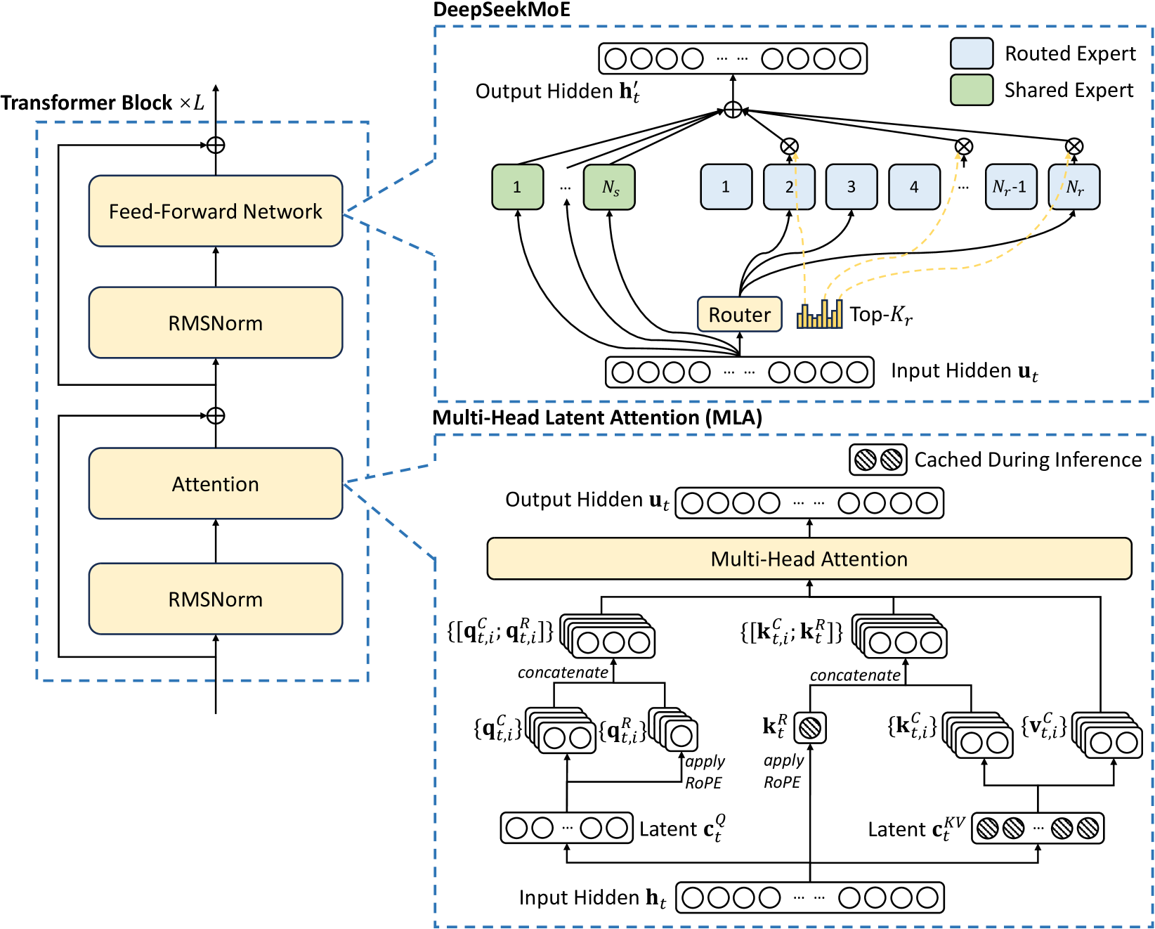
Figure 2: Illustration of the basic architecture of DeepSeek-V3. Following DeepSeek-V2, we adopt MLA and DeepSeekMoE for efficient inference and economical training.
2.1 Basic Architecture
The basic architecture of DeepSeek-V3 is still within the Transformer (Vaswani et al., 2017) framework. For efficient inference and economical training, DeepSeek-V3 also adopts MLA and DeepSeekMoE, which have been thoroughly validated by DeepSeek-V2. Compared with DeepSeek-V2, an exception is that we additionally introduce an auxiliary-loss-free load balancing strategy (Wang et al., 2024a) for DeepSeekMoE to mitigate the performance degradation induced by the effort to ensure load balance. Figure 2 illustrates the basic architecture of DeepSeek-V3, and we will briefly review the details of MLA and DeepSeekMoE in this section.
2.1.1 Multi-Head Latent Attention
For attention, DeepSeek-V3 adopts the MLA architecture. Let $d$ denote the embedding dimension, $n_{h}$ denote the number of attention heads, $d_{h}$ denote the dimension per head, and $\mathbf{h}_{t}∈\mathbb{R}^{d}$ denote the attention input for the $t$ -th token at a given attention layer. The core of MLA is the low-rank joint compression for attention keys and values to reduce Key-Value (KV) cache during inference:
$$
\displaystyle\boxed{\color[rgb]{0,0,1}\definecolor[named]{pgfstrokecolor}{rgb}%
{0,0,1}\mathbf{c}_{t}^{KV}} \displaystyle=W^{DKV}\mathbf{h}_{t}, \displaystyle[\mathbf{k}_{t,1}^{C};\mathbf{k}_{t,2}^{C};...;\mathbf{k}_{t,n_{h%
}}^{C}]=\mathbf{k}_{t}^{C} \displaystyle=W^{UK}\mathbf{c}_{t}^{KV}, \displaystyle\boxed{\color[rgb]{0,0,1}\definecolor[named]{pgfstrokecolor}{rgb}%
{0,0,1}\mathbf{k}_{t}^{R}} \displaystyle=\operatorname{RoPE}({W^{KR}}\mathbf{h}_{t}), \displaystyle\mathbf{k}_{t,i} \displaystyle=[\mathbf{k}_{t,i}^{C};\mathbf{k}_{t}^{R}], \displaystyle[\mathbf{v}_{t,1}^{C};\mathbf{v}_{t,2}^{C};...;\mathbf{v}_{t,n_{h%
}}^{C}]=\mathbf{v}_{t}^{C} \displaystyle=W^{UV}\mathbf{c}_{t}^{KV}, \tag{1}
$$
where $\mathbf{c}_{t}^{KV}∈\mathbb{R}^{d_{c}}$ is the compressed latent vector for keys and values; $d_{c}(\ll d_{h}n_{h})$ indicates the KV compression dimension; $W^{DKV}∈\mathbb{R}^{d_{c}× d}$ denotes the down-projection matrix; $W^{UK},W^{UV}∈\mathbb{R}^{d_{h}n_{h}× d_{c}}$ are the up-projection matrices for keys and values, respectively; $W^{KR}∈\mathbb{R}^{d_{h}^{R}× d}$ is the matrix used to produce the decoupled key that carries Rotary Positional Embedding (RoPE) (Su et al., 2024); $\operatorname{RoPE}(·)$ denotes the operation that applies RoPE matrices; and $[·;·]$ denotes concatenation. Note that for MLA, only the blue-boxed vectors (i.e., $\color[rgb]{0,0,1}\definecolor[named]{pgfstrokecolor}{rgb}{0,0,1}\mathbf{c}_{t%
}^{KV}$ and $\color[rgb]{0,0,1}\definecolor[named]{pgfstrokecolor}{rgb}{0,0,1}\mathbf{k}_{t%
}^{R}$ ) need to be cached during generation, which results in significantly reduced KV cache while maintaining performance comparable to standard Multi-Head Attention (MHA) (Vaswani et al., 2017).
For the attention queries, we also perform a low-rank compression, which can reduce the activation memory during training:
$$
\displaystyle\mathbf{c}_{t}^{Q} \displaystyle=W^{DQ}\mathbf{h}_{t}, \displaystyle[\mathbf{q}_{t,1}^{C};\mathbf{q}_{t,2}^{C};...;\mathbf{q}_{t,n_{h%
}}^{C}]=\mathbf{q}_{t}^{C} \displaystyle=W^{UQ}\mathbf{c}_{t}^{Q}, \displaystyle[\mathbf{q}_{t,1}^{R};\mathbf{q}_{t,2}^{R};...;\mathbf{q}_{t,n_{h%
}}^{R}]=\mathbf{q}_{t}^{R} \displaystyle=\operatorname{RoPE}({W^{QR}}\mathbf{c}_{t}^{Q}), \displaystyle\mathbf{q}_{t,i} \displaystyle=[\mathbf{q}_{t,i}^{C};\mathbf{q}_{t,i}^{R}], \tag{6}
$$
where $\mathbf{c}_{t}^{Q}∈\mathbb{R}^{d_{c}^{\prime}}$ is the compressed latent vector for queries; $d_{c}^{\prime}(\ll d_{h}n_{h})$ denotes the query compression dimension; $W^{DQ}∈\mathbb{R}^{d_{c}^{\prime}× d},W^{UQ}∈\mathbb{R}^{d_{h}n_{h}%
× d_{c}^{\prime}}$ are the down-projection and up-projection matrices for queries, respectively; and $W^{QR}∈\mathbb{R}^{d_{h}^{R}n_{h}× d_{c}^{\prime}}$ is the matrix to produce the decoupled queries that carry RoPE.
Ultimately, the attention queries ( $\mathbf{q}_{t,i}$ ), keys ( $\mathbf{k}_{j,i}$ ), and values ( $\mathbf{v}_{j,i}^{C}$ ) are combined to yield the final attention output $\mathbf{u}_{t}$ :
$$
\displaystyle\mathbf{o}_{t,i} \displaystyle=\sum_{j=1}^{t}\operatorname{Softmax}_{j}(\frac{\mathbf{q}_{t,i}^%
{T}\mathbf{k}_{j,i}}{\sqrt{d_{h}+d_{h}^{R}}})\mathbf{v}_{j,i}^{C}, \displaystyle\mathbf{u}_{t} \displaystyle=W^{O}[\mathbf{o}_{t,1};\mathbf{o}_{t,2};...;\mathbf{o}_{t,n_{h}}], \tag{10}
$$
where $W^{O}∈\mathbb{R}^{d× d_{h}n_{h}}$ denotes the output projection matrix.
2.1.2 DeepSeekMoE with Auxiliary-Loss-Free Load Balancing
Basic Architecture of DeepSeekMoE.
For Feed-Forward Networks (FFNs), DeepSeek-V3 employs the DeepSeekMoE architecture (Dai et al., 2024). Compared with traditional MoE architectures like GShard (Lepikhin et al., 2021), DeepSeekMoE uses finer-grained experts and isolates some experts as shared ones. Let $\mathbf{u}_{t}$ denote the FFN input of the $t$ -th token, we compute the FFN output $\mathbf{h}_{t}^{\prime}$ as follows:
$$
\displaystyle\mathbf{h}_{t}^{\prime} \displaystyle=\mathbf{u}_{t}+\sum_{i=1}^{N_{s}}{\operatorname{FFN}^{(s)}_{i}%
\left(\mathbf{u}_{t}\right)}+\sum_{i=1}^{N_{r}}{g_{i,t}\operatorname{FFN}^{(r)%
}_{i}\left(\mathbf{u}_{t}\right)}, \displaystyle g_{i,t} \displaystyle=\frac{g^{\prime}_{i,t}}{\sum_{j=1}^{N_{r}}g^{\prime}_{j,t}}, \displaystyle g^{\prime}_{i,t} \displaystyle=\begin{cases}s_{i,t},&s_{i,t}\in\operatorname{Topk}(\{s_{j,t}|1%
\leqslant j\leqslant N_{r}\},K_{r}),\\
0,&\text{otherwise},\end{cases} \displaystyle s_{i,t} \displaystyle=\operatorname{Sigmoid}\left({\mathbf{u}_{t}}^{T}\mathbf{e}_{i}%
\right), \tag{12}
$$
where $N_{s}$ and $N_{r}$ denote the numbers of shared experts and routed experts, respectively; $\operatorname{FFN}^{(s)}_{i}(·)$ and $\operatorname{FFN}^{(r)}_{i}(·)$ denote the $i$ -th shared expert and the $i$ -th routed expert, respectively; $K_{r}$ denotes the number of activated routed experts; $g_{i,t}$ is the gating value for the $i$ -th expert; $s_{i,t}$ is the token-to-expert affinity; $\mathbf{e}_{i}$ is the centroid vector of the $i$ -th routed expert; and $\operatorname{Topk}(·,K)$ denotes the set comprising $K$ highest scores among the affinity scores calculated for the $t$ -th token and all routed experts. Slightly different from DeepSeek-V2, DeepSeek-V3 uses the sigmoid function to compute the affinity scores, and applies a normalization among all selected affinity scores to produce the gating values.
Auxiliary-Loss-Free Load Balancing.
For MoE models, an unbalanced expert load will lead to routing collapse (Shazeer et al., 2017) and diminish computational efficiency in scenarios with expert parallelism. Conventional solutions usually rely on the auxiliary loss (Fedus et al., 2021; Lepikhin et al., 2021) to avoid unbalanced load. However, too large an auxiliary loss will impair the model performance (Wang et al., 2024a). To achieve a better trade-off between load balance and model performance, we pioneer an auxiliary-loss-free load balancing strategy (Wang et al., 2024a) to ensure load balance. To be specific, we introduce a bias term $b_{i}$ for each expert and add it to the corresponding affinity scores $s_{i,t}$ to determine the top-K routing:
$$
\displaystyle g^{\prime}_{i,t} \displaystyle=\begin{cases}s_{i,t},&s_{i,t}+b_{i}\in\operatorname{Topk}(\{s_{j%
,t}+b_{j}|1\leqslant j\leqslant N_{r}\},K_{r}),\\
0,&\text{otherwise}.\end{cases} \tag{16}
$$
Note that the bias term is only used for routing. The gating value, which will be multiplied with the FFN output, is still derived from the original affinity score $s_{i,t}$ . During training, we keep monitoring the expert load on the whole batch of each training step. At the end of each step, we will decrease the bias term by $\gamma$ if its corresponding expert is overloaded, and increase it by $\gamma$ if its corresponding expert is underloaded, where $\gamma$ is a hyper-parameter called bias update speed. Through the dynamic adjustment, DeepSeek-V3 keeps balanced expert load during training, and achieves better performance than models that encourage load balance through pure auxiliary losses.
Complementary Sequence-Wise Auxiliary Loss.
Although DeepSeek-V3 mainly relies on the auxiliary-loss-free strategy for load balance, to prevent extreme imbalance within any single sequence, we also employ a complementary sequence-wise balance loss:
$$
\displaystyle\mathcal{L}_{\mathrm{Bal}} \displaystyle=\alpha\sum_{i=1}^{N_{r}}{f_{i}P_{i}}, \displaystyle f_{i}=\frac{N_{r}}{K_{r}T}\sum_{t=1}^{T}\mathds{1} \displaystyle\left(s_{i,t}\in\operatorname{Topk}(\{s_{j,t}|1\leqslant j%
\leqslant N_{r}\},K_{r})\right), \displaystyle s^{\prime}_{i,t} \displaystyle=\frac{s_{i,t}}{\sum_{j=1}^{N_{r}}s_{j,t}}, \displaystyle P_{i} \displaystyle=\frac{1}{T}\sum_{t=1}^{T}{s^{\prime}_{i,t}}, \tag{17}
$$
where the balance factor $\alpha$ is a hyper-parameter, which will be assigned an extremely small value for DeepSeek-V3; $\mathds{1}(·)$ denotes the indicator function; and $T$ denotes the number of tokens in a sequence. The sequence-wise balance loss encourages the expert load on each sequence to be balanced.
Node-Limited Routing.
Like the device-limited routing used by DeepSeek-V2, DeepSeek-V3 also uses a restricted routing mechanism to limit communication costs during training. In short, we ensure that each token will be sent to at most $M$ nodes, which are selected according to the sum of the highest $\frac{K_{r}}{M}$ affinity scores of the experts distributed on each node. Under this constraint, our MoE training framework can nearly achieve full computation-communication overlap.
No Token-Dropping.
Due to the effective load balancing strategy, DeepSeek-V3 keeps a good load balance during its full training. Therefore, DeepSeek-V3 does not drop any tokens during training. In addition, we also implement specific deployment strategies to ensure inference load balance, so DeepSeek-V3 also does not drop tokens during inference.
<details>
<summary>x3.png Details</summary>
### Visual Description
# Technical Diagram Analysis: Multi-Token Prediction (MTP) Architecture
This document provides a detailed technical extraction of the provided architectural diagram, which illustrates a machine learning model designed for Multi-Token Prediction (MTP).
## 1. High-Level Overview
The diagram depicts a sequential architecture consisting of a **Main Model** followed by multiple **MTP Modules** (MTP Module 1 and MTP Module 2 are shown, with an ellipsis indicating further modules). The system is designed to predict multiple future tokens simultaneously by shifting the input window and sharing weights across specific layers.
---
## 2. Component Breakdown
### A. Input and Target Tokens (Data Flow)
The diagram tracks the flow of tokens through three distinct stages.
| Stage | Input Tokens | Target Tokens | Prediction Goal |
| :--- | :--- | :--- | :--- |
| **Main Model** | $t_1, t_2, t_3, t_4$ | $t_2, t_3, t_4, t_5$ | Next Token Prediction |
| **MTP Module 1** | $t_2, t_3, t_4, t_5$ | $t_3, t_4, t_5, t_6$ | $Next^2$ Token Prediction |
| **MTP Module 2** | $t_3, t_4, t_5, t_6$ | $t_4, t_5, t_6, t_7$ | $Next^3$ Token Prediction |
### B. Main Model Structure
Contained within a blue dashed boundary.
- **Input:** $t_1$ through $t_4$.
- **Embedding Layer:** (Green) Shared across all modules.
- **Transformer Block $\times L$:** (Yellow) A stack of $L$ transformer blocks processing the embeddings.
- **Output Head:** (Green) Shared across all modules. Produces the final hidden state.
- **Loss Function:** Cross-Entropy Loss comparing output to targets $t_2 \dots t_5$.
- **Loss Label:** $\mathcal{L}_{Main}$
### C. MTP Module 1 Structure
Contained within a blue dashed boundary.
- **Input:** $t_2$ through $t_5$.
- **Embedding Layer:** (Green) Shared with Main Model.
- **RMSNorm Layers:** Two parallel RMSNorm blocks.
- One receives input from the Shared Embedding Layer.
- The other receives the hidden state output from the **Main Model's** Transformer stack.
- **Concatenation:** The outputs of the two RMSNorm layers are merged.
- **Linear Projection:** (Yellow) Processes the concatenated representation.
- **Transformer Block:** (Yellow) A single transformer block.
- **Output Head:** (Green) Shared with Main Model.
- **Loss Function:** Cross-Entropy Loss comparing output to targets $t_3 \dots t_6$.
- **Loss Label:** $\mathcal{L}_{MTP}^1$
### D. MTP Module 2 Structure
Contained within a blue dashed boundary.
- **Input:** $t_3$ through $t_6$.
- **Embedding Layer:** (Green) Shared with previous modules.
- **RMSNorm Layers:** Two parallel RMSNorm blocks.
- One receives input from the Shared Embedding Layer.
- The other receives the hidden state output from **MTP Module 1's** Transformer Block.
- **Concatenation:** Merges the two RMSNorm outputs.
- **Linear Projection:** (Yellow) Processes the concatenated representation.
- **Transformer Block:** (Yellow) A single transformer block.
- **Output Head:** (Green) Shared with previous modules.
- **Loss Function:** Cross-Entropy Loss comparing output to targets $t_4 \dots t_7$.
- **Loss Label:** $\mathcal{L}_{MTP}^2$
---
## 3. Shared Components and Connections
The diagram uses specific visual cues to denote shared parameters and data flow:
1. **Shared Layers (Green Blocks):**
* **Embedding Layer:** Connected by a green dotted line labeled "Shared" across all three modules.
* **Output Head:** Connected by a green dotted line labeled "Shared" across all three modules.
2. **Hidden State Propagation:**
* A solid black line carries the output from the Main Model's Transformer stack into the RMSNorm of MTP Module 1.
* A solid black line carries the output from MTP Module 1's Transformer Block into the RMSNorm of MTP Module 2.
3. **Loss Aggregation:**
* Each module contributes a specific loss component ($\mathcal{L}_{Main}$, $\mathcal{L}_{MTP}^1$, $\mathcal{L}_{MTP}^2$), suggesting a multi-task objective function.
---
## 4. Textual Transcriptions
### Labels and Headers
* **Top Row:** Target Tokens
* **Bottom Row:** Input Tokens
* **Main Model Header:** Main Model (*Next Token Prediction*)
* **MTP Module 1 Header:** MTP Module 1 (*Next$^2$ Token Prediction*)
* **MTP Module 2 Header:** MTP Module 2 (*Next$^3$ Token Prediction*)
### Internal Block Text
* `Cross-Entropy Loss`
* `Output Head`
* `Transformer Block × L`
* `Transformer Block`
* `Linear Projection`
* `RMSNorm`
* `Embedding Layer`
* `concatenation`
* `Shared` (associated with green dotted lines)
### Mathematical Notations
* **Tokens:** $t_1, t_2, t_3, t_4, t_5, t_6, t_7$
* **Losses:** $\mathcal{L}_{Main}$, $\mathcal{L}_{MTP}^1$, $\mathcal{L}_{MTP}^2$
* **Variables:** $L$ (number of blocks in Main Model)
</details>
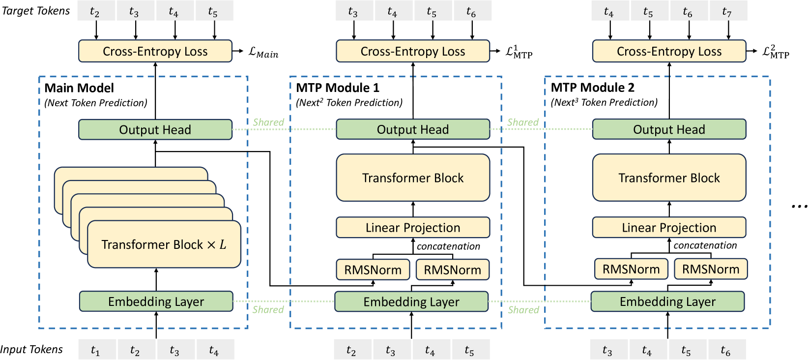
Figure 3: Illustration of our Multi-Token Prediction (MTP) implementation. We keep the complete causal chain for the prediction of each token at each depth.
2.2 Multi-Token Prediction
Inspired by Gloeckle et al. (2024), we investigate and set a Multi-Token Prediction (MTP) objective for DeepSeek-V3, which extends the prediction scope to multiple future tokens at each position. On the one hand, an MTP objective densifies the training signals and may improve data efficiency. On the other hand, MTP may enable the model to pre-plan its representations for better prediction of future tokens. Figure 3 illustrates our implementation of MTP. Different from Gloeckle et al. (2024), which parallelly predicts $D$ additional tokens using independent output heads, we sequentially predict additional tokens and keep the complete causal chain at each prediction depth. We introduce the details of our MTP implementation in this section.
MTP Modules.
To be specific, our MTP implementation uses $D$ sequential modules to predict $D$ additional tokens. The $k$ -th MTP module consists of a shared embedding layer $\operatorname{Emb}(·)$ , a shared output head $\operatorname{OutHead}(·)$ , a Transformer block $\operatorname{TRM}_{k}(·)$ , and a projection matrix $M_{k}∈\mathbb{R}^{d× 2d}$ . For the $i$ -th input token $t_{i}$ , at the $k$ -th prediction depth, we first combine the representation of the $i$ -th token at the $(k-1)$ -th depth $\mathbf{h}_{i}^{k-1}∈\mathbb{R}^{d}$ and the embedding of the $(i+k)$ -th token $Emb(t_{i+k})∈\mathbb{R}^{d}$ with the linear projection:
$$
\mathbf{h}_{i}^{\prime k}=M_{k}[\operatorname{RMSNorm}(\mathbf{h}_{i}^{k-1});%
\operatorname{RMSNorm}(\operatorname{Emb}(t_{i+k}))], \tag{21}
$$
where $[·;·]$ denotes concatenation. Especially, when $k=1$ , $\mathbf{h}_{i}^{k-1}$ refers to the representation given by the main model. Note that for each MTP module, its embedding layer is shared with the main model. The combined $\mathbf{h}_{i}^{\prime k}$ serves as the input of the Transformer block at the $k$ -th depth to produce the output representation at the current depth $\mathbf{h}_{i}^{k}$ :
$$
\mathbf{h}_{1:T-k}^{k}=\operatorname{TRM}_{k}(\mathbf{h}_{1:T-k}^{\prime k}), \tag{22}
$$
where $T$ represents the input sequence length and i:j denotes the slicing operation (inclusive of both the left and right boundaries). Finally, taking $\mathbf{h}_{i}^{k}$ as the input, the shared output head will compute the probability distribution for the $k$ -th additional prediction token $P_{i+1+k}^{k}∈\mathbb{R}^{V}$ , where $V$ is the vocabulary size:
$$
P_{i+k+1}^{k}=\operatorname{OutHead}(\mathbf{h}_{i}^{k}). \tag{23}
$$
The output head $\operatorname{OutHead}(·)$ linearly maps the representation to logits and subsequently applies the $\operatorname{Softmax}(·)$ function to compute the prediction probabilities of the $k$ -th additional token. Also, for each MTP module, its output head is shared with the main model. Our principle of maintaining the causal chain of predictions is similar to that of EAGLE (Li et al., 2024b), but its primary objective is speculative decoding (Xia et al., 2023; Leviathan et al., 2023), whereas we utilize MTP to improve training.
MTP Training Objective.
For each prediction depth, we compute a cross-entropy loss $\mathcal{L}_{\text{MTP}}^{k}$ :
$$
\mathcal{L}_{\text{MTP}}^{k}=\operatorname{CrossEntropy}(P_{2+k:T+1}^{k},t_{2+%
k:T+1})=-\frac{1}{T}\sum_{i=2+k}^{T+1}\log P_{i}^{k}[t_{i}], \tag{24}
$$
where $T$ denotes the input sequence length, $t_{i}$ denotes the ground-truth token at the $i$ -th position, and $P_{i}^{k}[t_{i}]$ denotes the corresponding prediction probability of $t_{i}$ , given by the $k$ -th MTP module. Finally, we compute the average of the MTP losses across all depths and multiply it by a weighting factor $\lambda$ to obtain the overall MTP loss $\mathcal{L}_{\text{MTP}}$ , which serves as an additional training objective for DeepSeek-V3:
$$
\mathcal{L}_{\text{MTP}}=\frac{\lambda}{D}\sum_{k=1}^{D}\mathcal{L}_{\text{MTP%
}}^{k}. \tag{25}
$$
MTP in Inference.
Our MTP strategy mainly aims to improve the performance of the main model, so during inference, we can directly discard the MTP modules and the main model can function independently and normally. Additionally, we can also repurpose these MTP modules for speculative decoding to further improve the generation latency.
3 Infrastructures
3.1 Compute Clusters
DeepSeek-V3 is trained on a cluster equipped with 2048 NVIDIA H800 GPUs. Each node in the H800 cluster contains 8 GPUs connected by NVLink and NVSwitch within nodes. Across different nodes, InfiniBand (IB) interconnects are utilized to facilitate communications.
3.2 Training Framework
The training of DeepSeek-V3 is supported by the HAI-LLM framework, an efficient and lightweight training framework crafted by our engineers from the ground up. On the whole, DeepSeek-V3 applies 16-way Pipeline Parallelism (PP) (Qi et al., 2023a), 64-way Expert Parallelism (EP) (Lepikhin et al., 2021) spanning 8 nodes, and ZeRO-1 Data Parallelism (DP) (Rajbhandari et al., 2020).
In order to facilitate efficient training of DeepSeek-V3, we implement meticulous engineering optimizations. Firstly, we design the DualPipe algorithm for efficient pipeline parallelism. Compared with existing PP methods, DualPipe has fewer pipeline bubbles. More importantly, it overlaps the computation and communication phases across forward and backward processes, thereby addressing the challenge of heavy communication overhead introduced by cross-node expert parallelism. Secondly, we develop efficient cross-node all-to-all communication kernels to fully utilize IB and NVLink bandwidths and conserve Streaming Multiprocessors (SMs) dedicated to communication. Finally, we meticulously optimize the memory footprint during training, thereby enabling us to train DeepSeek-V3 without using costly Tensor Parallelism (TP).
3.2.1 DualPipe and Computation-Communication Overlap
<details>
<summary>x4.png Details</summary>
### Visual Description
# Technical Document Extraction: Computation and Communication Timeline
## 1. Document Overview
This image is a horizontal timeline diagram illustrating the interleaving of **Computation** and **Communication** tasks over **Time**. It specifically details the execution flow of a neural network layer (likely a Transformer block, given the MLP and ATTN labels) during distributed training.
## 2. Legend and Symbols
The diagram uses specific symbols to denote the phase of the data chunk:
* **$\triangle$ (White Triangle):** Forward chunk
* **$\blacktriangle$ (Black Triangle):** Backward chunk
## 3. Component Isolation
### A. Y-Axis Labels (Left Side)
* **Computation:** The top row of the timeline, representing processing tasks.
* **Communication:** The bottom row of the timeline, representing data transfer tasks.
### B. X-Axis (Bottom)
* **Time:** Indicated by a label and a right-pointing arrow ($\rightarrow$), showing that the sequence progresses from left to right.
### C. Color Coding
* **Lime Green:** Backward-related computation/communication.
* **Light Blue:** Weight-related computation.
* **Orange/Yellow:** Forward-related computation/communication.
* **Purple:** Pipeline Parallelism (PP) overhead.
* **Red (Vertical Bars):** Synchronization points or barriers.
---
## 4. Sequence of Operations (Timeline Flow)
The timeline is divided into two main phases: the **MLP (Multi-Layer Perceptron)** phase and the **ATTN (Attention)** phase, separated by a red synchronization bar.
### Phase 1: MLP Operations
| Row | Task Label | Symbol | Color | Description |
| :--- | :--- | :--- | :--- | :--- |
| **Computation** | MLP(B) | $\blacktriangle$ | Lime Green | Backward pass computation for MLP. |
| **Computation** | MLP(W) | $\blacktriangle$ | Light Blue | Weight gradient computation for MLP. |
| **Computation** | MLP(F) | $\triangle$ | Orange | Forward pass computation for MLP. |
| **Communication** | DISPATCH(F) | $\triangle$ | Orange | Forward dispatch communication (overlaps with MLP(B) and MLP(W)). |
| **Communication** | DISPATCH(B) | $\blacktriangle$ | Lime Green | Backward dispatch communication (overlaps with MLP(F)). |
### Phase 2: ATTN Operations
| Row | Task Label | Symbol | Color | Description |
| :--- | :--- | :--- | :--- | :--- |
| **Computation** | ATTN(B) | $\blacktriangle$ | Lime Green | Backward pass computation for Attention. |
| **Computation** | ATTN(W) | $\blacktriangle$ | Light Blue | Weight gradient computation for Attention. |
| **Computation** | ATTN(F) | $\triangle$ | Orange | Forward pass computation for Attention. |
| **Communication** | COMBINE(F) | $\triangle$ | Orange | Forward combine communication (overlaps with ATTN(B)). |
| **Communication** | PP | N/A | Purple | Pipeline Parallelism communication/stall. |
| **Communication** | COMBINE(B) | $\blacktriangle$ | Lime Green | Backward combine communication (overlaps with ATTN(W) and ATTN(F)). |
---
## 5. Key Trends and Technical Observations
* **Concurrency/Overlapping:** The diagram demonstrates a high degree of overlap between computation and communication. For example, while the system is performing `MLP(F)` (Forward computation), it is simultaneously performing `DISPATCH(B)` (Backward communication).
* **Symmetry:** The structure of the MLP phase and the ATTN phase are similar, both involving a sequence of Backward (B), Weight (W), and Forward (F) computations.
* **Synchronization:** Red vertical bars indicate strict boundaries where computation and communication must synchronize before proceeding to the next major block (e.g., between MLP and ATTN).
* **Pipeline Overhead:** The `PP` (Purple) block in the communication row represents a specific interval where pipeline-related communication occurs, notably occurring between the Forward and Backward combine steps in the Attention phase.
</details>
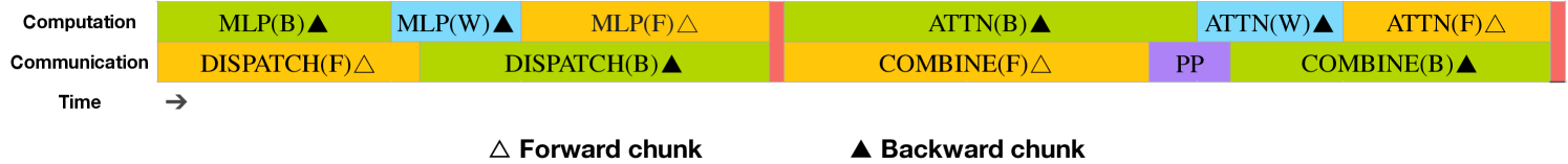
Figure 4: Overlapping strategy for a pair of individual forward and backward chunks (the boundaries of the transformer blocks are not aligned). Orange denotes forward, green denotes "backward for input", blue denotes "backward for weights", purple denotes PP communication, and red denotes barriers. Both all-to-all and PP communication can be fully hidden.
For DeepSeek-V3, the communication overhead introduced by cross-node expert parallelism results in an inefficient computation-to-communication ratio of approximately 1:1. To tackle this challenge, we design an innovative pipeline parallelism algorithm called DualPipe, which not only accelerates model training by effectively overlapping forward and backward computation-communication phases, but also reduces the pipeline bubbles.
The key idea of DualPipe is to overlap the computation and communication within a pair of individual forward and backward chunks. To be specific, we divide each chunk into four components: attention, all-to-all dispatch, MLP, and all-to-all combine. Specially, for a backward chunk, both attention and MLP are further split into two parts, backward for input and backward for weights, like in ZeroBubble (Qi et al., 2023b). In addition, we have a PP communication component. As illustrated in Figure 4, for a pair of forward and backward chunks, we rearrange these components and manually adjust the ratio of GPU SMs dedicated to communication versus computation. In this overlapping strategy, we can ensure that both all-to-all and PP communication can be fully hidden during execution. Given the efficient overlapping strategy, the full DualPipe scheduling is illustrated in Figure 5. It employs a bidirectional pipeline scheduling, which feeds micro-batches from both ends of the pipeline simultaneously and a significant portion of communications can be fully overlapped. This overlap also ensures that, as the model further scales up, as long as we maintain a constant computation-to-communication ratio, we can still employ fine-grained experts across nodes while achieving a near-zero all-to-all communication overhead.
<details>
<summary>x5.png Details</summary>
### Visual Description
# Technical Document Extraction: Pipeline Parallelism Schedule
## 1. Overview
This image is a technical timing diagram (Gantt-style chart) illustrating a pipeline parallelism execution schedule across multiple computational devices. It visualizes the interleaving of forward and backward passes for various micro-batches over a timeline.
## 2. Component Isolation
### Header / Y-Axis (Left)
The vertical axis lists the computational units involved in the pipeline:
* **Device 0** (Top)
* **Device 1**
* **Device 2**
* **Device 3**
* **Device 4**
* **Device 5**
* **Device 6**
* **Device 7** (Bottom)
### Footer / X-Axis (Bottom)
* **Label:** "Time" with a right-pointing arrow ($\rightarrow$), indicating that the horizontal axis represents chronological progression.
### Legend (Bottom)
The legend defines the operations represented by colored blocks and numerical labels:
* **Orange Block:** Forward
* **Dark Green Block:** Backward
* **Light Green Block:** Backward for input
* **Blue Block:** Backward for weights
* **Split Orange/Green Block:** Overlapped forward & Backward
---
## 3. Data Extraction and Flow Analysis
### Execution Pattern
The diagram shows a "1F1B" (One Forward, One Backward) or similar pipelining strategy with 8 devices and 10 micro-batches (numbered 0 through 9).
#### The Forward Pass (Orange)
* **Trend:** The forward pass initiates at Device 0 and propagates down to Device 7. There is a staggered start (pipeline bubble) where Device $n$ starts its forward pass for micro-batch 0 exactly one time step after Device $n-1$.
* **Micro-batches:** 0, 1, 2, 3, 4, 5, 6, 7, 8, 9.
* **Observation:** On Device 0, forward passes for micro-batches 0-6 occur consecutively before the first backward pass begins.
#### The Backward Pass (Green/Blue)
* **Trend:** Backward passes generally move from Device 7 up to Device 0.
* **Components:**
* **Backward for input (Light Green):** Usually follows the forward pass of the same micro-batch on the same device.
* **Backward for weights (Blue):** Often clustered toward the end of the timeline, particularly visible on Devices 0, 6, and 7.
* **Overlapped (Split Orange/Green):** Occurs mid-pipeline (e.g., Device 0, micro-batch 7) where a forward pass and a backward pass are executed concurrently.
### Device-Specific Activity (Sample Rows)
| Device | Initial Forward Sequence | Mid-Pipeline Behavior | End-of-Pipe Behavior |
| :--- | :--- | :--- | :--- |
| **Device 0** | 0, 1, 2, 3, 4, 5, 6 | Overlaps Forward 7 with Backward; then alternating. | Ends with weight updates (Blue 6, 7, 8, 9). |
| **Device 4** | Starts at $T=4$ with micro-batch 0. | Alternates Forward (Orange) and Backward (Green). | Ends with Backward 9 and Weight 8, 9. |
| **Device 7** | Starts at $T=7$ with micro-batch 0. | Immediate transition to Backward 0, 1, 2, 3. | Ends with a dense block of Weight updates (Blue). |
---
## 4. Key Technical Observations
1. **Pipeline Depth:** There are 8 stages (Devices 0-7).
2. **Startup Latency:** There is a clear "ramp-up" period where devices are idle (white space) waiting for the first micro-batch to reach them. Device 7 does not begin work until 7 time units have passed.
3. **Steady State:** The middle section of the diagram shows the "steady state" where devices are fully utilized, performing interleaved forward and backward tasks.
4. **Communication/Dependency:** The diagonal shift of the numbers (e.g., Forward 0 moving from Device 0 at $T=0$ to Device 7 at $T=7$) confirms a sequential dependency between devices for the forward pass, and a reverse dependency for the backward pass.
5. **Resource Optimization:** The "Overlapped forward & Backward" blocks indicate specific points where the hardware is capable of bi-directional communication or concurrent computation to reduce total execution time (Makespan).
</details>
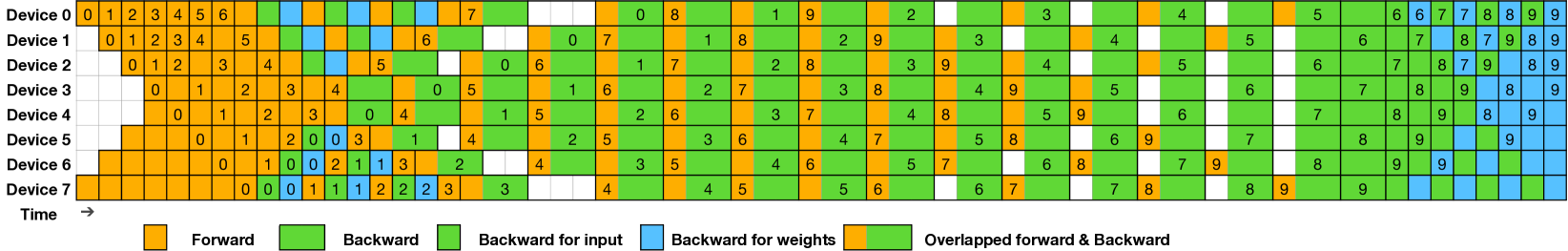
Figure 5: Example DualPipe scheduling for 8 PP ranks and 20 micro-batches in two directions. The micro-batches in the reverse direction are symmetric to those in the forward direction, so we omit their batch ID for illustration simplicity. Two cells enclosed by a shared black border have mutually overlapped computation and communication.
In addition, even in more general scenarios without a heavy communication burden, DualPipe still exhibits efficiency advantages. In Table 2, we summarize the pipeline bubbles and memory usage across different PP methods. As shown in the table, compared with ZB1P (Qi et al., 2023b) and 1F1B (Harlap et al., 2018), DualPipe significantly reduces the pipeline bubbles while only increasing the peak activation memory by $\frac{1}{PP}$ times. Although DualPipe requires keeping two copies of the model parameters, this does not significantly increase the memory consumption since we use a large EP size during training. Compared with Chimera (Li and Hoefler, 2021), DualPipe only requires that the pipeline stages and micro-batches be divisible by 2, without requiring micro-batches to be divisible by pipeline stages. In addition, for DualPipe, neither the bubbles nor activation memory will increase as the number of micro-batches grows.
| 1F1B ZB1P DualPipe (Ours) | $(PP-1)(F+B)$ $(PP-1)(F+B-2W)$ $(\frac{PP}{2}-1)(F\&B+B-3W)$ | $1×$ $1×$ $2×$ | $PP$ $PP$ $PP+1$ |
| --- | --- | --- | --- |
Table 2: Comparison of pipeline bubbles and memory usage across different pipeline parallel methods. $F$ denotes the execution time of a forward chunk, $B$ denotes the execution time of a full backward chunk, $W$ denotes the execution time of a "backward for weights" chunk, and $F\&B$ denotes the execution time of two mutually overlapped forward and backward chunks.
3.2.2 Efficient Implementation of Cross-Node All-to-All Communication
In order to ensure sufficient computational performance for DualPipe, we customize efficient cross-node all-to-all communication kernels (including dispatching and combining) to conserve the number of SMs dedicated to communication. The implementation of the kernels is co-designed with the MoE gating algorithm and the network topology of our cluster. To be specific, in our cluster, cross-node GPUs are fully interconnected with IB, and intra-node communications are handled via NVLink. NVLink offers a bandwidth of 160 GB/s, roughly 3.2 times that of IB (50 GB/s). To effectively leverage the different bandwidths of IB and NVLink, we limit each token to be dispatched to at most 4 nodes, thereby reducing IB traffic. For each token, when its routing decision is made, it will first be transmitted via IB to the GPUs with the same in-node index on its target nodes. Once it reaches the target nodes, we will endeavor to ensure that it is instantaneously forwarded via NVLink to specific GPUs that host their target experts, without being blocked by subsequently arriving tokens. In this way, communications via IB and NVLink are fully overlapped, and each token can efficiently select an average of 3.2 experts per node without incurring additional overhead from NVLink. This implies that, although DeepSeek-V3 selects only 8 routed experts in practice, it can scale up this number to a maximum of 13 experts (4 nodes $×$ 3.2 experts/node) while preserving the same communication cost. Overall, under such a communication strategy, only 20 SMs are sufficient to fully utilize the bandwidths of IB and NVLink.
In detail, we employ the warp specialization technique (Bauer et al., 2014) and partition 20 SMs into 10 communication channels. During the dispatching process, (1) IB sending, (2) IB-to-NVLink forwarding, and (3) NVLink receiving are handled by respective warps. The number of warps allocated to each communication task is dynamically adjusted according to the actual workload across all SMs. Similarly, during the combining process, (1) NVLink sending, (2) NVLink-to-IB forwarding and accumulation, and (3) IB receiving and accumulation are also handled by dynamically adjusted warps. In addition, both dispatching and combining kernels overlap with the computation stream, so we also consider their impact on other SM computation kernels. Specifically, we employ customized PTX (Parallel Thread Execution) instructions and auto-tune the communication chunk size, which significantly reduces the use of the L2 cache and the interference to other SMs.
3.2.3 Extremely Memory Saving with Minimal Overhead
In order to reduce the memory footprint during training, we employ the following techniques.
Recomputation of RMSNorm and MLA Up-Projection.
We recompute all RMSNorm operations and MLA up-projections during back-propagation, thereby eliminating the need to persistently store their output activations. With a minor overhead, this strategy significantly reduces memory requirements for storing activations.
Exponential Moving Average in CPU.
During training, we preserve the Exponential Moving Average (EMA) of the model parameters for early estimation of the model performance after learning rate decay. The EMA parameters are stored in CPU memory and are updated asynchronously after each training step. This method allows us to maintain EMA parameters without incurring additional memory or time overhead.
Shared Embedding and Output Head for Multi-Token Prediction.
With the DualPipe strategy, we deploy the shallowest layers (including the embedding layer) and deepest layers (including the output head) of the model on the same PP rank. This arrangement enables the physical sharing of parameters and gradients, of the shared embedding and output head, between the MTP module and the main model. This physical sharing mechanism further enhances our memory efficiency.
3.3 FP8 Training
<details>
<summary>x6.png Details</summary>
### Visual Description
# Technical Document Extraction: Mixed-Precision Training Flow Diagram
## 1. Document Overview
This image is a technical architectural diagram illustrating the data flow and precision casting (quantization) logic for a deep learning training iteration. It specifically details the interactions between Forward Propagation (**Fprop**), Data Gradient calculation (**Dgrad**), and Weight Gradient calculation (**Wgrad**) using mixed-precision formats (BF16, FP32, and FP8).
---
## 2. Component Isolation
### A. Data Nodes (Grey Rectangles)
These represent the tensors stored in memory at various stages of the training loop.
* **Input**: Labeled as **BF16**.
* **Weight**: Central node used by Fprop and Dgrad.
* **Output**: Result of the forward pass.
* **Output Gradient**: Labeled as **BF16**; the starting point for the backward pass.
* **Input Gradient**: The final result of the Dgrad process.
* **Weight Gradient**: Labeled as **FP32**; the result of the Wgrad process.
* **Optimizer States**: Receives data from Weight Gradient.
* **Master Weight**: High-precision weight storage used to update the model.
### B. Computational Blocks (Yellow Rounded Rectangles)
These represent the arithmetic operations (Matrix Multiplication and Accumulation). Each contains a multiplication symbol ($\otimes$) and a summation symbol ($\sum$).
* **Fprop (Forward Propagation)**: Accumulation occurs in **FP32**.
* **Dgrad (Data Gradient)**: Accumulation occurs in **FP32**.
* **Wgrad (Weight Gradient)**: Accumulation occurs in **FP32**.
---
## 3. Process Flow and Precision Transitions
The diagram tracks how data is cast between formats (e.g., "To FP8") as it moves between nodes and computational blocks.
### Forward Propagation (Fprop)
1. **Input (BF16)** is cast **To FP8** and enters the Fprop block.
2. **Weight** enters the Fprop block (implied FP8 conversion based on the multiplication operation).
3. Inside **Fprop**, multiplication is performed, and results are accumulated in **FP32**.
4. The result is cast **To BF16** to become the **Output**.
### Data Gradient (Dgrad) - Backward Pass
1. **Output Gradient (BF16)** is cast **To FP8** and enters the Dgrad block.
2. **Weight** enters the Dgrad block.
3. Inside **Dgrad**, multiplication is performed, and results are accumulated in **FP32**.
4. The result is cast **To BF16** to become the **Input Gradient**.
### Weight Gradient (Wgrad) - Backward Pass
1. **Input (BF16)** is routed from the start, cast **To FP8**, and enters the Wgrad block.
2. **Output Gradient (BF16)** is cast **To FP8** and enters the Wgrad block.
3. Inside **Wgrad**, multiplication is performed, and results are accumulated in **FP32**.
4. The result is output as the **Weight Gradient (FP32)**.
### Optimizer and Weight Update
1. **Weight Gradient (FP32)** is cast **To BF16** and enters **Optimizer States**.
2. **Optimizer States** feeds into the **Master Weight** (cast **To FP32**).
3. The **Master Weight** is cast **To FP8** to update the active **Weight** used in the next Fprop/Dgrad cycle.
---
## 4. Summary of Precision Formats
| Component / Path | Precision Format |
| :--- | :--- |
| Primary Storage (Input, Output, Gradients) | BF16 |
| Internal Accumulation (Fprop, Dgrad, Wgrad) | FP32 |
| Master Weight / Weight Gradient | FP32 |
| Computational Inputs (Casting) | FP8 |
## 5. Spatial Grounding and Logic Check
* **Header/Top Row**: Shows the forward path (Input $\rightarrow$ Fprop $\rightarrow$ Output) and the start of the weight gradient path.
* **Middle Row**: Shows the Weight management (Weight $\rightarrow$ Master Weight $\rightarrow$ Optimizer States).
* **Bottom Row**: Shows the backward path (Input Gradient $\leftarrow$ Dgrad $\leftarrow$ Output Gradient).
* **Trend/Logic**: The diagram consistently shows that while storage and accumulation happen in higher precision (BF16/FP32), the operands for the heavy matrix multiplications are down-cast to **FP8** to optimize computational throughput.
</details>
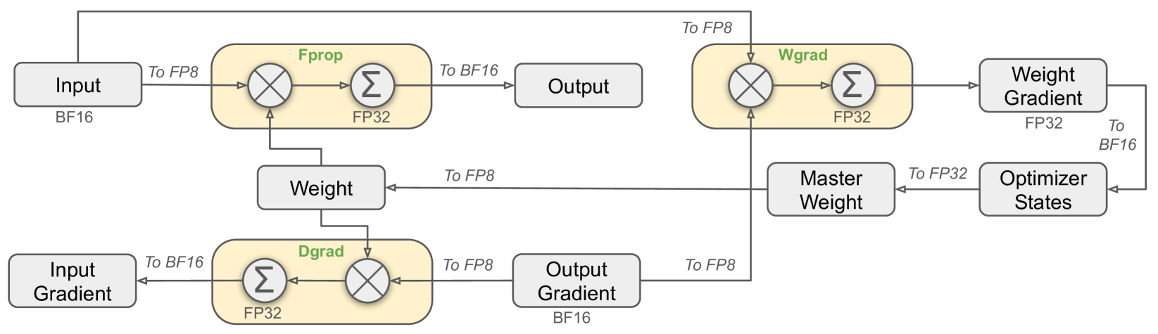
Figure 6: The overall mixed precision framework with FP8 data format. For clarification, only the Linear operator is illustrated.
Inspired by recent advances in low-precision training (Peng et al., 2023b; Dettmers et al., 2022; Noune et al., 2022), we propose a fine-grained mixed precision framework utilizing the FP8 data format for training DeepSeek-V3. While low-precision training holds great promise, it is often limited by the presence of outliers in activations, weights, and gradients (Sun et al., 2024; He et al., ; Fishman et al., 2024). Although significant progress has been made in inference quantization (Xiao et al., 2023; Frantar et al., 2022), there are relatively few studies demonstrating successful application of low-precision techniques in large-scale language model pre-training (Fishman et al., 2024). To address this challenge and effectively extend the dynamic range of the FP8 format, we introduce a fine-grained quantization strategy: tile-wise grouping with $1× N_{c}$ elements or block-wise grouping with $N_{c}× N_{c}$ elements. The associated dequantization overhead is largely mitigated under our increased-precision accumulation process, a critical aspect for achieving accurate FP8 General Matrix Multiplication (GEMM). Moreover, to further reduce memory and communication overhead in MoE training, we cache and dispatch activations in FP8, while storing low-precision optimizer states in BF16. We validate the proposed FP8 mixed precision framework on two model scales similar to DeepSeek-V2-Lite and DeepSeek-V2, training for approximately 1 trillion tokens (see more details in Appendix B.1). Notably, compared with the BF16 baseline, the relative loss error of our FP8-training model remains consistently below 0.25%, a level well within the acceptable range of training randomness.
3.3.1 Mixed Precision Framework
Building upon widely adopted techniques in low-precision training (Kalamkar et al., 2019; Narang et al., 2017), we propose a mixed precision framework for FP8 training. In this framework, most compute-density operations are conducted in FP8, while a few key operations are strategically maintained in their original data formats to balance training efficiency and numerical stability. The overall framework is illustrated in Figure 6.
Firstly, in order to accelerate model training, the majority of core computation kernels, i.e., GEMM operations, are implemented in FP8 precision. These GEMM operations accept FP8 tensors as inputs and produce outputs in BF16 or FP32. As depicted in Figure 6, all three GEMMs associated with the Linear operator, namely Fprop (forward pass), Dgrad (activation backward pass), and Wgrad (weight backward pass), are executed in FP8. This design theoretically doubles the computational speed compared with the original BF16 method. Additionally, the FP8 Wgrad GEMM allows activations to be stored in FP8 for use in the backward pass. This significantly reduces memory consumption.
Despite the efficiency advantage of the FP8 format, certain operators still require a higher precision due to their sensitivity to low-precision computations. Besides, some low-cost operators can also utilize a higher precision with a negligible overhead to the overall training cost. For this reason, after careful investigations, we maintain the original precision (e.g., BF16 or FP32) for the following components: the embedding module, the output head, MoE gating modules, normalization operators, and attention operators. These targeted retentions of high precision ensure stable training dynamics for DeepSeek-V3. To further guarantee numerical stability, we store the master weights, weight gradients, and optimizer states in higher precision. While these high-precision components incur some memory overheads, their impact can be minimized through efficient sharding across multiple DP ranks in our distributed training system.
<details>
<summary>x7.png Details</summary>
### Visual Description
# Technical Document Extraction: Quantization and Accumulation Precision Diagrams
This document provides a detailed technical extraction of the provided image, which illustrates two methods for optimizing neural network computations: (a) Fine-grained quantization and (b) Increasing accumulation precision.
---
## General Information
- **Language:** English
- **Primary Components:** Two main sub-figures labeled (a) and (b).
- **Context:** High-performance computing, specifically focusing on Tensor Core and CUDA Core operations for General Matrix Multiplication (GEMM).
---
## (a) Fine-grained Quantization
This section describes the data structure and processing flow for quantized matrix multiplication.
### 1. Input Component (Top Left)
* **Structure:** A large horizontal matrix labeled with a height of **1** and a width segment labeled **$N_C$**.
* **Scaling Factor:** Above the main matrix is a smaller vector representing "Scaling Factor." It contains teal-colored blocks.
* **Relationship:** The diagram shows a zoomed-in view where a specific segment of the input matrix (length $N_C$) corresponds to a specific teal scaling factor block.
### 2. Weight Component (Center)
* **Structure:** A large vertical matrix. A vertical segment is labeled with height **$N_C$** and width **$N_C$**.
* **Scaling Factor:** Above the weight matrix is a vertical vector of "Scaling Factor" blocks (light pink/purple).
* **Relationship:** A specific $N_C \times N_C$ block in the weight matrix (highlighted in yellow) corresponds to a specific scaling factor in the vector above.
### 3. Tensor Core Operation (Middle Left)
* **Equation:** [Pink Rectangle] = [Green Rectangle] $\times$ [Yellow Square]
* **Label:** "Tensor Core"
* **Description:** Represents the low-precision matrix multiplication performed by the Tensor Core using the quantized inputs and weights.
### 4. Output Component (Bottom Left)
* **Equation:** [Pink Rectangle] $*$ [Teal Square] $*$ [Light Purple Square] = [Resultant Pink/Purple Rectangle]
* **Label:** "CUDA Core"
* **Description:** This represents the de-quantization step. The low-precision result from the Tensor Core is multiplied by the Input Scaling Factor (Teal) and the Weight Scaling Factor (Light Purple) to produce the final output in a larger matrix.
---
## (b) Increasing Accumulation Precision
This section describes the evolution of Warpgroup Matrix Multiply-Accumulate (WGMMA) operations to improve precision.
### 1. WGMMA Comparison (Top Right)
* **WGMMA 1:** Shows a Green GEMM input and an Orange GEMM input feeding into a single Pink "Low Prec Acc" (Low Precision Accumulator) block.
* **WGMMA 4:** Shows the same inputs, but the output Pink block is part of a larger flow. An arrow indicates that the result of the accumulation is passed down to the next stage.
* **Legend (Spatial Grounding: Bottom right of this sub-section):**
* **Pink Square:** Low Prec Acc (Low Precision Accumulator)
* **Yellow / Green Squares:** GEMM Input
* **Label:** "Tensor Core"
### 2. Output and Precision Refinement (Bottom Right)
* **Components:**
* A horizontal rectangle labeled **$N_C$ Interval**.
* Inside the rectangle is a Pink block (Low Prec Acc).
* A Teal block labeled **Scaling Factor** is on the left.
* A Pink block labeled **FP32 Register** is on the right.
* **Flow:** The output from "WGMMA 4" (Tensor Core) feeds into the $N_C$ Interval block.
* **Label:** "CUDA Core"
* **Legend (Spatial Grounding: Bottom right of this sub-section):**
* **Teal Square:** Scaling Factor
* **Pink Square:** FP32 Register
---
## Summary of Key Data and Labels
| Category | Labels / Components |
| :--- | :--- |
| **Mathematical Variables** | $N_C$, 1 |
| **Hardware Units** | Tensor Core, CUDA Core |
| **Data Types/Roles** | Scaling Factor, GEMM Input, Low Prec Acc, FP32 Register, $N_C$ Interval |
| **Operations** | WGMMA 1, WGMMA 4, Multiplication ($\times$), Scalar Multiplication ($*$) |
### Visual Trend Verification
* **Quantization Flow:** The diagram moves from high-level matrix structures (Input/Weight) to specific hardware operations (Tensor Core) and finally to de-quantization (CUDA Core).
* **Precision Flow:** The diagram shows a transition from a simple accumulation (WGMMA 1) to a more complex, higher-precision accumulation (WGMMA 4) that integrates with FP32 registers for better numerical stability over an $N_C$ interval.
</details>
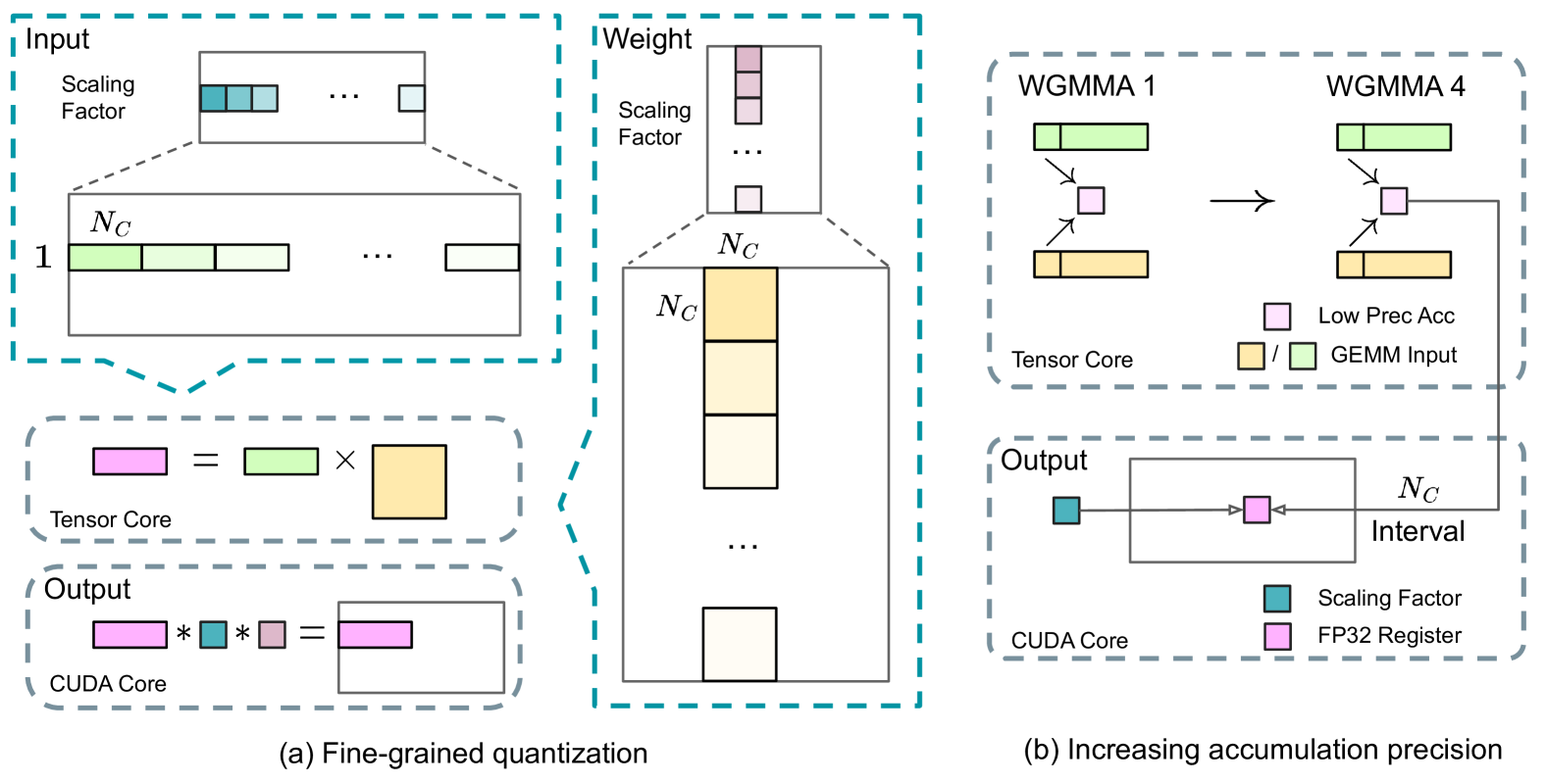
Figure 7: (a) We propose a fine-grained quantization method to mitigate quantization errors caused by feature outliers; for illustration simplicity, only Fprop is illustrated. (b) In conjunction with our quantization strategy, we improve the FP8 GEMM precision by promoting to CUDA Cores at an interval of $N_{C}=128$ elements MMA for the high-precision accumulation.
3.3.2 Improved Precision from Quantization and Multiplication
Based on our mixed precision FP8 framework, we introduce several strategies to enhance low-precision training accuracy, focusing on both the quantization method and the multiplication process.
Fine-Grained Quantization.
In low-precision training frameworks, overflows and underflows are common challenges due to the limited dynamic range of the FP8 format, which is constrained by its reduced exponent bits. As a standard practice, the input distribution is aligned to the representable range of the FP8 format by scaling the maximum absolute value of the input tensor to the maximum representable value of FP8 (Narang et al., 2017). This method makes low-precision training highly sensitive to activation outliers, which can heavily degrade quantization accuracy. To solve this, we propose a fine-grained quantization method that applies scaling at a more granular level. As illustrated in Figure 7 (a), (1) for activations, we group and scale elements on a 1x128 tile basis (i.e., per token per 128 channels); and (2) for weights, we group and scale elements on a 128x128 block basis (i.e., per 128 input channels per 128 output channels). This approach ensures that the quantization process can better accommodate outliers by adapting the scale according to smaller groups of elements. In Appendix B.2, we further discuss the training instability when we group and scale activations on a block basis in the same way as weights quantization.
One key modification in our method is the introduction of per-group scaling factors along the inner dimension of GEMM operations. This functionality is not directly supported in the standard FP8 GEMM. However, combined with our precise FP32 accumulation strategy, it can be efficiently implemented.
Notably, our fine-grained quantization strategy is highly consistent with the idea of microscaling formats (Rouhani et al., 2023b), while the Tensor Cores of NVIDIA next-generation GPUs (Blackwell series) have announced the support for microscaling formats with smaller quantization granularity (NVIDIA, 2024a). We hope our design can serve as a reference for future work to keep pace with the latest GPU architectures.
Increasing Accumulation Precision.
Low-precision GEMM operations often suffer from underflow issues, and their accuracy largely depends on high-precision accumulation, which is commonly performed in an FP32 precision (Kalamkar et al., 2019; Narang et al., 2017). However, we observe that the accumulation precision of FP8 GEMM on NVIDIA H800 GPUs is limited to retaining around 14 bits, which is significantly lower than FP32 accumulation precision. This problem will become more pronounced when the inner dimension K is large (Wortsman et al., 2023), a typical scenario in large-scale model training where the batch size and model width are increased. Taking GEMM operations of two random matrices with K = 4096 for example, in our preliminary test, the limited accumulation precision in Tensor Cores results in a maximum relative error of nearly 2%. Despite these problems, the limited accumulation precision is still the default option in a few FP8 frameworks (NVIDIA, 2024b), severely constraining the training accuracy.
In order to address this issue, we adopt the strategy of promotion to CUDA Cores for higher precision (Thakkar et al., 2023). The process is illustrated in Figure 7 (b). To be specific, during MMA (Matrix Multiply-Accumulate) execution on Tensor Cores, intermediate results are accumulated using the limited bit width. Once an interval of $N_{C}$ is reached, these partial results will be copied to FP32 registers on CUDA Cores, where full-precision FP32 accumulation is performed. As mentioned before, our fine-grained quantization applies per-group scaling factors along the inner dimension K. These scaling factors can be efficiently multiplied on the CUDA Cores as the dequantization process with minimal additional computational cost.
It is worth noting that this modification reduces the WGMMA (Warpgroup-level Matrix Multiply-Accumulate) instruction issue rate for a single warpgroup. However, on the H800 architecture, it is typical for two WGMMA to persist concurrently: while one warpgroup performs the promotion operation, the other is able to execute the MMA operation. This design enables overlapping of the two operations, maintaining high utilization of Tensor Cores. Based on our experiments, setting $N_{C}=128$ elements, equivalent to 4 WGMMAs, represents the minimal accumulation interval that can significantly improve precision without introducing substantial overhead.
Mantissa over Exponents.
In contrast to the hybrid FP8 format adopted by prior work (NVIDIA, 2024b; Peng et al., 2023b; Sun et al., 2019b), which uses E4M3 (4-bit exponent and 3-bit mantissa) in Fprop and E5M2 (5-bit exponent and 2-bit mantissa) in Dgrad and Wgrad, we adopt the E4M3 format on all tensors for higher precision. We attribute the feasibility of this approach to our fine-grained quantization strategy, i.e., tile and block-wise scaling. By operating on smaller element groups, our methodology effectively shares exponent bits among these grouped elements, mitigating the impact of the limited dynamic range.
Online Quantization.
Delayed quantization is employed in tensor-wise quantization frameworks (NVIDIA, 2024b; Peng et al., 2023b), which maintains a history of the maximum absolute values across prior iterations to infer the current value. In order to ensure accurate scales and simplify the framework, we calculate the maximum absolute value online for each 1x128 activation tile or 128x128 weight block. Based on it, we derive the scaling factor and then quantize the activation or weight online into the FP8 format.
3.3.3 Low-Precision Storage and Communication
In conjunction with our FP8 training framework, we further reduce the memory consumption and communication overhead by compressing cached activations and optimizer states into lower-precision formats.
Low-Precision Optimizer States.
We adopt the BF16 data format instead of FP32 to track the first and second moments in the AdamW (Loshchilov and Hutter, 2017) optimizer, without incurring observable performance degradation. However, the master weights (stored by the optimizer) and gradients (used for batch size accumulation) are still retained in FP32 to ensure numerical stability throughout training.
Low-Precision Activation.
As illustrated in Figure 6, the Wgrad operation is performed in FP8. To reduce the memory consumption, it is a natural choice to cache activations in FP8 format for the backward pass of the Linear operator. However, special considerations are taken on several operators for low-cost high-precision training:
(1) Inputs of the Linear after the attention operator. These activations are also used in the backward pass of the attention operator, which makes it sensitive to precision. We adopt a customized E5M6 data format exclusively for these activations. Additionally, these activations will be converted from an 1x128 quantization tile to an 128x1 tile in the backward pass. To avoid introducing extra quantization error, all the scaling factors are round scaled, i.e., integral power of 2.
(2) Inputs of the SwiGLU operator in MoE. To further reduce the memory cost, we cache the inputs of the SwiGLU operator and recompute its output in the backward pass. These activations are also stored in FP8 with our fine-grained quantization method, striking a balance between memory efficiency and computational accuracy.
Low-Precision Communication.
Communication bandwidth is a critical bottleneck in the training of MoE models. To alleviate this challenge, we quantize the activation before MoE up-projections into FP8 and then apply dispatch components, which is compatible with FP8 Fprop in MoE up-projections. Like the inputs of the Linear after the attention operator, scaling factors for this activation are integral power of 2. A similar strategy is applied to the activation gradient before MoE down-projections. For both the forward and backward combine components, we retain them in BF16 to preserve training precision in critical parts of the training pipeline.
3.4 Inference and Deployment
We deploy DeepSeek-V3 on the H800 cluster, where GPUs within each node are interconnected using NVLink, and all GPUs across the cluster are fully interconnected via IB. To simultaneously ensure both the Service-Level Objective (SLO) for online services and high throughput, we employ the following deployment strategy that separates the prefilling and decoding stages.
3.4.1 Prefilling
The minimum deployment unit of the prefilling stage consists of 4 nodes with 32 GPUs. The attention part employs 4-way Tensor Parallelism (TP4) with Sequence Parallelism (SP), combined with 8-way Data Parallelism (DP8). Its small TP size of 4 limits the overhead of TP communication. For the MoE part, we use 32-way Expert Parallelism (EP32), which ensures that each expert processes a sufficiently large batch size, thereby enhancing computational efficiency. For the MoE all-to-all communication, we use the same method as in training: first transferring tokens across nodes via IB, and then forwarding among the intra-node GPUs via NVLink. In particular, we use 1-way Tensor Parallelism for the dense MLPs in shallow layers to save TP communication.
To achieve load balancing among different experts in the MoE part, we need to ensure that each GPU processes approximately the same number of tokens. To this end, we introduce a deployment strategy of redundant experts, which duplicates high-load experts and deploys them redundantly. The high-load experts are detected based on statistics collected during the online deployment and are adjusted periodically (e.g., every 10 minutes). After determining the set of redundant experts, we carefully rearrange experts among GPUs within a node based on the observed loads, striving to balance the load across GPUs as much as possible without increasing the cross-node all-to-all communication overhead. For the deployment of DeepSeek-V3, we set 32 redundant experts for the prefilling stage. For each GPU, besides the original 8 experts it hosts, it will also host one additional redundant expert.
Furthermore, in the prefilling stage, to improve the throughput and hide the overhead of all-to-all and TP communication, we simultaneously process two micro-batches with similar computational workloads, overlapping the attention and MoE of one micro-batch with the dispatch and combine of another.
Finally, we are exploring a dynamic redundancy strategy for experts, where each GPU hosts more experts (e.g., 16 experts), but only 9 will be activated during each inference step. Before the all-to-all operation at each layer begins, we compute the globally optimal routing scheme on the fly. Given the substantial computation involved in the prefilling stage, the overhead of computing this routing scheme is almost negligible.
3.4.2 Decoding
During decoding, we treat the shared expert as a routed one. From this perspective, each token will select 9 experts during routing, where the shared expert is regarded as a heavy-load one that will always be selected. The minimum deployment unit of the decoding stage consists of 40 nodes with 320 GPUs. The attention part employs TP4 with SP, combined with DP80, while the MoE part uses EP320. For the MoE part, each GPU hosts only one expert, and 64 GPUs are responsible for hosting redundant experts and shared experts. All-to-all communication of the dispatch and combine parts is performed via direct point-to-point transfers over IB to achieve low latency. Additionally, we leverage the IBGDA (NVIDIA, 2022) technology to further minimize latency and enhance communication efficiency.
Similar to prefilling, we periodically determine the set of redundant experts in a certain interval, based on the statistical expert load from our online service. However, we do not need to rearrange experts since each GPU only hosts one expert. We are also exploring the dynamic redundancy strategy for decoding. However, this requires more careful optimization of the algorithm that computes the globally optimal routing scheme and the fusion with the dispatch kernel to reduce overhead.
Additionally, to enhance throughput and hide the overhead of all-to-all communication, we are also exploring processing two micro-batches with similar computational workloads simultaneously in the decoding stage. Unlike prefilling, attention consumes a larger portion of time in the decoding stage. Therefore, we overlap the attention of one micro-batch with the dispatch+MoE+combine of another. In the decoding stage, the batch size per expert is relatively small (usually within 256 tokens), and the bottleneck is memory access rather than computation. Since the MoE part only needs to load the parameters of one expert, the memory access overhead is minimal, so using fewer SMs will not significantly affect the overall performance. Therefore, to avoid impacting the computation speed of the attention part, we can allocate only a small portion of SMs to dispatch+MoE+combine.
3.5 Suggestions on Hardware Design
Based on our implementation of the all-to-all communication and FP8 training scheme, we propose the following suggestions on chip design to AI hardware vendors.
3.5.1 Communication Hardware
In DeepSeek-V3, we implement the overlap between computation and communication to hide the communication latency during computation. This significantly reduces the dependency on communication bandwidth compared to serial computation and communication. However, the current communication implementation relies on expensive SMs (e.g., we allocate 20 out of the 132 SMs available in the H800 GPU for this purpose), which will limit the computational throughput. Moreover, using SMs for communication results in significant inefficiencies, as tensor cores remain entirely under-utilized.
Currently, the SMs primarily perform the following tasks for all-to-all communication:
- Forwarding data between the IB (InfiniBand) and NVLink domain while aggregating IB traffic destined for multiple GPUs within the same node from a single GPU.
- Transporting data between RDMA buffers (registered GPU memory regions) and input/output buffers.
- Executing reduce operations for all-to-all combine.
- Managing fine-grained memory layout during chunked data transferring to multiple experts across the IB and NVLink domain.
We aspire to see future vendors developing hardware that offloads these communication tasks from the valuable computation unit SM, serving as a GPU co-processor or a network co-processor like NVIDIA SHARP Graham et al. (2016). Furthermore, to reduce application programming complexity, we aim for this hardware to unify the IB (scale-out) and NVLink (scale-up) networks from the perspective of the computation units. With this unified interface, computation units can easily accomplish operations such as read, write, multicast, and reduce across the entire IB-NVLink-unified domain via submitting communication requests based on simple primitives.
3.5.2 Compute Hardware
Higher FP8 GEMM Accumulation Precision in Tensor Cores.
In the current Tensor Core implementation of the NVIDIA Hopper architecture, FP8 GEMM suffers from limited accumulation precision. After aligning 32 mantissa products by right-shifting based on the maximum exponent, the Tensor Core only uses the highest 14 bits of each mantissa product for addition, and truncates bits exceeding this range. The accumulation of addition results into registers also employs 14-bit precision. Our implementation partially mitigates the limitation by accumulating the addition results of 128 FP8 $×$ FP8 multiplications into registers with FP32 precision in the CUDA core. Although helpful in achieving successful FP8 training, it is merely a compromise due to the Hopper architecture’s hardware deficiency in FP8 GEMM accumulation precision. Future chips need to adopt higher precision.
Support for Tile- and Block-Wise Quantization.
Current GPUs only support per-tensor quantization, lacking the native support for fine-grained quantization like our tile- and block-wise quantization. In the current implementation, when the $N_{C}$ interval is reached, the partial results will be copied from Tensor Cores to CUDA cores, multiplied by the scaling factors, and added to FP32 registers on CUDA cores. Although the dequantization overhead is significantly mitigated combined with our precise FP32 accumulation strategy, the frequent data movements between Tensor Cores and CUDA cores still limit the computational efficiency. Therefore, we recommend future chips to support fine-grained quantization by enabling Tensor Cores to receive scaling factors and implement MMA with group scaling. In this way, the whole partial sum accumulation and dequantization can be completed directly inside Tensor Cores until the final result is produced, avoiding frequent data movements.
Support for Online Quantization.
The current implementations struggle to effectively support online quantization, despite its effectiveness demonstrated in our research. In the existing process, we need to read 128 BF16 activation values (the output of the previous computation) from HBM (High Bandwidth Memory) for quantization, and the quantized FP8 values are then written back to HBM, only to be read again for MMA. To address this inefficiency, we recommend that future chips integrate FP8 cast and TMA (Tensor Memory Accelerator) access into a single fused operation, so quantization can be completed during the transfer of activations from global memory to shared memory, avoiding frequent memory reads and writes. We also recommend supporting a warp-level cast instruction for speedup, which further facilitates the better fusion of layer normalization and FP8 cast. Alternatively, a near-memory computing approach can be adopted, where compute logic is placed near the HBM. In this case, BF16 elements can be cast to FP8 directly as they are read from HBM into the GPU, reducing off-chip memory access by roughly 50%.
Support for Transposed GEMM Operations.
The current architecture makes it cumbersome to fuse matrix transposition with GEMM operations. In our workflow, activations during the forward pass are quantized into 1x128 FP8 tiles and stored. During the backward pass, the matrix needs to be read out, dequantized, transposed, re-quantized into 128x1 tiles, and stored in HBM. To reduce memory operations, we recommend future chips to enable direct transposed reads of matrices from shared memory before MMA operation, for those precisions required in both training and inference. Combined with the fusion of FP8 format conversion and TMA access, this enhancement will significantly streamline the quantization workflow.
4 Pre-Training
4.1 Data Construction
Compared with DeepSeek-V2, we optimize the pre-training corpus by enhancing the ratio of mathematical and programming samples, while expanding multilingual coverage beyond English and Chinese. Also, our data processing pipeline is refined to minimize redundancy while maintaining corpus diversity. Inspired by Ding et al. (2024), we implement the document packing method for data integrity but do not incorporate cross-sample attention masking during training. Finally, the training corpus for DeepSeek-V3 consists of 14.8T high-quality and diverse tokens in our tokenizer.
In the training process of DeepSeekCoder-V2 (DeepSeek-AI, 2024a), we observe that the Fill-in-Middle (FIM) strategy does not compromise the next-token prediction capability while enabling the model to accurately predict middle text based on contextual cues. In alignment with DeepSeekCoder-V2, we also incorporate the FIM strategy in the pre-training of DeepSeek-V3. To be specific, we employ the Prefix-Suffix-Middle (PSM) framework to structure data as follows:
| | $\displaystyle\texttt{<|fim\_begin|>}f_{\text{pre}}\texttt{<|fim\_hole|>}f_{%
\text{suf}}\texttt{<|fim\_end|>}f_{\text{middle}}\texttt{<|eos\_token|>}.$ | |
| --- | --- | --- |
This structure is applied at the document level as a part of the pre-packing process. The FIM strategy is applied at a rate of 0.1, consistent with the PSM framework.
The tokenizer for DeepSeek-V3 employs Byte-level BPE (Shibata et al., 1999) with an extended vocabulary of 128K tokens. The pretokenizer and training data for our tokenizer are modified to optimize multilingual compression efficiency. In addition, compared with DeepSeek-V2, the new pretokenizer introduces tokens that combine punctuations and line breaks. However, this trick may introduce the token boundary bias (Lundberg, 2023) when the model processes multi-line prompts without terminal line breaks, particularly for few-shot evaluation prompts. To address this issue, we randomly split a certain proportion of such combined tokens during training, which exposes the model to a wider array of special cases and mitigates this bias.
4.2 Hyper-Parameters
Model Hyper-Parameters.
We set the number of Transformer layers to 61 and the hidden dimension to 7168. All learnable parameters are randomly initialized with a standard deviation of 0.006. In MLA, we set the number of attention heads $n_{h}$ to 128 and the per-head dimension $d_{h}$ to 128. The KV compression dimension $d_{c}$ is set to 512, and the query compression dimension $d_{c}^{\prime}$ is set to 1536. For the decoupled queries and key, we set the per-head dimension $d_{h}^{R}$ to 64. We substitute all FFNs except for the first three layers with MoE layers. Each MoE layer consists of 1 shared expert and 256 routed experts, where the intermediate hidden dimension of each expert is 2048. Among the routed experts, 8 experts will be activated for each token, and each token will be ensured to be sent to at most 4 nodes. The multi-token prediction depth $D$ is set to 1, i.e., besides the exact next token, each token will predict one additional token. As DeepSeek-V2, DeepSeek-V3 also employs additional RMSNorm layers after the compressed latent vectors, and multiplies additional scaling factors at the width bottlenecks. Under this configuration, DeepSeek-V3 comprises 671B total parameters, of which 37B are activated for each token.
Training Hyper-Parameters.
We employ the AdamW optimizer (Loshchilov and Hutter, 2017) with hyper-parameters set to $\beta_{1}=0.9$ , $\beta_{2}=0.95$ , and $\mathrm{weight\_decay}=0.1$ . We set the maximum sequence length to 4K during pre-training, and pre-train DeepSeek-V3 on 14.8T tokens. As for the learning rate scheduling, we first linearly increase it from 0 to $2.2× 10^{-4}$ during the first 2K steps. Then, we keep a constant learning rate of $2.2× 10^{-4}$ until the model consumes 10T training tokens. Subsequently, we gradually decay the learning rate to $2.2× 10^{-5}$ in 4.3T tokens, following a cosine decay curve. During the training of the final 500B tokens, we keep a constant learning rate of $2.2× 10^{-5}$ in the first 333B tokens, and switch to another constant learning rate of $7.3× 10^{-6}$ in the remaining 167B tokens. The gradient clipping norm is set to 1.0. We employ a batch size scheduling strategy, where the batch size is gradually increased from 3072 to 15360 in the training of the first 469B tokens, and then keeps 15360 in the remaining training. We leverage pipeline parallelism to deploy different layers of a model on different GPUs, and for each layer, the routed experts will be uniformly deployed on 64 GPUs belonging to 8 nodes. As for the node-limited routing, each token will be sent to at most 4 nodes (i.e., $M=4$ ). For auxiliary-loss-free load balancing, we set the bias update speed $\gamma$ to 0.001 for the first 14.3T tokens, and to 0.0 for the remaining 500B tokens. For the balance loss, we set $\alpha$ to 0.0001, just to avoid extreme imbalance within any single sequence. The MTP loss weight $\lambda$ is set to 0.3 for the first 10T tokens, and to 0.1 for the remaining 4.8T tokens.
<details>
<summary>x8.png Details</summary>
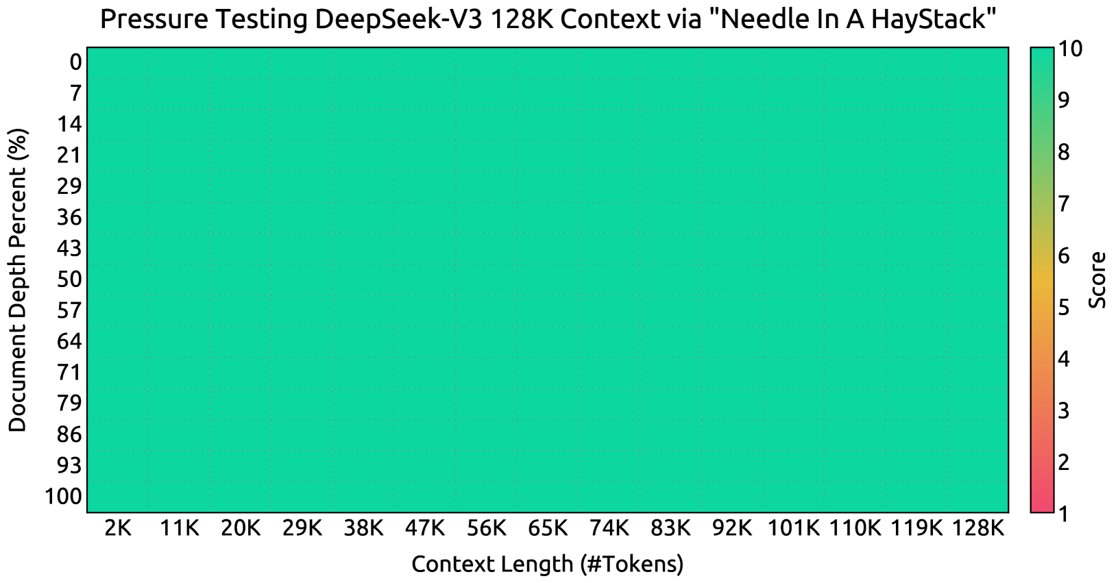
### Visual Description
# Technical Document Extraction: DeepSeek-V3 Needle In A Haystack Performance
## 1. Header Information
* **Title:** Pressure Testing DeepSeek-V3 128K Context via "Needle In A HayStack"
* **Subject:** Large Language Model (LLM) context window retrieval performance.
* **Model Tested:** DeepSeek-V3.
* **Maximum Context Tested:** 128,000 tokens (128K).
## 2. Chart Component Analysis
### A. Main Chart Area (Heatmap)
* **Type:** Heatmap visualization.
* **X-Axis (Horizontal):** Context Length (#Tokens).
* **Range:** 2K to 128K.
* **Markers:** 2K, 11K, 20K, 29K, 38K, 47K, 56K, 65K, 74K, 83K, 92K, 101K, 110K, 119K, 128K.
* **Y-Axis (Vertical):** Document Depth Percent (%).
* **Range:** 0% to 100%.
* **Markers:** 0, 7, 14, 21, 29, 36, 43, 50, 57, 64, 71, 79, 86, 93, 100.
* **Grid:** A fine dotted grid overlaying the heatmap area, corresponding to the axis markers.
### B. Legend (Spatial Grounding: Right Side)
* **Label:** Score
* **Scale:** 1 to 10.
* **Color Gradient:**
* **10 (Top):** Bright Green / Teal (#10b981 equivalent).
* **7-8 (Middle-High):** Yellow-Green.
* **5-6 (Middle):** Yellow / Orange.
* **1 (Bottom):** Red / Pink.
## 3. Data Extraction and Trend Verification
### Trend Analysis
The heatmap displays a uniform, solid block of color across the entire grid.
* **Visual Observation:** Every cell in the 15x15 grid (representing the intersection of all tested context lengths and all document depths) is colored in the bright teal/green associated with the highest score on the legend.
* **Trend Verification:** There is zero variance in performance. The "line" of performance across any depth or any context length is perfectly flat at the maximum value.
### Data Points
| Metric | Value |
| :--- | :--- |
| **Minimum Score Observed** | 10 |
| **Maximum Score Observed** | 10 |
| **Average Score** | 10 |
| **Retrieval Accuracy** | 100% (indicated by the uniform score of 10) |
## 4. Technical Summary
The image represents a "perfect" result for the Needle In A Haystack pressure test.
* **Context Handling:** DeepSeek-V3 demonstrates 100% retrieval accuracy across its entire 128K token context window.
* **Depth Independence:** The model's ability to retrieve information (the "needle") is not affected by where that information is placed within the document (the "haystack"), whether it is at the very beginning (0%), the middle (50%), or the very end (100%).
* **Scale Independence:** Performance does not degrade as the context length increases from 2K tokens to the maximum 128K tokens.
**Conclusion:** The data indicates that DeepSeek-V3 possesses a robust long-context recall capability, maintaining peak performance (Score 10) across all tested parameters.
</details>
Figure 8: Evaluation results on the ”Needle In A Haystack” (NIAH) tests. DeepSeek-V3 performs well across all context window lengths up to 128K.
4.3 Long Context Extension
We adopt a similar approach to DeepSeek-V2 (DeepSeek-AI, 2024c) to enable long context capabilities in DeepSeek-V3. After the pre-training stage, we apply YaRN (Peng et al., 2023a) for context extension and perform two additional training phases, each comprising 1000 steps, to progressively expand the context window from 4K to 32K and then to 128K. The YaRN configuration is consistent with that used in DeepSeek-V2, being applied exclusively to the decoupled shared key $\mathbf{k}^{R}_{t}$ . The hyper-parameters remain identical across both phases, with the scale $s=40$ , $\alpha=1$ , $\beta=32$ , and the scaling factor $\sqrt{t}=0.1\ln{s}+1$ . In the first phase, the sequence length is set to 32K, and the batch size is 1920. During the second phase, the sequence length is increased to 128K, and the batch size is reduced to 480. The learning rate for both phases is set to $7.3× 10^{-6}$ , matching the final learning rate from the pre-training stage.
Through this two-phase extension training, DeepSeek-V3 is capable of handling inputs up to 128K in length while maintaining strong performance. Figure 8 illustrates that DeepSeek-V3, following supervised fine-tuning, achieves notable performance on the "Needle In A Haystack" (NIAH) test, demonstrating consistent robustness across context window lengths up to 128K.
4.4 Evaluations
4.4.1 Evaluation Benchmarks
The base model of DeepSeek-V3 is pretrained on a multilingual corpus with English and Chinese constituting the majority, so we evaluate its performance on a series of benchmarks primarily in English and Chinese, as well as on a multilingual benchmark. Our evaluation is based on our internal evaluation framework integrated in our HAI-LLM framework. Considered benchmarks are categorized and listed as follows, where underlined benchmarks are in Chinese and double-underlined benchmarks are multilingual ones:
Multi-subject multiple-choice datasets include MMLU (Hendrycks et al., 2020), MMLU-Redux (Gema et al., 2024), MMLU-Pro (Wang et al., 2024b), MMMLU (OpenAI, 2024b), C-Eval (Huang et al., 2023), and CMMLU (Li et al., 2023).
Language understanding and reasoning datasets include HellaSwag (Zellers et al., 2019), PIQA (Bisk et al., 2020), ARC (Clark et al., 2018), and BigBench Hard (BBH) (Suzgun et al., 2022).
Closed-book question answering datasets include TriviaQA (Joshi et al., 2017) and NaturalQuestions (Kwiatkowski et al., 2019).
Reading comprehension datasets include RACE Lai et al. (2017), DROP (Dua et al., 2019), C3 (Sun et al., 2019a), and CMRC (Cui et al., 2019).
Reference disambiguation datasets include CLUEWSC (Xu et al., 2020) and WinoGrande Sakaguchi et al. (2019).
Language modeling datasets include Pile (Gao et al., 2020).
Chinese understanding and culture datasets include CCPM (Li et al., 2021).
Math datasets include GSM8K (Cobbe et al., 2021), MATH (Hendrycks et al., 2021), MGSM (Shi et al., 2023), and CMath (Wei et al., 2023).
Code datasets include HumanEval (Chen et al., 2021), LiveCodeBench-Base (0801-1101) (Jain et al., 2024), MBPP (Austin et al., 2021), and CRUXEval (Gu et al., 2024).
Standardized exams include AGIEval (Zhong et al., 2023). Note that AGIEval includes both English and Chinese subsets.
Following our previous work (DeepSeek-AI, 2024b, c), we adopt perplexity-based evaluation for datasets including HellaSwag, PIQA, WinoGrande, RACE-Middle, RACE-High, MMLU, MMLU-Redux, MMLU-Pro, MMMLU, ARC-Easy, ARC-Challenge, C-Eval, CMMLU, C3, and CCPM, and adopt generation-based evaluation for TriviaQA, NaturalQuestions, DROP, MATH, GSM8K, MGSM, HumanEval, MBPP, LiveCodeBench-Base, CRUXEval, BBH, AGIEval, CLUEWSC, CMRC, and CMath. In addition, we perform language-modeling-based evaluation for Pile-test and use Bits-Per-Byte (BPB) as the metric to guarantee fair comparison among models using different tokenizers.
| | Benchmark (Metric) | # Shots | DeepSeek-V2 | Qwen2.5 | LLaMA-3.1 | DeepSeek-V3 |
| --- | --- | --- | --- | --- | --- | --- |
| Base | 72B Base | 405B Base | Base | | | |
| Architecture | - | MoE | Dense | Dense | MoE | |
| # Activated Params | - | 21B | 72B | 405B | 37B | |
| # Total Params | - | 236B | 72B | 405B | 671B | |
| English | Pile-test (BPB) | - | 0.606 | 0.638 | 0.542 | 0.548 |
| BBH (EM) | 3-shot | 78.8 | 79.8 | 82.9 | 87.5 | |
| MMLU (EM) | 5-shot | 78.4 | 85.0 | 84.4 | 87.1 | |
| MMLU-Redux (EM) | 5-shot | 75.6 | 83.2 | 81.3 | 86.2 | |
| MMLU-Pro (EM) | 5-shot | 51.4 | 58.3 | 52.8 | 64.4 | |
| DROP (F1) | 3-shot | 80.4 | 80.6 | 86.0 | 89.0 | |
| ARC-Easy (EM) | 25-shot | 97.6 | 98.4 | 98.4 | 98.9 | |
| ARC-Challenge (EM) | 25-shot | 92.2 | 94.5 | 95.3 | 95.3 | |
| HellaSwag (EM) | 10-shot | 87.1 | 84.8 | 89.2 | 88.9 | |
| PIQA (EM) | 0-shot | 83.9 | 82.6 | 85.9 | 84.7 | |
| WinoGrande (EM) | 5-shot | 86.3 | 82.3 | 85.2 | 84.9 | |
| RACE-Middle (EM) | 5-shot | 73.1 | 68.1 | 74.2 | 67.1 | |
| RACE-High (EM) | 5-shot | 52.6 | 50.3 | 56.8 | 51.3 | |
| TriviaQA (EM) | 5-shot | 80.0 | 71.9 | 82.7 | 82.9 | |
| NaturalQuestions (EM) | 5-shot | 38.6 | 33.2 | 41.5 | 40.0 | |
| AGIEval (EM) | 0-shot | 57.5 | 75.8 | 60.6 | 79.6 | |
| Code | HumanEval (Pass@1) | 0-shot | 43.3 | 53.0 | 54.9 | 65.2 |
| MBPP (Pass@1) | 3-shot | 65.0 | 72.6 | 68.4 | 75.4 | |
| LiveCodeBench-Base (Pass@1) | 3-shot | 11.6 | 12.9 | 15.5 | 19.4 | |
| CRUXEval-I (EM) | 2-shot | 52.5 | 59.1 | 58.5 | 67.3 | |
| CRUXEval-O (EM) | 2-shot | 49.8 | 59.9 | 59.9 | 69.8 | |
| Math | GSM8K (EM) | 8-shot | 81.6 | 88.3 | 83.5 | 89.3 |
| MATH (EM) | 4-shot | 43.4 | 54.4 | 49.0 | 61.6 | |
| MGSM (EM) | 8-shot | 63.6 | 76.2 | 69.9 | 79.8 | |
| CMath (EM) | 3-shot | 78.7 | 84.5 | 77.3 | 90.7 | |
| Chinese | CLUEWSC (EM) | 5-shot | 82.0 | 82.5 | 83.0 | 82.7 |
| C-Eval (EM) | 5-shot | 81.4 | 89.2 | 72.5 | 90.1 | |
| CMMLU (EM) | 5-shot | 84.0 | 89.5 | 73.7 | 88.8 | |
| CMRC (EM) | 1-shot | 77.4 | 75.8 | 76.0 | 76.3 | |
| C3 (EM) | 0-shot | 77.4 | 76.7 | 79.7 | 78.6 | |
| CCPM (EM) | 0-shot | 93.0 | 88.5 | 78.6 | 92.0 | |
| Multilingual | MMMLU-non-English (EM) | 5-shot | 64.0 | 74.8 | 73.8 | 79.4 |
Table 3: Comparison among DeepSeek-V3-Base and other representative open-source base models. All models are evaluated in our internal framework and share the same evaluation setting. Scores with a gap not exceeding 0.3 are considered to be at the same level. DeepSeek-V3-Base achieves the best performance on most benchmarks, especially on math and code tasks.
4.4.2 Evaluation Results
In Table 3, we compare the base model of DeepSeek-V3 with the state-of-the-art open-source base models, including DeepSeek-V2-Base (DeepSeek-AI, 2024c) (our previous release), Qwen2.5 72B Base (Qwen, 2024b), and LLaMA-3.1 405B Base (AI@Meta, 2024b). We evaluate all these models with our internal evaluation framework, and ensure that they share the same evaluation setting. Note that due to the changes in our evaluation framework over the past months, the performance of DeepSeek-V2-Base exhibits a slight difference from our previously reported results. Overall, DeepSeek-V3-Base comprehensively outperforms DeepSeek-V2-Base and Qwen2.5 72B Base, and surpasses LLaMA-3.1 405B Base in the majority of benchmarks, essentially becoming the strongest open-source model.
From a more detailed perspective, we compare DeepSeek-V3-Base with the other open-source base models individually. (1) Compared with DeepSeek-V2-Base, due to the improvements in our model architecture, the scale-up of the model size and training tokens, and the enhancement of data quality, DeepSeek-V3-Base achieves significantly better performance as expected. (2) Compared with Qwen2.5 72B Base, the state-of-the-art Chinese open-source model, with only half of the activated parameters, DeepSeek-V3-Base also demonstrates remarkable advantages, especially on English, multilingual, code, and math benchmarks. As for Chinese benchmarks, except for CMMLU, a Chinese multi-subject multiple-choice task, DeepSeek-V3-Base also shows better performance than Qwen2.5 72B. (3) Compared with LLaMA-3.1 405B Base, the largest open-source model with 11 times the activated parameters, DeepSeek-V3-Base also exhibits much better performance on multilingual, code, and math benchmarks. As for English and Chinese language benchmarks, DeepSeek-V3-Base shows competitive or better performance, and is especially good on BBH, MMLU-series, DROP, C-Eval, CMMLU, and CCPM.
Due to our efficient architectures and comprehensive engineering optimizations, DeepSeek-V3 achieves extremely high training efficiency. Under our training framework and infrastructures, training DeepSeek-V3 on each trillion tokens requires only 180K H800 GPU hours, which is much cheaper than training 72B or 405B dense models.
| Benchmark (Metric) | # Shots | Small MoE | Small MoE | Large MoE | Large MoE |
| --- | --- | --- | --- | --- | --- |
| Baseline | w/ MTP | Baseline | w/ MTP | | |
| # Activated Params (Inference) | - | 2.4B | 2.4B | 20.9B | 20.9B |
| # Total Params (Inference) | - | 15.7B | 15.7B | 228.7B | 228.7B |
| # Training Tokens | - | 1.33T | 1.33T | 540B | 540B |
| Pile-test (BPB) | - | 0.729 | 0.729 | 0.658 | 0.657 |
| BBH (EM) | 3-shot | 39.0 | 41.4 | 70.0 | 70.7 |
| MMLU (EM) | 5-shot | 50.0 | 53.3 | 67.5 | 66.6 |
| DROP (F1) | 1-shot | 39.2 | 41.3 | 68.5 | 70.6 |
| TriviaQA (EM) | 5-shot | 56.9 | 57.7 | 67.0 | 67.3 |
| NaturalQuestions (EM) | 5-shot | 22.7 | 22.3 | 27.2 | 28.5 |
| HumanEval (Pass@1) | 0-shot | 20.7 | 26.8 | 44.5 | 53.7 |
| MBPP (Pass@1) | 3-shot | 35.8 | 36.8 | 61.6 | 62.2 |
| GSM8K (EM) | 8-shot | 25.4 | 31.4 | 72.3 | 74.0 |
| MATH (EM) | 4-shot | 10.7 | 12.6 | 38.6 | 39.8 |
Table 4: Ablation results for the MTP strategy. The MTP strategy consistently enhances the model performance on most of the evaluation benchmarks.
4.5 Discussion
4.5.1 Ablation Studies for Multi-Token Prediction
In Table 4, we show the ablation results for the MTP strategy. To be specific, we validate the MTP strategy on top of two baseline models across different scales. At the small scale, we train a baseline MoE model comprising 15.7B total parameters on 1.33T tokens. At the large scale, we train a baseline MoE model comprising 228.7B total parameters on 540B tokens. On top of them, keeping the training data and the other architectures the same, we append a 1-depth MTP module onto them and train two models with the MTP strategy for comparison. Note that during inference, we directly discard the MTP module, so the inference costs of the compared models are exactly the same. From the table, we can observe that the MTP strategy consistently enhances the model performance on most of the evaluation benchmarks.
4.5.2 Ablation Studies for the Auxiliary-Loss-Free Balancing Strategy
In Table 5, we show the ablation results for the auxiliary-loss-free balancing strategy. We validate this strategy on top of two baseline models across different scales. At the small scale, we train a baseline MoE model comprising 15.7B total parameters on 1.33T tokens. At the large scale, we train a baseline MoE model comprising 228.7B total parameters on 578B tokens. Both of the baseline models purely use auxiliary losses to encourage load balance, and use the sigmoid gating function with top-K affinity normalization. Their hyper-parameters to control the strength of auxiliary losses are the same as DeepSeek-V2-Lite and DeepSeek-V2, respectively. On top of these two baseline models, keeping the training data and the other architectures the same, we remove all auxiliary losses and introduce the auxiliary-loss-free balancing strategy for comparison. From the table, we can observe that the auxiliary-loss-free strategy consistently achieves better model performance on most of the evaluation benchmarks.
| Benchmark (Metric) | # Shots | Small MoE | Small MoE | Large MoE | Large MoE |
| --- | --- | --- | --- | --- | --- |
| Aux-Loss-Based | Aux-Loss-Free | Aux-Loss-Based | Aux-Loss-Free | | |
| # Activated Params | - | 2.4B | 2.4B | 20.9B | 20.9B |
| # Total Params | - | 15.7B | 15.7B | 228.7B | 228.7B |
| # Training Tokens | - | 1.33T | 1.33T | 578B | 578B |
| Pile-test (BPB) | - | 0.727 | 0.724 | 0.656 | 0.652 |
| BBH (EM) | 3-shot | 37.3 | 39.3 | 66.7 | 67.9 |
| MMLU (EM) | 5-shot | 51.0 | 51.8 | 68.3 | 67.2 |
| DROP (F1) | 1-shot | 38.1 | 39.0 | 67.1 | 67.1 |
| TriviaQA (EM) | 5-shot | 58.3 | 58.5 | 66.7 | 67.7 |
| NaturalQuestions (EM) | 5-shot | 23.2 | 23.4 | 27.1 | 28.1 |
| HumanEval (Pass@1) | 0-shot | 22.0 | 22.6 | 40.2 | 46.3 |
| MBPP (Pass@1) | 3-shot | 36.6 | 35.8 | 59.2 | 61.2 |
| GSM8K (EM) | 8-shot | 27.1 | 29.6 | 70.7 | 74.5 |
| MATH (EM) | 4-shot | 10.9 | 11.1 | 37.2 | 39.6 |
Table 5: Ablation results for the auxiliary-loss-free balancing strategy. Compared with the purely auxiliary-loss-based method, the auxiliary-loss-free strategy consistently achieves better model performance on most of the evaluation benchmarks.
4.5.3 Batch-Wise Load Balance VS. Sequence-Wise Load Balance
The key distinction between auxiliary-loss-free balancing and sequence-wise auxiliary loss lies in their balancing scope: batch-wise versus sequence-wise. Compared with the sequence-wise auxiliary loss, batch-wise balancing imposes a more flexible constraint, as it does not enforce in-domain balance on each sequence. This flexibility allows experts to better specialize in different domains. To validate this, we record and analyze the expert load of a 16B auxiliary-loss-based baseline and a 16B auxiliary-loss-free model on different domains in the Pile test set. As illustrated in Figure 9, we observe that the auxiliary-loss-free model demonstrates greater expert specialization patterns as expected.
To further investigate the correlation between this flexibility and the advantage in model performance, we additionally design and validate a batch-wise auxiliary loss that encourages load balance on each training batch instead of on each sequence. The experimental results show that, when achieving a similar level of batch-wise load balance, the batch-wise auxiliary loss can also achieve similar model performance to the auxiliary-loss-free method. To be specific, in our experiments with 1B MoE models, the validation losses are: 2.258 (using a sequence-wise auxiliary loss), 2.253 (using the auxiliary-loss-free method), and 2.253 (using a batch-wise auxiliary loss). We also observe similar results on 3B MoE models: the model using a sequence-wise auxiliary loss achieves a validation loss of 2.085, and the models using the auxiliary-loss-free method or a batch-wise auxiliary loss achieve the same validation loss of 2.080.
In addition, although the batch-wise load balancing methods show consistent performance advantages, they also face two potential challenges in efficiency: (1) load imbalance within certain sequences or small batches, and (2) domain-shift-induced load imbalance during inference. The first challenge is naturally addressed by our training framework that uses large-scale expert parallelism and data parallelism, which guarantees a large size of each micro-batch. For the second challenge, we also design and implement an efficient inference framework with redundant expert deployment, as described in Section 3.4, to overcome it.
<details>
<summary>x9.png Details</summary>
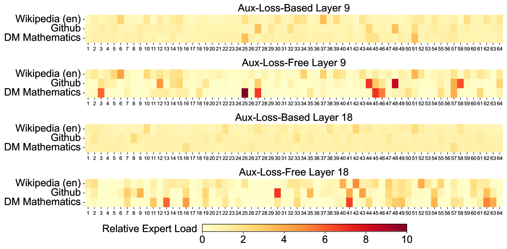
### Visual Description
# Technical Document Extraction: Expert Load Heatmaps
## 1. Document Overview
This image contains four heatmaps visualizing the "Relative Expert Load" across 64 different experts for three specific datasets. The data compares two different model training methodologies (Aux-Loss-Based vs. Aux-Loss-Free) at two different depths within a neural network (Layer 9 and Layer 18).
## 2. Global Components
### Legend (Footer)
* **Location:** Bottom center of the image.
* **Title:** Relative Expert Load
* **Scale:** Continuous color gradient.
* **0 (Light Yellow):** Low relative load.
* **10 (Dark Red/Maroon):** High relative load.
* **Markers:** 0, 2, 4, 6, 8, 10.
### Axis Definitions (Common to all charts)
* **Y-Axis (Categories):**
1. Wikipedia (en)
2. Github
3. DM Mathematics
* **X-Axis (Experts):**
* Numbered 1 through 64.
---
## 3. Heatmap Analysis
### Chart 1: Aux-Loss-Based Layer 9
* **Trend:** This chart shows a highly uniform distribution. Most experts have a load near 0 (light yellow). There are very few "hot spots," suggesting the auxiliary loss successfully balanced the load across experts.
* **Key Data Points:**
* **Wikipedia (en):** Slight activity at Expert 6 and Expert 25.
* **Github:** Slight activity at Expert 27, 44, and 48.
* **DM Mathematics:** Slight activity at Expert 25 and 51.
### Chart 2: Aux-Loss-Free Layer 9
* **Trend:** Significant specialization and load imbalance compared to the Aux-Loss-Based version. Several experts show high intensity (orange to dark red), indicating they are being heavily utilized by specific datasets while others are ignored.
* **Key Data Points:**
* **Wikipedia (en):** Moderate load at Expert 6 and 51.
* **Github:** High load (Red) at Expert 44 and 48. Moderate load at Expert 12, 27, and 58.
* **DM Mathematics:** Very high load (Dark Red/Maroon) at Expert 25. High load (Orange/Red) at Expert 3, 27, 45, and 46.
### Chart 3: Aux-Loss-Based Layer 18
* **Trend:** The most uniform of all four charts. The expert load is almost perfectly distributed with nearly no visible variation in the light yellow color.
* **Key Data Points:**
* Minimal visible peaks. Very slight shading at Expert 10 (Github) and Expert 16 (DM Mathematics).
### Chart 4: Aux-Loss-Free Layer 18
* **Trend:** Shows moderate specialization. While not as extreme as Layer 9 Aux-Loss-Free, there is clear "expert picking" where certain experts are preferred for specific tasks.
* **Key Data Points:**
* **Wikipedia (en):** Moderate load at Expert 1 and 41.
* **Github:** High load (Red) at Expert 30. Moderate load at Expert 42.
* **DM Mathematics:** High load (Orange/Red) at Expert 13, 16, 41, and 62.
---
## 4. Comparative Summary
| Feature | Aux-Loss-Based | Aux-Loss-Free |
| :--- | :--- | :--- |
| **Expert Distribution** | Highly uniform; low variance. | Highly specialized; high variance. |
| **Peak Load Values** | Rarely exceeds 2-3 on the scale. | Frequently reaches 8-10 on the scale. |
| **Layer 9 vs 18** | Layer 18 is more uniform than Layer 9. | Both layers show significant "hot spots," but patterns differ. |
**Conclusion:** The "Aux-Loss-Based" method effectively prevents expert collapse and ensures a balanced workload across all 64 experts. The "Aux-Loss-Free" method allows the model to naturally gravitate toward specific experts for specific data types (e.g., Expert 25 for DM Mathematics in Layer 9), resulting in much higher relative loads on a subset of the available experts.
</details>
Figure 9: Expert load of auxiliary-loss-free and auxiliary-loss-based models on three domains in the Pile test set. The auxiliary-loss-free model shows greater expert specialization patterns than the auxiliary-loss-based one. The relative expert load denotes the ratio between the actual expert load and the theoretically balanced expert load. Due to space constraints, we only present the results of two layers as an example, with the results of all layers provided in Appendix C.
5 Post-Training
5.1 Supervised Fine-Tuning
We curate our instruction-tuning datasets to include 1.5M instances spanning multiple domains, with each domain employing distinct data creation methods tailored to its specific requirements.
Reasoning Data.
For reasoning-related datasets, including those focused on mathematics, code competition problems, and logic puzzles, we generate the data by leveraging an internal DeepSeek-R1 model. Specifically, while the R1-generated data demonstrates strong accuracy, it suffers from issues such as overthinking, poor formatting, and excessive length. Our objective is to balance the high accuracy of R1-generated reasoning data and the clarity and conciseness of regularly formatted reasoning data.
To establish our methodology, we begin by developing an expert model tailored to a specific domain, such as code, mathematics, or general reasoning, using a combined Supervised Fine-Tuning (SFT) and Reinforcement Learning (RL) training pipeline. This expert model serves as a data generator for the final model. The training process involves generating two distinct types of SFT samples for each instance: the first couples the problem with its original response in the format of <problem, original response>, while the second incorporates a system prompt alongside the problem and the R1 response in the format of <system prompt, problem, R1 response>.
The system prompt is meticulously designed to include instructions that guide the model toward producing responses enriched with mechanisms for reflection and verification. During the RL phase, the model leverages high-temperature sampling to generate responses that integrate patterns from both the R1-generated and original data, even in the absence of explicit system prompts. After hundreds of RL steps, the intermediate RL model learns to incorporate R1 patterns, thereby enhancing overall performance strategically.
Upon completing the RL training phase, we implement rejection sampling to curate high-quality SFT data for the final model, where the expert models are used as data generation sources. This method ensures that the final training data retains the strengths of DeepSeek-R1 while producing responses that are concise and effective.
Non-Reasoning Data.
For non-reasoning data, such as creative writing, role-play, and simple question answering, we utilize DeepSeek-V2.5 to generate responses and enlist human annotators to verify the accuracy and correctness of the data.
SFT Settings.
We fine-tune DeepSeek-V3-Base for two epochs using the SFT dataset, using the cosine decay learning rate scheduling that starts at $5× 10^{-6}$ and gradually decreases to $1× 10^{-6}$ . During training, each single sequence is packed from multiple samples. However, we adopt a sample masking strategy to ensure that these examples remain isolated and mutually invisible.
5.2 Reinforcement Learning
5.2.1 Reward Model
We employ a rule-based Reward Model (RM) and a model-based RM in our RL process.
Rule-Based RM.
For questions that can be validated using specific rules, we adopt a rule-based reward system to determine the feedback. For instance, certain math problems have deterministic results, and we require the model to provide the final answer within a designated format (e.g., in a box), allowing us to apply rules to verify the correctness. Similarly, for LeetCode problems, we can utilize a compiler to generate feedback based on test cases. By leveraging rule-based validation wherever possible, we ensure a higher level of reliability, as this approach is resistant to manipulation or exploitation.
Model-Based RM.
For questions with free-form ground-truth answers, we rely on the reward model to determine whether the response matches the expected ground-truth. Conversely, for questions without a definitive ground-truth, such as those involving creative writing, the reward model is tasked with providing feedback based on the question and the corresponding answer as inputs. The reward model is trained from the DeepSeek-V3 SFT checkpoints. To enhance its reliability, we construct preference data that not only provides the final reward but also includes the chain-of-thought leading to the reward. This approach helps mitigate the risk of reward hacking in specific tasks.
5.2.2 Group Relative Policy Optimization
Similar to DeepSeek-V2 (DeepSeek-AI, 2024c), we adopt Group Relative Policy Optimization (GRPO) (Shao et al., 2024), which foregoes the critic model that is typically with the same size as the policy model, and estimates the baseline from group scores instead. Specifically, for each question $q$ , GRPO samples a group of outputs $\{o_{1},o_{2},·s,o_{G}\}$ from the old policy model $\pi_{\theta_{old}}$ and then optimizes the policy model $\pi_{\theta}$ by maximizing the following objective:
$$
\begin{split}\mathcal{J}_{GRPO}(\theta)&=\mathbb{E}{[q\sim P(Q),\{o_{i}\}_{i=1%
}^{G}\sim\pi_{\theta_{old}}(O|q)]}\\
&\frac{1}{G}\sum_{i=1}^{G}\left(\min\left(\frac{\pi_{\theta}(o_{i}|q)}{\pi_{%
\theta_{old}}(o_{i}|q)}A_{i},\text{clip}\left(\frac{\pi_{\theta}(o_{i}|q)}{\pi%
_{\theta_{old}}(o_{i}|q)},1-\varepsilon,1+\varepsilon\right)A_{i}\right)-\beta%
\mathbb{D}_{KL}\left(\pi_{\theta}||\pi_{ref}\right)\right),\end{split} \tag{26}
$$
$$
\mathbb{D}_{KL}\left(\pi_{\theta}||\pi_{ref}\right)=\frac{\pi_{ref}(o_{i}|q)}{%
\pi_{\theta}(o_{i}|q)}-\log\frac{\pi_{ref}(o_{i}|q)}{\pi_{\theta}(o_{i}|q)}-1, \tag{27}
$$
where $\varepsilon$ and $\beta$ are hyper-parameters; $\pi_{ref}$ is the reference model; and $A_{i}$ is the advantage, derived from the rewards $\{r_{1},r_{2},...,r_{G}\}$ corresponding to the outputs within each group:
$$
A_{i}=\frac{r_{i}-{\operatorname{mean}(\{r_{1},r_{2},\cdots,r_{G}\})}}{{%
\operatorname{std}(\{r_{1},r_{2},\cdots,r_{G}\})}}. \tag{28}
$$
We incorporate prompts from diverse domains, such as coding, math, writing, role-playing, and question answering, during the RL process. This approach not only aligns the model more closely with human preferences but also enhances performance on benchmarks, especially in scenarios where available SFT data are limited.
5.3 Evaluations
5.3.1 Evaluation Settings
Evaluation Benchmarks.
Apart from the benchmark we used for base model testing, we further evaluate instructed models on IFEval (Zhou et al., 2023), FRAMES (Krishna et al., 2024), LongBench v2 (Bai et al., 2024), GPQA (Rein et al., 2023), SimpleQA (OpenAI, 2024c), C-SimpleQA (He et al., 2024), SWE-Bench Verified (OpenAI, 2024d), Aider https://aider.chat, LiveCodeBench (Jain et al., 2024) (questions from August 2024 to November 2024), Codeforces https://codeforces.com, Chinese National High School Mathematics Olympiad (CNMO 2024) https://www.cms.org.cn/Home/comp/comp/cid/12.html, and American Invitational Mathematics Examination 2024 (AIME 2024) (MAA, 2024).
Compared Baselines.
We conduct comprehensive evaluations of our chat model against several strong baselines, including DeepSeek-V2-0506, DeepSeek-V2.5-0905, Qwen2.5 72B Instruct, LLaMA-3.1 405B Instruct, Claude-Sonnet-3.5-1022, and GPT-4o-0513. For the DeepSeek-V2 model series, we select the most representative variants for comparison. For closed-source models, evaluations are performed through their respective APIs.
Detailed Evaluation Configurations.
For standard benchmarks including MMLU, DROP, GPQA, and SimpleQA, we adopt the evaluation prompts from the simple-evals framework https://github.com/openai/simple-evals. We utilize the Zero-Eval prompt format (Lin, 2024) for MMLU-Redux in a zero-shot setting. For other datasets, we follow their original evaluation protocols with default prompts as provided by the dataset creators. For code and math benchmarks, the HumanEval-Mul dataset includes 8 mainstream programming languages (Python, Java, Cpp, C#, JavaScript, TypeScript, PHP, and Bash) in total. We use CoT and non-CoT methods to evaluate model performance on LiveCodeBench, where the data are collected from August 2024 to November 2024. The Codeforces dataset is measured using the percentage of competitors. SWE-Bench verified is evaluated using the agentless framework (Xia et al., 2024). We use the “diff” format to evaluate the Aider-related benchmarks. For mathematical assessments, AIME and CNMO 2024 are evaluated with a temperature of 0.7, and the results are averaged over 16 runs, while MATH-500 employs greedy decoding. We allow all models to output a maximum of 8192 tokens for each benchmark.
| | Benchmark (Metric) | DeepSeek | DeepSeek | Qwen2.5 | LLaMA-3.1 | Claude-3.5- | GPT-4o | DeepSeek |
| --- | --- | --- | --- | --- | --- | --- | --- | --- |
| V2-0506 | V2.5-0905 | 72B-Inst. | 405B-Inst. | Sonnet-1022 | 0513 | V3 | | |
| Architecture | MoE | MoE | Dense | Dense | - | - | MoE | |
| # Activated Params | 21B | 21B | 72B | 405B | - | - | 37B | |
| # Total Params | 236B | 236B | 72B | 405B | - | - | 671B | |
| English | MMLU (EM) | 78.2 | 80.6 | 85.3 | 88.6 | 88.3 | 87.2 | 88.5 |
| MMLU-Redux (EM) | 77.9 | 80.3 | 85.6 | 86.2 | 88.9 | 88.0 | 89.1 | |
| MMLU-Pro (EM) | 58.5 | 66.2 | 71.6 | 73.3 | 78.0 | 72.6 | 75.9 | |
| DROP (3-shot F1) | 83.0 | 87.8 | 76.7 | 88.7 | 88.3 | 83.7 | 91.6 | |
| IF-Eval (Prompt Strict) | 57.7 | 80.6 | 84.1 | 86.0 | 86.5 | 84.3 | 86.1 | |
| GPQA-Diamond (Pass@1) | 35.3 | 41.3 | 49.0 | 51.1 | 65.0 | 49.9 | 59.1 | |
| SimpleQA (Correct) | 9.0 | 10.2 | 9.1 | 17.1 | 28.4 | 38.2 | 24.9 | |
| FRAMES (Acc.) | 66.9 | 65.4 | 69.8 | 70.0 | 72.5 | 80.5 | 73.3 | |
| LongBench v2 (Acc.) | 31.6 | 35.4 | 39.4 | 36.1 | 41.0 | 48.1 | 48.7 | |
| Code | HumanEval-Mul (Pass@1) | 69.3 | 77.4 | 77.3 | 77.2 | 81.7 | 80.5 | 82.6 |
| LiveCodeBench (Pass@1-COT) | 18.8 | 29.2 | 31.1 | 28.4 | 36.3 | 33.4 | 40.5 | |
| LiveCodeBench (Pass@1) | 20.3 | 28.4 | 28.7 | 30.1 | 32.8 | 34.2 | 37.6 | |
| Codeforces (Percentile) | 17.5 | 35.6 | 24.8 | 25.3 | 20.3 | 23.6 | 51.6 | |
| SWE Verified (Resolved) | - | 22.6 | 23.8 | 24.5 | 50.8 | 38.8 | 42.0 | |
| Aider-Edit (Acc.) | 60.3 | 71.6 | 65.4 | 63.9 | 84.2 | 72.9 | 79.7 | |
| Aider-Polyglot (Acc.) | - | 18.2 | 7.6 | 5.8 | 45.3 | 16.0 | 49.6 | |
| Math | AIME 2024 (Pass@1) | 4.6 | 16.7 | 23.3 | 23.3 | 16.0 | 9.3 | 39.2 |
| MATH-500 (EM) | 56.3 | 74.7 | 80.0 | 73.8 | 78.3 | 74.6 | 90.2 | |
| CNMO 2024 (Pass@1) | 2.8 | 10.8 | 15.9 | 6.8 | 13.1 | 10.8 | 43.2 | |
| Chinese | CLUEWSC (EM) | 89.9 | 90.4 | 91.4 | 84.7 | 85.4 | 87.9 | 90.9 |
| C-Eval (EM) | 78.6 | 79.5 | 86.1 | 61.5 | 76.7 | 76.0 | 86.5 | |
| C-SimpleQA (Correct) | 48.5 | 54.1 | 48.4 | 50.4 | 51.3 | 59.3 | 64.8 | |
Table 6: Comparison between DeepSeek-V3 and other representative chat models. All models are evaluated in a configuration that limits the output length to 8K. Benchmarks containing fewer than 1000 samples are tested multiple times using varying temperature settings to derive robust final results. DeepSeek-V3 stands as the best-performing open-source model, and also exhibits competitive performance against frontier closed-source models.
5.3.2 Standard Evaluation
Table 6 presents the evaluation results, showcasing that DeepSeek-V3 stands as the best-performing open-source model. Additionally, it is competitive against frontier closed-source models like GPT-4o and Claude-3.5-Sonnet.
English Benchmarks.
MMLU is a widely recognized benchmark designed to assess the performance of large language models, across diverse knowledge domains and tasks. DeepSeek-V3 demonstrates competitive performance, standing on par with top-tier models such as LLaMA-3.1-405B, GPT-4o, and Claude-Sonnet 3.5, while significantly outperforming Qwen2.5 72B. Moreover, DeepSeek-V3 excels in MMLU-Pro, a more challenging educational knowledge benchmark, where it closely trails Claude-Sonnet 3.5. On MMLU-Redux, a refined version of MMLU with corrected labels, DeepSeek-V3 surpasses its peers. In addition, on GPQA-Diamond, a PhD-level evaluation testbed, DeepSeek-V3 achieves remarkable results, ranking just behind Claude 3.5 Sonnet and outperforming all other competitors by a substantial margin.
In long-context understanding benchmarks such as DROP, LongBench v2, and FRAMES, DeepSeek-V3 continues to demonstrate its position as a top-tier model. It achieves an impressive 91.6 F1 score in the 3-shot setting on DROP, outperforming all other models in this category. On FRAMES, a benchmark requiring question-answering over 100k token contexts, DeepSeek-V3 closely trails GPT-4o while outperforming all other models by a significant margin. This demonstrates the strong capability of DeepSeek-V3 in handling extremely long-context tasks. The long-context capability of DeepSeek-V3 is further validated by its best-in-class performance on LongBench v2, a dataset that was released just a few weeks before the launch of DeepSeek V3. On the factual knowledge benchmark, SimpleQA, DeepSeek-V3 falls behind GPT-4o and Claude-Sonnet, primarily due to its design focus and resource allocation. DeepSeek-V3 assigns more training tokens to learn Chinese knowledge, leading to exceptional performance on the C-SimpleQA. On the instruction-following benchmark, DeepSeek-V3 significantly outperforms its predecessor, DeepSeek-V2-series, highlighting its improved ability to understand and adhere to user-defined format constraints.
Code and Math Benchmarks.
Coding is a challenging and practical task for LLMs, encompassing engineering-focused tasks like SWE-Bench-Verified and Aider, as well as algorithmic tasks such as HumanEval and LiveCodeBench. In engineering tasks, DeepSeek-V3 trails behind Claude-Sonnet-3.5-1022 but significantly outperforms open-source models. The open-source DeepSeek-V3 is expected to foster advancements in coding-related engineering tasks. By providing access to its robust capabilities, DeepSeek-V3 can drive innovation and improvement in areas such as software engineering and algorithm development, empowering developers and researchers to push the boundaries of what open-source models can achieve in coding tasks. In algorithmic tasks, DeepSeek-V3 demonstrates superior performance, outperforming all baselines on benchmarks like HumanEval-Mul and LiveCodeBench. This success can be attributed to its advanced knowledge distillation technique, which effectively enhances its code generation and problem-solving capabilities in algorithm-focused tasks.
On math benchmarks, DeepSeek-V3 demonstrates exceptional performance, significantly surpassing baselines and setting a new state-of-the-art for non-o1-like models. Specifically, on AIME, MATH-500, and CNMO 2024, DeepSeek-V3 outperforms the second-best model, Qwen2.5 72B, by approximately 10% in absolute scores, which is a substantial margin for such challenging benchmarks. This remarkable capability highlights the effectiveness of the distillation technique from DeepSeek-R1, which has been proven highly beneficial for non-o1-like models.
Chinese Benchmarks.
Qwen and DeepSeek are two representative model series with robust support for both Chinese and English. On the factual benchmark Chinese SimpleQA, DeepSeek-V3 surpasses Qwen2.5-72B by 16.4 points, despite Qwen2.5 being trained on a larger corpus compromising 18T tokens, which are 20% more than the 14.8T tokens that DeepSeek-V3 is pre-trained on.
On C-Eval, a representative benchmark for Chinese educational knowledge evaluation, and CLUEWSC (Chinese Winograd Schema Challenge), DeepSeek-V3 and Qwen2.5-72B exhibit similar performance levels, indicating that both models are well-optimized for challenging Chinese-language reasoning and educational tasks.
| DeepSeek-V2.5-0905 Qwen2.5-72B-Instruct LLaMA-3.1 405B | 76.2 81.2 69.3 | 50.5 49.1 40.5 |
| --- | --- | --- |
| GPT-4o-0513 | 80.4 | 51.1 |
| Claude-Sonnet-3.5-1022 | 85.2 | 52.0 |
| DeepSeek-V3 | 85.5 | 70.0 |
Table 7: English open-ended conversation evaluations. For AlpacaEval 2.0, we use the length-controlled win rate as the metric.
5.3.3 Open-Ended Evaluation
In addition to standard benchmarks, we also evaluate our models on open-ended generation tasks using LLMs as judges, with the results shown in Table 7. Specifically, we adhere to the original configurations of AlpacaEval 2.0 (Dubois et al., 2024) and Arena-Hard (Li et al., 2024a), which leverage GPT-4-Turbo-1106 as judges for pairwise comparisons. On Arena-Hard, DeepSeek-V3 achieves an impressive win rate of over 86% against the baseline GPT-4-0314, performing on par with top-tier models like Claude-Sonnet-3.5-1022. This underscores the robust capabilities of DeepSeek-V3, especially in dealing with complex prompts, including coding and debugging tasks. Furthermore, DeepSeek-V3 achieves a groundbreaking milestone as the first open-source model to surpass 85% on the Arena-Hard benchmark. This achievement significantly bridges the performance gap between open-source and closed-source models, setting a new standard for what open-source models can accomplish in challenging domains.
Similarly, DeepSeek-V3 showcases exceptional performance on AlpacaEval 2.0, outperforming both closed-source and open-source models. This demonstrates its outstanding proficiency in writing tasks and handling straightforward question-answering scenarios. Notably, it surpasses DeepSeek-V2.5-0905 by a significant margin of 20%, highlighting substantial improvements in tackling simple tasks and showcasing the effectiveness of its advancements.
5.3.4 DeepSeek-V3 as a Generative Reward Model
We compare the judgment ability of DeepSeek-V3 with state-of-the-art models, namely GPT-4o and Claude-3.5. Table 8 presents the performance of these models in RewardBench (Lambert et al., 2024). DeepSeek-V3 achieves performance on par with the best versions of GPT-4o-0806 and Claude-3.5-Sonnet-1022, while surpassing other versions. Additionally, the judgment ability of DeepSeek-V3 can also be enhanced by the voting technique. Therefore, we employ DeepSeek-V3 along with voting to offer self-feedback on open-ended questions, thereby improving the effectiveness and robustness of the alignment process.
| Model GPT-4o-0513 GPT-4o-0806 | Chat 96.6 96.1 | Chat-Hard 70.4 76.1 | Safety 86.7 88.1 | Reasoning 84.9 86.6 | Average 84.7 86.7 |
| --- | --- | --- | --- | --- | --- |
| GPT-4o-1120 | 95.8 | 71.3 | 86.2 | 85.2 | 84.6 |
| Claude-3.5-sonnet-0620 | 96.4 | 74.0 | 81.6 | 84.7 | 84.2 |
| Claude-3.5-sonnet-1022 | 96.4 | 79.7 | 91.1 | 87.6 | 88.7 |
| DeepSeek-V3 | 96.9 | 79.8 | 87.0 | 84.3 | 87.0 |
| DeepSeek-V3 (maj@6) | 96.9 | 82.6 | 89.5 | 89.2 | 89.6 |
Table 8: Performances of GPT-4o, Claude-3.5-sonnet and DeepSeek-V3 on RewardBench.
5.4 Discussion
5.4.1 Distillation from DeepSeek-R1
We ablate the contribution of distillation from DeepSeek-R1 based on DeepSeek-V2.5. The baseline is trained on short CoT data, whereas its competitor uses data generated by the expert checkpoints described above.
Table 9 demonstrates the effectiveness of the distillation data, showing significant improvements in both LiveCodeBench and MATH-500 benchmarks. Our experiments reveal an interesting trade-off: the distillation leads to better performance but also substantially increases the average response length. To maintain a balance between model accuracy and computational efficiency, we carefully selected optimal settings for DeepSeek-V3 in distillation.
Our research suggests that knowledge distillation from reasoning models presents a promising direction for post-training optimization. While our current work focuses on distilling data from mathematics and coding domains, this approach shows potential for broader applications across various task domains. The effectiveness demonstrated in these specific areas indicates that long-CoT distillation could be valuable for enhancing model performance in other cognitive tasks requiring complex reasoning. Further exploration of this approach across different domains remains an important direction for future research.
| DeepSeek-V2.5 Baseline DeepSeek-V2.5 +R1 Distill | 31.1 37.4 | 718 783 | 74.6 83.2 | 769 1510 |
| --- | --- | --- | --- | --- |
Table 9: The contribution of distillation from DeepSeek-R1. The evaluation settings of LiveCodeBench and MATH-500 are the same as in Table 6.
5.4.2 Self-Rewarding
Rewards play a pivotal role in RL, steering the optimization process. In domains where verification through external tools is straightforward, such as some coding or mathematics scenarios, RL demonstrates exceptional efficacy. However, in more general scenarios, constructing a feedback mechanism through hard coding is impractical. During the development of DeepSeek-V3, for these broader contexts, we employ the constitutional AI approach (Bai et al., 2022), leveraging the voting evaluation results of DeepSeek-V3 itself as a feedback source. This method has produced notable alignment effects, significantly enhancing the performance of DeepSeek-V3 in subjective evaluations. By integrating additional constitutional inputs, DeepSeek-V3 can optimize towards the constitutional direction. We believe that this paradigm, which combines supplementary information with LLMs as a feedback source, is of paramount importance. The LLM serves as a versatile processor capable of transforming unstructured information from diverse scenarios into rewards, ultimately facilitating the self-improvement of LLMs. Beyond self-rewarding, we are also dedicated to uncovering other general and scalable rewarding methods to consistently advance the model capabilities in general scenarios.
5.4.3 Multi-Token Prediction Evaluation
Instead of predicting just the next single token, DeepSeek-V3 predicts the next 2 tokens through the MTP technique. Combined with the framework of speculative decoding (Leviathan et al., 2023; Xia et al., 2023), it can significantly accelerate the decoding speed of the model. A natural question arises concerning the acceptance rate of the additionally predicted token. Based on our evaluation, the acceptance rate of the second token prediction ranges between 85% and 90% across various generation topics, demonstrating consistent reliability. This high acceptance rate enables DeepSeek-V3 to achieve a significantly improved decoding speed, delivering 1.8 times TPS (Tokens Per Second).
6 Conclusion, Limitations, and Future Directions
In this paper, we introduce DeepSeek-V3, a large MoE language model with 671B total parameters and 37B activated parameters, trained on 14.8T tokens. In addition to the MLA and DeepSeekMoE architectures, it also pioneers an auxiliary-loss-free strategy for load balancing and sets a multi-token prediction training objective for stronger performance. The training of DeepSeek-V3 is cost-effective due to the support of FP8 training and meticulous engineering optimizations. The post-training also makes a success in distilling the reasoning capability from the DeepSeek-R1 series of models. Comprehensive evaluations demonstrate that DeepSeek-V3 has emerged as the strongest open-source model currently available, and achieves performance comparable to leading closed-source models like GPT-4o and Claude-3.5-Sonnet. Despite its strong performance, it also maintains economical training costs. It requires only 2.788M H800 GPU hours for its full training, including pre-training, context length extension, and post-training.
While acknowledging its strong performance and cost-effectiveness, we also recognize that DeepSeek-V3 has some limitations, especially on the deployment. Firstly, to ensure efficient inference, the recommended deployment unit for DeepSeek-V3 is relatively large, which might pose a burden for small-sized teams. Secondly, although our deployment strategy for DeepSeek-V3 has achieved an end-to-end generation speed of more than two times that of DeepSeek-V2, there still remains potential for further enhancement. Fortunately, these limitations are expected to be naturally addressed with the development of more advanced hardware.
DeepSeek consistently adheres to the route of open-source models with longtermism, aiming to steadily approach the ultimate goal of AGI (Artificial General Intelligence). In the future, we plan to strategically invest in research across the following directions.
- We will consistently study and refine our model architectures, aiming to further improve both the training and inference efficiency, striving to approach efficient support for infinite context length. Additionally, we will try to break through the architectural limitations of Transformer, thereby pushing the boundaries of its modeling capabilities.
- We will continuously iterate on the quantity and quality of our training data, and explore the incorporation of additional training signal sources, aiming to drive data scaling across a more comprehensive range of dimensions.
- We will consistently explore and iterate on the deep thinking capabilities of our models, aiming to enhance their intelligence and problem-solving abilities by expanding their reasoning length and depth.
- We will explore more comprehensive and multi-dimensional model evaluation methods to prevent the tendency towards optimizing a fixed set of benchmarks during research, which may create a misleading impression of the model capabilities and affect our foundational assessment.
References
- AI@Meta (2024a) AI@Meta. Llama 3 model card, 2024a. URL https://github.com/meta-llama/llama3/blob/main/MODEL_CARD.md.
- AI@Meta (2024b) AI@Meta. Llama 3.1 model card, 2024b. URL https://github.com/meta-llama/llama-models/blob/main/models/llama3_1/MODEL_CARD.md.
- Anthropic (2024) Anthropic. Claude 3.5 sonnet, 2024. URL https://www.anthropic.com/news/claude-3-5-sonnet.
- Austin et al. (2021) J. Austin, A. Odena, M. Nye, M. Bosma, H. Michalewski, D. Dohan, E. Jiang, C. Cai, M. Terry, Q. Le, et al. Program synthesis with large language models. arXiv preprint arXiv:2108.07732, 2021.
- Bai et al. (2022) Y. Bai, S. Kadavath, S. Kundu, A. Askell, J. Kernion, A. Jones, A. Chen, A. Goldie, A. Mirhoseini, C. McKinnon, et al. Constitutional AI: Harmlessness from AI feedback. arXiv preprint arXiv:2212.08073, 2022.
- Bai et al. (2024) Y. Bai, S. Tu, J. Zhang, H. Peng, X. Wang, X. Lv, S. Cao, J. Xu, L. Hou, Y. Dong, J. Tang, and J. Li. LongBench v2: Towards deeper understanding and reasoning on realistic long-context multitasks. arXiv preprint arXiv:2412.15204, 2024.
- Bauer et al. (2014) M. Bauer, S. Treichler, and A. Aiken. Singe: leveraging warp specialization for high performance on GPUs. In Proceedings of the 19th ACM SIGPLAN Symposium on Principles and Practice of Parallel Programming, PPoPP ’14, page 119–130, New York, NY, USA, 2014. Association for Computing Machinery. ISBN 9781450326568. 10.1145/2555243.2555258. URL https://doi.org/10.1145/2555243.2555258.
- Bisk et al. (2020) Y. Bisk, R. Zellers, R. L. Bras, J. Gao, and Y. Choi. PIQA: reasoning about physical commonsense in natural language. In The Thirty-Fourth AAAI Conference on Artificial Intelligence, AAAI 2020, The Thirty-Second Innovative Applications of Artificial Intelligence Conference, IAAI 2020, The Tenth AAAI Symposium on Educational Advances in Artificial Intelligence, EAAI 2020, New York, NY, USA, February 7-12, 2020, pages 7432–7439. AAAI Press, 2020. 10.1609/aaai.v34i05.6239. URL https://doi.org/10.1609/aaai.v34i05.6239.
- Chen et al. (2021) M. Chen, J. Tworek, H. Jun, Q. Yuan, H. P. de Oliveira Pinto, J. Kaplan, H. Edwards, Y. Burda, N. Joseph, G. Brockman, A. Ray, R. Puri, G. Krueger, M. Petrov, H. Khlaaf, G. Sastry, P. Mishkin, B. Chan, S. Gray, N. Ryder, M. Pavlov, A. Power, L. Kaiser, M. Bavarian, C. Winter, P. Tillet, F. P. Such, D. Cummings, M. Plappert, F. Chantzis, E. Barnes, A. Herbert-Voss, W. H. Guss, A. Nichol, A. Paino, N. Tezak, J. Tang, I. Babuschkin, S. Balaji, S. Jain, W. Saunders, C. Hesse, A. N. Carr, J. Leike, J. Achiam, V. Misra, E. Morikawa, A. Radford, M. Knight, M. Brundage, M. Murati, K. Mayer, P. Welinder, B. McGrew, D. Amodei, S. McCandlish, I. Sutskever, and W. Zaremba. Evaluating large language models trained on code. CoRR, abs/2107.03374, 2021. URL https://arxiv.org/abs/2107.03374.
- Clark et al. (2018) P. Clark, I. Cowhey, O. Etzioni, T. Khot, A. Sabharwal, C. Schoenick, and O. Tafjord. Think you have solved question answering? try arc, the AI2 reasoning challenge. CoRR, abs/1803.05457, 2018. URL http://arxiv.org/abs/1803.05457.
- Cobbe et al. (2021) K. Cobbe, V. Kosaraju, M. Bavarian, M. Chen, H. Jun, L. Kaiser, M. Plappert, J. Tworek, J. Hilton, R. Nakano, et al. Training verifiers to solve math word problems. arXiv preprint arXiv:2110.14168, 2021.
- Cui et al. (2019) Y. Cui, T. Liu, W. Che, L. Xiao, Z. Chen, W. Ma, S. Wang, and G. Hu. A span-extraction dataset for Chinese machine reading comprehension. In K. Inui, J. Jiang, V. Ng, and X. Wan, editors, Proceedings of the 2019 Conference on Empirical Methods in Natural Language Processing and the 9th International Joint Conference on Natural Language Processing (EMNLP-IJCNLP), pages 5883–5889, Hong Kong, China, Nov. 2019. Association for Computational Linguistics. 10.18653/v1/D19-1600. URL https://aclanthology.org/D19-1600.
- Dai et al. (2024) D. Dai, C. Deng, C. Zhao, R. X. Xu, H. Gao, D. Chen, J. Li, W. Zeng, X. Yu, Y. Wu, Z. Xie, Y. K. Li, P. Huang, F. Luo, C. Ruan, Z. Sui, and W. Liang. Deepseekmoe: Towards ultimate expert specialization in mixture-of-experts language models. CoRR, abs/2401.06066, 2024. URL https://doi.org/10.48550/arXiv.2401.06066.
- DeepSeek-AI (2024a) DeepSeek-AI. Deepseek-coder-v2: Breaking the barrier of closed-source models in code intelligence. CoRR, abs/2406.11931, 2024a. URL https://doi.org/10.48550/arXiv.2406.11931.
- DeepSeek-AI (2024b) DeepSeek-AI. Deepseek LLM: scaling open-source language models with longtermism. CoRR, abs/2401.02954, 2024b. URL https://doi.org/10.48550/arXiv.2401.02954.
- DeepSeek-AI (2024c) DeepSeek-AI. Deepseek-v2: A strong, economical, and efficient mixture-of-experts language model. CoRR, abs/2405.04434, 2024c. URL https://doi.org/10.48550/arXiv.2405.04434.
- Dettmers et al. (2022) T. Dettmers, M. Lewis, Y. Belkada, and L. Zettlemoyer. Gpt3. int8 (): 8-bit matrix multiplication for transformers at scale. Advances in Neural Information Processing Systems, 35:30318–30332, 2022.
- Ding et al. (2024) H. Ding, Z. Wang, G. Paolini, V. Kumar, A. Deoras, D. Roth, and S. Soatto. Fewer truncations improve language modeling. arXiv preprint arXiv:2404.10830, 2024.
- Dua et al. (2019) D. Dua, Y. Wang, P. Dasigi, G. Stanovsky, S. Singh, and M. Gardner. DROP: A reading comprehension benchmark requiring discrete reasoning over paragraphs. In J. Burstein, C. Doran, and T. Solorio, editors, Proceedings of the 2019 Conference of the North American Chapter of the Association for Computational Linguistics: Human Language Technologies, NAACL-HLT 2019, Minneapolis, MN, USA, June 2-7, 2019, Volume 1 (Long and Short Papers), pages 2368–2378. Association for Computational Linguistics, 2019. 10.18653/V1/N19-1246. URL https://doi.org/10.18653/v1/n19-1246.
- Dubois et al. (2024) Y. Dubois, B. Galambosi, P. Liang, and T. B. Hashimoto. Length-controlled alpacaeval: A simple way to debias automatic evaluators. arXiv preprint arXiv:2404.04475, 2024.
- Fedus et al. (2021) W. Fedus, B. Zoph, and N. Shazeer. Switch transformers: Scaling to trillion parameter models with simple and efficient sparsity. CoRR, abs/2101.03961, 2021. URL https://arxiv.org/abs/2101.03961.
- Fishman et al. (2024) M. Fishman, B. Chmiel, R. Banner, and D. Soudry. Scaling FP8 training to trillion-token llms. arXiv preprint arXiv:2409.12517, 2024.
- Frantar et al. (2022) E. Frantar, S. Ashkboos, T. Hoefler, and D. Alistarh. Gptq: Accurate post-training quantization for generative pre-trained transformers. arXiv preprint arXiv:2210.17323, 2022.
- Gao et al. (2020) L. Gao, S. Biderman, S. Black, L. Golding, T. Hoppe, C. Foster, J. Phang, H. He, A. Thite, N. Nabeshima, et al. The Pile: An 800GB dataset of diverse text for language modeling. arXiv preprint arXiv:2101.00027, 2020.
- Gema et al. (2024) A. P. Gema, J. O. J. Leang, G. Hong, A. Devoto, A. C. M. Mancino, R. Saxena, X. He, Y. Zhao, X. Du, M. R. G. Madani, C. Barale, R. McHardy, J. Harris, J. Kaddour, E. van Krieken, and P. Minervini. Are we done with mmlu? CoRR, abs/2406.04127, 2024. URL https://doi.org/10.48550/arXiv.2406.04127.
- Gloeckle et al. (2024) F. Gloeckle, B. Y. Idrissi, B. Rozière, D. Lopez-Paz, and G. Synnaeve. Better & faster large language models via multi-token prediction. In Forty-first International Conference on Machine Learning, ICML 2024, Vienna, Austria, July 21-27, 2024. OpenReview.net, 2024. URL https://openreview.net/forum?id=pEWAcejiU2.
- Google (2024) Google. Our next-generation model: Gemini 1.5, 2024. URL https://blog.google/technology/ai/google-gemini-next-generation-model-february-2024.
- Graham et al. (2016) R. L. Graham, D. Bureddy, P. Lui, H. Rosenstock, G. Shainer, G. Bloch, D. Goldenerg, M. Dubman, S. Kotchubievsky, V. Koushnir, et al. Scalable hierarchical aggregation protocol (SHArP): A hardware architecture for efficient data reduction. In 2016 First International Workshop on Communication Optimizations in HPC (COMHPC), pages 1–10. IEEE, 2016.
- Gu et al. (2024) A. Gu, B. Rozière, H. Leather, A. Solar-Lezama, G. Synnaeve, and S. I. Wang. Cruxeval: A benchmark for code reasoning, understanding and execution, 2024.
- Guo et al. (2024) D. Guo, Q. Zhu, D. Yang, Z. Xie, K. Dong, W. Zhang, G. Chen, X. Bi, Y. Wu, Y. K. Li, F. Luo, Y. Xiong, and W. Liang. Deepseek-coder: When the large language model meets programming - the rise of code intelligence. CoRR, abs/2401.14196, 2024. URL https://doi.org/10.48550/arXiv.2401.14196.
- Harlap et al. (2018) A. Harlap, D. Narayanan, A. Phanishayee, V. Seshadri, N. Devanur, G. Ganger, and P. Gibbons. Pipedream: Fast and efficient pipeline parallel dnn training, 2018. URL https://arxiv.org/abs/1806.03377.
- (32) B. He, L. Noci, D. Paliotta, I. Schlag, and T. Hofmann. Understanding and minimising outlier features in transformer training. In The Thirty-eighth Annual Conference on Neural Information Processing Systems.
- He et al. (2024) Y. He, S. Li, J. Liu, Y. Tan, W. Wang, H. Huang, X. Bu, H. Guo, C. Hu, B. Zheng, et al. Chinese simpleqa: A chinese factuality evaluation for large language models. arXiv preprint arXiv:2411.07140, 2024.
- Hendrycks et al. (2020) D. Hendrycks, C. Burns, S. Basart, A. Zou, M. Mazeika, D. Song, and J. Steinhardt. Measuring massive multitask language understanding. arXiv preprint arXiv:2009.03300, 2020.
- Hendrycks et al. (2021) D. Hendrycks, C. Burns, S. Kadavath, A. Arora, S. Basart, E. Tang, D. Song, and J. Steinhardt. Measuring mathematical problem solving with the math dataset. arXiv preprint arXiv:2103.03874, 2021.
- Huang et al. (2023) Y. Huang, Y. Bai, Z. Zhu, J. Zhang, J. Zhang, T. Su, J. Liu, C. Lv, Y. Zhang, J. Lei, et al. C-Eval: A multi-level multi-discipline chinese evaluation suite for foundation models. arXiv preprint arXiv:2305.08322, 2023.
- Jain et al. (2024) N. Jain, K. Han, A. Gu, W. Li, F. Yan, T. Zhang, S. Wang, A. Solar-Lezama, K. Sen, and I. Stoica. Livecodebench: Holistic and contamination free evaluation of large language models for code. CoRR, abs/2403.07974, 2024. URL https://doi.org/10.48550/arXiv.2403.07974.
- Jiang et al. (2023) A. Q. Jiang, A. Sablayrolles, A. Mensch, C. Bamford, D. S. Chaplot, D. d. l. Casas, F. Bressand, G. Lengyel, G. Lample, L. Saulnier, et al. Mistral 7b. arXiv preprint arXiv:2310.06825, 2023.
- Joshi et al. (2017) M. Joshi, E. Choi, D. Weld, and L. Zettlemoyer. TriviaQA: A large scale distantly supervised challenge dataset for reading comprehension. In R. Barzilay and M.-Y. Kan, editors, Proceedings of the 55th Annual Meeting of the Association for Computational Linguistics (Volume 1: Long Papers), pages 1601–1611, Vancouver, Canada, July 2017. Association for Computational Linguistics. 10.18653/v1/P17-1147. URL https://aclanthology.org/P17-1147.
- Kalamkar et al. (2019) D. Kalamkar, D. Mudigere, N. Mellempudi, D. Das, K. Banerjee, S. Avancha, D. T. Vooturi, N. Jammalamadaka, J. Huang, H. Yuen, et al. A study of bfloat16 for deep learning training. arXiv preprint arXiv:1905.12322, 2019.
- Krishna et al. (2024) S. Krishna, K. Krishna, A. Mohananey, S. Schwarcz, A. Stambler, S. Upadhyay, and M. Faruqui. Fact, fetch, and reason: A unified evaluation of retrieval-augmented generation. CoRR, abs/2409.12941, 2024. 10.48550/ARXIV.2409.12941. URL https://doi.org/10.48550/arXiv.2409.12941.
- Kwiatkowski et al. (2019) T. Kwiatkowski, J. Palomaki, O. Redfield, M. Collins, A. P. Parikh, C. Alberti, D. Epstein, I. Polosukhin, J. Devlin, K. Lee, K. Toutanova, L. Jones, M. Kelcey, M. Chang, A. M. Dai, J. Uszkoreit, Q. Le, and S. Petrov. Natural questions: a benchmark for question answering research. Trans. Assoc. Comput. Linguistics, 7:452–466, 2019. 10.1162/tacl_a_00276. URL https://doi.org/10.1162/tacl_a_00276.
- Lai et al. (2017) G. Lai, Q. Xie, H. Liu, Y. Yang, and E. H. Hovy. RACE: large-scale reading comprehension dataset from examinations. In M. Palmer, R. Hwa, and S. Riedel, editors, Proceedings of the 2017 Conference on Empirical Methods in Natural Language Processing, EMNLP 2017, Copenhagen, Denmark, September 9-11, 2017, pages 785–794. Association for Computational Linguistics, 2017. 10.18653/V1/D17-1082. URL https://doi.org/10.18653/v1/d17-1082.
- Lambert et al. (2024) N. Lambert, V. Pyatkin, J. Morrison, L. Miranda, B. Y. Lin, K. Chandu, N. Dziri, S. Kumar, T. Zick, Y. Choi, et al. Rewardbench: Evaluating reward models for language modeling. arXiv preprint arXiv:2403.13787, 2024.
- Lepikhin et al. (2021) D. Lepikhin, H. Lee, Y. Xu, D. Chen, O. Firat, Y. Huang, M. Krikun, N. Shazeer, and Z. Chen. Gshard: Scaling giant models with conditional computation and automatic sharding. In 9th International Conference on Learning Representations, ICLR 2021. OpenReview.net, 2021. URL https://openreview.net/forum?id=qrwe7XHTmYb.
- Leviathan et al. (2023) Y. Leviathan, M. Kalman, and Y. Matias. Fast inference from transformers via speculative decoding. In International Conference on Machine Learning, ICML 2023, 23-29 July 2023, Honolulu, Hawaii, USA, volume 202 of Proceedings of Machine Learning Research, pages 19274–19286. PMLR, 2023. URL https://proceedings.mlr.press/v202/leviathan23a.html.
- Li et al. (2023) H. Li, Y. Zhang, F. Koto, Y. Yang, H. Zhao, Y. Gong, N. Duan, and T. Baldwin. CMMLU: Measuring massive multitask language understanding in Chinese. arXiv preprint arXiv:2306.09212, 2023.
- Li and Hoefler (2021) S. Li and T. Hoefler. Chimera: efficiently training large-scale neural networks with bidirectional pipelines. In Proceedings of the International Conference for High Performance Computing, Networking, Storage and Analysis, SC ’21, page 1–14. ACM, Nov. 2021. 10.1145/3458817.3476145. URL http://dx.doi.org/10.1145/3458817.3476145.
- Li et al. (2024a) T. Li, W.-L. Chiang, E. Frick, L. Dunlap, T. Wu, B. Zhu, J. E. Gonzalez, and I. Stoica. From crowdsourced data to high-quality benchmarks: Arena-hard and benchbuilder pipeline. arXiv preprint arXiv:2406.11939, 2024a.
- Li et al. (2021) W. Li, F. Qi, M. Sun, X. Yi, and J. Zhang. Ccpm: A chinese classical poetry matching dataset, 2021.
- Li et al. (2024b) Y. Li, F. Wei, C. Zhang, and H. Zhang. EAGLE: speculative sampling requires rethinking feature uncertainty. In Forty-first International Conference on Machine Learning, ICML 2024, Vienna, Austria, July 21-27, 2024. OpenReview.net, 2024b. URL https://openreview.net/forum?id=1NdN7eXyb4.
- Lin (2024) B. Y. Lin. ZeroEval: A Unified Framework for Evaluating Language Models, July 2024. URL https://github.com/WildEval/ZeroEval.
- Loshchilov and Hutter (2017) I. Loshchilov and F. Hutter. Decoupled weight decay regularization. arXiv preprint arXiv:1711.05101, 2017.
- Lundberg (2023) S. Lundberg. The art of prompt design: Prompt boundaries and token healing, 2023. URL https://towardsdatascience.com/the-art-of-prompt-design-prompt-boundaries-and-token-healing-3b2448b0be38.
- Luo et al. (2024) Y. Luo, Z. Zhang, R. Wu, H. Liu, Y. Jin, K. Zheng, M. Wang, Z. He, G. Hu, L. Chen, et al. Ascend HiFloat8 format for deep learning. arXiv preprint arXiv:2409.16626, 2024.
- MAA (2024) MAA. American invitational mathematics examination - aime. In American Invitational Mathematics Examination - AIME 2024, February 2024. URL https://maa.org/math-competitions/american-invitational-mathematics-examination-aime.
- Micikevicius et al. (2022) P. Micikevicius, D. Stosic, N. Burgess, M. Cornea, P. Dubey, R. Grisenthwaite, S. Ha, A. Heinecke, P. Judd, J. Kamalu, et al. FP8 formats for deep learning. arXiv preprint arXiv:2209.05433, 2022.
- Mistral (2024) Mistral. Cheaper, better, faster, stronger: Continuing to push the frontier of ai and making it accessible to all, 2024. URL https://mistral.ai/news/mixtral-8x22b.
- Narang et al. (2017) S. Narang, G. Diamos, E. Elsen, P. Micikevicius, J. Alben, D. Garcia, B. Ginsburg, M. Houston, O. Kuchaiev, G. Venkatesh, et al. Mixed precision training. In Int. Conf. on Learning Representation, 2017.
- Noune et al. (2022) B. Noune, P. Jones, D. Justus, D. Masters, and C. Luschi. 8-bit numerical formats for deep neural networks. arXiv preprint arXiv:2206.02915, 2022.
- NVIDIA (2022) NVIDIA. Improving network performance of HPC systems using NVIDIA Magnum IO NVSHMEM and GPUDirect Async. https://developer.nvidia.com/blog/improving-network-performance-of-hpc-systems-using-nvidia-magnum-io-nvshmem-and-gpudirect-async, 2022.
- NVIDIA (2024a) NVIDIA. Blackwell architecture. https://www.nvidia.com/en-us/data-center/technologies/blackwell-architecture/, 2024a.
- NVIDIA (2024b) NVIDIA. TransformerEngine, 2024b. URL https://github.com/NVIDIA/TransformerEngine. Accessed: 2024-11-19.
- OpenAI (2024a) OpenAI. Hello GPT-4o, 2024a. URL https://openai.com/index/hello-gpt-4o/.
- OpenAI (2024b) OpenAI. Multilingual massive multitask language understanding (mmmlu), 2024b. URL https://huggingface.co/datasets/openai/MMMLU.
- OpenAI (2024c) OpenAI. Introducing SimpleQA, 2024c. URL https://openai.com/index/introducing-simpleqa/.
- OpenAI (2024d) OpenAI. Introducing SWE-bench verified we’re releasing a human-validated subset of swe-bench that more, 2024d. URL https://openai.com/index/introducing-swe-bench-verified/.
- Peng et al. (2023a) B. Peng, J. Quesnelle, H. Fan, and E. Shippole. Yarn: Efficient context window extension of large language models. arXiv preprint arXiv:2309.00071, 2023a.
- Peng et al. (2023b) H. Peng, K. Wu, Y. Wei, G. Zhao, Y. Yang, Z. Liu, Y. Xiong, Z. Yang, B. Ni, J. Hu, et al. FP8-LM: Training FP8 large language models. arXiv preprint arXiv:2310.18313, 2023b.
- Qi et al. (2023a) P. Qi, X. Wan, G. Huang, and M. Lin. Zero bubble pipeline parallelism. arXiv preprint arXiv:2401.10241, 2023a.
- Qi et al. (2023b) P. Qi, X. Wan, G. Huang, and M. Lin. Zero bubble pipeline parallelism, 2023b. URL https://arxiv.org/abs/2401.10241.
- Qwen (2023) Qwen. Qwen technical report. arXiv preprint arXiv:2309.16609, 2023.
- Qwen (2024a) Qwen. Introducing Qwen1.5, 2024a. URL https://qwenlm.github.io/blog/qwen1.5.
- Qwen (2024b) Qwen. Qwen2.5: A party of foundation models, 2024b. URL https://qwenlm.github.io/blog/qwen2.5.
- Rajbhandari et al. (2020) S. Rajbhandari, J. Rasley, O. Ruwase, and Y. He. Zero: Memory optimizations toward training trillion parameter models. In SC20: International Conference for High Performance Computing, Networking, Storage and Analysis, pages 1–16. IEEE, 2020.
- Rein et al. (2023) D. Rein, B. L. Hou, A. C. Stickland, J. Petty, R. Y. Pang, J. Dirani, J. Michael, and S. R. Bowman. GPQA: A graduate-level google-proof q&a benchmark. arXiv preprint arXiv:2311.12022, 2023.
- Rouhani et al. (2023a) B. D. Rouhani, R. Zhao, A. More, M. Hall, A. Khodamoradi, S. Deng, D. Choudhary, M. Cornea, E. Dellinger, K. Denolf, et al. Microscaling data formats for deep learning. arXiv preprint arXiv:2310.10537, 2023a.
- Rouhani et al. (2023b) B. D. Rouhani, R. Zhao, A. More, M. Hall, A. Khodamoradi, S. Deng, D. Choudhary, M. Cornea, E. Dellinger, K. Denolf, et al. Microscaling data formats for deep learning. arXiv preprint arXiv:2310.10537, 2023b.
- Sakaguchi et al. (2019) K. Sakaguchi, R. L. Bras, C. Bhagavatula, and Y. Choi. Winogrande: An adversarial winograd schema challenge at scale, 2019.
- Shao et al. (2024) Z. Shao, P. Wang, Q. Zhu, R. Xu, J. Song, M. Zhang, Y. Li, Y. Wu, and D. Guo. Deepseekmath: Pushing the limits of mathematical reasoning in open language models. arXiv preprint arXiv:2402.03300, 2024.
- Shazeer et al. (2017) N. Shazeer, A. Mirhoseini, K. Maziarz, A. Davis, Q. V. Le, G. E. Hinton, and J. Dean. Outrageously large neural networks: The sparsely-gated mixture-of-experts layer. In 5th International Conference on Learning Representations, ICLR 2017. OpenReview.net, 2017. URL https://openreview.net/forum?id=B1ckMDqlg.
- Shi et al. (2023) F. Shi, M. Suzgun, M. Freitag, X. Wang, S. Srivats, S. Vosoughi, H. W. Chung, Y. Tay, S. Ruder, D. Zhou, D. Das, and J. Wei. Language models are multilingual chain-of-thought reasoners. In The Eleventh International Conference on Learning Representations, ICLR 2023, Kigali, Rwanda, May 1-5, 2023. OpenReview.net, 2023. URL https://openreview.net/forum?id=fR3wGCk-IXp.
- Shibata et al. (1999) Y. Shibata, T. Kida, S. Fukamachi, M. Takeda, A. Shinohara, T. Shinohara, and S. Arikawa. Byte pair encoding: A text compression scheme that accelerates pattern matching. 1999.
- Su et al. (2024) J. Su, M. Ahmed, Y. Lu, S. Pan, W. Bo, and Y. Liu. Roformer: Enhanced transformer with rotary position embedding. Neurocomputing, 568:127063, 2024.
- Sun et al. (2019a) K. Sun, D. Yu, D. Yu, and C. Cardie. Investigating prior knowledge for challenging chinese machine reading comprehension, 2019a.
- Sun et al. (2024) M. Sun, X. Chen, J. Z. Kolter, and Z. Liu. Massive activations in large language models. arXiv preprint arXiv:2402.17762, 2024.
- Sun et al. (2019b) X. Sun, J. Choi, C.-Y. Chen, N. Wang, S. Venkataramani, V. V. Srinivasan, X. Cui, W. Zhang, and K. Gopalakrishnan. Hybrid 8-bit floating point (HFP8) training and inference for deep neural networks. Advances in neural information processing systems, 32, 2019b.
- Suzgun et al. (2022) M. Suzgun, N. Scales, N. Schärli, S. Gehrmann, Y. Tay, H. W. Chung, A. Chowdhery, Q. V. Le, E. H. Chi, D. Zhou, et al. Challenging big-bench tasks and whether chain-of-thought can solve them. arXiv preprint arXiv:2210.09261, 2022.
- Thakkar et al. (2023) V. Thakkar, P. Ramani, C. Cecka, A. Shivam, H. Lu, E. Yan, J. Kosaian, M. Hoemmen, H. Wu, A. Kerr, M. Nicely, D. Merrill, D. Blasig, F. Qiao, P. Majcher, P. Springer, M. Hohnerbach, J. Wang, and M. Gupta. CUTLASS, Jan. 2023. URL https://github.com/NVIDIA/cutlass.
- Touvron et al. (2023a) H. Touvron, T. Lavril, G. Izacard, X. Martinet, M.-A. Lachaux, T. Lacroix, B. Rozière, N. Goyal, E. Hambro, F. Azhar, et al. LLaMA: Open and efficient foundation language models. arXiv preprint arXiv:2302.13971, 2023a.
- Touvron et al. (2023b) H. Touvron, L. Martin, K. Stone, P. Albert, A. Almahairi, Y. Babaei, N. Bashlykov, S. Batra, P. Bhargava, S. Bhosale, D. Bikel, L. Blecher, C. Canton-Ferrer, M. Chen, G. Cucurull, D. Esiobu, J. Fernandes, J. Fu, W. Fu, B. Fuller, C. Gao, V. Goswami, N. Goyal, A. Hartshorn, S. Hosseini, R. Hou, H. Inan, M. Kardas, V. Kerkez, M. Khabsa, I. Kloumann, A. Korenev, P. S. Koura, M. Lachaux, T. Lavril, J. Lee, D. Liskovich, Y. Lu, Y. Mao, X. Martinet, T. Mihaylov, P. Mishra, I. Molybog, Y. Nie, A. Poulton, J. Reizenstein, R. Rungta, K. Saladi, A. Schelten, R. Silva, E. M. Smith, R. Subramanian, X. E. Tan, B. Tang, R. Taylor, A. Williams, J. X. Kuan, P. Xu, Z. Yan, I. Zarov, Y. Zhang, A. Fan, M. Kambadur, S. Narang, A. Rodriguez, R. Stojnic, S. Edunov, and T. Scialom. Llama 2: Open foundation and fine-tuned chat models. CoRR, abs/2307.09288, 2023b. 10.48550/arXiv.2307.09288. URL https://doi.org/10.48550/arXiv.2307.09288.
- Vaswani et al. (2017) A. Vaswani, N. Shazeer, N. Parmar, J. Uszkoreit, L. Jones, A. N. Gomez, Ł. Kaiser, and I. Polosukhin. Attention is all you need. Advances in neural information processing systems, 30, 2017.
- Wang et al. (2024a) L. Wang, H. Gao, C. Zhao, X. Sun, and D. Dai. Auxiliary-loss-free load balancing strategy for mixture-of-experts. CoRR, abs/2408.15664, 2024a. URL https://doi.org/10.48550/arXiv.2408.15664.
- Wang et al. (2024b) Y. Wang, X. Ma, G. Zhang, Y. Ni, A. Chandra, S. Guo, W. Ren, A. Arulraj, X. He, Z. Jiang, T. Li, M. Ku, K. Wang, A. Zhuang, R. Fan, X. Yue, and W. Chen. Mmlu-pro: A more robust and challenging multi-task language understanding benchmark. CoRR, abs/2406.01574, 2024b. URL https://doi.org/10.48550/arXiv.2406.01574.
- Wei et al. (2023) T. Wei, J. Luan, W. Liu, S. Dong, and B. Wang. Cmath: Can your language model pass chinese elementary school math test?, 2023.
- Wortsman et al. (2023) M. Wortsman, T. Dettmers, L. Zettlemoyer, A. Morcos, A. Farhadi, and L. Schmidt. Stable and low-precision training for large-scale vision-language models. Advances in Neural Information Processing Systems, 36:10271–10298, 2023.
- Xi et al. (2023) H. Xi, C. Li, J. Chen, and J. Zhu. Training transformers with 4-bit integers. Advances in Neural Information Processing Systems, 36:49146–49168, 2023.
- Xia et al. (2024) C. S. Xia, Y. Deng, S. Dunn, and L. Zhang. Agentless: Demystifying llm-based software engineering agents. arXiv preprint, 2024.
- Xia et al. (2023) H. Xia, T. Ge, P. Wang, S. Chen, F. Wei, and Z. Sui. Speculative decoding: Exploiting speculative execution for accelerating seq2seq generation. In Findings of the Association for Computational Linguistics: EMNLP 2023, Singapore, December 6-10, 2023, pages 3909–3925. Association for Computational Linguistics, 2023. URL https://doi.org/10.18653/v1/2023.findings-emnlp.257.
- Xiao et al. (2023) G. Xiao, J. Lin, M. Seznec, H. Wu, J. Demouth, and S. Han. Smoothquant: Accurate and efficient post-training quantization for large language models. In International Conference on Machine Learning, pages 38087–38099. PMLR, 2023.
- Xu et al. (2020) L. Xu, H. Hu, X. Zhang, L. Li, C. Cao, Y. Li, Y. Xu, K. Sun, D. Yu, C. Yu, Y. Tian, Q. Dong, W. Liu, B. Shi, Y. Cui, J. Li, J. Zeng, R. Wang, W. Xie, Y. Li, Y. Patterson, Z. Tian, Y. Zhang, H. Zhou, S. Liu, Z. Zhao, Q. Zhao, C. Yue, X. Zhang, Z. Yang, K. Richardson, and Z. Lan. CLUE: A chinese language understanding evaluation benchmark. In D. Scott, N. Bel, and C. Zong, editors, Proceedings of the 28th International Conference on Computational Linguistics, COLING 2020, Barcelona, Spain (Online), December 8-13, 2020, pages 4762–4772. International Committee on Computational Linguistics, 2020. 10.18653/V1/2020.COLING-MAIN.419. URL https://doi.org/10.18653/v1/2020.coling-main.419.
- Zellers et al. (2019) R. Zellers, A. Holtzman, Y. Bisk, A. Farhadi, and Y. Choi. HellaSwag: Can a machine really finish your sentence? In A. Korhonen, D. R. Traum, and L. Màrquez, editors, Proceedings of the 57th Conference of the Association for Computational Linguistics, ACL 2019, Florence, Italy, July 28- August 2, 2019, Volume 1: Long Papers, pages 4791–4800. Association for Computational Linguistics, 2019. 10.18653/v1/p19-1472. URL https://doi.org/10.18653/v1/p19-1472.
- Zhong et al. (2023) W. Zhong, R. Cui, Y. Guo, Y. Liang, S. Lu, Y. Wang, A. Saied, W. Chen, and N. Duan. AGIEval: A human-centric benchmark for evaluating foundation models. CoRR, abs/2304.06364, 2023. 10.48550/arXiv.2304.06364. URL https://doi.org/10.48550/arXiv.2304.06364.
- Zhou et al. (2023) J. Zhou, T. Lu, S. Mishra, S. Brahma, S. Basu, Y. Luan, D. Zhou, and L. Hou. Instruction-following evaluation for large language models. arXiv preprint arXiv:2311.07911, 2023.
Appendix
Appendix A Contributions and Acknowledgments
Research & Engineering Aixin Liu Bing Xue Bingxuan Wang Bochao Wu Chengda Lu Chenggang Zhao Chengqi Deng Chenyu Zhang* Chong Ruan Damai Dai Daya Guo Dejian Yang Deli Chen Erhang Li Fangyun Lin Fucong Dai Fuli Luo* Guangbo Hao Guanting Chen Guowei Li H. Zhang Han Bao* Hanwei Xu Haocheng Wang* Haowei Zhang Honghui Ding Huajian Xin* Huazuo Gao Hui Qu Jianzhong Guo Jiashi Li Jiawei Wang* Jingchang Chen Jingyang Yuan Junjie Qiu Junlong Li Junxiao Song Kai Dong Kai Hu* Kaige Gao Kang Guan Kexin Huang Kuai Yu Lean Wang Lecong Zhang Liang Zhao Litong Wang Liyue Zhang Mingchuan Zhang Minghua Zhang Minghui Tang Panpan Huang Peiyi Wang Qiancheng Wang Qihao Zhu Qinyu Chen Qiushi Du Ruiqi Ge Ruisong Zhang Ruizhe Pan Runji Wang Runxin Xu Ruoyu Zhang Shanghao Lu Shangyan Zhou Shanhuang Chen Shengfeng Ye Shirong Ma Shiyu Wang Shuiping Yu Shunfeng Zhou Shuting Pan Tao Yun Tian Pei Wangding Zeng Wanjia Zhao* Wen Liu Wenfeng Liang Wenjun Gao Wenqin Yu Wentao Zhang Xiao Bi Xiaodong Liu Xiaohan Wang Xiaokang Chen Xiaokang Zhang Xiaotao Nie Xin Cheng Xin Liu Xin Xie Xingchao Liu Xingkai Yu Xinyu Yang Xinyuan Li Xuecheng Su Xuheng Lin Y.K. Li Y.Q. Wang Y.X. Wei Yang Zhang Yanhong Xu Yao Li Yao Zhao Yaofeng Sun Yaohui Wang Yi Yu Yichao Zhang Yifan Shi Yiliang Xiong Ying He Yishi Piao Yisong Wang Yixuan Tan Yiyang Ma* Yiyuan Liu Yongqiang Guo Yu Wu Yuan Ou Yuduan Wang Yue Gong Yuheng Zou Yujia He Yunfan Xiong Yuxiang Luo Yuxiang You Yuxuan Liu Yuyang Zhou Z.F. Wu Z.Z. Ren Zehui Ren Zhangli Sha Zhe Fu Zhean Xu Zhenda Xie Zhengyan Zhang Zhewen Hao Zhibin Gou Zhicheng Ma Zhigang Yan Zhihong Shao Zhiyu Wu Zhuoshu Li Zihui Gu Zijia Zhu Zijun Liu* Zilin Li Ziwei Xie Ziyang Song Ziyi Gao Zizheng Pan
Data Annotation Bei Feng Hui Li J.L. Cai Jiaqi Ni Lei Xu Meng Li Ning Tian R.J. Chen R.L. Jin Ruyi Chen S.S. Li Shuang Zhou Tianyu Sun X.Q. Li Xiangyue Jin Xiaojin Shen Xiaosha Chen Xiaowen Sun Xiaoxiang Wang Xinnan Song Xinyi Zhou Y.X. Zhu Yanhong Xu Yanping Huang Yaohui Li Yi Zheng Yuchen Zhu Yunxian Ma Zhen Huang Zhipeng Xu Zhongyu Zhang
Business & Compliance Dongjie Ji Jian Liang Jin Chen Leyi Xia Miaojun Wang Mingming Li Peng Zhang Shaoqing Wu Shengfeng Ye T. Wang W.L. Xiao Wei An Xianzu Wang Xinxia Shan Ying Tang Yukun Zha Yuting Yan Zhen Zhang
Within each role, authors are listed alphabetically by the first name. Names marked with * denote individuals who have departed from our team.
Appendix B Ablation Studies for Low-Precision Training
<details>
<summary>x10.png Details</summary>
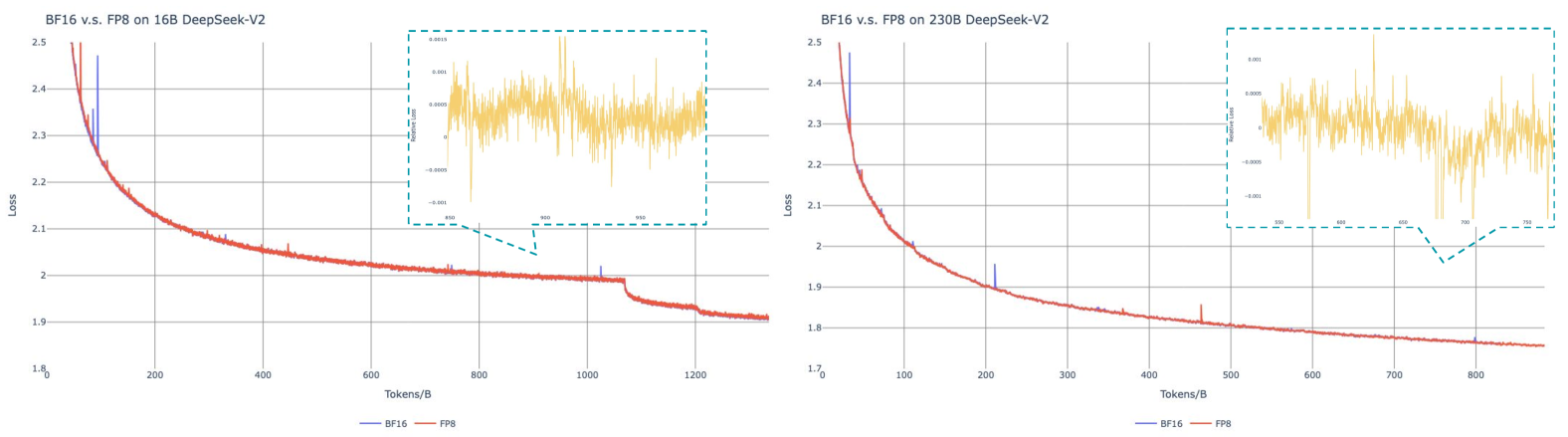
### Visual Description
# Technical Analysis: BF16 vs. FP8 Training Loss on DeepSeek-V2
This document provides a detailed extraction of data and trends from two side-by-side line charts comparing the training loss of the DeepSeek-V2 model using two different numerical formats: **BF16** (Blue) and **FP8** (Red).
---
## 1. General Layout and Components
The image consists of two primary panels, each containing a main line chart and an inset "Relative Loss" chart.
* **Left Panel:** DeepSeek-V2 16B parameter model.
* **Right Panel:** DeepSeek-V2 230B parameter model.
* **Legend (Common):** Located at the bottom center of each panel.
* **Blue Line:** BF16
* **Red Line:** FP8
* **X-Axis (Common):** Tokens/B (Tokens in Billions).
* **Y-Axis (Common):** Loss.
---
## 2. Left Chart: BF16 v.s. FP8 on 16B DeepSeek-V2
### Main Chart Data
* **X-Axis Range:** 0 to ~1350 Tokens/B. Markers at intervals of 200 (0, 200, 400, 600, 800, 1000, 1200).
* **Y-Axis Range:** 1.8 to 2.5. Markers at 1.8, 1.9, 2.0, 2.1, 2.2, 2.3, 2.4, 2.5.
* **Trend Analysis:**
* **BF16 (Blue):** Shows a sharp exponential decay initially, stabilizing into a gradual decline. There are several distinct vertical "spikes" (noise/instability) visible, notably around 100, 350, 750, and 1050 Tokens/B.
* **FP8 (Red):** Follows the BF16 curve almost perfectly. The red line is layered on top of the blue line, indicating nearly identical convergence behavior.
* **Key Observation:** At approximately 1080 Tokens/B, there is a sharp step-down in loss for both formats, likely indicating a learning rate decay or a change in training curriculum.
### Inset Chart: Relative Loss (16B)
* **Focus Area:** Approximately 850 to 980 Tokens/B.
* **Y-Axis:** Relative Loss (Range: -0.001 to 0.0015).
* **Content:** A yellow line representing the variance between the two formats. The values oscillate around 0.0005, indicating that the difference between FP8 and BF16 is extremely marginal (less than 0.1%).
---
## 3. Right Chart: BF16 v.s. FP8 on 230B DeepSeek-V2
### Main Chart Data
* **X-Axis Range:** 0 to ~900 Tokens/B. Markers at intervals of 100 (0, 100, 200, 300, 400, 500, 600, 700, 800).
* **Y-Axis Range:** 1.7 to 2.5. Markers at 1.7, 1.8, 1.9, 2.0, 2.1, 2.2, 2.3, 2.4, 2.5.
* **Trend Analysis:**
* **BF16 (Blue):** Similar to the 16B model, it shows a smooth convergence curve. Spikes are visible at roughly 50, 210, 340, 480, and 800 Tokens/B.
* **FP8 (Red):** Overlays the BF16 line with high precision. The convergence path is indistinguishable from BF16 at this scale.
* **Key Observation:** The overall loss is lower than the 16B model (ending near 1.75 vs 1.9), consistent with the higher capacity of a 230B parameter model.
### Inset Chart: Relative Loss (230B)
* **Focus Area:** Approximately 550 to 780 Tokens/B.
* **Y-Axis:** Relative Loss (Range: -0.001 to 0.001).
* **Content:** The yellow line shows the relative difference. While there are sharp downward spikes (reaching -0.001), the mean relative loss stays very close to 0.000, suggesting even tighter parity between FP8 and BF16 on the larger model.
---
## 4. Summary of Technical Findings
| Feature | 16B Model Observation | 230B Model Observation |
| :--- | :--- | :--- |
| **Convergence** | Identical for BF16 and FP8 | Identical for BF16 and FP8 |
| **Final Loss** | ~1.91 | ~1.76 |
| **Stability** | Occasional spikes in both formats | Occasional spikes in both formats |
| **Relative Delta** | Centered near 0.0005 | Centered near 0.0000 |
**Conclusion:** The data demonstrates that training DeepSeek-V2 using **FP8** precision yields results that are numerically and behaviorally equivalent to **BF16** training across both small (16B) and large (230B) scales, while likely offering computational efficiency gains not explicitly charted here.
</details>
Figure 10: Loss curves comparison between BF16 and FP8 training. Results are smoothed by Exponential Moving Average (EMA) with a coefficient of 0.9.
B.1 FP8 v.s. BF16 Training
We validate our FP8 mixed precision framework with a comparison to BF16 training on top of two baseline models across different scales. At the small scale, we train a baseline MoE model comprising approximately 16B total parameters on 1.33T tokens. At the large scale, we train a baseline MoE model comprising approximately 230B total parameters on around 0.9T tokens. We show the training curves in Figure 10 and demonstrate that the relative error remains below 0.25% with our high-precision accumulation and fine-grained quantization strategies.
B.2 Discussion About Block-Wise Quantization
Although our tile-wise fine-grained quantization effectively mitigates the error introduced by feature outliers, it requires different groupings for activation quantization, i.e., 1x128 in forward pass and 128x1 for backward pass. A similar process is also required for the activation gradient. A straightforward strategy is to apply block-wise quantization per 128x128 elements like the way we quantize the model weights. In this way, only transposition is required for backward. Therefore, we conduct an experiment where all tensors associated with Dgrad are quantized on a block-wise basis. The results reveal that the Dgrad operation which computes the activation gradients and back-propagates to shallow layers in a chain-like manner, is highly sensitive to precision. Specifically, block-wise quantization of activation gradients leads to model divergence on an MoE model comprising approximately 16B total parameters, trained for around 300B tokens. We hypothesize that this sensitivity arises because activation gradients are highly imbalanced among tokens, resulting in token-correlated outliers (Xi et al., 2023). These outliers cannot be effectively managed by a block-wise quantization approach.
Appendix C Expert Specialization Patterns of the 16B Aux-Loss-Based and Aux-Loss-Free Models
We record the expert load of the 16B auxiliary-loss-based baseline and the auxiliary-loss-free model on the Pile test set. The auxiliary-loss-free model tends to have greater expert specialization across all layers, as demonstrated in Figure 11.
<details>
<summary>x11.png Details</summary>
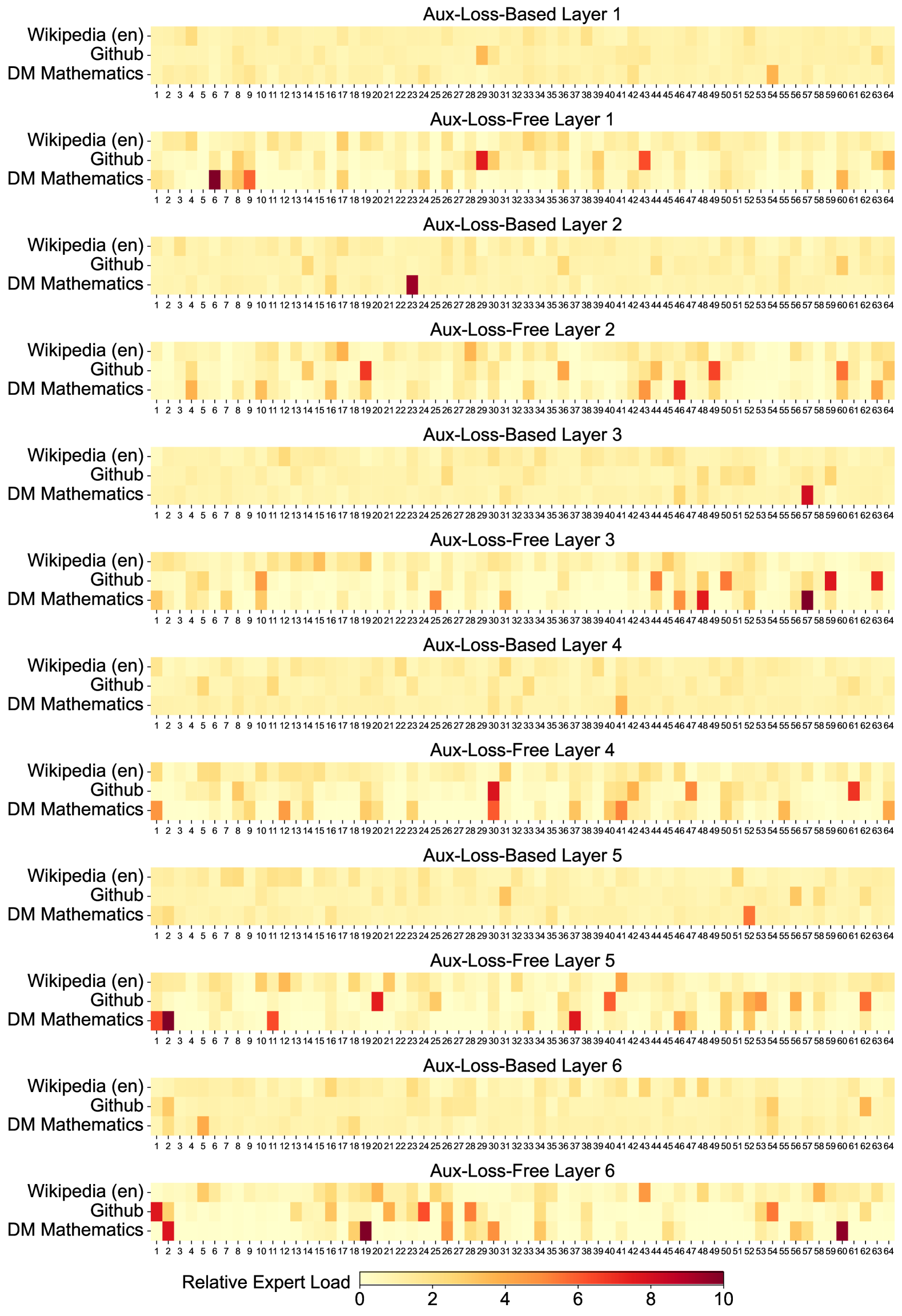
### Visual Description
# Technical Data Extraction: Expert Load Heatmaps
## Overview
This document contains a series of 12 heatmaps organized in pairs, comparing "Aux-Loss-Based" and "Aux-Loss-Free" routing mechanisms across six layers (Layer 1 through Layer 6) of a Mixture-of-Experts (MoE) neural network. The charts visualize the **Relative Expert Load** across three distinct datasets.
## Metadata and Legend
* **Language:** English (en)
* **Metric:** Relative Expert Load
* **Scale:** 0 to 10 (Linear gradient)
* **0 (Light Yellow):** Low load/utilization.
* **10 (Dark Red/Maroon):** High load/utilization.
* **X-Axis (Experts):** 64 discrete experts, labeled 1 through 64.
* **Y-Axis (Datasets):**
1. Wikipedia (en)
2. Github
3. DM Mathematics
---
## Comparative Analysis by Layer
### Layer 1
* **Aux-Loss-Based Layer 1:** Shows a highly uniform, low-intensity distribution (mostly light yellow). Expert 29 (Github) and Expert 54 (DM Mathematics) show slightly higher activation.
* **Aux-Loss-Free Layer 1:** Shows significantly higher variance and "hotspots."
* **DM Mathematics:** High load on Experts 6, 8, and 9.
* **Github:** High load on Experts 29 and 43.
* **Wikipedia:** Generally uniform but slightly higher intensity than the loss-based counterpart.
### Layer 2
* **Aux-Loss-Based Layer 2:** Very uniform distribution. The only significant outlier is **DM Mathematics** at Expert 23 (Dark Red).
* **Aux-Loss-Free Layer 2:** Increased specialization.
* **Github:** High load on Experts 19, 49, and 60.
* **DM Mathematics:** High load on Experts 4, 43, 46, and 64.
### Layer 3
* **Aux-Loss-Based Layer 3:** Extremely uniform across Wikipedia and Github. **DM Mathematics** shows a single high-load point at Expert 57.
* **Aux-Loss-Free Layer 3:**
* **Github:** High load on Experts 43, 45, 50, 59, and 64.
* **DM Mathematics:** High load on Experts 46, 47, and 57.
### Layer 4
* **Aux-Loss-Based Layer 4:** Uniform distribution with very minor intensity increases for DM Mathematics around Expert 41.
* **Aux-Loss-Free Layer 4:**
* **Github:** Significant hotspot at Expert 30.
* **DM Mathematics:** High load at Experts 1, 41, 42, 47, and 64.
### Layer 5
* **Aux-Loss-Based Layer 5:** Uniform distribution. Minor intensity for DM Mathematics at Expert 52.
* **Aux-Loss-Free Layer 5:**
* **Github:** High load at Experts 20, 40, 52, and 62.
* **DM Mathematics:** High load at Experts 1, 2, 11, 36, 40, and 46.
### Layer 6
* **Aux-Loss-Based Layer 6:** Uniform distribution. Minor intensity for DM Mathematics at Expert 6 and Expert 52.
* **Aux-Loss-Free Layer 6:**
* **Github:** High load at Expert 1.
* **DM Mathematics:** High load at Experts 2, 19, 25, 30, and 61.
---
## Key Trends and Observations
1. **Routing Mechanism Contrast:**
* **Aux-Loss-Based:** These layers exhibit a "load balancing" effect. The distribution is consistently pale, indicating that the auxiliary loss is successfully forcing the model to spread the computational load across all 64 experts relatively evenly.
* **Aux-Loss-Free:** These layers exhibit "Expert Specialization." Without the auxiliary loss constraint, specific experts become highly specialized for specific datasets (Github or DM Mathematics), resulting in dark red hotspots (high load) and many experts with near-zero load.
2. **Dataset Specificity:**
* **Wikipedia (en):** Consistently shows the most uniform and lowest relative load across all layers and both routing types. It appears to be the "baseline" data that is processed by a wide variety of experts.
* **DM Mathematics & Github:** These datasets consistently trigger high-load hotspots in the Aux-Loss-Free models, suggesting they require more specialized computation that the router naturally gravitates toward when unconstrained.
3. **Expert Utilization:**
* In the **Aux-Loss-Free** configuration, the "hot" experts change from layer to layer, suggesting that the model develops a hierarchical specialization strategy. For example, Expert 1 is a major hub for DM Mathematics in Layer 4 and 5, but shifts to Github in Layer 6.
</details>
(a) Layers 1-7
<details>
<summary>x12.png Details</summary>
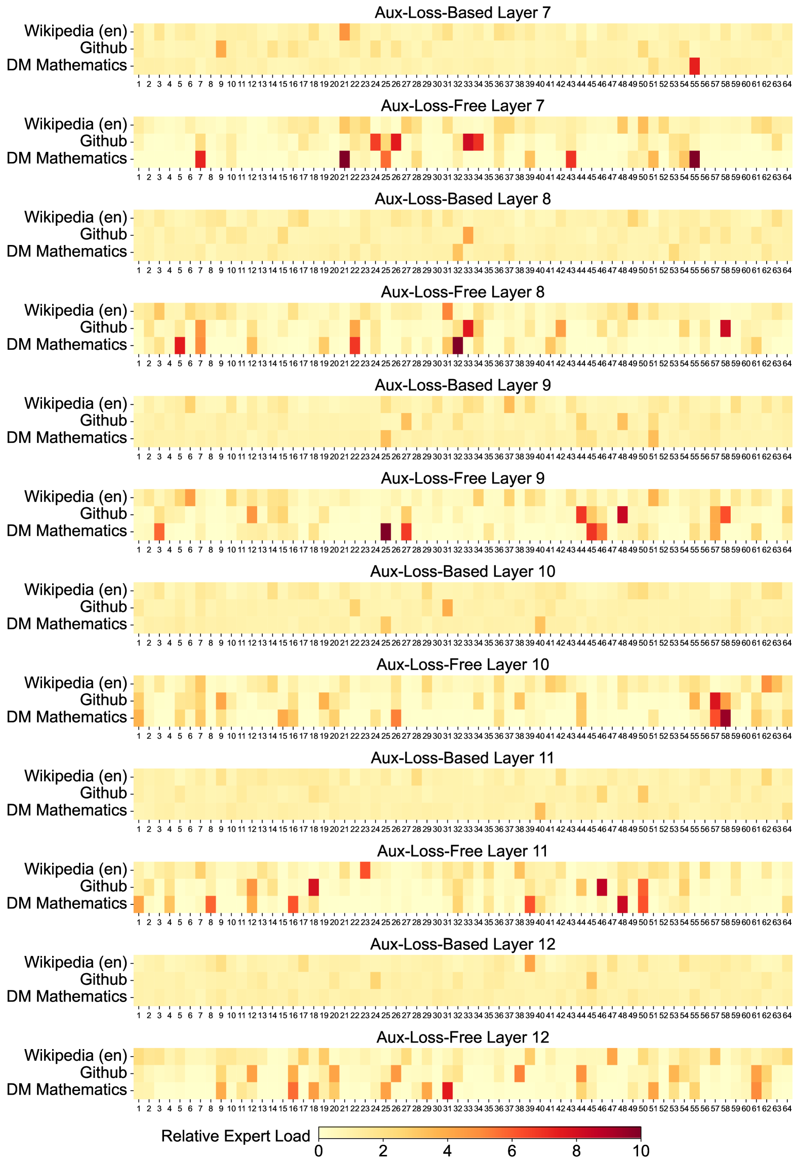
### Visual Description
# Technical Analysis of Expert Load Heatmaps
This document provides a comprehensive extraction and analysis of the provided image, which contains 12 heatmaps illustrating the "Relative Expert Load" across different layers and training methodologies of a Mixture-of-Experts (MoE) model.
## 1. General Metadata and Structure
* **Image Type:** A series of 12 vertically stacked heatmaps.
* **Primary Language:** English.
* **Core Metric:** **Relative Expert Load**.
* **Scale:** 0 to 10 (indicated by a color bar at the bottom).
* **Light Yellow (0):** Low load/utilization.
* **Dark Red (10):** High load/utilization.
* **Dimensions per Heatmap:**
* **Y-Axis (Categories):** 3 data sources: `Wikipedia (en)`, `Github`, and `DM Mathematics`.
* **X-Axis (Experts):** 64 individual experts, labeled 1 through 64.
## 2. Component Isolation: Heatmap Grid
The image is organized into pairs of heatmaps for Layers 7 through 12. Each pair compares an **"Aux-Loss-Based"** approach with an **"Aux-Loss-Free"** approach.
### Layer 7
* **Aux-Loss-Based Layer 7:** Shows a relatively uniform, low-intensity distribution (mostly light yellow). Notable slight increases in load for `Wikipedia (en)` at Expert 21 and `DM Mathematics` at Expert 55.
* **Aux-Loss-Free Layer 7:** Shows significantly higher variance and specialization.
* `DM Mathematics` shows high intensity (dark red) at Experts 7, 21, 26, 43, and 55.
* `Github` shows high intensity at Experts 24, 26, and 33.
### Layer 8
* **Aux-Loss-Based Layer 8:** Very uniform, low load across all experts and data sources.
* **Aux-Loss-Free Layer 8:** Increased specialization compared to the loss-based version.
* `DM Mathematics` peaks at Experts 5, 8, 22, and 32.
* `Github` shows a distinct peak at Expert 58.
### Layer 9
* **Aux-Loss-Based Layer 9:** Uniform low load. Minor activity for `DM Mathematics` at Expert 25.
* **Aux-Loss-Free Layer 9:**
* `DM Mathematics` shows strong specialization at Experts 4, 25, 27, and 45.
* `Github` shows peaks at Experts 44 and 48.
### Layer 10
* **Aux-Loss-Based Layer 10:** Uniform low load. Minor activity for `DM Mathematics` at Expert 40.
* **Aux-Loss-Free Layer 10:**
* `DM Mathematics` shows high load at Experts 1, 26, and 58.
* `Github` shows a peak at Expert 57.
### Layer 11
* **Aux-Loss-Based Layer 11:** Uniform low load. Minor activity for `DM Mathematics` at Expert 40.
* **Aux-Loss-Free Layer 11:**
* `DM Mathematics` shows high load at Experts 8, 16, 47, and 50.
* `Github` shows peaks at Experts 24 and 45.
### Layer 12
* **Aux-Loss-Based Layer 12:** Uniform low load across the board.
* **Aux-Loss-Free Layer 12:**
* `DM Mathematics` shows moderate to high load at Experts 25, 31, 51, and 62.
* `Github` shows moderate load at Experts 11, 22, and 38.
---
## 3. Data Trends and Observations
### Trend Verification
1. **Aux-Loss-Based Trend:** Across all layers (7-12), the "Aux-Loss-Based" models exhibit a "flat" or "smeared" distribution. The color remains consistently in the light yellow range (0-2), indicating that the auxiliary loss forces the model to distribute the load evenly across all 64 experts regardless of the input domain.
2. **Aux-Loss-Free Trend:** Across all layers, the "Aux-Loss-Free" models exhibit "sparsity" and "specialization." There are clear "hotspots" (dark orange to dark red, values 6-10) where specific experts are heavily utilized for specific data sources (e.g., Expert 55 for DM Mathematics in Layer 7).
### Comparative Analysis
* **Domain Specialization:** In the "Aux-Loss-Free" charts, `DM Mathematics` and `Github` often activate different experts. `Wikipedia (en)` tends to have a more distributed, lower-intensity load compared to the other two, likely due to its broader linguistic nature.
* **Expert Utilization:** The "Aux-Loss-Free" method allows for "expert collapse" or "expert specialization" where certain experts become highly tuned to specific tasks, whereas the "Aux-Loss-Based" method prevents this by design, resulting in the uniform appearance.
---
## 4. Legend and Scale Extraction
* **Location:** Bottom center of the image.
* **Label:** `Relative Expert Load`
* **Scale Markers:** `0, 2, 4, 6, 8, 10`
* **Color Gradient:**
* **0:** Pale Yellow (#FFF9C4 approx)
* **5:** Orange (#FF9800 approx)
* **10:** Deep Red/Maroon (#800000 approx)
## 5. Axis Labels and Categories
* **Y-Axis Labels (Top to Bottom for each chart):**
1. `Wikipedia (en)`
2. `Github`
3. `DM Mathematics`
* **X-Axis Labels:** Integers from `1` to `64`, representing the Expert ID. Every integer is labeled.
</details>
(b) Layers 7-13
<details>
<summary>x13.png Details</summary>
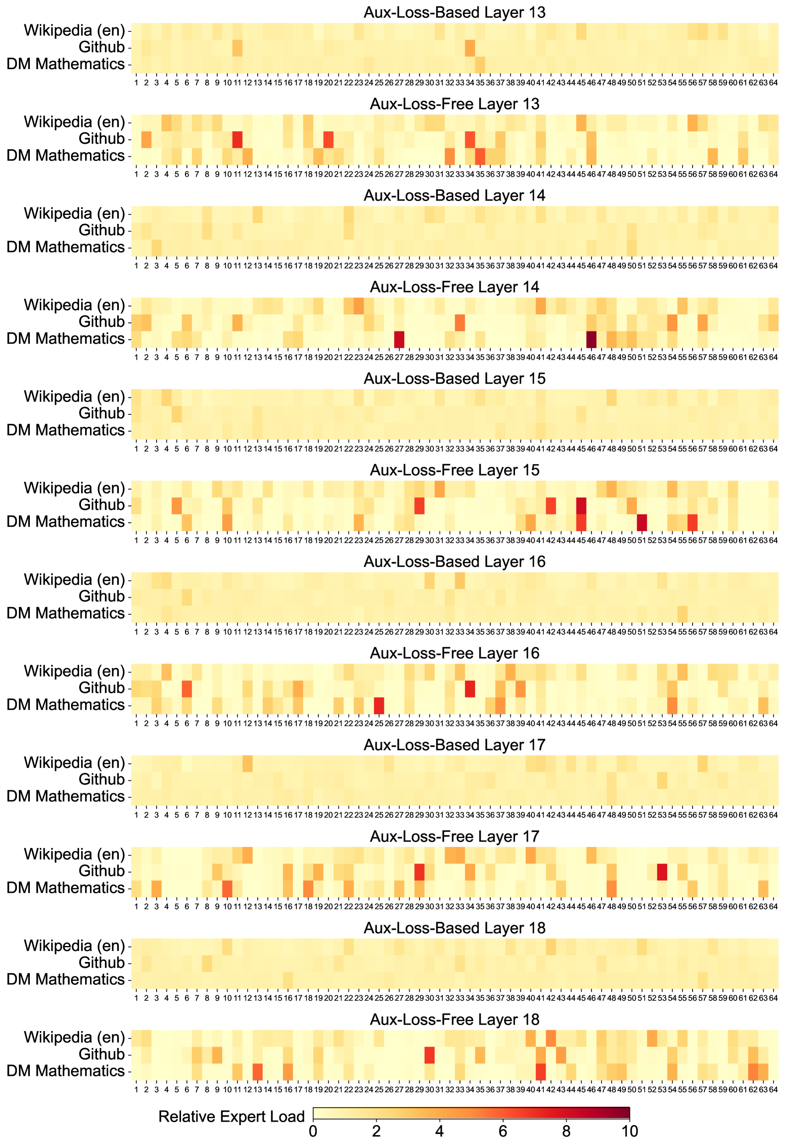
### Visual Description
# Technical Document Extraction: Relative Expert Load Heatmaps
## 1. Document Overview
This image contains a series of 12 heatmaps organized in a vertical stack. The charts compare the "Relative Expert Load" across different layers of a Mixture-of-Experts (MoE) neural network, specifically contrasting two training methodologies: **Aux-Loss-Based** and **Aux-Loss-Free**.
## 2. Global Metadata and Legend
* **Language:** English (en).
* **Metric:** Relative Expert Load.
* **Color Scale (Legend):** Located at the bottom center.
* **Range:** 0 to 10.
* **Gradient:** Light yellow (0) $\rightarrow$ Orange (5) $\rightarrow$ Deep Red (10).
* **X-Axis (Common to all charts):** Expert Index, ranging from **1 to 64**.
* **Y-Axis (Common to all charts):** Data Domains.
1. Wikipedia (en)
2. Github
3. DM Mathematics
## 3. Component Analysis by Layer
The heatmaps are presented in pairs (Aux-Loss-Based vs. Aux-Loss-Free) for Layers 13 through 18.
### Layer 13
* **Aux-Loss-Based Layer 13:** Shows a very uniform, low-intensity distribution (mostly light yellow). A slight increase in load is visible for Github at Expert 34 and DM Mathematics at Expert 35.
* **Aux-Loss-Free Layer 13:** Shows significantly higher variance and specialization.
* **Wikipedia:** Peaks around Experts 2, 5, 10.
* **Github:** Strong peak (Red, ~8-9) at Expert 11; secondary peaks at 20, 34, 46.
* **DM Mathematics:** Peaks at Experts 12, 33, 35, 46, 58, 62.
### Layer 14
* **Aux-Loss-Based Layer 14:** Highly uniform distribution. Almost no visible specialization; all values appear to be $<2$.
* **Aux-Loss-Free Layer 14:**
* **Wikipedia:** Moderate load at Experts 1, 24, 44, 55.
* **Github:** Moderate load at Experts 6, 11, 33, 54, 57.
* **DM Mathematics:** Distinct high-intensity peaks (Deep Red, ~10) at Experts **27** and **46**.
### Layer 15
* **Aux-Loss-Based Layer 15:** Uniform distribution with very slight intensity increases for Github at Expert 5.
* **Aux-Loss-Free Layer 15:**
* **Wikipedia:** Moderate load at Experts 2, 31.
* **Github:** Strong peaks at Experts 6, 29, 42, 45 (Red, ~9).
* **DM Mathematics:** Strong peaks at Experts 11, 23, 41, 45, 52, 57.
### Layer 16
* **Aux-Loss-Based Layer 16:** Uniform distribution. Slight yellow-orange tint at Expert 33 for Wikipedia and Expert 55 for DM Mathematics.
* **Aux-Loss-Free Layer 16:**
* **Wikipedia:** Peaks at Experts 2, 5, 30, 41.
* **Github:** Strong peak at Expert 6 (Orange-Red, ~7).
* **DM Mathematics:** Peaks at Experts 17, 25, 34, 54.
### Layer 17
* **Aux-Loss-Based Layer 17:** Uniform distribution. Slight intensity at Expert 11 for Wikipedia.
* **Aux-Loss-Free Layer 17:**
* **Wikipedia:** Peaks at Experts 11, 45.
* **Github:** Strong peak at Expert 29 (Red, ~8).
* **DM Mathematics:** Peaks at Experts 2, 10, 17, 21, 34, 47, 53 (Red, ~9).
### Layer 18
* **Aux-Loss-Based Layer 18:** Uniform distribution. Minimal variation across all 64 experts.
* **Aux-Loss-Free Layer 18:**
* **Wikipedia:** Peaks at Experts 1, 40.
* **Github:** Peaks at Experts 9, 11, 30, 41, 43.
* **DM Mathematics:** Strong peaks at Experts 15, 41, 54, 63.
## 4. Key Trends and Observations
1. **Methodological Contrast:** The **Aux-Loss-Based** models exhibit a "load balancing" effect where the work is spread almost evenly across all 64 experts. This results in a "washed out" heatmap with very few distinct features.
2. **Expert Specialization:** The **Aux-Loss-Free** models show high levels of specialization. Specific experts (e.g., Expert 46 in Layer 14 for DM Mathematics) take on a disproportionately high relative load (up to 10x the average).
3. **Domain Separation:** In the Aux-Loss-Free charts, different domains (Wikipedia vs. Github vs. Math) often activate different sets of experts within the same layer, indicating the model has learned to route domain-specific information to specialized sub-networks.
4. **Vertical Consistency:** While specialization is present in all Aux-Loss-Free layers, the specific "hot" experts change from layer to layer, suggesting a complex routing logic that evolves through the depth of the network.
</details>
(c) Layers 13-19
<details>
<summary>x14.png Details</summary>
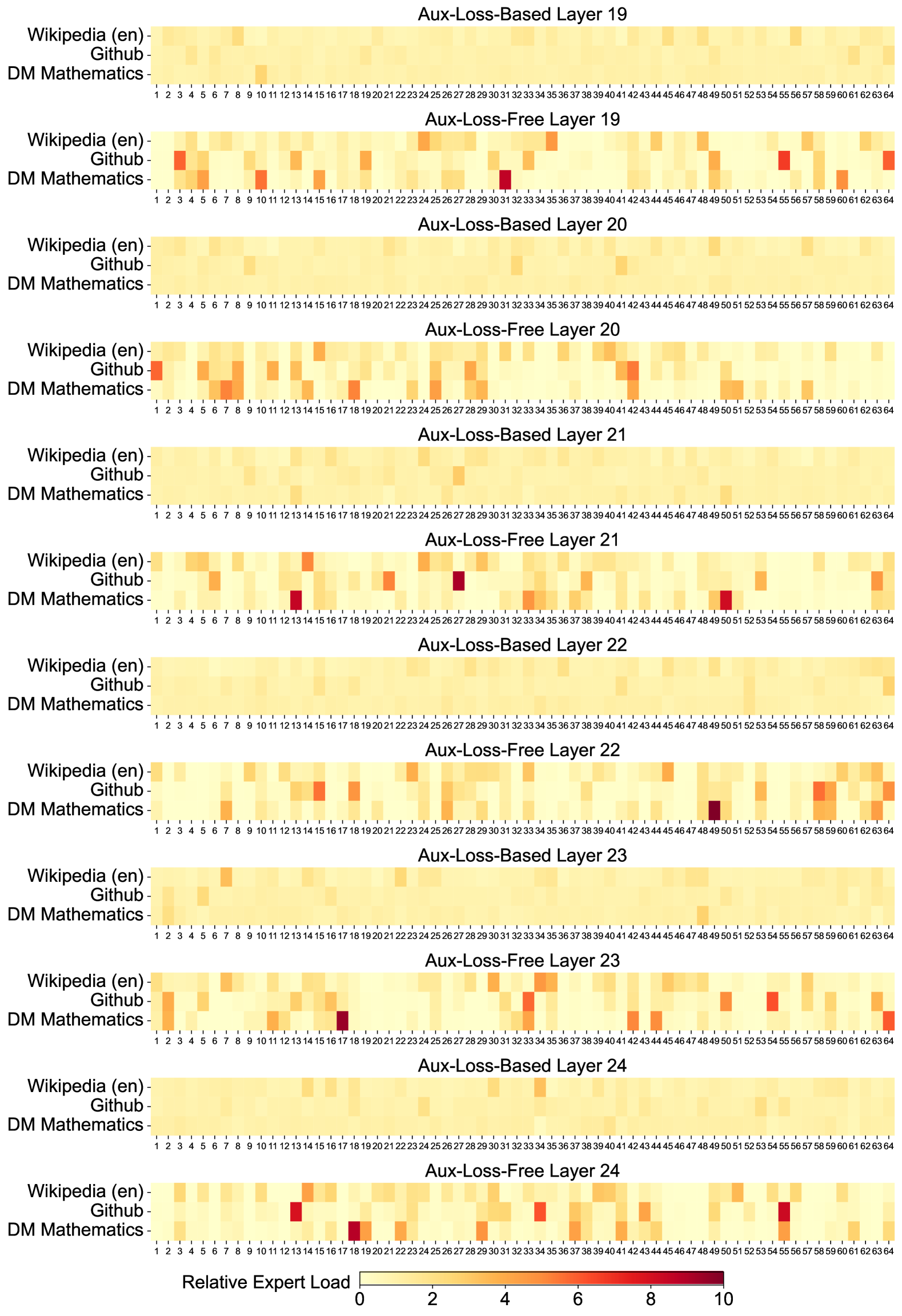
### Visual Description
# Technical Data Extraction: Expert Load Heatmaps (Layers 19-24)
## 1. Document Overview
This image contains a series of 12 heatmaps organized in pairs, comparing "Aux-Loss-Based" and "Aux-Loss-Free" training methods across six neural network layers (Layers 19 through 24). The charts visualize the "Relative Expert Load" across 64 distinct experts for three different datasets.
## 2. Global Components and Metadata
* **Language:** English.
* **Primary Metric:** Relative Expert Load.
* **Scale (Legend):** Located at the bottom center. It is a continuous color gradient ranging from 0 (Pale Yellow) to 10 (Deep Red/Maroon).
* **Y-Axis Categories (Datasets):**
1. Wikipedia (en)
2. Github
3. DM Mathematics
* **X-Axis Categories (Experts):** Numbered 1 through 64 for every heatmap.
* **Layout Structure:** 6 vertical blocks (Layers 19, 20, 21, 22, 23, 24). Each block contains two heatmaps:
* Top: Aux-Loss-Based
* Bottom: Aux-Loss-Free
---
## 3. Detailed Heatmap Analysis by Layer
### Layer 19
* **Aux-Loss-Based:** Shows a very uniform distribution. Most experts are in the 0-2 range (pale yellow). No significant spikes are visible.
* **Aux-Loss-Free:** Shows significant specialization and load imbalance.
* **Github:** High load (orange/red) on experts 4, 56, and 64.
* **DM Mathematics:** High load (dark red) on expert 31; significant load on experts 4, 6, 10, 15, 49, and 61.
### Layer 20
* **Aux-Loss-Based:** Highly uniform. Almost all experts across all datasets are pale yellow (~1-2 load).
* **Aux-Loss-Free:**
* **Wikipedia (en):** Slight increase in load around experts 25-30.
* **Github:** High load on experts 1, 41, and 42.
* **DM Mathematics:** High load on experts 6, 8, 18, 29, and 50.
### Layer 21
* **Aux-Loss-Based:** Uniform distribution; no expert exceeds the light orange threshold.
* **Aux-Loss-Free:**
* **Wikipedia (en):** Spike at expert 15.
* **Github:** Significant spike (dark red) at expert 27.
* **DM Mathematics:** Significant spikes (dark red) at experts 13 and 50.
### Layer 22
* **Aux-Loss-Based:** Uniform distribution.
* **Aux-Loss-Free:**
* **Wikipedia (en):** Moderate load across experts 58-64.
* **Github:** Spikes at experts 15 and 59.
* **DM Mathematics:** Very high load (darkest red) at expert 49; moderate load at experts 7 and 59.
### Layer 23
* **Aux-Loss-Based:** Uniform distribution.
* **Aux-Loss-Free:**
* **Wikipedia (en):** Spike at expert 7.
* **Github:** Spikes at experts 1, 33, and 54.
* **DM Mathematics:** High load (dark red) at expert 17; moderate load at experts 43 and 63.
### Layer 24
* **Aux-Loss-Based:** Uniform distribution.
* **Aux-Loss-Free:**
* **Wikipedia (en):** Spike at expert 15.
* **Github:** High load (dark red) at expert 13; moderate load at experts 4, 43, and 55.
* **DM Mathematics:** High load (dark red) at experts 18 and 55.
---
## 4. Key Trends and Observations
### Trend 1: Aux-Loss Impact
* **Aux-Loss-Based:** In all layers (19-24), the "Aux-Loss-Based" heatmaps appear visually "flat" and pale. This indicates that the auxiliary loss function is successfully enforcing a balanced load across all 64 experts, preventing any single expert from being over-utilized.
* **Aux-Loss-Free:** In all layers, the "Aux-Loss-Free" heatmaps show high contrast with specific "hot spots" (dark red cells). This indicates that without the auxiliary loss, the model naturally gravitates toward specific experts for specific datasets, leading to high expert specialization and load imbalance.
### Trend 2: Dataset Specialization (Aux-Loss-Free)
* **DM Mathematics** consistently shows the most extreme "hot spots" (values approaching 10 on the scale), suggesting mathematical tasks utilize highly specific neural pathways compared to general text (Wikipedia).
* **Github** also shows distinct specialization, often on different experts than DM Mathematics, indicating the model differentiates between code and mathematical logic.
### Trend 3: Expert Sparsity
* In the "Aux-Loss-Free" versions, many experts (columns) remain pale yellow across all three datasets, suggesting they are under-utilized or "dead" experts, while a small subset handles the majority of the relative load.
</details>
(d) Layers 19-25
<details>
<summary>x15.png Details</summary>
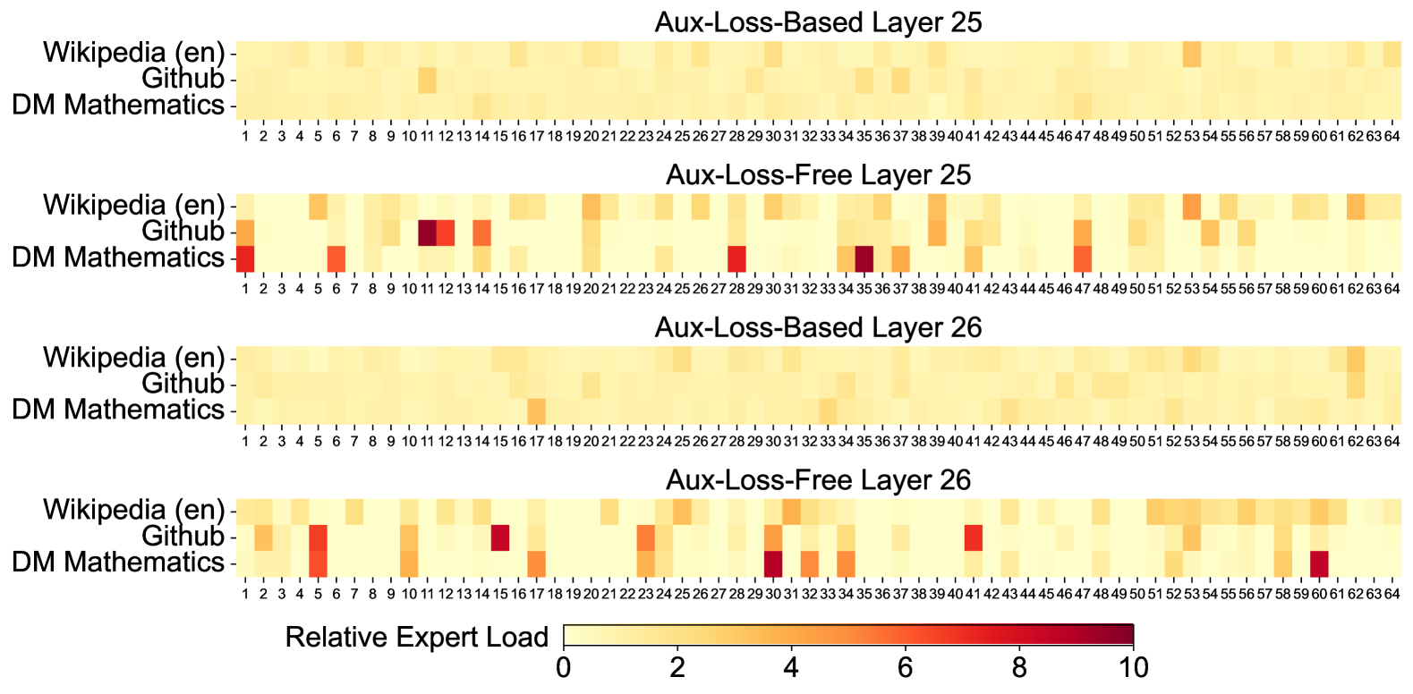
### Visual Description
# Technical Data Extraction: Relative Expert Load Heatmaps
This document provides a detailed extraction and analysis of the provided image, which contains four heatmaps illustrating "Relative Expert Load" across different model layers and training configurations.
## 1. Document Overview
The image consists of four vertically stacked heatmaps comparing two training methodologies (**Aux-Loss-Based** vs. **Aux-Loss-Free**) across two specific model layers (**Layer 25** and **Layer 26**).
### Global Components
* **X-Axis (All Charts):** Expert Index, ranging from **1 to 64**.
* **Y-Axis (All Charts):** Data Domains:
1. Wikipedia (en)
2. Github
3. DM Mathematics
* **Legend (Bottom Center):**
* **Title:** Relative Expert Load
* **Scale:** Linear gradient from 0 to 10.
* **Color Mapping:**
* Light Yellow: 0 (Low Load)
* Orange: ~5 (Medium Load)
* Dark Red/Maroon: 10 (High Load)
---
## 2. Heatmap Analysis by Region
### Region 1: Aux-Loss-Based Layer 25
* **Trend:** This chart shows a highly uniform distribution. The colors are almost exclusively light yellow, indicating that the load is balanced evenly across all 64 experts for all three domains.
* **Key Observations:**
* Slightly darker yellow/orange tint at Expert 53 for Wikipedia (en).
* Overall, no significant "specialization" or "hotspots" are visible.
### Region 2: Aux-Loss-Free Layer 25
* **Trend:** This chart shows high variance and significant expert specialization. Certain experts are heavily utilized by specific domains while others are ignored.
* **High Load Data Points (Hotspots):**
* **Wikipedia (en):** Moderate load at Expert 6, 20, 53, and 62.
* **Github:** High load (Dark Red) at Expert 11 and 12. Moderate load at Expert 1, 14, 20, 39, and 47.
* **DM Mathematics:** High load (Dark Red) at Expert 1, 35, and 47. Moderate load at Expert 6, 28, 37, and 41.
### Region 3: Aux-Loss-Based Layer 26
* **Trend:** Similar to Layer 25 (Aux-Loss-Based), this shows a very uniform, low-intensity distribution across all experts.
* **Key Observations:**
* Slightly higher load at Expert 17 for DM Mathematics.
* Slightly higher load at Expert 62 for Wikipedia (en).
* The "Aux-Loss-Based" method consistently results in a "smeared" load where no single expert carries a heavy burden.
### Region 4: Aux-Loss-Free Layer 26
* **Trend:** Like its Layer 25 counterpart, this shows distinct specialization and high-intensity hotspots, though the specific experts utilized have shifted.
* **High Load Data Points (Hotspots):**
* **Wikipedia (en):** Moderate load distributed across Experts 51-60.
* **Github:** High load at Expert 15 and 41. Moderate load at Expert 1, 5, 10, 23, 29, 32, and 53.
* **DM Mathematics:** High load (Dark Red) at Expert 30 and 60. Moderate load at Expert 5, 17, 23, 32, and 34.
---
## 3. Comparative Summary
| Feature | Aux-Loss-Based (Layers 25 & 26) | Aux-Loss-Free (Layers 25 & 26) |
| :--- | :--- | :--- |
| **Load Distribution** | Uniform / Balanced | Sparse / Specialized |
| **Peak Intensity** | Low (mostly < 2) | High (reaching 8-10) |
| **Domain Separation** | Low; domains use all experts similarly. | High; specific experts "belong" to specific domains. |
| **Visual Pattern** | Consistent light yellow wash. | Distinct orange and red blocks against yellow. |
## 4. Technical Conclusion
The data indicates that the **Aux-Loss-Based** training mechanism enforces a load-balancing constraint that prevents expert specialization, resulting in a near-even distribution of work across the 64 experts. Conversely, the **Aux-Loss-Free** approach allows the model to naturally gravitate toward expert specialization, where specific experts become highly activated for specific types of data (e.g., Github or Mathematics), leading to much higher "Relative Expert Load" values on a subset of the available experts.
</details>
(e) Layers 25-27
Figure 11: Expert load of auxiliary-loss-free and auxiliary-loss-based models on three domains in the Pile test set. The auxiliary-loss-free model shows greater expert specialization patterns than the auxiliary-loss-based one. The relative expert load denotes the ratio between the actual expert load and the theoretically balanced expert load.