# MuQ: Self-Supervised Music Representation Learning with Mel Residual Vector Quantization
## Abstract
Recent years have witnessed the success of foundation models pre-trained with self-supervised learning (SSL) in various music informatics understanding tasks, including music tagging, instrument classification, key detection, and more. In this paper, we propose a self-supervised music representation learning model for music understanding. Distinguished from previous studies adopting random projection or existing neural codec, the proposed model, named MuQ, is trained to predict tokens generated by Mel Residual Vector Quantization (Mel-RVQ). Our Mel-RVQ utilizes residual linear projection structure for Mel spectrum quantization to enhance the stability and efficiency of target extraction and lead to better performance. Experiments in a large variety of downstream tasks demonstrate that MuQ outperforms previous self-supervised music representation models with only 0.9K hours of open-source pre-training data. Scaling up the data to over 160K hours and adopting iterative training consistently improve the model performance. To further validate the strength of our model, we present MuQ-MuLan, a joint music-text embedding model based on contrastive learning, which achieves state-of-the-art performance in the zero-shot music tagging task on the MagnaTagATune dataset. Code and checkpoints are open source in https://github.com/tencent-ailab/MuQ.
## Introduction
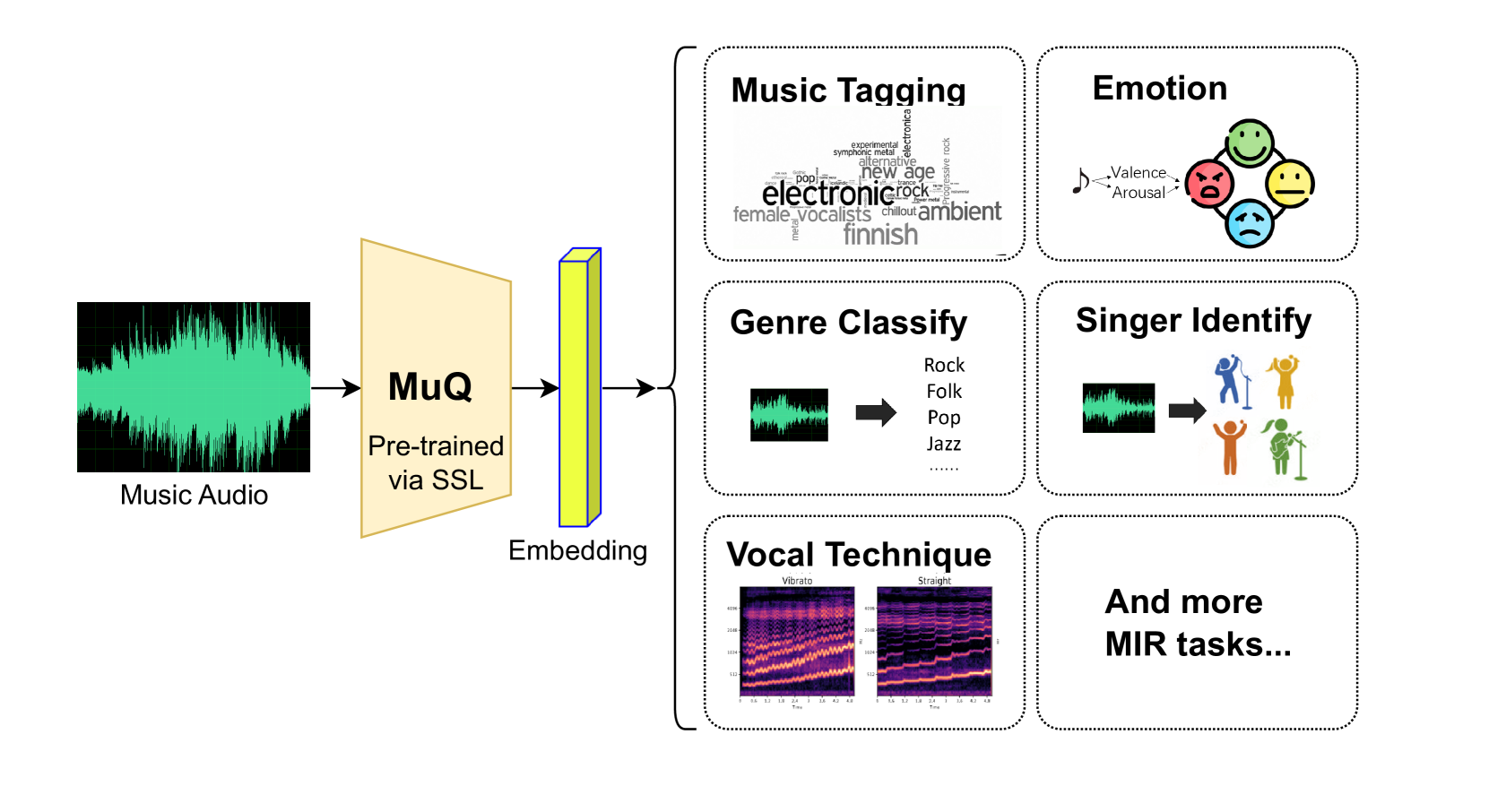
Self-supervised learning (SSL) has been introduced into speech and audio signal processing as a technique for learning latent semantic relationships from unlabeled raw data. Recently, several works (Li et al. 2023; Won, Hung, and Le 2023) apply SSL to music informatics understanding, and a number of pre-trained foundation models (PFMs) with generalized representation capabilities are built. Learning from unsupervised music data, these foundation models can achieve stunning performance in music understanding tasks such as genre classification, emotion prediction, and key detection (Yuan et al. 2023), and further provide semantic representations for more downstream tasks like music generation (Agostinelli et al. 2023) and music captioning (Deng et al. 2024), as illustrated in Figure 1.
<details>
<summary>x1.png Details</summary>
### Visual Description
## System Architecture Diagram: Music Processing Pipeline
### Overview
The diagram illustrates a music processing system that converts raw audio input into various music information retrieval (MIR) tasks. The pipeline begins with a spectrogram representation of music audio, processes it through a pre-trained MuQ model via self-supervised learning (SSL), and generates embeddings used for multiple downstream tasks including music tagging, emotion detection, genre classification, singer identification, vocal technique analysis, and additional MIR applications.
### Components/Axes
1. **Input**:
- **Music Audio**: Represented as a spectrogram (black background with green waveform-like pattern)
2. **Processing**:
- **MuQ**: Pre-trained via SSL (beige parallelogram)
- **Embedding**: Vertical yellow bar connecting MuQ to output tasks
3. **Output Tasks** (right-aligned boxes):
- **Music Tagging**: Contains text labels ("electronic", "rock", "new age", "female vocalists", "chillout", "ambient", "Finnish")
- **Emotion**: Circular diagram with four emoji faces (green smiley, red angry, blue sad, yellow neutral) labeled "Valence" and "Arousal"
- **Genre Classify**: Spectrogram input → text labels ("Rock", "Folk", "Pop", "Jazz")
- **Singer Identify**: Stick figure icons (orange male singer, green female singer)
- **Vocal Technique**: Two spectrograms labeled "Vibrato" (left) and "Straight" (right)
- **And more MIR tasks...**: Empty placeholder box
### Detailed Analysis
- **MuQ Processing**: The system uses a pre-trained MuQ model (likely a neural network architecture) that has been fine-tuned through self-supervised learning. This suggests the model was trained on unlabeled data before being adapted for specific tasks.
- **Embedding Generation**: The vertical yellow bar represents the transformation of raw audio features into a compressed, task-agnostic embedding space.
- **Task-Specific Outputs**:
- **Music Tagging**: Demonstrates multi-label classification capabilities, with tags spanning genre, instrumentation, mood, and cultural attributes.
- **Emotion Detection**: Uses a circular valence-arousal model with four discrete emotional states.
- **Genre Classification**: Shows hierarchical genre taxonomy (Rock > Folk > Pop > Jazz).
- **Singer Identification**: Visualizes gender-based singer classification through simplified iconography.
- **Vocal Technique Analysis**: Compares vibrato (periodic amplitude modulation) and straight tone (constant amplitude) through spectrogram visualization.
### Key Observations
1. The system architecture emphasizes modularity, with a single embedding space serving multiple MIR tasks.
2. Emotion detection uses a simplified 2D emotional space (valence × arousal) with discrete states rather than continuous values.
3. Genre classification appears to follow a tree-like taxonomy rather than flat categorization.
4. Vocal technique analysis focuses on amplitude modulation characteristics rather than spectral features.
### Interpretation
This architecture demonstrates a transfer learning approach where a single pre-trained model (MuQ) generates embeddings that can be adapted to various MIR tasks without retraining from scratch. The use of self-supervised learning suggests the system was initially trained on large unlabeled music datasets before being fine-tuned for specific applications. The diagram highlights the system's versatility in handling both categorical (genre, emotion) and continuous (vocal technique) analysis tasks. The inclusion of cultural tags ("Finnish") alongside technical features ("vibrato") indicates the system's capability to capture both acoustic and contextual music attributes. The empty "And more MIR tasks..." box implies extensibility to future applications like tempo detection, key recognition, or lyrical analysis.
</details>
Figure 1: Illustration of how the SSL pre-trained model works in music information retrieval (MIR) tasks.
A key challenge in music understanding and representation is that music is an extremely specific modality. Unlike speech or environmental sounds, music not only focuses on semantic information, but also emphasizes acoustic information, such as melody, chords, and tonality. As a result, previous semantics-oriented SSL methods have struggled to perform well on music tasks (Spijkervet and Burgoyne 2021; Li et al. 2022; Yuan et al. 2023), as they fail to simultaneously capture both semantic and acoustic information.
Recently, several studies have sought to develop a universal music representation that integrates both semantic and acoustic aspects. Among these efforts, two remarkable models are MERT (Li et al. 2023) and MusicFM (Won, Hung, and Le 2023). MERT employs a BERT-style masked language modeling (MLM) proxy task to predict discrete tokens from the masked audio parts, with an Encodec (Défossez et al. 2022) model as the tokenizer and uses an auxiliary Constant Q-Transform (CQT) target to enhance the modeling of acoustic information. MusicFM, on the other hand, directly utilizes a random projection quantizer derived from BEST-RQ (Chiu et al. 2022), and this tokenization approach provides a general target for learning music representation, without the need for additional CQT loss to capture acoustic modeling.
As discussed in (Chiu et al. 2022) and (Li et al. 2023), the target extractor (i.e., tokenizer) plays an important role in SSL, as models are trained to predict the tokenized pseudo-labels. BEST-RQ features a lightweight approach that allows for fast extraction of discrete targets. However, its performance is highly dependent on the initialization of the random projection layer, often requiring multiple attempts or a specific random seed to achieve optimal results. In contrast, the Encodec target (Défossez et al. 2022) used in MERT produces a series of residual targets, with the multi-target strategy shown beneficial to musical SSL (Li et al. 2023). As a neural codec trained on audio data, Encodec produces more stable labels compared to its random counterparts. However, using Encodec as tokenization is computational heavy and consumes a lot of GPU memory when applying online extraction, which can reduce the training efficiency. Also, it needs to be coupled with additional CQT reconstruction loss to perform well in acoustic representation.
To address the initialization dependency of the random projection quantizer in BEST-RQ and the inefficiency stemming from the heavy computation cost of Encodec in MERT, we introduce a model called MuQ, which learns Mu sic representations from Mel Q uantization targets. MuQ leverages a Mel-RVQ as the tokenizer to generate targets. The proposed Mel-RVQ is pre-trained on music data and employs a linear RVQ to directly quantize audio Mel spectrograms. Compared to the random-projection quantizer in BEST-RQ, the pre-trained Mel-RVQ produces more stable targets for SSL training and eliminates the model’s dependence on initialization. Additionally, compared to Encodec, the lightweight single-layer Mel-RVQ architecture offers greater extraction efficiency.
To further demonstrate the capabilities of the proposed MuQ model, we explore its application in another crucial area of music understanding: aligning music and text representations. For example, MuLan (Huang et al. 2022) employs contrastive learning to train both a music encoder and a text encoder, producing semantically consistent embeddings for both modalities and achieving coherent alignment between music and text. Recognizing the role that self-supervised learning models can play in providing effective initialization for downstream tasks, we leverage our MuQ to construct a joint music-text embedding model, named MuQ-MuLan.
Our main contributions are listed as follows:
- We introduce a novel music SSL model MuQ, which demonstrates state-of-the-art performance across a wide range of downstream music understanding tasks over previous MERT and MusicFM models.
- We propose the Mel Residual Vector Quantization (Mel-RVQ), which directly quantizes the Mel spectrum using a single linear layer RVQ, improving both training stability and efficiency.
- We further develop the MuQ-MuLan model, trained with contrastive learning on MuQ. MuQ-MuLan excels in aligning and jointly encoding music and text modalities, compared with the original MuLan model.
Our experiments demonstrate that the Mel-RVQ significantly enhances SSL performance across a variety of music downstream tasks. Notably, MuQ outperforms previous state-of-the-art (SOTA) SSL models MERT and MusicFM, even when trained on just 0.9K hours of data, which is 100x less than what comparable models require (Li et al. 2023; Won, Hung, and Le 2023). Additionally, our results show that MuQ-MuLan achieves a ROC-AUC score of 79.3 on the MagnaTagATune zero-shot music tagging task, surpassing the previous SOTA result (Huang et al. 2022).
## Related Work
Self-supervised learning for speech and audio
Self-supervised learning (SSL) (Mohamed et al. 2022) has been introduced to the field of speech and audio signal processing as a way to learn semantic representations from unlabeled audio data, and it is now widely used in tasks such as automatic speech recognition (Baevski et al. 2023) and audio event classification (Chen et al. 2024).
SSL often relies on well-designed targets. HuBERT (Hsu et al. 2021), for instance, uses K-means clustering labels to guide self-supervised learning in Masked Language Model (MLM) style, with these labels being extracted offline. BEST-RQ (Chiu et al. 2022) learns directly from targets generated by a randomly initialized projection quantizer, which can be extracted online. MT4SSL (Ma et al. 2022) integrates both online and offline objectives, applying the concept of multi-target self-supervised learning, where a distinct linear prediction head is used for each type of target.
Another important topic in SSL is iterative refinement training. Most existing iterative training practices are based on clustering. For example, HuBERT applies K-means clustering on the features of an existing model to train the next iteration of models. Similarly, Seed-ASR (Bai et al. 2024) first trains an SSL model on BEST-RQ and then iteratively trains on its features using K-means clustering.
In this paper, we take an alternative approach by iteratively training directly through the quantizer itself, without the need to apply K-means clustering.
Music processing and understanding
Music information retrieval (MIR) contains a large set of tasks to evaluate deep learning models’ understanding of music from audio signals or symbolized notation. For example, automatic music tagging task require models to do multi-label classification for tags like genre, instrument, and mood, given a music track (Won et al. 2020). Other MIR tasks include key detection, pitch detection, emotion analysis, etc (Yuan et al. 2023).
In recent years, SSL has been introduced into music understanding for building universal representational models capable of handling various MIR tasks. Some of these efforts include CLMR (Spijkervet and Burgoyne 2021) based on contrastive learning; MERT (Li et al. 2023) based on MLM proxy task; and more recently, MusicFM (Won, Hung, and Le 2023). These SSL-based models yield impressive performance across multiple MIR tasks, showing a generalized understanding of music.
Music-text joint embedding model
Bridging the gap between music and text modalities, music-text representation models learn joint embeddings from music-text pairwise data. Most of these models use a two-tower structure, consisting of both a music encoder and a text encoder, and are trained by contrastive learning loss.
LAION-CLAP (Wu et al. 2023) is a powerful open-source music-text encoder, with various model structures and versions trained on extensive data. MuLan (Huang et al. 2022) is also an exceptional music-text embedding model, but it is not open source for either the model or the data.
The MuQ-MuLan model introduced in this paper follows the ideas of former work but replaces the music encoder with our proposed MuQ model.
## Method
<details>
<summary>x2.png Details</summary>
### Visual Description
## Diagram: Audio Processing Pipeline with Conformer and Mel-RVQ Tokenization
### Overview
The diagram illustrates a technical workflow for audio signal processing, starting from a Mel Spectrum input and ending with Mel-RVQ Tokenization. The process involves masking, a Conformer neural network architecture, linear layers, and quantization steps. The flow is directional, with arrows indicating data transformation stages.
### Components/Axes
1. **Mel Spectrum** (Bottom)
- Visualized as a heatmap with purple/black coloration
- Represents frequency-domain audio features
2. **Masking** (Middle)
- Gray blocks overlaying portions of the Mel Spectrum
- Indicates selective data omission or focus areas
3. **Conformer** (Central)
- Rectangular component connecting Masking to Linear Layers
- Represents a conformer neural network architecture
4. **Linear Layers** (Top)
- Contains numerical values: 18, 38, 5, 127, 45, 78
- Arranged in a dashed-bordered box with alternating white/yellow shading
5. **Mel-RVQ Tokenization** (Right)
- Hexagonal component with dashed outline
- Represents vector quantization of Mel features
### Detailed Analysis
- **Mel Spectrum**:
- Shows spectral characteristics of audio signals
- Color intensity likely represents amplitude/energy levels
- **Masking**:
- Three gray blocks cover specific regions of the spectrum
- Suggests intentional data hiding or attention mechanism
- **Conformer**:
- Central processing unit with bidirectional data flow
- Connects raw features (Mel Spectrum) to higher-level abstractions
- **Linear Layers**:
- Numerical values may represent:
- Layer dimensions (e.g., 18→38→5)
- Quantization parameters (127, 45, 78)
- Alternating shading suggests hierarchical organization
- **Mel-RVQ Tokenization**:
- Final transformation stage
- Hexagonal shape implies discrete, quantized output
### Key Observations
1. **Directional Flow**:
- Data moves from raw features (bottom) to abstract representations (top)
- Masking precedes Conformer processing
2. **Quantization Evidence**:
- High-value numbers (127, 45, 78) in Linear Layers suggest bit-depth constraints
3. **Architectural Choices**:
- Conformer's bidirectional processing implies context-aware feature extraction
- RVQ tokenization indicates discrete representation for downstream tasks
### Interpretation
This diagram represents a hybrid audio processing pipeline combining:
1. **Feature Extraction**: Mel Spectrogram generation
2. **Data Augmentation**: Strategic masking for robustness
3. **Neural Processing**: Conformer architecture for temporal-spatial feature learning
4. **Quantization**: Linear layers and RVQ for efficient representation
The workflow suggests applications in:
- Speech recognition systems
- Audio compression
- Music information retrieval
- Voice activity detection
The masking step and RVQ tokenization are particularly indicative of modern neural audio codecs, where discrete representations enable efficient modeling while preserving perceptual quality. The Conformer's inclusion points to state-of-the-art temporal modeling capabilities, crucial for handling variable-length audio sequences.
</details>
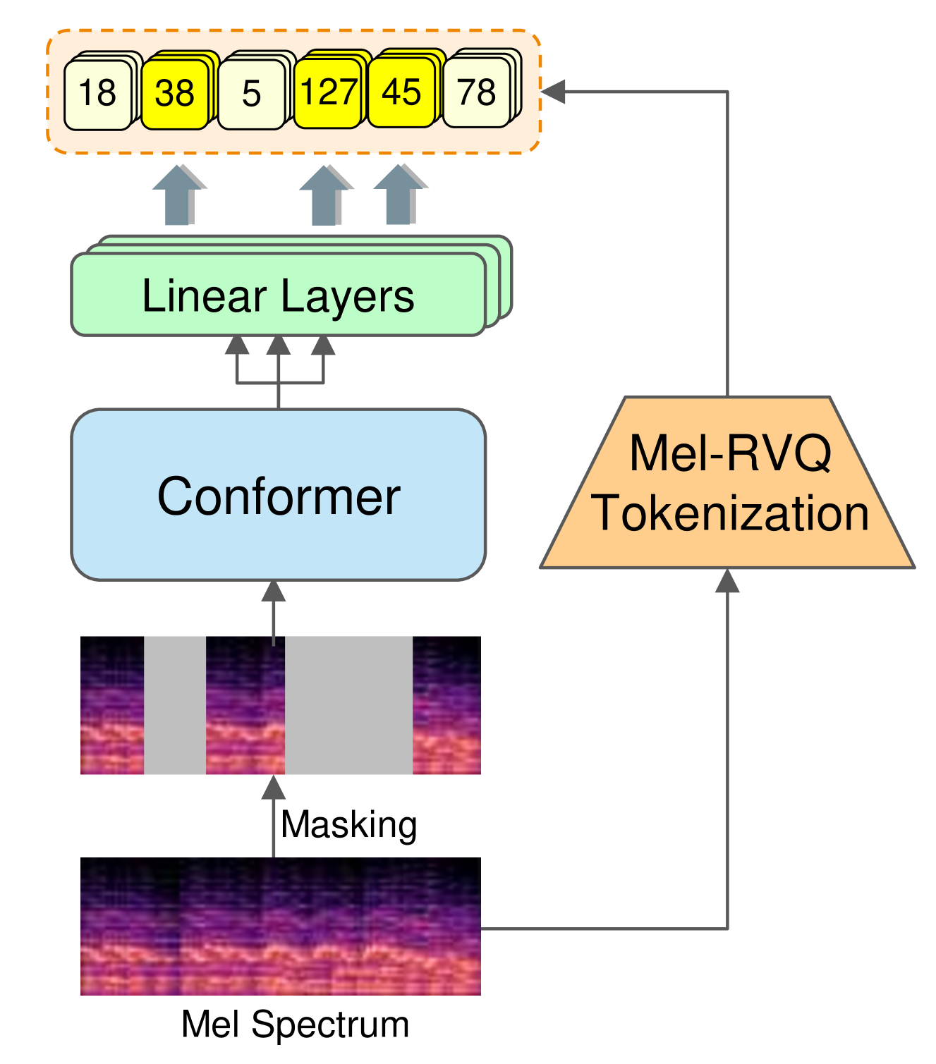
Figure 2: An overview of our proposed MuQ’s framework.
MuQ employs a self-supervised learning approach based on masked language modeling (MLM) and tokenized targets. The overall framework of MuQ is presented in Figure 2.
### Self-Supervised Framework of MuQ
MuQ directly takes the Mel spectrum of the music audio signal as input. The Mel spectrum is partially masked as random noise with a masking probability $p$ , and then fed into multiple layers of Conformer (Gulati et al. 2020) for context learning. The Conformer output is passed through linear layers, which serve as prediction heads. Finally, we calculate the cross-entropy loss between the target and predicted labels as the optimization objective.
The target labels are tokens extracted from the Mel spectrum by the Mel-RVQ, a quantization tokenizer proposed in this paper. Since Mel-RVQ produces $N$ tokens for each time step of the Mel spectrum, the MuQ model incorporates $N$ distinct linear layers to predict the different target tokens. In Figure 2, these multiple linear layers are illustrated as stacked blocks following the Conformer.
### Mel Residual Vector Quantization (Mel-RVQ)
<details>
<summary>x3.png Details</summary>
### Visual Description
## Diagram: Audio Quantization and Reconstruction Models
### Overview
The image presents three technical diagrams illustrating different audio quantization and reconstruction models:
1. **(a) Random-Projection Quantizer**: Focuses on token quantization using random projection and vector quantization (VQ).
2. **(b) Encodec Model**: Depicts waveform processing via convolutional blocks, residual vector quantization (RVQ), and loss functions.
3. **(c) Mel Residual Vector Quantization (Mel-RVQ)**: Shows spectrum prediction, linear decoding, and codebook-based quantization.
### Components/Axes
#### Diagram (a): Random-Projection Quantizer
- **Inputs**:
- `Random init` (initialization tokens).
- `Codebook` (mapping tokens to codebook indices).
- `Projection` (linear transformation of input tokens).
- **Process**:
- `Mel spectrum` (input audio feature) → `Projection` → `Codebook` → `VQ` (vector quantization).
- **Output**:
- `Quantized tokens` (used as SSL targets).
#### Diagram (b): Encodec Model
- **Inputs**:
- `Waveform` (raw audio signal).
- **Process**:
- `Conv block` (convolutional layers) → `Conv1D` (1D convolution) → `RVQ` (residual vector quantization).
- `N groups of quantized tokens` (output of RVQ).
- **Loss Functions**:
- `Reconstruction loss` (error between predicted and original waveform).
- `Discriminator loss` (adversarial loss for quality).
#### Diagram (c): Mel-RVQ
- **Inputs**:
- `Mel spectrum` (mel-frequency cepstral coefficients).
- **Process**:
- `Linear Decoder` (predicts waveform from quantized tokens).
- `RVQ` (residual quantization using codebooks).
- `Projection` (maps tokens to codebook indices).
- **Loss Functions**:
- `Reconstruction loss` (error between predicted and original spectrum).
- `Commitment loss` (enforces consistency between quantized and original tokens).
### Detailed Analysis
#### Diagram (a):
- **Flow**:
- `Random init` tokens are projected into a latent space, mapped to a `Codebook`, and quantized via `VQ`.
- `Mel spectrum` serves as the input feature for this pipeline.
- **Key Elements**:
- `Quantized tokens` are explicitly labeled as SSL (self-supervised learning) targets.
#### Diagram (b):
- **Flow**:
- `Waveform` is processed through stacked `Conv block` and `Conv1D` layers to produce a `Predicted waveform`.
- `RVQ` quantizes residuals into `N groups of quantized tokens`.
- **Losses**:
- `Reconstruction loss` and `Discriminator loss` are combined for training.
#### Diagram (c):
- **Flow**:
- `Predicted spectrum` is decoded via a `Linear Decoder` to reconstruct the waveform.
- `RVQ` quantizes residuals using `Codebooks`, with `Projection` mapping tokens to indices.
- **Losses**:
- `Reconstruction loss` and `Commitment loss` ensure fidelity and consistency.
### Key Observations
1. **Quantization Techniques**:
- All models use quantization (VQ or RVQ) to compress audio data.
- `Mel-RVQ` (c) focuses on spectral features, while (a) and (b) handle raw waveforms.
2. **Loss Functions**:
- (b) combines reconstruction and adversarial losses, suggesting a GAN-like training setup.
- (c) introduces `Commitment loss`, a novel constraint for token consistency.
3. **Codebook Usage**:
- (a) and (c) explicitly use `Codebooks` for token-to-index mapping, while (b) implies residual quantization without explicit codebook labels.
### Interpretation
- **Model Objectives**:
- (a) emphasizes SSL target generation via random projection and VQ.
- (b) balances waveform reconstruction with perceptual quality (via discriminator loss).
- (c) optimizes for spectral accuracy and token consistency (via commitment loss).
- **Technical Trade-offs**:
- `Random-Projection Quantizer` (a) prioritizes simplicity and SSL applicability.
- `Encodec Model` (b) uses convolutional layers for hierarchical feature extraction.
- `Mel-RVQ` (c) targets efficient spectral representation with residual quantization.
- **Applications**:
- These models likely serve speech/audio compression, enhancement, or generative tasks (e.g., text-to-speech).
- The inclusion of SSL targets in (a) suggests unsupervised learning applications.
### Limitations
- No numerical values or quantitative metrics are provided (e.g., loss magnitudes, compression ratios).
- The role of `N groups of quantized tokens` (b, c) is abstract without context on grouping criteria.
</details>
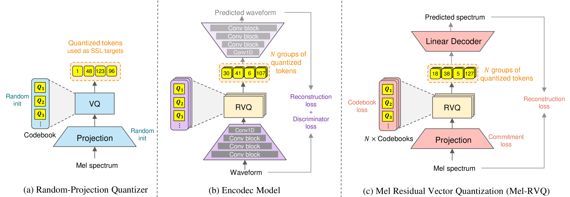
Figure 3: Comparison between (a) random-projection quantizer, (b)Encodec, and (c) proposed Mel Residual Vector Quantization (Mel-RVQ). Mel-RVQ draws on the lightweight structure of the random-projection quantizer, i.e., it uses only a single linear projection as the encoder, with the Mel spectrum as input. Also, Mel-RVQ borrows the proven effective residual structure from Encodec, but Mel-RVQ further benefits from a much simpler structure than the multiple convolutional layers in Encodec.
As shown in Figure 3, we depict the proposed Mel Residual Vector Quantization (Mel-RVQ) compared with the random-projection quantizer in BEST-RQ and the Encodec target used by MERT.
The proposed Mel-RVQ directly takes the Mel spectrum as input and then quantizes the Mel spectrum using residual vector quantization (RVQ). The encoder of Mel-RVQ is designed as a simple single-layer linear projection, and the decoder is also a single linear layer.
Mel-RVQ needs to be trained on music data in advance before it can be used to generate quantization targets in SSL training.
#### Training of Mel-RVQ
During the training of Mel-RVQ, the final loss function can be decomposed into three terms, as shown in Figure 3 (c) :
- Codebook loss trains the RVQ component to improve the fit of the codebook embedding $Q_τ$ to the dimensionality-reduced features $z$ . Formally,
$$
loss_code=∑_\begin{subarray{c}x∈ B,\\
z=M_Px\end{subarray}}{\|norm(Q_τ)-norm(
sg(z))\|^2} \tag{1}
$$
where $B$ refers to a mini-batch of data, $x$ denotes Mel spectrum input and $sg$ denotes stop-gradient. $M_P$ is the projection matrix and token $τ$ is the closest to the projected vector $z$ in the $l_2$ -normalized embedding space.
- Commitment loss trains the projection (i.e. encoder) for more optimal dimension reduction and fitting to embeddings. Expressed as
$$
loss_comm=∑_\begin{subarray{c}x∈ B,\\
z=M_Px\end{subarray}}{\|norm(z)-norm(sg(
Q_τ))\|^2} \tag{2}
$$
- Reconstruction loss trains the linear decoder (denoted as $M_D$ ) and the codebook to restore the original feature $x$ . The formula is
$$
loss_recon=∑_x∈ B{\|M_DQ_τ-x\|^2} \tag{3}
$$
The final loss used to train the Mel-RVQ is the weighted sum of the above three losses:
$$
loss=α· loss_code+β· loss_comm+loss_
recon \tag{4}
$$
where $α$ and $β$ are weighting factors, set as $α=1,β=0.25$ .
It is emphasized that both $M_D$ and $M_P$ used in Eq.(4) are simple linear layers, which distinguishes them from those in neural codecs like Encodec (Défossez et al. 2022).
#### Residual modeling of Mel-RVQ
Applying the residual modeling method to Mel-RVQ means that it yields multiple tokens for each time step of the audio. Assume there are $N$ codebooks in total, denoted as $\{Q_i^(n)\}_i=1^K$ for $n∈ 1… N$ . In this way, we have
$$
\displaystyle z^(n) \displaystyle=M_P^(n)r^(n-1) \displaystyleτ^(n) \displaystyle={\arg\min_i\|norm(z^(n))-norm(Q^(n)_i)\|} \displaystyle r^(n) \displaystyle=r^(n-1)-M_D^(n)Q^(n)_τ^(n) \tag{5}
$$
where $n∈ 1… N$ ; $r^(n)$ is the residual signal passed to next step in quantizer and $r^(1)=x$ . $M_P^(n)$ and $M_D^(n)$ denote the residual-projection matrices for the encoder and decoder, which contain multiple steps of projection. The superscript $(n)$ denotes the components or features corresponding to the quantizer at step $n$ .
#### Iterative refinement with RVQ
Iterative refinement is introduced in HuBERT (Hsu et al. 2021) as a method to improve the performance of SSL models, where clustering techniques like K-means are employed to produce new labels for the next iteration of training.
We suggest that residual vector quantization (RVQ) itself can serve as an alternative to the clustering in iterative enhancement. That is, we directly train a Mel-RVQ iter on the latent representations of an already trained MuQ model, to re-drive the training of MuQ at next iteration.
Specifically, the iterative training on MuQ has two stages:
- In the initial stage, a Mel-RVQ is trained on the Mel spectrum feature, and then the first version of MuQ is trained on the tokens produced by Mel-RVQ.
- In the iterative stage, the first version of MuQ is used to extract representation from the audio, and the $l$ th layer latent is used to train Mel-RVQ iter, which will be used in training the second version of MuQ, namely MuQ iter.
### Music-Text Contrastive Learning
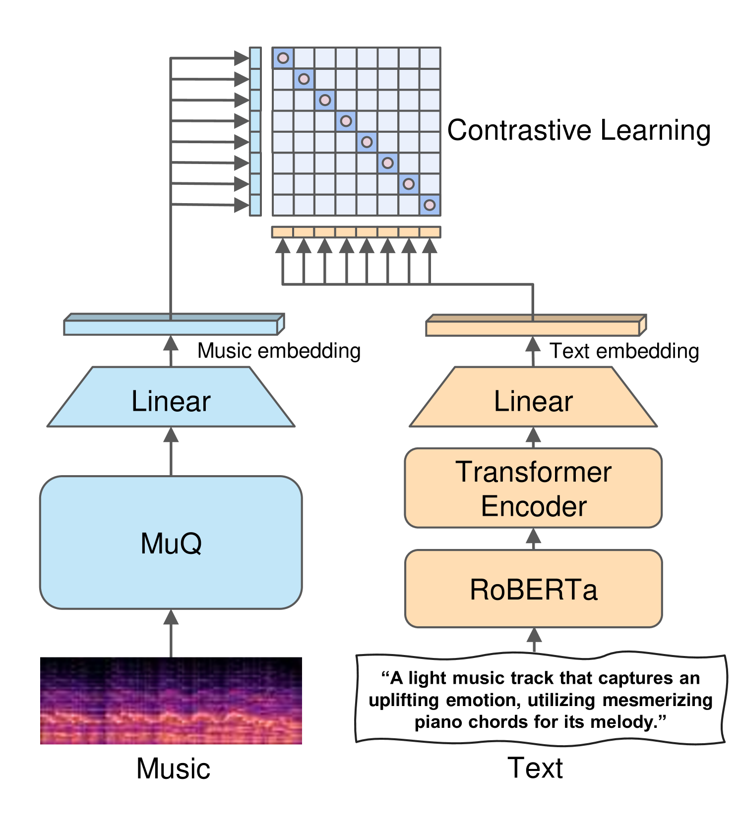
To verify the effectiveness of MuQ in more sophisticated downstream tasks, we trained a music-text joint embedding model, MuQ-MuLan. Similar to MuLan (Huang et al. 2022), MuQ-MuLan employs a two-tower multimodal architecture and is trained on a large amount of (music, text) paired data.
MuQ-MuLan consists of a music encoder and a text encoder. During training, the music and the corresponding text are fed to the encoders separately, where the text is a description of the music track, as shown in Figure 4.
For music modality inputs, a MuQ model with pre-trained parameters is first used to encode the audio into a latent representation. This representation is then average-pooled over the temporal dimension. Finally, it passes through a linear projection layer to produce a music embedding $e_m$ with dimension $d$ .
For text modality inputs, they are encoded by a pre-trained RoBERTa (Liu et al. 2019) model. As described in a previous study (Vasilakis, Bittner, and Pauwels 2024), the text encoder is critical to the performance of the two-tower model, so we append a few additional layers of Transformer encoder after RoBERTa. Likewise, the textual latent representations are average-pooled and passed through a linear projection layer to get text embedding $e_t$ with the same dimension $d$ .
We use decoupled contrastive learning (DCL) loss (Yeh et al. 2022). Formally, given the $i$ -th (music, text) pair in a mini-batch, for the embeddings $(e_m^(i),e_t^(i))$ , we have
$$
L_DCL=-log∑_(i,j)\frac{sim(e_m^(
i),e_t^(j))/σ}{∑_i≠ jsim(e_m^(
i),e_t^(j))/σ} \tag{6}
$$
where $sim$ denotes dot-product similarity, and $σ$ is temperature coefficient.
<details>
<summary>x4.png Details</summary>
### Visual Description
## Diagram: Contrastive Learning System for Music-Text Embeddings
### Overview
The diagram illustrates a contrastive learning framework that aligns embeddings from music and text modalities. It shows two parallel processing pipelines (music and text) converging into a contrastive learning module, represented by a grid of interconnected nodes.
### Components/Axes
1. **Music Pipeline**:
- **Input**: Music (represented as a spectrogram with purple-to-red gradients).
- **MuQ**: A dedicated music encoder (blue box).
- **Linear Layer**: Transforms MuQ output into a music embedding (blue arrow).
2. **Text Pipeline**:
- **Input**: Text example:
> “A light music track that captures an uplifting emotion, utilizing mesmerizing piano chords for its melody.”
- **RoBERTa**: A text encoder (orange box).
- **Transformer Encoder**: Processes RoBERTa output (orange box).
- **Linear Layer**: Transforms text encoder output into a text embedding (orange arrow).
3. **Contrastive Learning Module**:
- **Grid of Nodes**: Represents alignment/comparison of music and text embeddings (blue squares with pink dots).
- **Arrows**: Indicate directional flow between embeddings and the grid.
### Detailed Analysis
- **Music Embedding**: Derived from raw audio via MuQ and a linear layer.
- **Text Embedding**: Generated through RoBERTa, a transformer encoder, and a linear layer.
- **Contrastive Learning**: The grid symbolizes a mechanism to minimize distance between semantically related music-text pairs while maximizing separation for unrelated pairs.
### Key Observations
- **Modality-Specific Encoders**: MuQ (music) and RoBERTa (text) are domain-specific encoders.
- **Alignment Objective**: The contrastive learning grid suggests a Siamese network architecture for joint embedding space optimization.
- **Example Text**: The provided text emphasizes emotional and melodic attributes, likely used as a training example for text-music alignment.
### Interpretation
This system aims to bridge the semantic gap between music and text by learning shared representations. The contrastive learning module implies a self-supervised approach where the model learns to associate text descriptions (e.g., "uplifting emotion") with corresponding musical features (e.g., piano chords). The use of RoBERTa and MuQ highlights the integration of pre-trained models for efficient feature extraction. The diagram does not include numerical data but emphasizes architectural design for cross-modal tasks like music captioning or emotion recognition.
</details>
Figure 4: Overall architecture of MuQ-MuLan, a music-text joint embedding model trained with contrastive learning.
## Experiments Setup
### Model Settings
#### MuQ
We stack 12 layers of Conformer in MuQ, with 310M parameters in total. The number of codebooks for Mel-RVQ is set to $N=8$ and the codebook size is $K=1024$ . The input audio is fixed at 30 seconds with a sampling rate of 24K Hz. Audio inputs are 128-dimensional Mel spectrum, which are pooled to 25Hz before feeding to Conformer. The code is implemented with the Fairseq toolkit (Ott et al. 2019).
#### MuQ-MuLan
We use the pre-trained MuQ as the initialization for the music encoder. A pre-trained multilingual RoBERTa model xlm-roberta-base is used for the text encoder followed by 8 layers of Transformer, with the embedding dimension $d=512$ . MuQ-MuLan has 630M parameters in total, and all parameters stay unfrozen during the contrastive training.
### Pre-training
#### Dataset
We initially conduct pre-training on a smaller dataset, Music4all (Santana et al. 2020), containing 0.9K hours of open access music data. Subsequently, we scale up to a large-scale in-house dataset with 160K hours of music.
#### Training Details
Mel-RVQ is trained on the Music4all dataset using 1 GPU. Since the Mel-RVQ is very small (less than 0.3M), the training of Mel-RVQ is extremely fast and it takes less than 1 hour to complete.
All pre-training experiments are running with 32 A100-40G GPUs. Batch size is 192, and masking probability $p=0.6$ . For the pre-training on the Music4all dataset, we train for only 75K steps. For the experiments on the 160K hours of in-house data, we initially train MuQ for 200K steps. Subsequently, the $l=10$ th layer latent is used to train $Mel-RVQ_iter$ , followed by 150K steps of iterative training from scratch to obtain $MuQ_iter$ . The entire initial & iterative pre-training takes about 2 weeks.
### Contrastive Training
#### Dataset
The training data for contrast learning comes from 130K hours of music in-house, each with its corresponding text description. The text descriptions are limited to non-personal information such as genre, mood, instrument, tempo, keywords of the music.
#### Training Details
MuQ-Mulan is trained on 32 V100-32G GPUs with a batch size of 768. Following the practice of MuLan (Huang et al. 2022), we switch to taking 10 seconds as the length of the input audio. This significantly reduces memory consumption and enlarges batch size, which is critical for contrastive learning.
Table 1: Evaluation of proposed MuQ model in MARBLE benchmark (1/2). $MuQ_m4a$ denotes MuQ model pre-trained on Music4all, a relatively low resource dataset with 900 hours of music. $MuQ_iter$ denotes MuQ model using iterative refinement training. * indicates that the number is brought from the original paper.
| MERT MusicFM MuQ m4a | 78.6 * 83.8 84.0 $± 0.3$ | 65.6 * 63.9 63.7 $± 0.4$ | 61.2 * 60.3 60.0 $± 0.1$ | 74.7 * 76.3 76.0 $± 0.1$ | 87.1 * 92.0 95.2 $± 0.1$ | 76.9 * 78.4 80.8 $± 0.3$ | 75.7 76.5 76.4 $± 0.1$ | |
| --- | --- | --- | --- | --- | --- | --- | --- | --- |
| MuQ | 85.5 $± 0.9$ | 63.5 $± 0.7$ | 60.9 $± 0.2$ | 75.4 $± 0.2$ | 95.8 $± 0.1$ | 82.4 $± 0.3$ | 76.5 $± 0.1$ | |
| MuQ iter | 85.6 $± 0.7$ | 65.0 $± 0.8$ | 62.8 $± 0.1$ | 76.1 $± 0.1$ | 96.2 $± 0.1$ | 81.6 $± 0.1$ | 77.2 $± 0.1$ | |
Table 2: Evaluation of proposed MuQ model in MARBLE benchmark (2/2). Avg. denotes the average score calculated across the metrics of all tasks. Pretrain dataset identifies the source and size of the dataset for the pre-training stage of each model.
| MERT | 91.3 * | 40.2 * | 72.6 * | 94.4 * | 74.4 | - | 160K |
| --- | --- | --- | --- | --- | --- | --- | --- |
| MusicFM | 91.3 | 40.0 | 76.2 | 91.1 | 75.4 | MSD | - |
| MuQ m4a | 91.1 $± 0.0$ | 39.0 $± 0.1$ | 76.9 $± 0.2$ | 91.2 $± 0.1$ | 75.8 | Music4all | 0.9K |
| MuQ | 91.4 $± 0.0$ | 40.3 $± 0.1$ | 79.2 $± 0.1$ | 92.3 $± 0.2$ | 76.7 | In-house | 160K |
| MuQ iter | 91.4 $± 0.0$ | 40.1 $± 0.1$ | 79.7 $± 0.2$ | 91.3 $± 0.1$ | 77.0 | In-house | 160K |
### Downstream Tasks
We evaluate MuQ on the MARBLE benchmark (Yuan et al. 2023) and conduct experiments on a total of 9 downstream tasks. Note that all datasets appearing in the downstream tasks are not included in the pre-training data of MuQ.
Due to page limitations, we only provide a brief overview of the downstream tasks here. We encourage readers to refer to the Appendix I for details on these tasks.
- Genre classification aims to determine the most suitable genre for a song. We use the GTZAN dataset (Tzanetakis and Cook 2002) and report the accuracy scores.
- Key detection predicts the tonal scale and dominant pitch level. We use the Giantsteps dataset (Knees et al. 2015), and a refined accuracy metric (Raffel et al. 2014).
- Emotional analysis is taken on the Emomusic dataset (Soleymani et al. 2013). The metrics are determination coefficients for valence ( $R2^V$ ) and arousal ( $R2^A$ ) score.
- Singer identification on the VocalSet (Wilkins et al. 2018) dataset. The evaluation metric is accuracy.
- Vocal technique detection on the VocalSet (Wilkins et al. 2018). The evaluation metric is accuracy.
- Music tagging involves multi-label classification of 50 tags on the MagnaTagATune (Law et al. 2009b) dataset. The metrics are ROC-AUC and average precision (AP).
- Music structure analysis predicts the functional label for music segments on the Harmonix dataset (Nieto et al. 2019). The evaluation metric is accuracy.
- Instrument classification on the Nsynth dataset (Engel et al. 2017). The evaluation metric is accuracy.
- Pitch classification of the 128-pitch on the Nsynth dataset (Engel et al. 2017). The metric is accuracy.
In evaluating the pre-trained MuQ, we extract features from each layer and use a linear probe to perform downstream tasks. For the MuQ-MuLan experiments, we use a zero-shot approach for music tagging. This involves directly calculating the similarity between music and text embeddings to determine the prediction probability for each tag.
## Results and Analysis
### Performance of Pre-trained MuQ
We compare MuQ with two popular models, MERT and MusicFM. For MERT, we use MERT-v1-330M version (Li et al. 2023), the most superior of its releases on HuggingFace. For MusicFM, we use the checkpoint pre-trained on the MSD dataset (Bertin-Mahieux et al. 2011), which is publicly available by (Won, Hung, and Le 2023). All models are of around 330M parameters.
Table 1 and Table 2 present the results for three versions of MuQ. Considering the experiments are very extensive and time-consuming, we conduct 5 runs for MuQ models and report the mean scores and standard deviations for all tasks.
It is shown that for MuQ m4a, pre-trained on the 0.9K-hour Music4All dataset, already outperforms MERT and MusicFM. Training MuQ on a larger dataset further amplifies this advantage. Iterative training slightly improves the effectiveness of MuQ, resulting in MuQ iter with an average score of 77.0, which is our best-performing model.
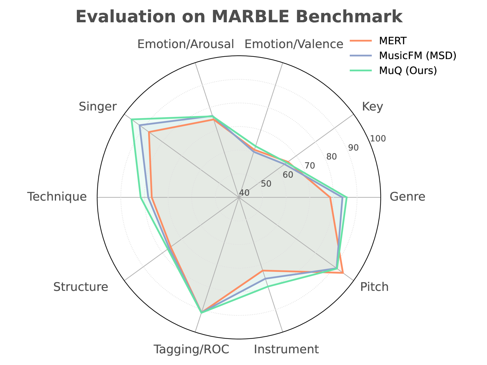
MuQ outperforms previous models on many downstream tasks, especially in genre classification, singer identification, vocal technique detection, music structure analysis and instrument classification. We visualize the result of MuQ in Figure 5.
<details>
<summary>x5.png Details</summary>
### Visual Description
## Radar Chart: Evaluation on MARBLE Benchmark
### Overview
The radar chart compares the performance of three models (MERT, MusicFM [MSD], and MuQ [Ours]) across seven evaluation dimensions on the MARBLE benchmark. The chart uses a circular layout with axes representing evaluation categories and radial distance indicating performance scores (0–100). Three colored lines represent the models, with MuQ (green) consistently outperforming others in specific categories.
### Components/Axes
- **Axes (Categories)**:
1. Emotion/Arousal
2. Emotion/Valence
3. Key
4. Genre
5. Pitch
6. Instrument
7. Tagging/ROC
- **Legend**:
- MERT (orange)
- MusicFM (MSD) (blue)
- MuQ (Ours) (green)
- **Axis Markers**:
- Radial scale from 0 to 100 (increments of 10).
- Axial labels positioned clockwise around the perimeter.
### Detailed Analysis
- **MERT (orange line)**:
- Peaks at **Tagging/ROC (90)** and **Pitch (85)**.
- Lowest in **Emotion/Valence (60)**.
- Moderate performance in **Genre (70)** and **Instrument (75)**.
- **MusicFM (MSD) (blue line)**:
- Highest in **Singer (85)**.
- Lowest in **Emotion/Valence (65)**.
- Strong in **Genre (80)** and **Pitch (85)**.
- **MuQ (Ours) (green line)**:
- Dominates **Tagging/ROC (95)** and **Singer (90)**.
- Slight dip in **Emotion/Valence (70)**.
- Strong in **Genre (85)** and **Instrument (80)**.
### Key Observations
1. **MuQ (Ours)** achieves the highest scores in **Tagging/ROC (95)** and **Singer (90)**, suggesting superior performance in these categories.
2. **MERT** excels in **Tagging/ROC (90)** but struggles with **Emotion/Valence (60)**.
3. **MusicFM (MSD)** performs best in **Singer (85)** but has notable weaknesses in **Emotion/Valence (65)** and **Instrument (70)**.
4. All models show variability in **Emotion/Arousal** (MERT: 75, MusicFM: 70, MuQ: 80), indicating inconsistent emotional analysis.
### Interpretation
The chart highlights **MuQ (Ours)** as the most robust model overall, particularly in **Tagging/ROC** and **Singer**, where it outperforms others by margins of 5–15 points. **MERT** demonstrates balanced but suboptimal performance, while **MusicFM (MSD)** excels in singer-related tasks but falters in emotional valence and instrument recognition. The disparity in **Emotion/Valence** scores across models suggests a critical area for improvement in affective computing applications.
The data implies that model selection should prioritize **MuQ** for tasks requiring tagging or singer identification, while **MusicFM** may be preferable for genre/pitch analysis despite its emotional valence limitations.
</details>
Figure 5: Visualization of radar plot on MARBLE benchmark.
### Ablation Study on Mel-RVQ
Table 3: Ablation study of different components in Mel-RVQ. All models are pre-trained on the Music4all dataset.
| | | | Genre | Key | Emotion | Singer | Tech | | |
| --- | --- | --- | --- | --- | --- | --- | --- | --- | --- |
| Model codebase | VQ type | Residual | Acc $↑$ | Acc Refined $↑$ | R2 V $↑$ | R2 A $↑$ | Acc $↑$ | Acc $↑$ | Average |
| Random | 2717 | 77.9 | 62.8 | 56.4 | 71.8 | 95.5 | 76.3 | 73.5 | |
| MusicFM | Trained | 2717 | 80.0 | 65.8 | 56.3 | 74.6 | 95.3 | 78.5 | 75.1 |
| Random | 1F5F8 | 77.6 | 62.1 | 56.5 | 74.1 | 95.7 | 76.5 | 73.8 | |
| MuQ | Trained | 1F5F8 | 84.0 | 63.7 | 60.0 | 76.0 | 95.2 | 80.8 | 76.6 |
We carry out an ablation study for Mel-RVQ in Table 3 to demonstrate the effect of its key components. In the ablation experiments, all models are pre-trained 75K steps on the Music4all with 310M parameters, and tested on 5 tasks.
The VQ type in Table 3 indicates whether the VQ is randomly initialized or trained on music data, and Residual indicates whether residual multiple codebooks are used. As shown, it’s crucial to train the VQ rather than leaving it random, as this boosts the performance of MusicFM and MuQ by 1.6 and 2.8, respectively. Also, the residual structure of Mel-RVQ is beneficial and allows MuQ to gain a significant advantage over MusicFM.
### Ablation Study on Music SSL Target
Table 4: Ablation study of target strategy. All models are pre-trained on Music4all dataset.
| Mel-RVQ Mel-RVQ Mel-RVQ | 1 4 8 | 82.8 78.3 83.4 | 45.9 65.1 65.8 | 55.3 59.0 59.7 | 74.6 73.7 76.2 | 93.7 95.2 95.7 | 75.4 79.5 80.1 | 71.3 75.1 76.8 |
| --- | --- | --- | --- | --- | --- | --- | --- | --- |
| Mel-RVQ (deeper) | 8 | 81.7 | 64.4 | 55.9 | 72.3 | 95.5 | 80.4 | 75.0 |
| Encodec | 8 | 82.4 | 65.3 | 57.1 | 74.1 | 95.2 | 77.9 | 75.3 |
We ablate the number of target tokens and tokenization SSL training, this involves some hyperparameters of Mel-RVQ, as well as a comparison with Encodec target.
As seen in Table 4, performance gradually improves as the number of codebooks increases. We believe this is because more codebooks allow the model to capture fine-grained audio features more effectively. This also implies the advantage of multi-target learning for SSL pre-training.
We also explore the depth of the Mel-RVQ encoder and decoder by scaling up the linear projection to a 3-layer fully connected network, referred to as Mel-RVQ (deeper) in Table 4. However, the results suggest that increasing the depth of the Mel-RVQ network actually degrades performance. This indicates that a single layer of linear projection is sufficient for Mel-RVQ to achieve optimal performance.
Finally, we compare Mel-RVQ with the Encodec target. It can be seen in Table 4 that Mel-RVQ, despite being a very lightweight structure, outperforms the Encodec tokenization target. We attribute this to the fact that the token produced by Encodec is a high abstraction of the music audio, which leads to it being more difficult for the model to learn.
### Performance of MuQ-MuLan
In Table 5 , we compare MuQ-MuLan with LAION-CLAP (Wu et al. 2023), Microsoft-CLAP 2023 (Elizalde, Deshmukh, and Wang 2023) and MuLan (Huang et al. 2022). We use the open-source larger_clap_music_and_speech version for LAION-CLAP, which is the best-performing checkpoint among its releases in our experiments. We also introduce two variants that employ MERT or MusicFM as the music encoder and refer to them as MERT-MuLan and MusicFM-MuLan.
Following previous study (Vasilakis, Bittner, and Pauwels 2024), we choose the proven superior MusCALL prompt: “A <label> track” for all models to test in our experiments.
Table 5: Experiment on the MagnaTagATune zero-shot music tagging task. Since MuLan is a closed source, the results of MuLan are taken from the paper (Huang et al. 2022).
| Model | Data (hours) | Metrics | |
| --- | --- | --- | --- |
| ROC-AUC $↑$ | PR-AUC $↑$ | | |
| LAION-CLAP | 4K | 73.9 | 25.0 |
| Microsoft-CLAP 2023 | - | 75.9 | 28.9 |
| MuLan | 370K | 78.2 * | - |
| MERT-MuLan | 130K | 75.5 | 24.6 |
| MusicFM-MuLan | 130K | 76.2 | 27.1 |
| MuQ-MuLan | 130K | 79.3 | 29.3 |
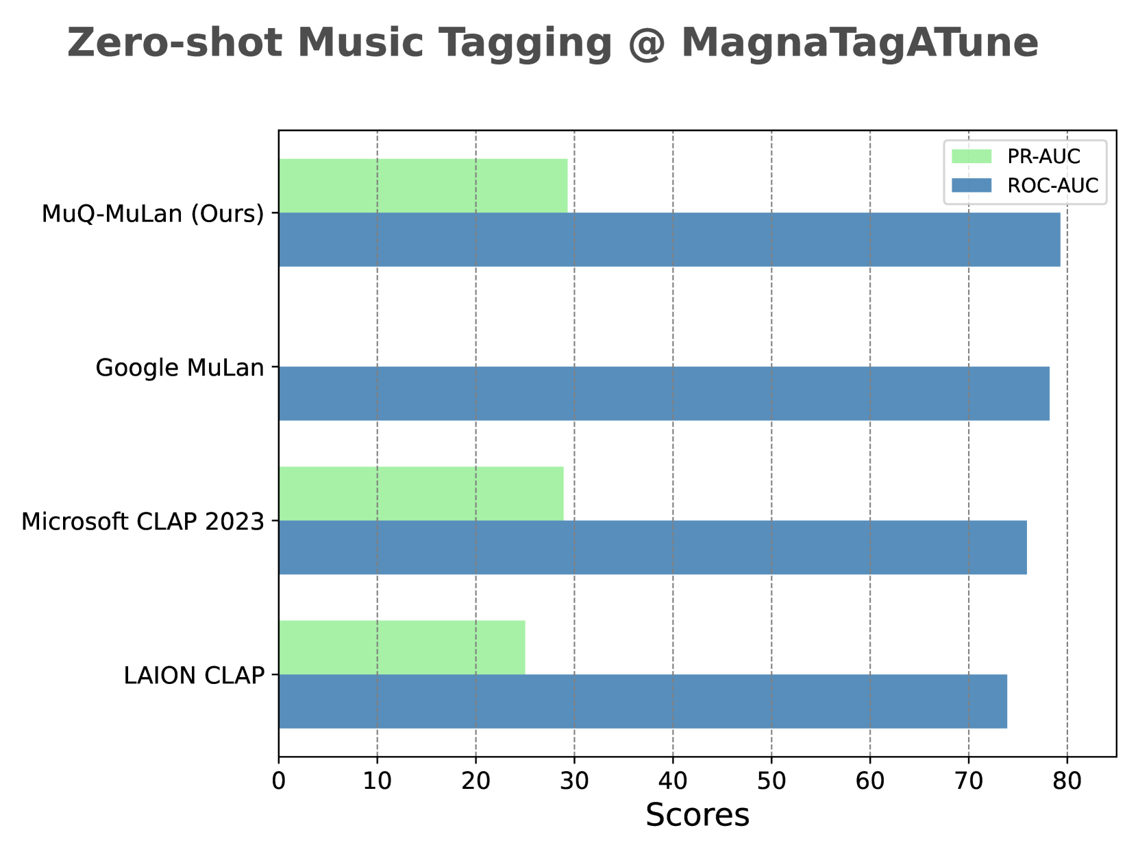
MuQ-MuLan outperforms previous models in both ROC-AUC and PR-AUC and reaches the SOTA in the zero-shot setting. Impressively, MuQ-MuLan still has a slight advantage over MuLan despite the gap in data amounts.
Although both use the same contrastive learning setup, MuQ-MuLan outperforms MERT-MuLan. Furthermore, even though MuQ and MusicFM have identical model structures, MuQ-MuLan still performs better. This suggests that MuQ provides a better initialization for contrastive training.
We visualize the performance of MuQ-MuLan in Figure 6, and plot the comparision with LAION-CLAP (Wu et al. 2023), Microsoft-CLAP 2023 (Elizalde, Deshmukh, and Wang 2023) and MuLan (Huang et al. 2022).
<details>
<summary>x6.png Details</summary>
### Visual Description
## Bar Chart: Zero-shot Music Tagging @ MagnaTagATune
### Overview
The chart compares zero-shot music tagging performance across four models using PR-AUC (Precision-Recall Area Under the Curve) and ROC-AUC (Receiver Operating Characteristic Area Under the Curve) metrics. Models are ranked by their ROC-AUC scores, with MuQ-MuLan (Ours) achieving the highest performance.
### Components/Axes
- **X-axis**: "Scores" (0–80 range, labeled in increments of 10)
- **Y-axis**: Model names (left-aligned, descending order):
1. MuQ-MuLan (Ours)
2. Google MuLan
3. Microsoft CLAP 2023
4. LAION CLAP
- **Legend**:
- Green: PR-AUC
- Blue: ROC-AUC
- **Bars**: Horizontal bars with distinct colors for PR-AUC (green) and ROC-AUC (blue). All bars extend rightward from the y-axis.
### Detailed Analysis
1. **MuQ-MuLan (Ours)**:
- PR-AUC: ~28 (green bar)
- ROC-AUC: ~80 (blue bar)
2. **Google MuLan**:
- PR-AUC: ~26 (green bar)
- ROC-AUC: ~78 (blue bar)
3. **Microsoft CLAP 2023**:
- PR-AUC: ~28 (green bar)
- ROC-AUC: ~76 (blue bar)
4. **LAION CLAP**:
- PR-AUC: ~24 (green bar)
- ROC-AUC: ~74 (blue bar)
### Key Observations
- **ROC-AUC Dominance**: All models show significantly higher ROC-AUC than PR-AUC, with differences ranging from 46 (LAION CLAP) to 52 (MuQ-MuLan).
- **MuQ-MuLan Superiority**: Outperforms others in both metrics, with ROC-AUC ~80 (highest) and PR-AUC ~28 (tied with Microsoft CLAP 2023).
- **Google MuLan vs. Microsoft CLAP 2023**: Google MuLan has slightly better ROC-AUC (78 vs. 76) but identical PR-AUC (26 vs. 28) to Microsoft CLAP 2023.
- **LAION CLAP**: Lowest performance in both metrics (~24 PR-AUC, ~74 ROC-AUC).
### Interpretation
The chart demonstrates that MuQ-MuLan achieves state-of-the-art zero-shot music tagging performance, with ROC-AUC scores consistently exceeding 74 across all models. The persistent gap between ROC-AUC and PR-AUC suggests that while models effectively rank relevant tags (ROC-AUC), precise retrieval of exact tags (PR-AUC) remains a challenge. MuQ-MuLan's dual leadership in both metrics indicates superior tagging robustness compared to existing solutions like Google MuLan and Microsoft CLAP 2023. The absence of error bars implies these are point estimates, and the lack of gridlines makes exact value verification challenging.
</details>
Figure 6: Visualization on zero-shot music tagging task in MagnaTagATune dataset.
### Layer-wise Analysis
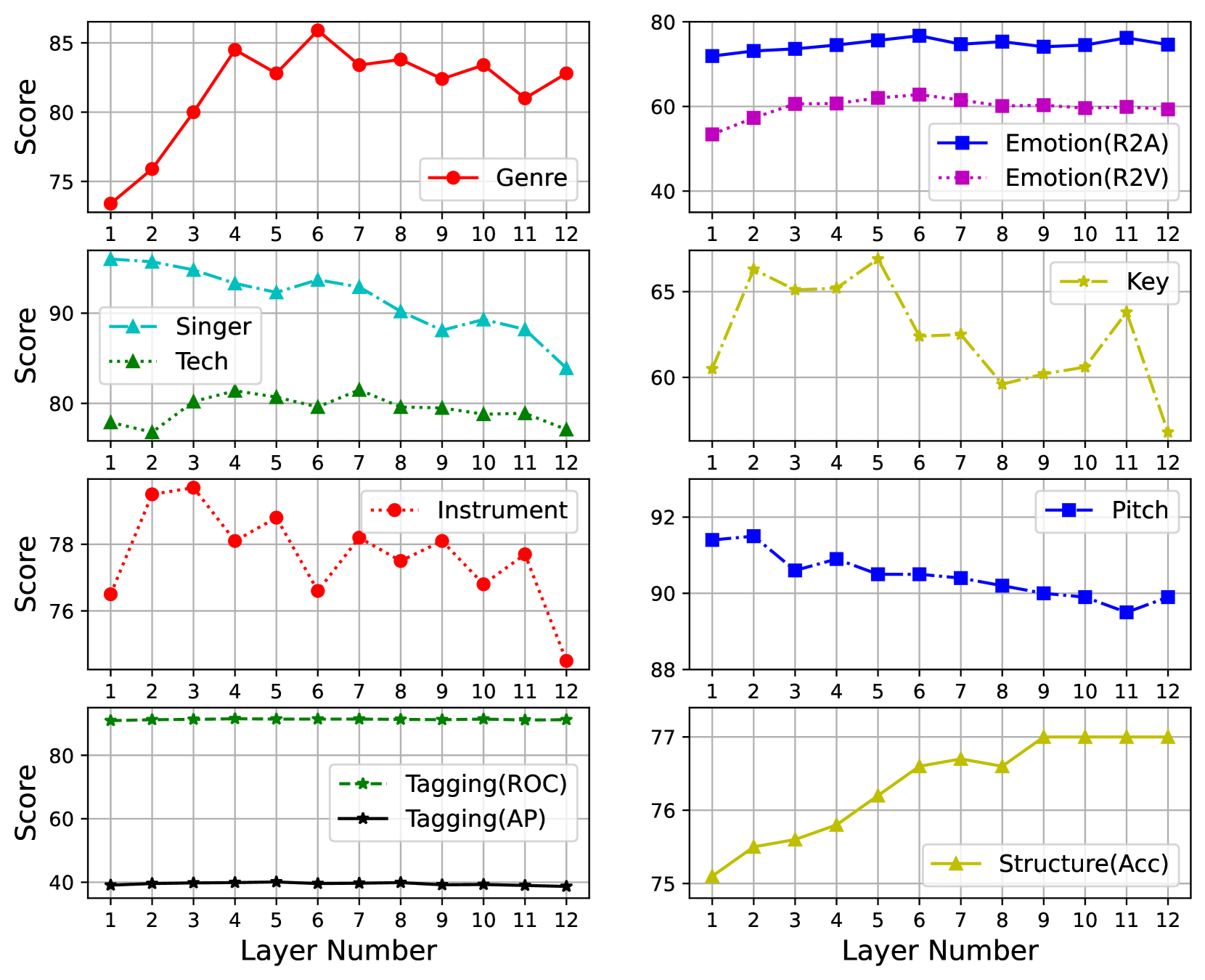
In Figure 7, we visualize the results of each layer’s features in various downstream tasks during one run of the MuQ model. The analysis can be summarized as follows:
- Semantic tasks, such as genre classification and structure analysis, generally achieve the best results at the higher layers. They focus more on semantic information such as the direction of the music and the overall style.
- Acoustic tasks, such as singer identification, instrument classification, pitch classification, and key detection, perform best at the lower layers. This implies that they are more closely associated with low-level characteristics such as the original audio features.
- Comprehensive tasks, such as music tagging, emotional analysis, and vocal tech classification, have a relatively even distribution across all layers. This suggests that they rely on various aspects.
<details>
<summary>x7.png Details</summary>
### Visual Description
## Line Charts: Multi-Series Performance Analysis
### Overview
The image contains two sets of three-line charts comparing performance metrics across 12 layers. Left side charts focus on musical elements (Genre, Singer/Tech, Instrument), while right side charts analyze emotional and structural aspects (Emotion, Key, Pitch, Structure). All charts use layer numbers (1-12) on the x-axis and score values on the y-axis.
### Components/Axes
**Left Charts:**
1. **Genre** (Red circles)
- X-axis: Layer Number (1-12)
- Y-axis: Score (75-85)
- Legend: Red = Genre
2. **Singer/Tech** (Cyan triangles + Green dashed)
- X-axis: Layer Number (1-12)
- Y-axis: Score (75-92)
- Legend: Cyan = Singer, Green = Tech
3. **Instrument** (Red dotted)
- X-axis: Layer Number (1-12)
- Y-axis: Score (75-79)
- Legend: Red = Instrument
**Right Charts:**
1. **Emotion (R2A/R2V)** (Blue squares + Magenta squares)
- X-axis: Layer Number (1-12)
- Y-axis: Score (40-80)
- Legend: Blue = R2A, Magenta = R2V
2. **Key** (Yellow stars)
- X-axis: Layer Number (1-12)
- Y-axis: Score (55-67)
- Legend: Yellow = Key
3. **Pitch** (Blue squares)
- X-axis: Layer Number (1-12)
- Y-axis: Score (88-92)
- Legend: Blue = Pitch
4. **Structure (Acc)** (Yellow triangles)
- X-axis: Layer Number (1-12)
- Y-axis: Score (75-78)
- Legend: Yellow = Structure
5. **Tagging (ROC/AP)** (Green stars + Black stars)
- X-axis: Layer Number (1-12)
- Y-axis: Score (39-82)
- Legend: Green = ROC, Black = AP
### Detailed Analysis
**Left Charts:**
1. **Genre** (Red circles)
- Scores: 74, 76, 80, 84, 83, 85, 83, 84, 82, 83, 81, 83
- Trend: Initial rise to peak at Layer 6 (85), then gradual decline with minor fluctuations
2. **Singer/Tech** (Cyan/Green)
- Singer: 92, 91, 90, 89, 88, 87, 86, 85, 84, 83, 82, 80
- Tech: 78, 77, 80, 81, 80, 81, 80, 81, 80, 79, 78, 77
- Trend: Singer shows steady decline; Tech fluctuates around 80
3. **Instrument** (Red dotted)
- Scores: 76, 78, 79, 78, 77, 76, 77, 78, 77, 76, 75, 74
- Trend: Minor fluctuations with overall slight decline
**Right Charts:**
1. **Emotion (R2A/R2V)**
- R2A: 78, 79, 79, 80, 80, 80, 79, 78, 77, 76, 75, 74
- R2V: 55, 57, 60, 61, 62, 62, 61, 60, 59, 58, 57, 56
- Trend: R2A stable decline; R2V gradual rise then decline
2. **Key** (Yellow stars)
- Scores: 60, 66, 65, 65, 67, 65, 64, 63, 62, 63, 66, 55
- Trend: Initial rise to Layer 5 peak (67), then sharp drop at Layer 12
3. **Pitch** (Blue squares)
- Scores: 91, 91, 90, 91, 90, 90, 90, 89, 88, 87, 86, 88
- Trend: Stable with minor fluctuations, slight dip at Layer 11
4. **Structure (Acc)** (Yellow triangles)
- Scores: 75, 76, 76, 76, 77, 77, 78, 78, 78, 78, 78, 78
- Trend: Gradual rise to plateau at Layer 9
5. **Tagging (ROC/AP)**
- ROC: Flat at 82 across all layers
- AP: Flat at 40 across all layers
### Key Observations
1. Genre shows highest variability with peak at Layer 6
2. Singer scores decline consistently while Tech remains stable
3. Instrument scores show minor fluctuations around 76-79
4. Emotion R2A maintains higher scores than R2V throughout
5. Key metric shows dramatic drop at final layer
6. Tagging ROC/AP demonstrate perfect stability
7. Pitch scores remain consistently high (86-91)
8. Structure scores plateau at 78 after Layer 9
### Interpretation
The data suggests:
1. **Genre** and **Instrument** metrics show more variability than technical elements
2. **Singer** performance degrades steadily while **Tech** remains consistent
3. **Emotion R2A** (likely representing positive emotions) maintains higher scores than R2V (possibly negative emotions)
4. **Key** metric's sharp drop at Layer 12 may indicate a structural weakness
5. **Tagging ROC/AP** stability suggests reliable performance in these metrics
6. **Pitch** consistency implies strong melodic foundation
7. **Structure** plateau suggests optimized compositional balance
The charts collectively indicate that while technical elements (Tech, Tagging) maintain stability, emotional and genre-related metrics show more variability. The dramatic drop in Key scores at Layer 12 warrants further investigation into potential structural issues in the final layer.
</details>
Figure 7: Layer-wise results of MuQ in MARBLE benchmark.
## Discussion
Additional explanation of Mel-RVQ
Although in this paper, we only discuss the case of Mel-RVQ with up to 8 codebooks, this does not mean that more codebooks are meaningless. Exploring Mel-RVQ with more codebooks may help understand the reasons why Mel-RVQ works and the limits of this advantage. The selection of layer 10 in iterative training is based on empirical intuition rather than rigorous experimental comparison. Due to limited computational resources, we did not explore other layers. We believe that iterating over other layers could potentially lead to better results, and this is a worthwhile topic of future research.
Potential role of virtual classes in SSL
The concept of virtual classes, introduced in (Chen, Deng, and Shen 2018), suggests that adding dummy classes to classification tasks can improve performance. We note that in fact the random projection quantizer in BEST-RQ, while having low codebook utilization, those codes that are never hit may in fact provide a role similar to that of virtual classes. In addition, we also observe in our early experiments with Mel-RVQ that virtual classes have a potential effect on the SSL training. Although our approach does not involve virtual classes, we believe their role in SSL merits further investigation.
Limitation and future work
Mel-RVQ is required to be pre-trained on music data before being used for SSL targeting. While we emphasize that the training process for Mel-RVQ is very fast (less than 1 hour), this is still not a completely out-of-the-box approach like BEST-RQ. In future work, we will also explore different model sizes (e.g., 90M $base$ size) for the requirements of different physical environments and computational conditions.
## Conclusion
In this study, we introduce MuQ, a novel self-supervised learning model for music representation and understanding. Building on this, we also present MuQ-MuLan, a joint music-text embedding model. MuQ uses Mel-RVQ as a quantization target, applying a linear projection RVQ structure to the Mel spectrum, which provides a simple yet powerful SSL target. Our model shows significant improvements over previous models like MERT and MusicFM, as demonstrated by its performance on the MARBLE benchmark. Additionally, experiments on the zero-shot music tagging task reveal that MuQ-MuLan achieves state-of-the-art music-text modal alignment. Our model code and checkpoints will be made open-source to support future research.
## Ethic Discussion
We recognize the potential ethical concerns associated with MuQ. Throughout the data handling process, we’ve made it a priority to follow ethical guidelines, ensuring that personal information is protected and that the model remains free from biases. We also guarantee that no audio will be distributed or shared. We believe our work can positively impact the community by advancing automated music analysis, and MuQ can serve as a valuable tool for musicians and creators.
## References
- Agostinelli et al. (2023) Agostinelli, A.; Denk, T. I.; Borsos, Z.; Engel, J.; Verzetti, M.; Caillon, A.; Huang, Q.; Jansen, A.; Roberts, A.; Tagliasacchi, M.; et al. 2023. MusicLM: Generating music from text. arXiv preprint arXiv:2301.11325.
- Baevski et al. (2023) Baevski, A.; Babu, A.; Hsu, W.-N.; and Auli, M. 2023. Efficient self-supervised learning with contextualized target representations for vision, speech and language. In Proc. ICML, 1416–1429. PMLR.
- Bai et al. (2024) Bai, Y.; Chen, J.; Chen, J.; et al. 2024. Seed-ASR: Understanding diverse speech and contexts with LLM-based speech recognition. arXiv preprint arXiv:2407.04675.
- Bertin-Mahieux et al. (2011) Bertin-Mahieux, T.; Ellis, D. P.; Whitman, B.; and Lamere, P. 2011. The million song dataset. In ISMIR.
- Castellon, Donahue, and Liang (2021) Castellon, R.; Donahue, C.; and Liang, P. 2021. Codified audio language modeling learns useful representations for music information retrieval. Cornell University - arXiv,Cornell University - arXiv.
- Chen, Deng, and Shen (2018) Chen, B.; Deng, W.; and Shen, H. 2018. Virtual class enhanced discriminative embedding learning. Advances in Neural Information Processing Systems, 31.
- Chen et al. (2024) Chen, W.; Liang, Y.; Ma, Z.; Zheng, Z.; and Chen, X. 2024. EAT: Self-supervised pre-training with efficient audio transformer. In Proc. IJCAI.
- Chiu et al. (2022) Chiu, C.-C.; Qin, J.; Zhang, Y.; Yu, J.; and Wu, Y. 2022. Self-supervised learning with random-projection quantizer for speech recognition. In ICML, 3915–3924.
- Deng et al. (2024) Deng, Z.; Ma, Y.; Liu, Y.; et al. 2024. MusiLingo: Bridging music and text with pre-trained language models for music captioning and query response. In Proc. NAACL.
- Défossez et al. (2022) Défossez, A.; Copet, J.; Synnaeve, G.; and Adi, Y. 2022. High fidelity neural audio compression. arXiv preprint arXiv:2210.13438.
- Elizalde, Deshmukh, and Wang (2023) Elizalde, B.; Deshmukh, S.; and Wang, H. 2023. Natural Language Supervision for General-Purpose Audio Representations. arXiv:2309.05767.
- Engel et al. (2017) Engel, J.; Resnick, C.; Roberts, A.; Dieleman, S.; Norouzi, M.; Eck, D.; and Simonyan, K. 2017. Neural audio synthesis of musical notes with wavenet autoencoders. In International Conference on Machine Learning, 1068–1077. PMLR.
- Gulati et al. (2020) Gulati, A.; Qin, J.; Chiu, C.-C.; et al. 2020. Conformer: Convolution-augmented transformer for speech recognition. arXiv preprint arXiv:2005.08100.
- Hsu et al. (2021) Hsu, W.-N.; Bolte, B.; Tsai, Y.-H. H.; Lakhotia, K.; Salakhutdinov, R.; and Mohamed, A. 2021. Hubert: Self-supervised speech representation learning by masked prediction of hidden units. IEEE/ACM transactions on audio, speech, and language processing, 29: 3451–3460.
- Huang et al. (2022) Huang, Q.; Jansen, A.; Lee, J.; Ganti, R.; Li, J. Y.; and Ellis, D. P. W. 2022. MuLan: A joint embedding of music audio and natural language. arXiv:2208.12415.
- Kereliuk, Sturm, and Larsen (2015) Kereliuk, C.; Sturm, B.; and Larsen, J. 2015. Deep Learning and Music Adversaries. IEEE Transactions on Multimedia,IEEE Transactions on Multimedia.
- Knees et al. (2015) Knees, P.; Faraldo Pérez, Á.; Boyer, H.; Vogl, R.; Böck, S.; Hörschläger, F.; Le Goff, M.; et al. 2015. Two data sets for tempo estimation and key detection in electronic dance music annotated from user corrections. In Proceedings of the 16th International Society for Music Information Retrieval Conference (ISMIR); 2015 Oct 26-30; Málaga, Spain.[Málaga]: International Society for Music Information Retrieval, 2015. p. 364-70. ISMIR.
- Korzeniowski and Widmer (2017) Korzeniowski, F.; and Widmer, G. 2017. End-to-End Musical Key Estimation Using a Convolutional Neural Network. arXiv: Learning,arXiv: Learning.
- Law et al. (2009a) Law, E.; West, K.; Mandel, M.; Bay, M.; and Downie, J. 2009a. Evaluation of Algorithms Using Games: The Case of Music Tagging. International Symposium/Conference on Music Information Retrieval,International Symposium/Conference on Music Information Retrieval.
- Law et al. (2009b) Law, E.; West, K.; Mandel, M. I.; Bay, M.; and Downie, J. S. 2009b. Evaluation of algorithms using games: The case of music tagging. In ISMIR, 387–392. International Society for Music Information Retrieval (ISMIR).
- Li et al. (2022) Li, Y.; Yuan, R.; Zhang, G.; Ma, Y.; Lin, C.; Chen, X.; Ragni, A.; Yin, H.; Hu, Z.; He, H.; et al. 2022. Map-music2vec: A simple and effective baseline for self-supervised music audio representation learning. arXiv preprint arXiv:2212.02508.
- Li et al. (2023) Li, Y.; Yuan, R.; Zhang, G.; et al. 2023. MERT: Acoustic music understanding model with large-scale self-supervised training. arXiv:2306.00107.
- Liu et al. (2019) Liu, Y.; Ott, M.; Goyal, N.; Du, J.; Joshi, M.; Chen, D.; Levy, O.; Lewis, M.; Zettlemoyer, L.; and Stoyanov, V. 2019. RoBERTa: A robustly optimized Bert pretraining approach. arXiv preprint arXiv:1907.11692.
- Ma et al. (2022) Ma, Z.; Zheng, Z.; Tang, C.; Wang, Y.; and Chen, X. 2022. MT4SSL: Boosting self-supervised speech representation learning by integrating multiple targets. arXiv preprint arXiv:2211.07321.
- Mohamed et al. (2022) Mohamed, A.; Lee, H.-y.; Borgholt, L.; Havtorn, J. D.; Edin, J.; Igel, C.; Kirchhoff, K.; Li, S.-W.; Livescu, K.; Maaløe, L.; et al. 2022. Self-supervised speech representation learning: A review. IEEE Journal of Selected Topics in Signal Processing, 16(6): 1179–1210.
- Nieto et al. (2019) Nieto, O.; McCallum, M. C.; Davies, M. E.; Robertson, A.; Stark, A. M.; and Egozy, E. 2019. The harmonix set: Beats, downbeats, and functional segment annotations of western popular music. In ISMIR, 565–572.
- Ott et al. (2019) Ott, M.; Edunov, S.; Baevski, A.; Fan, A.; Gross, S.; Ng, N.; Grangier, D.; and Auli, M. 2019. Fairseq: A fast, extensible toolkit for sequence modeling. In Proc. NAACL-HLT.
- Raffel et al. (2014) Raffel, C.; McFee, B.; Humphrey, E. J.; Salamon, J.; Nieto, O.; Liang, D.; Ellis, D. P.; and Raffel, C. C. 2014. MIR_EVAL: A transparent implementation of common MIR metrics. In ISMIR, volume 10, 2014.
- Santana et al. (2020) Santana, I. A. P.; Pinhelli, F.; Donini, J.; et al. 2020. Music4all: A new music database and its applications. In Proc. IWSSIP, 399–404. IEEE.
- Soleymani et al. (2013) Soleymani, M.; Caro, M. N.; Schmidt, E. M.; Sha, C.-Y.; and Yang, Y.-H. 2013. 1000 songs for emotional analysis of music. In Proceedings of the 2nd ACM international workshop on Crowdsourcing for multimedia.
- Spijkervet and Burgoyne (2021) Spijkervet, J.; and Burgoyne, J. A. 2021. Contrastive learning of musical representations. arXiv preprint arXiv:2103.09410.
- Tzanetakis and Cook (2002) Tzanetakis, G.; and Cook, P. 2002. Musical genre classification of audio signals. IEEE Transactions on Speech and Audio Processing, 293–302.
- Vasilakis, Bittner, and Pauwels (2024) Vasilakis, Y.; Bittner, R.; and Pauwels, J. 2024. I can listen but cannot read: An evaluation of two-tower multimodal systems for instrument recognition. arXiv preprint arXiv:2407.18058.
- Wang, Hung, and Smith (2022) Wang, J.-C.; Hung, Y.-N.; and Smith, J. B. 2022. To catch a chorus, verse, intro, or anything else: Analyzing a song with structural functions. In ICASSP 2022-2022 IEEE International Conference on Acoustics, Speech and Signal Processing (ICASSP), 416–420. IEEE.
- Wang et al. (2021) Wang, J.-C.; Smith, J. B.; Chen, J.; Song, X.; and Wang, Y. 2021. Supervised chorus detection for popular music using convolutional neural network and multi-task learning. In ICASSP 2021-2021 IEEE International Conference on Acoustics, Speech and Signal Processing (ICASSP), 566–570. IEEE.
- Wilkins et al. (2018) Wilkins, J.; Seetharaman, P.; Wahl, A.; and Pardo, B. 2018. VocalSet: A Singing Voice Dataset. In ISMIR, 468–474.
- Won et al. (2020) Won, M.; Ferraro, A.; Bogdanov, D.; and Serra, X. 2020. Evaluation of cnn-based automatic music tagging models. arXiv preprint arXiv:2006.00751.
- Won, Hung, and Le (2023) Won, M.; Hung, Y.-N.; and Le, D. 2023. A foundation model for music informatics. arXiv preprint arXiv:2311.03318.
- Wu et al. (2023) Wu, Y.; Chen, K.; Zhang, T.; Hui, Y.; Berg-Kirkpatrick, T.; and Dubnov, S. 2023. Large-scale contrastive language-audio pretraining with feature fusion and keyword-to-caption augmentation. In Proc. ICASSP.
- Yamamoto, Nam, and Terasawa (2022) Yamamoto, Y.; Nam, J.; and Terasawa, H. 2022. Deformable cnn and imbalance-aware feature learning for singing technique classification. arXiv preprint arXiv:2206.12230.
- Yeh et al. (2022) Yeh, C.-H.; Hong, C.-Y.; Hsu, Y.-C.; Liu, T.-L.; Chen, Y.; and LeCun, Y. 2022. Decoupled contrastive learning. In Proc. ECCV, 668–684. Springer.
- Yuan et al. (2023) Yuan, R.; Ma, Y.; Li, Y.; et al. 2023. MARBLE: Music audio representation benchmark for universal evaluation. arXiv preprint arXiv:2306.10548.
## Appendix I: Evaluation Details
### Downstream Tasks
We present here a detailed description of 9 downstream tasks involved in the evaluation, with their respective datasets and evaluation metrics. Most of the downstream tasks are based on the awesome MARBLE-benchmark (Yuan et al. 2023) implementation.
#### Genre classification
Music Genre classification is an important tasks of Music Information Retrieval (MIR). It aims to determine the most suitable genre for each song in dataset. We use the GTZAN dataset (Tzanetakis and Cook 2002) for this task.
The GTZAN dataset has a collection of 10 genres with 100 audio files each, all having a length of 30 seconds. We set windows of 10-seconds as inputs to get the features respectively, then combine the results to get the features used for the downstream task. We utilize the standard “fail-filtered” split (Kereliuk, Sturm, and Larsen 2015) for training and evaluating, then we provide the accuracy scores on testing set to show the final result.
#### Key detection
Key detection estimates the tonal scale and dominant pitch level of each given song. Specifically, the labels of the task contains major and minor scales for all pitch classes, that is, 24 classes in total.
We use the Giantsteps dataset (Knees et al. 2015), which has a collection of annotations for 604 2-min audio previews of songs, as the test set, and a commonly-used subset of the Giantsteps-MTG-keys dataset (Korzeniowski and Widmer 2017), for training and validation. We used the split method that was described in (Castellon, Donahue, and Liang 2021). Finally, we used the refined accuracy with error tolerance score (Raffel et al. 2014) following Table 6 to evaluate the performance of models.
Table 6: Calculation method of Refined Acc score
| Same key and mode | 1.0 |
| --- | --- |
| Estimated key is a perfect fifth above reference | 0.5 |
| Relative major/minor(same key signature) | 0.3 |
| Parallel major/minor(same key) | 0.2 |
| Other | 0.0 |
#### Emotional analysis
The Music Emotion Recognition aims to get the Emotion score of songs. We use the Emomusic dataset (Soleymani et al. 2013), which contains music clips of 45 seconds. The dataset has 1000 clips in total. After removing the duplicates, the size of the dataset is reduced to 744 songs. Each clip is labeled with two scores: valence score indicates positive and negative emotional responses, and arousal score indicates emotional intensity. The dataset split is same as (Castellon, Donahue, and Liang 2021).We divide the whole signal into 5s windows as the inputs of SSL models to get the features, then combine the features as the inputs of a simple regression models.
At testing stage, we can get multiple predictions. Each prediction of a given song is a pair of scores of valence score and arousal score, which is same as the ground truth. We calculate the determination coefficient (R2) between the model regression results and human annotations of arousal (R2A) and valence (R2V) (Soleymani et al. 2013) as metrics for the test results.
#### Singer identification
Singer identification is to recognize the corresponding singer based on the given singing audio.
We use the Vocalset dataset (Wilkins et al. 2018), which contains 20 different singers (11 male and 9 female) who perform 17 different singing techniques in various contexts. We randomly split the dataset into traning,validation and testing sets based on a ratio of 12:8:5, all of which contain the full 20 singers. The evaluation metric is accuracy.
#### Vocal technique detection
Vocal technique detection is to identify the techiques that the singer used in a given audio segement. We use the VocalSet dataset for this task. As the audio clips are divided into 3 seconds, the task only requires a judgement on the type of technique and not on the start and end of the technique. We used the same 10 different singing techniques as in (Yamamoto, Nam, and Terasawa 2022) as a subset and used the same 15 singers as the training and validation sets and 5 singers as the test set. Due to the lack of a standardized division between training and validation sets, we opted for a selection of 9 singers as the training set and 6 singers as the validation set. All segments originating from the same recording are assigned to the same portion of the split. For evaluation purposes, we employ accuracy as the metric in this classification task.
#### Music tagging
Music tagging assigns a set of fixed tags for a given song. Tag contains genre, instrumentation, mood and so on. We use the MagnaTagATune (MTT) (Law et al. 2009a) dataset. MTT dataset contains 25,863 music clips. Each clip is a 29-seconds-long excerpt belonging to one of the 5223 songs, 445 albums and 230 artists. The clips span a broad range of genres like Classical, Rock, Pop, Jazz, Blues and more. Each audio clip is labeled by human with a vector of binary annotations of 188 tags. The annotations include tags like ‘singer’, ‘no singer’, ‘violin’, ‘drums’, ‘classical’, ‘jazz’. The top 50 most popular tags are typically used for evaluation to ensure that there is enough training data for each tag.
For both datasets, we limit the tag vocabulary according to official instructions. We use all clips in MTT. The metrics are the macro-average of ROC-AUCs, a multiclass AUC as the average of the area under multiple binary ROC curves, and the average precision (AP) / PR-AUC, the weighted mean of precisions at each threshold, among all top-50 tags.
#### Music structure analysis
aims to split a music signal into non-overlapping sections and predict the functional label for each segment, including ‘intro’,‘verse’,‘chorus’ and so on. We use the Harmonix Set (Nieto et al. 2019) for the experiment. This is a frame-wise classification task. We first construct a probability curve based on the given data annotations, where each frame contains a boundary score and a function score.
To standardize the labels, we mapped the labels in the data following the setting in (Wang, Hung, and Smith 2022). Then, to ensure smooth training of the model, we create smoothed function and boundary activation curves. We smooth the transitions of the function activation curves using a Hanning window: a 1-second ramp from 0 to 1 prior to the onset, and a 1-second ramp down after the offset, as in (Wang et al. 2021). For boundary curves, we also set a duration of 0.6 seconds for each boundary using a Hanning window.
We use a simple LSTM model to predict frame-wise probabities of functional and boundary curves. Frame-wise accuracy for functional labels is used as metric.
#### Instrument classification
Instrument classification identify which instruments are used in a given music segment. We use the NSynth dataset (Engel et al. 2017) and MTG-instrument dataset.The NSynth Dataset is an audio dataset containing 300k musical notes, each with a unique pitch, timbre, and envelope. Each note is annotated with three additional pieces of information based on a combination of human evaluation and heuristic algorithms: Source, Family, and Qualities. Each segment may contain multiple instruments. We evaluate the model using ROC and AP scores.
#### Pitch classification
Pitch classification aims to detect the certain pitch of a given short audio clip in 128 pitch categories. We use the NSynth dataset (Engel et al. 2017) for this task, then we use accuracy score to evaluate the performance.