# rStar-Math: Small LLMs Can Master Math Reasoning with Self-Evolved Deep Thinking
## Abstract
We present rStar-Math to demonstrate that small language models (SLMs) can rival or even surpass the math reasoning capability of OpenAI o1, without distillation from superior models. rStar-Math achieves this by exercising “deep thinking” through Monte Carlo Tree Search (MCTS), where a math policy SLM performs test-time search guided by an SLM-based process reward model. rStar-Math introduces three innovations to tackle the challenges in training the two SLMs: (1) a novel code-augmented CoT data sythesis method, which performs extensive MCTS rollouts to generate step-by-step verified reasoning trajectories used to train the policy SLM; (2) a novel process reward model training method that avoids naïve step-level score annotation, yielding a more effective process preference model (PPM); (3) a self-evolution recipe in which the policy SLM and PPM are built from scratch and iteratively evolved to improve reasoning capabilities. Through 4 rounds of self-evolution with millions of synthesized solutions for 747k math problems, rStar-Math boosts SLMs’ math reasoning to state-of-the-art levels. On the MATH benchmark, it improves Qwen2.5-Math-7B from 58.8% to 90.0% and Phi3-mini-3.8B from 41.4% to 86.4%, surpassing o1-preview by +4.5% and +0.9%. On the USA Math Olympiad (AIME), rStar-Math solves an average of 53.3% (8/15) of problems, ranking among the top 20% the brightest high school math students. Code and data will be available at https://github.com/microsoft/rStar.
| Task (pass@1 Acc) | rStar-Math (Qwen-7B) | rStar-Math (Qwen-1.5B) | rStar-Math (Phi3-mini) | OpenAI o1-preview | OpenAI o1-mini | QWQ 32B-preview | GPT-4o | DeepSeek-V3 |
| --- | --- | --- | --- | --- | --- | --- | --- | --- |
| MATH | 90.0 | 88.6 | 86.4 | 85.5 | 90.0 | 90.6 | 76.6 | 90.2 |
| AIME 2024 | 53.3 | 46.7 | 43.3 | 44.6 | 56.7 | 50.0 | 9.3 | 39.2 |
| Olympiad Bench | 65.6 | 64.6 | 60.3 | - | 65.3 | 61.2 | 43.3 | 55.4 |
| College Math | 60.5 | 59.3 | 59.1 | - | 57.8 | 55.8 | 48.5 | 58.9 |
| Omni-Math | 50.5 | 48.5 | 46.0 | 52.5 | 60.5 | 49.6 | 30.5 | 35.9 |
Table 1: rStar-Math enables frontier math reasoning in SLMs via deep thinking over 64 trajectories.
footnotetext: Equal contribution. footnotetext: Project leader; correspondence to lzhani@microsoft.com footnotetext: Xinyu Guan and Youran Sun did this work during the internship at MSRA. Xinyu Guan (2001gxy@gmail.com) is with Peking University, Youran Sun is with Tsinghua University.
## 1 Introduction
Recent studies have demonstrated that large language models (LLMs) are capable of tackling mathematical problems (Team, 2024a; Yang et al., 2024; OpenAI, 2024; Liu et al., 2024). However, the conventional approach of having LLMs generate complete solutions in a single inference – akin to System 1 thinking (Daniel, 2011) – often yields fast but error-prone results (Valmeekam et al., 2023; OpenAI, 2023). In response, test-time compute scaling (Snell et al., 2024; Qi et al., 2024) suggests a paradigm shift toward a System 2-style thinking, which emulates human reasoning through a slower and deeper thought process. In this paradigm, an LLM serves as a policy model to generate multiple math reasoning steps, which are then evaluated by another LLM acting as a reward model (OpenAI, 2024). The steps and solutions deemed more likely to be correct are selected. The process repeats iteratively and ultimately derives the final answer.
In the test-time compute paradigm, the key is to train a powerful policy model that generates promising solution steps and a reliable reward model that accurately evaluates them, both of which depend on high-quality training data. Unfortunately, it is well-known that off-the-shelf high-quality math reasoning data is scarce, and synthesizing high-quality math data faces fundamental challenges. For the policy model, it is challenging to distinguish erroneous reasoning steps from the correct ones, complicating the elimination of low-quality data. It is worth noting that in math reasoning, a correct final answer does not ensure the correctness of the entire reasoning trace (Lanham et al., 2023). Incorrect intermediate steps significantly decrease data quality. As for the reward model, process reward modeling (PRM) shows a great potential by providing fine-grained feedback on intermediate steps (Lightman et al., 2023). However, the training data is even scarcer in this regard: accurate step-by-step feedback requires intense human labeling efforts and is impractical to scale, while those automatic annotation attempts show limited gains due to noisy reward scores (Luo et al., 2024; Wang et al., 2024c; Chen et al., 2024). Due to the above challenges, existing distill-based data synthesis approaches to training policy models, e.g., scaling up GPT4-distilled CoT data (Tang et al., 2024; Huang et al., 2024), have shown diminishing returns and cannot exceed the capability of their teacher model; meanwhile, as of today, training reliable PRMs for math reasoning remains an open question.
<details>
<summary>x1.png Details</summary>
### Visual Description
## Diagram: MCTS-Driven Deep Thinking and Self-Evolution Process
### Overview
The image is a technical diagram illustrating a multi-stage process for improving AI model reasoning through Monte Carlo Tree Search (MCTS) and iterative self-evolution. It is divided into three main panels: (a) a step-by-step verified reasoning trajectory, (b) the construction of preference pairs from Q-values, and (c) a four-round self-evolution cycle. The diagram uses a combination of tree structures, flowcharts, and labeled components to explain the methodology.
### Components/Axes
The diagram is segmented into three distinct panels, each with its own components:
**Panel (a): step-by-step verified reasoning trajectory**
* **Location:** Left side of the image.
* **Main Structure:** A tree diagram originating from a central blue node labeled "question".
* **Key Labels & Components:**
* **Top:** "MCTS-driven deep thinking" (Title).
* **Left of Tree:** "SLM" with a cat icon.
* **Right of Tree:** "PPM" with a robot icon.
* **Tree Nodes:** Circles containing numerical values (e.g., 0.8, 0.7, 0.5, -0.7, -0.9, 0.6).
* **Legend (Right of Tree):**
* Dashed purple box: "Apply Verifiers (PPM/python)"
* White circle: "One step"
* Green circle: "Answer step (correct)"
* Red circle: "Answer step (wrong)"
* **Bottom Label:** "(a) step-by-step verified reasoning trajectory"
**Panel (b): Construction of per-step preference pairs based on Q-values**
* **Location:** Top-right quadrant.
* **Main Structure:** A horizontal sequence of simplified tree structures showing progression.
* **Key Labels & Components:**
* **Top Arrow:** "Q-value filtering" pointing from left to right.
* **Sequence Labels:** "Step 1", "Step 2", "final step", "full solutions".
* **Node Colors:** Blue (root), Green (correct), Red (incorrect). The proportion of green nodes increases from left to right.
* **Bottom Label:** "(b) Construction of per-step preference pairs based on Q-values"
**Panel (c): 4 rounds of self-evolution**
* **Location:** Bottom-right quadrant.
* **Main Structure:** A horizontal flowchart showing four iterative rounds.
* **Key Labels & Components:**
* **Round 1:** "Terminal-guided MCTS" -> "SLM-r1" (with cat icon).
* **Round 2:** "Terminal-guided MCTS" -> "SLM-r2" -> "PPM-augmented" (with robot icon).
* **Round 3:** "SLM-r3" -> "PPM-augmented" (with robot icon).
* **Round 4:** "SLM-r4" -> "PPM-augmented" (with robot icon).
* **Icons:** A cat icon (labeled "SLM") and a robot icon (labeled "PPM") appear at various stages.
* **Bottom Label:** "(c) 4 rounds of self-evolution"
### Detailed Analysis
**Panel (a) Analysis:**
* The process starts with a "question" node.
* The tree expands with steps assigned numerical values (likely Q-values or confidence scores). Values range from positive (e.g., 0.8, 0.7) to negative (e.g., -0.7, -0.9).
* Dashed purple boxes ("Apply Verifiers") enclose specific nodes and their children, indicating verification is applied at those decision points.
* The terminal nodes are classified as correct (green) or wrong (red). The final row shows a mix: two green (correct) and two red (wrong) answer steps.
**Panel (b) Analysis:**
* This panel visualizes a filtering process. It starts with a tree containing many red (incorrect) nodes.
* Through "Q-value filtering" across sequential steps, the incorrect (red) branches are pruned.
* By the "final step" and "full solutions", the tree is dominated by green (correct) nodes, demonstrating the selection of higher-quality reasoning paths.
**Panel (c) Analysis:**
* This outlines an iterative training or refinement loop.
* **Round 1:** Uses "Terminal-guided MCTS" to produce an initial Small Language Model (SLM-r1).
* **Round 2:** The process is repeated, but the output is now augmented by a Preference/Policy Model (PPM), creating SLM-r2.
* **Rounds 3 & 4:** The cycle continues, with each new SLM version (r3, r4) being refined using the PPM-augmented data from the previous round. The icons suggest the SLM (cat) and PPM (robot) are distinct models collaborating.
### Key Observations
1. **Verification Integration:** Panel (a) explicitly shows that verification (via PPM/python) is not applied uniformly but at specific, likely critical, decision points in the reasoning tree.
2. **Value-Driven Pruning:** Panel (b) clearly links the pruning of incorrect reasoning paths to Q-values, showing a direct mechanism for quality improvement.
3. **Evolutionary Progression:** Panel (c) depicts a clear, staged evolution where the system's capability is built incrementally over four rounds, with the PPM playing an increasingly integral role after the first round.
4. **Visual Coding Consistency:** The color scheme (green=correct, red=wrong) is consistent across panels (a) and (b), creating a coherent visual language for success and failure.
### Interpretation
This diagram outlines a sophisticated framework for enhancing the reasoning capabilities of a Small Language Model (SLM). The core idea is to move beyond simple, single-path generation.
* **What it demonstrates:** It shows a method that combines **exploration** (via MCTS to generate multiple reasoning paths), **evaluation** (using verifiers and Q-values to score steps), and **selection** (pruning poor paths to construct preference pairs). This curated data is then used in a **self-evolution loop**, where the model progressively learns from its own refined outputs, augmented by a stronger Preference Model (PPM).
* **How elements relate:** Panel (a) is the core reasoning engine. Panel (b) is the data processing layer that converts the engine's outputs into training signals. Panel (c) is the macro-level training regimen that uses these signals to iteratively improve the base model (SLM). The PPM acts as a judge or guide throughout.
* **Notable Implications:** The process aims to produce more reliable and accurate model outputs by systematically identifying and reinforcing correct reasoning chains while discarding flawed ones. The "self-evolution" aspect suggests a goal of reducing reliance on external human feedback over time, as the model learns to improve using its own verified trajectories. The use of "Terminal-guided MCTS" in the first round implies an initial strategy to ensure the search process is directed toward plausible final answers.
**Language Note:** The diagram contains English text and labels. The cat and robot icons are symbolic and do not contain translatable text.
</details>
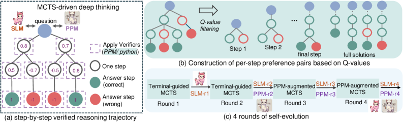
Figure 1: The overview of rStar-Math.
In this work, we introduce rStar-Math, a self-evolvable System 2-style reasoning approach that achieves the state-of-the-art math reasoning, rivaling and sometimes even surpassing OpenAI o1 on challenging math competition benchmarks with a model size as small as 7 billion. Unlike solutions relying on superior LLMs for data synthesis, rStar-Math leverages smaller language models (SLMs) with Monte Carlo Tree Search (MCTS) to establish a self-evolutionary process, iteratively generating higher-quality training data. To achieve self-evolution, rStar-Math introduces three key innovations.
First, a novel code-augmented CoT data synthesis method, which performs extensive MCTS rollouts to generate step-by-step verified reasoning trajectories with self-annotated MCTS Q-values. Specifically, math problem-solving is decomposed into multi-step generation within MCTS. At each step, the SLM serving as the policy model samples candidate nodes, each generating a one-step CoT and the corresponding Python code. To verify the generation quality, only nodes with successful Python code execution are retained, thus mitigating errors in intermediate steps. Moreover, extensive MCTS rollouts automatically assign a Q-value to each intermediate step based on its contribution: steps contributing to more trajectories that lead to the correct answer are given higher Q-values and considered higher quality. This ensures that the reasoning trajectories generated by SLMs consist of correct, high-quality intermediate steps.
Second, a novel method that trains an SLM acting as a process preference model, i.e., a PPM to implement the desired PRM, that reliably predicts a reward label for each math reasoning step. The PPM leverages the fact that, although Q-values are still not precise enough to score each reasoning step despite using extensive MCTS rollouts, the Q-values can reliably distinguish positive (correct) steps from negative (irrelevant/incorrect) ones. Thus the training method constructs preference pairs for each step based on Q-values and uses a pairwise ranking loss (Ouyang et al., 2022) to optimize PPM’s score prediction for each reasoning step, achieving reliable labeling. This approach avoids conventional methods that directly use Q-values as reward labels (Luo et al., 2024; Chen et al., 2024), which are inherently noisy and imprecise in stepwise reward assignment.
Finally, a four-round self-evolution recipe that progressively builds both a frontier policy model and PPM from scratch. We begin by curating a dataset of 747k math word problems from publicly available sources. In each round, we use the latest policy model and PPM to perform MCTS, generating increasingly high-quality training data using the above two methods to train a stronger policy model and PPM for next round. Each round achieves progressive refinement: (1) a stronger policy SLM, (2) a more reliable PPM, (3) generating better reasoning trajectories via PPM-augmented MCTS, and (4) improving training data coverage to tackle more challenging and even competition-level math problems.
Extensive experiments across four SLMs (1.5B-7B) and seven math reasoning tasks demonstrate the effectiveness of rStar-Math. Remarkably, rStar-Math improves all four SLMs, matching or even surpassing OpenAI o1 on challenging math benchmarks. On MATH benchmark, with 8 search trajectories, rStar-Math boosts Qwen2.5-Math-7B from 58.8% to 89.4% and Qwen2.5-Math-1.5B from 51.2% to 87.8%. With 64 trajectories, the scores rise to 90% and 88.4%, outperforming o1-preview by 4.5% and 2.6% and matching o1-mini’s 90%. On the Olympiad-level AIME 2024, rStar-Math solves on average 53.3% (8/15) of the problems, exceeding o1-preview by 8.7% and all other open-sourced LLMs. We further conduct comprehensive experiments to verify the superiority of step-by-step verified reasoning trajectories over state-of-the-art data synthesis baselines, as well as the PPM’s effectiveness compared to outcome reward models and Q value-based PRMs. Finally, we present key findings from rStar-Math deep thinking, including the intrinsic self-reflection capability and PPM’s preference for theorem-applications intermediate steps.
## 2 Related Works
Math Data Synthesis. Advancements in LLM math reasoning have largely relied on curating high-quality CoT data, with most leading approaches being GPT-distilled, using frontier models like GPT-4 for synthesis (Wang et al., 2024b; Gou et al., 2023; Luo et al., 2023). Notable works include NuminaMath (Jia LI and Polu, 2024a) and MetaMath (Yu et al., 2023b). While effective, this limits reasoning to the capabilities of the teacher LLM. Hard problems that the teacher LLM cannot solve are excluded in the training set. Even solvable problems may contain error-prone intermediate steps, which are hard to detect. Although rejection sampling methods (Yuan et al., 2023; Brown et al., 2024) can improve data quality, they do not guarantee correct intermediate steps. As a result, scaling up CoT data has diminishing returns, with gains nearing saturation—e.g., OpenMathInstruct-2 (Toshniwal et al., 2024) only sees a 3.9% boost on MATH despite an 8× increase in dataset size.
Scaling Test-time Compute has introduced new scaling laws, allowing LLMs to improve performance across by generating multiple samples and using reward models for best-solution selection (Snell et al., 2024; Wu et al., 2024; Brown et al., 2024). Various test-time search methods have been proposed (Kang et al., 2024; Wang et al., 2024a), including random sampling (Wang et al., 2023) and tree-search methods (Yao et al., 2024; Hao et al., 2023; Zhang et al., 2024b; Qi et al., 2024) like MCTS. However, open-source methods for scaling test-time computation have shown limited gains in math reasoning, often due to policy LLM or reward model limitations. rStar-Math addresses this by iteratively evolving the policy LLM and reward model, achieving System 2 mathematical reasoning performance comparable to OpenAI o1 (OpenAI, 2024).
Reward Models are crucial for effective System 2 reasoning but are challenging to obtain. Recent works include LLM-as-a-Judge for verification (Zheng et al., 2023; Qi et al., 2024) and specialized reward models like Outcome Reward Model (Yang et al., 2024; Yu et al., 2023a) and Process Reward Model (PRM) (Lightman et al., 2024). While PRMs offer promising dense, step-level reward signals for complex reasoning (Luo et al., 2024; Wang et al., 2024c), collecting step-level annotations remains an obstacle. While Kang et al. (2024); Wang et al. (2024a) rely on costly human-annotated datasets like PRM800k (Lightman et al., 2024), recent approaches (Wang et al., 2024c; Luo et al., 2024) explore automated annotation via Monte Carlo Sampling or MCTS. However, they struggle to generate precise reward scores, which limits performance gains. rStar-Math introduces a novel process preference reward (PPM) that eliminates the need for accurate step-level reward score annotation.
## 3 Methodology
### 3.1 Design Choices
MCTS for Effective System 2 Reasoning. We aim to train a math policy SLM and a process reward model (PRM), and integrating both within Monte Carlo Tree Search (MCTS) for System 2 deep thinking. MCTS is chosen for two key reasons. First, it breaks down complex math problems into simpler single-step generation tasks, reducing the difficulty for the policy SLM compared to other System 2 methods like Best-of-N (Brown et al., 2024) or self-consistency (Wang et al., 2023), which require generating full solutions in one inference. Second, the step-by-step generation in MCTS naturally yields step-level training data for both models. Standard MCTS rollout automatically assign Q-value to each step based on its contribution to the final correct answer, obviating the need for human-generated step-level annotations for process reward model training.
Ideally, advanced LLMs such as GPT-4 could be integrated within MCTS to generate training data. However, this approach faces two key challenges. First, even these powerful models struggle to consistently solve difficult problems, such as Olympiad-level mathematics. Consequently, the resulting training data would primarily consist of simpler solvable problems, limiting its diversity and quality. Second, annotating per-step Q-values demands extensive MCTS rollouts; insufficient tree exploration can lead to spurious Q-value assignments, such as overestimating suboptimal steps. Given that each rollout involves multiple single-step generations and these models are computationally expensive, increasing rollouts significantly raises inference costs.
Overview. To this end, we explore using two 7B SLMs (a policy SLM and a PRM) to generate higher-quality training data, with their smaller size allowing for extensive MCTS rollouts on accessible hardware (e.g., 4 $\times$ 40GB A100 GPUs). However, self-generating data presents greater challenges for SLMs, due to their weaker capabilities. SLMs frequently fail to generate correct solutions, and even when the final answer is correct, the intermediate steps are often flawed or of poor quality. Moreover, SLMs solve fewer challenging problems compared to advanced models like GPT-4.
This section introduces our methodology, as illustrated in Fig. 1. To mitigate errors and low-quality intermediate steps, we introduce a code-augmented CoT synthetic method, which performs extensive MCTS rollouts to generate step-by-step verified reasoning trajectories, annotated with Q-values. To further improve SLM performance on challenging problems, we introduce a four-round self-evolution recipe. In each round, both the policy SLM and the reward model are updated to stronger versions, progressively tackling more difficult problems and generating higher-quality training data. Finally, we present a novel process reward model training approach that eliminates the need for precise per-step reward annotations, yielding the more effective process preference model (PPM).
### 3.2 Step-by-Step Verified Reasoning Trajectory
We start by introducing our method for generating step-by-step verified reasoning trajectories with per-step Q-value annotations. Given a problem $x$ and a policy model $M$ , we run the standard MCTS to incrementally construct a search tree for step-by-step solution exploration. As shown in Fig. 1 (a), the root node represents question $x$ , while child nodes correspond to intermediate steps $s$ generated by $M$ . A root-to-leaf path ending at terminal node $s_{d}$ forms a trajectory $\mathbf{t}=x\oplus s_{1}\oplus s_{2}\oplus...\oplus s_{d}$ , with each step $s_{i}$ assigned a Q-value $Q(s_{i})$ . From the search tree $\mathcal{T}$ , we extract solution trajectories $\mathbb{T}=\{\mathbf{t}^{1},\mathbf{t}^{2},...,\mathbf{t}^{n}\}(n\geq 1)$ . Our goal is to select high-quality trajectories from $\mathcal{T}$ to construct the training set. For this purpose, we introduce code-augmented CoT synthesis method to filter out low-quality generations and perform extensive rollouts to improve the reliability of Q-value accuracy.
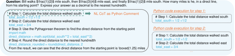
Code-augmented CoT Generation. Prior MCTS approaches primarily generate natural language (NL) CoTs (Qi et al., 2024; Zhang et al., 2024a). However, LLMs often suffer from hallucination, producing incorrect or irrelevant steps yet still arrive at the correct answer by chance (Lanham et al., 2023). These flawed steps are challenging to detect and eliminate. To address this, we propose a novel code execution augmented CoT. As shown in Fig. 2, the policy model generates a one-step NL CoT alongside its corresponding Python code, where the NL CoT is embedded as a Python comment. Only generations with successfully executed Python code are retained as valid candidates.
<details>
<summary>x2.png Details</summary>
### Visual Description
## [Screenshot]: Math Problem Solution with Python Code Execution
### Overview
The image is a screenshot of a problem-solving interface, likely from an educational or coding platform. It displays a word problem about calculating direct distance using the Pythagorean theorem, followed by a step-by-step solution presented in two parallel formats: a natural language (NL) step-by-step breakdown with embedded calculations, and corresponding Python code execution blocks. The layout is divided into a main left panel containing the problem and solution steps, and a narrower right panel showing the Python code execution for the first two steps.
### Components/Axes
The image is structured into distinct textual regions:
1. **Header/Question Bar (Top):** Contains the problem statement.
2. **Left Panel (Main Solution):** Contains the step-by-step solution with comments and calculations. A green arrow points from the first step's comment to the text "NL CoT as Python Comment".
3. **Right Panel (Code Execution):** Contains two separate, dashed-border boxes showing "Python code execution for step 1" and "Python code execution for step 2".
4. **Final Answer (Bottom of Left Panel):** The result is presented in a sentence with the numerical answer boxed.
**Textual Elements & Labels:**
* **Question Text:** "Bill walks $1\frac{1}{2}$ mile south, then $\frac{3}{4}$ mile east, and finally $1\frac{1}{2}$ mile south. How many miles is he, in a direct line, from his starting point? Express your answer as a decimal to the nearest hundredth."
* **Step Labels:** "# Step 1: Calculate the total distance walked south", "# Step 2: Calculate the total distance walked east", "# Step 3: Use the Pythagorean theorem to find the direct distance from the starting point", "# Step 4: Round the direct distance to the nearest hundredth".
* **Code/Variable Labels:** `total_south`, `total_east`, `direct_distance`, `direct_distance_rounded`.
* **Code Execution Headers:** "Python code execution for step 1:", "Python code execution for step 2:".
* **Final Statement:** "From the result, we can see that the direct distance from the starting point is \boxed{1.25} miles".
### Detailed Analysis
**Problem Statement:**
The problem describes a path: 1.5 miles south, then 0.75 miles east, then another 1.5 miles south. The goal is to find the straight-line (displacement) distance from the start.
**Solution Steps (Left Panel):**
* **Step 1:** Calculates total southward distance: `total_south = 1/2 + 1/2`. *Note: The written calculation `1/2 + 1/2` appears to be a simplification or error in the comment, as the problem states 1 1/2 miles twice, which is 1.5 + 1.5 = 3 miles total south. The code execution on the right uses `1/2 + 1/2`.*
* **Step 2:** Identifies eastward distance: `total_east = 3/4`.
* **Step 3:** Applies the Pythagorean theorem: `import math` followed by `direct_distance = math.sqrt(total_south**2 + total_east**2)`.
* **Step 4:** Rounds the result: `direct_distance_rounded = round(direct_distance, 2)`.
* **Final Answer:** States the result is 1.25 miles.
**Python Code Execution (Right Panel):**
* **Execution for Step 1:** Shows the code:
```python
# Step 1: Calculate the total distance walked south
total_south = 1/2 + 1/2
```
* **Execution for Step 2:** Shows the code:
```python
# Step 1: Calculate the total distance walked south
total_south = 1/2 + 1/2
# Step 2: Calculate the total distance walked east
total_east = 3/4
```
*Observation: The execution block for Step 2 redundantly includes the code from Step 1.*
### Key Observations
1. **Discrepancy in Southward Distance:** There is a clear inconsistency between the problem statement (1 1/2 miles twice = 3 miles total south) and the calculation shown in both the comment (`1/2 + 1/2`) and the Python code (`1/2 + 1/2`), which equals 1 mile total south. This is a critical error in the presented solution.
2. **Final Answer Inconsistency:** The final boxed answer is 1.25 miles. If we use the correct total south distance (3 miles) and east distance (0.75 miles), the Pythagorean calculation would be √(3² + 0.75²) = √(9 + 0.5625) = √9.5625 ≈ 3.09 miles. The answer 1.25 miles is only consistent with the erroneous calculation where total_south = 1 mile (√(1² + 0.75²) = √(1 + 0.5625) = √1.5625 = 1.25).
3. **Layout and Pedagogy:** The image demonstrates a "Natural Language Chain of Thought (CoT)" approach, where each reasoning step is commented in plain language before being translated into executable Python code. The green arrow explicitly highlights this relationship.
4. **Code Structure:** The Python code is simple, using basic arithmetic and the `math` module for the square root function. The final rounding step is shown but its execution is not displayed in the right panel.
### Interpretation
This screenshot captures a flawed educational example. Its primary purpose is to illustrate how to break down a word problem into programmable steps using natural language comments as a guide. However, the core mathematical content contains a significant error: the misinterpretation of the mixed number "1 1/2" as "1/2" in the calculation, leading to an incorrect final answer.
The image serves as a case study in the importance of verifying each step of a computational solution against the original problem statement. The discrepancy highlights a potential pitfall in automated or semi-automated problem-solving systems where a transcription or parsing error in an early step (converting "1 1/2" to "1/2") propagates through all subsequent calculations, resulting in a confidently presented but wrong answer. For a technical document, this image would be valuable not as a correct solution, but as an example of error analysis, debugging process, or the structure of a CoT-to-code workflow.
</details>
Figure 2: An example of Code-augmented CoT.
Specifically, starting from the initial root node $x$ , we perform multiple MCTS iterations through selection, expansion, rollout, and back-propagation. At step $i$ , we collect the latest reasoning trajectory $x\oplus s_{1}\oplus s_{2}\oplus...\oplus s_{i-1}$ as the current state. Based on this state, we prompt (see Appendix A.3) the policy model to generate $n$ candidates $s_{i,0},...,s_{i,n-1}$ for step $i$ . Python code execution is then employed to filter valid nodes. As shown in Fig. 2, each generation $s_{i,j}$ is concatenated with the code from all previous steps, forming $s_{1}\oplus s_{2}\oplus...\oplus s_{i-1}\oplus s_{i,j}$ . Candidates that execute successfully are retained as valid nodes and scored by the PPM, which assigns a Q-value $q(s_{i})$ . Then, we use the well-known Upper Confidence bounds for Trees (UCT) (Kocsis and Szepesvári, 2006) to select the best node among the $n$ candidates. This selection process is mathematically represented as:
$$
\displaystyle\text{UCT}(s)=Q(s)+c\sqrt{\frac{\ln N_{parent}(s)}{N(s)}};\quad\text{where}\quad Q(s)=\frac{q(s)}{N(s)} \tag{1}
$$
where $N(s)$ denotes the number of visits to node $s$ , and $N_{\text{parent}}(s)$ is the visit count of $s$ ’s parent node. The predicted reward $q(s)$ is provided by the PPM and will be updated through back-propagation. $c$ is a constant that balances exploitation and exploration.
Extensive Rollouts for Q-value Annotation. Accurate Q-value $Q(s)$ annotation in Eq. 1 is crucial for guiding MCTS node selection towards correct problem-solving paths and identifying high-quality steps within trajectories. To improve Q-value reliability, we draw inspiration from Go players, who retrospectively evaluate the reward of each move based on game outcomes. Although initial estimates may be imprecise, repeated gameplay refines these evaluations over time. Similarly, in each rollout, we update the Q-value of each step based on its contribution to achieving the correct final answer. After extensive MCTS rollouts, steps consistently leading to correct answers achieve higher Q-values, occasional successes yield moderate Q-values, and consistently incorrect steps receive low Q-values. Specifically, we introduce two self-annotation methods to obtain these step-level Q-values. Fig. 1 (c) shows the detailed setting in the four rounds of self-evolution.
Terminal-guided annotation. During the first two rounds, when the PPM is unavailable or insufficiently accurate, we use terminal-guided annotation. Formally, let $q(s_{i})^{k}$ denote the q value for step $s_{i}$ after back-propagation in the $k^{th}$ rollout. Following AlphaGo (Silver et al., 2017) and rStar (Qi et al., 2024), we score each intermediate node based on its contribution to the final correct answer:
$$
\displaystyle q(s_{i})^{k}=q(s_{i})^{k-1}+q(s_{d})^{k}; \tag{2}
$$
where the initial q value $q(s_{i})^{0}=0$ in the first rollout. If this step frequently leads to a correct answer, its $q$ value will increase; otherwise, it decreases. Terminal nodes are scored as $q(s_{d})=1$ for correct answers and $q(s_{d})=-1$ otherwise, as shown in Fig. 1.
PRM-augmented annotation. Starting from the third round, we use PPM to score each step for more effective generation. Compared to terminal-guided annotation, which requires multiple rollouts for a meaningful $q$ value, PPM directly predicts a non-zero initial $q$ value. PPM-augmented MCTS also helps the policy model to generate higher-quality steps, guiding solutions towards correct paths. Formally, for step $s_{i}$ , PPM predicts an initial $q(s_{i})^{0}$ value based on the partial trajectory:
$$
\displaystyle q(s_{i})^{0}=PPM(x\oplus s_{1}\oplus s_{2}\oplus...\oplus s_{i-1}\oplus s_{i}) \tag{3}
$$
This $q$ value will be updated based on terminal node’s $q(s_{d})$ value through MCTS back-propagation in Eq. 2. For terminal node $s_{d}$ , we do not use PRM for scoring during training data generation. Instead, we assign a more accurate score based on ground truth labels as terminal-guided rewarding.
### 3.3 Process Preference Model
Process reward models, which provide granular step-level reward signals, is highly desirable for solving challenging math problems. However, obtaining high-quality step-level training data remains an open challenge. Existing methods rely on human annotations (Lightman et al., 2023) or MCTS-generated scores (Zhang et al., 2024a; Chen et al., 2024) to assign a score for each step. These scores then serve as training targets, with methods such as MSE loss (Chen et al., 2024) or pointwise loss (Wang et al., 2024c; Luo et al., 2024; Zhang et al., 2024a) used to minimize the difference between predicted and labeled scores. As a result, the precision of these annotated step-level reward scores directly determines the effectiveness of the resulting process reward model.
Unfortunately, precise per-step scoring remains a unsolved challenge. Although our extensive MCTS rollouts improve the reliability of Q-values, precisely evaluating fine-grained step quality presents a major obstacle. For instance, among a set of correct steps, it is difficult to rank them as best, second-best, or average and then assign precise scores. Similarly, among incorrect steps, differentiating the worst from moderately poor steps poses analogous challenges. Even expert human annotation struggles with consistency, particularly at scale, leading to inherent noise in training labels.
We introduce a novel training method that trains a process preference model (PPM) by constructing step-level positive-negative preference pairs. As shown in Fig. 1 (b), instead of using Q-values as direct reward labels, we use them to select steps from MCTS tree for preference pair construction. For each step, we select two candidates with the highest Q-values as positive steps and two with the lowest as negative steps. Critically, the selected positive steps must lead to a correct final answer, while negative steps must lead to incorrect answers. For intermediate steps (except the final answer step), the positive and negative pairs share the same preceding steps. For the final answer step, where identical reasoning trajectories rarely yield different final answers, we relax this restriction. We select two correct trajectories with the highest average Q-values as positive examples and two incorrect trajectories with the lowest average Q-values as negative examples. Following (Ouyang et al., 2022), we define our loss function using the standard Bradley-Terry model with a pairwise ranking loss:
$$
\displaystyle\mathcal{L}_{ppm}(\theta)=-\frac{1}{2\times 2}E_{(x,y_{i}^{pos},y_{i}^{neg}\in\mathbb{D})}[log(\sigma(r_{\theta}(x,y_{i}^{pos})-r_{\theta}(x,y_{i}^{neg})))] \displaystyle\text{when $i$ is not final answer step},y_{i}^{pos}=s_{1}\oplus...\oplus s_{i-1}\oplus s_{i}^{pos};y_{i}^{neg}=s_{1}\oplus...\oplus s_{i-1}\oplus s_{i}^{neg}\vskip-4.30554pt \tag{4}
$$
Here, $r_{\theta}(x,y_{i})$ denotes the output of the PPM, where $x$ is the problem and $y$ is the trajectory from the first step to the $i^{th}$ step.
### 3.4 Self-Evolved Deep Thinking
#### 3.4.1 Training with Step-by-Step Verified Reasoning Trajectory
Math Problems Collection. We collect a large dataset of 747k math word problems with final answer ground-truth labels, primarily from NuminaMath (Jia LI and Polu, 2024a) and MetaMath (Yu et al., 2023b). Notably, only competition-level problems (e.g., Olympiads and AIME/AMC) from NuminaMath are included, as we observe that grade-school-level problems do not significantly improve LLM complex math reasoning. To augment the limited competition-level problems, we follow (Li et al., 2024) and use GPT-4 to synthesize new problems based on the seed problems in 7.5k MATH train set and 3.6k AMC-AIME training split. However, GPT-4 often generated unsolvable problems or incorrect solutions for challenging seed problems. To filter these, we prompt GPT-4 to generate 10 solutions per problem, retaining only those with at least 3 consistent solutions.
Reasoning Trajectories Collection. Instead of using the original solutions in the 747k math dataset, we conduct extensive MCTS rollouts (Sec. 3.2) to generate higher-quality step-by-step verified reasoning trajectories. In each self-evolution round, we perform 16 rollouts per math problem, which leads to 16 reasoning trajectories. Problems are then categories by difficulty based on the correct ratio of the generated trajectories: easy (all solutions are correct), medium (a mix of correct and incorrect solutions) and hard (all solutions are incorrect). For hard problems with no correct trajectories, an additional MCTS with 16 rollouts is performed. After that, all step-by-step trajectories and their annotated Q-values are collected and filtered to train the policy SLM and process preference model.
Supervised Fine-tuning the Policy SLM. Through extensive experiments, we find that selecting high-quality reasoning trajectories is the key for fine-tuning a frontier math LLM. While methods such as GPT-distillation and Best-of-N can include low-quality or erroneous intermediate steps, a more effective approach ensures that every step in the trajectory is of high quality. To achieve this, we use per-step Q-values to select optimal trajectories from MCTS rollouts. Specifically, for each math problem, we select the top-2 trajectories with the highest average Q-values among those leading to correct answers as SFT training data.
Training PPM. The PPM is initialized from the fine-tuned policy model, with its next-token prediction head replaced by a scalar-value head consisting of a linear layer and a tanh function to constrain outputs to the range [-1, 1]. We filter out math problems where all solution trajectories are fully correct or incorrect. For problems with mixed outcomes, we select two positive and two negative examples for each step based on Q-values, which are used as preference pairs for training data.
#### 3.4.2 Recipe for Self-Evolution
Table 2: Percentage of the 747k math problems correctly solved in each round. Only problems have correct solutions are included in the training set. The first round uses DeepSeek-Coder-Instruct as the policy LLM, while later rounds use our fine-tuned 7B policy SLM.
| # | models in MCTS | GSM-level | MATH-level | Olympiad-level | All |
| --- | --- | --- | --- | --- | --- |
| Round 1 | DeepSeek-Coder-V2-Instruct | 96.61% | 67.36% | 20.99% | 60.17% |
| Round 2 | policy SLM-r1 | 97.88% | 67.40% | 56.04% | 66.60% |
| Round 3 | policy SLM-r2, PPM-r2 | 98.15% | 88.69% | 62.16% | 77.86% |
| Round 4 | policy SLM-r3, PPM-r3 | 98.15% | 94.53% | 80.58% | 90.25% |
Table 3: Pass@1 accuracy of the resulting policy SLM in each round, showing continuous improvement until surpassing the bootstrap model.
| Round# | MATH | AIME 2024 | AMC 2023 | Olympiad Bench | College Math | GSM8K | GaokaoEn 2023 |
| --- | --- | --- | --- | --- | --- | --- | --- |
| DeepSeek-Coder-V2-Instruct (bootstrap model) | 75.3 | 13.3 | 57.5 | 37.6 | 46.2 | 94.9 | 64.7 |
| Base (Qwen2.5-Math-7B) | 58.8 | 0.0 | 22.5 | 21.8 | 41.6 | 91.6 | 51.7 |
| policy SLM-r1 | 69.6 | 3.3 | 30.0 | 34.7 | 44.5 | 88.4 | 57.4 |
| policy SLM-r2 | 73.6 | 10.0 | 35.0 | 39.0 | 45.7 | 89.1 | 59.7 |
| policy SLM-r3 | 75.8 | 16.7 | 45.0 | 44.1 | 49.6 | 89.3 | 62.8 |
| policy SLM-r4 | 78.4 | 26.7 | 47.5 | 47.1 | 52.5 | 89.7 | 65.7 |
Table 4: The quality of PPM consistently improves across rounds. The policy model has been fixed with policy SLM-r1 for a fair comparison.
| Round# | MATH | AIME 2024 | AMC 2023 | Olympiad Bench | College Math | GSM8K | GaokaoEn 2023 |
| --- | --- | --- | --- | --- | --- | --- | --- |
| PPM-r1 | 75.2 | 10.0 | 57.5 | 35.7 | 45.4 | 90.9 | 60.3 |
| PPM-r2 | 84.1 | 26.7 | 75.0 | 52.7 | 54.2 | 93.3 | 73.0 |
| PPM-r3 | 85.2 | 33.3 | 77.5 | 59.5 | 55.6 | 93.9 | 76.6 |
| PPM-r4 | 87.0 | 43.3 | 77.5 | 61.5 | 56.8 | 94.2 | 77.8 |
Due to the weaker capabilities of SLMs, we perform four rounds of MCTS deep thinking to progressively generate higher-quality data and expand the training set with more challenging math problems. Each round uses MCTS to generate step-by-step verified reasoning trajectories, which are then used to train the new policy SLM and PPM. The new models are then applied in next round to generate higher-quality training data. Fig. 1 (c) and Table 2 detail the models used for data generation in each round, along with the identifiers of the trained policy model and PPM. Next, we outline the details and specific improvements targeted in each round.
Round 1: Bootstrapping an initial strong policy SLM-r1. To enable SLMs to self-generate reasonably good training data, we perform a bootstrap round to fine-tune an initial strong policy model, denoted as SLM-r1. As shown in Table 2, we run MCTS with DeepSeek-Coder-V2-Instruct (236B) to collect the SFT data. With no available reward model in this round, we use terminal-guided annotation for Q-values and limit MCTS to 8 rollouts for efficiency. For correct solutions, the top-2 trajectories with the highest average Q-values are selected as SFT data. We also train PPM-r1, but the limited rollouts yields unreliable Q-values, affecting the effectiveness of PPM-r1 ( Table 4).
Round 2: Training a reliable PPM-r2. In this round, with the policy model updated to the 7B SLM-r1, we conduct extensive MCTS rollouts for more reliable Q-value annotation and train the first reliable reward model, PPM-r2. Specifically, we perform 16 MCTS rollouts per problem. The resulting step-by-step verified reasoning trajectories show significant improvements in both quality and Q-value precision. As shown in Table 4, PPM-r2 is notably more effective than in the bootstrap round. Moreover, the policy SLM-r2 also continues to improve as expected (Table 3).
Round 3: PPM-augmented MCTS to significantly improve data quality. With the reliable PPM-r2, we perform PPM-augmented MCTS in this round to generate data, leading to significantly higher-quality trajectories that cover more math and Olympiad-level problems in the training set (Table 2). The generated reasoning trajectories and self-annotated Q-values are then used to train the new policy SLM-r3 and PPM-r3, both of which show significant improvements.
Round 4: Solving challenging math problems. After the third round, while grade school and MATH problems achieve high success rates, only 62.16% of Olympiad-level problems are included in the training set. This is NOT solely due to weak reasoning abilities in our SLMs, as many Olympiad problems remain unsolved by GPT-4 or o1. To improve coverage, we adopt a straightforward strategy. For unsolved problems after 16 MCTS rollouts, we perform an additional 64 rollouts, and if needed, increase to 128. We also conduct multiple MCTS tree expansions with different random seeds. This boosts the success rate of Olympiad-level problems to 80.58%.
After four rounds of self-evolution, 90.25% of the 747k math problems are successfully covered into the training set, as shown in Table 2. Among the remaining unsolved problems, a significant portion consists of synthetic questions. We manually review a random sample of 20 problems and find that 19 are incorrectly labeled with wrong answers. Based on this, we conclude that the remaining unsolved problems are of low quality and thus terminate the self-evolution at round 4.
## 4 Evaluation
### 4.1 Setup
Evaluation Datasets. We evaluate rStar-Math on diverse mathematical benchmarks. In addition to the widely-used GSM8K (Cobbe et al., 2021), we include challenging benchmarks from multiple domains: (i) competition and Olympiad-level benchmarks, such as MATH-500 (Lightman et al., 2023), AIME 2024 (AI-MO, 2024a), AMC 2023 (AI-MO, 2024b) and Olympiad Bench (He et al., 2024). Specifically, AIME is the exams designed to challenge the brightest high school math students in American, with the 2024 dataset comprising 30 problems from AIME I and II exams; (ii) college-level math problems from College Math (Tang et al., 2024) and (iii) out-of-domain math benchmark: GaoKao (Chinese College Entrance Exam) En 2023 (Liao et al., 2024).
Base Models and Setup. rStar-Math is a general approach applicable to various LLMs. To show its effectiveness and generalizability, we use SLMs of different sizes as the base policy models: Qwen2.5-Math-1.5B (Qwen, 2024b), Phi3-mini-Instruct (3B) (Microsoft, 2024; Abdin et al., 2024), Qwen2-Math-7B (Qwen, 2024a) and Qwen2.5-Math-7B (Qwen, 2024c). Among these, Phi3-mini-Instruct is a general-purpose SLM without specialization in math reasoning.
Due to limited GPU resources, we performed 4 rounds of self-evolution exclusively on Qwen2.5-Math-7B, yielding 4 evolved policy SLMs (Table 3) and 4 PPMs (Table 4). For the other 3 policy LLMs, we fine-tune them using step-by-step verified trajectories generated from Qwen2.5-Math-7B’s 4th round. The final PPM from this round is then used as the reward model for the 3 policy SLMs.
Baselines. rStar-Math is a System 2 method. We compare it against three strong baselines representing both System 1 and System 2 approaches: (i) Frontier LLMs, including GPT-4o, the latest Claude, OpenAI o1-preview and o1-mini. We measure their accuracy on AMC 2023, Olympiad Bench, College Math, Gaokao and GSM8K, with accuracy numbers for other benchmarks are taken from public technical reports (Team, 2024a). (ii) Open-sourced superior reasoning models, including DeepSeek-Coder-v2-Instruct, Mathstral (Team, 2024b), NuminaMath-72B (Jia LI and Polu, 2024a), and LLaMA3.1 (Dubey et al., 2024), which represent the current mainstream System 1 approaches for improving LLM math reasoning. (iii) Both System 1 and System 2 performance of the base models trained from the original models teams, including Instruct versions (e.g., Qwen2.5-Math-7B-Instruct) and Best-of-N (e.g., Qwen2.5-Math-72B-Instruct+Qwen2.5-Math-RM-72B). Notably, the reward model used for the three Qwen base models is a 72B ORM, significantly larger than our 7B PPM.
Evaluation Metric. We report Pass@1 accuracy for all baselines. For System 2 baselines, we use default evaluation settings, such as default thinking time for o1-mini and o1-preview. For Qwen models with Best-of-N, we re-evaluate MATH-500, AIME/AMC accuracy; other benchmarks results are from their technical reports. For a fair comparison, rStar-Math run MCTS to generate the same number of solutions as Qwen. Specifically, for AIME/AMC, we generate 16 trajectories for AIME/AMC and 8 for other benchmarks, using PPM to select the best solution. We also report performance with increased test-time computation using 64 trajectories, denoted as rStar-Math 64.
Table 5: The results of rStar-Math and other frontier LLMs on the most challenging math benchmarks. rStar-Math 64 shows the Pass@1 accuracy achieved when sampling 64 trajectories.
| | | Competition and College Level | | | OOD | | | |
| --- | --- | --- | --- | --- | --- | --- | --- | --- |
| Model | Method | MATH | AIME 2024 | AMC 2023 | Olympiad Bench | College Math | GSM8K | Gaokao En 2023 |
| Frontier LLMs | | | | | | | | |
| GPT-4o | System 1 | 76.6 | 9.3 | 47.5 | 43.3 | 48.5 | 92.9 | 67.5 |
| Claude3.5-Sonnet | System 1 | 78.3 | 16.0 | - | - | - | 96.4 | - |
| GPT-o1-preview | - | 85.5 | 44.6 | 90.0 | - | - | - | - |
| GPT-o1-mini | - | 90.0 | 56.7 | 95.0 | 65.3 | 57.8 | 94.8 | 78.4 |
| Open-Sourced Reasoning LLMs | | | | | | | | |
| DeepSeek-Coder-V2-Instruct | System 1 | 75.3 | 13.3 | 57.5 | 37.6 | 46.2 | 94.9 | 64.7 |
| Mathstral-7B-v0.1 | System 1 | 57.8 | 0.0 | 37.5 | 21.5 | 33.7 | 84.9 | 46.0 |
| NuminaMath-72B-CoT | System 1 | 64.0 | 3.3 | 70.0 | 32.6 | 39.7 | 90.8 | 58.4 |
| LLaMA3.1-8B-Instruct | System 1 | 51.4 | 6.7 | 25.0 | 15.4 | 33.8 | 76.6 | 38.4 |
| LLaMA3.1-70B-Instruct | System 1 | 65.4 | 23.3 | 50.0 | 27.7 | 42.5 | 94.1 | 54.0 |
| Qwen2.5-Math-72B-Instruct | System 1 | 85.6 | 30.0 | 70.0 | 49.0 | 49.5 | 95.9 | 71.9 |
| Qwen2.5-Math-72B-Instruct+72B ORM | System 2 | 85.8 | 36.7 | 72.5 | 54.5 | 50.6 | 96.4 | 76.9 |
| General Base Model: Phi3-mini-Instruct (3.8B) | | | | | | | | |
| Phi3-mini-Instruct (base model) | System 1 | 41.4 | 3.33 | 7.5 | 12.3 | 33.1 | 85.7 | 37.1 |
| rStar-Math (3.8B SLM+7B PPM) | System 2 | 85.4 | 40.0 | 77.5 | 59.3 | 58.0 | 94.5 | 77.1 |
| rStar-Math 64 (3.8B SLM+7B PPM) | System 2 | 86.4 | 43.3 | 80.0 | 60.3 | 59.1 | 94.7 | 77.7 |
| Math-Specialized Base Model: Qwen2.5-Math-1.5B | | | | | | | | |
| Qwen2.5-Math-1.5B (base model) | System 1 | 51.2 | 0.0 | 22.5 | 16.7 | 38.4 | 74.6 | 46.5 |
| Qwen2.5-Math-1.5B-Instruct | System 1 | 60.0 | 10.0 | 60.0 | 38.1 | 47.7 | 84.8 | 65.5 |
| Qwen2.5-Math-1.5B-Instruct+72B ORM | System 2 | 83.4 | 20.0 | 72.5 | 47.3 | 50.2 | 94.1 | 73.0 |
| rStar-Math (1.5B SLM+7B PPM) | System 2 | 87.8 | 46.7 | 80.0 | 63.5 | 59.0 | 94.3 | 77.7 |
| rStar-Math 64 (1.5B SLM+7B PPM) | System 2 | 88.6 | 46.7 | 85.0 | 64.6 | 59.3 | 94.8 | 79.5 |
| Math-Specialized Base Model: Qwen2-Math-7B | | | | | | | | |
| Qwen2-Math-7B (base model) | System 1 | 53.4 | 3.3 | 25.0 | 17.3 | 39.4 | 80.4 | 47.3 |
| Qwen2-Math-7B-Instruct | System 1 | 73.2 | 13.3 | 62.5 | 38.2 | 45.9 | 89.9 | 62.1 |
| Qwen2-Math-7B-Instruct+72B ORM | System 2 | 83.4 | 23.3 | 62.5 | 47.6 | 47.9 | 95.1 | 71.9 |
| rStar-Math (7B SLM+7B PPM) | System 2 | 88.2 | 43.3 | 80.0 | 63.1 | 58.4 | 94.6 | 78.2 |
| rStar-Math 64 (7B SLM+7B PPM) | System 2 | 88.6 | 46.7 | 85.0 | 63.4 | 59.3 | 94.8 | 79.2 |
| Math-Specialized Base Model: Qwen2.5-Math-7B | | | | | | | | |
| Qwen2.5-Math-7B (base model) | System 1 | 58.8 | 0.0 | 22.5 | 21.8 | 41.6 | 91.6 | 51.7 |
| Qwen2.5-Math-7B-Instruct | System 1 | 82.6 | 6.0 | 62.5 | 41.6 | 46.8 | 95.2 | 66.8 |
| Qwen2.5-Math-7B-Instruct+72B ORM | System 2 | 88.4 | 26.7 | 75.0 | 49.9 | 49.6 | 97.9 | 75.1 |
| rStar-Math (7B SLM+7B PPM) | System 2 | 89.4 | 50.0 | 87.5 | 65.3 | 59.0 | 95.0 | 80.5 |
| rStar-Math 64 (7B SLM+7B PPM) | System 2 | 90.0 | 53.3 | 87.5 | 65.6 | 60.5 | 95.2 | 81.3 |
### 4.2 Main Results
Results on diverse challenging math benchmarks. Table 5 shows the results of rStar-Math with comparing to state-of-the-art reasoning models. We highlight three key observations: (1) rStar-Math significantly improves SLMs math reasoning capabilities, achieving performance comparable to or surpassing OpenAI o1 with substantially smaller model size (1.5B-7B). For example, Qwen2.5-Math-7B, originally at 58.8% accuracy on MATH, improved dramatically to 90.0% with rStar-Math, outperforming o1-preview and Claude 3.5 Sonnet while matching o1-mini. On the College Math benchmark, rStar-Math exceeds o1-mini by 2.7%. On AIME 2024, rStar-Math scored 53.3%, ranking just below o1-mini, with the 7B model solving 8/15 problems in both AIME I and II, placing in the top 20% of the brightest high school math students. Notably, 8 of the unsolved problems were geometry-based, requiring visual understanding, a capability rStar-Mathcurrently does not support. (2) Despite using smaller policy models (1.5B-7B) and reward models (7B), rStar-Math significantly outperforms state-of-the-art System 2 baselines. Compared to Qwen Best-of-N baselines, which use the same base models (Qwen2-Math-7B, Qwen2.5-Math-1.5B/7B) but a 10 $\times$ larger reward model (Qwen2.5-Math-RM-72B), rStar-Math consistently improves the reasoning accuracy of all base models to state-of-the-art levels. Even against Best-of-N with a 10 $\times$ larger Qwen2.5-Math-72B-Instruct policy model, rStar-Math surpasses it on all benchmarks except GSM8K, using the same number of sampled solutions. (3) Beyond well-known benchmarks like MATH, GSM8K, and AIME, which may risk over-optimization, rStar-Math shows strong generalizability on other challenging math benchmarks, including Olympiad Bench, College Math, and the Chinese College Entrance Math Exam (Gaokao), setting new state-of-the-art scores. As discussed in Sec. 3.4, our training set is primarily sourced from public datasets, with no specific optimizations for these benchmarks.
<details>
<summary>scalinglaws.png Details</summary>
### Visual Description
## Multi-Panel Line Chart: Model Accuracy vs. Number of Sampled Solutions
### Overview
The image contains four line charts (panels) comparing the accuracy (in percentage) of five models across varying numbers of sampled solutions (x - axis: 1, 2, 4, 8, 16, 32, 64, logarithmic base - 2 scale). The panels are labeled “MATH”, “AIME 2024”, “Olympiad Bench”, and “College Math”. The y - axis for each panel represents “Accuracy (%)” with different ranges per panel.
### Components/Axes
- **X - axis (all panels)**: “#Sampled Solutions” with values 1, 2, 4, 8, 16, 32, 64 (logarithmic, base - 2 scale).
- **Y - axis (per panel)**:
- MATH: 78–90%
- AIME 2024: 20–45%
- Olympiad Bench: 45–65%
- College Math: 45–60%
- **Legend (top of image)**:
- o1 - preview: Blue dashed line (flat across sampled solutions).
- o1 - mini: Red dashed line (flat across sampled solutions).
- rStar - Math (7B SLM + 7B PPM): Teal solid line with circular markers (increasing trend).
- Qwen2.5 Best - of - N (7B SLM + 72B ORM): Purple dotted line with square markers (increasing trend).
- Qwen2.5 Best - of - N (72B LLM + 72B ORM): Yellow dotted line with circular markers (increasing trend).
### Detailed Analysis (Per Panel)
#### 1. MATH Panel
- **o1 - preview (blue dashed)**: Flat at ~85% accuracy (no change with sampled solutions).
- **o1 - mini (red dashed)**: Flat at ~90% accuracy (no change with sampled solutions).
- **rStar - Math (teal)**: Starts at ~78% (x = 1), rises to ~90% (x = 64). Trend: Strongly increasing with sampled solutions.
- **Qwen2.5 (7B SLM + 72B ORM, purple squares)**: Starts at ~82% (x = 1), rises to ~88% (x = 64). Trend: Increasing.
- **Qwen2.5 (72B LLM + 72B ORM, yellow circles)**: Starts at ~83% (x = 1), rises to ~87% (x = 64). Trend: Increasing.
#### 2. AIME 2024 Panel
- **o1 - preview (blue dashed)**: Flat at ~45% accuracy (no change with sampled solutions).
- **o1 - mini (red dashed)**: Flat at ~45% accuracy (no change with sampled solutions).
- **rStar - Math (teal)**: Starts at ~25% (x = 1), rises to ~45% (x = 64). Trend: Increasing.
- **Qwen2.5 (7B SLM + 72B ORM, purple squares)**: Starts at ~15% (x = 1), rises to ~30% (x = 64). Trend: Increasing.
- **Qwen2.5 (72B LLM + 72B ORM, yellow circles)**: Starts at ~20% (x = 1), rises to ~35% (x = 64). Trend: Increasing.
#### 3. Olympiad Bench Panel
- **o1 - preview (blue dashed)**: Flat at ~65% accuracy (no change with sampled solutions).
- **o1 - mini (red dashed)**: Flat at ~65% accuracy (no change with sampled solutions).
- **rStar - Math (teal)**: Starts at ~50% (x = 1), rises to ~65% (x = 64). Trend: Increasing.
- **Qwen2.5 (7B SLM + 72B ORM, purple squares)**: Starts at ~45% (x = 1), rises to ~55% (x = 64). Trend: Increasing.
- **Qwen2.5 (72B LLM + 72B ORM, yellow circles)**: Starts at ~48% (x = 1), rises to ~58% (x = 64). Trend: Increasing.
#### 4. College Math Panel
- **o1 - preview (blue dashed)**: Flat at ~58% accuracy (no change with sampled solutions).
- **o1 - mini (red dashed)**: Flat at ~58% accuracy (no change with sampled solutions).
- **rStar - Math (teal)**: Starts at ~52% (x = 1), rises to ~60% (x = 64). Trend: Increasing.
- **Qwen2.5 (7B SLM + 72B ORM, purple squares)**: Starts at ~45% (x = 1), rises to ~50% (x = 64). Trend: Increasing.
- **Qwen2.5 (72B LLM + 72B ORM, yellow circles)**: Starts at ~47% (x = 1), rises to ~52% (x = 64). Trend: Increasing.
### Key Observations
- **Flat Trends (o1 - preview, o1 - mini)**: These models show no accuracy improvement with more sampled solutions (flat lines), indicating their performance is independent of the number of solutions sampled.
- **Increasing Trends (rStar - Math, Qwen2.5 variants)**: All three models with “Best - of - N” or “rStar - Math” show accuracy increasing with more sampled solutions, meaning sampling more solutions improves their performance.
- **Model Comparison**:
- In MATH, o1 - mini (red) outperforms o1 - preview (blue) and Qwen2.5 variants, while rStar - Math approaches o1 - mini’s accuracy at high sampled solutions.
- In AIME 2024, Olympiad Bench, and College Math, o1 - preview and o1 - mini (both ~45%, ~65%, ~58% respectively) outperform Qwen2.5 variants, with rStar - Math approaching their accuracy at x = 64.
### Interpretation
The data implies that o1 - preview and o1 - mini have stable accuracy regardless of the number of sampled solutions, suggesting their performance is robust or not dependent on sampling more solutions. In contrast, rStar - Math and Qwen2.5 Best - of - N models benefit from more sampled solutions, with accuracy increasing as the number of solutions sampled grows. This could mean these models rely on sampling multiple solutions to find the best one (e.g., via a “best - of - N” strategy), while o1 - preview and o1 - mini might have a more deterministic or single - solution approach. The consistent outperformance of o1 - preview and o1 - mini across most panels (except MATH, where rStar - Math catches up) suggests they are more effective for these math - related tasks, especially when sampling solutions is not a factor. The increasing trend for rStar - Math and Qwen2.5 variants highlights the value of sampling more solutions for these models, potentially due to their reliance on generating multiple candidates and selecting the best one.
</details>
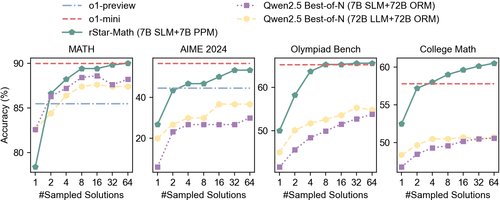
Figure 3: Reasoning performance under scaling up the test-time compute.
Scaling up test-time computation. rStar-Math uses MCTS to augment the policy model, searching solutions guided by the PPM. By increasing test-time computation, it explores more trajectories, potentially improving performance. In Fig. 3, we show the impact of test-time compute scaling by comparing the accuracy of the official Qwen Best-of-N across different numbers of sampled trajectories on four challenging math benchmarks. Sampling only one trajectory corresponds to the policy LLM’s Pass@1 accuracy, indicating a fallback to System 1 reasoning. We highlight two key observations: (1) With only 4 trajectories, rStar-Math significantly outperforms Best-of-N baselines, exceeding o1-preview and approaching o1-mini, demonstrating its effectiveness. (2) Scaling test-time compute improves reasoning accuracy across all benchmarks, though with varying trends. On Math, AIME, and Olympiad Bench, rStar-Math shows saturation or slow improvement at 64 trajectories, while on College Math, performance continues to improve steadily.
### 4.3 Ablation Study and Analysis
We ablate the effectiveness of our three innovations. For System 2-style inference, Pass@1 accuracy is measured with 16 trajectories for AIME and AMC, and 8 for other benchmarks.
Table 6: The continuously improved math reasoning capabilities through rStar-Math self-evolved deep thinking. Starting from round 2, the 7B base model powered by rStar-Math surpasses GPT-4o.
| Round# | MATH | AIME 2024 | AMC 2023 | Olympiad Bench | College Math | GSM8K | GaokaoEn 2023 |
| --- | --- | --- | --- | --- | --- | --- | --- |
| GPT-4o | 76.6 | 9.3 | 47.5 | 43.3 | 48.5 | 92.9 | 67.5 |
| Base 7B model | 58.8 | 0.0 | 22.5 | 21.8 | 41.6 | 91.6 | 51.7 |
| rStar-Math Round 1 | 75.2 | 10.0 | 57.5 | 35.7 | 45.4 | 90.9 | 60.3 |
| rStar-Math Round 2 | 86.6 | 43.3 | 75.0 | 59.4 | 55.6 | 94.0 | 76.4 |
| rStar-Math Round 3 | 87.0 | 46.7 | 80.0 | 61.6 | 56.5 | 94.2 | 77.1 |
| rStar-Math Round 4 | 89.4 | 50.0 | 87.5 | 65.3 | 59.0 | 95.0 | 80.5 |
The effectiveness of self-evolution. The impressive results in Table 5 are achieved after 4 rounds of rStar-Math self-evolved deep thinking. Table 6 shows the math reasoning performance in each round, demonstrating a continuous improvement in accuracy. In round 1, the main improvement comes from applying SFT to the base model. Round 2 brings a significant boost with the application of a stronger PPM in MCTS, which unlocks the full potential of System 2 deep reasoning. Notably, starting from round 2, rStar-Math outperforms GPT-4o. Rounds 3 and 4 show further improvements, driven by stronger System 2 reasoning through better policy SLMs and PPMs.
The effectiveness of step-by-step verified reasoning trajectory. rStar-Math generates step-by-step verified reasoning trajectories, which eliminate error intermediate steps and further expand training set with more challenging problems. To evaluate its effectiveness, we use the data generated from round 4 as SFT training data and compare it against three strong baselines: (i) GPT-distillation, which includes open-sourced CoT solutions synthesized using GPT-4, such as MetaMath (Yu et al., 2023b), NuminaMath-CoT (Jia LI and Polu, 2024b); (ii) Random sampling from self-generation, which use the same policy model (i.e., policy SLM-r3) to randomly generate trajectories; (iii) Rejection sampling, where 32 trajectories are randomly sampled from the policy model, with high-quality solutions ranked by our trained ORM (appendix A.1). For fairness, we select two correct trajectories for each math problem in baseline (ii) and (iii). All SFT experiments use the same training recipe.
Table 7: Ablation study on the effectiveness of our step-by-step verified reasoning trajectories as the SFT dataset. We report the SFT accuracy of Qwen2.5-Math-7B fine-tuned with different datasets.
| | Dataset | MATH | AIME | AMC | Olympiad Bench | College Math | GSM8K | GaokaoEn 2023 |
| --- | --- | --- | --- | --- | --- | --- | --- | --- |
| GPT-4o | - | 76.6 | 9.3 | 47.5 | 43.3 | 48.5 | 92.9 | 67.5 |
| GPT4-distillation (Open-sourced) | MetaMath | 55.2 | 3.33 | 32.5 | 19.1 | 39.2 | 85.1 | 43.6 |
| NuminaMath-CoT | 69.6 | 10.0 | 50.0 | 37.2 | 43.4 | 89.8 | 59.5 | |
| Self-generation by policy SLM-r3 | Random sample | 72.4 | 10.0 | 45.0 | 41.0 | 48.0 | 87.5 | 57.1 |
| Rejection sampling | 73.4 | 13.3 | 47.5 | 44.7 | 50.8 | 89.3 | 61.7 | |
| Step-by-step verified (ours) | 78.4 | 26.7 | 47.5 | 47.1 | 52.5 | 89.7 | 65.7 | |
Table 7 shows the math reasoning accuracy of Qwen2.5-Math-7B fine-tuned on different datasets. We highlight two observations: (i) Fine-tuning with our step-by-step verified trajectories significantly outperforms all other baselines. This is primarily due to our PPM-augmented MCTS for code-augmented CoT synthesis, which provides denser verification during math solution generation. It proves more effective than both random sampling, which lacks verification, and rejection sampling, where ORM provides only sparse verification. (ii) Even randomly sampled code-augmented CoT solutions from our SLM yields comparable or better performance than GPT-4 synthesized NuminaMath and MetaMath datasets. This indicates that our policy SLMs, after rounds of self-evolution, can generate high-quality math solutions. These results demonstrates the huge potential of our method to self-generate higher-quality reasoning data without relying on advanced LLM distillation.
The effectiveness of PPM. We train both a strong ORM and Q-value score-based PRM (PQM) for comparison. To ensure a fair evaluation, we use the highest-quality training data: the step-by-step verified trajectories generated in round 4, with selected math problems matching those used for PPM training. Similar to PPM, we use step-level Q-values as to select positive and negative trajectories for each math problem. The ORM is trained using a pairwise ranking loss (Ouyang et al., 2022), while the PQM follows (Chen et al., 2024; Zhang et al., 2024a) to use Q-values as reward labels and optimize with MSE loss. Detailed training settings are provided in Appendix A.1.
Table 8: Ablation study on the reward model. Process reward models (PQM and PPM) outperform ORM, with PPM pushing the frontier of math reasoning capabilities.
| RM | Inference | MATH | AIME | AMC | Olympiad Bench | College Math | GSM8K | GaokaoEn |
| --- | --- | --- | --- | --- | --- | --- | --- | --- |
| o1-mini | - | 90.0 | 56.7 | 95.0 | 65.3 | 55.6 | 94.8 | 78.6 |
| ORM | Best-of-N | 82.6 | 26.7 | 65.0 | 55.1 | 55.5 | 92.3 | 72.5 |
| PQM | MCTS | 88.2 | 46.7 | 85.0 | 62.9 | 57.6 | 94.6 | 79.5 |
| PPM | MCTS | 89.4 | 50.0 | 87.5 | 65.3 | 59.0 | 95.0 | 80.5 |
Table 8 compares the performance of ORM, PQM, and PPM for System 2 reasoning using our final round policy model. ORM provides reward signals only at the end of problem solving, so we use the Best-of-N method, while PRM and PPM leverage MCTS-driven search. As shown in Table 8, both PQM and PPM outperform ORM by providing denser step-level reward signals, leading to higher accuracy on complex math reasoning tasks. However, PQM struggles on more challenging benchmarks, such as MATH and Olympiad Bench, due to the inherent imprecision of Q-values. In contrast, PPM constructs step-level preference data for training, enabling our 7B policy model to achieve comparable or superior performance to o1-mini across all benchmarks.
## 5 Findings and Discussions
<details>
<summary>x3.png Details</summary>
### Visual Description
## [Diagram]: Solving a Diophantine Equation – Method Comparison
### Overview
The image is a flowchart comparing two approaches to solving the Diophantine equation: *"Given positive integers \( x \) and \( y \) such that \( 2x^2y^3 + 4y^3 = 149 + 3x^2 \), find \( x + y \)."* It contrasts a **"Low-quality Steps"** (symbolic math) approach (left) with an **"Intrinsic self-reflection"** (brute-force) approach (right), showing code snippets, performance scores (PPM), and outcomes (wrong vs. correct).
### Components/Axes (Diagram Elements)
- **Problem Statement** (top): *"Question: Given positive integers \( x \) and \( y \) such that \( 2x^2y^3 + 4y^3 = 149 + 3x^2 \), what is the value of \( x + y \)?"*
- **Left Column: "Low-quality Steps"** (symbolic math approach):
- Code blocks (with PPM scores, a performance metric):
1. Import symbols/define variables: `from sympy import symbols, Eq, solve; x, y = symbols('x y')` (PPM: -0.08)
2. Define equation: `equation = Eq(2*x**2*y**3 + 4*y**3, 149 + 3*x**2)` (PPM: -0.219)
3. Solve for \( y \) in terms of \( x \): `solution = solve(equation, y)` (PPM: -0.348)
4. Print solution: `print(solution)` (PPM: -0.517) – output is a complex algebraic expression (marked *"Wrong"*).
5. Final answer: *"The value of \( x + y \) is \(\boxed{8}\)"* (PPM: -0.529) – marked *"Wrong"*.
- **Right Column: "Intrinsic self-reflection"** (brute-force approach):
- Text: *"Intrinsic self-reflection: Thinking outside the box, find an easier solution!"*
- Code blocks (with PPM scores):
1. Brute-force loop: `for x_val in range(1, 10): for y_val in range(1, 10): if 2*x_val**2*y_val**3 + 4*y_val**3 == 149 + 3*x_val**2: print(f"x = {x_val}, y = {y_val}"); print(f"x + y = {x_val + y_val}"); break` (PPM: 0.620)
2. Print final answer: `print(x + y)` (PPM: 0.698) – output: *"x = 3, y = 2; x + y = 5"*
3. Final answer: *"The value of \( x + y \) is \(\boxed{5}\)"* (PPM: 0.835) – marked *"Correct"*.
### Detailed Analysis
- **Problem Type**: The equation is a Diophantine equation (seeking positive integer solutions for \( x, y \)).
- **Left Approach (Symbolic Math)**:
- Uses SymPy to solve the equation symbolically, yielding a complex expression for \( y \) in terms of \( x \) (unsuitable for integer constraints).
- Final answer (\( \boxed{8} \)) is incorrect.
- PPM scores are negative (poor performance).
- **Right Approach (Brute-Force)**:
- Searches small integers (1–9 for \( x, y \)) to find valid solutions.
- Finds \( x = 3, y = 2 \) (since \( 2(3)^2(2)^3 + 4(2)^3 = 144 + 32 = 176 \), and \( 149 + 3(3)^2 = 149 + 27 = 176 \)).
- Final answer (\( \boxed{5} \)) is correct.
- PPM scores are positive (good performance), increasing with each step.
### Key Observations
- **Method Effectiveness**: Brute-force (right) outperforms symbolic math (left) for integer solutions.
- **PPM Scores**: Negative scores (left) vs. positive scores (right) confirm the self-reflection method is superior.
- **Correctness**: The left answer (\( 8 \)) is wrong; the right answer (\( 5 \)) is correct.
- **Code Structure**: Left uses symbolic algebra; right uses nested loops for practical integer search.
### Interpretation
The diagram illustrates that for Diophantine equations (integer solutions), **brute-force search over small integers** is more effective than symbolic solving (which yields complex expressions unsuitable for integer constraints). The "intrinsic self-reflection" approach (thinking outside the box) leads to a correct solution, while the low-quality symbolic approach fails. This highlights the importance of choosing methods aligned with problem constraints (integer vs. symbolic solutions) and the value of practical, iterative approaches over purely algebraic ones for such problems.
</details>
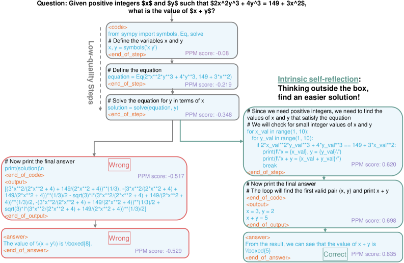
Figure 4: An example of intrinsic self-reflection during rStar-Math deep thinking.
The emergence of intrinsic self-reflection capability. A key breakthrough in OpenAI o1 is its intrinsic self-reflection capability. When the model makes an error, it recognizes the mistake and can self-correct with a correct answer (Noam Brown and Lightman, 2024). Yet it has consistently been found to be largely ineffective in open-sourced LLMs. The community has actively explored various approaches, including self-correction (Huang et al., 2023; Kumar et al., 2024), self-reflection (Renze and Guven, 2024; Shinn et al., 2024), to explicitly train or prompt LLMs to develop such capability.
In our experiments, we unexpectedly observe that our MCTS-driven deep thinking exhibits self-reflection during problem-solving. As shown in Fig. 4, the model initially formalizes an equation using SymPy in the first three steps, which would lead to an incorrect answer (left branch). Interestingly, in the fourth step (right branch), the policy model recognizes the low quality of its earlier steps and refrains from continuing along the initial problem-solving path. Instead, it backtracks and resolves the problem using a new, simpler approach, ultimately arriving at the correct answer. An additional example of self-correction is provided in Appendix A.2. Notably, no self-reflection training data or prompt was included, suggesting that advanced System 2 reasoning can foster intrinsic self-reflection.
<details>
<summary>ppm_study.png Details</summary>
### Visual Description
## [Bar Chart]: Performance Comparison of Math Problem-Solving Models
### Overview
This image is a horizontal bar chart comparing the Pass@1 accuracy (%) of four different AI models across five mathematical benchmarks. The chart evaluates both a base "Policy model" and the improvement achieved through additional methods (PPM for rStar models, ORM for the Qwen model). The benchmarks are MATH, AIME 2024, AMC 2023, Olympiad Bench, and College Math.
### Components/Axes
* **Legend (Top Center):**
* `rStar Policy model` (Light Green)
* `rStar 7B PPM improvement` (Dark Green)
* `Qwen 72B Policy model` (Light Blue)
* `Qwen 72B ORM improvement` (Light Purple)
* **Vertical Axis (Left):** Lists the four models being compared:
1. `rStar-Math (Qwen7B)`
2. `rStar-Math (Qwen1.5B)`
3. `rStar-Math (Phi3.8B)`
4. `Qwen2.5-Math-72B`
* **Horizontal Axes (Bottom of each column):** Each benchmark has its own x-axis labeled `Pass@1 accuracy (%)` with varying scales (0-100 for MATH, 0-40 for AIME, 0-100 for AMC, 0-50 for Olympiad, 0-50 for College Math).
* **Column Headers (Top of each data column):** The five benchmarks: `MATH`, `AIME 2024`, `AMC 2023`, `Olympiad Bench`, `College Math`.
### Detailed Analysis
The chart is segmented into five vertical columns, one per benchmark. Each column contains four horizontal bars, one for each model. Each bar is split into two segments: the left segment (light color) represents the base policy model's accuracy, and the right segment (darker color) represents the improvement from the additional method (PPM or ORM). The total accuracy is the sum of both segments, indicated by a number at the end of the bar.
**1. MATH Benchmark:**
* **rStar-Math (Qwen7B):** Policy: 78.4%, Total: 89.4% (Improvement: +11.0%)
* **rStar-Math (Qwen1.5B):** Policy: 74.8%, Total: 87.8% (Improvement: +13.0%)
* **rStar-Math (Phi3.8B):** Policy: 68.0%, Total: 85.4% (Improvement: +17.4%)
* **Qwen2.5-Math-72B:** Policy: 85.6%, Total: 85.8% (Improvement: +0.2%)
**2. AIME 2024 Benchmark:**
* **rStar-Math (Qwen7B):** Policy: 26.7%, Total: 50.0% (Improvement: +23.3%)
* **rStar-Math (Qwen1.5B):** Policy: 13.3%, Total: 46.7% (Improvement: +33.4%)
* **rStar-Math (Phi3.8B):** Policy: 10.0%, Total: 40.0% (Improvement: +30.0%)
* **Qwen2.5-Math-72B:** Policy: 30.0%, Total: 36.7% (Improvement: +6.7%)
**3. AMC 2023 Benchmark:**
* **rStar-Math (Qwen7B):** Policy: 47.5%, Total: 87.5% (Improvement: +40.0%)
* **rStar-Math (Qwen1.5B):** Policy: 47.5%, Total: 80.0% (Improvement: +32.5%)
* **rStar-Math (Phi3.8B):** Policy: 37.5%, Total: 77.5% (Improvement: +40.0%)
* **Qwen2.5-Math-72B:** Policy: 70.0%, Total: 72.5% (Improvement: +2.5%)
**4. Olympiad Bench Benchmark:**
* **rStar-Math (Qwen7B):** Policy: 47.1%, Total: 65.3% (Improvement: +18.2%)
* **rStar-Math (Qwen1.5B):** Policy: 42.5%, Total: 63.5% (Improvement: +21.0%)
* **rStar-Math (Phi3.8B):** Policy: 36.6%, Total: 59.3% (Improvement: +22.7%)
* **Qwen2.5-Math-72B:** Policy: 49.0%, Total: 54.5% (Improvement: +5.5%)
**5. College Math Benchmark:**
* **rStar-Math (Qwen7B):** Policy: 52.5%, Total: 59.0% (Improvement: +6.5%)
* **rStar-Math (Qwen1.5B):** Policy: 50.1%, Total: 59.0% (Improvement: +8.9%)
* **rStar-Math (Phi3.8B):** Policy: 49.5%, Total: 50.6% (Improvement: +1.1%)
* **Qwen2.5-Math-72B:** Policy: 49.5%, Total: 50.6% (Improvement: +1.1%)
### Key Observations
1. **Consistent Improvement:** All three `rStar-Math` models show substantial accuracy gains from the PPM method across all benchmarks, with the improvement segments (dark green) being visually prominent.
2. **Diminishing Returns for Large Model:** The `Qwen2.5-Math-72B` model shows very small improvements from the ORM method (light purple slivers), especially on MATH (+0.2%) and College Math (+1.1%).
3. **Benchmark Difficulty:** Performance varies greatly by benchmark. AIME 2024 yields the lowest scores (max 50%), while MATH and AMC 2023 allow for higher total accuracies (up to 89.4% and 87.5%, respectively).
4. **Model Scaling Trend:** Within the rStar models, the one based on the largest policy model (Qwen7B) generally achieves the highest total accuracy, but the smaller models (Qwen1.5B, Phi3.8B) often show larger *relative* improvements from PPM.
### Interpretation
This chart demonstrates the effectiveness of the "PPM" (likely a planning or process-based method) in boosting the mathematical reasoning performance of medium-sized language models (7B, 1.5B, 3.8B parameters). The gains are most dramatic on challenging competition-style benchmarks like AIME and AMC, where the base policy model's performance is low, suggesting PPM is particularly valuable for complex, multi-step problem-solving.
In contrast, the "ORM" (likely an outcome-based reward model) applied to the very large `Qwen2.5-Math-72B` provides minimal additional benefit. This implies that for state-of-the-art large models already fine-tuned for math, outcome-based verification may have reached a performance ceiling, or that the specific ORM method used here is less effective than PPM for these tasks. The data argues that architectural or methodological innovations (like PPM) can be more impactful than simply scaling up model size for achieving high performance on difficult mathematical reasoning tasks.
</details>
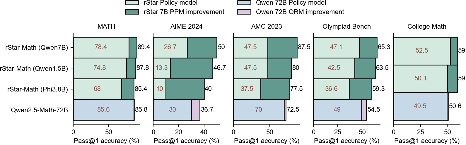
Figure 5: Pass@1 accuracy of policy models and their accuracy after applying System 2 reasoning with various reward models, shows that reward models primarily determine the final performance.
PPM shapes the reasoning boundary in System 2 deep thinking. Both the policy and reward models are crucial for System 2 deep reasoning. Our experiments show that once the policy model attains a reasonably strong capability level, (see Appendix A.1 ), the PPM becomes the key determinant of the upper performance limit. Fig. 5 summarizes the accuracy of policy models of different sizes, as well as the improvements achieved with reward models. Despite variations in Pass@1 accuracy due to differences in training strategies, datasets, and model scales, the reward model proves to be the dominant factor in System 2 reasoning. For instance, although the SFT accuracy of rStar-Math-7B is lower than Qwen2.5-Math-72B-Instruct, pairing it with our 7B PPM allows rStar-Math to outperform the 72B policy model with Qwen 72B ORM. Moreover, despite varying Pass@1 accuracy across our three policy SLM sizes, the final reasoning accuracy converges after applying the PPM.
PPM spots theorem-application steps. When solving challenging math problems, identifying and applying relevant theorems or key conclusions often form the cornerstone of successful problem-solving (Xin et al., 2024). In our experiments, we find that during rStar-Math problem-solving, our PPM effectively identifies critical theorem-application intermediate steps within policy model’s deep thinking process. These steps are predicted with high reward scores, guiding the policy model to generate the correct solution. Appendix A.2 provides examples where the PPM successfully identifies key theorems such as Fermat’s little theorem (Weisstein, a), Vieta’s formulas (Weisstein, b), the AM-GM inequality (amg, ), the Pythagorean theorem (pyt, ), and the Shoelace Theorem (sho, ), etc.
Generalization discussions. rStar-Math offers a general methodology for improving LLM reasoning applicable to various domains. First, rStar-Math can generalize to more challenging math tasks, such as theorem proving, though its current focus is on word problems due to dataset limitations. Nonetheless, rStar-Math demonstrates the potential to prove mathematical statements. As shown in Appendix A.2, it successfully proves an Olympiad-level problem involving Fermat’s Little Theorem, providing a step-by-step correct proof through its deep reasoning process. Second, rStar-Mathcan generalize to other domains, such as code and commonsense reasoning. Notably, synthesizing step-by-step verified training trajectories for general reasoning requires a mechanism to provide feedback on whether a given trajectory reaches the desired output at the end of MCTS rollout. For instance, in code reasoning, this could involve designing extensive test cases; in general reasoning, feedback could be obtained through human labeling or mutual verification with another LLM (Qi et al., 2024).
## 6 Conclusion
In this work, we present rStar-Math, a self-evolved System 2 deep thinking approach that significantly boosts the math reasoning capabilities of small LLMs, achieving state-of-the-art OpenAI o1-level performance. Our approach demonstrates that SLMs can self-generate high-quality training data for frontier-level math reasoning. Extensive experiments across four different-sized SLMs and challenging math benchmarks demonstrate the superiority of rStar-Math, with achieving leading results while outperforming existing math reasoning LLMs and Best-of-N baselines. We also reveal key findings, including the emergence of self-reflection and the effectiveness of the PPM in identifying critical intermediate steps, such as theorem-application steps. Finally, rStar-Math can achieve further improvements by collecting more challenging math problems, we leave this as future work.
## Acknowledgement
In the early stages of this work, we faced significant challenges due to limited GPU resources and restricted access to the GPT-4 API. We are deeply grateful to Qiufeng Yin and Chengmin Chi for their assistance in collecting math problems and providing GPT-4 resources for new math problem synthesis. Special thanks go to my colleagues, Lingxiao Ma, Ying Cao, Baotong Lu, Jing Liu, Jiahang Xu, Chengruidong Zhang, Siyuan Wang, Gaokai Zhang, Yujian Li, and Yang Wang, for generously sharing their GPU quotas with us.
## References
- [1] Inequality of arithmetic and geometric means. URL https://artofproblemsolving.com/wiki/index.php/AM-GM_Inequality.
- [2] Pythagorean theorem. URL https://en.wikipedia.org/wiki/Pythagorean_theorem.
- [3] Shoelace theorem. URL https://artofproblemsolving.com/wiki/index.php/Shoelace_Theorem.
- Abdin et al. [2024] Marah Abdin, Sam Ade Jacobs, Ammar Ahmad Awan, Jyoti Aneja, Ahmed Awadallah, Hany Awadalla, Nguyen Bach, Amit Bahree, Arash Bakhtiari, Harkirat Behl, et al. Phi-3 technical report: A highly capable language model locally on your phone. arXiv preprint arXiv:2404.14219, 2024.
- AI-MO [2024a] AI-MO. Aime 2024, 2024a. URL https://huggingface.co/datasets/AI-MO/aimo-validation-aime.
- AI-MO [2024b] AI-MO. Amc 2023, 2024b. URL https://huggingface.co/datasets/AI-MO/aimo-validation-amc.
- Brown et al. [2024] Bradley Brown, Jordan Juravsky, Ryan Ehrlich, Ronald Clark, Quoc V Le, Christopher Ré, and Azalia Mirhoseini. Large language monkeys: Scaling inference compute with repeated sampling. arXiv preprint arXiv:2407.21787, 2024.
- Chen et al. [2024] Guoxin Chen, Minpeng Liao, Chengxi Li, and Kai Fan. Alphamath almost zero: process supervision without process, 2024.
- Cobbe et al. [2021] Karl Cobbe, Vineet Kosaraju, Mohammad Bavarian, Mark Chen, Heewoo Jun, Lukasz Kaiser, Matthias Plappert, Jerry Tworek, Jacob Hilton, Reiichiro Nakano, et al. Training verifiers to solve math word problems. arXiv preprint arXiv:2110.14168, 2021.
- Daniel [2011] Kahneman Daniel. Thinking, fast and slow. Macmillan, 2011.
- Dubey et al. [2024] Abhimanyu Dubey, Abhinav Jauhri, Abhinav Pandey, Abhishek Kadian, Ahmad Al-Dahle, Aiesha Letman, Akhil Mathur, Alan Schelten, Amy Yang, Angela Fan, et al. The llama 3 herd of models. arXiv preprint arXiv:2407.21783, 2024.
- Gou et al. [2023] Zhibin Gou, Zhihong Shao, Yeyun Gong, Yujiu Yang, Minlie Huang, Nan Duan, Weizhu Chen, et al. Tora: A tool-integrated reasoning agent for mathematical problem solving. arXiv preprint arXiv:2309.17452, 2023.
- Hao et al. [2023] Shibo Hao, Yi Gu, Haodi Ma, Joshua Jiahua Hong, Zhen Wang, Daisy Zhe Wang, and Zhiting Hu. Reasoning with language model is planning with world model. arXiv preprint arXiv:2305.14992, 2023.
- He et al. [2024] Chaoqun He, Renjie Luo, Yuzhuo Bai, Shengding Hu, Zhen Leng Thai, Junhao Shen, Jinyi Hu, Xu Han, Yujie Huang, Yuxiang Zhang, et al. Olympiadbench: A challenging benchmark for promoting agi with olympiad-level bilingual multimodal scientific problems. arXiv preprint arXiv:2402.14008, 2024.
- Huang et al. [2023] Jie Huang, Xinyun Chen, Swaroop Mishra, Huaixiu Steven Zheng, Adams Wei Yu, Xinying Song, and Denny Zhou. Large language models cannot self-correct reasoning yet. arXiv preprint arXiv:2310.01798, 2023.
- Huang et al. [2024] Zhen Huang, Haoyang Zou, Xuefeng Li, Yixiu Liu, Yuxiang Zheng, Ethan Chern, Shijie Xia, Yiwei Qin, Weizhe Yuan, and Pengfei Liu. O1 replication journey – part 2: Surpassing o1-preview through simple distillation big progress or bitter lesson? Github, 2024. URL https://github.com/GAIR-NLP/O1-Journey.
- Jia LI and Polu [2024a] Lewis Tunstall Ben Lipkin Roman Soletskyi Shengyi Costa Huang Kashif Rasul Longhui Yu Albert Jiang Ziju Shen Zihan Qin Bin Dong Li Zhou Yann Fleureau Guillaume Lample Jia LI, Edward Beeching and Stanislas Polu. Numinamath. [https://github.com/project-numina/aimo-progress-prize](https://github.com/project-numina/aimo-progress-prize/blob/main/report/numina_dataset.pdf), 2024a.
- Jia LI and Polu [2024b] Lewis Tunstall Ben Lipkin Roman Soletskyi Shengyi Costa Huang Kashif Rasul Longhui Yu Albert Jiang Ziju Shen Zihan Qin Bin Dong Li Zhou Yann Fleureau Guillaume Lample Jia LI, Edward Beeching and Stanislas Polu. Numinamath cot, 2024b. URL https://huggingface.co/datasets/AI-MO/NuminaMath-CoT.
- Kang et al. [2024] Jikun Kang, Xin Zhe Li, Xi Chen, Amirreza Kazemi, and Boxing Chen. Mindstar: Enhancing math reasoning in pre-trained llms at inference time. arXiv preprint arXiv:2405.16265, 2024.
- Kocsis and Szepesvári [2006] Levente Kocsis and Csaba Szepesvári. Bandit based monte-carlo planning. volume 2006, pages 282–293, 09 2006. ISBN 978-3-540-45375-8. doi: 10.1007/11871842_29.
- Kumar et al. [2024] Aviral Kumar, Vincent Zhuang, Rishabh Agarwal, Yi Su, John D Co-Reyes, Avi Singh, Kate Baumli, Shariq Iqbal, Colton Bishop, Rebecca Roelofs, et al. Training language models to self-correct via reinforcement learning. arXiv preprint arXiv:2409.12917, 2024.
- Lanham et al. [2023] Tamera Lanham, Anna Chen, Ansh Radhakrishnan, Benoit Steiner, Carson Denison, Danny Hernandez, Dustin Li, Esin Durmus, Evan Hubinger, Jackson Kernion, et al. Measuring faithfulness in chain-of-thought reasoning. arXiv preprint arXiv:2307.13702, 2023.
- Li et al. [2024] Chen Li, Weiqi Wang, Jingcheng Hu, Yixuan Wei, Nanning Zheng, Han Hu, Zheng Zhang, and Houwen Peng. Common 7b language models already possess strong math capabilities. arXiv preprint arXiv:2403.04706, 2024.
- Liao et al. [2024] Minpeng Liao, Wei Luo, Chengxi Li, Jing Wu, and Kai Fan. Mario: Math reasoning with code interpreter output–a reproducible pipeline. arXiv preprint arXiv:2401.08190, 2024.
- Lightman et al. [2023] Hunter Lightman, Vineet Kosaraju, Yura Burda, Harri Edwards, Bowen Baker, Teddy Lee, Jan Leike, John Schulman, Ilya Sutskever, and Karl Cobbe. Let’s verify step by step. arXiv preprint arXiv:2305.20050, 2023.
- Lightman et al. [2024] Hunter Lightman, Vineet Kosaraju, Yuri Burda, Harrison Edwards, Bowen Baker, Teddy Lee, Jan Leike, John Schulman, Ilya Sutskever, and Karl Cobbe. Let’s verify step by step. In The Twelfth International Conference on Learning Representations, 2024. URL https://openreview.net/forum?id=v8L0pN6EOi.
- Liu et al. [2024] Aixin Liu, Bei Feng, Bing Xue, Bingxuan Wang, Bochao Wu, Chengda Lu, Chenggang Zhao, Chengqi Deng, Chenyu Zhang, Chong Ruan, et al. Deepseek-v3 technical report. arXiv preprint arXiv:2412.19437, 2024.
- Luo et al. [2023] Haipeng Luo, Qingfeng Sun, Can Xu, Pu Zhao, Jianguang Lou, Chongyang Tao, Xiubo Geng, Qingwei Lin, Shifeng Chen, and Dongmei Zhang. Wizardmath: Empowering mathematical reasoning for large language models via reinforced evol-instruct. arXiv preprint arXiv:2308.09583, 2023.
- Luo et al. [2024] Liangchen Luo, Yinxiao Liu, Rosanne Liu, Samrat Phatale, Harsh Lara, Yunxuan Li, Lei Shu, Yun Zhu, Lei Meng, Jiao Sun, et al. Improve mathematical reasoning in language models by automated process supervision. arXiv preprint arXiv:2406.06592, 2024.
- Microsoft [2024] Microsoft. Phi-3-mini-4k-instruct, 2024. URL https://huggingface.co/microsoft/Phi-3-mini-4k-instruct.
- Noam Brown and Lightman [2024] Ilge Akkaya Noam Brown and Hunter Lightman. Openai’s noam brown, ilge akkaya and hunter lightman on o1 and teaching llms to reason better, 2024. URL https://www.youtube.com/watch?v=jPluSXJpdrA.
- OpenAI [2023] OpenAI. Gpt-4 technical report. 2023.
- OpenAI [2024] OpenAI. Openai o1 system card. preprint, 2024.
- Ouyang et al. [2022] Long Ouyang, Jeffrey Wu, Xu Jiang, Diogo Almeida, Carroll Wainwright, Pamela Mishkin, Chong Zhang, Sandhini Agarwal, Katarina Slama, Alex Ray, et al. Training language models to follow instructions with human feedback. Advances in Neural Information Processing Systems, 35:27730–27744, 2022.
- Qi et al. [2024] Zhenting Qi, Mingyuan Ma, Jiahang Xu, Li Lyna Zhang, Fan Yang, and Mao Yang. Mutual reasoning makes smaller llms stronger problem-solvers. arXiv preprint arXiv:2408.06195, 2024.
- Qwen [2024a] Qwen. Qwen2-math-7b, 2024a. URL https://huggingface.co/Qwen/Qwen2-Math-7B.
- Qwen [2024b] Qwen. Qwen2.5-math-1.5b, 2024b. URL https://huggingface.co/Qwen/Qwen2.5-Math-1.5B.
- Qwen [2024c] Qwen. Qwen2.5-math-7b, 2024c. URL https://huggingface.co/Qwen/Qwen2.5-Math-7B.
- Renze and Guven [2024] Matthew Renze and Erhan Guven. Self-reflection in llm agents: Effects on problem-solving performance. arXiv preprint arXiv:2405.06682, 2024.
- Shinn et al. [2024] Noah Shinn, Federico Cassano, Ashwin Gopinath, Karthik Narasimhan, and Shunyu Yao. Reflexion: Language agents with verbal reinforcement learning. Advances in Neural Information Processing Systems, 36, 2024.
- Silver et al. [2017] David Silver, Thomas Hubert, Julian Schrittwieser, Ioannis Antonoglou, Matthew Lai, Arthur Guez, Marc Lanctot, Laurent Sifre, Dharshan Kumaran, Thore Graepel, et al. Mastering chess and shogi by self-play with a general reinforcement learning algorithm. arXiv preprint arXiv:1712.01815, 2017.
- Snell et al. [2024] Charlie Snell, Jaehoon Lee, Kelvin Xu, and Aviral Kumar. Scaling llm test-time compute optimally can be more effective than scaling model parameters. arXiv preprint arXiv:2408.03314, 2024.
- Tang et al. [2024] Zhengyang Tang, Xingxing Zhang, Benyou Wan, and Furu Wei. Mathscale: Scaling instruction tuning for mathematical reasoning. arXiv preprint arXiv:2403.02884, 2024.
- Team [2024a] Qwen Team. Qwq: Reflect deeply on the boundaries of the unknown, November 2024a. URL https://qwenlm.github.io/blog/qwq-32b-preview/.
- Team [2024b] The Mistral AI Team. Mathstral-7b-v0.1, 2024b. URL https://huggingface.co/mistralai/Mathstral-7B-v0.1.
- Toshniwal et al. [2024] Shubham Toshniwal, Wei Du, Ivan Moshkov, Branislav Kisacanin, Alexan Ayrapetyan, and Igor Gitman. Openmathinstruct-2: Accelerating ai for math with massive open-source instruction data. arXiv preprint arXiv:2410.01560, 2024.
- Valmeekam et al. [2023] Karthik Valmeekam, Sarath Sreedharan, Matthew Marquez, Alberto Olmo, and Subbarao Kambhampati. On the planning abilities of large language models (a critical investigation with a proposed benchmark). arXiv preprint arXiv:2302.06706, 2023.
- Wang et al. [2024a] Chaojie Wang, Yanchen Deng, Zhiyi Lv, Shuicheng Yan, and An Bo. Q*: Improving multi-step reasoning for llms with deliberative planning, 2024a.
- Wang et al. [2024b] Ke Wang, Houxing Ren, Aojun Zhou, Zimu Lu, Sichun Luo, Weikang Shi, Renrui Zhang, Linqi Song, Mingjie Zhan, and Hongsheng Li. Mathcoder: Seamless code integration in LLMs for enhanced mathematical reasoning. In The Twelfth International Conference on Learning Representations, 2024b. URL https://openreview.net/forum?id=z8TW0ttBPp.
- Wang et al. [2024c] Peiyi Wang, Lei Li, Zhihong Shao, R. X. Xu, Damai Dai, Yifei Li, Deli Chen, Y. Wu, and Zhifang Sui. Math-shepherd: Verify and reinforce llms step-by-step without human annotations, 2024c.
- Wang et al. [2023] Xuezhi Wang, Jason Wei, Dale Schuurmans, Quoc V Le, Ed H. Chi, Sharan Narang, Aakanksha Chowdhery, and Denny Zhou. Self-consistency improves chain of thought reasoning in language models. In The Eleventh International Conference on Learning Representations, 2023. URL https://openreview.net/forum?id=1PL1NIMMrw.
- Weisstein [a] Eric W. Weisstein. Fermat’s little theorem, a. URL https://mathworld.wolfram.com/FermatsLittleTheorem.html.
- Weisstein [b] Eric W. Weisstein. Vieta’s formulas, from mathworld—a wolfram web resource, b. URL http://mathworld.wolfram.com/Tree.html.
- Wu et al. [2024] Yangzhen Wu, Zhiqing Sun, Shanda Li, Sean Welleck, and Yiming Yang. An empirical analysis of compute-optimal inference for problem-solving with language models. arXiv preprint arXiv:2408.00724, 2024.
- Xin et al. [2024] Huajian Xin, Daya Guo, Zhihong Shao, Zhizhou Ren, Qihao Zhu, Bo Liu, Chong Ruan, Wenda Li, and Xiaodan Liang. Deepseek-prover: Advancing theorem proving in llms through large-scale synthetic data. arXiv preprint arXiv:2405.14333, 2024.
- Yang et al. [2024] An Yang, Beichen Zhang, Binyuan Hui, Bofei Gao, Bowen Yu, Chengpeng Li, Dayiheng Liu, Jianhong Tu, Jingren Zhou, Junyang Lin, et al. Qwen2. 5-math technical report: Toward mathematical expert model via self-improvement. arXiv preprint arXiv:2409.12122, 2024.
- Yao et al. [2024] Shunyu Yao, Dian Yu, Jeffrey Zhao, Izhak Shafran, Tom Griffiths, Yuan Cao, and Karthik Narasimhan. Tree of thoughts: Deliberate problem solving with large language models. Advances in Neural Information Processing Systems, 36, 2024.
- Yu et al. [2023a] Fei Yu, Anningzhe Gao, and Benyou Wang. Outcome-supervised verifiers for planning in mathematical reasoning. arXiv preprint arXiv:2311.09724, 2023a.
- Yu et al. [2023b] Longhui Yu, Weisen Jiang, Han Shi, Jincheng Yu, Zhengying Liu, Yu Zhang, James T Kwok, Zhenguo Li, Adrian Weller, and Weiyang Liu. Metamath: Bootstrap your own mathematical questions for large language models. arXiv preprint arXiv:2309.12284, 2023b.
- Yuan et al. [2023] Zheng Yuan, Hongyi Yuan, Chengpeng Li, Guanting Dong, Keming Lu, Chuanqi Tan, Chang Zhou, and Jingren Zhou. Scaling relationship on learning mathematical reasoning with large language models. arXiv preprint arXiv:2308.01825, 2023.
- Zhang et al. [2024a] Dan Zhang, Sining Zhoubian, Ziniu Hu, Yisong Yue, Yuxiao Dong, and Jie Tang. Rest-mcts*: Llm self-training via process reward guided tree search. arXiv preprint arXiv:2406.03816, 2024a.
- Zhang et al. [2024b] Di Zhang, Jiatong Li, Xiaoshui Huang, Dongzhan Zhou, Yuqiang Li, and Wanli Ouyang. Accessing gpt-4 level mathematical olympiad solutions via monte carlo tree self-refine with llama-3 8b. arXiv preprint arXiv:2406.07394, 2024b.
- Zheng et al. [2023] Lianmin Zheng, Wei-Lin Chiang, Ying Sheng, Siyuan Zhuang, Zhanghao Wu, Yonghao Zhuang, Zi Lin, Zhuohan Li, Dacheng Li, Eric Xing, Hao Zhang, Joseph E. Gonzalez, and Ion Stoica. Judging LLM-as-a-judge with MT-bench and chatbot arena. In Thirty-seventh Conference on Neural Information Processing Systems Datasets and Benchmarks Track, 2023.
## Appendix A Appendix
### A.1 Additional Experiments and Details
Data Generation Details. As detailed in Sec. 3.4, each round starts by self-generating step-by-step verified trajectories for 747k math word problems. The maximum tree depth $d$ is set to 16, with 16 MCTS rollouts conducted per problem by default. At each step, we allow to explore 8 candidate nodes, and the constant $c$ in Eq. 1 is set to 2 to promote greater exploration. In the bootstrap round, due to the large size of the initial policy model (236B), we used smaller parameters: 8 rollouts and 5 candidate nodes per step. To improve the accuracy of solving challenging problems in round 4, we increase the number of candidate nodes to 16 and conduct 2 MCTS tree expansions per problem using different random seeds. Detailed prompts are available in Appendix A.3.
Training Details. In each round, we collect step-by-step verified trajectories to fine-tune the policy LLM and train the PPM. To reduce noise in synthetic math problems (e.g., incorrect ground-truth answers labeled by GPT-4), we remove synthetic problems with trajectories achieving less than 50% accuracy. Based on our extensive experiments, the policy LLM is fine-tuned from the initial base model in each round, rather than training incrementally on the model from the previous round. All policy SLMs are trained for 2 epochs with a sequence length of 4096 tokens and a batch size of 128. We use AdamW optimizer with a linear learning rate scheduler, setting the initial learning rate to 7e-6 for Qwen models, and a cosine scheduler with an initial learning rate of 5e-6 for Phi3-mini-Instruct. The PPM is trained for 1 epoch with a batch size of 512 and an initial learning rate of 7e-6.
Training the ORM and PQM. The Outcome Reward Model (ORM) and the Q-value-based Process Reward Model (PQM) share the same model architecture and training parameters with our PPM. To train the ORM, we collect trajectories from math problems containing both correct and incorrect solutions. Specifically, the two trajectories with the highest average Q-values are selected as positive examples, while the two with the lowest are chosen as negative examples. Following Qwen2.5-Math (Yang et al., 2024), we adopt the pairwise ranking loss (Ouyang et al., 2022) to optimize the ORM. To train the PQM, we follow Chen et al. (2024) to use step-level Q-values as reward labels. Let $\mathbf{x}=x\oplus s_{1}\oplus s_{2}\oplus...\oplus s_{d}$ be the trajectory, with annotated Q-values $\mathbf{Q}=(Q(s_{1}),Q(s_{1}),...,Q(s_{d}))$ and predicted Q-values $\mathbf{Q^{\prime}}=(Q^{\prime}(s_{1}),Q^{\prime}(s_{1}),...,Q^{\prime}(s_{d}))$ for each step. To stabilize PQM training, we treat each trajectory as a single training sample and predict Q-values for all steps simultaneously, rather than splitting it into individual per-step samples. Specifically, to predict the Q-value $Q^{\prime}(s_{i})$ for step $s_{i}$ , PQM takes the trajectory from the question up to step $s_{i}$ (i.e., $x\oplus s_{1}\oplus s_{2}\oplus...\oplus s_{i}$ ) as input and outputs a value between -1 and 1. We use a mean squared error (MSE) loss for PQM training:
$$
\mathcal{L}_{prm}(\bf{x})=\|\bf{Q}-\bf{Q^{\prime}}\|^{2} \tag{6}
$$
Self-evolution Inference Costs. In the initial bootstrap round, we use DeepSeek-Coder-v2-Instruct (236B) as the policy model, using 10 nodes of 8×80GB H100 GPUs with 8 MCTS rollouts. This required approximately two weeks to finish the data generation. For rounds 2–4, using our fine-tuned 7B SLM as the policy model, data generation was performed on 15 nodes of 4×40GB A100 GPUs, with each round completed in three days. In the final round, to include more challenging problems, we increased the number of MCTS rollouts to 64, extending the data generation time to one week.
Table 9: Inference costs of rStar-Math. We show the average number of generated tokens required to generate a trajectory for a given question.
| MATH | AIME 2024 | AMC 2023 | Olympiad Bench | College Math | GSM8K | GaokaoEn 2023 |
| --- | --- | --- | --- | --- | --- | --- |
| 5453 | 15693 | 14544 | 7889 | 4503 | 3299 | 6375 |
Inference Setting. In our evaluation, we run multiple MCTS to generate candidate solution trajectories. For each problem, we generate 32 candidate nodes at each step and use the PPM to score each node. Since the PPM effectively provides step-level quality evaluations, we limit MCTS to just 4 rollouts per step to update the Q-values. After completing MCTS, the trajectory with the highest PPM score is selected as the final answer. Table 9 presents the average number of tokens generated to produce a trajectory in MCTS.
Table 10: Pass@1 (greedy) accuracy of our fine-tuned policy models for Phi3-mini, Qwen2.5-Math-1.5B, Qwen2-Math-7B and Qwen2.5-Math-7B.
| Model | MATH | AIME 2024 | AMC 2023 | Olympiad Bench | College Math | GSM8K | GaokaoEn 2023 |
| --- | --- | --- | --- | --- | --- | --- | --- |
| General Base Model: Phi3-mini-Instruct (3.8B) | | | | | | | |
| Phi3-mini-Instruct | 41.4 | 3.33 | 7.5 | 12.3 | 33.1 | 85.7 | 37.1 |
| Our policy model | 68.0 | 10.0 | 37.5 | 36.6 | 48.7 | 87.9 | 53.2 |
| Math-Specialized Base Model: Qwen2.5-Math-1.5B | | | | | | | |
| Qwen2.5-Math-1.5B | 51.2 | 0.0 | 22.5 | 16.7 | 38.4 | 74.6 | 46.5 |
| Qwen2.5-Math-1.5B-Instruct | 60.0 | 10.0 | 60.0 | 38.1 | 47.7 | 84.8 | 65.5 |
| Our policy model | 74.8 | 13.3 | 47.5 | 42.5 | 50.1 | 83.1 | 58.7 |
| Math-Specialized Base Model: Qwen2-Math-7B | | | | | | | |
| Qwen2-Math-7B | 53.4 | 3.3 | 25.0 | 17.3 | 39.4 | 80.4 | 47.3 |
| Qwen2-Math-7B-Instruct | 73.2 | 13.3 | 62.5 | 38.2 | 45.9 | 89.9 | 62.1 |
| Our policy model | 73.8 | 16.7 | 45.0 | 43.9 | 52.0 | 88.3 | 65.2 |
| Math-Specialized Base Model: Qwen2.5-Math-7B | | | | | | | |
| Qwen2.5-Math-7B | 58.8 | 0.0 | 22.5 | 21.8 | 41.6 | 91.6 | 51.7 |
| Qwen2.5-Math-7B-Instruct | 82.6 | 6.0 | 62.5 | 41.6 | 46.8 | 95.2 | 66.8 |
| Our policy model | 78.4 | 26.7 | 47.5 | 47.1 | 52.5 | 89.7 | 65.7 |
<details>
<summary>passnrandom.png Details</summary>
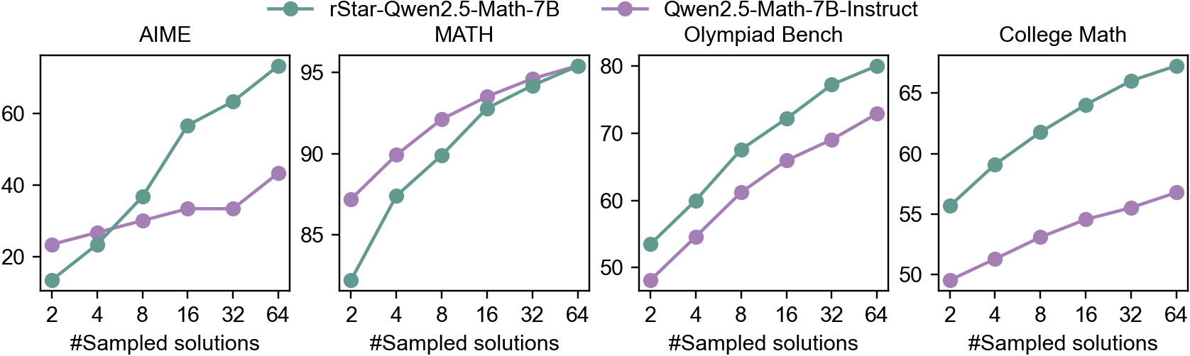
### Visual Description
## [Multi-Panel Line Chart]: Performance of Two Models on Math Benchmarks vs. Number of Sampled Solutions
### Overview
The image displays four separate line charts arranged horizontally, comparing the performance of two language models on four different mathematical benchmarks. The performance metric (y-axis) is plotted against the number of sampled solutions (x-axis). The two models are distinguished by color: a teal line for `rStar-Qwen2.5-Math-7B` and a purple line for `Qwen2.5-Math-7B-Instruct`.
### Components/Axes
* **Legend:** Located at the top center of the entire figure.
* Teal line with circle markers: `rStar-Qwen2.5-Math-7B`
* Purple line with circle markers: `Qwen2.5-Math-7B-Instruct`
* **Common X-Axis (All Charts):** Label: `#Sampled solutions`. Ticks and values: `2`, `4`, `8`, `16`, `32`, `64`.
* **Individual Chart Y-Axes:** Each chart has its own y-axis scale, representing a performance score (likely accuracy percentage).
* **AIME (Leftmost Chart):** Y-axis range approximately 10 to 70. Ticks at `20`, `40`, `60`.
* **MATH (Second from Left):** Y-axis range approximately 80 to 95. Ticks at `85`, `90`, `95`.
* **Olympiad Bench (Third from Left):** Y-axis range approximately 45 to 80. Ticks at `50`, `60`, `70`, `80`.
* **College Math (Rightmost Chart):** Y-axis range approximately 45 to 70. Ticks at `50`, `55`, `60`, `65`.
### Detailed Analysis
Data points are approximate values read from the chart positions.
**1. AIME Chart:**
* **Trend:** Both models show a strong upward trend. The `rStar` model (teal) starts lower but exhibits a much steeper slope, surpassing the `Instruct` model (purple) between 4 and 8 sampled solutions and maintaining a significant lead thereafter.
* **Data Points (Approximate):**
* `rStar-Qwen2.5-Math-7B` (Teal): (2, ~15), (4, ~23), (8, ~37), (16, ~57), (32, ~63), (64, ~68)
* `Qwen2.5-Math-7B-Instruct` (Purple): (2, ~23), (4, ~27), (8, ~30), (16, ~33), (32, ~33), (64, ~43)
**2. MATH Chart:**
* **Trend:** Both models show a consistent upward trend. The `Instruct` model (purple) starts higher, but the `rStar` model (teal) has a slightly steeper slope, nearly converging with the `Instruct` model at 64 samples.
* **Data Points (Approximate):**
* `rStar-Qwen2.5-Math-7B` (Teal): (2, ~82), (4, ~87), (8, ~90), (16, ~93), (32, ~94), (64, ~95)
* `Qwen2.5-Math-7B-Instruct` (Purple): (2, ~87), (4, ~90), (8, ~92), (16, ~93.5), (32, ~94.5), (64, ~95)
**3. Olympiad Bench Chart:**
* **Trend:** Both models show a strong, nearly parallel upward trend. The `rStar` model (teal) consistently outperforms the `Instruct` model (purple) by a margin of approximately 5-8 points across all sample sizes.
* **Data Points (Approximate):**
* `rStar-Qwen2.5-Math-7B` (Teal): (2, ~53), (4, ~60), (8, ~68), (16, ~72), (32, ~77), (64, ~80)
* `Qwen2.5-Math-7B-Instruct` (Purple): (2, ~48), (4, ~54), (8, ~61), (16, ~66), (32, ~69), (64, ~73)
**4. College Math Chart:**
* **Trend:** Both models show a steady upward trend. The `rStar` model (teal) maintains a consistent and significant lead over the `Instruct` model (purple) throughout.
* **Data Points (Approximate):**
* `rStar-Qwen2.5-Math-7B` (Teal): (2, ~56), (4, ~59), (8, ~62), (16, ~64), (32, ~66), (64, ~68)
* `Qwen2.5-Math-7B-Instruct` (Purple): (2, ~49), (4, ~51), (8, ~53), (16, ~55), (32, ~56), (64, ~57)
### Key Observations
1. **Universal Positive Correlation:** For both models and across all four benchmarks, performance improves as the number of sampled solutions increases from 2 to 64.
2. **Model Performance Gap:** The `rStar-Qwen2.5-Math-7B` model (teal) outperforms the `Qwen2.5-Math-7B-Instruct` model (purple) on three of the four benchmarks (AIME, Olympiad Bench, College Math) for most sample sizes. The gap is most pronounced in the AIME and Olympiad Bench tasks.
3. **Benchmark Difficulty:** The absolute performance levels vary significantly by benchmark. The MATH benchmark shows the highest scores (80-95), suggesting it is the "easiest" for these models. AIME shows the widest performance spread and the lowest starting scores, indicating higher difficulty.
4. **Diminishing Returns:** The rate of improvement (slope of the lines) generally decreases as the number of samples increases, particularly visible in the MATH and College Math charts for the `Instruct` model, suggesting diminishing returns from additional sampling.
### Interpretation
This data demonstrates the effectiveness of the `rStar` method (likely a form of self-refinement or reward-guided sampling) when applied to the Qwen2.5-Math-7B base model. The key finding is that `rStar` significantly boosts the model's mathematical problem-solving capabilities compared to its instruction-tuned counterpart (`Instruct`), especially on more challenging competition-style problems (AIME, Olympiad Bench).
The consistent upward trends validate the core premise of sampling multiple solutions: generating and presumably selecting from more candidate answers increases the probability of finding a correct one. The fact that `rStar`'s advantage grows with more samples in the AIME chart suggests its sampling or selection mechanism is particularly effective at leveraging increased computational budget to explore the solution space.
The variation in performance gaps across benchmarks implies that the benefits of the `rStar` approach are not uniform. It provides a massive boost on AIME (where it starts lower but ends much higher) but a more modest, consistent gain on College Math. This could indicate that `rStar` is better suited for problems requiring creative insight or multi-step reasoning (common in Olympiads) versus more procedural college-level math. The near-convergence on the MATH benchmark suggests a performance ceiling for this model size on that specific dataset, where both methods approach maximum achievable accuracy.
</details>
Figure 6: Pass@N accuracy with random sampling from different policy models. Compared to the official Qwen instruct version, our policy model exhibits a stronger ability to sample correct solutions.
<details>
<summary>passnmcts.png Details</summary>
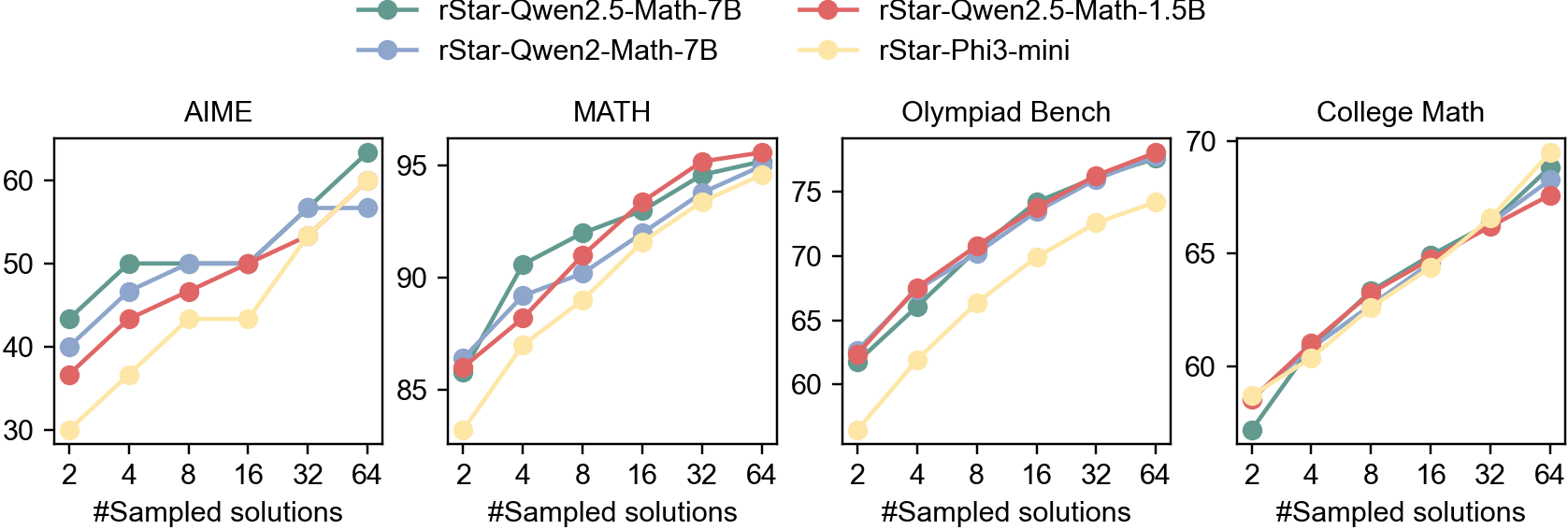
### Visual Description
## [Line Charts (Subplots)]: Performance of Four Models Across Mathematics Benchmarks with Increasing Sampled Solutions
### Overview
The image contains four horizontally arranged line charts (subplots), each representing a distinct mathematics benchmark: **AIME**, **MATH**, **Olympiad Bench**, and **College Math**. Each chart plots the performance (y-axis) of four models against the number of sampled solutions (x-axis, values: 2, 4, 8, 16, 32, 64). Models are distinguished by color:
- Green: *rStar-Qwen2.5-Math-7B*
- Red: *rStar-Qwen2.5-Math-1.5B*
- Blue: *rStar-Qwen2-Math-7B*
- Yellow: *rStar-Phi3-mini*
### Components/Axes
- **Legend**: Positioned at the top, listing four models with corresponding colors (green, red, blue, yellow).
- **X-axis (all charts)**: Labeled *“#Sampled solutions”* with tick marks at 2, 4, 8, 16, 32, 64.
- **Y-axis (per chart)**:
- *AIME*: Range ~30–60 (performance metric, e.g., accuracy).
- *MATH*: Range ~85–95.
- *Olympiad Bench*: Range ~60–75.
- *College Math*: Range ~60–70.
### Detailed Analysis (Per Chart)
#### 1. AIME Chart
- **Trend**: All models show increasing performance with more sampled solutions.
- **Data Points (approximate)**:
- Green (*rStar-Qwen2.5-Math-7B*): ~43 (2), ~50 (4), ~50 (8), ~50 (16), ~57 (32), ~62 (64).
- Red (*rStar-Qwen2.5-Math-1.5B*): ~37 (2), ~43 (4), ~47 (8), ~50 (16), ~53 (32), ~58 (64).
- Blue (*rStar-Qwen2-Math-7B*): ~40 (2), ~47 (4), ~50 (8), ~50 (16), ~57 (32), ~57 (64).
- Yellow (*rStar-Phi3-mini*): ~30 (2), ~37 (4), ~43 (8), ~43 (16), ~53 (32), ~60 (64).
#### 2. MATH Chart
- **Trend**: All models show increasing performance, converging at higher sampled solutions.
- **Data Points (approximate)**:
- Green: ~86 (2), ~90 (4), ~92 (8), ~93 (16), ~94 (32), ~95 (64).
- Red: ~86 (2), ~88 (4), ~91 (8), ~93 (16), ~94 (32), ~95 (64).
- Blue: ~86 (2), ~89 (4), ~91 (8), ~93 (16), ~94 (32), ~95 (64).
- Yellow: ~83 (2), ~87 (4), ~89 (8), ~91 (16), ~93 (32), ~94 (64).
#### 3. Olympiad Bench Chart
- **Trend**: All models show increasing performance, with green, red, blue converging at higher sampled solutions.
- **Data Points (approximate)**:
- Green: ~62 (2), ~66 (4), ~70 (8), ~73 (16), ~74 (32), ~75 (64).
- Red: ~63 (2), ~67 (4), ~70 (8), ~73 (16), ~74 (32), ~75 (64).
- Blue: ~62 (2), ~66 (4), ~70 (8), ~73 (16), ~74 (32), ~75 (64).
- Yellow: ~58 (2), ~62 (4), ~66 (8), ~70 (16), ~72 (32), ~73 (64).
#### 4. College Math Chart
- **Trend**: All models show increasing performance, with yellow (*rStar-Phi3-mini*) slightly outperforming others at 64 sampled solutions.
- **Data Points (approximate)**:
- Green: ~58 (2), ~61 (4), ~63 (8), ~65 (16), ~67 (32), ~69 (64).
- Red: ~59 (2), ~61 (4), ~63 (8), ~65 (16), ~67 (32), ~68 (64).
- Blue: ~59 (2), ~61 (4), ~63 (8), ~65 (16), ~67 (32), ~69 (64).
- Yellow: ~59 (2), ~61 (4), ~63 (8), ~65 (16), ~67 (32), ~70 (64).
### Key Observations
- **Performance Trend**: All models improve with more sampled solutions across all benchmarks, indicating that increasing sampled solutions enhances performance.
- **Model Comparison**:
- In *AIME*, *rStar-Phi3-mini* (yellow) starts lowest but rises to match/exceed others at 64.
- In *MATH*, all models converge to similar high performance at 64.
- In *Olympiad Bench*, green, red, blue converge, while yellow lags slightly.
- In *College Math*, yellow (*rStar-Phi3-mini*) slightly outperforms others at 64.
- **Consistency**: Green (*rStar-Qwen2.5-Math-7B*) and red (*rStar-Qwen2.5-Math-1.5B*) often perform similarly, suggesting comparable performance between the 7B and 1.5B variants.
### Interpretation
The charts demonstrate that increasing sampled solutions (from 2 to 64) consistently improves performance across all models and benchmarks. This suggests that sampling more solutions (e.g., in reasoning/generation tasks) enhances outcomes, likely due to increased diversity/quality of solutions. Convergence at higher sampled solutions (e.g., *MATH*, *Olympiad Bench*) implies diminishing returns or a performance ceiling. The slight outperformance of *rStar-Phi3-mini* in *College Math* at 64 may indicate its strength in that benchmark, while *rStar-Qwen2.5-Math* variants show strong cross-benchmark performance. This data informs how model size (7B vs. 1.5B) and architecture (Qwen2.5-Math vs. Phi3-mini) interact with sampling strategies in mathematical reasoning tasks.
(Note: All values are approximate, based on visual estimation of the charts.)
</details>
Figure 7: Pass@N accuracy with PPM-augmented MCTS. Under the same PPM guidance, the four policy models of varying sizes demonstrate convergent capabilities in sampling correct solutions.
Pass@N. Table 10 compares the math reasoning performance of our policy models with the instruct versions developed by the original model team. Our policy models do not consistently outperform the instruct versions. For example, on the Qwen2.5-Math-7B base model, Qwen2.5-Math-7B-Instruct achieves 4.2% higher accuracy on the MATH benchmark. However, in System 2 deep thinking paradigm, the pass@1 accuracy alone does not fully reflect the reasoning capabilities for the policy model. To provide a more comprehensive evaluation, Fig. 6 and Fig. 7 present the pass@N accuracy. In this metric, the policy model generates $N$ solutions under two settings: random sampling (Fig. 6) and PPM-augmented MCTS deep thinking (Fig. 7). A problem is considered solved if one solution is correct. As shown in Figure 6, our policy model achieves comparable Pass@64 accuracy with Qwen2.5-Math-7B-Instruct on MATH and significantly outperforms it on other benchmarks. Figure 7 further compares the pass@N accuracy of our four policy models (different sizes) after MCTS deep thinking under the same PPM guidance. We can observe that after generating 64 trajectories, the pass@N accuracy of different policy models becomes comparable.
### A.2 Examples of Reasoning Trajectories
Self-correction Example
Question: The coordinates of a parallelogram are (5, 3), (6, 8), (7, 4) and $(x,y)$ and $x>7$ . What is the value of $x+y$ Our trajectory: <code> # Import necessary libraries ⬇ import numpy as np <end_of_step> # Define the coordinates of the parallelogram ⬇ A = np. array ([5, 3]) B = np. array ([6, 8]) C = np. array ([7, 4]) <end_of_step> # Calculate the vector differences to find the missing coordinate D # In a parallelogram, the vector difference between two adjacent sides is equal to the vector difference between the other two adjacent sides # We can use the formula: D = A + (C - B) ⬇ D = A + (C - B) <end_of_step> # Since the coordinates provided are (5, 3), (6, 8), (7, 4) and (x, y), we can infer that the vector from B to C should be the same as the vector from A to the missing point (x, y) # This means: (x - 5, y - 3) = (1, -4) because the vector from B to C is (7 - 6, 4 - 8) = (1, -4) # Solve for x and y ⬇ x = 5 + 1 y = 3 + (-4) <end_of_step> # Verify that the point (x, y) exists and satisfies the condition x > 7 # Since x = 6 is not greater than 7, we need to use the correct formula that maintains the parallelogram property and x > 7 # Correcting the formula to find the other possible D [Self-correction!] ⬇ D = C + (B - A) <end_of_step> # Solve for x and y again ⬇ x = 7 + (6 - 5) y = 4 + (8 - 3) <end_of_step> # Verify that the point (x, y) exists and satisfies the condition x > 7 # Since x = 8 is greater than 7, which satisfies the condition given, we can now find the sum of x and y ⬇ x_plus_y = x + y <end_of_step> # Now print the final answer ⬇ print (x_plus_y) # This should print the value of x + y <end_of_code> <output> 17 <end_of_output> <answer> The value of x + y is $17$ <end_of_answer>
Math statement proof using Fermat’s little theorem
Question: If ( pt+a ) is a perfect square for some value of ( t ), then ( a ${}^{\frac{p-1}{2}}$ - 1 ) is divisible by ( p ) (where ( p ) is a prime number). Our trajectory for proving: <code> # Step 1: Define the variables ⬇ from sympy import symbols, isprime, sqrt, mod_inverse # Define the variables ⬇ p, t, a = symbols (’ p t a ’)\\ <end_of_step> # Step 2: Assume p*t + a is a perfect square # This means there exists an integer k such that p*t + a = k 2 # Rearrange to find a in terms of p, t, and k # a = k 2 - p*t <end_of_step> # Step 3: Use Fermat’s Little Theorem # Fermat’s Little Theorem states that if p is a prime and a is an integer not divisible by p, then a (p-1) $\equiv$ 1 (mod p) # We need to show that a ((p-1)/2) - 1 is divisible by p <end_of_step> # Step 4: Substitute a = k 2 - p*t into Fermat’s Little Theorem # a ((p-1)/2) $\equiv$ (k 2 - p*t) ((p-1)/2) (mod p) # Since p*t is divisible by p, (k 2 - p*t) ((p-1)/2) $\equiv$ k (p-1) (mod p) # By Fermat’s Little Theorem, k (p-1) $\equiv$ 1 (mod p) <end_of_step> # Step 5: Therefore, a ((p-1)/2) $\equiv$ 1 (mod p) # This implies a ((p-1)/2) - 1 $\equiv$ 0 (mod p) # Hence, a ((p-1)/2) - 1 is divisible by p <end_of_step> # Now print the final answer print("The expression a ((p-1)/2) - 1 is divisible by p.") <end_of_code> <output> The expression $a^{((p-1)/2)}$ - 1 is divisible by p. The statement is true. <end_of_output>
Problem-solving with application of the Vieta’s formulas and the AM-GM inequality
Question: Let $a$ be a positive real number such that all the roots of $x^{3}+ax^{2}+ax+1=0$ are real. Find the smallest possible value of $a.$ Our trajectory for proving: <code> # Step 1: Define the polynomial equation from sympy import symbols, solve, Eq # Define the variable and the parameter x, a = symbols(’x a’) <end_of_step> [PPM Score: -0.46430] # Step 2: Define the polynomial equation polynomial = x**3 + a*x**2 + a*x + 1 <end_of_step> [PPM Score: 0.53937] # Step 3: Use Vieta’s formulas to relate the coefficients to the roots # Since the polynomial is monic (leading coefficient is 1), the sum of the roots (taken one at a time) is -a # The sum of the products of the roots taken two at a time is a # The product of the roots is -1 # Since all roots are real, we can denote them as r1, r2, r3 # From Vieta’s formulas: # r1 + r2 + r3 = -a # r1*r2 + r2*r3 + r3*r1 = a # r1*r2*r3 = -1 <end_of_step> [PPM Score: 0.9989] # Step 4: Use the AM-GM inequality to find the minimum value of a # By AM-GM, (r1*r2 + r2*r3 + r3*r1) / 3 >= (r1*r2*r3) (2/3) # Substituting the known values: # a / 3 >= (-1) (2/3) # a / 3 >= 1 # a >= 3 <end_of_step> [PPM Score: 0.9999] # Step 5: Verify if a = 3 is achievable # If a = 3, then r1 + r2 + r3 = -3 and r1*r2 + r2*r3 + r3*r1 = 3 # We need to check if there exist real roots that satisfy these conditions # Consider the case where r1 = r2 = r3 = -1 # Then r1 + r2 + r3 = -3 and r1*r2 + r2*r3 + r3*r1 = 3, and r1*r2*r3 = -1 # Thus, a = 3 is achievable with real roots <end_of_step> [PPM Score: 1.0] # Step 6: Print the final answer print(3) <end_of_code> <output> 3 <end_of_output> <answer> The smallest possible value of a is $3$ . <end_of_answer>
Problem-solving with application the Shoelace Theorem
Question: In the diagram, $D$ and $E$ are the midpoints of $\overline{AB}$ and $\overline{BC}$ respectively. Determine the area of quadrilateral $DBEF$ . [asy] size(180); defaultpen(linewidth(.7pt)+fontsize(10pt)); pair A, B, C, D, E, F; A=(0,6); B=(0,0); C=(8,0); D=(0,3); E=(4,0); F=(8/3,2); draw(E–A–C–D); draw((-1,0)–(10,0), EndArrow); draw((0,-1)–(0,8), EndArrow); label(" $A(0,6)$ ", A, W); label(" $B(0,0)$ ", B, SW); label(" $C(8,0)$ ", C, S); label(" $D$ ", D, W); label(" $E$ ", E, S); label(" $F$ ", F, SW); label(" $x$ ", (10,0), dir(0)); label(" $y$ ", (0,8), dir(90)); [/asy] Our trajectory for proving: <code> # Step 1: Define the coordinates of points A, B, C, D, and E ⬇ A = (0, 6) B = (0, 0) C = (8, 0) D = (0, 3) # Midpoint of AB E = (4, 0) # Midpoint of BC <end_of_step> [PPM Score: -0.76639] # Step 2: Define the coordinates of point F using the section formula (known to be (8/3, 2)) ⬇ F = (8/3, 2) <end_of_step> [PPM Score: 0.8429] # Step 3: Use the Shoelace Theorem to find the area of quadrilateral DBEF # Shoelace Theorem formula: Area = 0.5 * |x1y2 + x2y3 + x3y4 + x4y1 - (y1x2 + y2x3 + y3x4 + y4x1)| # Coordinates of D, B, E, F are (0, 3), (0, 0), (4, 0), (8/3, 2) respectively ⬇ x1, y1 = D x2, y2 = B x3, y3 = E x4, y4 = F area = 0.5 * abs (x1 * y2 + x2 * y3 + x3 * y4 + x4 * y1 - (y1 * x2 + y2 * x3 + y3 * x4 + y4 * x1)) <end_of_step> [PPM Score: 0.9972] # Step 4: Print the area of quadrilateral DBEF ⬇ print (area) <end_of_code> <output> 8.0 <end_of_output> <answer> $8$ <end_of_answer>
### A.3 Prompt Examples
MCTS Prompt for DeepSeek-V2-Coder-Instruct (bootstrap round)
You are a powerful agent with broad math knowledge and great python programming skills. You need to use python interpreter to do accurate calculation on math equations. !!! Remember: 1. Use code solve the problem step by step. The solution should include three parts: <code>, <output>, and <answer>. 2. All calculations should be done in python code. Provide concise reasoning and thinking in the comments of the code. 3. The most related python packages include ‘math‘, ‘sympy‘, ‘scipy‘, and ‘numpy‘. 4. Please use the following template: Question: the input question <code>Construct the code step by step. Use <end_of_step> to indicate the end of each step. Ensure your code can execute correctly(excluding <end_of_step>) and print the answer. Avoid undefined variables (NameError), unimported packages, or formatting errors (SyntaxError, TypeError). In the last step of the code, print the final answer and add a comment: Now print the final answer.<end_of_code> <output>Execute the code in using the Python interpreter and display the printed results.<end_of_output> <answer>The concise answer without verbose context, put your final answer’s numerical part (without unit, only focus on the numerical part if it’s a choice question) in boxed.<end_of_answer> Now! It’s your turn. Question: {input} The following are 2 demonstration examples: Question: Terrell usually lifts two 20-pound weights 12 times. If he uses two 15-pound weights instead, how many times must Terrell lift them in order to lift the same total weight? <code> # Step 1: Calculate the total weight lifted with two 20-pound weights total_weight_20 = 2 * 20 * 12 <end_of_step> # Step 2: Calculate the weight lifted per repetition with two 15-pound weights weight_per_rep_15 = 2 * 15 <end_of_step> # Step 3: Calculate the number of repetitions needed to lift the same total weight with two 15-pound weights reps_needed = total_weight_20 / weight_per_rep_15 <end_of_step> # Now print the final answer print(reps_needed) <end_of_code> <output> 16.0 <end_of_output> <answer> From the result, we can see that Terrell must lift the 15-pound weights boxed16 times to lift the same total weight. <end_of_answer>, Question: Find the value of $x$ that satisfies $\frac{\sqrt{3x+5}}{\sqrt{6x+5}}=\frac{\sqrt{5}}{3}$ . Express your answer as a common fraction. <code> from sympy import symbols, Eq, solve, sqrt # Define the variable x x = symbols(’x’) <end_of_step> # Define the equation equation = Eq(sqrt(3*x + 5) / sqrt(6*x + 5), sqrt(5) / 3) <end_of_step> # Solve the equation for x solution = solve(equation, x) <end_of_step> # Now print the final answer print(solution) <end_of_code> <output> [20/3] <end_of_output> <answer> From the result, we can see that the value of x is $20 3$ <end_of_answer>
MCTS Prompt for our policy SLM
MCTS prompt for next step generation: <|user|>: {input question} <|assistant|>: Let’s think step by step and solve the problem with code. {trajectory of previous steps} SFT Prompt Example: <|user|>: How many numbers can you get by multiplying two or more distinct members of the set $\\ {1,2,3,5,11\\ }$ together? <|assistant|>: Let’s think step by step and solve the problem with code. <code> # Step 1: Create the set of numbers ⬇ numbers = {1, 2, 3, 5, 11} <end_of_step> # Step 2: Define a function to generate all possible products of two or more distinct members of the set ⬇ from itertools import combinations def generate_products (numbers): products = set () for r in range (2, len (numbers) + 1): # For combinations of 2, 3, 4, and 5 elements for combo in combinations (numbers, r): product = 1 for num in combo: product *= num products. add (product) return products <end_of_step> # Step 3: Calculate the products ⬇ unique_products = generate_products (numbers) <end_of_step> # Step 4: Calculate the number of unique products ⬇ num_unique_products = len (unique_products) <end_of_step> # Now print the final answer ⬇ print (num_unique_products) <end_of_code> <output> 15 <end_of_output> <answer> From the result, we can see that there are $15$ unique products. <end_of_answer>