2501.08281

# NeuroLogic: From Neural Representations to Interpretable Logic Rules **Authors**: Chuqin Geng, Anqi Xing, Li Zhang, Ziyu Zhao, Yuhe Jiang, Xujie Si ## Abstract Rule-based explanation methods offer rigorous and globally interpretable insights into neural network behavior. However, existing approaches are mostly limited to small fully connected networks and depend on costly layer-wise rule extraction and substitution processes. These limitations hinder their generalization to more complex architectures such as Transformers. Moreover, existing methods produce shallow, decision-tree-like rules that fail to capture rich, high-level abstractions in complex domains like computer vision and natural language processing. To address these challenges, we propose NeuroLogic, a novel framework that extracts interpretable logical rules directly from deep neural networks. Unlike previous methods, NeuroLogic can construct logic rules over hidden predicates derived from neural representations at any chosen layer, in contrast to costly layer-wise extraction and rewriting. This flexibility enables broader architectural compatibility and improved scalability. Furthermore, NeuroLogic supports richer logical constructs and can incorporate human prior knowledge to ground hidden predicates back to the input space, enhancing interpretability. We validate NeuroLogic on Transformer-based sentiment analysis, demonstrating its ability to extract meaningful, interpretable logic rules and provide deeper insights—tasks where existing methods struggle to scale. ## Introduction In recent years, deep neural networks have made remarkable progress across various domains, including computer vision (Krizhevsky, Sutskever, and Hinton 2012; He et al. 2016) and natural language processing (Sutskever, Vinyals, and Le 2014). As AI advances, the demand for interpretability has become increasingly urgent especially in high-stakes and regulated domains where understanding model decisions is critical (Lipton 2016; Doshi-Velez and Kim 2017; Guidotti et al. 2018). 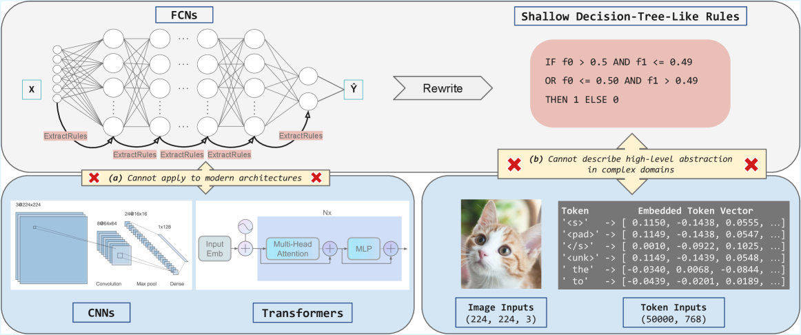Among various types of explanations for deep neural networks—such as attributions (Selvaraju et al. 2017) and hidden semantics (Bau et al. 2017) —rule-based methods that generate global logic rules over input sets, rather than local rules for individual samples, offer stronger interpretability and are highly preferred (Pedreschi et al. 2019). However, most existing rule-based explanation methods (Cohen 1995; Zilke, Loza Mencía, and Janssen 2016; Zarlenga, Shams, and Jamnik 2021a; Hemker, Shams, and Jamnik 2023) suffer from several limitations. We highlight three key issues, as illustrated in Figure 1: (1) they mostly rely on layer-by-layer rule extraction and rewriting to derive final rules, which introduces scalability limitations; (2) they are primarily tailored to fully connected networks (FCNs) and fail to generalize to modern deep neural network (DNN) architectures such as convolutional neural networks and Transformers; (3) the rules they produce are often shallow and decision-tree-like, lacking the ability to capture high-level abstractions, which limits their effectiveness in complex domains. To this end, we introduce NeuroLogic, a modern rule-based framework designed to address architectural dependence, limited scalability, and the shallow nature of existing decision rules. Our approach is inspired by Neural Activation Patterns (NAPs) (Geng et al. 2023, 2024) which are subsets of neurons that consistently activate for inputs belonging to the same class. Specifically, for any given layer, we identify salient neurons for each class and determine their optimal activation thresholds, converting these neurons into hidden predicates. These predicates represent high-level features learned by the model, where a true value indicates the presence of the corresponding feature in a given input. Based on these predicates, NeuroLogic constructs first-order logic (FOL) rules in a fully data-driven manner to approximate the internal behavior of neural networks. <details> <summary>x1.png Details</summary>  ### Visual Description ## [Technical Diagram]: Limitations of Rule Extraction from Neural Networks ### Overview The image is a technical diagram illustrating the challenges of extracting interpretable rules from neural networks, comparing **Fully Connected Networks (FCNs)** with modern architectures (CNNs, Transformers) and complex data domains (images, text tokens). It highlights two key limitations of shallow rule extraction. ### Components/Sections The diagram is divided into three interconnected sections: #### 1. Top Section: FCNs and Shallow Rule Extraction - **FCNs Diagram**: A neural network with input \( \boldsymbol{X} \), hidden layers, and output \( \boldsymbol{\hat{Y}} \). Arrows labeled *“ExtractRules”* point from hidden layers to a box of *“Shallow Decision-Tree-Like Rules”*. - **Shallow Rules Box**: Contains a binary rule: *“IF f0 > 0.5 AND f1 <= 0.49 OR f0 <= 0.50 AND f1 > 0.49 THEN 1 ELSE 0”* - **Limitation (a)**: A red “X” with text: *“(a) Cannot apply to modern architectures”* (links to the bottom-left section). #### 2. Bottom-Left Section: Modern Architectures (CNNs, Transformers) - **CNNs**: A diagram of a Convolutional Neural Network with layers: - Convolution: `3@224x224` (3 channels, 224×224 spatial dimensions). - Max pool: `8@64x64` (8 channels, 64×64 spatial dimensions). - Dense: `24@16x16` (24 channels, 16×16 spatial dimensions) → `1x128` (dense layer). - **Transformers**: A diagram of a Transformer block with: - *“Input Emb”* (input embedding), *“Multi-Head Attention”*, *“MLP”* (multi-layer perceptron), and *“Nx”* (indicating multiple stacked layers). - **Limitation (a)**: Red “X” with text: *“(a) Cannot apply to modern architectures”* (connects to the top FCN section). #### 3. Bottom-Right Section: Complex Domains (Image, Token Inputs) - **Image Inputs**: A cat image labeled *“Image Inputs (224, 224, 3)”* (dimensions: height, width, color channels). - **Token Inputs**: A table with the following data: | Token | Embedded Token Vector | |-------|-----------------------| | `<s>` | [0.1150, -0.1438, 0.0555, ...] | | `<pad>` | [0.1149, -0.1438, 0.0547, ...] | | `</s>` | — | | `<unk>` | — | | `the` | — | | `to` | — | *Note: Numerical vectors are provided for `<s>` and `<pad>` as examples; other tokens have similar embedded representations.* - **Limitation (b)**: A red “X” with text: *“(b) Cannot describe high-level abstraction in complex domains”* (points to the token/image inputs). ### Detailed Analysis - **FCNs vs. Modern Architectures**: Shallow rules (from FCNs) fail for CNNs/Transformers (limitation a) because these architectures use hierarchical, high-dimensional representations (e.g., CNNs for images, Transformers for sequences) that shallow rules cannot capture. - **Complex Domains**: Image (224×224×3) and token (50,000 tokens, 768-dimensional embeddings) inputs are high-dimensional and require deep abstraction. Shallow rules (e.g., the binary rule) cannot model the nuanced patterns in these domains (limitation b). - **Token Embeddings**: The embedded token vectors show how text tokens are represented numerically (e.g., `<s>` and `<pad>` have similar vectors, while `the` and `to` differ), illustrating the complexity of text representation. ### Key Observations - **Limitation (a)**: Rule extraction from simple FCNs (shallow rules) is incompatible with modern architectures (CNNs, Transformers) due to their complex, hierarchical structures. - **Limitation (b)**: Shallow rules cannot capture high-level abstractions in complex domains (images, text), where data requires deep, context-aware understanding. - **Token Embeddings**: The numerical vectors for tokens (e.g., `<s>`, `the`) demonstrate how text is embedded in a vector space, highlighting the complexity of text representation. ### Interpretation This diagram underscores a critical challenge in deep learning: **interpretable rule extraction** (e.g., shallow decision trees) works for simple FCNs but fails for modern architectures (CNNs, Transformers) and complex data (images, text). Shallow rules lack the expressivity to model hierarchical, high-dimensional representations, emphasizing the need for advanced interpretability methods (e.g., attention mechanisms, concept-based explanations) to bridge the gap between model complexity and human understanding. The image and token inputs illustrate that complex data demands deeper abstraction than shallow rules can provide, driving research into more robust interpretability techniques. (Note: All text and labels are transcribed directly from the image. The diagram uses visual cues (red “X”s, arrows) to emphasize limitations, and the token embedding table provides concrete examples of text representation in vector space.) </details> Figure 1: Existing rule-based methods fail to generalize to modern DNNs and their associated complex input domains. The remaining challenge is to ground these hidden predicates in the original input space to ensure interpretability. Unlike existing approaches that can only produce shallow, decision-tree-like rules, NeuroLogic features a flexible design that supports a wide range of interpretable surrogate methods, such as program synthesis, to learn rules with richer and more expressive structures. It can also incorporate human prior knowledge as high-level abstractions of complex input domains to enable more efficient and meaningful grounding. To demonstrate its capabilities, we apply NeuroLogic to extract logic rules from Transformer-based sentiment analysis—a setting where traditional rule-extraction methods struggle to scale. To the best of our knowledge, this is the first approach capable of extracting global logic rules from modern, complex architectures such as Transformers. We believe NeuroLogic represents a promising step toward opening the black box of deep neural networks. Our contributions are summarized as follows: - We propose NeuroLogic, a novel framework for extracting interpretable global logic rules from deep neural networks. By abandoning the costly layer-wise rule extraction and substitution paradigm, NeuroLogic achieves greater scalability and broad architectural compatibility. - The decoupled design of NeuroLogic enables flexible grounding, allowing the generation of more abstract and interpretable rules that transcend the limitations of shallow, decision tree–based explanations. - Experimental results on small-scale benchmarks demonstrate that NeuroLogic produces more compact rules with higher efficiency than state-of-the-art methods, while maintaining strong fidelity and predictive accuracy. - We further showcase the practical feasibility of NeuroLogic in extracting meaningful logic rules and providing insights into the internal mechanisms of Transformers—an area where existing approaches struggle to scale effectively. ## Preliminary #### Neural Networks for Classification Tasks We consider a general deep neural network $N$ used for classification. Let $z^l_i(x)$ denote the value of the $i$ -th neuron at layer $l$ for a given input $x$ . We do not assume any specific form for the transformation between layers, that is, the mapping from $z^l$ to $z^l+1$ can be arbitrary. This abstraction allows our analysis to be broadly applied across architectures. The network $N$ as a whole functions as $$ \displaystyleF^<N>:X→ℝ^|C|, \tag{1} $$ mapping an input $x∈ X$ from the dataset to a score vector over the class set $C$ . The predicted class is then given by $$ \displaystyle\hat{c}=\arg\max_c∈ CF^<N>_c(x). \tag{2} $$ #### First-Order Logic First-Order Logic (FOL) is a formal language for stating interpretable rules about objects and their relations/attributes. It extends propositional logic by introducing quantifiers such as: - Universal quantifier ( $∀$ ): meaning “for all”, e.g., $∀ x p(x)$ means $p(x)$ holds for every $x$ . - Existential quantifier ( $∃$ ): meaning “there exists”, e.g., $∃ x p(x)$ means there exists at least one $x$ for which $p(x)$ holds. We focus on FOL rules in Disjunctive Normal Form (DNF), which are disjunctions (ORs) of conjunctions (ANDs) of predicates. - A predicate is a simple condition or property on the input, e.g., $p_i(x)$ . - A clause is a conjunction (AND) of predicates, such as $p_1(x)∧ p_2(x)∧¬ p_3(x)$ . A DNF rule looks like a logical OR of multiple clauses: $$ \displaystyle∀ x, ≤ft(p_1(x)∧ p_2(x)\right)∨≤ft(p_3(x)∧¬ p_4(x)\right)⇒\textit{Label}(x)=c, \tag{3} $$ meaning that for every input $x$ , if any clause is satisfied, it is assigned to class $c$ . This structured form makes the rules easy to interpret and understand. 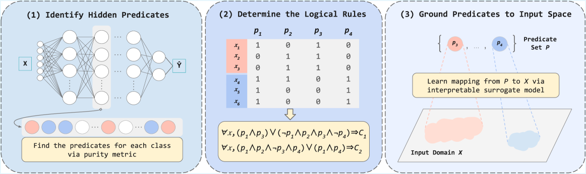## The NeuroLogic Framework In this section, we introduce NeuroLogic, a novel approach for extracting interpretable logic rules from DNNS. For clarity, we divide the NeuroLogic framework into three subtasks. An overview is illustrated in Figure 2. <details> <summary>x2.png Details</summary>  ### Visual Description ## [Diagram]: Three-Step Process for Interpretable Machine Learning ### Overview The image is a technical diagram illustrating a three-step methodological pipeline for extracting interpretable logical rules from a neural network. The process flows from left to right across three distinct panels, each enclosed in a dashed blue box. The overall goal is to move from a black-box model (a neural network) to human-understandable logical predicates grounded in the input data space. ### Components/Axes The diagram is divided into three sequential panels, labeled (1), (2), and (3). **Panel (1): Identify Hidden Predicates** * **Visual Component:** A schematic of a feedforward neural network. It has an input layer labeled **X**, multiple hidden layers (represented by circles and connecting lines), and an output layer labeled **Ŷ**. * **Textual Elements:** * Title: `(1) Identify Hidden Predicates` * A yellow text box at the bottom: `Find the predicates for each class via purity metric`. * Below the network, a sequence of colored circles (red, blue, white) represents data points or class assignments. * **Spatial Grounding:** The neural network diagram occupies the upper portion of the panel. The yellow text box is centered at the bottom. The colored circle sequence is positioned between the network and the text box. **Panel (2): Determine the Logical Rules** * **Visual Component:** A truth table and logical formulas. * **Textual Elements:** * Title: `(2) Determine the Logical Rules` * **Truth Table:** * Column Headers: `p₁`, `p₂`, `p₃`, `p₄` (representing predicates). * Row Labels: `x₁`, `x₂`, `x₃` (highlighted in a red background), `x₄`, `x₅`, `x₆` (highlighted in a blue background). * Table Content (Binary Values): | | p₁ | p₂ | p₃ | p₄ | |---|----|----|----|----| | x₁ | 1 | 0 | 1 | 0 | | x₂ | 0 | 1 | 1 | 0 | | x₃ | 0 | 1 | 1 | 0 | | x₄ | 1 | 1 | 0 | 1 | | x₅ | 1 | 0 | 0 | 1 | | x₆ | 1 | 0 | 0 | 1 | * **Logical Rules (below the table):** * `∀x, (p₁ ∧ p₃) ∨ (¬p₁ ∧ p₂ ∧ p₃ ∧ ¬p₄) ⇒ C₁` * `∀x, (p₁ ∧ p₂ ∧ ¬p₃ ∧ p₄) ∨ (p₁ ∧ p₄) ⇒ C₂` * **Spatial Grounding:** The truth table is centered in the upper half of the panel. The logical rules are centered below the table, connected by a downward arrow. **Panel (3): Ground Predicates to Input Space** * **Visual Component:** A conceptual mapping diagram. * **Textual Elements:** * Title: `(3) Ground Predicates to Input Space` * A set notation: `{p₃, ..., p₄}` labeled `Predicate Set P`. * A yellow text box: `Learn mapping from P to X via interpretable surrogate model`. * A 2D plane labeled `Input Domain X`, containing two amorphous, colored regions (one red, one blue). * **Spatial Grounding:** The predicate set `{p₃, ..., p₄}` is at the top. Dashed lines connect these predicates to the colored regions in the `Input Domain X` plane at the bottom. The yellow text box is centered between the predicate set and the input domain plane. ### Detailed Analysis The diagram presents a clear, linear workflow: 1. **Step 1 - Predicate Identification:** A neural network is analyzed to discover hidden, meaningful features or "predicates" (`p₁, p₂, p₃, p₄`). The "purity metric" suggests a method to find predicates that cleanly separate data points of different classes (represented by the red and blue circles). 2. **Step 2 - Rule Extraction:** The discovered predicates are evaluated across a set of data instances (`x₁` through `x₆`). The truth table shows the activation (1) or non-activation (0) of each predicate for each instance. Instances `x₁-x₃` (red group) and `x₄-x₆` (blue group) show distinct patterns. These patterns are then synthesized into formal logical rules (using AND `∧`, OR `∨`, NOT `¬`, and IMPLIES `⇒`) that define classes `C₁` and `C₂`. 3. **Step 3 - Grounding:** The abstract predicates (`p₃, p₄`) are mapped back to the original input space (`X`). This is done using an "interpretable surrogate model," which learns to associate the predicate activations with specific regions (the red and blue clouds) within the input domain. This step makes the logical rules tangible by showing what parts of the input data they correspond to. ### Key Observations * **Color Consistency:** The color coding is consistent across panels. Red and blue are used to denote two distinct classes or clusters. In Panel 1, red/blue circles represent classes. In Panel 2, the red/blue background highlights the two groups of instances (`x₁-x₃` vs. `x₄-x₆`). In Panel 3, the red/blue regions in the input domain correspond to these same classes. * **Predicate Specificity:** The truth table reveals that predicates are not uniformly active. For example, `p₃` is active for all red-group instances (`x₁, x₂, x₃`) but inactive for all blue-group instances (`x₄, x₅, x₆`), making it a strong differentiator. * **Rule Complexity:** The logical rule for `C₁` is more complex, involving a disjunction of two conjunctions. The rule for `C₂` is simpler. This may reflect the underlying complexity of the data distribution for each class. * **Spatial Flow:** The dashed lines in Panel 3 visually enforce the "grounding" concept, connecting abstract logical symbols to concrete data regions. ### Interpretation This diagram outlines a framework for **Explainable AI (XAI)**. It addresses the "black box" problem of neural networks by proposing a method to reverse-engineer their decision-making process into human-readable logic. * **What it demonstrates:** The pipeline shows how to distill complex, non-linear model behavior (the neural network) into a set of explicit, logical conditions (`if-then` rules) that are tied directly to the input data. This makes the model's reasoning transparent and auditable. * **Relationship between elements:** The panels are causally linked. The predicates found in Step 1 are the variables used in the truth table and rules of Step 2. The predicates from Step 2 are the ones grounded in Step 3. The entire process is a transformation from **subsymbolic** (network weights) to **symbolic** (logical rules) representation. * **Significance:** This approach is valuable for high-stakes domains (e.g., medicine, finance) where understanding *why* a model made a prediction is as important as the prediction itself. It allows users to verify that the model is relying on meaningful features (grounded in the input space) and logical rules that align with domain knowledge, rather than spurious correlations. The "surrogate model" in Step 3 is key, as it provides the final bridge between abstract logic and concrete data. </details> Figure 2: Overview of the NeuroLogic Framework. ### Identifying Hidden Predicates For a given layer $l$ , we aim to identify a subset of neurons that are highly indicative of a particular class $c∈ C$ . These neurons form what are known as Neural Activation Patterns (NAPs) (Geng et al. 2023, 2024). A neuron is considered part of the NAP for class $c$ if its activation is consistently higher for inputs from class $c$ compared to inputs from other classes. This behavior suggests that such neurons encode class-specific latent features at layer $l$ , as discussed in (Geng et al. 2024). To identify the NAP for a specific class $c$ , we evaluate how selectively each neuron responds to class $c$ versus other classes. Since each neuron’s activation is a scalar value, we can assess its discriminative power by learning a threshold $t$ . This threshold separates inputs from class $c$ and those from other classes based on activation values. Formally, we consider a neuron to support class $c$ if its activation $z_j^l(x)$ for input $x$ satisfies $z_j^l(x)≥ t$ . If this condition holds, we classify $x$ as belonging to class $c$ ; otherwise, it is classified as not belonging to $c$ . To quantify the effectiveness of a threshold $t$ , we use the purity metric, defined as: $$ \displaystylePurity(t)= \displaystyle\frac{≤ft|≤ft\{x∈ X_c:z_j^l(x)≥ t\right\}\right|}{|X_c|} \displaystyle+\frac{≤ft|≤ft\{x∈ X_¬ c:z_j^l(x)<t\right\}\right|}{|X_¬ c|} \tag{4} $$ Here, $X_c$ denotes the set of inputs from class $c$ , while $X_¬ c$ denotes inputs from all other classes. A high purity value means the neuron cleanly separates class $c$ from others, whereas a low value suggests ambiguous or overlapping activation responses. We conduct a linear search to determine the optimal threshold $t$ as its final purity. In our implementation, for each neuron, we compute its purity with respect to each class to determine its class preference. Then, for each class, we rank the neurons by that purity and keep the top- $k$ . These selected neurons are referred to as hidden predicates, denoted as $P$ , as they capture discriminative features that are highly specific to each class within the input space. ### Determining the Logical Rules Formally, a predicate $p_j$ at layer $l$ , together with its corresponding threshold $t_j$ , is defined as $p_j(x):=I[z_j^(l)(x)≥ t_j]$ . In this context, a True (1) assignment indicates the presence of the specific latent feature of class $c$ for input $x$ , while a False (0) assignment signifies its absence. Intuitively, the more predicates that fire, the stronger the evidence that $x$ belongs to class $c$ . However, this raises the question: to what extent should we believe that $x$ belongs to class $c$ based on the pattern of predicate activations? We address this question using a data-driven approach. Let $P_c^(l)=\{p_1,...,p_m\}$ be the $m$ predicates retained for class $c.$ Evaluating $P_c^(l)$ on every class example $x∈ X_c$ gives a multiset of binary vectors $p(x)∈\{0,1\}^m$ . Each distinct vector can be treated as a clause, and the union of all clauses forms a DNF rule: $$ ∀ x,\bigl(\bigvee_v∈V_c\bigl(\bigwedge_i:v_{i=1}p_i(x)\wedge\bigwedge_i:v_{i=0}¬ p_i(x)\bigr)\bigr)\implies Label(x)=c $$ where $V_c$ is the set of unique activation vectors for $X_c$ . For instance, suppose we have four predicates $p_1(x),p_2(x),p_3(x),p_4(x)$ (we will omit $x$ when the context is clear), and five distinct inputs yield the following patterns: $(1,1,1,1)$ , $(1,1,1,0)$ , $(1,1,1,0)$ , $(1,1,0,1)$ , and $(1,1,0,1)$ . We can then construct a disjunctive normal form (DNF) expression to derive a rule: $$ \displaystyle∀ x ( \displaystyle(p_1∧ p_2∧ p_3∧ p_4)∨(p_1∧ p_2∧ p_3∧¬ p_4) \displaystyle∨(p_1∧ p_2∧¬ p_3∧ p_4))⇒\textit{Label}(x)=c. \tag{5} $$ In practice, these predicates behave as soft switches: their purity is imperfect, sometimes firing on inputs from $X_¬ c$ . Consequently, the resulting DNF is best viewed as a comprehensive description and may include many predicates that are less relevant to the model’s actual classification behavior. To address this, we apply a decision tree learner to distill a more compact and representative version of the rule, which will serve as the (discriminative) rule-based model. ### Grounding Predicates to the Input Feature Space The final step is to ground these hidden predicates in the input space to make them human-interpretable. We adopt the definition of interpretability as the ability to explain model decisions in terms understandable to humans (Doshi-Velez and Kim 2017). Since ”understandability” is task and audience dependent, NeuroLogic is designed in a decoupled fashion where any grounding method can be plugged in, allowing injection of domain knowledge. This design also allows users to incorporate domain-specific knowledge where appropriate. Within the scope of this work, we present simple approaches for grounding predicates in simple input domains, as well as in the complex input domain of large vocabulary spaces for Transformers. Exploring general grounding strategies for diverse tasks and models remains a challenge, and we believe it requires collective efforts from the whole research community. #### Grounding Predicates in Simple Input Domains For deep neural networks (DNNs) applied to tasks with simple input domains (e.g., tabular data), we aim to ground each predicate $p_j$ directly in the raw input space. This enables more transparent and interpretable logic rules. We reframe the grounding task as a supervised classification problem. For a given predicate $p_j$ , we collect input examples where the predicate is activated versus deactivated, and then learn a symbolic function that approximates this distinction. Formally, for a target class $c$ and predicate $p_j$ , we define the activation set and deactivation set, respectively, as $$ \displaystyle D_1^(j) \displaystyle=\{x∈ X_c\mid p_j(x)=1\}, \displaystyle D_0^(j) \displaystyle=\{x∈ X_c\mid p_j(x)=0\}. \tag{6} $$ These are combined into a labeled dataset $$ \displaystyle D^(j)=\{(x,y)\mid x∈ D_1^(j)∪ D_0^(j), y=p_j(x)\}. \tag{8} $$ Then, to obtain expressive, compositional and human-readable logic rules as explanations, we employ program synthesis to learn a symbolic expression $φ_j$ from a domain-specific language (DSL) $L$ . Unlike traditional decision-tree-like rules, the symbolic language $L$ is richer: a composable grammar over input features that supports not only logical and comparison operators but also linear combinations and nonlinear functions. Specifically, the language includes: - Atomic abstractions formed by applying threshold comparisons to linear or nonlinear functions of the input features, for example, $$ \displaystyle a:=f(x)≤θ or f(x)>θ, \tag{9} $$ where $f(x)$ can be any linear or nonlinear transformation, such as polynomials, trigonometric functions, or other basis expansions. - Logical operators to combine these atomic abstractions into complex expressions: $$ \displaystyleφ::=a\mid¬φ\midφ_1∧φ_2\midφ_1∨φ_2. \tag{10} $$ The synthesis objective is to find an expression $φ_j∈L$ that minimizes a combination of classification loss and complexity, formally: $$ \displaystyleφ_j∈\arg\min_φ∈L≤ft[L_cls(φ;D^(j))+λ·Ω(φ)\right], \tag{11} $$ where $L_cls$ measures how well $φ$ approximates the predicate activations in $D^(j)$ , $Ω(φ)$ penalizes the complexity of the expression (e.g., number of literals or tree depth), and $λ$ balances the trade-off between accuracy and interpretability. This grounding approach also supports decision-tree-like rules, which are commonly used in existing methods. In this context, such rules can be viewed as a special case of the above atomic abstractions, where $f(x)$ corresponds to individual features. A simpler alternative is to leverage off-the-shelf decision tree algorithms: we train a decision tree classifier $f_j^DT$ such that $$ \displaystyle f_j^DT(x)≈ p_j(x), ∀ x∈ X_c. \tag{12} $$ The resulting decision tree provides a simpler rule-based approximation of predicate activations, effectively grounding $p_j$ in the input space in an interpretable manner. #### Grounding predicates in the vocabulary space The input space in NLP domains (i.e., vocabulary spaces) is typically extremely large, making it difficult to ground rules onto raw feature vectors. In such domains, it is more effective to incorporate human prior knowledge like words, tokens, or linguistic structure that are more semantically meaningful and ultimately guide the predictions made by transformer-based models (Tenney, Das, and Pavlick 2019a). In light of this, we define a set of atomic abstractions over the vocabulary spaces. Each atomic abstraction corresponds to a template specifying keywords along with their associated lexical structures. To ground the learned hidden predicates to this domain knowledge, we leverage causal inference (Zarlenga, Shams, and Jamnik 2021b; Vig et al. 2020). Formally, let $A=\{a_1,a_2,\dots,a_k\}$ be the set of atomic abstractions derived from domain knowledge (e.g., keywords or lexical patterns), and let $p_j$ be a learned hidden predicate extracted from the model’s internal representations, and $x$ be an input instance (e.g., a text sample). We define a causal intervention $do(¬ a_i)$ as flipping the truth value of atomic abstraction $a_i$ in the input $x$ (e.g., masking the keyword associated with $a_i$ ). The grounding procedure tests whether flipping $a_i$ changes the truth of the hidden predicate $p_j$ : $$ \displaystyle\textit{If} p_j(x)=\textit{True} \textit{and} p_j\bigl(do(¬ a_i)(x)\bigr)=\textit{False}, \tag{13} $$ then we infer a causal dependence of $p_j$ on $a_i$ , grounding $p_j$ to the atomic abstraction $a_i$ . By iterating over all atomic abstractions $a_i∈A$ , we establish a mapping: $$ \displaystyle G:p_j↦\{a_i∈A\mid\textit{flipping }a_i\textit{ negates }p_j\}, \tag{14} $$ which grounds the hidden predicate $p_j$ in terms of semantically meaningful domain knowledge. ## Evaluation | XOR ECLAIRE | Method C5.0 91.8 $±$ 1.0 | Accuracy (%) 52.6 $±$ 0.2 91.4 $±$ 2.4 | Fidelity (%) 53.0 $±$ 0.2 6.2 $±$ 0.4 | Runtime (s) 0.1 $±$ 0.0 87.0 $±$ 16.2 | Number of Clauses 1 $±$ 0 263.0 $±$ 49.1 | Avg Clause Length 1 $±$ 0 | | --- | --- | --- | --- | --- | --- | --- | | CGXPLAIN | 96.7 $±$ 1.7 | 92.4 $±$ 1.1 | 9.1 $±$ 1.8 | 3.6 $±$ 1.8 | 10.4 $±$ 7.2 | | | NeuroLogic | 89.6 $±$ 1.9 | 90.3 $±$ 1.6 | 1.2 $±$ 0.3 | 10.8 $±$ 3.5 | 6.8 $±$ 2.0 | | | MB-ER | C5.0 | 92.7 $±$ 0.9 | 89.3 $±$ 1.0 | 20.3 $±$ 0.8 | 21.8 $±$ 3 | 72.4 $±$ 14.5 | | ECLAIRE | 94.1 $±$ 1.6 | 94.7 $±$ 0.2 | 123.5 $±$ 36.8 | 48.3 $±$ 15.3 | 137.6 $±$ 24.7 | | | CGXPLAIN | 92.4 $±$ 0.7 | 94.7 $±$ 0.9 | 462.7 $±$ 34.0 | 5.9 $±$ 1.1 | 21.8 $±$ 3.4 | | | NeuroLogic | 92.8 $±$ 0.9 | 92.7 $±$ 1.4 | 6.0 $±$ 1.2 | 5.8 $±$ 1.0 | 3.7 $±$ 0.2 | | | MB-HIST | C5.0 | 87.9 $±$ 0.9 | 89.3 $±$ 1.0 | 16.06 $±$ 0.64 | 12.8 $±$ 3.1 | 35.2 $±$ 11.3 | | ECLAIRE | 88.9 $±$ 2.3 | 89.4 $±$ 1.8 | 174.5 $±$ 73.2 | 30.0 $±$ 12.4 | 74.7 $±$ 15.7 | | | CGXPLAIN | 89.4 $±$ 2.5 | 89.1 $±$ 3.6 | 285.3 $±$ 10.3 | 5.2 $±$ 1.9 | 27.8 $±$ 7.6 | | | NeuroLogic | 90.7 $±$ 0.9 | 92.0 $±$ 3.5 | 2.3 $±$ 0.2 | 3.6 $±$ 1.6 | 2.7 $±$ 0.3 | | | MAGIC | C5.0 | 82.8 $±$ 0.9 | 85.4 $±$ 2.5 | 1.9 $±$ 0.1 | 57.8 $±$ 4.5 | 208.7 $±$ 37.6 | | ECLAIRE | 84.6 $±$ 0.5 | 87.4 $±$ 1.2 | 240.0 $±$ 35.9 | 392.2 $±$ 73.9 | 1513.4 $±$ 317.8 | | | CGXPLAIN | 84.4 $±$ 0.8 | 91.5 $±$ 1.3 | 44.6 $±$ 2.9 | 7.4 $±$ 0.8 | 11.6 $±$ 1.9 | | | NeuroLogic | 84.6 $±$ 0.5 | 90.8 $±$ 0.7 | 17.0 $±$ 1.5 | 6.0 $±$ 0.0 | 3.6 $±$ 0.1 | | Table 1: Comparison of rule-based explanation methods across different benchmarks. The best results are highlighted in bold. In this section, we evaluate our approach, NeuroLogic, in two settings: (1) small-scale benchmarks and (2) transformer-based sentiment analysis. The former involves comparisons with baseline methods to assess NeuroLogic in terms of accuracy, efficiency, and interpretability. The latter focuses on a challenging, large-scale, real-world scenario where existing methods fail to scale, highlighting the practical viability and scalability of NeuroLogic. ### Small-Scale Benchmarks #### Setup and Baselines We evaluate NeuroLogic against popular rule-based explanation methods C5.0 This represents the use of the C5.0 decision tree algorithm to learn rules in an end-to-end manner., ECLAIRE (Zarlenga, Shams, and Jamnik 2021a), and CGXPLAIN (Hemker, Shams, and Jamnik 2023) on four standard interpretability benchmarks: XOR, MB-ER, MB-HIST, and MAGIC. For each baseline, we use the original implementation and follow the authors’ recommended hyperparameters. We evaluate all methods using five metrics: accuracy, fidelity (agreement with the original model), runtime, number of clauses, and average clause length, to assess both interpretability and performance. Further details on the experimental setup are provided in the Appendix. Notably, NeuroLogic consistently produces the most concise explanations, as reflected by both the number of clauses and the average clause length. In particular, it generates rule sets with substantially shorter average clause lengths—for example, on MB-HIST, it achieves $2.7± 0.3$ compared to $27.8± 7.6$ by the previous state-of-the-art, CGXPLAIN. This conciseness, along with fewer clauses, directly enhances interpretability and readability by reducing overall rule complexity. These results highlight a key advantage of NeuroLogic and align with our design goal of improving interpretability. By avoiding the costly layer-wise rule extraction and substitution paradigm employed by ECLAIRE and CGXPLAIN, NeuroLogic achieves significantly higher efficiency. Although C5.0 can be faster in some cases by directly extracting rules from DNNs, it often suffers from lower fidelity, reduced accuracy, or the generation of overly complex rule sets. For example, while C5.0 can complete rule extraction on XOR in just 0.1 seconds, its accuracy is only around 52%. In contrast, NeuroLogic consistently achieves strong performance in both fidelity and accuracy across all benchmarks. These results demonstrate that NeuroLogic strikes a favorable balance by effectively combining interpretability, computational efficiency, and faithfulness, outperforming existing rule-based methods. <details> <summary>x3.png Details</summary>  ### Visual Description ## Dual-Axis Line Chart: Rule Set Accuracy and Emotion Purity Across Layers ### Overview This is a dual-axis line chart tracking two distinct metrics across 6 sequential layers: **rule-based accuracy** (left y-axis) and **average purity of emotion detection** (right y-axis) for four emotions: Anger, Joy, Optimism, and Sadness. All metrics show a consistent upward trend as layer number increases. ### Components/Axes - **X-axis**: Labeled *Layer*, with discrete markers at positions 1, 2, 3, 4, 5, 6 (bottom-center horizontal axis). - **Left Y-axis**: Labeled *Accuracy*, with a linear scale ranging from 0.4 to 0.8, in increments of 0.1. - **Right Y-axis**: Labeled *Average Purity*, with a linear scale ranging from 1.1 to 1.8, in increments of 0.1. - **Legend (top-left corner, above chart area)**: - Black solid line with square markers: *Accuracy - Rule Set* - Blue dashed line with circle markers: *Purity - Anger* - Orange dashed line with square markers: *Purity - Joy* - Green dotted line with triangle markers: *Purity - Optimism* - Red dotted line with triangle markers: *Purity - Sadness* ### Detailed Analysis All data points are approximate values, with ±0.02 uncertainty for accuracy, ±0.05 uncertainty for purity: 1. **Accuracy - Rule Set (black solid line, left axis)** - Trend: Steadily increasing, with a sharp upward jump between Layer 2 and 3, then continues rising to near the maximum scale value. - Data points: - Layer 1: ~0.39 - Layer 2: ~0.44 - Layer 3: ~0.63 - Layer 4: ~0.67 - Layer 5: ~0.79 - Layer 6: ~0.80 2. **Purity - Anger (blue dashed line, right axis)** - Trend: Consistent upward slope, accelerating slightly after Layer 3, ending at the maximum purity scale value. - Data points: - Layer 1: ~1.10 - Layer 2: ~1.15 - Layer 3: ~1.35 - Layer 4: ~1.45 - Layer 5: ~1.70 - Layer 6: ~1.80 3. **Purity - Joy (orange dashed line, right axis)** - Trend: Steady increase, with a sharp rise between Layer 2 and 3, matching Anger's final purity value. - Data points: - Layer 1: ~1.15 - Layer 2: ~1.20 - Layer 3: ~1.38 - Layer 4: ~1.50 - Layer 5: ~1.75 - Layer 6: ~1.80 4. **Purity - Optimism (green dotted line, right axis)** - Trend: Gradual, slow increase, with the lowest final purity value among all emotion metrics. - Data points: - Layer 1: ~1.20 - Layer 2: ~1.25 - Layer 3: ~1.32 - Layer 4: ~1.40 - Layer 5: ~1.65 - Layer 6: ~1.70 5. **Purity - Sadness (red dotted line, right axis)** - Trend: Slow initial growth, then a steeper rise after Layer 3, ending between Optimism and Anger/Joy. - Data points: - Layer 1: ~1.10 - Layer 2: ~1.12 - Layer 3: ~1.28 - Layer 4: ~1.35 - Layer 5: ~1.60 - Layer 6: ~1.75 ### Key Observations - All metrics (accuracy and all purity scores) increase monotonically with layer number (1 to 6). - The *Accuracy - Rule Set* has the most dramatic growth, with a 43% increase between Layer 2 and 3. - *Purity - Anger* and *Purity - Joy* reach the highest purity value (~1.80) at Layer 6, tying for the top position. - *Purity - Optimism* has the lowest final purity (~1.70) and the most gradual growth trajectory. - At Layer 1, all purity metrics cluster between 1.10-1.20, while accuracy starts at ~0.39. ### Interpretation This chart demonstrates that deeper model layers (1 to 6) drive improvements in both rule-based task accuracy and emotion detection purity. The sharp accuracy jump between Layer 2 and 3 suggests a critical layer where the model learns key features for rule application, which correlates with a parallel rise in emotion purity. The fact that Anger and Joy reach the highest purity implies these emotions may be more distinct or easier for the model to isolate in deeper layers, while Optimism (with the lowest final purity) may be a more ambiguous or complex emotion for the model to detect with high precision. The consistent upward trend across all metrics indicates that deeper layers enhance both rule-based performance and refined emotion identification, suggesting a synergistic improvement in model capabilities as depth increases. 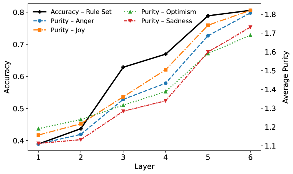</details> Figure 3: The (average) purity of predicates correlates with the rule model accuracy as layers go deeper. <details> <summary>x4.png Details</summary>  ### Visual Description ## Line Chart: Accuracy vs. Top-k Predicates for Different Layers ### Overview This is a line chart plotting the accuracy of six different model layers (Layer1 through Layer6) as a function of the number of top-k predicates considered. The chart demonstrates how predictive accuracy changes for each layer as more predicates are included, showing distinct performance tiers and trends. ### Components/Axes * **X-Axis:** Labeled **"Top-k Predicates"**. It has discrete markers at values: 1, 5, 10, 15, 20, 25, 30, 35, 40. * **Y-Axis:** Labeled **"Accuracy"**. It is a linear scale ranging from 0.0 to 0.8, with major tick marks at every 0.1 interval. * **Legend:** Positioned in the **bottom-right quadrant** of the chart area. It contains six entries, each with a unique color and marker symbol: * Layer1: Blue line with circle markers (●) * Layer2: Orange line with square markers (■) * Layer3: Green line with diamond markers (◆) * Layer4: Red line with upward-pointing triangle markers (▲) * Layer5: Purple line with downward-pointing triangle markers (▼) * Layer6: Brown line with plus/cross markers (+) ### Detailed Analysis All six data series originate at the same point: **(Top-k=1, Accuracy=0.0)**. From there, they exhibit a sharp increase in accuracy up to **Top-k=5**, followed by a plateau or gradual change. **Trend Verification & Approximate Data Points:** * **Layer6 (Brown, +):** Shows the highest overall accuracy. It rises sharply to ~0.79 at k=5, peaks at ~0.81 around k=25, and remains nearly flat, ending at ~0.81 at k=40. **Trend:** Rapid ascent to a high, stable plateau. * **Layer5 (Purple, ▼):** Follows a very similar path to Layer6 but is consistently slightly lower. It reaches ~0.76 at k=5, peaks at ~0.79 around k=15, and shows a very slight decline to ~0.76 at k=40. **Trend:** Rapid ascent to a high plateau with minimal decay. * **Layer4 (Red, ▲):** Occupies the next tier. It jumps to ~0.63 at k=5, peaks at ~0.67 around k=20, and then gradually declines to ~0.57 at k=40. **Trend:** Rapid ascent, a moderate peak, followed by a steady decline. * **Layer3 (Green, ◆):** Rises to ~0.54 at k=5, peaks at ~0.64 around k=20, and declines to ~0.51 at k=40. **Trend:** Similar shape to Layer4 but at a lower accuracy level. * **Layer2 (Orange, ■):** Increases to ~0.37 at k=5, peaks at ~0.44 around k=15, and then declines to ~0.34 at k=40. **Trend:** Moderate ascent, an early peak, and a steady decline. * **Layer1 (Blue, ●):** Shows the lowest performance. It rises to ~0.37 at k=5, peaks at ~0.41 around k=10, and then declines more noticeably to ~0.28 at k=40. **Trend:** Moderate ascent, the earliest peak among all layers, and the most pronounced decline. ### Key Observations 1. **Performance Hierarchy:** There is a clear and consistent stratification. From highest to lowest accuracy: Layer6 ≈ Layer5 > Layer4 > Layer3 > Layer2 > Layer1. 2. **Peak Location:** The Top-k value at which peak accuracy occurs varies by layer. Lower layers (Layer1, Layer2) peak earlier (k=10-15), while higher layers (Layer4, Layer5, Layer6) peak later (k=15-25). 3. **Post-Peak Behavior:** After reaching their peak, the accuracy of lower layers (Layer1, Layer2, Layer3) degrades more significantly as k increases towards 40. The highest layers (Layer5, Layer6) are remarkably stable, showing almost no degradation. 4. **Initial Convergence:** All layers start at 0% accuracy with only 1 predicate and experience their most dramatic performance gain between k=1 and k=5. ### Interpretation The data suggests a fundamental relationship between model depth (layer hierarchy) and the utilization of predicate information for accuracy. * **Layer Specialization:** Higher layers (5 and 6) are not only more accurate but also more robust. They can effectively leverage a larger set of top predicates (up to 40) without performance loss, indicating they may be integrating more complex, high-level features that remain relevant even as the candidate pool grows. * **Noise Sensitivity in Lower Layers:** The declining accuracy in lower layers (1, 2, 3) after a relatively early peak suggests they are more sensitive to noise. Adding more predicates beyond an optimal point (k=10-20) likely introduces irrelevant or conflicting signals that these less sophisticated layers cannot filter out, leading to performance degradation. * **Practical Implication:** For tasks relying on these layers, there is a clear trade-off. Using a higher layer provides better and more stable accuracy. If a lower layer must be used, the number of predicates (k) must be carefully tuned to its specific peak to avoid the detrimental effects of over-inclusion. The chart provides the empirical data needed to make that tuning decision for each layer. 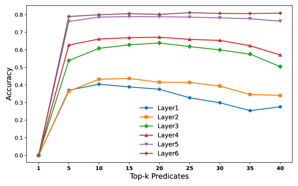</details> Figure 4: The impact of the number of predicates affects the rule model. | Class | Layer 1 (38.92%) | Layer 2 (43.70%) | Layer 3 (62.84%) | Layer 4 (66.92%) | Layer 5 (78.89%) | Layer 6 (80.58%) | | | | | | | | --- | --- | --- | --- | --- | --- | --- | --- | --- | --- | --- | --- | --- | | # Clauses | Length | # Clauses | Length | # Clauses | Length | # Clauses | Length | # Clauses | Length | # Clauses | Length | | | Anger | 70 | 4.29 | 91 | 4.27 | 91 | 4.82 | 75 | 4.51 | 42 | 4.19 | 33 | 4.15 | | Joy | 58 | 3.62 | 50 | 4.18 | 58 | 4.81 | 48 | 4.98 | 35 | 5.14 | 20 | 4.25 | | Optimism | 34 | 4.88 | 32 | 4.38 | 47 | 5.60 | 49 | 5.65 | 26 | 4.65 | 23 | 5.57 | | Sadness | 78 | 4.76 | 53 | 4.36 | 84 | 5.25 | 73 | 3.78 | 46 | 4.72 | 38 | 4.92 | Table 2: Number of clauses (# Clauses) and average clause length (Length) for each emotion class across Transformer layers after pruning. Per-layer rule-set accuracy is shown in parentheses following the layer number. | the i of | at_end at_end at_end | i i user | at_start before_verb at_start | it you so | after_verb after_verb after_subject | sad in sad | at_end after_subject after_verb | sad sad depression | at_end after_verb at_end | sad lost depression | at_end after_subject at_end | | --- | --- | --- | --- | --- | --- | --- | --- | --- | --- | --- | --- | | when | at_start | user | before_subject | but | at_start | sad | at_start | me | after_subject | sad | after_verb | | and | after_subject | a | after_subject | on | after_verb | the | before_verb | at | after_verb | sad | after_subject | | at | after_verb | i | after_verb | a | at_end | think | after_subject | sad | after_subject | sad | at_start | | be | after_subject | a | after_verb | of | at_start | sad | after_subject | sad | at_start | sadness | at_end | | to | at_end | is | after_subject | you | after_subject | depression | at_end | sadness | at_end | depression | at_start | | was | after_verb | to | after_verb | it | after_subject | in | at_start | depression | after_verb | depressing | at_end | | sad | at_end | i | after_subject | just | at_start | by | after_verb | be | after_verb | depressing | after_subject | | when | before_subject | user | before_verb | so | after_verb | user | after_verb | am | after_subject | lost | at_start | | like | after_subject | it | at_start | can | after_subject | be | after_subject | was | before_verb | nightmare | at_end | | when | before_verb | is | at_start | of | before_verb | think | at_start | at | after_subject | sadness | after_verb | | like | after_verb | and | after_verb | can | before_verb | with | after_subject | at | at_start | lost | at_end | | are | after_subject | my | after_verb | sad | after_verb | really | after_subject | depressing | at_end | anxiety | after_verb | Table 3: Top 15 keyword linguistic pattern pairs for class Sadness learned by the top DNF rule across layers 1–6. | | depression bad lost | sad depression lost | | --- | --- | --- | | terrorism | depressing | | | sadness | sadness | | | awful | sadly | | | anxiety | mourn | | | depressed | nightmare | | | feeling | anxiety | | | offended | never | | | F1 | 0.297 | 0.499 | Table 4: Top-10 words for the Sadness class from EmoLex and NeuroLogic. The bottom row reports the F1 scores. ### Transformer-based Sentiment Analysis #### Setup and Baselines We evaluate NeuroLogic on the Emotion task from the TweetEval benchmark, which contains approximately 5,000 posts from Twitter, each labeled with one of four emotions: Anger, Joy, Optimism, or Sadness (Barbieri et al. 2020). All experiments use the pretrained model, a 6-layer DistilBERT fine-tuned on the same TweetEval splits (Schmid 2024; Sanh et al. 2020). The pretrained model has a test accuracy of 80.59%. The model contains approximately 66 million parameters, and we empirically validate that existing methods fail to efficiently scale to this level of complexity. For rule grounding, we approximate predicate-level interventions by masking tokens that instantiate an atomic abstract $a_i$ and flip an active DNF clause to False, thereby identifying $a_i$ as its causal grounder. In our study, each $a_i$ is defined as a (keyword, linguistic pattern) pair, where the linguistic pattern may include structures such as at_start. We benchmark the grounded rules produced by NeuroLogic against a classical purely lexical baseline. To the best of our knowledge, no existing rule-extraction baseline is available for this task. EmoLex (Mohammad and Turney 2013) tags a tweet as Sadness whenever it contains any word from its emotion dictionary. This method relies on isolated keyword matching, with syntactical or other linguistic patterns ignored. Additional details are provided in the Appendix. #### Identifying Predicates We first extract hidden predicates from all six Transformer layers and observe that, as layers deepen, the predicates tend to exhibit higher purity, from average 1.1 to 1.8. This trend also correlates with the test accuracy from around 40 % to 80% of our rule-based model, as illustrated in Figure 3. These results suggest that deeper layers capture more essential and task-relevant decision-making patterns, consistent with prior findings in (Geng et al. 2023, 2024). Another notable observation is that, surprisingly, a small number of predicates—specifically the top five—are often sufficient to explain the model’s behavior. As shown in Figure 4, including more predicates beyond this point can even reduce accuracy, particularly in shallower layers (Layers 1 and 2). Middle layers (Layers 3 and 4) are less affected, while deeper layers (Layers 5 and 6) remain relatively stable. Upon closer inspection, we find that this decline is due to the added predicates being noisier and less semantically meaningful, thereby introducing spurious patterns that degrade rule quality. #### Constructing Rules Based on Figure 4, we select the top-15 predicates to construct the DNF rules, meaning that each clause initially consists of 15 predicates. However, after distillation, we find that, on average, fewer than five predicates are retained, as reported in Table 2. As a stand-alone classifier, the rule set distilled from Layer 6 achieves an accuracy of 80.58%, on par with the neural model’s accuracy ( $80.59\$ ). Notably, the distilled DNF rule sets primarily consist of positive predicates, with negations rarely appearing. This indicates that the underlying neuron activations function more like selective filters, each tuned to respond to specific input patterns rather than suppressing irrelevant ones. This aligns with the intuition that deeper transformer layers develop specialized units that favor and reinforce certain semantic or structural patterns, making the logic rules not only more compact but also more interpretable and faithful to the model’s decision boundaries. #### Grounding Rules To simplify our analysis, we focus on the Sadness class and the highest-scoring DNF rule per layer in Table 3. We claim this is empirically justified: Figure 5 (Appendix) shows that the class accuracy for each layer is explained significantly by the top DNF rule, so it effectively “decides” whether an example is labelled Sadness or not while the other rules handle outliers and more nuanced examples. In the earlier layers 1–2, high-frequency function keywords such as the, i, of, and at mostly describe surface positions i.e at_end. These words don’t include any Sadness emotional keywords but rather provides syntactic cues like subject boundaries and sentence structuring. This observation mirrors earlier probing attempts on Transformer layers (Tenney, Das, and Pavlick 2019b; Peters et al. 2018). In mid-layers 3–4, the introduction of explicit Sad keywords (sad, depression) starts to mix in with anchors like in and you. This indicates a slow transition where emotional content is starting to get attended to, but overall linguistic patterns that encode local syntax are still required for rules to fire. Finally, in the deep layers 5–6, it is evident that the top rule fires nearly exclusively on keywords that convey Sadness (sad, lost, textit depression, nightmare, anxiety, bad). Each keyword appears numerous times paired with different linguistic patterns, with certain keywords being refined and pushed up (lost, sadness, sad, depression). Additionally, we also see a pattern collapse in later layers where many of the same keywords appear with multiple patterns. Together, these trends show that deeper predicates become less about local syntax and more about whether a salient semantic token is present anywhere in the input–an observation shared in many other findings (de Vries, van Cranenburgh, and Nissim 2020; Peters et al. 2018). Table 4 compares the top-10 token cues for the class Sadness extracted by each method. NeuroLogic ’s top-10 list preserves core sadness cues like sad, depression, sadness, depressing, sadly, depressed, mourn, anxiety while promoting unique contextual hits like nightmare and never in place of more noisy terms like terrorism or feeling. Concretely, our method lifts the F1 from 0.297 to 0.499 by stripping out noisy cross-class terms without losing coverage. ## Related Work Interpreting neural networks with logic rules has been explored since before the deep learning era. These approaches are typically categorized into two groups: pedagogical and decompositional methods (Zhang et al. 2021; Craven and Shavlik 1994). Pedagogical approaches approximate the network in an end-to-end manner. For example, classic decision tree algorithms such as CART (Breiman et al. 1984) and C4.5 (Quinlan 1993) have been adapted to extract decision trees from trained neural networks (Craven and Shavlik 1995; Krishnan, Sivakumar, and Bhattacharya 1999; Boz 2002). In contrast, decompositional methods leverage internal network information, such as structure and learned weights, to extract rules by analyzing the model’s internal connections. A core challenge in rule extraction lies in identifying layerwise value ranges through these connections and mapping them back to input features. While recent works have explored more efficient search strategies (Zilke, Loza Mencía, and Janssen 2016; Zarlenga, Shams, and Jamnik 2021a; Hemker, Shams, and Jamnik 2023), these methods typically scale only to very small networks due to the exponential growth of the search space with the number of attributes. Our proposed method, NeuroLogic, combines the efficiency of pedagogical approaches with the faithfulness of decompositional ones, making it scalable to modern DNN models. Its flexible design also enables the generation of more abstract and interpretable rules, moving beyond the limitations of shallow, decision tree–style explanations. ## Conclusion In this work, we introduce NeuroLogic, a novel framework for extracting interpretable logic rules from modern deep neural networks. NeuroLogic abandons the costly paradigm of layer-wise rule extraction and substitution, enabling greater scalability and architectural compatibility. Its decoupled design allows for flexible grounding, supporting the generation of more abstract and interpretable rules. We demonstrate the practical feasibility of NeuroLogic in extracting meaningful logic rules and providing deeper insights into the inner workings of Transformers. ## References - Barbieri et al. (2020) Barbieri, F.; Camacho-Collados, J.; Espinosa Anke, L.; and Neves, L. 2020. TweetEval: Unified Benchmark and Comparative Evaluation for Tweet Classification. In Cohn, T.; He, Y.; and Liu, Y., eds., Findings of the Association for Computational Linguistics: EMNLP 2020, 1644–1650. Online: Association for Computational Linguistics. - Bau et al. (2017) Bau, D.; Zhou, B.; Khosla, A.; Oliva, A.; and Torralba, A. 2017. Network Dissection: Quantifying Interpretability of Deep Visual Representations. In 2017 IEEE Conference on Computer Vision and Pattern Recognition, CVPR 2017, Honolulu, HI, USA, July 21-26, 2017, 3319–3327. IEEE Computer Society. - Bock et al. (2004) Bock, R. K.; Chilingarian, A.; Gaug, M.; Hakl, F.; Hengstebeck, T.; Jiřina, M.; Klaschka, J.; Kotrč, E.; Savickỳ, P.; Towers, S.; et al. 2004. Methods for multidimensional event classification: a case study using images from a Cherenkov gamma-ray telescope. Nuclear Instruments and Methods in Physics Research Section A: Accelerators, Spectrometers, Detectors and Associated Equipment, 516(2-3): 511–528. - Boz (2002) Boz, O. 2002. Extracting decision trees from trained neural networks. In Proceedings of the Eighth ACM SIGKDD International Conference on Knowledge Discovery and Data Mining, July 23-26, 2002, Edmonton, Alberta, Canada, 456–461. ACM. - Breiman et al. (1984) Breiman, L.; Friedman, J. H.; Olshen, R. A.; and Stone, C. J. 1984. Classification and Regression Trees. Wadsworth. ISBN 0-534-98053-8. - Cohen (1995) Cohen, W. W. 1995. Fast Effective Rule Induction. In Prieditis, A.; and Russell, S., eds., Machine Learning, Proceedings of the Twelfth International Conference on Machine Learning, Tahoe City, California, USA, July 9-12, 1995, 115–123. Morgan Kaufmann. - Craven and Shavlik (1994) Craven, M. W.; and Shavlik, J. W. 1994. Using Sampling and Queries to Extract Rules from Trained Neural Networks. In Cohen, W. W.; and Hirsh, H., eds., Machine Learning, Proceedings of the Eleventh International Conference, Rutgers University, New Brunswick, NJ, USA, July 10-13, 1994, 37–45. Morgan Kaufmann. - Craven and Shavlik (1995) Craven, M. W.; and Shavlik, J. W. 1995. Extracting Tree-Structured Representations of Trained Networks. In Touretzky, D. S.; Mozer, M.; and Hasselmo, M. E., eds., Advances in Neural Information Processing Systems 8, NIPS, Denver, CO, USA, November 27-30, 1995, 24–30. MIT Press. - de Vries, van Cranenburgh, and Nissim (2020) de Vries, W.; van Cranenburgh, A.; and Nissim, M. 2020. What’s so special about BERT’s layers? A closer look at the NLP pipeline in monolingual and multilingual models. In Cohn, T.; He, Y.; and Liu, Y., eds., Findings of the Association for Computational Linguistics: EMNLP 2020, 4339–4350. Online: Association for Computational Linguistics. - Doshi-Velez and Kim (2017) Doshi-Velez, F.; and Kim, B. 2017. Towards A Rigorous Science of Interpretable Machine Learning. arXiv: Machine Learning. - Geng et al. (2023) Geng, C.; Le, N.; Xu, X.; Wang, Z.; Gurfinkel, A.; and Si, X. 2023. Towards Reliable Neural Specifications. In Krause, A.; Brunskill, E.; Cho, K.; Engelhardt, B.; Sabato, S.; and Scarlett, J., eds., International Conference on Machine Learning, ICML 2023, 23-29 July 2023, Honolulu, Hawaii, USA, volume 202 of Proceedings of Machine Learning Research, 11196–11212. PMLR. - Geng et al. (2024) Geng, C.; Wang, Z.; Ye, H.; Liao, S.; and Si, X. 2024. Learning Minimal NAP Specifications for Neural Network Verification. arXiv preprint arXiv:2404.04662. - Guidotti et al. (2018) Guidotti, R.; Monreale, A.; Turini, F.; Pedreschi, D.; and Giannotti, F. 2018. A Survey Of Methods For Explaining Black Box Models. CoRR, abs/1802.01933. - He et al. (2016) He, K.; Zhang, X.; Ren, S.; and Sun, J. 2016. Deep Residual Learning for Image Recognition. In 2016 IEEE Conference on Computer Vision and Pattern Recognition, CVPR 2016, Las Vegas, NV, USA, June 27-30, 2016, 770–778. IEEE Computer Society. - Hemker, Shams, and Jamnik (2023) Hemker, K.; Shams, Z.; and Jamnik, M. 2023. CGXplain: Rule-Based Deep Neural Network Explanations Using Dual Linear Programs. In Chen, H.; and Luo, L., eds., Trustworthy Machine Learning for Healthcare - First International Workshop, TML4H 2023, Virtual Event, May 4, 2023, Proceedings, volume 13932 of Lecture Notes in Computer Science, 60–72. Springer. - Krishnan, Sivakumar, and Bhattacharya (1999) Krishnan, R.; Sivakumar, G.; and Bhattacharya, P. 1999. Extracting decision trees from trained neural networks. Pattern Recognit., 32(12): 1999–2009. - Krizhevsky, Sutskever, and Hinton (2012) Krizhevsky, A.; Sutskever, I.; and Hinton, G. 2012. ImageNet Classification with Deep Convolutional Neural Networks. In Bartlett, P. L.; Pereira, F. C. N.; Burges, C. J. C.; Bottou, L.; and Weinberger, K. Q., eds., Advances in Neural Information Processing Systems 25: 26th Annual Conference on Neural Information Processing Systems 2012. Proceedings of a meeting held December 3-6, 2012, Lake Tahoe, Nevada, United States, 1106–1114. - Lipton (2016) Lipton, Z. C. 2016. The Mythos of Model Interpretability. CoRR, abs/1606.03490. - Mohammad and Turney (2013) Mohammad, S. M.; and Turney, P. D. 2013. CROWDSOURCING A WORD–EMOTION ASSOCIATION LEXICON. Computational Intelligence, 29(3): 436–465. - Pedreschi et al. (2019) Pedreschi, D.; Giannotti, F.; Guidotti, R.; Monreale, A.; Ruggieri, S.; and Turini, F. 2019. Meaningful Explanations of Black Box AI Decision Systems. In The Thirty-Third AAAI Conference on Artificial Intelligence, AAAI 2019, The Thirty-First Innovative Applications of Artificial Intelligence Conference, IAAI 2019, The Ninth AAAI Symposium on Educational Advances in Artificial Intelligence, EAAI 2019, Honolulu, Hawaii, USA, January 27 - February 1, 2019, 9780–9784. AAAI Press. - Pereira et al. (2016) Pereira, B.; Chin, S.-F.; Rueda, O. M.; Vollan, H.-K. M.; Provenzano, E.; Bardwell, H. A.; Pugh, M.; Jones, L.; Russell, R.; Sammut, S.-J.; et al. 2016. The somatic mutation profiles of 2,433 breast cancers refine their genomic and transcriptomic landscapes. Nature communications, 7(1): 11479. - Peters et al. (2018) Peters, M. E.; Neumann, M.; Zettlemoyer, L.; and Yih, W.-t. 2018. Dissecting Contextual Word Embeddings: Architecture and Representation. In Riloff, E.; Chiang, D.; Hockenmaier, J.; and Tsujii, J., eds., Proceedings of the 2018 Conference on Empirical Methods in Natural Language Processing, 1499–1509. Brussels, Belgium: Association for Computational Linguistics. - Quinlan (1993) Quinlan, J. R. 1993. C4.5: Programs for Machine Learning. Morgan Kaufmann. ISBN 1-55860-238-0. - Sanh et al. (2020) Sanh, V.; Debut, L.; Chaumond, J.; and Wolf, T. 2020. DistilBERT, a distilled version of BERT: smaller, faster, cheaper and lighter. arXiv:1910.01108. - Schmid (2024) Schmid, P. 2024. philschmid/DistilBERT-tweet-eval-emotion. https://huggingface.co/philschmid/DistilBERT-tweet-eval-emotion. Hugging Face model card, version accessed 31 Jul 2025. - Selvaraju et al. (2017) Selvaraju, R. R.; Das, A.; Vedantam, R.; Cogswell, M.; Parikh, D.; and Batra, D. 2017. Grad-CAM: Visual Explanations from Deep Networks via Gradient-Based Localization. In 2017 IEEE International Conference on Computer Vision (ICCV), 618–626. - Sutskever, Vinyals, and Le (2014) Sutskever, I.; Vinyals, O.; and Le, Q. V. 2014. Sequence to Sequence Learning with Neural Networks. In Ghahramani, Z.; Welling, M.; Cortes, C.; Lawrence, N. D.; and Weinberger, K. Q., eds., Advances in Neural Information Processing Systems 27: Annual Conference on Neural Information Processing Systems 2014, December 8-13 2014, Montreal, Quebec, Canada, 3104–3112. - Tenney, Das, and Pavlick (2019a) Tenney, I.; Das, D.; and Pavlick, E. 2019a. BERT Rediscovers the Classical NLP Pipeline. In Korhonen, A.; Traum, D. R.; and Màrquez, L., eds., Proceedings of the 57th Conference of the Association for Computational Linguistics, ACL 2019, Florence, Italy, July 28- August 2, 2019, Volume 1: Long Papers, 4593–4601. Association for Computational Linguistics. - Tenney, Das, and Pavlick (2019b) Tenney, I.; Das, D.; and Pavlick, E. 2019b. BERT Rediscovers the Classical NLP Pipeline. In Korhonen, A.; Traum, D.; and Màrquez, L., eds., Proceedings of the 57th Annual Meeting of the Association for Computational Linguistics, 4593–4601. Florence, Italy: Association for Computational Linguistics. - Vig et al. (2020) Vig, J.; Gehrmann, S.; Belinkov, Y.; Qian, S.; Nevo, D.; Singer, Y.; and Shieber, S. M. 2020. Causal Mediation Analysis for Interpreting Neural NLP: The Case of Gender Bias. CoRR, abs/2004.12265. - Zarlenga, Shams, and Jamnik (2021a) Zarlenga, M. E.; Shams, Z.; and Jamnik, M. 2021a. Efficient Decompositional Rule Extraction for Deep Neural Networks. CoRR, abs/2111.12628. - Zarlenga, Shams, and Jamnik (2021b) Zarlenga, M. E.; Shams, Z.; and Jamnik, M. 2021b. Efficient decompositional rule extraction for deep neural networks. arXiv preprint arXiv:2111.12628. - Zhang et al. (2021) Zhang, Y.; Tiño, P.; Leonardis, A.; and Tang, K. 2021. A Survey on Neural Network Interpretability. IEEE Trans. Emerg. Top. Comput. Intell., 5(5): 726–742. - Zilke, Loza Mencía, and Janssen (2016) Zilke, J. R.; Loza Mencía, E.; and Janssen, F. 2016. Deepred–rule extraction from deep neural networks. In Discovery Science: 19th International Conference, DS 2016, Bari, Italy, October 19–21, 2016, Proceedings 19, 457–473. Springer. ## Appendix A Additional Details on Small-Scale Benchmarks All experiments were conducted on a desktop equipped with a 2GHz Intel i7 processor and 32 GB of RAM. For each baseline, we used the original implementation and followed the authors’ recommended hyperparameters to ensure a fair comparison. We performed all experiments across five different random folds to initialize the train-test splits, the random initialization of the DNN, and the random inputs for the baselines. Regarding the metric of average clause length, there appears to be a discrepancy in how it is computed in (Zarlenga, Shams, and Jamnik 2021a) and (Hemker, Shams, and Jamnik 2023). Specifically, (Zarlenga, Shams, and Jamnik 2021a) seems to underestimate the average clause length. To ensure consistency and accuracy, we adopt the computation method used in (Hemker, Shams, and Jamnik 2023). To maintain consistency, we used the same DNN topology (i.e., number and depth of layers) as in the experiments reported by (Zarlenga, Shams, and Jamnik 2021a). For NeuroLogic, we applied it to the last hidden layer and used the C5.0 decision tree as the grounding method for optimal efficiency. Below is a detailed description of each dataset: #### MAGIC. The MAGIC dataset simulates the detection of high-energy gamma particles versus background cosmic hadrons using imaging signals captured by a ground-based atmospheric Cherenkov telescope (Bock et al. 2004). It consists of 19,020 samples with 10 handcrafted features extracted from the telescope’s “shower images.” The dataset is moderately imbalanced, with approximately 35% of instances belonging to the minority (gamma) class. #### Metabric-ER. This biomedical dataset is constructed from the METABRIC cohort and focuses on predicting Estrogen Receptor (ER) status—a key immunohistochemical marker for breast cancer—based on 1,000 features, including tumor characteristics, gene expression levels, clinical variables, and survival indicators. Of the 1,980 patients, roughly 24% are ER-positive, indicating the presence of hormone receptors that influence tumor growth. #### Metabric-Hist. Also derived from the METABRIC cohort (Pereira et al. 2016), this dataset uses the mRNA expression profiles of 1,694 patients (spanning 1,004 genes) to classify tumors into two major histological subtypes: Invasive Lobular Carcinoma (ILC) and Invasive Ductal Carcinoma (IDC). Positive diagnoses (ILC) account for only 8.7% of all samples, resulting in a highly imbalanced classification setting. #### XOR. A synthetic dataset commonly used as a benchmark for rule-based models. Each instance $x^(i)∈[0,1]^10$ is sampled independently from a uniform distribution. Labels are assigned according to a non-linear XOR logic over the first two dimensions: $$ y^(i)=round(x^(i)_1)⊕round(x^(i)_2), $$ where $⊕$ denotes the logical XOR operation. The dataset contains 1,000 instances. ## Appendix B Additional Details on Transformer-Based Sentiment Analysis All experiments are conducted on a machine running Ubuntu 22.04 LTS, equipped with an NVIDIA A100 GPU (40 GB VRAM), 85 GB of RAM, and dual Intel Xeon CPUs. #### EmoLex. We use the NRC Word-Emotion Association Lexicon (Mohammad and Turney 2013). Tweets are lower-cased and split into alphabetical word fragments with regex. The tweet is assigned emotion $e$ iff any word appears in the EmoLex list for $e$ . No lemmatisation, emoji handling, or other heuristics are applied. ### Grounding Rule Templates Procedure Given DNFs extracted in § Identifying Hidden Predicates, we ground each DNF to lexical templates of the underlying text. Our implementation (causal_word_lexical_batched does the following: #### Implementation We use spaCy 3.7 (en_core_web_sm) for sentence segmentation, POS tags, and dependency arcs. 1) Casual test. For every neuron-predicate in the learned DNF, we mask one candidate word. If the forward pass flips the DNF class prediction i.e any predicate in the DNF flips, the word is deemed causal. We then fit this word into the possible templates. 2) Template types. Once a word is deemed causal, we map it to the first matching template in the following order: 1. is_hashtag: word starts with “#”. 1. at_start / at_end: word’s index within its sentence falls in the first or last 20 % of tokens ( $α=0.20$ ). 1. before/after_subject: using spaCy, locate the first nsubj/nsubjpass; the word is before or after if it appears within a $±$ 6-token window of that subject. 1. before/after_verb: same window logic around the first main VERB. 1. exists: general template, applied to all templates. This assignment yields the (word, template) pair that forms the grounded rules. 3) Scoring & ordering. For every (word, template) rule, we compute a support score $$ s=(w) \frac{\texttt{flips}(w,t)}{\texttt{total}(w,t)}, (w)=\log\frac{N_docs+1}{df(w)+1}. $$ Templates with $s≥τ$ ( $τ=0.03$ ) are kept. The final rule list for each class is sorted in descending $s$ so highest score appears first. 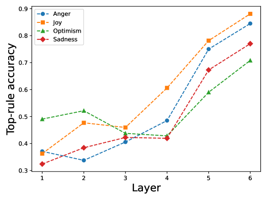### Top DNF rule accuracy for each class We report the class-wise accuracy achieved by the top DNF rule at each layer in Figure 5. The results show that each layer’s behavior can be effectively and consistently explained by its corresponding top DNF rule, demonstrating a strong alignment between the rule and the model’s internal representations. <details> <summary>x5.png Details</summary>  ### Visual Description ## Line Chart: Top-rule Accuracy Across Layers for Four Emotions ### Overview This image is a line chart displaying the "Top-rule accuracy" of four different emotions (Anger, Joy, Optimism, Sadness) across six sequential layers (1 through 6). The chart illustrates how the accuracy of a rule-based classification or detection system for these emotions changes as the model depth (layer) increases. ### Components/Axes * **Chart Type:** Multi-line chart with markers. * **X-Axis:** Labeled **"Layer"**. It has discrete integer markers from 1 to 6. * **Y-Axis:** Labeled **"Top-rule accuracy"**. It is a continuous scale ranging from 0.3 to 0.9, with major tick marks at 0.1 intervals (0.3, 0.4, 0.5, 0.6, 0.7, 0.8, 0.9). * **Legend:** Located in the **top-left corner** of the chart area. It defines four data series: * **Anger:** Blue dashed line with circle markers (`o`). * **Joy:** Orange dashed line with square markers (`s`). * **Optimism:** Green dashed line with triangle-up markers (`^`). * **Sadness:** Red dashed line with diamond markers (`D`). ### Detailed Analysis The chart plots the approximate accuracy values for each emotion at each layer. The following table reconstructs the data points based on visual inspection. Values are approximate. | Layer | Anger (Blue, Circle) | Joy (Orange, Square) | Optimism (Green, Triangle) | Sadness (Red, Diamond) | | :---- | :------------------- | :-------------------- | :------------------------- | :--------------------- | | 1 | ~0.37 | ~0.36 | ~0.49 | ~0.32 | | 2 | ~0.34 | ~0.48 | ~0.52 | ~0.39 | | 3 | ~0.41 | ~0.46 | ~0.44 | ~0.42 | | 4 | ~0.49 | ~0.61 | ~0.43 | ~0.42 | | 5 | ~0.75 | ~0.78 | ~0.59 | ~0.67 | | 6 | ~0.85 | ~0.88 | ~0.71 | ~0.77 | **Trend Verification per Series:** * **Anger (Blue):** Starts at ~0.37, dips at Layer 2 (~0.34), then shows a consistent and steep upward trend from Layer 3 onward, ending at ~0.85. * **Joy (Orange):** Starts at ~0.36, rises at Layer 2 (~0.48), dips slightly at Layer 3 (~0.46), then exhibits a strong, steady increase through Layers 4-6, achieving the highest final accuracy of ~0.88. * **Optimism (Green):** Begins as the highest at Layer 1 (~0.49), peaks at Layer 2 (~0.52), then declines to a low at Layer 4 (~0.43) before recovering with a moderate upward trend to ~0.71. * **Sadness (Red):** Shows the most consistent, gradual upward trend overall. It starts lowest at Layer 1 (~0.32) and increases nearly monotonically (with a plateau between Layers 3-4) to ~0.77. ### Key Observations 1. **General Upward Trend:** All four emotions show a significant increase in top-rule accuracy from the early layers (1-3) to the later layers (5-6). The most dramatic improvements occur between Layers 4 and 5. 2. **Performance Shift:** Optimism is the top-performing emotion in early layers (1-2), but is overtaken by both Joy and Anger in later layers. Joy becomes the highest-performing emotion by Layer 6. 3. **Convergence and Divergence:** The accuracy values for all emotions are relatively clustered between ~0.32 and ~0.52 in Layers 1-3. They begin to diverge significantly from Layer 4 onward, spreading across a wider range (from ~0.43 to ~0.61 at Layer 4, and from ~0.71 to ~0.88 at Layer 6). 4. **Relative Ordering Change:** The ranking of emotions by accuracy changes across layers. For example, at Layer 1: Optimism > Anger > Joy > Sadness. At Layer 6: Joy > Anger > Sadness > Optimism. ### Interpretation This chart likely visualizes the performance of a hierarchical or deep learning model where different layers capture increasingly complex features. The data suggests: * **Layer Specialization:** The early layers (1-3) may be extracting low-level, general features that are less discriminative for specific emotions, resulting in lower and more similar accuracy scores. The sharp rise in accuracy after Layer 4 indicates that deeper layers learn more abstract, emotion-specific representations. * **Emotion Complexity:** The differing trajectories imply that the rules or features defining "Optimism" might be more readily accessible in shallow processing, while "Joy" and "Anger" require deeper, more complex feature integration to be accurately identified by the top-rule mechanism. "Sadness" shows steady, linear improvement, suggesting its defining features are built up consistently across layers. * **Model Behavior:** The system's ability to apply its most confident rule ("top-rule") for classification improves dramatically with depth. This is a common pattern in deep neural networks, where higher-level layers form more semantically meaningful and separable representations. The crossover in performance (e.g., Joy surpassing Optimism) highlights that the optimal layer for extracting rules is emotion-dependent. **Language Declaration:** All text within the chart image is in English. </details> Figure 5: Top DNF rule accuracy for each class by layer. ### Code All code used for our experiments is available in the following GitHub repository: github.com/NeuroLogic2026/NeuroLogic. The sample code for purity-based predicates extraction. ⬇ 1 import torch 2 from typing import Dict, List, Tuple 3 4 def purity_rules ( 5 z_cls: torch. Tensor, # (N, H) CLS activations 6 y: torch. Tensor, # (N,) integer class labels 7 k: int = 15 # top-k neurons per class 8) -> Tuple [ 9 Dict [int, List [Tuple [int, float, int]]], # rules[c] = [(neuron, τ, support)] 10 Tuple [int, int, float, float, int] # best (class, neuron, τ, purity, support) 11]: 12 num_samples, hidden_size = z_cls. shape 13 num_classes = int (y. max (). item ()) + 1 14 15 purity = torch. empty (num_classes, hidden_size) 16 thr_mat = torch. empty (num_classes, hidden_size) 17 supp_mat = torch. empty (num_classes, hidden_size, dtype = torch. long) 18 19 class_counts = torch. bincount (y, minlength = num_classes) 20 21 for j in range (hidden_size): 22 a = z_cls [:, j] 23 idx = torch. argsort (a, descending = True) 24 a_sorted, y_sorted = a [idx], y [idx] 25 26 one_hot = torch. nn. functional. one_hot ( 27 y_sorted, num_classes = num_classes 28 ). cumsum (0) 29 total_seen = torch. arange (1, num_samples + 1) 30 31 for c in range (num_classes): 32 tp = one_hot [:, c] 33 fp = total_seen - tp 34 tn = (num_samples - class_counts [c]) - fp 35 36 tp_rate = tp. float () / class_counts [c]. clamp_min (1) 37 tn_rate = tn. float () / (num_samples - class_counts [c]). clamp_min (1) 38 p_scores = tp_rate + tn_rate 39 40 best = torch. argmax (p_scores) 41 purity [c, j] = p_scores [best] 42 thr_mat [c, j] = a_sorted [best]. item () 43 supp_mat [c, j] = total_seen [best]. item () 44 45 rules: Dict [int, List [Tuple [int, float, int]]] = { 46 c: [ 47 (j, thr_mat [c, j]. item (), supp_mat [c, j]. item ()) 48 for j in torch. topk (purity [c], k = min (k, hidden_size)). indices. tolist () 49 ] 50 for c in range (num_classes) 51 } 52 53 best_c, best_j = divmod (purity. argmax (). item (), hidden_size) 54 best_neuron = ( 55 best_c, 56 best_j, 57 thr_mat [best_c, best_j]. item (), 58 purity [best_c, best_j]. item (), 59 supp_mat [best_c, best_j]. 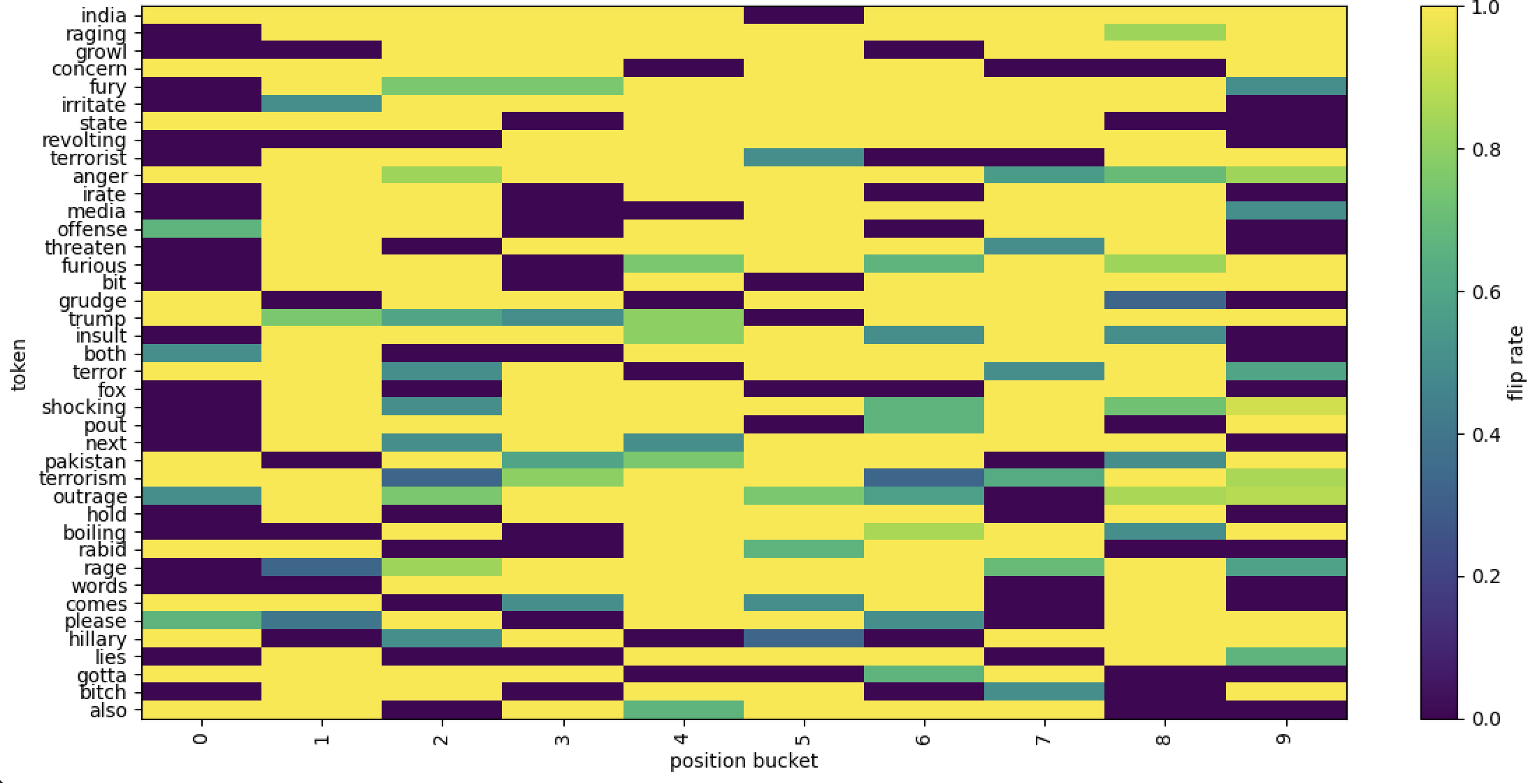item (), 60 ) 61 return rules, best_neuron ### Token Position Analysis Tables 6, 7, 9, and 9 present results for the classes Anger, Sadness, Optimism, and Joy, respectively. We identify causal tokens —words whose masking flips the activation of at least one class-specific predicate neuron. These words are grouped into 10 buckets based on their relative position within the input. <details> <summary>figures/LLM/heat_map_anger.png Details</summary>  ### Visual Description ## [Heatmap]: Token Flip Rate by Position Bucket ### Overview The image is a heatmap (2D grid plot) illustrating the **flip rate** (a measure of state change frequency) for various tokens (words) across 10 position buckets (0–9). The y-axis lists tokens, the x-axis lists position buckets, and a color bar (right) maps colors to flip rates (0.0 = dark purple, 1.0 = yellow; intermediate: teal = 0.4, green = 0.6, light green = 0.8). ### Components/Axes - **Y-axis (Tokens):** 40 tokens (rows) in order: `india, raging, growl, concern, fury, irritate, state, revolting, terrorist, anger, irate, media, offense, threaten, furious, bit, grudge, trump, insult, both, terror, fox, shocking, pout, next, pakistan, terrorism, outrage, hold, boiling, rabid, rage, words, comes, please, hillary, lies, gotta, bitch, also` - **X-axis (Position Buckets):** 10 buckets (columns) labeled `0, 1, 2, 3, 4, 5, 6, 7, 8, 9`. - **Color Bar (Legend):** Vertical bar on the right, labeled `flip rate`, with a gradient from 0.0 (dark purple) to 1.0 (yellow). Intermediate colors: teal (0.4), green (0.6), light green (0.8). ### Detailed Analysis (Key Trends by Token) We analyze flip rates (color) across position buckets (0–9) for each token, focusing on patterns: #### 1. High Flip Rate (Yellow, 1.0) - **Early Positions (0–1):** Tokens like `india, raging, growl, concern, state, media, outrage, rabid, comes, hillary, also` have high rates here. - **Late Positions (3–9):** Tokens like `revolting, irate, threaten, bit, insult, fox, pout, hold, boiling, words, lies, gotta, bitch` have high rates here (low in 0–2). #### 2. Low Flip Rate (Dark Purple, 0.0) - **Early Positions (0–2):** Tokens like `revolting, irate, threaten, bit, insult, fox, pout, hold, boiling, words, lies, gotta, bitch` have low rates here (high in 3–9). - **Late Positions (1–9):** Tokens like `grudge, rabid, comes, hillary, also` have low rates here (high only in 0). #### 3. Medium Flip Rate (Teal = 0.4, Green = 0.6) - **Teal (0.4):** Seen in `irritate (1), terror (2–3, 6–9), shocking (2–3), pakistan (2), terrorism (2, 6–9), please (1)`. - **Green (0.6):** Seen in `fury (2–3), offense (0–1), trump (1–4), terrorism (3), rage (2–3), please (0)`. ### Key Observations - **Position Bucket Patterns:** - Position `0` often has high/medium rates (e.g., `india, raging, growl, concern, state, media, outrage, rabid, comes, hillary, also, offense, trump, terror, please`). - Position `1` is mixed (low for most, medium for `irritate, trump, please`). - Position `2` is mixed (low for most, medium for `fury, terror, shocking, pakistan, terrorism, rage`). - Positions `3–9` are mostly high for many tokens (e.g., `revolting, irate, threaten, bit, insult, fox, pout, hold, boiling, words, lies, gotta, bitch`), with exceptions (e.g., `terrorist, trump, next, pakistan, terrorism, please`). - **Token-Specific Trends:** - `trump`: High at `0`, medium (0.6) at `1–4`, low at `5–9` (more state changes early). - `hillary`: High at `0`, low at `1–9` (fewer changes after the first position). - `terrorist`: Low at `0–2, 5–7`, medium (0.4) at `4`, high at `3, 8–9` (unusual pattern). ### Interpretation This heatmap likely analyzes **token state changes** (e.g., in NLP tasks like sentiment analysis, part-of-speech tagging, or model interpretability) across text positions (e.g., word positions in a sentence/document). - **Position Impact:** Later positions (3–9) often have higher flip rates, suggesting tokens in later text positions are more likely to change state (e.g., a model’s prediction for a word changes as it appears later in a sentence). - **Token Behavior:** Tokens related to anger (`fury, irritate, anger, irate, furious, rage`), terrorism (`terrorist, terror, terrorism`), and politics (`trump, hillary`) show distinct flip patterns, indicating how their “state” (e.g., sentiment, classification) evolves with position. - **Anomalies:** Tokens like `grudge, rabid, comes, hillary, also` have high flip rates only at position `0`, then low—suggesting rare state changes after the first position. This data helps identify how tokens behave across text positions, informing NLP model design or interpretability (e.g., why a model’s prediction for a word changes with its location in a sentence). </details> Figure 6: Heat map of keywords by positional bucket for class Anger. 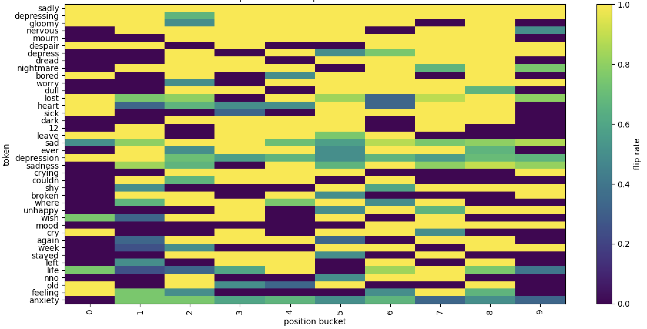<details> <summary>figures/LLM/heat_map_sadness.png Details</summary>  ### Visual Description ## [Heatmap]: Token Flip Rate by Position Bucket ### Overview The image is a heatmap (grid of colored cells) visualizing the **flip rate** (a measure of state change frequency) for various tokens (words) across 10 position buckets (0–9). The y-axis lists tokens, the x-axis lists position buckets, and a color bar (right) maps color to flip rate (0.0 = dark purple, 1.0 = yellow). ### Components/Axes - **Y-axis (Token)**: Vertical list of tokens (words) from top to bottom: `sadly, depressing, gloomy, nervous, mourn, despair, depress, dread, nightmare, bored, worry, dull, lost, heart, sick, dark, 12, leave, sad, ever, depression, sadness, crying, couldn’t, shy, broken, where, unhappy, wish, mood, cry, again, week, stayed, left, life, nno, old, feeling, anxiety` - **X-axis (Position Bucket)**: Horizontal axis with labels `0, 1, 2, 3, 4, 5, 6, 7, 8, 9` (10 buckets total). - **Color Bar (Flip Rate)**: Right-side vertical bar with a gradient from **dark purple (0.0)** to **yellow (1.0)**, labeled "flip rate". This encodes the flip rate for each (token, position bucket) cell. ### Detailed Analysis (Flip Rate by Token & Position) Each cell’s color indicates the flip rate (approximate values from color): | Token | Position Bucket 0 | 1 | 2 | 3 | 4 | 5 | 6 | 7 | 8 | 9 | |-------------|-------------------|-----|-----|-----|-----|-----|-----|-----|-----|-----| | `sadly` | 1.0 (yellow) | 1.0 | 1.0 | 1.0 | 1.0 | 1.0 | 1.0 | 1.0 | 1.0 | 1.0 | | `depressing`| 1.0 | 0.6 | 1.0 | 1.0 | 1.0 | 1.0 | 1.0 | 1.0 | 1.0 | 1.0 | | `gloomy` | 1.0 | 0.6 | 1.0 | 1.0 | 1.0 | 1.0 | 1.0 | 1.0 | 1.0 | 1.0 | | `nervous` | 0.0 (dark purple) | 0.0 | 1.0 | 0.0 | 1.0 | 0.0 | 1.0 | 1.0 | 1.0 | 0.6 | | `mourn` | 0.0 | 0.0 | 1.0 | 0.0 | 1.0 | 0.0 | 1.0 | 1.0 | 1.0 | 0.0 | | `despair` | 1.0 | 0.0 | 0.0 | 1.0 | 0.0 | 1.0 | 1.0 | 1.0 | 1.0 | 1.0 | | `depress` | 0.0 | 0.0 | 1.0 | 0.0 | 1.0 | 0.6 | 0.8 | 1.0 | 1.0 | 1.0 | | `dread` | 0.0 | 0.0 | 1.0 | 0.0 | 1.0 | 0.0 | 1.0 | 1.0 | 1.0 | 0.0 | | `nightmare` | 0.0 | 0.0 | 1.0 | 0.0 | 1.0 | 0.0 | 0.6 | 0.8 | 1.0 | 0.8 | | `bored` | 1.0 | 0.0 | 0.0 | 1.0 | 0.6 | 1.0 | 0.0 | 0.0 | 1.0 | 1.0 | | `worry` | 0.0 | 0.6 | 0.0 | 0.0 | 1.0 | 1.0 | 1.0 | 1.0 | 1.0 | 1.0 | | `dull` | 0.0 | 0.0 | 1.0 | 0.0 | 1.0 | 0.0 | 1.0 | 1.0 | 0.6 | 0.0 | | `lost` | 1.0 | 0.8 | 0.8 | 0.0 | 1.0 | 0.8 | 0.6 | 0.8 | 1.0 | 0.8 | | `heart` | 1.0 | 0.6 | 0.6 | 0.6 | 1.0 | 0.6 | 0.6 | 1.0 | 1.0 | 0.0 | | `sick` | 0.0 | 0.0 | 0.6 | 0.6 | 0.0 | 1.0 | 1.0 | 1.0 | 1.0 | 0.0 | | `dark` | 0.0 | 0.0 | 1.0 | 0.0 | 1.0 | 0.0 | 1.0 | 1.0 | 1.0 | 0.0 | | `12` | 0.0 | 0.0 | 1.0 | 0.0 | 1.0 | 0.0 | 1.0 | 1.0 | 0.0 | 0.0 | | `leave` | 1.0 | 0.0 | 0.0 | 1.0 | 0.8 | 0.8 | 1.0 | 0.0 | 0.0 | 1.0 | | `sad` | 0.6 | 0.8 | 0.8 | 1.0 | 0.8 | 0.8 | 0.8 | 0.8 | 0.8 | 0.8 | | `ever` | 0.0 | 0.6 | 0.6 | 1.0 | 0.6 | 0.6 | 0.6 | 0.6 | 0.6 | 0.0 | | `depression`| 1.0 | 0.8 | 0.8 | 0.6 | 0.6 | 0.6 | 0.6 | 0.6 | 0.6 | 0.6 | | `sadness` | 0.0 | 0.8 | 0.8 | 0.0 | 1.0 | 0.8 | 0.8 | 0.8 | 0.8 | 0.8 | | `crying` | 0.0 | 0.0 | 1.0 | 0.0 | 1.0 | 0.0 | 1.0 | 0.0 | 0.0 | 1.0 | | `couldn’t` | 0.0 | 0.6 | 0.6 | 0.0 | 0.0 | 0.6 | 0.6 | 0.0 | 0.0 | 1.0 | | `shy` | 0.0 | 0.0 | 1.0 | 0.0 | 1.0 | 0.0 | 1.0 | 0.0 | 0.0 | 1.0 | | `broken` | 0.0 | 0.0 | 1.0 | 0.0 | 1.0 | 0.0 | 1.0 | 0.0 | 0.0 | 1.0 | | `where` | 0.0 | 0.6 | 0.6 | 0.8 | 0.8 | 0.6 | 0.6 | 0.8 | 0.0 | 0.0 | | `unhappy` | 0.0 | 0.0 | 0.0 | 1.0 | 0.0 | 0.6 | 0.6 | 0.8 | 0.8 | 1.0 | | `wish` | 0.8 | 0.6 | 0.0 | 1.0 | 0.0 | 0.0 | 0.0 | 0.0 | 0.0 | 1.0 | | `mood` | 0.0 | 0.0 | 0.0 | 0.0 | 0.0 | 0.0 | 0.0 | 0.0 | 0.0 | 1.0 | | `cry` | 1.0 | 0.0 | 0.0 | 1.0 | 0.0 | 0.0 | 0.6 | 0.0 | 0.0 | 0.0 | | `again` | 0.0 | 0.6 | 1.0 | 0.0 | 1.0 | 0.0 | 1.0 | 1.0 | 1.0 | 0.0 | | `week` | 0.0 | 0.6 | 0.6 | 0.0 | 1.0 | 0.0 | 1.0 | 0.0 | 0.0 | 1.0 | | `stayed` | 0.0 | 0.6 | 0.0 | 1.0 | 0.0 | 1.0 | 1.0 | 1.0 | 1.0 | 0.0 | | `left` | 0.0 | 0.6 | 0.0 | 1.0 | 0.0 | 1.0 | 1.0 | 1.0 | 1.0 | 0.0 | | `life` | 0.8 | 0.6 | 0.6 | 0.6 | 0.0 | 0.8 | 0.8 | 0.8 | 0.8 | 0.6 | | `nno` | 0.0 | 0.0 | 1.0 | 0.0 | 1.0 | 0.0 | 1.0 | 1.0 | 0.0 | 0.0 | | `old` | 1.0 | 0.0 | 0.0 | 1.0 | 0.0 | 1.0 | 0.0 | 0.0 | 1.0 | 0.0 | | `feeling` | 0.0 | 0.8 | 0.8 | 0.6 | 0.6 | 0.6 | 0.8 | 0.8 | 0.8 | 0.6 | | `anxiety` | 0.0 | 0.8 | 0.8 | 0.6 | 0.6 | 0.6 | 0.8 | 0.8 | 0.8 | 0.6 | ### Key Observations - **High Flip Rate (Yellow)**: Tokens like `sadly`, `despair`, `sad`, `depression`, `sadness`, `life`, `feeling`, `anxiety` have dominant yellow cells (flip rate ~1.0) across most position buckets. - **Low Flip Rate (Dark Purple)**: Tokens like `mood`, `cry`, `broken`, `shy`, `crying` have frequent dark purple cells (flip rate ~0.0) in some buckets. - **Mixed Flip Rates (Teal/Green)**: Tokens like `lost`, `heart`, `ever`, `where`, `unhappy` show a mix of teal (0.6) and green (0.8) cells, indicating moderate flip rates. - **Position Bucket Patterns**: Buckets 0–2 often have more dark purple (low flip rate) for tokens like `nervous`, `mourn`, `dread`, while buckets 3–9 have more yellow (high flip rate) for many tokens. ### Interpretation This heatmap likely models **token flip rate** (state change frequency) across position buckets (e.g., word positions in a text sequence). Tokens related to negative emotions (sadness, depression, anxiety) have higher flip rates (more yellow), suggesting they are more dynamic or context-dependent. Tokens with lower flip rates (dark purple) may be more stable or less context-sensitive. The position buckets could represent sequential positions (e.g., in a sentence), showing how flip rate varies with position for each token—useful for natural language processing to understand token behavior across contexts. </details> Figure 7: Heat map of keywords by positional bucket for class Sadness. 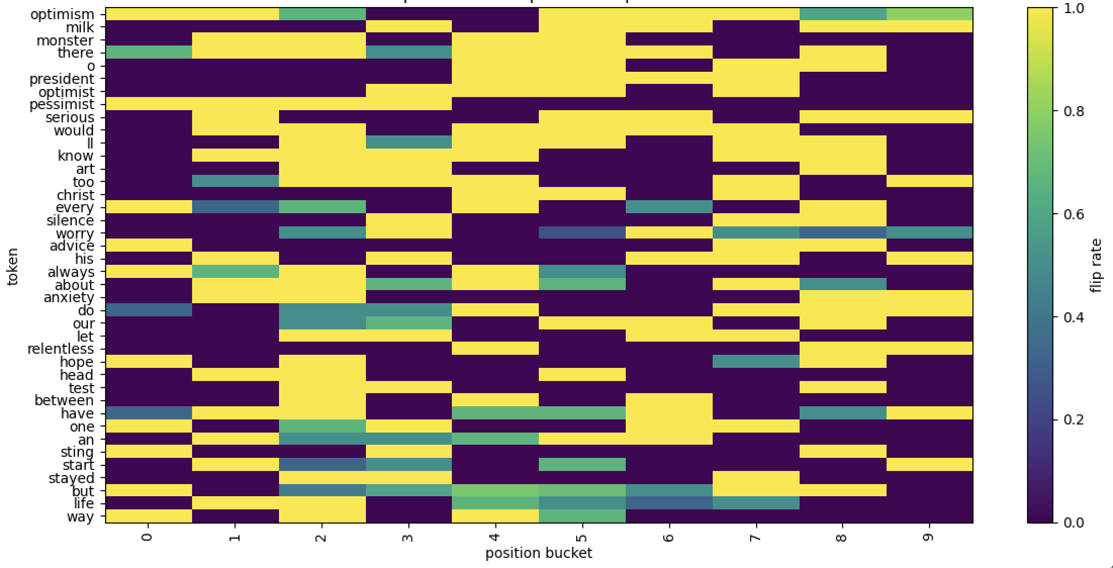<details> <summary>figures/LLM/heat_map_optimism.png Details</summary>  ### Visual Description ## [Heatmap]: Token Flip Rate by Position Bucket ### Overview The image is a heatmap (2D grid plot) visualizing the **flip rate** of various tokens across 10 position buckets (0–9). The y-axis lists tokens, the x-axis lists position buckets, and a color bar (right) maps color to flip rate (0.0 = dark purple, 1.0 = yellow). ### Components/Axes - **Y-axis (Vertical):** Labeled "token". Tokens (rows) include: *optimism, milk, monster, there, o, president, optimist, pessimist, serious, would, ll, know, art, too, christ, every, silence, worry, advice, his, always, about, anxiety, do, our, let, relentless, hope, head, test, between, have, one, an, sting, start, stayed, but, life, way*. - **X-axis (Horizontal):** Labeled "position bucket". Buckets (columns) are numbered 0–9 (10 total). - **Color Bar (Legend):** Labeled "flip rate". Color scale: - Dark purple: ~0.0 (low flip rate) - Teal: ~0.2–0.4 - Green: ~0.4–0.6 - Light green: ~0.6–0.8 - Yellow: ~0.8–1.0 (high flip rate) ### Detailed Analysis (Flip Rate by Token/Position) Each cell (token, position bucket) is colored by flip rate. Key patterns: #### High Flip Rate (Yellow, ~1.0) - Tokens like *optimism* (pos 0,1), *milk* (pos 2,9), *monster* (pos 1,2), *o* (pos 4,5), *president* (pos 4,5), *optimist* (pos 4,5), *pessimist* (pos 0,1,2), *serious* (pos 1), *would* (pos 2), *ll* (pos 4,5), *know* (pos 1,2), *art* (pos 2), *christ* (pos 4,5), *every* (pos 0), *advice* (pos 0), *his* (pos 1), *always* (pos 0), *about* (pos 1,2), *let* (pos 2), *relentless* (pos 4), *hope* (pos 0), *head* (pos 1), *test* (pos 2), *one* (pos 0), *sting* (pos 0), *start* (pos 1), *but* (pos 0), *life* (pos 1), *way* (pos 0) show high flip rates (yellow) in specific buckets. #### Low Flip Rate (Dark Purple, ~0.0) Most tokens have dark purple (low flip rate) in many buckets, especially positions 3–9 (e.g., *silence*, *anxiety*, *our*, *between*, *stayed* have near-zero flip rates across all buckets). #### Intermediate Flip Rates (Teal/Green) Tokens like *there* (pos 0,2), *every* (pos 1,2,5), *worry* (pos 2), *do* (pos 0,2,3), *have* (pos 0), *one* (pos 2), *an* (pos 2), *but* (pos 2) show intermediate flip rates (teal/green) in some buckets. ### Key Observations - **Positional Sensitivity:** Tokens like *o*, *president*, *optimist* have high flip rates (yellow) in positions 4–5, suggesting consistent "flipping" behavior in this range. - **Stability:** Tokens like *silence*, *anxiety*, *our* have near-zero flip rates (dark purple) across all buckets, indicating high stability. - **Mixed Behavior:** Tokens like *every*, *do* show mixed flip rates (teal/green) in some buckets, suggesting variable stability. ### Interpretation This heatmap likely analyzes **token dynamics** (e.g., in a sequence model or text processing) by measuring how often tokens "flip" (change state) across positions. High flip rates (yellow) in specific buckets imply positional sensitivity (e.g., tokens are more likely to change at positions 0–2 or 4–5). Low flip rates (dark purple) indicate stable tokens. This data could inform model design (e.g., prioritizing stable tokens for consistency) or text analysis (e.g., identifying position-dependent token behavior). (Note: All text is in English; no other languages are present.) </details> Figure 8: Heat map of keywords by positional bucket for class Optimism. 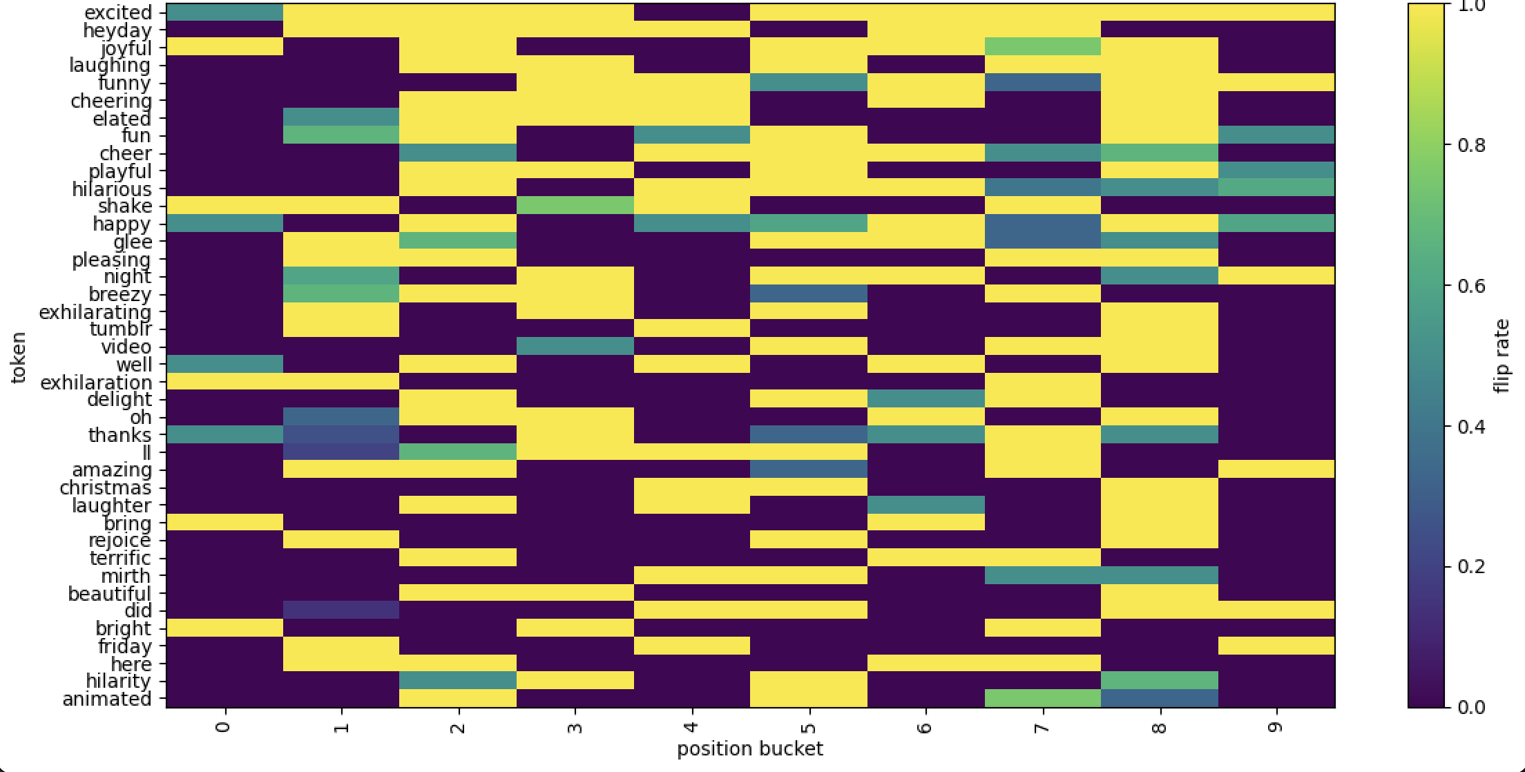<details> <summary>figures/LLM/heat_map_joy.png Details</summary>  ### Visual Description ## Heatmap: Token Flip Rate by Position Bucket ### Overview This image is a heatmap visualizing the "flip rate" of various tokens across different position buckets. The chart displays a grid where each cell's color represents a numerical value (flip rate) for a specific token at a specific position bucket. The tokens are listed vertically on the y-axis, and the position buckets are listed horizontally on the x-axis. A color scale bar on the right provides the key for interpreting the flip rate values. ### Components/Axes * **Chart Type:** Heatmap. * **Y-Axis (Vertical):** Labeled "token". It lists 40 distinct tokens (words/phrases). From top to bottom, they are: `excited`, `heyday`, `joyful`, `laughing`, `funny`, `cheering`, `elated`, `fun`, `cheer`, `playful`, `hilarious`, `shake`, `happy`, `glee`, `pleasing`, `night`, `breezy`, `exhilarating`, `tumblr`, `video`, `well`, `exhilaration`, `delight`, `oh`, `thanks`, `ll`, `amazing`, `christmas`, `laughter`, `bring`, `rejoice`, `terrific`, `mirth`, `beautiful`, `did`, `bright`, `friday`, `here`, `hilarity`, `animated`. * **X-Axis (Horizontal):** Labeled "position bucket". It displays 10 discrete buckets, numbered from `0` to `9`. * **Color Scale/Legend:** Located on the right side of the chart. It is a vertical bar labeled "flip rate". * **Scale Range:** 0.0 (bottom) to 1.0 (top). * **Color Mapping:** * Dark Purple/Indigo: ~0.0 - 0.2 (Low flip rate) * Teal/Blue-Green: ~0.4 - 0.6 (Medium flip rate) * Yellow: ~0.8 - 1.0 (High flip rate) * The gradient transitions smoothly between these colors. ### Detailed Analysis The heatmap shows the distribution of flip rates for each token across the 10 position buckets. The value in each cell is approximate, inferred from the color. **General Pattern Observation:** There is significant variation both between tokens and across position buckets for the same token. No single token has a uniform color across all buckets. **Token-Specific Trends (Selected Examples):** * **`excited`:** Shows a high flip rate (yellow) in buckets 1, 2, 3, 4, 5, 8, and 9. It has a medium rate (teal) in bucket 0 and a low rate (purple) in buckets 6 and 7. * **`heyday`:** Predominantly low flip rate (purple) across most buckets, with high rates (yellow) only in buckets 2, 3, and 4. * **`joyful`:** High rates (yellow) in buckets 0, 1, 2, 3, 4, 5, 8, and 9. Medium rate (green) in bucket 7. Low rate (purple) in bucket 6. * **`funny`:** High rates (yellow) in buckets 2, 3, 4, 5, 8, and 9. Medium rates (teal) in buckets 6 and 7. Low rate (purple) in buckets 0 and 1. * **`happy`:** High rates (yellow) in buckets 2, 3, 4, 5, 8, and 9. Medium rates (teal) in buckets 0 and 7. Low rate (purple) in buckets 1 and 6. * **`night`:** High rates (yellow) in buckets 1, 2, 3, 5, 8, and 9. Medium rates (teal) in buckets 0 and 7. Low rate (purple) in buckets 4 and 6. * **`christmas`:** Shows a very distinct pattern. It has a high flip rate (yellow) only in bucket 9. All other buckets (0-8) are dark purple, indicating a very low flip rate (~0.0). * **`friday`:** Similar to `christmas`, it has a high rate (yellow) only in bucket 9, with low rates elsewhere. * **`ll`:** Shows a high rate (yellow) in buckets 3, 4, 5, 6, and 7. Medium rates (teal/green) in buckets 2 and 8. Low rates in buckets 0, 1, and 9. **Position Bucket Trends:** * **Bucket 0:** Contains a mix of low (purple) and medium (teal) values. Notable high-rate tokens here are `joyful`, `shake`, and `bright`. * **Bucket 9:** Contains a high concentration of high flip rate (yellow) tokens, including `excited`, `joyful`, `funny`, `happy`, `night`, `amazing`, `christmas`, `friday`, and `animated`. * **Buckets 4 & 5:** Also show a high density of yellow cells across many tokens. ### Key Observations 1. **Cluster of High Activity:** Buckets 2, 3, 4, 5, 8, and 9 frequently show high flip rates (yellow) for many tokens, suggesting these positions are associated with higher token "flip" behavior. 2. **Low Activity Buckets:** Buckets 0, 1, 6, and 7 have more purple and teal cells, indicating generally lower flip rates. 3. **Token Specificity:** Some tokens have very localized high flip rates. The most extreme examples are `christmas` and `friday`, which are only high in bucket 9. `ll` has a distinct high-rate cluster in the middle buckets (3-7). 4. **Visual Outliers:** The rows for `christmas` and `friday` are visually striking due to their almost entirely purple background with a single yellow cell at the far right (bucket 9). ### Interpretation This heatmap likely visualizes the results of an experiment or analysis tracking how often ("flip rate") specific words (tokens) change their state, prediction, or association when they appear at different positions (buckets) within a sequence or document. * **What the data suggests:** The flip rate is not uniform. It is highly dependent on both the specific word and its positional context. Words related to positive emotion (`joyful`, `happy`, `excited`) and general terms (`funny`, `amazing`) tend to have higher flip rates across many positions. In contrast, context-specific nouns (`christmas`, `friday`) have a very high flip rate only at a specific position (bucket 9), which might correspond to the end of a sequence or a specific segment where their relevance changes dramatically. * **Relationship between elements:** The x-axis (position bucket) likely represents a normalized or binned measure of location within an input (e.g., first 10%, second 10%, etc.). The y-axis represents the vocabulary of interest. The color (flip rate) is the measured outcome. The chart reveals an interaction effect: the effect of position on flip rate varies by token. * **Potential meaning:** In a machine learning or NLP context, this could indicate that the model's confidence or internal representation for certain words is more volatile (prone to "flipping") at specific points in a text. For example, the model might be very certain about the meaning of "christmas" until it reaches the final segment (bucket 9), where new context causes a significant re-evaluation (high flip rate). Conversely, emotion words might be consistently re-evaluated throughout the sequence. This information could be used to understand model behavior, identify critical context windows, or improve model stability. </details> Figure 9: Heat map of keywords by positional bucket for class Joy. ### Top grounded rules Tables 5, 6, 7, 8, 9, 10 present the top five grounded rules, i.e., (Keyword, Template) pairs, associated with the top five neurons in each corresponding layer, respectively. | 438 | optimism | 1.2304 | is | before_verb | 14 | 1.00 | | --- | --- | --- | --- | --- | --- | --- | | a | exists | 14 | 1.00 | | | | | you | before_verb | 32 | 1.00 | | | | | you | at_start | 25 | 1.00 | | | | | you | after_subject | 22 | 1.00 | | | | | 683 | optimism | 1.2237 | is | before_verb | 17 | 1.00 | | a | exists | 13 | 1.00 | | | | | you | before_verb | 21 | 1.00 | | | | | you | at_start | 18 | 1.00 | | | | | you | after_subject | 16 | 1.00 | | | | | 568 | optimism | 1.2081 | is | before_verb | 20 | 1.00 | | a | exists | 17 | 1.00 | | | | | you | before_verb | 22 | 1.00 | | | | | you | at_start | 22 | 1.00 | | | | | you | after_subject | 19 | 1.00 | | | | | 389 | anger | 1.2037 | my | at_end | 12 | 1.00 | | it | at_start | 74 | 1.00 | | | | | it | exists | 55 | 1.00 | | | | | it | before_verb | 52 | 1.00 | | | | | it | at_end | 43 | 1.00 | | | | | 757 | optimism | 1.2006 | is | before_verb | 15 | 1.00 | | a | exists | 13 | 1.00 | | | | | you | before_verb | 26 | 1.00 | | | | | you | at_start | 23 | 1.00 | | | | | you | after_subject | 18 | 1.00 | | | | Table 5: Top-5 grounded rules in layer 1. | 734 | anger | 1.1921 | it | at_start | 61 | 1.00 | | --- | --- | --- | --- | --- | --- | --- | | it | after_verb | 73 | 1.00 | | | | | s | after_subject | 62 | 1.00 | | | | | that | after_subject | 84 | 1.00 | | | | | that | after_verb | 87 | 1.00 | | | | | 110 | anger | 1.1875 | it | at_start | 6 | 1.00 | | it | after_verb | 6 | 1.00 | | | | | s | after_subject | 5 | 1.00 | | | | | that | after_subject | 3 | 1.00 | | | | | that | after_verb | 1 | 1.00 | | | | | 756 | anger | 1.1739 | it | at_start | 52 | 1.00 | | it | after_verb | 63 | 1.00 | | | | | s | after_subject | 61 | 1.00 | | | | | that | after_subject | 64 | 1.00 | | | | | that | after_verb | 70 | 1.00 | | | | | 635 | anger | 1.1722 | it | at_start | 53 | 1.00 | | it | after_verb | 60 | 1.00 | | | | | s | after_subject | 65 | 1.00 | | | | | that | after_subject | 69 | 1.00 | | | | | that | after_verb | 78 | 1.00 | | | | | 453 | anger | 1.1628 | it | at_start | 52 | 1.00 | | it | after_verb | 62 | 1.00 | | | | | s | after_subject | 64 | 1.00 | | | | | that | after_subject | 69 | 1.00 | | | | | that | after_verb | 74 | 1.00 | | | | Table 6: Top-5 grounded rules in layer 2. | 509 | anger | 1.3988 | it | at_end | 16 | 1.00 | | --- | --- | --- | --- | --- | --- | --- | | that | before_subject | 8 | 1.00 | | | | | he | before_verb | 23 | 1.00 | | | | | he | at_start | 19 | 1.00 | | | | | user | after_subject | 16 | 1.00 | | | | | 495 | anger | 1.3886 | it | at_end | 10 | 1.00 | | that | before_subject | 14 | 1.00 | | | | | he | before_verb | 10 | 1.00 | | | | | he | at_start | 12 | 1.00 | | | | | user | after_subject | 13 | 1.00 | | | | | 652 | joy | 1.3743 | amazing | after_verb | 28 | 1.00 | | live | after_verb | 27 | 1.00 | | | | | ly | before_verb | 27 | 1.00 | | | | | ly | at_start | 27 | 1.00 | | | | | musically | at_end | 27 | 1.00 | | | | | 734 | anger | 1.3660 | it | at_end | 6 | 1.00 | | that | before_subject | 2 | 1.00 | | | | | he | before_verb | 1 | 1.00 | | | | | he | at_start | 1 | 1.00 | | | | | user | after_subject | 3 | 1.00 | | | | Table 7: Top-5 grounded rules in layer 3. | Neuron | Class | Purity | Keyword | Template | Flips | Rate | | --- | --- | --- | --- | --- | --- | --- | | 597 | joy | 1.5896 | is | before_verb | 1 | 1.00 | | 232 | joy | 1.5464 | is | before_verb | 4 | 1.00 | | amazing | after_verb | 1 | 1.00 | | | | | i | after_subject | 6 | 0.96 | | | | | i | after_verb | 8 | 0.96 | | | | | this | after_verb | 5 | 0.96 | | | | | 66 | joy | 1.5405 | is | before_verb | 2 | 1.00 | | this | after_verb | 1 | 0.96 | | | | | 399 | anger | 1.5323 | s | exists | 2 | 1.00 | | fucking | after_subject | 4 | 1.00 | | | | | but | before_subject | 1 | 1.00 | | | | | but | at_start | 1 | 1.00 | | | | | but | before_verb | 1 | 1.00 | | | | | 71 | joy | 1.5262 | is | before_verb | 8 | 1.00 | | amazing | after_verb | 1 | 1.00 | | | | | i | after_subject | 20 | 0.96 | | | | | i | after_verb | 17 | 0.96 | | | | | this | after_verb | 9 | 0.96 | | | | Table 8: Top-5 grounded rules in layer 4. | Neuron | Class | Purity | Keyword | Template | Flips | Rate | | --- | --- | --- | --- | --- | --- | --- | | 499 | joy | 1.8198 | today | at_start | 1 | 1.00 | | 258 | joy | 1.7694 | heyday | after_verb | 1 | 1.00 | | 698 | joy | 1.7653 | heyday | after_verb | 1 | 1.00 | | today | at_start | 3 | 1.00 | | | | | 221 | joy | 1.7426 | today | at_start | 1 | 1.00 | | 535 | joy | 1.7384 | heyday | after_verb | 2 | 1.00 | | glee | before_subject | 6 | 1.00 | | | | | today | at_start | 2 | 1.00 | | | | Table 9: Top-5 grounded rules in layer 5. | 122 | joy | 1.8478 | laughter | after_subject | 2 | 1.00 | | --- | --- | --- | --- | --- | --- | --- | | hilarious | after_subject | 1 | 0.88 | | | | | 344 | joy | 1.8359 | playful | exists | 1 | 1.00 | | smiling | after_subject | 2 | 1.00 | | | | | laughter | at_end | 1 | 1.00 | | | | | laughter | after_subject | 1 | 1.00 | | | | | hilarious | after_subject | 2 | 0.88 | | | | | 497 | joy | 1.8342 | laughter | after_subject | 1 | 1.00 | | hilarious | after_subject | 1 | 0.88 | | | | | 212 | joy | 1.8330 | playful | exists | 1 | 1.00 | | omg | before_subject | 1 | 1.00 | | | | | smiling | after_subject | 2 | 1.00 | | | | | laughter | at_end | 1 | 1.00 | | | | | laughter | after_subject | 3 | 1.00 | | | | | 452 | joy | 1.8261 | laughter | after_subject | 1 | 1.00 | | hilarious | after_subject | 1 | 0.88 | | | | Table 10: Top-5 grounded rules in layer 6. ### Top three rules per class for every layer Tables 11 and 12 present the top three grounded rules for each class across all layers. | Class | Keyword | Template | Flips | Total | Rate | Neuron | | --- | --- | --- | --- | --- | --- | --- | | Layer 1 | | | | | | | | anger | terrorism | after_subject | 19 | 19 | 1.00 | 125 | | anger | am | at_start | 19 | 19 | 1.00 | 125 | | anger | terrorism | after_subject | 17 | 19 | 1.00 | 695 | | joy | ly | before_verb | 27 | 27 | 1.00 | 505 | | joy | ly | at_start | 27 | 27 | 1.00 | 505 | | joy | musically | at_end | 27 | 27 | 1.00 | 505 | | optimism | can | after_subject | 17 | 19 | 1.00 | 563 | | optimism | your | after_verb | 18 | 21 | 1.00 | 438 | | optimism | your | after_verb | 18 | 21 | 1.00 | 563 | | sadness | want | after_subject | 17 | 19 | 1.00 | 52 | | sadness | lost | after_subject | 24 | 30 | 1.00 | 52 | | sadness | want | after_subject | 16 | 19 | 1.00 | 679 | | Layer 2 | | | | | | | | anger | have | after_subject | 67 | 86 | 1.00 | 298 | | anger | with | after_verb | 67 | 84 | 1.00 | 298 | | anger | have | after_subject | 65 | 86 | 1.00 | 136 | | sadness | my | after_verb | 83 | 94 | 1.00 | 698 | | sadness | is | after_subject | 96 | 110 | 1.00 | 712 | | sadness | my | after_verb | 72 | 94 | 1.00 | 712 | | Layer 3 | | | | | | | | anger | people | before_verb | 27 | 32 | 1.00 | 189 | | anger | why | before_verb | 23 | 30 | 1.00 | 189 | | anger | why | before_subject | 23 | 31 | 1.00 | 189 | | joy | ly | before_verb | 27 | 27 | 1.00 | 652 | | joy | ly | before_verb | 27 | 27 | 1.00 | 28 | | joy | ly | at_start | 27 | 27 | 1.00 | 652 | | optimism | be | after_subject | 22 | 26 | 1.00 | 459 | | optimism | be | after_subject | 22 | 26 | 1.00 | 416 | | optimism | be | after_subject | 19 | 26 | 1.00 | 157 | | sadness | sad | at_end | 25 | 27 | 1.00 | 316 | | sadness | sad | at_end | 24 | 27 | 1.00 | 498 | | sadness | sad | after_verb | 23 | 26 | 1.00 | 305 | Table 11: Top-3 grounded rules per class (Layers 1 to 3). | Class | Token | Keyword | Template | Total | Rate | Neuron | | --- | --- | --- | --- | --- | --- | --- | | Layer 4 | | | | | | | | anger | fucking | after_subject | 20 | 20 | 1.00 | 434 | | anger | anger | after_verb | 18 | 19 | 1.00 | 92 | | anger | terrorism | after_subject | 17 | 19 | 1.00 | 92 | | joy | amazing | after_verb | 29 | 31 | 1.00 | 95 | | joy | this | after_verb | 41 | 48 | 0.96 | 95 | | joy | is | before_verb | 19 | 25 | 1.00 | 95 | | optimism | be | after_subject | 22 | 26 | 1.00 | 416 | | optimism | you | at_start | 26 | 34 | 0.97 | 416 | | optimism | you | before_verb | 29 | 38 | 1.00 | 416 | | sadness | sad | at_end | 19 | 27 | 1.00 | 305 | | sadness | sad | at_end | 19 | 27 | 1.00 | 23 | | sadness | sad | at_end | 17 | 27 | 1.00 | 296 | | Layer 5 | | | | | | | | anger | awful | at_end | 15 | 19 | 0.84 | 92 | | anger | angry | after_subject | 22 | 27 | 0.93 | 92 | | anger | angry | after_verb | 21 | 27 | 0.89 | 92 | | optimism | it | at_start | 9 | 24 | 0.83 | 430 | | optimism | it | before_verb | 6 | 21 | 0.81 | 430 | | optimism | is | at_start | 8 | 29 | 0.76 | 459 | | sadness | sad | at_end | 23 | 27 | 0.93 | 246 | | sadness | sadness | exists | 17 | 23 | 0.83 | 433 | | sadness | sad | at_end | 22 | 27 | 0.93 | 433 | | Layer 6 | | | | | | | | anger | anger | after_verb | 14 | 19 | 0.89 | 531 | | anger | awful | at_end | 13 | 19 | 0.74 | 15 | | anger | anger | after_verb | 13 | 19 | 0.89 | 603 | | optimism | not | after_subject | 14 | 19 | 0.74 | 142 | | optimism | s | after_subject | 13 | 20 | 0.75 | 142 | | optimism | user | exists | 15 | 20 | 0.80 | 142 | | sadness | sadness | exists | 17 | 23 | 0.78 | 298 | | sadness | sad | exists | 25 | 31 | 0.81 | 298 | | sadness | sad | at_end | 21 | 27 | 0.89 | 242 | Table 12: Top-3 grounded rules per class (Layers 4 to 6).