2501.08603v3

## Monte Carlo Tree Search for Comprehensive Exploration in LLM-Based Automatic Heuristic Design Zhi Zheng 1 Zhuoliang Xie 2 Zhenkun Wang 2 Bryan Hooi 1 MCTS advantages MCTS advantages <details> <summary>Image 1 Details</summary>  ### Visual Description ## Scatter Plots: Populations in LLM-based AHD ### Overview The image presents four scatter plots, labeled (a) through (d), illustrating the relationship between "Performance" and "Feature of heuristic functions". The plots visualize populations of heuristic functions during an LLM-based Automated Heuristic Design (AHD) process. Each plot uses different symbols to represent different types of heuristic functions and their evolution. ### Components/Axes * **X-axis:** "Feature of heuristic functions" (appears on all four plots). The scale is not explicitly defined, but represents a continuous variable. * **Y-axis:** "Performance" (appears on all four plots). The scale is not explicitly defined, but represents a continuous variable. * **Plot (a) Legend:** * Dark Green Circles: "Heuristic functions in the original elite population" * Light Gray Circles: "LLM-based heuristic evolution" * White Circles: "Newly generated heuristic functions" * **Plot (b) Legend:** * Dark Green Circles: "Heuristic functions preserved in the updated elite population" * Red Crosses: "Discarded heuristic functions" * Light Green Triangles: "Newly generated heuristic functions" * **Plot (c) Legend:** * Light Blue Circles: "Tree node of heuristic function on MCTS depth k" * Light Blue Diamonds: "Existing MCTS edges" * **Plot (d) Legend:** * Light Blue Circles: "Better-performing tree nodes of heuristics outside local optima" * Yellow Stars: "New MCTS expansions" * Light Blue Diamonds: "Existing MCTS edges" * **Title:** "(a) Populations in LLM-based AHD" (for the first plot) ### Detailed Analysis or Content Details **Plot (a):** The plot shows a general downward trend. The dark green circles (original elite population) are scattered across the plot, with a concentration towards the upper-left. The light gray circles (LLM evolution) are more dispersed, and the white circles (newly generated) are mostly located towards the lower-left. * Approximate data points (estimated from visual inspection): * Dark Green: (0.2, 8), (0.3, 7), (0.4, 6), (0.5, 5), (0.6, 4), (0.7, 3), (0.8, 2) * Light Gray: (0.1, 5), (0.2, 4), (0.3, 3), (0.4, 2), (0.5, 1) * White: (0.1, 2), (0.2, 1), (0.3, 0.5) **Plot (b):** This plot shows a mix of preserved and discarded heuristic functions. The dark green circles (preserved) are concentrated in the upper-right, while the red crosses (discarded) are scattered towards the lower-left. The light green triangles (newly generated) are dispersed. * Approximate data points: * Dark Green: (0.3, 7), (0.4, 6), (0.5, 5), (0.6, 4), (0.7, 3) * Red Cross: (0.1, 2), (0.2, 1), (0.3, 0.5), (0.4, 0.2) * Light Green: (0.2, 3), (0.3, 2), (0.4, 1) **Plot (c):** This plot displays a network-like structure with nodes (light blue circles) connected by edges (light blue diamonds). The plot shows a downward trend in performance as the iterations of the tree search increase. The nodes are numbered 1 through 5. * Approximate data points: * Node 1: (0.2, 7) * Node 2: (0.4, 6) * Node 3: (0.6, 5) * Node 4: (0.8, 4) * Node 5: (1.0, 3) **Plot (d):** Similar to plot (c), this plot shows a network structure with nodes and edges. It also exhibits a downward trend in performance with increasing tree search iterations. A yellow star indicates a new MCTS expansion. * Approximate data points: * Node 1: (0.2, 6) * Node 2: (0.4, 5) * Node 3: (0.6, 4) * Node 4: (0.8, 3) * Node 5: (1.0, 2) * Yellow Star: (0.5, 4.5) ### Key Observations * In plots (a) and (b), the LLM-based evolution and newly generated functions tend to have lower performance than the original elite population. * Plots (c) and (d) demonstrate a clear trade-off between exploration (MCTS expansions) and exploitation (existing edges) in the tree search process. * The network structures in plots (c) and (d) suggest a hierarchical relationship between heuristic functions. ### Interpretation These plots illustrate the dynamics of heuristic function populations during an LLM-based AHD process. Plot (a) shows the initial population and the introduction of new heuristics through LLM evolution. Plot (b) demonstrates the selection process, where better-performing heuristics are preserved, and less effective ones are discarded. Plots (c) and (d) provide insights into the tree search process, showing how the algorithm explores different heuristic functions and refines its search strategy. The downward trends in performance in plots (c) and (d) likely represent the algorithm converging towards a local optimum. The yellow star in plot (d) indicates an attempt to escape this local optimum by expanding the search space. The overall data suggests that the LLM-based AHD process is effective in generating and evaluating heuristic functions, but it may require further refinement to avoid getting stuck in local optima. The use of MCTS and the visualization of the tree structure provide a valuable tool for understanding the algorithm's behavior and identifying areas for improvement. </details> Feature of heuristic functions Feature of heuristic functions The general adoptted population in exsiting LLM-based AHD methods will discard emporarily underperforming codes. MCTS allows (b) MCTS for higher-quality LLM-based AHD (Ours) MCTS developing based on temporarily underperforming codes which can help to jump out of local optima. The general adoptted population in exsiting LLM-based AHD methods will discard emporarily underperforming codes. MCTS allows MCTS developing based on temporarily underperforming codes which can help to jump out of local optima. 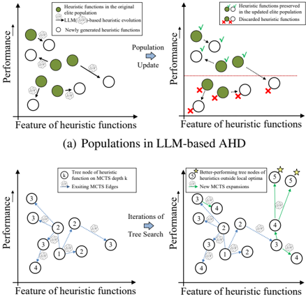© Copyright National University of Singapore. All Rights Reserved. Population is difficult to maintain diversity and MCTS can explore a wider heuristic func © Copyright National University of Singapore. All Rights Reserved. Population is difficult to maintain diversity and MCTS can explore a wider heuristic func Figure 1. The generally adopted population (a) in existing LLMbased AHD methods (Liu et al., 2024b; Ye et al., 2024a) directly discards low-performance heuristics (under the red dashed line in (a)), thus falling into local optima. MCTS provides chances to develop low-performance heuristics, so it can more comprehensively explore the space of heuristic functions with different features. ## Abstract Handcrafting heuristics for solving complex optimization tasks (e.g., route planning and task allocation) is a common practice but requires extensive domain knowledge. Recently, Large Language Model (LLM)-based automatic heuristic design (AHD) methods have shown promise in generating high-quality heuristics without manual interventions. Existing LLM-based AHD methods employ a population to maintain a fixed number of top-performing LLM-generated heuristics and introduce evolutionary computation (EC) to iteratively enhance the population. However, these population-based procedures cannot fully develop the potential of each heuristic and are prone to converge into local optima. To more comprehensively explore the space of heuristics, this paper proposes to use Monte Carlo Tree Search (MCTS) for LLM-based heuristic evolution. The proposed MCTS-AHD method organizes all LLMgenerated heuristics in a tree structure and can better develop the potential of temporarily underperforming heuristics. In experiments, MCTS-AHD delivers significantly higher-quality heuristics on various complex tasks. Our code is available 3 . ## 1. Introduction Manually designed heuristics are promising in addressing complex optimization tasks (e.g., combinatorial optimization (CO) problems) (Desale et al., 2015). They are widely used in real-world applications, such as traffic control (He et al., 2011), job scheduling (Rajendran, 1993), and robotics (Tan et al., 2021). However, manually crafted heuristics often contain intricate workflows and parameter settings, making their design labor-intensive and reliant on task-specific expert knowledge. To achieve easier heuristic design across various tasks, the concept of Automatic Heuristic Design (AHD) (Burke et al., 2013) (also known as Hyper-Heuristics (Ye et al., 2024a)) has attracted extensive attention. It seeks the best-performing heuristic algorithm among valid options. Genetic Programming (GP) (Langdon & Poli, 2013) is commonly employed for AHD, with GP-based AHD methods introducing a series of mutation operators to gradually refine heuristic algorithms (Duflo et al., 2019). Nevertheless, the effectiveness of GP-based methods still relies on human definitions of permissible operators (Liu et al., 2024b), which poses additional implementation difficulties. 1 School of Computing, National University of Singapore, Singapore 2 School of System Design and Intelligent Manufacturing, Southern University of Science and Technology, Shenzhen, China. Correspondence to: Bryan Hooi < bhooi@comp.nus.edu.sg > . 3 Our code is available at https://github.com/ zz1358m/MCTS-AHD-master/tree/main . In recent years, large language models (LLMs) have shown exceptional effectiveness in various domains (Hadi et al., 2023; 2024; Naveed et al., 2023). Leveraging LLMs to automatically enhance heuristics, LLM-based AHD methods (Liu et al., 2024c; Yu & Liu, 2024) can design high-quality heuristics for various complex tasks without manual interventions. EoH (Liu et al., 2023; 2024b) and Funsearch (Romera-Paredes et al., 2024) innovatively apply LLMs to AHD by designing a population-based evolutionary computation (EC) procedure. For a given task, several established general frameworks may exist for implementing heuristics, e.g., greedy solving frameworks or frameworks with searchbased ideas for CO problems. LLM-based AHD methods focus on designing key heuristic functions within one of these predefined general frameworks, rather than developing heuristics from scratch. These methods maintain a population of outstanding heuristic functions based on their performances on an evaluation dataset and iteratively prompt LLMsto generate new heuristic functions taking the existing ones as starting points. Building on this population-based EC framework, studies also introduce effective components. EoH develops several prompt strategies that guide LLMs in generating effective heuristics. ReEvo (Ye et al., 2024a) incorporates the reflection mechanism (Shinn et al., 2024) to enhance the reasoning of LLMs among heuristic function samples. HSEvo (Dat et al., 2024) presents diversity metrics and harmony search (Shi et al., 2013) to increase the diversity of the population without compromising effectiveness. These population-based methods eliminate inferior heuristic functions in order to focus more on top-performance ones. However, lower-performance heuristic functions still have the potential to be outstanding after steps of LLM-based refinement. Thus, as shown in Figure 1, the population structure may guide the evolution of heuristics getting stuck in suboptimal local optima. Funsearch and HSEvo employ multiple-population structures (Cant´ u-Paz et al., 1998) and diversity metrics, respectively, to improve the diversity of populations. Populations with these components can reduce the probability of premature convergence but still fail to explore the complex space of heuristics. To address these drawbacks, this paper proposes MCTSAHD, the first tree search method for LLM-based AHD, which employs a tree structure over all the heuristic functions generated so far and uses the Monte Carlo Tree Search (MCTS) algorithm with progressive widening technique (Coulom, 2007) to guide the evolution of further heuristics. Its advantages are: 1) Instead of directly discarding inferior heuristic functions, MCTS-AHD enables steps of LLMbased evolution on temporarily underperforming heuristic functions while keeping focus on better-performing ones, achieving a more comprehensive exploration of the heuristic space. 2) The tree structure in MCTS can benefit the LLMbased heuristic refinement, where MCTS-AHD presents a novel tree-special prompt strategy to inspire LLMs with the organized function samples in the MCTS tree paths. Moreover, as components, MCTS-AHD proposes an explorationdecay technique, which linearly decreases the rate at which we perform branching in MCTS as the algorithm progresses. We also present a novel thought-alignment procedure to generate precise linguistic descriptions of functions. In experiments, we implement MCTS-AHD to design heuristics with several general frameworks for a wide range of NPhard (Ausiello et al., 2012) CO problems and a Bayesian Optimization (BO)-related optimization task. MCTS-AHD achieves significantly higher-quality heuristics than handcrafted heuristics and existing LLM-based AHD methods. ## 2. Preliminary ## 2.1. Definition: AHD & LLM-based AHD AHD: For a given task P (e.g., a CO problem), AHD methods search for the best-performing heuristic h ∗ within a heuristic space H as follows: $$h ^ { * } = \underset { h \in H } { \arg \max } \, g ( h ) . \quad \quad ( 1 )$$ The heuristic space H contains all feasible heuristics for tasks P . Given a task P , heuristic h ∈ H is an algorithm mapping the set of task inputs (also called instances) I P into the corresponding set of solutions S P , i.e., h : I P → S P . For example, heuristics for an NP-hard CO task, Traveling Salesman Problem (TSP), map city coordinates (TSP instances) to travel tours (solutions). The function g ( · ) is a performance measure function for heuristics, g : H → R . For a CO task P minimizing an objective function f : S P → R , AHD methods estimate the performance function g by evaluating the heuristic h on a task-specific dataset D . Formally, we enumerate instances ins ∈ D ⊆ I P , obtain their solutions h ( ins ) by h , and calculate the expectation of the objective function values for the solutions as follows: $$g ( h ) = \mathbb { E } _ { i n s \in D } [ - f ( h ( i n s ) ) ] , \quad ( 2 )$$ The heuristics in H belong to a wide range of general frameworks, and the optimal heuristic could be implemented with multiple frameworks. To focus more on critical heuristic designs within each framework, AHD methods typically predefine a general framework and design only a key heuristic function with specified inputs and outputs within this framework. For example, heuristics for TSP within a step-by-step construction framework sequentially build TSP tours one city after another. AHD methods within this framework for TSP will design a key heuristic function to select the next city based on the partial tour of previously visited cities. For simplicity, we still denote the function to be designed as h . LLM-based AHD: LLM-based AHD introduces LLMs into the search process for the optimal heuristic function h ∗ (within a predefined framework). Existing LLM-based AHD methods (Liu et al., 2024b; Ye et al., 2024a) maintain a population of M heuristic functions { h 1 , . . . , h M } and employ EC to update the population iteratively. 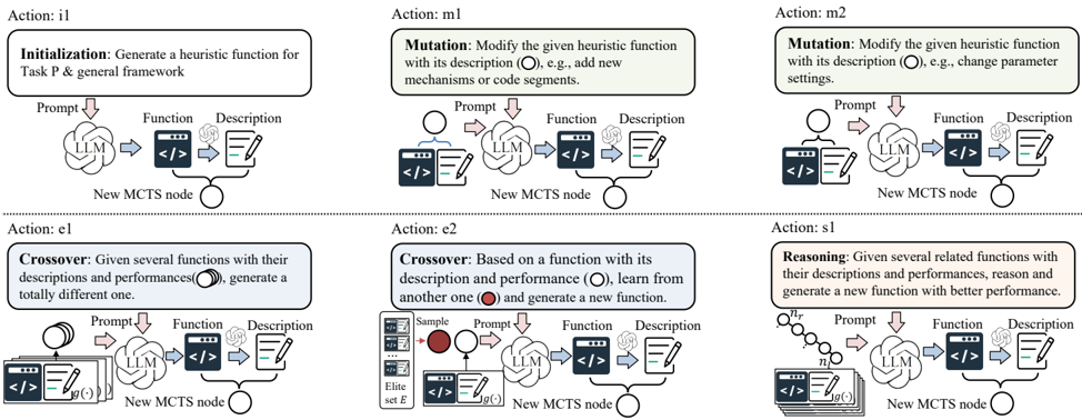Imitating mutation or crossover operators in EC, LLM-based LLM-base Actions Figure 2. LLM-based actions in MCTS-AHD for heuristic evolution. Actions include initializing a new heuristic (i1); two mutation actions (m1 and m2) to mutate an existing heuristic function into a new one with diverse mechanism or detail settings; two crossover actions (e1 and e2) to generate a new heuristic from multiple existing ones; and a novel tree-path reasoning action (s1) to get a better heuristic function from organized function samples on an MCTS tree path from the root node n r to a leaf node n l . <details> <summary>Image 2 Details</summary>  ### Visual Description \n ## Diagram: Automated Function Generation Pipeline ### Overview The image depicts a diagram illustrating a pipeline for automated function generation, likely within a reinforcement learning or automated programming context. It shows six distinct "Actions" (i1, m1, m2, e1, e2, s1), each representing a step in the process of creating and refining functions. Each action involves a Large Language Model (LLM), a function, a description, and the creation of a new MCTS (Monte Carlo Tree Search) node. ### Components/Axes The diagram consists of six horizontally arranged blocks, each labeled with an "Action:" prefix followed by a short identifier (i1, m1, m2, e1, e2, s1). Each block contains the following elements: * **Prompt:** Represented by a cloud shape with the word "Prompt" inside. * **LLM:** A rectangular box with a computer icon, labeled "LLM". * **Function:** A rectangular box with `</>` inside, labeled "Function". * **Description:** A rectangular box with a document icon, labeled "Description". * **New MCTS node:** A circular node labeled "New MCTS node". * **Arrows:** Arrows indicate the flow of information between these components. * **Additional elements:** Some actions include additional elements like "Sample", "Elite set E", and mathematical notations (η, η(c)). ### Detailed Analysis or Content Details **Action: i1 (Initialization)** * Text: "Initialization: Generate a heuristic function for Task P & general framework" * Flow: Prompt -> LLM -> Function -> Description -> New MCTS node. **Action: m1 (Mutation)** * Text: "Mutation: Modify the given heuristic function with its description (O), e.g., add new mechanisms or code segments." * Flow: Prompt -> LLM -> Function -> Description -> New MCTS node. * "O" is present in parentheses next to "description". **Action: m2 (Mutation)** * Text: "Mutation: Modify the given heuristic function with its description (O), e.g., change parameter settings." * Flow: Prompt -> LLM -> Function -> Description -> New MCTS node. * "O" is present in parentheses next to "description". **Action: e1 (Crossover)** * Text: "Crossover: Given several functions with their descriptions and performances(O), generate a totally different one." * Flow: `</>` -> Prompt -> LLM -> Function -> Description -> New MCTS node. * "O" is present in parentheses next to "performances". * "y(x)" is present next to the arrow from `</>` to Prompt. **Action: e2 (Crossover)** * Text: "Crossover: Based on a function with its description and performance (O), learn from another one (O) and generate a new function." * Flow: "Sample" -> Prompt -> LLM -> Function -> Description -> New MCTS node. * "Elite set E" is present next to "Sample". * "O" is present in parentheses next to "performance" and "another one". **Action: s1 (Reasoning)** * Text: "Reasoning: Given several related functions with their descriptions and performances, reason and generate a new function with better performance." * Flow: "η" -> Prompt -> LLM -> Function -> Description -> New MCTS node. * "η(c)" is present next to the arrow from "η" to Prompt. ### Key Observations * The LLM appears to be central to all actions, suggesting it's the core component for function generation and modification. * The "Description" component is consistently present, indicating that function descriptions play a crucial role in the process. * The actions "m1" and "m2" both involve "Mutation", but differ in the type of modification (adding mechanisms vs. changing parameters). * The actions "e1" and "e2" both involve "Crossover", but differ in the input and process. * The "O" notation consistently appears next to "description" or "performance", potentially representing an observation or output. * The use of "Elite set E" in "e2" suggests a selection mechanism for crossover. * The mathematical notations "η" and "η(c)" in "s1" suggest a quantitative approach to reasoning. ### Interpretation This diagram illustrates a sophisticated automated function generation pipeline leveraging a Large Language Model (LLM) and Monte Carlo Tree Search (MCTS). The pipeline employs a variety of techniques – Initialization, Mutation, Crossover, and Reasoning – to iteratively improve functions. The consistent inclusion of function descriptions suggests a focus on generating functions that are not only functional but also understandable and explainable. The "O" notation likely represents the observed output or performance of the function, used for guiding the iterative refinement process. The use of MCTS nodes indicates that the pipeline is likely exploring a search space of possible functions, guided by the LLM and the evaluation of function performance. The diagram suggests a system designed for automated algorithm discovery or program synthesis, where the LLM acts as a creative engine and MCTS provides a structured search strategy. The different crossover and mutation strategies suggest an attempt to balance exploration and exploitation in the search space. </details> © Copyright National University of Singapore. All Rights Reserved. AHD methods prompt LLMs to generate heuristics given existing heuristics from the population. In these methods, a heuristic h will only be retained for the next iteration if its performance g ( h ) estimated in the evaluation dataset D exceeds the worst-performing heuristic in the original population, i.e., g ( h ) > min i ∈{ 1 ,...,M } g ( h i ) . This property makes it difficult for population-based methods to adopt a worse-before-better strategy for the optimal heuristic h ∗ . ## 2.2. 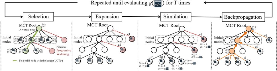Monte Carlo Tree Search MCTS Algorithm. MCTS ( ´ Swiechowski et al., 2023) is a decision-making algorithm widely used in games (Silver et al., 2016) and complex decision-making tasks (Fu et al., 2021). Recent studies also verify the power of MCTS in assisting LLMs to conduct multi-hop reasoning (Feng et al., 2023). In the MCTS tree, each node n c represents a state, and the MCTS will repeatedly select and expand the node with the highest potential judged by a UCT algorithm (Kocsis & Szepesv´ ari, 2006). Each MCTS tree node n c records a quality value Q ( n c ) and a visit count N ( n c ) representing the number of times the node has been selected. From an initial root node n r , MCTS gradually builds the MCTS tree to explore the entire state space. Each round of MCTS consists of four stages as follows: Selection : The selection stage identifies the most potential MCTS tree node for subsequent node expansions. From the root node n r , the selection stage iteratively selects the child node with the largest UCT value until it reaches a leaf node. Given a current node n c , the UCT values for its child nodes c ∈ Children ( n c ) are calculated as follows: $$U C T ( c ) = \left ( Q ( c ) + \lambda \cdot \sqrt { \frac { \ln ( N ( n _ { c } ) + 1 ) } { N ( c ) } } \right ) . \quad ( 3 )$$ Expansion : The expansion stage obtains multiple child nodes from the current (leaf) node n c by sampling several actions from the state of n c among all possible options. Simulation : The simulation stage evaluates all newly expanded leaf nodes for their quality value Q ( · ) . Backpropagation : The backpropagation process uses the results of simulations to update the values of Q ( · ) , N ( · ) for nodes on the tree path from n c to the root n r . After several iterations of MCTS, the MCTS tree can contain nodes with high-quality states for games or tasks. Progressive Widening. Conventional MCTS is not suitable for tasks with extensive action options or dynamically changing environments (Lee et al., 2020b). Progressive widening (Coulom, 2007) is a technique designed for MCTS to fit such tasks. It gradually adds new child nodes to non-leaf nodes as their visit counts N ( · ) increases. Formally, for node n c with child nodes children ( n c ) , a new child node will be added every time the following condition is satisfied: $$\lfloor N ( n ) ^ { \alpha } \rfloor \geq | c h i l d r e n ( n _ { c } ) | ,$$ where | children ( n c ) | is the number of child nodes of n c . ## 3. MCTS-AHD To address the challenges faced by population-based LLMbased AHD methods in overcoming local optima and explor- MCTS settings Figure 3. The MCTS process in MCTS-AHD contains four stages, i.e., selection , expansion , simulation , and backpropagation . MCTSAHD simulates the quality value of each node as the performance function values of their heuristics and the MCTS will terminate after total T performance evaluations. MCTS-AHD introduces the progressive widening technique to better crossover original heuristic functions with continuously generated new ones. It conducts the crossover actions e1 for the root node and action e2 for other nodes. <details> <summary>Image 3 Details</summary>  ### Visual Description \n ## Diagram: Monte Carlo Tree Search (MCTS) Process ### Overview The image depicts a diagram illustrating the four main stages of the Monte Carlo Tree Search (MCTS) algorithm: Selection, Expansion, Simulation, and Backpropagation. The diagram shows a tree-like structure representing the search space, with nodes representing game states and edges representing possible actions. The process is repeated until a specified condition (evaluating g(<b>) for T times) is met. ### Components/Axes The diagram is divided into four sections, each representing a stage of MCTS. Each section contains a tree diagram. The trees share a common structure, with "Initial nodes" at the top and branching nodes representing subsequent states. Labels within the nodes indicate state information (e.g., N(s), Q(s), UCT). Arrows indicate the flow of the algorithm. A legend is provided at the bottom-left, explaining the meaning of the green arrow. ### Detailed Analysis or Content Details **1. Selection:** * The title "Selection" is positioned at the top-left of the section. * The tree is labeled "MCT Root" at the top. * Nodes are labeled with "N(s)" and "Q(s)". * A green arrow originates from a node labeled "N(s)" and points to a child node labeled "Q(s)". The legend states: "To a child node with the largest UCT(i)". * Several nodes are highlighted in pink, indicating they are being considered. * A dashed red arrow labeled "Potential Progressive Widening" points to a lower level of the tree. **2. Expansion:** * The title "Expansion" is positioned at the top-center of the section. * The tree is labeled "MCT Root" at the top. * Nodes are labeled with "e1" and "e2". * A dashed red arrow labeled "Potential Progressive Widening" points to a lower level of the tree. **3. Simulation:** * The title "Simulation" is positioned at the top-center of the section. * The tree is labeled "MCT Root" at the top. * Nodes are labeled with "N(s) = 1", "Q(s) = x", "s1", and "m1". * Text within nodes: "r(s) = 1", "q(s) = x", "r(s) = 1", "q(s) = x". **4. Backpropagation:** * The title "Backpropagation" is positioned at the top-right of the section. * The tree is labeled "MCT Root" at the top. * Nodes are labeled with "e2", "m2", and "s1". * An orange arrow indicates the backpropagation path. * A node is highlighted in orange. **Overall Flow:** * A curved arrow connects the four sections, indicating the iterative nature of the MCTS algorithm. * The text "Repeated until evaluating g(<b>) for T times" is positioned above the curved arrow. ### Key Observations * The diagram visually represents the iterative process of MCTS, highlighting how the search tree expands and is updated with simulation results. * The use of color-coding (green, orange, pink) helps to emphasize the different stages and actions within the algorithm. * The labels within the nodes provide information about the state of the search process. ### Interpretation The diagram illustrates the core loop of the Monte Carlo Tree Search algorithm. The algorithm begins with a selection phase, where it traverses the tree to choose the most promising node based on the Upper Confidence Bound 1 applied to Trees (UCT) value. This is indicated by the green arrow. The expansion phase then adds a new node to the tree, representing a possible action from the selected node. Next, a simulation phase is performed, where a random playout is conducted from the newly expanded node to estimate the value of that state. Finally, the backpropagation phase updates the statistics of the nodes along the path from the expanded node back to the root, using the result of the simulation. This process is repeated iteratively until a stopping criterion is met, such as reaching a maximum number of simulations (T). The diagram effectively conveys the interplay between exploration (expanding new nodes) and exploitation (selecting nodes with high estimated values) that characterizes MCTS. The labels within the nodes (N(s), Q(s), r(s), q(s)) represent the number of visits, average reward, reward from the simulation, and estimated value, respectively. The progressive widening aspect suggests a strategy to balance exploration and exploitation by selectively expanding nodes. </details> © Copyright National University of Singapore. All Rights Reserved. ing complex heuristic spaces, this paper proposes a novel method called MCTS-AHD. It preserves all heuristic functions LLMs generated so far in an MCTS tree and employs MCTS with progressive widening for heuristic evolution. The MCTS root node n r is a virtual node without representing any heuristics, and each of the other nodes represents an executable Python implementation of a heuristic function h ∈ H along with its linguistic description. As LLM-based actions for MCTS node expansion, MCTS-AHD prompts LLMs in existing strategies (e.g., mutation, crossover) and a novel tree-path reasoning strategy. Moreover, to encourage the exploration of the heuristic space H in the early stages of MCTS and ensure convergence in the later stages, MCTSAHD presents an exploration-decay technique that linearly reduces the exploration factor in UCT. ## 3.1. LLM-based actions in MCTS-AHD To simulate the mutation or crossover operators in EC, LLMbased AHD methods prompt LLMs with several prompt strategies to generate new heuristic functions from existing ones (Liu et al., 2024b). Utilizing the advantage that the MCTS tree can record the relationships of all the generated heuristics, as shown in Figure 2, MCTS-AHD presents a novel MCTS-specific set of actions for LLM-based heuristic evolution, including action i1, e1, e2, m1, m2, and s1. The detailed prompts for these actions are in Appendix E.1. As a commonality, all prompts contain descriptions of the task P , the predefined general framework, and the inputs and outputs of the key heuristic function along with their meanings. For actions except i1, prompts also contain implementations and descriptions of existing heuristic functions. For each action, LLMs are supposed to output the Python code of a heuristic function and its linguistic description. Initial Action i1 : As an action for initialization, the action i1 aims to directly generate a heuristic function and its corresponding description from scratch by LLMs. Mutation Action m1 & m2 : MCTS-AHD incorporates two mutation actions, m1 & m2, to attempt more detailed designs within the original function workflow. Based on the inputted heuristic function, action m1 prompts LLMs to introduce new mechanisms and formulas, and action m2 prompts LLMs to modify the parameter settings. Crossover Action e1 : To explore heuristic functions with new workflows, we employ a crossover action e1 to generate a new heuristic function that diverges from multiple existing ones. These existing heuristic functions are inputted to LLMs with their performances g ( · ) and descriptions. Crossover Action e2 : The crossover action e2 prompts LLMs with a parent heuristic function, a reference heuristic function, and their respective performances. LLMs are supposed to identify the beneficial traits and settings in the reference one and craft an improved heuristic function based on the parent one. The reference is sampled from a dynamically maintained elite heuristic function set E consisting of heuristic functions with top 10 performances g ( · ) . Tree-path Reasoning Action s1 : The MCTS tree paths from the root n r to leaf nodes record the evolution history of heuristic functions. So, utilizing this feature, MCTS-AHD presents a novel action s1 to analyze all unique heuristic functions from the leaf node to be developed n l up to the root n r , identify advantageous designs in these heuristics, and generate an enhanced heuristic function. Generating Descriptions: The Thought-Alignment Process . Linguistic descriptions of heuristic functions can assist the reasoning of LLMs (Liu et al., 2024b), where EoH prompts LLMs for a description before outputting the function code. However, due to LLM hallucination (Huang et al., 2023), such a procedure could lead to uncorrelated codes and descriptions. For correlated and detailed descriptions, MCTS-AHD proposes a thought-alignment process that summarizes descriptions after the code generations. There- fore, performing all the MCTS-AHD actions calls LLMs twice. In the first call, we adopt the LLM-generated Python implementation of a heuristic function with action prompts. Then, we conduct a thought-alignment process, prompting LLMs to generate linguistic code descriptions in up to three sentences (refer to Appendix E.2 for prompts). The second LLM call is significantly shorter than the first one, so it will not cause a severe increase in execution time and token cost. ## 3.2. MCTS settings Figure 3 displays the MCTS process in MCTS-AHD. It first generates N I initial nodes representing and links them to a virtual root node n r that does not represent any heuristics. Subsequently, similar to the regular MCTS introduced in Section2.2, MCTS-AHD repeatedly performs the selection, expansion, simulation, and backpropagation stages as follows until the number of evaluations of heuristics approaches a limit T : Selection: In the selection process of MCTS-AHD, MCTSAHD normalizes the quality value Q ( · ) to enhance the homogeneity of different tasks in calculating UCT value for child nodes c ∈ Children ( n c ) of a node n c as follows: $$\begin{array} { r l } & { U C T ( c ) = \left ( \frac { Q ( c ) - q _ { \min } } { q _ { \max } - q _ { \min } } + \lambda \cdot \sqrt { \frac { \ln ( N ( n _ { c } ) + 1 ) } { N ( c ) } } \right ) , \quad e a r l y o r s . } \end{array}$$ where q max and q min are the upper and lower limits of quality values Q ( · ) that ever encountered in MCTS, respectively. From the root n r , MCTS iteratively selects a child node with the largest UCT value until reaching a leaf node. Expansion : For the leaf node selected in the selection stage, the expansion stage prompts LLMs with actions e2, m1, m2, and s1 to build its child nodes. To attempt various detail designs, in a single expansion stage, MCTS-AHD generates k child nodes with the actions m1 and m2, one with e2 and s1, respectively ( 2 k +2 child nodes in total). Simulation : Then, MCTS-AHD evaluates these newly generated heuristic functions h on the evaluation dataset D for their performances g ( h ) and directly sets their quality value as their performances, i.e., Q ( n l ) ← g ( h ) . We also record their visit count N ( n l ) ← 1 . Simultaneously, the elite set E for the action e2, q max , and q min will be updated. Backpropagation : The backpropagation process updates the quality values and the visit counts in MCTS as follows: <!-- formula-not-decoded --> Progressive Widening . Since the elite heuristic function set E for the action e2 updates gradually as the search progresses. MCTS-AHD introduces the progressive widening technique to enable the re-exploration of non-leaf nodes, especially nodes with higher visit counts. The progressive widening process will occur when the condition in Eq.(4) is satisfied and we have α = 0 . 5 for MCTS-AHD. We call the action e1 for a new child node when the root node n r qualifies the condition in Eq.(4), and we call action e2 when other nodes qualify. Heuristic functions inputted to the action e1 are uniformly selected from 2 to 5 different subtrees of MCTS. We implement the progressive widening process during the selection stage, then these nodes will also be processed in the simulation and backpropagation stages. Eventually, MCTS-AHD will output a heuristic function with the highest performance value throughout the MCTS. ## 3.3. Exploration-Decay The setting of the exploration factor λ in Eq.(5) determines the preferences of MCTS on exploration or exploitation (Browne et al., 2012). A larger λ promotes the exploration of temporarily inferior nodes, while a smaller λ stimulates concentration on nodes with higher quality values Q ( · ) . To facilitate a more comprehensive exploration in the early iterations of MCTS and ensure convergence in the later ones, MCTS-AHD presents an exploration-decay technique, linearly decaying the exploration factor λ in Eq.(5) as follows: $$\lambda = \lambda _ { 0 } * \frac { T - t } { T } .$$ Although having a task-specific setting λ 0 is helpful for high-quality heuristics, MCTS-AHD strives to keep the generalization ability, so we set λ 0 = 0 . 1 for all tasks. ## 4. Experiments This section evaluates the proposed MCTS on complex tasks, including NP-hard CO problems and a Cost-aware Acquisition Function (CAF) design task for BO (Yao et al., 2024c). The definitions of these tasks are in Appendix B. We implement MCTS-AHD to design key functions of a wide range of general frameworks (detailed in Appendix C) for these tasks, including step-by-step construction, Ant Colony Optimization (ACO), Guided Local Search (GLS), and BO. Settings. For experiments in this section, we set the number of initial tree nodes N I = 4 , λ 0 = 0 . 1 , α = 0 . 5 . The running time of each heuristic on the evaluation dataset D is limited to 60 seconds. The composition of evaluation datasets D for each task is detailed in Appendix D as well as the settings of general frameworks. Valuable LLM-based AHD methods should be flexible for various pre-trained LLMs, so we include both GPT-3.5-turbo and GPT-4o-mini . Baselines. To verify the ability of heuristics designed by MCTS-AHD, we introduce four types of heuristics as baselines: (a) Manually designed heuristics, e.g., Nearest-greedy Table 1. Designing heuristics with the step-by-step construction framework for TSP and KP. We evaluate methods on 6 test sets with 1,000 instances each. Test sets with in-domain scales (i.i.d. to the evaluation dataset D ) are underlined. Since AHD methods have no guarantees for generalization ability, the effect on in-domain datasets is more important. Optimal for TSP is obtained by LKH (Lin & Kernighan, 1973), and Optimal for KP is the result of OR-Tools. Each LLM-based AHD method is run three times and we report the average performances. The best-performing method with each LLM is shaded, and each test set's overall best result is in bold. | Task | TSP | TSP | TSP | TSP | TSP | TSP | KP | KP | KP | KP | KP | KP | |------------------------------|------------------------------|------------------------------|------------------------------|------------------------------|------------------------------|------------------------------|------------------------------|------------------------------|------------------------------|------------------------------|------------------------------|------------------------------| | N= | N =50 | N =50 | N =100 | N =100 | N =200 | N =200 | N =50, W =12.5 | N =50, W =12.5 | N =100, W =25 | N =100, W =25 | N =200, W =25 | N =200, W =25 | | Methods | Obj. ↓ | Gap | Obj. ↓ | Gap | Obj. ↓ | Gap | Obj. ↑ | Gap | Obj. ↑ | Gap | Obj. ↑ | Gap | | Optimal | 5.675 | - | 7.768 | - | 10.659 | - | 20.037 | - | 40.271 | - | 57.448 | - | | Greedy Construct | 6.959 | 22.62% | 9.706 | 24.94% | 13.461 | 26.29% | 19.985 | 0.26% | 40.225 | 0.12% | 57.395 | 0.09% | | POMO | 5.697 | 0.39% | 8.001 | 3.01% | 12.897 | 20.45% | 19.612 | 2.12% | 39.676 | 1.48% | 57.271 | 0.09% | | LLM-based AHD: GPT-3.5-turbo | LLM-based AHD: GPT-3.5-turbo | LLM-based AHD: GPT-3.5-turbo | LLM-based AHD: GPT-3.5-turbo | LLM-based AHD: GPT-3.5-turbo | LLM-based AHD: GPT-3.5-turbo | LLM-based AHD: GPT-3.5-turbo | LLM-based AHD: GPT-3.5-turbo | LLM-based AHD: GPT-3.5-turbo | LLM-based AHD: GPT-3.5-turbo | LLM-based AHD: GPT-3.5-turbo | LLM-based AHD: GPT-3.5-turbo | LLM-based AHD: GPT-3.5-turbo | | Funsearch | 6.683 | 17.75% | 9.240 | 18.95% | 12.808 | 19.61% | 19.985 | 0.26% | 40.225 | 0.12% | 57.395 | 0.09% | | EoH | 6.390 | 12.59% | 8.930 | 14.96% | 12.538 | 17.63% | 19.994 | 0.21% | 40.231 | 0.10% | 57.400 | 0.08% | | MCTS-AHD(Ours) | 6.346 | 11.82% | 8.861 | 14.08% | 12.418 | 16.51% | 19.997 | 0.20% | 40.233 | 0.09% | 57.393 | 0.10% | | LLM-based AHD: GPT-4o-mini | LLM-based AHD: GPT-4o-mini | LLM-based AHD: GPT-4o-mini | LLM-based AHD: GPT-4o-mini | LLM-based AHD: GPT-4o-mini | LLM-based AHD: GPT-4o-mini | LLM-based AHD: GPT-4o-mini | LLM-based AHD: GPT-4o-mini | LLM-based AHD: GPT-4o-mini | LLM-based AHD: GPT-4o-mini | LLM-based AHD: GPT-4o-mini | LLM-based AHD: GPT-4o-mini | LLM-based AHD: GPT-4o-mini | | Funsearch | 6.357 | 12.00% | 8.850 | 13.93% | 12.372 | 15.54% | 19.988 | 0.24% | 40.227 | 0.11% | 57.398 | 0.09% | | EoH | 6.394 | 12.67% | 8.894 | 14.49% | 12.437 | 16.68% | 19.993 | 0.22% | 40.231 | 0.10% | 57.399 | 0.09% | | MCTS-AHD(Ours) | 6.225 | 9.69% | 8.684 | 11.79% | 12.120 | 13.71% | 20.015 | 0.11% | 40.252 | 0.05% | 57.423 | 0.04% | (Rosenkrantz et al., 1977), ACO (Dorigo et al., 2006), EI (Mockus, 1974). (b) Traditional AHD method: GHPP (Duflo et al., 2019) (c) Neural Combinatorial Optimization (NCO) methods under the same general frameworks, e.g. POMO (Kwon et al., 2020) and DeepACO (Ye et al., 2024b). (d) Existing LMM-based AHD methods: Funsearch (Romera-Paredes et al., 2024), EoH (Liu et al., 2024b), ReEvo (Ye et al., 2024a), and the most recent work HSEvo (Dat et al., 2024). Funsearch, ReEvo, and HSEvo design heuristics from a handcrafted low-quality seed function, and we provide the same seed function for each design scenario without providing external knowledge. Instead, running EoH and MCTS-AHD does not require manually setting a seed function to initiate the heuristic evolution, so both methods demonstrate better applicability. We design heuristics with the proposed MCTS-AHD and LLM-based AHD baselines on a single Intel(R) i7-12700 CPU. Following similar settings of Liu et al. (2024b), for almost all tasks, we set the evaluation budget of LLM-based AHD methods on the evaluation dataset D as T = 1 , 000 . In designing heuristics for each application scenario, we conduct three independent runs for each LLM-based AHD method to reduce statistical biases. To verify the significant advantages of MCTS-AHD, we perform more runs on some tasks in Appendix F.3 to obtain the p-value. In designing heuristics with the step-by-step construction framework for the 0-1 Knapsack Problem (KP), executing MCTS-AHD with T =1,000 takes approximately three hours, 1M input tokens, 0.2M output tokens, about 0.3$ with GPT-4o-mini . Compared to LLM-based AHD baselines, there is no significant efficiency degradation or cost improvement. ## 4.1. MCTS-AHD for NP-hard CO Problems As commonly recognized complex tasks (Korte et al., 2011), this subsection evaluates MCTS-AHD on NP-hard CO prob- lems, including TSP, KP, Capacitated Vehicle Routing Problem (CVRP), Multiple Knapsack Problem (MKP), BinPacking Problem (BPP) with both online and offline settings (online BPP & offline BPP), and Admissible Set Problem (ASP). For these NP-hard CO problems, we apply MCTSAHDto automatically design heuristics with several general frameworks, including step-by-step construction, ACO, and GLS (GLS results are shown in Appendix F.2). Step-by-Step Construction Framework. The step-by-step construction framework (also known as the constructive heuristic framework) is simple but flexible for task solving, which constructs nodes in feasible CO solutions one by one (Asani et al., 2023). Besides being a general framework for LLM-based AHD methods, it is also the most common framework adopted in NCO methods (Vinyals et al., 2015; Bello et al., 2016). We use MCTS-AHD to design heuristics with the step-by-step construction framework for TSP, KP, online BPP, and ASP (with ASP results in Appendix F.1). TSP & KP . We first evaluate MCTS-AHD by designing TSP and KP heuristics within step-by-step construction frameworks. The key heuristic function to be designed should select the next TSP node or the next KP item to join taking the temporary solving state (e.g., selected and remaining TSP nodes or KP items) as inputs. This function will be executed recursively until a complete feasible solution is constructed. For all LLM-based AHD methods, the evaluation dataset D contains 64 50-node ( N =50) TSP instances for TSP and 64 100-item ( N =100) KP instances with capacity W = 25 for KP. Table 1 shows the performance of baseline heuristics and LLM-based AHD methods. The Greedy Construct baseline is the Nearest-greedy heuristic algorithm for TSP and it constructs KP solutions by the item with the largest value-weight-ratio. MCTS-AHD exhibits significant advantages on almost all test sets, surpassing manually designed heuristics and LLM-based AHD methods EoH and Fun- Table 2. Designing heuristics with the ACO general framework for solving TSP, CVRP, MKP, and offline BPP. Each test set contains 64 instances and LLM-based AHD methods' performances are averaged over three runs. | | TSP | TSP | TSP | TSP | CVRP | CVRP | CVRP | CVRP | MKP | MKP | MKP | MKP | Offline BPP | Offline BPP | Offline BPP | Offline BPP | |----------------------------|----------------------------|----------------------------|----------------------------|----------------------------|----------------------------|----------------------------|----------------------------|----------------------------|----------------------------|----------------------------|----------------------------|----------------------------|----------------------------|----------------------------|----------------------------|----------------------------| | Test sets | N =50 | N =50 | N =100 | N =100 | N =50, C =50 | N =50, C =50 | N =100, C =50 | N =100, C =50 | N =100, m =5 | N =100, m =5 | N =200, m =5 | N =200, m =5 | N =500, C =150 | N =500, C =150 | N =1,000, C =150 | N =1,000, C =150 | | Methods | Obj. ↓ | Gap | Obj. ↓ | Gap | Obj. ↓ | Gap | Obj. ↓ | Gap | Obj. ↑ | Gap | Obj. ↑ | Gap | Obj. ↓ | Gap | Obj. ↓ | Gap | | ACO | 5.992 | 3.28% | 8.948 | 9.40% | 11.355 | 27.77% | 18.778 | 25.76% | 22.738 | 2.28% | 40.672 | 4.30% | 208.828 | 2.81% | 417.938 | 3.15% | | DeepACO | 5.842 | 0.71% | 8.282 | 1.26% | 8.888 | 0.00% | 14.932 | 0.00% | 23.093 | 0.75% | 41.988 | 1.20% | 203.125 | 0.00% | 405.172 | 0.00% | | LLM-based AHD: GPT-4o-mini | LLM-based AHD: GPT-4o-mini | LLM-based AHD: GPT-4o-mini | LLM-based AHD: GPT-4o-mini | LLM-based AHD: GPT-4o-mini | LLM-based AHD: GPT-4o-mini | LLM-based AHD: GPT-4o-mini | LLM-based AHD: GPT-4o-mini | LLM-based AHD: GPT-4o-mini | LLM-based AHD: GPT-4o-mini | LLM-based AHD: GPT-4o-mini | LLM-based AHD: GPT-4o-mini | LLM-based AHD: GPT-4o-mini | LLM-based AHD: GPT-4o-mini | LLM-based AHD: GPT-4o-mini | LLM-based AHD: GPT-4o-mini | LLM-based AHD: GPT-4o-mini | | EoH | 5.828 | 0.45% | 8.263 | 1.03% | 9.359 | 5.31% | 15.681 | 5.02% | 23.139 | 0.56% | 41.994 | 1.19% | 204.646 | 0.75% | 408.599 | 0.85% | | ReEvo | 5.856 | 0.94% | 8.340 | 1.98% | 9.327 | 4.94% | 16.092 | 7.77% | 23.245 | 0.10% | 42.416 | 0.19% | 206.693 | 1.76% | 413.510 | 2.06% | | MCTS-AHD(Ours) | 5.801 | 0.00% | 8.179 | 0.00% | 9.286 | 4.48% | 15.782 | 5.70% | 23.269 | 0.00% | 42.498 | 0.00% | 204.094 | 0.48% | 407.323 | 0.53% | search. Moreover, compared to an advanced NCO method POMO which requires task-specific training, MCTS-AHD can design better heuristics in 200-node TSP and KP test sets, exhibiting its power to solve NP-hard CO problems. Online BPP . As another widely considered NP-hard CO problem, online BPP is the online variant of BPP. It allows only immediate bin packing decisions once a new item is received. It is generally adopted as a common evaluation scenario for LLM-based AHD methods. We follow (Liu et al., 2024b) to generate WeiBull BPP instances (Casti˜ neiras et al., 2012) and use four WeiBull instances with diverse scales as the evaluation dataset D . As shown in Table 3, online BPP heuristics designed by MCTS-AHD demonstrate a superior average performance of six test sets. Table 3. Design step-by-step construction heuristics for solving online BPP. The table exhibits the performance gaps of heuristics to the lower bound. Each LLM-based AHD method is run three times for the average gaps. Each test set contains five WeiBull BPP instances and we underline the four (in-domain) scales contained in D . The scale notations of test sets are abbreviated, e.g., 1k 100 represents 1,000 items and capacity W = 100 . | Online BPP | Online BPP | Online BPP | Online BPP | Online BPP | Online BPP | Online BPP | Online BPP | |----------------------------|----------------------------|----------------------------|----------------------------|----------------------------|----------------------------|----------------------------|----------------------------| | Test sets | 1k 100 | 1k 500 | 5k 100 | 5k 500 | 10k 100 | 10k 500 | Avg. | | Best Fit | 4.77% | 0.25% | 4.31% | 0.55% | 4.05% | 0.47% | 2.40% | | First Fit | 5.02% | 0.25% | 4.65% | 0.55% | 4.36% | 0.50% | 2.56% | | LLM-based AHD: GPT-4o-mini | LLM-based AHD: GPT-4o-mini | LLM-based AHD: GPT-4o-mini | LLM-based AHD: GPT-4o-mini | LLM-based AHD: GPT-4o-mini | LLM-based AHD: GPT-4o-mini | LLM-based AHD: GPT-4o-mini | LLM-based AHD: GPT-4o-mini | | Funsearch | 2.45% | 0.66% | 1.30% | 0.25% | 1.05% | 0.21% | 0.99% | | EoH | 2.69% | 0.25% | 1.63% | 0.53% | 1.47% | 0.45% | 1.17% | | ReEvo | 3.94% | 0.50% | 2.72% | 0.40% | 2.39% | 0.31% | 1.71% | | HSEvo | 2.64% | 1.07% | 1.43% | 0.32% | 1.13% | 0.21% | 1.13% | | MCTS-AHD | 2.45% | 0.50% | 1.06% | 0.32% | 0.74% | 0.26% | 0.89% | Ant Colony Optimization Framework . The ACO is an optimization algorithm inspired by the foraging behavior of ants, which contains a heuristic matrix and implements a path selection mechanism to solve combinatorial optimization problems by simulating the transfer of pheromones between ants (Dorigo et al., 2006; Kim et al., 2024). LLMbased AHD can design a generation function of the heuristic matrix, thereby transforming ACO into a framework and applying it to a variety of tasks. Following Ye et al. (2024a), MCTS-AHD designs heuristics within the ACO framework for four NP-hard CO problems: TSP, CVRP, MKP, and offline BPP. The design results using GPT-4o-mini as LLMs are shown in Table 2, where MCTS-AHD exhibits significant leads to EoH and ReEvo in all in-domain test sets across four CO problems and three out-of-domain test sets. Moreover, the proposed MCTS-AHD can consistently outperform manually designed ACO heuristics in all eight test sets and surpass an outstanding NCO method DeepACO (Ye et al., 2024b) in TSP and MKP test sets. ## 4.2. MCTS-AHD for Other Complex Tasks To assess whether MCTS-AHD can still perform well in optimization tasks beyond CO problems, we follow Yao et al. (2024c) to evaluate MCTS-AHD by designing heuristic CAFs for BO. The CAF is a crucial component for Cost-aware BO, helping to reach the global optimum in a cost-efficient manner. There are several advanced handcrafted heuristic CAFs, including EI (Mockus, 1974), EIpu (Snoek et al., 2012), and EI-cools (Lee et al., 2020a). We employ two synthetic instances with different landscapes and input dimensions (Ackley and Rastrigin in Table 4) as the evaluation dataset D for LLM-based AHD and also test the manually and automatically designed heuristics on ten other synthetic instances. During heuristic evolutions, we set the sampling budget to 12 and run 5 independent trials for average performances. As shown in Table 4, heuristic CAFs designed by the proposed MCTS-AHD demonstrate superior BO results that outperform both manually designed heuristics and EoH in six out of twelve synthetic instances. It verifies that MCTS-AHD not only performs well in NPhard CO problems but can also show great power in other complex optimization tasks. ## 5. Discussion Experiments have demonstrated the effectiveness of the proposed MCTS-AHD in designing high-quality heuristics for a wide range of application scenarios. This section first conducts essential ablation studies. Then, we will also analyze the advantages of utilizing MCTS in LLM-based AHD compared to the original population-based EC. Table 4. Designing CAFs for BO. The table shows the gaps to optimal when running BO on instances with manually designed CAFs and CAFs designed by LLM-based AHD methods. LLM-based AHD methods are run three times for the average gaps. In testing, the evaluation budgets for BO are 30 and we run 10 trials for average gaps. The results of EI, EIpu, and EI-cool are from Yao et al. (2024c). | Instances | Ackley | Rastrigin | Griewank | Rosenbrock | Levy | ThreeHumpCamel | StyblinskiTang | Hartmann | Powell | Shekel | Hartmann | Cosine8 | |----------------------------|----------------------------|----------------------------|----------------------------|----------------------------|----------------------------|----------------------------|----------------------------|----------------------------|----------------------------|----------------------------|----------------------------|----------------------------| | EI | 2.66% | 4.74% | 0.49% | 1.26% | 0.01% | 0.05% | 0.03% | 0.00% | 18.89% | 7.91% | 0.03% | 0.47% | | EIpu | 2.33% | 5.62% | 0.34% | 2.36% | 0.01% | 0.12% | 0.02% | 0.00% | 19.83% | 7.92% | 0.03% | 0.47% | | EI-cool | 2.74% | 5.78% | 0.34% | 2.29% | 0.01% | 0.07% | 0.03% | 0.00% | 14.95% | 8.21% | 0.03% | 0.54% | | LLM-based AHD: GPT-4o-mini | LLM-based AHD: GPT-4o-mini | LLM-based AHD: GPT-4o-mini | LLM-based AHD: GPT-4o-mini | LLM-based AHD: GPT-4o-mini | LLM-based AHD: GPT-4o-mini | LLM-based AHD: GPT-4o-mini | LLM-based AHD: GPT-4o-mini | LLM-based AHD: GPT-4o-mini | LLM-based AHD: GPT-4o-mini | LLM-based AHD: GPT-4o-mini | LLM-based AHD: GPT-4o-mini | LLM-based AHD: GPT-4o-mini | | EoH | 2.45% | 0.90% | 0.54% | 56.78% | 0.20% | 0.26% | 0.79% | 0.04% | 70.89% | 4.56% | 0.33% | 0.36% | | MCTS-AHD | 2.40% | 0.77% | 0.36% | 1.68% | 0.01% | 0.02% | 0.20% | 0.01% | 1.27% | 3.94% | 0.38% | 0.34% | ## 5.1. Ablation on Parameters and Components To validate the necessity of its components, as shown in Table 5, we first remove three proposed components of MCTS-AHD (Progressive Widening, Thought-alignment, and Exploration-decay) and use these variants to design stepby-step heuristics for TSP and KP. Line 3 to Line 5 in Table 5 reports their average optimality gaps over three runs, and all these variants exhibit a clear performance degradation in at least one task compared to the original MCTS-AHD. The actions for node expansion in MCTS-AHD are also essential. Actions e1 and e2 are associated with the progressive widening, so they cannot be ablated individually. According to Table 5, MCTS-AHD variants without actions s1, m1, and m2 could only design worse heuristics in at least one task, proving the significance of these LLM-based actions. The importance of action s1 also demonstrates that MCTS-AHD benefits from its organized tree structure. Meanwhile, we measure the sensitivity of the main parameter λ 0 . Results in the last two lines of Table 5 show that although the TSP and KP tasks may have respective preferences in the λ 0 setting, the default setting (i.e., λ 0 = 0 . 1 ) exhibits generally good quality. Table 5. Ablations on the components, actions, and parameter settings of MCTS-AHD. We use MCTS-AHD variants to design heuristics with the step-by-step construction framework for their optimality gaps on 1,000-instance test sets averaged over five runs . | Methods | TSP50 | KP100 | |------------------------------|---------|---------| | MCTS-AHD (Original, 10 runs) | 10.661% | 0.059% | | w/o Progressive Widening | 12.132% | 0.064% | | w/o Thought-alignment | 11.640% | 0.061% | | w/o Exploration-decay | 11.606% | 0.064% | | w/o Action s1 | 11.919% | 0.062% | | w/o Action m1 | 10.921% | 0.083% | | w/o Action m2 | 11.679% | 0.061% | | MCTS-AHD variant λ 0 = 0.05 | 11.080% | 0.056% | | MCTS-AHD variant λ 0 = 0.2 | 12.124% | 0.034% | ## 5.2. 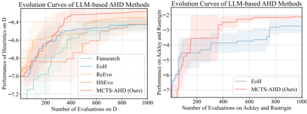MCTS versus Population-based EC Ability of MCTS-AHD in Escaping from Local Optima . As the main contribution of this paper, instead of populationbased EC, MCTS-AHD can manage inferior but potential heuristic functions, achieving a more comprehensive exploration of the heuristic space H thus avoiding falling into local optima. To verify this, we plot the performance curves of MCTS-AHD and LLM-based AHD baselines in designing step-by-step construction heuristics for TSP and designing CAFs for BOs. Each curve is averaged over at least five runs . As illustrated in Figure 4, all baseline methods with populations exhibit early convergences on performances, but MCTS-AHD can converge to significantly better performance via quick and continuous performance updates. <details> <summary>Image 4 Details</summary>  ### Visual Description \n ## Line Chart: Evolution Curves of LLM-based AHD Methods ### Overview The image presents two line charts comparing the performance of several LLM-based AHD (Algorithm Hyperparameter Design) methods. The left chart focuses on performance on a dataset labeled "D", while the right chart focuses on performance on the "Ackley and Rastrigin" datasets. Each chart displays the performance (y-axis) as a function of the number of evaluations (x-axis). The charts include shaded regions representing the standard deviation of the performance. ### Components/Axes **Left Chart:** * **Title:** Evolution Curves of LLM-based AHD Methods * **X-axis Label:** Number of Evaluations on D * **Y-axis Label:** Performance of Heuristics on D * **Y-axis Scale:** -2 to -6.2 * **Legend:** * Funsearch (Light Blue) * Eoh (Medium Blue) * ReRevo (Light Orange) * HSEvo (Medium Orange) * MCTS-AHD (Ours) (Light Red) **Right Chart:** * **Title:** Evolution Curves of LLM-based AHD Methods * **X-axis Label:** Number of Evaluations on Ackley and Rastrigin * **Y-axis Label:** Performance on Ackley and Rastrigin * **Y-axis Scale:** -2 to -6.2 * **Legend:** * Eoh (Blue) * MCTS-AHD (Ours) (Red) ### Detailed Analysis or Content Details **Left Chart (Performance on D):** * **Funsearch (Light Blue):** Starts around -5.8 at 0 evaluations, increases to approximately -5.2 by 100 evaluations, plateaus around -5.1 between 400 and 1000 evaluations. * **Eoh (Medium Blue):** Starts around -5.8 at 0 evaluations, increases steadily to approximately -5.0 by 1000 evaluations. * **ReRevo (Light Orange):** Starts around -5.8 at 0 evaluations, increases rapidly to approximately -4.8 by 200 evaluations, then plateaus around -4.7 between 400 and 1000 evaluations. * **HSEvo (Medium Orange):** Starts around -5.8 at 0 evaluations, increases to approximately -5.0 by 100 evaluations, then plateaus around -4.8 between 400 and 1000 evaluations. * **MCTS-AHD (Ours) (Light Red):** Starts around -5.8 at 0 evaluations, increases rapidly to approximately -4.6 by 200 evaluations, then fluctuates between -4.6 and -4.4 between 400 and 1000 evaluations. **Right Chart (Performance on Ackley and Rastrigin):** * **Eoh (Blue):** Starts around -5.8 at 0 evaluations, increases to approximately -5.0 by 200 evaluations, then fluctuates between -5.0 and -4.8 between 400 and 1000 evaluations. * **MCTS-AHD (Ours) (Red):** Starts around -5.8 at 0 evaluations, increases rapidly to approximately -4.6 by 200 evaluations, then fluctuates between -4.6 and -4.4 between 400 and 1000 evaluations. ### Key Observations * On both datasets, MCTS-AHD (Ours) consistently outperforms Funsearch and Eoh, especially in the initial stages of evaluation. * ReRevo and HSEvo show strong initial performance on dataset D, but their performance plateaus relatively early. * The shaded regions indicate a significant degree of variance in the performance of each method. * The performance improvement diminishes as the number of evaluations increases for all methods. ### Interpretation The charts demonstrate the effectiveness of the MCTS-AHD method compared to other LLM-based AHD methods. MCTS-AHD exhibits faster initial performance gains on both datasets, suggesting it can more efficiently explore the hyperparameter space. The plateaus observed in the performance curves indicate that the methods eventually converge to a local optimum, and further evaluations yield diminishing returns. The variance shown by the shaded regions suggests that the performance of these methods can be sensitive to the specific problem instance or random seed. The comparison between the two datasets suggests that the relative performance of the methods may vary depending on the characteristics of the optimization problem. The fact that MCTS-AHD consistently performs well across both datasets suggests its robustness and generalizability. </details> - (a) Design Step-by-step Construction heuristics for TSP - (b) Design CAFs for BO Figure 4. Evolution curves on two diverse application scenarios. Advantage scopes of MCTS-AHD . Compared to population-based baselines, we claim that MCTS-AHD demonstrates greater advantages in application scenarios with more complex heuristic spaces H and application scenarios with more descriptions as knowledge. We analyze these two claims with experiments in Appendix F.8. ## 6. Conclusion In conclusion, this paper first applies MCTS to LLM-based AHD. The proposed MCTS-AHD achieves a comprehensive exploration of the heuristic space and can finally design higher-quality heuristics for NP-hard complex tasks. For LLM-based AHD, MCTS can be a more promising evolution method compared to population-based EC. Limitation and Future Work : As a limitation of MCTSAHD, the convergence speed of MCTS-AHD can still be improved. In the future, we will consider designing MCTSpopulation hybrid methods for better evolution efficiency. ## Impact Statement This paper presents work whose goal is to advance the field of Machine Learning. There are many potential societal consequences of our work, none which we feel must be specifically highlighted here. ## References - Abgaryan, H., Harutyunyan, A., and Cazenave, T. Llms can schedule. arXiv preprint arXiv:2408.06993 , 2024. - Alhindi, A., Alhindi, A., Alhejali, A., Alsheddy, A., Tairan, N., and Alhakami, H. Moea/d-gls: a multiobjective memetic algorithm using decomposition and guided local search. Soft Computing , 23:9605-9615, 2019. - Ansari, Z. N. and Daxini, S. D. A state-of-the-art review on meta-heuristics application in remanufacturing. Archives of Computational Methods in Engineering , 29(1):427470, 2022. - Arnold, F. and S¨ orensen, K. Knowledge-guided local search for the vehicle routing problem. Computers & Operations Research , 105:32-46, 2019. - Arnold, F., Gendreau, M., and S¨ orensen, K. Efficiently solving very large-scale routing problems. Computers & operations research , 107:32-42, 2019. - Asani, E. O., Okeyinka, A. E., and Adebiyi, A. A. A computation investigation of the impact of convex hull subtour on the nearest neighbour heuristic. In 2023 International Conference on Science, Engineering and Business for Sustainable Development Goals (SEB-SDG) , volume 1, pp. 1-7. IEEE, 2023. - Ausiello, G., Crescenzi, P., Gambosi, G., Kann, V., Marchetti-Spaccamela, A., and Protasi, M. Complexity and approximation: Combinatorial optimization problems and their approximability properties . Springer Science & Business Media, 2012. - B¨ ack, T., Fogel, D. B., and Michalewicz, Z. Handbook of evolutionary computation. Release , 97(1):B1, 1997. - Bello, I., Pham, H., Le, Q. V., Norouzi, M., and Bengio, S. Neural combinatorial optimization with reinforcement learning. arXiv preprint arXiv:1611.09940 , 2016. - Berto, F., Hua, C., Zepeda, N. G., Hottung, A., Wouda, N., Lan, L., Park, J., Tierney, K., and Park, J. Routefinder: Towards foundation models for vehicle routing problems. arXiv preprint arXiv:2406.15007 , 2024. - Biggs, N. The traveling salesman problem a guided tour of combinatorial optimization, 1986. - Blot, A., Hoos, H. H., Jourdan, L., Kessaci-Marmion, M.- ´ E., and Trautmann, H. Mo-paramils: A multi-objective automatic algorithm configuration framework. In Learning and Intelligent Optimization: 10th International Conference, LION 10, Ischia, Italy, May 29-June 1, 2016, Revised Selected Papers 10 , pp. 32-47. Springer, 2016. - Brandfonbrener, D., Henniger, S., Raja, S., Prasad, T., Loughridge, C. R., Cassano, F., Hu, S. R., Yang, J., Byrd, W. E., Zinkov, R., et al. Vermcts: Synthesizing multistep programs using a verifier, a large language model, and tree search. In The 4th Workshop on Mathematical Reasoning and AI at NeurIPS'24 , 2024. - Brecklinghaus, J. and Hougardy, S. The approximation ratio of the greedy algorithm for the metric traveling salesman problem. Operations Research Letters , 43(3):259-261, 2015. - Browne, C. B., Powley, E., Whitehouse, D., Lucas, S. M., Cowling, P. I., Rohlfshagen, P., Tavener, S., Perez, D., Samothrakis, S., and Colton, S. A survey of monte carlo tree search methods. IEEE Transactions on Computational Intelligence and AI in games , 4(1):1-43, 2012. - Burke, E. K., Gendreau, M., Hyde, M., Kendall, G., Ochoa, G., ¨ Ozcan, E., and Qu, R. Hyper-heuristics: A survey of the state of the art. Journal of the Operational Research Society , 64(12):1695-1724, 2013. - Burke, E. K., Hyde, M. R., Kendall, G., Ochoa, G., ¨ Ozcan, E., and Woodward, J. R. A classification of hyperheuristic approaches: revisited. Handbook of metaheuristics , pp. 453-477, 2019. - Cant´ u-Paz, E. et al. A survey of parallel genetic algorithms. Calculateurs paralleles, reseaux et systems repartis , 10 (2):141-171, 1998. - Casti˜ neiras, I., De Cauwer, M., and O'Sullivan, B. Weibullbased benchmarks for bin packing. In International Conference on Principles and Practice of Constraint Programming , pp. 207-222. Springer, 2012. - Christofides, N. Worst-case analysis of a new heuristic for the travelling salesman problem. In Operations Research Forum , volume 3, pp. 20. Springer, 2022. - Coulom, R. Computing 'elo ratings' of move patterns in the game of go. ICGA journal , 30(4):198-208, 2007. - Dainese, N., Merler, M., Alakuijala, M., and Marttinen, P. Generating code world models with large language models guided by monte carlo tree search. arXiv preprint arXiv:2405.15383 , 2024. - Dat, P. V. T., Doan, L., and Binh, H. T. T. Hsevo: Elevating automatic heuristic design with diversity-driven harmony - search and genetic algorithm using llms. arXiv preprint arXiv:2412.14995 , 2024. - DeLorenzo, M., Chowdhury, A. B., Gohil, V., Thakur, S., Karri, R., Garg, S., and Rajendran, J. Make every move count: Llm-based high-quality rtl code generation using mcts. arXiv preprint arXiv:2402.03289 , 2024. - Desale, S., Rasool, A., Andhale, S., and Rane, P. Heuristic and meta-heuristic algorithms and their relevance to the real world: a survey. Int. J. Comput. Eng. Res. Trends , 351(5):2349-7084, 2015. - Dorigo, M., Birattari, M., and Stutzle, T. Ant colony optimization. IEEE computational intelligence magazine , 1 (4):28-39, 2006. - Drakulic, D., Michel, S., and Andreoli, J.-M. Goal: A generalist combinatorial optimization agent learning. arXiv preprint arXiv:2406.15079 , 2024. - Duflo, G., Kieffer, E., Brust, M. R., Danoy, G., and Bouvry, P. A gp hyper-heuristic approach for generating tsp heuristics. In 2019 IEEE International Parallel and Distributed Processing Symposium Workshops (IPDPSW) , pp. 521-529. IEEE, 2019. - Eiben, A. E. and Smith, J. E. Introduction to evolutionary computing . Springer, 2015. - Feng, X., Wan, Z., Wen, M., McAleer, S. M., Wen, Y., Zhang, W., and Wang, J. Alphazero-like tree-search can guide large language model decoding and training. arXiv preprint arXiv:2309.17179 , 2023. - Fischetti, M., Lodi, A., and Toth, P. Exact methods for the asymmetric traveling salesman problem. The traveling salesman problem and its variations , pp. 169-205, 2007. - Fu, Z.-H., Qiu, K.-B., and Zha, H. Generalize a small pre-trained model to arbitrarily large tsp instances. In Proceedings of the AAAI conference on artificial intelligence , volume 35, pp. 7474-7482, 2021. - Gao, C., Shang, H., Xue, K., Li, D., and Qian, C. Towards generalizable neural solvers for vehicle routing problems via ensemble with transferrable local policy, 2024. - Guo, P.-F., Chen, Y.-H., Tsai, Y .-D., and Lin, S.-D. Towards optimizing with large language models. arXiv preprint arXiv:2310.05204 , 2023. - Hadi, M. U., Qureshi, R., Shah, A., Irfan, M., Zafar, A., Shaikh, M. B., Akhtar, N., Wu, J., Mirjalili, S., et al. A survey on large language models: Applications, challenges, limitations, and practical usage. Authorea Preprints , 2023. - Hadi, M. U., Al Tashi, Q., Shah, A., Qureshi, R., Muneer, A., Irfan, M., Zafar, A., Shaikh, M. B., Akhtar, N., Wu, J., et al. Large language models: a comprehensive survey of its applications, challenges, limitations, and future prospects. Authorea Preprints , 2024. - He, K., Zhang, X., Ren, S., and Sun, J. Deep residual learning for image recognition. In Proceedings of the IEEE conference on computer vision and pattern recognition , pp. 770-778, 2016. - He, Q., Head, K. L., and Ding, J. Heuristic algorithm for priority traffic signal control. Transportation research record , 2259(1):1-7, 2011. - Helsgaun, K. An extension of the lin-kernighan-helsgaun tsp solver for constrained traveling salesman and vehicle routing problems. Roskilde: Roskilde University , 12: 966-980, 2017. - Hemberg, E., Moskal, S., and O'Reilly, U.-M. Evolving code with a large language model. Genetic Programming and Evolvable Machines , 25(2):21, 2024. - Huang, L., Yu, W., Ma, W., Zhong, W., Feng, Z., Wang, H., Chen, Q., Peng, W., Feng, X., Qin, B., et al. A survey on hallucination in large language models: Principles, taxonomy, challenges, and open questions. ACM Transactions on Information Systems , 2023. - Huang, X., Liu, W., Chen, X., Wang, X., Wang, H., Lian, D., Wang, Y., Tang, R., and Chen, E. Understanding the planning of llm agents: A survey. arXiv preprint arXiv:2402.02716 , 2024. - Hudson, B., Li, Q., Malencia, M., and Prorok, A. Graph neural network guided local search for the traveling salesperson problem. arXiv preprint arXiv:2110.05291 , 2021. - Jiang, X., Wu, Y., Wang, Y., and Zhang, Y. Unco: Towards unifying neural combinatorial optimization through large language model. arXiv preprint arXiv:2408.12214 , 2024. - Kambhampati, S., Valmeekam, K., Guan, L., Verma, M., Stechly, K., Bhambri, S., Saldyt, L., and Murthy, A. Llms can't plan, but can help planning in llm-modulo frameworks. arXiv preprint arXiv:2402.01817 , 2024. - Kim, M., Choi, S., Kim, H., Son, J., Park, J., and Bengio, Y. Ant colony sampling with gflownets for combinatorial optimization. arXiv preprint arXiv:2403.07041 , 2024. - Kocsis, L. and Szepesv´ ari, C. Bandit based monte-carlo planning. In European conference on machine learning , pp. 282-293. Springer, 2006. - Kool, W., Van Hoof, H., and Welling, M. Attention, learn to solve routing problems! arXiv preprint arXiv:1803.08475 , 2018. - Korte, B. H., Vygen, J., Korte, B., and Vygen, J. Combinatorial optimization , volume 1. Springer, 2011. - Kwon, Y.-D., Choo, J., Kim, B., Yoon, I., Gwon, Y., and Min, S. Pomo: Policy optimization with multiple optima for reinforcement learning. Advances in Neural Information Processing Systems , 33:21188-21198, 2020. - Kwon, Y.-D., Choo, J., Yoon, I., Park, M., Park, D., and Gwon, Y. Matrix encoding networks for neural combinatorial optimization. Advances in Neural Information Processing Systems , 34:5138-5149, 2021. - Lam, R., Willcox, K., and Wolpert, D. H. Bayesian optimization with a finite budget: An approximate dynamic programming approach. Advances in Neural Information Processing Systems , 29, 2016. - Langdon, W. B. and Poli, R. Foundations of genetic programming . Springer Science & Business Media, 2013. - Lange, R., Tian, Y., and Tang, Y. Large language models as evolution strategies. In Proceedings of the Genetic and Evolutionary Computation Conference Companion , pp. 579-582, 2024. - Lee, E. H., Perrone, V., Archambeau, C., and Seeger, M. Cost-aware bayesian optimization. arXiv preprint arXiv:2003.10870 , 2020a. - Lee, J., Jeon, W., Kim, G.-H., and Kim, K.-E. Montecarlo tree search in continuous action spaces with value gradients. In Proceedings of the AAAI conference on artificial intelligence , volume 34, pp. 4561-4568, 2020b. - Lehman, J., Gordon, J., Jain, S., Ndousse, K., Yeh, C., and Stanley, K. O. Evolution through large models. In Handbook of Evolutionary Machine Learning , pp. 331366. Springer, 2023. - Lin, S. and Kernighan, B. W. An effective heuristic algorithm for the traveling-salesman problem. Operations research , 21(2):498-516, 1973. - Liu, F., Tong, X., Yuan, M., and Zhang, Q. Algorithm evolution using large language model. arXiv preprint arXiv:2311.15249 , 2023. - Liu, F., Lin, X., Wang, Z., Zhang, Q., Xialiang, T., and Yuan, M. Multi-task learning for routing problem with cross-problem zero-shot generalization. In Proceedings of the 30th ACM SIGKDD Conference on Knowledge Discovery and Data Mining , pp. 1898-1908, 2024a. - Liu, F., Xialiang, T., Yuan, M., Lin, X., Luo, F., Wang, Z., Lu, Z., and Zhang, Q. Evolution of heuristics: Towards efficient automatic algorithm design using large language model. In Forty-first International Conference on Machine Learning , 2024b. - Liu, F., Yao, Y., Guo, P., Yang, Z., Lin, X., Tong, X., Yuan, M., Lu, Z., Wang, Z., and Zhang, Q. A systematic survey on large language models for algorithm design. arXiv preprint arXiv:2410.14716 , 2024c. - Liu, F., Zhang, R., Xie, Z., Sun, R., Li, K., Lin, X., Wang, Z., Lu, Z., and Zhang, Q. Llm4ad: A platform for algorithm design with large language model. arXiv preprint arXiv:2412.17287 , 2024d. - Liu, S., Chen, C., Qu, X., Tang, K., and Ong, Y.-S. Large language models as evolutionary optimizers. In 2024 IEEE Congress on Evolutionary Computation (CEC) , pp. 1-8. IEEE, 2024e. - L´ opez-Ib´ a˜ nez, M., Dubois-Lacoste, J., C´ aceres, L. P., Birattari, M., and St¨ utzle, T. The irace package: Iterated racing for automatic algorithm configuration. Operations Research Perspectives , 3:43-58, 2016. - Luong, P., Nguyen, D., Gupta, S., Rana, S., and Venkatesh, S. Adaptive cost-aware bayesian optimization. Knowledge-Based Systems , 232:107481, 2021. - Lusby, R. M., Larsen, J., Ehrgott, M., and Ryan, D. An exact method for the double tsp with multiple stacks. International Transactions in Operational Research , 17 (5):637-652, 2010. - Ma, Y., Li, J., Cao, Z., Song, W., Zhang, L., Chen, Z., and Tang, J. Learning to iteratively solve routing problems with dual-aspect collaborative transformer. Advances in Neural Information Processing Systems , 34:1109611107, 2021. - Mei, Y., Chen, Q., Lensen, A., Xue, B., and Zhang, M. Explainable artificial intelligence by genetic programming: A survey. IEEE Transactions on Evolutionary Computation , 27(3):621-641, 2022. - Merz, P. and Freisleben, B. Genetic local search for the tsp: New results. In Proceedings of 1997 IEEE International Conference on Evolutionary Computation (ICEC'97) , pp. 159-164. IEEE, 1997. - Meyerson, E., Nelson, M. J., Bradley, H., Gaier, A., Moradi, A., Hoover, A. K., and Lehman, J. Language model crossover: Variation through few-shot prompting. arXiv preprint arXiv:2302.12170 , 2023. - Mockus, J. On bayesian methods for seeking the extremum. In Proceedings of the IFIP Technical Conference , pp. 400-404, 1974. - Naveed, H., Khan, A. U., Qiu, S., Saqib, M., Anwar, S., Usman, M., Akhtar, N., Barnes, N., and Mian, A. A comprehensive overview of large language models. arXiv preprint arXiv:2307.06435 , 2023. - Qi, Z., Ma, M., Xu, J., Zhang, L. L., Yang, F., and Yang, M. Mutual reasoning makes smaller llms stronger problemsolvers. arXiv preprint arXiv:2408.06195 , 2024. - Rajendran, C. Heuristic algorithm for scheduling in a flowshop to minimize total flowtime. International Journal of Production Economics , 29(1):65-73, 1993. - Reinelt, G. Tsplib-a traveling salesman problem library. ORSA journal on computing , 3(4):376-384, 1991. - Romera-Paredes, B., Barekatain, M., Novikov, A., Balog, M., Kumar, M. P., Dupont, E., Ruiz, F. J., Ellenberg, J. S., Wang, P., Fawzi, O., et al. Mathematical discoveries from program search with large language models. Nature , 625 (7995):468-475, 2024. - Rosenkrantz, D. J., Stearns, R. E., and Lewis, II, P. M. An analysis of several heuristics for the traveling salesman problem. SIAM journal on computing , 6(3):563-581, 1977. - S´ anchez-D´ ıaz, X., Ortiz-Bayliss, J. C., Amaya, I., CruzDuarte, J. M., Conant-Pablos, S. E., and Terashima-Mar´ ın, H. A feature-independent hyper-heuristic approach for solving the knapsack problem. Applied Sciences , 11(21): 10209, 2021. - Sengupta, L., Mariescu-Istodor, R., and Fr¨ anti, P. Which local search operator works best for the open-loop tsp? Applied Sciences , 9(19):3985, 2019. - Shahriari, B., Swersky, K., Wang, Z., Adams, R. P., and De Freitas, N. Taking the human out of the loop: A review of bayesian optimization. Proceedings of the IEEE , 104 (1):148-175, 2015. - Shi, W. W., Han, W., and Si, W. C. A hybrid genetic algorithm based on harmony search and its improving. In Informatics and Management Science I , pp. 101-109. Springer, 2013. - Shinn, N., Cassano, F., Gopinath, A., Narasimhan, K., and Yao, S. Reflexion: Language agents with verbal reinforcement learning. Advances in Neural Information Processing Systems , 36, 2024. - Silver, D., Huang, A., Maddison, C. J., Guez, A., Sifre, L., Van Den Driessche, G., Schrittwieser, J., Antonoglou, I., Panneershelvam, V., Lanctot, M., et al. Mastering the game of go with deep neural networks and tree search. nature , 529(7587):484-489, 2016. - Snoek, J., Larochelle, H., and Adams, R. P. Practical bayesian optimization of machine learning algorithms. Advances in neural information processing systems , 25, 2012. - St¨ utzle, T. and L´ opez-Ib´ a˜ nez, M. Automated design of metaheuristic algorithms. Handbook of metaheuristics , pp. 541-579, 2019. - Sui, J., Ding, S., Xia, B., Liu, R., and Bu, D. Neuralgls: learning to guide local search with graph convolutional network for the traveling salesman problem. Neural Computing and Applications , 36(17):9687-9706, 2024. - ´ Swiechowski, M., Godlewski, K., Sawicki, B., and Ma´ ndziuk, J. Monte carlo tree search: A review of recent modifications and applications. Artificial Intelligence Review , 56(3):2497-2562, 2023. - Tan, C. S., Mohd-Mokhtar, R., and Arshad, M. R. A comprehensive review of coverage path planning in robotics using classical and heuristic algorithms. IEEE Access , 9: 119310-119342, 2021. - Tuononen, J. Analysis of rebuild local search operator for tsp. Master's thesis, It¨ a-Suomen yliopisto, 2022. - Vaswani, A., Shazeer, N., Parmar, N., Uszkoreit, J., Jones, L., Gomez, A. N., Kaiser, Ł., and Polosukhin, I. Attention is all you need. Advances in neural information processing systems , 30, 2017. - Vinyals, O., Fortunato, M., and Jaitly, N. Pointer networks. Advances in neural information processing systems , 28, 2015. - Voudouris, C. and Tsang, E. Guided local search and its application to the traveling salesman problem. European journal of operational research , 113(2):469-499, 1999. - Wei, J., Wang, X., Schuurmans, D., Bosma, M., Xia, F., Chi, E., Le, Q. V., Zhou, D., et al. Chain-of-thought prompting elicits reasoning in large language models. Advances in neural information processing systems , 35:24824-24837, 2022. - Weston, J. and Sukhbaatar, S. System 2 attention (is something you might need too). arXiv preprint arXiv:2311.11829 , 2023. - Williams, C. K. and Rasmussen, C. E. Gaussian processes for machine learning , volume 2. MIT press Cambridge, MA, 2006. - Wu, Y., Song, W., Cao, Z., Zhang, J., and Lim, A. Learning improvement heuristics for solving routing problems.. IEEE Transactions on Neural Networks and Learning Systems , 2021. - Wu, Z., Qi, Q., Zhuang, Z., Sun, H., and Wang, J. Pretokenization of numbers for large language models. In The Second Tiny Papers Track at ICLR 2024 , 2024. - Xin, L., Song, W., Cao, Z., and Zhang, J. Neurolkh: Combining deep learning model with lin-kernighan-helsgaun heuristic for solving the traveling salesman problem. Advances in Neural Information Processing Systems , 34: 7472-7483, 2021. - Yang, C., Wang, X., Lu, Y., Liu, H., Le, Q. V., Zhou, D., and Chen, X. Large language models as optimizers, 2024. URL https://arxiv.org/abs/2309.03409 . - Yao, S., Liu, F., Lin, X., Lu, Z., Wang, Z., and Zhang, Q. Multi-objective evolution of heuristic using large language model. arXiv preprint arXiv:2409.16867 , 2024a. - Yao, S., Yu, D., Zhao, J., Shafran, I., Griffiths, T., Cao, Y ., and Narasimhan, K. Tree of thoughts: Deliberate problem solving with large language models. Advances in Neural Information Processing Systems , 36, 2024b. - Yao, Y., Liu, F., Cheng, J., and Zhang, Q. Evolve cost-aware acquisition functions using large language models. In International Conference on Parallel Problem Solving from Nature , pp. 374-390. Springer, 2024c. - Ye, H., Wang, J., Cao, Z., Berto, F., Hua, C., Kim, H., Park, J., and Song, G. Reevo: Large language models as hyper-heuristics with reflective evolution. arXiv preprint arXiv:2402.01145 , 2024a. - Ye, H., Wang, J., Cao, Z., Liang, H., and Li, Y. Deepaco: neural-enhanced ant systems for combinatorial optimization. Advances in Neural Information Processing Systems , 36, 2024b. - Ye, H., Wang, J., Liang, H., Cao, Z., Li, Y., and Li, F. Glop: Learning global partition and local construction for solving large-scale routing problems in real-time. In Proceedings of the AAAI Conference on Artificial Intelligence , 2024c. - Yin, H., Kononova, A. V., B¨ ack, T., and van Stein, N. Controlling the mutation in large language models for the efficient evolution of algorithms. arXiv preprint arXiv:2412.03250 , 2024. - Yu, H. and Liu, J. Deep insights into automated optimization with large language models and evolutionary algorithms. arXiv preprint arXiv:2410.20848 , 2024. - Zhang, D., Huang, X., Zhou, D., Li, Y., and Ouyang, W. Accessing gpt-4 level mathematical olympiad solutions via monte carlo tree self-refine with llama-3 8b. arXiv preprint arXiv:2406.07394 , 2024a. - Zhang, D., Zhoubian, S., Hu, Z., Yue, Y., Dong, Y., and Tang, J. Rest-mcts*: Llm self-training via process reward guided tree search. arXiv preprint arXiv:2406.03816 , 2024b. - Zhang, Y., Pan, Y., Wang, Y., and Cai, J. Pybench: Evaluating llm agent on various real-world coding tasks. arXiv preprint arXiv:2407.16732 , 2024c. - Zheng, Z., Yao, S., Li, G., Han, L., and Wang, Z. Pareto improver: Learning improvement heuristics for multiobjective route planning. IEEE Transactions on Intelligent Transportation Systems , 2023. - Zheng, Z., Yao, S., Wang, Z., Tong, X., Yuan, M., and Tang, K. Dpn: Decoupling partition and navigation for neural solvers of min-max vehicle routing problems. arXiv preprint arXiv:2405.17272 , 2024a. - Zheng, Z., Zhou, C., Xialiang, T., Yuan, M., and Wang, Z. Udc: A unified neural divide-and-conquer framework for large-scale combinatorial optimization problems. arXiv preprint arXiv:2407.00312 , 2024b. - Zhou, A., Yan, K., Shlapentokh-Rothman, M., Wang, H., and Wang, Y.-X. Language agent tree search unifies reasoning acting and planning in language models. arXiv preprint arXiv:2310.04406 , 2023. ## A. Related Work This section presents a detailed literature review of various research areas related to LLM, AHD, MCTS, and CO problems. ## A.1. AHD Automatic Heuristic Design, also known as Hyper-Heuristics, (Burke et al., 2013) aims to find the best-performing heuristic among an extensive set of valid heuristics, i.e., the heuristic space. As the search strategy, AHD generally adopts the evolutionary algorithm to update heuristic algorithms automatically (St¨ utzle & L´ opez-Ib´ a˜ nez, 2019) using various effective methodologies and frameworks (Blot et al., 2016; L´ opez-Ib´ a˜ nez et al., 2016; Burke et al., 2019). GP (Mei et al., 2022) is a prevailing and effective approach for AHD. However, it requires hand-crafted operators for heuristic mutation and crossover (Duflo et al., 2019; S´ anchez-D´ ıaz et al., 2021). ## A.2. Neural Combinatorial Optimization (NCO) Traditional methods for NP-hard CO problems contain exact algorithms (Fischetti et al., 2007; Lusby et al., 2010) and approximation algorithms (including handcrafted heuristics) (Merz & Freisleben, 1997; Helsgaun, 2017). Integrating the deep learning technique (He et al., 2016; Vaswani et al., 2017), Neural Combinatorial Optimization (NCO) methods can obtain near-optimal results with less time consumption compared to traditional methods (Bello et al., 2016; Kool et al., 2018). These methods train neural networks for decision-making with diverse solving process (e.g., the LKH algorithm (Xin et al., 2021), the GLS algorithm (Sui et al., 2024; Hudson et al., 2021), improvement-based framework (Wu et al., 2021; Zheng et al., 2023), or step-by-step construction (Vinyals et al., 2015; Zheng et al., 2024a)). NCO methods can be regarded as a special kind of Hyper-Heuristics (AHD) (Ye et al., 2024a), where the solving process is the general framework of AHD and training NCO methods searches for the optimal parameter settings within a parameterized heuristic space. In contrast to traditional heuristics, NCO does not require expert knowledge so some NCO methods can be applied to multiple CO problems (Ye et al., 2024c; Zheng et al., 2024b; Liu et al., 2024a; Drakulic et al., 2024; Berto et al., 2024). Compared to NCO methods, designing heuristics with LLM-based AHD methods for NP-hard CO problems demonstrates better efficiency, better applicability, and lower implementation difficulty. Training an NCO model on a given framework would take several days or even several weeks on an advanced GPU (Kwon et al., 2020), whereas a high-quality heuristic can be generated in a few hours using the LLM-based AHD methods without GPU requirements. Considering applicability, NCO methods require special framework and network designs to solve special CO problems (Kwon et al., 2021), but LLM-based AHD methods can be applied to new CO problems without task-specific adaptations. NCO methods also bring implementation difficulties when creating complicated task environments for model training (Zheng et al., 2024b). Instead, LLM-based AHD methods only need some linguistic descriptions as the task environment. Moreover, LLM-based AHD methods can even demonstrate better results than NCO methods in some application scenarios, as shown in Table 1, Table 2, and Table 8, heuristics designed by the proposed MCTS-AHD can outperform advanced NCO methods under the same solving framework (e.g. POMO (Kwon et al., 2020), DeepACO (Ye et al., 2024b)) in 10 out of 16 test sets. ## A.3. LLM for EC EC is a generic optimization principle inspired by natural evolution (B¨ ack et al., 1997; Eiben & Smith, 2015). The core idea of EC is to generate a set of candidate solutions (called populations) by simulating genetic variation and natural selection in the process of biological evolution and to gradually optimize these solutions through an iterative process over multiple generations. Some recent work focuses on stimulating the crossover or mutation operators in the original evolutionary computation framework by prompting LLMs (Lehman et al., 2023; Meyerson et al., 2023; Lange et al., 2024) or introducing LLMs to generate auxiliary information (Ye et al., 2024a). LLM-based EC approaches can be specified to plenty of application scenarios, including planning (Kambhampati et al., 2024), code generation (Hemberg et al., 2024), and LLM-based AHD discussed in this article (Romera-Paredes et al., 2024). ## A.4. LLM for AHD LLM-based AHD methods with populations can be summarized as a four-part process (Liu et al., 2023; Romera-Paredes et al., 2024; Liu et al., 2024b; Ye et al., 2024a; Dat et al., 2024; Liu et al., 2024d), 1): Heuristics Initialization: LLM-based AHD methods employ LLMs to generate multiple initial heuristic functions or directly handcraft seed functions as initial heuristic functions. 2): Operator selection: Existing methods design a variety of prompts corresponding to mutation or crossover operators on parent heuristics. In this step, population-based methods will randomly select an operator to be executed. Afterward, these methods also select the parent heuristic(s) to be operated from the current population (Yin et al., 2024). 3): New heuristic generation: Next, LLM-based AHD methods will prompt LLMs for the Python code implementation of a new heuristic function based on the description of the task P , general framework, the prompt of selected operators, and the selected parent heuristics. 4): Population update: As the final step in each iteration, each newly generated heuristic h will run on the evaluation dataset D to obtain g ( h ) . The invalid heuristics will be discarded. The population will update according to performances g ( · ) of heuristics. The last three processes will run in a loop until the number of heuristic evaluations reaches a given budget T . Yao et al. (2024a) considers multiple objectives (for example, heuristic performance and execution efficiency) in LLM-based AHD. This article focuses only on heuristic performances, so we do not involve it as a baseline. ## A.5. LLM for CO Besides LLM-based AHD, there are also two ways to utilize LLMs for CO problems, including LLM-as-optimizer methods and (fine-tuned) LLM-as-solver methods. Yang et al. (2024) first develop LLMs as the optimizer for TSP tours. LLM-asoptimizer methods (Guo et al., 2023; Liu et al., 2024e) initially generate several feasible solutions for a single CO instance. Then, the LLM is iteratively prompted for better solutions by taking the existing top-performing solutions and their objective values as in-context information. Then, the newly generated solution in each iteration is evaluated for its objective value and inserted back into the in-context. LLM-as-solver methods directly treat LLMs as end-to-end CO instance solvers (Abgaryan et al., 2024; Jiang et al., 2024). These methods consider LLMs as pre-trained NCO models and establish environments to fine-tune LLMs for better performances on CO instances. LLM-based AHD methods, especially MCTS-AHD, are still the most promising directions for solving complex NP-hard CO problems. LLM-as-optimizer methods pose high demand for LLM's reasoning ability and knowledge storage, and current LLMs (Huang et al., 2024) can only offer extremely limited results on infamous and large-scale CO instances (refer to comparisons in Table 12). It should be noted that Kambhampati et al. (2024) also recommends using LLMs for module design instead of instance solving for planning tasks, where the module design process corresponds to the idea of LLM-based AHD. (Fine-tuned) LLM-as-solver methods (Abgaryan et al., 2024; Jiang et al., 2024) require additional training and face difficulties in configuring training environments. Moreover, unlike NCO models that represent each coordinate value as a piece of embeddings, LLMs face challenges in tokenizing high-precision coordinate numbers in a linguistic way (Wu et al., 2024). ## A.6. LLM Inference with MCTS With the great success of CoT (Wei et al., 2022) and ToT (Yao et al., 2024b) in enhancing the ability of LLM reasoning, a series of System 2 techniques (Weston & Sukhbaatar, 2023) have been proposed. Among them, MCTS has recently emerged as a powerful technique to enhance the reasoning capabilities of LLMs (Zhang et al., 2024b). These methods mainly construct MCTS in two ways (Feng et al., 2023), representing each node with a complete answer refined from the parents (Zhang et al., 2024a; Zhou et al., 2023) or a reasoning step following its parents (Qi et al., 2024). The MCTS-AHD in this paper belongs to the former, where each node represents a complete piece of executable function and its description. When dealing with commonsense QA or mathematical problems, System 2 techniques often use self-evaluation for MCTS simulation (Zhang et al., 2024a), but MCTS-AHD does not involve the self-evaluation or rollout (Silver et al., 2016) since AHD methods can easily obtain performances g ( · ) for tasks. ## A.7. LLM for Code Generation Recent LLMs have strong coding capabilities (Zhang et al., 2024c), and some recent papers have designed a series of structures based on reflection and MCTS (Dainese et al., 2024; DeLorenzo et al., 2024) to promote this ability. The LLM for code generation is a similar domain to LLM-based AHD. Compared to code generation tasks aiming at passing algorithm tests, LLM-based AHD faces significantly more challenges in finding the optimal heuristic (Liu et al., 2024c). LLM-based AHD needs to consider more on exploring the entire heuristic space and optimizing code performances by modifying parameter settings and detail designs. As a similar method to this paper, Brandfonbrener et al. (2024) uses MCTS with the progressive widening technique for code generation, but its specific MCTS and progressive widening procedure are totally different from the proposed MCTS-AHD. ## B. Definition of Tasks ## B.1. NP-hard CO Problems This paper conducts experiments on six NP-hard representative CO problems, including TSP, CVRP, KP, MKP, ASP, and BPP. For BPP, we consider both its online setting (online BPP) and offline setting (offline BPP). In this section, we will introduce the mathematical definitions of these CO problems in detail. Traveling Salesman Problem TSP is one of the most representative COPs (Biggs, 1986), which aims at finding the shortest path to visit each city once and returns to the starting point. An N -node TSP instance ins contains distance matrix { D = d j,k , j = 1 , . . . , N, k = 1 . . . , N } ∈ R N × N , where d j,k denotes the cost between nodes k and j , the goal is to minimize the following objective function (Zheng et al., 2024b): $$\min i m i z e \quad f ( s ) = \sum _ { t = 1 } ^ { N - 1 } d _ { s _ { t } , s _ { t + 1 } } + d _ { s _ { N } , s _ { 1 } } ,$$ where the solution s = ( s 1 , s 2 , . . . , s N ) is a permutation of all node indexes. All the feasible solutions satisfy the constraint of the degree of each node being two and containing no loop with lengths less than N. Capacitated Vehicle Routing Problem CVRP aims to plan several capacity-constrained vehicles starting at and returning to a depot, meeting the demands of multiple customers, and minimizing the total travel distance. Each CVRP instance contains a depot (the 0-th node) and several customers. With a distance matrix { D = d j,k , j = 0 , . . . , N, k = 0 . . . , N } , the CVRP can be expressed as follows: $$& \minimize \quad f ( s ) = \sum _ { j = 1 } ^ { q } C ( \rho ^ { j } ) , \quad C ( \rho ^ { j } ) = \sum _ { t = 0 } ^ { | \rho ^ { j } | - 1 } d _ { \rho ^ { j } _ { t } , \rho ^ { j } _ { t + 1 } } + d _ { \rho ^ { j } _ { n _ { j } } , \rho ^ { j } _ { 0 } } , \\ & s . t . \quad \, 0 \leq \delta _ { i } \leq C , \quad \sum _ { i \in \rho ^ { j } } \delta _ { i } \leq C , \quad i \in \{ 1 , \dots , n \} , j \in \{ 1 , \dots , q \} ,$$ where s is a solution representing the complete route of vehicles and consists of q sub-routes s = { ρ 1 , ρ 2 , . . . , ρ q } . Each sub-route ρ j = ( ρ j 1 , . . . , ρ j n j ) , j ∈ { 1 , . . . , q } starts from the depot s 0 and goes back to s 0 , n j represents the number of customer nodes in it. n = ∑ q j =1 n j is the total number of customer nodes; δ i denotes the demand of node i ; C denotes the capacity of the vehicle. This paper follows the settings of ReEvo (Ye et al., 2024a) when generating CVRP data sets, fixing the depot coordinates to (0.5, 0.5). 0-1 Knapsack Problem KP is a typical CO problem, consider loading items of a maximum total value to a W -capacity knapsack. Each item can only be picked once. KP solution s ⊆ { 1 , 2 , ..., N } records the selection item indexes. A KP instance ins records the value v i ∼ Uniform (0 , 1) and weight w i ∼ Uniform (0 , 1) of each candidate item. We follow the settings in Kool et al. (2018) in generating instances and have W = 25 for 100-item and 200-item KP instances and W = 12 . 5 for 50-item ones. We adopt a traditional greedy heuristic algorithm for the Greedy Construct in Table 1 (Kwon et al., 2020). This algorithm starts with an empty knapsack (as solution s ) and recursively adds the item that meets the capacity limit and has the maximum value-weight-ratio ( v i w i ) from the remaining items into the current knapsack (add this item to solution s as well). The algorithm will stop when the knapsack can no longer load more items. Multiple Knapsack Problem We follow the ReEvo (Ye et al., 2024a) settings for MKP instances, uniformly sampling the value v i ∼ Uniform (0 , 1) and weight for the m knapsack w ij ∼ Uniform (0 , 1) , i ∈ { 1 , . . . , m } , j ∈ { 1 , . . . , n } . We also uniformly sample the capacity of the m knapsacks C i , i ∈ { 1 , . . . , m } from (max j w ij , ∑ j w ij ) . Admissible Set Problem ASP constructs a set of n -dimensional vectors A (called an admissible set) where vectors a ∈ A ⊂ { 0 , 1 , 2 } n and the number of non-zero items is constrained to be w . ASP aims to maximize the size of the admissible set A under a certain constraint that for any three distinct vectors there is a coordinate in which their three respective values are { 0 , 0 , 1 } , { 0 , 0 , 2 } , or { 0 , 1 , 2 } . We formulate the objective function and constraints as follows: maximize |A| $$\ s . t . \quad & \sum _ { i = 1 } ^ { n } \mathbb { I } [ a _ { i } \neq 0 ] = w , \exists i \in \{ 1 , \dots , n \} , \{ a _ { i } , b _ { i } , c _ { i } \} \in \{ \{ 0 , 0 , 1 \} , \{ 0 , 0 , 2 \} , \{ 0 , 1 , 2 \} \} , \forall a , b , c \in \mathcal { A } ,$$ ̸ ̸ where I [ a i = 0] represents the number of non-zero items in vector a = ( a 1 , . . . , a n ) . Bin Packing Problem BPP is a classic NP-hard CO problem that aims to place a set of items with different sizes into as few W -capacity bins as possible. Online BPP requires making an immediate decision on which bin to place once a new item is received, while offline BPP does not require this. We follow Romera-Paredes et al. (2024) and Liu et al. (2024b) to generate WeiBull instances for online BPP and follow Ye et al. (2024a) to generate offline BPP instances with W = 150 and the size of items uniformly sampled from 20 to 100. ## B.2. Cost-Aware Acquisition Function Design in Bayesian Optimization Please refer to Appendix C.4 for relevant introductions. ## C. Definition of General Frameworks For NP-hard combinatorial optimization (CO) problems, we employ MCTS-AHD to design key functions within given general frameworks. To verify the framework-agnosticism of MCTS-AHD, we include three general frameworks for CO in experiments, e.g., step-by-step construction, GLS, and ACO, as well as the CAF design task using BO as the outer framework. Next, in this section, we will introduce these involved general frameworks in detail. ## C.1. Step-by-Step Construction Step-by-step construction is an intuitive framework capable of handling almost all CO problems. It considers gradually extending a solution ( s ) of an NP-hard CO problem from scratch until a complete and feasible solution is constructed. In each step of the construction (i.e., solution extension), the step-by-step construction framework assigns priority to each candidate (decision variable), and the candidate with the highest priority will be added to the solution. In the step-by-step construction framework, MCTS-AHD and LLM-based AHD baselines design the same key heuristic function that will be repeatedly executed to calculate the priority of candidates. This paper adopts the step-by-step construction framework for solving four CO problems, including TSP, KP, ASP, and online BPP. Built on this framework, Nearest-greedy is a prevailing manually designed heuristic for TSP that scores candidate nodes based sorely on their distance from the current node. Similarly, a greedy process that evaluates KP items based on their value-weight ratio is also commonly used. We consider these two handcrafted heuristics as the Greedy Construct baseline in Table 1. Additionally, in both TSP and KP, there is a series of NCO methods that train deep neural networks based on the step-by-step construction framework. Their neural networks can be considered as more efficient and sophisticated key functions for evaluating all candidate nodes or items. For involved CO problems, the detailed settings of the key heuristic function in the step-by-step construction frameworks are as follows: - For TSP, MCTS-AHD is responsible for designing a function to select the next node to visit based on node coordinates, starting point, distance matrix, and all unvisited nodes. - For KP, MCTS-AHD is responsible for selecting the next item to add to the knapsack based on the value and weight of all items to be chosen and the remaining capacity of the knapsack. - For ASP, the key function provides a score for the current vector to determine to what extent it is suitable to be added to the admissible set ( A ). - In MCTS-AHD, the function required for online BPP gives a preference score for adding the current newly input item to each bin based on the item's size and the remaining capacity of all bins. ## C.2. Ant Colony Optimization ACO is a meta-heuristic and evolutionary algorithm (EA) inspired by the behavior of ants to find the shortest route between their colony and food sources (Dorigo et al., 2006; Ansari & Daxini, 2022). ACO records a pheromone matrix τ and a heuristic matrix η . Each item in the matrix τ ij indicates the priority of including that edge ( i, j ) in a solution. The pheromone trails are iteratively updated based on the quality of the solutions found, encouraging future ants to follow better paths. The heuristic information on each edge (i.e., η ij ) is a problem-specific measure that indicates the immediate benefit of choosing a particular path. For solving TSP with ACO and a manually designed heuristic matrix, η ij is often set to the inverse of the distance between cities i and j , that is, η ij = 1 d ij . LLM-based AHD methods are employed to design a more effective heuristic matrix η based on the necessary problem-specific inputs. Ants construct solutions by moving from node to node, probabilistically choosing the next node based on a combination of pheromone and heuristic information. After all the ants have constructed their solutions, the pheromone levels update. An ACO iteration typically involves solution construction, optional local search, and pheromone update. By iteratively applying these steps, ACO algorithms can effectively explore the solution space and converge toward optimal or near-optimal solutions for NP-hard CO problems. We follow the settings in Ye et al. (2024a), evaluating MCTS-AHD by designing the heuristic metrics generation functions for TSP, CVRP, MKP, and offline BPP as follows: - For TSP, the function inputs the distance matrix. We adopt the parameter settings in ReEvo (Ye et al., 2024a), the number of ants is set to 30 during heuristic evaluation (when evaluating on the evaluation dataset D ), and the number of iterations is 100. In testing, we allow more optimization for all ACO baselines and increase the number of iterations to 500. - Functions for CVRP input the distance matrix, coordinates and demands of nodes, and the capacity C . Numbers of ants and iterations are set the same as TSP. - For MKP, the function inputs the values and weights of items. The number of ants is set to 10. The number of iterations is 50 for running on the evaluation dataset D and 100 for test sets. - For offline BPP, the function inputs the size of items and the capacity of bins. The number of ants is set to 20. The number of iterations is 15 for running on the evaluation dataset D and 100 for test sets. ACOfor Black-box Settings Black-box settings are proposed in ReEvo (Ye et al., 2024a) as novel application scenarios for LLM-based AHD. The black-box settings do not provide descriptions for the task P and the predefined general framework for heuristic design. The names of inputs in the to-be-designed key function will also be erased. These settings can simulate the application scenarios that cannot find any linguistic descriptions. This paper will evaluate AHD methods on both regular settings and black-box settings in Appendix F.8. For a better initial perception of the heuristic space H , we set N I = 10 for MCTS-AHD in designing heuristics with black-box settings. ## C.3. Guided Local Search The GLS framework uses local search algorithms (e.g., using 2-opt operators) for solution iterations and introduces a penalty mechanism to guide the search process escaping local optima. It shows capability on a wide range of CO problems with manually designed key functions (Voudouris & Tsang, 1999; Alhindi et al., 2019). We use LLM-based AHD methods to design the key heuristic function for generating knowledge-based matrices in the knowledge-guided local search (KGLS) framework (Arnold & S¨ orensen, 2019). Taking the TSP as an example, KGLS maintains a TSP solution while also preserving the ever-encountered best-performing solution. In each iteration of KGLS, KGLS first perturbs the TSP solution based on the generated knowledge matrix and then performs local searches using both 2-opt and relocate operators (Sengupta et al., 2019; Tuononen, 2022). We conduct 1200 iterations when running GLS heuristics on both the heuristic evolution process and testing for each CO instance. The number of perturbations to each solution is set to 30. ## C.4. Bayesian Optimization BO (Shahriari et al., 2015) is a method for solving the black-box optimization problem where the objective is to find the global minimum of an unknown function f ( x ) over a search space X , represented as: $$x ^ { * } = \arg \min _ { x \in \mathcal { X } } f ( x ) . \quad ( 1 1 )$$ Two core components of BO are the probabilistic surrogate model and the acquisition function (Mockus, 1974; Lam et al., 2016). In each iteration of BO, the probabilistic surrogate model is first trained using the available samples in the search space (BO typically employs a Gaussian process (GP) model (Williams & Rasmussen, 2006)). Then, the acquisition function utilizes the posterior information of the surrogate model to guide the subsequent search. Specifically, the next solution to evaluate at iteration t , denoted as x t , is chosen by maximizing the acquisition function: $$\begin{array} { r } { x _ { t } = \arg \max _ { x \in \mathcal { X } } \alpha ( x , M _ { t } ) , \quad ( 1 2 ) } \end{array}$$ where M t represents the information from the surrogate model at iteration t , and α ( x , M t ) represents the acquisition function value at x . After performing an expensive evaluation at x t , this point is added to the available training dataset of samples. BO iteratively executes surrogate benchmark training and sampling based on the acquisition function until a termination criterion is met. Finally, the best solution among those evaluated samples is returned as the solution to the problem. This article focuses on the cost-aware BO (Yao et al., 2024c; Luong et al., 2021; Snoek et al., 2012), which takes the number of expensive sample evaluations as the termination criterion. It not only focuses on optimizing the objective function but also considers the cost of evaluating the objective function. This method is beneficial in practical applications, especially when the evaluation cost of the objective function is high, like experimental design and hyper-parameter optimization of machine learning models. BO employs a CAF as the acquisition function in cost-aware settings to manage the sample efficiency, which is the design focus of the cost-aware BO methods. We adopt LLM-based AHD methods for designing the CAF. During CAF evolutions, MCTS-AHD and EoH run 5 independent cost-aware BO trails with at most 12 function samples. In testing, we set the evaluation budget to 30 and report the average result of 10 trials. ## D. Details of Evaluations & Experiments In this section, we provide a more detailed introduction to the setup of evaluation budgets T and evaluation datasets D used in the heuristic evaluation phase. Evaluation Settings in this paper are generally adopted from Funsearch (Romera-Paredes et al., 2024), EoH (Liu et al., 2024b), and ReEvo (Ye et al., 2024a). The Setting of T . The number of generations in EoH is set to 20. Its population size is 20 for online BPP and 10 for TSP and FSSP (810 evaluations for TSP, FFSP, and 1620 for online BPP). So, this paper designs a similar number for the maximum number of evaluations T , setting the T to 2,000 for online BPP (under the step-by-step construction framework) and setting T = 1 , 000 for other tasks. The Setting of D . For most involved tasks, MCTS-AHD adopts the same settings in LLM-based baseline methods (e.g., EoH, ReEvo, Funsearch) for the evaluation dataset D . As a special case, for online BPP under the step-by-step construction framework, baselines adopt 5 5,000-item WeiBull BPP instances with W =100. However, such a dataset setting often leads to heuristics that completely fail at other scales (e.g., 5,000-item with W =500), so we used a varying-scale setup (Gao et al., 2024) that included data with different characteristics in the evaluation dataset D . The detailed settings of the evaluation datasets are exhibited in Table 6 Pre-Trained Large Language Models . The pre-trained LLM is gpt-4o-mini-2024-07-18 for GPT-4o-mini and gpt3.5-turbo-0125 for GPT-3.5-turbo , we also use Claude-3.5-sonnet-20241022 for Claude-3.5-sonnet and DeepSeek-v3 , Qwen2.5-Coder-32b-Instruct in Appendix F.4. Table 6. Compositions of the evaluation dataset D on involved general frameworks and tasks. | Framework | Step-by-step Construction | Step-by-step Construction | |----------------------|--------------------------------|-----------------------------------------------------------------------------------------------------------------------------------------------------| | Task | TSP | KP | | Evaluation dataset D | 64 50-node TSP instances | 64 100-item KP instances (W=25) | | Framework | Step-by-step Construction | Step-by-step Construction | | Task | ASP | Online BPP | | Evaluation dataset D | 1 instance (n=15, w=10) | 4 WeiBull BPP instances 1,000-item instance with W=100 1,000-item instance with W=500 5,000-item instance with W=100 5,000-item instance with W=500 | | Framework | ACO | ACO | | Task | TSP | CVRP | | Evaluation dataset D | 5 50-node TSP instances | 10 50-node CVRP instances | | Framework | ACO | ACO | | Task | MKP | Offline BPP | | Evaluation dataset D | 5 100-item MKP instances (m=5) | 5 500-item BPP instances (W=150) | | Framework | GLS | CAF Design | | Task | TSP | - | | Evaluation dataset D | 10 TSP200 instances | 2 synthetic instances The Ackley instance The Rastrigin instance | Other Parameters. MCTS-AHD adopts the same set of parameters for all tasks involved, and here we will summarize the other parameters of MCTS-AHD in the evaluation phase. The temperature of LLMs is fixed at 1 . 0 . The number of initial nodes N I = 4 , the maximum depth of the MCTS tree H = 10 , the number of mutations in each expansion k = 2 , the maximum number of references in action e1 p ∈ { 2 , 3 , 4 , 5 } , the initial exploration parameter λ 0 = 0 . 1 , and the progressive widening parameter α = 0 . 5 . We consider λ 0 = 0 . 1 to be the most important setting of these and therefore ablate it in the main text, and we discuss the rest of the settings in Appendix F.7 to illustrate that none of these parameters are sensitive. ## E. Detailed Methodology ## E.1. Prompts of MCTS Actions MCTS-AHD contains 6 distinct actions i1, e1, e2, m1, m2, and s1 for MCTS initialization and expansion. Next, we describe the meaning and prompt engineering of each action. These prompts contain the problem description, existing heuristic functions as contexts, function name, input name, and output name according to the task P and the current MCTS. We execute the first LLM call through the following action prompts to obtain a design idea and its Python implementation for a heuristic function. The rest of this subsection provides examples for prompts, in which we highlight the unique part of each prompt in red colors (for all actions, we use the TSP task and the step-by-step construction framework as an example): - Initial Action i1 : Action i1 represents directly getting an idea of designing a valid heuristic function from scratch and a Python implementation directly through LLM. ## Prompt for Action i1 Solving Traveling Salesman Problem (TSP) with constructive heuristics. TSP requires finding the shortest path that visits all given nodes and returns to the starting node. First, describe the design idea and main steps of your algorithm in one sentence. The description must be inside a brace outside the code implementation. Next, implement it in Python as a function named 'select next node'. This function should accept 4 input(s): 'current node', 'destination node', 'unvisited nodes', 'distance matrix'. The function should return 1 output(s): 'next node'. The select next node function takes as input the current node, the destination node, a set of unvisited nodes, and a distance matrix, and returns the next node to visit. Do not give additional explanations. - Crossover Action e1 : Action e1 inputs several distinct heuristic functions with their codes, their descriptions, and their performances. The prompt asks the LLM to get an idea for a new heuristic function different from all these heuristic functions and its corresponding Python implementation. The heuristics are selected from 2 to 5 subtrees of the MCTS root. ## Prompt for Action e1 Solving Traveling Salesman Problem (TSP) with constructive heuristics. TSP requires finding the shortest path that visits all given nodes and returns to the starting node. ## I have k existing algorithms with their codes as follows: No.1 algorithm's description, its corresponding code and its objective value are: # Its Description # Its Python Code Implementation of A Function Objective value: # The Objective Value of the heuristic algorithm with the python code on a evaluation dataset. ... No.k algorithm's description, its corresponding code and its objective value are: - # Its Description # Its Python Code Implementation of A Function Objective value: # The Objective Value of the heuristic algorithm with the python code on a evaluation dataset. Please create a new algorithm that has a totally different form from the given algorithms. Try generating codes with different structures, flows or algorithms. The new algorithm should have a relatively low objective value. First, describe the design idea and main steps of your algorithm in one sentence. The description must be inside a brace outside the code implementation. Next, implement it in Python as a function named 'select next node'. This function should accept 4 input(s): 'current node', 'destination node', 'unvisited nodes', 'distance matrix'. The function should return 1 output(s): 'next node'. The select next node function takes as input the current node, the destination node, a set of unvisited nodes, and a distance matrix, and returns the next node to visit. Do not give additional explanations. - Crossover Action e2 : Action e2 inputs one parent heuristic function (with its code, description, and performance) and one reference heuristic function sampled from a 10-size top-performing elite heuristic function set E (we follow Liu et al. (2024b) in selecting a heuristic function from the set, the heuristic function in the set with rank r i will be sampled with a priority p i = 1 r i +10 ). The following prompt asks the LLM to design a new heuristic function based on the parent one and learn from the advantageous designs of the reference one. ## Prompt for Action e2 Solving Traveling Salesman Problem (TSP) with constructive heuristics. TSP requires finding the shortest path that visits all given nodes and returns to the starting node. ## I have 2 existing algorithms with their codes as follows: No.1 algorithm's description, its corresponding code and its objective value are: # Its Description # Its Python Code Implementation of A Function Objective value: # The Objective Value of the heuristic algorithm with the python code on a evaluation dataset. No.2 algorithm's description, its corresponding code and its objective value are: # Its Description # Its Python Code Implementation of A Function Objective value: # The Objective Value of the heuristic algorithm with the python code on a evaluation dataset. Please create a new algorithm that has a similar form to the No.2 algorithm and is inspired by the No.1 algorithm. The new algorithm should have an objective value lower than both algorithms. Firstly, list the common ideas in the No.1 algorithm that may give good performances. Secondly, based on the common idea, describe the design idea based on the No.len(indivs) algorithm and main steps of your algorithm in one sentence. The description must be inside a brace. Next, implement it in Python as a function named 'select next node'. This function should accept 4 input(s): 'current node', 'destination node', 'unvisited nodes', 'distance matrix'. The function should return 1 output(s): 'next node'. The select next node function takes as input the current node, the destination node, a set of unvisited nodes, and a distance matrix, and returns the next node to visit. Do not give additional explanations. - Mutation Action m1 : Action m1 inputs a heuristic function with its description and code, it attempts to introduce more new mechanisms and new formulas or program segments to the input code through LLM. ## Prompt for Action m1 Solving Traveling Salesman Problem (TSP) with constructive heuristics. TSP requires finding the shortest path that visits all given nodes and returns to the starting node. I have one algorithm with its code as follows.: # Its Description # Its Python Code Implementation of A Function Please create a new algorithm that has a different form but can be a modified version of the provided algorithm. Attempt to introduce more novel mechanisms and new equations or programme segments. First, describe the design idea and main steps of your algorithm in one sentence. The description must be inside a brace outside the code implementation. Next, implement it in Python as a function named 'select next node'. This function should accept 4 input(s): 'current node', 'destination node', 'unvisited nodes', 'distance matrix'. The function should return 1 output(s): 'next node'. The select next node function takes as input the current node, the destination node, a set of unvisited nodes, and a distance matrix, and returns the next node to visit. Do not give additional explanations. - Mutation Action m2 : Action m2 also inputs the description and implementation of a heuristic function, it attempts to generate a heuristic function with different parameter settings through LLM. ## Prompt for Action m2 Solving Traveling Salesman Problem (TSP) with constructive heuristics. TSP requires finding the shortest path that visits all given nodes and returns to the starting node. I have one algorithm with its code as follows.: # Its Description # Its Python Code Implementation of A Function Please identify the main algorithm parameters and help me in creating a new algorithm that has different parameter settings to equations compared to the provided algorithm. First, describe the design idea and main steps of your algorithm in one sentence. The description must be inside a brace outside the code implementation. Next, implement it in Python as a function named 'select next node'. This function should accept 4 input(s): 'current node', 'destination node', 'unvisited nodes', 'distance matrix'. The function should return 1 output(s): 'next node'. The select next node function takes as input the current node, the destination node, a set of unvisited nodes, and a distance matrix, and returns the next node to visit. Do not give additional explanations. - Tree-Path Reasoning Action s1 : Action s1 is a tree-special action that takes all diverse heuristic functions (with their codes, descriptions, and performances) on a leaf-to-root tree path as input. The following prompt asks the LLM to get a better heuristic function based on these inputted in-contexts. When there is only one unique heuristic function in the tree path, we do not perform the action s1. ## Prompt for Action s1 Solving Traveling Salesman Problem (TSP) with constructive heuristics. TSP requires finding the shortest path that visits all given nodes and returns to the starting node. I have k existing algorithms with their codes as follows: No.1 algorithm's description, its corresponding code and its objective value are: # Its Description # Its Python Code Implementation of A Function Objective value: # The Objective Value of the heuristic algorithm with the python code on a evaluation dataset. ... No.k algorithm's description, its corresponding code and its objective value are: # Its Description # Its Python Code Implementation of A Function Objective value: # The Objective Value of the heuristic algorithm with the python code on a evaluation dataset. Please help me create a new algorithm that is inspired by all the above algorithms with its objective value lower than any of them. Firstly, list some ideas in the provided algorithms that are clearly helpful to a better algorithm. Secondly, based on the listed ideas, describe the design idea and main steps of your new algorithm in one sentence. The description must be inside a brace. Thirdly, implement it in Python as a function named 'select next node'. This function should accept 4 input(s): 'current node', 'destination node', 'unvisited nodes', 'distance matrix'. The function should return 1 output(s): 'next node'. The select next node function takes as input the current node, the destination node, a set of unvisited nodes, and a distance matrix, and returns the next node to visit. Do not give additional explanations. ## E.2. The Prompt of the Thought-Alignment Process After obtaining the design idea and implementation by calling LLMs with the previous action prompts, MCTS-AHD will conduct the second LLM call. In the second LLM call, we will input the design idea and implementation obtained from the previous LLM call into the thought-alignment prompt as shown below for a more detailed and correlated heuristic function description. ## The thought-alignment Prompt Solving Traveling Salesman Problem (TSP) with constructive heuristics. TSP requires finding the shortest path that visits all given nodes and returns to the starting node. Following is the Design Idea of a heuristic algorithm for the problem and the code with function name 'select next node' for implementing the heuristic algorithm. The select next node function takes as input the current node, the destination node, a set of unvisited nodes, and a distance matrix, and returns the next node to visit. ## Design Idea: # The Design Idea ## Code: # The Python Code Implementation of A Function The content of the Design Idea idea cannot fully represent what the algorithm has done informative. So, now you should re-describe the algorithm using less than 3 sentences. Hint: You should reference the given Design Idea and highlight the most critical design ideas of the code. You can analyse the code to describe which variables are given higher priorities and which variables are given lower priorities, the parameters and the structure of the code. ## E.3. Examples of LLM Outputs This subsection provides two examples of LLM output in designing heuristics with MCTS-AHD. Every single LLM-based heuristic generation includes two LLM calls. The first call generates the Python code of a heuristic function with action prompts and the second call generates linguistic descriptions for heuristic functions with thought-alignment prompts. ## Example of LLM output #1: Designing TSP heuristics within the step-by-step solving framework. ## First Call Input: The prompt for an MCTS-AHD action. ## First Call Output: { The new algorithm will utilize a hybrid approach that weighs the immediate distance (1.2) more heavily while still considering the connection strength (0.6), ensuring that we select paths that are both cost-effective in the short term and reasonable in the longer term by optimizing the total accumulated cost. } ``` <loc_0><loc_0><loc_500><loc_499><_Python_>First Call Output: {The new algorithm will utilize a hybrid approach that weighs the immediate distance (1.2) more heavily while still considering the connection strength (0.6), ensuring that we select paths that are both cost-effective in the short term and reasonable in the longer term by optimizing the total accumulated cost.} def select_next_node(current_node, destination_node, unvisited_nodes, distance_matrix): if not unvisited_nodes: return None next_node = None min_combined_cost = float('inf') for candidate in unvisited_nodes: immediate_distance = distance_matrix[current_node][candidate] connection_strength = sum(distance_matrix[candidate][n] for n in unvisited_nodes if n != candidate) / (max(len(unvisited_nodes)-1, 1)) total_cost = immediate_distance current_candidate = candidate remaining_nodes = unvisited_nodes - {candidate} while remaining_nodes: best_next_node = min(remaining_nodes, key=lambda node: distance_matrix[current_candidate][node]) total_cost += distance_matrix[current_candidate][best_next_node] current_candidate = best_next_node remaining_nodes.remove(best_next_node) total_cost += distance_matrix[current_candidate][destination_node] combined_cost = (1.2 * immediate_distance) + (0.6 / (connection_strength + 1)) + total_cost if combined_cost < min_combined_cost: min_combined_cost = combined_cost next_node = candidate return next_node ``` ## Second Call Input: The prompt of the thought-alignment process. ## Second Call Output: The algorithm utilizes a hybrid approach to solve the Traveling Salesman Problem by prioritizing immediate distance (with a weight of 1.2) over connection strength (with a weight of 0.6) to select the next node to visit from a set of unvisited nodes. It calculates a combined cost that considers the immediate distance to a candidate node, the average connection strength to remaining unvisited nodes, and the total cost of visiting all remaining nodes before returning to the destination. The algorithm systematically evaluates candidate nodes based on this combined cost, ensuring a balance between short-term efficiency and overall path optimization. ## Example of LLM output #2: Designing CAF for Cost-aware BO. ## First Call Input: The prompt for an MCTS-AHD action. ## First Call Output: { The new algorithm evaluates the potential improvement over the best observed value while incorporating a compound risk factor based on both uncertainty and evaluation costs, adjusts the utility through a combination of historical performance scaling, and normalizes the results across the test inputs to favor those with high expected returns and low associated costs. } ``` The new algorithm evaluates the potential improvement over the best observed value while incorporating a compound risk factor based on both uncertainty and evaluation costs, adjusts the utility through a combination of historical performance scaling, and normalizes the results across the test inputs to favor those with high expected returns and low associated costs.} import torch def utility(train_x, train_y, best_x, best_y, test_x, mean_test_y, std_test_y, cost_test_y, budget_used, budget_total): # Calculate remaining budget remaining_budget = budget_total-budget_used # Adjust the mean based on uncertainty risk_factor = std_test_y / (std_test_y + 1e-10) adjusted_mean = mean_test_y * (1 - risk_factor) # Improvement over the best observed value improvement_score = adjusted_mean-best_y # Calculate cost-effectiveness with exponential decay based on evaluation costs cost_effectiveness = (improvement_score / (cost_test_y + 1e-10)) * torch.exp(-cost_test_y / (remaining_budget + 1e-10)) # Historical risk/variance for budget scaling historical_variance = torch.var(train_y, unbiased=False) budget_scaling = remaining_budget / (remaining_budget + historical_variance + 1e-10) # Combine cost-effectiveness with budget scaling final_utility = cost_effectiveness * budget_scaling # Normalize the utility values utility_value = (final_utility - torch.min(final_utility)) / (torch.max(final_utility) - torch.min(final_utility) + 1e-10) return utility_value ``` ## Second Call Input: The prompt of the thought-alignment process. ## Second Call Output: The algorithm evaluates potential improvements over the best observed value by leveraging a risk-adjusted mean of the predicted function, where uncertainty is factored in through the standard deviation. It incorporates costeffectiveness by weighing the expected improvement against evaluation costs, applying an exponential decay influenced by the remaining budget. Finally, the utility values are scaled by historical variance to prioritize inputs that promise higher expected returns while accounting for their associated costs, ultimately normalizing the output to facilitate comparison across test inputs. ## E.4. Total Algorithm Algorithm 1 provides a pseudo-code for the proposed MCTS-AHD method, which provides details of the flow and parameter settings. The procedure of MCTS-AHD mainly includes an initialization process (up to line 8) and a four-stage MCTS process (line 8 to line 39). ## Algorithm 1 MCTS-AHD: Monte Carlo Tree Search for Automatic Heuristic Design ``` E.4. Total Algorithm Algorithm 1 provides a pseudo-code for the proposed MCTS-AHD method, which provides details of the flow and parameter settings. The procedure of MCTS-AHD mainly includes an initialization process (up to line 8) and a four-stage MCTS process (line 8 to line 39). <section_header_level_1><loc_66><loc_56><loc_323><loc_63>Algorithm 1 MCTS-AHD: Monte Carlo Tree Search for Automatic Heuristic Design</section_header_level_1> ``` ## F. Experiment Details ## F.1. Designing Heuristics with the Step-by-step Construction Framework for ASP We apply MCTS-AHD to another NP-hard CO problem ASP (Romera-Paredes et al., 2024). ASP constructs a set of n-dimensional vectors A (named an admissible set) in which each vector ∈ { 0 , 1 , 2 } n and the number of non-zero items in each vector is constrained to be w . ASP aims to maximize the size of the admissible set A with another certain constraint between the vectors in the admissible set (detailed in Appendix B.1). LLM-based AHD methods are responsible for designing a priority function: { 0 , 1 , 2 } n → R , which is executed iteratively to construct A step by step. We use a single instance with n =15 and w =10 as the evaluation dataset D . The experiments in Table 7 test the heuristics on four different scales where MCTS-AHD also exhibits the best results compared to other existing LLM-based AHD methods in most test sets. Table 7. Designing step-by-step construction heuristics for ASP. Each LLM-based AHD method is run three times for its average performance. The size of A has a theoretically upper bound ( n w ) , and we take this value as Optimal. The test set of each scale contains only one instance and we underline the in-domain scale. The best-performing method for each LLM model is shaded and the overall best result is in bold. | Task | ASP | ASP | ASP | ASP | |------------------------------|------------------------------|------------------------------|------------------------------|------------------------------| | Methods | n =12, w =7 | n =15, w =10: | n =21, w =15: | n =24, w =17: | | Optimal | 792 | 3003 | 43596 | 237984 | | LLM-based AHD: GPT-3.5-turbo | LLM-based AHD: GPT-3.5-turbo | LLM-based AHD: GPT-3.5-turbo | LLM-based AHD: GPT-3.5-turbo | LLM-based AHD: GPT-3.5-turbo | | Funsearch | 612.0 | 2057.0 | 10664.0 | 37323.0 | | EoH | 772.0 | 2759.0 | 30869.3 | 147323.0 | | MCTS-AHD (Ours) | 784.0 | 2784.0 | 30608.0 | 150729.0 | | LLM-based AHD: GPT-4o-mini | LLM-based AHD: GPT-4o-mini | LLM-based AHD: GPT-4o-mini | LLM-based AHD: GPT-4o-mini | LLM-based AHD: GPT-4o-mini | | Funsearch | 622.0 | 2410.0 | 10758.7 | 43217.0 | | ReEvo | 784.0 | 2733.0 | 25753.7 | 115709.0 | | HSEvo | 744.0 | 2307.0 | 18756.3 | 81185.0 | | EoH | 779.0 | 2776.0 | 32716.7 | 160024.0 | | MCTS-AHD (Ours) | 775.0 | 2780.0 | 32900.3 | 163832.0 | ## F.2. Guided Local Search Framework To evaluate the performance of MCTS-AHD in designing the penalty heuristics of the GLS framework, we follow Ye et al. (2024a) in using MCTS-AHD for the key heuristic function to generate the knowledge matrix of KGLS (Arnold et al., 2019) and employing 10 TSP200 instances for performance evaluations (as D ). The number of local search iterations in GLS is set to 1200 for both heuristic designs and heuristic testings. We compare MCTS-AHD to LLM-based AHD baselines, NCO methods with GLS frameworks, and the original KGLS with manually designed heuristic functions. As shown in Table 8, the proposed MCTS-AHD can refine the KGLS on both the TSP200 and TSP500 test sets and MCTS-AHD generally outperforms other LLM-based AHD methods using GPT-4o-mini as the black-box pre-trained LLM. Table 8. Designing heuristics within the GLS general framework for solving TSP. KGLS, NCO methods, and heuristics from LLM-based AHD allow 1200 iterations of local search. The test sets of TSP with N =100 and N =200 are 1,000-instance test sets from Table 1 and for TSP500 and TSP1000, we prepare two 64-instance test sets. For NeuralGLS* and GNNGLS*, we use the results reported in Ye et al. (2024a). The table shows the gaps to optimal and each LLM-based AHD method is run three times for the average optimality gaps. | TSP-GLS | TSP-GLS | TSP-GLS | TSP-GLS | TSP-GLS | |--------------------------------------------|--------------------------------------------|--------------------------------------------|--------------------------------------------|--------------------------------------------| | N= | 100 | 200 | 500 | 1,000 | | Optimal | 0.0000% | 0.0000% | 0.0000% | 0.0000% | | KGLS | 0.0034% | 0.2270% | 0.9578% | 1.5348% | | NCO methods with the GLS general framework | NCO methods with the GLS general framework | NCO methods with the GLS general framework | NCO methods with the GLS general framework | NCO methods with the GLS general framework | | VRP-DACT (Ma et al., 2021) | 1.7943% | 91.9267% | - | - | | NeuOpt ( ? ) | 0.2950% | 0.9152% | - | - | | NeuralGLS* (Sui et al., 2024) | 0.470%* | 3.622%* | - | - | | GNNGLS* (Hudson et al., 2021) | 0.705%* | 3.522%* | - | - | | LLM-based AHD: GPT-4o-mini | LLM-based AHD: GPT-4o-mini | LLM-based AHD: GPT-4o-mini | LLM-based AHD: GPT-4o-mini | LLM-based AHD: GPT-4o-mini | | EoH | 0.0065% | 0.2025% | 0.9534% | 1.6083% | | ReEvo | 0.0076% | 0.2210% | 0.9993% | 1.6155% | | MCTS-AHD (Ours) | 0.0060% | 0.2106% | 0.9495% | 1.5985% | ## F.3. P-values for Significance The design performance of the LLM-based AHD method follows an implicit distribution. Although running a method three times can preliminarily indicate the advantages and disadvantages of this method, it still cannot prove the significant difference between its performance distribution algorithm and the performance distributions of comparison algorithms. In this section, we introduce the p-value to demonstrate the significant advantage of MCT-AHD compared to the main LLM-based AHD baseline EoH. We employ both EoH and MCTS-AHD to design up to ten heuristics for a portion of CO problems considered in this paper, and the results and p-values for each run are shown in Table 9. In any of the four application scenarios, there is at least a 96% confidence in satisfying the hypothesis that MCTS-AHD leads compared to an LLM-based AHD baseline with population EoH. Table 9. Up to ten runs of EoH and MCTS-AHD on a portion of NP-hard CO problems with step-by-step construction frameworks and ACO frameworks. 'avg' in the Table below represents the average and 'std' means the standard variant. The p-value is calculated with single-tailed t-tests. | CO Problem | Methods | run1 | run2 | run3 | run4 | run5 | run6 | run7 | run8 | run9 | run10 | avg | std | | |----------------------------------------------------------------|----------------------------------------------------------------|----------------------------------------------------------------|----------------------------------------------------------------|----------------------------------------------------------------|----------------------------------------------------------------|----------------------------------------------------------------|----------------------------------------------------------------|----------------------------------------------------------------|----------------------------------------------------------------|----------------------------------------------------------------|----------------------------------------------------------------|----------------------------------------------------------------|----------------------------------------------------------------|----------------------------------------------------------------| | General Framework: Step-by-step Construction, LLM: GPT-4o-mini | General Framework: Step-by-step Construction, LLM: GPT-4o-mini | General Framework: Step-by-step Construction, LLM: GPT-4o-mini | General Framework: Step-by-step Construction, LLM: GPT-4o-mini | General Framework: Step-by-step Construction, LLM: GPT-4o-mini | General Framework: Step-by-step Construction, LLM: GPT-4o-mini | General Framework: Step-by-step Construction, LLM: GPT-4o-mini | General Framework: Step-by-step Construction, LLM: GPT-4o-mini | General Framework: Step-by-step Construction, LLM: GPT-4o-mini | General Framework: Step-by-step Construction, LLM: GPT-4o-mini | General Framework: Step-by-step Construction, LLM: GPT-4o-mini | General Framework: Step-by-step Construction, LLM: GPT-4o-mini | General Framework: Step-by-step Construction, LLM: GPT-4o-mini | General Framework: Step-by-step Construction, LLM: GPT-4o-mini | General Framework: Step-by-step Construction, LLM: GPT-4o-mini | | TSP50 | EoH | 6.452 | 6.447 | 6.284 | 6.386 | 6.316 | 6.372 | 6.480 | 6.480 | 6.259 | 6.388 | 6.386 | 0.080 | | | TSP50 | MCTS-AHD | 6.174 | 6.156 | 6.347 | 6.356 | 6.285 | 6.274 | 6.257 | 6.365 | 6.289 | 6.302 | 6.280 | 0.071 | | | KP100, W = 25 | EoH | 40.229 | 40.231 | 40.232 | 40.231 | 40.234 | 40.264 | 40.240 | 40.235 | 40.229 | 40.235 | 40.236 | 0.010 | | | KP100, W = 25 | MCTS-AHD | 40.259 | 40.265 | 40.231 | 40.236 | 40.233 | 40.262 | 40.264 | 40.233 | 40.233 | 40.262 | 40.248 | 0.015 | | | General Framework: ACO, LLM: GPT-4o-mini | General Framework: ACO, LLM: GPT-4o-mini | General Framework: ACO, LLM: GPT-4o-mini | General Framework: ACO, LLM: GPT-4o-mini | General Framework: ACO, LLM: GPT-4o-mini | General Framework: ACO, LLM: GPT-4o-mini | General Framework: ACO, LLM: GPT-4o-mini | General Framework: ACO, LLM: GPT-4o-mini | General Framework: ACO, LLM: GPT-4o-mini | General Framework: ACO, LLM: GPT-4o-mini | General Framework: ACO, LLM: GPT-4o-mini | General Framework: ACO, LLM: GPT-4o-mini | General Framework: ACO, LLM: GPT-4o-mini | General Framework: ACO, LLM: GPT-4o-mini | General Framework: ACO, LLM: GPT-4o-mini | | TSP50 | EoH | 5.827 | 5.825 | 5.831 | 5.830 | 5.828 | - | - | - | - | - | 5.828 | 0.003 | | | TSP50 | MCTS-AHD | 5.798 | 5.779 | 5.827 | 5.742 | 5.830 | - | - | - | - | - | 5.795 | 0.036 | | | MKP100, m = 5 | EoH | 23.149 | 23.133 | 23.136 | 23.311 | 23.266 | - | - | - | - | - | 23.199 | 0.083 | | | MKP100, m = 5 | MCTS-AHD | 23.235 | 23.284 | 23.287 | 23.294 | 23.294 | - | - | - | - | - | 23.279 | 0.025 | | ## F.4. MCTS-AHD with Other LLMs Besides using GPT models as LLMs (as shown in the other part of this article), MCTS-AHD can cooperate with other open-source or closed-source LLMs as well. This subsection evaluates MCTS-AHD on designing step-by-step construction heuristics for TSP and KP utilizing other advanced pre-trained LLMs, including closed-source LLM Claude-3.5-sonnet and Open-source LLM DeepSeek-v3 , Qwen2.5-Coder-32b-Instruct . Performances of the designed heuristics are shown in Table 10, where heuristics design with Claude-3.5-sonnet , DeepSeek-v3 , and Qwen2.5-Coder-32b-Instruct can still surpass handcrafted heuristics in both TSP and KP test sets and outperform the advanced NCO method POMO (which needs task-specific training) in KP. Moreover, MCTS-AHD runs with GPT-4o-mini exhibit the best performance in each test set, demonstrating that GPT-4o mini could be the best choice in LLM for MCTS-AHD. Table 10. An extension of Table 1, employing both GPT models and open-source LLMs for MCTS-AHD. Each MCTS-AHD result is averaged over three runs and we highlight the MCTS-AHD result with the best performance on each test set. | | TSP | TSP | TSP | TSP | KP | KP | KP | KP | |----------------------------------------|--------------------|--------------------|--------------------|--------------------|--------------------|--------------------|--------------------|--------------------| | N= | N =50 | N =50 | N =100 | N =100 | N =100, W =25 | N =100, W =25 | N =200, W =25 | N =200, W =25 | | Method | Obj. ↓ | Gap | Obj. ↓ | Gap | Obj. ↑ | Gap | Obj. ↑ | Gap | | Optimal | 5.675 | - | 7.768 | - | 40.271 | - | 57.448 | - | | Greedy Construct | 6.959 | 22.62% | 9.706 | 24.94% | 40.225 | 0.12% | 57.395 | 0.09% | | POMO | 5.697 | 0.39% | 8.001 | 3.01% | 39.676 | 1.48% | 57.271 | 0.09% | | Closed-Source LLMs | Closed-Source LLMs | Closed-Source LLMs | Closed-Source LLMs | Closed-Source LLMs | Closed-Source LLMs | Closed-Source LLMs | Closed-Source LLMs | Closed-Source LLMs | | MCTS-AHD( GPT-3.5-turbo ) | 6.346 | 11.82% | 8.861 | 14.08% | 40.233 | 0.09% | 57.393 | 0.10% | | MCTS-AHD( GPT-4o-mini ) | 6.225 | 9.69% | 8.684 | 11.79% | 40.252 | 0.05% | 57.423 | 0.04% | | MCTS-AHD( Claude-3.5-sonnet ) | 6.503 | 14.57% | 9.036 | 16.32% | 40.233 | 0.10% | 57.396 | 0.09% | | Open-Source LLMs | Open-Source LLMs | Open-Source LLMs | Open-Source LLMs | Open-Source LLMs | Open-Source LLMs | Open-Source LLMs | Open-Source LLMs | Open-Source LLMs | | MCTS-AHD( DeepSeek-v3 ) | 6.348 | 11.85% | 8.859 | 14.04% | 40.233 | 0.10% | 57.402 | 0.08% | | MCTS-AHD( Qwen2.5-Coder-32b-Instruct ) | 6.272 | 10.52% | 8.685 | 11.81% | 40.235 | 0.09% | 57.402 | 0.08% | ## F.5. Results on TSPLib: Compare to GP-based AHD Methods We conduct tests on a well-known real-world TSP benchmark TSPLib (Reinelt, 1991) (we adopt instances with nodes less than 500 in this article) to compare the quality of MCTS-AHD to a GP-based AHD method GHPP (Duflo et al., 2019). Christofides (Christofides, 2022), Greedy (Brecklinghaus & Hougardy, 2015), Nearest insertion, and nearest-greedy (Rosenkrantz et al., 1977) are famous manually designed heuristics for TSP. We use the reported results of these algorithms in the article (Duflo et al., 2019). Meanwhile, the results of GHPP also come from Duflo et al. (2019). For LLM-based AHD methods EoH and MCTS-AHD, we use the best-performing step-by-step constructive heuristic among their three runs with GPT-4o-mini for their performances. We use the best-performing heuristic of ReEvo according to their report in Ye et al. (2024a). On each TSPLib instance, We run the heuristics of EoH, ReEvo, and MCTS-AHD three times with different starting nodes for an average performance. As shown in Table 11, the heuristic from MCTS-AHD can surpass manually designed baselines, the GP-based AHD method GHPP, and LLM-based AHD baselines in the average optimality gap. Table 11. Results of GP-based AHD method GPHH, LLM-based methods on designing heuristics for TSP with the step-by-step construction framework. Christofides, Greedy, Nearest insertion, and Nearest-greedy are manually designed heuristics for TSP where their results are also drawn from (Duflo et al., 2019). We report the optimality gap of each instance and heuristics designed by LLM-based AHD methods are run 3 times with different starting nodes for average performances. The leading LLM-designed heuristic on each instance is marked in shaded and the overall best heuristic is in bold. | Instance | Christofides | Greedy | Nearest insertion | Nearest-greedy | GPHH-best | EoH | ReEvo | MCTS-AHD | |-------------|----------------|----------|---------------------|------------------|-------------|--------|---------|------------| | ts225.tsp | 5.67% | 5.38% | 19.93% | 16.82% | 7.71% | 5.57% | 6.56% | 10.84% | | rat99.tsp | 9.43% | 22.30% | 21.05% | 21.79% | 14.09% | 18.78% | 12.41% | 10.46% | | bier127.tsp | 13.03% | 19.50% | 23.05% | 23.25% | 15.64% | 14.05% | 10.79% | 7.56% | | lin318.tsp | 13.80% | 18.75% | 24.44% | 25.78% | 14.30% | 14.03% | 16.63% | 14.07% | | eil51.tsp | 15.18% | 13.03% | 16.14% | 31.96% | 10.20% | 8.37% | 6.47% | 15.98% | | d493.tsp | 9.52% | 16.68% | 20.39% | 24.00% | 15.58% | 12.41% | 13.43% | 11.73% | | kroB100.tsp | 9.82% | 16.59% | 21.53% | 26.26% | 14.06% | 13.46% | 12.20% | 11.43% | | kroC100.tsp | 9.08% | 12.94% | 24.25% | 25.76% | 16.22% | 16.85% | 15.88% | 8.27% | | ch130.tsp | 10.09% | 28.40% | 19.21% | 25.66% | 14.77% | 12.26% | 9.40% | 10.18% | | pr299.tsp | 11.23% | 31.42% | 25.05% | 31.42% | 18.24% | 23.58% | 20.63% | 11.23% | | fl417.tsp | 15.57% | 12.64% | 25.52% | 32.42% | 22.72% | 20.47% | 19.15% | 10.20% | | kroA150.tsp | 13.44% | 20.24% | 19.09% | 26.08% | 15.59% | 18.36% | 11.62% | 10.08% | | pr264.tsp | 11.28% | 11.89% | 34.28% | 17.87% | 23.96% | 18.03% | 16.78% | 12.27% | | pr226.tsp | 14.17% | 21.44% | 28.02% | 24.65% | 15.51% | 19.90% | 18.02% | 7.15% | | pr439.tsp | 11.16% | 20.08% | 24.67% | 27.36% | 21.36% | 21.96% | 19.25% | 15.12% | | Average Gap | 11.50% | 18.09% | 23.11% | 25.41% | 16.00% | 15.87% | 13.95% | 11.10% | ## F.6. Compare to LLM-as-Optimizer Methods As discussed in Appendix A, another LLM-based approach for CO problems, LLM-as-optimizer methods cannot achieve outstanding performance in large-scale instances. Here we compare this type of method with the proposed MCTS-AHD. As shown in Table 12, LLM-as-optimizer methods LEMA (Liu et al., 2024e) and OPRO (Yang et al., 2024) can provide better solutions in very-small-scale TSP20 instances, but as the scale increases to TSP50, these methods will fail to achieve convergence in LLM-based solution optimizations. Table 12. Comparison of LLM-as-optimizer methods and MCTS-AHD designed heuristics. We display the optimality gap of MCTS-AHD on TSP20 and TSP50 test sets with 1,000 instances, respectively. Results of LEMA and OPRO are drawn from the original literature and the LLM for all methods in this table is GPT-3.5-turbo . | Methods | LEMA* | OPRO* | MCTS-AHD(step-by-step construction) | |-----------|---------|---------|---------------------------------------| | TSP20 | 3.94% | 4.40% | 7.71% | | TSP50 | - | 133.00% | 11.82% | ## F.7. Discussion: Ablation of Other Parameters In 5.1, we have provided partial ablation experiments, focusing mainly on verifying that λ -0 = 0 . 1 is a reasonable setting and validating the effectiveness of the three proposed components (Progressive Widening, Thought Alignment, and Exploration decay) and MCTS-AHD's expansion actions. MCTS-AHD also includes other parameters, such as the number of initial solutions N I , the threshold parameter for progressive widening α , and the number of actions m1 and m2 in each expansion k . We believe that MCTS-AHD is not sensitive to the settings of these parameters. In this section, we will introduce the reasons for their default settings and demonstrate their flexibility through ablation experiments. N I determines the number of initial nodes (i.e., heuristic samples), which affects the perception of heuristic space by LLM in the early iterations of the heuristic evolution. Table 13 shows that adjusting it to N I = 10 has no significant effect on the results, indicating that using N I = 4 is sufficient. Under the setting of evaluating T times in total, progressive widening allows the maximum number of level-1 tree nodes connected to the root to be at most ⌊ T α ⌋ . Larger α settings will drive the MCTS tree shallow, affecting the quality of multi-hop reasoning brought by MCTS. Therefore, we choose to set α = 0 . 5 to balance the depth of the MCTS tree and the importance of progressive widening. According to Table 13, changing this setting to α = 0 . 6 does not result in significant effect degradation. The setting of k = 2 allows MCTS to utilize the randomness brought about by LLM in trying different search directions in each expansion, and setting it to k = 1 does not cause a significant degradation in performances as well. Table 13. Ablation on the number of initial solution N I , the threshold parameter for progressive widening α , the number of actions m1 and m2 in each expansion k . The performances of MCTS-AHD variants are averaged over five runs. | | TSP50 | KP100 | |--------------------------------------------------|---------|---------| | N I = 4 (Default Setting in MCTS-AHD, 10 runs) | 10.661% | 0.059% | | N I = 10 | 11.094% | 0.047% | | α = 0 . 5 (Default Setting in MCTS-AHD, 10 runs) | 10.661% | 0.059% | | α = 0 . 6 | 10.891% | 0.063% | | k = 2 (Default Setting in MCTS-AHD, 10 runs) | 10.661% | 0.059% | | k = 1 | 11.380% | 0.049% | ## F.8. Discussion: The Advantage Scope of MCTS MCTS-AHD shows greater strengths in application scenarios with a more complex heuristic space H and tasks with more descriptions as knowledge. Figure 5. The relation of approximate heuristic space size n and the optimality gap ratio between EoH and MCTS-AHD (i.e., 1 -Gap MCTS -AHD / Gap EoH ). We consider EoH as a baseline for its applicability in all tasks. We do not include tasks with unavailable optimal objective values (e.g., online BPP). The legends have been simplified, for example, TSP-GLS-4o represents designing GLS heuristics for TSP with GPT-4o-mini . SC in the figure is an abbreviation for step-by-step construction. 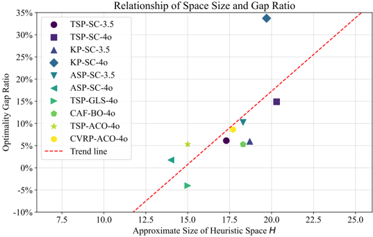<details> <summary>Image 5 Details</summary>  ### Visual Description \n ## Scatter Plot: Relationship of Space Size and Gap Ratio ### Overview This image presents a scatter plot illustrating the relationship between the "Approximate Size of Heuristic Space H" (x-axis) and the "Optimality Gap Ratio" (y-axis). Multiple data series, each representing a different algorithm or problem instance, are plotted as distinct markers. A trend line is also included. ### Components/Axes * **Title:** Relationship of Space Size and Gap Ratio * **X-axis:** Approximate Size of Heuristic Space H (Scale: 7.5 to 25.0, increments of 2.5) * **Y-axis:** Optimality Gap Ratio (Scale: -10% to 35%, increments of 5%) * **Legend:** Located in the top-left corner, listing the following data series with corresponding marker shapes and colors: * TSP-SC-3.5 (Purple Circle) * TSP-SC-4o (Purple Square) * KP-SC-3.5 (Blue Triangle) * KP-SC-4o (Blue Diamond) * ASP-SC-3.5 (Green Triangle) * ASP-SC-4o (Green Square) * TSP-GLS-4o (Olive Green Triangle) * CAF-BO-4o (Olive Green Circle) * TSP-ACO-4o (Yellow Star) * CVRP-ACO-4o (Yellow Circle) * **Trend Line:** Dashed red line, extending diagonally across the plot. ### Detailed Analysis The data points are scattered across the plot, with varying degrees of correlation to the trend line. Here's a breakdown of each data series, with approximate values based on visual inspection: * **TSP-SC-3.5 (Purple Circle):** The line slopes upward. Data points are approximately (15.5, -2%), (17.5, 6%), (19.0, 15%). * **TSP-SC-4o (Purple Square):** The line is relatively flat. Data point is approximately (20.0, 15%). * **KP-SC-3.5 (Blue Triangle):** The line slopes upward. Data point is approximately (17.5, 25%). * **KP-SC-4o (Blue Diamond):** The line slopes downward. Data point is approximately (20.0, 32%). * **ASP-SC-3.5 (Green Triangle):** The line slopes upward. Data point is approximately (15.0, 2%). * **ASP-SC-4o (Green Square):** The line slopes upward. Data point is approximately (17.5, 10%). * **TSP-GLS-4o (Olive Green Triangle):** The line slopes upward. Data point is approximately (15.0, -5%). * **CAF-BO-4o (Olive Green Circle):** The line slopes upward. Data point is approximately (18.0, 8%). * **TSP-ACO-4o (Yellow Star):** The line slopes upward. Data point is approximately (17.5, 5%). * **CVRP-ACO-4o (Yellow Circle):** The line slopes upward. Data point is approximately (15.5, 3%). The trend line itself appears to approximate a 45-degree angle, suggesting a positive correlation between the Approximate Size of Heuristic Space H and the Optimality Gap Ratio. ### Key Observations * The data points are widely dispersed, indicating a weak to moderate correlation overall. * KP-SC-4o (Blue Diamond) has the highest Optimality Gap Ratio, at approximately 32%, and a relatively high Approximate Size of Heuristic Space H, around 20. * TSP-GLS-4o (Olive Green Triangle) has a negative Optimality Gap Ratio, approximately -5%, and a relatively low Approximate Size of Heuristic Space H, around 15. * The trend line does not perfectly fit all data points, with some points lying significantly above or below it. ### Interpretation The plot explores the trade-off between the size of the search space (Approximate Size of Heuristic Space H) and the quality of the solution found (Optimality Gap Ratio). A larger search space *could* lead to better solutions (lower gap ratio), but it also increases the computational cost. The trend line suggests that, on average, increasing the search space tends to improve solution quality, but the scatter of the data indicates that this relationship is not deterministic. The significant variation among the different algorithms (TSP-SC, KP-SC, ASP-SC, etc.) suggests that the effectiveness of increasing the search space depends heavily on the specific algorithm used. Some algorithms (like TSP-GLS-4o) appear to achieve good results even with a relatively small search space, while others (like KP-SC-4o) require a larger space to achieve comparable performance. The outlier data points (e.g., TSP-GLS-4o with a negative gap ratio) may indicate cases where the algorithm has found a solution that is actually *better* than the optimal solution, or that the optimality gap calculation is flawed. Further investigation would be needed to determine the cause of these anomalies. The data suggests that there is no single "best" approach, and the optimal strategy depends on the specific problem and the available computational resources. </details> - Better in Application Scenarios with a More Complex Heuristic Space H . Each heuristic function can be expressed in the form of a 1 f 1 ( x ) + a 2 f 2 ( x ) + a 3 f 3 ( x ) + . . . + a n f n ( x ) , representing linear combinations of different sub- functions, where x denotes the particular input ( ins ) of the heuristic function h . The heuristic space H to be explored for an application scenario can be defined as the set of all meaningful sub-functions, i.e., H = Span { f 1 ( x ) , . . . } . To estimate the size of the set consisting of all meaningful sub-functions, we use OpenAI o1-mini-2024-09-12 to analyze the top 10 heuristic functions of EoH and MCTS-AHD in their respective 3 runs (6 runs and 60 heuristic functions in total), ordering LLM to break functions down into linearly independent sub-functions and use the number of sub-functions n to estimate the size of the heuristic space. We hypothesize that for more complex heuristic spaces, MCTS-AHD can explore the heuristic space more comprehensively compared to population-based methods such as EoH. To test this hypothesis, in Figure 5, we plot the relation of estimated heuristic space size n and the leads in optimality gap between MCTS-AHD and EoH (the y-axis in Figure, 1 -Gap MCTS -AHD / Gap EoH ). The results verify our hypothesis. As the trend line demonstrates, MCTS-AHD tends to achieve a more significant lead compared to the population-based baseline EoH in application scenarios with larger n . It indicates that MCTS-AHD may be more suitable for application scenarios with more complex heuristic spaces H . - Better in Application Scenarios with More Descriptions . As shown in Table 14, MCTS-AHD demonstrates a significant decrease in effectiveness in black-box settings, taking the lead only in the TSP task. This suggests that MCTS-AHD will perform better in application scenarios with more descriptions (e.g.,white-box cases). Table 14. Implementing MCTS-AHD on Black-box CO tasks with ACO general frameworks. We follow the settings of Ye et al. (2024a) in heuristic evolution and run each LLM-based method three times for average performance. The white-box results are the same as Table 2. | | TSP | CVRP | MKP | Offline BPP | |--------------------------------|--------------------------------|--------------------------------|--------------------------------|--------------------------------| | N= | N =50 | N =50, C =50 | N =100, m =5 | N =500, C =150 | | Methods | Obj. ↓ | Obj. ↓ | Obj. ↑ | Obj. ↓ | | ACO | 5.992 | 11.355 | 22.738 | 208.828 | | DeepACO | 5.842 | 8.888 | 23.093 | 203.125 | | White-box Setting: GPT-4o-mini | White-box Setting: GPT-4o-mini | White-box Setting: GPT-4o-mini | White-box Setting: GPT-4o-mini | White-box Setting: GPT-4o-mini | | EoH | 5.828 | 9.359 | 23.139 | 204.646 | | ReEvo | 5.856 | 9.327 | 23.245 | 206.693 | | MCTS-AHD(Ours) | 5.801 | 9.286 | 23.269 | 204.094 | | Black-box Setting: GPT-4o-mini | Black-box Setting: GPT-4o-mini | Black-box Setting: GPT-4o-mini | Black-box Setting: GPT-4o-mini | Black-box Setting: GPT-4o-mini | | EoH | 5.831 | 9.401 | 23.240 | 204.615 | | ReEvo | 5.860 | 9.404 | 23.196 | 206.021 | | MCTS-AHD(Ours) | 5.830 | 9.444 | 23.191 | 205.375 | We can explain that MCTS-AHD's better performance in application scenarios with complex heuristic space is highly beneficial from its ability to explore complex function spaces and escape from local optima. For its mediocre performance in black-box application scenarios, I believe this is mainly because compared to MCTS, which only performs limited expansion on each heuristic, the population structure is computationally intensive and often involves many rounds of LLM-based operations on a heuristic function in the population. So, the effectiveness of MCTS-AHD may require LLMs more on its generation quality in limited number of MCTS expansions. In contrast, black-box application scenarios make it difficult for LLMs to guarantee this condition, so these application scenarios will be tough for MCTS-AHD. ## G. Examples of Evolution To visually demonstrate the workflow of MCTS-AHD and its ability on exploration, we provide two examples of the evolution of heuristics in two tasks, as shown in Figure 6. The two examples of evolution clearly exhibit how MCTS-AHD conducts comprehensive explorations. For example, in designing heuristics with a step-by-step construction framework for TSP, MCTS-AHD can expand potential child nodes from nodes (e.g., MCTS node with 'Expansion: t=611') that are not among the top 10 optimal ones (the performance range of the top 10 optimal heuristics is the yellow shade), and ultimately reach the best heuristic. It reflects the superiority of employing MCTS as an optimization framework instead of population-based EC. Population-based LLM-based AHD methods such as EoH, ReEvo, and HSEvo lack consideration of worse-performing but potential heuristics. These algorithms will be obsessed with processing top-performance heuristic functions. When the top 10 heuristics cannot obtain new heuristics surpassing the top 10 performances with one LLM-based operation on heuristics, the evolution of heuristics will trap into local optima. 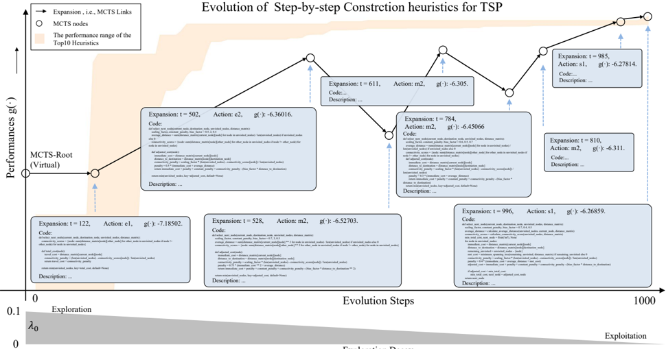<details> <summary>Image 6 Details</summary>  ### Visual Description \n ## Diagram: Evolution of Step-by-step Construction heuristics for TSP ### Overview This diagram illustrates the evolution of step-by-step construction heuristics for the Traveling Salesperson Problem (TSP). It depicts a landscape of performance (g(·)) over evolution steps, with expansions represented as nodes connected by arrows. The diagram visualizes the search process of Monte Carlo Tree Search (MCTS) and highlights the performance of the top 10 heuristics. ### Components/Axes * **Title:** Evolution of Step-by-step Construction heuristics for TSP * **Y-axis:** Performance g(·) - Ranges approximately from -8 to -6.2. * **X-axis:** Evolution Steps - Ranges from 0 to 1000. Labeled with "Exploration" on the left side (0-ish) and "Exploitation" on the right side (1000-ish). * **Legend:** * Arrow: Expansion, i.e., MCTS Links * Circle: MCTS nodes * Text: The performance range of the Top10 Heuristics * **Key Elements:** * MCTS-Root (Virtual) - Located at approximately (0, 0.1) * Expansion Nodes - Rectangular boxes at various points along the evolution steps, each containing information about the expansion. * Arrows - Connecting expansion nodes, indicating the MCTS search process. * Orange Shaded Area - Represents the performance landscape. ### Detailed Analysis / Content Details The diagram shows several expansion nodes with associated data. Here's a breakdown of each visible node: 1. **Expansion: t = 122** * Action: e1 * g(·): -7.18502 * Code: (Text block - see below) * Description: (Text block - see below) 2. **Expansion: t = 502** * Action: e2 * g(·): -6.36016 * Code: (Text block - see below) * Description: (Text block - see below) 3. **Expansion: t = 528** * Action: m2 * g(·): -6.52703 * Code: (Text block - see below) * Description: (Text block - see below) 4. **Expansion: t = 611** * Action: m2 * g(·): -6.305 * Code: (Text block - see below) * Description: (Text block - see below) 5. **Expansion: t = 784** * Action: m2 * g(·): -6.45066 * Code: (Text block - see below) * Description: (Text block - see below) 6. **Expansion: t = 810** * Action: m2 * g(·): -6.311 * Code: (Text block - see below) * Description: (Text block - see below) 7. **Expansion: t = 965** * Action: s1 * g(·): -6.27814 * Code: (Text block - see below) * Description: (Text block - see below) 8. **Expansion: t = 996** * Action: s1 * g(·): -6.26859 * Code: (Text block - see below) * Description: (Text block - see below) **Text Block Content (repeated in each expansion node):** ``` 1. random_restart_neighbor_search 2. random_restart_neighbor_search_2 3. random_restart_neighbor_search_3 4. random_restart_neighbor_search_4 5. random_restart_neighbor_search_5 6. random_restart_neighbor_search_6 7. random_restart_neighbor_search_7 8. random_restart_neighbor_search_8 9. random_restart_neighbor_search_9 10. random_restart_neighbor_search_10 ``` The text block is identical in each expansion node. It lists ten different search algorithms. ### Key Observations * The performance (g(·)) generally improves (becomes less negative) as the evolution steps increase, indicating a convergence towards better solutions. * The initial expansions (t=122, t=502) have significantly worse performance than later expansions. * The actions taken during expansion vary (e1, m2, s1), suggesting different heuristic strategies are being explored. * The orange shaded area represents a complex performance landscape, with potential local optima. * The MCTS search appears to be exploring different branches of the search space, as indicated by the arrows connecting the expansion nodes. ### Interpretation This diagram illustrates the application of MCTS to optimize step-by-step construction heuristics for the TSP. The evolution steps represent the iterations of the MCTS algorithm, where each expansion node corresponds to a new heuristic being evaluated. The performance metric g(·) quantifies the quality of the solution found by each heuristic. The diagram suggests that the MCTS algorithm is effectively exploring the search space and identifying better heuristics over time. The initial exploration phase (left side of the diagram) is characterized by high variance in performance, while the exploitation phase (right side) shows a more consistent improvement. The repeated text block within each expansion node indicates that the algorithm is evaluating different variations of the "random\_restart\_neighbor\_search" algorithm. The varying actions (e1, m2, s1) likely represent different parameters or configurations of these algorithms. The orange shaded area represents the complexity of the TSP problem and the challenges of finding optimal solutions. The diagram highlights the importance of exploration and exploitation in the search process, as well as the ability of MCTS to adaptively balance these two objectives. The diagram does not provide any quantitative data on the number of iterations or the specific parameters used in the MCTS algorithm. 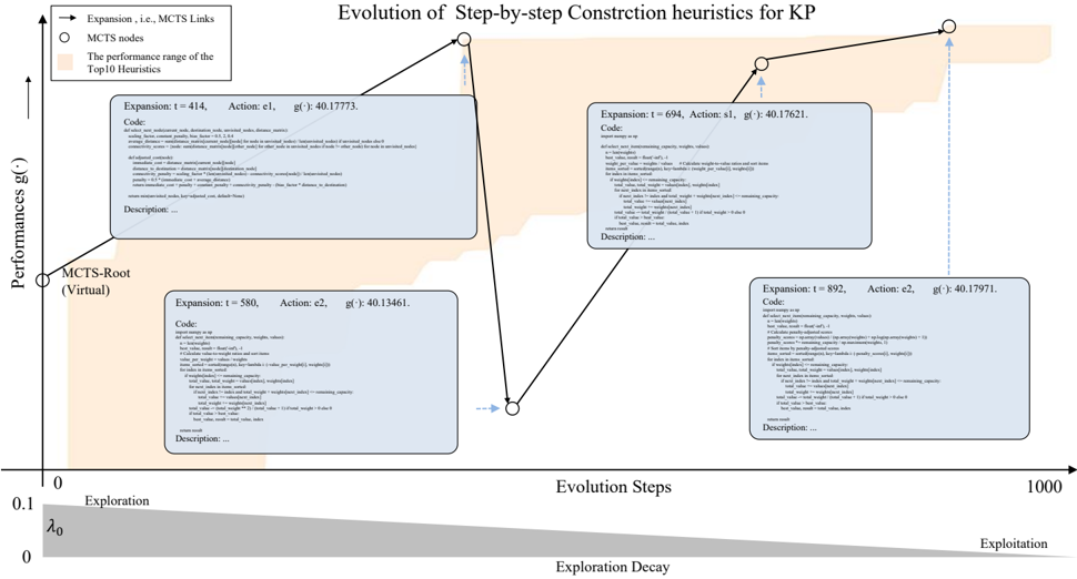</details> Exploration Decay (a) An Example of MCTS-AHD Evolution on Designing Step-by-step Construction Heuristics for TSP <details> <summary>Image 7 Details</summary>  ### Visual Description ## Diagram: Evolution of Step-by-step Construction Heuristics for KP ### Overview The image presents a diagram illustrating the evolution of step-by-step construction heuristics for a problem denoted as "KP" (likely Knapsack Problem). The diagram visualizes the performance of these heuristics over "Evolution Steps," with a focus on the trade-off between "Exploration" and "Exploitation." The diagram consists of four interconnected nodes representing different stages of heuristic development, linked by arrows indicating the progression of evolution. Each node contains code and a description field. ### Components/Axes * **Title:** "Evolution of Step-by-step Construction heuristics for KP" * **X-axis:** "Evolution Steps" ranging from 0 to 1000, labeled with "Exploration" at 0 and "Exploitation" at 1000. A label "Exploration Decay" is present below the axis. * **Y-axis:** "Performance g( )" ranging from 0 to 1.0, labeled with "λ₀" at 0.1. * **Legend:** * Black Arrow: "Expansion, i.e., MCTS Links" * White Circle: "MCTS nodes" * **Nodes:** Four rectangular nodes, each containing: * "Expansion: t = [value], Action: [value], g( ) = [value]" * "Code:" followed by a block of text. * "Description..." ### Detailed Analysis or Content Details The diagram shows four nodes connected by arrows, representing the evolution of heuristics. **Node 1 (Bottom-Left):** * Expansion: t = 414, Action: e1, g( ) = 40.17773. * Code: A block of text starting with "def _init_(self, env, params):" and continuing with several lines of code related to initialization and parameter settings. * Description: "Description..." **Node 2 (Bottom-Right):** * Expansion: t = 580, Action: e2, g( ) = 40.13461. * Code: A block of text starting with "def _init_(self, env, params):" and continuing with several lines of code, similar to Node 1, but with slight variations. * Description: "Description..." **Node 3 (Top-Right):** * Expansion: t = 694, Action: s1, g( ) = 40.17621. * Code: A block of text starting with "def _init_(self, env, params):" and continuing with several lines of code, similar to Node 1 and 2. * Description: "Description..." **Node 4 (Top-Left):** * Expansion: t = 892, Action: e2, g( ) = 40.17971. * Code: A block of text starting with "def _init_(self, env, params):" and continuing with several lines of code, similar to Node 1, 2 and 3. * Description: "Description..." The arrows indicate the flow of evolution. The arrow from Node 1 to Node 2 is a curved line. The arrow from Node 2 to Node 3 is a curved line. The arrow from Node 3 to Node 4 is a curved line. There is also a curved arrow connecting Node 4 back to Node 1, suggesting a cyclical or iterative process. The "MCTS-Root (Virtual)" label is positioned near Node 1. ### Key Observations * The performance values g( ) for all nodes are relatively close, ranging from approximately 40.13 to 40.18. * The "t" values (Expansion) increase with each step, indicating the progression of evolution. * The actions taken at each step vary (e1, e2, s1). * The code within each node appears to be similar, suggesting incremental changes to the heuristic. * The diagram emphasizes the balance between exploration and exploitation, as represented by the x-axis. ### Interpretation The diagram illustrates the iterative refinement of construction heuristics for the KP problem using a Monte Carlo Tree Search (MCTS) approach. The nodes represent different versions of the heuristic, and the arrows show how the heuristic evolves over time. The performance metric g( ) indicates the effectiveness of each heuristic. The relatively small differences in g( ) suggest that the evolution process is making incremental improvements. The cyclical arrow from Node 4 to Node 1 implies that the process is ongoing and potentially repeating, allowing for continuous refinement. The "MCTS-Root (Virtual)" label suggests that the initial heuristic is based on a virtual MCTS root, which is then iteratively improved. The code blocks within each node likely represent the implementation of the heuristic, and the "Description..." fields would provide further details about the specific changes made at each step. The diagram highlights the importance of balancing exploration and exploitation in the search for optimal heuristics. The consistent performance values suggest that the algorithm is converging towards a stable solution, but further evolution may be needed to achieve significant improvements. </details> (b) An Example of MCTS-AHD Evolution on Designing Step-by-step Construction Heuristics for KP © Copyright National University of Singapore. All Rights Reserved. Figure 6. Two examples of the heuristic evolution process of MCTS-AHD. We provide the performance function value g ( · ) of the heuristic function within each MCTS tree node. The 'Action' in each node represents one of the six actions of expanding this node. Codes are simplified by OpenAI GPT to reduce the space occupations. ## H. Baselines & Licenses For the optimal value in Table 1 and Table 8. We run LKH3 for TSP instances with adopting the commonly used setting in NCO methods (Kool et al., 2018). We set the LKH parameters RUNS = 10 and MAX TRAILS = 1,0000. For KP instances, we use Google OR-Tools for the optimal value. For manually designed heuristics with general frameworks , this paper includes Greedy Construct, the ACO algorithm (Dorigo et al., 2006), the KGLS algorithm (Arnold & S¨ orensen, 2019), and EI (Mockus, 1974), EIpu (Snoek et al., 2012), EI-cools (Lee et al., 2020a) for the CAF design task in BO. We implement KGSL by setting the heuristic matrix to the distance matrix, using the implementation of ACO in DeepACO (Ye et al., 2024b), and use the results reported in Yao et al. (2024c) for EI, EIpu, and EI-cools. For NCO baselines , this article implements POMO (Kwon et al., 2020), DeepACO (Ye et al., 2024b), VRP-DACT (Ma et al., 2021), and NeuOpt ( ? ). For a fair comparison, in Table 1, the reported POMO solutions are from a single start and generated without augmentations. The maximum operation on a solution is set to T = 1200 for VRP-DACT and NeuOpt. For AHD baselines , in TSPLib, we adopt the results of GHPP reported in (Duflo et al., 2019). For LLM-based AHD baselines , this article considers Funsearch (Romera-Paredes et al., 2024), EoH (Liu et al., 2024b), ReEvo (Ye et al., 2024a), and HSEvo (Dat et al., 2024), we follow all their parameter settings in evolutions (e.g., setting population size M = 20 for online BPP and M = 10 for other tasks). We try not to introduce too much external expert information. However, in implementations, Funsearch needs to maintain 10 relatively independent multiple populations from a certain inferior seed heuristic function. ReEvo relies more on the seed heuristic function, and the ReEvo method will become unavailable when all individuals in the elite population have the same objective function value. So, in some application scenarios (e.g., step-by-step construction for the KP task), it is too hard to find a good seed heuristic function that ensures the availability of the algorithm while trying not to provide too much external knowledge. In experiments, we use the same seed functions for baselines (Funsearch, ReEvo, and HSEvo), using seed functions proposed in Ye et al. (2024a) for ACO frameworks and GLS frameworks, random selection functions for step-by-step constructing TSP and ASP, and the best-known function proposed in Romera-Paredes et al. (2024) for online BPP. The proposed MCTS-AHD, exhibits better applicability and superior performance in most application scenarios, without the requirement of seed function design. In our seed function settings, ReEvo and its follow-up method HSEvo are not available in some application scenarios (e.g., KP, ACO), where we do not report their effects. ## H.1. License The licenses and URL of baselines are listed in Table 15. Table 15. A summary of licenses. | Resources | Type | License | URL | |--------------------|----------------------------------------------------------------------------------------------------|----------------------------------------------------------------------------------------------------|----------------------------------------------------------------------------------------------------| | LKH3 | Code | Available for academic research use | http://webhotel4.ruc.dk/˜keld/research/LKH-3/ | | OR-Tools | Code | MIT License | https://developers.google.com/optimization/pack/knapsack?hl=zh-cn | | POMO | Code | Available online | https://github.com/yd-kwon/POMO/tree/master | | DeepACO | Code | MIT License | https://github.com/henry-yeh/DeepACO | | VRP-DACT | Code | MIT License | https://github.com/yining043/VRP-DACT | | NeuOpt | Code | MIT License | https://github.com/yining043/NeuOpt | | Funsearch | Code | Apache License | https://github.com/google-deepmind/funsearch | | EoH | Code | MIT License | https://github.com/FeiLiu36/EoH/tree/main | | ReEvo | Code | MIT License | https://github.com/ai4co/reevo | | HSEvo | Code | Available online | https://github.com/datphamvn/HSEvo | | Synthetic problems | Dataset | Available Online | https://github.com/FeiLiu36/EoH/tree/main/examples/user_bo_caf | | TSPLib | Dataset Available for any non-commercial use http://comopt.ifi.uni-heidelberg.de/software/TSPLIB95 | Dataset Available for any non-commercial use http://comopt.ifi.uni-heidelberg.de/software/TSPLIB95 | Dataset Available for any non-commercial use http://comopt.ifi.uni-heidelberg.de/software/TSPLIB95 |