# Dispersive dark excitons in van der Waals ferromagnet CrI3
**Authors**: W. He, J. Sears, F. Barantani, T. Kim, J. W. Villanova, T. Berlijn, M. Lajer, M. A. McGuire, J. Pelliciari, V. Bisogni, S. Johnston, E. Baldini, M. Mitrano, M. P. M. Dean
> Current address: Stanford Institute for Materials and Energy Sciences, SLAC National Accelerator Laboratory, Menlo Park, CA 94025, USA; weihe@stanford.edu
> Department of Condensed Matter Physics and Materials Science, Brookhaven National Laboratory, Upton, New York 11973, USA
> Department of Physics, The University of Texas at Austin, Austin, Texas, USA, 78712
> National Synchrotron Light Source II, Brookhaven National Laboratory, Upton, New York 11973, USA
> Center for Nanophase Materials Sciences, Oak Ridge National Laboratory, Oak Ridge, Tennessee 37831, USA
> Materials Science and Technology Division, Oak Ridge National Laboratory, 1 Bethel Valley Road, Oak Ridge, Tennessee 37831, USA
> Department of Physics and Astronomy, The University of Tennessee, Knoxville, Tennessee 37966, USAInstitute for Advanced Materials and Manufacturing, The University of Tennessee, Knoxville, Tennessee 37996, USA
> Department of Physics, Harvard University, Cambridge, Massachusetts 02138, USA
> mdean@bnl.govDepartment of Condensed Matter Physics and Materials Science, Brookhaven National Laboratory, Upton, New York 11973, USA
(January 16, 2025)
Abstract
Spin-flip dark excitons are optical-dipole-forbidden quasiparticles with remarkable potential in optoelectronics, especially when they are realized within cleavable van der Waals materials. Despite this potential, dark excitons have not yet been definitively identified in ferromagnetic van der Waals materials. Here, we report two dark excitons in a model ferromagnetic material \ce CrI3 using high-resolution resonant inelastic x-ray scattering (RIXS) and show that they feature narrower linewidths compared to the bright excitons previously reported in this material. These excitons are shown to have spin-flip character, to disperse as a function of momentum, and to change through the ferromagnetic transition temperature. Given the versatility of van der Waals materials, these excitons hold promise for new types of magneto-optical functionality.
I Introduction
Excitons play a key role in determining the optical properties of solids, and their strong light-matter coupling paves the way for exploring new aspects of many-body physics [1]. Dark excitons are particularly interesting because they involve optical-dipole-forbidden transitions [2]. For this reason, they have reduced rates of radiative recombination and enhanced lifetimes and in many cases they can be sensitively controlled by external means, such as magnetic field [3]. These properties endow them with great potential in quantum information storage and communication [4].
Early studies of dark excitons began in the 1990s with quantum dots [5], followed by research on organic materials [6], and later expanded to transition-metal dichalcogenides [7]. The recent discovery of magnetic van der Waals (vdW) materials provides a new platform for studying excitons [8, 9, 10, 11, 12] and fascinating interactions between magnetism and excitons have been observed in several antiferromagnetic systems [13, 14, 15, 16, 17]. Understanding the electronic structure of these excitons and their interactions with magnetism is not only interesting from a fundamental point of view, but it may also offer new types of magneto-optical functionality such as optical read-out of magnetic states or quantum sensors [18]. \ce CrI3 provides an opportunity to study excitons in a ferromagnetic (FM) vdW material even down to the monolayer limit [19, 20]. Optical studies have revealed several bright excitons around $1.50$ , $1.85$ and $2.2$ eV in this material alongside several other optical features [21, 22, 23, 20]; however dark excitons have not been definitively identified.
Resonant inelastic x-ray scattering (RIXS) is directly sensitive to optically forbidden excitations and has recently emerged as a powerful probe of excitons and their interactions with magnetism, in several magnetic vdW materials [13, 15, 16, 24, 17, 25]. In this Letter, we use Cr $L_{3}$ -edge RIXS to identify two dark excitons near $1.7$ eV in \ce CrI3. Both dark excitons are much sharper than other bright excitons and disperse with a bandwidth ( $\sim 10$ meV) similar to the energy scale of magnetic exchange interactions in this material. Together with the change of their intensities across the FM ordering temperature $T_{\mathrm{c}}$ , our experimental findings suggest an intimate relationship between \ce CrI3’s dark excitons and its magnetism. The electronic character of the dark excitons is borne out by our exact diagonalization (ED) calculations, which reveal that these excitons are spin-flip transitions in nature and are predominantly governed by Hund’s coupling.
II Methods
Bulk single crystals of \ce CrI3 were synthesized by reacting the elements together in an evacuated fused silica ampoule [26]. \ce CrI3 undergoes a structural phase transition between the high-temperature monoclinic structure (space group $C2/m$ , #12) and the low-temperature rhomobohedral structure (space group $R\bar{3}$ , #148) over a broad temperature range ( $100$ – $220$ K) upon thermal cycling. The temperature of the sample was kept at $T=30$ K, deep into the FM phase of the material, unless otherwise specified. We consequently used the rhomobohedral unit cell notation with lattice parameters $a=b=6.867$ Å, $c=19.807$ Å, and $\gamma=120^{\circ}$ throughout the manuscript, and index reciprocal space in terms of scattering vector $\bm{Q}{}=(H,K,L)$ in reciprocal lattice units (r.l.u.).
To avoid sample degradation in air, we mounted the sample on a copper sample holder in a glove box, cleaved with scotch tape in \ce N2 atmosphere ( $\sim 3$ % relative humidity level) to expose a fresh surface, and directly transferred the cleaved sample into the RIXS sample chamber. The surface normal of the sample was parallel to the $c$ -axis. The in-plane orientation was determined by checking the residue on the scotch tape with a laboratory single-crystal x-ray diffractometer.
Cr $L_{3}$ -edge RIXS measurements were performed at the SIX 2-ID beamline of the National Synchrotron Light Source II. Data were taken with linear horizontal ( $\pi$ ) polarization in the $(H0L)$ scattering plane unless otherwise specified. The spectrometer was operated with a high energy resolution of $30.5$ meV full-width at half-maximum (FWHM) (the exit slit size was $30$ µm). Since the interlayer coupling in \ce CrI3 is weak, we fixed the scattering angle at $2\Theta=150^{\circ}$ and expressed $\bm{Q}$ in terms of the projected in-plane component of the momentum $H$ . An angle-dependent self-absorption correction [27] was applied to the RIXS spectra, which, however, does not affect exciton energies or relative intensity changes at fixed $\bm{Q}$ . The x-ray absorption spectroscopy (XAS) spectra were taken using the partial fluorescence yield mode with the RIXS detector, which covers the energy loss up to $\sim 11$ eV. The exit slit size was much larger ( $300$ µm) for the XAS measurements to increase the flux.
III Identification of dark excitons
<details>
<summary>x1.png Details</summary>
### Visual Description
# Technical Data Extraction: Resonant Inelastic X-ray Scattering (RIXS) Spectra
This document provides a comprehensive extraction of the data and components from the provided scientific figure, which displays RIXS (Resonant Inelastic X-ray Scattering) intensity maps and line profiles.
## 1. Image Structure and Layout
The image is divided into three primary panels:
* **Panel (a) [Top Left]:** A 2D heatmap showing the "Full range" of energy loss.
* **Panel (b) [Top Right]:** A 2D heatmap showing a "Zoom-in" of a specific energy loss region.
* **Panel (c) [Bottom]:** A 1D line plot showing integrated intensity vs. incident energy.
* **Color Bar [Middle]:** A shared legend for the heatmaps in panels (a) and (b).
---
## 2. Heatmap Data (Panels a and b)
### Shared Axis and Legend Information
* **X-axis (Horizontal):** Incident energy $E_i$ (eV). Range: 574 to 581 eV.
* **Y-axis (Vertical):** Energy loss (eV).
* **Panel (a) Range:** 0 to 11 eV.
* **Panel (b) Range:** 1.3 to 2.5 eV.
* **Color Scale (Intensity):** Measured in "Intensity (arb. units)".
* **Scale Range:** 0.00 (Grey/Black) to 0.20 (Red).
* **Gradient:** Grey $\rightarrow$ Blue ($\approx$ 0.04) $\rightarrow$ Cyan ($\approx$ 0.08) $\rightarrow$ Green ($\approx$ 0.12) $\rightarrow$ Yellow ($\approx$ 0.16) $\rightarrow$ Red ($\approx$ 0.20).
### Panel (a): Full Range Analysis
* **Components:**
* **Heatmap:** Shows high-intensity features (yellow/red) concentrated between 1.5 eV and 3.0 eV energy loss.
* **Black Line Plot (Overlay):** A line with circular markers is overlaid at the top of the heatmap (approx. 8 to 10.5 eV energy loss).
* **Trend:** The line starts at ~8.2 eV (at $E_i = 574$), rises to a peak of ~9.8 eV at $E_i \approx 575.2$, dips slightly, then reaches a broad maximum of ~10.4 eV at $E_i \approx 576.5$ before leveling off around 9.8 eV for higher incident energies.
### Panel (b): Zoom-in Analysis
This panel highlights specific electronic transitions labeled with dashed horizontal lines and text markers.
* **Labeled Features (Energy Loss Positions):**
* **B3 (Purple text):** Located at Energy loss $\approx$ 2.21 eV. Shows high intensity at $E_i \approx 576.5$ eV.
* **B2 (Dark Red text):** Located at Energy loss $\approx$ 1.88 eV.
* **D2 (Green text):** Located at Energy loss $\approx$ 1.71 eV. Shows two distinct resonance peaks at $E_i \approx 575.1$ and $E_i \approx 576.3$.
* **D1 (Orange text):** Located at Energy loss $\approx$ 1.66 eV.
* **B1 (Blue text):** Located at Energy loss $\approx$ 1.50 eV. Shows two distinct resonance peaks at $E_i \approx 575.1$ and $E_i \approx 576.3$.
---
## 3. Line Plot Data (Panel c)
### Axis and Legend Information
* **X-axis:** Incident energy $E_i$ (eV). Range: 574 to 581 eV.
* **Y-axis:** Int. Intensity (arb. units). Range: 0 to 23.
* **Legend [Spatial Grounding: Top Right of Panel c]:**
* **D1 (Orange circles):** Corresponds to the orange line.
* **D2 (Green squares):** Corresponds to the green line.
### Trend Verification and Data Points
* **Series D2 (Green Squares):**
* **Trend:** Shows a sharp, dominant peak followed by a secondary peak.
* **Peak 1 ($E_{t_{2g}}$):** Reaches maximum intensity of ~21 units at $E_i \approx 575.1$ eV. This is marked by a vertical dashed line labeled **$E_{t_{2g}}$**.
* **Peak 2 ($E_{e_g}$):** Reaches a secondary maximum of ~18 units at $E_i \approx 576.3$ eV. This is marked by a vertical dashed line labeled **$E_{e_g}$**.
* **Tail:** Intensity decays to ~5 units by $E_i = 580.5$ eV.
* **Series D1 (Orange Circles):**
* **Trend:** Significantly lower intensity than D2. Shows a multi-peak structure that mirrors the resonance positions of D2 but with different relative weights.
* **Feature 1:** Small peak of ~4.5 units at $E_i \approx 575.5$ eV.
* **Feature 2:** Peak of ~5.2 units at $E_i \approx 576.4$ eV (near the $E_{e_g}$ resonance).
* **Baseline:** Remains between 1 and 4 units across the rest of the range.
---
## 4. Summary of Key Transitions
| Label | Energy Loss (eV) | Primary Resonance ($E_i$) | Color Code |
| :--- | :--- | :--- | :--- |
| **B3** | ~2.21 | ~576.5 eV | Purple |
| **B2** | ~1.88 | - | Dark Red |
| **D2** | ~1.71 | 575.1 eV ($E_{t_{2g}}$) & 576.3 eV ($E_{e_g}$) | Green |
| **D1** | ~1.66 | 576.4 eV | Orange |
| **B1** | ~1.50 | 575.1 eV & 576.3 eV | Blue |
</details>
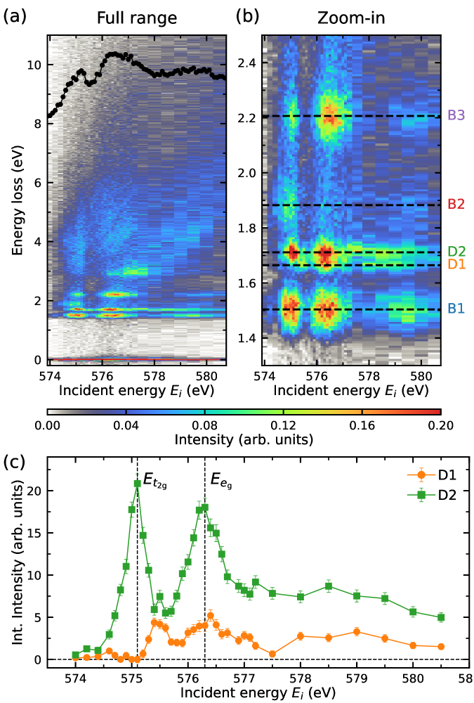
Figure 1: Resonance behavior of dark excitons. (a) Cr $L_{3}$ -edge RIXS incident energy map taken at $T=30$ K with $\pi$ -polarized x-rays incident on the sample at $\theta=14.5^{\circ}$ and scattered to $2\Theta=150^{\circ}$ in the ( $H0L$ ) scattering plane, corresponding to $H=-0.46$ r.l.u. The overlaid black curve on the top is XAS spectrum taken at the same conditions (including x-ray polarization, experimental geometry, and temperature). (b) Zoom of the exciton resonances. Horizontal dashed lines are fitted exciton energies. Two peaks near $1.7$ eV are identified as the dark excitons and denoted as D1 and D2. The other three peaks are bright excitons previously observed in optical measurements [21, 22, 23, 20] and therefore denoted as B1–B3. (c) The fitted integrated intensities of the two dark excitons as a function of incident photon energy $E_{i}$ through the $E_{t_{\mathrm{2g}}}$ and $E_{e_{\mathrm{g}}}$ resonances. D1 resonates at $E_{e_{\mathrm{g}}}$ , whereas D2 resonates at $E_{e_{\mathrm{g}}}$ and $E_{t_{\mathrm{2g}}}$ . As shown in Supplemental Material Sec. S1, these effects show minimal dichroism [28].
<details>
<summary>x2.png Details</summary>
### Visual Description
# Technical Data Extraction: Resonant Inelastic X-ray Scattering (RIXS) Spectra
This document provides a comprehensive extraction of the data and components from the provided scientific figure, which displays energy loss spectra and intensity heatmaps.
## 1. Global Metadata and Scale
* **Primary Language:** English.
* **Color Scale (Bottom Left):** A linear intensity scale ranging from **0.00 to 0.30 (arb. units)**.
* **Black/Grey:** Low intensity (~0.00 - 0.05).
* **Blue/Cyan:** Low-mid intensity (~0.05 - 0.15).
* **Green/Yellow:** Mid-high intensity (~0.15 - 0.25).
* **Red/Orange:** High intensity (~0.25 - 0.30).
---
## 2. Component Analysis
### Region (a) & (b): Intensity Heatmaps (Broad Range)
These panels show intensity as a function of momentum transfer ($H$) and Energy loss.
* **Y-axis (Shared):** Energy loss (eV), ranging from **1.3 to 2.4 eV**.
* **X-axis (Shared):** $H$ (r.l.u.), ranging from **-0.5 to 0.5**.
* **Panel (a) Condition:** $E_i = E_{t_{2g}}$
* **Panel (b) Condition:** $E_i = E_{e_g}$
* **Identified Features (Labels located between (b) and (c)):**
* **B1 (Blue):** Located at ~1.5 eV. Width/FWHM indicated as **61 meV**.
* **D1 (Orange):** Located at ~1.65 eV. Width/FWHM indicated as **7 meV**.
* **D2 (Green):** Located at ~1.71 eV. Width/FWHM indicated as **24 meV**.
* **B2 (Red):** Located at ~1.9 eV. Width/FWHM indicated as **91 meV**.
* **B3 (Purple):** Located at ~2.2 eV. Width/FWHM indicated as **78 meV**.
### Region (c): Line Profile and Peak Fitting
A detailed cross-section of the data at a specific momentum point.
* **Condition:** $H = -0.20$ (r.l.u.), $E_i = E_{e_g}$.
* **X-axis:** Energy loss (meV), ranging from **1200 to 2500 meV**.
* **Y-axis:** Intensity (arb. units), ranging from **0.0 to 0.4**.
* **Data Points:** Black circles with vertical error bars.
* **Fitted Components (Trend Verification):**
* **B1 (Blue Shaded):** Broad Gaussian/Lorentzian peak centered at ~1500 meV.
* **D1 (Orange Shaded):** Sharp, narrow peak centered at ~1650 meV.
* **D2 (Green Shaded):** Prominent peak centered at ~1710 meV.
* **B2 (Red Shaded):** Very broad, low-intensity feature centered at ~1900 meV.
* **B3 (Purple Shaded):** Broad peak centered at ~2200 meV.
* **Background (Grey Shaded):** A rising baseline starting from ~1400 meV and increasing toward higher energy loss.
### Region (d) & (e): High-Resolution Heatmaps (Zoomed)
These panels focus on the D1 and D2 features to show dispersion.
* **Y-axis (Shared):** Energy loss (meV), ranging from **1640 to 1730 meV**.
* **X-axis (Shared):** $H$ (r.l.u.), ranging from **-0.5 to 0.5**.
* **Trend Analysis:**
* **D2 (Green Line with Squares):** Shows a slight upward "hump" or cosine-like dispersion. It peaks at $H = 0$ (~1718 meV) and dips slightly toward $H = \pm 0.5$ (~1710 meV).
* **D1 (Orange Line with Circles):** Shows a slight downward dip at $H = 0$ (~1655 meV) and rises slightly toward the edges (~1665 meV).
* **Panel (d):** Raw intensity heatmap with overlaid dispersion points.
* **Panel (e):** Appears to be a processed or different resonance version of the same energy range, showing clearer separation of the D1 and D2 tracks.
---
## 3. Summary of Extracted Data Points (Approximate)
| Feature | Energy Center (meV) | Energy Center (eV) | Width (meV) | Color Code |
| :--- | :--- | :--- | :--- | :--- |
| **B1** | ~1500 | 1.50 | 61 | Blue |
| **D1** | ~1660 | 1.66 | 7 | Orange |
| **D2** | ~1715 | 1.71 | 24 | Green |
| **B2** | ~1900 | 1.90 | 91 | Red |
| **B3** | ~2200 | 2.20 | 78 | Purple |
## 4. Spatial Grounding of Labels
* **Legend/Labels [x, y]:** The primary labels for the peaks (B1, D1, D2, B2, B3) are positioned vertically between the heatmap (b) and the line plot (c), aligned with their respective energy levels on the Y-axis.
* **Panel Labels:** (a) Top-left of first heatmap; (b) Top-left of second heatmap; (c) Top-left of line plot; (d) Top-left of first zoomed heatmap; (e) Top-left of second zoomed heatmap.
</details>
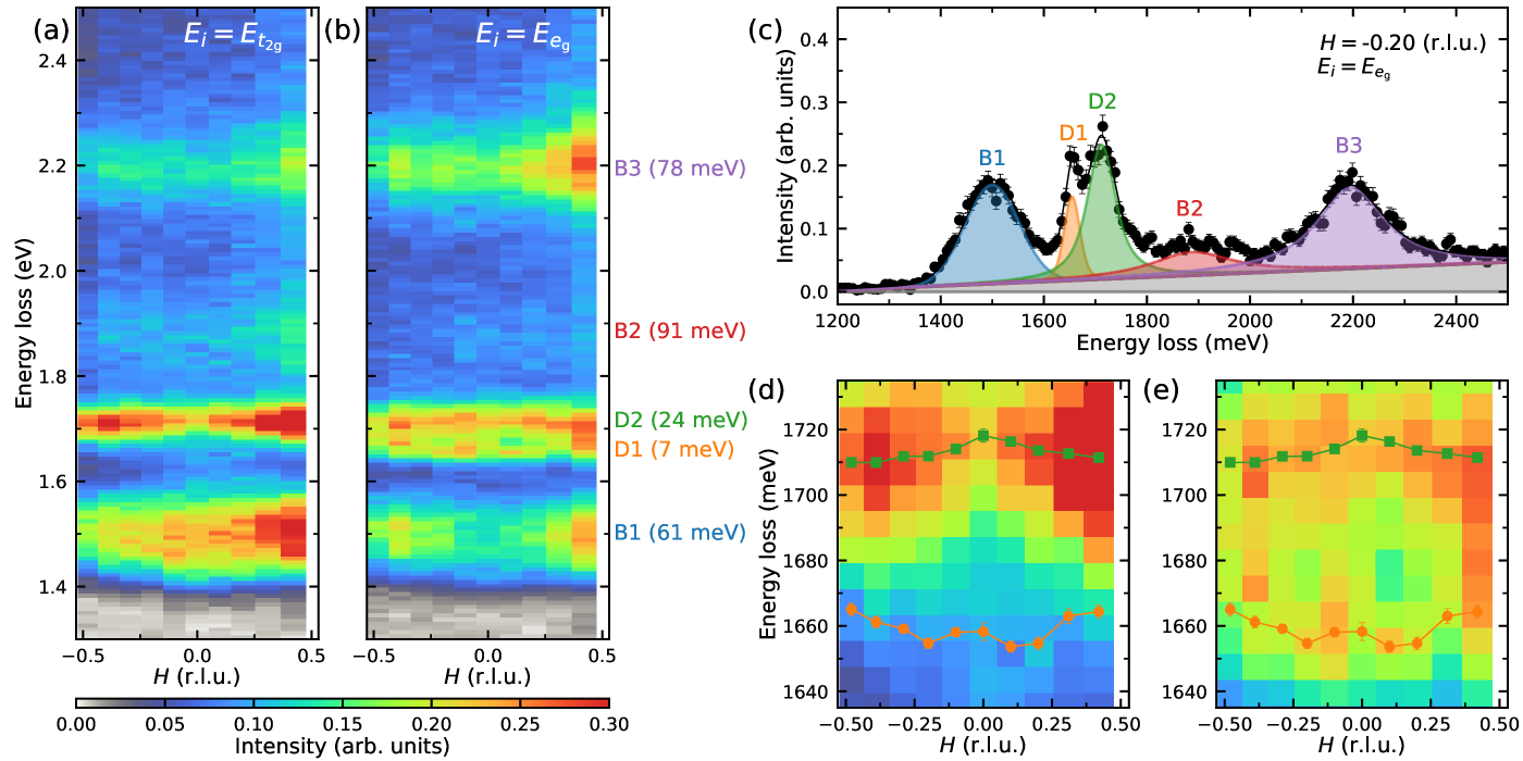
Figure 2: Dispersion of the dark excitons. (a),(b) RIXS intensity map at $T=30$ K as a function of in-plane momentum transfer $H$ measured with (a) $E_{i}=E_{t_{\mathrm{2g}}}$ where the D2 exciton is strongest and (b) $E_{i}=E_{e_{\mathrm{g}}}$ where the D1 and D2 excitons are visible. The two dark excitons are much narrower than the other bright excitons, as seen by inspecting the intrinsic resolution deconvolved HWHM of the peaks as included in brackets after the peak labels. (c) Representative fit at $H=-0.20$ r.l.u. with $E_{i}=E_{e_{\mathrm{g}}}$ . (d),(e) Zoom of the dark exciton dispersion at (d) $E_{i}=E_{t_{\mathrm{2g}}}$ and (e) $E_{i}=E_{e_{\mathrm{g}}}$ . For each momentum, we co-fit the spectra taken at the two resonances with shared exciton energies and widths. The co-fitted energy dispersion overlays the colormaps.
Figure 1 (a) shows Cr $L_{3}$ -edge RIXS spectra of \ce CrI3 as a function of incident x-ray energy. Peaks below $2.5$ eV energy loss are mainly local transitions within the Cr $3d$ orbital manifold, while broad features at higher energy can be ascribed to charge transfer processes that heavily involve ligand orbitals, and x-ray fluorescence arising from more extended states [29]. In the 1–3 eV energy window depicted in Fig. 1 (b), three peaks, located at $1.50$ eV, $1.88$ eV, and $2.21$ eV, match the exciton energies previously reported in optical experiments [21, 22, 23, 20], so we denote them as bright excitons B1–B3. More excitingly, two additional features are observed at $1.66$ eV and $1.71$ eV, which were not seen in prior RIXS measurements due to their lower resolution ( $180$ / $350$ meV ared to $30.5$ meV used here [30, 31]). These modes have not yet been definitively identified in optical spectra, so, following standard terminology in optics, we will refer to these as dark excitons and denote them as D1 and D2. We note that there are no additional features at energies below B1, contrary to an earlier prediction that the lowest energy dark excitons should exist around $0.9$ eV [32].
Figure 1 (b) exhibits two prominent resonances at $E_{i}=575.1$ eV and $576.3$ eV. Although there is strong $t_{\mathrm{2g}}$ - $e_{\mathrm{g}}$ mixing in \ce CrI3, these two resonances correspond to more $t_{2g}$ -like and more $e_{g}$ -like orbital manifolds, respectively, as shown in Supplemental Fig. S16. We therefore label them as $E_{t_{\mathrm{2g}}}$ and $E_{e_{\mathrm{g}}}$ resonances hereafter. As shown in Fig. 1 (c), D2 resonates with $t_{\mathrm{2g}}$ and $e_{\mathrm{g}}$ intermediate states, but D1 only resonates at the $e_{\mathrm{g}}$ condition. An additional small resonance is present around 575.5 eV, which is generated by the exchange part of the core-valence Coulomb interaction on the Cr site. We will use the excitons’ energy and angular dependence to identify their electronic character later in this Article.
IV Dark excitons dispersion
<details>
<summary>x3.png Details</summary>
### Visual Description
# Technical Data Extraction: Resonant Inelastic X-ray Scattering (RIXS) Temperature Dependence
This document provides a comprehensive extraction of data and trends from the provided scientific figure, which illustrates the temperature dependence of electronic excitations in a material (likely a vanadate or similar transition metal oxide) at two different momentum transfers ($H$).
---
## 1. Image Overview and Layout
The image is a multi-panel scientific plot consisting of six panels labeled **(a)** through **(f)**, organized into a $3 \times 2$ grid.
* **Top Row (a, b):** Color-mapped heatmaps showing Intensity vs. Energy loss and Temperature.
* **Middle Row (c, d):** Line plots showing Full Width at Half Maximum (FWHM) vs. Temperature.
* **Bottom Row (e, f):** Line plots showing Peak Height vs. Temperature.
* **Columns:** The left column (a, c, e) corresponds to $H = -0.39$ (r.l.u.). The right column (b, d, f) corresponds to $H = 0$ (r.l.u.).
---
## 2. Header and Global Metadata
* **Common X-axis (all panels):** Temperature (K), ranging from 0 to 325 K.
* **Critical Temperature ($T_c$):** Indicated by a vertical dashed black line at approximately **60 K** in all panels.
* **Incident Energy ($E_i$):** Labeled as $E_i = E_{t_{2g}}$ in panels (a) and (b).
* **Momentum Transfer ($H$):**
* Left Column: $H = -0.39$ (r.l.u.)
* Right Column: $H = 0$ (r.l.u.)
---
## 3. Heatmap Analysis (Panels a & b)
These panels show the spectral weight distribution.
### Axis and Scale
* **Y-axis:** Energy loss (eV), ranging from 1.3 to 2.5 eV.
* **Color Bar (Legend):** Located below panels (a) and (b).
* **Label:** Intensity (arb. units)
* **Range:** 0.00 (Grey/Blue) to 0.30 (Red).
* **Scale Markers:** 0.00, 0.05, 0.10, 0.15, 0.20, 0.25, 0.30.
### Identified Features (Labels on right of panel b)
The following spectral features are identified by color-coded labels:
* **B3 (Purple):** High energy feature around 2.2 eV.
* **B2 (Red):** Feature around 1.85 eV.
* **D2 (Green):** Strong feature around 1.7 eV.
* **D1 (Orange):** Feature around 1.65 eV (closely associated with D2).
* **B1 (Blue):** Feature around 1.45 - 1.5 eV.
### Visual Trends
* Intensity is highest at low temperatures (below $T_c$) for the D2 and B1 features.
* As temperature increases, the features broaden and their peak intensities generally decrease.
---
## 4. FWHM and Peak Height Analysis (Panels c, d, e, f)
### Legend for Line Plots (Spatial Grounding: Right of panel d/f)
The markers and colors correspond to the features identified in the heatmaps:
* **D1 (Orange Circle):** Low energy component.
* **D2 (Green Square):** Main peak component.
* **B1 (Blue Left-pointing Triangle):** Lower sideband.
* **B2 (Red Right-pointing Triangle):** Higher sideband.
* **B3 (Purple Up-pointing Triangle):** Highest energy component.
### FWHM Trends (Panels c & d)
* **Y-axis:** FWHM (meV), ranging from 0 to 350 meV.
* **General Trend:** All features show an upward slope, indicating thermal broadening as temperature increases.
* **Specific Observations:**
* **B2 (Red):** Shows the highest FWHM, increasing from ~180 meV to >300 meV.
* **D1 (Orange):** Remains the narrowest feature, staying below 100 meV.
* **Discontinuity:** There is a noticeable change in slope or a "kink" around $T_c$ (60 K), particularly for B2 and D2.
### Peak Height Trends (Panels e & f)
* **Y-axis:** Peak height (arb. units), ranging from 0.0 to 0.3.
* **General Trend:** Most features show a downward slope, indicating a loss of peak intensity with increasing temperature.
* **Specific Observations:**
* **D2 (Green):** Shows the most dramatic decrease, starting near 0.3 at low T and dropping to ~0.15 at 300 K.
* **B1 (Blue):** Also shows a significant linear decrease.
* **D1 (Orange):** In panel (e), the peak height is recorded as 0.0 (likely due to being unresolved or merged with D2 at that momentum), whereas in panel (f) it shows a low, stable intensity around 0.04.
* **Transition at $T_c$:** In panel (f), D2 and B1 show a distinct change in the rate of decrease exactly at the $T_c$ dashed line.
---
## 5. Summary Table of Extracted Components
| Feature Label | Color | Approx. Energy (eV) | FWHM Trend (T $\uparrow$) | Peak Height Trend (T $\uparrow$) |
| :--- | :--- | :--- | :--- | :--- |
| **B3** | Purple | ~2.2 | Gradual Increase | Slight Decrease |
| **B2** | Red | ~1.85 | Sharp Increase | Gradual Decrease |
| **D2** | Green | ~1.7 | Moderate Increase | Sharp Decrease |
| **D1** | Orange | ~1.65 | Stable / Low | Stable / Low |
| **B1** | Blue | ~1.45 | Moderate Increase | Sharp Decrease |
**Note on Language:** All text in the image is in English. No other languages were detected.
</details>
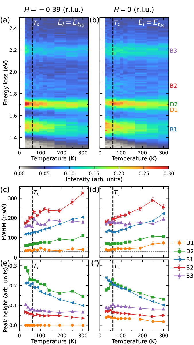
Figure 3: Temperature dependence of the dark excitons. (a),(b) RIXS intensity map as a function of temperature measured at two different in-plane momenta ( $H=-0.39$ and $H=0$ r.l.u., respectively) with the same incident energy $E_{t_{\mathrm{2g}}}$ . (c)–(f) Corresponding FWHM and peak height extracted from the fits as a function of temperature. Changes in peak height through $T_{c}$ primarily reflect changes in the integrated intensity of the peaks. We plot the peak intensity here because this quantity can be determined more precisely. Error bars represent one standard deviation. The fits were performed by co-fitting spectra taken at two incident energies with shared exciton energies and widths for each momentum and temperature. The data taken at the other incident energy $E_{e_{\mathrm{g}}}$ are shown in Supplemental Material Sec. S2 [28]. The vertical black lines indicate the FM transition temperature $T_{\mathrm{c}}$ and the horizontal black lines in (c)&(d) indicate the energy resolution.
Having identified the existence of dark excitons in \ce CrI3, we explore their propagation by mapping out their in-plane dispersion at the two resonant energies $E_{t_{\mathrm{2g}}}$ and $E_{e_{\mathrm{g}}}$ , as presented in Fig. 2 (a) and (b). Intriguingly, both excitons D1 and D2 exhibit a small dispersion but with opposite trends. We co-fit the spectra at the two different resonances, as described in Supplemental Material Sec. S3, and shown in Fig. 2 (c). The fitted exciton energies in Fig. 2 (d)&(e) confirm the presence of dispersion with similar bandwidths of $\sim 10$ meV. Such bandwidths are comparable to the energy scale of the magnon dispersion [33], hinting at the involvement of exciton-magnon interactions when these dark excitons propagate in the lattice. The widths of the two dark excitons are dramatically sharper than those of other bright excitons, especially D1, which is almost resolution limited and about ten times narrower than the bright excitons [see Fig. 2 (b)]. The three bright excitons do not exhibit any detectable dispersion (see Supplemental Fig. S9), likely due to their broader linewidths.
<details>
<summary>x4.png Details</summary>
### Visual Description
# Technical Data Extraction: RIXS Spectroscopy Analysis
This document provides a comprehensive extraction of data and technical components from the provided scientific figure, which compares experimental Resonant Inelastic X-ray Scattering (RIXS) data with theoretical simulations.
## 1. Image Overview and Layout
The image is a multi-panel scientific plot consisting of five distinct sub-figures labeled (a) through (e).
- **Panels (a) and (b):** 2D Heatmaps showing Intensity as a function of Incident Energy ($E_i$) and Energy Loss.
- **Panels (c), (d), and (e):** 1D Line and Scatter plots aligned vertically by a common X-axis (Energy loss).
---
## 2. Component Analysis
### Panel (a): Experimental Data (Heatmap)
* **Title:** Data
* **Y-axis:** Energy loss (eV). Range: 0.0 to 2.5. Markers every 0.5 units.
* **X-axis:** Incident energy $E_i$ (eV). Range: 574 to 581. Markers at 574, 576, 578, 580.
* **Color Scale (Footer):** Intensity (arb. units). Range: 0.00 (Black/Grey) to 0.20 (Red).
* **Key Features:**
* A strong elastic peak at Energy loss = 0 eV, centered around $E_i \approx 576.5$ eV.
* Four distinct inelastic features (horizontal bands) appearing between 1.5 eV and 2.3 eV energy loss.
* The features are most intense when the incident energy is tuned to the resonance near 576.5 eV.
### Panel (b): Theoretical Simulation (Heatmap)
* **Title:** Simulation
* **Y-axis:** Shared with Panel (a).
* **X-axis:** Shared with Panel (a).
* **Labels (Right side):** Four specific bands are identified with colored text:
* **B1** (Blue): Energy loss $\approx 1.5$ eV.
* **D1** (Orange): Energy loss $\approx 1.65$ eV.
* **D2** (Green): Energy loss $\approx 1.7$ eV.
* **B2** (Red): Energy loss $\approx 1.9$ eV.
* **B3** (Purple): Energy loss $\approx 2.25$ eV.
* **Trend:** The simulation closely matches the experimental data in panel (a), showing discrete horizontal excitations at specific energy losses.
### Panel (c): RIXS Intensity Spectrum
* **Y-axis:** RIXS intensity (arb. units). Range: 0.00 to 0.25.
* **X-axis:** Energy loss (eV). Range: -0.5 to 2.5.
* **Annotation:** $E_i = E_{e_g}$ (Top left).
* **Data Description:** A line plot showing sharp peaks.
* Elastic peak at 0 eV (highest intensity).
* Four vertical shaded regions correspond to the labels in Panel (b):
* **Blue (B1):** Peak at ~1.5 eV.
* **Orange/Green (D1/D2):** Peaks at ~1.65-1.7 eV.
* **Red (B2):** Peak at ~1.9 eV.
* **Purple (B3):** Peak at ~2.25 eV.
### Panel (d): Spin Expectation Value $\langle \hat{S}^2 \rangle$
* **Y-axis:** $\langle \hat{S}^2 \rangle$. Range: 0 to 4.
* **X-axis:** Energy loss (eV).
* **Trend Verification:**
* The value starts at approximately **3.75** for the ground state (0 eV) and the B1 excitation.
* There is a sharp drop to approximately **0.8 - 1.0** in the D1/D2 region (Green/Orange shading).
* The value returns to **3.75** for the B2 excitation (Red shading).
* The value drops again to approximately **0.8** for the B3 excitation (Purple shading).
### Panel (e): Electronic Configuration (Number of Electrons)
* **Y-axis:** Number of electrons. Range: 0 to 6.
* **X-axis:** Energy loss (eV).
* **Legend:**
* **Brown Up-Triangle ($\triangle$):** $L_{t_{2g}}$
* **Pink Down-Triangle ($\nabla$):** $L_{e_g}$
* **Grey Right-Triangle ($\rhd$):** $d_{t_{2g}}$
* **Yellow-Green Left-Triangle ($\lhd$):** $d_{e_g}$
* **Data Trends:**
* **$L_{t_{2g}}$ (Brown):** Remains nearly constant at ~5.8 electrons across all energy losses.
* **$L_{e_g}$ (Pink):** Remains nearly constant at ~3.2 electrons.
* **$d_{t_{2g}}$ (Grey):** Starts at ~3.1. It shows a significant dip to ~2.4 in the D1/D2 and B2 regions, returning to ~3.1 at B3.
* **$d_{e_g}$ (Yellow-Green):** Starts at ~1.0. It shows an inverse relationship to $d_{t_{2g}}$, peaking at ~1.8 in the B2 region and dropping back to ~1.0 at B3.
---
## 3. Summary of Key Data Points (Cross-Referenced)
| Feature Label | Color Code | Energy Loss (eV) | $\langle \hat{S}^2 \rangle$ | Primary Change in (e) |
| :--- | :--- | :--- | :--- | :--- |
| **Elastic** | N/A | 0.0 | ~3.75 | Baseline |
| **B1** | Blue | ~1.5 | ~3.75 | Minimal change |
| **D1 / D2** | Orange/Green | ~1.65 - 1.7 | **~0.9 (Drop)** | $d_{t_{2g}}$ decrease / $d_{e_g}$ increase |
| **B2** | Red | ~1.9 | ~3.75 | $d_{t_{2g}}$ decrease / $d_{e_g}$ increase |
| **B3** | Purple | ~2.25 | **~0.8 (Drop)** | Return to baseline $d$ counts |
## 4. Language Declaration
The text in this image is entirely in **English**. No other languages are present.
</details>
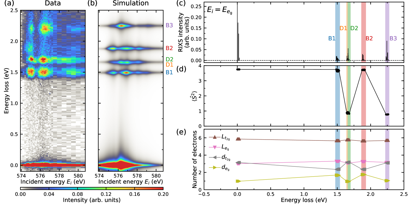
Figure 4: Electronic character of the dark excitons. (a) RIXS intensity map as a function of incident photon energy through the Cr $L_{3}$ resonance. This is the same data presented in Fig. 1 with an energy window chosen to highlight the low-energy excitations. (b) RIXS calculations that reproduce the energy and resonant profile of the five lowest energy excitons in the material. (c) Calculated RIXS stick diagram at the main resonant energy $E_{e_{\mathrm{g}}}$ . (d),(e) Analysis of the ground and excited states for the calculated RIXS spectrum. (d) Expectation value of the total spin operator squared $\langle\hat{S}^{2}\rangle$ . (e) Electron occupations of Cr $3d$ (denoted by $d$ ) and ligand (denoted by $L$ ) orbitals.
V Temperature dependence
Next, we measured the temperature dependence of RIXS spectra at $E_{i}=E_{t_{\mathrm{2g}}}$ through the FM transition temperature $T_{\mathrm{c}}=61$ K up to room temperature. Figure 3 plots data and fits at two momenta. All excitons show an overall trend toward larger widths at higher temperatures. Such behavior is similar to RIXS measurements of excitons in other related materials such as \ce NiPS3 [13] and nickel dihalides [24, 17]. D2 (and to a lesser extent B3) shows a clear anomaly around the FM transition temperature $T_{\mathrm{c}}$ . The trends are even opposite through $T_{\mathrm{c}}$ at the two selected momenta, demonstrating an unusual momentum-dependent coupling between magnetism and dark exciton states. Other bright excitons, such as B1, also exhibit anomalies across $T_{\mathrm{c}}$ at certain momenta and incident energies (See Supplemental Fig. S3). The momentum dependence of these anomalies indicates underlying physics that cannot be fully captured by established cluster-based methods commonly used to interpret RIXS. We also note that B1 (and to a lesser extent D2) softens steadily upon warming, particular above $T_{\mathrm{c}}$ , which is reminiscence of the exciton behavior in \ce NiPS3 and \ce NiI2 [13, 24]. Such interesting behavior might be related to the electron-phonon interactions, which was used to explain the electronic gap shift observed in optics [34].
VI Electronic character of excitons
An advantage of RIXS compared to optics is that it couples directly to dipole-forbidden transitions in a well-known way, allowing us to extract the electronic character of the excitons. Indeed, ambiguities in the optical cross section for these excitons has led to different suggestions for the types of excitations present in chromium trihalides in 1.50–1.85 eV window including features coming from trigonal crystal fields to vibronic structures [21, 22]. To interpret the present spectra, we built an Anderson impurity model (AIM) for \ce CrI3 and computed the RIXS spectrum using ED methods [35]. The model includes Coulomb repulsion, Hund’s coupling, crystal field, and hopping terms derived from the Wannierization of our \ce CrI3 density functional theory (DFT) calculations as detailed in Appendix A. The spectra, shown in Fig. 4 (a) and (b), capture the exciton energies including the double-peak structure of the two dark excitons and the overall trends in the resonances.
To identify the excitons, we report the final state expectation values of the spin-squared $\langle\hat{S}^{2}\rangle$ and electron population operators in Fig. 4 (c)-(e). We note that it is vital to have a small charge-transfer energy (in fact, the best fit is achieved using $\Delta=-1.3$ eV with an error bar of $\sim 1$ eV) to obtain the correct energies for the entire spectrum. Such a small (or even slightly negative) charge transfer energy leads to approximately four electrons in the $d$ states and approximately one hole occupying the ligand $e_{g}$ orbitals not only in the ground states but also in the low energy excitations, as shown in Fig. 4 (e), and in accordance with previous DFT -based results [32, 36, 37, 38]. The importance of charge-transfer is further underlined by the fact that a single-site atomic model cannot adequately fit the spectrum (see Supplemental Material Sec. 5A [28]). As such, the excitations observed here have substantial I character and are not strictly $dd$ -excitations. The non-dispersive modes observed here are well-described by the broader concept of ligand-field excitons [39]. However, since these are by definition local, the dispersive D1 and D2 are, in our opinion, best termed as excitons, although all these terms share some similarities See the supplemental Material Section S6 for more discussion of this issue..
The ground state features half-filled $t_{\mathrm{2g}}$ orbitals, with $\langle\hat{S}^{2}\rangle≈ 3.75$ , corresponding to a high-spin configuration with $S=3/2$ . The D1 and D2 dark excitons involve only a small change in electron population, with the largest component of charge motion being about 0.1 electrons moving from the ligand $L_{t_{2g}}$ to the $L_{e_{g}}$ states, the change from $d$ to $L$ states is even smaller at 0.03 electrons. More notable, this transition involves a low-spin configuration final state close to $S=1/2$ . Consequently, the energy scale of these dark excitons is determined mainly by the Hund’s coupling for Cr $3d$ orbitals, consistent with their spin-flip character. Although D1 and D2 have dominant $t_{2g}$ character, they feature non-zero mixing with the $e_{g}$ manifold [see Fig. 4 (e)]. This mixing endows D1 and D2 with a distinct orbital angular momentum, leading to their small energetic splitting and their distinct resonant profile at the $t_{2g}$ and $e_{g}$ conditions. The nearby bright excitons B1 and B2 are both crystal field transitions, conserving spin and moving an electron from the $t_{2g}$ to the $e_{g}$ states. Their energies are determined primarily by a combination of crystal field $10D_{q}$ and charge-transfer energy $\Delta$ (see Appendix A for the definitions of these quantities).
The higher-energy B3 exciton is again a spin-flip transition but with different symmetry that also redistributes a small amount of weight from the $t_{2g}$ to $e_{g}$ states. Its intensity exhibits a temperature dependence similar to that of the dark exciton D2 (although the change is less dramatic) in Fig. 3 (e) and (f), possibly implying their similar spin-flip character. B3 is particularly broad, suggesting that this mode may be coupling to other excitations. Such a coupling could play a role in the finite optical cross-section for this mode, which is larger than expected since it is a spin-flip transition. It is also possible that extended lattice models could be required to understand the detailed nature of the B2 and B3 excitons and their optical-cross section more fully, as suggested by many-body perturbation-theory plus Bethe-Salpeter equation calculations [32, 41].
VII Discussion and conclusions
The results here provide the first example of dispersive excitons in a FM vdW material, extending the recent identification of this phenomenon in antiferromagnetic vdW materials such as \ce NiPS3 [15] and nickel dihalides [17]. These dispersive excitons are all sharp spin-flip excitations bound by Hund’s exchange interactions. The sharpness of the exciton (i.e., its long lifetime) may be related to its spin-flip nature because such transitions do not involve charge redistribution and therefore have minimal couplings to phonons and reduced efficiency of radiative recombination [20]. Prior works have made similar arguments for \ce NiPS3 and \ce NiI2, where the spin-flip character of excitons is regarded as the major aspect of their physics [13, 15, 42]. The small electron transfer involved in the transition has been suggested to play a minor role, even though the magnitude of electron transfer in \ce NiPS3 is of order 0.2 electron and about seven times larger than the charge transfer observed here [15].
All these excitons also have appreciable ligand-hole involvement due to the small charge-transfer energy, which may facilitate the exciton propagation in the magnetic background [17]. However, there are also key distinctions between \ce CrI3 excitons and their counterparts in antiferromagnets. One clear difference is the exciton bandwidth. Phenomenologically, unlike the case in \ce NiPS3 or nickel dihalides where the exciton bandwidth is significantly smaller than the magnon bandwidth [15, 17], both dark excitons in \ce CrI3 have bandwidths comparable to the magnon bands [33]. In addition, these excitons exhibit a peculiar temperature dependence clearly correlated with $T_{\mathrm{c}}$ . Since \ce CrI3 exhibits layer-dependent magnetism [19], it would be of high interest to examine the exciton behaviors in the few-layer limit of \ce CrI3 in the near future. We also note that the energies of the \ce CrI3 dark excitons are higher than the electronic band gap, which was reported to be $1.1$ – $1.3$ eV [34] in \ce CrI3. This above-band-gap character may explain relatively large linewidth and their darkness in optics due to the strong sloping background coming from interband transitions. As a comparison, the previously discovered spin-flip excitons in \ce NiPS3 involve below-band-gap transitions [43, 13, 15].
In conclusion, we report two dark excitons in \ce CrI3 directly measured with high resolution RIXS. Our results showcase RIXS as a powerful tool in studying these dark states with a readily interpretable cross section and large momentum space coverage, complementary to optical measurements. The excitons feature strong coupling with the magnetism—they disperse with bandwidths similar to magnons and display unusual temperature dependence across the magnetic transition temperature. Our results will guide future optical experiments to detect and manipulate these dark excitons in \ce CrI3. In the past, various methods have been employed to brighten dark excitons in optical measurements, such as the application of an in-plane magnetic field [3], near-field coupling to surface plasmon polaritons [44], or by nano-optical tip-enhanced approaches [45]. With the better-targeted energies provided by our study, there is a high likelihood of probing these dark excitons in \ce CrI3 using these advanced optical techniques. Indeed, the possibility of accessing D1 and/or D2 optically is supported by a subset of the prior optical studies, which identified shoulder features in the spectra indicative of modes in the 1.7 eV range [20]. Moreover, our ED calculations will also inform future theory in more accurately describing the electronic properties of \ce CrI3. We believe that our discovery of dark excitons in \ce CrI3 is just the tip of the iceberg, and the utilization of RIXS will expedite the expansion of this family of materials and foster both the understanding of the fundamental physics and the potential applications of dark excitons in devices.
The supporting data for the plots in this article are openly available from the Zenodo database [46].
Acknowledgements. Work performed at Brookhaven National Laboratory and Harvard University was supported by the U.S. Department of Energy (DOE), Division of Materials Science, under Contract No. DE-SC0012704. Work performed at the University of Texas at Austin was supported by the United States Army Research Office (W911NF-23-1-0394) (F.B.) and the National Science Foundation under the NSF CAREER award 2441874 (E.B.). F.B. acknowledges additional support from the Swiss NSF under fellowship P500PT $\_$ 214437. S. J. was supported by the U.S. Department of Energy, Office of Science, Office of Basic Energy Sciences, under Award Number DE-SC0022311. Part of this research (T.B.) was conducted at the Center for Nanophase Materials Sciences, which is a DOE Office of Science User Facility. The work by J.W.V. is supported by the Quantum Science Center (QSC), a National Quantum Information Science Research Center of DOE. Crystal growth at ORNL as supported by the U.S. DOE, Office of Science, Basic Energy Sciences, Material Science and Engineering Division. This research used beamline 2-ID of the National Synchrotron Light Source II, a U.S. DOE Office of Science User Facility operated for the DOE Office of Science by Brookhaven National Laboratory under Contract No. DE-SC0012704. We also acknowledge glovebox resources made available through BNL/LDRD #19-013.
Appendix A ED RIXS calculations
The RIXS spectra in this work were simulated based on standard ED methods implemented in the open source software EDRIXS [35]. The RIXS cross section was calculated using the Kramers-Heisenberg formula with the polarization-dependent dipole approximation. The model we employ here is an AIM, which was constructed using the bonding ligand orbitals of a \ce CrI6 cluster model. Here, we provide details on the parameters that we used and the methods that we employed to determine them.
In an AIM, we can represent a cluster with fewer orbitals by using symmetry-adapted linear combinations of ligand orbitals [47], making the calculation numerically much more efficient with essentially no loss of accuracy. In our case, we have 10 Cr $3d$ spin-orbitals and 10 ligand spin-orbitals with the same symmetry, so there are 13 electrons in total occupying 20 spin-resolved orbitals in the initial and final states. In the intermediate states, the Cr $2p$ orbitals are included to simulate the core hole created in the RIXS process. The calculations were performed in the full basis using the Fortran ED solver provided in EDRIXS [35]. For the RIXS cross section calculations, we have the experimental geometry explicitly considered, i.e., the scattering angle $2\Theta$ is fixed to $150^{\circ}$ and the sample angle $\theta$ is kept at $14.5^{\circ}$ . An inverse core-hole lifetime $\Gamma_{c}=0.3$ eV HWHM was used to fit the observed width of the resonance and the final state energy loss spectra are broadened using a Lorentzian function with a FWHM of $0.03$ eV, in order to match the observed minimum width of the dark excitons.
The Hamiltonian of the model includes the Coulomb interactions, on-site energy for each orbital, hoppings between different orbitals, spin-orbit coupling, and the Zeeman interaction.
We parameterize the Coulomb interactions via Slater integrals, which include $F^{0}_{dd}$ , $F^{2}_{dd}$ , and $F^{4}_{dd}$ for the Cr $3d$ orbitals, and $F^{0}_{dp}$ , $F^{2}_{dp}$ , $G^{1}_{dp}$ , and $G^{3}_{dp}$ for the interactions between Cr $3d$ and $2p$ core orbitals in the intermediate states. $F^{0}_{dd}$ and $F^{0}_{dp}$ are related to the Cr $3d$ onsite Coulomb repulsion $U_{dd}$ and core-hole potential $U_{dp}$ , respectively, which are discussed later. The rest of the parameters are obtained by starting from their Hartree-Fock atomic values and scaling them down to account for the screening effect in the solids. For simplicity, we used two overall scaling factors, one for Cr $3d$ orbitals ( $k_{dd}$ ) and the other for the core-hole interactions ( $k_{dp}$ ).
Hopping integrals describe hybridization between different orbitals. This can be expressed using a $10× 10$ matrix $H_{\text{hopping}}$ . We determined the off-diagonal inter-orbital hopping parameters from first-principles by calculating the electronic structure with the VASP DFT code [48, 49]. In this case, we used the Perdew-Burke-Ernzerhof (PBE) generalized gradient approximation [50] for the exchange-correlation functional without spin-orbit coupling. We employed projector augmented wave pseudopotentials [51, 52], considering Cr $3p$ electrons as valence (Cr_pv). The energy cutoff was set to 350 eV and we used a $15× 15× 15$ Monkhorst-Pack $k$ -point mesh. We used an AMIX of $0.05$ and a SIGMA smearing parameter of $0.05$ eV. Finally, a tight-binding model is constructed using Wannier90 [53, 54, 55]. We performed a Wannier projection of Cr $3d$ and I $5p$ orbitals without maximal localization. Disentanglement was omitted since these states form a well-isolated band set within the chosen energy window. The band structure from DFT calculations and the Wannier projected bands are shown in Fig. S12. The ligand orbitals were constructed from the appropriate linear combinations of the Wannier orbitals [46]. The hopping terms we obtained from this method are listed below (in units of eV).
$$
H_{\text{hopping}}=\pNiceMatrix[first-row,first-col]&d_{3z^{2}-r^{2}}d_{xz}d_{%
yz}d_{x^{2}-y^{2}}d_{xy}L_{3z^{2}-r^{2}}L_{xz}L_{yz}L_{x^{2}-y^{2}}L_{xy}\\
d_{3z^{2}-r^{2}}-9.6340.0020.0010-0.003-2.008-0.011-0.019-0.0010.03\\
d_{xz}0.002-10.2440.0030.0030.003-0.001-1.272-0.0010.007-0.002\\
d_{yz}0.0010.003-10.244-0.0030.0030.006-0.002-1.272-0.002-0.001\\
d_{x^{2}-y^{2}}0.00.003-0.003-9.63400.001-0.0280.024-2.0080.004\\
d_{xy}-0.0030.0030.0030-10.2440.005-0.001-0.002-0.004-1.272\\
L_{3z^{2}-r^{2}}-2.008-0.0010.0060.001-0.0052.6890.010.0150.0-0.026\\
L_{xz}-0.011-1.272-0.002-0.028-0.0010.011.208-0.0170.024-0.017\\
L_{yz}-0.019-0.001-1.2720.024-0.0020.015-0.0171.208-0.021-0.017\\
L_{x^{2}-y^{2}}-0.0010.007-0.002-2.008-0.0040.00.024-0.0212.689-0.003\\
L_{xy}0.03-0.002-0.0010.004-1.272-0.026-0.017-0.017-0.0031.208\\ \tag{1}
$$
Since hopping depends on how electronic wavefunctions are spread between different atoms, it is only weakly influenced by strongly correlated physics and DFT generally captures the magnitude of hopping quite accurately. For this reason, we consider the off-diagonal inter-orbital hopping values fixed to the quoted DFT -derived values. The on-site energies correspond to the diagonal elements in the hopping matrix $H_{\text{hopping}}$ above. These on-site energies for the Cr $3d$ states are not easily obtainable from first principles because of the effects of strong correlations and the challenges in handling double-counting effects. We therefore consider the Cr $3d$ crystal field as a fitting parameter, which, in view of the approximately cubic symmetry of the Cr coordination, is specified by $10D_{q}$ , which represents the splitting between the $t_{\mathrm{2g}}$ and $e_{\mathrm{g}}$ orbitals.
Since Coulomb interactions in the I $5p$ states are relatively weak and since the probability that these states are occupied by multiple holes is relatively low, the crystal field on the states is more accurately captured by DFT, so to reduce the number of fitting parameters, we fix the ligand orbital crystal field $10D_{q}^{L}$ to the value extracted from our DFT results ( $1.481$ eV). In this work, we define the charge-transfer, $\Delta$ , and Coulomb repulsion, $U_{dd}$ , energies as the energy cost of specific transitions in the material with the Cr-ligand hopping switched off. $U_{dd}$ reflects a $d_{i}^{3}d_{j}^{3}→ d^{2}_{i}d_{j}^{4}$ transition and $\Delta$ is defined as the energy for a $d_{i}^{3}→ d^{4}_{i}\underline{L}$ transition, where $i$ and $j$ label Cr sites and $\underline{L}$ denotes an iodine ligand hole. These energies include the effect of the Cr crystal field and represent the energies for a transition into the lowest-energy ligand orbital (rather than the center of the I $p$ states). From a practical point of view, we perform our calculations varying the energy splitting of the Cr and ligand states and we subsequently determine $\Delta$ by diagonalizing the isolated Cr and ligand configurations and computing the appropriate differences in energy. The values of the diagonal elements in Eq. 1 are the final onsite energies determined for our model.
In the intermediate states with the presence of a core hole, we include a core-hole potential $U_{dp}$ . $U_{dd}$ is usually 4-6 eV in early transition metals and it is usually smaller when the charge transfer energy is small (which we will see is the case here), so we choose 4 eV [56, 57]. $U_{dp}$ is only weakly dependent on solid state effects, so we choose a typical value of 6 eV.
The spin-orbit coupling terms for the Cr $3d$ orbitals ( $\zeta_{\mathrm{i}}$ and $\zeta_{\mathrm{n}}$ for the initial and intermediate states, respectively) are weak and have negligible effects on the spectra. We consequently simply fixed them to their atomic values. Since we only measured RIXS energy map at the $L_{3}$ -edge, we also simply fixed the core-hole spin-orbit coupling parameter $\zeta_{\mathrm{c}}$ to its atomic value.
A small Zeeman interaction term $g\mu_{B}\mathbf{B}·\mathbf{S}$ was applied to the total spin angular momentum of the system, serving as the effective exchange field in the magnetically ordered state. We fixed $\mu_{B}B=0.005$ eV to match the energy scale of the exchange interactions in \ce CrI3 [33].
In summary, we have four free parameters in our model, i.e., $k_{dd}$ , $k_{dp}$ , $10D_{q}$ , and $\Delta$ . Most of these values are constrained by physical considerations. $k_{dd}$ and $k_{dp}$ quantify the screening. These are known to vary within a range of 0.5–0.9 from prior studies and these values will typically also have reasonably similar values since both are affected by similar screening processes [58]. $10D_{q}$ in $3d$ octahedrally coordinated transition metal material ranges from about 0.5–3 eV and since iodine is relatively large size in ionic radius and relativity weakly electronegative, we expect a value in the lower half of this range. $k_{dd}$ , $k_{dp}$ , $10D_{q}$ , and $\Delta$ have distinct effects on the RIXS energy map. $k_{dd}$ directly scales the Hund’s coupling and hence controls the energies of the dark excitons D1 and D2. The energies of the bright excitons B1 and B2 are primarily determined by both $10D_{q}$ and $\Delta$ . $k_{dp}$ mainly affects the resonance profiles of these peaks. Thanks to the richly detailed spectra, the finite physically reasonable range of parameters, and the distinct effects of different parameters, we successfully obtained a well-constrained model with final parameters as $k_{dd}=0.65$ , $k_{dp}=0.5$ , $10D_{q}=0.61$ eV, $\Delta=-1.3$ eV and verified that no other solutions exist. The level of agreement compares favorably with what can be expected for a model of this type accurately capturing the energy of the excitations while roughly capturing trends in peak intensities [13, 24, 15, 17]. The full list of parameters used in the model is shown in Tab. 1. The estimated error bars are $\sim 1$ eV for all the Coulomb interactions and the charge-transfer energy $\Delta$ and $\sim 0.2$ eV for $10D_{q}$ .
Table 1: Full list of parameters used in the AIM calculations. (Except for the hopping integrals, which are provided in Eq. 1.) $F_{dd,\mathrm{i}}$ and $F_{dd,\mathrm{n}}$ are for the initial and intermediate states, respectively. Units are eV.
| 0.61 | 1.481 | -1.3 | 4.0 | 6.0 | 7.005 | 4.391 | 7.537 | 4.726 | 3.263 | 2.394 | 1.361 | 0.035 | 0.047 | 5.667 |
| --- | --- | --- | --- | --- | --- | --- | --- | --- | --- | --- | --- | --- | --- | --- |
References
- Koch et al. [2006] S. Koch, M. Kira, G. Khitrova, and H. Gibbs, Semiconductor excitons in new light, Nature materials 5, 523 (2006).
- Kitzmann et al. [2022] W. R. Kitzmann, J. Moll, and K. Heinze, Spin-flip luminescence, Photochem. Photobiol. Sci. 21, 1309 (2022).
- Zhang et al. [2017] X.-X. Zhang, T. Cao, Z. Lu, Y.-C. Lin, F. Zhang, Y. Wang, Z. Li, J. C. Hone, J. A. Robinson, D. Smirnov, S. G. Louie, and T. F. Heinz, Magnetic brightening and control of dark excitons in monolayer WSe 2, Nat. Nanotechnol. 12, 883 (2017).
- Poem et al. [2010] E. Poem, Y. Kodriano, C. Tradonsky, N. H. Lindner, B. D. Gerardot, P. M. Petroff, and D. Gershoni, Accessing the dark exciton with light, Nat. Phys. 6, 993 (2010).
- Nirmal et al. [1995] M. Nirmal, D. J. Norris, M. Kuno, M. G. Bawendi, A. L. Efros, and M. Rosen, Observation of the “dark exciton” in CdSe quantum dots, Phys. Rev. Lett. 75, 3728 (1995).
- Congreve et al. [2013] D. N. Congreve, J. Lee, N. J. Thompson, E. Hontz, S. R. Yost, P. D. Reusswig, M. E. Bahlke, S. Reineke, T. V. Voorhis, and M. A. Baldo, External quantum efficiency above 100% in a singlet-exciton-fission–based organic photovoltaic cell, Science 340, 334 (2013).
- Wang et al. [2018] G. Wang, A. Chernikov, M. M. Glazov, T. F. Heinz, X. Marie, T. Amand, and B. Urbaszek, Colloquium: Excitons in atomically thin transition metal dichalcogenides, Rev. Mod. Phys. 90, 021001 (2018).
- Burch et al. [2018] K. S. Burch, D. Mandrus, and J. G. Park, Magnetism in two-dimensional van der Waals materials, Nature 563, 47 (2018).
- Gong and Zhang [2019] C. Gong and X. Zhang, Two-dimensional magnetic crystals and emergent heterostructure devices, Science 363, eaav4450 (2019).
- Wang et al. [2022] Q. H. Wang, A. Bedoya-Pinto, M. Blei, A. H. Dismukes, A. Hamo, S. Jenkins, M. Koperski, Y. Liu, Q.-C. Sun, E. J. Telford, H. H. Kim, M. Augustin, U. Vool, J.-X. Yin, L. H. Li, A. Falin, C. R. Dean, F. Casanova, R. F. L. Evans, M. Chshiev, A. Mishchenko, C. Petrovic, R. He, L. Zhao, A. W. Tsen, B. D. Gerardot, M. Brotons-Gisbert, Z. Guguchia, X. Roy, S. Tongay, Z. Wang, M. Z. Hasan, J. Wrachtrup, A. Yacoby, A. Fert, S. Parkin, K. S. Novoselov, P. Dai, L. Balicas, and E. J. G. Santos, The magnetic genome of two-dimensional van der Waals materials, ACS Nano 16, 6960 (2022).
- Ahn et al. [2024] Y. Ahn, X. Guo, S. Son, Z. Sun, and L. Zhao, Progress and prospects in two-dimensional magnetism of van der Waals materials, Prog. Quant. Electron. 93, 100498 (2024).
- Mak et al. [2019] K. F. Mak, J. Shan, and D. C. Ralph, Probing and controlling magnetic states in 2D layered magnetic materials, Nature Reviews Physics 1, 646 (2019).
- Kang et al. [2020] S. Kang, K. Kim, B. H. Kim, J. Kim, K. I. Sim, J. U. Lee, S. Lee, K. Park, S. Yun, T. Kim, A. Nag, A. Walters, M. Garcia-Fernandez, J. Li, L. Chapon, K. J. Zhou, Y. W. Son, J. H. Kim, H. Cheong, and J. G. Park, Coherent many-body exciton in van der Waals antiferromagnet NiPS 3, Nature 583, 785 (2020).
- Bae et al. [2022] Y. J. Bae, J. Wang, A. Scheie, J. Xu, D. G. Chica, G. M. Diederich, J. Cenker, M. E. Ziebel, Y. Bai, H. Ren, C. R. Dean, M. Delor, X. Xu, X. Roy, A. D. Kent, and X. Zhu, Exciton-coupled coherent magnons in a 2D semiconductor, Nature 609, 282 (2022).
- He et al. [2024a] W. He, Y. Shen, K. Wohlfeld, J. Sears, J. Li, J. Pelliciari, M. Walicki, S. Johnston, E. Baldini, V. Bisogni, M. Mitrano, and M. P. M. Dean, Magnetically propagating Hund’s exciton in van der Waals antiferromagnet NiPS 3, Nat. Commun. 15, 3496 (2024a).
- DiScala et al. [2024] M. F. DiScala, D. Staros, A. de la Torre, A. Lopez, D. Wong, C. Schulz, M. Barkowiak, V. Bisogni, J. Pelliciari, B. Rubenstein, and K. W. Plumb, Elucidating the role of dimensionality on the electronic structure of the van der waals antiferromagnet NiPS 3, Adv. Phys. Res. 3, 2300096 (2024).
- Occhialini et al. [2024] C. A. Occhialini, Y. Tseng, H. Elnaggar, Q. Song, M. Blei, S. A. Tongay, V. Bisogni, F. M. F. de Groot, J. Pelliciari, and R. Comin, Nature of excitons and their ligand-mediated delocalization in nickel dihalide charge-transfer insulators, Phys. Rev. X 14, 031007 (2024).
- Wilson et al. [2021] N. P. Wilson, W. Yao, J. Shan, and X. Xu, Excitons and emergent quantum phenomena in stacked 2D semiconductors, Nature 599, 383 (2021).
- Huang et al. [2017] B. Huang, G. Clark, E. Navarro-Moratalla, D. R. Klein, R. Cheng, K. L. Seyler, D. Zhong, E. Schmidgall, M. A. McGuire, D. H. Cobden, W. Yao, D. Xiao, P. Jarillo-Herrero, and X. Xu, Layer-dependent ferromagnetism in a van der Waals crystal down to the monolayer limit, Nature 546, 270 (2017).
- Jin et al. [2020] W. Jin, H. H. Kim, Z. Ye, G. Ye, L. Rojas, X. Luo, B. Yang, F. Yin, J. S. A. Horng, S. Tian, Y. Fu, G. Xu, H. Deng, H. Lei, A. W. Tsen, K. Sun, R. He, and L. Zhao, Observation of the polaronic character of excitons in a two-dimensional semiconducting magnet CrI 3, Nat. Commun. 11, 4780 (2020).
- Pollini and Spinolo [1970] I. Pollini and G. Spinolo, Intrinsic optical properties of CrCl 3, physica status solidi (b) 41, 691 (1970).
- Bermudez and McClure [1979] V. M. Bermudez and D. S. McClure, Spectroscopic studies of the two-dimensional magnetic insulators chromium trichloride and chromium tribromide—I, Journal of Physics and Chemistry of Solids 40, 129 (1979).
- Seyler et al. [2018] K. L. Seyler, D. Zhong, D. R. Klein, S. Gao, X. Zhang, B. Huang, E. Navarro-Moratalla, L. Yang, D. H. Cobden, M. A. McGuire, W. Yao, D. Xiao, P. Jarillo-Herrero, and X. Xu, Ligand-field helical luminescence in a 2D ferromagnetic insulator, Nat. Phys. 14, 277 (2018).
- Son et al. [2022] S. Son, Y. Lee, J. H. Kim, B. H. Kim, C. Kim, W. Na, H. Ju, S. Park, A. Nag, K.-J. Zhou, Y.-W. Son, H. Kim, W.-S. Noh, J.-H. Park, J. S. Lee, H. Cheong, J. H. Kim, and J.-G. Park, Multiferroic-enabled magnetic-excitons in 2d quantum-entangled van der waals antiferromagnet nii2, Advanced Materials 34, 2109144 (2022).
- Mitrano et al. [2024] M. Mitrano, S. Johnston, Y.-J. Kim, and M. P. M. Dean, Exploring quantum materials with resonant inelastic x-ray scattering, Phys. Rev. X 14, 040501 (2024).
- McGuire et al. [2015] M. A. McGuire, H. Dixit, V. R. Cooper, and B. C. Sales, Coupling of Crystal Structure and Magnetism in the Layered, Ferromagnetic Insulator CrI 3, Chem. Mater. 27, 612 (2015).
- Miao et al. [2017] H. Miao, J. Lorenzana, G. Seibold, Y. Y. Peng, A. Amorese, F. Yakhou-Harris, K. Kummer, N. B. Brookes, R. M. Konik, V. Thampy, G. D. Gu, G. Ghiringhelli, L. Braicovich, and M. P. M. Dean, High-temperature charge density wave correlations in La 1.875 Ba 0.125 CuO 4 without spin–charge locking, Proc. Natl. Acad. Sci. U.S.A. 114, 12430 (2017).
- [28] See Supplemental Material at [URL will be inserted by publisher] for further details of the calculations and fittings.
- Ament et al. [2011] L. J. Ament, M. Van Veenendaal, T. P. Devereaux, J. P. Hill, and J. Van Den Brink, Resonant inelastic x-ray scattering studies of elementary excitations, Rev. Mod. Phys. 83, 705 (2011).
- Ghosh et al. [2023] A. Ghosh, H. J. M. Jönsson, D. J. Mukkattukavil, Y. Kvashnin, D. Phuyal, P. Thunström, M. Agåker, A. Nicolaou, M. Jonak, R. Klingeler, M. V. Kamalakar, T. Sarkar, A. N. Vasiliev, S. M. Butorin, O. Eriksson, and M. Abdel-Hafiez, Magnetic circular dichroism in the $dd$ excitation in the van der Waals magnet CrI 3 probed by resonant inelastic x-ray scattering, Phys. Rev. B 107, 115148 (2023).
- Shao et al. [2021] Y. C. Shao, B. Karki, W. Huang, X. Feng, G. Sumanasekera, J.-H. Guo, Y.-D. Chuang, and B. Freelon, Spectroscopic Determination of Key Energy Scales for the Base Hamiltonian of Chromium Trihalides, J. Phys. Chem. Lett. 12, 724 (2021).
- Wu et al. [2019] M. Wu, Z. Li, T. Cao, and S. G. Louie, Physical origin of giant excitonic and magneto-optical responses in two-dimensional ferromagnetic insulators, Nat. Commun. 10, 2371 (2019).
- Chen et al. [2018] L. Chen, J.-H. Chung, B. Gao, T. Chen, M. B. Stone, A. I. Kolesnikov, Q. Huang, and P. Dai, Topological Spin Excitations in Honeycomb Ferromagnet CrI 3, Phys. Rev. X 8, 041028 (2018).
- Tomarchio et al. [2021] L. Tomarchio, S. Macis, L. Mosesso, L. T. Nguyen, A. Grilli, M. C. Guidi, R. J. Cava, and S. Lupi, Low energy electrodynamics of CrI 3 layered ferromagnet, Sci Rep 11, 23405 (2021).
- Wang et al. [2019] Y. L. Wang, G. Fabbris, M. P. Dean, and G. Kotliar, EDRIXS: An open source toolkit for simulating spectra of resonant inelastic x-ray scattering, Comput. Phys. Commun. 243, 151 (2019).
- Kashin et al. [2020] I. V. Kashin, V. V. Mazurenko, M. I. Katsnelson, and A. N. Rudenko, Orbitally-resolved ferromagnetism of monolayer CrI 3, 2D Mater. 7, 025036 (2020).
- Acharya et al. [2021] S. Acharya, D. Pashov, B. Cunningham, A. N. Rudenko, M. Rösner, M. Grüning, M. Van Schilfgaarde, and M. I. Katsnelson, Electronic structure of chromium trihalides beyond density functional theory, Phys. Rev. B 104, 155109 (2021).
- Kvashnin et al. [2022] Y. O. Kvashnin, A. N. Rudenko, P. Thunström, M. Rösner, and M. I. Katsnelson, Dynamical correlations in single-layer CrI 3, Phys. Rev. B 105, 205124 (2022).
- Ballhausen [1962] C. J. Ballhausen, Introduction to ligand field theory (McGraw Hill Book Company, 1962).
- Note [1] See the supplemental Material Section S6 for more discussion of this issue.
- Acharya et al. [2022] S. Acharya, D. Pashov, A. N. Rudenko, M. Rösner, M. v. Schilfgaarde, and M. I. Katsnelson, Real- and momentum-space description of the excitons in bulk and monolayer chromium tri-halides, npj 2D Mater. Appl. 6, 1 (2022).
- Hamad et al. [2024] I. J. Hamad, C. S. Helman, L. O. Manuel, A. E. Feiguin, and A. A. Aligia, Singlet polaron theory of low-energy optical excitations in ${\mathrm{nips}}_{3}$ , Phys. Rev. Lett. 133, 146502 (2024).
- Kim et al. [2018] S. Y. Kim, T. Y. Kim, L. J. Sandilands, S. Sinn, M. C. Lee, J. Son, S. Lee, K. Y. Choi, W. Kim, B. G. Park, C. Jeon, H. D. Kim, C. H. Park, J. G. Park, S. J. Moon, and T. W. Noh, Charge-Spin Correlation in van der Waals Antiferromagnet NiPS 3, Physical Review Letters 120, 136402 (2018).
- Zhou et al. [2017] Y. Zhou, G. Scuri, D. S. Wild, A. A. High, A. Dibos, L. A. Jauregui, C. Shu, K. De Greve, K. Pistunova, A. Y. Joe, T. Taniguchi, K. Watanabe, P. Kim, M. D. Lukin, and H. Park, Probing dark excitons in atomically thin semiconductors via near-field coupling to surface plasmon polaritons, Nat. Nanotechnol. 12, 856 (2017).
- Park et al. [2018] K.-D. Park, T. Jiang, G. Clark, X. Xu, and M. B. Raschke, Radiative control of dark excitons at room temperature by nano-optical antenna-tip Purcell effect, Nat. Nanotechnol. 13, 59 (2018).
- He et al. [2024b] W. He, J. Sears, F. Barantani, T. Kim, J. W. Villanova, T. Berlijn, M. Lajer, M. A. McGuire, J. Pelliciari, V. Bisogni, S. Johnston, E. Baldini, M. Mitrano, and M. P. M. Dean, Respository for: Dispersive dark excitons in van der Waals ferromagnet CrI 3 (2024b), to be assigned.
- Haverkort et al. [2012] M. W. Haverkort, M. Zwierzycki, and O. K. Andersen, Multiplet ligand-field theory using Wannier orbitals, Physical Review B 85, 165113 (2012).
- Kresse and Furthmüller [1996] G. Kresse and J. Furthmüller, Efficient iterative schemes for ab initio total-energy calculations using a plane-wave basis set, Phys. Rev. B 54, 11169 (1996).
- Kresse and Furthmüller [1996] G. Kresse and J. Furthmüller, Efficiency of ab-initio total energy calculations for metals and semiconductors using a plane-wave basis set, Computational Materials Science 6, 15 (1996).
- Perdew et al. [1996] J. P. Perdew, K. Burke, and M. Ernzerhof, Generalized gradient approximation made simple, Phys. Rev. Lett. 77, 3865 (1996).
- Blöchl [1994] P. E. Blöchl, Projector augmented-wave method, Phys. Rev. B 50, 17953 (1994).
- Kresse and Joubert [1999] G. Kresse and D. Joubert, From ultrasoft pseudopotentials to the projector augmented-wave method, Phys. Rev. B 59, 1758 (1999).
- Mostofi et al. [2014] A. A. Mostofi, J. R. Yates, G. Pizzi, Y.-S. Lee, I. Souza, D. Vanderbilt, and N. Marzari, An updated version of Wannier90: A tool for obtaining maximally-localised Wannier functions, Computer Physics Communications 185, 2309 (2014).
- Marzari and Vanderbilt [1997] N. Marzari and D. Vanderbilt, Maximally localized generalized Wannier functions for composite energy bands, Phys. Rev. B 56, 12847 (1997).
- Souza et al. [2001] I. Souza, N. Marzari, and D. Vanderbilt, Maximally localized Wannier functions for entangled energy bands, Phys. Rev. B 65, 035109 (2001).
- Bocquet et al. [1992] A. Bocquet, T. Saitoh, T. Mizokawa, and A. Fujimori, Systematics in the electronic structure of 3d transition-metal compounds, Solid State Communications 83, 11 (1992).
- Feldkemper and Weber [1998] S. Feldkemper and W. Weber, Generalized calculation of magnetic coupling constants for Mott-Hubbard insulators: Application to ferromagnetic Cr compounds, Phys. Rev. B 57, 7755 (1998).
- De Groot and Kotani [2008] F. De Groot and A. Kotani, Core level spectroscopy of solids (CRC press, 2008).