2501.12599v4

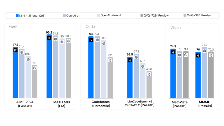
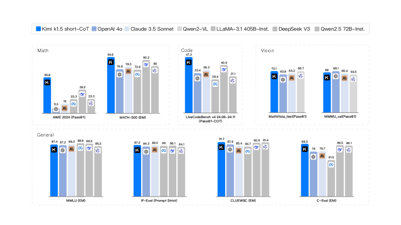
# Kimi k1.5: Scaling Reinforcement Learning with LLMs **Authors**: Kimi Team ## Abstract Language model pretraining with next token prediction has proved effective for scaling compute but is limited to the amount of available training data. Scaling reinforcement learning (RL) unlocks a new axis for the continued improvement of artificial intelligence, with the promise that large language models (LLMs) can scale their training data by learning to explore with rewards. However, prior published work has not produced competitive results. In light of this, we report on the training practice of Kimi k1.5, our latest multi-modal LLM trained with RL, including its RL training techniques, multi-modal data recipes, and infrastructure optimization. Long context scaling and improved policy optimization methods are key ingredients of our approach, which establishes a simplistic, effective RL framework without relying on more complex techniques such as Monte Carlo tree search, value functions, and process reward models. Notably, our system achieves state-of-the-art reasoning performance across multiple benchmarks and modalities—e.g., 77.5 on AIME, 96.2 on MATH 500, 94-th percentile on Codeforces, 74.9 on MathVista—matching OpenAI’s o1. Moreover, we present effective long2short methods that use long-CoT techniques to improve short-CoT models, yielding state-of-the-art short-CoT reasoning results—e.g., 60.8 on AIME, 94.6 on MATH500, 47.3 on LiveCodeBench—outperforming existing short-CoT models such as GPT-4o and Claude Sonnet 3.5 by a large margin (up to +550%). <details> <summary>x1.png Details</summary>  ### Visual Description \n ## Grouped Bar Chart: AI Model Performance Comparison ### Overview The image displays a grouped bar chart comparing the performance of five different AI models across six distinct benchmarks. The benchmarks are categorized into three domains: Math, Code, and Vision. The chart uses a consistent color scheme to represent each model, with numerical performance scores displayed atop each bar. ### Components/Axes * **Legend (Top Center):** A horizontal legend identifies the five models by color: * **Dark Blue:** Kimi k1.5 long-CoT * **Light Blue:** OpenAI o1 * **Very Light Blue:** OpenAI o1-mini * **Medium Gray:** QVQ-72B-Preview * **Light Gray:** QwQ-32B-Preview * **Chart Structure:** The chart is divided into three vertical panels, each representing a domain: 1. **Left Panel - Math:** Contains two benchmark groups. 2. **Center Panel - Code:** Contains two benchmark groups. 3. **Right Panel - Vision:** Contains two benchmark groups. * **X-Axis (Bottom):** Lists the six specific benchmarks, grouped by domain: * **Math:** `AIME 2024 (Pass@1)` and `MATH 500 (EM)` * **Code:** `Codeforces (Percentile)` and `LiveCodeBench v5 24.12-25.2 (Pass@1)` * **Vision:** `MathVista (Pass@1)` and `MMMU (Pass@1)` * **Y-Axis:** Not explicitly labeled with a scale or title. Performance is indicated by the height of the bars and the numerical labels on top of them. The metric varies by benchmark (e.g., Pass@1, EM, Percentile). ### Detailed Analysis Performance scores for each model on each benchmark are as follows: **1. Math Domain** * **AIME 2024 (Pass@1):** * Kimi k1.5 long-CoT: 77.5 * OpenAI o1: 74.4 * OpenAI o1-mini: 63.6 * QVQ-72B-Preview: 50 * QwQ-32B-Preview: (Bar present but no numerical label visible) * **MATH 500 (EM):** * Kimi k1.5 long-CoT: 98.2 * OpenAI o1: 94.8 * OpenAI o1-mini: 90 * QVQ-72B-Preview: 90.6 * QwQ-32B-Preview: (Bar present but no numerical label visible) **2. Code Domain** * **Codeforces (Percentile):** * Kimi k1.5 long-CoT: 94 * OpenAI o1: 94 * OpenAI o1-mini: 88 * QVQ-72B-Preview: 62 * QwQ-32B-Preview: (Bar present but no numerical label visible) * **LiveCodeBench v5 24.12-25.2 (Pass@1):** * Kimi k1.5 long-CoT: 62.5 * OpenAI o1: 67.2 * OpenAI o1-mini: 53.1 * QVQ-72B-Preview: 40.6 * QwQ-32B-Preview: (Bar present but no numerical label visible) **3. Vision Domain** * **MathVista (Pass@1):** * Kimi k1.5 long-CoT: 74.9 * OpenAI o1: 71 * OpenAI o1-mini: 71.4 * QVQ-72B-Preview: (Bar present but no numerical label visible) * QwQ-32B-Preview: (Bar present but no numerical label visible) * **MMMU (Pass@1):** * Kimi k1.5 long-CoT: 70 * OpenAI o1: 77.3 * OpenAI o1-mini: 70.3 * QVQ-72B-Preview: (Bar present but no numerical label visible) * QwQ-32B-Preview: (Bar present but no numerical label visible) **Note on Missing Labels:** Several bars, primarily for the `QwQ-32B-Preview` model (light gray) and some for `QVQ-72B-Preview` (medium gray), do not have numerical scores displayed on top. Their relative heights can be inferred visually. ### Key Observations 1. **Model Leadership:** The `Kimi k1.5 long-CoT` (dark blue) model is the top performer or tied for top in 4 out of the 6 benchmarks (AIME 2024, MATH 500, Codeforces, MathVista). 2. **Strong Contender:** The `OpenAI o1` (light blue) model is highly competitive, leading in `LiveCodeBench v5` and `MMMU`, and tying for first in `Codeforces`. 3. **Domain Strengths:** * **Math:** `Kimi k1.5 long-CoT` shows a clear lead on the AIME benchmark but is closely matched by others on MATH 500. * **Code:** `Kimi k1.5 long-CoT` and `OpenAI o1` are virtually identical on the Codeforces percentile metric, but `OpenAI o1` has a noticeable lead on the LiveCodeBench pass@1 metric. * **Vision:** Performance is more tightly clustered. `OpenAI o1` leads on MMMU, while `Kimi k1.5 long-CoT` leads on MathVista. 4. **Performance Drop-off:** The `OpenAI o1-mini` (very light blue) and the two "Preview" models (gray bars) generally score lower than the top two models across most benchmarks, with the `QwQ-32B-Preview` appearing to be the lowest-performing model where its bar height is visible. ### Interpretation This chart provides a comparative snapshot of frontier AI model capabilities as of the data's collection date (likely early 2025, given the benchmark names). The data suggests a competitive landscape where no single model dominates all categories. * **Specialization vs. Generalization:** `Kimi k1.5 long-CoT` demonstrates exceptional strength in mathematical reasoning and certain coding tasks, while `OpenAI o1` shows superior performance in other coding benchmarks and complex visual question answering (MMMU). This indicates potential specialization in model training or architecture. * **Benchmark Sensitivity:** The varying rankings across benchmarks (e.g., the flip between Kimi and OpenAI o1 on the two Code benchmarks) highlight that model evaluation is highly sensitive to the specific task and metric used. A model's "capability" is not a single number but a profile across diverse challenges. * **The "Preview" Gap:** The significant performance gap between the established models (Kimi, OpenAI o1) and the "Preview" models (QVQ, QwQ) suggests these are either less mature, smaller, or differently optimized models, possibly representing a different tier of capability or a work in progress. * **Implication for Users:** The choice of model would depend heavily on the primary use case. For math-heavy applications, Kimi k1.5 long-CoT appears strongest. For a mix of coding and visual reasoning, OpenAI o1 is a very strong contender. The chart argues against a one-size-fits-all approach to model selection. </details> Figure 1: Kimi k1.5 long-CoT results. <details> <summary>x2.png Details</summary>  ### Visual Description ## Bar Chart Comparison: AI Model Performance Across Multiple Benchmarks ### Overview The image is a composite bar chart comparing the performance of seven different large language models (LLMs) across eight distinct evaluation benchmarks. The benchmarks are grouped into four categories: Math, Code, Vision, and General. The chart uses a consistent color-coding scheme for each model, as defined in the legend at the top. ### Components/Axes * **Legend (Top Center):** A horizontal legend identifies seven models with associated color codes: * **Kimi k1.5 short-CoT:** Dark Blue * **OpenAI 4o:** Light Blue * **Claude 3.5 Sonnet:** Light Gray * **Qwen2-VL:** Medium Gray * **LLaMA-3.1 405B-Inst.:** Dark Gray * **DeepSeek V3:** Very Light Gray * **Qwen2.5 72B-Inst.:** Lightest Gray/White * **Chart Structure:** The image is divided into four main rectangular panels, each containing one or two bar charts. * **Top Left Panel (Math):** Contains two bar charts. * **Top Center Panel (Code):** Contains one bar chart. * **Top Right Panel (Vision):** Contains two bar charts. * **Bottom Row (General):** Contains four bar charts. * **Axes:** Each individual bar chart has: * **Y-axis:** Represents the performance score (percentage or metric-specific value). The scale is not explicitly numbered, but values are annotated on top of each bar. * **X-axis:** Lists the specific benchmark name for each group of bars. ### Detailed Analysis #### **Math Category (Top Left Panel)** 1. **Benchmark: AIME 2024 (Pass@1)** * **Kimi k1.5 short-CoT (Dark Blue):** 40.8 * **OpenAI 4o (Light Blue):** 9.3 * **Claude 3.5 Sonnet (Light Gray):** 16 * **Qwen2-VL (Medium Gray):** 23.3 * **LLaMA-3.1 405B-Inst. (Dark Gray):** 39.2 * **DeepSeek V3 (Very Light Gray):** 33.3 * **Qwen2.5 72B-Inst. (Lightest Gray):** 33.3 * **Trend:** Kimi k1.5 and LLaMA-3.1 are the top performers, significantly ahead of others. OpenAI 4o has the lowest score. 2. **Benchmark: MATH-500 (EM)** * **Kimi k1.5 short-CoT (Dark Blue):** 94.6 * **OpenAI 4o (Light Blue):** 74.6 * **Claude 3.5 Sonnet (Light Gray):** 78.3 * **Qwen2-VL (Medium Gray):** 73.8 * **LLaMA-3.1 405B-Inst. (Dark Gray):** 86.2 * **DeepSeek V3 (Very Light Gray):** 80 * **Qwen2.5 72B-Inst. (Lightest Gray):** 80 * **Trend:** Kimi k1.5 shows a dominant lead. LLaMA-3.1 is second. The remaining models cluster in the 73-80 range. #### **Code Category (Top Center Panel)** 1. **Benchmark: LiveCodeBench v4 24.08-24.11 (Pass@1-COT)** * **Kimi k1.5 short-CoT (Dark Blue):** 47.9 * **OpenAI 4o (Light Blue):** 33.4 * **Claude 3.5 Sonnet (Light Gray):** 36.3 * **Qwen2-VL (Medium Gray):** 29.4 * **LLaMA-3.1 405B-Inst. (Dark Gray):** 40.5 * **DeepSeek V3 (Very Light Gray):** 31.1 * **Qwen2.5 72B-Inst. (Lightest Gray):** (Bar present but value not clearly visible, appears to be the lowest) * **Trend:** Kimi k1.5 leads, followed by LLaMA-3.1 and Claude 3.5 Sonnet. Qwen2-VL and DeepSeek V3 are at the lower end. #### **Vision Category (Top Right Panel)** 1. **Benchmark: MathVista_test (Pass@1)** * **Kimi k1.5 short-CoT (Dark Blue):** 70.1 * **OpenAI 4o (Light Blue):** 63.6 * **Claude 3.5 Sonnet (Light Gray):** 65.3 * **Qwen2-VL (Medium Gray):** 69.7 * **LLaMA-3.1 405B-Inst. (Dark Gray):** (Bar present but value not clearly visible) * **DeepSeek V3 (Very Light Gray):** (Bar present but value not clearly visible) * **Qwen2.5 72B-Inst. (Lightest Gray):** (Bar present but value not clearly visible) * **Trend:** Kimi k1.5 and Qwen2-VL are the top performers, very close in score. OpenAI 4o is the lowest among the clearly labeled scores. 2. **Benchmark: MMMU_val (Pass@1)** * **Kimi k1.5 short-CoT (Dark Blue):** 68 * **OpenAI 4o (Light Blue):** 69.1 * **Claude 3.5 Sonnet (Light Gray):** 66.4 * **Qwen2-VL (Medium Gray):** 64.5 * **LLaMA-3.1 405B-Inst. (Dark Gray):** (Bar present but value not clearly visible) * **DeepSeek V3 (Very Light Gray):** (Bar present but value not clearly visible) * **Qwen2.5 72B-Inst. (Lightest Gray):** (Bar present but value not clearly visible) * **Trend:** OpenAI 4o has a slight lead over Kimi k1.5. Claude 3.5 Sonnet and Qwen2-VL follow closely. #### **General Category (Bottom Row)** 1. **Benchmark: MMLU (EM)** * **Kimi k1.5 short-CoT (Dark Blue):** 87.4 * **OpenAI 4o (Light Blue):** 87.2 * **Claude 3.5 Sonnet (Light Gray):** 88.3 * **Qwen2-VL (Medium Gray):** 88.6 * **LLaMA-3.1 405B-Inst. (Dark Gray):** 88.5 * **DeepSeek V3 (Very Light Gray):** 88.3 * **Qwen2.5 72B-Inst. (Lightest Gray):** (Bar present but value not clearly visible) * **Trend:** Extremely tight clustering. Qwen2-VL has a marginal lead. All models score between approximately 87.2 and 88.6. 2. **Benchmark: IFEval (Prompt Strict)** * **Kimi k1.5 short-CoT (Dark Blue):** 87.2 * **OpenAI 4o (Light Blue):** 84.3 * **Claude 3.5 Sonnet (Light Gray):** 86.5 * **Qwen2-VL (Medium Gray):** 86 * **LLaMA-3.1 405B-Inst. (Dark Gray):** 86.1 * **DeepSeek V3 (Very Light Gray):** 84.1 * **Qwen2.5 72B-Inst. (Lightest Gray):** (Bar present but value not clearly visible) * **Trend:** Kimi k1.5 leads. Claude, Qwen2-VL, and LLaMA-3.1 are tightly grouped in the mid-86s. OpenAI 4o and DeepSeek V3 are slightly lower. 3. **Benchmark: CLUEWSC (EM)** * **Kimi k1.5 short-CoT (Dark Blue):** 91.7 * **OpenAI 4o (Light Blue):** 87.9 * **Claude 3.5 Sonnet (Light Gray):** 85.4 * **Qwen2-VL (Medium Gray):** 86.7 * **LLaMA-3.1 405B-Inst. (Dark Gray):** 90.8 * **DeepSeek V3 (Very Light Gray):** 91.4 * **Qwen2.5 72B-Inst. (Lightest Gray):** (Bar present but value not clearly visible) * **Trend:** Kimi k1.5 and DeepSeek V3 are the top performers, both above 91. LLaMA-3.1 is also strong at 90.8. Claude 3.5 Sonnet is the lowest. 4. **Benchmark: C-Eval (EM)** * **Kimi k1.5 short-CoT (Dark Blue):** 88.2 * **OpenAI 4o (Light Blue):** 76 * **Claude 3.5 Sonnet (Light Gray):** 76.7 * **Qwen2-VL (Medium Gray):** 81.5 * **LLaMA-3.1 405B-Inst. (Dark Gray):** 86.5 * **DeepSeek V3 (Very Light Gray):** 86.1 * **Qwen2.5 72B-Inst. (Lightest Gray):** (Bar present but value not clearly visible) * **Trend:** Kimi k1.5 has a clear lead. LLaMA-3.1 and DeepSeek V3 are strong seconds. OpenAI 4o and Claude 3.5 Sonnet are notably lower. ### Key Observations 1. **Model Dominance:** The **Kimi k1.5 short-CoT** model (dark blue bar) is the top performer in 6 out of the 8 benchmarks shown (AIME 2024, MATH-500, LiveCodeBench, MathVista_test, IFEval, CLUEWSC, C-Eval). It shows particular strength in mathematical and coding reasoning tasks. 2. **Competitive Tiers:** Performance is not uniform. In benchmarks like **MMLU**, all models are extremely competitive (within ~1.4 points). In others like **AIME 2024** or **MATH-500**, there is a significant performance gap between the leader and the rest. 3. **Vision Benchmark Split:** In the Vision category, the leadership changes. **Qwen2-VL** is very competitive with Kimi k1.5 on MathVista, and **OpenAI 4o** takes a slight lead on MMMU_val. 4. **Language-Specific Benchmark:** The **C-Eval** benchmark (likely Chinese-language focused) shows a different ranking, with Kimi k1.5 leading, followed by LLaMA-3.1 and DeepSeek V3, while OpenAI 4o and Claude 3.5 Sonnet score significantly lower. 5. **Data Gaps:** For several models (particularly Qwen2.5 72B-Inst., and some bars for LLaMA-3.1 and DeepSeek V3 in the Vision section), the exact numerical score is not clearly legible on the chart, though the bar height is visible. ### Interpretation This chart provides a snapshot of the competitive landscape among leading LLMs as of the evaluation period (likely late 2024/early 2025 based on benchmark names). The data suggests that **Kimi k1.5 short-CoT** is a highly capable model, especially in tasks requiring complex reasoning (math, code, logic). Its consistent high performance across diverse domains indicates strong generalization. The tight clustering in general knowledge benchmarks like **MMLU** suggests that top-tier models have reached a similar plateau of broad knowledge. Differentiation now occurs in specialized, harder tasks (e.g., competition-level math, live coding) and in specific domains like vision-language understanding or instruction following (**IFEval**). The variation in rankings across benchmarks underscores that no single model is universally "best." The optimal choice depends on the specific application: **Qwen2-VL** for certain vision tasks, **OpenAI 4o** for MMMU, **DeepSeek V3** for CLUEWSC, etc. The strong showing of **LLaMA-3.1 405B-Inst.**, an open-weights model, across many benchmarks is notable, demonstrating that open models can compete closely with proprietary ones. The chart effectively communicates that the field is highly competitive, with rapid iteration leading to frequent changes in the state-of-the-art across different evaluation axes. </details> Figure 2: Kimi k1.5 short-CoT results. ## 1 Introduction Language model pretraining with next token prediction has been studied under the context of the scaling law, where proportionally scaling model parameters and data sizes leads to the continued improvement of intelligence. [19, 14] However, this approach is limited to the amount of available high-quality training data [50, 32]. In this report, we present the training recipe of Kimi k1.5, our latest multi-modal LLM trained with reinforcement learning (RL). The goal is to explore a possible new axis for continued scaling. Using RL with LLMs, the models learns to explore with rewards and thus is not limited to a pre-existing static dataset. There are a few key ingredients about the design and training of k1.5. - Long context scaling. We scale the context window of RL to 128k and observe continued improvement of performance with an increased context length. A key idea behind our approach is to use partial rollouts to improve training efficiency—i.e., sampling new trajectories by reusing a large chunk of previous trajectories, avoiding the cost to re-generate the new trajectories from scratch. Our observation identifies the context length as a key dimension of the continued scaling of RL with LLMs. - Improved policy optimization. We derive a formulation of RL with long-CoT and employ a variant of online mirror descent for robust policy optimization. This algorithm is further improved by our effective sampling strategy, length penalty, and optimization of the data recipe. - Simplistic Framework. Long context scaling, combined with the improved policy optimization methods, establishes a simplistic RL framework for learning with LLMs. Since we are able to scale the context length, the learned CoTs exhibit the properties of planning, reflection, and correction. An increased context length has an effect of increasing the number of search steps. As a result, we show that strong performance can be achieved without relying on more complex techniques such as Monte Carlo tree search, value functions, and process reward models. - Multimodalities. Our model is jointly trained on text and vision data, which has the capabilities of jointly reasoning over the two modalities. Moreover, we present effective long2short methods that use long-CoT techniques to improve short-CoT models. Specifically, our approaches include applying length penalty with long-CoT activations and model merging. Our long-CoT version achieves state-of-the-art reasoning performance across multiple benchmarks and modalities—e.g., 77.5 on AIME, 96.2 on MATH 500, 94-th percentile on Codeforces, 74.9 on MathVista—matching OpenAI’s o1. Our model also achieves state-of-the-art short-CoT reasoning results—e.g., 60.8 on AIME, 94.6 on MATH500, 47.3 on LiveCodeBench—outperforming existing short-CoT models such as GPT-4o and Claude Sonnet 3.5 by a large margin (up to +550%). Results are shown in Figures 1 and 2. ## 2 Approach: Reinforcement Learning with LLMs The development of Kimi k1.5 consists of several stages: pretraining, vanilla supervised fine-tuning (SFT), long-CoT supervised fine-turning, and reinforcement learning (RL). This report focuses on RL, beginning with an overview of the RL prompt set curation (Section 2.1) and long-CoT supervised finetuning (Section 2.2), followed by an in-depth discussion of RL training strategies in Section 2.3. Additional details on pretraining and vanilla supervised finetuning can be found in Section 2.5. ### 2.1 RL Prompt Set Curation Through our preliminary experiments, we found that the quality and diversity of the RL prompt set play a critical role in ensuring the effectiveness of reinforcement learning. A well-constructed prompt set not only guides the model toward robust reasoning but also mitigates the risk of reward hacking and overfitting to superficial patterns. Specifically, three key properties define a high-quality RL prompt set: - Diverse Coverage: Prompts should span a wide array of disciplines, such as STEM, coding, and general reasoning, to enhance the model’s adaptability and ensure broad applicability across different domains. - Balanced Difficulty: The prompt set should include a well-distributed range of easy, moderate, and difficult questions to facilitate gradual learning and prevent overfitting to specific complexity levels. - Accurate Evaluability: Prompts should allow objective and reliable assessment by verifiers, ensuring that model performance is measured based on correct reasoning rather than superficial patterns or random guess. To achieve diverse coverage in the prompt set, we employ automatic filters to select questions that require rich reasoning and are straightforward to evaluate. Our dataset includes problems from various domains, such as STEM fields, competitions, and general reasoning tasks, incorporating both text-only and image-text question-answering data. Furthermore, we developed a tagging system to categorize prompts by domain and discipline, ensuring balanced representation across different subject areas [24, 27]. We adopt a model-based approach that leverages the model’s own capacity to adaptively assess the difficulty of each prompt. Specifically, for every prompt, an SFT model generates answers ten times using a relatively high sampling temperature. The pass rate is then calculated and used as a proxy for the prompt’s difficulty—the lower the pass rate, the higher the difficulty. This approach allows difficulty evaluation to be aligned with the model’s intrinsic capabilities, making it highly effective for RL training. By leveraging this method, we can prefilter most trivial cases and easily explore different sampling strategies during RL training. To avoid potential reward hacking [9, 36], we need to ensure that both the reasoning process and the final answer of each prompt can be accurately verified. Empirical observations reveal that some complex reasoning problems may have relatively simple and easily guessable answers, leading to false positive verification—where the model reaches the correct answer through an incorrect reasoning process. To address this issue, we exclude questions that are prone to such errors, such as multiple-choice, true/false, and proof-based questions. Furthermore, for general question-answering tasks, we propose a simple yet effective method to identify and remove easy-to-hack prompts. Specifically, we prompt a model to guess potential answers without any CoT reasoning steps. If the model predicts the correct answer within $N$ attempts, the prompt is considered too easy-to-hack and removed. We found that setting $N=8$ can remove the majority easy-to-hack prompts. Developing more advanced verification models remains an open direction for future research. ### 2.2 Long-CoT Supervised Fine-Tuning With the refined RL prompt set, we employ prompt engineering to construct a small yet high-quality long-CoT warmup dataset, containing accurately verified reasoning paths for both text and image inputs. This approach resembles rejection sampling (RS) but focuses on generating long-CoT reasoning paths through prompt engineering. The resulting warmup dataset is designed to encapsulate key cognitive processes that are fundamental to human-like reasoning, such as planning, where the model systematically outlines steps before execution; evaluation, involving critical assessment of intermediate steps; reflection, enabling the model to reconsider and refine its approach; and exploration, encouraging consideration of alternative solutions. By performing a lightweight SFT on this warm-up dataset, we effectively prime the model to internalize these reasoning strategies. As a result, the fine-tuned long-CoT model demonstrates improved capability in generating more detailed and logically coherent responses, which enhances its performance across diverse reasoning tasks. ### 2.3 Reinforcement Learning #### 2.3.1 Problem Setting Given a training dataset $D=\{(x_i,y^*_i)\}_i=1^n$ of problems $x_i$ and corresponding ground truth answers $y^*_i$ , our goal is to train a policy model $π_θ$ to accurately solve test problems. In the context of complex reasoning, the mapping of problem $x$ to solution $y$ is non-trivial. To tackle this challenge, the chain of thought (CoT) method proposes to use a sequence of intermediate steps $z=(z_1,z_2,\dots,z_m)$ to bridge $x$ and $y$ , where each $z_i$ is a coherent sequence of tokens that acts as a significant intermediate step toward solving the problem [54]. When solving problem $x$ , thoughts $z_t∼π_θ(·|x,z_1,\dots,z_t-1)$ are auto-regressively sampled, followed by the final answer $y∼π_θ(·|x,z_1,\dots,z_m)$ . We use $y,z∼π_θ$ to denote this sampling procedure. Note that both the thoughts and final answer are sampled as a language sequence. To further enhance the model’s reasoning capabilities, planning algorithms are employed to explore various thought processes, generating improved CoT at inference time [58, 55, 44]. The core insight of these approaches is the explicit construction of a search tree of thoughts guided by value estimations. This allows the model to explore diverse continuations of a thought process or backtrack to investigate new directions when encountering dead ends. In more detail, let $T$ be a search tree where each node represents a partial solution $s=(x,z_1:|s|)$ . Here $s$ consists of the problem $x$ and a sequence of thoughts $z_1:|s|=(z_1,\dots,z_|s|)$ leading up to that node, with $|s|$ denoting number of thoughts in the sequence. The planning algorithm uses a critic model $v$ to provide feedback $v(x,z_1:|s|)$ , which helps evaluate the current progress towards solving the problem and identify any errors in the existing partial solution. We note that the feedback can be provided by either a discriminative score or a language sequence [61]. Guided by the feedbacks for all $s∈T$ , the planning algorithm selects the most promising node for expansion, thereby growing the search tree. The above process repeats iteratively until a full solution is derived. We can also approach planning algorithms from an algorithmic perspective. Given past search history available at the $t$ -th iteration $(s_1,v(s_1),\dots,s_t-1,v(s_t-1))$ , a planning algorithm $A$ iteratively determines the next search direction $A(s_t|s_1,v(s_1),\dots,s_t-1,v(s_t-1))$ and provides feedbacks for the current search progress $A(v(s_t)|s_1,v(s_1),\dots,s_t)$ . Since both thoughts and feedbacks can be viewed as intermediate reasoning steps, and these components can both be represented as sequence of language tokens, we use $z$ to replace $s$ and $v$ to simplify the notations. Accordingly, we view a planning algorithm as a mapping that directly acts on a sequence of reasoning steps $A(·|z_1,z_2,\dots)$ . In this framework, all information stored in the search tree used by the planning algorithm is flattened into the full context provided to the algorithm. This provides an intriguing perspective on generating high-quality CoT: Rather than explicitly constructing a search tree and implementing a planning algorithm, we could potentially train a model to approximate this process. Here, the number of thoughts (i.e., language tokens) serves as an analogy to the computational budget traditionally allocated to planning algorithms. Recent advancements in long context windows facilitate seamless scalability during both the training and testing phases. If feasible, this method enables the model to run an implicit search over the reasoning space directly via auto-regressive predictions. Consequently, the model not only learns to solve a set of training problems but also develops the ability to tackle individual problems effectively, leading to improved generalization to unseen test problems. We thus consider training the model to generate CoT with reinforcement learning (RL) [34]. Let $r$ be a reward model that justifies the correctness of the proposed answer $y$ for the given problem $x$ based on the ground truth $y^*$ , by assigning a value $r(x,y,y^*)∈\{0,1\}$ . For verifiable problems, the reward is directly determined by predefined criteria or rules. For example, in coding problems, we assess whether the answer passes the test cases. For problems with free-form ground truth, we train a reward model $r(x,y,y^*)$ that predicts if the answer matches the ground truth. Given a problem $x$ , the model $π_θ$ generates a CoT and the final answer through the sampling procedure $z∼π_θ(·|x)$ , $y∼π_θ(·|x,z)$ . The quality of the generated CoT is evaluated by whether it can lead to a correct final answer. In summary, we consider the following objective to optimize the policy $$ \displaystyle\max_θE_(x,y^*)∼D,(y,z)∼π_θ≤ft[r(x,y,y^*)\right] . \tag{1} $$ By scaling up RL training, we aim to train a model that harnesses the strengths of both simple prompt-based CoT and planning-augmented CoT. The model still auto-regressively sample language sequence during inference, thereby circumventing the need for the complex parallelization required by advanced planning algorithms during deployment. However, a key distinction from simple prompt-based methods is that the model should not merely follow a series of reasoning steps. Instead, it should also learn critical planning skills including error identification, backtracking and solution refinement by leveraging the entire set of explored thoughts as contextual information. #### 2.3.2 Policy Optimization We apply a variant of online policy mirror decent as our training algorithm [1, 31, 48]. The algorithm performs iteratively. At the $i$ -th iteration, we use the current model $π_θ_{i}$ as a reference model and optimize the following relative entropy regularized policy optimization problem, $$ \displaystyle\max_θE_(x,y^*)∼D≤ft[E_(y,z)∼π_{θ}≤ft[r(x,y,y^*)\right]-τKL(π_θ(x)||π_θ_{i}(x))\right] , \tag{2} $$ where $τ>0$ is a parameter controlling the degree of regularization. This objective has a closed form solution | | $\displaystyleπ^*(y,z|x)=π_θ_{i}(y,z|x)\exp(r(x,y,y^*)/τ)/Z .$ | | | --- | --- | --- | Here $Z=∑_y^\prime,z^{\prime}π_θ_{i}(y^\prime,z^\prime|x)\exp(r(x,y^\prime,y^*)/τ)$ is the normalization factor. Taking logarithm of both sides we have for any $(y,z)$ the following constraint is satisfied, which allows us to leverage off-policy data during optimization | | $\displaystyle r(x,y,y^*)-τ\log Z=τ\log\frac{π^*(y,z|x)}{π_θ_{i}(y,z|x)} .$ | | | --- | --- | --- | This motivates the following surrogate loss | | $\displaystyle L(θ)=E_(x,y^*)∼D≤ft[E_(y,z)∼π_{θ_{i}}≤ft[≤ft(r(x,y,y^*)-τ\log Z-τ\log\frac{π_θ(y,z|x)}{{π}_θ_{i}(y,z|x)}\right)^2\right]\right] .$ | | | --- | --- | --- | To approximate $τ\log Z$ , we use samples $(y_1,z_1),\dots,(y_k,z_k)∼π_θ_{i}$ : $τ\log Z≈τ\log\frac{1}{k}∑_j=1^k\exp(r(x,y_j,y^*)/τ)$ . We also find that using empirical mean of sampled rewards $\overline{r}=mean(r(x,y_1,y^*),\dots,r(x,y_k,y^*))$ yields effective practical results. This is reasonable since $τ\log Z$ approaches the expected reward under $π_θ_{i}$ as $τ→∞$ . Finally, we conclude our learning algorithm by taking the gradient of surrogate loss. For each problem $x$ , $k$ responses are sampled using the reference policy $π_θ_{i}$ , and the gradient is given by $$ \displaystyle\frac{1}{k}∑_j=1^k≤ft(∇_θ\logπ_θ(y_j,z_j|x)(r(x,y_j,y^*)-\overline{r})-\frac{τ}{2}∇_θ≤ft(\log\frac{π_θ(y_j,z_j|x)}{{π}_θ_{i}(y_j,z_j|x)}\right)^2\right) . \tag{3} $$ To those familiar with policy gradient methods, this gradient resembles the policy gradient of (2) using the mean of sampled rewards as the baseline [20, 2]. The main differences are that the responses are sampled from $π_θ_{i}$ rather than on-policy, and an $l_2$ -regularization is applied. Thus we could see this as the natural extension of a usual on-policy regularized policy gradient algorithm to the off-policy case [33]. We sample a batch of problems from $D$ and update the parameters to $θ_i+1$ , which subsequently serves as the reference policy for the next iteration. Since each iteration considers a different optimization problem due to the changing reference policy, we also reset the optimizer at the start of each iteration. We exclude the value network in our training system which has also been exploited in previous studies [2]. While this design choice significantly improves training efficiency, we also hypothesize that the conventional use of value functions for credit assignment in classical RL may not be suitable for our context. Consider a scenario where the model has generated a partial CoT $(z_1,z_2,\dots,z_t)$ and there are two potential next reasoning steps: $z_t+1$ and $z^\prime_t+1$ . Assume that $z_t+1$ directly leads to the correct answer, while $z^\prime_t+1$ contains some errors. If an oracle value function were accessible, it would indicate that $z_t+1$ preserves a higher value compared to $z^\prime_t+1$ . According to the standard credit assignment principle, selecting $z^\prime_t+1$ would be penalized as it has a negative advantages relative to the current policy. However, exploring $z^\prime_t+1$ is extremely valuable for training the model to generate long CoT. By using the justification of the final answer derived from a long CoT as the reward signal, the model can learn the pattern of trial and error from taking $z^\prime_t+1$ as long as it successfully recovers and reaches the correct answer. The key takeaway from this example is that we should encourage the model to explore diverse reasoning paths to enhance its capability in solving complex problems. This exploratory approach generates a wealth of experience that supports the development of critical planning skills. Our primary goal is not confined to attaining high accuracy on training problems but focuses on equipping the model with effective problem-solving strategies, ultimately improving its performance on test problems. #### 2.3.3 Length Penalty We observe an overthinking phenomenon that the model’s response length significantly increases during RL training. Although this leads to better performance, an excessively lengthy reasoning process is costly during training and inference, and overthinking is often not preferred by humans. To address this issue, we introduce a length reward to restrain the rapid growth of token length, thereby improving the model’s token efficiency. Given $k$ sampled responses $(y_1,z_1),\dots,(y_k,z_k)$ of problem $x$ with true answer $y^*$ , let $len(i)$ be the length of $(y_i,z_i)$ , $min\_len=\min_ilen(i)$ and $max\_len=\max_ilen(i)$ . If $max\_len=min\_len$ , we set length reward zero for all responses, as they have the same length. Otherwise the length reward is given by | | $\displaystylelen\_reward(i)=≤ft\{\begin{aligned} λ& If r(x,y_i,y^*)=1\ \min(0,λ)& If r(x,y_i,y^*)=0\ \end{aligned}\right. , where λ=0.5-\frac{len(i)-min\_len}{max\_len-min\_len} .$ | | | --- | --- | --- | In essence, we promote shorter responses and penalize longer responses among correct ones, while explicitly penalizing long responses with incorrect answers. This length-based reward is then added to the original reward with a weighting parameter. In our preliminary experiments, length penalty may slow down training during the initial phases. To alleviate this issue, we propose to gradually warm up the length penalty during training. Specifically, we employ standard policy optimization without length penalty, followed by a constant length penalty for the rest of training. #### 2.3.4 Sampling Strategies Although RL algorithms themselves have relatively good sampling properties (with more difficult problems providing larger gradients), their training efficiency is limited. Consequently, some well-defined prior sampling methods can yield potentially greater performance gains. We exploit multiple signals to further improve the sampling strategy. First, the RL training data we collect naturally come with different difficulty labels. For example, a math competition problem is more difficult than a primary school math problem. Second, because the RL training process samples the same problem multiple times, we can also track the success rate for each individual problem as a metric of difficulty. We propose two sampling methods to utilize these priors to improve training efficiency. Curriculum Sampling We start by training on easier tasks and gradually progress to more challenging ones. Since the initial RL model has limited performance, spending a restricted computation budget on very hard problems often yields few correct samples, resulting in lower training efficiency. Meanwhile, our collected data naturally includes grade and difficulty labels, making difficulty-based sampling an intuitive and effective way to improve training efficiency. Prioritized Sampling In addition to curriculum sampling, we use a prioritized sampling strategy to focus on problems where the model underperforms. We track the success rates $s_i$ for each problem $i$ and sample problems proportional to $1-s_i$ , so that problems with lower success rates receive higher sampling probabilities. This directs the model’s efforts toward its weakest areas, leading to faster learning and better overall performance. #### 2.3.5 More Details on Training Recipe Test Case Generation for Coding Since test cases are not available for many coding problems from the web, we design a method to automatically generate test cases that serve as a reward to train our model with RL. Our focus is primarily on problems that do not require a special judge. We also assume that ground truth solutions are available for these problems so that we can leverage the solutions to generate higher quality test cases. We utilize the widely recognized test case generation library, CYaRon https://github.com/luogu-dev/cyaron, to enhance our approach. We employ our base Kimi k1.5 to generate test cases based on problem statements. The usage statement of CYaRon and the problem description are provided as the input to the generator. For each problem, we first use the generator to produce 50 test cases and also randomly sample 10 ground truth submissions for each test case. We run the test cases against the submissions. A test case is deemed valid if at least 7 out of 10 submissions yield matching results. After this round of filtering, we obtain a set of selected test cases. A problem and its associated selected test cases are added to our training set if at least 9 out of 10 submissions pass the entire set of selected test cases. In terms of statistics, from a sample of 1,000 online contest problems, approximately 614 do not require a special judge. We developed 463 test case generators that produced at least 40 valid test cases, leading to the inclusion of 323 problems in our training set. Reward Modeling for Math One challenge in evaluating math solutions is that different written forms can represent the same underlying answer. For instance, $a^2-4$ and $(a+2)(a-2)$ may both be valid solutions to the same problem. We adopted two methods to improve the reward model’s scoring accuracy: 1. Classic RM: Drawing inspiration from the InstructGPT [35] methodology, we implemented a value-head based reward model and collected approximately 800k data points for fine-tuning. The model ultimately takes as input the “question,” the “reference answer,” and the “response,” and outputs a single scalar that indicates whether the response is correct. 1. Chain-of-Thought RM: Recent research [3, 30] suggests that reward models augmented with chain-of-thought (CoT) reasoning can significantly outperform classic approaches, particularly on tasks where nuanced correctness criteria matter—such as mathematics. Therefore, we collected an equally large dataset of about 800k CoT-labeled examples to fine-tune the Kimi model. Building on the same inputs as the Classic RM, the chain-of-thought approach explicitly generates a step-by-step reasoning process before providing a final correctness judgment in JSON format, enabling more robust and interpretable reward signals. During our manual spot checks, the Classic RM achieved an accuracy of approximately 84.4, while the Chain-of-Thought RM reached 98.5 accuracy. In the RL training process, we adopted the Chain-of-Thought RM to ensure more correct feedback. Vision Data To improve the model’s real-world image reasoning capabilities and to achieve a more effective alignment between visual inputs and large language models (LLMs), our vision reinforcement learning (Vision RL) data is primarily sourced from three distinct categories: Real-world data, Synthetic visual reasoning data, and Text-rendered data. 1. The real-world data encompass a range of science questions across various grade levels that require graphical comprehension and reasoning, location guessing tasks that necessitate visual perception and inference, and data analysis that involves understanding complex charts, among other types of data. These datasets improve the model’s ability to perform visual reasoning in real-world scenarios. 1. Synthetic visual reasoning data is artificially generated, including procedurally created images and scenes aimed at improving specific visual reasoning skills, such as understanding spatial relationships, geometric patterns, and object interactions. These synthetic datasets offer a controlled environment for testing the model’s visual reasoning capabilities and provide an endless supply of training examples. 1. Text-rendered data is created by converting textual content into visual format, enabling the model to maintain consistency when handling text-based queries across different modalities. By transforming text documents, code snippets, and structured data into images, we ensure the model provides consistent responses regardless of whether the input is pure text or text rendered as images (like screenshots or photos). This also helps to enhance the model’s capability when dealing with text-heavy images. Each type of data is essential in building a comprehensive visual language model that can effectively manage a wide range of real-world applications while ensuring consistent performance across various input modalities. ### 2.4 Long2short: Context Compression for Short-CoT Models Though long-CoT models achieve strong performance, it consumes more test-time tokens compared to standard short-CoT LLMs. However, it is possible to transfer the thinking priors from long-CoT models to short-CoT models so that performance can be improved even with limited test-time token budgets. We present several approaches for this long2short problem, including model merging [57], shortest rejection sampling, DPO [40], and long2short RL. Detailed descriptions of these methods are provided below: Model Merging Model merging has been found to be useful in maintaining generalization ability. We also discovered its effectiveness in improving token efficiency when merging a long-cot model and a short-cot model. This approach combines a long-cot model with a shorter model to obtain a new one without training. Specifically, we merge the two models by simply averaging their weights. Shortest Rejection Sampling We observed that our model generates responses with a large length variation for the same problem. Based on this, we designed the Shortest Rejection Sampling method. This method samples the same question $n$ times (in our experiments, $n=8$ ) and selects the shortest correct response for supervised fine-tuning. DPO Similar with Shortest Rejection Sampling, we utilize the Long CoT model to generate multiple response samples. The shortest correct solution is selected as the positive sample, while longer responses are treated as negative samples, including both wrong longer responses and correct longer responses (1.5 times longer than the chosen positive sample). These positive-negative pairs form the pairwise preference data used for DPO training. Long2short RL After a standard RL training phase, we select a model that offers the best balance between performance and token efficiency to serve as the base model, and conduct a separate long2short RL training phase. In this second phase, we apply the length penalty introduced in Section 2.3.3, and significantly reduce the maximum rollout length to further penalize responses that exceed the desired length while possibly correct. ### 2.5 Other Training Details #### 2.5.1 Pretraining The Kimi k1.5 base model is trained on a diverse, high-quality multimodal corpus. The language data covers five domains: English, Chinese, Code, Mathematics Reasoning, and Knowledge. Multimodal data, including Captioning, Image-text Interleaving, OCR, Knowledge, and QA datasets, enables our model to acquire vision-language capabilities. Rigorous quality control ensures relevance, diversity, and balance in the overall pretrain dataset. Our pretraining proceeds in three stages: (1) Vision-language pretraining, where a strong language foundation is established, followed by gradual multimodal integration; (2) Cooldown, which consolidates capabilities using curated and synthetic data, particularly for reasoning and knowledge-based tasks; and (3) Long-context activation, extending sequence processing to 131,072 tokens. More details regarding our pretraining efforts can be found in Appendix B. #### 2.5.2 Vanilla Supervised Finetuning We create the vanilla SFT corpus covering multiple domains. For non-reasoning tasks, including question-answering, writing, and text processing, we initially construct a seed dataset through human annotation. This seed dataset is used to train a seed model. Subsequently, we collect a diverse of prompts and employ the seed model to generate multiple responses to each prompt. Annotators then rank these responses and refine the top-ranked response to produce the final version. For reasoning tasks such as math and coding problems, where rule-based and reward modeling based verifications are more accurate and efficient than human judgment, we utilize rejection sampling to expand the SFT dataset. Our vanilla SFT dataset comprises approximately 1 million text examples. Specifically, 500k examples are for general question answering, 200k for coding, 200k for math and science, 5k for creative writing, and 20k for long-context tasks such as summarization, doc-qa, translation, and writing. In addition, we construct 1 million text-vision examples encompassing various categories including chart interpretation, OCR, image-grounded conversations, visual coding, visual reasoning, and math/science problems with visual aids. We first train the model at the sequence length of 32k tokens for 1 epoch, followed by another epoch at the sequence length of 128k tokens. In the first stage (32k), the learning rate decays from $2× 10^-5$ to $2× 10^-6$ , before it re-warmups to $1× 10^-5$ in the second stage (128k) and finally decays to $1× 10^-6$ . To improve training efficiency, we pack multiple training examples into each single training sequence. ### 2.6 RL Infrastructure <details> <summary>x3.png Details</summary>  ### Visual Description \n ## System Architecture Diagram: Reinforcement Learning Training Pipeline ### Overview The image displays a technical system architecture diagram illustrating a distributed reinforcement learning (RL) training pipeline. The diagram uses labeled boxes to represent system components and arrows to indicate the flow of data and model weights between them. The overall flow suggests an iterative training process where a policy model is improved using feedback from specialized reward models. ### Components/Axes The diagram consists of five primary component boxes and a legend, connected by directional arrows. **Primary Components (Boxes):** 1. **Rollout Workers** (Top-left, cream-colored box): A stack of boxes, indicating multiple instances. 2. **Trainer Workers** (Top-right, light blue box): A stack of boxes containing two sub-components: * **Policy Model** (Left sub-box, light blue) * **Reference Model** (Right sub-box, light purple) 3. **Master** (Center, light green box): The central coordinating component. 4. **Reward Models** (Bottom-left, light blue box): Contains four specialized sub-models: * **Code** (Top-left sub-box) * **Math** (Top-right sub-box) * **K-12** (Bottom-left sub-box) * **Vision** (Bottom-right sub-box) 5. **Replay Buffer** (Bottom-right, pink box): A storage component. **Legend (Bottom-right corner):** * **Solid Arrow (→):** Labeled "weight flow" * **Dashed Arrow (⇢):** Labeled "data flow" ### Detailed Analysis **Flow and Connections (Traced from Legend and Labels):** 1. **Weight Flow (Solid Arrows):** * From **Trainer Workers** to **Rollout Workers**: Labeled "weight". This indicates the current policy model weights are sent to the rollout workers for action generation. * Within **Trainer Workers**: A circular arrow labeled "gradient update" points from the "Policy Model" back to itself, indicating the model parameters are updated via gradient descent during training. 2. **Data Flow (Dashed Arrows):** * From **Rollout Workers** to **Master**: Labeled "rollout trajectories". The workers send generated experience data (state-action-reward sequences) to the master. * From **Master** to **Reward Models**: Labeled "eval request". The master sends data to be evaluated by the specialized reward models. * From **Master** to **Trainer Workers**: Labeled "training data". The master sends processed data (likely trajectories paired with rewards) to the trainers for policy updates. * Between **Master** and **Replay Buffer**: A bidirectional dashed arrow (no explicit label). This indicates the master can both store new experiences in and retrieve old experiences from the replay buffer. **Spatial Grounding:** * The **Legend** is positioned in the bottom-right corner of the diagram. * The **Master** component is centrally located, acting as the hub for all data flows. * The **Reward Models** are positioned in the bottom-left, receiving evaluation requests from the central Master. * The **Replay Buffer** is positioned in the bottom-right, adjacent to the legend. ### Key Observations * **Modular Reward System:** The "Reward Models" component is explicitly segmented into four distinct domains (Code, Math, K-12, Vision), suggesting the system is designed to train a generalist model or evaluate performance across diverse, specialized tasks. * **Centralized Coordination:** The "Master" node is critical, managing the flow of trajectories, evaluation requests, training data, and interaction with the replay buffer. It decouples the rollout, reward evaluation, and training processes. * **Standard RL Components:** The architecture includes classic RL elements: Rollout Workers (for environment interaction), a Replay Buffer (for experience storage), Trainer Workers (for policy optimization), and a Reward Model (for providing feedback). * **Dual-Model Training:** The "Trainer Workers" contain both a "Policy Model" (being trained) and a "Reference Model." This is a common setup in algorithms like PPO (Proximal Policy Optimization) or RLHF (Reinforcement Learning from Human Feedback), where the reference model provides a stability baseline to prevent the policy from diverging too far. ### Interpretation This diagram outlines a scalable, distributed reinforcement learning system, likely for training large language models or multi-modal agents. The architecture is designed for efficiency and specialization. * **What it demonstrates:** The system separates the computationally intensive tasks of generating experience (Rollout Workers), evaluating that experience (Reward Models), and updating the model (Trainer Workers). The Master orchestrates this pipeline, while the Replay Buffer enables learning from past experiences, improving sample efficiency. * **Relationships:** The flow is cyclical and iterative: Weights go out -> Trajectories come in -> Rewards are evaluated -> Training data is prepared -> The model is updated -> New weights go out. The specialized Reward Models imply the trained agent is intended to perform well across a broad set of intellectual and perceptual tasks (code, math, education, vision). * **Notable Implications:** The presence of a "Reference Model" strongly suggests the use of a constrained optimization method (like PPO) or an RLHF-style approach, which is crucial for aligning model behavior and preventing reward hacking. The multi-domain reward structure indicates an ambition to create a robust, general-purpose model rather than a narrow specialist. The architecture is built for parallelism, allowing each component to scale independently based on computational demand. </details> (a) System overview <details> <summary>x4.png Details</summary>  ### Visual Description ## Process Flow Diagram: Rollout Worker and Replay Buffer Interaction ### Overview This image is a technical process flow diagram illustrating the data flow and control logic for a "rollout worker" during "iteration N" of a machine learning or reinforcement learning training process. The diagram shows how prompts are processed, under what conditions they stop, and how the resulting data is stored in a "Replay Buffer." It specifically highlights the mechanism for handling "partial rollouts." ### Components/Axes The diagram is composed of the following labeled components and flow elements: 1. **Main Process Block (Top):** A large rectangle labeled **"rollout worker"**. Above it is the text **"iteration N"**. 2. **Input Source (Left):** The text **"from prompt set"** indicates the origin of the data streams entering the rollout worker. 3. **Output Destination (Bottom):** A rounded rectangle labeled **"Replay Buffer"**. 4. **Flow Lines & Symbols:** Three distinct horizontal lines enter the "rollout worker" from the left. Their paths and termination points within the worker block are defined by specific symbols, which are explained in a legend. 5. **Legend (Bottom-Right):** A key explaining the meaning of the line termination symbols: * **Solid line ending in a filled circle (●):** "normal stop" * **Solid line ending in an open diamond (◇):** "cut by length" * **Solid line with an 'X' mark (✕):** "repeat, early stop" 6. **Secondary Flow Label (Right):** The text **"save for partial rollout"** is connected via dashed lines to the diamond symbols. 7. **Process Label (Left):** The text **"partial rollout"** is positioned near the lines descending to the Replay Buffer. ### Detailed Analysis The diagram details three distinct data processing paths originating from the "prompt set": 1. **Path 1 (Top Line):** * **Trajectory:** Enters the "rollout worker" from the left. * **Termination:** Ends at a **filled circle (●)** on the right edge of the worker block. * **Legend Meaning:** This represents a **"normal stop"**. * **Flow:** A solid line descends directly from this termination point into the "Replay Buffer". 2. **Path 2 (Middle Line):** * **Trajectory:** Enters the worker, travels right, then turns downward. * **Termination:** Ends at an **open diamond (◇)** on the right edge of the worker block. * **Legend Meaning:** This represents a process **"cut by length"**. * **Associated Action:** A dashed line connects this diamond to the label **"save for partial rollout"**. * **Flow:** A solid line descends from the diamond's position into the "Replay Buffer". 3. **Path 3 (Bottom Line):** * **Trajectory:** Enters the worker and is immediately marked with an **'X' (✕)**. * **Legend Meaning:** This indicates a **"repeat, early stop"** condition. * **Flow:** After the 'X', the line continues, turns downward, and then splits. One branch goes to the "Replay Buffer". Another branch connects to the dashed line system associated with "save for partial rollout". **Spatial Grounding:** The legend is positioned in the bottom-right corner. The "save for partial rollout" label is on the right side, aligned with the diamond symbols. The "partial rollout" label is on the left, near the vertical lines feeding the buffer. The "Replay Buffer" is centrally located at the bottom. ### Key Observations * The diagram explicitly models different stopping conditions for a rollout process, which is critical for efficient training in reinforcement learning. * The **"cut by length" (◇)** and **"repeat, early stop" (✕)** conditions are both linked to the concept of a **"partial rollout"**, suggesting these are non-standard termination points that require special handling. * The dashed lines create a secondary data flow path specifically for saving information related to partial rollouts, separate from the main data stream to the replay buffer. * All three processing paths ultimately result in data being sent to the **"Replay Buffer"**, indicating it is the central storage for all generated experience, regardless of how the rollout ended. ### Interpretation This diagram illustrates a sophisticated data collection mechanism for iterative model training, likely in a reinforcement learning context. The "rollout worker" generates experience by interacting with an environment using a set of prompts. The key insight is the system's ability to handle incomplete or aborted trajectories ("partial rollouts") gracefully. Instead of discarding this data, it is categorized and saved. A "normal stop" represents a complete, successful episode. A "cut by length" suggests the episode was truncated due to a maximum step limit. A "repeat, early stop" implies the process was halted early, possibly due to a detected failure state or a need to re-sample. By storing all these outcomes in the Replay Buffer, the training algorithm can learn from both successful completions and various failure or truncation modes. The "save for partial rollout" mechanism may be used for techniques like importance sampling, trajectory stitching, or training value functions to handle incomplete episodes. This design promotes sample efficiency and robust learning by maximizing the utility of every interaction with the environment. 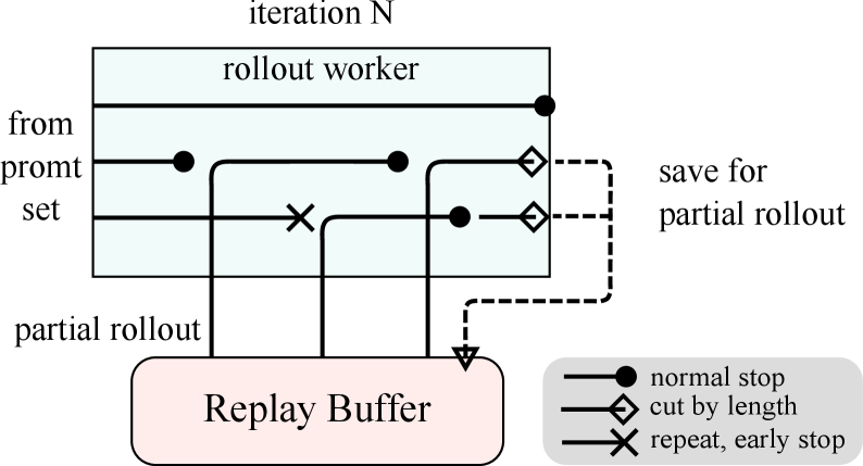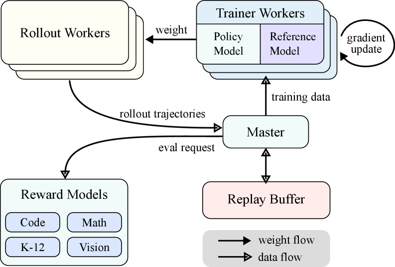</details> (b) Partial Rollout Figure 3: Large Scale Reinforcement Learning Training System for LLM #### 2.6.1 Large Scale Reinforcement Learning Training System for LLM In the realm of artificial intelligence, reinforcement learning (RL) has emerged as a pivotal training methodology for large language models (LLMs) [35] [16], drawing inspiration from its success in mastering complex games like Go, StarCraft II, and Dota 2 through systems such as AlphaGo [43], AlphaStar [51], and OpenAI Dota Five [4]. Following in this tradition, the Kimi k1.5 system adopts an iterative synchronous RL framework, meticulously designed to bolster the model’s reasoning capabilities through persistent learning and adaptation. A key innovation in this system is the introduction of a Partial Rollout technique, designed to optimize the handling of complex reasoning trajectories. The RL training system as illustrated in Figure 3(a) operates through an iterative synchronous approach, with each iteration encompassing a rollout phase and a training phase. During the rollout phase, rollout workers, coordinated by a central master, generate rollout trajectories by interacting with the model, producing sequences of responses to various inputs. These trajectories are then stored in a replay buffer, which ensures a diverse and unbiased dataset for training by disrupting temporal correlations. In the subsequent training phase, trainer workers access these experiences to update the model’s weights. This cyclical process allows the model to continuously learn from its actions, adjusting its strategies over time to enhance performance. The central master serves as the central conductor, managing the flow of data and communication between the rollout workers, trainer workers, evaluation with reward models and the replay buffer. It ensures that the system operates harmoniously, balancing the load and facilitating efficient data processing. The trainer workers access these rollout trajectories, whether completed in a single iteration or divided across multiple iterations, to compute gradient updates that refine the model’s parameters and enhance its performance. This process is overseen by a reward model, which evaluates the quality of the model’s outputs and provides essential feedback to guide the training process. The reward model’s evaluations are particularly pivotal in determining the effectiveness of the model’s strategies and steering the model towards optimal performance. Moreover, the system incorporates a code execution service, which is specifically designed to handle code-related problems and is integral to the reward model. This service evaluates the model’s outputs in practical coding scenarios, ensuring that the model’s learning is closely aligned with real-world programming challenges. By validating the model’s solutions against actual code executions, this feedback loop becomes essential for refining the model’s strategies and enhancing its performance in code-related tasks. #### 2.6.2 Partial Rollouts for Long CoT RL One of the primary ideas of our work is to scale long-context RL training. Partial rollouts is a key technique that effectively addresses the challenge of handling long-CoT features by managing the rollouts of both long and short trajectories. This technique establishes a fixed output token budget, capping the length of each rollout trajectory. If a trajectory exceeds the token limit during the rollout phase, the unfinished portion is saved to the replay buffer and continued in the next iteration. It ensures that no single lengthy trajectory monopolizes the system’s resources. Moreover, since the rollout workers operate asynchronously, when some are engaged with long trajectories, others can independently process new, shorter rollout tasks. The asynchronous operation maximizes computational efficiency by ensuring that all rollout workers are actively contributing to the training process, thereby optimizing the overall performance of the system. As illustrated in Figure 3(b), the partial rollout system works by breaking down long responses into segments across iterations (from iter n-m to iter n). The Replay Buffer acts as a central storage mechanism that maintains these response segments, where only the current iteration (iter n) requires on-policy computation. Previous segments (iter n-m to n-1) can be efficiently reused from the buffer, eliminating the need for repeated rollouts. This segmented approach significantly reduces the computational overhead: instead of rolling out the entire response at once, the system processes and stores segments incrementally, allowing for the generation of much longer responses while maintaining fast iteration times. During training, certain segments can be excluded from loss computation to further optimize the learning process, making the entire system both efficient and scalable. The implementation of partial rollouts also offers repeat detection. The system identifies repeated sequences in the generated content and terminates them early, reducing unnecessary computation while maintaining output quality. Detected repetitions can be assigned additional penalties, effectively discouraging redundant content generation in the prompt set. #### 2.6.3 Hybrid Deployment of Training and Inference <details> <summary>x5.png Details</summary>  ### Visual Description \n ## System Architecture Diagram: Distributed LLM Training and Inference Pod ### Overview The image is a technical system architecture diagram illustrating the components and data flow within a single computational "pod" designed for distributed large language model (LLM) training and inference. The diagram is divided into two primary subsystems—the Megatron Sidecar and the vLLM Sidecar—which coordinate through shared memory and external services. ### Components/Axes The diagram is structured within a large, rounded rectangle labeled **"pod"** at the top center. Inside, two major colored regions define the subsystems: 1. **Megatron Sidecar (Left, Light Blue Background):** * **Components (Boxes):** `Train`, `Onload`, `Offload`, `Wait rollout`, `Convert HF`, `Register Shard`, `Update Weight`, `Checkpoint Engine`. * **Flow:** Arrows indicate a cyclical process between `Train`, `Onload`, and `Offload`. `Offload` connects to `Wait rollout`. `Convert HF` feeds into `Register Shard`, which connects to `Update Weight`. Both `Register Shard` and `Update Weight` are contained within a dashed purple box labeled `Checkpoint Engine`. 2. **vLLM Sidecar (Right, Light Green Background):** * **Components (Boxes):** `Rollout`, `Dummy Start`, `Terminate`, `Update Weight`, `Start vLLM`, `Terminate vLLM`, `Checkpoint Engine`. * **Flow:** `Rollout` connects to both `Dummy Start` and `Terminate`. `Dummy Start` and `Start vLLM` both feed into `Update Weight`. `Update Weight` also receives input from `Terminate vLLM`. `Terminate` connects to `Terminate vLLM`. The components `Start vLLM`, `Update Weight`, and `Terminate vLLM` are contained within a dashed purple box labeled `Checkpoint Engine`. 3. **Shared Components & External Interfaces:** * **Shared Memory (Center, Purple Background):** A central box labeled `Shared Memory` sits between the two sidecars. It receives an arrow from the Megatron Sidecar's `Update Weight` and sends an arrow to the vLLM Sidecar's `Update Weight`. * **etcd (Bottom Center, Light Green Box):** An external service labeled `etcd` has bidirectional arrows connecting to both the Megatron and vLLM `Checkpoint Engine` components. * **Other Pods (Bottom Right, Gray Box):** A component labeled `Other Pods` is connected via a line labeled **"RDMA"** to the vLLM Sidecar's `Checkpoint Engine`. ### Detailed Analysis **Spatial Layout & Connections:** * The **Megatron Sidecar** occupies the left ~45% of the pod. Its internal `Checkpoint Engine` (purple dashed box) is positioned at the bottom of its region. * The **vLLM Sidecar** occupies the right ~45% of the pod. Its internal `Checkpoint Engine` is also at the bottom of its region. * The **Shared Memory** component is centrally located, acting as a bridge between the two sidecars' `Update Weight` processes. * **etcd** is positioned centrally below the pod, indicating its role as a shared coordination service for both checkpoint engines. * **Other Pods** are external, connected to the vLLM side via a high-speed **RDMA** (Remote Direct Memory Access) link. **Process Flow (Inferred from Arrows):** 1. **Megatron Sidecar (Training Focus):** The core loop appears to be `Train` -> `Onload` -> `Offload` -> `Wait rollout` -> back to `Train`. Parallel to this, model conversion (`Convert HF`) leads to sharding (`Register Shard`) and weight updates (`Update Weight`) within its checkpoint engine. 2. **vLLM Sidecar (Inference/Rollout Focus):** The process involves initiating rollouts (`Rollout`), which can start via a `Dummy Start` or a full `Start vLLM`. Weight updates (`Update Weight`) are a central hub, receiving inputs from start processes and termination signals (`Terminate vLLM`). The process can be cleanly stopped via `Terminate`. 3. **Coordination:** Model weights are synchronized from the Megatron training side to the vLLM inference side via **Shared Memory**. Both sides persist state and coordinate with the external **etcd** service. The vLLM side can also communicate with other pods via **RDMA**. ### Key Observations * **Asymmetric Design:** The two sidecars have distinct, specialized component sets. Megatron is oriented around a training loop and model sharding, while vLLM is oriented around managing inference instances (`vLLM`) and rollout processes. * **Centralized Weight Update:** The `Update Weight` component is a critical junction in both sidecars, suggesting that synchronizing model parameters is a key operation. * **Dual Checkpoint Engines:** Each sidecar has its own `Checkpoint Engine`, implying independent state management for training and inference processes, coordinated via `etcd`. * **Explicit External Links:** The diagram explicitly shows integration points with external systems (`etcd` for coordination, `Other Pods` via `RDMA` for distributed communication). ### Interpretation This diagram depicts a sophisticated architecture for decoupling LLM training from online inference/rollout within a single pod. The **Megatron Sidecar** likely handles the heavy computation of model training, while the **vLLM Sidecar** manages low-latency inference, possibly for reinforcement learning from human feedback (RLHF) or online serving. The **Shared Memory** bridge is crucial for efficiently transferring updated model weights from the training engine to the inference engine without going through slower storage or network layers. The use of **etcd** suggests a need for strong consistency in managing distributed state (like checkpoint metadata) across the two subsystems. The **RDMA** link to **Other Pods** indicates this pod is part of a larger cluster, where high-speed, low-latency communication between inference instances on different nodes is required. The architecture solves a key challenge in modern AI systems: how to continuously improve a model (training) while simultaneously serving it or using it to generate new data (inference/rollout) with minimal latency and data transfer overhead. The separation into "sidecars" within a pod allows for independent scaling and lifecycle management of these two workloads. 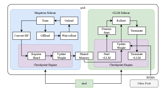</details> Figure 4: Hybrid Deployment Framework The RL training process comprises of the following phases: - Training Phase: At the outset, Megatron [42] and vLLM [21] are executed within separate containers, encapsulated by a shim process known as checkpoint-engine (Section 2.6.3). Megatron commences the training procedure. After the training is completed, Megatron offloads the GPU memory and prepares to transfer current weights to vLLM. - Inference Phase: Following Megatron’s offloading, vLLM starts with dummy model weights and updates them with the latest ones transferred from Megatron via Mooncake [39]. Upon completion of the rollout, the checkpoint-engine halts all vLLM processes. - Subsequent Training Phase: Once the memory allocated to vLLM is released, Megatron onloads the memory and initiates another round of training. We find existing works challenging to simultaneously support all the following characteristics. - Complex parallelism strategy: Megatron may have different parallelism strategy with vLLM. Training weights distributing in several nodes in Megatron could be challenging to be shared with vLLM. - Minimizing idle GPU resources: For On-Policy RL, recent works such as SGLang [62] and vLLM might reserve some GPUs during the training process, which conversely could lead to idle training GPUs. It would be more efficient to share the same devices between training and inference. - Capability of dynamic scaling: In some cases, a significant acceleration can be achieved by increasing the number of inference nodes while keeping the training process constant. Our system enables the efficient utilization of idle GPU nodes when needed. As illustrated in Figure 4, we implement this hybrid deployment framework (Section 2.6.3) on top of Megatron and vLLM, achieving less than one minute from training to inference phase and about ten seconds conversely. Hybrid Deployment Strategy We propose a hybrid deployment strategy for training and inference tasks, which leverages Kubernetes Sidecar containers sharing all available GPUs to collocate both workloads in one pod. The primary advantages of this strategy are: - It facilitates efficient resource sharing and management, preventing train nodes idling while waiting for inference nodes when both are deployed on separate nodes. - Leveraging distinct deployed images, training and inference can each iterate independently for better performance. - The architecture is not limited to vLLM, other frameworks can be conveniently integrated. Checkpoint Engine Checkpoint Engine is responsible for managing the lifecycle of the vLLM process, exposing HTTP APIs that enable triggering various operations on vLLM. For overall consistency and reliability, we utilize a global metadata system managed by the etcd service to broadcast operations and statuses. It could be challenging to entirely release GPU memory by vLLM offloading primarily due to CUDA graphs, NCCL buffers and NVIDIA drivers. To minimize modifications to vLLM, we terminate and restart it when needed for better GPU utilization and fault tolerance. The worker in Megatron converts the owned checkpoints into the Hugging Face format in shared memory. This conversion also takes Pipeline Parallelism and Expert Parallelism into account so that only Tensor Parallelism remains in these checkpoints. Checkpoints in shared memory are subsequently divided into shards and registered in the global metadata system. We employ Mooncake to transfer checkpoints between peer nodes over RDMA. Some modifications to vLLM are needed to load weight files and perform tensor parallelism conversion. #### 2.6.4 Code Sandbox We developed the sandbox as a secure environment for executing user-submitted code, optimized for code execution and code benchmark evaluation. By dynamically switching container images, the sandbox supports different use cases through MultiPL-E [6], DMOJ Judge Server https://github.com/DMOJ/judge-server, Lean, Jupyter Notebook, and other images. For RL in coding tasks, the sandbox ensures the reliability of training data judgment by providing consistent and repeatable evaluation mechanisms. Its feedback system supports multi-stage assessments, such as code execution feedback and repo-level editing, while maintaining a uniform context to ensure fair and equitable benchmark comparisons across programming languages. We deploy the service on Kubernetes for scalability and resilience, exposing it through HTTP endpoints for external integration. Kubernetes features like automatic restarts and rolling updates ensure availability and fault tolerance. To optimize performance and support RL environments, we incorporate several techniques into the code execution service to enhance efficiency, speed, and reliability. These include: - Using Crun: We utilize crun as the container runtime instead of Docker, significantly reducing container startup times. - Cgroup Reusing: We pre-create cgroups for container use, which is crucial in scenarios with high concurrency where creating and destroying cgroups for each container can become a bottleneck. - Disk Usage Optimization: An overlay filesystem with an upper layer mounted as tmpfs is used to control disk writes, providing a fixed-size, high-speed storage space. This approach is beneficial for ephemeral workloads. | Docker | 0.12 | | --- | --- | | Sandbox | 0.04 | (a) Container startup times | Docker Sandbox | 27 120 | | --- | --- | (b) Maximum containers started per second on a 16-core machine These optimizations improve RL efficiency in code execution, providing a consistent and reliable environment for evaluating RL-generated code, essential for iterative training and model improvement. ## 3 Experiments ### 3.1 Evaluation Since k1.5 is a multimodal model, we conducted comprehensive evaluation across various benchmarks for different modalities. The detailed evaluation setup can be found in Appendix C. Our benchmarks primarily consist of the following three categories: - Text Benchmark: MMLU [13], IF-Eval [63], CLUEWSC [56], C-EVAL [15] - Reasoning Benchmark: HumanEval-Mul, LiveCodeBench [17], Codeforces, AIME 2024, MATH-500 [26] - Vision Benchmark: MMMU [59], MATH-Vision [52], MathVista [29] ### 3.2 Main Results K1.5 long-CoT model The performance of the Kimi k1.5 long-CoT model is presented in Table 2. Through long-CoT supervised fine-tuning (described in Section 2.2) and vision-text joint reinforcement learning (discussed in Section 2.3), the model’s long-term reasoning capabilities are enhanced significantly. The test-time computation scaling further strengthens its performance, enabling the model to achieve state-of-the-art results across a range of modalities. Our evaluation reveals marked improvements in the model’s capacity to reason, comprehend, and synthesize information over extended contexts, representing a advancement in multi-modal AI capabilities. K1.5 short-CoT model The performance of the Kimi k1.5 short-CoT model is presented in Table 3. This model integrates several techniques, including traditional supervised fine-tuning (discussed in Section 2.5.2), reinforcement learning (explored in Section 2.3), and long-to-short distillation (outlined in Section 2.4). The results demonstrate that the k1.5 short-CoT model delivers competitive or superior performance compared to leading open-source and proprietary models across multiple tasks. These include text, vision, and reasoning challenges, with notable strengths in natural language understanding, mathematics, coding, and logical reasoning. | | Benchmark (Metric) | Language-only Model | Vision-Language Model | | | | | --- | --- | --- | --- | --- | --- | --- | | QwQ-32B | OpenAI | QVQ-72B | OpenAI | Kimi | | | | Preview | o1-mini | Preview | o1 | k1.5 | | | | Reasoning | MATH-500 (EM) | 90.6 | 90.0 | - | 94.8 | 96.2 | | AIME 2024 (Pass@1) | 50.0 | 63.6 | - | 74.4 | 77.5 | | | Codeforces (Percentile) | 62 | 88 | - | 94 | 94 | | | LiveCodeBench (Pass@1) | 40.6 | 53.1 | - | 67.2 | 62.5 | | | Vision | MathVista-Test (Pass@1) | - | - | 71.4 | 71.0 | 74.9 | | MMMU-Val (Pass@1) | - | - | 70.3 | 77.3 | 70.0 | | | MathVision-Full (Pass@1) | - | - | 35.9 | - | 38.6 | | Table 2: Performance of Kimi k1.5 long-CoT and flagship open-source and proprietary models. | | Benchmark (Metric) | Language-only Model | Vision-Language Model | | | | | | | --- | --- | --- | --- | --- | --- | --- | --- | --- | | Qwen2.5 | LLaMA-3.1 | DeepSeek | Qwen2-VL | Claude-3.5- | GPT-4o | Kimi | | | | 72B-Inst. | 405B-Inst. | V3 | | Sonnet-1022 | 0513 | k1.5 | | | | Text | MMLU (EM) | 85.3 | 88.6 | 88.5 | - | 88.3 | 87.2 | 87.4 | | IF-Eval (Prompt Strict) | 84.1 | 86.0 | 86.1 | - | 86.5 | 84.3 | 87.2 | | | CLUEWSC (EM) | 91.4 | 84.7 | 90.9 | - | 85.4 | 87.9 | 91.7 | | | C-Eval (EM) | 86.1 | 61.5 | 86.5 | - | 76.7 | 76.0 | 88.3 | | | Reasoning | MATH-500 (EM) | 80.0 | 73.8 | 90.2 | - | 78.3 | 74.6 | 94.6 | | AIME 2024 (Pass@1) | 23.3 | 23.3 | 39.2 | - | 16.0 | 9.3 | 60.8 | | | HumanEval-Mul (Pass@1) | 77.3 | 77.2 | 82.6 | - | 81.7 | 80.5 | 81.5 | | | LiveCodeBench (Pass@1) | 31.1 | 28.4 | 40.5 | - | 36.3 | 33.4 | 47.3 | | | Vision | MathVista-Test (Pass@1) | - | - | - | 69.7 | 65.3 | 63.8 | 70.1 | | MMMU-Val (Pass@1) | - | - | - | 64.5 | 66.4 | 69.1 | 68.0 | | | MathVision-Full (Pass@1) | - | - | - | 26.6 | 35.6 | 30.4 | 31.0 | | Table 3: Performance of Kimi k1.5 short-CoT and flagship open-source and proprietary models. VLM model performance were obtained from the OpenCompass benchmark platform (https://opencompass.org.cn/). ### 3.3 Long Context Scaling We employ a mid-sized model to study the scaling properties of RL with LLMs. Figure 5 illustrates the evolution of both training accuracy and response length across training iterations for the small model variant trained on the mathematical prompt set. As training progresses, we observe a concurrent increase in both response length and performance accuracy. Notably, more challenging benchmarks exhibit a steeper increase in response length, suggesting that the model learns to generate more elaborate solutions for complex problems. Figure 6 indicates a strong correlation between the model’s output context length and its problem-solving capabilities. Our final run of k1.5 scales to 128k context length and observes continued improvement on hard reasoning benchmarks. 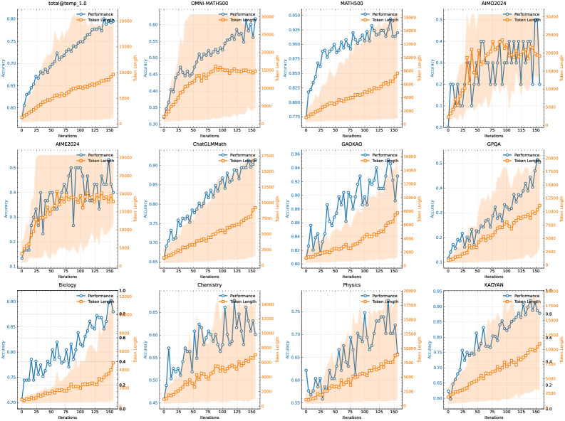<details> <summary>x6.png Details</summary>  ### Visual Description \n ## [Multi-Chart Grid]: Performance vs. Token Length Across Datasets ### Overview The image displays a 3x4 grid of 12 line charts. Each chart plots two metrics—"Performance" and "Token length"—against "Iterations" for a specific dataset or benchmark. The charts share a consistent visual style: a blue line with circle markers for "Performance" (left y-axis) and an orange line with square markers for "Token length" (right y-axis). A shaded orange region appears behind the "Token length" line in each plot. All charts have a legend in the top-right corner. ### Components/Axes * **Common Elements (All Charts):** * **X-axis Label:** `Iterations` * **Left Y-axis Label:** `Accuracy` * **Right Y-axis Label:** `Token length` * **Legend:** Located in the top-right corner of each subplot. Contains two entries: * `Performance` (Blue line, circle marker) * `Token length` (Orange line, square marker) * **Chart-Specific Titles and Axis Ranges:** 1. **Top-Left:** `total@temp_1.0` * Left Y-axis: ~0.40 to 0.80 * Right Y-axis: 0 to 3000 2. **Top-Center:** `OMNI-MATH500` * Left Y-axis: ~0.30 to 0.60 * Right Y-axis: 0 to 30000 3. **Top-Right:** `MATH500` * Left Y-axis: ~0.775 to 0.850 * Right Y-axis: 0 to 5000 4. **Top-Far Right:** `AIMO2024` * Left Y-axis: 0.1 to 0.5 * Right Y-axis: 0 to 30000 5. **Middle-Left:** `AIME2024` * Left Y-axis: 0.1 to 0.5 * Right Y-axis: 0 to 30000 6. **Middle-Center:** `ChatGLM-Math` * Left Y-axis: 0.55 to 0.80 * Right Y-axis: 0 to 17500 7. **Middle-Right:** `GAOKAO` * Left Y-axis: 0.20 to 0.36 * Right Y-axis: 0 to 16000 8. **Middle-Far Right:** `GPQA` * Left Y-axis: 0.1 to 0.5 * Right Y-axis: 0 to 17500 9. **Bottom-Left:** `Biology` * Left Y-axis: 0.70 to 1.0 * Right Y-axis: 0.0 to 1.0 (Note: Right axis appears scaled differently, likely representing a normalized token length or a different unit). 10. **Bottom-Center:** `Chemistry` * Left Y-axis: 0.45 to 0.85 * Right Y-axis: 0 to 16000 11. **Bottom-Right:** `Physics` * Left Y-axis: 0.55 to 0.75 * Right Y-axis: 0 to 17500 12. **Bottom-Far Right:** `KA0YAN` * Left Y-axis: 0.60 to 0.95 * Right Y-axis: 0.0 to 1.0 (Similar to Biology, right axis appears normalized). ### Detailed Analysis **General Trend Verification:** * **Performance (Blue Line):** In all 12 charts, the blue line shows a clear upward trend from left (iteration 0) to right (iteration ~150). The slope and volatility vary significantly between datasets. * **Token length (Orange Line):** The orange line also shows a consistent upward trend in all charts, but its slope is generally shallower and less volatile than the Performance line. **Chart-by-Chart Data Points (Approximate):** * **total@temp_1.0:** Performance rises steadily from ~0.42 to ~0.78. Token length increases from ~200 to ~2200. * **OMNI-MATH500:** Performance rises from ~0.32 to ~0.58. Token length increases from ~1000 to ~25000. * **MATH500:** Performance rises from ~0.78 to ~0.84. Token length increases from ~500 to ~4000. * **AIMO2024:** Performance is highly volatile, starting ~0.15, peaking near 0.5, and ending ~0.4. Token length increases from ~2000 to ~25000. * **AIME2024:** Performance is extremely volatile, with sharp peaks and troughs between 0.15 and 0.5. Token length increases from ~2000 to ~25000. * **ChatGLM-Math:** Performance rises smoothly from ~0.56 to ~0.79. Token length increases from ~1000 to ~16000. * **GAOKAO:** Performance is volatile, rising from ~0.22 to ~0.34. Token length increases from ~1000 to ~15000. * **GPQA:** Performance rises from ~0.12 to ~0.48. Token length increases from ~1000 to ~16000. * **Biology:** Performance rises from ~0.72 to ~0.98. Token length (on normalized scale) increases from ~0.05 to ~0.8. * **Chemistry:** Performance is volatile, rising from ~0.48 to ~0.82. Token length increases from ~1000 to ~15000. * **Physics:** Performance rises from ~0.56 to ~0.73. Token length increases from ~1000 to ~16000. * **KA0YAN:** Performance rises smoothly from ~0.62 to ~0.92. Token length (on normalized scale) increases from ~0.05 to ~0.8. ### Key Observations 1. **Positive Correlation:** There is a strong positive correlation between Iterations, Performance (Accuracy), and Token length across all benchmarks. As training/iterations progress, both accuracy and the length of generated tokens increase. 2. **Volatility Disparity:** The "Performance" metric exhibits significantly more volatility (sharp ups and downs) than the "Token length" metric, which grows more steadily. This is most extreme in the `AIME2024` and `AIMO2024` charts. 3. **Dataset Difficulty:** The absolute accuracy ranges suggest varying difficulty. `MATH500` and `Biology` show high baseline and final accuracy (>0.8), while `AIME2024`, `AIMO2024`, and `GPQA` show lower accuracy ranges, indicating they are more challenging benchmarks. 4. **Axis Scaling Anomaly:** The `Biology` and `KA0YAN` charts have a right y-axis (`Token length`) scaled from 0.0 to 1.0, unlike the others which use large integers. This suggests the token length data for these two subjects may have been normalized or represents a different metric (e.g., ratio). ### Interpretation The data strongly suggests a model training or iterative refinement process where increased computational effort (Iterations) leads to both improved problem-solving ability (higher Accuracy) and the generation of longer, more detailed solutions (higher Token length). The Peircean inference is that the model is learning to "think more" or elaborate its reasoning process as it improves. The volatility in Performance on certain math-heavy benchmarks (`AIME2024`, `AIMO2024`, `GAOKAO`) versus the smoother curves on others (`total@temp_1.0`, `ChatGLM-Math`, `KA0YAN`) may indicate that progress on highly complex, multi-step reasoning problems is less linear and more prone to plateaus or regressions during training, even as the model consistently produces longer outputs. The consistent lag of the Token length curve behind the Performance curve in the early iterations (visible as the orange line starting below the blue line's relative position) could imply that the model first learns to solve problems more correctly with concise answers, and only later learns to elaborate. Alternatively, it may simply reflect that the token count is a cumulative or slower-changing metric. The anomaly in the `Biology` and `KA0YAN` right-axis scaling is critical. If normalized, it indicates that token length growth for these subjects is being measured relative to a maximum, showing they approach a saturation point (~0.8 of max length) as performance nears perfection (~0.98 accuracy). This contrasts with other subjects where token length appears to grow without such a clear bound within the observed iteration window. </details> Figure 5: The changes on the training accuracy and length as train iterations grow. Note that the scores above come from an internal long-cot model with much smaller model size than k1.5 long-CoT model. The shaded area represents the 95% percentile of the response length. 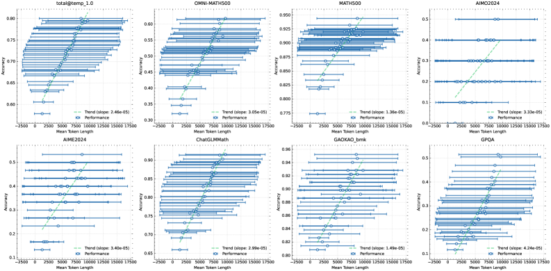<details> <summary>x7.png Details</summary>  ### Visual Description ## Scatter Plot Grid: Accuracy vs. Mean Token Length Across Benchmarks ### Overview The image displays a 2x4 grid of eight scatter plots. Each plot analyzes the relationship between "Mean Token Length" (x-axis) and "Accuracy" (y-axis) for a specific benchmark or dataset. All plots share a consistent visual style: blue circular data points with horizontal error bars, a green dashed trend line, and a legend in the bottom-right corner. The overall trend across all plots is a positive correlation between token length and accuracy. ### Components/Axes * **Grid Structure:** 2 rows, 4 columns. * **Common X-Axis (All Plots):** Label: "Mean Token Length". Scale: Linear, ranging from approximately -2500 to 17500. Major tick marks at 0, 2500, 5000, 7500, 10000, 12500, 15000, 17500. * **Common Y-Axis (All Plots):** Label: "Accuracy". Scale: Linear, but the range varies per plot. * **Data Series (All Plots):** * **Performance:** Represented by blue circles (`o`) with horizontal error bars (blue lines). Each point represents a bin of data. * **Trend:** Represented by a green dashed line (`--`). The legend includes the calculated slope value. * **Legend (All Plots):** Located in the bottom-right quadrant of each individual plot. Contains two entries: "Trend (slope: [value])" with a green dashed line icon, and "Performance" with a blue circle icon. ### Detailed Analysis **Plot 1 (Top-Left): `total@temp_1.0`** * **Y-Axis Range:** 0.60 to 0.80. * **Trend Slope:** 2.46e-05. * **Data Distribution:** Accuracy starts near 0.60 for the shortest token lengths and rises steadily to approximately 0.78 for the longest tokens. The trend line shows a clear, consistent upward slope. **Plot 2 (Top-Row, 2nd): `OMNI-MATH500`** * **Y-Axis Range:** 0.30 to 0.60. * **Trend Slope:** 3.05e-05. * **Data Distribution:** Accuracy begins around 0.32 and increases to about 0.58. The spread of data points (error bars) appears wider compared to the first plot. **Plot 3 (Top-Row, 3rd): `MATH500`** * **Y-Axis Range:** 0.775 to 0.950. * **Trend Slope:** 1.36e-05. * **Data Distribution:** This benchmark shows high baseline accuracy. It starts around 0.78 and climbs to approximately 0.93. The slope is the shallowest among the top row plots. **Plot 4 (Top-Right): `AIMO2024`** * **Y-Axis Range:** 0.0 to 0.5. * **Trend Slope:** 3.33e-05. * **Data Distribution:** Accuracy starts very low (~0.05) and shows a strong increase to about 0.45. The data points are more sparsely distributed along the x-axis compared to others. **Plot 5 (Bottom-Left): `AIME2024`** * **Y-Axis Range:** 0.1 to 0.5. * **Trend Slope:** 3.40e-05. * **Data Distribution:** Similar pattern to `AIMO2024`, starting near 0.12 and rising to around 0.48. The trend line is steep. **Plot 6 (Bottom-Row, 2nd): `ChatGLM-Math`** * **Y-Axis Range:** 0.65 to 0.90. * **Trend Slope:** 3.99e-05. * **Data Distribution:** High accuracy range, starting at ~0.67 and reaching ~0.88. The slope is relatively steep for this high-accuracy regime. **Plot 7 (Bottom-Row, 3rd): `GAOKAO_bmk`** * **Y-Axis Range:** 0.80 to 0.86. * **Trend Slope:** 1.49e-05. * **Data Distribution:** This plot has the narrowest y-axis range and the shallowest slope. Accuracy increases from ~0.81 to ~0.85. The data points are tightly clustered. **Plot 8 (Bottom-Right): `GPOA`** * **Y-Axis Range:** 0.1 to 0.5. * **Trend Slope:** 4.74e-05. * **Data Distribution:** Shows the steepest trend slope of all eight plots. Accuracy rises from a low of ~0.10 to ~0.48. ### Key Observations 1. **Universal Positive Correlation:** Every single benchmark demonstrates a positive linear relationship between the mean length of generated tokens and the accuracy score. 2. **Slope Variation:** The strength of this relationship (slope) varies significantly. `GPOA` (4.74e-05) and `ChatGLM-Math` (3.99e-05) show the strongest effects, while `GAOKAO_bmk` (1.49e-05) and `MATH500` (1.36e-05) show the weakest. 3. **Accuracy Baselines Differ:** The starting accuracy (y-intercept) differs greatly, from near zero (`AIMO2024`, `GPOA`) to very high (`MATH500`, `GAOKAO_bmk`). 4. **Error Bars:** All data points have horizontal error bars, indicating variability or a range of token lengths within each accuracy bin. The length of these bars varies, suggesting different levels of variance in response length for given accuracy levels. ### Interpretation The data strongly suggests that, across a diverse set of mathematical and reasoning benchmarks, **longer model responses (higher mean token length) are associated with higher accuracy.** This is not a causal claim from the chart alone, but a robust correlation. * **Possible Underlying Mechanism:** This could indicate that the model engages in more thorough reasoning, step-by-step derivation, or self-correction when it produces longer answers, which in turn leads to correct solutions. Shorter answers might represent rushed or incomplete reasoning. * **Benchmark Sensitivity:** The varying slopes imply that some benchmarks (`GPOA`, `ChatGLM-Math`) are more sensitive to response length than others (`GAOKAO_bmk`, `MATH500`). This could be due to the nature of the problems; some may inherently require more verbose solutions to solve correctly. * **Performance Floor:** For benchmarks like `AIMO2024` and `GPOA`, very short responses are almost always incorrect (accuracy near 0.1-0.2), suggesting a minimum "length of thought" is necessary to have any chance of success. * **Practical Implication:** This analysis provides empirical support for techniques that encourage or allow models to generate longer chains of thought (e.g., via prompting like "think step by step") to improve performance on complex reasoning tasks. The trade-off between computational cost (longer sequences) and accuracy gain is clearly visualized by the slope of each trend line. 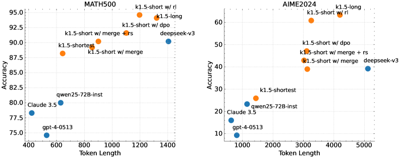</details> Figure 6: Model Performance Increases with Response Length <details> <summary>x8.png Details</summary>  ### Visual Description \n ## Scatter Plot Comparison: MATH500 vs. AIME2024 Benchmark Performance ### Overview The image displays two side-by-side scatter plots comparing the performance of various large language models on two different mathematical reasoning benchmarks: **MATH500** (left) and **AIME2024** (right). Each plot charts model **Accuracy** (y-axis) against **Token Length** (x-axis), which likely represents the model's context window or sequence length. Data points are color-coded, with orange representing variants of a model family labeled "k1.5" and blue representing other models (e.g., deepseek-v3, Claude 3.5, gpt-4-0513, qwen25-72B-inst). ### Components/Axes **Common Elements:** * **X-axis:** "Token Length" (linear scale). * **Y-axis:** "Accuracy" (linear scale, percentage). * **Data Points:** Labeled circles. Orange points are various "k1.5" model configurations. Blue points are comparison models. * **Titles:** Centered above each plot. **Left Plot: MATH500** * **Title:** "MATH500" * **X-axis Range:** ~400 to ~1400 * **Y-axis Range:** 75.0 to 95.0 * **Data Points & Approximate Coordinates (Token Length, Accuracy):** * **Orange (k1.5 family):** * `k1.5-shortest`: (~650, ~88.5) * `k1.5-short w/ merge`: (~900, ~89.0) * `k1.5-short w/ merge + rs`: (~1100, ~91.5) * `k1.5-short w/ dpo`: (~1200, ~93.0) * `k1.5-short w/ rl`: (~1200, ~95.0) *[Highest point]* * `k1.5-long`: (~1350, ~94.0) * **Blue (Other models):** * `gpt-4-0513`: (~550, ~75.0) *[Lowest point]* * `Claude 3.5`: (~450, ~78.5) * `qwen25-72B-inst`: (~650, ~80.0) * `deepseek-v3`: (~1400, ~90.0) **Right Plot: AIME2024** * **Title:** "AIME2024" * **X-axis Range:** ~1000 to ~5000 * **Y-axis Range:** 10 to 60 * **Data Points & Approximate Coordinates (Token Length, Accuracy):** * **Orange (k1.5 family):** * `k1.5-shortest`: (~1500, ~26.0) * `k1.5-short w/ merge`: (~3000, ~39.0) * `k1.5-short w/ merge + rs`: (~3200, ~43.0) * `k1.5-short w/ dpo`: (~3200, ~46.0) * `k1.5-short w/ rl`: (~3300, ~61.0) *[Highest point]* * `k1.5-long`: (~4200, ~63.0) *[Highest point, slightly above rl variant]* * **Blue (Other models):** * `gpt-4-0513`: (~1000, ~9.0) *[Lowest point]* * `Claude 3.5`: (~900, ~16.0) * `qwen25-72B-inst`: (~1200, ~21.0) * `deepseek-v3`: (~5100, ~39.0) ### Detailed Analysis **MATH500 Plot Analysis:** * **Trend Verification:** There is a clear positive correlation between Token Length and Accuracy for the k1.5 model family (orange points). The line formed by these points slopes upward from left to right. The blue comparison models do not follow a single clear trend relative to token length. * **Performance Hierarchy:** The `k1.5-short w/ rl` model achieves the highest accuracy (~95%). The `k1.5-long` model is close behind (~94%). The standard `gpt-4-0513` model shows the lowest accuracy (~75%) among the plotted points. * **Token Length Clustering:** The k1.5 models cluster in the higher token length range (650-1400), while the comparison models (except `deepseek-v3`) are in the lower range (450-650). **AIME2024 Plot Analysis:** * **Trend Verification:** A positive correlation is also visible for the k1.5 family, with accuracy generally increasing with token length. The slope appears steeper than in the MATH500 plot. The `deepseek-v3` point is an outlier in terms of token length (~5100) but has moderate accuracy (~39%). * **Performance Hierarchy:** The `k1.5-long` model achieves the highest accuracy (~63%), narrowly outperforming the `k1.5-short w/ rl` variant (~61%). The `gpt-4-0513` model again shows the lowest accuracy (~9%). * **Scale Difference:** The overall accuracy values are significantly lower on AIME2024 (max ~63%) compared to MATH500 (max ~95%), indicating this is a more challenging benchmark. Token lengths are also generally higher. ### Key Observations 1. **Consistent Leader:** The `k1.5-short w/ rl` (reinforcement learning) variant is a top performer on both benchmarks, suggesting the RL training method is highly effective. 2. **Benchmark Difficulty:** The AIME2024 benchmark yields much lower accuracy scores across all models, suggesting it is a more difficult test of mathematical reasoning. 3. **Token Length Advantage:** The k1.5 model family consistently operates at higher token lengths than the other models shown (except `deepseek-v3` on AIME2024), and this correlates with higher performance. 4. **Model Comparison:** On both benchmarks, the plotted `gpt-4-0513` and `Claude 3.5` points show lower accuracy than the k1.5 family and `deepseek-v3`. `qwen25-72B-inst` performs in the middle range. 5. **Scaling Effect:** Within the k1.5 family, moving from `k1.5-shortest` to `k1.5-long` generally involves an increase in both token length and accuracy. ### Interpretation The data suggests a strong relationship between model context length (token length) and performance on complex mathematical reasoning tasks, at least within the `k1.5` model family. The consistent superiority of the `k1.5-short w/ rl` variant highlights the potential of reinforcement learning techniques to boost reasoning capabilities beyond what is achieved with other methods like DPO (Direct Preference Optimization) or merge strategies. The stark difference in accuracy ranges between MATH500 and AIME2024 indicates these benchmarks test different levels or types of mathematical difficulty. AIME (American Invitational Mathematics Examination) problems are known to be highly challenging, which aligns with the lower scores. The fact that the `k1.5-long` model, with the largest context, performs best on the harder AIME2024 benchmark could imply that longer context windows are particularly beneficial for solving more complex, multi-step problems that require holding and manipulating more information. The plots do not show a simple linear scaling law for all models, as the blue comparison points are scattered. This implies that factors other than raw token length—such as training data, architecture, and fine-tuning methods (like RL, DPO)—are critical determinants of performance. The visualization effectively argues for the efficacy of the `k1.5` approach, particularly its RL variant, in advancing the state-of-the-art for mathematical reasoning in AI. </details> Figure 7: Long2Short Performance. All the k1.5 series demonstrate better token efficiency compared to other models. ### 3.4 Long2short We compared the proposed long2short RL algorithm with the DPO, shortest rejection sampling, and model merge methods introduced in the Section 2.4, focusing on the token efficiency for the long2short problem [8], specifically how the obtained long-cot model can benefit a short model. In Figure 7, k1.5-long represents our long-cot model selected for long2short training. k1.5-short w/ rl refers to the short model obtained using the long2short RL training. k1.5-short w/ dpo denotes the short model with improved token efficiency through DPO training. k1.5-short w/ merge represents the model after model merging, while k1.5-short w/ merge + rs indicates the short model obtained by applying shortest rejection sampling to the merged model. k1.5-shortest represents the shortest model we obtained during the long2short training. As shown in Figure 7, the proposed long2short RL algorithm demonstrates the highest token efficiency compared other mehtods such as DPO and model merge. Notably, all models in the k1.5 series (marked in orange) demonstrate superior token efficiency compared to other models (marked in blue). For instance, k1.5-short w/ rl achieves a Pass@1 score of 60.8 on AIME2024 (averaged over 8 runs) while utilizing only 3,272 tokens on average. Similarly, k1.5-shortest attains a Pass@1 score of 88.2 on MATH500 while consuming approximately the same number of tokens as other short models. ### 3.5 Ablation Studies Scaling of model size and context length Our main contribution is the application of RL to enhance the model’s capacity for generating extended CoT, thereby improving its reasoning ability. A natural question arises: how does this compare to simply increasing the model size? To demonstrate the effectiveness of our approach, we trained two models of different sizes using the same dataset and recorded the evaluation results and average inference lengths from all checkpoints during RL training. These results are shown in Figure 8. Notably, although the larger model initially outperforms the smaller one, the smaller model can achieve comparable performance by utilizing longer CoTs optimized through RL. However, the larger model generally shows better token efficiency than the smaller model. This also indicates that if one targets the best possible performance, scaling the context length of a larger model has a higher upper bound and is more token efficient. However, if test-time compute has a budget, training smaller models with a larger context length may be viable solutions. Effects of using negative gradients We investigate the effectiveness of using ReST [12] as the policy optimization algorithm in our setting. The primary distinction between ReST and other RL-based methods including ours is that ReST iteratively refines the model by fitting the best response sampled from the current model, without applying negative gradients to penalize incorrect responses. As illustrated in Figure 10, our method exhibits superior sample complexity compared to ReST, indicating that the incorporation of negative gradients markedly enhances the model’s efficiency in generating long CoT. Our method not only elevates the quality of reasoning but also optimizes the training process, achieving robust performance with fewer training samples. This finding suggests that the choice of policy optimization algorithm is crucial in our setting, as the performance gap between ReST and other RL-based methods is not as pronounced in other domains [12]. Therefore, our results highlight the importance of selecting an appropriate optimization strategy to maximize effectiveness in generating long CoT. Sampling strategies We further demonstrate the effectiveness of our curriculum sampling strategy, as introduced in Section 2.3.4. Our training dataset $D$ comprises a diverse mix of problems with varying levels of difficulty. With our curriculum sampling method, we initially use $D$ for a warm-up phase and then focus solely on hard questions to train the model. This approach is compared to a baseline method that employs a uniform sampling strategy without any curriculum adjustments. As illustrated in Figure 9, our results clearly show that the proposed curriculum sampling method significantly enhances the performance. This improvement can be attributed to the method’s ability to progressively challenge the model, allowing it to develop a more robust understanding and competency in handling complex problems. By focusing training efforts on more difficult questions after an initial general introduction, the model can better strengthen its reasoning and problem solving capabilities. 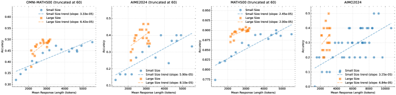<details> <summary>x9.png Details</summary>  ### Visual Description \n ## Scatter Plot Series: Model Accuracy vs. Response Length ### Overview The image displays four horizontally arranged scatter plots, each analyzing the relationship between model accuracy and mean response length (in tokens) for different mathematical benchmarks. Each plot compares two model size categories: "Small Size" (blue) and "Large Size" (orange). All plots include linear trend lines for each category. ### Components/Axes **Common Elements Across All Plots:** * **X-Axis:** `Mean Response Length (tokens)`. The scale varies per plot but generally ranges from approximately 0 to 5000 or 10000 tokens. * **Y-Axis:** `Accuracy`. The scale varies per plot, representing a proportion (e.g., 0.3 to 0.6). * **Legend:** Located in the top-left corner of each plot. It defines: * `Small Size` (Blue circle marker) * `Large Size` (Orange circle marker) * `Small Size trend (slope: [value])` (Blue dashed line) * `Large Size trend (slope: [value])` (Orange dashed line) **Individual Plot Details:** 1. **Plot 1 (Leftmost):** * **Title:** `OMNI-MATH500 (truncated at 60)` * **X-Axis Range:** ~0 to 5500 tokens. * **Y-Axis Range:** 0.30 to 0.60. * **Trend Line Slopes:** * Small Size: `3.33e-05` * Large Size: `6.42e-05` 2. **Plot 2 (Center-Left):** * **Title:** `AIME2024 (truncated at 60)` * **X-Axis Range:** ~0 to 5500 tokens. * **Y-Axis Range:** 0.10 to 0.50. * **Trend Line Slopes:** * Small Size: `5.90e-05` * Large Size: `8.10e-05` 3. **Plot 3 (Center-Right):** * **Title:** `MATH500 (truncated at 60)` * **X-Axis Range:** ~0 to 5500 tokens. * **Y-Axis Range:** 0.775 to 0.850. * **Trend Line Slopes:** * Small Size: `2.43e-05` * Large Size: `2.00e-05` 4. **Plot 4 (Rightmost):** * **Title:** `AIMC2024` * **X-Axis Range:** 0 to 10000 tokens. * **Y-Axis Range:** 0.0 to 0.5. * **Trend Line Slopes:** * Small Size: `3.25e-05` * Large Size: `8.84e-05` ### Detailed Analysis **Data Point Distribution & Trends:** * **OMNI-MATH500:** Small Size models (blue) cluster between 0.30-0.50 accuracy and 0-5000 tokens. Large Size models (orange) cluster higher, between 0.40-0.55 accuracy and 1000-3000 tokens. Both trends are positive; the Large Size trend line is steeper (slope: 6.42e-05 vs. 3.33e-05). * **AIME2024:** Small Size models show a wide spread from 0.10-0.45 accuracy. Large Size models are concentrated in a higher accuracy band (0.30-0.50) with response lengths mostly under 3000 tokens. Both trends are positive, with the Large Size slope being notably steeper (8.10e-05 vs. 5.90e-05). * **MATH500:** This plot has a much narrower, higher accuracy range (0.775-0.850). Small Size models are spread across the full length range. Large Size models are tightly clustered at the higher end of accuracy (0.82-0.85) and moderate lengths (1000-3000 tokens). Both trends are positive but shallow; here, the Small Size trend is slightly steeper (2.43e-05 vs. 2.00e-05). * **AIMC2024:** Data points are more sparse. Small Size models are scattered across low-to-mid accuracy (0.0-0.4). Large Size models form a distinct cluster at higher accuracy (0.3-0.5) and moderate lengths (1000-4000 tokens). Both trends are positive, with the Large Size slope being significantly steeper (8.84e-05 vs. 3.25e-05). ### Key Observations 1. **Consistent Positive Correlation:** In all four benchmarks, there is a positive correlation between mean response length and accuracy for both model sizes. 2. **Model Size Advantage:** Large Size models (orange) consistently achieve higher accuracy than Small Size models (blue) at comparable response lengths across all benchmarks. 3. **Slope Comparison:** The trend line for Large Size models is steeper than for Small Size models in three of the four plots (OMNI-MATH500, AIME2024, AIMC2024), suggesting accuracy may scale more favorably with increased length for larger models. MATH500 is the exception. 4. **Benchmark Difficulty:** The accuracy ranges suggest varying benchmark difficulty. MATH500 shows the highest overall accuracy (0.775-0.850), while AIME2024 and AIMC2024 show lower accuracy ceilings, indicating they may be more challenging. 5. **Data Truncation:** The titles for the first three plots note "(truncated at 60)", which likely means the underlying evaluation was limited to problems with up to 60 steps or a similar constraint, potentially affecting the maximum achievable response length and accuracy. ### Interpretation The data suggests a fundamental trade-off or relationship in language model performance on mathematical tasks: generating longer, more detailed responses is associated with higher accuracy. This could indicate that models which "think more" (produce more tokens) arrive at better solutions. The consistent performance gap between Large and Small Size models reinforces the understanding that model scale is a primary driver of capability. Furthermore, the generally steeper slopes for Large models imply they may be more efficient at converting additional computational effort (longer responses) into accuracy gains. The variation across benchmarks is insightful. The high, clustered accuracy on MATH500 suggests it may be a benchmark where models have reached a performance plateau, or it tests a more uniform skill set. In contrast, the wider spreads and lower ceilings on AIME2024 and AIMC2024 indicate these benchmarks likely contain more diverse or difficult problems that better differentiate model capabilities and expose the benefits of both scale and increased reasoning length. **Notable Anomaly:** The MATH500 plot is an outlier in two ways: it has the highest accuracy range and is the only plot where the Small Size trend slope is marginally steeper than the Large Size slope. This could be due to a ceiling effect, where Large Size models are already near-maximal performance, leaving less room for accuracy to improve with length. 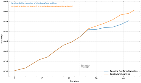</details> Figure 8: Model Performance vs Response Length of Different Model Sizes <details> <summary>x10.png Details</summary>  ### Visual Description \n ## Line Chart: Baseline vs. Curriculum Learning Accuracy Over Iterations ### Overview The image displays a line chart comparing the training accuracy of two machine learning approaches over 40+ iterations. The chart illustrates how "Curriculum Learning" (introducing harder problems after an initial phase) compares to a "Baseline" method of uniform sampling throughout training. A key transition point is marked. ### Components/Axes * **Chart Type:** Line chart with two data series. * **X-Axis:** Labeled "Iteration". Major tick marks are present at intervals of 10 (0, 10, 20, 30, 40). The axis extends slightly beyond 40. * **Y-Axis:** Labeled "Accuracy". Major tick marks are present at intervals of 0.05, ranging from 0.30 to 0.65. * **Legend:** Located in the bottom-right quadrant of the chart area. * A blue line is labeled "Baseline (Uniform Sampling)". * An orange line is labeled "Curriculum Learning". * **Annotations:** * A vertical, gray, dashed line is positioned at **Iteration 24**. It is labeled "Curriculum Transition" in small text to its right. * Text in the top-left corner provides context: * Blue text: "Baseline: Uniform sampling of mixed-easy/hard problems" * Orange text: "Curriculum: Uniform problems first, then hard problems (transition at iter 24)" ### Detailed Analysis **Trend Verification & Data Points (Approximate):** * **Baseline (Uniform Sampling) - Blue Line:** * **Trend:** Shows a steady, roughly linear upward slope throughout the entire training period. * **Key Points:** * Iteration 0: ~0.30 * Iteration 10: ~0.36 * Iteration 20: ~0.44 * Iteration 24 (at transition line): ~0.47 * Iteration 30: ~0.51 * Iteration 40: ~0.55 * Final Point (~Iteration 43): ~0.555 * **Curriculum Learning - Orange Line:** * **Trend:** Initially follows a similar upward slope to the baseline. After the marked transition point at iteration 24, the slope increases noticeably, showing accelerated improvement. * **Key Points:** * Iteration 0: ~0.30 (starts at nearly the same point as Baseline) * Iteration 10: ~0.36 * Iteration 20: ~0.44 * Iteration 24 (at transition line): ~0.47 (nearly identical to Baseline at this point) * **Post-Transition:** * Iteration 30: ~0.52 * Iteration 40: ~0.59 * Final Point (~Iteration 43): ~0.61 **Spatial Grounding:** The two lines are nearly superimposed from iteration 0 to 24. After the vertical "Curriculum Transition" line at x=24, the orange line (Curriculum Learning) diverges upward, consistently staying above the blue line (Baseline) for the remainder of the chart. ### Key Observations 1. **Identical Early Performance:** Both methods perform almost identically for the first 24 iterations, suggesting the initial "uniform problems" phase of the curriculum matches the baseline's mixed sampling. 2. **Divergence at Transition:** A clear and immediate divergence occurs at the marked transition point (Iteration 24). The curriculum learning line breaks away upward. 3. **Accelerated Learning:** The slope of the Curriculum Learning line becomes steeper after iteration 24, indicating a faster rate of accuracy improvement once harder problems are introduced. 4. **Final Performance Gap:** By the end of the plotted data, Curriculum Learning achieves a final accuracy of ~0.61, while the Baseline reaches ~0.555, resulting in a significant performance gap of approximately 0.055 accuracy points. ### Interpretation The data strongly suggests that the **curriculum learning strategy is more effective than uniform sampling** for this specific task. The key insight is that the benefit is not immediate but is triggered by a deliberate change in training data difficulty. * **What the data demonstrates:** The chart provides empirical evidence for the "curriculum learning" hypothesis in machine learning. It shows that structuring the learning process—starting with easier, more manageable examples before introducing complexity—can lead to better final model performance than exposing the model to all difficulty levels randomly from the start. * **Relationship between elements:** The vertical "Curriculum Transition" line is the critical experimental variable. The fact that the performance lines are coincident before this line and diverge after it isolates the transition as the causal factor for the improved outcome. The legend and annotations explicitly define this experimental setup. * **Notable implications:** The anomaly is not in the data points themselves but in the **sharp change in trend** for the orange line at iteration 24. This indicates a highly responsive learning system. The results imply that for this problem domain, the model benefits from a structured introduction to complexity, potentially allowing it to build a more robust foundational understanding before tackling harder examples, thereby avoiding negative interference or getting stuck in poor local minima early in training. </details> Figure 9: Analysis of curriculum learning approaches on model performance. 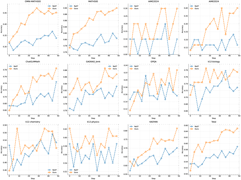<details> <summary>x11.png Details</summary>  ### Visual Description ## Line Charts: Comparative Accuracy of "ReST" vs. "Ours" Across Multiple Benchmarks ### Overview The image displays a grid of 12 line charts arranged in 3 rows and 4 columns. Each chart compares the performance of two methods, labeled "ReST" (blue line with circle markers) and "Ours" (orange line with circle markers), across a series of training or evaluation steps. The charts track "Accuracy" on the y-axis against "Step" on the x-axis. The overall visual impression is that the "Ours" method generally achieves higher accuracy and shows a more consistent upward trend compared to the more volatile "ReST" method. ### Components/Axes * **Chart Titles (Benchmarks):** Each subplot is titled with a specific benchmark or dataset name. Reading left-to-right, top-to-bottom, they are: 1. OMNI-MATH500 2. MATH500 3. AIM02024 4. AIME2024 5. ChatGLMMath 6. GAOKAO_bmk 7. GPOA 8. k12-biology 9. k12-chemistry 10. k12-physics 11. KADIAN 12. Total * **Axes:** * **X-axis (All Charts):** Labeled "Step". The scale runs from 0 to 50, with major tick marks at intervals of 10 (0, 10, 20, 30, 40, 50). * **Y-axis (All Charts):** Labeled "Accuracy". The scale and range vary significantly per chart to fit the data. * **Legend:** Located in the top-left corner of each subplot. It contains two entries: * A blue line with a circle marker labeled "ReST". * An orange line with a circle marker labeled "Ours". * **Data Series:** Each chart contains two line series corresponding to the legend. ### Detailed Analysis **Chart-by-Chart Data Point Approximation (Trend First, Then Key Points):** 1. **OMNI-MATH500:** * *Trend:* "Ours" shows a strong, steady upward trend. "ReST" is more volatile with a slight upward drift. * *Data:* "Ours" starts at ~0.32 (Step 0), rises to a peak of ~0.46 (Step ~35), and ends at ~0.45 (Step 50). "ReST" starts at ~0.30, dips to ~0.28 (Step 5), fluctuates, and ends at ~0.37. 2. **MATH500:** * *Trend:* "Ours" has a clear, strong upward trend. "ReST" is volatile with a moderate upward trend. * *Data:* "Ours" starts at ~0.78, climbs steadily to ~0.89 (Step 50). "ReST" starts at ~0.78, dips to ~0.76 (Step 10), and ends at ~0.81. 3. **AIM02024:** * *Trend:* Both series are highly volatile. "Ours" shows a general upward trend despite large swings. "ReST" is erratic with no clear trend. * *Data:* "Ours" starts at ~0.05, peaks at ~0.30 (Steps 30 & 45), ends at ~0.30. "ReST" starts at ~0.10, fluctuates wildly between ~0.05 and ~0.20, ends at ~0.10. 4. **AIME2024:** * *Trend:* "Ours" shows a strong upward trend. "ReST" is volatile with a slight upward trend. * *Data:* "Ours" starts at ~0.10, rises to ~0.40 (Step 40), ends at ~0.38. "ReST" starts at ~0.10, fluctuates between ~0.15 and ~0.23, ends at ~0.17. 5. **ChatGLMMath:** * *Trend:* "Ours" shows a steady upward trend. "ReST" is volatile with a slight upward trend. * *Data:* "Ours" starts at ~0.68, rises to ~0.78 (Step 50). "ReST" starts at ~0.68, fluctuates between ~0.66 and ~0.71, ends at ~0.74. 6. **GAOKAO_bmk:** * *Trend:* "Ours" shows a strong upward trend. "ReST" is volatile with a moderate upward trend. * *Data:* "Ours" starts at ~0.80, rises to ~0.88 (Step 40), ends at ~0.86. "ReST" starts at ~0.77, fluctuates between ~0.78 and ~0.83, ends at ~0.83. 7. **GPOA:** * *Trend:* Both series are highly volatile and intertwined. No clear, consistent leader. * *Data:* Both start near ~0.14. They fluctuate sharply between ~0.14 and ~0.22. At Step 50, "Ours" is at ~0.22 and "ReST" is at ~0.16. 8. **k12-biology:** * *Trend:* "Ours" shows a moderate upward trend. "ReST" is volatile with a slight upward trend. * *Data:* "Ours" starts at ~0.70, rises to ~0.78 (Step 45), ends at ~0.77. "ReST" starts at ~0.73, dips to ~0.66 (Step 10), fluctuates, ends at ~0.73. 9. **k12-chemistry:** * *Trend:* "Ours" is volatile but shows a general upward trend. "ReST" is also volatile with a slight upward trend. * *Data:* "Ours" starts at ~0.50, peaks at ~0.58 (Step 10 & 35), ends at ~0.56. "ReST" starts at ~0.54, dips to ~0.46 (Step 5), fluctuates, ends at ~0.54. 10. **k12-physics:** * *Trend:* "Ours" shows a moderate upward trend. "ReST" is volatile with no clear trend. * *Data:* "Ours" starts at ~0.58, rises to ~0.62 (Step 40), ends at ~0.60. "ReST" starts at ~0.57, fluctuates between ~0.52 and ~0.58, ends at ~0.55. 11. **KADIAN:** * *Trend:* "Ours" shows a strong, steady upward trend. "ReST" shows a moderate upward trend. * *Data:* "Ours" starts at ~0.60, rises to ~0.80 (Step 50). "ReST" starts at ~0.62, rises to ~0.70 (Step 50). 12. **Total:** * *Trend:* "Ours" shows a very strong, consistent upward trend. "ReST" shows a moderate, volatile upward trend. * *Data:* "Ours" starts at ~0.52, rises steadily to ~0.65 (Step 50). "ReST" starts at ~0.52, fluctuates between ~0.53 and ~0.58, ends at ~0.58. ### Key Observations 1. **Consistent Superiority:** In 11 out of 12 charts, the "Ours" method ends at a higher accuracy than "ReST". The only exception is GPOA, where they are close. 2. **Trend Stability:** The "Ours" line typically exhibits a smoother, more consistent upward trajectory. The "ReST" line is characterized by high volatility and frequent, sharp fluctuations. 3. **Benchmark Variability:** Performance gaps vary by benchmark. The gap is very large in OMNI-MATH500, AIME2024, and the "Total" chart. It is smallest in GPOA and k12-chemistry. 4. **Starting Points:** In most charts, both methods begin at a similar accuracy level at Step 0, making the subsequent divergence more notable. 5. **Peak Performance:** "Ours" often reaches its peak accuracy in the later steps (30-50), while "ReST" peaks are more scattered and often not sustained. ### Interpretation This collection of charts presents a compelling case for the effectiveness of the proposed method ("Ours") compared to the baseline ("ReST") across a diverse set of mathematical and scientific reasoning benchmarks. * **What the Data Suggests:** The data demonstrates that "Ours" not only achieves higher final accuracy but also learns more reliably and stably over time. The high volatility of "ReST" suggests its training or evaluation process is less robust, potentially sensitive to specific data batches or steps. * **Relationship Between Elements:** The "Total" chart aggregates the performance, confirming the overall trend seen in individual benchmarks. The consistency across different domains (general math, competition math, K12 subjects) indicates the improvement is not niche but broadly applicable. * **Notable Anomalies:** The GPOA chart is the primary outlier, where neither method shows a clear advantage and both are highly unstable. This suggests the GPOA benchmark may be particularly challenging or noisy, or that the methods behave differently on this specific task type. * **Underlying Implication:** The results imply that the architectural or training innovations in "Ours" lead to more effective and stable optimization for complex reasoning tasks. The steady climb of "Ours" suggests it continues to benefit from extended training (more steps), whereas "ReST" may plateau or become unstable. This has practical significance for resource allocation in model training. </details> Figure 10: Comparison with using ReST for policy optimization. ## 4 Conclusions We present the training recipe and system design of k1.5, our latest multi-modal LLM trained with RL. One of the key insights we extract from our practice is that the scaling of context length is crucial to the continued improvement of LLMs. We employ optimized learning algorithms and infrastructure optimization such as partial rollouts to achieve efficient long-context RL training. How to further improve the efficiency and scalability of long-context RL training remains an important question moving forward. Another contribution we made is a combination of techniques that enable improved policy optimization. Specifically, we formulate long-CoT RL with LLMs and derive a variant of online mirror descent for robust optimization. We also experiment with sampling strategies, length penalty, and optimizing the data recipe to achieve strong RL performance. We show that strong performance can be achieved by long context scaling and improved policy optimization, even without using more complex techniques such as Monte Carlo tree search, value functions, and process reward models. In the future, it will also be intriguing to study improving credit assignments and reducing overthinking without hurting the model’s exploration abilities. We have also observed the potential of long2short methods. These methods largely improve performance of short CoT models. Moreover, it is possible to combine long2short methods with long-CoT RL in an iterative way to further increase token efficiency and extract the best performance out of a given context length budget. ## References - [1] Yasin Abbasi-Yadkori et al. “Politex: Regret bounds for policy iteration using expert prediction” In International Conference on Machine Learning, 2019, pp. 3692–3702 PMLR - [2] Arash Ahmadian et al. “Back to basics: Revisiting reinforce style optimization for learning from human feedback in llms” In arXiv preprint arXiv:2402.14740, 2024 - [3] Zachary Ankner et al. “Critique-out-Loud Reward Models”, 2024 arXiv: https://arxiv.org/abs/2408.11791 - [4] Christopher Berner et al. “Dota 2 with large scale deep reinforcement learning” In arXiv preprint arXiv:1912.06680, 2019 - [5] Federico Cassano et al. “MultiPL-E: A Scalable and Extensible Approach to Benchmarking Neural Code Generation” In ArXiv, 2022 URL: https://arxiv.org/abs/2208.08227 - [6] Federico Cassano et al. “MultiPL-E: A Scalable and Polyglot Approach to Benchmarking Neural Code Generation” In IEEE Transactions on Software Engineering 49.7, 2023, pp. 3675–3691 DOI: 10.1109/TSE.2023.3267446 - [7] Jianlv Chen et al. “Bge m3-embedding: Multi-lingual, multi-functionality, multi-granularity text embeddings through self-knowledge distillation” In arXiv preprint arXiv:2402.03216, 2024 - [8] Xingyu Chen et al. “Do NOT Think That Much for 2+ 3=? On the Overthinking of o1-Like LLMs” In arXiv preprint arXiv:2412.21187, 2024 - [9] Tom Everitt et al. “Reward Tampering Problems and Solutions in Reinforcement Learning: A Causal Influence Diagram Perspective”, 2021 arXiv: https://arxiv.org/abs/1908.04734 - [10] Samir Yitzhak Gadre et al. “Datacomp: In search of the next generation of multimodal datasets” In Advances in Neural Information Processing Systems 36, 2024 - [11] Aaron Grattafiori et al. “The Llama 3 Herd of Models”, 2024 arXiv: https://arxiv.org/abs/2407.21783 - [12] Caglar Gulcehre et al. “Reinforced self-training (rest) for language modeling” In arXiv preprint arXiv:2308.08998, 2023 - [13] Dan Hendrycks et al. “Measuring Massive Multitask Language Understanding” In ArXiv abs/2009.03300, 2020 URL: https://arxiv.org/abs/2009.03300 - [14] Jordan Hoffmann et al. “Training Compute-Optimal Large Language Models”, 2022 arXiv: https://arxiv.org/abs/2203.15556 - [15] Yuzhen Huang et al. “C-Eval: A Multi-Level Multi-Discipline Chinese Evaluation Suite for Foundation Models” In ArXiv abs/2305.08322, 2023 URL: https://arxiv.org/abs/2305.08322 - [16] Aaron Jaech et al. “Openai o1 system card” In arXiv preprint arXiv:2412.16720, 2024 - [17] Naman Jain et al. “LiveCodeBench: Holistic and Contamination Free Evaluation of Large Language Models for Code” In ArXiv abs/2403.07974, 2024 URL: https://arxiv.org/abs/2403.07974 - [18] Armand Joulin et al. “Bag of tricks for efficient text classification” In arXiv preprint arXiv:1607.01759, 2016 - [19] Jared Kaplan et al. “Scaling Laws for Neural Language Models”, 2020 arXiv: https://arxiv.org/abs/2001.08361 - [20] Wouter Kool, Herke Hoof and Max Welling “Buy 4 reinforce samples, get a baseline for free!”, 2019 - [21] Woosuk Kwon et al. “Efficient Memory Management for Large Language Model Serving with PagedAttention” In Proceedings of the ACM SIGOPS 29th Symposium on Operating Systems Principles, 2023 - [22] Hugo Laurençon et al. “Obelics: An open web-scale filtered dataset of interleaved image-text documents” In Advances in Neural Information Processing Systems 36, 2024 - [23] Jeffrey Li et al. “Datacomp-lm: In search of the next generation of training sets for language models” In arXiv preprint arXiv:2406.11794, 2024 - [24] Ming Li et al. “From quantity to quality: Boosting llm performance with self-guided data selection for instruction tuning” In arXiv preprint arXiv:2308.12032, 2023 - [25] Raymond Li et al. “StarCoder: may the source be with you!”, 2023 arXiv: https://arxiv.org/abs/2305.06161 - [26] Hunter Lightman et al. “Let’s Verify Step by Step” In arXiv preprint arXiv:2305.20050, 2023 - [27] Wei Liu et al. “What makes good data for alignment? a comprehensive study of automatic data selection in instruction tuning” In arXiv preprint arXiv:2312.15685, 2023 - [28] Anton Lozhkov et al. “StarCoder 2 and The Stack v2: The Next Generation”, 2024 arXiv: https://arxiv.org/abs/2402.19173 - [29] Pan Lu et al. “Mathvista: Evaluating mathematical reasoning of foundation models in visual contexts” In arXiv preprint arXiv:2310.02255, 2023 - [30] Nat McAleese et al. “LLM Critics Help Catch LLM Bugs”, 2024 arXiv: https://arxiv.org/abs/2407.00215 - [31] Jincheng Mei et al. “On principled entropy exploration in policy optimization” In Proceedings of the 28th International Joint Conference on Artificial Intelligence, 2019, pp. 3130–3136 - [32] Niklas Muennighoff et al. “Scaling Data-Constrained Language Models”, 2023 arXiv: https://arxiv.org/abs/2305.16264 - [33] Ofir Nachum et al. “Bridging the gap between value and policy based reinforcement learning” In Advances in neural information processing systems 30, 2017 - [34] OpenAI “Learning to reason with LLMs”, 2024 URL: https://openai.com/index/learning-to-reason-with-llms/ - [35] Long Ouyang et al. “Training language models to follow instructions with human feedback” In Advances in neural information processing systems 35, 2022, pp. 27730–27744 - [36] Alexander Pan, Kush Bhatia and Jacob Steinhardt “The Effects of Reward Misspecification: Mapping and Mitigating Misaligned Models” In International Conference on Learning Representations, 2022 URL: https://openreview.net/forum?id=JYtwGwIL7ye - [37] Keiran Paster et al. “Openwebmath: An open dataset of high-quality mathematical web text” In arXiv preprint arXiv:2310.06786, 2023 - [38] Guilherme Penedo et al. “The fineweb datasets: Decanting the web for the finest text data at scale” In arXiv preprint arXiv:2406.17557, 2024 - [39] Ruoyu Qin et al. “Mooncake: A KVCache-centric Disaggregated Architecture for LLM Serving”, 2024 arXiv: https://arxiv.org/abs/2407.00079 - [40] Rafael Rafailov et al. “Direct preference optimization: Your language model is secretly a reward model” In Advances in Neural Information Processing Systems 36, 2024 - [41] Christoph Schuhmann et al. “Laion-5b: An open large-scale dataset for training next generation image-text models” In Advances in Neural Information Processing Systems 35, 2022, pp. 25278–25294 - [42] Mohammad Shoeybi et al. “Megatron-LM: Training Multi-Billion Parameter Language Models Using Model Parallelism”, 2020 arXiv: https://arxiv.org/abs/1909.08053 - [43] David Silver et al. “Mastering the game of go without human knowledge” In nature 550.7676 Nature Publishing Group, 2017, pp. 354–359 - [44] Charlie Snell et al. “Scaling llm test-time compute optimally can be more effective than scaling model parameters” In arXiv preprint arXiv:2408.03314, 2024 - [45] Dan Su et al. “Nemotron-CC: Transforming Common Crawl into a Refined Long-Horizon Pretraining Dataset” In arXiv preprint arXiv:2412.02595, 2024 - [46] Jianlin Su et al. “Roformer: Enhanced transformer with rotary position embedding” In Neurocomputing 568 Elsevier, 2024, pp. 127063 - [47] Gemini Team et al. “Gemini: A Family of Highly Capable Multimodal Models”, 2024 arXiv: https://arxiv.org/abs/2312.11805 - [48] Manan Tomar et al. “Mirror descent policy optimization” In arXiv preprint arXiv:2005.09814, 2020 - [49] Ashish Vaswani et al. “Attention is All you Need” In Advances in Neural Information Processing Systems 30 Curran Associates, Inc., 2017 URL: https://proceedings.neurips.cc/paper_files/paper/2017/file/3f5ee243547dee91fbd053c1c4a845aa-Paper.pdf - [50] Pablo Villalobos et al. “Will we run out of data? Limits of LLM scaling based on human-generated data”, 2024 arXiv: https://arxiv.org/abs/2211.04325 - [51] Oriol Vinyals et al. “Grandmaster level in StarCraft II using multi-agent reinforcement learning” In nature 575.7782 Nature Publishing Group, 2019, pp. 350–354 - [52] Ke Wang et al. “Measuring multimodal mathematical reasoning with math-vision dataset” In arXiv preprint arXiv:2402.14804, 2024 - [53] Haoran Wei et al. “General OCR Theory: Towards OCR-2.0 via a Unified End-to-end Model” In arXiv preprint arXiv:2409.01704, 2024 - [54] Jason Wei et al. “Chain-of-thought prompting elicits reasoning in large language models” In Advances in neural information processing systems 35, 2022, pp. 24824–24837 - [55] Yangzhen Wu et al. “Inference scaling laws: An empirical analysis of compute-optimal inference for problem-solving with language models” In arXiv preprint arXiv:2408.00724, 2024 - [56] Liang Xu et al. “CLUE: A Chinese Language Understanding Evaluation Benchmark” In International Conference on Computational Linguistics, 2020 URL: https://arxiv.org/abs/2004.05986 - [57] Enneng Yang et al. “Model merging in llms, mllms, and beyond: Methods, theories, applications and opportunities” In arXiv preprint arXiv:2408.07666, 2024 - [58] Shunyu Yao et al. “Tree of thoughts: Deliberate problem solving with large language models” In Advances in Neural Information Processing Systems 36, 2024 - [59] Xiang Yue et al. “Mmmu: A massive multi-discipline multimodal understanding and reasoning benchmark for expert agi” In Proceedings of the IEEE/CVF Conference on Computer Vision and Pattern Recognition, 2024, pp. 9556–9567 - [60] Xiang Yue et al. “Mammoth: Building math generalist models through hybrid instruction tuning” In arXiv preprint arXiv:2309.05653, 2023 - [61] Lunjun Zhang et al. “Generative verifiers: Reward modeling as next-token prediction, 2024” In URL https://arxiv. org/abs/2408.15240, 2024 - [62] Lianmin Zheng et al. “SGLang: Efficient Execution of Structured Language Model Programs”, 2024 arXiv: https://arxiv.org/abs/2312.07104 - [63] Jeffrey Zhou et al. “Instruction-Following Evaluation for Large Language Models” In ArXiv abs/2311.07911, 2023 URL: https://arxiv.org/abs/2311.07911 - [64] Wanrong Zhu et al. “Multimodal c4: An open, billion-scale corpus of images interleaved with text” In Advances in Neural Information Processing Systems 36, 2024 ## Appendix ## Appendix A Contributions Research & Development Angang Du Bofei Gao Bowei Xing Changjiu Jiang Cheng Chen Cheng Li Chenjun Xiao Chenzhuang Du Chonghua Liao* Congcong Wang Dehao Zhang Enming Yuan Enzhe Lu Flood Sung Guokun Lai Haiqing Guo Han Zhu Hao Ding Hao Hu Hao Yang Hao Zhang Haotian Yao Haotian Zhao Haoyu Lu Hongcheng Gao Huan Yuan Huabin Zheng Jingyuan Liu Jianlin Su Jianzhou Wang Jin Zhang Junjie Yan Lidong Shi Longhui Yu Mengnan Dong Neo Zhang Ningchen Ma* Qiwei Pan Qucheng Gong Shaowei Liu Shupeng Wei Sihan Cao Tao Jiang Weimin Xiong Weiran He Weihao Gao* Weixiao Huang Weixin Xu Wenhao Wu Wenyang He Xianqing Jia Xingzhe Wu Xinran Xu Xinyu Zhou Xinxing Zu Xuehai Pan Yang Li Yangyang Hu Yangyang Liu Yanru Chen Yejie Wang Yidao Qin Yibo Liu Yiping Bao Yifeng Liu* Yulun Du Yuzhi Wang Yuxin Wu Y. Charles Zaida Zhou Zhaoji Wang Zhaowei Li Zheng Zhang Zhexu Wang Zhiqi Huang Zhilin Yang Zihao Huang Ziyao Xu Zonghan Yang Zongyu Lin Data Annotation Chuning Tang Fengxiang Tang Guangda Wei Haoze Li Haozhen Yu Jia Chen Jianhang Guo Jie Zhao Junyan Wu Ling Ye Shengling Ma Siying Huang Xianghui Wei Yangyang Liu Ying Yang Zhen Zhu The listing of authors is in alphabetical order based on their first names. Names marked with an asterisk (*) indicate people who are no longer part of our team. ## Appendix B Pretraining Reinforcement learning (RL) efficiency is closely tied to the performance of the underlying base model. Frontier models such as Gemini [47] and Llama [11] highlight the importance of pretraining data quality in achieving high performance. However, many recent open-source models lack full transparency regarding their data processing pipelines and recipes, creating challenges for broader community understanding. While we are not open-sourcing our proprietary model at this time, we are committed to providing a comprehensive disclosure of our data pipeline and methodologies. In this section, we focus primarily on the multimodal pretraining data recipe, followed by a brief discussion of the model architecture and training stages. ### B.1 Language Data Our pretrain corpus is designed to provide comprehensive and high-quality data for training large language models (LLMs). It encompasses five domains: English, Chinese, Code, Mathematics & Reasoning, and Knowledge. We employ sophisticated filtering and quality control mechanisms for each domain to ensure the highest quality training data. For all pretrain data, we conducted rigorous individual validation for each data source to assess its specific contribution to the overall training recipe. This systematic evaluation ensures the quality and effectiveness of our diverse data composition. English and Chinese textual data we developed a multi-dimensional quality filtering framework that combines multiple scoring methods to reduce individual biases and ensure comprehensive quality assessment. Our framework incorporates: 1. Rule-based filtering: We implement domain-specific heuristics to remove problematic content, including duplicate content, machine-translated text, and low-quality web scrapes. We also filter out documents with excessive special characters, unusual formatting, or spam patterns. 1. FastText-based classification: We trained specialized FastText [18, 23] models to identify content quality based on linguistic features and semantic coherence. This helps identify documents with natural language flow and proper grammatical structure. 1. Embedding-based similarity analysis: Using document embeddings [7], we compute document-level similarity scores to identify and remove near-duplicates while preserving semantically valuable variations. This approach helps maintain diversity in our training corpus. 1. LLM-based quality assessment: Following [38], we leverage LLMs to score documents based on coherence, informativeness, and potential educational value. This method is particularly effective at identifying nuanced quality indicators that simpler methods might miss. The final quality score for each document is calculated as a combination of these individual scores. Based on extensive empirical analysis, we implement dynamic sampling rates, where high-quality documents are upsampled, while low-quality documents are downsampled during training. Code data The code data primarily consists of two categories. For the pure code data derived from code files, we adhered to the methodology of BigCode [25, 28] and conducted a comprehensive preprocessing of the dataset. Initially, we eliminated miscellaneous languages and applied a rule-based cleaning procedure to enhance data quality. Subsequently, we addressed language imbalance through strategic sampling techniques. Specifically, markup languages such as JSON, YAML, and YACC were down-sampled, while 32 major programming languages, including Python, C, C++, Java, and Go, were up-sampled to ensure a balanced representation. Regarding the text-code interleaved data sourced from various data sources, we use an embedding-based method to recall high-quality data. This approach ensures the diversity of the data and maintains its high quality. Math & Reasoning data The mathematics and reasoning component of our dataset is crucial for developing strong analytical and problem-solving capabilities. The mathematical pre-training data are mainly retrieved from web text and PDF documents collected from publicly available internet sources. [37] Initially, we discovered that our general-domain text extraction, data cleaning process and OCR models exhibited high false negative rates in the mathematical domain. Therefore, we first developed specialized data cleaning procedures and OCR models specifically for mathematical content, aiming to maximize the recall rate of mathematical data. Subsequently, we implemented a two-stage data cleaning process: 1. Using FastText model for initial cleaning to remove most irrelevant data. 1. Utilizing a fine-tuned language model to further clean the remaining data, resulting in high-quality mathematical data. Knowledge data The knowledge corpus is meticulously curated to ensure a comprehensive coverage in academic disciplines. Our knowledge base primarily consists of academic exercises, textbooks, research papers, and other general educational literature. A significant portion of these materials is digitized through OCR processing, for which we have developed proprietary models optimized for academic content, particularly for handling mathematical formulas and special symbols. We employ internal language models to annotate documents with multi-dimensional labels, including: 1. OCR quality metrics to assess recognition accuracy 1. Educational value indicators measuring pedagogical relevance 1. Document type classification (e.g., exercises, theoretical materials) Based on these multi-dimensional annotations, we implement a sophisticated filtering and sampling pipeline. First and foremost, documents are filtered through OCR quality thresholds. Our OCR quality assessment framework places special attention on detecting and filtering out common OCR artifacts, particularly repetitive text patterns that often indicate recognition failures. Beyond basic quality control, we carefully evaluate the educational value of each document through our scoring system. Documents with high pedagogical relevance and knowledge depth are prioritized, while maintaining a balance between theoretical depth and instructional clarity. This helps ensure that our training corpus contains high-quality educational content that can effectively contribute to the model’s knowledge acquisition. Finally, to optimize the overall composition of our training corpus, the sampling strategy for different document types is empirically determined through extensive experimentation. We conduct isolated evaluations to identify document subsets that contribute most significantly to the model’s knowledge acquisition capabilities. These high-value subsets are upsampled in the final training corpus. However, to maintain data diversity and ensure model generalization, we carefully preserve a balanced representation of other document types at appropriate ratios. This data-driven approach helps us optimize the trade-off between focused knowledge acquisition and broad generalization capabilities. ### B.2 Multimodal Data Our multi-modal pretraining corpus is designed to provide high-quality data that enables models to process and understand information from multiple modalities, including text, images, and videos. To this end, we also have curated high-quality data from five categories—captioning, interleaving, OCR (Optical Character Recognition), knowledge, and general question answering—to form the corpus. When constructing our training corpus, we developed several multi-modal data processing pipelines to ensure data quality, encompassing filtering, synthesis, and deduplication. Establishing an effective multi-modal data strategy is crucial during the joint training of vision and language, as it both preserves the capabilities of the language model and facilitates alignment of knowledge across diverse modalities. We provide a detailed description of these sources in this section, which is organized into the following categories: Caption data Our caption data provides the model with fundamental modality alignment and a broad range of world knowledge. By incorporating caption data, the multi-modal LLM gains wider world knowledge with high learning efficiency. We have integrated various open-source Chinese and English caption datasets like [41, 10] and also collected substantial in-house caption data from multiple sources. However, throughout the training process, we strictly limit the proportion of synthetic caption data to mitigate the risk of hallucination stemming from insufficient real-world knowledge. For general caption data, we follow a rigorous quality control pipeline that avoids duplication and maintain high image-text correlation. We also vary image resolution during pretraining to ensure that the vision tower remains effective when processing images of both high- and low-resolution. Image-text interleaving data During the pretraining phase, model is benefit from interleaving data for many aspects, for example, multi-image comprehension ability can be boosted by interleaving data; interleaving data always provide detailed knowledge for the given image; a longer multi-modal context learning ability can also be gained by the interleaving data. What’s more, we also find that interleaving data can contributes positively to maintaining the model’s language abilities. Thus, image-text interleaving data is an important part in our training corpus. Our multi-modal corpus considered open-sourced interleave datasets like [64, 22] and also constructed large-scale in-house data using resources like textbooks, webpages and tutorials. Further, we also find that synthesizing the interleaving data benefits the performance of multi-modal LLM for keeping the text knowledges. To ensure each image’s knowledge is sufficiently studied, for all the interleaving data, other than the standard filtering, deduping and other quality control pipeline, we also integrated a data reordering procedure for keeping all the image and text in the correct order. OCR data Optical Character Recognition (OCR) is a widely adopted technique that converts text from images into an editable format. In k1.5, a robust OCR capability is deemed essential for better aligning the model with human values. Accordingly, our OCR data sources are diverse, ranging from open-source to in-house datasets, and encompassing both clean and augmented images. In addition to the publicly available data, we have developed a substantial volume of in-house OCR datasets, covering multilingual text, dense text layouts, web-based content, and handwritten samples. Furthermore, following the principles outlined in OCR 2.0 [53], our model is also equipped to handle a variety of optical image types, including figures, tables, geometry diagrams, mermaid plots, and natural scene text. We apply extensive data augmentation techniques—such as rotation, distortion, color adjustments, and noise addition—to enhance the model’s robustness. As a result, our model achieves a high level of proficiency in OCR tasks. Knowledge data The concept of multi-modal knowledge data is analogous to the previously mentioned text pretraining data, except here we focus on assembling a comprehensive repository of human knowledge from diverse sources to further enhance the model’s capabilities. For example, carefully curated geometry data in our dataset is vital for developing visual reasoning skills, ensuring the model can interpret the abstract diagrams created by humans. Our knowledge corpus adheres to a standardized taxonomy to balance content across various categories, ensuring diversity in data sources. Similar to text-only corpora, which gather knowledge from textbooks, research papers, and other academic materials, multi-modal knowledge data employs both a layout parser and an OCR model to process content from these sources. While we also include filtered data from internet-based and other external resources. Because a significant portion of our knowledge corpus is sourced from internet-based materials, infographics can cause the model to focus solely on OCR-based information. In such cases, relying exclusively on a basic OCR pipeline may limit training effectiveness. To address this, we have developed an additional pipeline that better captures the purely textual information embedded within images. General QA Data During the training process, we observed that incorporating a substantial volume of high-quality QA datasets into pretraining offers significant benefits. Specifically, we included rigorous academic datasets addressing tasks such as grounding, table/chart question answering, web agents, and general QA. In addition, we compiled a large amount of in-house QA data to further enhance the model’s capabilities. To maintain balanced difficulty and diversity, we applied scoring models and meticulous manual categorization to our general question answering dataset, resulting in overall performance improvements. ### B.3 Model Architecture Kimi k-series models employ a variant of the Transformer decoder [49] that integrates multimodal capabilities alongside improvements in architecture and optimization strategies, illustrated in Figure 11. These advancements collectively support stable large-scale training and efficient inference, tailored specifically to large-scale reinforcement learning and the operational requirements of Kimi users. Extensive scaling experiments indicate that most of the base model performance comes from improvements in the quality and diversity of the pretraining data. Specific details regarding model architecture scaling experiments lie beyond the scope of this report and will be addressed in future publications. 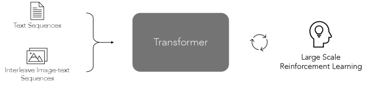<details> <summary>x12.png Details</summary>  ### Visual Description ## Diagram: Multimodal Transformer Training Pipeline ### Overview The image is a technical flowchart illustrating a machine learning pipeline. It depicts the flow of data from input sources through a central processing model and into a reinforcement learning refinement loop. The diagram is composed of simple line-art icons, text labels, and directional arrows on a plain white background. ### Components/Axes The diagram is organized into three main sections from left to right: 1. **Input Sources (Left Side):** * **Top Input:** An icon of a document with lines of text. The label below it reads: `Text Sequences`. * **Bottom Input:** An icon depicting a landscape image (mountains and sun) next to lines of text. The label below it reads: `Interleave Image-text Sequences`. * A large curly brace `}` groups these two inputs, with an arrow pointing from the brace to the central component. 2. **Central Processing Unit (Center):** * A large, solid gray rectangle with rounded corners. * The text `Transformer` is centered inside the rectangle in a white, sans-serif font. 3. **Output & Refinement Loop (Right Side):** * A circular arrow icon (↻) indicating a loop or iterative process. * An icon of a human head in profile with a lightbulb inside, symbolizing learning or ideation. * The text below this icon reads: `Large Scale Reinforcement Learning`. * An arrow points from the central `Transformer` box to the circular arrow, and another implied connection exists from the reinforcement learning component back into the loop. ### Detailed Analysis * **Data Flow:** The pipeline begins with two distinct types of input data: pure text sequences and interleaved sequences containing both images and text. These are fed jointly into the system. * **Core Model:** The combined input data is processed by a `Transformer` model, which is a standard architecture for handling sequential data like text and, in this multimodal context, image-text pairs. * **Training/Refinement Process:** The output or state of the Transformer model is then subjected to `Large Scale Reinforcement Learning`. The circular arrow explicitly denotes that this is not a one-pass process but an iterative loop, where the reinforcement learning process likely provides feedback to update or refine the Transformer model repeatedly. ### Key Observations * The diagram is abstract and does not specify the exact nature of the "Text Sequences" or "Interleave Image-text Sequences" (e.g., source, format, length). * The `Transformer` block is a black box; no internal architecture (encoder-decoder, specific layers) is detailed. * The reinforcement learning component is labeled as "Large Scale," implying significant computational resources and data are involved in this refinement stage. * The flow is strictly left-to-right with a feedback loop, suggesting a sequential yet cyclical training methodology. ### Interpretation This diagram represents a high-level schematic for training a large, multimodal AI model. The process suggests a two-stage or hybrid training approach: 1. **Initial Processing:** A Transformer model is first exposed to a mixture of unimodal (text) and multimodal (image-text) data. This allows the model to learn fundamental patterns in language and the relationships between visual and textual information. 2. **Iterative Refinement:** The model's outputs or behaviors are then evaluated and optimized using large-scale reinforcement learning. This technique is often used to align model outputs with specific goals, improve factual accuracy, or enhance helpfulness by rewarding desired behaviors. The loop indicates that the model is continuously improved through this feedback mechanism. The pipeline implies the creation of a versatile model capable of understanding and generating content across text and images, which is then fine-tuned at scale to perform specific tasks or adhere to certain guidelines effectively. The absence of specific data details indicates this is a conceptual overview of the system architecture rather than a technical specification. </details> Figure 11: Kimi k1.5 supports interleaved images and text as input, leveraging large-scale reinforcement learning to enhance the model’s reasoning capabilities. ### B.4 Training Stages The Kimi k1.5 model is trained in three stages: the vision-language pretraining stage, the vision-language cooldown stage, and the long-context activation stage. Each stage of the Kimi k1.5 model’s training focuses on a particular capability enhancement. Vision-language pretraining stage In this stage, the model is firstly trained solely on language data, establishing a robust language model foundation. Then the model is gradually introduced to interleaved vision-language data, acquiring multimodal capabilities. The visual tower is initially trained in isolation without updating the language model parameters, then we unfreeze the language model layers, and ultimately increase the proportion of vision-text data to 30%. The final data mixtures and their respective weights were determined through ablation studies conducted on smaller models. Vision-language cooldown stage The second stage serves as a cooldown phase, where the model is continue trained with high-quality language and vision-language datasets to ensure superior performance. Through empirical investigation, we observed that the incorporation of synthetic data during the cooldown phase yields significant performance improvements, particularly in mathematical reasoning, knowledge-based tasks, and code generation. The English and Chinese components of the cooldown dataset are curated from high-fidelity subsets of the pre-training corpus. For math, knowledge, and code domains, we employ a hybrid approach: utilizing selected pre-training subsets while augmenting them with synthetically generated content. Specifically, we leverage existing mathematical, knowledge and code corpora as source material to generate question-answer pairs through a proprietary language model, implementing rejection sampling techniques to maintain quality standards [60, 45]. These synthesized QA pairs undergo comprehensive validation before being integrated into the cooldown dataset. Long-context activation stage Finally, in the third stage, k1.5 is trained with upsampled long-context cooldown data, enabling it to process extended sequences and support tasks that demand longer context. To ensure excellent long-text capabilities of the base model, we upsampled long-context data and used 40% full attention data and 60% partial attention data during long context training. The full attention data came partly from high-quality natural data and partly from synthetic long context Q&A and summary data. The partial attention data came from uniform sampling of cooldown data. The RoPE frequency [46] was set to 1,000,000. During this stage, we gradually extended length activation training by increasing the maximum sequence length from 4,096 to 32,768, and ultimately to 131,072. ## Appendix C Evaluation Details ### C.1 Text Benchmark MMLU [13] covers 57 subjects in STEM, the humanities, social sciences, and more. It ranges in difficulty from an elementary level to an advanced professional level, and it tests both world knowledge and problem-solving ability. IF-Eval [63] is a benchmark for evaluating large language models’ ability to follow verifiable instructions. There are 500+ prompts with instructions such as "write an article with more than 800 words", etc. Due to a version shift, the number of IFEval reported in Table 3 derived from an intermediate model. We will update the scores based on the final model. CLUEWSC [56] is a coreference resolution task in CLUE benchmark, requiring models to determine if a pronoun and a noun phrase in a sentence co-refer, with data from Chinese fiction books. C-EVAL [15] is a comprehensive Chinese evaluation suite for assessing advanced knowledge and reasoning abilities of foundation models. It includes 13,948 multiple-choice questions across 52 disciplines and four difficulty levels. ### C.2 Reasoning Benchmark HumanEval-Mul is a subset of Multipl-E [5]. MultiPL-E extends the HumanEval benchmark and MBPP benchmark to 18 languages that encompass a range of programming paradigms and popularity. We choose HumanEval translations in 8 mainstream programming languages (Python, Java, Cpp, C#, JavaScript, TypeScript, PHP, and Bash). LiveCodeBench [17] serves as a comprehensive and contamination-free benchmark for assessing large language models (LLMs) in coding tasks. It features live updates to prevent data contamination, holistic evaluation across multiple coding scenarios, high-quality problems and tests, and balanced problem difficulty. We test short-CoT model with questions from 2408-2411 (release v4), and long-CoT model with questions from 2412-2502 (release v5). AIME 2024 comprises the competition questions for the AIME in 2024. The AIME is a prestigious, invitation-only math contest for top high school students, assessing advanced math skills and requiring solid foundation and high logical thinking. MATH-500 [26] is a comprehensive mathematics benchmark that contains 500 problems on various mathematics topics including algebra, calculus, probability, and more. Tests both computational ability and mathematical reasoning. Higher scores indicate stronger mathematical problem-solving capabilities. Codeforces is a well-known online judge platform and serves as a popular testbed for evaluating long-CoT coding models. To achieve higher rankings in the Div2 and Div3 competitions, we utilize majority voting on the code snippets generated by the k1.5 long-CoT model, employing test cases that are also generated by the same model. The percentile of the codeforce ELO rating was extracted from OpenAI Day12 talk https://www.youtube.com/watch?v=SKBG1sqdyIU&ab_channel=OpenAI c. ### C.3 Image Benchmark MMMU [59] encompasses a carefully curated collection of 11.5K multimodal questions sourced from college exams, quizzes, and textbooks. These questions span six major academic fields: Art & Design, Business, Science, Health & Medicine, Humanities & Social Science, and Tech & Engineering. MATH-Vision (MATH-V) [52] is a carefully curated collection of 3,040 high-quality mathematical problems with visual contexts that are sourced from real math competitions. It covers 16 distinct mathematical disciplines and is graded across 5 levels of difficulty. This dataset offers a comprehensive and diverse set of challenges, making it ideal for evaluating the mathematical reasoning abilities of LMMs. MathVista [29] is a benchmark that integrates challenges from a variety of mathematical and visual tasks, demanding participants to exhibit fine-grained, deep visual understanding along with compositional reasoning to successfully complete the tasks.