2501.14082

# Communicating Activations Between Language Model Agents **Authors**: Vignav Ramesh, Kenneth Li Abstract Communication between multiple language model (LM) agents has been shown to scale up the reasoning ability of LMs. While natural language has been the dominant medium for inter-LM communication, it is not obvious this should be the standard: not only does natural language communication incur high inference costs that scale quickly with the number of both agents and messages, but also the decoding process abstracts away too much rich information that could be otherwise accessed from the internal activations. In this work, we propose a simple technique whereby LMs communicate via activations; concretely, we pause an LM $B$ ’s computation at an intermediate layer, combine its current activation with another LM $A$ ’s intermediate activation via some function $f$ , then pass $f$ ’s output into the next layer of $B$ and continue the forward pass till decoding is complete. This approach scales up LMs on new tasks with zero additional parameters and data, and saves a substantial amount of compute over natural language communication. We test our method with various functional forms $f$ on two experimental setups—multi-player coordination games and reasoning benchmarks—and find that it achieves up to $27.0\%$ improvement over natural language communication across datasets with $<$ $1/4$ the compute, illustrating the superiority and robustness of activations as an alternative “language” for communication between LMs. Machine Learning, ICML 1 Introduction Language is for the purpose of communication. As large language models (LLMs) have been increasingly used to power autonomous, goal-driven agents capable of reasoning, tool usage, and adaptive decision-making (Yao et al., 2023; Xi et al., 2023; Wang et al., 2024; Ahn et al., 2022; Schick et al., 2023; Shen et al., 2023; Park et al., 2023; Nakano et al., 2022), communication between multiple cooperating agents has emerged as an intuitive approach to amplify the reasoning capabilities of LLMs (Wu et al., 2023). Explicit communication in natural language between multiple LLMs has been shown to encourage divergent thinking (Liang et al., 2023), improve factuality and reasoning (Du et al., 2023), enable integration of cross-domain knowledge (Sukhbaatar et al., 2024), and allow for modular composition of abilities in a complementary manner (Wu et al., 2023; Prasad et al., 2023). A critical problem with natural language communication, however, is that it incurs extremely high inference costs that scale quickly with the number of agents as well as length and number of messages (Du et al., 2023; Yang et al., 2023; Wu et al., 2023). Restricting LLM communication to natural language also raises the question: as LLMs are increasingly capable of handling larger, more complex tasks (sometimes with “super-human” ability) (Wei et al., 2022; Burns et al., 2023), might they communicate more effectively in representations of higher dimension than natural language? While using natural language as a communicative medium is appealing due to its interpretability, we claim that it may not be optimal for inter-LLM communication. Natural language generation uses only one token to represent the model’s belief over the entire vocabulary, which risks losing information embedded within the model output logits (Pham et al., 2024); furthermore, a model’s belief over the entire vocabulary is itself not always better (for communicative purposes) than the model’s (often richer) representation of the input in earlier layers. Indeed, Hernandez et al. (2024) find that by around the halfway point of an LM’s computation, it has developed “enriched entity representations” of the input, where entities in the prompt are populated with additional facts about that entity encoded in the model’s weights; but by the later layers these embeddings are transformed into a representation of the next word which leverages only parts of the previous, richer representations, when that full embedding would be quite useful for communication. Motivated by these concerns, this work outlines a simple technique whereby LLM agents communicate via activations, thus enabling more efficient (i.e., higher-entropy) communication at a fraction of the number of forward passes required at inference time. Concretely, we (1) pause a Transformer LM $B$ ’s computation at intermediate layer $j$ in the residual stream; (2) combine its post-layer $j$ activation with another LM $A$ ’s post-layer $k$ activation via some function $f$ ; and then (3) pass $f$ ’s output into the next layer $j+1$ of $B$ and continue its forward pass till decoding is complete. This approach scales up LLMs on new tasks by leveraging existing, frozen LLMs along with zero task-specific parameters and data, applying to diverse domains and settings. Furthermore, in requiring only a partial forward pass through $A$ and one forward pass through $B$ , this method saves a substantial amount of compute over traditional natural language communication, which we quantify in Section 3.2. We validate our method by testing this approach with various functional forms $f$ on two experimental setups: two multi-player coordination games, where $B$ is asked to complete a task requiring information provided in a prompt to $A$ ; and seven reasoning benchmarks spanning multiple domains: Biographies (Du et al., 2023), GSM8k (Cobbe et al., 2021), MMLU High School Psychology, MMLU Formal Logic, MMLU College Biology, MMLU Professional Law, and MMLU Public Relations (Hendrycks et al., 2021). Our activation communication protocol exhibits up to $27.0\%$ improvement over natural language communication across these datasets, using $<$ $1/4$ the compute. Critically, unlike prior work which test inter-LLM communication only on large-scale ( $>$ $70$ B) models (Du et al., 2023; Liang et al., 2023), we find that our approach generalizes across a wide array of LLM suites and sizes, enabling even smaller LLMs to unlock the benefits of communication. In summary, our contributions are two-fold: - We propose a novel inter-model communication protocol for LLM agents that is purely activation-based. - We perform comprehensive experiments to validate the improved performance of activation communication over traditional natural language communication. We also formally quantify our approach’s compute savings over natural language communication, illustrating the superiority and robustness of activations as an alternative “language” for communication between LMs. 2 Related Work Multi-agent communication The field of multi-agent communication has a long-standing history. Notably, prior works on emergent communication have showed that agents can autonomously evolve communication protocols when deployed in multi-agent environments that enable cooperative and competitive game-play (Sukhbaatar et al., 2016; Foerster et al., 2016; Lazaridou et al., 2017). However, recent experiments have demonstrated that learning meaningful languages from scratch, even with centralized training, remains difficult (Lowe et al., 2020; Chaabouni et al., 2019; Jaques et al., 2019). With the emergence of large pre-trained language models, allowing communication between LLMs in natural language has hence become a promising approach to enable coordination among multiple LLM agents (Li et al., 2023). Recent works have demonstrated that such conversations enable integration of cross-domain knowledge (Sukhbaatar et al., 2024), modular composition of abilities in a complementary manner (Wu et al., 2023), and improved task performance via splitting into subtasks (Prasad et al., 2023). Most notable is multiagent debate introduced by Du et al. (2023), where LLMs provide initial responses and then make refinements by iteratively considering inputs from peers. While such methods have been shown to improve performance on various tasks over vanilla and majority-vote (Wang et al., 2023) style prompting, these experiments have only focused on large models ( $\mathtt{GPT}$ - $\mathtt{3.5/4}$ , $\mathtt{LLaMA2}$ - $\mathtt{70B}$ and up), leaving the efficacy of debate on smaller, open-source models underexplored; our study addresses this gap by reimplementing Du et al. (2023) in experiments with smaller-scale ( $1-70$ B) models. More crucially, debate and similar natural language communication methods are extremely computationally expensive, which this work addresses (Yang et al., 2023; Wu et al., 2023). Notably, Pham et al. (2024) propose CIPHER, which uses input (tokenizer) embeddings (as opposed to activations) to enable multi-agent communication; specifically, CIPHER passes the average tokenizer embedding (weighted by the LLM’s next-token probabilities) between models. While (Pham et al., 2024) show this approach outperforms natural language debate, it (i) still faces substantial information loss relative to the model activations and (ii) does not save compute, as the number of these “average embeddings” passed between models is the same as the number of tokens passed between models in natural language communication. A related class of methods involves spending extra test-time compute reasoning in latent space (Geiping et al., 2025; Hao et al., 2024). Such latent reasoning approaches involving doing ”chain-of-thought in activation space,” e.g. by grafting LM activations into other layers/later forward passes through the same model (e.g., a form of “recurrent AC” within a single model); our approach can be viewed as doing exactly the same thing, but instead ”outsourcing” the CoT to another model (and thus reaping benefits from greater diversity of thoughts/reasoning paths from distinct models). Activation engineering Activation engineering involves editing an LLM’s intermediate layer representations during a forward pass to create desired changes to output text (Li et al., 2024; Turner et al., 2023). Past work has explored extracting latent steering vectors from a frozen LLM to control quality and content of completions (Subramani et al., 2022), as well as using “direction” vectors (computed as the difference in activations between two prompts) that enable inference-time control over high-level properties of generations (Li et al., 2024; Turner et al., 2023). This work involves activation editing that is similar to such prior works at a high level, though for the purpose of communication between LLM agents. Model composition and grafting Composing expert models has been a recurring strategy to improve large models, with different methods imposing different restrictions on the types of base LLMs that can be combined. Mixture of Experts (Shazeer et al., 2017) requires that all experts are trained simultaneously using the same data; Branch-Train-Mix (Sukhbaatar et al., 2024) trains a single base LM multiple times on different datasets, then learns a router on outputs. Crucially, these methods do not work when neither model can do the task at hand well (i.e., they solve the problem of choosing which of several outputs is best, not that of generating a high-quality output by recombining the disparate abilities of the various base LMs). Model grafting, in contrast, seeks to merge different models immediately prior to or at inference-time. Past works have explored this at the parameter level (e.g., task vector averaging as in Ilharco et al. (2023), which requires that the base models be well aligned), probability distribution / token level as in Shen et al. (2024) (which imposes few restrictions on the relationship between the base models, but by virtue of being token-based can result in cascading errors during decoding), and activation level (e.g., CALM (Bansal et al., 2024) which learns an attention layer on top of two models’ intermediate layer activations and thus enables broader integration of model abilities than token-level methods, but requires re-tuning of the attention mechanism for every model pair). In this work, we seek to unify CALM and other activation-level grafting techniques under a single framework, parameterized by the function $f$ used to combine activations; crucially, we explore simple forms of $f$ (e.g., sum, mean) that—unlike Bansal et al. (2024) —require zero additional task-specific parameters and data, and are far more compute-efficient. 3 Communicating Activations Between Language Models <details> <summary>extracted/6420159/overview.png Details</summary>  ### Visual Description ## Flowchart Diagram: Cookie Distribution System ### Overview The image contains two interconnected diagrams and a word problem. The left diagram shows a system with two components (A and B) connected by a function f, while the right diagram simplifies this into a function f feeding into a component labeled W. The word problem describes distributing 16 cookies equally among 4 friends. ### Components/Axes **Left Diagram:** - **Box A (Green):** Contains hierarchical elements: - `h_A,k` (bottom) - `h_A,k+1` (top) - Snowflake icon (top-right) - **Box B (Blue):** Contains hierarchical elements: - `h_B,j` (bottom) - `h_B,j+1` (top) - Snowflake icon (top-right) - **Function f (Yellow):** Connects A and B with bidirectional arrows - **Problem Text (Bottom):** "Janet bought 16 cookies... How many cookies does each friend get?" **Right Diagram:** - **Function f (Yellow):** Central element with bidirectional arrows - **Component W (Purple Trapezoid):** Receives input from f - **Input Elements:** `h_A,k` and `h_B,j` feeding into f ### Detailed Analysis **Left Diagram Flow:** 1. Box A processes sequential elements (`h_A,k` → `h_A,k+1`) 2. Box B processes parallel elements (`h_B,j` → `h_B,j+1`) 3. Function f mediates between A and B with: - Forward flow: A → f → B - Feedback loop: B → f → A 4. Snowflake icons suggest variable parameters or stochastic elements **Right Diagram Simplification:** - Function f combines inputs from both A and B - Component W represents the final output/result - Arrows indicate directional flow from inputs to output **Problem Context:** - Mathematical operation: 16 cookies ÷ 4 friends = 4 cookies/friend - Implied distribution mechanism matches the f → W flow ### Key Observations 1. **Hierarchical Processing:** Both A and B show tiered elements (k/k+1, j/j+1) 2. **Bidirectional Interaction:** f maintains feedback between A and B 3. **Simplification:** Right diagram abstracts the system into core components 4. **Problem-Solution Alignment:** The 4-cookie result matches the division operation 5. **Symbolic Elements:** Snowflakes may represent environmental factors or constraints ### Interpretation The diagrams model a resource distribution system where: - **A and B** represent distinct processing units with sequential/parallel operations - **Function f** acts as a mediator/transformer between units - **Component W** represents the final output/result - The cookie problem serves as a concrete example of the system's purpose The snowflake icons suggest the system incorporates variable parameters (e.g., changing conditions affecting distribution). The bidirectional flow between A and B implies iterative refinement or mutual adjustment. The trapezoidal W component in the right diagram likely represents aggregation or final processing, consistent with the arithmetic solution showing equal distribution. The system appears designed to handle distributed resources (like cookies) through coordinated processing units, with f enabling dynamic interaction between components to achieve equitable outcomes. 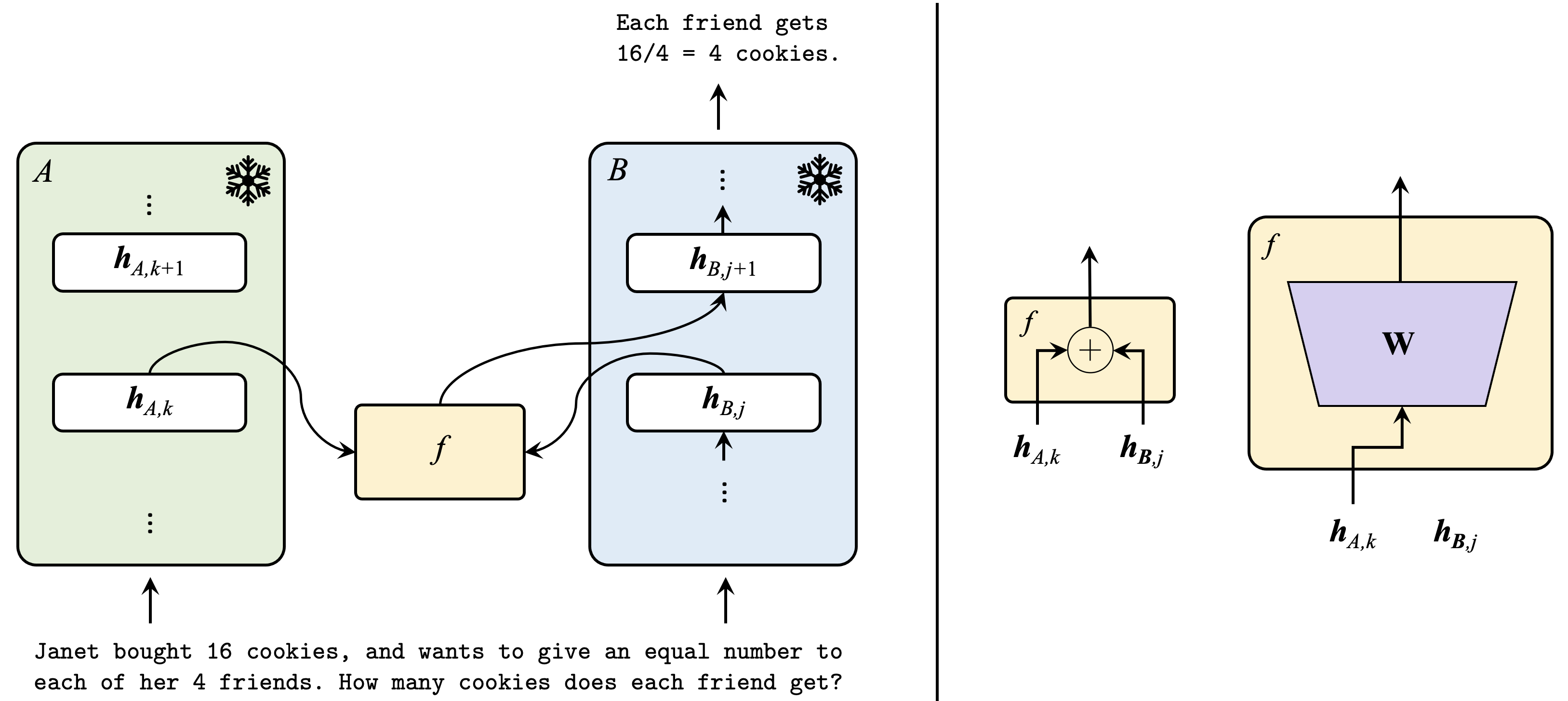</details> Figure 1: Overview of activation communication. (Left) Our method involves (1) pausing a Transformer LM $B$ ’s computation at layer $j$ in the residual stream; (2) combining its post-layer $j$ activation with another LM $A$ ’s post-layer $k$ activation via some function $f$ ; then (3) passing $f$ ’s output into the next layer $j+1$ of $B$ and continuing the forward pass till decoding is complete. (Right) Any function $f$ can be used to combine $A$ and $B$ ’s activations; we explore letting $f$ be the sum, mean, and replacement functions, as well as a task-agnostic learned linear layer (details in Section 3.1). We propose a simple yet effective technique whereby language models communicate via activations. We detail our approach in Section 3.1; provide analytical models of the compute saved over natural language communication in Section 3.2; and discuss the intuition behind this approach in Section 3.3. 3.1 Method Consider two language models, $A$ and $B$ , and some setting in which $B$ must perform a task where it would benefit from knowledge given to $A$ as a prompt/encoded in $A$ ’s weights (example settings in Section 4.1 / Section 4.2 respectively). We propose incorporating information from $A$ ’s post-layer $k$ activation $\bm{h}_{A,k}$ into $B$ ’s post-layer $j$ activation $\bm{h}_{B,j}$ (and vice versa, though for simplicity we henceforth only discuss the first direction) (Figure 1, left). More formally, suppose $A$ and $B$ (which have model dimensions $d_{A}$ and $d_{B}$ respectively) are given prompts $x_{A}$ and $x_{B}$ respectively, where $x_{A}$ is of length $t_{A}$ tokens and $x_{B}$ is of length $t_{B}$ tokens. We first run a partial forward pass of $B$ until layer $j$ (henceforth denoted $B_{≤ j}(x_{B})$ ) to get $\bm{h}_{B,j}∈\mathbb{R}^{t_{B}× d_{B}}$ . Then we (1) run a partial forward pass of $A$ until layer $k$ to get $A_{≤ k}(x_{1}):=\bm{h}_{A,k}∈\mathbb{R}^{t_{A}× d_{A}}$ ; (2) replace the activation of the last token $(\bm{h}_{B,j})_{t_{B}}∈\mathbb{R}^{d_{B}}$ $\longleftarrow f((\bm{h}_{A,k})_{t_{A}},(\bm{h}_{B,j})_{t_{B}})$ for some function $f:\mathbb{R}^{d_{A}+d_{B}}→\mathbb{R}^{d_{B}}$ ; then (3) continue $B$ ’s forward pass till decoding is complete, resulting in an output $y=B_{>k}(\bm{h}_{B,j})$ . Let $\bm{a}=(\bm{h}_{A,k})_{t_{A}}$ , $\bm{b}=(\bm{h}_{B,j})_{t_{B}}$ . For sake of simplicity assume $d_{A}=d_{B}$ . When $d_{A}≠ d_{B}$ , the $\mathtt{sum}$ , $\mathtt{mean}$ , and $\mathtt{replace}$ functions are defined as follows. Let $d=\min(d_{A},d_{B})$ and $\circ$ the concatenation operator. Then $f(\bm{a},\bm{b})=\bm{b}_{1:\max(d_{B}-d,0)}\circ\left(\bm{b}_{\max(d_{B}-d,0)+% 1:d_{B}}+\bm{a}_{\max(d_{A}-d,0)+1:d_{A}}\right)$ $\mathtt{(sum)}$ , $f(\bm{a},\bm{b})=\bm{b}_{1:\max(d_{B}-d,0)}\circ\frac{1}{2}\left(\bm{b}_{\max(% d_{B}-d,0)+1:d_{B}}+\bm{a}_{\max(d_{A}-d,0)+1:d_{A}}\right)$ $\mathtt{(mean)}$ , and $f(\bm{a},\bm{b})=\bm{b}_{1:\max(d_{B}-d,0)}\circ\bm{a}_{\max(d_{A}-d,0)+1:d_{A}}$ $\mathtt{(replace)}$ . We consider three non-learned functions $f$ : | | $\displaystyle f(\bm{a},\bm{b})$ | $\displaystyle=\bm{a}+\bm{b}\>\>\qquad\qquad\mathtt{(sum)}$ | | | --- | --- | --- | --- | For cases where, due to differences in $A$ and $B$ ’s training, $A$ and $B$ ’s activation spaces are quite different, we propose learning a task-agnostic (depends only on the models $A$ and $B$ ) linear layer $\bm{W}∈\mathbb{R}^{d_{B}}×\mathbb{R}^{d_{A}}$ that projects $\bm{a}$ onto $B$ ’s activation space. Note that this introduces zero additional task-specific parameters and data, as we propose learning this “mapping matrix” $\bm{W}$ only once for each model pair $(A,B)$ using general text, e.g. sequences from $A$ and/or $B$ ’s pretraining data mixes. We can then perform $\mathtt{sum}$ , $\mathtt{mean}$ , or $\mathtt{replace}$ with $\bm{W}\bm{a},\bm{b}$ instead of $\bm{a},\bm{b}$ . We propose training $\bm{W}$ to minimize MSE loss over a dataset of $N$ sentences $$ \mathcal{L}_{\rm MSE}\left(\{\bm{y}^{(i)}\}_{i=1}^{N},\{\bm{z}^{(i)}\}_{i=1}^{% N}\right)=\frac{1}{N}\sum_{i=1}^{N}\left\|\bm{z}^{(i)}-\bm{W}\bm{y}^{(i)}% \right\|_{2}^{2} $$ where each $(\bm{y}^{(i)},\bm{z}^{(i)})$ pair denotes the final-token layer- $26$ activations of $A$ and $B$ at layers $k$ and $j$ respectively given the same sentence as input. 3.2 Compute Analysis To understand the significance of activation communication, we must formally quantify the compute this procedure saves over natural language communication. For simplicity suppose the following (similar calculations can be made for the cases where $A$ and $B$ have differing model architectures and/or are given different prompts): - $A$ and $B$ both have $L$ layers (each with $H$ attention heads, key size $K$ , and feedforward size $F$ ), dimension $D$ , and vocab size $V$ - $A$ and $B$ are both given a prompt of $P$ tokens - $A$ can send $B$ a single $M$ -token message - $B$ must produce an output of $T$ tokens, given its prompt and $A$ ’s message Traditional methods require $M$ forward passes of $A$ given a $P$ -length input, plus $T$ forward passes of $B$ given a $(P+M)$ -length input. Following Hoffmann et al. (2022), this requires $$ \displaystyle M\big{(}4PVD+L(8PDKH+4P^{2}KH+3HP^{2} \displaystyle+4PDF)\big{)}+T\big{(}4(P+M)VD+L(8(P+M)DKH \displaystyle+4(P+M)^{2}KH+3H(P+M)^{2}+4(P+M)DF)\big{)} \tag{1} $$ FLOPs. In contrast, at inference time, our method requires only 1 partial (up till the $k$ th layer) forward pass of $A$ given a $P$ -length input, $T$ forward passes of $B$ given a $P$ -length input, and the activation replacement procedure. This requires $$ \displaystyle 2PVD+k(8PDKH+4P^{2}KH+3HP^{2} \displaystyle+4PDF)+T\big{(}4PVD+L(8PDKH+4P^{2}KH \displaystyle+3HP^{2}+4PDF)\big{)}+\mathcal{F}(D) \tag{2} $$ FLOPs, where $\mathcal{F}(D)=O(D)$ for non-learned $f$ and $O(D^{2})$ when $f$ is the mapping matrix. In all practical cases, (2) is substantially lower than (1). 3.3 Why should this work? Recall that Pham et al. (2024) propose CIPHER—communicating the average tokenizer embedding (weighted by the LLM’s next-token probabilities) between models. We build upon the intuition behind CIPHER, which goes as follows: the token sampling process during decoding risks substantial information loss from the model’s output logits, and communicating a model’s weighted-average tokenizer embedding essentially entails communicating both that model’s final answer and its belief in that answer (over the entire vocabulary). Communicating activations, then, can be thought of as communicating a strict superset of {next-token prediction, belief over entire vocabulary}, as activations of late-enough layers essentially encode the model’s entire knowledge about the provided context as well as its predicted completion and confidence in that completion (see Figures 1 and 7 in Hewitt & Manning (2019) and Hernandez et al. (2024), respectively, which show that linear probes tasked with predicting certain output characteristics from a Transformer’s intermediate layer embeddings of its input work poorly for early layers, extremely well after around the halfway point of computation, but then probe accuracy drops closer to the final layers). Note one important critique of multiagent debate: that in cases where multiple agents are uncertain about the answer, there is no reason why referencing other agents’ answers would generate more factual reasoning. Both CIPHER and activation communication solve this problem, as some notion of model confidence is being communicated along with its next-token prediction. Indeed, these curves of probe accuracy by layer indicate that the final layers and LM head “ throw away ” information not useful for next-token prediction that very well could be useful for communicative purposes; this is precisely why our proposed activation communication technique is not an iterative approach (there is no notion of “rounds” like in debate and CIPHER, which require an additional token budget to extract more and more information out of the LM), as one activation grafting step from $A$ to $B$ inherently communicates to $B$ all of $A$ ’s knowledge/beliefs about the prompt it was given. Moreover, the extra information over the model’s next-token prediction and confidence that is encoded in its activations is what makes activation communication more performant than its natural language counterpart, as we will see in Section 4. 4 Experiments | Countries | $x_{A}$ : “ $\mathtt{Alice}$ $\mathtt{is}$ $\mathtt{at}$ $\mathtt{the}$ $\mathtt{Acropolis}$ $\mathtt{of}$ $\mathtt{Athens}$ .” | | --- | --- | | $x_{B}$ : “ $\mathtt{Which}$ $\mathtt{country}$ $\mathtt{is}$ $\mathtt{Alice}$ $\mathtt{located}$ $\mathtt{in?}$ ” | | | $B$ ’s Expected Answer: “ $\mathtt{Greece}$ ” | | | Tip Sheets | $x_{A}$ : “ $\mathtt{Acme}$ $\mathtt{Inc.}$ $\mathtt{has}$ $\mathtt{taken}$ $\mathtt{a}$ $\mathtt{nosedive,}$ $\mathtt{as}$ $\mathtt{its}$ $\mathtt{quarterly}$ $\mathtt{earnings}$ $\mathtt{have}$ $\mathtt{dipped}$ $\mathtt{8\%}$ . | | $\mathtt{Meanwhile}$ $\mathtt{Doe}$ $\mathtt{LLC}$ $\mathtt{and}$ $\mathtt{Kiteflyer}$ $\mathtt{Labs}$ $\mathtt{have}$ $\mathtt{both}$ $\mathtt{reached}$ $\mathtt{record\text{-}high}$ $\mathtt{stock}$ | | | $\mathtt{prices}$ $\mathtt{of}$ $\mathtt{89,}$ $\mathtt{but}$ $\mathtt{Kiteflyer}$ $\mathtt{is}$ $\mathtt{involved}$ $\mathtt{in}$ $\mathtt{an}$ $\mathtt{IP}$ $\mathtt{lawsuit}$ $\mathtt{with}$ $\mathtt{its}$ $\mathtt{competitors.}^{\prime\prime}$ | | | $x_{B}$ : “ $\mathtt{You}$ $\mathtt{must}$ $\mathtt{invest}$ $\mathtt{in}$ $\mathtt{one}$ $\mathtt{company}$ $\mathtt{out}$ $\mathtt{of}$ { $\mathtt{Acme}$ $\mathtt{Inc.,}$ $\mathtt{Doe}$ $\mathtt{LLC,}$ $\mathtt{Kiteflyer}$ $\mathtt{Labs}$ }. | | | $\mathtt{Which}$ $\mathtt{do}$ $\mathtt{you}$ $\mathtt{invest}$ $\mathtt{in?}$ ” | | | $B$ ’s Expected Answer: “ $\mathtt{Doe\text{ }LLC}$ ” | | Table 1: Multi-player coordination games. Sample $\mathtt{(prompt,answer)}$ pairs for each game. We test our method on two distinct experimental setups: multi-player coordination games (Section 4.1) and reasoning benchmarks (Section 4.2). Qualitative results are available in Appendix A. 4.1 Multi-player coordination games Drawing from existing literature on multi-agent communication, we design two Lewis signaling games (Lewis, 2008; Lazaridou et al., 2016) to test the efficacy of activation communication (example prompts and answers in Table 1): 1. Countries, where $A$ is given as input a string of the format “ $\mathtt{[PERSON]\text{ }is\text{ }at\text{ }the\text{ }[LANDMARK]}$ ” and $B$ is asked “ $\mathtt{Which\text{ }country\text{ }is\text{ }[PERSON]\text{ }located\text{ }% in?}$ ” 1. Tip Sheets (inspired by Lewis et al. (2017)), where $A$ is given a simulated “tip sheet” and $B$ is asked to make an informed investment decision in accordance with the information in the tip sheet. | $\mathtt{LLaMA}$ - $\mathtt{3.2}$ - $\mathtt{3B}$ | ✗ | $0.0$ ( $0.0$ , $0.0$ ) | $38.6$ ( $38.6,39.4$ ) | | --- | --- | --- | --- | | Skyline | $84.0$ ( $83.5$ , $84.1$ ) | $100.0$ ( $100.0,100.0$ ) | | | NL | $69.0$ ( $68.7$ , $69.3$ ) | $74.3$ ( $74.0,74.6$ ) | | | AC ( $\mathtt{sum}$ ) | $34.0$ ( $33.9$ , $34.4$ ) | $50.0$ ( $49.6,50.3$ ) | | | AC ( $\mathtt{mean}$ ) | $36.0$ ( $35.5$ , $36.1$ ) | $80.0$ ( $79.8,80.4$ ) | | | AC ( $\mathtt{replace}$ ) | $\mathbf{78.0}$ ( $77.7$ , $78.2$ ) | $\mathbf{90.0}$ ( $89.9,90.3$ ) | | | $\mathtt{LLaMA}$ - $\mathtt{3.1}$ - $\mathtt{8B}$ | ✗ | $2.0$ ( $1.9$ , $2.1$ ) | $54.3$ ( $54.2,54.5$ ) | | Skyline | $86.0$ ( $85.7$ , $86.1$ ) | $100.0$ ( $100.0,100.0$ ) | | | NL | $77.0$ ( $76.6$ , $77.1$ ) | $85.7$ ( $85.3,85.8$ ) | | | AC ( $\mathtt{sum}$ ) | $71.0$ ( $70.9,71.4$ ) | $85.7$ ( $85.5,86.0$ ) | | | AC ( $\mathtt{mean}$ ) | $70.0$ ( $69.7,70.3$ ) | $92.9$ ( $92.7,93.1$ ) | | | AC ( $\mathtt{replace}$ ) | $\mathbf{83.0}$ ( $82.7,83.1$ ) | $\mathbf{95.7}$ ( $95.6,95.9$ ) | | Table 2: Accuracies (%) on both coordination games using two identical $\mathtt{LLaMA}$ family models. Communication at layer $k=j=26.$ $95\%$ confidence intervals ( $1000$ bootstrap iterations) reported in parentheses. We synthetically generate $100$ (Countries) and $70$ (Tip Sheets) different prompts and answers of the same format as the samples in Table 1, and report the proportion out of those samples that $B$ responds with an exact string match to the ground truth answer. As baselines, we consider a “silent” (✗) setup, where the agents are not allowed to communicate; a “single-agent skyline,” where a single LLM is given the concatenation of $A$ and $B$ ’s prompts; and traditional natural language communication, where $A$ is asked to output a message that is then given to $B$ along with $x_{B}$ . All decoding is done greedily. Table 2 presents the results for both coordination games using 2 different instances of the same model as the agents ( $A=B$ ). Across the 3B and 8B model sizes, activation communication (AC) with $f=\mathtt{replace}$ almost completely recovers the gap between the zero-communication (✗) and the single-agent skyline (Skyline), outperforming natural language communication (NL) using far less compute. We hypothesize that $\mathtt{replace}$ is more effective than $\mathtt{mean}$ and $\mathtt{sum}$ as the former is guaranteed to output a vector within $B$ ’s activation space, while the latter two likely do not (e.g., the norm of the vector outputted by $\mathtt{sum}$ will be around double that of a typical activation). Furthermore, most of the information $B$ needs is likely contained in its representations of previous tokens in the sequence, hence losing its final-token representation does not hurt. <details> <summary>extracted/6420159/contour.png Details</summary>  ### Visual Description ## Heatmap: Accuracy Analysis Across Countries and Tip Sheets ### Overview The image presents two side-by-side heatmaps comparing accuracy percentages (Acc. (%)) across two variables: **k** (x-axis) and **j** (y-axis). Each panel represents a different context: **(a) Countries** and **(b) Tip Sheets**. Both heatmaps use a color gradient from dark purple (0%) to yellow (100%) to indicate accuracy levels, with contour lines marking thresholds. A red diamond highlights a specific data point in each panel. --- ### Components/Axes 1. **Axes**: - **x-axis (k)**: Ranges from 5 to 30 in both panels. - **y-axis (j)**: Ranges from 5 to 30 in both panels. - **Color Scale**: Accuracy (%) from 0% (dark purple) to 100% (yellow), with intermediate thresholds (20%, 40%, 60%, 80%). 2. **Legends**: - Located on the right of each panel. - Gradient bar labeled "Acc. (%)" with numerical thresholds. 3. **Annotations**: - Red diamond markers in both panels: - **(a) Countries**: Positioned at **k=25, j=25**. - **(b) Tip Sheets**: Positioned at **k=25, j=20**. --- ### Detailed Analysis #### **(a) Countries Panel** - **Color Distribution**: - Dominated by dark purple (low accuracy) in the bottom-left quadrant (k=5–15, j=5–15). - Gradual transition to yellow (high accuracy) in the top-right quadrant (k=20–30, j=20–30). - Contour lines indicate sharp transitions in accuracy near the red diamond (k=25, j=25). - **Red Diamond**: - Located at **k=25, j=25**, where accuracy reaches ~80% (yellow region). - Surrounded by contour lines suggesting a local peak in accuracy. #### **(b) Tip Sheets Panel** - **Color Distribution**: - Mixed gradients: Dark purple (low accuracy) in the top-left (k=5–15, j=25–30) and bottom-right (k=20–30, j=5–15). - Yellow (high accuracy) dominates the central region (k=10–25, j=10–25). - Contour lines show irregular boundaries, indicating variable accuracy. - **Red Diamond**: - Located at **k=25, j=20**, where accuracy is ~60% (orange region). - Positioned near a contour line threshold (~60%), suggesting moderate accuracy. --- ### Key Observations 1. **Accuracy Peaks**: - **(a) Countries**: Highest accuracy (~80%) at **k=25, j=25**. - **(b) Tip Sheets**: Highest accuracy (~80%) in the central region, but the red diamond (k=25, j=20) shows only ~60% accuracy. 2. **Regional Variability**: - **(a) Countries**: Clear gradient from low to high accuracy. - **(b) Tip Sheets**: Fragmented accuracy patterns, with no single dominant peak. 3. **Red Diamond Placement**: - In **(a)**, the diamond aligns with a high-accuracy zone. - In **(b)**, the diamond is in a moderate-accuracy zone, despite the central region having higher accuracy. --- ### Interpretation The data suggests that **optimal combinations of k and j** differ between countries and tip sheets: - For **countries**, the red diamond at **k=25, j=25** represents a high-accuracy configuration, likely due to systematic factors (e.g., resource allocation, policy alignment). - For **tip sheets**, the red diamond at **k=25, j=20** indicates a suboptimal configuration, as the central region (k=10–25, j=10–25) shows higher accuracy. This could reflect contextual mismatches (e.g., tip sheets being less adaptable to variable conditions). The contour lines highlight **non-linear relationships** between k and j, emphasizing that accuracy is not uniformly distributed. The stark contrast between the two panels underscores the importance of context-specific optimization. 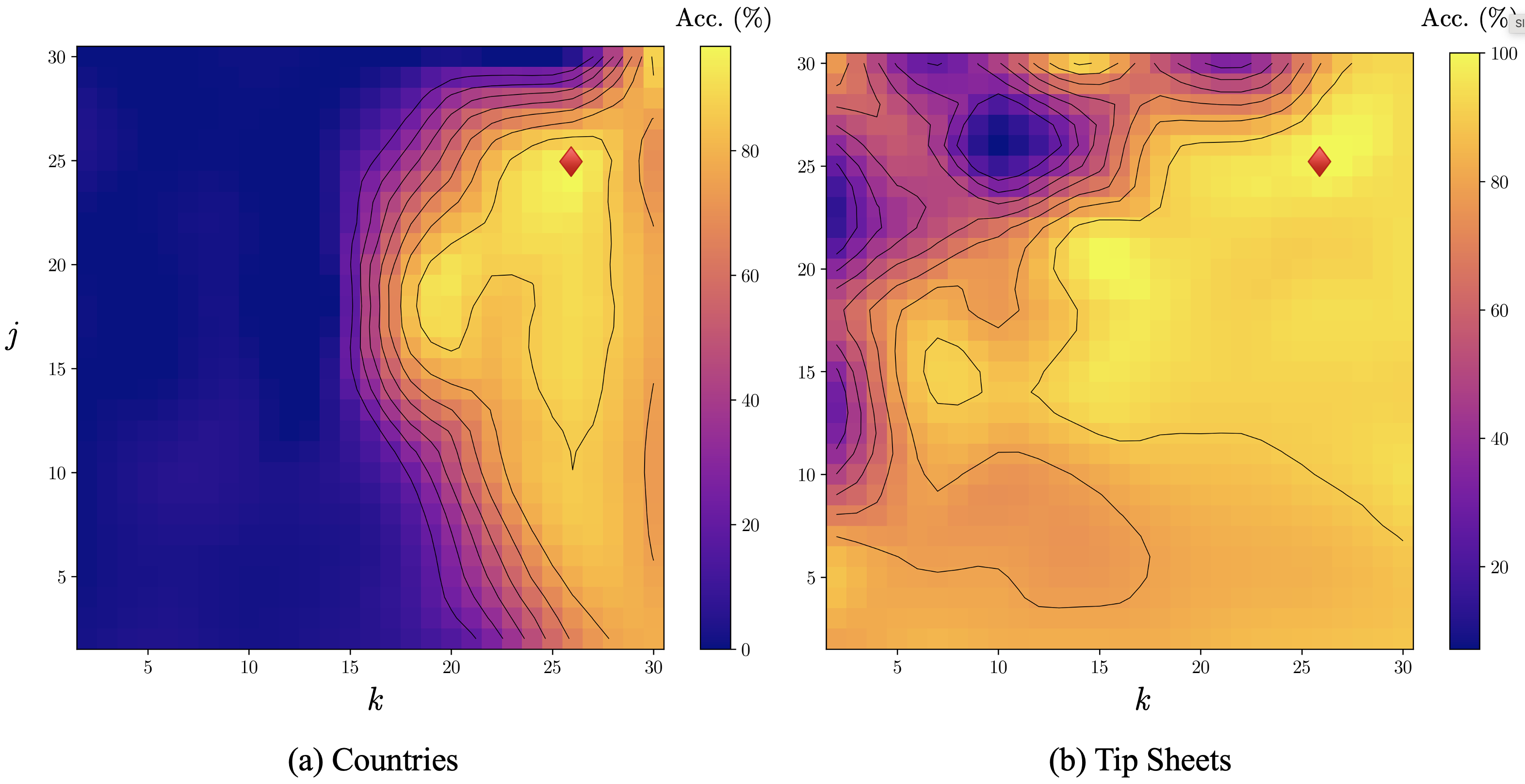</details> Figure 2: 2D contour plots of accuracy over different values of $k$ and $j$ (the layers at which we access/edit activations for $A$ / $B$ respectively). $k=j=26$ is roughly optimal ( $$ ) for both (a) Countries and (b) Tip Sheets. 4.2 Reasoning Benchmarks Next, we test our methods on a variety of reasoning benchmarks, spanning several real-world tasks and domains. Baselines We benchmark activation communication against the following two baselines: - Single Model: A single LLM responds to the prompt in natural language. - Natural Language Debate (NLD) (Du et al., 2023): Each LLM provides an initial response to the given prompt. Then, for each of $r-1$ subsequent rounds, each LLM is prompted to refine its previous response given the other agents’ responses as input. Note that NLD is the most direct baseline for our approach, as it is a state-of-the-art natural language communication protocol. We fix $r=2$ in our experiments. Note that we do not compare to Pham et al. (2024), as they communicate the input (tokenizer) embeddings rather than activations/output embeddings between models, and hence require a shared tokenizer and embedding table between agents which is extremely restrictive and prevents applicability to our experimental setup. To determine the values of $k$ and $j$ for activation communication (AC), we compute the accuracy on Countries and Tip Sheets for every pair $(k,j)∈\{1,...,30\}^{2}$ . Based on these results (shown in Figure 2) as well as Table 2, we fix $k=j=26$ and $f$ $=$ $\mathtt{replace}$ for the following experiments. Across all experiment configurations, we fix the decoding strategy to nucleus sampling with $p=0.9$ . Models We conduct most of our experiments using $\mathtt{LLaMA}$ - $\mathtt{3.2}$ - $\mathtt{3B}$ and $\mathtt{LLaMA}$ - $\mathtt{3.1}$ - $\mathtt{8B}$ as the two agents. Additionally, to test our approach’s robustness and generalizability, we conduct experiments with models belonging to various other suites within the $\mathtt{LLaMA}$ family and of several different sizes. Note that for these experiments, we restrict the setting to communication between different models (rather than multiple instances of the same model in Section 4.1), since the same model would have identical activations for the same prompts, meaning no information would be communicated in the grafting process. We argue that the multiple-model setting is realistic (perhaps more so than the setting of multiple instances of the same model), as recent advances in LLM development have led to the release of models with specialized abilities (Singhal et al., 2023) and of different sizes (Dubey et al., 2024) that merit complementary usage. Our work thus answers the question: How can we get the best performance by leveraging multiple models of distinct capabilities and sizes, relative to the added inference-time compute over a single forward pass through any single model? Datasets We evaluate our technique on seven reasoning datasets that span various real-world tasks and domains: (i) Biographies (Du et al., 2023), which asks the LLM to generate a factual biography of a famous computer scientist; (ii) GSM8k (Cobbe et al., 2021), a variety of grade school math problems created by human problem writers; and (iii) 5 datasets randomly drawn from MMLU (Hendrycks et al., 2021): High School Psychology (from the Social Sciences category), Formal Logic (from the Humanities category), College Biology (from the STEM category), Professional Law (from the Humanities Category), and Public Relations (from the Social Sciences category). We evaluate on a randomly-sampled size- $100$ subset of each dataset. In experiments involving the mapping matrix $\bm{W}$ , we instantiate $\bm{W}∈\mathbb{R}^{4096× 3072}$ using Xavier initialization and train for $10$ epochs on a dataset of $3072$ sentences We use $3072$ sentences as linear regression with $d$ -dimensional input has a sample complexity of $O(d)$ (Vapnik, 1999). randomly drawn from the Colossal Clean Crawled Corpus (C4) (Dodge et al., 2021). We use batch size $32$ and the Adam optimizer with learning rate $0.001$ . Metrics We measure the accuracy of the final response for the single models and AC. For NLD, we measure the accuracy of the majority-held final-round answer across agents when the answer is automatically verifiable (numeric in GSM8k, multiple choice for the MMLU datasets) or the average final-round answer across agents otherwise (Biographies). For GSM8k and the MMLU datasets, we report the proportion of samples in the dataset for which the generated answer exactly matches the ground-truth answer. For Biographies, following Du et al. (2023), we prompt an LLM judge ( $\mathtt{LLaMA}$ - $\mathtt{3.1}$ - $\mathtt{8B}$ ) to check whether each manually-decomposed fact in a ground-truth biography is supported ( $1$ ), partially supported ( $0.5$ ), or unsupported ( $0 0$ ) in the generated biography, taking the mean of these scores over all facts as the per-biography accuracy and the mean over all dataset samples as the total accuracy. | $\mathtt{3.2}$ - $\mathtt{3B}$ $\mathtt{3.1}$ - $\mathtt{8B}$ NLD | $79.4$ $± 0.0$ $83.9$ $± 0.0$ $80.2$ $± 0.1$ | $58.0$ $± 4.9$ $60.0$ $± 4.9$ $\mathbf{75.0}$ $± 4.3$ | $30.0$ $± 1.0$ $65.0$ $± 0.1$ $83.0$ $± 0.8$ | $16.0$ $± 0.8$ $42.0$ $± 0.1$ $37.0$ $± 0.1$ | $11.0$ $± 0.7$ $50.0$ $± 0.2$ $71.0$ $± 0.1$ | $0.0$ $± 0.0$ $20.0$ $± 0.8$ $30.0$ $± 0.1$ | $26.0$ $± 0.1$ $53.0$ $± 0.2$ $63.0$ $± 0.7$ | | --- | --- | --- | --- | --- | --- | --- | --- | | AC | $84.6$ $± 0.0$ | $64.0$ $± 4.8$ | $\mathbf{85.0}$ $± 0.8$ | $\mathbf{47.0}$ $± 0.1$ | $78.0$ $± 0.9$ | $30.0$ $± 0.1$ | $\mathbf{74.0}$ $± 0.1$ | | AC ( $\bm{W}$ ) | $\mathbf{86.8}$ $± 0.0$ | $66.0$ $± 4.8$ | $70.0$ $± 0.1$ | $35.0$ $± 0.1$ | $\mathbf{79.0}$ $± 0.9$ | $\mathbf{45.0}$ $± 0.1$ | $63.0$ $± 0.1$ | Table 3: Accuracies (%) on all seven reasoning benchmarks. NLD and all AC variants involve communication between $\mathtt{LLaMA}$ - $\mathtt{3.2}$ - $\mathtt{3B}$ ( $A$ ) and $\mathtt{LLaMA}$ - $\mathtt{3.1}$ - $\mathtt{8B}$ ( $B$ ); the performance of these models individually are presented in the first two rows of the table. NLD typically improves performance over at least one of the single model baselines; AC— both with and without the task-agnostic linear layer—consistently beats both baselines and NLD as well. Comprehensive evaluation with the $\mathtt{LLaMA}$ family Table 3 presents results on each of the seven reasoning benchmarks across various baselines and activation communication. Notably, while NLD consistently outperforms $\mathtt{LLaMA}$ - $\mathtt{3.2}$ - $\mathtt{3B}$ , it does not always display a performance improvement over $\mathtt{LLaMA}$ - $\mathtt{3.1}$ - $\mathtt{8B}$ ; but remarkably, AC consistently outperforms both single-model baselines. In fact, AC offers an up to $27.0\%$ improvement over NLD across six of the seven reasoning datasets. When applying $\bm{W}$ to $A$ ’s activation before performing the replacement function, we see even further gains of $2.6-50.0\%$ over vanilla AC for four of the seven datasets. We hypothesize that the benefits from the learned linear layer are less consistent across datasets because the subset of C4 data used to train $\bm{W}$ likely contains text more semantically similar to some datasets than others, hence some datasets provide $\bm{W}$ with out-of-distribution inputs which reduces performance compared to vanilla AC. While we fix $A$ as the smaller model and $B$ as the larger model in Table 3 (so as to ensure decoding happens with the presumably more capable model), this need not be the case; swapping $A$ and $B$ yields results of $81.5± 0.0$ and $61.0± 4.8$ on Biographies and GSM8k respectively (without the linear layer). While these accuracies are lower than their non-swapped counterparts, notably they still are higher than both single-model baselines (and higher than NLD for Biographies); plus this is much more compute-efficient as the smaller model is now the one requiring the full instead of partial forward pass. Note that we find AC outperforms NLD on 48 of the 57 datasets in the full MMLU benchmark; complete MMLU results, as well as a suite of additional experiments, are shown in Appendix B. 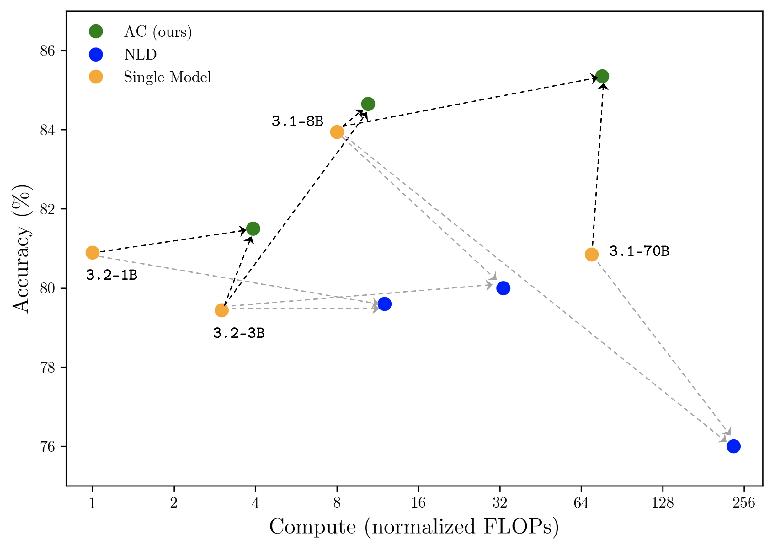Performance-compute tradeoff and generalization to different model scales Thus far, we have been considering the absolute performance of AC with respect to NLD, for which our method attains state-of-the-art results; however the superiority of activations as a language for inter-LLM communication is further illustrated by AC’s larger ratio of performance improvement to added inference-time compute over individual LMs. Figure 3 displays the results of single models, AC, and NLD across model scales and suites within the $\mathtt{LLaMA}$ family on the Biographies dataset. Incoming arrows to AC and NLD nodes denote the base models between which communication occurred. Not only does AC consistently outperform both single-model baselines unlike NLD, but also notice that the slope of each black line is far greater than the slope of each gray line, indicating that AC consistently achieves greater increases in accuracy per additional unit of inference-time compute (normalized by the compute of a single forward pass through $\mathtt{LLaMA}$ - $\mathtt{3.2}$ - $\mathtt{1B}$ on the given prompt) compared to NLD. Communication across model families Table 4 displays results for AC between models from the $\mathtt{Qwen}$ - $\mathtt{2.5}$ , $\mathtt{Gemma}$ - $\mathtt{2}$ , and $\mathtt{LLaMA}$ - $\mathtt{3}$ families. We see that AC beats NLD across the board, and beats both individual models for $4/5$ of the $6$ model pairs on Biographies/GSM8k respectively —demonstrating the efficacy of AC irrespective of model architecture, size, tokenizer, and training data. Moreover, these results are obtained without training $\bm{W}$ , meaning we do not need a separate projection layer between activation spaces to attain SOTA results, even for extremely distinct models! (We hypothesize this is because we are only replacing $B$ ’s last-token activation, hence $B$ can learn from $A$ without an extreme alteration to its activation distribution. An alternative explanation is to see this result as proof of the platonic representation hypothesis (Huh et al., 2024), which historical deep learning works have oft alluded to, including in the context of cross-model representation stitching (Moschella et al., 2023; Kornblith et al., 2019).) | $\mathtt{LLaMA}$ - $\mathtt{3.2}$ - $\mathtt{3B}$ , $\mathtt{LLaMA}$ - $\mathtt{3.1}$ - $\mathtt{8B}$ $\mathtt{Qwen}$ - $\mathtt{2.5}$ - $\mathtt{1.5B}$ , $\mathtt{Qwen}$ - $\mathtt{2.5}$ - $\mathtt{3B}$ $\mathtt{Gemma}$ - $\mathtt{2}$ - $\mathtt{2B}$ , $\mathtt{Gemma}$ - $\mathtt{2}$ - $\mathtt{9B}$ | $79.4$ $± 0.0$ / $58.0$ $± 4.9$ $59.4$ $± 0.9$ / $20.0$ $± 0.9$ $83.0$ $± 1.1$ / $45.0$ $± 1.1$ | $83.9$ $± 0.0$ / $60.0$ $± 4.9$ $85.5$ $± 1.1$ / $35.0$ $± 1.1$ $\mathbf{94.6}$ $± 0.9$ / $80.0$ $± 0.9$ | $80.2$ $± 0.1$ / $\mathbf{75.0}$ $± 4.3$ $63.2$ $± 1.1$ / $65.0$ $± 1.1$ $70.3$ $± 1.0$ / $70.0$ $± 1.0$ | $\mathbf{84.6}$ $± 0.0$ / $64.0$ $± 4.8$ $\mathbf{89.6}$ $± 1.0$ / $\mathbf{70.0}$ $± 1.0$ $88.1$ $± 0.7$ / $\mathbf{90.0}$ $± 0.7$ | | --- | --- | --- | --- | --- | | $\mathtt{Qwen}$ - $\mathtt{2.5}$ - $\mathtt{1.5B}$ , $\mathtt{LLaMA}$ - $\mathtt{3.2}$ - $\mathtt{3B}$ | $59.4$ $± 0.9$ / $20.0$ $± 0.9$ | $79.4$ $± 0.0$ / $58.0$ $± 4.9$ | $75.4$ $± 1.0$ / $\mathbf{75.0}$ $± 1.0$ | $\mathbf{79.5}$ $± 1.0$ / $75.0$ $± 1.0$ | | $\mathtt{LLaMA}$ - $\mathtt{3.2}$ - $\mathtt{3B}$ , $\mathtt{Gemma}$ - $\mathtt{2}$ - $\mathtt{2B}$ | $79.4$ $± 0.0$ / $58.0$ $± 4.9$ | $83.0$ $± 1.1$ / $45.0$ $± 1.1$ | $62.5$ $± 1.1$ / $55.0$ $± 1.1$ | $\mathbf{84.0}$ $± 0.1$ / $\mathbf{60.0}$ $± 1.1$ | | $\mathtt{Qwen}$ - $\mathtt{2.5}$ - $\mathtt{1.5B}$ , $\mathtt{Gemma}$ - $\mathtt{2}$ - $\mathtt{2B}$ | $59.4$ $± 0.9$ / $20.0$ $± 0.9$ | $\mathbf{83.0}$ $± 1.1$ / $45.0$ $± 1.1$ | $49.3$ $± 1.1$ / $50.0$ $± 1.1$ | $73.0$ $± 1.1$ / $\mathbf{55.0}$ $± 1.1$ | Table 4: Individual model, AC, and NLD accuracies across three model families. Each cell displays two values: Biographies score / GSM8k score. <details> <summary>extracted/6420159/TODO.png Details</summary>  ### Visual Description ## Scatter Plot: Model Accuracy vs. Compute Efficiency ### Overview The image is a scatter plot comparing the accuracy (in %) of three model configurations (AC, NLD, Single Model) against their computational cost (normalized FLOPs). The plot uses dashed lines to connect data points for each model, illustrating trends in performance relative to compute resources. ### Components/Axes - **X-axis (Compute)**: Normalized FLOPs, ranging from 1 to 256 (logarithmic scale). - **Y-axis (Accuracy)**: Percentage accuracy, ranging from 76% to 86%. - **Legend**: - Green: AC (ours) - Blue: NLD - Orange: Single Model - **Data Points**: Labeled with model configurations (e.g., "3.2-1B", "3.1-8B") and connected by dashed lines. ### Detailed Analysis #### AC (Ours) [Green] - **3.2-1B**: 4 FLOPs, 81.5% accuracy. - **3.1-8B**: 8 FLOPs, 84.2% accuracy. - **3.1-70B**: 64 FLOPs, 85.3% accuracy. - **Trend**: Steady upward trajectory as compute increases. #### NLD [Blue] - **3.2-3B**: 8 FLOPs, 79.5% accuracy. - **3.1-70B**: 64 FLOPs, 76.8% accuracy. - **3.2-1B**: 4 FLOPs, 80.1% accuracy. - **Trend**: Slight decline in accuracy with increased compute (e.g., 80.1% → 79.5% → 76.8%). #### Single Model [Orange] - **3.2-1B**: 4 FLOPs, 80.5% accuracy. - **3.2-3B**: 8 FLOPs, 79.2% accuracy. - **3.1-70B**: 64 FLOPs, 80.8% accuracy. - **Trend**: Minimal fluctuation, maintaining ~80% accuracy across compute levels. ### Key Observations 1. **AC (Ours)** achieves the highest accuracy (85.3%) at 64 FLOPs, outperforming other models at higher compute levels. 2. **NLD** shows a notable drop in accuracy (from 80.1% to 76.8%) as compute increases, suggesting inefficiency or overfitting. 3. **Single Model** maintains stable accuracy (~80%) but lags behind AC in performance. 4. **Compute vs. Accuracy**: AC demonstrates the best trade-off, achieving higher accuracy with relatively low compute (e.g., 84.2% at 8 FLOPs). ### Interpretation The data highlights the superiority of the AC model (ours) in balancing accuracy and computational efficiency. NLD's declining performance with increased compute suggests potential architectural limitations or suboptimal scaling. The Single Model serves as a baseline, but AC consistently outperforms it. The plot underscores the importance of model design in optimizing resource utilization, with AC achieving state-of-the-art results without excessive computational overhead. </details> Figure 3: Accuracy (%) vs. compute (# FLOPs normalized by single $\mathtt{LLaMA}$ - $\mathtt{3.2}$ - $\mathtt{1B}$ forward pass) for various configurations of AC and NLD on the Biographies dataset. AC () yields the greatest performance gains per additional unit of inference-time compute over each baseline (). 5 Conclusion We present a simple approach to enable effective and computationally efficient communication between language models by injecting information from the activations of one model into the activations of another during the forward pass. Salient features of this approach include: (i) Scales up LLMs on new tasks by leveraging existing, frozen LLMs along with zero additional task-specific parameters and data, (ii) Applies to diverse domains and settings, and (iii) Saves a substantial amount of compute. There are some limitations to this method. First, when not using the learned model-specific mapping discussed in Section 3.1, our method requires both models to have aligned embedding spaces, such that the activation of one model roughly retains its meaning in the other’s activation space (note that unlike past works such as Pham et al. (2024) we do not require shared tokenizers or aligned vocabularies, only aligned embeddings). While less restrictive than past works (Pham et al., 2024), this assumption is somewhat limiting, but can be relaxed when we let $f$ be the learned model-specific mapping; and in practice we find that even amongst different models in the $\mathtt{LLaMA}$ family, no such mapping is required for state-of-the-art results. Second, this method requires access to embeddings and will not work with black-box API access; however exploring API-only approaches is highly limiting, and recent releases of powerful open-source models (Dubey et al., 2024) merit the development of embedding-based techniques. Third, while a concern might be the limited interpretability of communicating activations as opposed to natural language, we note the following. First, there is a fundamental tradeoff between interpretability and information preservation (as activations, by virtue of being much higher-dimensional than the space of natural language, allow proportionally higher-entropy communication) (Pham et al., 2024), which merits discussion beyond the scope of this work. But second, we actually posit that our method suggests a new avenue towards interpreting LM activations: “translating” activations based on the beliefs they induce as messages in listening agents, similar to the method put forward in Andreas et al. (2018). We recognize this as a promising avenue for future research. Additional directions of future work include using AC to allow large LMs to leverage small, tunable LMs as “knowledge bases” during decoding (Lee et al., 2024), as in collaborative decoding (Shen et al., 2024) setups; and testing our approach on more complex coordination games (e.g., Lewis-style negotiation games (Lewis et al., 2017), Diplomacy). Impact Statement This paper presents work whose goal is to advance the field of Machine Learning. There are many potential societal consequences of our work, none which we feel must be specifically highlighted here. Acknowledgements The authors are grateful to Jacob Andreas, Yoon Kim, and Sham Kakade for their valuable discussions and feedback. References - Ahn et al. (2022) Ahn, M., Brohan, A., Brown, N., Chebotar, Y., Cortes, O., David, B., Finn, C., Fu, C., Gopalakrishnan, K., Hausman, K., Herzog, A., Ho, D., Hsu, J., Ibarz, J., Ichter, B., Irpan, A., Jang, E., Ruano, R. J., Jeffrey, K., Jesmonth, S., Joshi, N. J., Julian, R., Kalashnikov, D., Kuang, Y., Lee, K.-H., Levine, S., Lu, Y., Luu, L., Parada, C., Pastor, P., Quiambao, J., Rao, K., Rettinghouse, J., Reyes, D., Sermanet, P., Sievers, N., Tan, C., Toshev, A., Vanhoucke, V., Xia, F., Xiao, T., Xu, P., Xu, S., Yan, M., and Zeng, A. Do as i can, not as i say: Grounding language in robotic affordances, 2022. - Andreas et al. (2018) Andreas, J., Dragan, A., and Klein, D. Translating neuralese, 2018. - Bansal et al. (2024) Bansal, R., Samanta, B., Dalmia, S., Gupta, N., Vashishth, S., Ganapathy, S., Bapna, A., Jain, P., and Talukdar, P. Llm augmented llms: Expanding capabilities through composition, 2024. - Burns et al. (2023) Burns, C., Izmailov, P., Kirchner, J. H., Baker, B., Gao, L., Aschenbrenner, L., Chen, Y., Ecoffet, A., Joglekar, M., Leike, J., Sutskever, I., and Wu, J. Weak-to-strong generalization: Eliciting strong capabilities with weak supervision, 2023. - Chaabouni et al. (2019) Chaabouni, R., Kharitonov, E., Lazaric, A., Dupoux, E., and Baroni, M. Word-order biases in deep-agent emergent communication. In Korhonen, A., Traum, D., and Màrquez, L. (eds.), Proceedings of the 57th Annual Meeting of the Association for Computational Linguistics, pp. 5166–5175, Florence, Italy, July 2019. Association for Computational Linguistics. doi: 10.18653/v1/P19-1509. URL https://aclanthology.org/P19-1509. - Cobbe et al. (2021) Cobbe, K., Kosaraju, V., Bavarian, M., Chen, M., Jun, H., Kaiser, L., Plappert, M., Tworek, J., Hilton, J., Nakano, R., Hesse, C., and Schulman, J. Training verifiers to solve math word problems, 2021. - Dodge et al. (2021) Dodge, J., Sap, M., Marasović, A., Agnew, W., Ilharco, G., Groeneveld, D., Mitchell, M., and Gardner, M. Documenting large webtext corpora: A case study on the colossal clean crawled corpus, 2021. URL https://arxiv.org/abs/2104.08758. - Du et al. (2023) Du, Y., Li, S., Torralba, A., Tenenbaum, J. B., and Mordatch, I. Improving factuality and reasoning in language models through multiagent debate, 2023. - Dubey et al. (2024) Dubey, A., Jauhri, A., Pandey, A., Kadian, A., Al-Dahle, A., Letman, A., Mathur, A., Schelten, A., Yang, A., Fan, A., Goyal, A., Hartshorn, A., Yang, A., Mitra, A., Sravankumar, A., Korenev, A., Hinsvark, A., Rao, A., Zhang, A., Rodriguez, A., Gregerson, A., Spataru, A., Roziere, B., Biron, B., Tang, B., Chern, B., Caucheteux, C., Nayak, C., Bi, C., Marra, C., McConnell, C., Keller, C., Touret, C., Wu, C., Wong, C., Ferrer, C. C., Nikolaidis, C., Allonsius, D., Song, D., Pintz, D., Livshits, D., Esiobu, D., Choudhary, D., Mahajan, D., Garcia-Olano, D., Perino, D., Hupkes, D., Lakomkin, E., AlBadawy, E., Lobanova, E., Dinan, E., Smith, E. M., Radenovic, F., Zhang, F., Synnaeve, G., Lee, G., Anderson, G. L., Nail, G., Mialon, G., Pang, G., Cucurell, G., Nguyen, H., Korevaar, H., Xu, H., Touvron, H., Zarov, I., Ibarra, I. A., Kloumann, I., Misra, I., Evtimov, I., Copet, J., Lee, J., Geffert, J., Vranes, J., Park, J., Mahadeokar, J., Shah, J., van der Linde, J., Billock, J., Hong, J., Lee, J., Fu, J., Chi, J., Huang, J., Liu, J., Wang, J., Yu, J., Bitton, J., Spisak, J., Park, J., Rocca, J., Johnstun, J., Saxe, J., Jia, J., Alwala, K. V., Upasani, K., Plawiak, K., Li, K., Heafield, K., Stone, K., El-Arini, K., Iyer, K., Malik, K., Chiu, K., Bhalla, K., Rantala-Yeary, L., van der Maaten, L., Chen, L., Tan, L., Jenkins, L., Martin, L., Madaan, L., Malo, L., Blecher, L., Landzaat, L., de Oliveira, L., Muzzi, M., Pasupuleti, M., Singh, M., Paluri, M., Kardas, M., Oldham, M., Rita, M., Pavlova, M., Kambadur, M., Lewis, M., Si, M., Singh, M. K., Hassan, M., Goyal, N., Torabi, N., Bashlykov, N., Bogoychev, N., Chatterji, N., Duchenne, O., Çelebi, O., Alrassy, P., Zhang, P., Li, P., Vasic, P., Weng, P., Bhargava, P., Dubal, P., Krishnan, P., Koura, P. S., Xu, P., He, Q., Dong, Q., Srinivasan, R., Ganapathy, R., Calderer, R., Cabral, R. S., Stojnic, R., Raileanu, R., Girdhar, R., Patel, R., Sauvestre, R., Polidoro, R., Sumbaly, R., Taylor, R., Silva, R., Hou, R., Wang, R., Hosseini, S., Chennabasappa, S., Singh, S., Bell, S., Kim, S. S., Edunov, S., Nie, S., Narang, S., Raparthy, S., Shen, S., Wan, S., Bhosale, S., Zhang, S., Vandenhende, S., Batra, S., Whitman, S., Sootla, S., Collot, S., Gururangan, S., Borodinsky, S., Herman, T., Fowler, T., Sheasha, T., Georgiou, T., Scialom, T., Speckbacher, T., Mihaylov, T., Xiao, T., Karn, U., Goswami, V., Gupta, V., Ramanathan, V., Kerkez, V., Gonguet, V., Do, V., Vogeti, V., Petrovic, V., Chu, W., Xiong, W., Fu, W., Meers, W., Martinet, X., Wang, X., Tan, X. E., Xie, X., Jia, X., Wang, X., Goldschlag, Y., Gaur, Y., Babaei, Y., Wen, Y., Song, Y., Zhang, Y., Li, Y., Mao, Y., Coudert, Z. D., Yan, Z., Chen, Z., Papakipos, Z., Singh, A., Grattafiori, A., Jain, A., Kelsey, A., Shajnfeld, A., Gangidi, A., Victoria, A., Goldstand, A., Menon, A., Sharma, A., Boesenberg, A., Vaughan, A., Baevski, A., Feinstein, A., Kallet, A., Sangani, A., Yunus, A., Lupu, A., Alvarado, A., Caples, A., Gu, A., Ho, A., Poulton, A., Ryan, A., Ramchandani, A., Franco, A., Saraf, A., Chowdhury, A., Gabriel, A., Bharambe, A., Eisenman, A., Yazdan, A., James, B., Maurer, B., Leonhardi, B., Huang, B., Loyd, B., Paola, B. D., Paranjape, B., Liu, B., Wu, B., Ni, B., Hancock, B., Wasti, B., Spence, B., Stojkovic, B., Gamido, B., Montalvo, B., Parker, C., Burton, C., Mejia, C., Wang, C., Kim, C., Zhou, C., Hu, C., Chu, C.-H., Cai, C., Tindal, C., Feichtenhofer, C., Civin, D., Beaty, D., Kreymer, D., Li, D., Wyatt, D., Adkins, D., Xu, D., Testuggine, D., David, D., Parikh, D., Liskovich, D., Foss, D., Wang, D., Le, D., Holland, D., Dowling, E., Jamil, E., Montgomery, E., Presani, E., Hahn, E., Wood, E., Brinkman, E., Arcaute, E., Dunbar, E., Smothers, E., Sun, F., Kreuk, F., Tian, F., Ozgenel, F., Caggioni, F., Guzmán, F., Kanayet, F., Seide, F., Florez, G. M., Schwarz, G., Badeer, G., Swee, G., Halpern, G., Thattai, G., Herman, G., Sizov, G., Guangyi, Zhang, Lakshminarayanan, G., Shojanazeri, H., Zou, H., Wang, H., Zha, H., Habeeb, H., Rudolph, H., Suk, H., Aspegren, H., Goldman, H., Damlaj, I., Molybog, I., Tufanov, I., Veliche, I.-E., Gat, I., Weissman, J., Geboski, J., Kohli, J., Asher, J., Gaya, J.-B., Marcus, J., Tang, J., Chan, J., Zhen, J., Reizenstein, J., Teboul, J., Zhong, J., Jin, J., Yang, J., Cummings, J., Carvill, J., Shepard, J., McPhie, J., Torres, J., Ginsburg, J., Wang, J., Wu, K., U, K. H., Saxena, K., Prasad, K., Khandelwal, K., Zand, K., Matosich, K., Veeraraghavan, K., Michelena, K., Li, K., Huang, K., Chawla, K., Lakhotia, K., Huang, K., Chen, L., Garg, L., A, L., Silva, L., Bell, L., Zhang, L., Guo, L., Yu, L., Moshkovich, L., Wehrstedt, L., Khabsa, M., Avalani, M., Bhatt, M., Tsimpoukelli, M., Mankus, M., Hasson, M., Lennie, M., Reso, M., Groshev, M., Naumov, M., Lathi, M., Keneally, M., Seltzer, M. L., Valko, M., Restrepo, M., Patel, M., Vyatskov, M., Samvelyan, M., Clark, M., Macey, M., Wang, M., Hermoso, M. J., Metanat, M., Rastegari, M., Bansal, M., Santhanam, N., Parks, N., White, N., Bawa, N., Singhal, N., Egebo, N., Usunier, N., Laptev, N. P., Dong, N., Zhang, N., Cheng, N., Chernoguz, O., Hart, O., Salpekar, O., Kalinli, O., Kent, P., Parekh, P., Saab, P., Balaji, P., Rittner, P., Bontrager, P., Roux, P., Dollar, P., Zvyagina, P., Ratanchandani, P., Yuvraj, P., Liang, Q., Alao, R., Rodriguez, R., Ayub, R., Murthy, R., Nayani, R., Mitra, R., Li, R., Hogan, R., Battey, R., Wang, R., Maheswari, R., Howes, R., Rinott, R., Bondu, S. J., Datta, S., Chugh, S., Hunt, S., Dhillon, S., Sidorov, S., Pan, S., Verma, S., Yamamoto, S., Ramaswamy, S., Lindsay, S., Lindsay, S., Feng, S., Lin, S., Zha, S. C., Shankar, S., Zhang, S., Zhang, S., Wang, S., Agarwal, S., Sajuyigbe, S., Chintala, S., Max, S., Chen, S., Kehoe, S., Satterfield, S., Govindaprasad, S., Gupta, S., Cho, S., Virk, S., Subramanian, S., Choudhury, S., Goldman, S., Remez, T., Glaser, T., Best, T., Kohler, T., Robinson, T., Li, T., Zhang, T., Matthews, T., Chou, T., Shaked, T., Vontimitta, V., Ajayi, V., Montanez, V., Mohan, V., Kumar, V. S., Mangla, V., Albiero, V., Ionescu, V., Poenaru, V., Mihailescu, V. T., Ivanov, V., Li, W., Wang, W., Jiang, W., Bouaziz, W., Constable, W., Tang, X., Wang, X., Wu, X., Wang, X., Xia, X., Wu, X., Gao, X., Chen, Y., Hu, Y., Jia, Y., Qi, Y., Li, Y., Zhang, Y., Zhang, Y., Adi, Y., Nam, Y., Yu, Wang, Hao, Y., Qian, Y., He, Y., Rait, Z., DeVito, Z., Rosnbrick, Z., Wen, Z., Yang, Z., and Zhao, Z. The llama 3 herd of models, 2024. URL https://arxiv.org/abs/2407.21783. - Foerster et al. (2016) Foerster, J. N., Assael, Y. M., de Freitas, N., and Whiteson, S. Learning to communicate with deep multi-agent reinforcement learning, 2016. - Geiping et al. (2025) Geiping, J., McLeish, S., Jain, N., Kirchenbauer, J., Singh, S., Bartoldson, B. R., Kailkhura, B., Bhatele, A., and Goldstein, T. Scaling up test-time compute with latent reasoning: A recurrent depth approach, 2025. URL https://arxiv.org/abs/2502.05171. - Hao et al. (2024) Hao, S., Sukhbaatar, S., Su, D., Li, X., Hu, Z., Weston, J., and Tian, Y. Training large language models to reason in a continuous latent space, 2024. URL https://arxiv.org/abs/2412.06769. - Hendrycks et al. (2021) Hendrycks, D., Burns, C., Basart, S., Zou, A., Mazeika, M., Song, D., and Steinhardt, J. Measuring massive multitask language understanding, 2021. URL https://arxiv.org/abs/2009.03300. - Hernandez et al. (2024) Hernandez, E., Sharma, A. S., Haklay, T., Meng, K., Wattenberg, M., Andreas, J., Belinkov, Y., and Bau, D. Linearity of relation decoding in transformer language models, 2024. - Hewitt & Manning (2019) Hewitt, J. and Manning, C. D. A structural probe for finding syntax in word representations. In Burstein, J., Doran, C., and Solorio, T. (eds.), Proceedings of the 2019 Conference of the North American Chapter of the Association for Computational Linguistics: Human Language Technologies, Volume 1 (Long and Short Papers), pp. 4129–4138, Minneapolis, Minnesota, June 2019. Association for Computational Linguistics. doi: 10.18653/v1/N19-1419. URL https://aclanthology.org/N19-1419. - Hoffmann et al. (2022) Hoffmann, J., Borgeaud, S., Mensch, A., Buchatskaya, E., Cai, T., Rutherford, E., de Las Casas, D., Hendricks, L. A., Welbl, J., Clark, A., Hennigan, T., Noland, E., Millican, K., van den Driessche, G., Damoc, B., Guy, A., Osindero, S., Simonyan, K., Elsen, E., Rae, J. W., Vinyals, O., and Sifre, L. Training compute-optimal large language models, 2022. - Huh et al. (2024) Huh, M., Cheung, B., Wang, T., and Isola, P. The platonic representation hypothesis, 2024. URL https://arxiv.org/abs/2405.07987. - Ilharco et al. (2023) Ilharco, G., Ribeiro, M. T., Wortsman, M., Gururangan, S., Schmidt, L., Hajishirzi, H., and Farhadi, A. Editing models with task arithmetic, 2023. - Jaques et al. (2019) Jaques, N., Lazaridou, A., Hughes, E., Gulcehre, C., Ortega, P. A., Strouse, D., Leibo, J. Z., and de Freitas, N. Social influence as intrinsic motivation for multi-agent deep reinforcement learning, 2019. - Kornblith et al. (2019) Kornblith, S., Norouzi, M., Lee, H., and Hinton, G. Similarity of neural network representations revisited, 2019. URL https://arxiv.org/abs/1905.00414. - Lazaridou et al. (2016) Lazaridou, A., Peysakhovich, A., and Baroni, M. Multi-agent cooperation and the emergence of (natural) language. arXiv preprint arXiv:1612.07182, 2016. - Lazaridou et al. (2017) Lazaridou, A., Peysakhovich, A., and Baroni, M. Multi-agent cooperation and the emergence of (natural) language, 2017. - Lee et al. (2024) Lee, J., Yang, F., Tran, T., Hu, Q., Barut, E., Chang, K.-W., and Su, C. Can small language models help large language models reason better?: Lm-guided chain-of-thought, 2024. URL https://arxiv.org/abs/2404.03414. - Lewis (2008) Lewis, D. Convention: A philosophical study. John Wiley & Sons, 2008. - Lewis et al. (2017) Lewis, M., Yarats, D., Dauphin, Y. N., Parikh, D., and Batra, D. Deal or no deal? end-to-end learning for negotiation dialogues, 2017. - Li et al. (2023) Li, G., Hammoud, H. A. A. K., Itani, H., Khizbullin, D., and Ghanem, B. Camel: Communicative agents for ”mind” exploration of large language model society, 2023. URL https://arxiv.org/abs/2303.17760. - Li et al. (2024) Li, K., Patel, O., Viégas, F., Pfister, H., and Wattenberg, M. Inference-time intervention: Eliciting truthful answers from a language model. Advances in Neural Information Processing Systems, 36, 2024. - Liang et al. (2023) Liang, T., He, Z., Jiao, W., Wang, X., Wang, Y., Wang, R., Yang, Y., Tu, Z., and Shi, S. Encouraging divergent thinking in large language models through multi-agent debate, 2023. - Lowe et al. (2020) Lowe, R., Wu, Y., Tamar, A., Harb, J., Abbeel, P., and Mordatch, I. Multi-agent actor-critic for mixed cooperative-competitive environments, 2020. - Moschella et al. (2023) Moschella, L., Maiorca, V., Fumero, M., Norelli, A., Locatello, F., and Rodolà, E. Relative representations enable zero-shot latent space communication, 2023. URL https://arxiv.org/abs/2209.15430. - Nakano et al. (2022) Nakano, R., Hilton, J., Balaji, S., Wu, J., Ouyang, L., Kim, C., Hesse, C., Jain, S., Kosaraju, V., Saunders, W., Jiang, X., Cobbe, K., Eloundou, T., Krueger, G., Button, K., Knight, M., Chess, B., and Schulman, J. Webgpt: Browser-assisted question-answering with human feedback, 2022. - Park et al. (2023) Park, J. S., O’Brien, J. C., Cai, C. J., Morris, M. R., Liang, P., and Bernstein, M. S. Generative agents: Interactive simulacra of human behavior, 2023. - Pham et al. (2024) Pham, C., Liu, B., Yang, Y., Chen, Z., Liu, T., Yuan, J., Plummer, B. A., Wang, Z., and Yang, H. Let models speak ciphers: Multiagent debate through embeddings, 2024. - Prasad et al. (2023) Prasad, A., Koller, A., Hartmann, M., Clark, P., Sabharwal, A., Bansal, M., and Khot, T. Adapt: As-needed decomposition and planning with language models, 2023. - Schick et al. (2023) Schick, T., Dwivedi-Yu, J., Dessì, R., Raileanu, R., Lomeli, M., Zettlemoyer, L., Cancedda, N., and Scialom, T. Toolformer: Language models can teach themselves to use tools, 2023. - Shazeer et al. (2017) Shazeer, N., Mirhoseini, A., Maziarz, K., Davis, A., Le, Q., Hinton, G., and Dean, J. Outrageously large neural networks: The sparsely-gated mixture-of-experts layer, 2017. - Shen et al. (2024) Shen, S. Z., Lang, H., Wang, B., Kim, Y., and Sontag, D. Learning to decode collaboratively with multiple language models, 2024. - Shen et al. (2023) Shen, Y., Song, K., Tan, X., Li, D., Lu, W., and Zhuang, Y. Hugginggpt: Solving ai tasks with chatgpt and its friends in hugging face, 2023. - Singhal et al. (2023) Singhal, K., Tu, T., Gottweis, J., Sayres, R., Wulczyn, E., Hou, L., Clark, K., Pfohl, S., Cole-Lewis, H., Neal, D., Schaekermann, M., Wang, A., Amin, M., Lachgar, S., Mansfield, P., Prakash, S., Green, B., Dominowska, E., y Arcas, B. A., Tomasev, N., Liu, Y., Wong, R., Semturs, C., Mahdavi, S. S., Barral, J., Webster, D., Corrado, G. S., Matias, Y., Azizi, S., Karthikesalingam, A., and Natarajan, V. Towards expert-level medical question answering with large language models, 2023. URL https://arxiv.org/abs/2305.09617. - Subramani et al. (2022) Subramani, N., Suresh, N., and Peters, M. E. Extracting latent steering vectors from pretrained language models, 2022. - Sukhbaatar et al. (2016) Sukhbaatar, S., Szlam, A., and Fergus, R. Learning multiagent communication with backpropagation, 2016. - Sukhbaatar et al. (2024) Sukhbaatar, S., Golovneva, O., Sharma, V., Xu, H., Lin, X. V., Rozière, B., Kahn, J., Li, D., tau Yih, W., Weston, J., and Li, X. Branch-train-mix: Mixing expert llms into a mixture-of-experts llm, 2024. - Turner et al. (2023) Turner, A. M., Thiergart, L., Udell, D., Leech, G., Mini, U., and MacDiarmid, M. Activation addition: Steering language models without optimization, 2023. - Vapnik (1999) Vapnik, V. N. An overview of statistical learning theory. IEEE transactions on neural networks, 10(5):988–999, 1999. - Wang et al. (2024) Wang, L., Ma, C., Feng, X., Zhang, Z., Yang, H., Zhang, J., Chen, Z., Tang, J., Chen, X., Lin, Y., Zhao, W. X., Wei, Z., and Wen, J.-R. A survey on large language model based autonomous agents, 2024. - Wang et al. (2023) Wang, X., Wei, J., Schuurmans, D., Le, Q., Chi, E., Narang, S., Chowdhery, A., and Zhou, D. Self-consistency improves chain of thought reasoning in language models, 2023. URL https://arxiv.org/abs/2203.11171. - Wei et al. (2022) Wei, J., Tay, Y., Bommasani, R., Raffel, C., Zoph, B., Borgeaud, S., Yogatama, D., Bosma, M., Zhou, D., Metzler, D., Chi, E. H., Hashimoto, T., Vinyals, O., Liang, P., Dean, J., and Fedus, W. Emergent abilities of large language models, 2022. - Wu et al. (2023) Wu, Q., Bansal, G., Zhang, J., Wu, Y., Li, B., Zhu, E., Jiang, L., Zhang, X., Zhang, S., Liu, J., Awadallah, A. H., White, R. W., Burger, D., and Wang, C. Autogen: Enabling next-gen llm applications via multi-agent conversation, 2023. - Xi et al. (2023) Xi, Z., Chen, W., Guo, X., He, W., Ding, Y., Hong, B., Zhang, M., Wang, J., Jin, S., Zhou, E., Zheng, R., Fan, X., Wang, X., Xiong, L., Zhou, Y., Wang, W., Jiang, C., Zou, Y., Liu, X., Yin, Z., Dou, S., Weng, R., Cheng, W., Zhang, Q., Qin, W., Zheng, Y., Qiu, X., Huang, X., and Gui, T. The rise and potential of large language model based agents: A survey, 2023. - Yang et al. (2023) Yang, H., Yue, S., and He, Y. Auto-gpt for online decision making: Benchmarks and additional opinions, 2023. - Yao et al. (2023) Yao, S., Zhao, J., Yu, D., Du, N., Shafran, I., Narasimhan, K., and Cao, Y. React: Synergizing reasoning and acting in language models, 2023. Appendix A Qualitative Results <details> <summary>extracted/6420159/biog.png Details</summary>  ### Visual Description ## Screenshot: Joyce K. Reynolds Biography Document ### Overview The image shows a document containing a question, ground-truth biography, and responses from three models (LLaMA-3.2-3B, LLaMA-3.1-8B, AC). The text is structured with bullet points, highlights, and color-coded annotations. ### Components/Axes - **Question**: Bolded header asking for a bullet-point biography of Joyce K. Reynolds. - **Ground-Truth Biography**: Contains four bullet points with highlighted text in yellow and green. - **Model Responses**: Three sections (LLaMA-3.2-3B, LLaMA-3.1-8B, AC) with varying levels of accuracy and detail. ### Detailed Analysis #### Ground-Truth Biography 1. **Highlighted in yellow**: - "contributed to the development of protocols underlying the Internet." - "authored or co-authored many RFCs (Request for Comments) including Telnet, FTP, and POP protocols." 2. **Highlighted in green**: - "worked with Jon Postel to develop early functions of the Internet Assigned Numbers Authority and managed the root zone of DNS." 3. Additional points: - "She received the 2006 Postel Award for her services to the Internet." #### Model Responses **LLaMA-3.2-3B**: - Focuses on AI, usability, and human-computer interaction. - Mentions awards but omits specific contributions to internet protocols. **LLaMA-3.1-8B**: - Details her early career (born 1923, Cambridge, 1945 NPL work). - Highlights DBMS development but conflates timelines (e.g., DBMS in 1945). **AC**: - Most accurate: - "designed the Internet Protocol (IP) and the Transmission Control Protocol (TCP), which form the basis of the modern Internet." - Mentions RFCs, Jon Postel collaboration, and the 2006 Postel Award. - Correctly identifies the Jonathan B. Postel Service Award. ### Key Observations - **Accuracy**: The AC response aligns closely with the ground-truth, while LLaMA models introduce inaccuracies (e.g., DBMS timeline, AI focus). - **Highlights**: Yellow highlights emphasize internet protocol contributions; green highlights focus on DNS and Jon Postel collaboration. - **Awards**: The 2006 Postel Award and Jonathan B. Postel Service Award are consistently mentioned. ### Interpretation The document evaluates model responses against a ground-truth biography of Joyce K. Reynolds, a pioneer in internet protocol development. The AC response demonstrates superior accuracy by: 1. Correctly attributing IP/TCP design to her team. 2. Including specific RFCs (Telnet, FTP, POP) and DNS management. 3. Avoiding anachronisms (e.g., DBMS in 1945). The LLaMA models prioritize AI and usability, reflecting potential training data biases, while the AC response adheres to factual details about her foundational work in networking. The highlights in the ground-truth biography guide attention to her most impactful contributions. 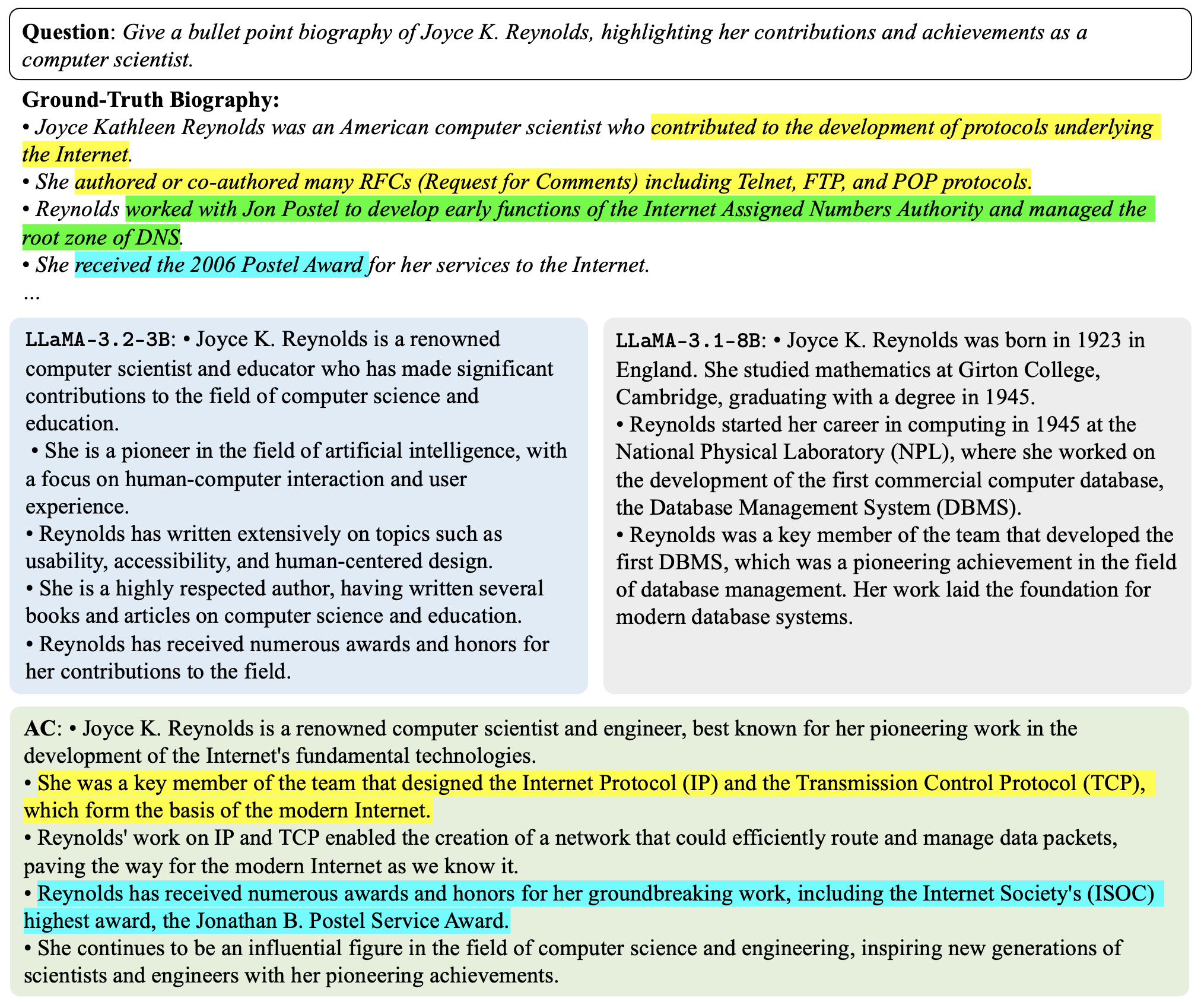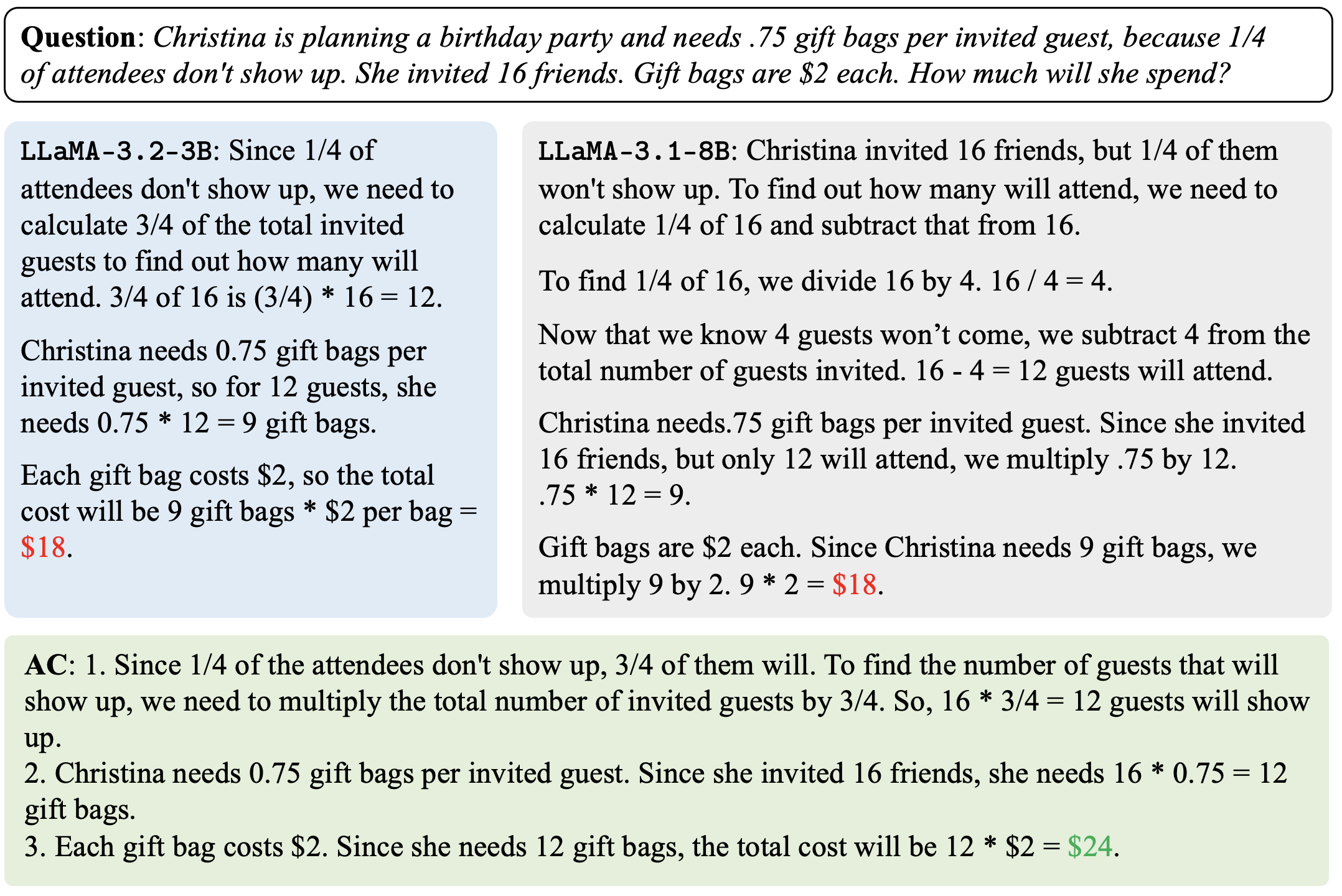</details> Figure 4: Example of AC on Biographies dataset. <details> <summary>extracted/6420159/gsm.png Details</summary>  ### Visual Description ## Screenshot: Problem-Solving Scenario for Gift Bag Cost Calculation ### Overview The image depicts a textual problem-solving scenario where Christina plans a birthday party. Key details include: - **Invited guests**: 16 friends - **Gift bag requirement**: 0.75 gift bags per invited guest - **No-show rate**: 1/4 of attendees - **Gift bag cost**: $2 each Three distinct methods (LLama-3.2-3B, LLama-3.1-8B, AC) are presented to calculate the total cost, with discrepancies in final results. --- ### Components/Axes 1. **Question Section** - Text: "Christina is planning a birthday party and needs 0.75 gift bags per invited guest, because 1/4 of attendees don’t show up. She invited 16 friends. Gift bags are $2 each. How much will she spend?" 2. **LLama-3.2-3B Section** - **Steps**: 1. Calculate 3/4 of 16 invited guests (since 1/4 don’t attend): `(3/4) * 16 = 12 guests` 2. Compute gift bags needed: `12 guests * 0.75 gift bags/guest = 9 gift bags` 3. Total cost: `9 gift bags * $2 = $18` 3. **LLama-3.1-8B Section** - **Steps**: 1. Calculate no-shows: `1/4 of 16 = 4 guests` 2. Attendees: `16 - 4 = 12 guests` 3. Gift bags: `12 guests * 0.75 = 9 gift bags` 4. Total cost: `9 * $2 = $18` 4. **AC Section** - **Steps**: 1. Attendees: `16 * 3/4 = 12 guests` 2. Gift bags: `16 * 0.75 = 12 gift bags` (applied to original invitees, not adjusted attendees) 3. Total cost: `12 * $2 = $24` 5. **Interpretation Section** - Highlights the discrepancy between methods, emphasizing the order of operations (applying the 0.75 gift bags per *invited* guest vs. per *attending* guest). --- ### Detailed Analysis - **LLama-3.2-3B**: - Correctly adjusts for no-shows first (`16 * 3/4 = 12`), then applies the 0.75 gift bags per *attending* guest. - Final cost: **$18**. - **LLama-3.1-8B**: - Explicitly subtracts no-shows (`16 - 4 = 12`) before calculating gift bags. - Final cost: **$18**. - **AC**: - Applies 0.75 gift bags to the *original* 16 guests (`16 * 0.75 = 12`), ignoring the no-show adjustment in this step. - Final cost: **$24**. --- ### Key Observations 1. **Discrepancy in Gift Bag Calculation**: - LLama methods assume 0.75 gift bags are needed *per attending guest* (after no-show adjustment). - AC method incorrectly applies 0.75 gift bags to the *original* 16 guests, leading to overestimation. 2. **Mathematical Consistency**: - Both LLama methods align in logic but differ slightly in phrasing (e.g., "3/4 of total invited" vs. "subtract 1/4"). - AC’s error stems from misapplying the 0.75 rate to the wrong guest count. 3. **Cost Implications**: - Overestimating gift bags (12 vs. 9) increases costs by **$6** (25% higher). --- ### Interpretation - **Problem Source**: The ambiguity lies in whether "0.75 gift bags per invited guest" applies *before* or *after* adjusting for no-shows. - LLama methods interpret it as post-adjustment (per attending guest). - AC interprets it as pre-adjustment (per invited guest). - **Real-World Relevance**: - The correct approach depends on the party’s logistics (e.g., pre-purchasing vs. preparing on-site). - AC’s method risks over-provisioning, while LLama methods optimize for actual attendance. - **Mathematical Lesson**: - Order of operations (e.g., adjusting for no-shows first) critically impacts outcomes in resource allocation problems. --- **Note**: The image contains no numerical data visualization (e.g., charts, graphs). All analysis is derived from textual steps and calculations. </details> Figure 5: Example of AC on GSM8k dataset. 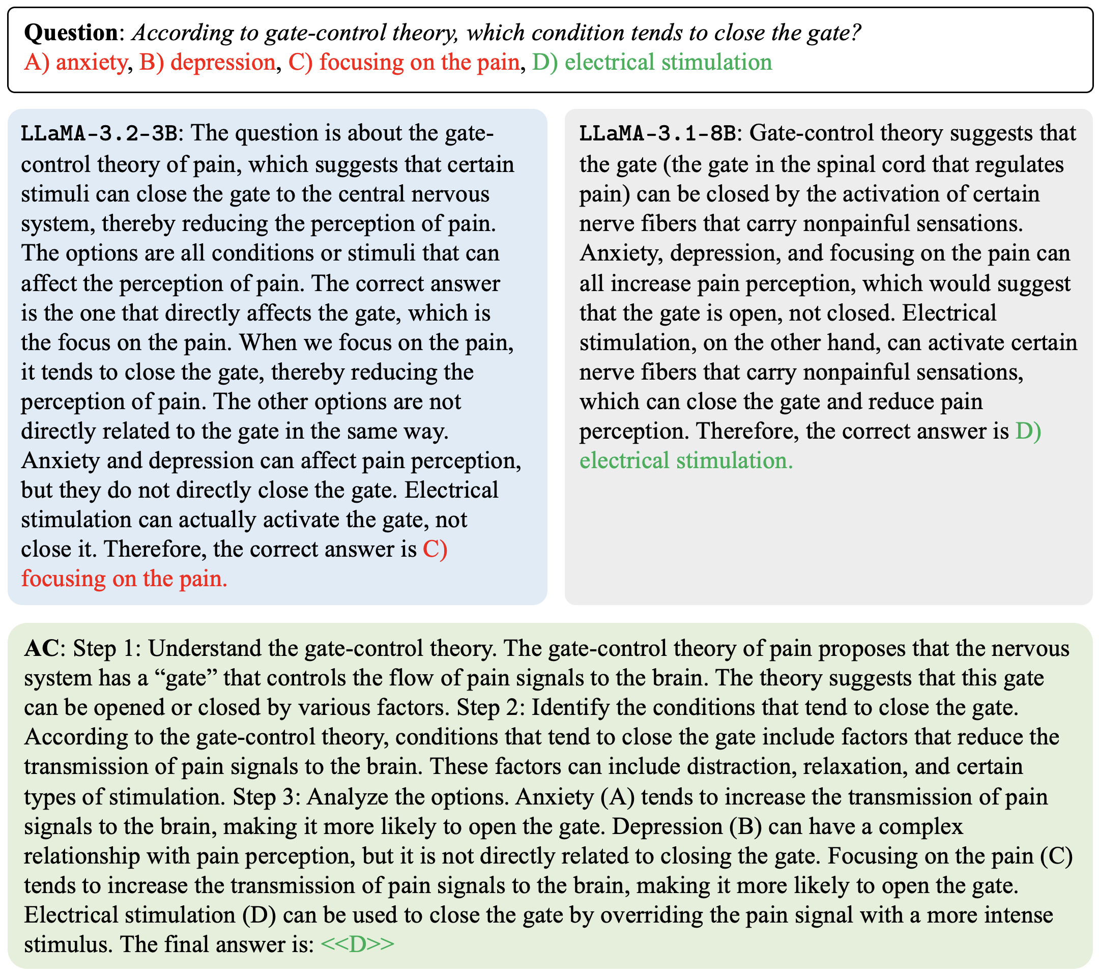<details> <summary>extracted/6420159/psych.png Details</summary>  ### Visual Description ## Screenshot: Gate-Control Theory Question Analysis ### Overview The image contains a multiple-choice question about the gate-control theory of pain, followed by explanations from two AI models (LLaMA-3.2-3B and LLaMA-3.1-8B) and a step-by-step analysis (AC). The question asks which condition "tends to close the gate" in the nervous system, with options A–D. --- ### Components/Axes - **Question**: "According to gate-control theory, which condition tends to close the gate?" - **Options**: - A) anxiety - B) depression - C) focusing on the pain - D) electrical stimulation - **Correct Answer Highlight**: D) electrical stimulation (green text). - **Model Explanations**: 1. **LLaMA-3.2-3B**: - Argues that focusing on the pain (C) closes the gate, reducing pain perception. - States anxiety and depression affect pain perception but do not directly close the gate. - Claims electrical stimulation activates the gate, increasing pain. - Final answer: C) focusing on the pain (red text). 2. **LLaMA-3.1-8B**: - Explains that electrical stimulation (D) activates nonpainful nerve fibers, closing the gate. - Notes anxiety, depression, and focusing on pain increase pain perception (gate open). - Final answer: D) electrical stimulation (green text). - **Step-by-Step Analysis (AC)**: - **Step 1**: Describes the gate-control theory’s mechanism. - **Step 2**: Identifies conditions that close the gate (e.g., distraction, relaxation). - **Step 3**: Analyzes options: - Anxiety (A) and depression (B) increase pain transmission (gate open). - Focusing on pain (C) increases transmission (gate open). - Electrical stimulation (D) overrides pain signals (gate closed). - **Final Answer**: D) electrical stimulation (green text). --- ### Detailed Analysis - **Textual Content**: - The question and options are presented in bold red text. - Model explanations use black text with key terms highlighted (e.g., "focusing on the pain" in red, "electrical stimulation" in green). - The AC analysis uses numbered steps with bold headings (e.g., "Step 1: Understand the gate-control theory"). - **Key Observations**: - Both models agree that **D) electrical stimulation** is the correct answer, but their reasoning differs: - LLaMA-3.2-3B incorrectly claims focusing on pain (C) closes the gate. - LLaMA-3.1-8B and AC correctly attribute gate closure to electrical stimulation (D). - Discrepancies in explanations highlight model-specific interpretations of the theory. --- ### Interpretation - **Theoretical Context**: - The gate-control theory posits that nonpainful stimuli (e.g., electrical stimulation) can close the "gate" in the spinal cord, reducing pain perception. - Anxiety, depression, and focusing on pain are associated with increased pain perception (gate open). - **Model Behavior**: - LLaMA-3.2-3B’s error in selecting C) suggests a potential misunderstanding of the theory’s emphasis on nonpainful stimuli. - LLaMA-3.1-8B and AC align with the theory’s core principle that electrical stimulation (a nonpainful stimulus) closes the gate. - **Implications**: - The question tests understanding of how specific stimuli modulate pain perception via the gate-control mechanism. - The AC analysis provides a structured breakdown of the theory, reinforcing the correct answer (D). --- ### Final Answer The correct answer is **D) electrical stimulation**, as it directly activates nonpainful nerve fibers to close the gate, reducing pain perception. </details> Figure 6: Example of AC on MMLU High School Psychology dataset. 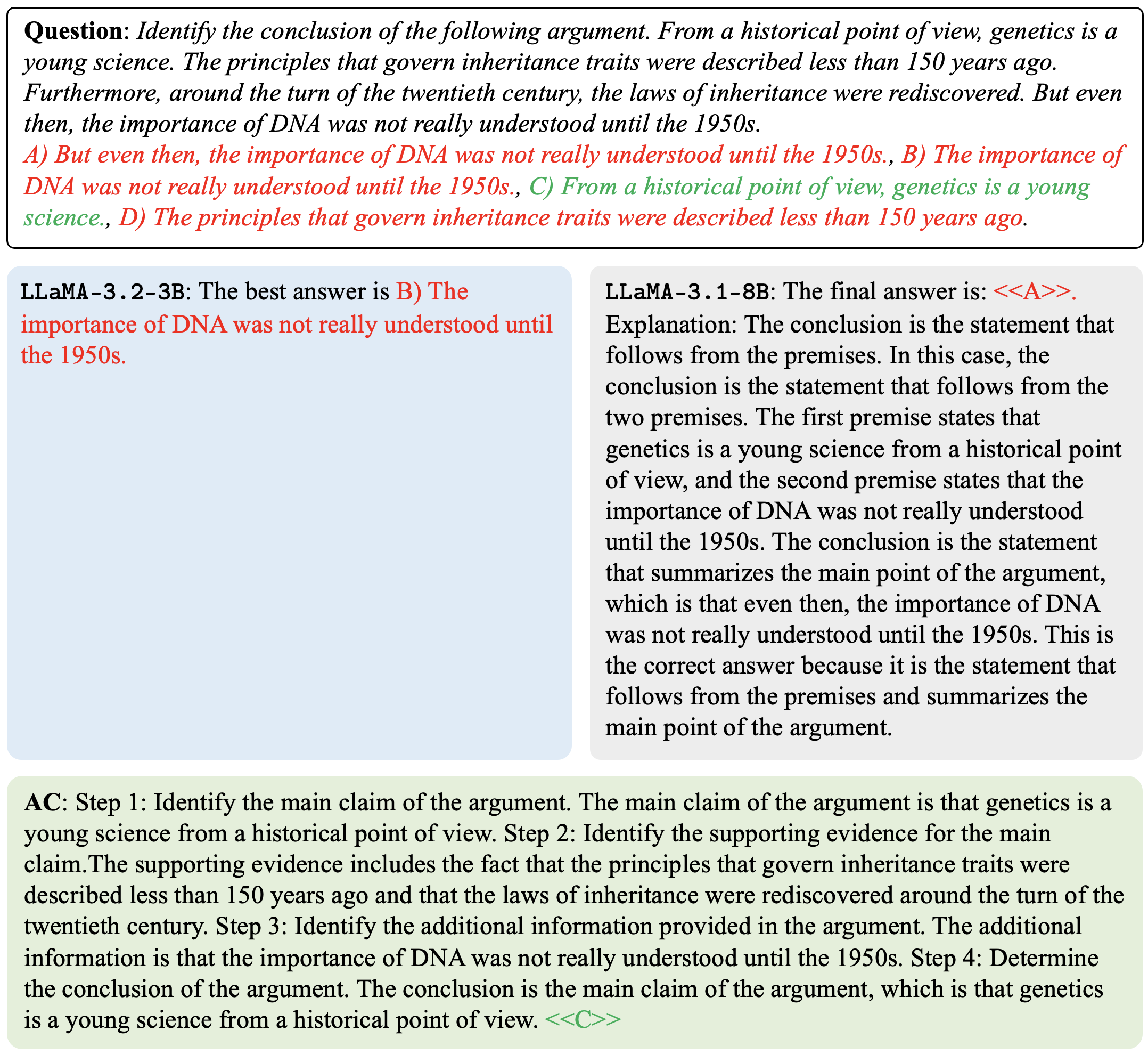<details> <summary>extracted/6420159/logic.png Details</summary>  ### Visual Description ## Textual Content: Argument Analysis on Genetics as a Young Science ### Overview The image contains a textual argument analysis task. It presents a question asking to identify the conclusion of an argument about genetics being a "young science" from a historical perspective. The argument includes premises about the timeline of genetic discoveries and DNA's role. Four answer choices (A–D) are provided, with explanations from two AI models (LLaMA-3.2-3B and LLaMA-3.1-8B) and a step-by-step reasoning process (AC). ### Components/Axes - **Question**: "Identify the conclusion of the following argument. From a historical point of view, genetics is a young science. The principles that govern inheritance traits were described less than 150 years ago. Furthermore, around the turn of the twentieth century, the laws of inheritance were rediscovered. But even then, the importance of DNA was not really understood until the 1950s." - **Answer Choices**: - **A)**: "But even then, the importance of DNA was not really understood until the 1950s." - **B)**: "The importance of DNA was not really understood until the 1950s." - **C)**: "From a historical point of view, genetics is a young science." - **D)**: "The principles that govern inheritance traits were described less than 150 years ago." - **Explanations**: - **LLaMA-3.2-3B**: States that the best answer is **B**, emphasizing that the conclusion follows from the premises. - **LLaMA-3.1-8B**: Confirms **A** as the final answer, explaining that the conclusion summarizes the premises. - **Step-by-Step Reasoning (AC)**: 1. **Step 1**: Identify the main claim (genetics is a young science). 2. **Step 2**: Supporting evidence (principles of inheritance described <150 years ago; laws rediscovered ~1900). 3. **Step 3**: Additional information (DNA's importance not understood until the 1950s). 4. **Step 4**: Conclusion (genetics is a young science). ### Detailed Analysis - **Question Text**: The argument establishes genetics as a young science by citing historical milestones: - Principles of inheritance described <150 years ago. - Laws of inheritance rediscovered ~1900. - DNA's importance not understood until the 1950s. - **Answer Choices**: - **A** and **B** both reference DNA's delayed understanding, but **A** includes the phrase "But even then," which is part of the original argument's structure. - **C** restates the main claim. - **D** repeats a premise. - **Model Explanations**: - **LLaMA-3.2-3B** argues **B** is correct because it directly follows from the premises. - **LLaMA-3.1-8B** claims **A** is correct, noting that the conclusion summarizes the premises. - **AC Reasoning**: The step-by-step process isolates the main claim (Step 1), supporting evidence (Steps 2–3), and concludes that genetics is a young science (Step 4). ### Key Observations - The argument hinges on the timeline of genetic discoveries to define genetics as a "young science." - **A** and **B** are semantically similar but differ in phrasing. **A** includes a transitional phrase ("But even then") from the original text, while **B** is a direct statement. - Both models agree on the conclusion but differ in their reasoning (e.g., **B** as a summary vs. **A** as a restatement). ### Interpretation The text demonstrates how conclusions are derived from premises in logical arguments. The debate between **A** and **B** highlights nuances in phrasing and the importance of transitional language in argument structure. The AC steps provide a framework for dissecting arguments, emphasizing the separation of claims, evidence, and conclusions. The models' conflicting interpretations suggest that the conclusion could be interpreted as either a restatement of the main claim (**A**) or a synthesis of the premises (**B**), depending on contextual emphasis. </details> Figure 7: Example of AC on MMLU Formal Logic dataset. 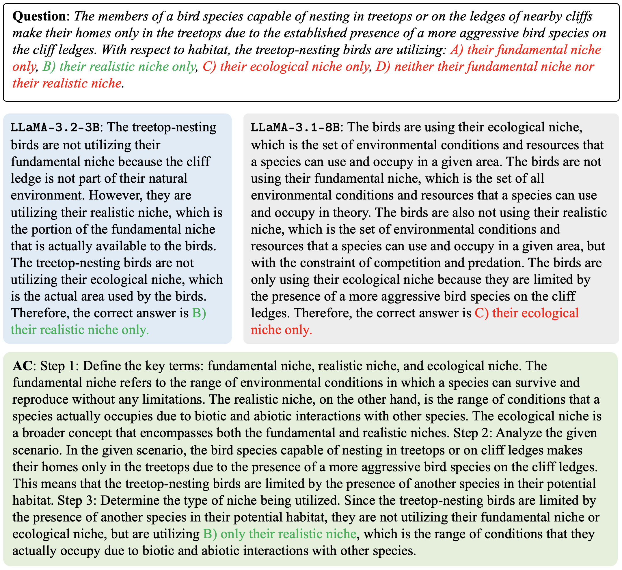<details> <summary>extracted/6420159/bio.png Details</summary>  ### Visual Description ## Screenshot: Ecological Niche Question and Model Responses ### Overview The image contains a multiple-choice question about ecological niches, followed by two model responses (LLaMA-3.2-3B and LLaMA-3.1-8B) and an annotated analysis (AC) explaining the reasoning. The question involves habitat utilization by bird species, with options labeled A-D. The AC section provides a step-by-step breakdown of niche definitions and scenario analysis. --- ### Components/Axes - **Question Text**: "The members of a bird species capable of nesting in treetops or on the ledges of nearby cliffs make their homes only in the treetops due to the established presence of a more aggressive bird species on the cliff ledges. With respect to habitat, the treetop-nesting birds are utilizing: A) their fundamental niche only, B) their realistic niche only, C) their ecological niche only, D) neither their fundamental niche nor their realistic niche." - **Model Responses**: - **LLaMA-3.2-3B**: Argues the birds use their **realistic niche only** (B), as they avoid the cliff ledges due to competition. - **LLaMA-3.1-8B**: Argues the birds use their **ecological niche only** (C), constrained by competition. - **AC Section**: - **Step 1**: Definitions of fundamental niche (unlimited survival/reproduction), realistic niche (actual occupancy due to interactions), and ecological niche (broader concept combining both). - **Step 2**: Analysis of the scenario: Birds avoid cliffs due to aggression, limiting their habitat. - **Step 3**: Conclusion: Birds utilize their **realistic niche only** (B), as their actual occupancy is restricted by biotic interactions. --- ### Detailed Analysis - **Question Structure**: - Four options (A-D) test understanding of niche concepts. - Key terms: *fundamental niche* (theoretical potential), *realistic niche* (actual occupancy), *ecological niche* (broader concept). - **Model Responses**: - **LLaMA-3.2-3B**: Focuses on the birds’ avoidance of cliffs (realistic niche) but incorrectly dismisses ecological niche. - **LLaMA-3.1-8B**: Correctly identifies the constraint of competition but misattributes it to the ecological niche. - **AC Breakdown**: - Step 1 clarifies niche definitions, emphasizing that the ecological niche includes both fundamental and realistic components. - Step 2 links the scenario to biotic interactions (aggressive species on cliffs). - Step 3 concludes that the birds’ actual habitat (treetops) reflects their **realistic niche only** (B), as their fundamental niche (unrestricted habitat) is unutilized. --- ### Key Observations 1. **Highlighted Answer**: The AC section explicitly states the correct answer is **B) their realistic niche only**, with the term "realistic niche" highlighted in green. 2. **Model Discrepancy**: The two models disagree on the answer (B vs. C), reflecting differing interpretations of niche constraints. 3. **Terminology Clarity**: The AC section resolves ambiguity by defining terms, showing that the ecological niche is a superset of the other two. --- ### Interpretation - **Ecological Concept**: The question tests the distinction between theoretical (fundamental) and actual (realistic) niches. The birds’ behavior (avoiding cliffs) demonstrates biotic constraints, aligning with the **realistic niche**. - **Model Limitations**: - LLaMA-3.2-3B correctly identifies the realistic niche but overlooks the broader ecological niche. - LLaMA-3.1-8B misapplies the ecological niche, which inherently includes both fundamental and realistic components. - **AC’s Role**: The annotated analysis provides a structured framework to resolve ambiguity, emphasizing that the ecological niche is not a separate category but a composite concept. This scenario underscores the importance of precise niche definitions in ecological modeling and highlights how AI models may interpret constraints differently based on training data. </details> Figure 8: Example of AC on MMLU College Biology dataset. 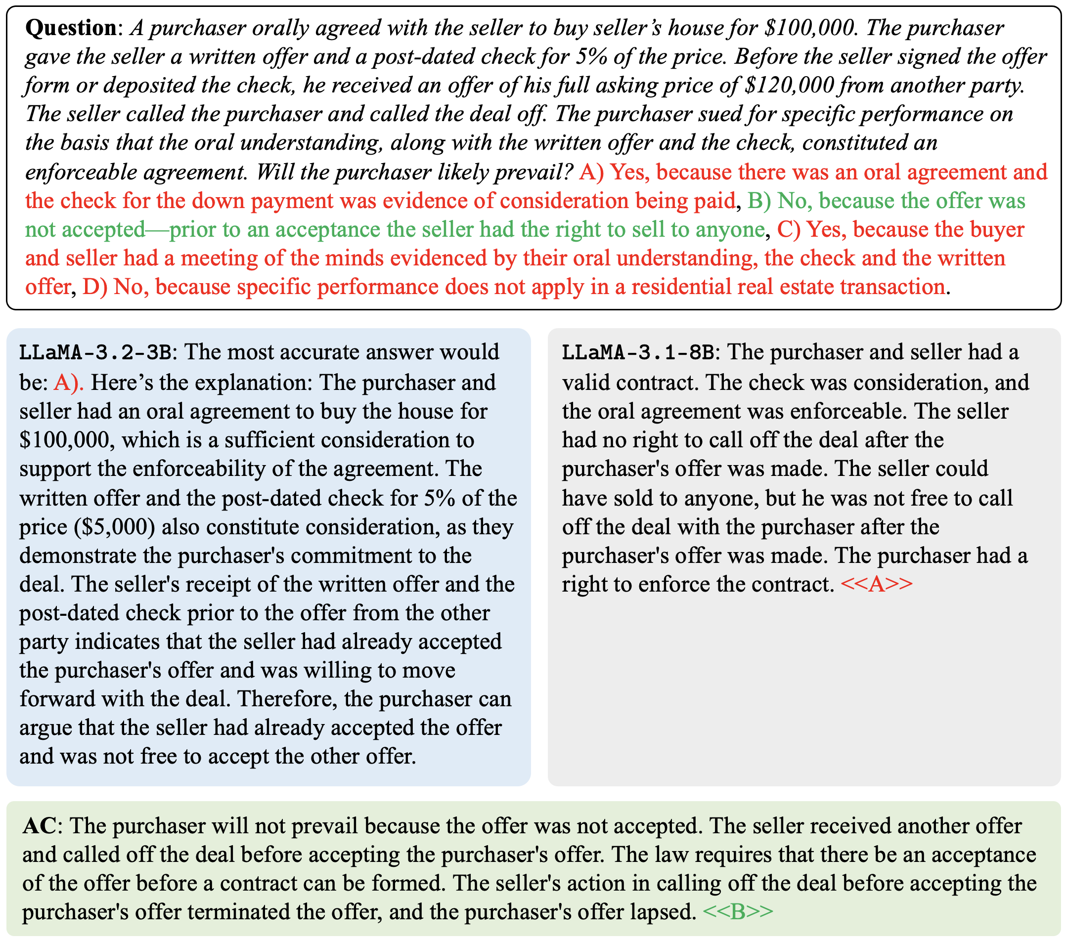<details> <summary>extracted/6420159/law.png Details</summary>  ### Visual Description ## Text-Based Legal Question Analysis ### Overview The image presents a legal scenario involving a real estate transaction dispute. It includes a multiple-choice question with four options (A-D), explanations for each answer, and references to legal codes (LLaMA-3.2-3B and LLaMA-3.1-8B) with their respective conclusions. The text is formatted with color highlights (red, green) for emphasis. ### Components/Axes 1. **Question Text**: - Describes a purchaser's oral agreement and written offer for a $100,000 house, including a post-dated check for 5% down payment. - Seller receives a higher offer ($120,000) and calls off the deal. Purchaser sues for specific performance. - Key legal issue: Whether the oral agreement + written offer + check constitutes an enforceable contract. 2. **Multiple-Choice Options (A-D)**: - **A**: Yes (oral agreement + check as consideration). - **B**: No (offer not accepted before acceptance by seller). - **C**: Yes (meeting of minds evidenced by oral agreement). - **D**: No (specific performance inapplicable to residential real estate). 3. **Legal Code References**: - **LLaMA-3.2-3B**: Concludes A is correct. Explains oral agreement + check as sufficient consideration; seller's receipt of written offer indicates acceptance. - **LLaMA-3.1-8B**: Concludes B is correct. Argues offer was not accepted before seller received higher offer; seller could not unilaterally terminate after acceptance. 4. **Additional Explanation (AC)**: - States purchaser cannot prevail because offer was not accepted. Seller's action in calling off the deal terminated the offer. ### Detailed Analysis - **Question Text**: - Purchaser orally agreed to buy a house for $100,000, provided a written offer and post-dated check for 5% ($5,000). - Seller received a higher offer ($120,000) and called off the deal. Purchaser sued for specific performance. - Legal debate centers on whether the oral agreement + written offer + check formed a binding contract. - **Option A Explanation**: - Argues oral agreement + check constitute consideration. Seller's receipt of written offer and post-dated check indicates acceptance. - Highlights that the seller's willingness to move forward supports enforceability. - **Option B Explanation**: - Claims offer was not accepted before seller received higher offer. Seller had right to sell to anyone but could not call off deal after acceptance. - Emphasizes that acceptance must occur before a contract is formed. - **Option C Explanation**: - Suggests meeting of minds (oral agreement + check) evidences a contract. However, this is contradicted by the requirement for acceptance before contract formation. - **Option D Explanation**: - States specific performance does not apply to residential real estate. This is factually incorrect, as specific performance is a common remedy in real estate disputes. - **Legal Code References**: - **LLaMA-3.2-3B**: Supports A, emphasizing that the seller's receipt of the written offer and check indicates acceptance, making the oral agreement enforceable. - **LLaMA-3.1-8B**: Supports B, arguing that the seller's acceptance of the higher offer terminated the original offer, preventing contract formation. - **Additional Explanation (AC)**: - Reinforces B's reasoning, stating the seller's action in calling off the deal before acceptance terminated the offer. ### Key Observations 1. **Contradictory Legal Reasoning**: The two legal codes (LLaMA-3.2-3B and LLaMA-3.1-8B) provide opposing conclusions (A vs. B), highlighting ambiguity in contract formation requirements. 2. **Highlighted Text**: - "not accepted" (green) in Option B's explanation emphasizes the timing of acceptance. - "oral understanding" (red) in Option A's explanation stresses the importance of mutual agreement. 3. **Factual Inaccuracy in Option D**: Specific performance is a valid remedy in residential real estate transactions, making this option incorrect. ### Interpretation The scenario tests the legal principle that a contract requires **offer, acceptance, and consideration**. The correct answer hinges on whether the seller's receipt of the written offer and post-dated check constitutes acceptance. - **LLaMA-3.2-3B's reasoning (A)** aligns with the **mailbox rule** in contract law, where acceptance is effective upon dispatch (here, the seller receiving the written offer). The check serves as consideration, making the oral agreement enforceable. - **LLaMA-3.1-8B's reasoning (B)** incorrectly assumes the seller's acceptance of a higher offer terminated the original offer. However, acceptance of one offer does not automatically revoke prior offers unless explicitly communicated. The **additional explanation (AC)** reinforces B's position but overlooks the fact that the seller's receipt of the written offer and check could imply acceptance, creating a binding contract. The ambiguity in the scenario reflects real-world legal disputes where courts must weigh factual circumstances against statutory requirements. </details> Figure 9: Example of AC on MMLU Professional Law dataset. 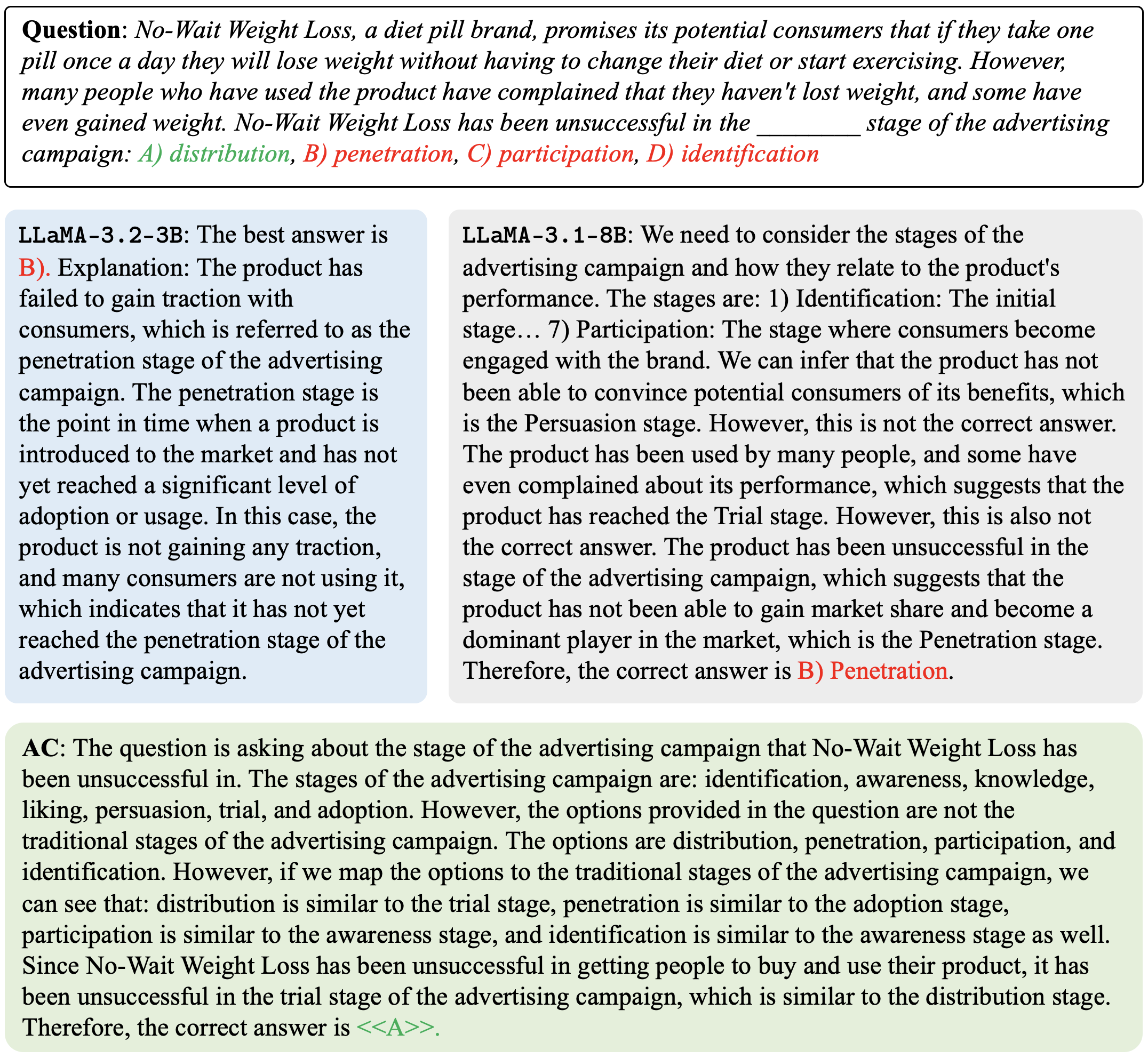<details> <summary>extracted/6420159/prel.png Details</summary>  ### Visual Description ## Screenshot: Multiple-Choice Question Analysis ### Overview The image contains a multiple-choice question about the stage of an advertising campaign where a diet pill product ("No-Wait Weight Loss") has been unsuccessful. Three model responses (LLaMA-3.2-3B, LLaMA-3.1-8B, and AC) provide reasoning for their answers. ### Components/Axes - **Question Text**: "No-Wait Weight Loss, a diet pill brand, promises its potential consumers that if they take one pill once a day they will lose weight without having to change their diet or start exercising. However, many people who have used the product have complained that they have not lost weight, and some have even gained weight. No-Wait Weight Loss has been unsuccessful in the ______ stage of the advertising campaign: A) distribution, B) penetration, C) participation, D) identification." - **Options**: A) distribution, B) penetration, C) participation, D) identification - **Model Responses**: 1. **LLaMA-3.2-3B** (Blue Box): - Explanation: The product has failed to gain traction with consumers, indicating it has not reached the penetration stage. - Conclusion: B) Penetration. 2. **LLaMA-3.1-8B** (Gray Box): - Explanation: Analyzes stages of the advertising campaign (identification, persuasion, trial, adoption). Maps the product’s failure to the penetration stage (similar to adoption). - Conclusion: B) Penetration. 3. **AC** (Green Box): - Explanation: Maps the given options to traditional advertising stages: - Distribution ≈ Trial stage - Penetration ≈ Adoption stage - Participation ≈ Awareness stage - Identification ≈ Awareness stage - Conclusion: A) Distribution (due to trial stage failure). ### Detailed Analysis - **Question Structure**: The question asks for the stage where the product’s performance (weight loss failure) indicates campaign underperformance. - **Model Reasoning**: - **LLaMA-3.2-3B**: Focuses on "penetration" as the stage where products fail to gain traction. - **LLaMA-3.1-8B**: Uses a traditional framework (identification → persuasion → trial → adoption) to argue penetration (adoption) is the correct stage. - **AC**: Reinterprets the options using traditional stages, concluding distribution (trial) is the correct answer. ### Key Observations - **Disagreement**: LLaMA models agree on B) Penetration, while AC argues for A) Distribution. - **Terminology Differences**: - AC redefines "penetration" as adoption, while LLaMA models treat it as a distinct stage. - AC’s mapping of options to traditional stages introduces ambiguity. ### Interpretation - **Correct Answer**: The LLaMA models’ consensus on B) Penetration aligns with standard marketing frameworks where "penetration" refers to the stage where a product fails to gain market share. AC’s argument hinges on redefining terms, which may not match the question’s intent. - **Underlying Logic**: - Penetration Stage: Products are introduced but fail to achieve significant adoption (matches the scenario of complaints and lack of traction). - Distribution Stage: Involves product availability, not consumer engagement (less relevant to performance complaints). - **Ambiguity**: AC’s reinterpretation of "penetration" as adoption highlights potential confusion in terminology. However, the question’s phrasing ("unsuccessful in the ______ stage") likely refers to the stage where consumer adoption fails, not product availability. - **Implications**: The debate underscores the importance of clear definitions in advertising campaign stages. Penetration (B) is the most contextually appropriate answer given the product’s failure to gain traction. </details> Figure 10: Example of AC on MMLU Public Relations dataset. Appendix B Additional Experiments B.1 Modifying Activations of All Tokens Recall that AC grafts the last-token layer- $k$ activation of $A$ into $B$ ’s last-token layer- $j$ activation. But is modifying just the last token activation enough to communicate information from $A$ to $B$ ? Note that after applying masked attention in each of the previous Transformer layers, the last token activation of $A$ attends to all tokens before it, hence incorporating information from the entire sequence. Indeed, this must be the case for activation communication to recover the gap between the zero-communication and skyline setups on both coordination games, which (for Tip Sheets in particular) require information starting at the first few tokens of $A$ ’s prompt to be communicated. To verify this empirically, we experiment with summing the activations of all tokens in the sequence rather than just the last (we cannot replace all tokens as this would just replace $B$ ’s layer- $j$ activation with $A$ ’s layer $k$ -activation). Results are shown in Table 5. | AC (replace) AC (sum) AC (all tokens) | $\mathbf{84.6}$ $± 0.0$ $79.7$ $± 0.0$ $76.0$ $± 0.0$ | $64.0$ $± 4.8$ $\mathbf{66.0}$ $± 4.7$ $62.0$ $± 4.9$ | $\mathbf{85.0}$ $± 0.8$ $65.0$ $± 4.8$ $35.0$ $± 4.8$ | $\mathbf{47.0}$ $± 0.1$ $42.0$ $± 4.9$ $42.0$ $± 4.9$ | $\mathbf{78.0}$ $± 0.9$ $50.0$ $± 5.0$ $61.0$ $± 4.9$ | $\mathbf{30.0}$ $± 0.1$ $25.0$ $± 4.3$ $15.0$ $± 3.6$ | $\mathbf{74.0}$ $± 0.1$ $37.0$ $± 4.8$ $26.0$ $± 4.4$ | | --- | --- | --- | --- | --- | --- | --- | --- | Table 5: Reasoning benchmark performance when varying tokens modified during AC. All methods involve communication between $\mathtt{LLaMA}$ - $\mathtt{3.2}$ - $\mathtt{3B}$ ( $A$ ) and $\mathtt{LLaMA}$ - $\mathtt{3.1}$ - $\mathtt{8B}$ ( $B$ ). The functional form $f$ is varied between last-token replacement, last-token summation, and summation for all tokens. Indeed, applying $f$ to all tokens decreases performance relative to applying $f$ to just the last token. Note that the fact performance generally decreases from $f=$ $\mathtt{replace}$ to $f=$ $\mathtt{sum}$ , and further with all tokens, is expected. The high performance of AC with $f=$ $\mathtt{replace}$ means that the edited last-token activation $\bm{b}$ retains some meaning in $B$ ’s activation space; it is less likely for this to be the case when $f=$ $\mathtt{sum}$ (at the very least $\bm{b}$ has norm roughly $2×$ that of $B$ ’s original last-token activation), and when doing this for all tokens we’d expect performance to decrease even further as now all activation vectors, not just the last, are out-of-distribution with respect to $B$ ’s activation space. B.2 Incorporating Chain-of-Thought Prompting How does AC perform in relation to NLD in cases where $A$ might incur a long response (possibly with chain-of-thought for intermediate answer computation)? I.e., does AC lose out on the benefits of CoT? First, note that we still reap the benefits of CoT when we sample a completion from $B$ after AC (where $B$ gets all the information encoding $A$ ’s “beliefs” about the prompt via AC, hence CoT on $A$ ’s side is not needed). To verify this, we experiment with prompting $A$ with CoT, generating a full response, and then passing the layer- $k$ last-token activation of the CoT response to $B$ as part of AC. Results are shown in Table 6. | AC AC ( $\bm{W}$ ) AC (CoT) | $84.6$ $± 0.0$ $\mathbf{86.8}$ $± 0.0$ $82.1$ $± 0.0$ | $64.0$ $± 4.8$ $\mathbf{66.0}$ $± 4.8$ $\mathbf{66.0}$ $± 4.0$ | $\mathbf{85.0}$ $± 0.8$ $70.0$ $± 0.1$ $80.0$ $± 4.0$ | $\mathbf{47.0}$ $± 0.1$ $35.0$ $± 0.1$ $26.0$ $± 4.4$ | $78.0$ $± 0.9$ $\mathbf{79.0}$ $± 0.9$ $67.0$ $± 4.7$ | $30.0$ $± 0.1$ $\mathbf{45.0}$ $± 0.1$ $40.0$ $± 4.9$ | $\mathbf{74.0}$ $± 0.1$ $63.0$ $± 0.1$ $63.0$ $± 4.8$ | | --- | --- | --- | --- | --- | --- | --- | --- | Table 6: Reasoning benchmark performance when sampling from $A$ with CoT. All methods involve communication between $\mathtt{LLaMA}$ - $\mathtt{3.2}$ - $\mathtt{3B}$ ( $A$ ) and $\mathtt{LLaMA}$ - $\mathtt{3.1}$ - $\mathtt{8B}$ ( $B$ ). Indeed, we empirically find our above intuition (in orange) to hold, as there is no significant improvement over vanilla AC when generating from $A$ using CoT. B.3 Learning $\bm{W}$ In-Distribution Recall our reasoning about the AC $(\bm{W})$ results from Section 4.2: “We hypothesize that the benefits from the learned linear layer are less consistent across datasets because the subset of C4 data used to train $\bm{W}$ likely contains text more semantically similar to some datasets than others, hence some datasets provide $\bm{W}$ with out-of-distribution inputs which reduces performance compared to vanilla AC.” Indeed, we verify this hypothesis by training $\bm{W}$ on the GSM8k train set (to produce $\bm{W}_{\textrm{in dist}}$ ) and then evaluating with this task-specific linear layer on the GSM8k test set. Results are shown in Table 7. | $64.0$ $± 4.8$ | $66.0$ $± 4.8$ | $\mathbf{78.0}$ $± 4.1$ | | --- | --- | --- | Table 7: GSM8k performance when learning $\bm{W}$ in-distribution. All AC variants involve communication between $\mathtt{LLaMA}$ - $\mathtt{3.2}$ - $\mathtt{3B}$ ( $A$ ) and $\mathtt{LLaMA}$ - $\mathtt{3.1}$ - $\mathtt{8B}$ ( $B$ ). Indeed, learning $\bm{W}$ in-distribution significantly boosts performance, confirming our hypothesis. Unfortunately we cannot run this experiment for the other datasets, as there is no in-distribution training data available for MMLU (we use all public data for testing). Hence, this suggests that AC ( $\bm{W}$ ) should unilaterally improve over vanilla AC if we choose a training set with good coverage across many tasks and distributions, such that there are sentences semantically similar to prompts across the span of downstream task datasets. B.4 Activation Space Similarity $\propto$ AC Performance Gain We conduct the following experiment: for each of the six pairs of models $A,B$ in the above experiment (see Table 4), we compute the increase in Biographies performance with AC relative to the average individual performance of $A$ and $B$ . We also compute the matrix analogue of the squared cosine similarity between the models’ activation spaces, $$ \frac{\lVert Y^{\top}X\rVert_{F}^{2}}{\lVert X\rVert_{F}^{2}\,\lVert Y\rVert_{% F}^{2}}, $$ where $X$ is the matrix of $A$ ’s activations on $3072$ sentences from C4 (the same dataset used to train $\bm{W}$ ), $Y$ is the corresponding matrix for $B$ , and $\lVert·\rVert_{F}$ denotes the Frobenius norm. This yields the plot in Figure 11. There is a clear positive correlation between the similarity of the activation distributions and the AC performance gain, as expected; the more aligned $A$ and $B$ ’s activation spaces are, the more semantically meaningful and useful the embedding we graft from $A$ to $B$ becomes. B.5 Communicating Activations Between Identical Models Note that AC as described in Section 3.1 only supports communication between distinct models. We can extend AC to work for communication between identical models as follows: let $A$ and $B$ be instances of the same model. We can sample a completion from $A$ with temperature and graft the last-token layer- $k$ activation of the completion into $B$ at layer $j$ as part of the AC procedure. This still saves a substantial amount of compute over NLD between 2 model instances, showing our technique can apply to this setting. Table 8 shows the results of this experiment. 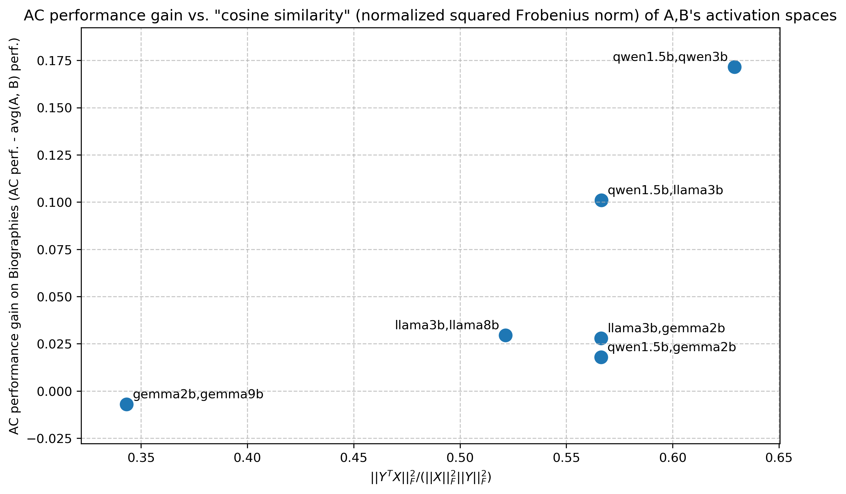<details> <summary>extracted/6420159/model-comparison-plot.png Details</summary>  ### Visual Description ## Scatter Plot: AC Performance Gain vs. Cosine Similarity ### Overview The image is a scatter plot comparing AC performance gain (on the y-axis) against cosine similarity (normalized squared Frobenius norm of activation spaces) on the x-axis. Data points are labeled with pairs of model names (e.g., "qwen1.5b,qwen3b"), and their positions reflect their respective metric values. ### Components/Axes - **Title**: "AC performance gain vs. 'cosine similarity' (normalized squared Frobenius norm) of A,B's activation spaces" - **X-axis**: - Label: `||Y^T X||_F²/(||X||_F² ||Y||_F²)` (normalized squared Frobenius norm) - Scale: 0.35 to 0.65 (approximate) - **Y-axis**: - Label: "AC performance gain on Biographies (AC perf. - avg(A, B) perf.)" - Scale: -0.025 to 0.175 (approximate) - **Data Points**: Blue dots with labels combining model names (e.g., "qwen1.5b,qwen3b"). No explicit legend is present, but all points are blue. ### Detailed Analysis 1. **Data Points**: - **qwen1.5b,qwen3b**: X ≈ 0.63, Y ≈ 0.17 (top-right corner). - **qwen1.5b,llama3b**: X ≈ 0.57, Y ≈ 0.10 (upper-middle-right). - **llama3b,llama8b**: X ≈ 0.52, Y ≈ 0.025 (middle-center). - **llama3b,gemma2b**: X ≈ 0.57, Y ≈ 0.02 (middle-right). - **qwen1.5b,gemma2b**: X ≈ 0.57, Y ≈ 0.015 (middle-right, slightly lower than "llama3b,gemma2b"). - **gemma2b,gemma9b**: X ≈ 0.35, Y ≈ -0.01 (bottom-left). 2. **Trends**: - Higher cosine similarity (x-axis) generally correlates with higher AC performance gain (y-axis), but exceptions exist. - The highest gain (0.17) occurs at the maximum x-value (0.63), suggesting a strong relationship between similarity and performance for "qwen1.5b,qwen3b". - Lower gains (e.g., -0.01 for "gemma2b,gemma9b") occur at lower x-values, indicating poorer performance for dissimilar models. ### Key Observations - **Outlier**: "qwen1.5b,gemma2b" has a high x-value (0.57) but a relatively low y-value (0.015), suggesting that high similarity does not always guarantee high performance. - **Consistency**: "qwen1.5b" pairs (e.g., with "qwen3b" or "llama3b") consistently show higher gains than "llama3b" or "gemma2b" pairs. - **Negative Gain**: "gemma2b,gemma9b" is the only point below the zero line, indicating a performance loss compared to the average. ### Interpretation The data suggests that models with higher cosine similarity in their activation spaces tend to exhibit better AC performance gains. However, the presence of outliers (e.g., "qwen1.5b,gemma2b") implies that similarity alone is not the sole determinant of performance. Architectural differences, training data, or other latent factors may influence results. The negative gain for "gemma2b,gemma9b" highlights cases where dissimilar models underperform, possibly due to conflicting activation patterns. This scatter plot underscores the importance of activation space alignment in model performance but also signals the need for further investigation into confounding variables. </details> Figure 11: AC performance gain over average $A$ / $B$ individual performance on Biographies, as a function of matrix “cosine similarity” between $A$ and $B$ ’s activation spaces. | $\mathtt{LLaMA}$ - $\mathtt{3.1}$ - $\mathtt{8B}$ NLD AC | $\mathbf{83.9}$ $± 0.0$ $80.8$ $± 0.0$ $83.7$ $± 0.0$ | $60.0$ $± 4.9$ $\mathbf{70.0}$ $± 3.7$ $60.0$ $± 4.9$ | $65.0$ $± 0.1$ $\mathbf{85.0}$ $± 3.6$ $\mathbf{85.0}$ $± 3.6$ | $\mathbf{42.0}$ $± 0.1$ $35.0$ $± 4.8$ $40.0$ $± 4.9$ | $50.0$ $± 0.2$ $\mathbf{78.0}$ $± 4.1$ $74.0$ $± 4.4$ | $20.0$ $± 0.8$ $\mathbf{40.0}$ $± 4.9$ $\mathbf{40.0}$ $± 4.9$ | $53.0$ $± 0.2$ $53.0$ $± 5.1$ $\mathbf{79.0}$ $± 4.1$ | | --- | --- | --- | --- | --- | --- | --- | --- | Table 8: Reasoning benchmark performance of communication between identical models. Both NLD and AC involve communication between 2 instances of $\mathtt{LLaMA}$ - $\mathtt{3.1}$ - $\mathtt{8B}$ . $512$ -token completions are sampled with temperature $0.7$ and debate is run for $2$ rounds. Indeed, while communication between multiple model instances doesn’t always show improvement over the single model itself (a well-known result from (Du et al., 2023)), AC matches/outperforms NLD on five of the seven datasets. The intuition behind debate between multiple identical model instances is that sampling multiple completions (with temperature) from the same model yields diverse reasoning paths that can be recombined into a stronger final answer. The above experiment shows that the same intuition holds for AC—we are sampling multiple times from the same model, but passing responses between agents via AC rather than as NL messages. B.6 Additional Rounds of Natural Language Debate In Section 4.2 we fix NLD to $2$ agents and $2$ rounds, however we find in additional experiments that AC outperforms NLD even with additional rounds, highlighting the superiority and robustness of activations as an alternative “language” for inter-LM communication. Results are shown in Table 9; we see that for 5 of the 7 reasoning benchmarks, AC beats NLD even with $3$ - $4$ rounds while using substantially less compute. | NLD (1 round) NLD (2 rounds) NLD (3 rounds) | $83.6$ $± 0.0$ $80.2$ $± 0.1$ $80.1$ $± 4.6$ | $72.0$ $± 4.5$ $75.0$ $± 4.3$ $\mathbf{79.0}$ $± 4.1$ | $65.0$ $± 4.8$ $83.0$ $± 0.8$ $70.0$ $± 4.6$ | $40.0$ $± 4.9$ $37.0$ $± 0.1$ $45.0$ $± 5.0$ | $68.0$ $± 4.6$ $71.0$ $± 0.1$ $63.0$ $± 4.8$ | $30.0$ $± 4.6$ $30.0$ $± 0.1$ $\mathbf{40.0}$ $± 4.9$ | $63.0$ $± 4.8$ $63.0$ $± 0.7$ $\mathbf{74.0}$ $± 4.4$ | | --- | --- | --- | --- | --- | --- | --- | --- | | NLD (4 rounds) | $78.0$ $± 0.0$ | $\mathbf{79.0}$ $± 4.1$ | * | * | * | * | * | | AC | $\mathbf{84.6}$ $± 0.0$ | $64.0$ $± 4.8$ | $\mathbf{85.0}$ $± 0.8$ | $\mathbf{47.0}$ $± 0.1$ | $\mathbf{78.0}$ $± 0.9$ | $30.0$ $± 0.1$ | $\mathbf{74.0}$ $± 0.1$ | ∗ Runs required too much compute Table 9: Reasoning benchmark performance of AC and NLD with varying number of rounds. All methods involve communication between $\mathtt{LLaMA}$ - $\mathtt{3.2}$ - $\mathtt{3B}$ ( $A$ ) and $\mathtt{LLaMA}$ - $\mathtt{3.1}$ - $\mathtt{8B}$ ( $B$ ). B.7 Full MMLU Benchmark Results Table 10 below displays complete results of both AC and NLD on the full MMLU benchmark. Notably, AC matches/outperforms NLD on 48/57 datasets, with substantially less compute used, indicating its superiority and robustness as an alternative “language” for inter-LLM communication. | Conceptual Physics High School Chemistry Security Studies | $60.0± 4.9$ $\mathbf{50.0± 5.0}$ $60.0± 4.9$ | $\mathbf{68.0± 4.6}$ $37.0± 4.8$ $60.0± 4.9$ | | --- | --- | --- | | Jurisprudence | $84.0± 3.6$ | $84.0± 3.6$ | | Logical Fallacies | $63.0± 4.8$ | $\mathbf{72.0± 4.5}$ | | College Computer Science | $44.0± 5.0$ | $44.0± 5.0$ | | International Law | $55.0± 5.0$ | $\mathbf{59.0± 4.9}$ | | Miscellaneous | $90.0± 3.0$ | $\mathbf{95.0± 2.2}$ | | Marketing | $70.0± 4.6$ | $\mathbf{85.0± 3.6}$ | | Elementary Mathematics | $\mathbf{75.0± 4.3}$ | $58.0± 4.9$ | | Machine Learning | $42.0± 4.9$ | $42.0± 4.9$ | | High School Macroeconomics | $44.0± 5.0$ | $\mathbf{75.0± 4.3}$ | | High School US History | $45.0± 5.0$ | $\mathbf{71.0± 4.6}$ | | Human Aging | $56.0± 5.0$ | $\mathbf{72.0± 4.5}$ | | Astronomy | $79.0± 4.1$ | $\mathbf{80.0± 4.0}$ | | Computer Security | $56.0± 5.0$ | $\mathbf{75.0± 4.3}$ | | High School Statistics | $\mathbf{55.0± 5.0}$ | $42.0± 4.9$ | | Professional Medicine | $\mathbf{79.0± 4.1}$ | $65.0± 4.8$ | | Electrical Engineering | $58.0± 4.9$ | $\mathbf{60.0± 4.9}$ | | High School Computer Science | $63.0± 4.8$ | $\mathbf{70.0± 4.6}$ | | College Physics | $\mathbf{50.0± 5.0}$ | $28.0± 4.5$ | | Management | $74.0± 4.1$ | $\mathbf{75.0± 4.3}$ | | Moral Scenarios | $40.0± 4.9$ | $40.0± 4.9$ | | World Religions | $58.0± 4.9$ | $\mathbf{72.0± 4.5}$ | | Virology | $47.0± 5.0$ | $\mathbf{50.0± 5.0}$ | | Philosophy | $67.0± 4.7$ | $\mathbf{70.0± 4.6}$ | | Abstract Algebra | $\mathbf{50.0± 5.0}$ | $28.0± 4.5$ | | High School Government and Politics | $\mathbf{80.0± 4.0}$ | $61.0± 4.9$ | | High School Biology | $60.0± 4.9$ | $\mathbf{65.0± 4.8}$ | | College Mathematics | $64.0± 4.8$ | $\mathbf{66.0± 2.4}$ | | Global Facts | $33.0± 5.0$ | $\mathbf{37.0± 4.8}$ | | High School World History | $71.0± 4.0$ | $\mathbf{74.0± 4.4}$ | | High School European History | $68.0± 4.0$ | $\mathbf{71.0± 4.6}$ | | College Medicine | $\mathbf{65.0± 4.8}$ | $53.0± 5.0$ | | High School Geography | $67.0± 4.7$ | $\mathbf{79.0± 4.1}$ | | Anatomy | $74.0± 4.4$ | $74.0± 4.4$ | | Human Sexuality | $75.0± 4.3$ | $75.0± 4.3$ | | Medical Genetics | $79.0± 4.1$ | $\mathbf{82.0± 3.8}$ | | Professional Accounting | $40.0± 4.9$ | $\mathbf{48.0± 4.5}$ | | US Foreign Policy | $89.0± 3.1$ | $\mathbf{90.0± 3.1}$ | | Business Ethics | ${43.0± 5.0}$ | $\mathbf{44.0± 5.0}$ | | College Chemistry | ${41.0± 5.0}$ | $\mathbf{47.0± 5.0}$ | | High School Physics | ${40.0± 5.0}$ | $\mathbf{47.0± 5.0}$ | | Professional Psychology | ${54.0± 4.8}$ | $\mathbf{55.0± 5.0}$ | | Sociology | ${68.0± 4.1}$ | $\mathbf{68.0± 4.6}$ | | High School Microeconomics | $95.0± 2.2$ | $95.0± 2.2$ | | High School Mathematics | $55.0± 5.0$ | $55.0± 5.0$ | | Prehistory | $\mathbf{75.0± 4.3}$ | $60.0± 4.9$ | | Nutrition | ${64.0± 4.5}$ | $\mathbf{70.0± 4.6}$ | | Clinical Knowledge | ${65.0± 4.3}$ | $65.0± 4.8$ | | Moral Disputes | ${58.0± 4.8}$ | $\mathbf{60.0± 4.9}$ | | Econometrics | ${40.0± 5.0}$ | $40.0± 4.9$ | | High School Psychology | $83.0± 0.8$ | $\mathbf{85.0± 0.8}$ | | Formal Logic | $37.0± 0.1$ | $\mathbf{47.0± 0.1}$ | | College Biology | $71.0± 0.1$ | $\mathbf{78.0± 0.9}$ | | Professional Law | $30.0± 0.1$ | $30.0± 0.1$ | | Public Relations | $63.0± 0.7$ | $\mathbf{74.0± 0.1}$ | | Average | $60.7± 2.0$ | $\mathbf{62.7± 2.2}$ | Table 10: Comparison of NLD vs. AC on the full MMLU benchmark (Hendrycks et al., 2021).