# Rollout Roulette: A Probabilistic Inference Approach to Inference-Time Scaling of LLMs using Particle-Based Monte Carlo Methods
**Authors**:
- Isha Puri
- Shiv Sudalairaj
- GX Xu
- Kai Xu
- Akash Srivastava (MIT CSAIL RedHat AI Innovation)
Abstract
Large language models (LLMs) have achieved significant performance gains via scaling up model sizes and/or data. However, recent evidence suggests diminishing returns from such approaches, motivating a pivot to scaling test-time compute. Existing deterministic inference-time scaling methods, usually with reward models, cast the task as a search problem, but suffer from a key limitation: early pruning. Due to inherently imperfect reward models, promising trajectories may be discarded prematurely, leading to suboptimal performance. We propose a novel inference-time scaling approach by adapting particle-based Monte Carlo methods. Our method maintains a diverse set of candidates and robustly balances exploration and exploitation. Our empirical evaluation demonstrates that our particle filtering methods have a 4–16x better scaling rate over deterministic search counterparts on both various challenging mathematical and more general reasoning tasks. Using our approach, we show that Qwen2.5-Math-1.5B-Instruct surpasses GPT-4o accuracy in only 4 rollouts, while Qwen2.5-Math-7B-Instruct scales to o1 level accuracy in only 32 rollouts. Our work not only presents an effective method to inference-time scaling, but also connects rich literature in probabilistic inference with inference-time scaling of LLMs to develop more robust algorithms in future work. Code and further information is available at https://probabilistic-inference-scaling.github.io/
1 Introduction
Large language models (LLMs) continue to improve through larger architectures and massive training corpora (kaplan2020scalinglawsneurallanguage, ; snell2024scalingllm, ). In parallel, inference-time scaling (ITS)—allocating more computation at inference time—has emerged as a complementary approach to improve performance without increasing model size. Recent work has shown that ITS enables smaller models to match or exceed the accuracy of larger ones on complex reasoning tasks (beeching2024scalingtesttimecompute, ), with proprietary systems like OpenAI’s o1 and o3 explicitly incorporating multi-trial inference for better answers (openai2024openaio1card, ).
<details>
<summary>x1.png Details</summary>
### Visual Description
# Technical Document Extraction: Mathematical Logic Flow Diagram
## 1. Overview
This image is a technical diagram illustrating two different logical paths (labeled "1" and "2") taken to solve a word problem. It evaluates the accuracy of each step in the reasoning process using numerical scores and visual indicators (checkmarks and crosses).
## 2. Component Isolation
### Region A: Problem Statement (Left)
* **Icon:** A calculator/math symbol sheet with a question mark.
* **Text Content:**
> "Jane has twice as many pencils as Mark. Together they have 9 pencils. How many pencils does Jane have?"
### Region B: Path Selection (Center-Left)
Two arrows originate from the problem statement, pointing to two distinct reasoning paths:
* **Path 1:** Represented by a thought bubble icon containing the number "1".
* **Path 2:** Represented by a thought bubble icon containing the number "2".
### Region C: Reasoning Path 1 (Top Right)
This path consists of three sequential steps leading to a correct conclusion.
| Step | Mathematical Reasoning Text | Score | Visual Indicator |
| :--- | :--- | :--- | :--- |
| **Step 1** | Total parts = 2 (Jane) + 1 (Mark) = 3 | 0.5156 | Red dotted box around score |
| **Step 2** | Each part = 9 / 3 = 3 pencils | 0.9375 | None |
| **Step 3** | Jane has 2 parts -> 2x3= 6. Final Answer: 6 pencils | 0.9883 | Green underline; Large green checkmark |
### Region D: Reasoning Path 2 (Bottom Right)
This path consists of two sequential steps leading to an incorrect conclusion.
| Step | Mathematical Reasoning Text | Score | Visual Indicator |
| :--- | :--- | :--- | :--- |
| **Step 1** | Total parts = 3 -> each part = 9/3 = 3 | 0.9453 | Green dotted box around score |
| **Step 2** | Jane gets 1 part -> 3. Final Answer: 3 pencils | 0.0133 | Red underline; Large red 'X' mark |
---
## 3. Data Analysis and Trends
### Logical Flow Comparison
* **Path 1 (Correct):** Correctly identifies the ratio (2:1), calculates the value of a single unit (3), and then multiplies by Jane's share (2) to reach the correct answer of 6. The scores increase as the logic progresses toward the final correct answer (0.5156 -> 0.9375 -> 0.9883).
* **Path 2 (Incorrect):** Correctly identifies the total parts (3) in Step 1, but fails in Step 2 by incorrectly assigning Jane only 1 part instead of 2. This results in a final answer of 3. The score drops significantly at the point of the logical error (0.9453 -> 0.0133).
### Visual Coding
* **Green Checkmark:** Indicates the successful completion of Path 1.
* **Red 'X':** Indicates the failure of Path 2.
* **Dotted Boxes:** A red dotted box highlights a lower confidence score in a correct path (Step 1 of Path 1), while a green dotted box highlights a high confidence score in the initial step of the incorrect path.
* **Underlines:** A green underline marks the correct final answer; a red underline marks the incorrect final answer.
## 4. Language Declaration
* **Primary Language:** English.
* **Other Languages:** None present.
</details>
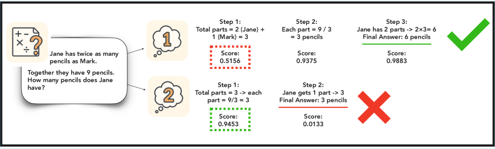
Figure 1: A true example of PRM assigning a lower score to the first step of a solution that turns out to be correct. In deterministic scaling methods, this solution would have been discarded in favor for one that had a higher initial PRM score but turned out to be incorrect.
Beyond answer-level scaling methods like self-consistency and best-of- $n$ sampling (brown2024largelanguage, ), a popular class of ITS methods formulates inference as search guided by a process reward model (PRM), which scores partial sequences step-by-step. This perspective has led to the adoption of algorithms like beam search (zhou2024languageagenttreesearch, ) and Monte Carlo tree search (guan2025rstarmathsmall, ). These methods refine LLM outputs by prioritizing trajectories that score highly according to the PRM. However, they also inherit a major limitation from classical search: early pruning. Because the PRM is an imperfect approximation of true correctness, these methods often eliminate promising candidates too early-based on noisy or miscalibrated partial scores. This failure mode is illustrated in Figure 1. The PRM assigns a higher initial score to Answer 2, which ultimately turns out to be incorrect, and a lower score to the correct Answer 1. A deterministic method like beam search would discard Answer 1 after the first step, never recovering it—even though it is the correct solution. Such brittleness is inherent to greedy search: once a path is pruned, it cannot be revisited.
To address this limitation, we instead maintain a distribution over the possible paths during generation to represent the uncertainty we would like to account for due to the imperfection in reward modeling and propagate it through sampling. We realize this approach in a probabilistic inference framework for inference-time scaling, in which we use particle filtering to sample from the posterior distribution over accepted trajectories. Our method maintains a weighted population of candidate sequences that evolves over time, balancing exploitation of high-PRM paths with stochastic exploration of alternatives. Unlike beam search, which targets the mode of an approximate distribution, particle filtering samples from the typical set, making it inherently more robust to noise and multi-modality in the reward landscape. High-scoring candidates are favored but not allowed to dominate, ensuring that low-probability (but potentially correct) paths remain in play.
We demonstrate that this simple shift-from deterministic search to sampling with uncertainty—produces strong empirical gains. On mathematical and reasoning tasks, our method significantly outperforms existing ITS approaches across multiple model families. For instance, using Qwen2.5-Math-1.5B-Instruct and a compute budget of 4, our method surpasses GPT-4o; with a budget of 32, the 7B model surpasses o1 accuracy.
Our key contributions are as follows.
1. We propose a particle filtering algorithm for inference-time scaling that mitigates early pruning by maintaining exploration across trajectories with uncertainty. We formulate ITS as posterior inference over a state space model defined by an LLM (transition model) and PRM (emission model), enabling principled application of probabilistic inference tools.
1. We present strong results on mathematical and out-of-domain reasoning tasks and study Particle Filtering’s scaling performance.
1. We ablate compute allocation strategies (parallel vs. iterative), PRM aggregation methods, and generation temperature, proposing a new model-based reward aggregation method that improves stability and performance.
1. We demonstrate that our proposed methods have 4–16x faster scaling speed than previous methods based on a search formulation on the MATH500 and AIME 2024 datasets, with small language models in the Llama and Qwen families. We show that PF can scale Qwen2.5-Math-1.5B-Instruct to surpasses GPT-4o accuracy with only a budget of 4 and scale Qwen2.5-Math-7B-Instruct to o1 accuracy with a budget of 32.
2 Background
State space models describe sequential systems that evolve stepwise, typically over time (Särkkä_2013, ). They consist of a sequence of latent states $\{x_{t}\}_{t=1}^{T}$ and corresponding observations $\{o_{t}\}_{t=1}^{T}$ The evolution of states is governed by a transition model $p(x_{t}\mid x_{<t-1})$ , and the observations are governed by the emission model $p(o_{t}|x_{t})$ . The joint distribution of states and observations is given by: $p(x_{1:T},o_{1:T})=p(x_{1}){\prod}_{t=2}^{T}p(x_{t}\mid x_{<t-1}){\prod}_{t=1}^{T}p(o_{t}\mid x_{t})$ , where $p(x_{1})$ is the prior.
Probabilistic inference in SSMs involves estimating the posterior distribution of the hidden states given the observations, $p(x_{1:T}|o_{1:T})$ (Särkkä_2013, ), which is generally intractable due to the high dimensionality of the state space and the dependencies in the model. Common approaches approximate the posterior through sampling-based methods or variational approaches (mackay2003information, ). Particle filtering (PF) is a sequential Monte Carlo method to approximate the posterior distribution in SSMs (nonlinearfiltering, ; sequentialmonte, ). PF represents the posterior using a set of $N$ weighted particles $\{x_{t}^{(i)},w_{t}^{(i)}\}_{i=1}^{N}$ , where $x_{t}^{(i)}$ denotes the $i^{\text{th}}$ particle at time $t$ , and $w_{t}^{(i)}$ is its associated weight. The algorithm iteratively propagates particles using the transition model and updates weights based on the emission model: $w_{t}^{(i)}\propto w_{t-1}^{(i)}p(o_{t}\mid x_{t}^{(i)})$ .
3 Method
<details>
<summary>x2.png Details</summary>
### Visual Description
# Technical Document Extraction: Particle Filtering for Mathematical Reasoning
This document describes a flowchart illustrating a multi-step reasoning process using a "particle filtering" approach to solve a word problem. The process involves generating steps, scoring them, and resampling based on those scores to reach a final answer.
## 1. Input Problem (Header/Left Region)
The process begins with a mathematical word problem contained in a speech bubble:
> "Jane has twice as many pencils as Mark. Together they have 9 pencils. How many pencils does Jane have?"
---
## 2. Process Flow Components
The diagram is organized into three main stages of generation and two intermediate resampling phases.
### Stage 1: Generate a 1st step / score (Pink Header)
Three initial "particles" (hypotheses) are generated:
| Particle | Content | Score |
| :--- | :--- | :--- |
| **Particle 1** | Step 1: Total parts = 2 (Jane) + 1 (Mark) = 3 | 0.3198 |
| **Particle 2** | Step 1: Total parts = 3 -> each part = 9/3 = 3 | 0.9453 |
| **Particle 3** | Step 1: Let J = x, M = 2x | 0.5898 |
### Phase 1: Resampling (Orange Header)
Based on the scores in Stage 1, the particles are redistributed:
* **Particle 2** (highest score) is resampled twice (indicated by black dotted lines leading to two different nodes).
* **Particle 1** is resampled once (indicated by a green dotted line).
* **Particle 3** is discarded (no lines lead from it).
---
### Stage 2: Generate a next step / score (Pink Header)
The resampled particles continue their reasoning:
| Particle | Content | Score | Notes |
| :--- | :--- | :--- | :--- |
| **Particle 1** | Step 2: Each part = 9 / 3 = 3 pencils | 0.9375 | Derived from previous Particle 1 |
| **Particle 2** | Step 2: Jane gets 1 part -> 3. Final Answer: 3 pencils. | 0.0133 | Completed its answer |
| **Particle 3** | Step 2: Mark = 1 part | 0.0392 | Derived from previous Particle 2 |
### Phase 2: Resampling (Orange Header)
* **Particle 1** (highest score in this stage) is resampled twice (indicated by a black dotted line and a green dotted line).
* The other particles are discarded or reach a terminal state with low scores.
---
### Stage 3: Generate a next step / score (Pink Header)
The final reasoning steps are generated:
| Particle | Content | Score | Notes |
| :--- | :--- | :--- | :--- |
| **Particle 1** | Step 3: Mark has 1 part = 3 pencils. Jane has other 6. Final Answer: 6 Pencils. | 0.8133 | Completed its answer |
| **Particle 3** | Step 3: Jane has 2 parts -> 2x3 = 6. Final Answer: 6 pencils. | 0.9883 | Completed its answer |
---
## 3. Final Selection (Green Region)
**Header:** "Select particle with highest reward as final answer"
The system selects the path with the highest final score (0.9883), which is highlighted by a green dotted line leading to the final consolidated solution block.
**Final Answer Content:**
* **Step 1:** Total parts = 2 (Jane) + 1 (Mark) = 3
* **Step 2:** Each part = 9 / 3 = 3 pencils
* **Step 3:** Jane has 2 parts -> 2x3 = 6
* **Final Answer:** 6 pencils
---
## 4. Visual Legend & Logic Summary
* **Color Coding:**
* **Pink Labels:** Action steps (Generation).
* **Orange Labels:** Selection steps (Resampling).
* **Blue Boxes:** Active reasoning particles. The saturation of blue roughly correlates with the confidence/score.
* **Green Box/Lines:** The "Winning" path and final output.
* **Trend Analysis:** The process filters out incorrect logic (like Particle 3's algebraic setup or Particle 2's incorrect Step 2 conclusion) by favoring paths with higher numerical scores during the resampling phases. The green dotted line traces the "optimal" path from Step 1 through to the final result.
</details>
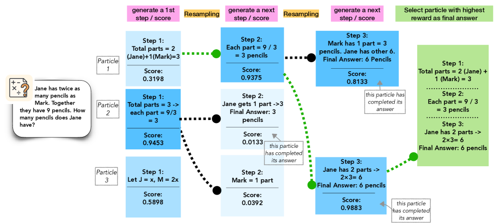
Figure 2: Inference-time scaling with particle filtering: initialize $n$ particles, generate a step for each, score with the PRM, resample via softmax-weighted scores, and repeat until full solutions are formed.
We formulate inference-time scaling for a language model $p_{M}$ as approximate posterior inference in a state space model (SSM) defined over token sequences. Let $x_{1:T}$ denote the sequence of generated tokens (or chunks, such as steps in a math problem), and let $o_{1:T}$ denote binary observations indicating whether the steps so far are accepted, given a prompt $c$ .
The forward model defines the joint distribution over latent states and observations as:
$$
\displaystyle p_{M}(x_{1:T},o_{1:T}\mid c)\propto\prod_{t=1}^{T}p_{M}(x_{t}\mid c,x_{<t-1})\prod_{t=1}^{T}p(o_{t}\mid c,x_{<t}), \tag{1}
$$
where the transition model $p_{M}(x_{t}\mid c,x_{<t-1})$ is given by the language model $M$ , and the emission model $p(o_{t}\mid c,x_{<t})$ is a Bernoulli distribution: $p(o_{t}\mid c,x_{<t})=\mathcal{B}(o_{t};r(c,x_{t}))$ , with reward function $r(c,x_{t})$ encoding the acceptability of the step $x_{t}$ . Figure 3 illustrates this SSM.
Given this model, our goal is to infer the posterior distribution over latent trajectories that yield fully accepted sequences, i.e., $p_{M}(x_{1:T}\mid c,o_{1:T}=\mathbf{1})$ . This formulation makes particle filtering a natural and theoretically grounded choice for inference.
In practice, the true reward function $r$ is often unavailable. Following prior work, we approximate it using a pre-trained preference or reward model (PRM) $\hat{r}$ suited to the target domain (e.g., math reasoning). This results in an approximate emission model: $\hat{p}(o_{t}\mid c,x_{<t})=\mathcal{B}(o_{t};\hat{r}(c,x_{<t}))$ . Substituting this into the forward model, we obtain the approximate joint distribution:
$$
\displaystyle\hat{p}_{M}(x{1:T},o_{1:T}\mid c)\propto\prod_{t=1}^{T}p_{M}(x_{t}\mid c,x_{<t-1})\prod_{t=1}^{T}\hat{p}(o_{t}\mid c,x_{<t}), \tag{2}
$$
and correspondingly aim to estimate the posterior $\hat{p}_{M}(x{1:T}\mid c,o_{1:T}=\mathbf{1})$ . $x_{1}$ $x_{2}$ $·s$ $x_{T}$ $c$ $o_{1}$ $o_{2}$ $·s$ $o_{T}$ $p_{M}(x_{1}\mid c)$ $p_{M}(x_{2}\mid c,x_{1})$ $p_{M}(x_{T}\mid c,x_{<T})$ $\hat{p}(o_{1}\mid c,x_{1})$ $\hat{p}(o_{2}\mid c,x_{2})$ $\hat{p}(o_{t}\mid c,x_{<t})$ language model reward model
Figure 3: State-space model for inference-time scaling. $c$ is a prompt, $x_{1},...,x_{T}$ are LLM outputs, and $o_{1},...,o_{T}$ are “observed” acceptances from a reward model. We estimate the latent states conditioned on $o_{t}=1$ for all $t$ .
3.1 Particle Filtering for Estimating the Posterior
We now apply particle filtering (PF) to approximate the posterior over accepted sequences $x_{1:T}$ under the model in (2). Each particle represents a partial trajectory, and inference proceeds by iteratively generating, scoring, and resampling these particles based on their reward-induced likelihood. At each time step $t$ , PF maintains a population of $N$ weighted particles. The algorithm proceeds as follows:
- Initialization ( $t=1$ ): Each particle is initialized by sampling the first token from the LLM: $x_{1}^{(i)}\sim p_{M}(x_{1}\mid c)$ .
- Propagation ( $t>1$ ): Each particle is extended by sampling the next token from the LLM conditioned on its history: $x_{t}^{(i)}\sim p_{M}(x_{t}\mid c,x_{<t-1}^{(i)})$ .
- Weight Update: Using a reward model $\hat{r}$ , each particle is assigned an unnormalized weight that reflects the likelihood of acceptance: $w_{t}^{(i)}\propto w_{t-1}^{(i)}·\hat{r}(c,x_{<t}^{(i)})$ .
- Resampling: To focus computation on promising trajectories, we sample a new population of particles from the current set using a softmax distribution over weights: $\mathbb{P}_{t}(j=i)={\exp(w_{t}^{(i)})}/{\sum{i\textquoteright=1}^{N}\exp(w_{t}^{(i\textquoteright)})}$ .
The next generation of particles is formed by sampling indices $j_{t}^{(1)},...,j_{t}^{(N)}\sim\mathbb{P}_{t}$ and retaining the corresponding sequences.
This procedure balances exploitation of high-reward partial generations with stochastic exploration, increasing the chances of recovering correct completions even when early steps are uncertain.
The algorithm can be implemented efficiently: both token sampling and reward computation can be parallelized across particles. With prefix caching, the total runtime is comparable to generating $N$ full completions independently.
Final Answer Selection
Particle filtering yields a weighted set of samples approximating the posterior, enabling principled answer selection strategies. While selecting the highest-weighted particle or using (weighted) majority voting better reflects the typical set, we adopt the standard practice of scoring all final outputs with an outcome reward model (ORM) and selecting the top-scoring one for fair comparison with prior work. Additionally, the posterior samples allow richer evaluation—for instance, estimating the expected correctness of the model under its own distribution, rather than relying solely on point estimates. Notably, samples from Algorithm 1 can be used to construct unbiased estimates of any expectation over (2). In the context of math and reasoning, it guarantees the expected accuracy is unbiased, which we formulate in Theorem 2 (proof in Appendix C).
**Theorem 1 (Unbiasedness of Expected Accuracy)**
*Let $\{(w^{(i)},x^{(i)})\}$ be weighted particles from Algorithm 1 and $\mathrm{is\_correct}(x)$ is a function to check the correctness of response $x$ . We have
$$
\mathbb{E}\left\{\sum_{i}\left[w^{(i)}\;\mathrm{is\_correct}(x^{(i)})\right]\right\}=\sum_{x}\left[\hat{p}_{M}(x_{1:T}\mid c,o_{1:T}=\mathbf{1})\;\mathrm{is\_correct}(x^{(i)})\right], \tag{3}
$$
where the expectation is over the randomness of the algorithm itself.*
Reward Aggregation with PRMs
To compute particle weights during generation, we aggregate per-step scores from the process reward model (PRM) $\hat{r}$ . Our default uses a product of step-level rewards to align with the factorized likelihood structure, but alternative aggregation strategies (e.g., min, last-step, or model-based) may offer different trade-offs. We describe and compare these strategies in detail in Appendix A and report ablation results in 4.5.
Sampling v.s. deterministic search
An alternative to our sampling-based approach is to treat inference-time scaling as an optimization problem under the approximate posterior (2), reducing to deterministic search methods like beam search or MCTS. However, these methods assume the reward model $\hat{r}$ is accurate at every step and prune aggressively based on early scores. In practice, PRMs are noisy and their preferences often shift during unrolling. As a result, deterministic search can irreversibly discard trajectories that may have low early scores but high posterior mass overall. Once pruned, such paths cannot be recovered.
In contrast, particle filtering maintains a distribution over partial sequences and uses stochastic resampling to balance exploration and exploitation. This allows recovery from early errors and robustness to reward noise. While beam search targets the mode of the approximate posterior-making it sensitive to local errors-PF samples from the typical set, smoothing over inconsistencies in $\hat{r}$ . Unlike search heuristics, PF provides consistent, unbiased estimators under mild assumptions, and naturally captures multi-modal solutions—critical when multiple valid completions exist. We validate these advantages empirically in Section 4.5.
Multiple iterations and parallel chains
The PF approach to inference-time scaling can be used to define a MCMC kernel that enables two new types of scaling: multiple iterations of complete answers inspired by PG and parallel simulations inspired by parallel tempering. We detail the methodology and results for both extensions in sections B.1 and B.2 in the appendix.
4 Evaluation
We evaluate our proposed methods in this section. We detail our experimental setup in Section 4.1 and start with highlighted results comparing against closed-source models and competitive inference-time scaling methods with open-source models (Section 4.2). We then study how the main algorithm, particle filtering, scales with more computation and compare it with competitors (Section 4.4). We further perform an extensive ablation study on key algorithmic choices like reward models, reward aggregation, final answer aggregation, and LLM temperatures (Section 4.5). Finally, we study different allocations of the compute budget through iterative and parallel extensions (Section 4.5).
4.1 Setup
Models
We consider two types of open-source small language models (SLMs) as our policy models for generating solutions. The first is general models, for which we evaluate Qwen2.5-1.5B-Instruct (qwen_2_5, ), Qwen2.5-7B-Instruct, Llama-3.2-1B-Instruct, and Llama-3.1-8B-Instruct (llama3, ). The second is math models, using Qwen2.5-Math-1.5B-Instruct and Qwen2.5-Math-7B-Instruct. These small models are well-suited for inference-time scaling, enabling efficient search of multiple trajectories.
Process Reward Models
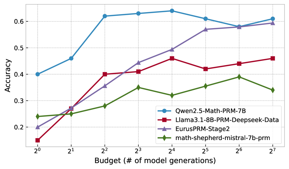
To guide our policy models, we utilized Qwen2.5-Math-PRM-7B (prmlessons, ), a 7B process reward model. We selected this model for its superior performance over other PRMs we tested, including Math-Shepherd-mistral-7b-prm (wang2024mathshepherdverifyreinforcellms, ), Llama3.1-8B-PRM-Deepseek-Data (xiong2024rlhflowmath, ), and EurusPRM-Stage2 (primerm, ). This result as an ablation study is provided in Section 4.5, where we also study the different ways to aggregate step-level rewards from PRMs discussed in Section 3.1.
Baselines
- Greedy: single greedy generation from the model, serving as the “bottom-line” performance.
- Self Consistency (wang2023selfconsistencyimproveschainthought, ): simplest scaling method, majority voting across candidates
- BoN/WBoN (brown2024largelanguage, ): simple RM-based scaling method, scores outputs with outcome reward models
- Beam Search (snell2024scalingllmtesttimecompute, ): structured search procedure that incrementally builds sequences by keeping the top- $k$ highest-scoring partial completions at each generation step.
- DVTS (beeching2024scalingtesttimecompute, ): a parallel extension of beam search that improves the exploration and performance.
Datasets
We evaluate our methods and baselines across a wide variety of tasks that span difficulty level and domain to test basic and advanced problem-solving and reasoning.
- MATH500 (math500, ): 500 competition-level problems from various mathematical domains.
- AIME 2024 (ai_mo_validation_aime, ): 30 high difficulty problems from the American Invitational Mathematics Examination (AIME I and II) 2024.
- NumGLUE Task 2 (Chemistry) (mishra2022numglue, ): 325 questions that test advanced reasoning across real-world tasks, mostly centered on the chemistry domain.
- FinanceBench (islam2023financebenchnewbenchmarkfinancial, ): 150 open-book financial question answering tasks grounded in real-world financial documents and analysis.
Parsing and scoring
Details on parsing and scoring functions across datasets in the Appendix H
4.2 Results on Mathematical Reasoning Datasets
<details>
<summary>x3.png Details</summary>
### Visual Description
# Technical Data Extraction: Model Accuracy vs. Generation Budget
## 1. Image Overview
This image is a line graph comparing the performance (Accuracy) of different inference methods applied to the **Llama-3.2-1B-Instruct** model against various baseline models. The performance is measured relative to a computational "Budget," defined as the number of model generations.
## 2. Axis Definitions
* **Y-Axis (Vertical):** Accuracy.
* **Range:** 0.2 to 0.7+ (labeled increments of 0.1).
* **X-Axis (Horizontal):** Budget (# of model generations).
* **Scale:** Logarithmic (base 2).
* **Markers:** $2^0, 2^1, 2^2, 2^3, 2^4, 2^5, 2^6, 2^7$ (representing 1 to 128 generations).
## 3. Baseline Reference Lines (Horizontal Dotted Lines)
These lines represent "0-shot CoT (Greedy)" performance for specific models, acting as static benchmarks.
* **GPT-4o:** Accuracy $\approx$ 0.76
* **Llama-3.1-70B-Instruct:** Accuracy $\approx$ 0.66
* **Llama-3.1-8B-Instruct:** Accuracy $\approx$ 0.42
* **Llama-3.2-1B-Instruct:** Accuracy $\approx$ 0.225
## 4. Legend and Data Series Analysis
The legend is located in the bottom-right quadrant of the chart area.
### Series 1: Ours-Particle Filtering (Llama-3.2-1B-Instruct)
* **Visual Identifier:** Blue line with square markers.
* **Trend:** Steepest upward slope in the early stages ($2^0$ to $2^3$), maintaining the highest accuracy among the 1B model methods across all budget levels.
* **Key Data Points (Approximate):**
* $2^0$: 0.21
* $2^2$: 0.43 (Surpasses Llama-3.1-8B-Instruct baseline)
* $2^7$: 0.60 (Approaching Llama-3.1-70B-Instruct baseline)
### Series 2: DVTS (Llama-3.2-1B-Instruct)
* **Visual Identifier:** Purple line with diamond markers.
* **Trend:** Steady upward slope. Starts at $2^2$ budget. Consistently performs between the Particle Filtering and Weighted BoN methods.
* **Key Data Points (Approximate):**
* $2^2$: 0.40
* $2^4$: 0.49
* $2^7$: 0.55
### Series 3: Weighted BoN (Llama-3.2-1B-Instruct)
* **Visual Identifier:** Red line with diamond markers.
* **Trend:** Upward slope, but the shallowest of the three experimental methods.
* **Key Data Points (Approximate):**
* $2^0$: 0.20
* $2^3$: 0.40
* $2^7$: 0.505
## 5. Summary Table of Extracted Data (Estimated Values)
| Budget ($2^n$) | Weighted BoN (Red) | Ours-Particle Filtering (Blue) | DVTS (Purple) |
| :--- | :--- | :--- | :--- |
| **$2^0$ (1)** | 0.20 | 0.21 | - |
| **$2^1$ (2)** | 0.27 | 0.31 | - |
| **$2^2$ (4)** | 0.34 | 0.43 | 0.40 |
| **$2^3$ (8)** | 0.40 | 0.50 | 0.44 |
| **$2^4$ (16)** | 0.43 | 0.53 | 0.49 |
| **$2^5$ (32)** | 0.47 | 0.57 | 0.50 |
| **$2^6$ (64)** | 0.48 | 0.60 | 0.53 |
| **$2^7$ (128)** | 0.51 | 0.60 | 0.55 |
## 6. Key Findings
1. **Scaling Efficiency:** The "Ours-Particle Filtering" method applied to a 1B model achieves the accuracy of a 0-shot 8B model with a budget of only 4 generations ($2^2$).
2. **Closing the Gap:** With a budget of 128 generations ($2^7$), the 1B model using Particle Filtering reaches ~60% accuracy, significantly narrowing the gap toward the 70B model's 66% baseline.
3. **Method Superiority:** Particle Filtering consistently outperforms both Weighted Best-of-N (BoN) and DVTS across the entire tested budget range.
</details>
(a) Llama-3.2-1B-Instruct
<details>
<summary>x4.png Details</summary>
### Visual Description
# Technical Document Extraction: Model Accuracy vs. Generation Budget
## 1. Image Overview
This image is a line graph comparing the performance (Accuracy) of different inference-time scaling methods against a computational budget (number of model generations). The chart specifically evaluates these methods using the **Llama-3.1-8B-Instruct** model as a base, while providing horizontal baselines for other models.
---
## 2. Component Isolation
### A. Header / Baselines (Top & Middle Regions)
The chart contains four horizontal black dotted lines representing "0-shot CoT (Greedy)" performance for various models. These serve as static benchmarks.
| Model | Approximate Accuracy |
| :--- | :--- |
| GPT-4o | 0.76 |
| Llama-3.1-70B-Instruct | 0.66 |
| Llama-3.1-8B-Instruct | 0.42 |
| Llama-3.2-1B-Instruct | 0.225 |
### B. Main Chart Area (Data Series)
The x-axis is logarithmic (base 2), and the y-axis is linear. There are three primary data series plotted.
#### Legend
* **Red Line with Diamond Markers**: `Weighted BoN (Llama-3.1-8B-Instruct)`
* **Blue Line with Square Markers**: `Ours-Particle Filtering (Llama-3.1-8B-Instruct)`
* **Purple Line with Diamond Markers**: `DVTS (Llama-3.1-8B-Instruct)`
* **Black Dotted Line**: `0-shot CoT (Greedy)` (Reference for the baselines mentioned in section A).
---
## 3. Trend Verification and Data Extraction
### Series 1: Ours-Particle Filtering (Blue Square)
* **Trend**: This is the highest-performing method. It shows a steep logarithmic growth from $2^0$ to $2^4$, then begins to plateau as it approaches the GPT-4o baseline.
* **Data Points (Approximate):**
* $2^0$ (1): 0.41
* $2^1$ (2): 0.52
* $2^2$ (4): 0.62
* $2^3$ (8): 0.69
* $2^4$ (16): 0.72
* $2^5$ (32): 0.74
* $2^6$ (64): 0.745
* $2^7$ (128): 0.75
### Series 2: DVTS (Purple Diamond)
* **Trend**: This series starts at a higher budget ($2^2$). It shows a steady upward slope, consistently performing better than Weighted BoN but significantly lower than Particle Filtering. It surpasses the Llama-3.1-70B-Instruct baseline at a budget of $2^6$.
* **Data Points (Approximate):**
* $2^2$ (4): 0.54
* $2^3$ (8): 0.59
* $2^4$ (16): 0.62
* $2^5$ (32): 0.63
* $2^6$ (64): 0.66
* $2^7$ (128): 0.67
### Series 3: Weighted BoN (Red Diamond)
* **Trend**: The lowest performing of the three active methods. It shows a steady but slower increase in accuracy, failing to reach the Llama-3.1-70B-Instruct baseline even at the maximum budget shown.
* **Data Points (Approximate):**
* $2^0$ (1): 0.39
* $2^1$ (2): 0.44
* $2^2$ (4): 0.49
* $2^3$ (8): 0.54
* $2^4$ (16): 0.575
* $2^5$ (32): 0.585
* $2^6$ (64): 0.59
* $2^7$ (128): 0.595
---
## 4. Axis and Labels
* **Y-Axis Title**: `Accuracy`
* **Y-Axis Markers**: 0.2, 0.3, 0.4, 0.5, 0.6, 0.7
* **X-Axis Title**: `Budget (# of model generations)`
* **X-Axis Markers (Log Scale)**: $2^0, 2^1, 2^2, 2^3, 2^4, 2^5, 2^6, 2^7$ (representing 1 to 128 generations).
---
## 5. Key Technical Insights
1. **Efficiency**: The "Ours-Particle Filtering" method using an 8B model achieves GPT-4o level performance (approx. 0.75) with a budget of 128 generations ($2^7$).
2. **Scaling**: All methods show diminishing returns as the budget increases, evidenced by the flattening of the curves at higher x-values.
3. **Model Comparison**: The 8B model using Particle Filtering outperforms the 70B model's greedy baseline at a budget of only 8 generations ($2^3$).
</details>
(b) Llama-3.1-8B-Instruct
<details>
<summary>x5.png Details</summary>
### Visual Description
# Technical Document Extraction: Model Accuracy vs. Generation Budget
## 1. Image Overview
This image is a line graph illustrating the relationship between computational budget (measured in the number of model generations) and the accuracy of various Large Language Model (LLM) inference strategies. The chart compares three dynamic sampling/filtering methods against several static baselines.
## 2. Component Isolation
### A. Header / Reference Baselines
The top and middle sections of the chart contain horizontal black dotted lines representing fixed performance benchmarks for specific models:
* **o1-preview**: Positioned at approximately **0.870** accuracy.
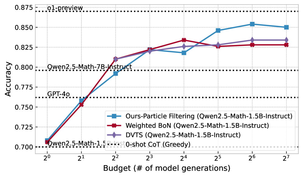
* **Qwen2.5-Math-7B-Instruct**: Positioned at approximately **0.796** accuracy.
* **GPT-4o**: Positioned at approximately **0.762** accuracy.
* **Qwen2.5-Math-1.5B-Instruct 0-shot CoT (Greedy)**: Positioned at the baseline of **0.700** accuracy.
### B. Main Chart Area (Data Series)
The chart plots three primary data series using a logarithmic scale for the X-axis. All three series use **Qwen2.5-Math-1.5B-Instruct** as the base model.
**Legend:**
* **Blue Line with Square Markers (■):** Ours-Particle Filtering
* **Red Line with Cross/Diamond Markers (✖/◆):** Weighted BoN (Best-of-N)
* **Purple Line with Diamond Markers (◆):** DVTS
### C. Axes and Scale
* **Y-Axis (Vertical):** Labeled **"Accuracy"**. Scale ranges from **0.700 to 0.875** with increments of 0.025.
* **X-Axis (Horizontal):** Labeled **"Budget (# of model generations)"**. It uses a base-2 logarithmic scale: $2^0, 2^1, 2^2, 2^3, 2^4, 2^5, 2^6, 2^7$ (representing 1 to 128 generations).
## 3. Trend Verification and Data Extraction
| Budget ($2^n$) | Ours-Particle Filtering (Blue ■) | Weighted BoN (Red ✖) | DVTS (Purple ◆) |
| :--- | :--- | :--- | :--- |
| $2^0$ (1) | 0.708 | 0.706 | 0.706 |
| $2^1$ (2) | 0.759 | 0.753 | 0.753 |
| $2^2$ (4) | 0.792 | 0.810 | 0.810 |
| $2^3$ (8) | 0.822 | 0.822 | 0.821 |
| $2^4$ (16) | 0.818 | 0.834 | 0.826 |
| $2^5$ (32) | 0.846 | 0.826 | 0.828 |
| $2^6$ (64) | 0.854 | 0.828 | 0.834 |
| $2^7$ (128) | 0.850 | 0.828 | 0.834 |
## 4. Key Findings and Observations
1. **Scaling Efficiency:** All three methods significantly improve the performance of the 1.5B model. By a budget of $2^2$ (4 generations), the 1.5B model using any of these methods outperforms the much larger **GPT-4o** baseline.
2. **Surpassing Larger Models:** By a budget of $2^3$ (8 generations), all three methods outperform the **Qwen2.5-Math-7B-Instruct** model.
3. **Particle Filtering Superiority:** While Weighted BoN and DVTS perform similarly, the "Ours-Particle Filtering" method shows superior scaling at higher budgets (32+ generations), approaching the performance of the **o1-preview** model.
4. **Diminishing Returns:** The Weighted BoN method appears to plateau or slightly regress after 16 generations ($2^4$), whereas Particle Filtering and DVTS continue to show gains or stability.
</details>
(c) Qwen2.5-Math-1.5B-Instruct
<details>
<summary>x6.png Details</summary>
### Visual Description
# Technical Document Extraction: Model Accuracy vs. Generation Budget
## 1. Image Overview
This image is a line graph comparing the performance (Accuracy) of different inference strategies for Large Language Models (LLMs) against a computational budget (number of model generations). The chart uses a logarithmic scale for the x-axis and includes several horizontal reference lines for baseline models.
## 2. Component Isolation
### A. Header / Reference Baselines
The top of the chart contains horizontal black dotted lines representing fixed performance benchmarks.
* **o1-preview**: Positioned at approximately **0.870** accuracy.
* **Qwen2.5-Math-7B-Instruct**: Positioned at approximately **0.796** accuracy.
* **GPT-4o**: Positioned at approximately **0.762** accuracy.
* **Qwen2.5-Math-1.5B-Instruct**: Positioned at approximately **0.700** accuracy.
### B. Main Chart Area (Data Series)
The chart plots four primary data series against a budget ranging from $2^0$ to $2^7$.
**Axis Labels:**
* **Y-Axis**: "Accuracy" (Range: 0.700 to 0.875, increments of 0.025).
* **X-Axis**: "Budget (# of model generations)" (Logarithmic scale: $2^0, 2^1, 2^2, 2^3, 2^4, 2^5, 2^6, 2^7$).
**Legend:**
1. **Blue line with square markers (■)**: `Ours-Particle Filtering (Qwen2.5-Math-7B-Instruct)`
2. **Red line with diamond markers (◆)**: `Weighted BoN (Qwen2.5-Math-7B-Instruct)`
3. **Purple line with diamond markers (◆)**: `DVTS (Qwen2.5-Math-7B-Instruct)`
4. **Black dotted line (---)**: `0-shot CoT (Greedy)` (Note: This serves as the baseline for the 7B model).
---
## 3. Trend Verification and Data Extraction
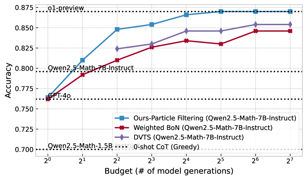
### Series 1: Ours-Particle Filtering (Blue, Square Markers)
* **Trend**: Steep upward slope from $2^0$ to $2^4$, then plateaus/saturates as it reaches the `o1-preview` baseline at $2^5$. This is the highest-performing method shown.
* **Data Points (Approximate):**
* $2^0$: 0.765
* $2^1$: 0.810
* $2^2$: 0.848
* $2^3$: 0.854
* $2^4$: 0.866
* $2^5$: 0.870 (Matches `o1-preview`)
* $2^6$: 0.870
* $2^7$: 0.870
### Series 2: DVTS (Purple, Diamond Markers)
* **Trend**: Steady upward slope, consistently performing between the Particle Filtering and Weighted BoN methods. It shows a significant jump between $2^1$ and $2^2$.
* **Data Points (Approximate):**
* $2^0$: 0.762 (Starts at GPT-4o level)
* $2^1$: 0.792
* $2^2$: 0.824
* $2^3$: 0.830
* $2^4$: 0.846
* $2^5$: 0.846
* $2^6$: 0.854
* $2^7$: 0.854
### Series 3: Weighted BoN (Red, Diamond Markers)
* **Trend**: Upward slope but with lower efficiency than the other two methods. It shows a slight dip/stagnation at $2^5$ before rising again at $2^6$.
* **Data Points (Approximate):**
* $2^0$: 0.762
* $2^1$: 0.792
* $2^2$: 0.810
* $2^3$: 0.826
* $2^4$: 0.834
* $2^5$: 0.830 (Slight decrease)
* $2^6$: 0.846
* $2^7$: 0.846
---
## 4. Summary Table of Extracted Data
| Budget ($2^n$) | Ours-Particle Filtering | DVTS | Weighted BoN |
| :--- | :--- | :--- | :--- |
| **$2^0$ (1)** | 0.765 | 0.762 | 0.762 |
| **$2^1$ (2)** | 0.810 | 0.792 | 0.792 |
| **$2^2$ (4)** | 0.848 | 0.824 | 0.810 |
| **$2^3$ (8)** | 0.854 | 0.830 | 0.826 |
| **$2^4$ (16)** | 0.866 | 0.846 | 0.834 |
| **$2^5$ (32)** | 0.870 | 0.846 | 0.830 |
| **$2^6$ (64)** | 0.870 | 0.854 | 0.846 |
| **$2^7$ (128)** | 0.870 | 0.854 | 0.846 |
## 5. Key Observations
* **Efficiency**: The "Ours-Particle Filtering" method reaches the performance level of `o1-preview` (the highest baseline) with a budget of $2^5$ (32 generations).
* **Baseline Comparison**: All three tested methods (Particle Filtering, DVTS, Weighted BoN) using the Qwen2.5-Math-7B-Instruct model eventually exceed the performance of GPT-4o and the base 7B-Instruct model's greedy decoding.
* **Saturation**: All methods appear to reach a performance plateau between $2^6$ and $2^7$ generations.
</details>
(d) Qwen2.5-Math-7B-Instruct
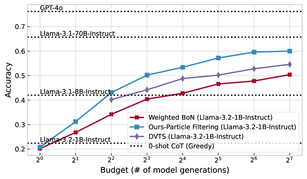
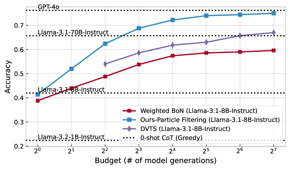
Figure 4: Accuracy vs. Generation Budget across models using different inference-time strategies.
We present our main results in Table 1, comparing Particle Filtering (PF) with a suite of strong inference-time scaling baselines on two challenging mathematical reasoning tasks: MATH500 and AIME 2024. All inference-time scaling methods are evaluated under a fixed compute budget of 32 generations per instance, using Qwen2.5-Math-PRM-7B as the reward model. Specifically, it serves as the PRM for PF, Beam Search, and DVTS, and as the ORM in WBoN.
- PF consistently achieves the best performance across all model sizes. Among all inference-time scaling methods, PF delivers the highest accuracy on both benchmarks, often outperforming alternatives by a significant margin.
- PF unlocks competitive performance even for small models. For instance, Qwen2.5-1.5B-Instruct, when scaled using PF, surpasses the much larger GPT-4o on both MATH500 and AIME 2024. This showcases the ability of inference-time compute to significantly improve performance without increasing model size.
- PF on Qwen2.5-Math-7B-Instruct outperforms o1-preview on MATH500. Scaling Qwen2.5-Math-7B with PF results in a new state-of-the-art among open models: 87.7% on MATH500 and 10/30 on AIME. This surpasses the o1-preview model and highlights the potential of inference-time scaling to close the gap with—or even exceed—the performance of proprietary frontier LLMs using smaller, open models.
For results on additional model families and broader ablations, see Appendix F.
| Model Closed Source LLMs GPT-4o | Method – | MATH500 76.2 | AIME 2024 4/30 |
| --- | --- | --- | --- |
| o1-preview | – | 87.0 | 12/30 |
| Claude 3.5 Sonnet | – | 78.2 | 5/30 |
| Open Source LLMs | | | |
| Llama-3.1 70B Instruct | – | 65.6 | 5/30 |
| Qwen-2.5 Math 72B Instruct | – | 82.0 | 9/30 |
| Open Source General SLMs | | | |
| Qwen-2.5 1.5B Instruct | Greedy | 54.4 | 1/30 |
| Self Consistency | 61.0 | 2/30 | |
| BoN | 67.8 | 1/30 | |
| WBoN | 69.2 | 2/30 | |
| Beam Search | 76.2 | 5/30 | |
| DVTS | 76.6 | 4/30 | |
| \rowcolor [HTML]C1DEB8 | \cellcolor [HTML]C1DEB8 Particle Filtering (Ours) | 79.3 | 6/30 |
| Open Source Math SLMs | | | |
| Qwen-2.5 Math 1.5B Instruct | Greedy | 70.0 | 3/30 |
| Self Consistency | 79.6 | 6/30 | |
| BoN | 81.8 | 4/30 | |
| WBoN | 82.6 | 4/30 | |
| Beam Search | 83.0 | 4/30 | |
| DVTS | 82.8 | 5/30 | |
| \rowcolor [HTML]C1DEB8 | \cellcolor [HTML]C1DEB8 Particle Filtering (Ours) | 84.6 | 7/30 |
| Qwen-2.5 Math 7B Instruct | Greedy | 79.6 | 5/30 |
| Self Consistency | 84.0 | 4/30 | |
| BoN | 82.6 | 5/30 | |
| WBoN | 83.0 | 5/30 | |
| Beam Search | 86.9 | 7/30 | |
| DVTS | 84.6 | 6/30 | |
| \rowcolor [HTML]C1DEB8 | \cellcolor [HTML]C1DEB8 Particle Filtering (Ours) | 87.7 | 10/30 |
Table 1: Results of various LLMs on MATH500 and AIME 2024, highlighting particle filtering performance. All methods used a compute budget of 32 generations with Qwen2.5-Math-PRM-7B as the reward model. Notably, Qwen2.5-Math-7B, with just 32 particles, matches o1-preview on MATH500, demonstrating PF’s effectiveness.
4.3 Results on Generalized Reasoning Datasets
To evaluate whether our inference-time scaling method generalizes beyond mathematical reasoning, we test Particle Filtering on two diverse instruction-following benchmarks: FinanceBench (islam2023financebenchnewbenchmarkfinancial, ), which evaluates financial QA over real-world documents, and NumGLUE Task 2 (Chemistry) (mishra2022numglue, ), which targets numerical reasoning in scientific contexts.
| Greedy | 62.67 | 71.69 |
| --- | --- | --- |
| BoN | 68.00 | 80.92 |
| Self Consistency | 68.67 | 79.32 |
| Beam Search | 67.33 | 80.47 |
| \rowcolor [HTML]C1DEB8 Particle Filtering (Ours) | 70.33 | 84.22 |
Table 2: Results on Non-Math Datasets
As shown in Table 2, Particle Filtering consistently outperforms all other inference-time scaling baselines, achieving the highest accuracy on both datasets. This shows that our method is effective not only for mathematical reasoning but also for broader instruction-following and domain-specific tasks. We use Llama 3.1-8B-Instruct as the policy model and Qwen2.5-Math-PRM-7B as the reward model, with 8 particles for FinanceBench and 32 for NumGLUE.
We note that although we use Qwen2.5-Math-PRM-7B - a reward model trained primarily for mathematical process evaluation - it performs surprisingly well as a reward model on these non-math domains. We hypothesize that such RMs implicitly learn broader reasoning evaluation capabilities during their training, not limited strictly to mathematical content. We leave deeper exploration of this hypothesis and the development of domain-specific or generalized PRMs for future work.
4.4 Scaling with inference-time compute
We now zoom in on how PF scales with inference-time compute. Figure 4 shows the change of performance (in terms of accuracy) with an increasing computation budget ( $N=1,2,4,8,16,32,64,128$ ) across Math SLMs and Non-Math SLMs. As we can see, PF scales 4–16x faster than the next best competitor DVTS, e.g. DVTS requires a budget of 32 to reach the same performance of PF with a budget of 8 with Llama-3.2-1B-Instruct and requires a budget of 128 to reach the performance of PF with a budget of 8 with LLama-3.1-8B-Instruct.
4.5 Ablation study
<details>
<summary>x7.png Details</summary>
### Visual Description
# Technical Data Extraction: Model Accuracy vs. Generation Budget
## 1. Image Overview
This image is a line graph plotting the **Accuracy** of four different Process Reward Models (PRMs) against a varying **Budget (# of model generations)**. The chart uses a logarithmic scale for the x-axis and a linear scale for the y-axis.
## 2. Axis and Legend Specifications
### Axis Labels
* **Y-Axis:** "Accuracy" (Linear scale ranging from approximately 0.15 to 0.65).
* **X-Axis:** "Budget (# of model generations)" (Logarithmic scale base 2, ranging from $2^0$ to $2^7$).
### Axis Markers
* **Y-Axis Markers:** 0.2, 0.3, 0.4, 0.5, 0.6.
* **X-Axis Markers:** $2^0$ (1), $2^1$ (2), $2^2$ (4), $2^3$ (8), $2^4$ (16), $2^5$ (32), $2^6$ (64), $2^7$ (128).
### Legend
| Color | Marker Shape | Label |
| :--- | :--- | :--- |
| **Blue** | Circle (●) | Qwen2.5-Math-PRM-7B |
| **Red** | Square (■) | Llama3.1-8B-PRM-Deepseek-Data |
| **Purple** | Triangle (▲) | EurusPRM-Stage2 |
| **Green** | Diamond (◆) | math-shepherd-mistral-7b-prm |
---
## 3. Data Series Analysis and Trends
### Series 1: Qwen2.5-Math-PRM-7B (Blue, Circle)
* **Trend:** This model consistently maintains the highest accuracy across almost all budget levels. It shows a sharp upward slope from $2^0$ to $2^2$, plateaus/peaks between $2^3$ and $2^4$, experiences a slight dip at $2^6$, and recovers at $2^7$.
* **Estimated Data Points:**
* $2^0$: 0.40
* $2^1$: 0.46
* $2^2$: 0.62
* $2^3$: 0.63
* $2^4$: 0.64 (Peak)
* $2^5$: 0.61
* $2^6$: 0.58
* $2^7$: 0.61
### Series 2: EurusPRM-Stage2 (Purple, Triangle)
* **Trend:** Shows the most consistent and steepest positive linear growth relative to the log-scale budget. It starts as the second-lowest performer and ends as the second-highest, nearly converging with the Qwen model at the highest budget.
* **Estimated Data Points:**
* $2^0$: 0.20
* $2^1$: 0.27
* $2^2$: 0.35
* $2^3$: 0.44
* $2^4$: 0.49
* $2^5$: 0.57
* $2^6$: 0.58
* $2^7$: 0.59
### Series 3: Llama3.1-8B-PRM-Deepseek-Data (Red, Square)
* **Trend:** Starts with the lowest accuracy at $2^0$. It shows a significant jump at $2^2$, followed by a generally upward but volatile trend, including a notable dip at $2^5$.
* **Estimated Data Points:**
* $2^0$: 0.15
* $2^1$: 0.27
* $2^2$: 0.40
* $2^3$: 0.41
* $2^4$: 0.46
* $2^5$: 0.42
* $2^6$: 0.44
* $2^7$: 0.46
### Series 4: math-shepherd-mistral-7b-prm (Green, Diamond)
* **Trend:** This is the lowest-performing model overall for budgets $> 2^1$. The trend is generally upward but very shallow compared to the others, with a peak at $2^6$ followed by a decline at $2^7$.
* **Estimated Data Points:**
* $2^0$: 0.24
* $2^1$: 0.25
* $2^2$: 0.28
* $2^3$: 0.35
* $2^4$: 0.32
* $2^5$: 0.35
* $2^6$: 0.39
* $2^7$: 0.34
---
## 4. Summary Table of Extracted Values (Approximate)
| Budget ($2^x$) | Qwen2.5 (Blue) | EurusPRM (Purple) | Llama3.1 (Red) | Math-Shepherd (Green) |
| :--- | :--- | :--- | :--- | :--- |
| **1 ($2^0$)** | 0.40 | 0.20 | 0.15 | 0.24 |
| **2 ($2^1$)** | 0.46 | 0.27 | 0.27 | 0.25 |
| **4 ($2^2$)** | 0.62 | 0.35 | 0.40 | 0.28 |
| **8 ($2^3$)** | 0.63 | 0.44 | 0.41 | 0.35 |
| **16 ($2^4$)** | 0.64 | 0.49 | 0.46 | 0.32 |
| **32 ($2^5$)** | 0.61 | 0.57 | 0.42 | 0.35 |
| **64 ($2^6$)** | 0.58 | 0.58 | 0.44 | 0.39 |
| **128 ($2^7$)** | 0.61 | 0.59 | 0.46 | 0.34 |
</details>
(a) Results of ablation comparing the performance of PF across PRMs.
<details>
<summary>x8.png Details</summary>
### Visual Description
# Technical Data Extraction: Model Accuracy vs. Budget
## 1. Image Overview
This image is a line graph illustrating the relationship between a computational budget (measured in the number of model generations) and the resulting accuracy of four different methodologies. The chart uses a logarithmic scale for the x-axis and a linear scale for the y-axis.
## 2. Component Isolation
### A. Header/Axes
* **Y-Axis Label:** "Accuracy" (Vertical, left-aligned).
* **Y-Axis Scale:** Linear, ranging from 0.2 to 0.6 with major ticks at intervals of 0.1.
* **X-Axis Label:** "Budget (# of model generations)" (Horizontal, bottom-centered).
* **X-Axis Scale:** Logarithmic (base 2), ranging from $2^0$ to $2^7$.
* **Grid:** Light gray dashed grid lines corresponding to both x and y axis markers.
### B. Legend (Spatial Grounding: Bottom Right)
The legend is located in the lower-right quadrant of the plot area.
* **Blue line with Circle markers ($\bullet$):** Model Aggregation
* **Red line with Square markers ($\blacksquare$):** Last
* **Purple line with Triangle markers ($\blacktriangle$):** Min
* **Green line with Diamond markers ($\blacksquare$):** Product
---
## 3. Data Series Analysis and Trend Verification
### Series 1: Model Aggregation (Blue, Circle)
* **Trend:** Shows a consistent upward trajectory with high stability. It starts at the lowest point and ends as the highest-performing method at the maximum budget.
* **Data Points (Approximate):**
* $2^0$: 0.22
* $2^1$: 0.31
* $2^2$: 0.41
* $2^3$: 0.52
* $2^4$: 0.55
* $2^5$: 0.60
* $2^6$: 0.57
* $2^7$: 0.60
### Series 2: Last (Red, Square)
* **Trend:** Generally upward but exhibits significant volatility at higher budgets. It reaches the absolute peak accuracy of the chart at $2^6$ before dropping sharply.
* **Data Points (Approximate):**
* $2^0$: 0.22
* $2^1$: 0.30
* $2^2$: 0.41
* $2^3$: 0.51
* $2^4$: 0.52
* $2^5$: 0.59
* $2^6$: 0.62 (Peak)
* $2^7$: 0.52
### Series 3: Min (Purple, Triangle)
* **Trend:** The lowest-performing series overall. It shows an initial jump at $2^1$, plateaus/dips at $2^2$, and then follows a slow upward trend that tapers off after $2^5$.
* **Data Points (Approximate):**
* $2^0$: 0.22
* $2^1$: 0.35
* $2^2$: 0.34
* $2^3$: 0.43
* $2^4$: 0.47
* $2^5$: 0.51
* $2^6$: 0.49
* $2^7$: 0.48
### Series 4: Product (Green, Diamond)
* **Trend:** Closely tracks the "Last" and "Model Aggregation" series in the early stages ($2^0$ to $2^3$). It underperforms compared to the top two series in the later stages, showing a peak at $2^5$ followed by a decline and slight recovery.
* **Data Points (Approximate):**
* $2^0$: 0.22
* $2^1$: 0.30
* $2^2$: 0.40
* $2^3$: 0.51
* $2^4$: 0.49
* $2^5$: 0.54
* $2^6$: 0.49
* $2^7$: 0.53
---
## 4. Reconstructed Data Table (Estimated Values)
| Budget ($2^n$) | Model Aggregation (Blue) | Last (Red) | Min (Purple) | Product (Green) |
| :--- | :--- | :--- | :--- | :--- |
| **$2^0$ (1)** | 0.22 | 0.22 | 0.22 | 0.22 |
| **$2^1$ (2)** | 0.31 | 0.30 | 0.35 | 0.30 |
| **$2^2$ (4)** | 0.41 | 0.41 | 0.34 | 0.40 |
| **$2^3$ (8)** | 0.52 | 0.51 | 0.43 | 0.51 |
| **$2^4$ (16)** | 0.55 | 0.52 | 0.47 | 0.49 |
| **$2^5$ (32)** | 0.60 | 0.59 | 0.51 | 0.54 |
| **$2^6$ (64)** | 0.57 | 0.62 | 0.49 | 0.49 |
| **$2^7$ (128)** | 0.60 | 0.52 | 0.48 | 0.53 |
## 5. Key Observations
* **Convergence:** All methods start at the same accuracy (~0.22) when the budget is $2^0$.
* **Top Performer:** "Model Aggregation" appears to be the most robust method, ending with the highest accuracy at the largest budget and showing less volatility than "Last".
* **Volatility:** The "Last" method shows the highest peak accuracy but suffers from a significant performance drop-off after $2^6$ generations.
* **Scaling:** Accuracy for all methods improves significantly as the budget increases from $2^0$ to $2^3$, after which the gains become more marginal or inconsistent.
</details>
(b) Effect of different aggregation strategies for Qwen2.5-Math-PRM-7B.
<details>
<summary>x9.png Details</summary>
### Visual Description
# Technical Document Extraction: Accuracy vs. Model Generation Budget
## 1. Image Overview
This image is a line graph illustrating the relationship between the computational budget (defined as the number of model generations) and the resulting accuracy of a system. The data is categorized by different "Temperature" (Temp) settings, ranging from 0.4 to 1.4.
## 2. Component Isolation
### A. Header/Axes
* **Y-Axis Label:** Accuracy
* **Y-Axis Scale:** Linear, ranging from 0.1 to 0.6 (with major ticks at 0.2, 0.3, 0.4, 0.5, 0.6).
* **X-Axis Label:** Budget (# of model generations)
* **X-Axis Scale:** Logarithmic (base 2), ranging from $2^0$ (1) to $2^7$ (128). Specific markers: $2^0, 2^1, 2^2, 2^3, 2^4, 2^5, 2^6, 2^7$.
### B. Legend (Spatial Grounding: Bottom Right [x≈0.8, y≈0.3])
The legend identifies six distinct data series based on color and marker:
* **Blue (●):** Temp=0.4
* **Dark Red (●):** Temp=0.6
* **Purple (●):** Temp=0.8
* **Green (●):** Temp=1.0
* **Orange (●):** Temp=1.2
* **Pink (●):** Temp=1.4
## 3. Trend Verification and Data Extraction
All series exhibit a general upward trend: as the budget (number of generations) increases, accuracy improves. However, the rate of improvement and the final saturation point vary by temperature.
### Data Table (Estimated Values)
| Budget ($2^n$) | Temp=0.4 (Blue) | Temp=0.6 (Red) | Temp=0.8 (Purple) | Temp=1.0 (Green) | Temp=1.2 (Orange) | Temp=1.4 (Pink) |
| :--- | :--- | :--- | :--- | :--- | :--- | :--- |
| **$2^0$ (1)** | 0.23 | 0.18 | 0.17 | 0.22 | 0.20 | 0.13 |
| **$2^1$ (2)** | 0.35 | 0.33 | 0.30 | 0.31 | 0.29 | 0.23 |
| **$2^2$ (4)** | 0.43 | 0.40 | 0.41 | 0.41 | 0.44 | 0.34 |
| **$2^3$ (8)** | 0.51 | 0.47 | 0.51 | 0.46 | 0.46 | 0.50 |
| **$2^4$ (16)** | 0.50 | 0.55 | 0.55 | 0.52 | 0.55 | 0.55 |
| **$2^5$ (32)** | 0.54 | 0.59 | 0.59 | 0.53 | 0.56 | 0.59 |
| **$2^6$ (64)** | 0.58 | 0.55 | 0.56 | 0.57 | 0.59 | 0.52 |
| **$2^7$ (128)** | 0.64 | 0.52 | 0.58 | 0.58 | 0.59 | 0.55 |
## 4. Key Observations and Analysis
* **Low Budget Performance ($2^0$ to $2^2$):** Lower temperatures (specifically Temp=0.4) generally start with higher accuracy. Temp=1.4 (Pink) is the clear underperformer at low budgets, starting significantly lower than the others.
* **Mid-Range Convergence ($2^3$ to $2^5$):** Between 8 and 32 generations, the performance of all temperature settings converges significantly, with most values falling between 0.45 and 0.60.
* **High Budget Performance ($2^6$ to $2^7$):**
* **Temp=0.4 (Blue)** shows the most consistent late-stage growth, achieving the highest overall accuracy of approximately 0.64 at the $2^7$ budget.
* **Temp=0.6 (Red)** and **Temp=1.4 (Pink)** exhibit "peaking" behavior, where accuracy actually declines or plateaus after $2^5$.
* **Temp=1.2 (Orange)** and **Temp=1.0 (Green)** show stable, high performance at the maximum budget, plateauing around 0.58-0.59.
* **Optimal Temperature:** While lower temperatures perform better at the extremes (very low and very high budgets), a mid-range temperature like 0.8 or 1.2 provides more consistent, competitive results across the middle of the budget spectrum.
</details>
(c) Results of ablation comparing the effect of temperature across different particle budget.
Performance of different PRMs
Figure 5(a) shows an ablation on 100 MATH500 questions, comparing our method’s accuracy across reward functions as the number of particles increases.
Qwen2.5-Math-PRM-7B consistently outperforms other models, making it the natural choice for our main results. Interestingly, while EurusPRM-Stage2 performs poorly with smaller budgets, it improves and eventually matches Qwen2.5-Math-PRM-7B at higher budgets.
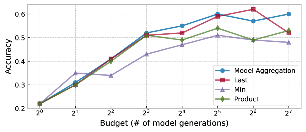
Reward aggregation within PRMs
As mentioned in Section 3.1 / Appendix A and reported by prior works (zhang2025lessonsdeveloping, ), there are multiple ways to use PRMs to calculate reward scores, which can significantly impact final performance. Figure 5(b) studies three existing methods for combining PRM scores—using the last reward, the minimum reward, and the product of all rewards. We also study “Model Aggregation," where the PRM is used as an ORM with partial answers.
As we can see, using Model Aggregation—in essence, feeding into a PRM the entire partial answer alongside the question - scales the best with an increasing budget.
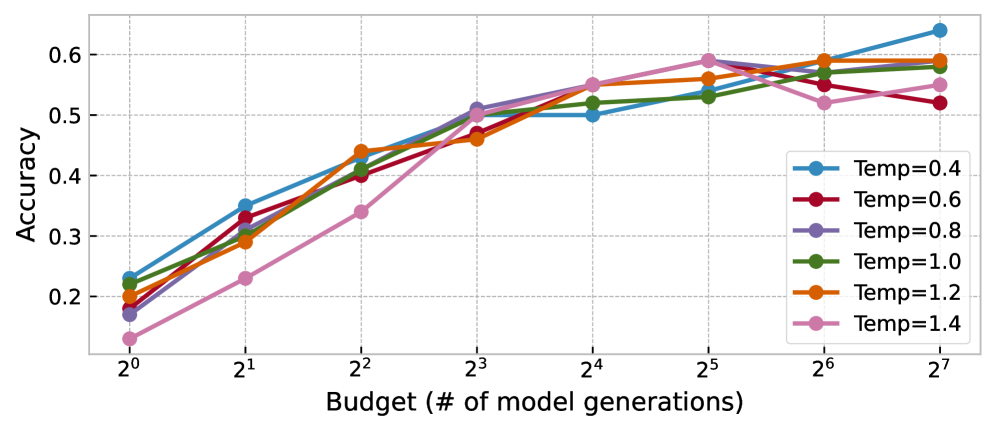
Controlling the state transition—temperatures in LLM generation
We investigate the effect of different LM sampling temperatures on the scaling of our method across varying numbers of particles. The results of our ablation study on a 100-question subset of MATH questions are shown in Figure 5(c).
Our findings show that the common LLM temperature range of 0.4–1.0 performs well, with minimal accuracy variation across budgets. Following (beeching2024scalingtesttimecompute, ), we use temperature 0.8 for all experiments.
Budget allocation over iterations and parallelism
The multi-iteration and parallel-chain extensions introduced in Section 3.1 / Appendix B provide two more axes to spend computation beyond the number of particles. We explore how different budget allocations affect performance in the appendix.
5 Related Work
Process reward models (PRMs) aim to provide more granular feedback by evaluating intermediate steps rather than only final outputs. They are trained via process supervision, a training approach where models receive feedback on each intermediate step of their reasoning process rather than only on the final outcome. (lightman2023letsverify, ) propose a step-by-step verification approach to PRMs, improving the reliability of reinforcement learning. DeepSeek PRM wang2024mathshepherdverifyreinforcellms uses Mistral to annotate training data for PRMs . (zhang2025lessonsdeveloping, ) introduces Qwen-PRM, which combines both Monte Carlo estimation and model/human annotation approach to prepare training data for a PRM. PRIME (cui2024process, ) proposes to train an outcome reward model (ORM) using an implicit reward objective. The paper shows that implicit reward objective directly learns a Q-function that provides rewards for each token, which can be leveraged to create process-level reward signal. This process eliminates the need for any process labels, and reaches competitive performance on PRM benchmarks.
Inference-time scaling is a key training-free strategy for enhancing LLM performance. (brown2024largelanguage, ) investigates best-of-N (BoN) decoding, showing quality gains via selective refinement. (snell2024scalingllm, ) analyzes how scaling compute improves inference efficiency from a compute-optimality view. While not implementing full Monte Carlo tree search (MCTS), (zhou2024languageagenttreesearch, ) explores a tree-search-inspired approach within language models. (guan2025rstarmathsmall, ) introduces rSTAR, which combines MCTS for data generation and training to improve mathematical reasoning. (beeching2024scalingtesttimecompute, ) discusses beam search and dynamic variable-time search (DVTS) as inference-time scaling methods for open-source LLMs. DVTS runs multiple subtrees in parallel to avoid all leaves getting stuck in local minima.
Particle-based Monte Carlo methods are powerful tools for probabilistic inference. Sequential Monte Carlo (sequentialmonte, ) or particle filtering (nonlinearfiltering, ) has been a classical way to approximate complex posterior distributions over state-space models. Particle Gibbs (PG) sampling (andrieu2010particlemarkov, ) extends these approaches by integrating MCMC techniques for improved inference. (lew2023sequentialmontecarlosteering, ) and (loula2025syntactic, ) use token-based SMC within probabilistic programs to steer LLMs, while (grand2025selfsteeringlanguagemodels, ) apply token-based SMC for self-constrained generation. zhao2024probabilisticinferencelanguagemodels and feng2024stepbystepreasoningmathproblems introduce Twisted SMC for inference in language models. We note that our method differs from feng2024stepbystepreasoningmathproblems in several key ways. First, TSMC relies on a ground-truth verifier and requires joint training of a generator and value function, whereas our approach uses an off-the-shelf generator and a noisy pretrained reward model (PRM), requiring no additional training. Second, our method generalizes to domains lacking ground-truth verifiers, such as instruction and broader language tasks. Finally, we demonstrate significantly stronger empirical results. The authors of TSMC did not release code, and their method requires additional training. We therefore compare our method—using the same generator model (DeepSeekMath7B) and dataset (MATH500) as in their results table—and find it achieves 75.4% accuracy with 128 samples, outperforming TSMC by 14.6 points using fewer than half the samples and no fine-tuning.
Decision making with uncertainty The way of representing uncertainty using softmax is often referred as Boltzmann exploration in the multi-armed bandit (MAB) literature (kuleshov2014algorithms, ). While formulating it as a MAB problem allows it to use a scheduling on the softmax temperature and to derive regret bounds (cesa2017boltzmann, ), we no longer have the same unbiasedness from the particle filtering / SMC formulation.
6 Conclusion
In this paper, we introduce a particle filtering algorithm for inference-time scaling. To address the limitations of deterministic inference-time scaling—namely, early pruning from imperfect reward models—we adapt particle-based Monte Carlo methods to maintain a diverse population of candidate sequences and balance exploration and exploitation. This probabilistic framing enables more resilient generation and opens a principled path for integrating uncertainty into LLM inference. Our evaluation shows these algorithms consistently outperform search-based approaches by a significant margin.
However, inference-time scaling comes with computational challenges. Hosting and running a reward model often introduces high latency, making the process more resource-intensive. For smaller models, prompt engineering is often required to ensure outputs adhere to the desired format. Finally, hyperparameters like budget are problem-dependent and may require tuning across domains.
We hope that the formal connection of inference scaling to probabilistic modeling established in this work will lead to systematic solutions for current limitations of these methods and pave the way for bringing advanced probabilistic inference algorithms into LLM inference-time scaling in future work.
References
- (1) AI-MO. Aimo validation aime dataset. https://huggingface.co/datasets/AI-MO/aimo-validation-aime, 2023. Accessed: 2025-01-24.
- (2) Christophe Andrieu, Arnaud Doucet, and Roman Holenstein. Particle Markov Chain Monte Carlo Methods. Journal of the Royal Statistical Society Series B: Statistical Methodology, 72(3):269–342, June 2010.
- (3) Edward Beeching, Lewis Tunstall, and Sasha Rush. Scaling test-time compute with open models, 2024.
- (4) Bradley Brown, Jordan Juravsky, Ryan Ehrlich, Ronald Clark, Quoc V. Le, Christopher Ré, and Azalia Mirhoseini. Large Language Monkeys: Scaling Inference Compute with Repeated Sampling, July 2024.
- (5) Nicolò Cesa-Bianchi, Claudio Gentile, Gábor Lugosi, and Gergely Neu. Boltzmann exploration done right. Advances in neural information processing systems, 30, 2017.
- (6) Ganqu Cui, Lifan Yuan, Zefan Wang, Hanbin Wang, Wendi Li, Bingxiang He, Yuchen Fan, Tianyu Yu, Qixin Xu, Weize Chen, Jiarui Yuan, Huayu Chen, Kaiyan Zhang, Xingtai Lv, Shuo Wang, Yuan Yao, Hao Peng, Yu Cheng, Zhiyuan Liu, Maosong Sun, Bowen Zhou, and Ning Ding. Process reinforcement through implicit rewards, 2025.
- (7) Pierre Del Moral. Sequential Monte Carlo Methods for Dynamic Systems: Journal of the American Statistical Association: Vol 93, No 443. https://www.tandfonline.com/doi/abs/10.1080/01621459.1998.10473765, 1997.
- (8) Shengyu Feng, Xiang Kong, Shuang Ma, Aonan Zhang, Dong Yin, Chong Wang, Ruoming Pang, and Yiming Yang. Step-by-step reasoning for math problems via twisted sequential monte carlo, 2024.
- (9) Gabriel Grand, Joshua B. Tenenbaum, Vikash K. Mansinghka, Alexander K. Lew, and Jacob Andreas. Self-steering language models, 2025.
- (10) Aaron Grattafiori, Abhimanyu Dubey, Abhinav Jauhri, Abhinav Pandey, Abhishek Kadian, Ahmad Al-Dahle, Aiesha Letman, Akhil Mathur, Alan Schelten, Alex Vaughan, Amy Yang, Angela Fan, Anirudh Goyal, Anthony Hartshorn, Aobo Yang, Archi Mitra, Archie Sravankumar, Artem Korenev, Arthur Hinsvark, Arun Rao, Aston Zhang, Aurelien Rodriguez, Austen Gregerson, Ava Spataru, Baptiste Roziere, Bethany Biron, Binh Tang, Bobbie Chern, Charlotte Caucheteux, Chaya Nayak, Chloe Bi, Chris Marra, Chris McConnell, Christian Keller, Christophe Touret, Chunyang Wu, Corinne Wong, Cristian Canton Ferrer, Cyrus Nikolaidis, Damien Allonsius, Daniel Song, Danielle Pintz, Danny Livshits, Danny Wyatt, David Esiobu, Dhruv Choudhary, Dhruv Mahajan, Diego Garcia-Olano, Diego Perino, Dieuwke Hupkes, Egor Lakomkin, Ehab AlBadawy, Elina Lobanova, Emily Dinan, Eric Michael Smith, Filip Radenovic, Francisco Guzmán, Frank Zhang, Gabriel Synnaeve, Gabrielle Lee, Georgia Lewis Anderson, Govind Thattai, Graeme Nail, Gregoire Mialon, Guan Pang, Guillem Cucurell, Hailey Nguyen, Hannah Korevaar, Hu Xu, Hugo Touvron, Iliyan Zarov, Imanol Arrieta Ibarra, Isabel Kloumann, Ishan Misra, Ivan Evtimov, Jack Zhang, Jade Copet, Jaewon Lee, Jan Geffert, Jana Vranes, Jason Park, Jay Mahadeokar, Jeet Shah, Jelmer van der Linde, Jennifer Billock, Jenny Hong, Jenya Lee, Jeremy Fu, Jianfeng Chi, Jianyu Huang, Jiawen Liu, Jie Wang, Jiecao Yu, Joanna Bitton, Joe Spisak, Jongsoo Park, Joseph Rocca, Joshua Johnstun, Joshua Saxe, Junteng Jia, Kalyan Vasuden Alwala, Karthik Prasad, Kartikeya Upasani, Kate Plawiak, Ke Li, Kenneth Heafield, Kevin Stone, Khalid El-Arini, Krithika Iyer, Kshitiz Malik, Kuenley Chiu, Kunal Bhalla, Kushal Lakhotia, Lauren Rantala-Yeary, Laurens van der Maaten, Lawrence Chen, Liang Tan, Liz Jenkins, Louis Martin, Lovish Madaan, Lubo Malo, Lukas Blecher, Lukas Landzaat, Luke de Oliveira, Madeline Muzzi, Mahesh Pasupuleti, Mannat Singh, Manohar Paluri, Marcin Kardas, Maria Tsimpoukelli, Mathew Oldham, Mathieu Rita, Maya Pavlova, Melanie Kambadur, Mike Lewis, Min Si, Mitesh Kumar Singh, Mona Hassan, Naman Goyal, Narjes Torabi, Nikolay Bashlykov, Nikolay Bogoychev, Niladri Chatterji, Ning Zhang, Olivier Duchenne, Onur Çelebi, Patrick Alrassy, Pengchuan Zhang, Pengwei Li, Petar Vasic, Peter Weng, Prajjwal Bhargava, Pratik Dubal, Praveen Krishnan, Punit Singh Koura, Puxin Xu, Qing He, Qingxiao Dong, Ragavan Srinivasan, Raj Ganapathy, Ramon Calderer, Ricardo Silveira Cabral, Robert Stojnic, Roberta Raileanu, Rohan Maheswari, Rohit Girdhar, Rohit Patel, Romain Sauvestre, Ronnie Polidoro, Roshan Sumbaly, Ross Taylor, Ruan Silva, Rui Hou, Rui Wang, Saghar Hosseini, Sahana Chennabasappa, Sanjay Singh, Sean Bell, Seohyun Sonia Kim, Sergey Edunov, Shaoliang Nie, Sharan Narang, Sharath Raparthy, Sheng Shen, Shengye Wan, Shruti Bhosale, Shun Zhang, Simon Vandenhende, Soumya Batra, Spencer Whitman, Sten Sootla, Stephane Collot, Suchin Gururangan, Sydney Borodinsky, Tamar Herman, Tara Fowler, Tarek Sheasha, Thomas Georgiou, Thomas Scialom, Tobias Speckbacher, Todor Mihaylov, Tong Xiao, Ujjwal Karn, Vedanuj Goswami, Vibhor Gupta, Vignesh Ramanathan, Viktor Kerkez, Vincent Gonguet, Virginie Do, Vish Vogeti, Vítor Albiero, Vladan Petrovic, Weiwei Chu, Wenhan Xiong, Wenyin Fu, Whitney Meers, Xavier Martinet, Xiaodong Wang, Xiaofang Wang, Xiaoqing Ellen Tan, Xide Xia, Xinfeng Xie, Xuchao Jia, Xuewei Wang, Yaelle Goldschlag, Yashesh Gaur, Yasmine Babaei, Yi Wen, Yiwen Song, Yuchen Zhang, Yue Li, Yuning Mao, Zacharie Delpierre Coudert, Zheng Yan, Zhengxing Chen, Zoe Papakipos, Aaditya Singh, Aayushi Srivastava, Abha Jain, Adam Kelsey, Adam Shajnfeld, Adithya Gangidi, Adolfo Victoria, Ahuva Goldstand, Ajay Menon, Ajay Sharma, Alex Boesenberg, Alexei Baevski, Allie Feinstein, Amanda Kallet, Amit Sangani, Amos Teo, Anam Yunus, Andrei Lupu, Andres Alvarado, Andrew Caples, Andrew Gu, Andrew Ho, Andrew Poulton, Andrew Ryan, Ankit Ramchandani, Annie Dong, Annie Franco, Anuj Goyal, Aparajita Saraf, Arkabandhu Chowdhury, Ashley Gabriel, Ashwin Bharambe, Assaf Eisenman, Azadeh Yazdan, Beau James, Ben Maurer, Benjamin Leonhardi, Bernie Huang, Beth Loyd, Beto De Paola, Bhargavi Paranjape, Bing Liu, Bo Wu, Boyu Ni, Braden Hancock, Bram Wasti, Brandon Spence, Brani Stojkovic, Brian Gamido, Britt Montalvo, Carl Parker, Carly Burton, Catalina Mejia, Ce Liu, Changhan Wang, Changkyu Kim, Chao Zhou, Chester Hu, Ching-Hsiang Chu, Chris Cai, Chris Tindal, Christoph Feichtenhofer, Cynthia Gao, Damon Civin, Dana Beaty, Daniel Kreymer, Daniel Li, David Adkins, David Xu, Davide Testuggine, Delia David, Devi Parikh, Diana Liskovich, Didem Foss, Dingkang Wang, Duc Le, Dustin Holland, Edward Dowling, Eissa Jamil, Elaine Montgomery, Eleonora Presani, Emily Hahn, Emily Wood, Eric-Tuan Le, Erik Brinkman, Esteban Arcaute, Evan Dunbar, Evan Smothers, Fei Sun, Felix Kreuk, Feng Tian, Filippos Kokkinos, Firat Ozgenel, Francesco Caggioni, Frank Kanayet, Frank Seide, Gabriela Medina Florez, Gabriella Schwarz, Gada Badeer, Georgia Swee, Gil Halpern, Grant Herman, Grigory Sizov, Guangyi, Zhang, Guna Lakshminarayanan, Hakan Inan, Hamid Shojanazeri, Han Zou, Hannah Wang, Hanwen Zha, Haroun Habeeb, Harrison Rudolph, Helen Suk, Henry Aspegren, Hunter Goldman, Hongyuan Zhan, Ibrahim Damlaj, Igor Molybog, Igor Tufanov, Ilias Leontiadis, Irina-Elena Veliche, Itai Gat, Jake Weissman, James Geboski, James Kohli, Janice Lam, Japhet Asher, Jean-Baptiste Gaya, Jeff Marcus, Jeff Tang, Jennifer Chan, Jenny Zhen, Jeremy Reizenstein, Jeremy Teboul, Jessica Zhong, Jian Jin, Jingyi Yang, Joe Cummings, Jon Carvill, Jon Shepard, Jonathan McPhie, Jonathan Torres, Josh Ginsburg, Junjie Wang, Kai Wu, Kam Hou U, Karan Saxena, Kartikay Khandelwal, Katayoun Zand, Kathy Matosich, Kaushik Veeraraghavan, Kelly Michelena, Keqian Li, Kiran Jagadeesh, Kun Huang, Kunal Chawla, Kyle Huang, Lailin Chen, Lakshya Garg, Lavender A, Leandro Silva, Lee Bell, Lei Zhang, Liangpeng Guo, Licheng Yu, Liron Moshkovich, Luca Wehrstedt, Madian Khabsa, Manav Avalani, Manish Bhatt, Martynas Mankus, Matan Hasson, Matthew Lennie, Matthias Reso, Maxim Groshev, Maxim Naumov, Maya Lathi, Meghan Keneally, Miao Liu, Michael L. Seltzer, Michal Valko, Michelle Restrepo, Mihir Patel, Mik Vyatskov, Mikayel Samvelyan, Mike Clark, Mike Macey, Mike Wang, Miquel Jubert Hermoso, Mo Metanat, Mohammad Rastegari, Munish Bansal, Nandhini Santhanam, Natascha Parks, Natasha White, Navyata Bawa, Nayan Singhal, Nick Egebo, Nicolas Usunier, Nikhil Mehta, Nikolay Pavlovich Laptev, Ning Dong, Norman Cheng, Oleg Chernoguz, Olivia Hart, Omkar Salpekar, Ozlem Kalinli, Parkin Kent, Parth Parekh, Paul Saab, Pavan Balaji, Pedro Rittner, Philip Bontrager, Pierre Roux, Piotr Dollar, Polina Zvyagina, Prashant Ratanchandani, Pritish Yuvraj, Qian Liang, Rachad Alao, Rachel Rodriguez, Rafi Ayub, Raghotham Murthy, Raghu Nayani, Rahul Mitra, Rangaprabhu Parthasarathy, Raymond Li, Rebekkah Hogan, Robin Battey, Rocky Wang, Russ Howes, Ruty Rinott, Sachin Mehta, Sachin Siby, Sai Jayesh Bondu, Samyak Datta, Sara Chugh, Sara Hunt, Sargun Dhillon, Sasha Sidorov, Satadru Pan, Saurabh Mahajan, Saurabh Verma, Seiji Yamamoto, Sharadh Ramaswamy, Shaun Lindsay, Shaun Lindsay, Sheng Feng, Shenghao Lin, Shengxin Cindy Zha, Shishir Patil, Shiva Shankar, Shuqiang Zhang, Shuqiang Zhang, Sinong Wang, Sneha Agarwal, Soji Sajuyigbe, Soumith Chintala, Stephanie Max, Stephen Chen, Steve Kehoe, Steve Satterfield, Sudarshan Govindaprasad, Sumit Gupta, Summer Deng, Sungmin Cho, Sunny Virk, Suraj Subramanian, Sy Choudhury, Sydney Goldman, Tal Remez, Tamar Glaser, Tamara Best, Thilo Koehler, Thomas Robinson, Tianhe Li, Tianjun Zhang, Tim Matthews, Timothy Chou, Tzook Shaked, Varun Vontimitta, Victoria Ajayi, Victoria Montanez, Vijai Mohan, Vinay Satish Kumar, Vishal Mangla, Vlad Ionescu, Vlad Poenaru, Vlad Tiberiu Mihailescu, Vladimir Ivanov, Wei Li, Wenchen Wang, Wenwen Jiang, Wes Bouaziz, Will Constable, Xiaocheng Tang, Xiaojian Wu, Xiaolan Wang, Xilun Wu, Xinbo Gao, Yaniv Kleinman, Yanjun Chen, Ye Hu, Ye Jia, Ye Qi, Yenda Li, Yilin Zhang, Ying Zhang, Yossi Adi, Youngjin Nam, Yu, Wang, Yu Zhao, Yuchen Hao, Yundi Qian, Yunlu Li, Yuzi He, Zach Rait, Zachary DeVito, Zef Rosnbrick, Zhaoduo Wen, Zhenyu Yang, Zhiwei Zhao, and Zhiyu Ma. The llama 3 herd of models, 2024.
- (11) Xinyu Guan, Li Lyna Zhang, Yifei Liu, Ning Shang, Youran Sun, Yi Zhu, Fan Yang, and Mao Yang. rStar-Math: Small LLMs Can Master Math Reasoning with Self-Evolved Deep Thinking, January 2025.
- (12) Pranab Islam, Anand Kannappan, Douwe Kiela, Rebecca Qian, Nino Scherrer, and Bertie Vidgen. Financebench: A new benchmark for financial question answering, 2023.
- (13) Jared Kaplan, Sam McCandlish, Tom Henighan, Tom B. Brown, Benjamin Chess, Rewon Child, Scott Gray, Alec Radford, Jeffrey Wu, and Dario Amodei. Scaling laws for neural language models, 2020.
- (14) Volodymyr Kuleshov and Doina Precup. Algorithms for multi-armed bandit problems. arXiv preprint arXiv:1402.6028, 2014.
- (15) Alexander K. Lew, Tan Zhi-Xuan, Gabriel Grand, and Vikash K. Mansinghka. Sequential monte carlo steering of large language models using probabilistic programs, 2023.
- (16) Hunter Lightman, Vineet Kosaraju, Yura Burda, Harri Edwards, Bowen Baker, Teddy Lee, Jan Leike, John Schulman, Ilya Sutskever, and Karl Cobbe. Let’s verify step by step, 2023.
- (17) Hunter Lightman, Vineet Kosaraju, Yura Burda, Harri Edwards, Bowen Baker, Teddy Lee, Jan Leike, John Schulman, Ilya Sutskever, and Karl Cobbe. Let’s Verify Step by Step, May 2023.
- (18) João Loula, Benjamin LeBrun, Li Du, Ben Lipkin, Clemente Pasti, Gabriel Grand, Tianyu Liu, Yahya Emara, Marjorie Freedman, Jason Eisner, Ryan Cotterell, Vikash Mansinghka, Alexander K. Lew, Tim Vieira, and Timothy J. O’Donnell. Syntactic and semantic control of large language models via sequential monte carlo. In The Thirteenth International Conference on Learning Representations, 2025.
- (19) David JC MacKay. Information theory, inference and learning algorithms. Cambridge university press, 2003.
- (20) Swaroop Mishra, Arindam Mitra, Neeraj Varshney, Bhavdeep Sachdeva, Peter Clark, Chitta Baral, and Ashwin Kalyan. Numglue: A suite of fundamental yet challenging mathematical reasoning tasks. ACL, 2022.
- (21) OpenAI, :, Aaron Jaech, Adam Kalai, Adam Lerer, Adam Richardson, Ahmed El-Kishky, Aiden Low, Alec Helyar, Aleksander Madry, Alex Beutel, Alex Carney, Alex Iftimie, Alex Karpenko, Alex Tachard Passos, Alexander Neitz, Alexander Prokofiev, Alexander Wei, Allison Tam, Ally Bennett, Ananya Kumar, Andre Saraiva, Andrea Vallone, Andrew Duberstein, Andrew Kondrich, Andrey Mishchenko, Andy Applebaum, Angela Jiang, Ashvin Nair, Barret Zoph, Behrooz Ghorbani, Ben Rossen, Benjamin Sokolowsky, Boaz Barak, Bob McGrew, Borys Minaiev, Botao Hao, Bowen Baker, Brandon Houghton, Brandon McKinzie, Brydon Eastman, Camillo Lugaresi, Cary Bassin, Cary Hudson, Chak Ming Li, Charles de Bourcy, Chelsea Voss, Chen Shen, Chong Zhang, Chris Koch, Chris Orsinger, Christopher Hesse, Claudia Fischer, Clive Chan, Dan Roberts, Daniel Kappler, Daniel Levy, Daniel Selsam, David Dohan, David Farhi, David Mely, David Robinson, Dimitris Tsipras, Doug Li, Dragos Oprica, Eben Freeman, Eddie Zhang, Edmund Wong, Elizabeth Proehl, Enoch Cheung, Eric Mitchell, Eric Wallace, Erik Ritter, Evan Mays, Fan Wang, Felipe Petroski Such, Filippo Raso, Florencia Leoni, Foivos Tsimpourlas, Francis Song, Fred von Lohmann, Freddie Sulit, Geoff Salmon, Giambattista Parascandolo, Gildas Chabot, Grace Zhao, Greg Brockman, Guillaume Leclerc, Hadi Salman, Haiming Bao, Hao Sheng, Hart Andrin, Hessam Bagherinezhad, Hongyu Ren, Hunter Lightman, Hyung Won Chung, Ian Kivlichan, Ian O’Connell, Ian Osband, Ignasi Clavera Gilaberte, Ilge Akkaya, Ilya Kostrikov, Ilya Sutskever, Irina Kofman, Jakub Pachocki, James Lennon, Jason Wei, Jean Harb, Jerry Twore, Jiacheng Feng, Jiahui Yu, Jiayi Weng, Jie Tang, Jieqi Yu, Joaquin Quiñonero Candela, Joe Palermo, Joel Parish, Johannes Heidecke, John Hallman, John Rizzo, Jonathan Gordon, Jonathan Uesato, Jonathan Ward, Joost Huizinga, Julie Wang, Kai Chen, Kai Xiao, Karan Singhal, Karina Nguyen, Karl Cobbe, Katy Shi, Kayla Wood, Kendra Rimbach, Keren Gu-Lemberg, Kevin Liu, Kevin Lu, Kevin Stone, Kevin Yu, Lama Ahmad, Lauren Yang, Leo Liu, Leon Maksin, Leyton Ho, Liam Fedus, Lilian Weng, Linden Li, Lindsay McCallum, Lindsey Held, Lorenz Kuhn, Lukas Kondraciuk, Lukasz Kaiser, Luke Metz, Madelaine Boyd, Maja Trebacz, Manas Joglekar, Mark Chen, Marko Tintor, Mason Meyer, Matt Jones, Matt Kaufer, Max Schwarzer, Meghan Shah, Mehmet Yatbaz, Melody Y. Guan, Mengyuan Xu, Mengyuan Yan, Mia Glaese, Mianna Chen, Michael Lampe, Michael Malek, Michele Wang, Michelle Fradin, Mike McClay, Mikhail Pavlov, Miles Wang, Mingxuan Wang, Mira Murati, Mo Bavarian, Mostafa Rohaninejad, Nat McAleese, Neil Chowdhury, Neil Chowdhury, Nick Ryder, Nikolas Tezak, Noam Brown, Ofir Nachum, Oleg Boiko, Oleg Murk, Olivia Watkins, Patrick Chao, Paul Ashbourne, Pavel Izmailov, Peter Zhokhov, Rachel Dias, Rahul Arora, Randall Lin, Rapha Gontijo Lopes, Raz Gaon, Reah Miyara, Reimar Leike, Renny Hwang, Rhythm Garg, Robin Brown, Roshan James, Rui Shu, Ryan Cheu, Ryan Greene, Saachi Jain, Sam Altman, Sam Toizer, Sam Toyer, Samuel Miserendino, Sandhini Agarwal, Santiago Hernandez, Sasha Baker, Scott McKinney, Scottie Yan, Shengjia Zhao, Shengli Hu, Shibani Santurkar, Shraman Ray Chaudhuri, Shuyuan Zhang, Siyuan Fu, Spencer Papay, Steph Lin, Suchir Balaji, Suvansh Sanjeev, Szymon Sidor, Tal Broda, Aidan Clark, Tao Wang, Taylor Gordon, Ted Sanders, Tejal Patwardhan, Thibault Sottiaux, Thomas Degry, Thomas Dimson, Tianhao Zheng, Timur Garipov, Tom Stasi, Trapit Bansal, Trevor Creech, Troy Peterson, Tyna Eloundou, Valerie Qi, Vineet Kosaraju, Vinnie Monaco, Vitchyr Pong, Vlad Fomenko, Weiyi Zheng, Wenda Zhou, Wes McCabe, Wojciech Zaremba, Yann Dubois, Yinghai Lu, Yining Chen, Young Cha, Yu Bai, Yuchen He, Yuchen Zhang, Yunyun Wang, Zheng Shao, and Zhuohan Li. Openai o1 system card, 2024.
- (22) Charlie Snell, Jaehoon Lee, Kelvin Xu, and Aviral Kumar. Scaling LLM Test-Time Compute Optimally can be More Effective than Scaling Model Parameters, August 2024.
- (23) Charlie Snell, Jaehoon Lee, Kelvin Xu, and Aviral Kumar. Scaling llm test-time compute optimally can be more effective than scaling model parameters, 2024.
- (24) Robert H. Swendsen and Jian-Sheng Wang. Nonlinear filtering: Interacting particle resolution - ScienceDirect. https://www.sciencedirect.com/science/article/abs/pii/S0764444297847787, 1986.
- (25) Simo Särkkä. Bayesian Filtering and Smoothing. Institute of Mathematical Statistics Textbooks. Cambridge University Press, 2013.
- (26) Peiyi Wang, Lei Li, Zhihong Shao, R. X. Xu, Damai Dai, Yifei Li, Deli Chen, Y. Wu, and Zhifang Sui. Math-shepherd: Verify and reinforce llms step-by-step without human annotations, 2024.
- (27) Xuezhi Wang, Jason Wei, Dale Schuurmans, Quoc Le, Ed Chi, Sharan Narang, Aakanksha Chowdhery, and Denny Zhou. Self-consistency improves chain of thought reasoning in language models, 2023.
- (28) Wei Xiong, Hanning Zhang, Nan Jiang, and Tong Zhang. An implementation of generative prm. https://github.com/RLHFlow/RLHF-Reward-Modeling, 2024.
- (29) An Yang, Beichen Zhang, Binyuan Hui, Bofei Gao, Bowen Yu, Chengpeng Li, Dayiheng Liu, Jianhong Tu, Jingren Zhou, Junyang Lin, Keming Lu, Mingfeng Xue, Runji Lin, Tianyu Liu, Xingzhang Ren, and Zhenru Zhang. Qwen2.5-math technical report: Toward mathematical expert model via self-improvement. arXiv preprint arXiv:2409.12122, 2024.
- (30) Lifan Yuan, Ganqu Cui, Hanbin Wang, Ning Ding, Xingyao Wang, Jia Deng, Boji Shan, Huimin Chen, Ruobing Xie, Yankai Lin, Zhenghao Liu, Bowen Zhou, Hao Peng, Zhiyuan Liu, and Maosong Sun. Advancing llm reasoning generalists with preference trees, 2024.
- (31) Zhenru Zhang, Chujie Zheng, Yangzhen Wu, Beichen Zhang, Runji Lin, Bowen Yu, Dayiheng Liu, Jingren Zhou, and Junyang Lin. The lessons of developing process reward models in mathematical reasoning. arXiv preprint arXiv:2501.07301, 2025.
- (32) Zhenru Zhang, Chujie Zheng, Yangzhen Wu, Beichen Zhang, Runji Lin, Bowen Yu, Dayiheng Liu, Jingren Zhou, and Junyang Lin. The Lessons of Developing Process Reward Models in Mathematical Reasoning, January 2025.
- (33) Stephen Zhao, Rob Brekelmans, Alireza Makhzani, and Roger Grosse. Probabilistic inference in language models via twisted sequential monte carlo, 2024.
- (34) Andy Zhou, Kai Yan, Michal Shlapentokh-Rothman, Haohan Wang, and Yu-Xiong Wang. Language agent tree search unifies reasoning acting and planning in language models, 2024.
Appendix A Aggregation Strategies for PRM Scores
To compute particle weights during generation, we aggregate per-step scores from the process reward model (PRM) $\hat{r}$ . Our default uses a product of step-level rewards to align with the factorized likelihood structure, but alternative aggregation strategies (e.g., min, last-step, or model-based) may offer different trade-offs.
The weight update step in particle filtering depends on how rewards are assigned to partial trajectories using a preference or reward model (PRM) $\hat{r}$ . Since PRMs often provide per-step scores, aggregating them into a single weight requires a strategy that balances theoretical correctness and practical utility.
We consider the following four aggregation approaches:
- Product ( $\mathrm{prod}$ ): Computes the product of step-level rewards across all tokens. This aligns directly with the factorized likelihood structure used in the PF objective ((2)), enabling online weight updates as generation proceeds.
- Minimum ( $\mathrm{min}$ ): Takes the minimum reward seen so far. This penalizes trajectories for weak intermediate steps, which may help in discouraging risky completions. However, it prevents online updates because the entire prefix must be scored to determine the weight.
- Last-step ( $\mathrm{last}$ ): Uses only the most recent step’s reward. Although not aligned with a likelihood-based interpretation, this method is computationally efficient and reflects the scoring mode used in [3].
- Model-based aggregation: Instead of relying on step-wise rewards, this method repurposes the PRM in a black-box fashion to assign a single scalar score to the full partial trajectory. This helps smooth over noisy token-level scores and can be more stable, especially when PRMs are inconsistent across steps. The model receives the prompt and prefix and returns a scalar reward.
Appendix G shows how the input format for this black-box mode differs from standard per-step PRM usage. We compare all strategies empirically in 4.5 and find that the optimal choice varies with the PRM’s training and evaluation objective.
Appendix B Multiple Iterations and Parallel Chains
Here, we explore how different ways to allocate budgets change the performance in the appendix. Specifically, we study for a fixed budget $N× T× M$ , how the combination of $N,T,M$ can yield the best performance, where $N$ is the number of particles, $T$ is the number of iterations, and $M$ is the number of parallelism.
B.1 Particle Gibbs
Particle Gibbs is a type of MCMC algorithm that uses PF as a transition kernel [2]. Specifically, at each iteration, PG samples a new set of particles using PF with a reference particle from the previous iteration. This integration combines the efficiency of PF with the theoretical guarantees of MCMC, making PG suitable for high-dimensional or challenging posterior distributions. The adaption of PG to inference-time scaling is essentially a multi-iteration extension of the PF algorithm presented, which works as follows: For each iteration, we run a modified PF step with an additional sampling step to sample 1 reference particle according to the equation in the resampling step of Section • ‣ 3.1. For any PF step that is not the initial step, the PF is executed with a reference particle: This reference particle is never replaced during the resampling step, but its partial trajectory can still be forked during resampling. We detail the PG version of inference-time scaling in Algorithm 2 of Appendix D. Note that typically, a reasonably large number of particles is needed to show the benefits of multiple iterations, which we also confirm in our results in Section 4.5.
Allocating budget between $N$ and $T$
<details>
<summary>x10.png Details</summary>
### Visual Description
# Technical Data Extraction: Accuracy vs. Model Generation Budget
## 1. Document Overview
This image is a line graph comparing the performance (Accuracy) of different sampling algorithms—**Particle Filtering** and three variants of **Particle Gibbs**—across an increasing computational budget.
## 2. Component Isolation
### Header/Metadata
* **Language:** English
* **Primary Subject:** Algorithm performance comparison.
### Main Chart Area (Axes and Grid)
* **Y-Axis Label:** `Accuracy`
* **Y-Axis Scale:** Linear, ranging from `0.35` to `0.60` with major tick intervals of `0.05`.
* **X-Axis Label:** `Budget (# of model generations)`
* **X-Axis Scale:** Logarithmic (base 2), with markers at $2^2$, $2^3$, $2^4$, $2^5$, $2^6$, and $2^7$.
* **Grid:** Light grey dashed grid lines for both horizontal and vertical axes.
### Legend (Spatial Grounding: Bottom Right [x≈0.7, y≈0.2])
The legend identifies four distinct data series:
1. **Blue line with Circle markers (●):** `Particle Filtering`
2. **Red line with Square markers (■):** `Particle Gibbs (4 particles per group)`
3. **Purple line with Diamond markers (♦):** `Particle Gibbs (8 particles per group)`
4. **Green line with Diamond markers (♦):** `Particle Gibbs (16 particles per group)`
---
## 3. Trend Verification and Data Extraction
### Series 1: Particle Filtering (Blue, Circle)
* **Trend:** Shows a strong upward trajectory from $2^2$ to $2^5$, reaching a peak. It experiences a slight dip at $2^6$ before recovering to its peak value at $2^7$. Generally the highest performing method.
* **Data Points:**
* $2^2$: ~0.42
* $2^3$: ~0.52
* $2^4$: ~0.55
* $2^5$: ~0.60
* $2^6$: ~0.57
* $2^7$: ~0.60
### Series 2: Particle Gibbs (4 particles per group) (Red, Square)
* **Trend:** The lowest performing series. It shows a steady, slow upward trend as the budget increases, with a slight plateau between $2^3$ and $2^4$, and a small dip at the final point ($2^7$).
* **Data Points:**
* $2^2$: ~0.33
* $2^3$: ~0.39
* $2^4$: ~0.40
* $2^5$: ~0.48
* $2^6$: ~0.50
* $2^7$: ~0.48
### Series 3: Particle Gibbs (8 particles per group) (Purple, Diamond)
* **Trend:** Starts at $2^3$. Shows a consistent upward trend until $2^6$, followed by a slight decrease at $2^7$. It consistently performs better than the 4-particle variant but lower than the 16-particle variant.
* **Data Points:**
* $2^3$: ~0.48
* $2^4$: ~0.52
* $2^5$: ~0.52 (Plateau)
* $2^6$: ~0.54
* $2^7$: ~0.52
### Series 4: Particle Gibbs (16 particles per group) (Green, Diamond)
* **Trend:** Starts at $2^4$. It begins at a high accuracy level, remains relatively stable (slight fluctuations), peaks at $2^6$, and then declines at $2^7$.
* **Data Points:**
* $2^4$: ~0.57
* $2^5$: ~0.56
* $2^6$: ~0.58
* $2^7$: ~0.54
---
## 4. Reconstructed Data Table (Estimated Values)
| Budget ($2^n$) | Particle Filtering (Blue) | PG (4 particles) (Red) | PG (8 particles) (Purple) | PG (16 particles) (Green) |
| :--- | :--- | :--- | :--- | :--- |
| **$2^2$ (4)** | 0.42 | 0.33 | N/A | N/A |
| **$2^3$ (8)** | 0.52 | 0.39 | 0.48 | N/A |
| **$2^4$ (16)** | 0.55 | 0.40 | 0.52 | 0.57 |
| **$2^5$ (32)** | 0.60 | 0.48 | 0.52 | 0.56 |
| **$2^6$ (64)** | 0.57 | 0.50 | 0.54 | 0.58 |
| **$2^7$ (128)** | 0.60 | 0.48 | 0.52 | 0.54 |
---
## 5. Key Observations
* **Scalability:** All methods generally improve as the budget increases, though most show a slight performance degradation or plateau at the highest budget ($2^7$).
* **Particle Gibbs Scaling:** Increasing the number of particles per group in the Particle Gibbs algorithm significantly improves accuracy for a given budget.
* **Efficiency:** Particle Filtering appears to be the most efficient algorithm shown, achieving higher accuracy at lower budgets compared to the Particle Gibbs variants.
</details>
Figure 6: Comparison of PF and Particle Gibbs with different numbers of iterations, evaluated on a 100-question subset of the MATH-500 dataset using Llama-3.2-1B-Instruct as the policy model.
Figure 6 shows results of Llama-3.2 1B model when configured with various test-time compute budget allocations. Although the plot shows that various Particle Gibbs configurations do not have a marked benefit over an equivalently budgeted particle filtering run, a PG experiment with 16 particles and 4 iterations powered by a Qwen 2.5 7B Math Instruct policy model achieved a 87.2% accuracy on MATH500, beating o1 performance. Configurations with larger $N$ values typically do better than equivalently budgeted runs with less particles.
B.2 Parallel Tempering
Parallel tempering
In parallel tempering (aka replica exchange MCMC sampling), multiple MCMC chains run in parallel at different temperatures and swap the states to allow better exploration. The key idea is that the chain running in high temperature can explore better, e.g. traversing between different modes of the target, and the swap makes it possible to let the low temperature chain exploit the new region found by the other chain. We detail the complete parallel tempering version of inference-time scaling in the Algorithms section of the Appendix below Algorithm 3 of D, while we only explore a special case of it (multiple chains with single iteration) in our experiments.
Allocating budget between $N$ and $M$
Figure 7 shows PF and 3 PT configurations over a set of increasing numbers of budgets.
<details>
<summary>x11.png Details</summary>
### Visual Description
# Technical Data Extraction: Accuracy vs. Model Generation Budget
## 1. Image Classification
This image is a **line graph** comparing the performance (Accuracy) of different sampling algorithms across varying computational budgets.
## 2. Component Isolation
### Header/Metadata
* **Language:** English
* **Primary Subject:** Performance comparison of Particle Filtering vs. Parallel Tempering variants.
### Axis Definitions
* **Y-Axis (Vertical):**
* **Label:** Accuracy
* **Scale:** Linear, ranging from 0.36 to 0.48 with major ticks every 0.02 units.
* **X-Axis (Horizontal):**
* **Label:** Budget (# of model generations)
* **Scale:** Logarithmic (Base 2), with markers at $2^2, 2^3, 2^4, 2^5, 2^6, 2^7$.
### Legend (Spatial Grounding: Bottom-Right [x≈0.7, y≈0.2])
The legend contains four entries, each associated with a specific color and marker shape:
1. **Blue line with Circle markers (●):** Particle Filtering
2. **Red line with Square markers (■):** Parallel Tempering (4 particles per group)
3. **Purple line with Triangle markers (▲):** Parallel Tempering (8 particles per group)
4. **Green line with Diamond markers (♦):** Parallel Tempering (16 particles per group)
---
## 3. Trend Verification and Data Extraction
### Series 1: Particle Filtering (Blue, Circle)
* **Trend:** Shows a steady, monotonic upward slope from $2^2$ to $2^4$, plateaus between $2^4$ and $2^5$, and then resumes a steady upward slope to $2^7$.
* **Data Points:**
* $2^2$: 0.40
* $2^3$: 0.41
* $2^4$: 0.42
* $2^5$: 0.42
* $2^6$: 0.44
* $2^7$: 0.46
### Series 2: Parallel Tempering (4 particles per group) (Red, Square)
* **Trend:** Shows the most significant initial gain between $2^2$ and $2^3$. It maintains a consistent upward slope throughout the entire budget range, ending at the same accuracy as Particle Filtering.
* **Data Points:**
* $2^2$: 0.35
* $2^3$: 0.39
* $2^4$: 0.40
* $2^5$: 0.41
* $2^6$: 0.43
* $2^7$: 0.46
### Series 3: Parallel Tempering (8 particles per group) (Purple, Triangle)
* **Trend:** Generally upward sloping, but exhibits a "sawtooth" pattern or fluctuation. It increases until $2^5$, drops slightly at $2^6$, and recovers at $2^7$. It starts at a higher budget ($2^3$) than the 4-particle version.
* **Data Points:**
* $2^3$: 0.40
* $2^4$: 0.41
* $2^5$: 0.43
* $2^6$: 0.42
* $2^7$: 0.44
### Series 4: Parallel Tempering (16 particles per group) (Green, Diamond)
* **Trend:** This is the highest-performing series. It shows a strong, consistent upward slope from its starting point at $2^4$ to the end of the budget range at $2^7$.
* **Data Points:**
* $2^4$: 0.42
* $2^5$: 0.45
* $2^6$: 0.46
* $2^7$: 0.48
---
## 4. Reconstructed Data Table
| Budget ($2^x$) | Particle Filtering (Blue ●) | PT - 4 particles (Red ■) | PT - 8 particles (Purple ▲) | PT - 16 particles (Green ♦) |
| :--- | :--- | :--- | :--- | :--- |
| **$2^2$ (4)** | 0.40 | 0.35 | - | - |
| **$2^3$ (8)** | 0.41 | 0.39 | 0.40 | - |
| **$2^4$ (16)** | 0.42 | 0.40 | 0.41 | 0.42 |
| **$2^5$ (32)** | 0.42 | 0.41 | 0.43 | 0.45 |
| **$2^6$ (64)** | 0.44 | 0.43 | 0.42 | 0.46 |
| **$2^7$ (128)** | 0.46 | 0.46 | 0.44 | 0.48 |
---
## 5. Key Observations
* **Scalability:** All methods show improved accuracy as the budget increases.
* **Particle Density:** For Parallel Tempering, increasing the number of particles per group generally shifts the curve upward (higher accuracy), though it requires a higher minimum budget to initialize.
* **Top Performer:** "Parallel Tempering (16 particles per group)" consistently outperforms all other methods once the budget reaches $2^5$.
* **Convergence:** At the maximum budget ($2^7$), Particle Filtering and Parallel Tempering (4 particles) converge at an accuracy of 0.46.
</details>
Figure 7: Comparison of PF and PT with different particle group sizes, evaluated on a 100-question subset of the MATH500 dataset using Llama-3.2-1B-Instruct as the policy model.
First, as we can see, for any fixed $N$ , increasing $M$ also improves the performance. This may be helpful when combining batch generation with distributed computing. Second, PT with $N=16$ has a better overall scaling than PF. This indicates that there is some optimal budget allocation over parallel chains that can further improve the overall performance of our main results.
We leave the exploration over the optimal configuration of $N,T,M$ jointly as a future work.
Appendix C Proof of Theorem 2
**Theorem 2 (Unbiasedness of Expected Accuracy)**
*Let $\{(w^{(i)},x^{(i)})\}$ be weighted particles from Algorithm 1 and $\mathrm{is\_correct}(x)$ is a function to check the correctness of response $x$ . We have
$$
\mathbb{E}\left\{\sum_{i}\left[w^{(i)}\;\mathrm{is\_correct}(x^{(i)})\right]\right\}=\sum_{x}\left[\hat{p}_{M}(x_{1:T}\mid c,o_{1:T}=\mathbf{1})\;\mathrm{is\_correct}(x^{(i)})\right],
$$
where the expectation is over the randomness of the algorithm itself.*
* Proof*
This is a direct result of applying the unbiasedness property of particle filtering on a well-defined expectation $p$ $\mathbb{E}_{x\sim p}\{f(x)\}$ of any function $f$ over a distribution $p$ : the Monte Carlo estimate using weighted samples from particle filtering is an unbiased estimate of this expectation. As $\mathrm{is\_correct}(·)$ is a binary function, the expectation of the estimate is finite thus well-defined and therefore the unbiasedness of accuracy holds. ∎
Appendix D Side by Side Comparison of Particle Filtering vs Beam Search
math problem +2.1 -1.2 +1.3 +0.1 softmax sample $N$ : $1,1,3,4$ distribution:
(a) Particle filtering uses the rewards to produce a softmax distribution and does stochastic expansion of $N$ based sampling.
math problem +2.1 -1.2 +1.3 +0.1 top- ${N\over M}$ selected: $1,3$ expand $M$
(b) Beam search treats the rewards as exact and performs deterministic expansion based on beam size $N$ and beam width $M$ .
Figure 8: A side-by-side comparison between particle filtering and its closest search-based counterpart, beam search. Compared with beam search in Figure 8(b) where the selection and expansion is deterministic (implicitly assumes the rewards are correct), particle filtering in Figure 8(a) trusts the rewards with uncertainty and propagates the expansion via sampling.
Appendix E Algorithms
Algorithm 1 Particle Filtering for Inference-Time Scaling
Input: the number of particles $N$ , a reward model $\hat{r}$ , a LLM $p_{M}$ and the prompt $c$
Initialize $N$ particles $\{x_{1}^{(i)}\sim p_{M}(·\mid c)\}_{i=1}^{N}$
$t← 1$
while not all particles stop do
Update rewards $\mathbf{w}=[\hat{r}(x_{1:t}^{(1)}),...,\hat{r}(x_{1:t}^{(N)})]$
Compute softmax distribution $\theta=\mathrm{softmax}(\mathbf{w})$
Sample indices $\{j_{t}^{(i)}\}_{i=1}^{N}\sim\mathbb{P}_{t}(j=i)=\theta_{i}$
Update the set of particles as $\{x_{1:t}^{(j_{t}^{(i)})}\}_{i=1}^{N}$
Transition $\{x_{t+1}^{(i)}\sim p_{M}(·\mid c,x_{1:t}^{(i)})\}_{i=1}^{N}$
$t← t+1$
end while
Return: the set of weighted particles in the end
Algorithm 2 Particle Gibbs for Inference-Time Scaling
Input: same as Algorithm 1 with the number of Gibbs iterations $T$
Run Algorithm 1 to get a set of particles $\{x_{1:t}^{(i)}\}_{i=1}^{N}$
for $j=1,...,T$ do
Compute rewards $\mathbf{w}=[\hat{r}(x_{1:t}^{(1)}),...,\hat{r}(x_{1:t}^{(N)})]$
Compute softmax distribution $\theta=\mathrm{softmax}(\mathbf{w})$
Sample reference particle $x_{1:t}^{\text{ref}}:=x_{1:t}^{(j)}$ where $j\sim\mathbb{P}(j=i)=\theta_{i}$
Initialize $N-1$ particles $\{x_{1}^{(i)}\sim p_{M}(·\mid c)\}_{i=1}^{N-1}$
$t← 1$
while not all particles stop do
Update $\mathbf{w}=[\hat{r}(x_{1:t}^{(1)}),...,\hat{r}(x_{1:t}^{(N-1)}),\hat{r}(x_{1:t}^{\text{ref}})]$
Compute softmax distribution $\theta=\mathrm{softmax}(\mathbf{w})$
Sample indices $\{j_{t}^{(i)}\}_{i=1}^{N}\sim\mathbb{P}_{t}(j=i)=\theta_{i}$
Update the set of particles as $\{x_{1:t}^{(j_{t}^{(i)})}\}_{i=1}^{N}$
Transition $\{x_{t+1}^{(i)}\sim p_{M}(·\mid c,x_{t+1}^{(i)})\}_{i=1}^{N}$
$t← t+1$
end while
end for
Return: the set of particles in the end
For a set of parallel chains with temperatures $T_{1}>T_{2}>...$ , at each iteration, we swap the states of every pair of neighboring chains $k,k+1$ with the following probability
$$
A=\min\left(1,\frac{\pi_{k}(x^{(k+1)})\pi_{k+1}(x^{(k)})}{\pi_{k}(x^{(k)})\pi_{k+1}(x^{(k+1)})}\right), \tag{4}
$$
where $\pi_{k},\pi_{k+1}$ are the two targets (with different temperatures) and $x_{k},x_{k+1}$ are their states before swapping.
Algorithm 3 Particle Gibbs with Parallel Tempering for Inference-Time Scaling
Input: same as Algorithm 2 with the number of parallel chains $M$ and a list of temperature $T_{1},...,T_{M}$
for $j=1,...,T$ do
for $k=1,...,M$ do
if $j=1$ then
Run Algorithm 1 to get a set of particles $\{x_{1:t}^{(i)}\}_{i=1}^{N}$ for chain $k$
else
Initialize $N-1$ particles $\{x_{1}^{(i)}\sim p_{M}(·\mid c)\}_{i=1}^{N-1}$
$t← 1$
while not all particles stop do
Update $\mathbf{w}=[\hat{r}(x_{1:t}^{(1)}),...,\hat{r}(x_{1:t}^{(N-1)}),\hat{r}(x_{1:t}^{\text{ref}})]$
Compute softmax distribution $\theta=\mathrm{softmax}(\mathbf{w}/T_{k})$
Sample indices $\{j_{t}^{(i)}\}_{i=1}^{N}\sim\mathbb{P}_{t}(j=i)=\theta_{i}$
Update the set of particles as $\{x_{1:t}^{(j_{t}^{(i)})}\}_{i=1}^{N}$
Transition $\{x_{t+1}^{(i)}\sim p_{M}(·\mid c,x_{t+1}^{(i)})\}_{i=1}^{N}$
$t← t+1$
end while
end if
Compute rewards $\mathbf{w}=[\hat{r}(x_{1:t}^{(1)}),...,\hat{r}(x_{1:t}^{(N)})]$
Compute softmax distribution $\theta=\mathrm{softmax}(\mathbf{w}/T_{k})$
Sample reference particle $x_{1:t}^{\text{ref}}:=x_{1:t}^{(j)}$ where $j\sim\mathbb{P}(j=i)=\theta_{i}$
end for
for $k=1,...,M-1$ do
Exchange the reference particle between chain $k$ and $k+1$ with probability according to (4)
end for
end for
Return: $M$ set of particles in the end
Appendix F Particle Filtering Results with More Generator Models
Below, we show further results using particle filtering to inference scale a wider variety of generator models.
| Llama-3.2-1B-Instruct | Greedy | 26.8 | 0.0 |
| --- | --- | --- | --- |
| \rowcolor [HTML]C1DEB8 | Particle Filtering (Ours) | 59.6 | 10.0 |
| Llama-3.2-8B-Instruct | Greedy | 49.9 | 6.6 |
| \rowcolor [HTML]C1DEB8 | Particle Filtering (Ours) | 74.4 | 16.6 |
| phi-4 | Greedy | 79.8 | 16.6 |
| \rowcolor [HTML]C1DEB8 | Particle Filtering (Ours) | 83.6 | 26.6 |
| Mistral-Small-24B-Instruct-2501 | Greedy | 69.2 | 10 |
| \rowcolor [HTML]C1DEB8 | Particle Filtering (Ours) | 83.4 | 23.3 |
Table 3: Performance of LLMs on MATH500 and AIME 2024 using greedy decoding and Particle Filtering (ours). Particle Filtering is run with 64 generations per problem.
Appendix G Inference Prompt Template
Evaluation System Prompt
Solve the following math problem efficiently and clearly: - For simple problems (2 steps or fewer): Provide a concise solution with minimal explanation. - For complex problems (3 steps or more): Use this step-by-step format: ## Step 1: [Concise description] [Brief explanation and calculations] ## Step 2: [Concise description] [Brief explanation and calculations] Regardless of the approach, always conclude with: Therefore, the final answer is: $\boxed{answer}$. I hope it is correct. Where [answer] is just the final number or expression that solves the problem.
PRM Input Format
## Step 1: [Concise description] [Brief explanation and calculations] <reward_token> ## Step 2: [Concise description] [Brief explanation and calculations] <reward_token> ## Step 3: [Concise description] [Brief explanation and calculations] <reward_token>
ORM Input Format
## Step 1: [Concise description] [Brief explanation and calculations] ## Step 2: [Concise description] [Brief explanation and calculations] ## Step 3: [Concise description] [Brief explanation and calculations] <reward_token>
Appendix H Evaluation details
Parsing and scoring
Following prior work on mathematical reasoning benchmarks [29], we apply their heuristic-based parsing and cleaning techniques to robustly extract the boxed expression. These heuristics handle spacing variations, formatting inconsistencies, and other artifacts in model outputs. For answer verification, we follow [3], converting responses to canonical form. Ground truth and generated answers are transformed from LaTeX into SymPy expressions, simplified for normalization, and converted back to LaTeX. Exact match is determined using two criteria: numerical equality, where expressions evaluate to the same float, and symbolic equality, where they are algebraically equivalent in SymPy [3]. Accuracy is computed as the fraction of problems where the generated answer exactly matches the ground truth.
NeurIPS Paper Checklist
1. Claims
1. Question: Do the main claims made in the abstract and introduction accurately reflect the paper’s contributions and scope?
1. Answer: [Yes]
1. Justification: We show experiments that directly address and back up every claim we make in the abstract and introduction. Please see the Evaluation section for our empirical results.
1. Guidelines:
- The answer NA means that the abstract and introduction do not include the claims made in the paper.
- The abstract and/or introduction should clearly state the claims made, including the contributions made in the paper and important assumptions and limitations. A No or NA answer to this question will not be perceived well by the reviewers.
- The claims made should match theoretical and experimental results, and reflect how much the results can be expected to generalize to other settings.
- It is fine to include aspirational goals as motivation as long as it is clear that these goals are not attained by the paper.
1. Limitations
1. Question: Does the paper discuss the limitations of the work performed by the authors?
1. Answer: [Yes]
1. Justification: We discuss several limitations of our work in the conclusion section. For clarity, we copy them here: "However, inference-time scaling comes with computational challenges. Hosting and running a reward model often introduces high latency, making the process more resource-intensive. For smaller models, prompt engineering is often required to ensure outputs adhere to the desired format. Finally, hyperparameters like budget are problem-dependent and may require tuning across domains."
1. Guidelines:
- The answer NA means that the paper has no limitation while the answer No means that the paper has limitations, but those are not discussed in the paper.
- The authors are encouraged to create a separate "Limitations" section in their paper.
- The paper should point out any strong assumptions and how robust the results are to violations of these assumptions (e.g., independence assumptions, noiseless settings, model well-specification, asymptotic approximations only holding locally). The authors should reflect on how these assumptions might be violated in practice and what the implications would be.
- The authors should reflect on the scope of the claims made, e.g., if the approach was only tested on a few datasets or with a few runs. In general, empirical results often depend on implicit assumptions, which should be articulated.
- The authors should reflect on the factors that influence the performance of the approach. For example, a facial recognition algorithm may perform poorly when image resolution is low or images are taken in low lighting. Or a speech-to-text system might not be used reliably to provide closed captions for online lectures because it fails to handle technical jargon.
- The authors should discuss the computational efficiency of the proposed algorithms and how they scale with dataset size.
- If applicable, the authors should discuss possible limitations of their approach to address problems of privacy and fairness.
- While the authors might fear that complete honesty about limitations might be used by reviewers as grounds for rejection, a worse outcome might be that reviewers discover limitations that aren’t acknowledged in the paper. The authors should use their best judgment and recognize that individual actions in favor of transparency play an important role in developing norms that preserve the integrity of the community. Reviewers will be specifically instructed to not penalize honesty concerning limitations.
1. Theory assumptions and proofs
1. Question: For each theoretical result, does the paper provide the full set of assumptions and a complete (and correct) proof?
1. Answer: [Yes]
1. Justification: We have 1 theorem in our paper, and its proof is provided in Appendix C.
1. Guidelines:
- The answer NA means that the paper does not include theoretical results.
- All the theorems, formulas, and proofs in the paper should be numbered and cross-referenced.
- All assumptions should be clearly stated or referenced in the statement of any theorems.
- The proofs can either appear in the main paper or the supplemental material, but if they appear in the supplemental material, the authors are encouraged to provide a short proof sketch to provide intuition.
- Inversely, any informal proof provided in the core of the paper should be complemented by formal proofs provided in appendix or supplemental material.
- Theorems and Lemmas that the proof relies upon should be properly referenced.
1. Experimental result reproducibility
1. Question: Does the paper fully disclose all the information needed to reproduce the main experimental results of the paper to the extent that it affects the main claims and/or conclusions of the paper (regardless of whether the code and data are provided or not)?
1. Answer: [Yes]
1. Justification: We include full details of how exactly our overall methodology work. We also provide key details into the hyperparameter selection and ablation process, which significantly helps reproducability. We also provide details into several reward model aggregation techniques, as well as why we chose the one we chose, in our paper. We also include details on several different Process Reward Models and include ablations showing why we chose the one we chose. Our experiments are reproducible.
1. Guidelines:
- The answer NA means that the paper does not include experiments.
- If the paper includes experiments, a No answer to this question will not be perceived well by the reviewers: Making the paper reproducible is important, regardless of whether the code and data are provided or not.
- If the contribution is a dataset and/or model, the authors should describe the steps taken to make their results reproducible or verifiable.
- Depending on the contribution, reproducibility can be accomplished in various ways. For example, if the contribution is a novel architecture, describing the architecture fully might suffice, or if the contribution is a specific model and empirical evaluation, it may be necessary to either make it possible for others to replicate the model with the same dataset, or provide access to the model. In general. releasing code and data is often one good way to accomplish this, but reproducibility can also be provided via detailed instructions for how to replicate the results, access to a hosted model (e.g., in the case of a large language model), releasing of a model checkpoint, or other means that are appropriate to the research performed.
- While NeurIPS does not require releasing code, the conference does require all submissions to provide some reasonable avenue for reproducibility, which may depend on the nature of the contribution. For example
1. If the contribution is primarily a new algorithm, the paper should make it clear how to reproduce that algorithm.
1. If the contribution is primarily a new model architecture, the paper should describe the architecture clearly and fully.
1. If the contribution is a new model (e.g., a large language model), then there should either be a way to access this model for reproducing the results or a way to reproduce the model (e.g., with an open-source dataset or instructions for how to construct the dataset).
1. We recognize that reproducibility may be tricky in some cases, in which case authors are welcome to describe the particular way they provide for reproducibility. In the case of closed-source models, it may be that access to the model is limited in some way (e.g., to registered users), but it should be possible for other researchers to have some path to reproducing or verifying the results.
1. Open access to data and code
1. Question: Does the paper provide open access to the data and code, with sufficient instructions to faithfully reproduce the main experimental results, as described in supplemental material?
1. Answer: [No]
1. Justification: We do not currently include code as to not break author confidentiality. However, we will completely open source our code upon acceptance of the paper to encourage as many people as possible to use our work.
1. Guidelines:
- The answer NA means that paper does not include experiments requiring code.
- Please see the NeurIPS code and data submission guidelines (https://nips.cc/public/guides/CodeSubmissionPolicy) for more details.
- While we encourage the release of code and data, we understand that this might not be possible, so “No” is an acceptable answer. Papers cannot be rejected simply for not including code, unless this is central to the contribution (e.g., for a new open-source benchmark).
- The instructions should contain the exact command and environment needed to run to reproduce the results. See the NeurIPS code and data submission guidelines (https://nips.cc/public/guides/CodeSubmissionPolicy) for more details.
- The authors should provide instructions on data access and preparation, including how to access the raw data, preprocessed data, intermediate data, and generated data, etc.
- The authors should provide scripts to reproduce all experimental results for the new proposed method and baselines. If only a subset of experiments are reproducible, they should state which ones are omitted from the script and why.
- At submission time, to preserve anonymity, the authors should release anonymized versions (if applicable).
- Providing as much information as possible in supplemental material (appended to the paper) is recommended, but including URLs to data and code is permitted.
1. Experimental setting/details
1. Question: Does the paper specify all the training and test details (e.g., data splits, hyperparameters, how they were chosen, type of optimizer, etc.) necessary to understand the results?
1. Answer: [Yes]
1. Justification: We provide full details on all datasets we used, as well as their citations. We list exactly which models and versions we used as generator models. We also provide key details into the hyperparameter selection and ablation process, which significantly helps reproducability. We also provide details into several reward model aggregation techniques, as well as why we chose the one we chose, in our paper. We also include details on several different Process Reward Models and include ablations showing why we chose the one we chose. Our experiments are reproducible.
1. Guidelines:
- The answer NA means that the paper does not include experiments.
- The experimental setting should be presented in the core of the paper to a level of detail that is necessary to appreciate the results and make sense of them.
- The full details can be provided either with the code, in appendix, or as supplemental material.
1. Experiment statistical significance
1. Question: Does the paper report error bars suitably and correctly defined or other appropriate information about the statistical significance of the experiments?
1. Answer: [No]
1. Justification: Due to computational limitations on an academic budget, we were not able to run every single experiment multiple times to produce accurate and fair error bars across every experiment in the paper. However, we have run many experiments several times during the research and development process (both several times and by several different people) and are very confident in our results.
1. Guidelines:
- The answer NA means that the paper does not include experiments.
- The authors should answer "Yes" if the results are accompanied by error bars, confidence intervals, or statistical significance tests, at least for the experiments that support the main claims of the paper.
- The factors of variability that the error bars are capturing should be clearly stated (for example, train/test split, initialization, random drawing of some parameter, or overall run with given experimental conditions).
- The method for calculating the error bars should be explained (closed form formula, call to a library function, bootstrap, etc.)
- The assumptions made should be given (e.g., Normally distributed errors).
- It should be clear whether the error bar is the standard deviation or the standard error of the mean.
- It is OK to report 1-sigma error bars, but one should state it. The authors should preferably report a 2-sigma error bar than state that they have a 96% CI, if the hypothesis of Normality of errors is not verified.
- For asymmetric distributions, the authors should be careful not to show in tables or figures symmetric error bars that would yield results that are out of range (e.g. negative error rates).
- If error bars are reported in tables or plots, The authors should explain in the text how they were calculated and reference the corresponding figures or tables in the text.
1. Experiments compute resources
1. Question: For each experiment, does the paper provide sufficient information on the computer resources (type of compute workers, memory, time of execution) needed to reproduce the experiments?
1. Answer: [No]
1. Justification: Although we include information about the computational burden of running inference time scaling experiments, we do not provide formal information about which exact computational resources we used, as we used different numbers of GPUs for different experiments. That being said, we have developed a (to be released upon acceptance) open source library for our work that is able to be used completely off the shelf and contains very simple information about how to run it.
1. Guidelines:
- The answer NA means that the paper does not include experiments.
- The paper should indicate the type of compute workers CPU or GPU, internal cluster, or cloud provider, including relevant memory and storage.
- The paper should provide the amount of compute required for each of the individual experimental runs as well as estimate the total compute.
- The paper should disclose whether the full research project required more compute than the experiments reported in the paper (e.g., preliminary or failed experiments that didn’t make it into the paper).
1. Code of ethics
1. Question: Does the research conducted in the paper conform, in every respect, with the NeurIPS Code of Ethics https://neurips.cc/public/EthicsGuidelines?
1. Answer: [Yes]
1. Justification: We can confirm that, in every respect, we do not violate the NeurIPS Code of Ethics. Our research does not have negative societal consequences, nor does it involve human subjects. We do not use any private or sensitive data.
1. Guidelines:
- The answer NA means that the authors have not reviewed the NeurIPS Code of Ethics.
- If the authors answer No, they should explain the special circumstances that require a deviation from the Code of Ethics.
- The authors should make sure to preserve anonymity (e.g., if there is a special consideration due to laws or regulations in their jurisdiction).
1. Broader impacts
1. Question: Does the paper discuss both potential positive societal impacts and negative societal impacts of the work performed?
1. Answer: [Yes]
1. Justification: Our work does not have any negative societal consequences. We discuss the positive impacts of inference scaling, as it opens up higher level language model performance to those who are only able to access smaller models.
1. Guidelines:
- The answer NA means that there is no societal impact of the work performed.
- If the authors answer NA or No, they should explain why their work has no societal impact or why the paper does not address societal impact.
- Examples of negative societal impacts include potential malicious or unintended uses (e.g., disinformation, generating fake profiles, surveillance), fairness considerations (e.g., deployment of technologies that could make decisions that unfairly impact specific groups), privacy considerations, and security considerations.
- The conference expects that many papers will be foundational research and not tied to particular applications, let alone deployments. However, if there is a direct path to any negative applications, the authors should point it out. For example, it is legitimate to point out that an improvement in the quality of generative models could be used to generate deepfakes for disinformation. On the other hand, it is not needed to point out that a generic algorithm for optimizing neural networks could enable people to train models that generate Deepfakes faster.
- The authors should consider possible harms that could arise when the technology is being used as intended and functioning correctly, harms that could arise when the technology is being used as intended but gives incorrect results, and harms following from (intentional or unintentional) misuse of the technology.
- If there are negative societal impacts, the authors could also discuss possible mitigation strategies (e.g., gated release of models, providing defenses in addition to attacks, mechanisms for monitoring misuse, mechanisms to monitor how a system learns from feedback over time, improving the efficiency and accessibility of ML).
1. Safeguards
1. Question: Does the paper describe safeguards that have been put in place for responsible release of data or models that have a high risk for misuse (e.g., pretrained language models, image generators, or scraped datasets)?
1. Answer: [No]
1. Justification: We do not release any data or models of our own. Instead, we only use off-the-shelf open source models, and therefore there are no possibilities of misuse.
1. Guidelines:
- The answer NA means that the paper poses no such risks.
- Released models that have a high risk for misuse or dual-use should be released with necessary safeguards to allow for controlled use of the model, for example by requiring that users adhere to usage guidelines or restrictions to access the model or implementing safety filters.
- Datasets that have been scraped from the Internet could pose safety risks. The authors should describe how they avoided releasing unsafe images.
- We recognize that providing effective safeguards is challenging, and many papers do not require this, but we encourage authors to take this into account and make a best faith effort.
1. Licenses for existing assets
1. Question: Are the creators or original owners of assets (e.g., code, data, models), used in the paper, properly credited and are the license and terms of use explicitly mentioned and properly respected?
1. Answer: [Yes]
1. Justification: Our work only uses open source models, and we cite every model that we use. Therefore, all creators of the original models are credited in this work.
1. Guidelines:
- The answer NA means that the paper does not use existing assets.
- The authors should cite the original paper that produced the code package or dataset.
- The authors should state which version of the asset is used and, if possible, include a URL.
- The name of the license (e.g., CC-BY 4.0) should be included for each asset.
- For scraped data from a particular source (e.g., website), the copyright and terms of service of that source should be provided.
- If assets are released, the license, copyright information, and terms of use in the package should be provided. For popular datasets, paperswithcode.com/datasets has curated licenses for some datasets. Their licensing guide can help determine the license of a dataset.
- For existing datasets that are re-packaged, both the original license and the license of the derived asset (if it has changed) should be provided.
- If this information is not available online, the authors are encouraged to reach out to the asset’s creators.
1. New assets
1. Question: Are new assets introduced in the paper well documented and is the documentation provided alongside the assets?
1. Answer: [N/A] .
1. Justification: We do not release any new assets in this paper - instead, we discuss how to enhance the performance of already existing open-sourced models.
1. Guidelines:
- The answer NA means that the paper does not release new assets.
- Researchers should communicate the details of the dataset/code/model as part of their submissions via structured templates. This includes details about training, license, limitations, etc.
- The paper should discuss whether and how consent was obtained from people whose asset is used.
- At submission time, remember to anonymize your assets (if applicable). You can either create an anonymized URL or include an anonymized zip file.
1. Crowdsourcing and research with human subjects
1. Question: For crowdsourcing experiments and research with human subjects, does the paper include the full text of instructions given to participants and screenshots, if applicable, as well as details about compensation (if any)?
1. Answer: [N/A]
1. Justification: Our research does not include any human subject experiments or crowdsourcing experiments.
1. Guidelines:
- The answer NA means that the paper does not involve crowdsourcing nor research with human subjects.
- Including this information in the supplemental material is fine, but if the main contribution of the paper involves human subjects, then as much detail as possible should be included in the main paper.
- According to the NeurIPS Code of Ethics, workers involved in data collection, curation, or other labor should be paid at least the minimum wage in the country of the data collector.
1. Institutional review board (IRB) approvals or equivalent for research with human subjects
1. Question: Does the paper describe potential risks incurred by study participants, whether such risks were disclosed to the subjects, and whether Institutional Review Board (IRB) approvals (or an equivalent approval/review based on the requirements of your country or institution) were obtained?
1. Answer: [N/A] .
1. Justification: Our work does not include any human subjects, and we did not need IRB approvals.
1. Guidelines:
- The answer NA means that the paper does not involve crowdsourcing nor research with human subjects.
- Depending on the country in which research is conducted, IRB approval (or equivalent) may be required for any human subjects research. If you obtained IRB approval, you should clearly state this in the paper.
- We recognize that the procedures for this may vary significantly between institutions and locations, and we expect authors to adhere to the NeurIPS Code of Ethics and the guidelines for their institution.
- For initial submissions, do not include any information that would break anonymity (if applicable), such as the institution conducting the review.
1. Declaration of LLM usage
1. Question: Does the paper describe the usage of LLMs if it is an important, original, or non-standard component of the core methods in this research? Note that if the LLM is used only for writing, editing, or formatting purposes and does not impact the core methodology, scientific rigorousness, or originality of the research, declaration is not required.
1. Answer: [N/A]
1. Justification: LLM usage did not impact the core methodology, scientific rigorousness, or originality of the research.
1. Guidelines:
- The answer NA means that the core method development in this research does not involve LLMs as any important, original, or non-standard components.
- Please refer to our LLM policy (https://neurips.cc/Conferences/2025/LLM) for what should or should not be described.