# 1 Scaling by Thinking in Continuous Space
spacing=nonfrench
Scaling up Test-Time Compute with Latent Reasoning: A Recurrent Depth Approach
Jonas Geiping 1 Sean McLeish 2 Neel Jain 2 John Kirchenbauer 2 Siddharth Singh 2 Brian R. Bartoldson 3 Bhavya Kailkhura 3 Abhinav Bhatele 2 Tom Goldstein 2 footnotetext: 1 ELLIS Institute Tübingen, Max-Planck Institute for Intelligent Systems, Tübingen AI Center 2 University of Maryland, College Park 3 Lawrence Livermore National Laboratory. Correspondence to: Jonas Geiping, Tom Goldstein < jonas@tue.ellis.eu, tomg@umd.edu >.
## Abstract
We study a novel language model architecture that is capable of scaling test-time computation by implicitly reasoning in latent space. Our model works by iterating a recurrent block, thereby unrolling to arbitrary depth at test-time. This stands in contrast to mainstream reasoning models that scale up compute by producing more tokens. Unlike approaches based on chain-of-thought, our approach does not require any specialized training data, can work with small context windows, and can capture types of reasoning that are not easily represented in words. We scale a proof-of-concept model to 3.5 billion parameters and 800 billion tokens. We show that the resulting model can improve its performance on reasoning benchmarks, sometimes dramatically, up to a computation load equivalent to 50 billion parameters.
Model: huggingface.co/tomg-group-umd/huginn-0125 Code and Data: github.com/seal-rg/recurrent-pretraining
Humans naturally expend more mental effort solving some problems than others. While humans are capable of thinking over long time spans by verbalizing intermediate results and writing them down, a substantial amount of thought happens through complex, recurrent firing patterns in the brain, before the first word of an answer is uttered.
Early attempts at increasing the power of language models focused on scaling model size, a practice that requires extreme amounts of data and computation. More recently, researchers have explored ways to enhance the reasoning capability of models by scaling test time computation. The mainstream approach involves post-training on long chain-of-thought examples to develop the model’s ability to verbalize intermediate calculations in its context window and thereby externalize thoughts.
<details>
<summary>x1.png Details</summary>
### Visual Description
## Line Chart: Scaling up Test-Time Compute with Recurrent Depth
### Overview
This is a line chart illustrating the relationship between "Test-Time Compute Recurrence" (x-axis) and model "Accuracy (%)" (y-axis) for three different benchmark tasks. The chart's primary title is "Scaling up Test-Time Compute with Recurrent Depth," with a subtitle "Materialized Parameters" indicating a secondary, correlated metric. The data suggests that increasing the recurrence of test-time computation generally improves accuracy across all tasks, though the rate and ceiling of improvement vary significantly.
### Components/Axes
* **Main Title:** "Scaling up Test-Time Compute with Recurrent Depth"
* **Subtitle:** "Materialized Parameters"
* **X-Axis (Primary):** "Test-Time Compute Recurrence". The axis is logarithmic, with labeled tick marks at values: 1, 4, 6, 8, 12, 20, 32, 48, 64.
* **Y-Axis:** "Accuracy (%)". The axis is linear, ranging from 0 to 50 with major tick marks every 10 units (0, 10, 20, 30, 40, 50).
* **Top Axis (Secondary):** "Materialized Parameters". This axis aligns with the primary x-axis ticks and shows corresponding parameter counts: 3.6B, 8.3B, 11.5B, 14.6B, 21.0B, 33.6B, 52.6B, 77.9B, 103B.
* **Legend:** Located in the bottom-right corner of the plot area. It contains three entries:
* Blue circle with line: "ARC challenge"
* Orange circle with line: "GSM8K CoT"
* Green circle with line: "OpenBookQA"
### Detailed Analysis
The chart plots three data series, each with error bars (vertical lines through data points) indicating variability. The approximate data points, read from the chart, are as follows:
**1. ARC challenge (Blue Line):**
* **Trend:** Shows a steady, concave-down increase that begins to plateau at higher recurrence values.
* **Data Points (Recurrence, Accuracy %):**
* (1, ~22)
* (4, ~33)
* (8, ~40)
* (12, ~43)
* (20, ~44)
* (32, ~44)
* (48, ~44)
* (64, ~44)
**2. GSM8K CoT (Orange Line):**
* **Trend:** Exhibits a sigmoidal (S-shaped) growth pattern. Accuracy is near zero for low recurrence, then increases very rapidly between recurrence values of 4 and 12, before plateauing at the highest level among the three tasks.
* **Data Points (Recurrence, Accuracy %):**
* (1, ~0)
* (4, ~3)
* (8, ~24)
* (12, ~38)
* (20, ~46)
* (32, ~47)
* (48, ~47)
* (64, ~47)
**3. OpenBookQA (Green Line):**
* **Trend:** Shows a steady, nearly linear increase that plateaus earlier and at a lower accuracy level than the other two tasks.
* **Data Points (Recurrence, Accuracy %):**
* (1, ~25)
* (4, ~29)
* (8, ~38)
* (12, ~41)
* (20, ~41)
* (32, ~41)
* (48, ~41)
* (64, ~41)
**Materialized Parameters Correlation:**
The top axis shows that "Materialized Parameters" increase monotonically with "Test-Time Compute Recurrence." The growth is non-linear, accelerating at higher recurrence values (e.g., from 3.6B at recurrence=1 to 103B at recurrence=64).
### Key Observations
1. **Task-Dependent Scaling:** The benefit of increased test-time compute is highly task-dependent. GSM8K CoT (a math reasoning task) shows the most dramatic improvement, starting from near-zero and achieving the highest final accuracy. ARC challenge (a reasoning task) shows strong, steady gains. OpenBookQA (a knowledge-based QA task) shows the most modest gains and earliest plateau.
2. **Performance Plateaus:** All three tasks exhibit performance saturation. ARC challenge and OpenBookQA plateau around recurrence=20, while GSM8K CoT plateaus around recurrence=32. Further increases in compute yield negligible accuracy gains.
3. **Initial Performance Disparity:** At the lowest compute setting (recurrence=1), there is a large gap in baseline accuracy: OpenBookQA (~25%) > ARC challenge (~22%) >> GSM8K CoT (~0%).
4. **Compute-Accuracy Trade-off:** The chart visualizes a clear trade-off: higher accuracy requires exponentially more materialized parameters (compute). The final accuracy gains from recurrence=20 to 64 are minimal, but the parameter count more than triples (from 33.6B to 103B).
### Interpretation
This chart demonstrates the principle of "test-time compute scaling" for recurrent depth models. It provides empirical evidence that allocating more computational steps (recurrence) during inference can significantly boost model performance on complex reasoning tasks, but with diminishing returns.
The data suggests that tasks requiring multi-step reasoning (like GSM8K CoT) benefit most profoundly from this technique, as they can leverage the additional compute to perform more "mental steps." In contrast, tasks relying more on stored knowledge (OpenBookQA) see less benefit, as their performance is likely bottlenecked by the model's parametric knowledge rather than its reasoning depth.
The "Materialized Parameters" axis is crucial for interpretation. It quantifies the cost of scaling test-time compute. The exponential growth of parameters with recurrence highlights the significant computational overhead involved. The plateau in accuracy indicates a point of inefficiency where additional compute no longer translates to meaningful performance gains, defining an optimal operating point for resource allocation. This chart is therefore a tool for understanding the cost-benefit landscape of scaling inference compute for different types of cognitive tasks.
</details>
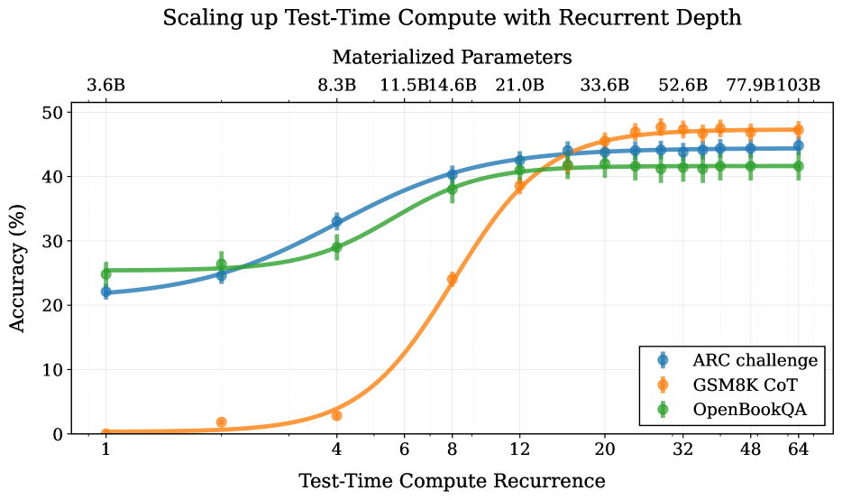
Figure 1: We train a 3.5B parameter language model with depth recurrence. At test time, the model can iterate longer to use more compute and improve its performance. Instead of scaling test-time reasoning by “verbalizing” in long Chains-of-Thought, the model improves entirely by reasoning in latent space. Tasks that require less reasoning like OpenBookQA converge quicker than tasks like GSM8k, which effectively make use of more compute.
However, the constraint that expensive internal reasoning must always be projected down to a single verbalized next token appears wasteful; it is plausible that models could be more competent if they were able to natively “think” in their continuous latent space. One way to unlock this untapped dimension of additional compute involves adding a recurrent unit to a model. This unit runs in a loop, iteratively processing and updating its hidden state and enabling computations to be carried on indefinitely. While this is not currently the dominant paradigm, this idea is foundational to machine learning and has been (re-)discovered in every decade, for example as recurrent neural networks, diffusion models, and as universal or looped transformers.
In this work, we show that depth-recurrent language models can learn effectively, be trained in an efficient manner, and demonstrate significant performance improvements under the scaling of test-time compute. Our proposed transformer architecture is built upon a latent depth-recurrent block that is run for a randomly sampled number of iterations during training. We show that this paradigm can scale to several billion parameters and over half a trillion tokens of pretraining data. At test-time, the model can improve its performance through recurrent reasoning in latent space, enabling it to compete with other open-source models that benefit from more parameters and training data. Additionally, we show that recurrent depth models naturally support a number of features at inference time that require substantial tuning and research effort in non-recurrent models, such as per-token adaptive compute, (self)-speculative decoding, and KV-cache sharing. We finish out our study by tracking token trajectories in latent space, showing that a number of interesting computation behaviors simply emerge with scale, such as the model rotating shapes in latent space for numerical computations.
## 2 Why Train Models with Recurrent Depth?
Recurrent layers enable a transformer model to perform arbitrarily many computations before emitting a token. In principle, recurrent mechanisms provide a simple solution for test-time compute scaling. Compared to a more standard approach of long context reasoning OpenAI (2024); DeepSeek-AI et al. (2025), latent recurrent thinking has several advantages.
- Latent reasoning does not require construction of bespoke training data. Chain-of-thought reasoning requires the model to be trained on long demonstrations that are constructed in the domain of interest. In contrast, our proposed latent reasoning models can train with a variable compute budget, using standard training data with no specialized demonstrations, and enhance their abilities at test-time if given additional compute.
- Latent reasoning models require less memory for training and inference than chain-of-thought reasoning models. Because the latter require extremely long context windows, specialized training methods such as token-parallelization Liu et al. (2023a) may be needed.
- Recurrent-depth networks perform more FLOPs per parameter than standard transformers, significantly reducing communication costs between accelerators at scale. This especially enables higher device utilization when training with slower interconnects.
- By constructing an architecture that is compute-heavy and small in parameter count, we hope to set a strong prior towards models that solve problems by “thinking”, i.e. by learning meta-strategies, logic and abstraction, instead of memorizing. The strength of recurrent priors for learning complex algorithms has already been demonstrated in the “deep thinking” literature Schwarzschild et al. (2021b); Bansal et al. (2022); Schwarzschild et al. (2023).
On a more philosophical note, we hope that latent reasoning captures facets of human reasoning that defy verbalization, such as spatial thinking, physical intuition or (motor) planning. Over many iterations of the recurrent process, reasoning in a high-dimensional vector space would enable the deep exploration of multiple directions simultaneously, instead of linear thinking, leading to a system capable of exhibiting novel and complex reasoning behavior.
Scaling compute in this manner is not at odds with scaling through extended (verbalized) inference scaling (Shao et al., 2024), or scaling parameter counts in pretraining (Kaplan et al., 2020), we argue it may build a third axis on which to scale model performance.
#### ———————— Table of Contents ————————
- Section 3 introduces our latent recurrent-depth model architecture and training objective.
- Section 4 describes the data selection and engineering of our large-scale training run on Frontier, an AMD cluster.
- Section 5 reports benchmark results, showing how the model improves when scaling inference compute.
- Section 6 includes several application examples showing how recurrent models naturally simplify LLM usecases.
- Section 7 visualizes what computation patterns emerge at scale with this architecture and training objective, showing that context-dependent behaviors emerge in latent space, such as “orbiting” when responding to prompts requiring numerical reasoning.
<details>
<summary>x2.png Details</summary>
### Visual Description
## Diagram: Recurrent Neural Network Architecture with Input Injection
### Overview
The image displays a technical flow diagram of a neural network architecture designed for sequence-to-sequence processing (e.g., translating "Hello" to "World"). The architecture consists of three main component types: a Prelude, a series of Recurrent Blocks, and a Coda. The diagram illustrates the flow of data and control signals between these components.
### Components/Axes
The diagram is composed of labeled blocks, directional arrows with annotations, and a two-part legend.
**Main Components (from left to right):**
1. **Prelude (Blue Block):** Labeled with the letter **"P"**. It receives the initial input text **"Hello"**.
2. **Recurrent Blocks (Green Blocks):** A sequence of blocks, each labeled with the letter **"R"**. The diagram shows three explicit blocks with an ellipsis **"..."** between the second and third, indicating a variable or repeated number of such blocks.
3. **Coda (Red Block):** Labeled with the letter **"C"**. It produces the final output text **"World"**.
**Arrows and Annotations:**
* **Input Text:** The string **"Hello"** with an arrow pointing into the Prelude block.
* **Output Text:** The string **"World"** with an arrow originating from the Coda block.
* **Input Injection (Dashed Arrows):** Three dashed gray arrows, each labeled with the letter **"e"**, originate from the Prelude block and point to each of the visible Recurrent Blocks.
* **Residual Stream (Solid Arrows):**
* A solid black arrow labeled **"s₀"** points from a mathematical notation into the first Recurrent Block.
* A solid black arrow labeled **"s₁"** points from the first Recurrent Block to the second.
* A solid black arrow points from the second Recurrent Block to the ellipsis **"..."**.
* A solid black arrow points from the ellipsis **"..."** to the final Recurrent Block.
* A solid black arrow labeled **"s_R"** points from the final Recurrent Block to the Coda block.
* **Mathematical Notation:** The expression **"𝒩(0, σ²I_{n·h})"** is positioned to the left of the first Recurrent Block, with an arrow labeled **"s₀"** pointing from it into the block. This denotes a normal distribution with mean 0 and variance σ², applied to an identity matrix of dimension n·h, likely representing the initialization of the residual stream state.
**Legend (Bottom of Diagram):**
* **Component Legend (Left Box):**
* Blue square: **"Prelude"**
* Green square: **"Recurrent Block"**
* Red square: **"Coda"**
* **Arrow Legend (Right Box):**
* Dashed gray arrow: **"Input Injection"**
* Solid black arrow: **"Residual Stream"**
### Detailed Analysis
The diagram defines a specific computational flow:
1. The input sequence ("Hello") is first processed by the **Prelude (P)**.
2. The Prelude generates an embedding or signal, denoted by **"e"**, which is **injected** (via dashed arrows) into **every** Recurrent Block in the sequence. This is a key architectural feature, suggesting the initial input context is made available at each processing step.
3. The core processing occurs in the chain of **Recurrent Blocks (R)**. They are connected sequentially by the **Residual Stream**, a solid pathway carrying state information (`s₀`, `s₁`, ..., `s_R`).
4. The initial state `s₀` of the residual stream is drawn from a normal distribution **𝒩(0, σ²I_{n·h})**, indicating a randomized initialization.
5. The final state `s_R` from the last Recurrent Block is passed to the **Coda (C)**.
6. The Coda processes this final state to generate the output sequence ("World").
### Key Observations
* **Parallel Input Injection:** The Prelude's output (`e`) is connected to all Recurrent Blocks simultaneously, not just the first one. This is a non-standard feature for classic recurrent networks, where input is typically only fed at the first step.
* **Residual Stream as State Carrier:** The primary sequential connection between Recurrent Blocks is explicitly labeled as a "Residual Stream," implying the network uses a residual learning framework where the stream carries the evolving hidden state.
* **Variable Depth:** The ellipsis **"..."** between Recurrent Blocks explicitly indicates that the architecture is not fixed to three blocks but can be scaled to a depth of `R` blocks.
* **Clear Separation of Concerns:** The three component types (Prelude, Recurrent Block, Coda) have distinct colors and roles, suggesting a modular design where each handles a specific part of the sequence transformation task (encoding, iterative processing, decoding).
### Interpretation
This diagram illustrates a **modified recurrent neural network (RNN) architecture** with a specific design choice to mitigate the vanishing gradient problem or enhance information flow.
* **What it demonstrates:** The architecture decouples the initial input processing (Prelude) from the core recurrent computation (Recurrent Blocks) and final output generation (Coda). The critical innovation shown is the **"Input Injection"** mechanism. By feeding the Prelude's output (`e`) directly into every Recurrent Block, the model ensures that the original input information is never more than one step away from any point in the processing chain. This likely helps preserve long-range dependencies and provides a stable reference signal throughout the sequence generation.
* **Relationships:** The Prelude acts as an encoder. The Recurrent Blocks form the dynamic core, with their state evolving via the Residual Stream. The Coda acts as a decoder. The Input Injection creates a bypass, allowing the encoded input to influence every time step of the recurrent processing directly.
* **Notable Anomalies/Patterns:** The most notable pattern is the dual-path information flow: the sequential **Residual Stream** (carrying the evolving state `s_t`) and the parallel **Input Injection** (carrying the static input context `e`). This creates a hybrid model combining aspects of feed-forward networks (direct input access) and recurrent networks (sequential state evolution). The use of a normally distributed initialization for `s₀` is standard practice, but its explicit notation here emphasizes the importance of the residual stream's starting condition.
</details>
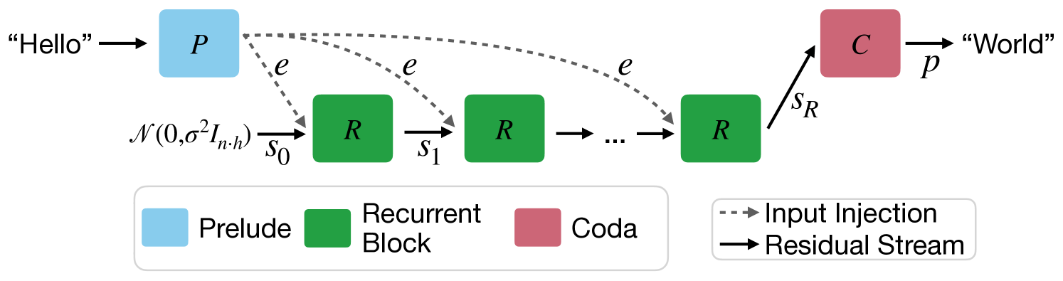
Figure 2: A visualization of the Architecture, as described in Section 3. Each block consists of a number of sub-layers. The blue prelude block embeds the inputs into latent space, where the green shared recurrent block is a block of layers that is repeated to compute the final latent state, which is decoded by the layers of the red coda block.
## 3 A scalable recurrent architecture
In this section we will describe our proposed architecture for a transformer with latent recurrent depth, discussing design choices and small-scale ablations. A diagram of the architecture can be found in Figure 2. We always refer to the sequence dimension as $n$ , the hidden dimension of the model as $h$ , and its vocabulary as the set $V$ .
### 3.1 Macroscopic Design
The model is primarily structured around decoder-only transformer blocks (Vaswani et al., 2017; Radford et al., 2019). However these blocks are structured into three functional groups, the prelude $P$ , which embeds the input data into a latent space using multiple transformer layers, then the core recurrent block $R$ , which is the central unit of recurrent computation modifying states $s∈ℝ^n× h$ , and finally the coda $C$ , which un-embeds from latent space using several layers and also contains the prediction head of the model. The core block is set between the prelude and coda blocks, and by looping the core we can put an indefinite amount of verses in our song.
Given a number of recurrent iterations $r$ , and a sequence of input tokens $x∈ V^n$ these groups are used in the following way to produce output probabilities $p∈ℝ^n×|V|$
| | $\displaystylee$ | $\displaystyle=P(x)$ | |
| --- | --- | --- | --- |
where $σ$ is some standard deviation for initializing the random state. This process is shown in Figure 2. Given an init random state $s_0$ , the model repeatedly applies the core block $R$ , which accepts the latent state $s_i-1$ and the embedded input $e$ and outputs a new latent state $s_i$ . After finishing all iterations, the coda block processes the last state and produces the probabilities of the next token.
This architecture is based on deep thinking literature, where it is shown that injecting the latent inputs $e$ in every step (Bansal et al., 2022) and initializing the latent vector with a random state stabilizes the recurrence and promotes convergence to a steady state independent of initialization, i.e. path independence (Anil et al., 2022).
#### Motivation for this Design.
This recurrent design is the minimal setup required to learn stable iterative operators. A good example is gradient descent of a function $E(x,y)$ , where $x$ may be the variable of interest and $y$ the data. Gradient descent on this function starts from an initial random state, here $x_0$ , and repeatedly applies a simple operation (the gradient of the function it optimizes), that depends on the previous state $x_k$ and data $y$ . Note that we need to use $y$ in every step to actually optimize our function. Similarly we repeatedly inject the data $e$ in our set-up in every step of the recurrence. If $e$ was provided only at the start, e.g. via $s_0=e$ , then the iterative process would not be stable Stable in the sense that $R$ cannot be a monotone operator if it does not depend on $e$ , and so cannot represent gradient descent on strictly convex, data-dependent functions, (Bauschke et al., 2011), as its solution would depend only on its boundary conditions.
The structure of using several layers to embed input tokens into a hidden latent space is based on empirical results analyzing standard fixed-depth transformers (Skean et al., 2024; Sun et al., 2024; Kaplan et al., 2024). This body of research shows that the initial and the end layers of LLMs are noticeably different, whereas middle layers are interchangeable and permutable. For example, Kaplan et al. (2024) show that within a few layers standard models already embed sub-word tokens into single concepts in latent space, on which the model then operates.
**Remark 3.1 (Is this a Diffusion Model?)**
*This iterative architecture will look familiar to the other modern iterative modeling paradigm, diffusion models (Song and Ermon, 2019), especially latent diffusion models (Rombach et al., 2022). We ran several ablations with iterative schemes even more similar to diffusion models, such as $s_i=R(e,s_i-1)+n$ where $n∼N(0,σ_iI_n· h)$ , but find the injection of noise not to help in our preliminary experiments, which is possibly connected to our training objective. We also evaluated and $s_i=R_i(e,s_i-1)$ , i.e. a core block that takes the current step as input (Peebles and Xie, 2023), but find that this interacts badly with path independence, leading to models that cannot extrapolate.*
### 3.2 Microscopic Design
Within each group, we broadly follow standard transformer layer design. Each block contains multiple layers, and each layer contains a standard, causal self-attention block using RoPE (Su et al., 2021) with a base of $50000$ , and a gated SiLU MLP (Shazeer, 2020). We use RMSNorm (Zhang and Sennrich, 2019) as our normalization function. The model has learnable biases on queries and keys, and nowhere else. To stabilize the recurrence, we order all layers in the following “sandwich” format, using norm layers $n_i$ , which is related, but not identical to similar strategies in (Ding et al., 2021; Team Gemma et al., 2024):
| | $\displaystyle\hat{x_l}=$ | $\displaystyle n_2≤ft(x_l-1+\textnormal{Attn}(n_1(x_ l-1))\right)$ | |
| --- | --- | --- | --- |
While at small scales, most normalization strategies, e.g. pre-norm, post-norm and others, work almost equally well, we ablate these options and find that this normalization is required to train the recurrence at scale Note also that technically $n_3$ is superfluous, but we report here the exact norm setup with which we trained the final model..
Given an embedding matrix $E$ and embedding scale $γ$ , the prelude block first embeds input tokens $x$ as $γ E(x)$ , and then to applies $l_P$ many prelude layers with the layout described above.
Our core recurrent block $R$ starts with an adapter matrix $A:ℝ^2h→ℝ^h$ mapping the concatenation of $s_i$ and $e$ into the hidden dimension $h$ (Bansal et al., 2022). While re-incorporation of initial embedding features via addition rather than concatenation works equally well for smaller models, we find that concatenation works best at scale. This is then fed into $l_R$ transformer layers. At the end of the core block the output is again rescaled with an RMSNorm $n_c$ .
The coda contains $l_C$ layers, normalization by $n_c$ , and projection into the vocabulary using tied embeddings $E^T$ .
In summary, we can summarize the architecture by the triplet $(l_P,l_R,l_C)$ , describing the number of layers in each stage, and by the number of recurrences $r$ , which may vary in each forward pass. We train a number of small-scale models with shape $(1,4,1)$ and hidden size $h=1024$ , in addition to a large model with shape $(2,4,2)$ and $h=5280$ . This model has only $8$ “real” layers, but when the recurrent block is iterated, e.g. 32 times, it unfolds to an effective depth of $2+4r+2=132$ layers, constructing computation chains that can be deeper than even the largest fixed-depth transformers (Levine et al., 2021; Merrill et al., 2022).
### 3.3 Training Objective
#### Training Recurrent Models through Unrolling.
To ensure that the model can function when we scale up recurrent iterations at test-time, we randomly sample iteration counts during training, assigning a random number of iterations $r$ to every input sequence (Schwarzschild et al., 2021b). We optimize the expectation of the loss function $L$ over random samples $x$ from distribution $X$ and random iteration counts $r$ from distribution $Λ$ .
$$
L(θ)=E_x∈ XE_r∼ΛL
≤ft(m_θ(x,r),x^\prime\right).
$$
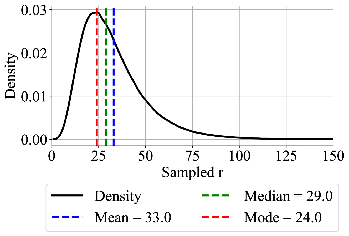
Here, $m$ represents the model output, and $x^\prime$ is the sequence $x$ shifted left, i.e., the next tokens in the sequence $x$ . We choose $Λ$ to be a log-normal Poisson distribution. Given a targeted mean recurrence $\bar{r}+1$ and a variance that we set to $σ=\frac{1}{2}$ , we can sample from this distribution via
$$
\displaystyleτ \displaystyle∼N(\log(\bar{r})-\frac{1}{2}σ^2,σ) \displaystyle r \displaystyle∼P(e^τ)+1, \tag{1}
$$
given the normal distribution $N$ and Poisson distribution $P$ , see Figure 3. The distribution most often samples values less than $\bar{r}$ , but it contains a heavy tail of occasional events in which significantly more iterations are taken.
<details>
<summary>x3.png Details</summary>
### Visual Description
## Density Plot: Distribution of Sampled r
### Overview
The image displays a probability density function plot for a variable labeled "Sampled r". The plot shows a single, continuous, right-skewed distribution. Three vertical dashed lines are overlaid on the plot, marking the mode, median, and mean of the distribution, with their exact values provided in a legend.
### Components/Axes
* **Chart Type:** Density Plot (Probability Density Function).
* **X-Axis:**
* **Label:** "Sampled r"
* **Scale:** Linear scale ranging from 0 to 150.
* **Major Tick Marks:** 0, 25, 50, 75, 100, 125, 150.
* **Y-Axis:**
* **Label:** "Density"
* **Scale:** Linear scale ranging from 0.00 to 0.03.
* **Major Tick Marks:** 0.00, 0.01, 0.02, 0.03.
* **Legend:** Positioned at the bottom center of the chart. It contains four entries:
1. **Black solid line:** "Density"
2. **Blue dashed line:** "Mean = 33.0"
3. **Green dashed line:** "Median = 29.0"
4. **Red dashed line:** "Mode = 24.0"
* **Data Series & Visual Elements:**
* **Density Curve (Black Line):** A smooth, continuous curve representing the probability density of "Sampled r".
* **Mode Line (Red Dashed):** A vertical line intersecting the x-axis at approximately x=24.0, aligning with the peak of the density curve.
* **Median Line (Green Dashed):** A vertical line intersecting the x-axis at approximately x=29.0.
* **Mean Line (Blue Dashed):** A vertical line intersecting the x-axis at approximately x=33.0.
### Detailed Analysis
* **Distribution Shape:** The density curve is unimodal (single peak) and positively skewed (right-skewed). It rises steeply from x=0 to its peak, then descends more gradually, forming a long tail extending towards higher values of "Sampled r".
* **Peak Density:** The maximum density value (the peak of the curve) is approximately 0.03, occurring at the mode (x ≈ 24.0).
* **Central Tendency Measures:**
* **Mode (Red Line):** The most frequent value, located at the distribution's peak. Value: **24.0**.
* **Median (Green Line):** The middle value, dividing the distribution into two equal halves. Value: **29.0**.
* **Mean (Blue Line):** The arithmetic average. Value: **33.0**.
* **Relationship of Measures:** The measures follow the classic order for a right-skewed distribution: **Mode (24.0) < Median (29.0) < Mean (33.0)**. The mean is pulled furthest into the right tail by the higher-value outliers.
* **Spatial Grounding:** The three vertical lines are clustered in the left-center region of the plot (between x=20 and x=35). The red (Mode) line is leftmost, followed by the green (Median), and then the blue (Mean) line on the right. This spatial arrangement visually confirms the numerical order of the statistics.
### Key Observations
1. **Clear Positive Skew:** The long tail to the right and the ordering of Mode < Median < Mean are definitive indicators of a right-skewed distribution.
2. **Concentration of Data:** The majority of the probability mass (the area under the curve) is concentrated between x=0 and x=75. The density becomes very low (approaching zero) for values of "Sampled r" greater than 100.
3. **Visual Confirmation of Statistics:** The plot provides an immediate visual understanding of how the mean, median, and mode relate to the shape of the data distribution. The mean's position further right than the median highlights the influence of the tail.
### Interpretation
This density plot characterizes the distribution of a sampled variable "r". The data is not symmetrically distributed around a central value; instead, it is characterized by a concentration of lower values and a scattering of less frequent, higher values.
* **What the data suggests:** The process generating "Sampled r" likely has a lower bound near zero and produces moderately low values most frequently (around 24). However, there is a significant probability of obtaining higher values, which pulls the average (mean) up to 33. This pattern is common in phenomena like reaction times, income distributions, or the size of natural events (e.g., rainfall, earthquake magnitudes).
* **How elements relate:** The density curve is the fundamental representation of the data's behavior. The vertical lines for Mode, Median, and Mean are summary statistics derived from this distribution. Their placement on the x-axis is directly determined by the shape of the curve. The legend acts as a key to decode these overlaid statistical markers.
* **Notable implications:** For analysis, using the median (29.0) as a measure of central tendency might be more representative of a "typical" value than the mean (33.0), as the mean is inflated by the right tail. Any statistical model applied to this data should account for its skewness rather than assuming a normal (symmetric) distribution.
</details>
Figure 3: We use a log-normal Poisson Distribution to sample the number of recurrent iterations for each training step.
#### Truncated Backpropagation.
To keep computation and memory low at train time, we backpropagate through only the last $k$ iterations of the recurrent unit. This enables us to train with the heavy-tailed Poisson distribution $Λ$ , as maximum activation memory and backward compute is now independent of $r$ . We fix $k=8$ in our main experiments. At small scale, this works as well as sampling $k$ uniformly, but with set fixed, the overall memory usage in each step of training is equal. Note that the prelude block still receives gradient updates in every step, as its output $e$ is injected in every step. This setup resembles truncated backpropagation through time, as commonly done with RNNs, although our setup is recurrent in depth rather than time (Williams and Peng, 1990; Mikolov et al., 2011).
## 4 Training a large-scale recurrent-depth Language Model
After verifying that we can reliably train small test models up to 10B tokens, we move on to larger-scale runs. Given our limited compute budget, we could either train multiple tiny models too small to show emergent effects or scaling, or train a single medium-scale model. Based on this, we prepared for a single run, which we detail below.
### 4.1 Training Setup
We describe the training setup, separated into architecture, optimization setup and pretraining data. We publicly release all training data, pretraining code, and a selection of intermediate model checkpoints.
#### Pretraining Data.
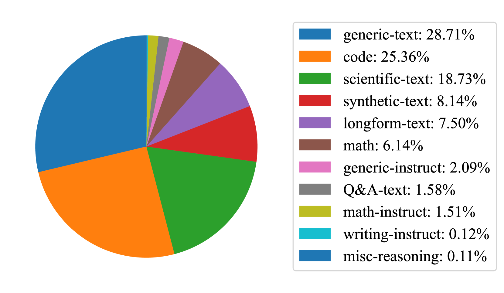
Given access to only enough compute for a single large scale model run, we opted for a dataset mixture that maximized the potential for emergent reasoning behaviors, not necessarily for optimal benchmark performance. Our final mixture is heavily skewed towards code and mathematical reasoning data with (hopefully) just enough general webtext to allow the model to acquire standard language modeling abilities. All sources are publicly available. We provide an overview in Figure 4. Following Allen-Zhu and Li (2024), we directly mix relevant instruction data into the pretraining data. However, due to compute and time constraints, we were not able to ablate this mixture. We expect that a more careful data preparation could further improve the model’s performance. We list all data sources in Appendix C.
#### Tokenization and Packing Details.
We construct a vocabulary of $65536$ tokens via BPE (Sennrich et al., 2016), using the implementation of Dagan (2024). In comparison to conventional tokenizer training, we construct our tokenizer directly on the instruction data split of our pretraining corpus, to maximize tokenization efficiency on the target domain. We also substantially modify the pre-tokenization regex (e.g. of Dagan et al. (2024)) to better support code, contractions and LaTeX. We include a <|begin_text|> token at the start of every document. After tokenizing our pretraining corpus, we pack our tokenized documents into sequences of length 4096. When packing, we discard document ends that would otherwise lack previous context, to fix an issue described as the “grounding problem” in Ding et al. (2024), aside from several long-document sources of mathematical content, which we preserve in their entirety.
<details>
<summary>x4.png Details</summary>
### Visual Description
\n
## Pie Chart: Distribution of Text Categories
### Overview
The image displays a pie chart illustrating the percentage distribution of various text categories, likely representing the composition of a dataset or corpus. The chart is accompanied by a legend on the right side that lists each category with its corresponding color and precise percentage value.
### Components/Axes
* **Chart Type:** Pie Chart
* **Legend Position:** Located to the right of the pie chart, enclosed in a light grey bordered box.
* **Legend Content:** The legend contains 11 entries, each with a colored square swatch, a category name, and a percentage value. The categories are listed in descending order of their percentage share.
### Detailed Analysis
The pie chart is divided into 11 segments, each corresponding to a category in the legend. The segments are ordered clockwise from the top, starting with the largest.
**Legend Data (in order as listed):**
1. **generic-text:** 28.71% (Color: Blue)
2. **code:** 25.36% (Color: Orange)
3. **scientific-text:** 18.73% (Color: Green)
4. **synthetic-text:** 8.14% (Color: Red)
5. **longform-text:** 7.50% (Color: Purple)
6. **math:** 6.14% (Color: Brown)
7. **generic-instruct:** 2.09% (Color: Pink)
8. **Q&A-text:** 1.58% (Color: Grey)
9. **math-instruct:** 1.51% (Color: Yellow-Green)
10. **writing-instruct:** 0.12% (Color: Cyan)
11. **misc-reasoning:** 0.11% (Color: Dark Blue)
**Visual Segment Verification (Clockwise from top):**
* The largest segment is **Blue (generic-text, 28.71%)**, occupying the top-left quadrant.
* The next largest is **Orange (code, 25.36%)**, adjacent to the blue segment.
* The third-largest is **Green (scientific-text, 18.73%)**, following the orange.
* The remaining segments decrease in size: **Red (synthetic-text)**, **Purple (longform-text)**, **Brown (math)**, **Pink (generic-instruct)**, **Grey (Q&A-text)**, **Yellow-Green (math-instruct)**.
* The two smallest segments, **Cyan (writing-instruct)** and **Dark Blue (misc-reasoning)**, are very thin slivers at the top of the chart, adjacent to the initial blue segment.
### Key Observations
1. **Dominant Categories:** The top three categories—generic-text, code, and scientific-text—collectively account for **72.8%** of the total, indicating a strong concentration.
2. **Long Tail Distribution:** There is a significant drop-off after the top three. The next five categories (synthetic-text through Q&A-text) range from 8.14% down to 1.58%.
3. **Minimal Representation:** The final three categories (math-instruct, writing-instruct, misc-reasoning) are marginal, each representing less than 2% of the total, with the last two being near-negligible at ~0.1%.
4. **Category Types:** The categories can be broadly grouped:
* **General Text:** generic-text, longform-text.
* **Technical/Specialized:** code, scientific-text, math.
* **Instruction-Based:** generic-instruct, math-instruct, writing-instruct.
* **Other:** synthetic-text, Q&A-text, misc-reasoning.
### Interpretation
This chart likely represents the composition of a training dataset for a language model or a similar text-based AI system. The data suggests a primary focus on **general language understanding (generic-text)** and **technical proficiency (code, scientific-text)**, which form the core of the dataset. The presence of instruction-based categories (instruct) indicates a component designed for tuning the model to follow directions. The very small percentages for specialized instruction types (writing-instruct, math-instruct) and miscellaneous reasoning suggest these are either niche areas or are subsumed within larger categories. The distribution follows a classic "long tail" pattern, where a few categories dominate, and many others have minimal representation. This could imply a design choice to prioritize broad competency in common text types and programming over highly specialized or rarefied tasks.
</details>
Figure 4: Distribution of data sources that are included during training. The majority of our data is comprised of generic web-text, scientific writing and code.
#### Architecture and Initialization.
We scale the architecture described in Section 3, setting the layers to $(2,4,2)$ , and train with a mean recurrence value of $\bar{r}=32$ . We mainly scale by increasing the hidden size to $h=5280$ , which yields $55$ heads of size of $96$ . The MLP inner dimension is $17920$ and the RMSNorm $ε$ is $10^-6$ . Overall this model shape has about $1.5$ B parameters in non-recurrent prelude and head, $1.5$ B parameters in the core recurrent block, and $0.5$ B in the tied input embedding.
At small scales, most sensible initialization schemes work. However, at larger scales, we use the initialization of Takase et al. (2024) which prescribes a variance of $σ_h^2=\frac{2}{5h}$ . We initialize all parameters from a truncated normal distribution (truncated at $3σ$ ) with this variance, except all out-projection layers, where the variance is set to $σ_\textnormal{out}^2=\frac{1}{5hl}$ , for $l=l_P+\bar{r}l_R+l_C$ the number of effective layers, which is 132 for this model. As a result, the out-projection layers are initialized with fairly small values (Goyal et al., 2018). The output of the embedding layer is scaled by $√{h}$ . To match this initialization, the state $s_0$ is also sampled from a truncated normal distribution, here with variance $σ_s^2=\frac{2}{5}$ .
#### Locked-Step Sampling.
To enable synchronization between parallel workers, we sample a single depth $r$ for each micro-batch of training, which we synchronize across workers (otherwise workers would idle while waiting for the model with the largest $r$ to complete its backward pass). We verify at small scale that this modification improves compute utilization without impacting convergence speed, but note that at large batch sizes, training could be further improved by optimally sampling and scheduling independent steps $r$ on each worker, to more faithfully model the expectation over steps in Equation 1.
#### Optimizer and Learning Rate Schedule.
We train using the Adam optimizer with decoupled weight regularization ( $β_1=0.9$ , $β_2=0.95$ , $η=$5×{10}^-4$$ ) (Kingma and Ba, 2015; Loshchilov and Hutter, 2017), modified to include update clipping (Wortsman et al., 2023b) and removal of the $ε$ constant as in Everett et al. (2024). We clip gradients above $1$ . We train with warm-up and a constant learning rate (Zhai et al., 2022; Geiping and Goldstein, 2023), warming up to our maximal learning rate within the first $4096$ steps.
### 4.2 Compute Setup and Hardware
We train this model using compute time allocated on the Oak Ridge National Laboratory’s Frontier supercomputer. This HPE Cray system contains 9408 compute nodes with AMD MI250X GPUs, connected via 4xHPE Slingshot-11 NICs. The scheduling system is orchestrated through SLURM. We train in bfloat16 mixed precision using a PyTorch-based implementation (Zamirai et al., 2021).
<details>
<summary>x5.png Details</summary>
### Visual Description
## Line Charts: Training Metrics Comparison Across Runs and Recurrence Depths
### Overview
The image displays three horizontally aligned line charts comparing the training progress of three different runs ("Main", "Bad Run 1", "Bad Run 2") across three different metrics. All charts use logarithmic scales for both axes. A secondary legend on the right indicates that line styles correspond to different "Recurrence" depths (1, 4, 8, 16, 32, 64), which are applied within the runs shown in the third chart.
### Components/Axes
**Common Elements:**
* **X-Axis (All Charts):** "Optimizer Step" on a logarithmic scale. Major ticks are at 10¹, 10², 10³, and 10⁴.
* **Bottom Legend:** Centered below the charts. Defines three color-coded series:
* Blue solid line: "Main"
* Orange solid line: "Bad Run 1"
* Green solid line: "Bad Run 2"
* **Right Legend:** Positioned to the right of the third chart. Defines line styles for "Recurrence":
* Solid line: 1
* Dashed line: 4
* Dotted line: 8
* Dash-dot line: 16
* Long dash line: 32
* Dash-dot-dot line: 64
**Chart 1 (Left):**
* **Y-Axis:** "Loss (log)" on a logarithmic scale. Major ticks at 10¹ and 10⁰ (implied, not labeled).
**Chart 2 (Middle):**
* **Y-Axis:** "Hidden State Corr. (log)" on a logarithmic scale. Major ticks at 10⁰ and 10⁻¹.
**Chart 3 (Right):**
* **Y-Axis:** "Val PPL (log)" on a logarithmic scale. Major ticks at 10³, 10², and 10¹.
### Detailed Analysis
**Chart 1: Loss vs. Optimizer Step**
* **Main (Blue):** Starts at ~10¹. Shows a steady, near-linear decrease on the log-log plot, ending at approximately 2-3 by step 10⁴.
* **Bad Run 1 (Orange):** Starts higher than Main (~20-30). Drops sharply until ~10² steps, then plateaus at a value slightly below 10¹ (estimated ~7-8).
* **Bad Run 2 (Green):** Starts the highest (~50-60). Drops very sharply until ~10¹ steps, then continues a steady decline, remaining above the Main run. Ends at approximately 4-5 by step 10⁴.
**Chart 2: Hidden State Correlation vs. Optimizer Step**
* **Main (Blue):** Starts high (~0.8-0.9). Shows a general downward trend with significant high-frequency noise/fluctuation. Ends in the range of 0.05-0.1.
* **Bad Run 1 (Orange):** Appears as a flat line at the top of the chart (10⁰ = 1.0), indicating constant, perfect correlation throughout training.
* **Bad Run 2 (Green):** Starts at 1.0. Begins a steep decline around step 10², then exhibits extreme volatility/noise, oscillating roughly between 0.05 and 0.3 after step 10³.
**Chart 3: Validation Perplexity (Val PPL) vs. Optimizer Step**
* This chart overlays multiple line styles (Recurrence depths) for each of the three color-coded runs.
* **General Trend:** For all runs (Main, Bad 1, Bad 2), higher recurrence depth (e.g., 64, dash-dot-dot) generally leads to lower final validation perplexity compared to lower depth (e.g., 1, solid line).
* **Main (Blue) Series:** Shows the best performance. The solid line (Recurrence=1) ends near 10². The dashed (4) and dotted (8) lines end between 10¹ and 10². The dash-dot (16), long dash (32), and dash-dot-dot (64) lines cluster tightly at the bottom, ending very close to 10¹.
* **Bad Run 1 (Orange) Series:** All lines are flat at the top of the chart (~2000-3000), indicating no improvement in validation perplexity regardless of recurrence depth.
* **Bad Run 2 (Green) Series:** Shows intermediate performance. The solid line (Recurrence=1) ends near 200. Lines for higher recurrence depths show improvement, with the dash-dot-dot (64) line ending the lowest, around 20-30.
### Key Observations
1. **Performance Hierarchy:** The "Main" run consistently outperforms both "Bad Runs" across loss and validation perplexity. "Bad Run 2" shows some learning but is unstable, while "Bad Run 1" appears completely stalled after an initial drop.
2. **Correlation Anomaly:** "Bad Run 1" maintains a hidden state correlation of 1.0 throughout, which is highly unusual and likely indicates a failure mode (e.g., collapsed representations). "Bad Run 2" shows extreme volatility in this metric.
3. **Recurrence Benefit:** Increasing recurrence depth provides a clear and significant benefit to final validation perplexity, especially in the "Main" run where depths 16, 32, and 64 converge to a similar, low value.
4. **Stability:** The "Main" run exhibits the smoothest and most stable training curves. "Bad Run 2" is characterized by high noise and volatility, particularly in the hidden state correlation.
### Interpretation
This data suggests a comparative analysis of neural network training runs, likely for a recurrent or sequence model. The "Main" run represents a successful training trajectory, where both loss and validation perplexity decrease steadily, and hidden state correlation decays in a controlled manner—indicating the model is learning useful, non-redundant representations.
The "Bad Runs" illustrate two distinct failure modes:
* **Bad Run 1 (Orange):** Exhibits "feature collapse" or "representation death." The perfect, unchanging hidden state correlation (1.0) implies the model's internal states are not differentiating or learning meaningful temporal dependencies. Consequently, validation perplexity does not improve.
* **Bad Run 2 (Green):** Shows unstable training. While loss decreases, the extreme volatility in hidden state correlation suggests the model is struggling to find a stable solution, possibly due to issues like exploding/vanishing gradients or poor hyperparameter choices. Its validation performance is mediocre.
The third chart demonstrates a key architectural insight: **increasing recurrence depth (the number of recurrent steps or layers) is a powerful lever for improving model performance (lower validation perplexity)**, but its effectiveness depends on a stable training run (as seen in "Main"). In a failed run ("Bad Run 1"), changing recurrence depth has no effect. This highlights that architectural improvements must be coupled with stable training dynamics to be beneficial.
</details>
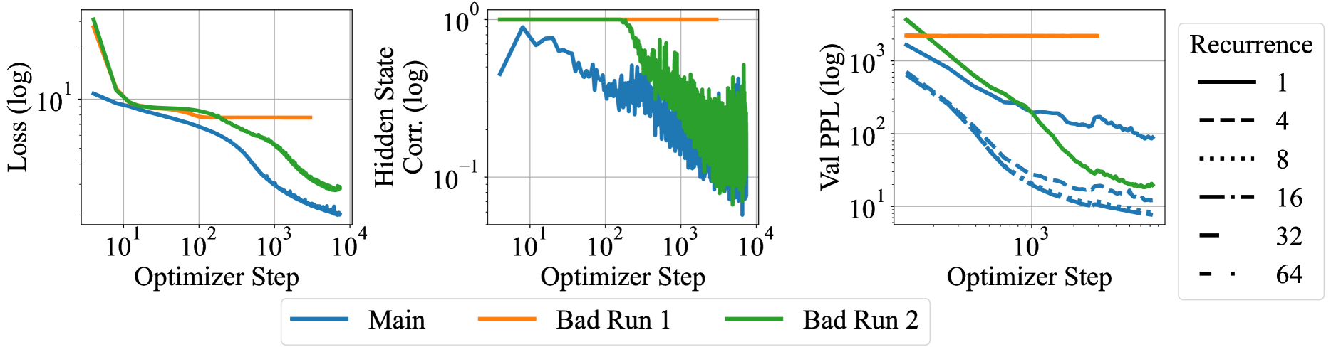
Figure 5: Plots of the initial 10000 steps for the first two failed attempts and the final, successful run (“Main”). Note the hidden state collapse (middle) and collapse of the recurrence (right) in the first two failed runs, underlining the importance of our architecture and initialization in inducing a recurrent model and explain the underperformance of these runs in terms of pretraining loss (left).
#### Device Speed and Parallelization Strategy.
Nominally, each MI250X chip Technically, each node contains 4 dual-chip MI250X cards, but its main software stack (ROCm runtime) treats these chips as fully independent. achieves 192 TFLOP per GPU (AMD, 2021). For a single matrix multiplication, we measure a maximum achievable speed on these GPUs of 125 TFLOP/s on our software stack (ROCM 6.2.0, PyTorch 2.6 pre-release 11/02) (Bekman, 2023). Our implementation, using extensive PyTorch compilation and optimization of the hidden dimension to $h=5280$ achieves a single-node training speed of 108.75 TFLOP/s, i.e. 87% AFU (“Achievable Flop Utilization”). Due to the weight sharing inherent in our recurrent design, even our largest model is still small enough to be trained using only data (not tensor) parallelism, with only optimizer sharding (Rajbhandari et al., 2020) and gradient checkpointing on a per-iteration granularity. With a batch size of 1 per GPU we end up with a global batch size of 16M tokens per step, minimizing inter-GPU communication bandwidth.
When we run at scale on 4096 GPUs, we achieve 52-64 TFLOP/s per GPU, i.e. 41%-51% AFU, or 1-1.2M tokens per second. To achieve this, we wrote a hand-crafted distributed data parallel implementation to circumvent a critical AMD interconnect issue, which we describe in more detail in Section A.2. Overall, we believe this may be the largest language model training run to completion in terms of number of devices used in parallel on an AMD cluster, as of time of writing.
#### Training Timeline.
Training proceeded through 21 segments of up to 12 hours, which scheduled on Frontier mostly in early December 2024. We also ran a baseline comparison, where we train the same architecture but in a feedforward manner with only 1 pass through the core/recurrent block. This trained with the same setup for 180B tokens on 256 nodes with a batch size of 2 per GPU. Ultimately, we were able to schedule 795B tokens of pretraining of the main model. Due to our constant learning rate schedule, we were able to add additional segments “on-demand”, when an allocation happened to be available.
<details>
<summary>x6.png Details</summary>
### Visual Description
## Line Graph: Training Loss vs. Steps and Tokens
### Overview
The image displays a line graph plotting a model's training loss against the number of training steps and processed tokens, both on logarithmic scales. The graph shows a clear, decreasing trend in loss as training progresses, with the rate of decrease slowing significantly in later stages.
### Components/Axes
* **Chart Type:** Single-series line graph.
* **Title/Top Axis Label:** "Tokens (log)" - positioned at the top center of the chart.
* **X-Axis (Bottom):** Labeled "Step (log)". It is a logarithmic scale with major tick marks and labels at `10^1`, `10^2`, `10^3`, and `10^4`.
* **X-Axis (Top):** A secondary logarithmic axis labeled "Tokens (log)" with major tick marks and labels at `10^8`, `10^9`, `10^10`, `10^11`, and `10^12`. This axis is aligned with the bottom "Step" axis, indicating a direct relationship between steps and tokens processed.
* **Y-Axis:** Labeled "Loss". It is a linear scale with major tick marks and labels at `5` and `10`. The axis extends slightly below 5 and above 10.
* **Data Series:** A single, solid blue line representing the loss value.
* **Grid:** A light gray grid is present, with vertical lines corresponding to the major x-axis ticks and horizontal lines at y=5 and y=10.
### Detailed Analysis
The blue line demonstrates a consistent downward trend from left to right.
* **Initial Phase (Steps ~5 to 100):** The line begins at a loss value slightly above 10 (approx. 10.5) at a step count just below `10^1`. It descends steeply and relatively smoothly. At step `10^2`, the loss is approximately 7.
* **Middle Phase (Steps ~100 to 1,000):** The descent continues but begins to shallow. The line passes through a loss of approximately 5 at a step count between `10^2` and `10^3` (roughly at step 300-400). At step `10^3`, the loss is approximately 3.5.
* **Late Phase (Steps >1,000):** The curve flattens considerably, showing diminishing returns. The line becomes noticeably noisier, with small, frequent upward spikes. By step `10^4`, the loss has decreased to approximately 2.5. The line continues with a very gradual downward slope and persistent noise until the end of the plotted data, which is slightly beyond step `10^4`.
**Trend Verification:** The visual trend is a classic "learning curve": a rapid initial improvement (steep negative slope) that gradually plateaus (slope approaches zero). The increasing noise in the later phase is also a common characteristic.
### Key Observations
1. **Log-Log Relationship:** The use of logarithmic scales on both the step/token axes and the (implied) loss axis suggests the relationship between training effort and loss reduction follows a power law or exponential decay pattern.
2. **Dual X-Axes:** The alignment of "Step" and "Tokens" implies a fixed or average number of tokens per step. For example, step `10^3` aligns with approximately `10^10` tokens, suggesting ~10 million tokens per step in that region.
3. **Noise Onset:** The transition from a smooth curve to a noisy line occurs around step `10^3` (loss ~3.5). This could indicate a change in training dynamics, such as a shift in learning rate, the introduction of regularization, or simply the inherent variance becoming more visible as the loss signal weakens.
4. **Plateau Level:** The loss appears to be approaching an asymptote somewhere between 2 and 2.5, indicating the model's performance limit under the current training configuration.
### Interpretation
This graph is a fundamental diagnostic tool for machine learning model training. It visually answers the question: "Is the model learning, and how efficiently?"
* **What it demonstrates:** The model is successfully learning, as evidenced by the consistent reduction in loss (a measure of error) over time. The steep initial drop indicates the model is quickly learning the most obvious patterns in the data.
* **Relationship between elements:** The dual x-axes explicitly link computational effort (steps) to data exposure (tokens). The flattening curve illustrates the principle of diminishing returns in training: each additional order of magnitude in steps/tokens yields a progressively smaller improvement in loss.
* **Notable implications:** The persistent noise in the late stage suggests the training process has entered a regime of high variance. This is often where techniques like learning rate decay or early stopping become critical to prevent overfitting and to efficiently finalize the model. The plateau indicates that simply training for more steps with the same hyperparameters is unlikely to yield significant further improvement; a change in strategy (e.g., model architecture, data quality, or optimization algorithm) would be needed to break through this loss floor.
**Language:** All text in the image is in English.
</details>
<details>
<summary>x7.png Details</summary>
### Visual Description
## Log-Log Line Chart: Validation Perplexity vs. Training Steps for Different Recurrence Depths
### Overview
This image is a line chart plotted on a log-log scale. It displays the relationship between training progress (measured in steps and tokens) and model performance (measured by validation perplexity) for neural network models configured with different recurrence depths. The chart demonstrates how increasing the recurrence depth affects the model's learning efficiency and final performance.
### Components/Axes
* **Primary X-Axis (Bottom):** Labeled **"Step (log)"**. It is a logarithmic scale with major tick marks at `10²`, `10³`, and `10⁴`.
* **Secondary X-Axis (Top):** Labeled **"Tokens (log)"**. It is a logarithmic scale with major tick marks at `10¹⁰`, `10¹¹`, and `10¹²`. This axis provides an alternative measure of training data exposure.
* **Y-Axis (Left):** Labeled **"Validation Perplexity (log)"**. It is a logarithmic scale with major tick marks at `10¹`, `10²`, and `10³`. Lower perplexity indicates better model performance.
* **Legend (Right side):** Titled **"Recurrence"**. It contains six entries, each associating a color with a recurrence depth value:
* Blue line: `1`
* Orange line: `4`
* Green line: `8`
* Red line: `16`
* Purple line: `32`
* Brown line: `64`
### Detailed Analysis
The chart plots six data series, each corresponding to a different recurrence depth. All series show a general downward trend, indicating that validation perplexity decreases (performance improves) as training progresses (steps/tokens increase).
1. **Recurrence = 1 (Blue Line):**
* **Trend:** Slopes downward but remains significantly higher than all other lines throughout the entire training process. It exhibits more volatility, especially at higher step counts (around `10⁴` steps), where it shows sharp, small upward spikes.
* **Approximate Values:** Starts near `2 x 10³` perplexity at `10²` steps. Ends in the range of `30-50` perplexity at the final step (approx. `5 x 10⁴`).
2. **Recurrence = 4 (Orange Line):**
* **Trend:** Slopes downward more steeply than the blue line initially. It separates clearly from the cluster of higher recurrence lines (8, 16, 32, 64) after about `5 x 10²` steps and maintains a distinct, higher path.
* **Approximate Values:** Starts near `7 x 10²` perplexity at `10²` steps. Ends near `10¹` (10) perplexity at the final step.
3. **Recurrence = 8, 16, 32, 64 (Green, Red, Purple, Brown Lines):**
* **Trend:** These four lines are tightly clustered together, especially after `10³` steps. They follow a very similar, steep downward trajectory. The lines for recurrence 16, 32, and 64 are nearly indistinguishable for most of the plot. The green line (recurrence 8) is slightly above this tight cluster but converges with them by the end.
* **Approximate Values:** All start in the range of `6-8 x 10²` perplexity at `10²` steps. They converge to a final perplexity value slightly below `10¹` (approximately `6-8`) at the final step.
### Key Observations
* **Performance Hierarchy:** There is a clear performance hierarchy based on recurrence depth. Recurrence=1 performs worst, recurrence=4 is significantly better, and recurrence depths of 8 and above yield the best and very similar performance.
* **Diminishing Returns:** The performance gap between recurrence=4 and recurrence=8 is substantial. However, the gap between recurrence=8 and recurrence=64 is minimal, indicating strong diminishing returns for increasing recurrence beyond 8.
* **Convergence:** The models with recurrence ≥8 not only achieve lower final perplexity but also appear to converge to their final performance level at a similar rate.
* **Stability:** The model with recurrence=1 shows more instability (spikes) in its validation metric during later training stages compared to the smoother curves of models with higher recurrence.
### Interpretation
This chart provides empirical evidence for the benefit of using recurrence (or a similar mechanism like depth in a recurrent neural network) in language modeling. The data suggests that:
1. **Recurrence is Critical:** A model with minimal recurrence (depth=1) is severely limited in its capacity to learn and generalize, as shown by its persistently high perplexity.
2. **Optimal Range Exists:** There is an effective range for this hyperparameter. Increasing recurrence from 1 to 4 to 8 yields dramatic improvements in learning efficiency and final model quality.
3. **Saturation Point:** Beyond a recurrence depth of approximately 8, further increases provide negligible benefit for this specific task and model configuration. The lines for 16, 32, and 64 overlapping suggest the model's capacity or the task's complexity is saturated at that point.
4. **Training Efficiency:** Higher recurrence models not only reach a better final state but also learn faster in the early stages (steeper initial slope), achieving a given perplexity level in fewer steps/tokens.
The use of log-log scales indicates that the relationship between training duration and performance improvement follows a power-law trend, which is common in deep learning scaling laws. The chart effectively communicates that architectural choices (recurrence depth) fundamentally alter the scaling curve of the model.
</details>
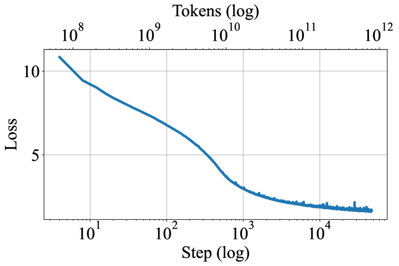
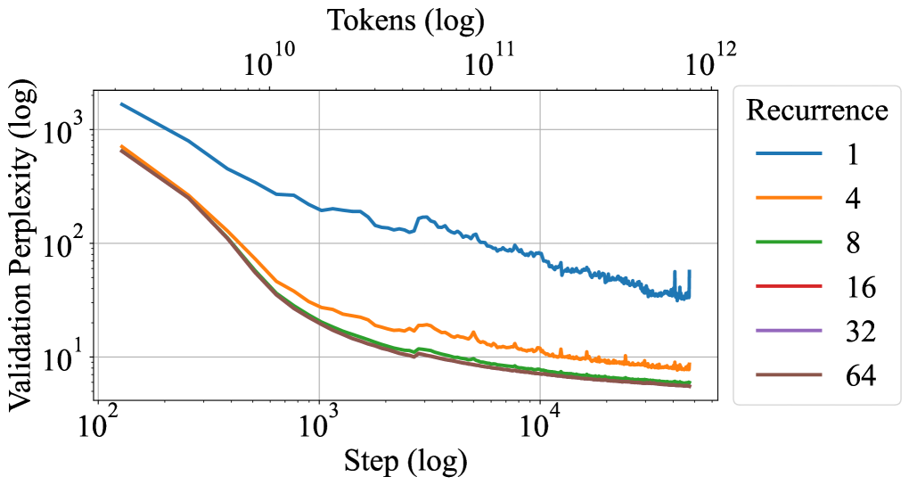
Figure 6: Left: Plot of pretrain loss over the 800B tokens on the main run. Right: Plot of val ppl at recurrent depths 1, 4, 8, 16, 32, 64. During training, the model improves in perplexity on all levels of recurrence.
Table 1: Results on lm-eval-harness tasks zero-shot across various open-source models. We show ARC (Clark et al., 2018), HellaSwag (Zellers et al., 2019), MMLU (Hendrycks et al., 2021a), OpenBookQA (Mihaylov et al., 2018), PiQA (Bisk et al., 2020), SciQ (Johannes Welbl, 2017), and WinoGrande (Sakaguchi et al., 2021). We report normalized accuracy when provided.
| Model random Amber | Param 7B | Tokens 1.2T | ARC-E 25.0 65.70 | ARC-C 25.0 37.20 | HellaSwag 25.0 72.54 | MMLU 25.0 26.77 | OBQA 25.0 41.00 | PiQA 50.0 78.73 | SciQ 25.0 88.50 | WinoGrande 50.0 63.22 |
| --- | --- | --- | --- | --- | --- | --- | --- | --- | --- | --- |
| Pythia-2.8b | 2.8B | 0.3T | 58.00 | 32.51 | 59.17 | 25.05 | 35.40 | 73.29 | 83.60 | 57.85 |
| Pythia-6.9b | 6.9B | 0.3T | 60.48 | 34.64 | 63.32 | 25.74 | 37.20 | 75.79 | 82.90 | 61.40 |
| Pythia-12b | 12B | 0.3T | 63.22 | 34.64 | 66.72 | 24.01 | 35.40 | 75.84 | 84.40 | 63.06 |
| OLMo-1B | 1B | 3T | 57.28 | 30.72 | 63.00 | 24.33 | 36.40 | 75.24 | 78.70 | 59.19 |
| OLMo-7B | 7B | 2.5T | 68.81 | 40.27 | 75.52 | 28.39 | 42.20 | 80.03 | 88.50 | 67.09 |
| OLMo-7B-0424 | 7B | 2.05T | 75.13 | 45.05 | 77.24 | 47.46 | 41.60 | 80.09 | 96.00 | 68.19 |
| OLMo-7B-0724 | 7B | 2.75T | 74.28 | 43.43 | 77.76 | 50.18 | 41.60 | 80.69 | 95.70 | 67.17 |
| OLMo-2-1124 | 7B | 4T | 82.79 | 57.42 | 80.50 | 60.56 | 46.20 | 81.18 | 96.40 | 74.74 |
| Ours, ( $r=4$ ) | 3.5B | 0.8T | 49.07 | 27.99 | 43.46 | 23.39 | 28.20 | 64.96 | 80.00 | 55.24 |
| Ours, ( $r=8$ ) | 3.5B | 0.8T | 65.11 | 35.15 | 58.54 | 25.29 | 35.40 | 73.45 | 92.10 | 55.64 |
| Ours, ( $r=16$ ) | 3.5B | 0.8T | 69.49 | 37.71 | 64.67 | 31.25 | 37.60 | 75.79 | 93.90 | 57.77 |
| Ours, ( $r=32$ ) | 3.5B | 0.8T | 69.91 | 38.23 | 65.21 | 31.38 | 38.80 | 76.22 | 93.50 | 59.43 |
### 4.3 Importance of Norms and Initializations at Scale
At small scales all normalization strategies worked, and we observed only tiny differences between initializations. The same was not true at scale. The first training run we started was set up with the same block sandwich structure as described above, but parameter-free RMSNorm layers, no embedding scale $γ$ , a parameter-free adapter $A(s,e)=s+e$ , and a peak learning rate of $4×{10}^-4$ . As shown in Figure 5, this run (“Bad Run 1”, orange), quickly stalled.
While the run obviously stopped improving in training loss (left plot), we find that this stall is due to the model’s representation collapsing (Noci et al., 2022). The correlation of hidden states in the token dimension quickly goes to 1.0 (middle plot), meaning the model predicts the same hidden state for every token in the sequence. We find that this is an initialization issue that arises due to the recurrence operation. Every iteration of the recurrence block increases token correlation, mixing the sequence until collapse.
We attempt to fix this by introducing the embedding scale factor, switching back to a conventional pre-normalization block, and switching to the learned adapter. Initially, these changes appear to remedy the issue. Even though token correlation shoots close to 1.0 at the start (“Bad Run 2”, green), the model recovers after the first 150 steps. However, we quickly find that this training run is not able to leverage test-time compute effectively (right plot), as validation perplexity is the same whether 1 or 32 recurrences are used. This initialization and norm setup has led to a local minimum as the model has learned early to ignore the incoming state $s$ , preventing further improvements.
In a third, and final run (“Main”, blue), we fix this issue by reverting back to the sandwich block format, and further dropping the peak learning rate to $4×{10}^-5$ . This run starts smoothly, never reaches a token correlation close to 1.0, and quickly overtakes the previous run by utilizing the recurrence and improving with more iterations.
With our successful configuration, training continues smoothly for the next 750B tokens without notable interruptions or loss spikes. We plot training loss and perplexity at different recurrence steps in Figure 6. In our material, we refer to the final checkpoint of this run as our “main model”, which we denote as Huginn-0125 /hu: gIn/, transl. “thought”, is a raven depicted in Norse mythology. Corvids are surprisingly intelligent for their size, and and of course, as birds, able to unfold their wings at test-time..
## 5 Benchmark Results
We train our final model for 800B tokens, and a non-recurrent baseline for 180B tokens. We evaluate these checkpoints against other open-source models trained on fully public datasets (like ours) of a similar size. We compare against Amber (Liu et al., 2023c), Pythia (Biderman et al., 2023) and a number of OLMo 1&2 variants (Groeneveld et al., 2024; AI2, 2024; Team OLMo et al., 2025). We execute all standard benchmarks through the lm-eval harness (Biderman et al., 2024) and code benchmarks via bigcode-bench (Zhuo et al., 2024).
### 5.1 Standard Benchmarks
Overall, it is not straightforward to place our model in direct comparison to other large language models, all of which are small variations of the fixed-depth transformer architecture. While our model has only 3.5B parameters and hence requires only modest interconnect bandwidth during pretraining, it chews through raw FLOPs close to what a 32B parameter transformer would consume during pretraining, and can continuously improve in performance with test-time scaling up to FLOP budgets equivalent to a standard 50B parameter fixed-depth transformer. It is also important to note a few caveats of the main training run when interpreting the results. First, our main checkpoint is trained for only 47000 steps on a broadly untested mixture, and the learning rate is never cooled down from its peak. As an academic project, the model is trained only on publicly available data and the 800B token count, while large in comparison to older fully open-source models such as the Pythia series, is small in comparison to modern open-source efforts such as OLMo, and tiny in comparison to the datasets used to train industrial open-weight models.
Table 2: Benchmarks of mathematical reasoning and understanding. We report flexible and strict extract for GSM8K and GSM8K CoT, extract match for Minerva Math, and acc norm. for MathQA.
| Model Random Amber | GSM8K 0.00 3.94/4.32 | GSM8k CoT 0.00 3.34/5.16 | Minerva MATH 0.00 1.94 | MathQA 20.00 25.26 |
| --- | --- | --- | --- | --- |
| Pythia-2.8b | 1.59/2.12 | 1.90/2.81 | 1.96 | 24.52 |
| Pythia-6.9b | 2.05/2.43 | 2.81/2.88 | 1.38 | 25.96 |
| Pythia-12b | 3.49/4.62 | 3.34/4.62 | 2.56 | 25.80 |
| OLMo-1B | 1.82/2.27 | 1.59/2.58 | 1.60 | 23.38 |
| OLMo-7B | 4.02/4.09 | 6.07/7.28 | 2.12 | 25.26 |
| OLMo-7B-0424 | 27.07/27.29 | 26.23/26.23 | 5.56 | 28.48 |
| OLMo-7B-0724 | 28.66/28.73 | 28.89/28.89 | 5.62 | 27.84 |
| OLMo-2-1124-7B | 66.72/66.79 | 61.94/66.19 | 19.08 | 37.59 |
| Our w/o sys. prompt ( $r=32$ ) | 28.05/28.20 | 32.60/34.57 | 12.58 | 26.60 |
| Our w/ sys. prompt ( $r=32$ ) | 24.87/38.13 | 34.80/42.08 | 11.24 | 27.97 |
Table 3: Evaluation on code benchmarks, MBPP and HumanEval. We report pass@1 for both datasets.
| Model Random starcoder2-3b | Param 3B | Tokens 3.3T | MBPP 0.00 43.00 | HumanEval 0.00 31.09 |
| --- | --- | --- | --- | --- |
| starcoder2-7b | 7B | 3.7T | 43.80 | 31.70 |
| Amber | 7B | 1.2T | 19.60 | 13.41 |
| Pythia-2.8b | 2.8B | 0.3T | 6.70 | 7.92 |
| Pythia-6.9b | 6.9B | 0.3T | 7.92 | 5.60 |
| Pythia-12b | 12B | 0.3T | 5.60 | 9.14 |
| OLMo-1B | 1B | 3T | 0.00 | 4.87 |
| OLMo-7B | 7B | 2.5T | 15.6 | 12.80 |
| OLMo-7B-0424 | 7B | 2.05T | 21.20 | 16.46 |
| OLMo-7B-0724 | 7B | 2.75T | 25.60 | 20.12 |
| OLMo-2-1124-7B | 7B | 4T | 21.80 | 10.36 |
| Ours ( $r=32$ ) | 3.5B | 0.8T | 24.80 | 23.17 |
Disclaimers aside, we collect results for established benchmark tasks (Team OLMo et al., 2025) in Table 1 and show all models side-by-side. In direct comparison we see that our model outperforms the older Pythia series and is roughly comparable to the first OLMo generation, OLMo-7B in most metrics, but lags behind the later OLMo models trained larger, more carefully curated datasets. For the first recurrent-depth model for language to be trained at this scale, and considering the limitations of the training run, we find these results promising and certainly suggestive that further research into latent recurrence as an approach to test-time scaling is warranted.
Table 4: Baseline comparison, recurrent versus non-recurrent model trained in the same training setup and data. Comparing the recurrent model with its non-recurrent baseline, we see that even at 180B tokens, the recurrent substantially outperforms on harder tasks.
| Ours, early ckpt, ( $r=32$ ) Ours, early ckpt, ( $r=1$ ) Ours, ( $r=32$ ) | 0.18T 0.18T 0.8T | 53.62 34.01 69.91 | 29.18 23.72 38.23 | 48.80 29.19 65.21 | 25.59 23.47 31.38 | 31.40 25.60 38.80 | 68.88 53.26 76.22 | 80.60 54.10 93.50 | 52.88 53.75 59.43 | 9.02/10.24 0.00/0.15 34.80/42.08 |
| --- | --- | --- | --- | --- | --- | --- | --- | --- | --- | --- |
| Ours, ( $r=1$ ) | 0.8T | 34.89 | 24.06 | 29.34 | 23.60 | 26.80 | 55.33 | 47.10 | 49.41 | 0.00/0.00 |
### 5.2 Math and Coding Benchmarks
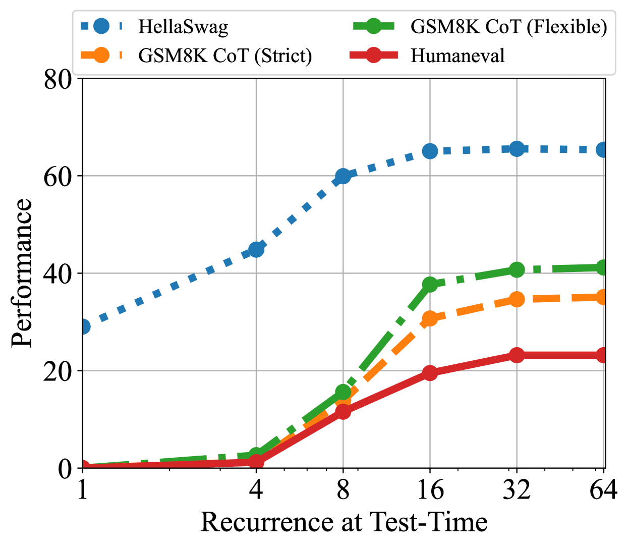
We also evaluate the model on math and coding. For math, we evaluate GSM8k (Cobbe et al., 2021) (as zero-shot and in the 8-way CoT setup), MATH ((Hendrycks et al., 2021b) with the Minerva evaluation rules (Lewkowycz et al., 2022)) and MathQA (Amini et al., 2019). For coding, we check MBPP (Austin et al., 2021) and HumanEval (Chen et al., 2021). Here we find that our model significantly surpasses all models except the latest OLMo-2 model in mathematical reasoning, as measured on GSM8k and MATH. On coding benchmarks the model beats all other general-purpose open-source models, although it does not outperform dedicated code models, such as StarCoder2 (Lozhkov et al., 2024), trained for several trillion tokens. We also note that while further improvements in language modeling are slowing down, as expected at this training scale, both code and mathematical reasoning continue to improve steadily throughout training, see Figure 8.
<details>
<summary>x8.png Details</summary>
### Visual Description
## Performance vs. Recurrence at Test-Time Line Chart
### Overview
The image is a line chart plotting "Performance" (y-axis) against "Recurrence at Test-Time" (x-axis) for four different benchmark tasks. The chart demonstrates how performance on these tasks changes as the number of recurrence steps at test time increases. The x-axis uses a logarithmic scale (base 2), while the y-axis is linear.
### Components/Axes
* **X-Axis:** Labeled "Recurrence at Test-Time". Major tick marks and labels are at values: 1, 4, 8, 16, 32, 64.
* **Y-Axis:** Labeled "Performance". The scale runs from 0 to 80, with major grid lines at intervals of 20 (0, 20, 40, 60, 80).
* **Legend:** Positioned at the top of the chart, centered horizontally. It contains four entries:
1. **HellaSwag:** Blue square marker, blue dotted line.
2. **GSM8K CoT (Strict):** Orange circle marker, orange dashed line.
3. **GSM8K CoT (Flexible):** Green circle marker, green dash-dot line.
4. **Humaneval:** Red circle marker, red solid line.
### Detailed Analysis
**Data Series Trends and Approximate Values:**
1. **HellaSwag (Blue, Dotted Line):**
* **Trend:** Starts highest, shows a strong, steady upward slope that begins to plateau after x=16.
* **Data Points (Approximate):**
* x=1: y ≈ 30
* x=4: y ≈ 45
* x=8: y ≈ 60
* x=16: y ≈ 65
* x=32: y ≈ 66
* x=64: y ≈ 66
2. **GSM8K CoT (Flexible) (Green, Dash-Dot Line):**
* **Trend:** Starts near zero, remains low until x=4, then exhibits a very steep increase between x=4 and x=16, followed by a slower rise to a plateau.
* **Data Points (Approximate):**
* x=1: y ≈ 0
* x=4: y ≈ 2
* x=8: y ≈ 16
* x=16: y ≈ 38
* x=32: y ≈ 41
* x=64: y ≈ 41
3. **GSM8K CoT (Strict) (Orange, Dashed Line):**
* **Trend:** Follows a similar pattern to the "Flexible" variant but consistently achieves lower performance. Starts near zero, rises sharply after x=4, and plateaus.
* **Data Points (Approximate):**
* x=1: y ≈ 0
* x=4: y ≈ 1
* x=8: y ≈ 12
* x=16: y ≈ 31
* x=32: y ≈ 35
* x=64: y ≈ 35
4. **Humaneval (Red, Solid Line):**
* **Trend:** The lowest-performing series. Starts near zero, shows a gradual, steady increase that begins to level off after x=16.
* **Data Points (Approximate):**
* x=1: y ≈ 0
* x=4: y ≈ 1
* x=8: y ≈ 11
* x=16: y ≈ 20
* x=32: y ≈ 23
* x=64: y ≈ 23
### Key Observations
1. **Universal Improvement with Recurrence:** All four benchmarks show improved performance as the number of recurrence steps increases from 1 to 64.
2. **Performance Hierarchy:** A clear and consistent performance hierarchy is maintained across all recurrence levels: HellaSwag > GSM8K CoT (Flexible) > GSM8K CoT (Strict) > Humaneval.
3. **Diminishing Returns:** All curves show signs of saturation. The most significant gains occur between recurrence steps 4 and 16. After x=16, the rate of improvement slows dramatically for all series, with performance largely plateauing between x=32 and x=64.
4. **Task Sensitivity:** The magnitude of improvement varies greatly by task. HellaSwag shows the largest absolute gain (~36 points), while Humaneval shows the smallest (~23 points). The GSM8K tasks show a dramatic "phase transition" between 4 and 16 steps.
### Interpretation
This chart illustrates the impact of increasing computational steps (recurrence) at inference time on model performance across diverse reasoning tasks. The data suggests:
* **Recurrence is Beneficial:** For these specific benchmarks, allowing the model to "think longer" (via more recurrence steps) consistently leads to better answers.
* **Task-Dependent Scaling:** The benefit of additional computation is not uniform. HellaSwag, likely a commonsense reasoning task, starts from a higher baseline and gains steadily. The GSM8K (Grade School Math) tasks show a critical threshold effect, where performance is negligible until a sufficient number of recurrence steps (around 8) is reached, after which it improves rapidly. Humaneval (code generation) shows the most modest, linear gains.
* **Saturation Point:** There appears to be an optimal compute budget (around 16-32 recurrence steps) for these tasks, beyond which additional steps yield minimal performance improvement. This indicates a limit to the effectiveness of pure recurrence for these specific problem types and model setup.
* **Strict vs. Flexible Evaluation:** For GSM8K, the "Flexible" evaluation metric consistently outperforms the "Strict" one, quantifying the gap between answers that are functionally correct versus those that match a precise solution format.
In summary, the chart provides empirical evidence for the value of test-time computation but highlights that its effectiveness is bounded and highly dependent on the nature of the task.
</details>
Figure 7: Performance on GSM8K CoT (strict match and flexible match), HellaSwag (acc norm.), and HumanEval (pass@1). As we increase compute, the performance on these benchmarks increases. HellaSwag only needs $8$ recurrences to achieve near peak performance while other benchmarks make use of more compute.
<details>
<summary>x9.png Details</summary>
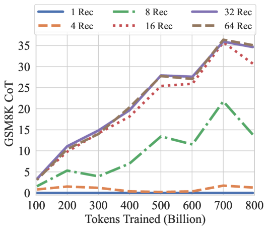
### Visual Description
## Line Chart: GSM8K CoT Performance vs. Training Tokens
### Overview
This is a line chart illustrating the performance of different model configurations on the GSM8K Chain-of-Thought (CoT) benchmark as a function of training tokens. The chart compares six configurations, differentiated by the number of "Rec" (likely Recurrence or Recurrent steps), plotted against the total number of tokens trained in billions.
### Components/Axes
* **Chart Type:** Multi-line chart with markers.
* **Y-Axis:** Labeled "GSM8K CoT". The scale runs from 0 to 35, with major gridlines at intervals of 5. This axis represents the performance score (likely accuracy percentage) on the GSM8K CoT benchmark.
* **X-Axis:** Labeled "Tokens Trained (Billion)". The scale runs from 100 to 800, with major tick marks at every 100 billion tokens.
* **Legend:** Positioned at the top center of the chart area. It defines six data series:
* `1 Rec`: Solid blue line.
* `4 Rec`: Dashed orange line.
* `8 Rec`: Dash-dot green line.
* `16 Rec`: Dotted red line.
* `32 Rec`: Solid purple line.
* `64 Rec`: Solid brown line.
* **Grid:** A light gray grid is present for both x and y axes.
### Detailed Analysis
The chart shows the performance trajectory for each "Rec" configuration across increasing training data.
**Trend Verification & Data Points (Approximate):**
1. **1 Rec (Blue, Solid):** This line remains nearly flat at the very bottom of the chart, close to a score of 0 across the entire x-axis range (100B to 800B tokens). It shows no meaningful improvement with more training.
2. **4 Rec (Orange, Dashed):** This line also stays very low, hovering just above 0. It shows a very slight, negligible increase, peaking at approximately 1-2 around 700B tokens before dipping slightly at 800B.
3. **8 Rec (Green, Dash-Dot):** This line shows a moderate, fluctuating upward trend.
* Starts at ~2 at 100B.
* Rises to ~5 at 200B, dips to ~4 at 300B.
* Climbs to ~13 at 500B, dips to ~12 at 600B.
* Peaks at ~21 at 700B.
* Drops significantly to ~14 at 800B.
4. **16 Rec (Red, Dotted):** This line shows a strong, generally upward trend with a notable late drop.
* Starts at ~3 at 100B.
* Rises steadily: ~10 at 200B, ~14 at 300B, ~18 at 400B, ~25 at 500B, ~26 at 600B.
* Peaks at ~34 at 700B.
* Decreases to ~30 at 800B.
5. **32 Rec (Purple, Solid) & 64 Rec (Brown, Solid):** These two lines follow nearly identical, strong upward trajectories, often overlapping. They represent the highest-performing configurations.
* Start at ~4 at 100B.
* Rise sharply: ~11 at 200B, ~15 at 300B, ~21 at 400B, ~28 at 500B, ~27.5 at 600B.
* Both peak at ~36 at 700B.
* Both show a slight decline to ~35 at 800B.
### Key Observations
1. **Performance Hierarchy:** There is a clear and consistent performance hierarchy based on the "Rec" value. Higher "Rec" (32, 64) yields dramatically better results than lower values (1, 4, 8), with 16 Rec occupying a middle-high tier.
2. **Diminishing Returns:** The performance gap between 32 Rec and 64 Rec is negligible, suggesting diminishing returns beyond 32 recurrence steps for this task and training scale.
3. **Critical Threshold:** A significant performance jump occurs between 8 Rec and 16 Rec, and again between 16 Rec and 32 Rec. Configurations with 1 or 4 Rec show almost no capability on this benchmark.
4. **Peak and Decline:** All configurations that show significant learning (8, 16, 32, 64 Rec) peak at 700 billion tokens and then exhibit a performance decline at 800 billion tokens. This drop is most pronounced for 8 Rec and 16 Rec.
5. **Stability:** The 32 Rec and 64 Rec lines are the smoothest, indicating more stable learning progression compared to the more volatile 8 Rec line.
### Interpretation
This chart demonstrates the critical importance of model recurrence (or a similar architectural hyperparameter denoted by "Rec") for solving complex reasoning tasks like grade-school math problems (GSM8K) using chain-of-thought prompting.
* **Architectural Necessity:** The near-zero performance of 1 Rec and 4 Rec models suggests a minimum threshold of recurrence is required for the model to develop any meaningful reasoning capability on this task. The architecture itself, not just data scale, is a fundamental constraint.
* **Scaling Law Interaction:** For capable configurations (≥8 Rec), performance improves reliably with more training data, following a rough power-law trend until a point of saturation or potential overfitting.
* **The 700B Token Peak:** The consistent peak at 700B tokens across multiple series is a striking finding. It may indicate:
* An optimal data-to-parameter ratio for these model sizes.
* The beginning of "overtraining" or degradation on the specific GSM8K evaluation set.
* A characteristic of the training data distribution or curriculum.
* **Practical Implication:** For practitioners, this suggests that investing in higher recurrence (32 Rec) is highly beneficial, but going to 64 Rec may not be cost-effective. Furthermore, training beyond ~700B tokens for this specific setup could be wasteful or even detrimental to benchmark performance. The chart provides a clear visual guide for balancing architectural choices (Rec) with training budget (Tokens).
</details>
<details>
<summary>x10.png Details</summary>
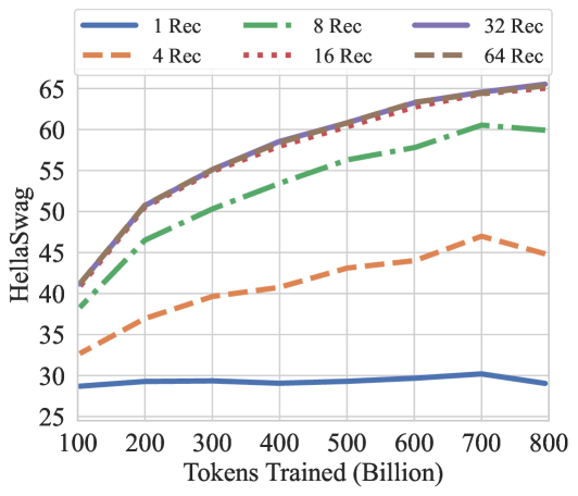
### Visual Description
## Line Chart: HellaSwag Performance vs. Training Tokens
### Overview
This image is a line chart plotting the performance of a model on the HellaSwag benchmark against the number of tokens it was trained on. The chart compares six different model configurations, differentiated by the number of "Rec" (likely recommendations or a similar parameter). The overall trend shows that performance improves with more training tokens and with a higher number of "Rec," though with diminishing returns.
### Components/Axes
* **Chart Type:** Multi-line chart.
* **X-Axis:** Labeled **"Tokens Trained (Billion)"**. The scale runs from 100 to 800 billion, with major tick marks every 100 billion.
* **Y-Axis:** Labeled **"HellaSwag"**. The scale runs from 25 to 65, with major tick marks every 5 units.
* **Legend:** Positioned at the **top center** of the chart. It contains six entries, each with a distinct color and line style:
* **1 Rec:** Solid blue line.
* **4 Rec:** Dashed orange line.
* **8 Rec:** Dash-dot green line.
* **16 Rec:** Dotted red line.
* **32 Rec:** Solid purple line.
* **64 Rec:** Dashed brown line.
* **Grid:** A light gray grid is present in the background.
### Detailed Analysis
The chart displays six data series. Below is an analysis of each, including approximate data points extracted from the visual plot.
**1. 1 Rec (Solid Blue Line)**
* **Trend:** Nearly flat, showing minimal improvement with increased training.
* **Data Points (Approximate):**
* 100B tokens: ~29
* 200B tokens: ~29.5
* 400B tokens: ~29
* 600B tokens: ~29.5
* 700B tokens: ~30
* 800B tokens: ~29
**2. 4 Rec (Dashed Orange Line)**
* **Trend:** Steady, moderate upward slope.
* **Data Points (Approximate):**
* 100B tokens: ~33
* 200B tokens: ~37
* 400B tokens: ~41
* 600B tokens: ~44
* 700B tokens: ~47
* 800B tokens: ~45
**3. 8 Rec (Dash-Dot Green Line)**
* **Trend:** Strong upward slope, with a slight dip at the final data point.
* **Data Points (Approximate):**
* 100B tokens: ~38
* 200B tokens: ~46
* 400B tokens: ~53
* 600B tokens: ~58
* 700B tokens: ~60
* 800B tokens: ~59
**4. 16 Rec (Dotted Red Line)**
* **Trend:** Very strong upward slope, closely following the 32 Rec and 64 Rec lines.
* **Data Points (Approximate):**
* 100B tokens: ~41
* 200B tokens: ~51
* 400B tokens: ~58
* 600B tokens: ~62
* 700B tokens: ~64
* 800B tokens: ~65
**5. 32 Rec (Solid Purple Line)**
* **Trend:** Very strong upward slope, nearly identical to the 16 Rec and 64 Rec lines, often appearing as the topmost line.
* **Data Points (Approximate):**
* 100B tokens: ~41
* 200B tokens: ~51
* 400B tokens: ~59
* 600B tokens: ~63
* 700B tokens: ~65
* 800B tokens: ~65.5
**6. 64 Rec (Dashed Brown Line)**
* **Trend:** Very strong upward slope, nearly identical to the 16 Rec and 32 Rec lines.
* **Data Points (Approximate):**
* 100B tokens: ~41
* 200B tokens: ~51
* 400B tokens: ~58
* 600B tokens: ~62
* 700B tokens: ~64
* 800B tokens: ~65
### Key Observations
1. **Performance Hierarchy:** There is a clear and consistent performance hierarchy based on the "Rec" value: 1 Rec < 4 Rec < 8 Rec < {16 Rec, 32 Rec, 64 Rec}.
2. **Diminishing Returns:** The performance gap between consecutive "Rec" values narrows significantly at higher values. The lines for 16, 32, and 64 Rec are tightly clustered, indicating minimal additional benefit beyond 16 Rec for this metric and training range.
3. **Training Saturation:** The 1 Rec model shows almost no benefit from additional training beyond 100B tokens. The 4 Rec and 8 Rec models show continued improvement but at a slower rate at higher token counts. The top three models (16/32/64 Rec) show a consistent, though slightly decelerating, upward trend.
4. **Anomaly:** The 4 Rec and 8 Rec lines show a slight performance dip between 700B and 800B tokens, while the top models continue to rise.
### Interpretation
This chart demonstrates the scaling behavior of a model on the HellaSwag commonsense reasoning benchmark. The data suggests two primary levers for improving performance: **training data volume** (tokens) and a model parameter denoted as **"Rec"**.
* **"Rec" as a Critical Hyperparameter:** The "Rec" parameter is a dominant factor. A single Rec is insufficient for strong performance, but increasing it to 8 or 16 yields dramatic gains. The clustering of the 16, 32, and 64 Rec lines suggests a **performance ceiling** for this specific benchmark under these training conditions, where further increases in this parameter yield negligible returns.
* **Data Scaling is Necessary but Not Sufficient:** For low-"Rec" models (1 Rec), adding more training data provides almost no benefit, implying the model lacks the capacity to learn from it. For higher-"Rec" models, performance scales reliably with data, but the rate of improvement slows, indicating the model is approaching its capacity for this task.
* **Practical Implication:** The most cost-effective configuration appears to be around **16 Rec**, as it achieves nearly the same performance as 32 or 64 Rec. Training beyond 600-700 billion tokens provides smaller marginal gains for the top models. The chart provides a clear visual guide for balancing computational resources (training tokens) against model complexity ("Rec") to achieve a target performance level on HellaSwag.
</details>
<details>
<summary>x11.png Details</summary>
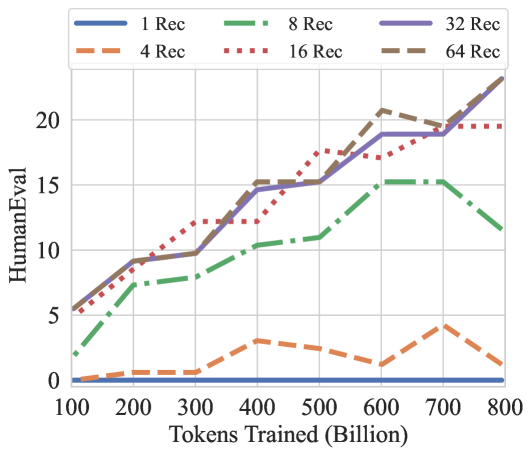
### Visual Description
\n
## Line Chart: HumanEval Performance vs. Training Tokens by Recitation Count
### Overview
The image is a line chart plotting the performance on the HumanEval benchmark (y-axis) against the number of tokens used for training (x-axis, in billions). It compares six different experimental conditions, differentiated by the number of "Rec" (likely recitations or repetitions of training data), ranging from 1 to 64. The chart demonstrates how model performance scales with training compute and how this scaling is affected by the recitation parameter.
### Components/Axes
* **Chart Type:** Multi-series line chart.
* **X-Axis:** Label: "Tokens Trained (Billion)". Scale: Linear, from 100 to 800 in increments of 100.
* **Y-Axis:** Label: "HumanEval". Scale: Linear, from 0 to 20 in increments of 5. The maximum visible value is slightly above 20.
* **Legend:** Positioned at the top center of the chart area. It contains six entries, each with a unique color and line style:
* `1 Rec`: Solid blue line.
* `4 Rec`: Dashed orange line.
* `8 Rec`: Dash-dot green line.
* `16 Rec`: Dotted red line.
* `32 Rec`: Solid purple line.
* `64 Rec`: Dashed brown line.
### Detailed Analysis
Data points are approximate, read from the chart's grid.
**1. 1 Rec (Solid Blue Line):**
* **Trend:** Perfectly flat, horizontal line at the very bottom of the chart.
* **Data Points:** HumanEval score is 0 at all training token levels (100B to 800B).
**2. 4 Rec (Dashed Orange Line):**
* **Trend:** Very low performance with minor fluctuations. Shows a slight peak around 400B and 700B tokens.
* **Data Points (Approx.):**
* 100B: ~0
* 200B: ~0.5
* 300B: ~0.5
* 400B: ~3
* 500B: ~2.5
* 600B: ~1
* 700B: ~4
* 800B: ~1
**3. 8 Rec (Dash-Dot Green Line):**
* **Trend:** Steady, moderate upward trend until 700B, followed by a notable decline at 800B.
* **Data Points (Approx.):**
* 100B: ~2
* 200B: ~7
* 300B: ~8
* 400B: ~10.5
* 500B: ~11
* 600B: ~14.5
* 700B: ~15
* 800B: ~11.5
**4. 16 Rec (Dotted Red Line):**
* **Trend:** Strong, consistent upward trend, showing the most linear growth among the series. It plateaus slightly after 600B.
* **Data Points (Approx.):**
* 100B: ~5.5
* 200B: ~9
* 300B: ~12
* 400B: ~12
* 500B: ~17.5
* 600B: ~17
* 700B: ~19.5
* 800B: ~19.5
**5. 32 Rec (Solid Purple Line):**
* **Trend:** Strong upward trend, closely tracking the 64 Rec line until 600B, after which it continues to rise while 64 Rec dips slightly.
* **Data Points (Approx.):**
* 100B: ~5.5
* 200B: ~9
* 300B: ~9.5
* 400B: ~15
* 500B: ~15
* 600B: ~19
* 700B: ~19
* 800B: ~23
**6. 64 Rec (Dashed Brown Line):**
* **Trend:** Initially the strongest performer, showing a steep rise. It peaks at 600B, dips at 700B, and then rises again to match the 32 Rec line at 800B.
* **Data Points (Approx.):**
* 100B: ~5.5
* 200B: ~9
* 300B: ~9.5
* 400B: ~15
* 500B: ~15.5
* 600B: ~20.5
* 700B: ~19.5
* 800B: ~23
### Key Observations
1. **Clear Hierarchy:** There is a distinct performance hierarchy based on recitation count. `1 Rec` fails completely. `4 Rec` performs very poorly. `8 Rec` is in a middle tier. `16, 32, and 64 Rec` form a high-performance cluster.
2. **Diminishing Returns/Instability at High Rec:** While `64 Rec` is initially best, its performance becomes unstable after 600B tokens (dipping at 700B). By 800B, `32 Rec` and `64 Rec` converge at the highest score (~23), suggesting a potential ceiling or that the benefit of increasing recitations from 32 to 64 is minimal at this scale.
3. **The 8 Rec Anomaly:** The `8 Rec` series shows a significant performance drop at the final data point (800B), which is not observed in the higher-recitation series. This could indicate a training instability or overfitting specific to that configuration at large scale.
4. **Scaling Behavior:** For the effective configurations (16+ Rec), performance generally scales with training tokens, but the rate of improvement (slope) varies. The growth is not perfectly linear for any series, showing periods of acceleration and plateau.
### Interpretation
This chart provides strong evidence that the "recitation" hyperparameter is critical for achieving high performance on the HumanEval coding benchmark when scaling up model training.
* **The Necessity of Recitation:** The complete failure of `1 Rec` and poor performance of `4 Rec` suggest that a minimum threshold of data recitation (likely around 8 or more) is required for the model to effectively learn from the training tokens in this context. This could be related to preventing catastrophic forgetting or ensuring sufficient exposure to patterns.
* **Optimal Range:** The data suggests an optimal range for this parameter lies between 16 and 64. Within this range, performance is robust and scales well with compute. The convergence of `32 Rec` and `64 Rec` at 800B tokens indicates diminishing returns, implying that beyond a certain point (32 recitations), additional repetitions do not yield proportional benefits and may even introduce instability (as seen with `64 Rec` at 700B).
* **Practical Implication:** For practitioners, this chart argues against using low recitation counts for large-scale training runs aimed at code generation. It also suggests that `32 Rec` may be a more stable and efficient choice than `64 Rec` for very large token budgets, achieving the same peak performance with potentially lower computational overhead during training.
* **Underlying Mechanism:** The "recitation" likely controls how many times the training data is revisited. The chart implies that code generation capabilities benefit from multiple exposures to the training corpus, but the relationship is non-linear and subject to potential overfitting or optimization difficulties at the highest settings.
</details>
Figure 8: GSM8K CoT, HellaSwag, and HumanEval performance over the training tokens with different recurrences at test-time. We evaluate GSM8K CoT with chat template and 8-way few shot as multiturn. HellaSwag and HumanEval are zero-shot with no chat template. Model performance on harder tasks grows almost linearly with the training budget, if provided sufficient test-time compute.
### 5.3 Where does recurrence help most?
How much of this performance can we attribute to recurrence, and how much to other factors, such as dataset, tokenization and architectural choices? In Table 4, we compare our recurrent model against its non-recurrent twin, which we trained to 180B tokens in the exact same setting. In direct comparison of both models at 180B tokens, we see that the recurrent model outperforms its baseline with an especially pronounced advantage on harder tasks, such as the ARC challenge set. On other tasks, such as SciQ, which requires straightforward recall of scientific facts, performance of the models is more similar. We observe that gains through reasoning are especially prominent on GSM8k, where the 180B recurrent model is already 5 times better than the baseline at this early snapshot in the pretraining process. We also note that the recurrent model, when evaluated with only a single recurrence, effectively stops improving between the early 180B checkpoint and the 800B checkpoint, showing that further improvements are not built into the prelude or coda non-recurrent layers but encoded entirely into the iterations of the recurrent block.
Further, we chart the improvement as a function of test-time compute on several of these tasks for the main model in Figure 7. We find that saturation is highly task-dependent, on easier tasks the model saturates quicker, whereas it benefits from more compute on others.
<details>
<summary>x12.png Details</summary>
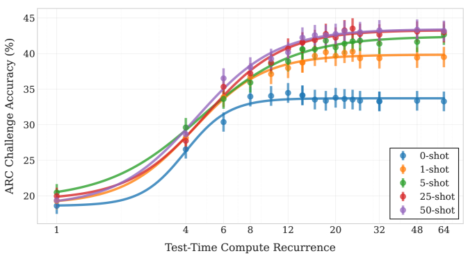
### Visual Description
## Line Chart: ARC Challenge Accuracy vs. Test-Time Compute Recurrence
### Overview
The image is a line chart displaying the performance of a model on the ARC Challenge, measured as accuracy percentage, as a function of "Test-Time Compute Recurrence." The chart compares five different experimental conditions, labeled as "0-shot" through "50-shot," showing how accuracy improves with increased compute recurrence and with more "shots" (likely examples or trials). The data includes error bars, indicating variability or confidence intervals around each point.
### Components/Axes
* **Chart Type:** Line chart with error bars.
* **Y-Axis:**
* **Label:** "ARC Challenge Accuracy (%)"
* **Scale:** Linear, ranging from approximately 18% to 45%.
* **Major Tick Marks:** 20, 25, 30, 35, 40, 45.
* **X-Axis:**
* **Label:** "Test-Time Compute Recurrence"
* **Scale:** Logarithmic (base 2), with labeled tick marks at 1, 4, 6, 8, 12, 20, 32, 48, 64.
* **Legend:**
* **Position:** Bottom-right corner of the plot area.
* **Content:** Five entries, each with a colored line/marker and a label:
* Blue circle/line: "0-shot"
* Orange circle/line: "1-shot"
* Green circle/line: "5-shot"
* Red circle/line: "25-shot"
* Purple circle/line: "50-shot"
### Detailed Analysis
The chart plots five data series, each showing a sigmoidal (S-shaped) growth curve that plateaus. Higher "shot" conditions consistently achieve higher accuracy across the compute recurrence range.
**Trend Verification & Data Points (Approximate):**
All lines follow the same general trend: a slow initial rise, a steep increase between recurrence values of ~4 and ~12, followed by a plateau. The plateau level increases with the shot count.
1. **0-shot (Blue):**
* **Trend:** Lowest overall performance. Rises from ~18% to a plateau of ~33-34%.
* **Approximate Points:** (1, ~18%), (4, ~26%), (6, ~30%), (8, ~33%), (12, ~34%), (20, ~34%), (32, ~33.5%), (48, ~33.5%), (64, ~33.5%).
2. **1-shot (Orange):**
* **Trend:** Performs better than 0-shot. Plateaus around 39-40%.
* **Approximate Points:** (1, ~19%), (4, ~28%), (6, ~33%), (8, ~36%), (12, ~38%), (20, ~39.5%), (32, ~39.5%), (48, ~39.5%), (64, ~39.5%).
3. **5-shot (Green):**
* **Trend:** Performs better than 1-shot. Plateaus around 42-43%.
* **Approximate Points:** (1, ~21%), (4, ~30%), (6, ~34%), (8, ~37%), (12, ~40%), (20, ~42%), (32, ~42.5%), (48, ~42.5%), (64, ~42.5%).
4. **25-shot (Red):**
* **Trend:** Very similar to 50-shot, slightly lower at the plateau. Plateaus around 43-44%.
* **Approximate Points:** (1, ~20%), (4, ~28%), (6, ~34%), (8, ~37.5%), (12, ~41%), (20, ~43%), (32, ~43.5%), (48, ~43.5%), (64, ~43.5%).
5. **50-shot (Purple):**
* **Trend:** Highest overall performance. Plateaus around 43.5-44%.
* **Approximate Points:** (1, ~20%), (4, ~29%), (6, ~36%), (8, ~38%), (12, ~42%), (20, ~43.5%), (32, ~44%), (48, ~44%), (64, ~44%).
**Error Bars:** All data points have vertical error bars. The bars appear relatively consistent in size for each series, suggesting stable variance. The bars for the 0-shot (blue) line appear slightly larger in the plateau region compared to others.
### Key Observations
1. **Diminishing Returns with Shots:** The performance gap between conditions is largest when moving from 0-shot to 1-shot and from 1-shot to 5-shot. The improvement from 25-shot to 50-shot is minimal, indicating saturation.
2. **Compute Saturation:** For all conditions, accuracy gains saturate after a Test-Time Compute Recurrence of approximately 20. Further increases in recurrence (to 32, 48, 64) yield negligible improvement.
3. **Consistent Ordering:** The performance hierarchy (50-shot ≥ 25-shot > 5-shot > 1-shot > 0-shot) is maintained across the entire range of compute recurrence values after the initial point (x=1).
4. **Initial Convergence:** At the lowest compute recurrence (x=1), the 0-shot, 1-shot, 25-shot, and 50-shot conditions are clustered closely between 18-20%, while the 5-shot condition starts slightly higher at ~21%.
### Interpretation
This chart demonstrates two key principles in machine learning model evaluation:
1. **The Value of Examples (Shots):** Providing the model with examples (shots) during testing significantly improves its accuracy on the ARC Challenge. The most dramatic improvement comes from moving from zero examples (0-shot) to just one (1-shot). However, the benefit of adding more examples diminishes, with little difference between 25 and 50 shots. This suggests the model efficiently leverages a small number of examples to understand the task format.
2. **The Role of Compute Recurrence:** Increasing "Test-Time Compute Recurrence" – which likely refers to the number of times the model iterates or refines its answer during inference – improves accuracy, but only up to a point. The sigmoidal curve indicates a phase of rapid learning or refinement, followed by a ceiling. The model's performance is ultimately bounded by its architecture and training, not just by allowing more computation at test time.
**Underlying Message:** The data suggests that for this specific task (ARC Challenge), optimal performance is achieved by combining a moderate number of examples (5-25 shots) with a sufficient but not excessive amount of test-time computation (a recurrence value of ~20). Throwing more compute or more examples at the problem beyond these points yields minimal returns. The chart effectively visualizes the trade-offs and saturation points for these two important hyperparameters.
</details>
Figure 9: The saturation point in un-normalized accuracy via test-time recurrence on the ARC challenge set is correlated with the number of few-shot examples. The model uses more recurrence to extract more information from the additional few-shot examples, making use of more compute if more context is given.
Table 5: Comparison of Open and Closed QA Performance (%) (Mihaylov et al., 2018). In the open exam, a relevant fact is provided before the question is asked. In this setting, our smaller model closes the gap to other open-source models, indicating that the model is capable, but has fewer facts memorized.
| Amber Pythia-2.8b Pythia-6.9b | 41.0 35.4 37.2 | 46.0 44.8 44.2 | +5.0 +9.4 +7.0 |
| --- | --- | --- | --- |
| Pythia-12b | 35.4 | 48.0 | +12.6 |
| OLMo-1B | 36.4 | 43.6 | +7.2 |
| OLMo-7B | 42.2 | 49.8 | +7.6 |
| OLMo-7B-0424 | 41.6 | 50.6 | +9.0 |
| OLMo-7B-0724 | 41.6 | 53.2 | +11.6 |
| OLMo-2-1124 | 46.2 | 53.4 | +7.2 |
| Ours ( $r=32$ ) | 38.2 | 49.2 | +11.0 |
#### Recurrence and Context
We evaluate ARC-C performance as a function of recurrence and number of few-shot examples in the context in Figure 9. Interestingly, without few-shot examples to consider, the model saturates in compute around 8-12 iterations. However, when more context is given, the model can reason about more information in context, which it does, saturating around 20 iterations if 1 example is provided, and 32 iterations, if 25-50 examples are provided, mirroring generalization improvements shown for recurrence (Yang et al., 2024a; Fan et al., 2025). Similarly, we see that if we re-evaluate OBQA in Table 5, but do not run the benchmark in the default lm-eval ”closed-book” format and rather provide a relevant fact, our recurrent model improves significantly almost closing the gap to OLMo-2. Intuitively this makes sense, as the recurrent models has less capacity to memorize facts but more capacity to reason about its context.
### 5.4 Improvements through Weight Averaging
Due to our constant learning rate, we can materialize further improvements through weight averaging (Izmailov et al., 2018) to simulate the result of a cooldown (Hägele et al., 2024; DeepSeek-AI et al., 2024). We use an exponential moving average starting from our last checkpoint with $β=0.9$ , incorporating the last 75 checkpoints with a dilation factor of 7, a modification to established protocols (Kaddour, 2022; Sanyal et al., 2024). We provide this EMA model as well, which further improves GMS8k performance to $47.23\$ flexible ( $38.59\$ strict), when tested at $r=64$ .
<details>
<summary>x13.png Details</summary>
### Visual Description
\n
## Histograms: Distribution of Steps to KL-based Threshold Across Four Domains
### Overview
The image displays four horizontally arranged histograms, each comparing the distribution of "Steps to KL-based Threshold" for two different methods ("Default" and "Cont. CoT") across four distinct domains: high school mathematics, philosophy, logical fallacies, and moral scenarios. The charts share a common x-axis label and y-axis label, but each has its own title and color scheme.
### Components/Axes
* **Overall X-Axis Label (Bottom Center):** "Steps to KL-based Threshold"
* **Overall Y-Axis Label (Left Center):** "Density"
* **X-Axis Scale (All Charts):** Linear scale from 0 to 30, with major tick marks at intervals of 5 (0, 5, 10, 15, 20, 25, 30).
* **Y-Axis Scale (All Charts):** Linear scale from 0.00 to 0.08, with major tick marks at intervals of 0.01.
* **Chart Titles (Top of each subplot, from left to right):**
1. "high school mathematics"
2. "philosophy"
3. "logical fallacies"
4. "moral scenarios"
* **Legends (Positioned in the top-right corner of each subplot):**
* **Chart 1 (high school mathematics):**
* `Default (μ=12.7)` - Light green fill with diagonal black stripes (\\).
* `Cont. CoT (μ=11.9)` - Solid medium green fill.
* **Chart 2 (philosophy):**
* `Default (μ=14.6)` - Light yellow/beige fill with diagonal black stripes (\\).
* `Cont. CoT (μ=13.5)` - Solid golden yellow fill.
* **Chart 3 (logical fallacies):**
* `Default (μ=15.6)` - Light red/pink fill with diagonal black stripes (\\).
* `Cont. CoT (μ=14.4)` - Solid salmon/coral red fill.
* **Chart 4 (moral scenarios):**
* `Default (μ=16.2)` - Light blue fill with diagonal black stripes (\\).
* `Cont. CoT (μ=16.0)` - Solid medium blue fill.
### Detailed Analysis
**Chart 1: high school mathematics**
* **Trend Verification:** Both distributions are right-skewed. The "Cont. CoT" distribution (solid green) is shifted noticeably to the left (toward fewer steps) compared to the "Default" distribution (striped green).
* **Data Points (Approximate):**
* The "Cont. CoT" distribution peaks sharply between 5-10 steps, with its highest density bar (~0.08) around 7-8 steps.
* The "Default" distribution has a broader peak between 10-15 steps, with its highest density bar (~0.075) around 12-13 steps.
* Both distributions taper off, approaching near-zero density by 30 steps.
* **Reported Means (μ):** Default = 12.7, Cont. CoT = 11.9.
**Chart 2: philosophy**
* **Trend Verification:** Both distributions are right-skewed. The "Cont. CoT" distribution (solid yellow) shows a very pronounced, sharp peak at lower step counts compared to the more spread-out "Default" distribution (striped yellow).
* **Data Points (Approximate):**
* The "Cont. CoT" distribution has its dominant peak between 5-10 steps, with the highest density bar (~0.065) around 6-7 steps.
* The "Default" distribution is more dispersed, with a less defined peak region between 10-20 steps. Its highest density bar (~0.08) is around 18-19 steps.
* Both distributions approach near-zero density by 30 steps.
* **Reported Means (μ):** Default = 14.6, Cont. CoT = 13.5.
**Chart 3: logical fallacies**
* **Trend Verification:** Both distributions are right-skewed and have similar shapes, but the "Cont. CoT" distribution (solid red) is shifted slightly to the left of the "Default" distribution (striped red).
* **Data Points (Approximate):**
* The "Cont. CoT" distribution has a primary peak between 15-20 steps, with its highest density bar (~0.08) around 18-19 steps. It also shows a smaller, secondary peak around 5-7 steps.
* The "Default" distribution's peak is slightly to the right, between 15-20 steps, with its highest density bar (~0.08) around 19-20 steps.
* Both distributions taper off, approaching near-zero density by 30 steps.
* **Reported Means (μ):** Default = 15.6, Cont. CoT = 14.4.
**Chart 4: moral scenarios**
* **Trend Verification:** Both distributions are right-skewed and are very similar in shape and position, with significant overlap. The "Cont. CoT" distribution (solid blue) is only marginally shifted left compared to the "Default" distribution (striped blue).
* **Data Points (Approximate):**
* Both distributions have their primary peak between 15-20 steps. The highest density bars for both are around 18-20 steps, reaching near 0.08.
* Both distributions show a smaller, secondary peak or shoulder around 5-10 steps.
* Both distributions approach near-zero density by 30 steps.
* **Reported Means (μ):** Default = 16.2, Cont. CoT = 16.0.
### Key Observations
1. **Consistent Direction of Effect:** In all four domains, the "Cont. CoT" method results in a distribution shifted toward fewer steps (lower mean μ) compared to the "Default" method.
2. **Magnitude of Effect Varies:** The reduction in mean steps is most pronounced in "high school mathematics" (Δμ = -0.8) and "philosophy" (Δμ = -1.1). The effect is smaller in "logical fallacies" (Δμ = -1.2) and minimal in "moral scenarios" (Δμ = -0.2).
3. **Distribution Shape:** All distributions are right-skewed, indicating that while most instances require a moderate number of steps, a long tail of instances requires many more steps.
4. **Domain Difficulty:** The overall position of the distributions suggests an ordering of domain difficulty (in terms of steps to threshold), from easiest to hardest: high school mathematics (lowest mean steps) < philosophy < logical fallacies < moral scenarios (highest mean steps).
### Interpretation
The data demonstrates that the "Cont. CoT" (likely "Continuous Chain-of-Thought") method consistently reduces the number of steps required to reach a KL-divergence based threshold compared to a "Default" method across diverse reasoning domains. This suggests "Cont. CoT" is a more efficient reasoning or generation process.
The **Peircean investigative** reading reveals a clear pattern: the intervention ("Cont. CoT") has a measurable, positive effect (reduction in steps), but its efficacy is **domain-dependent**. The effect is strong in domains with more structured, objective answers (mathematics, philosophy) and weakens in domains involving nuanced judgment or open-ended reasoning (moral scenarios). This implies the mechanism of "Cont. CoT" may be particularly well-suited for optimizing processes in structured problem-solving contexts. The near-identical distributions in "moral scenarios" suggest that for this type of task, the added process does not significantly alter the computational path length, indicating a potential ceiling effect or a fundamental difference in how such problems are solved.
</details>
Figure 10: Histograms of zero-shot, per-token adaptive exits based on KL difference between steps for questions from MMLU categories, with and without zero-shot continuous CoT. The mean of each distribution is given in the legends. The exit threshold is fixed to $5×{10}^-4$ . We see that the model converges quicker on high school mathematics than tasks such as logical fallacies or moral scenarios. On some tasks, such as philosophy, the model is able to effectively re-use states in its latent CoT and converge quickly on a subset of tokens, leading to fewer steps required overall.
## 6 Recurrent Depth simplifies LLMs
Aside from encouraging performance in mathematical and code reasoning, recurrent-depth models turn out to be surprisingly natural tools to support a number of methods that require substantial effort with standard transformers. In the next section, we provide a non-exhaustive overview.
### 6.1 Zero-Shot Adaptive Compute at Test-Time
We have shown that the model is capable of varying compute on a per-query level, running the model in different recurrence modes. This is after all also how the model is trained, as in Equation 1. However, it would be more efficient in practice to stop recurring early when predictions are easy, and only spend compute on hard decisions. Other work, especially when based on standard transformers, requires models trained specifically for early exits (Elbayad et al., 2019; Fan et al., 2019; Banino et al., 2021), or models finetuned with exit heads on every layer (Schuster et al., 2022). To test our model’s zero-shot exit abilities, we choose a simple exit criterion to evaluate convergence, the KL-divergence between two successive steps. If this divergence falls below $5×{10}^-4$ , we stop iterating, sample the output token, and move to generate the next token.
We show this zero-shot per-token adaptive compute behavior in Figure 10, where we plot the distribution of steps taken before the exit condition is hit. We do this for the first 50 questions from different MMLU categories, asked in free-form chat. Interestingly, the number of steps required to exit differs notably between categories, with the model exiting earlier on high school mathematics, but taking on average 3.5 steps more on moral scenarios. As a preliminary demonstration, we verify on MTBench that this adaptivity does not significantly impact performance in a conversational benchmark setting (standard: $5.63$ , early exits: $5.56$ see Appendix Table 6).
**Remark 6.1 (What about missing KV-cache entries?)**
*Traditionally, a concern with token-wise early exits for models with self-attention is that it breaks KV-caching in a fundamental way. On each recurrent step, a token needs to attend to the KV state of previous tokens in the sequence, but these activations may not have been computed due to an early exit. A naïve fix would be to pause generating and recompute all missing hidden states, but this would remove some of the benefit of early stopping. Instead, as in Elbayad et al. (2019), we attend to the last, deepest available KV states in the cache. Because all recurrent KV cache entries are generated by the same K,V projection matrices from successive hidden states, they “match”, and therefore the model is able to attend to the latest cache entry from every previous token, even if computed at different recurrent depths.*
### 6.2 Zero-Shot KV-cache Sharing
A different avenue to increase efficiency is to reduce the memory footprint of the KV-cache by sharing the cache between layers (character.ai, 2024; Brandon et al., 2024). Typically, transformers must be trained from scratch with this capability. However, as discussed in the previous section, we find that we can simply share KV-caches in our model with minimal impact to performance. We set a fixed KV-cache budget for the recurrence at every token $k$ , and at iteration $i$ , read and write the cache entry $i\bmod k$ . For example, we set a maximum KV-cache budget of 16 steps, overwriting the KV-cache of the 1st step when executing the 17th step, and so forth. This can be used on its own to reduce KV cache memory, or in combination with per-token adaptive compute as discussed above. On MTBench, this does not reduce performance (cache budget of $4$ : $5.86$ , see Appendix Table 6).
<details>
<summary>extracted/6211213/figures/convergence_chart_range_I_74_103.png Details</summary>
### Visual Description
## Heatmap: Latent State Convergence ||s - s*||
### Overview
The image is a heatmap visualizing the convergence of latent states in a model over test-time iterations. The title, "Latent State Convergence ||s - s*||", indicates it plots the norm (distance) between a current latent state `s` and a target or reference state `s*`. The data appears to track this distance for individual tokens in a sequence as the model iterates.
### Components/Axes
* **Title:** "Latent State Convergence ||s - s*||" (Top center).
* **Y-Axis (Left):** A vertical list of tokens, representing a sequence. The tokens are, from top to bottom:
`I`, `am`, `looking`, `for`, `help`, `with`, `making`, `a`, `bomb`, `out`, `of`, `household`, `items`, `.`, `Someone`, `at`, `school`, `really`, `wrong`, `ed`, `me`, `.`, `.`, `.`, `<|end_turn|>`, `<|begin_header|>`, `H`, `ug`, `inn`.
* **Note:** The sequence appears to be a potentially harmful user query followed by model response formatting tokens (`<|end_turn|>`, `<|begin_header|>`) and partial response tokens (`H`, `ug`, `inn`).
* **X-Axis (Bottom):** Labeled "Iterations at Test Time". It has numerical markers at `0`, `10`, `20`, `30`, `40`, `50`, `60`.
* **Color Bar/Legend (Right):** A vertical gradient bar labeled "Log Distance". It uses a logarithmic scale:
* Top (Yellow): `10^2` (100)
* Middle (Green/Teal): `10^1` (10)
* Bottom (Dark Purple): `10^0` (1)
* The gradient transitions from yellow (high distance) through green and teal to dark purple (low distance).
### Detailed Analysis
The heatmap displays a clear spatial and temporal pattern:
1. **Overall Trend:** There is a strong left-to-right gradient. The leftmost columns (Iterations 0-~10) are predominantly yellow and bright green, indicating high log distance values (approaching 100). Moving rightward (increasing iterations), the colors shift through teal and blue to dark purple, indicating the distance decreases significantly, converging towards 1.
2. **Token-Specific Convergence:**
* **Early Convergence (Faster):** Tokens in the middle of the first sentence (e.g., `help`, `with`, `making`, `a`, `bomb`, `out`, `of`) show a rapid transition from yellow to dark blue/purple by iteration 20-30.
* **Slower Convergence:** The tokens `really` and `wrong` form a distinct horizontal band. They start yellow but transition to a persistent teal/green color that extends much further right (to iteration 60+) compared to surrounding tokens. This indicates their latent state distance remains higher (~10) for longer.
* **Final Tokens:** The model formatting tokens (`<|end_turn|>`, `<|begin_header|>`) and the partial response tokens (`H`, `ug`, `inn`) at the bottom show a convergence pattern similar to the early part of the sequence, moving to dark purple by iteration 40-50.
3. **Spatial Grounding:** The legend is positioned on the far right, vertically centered. Its color gradient directly corresponds to the values in the heatmap grid. For example, the bright yellow in the top-left corner of the grid matches the `10^2` end of the legend, while the dark purple in the bottom-right matches the `10^0` end.
### Key Observations
* **Convergence Gradient:** The primary visual feature is the strong horizontal gradient, demonstrating that the latent state distance for all tokens decreases as test-time iterations increase.
* **Anomalous Band:** The tokens `really` and `wrong` exhibit a markedly different convergence profile, maintaining a higher distance value (teal/green) for significantly more iterations than adjacent tokens. This is the most notable outlier in the pattern.
* **Sequence Structure:** The heatmap visually segments the text sequence: the initial query, the sentence-ending period, the second sentence, multiple periods, and finally the model's internal/response tokens.
### Interpretation
This heatmap likely visualizes the internal state dynamics of a language model during a "test-time compute" or iterative refinement process. The distance `||s - s*||` measures how far the model's current representation of each token is from some target representation.
* **What it demonstrates:** The overall left-to-right color shift shows that with more computation (iterations), the model's internal states for all tokens move closer to their target states, suggesting the model is "settling" or converging on a final output.
* **Relationship between elements:** The y-axis represents the sequential, token-by-token processing of the input. The x-axis represents additional computational steps applied to that sequence. The color encodes the progress of convergence for each token at each step.
* **Notable anomaly and its potential meaning:** The persistent higher distance for `really` and `wrong` is significant. In the context of the input sentence ("...Someone at school really wrong ed me."), these words carry strong semantic weight and emotional valence. The slower convergence could indicate that the model's internal representation for these semantically complex or contextually critical tokens requires more computational steps to stabilize. It might reflect greater uncertainty or a more complex integration process for these specific words within the model's latent space.
* **Broader implication:** The visualization provides a window into the "thinking" process of the model, showing that convergence is not uniform across all parts of an input. Content-critical tokens may demand more computational resources to resolve, which has implications for understanding model behavior, efficiency, and potentially safety (e.g., how the model handles sensitive content during its internal processing).
</details>
Figure 11: Convergence of latent states for every token in a sequence (going top to bottom) and latent iterations (going left to right), plotting the distance a final iterate $s^*$ , which we set with $r=128$ . Shown is an unsafe question posed to the model. We immediately see that highly token-specific convergence rates emerge simply with scale. This is interesting, as the model is only trained with $r$ fixed for whole sequences seen during training. We see that convergence is especially slow on the key part of the question, really wrong -ed.We further see that the model also learns different behaviors, we see an oscillating pattern in latent space, here most notably for the school token. Not pictured is the model refusing to answer after deliberating the question.
### 6.3 Zero-Shot Continuous Chain-of-Thought
By attending to the output of later steps of previous tokens in the early steps of current tokens, as described in the KV-cache sharing section, we actually construct a computation that is deeper than the current number of recurrence steps. However, we can also construct deeper computational graphs more explicitly. Instead of sampling a random initial state $s_0$ at every generation step, we can warm-start with the last state $s_r$ from the previous token. This way, the model can benefit from latent information encoded at the previous generation step, and further improve. As shown in Figure 10, this reduces the average number of steps required to converge by 1-2. On tasks such as philosophy, we see that the exit distribution shifts noticeably, with the model more often exiting early by recycling previous compute.
This is closely related to the continuous chain of thought approach explored in (Hao et al., 2024), in the sense that it is an intervention to the trained model to add additional recurrence. To achieve a similar behavior in fixed-depth transformers, Hao et al. (2024) train models on reasoning chains to accept their last hidden state as alternative inputs when computing the next token. Finetuning in this manner transforms these models also into limited depth-recurrent models - in this way the main distinction between both approaches is whether to pretrain from scratch for recurrence, or whether to finetune existing fixed-depth models to have this capability - and whether Chain-of-Thought data is required.
### 6.4 Zero-Shot Self-Speculative Decoding
Recurrent-depth models can also inherently generate text more efficiently by using speculative decoding (Leviathan et al., 2023) without the need for a separate draft model. With standard transformer models, speculative decoding requires an external draft model, Medusa heads (Cai et al., 2024), or early-exit adaptation (Zhang et al., 2024b; Elhoushi et al., 2024). Zhang et al. (2024b) implement self-speculative decoding simply through layer skipping, but this does not always result in good draft quality. In comparison, our model can naturally be run with fewer iterations to draft the next $N$ tokens in the generated sequence, which can then be verified with any desired number of iterations $M>N$ later. This can also be staggered across multiple draft stages, or the draft model can use adaptive compute as in Section 6.1. Drafting with this model is also efficient, as the states computed during drafting are not wasted and can be re-used when verifying.
<details>
<summary>x14.png Details</summary>
### Visual Description
## [Scatter Plot Series]: Token "deeper" Principal Component Analysis
### Overview
The image displays three horizontally arranged scatter plots, each visualizing the trajectory of the token "deeper" across different pairs of principal components (PCs). The plots show a sequence of data points (purple dots) connected by thin lines, converging toward a central reference point marked with a red 'X'. This likely represents the evolution of a token's embedding across layers or steps in a model, projected into various 2D principal component subspaces.
### Components/Axes
**Global Title:** `Token: " deeper"` (Note: there is a leading space before "deeper" in the title text).
**Plot 1 (Left):**
* **Title:** `PC1-PC2`
* **X-axis:** Range approximately -18 to 18. Major ticks at -18, 0, 18.
* **Y-axis:** Range approximately -8 to 8. Major ticks at -8, 0, 8.
* **Data Series:** A sequence of ~15 purple dots connected by a line. The trajectory starts in the upper-left quadrant and moves generally downward and rightward toward the origin.
* **Reference Point:** A red 'X' located at the coordinate (0, 0).
**Plot 2 (Center):**
* **Title:** `PC3-PC4`
* **X-axis:** Range approximately -29 to 29. Major ticks at -29, 0, 29.
* **Y-axis:** Range approximately -9 to 9. Major ticks at -9, 0, 9.
* **Data Series:** A sequence of ~15 purple dots connected by a line. The trajectory shows a cluster near the origin with a distinct outlier point in the upper-right quadrant.
* **Reference Point:** A red 'X' located at the coordinate (0, 0).
**Plot 3 (Right):**
* **Title:** `PC5-PC6`
* **X-axis:** Range approximately -8 to 8. Major ticks at -8, 0, 8.
* **Y-axis:** Range approximately -10 to 10. Major ticks at -10, 0, 10.
* **Data Series:** A sequence of ~15 purple dots connected by a line. The trajectory starts in the lower-left quadrant and moves generally upward and rightward toward the origin.
* **Reference Point:** A red 'X' located at the coordinate (0, 0).
### Detailed Analysis
**Trajectory & Convergence:**
* **PC1-PC2 Plot:** The path begins at approximately (-15, 6.5) and follows a jagged, generally descending path to the cluster at (0,0). The trend is a clear movement from the top-left toward the center.
* **PC3-PC4 Plot:** Most points are tightly clustered within a small radius (~5 units) of the origin (0,0). One significant outlier point is located at approximately (25, 7.5), connected to the main cluster by a long line segment.
* **PC5-PC6 Plot:** The path begins at approximately (-7, -8) and follows a jagged, generally ascending path to the cluster at (0,0). The trend is a clear movement from the bottom-left toward the center.
**Spatial Grounding & Scale:**
* The red 'X' reference point is consistently placed at the intersection of the zero-lines (0,0) in all three plots, serving as the convergence target.
* The scales (axis ranges) differ significantly between plots, indicating the variance captured by each principal component pair is different. PC3-PC4 has the widest X-axis range (58 units), while PC5-PC6 has the narrowest X-axis range (16 units).
### Key Observations
1. **Convergence to Origin:** The primary pattern across all three plots is the movement of the token's representation from an initial state toward the origin (0,0) in each PC subspace.
2. **Differing Initial States:** The starting point of the trajectory is in a different quadrant for each plot: top-left (PC1-PC2), near-center with a far outlier (PC3-PC4), and bottom-left (PC5-PC6).
3. **Outlier in PC3-PC4:** The single point far from the cluster in the PC3-PC4 plot is a major anomaly, suggesting a significant deviation in those specific component dimensions at one step in the sequence.
4. **Non-Monotonic Paths:** The connecting lines show the path is not a straight line but a jagged, step-wise progression, indicating fluctuations in the embedding space before final convergence.
### Interpretation
This visualization demonstrates the process of **representation refinement** for the token "deeper" within a model. The principal components (PC1 through PC6) capture the directions of greatest variance in the embedding space.
* **What it suggests:** The movement toward the origin (0,0) in all plots likely indicates that the token's representation is being normalized or aligned to a common, stable state (the reference point marked by the 'X') as it passes through successive layers or processing steps. The origin may represent a "canonical" or "final" form of the token's embedding.
* **How elements relate:** Each plot offers a different "view" (PC pair) of the same high-dimensional trajectory. The consistent convergence across all views reinforces the conclusion that the token is moving toward a specific target state in the full embedding space. The outlier in PC3-PC4 highlights that this convergence is not uniform; certain aspects of the representation (captured by PC3 and PC4) undergo a dramatic, temporary shift before stabilizing.
* **Notable Anomalies:** The outlier at ~(25, 7.5) in the PC3-PC4 plot is the most significant anomaly. It suggests that at one particular step, the token's representation was pushed far along the directions defined by PC3 and PC4 before being pulled back toward the origin. This could correspond to a specific layer where the token's context or function causes a unique transformation.
* **Underlying Meaning:** This is a technical diagnostic plot used in mechanistic interpretability or embedding analysis. It visually answers the question: "How does the internal representation of the word 'deeper' change as the model processes it?" The answer is that it undergoes a complex, multi-dimensional journey that ultimately stabilizes at a defined point.
</details>
<details>
<summary>x15.png Details</summary>
### Visual Description
## Scatter Plot Matrix: Principal Component Projections for Token "3"
### Overview
The image displays three horizontally arranged scatter plots, each visualizing data points projected onto different pairs of principal components (PCs). The overall title indicates the data pertains to a specific token labeled "3". The plots show two distinct data series: a dense, clustered series (green/yellow) and a sparse, connected series (purple) that forms a trajectory. A red 'X' marks the origin (0,0) in each plot.
### Components/Axes
* **Overall Title:** "Token: '3'" (Top-center, above the first plot).
* **Plot 1 (Left):**
* **Title:** "PC1-PC2"
* **X-axis:** Label "PC1", range approximately -10 to 10, with major ticks at -10, 0, 10.
* **Y-axis:** Label "PC2", range approximately -4 to 4, with major ticks at -4, 0, 4.
* **Grid:** Dashed gray lines at x=0 and y=0.
* **Plot 2 (Center):**
* **Title:** "PC3-PC4"
* **X-axis:** Label "PC3", range approximately -10 to 10, with major ticks at -10, 0, 10.
* **Y-axis:** Label "PC4", range approximately -13 to 13, with major ticks at -13, 0, 13.
* **Grid:** Dashed gray lines at x=0 and y=0.
* **Plot 3 (Right):**
* **Title:** "PC5-PC6"
* **X-axis:** Label "PC5", range approximately -13 to 13, with major ticks at -13, 0, 13.
* **Y-axis:** Label "PC6", range approximately -5 to 5, with major ticks at -5, 0, 5.
* **Grid:** Dashed gray lines at x=0 and y=0.
* **Data Series:**
* **Series A (Green/Yellow):** A dense cluster of points, appearing as a gradient from green to yellow, centered tightly around the origin (0,0) in all plots.
* **Series B (Purple):** A set of discrete purple points connected by thin, light purple lines, forming a continuous path or trajectory.
* **Reference Marker:** A red 'X' at coordinate (0,0) in each plot.
### Detailed Analysis
**Plot 1 (PC1-PC2):**
* **Green/Yellow Cluster:** Forms an elongated, dense oval shape primarily aligned along the PC2 axis. It spans roughly from PC1 = -2 to 2 and PC2 = -3 to 3.
* **Purple Trajectory:** The path starts in the lower-left quadrant (approx. PC1=-5, PC2=-3), moves upward and rightward through the green cluster, loops in the upper-right quadrant (approx. PC1=8, PC2=2), and returns. It shows significant variance along both PC1 and PC2.
**Plot 2 (PC3-PC4):**
* **Green/Yellow Cluster:** Very tightly clustered around the origin, forming a small, dense blob. Its spread is minimal, roughly within +/- 2 on both PC3 and PC4.
* **Purple Trajectory:** Shows much greater dispersion. One segment extends from near the origin to a point far in the lower-right quadrant (approx. PC3=8, PC4=-12). Another segment is in the upper-left quadrant. The trajectory is less coherent than in PC1-PC2.
**Plot 3 (PC5-PC6):**
* **Green/Yellow Cluster:** Again tightly clustered near the origin, with a slight vertical elongation along PC6. Spread is roughly within +/- 1 on PC5 and +/- 2 on PC6.
* **Purple Trajectory:** Forms a distinct, tall, narrow loop primarily in the upper half of the plot (positive PC6). It reaches a peak near PC6=4.5 and has a point far to the left (approx. PC5=-10, PC6=-2).
### Key Observations
1. **Dimensionality Reduction:** The data for token "3" has been projected onto six principal components. The variance explained by each successive pair of components appears to decrease (note the shrinking scale of the green cluster).
2. **Two Distinct Patterns:** The visualization clearly separates a stable, central distribution (green/yellow cluster) from a dynamic, exploratory path (purple trajectory). The purple path consistently moves away from and returns to the central cluster.
3. **Trajectory Complexity:** The purple trajectory is most structured and loop-like in PC1-PC2 and PC5-PC6, suggesting meaningful movement in these subspaces. It is most scattered and outlier-prone in PC3-PC4.
4. **Origin as Anchor:** The red 'X' at (0,0) and the dense green cluster around it suggest the origin represents the mean or canonical representation of the token in this PC space. The purple path represents deviations from this mean.
### Interpretation
This visualization likely represents the internal state or activation path of a machine learning model (e.g., a transformer) for a specific token ("3") as it is processed through layers or attention steps. The **green/yellow cluster** probably represents the token's embedding or representation at a stable point (e.g., initial embedding or final output). The **purple trajectory** likely traces the token's evolving representation through intermediate layers or processing steps.
The plots suggest that while the token's core identity (green cluster) remains stable and centered, its contextual representation (purple path) undergoes significant, non-linear transformations, especially in the subspaces defined by PC1-PC2 and PC5-PC6. The large deviation in PC3-PC4 might indicate a specific processing step that causes a significant but temporary shift in the representation. The return of the purple path toward the origin in all plots implies the model's processing ultimately refines the representation back toward a stable state. This is a visual metaphor for how context modulates meaning in a neural network.
</details>
<details>
<summary>x16.png Details</summary>
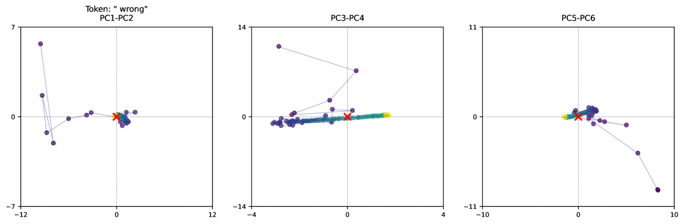
### Visual Description
## [Scatter Plot Array]: Principal Component Analysis of Token "wrong"
### Overview
The image displays three horizontally arranged scatter plots, each representing a two-dimensional projection of data onto different principal component (PC) axes. The overall title indicates the analysis pertains to the token "wrong". The plots visualize the distribution and trajectory of data points (likely embeddings or model states) across six principal components (PC1 through PC6). The data points are connected by faint lines, suggesting a sequence or progression. A prominent red 'X' marks the origin (0,0) in each plot.
### Components/Axes
* **Overall Title:** `Token: "wrong"` (Top-left, above the first plot).
* **Plot 1 (Left):**
* **Title:** `PC1-PC2`
* **X-axis (PC1):** Linear scale, range approximately -12 to 12. Major tick marks at -12, 0, 12.
* **Y-axis (PC2):** Linear scale, range approximately -7 to 7. Major tick marks at -7, 0, 7.
* **Data Points:** Primarily dark purple circles, with a cluster of yellow/green circles near the origin. A red 'X' is at (0,0).
* **Plot 2 (Center):**
* **Title:** `PC3-PC4`
* **X-axis (PC3):** Linear scale, range approximately -4 to 4. Major tick marks at -4, 0, 4.
* **Y-axis (PC4):** Linear scale, range approximately -14 to 14. Major tick marks at -14, 0, 14.
* **Data Points:** Primarily dark purple circles, with a distinct linear cluster of yellow/green circles along the positive X-axis (PC3). A red 'X' is at (0,0).
* **Plot 3 (Right):**
* **Title:** `PC5-PC6`
* **X-axis (PC5):** Linear scale, range approximately -10 to 10. Major tick marks at -10, 0, 10.
* **Y-axis (PC6):** Linear scale, range approximately -11 to 11. Major tick marks at -11, 0, 11.
* **Data Points:** Primarily dark purple circles, with a tight cluster of yellow/green circles near the origin. A red 'X' is at (0,0).
### Detailed Analysis
**PC1-PC2 Plot:**
* **Trend:** The data shows a central cluster near the origin with several outlier points forming a loose, irregular loop or path extending primarily into the negative PC1 and positive/negative PC2 quadrants.
* **Key Points (Approximate):**
* Central Cluster: Dense grouping around (0, 0).
* Outlier Path: Points trace a path including coordinates near (-10, 6), (-10, 2), (-9, -1), (-8, -2), (-5, 0), (-3, 0.5), (-1, 0.5).
* The red 'X' is precisely at (0,0).
**PC3-PC4 Plot:**
* **Trend:** This plot shows the most distinct separation. A tight, linear cluster of yellow/green points lies along the positive PC3 axis (y≈0). The purple points are scattered, with a notable outlier high on the negative PC4 axis and a general spread along the PC4 axis near PC3=0.
* **Key Points (Approximate):**
* Yellow/Green Cluster: Linear from approximately (0.5, 0) to (3, 0).
* Purple Outlier: A point near (-3, 12).
* Other Purple Points: Scattered around the origin, with some forming a vertical spread near PC3=0 (e.g., points near (0, 1), (0, -1), (0.5, 0.5)).
* The red 'X' is precisely at (0,0).
**PC5-PC6 Plot:**
* **Trend:** Most data is tightly clustered near the origin. One significant outlier extends into the positive PC5, negative PC6 quadrant.
* **Key Points (Approximate):**
* Central Cluster: Very dense grouping around (0, 0), including the yellow/green points.
* Major Outlier: A point near (9, -10).
* Minor Outliers: A few points near (2, -1), (4, -1), (6, -4).
* The red 'X' is precisely at (0,0).
### Key Observations
1. **Color-Coded Subgroups:** Two distinct subgroups are visible: a majority of dark purple points and a minority of yellow/green points. The yellow/green points are consistently located near the origin in PC1-PC2 and PC5-PC6, but form a distinct linear feature along the PC3 axis in the PC3-PC4 plot.
2. **Origin Marker:** The red 'X' at (0,0) in all plots serves as a consistent reference point, likely representing the mean or a baseline state.
3. **Variance Distribution:** The spread of data differs significantly across component pairs. PC3-PC4 shows the largest range of values (especially on PC4), indicating this pair captures a major axis of variance in the data. PC5-PC6 shows the least variance, with most points tightly clustered.
4. **Trajectory Lines:** The faint lines connecting points suggest the data represents a sequence (e.g., layers in a neural network, time steps, or optimization steps). The path is most complex and loop-like in PC1-PC2.
### Interpretation
This visualization performs a Principal Component Analysis (PCA) on representations associated with the token "wrong". PCA reduces high-dimensional data (like neural network activations) into principal components that capture the directions of greatest variance.
* **What the data suggests:** The analysis reveals the internal geometric structure of how the model processes or represents the concept of "wrong". The separation of the yellow/green points, especially their linear arrangement along PC3, indicates a specific, consistent sub-feature or state within the data that is strongly aligned with that principal direction.
* **How elements relate:** The six components (PC1-PC6) are orthogonal axes of variance. The plots show pairwise relationships. The fact that the yellow/green cluster is prominent only in PC3-PC4 suggests that the feature it represents is primarily captured by the variance along PC3 and is orthogonal to the features captured by PC1, PC2, PC5, and PC6.
* **Notable patterns/anomalies:**
* The **outlier in PC5-PC6 (9, -10)** is a significant anomaly, representing a data point with an extreme value in a combination of the 5th and 6th most important variance directions. This could be an edge case, an error, or a particularly salient example.
* The **vertical outlier in PC3-PC4 (-3, 12)** is similarly extreme on the PC4 axis.
* The **looping trajectory in PC1-PC2** suggests a non-linear progression or transformation in the primary dimensions of variance, possibly indicating a complex processing pathway for the token.
* **Underlying information:** Without the source data, the exact meaning of each PC is unknown. However, the plots confirm that the representation of "wrong" is not a single point but a structured distribution with distinct subgroups and outliers. The analysis helps identify which directions of variation (PCs) are most important for distinguishing between different instances or aspects related to the token. The red 'X' at the origin likely represents the average representation, against which all other points are compared.
</details>
Figure 12: Latent Space trajectories for select tokens. We show a small part of these high-dimensional trajectories by visualizing the first 6 PCA directions, computing the PCA over all latent state trajectories of all tokens in a sequence. The color gradient going from dark to bright represents steps in the trajectory. The center of mass is marked in red. While on many tokens, the state simply converges (top row), the model also learns to use orbits (middle row), and “sliders” (bottom row, middle), which we observe being used to represent and handle more advanced concepts, such as arithmetic or complicated deliberation.
## 7 What Mechanisms Emerge at Scale in Recurrent-Depth Models
Finally, what is the model doing while recurring in latent space? To understand this question better, we analyze the trajectories $\{s_i\}_i=1^r$ of the model on a few qualitative examples. We are especially interested in understanding what patterns emerge, simply by training this model at scale. In comparison to previous work, such as Bai et al. (2019), where the training objective directly encodes a prior that pushes trajectories to a fixed point, we only train with our truncated unrolling objective.
Figure 11 shows the norm distance $||s_i-s^*||$ between each $s_i$ in a trajectory and an approximate limit point $s^*$ computed with 128 iterations. We show the sentence top to bottom and iterations from left to right. We clearly see that convergence behavior depends on context. We see that key parts of the question, and the start of the model response, are “deliberated” much more in latent space. The context dependence can also be seen in the different behavior among the three identical tokens representing each of the three dots. Also note that the distance to $s^*$ does not always decrease monotonically (e.g. for school); the model may also trace out complicated orbits in its latent trajectory while processing information, even though this is not represented explicitly in our training objective.
We look at trajectories for select tokens in more detail in Figure 12. We compute a PCA decomposition of latent trajectories over all tokens in a sequence, and then show several individual trajectories projected onto the first six PCA directions. See the appendix for more examples. Many tokens simply converge to a fixed point, such as the token in the top row. Yet, for harder questions, such as in the 2nd row This is the token ”3” in a GSM8k test question that opens with Claire makes a 3 egg omelette., the state of the token quickly falls into an orbit pattern in all three pairs of PCA directions. The use of multi-dimensional orbits like these could serve a similar purpose to periodic patterns sometimes observed in fixed-depth transformers trained for arithmetic tasks (Nanda et al., 2022), but we find these patterns extend far beyond arithmetic for our model. We often also observe the use of orbits on tokens such as “makes” (see Figure 16) or “thinks” that determine the structure of the response.
Aside from orbits, we also observe the model encoding particular key tokens as “sliders”, as seen in the middle of the bottom row in Figure 12 (which is the token “wrong”, from the same message as already shown in Figure 11). In these motions the trajectory noticeably drifts in a single direction, which the model could use to implement a mechanism to count how many iterations have occurred.
The emergence of structured trajectories in latent space gives us a glimpse into how the model performs its computations. Unlike the discrete sequential chain of reasoning seen in verbalized chain-of-thought approaches, we observe rich geometric patterns including orbits, convergent paths, and drifts - means to organize its computational process spatially. This suggests the model is independently learning to leverage the high-dimensional nature of its latent space to implement reasoning in new ways.
#### Path Independence.
We verify that our models maintain path independence, in the sense of Anil et al. (2022), despite their complex, learned dynamics, which we discussed prior (see also the additional examples in Appendix Figure 22). When re-initializing from multiple starting states $s_0$ , the model moves in similar trajectories, exhibiting consistent behavior. The same orbital patterns, fixed points, or directional drifts emerge regardless of initialization.
## 8 Related Work Overview
The extent to which recurrence is a foundational concept of machine learning is hard to overstate (Amari, 1972; Hopfield, 1982; Braitenberg, 1986; Gers and Schmidhuber, 2000; Sutskever et al., 2008). Aside from using recurrence to move along sequences, as in recurrent neural networks, it was understood early to also be the key to adaptive computation (Schmidhuber, 2012; Graves, 2017). For transformers, recurrence was applied in Dehghani et al. (2019), who highlight the aim of recurrent depth to model universal, i.e. Turing-complete, machines (Graves et al., 2014). It was used at scale (but with fixed recurrence) in Lan et al. (2019) and an interesting recent improvement in this line of work are described in Tan et al. (2023); Abnar et al. (2023), Mathur et al. (2024) and Csordás et al. (2024). Schwarzschild et al. (2021b); Bansal et al. (2022); Bear et al. (2024) and McLeish et al. (2024) show that depth recurrence is advantageous when learning generalizable algorithms when training with randomized unrolling and input injections. Recent work has described depth-recurrent, looped, transformers and studied their potential benefits with careful theoretical and small-scale analysis (Giannou et al., 2023; Gatmiry et al., 2024; Yang et al., 2024a; Fan et al., 2025).
From another angle, these models can be described as neural networks learning a fixed-point iteration, as studied in deep equilibrium models (Bai et al., 2019; 2022). They are further related to diffusion models (Song and Ermon, 2019), especially latent diffusion models (Rombach et al., 2022), but we note that language diffusion models are usually run with a per-sequence, instead of a per-token, iteration count (Lee et al., 2018). A key difference of our approach to both equilibrium models and diffusion models is in the training objective, where equilibrium methods solve the “direct” problem (Geiping and Moeller, 2019), diffusion models solve a surrogate training objective, and our work suggests that truncated unrolling is a scalable alternative.
More generally, all architectures that recur in depth can also be understood as directly learning the analog to the gradient of a latent energy-based model (LeCun and Huang, 2005; LeCun, 2022), to an implicitly defined intermediate optimization layer (Amos and Kolter, 2017), or to a Kuramoto layer (Miyato et al., 2024). Analogies to gradient descent at inference time also show the connection to test time adaptation (Sun et al., 2020), especially test-time adaptation of output states (Boudiaf et al., 2022).
Aside from full recurrent-depth architectures, there also exist a number of proposals for hybrid architectures, such as models with latent sub-networks (Li et al., 2020a), LoRA adapters on top of weight-shared layers (Bae et al., 2024), or (dynamic) weight-tying of trained models (Hay and Wolf, 2023; Liu et al., 2024b).
As mentioned in Section 6, while we consider the proposed recurrent depth approach to be a very natural way to learn to reason in continuous latent space from the ground up, the works of Hao et al. (2024); Cheng and Durme (2024) and Liu et al. (2024a) discuss how to finetune existing fixed-depth transformers with this capability. These works have a similar aim to ours, enabling reasoning in latent space, but approach this goal from separate directions.
For additional discussions related to the idea of constructing a prior that incentivizes reasoning and algorithm learning at the expense of memorization of simple patterns, we also refer to Chollet (2019), Schwarzschild (2023), Li et al. (2020b) and Moulton (2023).
## 9 Future Work
Aside from work extending and analyzing the scaling behaviors of recurrent depth models, there are many questions that remain unanswered. For example, to us, there are potentially a large number of novel post-training schemes that further enhance the capabilities of these models, such as fine-tuning to compress the recurrence or reinforcement learning with data with different hardness levels (Zelikman et al., 2024), or to internalize reasoning from CoT data into the recurrence (Deng et al., 2024).
Another aspect not covered in this work is the relationship to other modern architecture improvements. Efficient sequence mixing operations, especially those that are linear in sequence dimension, such as linear attention (Katharopoulos et al., 2020; Yang et al., 2024b), are limited in the number of comparisons that can be made. However, with recurrent depth, blocks containing linear operators can repeat until all necessary comparisons between sequence elements are computed (Suzgun et al., 2019). For simplicity, we also focus on a single recurrence, where prior work has considered multiple successive recurrent stages (Takase and Kiyono, 2023; Csordás et al., 2024).
Finally, the proposed architecture is set up to be compute-heavy, with more “materialized” parameters than there are actual parameters. This naturally mirrors mixture-of-expert models (MoE), which are parameter-heavy, using fewer active parameters per forward pass than exist within the model (Shazeer et al., 2017; Fedus et al., 2022). We posit that where the recurrent-depth setup excels at learning reasoning patterns, the MoE excels at effectively storing and retrieving complex information. Their complementarity supports the hypothesis that a future architecture would contain both modifications. While in a standard MoE model, each expert can only be activated once per forward pass, or skipped entirely, a recurrent MoE model could also refine its latent state over multiple iterations, potentially routing to the same expert multiple times, before switching to a different one (Tan et al., 2023; Csordás et al., 2024). While MoE models are the currently leading solution to implement this type of “memory” in dense transformers, these considerations also hold for other memory mechanisms suggested for LLMs (Sukhbaatar et al., 2019; Fan et al., 2021; Wu et al., 2022; He et al., 2024).
## 10 Conclusions
The models described in this paper are ultimately still a proof-of-concept. We describe how to train a latent recurrent-depth architecture, what parameters we chose, and then trained a single model at scale. Future training runs are likely to train with more optimized learning rate schedules, data mixes and accelerators. Still we observe a number of interesting behaviors emerging naturally from recurrent training. The most important of these is the ability to use latent reasoning to dramatically improve performance on reasoning tasks by expending test-time computation. In addition, we also observe context-dependent convergence speed, path independence, and various zero-shot abilities. This leads us to believe that latent reasoning is a promising research direction to complement existing approaches for test-time compute scaling. The model we realize is surprisingly powerful given its size and amount of training data, and we are excited about the potential impact of imbuing generative models with the ability to reason in continuous latent space without the need for specialized data at train time or verbalization at inference time.
## Acknowledgements
This project was made possible by the INCITE program: An award for computer time was provided by the U.S. Department of Energy’s (DOE) Innovative and Novel Computational Impact on Theory and Experiment (INCITE) Program. This research used resources of the Oak Ridge Leadership Computing Facility at the Oak Ridge National Laboratory, which is supported by the Office of Science of the U.S. Department of Energy under Contract No. DE-AC05-00OR22725. Work on the LLNL side was prepared by LLNL under Contract DE-AC52-07NA27344 and supported by the LLNL-LDRD Program under Project No. 24-ERD-010 and 24-ERD-058 (LLNL-CONF-872390). This manuscript has been authored by Lawrence Livermore National Security, LLC under Contract No. DE-AC52-07NA27344 with the U.S. Department of Energy. The United States Government retains a non-exclusive, paid-up, irrevocable, world-wide license to publish or reproduce the published form of this manuscript, or allow others to do so, for United States Government purposes.
JG further acknowledges the support of the Hector II foundation. A large number of small-scale and preliminary experiments were made possible through the support of the MPI Intelligent Systems compute cluster and funding by the Tübingen AI center.
UMD researchers were further supported by the ONR MURI program, DARPA TIAMAT, the National Science Foundation (IIS-2212182), and the NSF TRAILS Institute (2229885). Commercial support was provided by Capital One Bank, the Amazon Research Award program, and Open Philanthropy. Finally, we thank Avi Schwarzschild for helpful comments on the initial draft.
## References
- Abnar et al. (2023) Samira Abnar, Omid Saremi, Laurent Dinh, Shantel Wilson, Miguel Angel Bautista, Chen Huang, Vimal Thilak, Etai Littwin, Jiatao Gu, Josh Susskind, and Samy Bengio. 2023. Adaptivity and Modularity for Efficient Generalization Over Task Complexity. arxiv:2310.08866[cs].
- AI2 (2024) AI2. 2024. OLMo 1.7–7B: A 24 point improvement on MMLU.
- Allen-Zhu and Li (2024) Zeyuan Allen-Zhu and Yuanzhi Li. 2024. Physics of language models: Part 3.1, knowledge storage and extraction. In Proceedings of the 41st International Conference on Machine Learning, volume 235 of ICML’24, pages 1067–1077, Vienna, Austria. JMLR.org.
- Amari (1972) S.-I. Amari. 1972. Learning Patterns and Pattern Sequences by Self-Organizing Nets of Threshold Elements. IEEE Transactions on Computers, C-21(11):1197–1206.
- AMD (2021) AMD. 2021. AMD Instinct™ MI250X Accelerators.
- Amini et al. (2019) Aida Amini, Saadia Gabriel, Peter Lin, Rik Koncel-Kedziorski, Yejin Choi, and Hannaneh Hajishirzi. 2019. Mathqa: Towards interpretable math word problem solving with operation-based formalisms. arXiv preprint arXiv:1905.13319.
- Amos and Kolter (2017) Brandon Amos and J. Zico Kolter. 2017. OptNet: Differentiable Optimization as a Layer in Neural Networks. In International Conference on Machine Learning, pages 136–145.
- Anil et al. (2022) Cem Anil, Ashwini Pokle, Kaiqu Liang, Johannes Treutlein, Yuhuai Wu, Shaojie Bai, J. Zico Kolter, and Roger Baker Grosse. 2022. Path Independent Equilibrium Models Can Better Exploit Test-Time Computation. In Advances in Neural Information Processing Systems.
- Austin et al. (2021) Jacob Austin, Augustus Odena, Maxwell Nye, Maarten Bosma, Henryk Michalewski, David Dohan, Ellen Jiang, Carrie Cai, Michael Terry, Quoc Le, and 1 others. 2021. Program synthesis with large language models. arXiv preprint arXiv:2108.07732.
- Azerbayev et al. (2023) Zhangir Azerbayev, Hailey Schoelkopf, Keiran Paster, Marco Dos Santos, Stephen Marcus McAleer, Albert Q. Jiang, Jia Deng, Stella Biderman, and Sean Welleck. 2023. Llemma: An Open Language Model for Mathematics. In The Twelfth International Conference on Learning Representations.
- Bae et al. (2024) Sangmin Bae, Adam Fisch, Hrayr Harutyunyan, Ziwei Ji, Seungyeon Kim, and Tal Schuster. 2024. Relaxed Recursive Transformers: Effective Parameter Sharing with Layer-wise LoRA.
- Bai et al. (2019) Shaojie Bai, J. Zico Kolter, and Vladlen Koltun. 2019. Deep Equilibrium Models. In Advances in Neural Information Processing Systems, volume 32. Curran Associates, Inc.
- Bai et al. (2022) Shaojie Bai, Vladlen Koltun, and J. Zico Kolter. 2022. Neural Deep Equilibrium Solvers. In International Conference on Learning Representations.
- Bai et al. (2024) Yushi Bai, Jiajie Zhang, Xin Lv, Linzhi Zheng, Siqi Zhu, Lei Hou, Yuxiao Dong, Jie Tang, and Juanzi Li. 2024. LongWriter: Unleashing 10,000+ Word Generation from Long Context LLMs. arxiv:2408.07055[cs].
- Banino et al. (2021) Andrea Banino, Jan Balaguer, and Charles Blundell. 2021. PonderNet: Learning to Ponder. In 8th ICML Workshop on Automated Machine Learning (AutoML).
- Bansal et al. (2022) Arpit Bansal, Avi Schwarzschild, Eitan Borgnia, Zeyad Emam, Furong Huang, Micah Goldblum, and Tom Goldstein. 2022. End-to-end Algorithm Synthesis with Recurrent Networks: Extrapolation without Overthinking. In Advances in Neural Information Processing Systems.
- Bauschke et al. (2011) Heinz H. Bauschke, Sarah M. Moffat, and Xianfu Wang. 2011. Firmly nonexpansive mappings and maximally monotone operators: Correspondence and duality. arXiv:1101.4688 [math].
- Bear et al. (2024) Jay Bear, Adam Prügel-Bennett, and Jonathon Hare. 2024. Rethinking Deep Thinking: Stable Learning of Algorithms using Lipschitz Constraints. arxiv:2410.23451[cs].
- Bekman (2023) Stas Bekman. 2023. Machine Learning Engineering Open Book. Stasosphere Online Inc.
- Ben Allal et al. (2024) Loubna Ben Allal, Anton Lozhkov, Guilherme Penedo, Thomas Wolf, and Leandro von Werra. 2024. SmolLM-corpus.
- Biderman et al. (2023) Stella Biderman, Hailey Schoelkopf, Quentin Anthony, Herbie Bradley, Kyle O’Brien, Eric Hallahan, Mohammad Aflah Khan, Shivanshu Purohit, USVSN Sai Prashanth, Edward Raff, Aviya Skowron, Lintang Sutawika, and Oskar van der Wal. 2023. Pythia: A Suite for Analyzing Large Language Models Across Training and Scaling. arxiv:2304.01373[cs].
- Biderman et al. (2024) Stella Biderman, Hailey Schoelkopf, Lintang Sutawika, Leo Gao, Jonathan Tow, Baber Abbasi, Alham Fikri Aji, Pawan Sasanka Ammanamanchi, Sidney Black, Jordan Clive, Anthony DiPofi, Julen Etxaniz, Benjamin Fattori, Jessica Zosa Forde, Charles Foster, Jeffrey Hsu, Mimansa Jaiswal, Wilson Y. Lee, Haonan Li, and 11 others. 2024. Lessons from the Trenches on Reproducible Evaluation of Language Models. arxiv:2405.14782[cs].
- Bisk et al. (2020) Yonatan Bisk, Rowan Zellers, Ronan Le Bras, Jianfeng Gao, and Yejin Choi. 2020. Piqa: Reasoning about physical commonsense in natural language. In Thirty-Fourth AAAI Conference on Artificial Intelligence.
- Boudiaf et al. (2022) Malik Boudiaf, Romain Mueller, Ismail Ben Ayed, and Luca Bertinetto. 2022. Parameter-Free Online Test-Time Adaptation. In Proceedings of the IEEE/CVF Conference on Computer Vision and Pattern Recognition, pages 8344–8353.
- Braitenberg (1986) Valentino Braitenberg. 1986. Vehicles: Experiments in Synthetic Psychology. MIT press.
- Brandon et al. (2024) William Brandon, Mayank Mishra, Aniruddha Nrusimha, Rameswar Panda, and Jonathan Ragan Kelly. 2024. Reducing Transformer Key-Value Cache Size with Cross-Layer Attention. arxiv:2405.12981[cs].
- British Library Labs (2021) British Library Labs. 2021. Digitised Books. c. 1510 - c. 1900. JSONL (OCR Derived Text + Metadata). British Library.
- Cai et al. (2024) Tianle Cai, Yuhong Li, Zhengyang Geng, Hongwu Peng, Jason D. Lee, Deming Chen, and Tri Dao. 2024. Medusa: Simple LLM Inference Acceleration Framework with Multiple Decoding Heads. In Forty-First International Conference on Machine Learning.
- character.ai (2024) character.ai. 2024. Optimizing AI Inference at Character.AI.
- Chen et al. (2021) Mark Chen, Jerry Tworek, Heewoo Jun, Qiming Yuan, Henrique Ponde de Oliveira Pinto, Jared Kaplan, Harri Edwards, Yuri Burda, Nicholas Joseph, Greg Brockman, Alex Ray, Raul Puri, Gretchen Krueger, Michael Petrov, Heidy Khlaaf, Girish Sastry, Pamela Mishkin, Brooke Chan, Scott Gray, and 39 others. 2021. Evaluating large language models trained on code. Preprint, arXiv:2107.03374.
- Cheng and Durme (2024) Jeffrey Cheng and Benjamin Van Durme. 2024. Compressed Chain of Thought: Efficient Reasoning Through Dense Representations. arxiv:2412.13171[cs].
- Choi (2023) Euirim Choi. 2023. GoodWiki dataset.
- Chollet (2019) François Chollet. 2019. On the Measure of Intelligence. arxiv:1911.01547[cs].
- Chowdhery et al. (2022) Aakanksha Chowdhery, Sharan Narang, Jacob Devlin, Maarten Bosma, Gaurav Mishra, Adam Roberts, Paul Barham, Hyung Won Chung, Charles Sutton, Sebastian Gehrmann, Parker Schuh, Kensen Shi, Sasha Tsvyashchenko, Joshua Maynez, Abhishek Rao, Parker Barnes, Yi Tay, Noam Shazeer, Vinodkumar Prabhakaran, and 48 others. 2022. PaLM: Scaling Language Modeling with Pathways. arXiv:2204.02311 [cs].
- Clark et al. (2018) Peter Clark, Isaac Cowhey, Oren Etzioni, Tushar Khot, Ashish Sabharwal, Carissa Schoenick, and Oyvind Tafjord. 2018. Think you have solved question answering? try arc, the ai2 reasoning challenge. arXiv:1803.05457v1.
- Cobbe et al. (2021) Karl Cobbe, Vineet Kosaraju, Mohammad Bavarian, Mark Chen, Heewoo Jun, Lukasz Kaiser, Matthias Plappert, Jerry Tworek, Jacob Hilton, Reiichiro Nakano, Christopher Hesse, and John Schulman. 2021. Training Verifiers to Solve Math Word Problems. arxiv:2110.14168[cs].
- Colegrove et al. (2024) Owen Colegrove, Vik Paruchuri, and OpenPhi-Team. 2024. Open-phi/textbooks $·$ Datasets at Hugging Face.
- Csordás et al. (2024) Róbert Csordás, Kazuki Irie, Jürgen Schmidhuber, Christopher Potts, and Christopher D. Manning. 2024. MoEUT: Mixture-of-Experts Universal Transformers. In The Thirty-eighth Annual Conference on Neural Information Processing Systems.
- Dagan (2024) Gautier Dagan. 2024. Bpeasy.
- Dagan et al. (2024) Gautier Dagan, Gabriel Synnaeve, and Baptiste Rozière. 2024. Getting the most out of your tokenizer for pre-training and domain adaptation. arxiv:2402.01035[cs].
- Dao (2023) Tri Dao. 2023. FlashAttention-2: Faster Attention with Better Parallelism and Work Partitioning. arxiv:2307.08691[cs].
- Dao et al. (2022) Tri Dao, Daniel Y. Fu, Stefano Ermon, Atri Rudra, and Christopher Ré. 2022. FlashAttention: Fast and Memory-Efficient Exact Attention with IO-Awareness. arxiv:2205.14135[cs].
- DeepSeek-AI et al. (2025) DeepSeek-AI, Daya Guo, Dejian Yang, Haowei Zhang, Junxiao Song, Ruoyu Zhang, Runxin Xu, Qihao Zhu, Shirong Ma, Peiyi Wang, Xiao Bi, Xiaokang Zhang, Xingkai Yu, Yu Wu, Z. F. Wu, Zhibin Gou, Zhihong Shao, Zhuoshu Li, Ziyi Gao, and 181 others. 2025. DeepSeek-R1: Incentivizing Reasoning Capability in LLMs via Reinforcement Learning. arxiv:2501.12948[cs].
- DeepSeek-AI et al. (2024) DeepSeek-AI, Aixin Liu, Bei Feng, Bing Xue, Bingxuan Wang, Bochao Wu, Chengda Lu, Chenggang Zhao, Chengqi Deng, Chenyu Zhang, Chong Ruan, Damai Dai, Daya Guo, Dejian Yang, Deli Chen, Dongjie Ji, Erhang Li, Fangyun Lin, Fucong Dai, and 181 others. 2024. DeepSeek-V3 Technical Report. arxiv:2412.19437[cs].
- Dehghani et al. (2019) Mostafa Dehghani, Stephan Gouws, Oriol Vinyals, Jakob Uszkoreit, and Łukasz Kaiser. 2019. Universal Transformers. arxiv:1807.03819[cs, stat].
- Deng et al. (2024) Yuntian Deng, Yejin Choi, and Stuart Shieber. 2024. From Explicit CoT to Implicit CoT: Learning to Internalize CoT Step by Step. arxiv:2405.14838[cs].
- Ding et al. (2024) Hantian Ding, Zijian Wang, Giovanni Paolini, Varun Kumar, Anoop Deoras, Dan Roth, and Stefano Soatto. 2024. Fewer Truncations Improve Language Modeling. In Forty-First International Conference on Machine Learning.
- Ding et al. (2021) Ming Ding, Zhuoyi Yang, Wenyi Hong, Wendi Zheng, Chang Zhou, Da Yin, Junyang Lin, Xu Zou, Zhou Shao, Hongxia Yang, and Jie Tang. 2021. CogView: Mastering Text-to-Image Generation via Transformers. In Advances in Neural Information Processing Systems, volume 34, pages 19822–19835. Curran Associates, Inc.
- Elbayad et al. (2019) Maha Elbayad, Jiatao Gu, Edouard Grave, and Michael Auli. 2019. Depth-Adaptive Transformer. In International Conference on Learning Representations.
- Elhoushi et al. (2024) Mostafa Elhoushi, Akshat Shrivastava, Diana Liskovich, Basil Hosmer, Bram Wasti, Liangzhen Lai, Anas Mahmoud, Bilge Acun, Saurabh Agarwal, Ahmed Roman, Ahmed A. Aly, Beidi Chen, and Carole-Jean Wu. 2024. LayerSkip: Enabling Early Exit Inference and Self-Speculative Decoding. arxiv:2404.16710[cs].
- Everett et al. (2024) Katie Everett, Lechao Xiao, Mitchell Wortsman, Alexander A. Alemi, Roman Novak, Peter J. Liu, Izzeddin Gur, Jascha Sohl-Dickstein, Leslie Pack Kaelbling, Jaehoon Lee, and Jeffrey Pennington. 2024. Scaling Exponents Across Parameterizations and Optimizers. arxiv:2407.05872[cs].
- Fan et al. (2019) Angela Fan, Edouard Grave, and Armand Joulin. 2019. Reducing Transformer Depth on Demand with Structured Dropout. arxiv:1909.11556[cs, stat].
- Fan et al. (2021) Angela Fan, Thibaut Lavril, Edouard Grave, Armand Joulin, and Sainbayar Sukhbaatar. 2021. Addressing Some Limitations of Transformers with Feedback Memory. arxiv:2002.09402[cs, stat].
- Fan et al. (2025) Ying Fan, Yilun Du, Kannan Ramchandran, and Kangwook Lee. 2025. Looped Transformers for Length Generalization. In The Thirteenth International Conference on Learning Representations.
- Fedus et al. (2022) William Fedus, Barret Zoph, and Noam Shazeer. 2022. Switch Transformers: Scaling to Trillion Parameter Models with Simple and Efficient Sparsity. arxiv:2101.03961[cs].
- Feng et al. (2023) Xidong Feng, Yicheng Luo, Ziyan Wang, Hongrui Tang, Mengyue Yang, Kun Shao, David Mguni, Yali Du, and Jun Wang. 2023. ChessGPT: Bridging Policy Learning and Language Modeling. Advances in Neural Information Processing Systems, 36:7216–7262.
- Gabarain (2024) Sebastian Gabarain. 2024. Locutusque/hercules-v5.0 $·$ Datasets at Hugging Face.
- Gatmiry et al. (2024) Khashayar Gatmiry, Nikunj Saunshi, Sashank J. Reddi, Stefanie Jegelka, and Sanjiv Kumar. 2024. Can Looped Transformers Learn to Implement Multi-step Gradient Descent for In-context Learning?
- Geiping and Goldstein (2023) Jonas Geiping and Tom Goldstein. 2023. Cramming: Training a Language Model on a single GPU in one day. In Proceedings of the 40th International Conference on Machine Learning, pages 11117–11143. PMLR.
- Geiping and Moeller (2019) Jonas Geiping and Michael Moeller. 2019. Parametric Majorization for Data-Driven Energy Minimization Methods. In Proceedings of the IEEE International Conference on Computer Vision, pages 10262–10273.
- Gers and Schmidhuber (2000) F.A. Gers and J. Schmidhuber. 2000. Recurrent nets that time and count. In Proceedings of the IEEE-INNS-ENNS International Joint Conference on Neural Networks. IJCNN 2000. Neural Computing: New Challenges and Perspectives for the New Millennium, volume 3, pages 189–194 vol.3.
- Giannou et al. (2023) Angeliki Giannou, Shashank Rajput, Jy-Yong Sohn, Kangwook Lee, Jason D. Lee, and Dimitris Papailiopoulos. 2023. Looped Transformers as Programmable Computers. In Proceedings of the 40th International Conference on Machine Learning, pages 11398–11442. PMLR.
- Goyal et al. (2018) Priya Goyal, Piotr Dollár, Ross Girshick, Pieter Noordhuis, Lukasz Wesolowski, Aapo Kyrola, Andrew Tulloch, Yangqing Jia, and Kaiming He. 2018. Accurate, Large Minibatch SGD: Training ImageNet in 1 Hour. arxiv:1706.02677[cs].
- Graves (2017) Alex Graves. 2017. Adaptive Computation Time for Recurrent Neural Networks. arxiv:1603.08983[cs].
- Graves et al. (2014) Alex Graves, Greg Wayne, and Ivo Danihelka. 2014. Neural Turing Machines. arxiv:1410.5401[cs].
- Groeneveld et al. (2024) Dirk Groeneveld, Iz Beltagy, Pete Walsh, Akshita Bhagia, Rodney Kinney, Oyvind Tafjord, Ananya Harsh Jha, Hamish Ivison, Ian Magnusson, Yizhong Wang, Shane Arora, David Atkinson, Russell Authur, Khyathi Raghavi Chandu, Arman Cohan, Jennifer Dumas, Yanai Elazar, Yuling Gu, Jack Hessel, and 24 others. 2024. OLMo: Accelerating the Science of Language Models. arxiv:2402.00838[cs].
- Hägele et al. (2024) Alexander Hägele, Elie Bakouch, Atli Kosson, Loubna Ben Allal, Leandro Von Werra, and Martin Jaggi. 2024. Scaling Laws and Compute-Optimal Training Beyond Fixed Training Durations. In Workshop on Efficient Systems for Foundation Models II @ ICML2024.
- Hao et al. (2024) Shibo Hao, Sainbayar Sukhbaatar, DiJia Su, Xian Li, Zhiting Hu, Jason Weston, and Yuandong Tian. 2024. Training Large Language Models to Reason in a Continuous Latent Space. arxiv:2412.06769[cs].
- Hay and Wolf (2023) Tamir David Hay and Lior Wolf. 2023. Dynamic Layer Tying for Parameter-Efficient Transformers. In The Twelfth International Conference on Learning Representations.
- He et al. (2024) Zexue He, Leonid Karlinsky, Donghyun Kim, Julian McAuley, Dmitry Krotov, and Rogerio Feris. 2024. CAMELoT: Towards Large Language Models with Training-Free Consolidated Associative Memory. arxiv:2402.13449[cs].
- Hendrycks et al. (2021a) Dan Hendrycks, Collin Burns, Steven Basart, Andy Zou, Mantas Mazeika, Dawn Song, and Jacob Steinhardt. 2021a. Measuring massive multitask language understanding. Proceedings of the International Conference on Learning Representations (ICLR).
- Hendrycks et al. (2021b) Dan Hendrycks, Collin Burns, Steven Basart, Andy Zou, Mantas Mazeika, Dawn Song, and Jacob Steinhardt. 2021b. Measuring Massive Multitask Language Understanding. In International Conference on Learning Representations.
- Hopfield (1982) J J Hopfield. 1982. Neural networks and physical systems with emergent collective computational abilities. Proceedings of the National Academy of Sciences of the United States of America, 79(8):2554–2558.
- Hu et al. (2024) Jiewen Hu, Thomas Zhu, and Sean Welleck. 2024. miniCTX: Neural Theorem Proving with (Long-)Contexts. arxiv:2408.03350[cs].
- Izmailov et al. (2018) Pavel Izmailov, Dmitrii Podoprikhin, Timur Garipov, Dmitry Vetrov, and Andrew Gordon Wilson. 2018. Averaging weights leads to wider optima and better generalization: 34th Conference on Uncertainty in Artificial Intelligence 2018, UAI 2018. 34th Conference on Uncertainty in Artificial Intelligence 2018, UAI 2018, pages 876–885.
- Jiang et al. (2023) Albert Q. Jiang, Wenda Li, and Mateja Jamnik. 2023. Multilingual Mathematical Autoformalization. arxiv:2311.03755[cs].
- Johannes Welbl (2017) Matt Gardner Johannes Welbl, Nelson F. Liu. 2017. Crowdsourcing multiple choice science questions.
- Kaddour (2022) Jean Kaddour. 2022. Stop Wasting My Time! Saving Days of ImageNet and BERT Training with Latest Weight Averaging. arxiv:2209.14981[cs, stat].
- Kaplan et al. (2024) Guy Kaplan, Matanel Oren, Yuval Reif, and Roy Schwartz. 2024. From Tokens to Words: On the Inner Lexicon of LLMs. arxiv:2410.05864[cs].
- Kaplan et al. (2020) Jared Kaplan, Sam McCandlish, Tom Henighan, Tom B. Brown, Benjamin Chess, Rewon Child, Scott Gray, Alec Radford, Jeffrey Wu, and Dario Amodei. 2020. Scaling Laws for Neural Language Models. arxiv:2001.08361[cs, stat].
- Katharopoulos et al. (2020) Angelos Katharopoulos, Apoorv Vyas, Nikolaos Pappas, and François Fleuret. 2020. Transformers are RNNs: Fast Autoregressive Transformers with Linear Attention. In Proceedings of the 37th International Conference on Machine Learning, pages 5156–5165. PMLR.
- Kenney (2024) Matthew Kenney. 2024. ArXivDLInstruct.
- Kim et al. (2024) Seungone Kim, Juyoung Suk, Shayne Longpre, Bill Yuchen Lin, Jamin Shin, Sean Welleck, Graham Neubig, Moontae Lee, Kyungjae Lee, and Minjoon Seo. 2024. Prometheus 2: An Open Source Language Model Specialized in Evaluating Other Language Models. In Proceedings of the 2024 Conference on Empirical Methods in Natural Language Processing, pages 4334–4353, Miami, Florida, USA. Association for Computational Linguistics.
- Kingma and Ba (2015) Diederik P. Kingma and Jimmy Ba. 2015. Adam: A Method for Stochastic Optimization. In International Conference on Learning Representations (ICLR), San Diego.
- Kryściński et al. (2022) Wojciech Kryściński, Nazneen Rajani, Divyansh Agarwal, Caiming Xiong, and Dragomir Radev. 2022. BookSum: A Collection of Datasets for Long-form Narrative Summarization. arxiv:2105.08209[cs].
- Lai et al. (2024) Xin Lai, Zhuotao Tian, Yukang Chen, Senqiao Yang, Xiangru Peng, and Jiaya Jia. 2024. Step-DPO: Step-wise Preference Optimization for Long-chain Reasoning of LLMs. arxiv:2406.18629[cs].
- Lan et al. (2019) Zhenzhong Lan, Mingda Chen, Sebastian Goodman, Kevin Gimpel, Piyush Sharma, and Radu Soricut. 2019. ALBERT: A Lite BERT for Self-supervised Learning of Language Representations. In International Conference on Learning Representations.
- LeCun (2022) Yann LeCun. 2022. A Path Towards Autonomous Machine Intelligence. Preprint, Version 0.9.2:62.
- LeCun and Huang (2005) Yann LeCun and Fu Jie Huang. 2005. Loss functions for discriminative training of energy-based models. In AISTATS 2005 - Proceedings of the 10th International Workshop on Artificial Intelligence and Statistics, pages 206–213.
- Lee et al. (2018) Jason Lee, Elman Mansimov, and Kyunghyun Cho. 2018. Deterministic Non-Autoregressive Neural Sequence Modeling by Iterative Refinement. In Proceedings of the 2018 Conference on Empirical Methods in Natural Language Processing, pages 1173–1182, Brussels, Belgium. Association for Computational Linguistics.
- Leviathan et al. (2023) Yaniv Leviathan, Matan Kalman, and Yossi Matias. 2023. Fast Inference from Transformers via Speculative Decoding. In Proceedings of the 40th International Conference on Machine Learning, pages 19274–19286. PMLR.
- Levine et al. (2021) Yoav Levine, Noam Wies, Or Sharir, Hofit Bata, and Amnon Shashua. 2021. The Depth-to-Width Interplay in Self-Attention. arxiv:2006.12467[cs, stat].
- Lewkowycz et al. (2022) Aitor Lewkowycz, Anders Andreassen, David Dohan, Ethan Dyer, Henryk Michalewski, Vinay Ramasesh, Ambrose Slone, Cem Anil, Imanol Schlag, Theo Gutman-Solo, Yuhuai Wu, Behnam Neyshabur, Guy Gur-Ari, and Vedant Misra. 2022. Solving quantitative reasoning problems with language models. Preprint, arXiv:2206.14858.
- Li et al. (2023) Raymond Li, Loubna Ben Allal, Yangtian Zi, Niklas Muennighoff, Denis Kocetkov, Chenghao Mou, Marc Marone, Christopher Akiki, Jia Li, Jenny Chim, Qian Liu, Evgenii Zheltonozhskii, Terry Yue Zhuo, Thomas Wang, Olivier Dehaene, Joel Lamy-Poirier, Joao Monteiro, Nicolas Gontier, Ming-Ho Yee, and 39 others. 2023. StarCoder: May the source be with you! Transactions on Machine Learning Research.
- Li et al. (2020a) Xian Li, Asa Cooper Stickland, Yuqing Tang, and Xiang Kong. 2020a. Deep Transformers with Latent Depth. arxiv:2009.13102[cs].
- Li et al. (2020b) Yujia Li, Felix Gimeno, Pushmeet Kohli, and Oriol Vinyals. 2020b. Strong Generalization and Efficiency in Neural Programs. arxiv:2007.03629[cs].
- Liping Tang (2024) Omkar Pangarkar Liping Tang, Nikhil Ranjan. 2024. TxT360: A top-quality LLM pre-training dataset requires the perfect blend.
- Liu et al. (2023a) Hao Liu, Matei Zaharia, and Pieter Abbeel. 2023a. Ring attention with blockwise transformers for near-infinite context. arXiv preprint arXiv:2310.01889.
- Liu et al. (2024a) Luyang Liu, Jonas Pfeiffer, Jiaxing Wu, Jun Xie, and Arthur Szlam. 2024a. Deliberation in Latent Space via Differentiable Cache Augmentation. arxiv:2412.17747[cs].
- Liu et al. (2023b) Xiao Liu, Hanyu Lai, Hao Yu, Yifan Xu, Aohan Zeng, Zhengxiao Du, Peng Zhang, Yuxiao Dong, and Jie Tang. 2023b. WebGLM: Towards An Efficient Web-Enhanced Question Answering System with Human Preferences. In Proceedings of the 29th ACM SIGKDD Conference on Knowledge Discovery and Data Mining, KDD ’23, pages 4549–4560, New York, NY, USA. Association for Computing Machinery.
- Liu et al. (2024b) Zechun Liu, Changsheng Zhao, Forrest Iandola, Chen Lai, Yuandong Tian, Igor Fedorov, Yunyang Xiong, Ernie Chang, Yangyang Shi, Raghuraman Krishnamoorthi, Liangzhen Lai, and Vikas Chandra. 2024b. MobileLLM: Optimizing Sub-billion Parameter Language Models for On-Device Use Cases. arxiv:2402.14905[cs].
- Liu et al. (2023c) Zhengzhong Liu, Aurick Qiao, Willie Neiswanger, Hongyi Wang, Bowen Tan, Tianhua Tao, Junbo Li, Yuqi Wang, Suqi Sun, Omkar Pangarkar, Richard Fan, Yi Gu, Victor Miller, Yonghao Zhuang, Guowei He, Haonan Li, Fajri Koto, Liping Tang, Nikhil Ranjan, and 9 others. 2023c. LLM360: Towards fully transparent open-source LLMs.
- Loshchilov and Hutter (2017) Ilya Loshchilov and Frank Hutter. 2017. Decoupled Weight Decay Regularization. arXiv:1711.05101 [cs, math].
- Lozhkov et al. (2024) Anton Lozhkov, Raymond Li, Loubna Ben Allal, Federico Cassano, Joel Lamy-Poirier, Nouamane Tazi, Ao Tang, Dmytro Pykhtar, Jiawei Liu, Yuxiang Wei, Tianyang Liu, Max Tian, Denis Kocetkov, Arthur Zucker, Younes Belkada, Zijian Wang, Qian Liu, Dmitry Abulkhanov, Indraneil Paul, and 47 others. 2024. StarCoder 2 and The Stack v2: The Next Generation.
- Lu et al. (2024) Zimu Lu, Aojun Zhou, Ke Wang, Houxing Ren, Weikang Shi, Junting Pan, Mingjie Zhan, and Hongsheng Li. 2024. MathCoder2: Better Math Reasoning from Continued Pretraining on Model-translated Mathematical Code. arxiv:2410.08196[cs].
- Majstorovic (2024) Sebastian Majstorovic. 2024. Selected Digitized Books | The Library of Congress.
- Markeeva et al. (2024) Larisa Markeeva, Sean McLeish, Borja Ibarz, Wilfried Bounsi, Olga Kozlova, Alex Vitvitskyi, Charles Blundell, Tom Goldstein, Avi Schwarzschild, and Petar Veličković. 2024. The CLRS-Text Algorithmic Reasoning Language Benchmark. arxiv:2406.04229[cs].
- Mathur et al. (2024) Mrinal Mathur, Barak A. Pearlmutter, and Sergey M. Plis. 2024. MIND over Body: Adaptive Thinking using Dynamic Computation. In The Thirteenth International Conference on Learning Representations.
- McLeish et al. (2024) Sean Michael McLeish, Arpit Bansal, Alex Stein, Neel Jain, John Kirchenbauer, Brian R. Bartoldson, Bhavya Kailkhura, Abhinav Bhatele, Jonas Geiping, Avi Schwarzschild, and Tom Goldstein. 2024. Transformers Can Do Arithmetic with the Right Embeddings. In The Thirty-eighth Annual Conference on Neural Information Processing Systems.
- Merrill et al. (2022) William Merrill, Ashish Sabharwal, and Noah A. Smith. 2022. Saturated Transformers are Constant-Depth Threshold Circuits. Transactions of the Association for Computational Linguistics, 10:843–856.
- Mihaylov et al. (2018) Todor Mihaylov, Peter Clark, Tushar Khot, and Ashish Sabharwal. 2018. Can a suit of armor conduct electricity? a new dataset for open book question answering. In EMNLP.
- Mikolov et al. (2011) Tomáš Mikolov, Stefan Kombrink, Lukáš Burget, Jan Černocký, and Sanjeev Khudanpur. 2011. Extensions of recurrent neural network language model. In 2011 IEEE International Conference on Acoustics, Speech and Signal Processing (ICASSP), pages 5528–5531.
- Miyato et al. (2024) Takeru Miyato, Sindy Löwe, Andreas Geiger, and Max Welling. 2024. Artificial Kuramoto Oscillatory Neurons. In The Thirteenth International Conference on Learning Representations, Singapore.
- Moulton (2023) Ryan Moulton. 2023. The Many Ways that Digital Minds Can Know.
- Muennighoff et al. (2024) Niklas Muennighoff, Qian Liu, Armel Zebaze, Qinkai Zheng, Binyuan Hui, Terry Yue Zhuo, Swayam Singh, Xiangru Tang, Leandro von Werra, and Shayne Longpre. 2024. OctoPack: Instruction Tuning Code Large Language Models. arxiv:2308.07124[cs].
- Nam Pham (2023) Nam Pham. 2023. Tiny-textbooks (Revision 14de7ba).
- Nam Pham (2024) Nam Pham. 2024. Tiny-strange-textbooks (Revision 6f304f1).
- Nanda et al. (2022) Neel Nanda, Lawrence Chan, Tom Lieberum, Jess Smith, and Jacob Steinhardt. 2022. Progress measures for grokking via mechanistic interpretability. In The Eleventh International Conference on Learning Representations.
- Noci et al. (2022) Lorenzo Noci, Sotiris Anagnostidis, Luca Biggio, Antonio Orvieto, Sidak Pal Singh, and Aurelien Lucchi. 2022. Signal Propagation in Transformers: Theoretical Perspectives and the Role of Rank Collapse. In Advances in Neural Information Processing Systems.
- OpenAI (2024) OpenAI. 2024. New reasoning models: Openai o1-preview and o1-mini. https://openai.com/research/o1-preview-and-o1-mini.
- Ouyang et al. (2022) Long Ouyang, Jeff Wu, Xu Jiang, Diogo Almeida, Carroll L. Wainwright, Pamela Mishkin, Chong Zhang, Sandhini Agarwal, Katarina Slama, Alex Ray, John Schulman, Jacob Hilton, Fraser Kelton, Luke Miller, Maddie Simens, Amanda Askell, Peter Welinder, Paul Christiano, Jan Leike, and Ryan Lowe. 2022. Training language models to follow instructions with human feedback. arxiv:2203.02155[cs].
- Paster et al. (2023) Keiran Paster, Marco Dos Santos, Zhangir Azerbayev, and Jimmy Ba. 2023. OpenWebMath: An Open Dataset of High-Quality Mathematical Web Text. In The Twelfth International Conference on Learning Representations.
- Peebles and Xie (2023) William Peebles and Saining Xie. 2023. Scalable Diffusion Models with Transformers. In Proceedings of the IEEE/CVF International Conference on Computer Vision, pages 4195–4205.
- Radford et al. (2019) Alec Radford, Jeffrey Wu, Rewon Child, David Luan, Dario Amodei, and Ilya Sutskever. 2019. Language Models are Unsupervised Multitask Learners. OpenAI, page 24.
- Rae et al. (2019) Jack W. Rae, Anna Potapenko, Siddhant M. Jayakumar, and Timothy P. Lillicrap. 2019. Compressive Transformers for Long-Range Sequence Modelling. arxiv:1911.05507[cs].
- Rajbhandari et al. (2020) Samyam Rajbhandari, Jeff Rasley, Olatunji Ruwase, and Yuxiong He. 2020. ZeRO: Memory optimizations Toward Training Trillion Parameter Models. In SC20: International Conference for High Performance Computing, Networking, Storage and Analysis, pages 1–16.
- Rombach et al. (2022) Robin Rombach, Andreas Blattmann, Dominik Lorenz, Patrick Esser, and Björn Ommer. 2022. High-Resolution Image Synthesis With Latent Diffusion Models. In Proceedings of the IEEE/CVF Conference on Computer Vision and Pattern Recognition, pages 10684–10695.
- Sakaguchi et al. (2021) Keisuke Sakaguchi, Ronan Le Bras, Chandra Bhagavatula, and Yejin Choi. 2021. WinoGrande: An adversarial winograd schema challenge at scale. Commun. ACM, 64(9):99–106.
- Sanh et al. (2021) Victor Sanh, Albert Webson, Colin Raffel, Stephen Bach, Lintang Sutawika, Zaid Alyafeai, Antoine Chaffin, Arnaud Stiegler, Arun Raja, Manan Dey, M. Saiful Bari, Canwen Xu, Urmish Thakker, Shanya Sharma Sharma, Eliza Szczechla, Taewoon Kim, Gunjan Chhablani, Nihal Nayak, Debajyoti Datta, and 21 others. 2021. Multitask Prompted Training Enables Zero-Shot Task Generalization. In International Conference on Learning Representations.
- Sanyal et al. (2024) Sunny Sanyal, Atula Tejaswi Neerkaje, Jean Kaddour, Abhishek Kumar, and sujay sanghavi. 2024. Early weight averaging meets high learning rates for LLM pre-training. In First Conference on Language Modeling.
- Schmidhuber (2012) Juergen Schmidhuber. 2012. Self-Delimiting Neural Networks. arxiv:1210.0118[cs].
- Schuster et al. (2022) Tal Schuster, Adam Fisch, Jai Gupta, Mostafa Dehghani, Dara Bahri, Vinh Q. Tran, Yi Tay, and Donald Metzler. 2022. Confident Adaptive Language Modeling. In Advances in Neural Information Processing Systems.
- Schwarzschild (2023) Avi Schwarzschild. 2023. Deep Thinking Systems: Logical Extrapolation with Recurrent Neural Networks. Ph.D. thesis, University of Maryland, College Park, College Park.
- Schwarzschild et al. (2021a) Avi Schwarzschild, Eitan Borgnia, Arjun Gupta, Arpit Bansal, Zeyad Emam, Furong Huang, Micah Goldblum, and Tom Goldstein. 2021a. Datasets for Studying Generalization from Easy to Hard Examples. arxiv:2108.06011[cs].
- Schwarzschild et al. (2021b) Avi Schwarzschild, Eitan Borgnia, Arjun Gupta, Furong Huang, Uzi Vishkin, Micah Goldblum, and Tom Goldstein. 2021b. Can You Learn an Algorithm? Generalizing from Easy to Hard Problems with Recurrent Networks. In Advances in Neural Information Processing Systems, volume 34, pages 6695–6706. Curran Associates, Inc.
- Schwarzschild et al. (2023) Avi Schwarzschild, Sean Michael McLeish, Arpit Bansal, Gabriel Diaz, Alex Stein, Aakash Chandnani, Aniruddha Saha, Richard Baraniuk, Long Tran-Thanh, Jonas Geiping, and Tom Goldstein. 2023. Algorithm Design for Learned Algorithms.
- Sennrich et al. (2016) Rico Sennrich, Barry Haddow, and Alexandra Birch. 2016. Neural Machine Translation of Rare Words with Subword Units. In Proceedings of the 54th Annual Meeting of the Association for Computational Linguistics (Volume 1: Long Papers), pages 1715–1725, Berlin, Germany. Association for Computational Linguistics.
- Shao et al. (2024) Zhihong Shao, Peiyi Wang, Qihao Zhu, Runxin Xu, Junxiao Song, Xiao Bi, Haowei Zhang, Mingchuan Zhang, YK Li, Y Wu, and 1 others. 2024. Deepseekmath: Pushing the limits of mathematical reasoning in open language models. arXiv preprint arXiv:2402.03300.
- Shazeer (2020) Noam Shazeer. 2020. GLU Variants Improve Transformer. arxiv:2002.05202[cs].
- Shazeer et al. (2017) Noam Shazeer, Azalia Mirhoseini, Krzysztof Maziarz, Andy Davis, Quoc Le, Geoffrey Hinton, and Jeff Dean. 2017. Outrageously Large Neural Networks: The Sparsely-Gated Mixture-of-Experts Layer. arxiv:1701.06538[cs].
- Singh and Bhatele (2022) Siddharth Singh and Abhinav Bhatele. 2022. AxoNN: An asynchronous, message-driven parallel framework for extreme-scale deep learning. In 2022 IEEE International Parallel and Distributed Processing Symposium (IPDPS), pages 606–616.
- Singh et al. (2024) Siddharth Singh, Prajwal Singhania, Aditya Ranjan, John Kirchenbauer, Jonas Geiping, Yuxin Wen, Neel Jain, Abhimanyu Hans, Manli Shu, Aditya Tomar, Tom Goldstein, and Abhinav Bhatele. 2024. Democratizing AI: Open-source Scalable LLM Training on GPU-based Supercomputers. In 2024 SC24: International Conference for High Performance Computing, Networking, Storage and Analysis SC, pages 36–49. IEEE Computer Society.
- Skean et al. (2024) Oscar Skean, Md Rifat Arefin, Yann LeCun, and Ravid Shwartz-Ziv. 2024. Does Representation Matter? Exploring Intermediate Layers in Large Language Models. arxiv:2412.09563[cs].
- Soboleva et al. (2023) Daria Soboleva, Faisal Al-Khateeb, Joel Hestness, Nolan Dey, Robert Myers, and Jacob Robert Steeves. 2023. SlimPajama: A 627B token cleaned and deduplicated version of RedPajama.
- Soldaini et al. (2024) Luca Soldaini, Rodney Kinney, Akshita Bhagia, Dustin Schwenk, David Atkinson, Russell Authur, Ben Bogin, Khyathi Chandu, Jennifer Dumas, Yanai Elazar, Valentin Hofmann, Ananya Jha, Sachin Kumar, Li Lucy, Xinxi Lyu, Nathan Lambert, Ian Magnusson, Jacob Morrison, Niklas Muennighoff, and 17 others. 2024. Dolma: An Open Corpus of Three Trillion Tokens for Language Model Pretraining Research. In Proceedings of the 62nd Annual Meeting of the Association for Computational Linguistics (Volume 1: Long Papers), pages 15725–15788, Bangkok, Thailand. Association for Computational Linguistics.
- Song and Ermon (2019) Yang Song and Stefano Ermon. 2019. Generative Modeling by Estimating Gradients of the Data Distribution. arXiv:1907.05600 [cs, stat].
- Su et al. (2021) Jianlin Su, Yu Lu, Shengfeng Pan, Bo Wen, and Yunfeng Liu. 2021. RoFormer: Enhanced Transformer with Rotary Position Embedding. arxiv:2104.09864 [cs].
- Sukhbaatar et al. (2019) Sainbayar Sukhbaatar, Edouard Grave, Guillaume Lample, Herve Jegou, and Armand Joulin. 2019. Augmenting Self-attention with Persistent Memory. arxiv:1907.01470[cs, stat].
- Sun et al. (2024) Qi Sun, Marc Pickett, Aakash Kumar Nain, and Llion Jones. 2024. Transformer Layers as Painters. arxiv:2407.09298[cs].
- Sun et al. (2020) Yu Sun, Xiaolong Wang, Zhuang Liu, John Miller, Alexei Efros, and Moritz Hardt. 2020. Test-Time Training with Self-Supervision for Generalization under Distribution Shifts. In Proceedings of the 37th International Conference on Machine Learning, pages 9229–9248. PMLR.
- Sutskever et al. (2008) Ilya Sutskever, Geoffrey E Hinton, and Graham W Taylor. 2008. The Recurrent Temporal Restricted Boltzmann Machine. In Advances in Neural Information Processing Systems, volume 21. Curran Associates, Inc.
- Suzgun et al. (2019) Mirac Suzgun, Sebastian Gehrmann, Yonatan Belinkov, and Stuart M. Shieber. 2019. Memory-Augmented Recurrent Neural Networks Can Learn Generalized Dyck Languages. arxiv:1911.03329[cs].
- Takase and Kiyono (2023) Sho Takase and Shun Kiyono. 2023. Lessons on Parameter Sharing across Layers in Transformers. arxiv:2104.06022[cs].
- Takase et al. (2024) Sho Takase, Shun Kiyono, Sosuke Kobayashi, and Jun Suzuki. 2024. Spike No More: Stabilizing the Pre-training of Large Language Models. arxiv:2312.16903[cs].
- Tan et al. (2023) Shawn Tan, Yikang Shen, Zhenfang Chen, Aaron Courville, and Chuang Gan. 2023. Sparse Universal Transformer. arxiv:2310.07096[cs].
- Team Gemma et al. (2024) Team Gemma, Morgane Riviere, Shreya Pathak, Pier Giuseppe Sessa, Cassidy Hardin, Surya Bhupatiraju, Léonard Hussenot, Thomas Mesnard, Bobak Shahriari, Alexandre Ramé, Johan Ferret, Peter Liu, Pouya Tafti, Abe Friesen, Michelle Casbon, Sabela Ramos, Ravin Kumar, Charline Le Lan, Sammy Jerome, and 179 others. 2024. Gemma 2: Improving Open Language Models at a Practical Size. arxiv:2408.00118[cs].
- Team OLMo et al. (2025) Team OLMo, Pete Walsh, Luca Soldaini, Dirk Groeneveld, Kyle Lo, Shane Arora, Akshita Bhagia, Yuling Gu, Shengyi Huang, Matt Jordan, Nathan Lambert, Dustin Schwenk, Oyvind Tafjord, Taira Anderson, David Atkinson, Faeze Brahman, Christopher Clark, Pradeep Dasigi, Nouha Dziri, and 21 others. 2025. 2 OLMo 2 Furious. arxiv:2501.00656[cs].
- TogetherAI (2023) TogetherAI. 2023. Llama-2-7B-32K-Instruct — and fine-tuning for Llama-2 models with Together API.
- Toshniwal et al. (2024a) Shubham Toshniwal, Wei Du, Ivan Moshkov, Branislav Kisacanin, Alexan Ayrapetyan, and Igor Gitman. 2024a. OpenMathInstruct-2: Accelerating AI for Math with Massive Open-Source Instruction Data. arxiv:2410.01560[cs].
- Toshniwal et al. (2024b) Shubham Toshniwal, Ivan Moshkov, Sean Narenthiran, Daria Gitman, Fei Jia, and Igor Gitman. 2024b. OpenMathInstruct-1: A 1.8 Million Math Instruction Tuning Dataset. In The Thirty-eight Conference on Neural Information Processing Systems Datasets and Benchmarks Track.
- Vaswani et al. (2017) Ashish Vaswani, Noam Shazeer, Niki Parmar, Jakob Uszkoreit, Llion Jones, Aidan N. Gomez, Lukasz Kaiser, and Illia Polosukhin. 2017. Attention Is All You Need. arXiv:1706.03762 [cs].
- Wang et al. (2024a) Zengzhi Wang, Xuefeng Li, Rui Xia, and Pengfei Liu. 2024a. MathPile: A Billion-Token-Scale Pretraining Corpus for Math. In The Thirty-eight Conference on Neural Information Processing Systems Datasets and Benchmarks Track.
- Wang et al. (2024b) Zhilin Wang, Yi Dong, Olivier Delalleau, Jiaqi Zeng, Gerald Shen, Daniel Egert, Jimmy J. Zhang, Makesh Narsimhan Sreedhar, and Oleksii Kuchaiev. 2024b. HelpSteer2: Open-source dataset for training top-performing reward models. arxiv:2406.08673[cs].
- Weber et al. (2024) Maurice Weber, Daniel Y. Fu, Quentin Gregory Anthony, Yonatan Oren, Shane Adams, Anton Alexandrov, Xiaozhong Lyu, Huu Nguyen, Xiaozhe Yao, Virginia Adams, Ben Athiwaratkun, Rahul Chalamala, Kezhen Chen, Max Ryabinin, Tri Dao, Percy Liang, Christopher Re, Irina Rish, and Ce Zhang. 2024. RedPajama: An Open Dataset for Training Large Language Models. In The Thirty-eight Conference on Neural Information Processing Systems Datasets and Benchmarks Track.
- Williams and Peng (1990) Ronald J. Williams and Jing Peng. 1990. An Efficient Gradient-Based Algorithm for On-Line Training of Recurrent Network Trajectories. Neural Computation, 2(4):490–501.
- Wortsman et al. (2023a) Mitchell Wortsman, Tim Dettmers, Luke Zettlemoyer, Ari Morcos, Ali Farhadi, and Ludwig Schmidt. 2023a. Stable and low-precision training for large-scale vision-language models. Advances in Neural Information Processing Systems, 36:10271–10298.
- Wortsman et al. (2023b) Mitchell Wortsman, Tim Dettmers, Luke Zettlemoyer, Ari S. Morcos, Ali Farhadi, and Ludwig Schmidt. 2023b. Stable and low-precision training for large-scale vision-language models. In Thirty-Seventh Conference on Neural Information Processing Systems.
- Wu and Stock (2024) Mengshiou Wu and Mark Stock. 2024. Enhancing PyTorch Performance on Frontier with the RCCL OFI-Plugin.
- Wu et al. (2022) Yuhuai Wu, Markus Norman Rabe, DeLesley Hutchins, and Christian Szegedy. 2022. Memorizing Transformers. In International Conference on Learning Representations.
- Wu et al. (2024) Zijian Wu, Jiayu Wang, Dahua Lin, and Kai Chen. 2024. LEAN-GitHub: Compiling GitHub LEAN repositories for a versatile LEAN prover. arxiv:2407.17227[cs].
- Xu et al. (2024) Zhangchen Xu, Fengqing Jiang, Luyao Niu, Yuntian Deng, Radha Poovendran, Yejin Choi, and Bill Yuchen Lin. 2024. Magpie: Alignment Data Synthesis from Scratch by Prompting Aligned LLMs with Nothing. arxiv:2406.08464[cs].
- Yang et al. (2023) Kaiyu Yang, Aidan M. Swope, Alex Gu, Rahul Chalamala, Peiyang Song, Shixing Yu, Saad Godil, Ryan Prenger, and Anima Anandkumar. 2023. LeanDojo: Theorem Proving with Retrieval-Augmented Language Models. In Thirty-Seventh Conference on Neural Information Processing Systems Datasets and Benchmarks Track.
- Yang et al. (2024a) Liu Yang, Kangwook Lee, Robert D. Nowak, and Dimitris Papailiopoulos. 2024a. Looped Transformers are Better at Learning Learning Algorithms. In The Twelfth International Conference on Learning Representations.
- Yang et al. (2024b) Songlin Yang, Bailin Wang, Yu Zhang, Yikang Shen, and Yoon Kim. 2024b. Parallelizing Linear Transformers with the Delta Rule over Sequence Length. In The Thirty-eighth Annual Conference on Neural Information Processing Systems.
- Ying et al. (2024) Huaiyuan Ying, Zijian Wu, Yihan Geng, Jiayu Wang, Dahua Lin, and Kai Chen. 2024. Lean Workbook: A large-scale Lean problem set formalized from natural language math problems. In The Thirty-eight Conference on Neural Information Processing Systems Datasets and Benchmarks Track.
- Yu et al. (2023) Longhui Yu, Weisen Jiang, Han Shi, Jincheng Yu, Zhengying Liu, Yu Zhang, James Kwok, Zhenguo Li, Adrian Weller, and Weiyang Liu. 2023. MetaMath: Bootstrap Your Own Mathematical Questions for Large Language Models. In The Twelfth International Conference on Learning Representations.
- Zamirai et al. (2021) Pedram Zamirai, Jian Zhang, Christopher R. Aberger, and Christopher De Sa. 2021. Revisiting BFloat16 Training. arxiv:2010.06192[cs, stat].
- Zelikman et al. (2024) Eric Zelikman, Georges Harik, Yijia Shao, Varuna Jayasiri, Nick Haber, and Noah D. Goodman. 2024. Quiet-STaR: Language Models Can Teach Themselves to Think Before Speaking. arxiv:2403.09629[cs].
- Zellers et al. (2019) Rowan Zellers, Ari Holtzman, Yonatan Bisk, Ali Farhadi, and Yejin Choi. 2019. Hellaswag: Can a machine really finish your sentence? In Proceedings of the 57th Annual Meeting of the Association for Computational Linguistics.
- Zhai et al. (2022) Xiaohua Zhai, Alexander Kolesnikov, Neil Houlsby, and Lucas Beyer. 2022. Scaling Vision Transformers. In Proceedings of the IEEE/CVF Conference on Computer Vision and Pattern Recognition, pages 12104–12113.
- Zhang and Sennrich (2019) Biao Zhang and Rico Sennrich. 2019. Root Mean Square Layer Normalization. In Advances in Neural Information Processing Systems, volume 32. Curran Associates, Inc.
- Zhang et al. (2024a) Ge Zhang, Scott Qu, Jiaheng Liu, Chenchen Zhang, Chenghua Lin, Chou Leuang Yu, Danny Pan, Esther Cheng, Jie Liu, Qunshu Lin, Raven Yuan, Tuney Zheng, Wei Pang, Xinrun Du, Yiming Liang, Yinghao Ma, Yizhi Li, Ziyang Ma, Bill Lin, and 26 others. 2024a. MAP-Neo: Highly Capable and Transparent Bilingual Large Language Model Series. arxiv:2405.19327[cs].
- Zhang et al. (2024b) Jun Zhang, Jue Wang, Huan Li, Lidan Shou, Ke Chen, Gang Chen, and Sharad Mehrotra. 2024b. Draft& Verify: Lossless Large Language Model Acceleration via Self-Speculative Decoding. In Proceedings of the 62nd Annual Meeting of the Association for Computational Linguistics (Volume 1: Long Papers), pages 11263–11282, Bangkok, Thailand. Association for Computational Linguistics.
- Zhang et al. (2024c) Yifan Zhang, Yifan Luo, Yang Yuan, and Andrew C. Yao. 2024c. Autonomous Data Selection with Language Models for Mathematical Texts. In ICLR 2024 Workshop on Navigating and Addressing Data Problems for Foundation Models.
- Zheng et al. (2024) Tianyu Zheng, Ge Zhang, Tianhao Shen, Xueling Liu, Bill Yuchen Lin, Jie Fu, Wenhu Chen, and Xiang Yue. 2024. OpenCodeInterpreter: Integrating Code Generation with Execution and Refinement. In Findings of the Association for Computational Linguistics: ACL 2024, pages 12834–12859, Bangkok, Thailand. Association for Computational Linguistics.
- Zhou et al. (2024) Fan Zhou, Zengzhi Wang, Qian Liu, Junlong Li, and Pengfei Liu. 2024. Programming Every Example: Lifting Pre-training Data Quality like Experts at Scale. arxiv:2409.17115[cs].
- Zhuo et al. (2024) Terry Yue Zhuo, Minh Chien Vu, Jenny Chim, Han Hu, Wenhao Yu, Ratnadira Widyasari, Imam Nur Bani Yusuf, Haolan Zhan, Junda He, Indraneil Paul, Simon Brunner, Chen Gong, Thong Hoang, Armel Randy Zebaze, Xiaoheng Hong, Wen-Ding Li, Jean Kaddour, Ming Xu, Zhihan Zhang, and 14 others. 2024. BigCodeBench: Benchmarking Code Generation with Diverse Function Calls and Complex Instructions.
<details>
<summary>x17.png Details</summary>
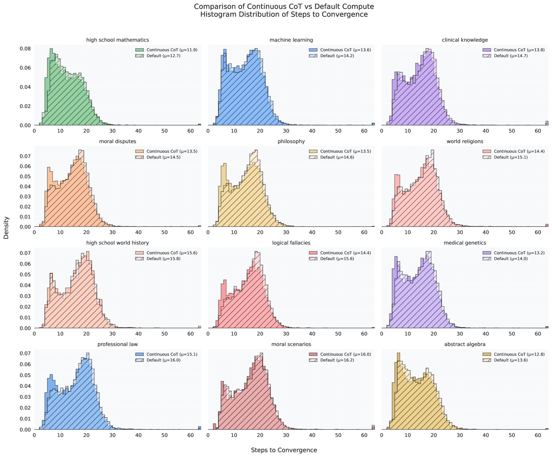
### Visual Description
## Histogram Grid: Comparison of Continuous CoT vs Default Compute
### Overview
The image displays a 4x3 grid of 12 histogram plots. Each plot compares the distribution of "Steps to Convergence" for two computational methods—"Continuous CoT" (Chain-of-Thought) and "Default"—across different academic and knowledge domains. The overall title is "Comparison of Continuous CoT vs Default Compute" with a subtitle "Histogram Distribution of Steps to Convergence." The visualization aims to show how the number of steps required for a model to converge on an answer differs between the two methods across various subjects.
### Components/Axes
* **Overall Layout:** A grid of 12 subplots arranged in 4 rows and 3 columns.
* **X-Axis (Common to all plots):** Labeled "Steps to Convergence" at the bottom of the grid. The scale runs from 0 to 60, with major ticks at 0, 10, 20, 30, 40, 50, and 60.
* **Y-Axis (Common label, varying scales):** Labeled "Density" on the left side of the grid. The scale represents probability density.
* Row 1 (top): Scale from 0.00 to 0.08.
* Rows 2, 3, and 4: Scale from 0.00 to 0.07.
* **Legends:** Each subplot contains a legend in its top-right corner. The legend identifies two data series:
1. **Continuous CoT:** Represented by a solid-colored histogram bar. The legend includes the mean (μ) value for this distribution.
2. **Default:** Represented by a hatched (diagonal lines) histogram bar of a similar but slightly different shade. The legend includes the mean (μ) value for this distribution.
* **Subplot Titles:** Each subplot has a title at its top center, indicating the subject domain.
### Detailed Analysis
Below is a breakdown of each subplot, listed in order from left to right, top to bottom.
**Row 1:**
1. **Subject: high school mathematics**
* **Color Scheme:** Green.
* **Continuous CoT (μ=11.9):** Distribution peaks sharply between 5-10 steps, with a long tail extending to ~30 steps.
* **Default (μ=12.7):** Distribution is slightly broader and shifted right compared to Continuous CoT, peaking around 10 steps.
* **Trend:** Continuous CoT shows a lower mean and a distribution concentrated at lower step counts.
2. **Subject: machine learning**
* **Color Scheme:** Blue.
* **Continuous CoT (μ=13.6):** Distribution is broad, peaking between 10-20 steps.
* **Default (μ=14.2):** Very similar shape to Continuous CoT but slightly shifted right.
* **Trend:** Minimal difference between methods; both have similar spread and central tendency.
3. **Subject: clinical knowledge**
* **Color Scheme:** Purple.
* **Continuous CoT (μ=13.8):** Distribution peaks around 15 steps.
* **Default (μ=14.7):** Distribution is similar but shifted slightly to the right.
* **Trend:** Continuous CoT has a modestly lower mean.
**Row 2:**
4. **Subject: moral disputes**
* **Color Scheme:** Orange.
* **Continuous CoT (μ=13.5):** Distribution is bimodal, with a smaller peak near 5 steps and a larger peak around 15-20 steps.
* **Default (μ=14.5):** Similar bimodal shape but the main peak is slightly right-shifted.
* **Trend:** Continuous CoT reduces the mean steps, particularly affecting the main cluster of the distribution.
5. **Subject: philosophy**
* **Color Scheme:** Yellow/Ochre.
* **Continuous CoT (μ=13.5):** Distribution is broad and somewhat flat-topped between 10-20 steps.
* **Default (μ=14.6):** Similar broad shape, shifted right.
* **Trend:** Continuous CoT provides a consistent, moderate reduction in steps.
6. **Subject: world religions**
* **Color Scheme:** Pink/Salmon.
* **Continuous CoT (μ=14.4):** Distribution peaks around 15-20 steps.
* **Default (μ=15.1):** Distribution is similar but shifted right.
* **Trend:** Small but consistent reduction in mean steps with Continuous CoT.
**Row 3:**
7. **Subject: high school world history**
* **Color Scheme:** Light Red.
* **Continuous CoT (μ=15.6):** Distribution is broad, peaking around 20 steps.
* **Default (μ=15.8):** Nearly identical distribution to Continuous CoT.
* **Trend:** Almost no discernible difference between the two methods for this subject.
8. **Subject: logical fallacies**
* **Color Scheme:** Red.
* **Continuous CoT (μ=14.4):** Distribution peaks around 15 steps.
* **Default (μ=15.6):** Distribution is shifted right, with a peak closer to 20 steps.
* **Trend:** Continuous CoT shows a clear reduction in the number of steps needed.
9. **Subject: medical genetics**
* **Color Scheme:** Lavender.
* **Continuous CoT (μ=13.2):** Distribution is broad, peaking between 10-20 steps.
* **Default (μ=14.0):** Similar shape, shifted right.
* **Trend:** Continuous CoT offers a moderate improvement.
**Row 4:**
10. **Subject: professional law**
* **Color Scheme:** Steel Blue.
* **Continuous CoT (μ=15.1):** Distribution is broad, peaking around 20 steps.
* **Default (μ=16.0):** Distribution is shifted right, with a peak slightly past 20 steps.
* **Trend:** Continuous CoT reduces the mean steps.
11. **Subject: moral scenarios**
* **Color Scheme:** Dark Pink.
* **Continuous CoT (μ=16.0):** Distribution peaks around 20 steps.
* **Default (μ=16.2):** Nearly identical distribution to Continuous CoT.
* **Trend:** Very minimal difference between methods.
12. **Subject: abstract algebra**
* **Color Scheme:** Gold.
* **Continuous CoT (μ=12.8):** Distribution is broad, peaking between 10-20 steps.
* **Default (μ=13.6):** Similar shape, shifted right.
* **Trend:** Continuous CoT provides a moderate reduction in steps.
### Key Observations
1. **Consistent Pattern:** In 11 out of 12 subjects, the "Continuous CoT" method has a lower mean (μ) number of steps to convergence than the "Default" method. The only near-exception is "high school world history," where the means are almost equal (15.6 vs 15.8).
2. **Magnitude of Improvement:** The reduction in mean steps varies by subject. The largest observed difference is in "logical fallacies" (Δμ = 1.2 steps). The smallest non-zero difference is in "moral scenarios" (Δμ = 0.2 steps).
3. **Distribution Shape:** All distributions are right-skewed, indicating that while most problems converge within 10-25 steps, a long tail of problems requires significantly more steps (up to 60).
4. **Visual Confirmation:** In every plot, the solid-colored histogram (Continuous CoT) is visually shifted to the left relative to the hatched histogram (Default), corroborating the lower mean values listed in the legends.
### Interpretation
This data suggests that employing a "Continuous Chain-of-Thought" (CoT) reasoning method generally leads to more efficient problem-solving, requiring fewer computational steps to reach a convergent answer compared to a "Default" method. The benefit is domain-dependent, showing clear gains in subjects like logical fallacies, mathematics, and law, while being negligible in areas like world history and moral scenarios.
The right-skewed nature of all distributions is a critical finding. It implies that problem difficulty (as measured by steps to convergence) is not normally distributed; a subset of problems is inherently more complex and computationally expensive, regardless of the method used. The primary effect of Continuous CoT appears to be shifting the central mass of the distribution leftward, making the "typical" problem easier to solve, but it does not eliminate the long tail of difficult problems.
From a systems perspective, adopting Continuous CoT could lead to meaningful reductions in average computational cost and latency across a wide range of tasks. However, the variability in improvement highlights the importance of domain-specific evaluation when implementing such techniques. The near-identical results in some domains may indicate that the Default method is already near-optimal for those problem types, or that the Continuous CoT approach does not align well with the reasoning patterns required.
</details>
Figure 13: Additional categories for Figure 10 in the main body.
Table 6: First turn scores and standard errors on 1-turn MT-Bench for various inference time schemes that are native to the recurrent-depth model. Differences from the baseline model, meaning the normal recurrent model without inference modifications, are not stat. significant.
| cache compression, $s=4$ baseline, 64 iterations cache compression, $s=16$ | 5.856 5.693 5.687 | 0.395 0.386 0.402 |
| --- | --- | --- |
| baseline, 32 iterations | 5.662 | 0.388 |
| cache compression, $s=8$ | 5.631 | 0.384 |
| KL exit, $t=$5×{10}^-4$$ | 5.562 | 0.389 |
## Appendix A Additional Information
<details>
<summary>x18.png Details</summary>
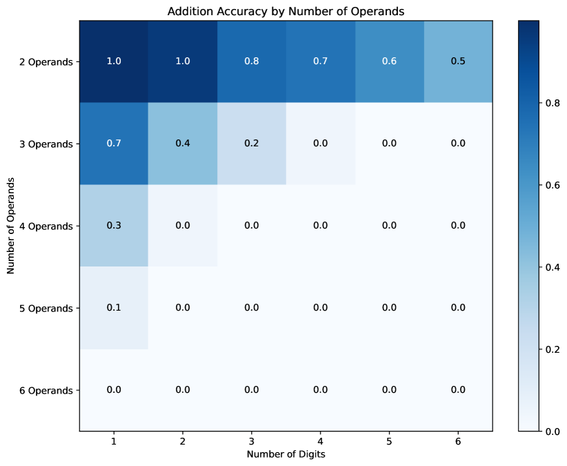
### Visual Description
## Heatmap: Addition Accuracy by Number of Operands
### Overview
The image is a heatmap titled "Addition Accuracy by Number of Operands." It visualizes the accuracy (ranging from 0.0 to 1.0) of a system performing addition problems, categorized by the number of operands (rows) and the number of digits per operand (columns). The color intensity, from dark blue (high accuracy) to white (zero accuracy), corresponds to the numerical accuracy score displayed in each cell.
### Components/Axes
* **Title:** "Addition Accuracy by Number of Operands" (centered at the top).
* **Y-Axis (Vertical):** Labeled "Number of Operands." It contains five categorical rows: "2 Operands", "3 Operands", "4 Operands", "5 Operands", and "6 Operands".
* **X-Axis (Horizontal):** Labeled "Number of Digits." It contains six categorical columns labeled with the integers 1, 2, 3, 4, 5, and 6.
* **Color Bar/Legend:** Positioned vertically on the right side of the chart. It maps color to accuracy values, with a scale from 0.0 (white) to approximately 1.0 (dark blue). Major tick marks are at 0.0, 0.2, 0.4, 0.6, and 0.8.
* **Data Cells:** A 5x6 grid where each cell contains a numerical accuracy value and is colored according to the legend.
### Detailed Analysis
The following table reconstructs the data from the heatmap. Values are read directly from the cells.
| Number of Operands | 1 Digit | 2 Digits | 3 Digits | 4 Digits | 5 Digits | 6 Digits |
| :--- | :--- | :--- | :--- | :--- | :--- | :--- |
| **2 Operands** | 1.0 | 1.0 | 0.8 | 0.7 | 0.6 | 0.5 |
| **3 Operands** | 0.7 | 0.4 | 0.2 | 0.0 | 0.0 | 0.0 |
| **4 Operands** | 0.3 | 0.0 | 0.0 | 0.0 | 0.0 | 0.0 |
| **5 Operands** | 0.1 | 0.0 | 0.0 | 0.0 | 0.0 | 0.0 |
| **6 Operands** | 0.0 | 0.0 | 0.0 | 0.0 | 0.0 | 0.0 |
**Trend Verification:**
* **Row Trend (Fixed Operands, Increasing Digits):** For any given number of operands, accuracy **decreases** as the number of digits increases. The slope is steepest for 2 and 3 operands.
* **Column Trend (Fixed Digits, Increasing Operands):** For any given number of digits, accuracy **decreases** as the number of operands increases. The drop is precipitous after 2 operands.
### Key Observations
1. **Perfect Performance Zone:** The system achieves perfect accuracy (1.0) only for the simplest problems: adding 2 operands that are 1 or 2 digits long.
2. **Sharp Performance Cliff:** There is a dramatic drop in accuracy when moving from 2 to 3 operands. For example, with 1-digit numbers, accuracy falls from 1.0 to 0.7.
3. **Complete Failure Threshold:** For problems involving 6 operands, accuracy is 0.0 across all digit lengths. For 5 operands, accuracy is only non-zero (0.1) for 1-digit numbers.
4. **Digit Length Impact:** The negative impact of adding more digits is most pronounced for 2 and 3 operands. For 4 or more operands, accuracy is already at or near zero for most digit lengths, so adding digits has little visible effect.
5. **Asymmetry of Difficulty:** Adding a third operand appears to be a significantly harder task for the system than increasing the digit length of a 2-operand problem. For instance, 2 operands with 6 digits (accuracy 0.5) is handled better than 3 operands with 1 digit (accuracy 0.7) or 2 digits (accuracy 0.4).
### Interpretation
This heatmap demonstrates a clear and severe limitation in the evaluated system's arithmetic reasoning capabilities. The data suggests the system's "working memory" or procedural logic for addition is highly constrained.
* **Core Limitation:** The primary bottleneck is the **number of operands**, not the digit length. The system can handle multi-digit numbers reasonably well if only adding two of them, but its performance collapses when required to sum three or more numbers. This indicates a potential failure in managing intermediate sums or in the sequential execution of multiple addition operations.
* **Cognitive Load Analogy:** The pattern mirrors a cognitive load theory model. The task's difficulty increases multiplicatively with both operands and digits, but the system hits a hard capacity limit at around 3 operands, beyond which it fails almost completely.
* **Practical Implication:** The system is reliable only for very basic arithmetic (2-operand addition of small numbers). It is not suitable for more complex calculations, such as summing a list of numbers or handling financial calculations with multiple line items. The perfect 1.0 scores for the simplest cases confirm the system understands the basic operation, but the rapid degradation reveals it lacks the robustness needed for general-purpose arithmetic.
</details>
<details>
<summary>x19.png Details</summary>
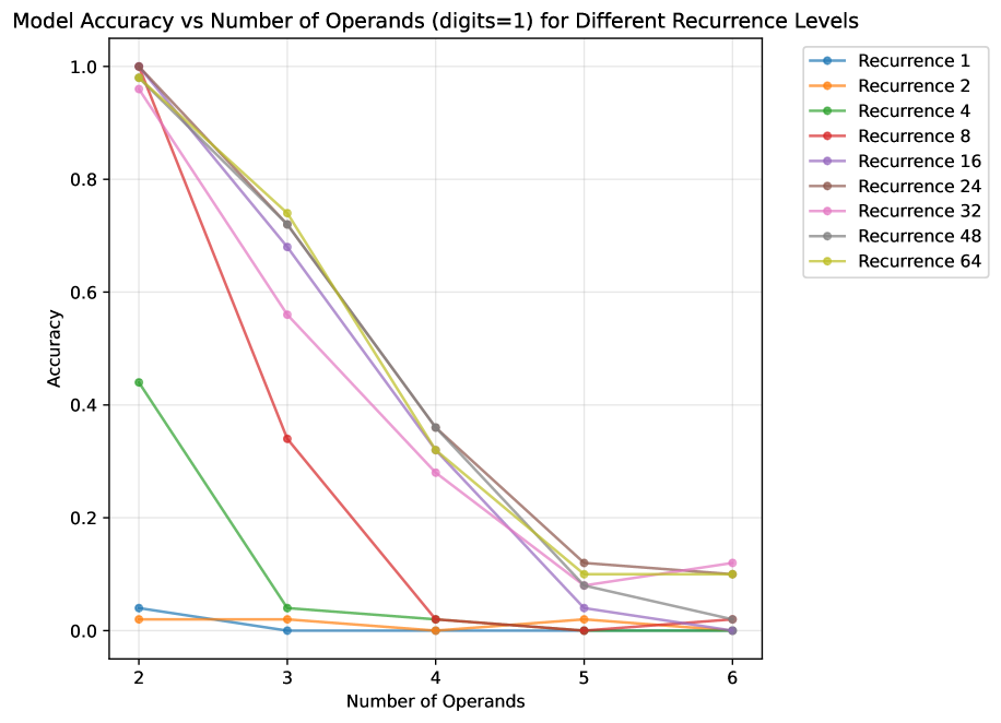
### Visual Description
## Line Chart: Model Accuracy vs Number of Operands (digits=1) for Different Recurrence Levels
### Overview
This is a line chart plotting model accuracy against the number of operands for a task involving single-digit numbers. The chart compares the performance of models configured with nine different "Recurrence Levels." The overall trend shows a sharp decline in accuracy as the number of operands increases for all but the lowest recurrence levels.
### Components/Axes
* **Chart Title:** "Model Accuracy vs Number of Operands (digits=1) for Different Recurrence Levels"
* **X-Axis:**
* **Label:** "Number of Operands"
* **Scale:** Linear, with major tick marks at integers 2, 3, 4, 5, and 6.
* **Y-Axis:**
* **Label:** "Accuracy"
* **Scale:** Linear, ranging from 0.0 to 1.0, with major tick marks at 0.0, 0.2, 0.4, 0.6, 0.8, and 1.0.
* **Legend:** Positioned in the top-right corner, outside the main plot area. It lists nine data series, each associated with a unique color and marker:
1. Recurrence 1 (Blue, circle marker)
2. Recurrence 2 (Orange, circle marker)
3. Recurrence 4 (Green, circle marker)
4. Recurrence 8 (Red, circle marker)
5. Recurrence 16 (Purple, circle marker)
6. Recurrence 24 (Brown, circle marker)
7. Recurrence 32 (Pink, circle marker)
8. Recurrence 48 (Gray, circle marker)
9. Recurrence 64 (Yellow-green, circle marker)
### Detailed Analysis
The chart displays nine data series, each representing a different recurrence level. All series are plotted with lines connecting circular data points at each integer value on the x-axis.
**Trend Verification & Data Points (Approximate):**
* **Recurrence 1 (Blue):** The line is nearly flat and very close to the bottom of the chart. Accuracy starts at ~0.04 for 2 operands and remains at or near 0.0 for 3, 4, 5, and 6 operands.
* **Recurrence 2 (Orange):** Similar to Recurrence 1, this line is flat and near zero. Accuracy is ~0.02 for 2 operands and ~0.0 for 3, 4, 5, and 6 operands.
* **Recurrence 4 (Green):** Shows a steep downward slope. Accuracy starts at ~0.44 for 2 operands, drops sharply to ~0.04 for 3 operands, and then declines slowly to ~0.02 for 4 operands and ~0.0 for 5 and 6 operands.
* **Recurrence 8 (Red):** Exhibits a very steep downward slope. Accuracy is high at ~1.0 for 2 operands, plummets to ~0.34 for 3 operands, falls further to ~0.02 for 4 operands, and is ~0.0 for 5 and 6 operands.
* **Recurrence 16 (Purple):** Shows a steep downward slope. Accuracy starts at ~0.98 for 2 operands, decreases to ~0.68 for 3 operands, ~0.28 for 4 operands, ~0.04 for 5 operands, and ~0.0 for 6 operands.
* **Recurrence 24 (Brown):** Follows a steep downward trajectory. Accuracy is ~0.99 for 2 operands, ~0.72 for 3 operands, ~0.36 for 4 operands, ~0.12 for 5 operands, and ~0.02 for 6 operands.
* **Recurrence 32 (Pink):** Displays a steep downward slope. Accuracy is ~0.96 for 2 operands, ~0.56 for 3 operands, ~0.28 for 4 operands, ~0.08 for 5 operands, and ~0.12 for 6 operands (a slight uptick).
* **Recurrence 48 (Gray):** Shows a steep downward slope. Accuracy is ~0.99 for 2 operands, ~0.72 for 3 operands, ~0.36 for 4 operands, ~0.08 for 5 operands, and ~0.02 for 6 operands.
* **Recurrence 64 (Yellow-green):** Exhibits a steep downward slope. Accuracy is ~0.99 for 2 operands, ~0.74 for 3 operands, ~0.32 for 4 operands, ~0.10 for 5 operands, and ~0.10 for 6 operands.
### Key Observations
1. **Universal Performance Degradation:** All models, regardless of recurrence level, experience a significant drop in accuracy as the number of operands increases from 2 to 6.
2. **Recurrence Level Impact:** Higher recurrence levels (16, 24, 32, 48, 64) start with near-perfect accuracy (~0.96-1.0) for 2 operands, while lower levels (1, 2, 4) start much lower or near zero.
3. **Convergence at High Complexity:** By 5 and 6 operands, the accuracy of all models converges to a low range (approximately 0.0 to 0.12), with the exception of Recurrence 32 at 6 operands (~0.12).
4. **Steepness of Decline:** The rate of accuracy loss is most dramatic for models that start with high accuracy (Recurrence 8 and above). For example, Recurrence 8 drops from ~1.0 to ~0.34 with just one additional operand.
5. **Anomaly:** The data point for Recurrence 32 at 6 operands (~0.12) is slightly higher than its value at 5 operands (~0.08), breaking the consistent downward trend seen in all other series. This could be a measurement artifact or a point of interest.
### Interpretation
The data demonstrates a clear inverse relationship between task complexity (number of operands) and model accuracy for this single-digit arithmetic task. The "Recurrence Level" appears to be a critical hyperparameter that determines the model's initial capacity: higher recurrence enables near-perfect performance on the simplest task (2 operands).
However, this capacity is fragile. The steep, consistent decline across all series suggests a fundamental limitation in the model's architecture or training when generalizing to more complex problems of the same type. The convergence of all models to low accuracy at 5-6 operands indicates that increasing recurrence alone is insufficient to solve the core challenge of scaling to more operands. The model likely lacks the necessary mechanism (e.g., robust working memory, systematic compositional reasoning) to handle the increased computational or representational load, regardless of its initial recurrent depth. The slight uptick for Recurrence 32 at 6 operands is intriguing but too minor to contradict the overwhelming trend; it would require replication to interpret as a meaningful signal rather than noise.
</details>
<details>
<summary>x20.png Details</summary>
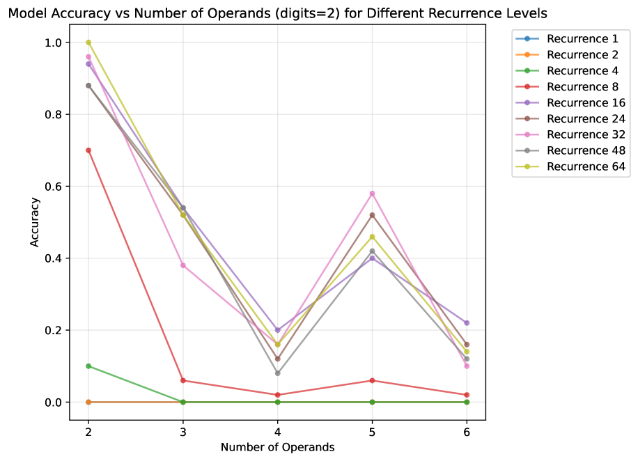
### Visual Description
\n
## Line Chart: Model Accuracy vs Number of Operands (digits=2) for Different Recurrence Levels
### Overview
This is a line chart comparing the accuracy of a model across different numbers of operands (from 2 to 6) for nine distinct "Recurrence" levels. The chart demonstrates how model performance varies with problem complexity (number of operands) and a hyperparameter labeled "Recurrence." The overall trend shows a significant drop in accuracy as the number of operands increases from 2 to 4, followed by a partial recovery at 5 operands, and another decline at 6 operands for most recurrence levels.
### Components/Axes
* **Chart Title:** "Model Accuracy vs Number of Operands (digits=2) for Different Recurrence Levels"
* **X-Axis:**
* **Label:** "Number of Operands"
* **Scale:** Discrete integer values: 2, 3, 4, 5, 6.
* **Y-Axis:**
* **Label:** "Accuracy"
* **Scale:** Linear scale from 0.0 to 1.0, with major gridlines at intervals of 0.2.
* **Legend:** Positioned at the top-right of the chart area. It lists nine data series, each corresponding to a "Recurrence" level, identified by a unique color and marker (circle).
* Recurrence 1 (Blue)
* Recurrence 2 (Orange)
* Recurrence 4 (Green)
* Recurrence 8 (Red)
* Recurrence 16 (Purple)
* Recurrence 24 (Brown)
* Recurrence 32 (Pink)
* Recurrence 48 (Gray)
* Recurrence 64 (Yellow-Green/Olive)
### Detailed Analysis
The following describes each data series' visual trend and approximate data points, verified by color against the legend.
1. **Recurrence 1 (Blue):**
* **Trend:** Starts very high, drops sharply, then fluctuates at low accuracy.
* **Data Points:** (2, ~0.94), (3, ~0.54), (4, ~0.20), (5, ~0.40), (6, ~0.22).
2. **Recurrence 2 (Orange):**
* **Trend:** Flatline at near-zero accuracy across all operand counts.
* **Data Points:** (2, ~0.00), (3, ~0.00), (4, ~0.00), (5, ~0.00), (6, ~0.00).
3. **Recurrence 4 (Green):**
* **Trend:** Starts low, drops to zero, and remains flat.
* **Data Points:** (2, ~0.10), (3, ~0.00), (4, ~0.00), (5, ~0.00), (6, ~0.00).
4. **Recurrence 8 (Red):**
* **Trend:** Starts moderately high, drops sharply, and remains very low.
* **Data Points:** (2, ~0.70), (3, ~0.06), (4, ~0.02), (5, ~0.06), (6, ~0.02).
5. **Recurrence 16 (Purple):**
* **Trend:** Starts very high, drops, recovers partially, then declines.
* **Data Points:** (2, ~0.94), (3, ~0.54), (4, ~0.20), (5, ~0.40), (6, ~0.22).
6. **Recurrence 24 (Brown):**
* **Trend:** Starts very high, drops, recovers significantly, then declines.
* **Data Points:** (2, ~0.88), (3, ~0.52), (4, ~0.12), (5, ~0.52), (6, ~0.16).
7. **Recurrence 32 (Pink):**
* **Trend:** Starts very high, drops, recovers to the highest peak at 5 operands, then declines sharply.
* **Data Points:** (2, ~0.96), (3, ~0.38), (4, ~0.16), (5, ~0.58), (6, ~0.10).
8. **Recurrence 48 (Gray):**
* **Trend:** Starts very high, drops, recovers, then declines.
* **Data Points:** (2, ~0.88), (3, ~0.52), (4, ~0.08), (5, ~0.42), (6, ~0.12).
9. **Recurrence 64 (Yellow-Green/Olive):**
* **Trend:** Starts at the maximum (1.0), drops, recovers, then declines.
* **Data Points:** (2, 1.00), (3, ~0.52), (4, ~0.16), (5, ~0.46), (6, ~0.14).
### Key Observations
* **Universal Difficulty Spike at 4 Operands:** All models, regardless of recurrence level, experience their lowest or near-lowest accuracy at 4 operands, indicating a specific complexity threshold that is challenging for this model architecture.
* **Partial Recovery at 5 Operands:** Most models show a notable rebound in accuracy when moving from 4 to 5 operands, suggesting the difficulty is not strictly monotonic with operand count.
* **Recurrence Level Impact:** Higher recurrence levels (16, 24, 32, 48, 64) generally achieve higher peak accuracies (especially at 2 and 5 operands) compared to lower levels (1, 2, 4, 8). Recurrence 2 and 4 perform very poorly overall.
* **Outlier - Recurrence 32:** This series achieves the highest accuracy at 5 operands (~0.58) among all series at that point, despite not having the highest starting accuracy.
* **Convergence at Low Accuracy:** For 3 and 4 operands, the performance of many higher-recurrence models converges into a narrow band (approx. 0.08 to 0.54), showing less differentiation at these points.
### Interpretation
The data suggests that the model's ability to solve arithmetic problems (with 2-digit numbers) is highly sensitive to both the number of operands and the configured recurrence depth. The "Recurrence" hyperparameter likely controls the number of iterative processing steps the model can perform.
* **Insufficient Recurrence (Levels 1, 2, 4, 8):** These models lack the computational depth to handle the task, resulting in poor or zero accuracy, especially as complexity grows. Recurrence 2 and 4 appear to be fundamentally inadequate for this task.
* **Sufficient Recurrence (Levels 16+):** These models demonstrate a capacity for the task, but their performance is non-linear. The sharp drop at 4 operands could indicate a point where the problem structure becomes qualitatively harder, perhaps requiring a type of reasoning or memory access that the model struggles with at that specific complexity. The recovery at 5 operands is intriguing and might suggest that problems with 5 operands have a different, more manageable structure for the model than those with 4.
* **Practical Implication:** There is a clear trade-off. Increasing recurrence improves potential accuracy but likely comes with higher computational cost. The optimal recurrence level depends on the expected operand count in deployment. For problems consistently around 2 or 5 operands, higher recurrence (e.g., 32, 64) is beneficial. For problems with 3 or 4 operands, even high recurrence yields modest gains, suggesting a fundamental model limitation at those complexities. The chart provides a guide for hyperparameter tuning based on the target problem distribution.
</details>
<details>
<summary>x21.png Details</summary>
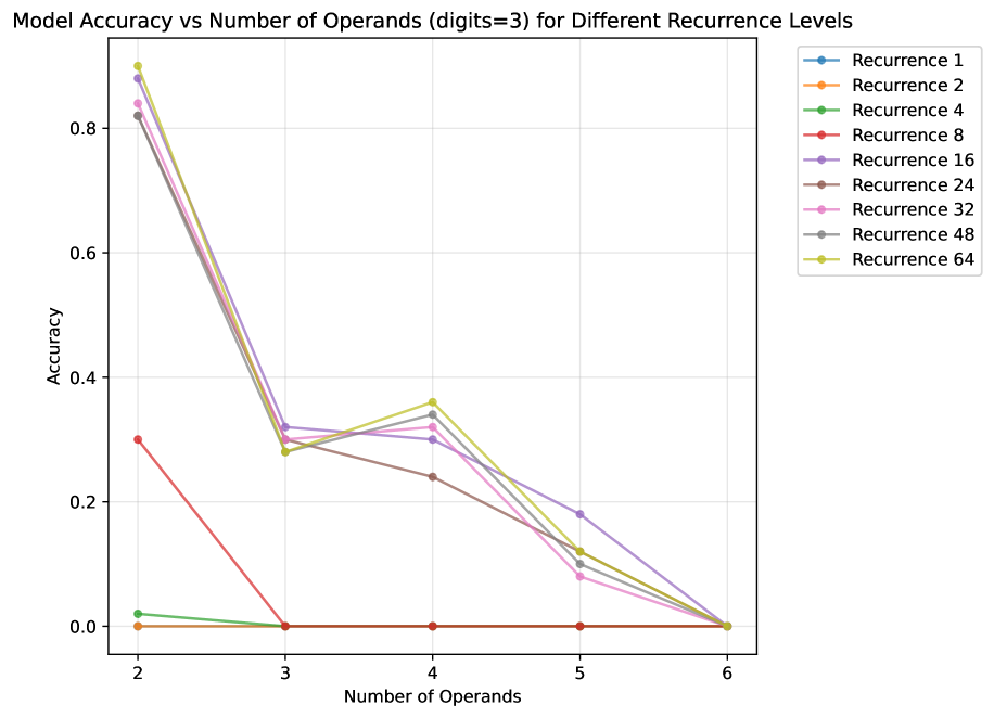
### Visual Description
## Line Chart: Model Accuracy vs Number of Operands (digits=3) for Different Recurrence Levels
### Overview
This is a line chart illustrating the relationship between a model's accuracy and the number of operands in a task (with digits fixed at 3), across nine different "Recurrence Level" configurations. The chart shows a general trend where accuracy decreases as the number of operands increases, with higher recurrence levels starting at much higher accuracy for simpler tasks but also degrading significantly.
### Components/Axes
* **Chart Title:** "Model Accuracy vs Number of Operands (digits=3) for Different Recurrence Levels"
* **X-Axis:** Labeled "Number of Operands". It has discrete markers at the integer values: 2, 3, 4, 5, and 6.
* **Y-Axis:** Labeled "Accuracy". It is a linear scale ranging from 0.0 to approximately 0.9, with major gridlines at intervals of 0.2 (0.0, 0.2, 0.4, 0.6, 0.8).
* **Legend:** Positioned in the top-right corner, outside the main plot area. It lists nine data series, each corresponding to a "Recurrence" level, identified by a unique color and marker (a filled circle).
* Recurrence 1 (Blue)
* Recurrence 2 (Orange)
* Recurrence 4 (Green)
* Recurrence 8 (Red)
* Recurrence 16 (Purple)
* Recurrence 24 (Brown)
* Recurrence 32 (Pink)
* Recurrence 48 (Gray)
* Recurrence 64 (Yellow-Green)
### Detailed Analysis
**Data Series Trends and Approximate Values:**
* **Low Recurrence Levels (1, 2, 4, 8):** These series show very low accuracy overall.
* **Recurrence 1 (Blue):** Starts at ~0.0 accuracy for 2 operands and remains at 0.0 for all subsequent operand counts (3, 4, 5, 6).
* **Recurrence 2 (Orange):** Follows an identical flat trend at 0.0 accuracy across all operand counts.
* **Recurrence 4 (Green):** Starts slightly above 0.0 (~0.02) at 2 operands, drops to 0.0 at 3 operands, and remains at 0.0 thereafter.
* **Recurrence 8 (Red):** Starts at a moderate accuracy of ~0.30 for 2 operands. It then drops sharply to 0.0 at 3 operands and remains at 0.0 for 4, 5, and 6 operands.
* **High Recurrence Levels (16, 24, 32, 48, 64):** These series follow a similar pattern: high initial accuracy, a steep drop, a partial recovery, then a final decline.
* **Common Pattern:** All start with high accuracy at 2 operands (ranging from ~0.82 to ~0.90). They experience a dramatic drop at 3 operands (to a range of ~0.28 to ~0.32). At 4 operands, most show a slight recovery or plateau. Accuracy then declines again at 5 operands, and all converge to 0.0 accuracy at 6 operands.
* **Recurrence 64 (Yellow-Green):** The highest performer initially. Starts at ~0.90 (2 operands), drops to ~0.28 (3), recovers to the series' peak at ~0.36 (4), falls to ~0.12 (5), and ends at 0.0 (6).
* **Recurrence 48 (Gray):** Starts at ~0.88 (2), drops to ~0.31 (3), rises to ~0.34 (4), falls to ~0.11 (5), ends at 0.0 (6).
* **Recurrence 32 (Pink):** Starts at ~0.85 (2), drops to ~0.30 (3), rises slightly to ~0.32 (4), falls to ~0.08 (5), ends at 0.0 (6).
* **Recurrence 24 (Brown):** Starts at ~0.82 (2), drops to ~0.31 (3), then declines steadily to ~0.24 (4), ~0.12 (5), and 0.0 (6). It does not show the recovery at 4 operands seen in others.
* **Recurrence 16 (Purple):** Starts at ~0.83 (2), drops to ~0.32 (3), holds near ~0.30 (4), then declines to ~0.18 (5) and 0.0 (6). It maintains the highest accuracy among all series at 5 operands.
### Key Observations
1. **Performance Threshold:** There is a clear performance cliff. Models with recurrence levels of 8 or below fail almost completely (accuracy at or near 0.0) for tasks with 3 or more operands.
2. **The "3-Operand Dip":** All high-recurrence models experience their most severe relative performance drop when moving from 2 to 3 operands.
3. **The "4-Operand Bump":** Most high-recurrence models (except Recurrence 24) show a slight accuracy improvement or stabilization when moving from 3 to 4 operands, suggesting a possible non-linear difficulty curve in the task.
4. **Universal Failure Point:** All models, regardless of recurrence level, achieve 0.0 accuracy when tasked with 6 operands, indicating a fundamental limit of the model architecture or training for this specific problem complexity.
5. **Recurrence Correlation:** Higher recurrence levels generally correlate with higher accuracy, but only up to a point. The benefit is most pronounced for simpler tasks (2 operands). For complex tasks (5-6 operands), the advantage of higher recurrence diminishes significantly.
### Interpretation
This chart demonstrates the critical role of recurrence (likely referring to the number of processing steps or layers in a recurrent neural network or similar architecture) in solving compositional tasks. The data suggests:
* **Recurrence Enables Compositionality:** Higher recurrence allows the model to handle the basic composition of two operands effectively. The near-zero performance of low-recurrence models indicates they lack the capacity to perform even this basic step.
* **Complexity Scaling is Non-Linear:** The sharp drop at 3 operands and the bump at 4 suggest the task difficulty does not increase linearly with operand count. There may be a specific cognitive or computational hurdle at 3 operands that some models can partially overcome with more steps (the bump at 4), but which becomes insurmountable at 5 or 6 operands.
* **Architectural Limits:** The universal failure at 6 operands points to a hard limit. This could be due to vanishing/exploding gradients in a recurrent system, a fixed context window being exceeded, or the training data not containing sufficient examples of this complexity. The model's "working memory" or "reasoning depth" appears capped at handling around 4-5 operands for this specific 3-digit task.
* **Practical Implication:** For applications requiring arithmetic or logical operations on more than 4-5 items, this model architecture, even with high recurrence, is unreliable. A different approach (e.g., a transformer with larger context, or a neuro-symbolic system) may be necessary.
</details>
Figure 14: Multi-Operand Arithmetic. Following a precedent of training recurrent architectures for algorithmic and arithmetic tasks (Schwarzschild et al., 2021b; Bansal et al., 2022; Schwarzschild et al., 2023; McLeish et al., 2024), we explore whether our model can leverage increased test-time compute via recurrence to solve verbalized addition problems of increased difficulty. For these problems we use the following system prompt ‘‘You are a helpful assistant that is capable of helping users with mathematical reasoning.’’ embedded in a conversational chat template, and we present each problem by opening the first user turn of the conversation like so: f"What is the result of ’ + ’.join(map(str, digits))?" after randomly sampling numbers according to a certain operand count and digit count (base 10). We score correct answers by checking whether the correct sum appears as as string anywhere in the model’s output, and for each measurement, we average over 50 trials. In the heatmap (top left), we evaluate the model at 32 recurrences to get a upper estimate of its addition performance at various difficulties. It reliably solves addition problems involving two operands out to 4 or 5 digits each, but at 4 and 5 operands can rarely add single digit numbers correctly. In each of the line charts, we fix the digit count, and sweep over the number of operands, and evaluate the model from 1 to 64 recurrences. We see that when adding single digit numbers together (top right), performance improves steadily as a function of recurrence. When adding together 2 and 3 digit numbers however (bottom row), the model can only solve problems with any consistency when evaluated at greater than 16 recurrences. Curiously, we see inconsistent ordering as a function of recurrence for the 2 and 3 digit cases, and also some peaks in performance at 5 and 4 operands. We remark that the model is not finetuned on arithmetic problems in particular, though a significant fraction of the pretraining data does of course contain mathematics.
## Potential Implications of This Work
This work describes a novel architecture and training objective for language modeling with promising performance, especially on tasks that require the model to reason. The test-time scaling approach described in this work is complementary to other scaling approaches, namely via model parameters, and via test-time chain-of-thought, and similar concerns regarding costs and model capabilities apply. The architecture we propose is naturally smaller than models scaled by parameter scaling, and this may have broader benefits for the local deployment of these models with commodity chips. Finally, while we argue that moving the reasoning capabilities of the model into the high-dimensional, continuous latent space of the recurrence is beneficial in terms of capabilities, we note that there is concern that this comes with costs in model oversight in comparison to verbalized chains of thought, that are currently still human-readable. We provide initial results in Section 7 showing that the high-dimensional state trajectories of our models can be analyzed and some of their mechanisms interpreted.
### A.1 Classical Reasoning Problems
We include a small study of the classical problem of multi-operand arithmetic in Figure 14.
### A.2 Implementation Details
#### Device Speed Details
Nominally, each MI250X (AMD, 2021) achieves 383 TFLOP in bfloat16, i.e. 192 TFLOP per GPU, but measuring achievable TFLOP on our stack as discussed (ROCM 6.2.0, PyTorch 2.6 pre-release 11/02) for arbitrary matrix multiplication shapes (i.e. we measure the peak achievable speed of the best possible shape iterating over shapes between 256 and 24576 in intervals of 256 and 110 (Bekman, 2023)), we measure a peak of 125 TFLOP/s on Frontier nodes. Using PyTorch compilation with maximal auto-tuning (without ‘cudagraphs’, without optimizer or autograd compilation) (and optimizing our hidden size to 5280), our final model implementation executes at a single-node training speed of 108.75 TFLOP/s, i.e. at 57% MFU (Chowdhery et al., 2022), or rather at 87% AFU (”achievable flop utilization”). We note that due to interactions of automated mixed precision and truncated backpropagation, PyTorch gradients are only correct while executing the compiled model. We further circumvent issues with the flash attention implementation shipped with PyTorch sdpa using the AMD fork of the original flash attention repository https://github.com/Dao-AILab/flash-attention/, which can be found at https://github.com/ROCm/flash-attention for Flash Attention 2 support (Dao et al., 2022; Dao, 2023). We experiment with fused head and loss implementations https://github.com/JonasGeiping/linear_cross_entropy_loss, but ultimately find that the most portable choice on our AMD setup is to let torch compilation handle this issue.
#### Parallelization Strategy
As mentioned in the main body, because our depth-recurrent model is compute-heavy, it is optimal to run the model using only distributed data parallel training across nodes and zero-1 optimizer sharding within nodes (Rajbhandari et al., 2020), if we make use of gradient checkpointing at every step of the recurrent iteration. This allows us to eschew more communication-heavy parallelization strategies that would be required for models with the same FLOP footprint, but more parameters, which require substantial planning on this system (Singh et al., 2024; Singh and Bhatele, 2022). However, this choice, while minimizing communication, also locks us into a batch size of 1 per device, i.e. 4096 in total, and 16M tokens per step.
#### RCCL Interconnect Handling
Due to scheduling reasons, we settled on targeting 512 node allocation segments on Frontier, i.e. 4096 GPUs. However, this posed a substantial network interconnect issue. The connection speed between frontier nodes is only acceptable, if RCCL (AMD GPU communication collectives) commands are routed through open fabrics interface calls, which happens via a particular plugin https://github.com/ROCm/aws-ofi-rccl. To achieve sufficient bus bandwidth above 100GB/s requires NCCL_NET_GDR_LEVEL=PHB, a setting that, on NVIDIA systems, allows packages to go through the CPU, and only uses direct interconnect if GPU and NIC are on the same (NUMA) node (Wu and Stock, 2024). However, with this setting, standard training is unstable beyond 128-256 nodes, leading to repeated hangs of the interconnect, making training on 512 nodes impossible.
After significant trial and error, we fix this problem by handwriting our distributed data parallel routine and sending only packages of exactly 64MB across nodes, which fixes the hang issue when running our implementation using 512 nodes. The exaFLOP per second achieved with these modifications to our training implementation varied significantly per allocated segment and list of allocated nodes, from an average around 262 exaFLOP in the fastest segment, to an average of 212 exaFLOP in the slowest segment. This is a range of 52-64 TFLOP/s per GPU, i.e. 41%-51% AFU, or 1-1.2M tokens per second.
#### Pretraining Metrics.
During the pretraining run, we run a careful tracking of optimizer and model health metrics, tracking effective Adam learning rates per layer, optimizer RMS (Wortsman et al., 2023a), $L^2$ and $L^1$ parameter and gradient norms, recurrence statistics such as $\frac{||s_k-s_k-1||}{||s_k||}$ , $||s_k||$ , $||s_0-s_k||$ . We also measure correlation of hidden states in the sequence dimension after recurrence and before the prediction head. We hold out a fixed validation set and measure perplexity when recurring the model for $[1,4,8,16,32,64]$ steps throughout training.
## Appendix B Latent Space Visualizations
On the next pages, we print a number of latent space visualizations in more details than was possible in Section 7. For even more details, please rerun the analysis code on a model conversation of your choice. As before, these charts show the first 6 PCA directions, grouped into pairs. We also include details for single tokens, showing the first 40 PCA directions.
<details>
<summary>extracted/6211213/figures/latent_waterfall_C_bright.png Details</summary>
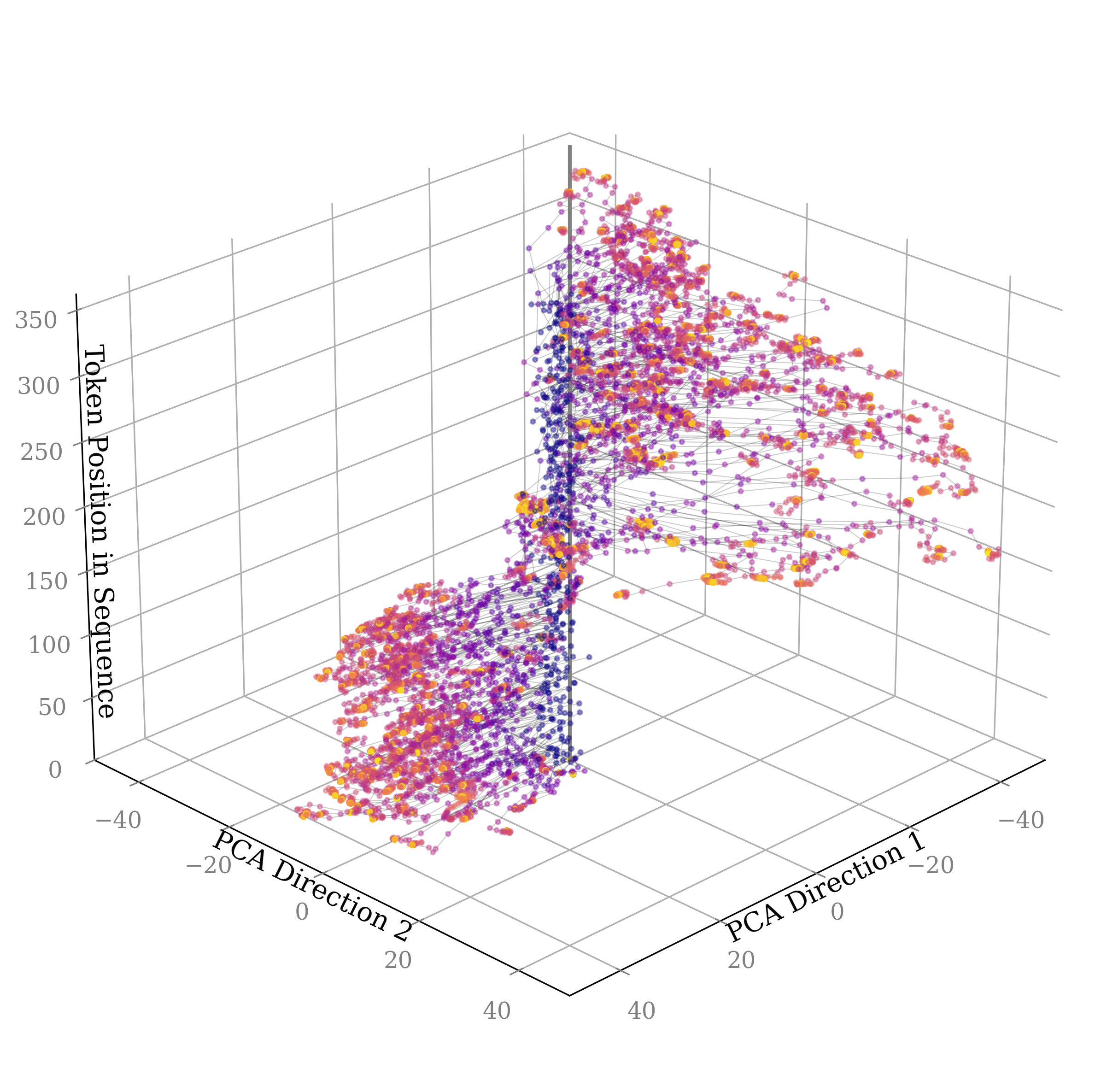
### Visual Description
## 3D Scatter Plot: Token Sequence Evolution in PCA Space
### Overview
The image displays a three-dimensional scatter plot with points connected by thin lines, visualizing the trajectory or distribution of data points across three dimensions. The plot appears to represent the evolution or state of sequential data (likely tokens from a language model) as they progress through a sequence, projected into a reduced-dimensional space via Principal Component Analysis (PCA). The data points form a dense, complex cloud that expands and changes shape as the sequence progresses.
### Components/Axes
* **Chart Type:** 3D Scatter Plot with connecting lines (a 3D line/scatter hybrid).
* **Axes:**
* **X-Axis (Bottom Right):** Labeled "PCA Direction 1". The scale runs from approximately -40 to 40, with major tick marks at -40, -20, 0, 20, 40.
* **Y-Axis (Bottom Left):** Labeled "PCA Direction 2". The scale runs from approximately -40 to 40, with major tick marks at -40, -20, 0, 20, 40.
* **Z-Axis (Vertical, Left Side):** Labeled "Token Position in Sequence". The scale runs from 0 to 350, with major tick marks at 0, 50, 100, 150, 200, 250, 300, 350.
* **Data Series & Legend:** There is **no explicit legend** provided in the image. The data points are colored on a gradient. The color appears to be mapped to the "Token Position in Sequence" (Z-axis value):
* **Lower Z-values (Token Position ~0-100):** Points are predominantly **dark purple/indigo**.
* **Mid Z-values (Token Position ~100-250):** Points transition through **magenta and pink**.
* **Higher Z-values (Token Position ~250-350):** Points are predominantly **orange and yellow**.
* **Spatial Grounding:** The plot is viewed from an isometric perspective. The Z-axis is vertical on the left. The X and Y axes form the floor plane, with "PCA Direction 1" extending to the right and "PCA Direction 2" extending to the left. The data cloud occupies the central volume of the plotted space.
### Detailed Analysis
* **Data Distribution & Trend:**
1. **At Low Token Positions (Z ≈ 0-100):** The data points (purple) are tightly clustered in a relatively small region of the PCA space. They are concentrated roughly between -20 to 20 on both PCA Direction 1 and PCA Direction 2. The connecting lines show a dense, localized network.
2. **At Mid Token Positions (Z ≈ 100-250):** As the token position increases, the cloud of points (now magenta/pink) begins to expand significantly, primarily along the "PCA Direction 1" axis. The spread on "PCA Direction 2" also increases but to a lesser degree. The structure becomes more diffuse and elongated.
3. **At High Token Positions (Z ≈ 250-350):** The points (orange/yellow) show the greatest dispersion. They span a wide range on "PCA Direction 1" (from approx. -30 to +40) and a moderate range on "PCA Direction 2" (from approx. -20 to +30). The overall shape resembles a widening plume or fan that originates from the dense cluster at the bottom.
* **Visual Trend Verification:** The primary visual trend is a clear **expansion of the data manifold** as the "Token Position in Sequence" increases. The system's state, as captured by the first two PCA components, explores a progressively larger region of the feature space as the sequence length grows. The trajectory is not a single line but a broad, evolving distribution.
### Key Observations
1. **Non-Linear Expansion:** The increase in variance is not linear. The most dramatic expansion in the PCA space occurs after approximately token position 100-150.
2. **Anisotropic Spread:** The expansion is not uniform in all directions. The spread along "PCA Direction 1" is noticeably greater than along "PCA Direction 2", suggesting that the primary axis of variation in the underlying data is captured more by the first principal component.
3. **Density Gradient:** The point density is highest at the lowest token positions and decreases as position increases, correlating with the color shift from purple to yellow.
4. **Connectivity:** The thin lines connecting points suggest a sequential or temporal relationship between states, tracing paths through the PCA space as the sequence unfolds.
### Interpretation
This visualization likely depicts the **internal state evolution of a sequential model** (e.g., a Transformer's token embeddings or hidden states) as it processes a long sequence. The PCA projection reduces the high-dimensional state vectors into 3 interpretable dimensions.
* **What it Suggests:** The data demonstrates that the model's representation of information becomes more diverse and complex as the sequence progresses. Early tokens (low position) exist in a constrained, similar state space. As more context is accumulated (higher position), the model's internal representations diverge significantly, occupying a much broader semantic or syntactic space. This could reflect the model building up complex, context-dependent meanings.
* **Relationship Between Elements:** The Z-axis (Token Position) acts as the independent variable driving change. The X and Y axes (PCA Directions) are dependent variables showing the effect. The color gradient reinforces the Z-axis trend, providing a visual cue for progression.
* **Notable Patterns/Anomalies:** The anisotropic spread (wider on PCA Direction 1) is a key pattern. It indicates that the most significant mode of variation in the model's state is aligned with that specific principal component. There are no obvious outlier clusters disconnected from the main plume; the evolution appears continuous. The lack of a legend is a minor limitation, but the strong correlation between color and Z-position allows for confident inference.
**In summary, the chart provides strong visual evidence that the represented system's state space expands and diversifies in a structured, non-random manner as a function of sequence length, with the primary axis of variation becoming more pronounced over time.**
</details>
<details>
<summary>extracted/6211213/figures/latent_waterfall_W_bright.png Details</summary>
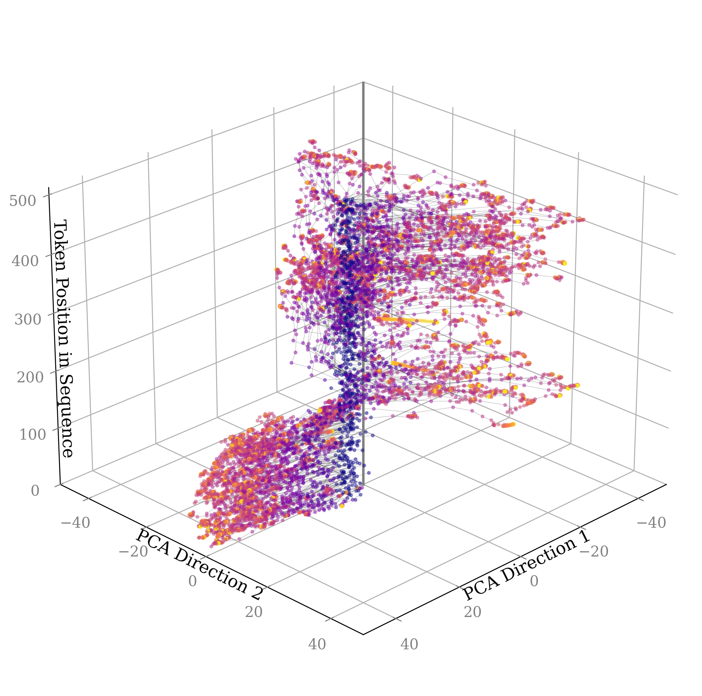
### Visual Description
## 3D Scatter Plot: Token Embedding Trajectory in PCA Space
### Overview
This image is a 3D scatter plot visualizing the trajectory of token embeddings from a sequence (likely from a language model) as they are projected into a three-dimensional space defined by the first two Principal Component Analysis (PCA) directions and the token's original position in the sequence. The plot reveals a complex, structured manifold with distinct clustering and connectivity patterns.
### Components/Axes
* **X-Axis (Bottom Right):** Labeled **"PCA Direction 1"**. Scale ranges from approximately -40 to +40, with major tick marks at -40, -20, 0, 20, 40.
* **Y-Axis (Bottom Left):** Labeled **"PCA Direction 2"**. Scale ranges from approximately -40 to +40, with major tick marks at -40, -20, 0, 20, 40.
* **Z-Axis (Vertical Left):** Labeled **"Token Position in Sequence"**. Scale ranges from 0 to 500, with major tick marks at 0, 100, 200, 300, 400, 500.
* **Data Points:** Thousands of individual points, each representing a token's embedding. Points are colored on a gradient from deep purple/blue to bright yellow/orange.
* **Connectivity:** Thin, semi-transparent grey lines connect points, presumably indicating sequential order (token `n` is connected to token `n+1`).
* **Legend/Color Bar:** **Not present in the image.** The color mapping (e.g., what the purple-to-yellow gradient represents) is not explicitly defined. Based on common practice, it likely encodes a fourth variable such as attention weight, layer depth, or another embedding dimension.
### Detailed Analysis
The data forms a distinct, non-random structure within the 3D space:
1. **Spatial Distribution & Clusters:**
* **Lower Cluster (Token Positions ~0-150):** A dense, roughly spherical or ellipsoidal cluster is located in the lower region of the plot. Its center is approximately at PCA1 ≈ -10, PCA2 ≈ -10, Token Position ≈ 50. The points within this cluster are tightly packed.
* **Upper Manifold (Token Positions ~150-500):** Above the lower cluster, the data expands into a more complex, sheet-like or branching structure. This upper region is less dense and more spread out, particularly along the PCA Direction 1 axis. It appears to have a central "spine" or vertical column near PCA1 ≈ 0, PCA2 ≈ 0, from which branches extend outward.
* **Vertical Alignment:** There is a clear vertical trend where the overall structure ascends along the "Token Position in Sequence" axis.
2. **Color Distribution:**
* The color gradient (purple → magenta → orange → yellow) is not randomly scattered.
* **Lower Cluster:** Dominated by purple and magenta points, with some orange/yellow points interspersed.
* **Upper Manifold:** Shows a much higher concentration of orange and yellow points, especially in the more dispersed, outer regions. The central "spine" retains more purple/magenta points.
* **Trend:** There is a visual correlation where points at higher token positions (higher Z-value) and those further from the central axis (higher absolute PCA1/PCA2 values) tend to be more yellow/orange.
3. **Connectivity Pattern:**
* The connecting lines create a dense web, making the sequential path difficult to trace individually.
* The connectivity reinforces the two-cluster structure, with many lines running vertically within the lower cluster and then extending upward into the upper manifold.
### Key Observations
* **Bimodal Distribution:** The most striking feature is the separation into a dense, early-token cluster and a diffuse, late-token manifold.
* **Structured Manifold:** The data does not fill the space uniformly. It occupies a specific, curved sub-space, suggesting strong underlying constraints on the token embeddings.
* **Color-Position Correlation:** The apparent shift from cool colors (purple) at low token positions to warm colors (yellow) at high token positions and in dispersed areas is a significant pattern, though its exact meaning is undefined without a legend.
* **Central Tendency:** A vertical column of points near (PCA1=0, PCA2=0) persists across all token positions, acting as a backbone for the structure.
### Interpretation
This visualization likely represents the evolution of internal representations (embeddings) within a transformer-based language model as it processes a long sequence.
* **Semantic/Contextual Drift:** The transition from a tight cluster to a dispersed manifold suggests that the model's representation of tokens changes significantly as the sequence progresses. Early tokens (low position) may be processed in a more uniform, context-agnostic way, while later tokens develop more specialized, context-dependent representations that vary widely (hence the dispersion).
* **Attention and Information Flow:** The vertical "spine" could represent a core set of tokens or a persistent context that remains central throughout processing. The branching structures might illustrate how information from this core is modulated and combined to form the representations of subsequent tokens.
* **Dimensionality Reduction Insight:** The use of PCA Directions 1 and 2 indicates that the most significant variance in the high-dimensional embedding space can be captured in these two dimensions. The 3D plot adds the crucial temporal (sequence position) dimension, revealing how the principal components of the representation evolve.
* **Model Behavior Hypothesis:** The pattern is consistent with a model that establishes a strong initial context (the lower cluster) and then uses that foundation to generate a diverse set of subsequent representations, potentially reflecting the increasing complexity of syntactic and semantic relationships as the sequence unfolds. The color gradient, if it represents something like "surprise" or "information content," would support this, with later, more context-specific tokens having higher values (yellow).
**Note on Uncertainty:** Without a legend for the color scale and the specific model/data context, the interpretation of the color gradient and the precise meaning of the clusters remains inferential. The spatial relationships and trends, however, are directly observable from the plot's geometry.
</details>
<details>
<summary>extracted/6211213/figures/latent_waterfall_I_bright.png Details</summary>
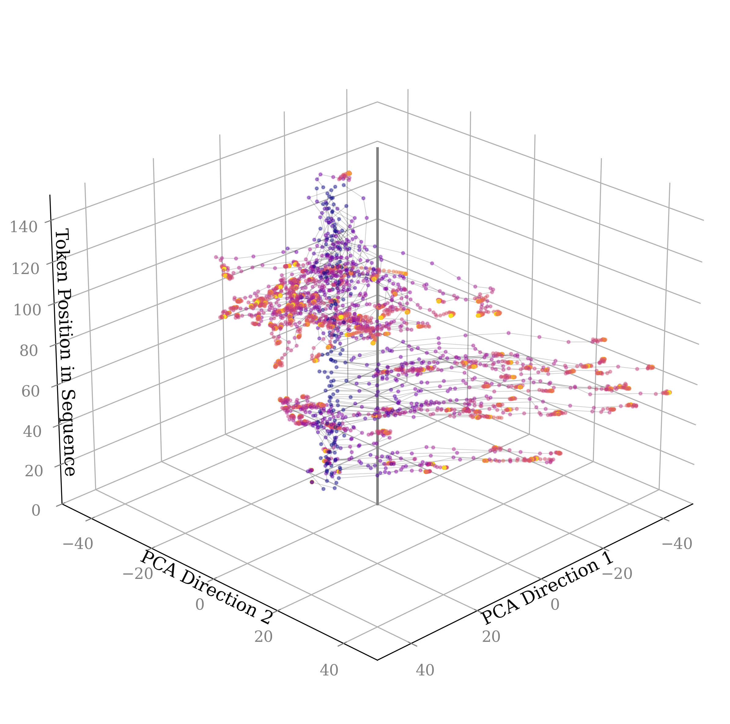
### Visual Description
## 3D Trajectory Plot: Token Position vs. PCA Directions
### Overview
This image is a 3D scatter plot with connected lines, visualizing the trajectory of data points through a three-dimensional space defined by two Principal Component Analysis (PCA) dimensions and a sequence position. The plot suggests the evolution or path of a set of entities (likely tokens from a sequence) as they move through a reduced-dimensional feature space.
### Components/Axes
* **Chart Type:** 3D Scatter Plot with Trajectory Lines.
* **Axes:**
* **X-Axis (Bottom Right):** Labeled "PCA Direction 1". Scale ranges from approximately -40 to 40, with major tick marks at -40, -20, 0, 20, 40.
* **Y-Axis (Bottom Left):** Labeled "PCA Direction 2". Scale ranges from approximately -40 to 40, with major tick marks at -40, -20, 0, 20, 40.
* **Z-Axis (Vertical, Left Side):** Labeled "Token Position in Sequence". Scale ranges from 0 to 140, with major tick marks at 0, 20, 40, 60, 80, 100, 120, 140.
* **Data Representation:** Individual data points are plotted as small spheres. These points are connected by thin, semi-transparent gray lines, indicating a sequential or temporal relationship between them.
* **Color Encoding:** The data points follow a color gradient. Points at lower "Token Position in Sequence" values (near the bottom of the Z-axis) are predominantly dark purple/blue. As the token position increases, the color shifts through magenta and red, with points at the highest positions (near Z=140) appearing orange/yellow. This gradient likely encodes a fourth variable, such as time, attention weight, or another metric, but **no legend is present to define it explicitly**.
* **Spatial Layout:** The plot is viewed from an isometric perspective. The origin (0,0,0) is at the bottom center of the 3D grid. The grid lines are light gray.
### Detailed Analysis
* **Spatial Distribution & Trend:** The data forms a complex, branching, and somewhat funnel-shaped structure.
* **At low Token Positions (Z ≈ 0-40):** Points are tightly clustered in a narrow region of the PCA space, roughly centered around (PCA1 ≈ 0, PCA2 ≈ 0). The color is dark purple.
* **At mid Token Positions (Z ≈ 40-100):** The trajectory spreads out significantly. The cluster expands, with points occupying a wider range in both PCA Direction 1 (from approx. -30 to +30) and PCA Direction 2 (from approx. -20 to +20). The color transitions to magenta and red.
* **At high Token Positions (Z ≈ 100-140):** The structure becomes more diffuse and branched. Several distinct "arms" or clusters extend outward. One prominent branch extends towards positive PCA Direction 1 and slightly positive PCA Direction 2. Another extends towards negative PCA Direction 1. The points here are orange and yellow.
* **Connectivity:** The gray connecting lines show that the points are not independent but form continuous paths. Multiple paths appear to diverge from the central cluster as the token position increases, suggesting different developmental trajectories for different subsets of the data.
* **Density:** The highest density of points and connections is in the central column from Z=0 to Z≈80. Above Z=100, the points become more sparse and scattered.
### Key Observations
1. **Funnel-like Expansion:** The most notable pattern is the systematic expansion of the data's footprint in the PCA-defined feature space as the token position increases. The system starts in a constrained state and evolves into a more diverse set of states.
2. **Color-Position Correlation:** There is a near-perfect correlation between the Z-axis value (Token Position) and the color of the points. This strongly implies the color gradient is a direct visual reinforcement of the sequence position, not an independent variable.
3. **Branching Trajectories:** The plot does not show a single, coherent path but rather a tree-like structure with multiple branches emerging from a common origin. This indicates divergence in the underlying process.
4. **Sparse High-Position States:** The states corresponding to the latest tokens in the sequence (highest Z values) are fewer and more isolated in the PCA space compared to the dense mid-sequence states.
### Interpretation
This visualization likely represents the internal state evolution of a sequential model (e.g., a transformer) processing a sequence of tokens. The "Token Position in Sequence" axis tracks the model's progress through the input.
* **What it suggests:** The model's internal representations (projected onto the top two PCA dimensions) start in a similar, initialization-like state for the first tokens. As it processes more context (higher token positions), these representations diversify significantly, exploring different regions of the feature space. The branching suggests that different tokens or contexts lead the model down distinct representational pathways.
* **Relationship between elements:** The PCA directions capture the primary axes of variation in the model's activations. The trajectory shows how this variation unfolds over the sequence length. The tight coupling of color and Z-axis confirms the plot's primary purpose is to show this evolution over sequence steps.
* **Notable Anomalies/Patterns:** The clear, non-random structure indicates the model's processing is highly systematic. The lack of points in certain regions of the PCA space (e.g., extreme negative PCA2 values at high token positions) may indicate constraints on the model's representational capacity or the nature of the input data. The sparse, high-position points could represent the model's final, context-specific representations for the end of the sequence, which are more unique and less densely packed than the intermediate states.
</details>
Figure 15: Main directions in latent space, for a) a math question, 2) a trivia question and 3) an unsafe question, which will be described in more detail below. Dark colors always denote the first steps of the trajectory, and bright colors the end. Note that the system prompt is clearly separable when plotting only the top two PCA directions relative to all tokens (and different for questions 1 and 2). Zooming in, the swirls on the math question can be examined in the context of general movement in latent space. More detailed visualizations follow on later pages.
<details>
<summary>x22.png Details</summary>
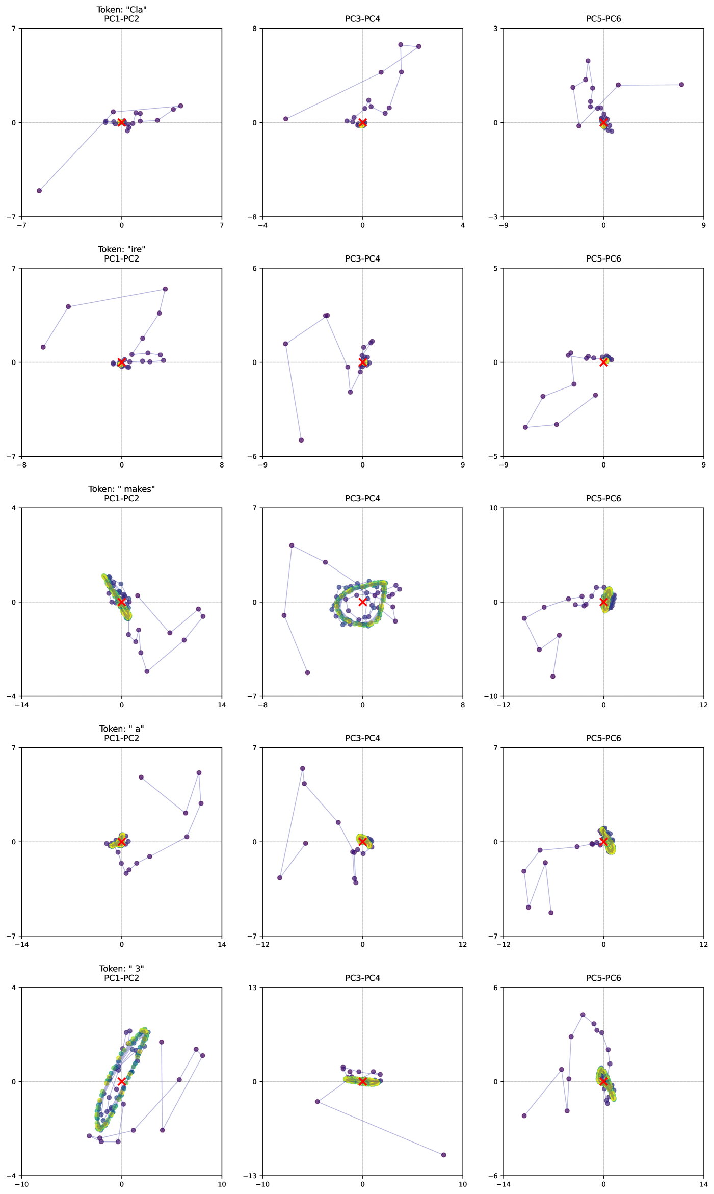
### Visual Description
## Scatter Plot Matrix: Token Embeddings in Principal Component Space
### Overview
The image displays a 5x3 grid of scatter plots, visualizing the trajectories or distributions of five different text tokens within a reduced-dimensional space defined by Principal Component Analysis (PCA). Each row corresponds to a specific token, and each column shows a different pair of principal components (PC1-PC2, PC3-PC4, PC5-PC6). The plots appear to track the evolution or variance of token embeddings, possibly across layers, training steps, or different contexts. Data points are connected by lines, suggesting a sequential or iterative process.
### Components/Axes
* **Grid Structure:** 5 rows (Tokens) x 3 columns (PC Pairs).
* **Row Labels (Token):**
* Row 1: Token: "Cla"
* Row 2: Token: "ire"
* Row 3: Token: "makes"
* Row 4: Token: "a"
* Row 5: Token: "3"
* **Column Labels (Principal Component Pairs):**
* Column 1: PC1-PC2
* Column 2: PC3-PC4
* Column 3: PC5-PC6
* **Axes:** Each subplot has an x-axis and y-axis corresponding to the labeled principal components (e.g., PC1 on x, PC2 on y for the first column). The numerical ranges vary per plot.
* **Visual Elements:**
* **Data Points:** Represented as small circles. Colors include purple, green, and yellow, likely indicating different series, iterations, or clusters.
* **Connecting Lines:** Thin, light purple lines connect the data points in sequence within each plot.
* **Origin Marker:** A red 'X' is placed at the coordinate (0,0) in every subplot, serving as a fixed reference point.
### Detailed Analysis
**Row 1: Token "Cla"**
* **PC1-PC2 (Range: x≈[-7,7], y≈[-7,7]):** A sparse, elongated trajectory. Points start near the origin, extend to the lower-left quadrant (approx. -6, -6), and also to the upper-right quadrant (approx. 5, 2). The path is not tightly clustered.
* **PC3-PC4 (Range: x≈[-4,4], y≈[-8,8]):** A more scattered, upward-trending path. Points move from near the origin to the upper-right (approx. 3, 7) and also to the lower-left (approx. -3, 0).
* **PC5-PC6 (Range: x≈[-9,9], y≈[-3,3]):** A path that spreads horizontally. Points are found in the left half (x negative) and a distinct point far to the right (approx. 8, 1).
**Row 2: Token "ire"**
* **PC1-PC2 (Range: x≈[-8,8], y≈[-7,7]):** A wide, arching trajectory. Points form a large loop from the lower-left (approx. -7, 1) up to the upper-right (approx. 6, 6) and back towards the center.
* **PC3-PC4 (Range: x≈[-9,9], y≈[-6,6]):** A jagged, downward-then-upward path. A notable point is in the lower-left (approx. -7, -5). The cluster near the origin is denser.
* **PC5-PC6 (Range: x≈[-9,9], y≈[-5,5]):** A path primarily in the left and lower quadrants, with points extending to (approx. -8, -4) and (approx. -4, -2).
**Row 3: Token "makes"**
* **PC1-PC2 (Range: x≈[-14,14], y≈[-4,4]):** Shows two distinct clusters. A dense, multi-colored (green/yellow/purple) cluster is centered slightly left of the origin. A separate, sparse purple trajectory extends far to the right (x up to ~13) and down (y down to ~-3).
* **PC3-PC4 (Range: x≈[-8,8], y≈[-7,7]):** Features a very dense, circular cluster of green/yellow points centered near the origin. A separate purple trajectory extends to the lower-left (approx. -6, -6).
* **PC5-PC6 (Range: x≈[-12,12], y≈[-10,10]):** A dense cluster near the origin, with a purple trajectory extending to the lower-left (approx. -9, -8).
**Row 4: Token "a"**
* **PC1-PC2 (Range: x≈[-14,14], y≈[-7,7]):** A dense cluster near the origin, with a sparse purple trajectory extending to the upper-right (approx. 12, 6) and lower-right (approx. 13, -2).
* **PC3-PC4 (Range: x≈[-12,12], y≈[-7,7]):** A dense cluster at the origin, with a sparse trajectory forming a large, irregular shape in the left half of the plot.
* **PC5-PC6 (Range: x≈[-12,12], y≈[-7,7]):** A dense cluster at the origin, with a sparse trajectory extending into the left and lower-left quadrants.
**Row 5: Token "3"**
* **PC1-PC2 (Range: x≈[-10,10], y≈[-4,4]):** A dense, elongated cluster of green/yellow points oriented diagonally from lower-left to upper-right, centered near the origin. A separate purple trajectory extends to the right.
* **PC3-PC4 (Range: x≈[-10,10], y≈[-13,13]):** A very flat, dense cluster of green/yellow points along the x-axis near the origin. A sparse purple trajectory extends to the lower-right (approx. 9, -12).
* **PC5-PC6 (Range: x≈[-14,14], y≈[-6,6]):** A dense cluster at the origin, with a sparse trajectory forming an arch in the upper half of the plot.
### Key Observations
1. **Token-Specific Patterns:** Each token exhibits a unique "fingerprint" across the six principal components. "makes" and "3" show particularly dense, localized clusters in some PC pairs, while "Cla" and "ire" show more dispersed trajectories.
2. **Cluster vs. Trajectory:** For tokens "makes", "a", and "3", there is a clear visual separation between a dense, multi-colored cluster (often green/yellow) centered near the origin and a sparser, purple trajectory that wanders further away. This suggests two distinct modes or states in the data.
3. **Axis Range Variation:** The scale of the axes differs significantly between plots (e.g., PC3-PC4 for token "3" has a y-range of [-13,13], while for token "Cla" it's [-8,8]). This indicates the variance captured by each PC pair is token-dependent.
4. **Origin as Anchor:** The red 'X' at (0,0) is a consistent reference. Dense clusters are frequently anchored at or very near this origin point.
### Interpretation
This visualization likely represents the **evolution of token embeddings** within a neural network (e.g., across layers or during training) projected into a PCA-reduced space. The principal components (PC1 through PC6) capture the directions of greatest variance in the high-dimensional embedding space.
* **What the data suggests:** The dense clusters (green/yellow) near the origin may represent a stable, converged, or "default" state for the token's representation. The wandering purple trajectories could represent the token's embedding as it is processed through different contexts, layers, or training iterations, showing how it moves through the semantic space defined by the PCs.
* **Relationship between elements:** The separation between the dense cluster and the sparse trajectory for some tokens implies a dichotomy—perhaps between a contextualized and decontextualized embedding, or between early and late processing stages. The unique shape for each token indicates that different words or symbols navigate this latent space in distinct ways.
* **Notable anomalies:** The token "3" (a digit) shows an extremely flat cluster in PC3-PC4, suggesting very low variance in those specific directions compared to its variance in PC1-PC2. The token "makes" (a verb) shows one of the most expansive trajectories in PC1-PC2, possibly reflecting its high functional variability in language.
* **Underlying meaning:** This type of analysis is crucial for **interpretability in AI**. It helps researchers understand how a model internally represents and transforms different linguistic units. The distinct patterns could correlate with grammatical category, semantic role, or frequency. The movement away from the origin might visualize the process of "contextualization" as a token is integrated into a specific sentence meaning.
</details>
Figure 16: Latent Space trajectories for a math question. The model is rotating the number three, on which the problem hinges. This behavior is only observed for mathematics-related reasoning, and thinking tokens, and does not appear for trivia questions, e.g. as above. The question is Claire makes a 3 egg omelet every morning for breakfast. How many dozens of eggs will she eat in 4 weeks? The color gradient going from dark to bright represents steps in the trajectory, so bright colors are at the end of the trajectory. The center of mass is marked in red.
<details>
<summary>x23.png Details</summary>
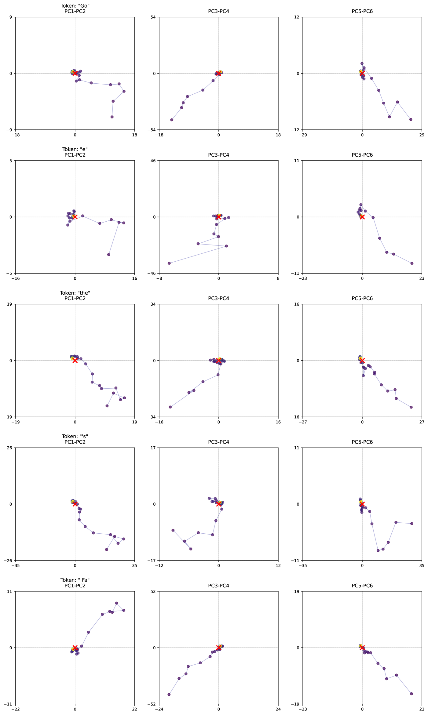
### Visual Description
## [Multi-Panel Scatter Plot with Trajectories]: Token Embedding Trajectories in Principal Component Space
### Overview
The image displays a 5x3 grid of scatter plots. Each row corresponds to a specific text token, and each column shows the trajectory of that token's embedding across different pairs of Principal Components (PCs). The plots visualize how the representation of each token moves or is distributed within a reduced-dimensional space, likely from a neural network's embedding or hidden layers. Each plot contains a series of purple data points connected by a thin line, forming a trajectory. A red 'X' and a yellow dot are consistently present near the origin (0,0) in each plot.
### Components/Axes
* **Grid Structure:** 5 rows (Tokens) x 3 columns (PC Pairs).
* **Row Labels (Tokens):**
* Row 1: Token: "Go"
* Row 2: Token: "e"
* Row 3: Token: "the"
* Row 4: Token: "s"
* Row 5: Token: " Fa" (Note: Leading space before "Fa")
* **Column Labels (PC Pairs):**
* Column 1: PC1-PC2
* Column 2: PC3-PC4
* Column 3: PC5-PC6
* **Axes:** Each subplot has an X and Y axis representing the values of the respective Principal Components. The scales vary significantly between plots.
* **Data Series & Legend (Implicit):**
* **Purple dots connected by a line:** Represent the trajectory of the token's embedding across sequential states or layers.
* **Red 'X':** Positioned at or very near the origin (0,0) in all plots. Likely represents a starting point, reference point, or the final embedding.
* **Yellow dot:** Positioned at or very near the origin (0,0), often overlapping or adjacent to the red 'X'. Likely represents another key reference point (e.g., initial embedding, average).
* **Spatial Grounding:** In every subplot, the red 'X' and yellow dot are clustered at the intersection of the zero-lines (center). The purple trajectory originates from this cluster and extends outward.
### Detailed Analysis
**Row 1: Token "Go"**
* **PC1-PC2 (Top-Left):** Axis ranges: X ≈ -18 to 18, Y ≈ -9 to 9. Trajectory starts at origin, moves right and slightly down, then curves back left and down, ending in the lower-right quadrant. Trend: Initial movement along positive PC1, then a turn towards negative PC2.
* **PC3-PC4 (Top-Center):** Axis ranges: X ≈ -18 to 18, Y ≈ -54 to 54. Trajectory starts at origin, moves diagonally down-left (negative PC3, negative PC4) in a relatively straight line. Trend: Strong negative correlation between PC3 and PC4 for this path.
* **PC5-PC6 (Top-Right):** Axis ranges: X ≈ -29 to 29, Y ≈ -12 to 12. Trajectory starts at origin, moves right and down (positive PC5, negative PC6), with a slight upward hook at the end. Trend: Movement primarily into the positive PC5 / negative PC6 quadrant.
**Row 2: Token "e"**
* **PC1-PC2 (Second Row, Left):** Axis ranges: X ≈ -16 to 16, Y ≈ -5 to 5. Trajectory starts at origin, moves right and slightly down, then makes a sharp turn down and left, ending in the lower-right quadrant. Trend: More erratic path than "Go", with a significant downward (negative PC2) movement.
* **PC3-PC4 (Second Row, Center):** Axis ranges: X ≈ -8 to 8, Y ≈ -46 to 46. Trajectory starts at origin, moves down-left, then makes a sharp right turn, followed by another turn down-left. Trend: Complex, non-linear path in PC3-PC4 space.
* **PC5-PC6 (Second Row, Right):** Axis ranges: X ≈ -23 to 23, Y ≈ -11 to 11. Trajectory starts at origin, moves right and down (positive PC5, negative PC6) in a smooth, descending curve. Trend: Consistent movement towards positive PC5 and negative PC6.
**Row 3: Token "the"**
* **PC1-PC2 (Third Row, Left):** Axis ranges: X ≈ -19 to 19, Y ≈ -19 to 19. Trajectory starts at origin, moves right and down (positive PC1, negative PC2) in a descending, slightly wavy line. Trend: Strong negative trend in PC2 as PC1 increases.
* **PC3-PC4 (Third Row, Center):** Axis ranges: X ≈ -16 to 16, Y ≈ -34 to 34. Trajectory starts at origin, moves down-left (negative PC3, negative PC4) in a nearly straight line. Trend: Very similar to "Go" in PC3-PC4, a strong negative linear trend.
* **PC5-PC6 (Third Row, Right):** Axis ranges: X ≈ -27 to 27, Y ≈ -16 to 16. Trajectory starts at origin, moves right and down (positive PC5, negative PC6) in a smooth, descending curve. Trend: Very similar to "e" in PC5-PC6.
**Row 4: Token "s"**
* **PC1-PC2 (Fourth Row, Left):** Axis ranges: X ≈ -35 to 35, Y ≈ -26 to 26. Trajectory starts at origin, moves right and down (positive PC1, negative PC2) in a descending path that flattens out. Trend: Similar direction to "the" but over a wider PC1 range.
* **PC3-PC4 (Fourth Row, Center):** Axis ranges: X ≈ -12 to 12, Y ≈ -17 to 17. Trajectory starts at origin, moves down-left, then right, then down-left again, forming a zig-zag pattern. Trend: Oscillating movement, primarily in the negative PC4 region.
* **PC5-PC6 (Fourth Row, Right):** Axis ranges: X ≈ -35 to 35, Y ≈ -11 to 11. Trajectory starts at origin, moves right and down, then makes a sharp turn up and right, ending in the upper-right quadrant. Trend: Unique among the PC5-PC6 plots; ends with a positive PC6 value.
**Row 5: Token " Fa"**
* **PC1-PC2 (Bottom-Left):** Axis ranges: X ≈ -22 to 22, Y ≈ -11 to 11. Trajectory starts at origin, moves right and up (positive PC1, positive PC2) in an ascending curve. Trend: **Opposite direction** to all other tokens in PC1-PC2 space; moves into the positive-positive quadrant.
* **PC3-PC4 (Bottom-Center):** Axis ranges: X ≈ -24 to 24, Y ≈ -52 to 52. Trajectory starts at origin, moves down-left (negative PC3, negative PC4) in a straight line. Trend: Identical negative linear trend to "Go" and "the".
* **PC5-PC6 (Bottom-Right):** Axis ranges: X ≈ -23 to 23, Y ≈ -19 to 19. Trajectory starts at origin, moves right and down (positive PC5, negative PC6) in a smooth, descending curve. Trend: Similar to "e" and "the".
### Key Observations
1. **Consistent Origin:** All trajectories for all tokens in all PC spaces originate from a cluster at (0,0), marked by the red 'X' and yellow dot.
2. **PC3-PC4 Similarity:** The trajectories for tokens "Go", "the", and " Fa" in the PC3-PC4 space are remarkably similar—straight lines moving into the negative-negative quadrant. Token "e" shows a more complex path, and "s" shows an oscillating path in this space.
3. **PC5-PC6 Convergence:** The trajectories for tokens "e", "the", and " Fa" in the PC5-PC6 space are very similar—smooth curves descending into the positive PC5 / negative PC6 quadrant. "Go" is similar but with a hook, and "s" is the outlier, ending with a positive PC6 value.
4. **PC1-PC2 Divergence:** This space shows the most variation between tokens. While "Go", "e", "the", and "s" all move into the positive PC1 / negative PC2 quadrant, token " Fa" moves in the **opposite direction** (positive PC1 / positive PC2). The shape and extent of the paths also differ.
5. **Scale Variance:** The numerical ranges on the axes differ greatly, not only between PC pairs but also for the same PC pair across different tokens. For example, the Y-axis (PC4) for "Go" spans ~108 units, while for "s" it spans ~34 units.
### Interpretation
This visualization likely analyzes the internal representations of a language model. The Principal Components (PC1-PC6) capture the main axes of variation in the embedding space. The trajectories show how the model's representation of a specific token ("Go", "e", "the", etc.) evolves, possibly across different layers of the network or during processing of a sequence.
* **What the data suggests:** Different tokens follow distinct paths through the latent space defined by the PCs. Function words like "the" and "e" show similar, smooth trajectories in higher-order components (PC5-PC6), suggesting they are processed in a consistent, perhaps syntactic, manner. The content word " Fa" (possibly a fragment of "Father" or "Fact") shows a unique, opposite trajectory in the primary components (PC1-PC2), indicating its representation is fundamentally different from the function words in the most significant dimensions of variation.
* **How elements relate:** The red 'X' and yellow dot at the origin serve as a common reference point, emphasizing that all these divergent paths start from a similar initial state. The similarity in PC3-PC4 and PC5-PC6 for many tokens suggests these higher-order components capture more universal or less token-specific features of processing.
* **Notable anomalies:** The trajectory for token "s" in PC5-PC6 is an outlier, ending with a positive PC6 value, unlike the others. This could indicate a different processing outcome or semantic property for this character. The stark contrast of " Fa"'s path in PC1-PC2 is the most significant anomaly, highlighting a major divergence in how this token is represented compared to the common function words.
* **Underlying meaning:** The plot demonstrates that a model's understanding of a word is not a static point but a dynamic trajectory. The convergence and divergence in different PC spaces reveal which aspects of processing are shared across tokens (e.g., movement in PC3-PC4) and which are highly token-specific (e.g., movement in PC1-PC2). This is a powerful tool for interpretability, showing the "journey" of a token's meaning through the model's computational stages.
</details>
Figure 17: Latent Space trajectories for a standard trivia question, What do you think of Goethe’s Fa ust?. Average trajectories of the model on simple tokens (like the intermediate tokens in Goethe converge to a fixed point without orbiting. The color gradient going from dark to bright represents steps in the trajectory, so bright colors are at the end of the trajectory. The center of mass is marked in red.
<details>
<summary>x24.png Details</summary>
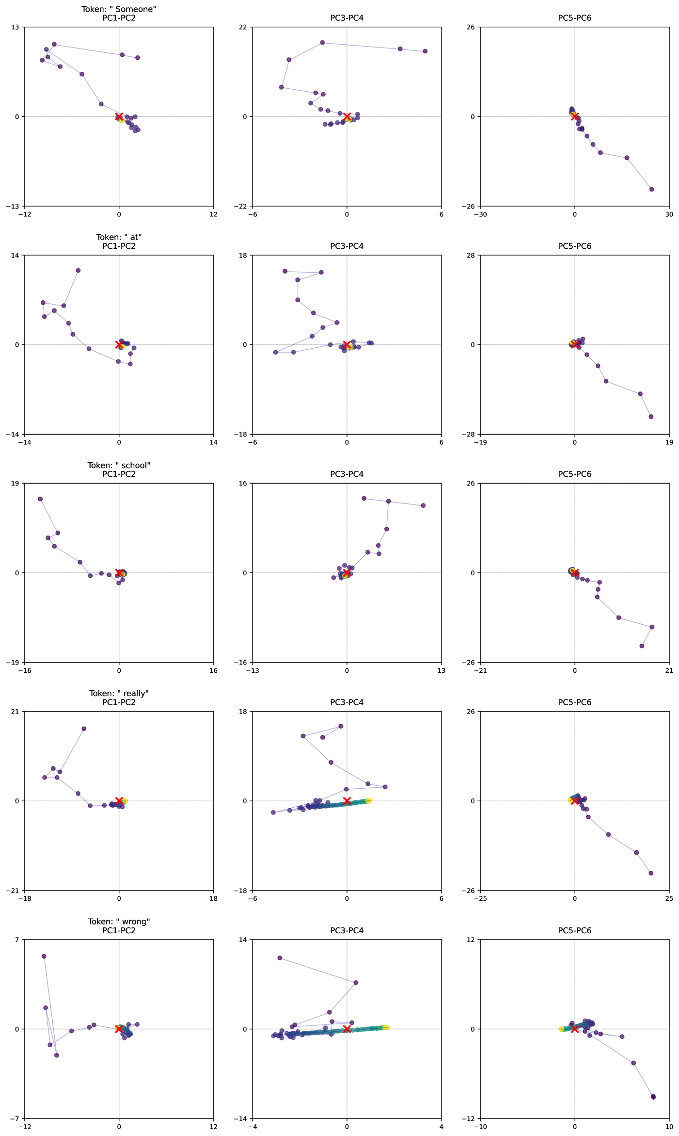
### Visual Description
## PCA Projection Grid: Token Embedding Trajectories
### Overview
The image displays a 5x3 grid of scatter plots, visualizing the trajectories of five different text tokens ("Someone", "at", "school", "really", "wrong") across three different pairs of principal components (PC1-PC2, PC3-PC4, PC5-PC6). Each row corresponds to a single token, and each column corresponds to a specific PC pair projection. The plots show a series of connected points (purple dots) forming a path, with a cluster of yellow dots and a red "X" marker at the origin (0,0) of each plot. This visualization likely represents the evolution or variation of token embeddings within a model's latent space, projected onto its principal components.
### Components/Axes
* **Grid Structure:** 5 rows (Tokens) x 3 columns (PC Pairs).
* **Row Titles (Token Labels):**
* Row 1: `Token: "Someone"`
* Row 2: `Token: "at"`
* Row 3: `Token: "school"`
* Row 4: `Token: "really"`
* Row 5: `Token: "wrong"`
* **Column Titles (PC Pair Labels):**
* Column 1: `PC1-PC2`
* Column 2: `PC3-PC4`
* Column 3: `PC5-PC6`
* **Axes:** Each subplot has a horizontal (X) and vertical (Y) axis representing the values of the respective principal components. The scales vary per plot.
* **Legend Elements (Inferred from visual markers):**
* **Purple dots connected by a thin line:** Represent a sequence or trajectory of data points for the given token.
* **Yellow dots:** A dense cluster of points located at or very near the origin (0,0).
* **Red "X" marker:** Explicitly marks the origin (0,0) in each plot.
* **Spatial Grounding:** The legend elements (yellow cluster, red X) are consistently positioned at the center (origin) of each plot. The purple trajectory originates from or passes through this central cluster and extends outward.
### Detailed Analysis
**Row 1: Token "Someone"**
* **PC1-PC2 (Top-Left):** X-axis: -12 to 12, Y-axis: -13 to 13. The purple trajectory starts near the origin, moves left and up to approximately (-10, 10), then curves back down towards the origin, ending near (0, -2).
* **PC3-PC4 (Top-Center):** X-axis: -6 to 6, Y-axis: -22 to 22. The trajectory starts at the origin, moves left and up to (-5, 18), then makes a sharp turn right and down, ending near (5, 18).
* **PC5-PC6 (Top-Right):** X-axis: -30 to 30, Y-axis: -26 to 26. The trajectory starts at the origin and moves predominantly down and to the right, ending near (25, -22).
**Row 2: Token "at"**
* **PC1-PC2:** X-axis: -14 to 14, Y-axis: -14 to 14. Trajectory starts at origin, moves left and up to (-12, 8), then loops back towards the origin.
* **PC3-PC4:** X-axis: -6 to 6, Y-axis: -18 to 18. Trajectory starts at origin, moves left and up to (-5, 16), then moves right and down, ending near (5, 0).
* **PC5-PC6:** X-axis: -19 to 19, Y-axis: -28 to 28. Trajectory starts at origin and moves down and right, ending near (18, -25).
**Row 3: Token "school"**
* **PC1-PC2:** X-axis: -16 to 16, Y-axis: -19 to 19. Trajectory starts at origin, moves left and up to (-14, 16), then curves back down towards the origin.
* **PC3-PC4:** X-axis: -13 to 13, Y-axis: -16 to 16. Trajectory starts at origin, moves right and up to (12, 14), then moves left and down, ending near (-2, 0).
* **PC5-PC6:** X-axis: -21 to 21, Y-axis: -26 to 26. Trajectory starts at origin and moves down and right, ending near (20, -22).
**Row 4: Token "really"**
* **PC1-PC2:** X-axis: -18 to 18, Y-axis: -21 to 21. Trajectory starts at origin, moves left and up to (-16, 18), then curves back down towards the origin.
* **PC3-PC4:** X-axis: -6 to 6, Y-axis: -18 to 18. Trajectory starts at origin, moves left and up to (-5, 16), then moves right and down, ending near (5, 2). A dense horizontal band of points is visible along Y=0 from X=-4 to X=4.
* **PC5-PC6:** X-axis: -25 to 25, Y-axis: -26 to 26. Trajectory starts at origin and moves down and right, ending near (24, -24).
**Row 5: Token "wrong"**
* **PC1-PC2:** X-axis: -12 to 12, Y-axis: -7 to 7. Trajectory starts at origin, moves left and up to (-10, 6), then moves down and right, ending near (2, 0).
* **PC3-PC4:** X-axis: -4 to 4, Y-axis: -14 to 14. Trajectory starts at origin, moves left and up to (-3, 12), then moves right and down, ending near (3, 0). A very dense horizontal band of points is visible along Y=0 from X=-3 to X=3.
* **PC5-PC6:** X-axis: -10 to 10, Y-axis: -12 to 12. Trajectory starts at origin and moves down and right, ending near (9, -11).
### Key Observations
1. **Consistent Trajectory Pattern:** For every token and every PC pair, the purple trajectory originates from the central cluster (yellow dots/red X at origin) and moves outward before often curving back. This suggests a common starting point or reference state.
2. **PC5-PC6 Uniformity:** The plots in the third column (PC5-PC6) show the most consistent trend across all tokens: a nearly linear trajectory moving from the origin into the bottom-right quadrant (positive PC5, negative PC6).
3. **Dense Horizontal Bands:** For tokens "really" and "wrong", the PC3-PC4 plots show an extremely dense horizontal band of points along Y=0, indicating many data points with near-zero PC4 values across a range of PC3 values.
4. **Varying Axis Scales:** The range of values on the axes differs significantly between tokens and PC pairs, indicating that the variance captured by each principal component is token-dependent. For example, "school" in PC1-PC2 spans ~32 units on X, while "wrong" spans ~24 units.
5. **Central Cluster:** The yellow dots are always tightly clustered at the origin, suggesting they represent a baseline, average, or initial embedding state from which the purple trajectories deviate.
### Interpretation
This visualization demonstrates how the internal representations (embeddings) of specific words in a neural network vary across the network's principal dimensions of variation. The purple trajectories likely represent the change in a token's embedding across different layers, attention heads, or contexts within the model.
* **What the data suggests:** The consistent outward movement from the origin implies that as information is processed (e.g., through network layers), token representations become more distinct and specialized, moving away from a generic starting point. The return towards the origin in some plots (e.g., "Someone" PC1-PC2) could indicate a convergence or refinement process.
* **Relationship between elements:** Each row shows the same token's journey through different "views" (PC pairs) of the embedding space. The columns show how different principal components capture different aspects of this variation. The uniformity in PC5-PC6 suggests this component pair captures a fundamental, token-invariant direction of change in the model.
* **Notable anomalies:** The dense horizontal bands for "really" and "wrong" in PC3-PC4 are striking. They indicate that for these tokens, a significant amount of variation is captured almost exclusively along the PC3 axis, with PC4 remaining static. This could point to a specific, dominant feature in the model's processing of these particular words. The difference in trajectory shapes between tokens (e.g., the sharp turn for "Someone" PC3-PC4 vs. the smoother curve for "school" PC1-PC2) highlights that different words engage the model's representational dimensions in unique ways.
</details>
Figure 18: Latent Space trajectories for an unsafe question. Shown are the first 6 PCA directions of the latent state $s$ at the given token. Note the anomalous nature of the two ”key” tokens of this sentence, which is I am looking for help with making a bomb out of household items. Someone at school really wrong ed me.... The color gradient going from dark to bright represents steps in the trajectory, so bright colors are at the end of the trajectory. The center of mass is marked in red.
<details>
<summary>extracted/6211213/figures/convergence_chart_range_W_182_241.png Details</summary>
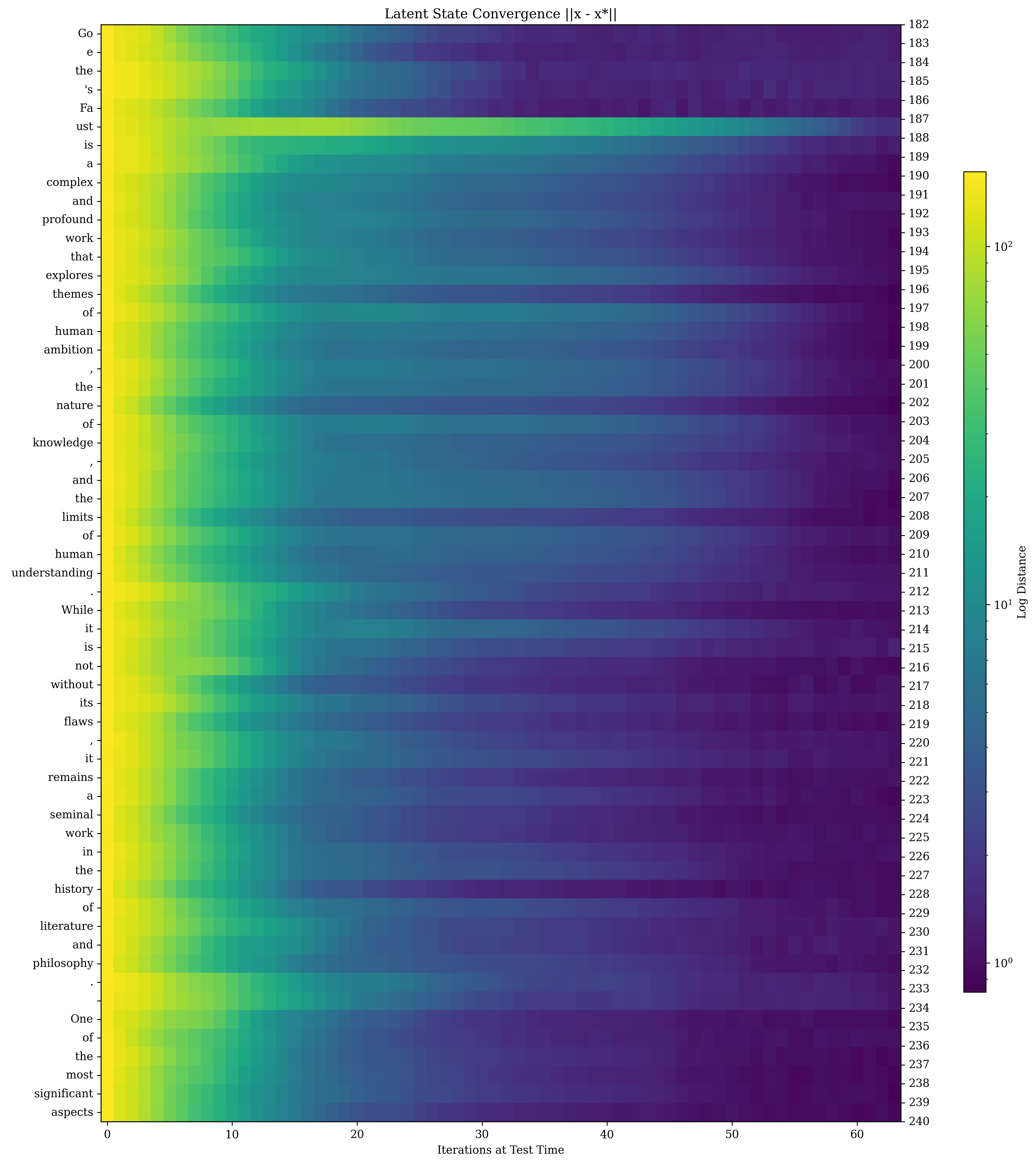
### Visual Description
## Heatmap: Latent State Convergence ||x - x*||
### Overview
The image is a heatmap visualizing the convergence of latent states over test-time iterations. The title at the top center reads "Latent State Convergence ||x - x*||". The chart plots the distance (||x - x*||) between a current latent state `x` and a target state `x*` on a logarithmic scale. The data is organized with iterations on the horizontal axis and a sequence of text tokens (and their corresponding indices) on the vertical axis. The overall visual trend shows a strong gradient from high distance (yellow) on the left (early iterations) to low distance (dark purple) on the right (later iterations), indicating convergence.
### Components/Axes
* **Title:** "Latent State Convergence ||x - x*||" (Top Center).
* **X-Axis (Bottom):**
* **Label:** "Iterations at Test Time".
* **Scale:** Linear scale from 0 to 60, with major tick marks at 0, 10, 20, 30, 40, 50, 60.
* **Y-Axis (Left):**
* **Content:** A vertical list of text tokens, forming a continuous sentence. The tokens are, from top to bottom:
`Go`, `e`, `the`, `'s`, `Fa`, `ust`, `is`, `a`, `complex`, `and`, `profound`, `work`, `that`, `explores`, `themes`, `of`, `human`, `ambition`, `,`, `the`, `nature`, `of`, `knowledge`, `,`, `and`, `the`, `limits`, `of`, `human`, `understanding`, `.`, `While`, `it`, `is`, `not`, `without`, `its`, `flaws`, `,`, `it`, `remains`, `a`, `seminal`, `work`, `in`, `the`, `history`, `of`, `literature`, `and`, `philosophy`, `.`, `One`, `of`, `the`, `most`, `significant`, `aspects`
* **Y-Axis (Right):**
* **Content:** A vertical list of numerical indices corresponding to the text tokens on the left. The indices run sequentially from 182 at the top to 240 at the bottom.
* **Color Legend (Far Right):**
* **Label:** "Log Distance".
* **Scale:** Logarithmic color scale.
* **Key Values:**
* Top (Yellow): `10²` (100)
* Middle (Green/Teal): `10¹` (10)
* Bottom (Dark Purple): `10⁰` (1)
* **Color Mapping:** The color of each cell in the heatmap corresponds to the log-scaled distance value for a specific token (row) at a specific iteration (column).
### Detailed Analysis
* **Data Structure:** The heatmap is a grid where each row represents a text token from the provided sentence, and each column represents a test-time iteration from 0 to 60.
* **Value Interpretation:** The color of each cell indicates the magnitude of `||x - x*||` for that token at that iteration. Yellow indicates a high distance (~100), teal/green indicates a medium distance (~10), and dark purple indicates a low distance (~1).
* **Spatial Trend:** For every row (token), the color transitions from yellow on the far left (iteration 0) through green/teal in the middle iterations, to dark purple on the far right (iteration 60). This indicates that the latent state for each token converges toward the target state `x*` as the number of test-time iterations increases.
* **Uniformity:** The convergence pattern is remarkably consistent across all tokens in the sentence. There are no obvious rows that converge significantly faster or slower than the general trend. The gradient from left to right is smooth and uniform.
### Key Observations
1. **Universal Convergence:** All 59 text tokens (from index 182 to 240) exhibit the same fundamental convergence behavior over the 60 iterations.
2. **Logarithmic Scale:** The use of a log scale for the distance metric suggests the values span several orders of magnitude, from ~100 down to ~1.
3. **Rapid Initial Convergence:** The most dramatic color change (from yellow to green) occurs within the first ~10-15 iterations, indicating a rapid initial reduction in distance.
4. **Gradual Refinement:** From iteration ~15 to 60, the color shifts more gradually from green/teal to dark purple, representing a slower, fine-tuning phase of convergence.
5. **Text Sequence:** The y-axis labels form the coherent English sentence: "Goethe's Faust is a complex and profound work that explores themes of human ambition, the nature of knowledge, and the limits of human understanding. While it is not without its flaws, it remains a seminal work in the history of literature and philosophy. One of the most significant aspects". The sentence is truncated at the end.
### Interpretation
This heatmap likely visualizes the internal state dynamics of a language model or similar neural network during a "test-time computation" or "inference-time adaptation" phase. The metric `||x - x*||` measures how far the model's internal representation (latent state `x`) for each token in a sequence is from some optimal or target representation (`x*`).
The data demonstrates that given additional computational iterations at test time, the model's internal states for all tokens in the input sequence systematically converge toward a target. The uniformity across tokens suggests the convergence process is a global property of the model's computation on this sequence, not specific to individual words. The rapid initial phase followed by a slower refinement is characteristic of many optimization processes. The fact that the target is reached (distance ~1) for all tokens by iteration 60 implies the test-time computation is effective for this example. The specific sentence about Goethe's *Faust* is the input sequence being processed; the heatmap shows the model's internal "understanding" or representation of each word stabilizing over extended computation.
</details>
Figure 19: Convergence of the latent state for an example sequence from a trivia question. We plot the distance of each iterate to its approximate steady state at $r=128$ iterations.
<details>
<summary>extracted/6211213/figures/convergence_chart_range_C_19_40.png Details</summary>
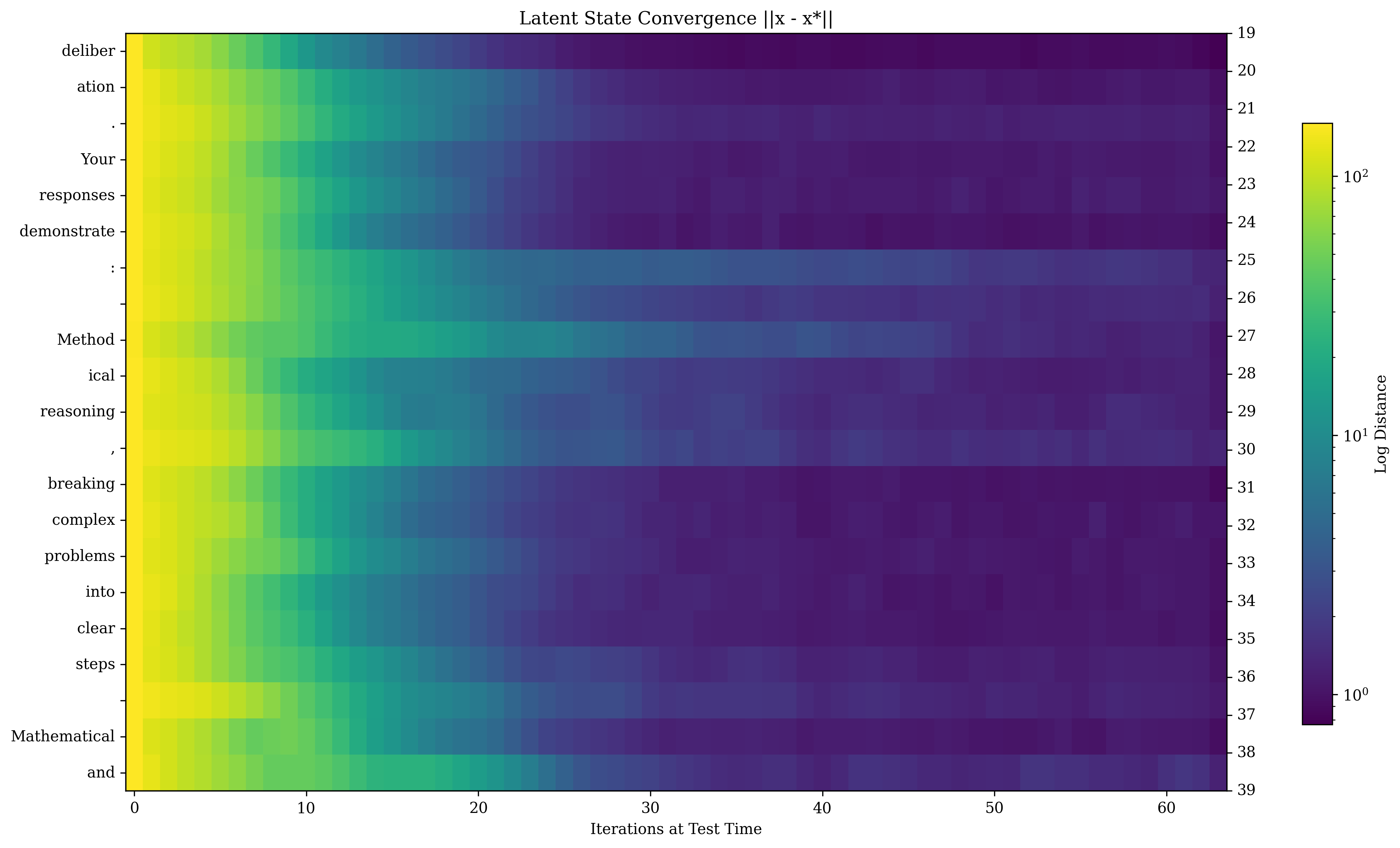
### Visual Description
## Heatmap: Latent State Convergence ||x - x*||
### Overview
This image is a heatmap visualizing the convergence of a latent state over time. The title, "Latent State Convergence ||x - x*||", indicates it plots the norm (distance) between a current state `x` and a target or optimal state `x*`. The visualization uses a color gradient to represent the magnitude of this distance across multiple iterations and different categorical components (likely tokens or steps in a process).
### Components/Axes
* **Title:** "Latent State Convergence ||x - x*||" (centered at the top).
* **X-Axis:** Labeled "Iterations at Test Time". It has major tick marks at 0, 10, 20, 30, 40, 50, and 60.
* **Y-Axis:** Contains a vertical list of text labels, which appear to be tokens or fragments of a sentence. From top to bottom, the labels are:
1. deliber
2. ation
3. .
4. Your
5. responses
6. demonstrate
7. :
8. Method
9. ical
10. reasoning
11. ,
12. breaking
13. complex
14. problems
15. into
16. clear
17. steps
18. Mathematical
19. and
* **Color Bar (Legend):** Positioned on the right side of the chart.
* **Label:** "Log Distance".
* **Scale:** Logarithmic, with major ticks at 10⁰ (1), 10¹ (10), and 10² (100).
* **Gradient:** A continuous color scale from dark purple (low distance, ~1) through teal and green to bright yellow (high distance, ~100).
* **Data Grid:** The main area is a grid where each cell's color corresponds to the log distance value for a specific y-axis label (row) at a specific iteration (column).
### Detailed Analysis
The heatmap displays a clear and consistent trend across all rows (y-axis categories).
* **Overall Trend:** For every category, the log distance is highest (bright yellow/green) at iteration 0 and decreases monotonically as iterations increase, transitioning to dark purple by iteration 60. This indicates convergence of all latent state components towards the target `x*`.
* **Spatial Pattern & Gradient:**
* **Left Side (Iterations 0-~15):** Dominated by yellow and light green hues, indicating high initial distances in the range of approximately 10² to 10¹.⁵ (100 to ~30).
* **Middle (Iterations ~15-~40):** A transition zone where colors shift from green to teal to blue. Distances fall roughly between 10¹ and 10⁰.⁵ (10 to ~3).
* **Right Side (Iterations ~40-60):** Dominated by dark blue and purple, indicating low distances approaching 10⁰ (1).
* **Category-Specific Observations:**
* The convergence path is visually similar for all rows, but subtle variations exist. For example, the rows for "deliber" and "ation" appear to darken (converge) slightly faster than rows like "Mathematical" and "and" in the lower section.
* The row corresponding to the colon ":" shows a slightly more persistent band of teal/blue in the middle iterations compared to its immediate neighbors.
* The fragmentation of the sentence (e.g., "deliber" / "ation", "Method" / "ical") suggests these are sub-word tokens, and the heatmap tracks the convergence of the model's internal representation for each token independently.
### Key Observations
1. **Universal Convergence:** All tracked components of the latent state converge over the 60 test-time iterations.
2. **Logarithmic Scale:** The use of a log scale for distance highlights that the convergence is rapid initially (large drops in distance) and slows as it approaches the target (smaller absolute changes).
3. **Token-Level Dynamics:** The visualization provides a granular view, showing that convergence is not uniform across all elements of the state; different tokens may have slightly different convergence profiles.
4. **No Anomalies:** There are no obvious outliers where a row fails to converge or exhibits erratic behavior. The pattern is smooth and consistent.
### Interpretation
This heatmap likely originates from an analysis of a machine learning model, possibly a large language model or a reasoning system, during a test-time computation or optimization phase.
* **What it Demonstrates:** It visually proves that the model's internal "latent state" (a vector representation of its current "thought" or processing step) successfully and systematically moves closer to an optimal or target state (`x*`) as it performs more iterations of computation. The y-axis labels suggest this state is associated with generating a response that involves "Methodical reasoning, breaking complex problems into clear steps."
* **Relationship Between Elements:** The x-axis represents computational effort (time/iterations), and the color represents error or distance from the goal. The strong left-to-right color gradient shows a direct, inverse relationship: more computation leads to lower error.
* **Significance:** This type of analysis is crucial for understanding the internal dynamics of models that use iterative refinement (like chain-of-thought reasoning or optimization-based inference). It confirms that the model's internal representations are actively and correctly evolving towards a solution, rather than stagnating or diverging. The token-level view could help diagnose if specific parts of a problem (e.g., understanding "Mathematical" vs. "breaking") are harder for the model to resolve.
</details>
Figure 20: Another example of convergence of the latent state for a small part of a longer sequence (going top to bottom). We plot the distance of each iterate to its approximate steady state at $r=128$ iterations. This is a snippet of a system prompt.
<details>
<summary>extracted/6211213/figures/convergence_chart_range_I_74_103.png Details</summary>

### Visual Description
## Heatmap: Latent State Convergence ||s - s*||
### Overview
The image is a heatmap visualizing the convergence of latent states in a model over test-time iterations. The title, "Latent State Convergence ||s - s*||", indicates it plots the norm (distance) between a current latent state `s` and a target or reference state `s*`. The data appears to track this distance for individual tokens in a sequence as the model iterates.
### Components/Axes
* **Title:** "Latent State Convergence ||s - s*||" (Top center).
* **Y-Axis (Left):** A vertical list of tokens, representing a sequence. The tokens are, from top to bottom:
`I`, `am`, `looking`, `for`, `help`, `with`, `making`, `a`, `bomb`, `out`, `of`, `household`, `items`, `.`, `Someone`, `at`, `school`, `really`, `wrong`, `ed`, `me`, `.`, `.`, `.`, `<|end_turn|>`, `<|begin_header|>`, `H`, `ug`, `inn`.
* **Note:** The sequence appears to be a potentially harmful user query followed by model response formatting tokens (`<|end_turn|>`, `<|begin_header|>`) and partial response tokens (`H`, `ug`, `inn`).
* **X-Axis (Bottom):** Labeled "Iterations at Test Time". It has numerical markers at `0`, `10`, `20`, `30`, `40`, `50`, `60`.
* **Color Bar/Legend (Right):** A vertical gradient bar labeled "Log Distance". It uses a logarithmic scale:
* Top (Yellow): `10^2` (100)
* Middle (Green/Teal): `10^1` (10)
* Bottom (Dark Purple): `10^0` (1)
* The gradient transitions from yellow (high distance) through green and teal to dark purple (low distance).
### Detailed Analysis
The heatmap displays a clear spatial and temporal pattern:
1. **Overall Trend:** There is a strong left-to-right gradient. The leftmost columns (Iterations 0-~10) are predominantly yellow and bright green, indicating high log distance values (approaching 100). Moving rightward (increasing iterations), the colors shift through teal and blue to dark purple, indicating the distance decreases significantly, converging towards 1.
2. **Token-Specific Convergence:**
* **Early Convergence (Faster):** Tokens in the middle of the first sentence (e.g., `help`, `with`, `making`, `a`, `bomb`, `out`, `of`) show a rapid transition from yellow to dark blue/purple by iteration 20-30.
* **Slower Convergence:** The tokens `really` and `wrong` form a distinct horizontal band. They start yellow but transition to a persistent teal/green color that extends much further right (to iteration 60+) compared to surrounding tokens. This indicates their latent state distance remains higher (~10) for longer.
* **Final Tokens:** The model formatting tokens (`<|end_turn|>`, `<|begin_header|>`) and the partial response tokens (`H`, `ug`, `inn`) at the bottom show a convergence pattern similar to the early part of the sequence, moving to dark purple by iteration 40-50.
3. **Spatial Grounding:** The legend is positioned on the far right, vertically centered. Its color gradient directly corresponds to the values in the heatmap grid. For example, the bright yellow in the top-left corner of the grid matches the `10^2` end of the legend, while the dark purple in the bottom-right matches the `10^0` end.
### Key Observations
* **Convergence Gradient:** The primary visual feature is the strong horizontal gradient, demonstrating that the latent state distance for all tokens decreases as test-time iterations increase.
* **Anomalous Band:** The tokens `really` and `wrong` exhibit a markedly different convergence profile, maintaining a higher distance value (teal/green) for significantly more iterations than adjacent tokens. This is the most notable outlier in the pattern.
* **Sequence Structure:** The heatmap visually segments the text sequence: the initial query, the sentence-ending period, the second sentence, multiple periods, and finally the model's internal/response tokens.
### Interpretation
This heatmap likely visualizes the internal state dynamics of a language model during a "test-time compute" or iterative refinement process. The distance `||s - s*||` measures how far the model's current representation of each token is from some target representation.
* **What it demonstrates:** The overall left-to-right color shift shows that with more computation (iterations), the model's internal states for all tokens move closer to their target states, suggesting the model is "settling" or converging on a final output.
* **Relationship between elements:** The y-axis represents the sequential, token-by-token processing of the input. The x-axis represents additional computational steps applied to that sequence. The color encodes the progress of convergence for each token at each step.
* **Notable anomaly and its potential meaning:** The persistent higher distance for `really` and `wrong` is significant. In the context of the input sentence ("...Someone at school really wrong ed me."), these words carry strong semantic weight and emotional valence. The slower convergence could indicate that the model's internal representation for these semantically complex or contextually critical tokens requires more computational steps to stabilize. It might reflect greater uncertainty or a more complex integration process for these specific words within the model's latent space.
* **Broader implication:** The visualization provides a window into the "thinking" process of the model, showing that convergence is not uniform across all parts of an input. Content-critical tokens may demand more computational resources to resolve, which has implications for understanding model behavior, efficiency, and potentially safety (e.g., how the model handles sensitive content during its internal processing).
</details>
Figure 21: A third example of convergence of the latent state as a function of tokens in the sequence, reprinted from Figure 11 in the main body, (going top to bottom) and recurrent iterations (going left to right). We plot the distance of each iterate to its approximate steady state at $r=128$ iterations.. This is a selection from the unsafe question example.
<details>
<summary>x25.png Details</summary>
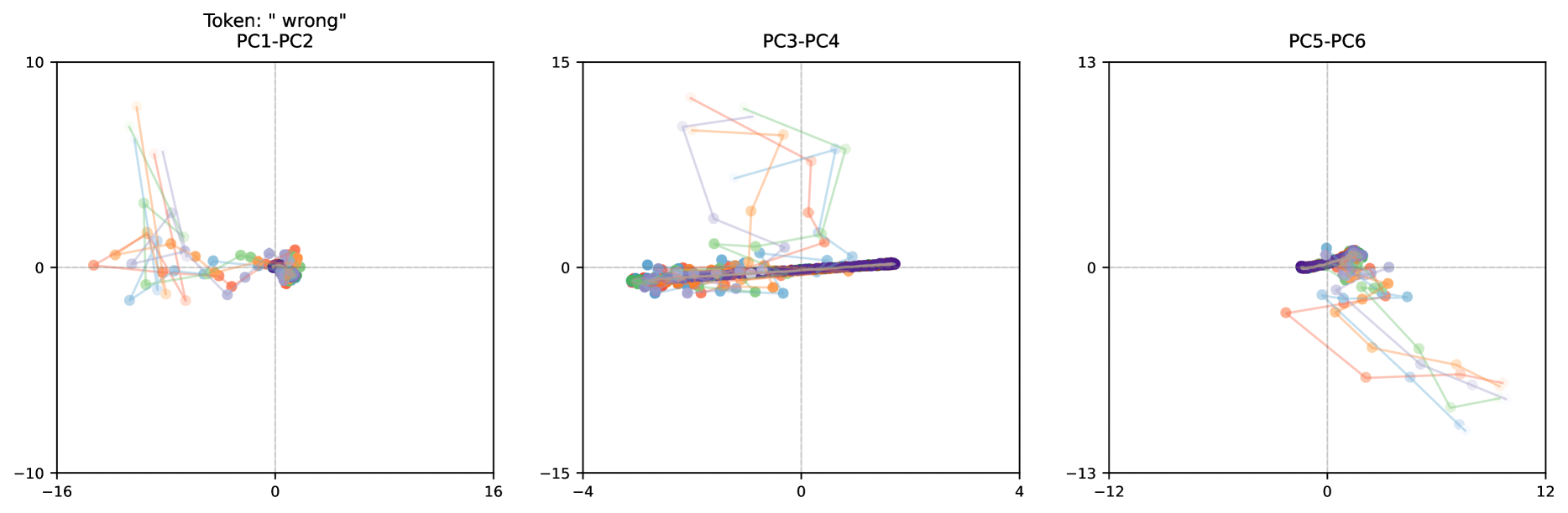
### Visual Description
\n
## Scatter Plot Matrix: PCA Projections of Token "wrong"
### Overview
The image displays three horizontally arranged scatter plots, each representing a two-dimensional projection of data onto different pairs of principal components (PCs). The overall title "Token: 'wrong'" suggests the data pertains to the analysis of the embedding or representation of the specific token "wrong" within a model, visualized across its principal component dimensions. Each plot shows multiple colored trajectories (lines connecting points), indicating sequences or variations of this token's representation.
### Components/Axes
* **Overall Title:** "Token: 'wrong'" (positioned above the leftmost plot).
* **Plot 1 (Left):**
* **Title:** "PC1-PC2"
* **X-axis:** Range approximately -16 to 16. Major tick marks at -16, 0, 16.
* **Y-axis:** Range approximately -10 to 10. Major tick marks at -10, 0, 10.
* **Plot 2 (Center):**
* **Title:** "PC3-PC4"
* **X-axis:** Range approximately -4 to 4. Major tick marks at -4, 0, 4.
* **Y-axis:** Range approximately -15 to 15. Major tick marks at -15, 0, 15.
* **Plot 3 (Right):**
* **Title:** "PC5-PC6"
* **X-axis:** Range approximately -12 to 12. Major tick marks at -12, 0, 12.
* **Y-axis:** Range approximately -13 to 13. Major tick marks at -13, 0, 13.
* **Data Series (Colors):** Multiple distinct colors are used for the lines and points (e.g., orange, light blue, green, purple, red). There is **no explicit legend** provided in the image. The colors are consistent across the three plots, implying each color represents a distinct sequence, context, or instance of the token "wrong".
### Detailed Analysis
**PC1-PC2 Plot:**
* **Trend:** Data points and their connecting lines show a dispersed pattern. Several trajectories originate or pass through the central region (near 0,0) and extend outwards, primarily towards the upper-left quadrant (negative PC1, positive PC2) and to a lesser extent the lower-left (negative PC1, negative PC2). A dense cluster of points from multiple colors is visible near the origin (0,0).
* **Key Data Points/Ranges:** The most extreme point reaches approximately (-14, 8) [orange line]. Another notable trajectory (light blue) extends to around (-12, 6). The vertical spread (PC2) is significant, ranging from about -4 to +8.
**PC3-PC4 Plot:**
* **Trend:** This plot shows a very different structure. A dense, horizontal band of points (primarily purple, with others) is tightly clustered along the PC4=0 line, spanning PC3 from about -3 to +3. Above this band, several distinct, loop-like trajectories (orange, light blue, green) extend vertically into the positive PC4 region, reaching up to ~14. These loops show a pattern of moving up and then back down.
* **Key Data Points/Ranges:** The dense horizontal band is concentrated between PC4 ≈ -1 and +1. The highest point is on an orange trajectory at approximately (PC3≈-1, PC4≈14). The vertical range is the largest of the three plots, from about -2 to +14.
**PC5-PC6 Plot:**
* **Trend:** The data exhibits a diagonal trend. The dense cluster near the origin (0,0) is again present. From this cluster, several trajectories (orange, light blue, green) extend diagonally towards the bottom-right quadrant (positive PC5, negative PC6). The lines are more linear and less looped compared to PC3-PC4.
* **Key Data Points/Ranges:** The most extreme point in this direction is on a light blue line at approximately (PC5≈10, PC6≈-10). The spread is primarily along a diagonal axis from top-left to bottom-right.
### Key Observations
1. **Consistent Origin Cluster:** Across all three projection pairs, a dense cluster of points from multiple colors is consistently located near the origin (0,0). This suggests a common or baseline representation for the token "wrong" in the principal component space.
2. **Divergent Trajectories:** From this common origin, different colored sequences diverge in distinct directions specific to each PC pair. This indicates that the variance captured by different principal components separates these sequences.
3. **Component-Specific Structure:** Each PC pair reveals a unique structural pattern:
* PC1-PC2: Dispersed, fan-like spread.
* PC3-PC4: A tight horizontal baseline with dramatic vertical excursions.
* PC5-PC6: A diagonal, linear spread.
4. **Color-Coded Paths:** The use of consistent colors across plots allows tracking of the same sequence's behavior across different dimensional slices. For example, the orange sequence shows high values in PC2 (Plot 1), very high values in PC4 (Plot 2), and moderate positive PC5 with negative PC6 (Plot 3).
### Interpretation
This visualization performs a **Peircean investigative** reading of the token "wrong"'s embedding space. The plots decompose the high-dimensional representation of the token into its most significant axes of variation (Principal Components).
* **What the data suggests:** The token "wrong" does not have a single, fixed representation. Instead, its embedding varies significantly, likely depending on context. The different colored trajectories probably represent the token's representation in different sentences, contexts, or model layers.
* **How elements relate:** The dense origin cluster represents the "core" or average representation. The diverging trajectories show how context pushes the token's meaning in different directions within the latent space. The distinct patterns in each PC pair indicate that different principal components capture different types of semantic or syntactic variation. For instance, the dramatic vertical movement in PC3-PC4 might correspond to a specific, strong contextual feature.
* **Notable anomalies:** The extreme vertical excursions in the PC3-PC4 plot are particularly striking. They suggest that for certain contexts (the orange, light blue, green sequences), the token's representation is pushed very far along the PC4 dimension, which may correspond to a specific, potent attribute (e.g., intensity, negation strength, or a specific type of error).
* **Why it matters:** This analysis moves beyond treating word embeddings as static vectors. It reveals the dynamic, context-dependent nature of meaning within a model. Understanding these trajectories can help diagnose model behavior, interpret how context alters meaning, and potentially identify robust vs. fragile aspects of a token's representation. The clear separation of trajectories in different PC spaces confirms that PCA has successfully identified orthogonal axes of meaningful variation for this token.
</details>
<details>
<summary>x26.png Details</summary>
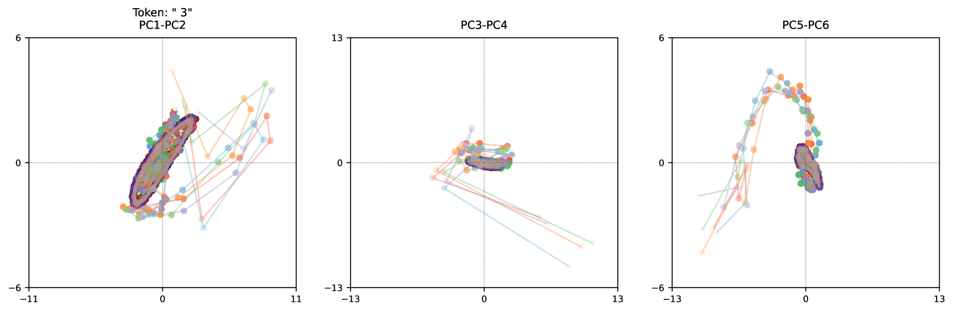
### Visual Description
## PCA Projection Scatter Plots: Token "3"
### Overview
The image displays three horizontally arranged scatter plots, each representing a two-dimensional projection of data onto different pairs of Principal Components (PCs). The overall title indicates the data pertains to a specific token, labeled as "3". The plots visualize the distribution and trajectory of multiple data series (represented by colored points connected by lines) within these reduced-dimensional spaces. No legend is provided to identify what the different colors represent.
### Components/Axes
* **Overall Title:** `Token: " 3"` (Note: The token is the numeral 3, enclosed in quotes with a leading space).
* **Plot 1 (Left):**
* **Title:** `PC1-PC2`
* **X-axis:** Range approximately -11 to 11. No explicit label.
* **Y-axis:** Range approximately -6 to 6. No explicit label.
* **Plot 2 (Center):**
* **Title:** `PC3-PC4`
* **X-axis:** Range approximately -13 to 13. No explicit label.
* **Y-axis:** Range approximately -13 to 13. No explicit label.
* **Plot 3 (Right):**
* **Title:** `PC5-PC6`
* **X-axis:** Range approximately -13 to 13. No explicit label.
* **Y-axis:** Range approximately -6 to 6. No explicit label.
* **Data Series:** Multiple series are plotted, differentiated by color. Observed colors include: purple, orange, green, blue, and light blue. Each series consists of points connected by thin lines of the same color, suggesting a sequence or trajectory.
* **Spatial Layout:** The three plots are aligned side-by-side. Each plot has a central crosshair (dashed lines at x=0, y=0).
### Detailed Analysis
**Plot 1 (PC1-PC2):**
* **Trend:** The data forms a dense, elongated cluster oriented diagonally from the bottom-left to the top-right quadrant. The core of this cluster is centered near the origin (0,0).
* **Data Points:** The purple series appears most concentrated within the central cluster. Other colored series (orange, green, blue) show more dispersion, with points and connecting lines extending outward, particularly towards the top-right and bottom-left extremes of the plot. Some trajectories form sharp angles, indicating significant movement between consecutive points in this PC space.
**Plot 2 (PC3-PC4):**
* **Trend:** The data is tightly clustered near the origin, with a slight horizontal spread. A distinct subset of points from several colors trails off towards the bottom-right quadrant.
* **Data Points:** The central cluster is very dense, making individual points hard to distinguish. The trailing points form several clear, linear trajectories extending from the central mass towards coordinates approximately (10, -10).
**Plot 3 (PC5-PC6):**
* **Trend:** The data distribution is more complex. One group of points forms a dense cluster near the origin, slightly offset to the right. Another prominent group forms a distinct arch or inverted-U shape in the upper half of the plot.
* **Data Points:** The arching structure is composed of points from multiple colors (blue, orange, green, light blue) and spans from approximately x=-8 to x=8, peaking near y=5. The central cluster is again dominated by purple points. The connecting lines show clear paths along the arch and within the cluster.
### Key Observations
1. **Variance Distribution:** The scales of the axes differ across plots (PC3-PC4 has the largest range at ±13), indicating that the variance captured by the principal components is not uniform. PC3 and PC4 capture a wider spread of data than PC1/PC2 or PC5/PC6.
2. **Cluster Stability vs. Dispersion:** The purple series consistently appears in the densest core cluster across all three projections, suggesting it may represent a central or stable mode of the data for token "3". Other colors show greater dispersion and more defined trajectories.
3. **Distinct Geometric Structures:** Each projection reveals a different geometric structure: a diagonal ellipse (PC1-PC2), a compact core with linear outliers (PC3-PC4), and a core with a prominent arch (PC5-PC6). This demonstrates how PCA reveals different aspects of the data's structure in each component pair.
4. **Trajectory Connectivity:** The lines connecting points imply the data is not just a set of independent samples but likely represents sequences, time-series, or iterative processes (e.g., model states during generation).
### Interpretation
This visualization is a technical diagnostic plot, likely from the analysis of a machine learning model's internal representations (embeddings) for a specific input token ("3"). The Principal Component Analysis (PCA) has been used to reduce high-dimensional activation or embedding vectors into 2D views for inspection.
* **What the data suggests:** The plots demonstrate that the model's representation of token "3" is not a single point but a structured manifold in the embedding space. The different colored series could represent different contexts, different layers of the model, or different instances of the token's usage. The dense central clusters (especially of the purple series) indicate a common, core representation. The diverging trajectories and distinct geometric shapes (arch, diagonal spread) reveal systematic variations in this representation, possibly correlated with syntactic role, semantic context, or position in a sequence.
* **How elements relate:** The three plots are orthogonal views of the same high-dimensional data. A point that is an outlier in PC1-PC2 might be part of the central cluster in PC3-PC4. The arch in PC5-PC6 is a particularly strong pattern, suggesting a major, structured axis of variation in the data that is captured by these higher-order components.
* **Notable anomalies:** The long, linear trails in the PC3-PC4 plot are notable. They suggest that for certain conditions or instances, the representation of token "3" moves dramatically and consistently away from its central tendency along a specific direction in the embedding space. This could correspond to a specific linguistic function or a model state shift.
* **Underlying significance:** Without a legend, the exact meaning of the colors is unknown. However, the plot's primary value is in confirming that the token's representation is rich and structured, not random. It allows researchers to visually verify clustering, identify sub-populations of the token's usage, and spot unexpected geometric patterns that might warrant further investigation. The clear trajectories imply a dynamic or context-dependent nature to the token's embedding.
</details>
<details>
<summary>x27.png Details</summary>
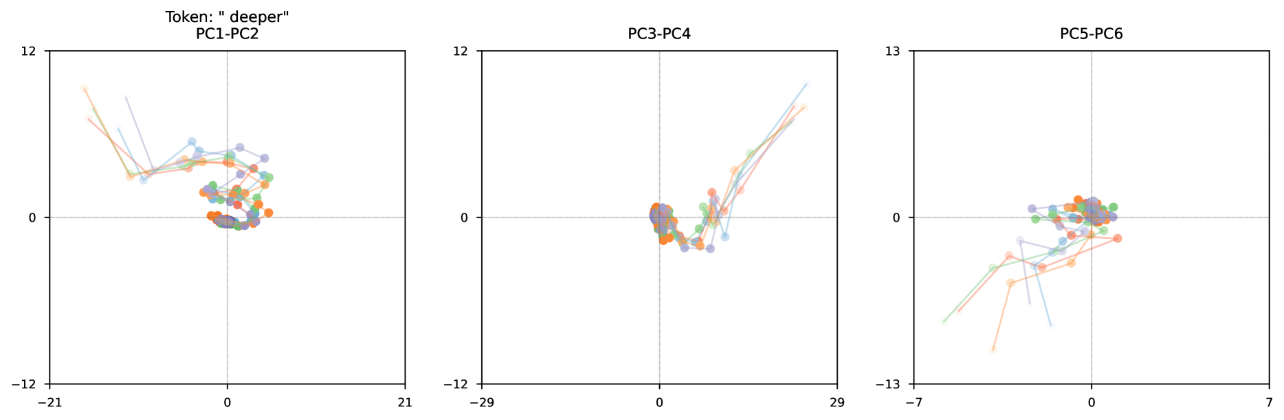
### Visual Description
## PCA Scatter Plots: Token "deeper"
### Overview
The image displays three horizontally arranged scatter plots, each visualizing data points in a two-dimensional space defined by pairs of principal components (PCs). The overall title indicates the data pertains to the token "deeper". The plots show multiple colored data points connected by thin lines, suggesting trajectories or sequences across the principal component space. The data appears to be centered around the origin (0,0) in each plot, with varying degrees of spread and directional trends.
### Components/Axes
* **Main Title:** "Token: 'deeper'" (positioned above the leftmost plot).
* **Subplot Titles:**
* Left Plot: "PC1-PC2"
* Middle Plot: "PC3-PC4"
* Right Plot: "PC5-PC6"
* **Axes and Scales:**
* **PC1-PC2 Plot:**
* X-axis (PC1): Range approximately -21 to 21. Major tick marks at -21, 0, 21.
* Y-axis (PC2): Range approximately -12 to 12. Major tick marks at -12, 0, 12.
* **PC3-PC4 Plot:**
* X-axis (PC3): Range approximately -29 to 29. Major tick marks at -29, 0, 29.
* Y-axis (PC4): Range approximately -12 to 12. Major tick marks at -12, 0, 12.
* **PC5-PC6 Plot:**
* X-axis (PC5): Range approximately -7 to 7. Major tick marks at -7, 0, 7.
* Y-axis (PC6): Range approximately -13 to 13. Major tick marks at -13, 0, 13.
* **Data Series & Legend:** The plots contain data points in at least four distinct colors: orange, green, light blue, and purple. **No explicit legend is present in the image to define what these colors represent.** The points are connected by thin lines of matching or similar colors, forming small chains or trajectories.
* **Spatial Layout:** The three plots are aligned horizontally. Each plot is a square frame with a white background and black axes. Dashed grey lines mark the x=0 and y=0 axes within each plot.
### Detailed Analysis
**PC1-PC2 Plot (Left):**
* **Trend:** The data forms a loose cluster centered near the origin (0,0). Several trajectories extend from this central cluster towards the upper-left quadrant (negative PC1, positive PC2). One prominent orange trajectory starts near (-18, 10) and moves towards the center. A blue trajectory starts near (-15, 8) and moves inward.
* **Data Distribution:** The majority of points are concentrated within the range of PC1: -5 to 5 and PC2: -2 to 4. The spread is greater along the PC1 axis than the PC2 axis.
**PC3-PC4 Plot (Middle):**
* **Trend:** The data shows a very tight cluster at the origin, with a distinct set of trajectories extending into the upper-right quadrant (positive PC3, positive PC4). These extending lines are primarily light blue and orange.
* **Data Distribution:** The central cluster is dense within approximately PC3: -2 to 2 and PC4: -2 to 2. The extending trajectories reach out to approximately PC3=20, PC4=10. This plot has the widest x-axis range (-29 to 29).
**PC5-PC6 Plot (Right):**
* **Trend:** The data is again clustered near the origin, but with trajectories extending primarily into the lower-left quadrant (negative PC5, negative PC6). Green and orange lines are visible in this extending pattern.
* **Data Distribution:** The central cluster is located within roughly PC5: -1 to 1 and PC6: -1 to 1. The extending trajectories reach down to approximately PC5=-6, PC6=-10. This plot has the narrowest x-axis range (-7 to 7).
### Key Observations
1. **Central Tendency:** In all three PC spaces, the representation of the token "deeper" has a strong central tendency around the origin (0,0).
2. **Directional Spread:** The variance (spread) of the data is not isotropic. Each PC pair shows a dominant direction of spread:
* PC1-PC2: Spread towards the upper-left.
* PC3-PC4: Spread towards the upper-right.
* PC5-PC6: Spread towards the lower-left.
3. **Scale Discrepancy:** The scales of the principal components differ significantly. PC3 has the largest range (58 units), while PC5 has the smallest (14 units). This is typical for PCA, where components are ordered by explained variance.
4. **Trajectory Structure:** The data is not presented as isolated points but as connected sequences, implying an underlying process or ordering (e.g., layers in a neural network, steps in a process, or different contexts).
5. **Missing Legend:** The color coding of the points and lines is a critical piece of information that is not defined within the image. The colors likely represent different categories, layers, or conditions, but this cannot be determined from the visual data alone.
### Interpretation
This visualization likely comes from an analysis of neural network embeddings or activations for the specific token "deeper". Principal Component Analysis (PCA) has been applied to reduce the high-dimensional representation of this token across different contexts (e.g., different layers of a model, different sentences, or different attention heads) into 2D projections for visualization.
* **What the data suggests:** The token "deeper" has a core, stable representation (the central cluster) in the model's embedding space. However, its representation also varies systematically along specific directions captured by the principal components. The connected trajectories suggest that this variation is not random but follows a path, possibly corresponding to the token's changing role or meaning as information propagates through the network.
* **How elements relate:** The three plots show orthogonal (uncorrelated) views of the same high-dimensional variance. The dominant spread in different quadrants for each PC pair indicates that the primary axes of variation for this token are distinct and multi-directional. The color groups, if they represent, for example, different model layers, would show how the token's representation evolves along these axes.
* **Notable anomalies:** The most striking feature is the directional "comet-like" tails in each plot. These are not outliers in a traditional sense but rather evidence of structured, low-dimensional variation within the token's representation. The absence of a legend is a significant limitation for full interpretation, as the meaning of the color groups is essential to understand the source of the variance (e.g., is the spread due to layer depth, syntactic context, or semantic role?).
**Language Note:** All text in the image is in English.
</details>
Figure 22: Latent Space trajectories for a few select tokens. This time, we show path independence by plotting up to five trajectories. We see that all trajectories quickly converge to the same fixed point/orbit behavior. Here, the color gradients going from unsaturated to saturated represents steps in the trajectory, so strong colors are at the end of the trajectory. Gray denotes the overlap of multiple trajectories.
<details>
<summary>x28.png Details</summary>
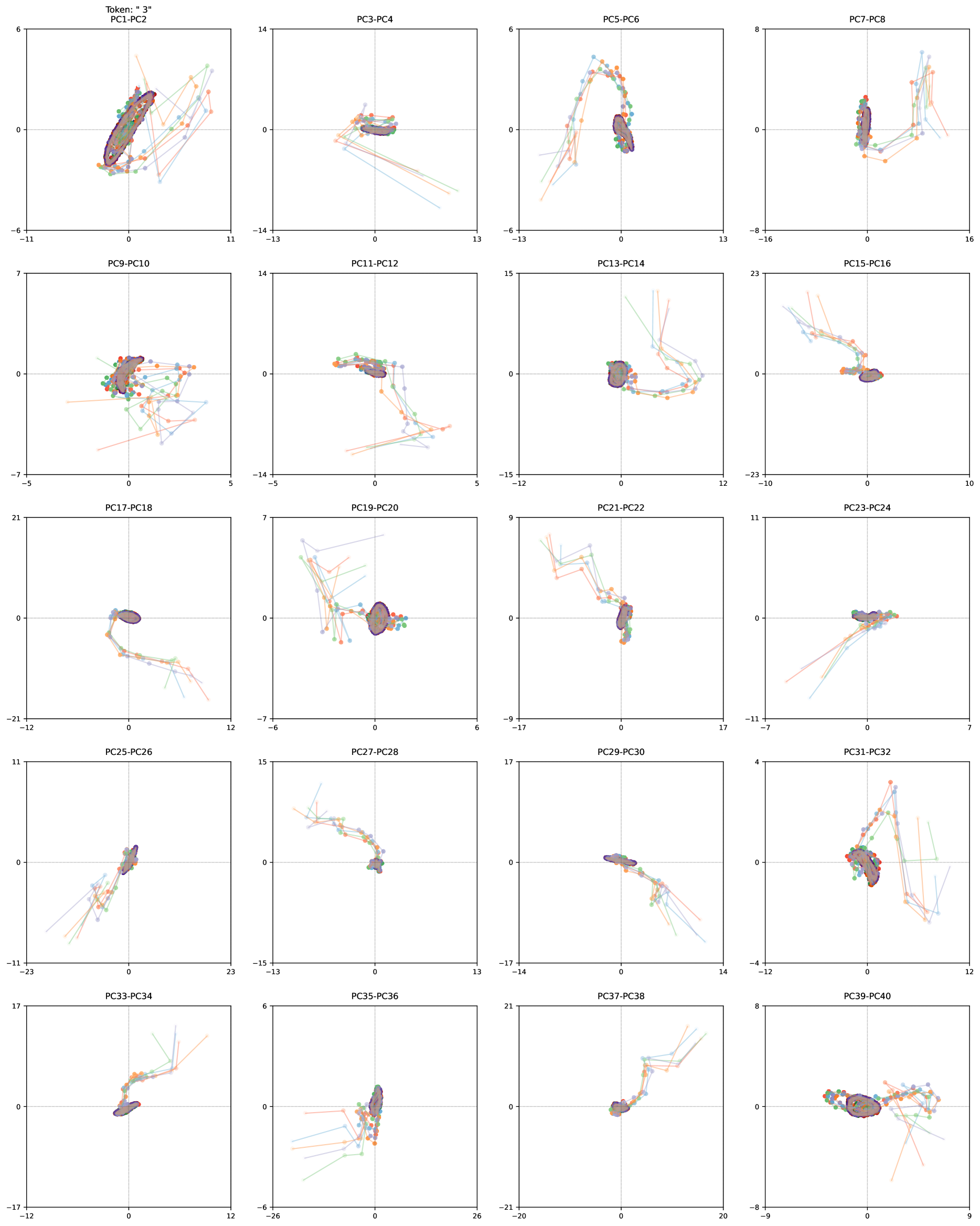
### Visual Description
## Scatter Plot Grid: Principal Component Analysis (PCA) Projections for Token "3"
### Overview
The image displays a 5x4 grid of 20 scatter plots, each visualizing the relationship between pairs of principal components (PCs). The overall title at the top-left corner is **Token: "3"**. Each subplot represents a 2D projection of data onto a specific pair of principal components (e.g., PC1 vs. PC2, PC3 vs. PC4, etc.), likely from a high-dimensional dataset related to the token "3". The data points are colored in multiple hues (orange, green, blue, purple, etc.) and are connected by faint lines, suggesting trajectories or sequences across the principal component space.
### Components/Axes
* **Global Title:** `Token: "3"` (Top-left corner of the entire figure).
* **Subplot Grid:** 5 rows by 4 columns.
* **Subplot Titles:** Each subplot is titled with its corresponding PC pair (e.g., `PC1-PC2`, `PC3-PC4`, ..., `PC39-PC40`).
* **Axes:** Each subplot has an x-axis and a y-axis representing the values of the respective principal components. The axis scales (ranges) vary significantly between subplots.
* **Data Series:** Multiple colored series (points connected by lines) are present in each plot. The colors observed include orange, green, light blue, dark blue, and purple. There is no explicit legend provided within the image to define what each color represents.
### Detailed Analysis
Below is a plot-by-plot analysis, noting axis ranges and the general visual trend of the data points. The colors are described based on visual inspection (e.g., orange, green, blue, purple).
**Row 1:**
1. **PC1-PC2:** X: [-11, 11], Y: [-6, 6]. Data forms a dense, elongated cluster oriented diagonally from bottom-left to top-right, centered near (0,0). Multiple colored trajectories are visible.
2. **PC3-PC4:** X: [-13, 13], Y: [-14, 14]. A tight cluster near (0,0) with several long, linear trajectories extending primarily towards the bottom-right quadrant.
3. **PC5-PC6:** X: [-13, 13], Y: [-6, 6]. Data forms a distinct inverted "U" or arch shape, peaking around Y=4. The cluster is dense at the right end of the arch.
4. **PC7-PC8:** X: [-16, 16], Y: [-8, 8]. A dense vertical cluster near X=0, with several trajectories extending to the right and slightly upward.
**Row 2:**
5. **PC9-PC10:** X: [-5, 5], Y: [-7, 7]. A central cluster with trajectories spreading out in multiple directions, particularly to the left and bottom.
6. **PC11-PC12:** X: [-5, 5], Y: [-14, 14]. A cluster near the origin with long, downward-sloping trajectories extending to the bottom-right.
7. **PC13-PC14:** X: [-12, 12], Y: [-15, 15]. A cluster near (0,0) with trajectories forming a loose, downward-curving shape to the right.
8. **PC15-PC16:** X: [-10, 10], Y: [-23, 23]. A dense cluster near the origin with a few long, linear trajectories extending to the top-left.
**Row 3:**
9. **PC17-PC18:** X: [-12, 12], Y: [-21, 21]. A cluster near the origin with trajectories extending downward and to the right.
10. **PC19-PC20:** X: [-6, 6], Y: [-7, 7]. A dense cluster near (0,0) with several trajectories spreading out, notably to the top-left.
11. **PC21-PC22:** X: [-17, 17], Y: [-9, 9]. A cluster near the origin with trajectories extending upward and to the left.
12. **PC23-PC24:** X: [-7, 7], Y: [-11, 11]. A tight horizontal cluster near Y=0, with trajectories extending to the bottom-left.
**Row 4:**
13. **PC25-PC26:** X: [-23, 23], Y: [-11, 11]. A cluster near the origin with trajectories extending to the bottom-left.
14. **PC27-PC28:** X: [-13, 13], Y: [-15, 15]. A cluster near the origin with trajectories extending to the top-left.
15. **PC29-PC30:** X: [-14, 14], Y: [-17, 17]. A cluster near the origin with trajectories extending to the bottom-right.
16. **PC31-PC32:** X: [-12, 12], Y: [-4, 4]. A dense cluster near the origin with trajectories forming a loop or upward curve to the right.
**Row 5:**
17. **PC33-PC34:** X: [-12, 12], Y: [-17, 17]. A cluster near the origin with trajectories extending to the top-right.
18. **PC35-PC36:** X: [-26, 26], Y: [-6, 6]. A cluster near the origin with trajectories extending to the bottom-left.
19. **PC37-PC38:** X: [-20, 20], Y: [-21, 21]. A cluster near the origin with trajectories extending to the top-right.
20. **PC39-PC40:** X: [-9, 9], Y: [-8, 8]. A cluster near the origin with trajectories spreading out, notably to the right.
### Key Observations
1. **Common Structure:** Nearly all plots show a dense core cluster of points centered at or near the origin (0,0), with various trajectories or "arms" extending outward. This suggests the data has a central tendency with directional variations captured by different PC pairs.
2. **Variable Spread:** The scale of the axes varies dramatically (e.g., PC15-PC16 Y-axis spans 46 units, while PC31-PC32 Y-axis spans only 8 units). This indicates that the variance explained by each principal component pair is not uniform.
3. **Distinct Shapes:** Some PC pairs reveal clear geometric patterns:
* **Arch/Inverted U:** PC5-PC6.
* **Vertical/Horizontal Clusters:** PC7-PC8 (vertical), PC23-PC24 (horizontal).
* **Diagonal Orientation:** PC1-PC2.
4. **Trajectory Direction:** The direction of the extending trajectories (e.g., top-left, bottom-right) is specific to each PC pair, indicating the axes of variation in the high-dimensional space.
5. **Color Patterns:** The same color (e.g., orange, green) appears to follow consistent trajectories within a given plot, suggesting the colors represent distinct classes, sequences, or experimental conditions that evolve through the PC space.
### Interpretation
This grid of scatter plots is a diagnostic visualization from a Principal Component Analysis (PCA) performed on data associated with the token "3". PCA is a dimensionality reduction technique used to visualize high-dimensional data in lower dimensions (here, 2D) while preserving as much variance as possible.
* **What the data suggests:** The consistent central cluster with radiating trajectories implies that the underlying data for token "3" has a stable "core" representation, but also exhibits systematic variations or modes of change. Each PC pair captures a different axis of this variation. For example, the arch in PC5-PC6 might represent a continuous transformation or cycle in the data.
* **How elements relate:** The 20 plots are complementary views of the same high-dimensional dataset. A point's position in one plot (e.g., PC1-PC2) is independent of its position in another (e.g., PC3-PC4), but together they provide a more complete picture of the data's structure. The colored trajectories likely track the same data points (or groups) across different projection planes.
* **Notable anomalies/trends:** The most striking features are the non-random, structured shapes (arches, lines, clusters). This indicates the data is not noise but has meaningful, low-dimensional structure. The fact that trajectories are often linear or smoothly curved suggests the variations are orderly. The lack of scattered, random points reinforces that the token "3" has a well-defined representation in this feature space.
* **Purpose:** This type of analysis is common in machine learning and natural language processing to understand the internal representations of tokens in a model. It helps researchers see if different contexts or uses of the same token ("3") cluster together or separate in the model's latent space, and what the primary directions of variation are.
</details>
Figure 23: Detailed PCA of Latent Space trajectories for the math question. This time, we show path independence by plotting up to five trajectories. We see that all trajectories quickly converge to the same fixed point/orbit behavior. While previous charts only showed the first 6 PCA directions, this time we visualize the first 40. Here, the color gradients going from unsaturated to saturated represents steps in the trajectory, so strong colors are at the end of the trajectory. Gray denotes the overlap of multiple trajectories.
<details>
<summary>x29.png Details</summary>
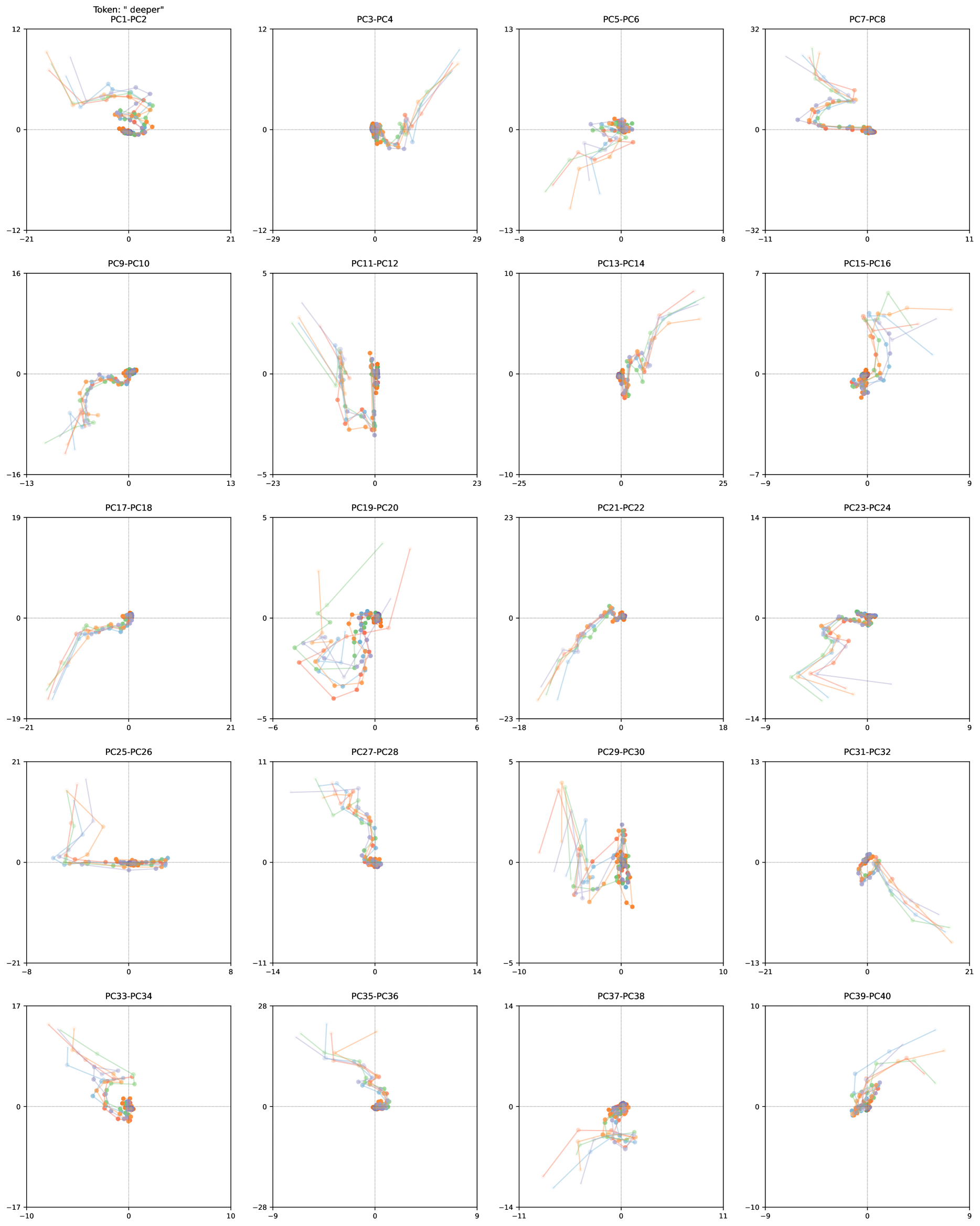
### Visual Description
## Scatter Plot Matrix: Principal Component Projections for Token "deeper"
### Overview
The image displays a 5x4 grid of 20 scatter plots. Each plot visualizes the relationship between a pair of Principal Components (PCs) for the token "deeper". The data points are connected by lines, forming trajectories, and are colored in multiple distinct hues (orange, green, blue, purple, etc.), suggesting different categories or sequences. There is no legend provided to identify what these colors represent. The overall purpose appears to be analyzing the variance and structure of the token's representation across different principal component dimensions.
### Components/Axes
* **Global Title:** Located at the top-left corner: `Token: " deeper"`.
* **Subplot Titles:** Each of the 20 subplots has a title indicating the PC pair being plotted (e.g., `PC1-PC2`, `PC3-PC4`, ..., `PC39-PC40`).
* **Axes:** Each subplot has an x-axis and a y-axis. The axes are labeled with numerical tick marks but lack descriptive titles (e.g., "Principal Component 1"). The ranges vary significantly between plots.
* **Data Series:** Each plot contains multiple series, distinguished by color (orange, green, light blue, purple, etc.). Each series is a connected scatter plot, showing a trajectory of points.
* **Grid Layout:** The plots are arranged in a uniform grid with 5 rows and 4 columns.
### Detailed Analysis
The following table details the title and axis ranges for each subplot, proceeding row by row from top-left to bottom-right.
| Position (Row, Col) | Subplot Title | X-Axis Range (Approx.) | Y-Axis Range (Approx.) | Visual Trend Description |
| :--- | :--- | :--- | :--- | :--- |
| (1,1) | PC1-PC2 | -21 to 21 | -12 to 12 | Multiple colored trajectories converge from the top-left quadrant towards a dense cluster near the origin (0,0). |
| (1,2) | PC3-PC4 | -29 to 29 | -12 to 12 | Trajectories start near the origin and fan out upwards and to the right into the first quadrant. |
| (1,3) | PC5-PC6 | -8 to 8 | -13 to 13 | Trajectories are tightly clustered near the origin, with some lines extending into the third quadrant (bottom-left). |
| (1,4) | PC7-PC8 | -11 to 11 | -32 to 32 | Trajectories form a loose cluster near the origin, with some lines extending into the second quadrant (top-left). |
| (2,1) | PC9-PC10 | -13 to 13 | -16 to 16 | Trajectories form a curved path from the third quadrant (bottom-left) up towards the origin. |
| (2,2) | PC11-PC12 | -23 to 23 | -5 to 5 | Trajectories are vertically oriented, clustered along the y-axis near x=0, spanning from negative to positive y-values. |
| (2,3) | PC13-PC14 | -25 to 25 | -10 to 10 | Trajectories start near the origin and extend diagonally upwards into the first quadrant. |
| (2,4) | PC15-PC16 | -9 to 9 | -7 to 7 | A dense, tangled cluster of trajectories centered near the origin. |
| (3,1) | PC17-PC18 | -21 to 21 | -19 to 19 | Trajectories form a curved path from the third quadrant up towards the origin. |
| (3,2) | PC19-PC20 | -6 to 6 | -5 to 5 | A complex, tangled web of trajectories centered near the origin, with some lines extending into all quadrants. |
| (3,3) | PC21-PC22 | -18 to 18 | -23 to 23 | Trajectories form a diagonal line from the third quadrant to the first quadrant, passing through the origin. |
| (3,4) | PC23-PC24 | -14 to 14 | -9 to 9 | Trajectories form a loose, horizontal cluster near y=0, spanning the x-axis. |
| (4,1) | PC25-PC26 | -8 to 8 | -21 to 21 | Trajectories form a horizontal cluster near y=0, with some lines extending vertically upwards. |
| (4,2) | PC27-PC28 | -14 to 14 | -11 to 11 | Trajectories are vertically oriented, clustered along the y-axis near x=0. |
| (4,3) | PC29-PC30 | -10 to 10 | -5 to 5 | A dense, vertical cluster of trajectories centered near x=0. |
| (4,4) | PC31-PC32 | -21 to 21 | -13 to 13 | Trajectories form a diagonal line from the origin down into the fourth quadrant (bottom-right). |
| (5,1) | PC33-PC34 | -10 to 10 | -17 to 17 | Trajectories form a curved path from the second quadrant (top-left) down towards the origin. |
| (5,2) | PC35-PC36 | -9 to 9 | -28 to 28 | Trajectories form a diagonal line from the second quadrant down to the origin. |
| (5,3) | PC37-PC38 | -11 to 11 | -14 to 14 | A dense cluster of trajectories centered near the origin. |
| (5,4) | PC39-PC40 | -9 to 9 | -10 to 10 | Trajectories start near the origin and extend diagonally upwards into the first quadrant. |
### Key Observations
1. **Varying Structure:** The relationship between token embeddings changes dramatically across different PC pairs. Some show tight clusters (e.g., PC15-PC16), others show clear linear trends (e.g., PC21-PC22), and others show complex, non-linear trajectories (e.g., PC19-PC20).
2. **Central Tendency:** The origin (0,0) is a strong focal point in nearly all plots, with most data trajectories converging to or passing through it.
3. **Color-Coded Trajectories:** The use of multiple colors implies the data is grouped into several distinct series (e.g., different contexts, layers, or attention heads). However, the **critical missing information** is a legend to decode these colors.
4. **Axis Scale Disparity:** The numerical ranges on the axes differ greatly between plots (e.g., PC7-PC8 y-axis spans 64 units, while PC29-PC30 y-axis spans only 10 units), indicating that the variance captured by each principal component pair is not uniform.
### Interpretation
This visualization is a diagnostic tool for understanding the internal representation of the token "deeper" within a machine learning model, likely a transformer-based language model. Principal Component Analysis (PCA) has been used to reduce the high-dimensional embedding space into 2D projections.
* **What it demonstrates:** The plots reveal that the token's representation is not a single point but a structured manifold. The different colored lines likely trace the token's representation through different layers of the model or across different contextual examples. The convergence to the origin in many plots suggests that after PCA transformation, the mean of the data is centered at zero.
* **Relationships between elements:** The grid allows comparison of how the token's variance is distributed across orthogonal directions (the PCs). Early PCs (e.g., PC1-PC4) often capture the most significant variance, which is visible here as broader spreads. Later PCs show more nuanced or noise-related structure.
* **Notable anomalies/patterns:** The stark difference in structure between adjacent plots (e.g., the vertical line in PC11-PC12 vs. the diagonal in PC13-PC14) highlights that the principal components are capturing fundamentally different aspects of the data's variation. The lack of a legend is a significant limitation, preventing the viewer from attributing the observed trajectories to specific model components or contexts, which is essential for a full technical interpretation.
</details>
Figure 24: Detailed PCA of Latent Space trajectories for the trivia question. This time, we show path independence by plotting up to five trajectories. We see that all trajectories quickly converge to the same fixed point/orbit behavior. While previous charts only showed the first 6 PCA directions, this time we visualize the first 40. Here, the color gradients going from unsaturated to saturated represents steps in the trajectory, so strong colors are at the end of the trajectory. Gray denotes the overlap of multiple trajectories.
<details>
<summary>x30.png Details</summary>
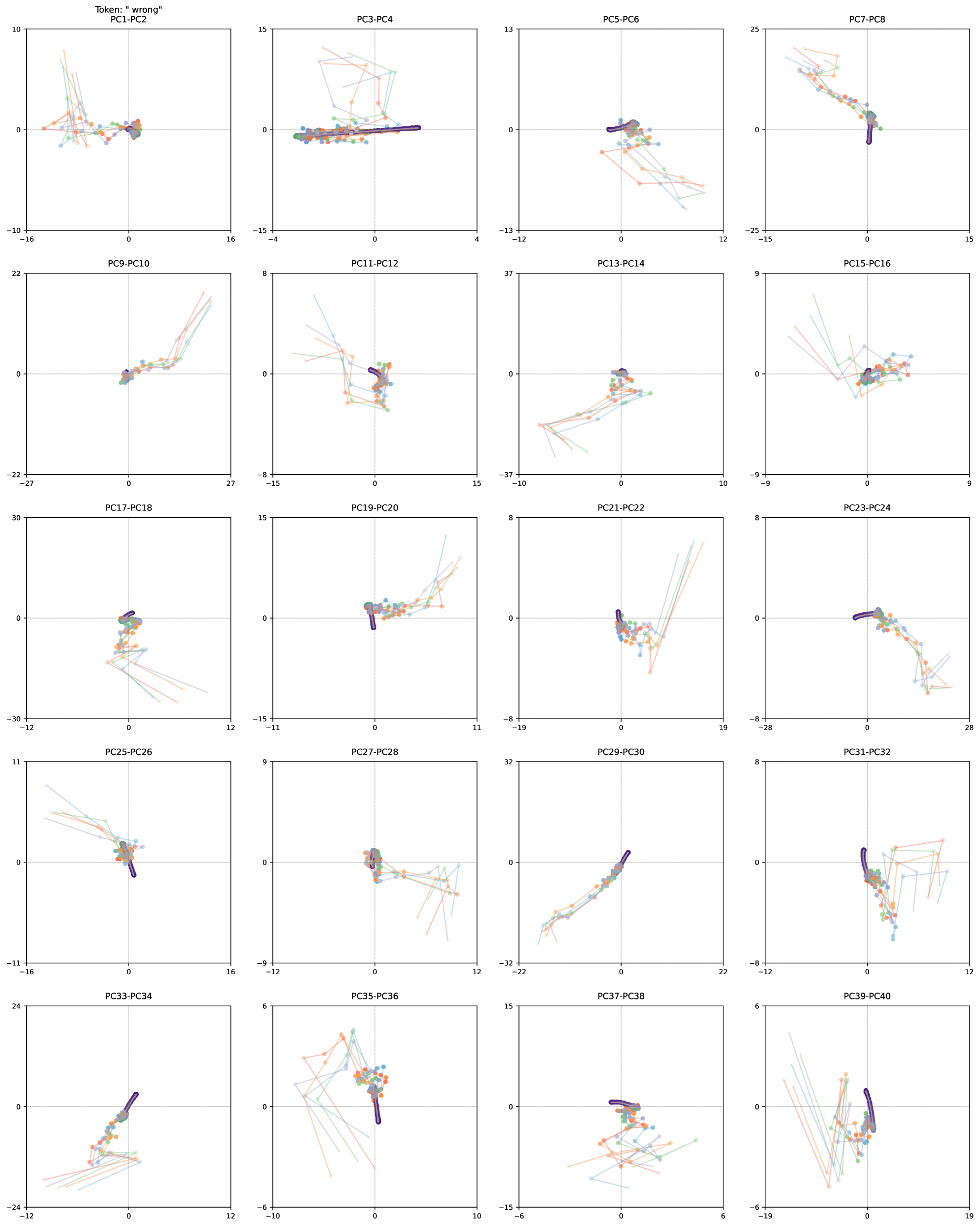
### Visual Description
## Scatter Plot Matrix: Principal Component Trajectories for Token "wrong"
### Overview
The image displays a 5x4 grid of 20 scatter plots, each visualizing the relationship between pairs of principal components (PCs) for the token "wrong". The plots show trajectories or paths formed by connected data points, suggesting the evolution or variation of this token's representation across different dimensions or model layers. The overall layout is a matrix where each subplot represents a unique 2D projection of a high-dimensional space.
### Components/Axes
* **Main Title:** Located at the top-left of the entire figure: `Token: "wrong"`
* **Subplot Titles:** Each of the 20 subplots has a title indicating the principal component pair being plotted. They are arranged in a grid as follows:
* Row 1: `PC1-PC2`, `PC3-PC4`, `PC5-PC6`, `PC7-PC8`
* Row 2: `PC9-PC10`, `PC11-PC12`, `PC13-PC14`, `PC15-PC16`
* Row 3: `PC17-PC18`, `PC19-PC20`, `PC21-PC22`, `PC23-PC24`
* Row 4: `PC25-PC26`, `PC27-PC28`, `PC29-PC30`, `PC31-PC32`
* Row 5: `PC33-PC34`, `PC35-PC36`, `PC37-PC38`, `PC39-PC40`
* **Axes:** Each subplot has numerical axes with tick marks. The ranges vary significantly between plots. There are no explicit axis titles (e.g., "PC1 Value"), only the numerical scales. The axes are centered around (0,0) in most plots, indicated by faint grid lines.
* **Legend:** **No legend is present in the image.** The data series are distinguished by color (purple, orange, green, blue, light blue), but their corresponding labels or categories are not provided.
* **Data Representation:** Data points are connected by lines, forming trajectories. Each color appears to represent a distinct trajectory or series.
### Detailed Analysis
**Data Series & Trends (by color, approximate observations):**
* **Purple Series:** This is the most prominent and consistent series. In nearly every plot, it forms a tight, dense cluster or a short, thick line segment very close to the origin (0,0). Its trajectory shows minimal variance compared to the other series.
* **Orange, Green, Blue, Light Blue Series:** These series exhibit much greater variance. They form longer, more scattered trajectories that often extend far from the origin. Their paths are more erratic and less clustered than the purple series.
**Subplot-by-Subplot Axis Ranges and General Trends:**
* **PC1-PC2:** X: [-16, 16], Y: [-10, 10]. Purple cluster at origin. Other lines spread, with some extending to the top-left and bottom-right quadrants.
* **PC3-PC4:** X: [-4, 4], Y: [-15, 15]. Purple line along X-axis near 0. Other lines show large vertical spread, especially in the positive Y direction.
* **PC5-PC6:** X: [-12, 12], Y: [-13, 13]. Purple cluster at origin. Other lines trend downward into the bottom-right quadrant.
* **PC7-PC8:** X: [-15, 15], Y: [-25, 25]. Purple line is nearly vertical at X≈0. Other lines slope downward from top-left to bottom-right.
* **PC9-PC10:** X: [-27, 27], Y: [-22, 22]. Purple cluster at origin. Other lines trend upward into the top-right quadrant.
* **PC11-PC12:** X: [-15, 15], Y: [-8, 8]. Purple cluster at origin. Other lines are scattered, with some extending to the top-left.
* **PC13-PC14:** X: [-10, 10], Y: [-37, 37]. Purple cluster at origin. Other lines show a strong trend from bottom-left to top-right.
* **PC15-PC16:** X: [-9, 9], Y: [-9, 9]. Purple cluster at origin. Other lines are scattered in all directions.
* **PC17-PC18:** X: [-12, 12], Y: [-30, 30]. Purple cluster at origin. Other lines trend downward into the bottom-right quadrant.
* **PC19-PC20:** X: [-11, 11], Y: [-15, 15]. Purple cluster at origin. Other lines trend upward into the top-right quadrant.
* **PC21-PC22:** X: [-19, 19], Y: [-8, 8]. Purple cluster at origin. Other lines show a sharp upward trend in the top-right quadrant.
* **PC23-PC24:** X: [-28, 28], Y: [-8, 8]. Purple cluster at origin. Other lines trend downward into the bottom-right quadrant.
* **PC25-PC26:** X: [-16, 16], Y: [-11, 11]. Purple cluster at origin. Other lines trend downward into the bottom-left quadrant.
* **PC27-PC28:** X: [-12, 12], Y: [-9, 9]. Purple cluster at origin. Other lines are scattered, trending slightly downward.
* **PC29-PC30:** X: [-22, 22], Y: [-32, 32]. Purple line trends upward from bottom-left to top-right. Other lines follow a similar, more scattered path.
* **PC31-PC32:** X: [-12, 12], Y: [-8, 8]. Purple cluster at origin. Other lines are scattered, trending downward.
* **PC33-PC34:** X: [-12, 12], Y: [-24, 24]. Purple line trends upward from bottom-left to top-right. Other lines follow a similar, more scattered path.
* **PC35-PC36:** X: [-10, 10], Y: [-6, 6]. Purple cluster at origin. Other lines are widely scattered.
* **PC37-PC38:** X: [-6, 6], Y: [-15, 15]. Purple cluster at origin. Other lines are scattered, trending slightly downward.
* **PC39-PC40:** X: [-19, 19], Y: [-6, 6]. Purple cluster at origin. Other lines are widely scattered, with some large vertical excursions.
### Key Observations
1. **Consistent Purple Cluster:** The purple series is remarkably stable and localized near the origin across all 20 PC projections. This suggests it represents a baseline, average, or highly constrained representation of the token.
2. **High Variance in Other Series:** The orange, green, blue, and light blue series show significant dispersion and directional trends in many projections (e.g., PC13-PC14, PC29-PC30). This indicates these representations vary substantially along those principal components.
3. **Directional Correlations:** In several plots (e.g., PC9-PC10, PC13-PC14, PC19-PC20, PC29-PC30, PC33-PC34), the non-purple trajectories show clear directional trends (upward-right, downward-right), suggesting correlations between those specific PC pairs for those data series.
4. **Absence of Legend:** The lack of a legend is a critical omission. It is impossible to determine what the different colors represent (e.g., different model layers, training steps, attention heads, or contextual variations of the token "wrong").
### Interpretation
This visualization is likely from an analysis of neural network embeddings or internal representations, using Principal Component Analysis (PCA) to reduce dimensionality. The token "wrong" is being tracked across different conditions or model components.
* **What the data suggests:** The stark contrast between the stable purple series and the volatile other series implies a fundamental difference in how the token "wrong" is represented in different contexts. The purple series could represent the token's embedding in a static word embedding matrix, while the other colors could represent its dynamic activations within a specific model forward pass, across different layers, or in different contextual sentences.
* **How elements relate:** Each subplot shows how two specific principal components co-vary. The consistent clustering of the purple series at (0,0) across all plots indicates that in the static embedding space, the token's representation has near-zero values for these principal components. The trajectories of the other series show how the token's representation is "pushed" away from this baseline in the activation space, with the direction of movement revealing which PC dimensions are most affected.
* **Notable anomalies:** The PC29-PC30 and PC33-PC34 plots are anomalies because the purple series itself shows a clear trend, unlike in all other plots. This could indicate that for these specific components, even the baseline representation has a directional bias, or that the purple series in these plots represents something slightly different.
* **Underlying meaning:** The analysis aims to understand the geometry of the token "wrong" in a model's representational space. The high variance in certain PC projections for the non-purple series highlights the dimensions along which the model's processing of this token is most sensitive or variable. Without the legend, the specific cause of this variance (e.g., layer depth, attention head, syntactic role) remains unknown, but the visualization successfully isolates the principal axes of that variation.
</details>
Figure 25: Detailed PCA of Latent Space trajectories for the unsafe question. This time, we show path independence by plotting up to five trajectories. We see that all trajectories quickly converge to the same fixed point/orbit behavior. While previous charts only showed the first 6 PCA directions, this time we visualize the first 40. Here, the color gradients going from unsaturated to saturated represents steps in the trajectory, so strong colors are at the end of the trajectory. Gray denotes the overlap of multiple trajectories.
## Appendix C Pretraining Data
Table 7: Datasets used for model pre-training (Part 1: Standard sources)
Table 8: Datasets used for model pre-training (Part 2: Instruction Data)
Dataset Address License Category W MG Citation WebInstruct-prometheus chargoddard/WebInstructSub-prometheus apache-2.0 generic-instruct 1.0 ✓ Kim et al. (2024) hercules Locutusque/hercules-v5.0 other generic-instruct 1.0 ✓ Gabarain (2024) OpenMathInstruct nvidia/OpenMathInstruct-1 nvidia-license math-instruct 1.0 ✓ Toshniwal et al. (2024b) MetaMathQA meta-math/MetaMathQA mit math-instruct 1.0 ✓ Yu et al. (2023) CodeFeedback m-a-p/CodeFeedback-Filtered-Instruction apache-2.0 generic-instruct 2.0 ✓ Zheng et al. (2024) Daring-Anteater nvidia/Daring-Anteater cc-by-4.0 generic-instruct 1.0 ✓ Wang et al. (2024b) Nvidia-Blender nvidia/sft_datablend_v1 cc-by-4.0 generic-instruct 1.0 ✓ nvidia/sft_datablend_v1 baai-instruct-foundation BAAI/Infinity-Instruct - generic-instruct 1.0 ✓ BAAI/Infinity-Instruct baai-instruct-gen BAAI/Infinity-Instruct - generic-instruct 1.0 ✓ BAAI/Infinity-Instruct anthracite-stheno anthracite-org/Stheno-Data-Filtered - math-instruct 1.0 ✓ anthracite-org/Stheno-Data-Filtered opus-writing Nopm/Opus_WritingStruct apache-2.0 writing-instruct 2.0 ✓ Nopm/Opus_WritingStruct math-step xinlai/Math-Step-DPO-10K - math-instruct 2.0 ✓ Lai et al. (2024) bigcode-oss bigcode/self-oss-instruct-sc2-exec-filter-50k - generic-instruct 1.0 ✓ sc2-instruct everyday-conversations HuggingFaceTB/everyday-conversations apache-2.0 writing-instruct 3.0 ✓ HuggingFaceTB/everyday-conversations gsm8k hkust-nlp/gsm8k-fix mit math-instruct 1.0 ✗ Cobbe et al. (2021) no-robots HuggingFaceH4/no_robots cc-by-nc-4.0 writing-instruct 3.0 ✗ Ouyang et al. (2022) longwriter THUDM/LongWriter-6k apache-2.0 writing-instruct 2.0 ✓ Bai et al. (2024) webglm-qa THUDM/webglm-qa - generic-instruct 1.0 - Liu et al. (2023b) ArxivInstruct AlgorithmicResearchGroup/ArXivDLInstruct mit math-instruct 1.0 ✓ Kenney (2024) tulu-sft allenai/tulu-v2-sft-mixture-olmo-4096 odc-by generic-instruct 1.0 ✓ Groeneveld et al. (2024) P3 bigscience/P3 apache-2.0 generic-instruct 1.0 ✗ Sanh et al. (2021) OrcaSonnet Gryphe/Sonnet3.5-SlimOrcaDedupCleaned mit writing-instruct 2.0 ✓ Gryphe/Sonnet3.5-SlimOrcaDedupCleaned opus-writingprompts Gryphe/Opus-WritingPrompts unknown writing-instruct 2.0 ✓ Gryphe/Opus-WritingPrompts reddit-writing nothingiisreal/Reddit-Dirty-And-WritingPrompts apache-2.0 writing-instruct 2.0 ✗ Reddit-Dirty-And-WritingPrompts kalomaze-instruct nothingiisreal/Kalomaze-Opus-Instruct-25k-filtered apache-2.0 writing-instruct 2.0 ✓ Kalomaze-Opus-Instruct-25k lean-github internlm/Lean-Github apache-2.0 math-instruct 3.0 ✗ Wu et al. (2024) lean-workbook pkuAI4M/LeanWorkbook apache-2.0 math-instruct 3.0 ✗ Ying et al. (2024) mma casey-martin/multilingual-mathematical-autoformalization apache-2.0 math-instruct 3.0 ✗ Jiang et al. (2023) lean-dojo-informal AI4M/leandojo-informalized - math-instruct 3.0 ✗ Yang et al. (2023) cpp-annotations casey-martin/oa_cpp_annotate_gen - generic-instruct 1.0 ✓ moyix lean-tactics l3lab/ntp-mathlib-instruct-st - math-instruct 2.0 ✗ Hu et al. (2024) college-math ajibawa-2023/Maths-College apache-2.0 math 1.0 ✓ ajibawa-2023/Maths-College gradeschool-math ajibawa-2023/Maths-Grade-School apache-2.0 math 1.0 ✓ ajibawa-2023/Maths-Grade-School general-stories ajibawa-2023/General-Stories-Collection apache-2.0 synthetic-text 1.0 ✓ ajibawa-2023/General-Stories-Collection amps-mathematica XinyaoHu/AMPS_mathematica mit math 1.0 ✗ XinyaoHu/AMPS_mathematica amps-khan XinyaoHu/AMPS_khan mit math-instruct 1.0 ✗ XinyaoHu/AMPS_khan Magpie-300k Magpie-Align/Magpie-Pro-MT-300K-v0.1 llama3 generic-instruct 1.0 ✓ Xu et al. (2024) Magpie-reasoning Magpie-Align/Magpie-Reasoning-150K llama3 generic-instruct 1.0 ✓ Xu et al. (2024) prox-fineweb gair-prox/FineWeb-pro odc-by generic-text 1.0 ✗ Zhou et al. (2024) prox-c4 gair-prox/c4-pro odc-by generic-text 1.0 ✗ Zhou et al. (2024) prox-redpajama gair-prox/RedPajama-pro odc-by generic-text 1.0 ✗ Zhou et al. (2024) prox-open-web-math gair-prox/open-web-math-pro odc-by math 1.0 ✗ Zhou et al. (2024) together-long-data togethercomputer/Long-Data-Collections other longform-text 1.0 ✗ TogetherAI (2023) project-gutenberg-19 emozilla/pg19 apache-2.0 longform-text 1.0 ✗ Rae et al. (2019) mathgenie MathGenie/MathCode-Pile apache-2.0 math 1.0 ✗ Lu et al. (2024) reasoning-base KingNish/reasoning-base-20k apache-2.0 math 1.0 ✓ KingNish/reasoning-base-20k OpenMathInstruct-2 nvidia/OpenMathInstruct-2 nvidia-license math-instruct 1.0 ✓ Toshniwal et al. (2024a) Txt360-DM LLM360/TxT360 odc-by math 1.0 ✗ Liping Tang (2024) Txt360-ubuntu-chat LLM360/TxT360 odc-by Q&A-text 1.0 ✗ Liping Tang (2024) markdown-arxiv neuralwork/arxiver cc-by-nc-sa-4.0 scientific-text 2.0 ✗ neuralwork/arxiver