2502.07864

# TransMLA: MLA Is All You Need **Authors**: Xiaomi Corp., Beijing, China > Equal contribution.Corresponding author: ## Abstract Modern large-language models often face communication bottlenecks on current hardware rather than computational limitations. Multi-head latent attention (MLA) addresses this by compressing the key-value cache using low-rank matrices, while the Absorb operation prevents the KV cache from reverting to its original size, significantly boosting both training and inference speed. Despite the success of DeepSeek V2/V3/R1, most model providers have heavily invested in optimizing GQA-based models and, therefore, lack strong incentives to retrain MLA-based models from scratch. This paper demonstrates that MLA provides superior expressive power compared to GQA with the same KV cache overhead, thereby offering a rationale for transitioning from GQA to MLA. In addition, we introduce TransMLA, a framework that seamlessly converts any GQA-based pre-trained model (e.g., LLaMA, Qwen, Gemma, Mistral/Mixtral) into an MLA-based model. For the first time, our method enables direct conversion of these models into a format compatible with DeepSeek’s codebase, allowing them to fully leverage DeepSeek-specific optimizations such as vLLM and SGlang. By compressing 93% of the KV cache in LLaMA-2-7B, we achieve a 10.6x speedup with an 8K context length while maintaining meaningful output. Moreover, the model requires only 6B tokens for fine-tuning to recover comparable performance across multiple benchmarks. TransMLA provides a practical path for migrating GQA-based models to the MLA structure, and when combined with DeepSeek’s advanced optimizations—such as FP8 quantization and Multi-Token Prediction—further inference acceleration can be achieved. <details> <summary>x1.png Details</summary>  ### Visual Description ## Diagram: Query Processing Methods Comparison (GQA, MLA, MQA) ### Overview The diagram illustrates three query processing architectures (GQA, MLA, MQA) using colored rectangles and arrows to represent data flow and caching mechanisms. Blue and orange colors denote cached data during inference, with dashed lines indicating connections between components. ### Components/Axes - **Legend**: - Top-right corner: - Blue rectangle labeled "Cached During Inference" - Orange rectangle labeled "Cached During Inference" - **GQA Section** (Leftmost): - Dashed box containing: - Vertical blue rectangle labeled "K" - Vertical orange rectangle labeled "d" - Horizontal arrow labeled "g" between K and d - Three small squares below K (blue, light blue, orange) - **MLA Section** (Center): - Dashed box containing: - Three vertical blue rectangles labeled "h" - Three vertical orange rectangles labeled "gd" - Projection arrow labeled "proj" between h and gd - Three small squares below h (blue, light blue, orange) - **MQA Section** (Rightmost): - Dashed box containing: - Vertical blue/orange split rectangle labeled "gd" - Vertical orange rectangle labeled "T" - Three small squares below gd (blue/white, white/orange, white/orange) ### Spatial Grounding - Legend: Top-right corner - GQA: Leftmost section - MLA: Center section - MQA: Rightmost section - Arrows flow left-to-right between sections ### Detailed Analysis 1. **GQA**: - Basic architecture with direct connection between K (blue) and d (orange) - Three small squares below K suggest input/query components - No intermediate processing steps shown 2. **MLA**: - Introduces hierarchical processing with three "h" (blue) and "gd" (orange) components - Projection arrow ("proj") indicates transformation between layers - Maintains three input components below h 3. **MQA**: - Combines gd (blue/orange split) with T (orange) - Three output components below gd show mixed caching states - Final architecture appears most complex with additional processing step (T) ### Key Observations 1. Caching mechanism evolves from simple (GQA) to complex (MQA) 2. Blue consistently represents query-related components (K, h, gd) 3. Orange represents data/cache components (d, gd, T) 4. MQA shows split caching (blue/white) in final components 5. Projection arrow in MLA suggests intermediate data transformation ### Interpretation The diagram demonstrates a progression in query processing complexity: 1. **GQA** represents a baseline architecture with direct key-value storage 2. **MLA** introduces hierarchical processing with intermediate transformations 3. **MQA** combines caching and final processing steps, showing mixed caching states The color coding reveals: - Blue components maintain query context throughout processing - Orange components represent cached data that persists through inference - MQA's split caching (blue/white) suggests partial data retention or state transitions This visualization likely represents attention mechanisms in transformer architectures, where: - K = Keys - Q = Queries - d = Values - h = Attention heads - gd = Cached attention scores - T = Final output threshold or token </details> (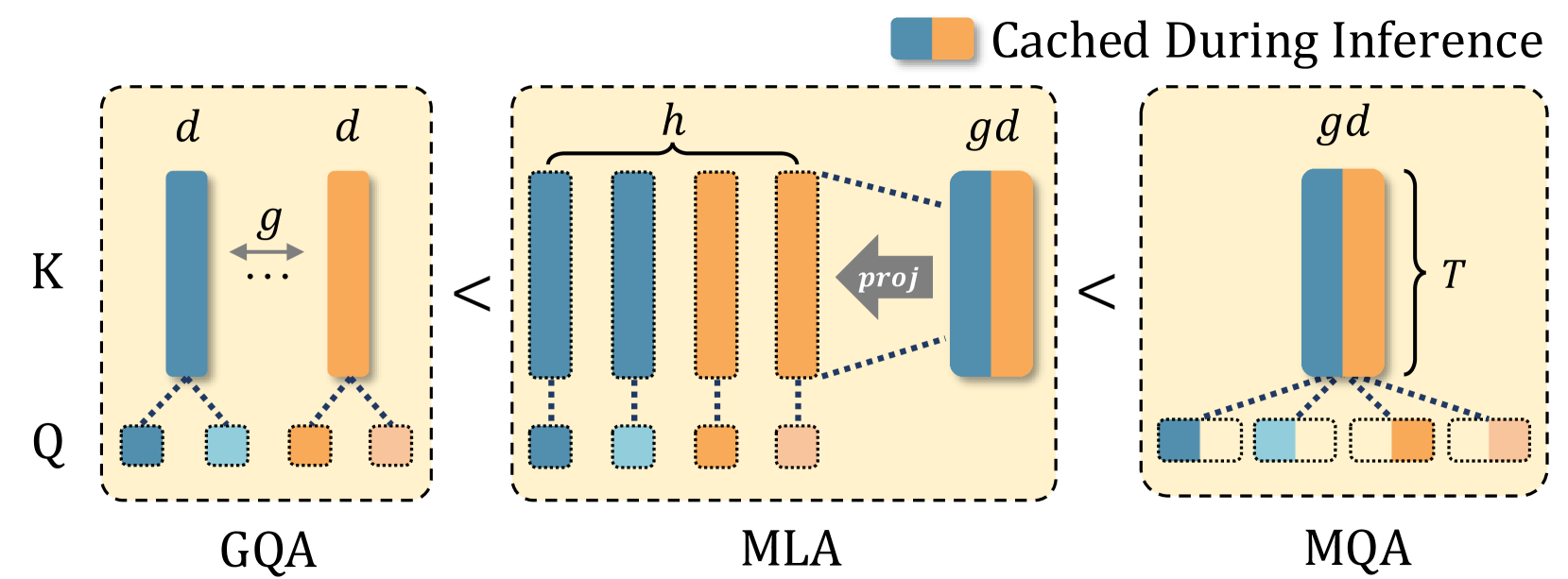a) Given the same KV cache size, the expressiveness increases in the order of GQA, MLA, and MQA. <details> <summary>x2.png Details</summary>  ### Visual Description ## Diagram: Technical Process Flow with RoPE, FreqFold, and BKV-PCA Components ### Overview The diagram illustrates a three-stage technical process involving matrix operations and dimensionality reduction techniques. It uses color-coded bars and labeled components to represent relationships between variables (K, V, C_kv) and methods (RoPE, FreqFold, BKV-PCA). The flow progresses from raw input (K) through processing stages to final output (C_kv). ### Components/Axes 1. **Panels**: - **Left Panel (K)**: Four blue bars labeled "K" with decreasing heights. - **Center Panel (RoPE & FreqFold)**: - Blue bar labeled "K_rope" - Red-dashed box containing: - Blue bar labeled "K_nope" - Orange bars labeled "V" - **Right Panel (K_nope V)**: - Blue bar labeled "K_nope" - Gray gradient bar labeled "C_kv" 2. **Legends**: - **Top Right**: - Green square labeled "RoPE" - Bar chart with: - Red bar labeled "K" - Blue bar labeled "K" - Orange bar labeled "K" - Green bar labeled "K" - **Center Panel**: - Blue dashed box labeled "RoPE & FreqFold" - Red dashed box labeled "BKV-PCA" 3. **Arrows**: - Gray arrows from "K_nope" to "C_kv" in the right panel. ### Detailed Analysis 1. **Left Panel (K)**: - Four blue bars represent decreasing magnitudes of variable K. - No explicit numerical values provided; relative heights suggest ordered values (e.g., K₁ > K₂ > K₃ > K₄). 2. **Center Panel (RoPE & FreqFold)**: - **K_rope**: Single blue bar taller than K_nope, indicating higher magnitude. - **K_nope**: Blue bar under red-dashed box, shorter than K_rope. - **V**: Three orange bars of varying heights, possibly representing transformed values from K_nope. - **BKV-PCA**: Red-dashed box encloses K_nope and V, suggesting a combined processing step. 3. **Right Panel (K_nope V)**: - **K_nope**: Blue bar matches the center panel's K_nope. - **C_kv**: Gray gradient bar with four segments, likely a composite of K_nope and V processed via BKV-PCA. - Arrows imply a direct relationship between K_nope and C_kv. ### Key Observations - **Color Consistency**: Blue consistently represents K/K_nope across panels. Orange represents V, and gray represents C_kv. - **Dimensionality Reduction**: The transition from discrete bars (K, V) to a gradient bar (C_kv) suggests a dimensionality reduction or feature extraction process. - **Method Differentiation**: RoPE and FreqFold are grouped in the center panel, while BKV-PCA is isolated in the right panel, indicating sequential processing stages. ### Interpretation This diagram likely represents a machine learning or signal processing pipeline: 1. **Input Stage (K)**: Raw data (K) is processed through RoPE and FreqFold methods. 2. **Intermediate Processing (K_rope/K_nope, V)**: RoPE distinguishes between K_rope (retained) and K_nope (discarded), while FreqFold transforms K_nope into V. 3. **Final Output (C_kv)**: BKV-PCA combines K_nope and V into a compressed representation (C_kv), with the gradient bar indicating a continuous or multi-dimensional output. The use of dashed boxes and arrows emphasizes hierarchical relationships between components, with RoPE acting as a filtering mechanism and BKV-PCA as a dimensionality reduction technique. The absence of numerical values suggests the diagram focuses on conceptual relationships rather than quantitative results. 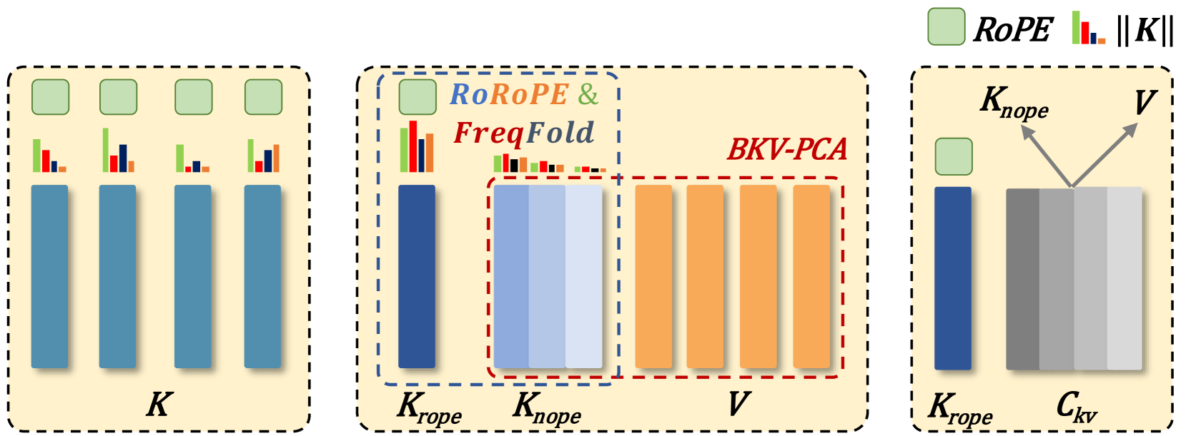</details> (b) TransMLA concentrates positional information into $K_rope$ and compresses $K_nope$ and $V$ . Figure 1: GQA, MLA, and MQA can be equivalently transformed in one direction, illustrating a gradual increase in expressive power. RoRoPE aggregates positional information in the first head, eliminating the need for RoPE in others. FreqFold further enhances this effect. Finally, after balancing the magnitudes of $K_rope$ and $V$ , a joint low-rank approximation is applied to compress the KV cache. ## 1 Introduction Advanced Large language models (LLMs)—GPT-4o OpenAI (2024), Claude 3.7 Sonnet Anthropic (2024), Gemini-2.5 Team et al. (2024a), LLaMA-4 AI@Meta (2024), Mistral-3 Mistral (2024), Qwen-3 Qwen (2024), DeepSeek V3/R1 Liu et al. (2024a); Guo et al. (2025), Gemma-3 Team et al. (2024b), and Phi-4 Abdin et al. (2024) —rapidly evolving frontier for both research and applications. LLMs rely on next-token prediction Radford (2018); Brown et al. (2020): tokens are generated sequentially, and self-attention is computed over all preceding tokens. To avoid redundant computation, implementations store the intermediate key–value (KV) pairs in a cache. Yet, as model and context sizes grow, the KV cache itself becomes a major bottleneck for inference. To mitigate these challenges, Group-Query Attention (GQA) Ainslie et al. (2023) groups the query heads so that every head within a group shares a single key and value head. When the number of groups is one, GQA degenerates to Multi-Query Attention (MQA) Shazeer (2019). When the number of groups equals the number of heads, it reduces to the standard Multi-Head Attention (MHA) Vaswani et al. (2017). While both GQA and MQA cut the size of the KV cache relative to MHA, they do so at the cost of model quality. Post-training KV-cache compression techniques—such as Duo-Attention Xiao et al. (2024), KiVi Liu et al. (2024b), KV-Quant Hooper et al. (2024), and H 2 O Zhang et al. (2023) —further shrink memory usage, but their non-standard implementations demand specialized optimizations, hindering widespread adoption. Multi-Head Latent Attention (MLA)—introduced with DeepSeek V2 DeepSeek-AI (2024) and further refined in DeepSeek V3 DeepSeek-AI (2024) and DeepSeek R1 Guo et al. (2025) —offers a pre-trained KV-cache compression strategy that strikes an excellent balance between computational efficiency and model quality. Models equipped with MLA deliver state-of-the-art results while driving training and inference costs to new lows. Moreover, the DeepSeek team’s ongoing commitment to open-source releases provides highly optimized implementations and deployment recipes, making these advances readily accessible to the community. In this paper, we first prove that MLA consistently offers higher expressive power than GQA under the same KV cache overhead, which theoretically explains the advantage of MLA. However, a practical obstacle preventing model vendors from switching to MLA is the substantial prior investment on GQA-based models. This motivates us to ask, can we seamlessly convert a GQA-based pretrained model, such as LLaMA AI@Meta (2024) and Qwen Qwen (2024), to MLA so that we can inherit the model weights and pretraining effort, rather than training MLA from scratch? A key obstacle to converting a GQA-based model to MLA is that every query–key head carries its own Rotary Positional Embedding (RoPE) (Su et al., 2024), blocking the Absorb operation (Chang et al., 2024) that DeepSeek uses to switch between compute- and memory-efficient modes. Borrowing from DeepSeek’s Decoupled RoPE scheme, we concentrate the positional signal in $K$ into a small subset of dimensions, $K_rope$ . The remaining dimensions, $K_nope$ , contain little positional content; we drop their RoPE and merge them with $V$ for low-rank decomposition. Once RoPE is isolated, the key up-projection—now RoPE-free—can be absorbed into the query projection exactly as in DeepSeek, enabling seamless MLA conversion. To efficiently concentrate positional information into fewer dimensions, we introduce RoRoPE —a novel technique that performs principal component analysis (PCA) on the key output, applies rotation across the two ends of RoPE, and consolidates the principal components of all attention heads into the dimensions of the first attention head. We theoretically prove that the product remains invariant after rotating the query and key using a matrix $U$ , as long as $U$ satisfies two conditions: (1) rotation occurs only within the same dimension across all attention heads, and (2) the real and imaginary components of RoPE are rotated in the same manner. Additionally, by exploiting the frequency similarity between adjacent RoPE dimensions, we propose FreqFold, a technique that improves the concentration efficiency in the first attention head. Finally, we found that the $\ell_2$ -norm of $K_nope$ is far larger than that of $V$ . If we run PCA on the concatenated matrix $\bigl{[}K_nope;V\bigr{]}$ without adjustment, the principal components are dominated by $K_nope$ , leading to severe information loss from the value subspace and a sharp drop in accuracy. We therefore introduce a Balanced Key–Value (BKV) procedure: we first rescale $K_nope$ and $V$ so that their norms match, and only then perform joint PCA. This simple normalization restores balance between the two subspaces and delivers a marked improvement in compression quality. The above innovations collectively form our TransMLA method. Using TransMLA, we compressed the KV cache of LLaMA-2 by 68.75%, with only a 1.65% performance drop across 6 benchmarks for training free. In contrast, a concurrent method, MHA2MLA Ji et al. (2025), experienced a 21.85% performance decline. At a compression rate of 93%, the model still maintained meaningful responses, and after training with just 6B tokens, its performance was mostly restored. We tested both the original and TransMLA models on three different hardware setups using vLLM, achieving up to a 10.6x speedup compared to the original GQA models, demonstrating the great potential of TransMLA. Moreover, the TransMLA models are fully compatible with DeepSeek’s code, enjoying DeepSeek’s ecosystem to accelerate inference and seamlessly integrate with various hardware and frameworks. ## 2 Related Work In large language models, autoregressive decoding reuses past activations by storing their key–value (KV) pairs in a cache. Because the size of this cache grows linearly with sequence length, its memory footprint quickly becomes the limiting factor for very long contexts. Consequently, shrinking the KV cache without compromising accuracy has become a pivotal research focus, motivating a spectrum of architectural innovations and compression strategies. Multi-Query Attention (MQA) Shazeer (2019) and Group-Query Attention (GQA) Ainslie et al. (2023) shrink the KV cache by letting every query in a group share a single key and value head. Although both schemes save memory relative to Multi-Head Attention (MHA) Vaswani et al. (2017), they usually give up some accuracy. Multi-Head Latent Attention (MLA)—introduced with DeepSeek V2 DeepSeek-AI (2024) and refined in later releases DeepSeek V3/R1 DeepSeek-AI (2024); Guo et al. (2025) —offers a more favorable trade-off, delivering near-state-of-the-art quality while cutting training and inference costs. Grouped Latent Attention (GLA) Zadouri et al. (2025) provides a parallel-friendly implementation of latent attention that further accelerates MLA inference. By contrast, Tensor Product Attention (TPA) Zhang et al. (2025) tackles the memory bottleneck by dynamically factorizing activations, slashing the runtime KV cache by an order of magnitude, but it necessitates training the model from scratch. TransMLA fills this gap: rather than proposing yet another attention variant, it converts an existing GQA model into an MLA model with only light fine-tuning, restoring accuracy while inheriting MLA’s memory and speed advantages. Another approach is to optimize the KV cache of existing pre-trained models. For example, dynamic token pruning is employed by LazyLLM Fu et al. (2024), A2SF Jo and Shin (2024), and SnapKV Li et al. (2024). These methods selectively prune less important tokens from the KV cache. Sharing KV representations across layers, as in YONO Sun et al. (2024), MiniCache Liu et al. (2024c), and MLKV Zuhri et al. (2024), reduces memory by reusing the same KV cache across multiple layers. This can drastically lower memory usage and speed up inference. Although effective, both families of methods usually require custom kernels or runtime tweaks, complicating deployment and limiting adoption. TransMLA, by contrast, plugs directly into the mature DeepSeek ecosystem—converted checkpoints load out-of-the-box, delivering MLA-level speed-ups across every DeepSeek-supported platform. There are two works most related to TransMLA. One is Palu Chang et al. (2024), which reduces KV cache size by applying low-rank decomposition on both the keys and values, enabling speedup through tailored optimizations. However, Palu does not specifically handle RoPE, which prevents it from using the Absorb operation during inference. Therefore, Palu needs to project the compressed representations back to their original size. This projection incurs significant computational overhead during inference, limiting the overall acceleration. Another concurrent work, MHA2MLA Ji et al. (2025), also claims to convert MHA to MLA and decouple RoPE from the main computational path. It is important to clarify that TransMLA is not simply a GQA extension of MHA2MLA—both TransMLA and MHA2MLA support MHA and GQA architectures. However, MHA2MLA determines which RoPE dimensions to remove solely based on the norms of the query and key vectors, which tends to cause larger information loss when pruning the same proportion of positions. Also, the distribution of important dimensions in MHA2MLA is uneven, requiring sparse indexing that complicates optimization and acceleration. Their work reports compression ratios of the KV cache but does not demonstrate actual inference speedup. Furthermore, MHA2MLA directly applies joint singular value decomposition to KV, resulting in higher loss compared to our balanced key-value PCA method. ## 3 Preliminary ### 3.1 Rotary Position Embedding (RoPE) RoPE Su et al. (2024) is a position encoding method that encodes the absolute positions with different rotations and incorporates the explicit relative position dependency in the self-attention formulation. It applies different rotations to tokens in different positions to encode the position information. Consider $x_t∈ℝ^d$ to be the embedding of the $t$ -th token with the hidden size $d$ . The RoPE operation upon $x_t$ produces a representation $x_t^R$ that encodes both semantic and positional information: $$ x_t^R=RoPE(x_t,t)=\begin{pmatrix}x_t ^(1)\\ x_t^(2)\\ x_t^(3)\\ x_t^(4)\\ ⋮\\ x_t^(d-1)\\ x_t^(d)\end{pmatrix}⊗\begin{pmatrix}\cos{tθ_1}\\ \cos{tθ_1}\\ \cos{tθ_2}\\ \cos{tθ_2}\\ ⋮\\ \cos{tθ_d/2}\\ \cos{tθ_d/2}\end{pmatrix}\\ +\begin{pmatrix}-x_t^(2)\\ x_t^(1)\\ -x_t^(4)\\ x_t^(3)\\ ⋮\\ -x_t^(d)\\ x_t^(d-1)\end{pmatrix}⊗\begin{pmatrix}\sin{tθ_1}\\ \sin{tθ_1}\\ \sin{tθ_2}\\ \sin{tθ_2}\\ ⋮\\ \sin{tθ_d/2}\\ \sin{tθ_d/2}\end{pmatrix}, \tag{1} $$ where $⊗$ denotes the element-wise multiplication of two vectors, $x_t^(i)∈ℝ$ denotes the $i$ -th element of $x_t$ , and $θ_i=10000^-2(i-1)/d$ is the $i$ -th rotation angle. If we interpret every two elements in the embedding as a representation in the complex coordinate system, we can divide $x_t$ into paired dimensions, where the odd-indexed dimensions $x_t^(2k-1)$ represent the real parts and the even-indexed dimensions $x_t^(2k)$ represent the imaginary parts. ### 3.2 Group Query Attention Let the $t$ -th token of the input sequence be $x_t∈ℝ^D$ , where $D$ denotes the hidden dimension. To reduce the memory overhead of the KV cache, GQA divides the $h$ query heads uniformly into $g$ groups, with all query heads within a group sharing the same key and value vectors. Specifically, let $W^Q∈ℝ^hd× D$ , $W^K,W^V∈ℝ^gd× D$ and $W^O∈ℝ^D× hd$ be the projection matrices for the query, key, value and output, where $d=D/h$ denotes the dimension per head. GQA first computes the concatenated queries $q_t$ , keys $k_t$ , and values $v_t$ , and then slices them into heads or groups for attention computation: $$ \displaystyle[q_t,1;q_t,2;...;q_t,h]= q_t \displaystyle={W^Q}x_t, \displaystyle[k_t,1;k_t,2;...;k_t,g]= k_t \displaystyle={W^K}x_t, \displaystyle[v_t,1;v_t,2;...;v_t,g]= v_t \displaystyle={W^V}x_t, \tag{2} $$ where each $q_t,i∈ℝ^d$ corresponds to the query vector of the i-th head, and $k_t,j,v_t,j∈ℝ^d$ correspond to the key and value vectors of the j-th group. Using the notation in Section 3.1, after applying RoPE to $q_t,i,k_t,i$ , we can obtain the attention output for the $t$ -th token as follows: $$ \displaystyleo_t,i \displaystyle=∑_j=1^tsoftmax_j(\frac{{q^R_t,i}^ ⊤k^R_j,\lceil i/\frac{h{g}\rceil}}{√{d}})v_j, \lceil i/\frac{h{g}\rceil}, \displaystyley_t \displaystyle=W^O[o_t,1;o_t,2;...;o_t,h]. \tag{5} $$ As we can see, in GQA, each key and value head corresponds to $\frac{h}{g}$ query heads. When $\boldsymbol{g=h}$ , GQA becomes MHA, and when $\boldsymbol{g=1}$ , GQA becomes Multi-Query Attention (MQA). ### 3.3 Multi-Head Latent Attention MLA saves KV cache by multiplying the matrix $W^DKV∈ℝ^r_kv× D$ with the input sequence to obtain low-rank latent features. Then, it uses the matrices $W^UK$ and $W^UV∈ℝ^hd× r_kv$ to derive the key $k$ and value $v$ representations for each attention head. Additionally, MLA also decomposes $W^Q$ to $W^DQ∈ℝ^r_q× D$ and $W^UQ∈ℝ^hd× r_q$ , which reduces the activation memory during training. For positional embedding, MLA uses a decoupled RoPE strategy that uses additional multi-head queries $q_t,i^R∈ℝ^d^{R}$ and a shared key $k_t^R∈ℝ^d^{R}$ , which are generated from $W^QR∈ℝ^hd^{R× r_q}$ and $W^KR∈ℝ^d^{R× d}$ , to carry RoPE, where $d^R$ denotes the per-head dimension of the decoupled queries and key. $$ \displaystylec_t^KV \displaystyle=W^DKVx_t, \displaystyle[k_t,1^C;k_t,2^C;...;k_t,h^ C] \displaystyle=k_t^C=W^UKc_t^KV, \displaystylek_t^R \displaystyle=RoPE({W^KR}x_t,t), \displaystylek_t,i \displaystyle=[k_t,i^C;k_t^R], \tag{7} $$ $$ \displaystylec_t^Q \displaystyle=W^DQx_t, \displaystyle[q_t,1^C;q_t,2^C;...;q_t,h^ C] \displaystyle=q_t^C=W^UQc_t^Q, \displaystyle[q_t,1^R;q_t,2^R;...;q_t,h^ R] \displaystyle=q_t^R=RoPE({W^QR}c_t^Q,t), \displaystyleq_t,i \displaystyle=[q_t,i^C;q_t,i^R]. \tag{8} $$ MLA supports switching between two computational paradigms tailored for different stages. During the compute-intensive training phase, it operates in a paradigm similar to standard MHA, where the computational overhead is slightly lower than that of conventional MHA, as shown in Equation 3.3. For communication-intensive inference, it can seamlessly switch to a paradigm resembling MQA, as described in Equation 10. In this inference paradigm, the latent features function as a shared large KV head, which interacts with all query heads and output heads to produce the final output efficiently. This operation is called the Absorb operation, which is crucial for accelerating inference speed. $\displaystyle[v_t,1^C;v_t,2^C;...;v_t,h^ C]$ $\displaystyle=v_t^C=W^UVc_t^KV,$ $\displaystyleo_t,i$ $\displaystyle=∑_j=1^tsoftmax_j(\frac{q_t,i^T k_j,i}{√{d+d^R}})v_j,i^C,$ $\displaystyley_t$ $\displaystyle=W^O[o_t,1;o_t,2;...;o_t,h],$ (9) $\displaystyle\hat{q}_t,i$ $\displaystyle=[{W^UK_i}^⊤q_t,i^C;q_t,i^R],~ {}~{}~{}\hat{k}_t=[c_t^KV;k_t^R],$ $\displaystyle\hat{o}_t,i$ $\displaystyle=∑_j=1^tsoftmax_j(\frac{\hat{q}_t,i^T \hat{k}_j}{√{d+d^R}})c_j^KV,$ $\displaystyley_t$ $\displaystyle=W^O[W^UV_1\hat{o}_t,1;...;W^UV_h \hat{o}_t,h],$ (10) where $W_i^\{UK,UV\}$ denotes slices of the projection matrices corresponding to the $i$ -th attention head. One of the main contributions of this paper is the seamless support for the Absorb operation, significantly enhancing inference speed. ## 4 TransMLA In this section we formally present TransMLA, motivated by two observations: 1. For a fixed KV-cache budget, MLA is strictly more expressive than GQA. As proven in Appendix A (and illustrated in Figure 1(a)), any GQA layer can be rewritten as an MLA layer by introducing a single additional projection matrix. The reverse transformation is not always possible, implying that MLA subsumes GQA. When Rotary Positional Embeddings (RoPE) are present, the MLA equivalent must be expressed in the absorbed form. 2. Inference acceleration occurs only when MLA uses a smaller KV cache. Although one can build an MLA-equivalent representation of a GQA model, speedups arise only if the number of stored KV vectors is actually reduced. TransMLA therefore converts a GQA-based network into a DeepSeek-like MLA architecture, allowing the transformed model to run directly on DeepSeek’s optimized inference stack and realize the full memory–latency benefits. <details> <summary>x3.png Details</summary>  ### Visual Description ## Diagram: Dimensionality Reduction and Feature Selection Process ### Overview The diagram illustrates a multi-stage data processing pipeline involving dimensionality reduction and feature selection. It shows four groups of data (Group 1-4) with varying dimensionality (dim=1-8), followed by Principal Component Analysis (PCA) and a RoPE/NoPE classification system. The visualization uses blue and orange lines to represent different data groups, with spatial transitions indicating processing stages. ### Components/Axes 1. **Groups**: - Group 1 (blue lines) - Group 2 (orange lines) - Group 3 (blue lines) - Group 4 (orange lines) 2. **Dimensions**: - dim=1 (most wavy lines) - dim=2-8 (progressively straighter lines) 3. **Processing Stages**: - Original data (top section) - PCA (middle section) - RoPE/NoPE classification (bottom section) 4. **Legend**: - Blue = Group 1 - Orange = Group 2 - *Note: Groups 3 and 4 lack explicit legend entries despite being visually present* ### Detailed Analysis 1. **Original Data (Groups 1-4)**: - dim=1: Highly wavy lines with significant curvature - dim=2-4: Gradual reduction in wave amplitude - dim=5-8: Nearly straight lines with minimal curvature - *Spatial Pattern*: Groups alternate between blue (Group 1) and orange (Group 2) lines, with Groups 3 and 4 appearing as continuation of the pattern but without explicit grouping markers 2. **PCA Transition**: - Reduced to 4 principal components (dim=1-4) - Lines become more linear and parallel - Loss of original group color differentiation (both blue and orange lines merge) 3. **RoPE/NoPE Classification**: - RoPE (Retained Principal Components): - dim=1-2: Maintains some curvature - dim=3-4: Linear but distinct from NoPE - NoPE (Non-Retained Principal Components): - dim=5-8: Completely removed (empty space) - *Spatial Pattern*: Clear separation between retained (RoPE) and discarded (NoPE) components ### Key Observations 1. **Legend Inconsistency**: Groups 3 and 4 are visually present but lack legend entries, suggesting either: - Omission in legend design - Intentional exclusion from primary analysis - Potential data categorization error 2. **Dimensionality Impact**: - Higher dimensions (dim=5-8) show near-linear patterns - Suggests original data may have been artificially constructed with increasing linearity 3. **Feature Selection Effectiveness**: - PCA reduces complexity but loses group differentiation - RoPE preserves critical curvature in first 2 dimensions - NoPE effectively removes higher-dimensional noise ### Interpretation This diagram demonstrates a dimensionality reduction workflow where: 1. **Data Complexity Reduction**: PCA successfully simplifies the data structure but at the cost of losing original group distinctions 2. **Feature Importance**: The first two principal components (RoPE) retain meaningful curvature patterns, while higher dimensions (NoPE) appear to contain less discriminative information 3. **Group Representation**: The absence of Groups 3 and 4 in the legend raises questions about their role in the analysis - they may represent: - Secondary data categories - Noise components - Unlabeled outliers The workflow suggests a two-stage analysis where initial dimensionality reduction (PCA) is followed by feature selection (RoPE/NoPE) to identify the most informative components. The visual progression from wavy to linear patterns across dimensions indicates an artificial construction where higher dimensions lose their original discriminative power. 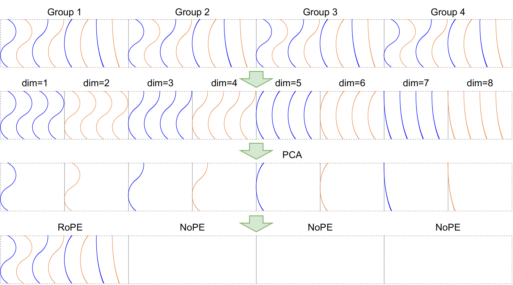</details> Figure 2: Pipeline of RoRoPE for decoupling RoPE. Blue lines denote real-part dimensions, orange lines denote imaginary-part dimensions. When the keys from multiple heads are concatenated, permuting dimensions does not change the computation, so we gather the same dimension (i.e., the same rotational frequency) across all heads and apply joint principal-component analysis—using the identical procedure for the real and imaginary parts. For each frequency we keep a single principal component, which captures the dominant positional variation and can be represented by a standard RoPE in one attention head. ### 4.1 Merging All Key Heads as One Because MLA ties all KV heads to a single latent dimension, the first step in converting a GQA layer to MLA is to merge every GQA key–value group into one latent head before any KV-cache compression is applied. For each query head $i$ , we introduce $W^UK_i∈ℝ^d× gd$ with the group index $j=≤ft\lceil\frac{i}{h/g}\right\rceil-1$ , and initialize the matrix ${W^UK_i}{[:,jd:(j+1)d]}$ to be $I_d$ (identity matrix of shape $d× d$ ), with all other elements set to 0. (We adopt the matrix indexing notation used in Python and PyTorch, and will continue to do so throughout this work without further explanation.) This initialization allows the projection of the key’s latent representation to be simultaneously mapped onto multiple query heads, with only the corresponding key head being multiplied by the appropriate query head. Similarly, during the computation of the multiple heads of the values, the attention scores for each head are multiplied accordingly. To keep the output unchanged, we similarly initialize $W^UV_i$ so that only the corresponding value head is an identity mapping, while all other elements are set to zero. Since we have now merged all the key heads into a single head, in order to ensure that this transformation is equivalent to the original, we also merge the RoPE operations from different heads into one large RoPE operation, denoted as $\widehat{RoPE}$ , applied to the entire merged key head. Since the original RoPE operation in GQA is the same for each head, $\widehat{RoPE}$ simply applies the same RoPE operation repeatedly for every $d$ dimensions. In this way, the computation of GQA attention is transformed into the following form: $$ \displaystyle[c_t^K;c_t^V]=c_t^KV \displaystyle=W^DKVx_t,~{}~{}W^DKV=\begin{pmatrix}W^K\\ W^V\end{pmatrix}∈ℝ^2gd× D \displaystyle[q_t,1;q_t,2;...;q_t,h]= q_t \displaystyle={W^Q}x_t,~{}~{}{W^Q}∈ℝ^hd× D \displaystyle\hat{q}_t,i^R \displaystyle=\widehat{RoPE}(≤ft(W^UK_i\right)^⊤q_ t,i,t),~{}~{}\hat{k}_t^R=\widehat{RoPE}(c_t^K ,t) \displaystyle\hat{o}_t,i \displaystyle=∑_j=1^tsoftmax_j≤ft(\frac{≤ft(\hat{q }_t,i^R\right)^⊤\hat{k}_j^R}{√{d}}\right)c _j^V, \displaystyley_t \displaystyle=W^O[W^UV_1\hat{o}_t,1;...;W^UV_h \hat{o}_t,h]. \tag{11} $$ It is evident that the total KV cache size remains unchanged since we still need to store $c_t^KV∈ℝ^2gd$ for each token, which is the same as in the original GQA model. However, the dimension of each attention head has increased by a factor of $g$ , and the introduction of new parameters $W^UK_i$ and $W^UV_i$ leads to higher computational costs. To achieve actual acceleration in the transformed MLA, compressing the KV cache is therefore essential. By merging multiple KV heads, we can better identify shared principal components and represent the KV cache in a lower-dimensional latent space. Moreover, merging multiple key heads is crucial for efficiently decoupling RoPE in the subsequent steps. ### 4.2 Rotating Queries and Keys to Minimize Transformation Loss Towards Decoupled RoPE As illustrated in Figure 2, applying RoRoPE to the merged head removes the bulk of the positional signal from K. In Equation 14, the term $≤ft(\hat{q}^R_t,i\right)^⊤\hat{k}_j^R$ can be expressed as the sum of inner products over paired dimensions across multiple attention heads, incorporating positional information: $$ ≤ft(\hat{q}^R_t,i\right)^⊤\hat{k}_j^R=∑_l =1^d/2≤ft[{\hat{q}_t,i}^[2l-1::d];\hat{q}_t,i^[2 l::d]\right]^R^{⊤}≤ft[\hat{k}_j^[2l-1::d];\hat{k }_j^[2l::d]\right]^R. \tag{16} $$ Here, the notation $[2l::d]$ is inspired by Python slicing syntax and denotes selecting elements starting from the $(2l)$ -th dimension, then taking every $d$ -th element thereafter until the end of the vector. The vector $≤ft[{\hat{q}_t,i}^[2l-1::d];\hat{q}_t,i^[2l::d] \right]^R$ thus has dimension $2g$ . Since multiple key heads are concatenated into a single head and each head shares the same RoPE, the real and imaginary components corresponding to the $l$ -th 2D subspace (i.e., the paired two dimensions) of RoPE within each original attention head can be expressed as follows: $$ \displaystyle≤ft[\hat{q}_t,i^[2l-1::d];\hat{q}_t,i^ [2l::d]\right]^R=\cos tθ_l≤ft[\hat{q}_t,i^[2l-1::d]; \hat{q}_t,i^[2l::d]\right]+\sin tθ_l≤ft[-\hat{q }_t,i^[2l::d];\hat{q}_t,i^[2l-1::d]\right], \displaystyle≤ft[{\hat{k}_j^[2l-1::d]};{\hat{k}_j^[ 2l::d]}\right]^R=\cos jθ_l≤ft[\hat{k}_j^[2l-1::d]; \hat{k}_j^[2l::d]\right]+\sin jθ_l≤ft[-\hat{k}_j^[2l::d];\hat{k}_j^[2l-1::d]\right]. \tag{17} $$ When the concatenated real and imaginary components of $\hat{q}_t,i$ and $\hat{k}_j$ within the $l$ -th 2-dimensional subspace are multiplied by an orthogonal matrix $U_l∈ℝ^g× g$ , the inner product with RoPE applied remains invariant. Specifically, $$ ∑_l=1^d/2≤ft(≤ft[U_l\hat{q}_t,i^[2l-1::d]; U_l\hat{q}_t,i^[2l::d]\right]\right)^R^{⊤}≤ft( ≤ft[U_l\hat{k}_j^[2l-1::d];U_l\hat{ k}_j^[2l::d]\right]\right)^R=\hat{q}^R^{⊤}_t,i \hat{k}_j^R. \tag{19} $$ This demonstrates that the rotational transformation $U_l$ preserves the RoPE-based inner product structure. Simply put, because the same rotation values (i.e., $\cos tθ_l$ and $\sin tθ_l$ ) are applied identically to each dimension of the $l$ -th 2D subspace across all attention heads, any orthogonal transformation $U_l^⊤U_l=I$ applied to these dimensions within the same subspace leaves the inner product $\hat{q}^R^{⊤}_t,i\hat{k}_j^R$ unchanged. However, the preceding equation reveals a critical constraint: for the inner product’s value to remain unchanged after transformation, the same orthogonal matrix $U_l$ must be applied to both the real ( $2l-1$ ) and imaginary ( $2l$ ) components of the key vectors within each 2D subspace. For a detailed proof and our proposed solution, please refer to Appendix B. We apply Principal Component Analysis (PCA) to the attention heads in the context of RoPE, introducing a method we call RoRoPE. Using a small dataset, we extract the key output, compute its principal component projection matrices $\{U_l\}_l∈\{1,\dots,d/2\}$ , and rotate both $W^K$ and $W^UK$ (as shown in Eq 13, $\hat{q}_t,i$ and $\hat{k}_j$ are generated from $W^UK$ and $W^K$ respectively, so rotating $\hat{q}_t,i$ and $\hat{k}_j$ can be achieved by rotating $W^UK$ and $W^K$ ) using a similar procedure as described above. This rotation effectively concentrates the essential information into the first few heads. As an equivalent transformation, instead of discarding all non-principal components of the key, we remove their RoPE encoding while preserving positional information within the principal components. To enable the transformed model to utilize standard RoPE, we represent the principal component information for corresponding positions across other heads using the dimensions of the first attention head. However, using a one-dimensional space for all positional information proves limiting. To address this, we exploit the similar frequencies of adjacent dimensions in RoPE, treating them as equivalent positions. This allows us to use multiple dimensions within a single attention head to represent positional information, a technique we refer to as FreqFold. Additional information on FreqFold can be found in Appendix C. ### 4.3 A Balanced Approach to Joint Low-Rank Approximation of NoPE Keys and Values In the previous section, we split the key heads into one carrying positional information and the others without positional information, achieving minimal loss. We then apply Principal Component Analysis (PCA) jointly on the values and the non-positional components of the keys (i.e. NoPE-Key), using activations collected from a small calibration dataset, thereby compressing the projection matrices into a low-rank latent space. However, we observed that although the principal components of the keys were effectively separated with RoRoPE, the norm of the residual key features remained significantly larger than that of the Value. This imbalance caused the direct decomposition to favor principal component directions dominated by the keys. To mitigate this, we scale $W^DK$ by dividing it by $$ α=\frac{E_t[\|W^DK_NoPEx_t\|_2]}{ E_t[\|W^DVx_t\|_2]} \tag{20} $$ and correspondingly scale $W^UK$ by multiplying it by $α$ . Here, $W^DK_RoPE∈ℝ^d× D,W^DK_NoPE∈R ^(g-1)d× D$ represent the parts of $W^DK$ obtained after the operations described in the previous section, where $W^DK_RoPE$ corresponds to one head that uses RoPE, and $W^DK_NoPE$ corresponds to the remaining heads that do not use RoPE. This transformation is mathematically equivalent and does not affect the overall model outputs, while significantly enhancing the effectiveness of KV cache compression in subsequent steps. More details is provided in the Appendix D. ## 5 Experiment ### 5.1 Main Experiment In this section, we present our main experimental results. Following the experimental setup of MHA2MLA, we converted two models—smolLM 1.7B and Llama 2 7B—into the MLA architecture. We evaluated the models’ performance on six benchmarks at three stages: before conversion, immediately after conversion without further training, and after conversion followed by training. For the training process, we used a subset of the pretraining corpus used for the smolLM model. The fine-tuned results of MHA2MLA are taken directly from the original paper. Our experiments were conducted on an 8-GPU machine, each GPU having 40GB of memory and delivering 312 TFLOPS of FP16 compute power. Detailed experimental hyperparameter settings are provided in the Appendix E. Table 1: Commonsense reasoning ability of two LLMs with TransMLA compared to MHA2MLA. The six benchmarks include MMLU (Hendrycks et al. (2021)), ARC easy and challenge (ARC, Clark et al. (2018)), PIQA (Bisk et al. (2020)), HellaSwag (HS, Zellers et al. (2019)), OpenBookQA (OBQA, Mihaylov et al. (2018)), and Winogrande (WG, Sakaguchi et al. (2021)). Tokens refers to the number of tokens used for further training after the TransMLA conversion. A value of 0 indicates that the model was evaluated immediately after conversion, without any fine-tuning. | Model SmolLM-1.7B - MHA2MLA | Tokens 1T 0 | KV Mem. – -68.75% | Avg. 55.90 40.97 | MMLU 39.27 27.73 | ARC 59.87 41.96 | PIQA 75.73 63.00 | HS 62.93 29.19 | OBQA 42.80 34.40 | WG 54.85 49.53 | | --- | --- | --- | --- | --- | --- | --- | --- | --- | --- | | -81.25% | 37.14 | 26.57 | 32.73 | 55.77 | 26.90 | 31.40 | 49.49 | | | | -87.50% | 34.01 | 25.32 | 27.15 | 51.36 | 25.47 | 26.20 | 48.54 | | | | -68.75% | 54.76 | 38.11 | 57.13 | 76.12 | 61.35 | 42.00 | 53.83 | | | | 6B | -81.25% | 54.65 | 37.87 | 56.81 | 75.84 | 60.41 | 42.60 | 54.38 | | | -87.50% | 53.61 | 37.17 | 55.50 | 74.86 | 58.55 | 41.20 | 54.38 | | | | - TransMLA | | -68.75% | 51.95 | 35.70 | 55.68 | 73.94 | 53.04 | 39.80 | 53.51 | | 0 | -81.25% | 47.73 | 32.87 | 47.89 | 69.75 | 48.16 | 36.20 | 51.46 | | | -87.50% | 44.12 | 29.97 | 41.72 | 66.87 | 41.15 | 34.80 | 50.28 | | | | 300M | -68.75% | 55.24 | 38.60 | 58.95 | 74.97 | 61.52 | 43.00 | 54.38 | | | 700M | -81.25% | 54.78 | 37.79 | 57.53 | 75.52 | 59.88 | 42.80 | 55.17 | | | 1B | -87.50% | 54.01 | 37.24 | 56.32 | 74.81 | 60.08 | 42.40 | 53.20 | | | LLaMA-2-7B | 2T | – | 59.85 | 41.43 | 59.24 | 78.40 | 73.29 | 41.80 | 64.96 | | - MHA2MLA | | -68.75% | 37.90 | 25.74 | 32.87 | 59.41 | 28.68 | 28.60 | 52.09 | | 0 | -81.25% | 34.02 | 25.50 | 26.44 | 53.43 | 27.19 | 22.60 | 49.01 | | | -87.50% | 32.70 | 25.41 | 25.79 | 50.60 | 26.52 | 19.40 | 48.46 | | | | -68.75% | 59.51 | 41.36 | 59.51 | 77.37 | 71.72 | 44.20 | 62.90 | | | | 6B | -81.25% | 59.61 | 40.86 | 59.74 | 77.75 | 70.75 | 45.60 | 62.98 | | | -87.50% | 58.96 | 40.39 | 59.29 | 77.75 | 69.70 | 43.40 | 63.22 | | | | - TransMLA | 0 | -68.75% | 58.20 | 39.90 | 57.66 | 77.48 | 70.22 | 41.00 | 62.90 | | -87.50% | 51.19 | 34.39 | 45.38 | 71.27 | 60.73 | 37.40 | 57.93 | | | | -92.97% | 43.26 | 28.93 | 36.32 | 63.38 | 45.87 | 31.60 | 53.43 | | | | 500M | -68.75% | 59.82 | 40.87 | 59.18 | 77.91 | 71.82 | 45.20 | 63.93 | | | 3B | -87.50% | 59.36 | 40.77 | 58.84 | 78.18 | 71.28 | 43.60 | 63.46 | | | 6B | -92.97% | 58.68 | 40.82 | 59.72 | 76.55 | 69.97 | 43.60 | 61.40 | | From Table 1, we observe that TransMLA efficiently facilitates architecture migration across various models and KV cache compression ratios. Notably, the untrained performance of MLA models initialized with TransMLA shows minimal degradation in capability compared to the original models—significantly less than the degradation observed with MHA2MLA under equivalent KV cache compression. In fact, using TransMLA to compress the KV cache of Llama 2 7B to just 7.03% of its original size still results in better performance than MHA2MLA’s compression to 31.25% on the same model. This highlights the effectiveness of our proposed techniques includes RoRoPE, FreqFold and activation-based balanced KV low-rank factorization. The low-loss transformation achieved by TransMLA enables us to recover the original model performance with minimal training overhead. As shown in the table, TransMLA achieves stronger performance than MHA2MLA-6B while using significantly fewer training tokens. For instance, when transforming smolLM 1.7B and compressing the KV cache to 31.25% of its original size, we only need 4.9% of the training data used by MHA2MLA and 2 hours training to surpass its performance. ### 5.2 Key Norm Analysis Reveals the Impact of RoRoPE and FreqFold In this section, we conduct a detailed analysis of the distribution of key activations in the attention module to demonstrate the effectiveness of our proposed methods. 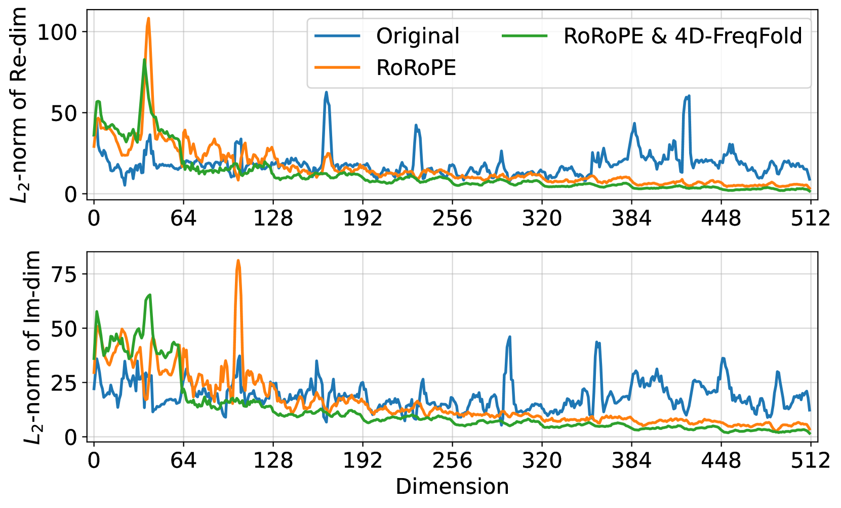Figure 3(a) presents the average L2 norm of each key dimension in the first attention layer of the LLaMA 3 8B model, computed on a subset of the WikiText-2 Merity et al. (2016) dataset. We compare the original model (in blue), the model transformed using our RoRoPE equivalence method (in orange), and the further approximated model using 4D FreqFold (in green). The top and bottom halves of the plot correspond to pairs of dimensions that share the same rotation angle in RoPE, which we refer to as the real (Re-dim) and imaginary (Im-dim) dimensions. We observe that the original model exhibits a highly uneven norm distribution across key dimensions, with numerous outliers. This suggests that naively removing RoPE from certain heads would likely result in significant performance degradation. After applying our RoRoPE transformation, as shown by the orange line, the key dimensions with large norms are nearly all concentrated to the first two heads (dimension 0-128). Further applying the 4D FreqFold approximation compresses the tail (i.e., higher-index dimensions) even more, leading to an even sharper concentration of high-norm key dimensions. This concentrated structure is highly beneficial for the subsequent RoPE removal step as shown in Figure 3(b). <details> <summary>x4.png Details</summary>  ### Visual Description ## Line Graph: L2-Norm Analysis Across Dimensions ### Overview The image contains two vertically stacked line graphs comparing the L2-norm of real and imaginary dimensions across 512 dimensions. Three data series are plotted: "Original" (blue), "RoRoPE" (orange), and "RoRoPE & 4D-FreqFold" (green). The graphs show fluctuating values with distinct peaks and troughs, suggesting dimensional variability in the measured norms. ### Components/Axes - **X-axis (Top/Bottom Subplots)**: Labeled "Dimension" with ticks at 0, 64, 128, 192, 256, 320, 384, 448, and 512. - **Y-axis (Top Subplot)**: Labeled "L2-norm of Re-dim" with values ranging from 0 to 100. - **Y-axis (Bottom Subplot)**: Labeled "L2-norm of Im-dim" with values ranging from 0 to 75. - **Legend**: Located in the top-right corner of the top subplot, with three entries: - Blue: "Original" - Orange: "RoRoPE" - Green: "RoRoPE & 4D-FreqFold" ### Detailed Analysis #### Top Subplot (Real Dimensions) - **Original (Blue)**: Dominates with sharp peaks (e.g., ~80 at dimension 64, ~90 at 192, ~70 at 384). Values drop to ~10–20 between peaks. - **RoRoPE (Orange)**: Smoother curve with smaller peaks (e.g., ~40 at 64, ~30 at 192, ~20 at 384). Fluctuates between ~5–30. - **RoRoPE & 4D-FreqFold (Green)**: Most stable, with minimal peaks (e.g., ~20 at 64, ~15 at 192, ~10 at 384). Fluctuates between ~2–15. #### Bottom Subplot (Imaginary Dimensions) - **Original (Blue)**: Peaks at ~60 (dimension 64), ~50 (192), and ~40 (384). Drops to ~5–15 between peaks. - **RoRoPE (Orange)**: Reduced peaks (e.g., ~30 at 64, ~20 at 192, ~10 at 384). Fluctuates between ~5–20. - **RoRoPE & 4D-FreqFold (Green)**: Near-flat line with values ~5–10 across all dimensions. ### Key Observations 1. **Original Data**: Exhibits high variability with pronounced spikes in both real and imaginary dimensions, particularly at dimensions 64, 192, and 384. 2. **RoRoPE**: Reduces peak magnitudes by ~50% compared to Original but retains moderate fluctuations. 3. **Combined Method (RoRoPE + 4D-FreqFold)**: Achieves the lowest L2-norm values, with near-flat lines in the imaginary dimension subplot and minimal peaks in the real dimension subplot. 4. **Dimensional Correlation**: Peaks in the Original data align across both subplots, suggesting shared dimensional dependencies. ### Interpretation The data demonstrates that the "RoRoPE & 4D-FreqFold" method significantly stabilizes L2-norm values compared to the Original and RoRoPE alone. The Original data’s spikes may indicate noise, artifacts, or high-dimensional dependencies that the combined method mitigates. The RoRoPE method acts as an intermediate step, reducing but not eliminating variability. This suggests that 4D-FreqFold introduces regularization or dimensionality reduction, critical for applications requiring stable norm distributions (e.g., signal processing, machine learning). The alignment of peaks in the Original data implies that dimensional interactions are a key factor in the observed variability. </details> (a) Key norms of the first layer. <details> <summary>x5.png Details</summary>  ### Visual Description ## Line Graph: Log of Perplexity vs. RoPE Removal Ratio ### Overview The graph compares the performance of various methods in maintaining low perplexity as the RoPE (Rotary Positional Encoding) removal ratio increases. The y-axis uses a logarithmic scale to emphasize differences in perplexity values across methods. ### Components/Axes - **X-axis**: RoPE Removal Ratio (%) ranging from 0% to 80% in 20% increments. - **Y-axis**: Log of Perplexity (scale from ~2 to ~8). - **Legend**: Located on the right, with color-coded lines and markers for each method: - **Vanilla PCA**: Green circles (flat line at ~8). - **MHA2MLA**: Blue squares (flat until 80%, then spikes to ~5.5). - **RoRoPE**: Orange diamonds (flat at ~2). - **RoRoPE & 2D-FreqFold**: Yellow stars (flat at ~2). - **RoRoPE & 4D-FreqFold**: Red diamonds (flat at ~2). - **RoRoPE & 8D-FreqFold**: Orange stars (flat at ~2, slight upward trend). ### Detailed Analysis 1. **Vanilla PCA** (green circles): - Remains nearly flat at ~8 across all removal ratios. - Slight dip to ~7.8 at 80% removal. 2. **MHA2MLA** (blue squares): - Stays near ~2 for 0–60% removal. - Sharp increase to ~5.5 at 80% removal. 3. **RoRoPE** (orange diamonds): - Flat at ~2 across all ratios. 4. **RoRoPE & 2D-FreqFold** (yellow stars): - Flat at ~2 across all ratios. 5. **RoRoPE & 4D-FreqFold** (red diamonds): - Flat at ~2 across all ratios. 6. **RoRoPE & 8D-FreqFold** (orange stars): - Flat at ~2 for 0–60% removal. - Slight upward trend to ~2.3 at 80% removal. ### Key Observations - **Vanilla PCA** exhibits the highest perplexity but remains stable. - **MHA2MLA** shows a dramatic increase in perplexity only at 80% removal, suggesting sensitivity to high removal ratios. - **RoRoPE combinations** (2D, 4D, 8D-FreqFold) maintain the lowest perplexity (~2), with 8D-FreqFold showing marginal improvement at high removal ratios. - The logarithmic y-axis amplifies the visual impact of MHA2MLA's spike at 80%. ### Interpretation The data suggests that **RoRoPE-based methods** (especially with higher FreqFold dimensions like 8D) are more robust to RoPE removal, maintaining low perplexity even as removal ratios increase. **Vanilla PCA** performs poorly in terms of perplexity but is stable, while **MHA2MLA** struggles at high removal ratios. The slight upward trend in the 8D-FreqFold combination indicates potential scalability benefits, though further validation is needed. This highlights the trade-offs between stability and performance across different architectural choices. </details> (b) RoPE removal results, evaluated on WikiText-2. Figure 3: Visualization of key norms and RoPE removal results on LLaMA 3 8B model. The top and bottom halves of the left figure correspond to pairs of dimensions that share the same rotation angle in RoPE, which we refer to as the real (Re-dim) and imaginary (Im-dim) dimensions. 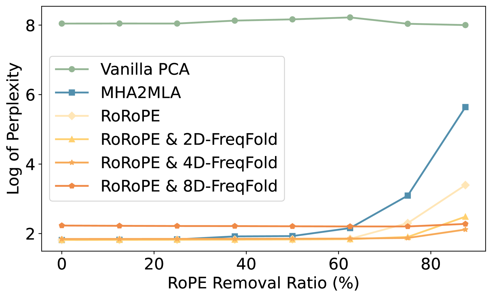In Figure 3(b), we present the log-perplexity of the LLaMA 3 8B model on WikiText-2 as RoPE components are progressively removed. We observe that our proposed RoRoPE method significantly outperforms MHA2MLA’s per-head dimension selection strategy, especially at high removal ratio. Furthermore, incorporating similar-dimension approximation leads to even better performance under extreme removal rates. At 90% removal ration, RoRoPE + 4D-FreqFold still maintains a log-perplexity about 2, while MHA2MLA reaches nearly 6, which no longer generates meaningful outputs. At the same time, we observe that overly aggressive FreqFold (i.e., using too many dimensions) can degrade performance, as the loss introduced by approximation of nearby dimensions can outweigh the benefit in concentrating the principal components. This figure suggests that for LLaMA 3 8B, the sweet spot lies in applying RoRoPE combined with 4D FreqFold. 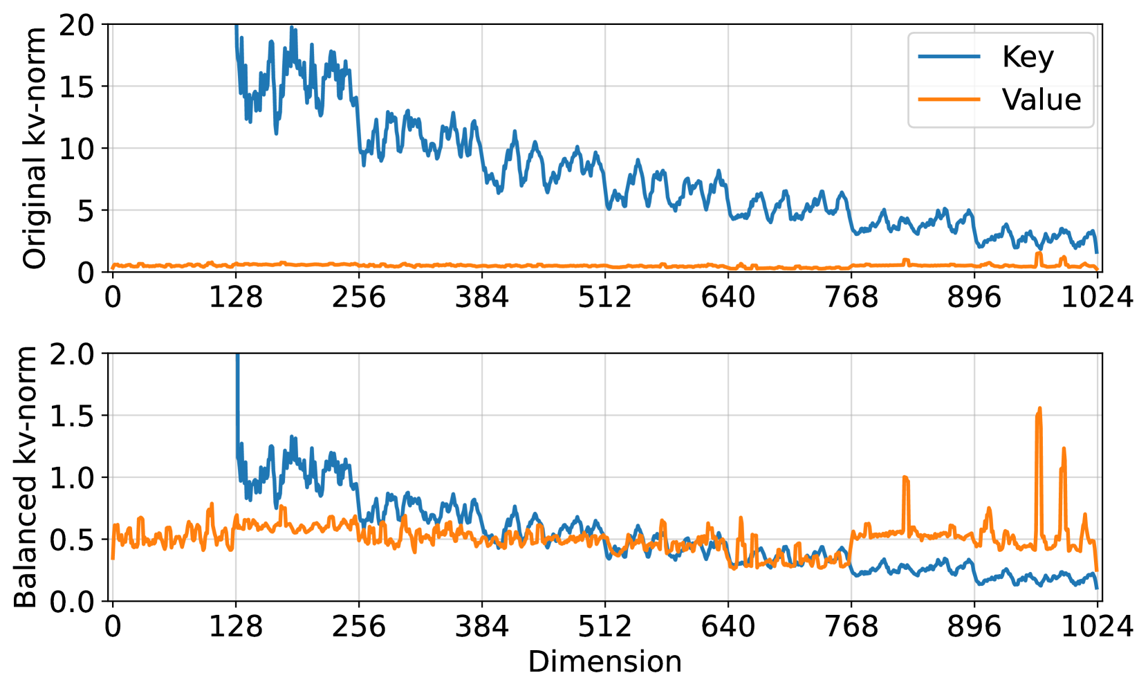### 5.3 Key-Value Norm Disparity Motivates KV Balancing In Figure 4(a), we visualize the norm magnitudes of the key and value activations in the first layer of LLaMA 3 8B before and after KV balancing. Note that both the key and value shown here are activations after applying the RoRoPE principal component concentration, and the first head of the key—reserved for RoPE—is excluded. As a result, the value and the remaining key components shown in the figure are precisely the elements we aim to compress jointly into a lower-dimensional space via PCA. <details> <summary>x6.png Details</summary>  ### Visual Description ## Line Graphs: Original vs. Balanced kv-norm Values ### Overview The image contains two vertically stacked line graphs comparing "Key" (blue) and "Value" (orange) metrics across dimensions 0–1024. The top graph shows "Original kv-norm" values, while the bottom graph displays "Balanced kv-norm" values. Both graphs use logarithmic scaling on the x-axis (Dimension) and linear scaling on the y-axis (kv-norm). ### Components/Axes - **X-axis (Dimension)**: - Labels: 0, 128, 256, 384, 512, 640, 768, 896, 1024 - Scale: Linear increments of 128 - **Y-axis (Top Graph - Original kv-norm)**: - Range: 0–20 - Labels: 0, 5, 10, 15, 20 - **Y-axis (Bottom Graph - Balanced kv-norm)**: - Range: 0–2.0 - Labels: 0, 0.5, 1.0, 1.5, 2.0 - **Legend**: - Position: Top-right corner of the top graph - Labels: - Blue line = "Key" - Orange line = "Value" ### Detailed Analysis #### Top Graph (Original kv-norm) - **Key (Blue Line)**: - Starts at ~18 at dimension 0, spikes to ~20 at dimension 128, then declines sharply to ~5 by dimension 256. - Fluctuates between ~3–10 between dimensions 256–1024, with minor peaks (e.g., ~8 at 512, ~6 at 768). - **Value (Orange Line)**: - Remains nearly flat at ~0.2 across all dimensions, with minor noise (<0.1 variation). #### Bottom Graph (Balanced kv-norm) - **Key (Blue Line)**: - Starts at ~1.8 at dimension 0, spikes to ~2.0 at dimension 128, then declines to ~0.5 by dimension 256. - Fluctuates between ~0.2–0.8 between dimensions 256–1024, with a notable peak (~1.2) at dimension 896. - **Value (Orange Line)**: - Starts at ~0.5 at dimension 0, rises to ~0.7 at dimension 128, then stabilizes between ~0.4–0.6 until dimension 768. - Shows sharp spikes (~1.5 at 896 and ~1.2 at 1024), exceeding Key values in these regions. ### Key Observations 1. **Original vs. Balanced Disparity**: - In the original graph, Key values are orders of magnitude higher than Value (e.g., 18 vs. 0.2 at dimension 0). - Balancing reduces this gap (e.g., 1.8 vs. 0.5 at dimension 0), but Value retains higher variability in later dimensions. 2. **Spike at Dimension 128**: - Both graphs show a pronounced spike in Key values at dimension 128 (~20 in original, ~2.0 in balanced), suggesting a localized anomaly or outlier. 3. **Value Spikes in Balanced Graph**: - Value exhibits unexpected peaks at dimensions 896 and 1024 (~1.5 and ~1.2, respectively), which are absent in the original graph. ### Interpretation - **Normalization Impact**: The "Balanced kv-norm" graph demonstrates that scaling reduces Key-Value disparities, but Value retains higher relative variability in later dimensions. - **Anomaly at 128**: The consistent spike in Key values at dimension 128 across both graphs suggests a systemic issue (e.g., data corruption, outlier event) requiring investigation. - **Value Behavior**: The late-stage spikes in Value (896–1024) in the balanced graph may indicate unaddressed imbalances or secondary factors affecting Value metrics post-normalization. *Note: All values are approximate due to the absence of gridlines or exact numerical annotations.* </details> (a) Norm magnitude of keys and values before and after KV balancing is applied. <details> <summary>x7.png Details</summary>  ### Visual Description ## Bar Chart: Log of Perplexity vs Key-Value Cache Compression Ratio ### Overview The chart compares the log of perplexity across four methods (W-based, W-based with BKV, WX-based, WX-based with BKV) at three key-value cache compression ratios (75.0%, 78.125%, 87.5%). Perplexity values are plotted on a logarithmic scale (2–10), with higher values indicating worse performance. ### Components/Axes - **X-axis**: Key-Value Cache Compression Ratio (%) - Categories: 75.0%, 78.125%, 87.5% - **Y-axis**: Log of Perplexity (2–10) - **Legend**: - Orange: W-based - Light Blue: WX-based - Dark Blue: WX-based with BKV - Red-Orange: W-based with BKV ### Detailed Analysis 1. **75.0% Compression Ratio** - W-based: ~8.0 - W-based with BKV: ~6.1 - WX-based: ~3.3 - WX-based with BKV: ~2.7 2. **78.125% Compression Ratio** - W-based: ~8.1 - W-based with BKV: ~6.5 - WX-based: ~3.6 - WX-based with BKV: ~2.9 3. **87.5% Compression Ratio** - W-based: ~8.5 - W-based with BKV: ~6.8 - WX-based: ~4.7 - WX-based with BKV: ~3.6 ### Key Observations - **W-based methods** consistently show the highest perplexity (worst performance), increasing slightly with higher compression ratios. - **BKV integration** reduces perplexity for both W-based and WX-based methods, with WX-based with BKV achieving the lowest values. - **WX-based with BKV** demonstrates the most significant performance improvement, particularly at 87.5% compression (perplexity ~3.6 vs. ~8.5 for W-based). - **WX-based alone** performs better than W-based but still lags behind WX-based with BKV. ### Interpretation The data suggests that **BKV integration** significantly improves performance (lower perplexity) for both W-based and WX-based methods. The WX-based approach with BKV achieves the best results, likely due to more efficient handling of key-value pairs under compression. Higher compression ratios (e.g., 87.5%) exacerbate performance degradation for non-BKV methods, highlighting the importance of BKV for maintaining perplexity in compressed cache systems. The logarithmic scale emphasizes relative differences, showing that WX-based with BKV outperforms others by ~2–3x in perplexity reduction. </details> (b) Comparison of different methods of KV cache compression, with and without KV balancing. 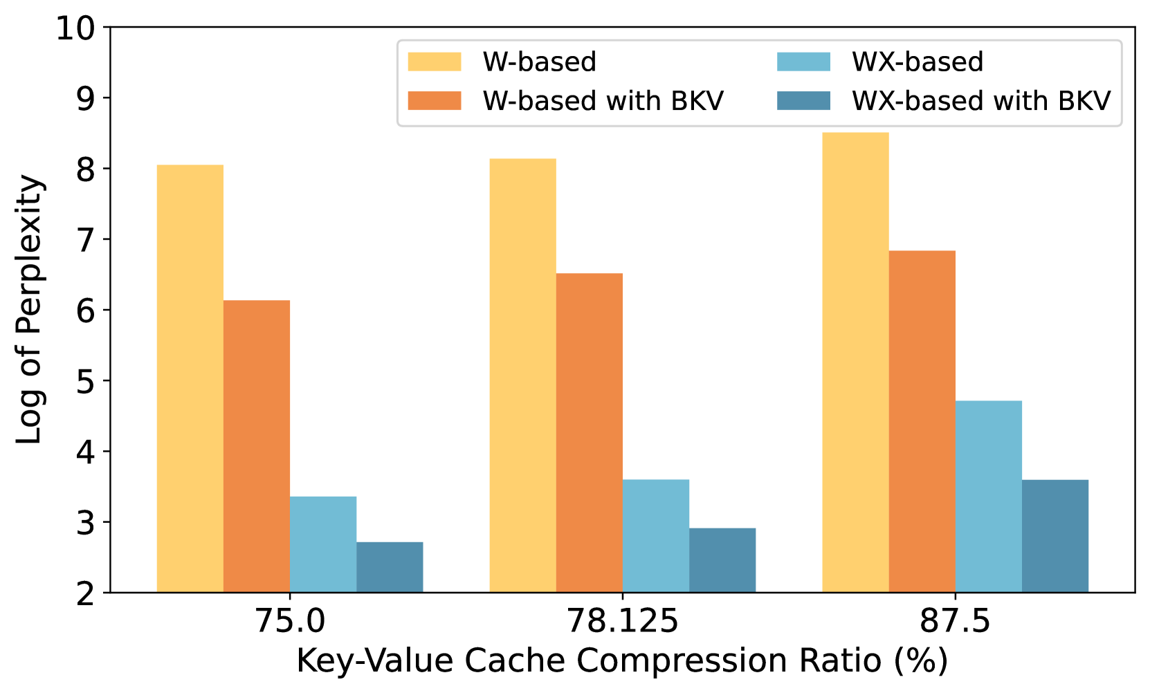Figure 4: Visualization of the norms of keys and values for the first layer of LLaMA 3 8B and the perplexity results after joint low-rank compression of keys and values under WikiText-2. Here, W-based and WX-based refer to PCA applied on the attention weights and the activation outputs, respectively. BKV denotes the application of KV balancing. It is evident that even after removing the first head with the highest norm, the overall norm of the key remains significantly larger than that of the value. This norm disparity poses a substantial challenge for joint compression into a shared latent space. In particular, such imbalance can bias the PCA toward directions aligned with the key, rather than the value, leading to suboptimal representation of the value components. The lower part of Figure 4(a) shows the norm distribution of keys and values after applying KV balancing. At this point, the norms of keys and values become more aligned, which is beneficial for performing joint PCA. This observation is further supported by the results in Figure 4(b), where KV balancing consistently reduces the loss incurred by jointly applying low-rank approximation to keys and values—whether the PCA is based on weights or on activations. Figure 4(b) also demonstrates that activation-based PCA yields significantly better results than weight-based PCA. ### 5.4 Hardware-Agnostic Inference Speedup with TransMLA By converting MHA/GQA models into MLA models that are fully compatible with the DeepSeek codebase and compressing the KV cache, TransMLA enables us to leverage all optimizations and tooling available in DeepSeek. Using the vLLM framework, we achieve substantial real-world inference speedups. 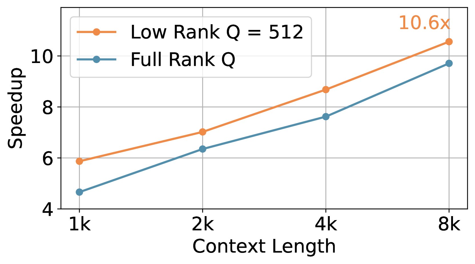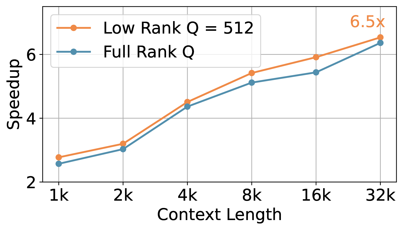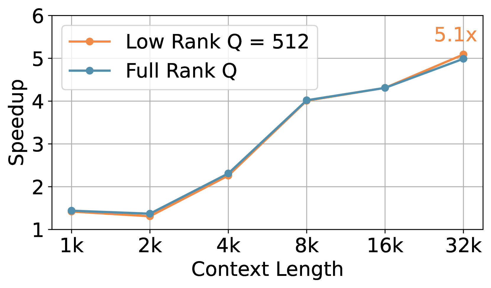In Figure 5, we benchmarked the inference performance of an MLA model—with a 92.97% reduction in KV cache size—on three consumer-grade AI accelerators with different compute capabilities and memory sizes: 165.2 TFLOPS with 24GB memory, 312 TFLOPS with 40GB memory, and 320 TFLOPS with 64GB memory. The figure shows the inference speedup of the MLA model relative to the original MHA model. Low-rank Q and Full-rank Q indicate whether the query projections were also compressed. Context length represents the total sequence length (i.e., context length plus generated tokens). Our experiments show that the inference speedup of MLA models increases as the context length grows, which aligns with our expectations. Since the primary performance gain of MLA stems from KV cache compression, longer contexts lead to more substantial savings and thus higher speedups. Remarkably, for the 8K context window on the first hardware platform, the TransMLA-transformed model achieves an impressive 10.6x inference acceleration. To the best of our knowledge, the MHA2MLA method has not reported any inference speedup results. <details> <summary>x8.png Details</summary>  ### Visual Description ## Line Chart: Speedup vs. Context Length ### Overview The chart compares the speedup performance of two configurations ("Low Rank Q = 512" and "Full Rank Q") across varying context lengths (1k, 2k, 4k, 8k). Speedup is measured on the y-axis (logarithmic scale implied by the 10.6x annotation), while context length is plotted on the x-axis. The legend is positioned in the top-right corner. ### Components/Axes - **Y-Axis (Speedup)**: Labeled "Speedup" with a linear scale from 4 to 10.6x. Gridlines are visible at intervals of 2. - **X-Axis (Context Length)**: Labeled "Context Length" with discrete markers at 1k, 2k, 4k, and 8k. - **Legend**: Located in the top-right corner, with: - **Orange line**: "Low Rank Q = 512" - **Blue line**: "Full Rank Q" ### Detailed Analysis - **Low Rank Q = 512 (Orange Line)**: - **1k**: Speedup ≈ 6.0 - **2k**: Speedup ≈ 7.0 - **4k**: Speedup ≈ 8.5 - **8k**: Speedup ≈ 10.6x (annotated as "10.6x" at the endpoint) - **Full Rank Q (Blue Line)**: - **1k**: Speedup ≈ 4.5 - **2k**: Speedup ≈ 6.2 - **4k**: Speedup ≈ 7.6 - **8k**: Speedup ≈ 9.7 ### Key Observations 1. Both configurations show **increasing speedup** with longer context lengths. 2. The **Low Rank Q = 512** configuration consistently outperforms **Full Rank Q** across all context lengths. 3. At **8k context length**, the speedup ratio between the two configurations is **~1.1x** (10.6x vs. 9.7x), though the orange line's endpoint annotation emphasizes its superior performance. ### Interpretation The data suggests that **Low Rank Q = 512** scales more efficiently with increasing context length compared to Full Rank Q. The 10.6x speedup at 8k context implies a **10.6x performance improvement** over a baseline (likely 1x speedup at 1k, though not explicitly shown). This trend highlights the advantage of using lower-rank quantization for large-scale context processing. The blue line's slower growth indicates diminishing returns for Full Rank Q as context length increases. </details> (a) 165.2 TFLOPS | 24GB <details> <summary>x9.png Details</summary>  ### Visual Description ## Line Graph: Speedup vs. Context Length ### Overview The image depicts a line graph comparing the performance of two configurations ("Low Rank Q = 512" and "Full Rank Q") across varying context lengths. The y-axis represents "Speedup" (multiplicative factor), while the x-axis represents "Context Length" in thousands of tokens. Two lines are plotted: an orange line for "Low Rank Q = 512" and a blue line for "Full Rank Q". The graph includes a legend in the top-left corner and a note indicating a "6.5x" multiplier at the upper-right corner. --- ### Components/Axes - **X-axis (Horizontal)**: - Label: "Context Length" - Scale: 1k, 2k, 4k, 8k, 16k, 32k (logarithmic spacing) - **Y-axis (Vertical)**: - Label: "Speedup" - Scale: 2 to 6.5x (linear scale) - **Legend**: - Position: Top-left corner - Entries: - Orange: "Low Rank Q = 512" - Blue: "Full Rank Q" - **Annotations**: - "6.5x" text in orange at the upper-right corner, aligned with the orange line's endpoint. --- ### Detailed Analysis #### Data Points (Approximate Values) - **Low Rank Q = 512 (Orange Line)**: - 1k: ~2.5x - 2k: ~3.0x - 4k: ~4.5x - 8k: ~5.5x - 16k: ~6.0x - 32k: ~6.5x - **Full Rank Q (Blue Line)**: - 1k: ~2.3x - 2k: ~3.2x - 4k: ~4.3x - 8k: ~5.2x - 16k: ~5.5x - 32k: ~6.3x #### Trends - Both lines exhibit a **monotonic upward trend**, indicating increasing speedup with longer context lengths. - The orange line ("Low Rank Q = 512") consistently outperforms the blue line ("Full Rank Q") across all context lengths. - The gap between the two lines widens at larger context lengths (e.g., 32k: 6.5x vs. 6.3x). - The "6.5x" annotation aligns with the orange line's endpoint at 32k context length. --- ### Key Observations 1. **Performance Scaling**: Speedup increases logarithmically with context length for both configurations. 2. **Efficiency Advantage**: The "Low Rank Q = 512" configuration achieves ~3–4% higher speedup than "Full Rank Q" at all context lengths. 3. **Diminishing Returns**: The speedup growth rate slows as context length increases (e.g., 16k to 32k yields only a 0.5x increase for "Low Rank Q"). 4. **Multiplier Significance**: The "6.5x" annotation suggests a baseline comparison (e.g., vs. a reference model or system). --- ### Interpretation The data demonstrates that reducing the rank of parameter Q (to 512) significantly improves computational efficiency without sacrificing performance, particularly at larger context lengths. The "6.5x" multiplier likely represents a speedup relative to a baseline system (e.g., unoptimized full-rank implementation). The widening gap between the two lines at higher context lengths implies that low-rank approximations become more advantageous as computational demands grow. This aligns with theoretical expectations, where lower-rank matrices reduce memory and computation requirements while maintaining approximate performance. **Critical Insight**: The choice of Q = 512 strikes a balance between model complexity and efficiency, offering near-optimal speedup with minimal performance loss compared to full-rank implementations. The logarithmic scaling suggests that further context length increases may yield diminishing returns, warranting further investigation into hardware-specific optimizations. </details> (b) 312 TFLOPS | 40GB <details> <summary>x10.png Details</summary>  ### Visual Description ## Line Graph: Speedup vs. Context Length ### Overview The image is a line graph comparing the performance of two models ("Low Rank Q = 512" and "Full Rank Q") across varying context lengths. The y-axis represents "Speedup" (1–6), and the x-axis represents "Context Length" (1k–32k). Two lines are plotted: an orange line for "Low Rank Q = 512" and a blue line for "Full Rank Q." A note indicates a "5.1x" speedup at the 32k context length. ### Components/Axes - **X-axis (Context Length)**: Labeled "Context Length" with markers at 1k, 2k, 4k, 8k, 16k, and 32k. - **Y-axis (Speedup)**: Labeled "Speedup" with increments of 1 (1–6). - **Legend**: Located in the top-left corner, with: - Orange line: "Low Rank Q = 512" - Blue line: "Full Rank Q" - **Annotations**: "5.1x" text in orange at the top-right corner near the 32k mark. ### Detailed Analysis - **Low Rank Q = 512 (Orange Line)**: - **1k**: ~1.3 speedup - **2k**: ~1.2 speedup - **4k**: ~2.2 speedup - **8k**: ~4.0 speedup - **16k**: ~4.3 speedup - **32k**: ~5.1 speedup - **Full Rank Q (Blue Line)**: - **1k**: ~1.3 speedup - **2k**: ~1.2 speedup - **4k**: ~2.2 speedup - **8k**: ~4.0 speedup - **16k**: ~4.3 speedup - **32k**: ~5.0 speedup ### Key Observations 1. Both models show increasing speedup with longer context lengths. 2. The "Low Rank Q = 512" model starts slightly below "Full Rank Q" at 1k but surpasses it at 32k. 3. The "5.1x" annotation highlights a significant performance gain for "Low Rank Q = 512" at the maximum context length. 4. The lines converge at lower context lengths (1k–8k) but diverge sharply at 32k. ### Interpretation The data suggests that the "Low Rank Q = 512" model becomes more efficient than "Full Rank Q" as context length increases, likely due to architectural optimizations that scale better with larger data. The 5.1x speedup at 32k indicates a substantial performance advantage, which could be critical for applications requiring high-speed processing of large contexts. The initial dip at 2k may reflect transient inefficiencies or optimization trade-offs. The divergence at 32k underscores the importance of model design for scalability in high-demand scenarios. </details> (c) 320 TFLOPS | 64GB Figure 5: Inference speedups with TransMLA comparing to the original LLaMA2 7B model on three consumer-grade AI accelerators. Low-rank Q and Full-rank Q indicate whether the query projections were also compressed. Context length represents the total sequence length. ## 6 Conclusion, Limitation and Future Work In this work, we demonstrate that the expressive power of TransMLA is stronger than GQA under the same KV cache. To help existing GQA transition to the MLA structure with minimal cost, we propose the TransMLA method. By using the RoRoPE method, the multi-head KV positional information is concentrated into the first head, and FreqFold further enhances this extraction effect. The positional information of the remaining query-key heads is removed, and the Balance KV norm method is used to jointly compress the values and the remaining heads of keys. TransMLA can convert models such as LLaMA and Qwen into MLA-based models, and the converted model incurs very little loss compared to the original model, with performance being recoverable through training with only a few tokens. Additionally, TransMLA can easily leverage the DeepSeek ecosystem for accelerated inference, achieving significant throughput improvements across various hardware platforms. Although TransMLA significantly reduces the loss introduced by decoupling RoPE via RoRoPE and FreqFold, and alleviates KV cache compression loss through KV balancing, the KV balancing technique itself is relatively trivial. Are there alternative, more powerful mathematical tools that can better handle the disparity between the norm of the keys and values and deliver improved performance at the same compression rate, thereby enabling truly training-free conversion? Furthermore, TransMLA needs to be validated across a broader range of models, and should be integrated with pruning, quantization, token selection, and other optimization techniques to fully explore the upper bounds of inference acceleration. ## References - OpenAI [2024] OpenAI. Hello GPT-4o, 2024. URL https://openai.com/index/hello-gpt-4o/. - Anthropic [2024] Anthropic. Claude 3.5 sonnet, 2024. URL https://www.anthropic.com/news/claude-3-5-sonnet. - Team et al. [2024a] Gemini Team, Petko Georgiev, Ving Ian Lei, Ryan Burnell, Libin Bai, Anmol Gulati, Garrett Tanzer, Damien Vincent, Zhufeng Pan, Shibo Wang, et al. Gemini 1.5: Unlocking multimodal understanding across millions of tokens of context. arXiv preprint arXiv:2403.05530, 2024a. - AI@Meta [2024] AI@Meta. Llama 3 model card, 2024. URL https://github.com/meta-llama/llama3/blob/main/MODEL_CARD.md. - Mistral [2024] Mistral. Cheaper, better, faster, stronger: Continuing to push the frontier of ai and making it accessible to all, 2024. URL https://mistral.ai/news/mixtral-8x22b. - Qwen [2024] Qwen. Qwen2.5: A party of foundation models, 2024. URL https://qwenlm.github.io/blog/qwen2.5. - Liu et al. [2024a] Aixin Liu, Bei Feng, Bing Xue, Bingxuan Wang, Bochao Wu, Chengda Lu, Chenggang Zhao, Chengqi Deng, Chenyu Zhang, Chong Ruan, et al. Deepseek-v3 technical report. arXiv preprint arXiv:2412.19437, 2024a. - Guo et al. [2025] Daya Guo, Dejian Yang, Haowei Zhang, Junxiao Song, Ruoyu Zhang, Runxin Xu, Qihao Zhu, Shirong Ma, Peiyi Wang, Xiao Bi, et al. Deepseek-r1: Incentivizing reasoning capability in llms via reinforcement learning. arXiv preprint arXiv:2501.12948, 2025. - Team et al. [2024b] Gemma Team, Morgane Riviere, Shreya Pathak, Pier Giuseppe Sessa, Cassidy Hardin, Surya Bhupatiraju, Léonard Hussenot, Thomas Mesnard, Bobak Shahriari, Alexandre Ramé, et al. Gemma 2: Improving open language models at a practical size. arXiv preprint arXiv:2408.00118, 2024b. - Abdin et al. [2024] Marah Abdin, Jyoti Aneja, Harkirat Behl, Sébastien Bubeck, Ronen Eldan, Suriya Gunasekar, Michael Harrison, Russell J Hewett, Mojan Javaheripi, Piero Kauffmann, et al. Phi-4 technical report. arXiv preprint arXiv:2412.08905, 2024. - Radford [2018] Alec Radford. Improving language understanding by generative pre-training. 2018. - Brown et al. [2020] Tom Brown, Benjamin Mann, Nick Ryder, Melanie Subbiah, Jared D Kaplan, Prafulla Dhariwal, Arvind Neelakantan, Pranav Shyam, Girish Sastry, Amanda Askell, et al. Language models are few-shot learners. Advances in neural information processing systems, 33:1877–1901, 2020. - Ainslie et al. [2023] Joshua Ainslie, James Lee-Thorp, Michiel de Jong, Yury Zemlyanskiy, Federico Lebrón, and Sumit Sanghai. Gqa: Training generalized multi-query transformer models from multi-head checkpoints. arXiv preprint arXiv:2305.13245, 2023. - Shazeer [2019] Noam Shazeer. Fast transformer decoding: One write-head is all you need. arXiv preprint arXiv:1911.02150, 2019. - Vaswani et al. [2017] Ashish Vaswani, Noam Shazeer, Niki Parmar, Jakob Uszkoreit, Llion Jones, Aidan N Gomez, Łukasz Kaiser, and Illia Polosukhin. Attention is all you need. NeurIPS, 2017. - Xiao et al. [2024] Guangxuan Xiao, Jiaming Tang, Jingwei Zuo, Junxian Guo, Shang Yang, Haotian Tang, Yao Fu, and Song Han. Duoattention: Efficient long-context llm inference with retrieval and streaming heads. arXiv preprint arXiv:2410.10819, 2024. - Liu et al. [2024b] Zhiyang Liu, Dong Zhang, Xinyi Li, and Ji Wu. Kivi: Quantized key-value representation for efficient long-context transformers. arXiv preprint arXiv:2402.06732, 2024b. - Hooper et al. [2024] James Hooper, Li Dai, Zhen Zhang, and Seung-Hwan Lee. Kvquant: Quantization for efficient key-value caching in transformer models. arXiv preprint arXiv:2402.12345, 2024. - Zhang et al. [2023] Zhenyu Zhang, Ying Sheng, Tianyi Zhou, Tianlong Chen, Lianmin Zheng, Ruisi Cai, Zhao Song, Yuandong Tian, Christopher Ré, Clark Barrett, et al. H2o: Heavy-hitter oracle for efficient generative inference of large language models. Advances in Neural Information Processing Systems, 36:34661–34710, 2023. - DeepSeek-AI [2024] DeepSeek-AI. Deepseek-v2: A strong, economical, and efficient mixture-of-experts language model. CoRR, abs/2405.04434, 2024. URL https://doi.org/10.48550/arXiv.2405.04434. - Su et al. [2024] Jianlin Su, Murtadha Ahmed, Yu Lu, Shengfeng Pan, Wen Bo, and Yunfeng Liu. Roformer: Enhanced transformer with rotary position embedding. Neurocomputing, 568:127063, 2024. - Chang et al. [2024] Chi-Chih Chang, Wei-Cheng Lin, Chien-Yu Lin, Chong-Yan Chen, Yu-Fang Hu, Pei-Shuo Wang, Ning-Chi Huang, Luis Ceze, Mohamed S Abdelfattah, and Kai-Chiang Wu. Palu: Compressing kv-cache with low-rank projection. arXiv preprint arXiv:2407.21118, 2024. - Ji et al. [2025] Tao Ji, Bin Guo, Yuanbin Wu, Qipeng Guo, Lixing Shen, Zhan Chen, Xipeng Qiu, Qi Zhang, and Tao Gui. Towards economical inference: Enabling deepseek’s multi-head latent attention in any transformer-based llms. arXiv preprint arXiv:2502.14837, 2025. - Zadouri et al. [2025] Ted Zadouri, Hubert Strauss, and Tri Dao. Hardware-efficient attention for fast decoding. arXiv preprint arXiv:2505.21487, 2025. - Zhang et al. [2025] Yifan Zhang, Yifeng Liu, Huizhuo Yuan, Zhen Qin, Yang Yuan, Quanquan Gu, and Andrew Chi-Chih Yao. Tensor product attention is all you need. arXiv preprint arXiv:2501.06425, 2025. - Fu et al. [2024] Qichen Fu, Minsik Cho, Thomas Merth, Sachin Mehta, Mohammad Rastegari, and Mahyar Najibi. Lazyllm: Dynamic token pruning for efficient long context llm inference. arXiv preprint arXiv:2407.14057, 2024. - Jo and Shin [2024] Hyun-rae Jo and Dongkun Shin. A2sf: Accumulative attention scoring with forgetting factor for token pruning in transformer decoder. arXiv preprint arXiv:2407.20485, 2024. - Li et al. [2024] Yuhong Li, Yingbing Huang, Bowen Yang, Bharat Venkitesh, Acyr Locatelli, Hanchen Ye, Tianle Cai, Patrick Lewis, and Deming Chen. Snapkv: Llm knows what you are looking for before generation. arXiv preprint arXiv:2404.14469, 2024. - Sun et al. [2024] Tian Sun, Li Zhang, and Shuang Wu. You only need one: Efficient kv sharing across transformer layers. Proceedings of the 42nd International Conference on Machine Learning (ICML), 2024. - Liu et al. [2024c] Akide Liu, Jing Liu, Zizheng Pan, Yefei He, Gholamreza Haffari, and Bohan Zhuang. Minicache: Kv cache compression in depth dimension for large language models. arXiv preprint arXiv:2405.14366, 2024c. - Zuhri et al. [2024] Zayd Muhammad Kawakibi Zuhri, Muhammad Farid Adilazuarda, Ayu Purwarianti, and Alham Fikri Aji. Mlkv: Multi-layer key-value heads for memory efficient transformer decoding. arXiv preprint arXiv:2406.09297, 2024. - Hendrycks et al. [2021] Dan Hendrycks, Collin Burns, Steven Basart, Andy Zou, Mantas Mazeika, Dawn Song, and Jacob Steinhardt. Measuring massive multitask language understanding. In 9th International Conference on Learning Representations, ICLR 2021, Virtual Event, Austria, May 3-7, 2021. OpenReview.net, 2021. URL https://openreview.net/forum?id=d7KBjmI3GmQ. - Clark et al. [2018] Peter Clark, Isaac Cowhey, Oren Etzioni, Tushar Khot, Ashish Sabharwal, Carissa Schoenick, and Oyvind Tafjord. Think you have solved question answering? try arc, the AI2 reasoning challenge. CoRR, abs/1803.05457, 2018. URL http://arxiv.org/abs/1803.05457. - Bisk et al. [2020] Yonatan Bisk, Rowan Zellers, Ronan Le Bras, Jianfeng Gao, and Yejin Choi. PIQA: reasoning about physical commonsense in natural language. In The Thirty-Fourth AAAI Conference on Artificial Intelligence, AAAI 2020, The Thirty-Second Innovative Applications of Artificial Intelligence Conference, IAAI 2020, The Tenth AAAI Symposium on Educational Advances in Artificial Intelligence, EAAI 2020, New York, NY, USA, February 7-12, 2020, pages 7432–7439. AAAI Press, 2020. doi: 10.1609/AAAI.V34I05.6239. URL https://doi.org/10.1609/aaai.v34i05.6239. - Zellers et al. [2019] Rowan Zellers, Ari Holtzman, Yonatan Bisk, Ali Farhadi, and Yejin Choi. Hellaswag: Can a machine really finish your sentence? In Anna Korhonen, David R. Traum, and Lluís Màrquez, editors, Proceedings of the 57th Conference of the Association for Computational Linguistics, ACL 2019, Florence, Italy, July 28- August 2, 2019, Volume 1: Long Papers, pages 4791–4800. Association for Computational Linguistics, 2019. doi: 10.18653/V1/P19-1472. URL https://doi.org/10.18653/v1/p19-1472. - Mihaylov et al. [2018] Todor Mihaylov, Peter Clark, Tushar Khot, and Ashish Sabharwal. Can a suit of armor conduct electricity? A new dataset for open book question answering. In Ellen Riloff, David Chiang, Julia Hockenmaier, and Jun’ichi Tsujii, editors, Proceedings of the 2018 Conference on Empirical Methods in Natural Language Processing, Brussels, Belgium, October 31 - November 4, 2018, pages 2381–2391. Association for Computational Linguistics, 2018. doi: 10.18653/V1/D18-1260. URL https://doi.org/10.18653/v1/d18-1260. - Sakaguchi et al. [2021] Keisuke Sakaguchi, Ronan Le Bras, Chandra Bhagavatula, and Yejin Choi. Winogrande: an adversarial winograd schema challenge at scale. Commun. ACM, 64(9):99–106, 2021. doi: 10.1145/3474381. URL https://doi.org/10.1145/3474381. - Merity et al. [2016] Stephen Merity, Caiming Xiong, James Bradbury, and Richard Socher. Pointer sentinel mixture models, 2016. - Ben Allal et al. [2024] Loubna Ben Allal, Anton Lozhkov, Guilherme Penedo, Thomas Wolf, and Leandro von Werra. Smollm-corpus. 2024. URL https://huggingface.co/datasets/HuggingFaceTB/smollm-corpus. - Lozhkov et al. [2024a] Anton Lozhkov, Loubna Ben Allal, Leandro von Werra, and Thomas Wolf. Fineweb-edu: the finest collection of educational content, 2024a. URL https://huggingface.co/datasets/HuggingFaceFW/fineweb-edu. - Wu et al. [2024] Xun Wu, Shaohan Huang, and Furu Wei. Mixture of lora experts. arXiv preprint arXiv:2404.13628, 2024. - Lozhkov et al. [2024b] Anton Lozhkov, Raymond Li, Loubna Ben Allal, Federico Cassano, Joel Lamy-Poirier, Nouamane Tazi, Ao Tang, Dmytro Pykhtar, Jiawei Liu, Yuxiang Wei, Tianyang Liu, Max Tian, Denis Kocetkov, Arthur Zucker, Younes Belkada, Zijian Wang, Qian Liu, Dmitry Abulkhanov, Indraneil Paul, Zhuang Li, Wen-Ding Li, Megan Risdal, Jia Li, Jian Zhu, Terry Yue Zhuo, Evgenii Zheltonozhskii, Nii Osae Osae Dade, Wenhao Yu, Lucas Krauß, Naman Jain, Yixuan Su, Xuanli He, Manan Dey, Edoardo Abati, Yekun Chai, Niklas Muennighoff, Xiangru Tang, Muhtasham Oblokulov, Christopher Akiki, Marc Marone, Chenghao Mou, Mayank Mishra, Alex Gu, Binyuan Hui, Tri Dao, Armel Zebaze, Olivier Dehaene, Nicolas Patry, Canwen Xu, Julian McAuley, Han Hu, Torsten Scholak, Sebastien Paquet, Jennifer Robinson, Carolyn Jane Anderson, Nicolas Chapados, Mostofa Patwary, Nima Tajbakhsh, Yacine Jernite, Carlos Muñoz Ferrandis, Lingming Zhang, Sean Hughes, Thomas Wolf, Arjun Guha, Leandro von Werra, and Harm de Vries. Starcoder 2 and the stack v2: The next generation, 2024b. - Paster et al. [2023] Keiran Paster, Marco Dos Santos, Zhangir Azerbayev, and Jimmy Ba. Openwebmath: An open dataset of high-quality mathematical web text, 2023. - Stack Overflow [2025] Stack Overflow. Stack overflow, 2025. URL https://stackoverflow.com. Accessed: 2025-05-21. - Allal et al. [2025a] Loubna Ben Allal, Anton Lozhkov, Elie Bakouch, Gabriel Martín Blázquez, Guilherme Penedo, Lewis Tunstall, Andrés Marafioti, Hynek Kydlíček, Agustín Piqueres Lajarín, Vaibhav Srivastav, et al. Smollm2: When smol goes big–data-centric training of a small language model. arXiv preprint arXiv:2502.02737, 2025a. - Allal et al. [2025b] Loubna Ben Allal, Anton Lozhkov, Elie Bakouch, Gabriel Martín Blázquez, Guilherme Penedo, Lewis Tunstall, Andrés Marafioti, Hynek Kydlíček, Agustín Piqueres Lajarín, Vaibhav Srivastav, Joshua Lochner, Caleb Fahlgren, Xuan-Son Nguyen, Clémentine Fourrier, Ben Burtenshaw, Hugo Larcher, Haojun Zhao, Cyril Zakka, Mathieu Morlon, Colin Raffel, Leandro von Werra, and Thomas Wolf. Smollm2: When smol goes big – data-centric training of a small language model, 2025b. URL https://arxiv.org/abs/2502.02737. ## Appendix A Enhanced Expressive Power of MLA with Decoupled RoPE ### A.1 Introduction This section provides a theoretical analysis to demonstrate that Multi-Head Latent Attention (MLA) with decoupled Rotary Position Embedding (RoPE), as described in Section 3.3 of the main paper, possesses greater expressive power than Grouped-Query Attention (GQA) (Section 3.2). This analysis assumes comparable KV cache sizes and number of query heads. Our primary argument focuses on the core projection mechanisms that generate queries, keys, and values, abstracting away from the specifics of RoPE application initially. We first present the following proposition concerning the relative expressiveness of these core mechanisms: **Proposition 1** *Given the same KV cache size and number of query heads, the expressiveness of the core attention projection mechanisms follows the order: $\rm GQA<MLA_Factorized<MQA$ .* Here, $\rm MLA_Factorized$ refers to an attention mechanism employing low-rank factorization for its key and value projections, representing the content-processing aspect of the full MLA. It is important to note that in the proposition, the query projection in $\rm MLA_Factorized$ does not undergo low-rank factorization; this differs from the full MLA, where the query is also factorized. After proving this proposition, we will discuss how the full MLA architecture, which incorporates such an $\rm MLA_Factorized$ core for its content components and an $\rm MQA$ core for its decoupled RoPE components, is thereby more expressive than GQA. For this analysis, we primarily consider the impact of the architectural structure on representational capacity, setting aside the direct effects of RoPE itself on the expressiveness comparison between the fundamental GQA, MLA-Factorized, and MQA structures. 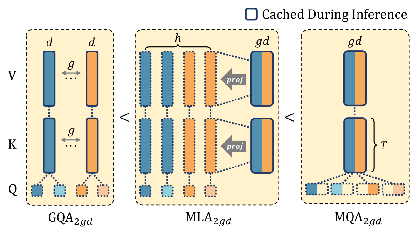<details> <summary>x11.png Details</summary>  ### Visual Description ## Diagram: Comparison of Attention Mechanisms in Transformer Architectures ### Overview The diagram illustrates three transformer-based attention mechanisms: **GQA2gd**, **MLA2gd**, and **MQA2gd**. Each block represents a distinct architectural approach, with components labeled for query (Q), key (K), value (V), and projection operations. Arrows indicate information flow, and the legend highlights elements "Cached During Inference." ### Components/Axes 1. **GQA2gd Block**: - **V, K, Q**: Vertical stacks labeled "V" (value), "K" (key), and "Q" (query), with bidirectional arrows labeled "g" between them. - **Structure**: Simplest configuration, with direct interactions between Q, K, and V. 2. **MLA2gd Block**: - **h Layers**: Multiple horizontal layers (labeled "h") with alternating blue and orange segments. - **Projection Arrows**: Labeled "proj," connecting layers to "gd" blocks on the right. - **Caching**: Blue squares marked "Cached During Inference" at the bottom. 3. **MQA2gd Block**: - **gd Blocks**: Stacked "gd" components with a "T" block below, connected by arrows. - **Caching**: Blue and orange squares marked "Cached During Inference" at the bottom. 4. **Legend**: - **Cached During Inference**: Blue square symbol, applied to specific components in MLA2gd and MQA2gd. ### Detailed Analysis - **GQA2gd**: - Direct interactions between Q, K, and V via "g" arrows. No projections or caching. - Simplest architecture, likely representing a baseline. - **MLA2gd**: - Introduces **h layers** with internal structure (blue/orange segments). - Projections ("proj") aggregate outputs into "gd" blocks. - Caching applied to bottom-layer components (blue squares). - **MQA2gd**: - Stacked "gd" blocks with a "T" component below, suggesting hierarchical processing. - Caching applied to both blue and orange squares, indicating broader reuse. ### Key Observations - **Complexity Progression**: GQA2gd < MLA2gd < MQA2gd in terms of architectural layers and operations. - **Caching Strategy**: MQA2gd caches more components (both colors) than MLA2gd (only blue). - **Projection Usage**: MLA2gd relies heavily on projections to consolidate layer outputs. ### Interpretation This diagram highlights trade-offs in transformer attention mechanisms: 1. **GQA2gd** prioritizes simplicity, with minimal computational overhead but limited scalability. 2. **MLA2gd** introduces layered processing (via "h") and selective caching, balancing efficiency and complexity. 3. **MQA2gd** optimizes further by caching both query and key-value components (via "T"), likely reducing redundant computations during inference. The "Cached During Inference" label suggests these mechanisms aim to improve latency by reusing precomputed values. MQA2gd’s dual caching (blue/orange) may reflect a more aggressive optimization strategy compared to MLA2gd’s single-color caching. The progression implies a design philosophy where later architectures (MLA2gd, MQA2gd) address scalability and efficiency challenges inherent in simpler models like GQA2gd. </details> Figure 6: Comparison of Multi-Query Attention (MQA), Group Query Attention (GQA), and Multi-Head Latent Attention (MLA). In this work, we illustrate that given the same KV cache size, the expressiveness increases in the order of GQA, MLA, and MQA. In the figure, $h,d,g$ denote the number of heads, hidden dimension of each head, and the number of groups (K/V heads) in GQA, respectively. In MQA, the head dimension is set to $gd$ to align the KV cache size with GQA and MLA. As a result, the KV cache size per token per layer for all three approaches is $2gd$ ### A.2 Proof of Proposition 1 Let $D$ be the hidden dimension of the input token $x_t∈ℝ^D$ , $h$ be the number of query heads, and $d=D/h$ be the dimension per head. In GQA, query heads are divided into $g$ groups. For fair KV cache comparison, the latent dimension for keys and values in $\rm MLA_Factorized$ ( $r_kv$ ) and the head dimension of MQA will be related to $gd$ . Specifically, if the KV cache per token in GQA is $2gd$ for both keys and values, then in $\rm MLA_Factorized$ , $r_kv=2gd$ , and in MQA, the head dimension is also $2gd$ ; this ensures the KV cache sizes are aligned. #### A.2.1 GQA $≤$ MLA Factorized In GQA, query head $q_t,i$ attends to key $k_j,\lceil i/(h/g)\rceil$ and value $v_j,\lceil i/(h/g)\rceil$ . The GQA key projection $W^K∈ℝ^gd× D$ produces $g$ distinct key vectors $[k_t,1;\dots;k_t,g]$ . Similarly, $W^V∈ℝ^gd× D$ produces value vectors. We define effective per-query-head projection matrices $W^\prime K∈ℝ^hd× D$ and $W^\prime V∈ℝ^hd× D$ for GQA: $$ \displaystyle W^\prime K \displaystyle=\begin{pmatrix}W^\prime K_1\\ ⋮\\ W^\prime K_h\end{pmatrix},where W^\prime K_i=W^K_\lceil i/(h /g)\rceil, \displaystyle W^\prime V \displaystyle=\begin{pmatrix}W^\prime V_1\\ ⋮\\ W^\prime V_h\end{pmatrix},where W^\prime V_i=W^V_\lceil i/(h /g)\rceil. \tag{21} $$ Here, $W^K_k$ is the $k$ -th $d× D$ block of $W^K$ . Thus, $k^\prime_j,i=W^\prime K_ix_j=k_j,\lceil i /(h/g)\rceil$ , and similarly for values. The matrices $W^\prime K$ and $W^\prime V$ have ranks at most $gd$ . An $\rm MLA_Factorized$ mechanism generates keys via $k_j,i=(W^UK(W^DKVx_j))_i$ , where $W^DKV∈ℝ^r_kv× D$ and $W^UK∈ℝ^hd× r_kv$ . A similar formulation applies for values with $W^UV∈ℝ^hd× r_kv$ . To demonstrate expressive capability, GQA $≤\rm MLA_Factorized$ , we set $r_kv=2gd$ . Let $W^DKV=\begin{pmatrix}W^K\ W^V\end{pmatrix}∈ℝ^2gd× D$ . We seek $W^UK,W^UV∈ℝ^hd× 2gd$ such that $W^\prime K=W^UKW^DKV,W^\prime V=W^UVW^DKV$ . This is achieved by setting $W^UK_i,W^UV_i∈ℝ^d× 2gd$ (the block for head $i$ ) as selector matrices: $$ \displaystyle W^UK_i=[\underbrace{0_d× d,\dots,0_d× d}_k-1 blocks,I_d× d,\underbrace{0 _d× d,\dots,0_d× d}_2g-k blocks], \displaystyle W^UV_i=[\underbrace{0_d× d,\dots,0_d× d}_g+k-1 blocks,I_d× d,\underbrace{ 0_d× d,\dots,0_d× d}_g-k blocks], \tag{23} $$ where $k=\lceil i/(h/g)\rceil$ . Thus, GQA’s key/value generation can be replicated by an $\rm MLA_Factorized$ model with $r_kv=2gd$ and specific sparse structures for $W^UK$ and $W^UV$ . The KV cache size $2gd×(sequence length)$ is preserved since we will be caching $c^KV_j=W^DKVx_j∈ℝ^2gd$ . On that account, the theoretical expressive power of GQA is less than or equal to that of $\rm MLA_Factorized$ given the same KV cache size. #### A.2.2 MLA Factorized $≤$ MQA Consider an MLA-Factorized model where queries are $q_t,i=W^Q_ix_t$ (assuming $W^Q_i∈ℝ^d× D$ is the $i$ -th block of $W^Q$ ) and keys are $k_j,i=(W^UK_i(W^DKVx_j))$ . The attention score for head $i$ involves $q_t,i^⊤k_j,i$ : $$ q_t,i^⊤k_j,i=(W^Q_ix_t)^⊤(W^UK _i(W^DKVx_j)). \tag{25} $$ This can be rewritten as: $$ q_t,i^⊤k_j,i=(\underbrace{(W^UK_i)^⊤W^Q_i}_W^\prime Q_ix_t)^⊤(W^DKVx_j). \tag{26} $$ Let $\hat{q}_t,i=W^\prime Q_ix_t∈ℝ^2gd$ and $c^KV_j=W^DKVx_j∈ℝ^2gd$ . The computation of attention output becomes: $$ \displaystyleo_t,i \displaystyle=∑_jsoftmax_j(\frac{\hat{q}_t,i^⊤ c^KV_j}{√{d}})W^UV_ic^KV_j, \displaystyley_t \displaystyle=W^O[o_t,1;o_t,2;...;o_t,h] \displaystyle=\underbrace{W^O\begin{pmatrix}W^UV_1&&\\ &W^UV_2&\\ &&⋱&\\ &&&W^UV_h\\ \end{pmatrix}}_W^\prime O\begin{pmatrix}softmax_j(\frac{\hat{ q}_t,1^⊤c^KV_j}{√{d}})c^KV_j\\ ⋮\\ softmax_j(\frac{\hat{q}_t,1^⊤c^KV_j}{ √{d}})c^KV_j\\ \end{pmatrix}. \tag{27} $$ This is an MQA formulation where each modified query $\hat{q}_t,i$ (now of dimension $2gd$ ) attends to a shared key and value $c^KV_j$ . This indicates that the computations within MLA-Factorized can be structured to use shared intermediate key and value representations akin to MQA’s core. Thus, any MLA-Factorized model can be represented as an MQA model with a shared key/value of dimension $2gd$ . #### A.2.3 Strict Inequalities: GQA $<$ MLA Factorized $<$ MQA The relationships are strict: GQA $<$ MLA Factorized When GQA is represented as an $\rm MLA_Factorized$ model, the up-projection matrices $W^UK$ and $W^UV$ must adopt specific sparse, block-selector structures. A general $\rm MLA_Factorized$ model imposes no such constraints; $W^UK$ and $W^UV$ are typically dense and fully learnable. This allows a general $\rm MLA_Factorized$ to create $h$ distinct key (and value) vectors by combining features from the $r_kv$ -dimensional latent space in complex ways. GQA is restricted to $g$ unique key (and value) vectors that are merely replicated $h/g$ times. If $h>g$ , $\rm MLA_Factorized$ can generate a richer set of interaction patterns. Thus, $\rm MLA_Factorized$ has strictly greater expressive power. MLA Factorized $<$ MQA Consider the bilinear form $x_t^⊤Mx_j$ in the attention score. In $\rm MLA_Factorized$ , for head $i$ , $M_MLA,i=(W^Q_i)^⊤W^UK_iW^DKV$ . The maximum rank of the transformation is determined by the smallest one among the ranks of $W^Q_i∈ℝ^d× D$ , $W^UK_i∈ℝ^d× 2gd$ , and $W^DKV∈ℝ^2gd× D$ , which is at most $d$ . However, in the MQA form derived from $\rm MLA_Factorized$ , the rank of the interaction matrix here, $(W^\prime Q_i)^⊤W^DKV$ , is determined by the smallest one among the ranks of $W^\prime Q_i∈ℝ^2gd× D$ and $W^DKV∈ℝ^2gd× D$ , which is at most $2gd$ . Since $2gd≥ d$ , MQA allows for a potentially higher-rank interaction between the (modified) query and the shared key representations compared to the per-head effective rank in $\rm MLA_Factorized$ ’s original formulation. This indicates that MQA has a greater representational capacity for the scoring mechanism. ### A.3 Expressiveness of MLA with Decoupled RoPE The full MLA architecture, as defined in Section 3.3 (main paper), employs a decoupled RoPE strategy. The query $q_t,i$ and key $k_t,i$ for head $i$ (in the MHA-like training paradigm, Equation 3.3) are: $$ \displaystyleq_t,i \displaystyle=[q_t,i^C;q_t,i^R] \displaystylek_t,i \displaystyle=[k_t,i^C;k_t^R] \tag{29} $$ where $k_t^R$ is a shared RoPE key component across all heads for token $t$ . The bilinear attention score (numerator of the softmax argument) for head $i$ between query at $t$ and key at $j$ is: $$ (q_t,i^C)^⊤k_j,i^C+(q_t,i^R)^⊤ k_j^R \tag{31} $$ Let’s analyze the two components of this score: 1. Content Component Interaction: $(q_t,i^C)^⊤k_j,i^C$ . The content keys $k_j,i^C$ are derived from $W^UK(W^DKVx_j)$ . This key generation mechanism for $k_j,i^C$ is precisely that of the $\rm MLA_Factorized$ model discussed in Section A.1. As established, MLA-Factorized is strictly more expressive than GQA for the non-positional part of the representation. 1. Positional Component Interaction: $(q_t,i^R)^⊤k_j^R$ . This interaction, where $h$ distinct query-side RoPE components $q_t,i^R$ attend to a single, shared key-side RoPE component $k_j^R$ , is an MQA structure specifically for the positional information. As shown in Section A.2.3, MQA is strictly more expressive than $\rm MLA_Factorized$ , and by extension, GQA. In summary, we have demonstrated that the expressive power of MLA with decoupled RoPE is stronger than that of the traditional GQA. However, it is worth noting that in the previously proven proposition, the $\rm MLA_Factorized$ does not have a low-rank decomposition on the query; this differs from DeepSeek MLA. In the full MLA architecture, the query is also decomposed. ## Appendix B Proof of RoPE Inner Product Invariance under Orthogonal Transformation In this subsection, we provide a rigorous proof of Equation 19, namely: $$ ∑_l=1^d/2≤ft(≤ft[U_l\hat{q}_t,i^[2l-1::d]; U_l\hat{q}_t,i^[2l::d]\right]\right)^R^{⊤}≤ft( ≤ft[U_l\hat{k}_j^[2l-1::d];U_l\hat{ k}_j^[2l::d]\right]\right)^R=\hat{q}^R^{⊤}_t,i \hat{k}_j^R. $$ Here, $d$ is the dimension of each original attention head. The notation $q_t,i^[2l-1::d]$ (and similarly for other terms) refers to an $h$ -dimensional vector collecting the $(2l-1)$ -th components from each of the $h$ original attention heads. The matrix $U_l$ is an $h× h$ orthogonal matrix. The superscript $R$ denotes the application of RoPE. * Proof* For the sake of convenience, we omit all $i,j,k$ and let $q_x,l=q_t,i^[2l-1::]$ and $q_y,l=q_t,i^[2l::]$ . These are $h$ -dimensional vectors. Similarly, let $k_x,l=k_j^[2l-1::]$ and $k_y,l=k_j^[2l::]$ . The RoPE transformation, as defined by Equations (17) and (18) in the main text, applies as follows for a query vector at position $t$ and key vector at position $j$ within the $l$ -th subspace: For the query vector components: | | $\displaystyle(q_x,l)^R$ | $\displaystyle=q_x,l\cos(tθ_l)-q_y,l\sin(tθ_ l)$ | | | --- | --- | --- | --- | For the key vector components: | | $\displaystyle(k_x,l)^R$ | $\displaystyle=k_x,l\cos(jθ_l)-k_y,l\sin(jθ_ l)$ | | | --- | --- | --- | --- | We use the shorthand $c_t=\cos(tθ_l)$ , $s_t=\sin(tθ_l)$ , $c_j=\cos(jθ_l)$ , and $s_j=\sin(jθ_l)$ . The right-hand side (RHS) of Equation (19) is given by the definition of the RoPE inner product: | | $\displaystyle{q_t,i^R}^⊤k_j^R$ | $\displaystyle=∑_l=1^d/2≤ft[(q_x,l)^R;(q_y,l)^R\right]^⊤≤ft[(k_x,l)^R;(k_y,l)^R\right]$ | | | --- | --- | --- | --- | Let $S_l$ be the $l$ -th term in this sum: | | $\displaystyle S_l$ | $\displaystyle=(c_tq_x,l-s_tq_y,l)^⊤(c_j k_x,l-s_jk_y,l)+(s_tq_x,l+c_tq _y,l)^⊤(s_jk_x,l+c_jk_y,l)$ | | | --- | --- | --- | --- | Now, let’s analyze the left-hand side (LHS) of Equation (19). Let $q^\prime_x,l=U_lq_x,l$ and $q^\prime_y,l=U_lq_y,l$ . Similarly, let $k^\prime_x,l=U_lk_x,l$ and $k^\prime_y,l=U_lk_y,l$ . The $l$ -th term of the LHS sum, denoted $S^\prime_l$ , is: | | $\displaystyle S^\prime_l$ | $\displaystyle=≤ft(((q^\prime_x,l)^R)^⊤(k^ \prime_x,l)^R+((q^\prime_y,l)^R)^⊤(k^\prime _y,l)^R\right).$ | | | --- | --- | --- | --- | This has the same structure as $S_l$ , just with primed variables: | | $\displaystyle S^\prime_l=\cos((t-j)θ_l)((q^\prime_x,l) ^⊤k^\prime_x,l+(q^\prime_y,l)^⊤k^\prime_y,l)+\sin((t-j)θ_l)((q^\prime_x,l)^⊤ k^\prime_y,l-(q^\prime_y,l)^⊤k^\prime _x,l).$ | | | --- | --- | --- | We need to show that the dot product terms involving primed variables are equal to their unprimed counterparts. Consider the first coefficient term: | | $\displaystyle(q^\prime_x,l)^⊤k^\prime_x,l+( q^\prime_y,l)^⊤k^\prime_y,l$ | $\displaystyle=(U_lq_x,l)^⊤(U_lk _x,l)+(U_lq_y,l)^⊤(U_lk_y,l)$ | | | --- | --- | --- | --- | The last equation holds because $U_l$ is an orthogonal matrix. This matches the corresponding term in $S_l$ . The same applies to the second coefficient term. In this way, we have proven that $S^\prime_l=S_l$ for each $l∈\{1,\dots,d/2\}$ . This implies that the LHS of Equation (19) is equal to its RHS: $$ ∑_l=1^d/2≤ft(≤ft[U_lq_t,i^[2l-1::]; U_lq_t,i^[2l::]\right]\right)^R^{⊤}≤ft(≤ft[U _lk_j^[2l-1::];U_lk_j^[2l::]\right] \right)^R={q_t,i^R}^⊤k_j^R. $$ This completes the proof, demonstrating that the orthogonal transformation $U_l$ applied to the $h$ -dimensional vectors representing the $l$ -th 2D subspace components across heads preserves the RoPE-based inner product structure. ∎ In practice, we leverage this rotational invariance property to find a set of optimal orthogonal matrices $\{U_l\}$ that concentrate the principal components of the key vectors into the first few attention heads. The preceding proof reveals a critical constraint: for the inner product’s value to remain unchanged after transformation, the same orthogonal matrix $U_l$ must be applied to both the real ( $2l-1$ ) and imaginary ( $2l$ ) components of the key vectors within each 2D subspace. This requirement precludes performing separate PCA on the real and imaginary parts. We must therefore find a single rotation that is jointly optimal for both. Specifically, we formulate this as a joint optimization problem. First, we process a calibration dataset (e.g., Wikitext-2) to collect the key activations at each layer. For each RoPE subspace $l∈\{1,\dots,d/2\}$ , we obtain two collections of $n× h$ -dimensional matrices (where $n$ denotes the number of samples): the "real" parts $\{K_x,l\}_l$ and the "imaginary" parts $\{K_y,l\}_l$ . To find a single transformation $U_l$ that simultaneously compresses the information from both sets into the first few heads, we proceed as follows. Let $σ_x,l=K_x,l^⊤K_x,l$ and $σ_y,l=K_y,l^⊤K_y,l$ be the $h× h$ covariance matrices of the real and imaginary key components, respectively. Our objective is to find an orthogonal matrix $U_l$ that maximizes the variance—or energy—concentrated in the first $m$ heads after rotation. This corresponds to maximizing the trace of the top-left $m× m$ submatrix of the summed covariance of the rotated vectors. The problem is formally stated as: $$ \underset{U_l}{\max} Tr≤ft[(U_l^T( σ_x,l+σ_y,l)U_l)_:m,:m\right] s.t. U_l^TU_l=I. \tag{32} $$ Here, $U_l$ is the $h× h$ orthogonal optimization variable, and $(·)_:m,:m$ denotes the top-left $m× m$ submatrix. The solution to this trace maximization problem is obtained by performing an eigendecomposition on the summed covariance matrix $σ_x,l+σ_y,l$ . The resulting matrix $U_l$ , whose columns are the eigenvectors sorted in descending order of their corresponding eigenvalues, is the optimal orthogonal transformation $U_l$ . By applying this rotation, we ensure that the principal components from both the real and imaginary dimensions of the keys are aligned and concentrated within the first few heads. Consequently, we can discard the RoPE components from the remaining heads in both queries and keys while preserving the most significant positional information, thereby minimizing the performance degradation. 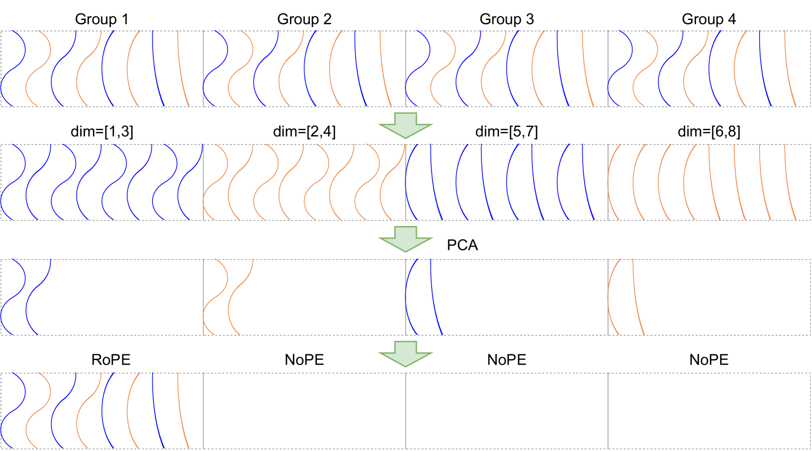## Appendix C FreqFold: Detailed Mechanism, Example, and PCA Efficiency <details> <summary>x12.png Details</summary>  ### Visual Description ## Diagram: Dimensionality Reduction Process Across Groups ### Overview The diagram illustrates a multi-stage dimensionality reduction workflow applied to four distinct groups (Group 1–4). It visualizes how data represented by wavy lines (blue and orange) is transformed through Principal Component Analysis (PCA) into two outcomes: RoPE (Retained Principal Components) and NoPE (Discarded Components). The process emphasizes how dimensionality constraints (e.g., dim=[1,3]) influence the retention or elimination of features. --- ### Components/Axes 1. **Groups**: - Four horizontal bands labeled **Group 1** to **Group 4**, each with wavy lines in **blue** and **orange**. - Dimensions specified below each group: - Group 1: `dim=[1,3]` - Group 2: `dim=[2,4]` - Group 3: `dim=[5,7]` - Group 4: `dim=[6,8]` 2. **PCA Stage**: - Arrows point downward from the groups to a central **PCA** block. - PCA processes the input data, reducing dimensionality. - Outputs split into **RoPE** (Retained) and **NoPE** (Discarded). 3. **RoPE/NoPE Outcomes**: - **RoPE**: Contains simplified wavy lines (blue/orange) in Group 1 and Group 2. - **NoPE**: Empty for Groups 3 and 4, with only partial lines in Group 1 and Group 2. --- ### Detailed Analysis 1. **Group-Specific Dimensionality**: - Groups 1–2 have overlapping dimension ranges (`[1,3]` and `[2,4]`), suggesting incremental complexity. - Groups 3–4 use higher dimensions (`[5,7]` and `[6,8]`), indicating denser data representations. 2. **Line Color Consistency**: - **Blue lines** dominate all stages, while **orange lines** appear only in Groups 1–2 and RoPE for Group 1. - No orange lines in PCA or NoPE sections, implying orange features are either filtered out or not retained. 3. **PCA Transformation**: - Groups 1–2 retain partial data in RoPE (e.g., Group 1 RoPE retains orange lines). - Groups 3–4 produce **NoPE** with no retained lines, suggesting complete dimensional collapse. 4. **NoPE Behavior**: - Groups 3–4 have **NoPE** blocks with no lines, indicating all components are discarded. - Group 1’s NoPE retains a single orange line, while Group 2’s NoPE retains one blue line. --- ### Key Observations - **Dimensionality Impact**: Higher-dimensional groups (3–4) fully collapse to NoPE, while lower-dimensional groups (1–2) retain partial data in RoPE. - **Color Significance**: Orange lines are selectively retained in RoPE for Group 1, suggesting they represent critical features in lower dimensions. - **PCA Efficiency**: PCA aggressively discards data in higher-dimensional groups, leaving NoPE empty. --- ### Interpretation This diagram demonstrates how PCA reduces data complexity across groups with varying dimensionality. The retention of orange lines in Group 1’s RoPE implies these features are preserved as principal components, while their absence in higher-dimensional groups (3–4) highlights the trade-off between dimensionality and feature retention. The empty NoPE blocks for Groups 3–4 suggest that PCA eliminates all non-principal components in these cases, potentially losing nuanced information. The workflow underscores the importance of dimension selection in balancing data compression and feature preservation. </details> Figure 7: Pipeline of RoRoPE with FreqFold. RoRoPE encodes the entire frequency spectrum of all attention heads in a single latent dimension, which limits its expressive power. FreqFold remedies this by clustering adjacent-frequency dimensions and extracting their principal components jointly, allocating a higher-dimensional subspace to similar features. This richer representation enables $K_rope$ to retain far more positional information. This appendix provides a detailed explanation of the FreqFold technique, illustrates its operation with a concrete example, and formally connects its benefits to a general principle of Principal Component Analysis (PCA) concerning structured data. This justification clarifies FreqFold’s role in minimizing transformation loss towards decoupled RoPE within the RoRoPE framework (Section 4.2). ### C.1 Detailed Explanation of FreqFold and RoRoPE’s PCA In the RoRoPE framework, Rotary Position Embedding (RoPE) is applied. RoPE encodes positional information by rotating pairs of feature dimensions. For each RoPE frequency index $l∈\{1,…,d/2\}$ , the corresponding pair of dimensions $([2l-1::d],[2l::d])$ from query and key vectors are rotated. When multiple original attention heads are used (say, $g$ heads), and their key/query projection outputs are concatenated, the RoPE operation for a specific frequency index $l$ applies to a $2g$ -dimensional vector segment (formed by concatenating the $l$ -th 2D RoPE subspace from each of the $g$ heads). RoRoPE then applies PCA via matrices $\{U_l\}_l=1^d/2$ to these $2g$ -dimensional segments, independently for each frequency index $l$ . The core idea of FreqFold is to approximate numerically similar RoPE base frequencies as being effectively identical. For instance, if RoPE uses original base frequencies $θ_l_1,θ_l_2,…,θ_l_{M}$ that are close in value, $M$ D-FreqFold might treat them all as a single, representative frequency $θ^*$ . This approximation has a significant implication for how PCA is applied in RoRoPE: - Without FreqFold (Standard RoRoPE PCA): For each distinct RoPE frequency index $l$ , a separate PCA transformation $U_l$ is learned and applied to the corresponding $2g$ -dimensional key/query segments. - With FreqFold: If $M$ original RoPE frequency indices (say $l_1,…,l_M$ ) are grouped together by FreqFold due to their frequency similarity, the $M$ corresponding $2g$ -dimensional segments are effectively concatenated. Instead of $M$ separate PCAs on $2g$ -dimensional vectors, a single PCA is performed on the resulting $M· 2g$ -dimensional vectors. #### C.1.1 Illustrative Example of FreqFold Let’s consider a scenario with $g=2$ key heads, and each head has $d_head=8$ dimensions. Thus, there are $d/2=8/2=4$ distinct RoPE frequency indices per head, which we denote as $φ_1,φ_2,φ_3,φ_4$ . The total number of dimensions is $2× 8=16$ . The RoPE angles for these 16 dimensions could be conceptualized as follows (repeating for each pair, and across heads): - Head 1 (dims 1-8): $(φ_1,φ_1),(φ_2,φ_2),(φ_3,φ_3),(φ_4,φ_4)$ - Head 2 (dims 9-16): $(φ_1,φ_1),(φ_2,φ_2),(φ_3,φ_3),(φ_4,φ_4)$ Case 1: RoRoPE without FreqFold For each frequency index $φ_l$ , RoRoPE groups the corresponding dimensions from all $g=2$ heads. Each such group forms $2g=2× 2=4$ -dimensional vectors (across $N$ samples). - Group for $φ_1$ : Dimensions $\{1,2\}$ from Head 1 and $\{9,10\}$ from Head 2. PCA is applied to these $N$ samples of 4D vectors. - Group for $φ_2$ : Dimensions $\{3,4\}$ from Head 1 and $\{11,12\}$ from Head 2. PCA is applied to these $N$ samples of 4D vectors. - Group for $φ_3$ : Dimensions $\{5,6\}$ from Head 1 and $\{13,14\}$ from Head 2. PCA is applied to these $N$ samples of 4D vectors. - Group for $φ_4$ : Dimensions $\{7,8\}$ from Head 1 and $\{15,16\}$ from Head 2. PCA is applied to these $N$ samples of 4D vectors. Here, RoRoPE performs 4 separate PCA operations. Case 2: RoRoPE with 2D-FreqFold 2D-FreqFold implies we are pairing up original frequencies. Suppose FreqFold approximates $φ_1≈φ_2$ (calling this effective frequency $Φ_A=φ_1$ ) and $φ_3≈φ_4$ (calling this $Φ_B=φ_3$ ). - Effective Group for $Φ_A$ : This group now includes all dimensions originally associated with $φ_1$ OR $φ_2$ . - Original $φ_1$ -dimensions: $\{1,2\}$ from Head 1; $\{9,10\}$ from Head 2. (Forms a 4D segment $S_φ_1$ ) - Original $φ_2$ -dimensions: $\{3,4\}$ from Head 1; $\{11,12\}$ from Head 2. (Forms a 4D segment $S_φ_2$ ) With FreqFold, these segments $S_φ_1$ and $S_φ_2$ are concatenated. PCA is now applied to the $N$ samples of $(4+4)=8$ -dimensional vectors formed by $[S_φ_1,S_φ_2]$ . Effectively, dimensions $\{1,2,3,4\}$ from Head 1 are combined with $\{9,10,11,12\}$ from Head 2. - Effective Group for $Φ_B$ : Similarly, this group includes dimensions originally for $φ_3$ OR $φ_4$ . - Original $φ_3$ -dimensions: $\{5,6\}$ from Head 1; $\{13,14\}$ from Head 2. (Forms $S_φ_3$ ) - Original $φ_4$ -dimensions: $\{7,8\}$ from Head 1; $\{15,16\}$ from Head 2. (Forms $S_φ_4$ ) PCA is applied to the $N$ samples of 8-dimensional vectors formed by $[S_φ_3,S_φ_4]$ . Here, RoRoPE with FreqFold performs 2 PCA operations, but each operates on larger, 8-dimensional vectors which are concatenations of what were previously separate PCA targets. ### C.2 Formalizing the Benefit of FreqFold in PCA The example above illustrates that FreqFold causes a re-grouping and concatenation of data segments prior to PCA. The benefit of this concatenation is explained by the following proposition. It states that performing PCA jointly on these concatenated segments (as FreqFold enables) is more effective at preserving variance (and thus minimizing loss) than the alternative of performing separate PCAs on the original, smaller segments and then notionally combining their outcomes. Consider one such FreqFold merge: suppose $M$ original RoPE frequency indices $l_1,…,l_M$ are deemed equivalent by FreqFold. Without FreqFold, each $l_p$ would correspond to a dataset $X_p$ (e.g., $N$ samples of $2g$ -dimensional key segments). With FreqFold, these $M$ datasets are concatenated into a single larger dataset $X_merged=[X_1,X_2,…,X_M]$ , and PCA is applied to $X_merged$ . **Proposition 2** *Let $M$ distinct groups of key segments $X_1,X_2,…,X_M$ be identified. Each $X_p∈ℝ^N× d^{\prime}$ (where $p∈\{1,…,M\}$ ) consists of $N$ samples of $d^\prime$ -dimensional vectors. Assume data in each $X_p$ is mean-centered. Let $S_p=\frac{1}{N-1}X_p^TX_p∈ℝ^d^{\prime× d^\prime}$ be its covariance matrix. FreqFold causes these $M$ groups to be merged for a single PCA operation. Define $V_1=∑_p=1^Mλ_p,1$ , where $λ_p,1$ is the largest eigenvalue of $S_p$ . This $V_1$ represents the sum of variances if each of the $M$ original groups $X_p$ were individually reduced to its single most dominant dimension. Let $Z=[X_1,X_2,…,X_M]∈ℝ^N×(M· d^{\prime)}$ be the dataset formed by concatenating the features (columns) of these $M$ groups. Let $S_concat=\frac{1}{N-1}Z^TZ∈ℝ^(M· d^{\prime)×(M· d ^\prime)}$ be its covariance matrix. Define $V_2=∑_j=1^Mμ_j$ , where $μ_1≥μ_2≥…≥μ_M$ are the $M$ largest eigenvalues of $S_concat$ . This $V_2$ represents the variance captured if the concatenated data $Z$ is reduced to $M$ dimensions using PCA. Then, the variance captured by the joint PCA on the FreqFold-merged data ( $V_2$ ) is greater than or equal to the sum of variances from optimally reducing each original group to one dimension ( $V_1$ ): $$ V_2≥ V_1 $$* This proposition explains that FreqFold’s strategy of enabling PCA over larger, concatenated segments (formed by merging data from RoPE frequencies deemed similar) is mathematically favored for variance preservation compared to separate, more fragmented PCAs. ### C.3 Proof of Proposition 2 The objective is to prove that $V_2≥ V_1$ , using the notation from Proposition 2. The proof strategy is to construct a specific $M$ -dimensional subspace for the concatenated data $Z$ . We show that the variance captured by projecting $Z$ onto this particular subspace equals $V_1$ . Since the PCA procedure yielding $V_2$ finds the optimal $M$ -dimensional subspace maximizing captured variance, $V_2$ must be at least $V_1$ . Let $λ_p,1$ be the largest eigenvalue of $S_p$ (covariance of $X_p$ ), and $\bm{w}_p,1∈ℝ^d^{\prime}$ be its corresponding eigenvector. So, $S_p\bm{w}_p,1=λ_p,1\bm{w}_p,1$ and $\bm{w}_p,1^T\bm{w}_p,1=1$ . The variance $λ_p,1=\bm{w}_p,1^TS_p\bm{w}_p,1$ . $V_1=∑_p=1^Mλ_p,1$ . For the concatenated data $Z$ , $V_2=∑_j=1^Mμ_j$ . By Ky Fan’s theorem for matrix eigenvalues: $$ V_2=\max_\begin{subarray{c}U∈ℝ^(M· d^{\prime)× M}\\ U^TU=I_M\end{subarray}}Tr(U^TS_concatU) $$ where $U$ ’s columns form an orthonormal basis for an $M$ -dimensional subspace of $ℝ^M· d^{\prime}$ . Construct $U^*=[\bm{u}_1^*,…,\bm{u}_M^*]∈ℝ^(M· d^{\prime) × M}$ . For $p∈\{1,…,M\}$ , define $\bm{u}_p^*∈ℝ^M· d^{\prime}$ : $$ \bm{u}_p^*=\begin{pmatrix}\bm{0}_d^\prime× 1\\ ⋮\\ \bm{w}_p,1&(as the p-th block of size d^\prime)\\ ⋮\\ \bm{0}_d^\prime× 1\end{pmatrix} $$ The set $\{\bm{u}_1^*,…,\bm{u}_M^*\}$ is orthonormal. The variance retained by projecting $Z$ onto the subspace of $U^*$ is: $$ Tr((U^*)^TS_concatU^*)=∑_p=1^M(\bm{u}_p^*)^TS_ concat\bm{u}_p^* $$ Let $S_qr$ be the $(q,r)$ -th block of $S_concat$ , where $S_qr=\frac{1}{N-1}X_q^TX_r$ . Note $S_pp=S_p$ . Each term $(\bm{u}_p^*)^TS_concat\bm{u}_p^*=\bm{w}_p,1^TS_pp\bm{w}_p,1 =\bm{w}_p,1^TS_p\bm{w}_p,1=λ_p,1$ . So, $Tr((U^*)^TS_concatU^*)=∑_p=1^Mλ_p,1=V_1$ . Since $V_2$ is the maximum possible variance: $$ V_2≥Tr((U^*)^TS_concatU^*)=V_1 $$ Thus, $V_2≥ V_1$ . This proves Proposition 2. ### C.4 Discussion on the Trade-off in FreqFold While Proposition 2 demonstrates a clear benefit of FreqFold in terms of PCA efficiency—specifically, that merging M original frequency groups allows for greater variance preservation when reducing to M dimensions—it is crucial to acknowledge an inherent trade-off. The foundational assumption of FreqFold is the approximation of numerically similar RoPE base frequencies as effectively identical. This approximation, by its very nature, introduces a degree of deviation from the original, precise RoPE formulation. The extent of this deviation, and thus the potential loss in the fidelity of positional encoding, typically correlates with how aggressively frequencies are grouped. A larger $M$ or a looser criterion for similarity when grouping frequencies can amplify this approximation error. Consequently, while increasing the dimensionality of vectors undergoing PCA is beneficial from the perspective of PCA variance capture as shown by the proposition, it may simultaneously increase the lossiness of the RoPE approximation itself. Therefore, the practical application of FreqFold requires a careful balancing act. The parameter M (representing the number of original RoPE frequencies treated as one effective frequency for PCA purposes) or the specific grouping strategy for frequencies must be chosen to optimize this trade-off. ## Appendix D Balancing Key-Value Norms and Low-Rank Approximation This appendix elaborates on the Key-Value (KV) balancing technique and the subsequent joint low-rank approximation applied to the NoPE (No Positional Encoding) components of the keys and the values, as mentioned in Section 4.3 of the main paper. After the RoRoPE procedure (Section 4.2), the key projection matrix $W^K$ is effectively split into two components: $W^DK_RoPE∈ℝ^d× D$ corresponding to the single head that retains RoPE, and $W^DK_NoPE∈ℝ^(g-1)d× D$ corresponding to the remaining $g-1$ head components that do not use RoPE. The value projection matrix is denoted as $W^DV∈ℝ^gd× D$ . ### D.1 KV Balancing: Purpose and Formulation Purpose The primary goal of KV balancing is to ensure that the principal component analysis (PCA), when applied jointly to the NoPE key and value activations, is not disproportionately influenced by components with larger norms. We observed that the activations derived from $W^DK_NoPE$ (i.e., $k_\textbf{NoPE,t}=W^DK_NoPEx_t$ ) often have a significantly larger average norm than those from $W^DV$ (i.e., $v_t=W^DVx_t$ ). Without balancing, PCA would predominantly capture the variance within the NoPE key components, potentially neglecting important variations in the value components. Formulation To address this imbalance, we introduce a scaling factor $α$ . This factor is computed as the ratio of the expected L2 norms of the NoPE key activations to the value activations, based on a calibration dataset: $$ α=\frac{E_t[\|W^DK_NoPEx_t\|_2]}{ E_t[\|W^DVx_t\|_2]} \tag{33} $$ where $x_t∈ℝ^D$ is the $t$ -th input token. While the main paper states scaling $W^DK_NoPE$ by $1/α$ and $W^UK$ by $α$ for mathematical equivalence in the model’s output, for the purpose of deriving the PCA projection, we effectively use scaled NoPE key activations. That is, the activations used to compute the PCA basis are $k^\prime_NoPE,t=1/α· W^DK_NoPE x_t$ and $v_t=W^DVx_t$ . This ensures that the PCA process considers features from keys and values on a more equitable footing with respect to their magnitudes. The subsequent low-rank decomposition will then be applied to $W^DK_NoPE$ and $W^DV$ , using the PCA basis derived from these balanced activations. ### D.2 Joint Low-Rank Approximation of NoPE Keys and Values using PCA After determining the scaling factor $α$ , we proceed to compress the projection matrices associated with the NoPE keys ( $W^DK_NoPE$ ) and all values ( $W^DV$ ) jointly. The process is as follows: 1. Collect Calibrated Activations: A small calibration dataset (WikiText-2) is used. For each input $x_t$ from this dataset, we compute the scaled NoPE key activations $k^\prime_NoPE,t$ and the value activations $v_t$ . These are concatenated to form combined activation vectors: $$ c_NoPE,t=\begin{pmatrix}k^\prime_NoPE,t \\ v_t\end{pmatrix}∈ℝ^(2g-1)d \tag{34} $$ 2. Perform PCA: PCA is performed on the set of collected combined activation vectors $\{c_NoPE,t\}$ . This involves computing the covariance matrix of these vectors and finding its principal components. The eigenvectors (corresponding to the largest eigenvalues) are selected to form the columns of a projection matrix $R_KV∈ℝ^((2g-1)d)× r_kv$ , where $r_kv$ is the reduced rank. This matrix $R_KV$ captures the directions of highest variance in the (balanced) combined NoPE key and value activation space. 3. Low-Rank Decomposition of Projection Matrices: Let $W^DKV=\begin{pmatrix}W^DK_NoPE\ W^DV\end{pmatrix}∈ℝ^((2g-1)d)× D$ be the initial projection matrix that transforms the input $x_t$ into an intermediate NoPE Key and Value representation $c_NoPE,t=W^DKVx_t$ . Further, let $W^UKV=\begin{pmatrix}W^UK_NoPE&0\ 0&W^UV\end{pmatrix}∈ℝ^2hd×((2g-1)d)$ represent the subsequent collective projection matrix that takes $c_NoPE,t$ and processes it to produce the actual keys and values required by the attention mechanism for the NoPE components, where $W^UK_RoPE∈ℝ^hd× gd$ and $W^UK_NoPE∈ℝ^hd×(g-1)d$ are two parts of $W^UK$ hat participate in and do not participate in the RoPE computation, respectively. The original sequence of operations for these components can be expressed as $W^UKVW^DKVx_t∈ℝ^2hd$ , in which the first $hd$ elements correspond to the keys and the following $hd$ elements correspond to the values. To introduce a low-rank bottleneck, we modify both $W^DKV$ and $W^UKV$ using the PCA projection matrix $R_KV$ . - The initial projection matrix $W^DKV$ is transformed into ${W^DKV}^\prime∈ℝ^r_kv× D$ : $$ {W^DKV}^\prime=R_KV^TW^DKV \tag{35} $$ This new matrix ${W^DKV}^\prime$ takes the original input $x_t$ and projects it into a compressed $r_kv$ -dimensional latent space, which is the actual content stored in the KV cache for the NoPE components. - The subsequent projection matrix $W^UKV$ is transformed into ${W^UKV}^\prime∈ℝ^2hd× r_kv$ : $$ {W^UKV}^\prime=W^UKVR_KV \tag{36} $$ This new matrix ${W^UKV}^\prime$ now takes the compressed latent representation as input and produces the final representations for the NoPE components that are used in the attention calculation. As we can see, ${W^UKV}^\prime$ is actually the concatenated form of $W^UK$ and $W^UV$ in MLA: $$ {W^UKV}^\prime=\begin{pmatrix}W^UK\\ W^UV\end{pmatrix} \tag{37} $$ This joint decomposition allows for a more holistic compression by identifying shared latent structures between NoPE keys and values, guided by the balanced PCA. ## Appendix E Experimental Settings of Fine-tuning Datasets Following the experimental setups of MHA2MLA, we fine-tune our models using the prtraining corpus from SmolLM Ben Allal et al. [2024]. The dataset comprises FineWeb-Edu-Dedup Lozhkov et al. [2024a], Cosmopedia-v2 — a synthetic dataset generated by Mixtral Wu et al. [2024], Python-Edu from StarCoder Lozhkov et al. [2024b], Open-Web-Math Paster et al. [2023], and data from StackOverflow Stack Overflow [2025]. To ensure a fair comparison with the MHA2MLA baseline, we constructed our training dataset using the same data composition strategy. Specifically, we replicate the dataset mixing ratios used in the MHA2MLA setup to maintain experimental consistency, which is shown in Table 2. Table 2: Composition of the training dataset. | fineweb-edu-dedup cosmopedia-v2 python-edu | 0.70 0.15 0.06 | | --- | --- | | open-web-math | 0.08 | | stackoverflow | 0.01 | Hyperparameters The fine-tuning hyperparameters for models of all sizes are listed in Table 3. In the table, entries with a slash (/) indicate a two-step training process. Table 3: Training details across different models. | | SmolLM 1B7 | | LLaMA2 7B | | | | --- | --- | --- | --- | --- | --- | | -68.75% | -87.50% | -68.75% | -87.50% | -92.97% | | | Batch size | 64 | 64 | 64 | 64 / 64 | 256 / 64 | | Learning rate | 1e-4 | 1e-4 | 2e-5 | 2e-5 / 2e-5 | 1e-4 / 2e-5 | | Tokens | 300M | 1B | 500M | 2B / 1B | 5B / 1B | | Warmup ratio | 0.03 | 0.08 | 0 | 0 / 0.03 | 0 / 0.03 | | lr scheduler | constant | constant | constant | constant / cosine | constant / cosine | | Sequence length | 2048 | 2048 | 4096 | 4096 | 4096 | ## Appendix F Detail Information for vLLM Benchmark In Section 5.4, we demonstrated the speedup achieved by TransMLA—which compresses 92.97% of the KV cache—compared to the original LLaMA-2-7B model. This section provides a detailed analysis of throughput across various hardware configurations. To account for the effects of both the prefilling and decoding stages, we adopt a setting where the input and output lengths are equal. For instance, with a total context length of 1k, we set the input length to 512 tokens and the output length to 512 tokens. Most experiments are conducted using 100 requests to compute the average throughput. However, for shorter context lengths such as 1k, inference is extremely fast, leading to some timing fluctuations. To mitigate this, we increase the number of requests to 1000 for more stable measurements. While the original LLaMA-2-7B model supports a maximum context length of 4096 tokens, we extend this limit to 32k tokens in our evaluation. Detailed throughput results are presented in Table 4. On a GPU with 165.2 TFLOPS of compute and 24GB of memory, the LLaMA-2-7B model runs out of memory when the context length reaches 16k tokens. In contrast, TransMLA sustains a throughput of 414.41 tokens per second under the same conditions. On a more powerful GPU with 320 TFLOPS and 64GB of memory, we employ a development version of the vLLM framework. We anticipate that the throughput of TransMLA will improve further with the release of future optimized versions of the framework tailored for this hardware. Table 4: Throughput comparison between LLaMA-2-7b and TransMLA at varying input lengths and number of requests. | 1K TransMLA 2K | 1000 3043.65 100 | LLaMA-2-7b 4062.43 LLaMA-2-7b | 653.81 1798.17 352.85 | 1579.26 850.14 | 1249.13 789.31 | | --- | --- | --- | --- | --- | --- | | TransMLA | 2241.87 | 2577.01 | 1080.73 | | | | 4K | 100 | LLaMA-2-7b | 173.09 | 441.37 | 442.63 | | TransMLA | 1318.78 | 1926.15 | 1021.03 | | | | 8K | 100 | LLaMA-2-7b | 85.80 | 218.51 | 216.66 | | TransMLA | 832.69 | 1118.18 | 870.15 | | | | 16K | 100 | LLaMA-2-7b | OOM | 110.58 | 112.13 | | TransMLA | 414.41 | 601.36 | 483.22 | | | | 32K | 100 | LLaMA-2-7b | OOM | 38.32 | 55.69 | | TransMLA | OOM | 243.81 | 278.09 | | | ## Appendix G Case Study To provide an intuitive understanding of TransMLA’s impact on model performance, this section presents several examples from vLLM’s docs. We compare the outputs of three model variants: (1) a model with 92.97% of its KV cache compressed without any fine-tuning; (2) a model pretrained on 6B tokens, as detailed in Table 1; and (3) a model fine-tuned for one epoch on the SmolTalk dataset, following the setup described in Allal et al. [2025a]. The results are summarized in Table 5. As shown in Table 5, even without any additional training, the compressed model is still able to produce coherent and meaningful responses. This demonstrates the effectiveness of techniques such as RoRoPE, FreqFold, and BKV-PCA in significantly mitigating performance degradation. Moreover, with a modest amount of pretraining or supervised fine-tuning (SFT), the model’s performance improves substantially. These findings highlight TransMLA’s potential as a general framework for converting various GQA models into MLA models, with promising prospects for aligning with the performance of advanced systems like DeepSeek R1. Table 5: Examples from different model configurations. Red indicates input; black indicates output. “w/o Training” denotes the TransMLA-compressed model (92.97% KV cache) without further training. “Pre-Training” and “Fine-Tuning” show outputs after pretraining on a 6B-token corpus and SFT on SmolTalk Allal et al. [2025b], respectively. | w/o Training | Hello, my name is Katiu, my father’s dog, the pet of the 3600 year-old tribe, Kint. The Kangs were part of a race of reptiles. A small handful | | --- | --- | | Pre-Training | Hello, my name is Sasha and I am in third grade at Meadows. You may be wondering what this article is about. Well, I have been doing a lot of research on the water cycle and decided to write about it. | | Fine-Tuning | Hello, my name is Emily, and I’m a 20-year-old college student. My hobbies include painting, writing, and photography. I also enjoy playing the guitar. | | w/o Training | The president of the United States is elected by the legislature. The legislature controls the national armed forces, but only provides the funds to establishing a national guard. | | Pre-Training | The president of the United States is elected to a four-year term by the people of each state in a general election held every four years on the Tuesday following the first Monday in November. | | Fine-Tuning | The president of the United States is not a position to be taken lightly. This person is the chief executive of the United States of America, and has immense power and influence. | | w/o Training | The capital of France is Paris. Its geographical position in the Iberian Plain of France, Spain, Spain, and Morocco are the four largest cities. This region is located in Asia, Spain and Morocco. | | Pre-Training | The capital of France is a major business city and it is a favorite destination for businesses from all over the world. It has a strategic location in the heart of the European Union, which makes it one of the most popular cities in Europe. | | Fine-Tuning | The capital of France is Paris, and it is one of the most popular tourist destinations in the world. It is a city that offers something for everyone, from art and history to food and fashion. | | w/o Training | The future of AI is in serious risk to create a major breakthrough in this emerging phenomenon in the history of artificial intelligence. | | Pre-Training | The future of AI is looking bright. With advancements in technology and the increasing availability of data, AI is expected to become more intelligent and capable of performing even more complex tasks. | | Fine-Tuning | The future of AI is The future of AI is more nuanced and complex than we might think. Here are some potential developments that could shape the future of AI. |