# Unifying Explainable Anomaly Detection and Root Cause Analysis in Dynamical Systems
Abstract
Dynamical systems, prevalent in various scientific and engineering domains, are susceptible to anomalies that can significantly impact their performance and reliability. This paper addresses the critical challenges of anomaly detection, root cause localization, and anomaly type classification in dynamical systems governed by ordinary differential equations (ODEs). We define two categories of anomalies: cyber anomalies, which propagate through interconnected variables, and measurement anomalies, which remain localized to individual variables. To address these challenges, we propose the Interpretable Causality Ordinary Differential Equation (ICODE) Networks, a model-intrinsic explainable learning framework. ICODE leverages Neural ODEs for anomaly detection while employing causality inference through an explanation channel to perform root cause analysis (RCA), elucidating why specific time periods are flagged as anomalous. ICODE is designed to simultaneously perform anomaly detection, RCA, and anomaly type classification within a single, interpretable framework. Our approach is grounded in the hypothesis that anomalies alter the underlying ODEs of the system, manifesting as changes in causal relationships between variables. We provide a theoretical analysis of how perturbations in learned model parameters can be utilized to identify anomalies and their root causes in time series data. Comprehensive experimental evaluations demonstrate the efficacy of ICODE across various dynamical systems, showcasing its ability to accurately detect anomalies, classify their types, and pinpoint their origins.
Introduction
<details>
<summary>x1.png Details</summary>
### Visual Description
# Technical Document Extraction: Machine Learning Model Comparison
This image contains two comparative diagrams, labeled **(a)** and **(b)**, illustrating the difference between a traditional "Black box" machine learning approach and a proposed explainable model named **ICODE**.
---
## Section (a): Traditional Black Box Model
This section describes a linear pipeline for a single-task machine learning process.
### 1. Input Component
* **Visual Representation:** A directed graph consisting of three nodes: $x_0$, $x_1$, and $x_2$.
* **Connectivity:**
* Bidirectional arrows between $x_0$ and $x_2$.
* Bidirectional arrows between $x_0$ and $x_1$.
* A unidirectional arrow from $x_2$ to $x_1$.
* **Label:** "Input"
### 2. Processing Component
* **Visual Representation:** A 3D black box labeled with three question marks (**???**). Inside the box, a white inset shows a dense neural network diagram (multiple layers of interconnected nodes).
* **Label:** "Black box model"
### 3. Output Component
* **Flow:** An arrow points from the Black box to a variable $y$.
* **Container:** A dashed rectangular box.
* **Header Text:** **Single Task** (in red font).
* **Description Text:** "Either *anomaly detection* or *root cause localization*"
* **Logic:** The model is limited to performing one specific task at a time.
---
## Section (b): ICODE (Proposed Explainable Model)
This section describes a multi-faceted pipeline capable of performing multiple tasks simultaneously through an explainable framework.
### 1. Input Component
* **Visual Representation:** Identical to section (a); a directed graph with nodes $x_0$, $x_1$, and $x_2$.
* **Label:** "Input"
### 2. Processing Component (ICODE)
* **Label:** ***ICODE*** **(Our Model)** (in green font).
* **Sub-components:**
* **Coordinate Plot:** A graph with axes $x$ (vertical) and $t$ (horizontal). It shows a blue curve with two red data points. Arrows from these points lead into the next sub-component.
* **Explainable Model Box:** A dashed box containing:
* The mathematical expression: $\frac{dx}{dt}$ (representing differential equations).
* A simplified graph/network diagram.
* A lightbulb icon (symbolizing insight/explainability).
* Label: "Explainable model"
### 3. Intermediate Component: Dependency Matrix
* **Visual Representation:** A $3 \times 3$ grid (matrix) colored in light blue.
* **Label:** "Dependency Matrix $C$"
* **Flow:** This matrix is derived directly from the Explainable model.
### 4. Output Component
* **Container:** A dashed rectangular box.
* **Header Text:** **Multiple Tasks** (in green font).
* **Task Breakdown:**
* **Task 1:** *Anomaly detection* (derived from output $y$).
* **Task 2:** *Classification*: *Measurement* anomaly or *cyber* anomaly? (indicated with a red question mark; derived from the Dependency Matrix).
* **Task 3:** *Root Cause localization*: $x_0$ or $x_1$ or $x_2$? (indicated with a red question mark; derived from the Dependency Matrix).
---
## Summary of Key Differences
| Feature | (a) Black Box Model | (b) ICODE (Proposed) |
| :--- | :--- | :--- |
| **Transparency** | Opaque ("???") | Explainable ($\frac{dx}{dt}$, lightbulb) |
| **Task Capacity** | Single Task | Multiple Tasks (Simultaneous) |
| **Output Detail** | Binary/Limited choice | Detailed classification and localization |
| **Intermediate Data** | None shown | Dependency Matrix $C$ |
| **Mathematical Basis** | Neural Network | Differential Equations/Dynamics |
</details>
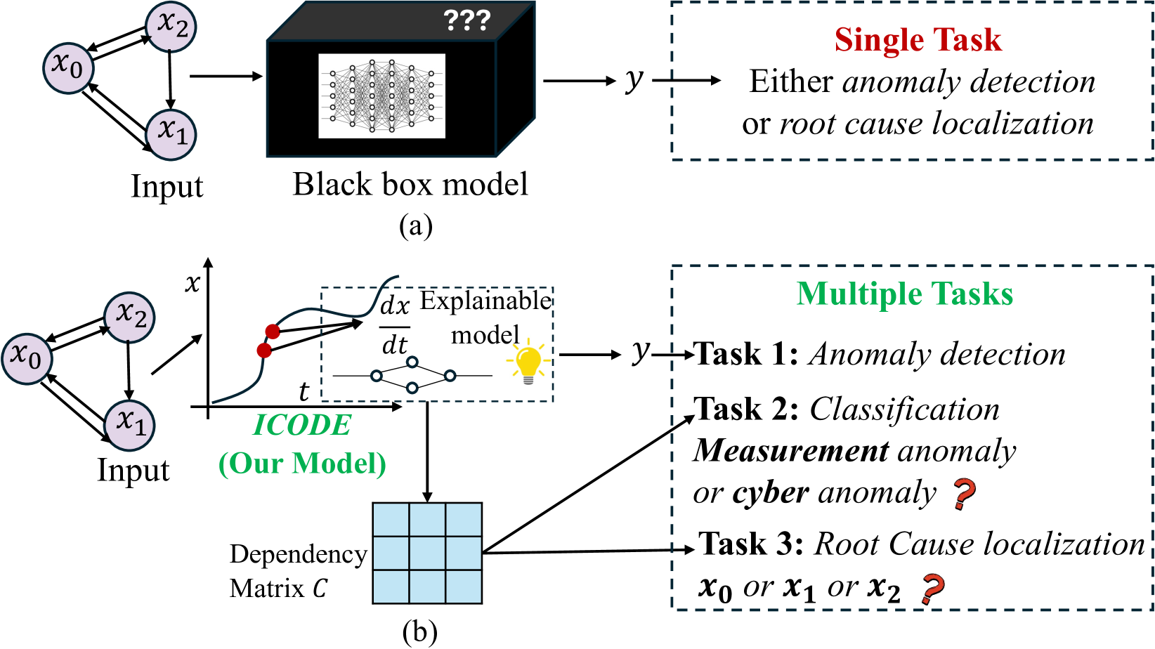
Figure 1: (a) Traditional models typically perform either anomaly detection or root cause localization in isolation, limiting their comprehensive analysis capabilities. (b) Our proposed model integrates anomaly detection, anomaly type classification and root cause localization within a single model. It achieves this by leveraging both the model output and the learned dependency matrix, which encapsulates the causal relationships between variables in the system.
.
Dynamical systems, which describe the evolution of variables over time, are fundamental to numerous domains, including natural sciences such as physics (Willard et al. 2020), biology (Laurie and Lu 2023), and chemistry (Keith et al. 2021), as well as engineering fields like transportation systems (Shepherd 2014) and power systems (Ju et al. 2021). These systems often encounter various types of anomalies, each with potentially different levels of urgency and impact (Gao et al. 2022). For instance, in a traffic management system, anomalies can range from minor sensor malfunctions to major incidents like accidents or road closures. The urgency and impact of these anomalies can vary significantly: a critical accident requires immediate attention and may have widespread effects on traffic flow across the network, whereas a single malfunctioning speed sensor might not necessitate urgent intervention if the overall transportation network is functioning normally. Similarly, in a power grid, a sudden voltage spike could indicate a potentially catastrophic equipment failure requiring immediate action, while a gradual drift in a non-critical sensor reading might be addressed during routine maintenance. This variability in urgency and impact underscores the importance of not only detecting anomalies but also comprehensively understanding their origins and potential consequences, a process commonly referred to as root cause analysis (RCA).
Machine learning (ML) based anomaly detection (Pang et al. 2021) and RCA algorithms (Soldani and Brogi 2022) have emerged as state-of-the-art approaches due to their capability to learn complex functions through data-driven methods (Teng 2010; Blázquez-García et al. 2021) . However, existing models face several challenges. First, deep neural network-based models (Choi et al. 2021; Li and Jung 2023) typically require large datasets to train complex ML networks, often producing only binary results indicating the presence or absence of an anomaly. This is insufficient for many applications where pinpointing the underlying causes of system faults is equally important (Wang et al. 2023a). Second, beyond localizing the root cause, understanding the type of anomaly is crucial for determining its urgency and appropriate response. Existing models, particularly complex deep learning based models, cannot be used to differentiate types of anomalies as relevant to dynamical systems in consideration, thus limiting their scope of application. Last, many dynamical systems adhere to differential equations, complicating the learning process and making it difficult to develop models that can accurately detect anomalies and perform RCA in such systems.
In this work, we address these challenges by first mathematically defining two types of anomalies that are commonly observed in dynamical systems (Luo et al. 2021): cyber anomalies and measurement anomalies. While these types of anomalies are known to exist in practice, our contribution lies in providing a mathematical framework for their definition and analysis. Measurement anomalies are typically caused by errors during data acquisition and are confined to local faults. For example, in a power grid, if a voltage sensor at a single substation displays an incorrect reading due to calibration issues, it would be considered a measurement anomaly. Conversely, cyber anomalies result from interactions between variables, with the root cause potentially affecting neighboring sensors. In the power grid context, a cyber anomaly could manifest as a cascading voltage instability, where a fault in one part of the network propagates and affects voltage readings across multiple interconnected substations. This mathematical distinction is crucial for understanding the scope and potential impact of detected anomalies and forms the foundation for our subsequent analysis and model development.
Our primary objective is to develop an interpretable ML model capable of performing anomaly detection, type classification and RCA, within a single model, based on causality inference, as shown in Figure 1. Our driving hypothesis is that if a variable in a dynamical system adheres to an ordinary differential equation (ODE), an anomaly would alter the ODE, which can be monitored by changes in the causality relationship (i.e., changes in the causal graph weights learned from data). Simultaneously, changes in this relationship can indicate the type of error. Consequently, we reframe the problem as causality inference with high accuracy within the corresponding ODE system.
Inspired by Neural ODEs (Chen et al. 2018), we introduce the Interpretable Causality Ordinary Differential Equation (ICODE) Networks, a novel prediction-based model for anomaly detection and root cause analysis in dynamical systems. ICODE utilizes Neural ODEs to capture system evolution, learning the governing ODEs directly rather than the integration process, which enhances both accuracy and efficiency in modeling dynamical systems. The model detects anomalies by identifying significant deviations between predicted variables and ground truth, indicating substantial changes in the underlying ODEs. Crucially, ICODE’s interpretability stems from its ability to analyze the learned parameters, which represent causality relationships within the system. Upon detecting an anomaly, this analysis enables the determination of both the type and location of the root cause, providing valuable insights into system behavior during anomalies.
<details>
<summary>x2.png Details</summary>
### Visual Description
# Technical Document Extraction: Anomaly Propagation in Dynamical Systems
This image illustrates the difference between measurement anomalies and cyber (systemic) anomalies within a dynamical system where one variable depends on another.
## 1. System Architecture and Dependency (Left Panel)
The left section establishes the causal relationship between variables $x_1$ and $x_2$.
### (a) Dependency Graph
* **Components:** Four nodes representing real states ($x_1, x_2$) and their corresponding measurements ($\hat{x}_1, \hat{x}_2$).
* **Flow:** A directed arrow points from $x_1$ to $x_2$, indicating that $x_2$ depends on $x_1$.
* **Measurement Links:** Vertical lines connect $x_1$ to $\hat{x}_1$ and $x_2$ to $\hat{x}_2$.
* **Caption:** "(a) $x_2$ depends on $x_1$"
---
## 2. Scenario 1: Measurement Anomaly (Top Row)
This scenario describes an error that occurs only at the sensor/measurement level.
### (b) Logical Diagram
* **Anomaly Location:** The node $\hat{x}_1$ is highlighted in red.
* **Caption:** "(b) Anomaly is in $\hat{x}_1$ (the measurement of $x_1$). No error propagation"
### (c) Time-Series Analysis
The charts plot value ($x(t)$) against time ($t$). A vertical dashed orange line separates the "Normal period" (blue background) from the "Anomaly period" (pink background).
**Legend:**
* **Black Line:** Real value
* **Red Line:** Measurement value
#### Chart $x_1(t)$ (Measurement Anomaly)
* **Normal Period:** The black and red lines are closely aligned, showing a gradual upward slope.
* **Anomaly Period:**
* **Trend:** The black line (Real value) continues its smooth upward trajectory.
* **Trend:** The red line (Measurement) drops abruptly to a flat constant value near zero.
* **Annotation:** A red circle highlights the divergence point. Text states: **"Anomaly *does not change* ODE"**.
#### Chart $x_2(t)$ (Measurement Anomaly)
* **Normal Period:** Black and red lines are aligned, sloping upward.
* **Anomaly Period:**
* **Trend:** Both the black and red lines continue to follow the same smooth upward trajectory, unaffected by the fault in $\hat{x}_1$.
* **Annotation:** A red circle highlights the transition. Text states: **"Anomaly *can not affect* $x_2$"**.
---
## 3. Scenario 2: Cyber Anomaly (Bottom Row)
This scenario describes an anomaly that affects the actual state of the system, leading to error propagation.
### (d) Logical Diagram
* **Anomaly Location:** The node $x_1$ is highlighted in red.
* **Caption:** "(d) Anomaly is in $x_1$. The error propagates from $x_1$ to $x_2$"
### (e) Time-Series Analysis
The charts use the same axes and legend as Scenario 1.
#### Chart $x_1(t)$ (Cyber Anomaly)
* **Normal Period:** Black and red lines are aligned, sloping upward.
* **Anomaly Period:**
* **Trend:** Both the black and red lines begin to fluctuate erratically (oscillating up and down). Because the anomaly is in the state $x_1$ itself, the measurement $\hat{x}_1$ tracks the faulty real value.
* **Annotation:** A red circle highlights the start of the oscillation. Text states: **"Anomaly *changes* ODE"**.
#### Chart $x_2(t)$ (Cyber Anomaly)
* **Normal Period:** Black and red lines are aligned, sloping upward.
* **Anomaly Period:**
* **Trend:** Both the black and red lines exhibit the same erratic, oscillating behavior seen in $x_1$. This demonstrates that the fault in the state of $x_1$ has propagated to the state of $x_2$.
* **Annotation:** A red circle highlights the start of the propagated oscillation. Text states: **"Anomaly *can affect* $x_2$"**.
---
## Summary of Key Findings
| Feature | Measurement Anomaly (c) | Cyber Anomaly (e) |
| :--- | :--- | :--- |
| **Primary Fault** | Sensor/Measurement ($\hat{x}_1$) | System State ($x_1$) |
| **Effect on ODE** | None (Real value remains smooth) | Changes ODE (Real value becomes erratic) |
| **Propagation** | Does not propagate to $x_2$ | Propagates to $x_2$ |
| **Measurement Tracking** | Measurement diverges from Real | Measurement follows the faulty Real value |
</details>
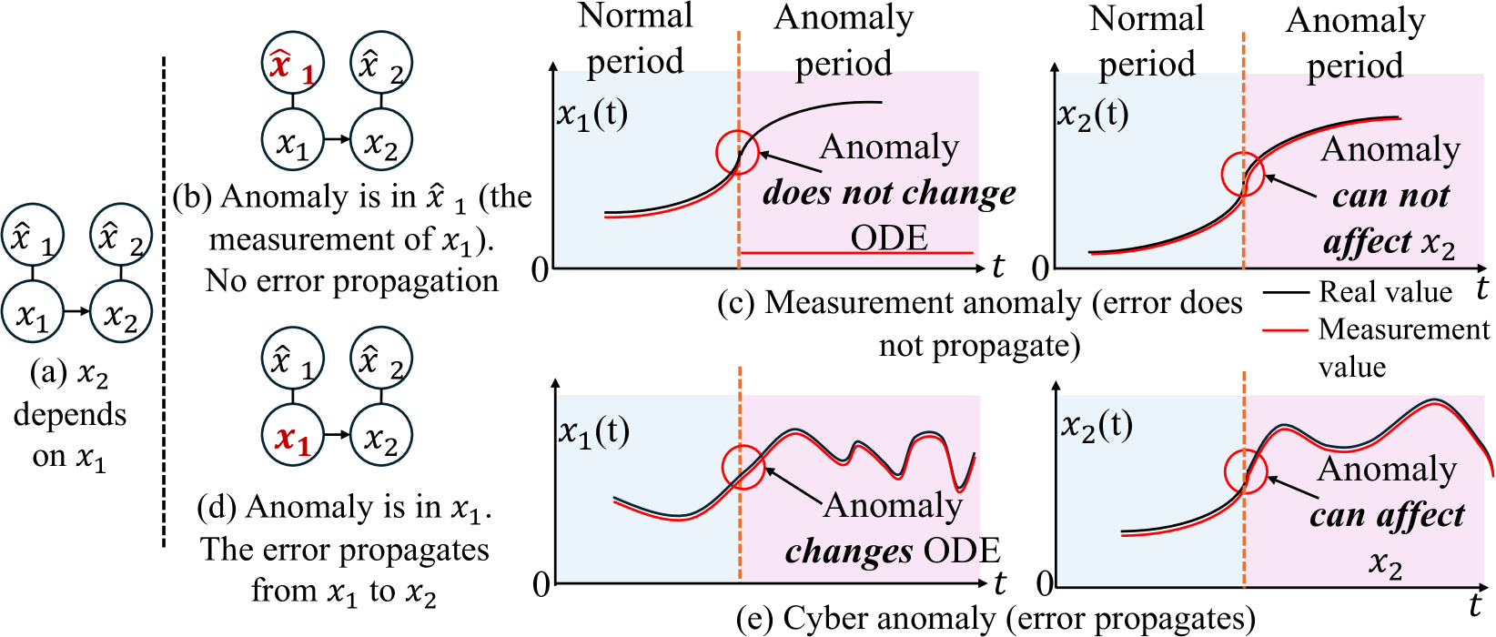
Figure 2: Comparison of Measurement and Cyber Anomalies in a Two-variable System (a) Normal state. (b) Measurement anomaly affects the measurement of a variable without altering underlying ODEs. (c) Measurment anomaly does not propagate to dependent variables. (d) Cyber anomaly alters the underlying ODE and lead to an anomaly. (e) Cyber anomaly propagates anomalies to dependent variables.
.
We summarize our contributions as follows:
- We define cyber anomalies and measurement anomalies based on whether the root cause affects dependent variables or remains localized.
- We propose an interpretable ML model called Interpretable Causality Ordinary Differential Equation (ICODE) Networks, which utilizes Neural Ordinary Differential Equations Networks for anomaly detection, anomaly type classification and root cause localization.
- We provide a theoretical analysis of the pattern of changes in learned parameters that can be used to localize root causes and classify the anomaly type in dynamical systems data when the ODE is altered.
- Extensive experiments on three simulated ODE systems demonstrate ICODE’s superior performance in anomaly detection, root cause localization, and anomaly type classification compared to state-of-the-art methods.
Related Work
Anomaly detection models. Deep learning models (Pang et al. 2021) have been widely adopted for anomaly detection due to their powerful capabilities. Variational autoencoder (VAE) based models (Zhou et al. 2021) are utilized to learn latent representations for this task. The Anomaly Transformer (Xu et al. 2021) demonstrates significant effectiveness by jointly modeling pointwise representations and pairwise associations. Additionally, a diffusion model (Xiao et al. 2023) has been proposed to detect anomalies through data imputation. However, as these models grow in size and complexity, they become increasingly opaque, providing only binary detection results without insight into the underlying decision-making process. Moreover, these models typically require large datasets, which may not be feasible in many real-world applications.
<details>
<summary>x3.png Details</summary>
### Visual Description
# Technical Document Extraction: Anomaly Detection and Root Cause Localization Workflow
This document describes a technical flow diagram illustrating a process for detecting anomalies, classifying their types, and localizing root causes using Ordinary Differential Equations (ODE) and adjacency matrices.
## 1. Component Isolation
The diagram is organized into a sequential pipeline with five primary stages, indicated by numbered black circles (1 through 5).
### Region A: Input Data (Normal Period)
* **Labels:** $x_0, x_1, x_2$ (representing three distinct variables or sensors).
* **Visual Representation:** Three horizontal time-series bars.
* $x_0$: Yellow/Orange blocks.
* $x_1$: Light Blue blocks.
* $x_2$: Light Purple blocks.
* **Caption:** "Normal period".
### Region B: Model Learning (ODE)
* **Header Text:** "ODE learned from normal period".
* **Process (1):** An arrow leads from the Normal Period data into a large integral symbol ($\int$), representing the learning of an ODE model.
* **Internal Components:**
* **Directed Graph:** Shows relationships between variables. $x_0 \rightarrow x_2$, $x_2 \rightarrow x_1$, and $x_1 \rightarrow x_0$.
* **Adjacency Matrix:** A $3 \times 3$ grid (labeled 0, 1, 2 on both axes). In this "normal" state, the grid cells are empty/white, representing the baseline learned structure.
### Region C: Anomaly Data Patterns
* **Process (2):** An arrow leads from the learned model to the anomaly data section.
* **Label:** "Anomaly data".
* **Pattern A:**
* $x_0$: Red blocks (indicating anomaly).
* $x_1, x_2$: Normal colored blocks (Light Blue/Purple).
* **Caption:** "Anomaly period Pattern A".
* **Pattern B:**
* $x_0, x_1, x_2$: All show a transition from normal colors to Red blocks.
* **Caption:** "Anomaly period Pattern B".
### Region D: Anomaly Classification and Localization
* **Process (3):** A bracket groups the learned model and anomaly data, feeding into two possible branching paths ("or").
* **Footer Labels (Columns):**
1. "Adjacency matrix in retrained model"
2. "Anomaly type classification"
3. "Root cause localization"
#### Path 1: Measurement Anomaly
* **Process (4):** Retrained Adjacency Matrix.
* **Matrix State:** Column 0 is highlighted in **Red**. Columns 1 and 2 are white.
* **Classification:** A rounded box labeled "**Measurement anomaly**".
* **Process (5):** Root Cause Localization.
* **Graph State:** Node $x_0$ is colored **Red**. Nodes $x_1$ and $x_2$ remain normal colors.
* **Text:** "Root Cause: $x_0$".
#### Path 2: Cyber Anomaly
* **Process (4):** Retrained Adjacency Matrix.
* **Matrix State:** Row 0 and Column 0 (specifically the intersection and adjacent cells $(0,0), (0,1), (1,0)$) are highlighted in **Red**.
* **Classification:** A rounded box labeled "**Cyber anomaly**".
* **Process (5):** Root Cause Localization.
* **Graph State:** Node $x_1$ is colored **Red**. Nodes $x_0$ and $x_2$ remain normal colors.
* **Text:** "Root Cause: $x_1$".
---
## 2. Data Table: Adjacency Matrix States
The following table reconstructs the visual state of the $3 \times 3$ matrices during different phases:
| Phase | Cell (0,0) | Cell (0,1) | Cell (0,2) | Cell (1,0) | Cell (1,1) | Cell (1,2) | Cell (2,0) | Cell (2,1) | Cell (2,2) |
| :--- | :--- | :--- | :--- | :--- | :--- | :--- | :--- | :--- | :--- |
| **Normal Period** | White | White | White | White | White | White | White | White | White |
| **Measurement Anomaly** | **Red** | White | White | **Red** | White | White | **Red** | White | White |
| **Cyber Anomaly** | **Red** | **Red** | White | **Red** | White | White | White | White | White |
---
## 3. Logic and Trend Summary
1. **Learning Phase:** The system establishes a baseline (ODE) and a dependency graph ($x_0 \to x_2 \to x_1 \to x_0$) from normal data.
2. **Detection Phase:** When "Anomaly data" is introduced (Pattern A or B), the model is retrained.
3. **Classification Logic:**
* If the retraining results in a **vertical anomaly** in the adjacency matrix (Column 0), it is classified as a **Measurement anomaly**, pointing to $x_0$ as the root cause.
* If the retraining results in an **L-shaped anomaly** in the adjacency matrix (Row 0/Column 0 intersection), it is classified as a **Cyber anomaly**, pointing to $x_1$ as the root cause.
4. **Localization:** The final output identifies the specific node ($x_0$ or $x_1$) responsible for the system deviation.
</details>
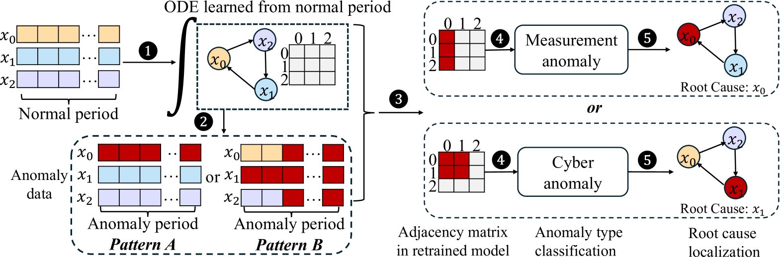
Figure 3: A 3-variable example dynamical system. 1 Train ICODE using data from normal periods to establish the baseline causality relationship $C$ . 2 Apply the trained ICODE to detect anomalies in anomaly period. 3 Retrain the model using the anomalous data to obtain a new causality relationship $C^{\prime}$ . 4 Analyze the causality difference $|C-C^{\prime}|$ to classify the anomaly type; 5 Apply Eq. (11) or Eq. (12) to identify the root cause.
.
Root Cause Analysis models. Root cause analysis (RCA) using machine learning (Lei et al. 2020; Richens, Lee, and Johri 2020) has gained increasing popularity in recent years. For example, a variational autoencoder model (Han et al. 2023) leverages a known causal graph to identify root causes based on Pearl’s structural causal model. However, these models often require precise causal relationships and separate models for anomaly detection, which is challenging in practice. Obtaining accurate causal graphs is sometimes challenging, and deploying two individual models can be cost-prohibitive. Other RCA methods based on causal structures have been proposed (Budhathoki et al. 2022; Wang et al. 2023b), but they typically assume anomalies are outliers, which is not always valid, leading to potential inaccuracies in the learned causality architecture.
Model Explainability using Neural ODEs. Model-intrinsic-explainable models are designed with inherent transparency, allowing direct interpretation of their decisions and processes from their internal structures (Lakkaraju, Bach, and Leskovec 2016; Lou, Caruana, and Gehrke 2012). Self-explainable Neural Networks (SENN) employ explainable basis concepts for explicit and faithful predictions and classification (Alvarez Melis and Jaakkola 2018). Building on SENN, the GVAR model learns causal relationships within time series data using an interpretable framework (Marcinkevičs and Vogt 2021). Additionally, time series systems often follow differential equations, and Neural ODEs have been proposed to approximate these systems (Jia and Benson 2019; Asikis, Böttcher, and Antulov-Fantulin 2022). However, using model-intrinsic-explainable models enhanced by Neural ODEs to learn patterns in dynamic systems for anomaly detection and RCA remains largely unexplored.
Notations and Problem definition
Consider a time series in a dynamical system with $p$ variables: $X(t)=\{x_{1}(t),x_{2}(t),...,x_{p}(t)\}$ , which follows causal relationships represented by a directed graph $\mathcal{G}=\{X(t),\mathcal{E}\}$ . In this graph, each node $x_{i}$ corresponds to a variable in $X(t)$ , and each edge $(i,j)∈\mathcal{E}$ indicates whether variable $x_{i}$ can influence variable $x_{j}$ . We assume the evolution of variable $x_{i}$ satisfies a differential equation:
$$
\displaystyle\frac{dx_{i}(t)}{dt} \displaystyle=f_{i}\left(X(t),\mathcal{G}\right),\forall 1\leq i\leq p, \displaystyle x_{i}(t) \displaystyle=x_{i}(0)+\int_{0}^{t}f_{i}\left(X(t),\mathcal{G}\right)dt, \tag{1}
$$
where where $f_{i}$ is an unknown nonlinear function specifying the evolution of $x_{i}$ at time $t$ . Sensors are deployed to measure variables, denoted as $\{\hat{x}_{1},\hat{x}_{2},...,\hat{x}_{p}\}$ , with noise $\epsilon$ :
$$
\hat{x}_{i}=x_{i}+\epsilon. \tag{2}
$$
We define two types of anomalies: the measurement anomaly and the cyber anomaly. The measurement anomaly only affects the measurement of the variable but does not affect the differential equation, as illustrated in Figure 2.
**Definition 1**
*Measurement Anomaly: We define a system to exhibit a measurement anomaly in variable $i$ at time $t$ , if the variable measurement at time $t$ is given by:
$$
\displaystyle\hat{x}_{i}^{\prime}(t) \displaystyle=A(\hat{x}_{i}(t)), \tag{3}
$$
where $A(·)$ is an anomalous function such that $A(x)≠ x$ .*
For our theoretical analysis, we assume that for a period of time, $A(·)$ does not change. Unlike measurement anomalies, cyber anomalies directly alter variables within the ODE, modifying the system’s evolution and potentially propagating to dependent variables. Such anomalies can be caused by cyber-attacks, including false data injection (Sayghe et al. 2020), which fundamentally disrupt the system’s dynamics.
**Definition 2**
*Cyber Anomaly: We define a system to exhibit a cyber anomaly in variable $i$ at time $t$ , with anomalous function denoted as $A(·)$ , if variable $x_{i}$ is changed to
$$
x_{i}^{\prime}(t)=A(x_{i}(t)),A(x)\neq x. \tag{4}
$$*
Given a $t$ -length measurement of time series, we aim to propose a model-intrinsic-explainable model to conduct:
1. Detect whether the system has an anomaly.
1. Determine the type of root cause (measurement anomaly or cyber anomaly).
1. Identify which variable is the root cause of the anomaly.
We achieve this by proposing a model that can demonstrate the change in the causality relationship given the $t$ -length time sequence.
Methodology
We propose a model-intrinsic-explainable framework for time series prediction called Interpretable Causality Ordinary Differential Equation (ICODE) networks. This model is designed to make predictions by learning the driven ODE in the dynamical system and inferring causality relationships within a time series through its explanation channel. The ICODE model is defined as follows
$$
\displaystyle\frac{dX(t)}{dt} \displaystyle=\Phi_{\theta}(X(t))X(t)+b, \displaystyle\hat{X}(t+1) \displaystyle=X(t)+\int_{t}^{t+1}\left(\Phi_{\theta}(X(\tau))X(\tau)+b\right)d\tau, \tag{5}
$$
where $b∈\mathbb{R}^{p× 1}$ is the bias term. $\Phi_{\theta}(X(t)):\mathbb{R}^{p}→\mathbb{R}^{p× p}$ is a neural network parameterised by $\theta$ , learning the ODE governing the dynamical system. The output of $\Phi_{\theta}(X(t))$ is an $p$ by $p$ matrix representing the causality dependency between variables, corresponding to the weight in causality graph $\mathcal{G}$ . Specifically, the element at $i,j$ of $\Phi_{\theta}(X(t))$ represents the influence of $x_{j}(t+\delta t)$ on $x_{i}(t)$ , where $\delta t$ is a very small time interval. A larger element at $i,j$ of $\Phi_{\theta}(X(t))$ indicates a high likelihood $(i,j)$ is an edge in $\mathcal{E}$ .
As shown in Eq. (5), the model could predict $X(t+1)$ based on the input $X(t)$ at time $t$ , by letting the neural network $\Phi_{\theta}(·)$ learn the evolution of $X(t)$ . For this reason, we employ Neural ODE, a machine learning framework that approximates the integral process, given the initial value, differential equation, and time interval. The prediction is then given by:
$$
\displaystyle\hat{X}(t+1)= \displaystyle NeuralODE(X(t), \displaystyle(\Phi_{\theta}(X(t))X(t)+b),[t,t+1]). \tag{6}
$$
The dependency matrix, representing relationships between variables in $X(t)$ , can be explored through $\Phi_{\theta}(X(t))$ . Enforcing sparsity in $\Phi_{\theta}(X(t))$ is crucial, as it ensures that the learned model captures the immediate dependence between variables as expressed through the differential equation. This sparsity is essential for accurately representing the true causal structure. To achieve this sparsity in $\Phi_{\theta}(X(t))$ , we train ICODE using the following loss function:
$$
\frac{1}{T-1}\sum_{t=0}^{T-1}(\hat{X}(t+1)-X(t+1))^{2}+\frac{\lambda}{T-1}\sum%
_{t=0}^{T-1}R(\Phi_{\theta}(X(t+1)), \tag{7}
$$
where the first term represents the mean squared error (MSE) of the one-step prediction using ICODE, and $R(·)$ is a sparsity-inducing penalty term. $\lambda$ is a hyperparameter that balances the importance of sparsity. The architecture of ICODE is shown in Figure 3.
Anomaly Detection
Anomalies in the system, whether cyber anomalies or measurement anomalies, cause significant deviations in the prediction $\hat{X}(t+1)$ from the ground truth $X(t+1)$ . The anomaly score is calculated as follows:
$$
AnomalyScore=\sum_{t=1}^{T}|\hat{X}(t)-X(t)|. \tag{8}
$$
Anomaly Type Classification
Our hypothesis is that the root cause of an anomaly is located at the variable where the causality relationship changes significantly. The causality relationship is inferred from $\Phi_{\theta}(·)$ (Marcinkevičs and Vogt 2021):
$$
C_{i,j}=median_{0\leq t\leq T-1}\left\{|\Phi_{\theta,(i,j)}(X(t))|\right\},%
\textit{for }1\leq i,j\leq p. \tag{9}
$$
We compute the causality relationship matrix $C_{i,j}$ during normal periods and $C^{\prime}_{i,j}$ during anomaly periods, where a higher value in $C_{i,j}$ and $C^{\prime}_{i,j}$ represents a variable of high likelihood $i$ that influences variable $j$ during normal and anomaly period respectively.
The inherent differences between cyber anomalies and measurement anomalies manifest in how they affect the underlying ODEs and, consequently, the causality relationships learned by ICODE. This distinction forms the basis for our anomaly type classification. To determine the type of anomaly, we calculate a measurement anomaly score $M$ , which indicates the probability that observed causality changes are due to a measurement anomaly. The score is given by:
$$
M(C,C^{\prime})=\max_{i}\sum_{j=1}^{p}\frac{\mathbb{I}\left(|C_{i,j}-C^{\prime%
}_{i,j}|\geq\bar{\gamma}\right)}{p}, \tag{10}
$$
where $C$ and $C^{\prime}$ are the causality matrices in non-anomalous and anomalous data, $\bar{\gamma}$ is a threshold used to select the $m$ largest values, $\mathbb{I}$ is an indicator function used to select the top $m$ elements in $|C-C^{\prime}|$ , and $p$ is the number of variables.
The calculation process involves calculating the proportion of the largest $m$ elements in the difference matrix $|C-C^{\prime}|$ for each row, and taking the maximum proportion as the measurement score $M(C,C^{\prime})$ . A greater $M(C,C^{\prime})$ indicates a higher likelihood that the anomaly is a measurement anomaly, since the changes are concentrated on one column. While a lower score suggests a cyber anomaly. This classification is crucial for subsequent root cause localization, which we will discuss in the following section.
Root Cause Localization
The root cause score representing the likelihood of variable $i$ being the root cause of measurement anomalies is given by:
$$
S(i)=\left(\sum_{j=1}^{p}|{C}_{i,j}-{C}^{\prime}_{i,j}|+\sum_{j=1}^{p}|{C}_{j,%
i}-{C}^{\prime}_{j,i}|\right)_{i}. \tag{11}
$$
The root cause location is indicated by the largest combined change across both the row (first term) and column (second term) sums. Whereas the root cause score of variable $i$ causing cyber anomalies is given by:
$$
S^{\prime}(i)=\sum_{k\in\{k:{C}_{i,k}=1\ or\ {C}_{k,i}=1\}}S(k), \tag{12}
$$
representing the sum of the changed weight that is related to variable $i$ according to the learned causality graph.
Theoretical Analysis
In this section, we provide theoretical support for how measurement and cyber anomalies distinctly affect the weights of the causal graph, as represented by the properties of $|C-C^{\prime}|$ , when finite difference methods are used to approximate the integration in Eq. (5). The fundamental difference between these anomaly types lies in their position relative to the integral process in the dynamical system. Measurement anomalies occur outside the integral function, leading to a localized impact on the causal graph. We formalize this observation in the following theorem:
**Theorem 1**
*Consider a dynamical system $X(t)$ as learned using Eq. (5), where $\mathcal{G}=(X(t),\mathcal{E})$ denotes the underlying dependency graph. Let $C(·,·)$ and $C^{\prime}(·,·)$ denote the causality matrices extracted using non-anomalous and anomalous data, respectively. Assuming $C(i,j)≠ 0$ iff $(i,j)∈\mathcal{E}$ , and the diagonal elements of $C$ are much larger than the off-diagonal elements, $C(i,i)\gg C(i,j),i≠ j$ , then (1) If the anomaly is a measurement anomaly at variable $k$ , then $|C(k,j)-C’(k,j)|\gg|C(k^{\prime},j)-C’(k^{\prime},j)|>0$ , where $(k,k^{\prime})∈\mathcal{E}$ . (2) If the anomaly is a cyber anomaly at variable $k$ , then $|C(k,j)-C’(k,j)|>0$ only if $(k,j)∈\mathcal{E}$ .*
* Proof*
See Appendix. ∎
Theorem 1 indicates that a measurement anomaly with a root cause in variable $i$ only alters the values of $|C-C^{\prime}|$ in column $i$ or row $i$ of the causality matrix. This localized effect is consistent with the nature of measurement anomalies, which implies that the dependency of the affected variable on any other variable can be altered regardless of ground truth dependence. In contrast, cyber anomalies occur within the integral function, allowing their effects to propagate to dependent variables. Theorem 1 also suggests that a cyber anomaly with a root cause in variable $i$ can alter the values of $|C-C^{\prime}|$ for all edges connected to variable $i$ and variable $j$ , where the edge $(i,j)$ in causal graph $\mathcal{G}$ . This more extensive impact reflects the propagating nature of cyber anomalies through interconnected variables in the system.
Experiments
The distinct patterns of change in the causality relationships $|C-C^{\prime}|$ for measurement and cyber anomalies provide a robust foundation for anomaly type classification. Measurement anomalies produce a concentrated change in the causality matrix, primarily affecting a single variable’s relationships, aligning with scenarios like sensor errors or calibration issues. Conversely, cyber anomalies result in a more diffuse pattern of changes, reflecting their ability to propagate through interconnected systems. These theoretical insights not only support our anomaly classification approach but also provide a deeper understanding of how different types of anomalies manifest in dynamical systems, enabling more targeted and appropriate responses to system irregularities. The Purpose of our experiments is
- We evaluate ICODE’s performance in identifying anomalies within dynamical systems, comparing it to state-of-the-art methods.
- We examine the model’s capability to accurately pinpoint the location of the root cause, comparing it to state-of-the-art methods.
- We demonstrate ICODE’s unique ability to categorize anomalies.
Experiment Settings
Our experiments involve three simulated ODE systems, each comprising $20$ variables. For each system, we generate $100,000$ data points spanning normal, cyber anomaly, and measurement anomaly periods using specified ODEs. In both the cyber and measurement anomaly simulation process, we create $500$ data points for each anomaly instance, with every set of $500$ points sharing a common root cause. To form our final datasets, we downsample each period individually to $10,000$ points.
N-species Lotka-volterra System
The original Lotka–Volterra system (Bacaër 2011) are used to model the relationship among $p$ predator and prey species, and the corresponding population sizes are denoted by $X(t)=\{x_{1}(t),x_{2}(t),...,x_{p}(t)\}$ . Population dynamics are given by the following coupled differential equations:
$$
\displaystyle\frac{dx_{i}}{dt}=r_{i}x_{i}\left(1-\frac{\sum_{j=1}^{p}\beta_{ij%
}x_{j}}{K_{i}}\right), \tag{13}
$$
where $r_{i}$ is inherent percapita growth rate, and $K_{i}$ is the carrying capacity, and $\beta_{ij}$ represents the effect of species $j$ on species $i$ . We initialize $\beta_{ij}$ randomly.
Lorenz-96 system
Consider the Lorenz-96 system with $n$ variables denoted as $X(t)=\{x_{1}(t),x_{2}(t),...,x_{p}(t)\}$ , following an ordinary differential equation:
$$
\frac{dx_{i}(t)}{dt}=(x_{i+1}(t)-x_{i-2}(t))x_{i-1}(t)-x_{i}(t)+F,\forall 1%
\leq i\leq n, \tag{14}
$$
where $x_{0}:=x_{p}$ , $x_{-1}:=x_{p-1}$ , and $F$ is a forcing constant. We set $F=10$ .
Reaction-diffusion system
Reaction-diffusion systems consist of a local reaction and a diffusion, which cause the substances to spread out, and are used in modeling many domains in biology (Fisher 1937), geology, and transportation. We pick up one reaction-diffusion system with $n$ variables denoted as $X(t)=\{x_{1}(t),x_{2}(t),...,x_{p}(t)\}$ , while the neighboring variables are connected by a diffusion process (e.g., $x_{i}$ is connected to $x_{i-1}$ and $x_{i+1}$ ):
$$
\frac{dx_{i}}{dt}=(x_{i-1}-x_{i})+(x_{i+1}-x_{i})+x_{i}(1-x_{i}), \tag{15}
$$
where the first two terms represent a diffusion process with diffusion coefficients $1$ , and the third term represents the local reaction called Fisher’s equation (Fisher 1937).
Anomaly Simulation
We simulate the anomaly using the following equation:
$$
A(x_{i})=x_{i}+a,a\sim\mathcal{N}(\alpha,1) \tag{16}
$$
where $a$ is a random variable from a Gaussian distribution with mean $\alpha$ and variance $1$ . We differentiate between measurement and cyber anomalies. Measurement anomalies are added to one variable after time series simulation, without altering the underlying ODE. Cyber anomalies, conversely, are incorporated during time series simulation, changing the underlying ODE.
Table 1: Performance of ICODE compared to baseline models in anomaly detection.
| | | | Lotka-valterra Precision | Lorenz-96 Recall | Reaction-diffusion F1 | Precision | Recall | F1 | Precision | Recall | F1 |
| --- | --- | --- | --- | --- | --- | --- | --- | --- | --- | --- | --- |
| $\alpha=0.5$ | Deep SVDD | | 0.9033 | 0.9102 | 0.9067 | 0.9232 | 0.9019 | 0.9124 | 0.9235 | 0.9444 | 0.9338 |
| Anomaly Transformer | | 0.9284 | 0.9311 | 0.9307 | 0.9555 | 0.9434 | 0.9494 | 0.9514 | 0.9548 | 0.9514 | |
| ICODE | | 0.9240 | 0.9363 | 0.9301 | 0.9475 | 0.9593 | 0.9533 | 0.9675 | 0.9624 | 0.9649 | |
| $\alpha=1$ | Deep SVDD | | 0.9224 | 0.9342 | 0.9282 | 0.9310 | 0.9326 | 0.9317 | 0.9468 | 0.9658 | 0.9562 |
| Anomaly Transformer | | 0.9374 | 0.9345 | 0.9359 | 0.9607 | 0.9568 | 0.9587 | 0.9815 | 0.9763 | 0.9788 | |
| ICODE | | 0.9367 | 0.9472 | 0.9419 | 0.9595 | 0.9693 | 0.9594 | 0.9827 | 0.9772 | 0.9799 | |
Baselines
For anomaly detection, we compare our model with Deep SVDD (Zhou et al. 2021) and Anomaly Transformer (Xu et al. 2021) to demonstrate comparable performance on simulated datasets. For root cause analysis, we benchmark against RootClam (Han et al. 2023) and CausalRCA (Budhathoki et al. 2022), which are state-of-the-art models in RCA.
Results and Analysis
Anomaly Detection
We train our model’s anomaly detection performance using a dataset of $10000$ data points collected during normal operating conditions. To test the model, we create a mixed dataset containing samples from both normal and anomaly periods. In this section, we do not distinguish between anomaly types; all anomaly samples (both cyber and measurement anomaly) are marked as $1$ , while samples from non-anomaly time periods are marked as $0 0$ . Anomaly scores are calculated for all samples using Eq. (8), with samples with anomaly scores exceeding a specified threshold classified as anomalies. We conduct experiments with $\alpha$ values of $0.5$ and $1.0$ in Eq. (16) to assess the model’s sensitivity under different level of anomalies. Performance is measured using precision, recall, and F1 scores across three distinct datasets, with results shown in Table 1.
Table 1 shows that our method ICODE consistently outperforms the classical Deep SVDD and anomaly transformer model across all metrics, likely due to our ODE-based architecture simplifying the learning process. Compared to the Anomaly Transformer, our model shows slightly better performance overall, though marginally lower precision and F1 scores are observed with $\alpha=0.5$ . This suggests that while our approach is generally more effective, it may be less adept at capturing subtle anomalies that occur with lower $\alpha$ values, compared to deep learning models. The superior performance of our model can be attributed to its ODE-based design, which leverages the quadratic nature of ODEs to more accurately model system dynamics and detect anomalies.
Root Cause Localization
Table 2: Performance of ICODE compared to baseline models in root cause localization.
| | | | Lotka-valterra Top 1 | Lorenz-96 Top 3 | Reaction-diffusion Top 5 | Top 1 | Top 3 | Top 5 | Top 1 | Top 3 | Top 5 |
| --- | --- | --- | --- | --- | --- | --- | --- | --- | --- | --- | --- |
| $\alpha=0.5$ | CausalRCA | | 0.1565 | 0.3424 | 0.4805 | 0.6766 | 0.6928 | 0.7369 | 0.9235 | 0.9481 | 0.9655 |
| RootClam | | 0.3360 | 0.4247 | 0.5699 | 0.6260 | 0.6315 | 0.6724 | 0.9395 | 0.9681 | 0.9709 | |
| ICODE | | 0.6713 | 0.7124 | 0.7246 | 0.7546 | 0.7742 | 0.7883 | 0.9645 | 0.9783 | 0.9748 | |
| $\alpha=1$ | CausalRCA | | 0.2724 | 0.3922 | 0.5269 | 0.6978 | 0.7485 | 0.7538 | 0.8857 | 0.9563 | 0.9736 |
| RootClam | | 0.5546 | 0.5630 | 0.6554 | 0.6519 | 0.7586 | 0.7936 | 0.6554 | 0.9763 | 0.9788 | |
| ICODE | | 0.7710 | 0.8109 | 0.8385 | 0.7632 | 0.7890 | 0.8241 | 0.9798 | 0.9911 | 0.9952 | |
We evaluate ICODE’s root cause localization performance using simulated anomaly data. Based on the model trained in the previous section, we retrain it on $500$ samples from each anomaly period to obtain a new causal graph. In Eq. (10), $m=10$ and $\bar{\gamma}$ is the threshold of largest $10$ elements. An anomaly is categorized as a measurement anomaly if $M(C,C^{\prime})≥ 0.8$ ; otherwise, it is classified as a cyber anomaly. We then apply Eq. (11) or Eq. (12) to localize the root cause, ranking variables based on their root cause scores. Performance is assessed using Top-k accuracy, which measures whether the true root cause is included in the output top k set. This process is repeated for each anomaly period, with results summarized in Table 2.
Table 2 shows that ICODE outperforms baseline models CausalRCA and RootClam, achieving higher Top-1, Top-3, and Top-5 accuracy across all three simulated datasets. The reaction-diffusion system, with its linear ODE function, yields relatively good results for all models. Performance degrades for Lotka-Volterra and Lorenz-96 systems, which we attribute to its more complex dynamics making causality inference more challenging.
<details>
<summary>x4.png Details</summary>
### Visual Description
# Technical Document Extraction: Directed Graph Diagram
## 1. Image Overview
This image is a technical diagram representing a **Directed Graph**, likely illustrating a state transition, a neural network node, or a mathematical dependency structure. It consists of four circular nodes and three directed edges (arrows).
## 2. Component Isolation
### Node Analysis
All nodes are visually identical: light purple/lavender fill with a thick dark navy/black border. Each node contains a mathematical label in black italicized serif font.
| Node Position | Label | Description |
| :--- | :--- | :--- |
| **Top Left** | $x_{i-1}$ | Input node representing a previous state or index. |
| **Middle Left** | $x_{i+1}$ | Input node representing a subsequent index. |
| **Bottom Left** | $x_{i+2}$ | Input node representing a further subsequent index. |
| **Right** | $x_{i}$ | The central/target node receiving all inputs. |
### Edge (Flow) Analysis
The diagram illustrates the flow of information or dependency toward the central node $x_{i}$.
1. **Inbound Edge 1:** A straight arrow originates from $x_{i-1}$ and points to $x_{i}$.
2. **Inbound Edge 2:** A straight arrow originates from $x_{i+1}$ and points to $x_{i}$.
3. **Inbound Edge 3:** A straight arrow originates from $x_{i+2}$ and points to $x_{i}$.
</details>
(a)
<details>
<summary>x5.png Details</summary>
### Visual Description
# Technical Document Extraction: Binary Relationship Matrix
## 1. Image Overview
This image represents a $20 \times 20$ binary matrix (or heatmap) illustrating the relationship between "Cause" (x-axis) and "Effect" (y-axis). The matrix uses numerical values (0 and 1) and color coding (light blue for 1, white for 0) to denote the presence or absence of a relationship.
## 2. Component Isolation
### Header/Labels
- **Y-Axis Label:** "Effect" (oriented vertically on the left).
- **X-Axis Label:** "Cause" (oriented horizontally at the bottom).
### Axis Markers
- **Y-Axis (Effect):** Integers from **0 to 19**, ordered top-to-bottom.
- **X-Axis (Cause):** Integers from **0 to 19**, ordered left-to-right. Note: Labels 10 through 19 are rotated 90 degrees clockwise.
### Main Data Region
- A grid of $20 \times 20$ cells.
- **Value '1' (Light Blue Background):** Indicates an active relationship.
- **Value '0' (White Background):** Indicates no relationship.
---
## 3. Data Table Reconstruction
The following table represents the matrix. Rows correspond to **Effect** and columns correspond to **Cause**.
| Effect \ Cause | 0 | 1 | 2 | 3 | 4 | 5 | 6 | 7 | 8 | 9 | 10 | 11 | 12 | 13 | 14 | 15 | 16 | 17 | 18 | 19 |
| :--- | :---: | :---: | :---: | :---: | :---: | :---: | :---: | :---: | :---: | :---: | :---: | :---: | :---: | :---: | :---: | :---: | :---: | :---: | :---: | :---: |
| **0** | 1 | 1 | 0 | 0 | 0 | 0 | 0 | 0 | 0 | 0 | 0 | 0 | 0 | 0 | 0 | 0 | 0 | 0 | 1 | 1 |
| **1** | 1 | 1 | 1 | 0 | 0 | 0 | 0 | 0 | 0 | 0 | 0 | 0 | 0 | 0 | 0 | 0 | 0 | 0 | 0 | 1 |
| **2** | 1 | 1 | 1 | 1 | 0 | 0 | 0 | 0 | 0 | 0 | 0 | 0 | 0 | 0 | 0 | 0 | 0 | 0 | 0 | 0 |
| **3** | 0 | 1 | 1 | 1 | 1 | 0 | 0 | 0 | 0 | 0 | 0 | 0 | 0 | 0 | 0 | 0 | 0 | 0 | 0 | 0 |
| **4** | 0 | 0 | 1 | 1 | 1 | 1 | 0 | 0 | 0 | 0 | 0 | 0 | 0 | 0 | 0 | 0 | 0 | 0 | 0 | 0 |
| **5** | 0 | 0 | 0 | 1 | 1 | 1 | 1 | 0 | 0 | 0 | 0 | 0 | 0 | 0 | 0 | 0 | 0 | 0 | 0 | 0 |
| **6** | 0 | 0 | 0 | 0 | 1 | 1 | 1 | 1 | 0 | 0 | 0 | 0 | 0 | 0 | 0 | 0 | 0 | 0 | 0 | 0 |
| **7** | 0 | 0 | 0 | 0 | 0 | 1 | 1 | 1 | 1 | 0 | 0 | 0 | 0 | 0 | 0 | 0 | 0 | 0 | 0 | 0 |
| **8** | 0 | 0 | 0 | 0 | 0 | 0 | 1 | 1 | 1 | 1 | 0 | 0 | 0 | 0 | 0 | 0 | 0 | 0 | 0 | 0 |
| **9** | 0 | 0 | 0 | 0 | 0 | 0 | 0 | 1 | 1 | 1 | 1 | 0 | 0 | 0 | 0 | 0 | 0 | 0 | 0 | 0 |
| **10** | 0 | 0 | 0 | 0 | 0 | 0 | 0 | 0 | 1 | 1 | 1 | 1 | 0 | 0 | 0 | 0 | 0 | 0 | 0 | 0 |
| **11** | 0 | 0 | 0 | 0 | 0 | 0 | 0 | 0 | 0 | 1 | 1 | 1 | 1 | 0 | 0 | 0 | 0 | 0 | 0 | 0 |
| **12** | 0 | 0 | 0 | 0 | 0 | 0 | 0 | 0 | 0 | 0 | 1 | 1 | 1 | 1 | 0 | 0 | 0 | 0 | 0 | 0 |
| **13** | 0 | 0 | 0 | 0 | 0 | 0 | 0 | 0 | 0 | 0 | 0 | 1 | 1 | 1 | 1 | 0 | 0 | 0 | 0 | 0 |
| **14** | 0 | 0 | 0 | 0 | 0 | 0 | 0 | 0 | 0 | 0 | 0 | 0 | 1 | 1 | 1 | 1 | 0 | 0 | 0 | 0 |
| **15** | 0 | 0 | 0 | 0 | 0 | 0 | 0 | 0 | 0 | 0 | 0 | 0 | 0 | 1 | 1 | 1 | 1 | 0 | 0 | 0 |
| **16** | 0 | 0 | 0 | 0 | 0 | 0 | 0 | 0 | 0 | 0 | 0 | 0 | 0 | 0 | 1 | 1 | 1 | 1 | 0 | 0 |
| **17** | 0 | 0 | 0 | 0 | 0 | 0 | 0 | 0 | 0 | 0 | 0 | 0 | 0 | 0 | 0 | 1 | 1 | 1 | 1 | 0 |
| **18** | 0 | 0 | 0 | 0 | 0 | 0 | 0 | 0 | 0 | 0 | 0 | 0 | 0 | 0 | 0 | 0 | 1 | 1 | 1 | 1 |
| **19** | 1 | 0 | 0 | 0 | 0 | 0 | 0 | 0 | 0 | 0 | 0 | 0 | 0 | 0 | 0 | 0 | 0 | 1 | 1 | 1 |
---
## 4. Structural Analysis and Trends
### Banded Structure
The matrix exhibits a **circulant banded structure**. The value '1' (blue) forms a diagonal band that wraps around the edges of the matrix.
1. **Main Diagonal:** The central diagonal (where Cause = Effect) consists entirely of '1's.
2. **Band Width:** The band of '1's is 4 units wide. Specifically, for any Effect $i$, the Cause $j$ is '1' if $j \in \{i-1, i, i+1, i+2\} \pmod{20}$.
3. **Symmetry/Shift:** The pattern is a constant shift. As you move down one row (Effect), the block of four '1's shifts one column to the right (Cause).
4. **Boundary Wrapping (Cyclic Property):**
* At **Effect 0**, the '1's are at Cause 18, 19, 0, and 1.
* At **Effect 1**, the '1's are at Cause 19, 0, 1, and 2.
* At **Effect 18**, the '1's are at Cause 16, 17, 18, and 19.
* At **Effect 19**, the '1's are at Cause 17, 18, 19, and 0.
### Summary of Logic
This matrix represents a system where each "Effect" is influenced by its corresponding "Cause" index, the one preceding it, and the two following it in a modulo-20 circular array. This is characteristic of a **circulant matrix** often used in digital signal processing or periodic boundary condition simulations.
</details>
(b)
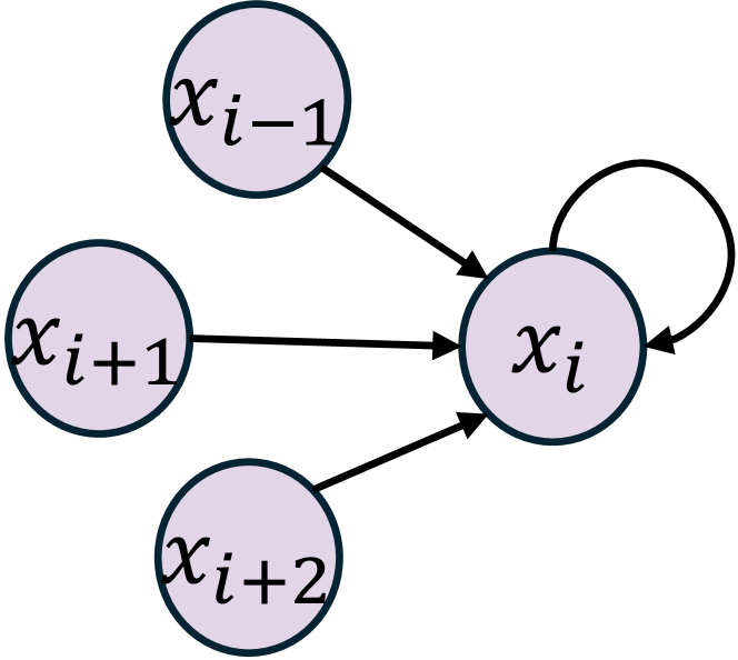
Figure 4: (a) Graph representation $\mathcal{G}$ of causality relationship in the Lorenz-96 system. (b) Adjacency matrix of the causality graph $\mathcal{G}$ .
These results support our hypothesis that learning the ODE in dynamical systems can improve anomaly detection and root cause localization. ICODE’s approach aligns with the mechanism of anomaly occurrence: exceptions due to ODE changes are located by learning about the ODE and inferring the root cause through changes in ICODE parameters. In contrast, baseline models lack this grounding in dynamical systems science. CausalRCA’s causal inference model may struggle to learn causal relationships in this context, while RootClam’s use of distribution changes for root cause localization may be less effective in dynamical systems. In the following part, we will discuss the anomaly type classification based on the proposed theorems.
Anomaly Type Classification
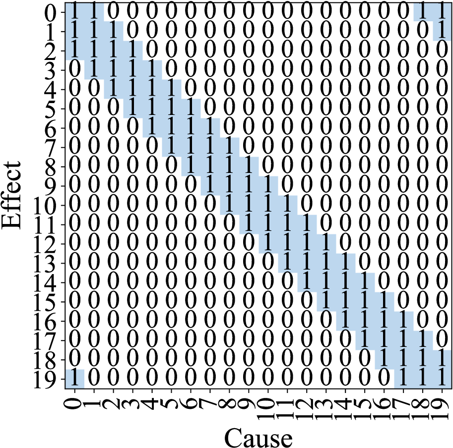
To better demonstrate the impact of different anomalies, we provide an intuitive description of anomaly behavior using the Lorenz-96 system with $\alpha=5$ , demonstrating strong cyber and measurement anomalies in a dynamical system. Figure 4a illustrates the causality relationship in the Lorenz-96 system, with the corresponding adjacency matrix shown in Figure 4b.
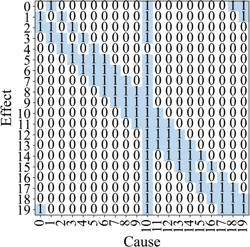
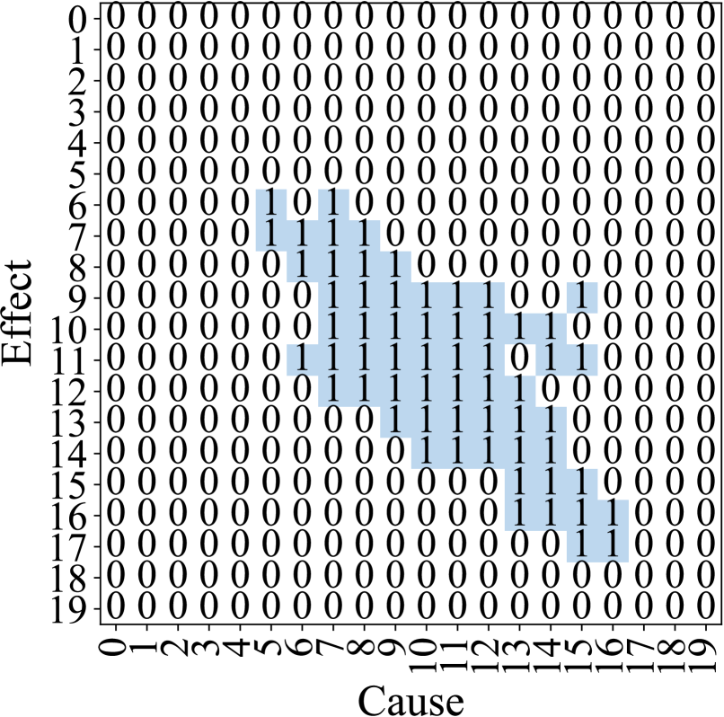
To analyze anomaly patterns, we simulate $500$ data points each for cyber and measurement anomalies with the root cause at variable 10. For clarity, we employ K-means clustering to categorize weights into two clusters: high dependency ( $1$ ) and low dependency ( $0 0$ ). Figures 5a and 5b depict the resulting adjacency matrices during measurement anomalies and cyber anomalies, respectively. Our analysis reveals distinct patterns for each anomaly type. In measurement anomalies (Figure 5a), changes in causality relationships are localized, with significant alterations primarily in variable $10$ ’s dependencies compared to the normal state (Figure 4b). Conversely, cyber anomalies (Figure 5b) exhibit a more diffuse pattern, where variables proximal to the root cause show more substantial changes.
These observations form the basis for our anomaly type classification strategy. It is important to note that this example represents an ideal case with optimal training conditions. In real-world cases, particularly with lower $\alpha$ values (e.g., $\alpha=0.5$ ), the distinctions may be less pronounced. Since cyber and measurement anomalies are specifically defined in our work, there are no existing approaches available for comparison.
Table 3: Performance of ICODE in anomaly classification.
| 0.5 1 | 0.929 0.916 | 0.952 0.961 | 0.971 0.974 |
| --- | --- | --- | --- |
Table 3 presents the classification results based on the criteria mentioned in root cause localization. The results in Table 3 demonstrate ICODE’s high accuracy in anomaly type classification, providing reliable insights that are not available from baseline models. These findings further support our hypothesis that changes in causality relationships can effectively address three key tasks: anomaly detection, root cause localization, and anomaly classification. We believe that such explanatory capabilities are important to domain experts in system diagnostics, offering a level of interpretability crucial for real-world applications in complex dynamical systems.
<details>
<summary>x6.png Details</summary>
### Visual Description
# Technical Document Extraction: Adjacency Matrix Analysis
## 1. Image Overview
The image displays a 20x20 binary matrix (or heatmap) representing a causal relationship between variables. The matrix uses numerical values (0 and 1) and light blue shading to indicate the presence of an "Effect" based on a "Cause."
## 2. Component Isolation
### Header/Labels
- **Y-Axis Label:** "Effect" (oriented vertically on the left).
- **X-Axis Label:** "Cause" (oriented horizontally at the bottom).
- **Y-Axis Markers:** Integers from **0 to 19** (top to bottom).
- **X-Axis Markers:** Integers from **0 to 19** (left to right, rotated 90 degrees).
### Main Chart Area
The chart is a grid where each cell contains either a `0` (white background) or a `1` (light blue background). The blue shading strictly corresponds to the presence of a `1`.
## 3. Data Table Reconstruction
The following table represents the matrix data. Rows represent the **Effect** index, and columns represent the **Cause** index.
| Effect \ Cause | 0 | 1 | 2 | 3 | 4 | 5 | 6 | 7 | 8 | 9 | 10 | 11 | 12 | 13 | 14 | 15 | 16 | 17 | 18 | 19 |
| :--- | :---: | :---: | :---: | :---: | :---: | :---: | :---: | :---: | :---: | :---: | :---: | :---: | :---: | :---: | :---: | :---: | :---: | :---: | :---: | :---: |
| **0** | 0 | 1 | 0 | 0 | 0 | 0 | 0 | 0 | 0 | 0 | 1 | 0 | 0 | 0 | 0 | 0 | 0 | 0 | 1 | 1 |
| **1** | 1 | 0 | 1 | 0 | 0 | 0 | 0 | 0 | 0 | 0 | 1 | 0 | 0 | 0 | 0 | 0 | 0 | 0 | 0 | 1 |
| **2** | 1 | 1 | 0 | 1 | 0 | 0 | 0 | 0 | 0 | 0 | 1 | 0 | 0 | 0 | 0 | 0 | 0 | 0 | 0 | 0 |
| **3** | 0 | 1 | 1 | 0 | 1 | 0 | 0 | 0 | 0 | 0 | 1 | 0 | 0 | 0 | 0 | 0 | 0 | 0 | 0 | 0 |
| **4** | 0 | 0 | 1 | 1 | 0 | 1 | 0 | 0 | 0 | 0 | 0 | 0 | 0 | 0 | 0 | 0 | 0 | 0 | 0 | 0 |
| **5** | 0 | 0 | 0 | 1 | 1 | 1 | 1 | 0 | 0 | 0 | 1 | 0 | 0 | 0 | 0 | 0 | 0 | 0 | 0 | 0 |
| **6** | 0 | 0 | 0 | 0 | 1 | 1 | 1 | 1 | 0 | 0 | 1 | 0 | 0 | 0 | 0 | 0 | 0 | 0 | 0 | 0 |
| **7** | 0 | 0 | 0 | 0 | 0 | 1 | 1 | 1 | 1 | 0 | 1 | 0 | 0 | 0 | 0 | 0 | 0 | 0 | 0 | 0 |
| **8** | 0 | 0 | 0 | 0 | 0 | 0 | 1 | 1 | 1 | 1 | 1 | 0 | 0 | 0 | 0 | 0 | 0 | 0 | 0 | 0 |
| **9** | 0 | 0 | 0 | 0 | 0 | 0 | 0 | 1 | 1 | 1 | 1 | 0 | 0 | 0 | 0 | 0 | 0 | 0 | 0 | 0 |
| **10** | 0 | 0 | 0 | 0 | 0 | 0 | 0 | 0 | 1 | 1 | 1 | 1 | 0 | 0 | 0 | 0 | 0 | 0 | 0 | 0 |
| **11** | 0 | 0 | 0 | 0 | 0 | 0 | 0 | 0 | 0 | 1 | 1 | 1 | 1 | 0 | 0 | 0 | 0 | 0 | 0 | 0 |
| **12** | 0 | 0 | 0 | 0 | 0 | 0 | 0 | 0 | 0 | 0 | 1 | 1 | 1 | 1 | 0 | 0 | 0 | 0 | 0 | 0 |
| **13** | 0 | 0 | 0 | 0 | 0 | 0 | 0 | 0 | 0 | 0 | 1 | 1 | 1 | 1 | 1 | 0 | 0 | 0 | 0 | 0 |
| **14** | 0 | 0 | 0 | 0 | 0 | 0 | 0 | 0 | 0 | 0 | 1 | 0 | 1 | 1 | 1 | 1 | 0 | 0 | 0 | 0 |
| **15** | 0 | 0 | 0 | 0 | 0 | 0 | 0 | 0 | 0 | 0 | 1 | 0 | 0 | 1 | 1 | 0 | 1 | 0 | 0 | 0 |
| **16** | 0 | 0 | 0 | 0 | 0 | 0 | 0 | 0 | 0 | 0 | 1 | 0 | 0 | 0 | 1 | 1 | 0 | 1 | 0 | 0 |
| **17** | 0 | 0 | 0 | 0 | 0 | 0 | 0 | 0 | 0 | 0 | 1 | 0 | 0 | 0 | 0 | 1 | 1 | 1 | 1 | 0 |
| **18** | 0 | 0 | 0 | 0 | 0 | 0 | 0 | 0 | 0 | 0 | 1 | 0 | 0 | 0 | 0 | 0 | 1 | 1 | 1 | 1 |
| **19** | 1 | 0 | 0 | 0 | 0 | 0 | 0 | 0 | 0 | 0 | 1 | 0 | 0 | 0 | 0 | 0 | 0 | 1 | 1 | 1 |
## 4. Key Trends and Structural Observations
### Banded Structure (Local Connectivity)
The matrix exhibits a strong **diagonal banding pattern**. Most `1` values are clustered around the main diagonal, suggesting that each variable (index $i$) is primarily caused by its immediate neighbors (indices $i-1, i, i+1$).
* **Trend Verification:** The "1" values form a thick line sloping downward from the top-left to the bottom-right.
### Global Hub (Column 10)
A significant vertical feature is present at **Cause 10**.
* **Observation:** Column 10 is almost entirely populated with `1`s (except for Effect 4).
* **Interpretation:** Variable 10 acts as a "Universal Cause" or a central hub that influences nearly every other variable in the system.
### Boundary Conditions (Wrap-around)
There are `1` values in the extreme corners:
* **Top-Right:** Effect 0 is caused by 18 and 19; Effect 1 is caused by 19.
* **Bottom-Left:** Effect 19 is caused by 0.
* **Interpretation:** This suggests a periodic or circular boundary condition where the end of the sequence (19) connects back to the beginning (0).
### Symmetry
The matrix is largely symmetric, but not perfectly so. For example, at (Effect 0, Cause 1) there is a `1`, and at (Effect 1, Cause 0) there is a `1`. However, the "Hub" at Cause 10 is not mirrored by a "Hub" at Effect 10, indicating a directed relationship rather than a simple correlation.
</details>
(a) Measurement Anomaly
<details>
<summary>x7.png Details</summary>
### Visual Description
# Technical Document Extraction: Cause-Effect Matrix
## 1. Image Overview
This image is a technical visualization of a binary matrix, likely representing a causal relationship or a reachability matrix in a system analysis. It maps "Cause" (horizontal axis) against "Effect" (vertical axis).
## 2. Component Isolation
### Header/Labels
- **Vertical Axis (Y-Axis):** Labeled "Effect". It contains numerical markers from **0 to 19**.
- **Horizontal Axis (X-Axis):** Labeled "Cause". It contains numerical markers from **0 to 19**.
### Main Chart Area
- **Data Type:** Binary Matrix (values are either `0` or `1`).
- **Visual Encoding:**
- Cells containing `0` have a white background.
- Cells containing `1` are highlighted with a light blue background.
- **Trend Observation:** The "1" values form a diagonal cluster starting around Cause 5, Effect 6 and extending to Cause 17, Effect 17. This indicates a delayed causal relationship where causes at time $t$ result in effects at time $t+n$.
---
## 3. Data Table Reconstruction
The following table represents the $20 \times 20$ matrix. Rows represent **Effect** (0-19) and columns represent **Cause** (0-19).
| Effect \ Cause | 0 | 1 | 2 | 3 | 4 | 5 | 6 | 7 | 8 | 9 | 10 | 11 | 12 | 13 | 14 | 15 | 16 | 17 | 18 | 19 |
| :--- | :-: | :-: | :-: | :-: | :-: | :-: | :-: | :-: | :-: | :-: | :-: | :-: | :-: | :-: | :-: | :-: | :-: | :-: | :-: | :-: |
| **0** | 0 | 0 | 0 | 0 | 0 | 0 | 0 | 0 | 0 | 0 | 0 | 0 | 0 | 0 | 0 | 0 | 0 | 0 | 0 | 0 |
| **1** | 0 | 0 | 0 | 0 | 0 | 0 | 0 | 0 | 0 | 0 | 0 | 0 | 0 | 0 | 0 | 0 | 0 | 0 | 0 | 0 |
| **2** | 0 | 0 | 0 | 0 | 0 | 0 | 0 | 0 | 0 | 0 | 0 | 0 | 0 | 0 | 0 | 0 | 0 | 0 | 0 | 0 |
| **3** | 0 | 0 | 0 | 0 | 0 | 0 | 0 | 0 | 0 | 0 | 0 | 0 | 0 | 0 | 0 | 0 | 0 | 0 | 0 | 0 |
| **4** | 0 | 0 | 0 | 0 | 0 | 0 | 0 | 0 | 0 | 0 | 0 | 0 | 0 | 0 | 0 | 0 | 0 | 0 | 0 | 0 |
| **5** | 0 | 0 | 0 | 0 | 0 | 0 | 0 | 0 | 0 | 0 | 0 | 0 | 0 | 0 | 0 | 0 | 0 | 0 | 0 | 0 |
| **6** | 0 | 0 | 0 | 0 | 0 | **1** | 0 | **1** | 0 | 0 | 0 | 0 | 0 | 0 | 0 | 0 | 0 | 0 | 0 | 0 |
| **7** | 0 | 0 | 0 | 0 | 0 | **1** | **1** | **1** | **1** | 0 | 0 | 0 | 0 | 0 | 0 | 0 | 0 | 0 | 0 | 0 |
| **8** | 0 | 0 | 0 | 0 | 0 | 0 | **1** | **1** | **1** | **1** | 0 | 0 | 0 | 0 | 0 | 0 | 0 | 0 | 0 | 0 |
| **9** | 0 | 0 | 0 | 0 | 0 | 0 | 0 | **1** | **1** | **1** | **1** | **1** | **1** | 0 | 0 | **1** | 0 | 0 | 0 | 0 |
| **10** | 0 | 0 | 0 | 0 | 0 | 0 | 0 | **1** | **1** | **1** | **1** | **1** | **1** | **1** | **1** | 0 | 0 | 0 | 0 | 0 |
| **11** | 0 | 0 | 0 | 0 | 0 | 0 | **1** | **1** | **1** | **1** | **1** | **1** | **1** | 0 | **1** | **1** | 0 | 0 | 0 | 0 |
| **12** | 0 | 0 | 0 | 0 | 0 | 0 | 0 | **1** | **1** | **1** | **1** | **1** | **1** | **1** | 0 | 0 | 0 | 0 | 0 | 0 |
| **13** | 0 | 0 | 0 | 0 | 0 | 0 | 0 | 0 | 0 | **1** | **1** | **1** | **1** | **1** | **1** | 0 | 0 | 0 | 0 | 0 |
| **14** | 0 | 0 | 0 | 0 | 0 | 0 | 0 | 0 | 0 | 0 | **1** | **1** | **1** | **1** | **1** | 0 | 0 | 0 | 0 | 0 |
| **15** | 0 | 0 | 0 | 0 | 0 | 0 | 0 | 0 | 0 | 0 | 0 | 0 | 0 | **1** | **1** | **1** | **1** | 0 | 0 | 0 |
| **16** | 0 | 0 | 0 | 0 | 0 | 0 | 0 | 0 | 0 | 0 | 0 | 0 | 0 | **1** | **1** | **1** | **1** | 0 | 0 | 0 |
| **17** | 0 | 0 | 0 | 0 | 0 | 0 | 0 | 0 | 0 | 0 | 0 | 0 | 0 | 0 | 0 | **1** | **1** | 0 | 0 | 0 |
| **18** | 0 | 0 | 0 | 0 | 0 | 0 | 0 | 0 | 0 | 0 | 0 | 0 | 0 | 0 | 0 | 0 | 0 | 0 | 0 | 0 |
| **19** | 0 | 0 | 0 | 0 | 0 | 0 | 0 | 0 | 0 | 0 | 0 | 0 | 0 | 0 | 0 | 0 | 0 | 0 | 0 | 0 |
---
## 4. Detailed Data Analysis
### Active Regions (The "1" Cluster)
The matrix is sparse, with the majority of values being `0`. The "active" causal relationships (marked as `1`) are concentrated in the following coordinates:
* **Effect 6:** Causes {5, 7}
* **Effect 7:** Causes {5, 6, 7, 8}
* **Effect 8:** Causes {6, 7, 8, 9}
* **Effect 9:** Causes {7, 8, 9, 10, 11, 12, 15}
* **Effect 10:** Causes {7, 8, 9, 10, 11, 12, 13, 14}
* **Effect 11:** Causes {6, 7, 8, 9, 10, 11, 12, 14, 15}
* **Effect 12:** Causes {7, 8, 9, 10, 11, 12, 13}
* **Effect 13:** Causes {9, 10, 11, 12, 13, 14}
* **Effect 14:** Causes {10, 11, 12, 13, 14}
* **Effect 15:** Causes {13, 14, 15, 16}
* **Effect 16:** Causes {13, 14, 15, 16}
* **Effect 17:** Causes {15, 16}
### Null Regions
* **Rows 0-5 and 18-19:** Contain exclusively `0`s across all causes.
* **Columns 0-4 and 17-19:** Contain exclusively `0`s across all effects.
### Structural Observations
1. **Diagonal Nature:** The data points follow a roughly diagonal path from the top-left of the center to the bottom-right of the center.
2. **Discontinuities:** There are internal "holes" (zeros surrounded by ones), such as at (Cause 6, Effect 6) and (Cause 13, Effect 11).
3. **Symmetry:** The matrix is not perfectly symmetrical, suggesting a directed relationship where the influence of a Cause on an Effect is specific to the time/index offset.
</details>
(b) Cyber Anomaly
Figure 5: Causality relationships during measurement and cyber anomalies when variable $10$ is the root cause. (a) The causality changes caused by the measurement anomaly are concentrated in the root cause variable. (b) The cyber anomaly changes the causal graph globally.
Conclusion
In this paper, we present ICODE, a novel approach integrating anomaly detection, classification and root cause localization in dynamical systems. Leveraging Neural ODEs to model system dynamics and interpret causality relationships, ICODE demonstrates superior performance over state-of-the-art methods. Its key contribution lies in its interpretability, providing valuable insights into system behavior during anomalous events by analyzing changes in learned causality relationships. While showing promising results, future work should focus on testing ICODE on more complex real-world datasets and exploring its applicability across different domains. Overall, ICODE represents a significant advancement in anomaly analysis for dynamical systems, offering a comprehensive, interpretable solution that bridges the gap between anomaly detection with root cause analysis, and explainable AI.
Acknowledgements
This work was sponsored by a Research Futures grant from Lehigh University and the Office of Naval Research (ONR) under grant number N00014-22-1-2626.
References
- Alvarez Melis and Jaakkola (2018) Alvarez Melis, D.; and Jaakkola, T. 2018. Towards robust interpretability with self-explaining neural networks. Advances in neural information processing systems, 31.
- Asikis, Böttcher, and Antulov-Fantulin (2022) Asikis, T.; Böttcher, L.; and Antulov-Fantulin, N. 2022. Neural ordinary differential equation control of dynamics on graphs. Physical Review Research.
- Bacaër (2011) Bacaër, N. 2011. A short history of mathematical population dynamics, volume 618. Springer.
- Blázquez-García et al. (2021) Blázquez-García, A.; Conde, A.; Mori, U.; and Lozano, J. A. 2021. A review on outlier/anomaly detection in time series data. ACM computing surveys (CSUR), 54(3): 1–33.
- Budhathoki et al. (2022) Budhathoki, K.; Minorics, L.; Blöbaum, P.; and Janzing, D. 2022. Causal structure-based root cause analysis of outliers. In International Conference on Machine Learning, 2357–2369. PMLR.
- Chen et al. (2018) Chen, R. T.; Rubanova, Y.; Bettencourt, J.; and Duvenaud, D. K. 2018. Neural ordinary differential equations. Advances in neural information processing systems, 31.
- Choi et al. (2021) Choi, K.; Yi, J.; Park, C.; and Yoon, S. 2021. Deep learning for anomaly detection in time-series data: Review, analysis, and guidelines. IEEE access, 9: 120043–120065.
- Fisher (1937) Fisher, R. A. 1937. The wave of advance of advantageous genes. Annals of eugenics, 7(4): 355–369.
- Gao et al. (2022) Gao, K.; Chen, Z.-D.; Weng, S.; Zhu, H.-P.; and Wu, L.-Y. 2022. Detection of multi-type data anomaly for structural health monitoring using pattern recognition neural network. Smart Struct. Syst, 29(1): 129–140.
- Han et al. (2023) Han, X.; Zhang, L.; Wu, Y.; and Yuan, S. 2023. On root cause localization and anomaly mitigation through causal inference. In Proceedings of the 32nd ACM International Conference on Information and Knowledge Management, 699–708.
- Jia and Benson (2019) Jia, J.; and Benson, A. R. 2019. Neural jump stochastic differential equations. Advances in Neural Information Processing Systems, 32.
- Ju et al. (2021) Ju, Y.; Tian, X.; Liu, H.; and Ma, L. 2021. Fault detection of networked dynamical systems: A survey of trends and techniques. International Journal of Systems Science, 52(16): 3390–3409.
- Keith et al. (2021) Keith, J. A.; Vassilev-Galindo, V.; Cheng, B.; Chmiela, S.; Gastegger, M.; Muller, K.-R.; and Tkatchenko, A. 2021. Combining machine learning and computational chemistry for predictive insights into chemical systems. Chemical reviews, 121(16): 9816–9872.
- Lakkaraju, Bach, and Leskovec (2016) Lakkaraju, H.; Bach, S. H.; and Leskovec, J. 2016. Interpretable Decision Sets: A Joint Framework for Description and Prediction. In SIGKDD.
- Laurie and Lu (2023) Laurie, M.; and Lu, J. 2023. Explainable deep learning for tumor dynamic modeling and overall survival prediction using Neural-ODE. npj Systems Biology and Applications, 9(1): 58.
- Lei et al. (2020) Lei, Y.; Yang, B.; Jiang, X.; Jia, F.; Li, N.; and Nandi, A. K. 2020. Applications of machine learning to machine fault diagnosis: A review and roadmap. Mechanical systems and signal processing, 138: 106587.
- Li and Jung (2023) Li, G.; and Jung, J. J. 2023. Deep learning for anomaly detection in multivariate time series: Approaches, applications, and challenges. Information Fusion, 91: 93–102.
- Lou, Caruana, and Gehrke (2012) Lou, Y.; Caruana, R.; and Gehrke, J. 2012. Intelligible Models for Classification and Regression. In SIGKDD.
- Luo et al. (2021) Luo, Y.; Xiao, Y.; Cheng, L.; Peng, G.; and Yao, D. 2021. Deep learning-based anomaly detection in cyber-physical systems: Progress and opportunities. ACM Computing Surveys (CSUR), 54(5): 1–36.
- Marcinkevičs and Vogt (2021) Marcinkevičs, R.; and Vogt, J. E. 2021. Interpretable models for granger causality using self-explaining neural networks. arXiv preprint arXiv:2101.07600.
- Pang et al. (2021) Pang, G.; Shen, C.; Cao, L.; and Hengel, A. V. D. 2021. Deep learning for anomaly detection: A review. ACM computing surveys (CSUR), 54(2): 1–38.
- Richens, Lee, and Johri (2020) Richens, J. G.; Lee, C. M.; and Johri, S. 2020. Improving the accuracy of medical diagnosis with causal machine learning. Nature communications, 11(1): 3923.
- Sayghe et al. (2020) Sayghe, A.; Hu, Y.; Zografopoulos, I.; Liu, X.; Dutta, R. G.; Jin, Y.; and Konstantinou, C. 2020. Survey of machine learning methods for detecting false data injection attacks in power systems. IET Smart Grid, 3(5): 581–595.
- Shepherd (2014) Shepherd, S. 2014. A review of system dynamics models applied in transportation. Transportmetrica B: Transport Dynamics, 2(2): 83–105.
- Soldani and Brogi (2022) Soldani, J.; and Brogi, A. 2022. Anomaly detection and failure root cause analysis in (micro) service-based cloud applications: A survey. ACM Computing Surveys (CSUR), 55(3): 1–39.
- Teng (2010) Teng, M. 2010. Anomaly detection on time series. In 2010 IEEE International Conference on Progress in Informatics and Computing, volume 1, 603–608. IEEE.
- Wang et al. (2023a) Wang, D.; Chen, Z.; Fu, Y.; Liu, Y.; and Chen, H. 2023a. Incremental causal graph learning for online root cause analysis. In Proceedings of the 29th ACM SIGKDD Conference on Knowledge Discovery and Data Mining, 2269–2278.
- Wang et al. (2023b) Wang, D.; Chen, Z.; Ni, J.; Tong, L.; Wang, Z.; Fu, Y.; and Chen, H. 2023b. Interdependent causal networks for root cause localization. In Proceedings of the 29th ACM SIGKDD Conference on Knowledge Discovery and Data Mining, 5051–5060.
- Willard et al. (2020) Willard, J.; Jia, X.; Xu, S.; Steinbach, M.; and Kumar, V. 2020. Integrating physics-based modeling with machine learning: A survey. arXiv preprint arXiv:2003.04919, 1(1): 1–34.
- Xiao et al. (2023) Xiao, C.; Gou, Z.; Tai, W.; Zhang, K.; and Zhou, F. 2023. Imputation-based time-series anomaly detection with conditional weight-incremental diffusion models. In Proceedings of the 29th ACM SIGKDD Conference on Knowledge Discovery and Data Mining, 2742–2751.
- Xu et al. (2021) Xu, J.; Wu, H.; Wang, J.; and Long, M. 2021. Anomaly transformer: Time series anomaly detection with association discrepancy. arXiv preprint arXiv:2110.02642.
- Zhou et al. (2021) Zhou, Y.; Liang, X.; Zhang, W.; Zhang, L.; and Song, X. 2021. VAE-based deep SVDD for anomaly detection. Neurocomputing, 453: 131–140.
Proof
**Theorem 1**
*Consider a dynamical system $X(t)$ as learned using Eq. (5), where $\mathcal{G}=(X(t),\mathcal{E})$ denotes the underlying dependency graph. Let $C(·,·)$ and $C^{\prime}(·,·)$ denote the causality matrices extracted using non-anomalous and anomalous data, respectively. Assuming $C(i,j)≠ 0$ iff $(i,j)∈\mathcal{E}$ , and the diagonal elements of $C$ are much larger than the off-diagonal elements, $C(i,i)\gg C(i,j),i≠ j$ , then (1) If the anomaly is a measurement anomaly at variable $k$ , then $|C(k,j)-C’(k,j)|\gg|C(k^{\prime},j)-C’(k^{\prime},j)|>0$ , where $(k,k^{\prime})∈\mathcal{E}$ . (2) If the anomaly is a cyber anomaly at variable $k$ , then $|C(k,j)-C’(k,j)|>0$ only if $(k,j)∈\mathcal{E}$ .*
* Proof*
Part 1 Measurement Anomaly: We start by assuming the model defined in Eq. (5) learns the dynamical system with high accuracy, and $\Phi(·)$ represents the learned ODE governing the dynamical system:
$$
\displaystyle\frac{dX(t)}{dt} \displaystyle=\Phi_{\theta}(X(t))X(t), \displaystyle X(t+1) \displaystyle=X(t)+\int_{t}^{t+1}\Phi_{\theta}(X(\tau))X(\tau)d\tau, \tag{17}
$$
where $X(t)$ is the state of the system at time $t$ , and $\Phi_{\theta}(·):\mathbb{R}^{p}→\mathbb{R}^{p× p}$ is a neural network learning the dependency with parameter $\theta$ . We denote the neural network trained on the system with anomalies as $\Phi_{\theta^{\prime}}(·)$ . When the system undergoes a measurement anomaly, the ODE in Eq. (17) modifies to:
$$
\tilde{X}(t+1)=\tilde{X}(t)+\left(\int_{t}^{t+1}\Phi_{\theta^{\prime}}(\tilde{%
X}(\tau))(\tilde{X}(\tau))d\tau\right), \tag{18}
$$
where $\tilde{X}$ represents the reading with anomaly, and $Z(t)=A(X(t))-X(t)$ is the impact of the anomaly on the variable observation, with only one non-zero element. By replacing $\tilde{X}(t)=X(t)+Z$ , we have
$$
{X}(t+1)-{X}(t)=\left(\int_{t}^{t+1}\Phi_{\theta^{\prime}}(\tilde{X}(\tau))({X%
}(\tau)+Z)d\tau\right), \tag{19}
$$
where ${X}(t+1)-{X}(t)$ could be calculated using the evolution in the normal period:
$$
{X}(t+1)-{X}(t)=\left(\int_{t}^{t+1}\Phi_{\theta}({X}(\tau)){X}(\tau)d\tau%
\right). \tag{20}
$$ By Eq. (19) and Eq. (20), and since the equation holds for any $t$ :
$$
\Phi_{\theta}({X}(t)){X}(t)=\Phi_{\theta^{\prime}}(\tilde{X}(t))({X}(t)+Z). \tag{21}
$$ The difference between $\Phi_{\theta}(·)$ and $\Phi_{\theta^{\prime}}(·)$ can be expressed as:
$$
(\Phi_{\theta}(X(t))-\Phi_{\theta^{\prime}}(\tilde{X}(t)))X(t)=\Phi_{\theta^{%
\prime}}(X(t))Z. \tag{22}
$$ Since $Z$ contains only one non-zero element (denoted $z$ ), the product $\Phi_{\theta^{\prime}}(X(t))Z$ is sparse, with only a few non-zero components corresponding to the root cause $k$ and its neighbor $k^{\prime}$ where $(k,k^{\prime})∈\mathcal{E}$ . Given that the diagonal entries of $\Phi_{\theta^{\prime}}(X(t))$ are much larger than the off-diagonal ones, i.e., $C(i,i)\gg C(i,j)$ , we have:
$$
\displaystyle(\Phi_{\theta^{\prime}}(X(t))Z)_{k} \displaystyle=\Phi_{\theta^{\prime}}(X(t))_{k,k}z\gg \displaystyle\Phi_{\theta^{\prime}}(X(t))_{k,k^{\prime}}z \displaystyle=(\Phi_{\theta^{\prime}}(X(t))Z)_{k^{\prime}}. \tag{23}
$$ This implies that the $k$ -th row of the matrix difference $|\Phi_{\theta}(X(t))-\Phi_{\theta^{\prime}}(X(t))|$ will exhibit a significantly larger magnitude than the others. Specifically,
$$
|C(k,j)-C^{\prime}(k,j)|\gg|C(k^{\prime},j)-C^{\prime}(k^{\prime},j)|>0,
$$
where $k$ is the root cause and $(k,j)∈\mathcal{E}$ . Part 2 Cyber Anomaly: We consider the trained model representing a cyber anomaly, defined similarly to the measurement anomaly case with $Z(t)=A(X(t))-X(t)$ :
$$
X(t+1)=X(t)+\int_{t}^{t+1}\Phi_{\theta}(X(\tau))\left(X(\tau)+Z(\tau)\right)d\tau, \tag{24}
$$
where $Z$ represents the anomaly, with only one non-zero element. The difference between the neural networks $\Phi_{\theta}(X(t))$ and $\Phi_{\theta^{\prime}}(X(t))$ is given by:
$$
(\Phi_{\theta}(X(t))-\Phi_{\theta^{\prime}}(X(t)))X(t)=\int_{t}^{t+1}\Phi_{%
\theta}(X(\tau))Z(\tau)d\tau. \tag{25}
$$
To prove our theorem, we set up a proof by contradiction: Suppose there exists $i=k$ and $(i,j)∈\mathcal{E}$ such that $C(i,j)-C^{\prime}(i,j)=0$ . This would imply that $(\Phi_{\theta}(X(t))-\Phi_{\theta^{\prime}}(X(t)))=0$ , leading to:
$$
\int_{t}^{t+1}\Phi_{\theta}(X(\tau))Z(\tau)d\tau=0. \tag{26}
$$
However, Eq. (26) implies that $Z(t)=0$ , which contradicts the definition of an anomaly where $A(x)≠ x$ . Therefore, our initial assumption must be false, proving the theorem. ∎