# A-Mem: Agentic Memory for LLM Agents
## Abstract
While large language model (LLM) agents can effectively use external tools for complex real-world tasks, they require memory systems to leverage historical experiences. Current memory systems enable basic storage and retrieval but lack sophisticated memory organization, despite recent attempts to incorporate graph databases. Moreover, these systems’ fixed operations and structures limit their adaptability across diverse tasks. To address this limitation, this paper proposes a novel agentic memory system for LLM agents that can dynamically organize memories in an agentic way. Following the basic principles of the Zettelkasten method, we designed our memory system to create interconnected knowledge networks through dynamic indexing and linking. When a new memory is added, we generate a comprehensive note containing multiple structured attributes, including contextual descriptions, keywords, and tags. The system then analyzes historical memories to identify relevant connections, establishing links where meaningful similarities exist. Additionally, this process enables memory evolution – as new memories are integrated, they can trigger updates to the contextual representations and attributes of existing historical memories, allowing the memory network to continuously refine its understanding. Our approach combines the structured organization principles of Zettelkasten with the flexibility of agent-driven decision making, allowing for more adaptive and context-aware memory management. Empirical experiments on six foundation models show superior improvement against existing SOTA baselines.
<details>
<summary>x1.png Details</summary>

### Visual Description
Icon/Small Image (25x24)
</details>
Code for Benchmark Evaluation: https://github.com/WujiangXu/AgenticMemory
<details>
<summary>x2.png Details</summary>

### Visual Description
Icon/Small Image (25x24)
</details>
Code for Production-ready Agentic Memory: https://github.com/WujiangXu/A-mem-sys
## 1 Introduction
Large Language Model (LLM) agents have demonstrated remarkable capabilities in various tasks, with recent advances enabling them to interact with environments, execute tasks, and make decisions autonomously [23, 33, 7]. They integrate LLMs with external tools and delicate workflows to improve reasoning and planning abilities. Though LLM agent has strong reasoning performance, it still needs a memory system to provide long-term interaction ability with the external environment [35].
Existing memory systems [25, 39, 28, 21] for LLM agents provide basic memory storage functionality. These systems require agent developers to predefine memory storage structures, specify storage points within the workflow, and establish retrieval timing. Meanwhile, to improve structured memory organization, Mem0 [8], following the principles of RAG [9, 18, 30], incorporates graph databases for storage and retrieval processes. While graph databases provide structured organization for memory systems, their reliance on predefined schemas and relationships fundamentally limits their adaptability. This limitation manifests clearly in practical scenarios - when an agent learns a novel mathematical solution, current systems can only categorize and link this information within their preset framework, unable to forge innovative connections or develop new organizational patterns as knowledge evolves. Such rigid structures, coupled with fixed agent workflows, severely restrict these systems’ ability to generalize across new environments and maintain effectiveness in long-term interactions. The challenge becomes increasingly critical as LLM agents tackle more complex, open-ended tasks, where flexible knowledge organization and continuous adaptation are essential. Therefore, how to design a flexible and universal memory system that supports LLM agents’ long-term interactions remains a crucial challenge.
<details>
<summary>x3.png Details</summary>
### Visual Description
## Diagram: LLM Agent System Architecture
### Overview
The image is a conceptual diagram illustrating the high-level architecture and information flow of a Large Language Model (LLM) agent system. It depicts three primary components and their bidirectional interactions.
### Components/Axes
The diagram consists of three main graphical components arranged horizontally from left to right, connected by labeled arrows.
1. **Component 1 (Left):**
* **Icon:** A stylized globe, colored blue (oceans) and green (landmasses).
* **Label:** "Environment" (text positioned directly below the icon).
* **Position:** Left side of the diagram.
2. **Component 2 (Center):**
* **Icon:** A blue robot head with a smiling face, resembling a chat bubble or agent avatar.
* **Label:** "LLM Agents" (text positioned directly below the icon).
* **Position:** Center of the diagram.
3. **Component 3 (Right):**
* **Icon:** A stack of three horizontal, light purple rectangles, representing a database or memory store.
* **Label:** "Memory" (text positioned directly below the icon).
* **Position:** Right side of the diagram.
4. **Interaction Arrows & Labels:**
* **Between Environment and LLM Agents:** A pair of horizontal, black arrows pointing in opposite directions. The label "Interaction" is placed centrally between these arrows.
* **Between LLM Agents and Memory:** A pair of horizontal, black arrows pointing in opposite directions.
* The top arrow points from LLM Agents to Memory and is labeled "Write".
* The bottom arrow points from Memory to LLM Agents and is labeled "Read".
### Detailed Analysis
The diagram defines a clear, cyclical data flow:
1. The **LLM Agents** engage in a bidirectional **Interaction** with the external **Environment**. This implies the agents perceive information from the environment and can act upon it.
2. The **LLM Agents** have a bidirectional connection with **Memory**.
* **Write:** The agents can store information, experiences, or learned data into the memory component.
* **Read:** The agents can retrieve previously stored information from memory to inform their interactions with the environment.
### Key Observations
* The architecture is symmetric and linear, emphasizing a clear separation of concerns between the external world (Environment), the processing unit (LLM Agents), and the internal storage (Memory).
* All interactions are explicitly bidirectional, highlighting that information flows in both directions for each connection.
* The use of simple, universal icons (globe, robot, database stack) makes the diagram easily interpretable without specialized knowledge.
### Interpretation
This diagram presents a foundational model for autonomous or semi-autonomous AI agents powered by LLMs. It abstracts away the complexities of the LLM's internal workings to focus on its role as an interactive agent.
* **What it demonstrates:** The core loop of an intelligent agent: **Perceive** (Read from Memory/Interact with Environment) -> **Reason/Decide** (within LLM Agents) -> **Act** (Write to Memory/Interact with Environment).
* **Relationships:** The Environment is the source of tasks and context. The LLM Agent is the central reasoning engine. Memory provides persistence, allowing the agent to learn from past interactions and maintain state across multiple interactions, which is crucial for complex, multi-step tasks.
* **Notable Implication:** The separation of "Memory" from the "LLM Agents" suggests an architecture where the agent's knowledge base or context window is managed externally, potentially allowing for larger, more persistent, or more structured memory than what is contained within the model's immediate parameters. This is a key design pattern for building more capable and persistent AI systems.
</details>
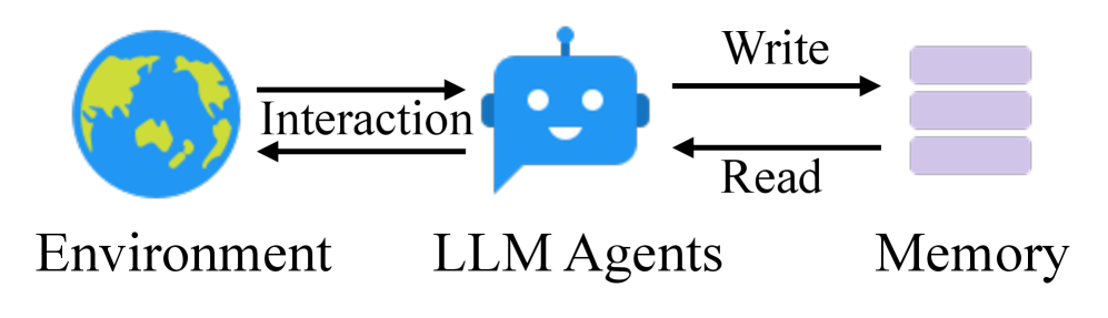
(a) Traditional memory system.
<details>
<summary>x4.png Details</summary>

### Visual Description
## Diagram: LLM Agent System Architecture
### Overview
The image is a system architecture diagram illustrating the interaction flow between an environment, Large Language Model (LLM) agents, and a specialized memory system called "Agentic Memory." It depicts a closed-loop process where agents perceive, act, and learn.
### Components/Axes
The diagram consists of three primary components arranged horizontally from left to right, connected by labeled arrows indicating data or control flow.
1. **Environment** (Leftmost component):
* **Icon:** A stylized blue and green globe, representing the external world or operational context.
* **Label:** "Environment" (text below the icon).
2. **LLM Agents** (Central component):
* **Icon:** A blue robot head with a smiling face and an antenna, symbolizing the AI agent.
* **Label:** "LLM Agents" (text below the icon).
3. **Agentic Memory** (Rightmost component):
* **Icon:** A blue robot head (identical to the LLM Agents icon) positioned to the left of three stacked, light purple rectangular blocks, representing memory storage units.
* **Label:** "Agentic Memory" (text below the icon cluster).
* **Spatial Placement:** This entire component is enclosed within a faint, light blue rectangular background, visually grouping the agent icon and memory blocks as a single subsystem.
### Detailed Analysis
The flow of information and actions is defined by the arrows connecting the components:
* **Interaction Flow (Environment ↔ LLM Agents):**
* A double-headed arrow connects the Environment and LLM Agents.
* The arrow is labeled with the word **"Interaction"** placed centrally above it.
* This indicates a bidirectional relationship: the agent perceives the environment and acts upon it.
* **Memory Access Flow (LLM Agents ↔ Agentic Memory):**
* Two separate, single-headed arrows connect the LLM Agents to the Agentic Memory subsystem.
* The top arrow points from the LLM Agents to the Agentic Memory and is labeled **"Write"**.
* The bottom arrow points from the Agentic Memory back to the LLM Agents and is labeled **"Read"**.
* This signifies that agents can store information (write) into and retrieve information (read) from the dedicated memory system.
### Key Observations
* **Bidirectional Core Loop:** The primary interaction between the agent and its environment is explicitly bidirectional, forming a perception-action cycle.
* **Dedicated Memory System:** Memory is not an internal component of the LLM Agent but a separate, specialized subsystem ("Agentic Memory") that the agent interfaces with via clear read/write operations.
* **Visual Grouping:** The Agentic Memory component is visually distinct due to its background highlight, emphasizing its role as a cohesive unit separate from the core agent.
* **Symmetry in Icons:** The use of the same robot head icon for both "LLM Agents" and within "Agentic Memory" suggests a strong conceptual link, possibly indicating that the memory is agent-centric or structured for agent use.
### Interpretation
This diagram presents a conceptual model for an advanced AI agent system that separates core reasoning (LLM Agents) from persistent, structured memory (Agentic Memory). The architecture suggests several key principles:
1. **Embodied Cognition:** The agent is not a disembodied model but is situated within an "Environment," emphasizing the importance of real-world or simulated context for its operations.
2. **Memory as a Service:** By externalizing memory into a dedicated subsystem with explicit read/write channels, the design promotes modularity, scalability, and potentially more sophisticated memory management (e.g., different memory types, indexing, or retrieval strategies) than what might be natively available within an LLM's context window.
3. **Learning and Adaptation:** The "Write" pathway is crucial for learning. It implies the agent can record experiences, facts, or learned strategies into its agentic memory for future use, enabling long-term adaptation and improvement beyond a single interaction session.
4. **Investigative Lens (Peircean):** The diagram is an *iconic* and *indexical* representation. It *iconically* resembles the system's structure (globe=world, robot=agent). It is *indexical* because the arrows point directly to the causal relationships (interaction causes state changes, read/write operations cause data transfer). The *symbolic* labels ("LLM Agents," "Agentic Memory") ground these relationships in specific technical concepts. The model argues that effective agentic AI requires a clear separation between perception/action, reasoning, and memory storage, with well-defined interfaces between them.
</details>
(b) Our proposed agentic memory.
Figure 1: Traditional memory systems require predefined memory access patterns specified in the workflow, limiting their adaptability to diverse scenarios. Contrastly, our A-Mem enhances the flexibility of LLM agents by enabling dynamic memory operations.
In this paper, we introduce a novel agentic memory system, named as A-Mem, for LLM agents that enables dynamic memory structuring without relying on static, predetermined memory operations. Our approach draws inspiration from the Zettelkasten method [15, 1], a sophisticated knowledge management system that creates interconnected information networks through atomic notes and flexible linking mechanisms. Our system introduces an agentic memory architecture that enables autonomous and flexible memory management for LLM agents. For each new memory, we construct comprehensive notes, which integrates multiple representations: structured textual attributes including several attributes and embedding vectors for similarity matching. Then A-Mem analyzes the historical memory repository to establish meaningful connections based on semantic similarities and shared attributes. This integration process not only creates new links but also enables dynamic evolution when new memories are incorporated, they can trigger updates to the contextual representations of existing memories, allowing the entire memories to continuously refine and deepen its understanding over time. The contributions are summarized as:
We present A-Mem, an agentic memory system for LLM agents that enables autonomous generation of contextual descriptions, dynamic establishment of memory connections, and intelligent evolution of existing memories based on new experiences. This system equips LLM agents with long-term interaction capabilities without requiring predetermined memory operations.
We design an agentic memory update mechanism where new memories automatically trigger two key operations: link generation and memory evolution. Link generation automatically establishes connections between memories by identifying shared attributes and similar contextual descriptions. Memory evolution enables existing memories to dynamically adapt as new experiences are analyzed, leading to the emergence of higher-order patterns and attributes.
We conduct comprehensive evaluations of our system using a long-term conversational dataset, comparing performance across six foundation models using six distinct evaluation metrics, demonstrating significant improvements. Moreover, we provide T-SNE visualizations to illustrate the structured organization of our agentic memory system.
## 2 Related Work
### 2.1 Memory for LLM Agents
Prior works on LLM agent memory systems have explored various mechanisms for memory management and utilization [23, 21, 8, 39]. Some approaches complete interaction storage, which maintains comprehensive historical records through dense retrieval models [39] or read-write memory structures [24]. Moreover, MemGPT [25] leverages cache-like architectures to prioritize recent information. Similarly, SCM [32] proposes a Self-Controlled Memory framework that enhances LLMs’ capability to maintain long-term memory through a memory stream and controller mechanism. However, these approaches face significant limitations in handling diverse real-world tasks. While they can provide basic memory functionality, their operations are typically constrained by predefined structures and fixed workflows. These constraints stem from their reliance on rigid operational patterns, particularly in memory writing and retrieval processes. Such inflexibility leads to poor generalization in new environments and limited effectiveness in long-term interactions. Therefore, designing a flexible and universal memory system that supports agents’ long-term interactions remains a crucial challenge.
### 2.2 Retrieval-Augmented Generation
Retrieval-Augmented Generation (RAG) has emerged as a powerful approach to enhance LLMs by incorporating external knowledge sources [18, 6, 10]. The standard RAG [37, 34] process involves indexing documents into chunks, retrieving relevant chunks based on semantic similarity, and augmenting the LLM’s prompt with this retrieved context for generation. Advanced RAG systems [20, 12] have evolved to include sophisticated pre-retrieval and post-retrieval optimizations. Building upon these foundations, recent researches has introduced agentic RAG systems that demonstrate more autonomous and adaptive behaviors in the retrieval process. These systems can dynamically determine when and what to retrieve [4, 14], generate hypothetical responses to guide retrieval, and iteratively refine their search strategies based on intermediate results [31, 29].
However, while agentic RAG approaches demonstrate agency in the retrieval phase by autonomously deciding when and what to retrieve [4, 14, 38], our agentic memory system exhibits agency at a more fundamental level through the autonomous evolution of its memory structure. Inspired by the Zettelkasten method, our system allows memories to actively generate their own contextual descriptions, form meaningful connections with related memories, and evolve both their content and relationships as new experiences emerge. This fundamental distinction in agency between retrieval versus storage and evolution distinguishes our approach from agentic RAG systems, which maintain static knowledge bases despite their sophisticated retrieval mechanisms.
## 3 Methodolodgy
Our proposed agentic memory system draws inspiration from the Zettelkasten method, implementing a dynamic and self-evolving memory system that enables LLM agents to maintain long-term memory without predetermined operations. The system’s design emphasizes atomic note-taking, flexible linking mechanisms, and continuous evolution of knowledge structures.
<details>
<summary>x5.png Details</summary>
### Visual Description
## System Architecture Diagram: LLM-Based Memory System for Agents
### Overview
The image is a technical system architecture diagram illustrating a four-stage pipeline for an LLM (Large Language Model) agent memory system. The system processes interactions from an environment, constructs structured "Notes," organizes them into a memory store, evolves the memory over time, and retrieves relevant information to inform agent actions. The diagram flows from left to right, depicting a cyclical process of memory creation, storage, refinement, and usage.
### Components/Axes
The diagram is divided into four primary vertical sections, each with a header:
1. **Note Construction** (Leftmost section)
2. **Link Generation** (Center-left)
3. **Memory Evolution** (Center-right)
4. **Memory Retrieval** (Rightmost section)
**Key Visual Components & Labels:**
* **Icons:** Globe (Environment), Robot (LLM Agents), Database cylinder (Memory), Document/Note icons, LLM symbol (spiral/gear), Text Model icon, Query icon.
* **Textual Labels & Flow Arrows:**
* `Environment`, `LLM Agents`, `Interaction`, `Write`, `Conversation 1`, `Conversation 2`, `LLM`, `Note`, `Note Attributes:`, `Timestamp`, `Content`, `Context`, `Keywords`, `Tags`, `Embedding`.
* `Memory`, `Box 1`, `Box i`, `Box j`, `Box n`, `Top-k`, `Retrieve`, `Store`, `m_j`.
* `Box n+1`, `Box n+2`, `LLM`, `Action`, `Evolve`.
* `Retrieve`, `Query`, `Text Model`, `Query Embedding`, `Top-k`, `1st`, `Relative Memory`, `LLM Agents`.
### Detailed Analysis
**1. Note Construction (Left Section):**
* **Process:** An `Environment` (globe icon) and `LLM Agents` (robot icon) engage in `Interaction`. This interaction is used to `Write` conversations.
* **Example Conversations:** Two text boxes show example dialogues:
* `Conversation 1`: "Can you help me implement a custom cache system for my web application? I need it to handle both memory and disk storage."
* `Conversation 2`: "The cache system works great, but we're seeing high memory usage in production. Can we modify it to implement an LRU eviction policy?"
* **Note Creation:** Each conversation is processed by an `LLM` (spiral icon) to generate a structured `Note`.
* **Note Attributes:** A list specifies the components of a Note: `Timestamp`, `Content`, `Context`, `Keywords`, `Tags`, and an `Embedding` (represented by a pink bar graph).
**2. Link Generation (Center-Left Section):**
* **Memory Store:** A central `Memory` database contains multiple storage units labeled as `Box 1`, `Box i`, `Box j`, through `Box n`. Each Box contains multiple document icons.
* **Retrieval & Processing:** A `Retrieve` arrow points from the `Memory` to a selection process labeled `Top-k`. This selects a subset of notes (represented by a cluster of document icons labeled `m_j`).
* **LLM Processing & Storage:** The selected notes (`m_j`) are processed by an `LLM`. The output is then directed via a `Store` arrow into new memory boxes: `Box n+1` and `Box n+2`.
**3. Memory Evolution (Center-Right Section):**
* **Input:** Takes the newly created `Box n+1` and `Box n+2` from the Link Generation stage.
* **Process:** These boxes are fed into an `LLM`.
* **Output:** The LLM produces an `Action` (document icons) which leads to an `Evolve` step (represented by a circular arrow icon), suggesting an update or refinement process for the memory structure.
**4. Memory Retrieval (Right Section):**
* **Query Input:** A `Query` (question mark icon) is processed by a `Text Model` to create a `Query Embedding` (pink bar graph).
* **Retrieval:** This embedding is used to `Retrieve` information from the main `Memory` store (arrow points left to the Link Generation section's Memory).
* **Ranking & Output:** The retrieval yields a `Top-k` result, with the `1st` ranked result highlighted as `Relative Memory` (a set of three document icons).
* **Action:** This `Relative Memory` is then passed to the `LLM Agents` (robot icon) to inform their next action.
### Key Observations
* **Cyclical Flow:** The diagram depicts a closed-loop system where agent interactions generate memory, which is stored, evolved, and then retrieved to guide future agent actions, creating a continuous learning cycle.
* **LLM as Core Processor:** The LLM symbol appears in three distinct stages (Note Construction, Link Generation/Memory Evolution, and implicitly in Retrieval via the Text Model), highlighting its central role in structuring, processing, and utilizing unstructured conversational data.
* **Hierarchical Memory:** Memory is not a flat list but is organized into `Boxes`, suggesting a structured or clustered organization. The `Top-k` mechanism is used both for selecting notes to process and for retrieving relevant memories.
* **From Unstructured to Structured:** The system's primary function is to transform raw, unstructured `Conversation` text into structured, attribute-rich `Notes` with embeddings, making them machine-searchable and actionable.
* **Evolution Mechanism:** The dedicated `Memory Evolution` stage implies the system doesn't just store data statically but has a mechanism to update, consolidate, or refine its memory structure over time based on new information.
### Interpretation
This diagram outlines a sophisticated cognitive architecture for AI agents, addressing the critical challenge of long-term memory and experience accumulation. The system's design suggests several key principles:
1. **Experience as Data:** Every agent interaction is treated as a valuable data point to be captured, not just a transient event. This enables learning from past successes and failures.
2. **Structured Abstraction:** The conversion of conversations into "Notes" with metadata (keywords, tags, context) and embeddings is a form of abstraction. It allows the system to move beyond keyword matching to semantic understanding and relationship mapping between different experiences.
3. **Dynamic Knowledge Base:** The `Link Generation` and `Memory Evolution` stages indicate this is not a static log. The system actively processes its memories to form new links (`m_j` processed into `Box n+1/n+2`) and evolve its understanding, mimicking how human memory consolidates and reorganizes information.
4. **Context-Aware Retrieval:** The retrieval process uses a query embedding to find the `Relative Memory`, implying semantic search. This ensures agents recall not just exact matches but contextually relevant past experiences, which is crucial for complex, ongoing tasks.
5. **Scalability & Efficiency:** The use of `Top-k` selection at multiple stages is a practical design choice for scalability, allowing the system to work with a large memory store by focusing processing and retrieval on the most relevant subsets.
**Underlying Purpose:** The architecture aims to create agents that are not stateless but have a persistent, evolving "experience memory." This would allow for more coherent, personalized, and improved long-term performance in tasks like technical support (as hinted by the cache system example), interactive storytelling, or complex project management, where context from distant past interactions is vital. The explicit "Evolve" step is particularly notable, suggesting the system is designed to improve its own memory organization over time, a step towards more autonomous and adaptive AI.
</details>
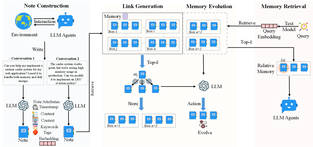
Figure 2: Our A-Mem architecture comprises three integral parts in memory storage. During note construction, the system processes new interaction memories and stores them as notes with multiple attributes. The link generation process first retrieves the most relevant historical memories and then employs an LLM to determine whether connections should be established between them. The concept of a ’box’ describes that related memories become interconnected through their similar contextual descriptions, analogous to the Zettelkasten method. However, our approach allows individual memories to exist simultaneously within multiple different boxes. During the memory retrieval stage, we extract query embeddings using a text encoding model and search the memory database for relevant matches. When related memory is retrieved, similar memories that are linked within the same box are also automatically accessed.
### 3.1 Note Construction
Building upon the Zettelkasten method’s principles of atomic note-taking and flexible organization, we introduce an LLM-driven approach to memory note construction. When an agent interacts with its environment, we construct structured memory notes that capture both explicit information and LLM-generated contextual understanding. Each memory note $m_i$ in our collection $M=\{m_1,m_2,...,m_N\}$ is represented as:
$$
m_i=\{c_i,t_i,K_i,G_i,X_i,e_i,L_i\} \tag{1}
$$
where $c_i$ represents the original interaction content, $t_i$ is the timestamp of the interaction, $K_i$ denotes LLM-generated keywords that capture key concepts, $G_i$ contains LLM-generated tags for categorization, $X_i$ represents the LLM-generated contextual description that provides rich semantic understanding, and $L_i$ maintains the set of linked memories that share semantic relationships. To enrich each memory note with meaningful context beyond its basic content and timestamp, we leverage an LLM to analyze the interaction and generate these semantic components. The note construction process involves prompting the LLM with carefully designed templates $P_s1$ :
$$
K_i,G_i,X_i←LLM(c_i \Vert t_i \Vert P_s1) \tag{2}
$$
Following the Zettelkasten principle of atomicity, each note captures a single, self-contained unit of knowledge. To enable efficient retrieval and linking, we compute a dense vector representation via a text encoder [27] that encapsulates all textual components of the note:
$$
e_i=f_enc[ concat(c_i,K_i,G_i,X_i) ] \tag{3}
$$
By using LLMs to generate enriched components, we enable autonomous extraction of implicit knowledge from raw interactions. The multi-faceted note structure ( $K_i$ , $G_i$ , $X_i$ ) creates rich representations that capture different aspects of the memory, facilitating nuanced organization and retrieval. Additionally, the combination of LLM-generated semantic components with dense vector representations provides both context and computationally efficient similarity matching.
### 3.2 Link Generation
Our system implements an autonomous link generation mechanism that enables new memory notes to form meaningful connections without predefined rules. When the constrctd memory note $m_n$ is added to the system, we first leverage its semantic embedding for similarity-based retrieval. For each existing memory note $m_j∈M$ , we compute a similarity score:
$$
s_n,j=\frac{e_n· e_j}{|e_n||e_j|} \tag{4}
$$
The system then identifies the top- $k$ most relevant memories:
$$
M_near^n=\{m_j| rank(s_n,j)≤ k,m_j∈M\} \tag{5}
$$
Based on these candidate nearest memories, we prompt the LLM to analyze potential connections based on their potential common attributes. Formally, the link set of memory $m_n$ update like:
$$
L_i←LLM(m_n \VertM_near^n \Vert P_s2) \tag{6}
$$
Each generated link $l_i$ is structured as: $L_i=\{m_i,...,m_k\}$ . By using embedding-based retrieval as an initial filter, we enable efficient scalability while maintaining semantic relevance. A-Mem can quickly identify potential connections even in large memory collections without exhaustive comparison. More importantly, the LLM-driven analysis allows for nuanced understanding of relationships that goes beyond simple similarity metrics. The language model can identify subtle patterns, causal relationships, and conceptual connections that might not be apparent from embedding similarity alone. We implements the Zettelkasten principle of flexible linking while leveraging modern language models. The resulting network emerges organically from memory content and context, enabling natural knowledge organization.
### 3.3 Memory Evolution
After creating links for the new memory, A-Mem evolves the retrieved memories based on their textual information and relationships with the new memory. For each memory $m_j$ in the nearest neighbor set $M_near^n$ , the system determines whether to update its context, keywords, and tags. This evolution process can be formally expressed as:
$$
m_j^*←LLM(m_n \VertM_near^n∖ m_j \Vert m_j \Vert P_s3) \tag{7}
$$
The evolved memory $m_j^*$ then replaces the original memory $m_j$ in the memory set $M$ . This evolutionary approach enables continuous updates and new connections, mimicking human learning processes. As the system processes more memories over time, it develops increasingly sophisticated knowledge structures, discovering higher-order patterns and concepts across multiple memories. This creates a foundation for autonomous memory learning where knowledge organization becomes progressively richer through the ongoing interaction between new experiences and existing memories.
### 3.4 Retrieve Relative Memory
In each interaction, our A-Mem performs context-aware memory retrieval to provide the agent with relevant historical information. Given a query text $q$ from the current interaction, we first compute its dense vector representation using the same text encoder used for memory notes:
$$
e_q=f_enc(q) \tag{8}
$$
The system then computes similarity scores between the query embedding and all existing memory notes in $M$ using cosine similarity:
$$
s_q,i=\frac{e_q· e_i}{|e_q||e_i|},where e_i∈ m_i, ∀ m_i∈M \tag{9}
$$
Then we retrieve the k most relevant memories from the historical memory storage to construct a contextually appropriate prompt.
$$
M_retrieved=\{m_i|rank(s_q,i)≤ k,m_i∈M\} \tag{10}
$$
These retrieved memories provide relevant historical context that helps the agent better understand and respond to the current interaction. The retrieved context enriches the agent’s reasoning process by connecting the current interaction with related past experiences stored in the memory system.
## 4 Experiment
### 4.1 Dataset and Evaluation
To evaluate the effectiveness of instruction-aware recommendation in long-term conversations, we utilize the LoCoMo dataset [22], which contains significantly longer dialogues compared to existing conversational datasets [36, 13]. While previous datasets contain dialogues with around 1K tokens over 4-5 sessions, LoCoMo features much longer conversations averaging 9K tokens spanning up to 35 sessions, making it particularly suitable for evaluating models’ ability to handle long-range dependencies and maintain consistency over extended conversations. The LoCoMo dataset comprises diverse question types designed to comprehensively evaluate different aspects of model understanding: (1) single-hop questions answerable from a single session; (2) multi-hop questions requiring information synthesis across sessions; (3) temporal reasoning questions testing understanding of time-related information; (4) open-domain knowledge questions requiring integration of conversation context with external knowledge; and (5) adversarial questions assessing models’ ability to identify unanswerable queries. In total, LoCoMo contains 7,512 question-answer pairs across these categories. Besides, we use a new dataset, named DialSim [16], to evaluate the effectiveness of our memory system. It is question-answering dataset derived from long-term multi-party dialogues. The dataset is derived from popular TV shows (Friends, The Big Bang Theory, and The Office), covering 1,300 sessions spanning five years, containing approximately 350,000 tokens, and including more than 1,000 questions per session from refined fan quiz website questions and complex questions generated from temporal knowledge graphs.
For comparison baselines, we compare to LoCoMo [22], ReadAgent [17], MemoryBank [39] and MemGPT [25]. The detailed introduction of baselines can be found in Appendix A.1 For evaluation, we employ two primary metrics: the F1 score to assess answer accuracy by balancing precision and recall, and BLEU-1 [26] to evaluate generated response quality by measuring word overlap with ground truth responses. Also, we report the average token length for answering one question. Besides reporting experiment results with four additional metrics (ROUGE-L, ROUGE-2, METEOR, and SBERT Similarity), we also present experimental outcomes using different foundation models including DeepSeek-R1-32B [11], Claude 3.0 Haiku [2], and Claude 3.5 Haiku [3] in Appendix A.3.
### 4.2 Implementation Details
For all baselines and our proposed method, we maintain consistency by employing identical system prompts as detailed in Appendix B. The deployment of Qwen-1.5B/3B and Llama 3.2 1B/3B models is accomplished through local instantiation using Ollama https://github.com/ollama/ollama, with LiteLLM https://github.com/BerriAI/litellm managing structured output generation. For GPT models, we utilize the official structured output API. In our memory retrieval process, we primarily employ $k$ =10 for top- $k$ memory selection to maintain computational efficiency, while adjusting this parameter for specific categories to optimize performance. The detailed configurations of $k$ can be found in Appendix A.5. For text embedding, we implement the all-minilm-l6-v2 model across all experiments.
Table 1: Experimental results on LoCoMo dataset of QA tasks across five categories (Multi Hop, Temporal, Open Domain, Single Hop, and Adversial) using different methods. Results are reported in F1 and BLEU-1 (%) scores. The best performance is marked in bold, and our proposed method A-Mem (highlighted in gray) demonstrates competitive performance across six foundation language models.
| Model | Method | Category | Average | | | | | | | | | | | | |
| --- | --- | --- | --- | --- | --- | --- | --- | --- | --- | --- | --- | --- | --- | --- | --- |
| Multi Hop | Temporal | Open Domain | Single Hop | Adversial | Ranking | Token | | | | | | | | | |
| F1 | BLEU | F1 | BLEU | F1 | BLEU | F1 | BLEU | F1 | BLEU | F1 | BLEU | Length | | | |
| GPT | 4o-mini | LoCoMo | 25.02 | 19.75 | 18.41 | 14.77 | 12.04 | 11.16 | 40.36 | 29.05 | 69.23 | 68.75 | 2.4 | 2.4 | 16,910 |
| ReadAgent | 9.15 | 6.48 | 12.60 | 8.87 | 5.31 | 5.12 | 9.67 | 7.66 | 9.81 | 9.02 | 4.2 | 4.2 | 643 | | |
| MemoryBank | 5.00 | 4.77 | 9.68 | 6.99 | 5.56 | 5.94 | 6.61 | 5.16 | 7.36 | 6.48 | 4.8 | 4.8 | 432 | | |
| MemGPT | 26.65 | 17.72 | 25.52 | 19.44 | 9.15 | 7.44 | 41.04 | 34.34 | 43.29 | 42.73 | 2.4 | 2.4 | 16,977 | | |
| A-Mem | 27.02 | 20.09 | 45.85 | 36.67 | 12.14 | 12.00 | 44.65 | 37.06 | 50.03 | 49.47 | 1.2 | 1.2 | 2,520 | | |
| 4o | LoCoMo | 28.00 | 18.47 | 9.09 | 5.78 | 16.47 | 14.80 | 61.56 | 54.19 | 52.61 | 51.13 | 2.0 | 2.0 | 16,910 | |
| ReadAgent | 14.61 | 9.95 | 4.16 | 3.19 | 8.84 | 8.37 | 12.46 | 10.29 | 6.81 | 6.13 | 4.0 | 4.0 | 805 | | |
| MemoryBank | 6.49 | 4.69 | 2.47 | 2.43 | 6.43 | 5.30 | 8.28 | 7.10 | 4.42 | 3.67 | 5.0 | 5.0 | 569 | | |
| MemGPT | 30.36 | 22.83 | 17.29 | 13.18 | 12.24 | 11.87 | 60.16 | 53.35 | 34.96 | 34.25 | 2.4 | 2.4 | 16,987 | | |
| A-Mem | 32.86 | 23.76 | 39.41 | 31.23 | 17.10 | 15.84 | 48.43 | 42.97 | 36.35 | 35.53 | 1.6 | 1.6 | 1,216 | | |
| Qwen2.5 | 1.5b | LoCoMo | 9.05 | 6.55 | 4.25 | 4.04 | 9.91 | 8.50 | 11.15 | 8.67 | 40.38 | 40.23 | 3.4 | 3.4 | 16,910 |
| ReadAgent | 6.61 | 4.93 | 2.55 | 2.51 | 5.31 | 12.24 | 10.13 | 7.54 | 5.42 | 27.32 | 4.6 | 4.6 | 752 | | |
| MemoryBank | 11.14 | 8.25 | 4.46 | 2.87 | 8.05 | 6.21 | 13.42 | 11.01 | 36.76 | 34.00 | 2.6 | 2.6 | 284 | | |
| MemGPT | 10.44 | 7.61 | 4.21 | 3.89 | 13.42 | 11.64 | 9.56 | 7.34 | 31.51 | 28.90 | 3.4 | 3.4 | 16,953 | | |
| A-Mem | 18.23 | 11.94 | 24.32 | 19.74 | 16.48 | 14.31 | 23.63 | 19.23 | 46.00 | 43.26 | 1.0 | 1.0 | 1,300 | | |
| 3b | LoCoMo | 4.61 | 4.29 | 3.11 | 2.71 | 4.55 | 5.97 | 7.03 | 5.69 | 16.95 | 14.81 | 3.2 | 3.2 | 16,910 | |
| ReadAgent | 2.47 | 1.78 | 3.01 | 3.01 | 5.57 | 5.22 | 3.25 | 2.51 | 15.78 | 14.01 | 4.2 | 4.2 | 776 | | |
| MemoryBank | 3.60 | 3.39 | 1.72 | 1.97 | 6.63 | 6.58 | 4.11 | 3.32 | 13.07 | 10.30 | 4.2 | 4.2 | 298 | | |
| MemGPT | 5.07 | 4.31 | 2.94 | 2.95 | 7.04 | 7.10 | 7.26 | 5.52 | 14.47 | 12.39 | 2.4 | 2.4 | 16,961 | | |
| A-Mem | 12.57 | 9.01 | 27.59 | 25.07 | 7.12 | 7.28 | 17.23 | 13.12 | 27.91 | 25.15 | 1.0 | 1.0 | 1,137 | | |
| Llama 3.2 | 1b | LoCoMo | 11.25 | 9.18 | 7.38 | 6.82 | 11.90 | 10.38 | 12.86 | 10.50 | 51.89 | 48.27 | 3.4 | 3.4 | 16,910 |
| ReadAgent | 5.96 | 5.12 | 1.93 | 2.30 | 12.46 | 11.17 | 7.75 | 6.03 | 44.64 | 40.15 | 4.6 | 4.6 | 665 | | |
| MemoryBank | 13.18 | 10.03 | 7.61 | 6.27 | 15.78 | 12.94 | 17.30 | 14.03 | 52.61 | 47.53 | 2.0 | 2.0 | 274 | | |
| MemGPT | 9.19 | 6.96 | 4.02 | 4.79 | 11.14 | 8.24 | 10.16 | 7.68 | 49.75 | 45.11 | 4.0 | 4.0 | 16,950 | | |
| A-Mem | 19.06 | 11.71 | 17.80 | 10.28 | 17.55 | 14.67 | 28.51 | 24.13 | 58.81 | 54.28 | 1.0 | 1.0 | 1,376 | | |
| 3b | LoCoMo | 6.88 | 5.77 | 4.37 | 4.40 | 10.65 | 9.29 | 8.37 | 6.93 | 30.25 | 28.46 | 2.8 | 2.8 | 16,910 | |
| ReadAgent | 2.47 | 1.78 | 3.01 | 3.01 | 5.57 | 5.22 | 3.25 | 2.51 | 15.78 | 14.01 | 4.2 | 4.2 | 461 | | |
| MemoryBank | 6.19 | 4.47 | 3.49 | 3.13 | 4.07 | 4.57 | 7.61 | 6.03 | 18.65 | 17.05 | 3.2 | 3.2 | 263 | | |
| MemGPT | 5.32 | 3.99 | 2.68 | 2.72 | 5.64 | 5.54 | 4.32 | 3.51 | 21.45 | 19.37 | 3.8 | 3.8 | 16,956 | | |
| A-Mem | 17.44 | 11.74 | 26.38 | 19.50 | 12.53 | 11.83 | 28.14 | 23.87 | 42.04 | 40.60 | 1.0 | 1.0 | 1,126 | | |
### 4.3 Empricial Results
Performance Analysis. In our empirical evaluation, we compared A-Mem with four competitive baselines including LoCoMo [22], ReadAgent [17], MemoryBank [39], and MemGPT [25] on the LoCoMo dataset. For non-GPT foundation models, our A-Mem consistently outperforms all baselines across different categories, demonstrating the effectiveness of our agentic memory approach. For GPT-based models, while LoCoMo and MemGPT show strong performance in certain categories like Open Domain and Adversial tasks due to their robust pre-trained knowledge in simple fact retrieval, our A-Mem demonstrates superior performance in Multi-Hop tasks achieves at least two times better performance that require complex reasoning chains. In addition to experiments on the LoCoMo dataset, we also compare our method on the DialSim dataset against LoCoMo and MemGPT. A-Mem consistently outperforms all baselines across evaluation metrics, achieving an F1 score of 3.45 (a 35% improvement over LoCoMo’s 2.55 and 192% higher than MemGPT’s 1.18). The effectiveness of A-Mem stems from its novel agentic memory architecture that enables dynamic and structured memory management. Unlike traditional approaches that use static memory operations, our system creates interconnected memory networks through atomic notes with rich contextual descriptions, enabling more effective multi-hop reasoning. The system’s ability to dynamically establish connections between memories based on shared attributes and continuously update existing memory descriptions with new contextual information allows it to better capture and utilize the relationships between different pieces of information.
Table 2: Comparison of different memory mechanisms across multiple evaluation metrics on DialSim [16]. Higher scores indicate better performance, with A-Mem showing superior results across all metrics.
| Method | F1 | BLEU-1 | ROUGE-L | ROUGE-2 | METEOR | SBERT Similarity |
| --- | --- | --- | --- | --- | --- | --- |
| LoCoMo | 2.55 | 3.13 | 2.75 | 0.90 | 1.64 | 15.76 |
| MemGPT | 1.18 | 1.07 | 0.96 | 0.42 | 0.95 | 8.54 |
| A-Mem | 3.45 | 3.37 | 3.54 | 3.60 | 2.05 | 19.51 |
Cost-Efficiency Analysis. A-Mem demonstrates significant computational and cost efficiency alongside strong performance. The system requires approximately 1,200 tokens per memory operation, achieving an 85-93% reduction in token usage compared to baseline methods (LoCoMo and MemGPT with 16,900 tokens) through our selective top-k retrieval mechanism. This substantial token reduction directly translates to lower operational costs, with each memory operation costing less than $0.0003 when using commercial API services—making large-scale deployments economically viable. Processing times average 5.4 seconds using GPT-4o-mini and only 1.1 seconds with locally-hosted Llama 3.2 1B on a single GPU. Despite requiring multiple LLM calls during memory processing, A-Mem maintains this cost-effective resource utilization while consistently outperforming baseline approaches across all foundation models tested, particularly doubling performance on complex multi-hop reasoning tasks. This balance of low computational cost and superior reasoning capability highlights A-Mem ’s practical advantage for deployment in the real world.
Table 3: An ablation study was conducted to evaluate our proposed method against the GPT-4o-mini base model. The notation ’w/o’ indicates experiments where specific modules were removed. The abbreviations LG and ME denote the link generation module and memory evolution module, respectively.
| Method | Category | | | | | | | | | |
| --- | --- | --- | --- | --- | --- | --- | --- | --- | --- | --- |
| Multi Hop | Temporal | Open Domain | Single Hop | Adversial | | | | | | |
| F1 | BLEU-1 | F1 | BLEU-1 | F1 | BLEU-1 | F1 | BLEU-1 | F1 | BLEU-1 | |
| w/o LG & ME | 9.65 | 7.09 | 24.55 | 19.48 | 7.77 | 6.70 | 13.28 | 10.30 | 15.32 | 18.02 |
| w/o ME | 21.35 | 15.13 | 31.24 | 27.31 | 10.13 | 10.85 | 39.17 | 34.70 | 44.16 | 45.33 |
| A-Mem | 27.02 | 20.09 | 45.85 | 36.67 | 12.14 | 12.00 | 44.65 | 37.06 | 50.03 | 49.47 |
### 4.4 Ablation Study
To evaluate the effectiveness of the Link Generation (LG) and Memory Evolution (ME) modules, we conduct the ablation study by systematically removing key components of our model. When both LG and ME modules are removed, the system exhibits substantial performance degradation, particularly in Multi Hop reasoning and Open Domain tasks. The system with only LG active (w/o ME) shows intermediate performance levels, maintaining significantly better results than the version without both modules, which demonstrates the fundamental importance of link generation in establishing memory connections. Our full model, A-Mem, consistently achieves the best performance across all evaluation categories, with particularly strong results in complex reasoning tasks. These results reveal that while the link generation module serves as a critical foundation for memory organization, the memory evolution module provides essential refinements to the memory structure. The ablation study validates our architectural design choices and highlights the complementary nature of these two modules in creating an effective memory system.
<details>
<summary>x6.png Details</summary>
### Visual Description
## Grouped Bar Chart: Performance Metrics by k Values
### Overview
The image displays a grouped bar chart comparing two performance metrics, F1 and BLEU-1, across five different "k values" (10, 20, 30, 40, 50). The chart uses a blue and orange color scheme to differentiate the two metrics.
### Components/Axes
* **Chart Type:** Grouped Bar Chart.
* **X-Axis:** Labeled "k values". It has five categorical tick marks: 10, 20, 30, 40, and 50.
* **Y-Axis:** Numerical scale ranging from 12.5 to 27.5, with major gridlines at intervals of 2.5 (12.5, 15.0, 17.5, 20.0, 22.5, 25.0, 27.5). The axis title is not explicitly shown, but the values represent the score for the metrics.
* **Legend:** Located in the top-left corner of the plot area.
* A blue square corresponds to the label "F1".
* An orange square corresponds to the label "BLEU-1".
* **Data Labels:** Each bar has its exact numerical value displayed directly above it.
### Detailed Analysis
The chart presents paired bars for each k value. The left bar in each pair is blue (F1), and the right bar is orange (BLEU-1).
**Data Series: F1 (Blue Bars)**
* **Trend:** The F1 score increases sharply from k=10 to k=20, continues to increase to a peak at k=40, and then shows a very slight decrease at k=50.
* **Data Points:**
* k=10: 19.91
* k=20: 25.87
* k=30: 26.97
* k=40: 27.02
* k=50: 26.81
**Data Series: BLEU-1 (Orange Bars)**
* **Trend:** The BLEU-1 score increases from k=10 to k=30, then plateaus with very minor fluctuations for k=40 and k=50.
* **Data Points:**
* k=10: 14.36
* k=20: 19.45
* k=30: 20.19
* k=40: 20.09
* k=50: 20.15
### Key Observations
1. **Consistent Performance Gap:** The F1 score is consistently higher than the BLEU-1 score for every k value. The gap is smallest at k=10 (5.55 points) and largest at k=20 (6.42 points).
2. **Peak Performance:** Both metrics achieve their highest values at k=40 (F1: 27.02) and k=30 (BLEU-1: 20.19). The performance for both metrics is very similar between k=30, 40, and 50, suggesting a plateau.
3. **Initial Sensitivity:** Both metrics show the most significant improvement when moving from k=10 to k=20. The rate of improvement slows considerably for higher k values.
4. **Stability at High k:** For k values of 30 and above, the scores for both metrics are remarkably stable, with changes of less than 0.2 points between consecutive steps.
### Interpretation
This chart likely evaluates the performance of a machine learning or information retrieval system where "k" is a key hyperparameter (e.g., number of retrieved documents, nearest neighbors, or clusters).
* **What the data suggests:** Increasing the k value from 10 to 30 yields substantial gains in both F1 (a measure of a test's accuracy, combining precision and recall) and BLEU-1 (a metric for evaluating machine-translated text against reference translations, focusing on unigram precision). Beyond k=30, there are diminishing returns; performance stabilizes or even slightly regresses. This indicates an optimal operating point for k likely lies between 30 and 40 for this specific task and evaluation setup.
* **Relationship between elements:** The parallel trends of F1 and BLEU-1 suggest that the factor "k" influences both aspects of system performance in a similar manner. The consistent gap indicates that the system is inherently better at optimizing for the F1 criterion than for the BLEU-1 criterion under these conditions.
* **Notable anomaly:** The slight dip in F1 at k=50 (26.81) compared to k=40 (27.02) is minimal but could indicate the onset of overfitting or noise introduction as k becomes too large. The BLEU-1 score, however, remains virtually unchanged, suggesting different sensitivity of the metrics to this parameter at its upper range.
</details>
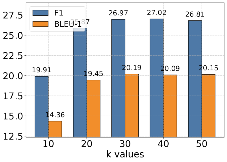
(a) Multi Hop
<details>
<summary>x7.png Details</summary>
### Visual Description
## Grouped Bar Chart: F1 vs. BLEU-1 Scores Across k Values
### Overview
This is a grouped bar chart comparing the performance of two metrics, F1 and BLEU-1, across five different "k values" (10, 20, 30, 40, 50). The chart demonstrates how these two evaluation scores change as the parameter `k` increases.
### Components/Axes
* **Chart Type:** Grouped Bar Chart.
* **X-Axis:** Labeled **"k values"**. It contains five categorical groups: `10`, `20`, `30`, `40`, `50`.
* **Y-Axis:** Numerical scale ranging from **35.0** to **47.5**, with major tick marks at intervals of 2.5 (35.0, 37.5, 40.0, 42.5, 45.0, 47.5). The axis title is not explicitly stated but represents the score value.
* **Legend:** Positioned in the **top-left corner** of the chart area.
* A blue square corresponds to the label **"F1"**.
* An orange square corresponds to the label **"BLEU-1"**.
* **Data Series:** Two series of bars are plotted for each k value.
* **F1 Series (Blue Bars):** Positioned on the **left** within each k-value group.
* **BLEU-1 Series (Orange Bars):** Positioned on the **right** within each k-value group.
### Detailed Analysis
**Data Points and Trends:**
1. **k = 10:**
* **F1 (Blue, Left):** The bar height corresponds to the value **43.60**, annotated directly above the bar.
* **BLEU-1 (Orange, Right):** The bar height corresponds to the value **35.53**, annotated directly above the bar.
* *Trend Check:* F1 score is significantly higher than BLEU-1 at this starting point.
2. **k = 20:**
* **F1 (Blue, Left):** The bar height corresponds to the value **45.03**, annotated directly above the bar.
* **BLEU-1 (Orange, Right):** The bar height corresponds to the value **35.85**, annotated directly above the bar.
* *Trend Check:* Both scores show a slight increase from k=10. The F1 score increases by ~1.43 points, while BLEU-1 increases by ~0.32 points.
3. **k = 30:**
* **F1 (Blue, Left):** The bar height corresponds to the value **45.22**, annotated directly above the bar.
* **BLEU-1 (Orange, Right):** The bar height corresponds to the value **36.44**, annotated directly above the bar.
* *Trend Check:* F1 continues a very slight upward trend (+0.19). BLEU-1 shows a more noticeable increase (+0.59).
4. **k = 40:**
* **F1 (Blue, Left):** The bar height corresponds to the value **45.85**, annotated directly above the bar.
* **BLEU-1 (Orange, Right):** The bar height corresponds to the value **36.67**, annotated directly above the bar.
* *Trend Check:* This represents the **peak value for both metrics** in this chart. F1 increases by +0.63, and BLEU-1 increases by +0.23 from k=30.
5. **k = 50:**
* **F1 (Blue, Left):** The bar height corresponds to the value **45.60**, annotated directly above the bar.
* **BLEU-1 (Orange, Right):** The bar height corresponds to the value **35.76**, annotated directly above the bar.
* *Trend Check:* Both metrics show a **decline** from their peak at k=40. F1 decreases by -0.25, and BLEU-1 decreases more sharply by -0.91.
### Key Observations
1. **Consistent Performance Gap:** The F1 score is consistently and significantly higher (by approximately 8-10 points) than the BLEU-1 score across all tested k values.
2. **Similar Trend Pattern:** Both metrics follow a similar trajectory: they increase from k=10 to k=40 and then decrease at k=50. This suggests the parameter `k` influences both evaluation aspects in a correlated manner.
3. **Optimal k Value:** The data indicates that **k=40** yields the highest performance for both the F1 and BLEU-1 metrics within the tested range.
4. **Sensitivity at Higher k:** The drop in performance from k=40 to k=50 is more pronounced for BLEU-1 (-0.91) than for F1 (-0.25), suggesting BLEU-1 may be more sensitive to increases in `k` beyond the optimal point.
### Interpretation
This chart likely evaluates a machine learning or natural language processing model where `k` is a hyperparameter (e.g., the number of candidates considered, beam search width, or nearest neighbors). The F1 score (a measure of a test's accuracy, balancing precision and recall) and BLEU-1 (a metric for evaluating machine-translated text against human references, focusing on unigram precision) are used as complementary performance indicators.
The data suggests that increasing the `k` parameter generally improves model performance up to a point (k=40), after which performance degrades. This is a classic example of a **bias-variance tradeoff** or a **diminishing returns** scenario. A very low `k` might be too restrictive (high bias), missing good solutions. An excessively high `k` (k=50) might introduce noise or computational inefficiency (high variance), leading to worse outcomes. The consistent gap between F1 and BLEU-1 implies that while the model's overall predictive accuracy (F1) is relatively high, its specific precision in matching reference outputs (BLEU-1) is lower, which is common in generative tasks. The key takeaway for a practitioner would be to set `k` to approximately 40 for optimal results on these combined metrics.
</details>
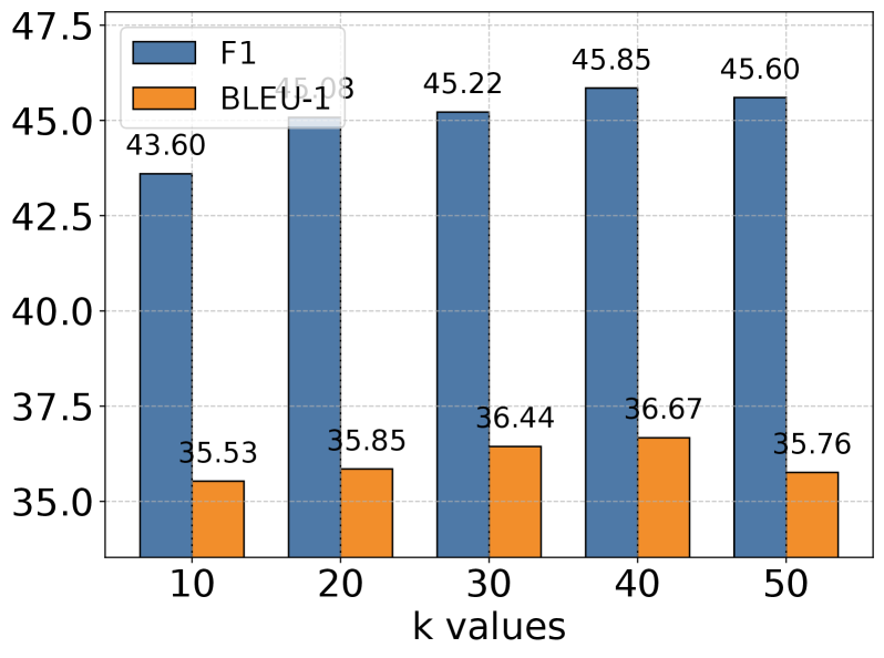
(b) Temporal
<details>
<summary>x8.png Details</summary>
### Visual Description
## Grouped Bar Chart: F1 vs. BLEU-1 Scores by k Value
### Overview
The image is a grouped bar chart comparing the performance of two metrics, F1 and BLEU-1, across five different values of a parameter labeled "k". The chart displays numerical scores on the y-axis against discrete k values on the x-axis. Each k value has a pair of bars: a blue bar for the F1 score and an orange bar for the BLEU-1 score.
### Components/Axes
* **Chart Type:** Grouped Bar Chart.
* **X-Axis:**
* **Label:** "k values"
* **Categories/Markers:** 10, 20, 30, 40, 50.
* **Y-Axis:**
* **Scale:** Linear, ranging from 6 to 14.
* **Major Tick Marks:** 6, 8, 10, 12, 14.
* **Legend:**
* **Position:** Top-left corner of the chart area.
* **Items:**
* A blue square labeled "F1".
* An orange square labeled "BLEU-1".
* **Data Labels:** Each bar has its exact numerical value displayed directly above it.
### Detailed Analysis
The chart presents the following data points for each k value:
| k value | F1 Score (Blue Bar) | BLEU-1 Score (Orange Bar) |
| :------ | :------------------ | :------------------------ |
| **10** | 7.38 | 7.03 |
| **20** | 10.29 | 9.61 |
| **30** | 12.24 | 10.57 |
| **40** | 10.35 | 9.76 |
| **50** | 12.14 | 12.00 |
**Trend Verification:**
* **F1 Series (Blue):** The line connecting the tops of the blue bars shows an overall upward trend from k=10 to k=50, with a notable peak at k=30 (12.24) and a dip at k=40 (10.35) before rising again at k=50.
* **BLEU-1 Series (Orange):** The line connecting the tops of the orange bars also shows a general upward trend. It increases from k=10 to k=30, dips slightly at k=40, and then reaches its highest point at k=50.
### Key Observations
1. **Consistent Performance Gap:** For every k value shown, the F1 score is higher than the corresponding BLEU-1 score.
2. **Peak Performance:** The highest F1 score (12.24) occurs at k=30. The highest BLEU-1 score (12.00) occurs at k=50.
3. **Performance Dip at k=40:** Both metrics show a decrease in score when moving from k=30 to k=40, breaking the otherwise increasing trend.
4. **Convergence at k=50:** At k=50, the scores for F1 (12.14) and BLEU-1 (12.00) are very close, representing the smallest gap between the two metrics on the chart.
5. **Lowest Performance:** The lowest scores for both metrics are at k=10 (F1: 7.38, BLEU-1: 7.03).
### Interpretation
This chart likely illustrates the results of a hyperparameter tuning experiment for a machine learning model, possibly in natural language processing or information retrieval, where "k" is a key parameter (e.g., number of retrieved documents, beam search size, or a similar top-k selection parameter).
The data suggests that increasing the k value generally improves both F1 (a measure of a test's accuracy, considering both precision and recall) and BLEU-1 (a metric for evaluating machine-generated text against reference texts). However, the relationship is not perfectly linear. The peak in F1 at k=30 followed by a dip at k=40 indicates a potential optimal point or a region of instability in model performance. The convergence of scores at k=50 might imply that at higher k values, the model's behavior as measured by these two distinct metrics becomes more similar.
The consistent superiority of F1 over BLEU-1 scores could indicate that the model is better optimized for the task measured by F1, or that the BLEU-1 metric is inherently more challenging for this specific task. The dip at k=40 is a critical anomaly that would warrant further investigation—it could signal overfitting, a change in data distribution for that test case, or an interaction effect with other parameters. Overall, the chart demonstrates that parameter "k" has a significant and non-monotonic impact on model performance, with k=30 and k=50 being the most promising values tested.
</details>
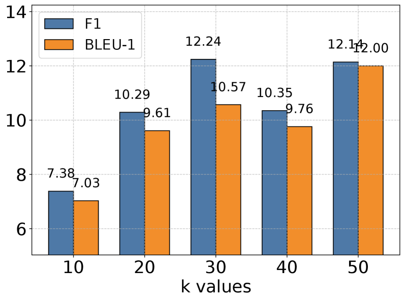
(c) Open Domain
<details>
<summary>x9.png Details</summary>
### Visual Description
## Grouped Bar Chart: Performance Metrics vs. k Values
### Overview
The image displays a grouped bar chart comparing two performance metrics, F1 and BLEU-1, across five different "k values." The chart shows a clear positive correlation between the k value and both performance scores.
### Components/Axes
* **Chart Type:** Grouped Bar Chart.
* **X-Axis:** Labeled "k values". It has five categorical tick marks: `10`, `20`, `30`, `40`, and `50`.
* **Y-Axis:** Numerical scale ranging from 25 to 45, with major gridlines at intervals of 5 (25, 30, 35, 40, 45). The axis title is not explicitly shown, but the values represent performance scores.
* **Legend:** Located in the top-left corner of the chart area.
* A blue square is labeled "F1".
* An orange square is labeled "BLEU-1".
* **Data Labels:** Each bar has its exact numerical value displayed directly above it.
### Detailed Analysis
The chart presents paired data for each k value. The left bar (blue) in each pair represents the F1 score, and the right bar (orange) represents the BLEU-1 score.
**Data Points (k value: F1, BLEU-1):**
* **k=10:** F1 = 31.15, BLEU-1 = 25.43
* **k=20:** F1 = 33.67, BLEU-1 = 28.31
* **k=30:** F1 = 38.15, BLEU-1 = 32.12
* **k=40:** F1 = 41.55, BLEU-1 = 34.32
* **k=50:** F1 = 44.55, BLEU-1 = 37.02
**Trend Verification:**
* **F1 Series (Blue Bars):** The line formed by the tops of the blue bars slopes consistently upward from left to right. The value increases from 31.15 at k=10 to 44.55 at k=50.
* **BLEU-1 Series (Orange Bars):** The line formed by the tops of the orange bars also slopes consistently upward from left to right. The value increases from 25.43 at k=10 to 37.02 at k=50.
### Key Observations
1. **Consistent Positive Trend:** Both F1 and BLEU-1 scores increase monotonically as the k value increases from 10 to 50.
2. **Performance Gap:** The F1 score is consistently higher than the BLEU-1 score at every k value. The absolute gap between them widens slightly as k increases (from a difference of ~5.72 at k=10 to ~7.53 at k=50).
3. **Linear Progression:** The increase in both metrics appears roughly linear across the sampled k values, with no obvious plateau or diminishing returns within this range.
4. **Relative Improvement:** From k=10 to k=50, the F1 score improves by approximately 13.40 points (a ~43% relative increase), while the BLEU-1 score improves by approximately 11.59 points (a ~46% relative increase).
### Interpretation
This chart likely illustrates the results of a hyperparameter tuning experiment for a machine learning model, where "k" is a key parameter (e.g., number of neighbors, beam size, or retrieved passages). The data suggests that increasing the k value within the tested range (10 to 50) leads to better model performance as measured by both the F1 score (which balances precision and recall) and the BLEU-1 score (which measures n-gram overlap with reference text, common in translation or generation tasks).
The consistent gap indicates that the model achieves a better balance of precision and recall (F1) than it does literal surface-form overlap (BLEU-1). The steady, parallel improvement of both metrics implies that the benefit of increasing k is robust and affects different aspects of performance similarly. A practitioner would use this data to select an optimal k value, likely favoring k=50 for maximum performance, while also considering computational costs that typically increase with k. The absence of a performance peak suggests that testing values beyond 50 could be warranted to find the point of diminishing returns.
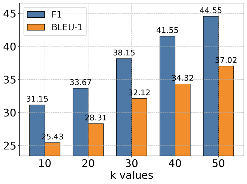
</details>
(d) Single Hop
<details>
<summary>x10.png Details</summary>
### Visual Description
## Grouped Bar Chart: Performance Metrics (F1 and BLEU-1) vs. k Values
### Overview
The image displays a grouped bar chart comparing two performance metrics, F1 and BLEU-1, across five different "k values" (10, 20, 30, 40, 50). The chart illustrates how these metrics change as the parameter `k` increases, showing a general upward trend that peaks at k=40 before a slight decline at k=50.
### Components/Axes
* **Chart Type:** Grouped (clustered) bar chart.
* **X-Axis:** Labeled "k values". It has five categorical tick marks: `10`, `20`, `30`, `40`, `50`.
* **Y-Axis:** Numerical scale representing the metric score. The axis is labeled with major ticks at `30`, `35`, `40`, `45`, `50`. The scale appears to start at approximately 28 and extend to just above 50.
* **Legend:** Located in the top-left corner of the plot area.
* A blue rectangle is labeled **F1**.
* An orange rectangle is labeled **BLEU-1**.
* **Data Series & Labels:** Each "k value" category contains two bars. The exact numerical value is printed above each bar.
* **F1 Series (Blue Bars, Left in each group):**
* k=10: 30.29
* k=20: 39.11
* k=30: 43.86
* k=40: 50.03
* k=50: 47.76
* **BLEU-1 Series (Orange Bars, Right in each group):**
* k=10: 29.49
* k=20: 38.35
* k=30: 43.19
* k=40: 49.47
* k=50: 47.24
### Detailed Analysis
The chart presents paired data for each k value. The visual trend for both series is a consistent increase from k=10 to k=40, followed by a decrease at k=50.
* **At k=10:** F1 (30.29) is slightly higher than BLEU-1 (29.49).
* **At k=20:** Both metrics show significant growth. F1 (39.11) remains higher than BLEU-1 (38.35).
* **At k=30:** The upward trend continues. F1 (43.86) and BLEU-1 (43.19) are very close in value.
* **At k=40:** Both metrics reach their peak. F1 (50.03) is the highest value in the chart. BLEU-1 (49.47) is also at its maximum.
* **At k=50:** Both metrics decline from their peaks. F1 drops to 47.76 and BLEU-1 to 47.24. The gap between them remains small.
### Key Observations
1. **Strong Positive Correlation:** There is a clear positive correlation between the k value and both performance metrics up to k=40.
2. **Peak Performance:** The optimal performance for both F1 and BLEU-1, as presented in this chart, occurs at **k=40**.
3. **Consistent Metric Relationship:** The F1 score is consistently higher than the BLEU-1 score for every k value, though the difference is often marginal (less than 1 point).
4. **Synchronized Trend:** The two metrics move in near-perfect synchronization, rising and falling together across the tested k values.
5. **Diminishing Returns/Overfitting:** The drop in performance at k=50 suggests that increasing the parameter beyond 40 may lead to diminishing returns or potential overfitting in the underlying model or system being evaluated.
### Interpretation
This chart likely evaluates the performance of a machine learning or natural language processing system where `k` is a key hyperparameter (e.g., the number of retrieved documents, nearest neighbors, or generated candidates). The F1 score (a measure of a test's accuracy, balancing precision and recall) and BLEU-1 score (a metric for evaluating machine-generated text against reference texts, focusing on unigram precision) are used as complementary evaluation metrics.
The data suggests that increasing `k` improves system performance up to an optimal point (k=40). This could mean that considering more candidates (`k`) provides better information or coverage. However, the decline at k=50 indicates a threshold where adding more candidates introduces noise or irrelevant information, degrading output quality. The close tracking of F1 and BLEU-1 implies that improvements in one aspect of performance (e.g., recall via F1) are accompanied by improvements in another (e.g., surface-level precision via BLEU-1), indicating a robust improvement in the system's overall output quality up to the optimal `k`. The chart provides clear empirical evidence for selecting k=40 as the best setting among those tested for this particular system and evaluation setup.
</details>
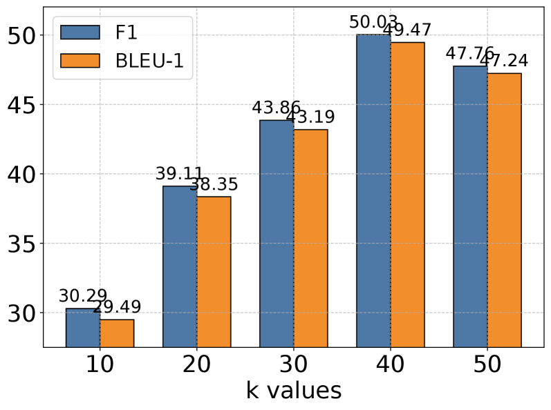
(e) Adversarial
Figure 3: Impact of memory retrieval parameter k across different task categories with GPT-4o-mini as the base model. While larger k values generally improve performance by providing richer historical context, the gains diminish beyond certain thresholds, suggesting a trade-off between context richness and effective information processing. This pattern is consistent across all evaluation categories, indicating the importance of balanced context retrieval for optimal performance.
### 4.5 Hyperparameter Analysis
We conducted extensive experiments to analyze the impact of the memory retrieval parameter k, which controls the number of relevant memories retrieved for each interaction. As shown in Figure 3, we evaluated performance across different k values (10, 20, 30, 40, 50) on five categories of tasks using GPT-4o-mini as our base model. The results reveal an interesting pattern: while increasing k generally leads to improved performance, this improvement gradually plateaus and sometimes slightly decreases at higher values. This trend is particularly evident in Multi Hop and Open Domain tasks. The observation suggests a delicate balance in memory retrieval - while larger k values provide richer historical context for reasoning, they may also introduce noise and challenge the model’s capacity to process longer sequences effectively. Our analysis indicates that moderate k values strike an optimal balance between context richness and information processing efficiency.
Table 4: Comparison of memory usage and retrieval time across different memory methods and scales.
| Memory Size | Method | Memory Usage (MB) | Retrieval Time ( $μs$ ) |
| --- | --- | --- | --- |
| 1,000 | A-Mem | 1.46 | 0.31 0.30 |
| MemoryBank [39] | 1.46 | 0.24 0.20 | |
| ReadAgent [17] | 1.46 | 43.62 8.47 | |
| 10,000 | A-Mem | 14.65 | 0.38 0.25 |
| MemoryBank [39] | 14.65 | 0.26 0.13 | |
| ReadAgent [17] | 14.65 | 484.45 93.86 | |
| 100,000 | A-Mem | 146.48 | 1.40 0.49 |
| MemoryBank [39] | 146.48 | 0.78 0.26 | |
| ReadAgent [17] | 146.48 | 6,682.22 111.63 | |
| 1,000,000 | A-Mem | 1464.84 | 3.70 0.74 |
| MemoryBank [39] | 1464.84 | 1.91 0.31 | |
| ReadAgent [17] | 1464.84 | 120,069.68 1,673.39 | |
### 4.6 Scaling Analysis
To evaluate storage costs with accumulating memory, we examined the relationship between storage size and retrieval time across our A-Mem system and two baseline approaches: MemoryBank [39] and ReadAgent [17]. We evaluated these three memory systems with identical memory content across four scale points, increasing the number of entries by a factor of 10 at each step (from 1,000 to 10,000, 100,000, and finally 1,000,000 entries). The experimental results reveal key insights about our A-Mem system’s scaling properties: In terms of space complexity, all three systems exhibit identical linear memory usage scaling ( $O(N)$ ), as expected for vector-based retrieval systems. This confirms that A-Mem introduces no additional storage overhead compared to baseline approaches. For retrieval time, A-Mem demonstrates excellent efficiency with minimal increases as memory size grows. Even when scaling to 1 million memories, A-Mem ’s retrieval time increases only from 0.31 $μs$ to 3.70 $μs$ , representing exceptional performance. While MemoryBank shows slightly faster retrieval times, A-Mem maintains comparable performance while providing richer memory representations and functionality. Based on our space complexity and retrieval time analysis, we conclude that A-Mem ’s retrieval mechanisms maintain excellent efficiency even at large scales. The minimal growth in retrieval time across memory sizes addresses concerns about efficiency in large-scale memory systems, demonstrating that A-Mem provides a highly scalable solution for long-term conversation management. This unique combination of efficiency, scalability, and enhanced memory capabilities positions A-Mem as a significant advancement in building powerful and long-term memory mechanism for LLM Agents.
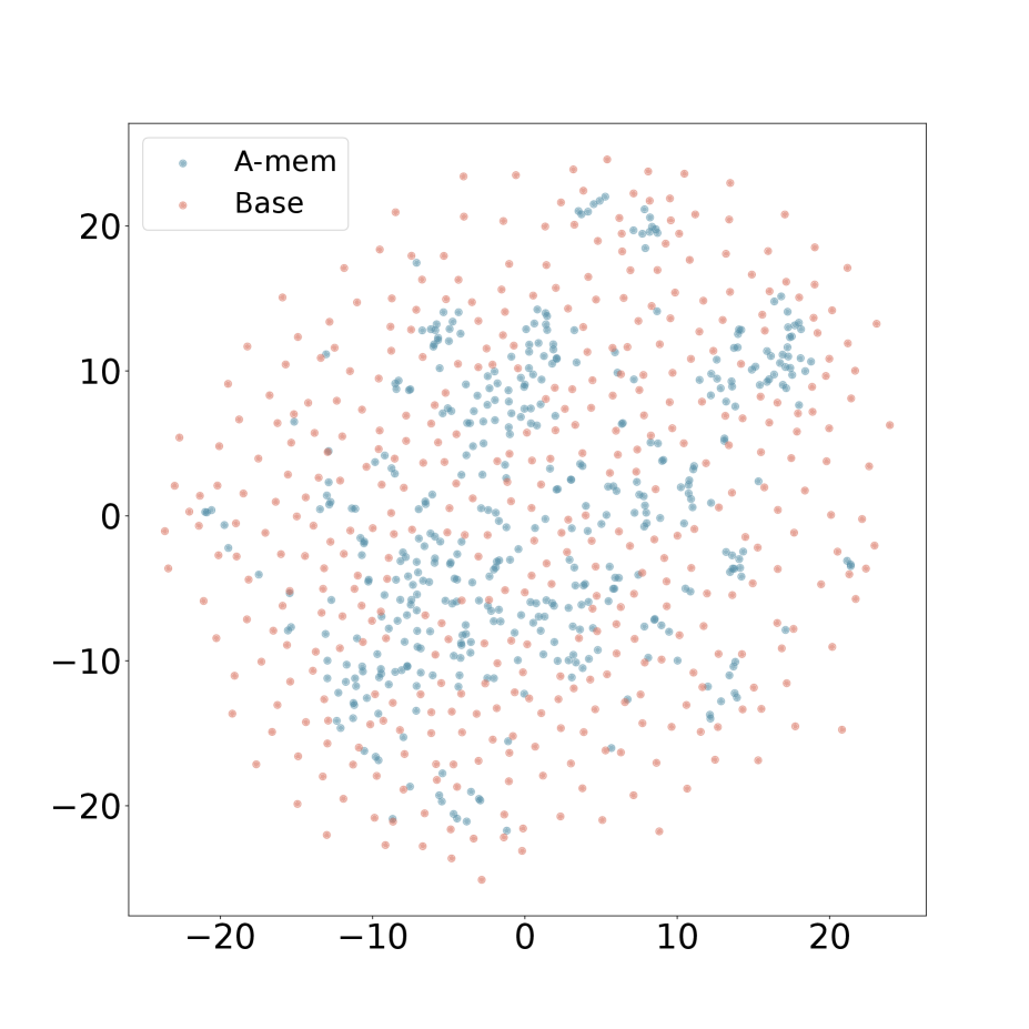
### 4.7 Memory Analysis
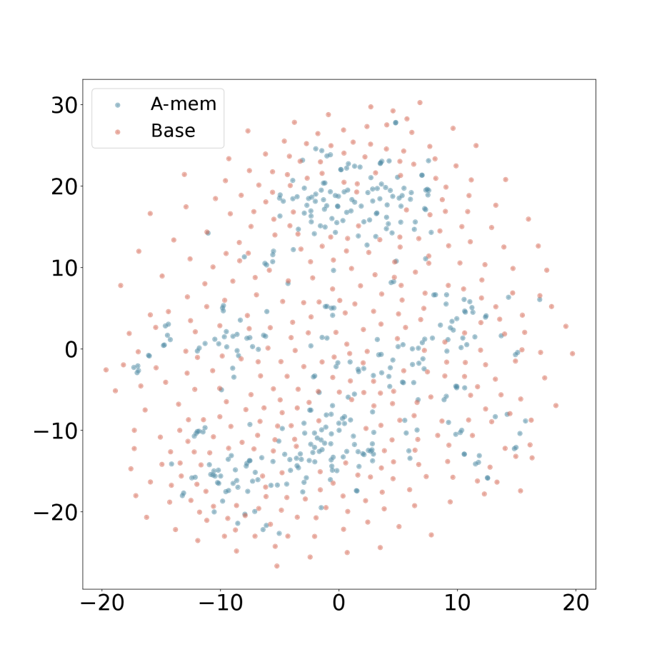
We present the t-SNE visualization in Figure 4 of memory embeddings to demonstrate the structural advantages of our agentic memory system. Analyzing two dialogues sampled from long-term conversations in LoCoMo [22], we observe that A-Mem (shown in blue) consistently exhibits more coherent clustering patterns compared to the baseline system (shown in red). This structural organization is particularly evident in Dialogue 2, where well-defined clusters emerge in the central region, providing empirical evidence for the effectiveness of our memory evolution mechanism and contextual description generation. In contrast, the baseline memory embeddings display a more dispersed distribution, demonstrating that memories lack structural organization without our link generation and memory evolution components. These visualization results validate that A-Mem can autonomously maintain meaningful memory structures through dynamic evolution and linking mechanisms. More results can be seen in Appendix A.4.
<details>
<summary>x11.png Details</summary>
### Visual Description
## Scatter Plot: A-mem vs. Base Distribution
### Overview
The image is a 2D scatter plot comparing the distribution of two datasets labeled "A-mem" and "Base". The plot visualizes the spatial spread and clustering of data points across a shared coordinate system.
### Components/Axes
* **Chart Type:** Scatter Plot
* **X-Axis:** Linear scale ranging from approximately -25 to +25. Major tick marks are labeled at -20, -10, 0, 10, and 20. No axis title is present.
* **Y-Axis:** Linear scale ranging from approximately -25 to +25. Major tick marks are labeled at -20, -10, 0, 10, and 20. No axis title is present.
* **Legend:** Located in the top-left corner of the plot area. It contains two entries:
* A blue dot labeled "A-mem".
* A pink/salmon dot labeled "Base".
* **Data Points:** The plot contains hundreds of individual points, each representing a single data observation from one of the two series.
### Detailed Analysis
**Data Series: A-mem (Blue Points)**
* **Visual Trend:** The blue points form a relatively dense, centrally concentrated cluster. The distribution appears roughly elliptical or cloud-like, centered near the origin (0,0).
* **Spatial Distribution:** The highest density of blue points is found within the region defined by x ≈ -10 to +10 and y ≈ -10 to +10. The cluster extends outward but becomes sparser. The points are not uniformly distributed; there are visible sub-clusters and voids within the main cloud.
* **Range:** The points span nearly the entire visible axis range, from approximately x = -22 to x = +22 and y = -22 to y = +24.
**Data Series: Base (Pink/Salmon Points)**
* **Visual Trend:** The pink points are much more widely and evenly dispersed across the entire plot area compared to the blue points. They do not form a single tight cluster.
* **Spatial Distribution:** The pink points appear to fill the background space more uniformly. They are present in all quadrants and at the peripheries where blue points are sparse or absent. Their distribution suggests a higher variance or a more random spread.
* **Range:** The points span the full visible axis range, from approximately x = -24 to x = +24 and y = -24 to y = +24.
**Cross-Reference & Spatial Grounding:**
* The legend in the top-left correctly maps the blue color to "A-mem" and the pink color to "Base".
* The central, dense cluster is composed exclusively of blue ("A-mem") points.
* The widely scattered points forming the background and outer edges are predominantly pink ("Base") points, though some blue points are also present at the fringes.
### Key Observations
1. **Distinct Distributions:** The two datasets exhibit fundamentally different spatial distributions. "A-mem" is clustered and centralized, while "Base" is dispersed and widespread.
2. **Central Overlap:** There is significant overlap in the central region (roughly within ±10 on both axes), where both blue and pink points are intermingled, though blue points dominate the very center.
3. **Peripheral Dominance:** The outer regions of the plot (beyond ±15 on either axis) are almost exclusively populated by pink ("Base") points.
4. **Density Gradient:** The "A-mem" series shows a clear density gradient, peaking at the center and fading outward. The "Base" series shows a much flatter density profile.
### Interpretation
This scatter plot likely visualizes the output of a dimensionality reduction technique (like t-SNE or PCA) applied to two different models or data representations ("A-mem" and "Base"). The key insight is the difference in their latent space organization.
* **What the data suggests:** The "A-mem" representation has learned a more structured and compact encoding, where similar items are mapped close together in the center of the space. This is often desirable for tasks requiring generalization or clustering. The "Base" representation appears more entangled or less structured, with data points scattered more randomly. This could indicate a less specialized or less trained model.
* **Relationship between elements:** The plot directly compares the geometric properties of the two representations. The central clustering of "A-mem" versus the dispersion of "Base" is the primary relationship being demonstrated.
* **Notable anomalies/trends:** The most significant trend is the stark contrast in distribution shape and density. There are no obvious outlier points that belong to one series but are located deep within the typical region of the other; the separation is more about overall distribution than individual point misplacement. The visualization strongly implies that the "A-mem" method produces a more organized internal representation of the data compared to the "Base" method.
</details>
(a) Dialogue 1
<details>
<summary>x12.png Details</summary>
### Visual Description
## Scatter Plot: A-mem vs. Base Data Points
### Overview
The image is a 2D scatter plot displaying two distinct datasets, labeled "A-mem" and "Base," plotted against common X and Y axes. The plot visualizes the distribution and relative spread of these two groups of data points within a defined coordinate space.
### Components/Axes
* **Chart Type:** Scatter Plot.
* **Legend:** Located in the top-left corner of the plot area. It contains two entries:
* A blue dot labeled "A-mem".
* A pink/salmon dot labeled "Base".
* **X-Axis:**
* **Label:** Not explicitly labeled with a title (e.g., "X Value" or "Dimension 1").
* **Scale:** Linear scale ranging from approximately -20 to +20.
* **Major Tick Marks:** At intervals of 10: -20, -10, 0, 10, 20.
* **Y-Axis:**
* **Label:** Not explicitly labeled with a title (e.g., "Y Value" or "Dimension 2").
* **Scale:** Linear scale ranging from approximately -20 to +30.
* **Major Tick Marks:** At intervals of 10: -20, -10, 0, 10, 20, 30.
### Detailed Analysis
* **Data Series - "A-mem" (Blue Points):**
* **Visual Trend:** The blue points form a relatively dense, centrally-located cluster. The distribution appears roughly elliptical or cloud-like, centered near the origin (0,0).
* **Spatial Distribution:** The cluster is most concentrated in the region from approximately X: -10 to +10 and Y: -10 to +20. The density of points decreases noticeably towards the periphery of this range. There are very few blue points beyond X = ±15 or Y = -15/25.
* **Approximate Range:** X: ~[-18, +18], Y: ~[-18, +28].
* **Data Series - "Base" (Pink Points):**
* **Visual Trend:** The pink points are much more widely and sparsely dispersed across the entire plot area compared to the blue points. They do not form a single tight cluster but rather a broad, diffuse cloud.
* **Spatial Distribution:** The pink points cover nearly the entire visible coordinate space. They are present in all quadrants and extend to the edges of the plotted range on all sides. The distribution appears relatively uniform without a single clear center of mass, though there may be a slight increase in density towards the center.
* **Approximate Range:** X: ~[-20, +20], Y: ~[-20, +30].
### Key Observations
1. **Distinct Distributions:** The most prominent feature is the stark contrast in spread between the two datasets. "A-mem" is tightly clustered, while "Base" is highly dispersed.
2. **Overlap Zone:** There is a significant area of overlap, primarily in the central region of the plot (roughly X: -10 to +10, Y: -10 to +15), where both blue and pink points are intermingled. However, the periphery is dominated almost exclusively by pink "Base" points.
3. **Asymmetry in Y-Axis:** The overall data, driven by the "Base" series, extends further in the positive Y direction (up to +30) than in the negative Y direction (down to -20).
4. **No Apparent Correlation:** For either dataset, there is no visually obvious linear or non-linear correlation between the X and Y variables. The points do not form clear lines or curves.
### Interpretation
This scatter plot likely compares the performance, embedding space, or some other two-dimensional characteristic of two different models, algorithms, or data processing methods ("A-mem" and "Base").
* **What the Data Suggests:** The tight clustering of "A-mem" points indicates **consistency, stability, or focused representation**. This could mean the "A-mem" method produces outputs that are very similar to each other in this feature space, suggesting lower variance or a more constrained operational range. Conversely, the wide dispersion of "Base" points indicates **high variability, diversity, or a broader exploration** of the feature space. This could represent a baseline model with less specialization or a method that generates more varied outputs.
* **Relationship Between Elements:** The plot directly contrasts these two behaviors. The "Base" distribution essentially forms the background "noise" or full potential space, within which the "A-mem" method has learned to concentrate its outputs. The overlap zone shows where the methods produce similar results, while the pink-only periphery highlights the unique, extreme outputs generated only by the "Base" method.
* **Notable Implications:** If this plot represents, for example, the latent space of generated text or image embeddings, "A-mem" might be a model fine-tuned for a specific task, leading to more focused generations. "Base" could be a general-purpose model. The lack of correlation suggests the axes represent independent dimensions of variation. The key takeaway is the fundamental difference in the *spread* of the data, which is often a critical metric for evaluating model behavior, robustness, or mode collapse.
</details>
(b) Dialogue 2
Figure 4: T-SNE Visualization of Memory Embeddings Showing More Organized Distribution with A-Mem (blue) Compared to Base Memory (red) Across Different Dialogues. Base Memory represents A-Mem without link generation and memory evolution.
## 5 Conclusions
In this work, we introduced A-Mem, a novel agentic memory system that enables LLM agents to dynamically organize and evolve their memories without relying on predefined structures. Drawing inspiration from the Zettelkasten method, our system creates an interconnected knowledge network through dynamic indexing and linking mechanisms that adapt to diverse real-world tasks. The system’s core architecture features autonomous generation of contextual descriptions for new memories and intelligent establishment of connections with existing memories based on shared attributes. Furthermore, our approach enables continuous evolution of historical memories by incorporating new experiences and developing higher-order attributes through ongoing interactions. Through extensive empirical evaluation across six foundation models, we demonstrated that A-Mem achieves superior performance compared to existing state-of-the-art baselines in long-term conversational tasks. Visualization analysis further validates the effectiveness of our memory organization approach. These results suggest that agentic memory systems can significantly enhance LLM agents’ ability to utilize long-term knowledge in complex environments.
## 6 Limitations
While our agentic memory system achieves promising results, we acknowledge several areas for potential future exploration. First, although our system dynamically organizes memories, the quality of these organizations may still be influenced by the inherent capabilities of the underlying language models. Different LLMs might generate slightly different contextual descriptions or establish varying connections between memories. Additionally, while our current implementation focuses on text-based interactions, future work could explore extending the system to handle multimodal information, such as images or audio, which could provide richer contextual representations.
## References
- [1] Sönke Ahrens. How to Take Smart Notes: One Simple Technique to Boost Writing, Learning and Thinking. Amazon, 2017. Second Edition.
- [2] Anthropic. The claude 3 model family: Opus, sonnet, haiku. Anthropic, Mar 2024. Accessed May 2025.
- [3] Anthropic. Claude 3.5 sonnet model card addendum. Technical report, Anthropic, 2025. Accessed May 2025.
- [4] Akari Asai, Zeqiu Wu, Yizhong Wang, Avirup Sil, and Hannaneh Hajishirzi. Self-rag: Learning to retrieve, generate, and critique through self-reflection. arXiv preprint arXiv:2310.11511, 2023.
- [5] Satanjeev Banerjee and Alon Lavie. Meteor: An automatic metric for mt evaluation with improved correlation with human judgments. In Proceedings of the acl workshop on intrinsic and extrinsic evaluation measures for machine translation and/or summarization, pages 65–72, 2005.
- [6] Sebastian Borgeaud, Arthur Mensch, Jordan Hoffmann, Trevor Cai, Eliza Rutherford, Katie Millican, George Bm Van Den Driessche, Jean-Baptiste Lespiau, Bogdan Damoc, Aidan Clark, et al. Improving language models by retrieving from trillions of tokens. In International conference on machine learning, pages 2206–2240. PMLR, 2022.
- [7] Xiang Deng, Yu Gu, Boyuan Zheng, Shijie Chen, Sam Stevens, Boshi Wang, Huan Sun, and Yu Su. Mind2web: Towards a generalist agent for the web. Advances in Neural Information Processing Systems, 36:28091–28114, 2023.
- [8] Khant Dev and Singh Taranjeet. mem0: The memory layer for ai agents. https://github.com/mem0ai/mem0, 2024.
- [9] Darren Edge, Ha Trinh, Newman Cheng, Joshua Bradley, Alex Chao, Apurva Mody, Steven Truitt, and Jonathan Larson. From local to global: A graph rag approach to query-focused summarization. arXiv preprint arXiv:2404.16130, 2024.
- [10] Yunfan Gao, Yun Xiong, Xinyu Gao, Kangxiang Jia, Jinliu Pan, Yuxi Bi, Yi Dai, Jiawei Sun, and Haofen Wang. Retrieval-augmented generation for large language models: A survey. arXiv preprint arXiv:2312.10997, 2023.
- [11] Daya Guo, Dejian Yang, Haowei Zhang, Junxiao Song, Ruoyu Zhang, Runxin Xu, Qihao Zhu, Shirong Ma, Peiyi Wang, Xiao Bi, et al. Deepseek-r1: Incentivizing reasoning capability in llms via reinforcement learning. arXiv preprint arXiv:2501.12948, 2025.
- [12] I. Ilin. Advanced rag techniques: An illustrated overview, 2023.
- [13] Jihyoung Jang, Minseong Boo, and Hyounghun Kim. Conversation chronicles: Towards diverse temporal and relational dynamics in multi-session conversations. arXiv preprint arXiv:2310.13420, 2023.
- [14] Zhengbao Jiang, Frank F Xu, Luyu Gao, Zhiqing Sun, Qian Liu, Jane Dwivedi-Yu, Yiming Yang, Jamie Callan, and Graham Neubig. Active retrieval augmented generation. arXiv preprint arXiv:2305.06983, 2023.
- [15] David Kadavy. Digital Zettelkasten: Principles, Methods, & Examples. Google Books, May 2021.
- [16] Jiho Kim, Woosog Chay, Hyeonji Hwang, Daeun Kyung, Hyunseung Chung, Eunbyeol Cho, Yohan Jo, and Edward Choi. Dialsim: A real-time simulator for evaluating long-term multi-party dialogue understanding of conversational agents. arXiv preprint arXiv:2406.13144, 2024.
- [17] Kuang-Huei Lee, Xinyun Chen, Hiroki Furuta, John Canny, and Ian Fischer. A human-inspired reading agent with gist memory of very long contexts. arXiv preprint arXiv:2402.09727, 2024.
- [18] Patrick Lewis, Ethan Perez, Aleksandra Piktus, Fabio Petroni, Vladimir Karpukhin, Naman Goyal, Heinrich Küttler, Mike Lewis, Wen-tau Yih, Tim Rocktäschel, et al. Retrieval-augmented generation for knowledge-intensive nlp tasks. Advances in Neural Information Processing Systems, 33:9459–9474, 2020.
- [19] Chin-Yew Lin. Rouge: A package for automatic evaluation of summaries. In Text summarization branches out, pages 74–81, 2004.
- [20] Xi Victoria Lin, Xilun Chen, Mingda Chen, Weijia Shi, Maria Lomeli, Rich James, Pedro Rodriguez, Jacob Kahn, Gergely Szilvasy, Mike Lewis, et al. Ra-dit: Retrieval-augmented dual instruction tuning. arXiv preprint arXiv:2310.01352, 2023.
- [21] Zhiwei Liu, Weiran Yao, Jianguo Zhang, Liangwei Yang, Zuxin Liu, Juntao Tan, Prafulla K Choubey, Tian Lan, Jason Wu, Huan Wang, et al. Agentlite: A lightweight library for building and advancing task-oriented llm agent system. arXiv preprint arXiv:2402.15538, 2024.
- [22] Adyasha Maharana, Dong-Ho Lee, Sergey Tulyakov, Mohit Bansal, Francesco Barbieri, and Yuwei Fang. Evaluating very long-term conversational memory of llm agents. arXiv preprint arXiv:2402.17753, 2024.
- [23] Kai Mei, Zelong Li, Shuyuan Xu, Ruosong Ye, Yingqiang Ge, and Yongfeng Zhang. Aios: Llm agent operating system. arXiv e-prints, pp. arXiv–2403, 2024.
- [24] Ali Modarressi, Ayyoob Imani, Mohsen Fayyaz, and Hinrich Schütze. Ret-llm: Towards a general read-write memory for large language models. arXiv preprint arXiv:2305.14322, 2023.
- [25] Charles Packer, Sarah Wooders, Kevin Lin, Vivian Fang, Shishir G Patil, Ion Stoica, and Joseph E Gonzalez. Memgpt: Towards llms as operating systems. arXiv preprint arXiv:2310.08560, 2023.
- [26] Kishore Papineni, Salim Roukos, Todd Ward, and Wei-Jing Zhu. Bleu: a method for automatic evaluation of machine translation. In Proceedings of the 40th annual meeting of the Association for Computational Linguistics, pages 311–318, 2002.
- [27] Nils Reimers and Iryna Gurevych. Sentence-bert: Sentence embeddings using siamese bert-networks. In Proceedings of the 2019 Conference on Empirical Methods in Natural Language Processing. Association for Computational Linguistics, 11 2019.
- [28] Aymeric Roucher, Albert Villanova del Moral, Thomas Wolf, Leandro von Werra, and Erik Kaunismäki. ‘smolagents‘: a smol library to build great agentic systems. https://github.com/huggingface/smolagents, 2025.
- [29] Zhihong Shao, Yeyun Gong, Yelong Shen, Minlie Huang, Nan Duan, and Weizhu Chen. Enhancing retrieval-augmented large language models with iterative retrieval-generation synergy. arXiv preprint arXiv:2305.15294, 2023.
- [30] Zeru Shi, Kai Mei, Mingyu Jin, Yongye Su, Chaoji Zuo, Wenyue Hua, Wujiang Xu, Yujie Ren, Zirui Liu, Mengnan Du, et al. From commands to prompts: Llm-based semantic file system for aios. arXiv preprint arXiv:2410.11843, 2024.
- [31] Harsh Trivedi, Niranjan Balasubramanian, Tushar Khot, and Ashish Sabharwal. Interleaving retrieval with chain-of-thought reasoning for knowledge-intensive multi-step questions. arXiv preprint arXiv:2212.10509, 2022.
- [32] Bing Wang, Xinnian Liang, Jian Yang, Hui Huang, Shuangzhi Wu, Peihao Wu, Lu Lu, Zejun Ma, and Zhoujun Li. Enhancing large language model with self-controlled memory framework. arXiv preprint arXiv:2304.13343, 2023.
- [33] Xingyao Wang, Boxuan Li, Yufan Song, Frank F Xu, Xiangru Tang, Mingchen Zhuge, Jiayi Pan, Yueqi Song, Bowen Li, Jaskirat Singh, et al. Openhands: An open platform for ai software developers as generalist agents. arXiv preprint arXiv:2407.16741, 2024.
- [34] Zhiruo Wang, Jun Araki, Zhengbao Jiang, Md Rizwan Parvez, and Graham Neubig. Learning to filter context for retrieval-augmented generation. arXiv preprint arXiv:2311.08377, 2023.
- [35] Lilian Weng. Llm-powered autonomous agents. lilianweng.github.io, Jun 2023.
- [36] J Xu. Beyond goldfish memory: Long-term open-domain conversation. arXiv preprint arXiv:2107.07567, 2021.
- [37] Wenhao Yu, Hongming Zhang, Xiaoman Pan, Kaixin Ma, Hongwei Wang, and Dong Yu. Chain-of-note: Enhancing robustness in retrieval-augmented language models. arXiv preprint arXiv:2311.09210, 2023.
- [38] Zichun Yu, Chenyan Xiong, Shi Yu, and Zhiyuan Liu. Augmentation-adapted retriever improves generalization of language models as generic plug-in. arXiv preprint arXiv:2305.17331, 2023.
- [39] Wanjun Zhong, Lianghong Guo, Qiqi Gao, He Ye, and Yanlin Wang. Memorybank: Enhancing large language models with long-term memory. In Proceedings of the AAAI Conference on Artificial Intelligence, volume 38, pages 19724–19731, 2024. Contents
1. 1 Introduction
1. 2 Related Work
1. 2.1 Memory for LLM Agents
1. 2.2 Retrieval-Augmented Generation
1. 3 Methodolodgy
1. 3.1 Note Construction
1. 3.2 Link Generation
1. 3.3 Memory Evolution
1. 3.4 Retrieve Relative Memory
1. 4 Experiment
1. 4.1 Dataset and Evaluation
1. 4.2 Implementation Details
1. 4.3 Empricial Results
1. 4.4 Ablation Study
1. 4.5 Hyperparameter Analysis
1. 4.6 Scaling Analysis
1. 4.7 Memory Analysis
1. 5 Conclusions
1. 6 Limitations
1. A Experiment
1. A.1 Detailed Baselines Introduction
1. A.2 Evaluation Metric
1. A.3 Comparison Results
1. A.4 Memory Analysis
1. A.5 Hyperparameters setting
1. B Prompt Templates and Examples
1. B.1 Prompt Template of Note Construction
1. B.2 Prompt Template of Link Generation
1. B.3 Prompt Template of Memory Evolution
1. B.4 Examples of Q/A with A-Mem
## APPENDIX
## Appendix A Experiment
### A.1 Detailed Baselines Introduction
LoCoMo [22] takes a direct approach by leveraging foundation models without memory mechanisms for question answering tasks. For each query, it incorporates the complete preceding conversation and questions into the prompt, evaluating the model’s reasoning capabilities.
ReadAgent [17] tackles long-context document processing through a sophisticated three-step methodology: it begins with episode pagination to segment content into manageable chunks, followed by memory gisting to distill each page into concise memory representations, and concludes with interactive look-up to retrieve pertinent information as needed.
MemoryBank [39] introduces an innovative memory management system that maintains and efficiently retrieves historical interactions. The system features a dynamic memory updating mechanism based on the Ebbinghaus Forgetting Curve theory, which intelligently adjusts memory strength according to time and significance. Additionally, it incorporates a user portrait building system that progressively refines its understanding of user personality through continuous interaction analysis.
MemGPT [25] presents a novel virtual context management system drawing inspiration from traditional operating systems’ memory hierarchies. The architecture implements a dual-tier structure: a main context (analogous to RAM) that provides immediate access during LLM inference, and an external context (analogous to disk storage) that maintains information beyond the fixed context window.
### A.2 Evaluation Metric
The F1 score represents the harmonic mean of precision and recall, offering a balanced metric that combines both measures into a single value. This metric is particularly valuable when we need to balance between complete and accurate responses:
$$
F1=2·\frac{precision·recall}{precision+recall} \tag{11}
$$
where
$$
precision=\frac{true positives}{true positives+false positives} \tag{12}
$$
$$
recall=\frac{true positives}{true positives+false negatives} \tag{13}
$$
In question-answering systems, the F1 score serves a crucial role in evaluating exact matches between predicted and reference answers. This is especially important for span-based QA tasks, where systems must identify precise text segments while maintaining comprehensive coverage of the answer.
BLEU-1 [26] provides a method for evaluating the precision of unigram matches between system outputs and reference texts:
$$
BLEU-1=BP·\exp(\tsum\slimits@_n=1^1w_n\log p_n) \tag{14}
$$
where
$$
BP=\begin{cases}1&if c>r\\
e^1-r/c&if c≤ r\end{cases} \tag{15}
$$
$$
p_n=\frac{\tsum\slimits@_i\tsum\slimits@_k\min(h_ik,m_ik)}{\tsum\slimits@_i\tsum\slimits@_kh_ik} \tag{16}
$$
Here, $c$ is candidate length, $r$ is reference length, $h_ik$ is the count of n-gram i in candidate k, and $m_ik$ is the maximum count in any reference. In QA, BLEU-1 evaluates the lexical precision of generated answers, particularly useful for generative QA systems where exact matching might be too strict.
ROUGE-L [19] measures the longest common subsequence between the generated and reference texts.
$$
ROUGE-L=\frac{(1+β^2)R_lP_l}{R_l+β^2P_l} \tag{17}
$$
$$
R_l=\frac{LCS(X,Y)}{|X|} \tag{18}
$$
$$
P_l=\frac{LCS(X,Y)}{|Y|} \tag{19}
$$
where $X$ is reference text, $Y$ is candidate text, and LCS is the Longest Common Subsequence.
ROUGE-2 [19] calculates the overlap of bigrams between the generated and reference texts.
$$
ROUGE-2=\frac{\tsum\slimits@_bigram∈\text{ref}\min(Count_ref(bigram),Count_cand(bigram))}{\tsum\slimits@_bigram∈\text{ref}Count_ref(bigram)} \tag{20}
$$
Both ROUGE-L and ROUGE-2 are particularly useful for evaluating the fluency and coherence of generated answers, with ROUGE-L focusing on sequence matching and ROUGE-2 on local word order.
METEOR [5] computes a score based on aligned unigrams between the candidate and reference texts, considering synonyms and paraphrases.
$$
METEOR=F_mean·(1-Penalty) \tag{21}
$$
$$
F_mean=\frac{10P· R}{R+9P} \tag{22}
$$
$$
Penalty=0.5·(\frac{ch}{m})^3 \tag{23}
$$
where $P$ is precision, $R$ is recall, ch is number of chunks, and $m$ is number of matched unigrams. METEOR is valuable for QA evaluation as it considers semantic similarity beyond exact matching, making it suitable for evaluating paraphrased answers.
SBERT Similarity [27] measures the semantic similarity between two texts using sentence embeddings.
$$
SBERT\_Similarity=\cos(SBERT(x),SBERT(y)) \tag{24}
$$
$$
\cos(a,b)=\frac{a· b}{\|a\|\|b\|} \tag{25}
$$
SBERT( $x$ ) represents the sentence embedding of text. SBERT Similarity is particularly useful for evaluating semantic understanding in QA systems, as it can capture meaning similarities even when the lexical overlap is low.
Table 5: Experimental results on LoCoMo dataset of QA tasks across five categories (Multi Hop, Temporal, Open Domain, Single Hop, and Adversial) using different methods. Results are reported in ROUGE-2 and ROUGE-L scores, abbreviated to RGE-2 and RGE-L. The best performance is marked in bold, and our proposed method A-Mem (highlighted in gray) demonstrates competitive performance across six foundation language models.
| Model | Method | Category | | | | | | | | | | |
| --- | --- | --- | --- | --- | --- | --- | --- | --- | --- | --- | --- | --- |
| Multi Hop | Temporal | Open Domain | Single Hop | Adversial | | | | | | | | |
| RGE-2 | RGE-L | RGE-2 | RGE-L | RGE-2 | RGE-L | RGE-2 | RGE-L | RGE-2 | RGE-L | | | |
| GPT | 4o-mini | LoCoMo | 9.64 | 23.92 | 2.01 | 18.09 | 3.40 | 11.58 | 26.48 | 40.20 | 60.46 | 69.59 |
| ReadAgent | 2.47 | 9.45 | 0.95 | 13.12 | 0.55 | 5.76 | 2.99 | 9.92 | 6.66 | 9.79 | | |
| MemoryBank | 1.18 | 5.43 | 0.52 | 9.64 | 0.97 | 5.77 | 1.64 | 6.63 | 4.55 | 7.35 | | |
| MemGPT | 10.58 | 25.60 | 4.76 | 25.22 | 0.76 | 9.14 | 28.44 | 42.24 | 36.62 | 43.75 | | |
| A-Mem | 10.61 | 25.86 | 21.39 | 44.27 | 3.42 | 12.09 | 29.50 | 45.18 | 42.62 | 50.04 | | |
| 4o | LoCoMo | 11.53 | 30.65 | 1.68 | 8.17 | 3.21 | 16.33 | 45.42 | 63.86 | 45.13 | 52.67 | |
| ReadAgent | 3.91 | 14.36 | 0.43 | 3.96 | 0.52 | 8.58 | 4.75 | 13.41 | 4.24 | 6.81 | | |
| MemoryBank | 1.84 | 7.36 | 0.36 | 2.29 | 2.13 | 6.85 | 3.02 | 9.35 | 1.22 | 4.41 | | |
| MemGPT | 11.55 | 30.18 | 4.66 | 15.83 | 3.27 | 14.02 | 43.27 | 62.75 | 28.72 | 35.08 | | |
| A-Mem | 12.76 | 31.71 | 9.82 | 25.04 | 6.09 | 16.63 | 33.67 | 50.31 | 30.31 | 36.34 | | |
| Qwen2.5 | 1.5b | LoCoMo | 1.39 | 9.24 | 0.00 | 4.68 | 3.42 | 10.59 | 3.25 | 11.15 | 35.10 | 43.61 |
| ReadAgent | 0.74 | 7.14 | 0.10 | 2.81 | 3.05 | 12.63 | 1.47 | 7.88 | 20.73 | 27.82 | | |
| MemoryBank | 1.51 | 11.18 | 0.14 | 5.39 | 1.80 | 8.44 | 5.07 | 13.72 | 29.24 | 36.95 | | |
| MemGPT | 1.16 | 11.35 | 0.00 | 7.88 | 2.87 | 14.62 | 2.18 | 9.82 | 23.96 | 31.69 | | |
| A-Mem | 4.88 | 17.94 | 5.88 | 27.23 | 3.44 | 16.87 | 12.32 | 24.38 | 36.32 | 46.60 | | |
| 3b | LoCoMo | 0.49 | 4.83 | 0.14 | 3.20 | 1.31 | 5.38 | 1.97 | 6.98 | 12.66 | 17.10 | |
| ReadAgent | 0.08 | 4.08 | 0.00 | 1.96 | 1.26 | 6.19 | 0.73 | 4.34 | 7.35 | 10.64 | | |
| MemoryBank | 0.43 | 3.76 | 0.05 | 1.61 | 0.24 | 6.32 | 1.03 | 4.22 | 9.55 | 13.41 | | |
| MemGPT | 0.69 | 5.55 | 0.05 | 3.17 | 1.90 | 7.90 | 2.05 | 7.32 | 10.46 | 14.39 | | |
| A-Mem | 2.91 | 12.42 | 8.11 | 27.74 | 1.51 | 7.51 | 8.80 | 17.57 | 21.39 | 27.98 | | |
| Llama 3.2 | 1b | LoCoMo | 2.51 | 11.48 | 0.44 | 8.25 | 1.69 | 13.06 | 2.94 | 13.00 | 39.85 | 52.74 |
| ReadAgent | 0.53 | 6.49 | 0.00 | 4.62 | 5.47 | 14.29 | 1.19 | 8.03 | 34.52 | 45.55 | | |
| MemoryBank | 2.96 | 13.57 | 0.23 | 10.53 | 4.01 | 18.38 | 6.41 | 17.66 | 41.15 | 53.31 | | |
| MemGPT | 1.82 | 9.91 | 0.06 | 6.56 | 2.13 | 11.36 | 2.00 | 10.37 | 38.59 | 50.31 | | |
| A-Mem | 4.82 | 19.31 | 1.84 | 20.47 | 5.99 | 18.49 | 14.82 | 29.78 | 46.76 | 60.23 | | |
| 3b | LoCoMo | 0.98 | 7.22 | 0.03 | 4.45 | 2.36 | 11.39 | 2.85 | 8.45 | 25.47 | 30.26 | |
| ReadAgent | 2.47 | 1.78 | 3.01 | 3.01 | 5.07 | 5.22 | 3.25 | 2.51 | 15.78 | 14.01 | | |
| MemoryBank | 1.83 | 6.96 | 0.25 | 3.41 | 0.43 | 4.43 | 2.73 | 7.83 | 14.64 | 18.59 | | |
| MemGPT | 0.72 | 5.39 | 0.11 | 2.85 | 0.61 | 5.74 | 1.45 | 4.42 | 16.62 | 21.47 | | |
| A-Mem | 6.02 | 17.62 | 7.93 | 27.97 | 5.38 | 13.00 | 16.89 | 28.55 | 35.48 | 42.25 | | |
Table 6: Experimental results on LoCoMo dataset of QA tasks across five categories (Multi Hop, Temporal, Open Domain, Single Hop, and Adversial) using different methods. Results are reported in METEOR and SBERT Similarity scores, abbreviated to ME and SBERT. The best performance is marked in bold, and our proposed method A-Mem (highlighted in gray) demonstrates competitive performance across six foundation language models.
| Model | Method | Category | | | | | | | | | | |
| --- | --- | --- | --- | --- | --- | --- | --- | --- | --- | --- | --- | --- |
| Multi Hop | Temporal | Open Domain | Single Hop | Adversial | | | | | | | | |
| ME | SBERT | ME | SBERT | ME | SBERT | ME | SBERT | ME | SBERT | | | |
| GPT | 4o-mini | LoCoMo | 15.81 | 47.97 | 7.61 | 52.30 | 8.16 | 35.00 | 40.42 | 57.78 | 63.28 | 71.93 |
| ReadAgent | 5.46 | 28.67 | 4.76 | 45.07 | 3.69 | 26.72 | 8.01 | 26.78 | 8.38 | 15.20 | | |
| MemoryBank | 3.42 | 21.71 | 4.07 | 37.58 | 4.21 | 23.71 | 5.81 | 20.76 | 6.24 | 13.00 | | |
| MemGPT | 15.79 | 49.33 | 13.25 | 61.53 | 4.59 | 32.77 | 41.40 | 58.19 | 39.16 | 47.24 | | |
| A-Mem | 16.36 | 49.46 | 23.43 | 70.49 | 8.36 | 38.48 | 42.32 | 59.38 | 45.64 | 53.26 | | |
| 4o | LoCoMo | 16.34 | 53.82 | 7.21 | 32.15 | 8.98 | 43.72 | 53.39 | 73.40 | 47.72 | 56.09 | |
| ReadAgent | 7.86 | 37.41 | 3.76 | 26.22 | 4.42 | 30.75 | 9.36 | 31.37 | 5.47 | 12.34 | | |
| MemoryBank | 3.22 | 26.23 | 2.29 | 23.49 | 4.18 | 24.89 | 6.64 | 23.90 | 2.93 | 10.01 | | |
| MemGPT | 16.64 | 55.12 | 12.68 | 35.93 | 7.78 | 37.91 | 52.14 | 72.83 | 31.15 | 39.08 | | |
| A-Mem | 17.53 | 55.96 | 13.10 | 45.40 | 10.62 | 38.87 | 41.93 | 62.47 | 32.34 | 40.11 | | |
| Qwen2.5 | 1.5b | LoCoMo | 4.99 | 32.23 | 2.86 | 34.03 | 5.89 | 35.61 | 8.57 | 29.47 | 40.53 | 50.49 |
| ReadAgent | 3.67 | 28.20 | 1.88 | 27.27 | 8.97 | 35.13 | 5.52 | 26.33 | 24.04 | 34.12 | | |
| MemoryBank | 5.57 | 35.40 | 2.80 | 32.47 | 4.27 | 33.85 | 10.59 | 32.16 | 32.93 | 42.83 | | |
| MemGPT | 5.40 | 35.64 | 2.35 | 39.04 | 7.68 | 40.36 | 7.07 | 30.16 | 27.24 | 40.63 | | |
| A-Mem | 9.49 | 43.49 | 11.92 | 61.65 | 9.11 | 42.58 | 19.69 | 41.93 | 40.64 | 52.44 | | |
| 3b | LoCoMo | 2.00 | 24.37 | 1.92 | 25.24 | 3.45 | 25.38 | 6.00 | 21.28 | 16.67 | 23.14 | |
| ReadAgent | 1.78 | 21.10 | 1.69 | 20.78 | 4.43 | 25.15 | 3.37 | 18.20 | 10.46 | 17.39 | | |
| MemoryBank | 2.37 | 17.81 | 2.22 | 21.93 | 3.86 | 20.65 | 3.99 | 16.26 | 15.49 | 20.77 | | |
| MemGPT | 3.74 | 24.31 | 2.25 | 27.67 | 6.44 | 29.59 | 6.24 | 22.40 | 13.19 | 20.83 | | |
| A-Mem | 6.25 | 33.72 | 14.04 | 62.54 | 6.56 | 30.60 | 15.98 | 33.98 | 27.36 | 33.72 | | |
| Llama 3.2 | 1b | LoCoMo | 5.77 | 38.02 | 3.38 | 45.44 | 6.20 | 42.69 | 9.33 | 34.19 | 46.79 | 60.74 |
| ReadAgent | 2.97 | 29.26 | 1.31 | 26.45 | 7.13 | 39.19 | 5.36 | 26.44 | 42.39 | 54.35 | | |
| MemoryBank | 6.77 | 39.33 | 4.43 | 45.63 | 7.76 | 42.81 | 13.01 | 37.32 | 50.43 | 60.81 | | |
| MemGPT | 5.10 | 32.99 | 2.54 | 41.81 | 3.26 | 35.99 | 6.62 | 30.68 | 45.00 | 61.33 | | |
| A-Mem | 9.01 | 45.16 | 7.50 | 54.79 | 8.30 | 43.42 | 22.46 | 47.07 | 53.72 | 68.00 | | |
| 3b | LoCoMo | 3.69 | 27.94 | 2.96 | 20.40 | 6.46 | 32.17 | 6.58 | 22.92 | 29.02 | 35.74 | |
| ReadAgent | 1.21 | 17.40 | 2.33 | 12.02 | 3.39 | 19.63 | 2.46 | 14.63 | 14.37 | 21.25 | | |
| MemoryBank | 3.84 | 25.06 | 2.73 | 13.65 | 3.05 | 21.08 | 6.35 | 22.02 | 17.14 | 24.39 | | |
| MemGPT | 2.78 | 22.06 | 2.21 | 14.97 | 3.63 | 23.18 | 3.47 | 17.81 | 20.50 | 26.87 | | |
| A-Mem | 9.74 | 39.32 | 13.19 | 59.70 | 8.09 | 32.27 | 24.30 | 42.86 | 39.74 | 46.76 | | |
Table 7: Experimental results on LoCoMo dataset of QA tasks across five categories (Multi Hop, Temporal, Open Domain, Single Hop, and Adversial) using different methods. Results are reported in F1 and BLEU-1 (%) scores with different foundation models.
| Method | Category | | | | | | | | | |
| --- | --- | --- | --- | --- | --- | --- | --- | --- | --- | --- |
| Multi Hop | Temporal | Open Domain | Single Hop | Adversial | | | | | | |
| F1 | BLEU-1 | F1 | BLEU-1 | F1 | BLEU-1 | F1 | BLEU-1 | F1 | BLEU-1 | |
| DeepSeek-R1-32B | | | | | | | | | | |
| LoCoMo | 8.58 | 6.48 | 4.79 | 4.35 | 12.96 | 12.52 | 10.72 | 8.20 | 21.40 | 20.23 |
| MemGPT | 8.28 | 6.25 | 5.45 | 4.97 | 10.97 | 9.09 | 11.34 | 9.03 | 30.77 | 29.23 |
| A-Mem | 15.02 | 10.64 | 14.64 | 11.01 | 14.81 | 12.82 | 15.37 | 12.30 | 27.92 | 27.19 |
| Claude 3.0 Haiku | | | | | | | | | | |
| LoCoMo | 4.56 | 3.33 | 0.82 | 0.59 | 2.86 | 3.22 | 3.56 | 3.24 | 3.46 | 3.42 |
| MemGPT | 7.65 | 6.36 | 1.65 | 1.26 | 7.41 | 6.64 | 8.60 | 7.29 | 7.66 | 7.37 |
| A-Mem | 19.28 | 14.69 | 16.65 | 12.23 | 11.85 | 9.61 | 34.72 | 30.05 | 35.99 | 34.87 |
| Claude 3.5 Haiku | | | | | | | | | | |
| LoCoMo | 11.34 | 8.21 | 3.29 | 2.69 | 3.79 | 3.58 | 14.01 | 12.57 | 7.37 | 7.12 |
| MemGPT | 8.27 | 6.55 | 3.99 | 2.76 | 4.71 | 4.48 | 16.52 | 14.89 | 5.64 | 5.45 |
| A-Mem | 29.70 | 23.19 | 31.54 | 27.53 | 11.42 | 9.47 | 42.60 | 37.41 | 13.65 | 12.71 |
### A.3 Comparison Results
Our comprehensive evaluation using ROUGE-2, ROUGE-L, METEOR, and SBERT metrics demonstrates that A-Mem achieves superior performance while maintaining remarkable computational efficiency. Through extensive empirical testing across various model sizes and task categories, we have established A-Mem as a more effective approach compared to existing baselines, supported by several compelling findings. In our analysis of non-GPT models, specifically Qwen2.5 and Llama 3.2, A-Mem consistently outperforms all baseline approaches across all metrics. The Multi-Hop category showcases particularly striking results, where Qwen2.5-15b with A-Mem achieves a ROUGE-L score of 27.23, dramatically surpassing LoComo’s 4.68 and ReadAgent’s 2.81 - representing a nearly six-fold improvement. This pattern of superiority extends consistently across METEOR and SBERT scores. When examining GPT-based models, our results reveal an interesting pattern. While LoComo and MemGPT demonstrate strong capabilities in Open Domain and Adversarial tasks, A-Mem shows remarkable superiority in Multi-Hop reasoning tasks. Using GPT-4o-mini, A-Mem achieves a ROUGE-L score of 44.27 in Multi-Hop tasks, more than doubling LoComo’s 18.09. This significant advantage maintains consistency across other metrics, with METEOR scores of 23.43 versus 7.61 and SBERT scores of 70.49 versus 52.30. The significance of these results is amplified by A-Mem ’s exceptional computational efficiency. Our approach requires only 1,200-2,500 tokens, compared to the substantial 16,900 tokens needed by LoComo and MemGPT. This efficiency stems from two key architectural innovations: First, our novel agentic memory architecture creates interconnected memory networks through atomic notes with rich contextual descriptions, enabling more effective capture and utilization of information relationships. Second, our selective top-k retrieval mechanism facilitates dynamic memory evolution and structured organization. The effectiveness of these innovations is particularly evident in complex reasoning tasks, as demonstrated by the consistently strong Multi-Hop performance across all evaluation metrics. Besides, we also show the experimental results with different foundational models including DeepSeek-R1-32B [11], Claude 3.0 Haiku [2] and Claude 3.5 Haiku [3].
### A.4 Memory Analysis
In addition to the memory visualizations of the first two dialogues shown in the main text, we present additional visualizations in Fig. 5 that demonstrate the structural advantages of our agentic memory system. Through analysis of two dialogues sampled from long-term conversations in LoCoMo [22], we observe that A-Mem (shown in blue) consistently produces more coherent clustering patterns compared to the baseline system (shown in red). This structural organization is particularly evident in Dialogue 2, where distinct clusters emerge in the central region, providing empirical support for the effectiveness of our memory evolution mechanism and contextual description generation. In contrast, the baseline memory embeddings exhibit a more scattered distribution, indicating that memories lack structural organization without our link generation and memory evolution components. These visualizations validate that A-Mem can autonomously maintain meaningful memory structures through its dynamic evolution and linking mechanisms.
<details>
<summary>x13.png Details</summary>
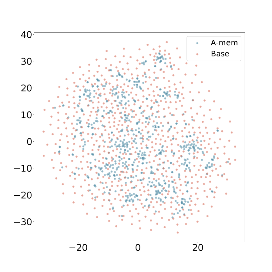
### Visual Description
## Scatter Plot: Comparison of Two Data Series (A-mem vs. Base)
### Overview
The image is a 2D scatter plot comparing the distribution of two datasets labeled "A-mem" and "Base". The plot displays a large number of individual data points plotted against two unlabeled numerical axes. The visual suggests a comparison of clustering, spread, and central tendency between the two groups.
### Components/Axes
* **Chart Type:** Scatter Plot.
* **Title:** None present.
* **X-Axis:**
* **Scale:** Linear numerical scale.
* **Range:** Approximately -30 to +30.
* **Major Tick Marks:** Located at -20, 0, and 20.
* **Label:** None.
* **Y-Axis:**
* **Scale:** Linear numerical scale.
* **Range:** Approximately -35 to +40.
* **Major Tick Marks:** Located at -30, -20, -10, 0, 10, 20, 30, 40.
* **Label:** None.
* **Legend:**
* **Position:** Top-right corner of the plot area.
* **Items:**
1. **A-mem:** Represented by blue/teal colored dots.
2. **Base:** Represented by pink/salmon colored dots.
### Detailed Analysis
* **Data Series - A-mem (Blue/Teal Points):**
* **Spatial Distribution:** The points form a relatively dense, elongated cluster. The core of this cluster is centered near the origin (0,0) and extends diagonally from the lower-left quadrant (approx. x=-15, y=-20) to the upper-right quadrant (approx. x=15, y=25).
* **Density:** High density in the central region, particularly between x: -10 to 10 and y: -10 to 20. The density decreases noticeably towards the periphery of its range.
* **Spread:** The series has a more constrained spread compared to the "Base" series. Most points fall within an approximate bounding box of x: [-20, 20] and y: [-25, 30].
* **Data Series - Base (Pink/Salmon Points):**
* **Spatial Distribution:** The points are widely dispersed across nearly the entire visible plot area. They do not form a single tight cluster but rather a broad, diffuse cloud.
* **Density:** Lower overall density compared to the core of the "A-mem" series. The distribution appears more uniform, with no single area of extreme concentration.
* **Spread:** The series exhibits a much larger spread. Points are found from approximately x: [-30, 30] and y: [-35, 40]. This series defines the outer boundaries of the data shown on the plot.
* **Relationship Between Series:**
* The "A-mem" cluster is largely contained within the broader cloud of "Base" points.
* There is significant overlap between the two series, especially in the central region of the plot.
* The "A-mem" series appears to be a subset or a more focused grouping within the larger, more variable "Base" population.
### Key Observations
1. **Clustering vs. Dispersion:** The most striking visual difference is the tight clustering of the "A-mem" data versus the wide dispersion of the "Base" data.
2. **Central Tendency:** The "A-mem" series has a clear central tendency near the origin (0,0). The "Base" series lacks a single strong central point, though its geometric center is also near the origin.
3. **Range Asymmetry:** The "Base" series extends further in all directions, particularly in the positive Y direction (up to ~40) and the negative X direction (down to ~-30).
4. **Absence of Labels:** The lack of axis titles or a chart title provides no context for what the X and Y dimensions represent (e.g., features, coordinates, principal components).
### Interpretation
This scatter plot visually demonstrates a fundamental difference in the structure of two datasets. The "A-mem" data suggests a more homogeneous, consistent, or optimized set of observations, where values are concentrated around a mean. In contrast, the "Base" data indicates high variability, heterogeneity, or a broader population from which the "A-mem" group may be derived or selected.
Without axis labels, the specific meaning is ambiguous, but common interpretations in technical contexts could include:
* **Dimensionality Reduction (e.g., t-SNE, PCA):** The plot could show embeddings of data points in a 2D latent space, where "A-mem" represents a model's focused memory or a specific class, and "Base" represents the general data distribution.
* **Feature Comparison:** It could plot two features against each other for two different systems or conditions, showing that one system ("A-mem") produces more consistent outputs.
* **Optimization Landscape:** The clusters might represent solutions found by different algorithms, with "A-mem" converging to a narrower region of the solution space.
The key takeaway is the stark contrast in variance. The "A-mem" series exhibits lower variance and higher precision, while the "Base" series shows higher variance and a wider range of outcomes. This could imply that the "A-mem" condition, model, or process leads to more predictable and concentrated results.
</details>
(a) Dialogue 3
<details>
<summary>x14.png Details</summary>
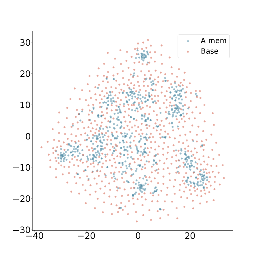
### Visual Description
## Scatter Plot: A-mem vs. Base Data Distribution
### Overview
The image is a 2D scatter plot comparing the spatial distribution of two datasets, labeled "A-mem" and "Base". The plot visualizes the relative positioning of numerous data points across a Cartesian coordinate system, revealing distinct clustering patterns for the two groups.
### Components/Axes
* **Plot Type:** Scatter plot.
* **X-Axis:** Horizontal axis with numerical markers. The visible range is from approximately **-40 to 20**, with major tick marks at -40, -20, 0, and 20. There is no explicit axis title.
* **Y-Axis:** Vertical axis with numerical markers. The visible range is from approximately **-30 to 30**, with major tick marks at -30, -20, -10, 0, 10, 20, and 30. There is no explicit axis title.
* **Legend:** Located in the **top-right corner** of the plot area. It contains two entries:
* A blue dot labeled **"A-mem"**.
* A pink/salmon dot labeled **"Base"**.
* **Data Points:** Hundreds of individual points plotted according to their (x, y) coordinates. Points are colored according to their series as defined in the legend.
### Detailed Analysis
**1. "A-mem" Series (Blue Points):**
* **Visual Trend:** The blue points are not uniformly distributed. They form several distinct, dense clusters separated by areas of lower density.
* **Spatial Distribution & Key Clusters:**
* A major, dense cluster is centered near the origin **(0, 0)**, extending roughly from x=-10 to x=10 and y=-10 to y=10.
* Another significant cluster is located in the **upper-right quadrant**, centered approximately at **(15, 10)**.
* A smaller, distinct cluster appears in the **lower-left quadrant**, centered near **(-25, -5)**.
* Additional smaller groupings are visible in the **upper-left quadrant** (around (-10, 15)) and the **lower-right quadrant** (around (15, -15)).
* **Range:** The points span nearly the entire visible plot area, from x ≈ -35 to x ≈ 25 and y ≈ -25 to y ≈ 25.
**2. "Base" Series (Pink Points):**
* **Visual Trend:** The pink points are widely and more evenly dispersed across the entire plot area, forming a broad, diffuse cloud.
* **Spatial Distribution:** They lack the tight clustering seen in the "A-mem" series. The density appears relatively uniform, though slightly sparser at the extreme edges of the distribution (e.g., near x=-40, y=-30).
* **Range:** The points cover a slightly wider area than the "A-mem" series, extending from x ≈ -40 to x ≈ 30 and y ≈ -30 to y ≈ 30.
**3. Relationship Between Series:**
* The "A-mem" clusters are embedded within the broader "Base" cloud.
* The dense central "A-mem" cluster overlaps significantly with the central region of the "Base" distribution.
* The other "A-mem" clusters (e.g., upper-right, lower-left) are located in regions that are also populated by "Base" points, but the "A-mem" points are much more concentrated there.
### Key Observations
1. **Clustering vs. Dispersion:** The most striking feature is the structural difference between the two datasets. "A-mem" exhibits clear multimodality (multiple clusters), while "Base" appears unimodal and diffuse.
2. **Spatial Overlap:** Despite different distributions, both series occupy the same general feature space, with significant overlap in the central region.
3. **Cluster Locations:** The "A-mem" clusters are not randomly placed; they appear in specific quadrants, suggesting potential subgroups or states within that dataset.
4. **Density Gradient:** The "Base" series shows a subtle density gradient, being densest near the center (0,0) and gradually thinning toward the periphery.
### Interpretation
This scatter plot likely visualizes the output of a dimensionality reduction technique (like t-SNE or UMAP) applied to two different models or conditions ("A-mem" and "Base"). The plot suggests:
* **Underlying Structure:** The "A-mem" model or condition produces representations (or data points) that naturally separate into distinct, meaningful clusters. This could indicate it has learned to categorize or differentiate between several underlying states, concepts, or classes within the data.
* **Baseline Distribution:** The "Base" model/condition produces a more homogeneous, less structured representation, suggesting it does not differentiate the underlying data as sharply.
* **Relationship:** The "A-mem" clusters emerging from the "Base" cloud could imply that "A-mem" is a specialized or refined version of "Base," where specific patterns have been amplified and separated from the general background noise.
* **Investigative Insight:** A researcher would use this plot to argue that the "A-mem" approach leads to more structured and potentially more interpretable internal representations. The next step would be to investigate what real-world categories or data attributes correspond to each of the identified "A-mem" clusters. The lack of axis labels limits direct physical interpretation but is common in such embedding visualizations where the axes represent abstract, non-linear dimensions.
</details>
(b) Dialogue 4
<details>
<summary>x15.png Details</summary>
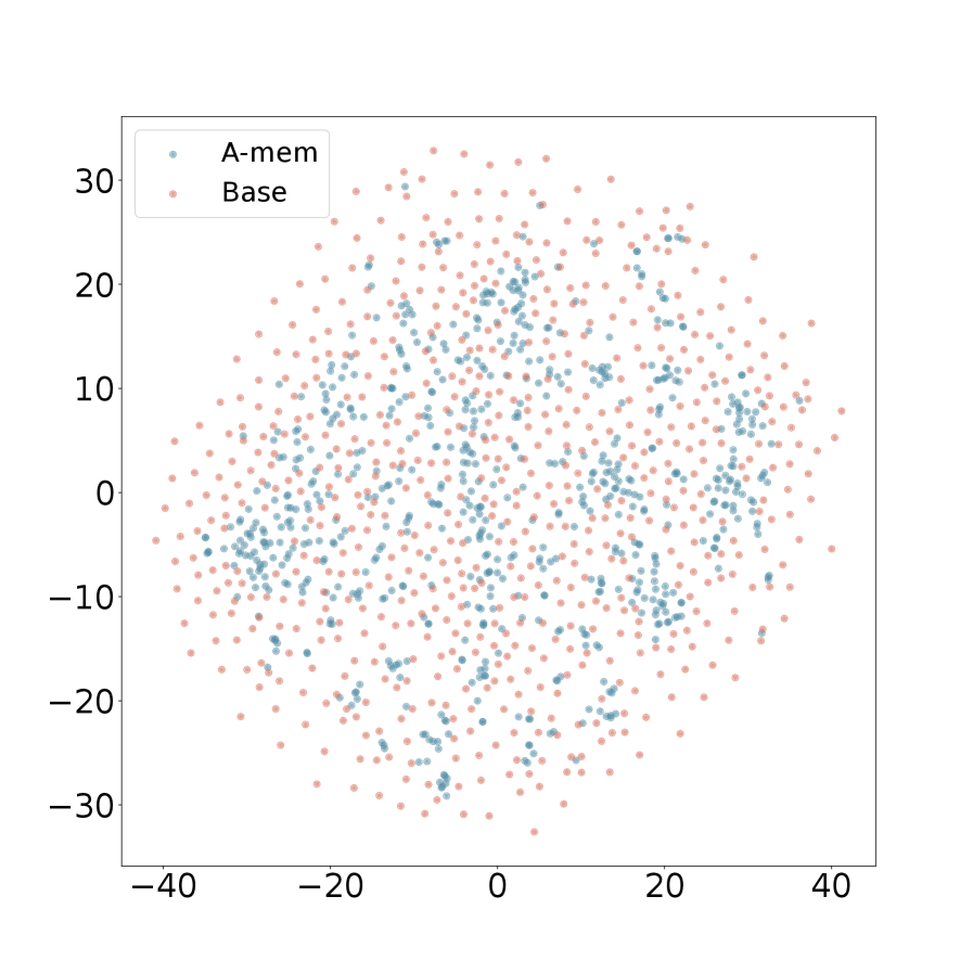
### Visual Description
## Scatter Plot: A-mem vs. Base Distribution
### Overview
The image is a 2D scatter plot comparing the spatial distribution of two data series, labeled "A-mem" and "Base". The plot displays a large number of individual data points plotted against a common, unlabeled coordinate system. The primary visual information is the relative density and spread of the two point clouds.
### Components/Axes
* **Legend:** Located in the top-left corner of the plot area.
* **A-mem:** Represented by blue/teal colored dots.
* **Base:** Represented by pink/salmon colored dots.
* **X-Axis:** Horizontal axis with numerical markers. The visible range is from approximately -40 to +40, with major tick marks at intervals of 20 (-40, -20, 0, 20, 40). There is no axis title or label.
* **Y-Axis:** Vertical axis with numerical markers. The visible range is from approximately -30 to +30, with major tick marks at intervals of 10 (-30, -20, -10, 0, 10, 20, 30). There is no axis title or label.
* **Plot Area:** A white background containing the two overlaid point clouds.
### Detailed Analysis
* **Data Series - A-mem (Blue):**
* **Trend/Distribution:** The blue points form a relatively dense, roughly circular cluster centered near the origin (0,0). The distribution appears tighter and more concentrated.
* **Spatial Extent:** The points are primarily contained within the range of approximately -25 to +25 on the x-axis and -20 to +20 on the y-axis. The density is highest near the center and decreases outward.
* **Data Series - Base (Pink):**
* **Trend/Distribution:** The pink points are much more widely dispersed, forming a larger, more diffuse cloud that encompasses the A-mem cluster.
* **Spatial Extent:** The points span nearly the entire visible plot area, from approximately -40 to +40 on the x-axis and -30 to +30 on the y-axis. The distribution is less dense overall compared to the A-mem series.
* **Overlap and Relationship:** The A-mem (blue) cluster is almost entirely contained within the broader Base (pink) cloud. There is significant overlap in the central region, but the Base series has many points in the periphery where A-mem points are absent.
### Key Observations
1. **Distinct Distributions:** The two series exhibit fundamentally different spatial distributions. A-mem is centralized and compact, while Base is expansive and diffuse.
2. **Containment:** The A-mem distribution appears to be a subset of the Base distribution in terms of spatial coverage.
3. **Density Gradient:** The A-mem series shows a clear density gradient, peaking at the center. The Base series has a more uniform, though still centrally weighted, density across a much larger area.
4. **Missing Information:** The plot lacks a title, axis titles, and units, which limits the contextual interpretation of what the coordinates represent.
### Interpretation
This scatter plot visually demonstrates a significant difference in the variance or spread between two groups or models, labeled "A-mem" and "Base". Assuming the axes represent some form of feature space, latent variable, or error metric:
* The **A-mem** system/model produces outputs or has characteristics that are highly consistent and clustered around a central mean (near 0,0). This suggests lower variance, higher precision, or a more constrained operational range.
* The **Base** system/model exhibits much higher variance, with outputs spread across a wider range of values. This indicates less consistency, greater diversity in results, or a broader operational scope.
* The relationship suggests that "A-mem" might be a refined, regularized, or specialized version of the "Base" system, where the modifications have the effect of reducing output variability and centering it around a target (the origin). The "Base" represents the unrefined or original state with inherent, wider dispersion.
**Note on Language:** All text in the image is in English.
</details>
(c) Dialogue 5
<details>
<summary>x16.png Details</summary>
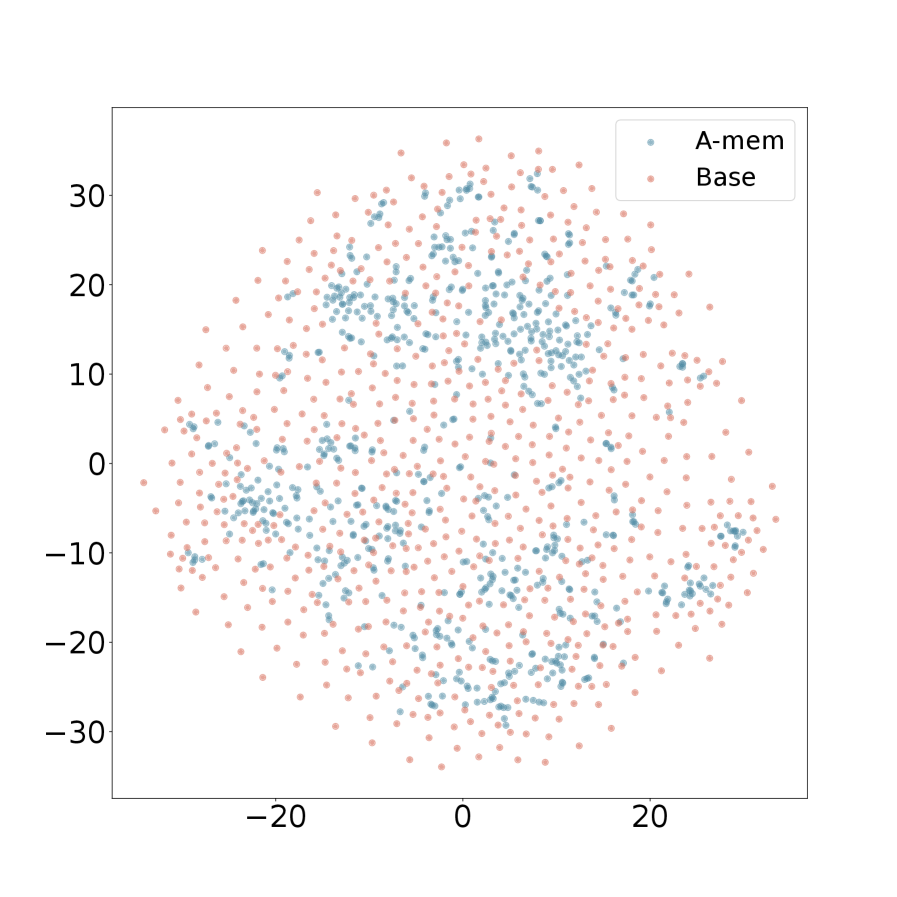
### Visual Description
## Scatter Plot: Comparison of "A-mem" and "Base" Distributions
### Overview
The image is a 2D scatter plot displaying two distinct data series, labeled "A-mem" and "Base," plotted on a Cartesian coordinate system. The data points form a dense, roughly circular cloud centered at the origin (0,0). The plot lacks a main title and axis labels, which limits the contextual interpretation of the data.
### Components/Axes
* **Legend:** Located in the top-right corner of the plot area. It contains two entries:
* A light blue dot labeled **"A-mem"**.
* A light pink dot labeled **"Base"**.
* **X-Axis:** Horizontal axis with numerical markers. The visible major tick marks are at **-20, 0, and 20**. The axis extends approximately from -30 to +30. **No axis title or label is present.**
* **Y-Axis:** Vertical axis with numerical markers. The visible major tick marks are at **-30, -20, -10, 0, 10, 20, and 30**. The axis extends approximately from -35 to +35. **No axis title or label is present.**
* **Data Points:** Hundreds of individual points for each series, plotted as small, solid circles.
### Detailed Analysis
* **Spatial Distribution & Trend:** Both data series ("A-mem" and "Base") are distributed in a broad, roughly circular cluster centered around the coordinate (0,0). There is no clear linear or directional trend; the overall pattern is a diffuse cloud.
* **Series Comparison:**
* **"A-mem" (Light Blue):** These points are densely concentrated in the central region of the plot, particularly within the approximate range of -15 to +15 on both axes. The density appears highest near the origin.
* **"Base" (Light Pink):** These points are more widely dispersed. While they also populate the central region, they extend further towards the periphery of the circular cluster, especially noticeable in the outer regions beyond ±20 on the axes.
* **Overlap:** There is significant spatial overlap between the two series throughout the central area of the plot. No distinct, separate clusters for each series are visible.
### Key Observations
1. **Missing Critical Metadata:** The complete absence of axis titles and a chart title is a major omission for a technical document, rendering the quantitative meaning of the coordinates unknown.
2. **Central vs. Peripheral Spread:** The most notable visual pattern is the difference in dispersion. The "A-mem" series exhibits a tighter, more centrally concentrated distribution, while the "Base" series shows a broader, more scattered distribution.
3. **Circular Symmetry:** The overall shape of the combined data cloud is approximately circular and symmetric about the origin, suggesting the underlying data may be normalized or centered.
4. **High Density:** The plot contains a large number of data points for both series, indicating a substantial dataset.
### Interpretation
This scatter plot visually compares the distribution of two datasets or model outputs ("A-mem" and "Base") in a two-dimensional space. The key insight is the difference in variance or spread between the two.
* **What the data suggests:** The "A-mem" data points are more tightly clustered around the central mean (0,0), indicating lower variance or a more focused representation. The "Base" data points have higher variance, spreading out more widely from the center. This could imply that the "A-mem" method or model produces more consistent, less dispersed results compared to the "Base" method.
* **Relationship between elements:** The significant overlap in the central region suggests that for a large portion of the data, the two series produce similar or indistinguishable values in this 2D projection. The differentiation occurs primarily at the tails of the distribution.
* **Notable Anomalies:** The primary anomaly is the lack of axis labels, which is a critical flaw for data communication. Without knowing what the X and Y axes represent (e.g., principal components, latent dimensions, error metrics), the practical significance of the spread and clustering cannot be determined. The plot effectively shows *that* there is a difference in distribution shape but not *what* that difference means in a real-world context.
* **Peircean Investigative Reading:** The sign (the plot) indicates a comparison. The icon (the visual spread) resembles a difference in consistency. The interpretant (the likely conclusion for a viewer) is that "A-mem" is more precise or stable than "Base," but this conclusion is tentative due to the missing symbolic information (axis labels). The plot successfully communicates a relative difference but fails to communicate absolute meaning.
</details>
(d) Dialogue 6
<details>
<summary>x17.png Details</summary>
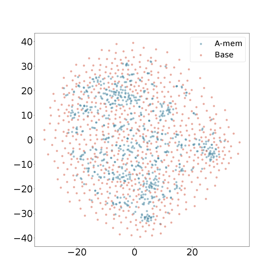
### Visual Description
## Scatter Plot: A-mem vs. Base Distribution
### Overview
The image is a 2D scatter plot comparing the spatial distribution of two data series, labeled "A-mem" and "Base". The plot displays a large number of individual data points plotted against two unlabeled numerical axes. The overall visual impression is of two overlapping, cloud-like distributions with different densities and spreads.
### Components/Axes
* **Legend:** Located in the top-right corner of the plot area. It contains two entries:
* A blue dot labeled **"A-mem"**.
* A pink/salmon dot labeled **"Base"**.
* **X-Axis:** A horizontal numerical axis. Major tick marks and labels are present at **-20, 0, and 20**. The visible range extends slightly beyond these values, approximately from -25 to +25.
* **Y-Axis:** A vertical numerical axis. Major tick marks and labels are present at **-40, -30, -20, -10, 0, 10, 20, 30, and 40**. The visible range is from approximately -45 to +45.
* **Data Points:** Hundreds of small, circular markers. Blue markers represent the "A-mem" series, and pink markers represent the "Base" series.
### Detailed Analysis
* **Spatial Distribution & Density:**
* **"Base" Series (Pink):** This series forms a broad, roughly circular or elliptical cloud that fills most of the plot area. The points are widely dispersed, with a higher density near the center (around coordinate (0,0)) and gradually thinning out towards the periphery. The distribution appears relatively uniform in its spread.
* **"A-mem" Series (Blue):** This series is also widely distributed but shows a distinctly different pattern. It is less uniformly spread than the "Base" series. The blue points appear to form a denser, more concentrated cluster that is slightly offset from the absolute center. This cluster is most prominent in the region roughly between X = -10 to +10 and Y = -20 to +20. Outside this central cluster, blue points are scattered more sparsely, often intermingled with the pink points.
* **Overlap and Relationship:** There is significant overlap between the two distributions, particularly in the central region of the plot. However, the "A-mem" points are not randomly scattered within the "Base" cloud; they exhibit a clear tendency to group together, suggesting a more constrained or focused distribution compared to the more expansive "Base" distribution.
* **Trend Verification:** Neither series shows a linear trend (e.g., a clear upward or downward slope). Both are best described as amorphous clouds. The primary visual trend is the difference in **clustering density** between the two series.
### Key Observations
1. **Density Gradient:** The "Base" (pink) series has a clear density gradient, peaking at the center and fading outward. The "A-mem" (blue) series has a more complex density profile, with a pronounced central cluster and a sparse periphery.
2. **Central Tendency:** The highest density of "A-mem" points appears to be centered slightly to the left (negative X) and below (negative Y) the plot's origin (0,0), though the overall cloud is still centered near the origin.
3. **Absence of Axis Titles:** The plot lacks descriptive labels for the X and Y axes, making it impossible to know what specific variables or dimensions are being compared without external context.
4. **Scale:** The Y-axis has a larger numerical range (80 units) compared to the X-axis (40 units), but the visual scaling appears to be 1:1, making the distribution look circular.
### Interpretation
This scatter plot likely visualizes the output of a dimensionality reduction technique (like t-SNE or PCA) applied to two different datasets or model states, projecting high-dimensional data into a 2D space for comparison.
* **What the data suggests:** The plot demonstrates that the "A-mem" data points occupy a more specific and concentrated region within the broader feature space defined by the "Base" data. This could indicate that the "A-mem" condition (perhaps a model with a specific memory mechanism) produces more consistent, similar, or focused internal representations compared to the more varied or exploratory "Base" condition.
* **Relationship between elements:** The "Base" distribution acts as a background or reference manifold. The "A-mem" distribution is a subset or a specialization within that manifold. The significant overlap shows they share common characteristics, but the distinct clustering of "A-mem" points highlights a key differentiating factor.
* **Notable Anomalies/Patterns:** The most significant pattern is the **clustering vs. dispersion** dichotomy. There are no obvious outlier points far removed from the main clouds. The primary insight is not in individual points but in the collective shape and density of the two point clouds. The lack of axis labels is a critical limitation for full technical interpretation, as the meaning of the spatial separation is unknown.
</details>
(e) Dialogue 7
<details>
<summary>x18.png Details</summary>
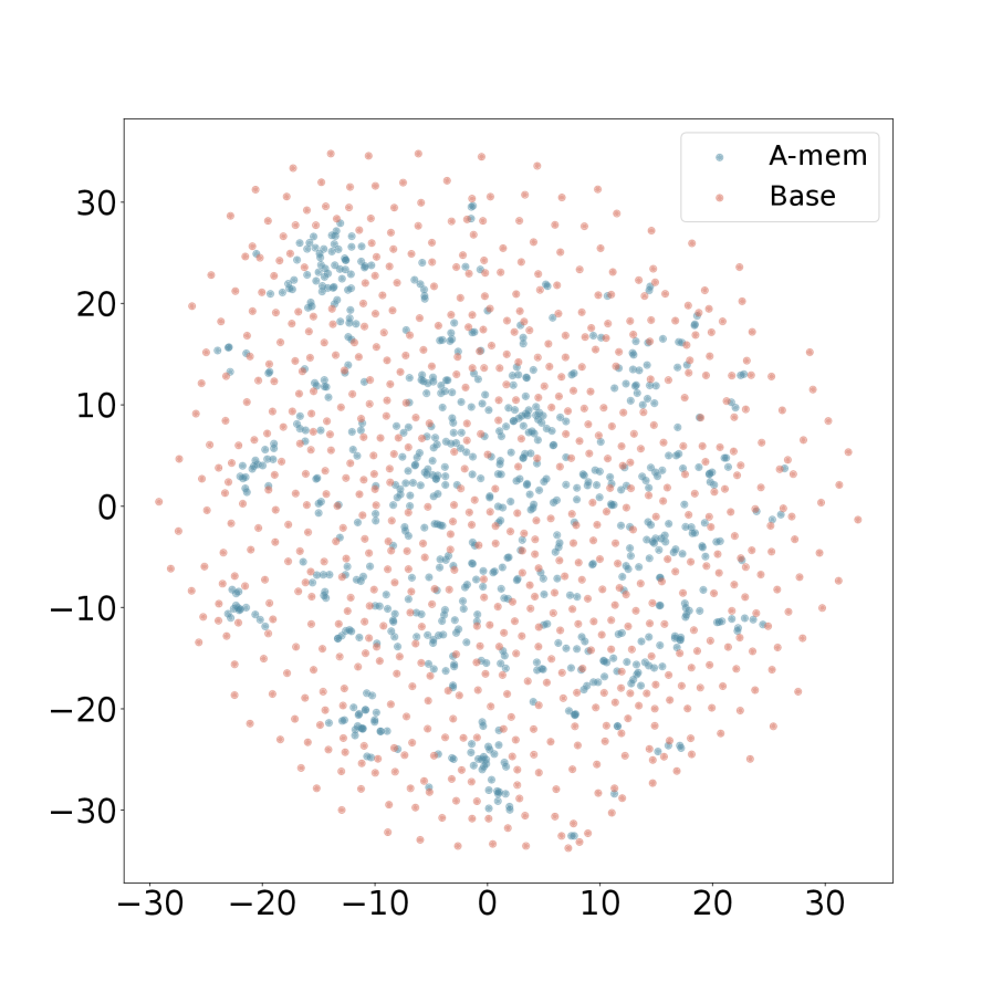
### Visual Description
## Scatter Plot: A-mem vs. Base Distribution
### Overview
The image is a 2D scatter plot comparing the spatial distribution of two data series, labeled "A-mem" and "Base". The plot displays a cloud of points for each series on a common coordinate system, allowing for visual comparison of their spread, density, and central tendency. No explicit axis titles are provided, suggesting the axes represent two generic dimensions or features.
### Components/Axes
* **Chart Type:** Scatter Plot.
* **Legend:** Located in the top-right corner of the plot area. It contains two entries:
* A blue dot labeled **"A-mem"**.
* A pink/salmon dot labeled **"Base"**.
* **X-Axis:** A horizontal numerical axis. Major tick marks and labels are present at intervals of 10, ranging from **-30** to **30**. The axis line is solid black.
* **Y-Axis:** A vertical numerical axis. Major tick marks and labels are present at intervals of 10, ranging from **-30** to **30**. The axis line is solid black.
* **Plot Area:** A white background enclosed by the axes. No grid lines are visible.
### Detailed Analysis
* **Data Series - "A-mem" (Blue Points):**
* **Trend/Distribution:** The blue points form a relatively dense, centralized cluster. The distribution appears roughly elliptical or circular, centered near the origin (0,0).
* **Spatial Spread:** The points are concentrated within an approximate range of **-20 to +20** on both the X and Y axes. The density is highest near the center and gradually decreases outward. There are very few points beyond the ±20 range on either axis.
* **Visual Density:** The cluster is dense enough that individual points overlap significantly, especially near the center.
* **Data Series - "Base" (Pink Points):**
* **Trend/Distribution:** The pink points form a much more diffuse, widespread cloud that encompasses the entire visible plot area.
* **Spatial Spread:** The points are distributed across the full range of the axes, from approximately **-30 to +30** on both X and Y. While there is a slight concentration towards the center, the points maintain a significant presence even at the extreme edges of the plot.
* **Visual Density:** The points are more sparsely distributed compared to the blue series, with less overlap. They create a background "noise" or "cloud" against which the blue cluster is situated.
* **Spatial Relationship:** The "A-mem" (blue) cluster is entirely contained within the broader "Base" (pink) cloud. The blue points do not extend to the peripheries occupied by the pink points.
### Key Observations
1. **Variance Contrast:** The most striking observation is the dramatic difference in variance (spread) between the two series. "Base" exhibits high variance across both dimensions, while "A-mem" exhibits low variance.
2. **Central Tendency:** Both distributions appear centered around the origin (0,0), but the "A-mem" series has a much tighter central tendency.
3. **Outliers:** The "Base" series contains numerous points that could be considered outliers relative to the "A-mem" cluster, located in the outer regions of the plot (e.g., near (-30, 10), (25, -20)).
4. **Overlap Zone:** There is a significant region of overlap where both blue and pink points coexist, primarily within the central ±20 range. However, the blue points dominate the visual density in the very center.
### Interpretation
This scatter plot visually demonstrates a fundamental difference in the behavior or characteristics of the "A-mem" and "Base" entities.
* **What the data suggests:** The "A-mem" method, model, or dataset produces results that are highly consistent and confined to a specific, predictable region of the feature space. In contrast, the "Base" method produces results that are highly variable, exploring or occupying a much wider range of possible states.
* **How elements relate:** The plot implies that "A-mem" might be a constrained, regularized, or optimized version of "Base". The "Base" distribution could represent a baseline, raw, or uncontrolled state, while "A-mem" represents a state where variance has been significantly reduced, focusing the output around a central mean.
* **Notable implications:** If this plot represents, for example, the latent space of two neural networks, it would suggest "A-mem" has learned a more compact and focused representation. If it represents experimental results, "A-mem" shows higher precision and reproducibility. The lack of axis labels means the specific meaning of the dimensions is unknown, but the pattern of **reduced variance** is the key takeaway. The "Base" series acts as a reference, showing the full scope of possibility, against which the focused performance of "A-mem" is highlighted.
</details>
(f) Dialogue 8
<details>
<summary>x19.png Details</summary>
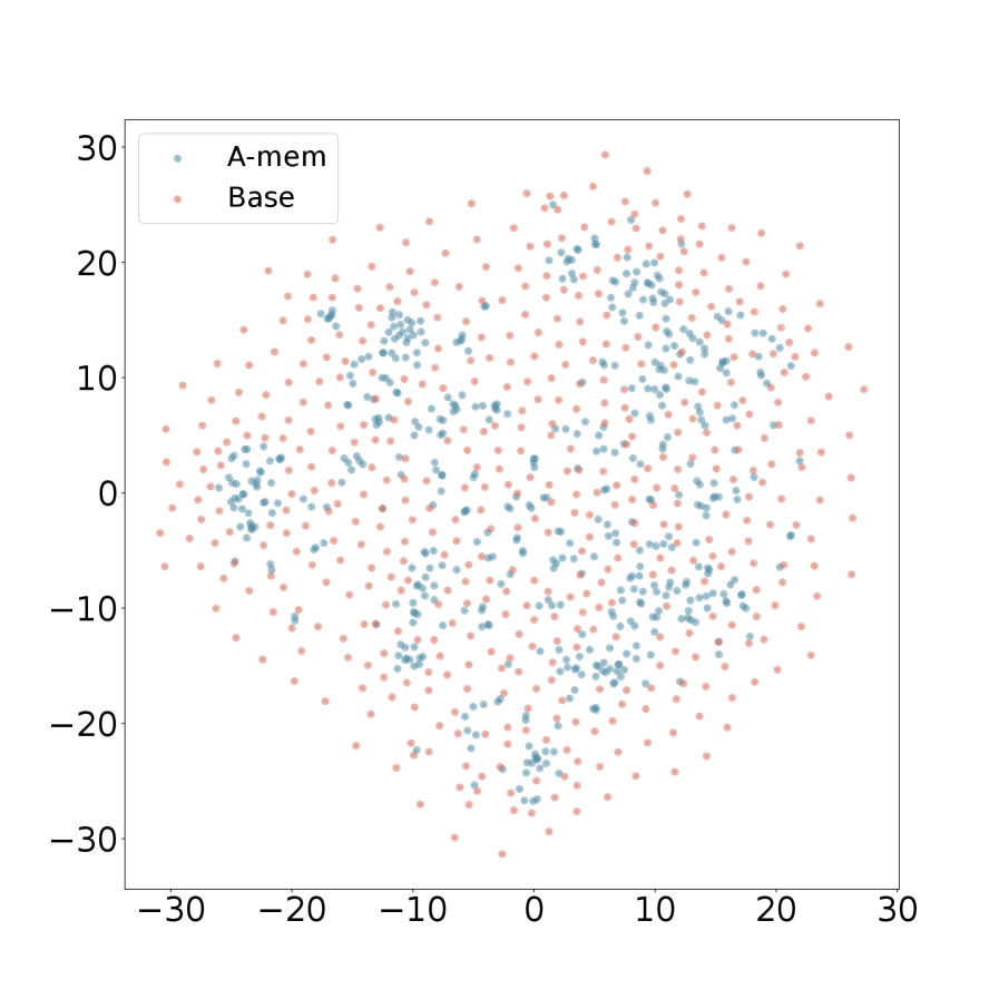
### Visual Description
## Scatter Plot: A-mem vs. Base Distribution
### Overview
The image is a 2D scatter plot comparing the spatial distribution of two data series, labeled "A-mem" and "Base". The plot displays a cloud of points on a Cartesian coordinate system, with both axes ranging from approximately -30 to +30. The data appears to represent some form of embedding or latent space visualization, where the relative positions and clustering of points are the primary information.
### Components/Axes
* **Plot Type:** Scatter Plot.
* **X-Axis:** Linear scale. Major tick marks and labels are present at intervals of 10: -30, -20, -10, 0, 10, 20, 30. There is no explicit axis title.
* **Y-Axis:** Linear scale. Major tick marks and labels are present at intervals of 10: -30, -20, -10, 0, 10, 20, 30. There is no explicit axis title.
* **Legend:** Located in the top-left corner of the plot area. It contains two entries:
* A blue-gray dot labeled **"A-mem"**.
* A salmon/light red dot labeled **"Base"**.
* **Data Points:** Hundreds of individual points are plotted, corresponding to the two series defined in the legend.
### Detailed Analysis
**1. Data Series "A-mem" (Blue-Gray Points):**
* **Visual Trend:** These points form a relatively dense, centrally concentrated cluster. The distribution appears roughly circular or elliptical, centered near the origin (0,0).
* **Spatial Distribution:** The highest density of "A-mem" points is within the region bounded approximately by X: [-15, 15] and Y: [-15, 15]. The points become sparser as you move away from this central region. Very few "A-mem" points are located beyond ±20 on either axis.
* **Approximate Bounds:** The visible extremes for this series are roughly X: [-20, 20] and Y: [-20, 20].
**2. Data Series "Base" (Salmon/Light Red Points):**
* **Visual Trend:** These points are much more widely dispersed across the entire plot area. They do not form a single tight cluster but instead create a broad, diffuse cloud.
* **Spatial Distribution:** "Base" points are found throughout the range of the axes, from approximately -30 to +30 on both X and Y. They completely surround the denser "A-mem" cluster. The density of "Base" points appears more uniform compared to the peaked density of "A-mem".
* **Approximate Bounds:** The visible extremes for this series span nearly the full axis ranges: X: [-30, 30] and Y: [-30, 30].
**3. Relationship Between Series:**
* The "A-mem" distribution is entirely contained within the spatial extent of the "Base" distribution.
* There is significant overlap between the two series in the central region of the plot (roughly within ±15 on both axes).
* The outer periphery of the plot (beyond ±20) is populated almost exclusively by "Base" points.
### Key Observations
* **Variance Difference:** The most striking observation is the difference in variance or spread. "A-mem" exhibits low variance (tight clustering), while "Base" exhibits high variance (wide dispersion).
* **Central Tendency:** Both distributions appear to be centered around the origin (0,0), but "A-mem" has a much stronger central tendency.
* **No Clear Outliers:** Given the diffuse nature of the "Base" series, no single point can be definitively labeled an outlier relative to its own series. However, all "A-mem" points could be considered outliers relative to the full spatial range defined by the "Base" series.
* **Missing Context:** The plot lacks axis titles, a main title, or any descriptive caption. This omits crucial information about what the axes represent (e.g., dimensions, features, coordinates) and the overall subject of the comparison.
### Interpretation
This scatter plot visually demonstrates a fundamental difference in the structure of two datasets or model outputs, "A-mem" and "Base".
* **What the data suggests:** The "A-mem" data is highly constrained or focused within a specific region of the feature space represented by the axes. This could indicate a model that produces consistent, similar outputs ("A-mem") or a dataset with low intrinsic dimensionality. In contrast, the "Base" data is highly variable and explores a much broader region of the space, suggesting a model with higher entropy, a more diverse dataset, or a less constrained process.
* **How elements relate:** The containment of the "A-mem" cluster within the "Base" cloud implies that the "A-mem" distribution may be a specialized, refined, or converged subset of the more general "Base" distribution. It could represent the result of a training process, a filtering operation, or a more focused sampling strategy applied to the "Base" population.
* **Notable implications:** Without axis labels, the practical significance is abstract. However, in contexts like machine learning (e.g., visualizing word embeddings, model activations, or generative model outputs), this pattern is classic. It often shows a baseline or random model ("Base") producing scattered, unstructured representations, while a trained or specialized model ("A-mem") organizes its representations into a tighter, more meaningful cluster. The plot argues for the effectiveness of whatever process "A-mem" represents in reducing variance and creating consistency.
</details>
(g) Dialogue 9
<details>
<summary>x20.png Details</summary>
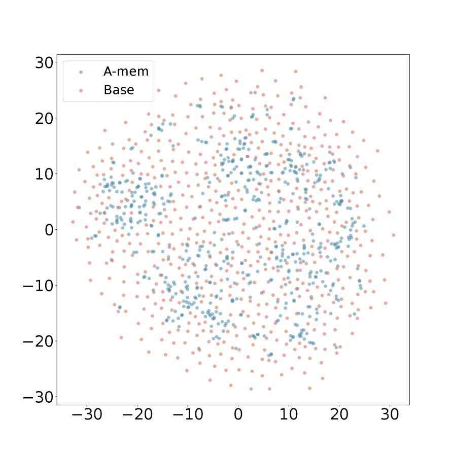
### Visual Description
## Scatter Plot: Comparison of "A-mem" and "Base" Data Distributions
### Overview
The image is a 2D scatter plot comparing the spatial distribution of two data series, labeled "A-mem" and "Base". The plot displays a large number of individual data points plotted against a common, unlabeled coordinate system. The visual suggests a comparison of clustering, spread, and central tendency between the two groups.
### Components/Axes
* **Chart Type:** Scatter Plot.
* **Legend:** Located in the top-left corner of the plot area.
* **A-mem:** Represented by blue/teal colored dots.
* **Base:** Represented by pink/salmon colored dots.
* **X-Axis:**
* **Scale:** Linear.
* **Range:** Approximately -30 to +30.
* **Major Tick Marks:** At intervals of 10 (-30, -20, -10, 0, 10, 20, 30).
* **Label:** No explicit axis title is present.
* **Y-Axis:**
* **Scale:** Linear.
* **Range:** Approximately -30 to +30.
* **Major Tick Marks:** At intervals of 10 (-30, -20, -10, 0, 10, 20, 30).
* **Label:** No explicit axis title is present.
* **Plot Area:** A square region bounded by the axes, containing all data points.
### Detailed Analysis
* **Data Series - "A-mem" (Blue/Teal Points):**
* **Spatial Distribution:** The points form a relatively dense, roughly circular cluster centered near the origin (0,0).
* **Spread:** The majority of points are concentrated within the range of approximately -15 to +15 on both axes. The density decreases noticeably towards the periphery of this range.
* **Trend/Pattern:** Shows a clear central tendency with moderate dispersion. There is no obvious linear or non-linear trend; the distribution appears isotropic (similar in all directions from the center).
* **Data Series - "Base" (Pink/Salmon Points):**
* **Spatial Distribution:** The points are much more widely and diffusely scattered across the entire plot area.
* **Spread:** Points are present across the full visible range, from approximately -30 to +30 on both axes. The density is lower than the "A-mem" series in the central region but higher in the outer regions.
* **Trend/Pattern:** Exhibits a high degree of variance with no strong central cluster. The distribution appears roughly uniform or randomly scattered within the bounded square area, with a slight visual impression of being more dispersed than a perfect uniform distribution.
* **Relative Comparison:**
* The "A-mem" series is visually nested within the broader "Base" series.
* The central region (e.g., within ±10 on both axes) is dominated by blue "A-mem" points, though pink "Base" points are also present.
* The peripheral regions (e.g., beyond ±20 on either axis) are almost exclusively populated by pink "Base" points.
### Key Observations
1. **Distinct Clustering vs. Dispersion:** The most salient feature is the stark contrast in spatial distribution. "A-mem" demonstrates tight clustering, while "Base" shows wide dispersion.
2. **Overlap Zone:** There is a significant area of overlap in the central region of the plot where both data series are present, though "A-mem" points are denser there.
3. **Boundary Effects:** The "Base" series appears to fill the entire plotted square, suggesting its data range may extend to or beyond the axis limits. The "A-mem" series is fully contained within the plot boundaries.
4. **No Apparent Correlation:** For either series individually, there is no visible correlation between the X and Y values (e.g., no diagonal banding). The points appear randomly distributed within their respective envelopes.
### Interpretation
This scatter plot likely visualizes the output of a dimensionality reduction technique (like t-SNE or PCA) applied to two different datasets or model states, projecting high-dimensional data into 2D for comparison.
* **What the data suggests:** The "A-mem" data points occupy a much smaller, more defined region of the feature space compared to the "Base" points. This implies that the entities or samples represented by "A-mem" are more similar to each other (have lower variance) in the underlying measured characteristics than those represented by "Base".
* **Relationship between elements:** The plot directly contrasts two conditions. "Base" could represent a baseline, control, or initial state with high variability. "A-mem" could represent a state after some process (e.g., training, memory consolidation, filtering) that has reduced variability and increased consistency, pulling the data points toward a central prototype or mean.
* **Notable implications:** The visualization strongly argues that the "A-mem" condition leads to a more focused and consistent representation. If this relates to a machine learning model, "A-mem" might produce more confident or specialized representations. If it relates to experimental data, "A-mem" might indicate a treatment that reduces noise or standardizes responses. The lack of axis labels is a critical limitation; the interpretation hinges on knowing what the X and Y dimensions represent (e.g., principal components, latent variables).
</details>
(h) Dialogue 10
Figure 5: T-SNE Visualization of Memory Embeddings Showing More Organized Distribution with A-Mem (blue) Compared to Base Memory (red) Across Different Dialogues. Base Memory represents A-Mem without link generation and memory evolution.
### A.5 Hyperparameters setting
All hyperparameter k values are presented in Table 8. For models that have already achieved state-of-the-art (SOTA) performance with k=10, we maintain this value without further tuning.
Table 8: Selection of k values in retriever across specific categories and model choices.
| Model | Multi Hop | Temporal | Open Domain | Single Hop | Adversial |
| --- | --- | --- | --- | --- | --- |
| GPT-4o-mini | 40 | 40 | 50 | 50 | 40 |
| GPT-4o | 40 | 40 | 50 | 50 | 40 |
| Qwen2.5-1.5b | 10 | 10 | 10 | 10 | 10 |
| Qwen2.5-3b | 10 | 10 | 50 | 10 | 10 |
| Llama3.2-1b | 10 | 10 | 10 | 10 | 10 |
| Llama3.2-3b | 10 | 20 | 10 | 10 | 10 |
## Appendix B Prompt Templates and Examples
### B.1 Prompt Template of Note Construction
The prompt template in Note Construction: $P_s1$ Generate a structured analysis of the following content by: 1. Identifying the most salient keywords (focus on nouns, verbs, and key concepts) 2. Extracting core themes and contextual elements 3. Creating relevant categorical tags Format the response as a JSON object: { "keywords": [ // several specific, distinct keywords that capture key concepts and terminology // Order from most to least important // Don’t include keywords that are the name of the speaker or time // At least three keywords, but don’t be too redundant. ], "context": // one sentence summarizing: // - Main topic/domain // - Key arguments/points // - Intended audience/purpose , "tags": [ // several broad categories/themes for classification // Include domain, format, and type tags // At least three tags, but don’t be too redundant. ] } Content for analysis:
### B.2 Prompt Template of Link Generation
The prompt template in Link Generation: $P_s2$ You are an AI memory evolution agent responsible for managing and evolving a knowledge base. Analyze the the new memory note according to keywords and context, also with their several nearest neighbors memory. The new memory context: {context} content: {content} keywords: {keywords} The nearest neighbors memories: {nearest_neighbors_memories} Based on this information, determine: Should this memory be evolved? Consider its relationships with other memories.
### B.3 Prompt Template of Memory Evolution
The prompt template in Memory Evolution: $P_s3$ You are an AI memory evolution agent responsible for managing and evolving a knowledge base. Analyze the the new memory note according to keywords and context, also with their several nearest neighbors memory. Make decisions about its evolution. The new memory context:{context} content: {content} keywords: {keywords} The nearest neighbors memories:{nearest_neighbors_memories} Based on this information, determine: 1. What specific actions should be taken (strengthen, update_neighbor)? 1.1 If choose to strengthen the connection, which memory should it be connected to? Can you give the updated tags of this memory? 1.2 If choose to update neighbor, you can update the context and tags of these memories based on the understanding of these memories. Tags should be determined by the content of these characteristic of these memories, which can be used to retrieve them later and categorize them. All the above information should be returned in a list format according to the sequence: [[new_memory],[neighbor_memory_1], ...[neighbor_memory_n]] These actions can be combined. Return your decision in JSON format with the following structure: {{ "should_evolve": true/false, "actions": ["strengthen", "merge", "prune"], "suggested_connections": ["neighbor_memory_ids"], "tags_to_update": ["tag_1",..."tag_n"], "new_context_neighborhood": ["new context",...,"new context"], "new_tags_neighborhood": [["tag_1",...,"tag_n"],...["tag_1",...,"tag_n"]], }}
### B.4 Examples of Q/A with A-Mem
Example: Question 686: Which hobby did Dave pick up in October 2023? Prediction: photography Reference: photography talk start time:10:54 am on 17 November, 2023 memory content: Speaker Davesays : Hey Calvin, long time no talk! A lot has happened. I’ve taken up photography and it’s been great - been taking pics of the scenery around here which is really cool. memory context: The main topic is the speaker’s new hobby of photography, highlighting their enjoyment of capturing local scenery, aimed at engaging a friend in conversation about personal experiences. memory keywords: [’photography’, ’scenery’, ’conversation’, ’experience’, ’hobby’] memory tags: [’hobby’, ’photography’, ’personal development’, ’conversation’, ’leisure’] talk start time:6:38 pm on 21 July, 2023 memory content: Speaker Calvinsays : Thanks, Dave! It feels great having my own space to work in. I’ve been experimenting with different genres lately, pushing myself out of my comfort zone. Adding electronic elements to my songs gives them a fresh vibe. It’s been an exciting process of self-discovery and growth! memory context: The speaker discusses their creative process in music, highlighting experimentation with genres and the incorporation of electronic elements for personal growth and artistic evolution. memory keywords: [’space’, ’experimentation’, ’genres’, ’electronic’, ’self-discovery’, ’growth’] memory tags: [’music’, ’creativity’, ’self-improvement’, ’artistic expression’]
## NeurIPS Paper Checklist
The checklist is designed to encourage best practices for responsible machine learning research, addressing issues of reproducibility, transparency, research ethics, and societal impact. Do not remove the checklist: The papers not including the checklist will be desk rejected. The checklist should follow the references and follow the (optional) supplemental material. The checklist does NOT count towards the page limit.
Please read the checklist guidelines carefully for information on how to answer these questions. For each question in the checklist:
- You should answer [Yes] , [No] , or [N/A] .
- [N/A] means either that the question is Not Applicable for that particular paper or the relevant information is Not Available.
- Please provide a short (1–2 sentence) justification right after your answer (even for NA).
The checklist answers are an integral part of your paper submission. They are visible to the reviewers, area chairs, senior area chairs, and ethics reviewers. You will be asked to also include it (after eventual revisions) with the final version of your paper, and its final version will be published with the paper.
The reviewers of your paper will be asked to use the checklist as one of the factors in their evaluation. While " [Yes] " is generally preferable to " [No] ", it is perfectly acceptable to answer " [No] " provided a proper justification is given (e.g., "error bars are not reported because it would be too computationally expensive" or "we were unable to find the license for the dataset we used"). In general, answering " [No] " or " [N/A] " is not grounds for rejection. While the questions are phrased in a binary way, we acknowledge that the true answer is often more nuanced, so please just use your best judgment and write a justification to elaborate. All supporting evidence can appear either in the main paper or the supplemental material, provided in appendix. If you answer [Yes] to a question, in the justification please point to the section(s) where related material for the question can be found.
IMPORTANT, please:
- Delete this instruction block, but keep the section heading “NeurIPS Paper Checklist",
- Keep the checklist subsection headings, questions/answers and guidelines below.
- Do not modify the questions and only use the provided macros for your answers.
1. Claims
1. Question: Do the main claims made in the abstract and introduction accurately reflect the paper’s contributions and scope?
1. Answer: [Yes]
1. Justification: The abstract and the introduction summarizes our main contributions.
1. Guidelines:
- The answer NA means that the abstract and introduction do not include the claims made in the paper.
- The abstract and/or introduction should clearly state the claims made, including the contributions made in the paper and important assumptions and limitations. A No or NA answer to this question will not be perceived well by the reviewers.
- The claims made should match theoretical and experimental results, and reflect how much the results can be expected to generalize to other settings.
- It is fine to include aspirational goals as motivation as long as it is clear that these goals are not attained by the paper.
1. Limitations
1. Question: Does the paper discuss the limitations of the work performed by the authors?
1. Answer: [Yes]
1. Justification: This paper cover a section of the limiations.
1. Guidelines:
- The answer NA means that the paper has no limitation while the answer No means that the paper has limitations, but those are not discussed in the paper.
- The authors are encouraged to create a separate "Limitations" section in their paper.
- The paper should point out any strong assumptions and how robust the results are to violations of these assumptions (e.g., independence assumptions, noiseless settings, model well-specification, asymptotic approximations only holding locally). The authors should reflect on how these assumptions might be violated in practice and what the implications would be.
- The authors should reflect on the scope of the claims made, e.g., if the approach was only tested on a few datasets or with a few runs. In general, empirical results often depend on implicit assumptions, which should be articulated.
- The authors should reflect on the factors that influence the performance of the approach. For example, a facial recognition algorithm may perform poorly when image resolution is low or images are taken in low lighting. Or a speech-to-text system might not be used reliably to provide closed captions for online lectures because it fails to handle technical jargon.
- The authors should discuss the computational efficiency of the proposed algorithms and how they scale with dataset size.
- If applicable, the authors should discuss possible limitations of their approach to address problems of privacy and fairness.
- While the authors might fear that complete honesty about limitations might be used by reviewers as grounds for rejection, a worse outcome might be that reviewers discover limitations that aren’t acknowledged in the paper. The authors should use their best judgment and recognize that individual actions in favor of transparency play an important role in developing norms that preserve the integrity of the community. Reviewers will be specifically instructed to not penalize honesty concerning limitations.
1. Theory assumptions and proofs
1. Question: For each theoretical result, does the paper provide the full set of assumptions and a complete (and correct) proof?
1. Answer: [N/A]
1. Justification: N/A
1. Guidelines:
- The answer NA means that the paper does not include theoretical results.
- All the theorems, formulas, and proofs in the paper should be numbered and cross-referenced.
- All assumptions should be clearly stated or referenced in the statement of any theorems.
- The proofs can either appear in the main paper or the supplemental material, but if they appear in the supplemental material, the authors are encouraged to provide a short proof sketch to provide intuition.
- Inversely, any informal proof provided in the core of the paper should be complemented by formal proofs provided in appendix or supplemental material.
- Theorems and Lemmas that the proof relies upon should be properly referenced.
1. Experimental result reproducibility
1. Question: Does the paper fully disclose all the information needed to reproduce the main experimental results of the paper to the extent that it affects the main claims and/or conclusions of the paper (regardless of whether the code and data are provided or not)?
1. Answer: [Yes]
1. Justification: Both code and datasets are available.
1. Guidelines:
- The answer NA means that the paper does not include experiments.
- If the paper includes experiments, a No answer to this question will not be perceived well by the reviewers: Making the paper reproducible is important, regardless of whether the code and data are provided or not.
- If the contribution is a dataset and/or model, the authors should describe the steps taken to make their results reproducible or verifiable.
- Depending on the contribution, reproducibility can be accomplished in various ways. For example, if the contribution is a novel architecture, describing the architecture fully might suffice, or if the contribution is a specific model and empirical evaluation, it may be necessary to either make it possible for others to replicate the model with the same dataset, or provide access to the model. In general. releasing code and data is often one good way to accomplish this, but reproducibility can also be provided via detailed instructions for how to replicate the results, access to a hosted model (e.g., in the case of a large language model), releasing of a model checkpoint, or other means that are appropriate to the research performed.
- While NeurIPS does not require releasing code, the conference does require all submissions to provide some reasonable avenue for reproducibility, which may depend on the nature of the contribution. For example
1. If the contribution is primarily a new algorithm, the paper should make it clear how to reproduce that algorithm.
1. If the contribution is primarily a new model architecture, the paper should describe the architecture clearly and fully.
1. If the contribution is a new model (e.g., a large language model), then there should either be a way to access this model for reproducing the results or a way to reproduce the model (e.g., with an open-source dataset or instructions for how to construct the dataset).
1. We recognize that reproducibility may be tricky in some cases, in which case authors are welcome to describe the particular way they provide for reproducibility. In the case of closed-source models, it may be that access to the model is limited in some way (e.g., to registered users), but it should be possible for other researchers to have some path to reproducing or verifying the results.
1. Open access to data and code
1. Question: Does the paper provide open access to the data and code, with sufficient instructions to faithfully reproduce the main experimental results, as described in supplemental material?
1. Answer: [Yes]
1. Justification: We provide the code link in the abstract.
1. Guidelines:
- The answer NA means that paper does not include experiments requiring code.
- Please see the NeurIPS code and data submission guidelines (https://nips.cc/public/guides/CodeSubmissionPolicy) for more details.
- While we encourage the release of code and data, we understand that this might not be possible, so “No” is an acceptable answer. Papers cannot be rejected simply for not including code, unless this is central to the contribution (e.g., for a new open-source benchmark).
- The instructions should contain the exact command and environment needed to run to reproduce the results. See the NeurIPS code and data submission guidelines (https://nips.cc/public/guides/CodeSubmissionPolicy) for more details.
- The authors should provide instructions on data access and preparation, including how to access the raw data, preprocessed data, intermediate data, and generated data, etc.
- The authors should provide scripts to reproduce all experimental results for the new proposed method and baselines. If only a subset of experiments are reproducible, they should state which ones are omitted from the script and why.
- At submission time, to preserve anonymity, the authors should release anonymized versions (if applicable).
- Providing as much information as possible in supplemental material (appended to the paper) is recommended, but including URLs to data and code is permitted.
1. Experimental setting/details
1. Question: Does the paper specify all the training and test details (e.g., data splits, hyperparameters, how they were chosen, type of optimizer, etc.) necessary to understand the results?
1. Answer: [Yes]
1. Justification: We cover all the details in the paper.
1. Guidelines:
- The answer NA means that the paper does not include experiments.
- The experimental setting should be presented in the core of the paper to a level of detail that is necessary to appreciate the results and make sense of them.
- The full details can be provided either with the code, in appendix, or as supplemental material.
1. Experiment statistical significance
1. Question: Does the paper report error bars suitably and correctly defined or other appropriate information about the statistical significance of the experiments?
1. Answer: [No]
1. Justification: The experiments utilize the API of Large Language Models. Multiple calls will significantly increase costs.
1. Guidelines:
- The answer NA means that the paper does not include experiments.
- The authors should answer "Yes" if the results are accompanied by error bars, confidence intervals, or statistical significance tests, at least for the experiments that support the main claims of the paper.
- The factors of variability that the error bars are capturing should be clearly stated (for example, train/test split, initialization, random drawing of some parameter, or overall run with given experimental conditions).
- The method for calculating the error bars should be explained (closed form formula, call to a library function, bootstrap, etc.)
- The assumptions made should be given (e.g., Normally distributed errors).
- It should be clear whether the error bar is the standard deviation or the standard error of the mean.
- It is OK to report 1-sigma error bars, but one should state it. The authors should preferably report a 2-sigma error bar than state that they have a 96% CI, if the hypothesis of Normality of errors is not verified.
- For asymmetric distributions, the authors should be careful not to show in tables or figures symmetric error bars that would yield results that are out of range (e.g. negative error rates).
- If error bars are reported in tables or plots, The authors should explain in the text how they were calculated and reference the corresponding figures or tables in the text.
1. Experiments compute resources
1. Question: For each experiment, does the paper provide sufficient information on the computer resources (type of compute workers, memory, time of execution) needed to reproduce the experiments?
1. Answer: [Yes]
1. Justification: It could be found in the experimental part.
1. Guidelines:
- The answer NA means that the paper does not include experiments.
- The paper should indicate the type of compute workers CPU or GPU, internal cluster, or cloud provider, including relevant memory and storage.
- The paper should provide the amount of compute required for each of the individual experimental runs as well as estimate the total compute.
- The paper should disclose whether the full research project required more compute than the experiments reported in the paper (e.g., preliminary or failed experiments that didn’t make it into the paper).
1. Code of ethics
1. Question: Does the research conducted in the paper conform, in every respect, with the NeurIPS Code of Ethics https://neurips.cc/public/EthicsGuidelines?
1. Answer: [N/A]
1. Justification: N/A
1. Guidelines:
- The answer NA means that the authors have not reviewed the NeurIPS Code of Ethics.
- If the authors answer No, they should explain the special circumstances that require a deviation from the Code of Ethics.
- The authors should make sure to preserve anonymity (e.g., if there is a special consideration due to laws or regulations in their jurisdiction).
1. Broader impacts
1. Question: Does the paper discuss both potential positive societal impacts and negative societal impacts of the work performed?
1. Answer: [No]
1. Justification: We don’t discuss this aspect because we provide only the memory system for LLM agents. Different LLM agents may create varying societal impacts, which are beyond the scope of our work.
1. Guidelines:
- The answer NA means that there is no societal impact of the work performed.
- If the authors answer NA or No, they should explain why their work has no societal impact or why the paper does not address societal impact.
- Examples of negative societal impacts include potential malicious or unintended uses (e.g., disinformation, generating fake profiles, surveillance), fairness considerations (e.g., deployment of technologies that could make decisions that unfairly impact specific groups), privacy considerations, and security considerations.
- The conference expects that many papers will be foundational research and not tied to particular applications, let alone deployments. However, if there is a direct path to any negative applications, the authors should point it out. For example, it is legitimate to point out that an improvement in the quality of generative models could be used to generate deepfakes for disinformation. On the other hand, it is not needed to point out that a generic algorithm for optimizing neural networks could enable people to train models that generate Deepfakes faster.
- The authors should consider possible harms that could arise when the technology is being used as intended and functioning correctly, harms that could arise when the technology is being used as intended but gives incorrect results, and harms following from (intentional or unintentional) misuse of the technology.
- If there are negative societal impacts, the authors could also discuss possible mitigation strategies (e.g., gated release of models, providing defenses in addition to attacks, mechanisms for monitoring misuse, mechanisms to monitor how a system learns from feedback over time, improving the efficiency and accessibility of ML).
1. Safeguards
1. Question: Does the paper describe safeguards that have been put in place for responsible release of data or models that have a high risk for misuse (e.g., pretrained language models, image generators, or scraped datasets)?
1. Answer: [N/A]
1. Justification: N/A
1. Guidelines:
- The answer NA means that the paper poses no such risks.
- Released models that have a high risk for misuse or dual-use should be released with necessary safeguards to allow for controlled use of the model, for example by requiring that users adhere to usage guidelines or restrictions to access the model or implementing safety filters.
- Datasets that have been scraped from the Internet could pose safety risks. The authors should describe how they avoided releasing unsafe images.
- We recognize that providing effective safeguards is challenging, and many papers do not require this, but we encourage authors to take this into account and make a best faith effort.
1. Licenses for existing assets
1. Question: Are the creators or original owners of assets (e.g., code, data, models), used in the paper, properly credited and are the license and terms of use explicitly mentioned and properly respected?
1. Answer: [Yes]
1. Justification: Their contribution has already been properly acknowledged and credited.
1. Guidelines:
- The answer NA means that the paper does not use existing assets.
- The authors should cite the original paper that produced the code package or dataset.
- The authors should state which version of the asset is used and, if possible, include a URL.
- The name of the license (e.g., CC-BY 4.0) should be included for each asset.
- For scraped data from a particular source (e.g., website), the copyright and terms of service of that source should be provided.
- If assets are released, the license, copyright information, and terms of use in the package should be provided. For popular datasets, paperswithcode.com/datasets has curated licenses for some datasets. Their licensing guide can help determine the license of a dataset.
- For existing datasets that are re-packaged, both the original license and the license of the derived asset (if it has changed) should be provided.
- If this information is not available online, the authors are encouraged to reach out to the asset’s creators.
1. New assets
1. Question: Are new assets introduced in the paper well documented and is the documentation provided alongside the assets?
1. Answer: [N/A]
1. Justification: N/A
1. Guidelines:
- The answer NA means that the paper does not release new assets.
- Researchers should communicate the details of the dataset/code/model as part of their submissions via structured templates. This includes details about training, license, limitations, etc.
- The paper should discuss whether and how consent was obtained from people whose asset is used.
- At submission time, remember to anonymize your assets (if applicable). You can either create an anonymized URL or include an anonymized zip file.
1. Crowdsourcing and research with human subjects
1. Question: For crowdsourcing experiments and research with human subjects, does the paper include the full text of instructions given to participants and screenshots, if applicable, as well as details about compensation (if any)?
1. Answer: [N/A]
1. Justification: N/A
1. Guidelines:
- The answer NA means that the paper does not involve crowdsourcing nor research with human subjects.
- Including this information in the supplemental material is fine, but if the main contribution of the paper involves human subjects, then as much detail as possible should be included in the main paper.
- According to the NeurIPS Code of Ethics, workers involved in data collection, curation, or other labor should be paid at least the minimum wage in the country of the data collector.
1. Institutional review board (IRB) approvals or equivalent for research with human subjects
1. Question: Does the paper describe potential risks incurred by study participants, whether such risks were disclosed to the subjects, and whether Institutional Review Board (IRB) approvals (or an equivalent approval/review based on the requirements of your country or institution) were obtained?
1. Answer: [N/A]
1. Justification: N/A
1. Guidelines:
- The answer NA means that the paper does not involve crowdsourcing nor research with human subjects.
- Depending on the country in which research is conducted, IRB approval (or equivalent) may be required for any human subjects research. If you obtained IRB approval, you should clearly state this in the paper.
- We recognize that the procedures for this may vary significantly between institutions and locations, and we expect authors to adhere to the NeurIPS Code of Ethics and the guidelines for their institution.
- For initial submissions, do not include any information that would break anonymity (if applicable), such as the institution conducting the review.
1. Declaration of LLM usage
1. Question: Does the paper describe the usage of LLMs if it is an important, original, or non-standard component of the core methods in this research? Note that if the LLM is used only for writing, editing, or formatting purposes and does not impact the core methodology, scientific rigorousness, or originality of the research, declaration is not required.
1. Answer: [N/A]
1. Justification: N/A
1. Guidelines:
- The answer NA means that the core method development in this research does not involve LLMs as any important, original, or non-standard components.
- Please refer to our LLM policy (https://neurips.cc/Conferences/2025/LLM) for what should or should not be described.