# S2r: Teaching LLMs to Self-verify and Self-correct via Reinforcement Learning
> Equal contribution. This work was done during Peisong, Cheng, Jiaqi and Bang were interning at Tencent.Corresponding authors.
Abstract
Recent studies have demonstrated the effectiveness of LLM test-time scaling. However, existing approaches to incentivize LLMs’ deep thinking abilities generally require large-scale data or significant training efforts. Meanwhile, it remains unclear how to improve the thinking abilities of less powerful base models. In this work, we introduce S 2 r, an efficient framework that enhances LLM reasoning by teaching models to self-verify and self-correct during inference. Specifically, we first initialize LLMs with iterative self-verification and self-correction behaviors through supervised fine-tuning on carefully curated data. The self-verification and self-correction skills are then further strengthened by both outcome-level and process-level reinforcement learning, with minimized resource requirements, enabling the model to adaptively refine its reasoning process during inference. Our results demonstrate that, with only 3.1k self-verifying and self-correcting behavior initialization samples, Qwen2.5-math-7B achieves an accuracy improvement from 51.0% to 81.6%, outperforming models trained on an equivalent amount of long-CoT distilled data. Extensive experiments and analysis based on three base models across both in-domain and out-of-domain benchmarks validate the effectiveness of S 2 r. Our code and data are available at https://github.com/NineAbyss/S2R.
S 2 r: Teaching LLMs to Self-verify and Self-correct via Reinforcement Learning
Ruotian Ma 1 thanks: Equal contribution. This work was done during Peisong, Cheng, Jiaqi and Bang were interning at Tencent., Peisong Wang 2 footnotemark: , Cheng Liu 1, Xingyan Liu 1, Jiaqi Chen 3, Bang Zhang 1, Xin Zhou 4, Nan Du 1 thanks: Corresponding authors. , Jia Li 5 To ensure a fair comparison, we report the Pass@1 (greedy) accuracy obtained without the process preference model of rStar, rather than the result obtained with increased test-time computation using 64 trajectories. 1 Tencent 2 Tsinghua University 3 The University of Hong Kong 4 Fudan University 5 The Hong Kong University of Science and Technology (Guangzhou) ruotianma@tencent.com, wps22@mails.tsinghua.edu.cn
1 Introduction
Recent advancements in Large Language Models (LLMs) have demonstrated a paradigm shift from scaling up training-time efforts to test-time compute Snell et al. (2024a); Kumar et al. (2024); Qi et al. (2024); Yang et al. (2024). The effectiveness of scaling test-time compute is illustrated by OpenAI o1 OpenAI (2024), which shows strong reasoning abilities by performing deep and thorough thinking, incorporating essential skills like self-checking, self-verifying, self-correcting and self-exploring during the model’s reasoning process. This paradigm not only enhances reasoning in domains like mathematics and science but also offers new insights into improving the generalizability, helpfulness and safety of LLMs across various general tasks OpenAI (2024); Guo et al. (2025).
<details>
<summary>x1.png Details</summary>
### Visual Description
\n
## Scatter Plot: MATH500 Performance
### Overview
This image presents a scatter plot comparing the performance of several language models on the MATH500 dataset. The plot visualizes the relationship between model accuracy and data size. Each point represents a different model, with its position determined by its accuracy score and the logarithm of the data size used for training.
### Components/Axes
* **Title:** MATH500 (top-center)
* **X-axis:** Data Size (log₁₀) - ranging from approximately 3 to 8.
* **Y-axis:** Accuracy (%) - ranging from approximately 76% to 86%.
* **Data Points:** Representing different models. Each point is labeled with the model name.
* **Gridlines:** Light gray horizontal and vertical lines providing a visual reference.
### Detailed Analysis
The scatter plot displays the following data points:
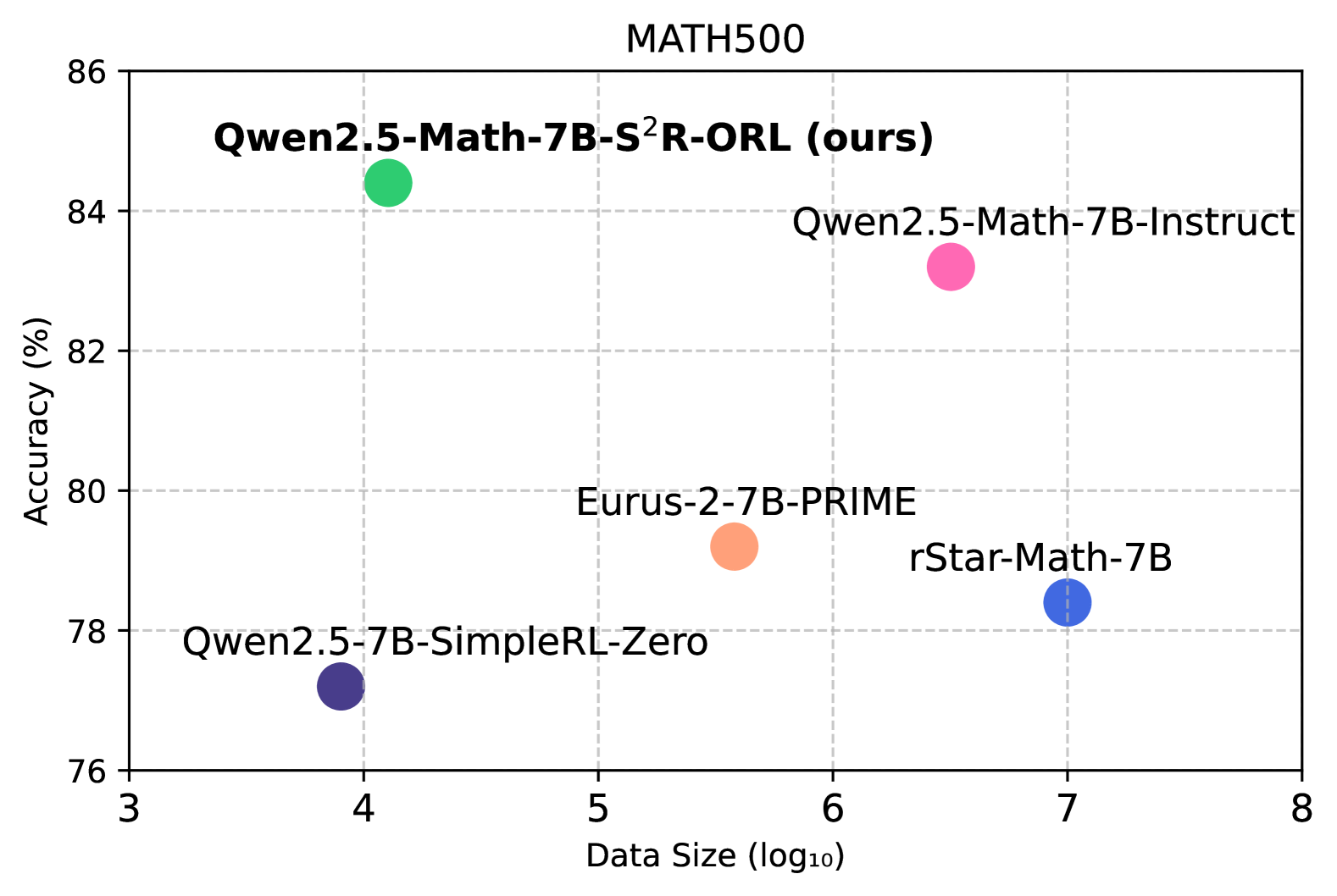
1. **Qwen2.5-Math-7B-S²R-ORL (ours):** Located at approximately (4.2, 84.5). This model exhibits the highest accuracy among those plotted.
2. **Qwen2.5-Math-7B-Instruct:** Located at approximately (6.5, 84.2). This model has a high accuracy, slightly lower than the previous one.
3. **rStar-Math-7B:** Located at approximately (7.2, 78.5). This model has a lower accuracy compared to the Qwen models.
4. **Eurus-2-7B-PRIME:** Located at approximately (5.2, 80.2). This model's accuracy is between the Qwen models and rStar-Math-7B.
5. **Qwen2.5-7B-SimpleRL-Zero:** Located at approximately (4.0, 77.5). This model has the lowest accuracy among those plotted.
The points are colored as follows:
* Qwen2.5-Math-7B-S²R-ORL (ours): Green
* Qwen2.5-Math-7B-Instruct: Pink
* rStar-Math-7B: Blue
* Eurus-2-7B-PRIME: Black
* Qwen2.5-7B-SimpleRL-Zero: Purple
### Key Observations
* The Qwen2.5-Math-7B-S²R-ORL model demonstrates the highest accuracy on the MATH500 dataset.
* There appears to be a positive correlation between data size and accuracy, although it is not strictly linear. Models trained on larger datasets (higher log₁₀ values) generally exhibit higher accuracy.
* Qwen2.5-Math-7B-S²R-ORL and Qwen2.5-Math-7B-Instruct have similar accuracy, despite different training approaches.
* Qwen2.5-7B-SimpleRL-Zero has the lowest accuracy and a relatively small data size.
### Interpretation
The data suggests that the Qwen2.5-Math-7B-S²R-ORL model is the most effective among those tested on the MATH500 benchmark. The positive correlation between data size and accuracy indicates that increasing the amount of training data generally improves model performance. The close performance of Qwen2.5-Math-7B-S²R-ORL and Qwen2.5-Math-7B-Instruct suggests that the specific training methodology (S²R-ORL vs. Instruct) has a relatively small impact on accuracy when the underlying model architecture and size are the same. The lower performance of Qwen2.5-7B-SimpleRL-Zero could be attributed to its smaller training dataset or a less effective training strategy. The plot provides a comparative analysis of different language models, highlighting their strengths and weaknesses in solving mathematical problems. The "ours" label on the highest performing model suggests this is a new model being presented by the authors of the plot.
</details>
Figure 1: The data efficiency of S 2 r compared to competitive methods, with all models initialized from Qwen2.5-Math-7B.
Recent studies have made various attempts to replicate the success of o1. These efforts include using large-scale Monte Carlo Tree Search (MCTS) to construct long-chain-of-thought (long-CoT) training data, or to scale test-time reasoning to improve the performance of current models Guan et al. (2025); Zhao et al. (2024); Snell et al. (2024b); constructing high-quality long-CoT data for effective behavior cloning with substantial human effort Qin et al. (2024); and exploring reinforcement learning to enhance LLM thinking abilities on large-scale training data and models Guo et al. (2025); Team et al. (2025); Cui et al. (2025); Yuan et al. (2024). Recently, DeepSeek R1 Guo et al. (2025) demonstrated that large-scale reinforcement learning can incentivize LLM’s deep thinking abilities, with the R1 series showcasing the promising potential of long-thought reasoning. However, these approaches generally requires significant resources to enhance LLMs’ thinking abilities, including large datasets, substantial training-time compute, and considerable human effort and time costs. Meanwhile, it remains unclear how to incentivize valid thinking in smaller or less powerful LLMs beyond distilling knowledge from more powerful models.
In this work, we propose S 2 r, an efficient alternative to enhance the thinking abilities of LLMs, particularly for smaller or less powerful LLMs. Instead of having LLMs imitate the thinking process of larger, more powerful models, S 2 r focus on teaching LLMs to think deeply by iteratively adopting two critical thinking skills: self-verifying and self-correcting. By acquiring these two capabilities, LLMs can continuously reassess their solutions, identify mistakes during solution exploration, and refine previous solutions after self-checking. Such a paradigm also enables flexible allocation of test-time compute to different levels of problems. Our results show that, with only 3.1k training samples, Qwen2.5-math-7B significantly benefits from learning self-verifying and self-correcting behaviors, achieving a 51.0% to 81.6% accuracy improvement on the Math500 test set. This performance outperforms the same base model distilled from an equivalent amount of long-CoT data (accuracy 80.2%) from QwQ-32B-Preview Team (2024a).
More importantly, S 2 r employs both outcome-level and process-level reinforcement learning (RL) to further enhance the LLMs’ self-verifying and self-correcting capabilities. Using only rule-based reward models, RL improves the validity of both the self-verification and self-correction process, allowing the models to perform more flexible and effective test-time scaling through a self-directed trial-and-error process. By comparing outcome-level and process-level RL for our task, we found that process-level supervision is particularly effective in boosting accuracy of the thinking skills at intermediate steps, which might benefit base models with limited reasoning abilities. In contrast, outcome-level supervision enables models explore more flexible trial-and-error paths towards the correct final answer, leading to consistent improvement in the reasoning abilities of more capable base models. Additionally, we further show the potential of offline reinforcement learning as a more efficient alternative to the online RL training.
We conducted extensive experiments across 3 LLMs on 7 math reasoning benchmarks. Experimental results demonstrate that S 2 r outperforms competitive baselines in math reasoning, including recently-released advanced o1-like models Eurus-2-7B-PRIME Cui et al. (2025), rStar-Math-7B Guan et al. (2025) and Qwen2.5-7B-SimpleRL Zeng et al. (2025). We also found that S 2 r is generalizable to out-of-domain general tasks, such as MMLU-PRO, highlighting the validity of the learned self-verifying and self-correcting abilities. Additionally, we conducted a series of analytical experiments to better demonstrate the reasoning mechanisms of the obtained models, and provide insights into performing online and offline RL training for enhancing LLM reasoning.
2 Methodology
The main idea behind teaching LLMs self-verification and self-correction abilities is to streamline deep thinking into a critical paradigm: self-directed trial-and-error with self-verification and self-correction. Specifically: (1) LLMs are allowed to explore any potential (though possibly incorrect) solutions, especially when tackling difficult problems; (2) during the process, self-verification is essential for detecting mistakes on-the-fly; (3) self-correction enables the model to fix detected mistakes. This paradigm forms an effective test-time scaling approach that is more accessible for less powerful base models and is generalizable across various tasks.
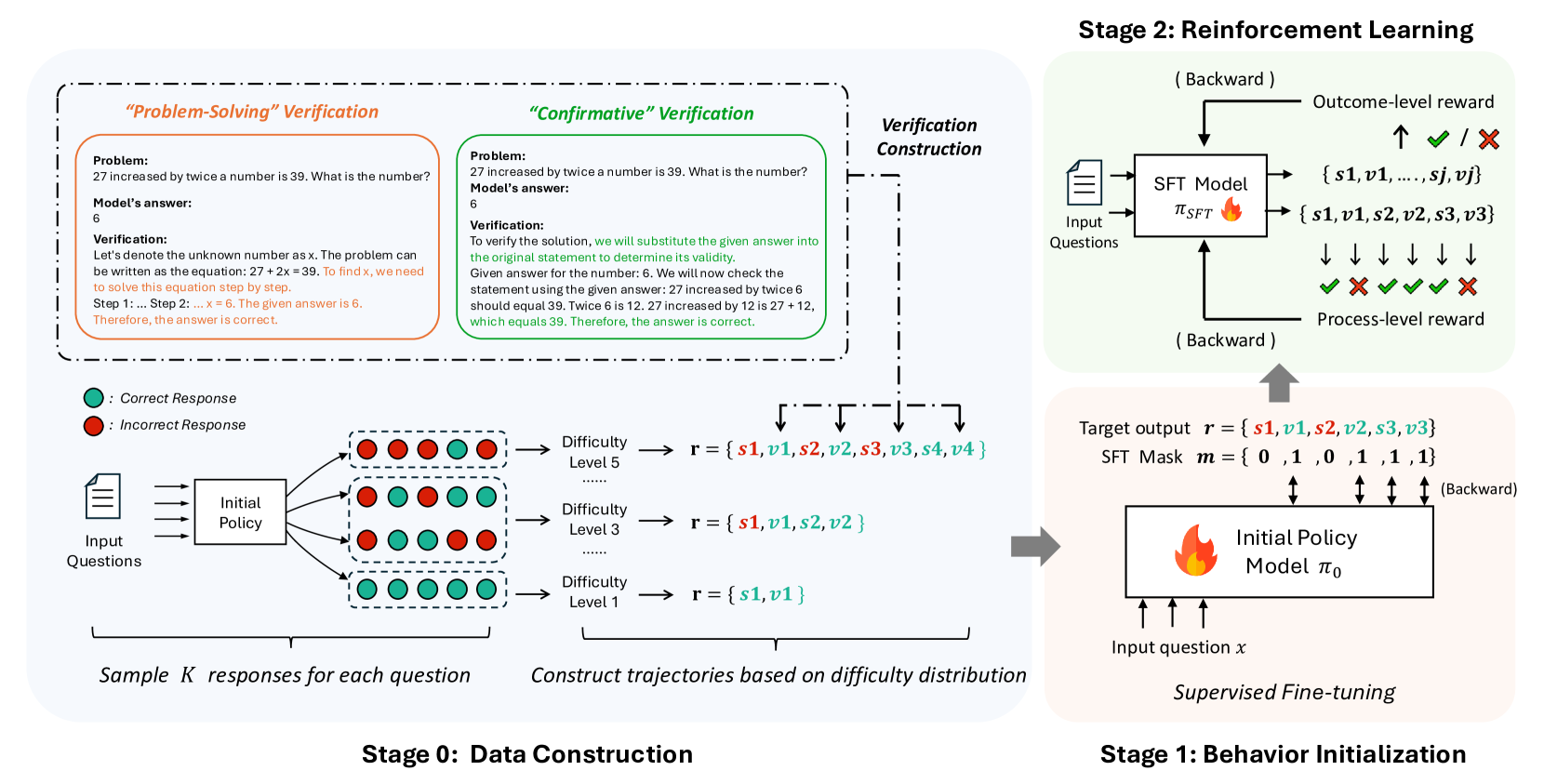
In this section, we first formally define the problem (§ 2.1). Next, we present the two-stage training framework of S 2 r, as described in Figure 2:
Stage 1: Behavior Initialization: We first construct dynamic self-verifying and self-correcting trial-and-error trajectories to initialize the desired behavior. Then, we apply supervised fine-tuning (SFT) to the initial policy models using these trajectories, resulting in behavior-initialized policy models (§ 2.2);
Stage 2: Reinforcement Learning: Following behavior initialization, we employ reinforcement learning to further enhance the self-verifying and self-correcting capabilities of the policy models. We explore both outcome-level and process-level RL methods, as well as their offline versions (§ 2.3).
<details>
<summary>x2.png Details</summary>
### Visual Description
\n
## Diagram: Reinforcement Learning for Verification
### Overview
This diagram illustrates a multi-stage process for training a model to verify mathematical problem solutions using reinforcement learning. The process is broken down into four stages: Data Construction, Reinforcement Learning, Behavior Initialization, and Verification Construction. It details the flow of information, the types of rewards used, and the components involved in each stage.
### Components/Axes
The diagram is structured into four main stages, labeled "Stage 0: Data Construction", "Stage 1: Behavior Initialization", "Stage 2: Reinforcement Learning", and "Verification Construction". Each stage contains several components and arrows indicating the flow of data.
* **Stage 0: Data Construction:** Includes "Input Questions", "Initial Policy", "Difficulty Level 1", "Difficulty Level 3", "Difficulty Level 5", and "Sample k responses for each question". Green circles represent "Correct Response" and red circles represent "Incorrect Response".
* **Stage 1: Behavior Initialization:** Includes "Input question x", "Initial Policy", "Model π₀", and "Supervised Fine-tuning".
* **Stage 2: Reinforcement Learning:** Includes "SFT Model", "Input Questions", "Outcome-level reward", "Process-level reward", and the set of states {s1, v1, s2, v2, s3, v3}.
* **Verification Construction:** Contains two problem examples: "Problem-Solving" Verification and "Confirmatory" Verification.
### Detailed Analysis or Content Details
**Stage 0: Data Construction**
* Input Questions are fed into an Initial Policy.
* The Initial Policy generates responses, which are categorized as either Correct (green circle) or Incorrect (red circle).
* Responses are constructed into trajectories based on difficulty distribution, with three difficulty levels: Level 1, Level 3, and Level 5.
* Difficulty Level 1: r = {s1, v1}
* Difficulty Level 3: r = {s1, v1, s2, v2}
* Difficulty Level 5: r = {s1, v1, s2, v2, s3, v3, s4, v4}
* The output is "Sample k responses for each question".
**Stage 1: Behavior Initialization**
* An Input question x is fed into the Initial Policy.
* The Initial Policy generates a Model π₀.
* The Model π₀ undergoes Supervised Fine-tuning.
**Stage 2: Reinforcement Learning**
* Input Questions are fed into an SFT Model.
* The SFT Model generates a sequence of states {s1, v1, s2, v2, s3, v3}.
* Two types of rewards are used: Outcome-level reward (represented by a checkmark or cross) and Process-level reward.
* The flow is "Backward".
**Verification Construction**
* **"Problem-Solving" Verification:**
* Problem: "27 increased by twice a number is 39. What is the number?"
* Model's answer: 6
* Verification: "Let's denote the unknown number as x. The problem can be written as the equation: 27 + 2x = 39. To find x, we need to solve this equation step by step. Step 1: ... Step 6. The given answer is 6. Therefore, the answer is correct."
* **"Confirmatory" Verification:**
* Problem: "27 increased by twice a number is 39. What is the number?"
* Model's answer: 6
* Verification: "To verify the solution, we will substitute the given answer into the original statement to determine its validity. Given answer for the number 6. We will now check the statement using the given answer: 27 increased by twice 6 should equal 39. Twice 6 is 12. 27 increased by 12 is 27 + 12, which equals 39. Therefore, the answer is correct."
**Target Output**
* Target output r = {s1, v1, s2, v2, s3, v3}
* SFT Mask m = {0, 1, 0, 1, 1, 1, 1}
### Key Observations
* The diagram emphasizes a backward flow of information in the Reinforcement Learning stage, indicated by the "Backward" labels.
* The verification process provides both a problem-solving approach and a confirmatory approach.
* The SFT Mask suggests a selective application of the SFT model to certain states.
* The use of both Outcome-level and Process-level rewards indicates a nuanced reward structure.
### Interpretation
The diagram outlines a sophisticated approach to training a verification model. The data construction stage generates a diverse dataset with varying difficulty levels. The reinforcement learning stage leverages both outcome and process rewards to guide the model's learning. The backward flow suggests a policy gradient approach, where the model learns from the consequences of its actions. The inclusion of both "Problem-Solving" and "Confirmatory" verification methods indicates a desire for robust and reliable verification capabilities. The SFT mask suggests a method for focusing the model's attention on specific parts of the verification process. Overall, the diagram demonstrates a well-structured and thoughtful approach to building a verification system using reinforcement learning. The use of both problem-solving and confirmatory verification suggests a focus on both the correctness of the answer and the validity of the reasoning process.
</details>
Figure 2: Overview of S 2 r.
2.1 Problem Setup
We formulate the desired LLM reasoning paradigm as a sequential decision-making process under a reinforcement learning framework. Given a problem $x$ , the language model policy $\pi$ is expected to generate a sequence of interleaved reasoning actions $y=(a_{1},a_{2},·s,a_{T})$ until reaching the termination action <end>. We represent the series of actions before an action $a_{t}∈ y$ as $y_{:a_{t}}$ , i.e., $y_{:a_{t}}=(a_{1},a_{2},·s,a_{t-i})$ , where $a_{t}$ is excluded. The number of tokens in $y$ is denoted as $|y|$ , and the total number of actions in $y$ is denoted as $|y|_{a}$ .
We restrict the action space to three types: “ solve ”, “ verify ”, and “ <end> ”, where “ solve ” actions represent direct attempts to solve the problem, “ verify ” actions correspond to self-assessments of the preceding solution, and “ <end> ” actions signal the completion of the reasoning process. We denote the type of action $a_{i}$ as $Type(·)$ , where $Type(a_{i})∈\{\texttt{verify},\texttt{solve},\texttt{<end>}\}$ . We expect the policy to learn to explore new solutions by generating “ solve ” actions, to self-verify the correctness of preceding solutions with “ verify ” actions, and to correct the detected mistakes with new “ solve ” actions if necessary. Therefore, for each action $a_{i}$ , the type of the next action $a_{i+1}$ is determined by the following rules:
$$
Type(a_{i+1})=\begin{cases}\texttt{verify},&Type(a_{i})=\texttt{solve}\\
\texttt{solve},&Type(a_{i})=\texttt{verify}\\
&\text{ and }\text{Parser}(a_{i})=\textsc{incorrect}\\
\texttt{<end>},&Type(a_{i})=\texttt{verify}\\
&\text{ and }\text{Parser}(a_{i})=\textsc{correct}\\
\end{cases}
$$
Here, $Parser(a)∈\{\textsc{correct},\textsc{incorrect}\}$ (for any action $a$ where $Type(a)=\texttt{verify}$ ) is a function (e.g., a regex) that converts the model’s free-form verification text into binary judgments.
For simplicity, we denote the $j$ -th solve action as $s_{j}$ and the $j$ -th verify action as $v_{j}$ . Then we have $y=(s_{1},v_{1},s_{2},v_{2},·s,s_{k},v_{k},\texttt{<end>})$ .
2.2 Initializing Self-verification and Self-correction Behaviors
2.2.1 Learning Valid Self-verification
Learning to perform valid self-verification is the most crucial part in S 2 r, as models can make mistakes during trial-and-error, and recognizing intermediate mistakes is critical for reaching the correct answer. In this work, we explore two methods for constructing self-verification behavior.
“Problem-Solving” Verification
The most intuitive method for verification construction is to directly query existing models to generate verifications on the policy models’ responses, and then filter for valid verifications. By querying existing models using different prompts, we found that existing models tend to perform verification in a “Problem-Solving” manner, i.e., by re-solving the problem and checking whether the answer matches the given one. We refer to this kind of verification as “Problem-Solving” Verification.
“Confirmative” Verification
"Problem-solving" verification is intuitively not the ideal verification behavior we seek. Ideally, we expect the model to think outside the box and re-examine the solution from a new perspective, rather than thinking from the same problem-solving view for verification. We refer to this type of verification behavior as “Confirmative” Verification. Specifically, we construct “Confirmative” Verification by prompting existing LLMs to "verify the correctness of the answer without re-solving the problem", and filtering out invalid verifications using LLM-as-a-judge. The detail implementation can be found in Appendix § A.1.
2.2.2 Learning Self-correction
Another critical part of S 2 r is enabling the model to learn self-correction. Inspired by Kumar et al. (2024) and Snell et al. (2024b), we initialize the self-correcting behavior by concatenating a series of incorrect solutions (each followed by a verification recognizing the mistakes) with a final correct solution. As demonstrated by Kumar et al. (2024), LLMs typically fail to learn valid self-correction behavior through SFT, but the validity of self-correction can be enhanced through reinforcement learning. Therefore, we only initialize the self-correcting behavior at this stage, leaving further enhancement of the self-correcting capabilities to the RL stage.
2.2.3 Constructing Dynamic Trial-and-Error Trajectory
We next construct the complete trial-and-error trajectories for behavior initialization SFT, following three principles:
- To ensure the diversity of the trajectories, we construct trajectories of various lengths. Specifically, we cover $k∈\{1,2,3,4\}$ for $y=(a_{1},·s,a_{2k})=(s_{1},v_{1},·s,s_{k},v_{k})$ in the trajectories.
- To ensure that the LLMs learn to verify and correct their own errors, we construct the failed trials in each trajectory by sampling and filtering from the LLMs’ own responses.
- As a plausible test-time scaling method allocates reasonable effort to varying levels of problems, it is important to ensure the trial-and-error trajectories align with the difficulty level of problems. Specifically, more difficult problems will require more trial-and-error iterations before reaching the correct answer. Thus, we determine the length of each trajectory based on the accuracy of the sampled responses for each base model.
2.2.4 Supervised Fine-tuning for Thinking Behavior Initialization
Once the dynamic self-verifying and self-correcting training data $\mathcal{D}_{SFT}$ is ready, we optimize the policy $\pi$ for thinking behavior initialization by minimizing the following objective:
$$
\mathcal{L}=-\mathbb{E}_{(x,y)\sim\mathcal{D}_{SFT}}\sum_{a_{t}\in y}\delta_{%
mask}(a_{t})\log\pi(a_{t}\mid x,y_{:a_{t}}) \tag{1}
$$
where the mask function $\delta_{mask}(a_{t})$ for action $a_{t}$ in $y=(a_{1},·s,a_{T})$ is defined as:
$$
\delta_{mask}(a_{t})=\begin{cases}1,&\text{if }Type(a_{t})=\texttt{verify}\\
1,&\text{if }Type(a_{t})=\texttt{solve}\text{ and }t=T-1\\
1,&\text{if }Type(a_{t})=\texttt{<end>}\text{ and }t=T\\
0,&\text{otherwise}\end{cases}
$$
That is, we optimize the probability of all verifications and only the last correct solution $s_{N}$ by using masks during training.
2.3 Boosting Thinking Capabilities via Reinforcement Learning
After Stage 1, we initialized the policy model $\pi$ with self-verification and self-correction behavior, obtaining $\pi_{SFT}$ . We then explore further enhancing these thinking capabilities of $\pi_{SFT}$ via reinforcement learning. Specifically, we explore two simple RL algorithms: the outcome-level REINFORCE Leave-One-Out (RLOO) algorithm and a proces-level group-based RL algorithm.
2.3.1 Outcome-level RLOO
We first introduce the outcome-level REINFORCE Leave-One-Out (RLOO) algorithm Ahmadian et al. (2024); Kool et al. (2019) to further enhance the self-verification and self-correction capabilities of $\pi_{SFT}$ . Given a problem $x$ and the response $y=(s_{1},v_{1},...,s_{T},v_{T})$ , we define the reward function $R_{o}(x,y)$ based on the correctness of the last solution $s_{T}$ :
$$
R_{o}(x,y)=\begin{cases}1,&V_{golden}(s_{T})=\texttt{correct}\\
-1,&otherwise\\
\end{cases}
$$
Here $V_{golden}(·)∈\{\texttt{correct},\texttt{incorrect}\}$ represents ground-truth validation by matching the golden answer with the given solution. We calculate the advantage of each response $y$ using an estimated baseline and KL reward shaping as follows:
$$
A(x,y)=R_{o}(x,y)-\hat{b}-\beta\log\frac{\pi_{\theta_{old}}(y|x)}{\pi_{ref}(y|%
x)} \tag{2}
$$
where $\beta$ is the KL divergence regularization coefficient, and $\pi_{\text{ref}}$ is the reference policy (in our case, $\pi_{SFT}$ ). $\hat{b}(x,y^{(m)})=\frac{1}{M-1}\sum_{\begin{subarray}{c}j=1,...,M\\
j≠ m\end{subarray}}.R_{o}(x,y^{(j)})$ is the baseline estimation of RLOO, which represents the leave-one-out mean of $M$ sampled outputs $\{y^{(1)},...y^{(M)}\}$ for each input $x$ , serving as a baseline estimation for each $y^{(m)}$ . Then, we optimize the policy $\pi_{\theta}$ by minimizing the following objective after each sampling episode based on $\pi_{\theta_{old}}$ :
$$
\begin{split}\mathcal{L}(\theta)\ &=\ -\mathbb{E}_{\begin{subarray}{c}x\sim%
\mathcal{D}\\
y\sim\pi_{\theta_{\text{old}}}(\cdot|x)\end{subarray}}\bigg{[}\min\big{(}r(%
\theta)A(x,y),\\
&\text{clip}\big{(}r(\theta),1-\epsilon,1+\epsilon\big{)}A(x,y)\big{)}\bigg{]}%
\end{split} \tag{3}
$$
where $r(\theta)=\frac{\pi_{\theta}(y|x)}{\pi_{\theta_{\text{old}}}(y|x)}$ is the probability ratio.
When implementing the above loss function, we treat $y$ as a complete trajectory sampled with an input problem $x$ , meaning we optimize the entire trajectory with outcome-level supervision. With this approach, we aim to incentivize the policy model to explore more dynamic self-verification and self-correcting trajectories on its own, which has been demonstrated as an effective practice in recent work Guo et al. (2025); Team et al. (2025).
2.3.2 Process-level Group-based RL
Process-level supervision has demonstrated effectiveness in math reasoning Lightman et al. (2023a); Wang et al. (2024c). Since the trajectory of S 2 r thinking is naturally divided into self-verification and self-correction processes, it is intuitive to adopt process-level supervision for RL training.
Inspired by RLOO and process-level GRPO Shao et al. (2024), we designed a group-based process-level optimization method. Specifically, we regard each action $a$ in the output trajectory $y$ as a sub-process and define the action level reward function $R_{a}(a\mid x,y_{:a})$ based on the action type. For each “ solve ” action $s_{j}$ , we expect the policy to generate the correct solution; for each “ verify ” action $v_{j}$ , we expect the verification to align with the actual solution validity. The corresponding rewards are defined as follows:
$$
R_{a}(s_{j}\mid x,y_{:s_{j}})=\begin{cases}1,&V_{golden}(s_{j})=\texttt{%
correct}\\
-1,&otherwise\\
\end{cases}
$$
$$
R_{a}(v_{j}\mid x,y_{:v_{j}})=\begin{cases}1,&Parser(v_{j})=V_{golden}(s_{j})%
\\
-1,&otherwise\\
\end{cases}
$$
To calculate the advantage of each action $a_{t}$ , we estimate the baseline as the average reward of the group of actions sharing the same reward context:
$$
\mathbf{R}(a_{t}\mid x,y)=\left(R_{a}(a_{i}\mid x,y_{:a_{i}})\right)_{i=1}^{t-1}
$$
which is defined as the reward sequence of the previous actions $y_{:a_{t}}$ of each action $a_{t}$ . We denote the set of actions sharing the same reward context $\mathbf{R}(a_{t}\mid x,y)$ as $\mathcal{G}(\mathbf{R}(a_{t}\mid x,y))$ . Then the baseline can be estimated as follows:
$$
\begin{split}&\hat{b}(a_{t}\mid x,y)=\\
&\frac{1}{|\mathcal{G}(\mathbf{R}(a_{t}|x,y))|}\sum_{a\in\mathcal{G}(\mathbf{R%
}(a_{t}|x,y))}R_{a}(a|x^{(a)},y^{(a)}_{:a})\end{split} \tag{4}
$$
And the advantage of each action $a_{t}$ is:
$$
\begin{split}A(a_{t}\mid x,y)=&R_{a}(a_{t}\mid x,y_{:a_{t}})-\hat{b}(a_{t}\mid
x%
,y)\\
&-\beta\log\frac{\pi_{\theta_{old}}(a_{t}\mid x,y)}{\pi_{\text{ref}}(a_{t}\mid
x%
,y)}\end{split} \tag{5}
$$
The main idea of the group-based baseline estimation is that the actions sharing the same reward context are provided with similar amounts of information before the action is taken. For instance, all actions sharing a reward context consisting of one failed attempt and one successful verification (i.e., $\mathbf{R}(a_{t}|x,y)=(-1,1)$ ) are provided with the information about the problem, a failed attempt, and the reassessment on the failure. Given the same amount of information, it is reasonable to estimate a baseline using the average reward of these actions.
Putting it all together, we minimize the following surrogate loss function to update the policy parameters $\theta$ , using trajectories collected from $\pi_{old}$ :
$$
\begin{split}\mathcal{L}(\theta)\ &=\ -\mathbb{E}_{\begin{subarray}{c}x\sim%
\mathcal{D}\\
y\sim\pi_{\theta_{\text{old}}}(\cdot|x)\end{subarray}}\bigg{[}\frac{1}{|y|_{a}%
}\sum_{a\in y}\min\big{(}r_{a}(\theta)A(a|x,y_{:a}),\\
&\text{clip}\big{(}r_{a}(\theta),1-\epsilon,1+\epsilon\big{)}A(a|x,y_{:a})\big%
{)}\bigg{]}\end{split} \tag{6}
$$
where $r_{a}(\theta)=\frac{\pi_{\theta}(a|x,y_{:a})}{\pi_{\theta_{\text{old}}}(a|x,y_%
{:a})}$ is the importance ratio.
2.4 More Efficient Training with Offline RL
While online RL is known for its high resource requirements, offline RL, which does not require real-time sampling during training, offers a more efficient alternative for RL training. Additionally, offline sampling allows for more accurate baseline calculations with better trajectories grouping for each policy. As part of our exploration into more efficient RL training in S 2 r framework, we also experimented with offline RL to assess its potential in further enhancing the models’ thinking abilities. In Appendix § D.2, we include more details and formal definition for offline RL training.
3 Experiment
To verify the effectiveness of the proposed method, we conducted extensive experiments across 3 different base policy models on various benchmarks.
| Stage 1: Behavior Initialization | | |
| --- | --- | --- |
| Base Model | Source | # Training Data |
| Llama-3.1-8B-Instruct | MATH | 4614 |
| Qwen2-7B-Instruct | MATH | 4366 |
| Qwen2.5-Math-7B | MATH | 3111 |
| Stage 2: Reinforcement Learning | | |
| Base Model | Source | # Training Data |
| Llama-3.1-8B-Instruct | MATH+GSM8K | 9601 |
| Qwen2-7B-Instruct | MATH+GSM8K | 9601 |
| Qwen2.5-Math-7B | MATH+OpenMath2.0 | 10000 |
Table 1: Training data statistics.
Table 2: The performance of S 2 r and other strong baselines on the most challenging math benchmarks is presented. BI refers to the behavior-initialized models through supervised fine-tuning, ORL denotes models trained with outcome-level RL, and PRL refers to models trained with process-level RL. The highest results are highlighted in bold and the second-best results are marked with underline. For some baselines, we use the results from their original reports or from Guan et al. (2025), denoted by ∗.
3.1 Experiment Setup
Base Models
To evaluate the general applicability of our method across different LLMs, we conducted experiments using three distinct base models: Llama-3.1-8B-Instruct Dubey et al. (2024), Qwen2-7B-Instruct qwe (2024), and Qwen2.5-Math-7B Qwen (2024). Llama-3.1-8B-Instruct and Qwen2-7B-Instruct are versatile general-purpose models trained on diverse domains without a specialized focus on mathematical reasoning. In contrast, Qwen2.5-Math-7B is a state-of-the-art model specifically tailored for mathematical problem-solving and has been widely adopted in recent research on math reasoning Guan et al. (2025); Cui et al. (2025); Zeng et al. (2025).
Training Data Setup
For Stage 1: Behavior Initialization, we used the widely adopted MATH Hendrycks et al. (2021a) training set for dynamic trial-and-error data collection We use the MATH split from Lightman et al. (2023a), i.e., 12000 problems for training and 500 problems for testing.. For each base model, we sampled 5 responses per problem in the training data. After data filtering and sampling, we constructed a dynamic trial-and-error training set consisting of 3k-4k instances for each base model. Detailed statistics of the training set are shown in Table 1. For Stage 2: Reinforcement Learning, we used the MATH+GSM8K Cobbe et al. (2021a) training data for RL training on the policy $\pi_{SFT}$ initialized from Llama-3.1-8B-Instruct and Qwen2-7B-Instruct. Since Qwen2.5-math-7b already achieves high accuracy on the GSM8K training data after Stage 1, we additionally include training data randomly sampled from the OpenMath2 dataset Toshniwal et al. (2024). Following Cui et al. (2025), we filter out excessively easy or difficult problems based on each $\pi_{SFT}$ from Stage 1 to enhance the efficiency and stability of RL training, resulting in RL training sets consisting of approximately 10000 instances. Detailed statistics of the final training data can be found in Table 1. Additional details on training data construction can be found in in Appendix § A.1.
Baselines
We benchmark our proposed method against four categories of strong baselines:
- Frontier LLMs includes cutting-edge proprietary models such as GPT-4o, the latest Claude, and OpenAI’s o1-preview and o1-mini.
- Top-tier open-source reasoning models covers state-of-the-art open-source models known for their strong reasoning capabilities, including Mathstral-7B-v0.1 Team (2024b), NuminaMath-72B LI et al. (2024), LLaMA3.1-70B-Instruct Dubey et al. (2024), and Qwen2.5-Math-72B-Instruct Yang et al. (2024).
- Enhanced models built on Qwen2.5-Math-7B: Given the recent popularity of Qwen2.5-Math-7B as a base policy model, we evaluate S 2 r against three competitive baselines that have demonstrated superior performance based on Qwen2.5-Math-7B: Eurus-2-7B-PRIME Cui et al. (2025), rStar-Math-7B Guan et al. (2025), and Qwen2.5-7B-SimpleRL Zeng et al. (2025). These models serve as direct and strong baseline for our Qwen2.5-Math-7B-based variants.
- SFT with different CoT constructions: We also compare with training on competitive types of CoT reasoning, including the original CoT solution in the training datasets, and Long-CoT solutions distilled from QwQ-32B-Preview Team (2024a), a widely adopted open-source o1-like model Chen et al. (2024c); Guan et al. (2025); Zheng et al. (2024). Specifically, to ensure a fair comparison between behavior initialization with long-CoT and S 2 r, we use long-CoT data of the same size as our behavior initialization data. We provide more details on the baseline data construction in Appendix § A.2.3.
More details on the baselines are included in Appendix § A.2.
Evaluation Datasets
We evaluate the proposed method on 7 diverse mathematical benchmarks. To ensure a comprehensive evaluation, in addition to the in-distribution GSM8K Cobbe et al. (2021b) and MATH500 Lightman et al. (2023a) test sets, we include challenging out-of-distribution benchmarks covering various difficulty levels and mathematical domains, including the AIME 2024 competition problems AI-MO (2024a), the AMC 2023 exam AI-MO (2024b), the advanced reasoning tasks from Olympiad Bench He et al. (2024), and college-level problem sets from College Math Tang et al. (2024a). Additionally, we assess performance on real-world standardized tests, the GaoKao (Chinese College Entrance Exam) En 2023 Liao et al. (2024). A detailed description of these datasets is provided in Appendix § B.1.
Evaluation Metrics
We report Pass@1 accuracy for all baselines. For inference, we employ vLLM Kwon et al. (2023) and develop evaluation scripts based on Qwen Math’s codebase. All evaluations are performed using greedy decoding. Details of the prompts used during inference are provided in Appendix § A.3. All implementation details, including hyperparameter settings, can be found in Appendix § B.2.
3.2 Main Results
Table 2 shows the main results of S 2 r compared with baseline methods. We can observe that: (1) S 2 r consistently improves the reasoning abilities of models across all base models. Notably, on Qwen2.5-Math-7B, the proposed method improves the base model by 32.2% on MATH500 and by 34.3% on GSM8K. (2) Generally, S 2 r outperforms the baseline methods derived from the same base models across most benchmarks. Specifically, on Qwen2.5-Math-7B, S 2 r surpasses several recently proposed competitive baselines, such as Eurus-2-7B-PRIME, rStar-Math-7B and Qwen2.5-7B-SimpleRL. While Eurus-2-7B-PRIME and rStar-Math-7B rely on larger training datasets (Figure 1) and require more data construction and reward modeling efforts, S 2 r only needs linear sampling efforts for data construction, 10k RL training data and rule-based reward modeling. These results highlight the efficiency of S 2 r. (3) With the same scale of SFT data, S 2 r also outperforms the long-CoT models distilled from QwQ-32B-Preview, demonstrating that learning to self-verify and self-correct is an effective alternative to long-CoT for test-time scaling in smaller LLMs.
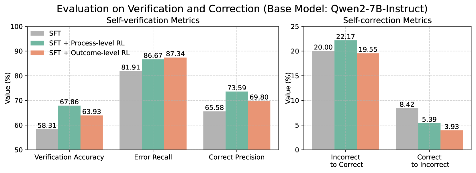
Comparing process-level and outcome-level RL, we find that outcome-level RL generally outperforms process-level RL across the three models. This is likely because outcome-level RL allows models to explore trajectories without emphasizing intermediate accuracy, which may benefit enhancing long-thought reasoning in stronger base models like Qwen2.5-Math-7B. In contrast, process-level RL, which provides guidance for each intermediate verification and correction step, may be effective for models with lower initial capabilities, such as Qwen2-7B-Instruct. As shown in Figure 3, process-level RL can notably enhance the verification and correction abilities of Qwen2-7B- S 2 r -BI.
| Model | FOLIO | CRUX- Eval | Strategy- QA | MMLUPro- STEM |
| --- | --- | --- | --- | --- |
| Qwen2.5-Math-72B-Instruct | 69.5 | 68.6 | 94.3 | 66.0 |
| Llama-3.1-70B-Instruct ∗ | 65.0 | 59.6 | 88.8 | 61.7 |
| OpenMath2-Llama3.1-70B ∗ | 68.5 | 35.1 | 95.6 | 55.0 |
| QwQ-32B-Preview ∗ | 84.2 | 65.2 | 88.2 | 71.9 |
| Eurus-2-7B-PRIME | 56.7 | 50.0 | 79.0 | 53.7 |
| Qwen2.5-Math-7B-Instruct | 61.6 | 28.0 | 81.2 | 44.7 |
| Qwen2.5-Math-7B | 37.9 | 40.8 | 61.1 | 46.0 |
| Qwen2.5-Math-7B- S 2 r -BI (ours) | 58.1 | 48.0 | 88.7 | 49.8 |
| Qwen2.5-Math-7B- S 2 r -ORL (ours) | 61.6 | 50.9 | 90.8 | 50.0 |
Table 3: Performance of the proposed method and the baseline methods on 4 cross-domain tasks. The results with ∗ are reported by Shen et al. (2025).
3.3 Generalizing to Cross-domain Tasks
Despite training on math reasoning tasks, we found that the learned self-verifying and self-correcting capability can also generalize to out-of-distribution general domains. In Table 3, we evaluate the SFT model and the outcome-level RL model based on Qwen2.5-Math-7B on four cross-domain tasks: FOLIO Han et al. (2022) on logical reasoning, CRUXEval Gu et al. (2024) on code reasoning, StrategyQA Geva et al. (2021) on multi-hop reasoning and MMLUPro-STEM on multi-task complex understanding Wang et al. (2024d); Shen et al. (2025), with details of these datasets provided in Appendix § B.1. The results show that after learning to self-verify and self-correct, the proposed method effectively boosts the base model’s performance across all tasks and achieves comparative results to the baseline models. These findings indicate that the learned self-verifying and self-correcting capabilities are general thinking skills, which can also benefit reasoning in general domains. Additionally, we expect that the performance in specific domains can be further improved by applying S 2 r training on domain data with minimal reward model requirements (e.g., rule-based or LLM-as-a-judge). For better illustration, we show cases on how the trained models perform self-verifying and self-correcting on general tasks in Appendix § E.
3.4 Analyzing Self-verification and Self-correction Abilities
In this section, we conduct analytical experiments on the models’ self-verification and self-correction capabilities from various perspectives.
3.4.1 Problem-solving v.s. Confirmative Verification
We first compare the Problem-solving and Confirmative Verification methods described in § 2.2.1. In Table 4, we present the verification results of different methods on the Math500 test set. We report the overall verification accuracy, as well as the initial verification accuracy when the initial answer is correct ( $V_{golden}(s_{0})=\texttt{correct}$ ) and incorrect ( $V_{golden}(s_{0})=\texttt{incorrect}$ ), respectively.
| Base Model | Methods | Overall Verification Acc. | Initial Verification Acc. | |
| --- | --- | --- | --- | --- |
| $V_{golden}(s_{0})$ $=\texttt{correct}$ | $V_{golden}(s_{0})$ $=\texttt{incorrect}$ | | | |
| Llama3.1-8B-Instruct | Problem-solving | 80.10 | 87.28 | 66.96 |
| Confirmative | 65.67 | 77.27 | 78.22 | |
| Qwen2-7B-Instruct | Problem-solving | 73.28 | 90.24 | 67.37 |
| Confirmative | 58.31 | 76.16 | 70.05 | |
| Qwen2.5-Math-7B | Problem-solving | 77.25 | 91.21 | 56.67 |
| Confirmative | 61.58 | 82.80 | 68.04 | |
Table 4: Comparison of problem-solving and confirmative verification.
We observe from the table that: (1) Generally, problem-solving verification achieves superior overall accuracy compared to confirmative verification. This result is intuitive, as existing models are trained for problem-solving, and recent studies have highlighted the difficulty of existing LLMs in performing reverse thinking Berglund et al. (2023); Chen et al. (2024b). During data collection, we also found that existing models tend to verify through problem-solving, even when prompted to verify without re-solving (see Table 6 in Appendix § A.1). (2) In practice, accuracy alone does not fully reflect the validity of a method. For example, when answer accuracy is sufficiently high, predicting all answers as correct will naturally lead to high verification accuracy, but this is not a desired behavior. By further examining the initial verification accuracy for both correct and incorrect answers, we found that problem-solving verification exhibits a notable bias toward predicting answers as correct, while the predictions from confirmative verification are more balanced. We deduce that this bias arises might be because problem-solving verification is more heavily influenced by the preceding solution, aligning with previous studies showing that LLMs struggle to identify their own errors Huang et al. (2023); Tyen et al. (2023). In contrast, confirmative verification performs verification from different perspectives, making it less influenced by the LLMs’ preceding solution.
In all experiments, we used confirmative verification for behavior initialization.
3.4.2 Boosting Self-verifying and Self-correcting with RL
In this experiment, we investigate the effect of RL training on the models’ self-verifying and self-correcting capabilities.
We assess self-verification using the following metrics: (1) Verification Accuracy: The overall accuracy of verification predictions, as described in § 3.4.1. (2) Error Recall: The recall of verification when the preceding answers are incorrect. (3) Correct Precision: The precision of verification when it predicts the answers as correct. Both Error Recall and Correct Precision directly affect the final answer accuracy: if verification fails to detect an incorrect answer, or if it incorrectly predicts an answer as correct, the final answer will be wrong.
For self-correction, we use the following metrics: (1) Incorrect to Correct Rate: the rate at which the model successfully corrects an incorrect initial answer to a correct final answer. (2) Correct to Incorrect Rate: the rate at which the model incorrectly changes a correct initial answer to an incorrect final answer. We provide the formal definitions of the metrics used in Appendix § C.
<details>
<summary>x3.png Details</summary>
### Visual Description
\n
## Bar Charts: Evaluation on Verification and Correction
### Overview
The image presents two sets of bar charts comparing the performance of a base model (Qwen2-7B-Instruct) with different training approaches: Supervised Fine-Tuning (SFT), SFT + Process-level Reinforcement Learning (RL), and SFT + Outcome-level RL. The left chart focuses on "Self-verification Metrics," while the right chart focuses on "Self-correction Metrics." Both charts display values as percentages.
### Components/Axes
* **Title:** "Evaluation on Verification and Correction (Base Model: Qwen2-7B-Instruct)" - positioned at the top-center of the image.
* **Left Chart Title:** "Self-verification Metrics" - positioned above the left chart.
* **Right Chart Title:** "Self-correction Metrics" - positioned above the right chart.
* **Y-axis Label (Both Charts):** "Value (%)" - positioned on the left side of both charts. The scale ranges from 50 to 100 for the left chart and from 0 to 25 for the right chart.
* **X-axis Labels (Left Chart):** "Verification Accuracy", "Error Recall", "Correct Precision" - positioned along the bottom of the left chart.
* **X-axis Labels (Right Chart):** "Incorrect to Correct", "Correct to Incorrect" - positioned along the bottom of the right chart.
* **Legend (Top-Left of Left Chart):**
* SFT (Blue)
* SFT + Process-level RL (Green)
* SFT + Outcome-level RL (Red)
### Detailed Analysis or Content Details
**Left Chart: Self-verification Metrics**
* **Verification Accuracy:**
* SFT: Approximately 58.31%
* SFT + Process-level RL: Approximately 67.86%
* SFT + Outcome-level RL: Approximately 63.93%
* Trend: The SFT + Process-level RL shows the highest value, indicating improved verification accuracy.
* **Error Recall:**
* SFT: Approximately 81.91%
* SFT + Process-level RL: Approximately 86.67%
* SFT + Outcome-level RL: Approximately 87.34%
* Trend: SFT + Outcome-level RL shows the highest value, indicating improved error recall.
* **Correct Precision:**
* SFT: Approximately 65.58%
* SFT + Process-level RL: Approximately 73.59%
* SFT + Outcome-level RL: Approximately 69.80%
* Trend: SFT + Process-level RL shows the highest value, indicating improved correct precision.
**Right Chart: Self-correction Metrics**
* **Incorrect to Correct:**
* SFT: Approximately 20.00%
* SFT + Process-level RL: Approximately 22.17%
* SFT + Outcome-level RL: Approximately 19.55%
* Trend: SFT + Process-level RL shows the highest value, indicating improved ability to correct incorrect statements.
* **Correct to Incorrect:**
* SFT: Approximately 8.42%
* SFT + Process-level RL: Approximately 5.39%
* SFT + Outcome-level RL: Approximately 3.93%
* Trend: SFT + Outcome-level RL shows the lowest value, indicating improved ability to avoid incorrectly altering correct statements.
### Key Observations
* In the Self-verification Metrics chart, SFT + Process-level RL consistently performs well in Verification Accuracy and Correct Precision, while SFT + Outcome-level RL excels in Error Recall.
* In the Self-correction Metrics chart, SFT + Process-level RL shows the highest value for Incorrect to Correct, while SFT + Outcome-level RL shows the lowest value for Correct to Incorrect.
* The addition of Reinforcement Learning (both process and outcome level) consistently improves performance over the base SFT model across all metrics.
### Interpretation
The data suggests that incorporating Reinforcement Learning into the training process of the Qwen2-7B-Instruct model significantly enhances both its self-verification and self-correction capabilities. The choice between Process-level RL and Outcome-level RL appears to depend on the specific metric being optimized. Process-level RL seems to be more effective at improving accuracy and precision, while Outcome-level RL is better at minimizing the introduction of errors during correction. The charts demonstrate a clear trade-off between these two aspects of performance. The model's ability to both verify its own outputs and correct errors is crucial for building reliable and trustworthy AI systems. The consistent improvement across all metrics with the addition of RL highlights the effectiveness of this technique for enhancing model performance.
</details>
(a)
<details>
<summary>x4.png Details</summary>
### Visual Description
## Bar Chart: Evaluation on Verification and Correction
### Overview
This image presents a bar chart comparing the performance of a base model (Qwen2.5-Math-7B) and its variations trained with different reinforcement learning (RL) techniques. The chart is split into two sections: "Self-verification Metrics" and "Self-correction Metrics". Each section displays three data series representing different training approaches: Supervised Fine-Tuning (SFT), SFT + Process-level RL, and SFT + Outcome-level RL. The y-axis represents "Value (%)".
### Components/Axes
* **Title:** Evaluation on Verification and Correction (Base Model: Qwen2.5-Math-7B)
* **Subtitle 1:** Self-verification Metrics
* **Subtitle 2:** Self-correction Metrics
* **X-axis (Self-verification):** Verification Accuracy, Error Recall, Correct Precision
* **X-axis (Self-correction):** Incorrect to Correct, Correct to Incorrect
* **Y-axis:** Value (%) - Scale ranges from 0 to 90 for the left chart and 0 to 14 for the right chart.
* **Legend:**
* SFT (Red)
* SFT + Process-level RL (Green)
* SFT + Outcome-level RL (Teal)
### Detailed Analysis or Content Details
**Self-verification Metrics (Left Chart)**
* **Verification Accuracy:**
* SFT: Approximately 61.58%
* SFT + Process-level RL: Approximately 66.49%
* SFT + Outcome-level RL: Approximately 74.61%
* Trend: The bars increase in height from SFT to SFT + Process-level RL to SFT + Outcome-level RL.
* **Error Recall:**
* SFT: Approximately 64.75%
* SFT + Process-level RL: Approximately 66.83%
* SFT + Outcome-level RL: Approximately 70.11%
* Trend: The bars increase in height from SFT to SFT + Process-level RL to SFT + Outcome-level RL.
* **Correct Precision:**
* SFT: Approximately 84.94%
* SFT + Process-level RL: Approximately 87.85%
* SFT + Outcome-level RL: Approximately 90.28%
* Trend: The bars increase in height from SFT to SFT + Process-level RL to SFT + Outcome-level RL.
**Self-correction Metrics (Right Chart)**
* **Incorrect to Correct:**
* SFT: Approximately 6.52%
* SFT + Process-level RL: Approximately 12.22%
* SFT + Outcome-level RL: Approximately 13.64%
* Trend: The bars increase in height from SFT to SFT + Process-level RL to SFT + Outcome-level RL.
* **Correct to Incorrect:**
* SFT: Approximately 0.97%
* SFT + Process-level RL: Approximately 1.46%
* SFT + Outcome-level RL: Approximately 1.96%
* Trend: The bars increase in height from SFT to SFT + Process-level RL to SFT + Outcome-level RL.
### Key Observations
* In all metrics, the "SFT + Outcome-level RL" consistently outperforms both "SFT" and "SFT + Process-level RL".
* The "SFT + Process-level RL" generally shows improvement over the base "SFT" model.
* The "Incorrect to Correct" metric shows a more substantial increase with RL training compared to the "Correct to Incorrect" metric.
* The scale of the Y-axis differs between the two charts, indicating different ranges of values for self-verification and self-correction metrics.
### Interpretation
The data suggests that incorporating reinforcement learning, particularly at the outcome level, significantly improves both the self-verification and self-correction capabilities of the Qwen2.5-Math-7B model. The model is better at identifying and correcting errors when trained with outcome-level RL. The larger gains observed in the "Incorrect to Correct" metric suggest that the RL training is particularly effective in enabling the model to recover from incorrect initial responses. The consistent improvement across all metrics indicates that the RL techniques are generally beneficial for enhancing the model's performance in both verifying its own work and correcting its mistakes. The difference in Y-axis scales suggests that the magnitude of improvement is greater in the self-verification metrics than in the self-correction metrics. This could indicate that the model is already relatively good at correcting its own errors, but has more room for improvement in accurately assessing the correctness of its initial responses.
</details>
(b)
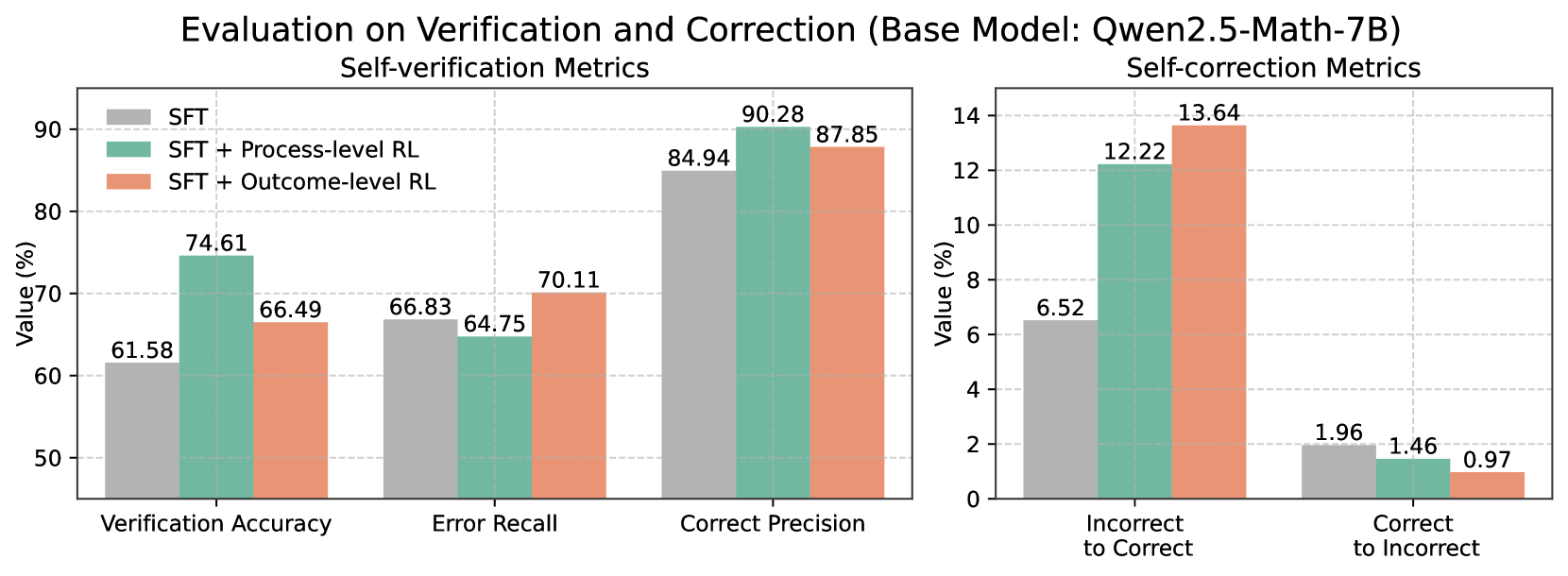
Figure 3: Evaluation on verification and correction.
In Figure 3, we present the results of the behavior-initialized model (SFT) and different RL models obtained from Qwen2.5-Math-7B. We observe that: (1) Both RL methods effectively enhance self-verification accuracy. The process-level RL shows larger improvement on accuracy, while the outcome-level RL consistently improves Error Recall and Correct Precision. This might be because process-level supervision indiscriminately promotes verification accuracy in intermediate steps, while outcome-level supervision allows the policy model to explore freely in intermediate steps and only boosts the final answer accuracy, thus mainly enhancing Error Recall and Correct Precision (which directly relate to final answer accuracy). (2) Both RL methods can successfully enhance the models’ self-correction capability. Notably, the model’s ability to correct incorrect answers is significantly improved after RL training. The rate of model mistakenly altering correct answers is also notably reduced. This comparison demonstrates that S 2 r can substantially enhance the validity of models’ self-correction ability.
<details>
<summary>x5.png Details</summary>
### Visual Description
## Bar Chart: Accuracy and Trial Numbers across Difficulty Level
### Overview
This bar chart compares the accuracy and trial numbers of a model (Llama3.1-8B-Instruct) across five difficulty levels (Level 1 to Level 5). Two training methods are compared: Supervised Fine-Tuning (SFT) and SFT combined with Reinforcement Learning (SFT+RL). Accuracy is represented on the primary y-axis (left), while trial numbers are represented on the secondary y-axis (right).
### Components/Axes
* **Title:** Accuracy and Trial Numbers across Difficulty Level (Base Model: Llama3.1-8B-Instruct) - positioned at the top-center.
* **X-axis:** Difficulty Level - labeled at the bottom, with markers for Level 1, Level 2, Level 3, Level 4, and Level 5.
* **Primary Y-axis (left):** Accuracy - ranging from 0.2 to 1.0.
* **Secondary Y-axis (right):** Trial Numbers - ranging from 0 to 6.
* **Legend:** Located at the top-right.
* SFT Accuracy (Green)
* SFT+RL Accuracy (Dark Green)
* SFT Trials (Red)
* SFT+RL Trials (Dark Red)
### Detailed Analysis
The chart consists of paired bars for each difficulty level, representing accuracy and trial numbers for both SFT and SFT+RL.
**Level 1:**
* SFT Accuracy: Approximately 0.930 (Green bar)
* SFT+RL Accuracy: Approximately 0.814 (Dark Green bar)
* SFT Trials: Approximately 3.279 (Red bar)
* SFT+RL Trials: Approximately 2.209 (Dark Red bar)
**Level 2:**
* SFT Accuracy: Approximately 0.733 (Green bar)
* SFT+RL Accuracy: Approximately 0.722 (Dark Green bar)
* SFT Trials: Approximately 3.367 (Red bar)
* SFT+RL Trials: Approximately 2.844 (Dark Red bar)
**Level 3:**
* SFT Accuracy: Approximately 0.4219 (Green bar)
* SFT+RL Accuracy: Approximately 0.638 (Dark Green bar)
* SFT Trials: Approximately 3.924 (Red bar)
* SFT+RL Trials: Approximately 0.610 (Dark Red bar)
**Level 4:**
* SFT Accuracy: Approximately 0.445 (Green bar)
* SFT+RL Accuracy: Approximately 0.367 (Dark Green bar)
* SFT Trials: Approximately 5.117 (Red bar)
* SFT+RL Trials: Approximately 3 (Dark Red bar)
**Level 5:**
* SFT Accuracy: Approximately 0.276 (Green bar)
* SFT+RL Accuracy: Approximately 0.239 (Dark Green bar)
* SFT Trials: Approximately 4.104 (Red bar)
* SFT+RL Trials: Approximately 5.254 (Dark Red bar)
**Trends:**
* **SFT Accuracy:** Generally decreases as difficulty level increases. Starts high at Level 1 and declines to Level 5.
* **SFT+RL Accuracy:** Shows a more complex trend. It starts lower than SFT at Level 1, but surpasses SFT at Level 3. It then declines at Level 4 and Level 5.
* **SFT Trials:** Generally increases with difficulty level, with a slight dip between Level 2 and Level 3.
* **SFT+RL Trials:** Increases with difficulty level, with a significant increase at Level 5.
### Key Observations
* At Level 1, SFT has significantly higher accuracy than SFT+RL.
* At Level 3, SFT+RL surpasses SFT in accuracy.
* Trial numbers generally increase with difficulty for both methods, suggesting more attempts are needed to achieve results at higher difficulty levels.
* The gap between SFT and SFT+RL trial numbers widens at higher difficulty levels.
### Interpretation
The data suggests that while SFT performs better on easier tasks (Level 1), the addition of Reinforcement Learning (RL) improves performance on more challenging tasks (Level 3). However, this improvement comes at the cost of increased trial numbers, particularly at the highest difficulty levels. This indicates that while RL can enhance the model's ability to solve complex problems, it requires more training iterations. The decreasing accuracy of both methods as difficulty increases highlights the inherent limitations of the model in tackling increasingly complex tasks. The diverging trial numbers suggest that RL may be more sensitive to the difficulty of the task, requiring more exploration and refinement to achieve optimal performance. The chart provides valuable insights into the trade-offs between accuracy, training effort, and difficulty level when choosing between SFT and SFT+RL for this specific model (Llama3.1-8B-Instruct).
</details>
(a)
<details>
<summary>x6.png Details</summary>
### Visual Description
## Bar Chart: Accuracy and Trial Numbers across Difficulty Level (Base Model: Qwen2.5-Math-7B)
### Overview
This bar chart compares the accuracy and trial numbers of a base model (Qwen2.5-Math-7B) across five difficulty levels (Level 1 to Level 5). It presents two sets of data for each difficulty level: accuracy achieved through Supervised Fine-Tuning (SFT) and accuracy achieved through SFT combined with Reinforcement Learning (SFT+RL), as well as the corresponding trial numbers for both methods. The chart uses bar graphs to represent accuracy and a secondary y-axis to represent trial numbers.
### Components/Axes
* **Title:** Accuracy and Trial Numbers across Difficulty Level (Base Model: Qwen2.5-Math-7B) - positioned at the top-center.
* **X-axis:** Difficulty Level (Level 1, Level 2, Level 3, Level 4, Level 5) - positioned at the bottom.
* **Y-axis (left):** Accuracy - ranging from approximately 0.60 to 1.00.
* **Y-axis (right):** Trial Numbers - ranging from 0.0 to 2.5.
* **Legend (top-right):**
* SFT Accuracy (Green)
* SFT Trials (Light Green)
* SFT+RL Accuracy (Red)
* SFT+RL Trials (Light Red)
### Detailed Analysis
The chart consists of paired bar graphs for each difficulty level. The left bar in each pair represents accuracy, and the right bar represents trial numbers.
**Level 1:**
* SFT Accuracy: Approximately 0.930
* SFT Trials: Approximately 0.930
* SFT+RL Accuracy: Approximately 1.116
* SFT+RL Trials: Approximately 1.047
**Level 2:**
* SFT Accuracy: Approximately 0.944
* SFT Trials: Approximately 0.944
* SFT+RL Accuracy: Approximately 1.311
* SFT+RL Trials: Approximately 1.244
**Level 3:**
* SFT Accuracy: Approximately 0.962
* SFT Trials: Approximately 0.943
* SFT+RL Accuracy: Approximately 1.771
* SFT+RL Trials: Approximately 1.790
**Level 4:**
* SFT Accuracy: Approximately 0.773
* SFT Trials: Approximately 0.836
* SFT+RL Accuracy: Approximately 1.828
* SFT+RL Trials: Approximately 1.883
**Level 5:**
* SFT Accuracy: Approximately 0.649
* SFT Trials: Approximately 0.619
* SFT+RL Accuracy: Approximately 2.254
* SFT+RL Trials: Approximately 2.149
**Trends:**
* **SFT Accuracy:** Generally high across all difficulty levels, with a slight decrease at Level 5.
* **SFT+RL Accuracy:** Shows a clear increasing trend with difficulty level, peaking at Level 5.
* **SFT Trials:** Relatively stable across all difficulty levels.
* **SFT+RL Trials:** Increases with difficulty level, mirroring the trend in SFT+RL Accuracy.
### Key Observations
* SFT+RL consistently outperforms SFT in terms of accuracy, especially at higher difficulty levels.
* The trial numbers for SFT+RL increase significantly with difficulty, suggesting that more trials are needed to achieve higher accuracy with reinforcement learning.
* Accuracy for SFT decreases at Level 5, while SFT+RL accuracy continues to increase. This suggests that reinforcement learning becomes more crucial as the difficulty increases.
* The SFT+RL accuracy at Level 1 is higher than 1.0, which is not possible. This is likely an error in the data or visualization.
### Interpretation
The data suggests that combining Supervised Fine-Tuning with Reinforcement Learning significantly improves the performance of the Qwen2.5-Math-7B model, particularly on more challenging tasks. The increasing trial numbers for SFT+RL indicate that reinforcement learning requires more iterations to converge to optimal solutions. The anomaly at Level 1 for SFT+RL accuracy should be investigated further. The chart demonstrates the benefits of incorporating reinforcement learning into the training process for complex mathematical problem-solving, and highlights the importance of considering the difficulty level when evaluating model performance. The relationship between difficulty level and trial numbers suggests a trade-off between accuracy and computational cost. As the difficulty increases, more trials are needed to achieve higher accuracy, which may require more resources and time.
</details>
(b)
Figure 4: The accuracy and average trial number of different models across difficulty levels. Evaluated on MATH500 test set.
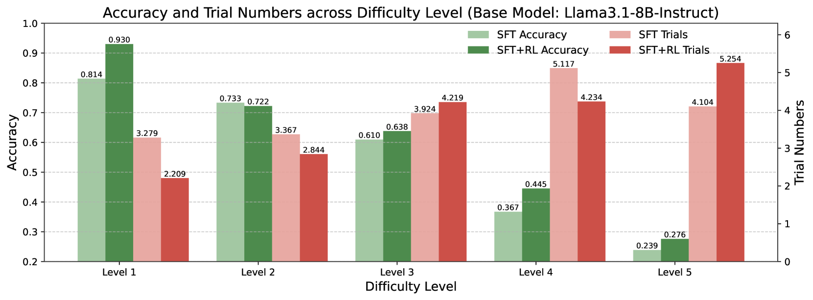
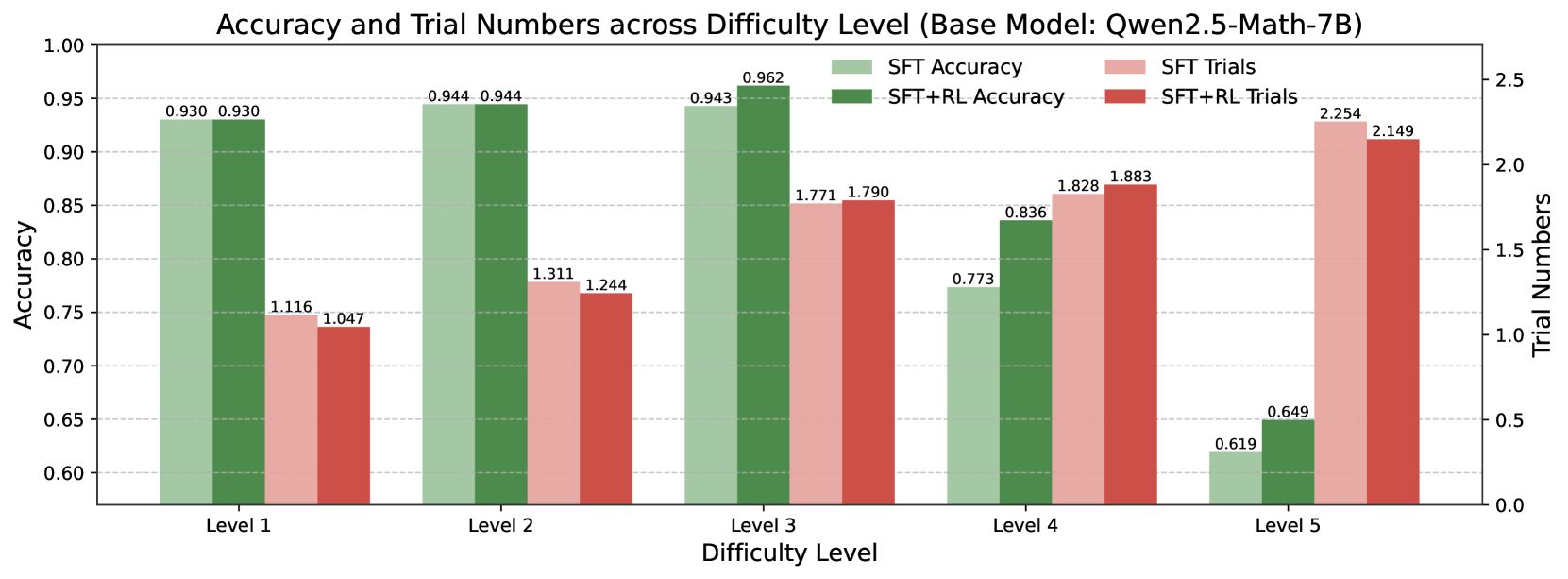
3.4.3 Improvement across Difficulty Levels
To further illustrate the effect of S 2 r training, Figure 4 shows the answer accuracy and average number of trials (i.e., the average value of " $K$ " across all $y=(s_{1},v_{1},·s,s_{K},v_{K})$ under each difficulty level) for the SFT and SFT+RL models. We observe that: (1) By learning to self-verify and self-correct during reasoning, the models learn to dynamically allocate test-time effort. For easier problems, the models can reach a confident answer with fewer trials, while for more difficult problems, they require more trials to achieve a confident answer. (2) RL further improves test-time effort allocation, particularly for less capable model (e.g., Llama3.1-8B-Instruct). (3) After RL training, the answer accuracy for more difficult problems is notably improved, demonstrating the effectiveness of the self-verifying and self-correcting paradigm in enhancing the models’ reasoning abilities.
| | Datasets | xx Average xx | | | | | | |
| --- | --- | --- | --- | --- | --- | --- | --- | --- |
| Model | MATH 500 | AIME 2024 | AMC 2023 | College Math | Olympiad Bench | GSM8K | GaokaoEn 2023 | |
| General Model: Qwen2-7B-Instruct | | | | | | | | |
| Qwen2-7B-Instruct | 51.2 | 3.3 | 30.0 | 18.2 | 19.1 | 86.4 | 39.0 | 35.3 |
| Qwen2-7B- S 2 r -BI (ours) | 61.2 | 3.3 | 27.5 | 41.1 | 27.1 | 87.4 | 49.1 | 42.4 |
| Qwen2-7B- S 2 r -PRL (ours) | 65.4 | 6.7 | 35.0 | 36.7 | 27.0 | 89.0 | 49.9 | 44.2 |
| Qwen2-7B- S 2 r -ORL (ours) | 64.8 | 3.3 | 42.5 | 34.7 | 26.2 | 86.4 | 50.9 | 44.1 |
| Qwen2-7B–Instruct- S 2 r -PRL-offline (ours) | 61.6 | 10.0 | 32.5 | 40.2 | 26.5 | 87.6 | 50.4 | 44.1 |
| Qwen2-7B-Instruct- S 2 r -ORL-offline (ours) | 61.0 | 6.7 | 37.5 | 40.5 | 27.3 | 87.4 | 49.6 | 44.3 |
| Math-Specialized Model: Qwen2.5-Math-7B | | | | | | | | |
| Qwen2.5-Math-7B | 51.0 | 16.7 | 45.0 | 21.5 | 16.7 | 58.3 | 39.7 | 35.6 |
| Qwen2.5-Math-7B- S 2 r -BI (ours) | 81.6 | 23.3 | 60.0 | 43.9 | 44.4 | 91.9 | 70.1 | 59.3 |
| Qwen2.5-Math-7B- S 2 r -PRL (ours) | 83.4 | 26.7 | 70.0 | 43.8 | 46.4 | 93.2 | 70.4 | 62.0 |
| Qwen2.5-Math-7B- S 2 r -ORL (ours) | 84.4 | 23.3 | 77.5 | 43.8 | 44.9 | 92.9 | 70.1 | 62.4 |
| Qwen2.5-Math-7B- S 2 r -PRL-offline (ours) | 83.4 | 23.3 | 62.5 | 50.0 | 46.7 | 92.9 | 72.2 | 61.6 |
| Qwen2.5-Math-7B- S 2 r -ORL-offline (ours) | 82.0 | 20.0 | 67.5 | 49.8 | 45.8 | 92.6 | 70.4 | 61.2 |
Table 5: Comparison of S 2 r using online and offline RL training.
3.5 Exploring Offline RL
As described in § 2.4, we explore offline RL as a more efficient alternative to online RL training, given the effectiveness of offline RL has been demonstrated in recent studies Baheti et al. (2023); Cheng et al. (2025); Wang et al. (2024b).
Table 5 presents the results of offline RL with process-level and outcome-level supervision, compared to online RL. We can observe that: (1) Different from online RL, process-level supervision outperforms outcome-level supervision in offline RL training. This interesting phenomenon may be due to: a) Outcome-level RL, which excels at allowing models to freely explore dynamic trajectories, is more suitable for on-the-fly sampling during online parameter updating. b) In contrast, process-level RL, which requires accurate baseline estimation for intermediate steps, benefits from offline trajectory sampling, which can provide more accurate baseline estimates with larger scale data sampling. (2) Offline RL consistently improves performance over the behavior-initialized models across most benchmarks and achieves comparable results to online RL. These results highlight the potential of offline RL as a more efficient alternative for enhancing LLMs’ deep reasoning.
4 Related Work
4.1 Scaling Test-time Compute
Scaling test-time compute recently garners wide attention in LLM reasoning Snell et al. (2024b); Wu et al. (2024); Brown et al. (2024). Existing studies have explored various methods for scaling up test-time compute, including: (1) Aggregation-based methods that samples multiple responses for each question and obtains the final answer with self-consistency Wang et al. (2023) or by selecting best-of-N answer using a verifier or reward model Wang et al. (2024c); Zhang et al. (2024b); Lightman et al. (2023b); Havrilla et al. (2024b); (2) Search-based methods that apply search algorithms such as Monte Carlo Tree Search Tian et al. (2024); Wang et al. (2024a); Zhang et al. (2024a); Qi et al. (2024), beam search Snell et al. (2024b), or other effective algorithms Feng et al. (2023); Yao et al. (2023) to search for correct trajectories; (3) Iterative-refine-based methods that iteratively improve test performance through self-refinement Madaan et al. (2024a); Shinn et al. (2024); Chen et al. (2024a, 2025). Recently, there has been a growing focus on training LLMs to perform test-time search on their own, typically by conducting longer and deeper thinking OpenAI (2024); Guo et al. (2025). These test-time scaling efforts not only directly benefit LLM reasoning, but can also be integrated back into training time, enabling iterative improvement for LLM reasoning Qin et al. (2024); Feng et al. (2023); Snell et al. (2024b); Luong et al. (2024). In this work, we also present an efficient framework for training LLMs to perform effective test-time scaling through self-verification and self-correction iterations. This approach is achieved without extensive efforts, and the performance of S 2 r can also be consistently promoted via iterative training.
4.2 Self-verification and Self-correction
Enabling LLMs to perform effective self-verification and self-correction is a promising solution for achieving robust reasoning for LLMs Madaan et al. (2024b); Shinn et al. (2023); Paul et al. (2023); Lightman et al. (2023a), and these abilities are also critical for performing deep reasoning. Previous studies have shown that direct prompting of LLMs for self-verification or self-correction is suboptimal in most scenarios Huang et al. (2023); Tyen et al. (2023); Ma et al. (2024); Zhang et al. (2024c). As a result, recent studies have explored various approaches to enhance these capabilities during post-training Saunders et al. (2022); Rosset et al. (2024); Kumar et al. (2024). These methods highlight the potential of using human-annotated or LLM-generated data to equip LLMs with self-verification or self-correction capabilities Zhang et al. (2024d); Jiang et al. (2024), while also indicating that behavior imitation via supervised fine-tuning alone is insufficient for achieving valid self-verification or self-correction Kumar et al. (2024); Qu et al. (2025); Kamoi et al. (2024). In this work, we propose effective methods to enhance LLMs’ self-verification and self-correction abilities through principled imitation data construction and RL training, and demonstrate the effectiveness of our approach with in-depth analysis.
4.3 RL for LLM Reasoning
Reinforcement learning has proven effective in enhancing LLM performance across various tasks Ziegler et al. (2019); Stiennon et al. (2020); Bai et al. (2022); Ouyang et al. (2022); Setlur et al. (2025). In LLM reasoning, previous studies typically employ RL in an actor-critic framework Lightman et al. (2024); Tajwar et al. (2024); Havrilla et al. (2024a), and research on developing accurate reward models for RL training has been a long-standing focus, particularly in reward modeling for Process-level RL Lightman et al. (2024); Setlur et al. (2024, 2025); Luo et al. (2024). Recently, several studies have demonstrate that simplified reward modeling and advantage estimation Ahmadian et al. (2024); Shao et al. (2024); Team et al. (2025); Guo et al. (2025) in RL training can also effectively enhance LLM reasoning. Recent advances in improving LLMs’ deep thinking Guo et al. (2025); Team et al. (2025) further highlight the effectiveness of utilizing unhackable rewards Gao et al. (2023); Everitt et al. (2021) to consistently enhance LLM reasoning. In this work, we also show that simplified advantage estimation and RL framework enable effective improvements on LLM reasoning. Additionally, we conducted an analysis on process-level RL, outcome-level RL and offline RL, providing insights for future work in RL for LLM reasoning.
5 Conclusion
In this work, we propose S 2 r, an efficient framework for enhancing LLM reasoning by teaching LLMs to iteratively self-verify and self-correct during reasoning. We introduce a principled approach for behavior initialization, and explore both outcome-level and process-level RL to further strengthen the models’ thinking abilities. Experimental results across three different base models on seven math reasoning benchmarks demonstrate that S 2 r significantly enhances LLM reasoning with minimal resource requirements. Since self-verification and self-correction are two crucial abilities for LLMs’ deep reasoning, S 2 r offers an interpretable framework for understanding how SFT and RL enhance LLMs’ deep reasoning. It also offers insights into the selection of RL strategies for enhancing LLMs’ long-CoT reasoning.
References
- qwe (2024) 2024. Qwen2 technical report.
- Ahmadian et al. (2024) Arash Ahmadian, Chris Cremer, Matthias Gallé, Marzieh Fadaee, Julia Kreutzer, Olivier Pietquin, Ahmet Üstün, and Sara Hooker. 2024. Back to basics: Revisiting reinforce style optimization for learning from human feedback in llms. arXiv preprint arXiv:2402.14740.
- AI-MO (2024a) AI-MO. 2024a. Aime 2024.
- AI-MO (2024b) AI-MO. 2024b. Amc 2023.
- Baheti et al. (2023) Ashutosh Baheti, Ximing Lu, Faeze Brahman, Ronan Le Bras, Maarten Sap, and Mark Riedl. 2023. Leftover lunch: Advantage-based offline reinforcement learning for language models. arXiv preprint arXiv:2305.14718.
- Bai et al. (2022) Yuntao Bai, Andy Jones, Kamal Ndousse, Amanda Askell, Anna Chen, Nova DasSarma, Dawn Drain, Stanislav Fort, Deep Ganguli, Tom Henighan, et al. 2022. Training a helpful and harmless assistant with reinforcement learning from human feedback. arXiv preprint arXiv:2204.05862.
- Berglund et al. (2023) Lukas Berglund, Meg Tong, Max Kaufmann, Mikita Balesni, Asa Cooper Stickland, Tomasz Korbak, and Owain Evans. 2023. The reversal curse: Llms trained on" a is b" fail to learn" b is a". arXiv preprint arXiv:2309.12288.
- Brown et al. (2024) Bradley Brown, Jordan Juravsky, Ryan Ehrlich, Ronald Clark, Quoc V Le, Christopher Ré, and Azalia Mirhoseini. 2024. Large language monkeys: Scaling inference compute with repeated sampling. arXiv preprint arXiv:2407.21787.
- Chen et al. (2025) Jiefeng Chen, Jie Ren, Xinyun Chen, Chengrun Yang, Ruoxi Sun, and Sercan Ö Arık. 2025. Sets: Leveraging self-verification and self-correction for improved test-time scaling. arXiv preprint arXiv:2501.19306.
- Chen et al. (2024a) Justin Chih-Yao Chen, Archiki Prasad, Swarnadeep Saha, Elias Stengel-Eskin, and Mohit Bansal. 2024a. Magicore: Multi-agent, iterative, coarse-to-fine refinement for reasoning. arXiv preprint arXiv:2409.12147.
- Chen et al. (2024b) Justin Chih-Yao Chen, Zifeng Wang, Hamid Palangi, Rujun Han, Sayna Ebrahimi, Long Le, Vincent Perot, Swaroop Mishra, Mohit Bansal, Chen-Yu Lee, et al. 2024b. Reverse thinking makes llms stronger reasoners. arXiv preprint arXiv:2411.19865.
- Chen et al. (2024c) Xingyu Chen, Jiahao Xu, Tian Liang, Zhiwei He, Jianhui Pang, Dian Yu, Linfeng Song, Qiuzhi Liu, Mengfei Zhou, Zhuosheng Zhang, et al. 2024c. Do not think that much for 2+ 3=? on the overthinking of o1-like llms. arXiv preprint arXiv:2412.21187.
- Cheng et al. (2025) Pengyu Cheng, Tianhao Hu, Han Xu, Zhisong Zhang, Yong Dai, Lei Han, Xiaolong Li, et al. 2025. Self-playing adversarial language game enhances llm reasoning. Advances in Neural Information Processing Systems, 37:126515–126543.
- Cobbe et al. (2021a) Karl Cobbe, Vineet Kosaraju, Mohammad Bavarian, Mark Chen, Heewoo Jun, Lukasz Kaiser, Matthias Plappert, Jerry Tworek, Jacob Hilton, Reiichiro Nakano, Christopher Hesse, and John Schulman. 2021a. Training verifiers to solve math word problems. arXiv preprint arXiv:2110.14168.
- Cobbe et al. (2021b) Karl Cobbe, Vineet Kosaraju, Mohammad Bavarian, Mark Chen, Heewoo Jun, Lukasz Kaiser, Matthias Plappert, Jerry Tworek, Jacob Hilton, Reiichiro Nakano, et al. 2021b. Training verifiers to solve math word problems. arXiv preprint arXiv:2110.14168.
- Cui et al. (2025) Ganqu Cui, Lifan Yuan, Zefan Wang, Hanbin Wang, Wendi Li, Bingxiang He, Yuchen Fan, Tianyu Yu, Qixin Xu, Weize Chen, et al. 2025. Process reinforcement through implicit rewards. arXiv preprint arXiv:2502.01456.
- Dubey et al. (2024) Abhimanyu Dubey, Abhinav Jauhri, Abhinav Pandey, Abhishek Kadian, Ahmad Al-Dahle, Aiesha Letman, Akhil Mathur, Alan Schelten, Amy Yang, Angela Fan, et al. 2024. The llama 3 herd of models. arXiv preprint arXiv:2407.21783.
- Everitt et al. (2021) Tom Everitt, Marcus Hutter, Ramana Kumar, and Victoria Krakovna. 2021. Reward tampering problems and solutions in reinforcement learning: A causal influence diagram perspective. Synthese, 198(Suppl 27):6435–6467.
- Feng et al. (2023) Xidong Feng, Ziyu Wan, Muning Wen, Ying Wen, Weinan Zhang, and Jun Wang. 2023. Alphazero-like tree-search can guide large language model decoding and training. arXiv preprint arXiv:2309.17179.
- Gao et al. (2023) Leo Gao, John Schulman, and Jacob Hilton. 2023. Scaling laws for reward model overoptimization. In International Conference on Machine Learning, pages 10835–10866. PMLR.
- Geva et al. (2021) Mor Geva, Daniel Khashabi, Elad Segal, Tushar Khot, Dan Roth, and Jonathan Berant. 2021. Did Aristotle Use a Laptop? A Question Answering Benchmark with Implicit Reasoning Strategies. Transactions of the Association for Computational Linguistics (TACL).
- Gu et al. (2024) Alex Gu, Baptiste Rozière, Hugh Leather, Armando Solar-Lezama, Gabriel Synnaeve, and Sida I. Wang. 2024. Cruxeval: A benchmark for code reasoning, understanding and execution. arXiv preprint arXiv:2401.03065.
- Guan et al. (2025) Xinyu Guan, Li Lyna Zhang, Yifei Liu, Ning Shang, Youran Sun, Yi Zhu, Fan Yang, and Mao Yang. 2025. rstar-math: Small llms can master math reasoning with self-evolved deep thinking. arXiv preprint arXiv:2501.04519.
- Guo et al. (2025) Daya Guo, Dejian Yang, Haowei Zhang, Junxiao Song, Ruoyu Zhang, Runxin Xu, Qihao Zhu, Shirong Ma, Peiyi Wang, Xiao Bi, et al. 2025. Deepseek-r1: Incentivizing reasoning capability in llms via reinforcement learning. arXiv preprint arXiv:2501.12948.
- Han et al. (2022) Simeng Han, Hailey Schoelkopf, Yilun Zhao, Zhenting Qi, Martin Riddell, Luke Benson, Lucy Sun, Ekaterina Zubova, Yujie Qiao, Matthew Burtell, et al. 2022. Folio: Natural language reasoning with first-order logic. arXiv preprint arXiv:2209.00840.
- Havrilla et al. (2024a) Alex Havrilla, Yuqing Du, Sharath Chandra Raparthy, Christoforos Nalmpantis, Jane Dwivedi-Yu, Maksym Zhuravinskyi, Eric Hambro, Sainbayar Sukhbaatar, and Roberta Raileanu. 2024a. Teaching large language models to reason with reinforcement learning. arXiv preprint arXiv:2403.04642.
- Havrilla et al. (2024b) Alex Havrilla, Sharath Raparthy, Christoforus Nalmpantis, Jane Dwivedi-Yu, Maksym Zhuravinskyi, Eric Hambro, and Roberta Raileanu. 2024b. Glore: When, where, and how to improve llm reasoning via global and local refinements. arXiv preprint arXiv:2402.10963.
- He et al. (2024) Chaoqun He, Renjie Luo, Yuzhuo Bai, Shengding Hu, Zhen Leng Thai, Junhao Shen, Jinyi Hu, Xu Han, Yujie Huang, Yuxiang Zhang, et al. 2024. Olympiadbench: A challenging benchmark for promoting agi with olympiad-level bilingual multimodal scientific problems. arXiv preprint arXiv:2402.14008.
- Hendrycks et al. (2021a) Dan Hendrycks, Collin Burns, Saurav Kadavath, Akul Arora, Steven Basart, Eric Tang, Dawn Song, and Jacob Steinhardt. 2021a. Measuring mathematical problem solving with the math dataset. In Thirty-fifth Conference on Neural Information Processing Systems Datasets and Benchmarks Track (Round 2).
- Hendrycks et al. (2021b) Dan Hendrycks, Collin Burns, Saurav Kadavath, Akul Arora, Steven Basart, Eric Tang, Dawn Song, and Jacob Steinhardt. 2021b. Measuring mathematical problem solving with the math dataset. arXiv preprint arXiv:2103.03874.
- Huang et al. (2023) Jie Huang, Xinyun Chen, Swaroop Mishra, Huaixiu Steven Zheng, Adams Wei Yu, Xinying Song, and Denny Zhou. 2023. Large language models cannot self-correct reasoning yet. arXiv preprint arXiv:2310.01798.
- Jiang et al. (2024) Huchen Jiang, Yangyang Ma, Chaofan Ding, Kexin Luan, and Xinhan Di. 2024. Towards intrinsic self-correction enhancement in monte carlo tree search boosted reasoning via iterative preference learning. arXiv preprint arXiv:2412.17397.
- Kamoi et al. (2024) Ryo Kamoi, Yusen Zhang, Nan Zhang, Jiawei Han, and Rui Zhang. 2024. When can llms actually correct their own mistakes? a critical survey of self-correction of llms. Transactions of the Association for Computational Linguistics, 12:1417–1440.
- Kool et al. (2019) Wouter Kool, Herke van Hoof, and Max Welling. 2019. Buy 4 reinforce samples, get a baseline for free!
- Kumar et al. (2024) Aviral Kumar, Vincent Zhuang, Rishabh Agarwal, Yi Su, John D Co-Reyes, Avi Singh, Kate Baumli, Shariq Iqbal, Colton Bishop, Rebecca Roelofs, et al. 2024. Training language models to self-correct via reinforcement learning. arXiv preprint arXiv:2409.12917.
- Kwon et al. (2023) Woosuk Kwon, Zhuohan Li, Siyuan Zhuang, Ying Sheng, Lianmin Zheng, Cody Hao Yu, Joseph E. Gonzalez, Hao Zhang, and Ion Stoica. 2023. Efficient memory management for large language model serving with pagedattention. In Proceedings of the ACM SIGOPS 29th Symposium on Operating Systems Principles.
- LI et al. (2024) Jia LI, Edward Beeching, Lewis Tunstall, Ben Lipkin, Roman Soletskyi, Shengyi Costa Huang, Kashif Rasul, Longhui Yu, Albert Jiang, Ziju Shen, Zihan Qin, Bin Dong, Li Zhou, Yann Fleureau, Guillaume Lample, and Stanislas Polu. 2024. Numinamath. [https://github.com/project-numina/aimo-progress-prize](https://github.com/project-numina/aimo-progress-prize/blob/main/report/numina_dataset.pdf).
- Liao et al. (2024) Minpeng Liao, Wei Luo, Chengxi Li, Jing Wu, and Kai Fan. 2024. Mario: Math reasoning with code interpreter output–a reproducible pipeline. arXiv preprint arXiv:2401.08190.
- Lightman et al. (2023a) Hunter Lightman, Vineet Kosaraju, Yura Burda, Harri Edwards, Bowen Baker, Teddy Lee, Jan Leike, John Schulman, Ilya Sutskever, and Karl Cobbe. 2023a. Let’s verify step by step. arXiv preprint arXiv:2305.20050.
- Lightman et al. (2023b) Hunter Lightman, Vineet Kosaraju, Yura Burda, Harri Edwards, Bowen Baker, Teddy Lee, Jan Leike, John Schulman, Ilya Sutskever, and Karl Cobbe. 2023b. Let’s verify step by step. arXiv preprint arXiv:2305.20050.
- Lightman et al. (2024) Hunter Lightman, Vineet Kosaraju, Yuri Burda, Harrison Edwards, Bowen Baker, Teddy Lee, Jan Leike, John Schulman, Ilya Sutskever, and Karl Cobbe. 2024. Let’s verify step by step. In The Twelfth International Conference on Learning Representations.
- Luo et al. (2024) Liangchen Luo, Yinxiao Liu, Rosanne Liu, Samrat Phatale, Harsh Lara, Yunxuan Li, Lei Shu, Yun Zhu, Lei Meng, Jiao Sun, et al. 2024. Improve mathematical reasoning in language models by automated process supervision. arXiv preprint arXiv:2406.06592.
- Luong et al. (2024) Trung Quoc Luong, Xinbo Zhang, Zhanming Jie, Peng Sun, Xiaoran Jin, and Hang Li. 2024. Reft: Reasoning with reinforced fine-tuning. arXiv preprint arXiv:2401.08967.
- Ma et al. (2024) Ruotian Ma, Xiaolei Wang, Xin Zhou, Jian Li, Nan Du, Tao Gui, Qi Zhang, and Xuanjing Huang. 2024. Are large language models good prompt optimizers? arXiv preprint arXiv:2402.02101.
- Madaan et al. (2024a) Aman Madaan, Niket Tandon, Prakhar Gupta, Skyler Hallinan, Luyu Gao, Sarah Wiegreffe, Uri Alon, Nouha Dziri, Shrimai Prabhumoye, Yiming Yang, et al. 2024a. Self-refine: Iterative refinement with self-feedback. Advances in Neural Information Processing Systems, 36.
- Madaan et al. (2024b) Aman Madaan, Niket Tandon, Prakhar Gupta, Skyler Hallinan, Luyu Gao, Sarah Wiegreffe, Uri Alon, Nouha Dziri, Shrimai Prabhumoye, Yiming Yang, et al. 2024b. Self-refine: Iterative refinement with self-feedback. Advances in Neural Information Processing Systems, 36.
- OpenAI (2024) OpenAI. 2024. Openai o1 system card. preprint.
- Ouyang et al. (2022) Long Ouyang, Jeffrey Wu, Xu Jiang, Diogo Almeida, Carroll Wainwright, Pamela Mishkin, Chong Zhang, Sandhini Agarwal, Katarina Slama, Alex Ray, et al. 2022. Training language models to follow instructions with human feedback. Advances in neural information processing systems, 35:27730–27744.
- Paul et al. (2023) Debjit Paul, Mete Ismayilzada, Maxime Peyrard, Beatriz Borges, Antoine Bosselut, Robert West, and Boi Faltings. 2023. Refiner: Reasoning feedback on intermediate representations. arXiv preprint arXiv:2304.01904.
- Qi et al. (2024) Zhenting Qi, Mingyuan Ma, Jiahang Xu, Li Lyna Zhang, Fan Yang, and Mao Yang. 2024. Mutual reasoning makes smaller llms stronger problem-solvers. arXiv preprint arXiv:2408.06195.
- Qin et al. (2024) Yiwei Qin, Xuefeng Li, Haoyang Zou, Yixiu Liu, Shijie Xia, Zhen Huang, Yixin Ye, Weizhe Yuan, Hector Liu, Yuanzhi Li, et al. 2024. O1 replication journey: A strategic progress report–part 1. arXiv preprint arXiv:2410.18982.
- Qu et al. (2025) Yuxiao Qu, Tianjun Zhang, Naman Garg, and Aviral Kumar. 2025. Recursive introspection: Teaching language model agents how to self-improve. Advances in Neural Information Processing Systems, 37:55249–55285.
- Qwen (2024) Qwen. 2024. Qwen2.5-math-7b.
- Rosset et al. (2024) Corby Rosset, Ching-An Cheng, Arindam Mitra, Michael Santacroce, Ahmed Awadallah, and Tengyang Xie. 2024. Direct nash optimization: Teaching language models to self-improve with general preferences. arXiv preprint arXiv:2404.03715.
- Saunders et al. (2022) William Saunders, Catherine Yeh, Jeff Wu, Steven Bills, Long Ouyang, Jonathan Ward, and Jan Leike. 2022. Self-critiquing models for assisting human evaluators. arXiv preprint arXiv:2206.05802.
- Setlur et al. (2025) Amrith Setlur, Saurabh Garg, Xinyang Geng, Naman Garg, Virginia Smith, and Aviral Kumar. 2025. Rl on incorrect synthetic data scales the efficiency of llm math reasoning by eight-fold. Advances in Neural Information Processing Systems, 37:43000–43031.
- Setlur et al. (2024) Amrith Setlur, Chirag Nagpal, Adam Fisch, Xinyang Geng, Jacob Eisenstein, Rishabh Agarwal, Alekh Agarwal, Jonathan Berant, and Aviral Kumar. 2024. Rewarding progress: Scaling automated process verifiers for llm reasoning. arXiv preprint arXiv:2410.08146.
- Shao et al. (2024) Zhihong Shao, Peiyi Wang, Qihao Zhu, Runxin Xu, Junxiao Song, Xiao Bi, Haowei Zhang, Mingchuan Zhang, YK Li, Y Wu, et al. 2024. Deepseekmath: Pushing the limits of mathematical reasoning in open language models. arXiv preprint arXiv:2402.03300.
- Shen et al. (2025) Maohao Shen, Guangtao Zeng, Zhenting Qi, Zhang-Wei Hong, Zhenfang Chen, Wei Lu, Gregory Wornell, Subhro Das, David Cox, and Chuang Gan. 2025. Satori: Reinforcement learning with chain-of-action-thought enhances llm reasoning via autoregressive search. arXiv preprint arXiv:2502.02508.
- Shinn et al. (2024) Noah Shinn, Federico Cassano, Ashwin Gopinath, Karthik Narasimhan, and Shunyu Yao. 2024. Reflexion: Language agents with verbal reinforcement learning. Advances in Neural Information Processing Systems, 36.
- Shinn et al. (2023) Noah Shinn, Beck Labash, and Ashwin Gopinath. 2023. Reflexion: an autonomous agent with dynamic memory and self-reflection. arXiv preprint arXiv:2303.11366.
- Snell et al. (2024a) Charlie Snell, Jaehoon Lee, Kelvin Xu, and Aviral Kumar. 2024a. Scaling llm test-time compute optimally can be more effective than scaling model parameters. arXiv preprint arXiv:2408.03314.
- Snell et al. (2024b) Charlie Snell, Jaehoon Lee, Kelvin Xu, and Aviral Kumar. 2024b. Scaling llm test-time compute optimally can be more effective than scaling model parameters. Preprint, arXiv:2408.03314.
- Stiennon et al. (2020) Nisan Stiennon, Long Ouyang, Jeffrey Wu, Daniel Ziegler, Ryan Lowe, Chelsea Voss, Alec Radford, Dario Amodei, and Paul F Christiano. 2020. Learning to summarize with human feedback. Advances in Neural Information Processing Systems, 33:3008–3021.
- Tajwar et al. (2024) Fahim Tajwar, Anikait Singh, Archit Sharma, Rafael Rafailov, Jeff Schneider, Tengyang Xie, Stefano Ermon, Chelsea Finn, and Aviral Kumar. 2024. Preference fine-tuning of llms should leverage suboptimal, on-policy data. arXiv preprint arXiv:2404.14367.
- Tang et al. (2024a) Zhengyang Tang, Xingxing Zhang, Benyou Wan, and Furu Wei. 2024a. Mathscale: Scaling instruction tuning for mathematical reasoning. arXiv preprint arXiv:2403.02884.
- Tang et al. (2024b) Zhengyang Tang, Xingxing Zhang, Benyou Wang, and Furu Wei. 2024b. Mathscale: Scaling instruction tuning for mathematical reasoning. arXiv preprint arXiv:2403.02884.
- Team et al. (2025) Kimi Team, Angang Du, Bofei Gao, Bowei Xing, Changjiu Jiang, Cheng Chen, Cheng Li, Chenjun Xiao, Chenzhuang Du, Chonghua Liao, et al. 2025. Kimi k1. 5: Scaling reinforcement learning with llms. arXiv preprint arXiv:2501.12599.
- Team (2024a) Qwen Team. 2024a. Qwq: Reflect deeply on the boundaries of the unknown.
- Team (2024b) The Mistral AI Team. 2024b. Mathstral-7b-v0.1.
- Tian et al. (2024) Ye Tian, Baolin Peng, Linfeng Song, Lifeng Jin, Dian Yu, Haitao Mi, and Dong Yu. 2024. Toward self-improvement of llms via imagination, searching, and criticizing. arXiv preprint arXiv:2404.12253.
- Toshniwal et al. (2024) Shubham Toshniwal, Wei Du, Ivan Moshkov, Branislav Kisacanin, Alexan Ayrapetyan, and Igor Gitman. 2024. Openmathinstruct-2: Accelerating ai for math with massive open-source instruction data. arXiv preprint arXiv:2410.01560.
- Tyen et al. (2023) Gladys Tyen, Hassan Mansoor, Peter Chen, Tony Mak, and Victor Cărbune. 2023. Llms cannot find reasoning errors, but can correct them! arXiv preprint arXiv:2311.08516.
- Wang et al. (2024a) Chaojie Wang, Yanchen Deng, Zhiyi Lv, Shuicheng Yan, and An Bo. 2024a. Q*: Improving multi-step reasoning for llms with deliberative planning. Preprint, arXiv:2406.14283.
- Wang et al. (2024b) Huaijie Wang, Shibo Hao, Hanze Dong, Shenao Zhang, Yilin Bao, Ziran Yang, and Yi Wu. 2024b. Offline reinforcement learning for llm multi-step reasoning. arXiv preprint arXiv:2412.16145.
- Wang et al. (2024c) Peiyi Wang, Lei Li, Zhihong Shao, R. X. Xu, Damai Dai, Yifei Li, Deli Chen, Y. Wu, and Zhifang Sui. 2024c. Math-shepherd: Verify and reinforce llms step-by-step without human annotations. Preprint, arXiv:2312.08935.
- Wang et al. (2023) Xuezhi Wang, Jason Wei, Dale Schuurmans, Quoc V Le, Ed H. Chi, Sharan Narang, Aakanksha Chowdhery, and Denny Zhou. 2023. Self-consistency improves chain of thought reasoning in language models. In The Eleventh International Conference on Learning Representations.
- Wang et al. (2024d) Yubo Wang, Xueguang Ma, Ge Zhang, Yuansheng Ni, Abhranil Chandra, Shiguang Guo, Weiming Ren, Aaran Arulraj, Xuan He, Ziyan Jiang, et al. 2024d. Mmlu-pro: A more robust and challenging multi-task language understanding benchmark. arXiv preprint arXiv:2406.01574.
- Wu et al. (2024) Yangzhen Wu, Zhiqing Sun, Shanda Li, Sean Welleck, and Yiming Yang. 2024. An empirical analysis of compute-optimal inference for problem-solving with language models. arXiv preprint arXiv:2408.00724.
- Yang et al. (2024) An Yang, Beichen Zhang, Binyuan Hui, Bofei Gao, Bowen Yu, Chengpeng Li, Dayiheng Liu, Jianhong Tu, Jingren Zhou, Junyang Lin, et al. 2024. Qwen2. 5-math technical report: Toward mathematical expert model via self-improvement. arXiv preprint arXiv:2409.12122.
- Yao et al. (2023) Shunyu Yao, Dian Yu, Jeffrey Zhao, Izhak Shafran, Tom Griffiths, Yuan Cao, and Karthik Narasimhan. 2023. Tree of thoughts: Deliberate problem solving with large language models. Advances in neural information processing systems, 36:11809–11822.
- Yuan et al. (2024) Lifan Yuan, Wendi Li, Huayu Chen, Ganqu Cui, Ning Ding, Kaiyan Zhang, Bowen Zhou, Zhiyuan Liu, and Hao Peng. 2024. Free process rewards without process labels. arXiv preprint arXiv:2412.01981.
- Zeng et al. (2025) Weihao Zeng, Yuzhen Huang, Wei Liu, Keqing He, Qian Liu, Zejun Ma, and Junxian He. 2025. 7b model and 8k examples: Emerging reasoning with reinforcement learning is both effective and efficient. https://hkust-nlp.notion.site/simplerl-reason. Notion Blog.
- Zhang et al. (2024a) Dan Zhang, Sining Zhoubian, Ziniu Hu, Yisong Yue, Yuxiao Dong, and Jie Tang. 2024a. Rest-mcts*: Llm self-training via process reward guided tree search. arXiv preprint arXiv:2406.03816.
- Zhang et al. (2024b) Lunjun Zhang, Arian Hosseini, Hritik Bansal, Mehran Kazemi, Aviral Kumar, and Rishabh Agarwal. 2024b. Generative verifiers: Reward modeling as next-token prediction. In The 4th Workshop on Mathematical Reasoning and AI at NeurIPS’24.
- Zhang et al. (2024c) Qingjie Zhang, Han Qiu, Di Wang, Haoting Qian, Yiming Li, Tianwei Zhang, and Minlie Huang. 2024c. Understanding the dark side of llms’ intrinsic self-correction. arXiv preprint arXiv:2412.14959.
- Zhang et al. (2024d) Yunxiang Zhang, Muhammad Khalifa, Lajanugen Logeswaran, Jaekyeom Kim, Moontae Lee, Honglak Lee, and Lu Wang. 2024d. Small language models need strong verifiers to self-correct reasoning. arXiv preprint arXiv:2404.17140.
- Zhao et al. (2024) Yu Zhao, Huifeng Yin, Bo Zeng, Hao Wang, Tianqi Shi, Chenyang Lyu, Longyue Wang, Weihua Luo, and Kaifu Zhang. 2024. Marco-o1: Towards open reasoning models for open-ended solutions. arXiv preprint arXiv:2411.14405.
- Zheng et al. (2024) Chujie Zheng, Zhenru Zhang, Beichen Zhang, Runji Lin, Keming Lu, Bowen Yu, Dayiheng Liu, Jingren Zhou, and Junyang Lin. 2024. Processbench: Identifying process errors in mathematical reasoning. arXiv preprint arXiv:2412.06559.
- Ziegler et al. (2019) Daniel M Ziegler, Nisan Stiennon, Jeffrey Wu, Tom B Brown, Alec Radford, Dario Amodei, Paul Christiano, and Geoffrey Irving. 2019. Fine-tuning language models from human preferences. arXiv preprint arXiv:1909.08593.
Appendix A Implementation Details
A.1 Verification Processing and SFT Data Construction
Given the responses sampled from the original LLM policy, we prompt frontier LLMs for initial verifications. In order to construct more valid verification, we force the LLMs to “verify without re-solving the problem” and filter out invalid verifications during data processing. We found that despite being instructed to "verify without re-solving the problem", most existing LLMs still biased to solve the problem again, as shown in Table 6. Finally, we collected the verification data by querying gpt-4-preview-1106 https://openai.com/api/ , which shows strong instruction-following ability to "verify without re-solving the problem" and can perform plausible verification such as adopting reverse thinking, inductive reasoning and other methods.
For these collected prompts, we refine the remaining verifications using gpt-4o to improve fluency and clarity. During this refinement, we instruct gpt-4o to append a conclusion at the end of each verification based on its stance—for example: “Therefore, the answer is correct/incorrect/cannot verify.” Finally, we discard any verifications where the judgment does not align with the actual correctness of the answer. The prompts we used during the whole process are provided in Appendix § A.3.
With the refined and filtered verifications, we construct the SFT data as follows. For each problem, we determine the number of answer attempts required to eventually obtain a correct answer based on the accuracy from the initial sampling. The lower the accuracy, the more rounds of responses are generated. In our implementation, we categorize all problems into four difficulty levels and construct answer sequences with 1, 2, 3, or 4 rounds, according to descending accuracy. Then, after an incorrect answer, we append “Wait, let me recheck my solution” along with the corresponding verification. If that answer is not the final attempt, we further append “Let me try again.” We ensure that the last answer in the sequence is correct. Additionally, we ensure that the answers in each round for a given problem are distinct. Figure 5 is an example of SFT data constructed with 4 rounds of responses.
A.2 Baseline Details
A.2.1 Baseline Implementations
In Table 2, the reported results for Frontier LLMs and Top-tier Open-source Reasoning LLMs are sourced from the original reports and Guan et al. (2025). We evaluate Llama-3.1-8B-Instruct Dubey et al. (2024), Qwen2-7B-Instruct qwe (2024), Qwen2.5-Math-7B, Qwen2.5-Math-7B-Instruct and Qwen2.5-Math-72B-Instruct Yang et al. (2024) using the same process described in Section § 3.1. For Eurus-7B-PRIME Cui et al. (2025), rStar-Math-7B Guan et al. (2025), and Qwen2.5-7B-SimpleRL Zeng et al. (2025), we report results directly from the original papers.
In Table 3, the results for Llama-3.1-70B-Instruct and QwQ-32B-Preview are taken from Shen et al. (2025). For the remaining baselines, we follow the official evaluation protocol of the dataset project https://github.com/Yale-LILY/FOLIO https://github.com/facebookresearch/cruxeval https://github.com/eladsegal/strategyqa https://github.com/TIGER-AI-Lab/MMLU-Pro .
A.2.2 Baseline License
In this work, we utilize the Llama-3.1-8B-Instruct model, whose license can be reviewed at https://huggingface.co/meta-llama/Llama-3.1-8B-Instruct/blob/main/LICENSE. In addition, the models Qwen2-7B-Instruct, Qwen2.5-Math-7B, Eurus-2-7B-PRIME, and project vLLM are distributed under the Apache License 2.0. We gratefully acknowledge the contributions of the open-source community and strictly adhere to the terms of the respective licenses.
A.2.3 Baseline SFT Data Construction
Original Solution SFT Data
In this setting, we use the solution from the original dataset as sft data. To ensure a fair comparison, we maintain the same training data volume as our behavior initialization approaches.
Long CoT SFT Data
We also introduce a baseline by fine-tuning on Long CoT responses generated by QwQ-32B-Preview Team (2024a). Specifically, we instruct QwQ to generate responses to given problems and filter out those with incorrect answers. The remaining high-quality responses are then used for supervised fine-tuning. Importantly, we ensure that the total training data volume remains consistent with that used in our behavior initialization approach. The prompt we use for QwQ is provided in Appendix § A.3.
A.3 Prompts
The prompts we use in all experiments are as follows:
Sampling Responses During Training/Inference
⬇
Please reason step by step, and put your final answer within
\ boxed {}.
Problem: {problem}
Verification Refinement
⬇
You are a math teacher. I will give you a math problem and an answer.
Verify the answer ’ s correctness without step - by - step solving. Use alternative verification methods.
Question: {problem}
Answer: {answer}
Verification:
Verification Collection
⬇
Refine this verification text to read as a natural self - check within a solution. Maintain logical flow and professionalism.
Key Requirements:
1. Avoid phrases like " without solving step - by - step " or " as a math teacher ".
2. Treat the answer as your own prior solution.
3. Conclude with EXACTLY one of:
Therefore, the answer is correct.
Therefore, the answer is incorrect.
Therefore, the answer cannot be verified.
Original text: {verification}
Appendix B Detailed Experiment Settings
| Without Asking for Confirmative Verification | |
| --- | --- |
| Model | Confirmative out of 100 |
| GPT-4o | 26 |
| GPT-4-Preview-1106 | 32 |
| QwQ-32B-preview | 37 |
| Llama-3.1-70B-Instruct | 28 |
| Asking for Confirmative Verification | |
| Model | Confirmative out of 100 |
| GPT-4o | 44 |
| GPT-4-Preview-1106 | 61 |
| QwQ-32B-preview | 58 |
| Llama-3.1-70B-Instruct | 50 |
Table 6:
B.1 Datasets
Details of each test dataset we used as benchmark are as follows:
B.1.1 In-domain Datasets
MATH500 Lightman et al. (2023b) offers a streamlined slice of the broader MATH Hendrycks et al. (2021b) dataset, comprising 500 test problems selected through uniform sampling. Despite its smaller scope, it maintains a distribution of topics and difficulty levels that mirrors the larger MATH corpus.
GSM8K Cobbe et al. (2021a) features around 8,500 grade-school math word problems. The dataset focuses on simple arithmetic through early algebra and includes 1,319 distinct tasks in its test set.
OlympiadBench He et al. (2024) collects 8,476 advanced math and physics questions drawn from Olympiad contexts, with some originating from the Chinese college entrance exam. We use the subset of 674 text-only competition questions, providing open-ended math challenges.
AMC2023 AI-MO (2024b) and AIME AI-MO (2024a) each supply a set of challenging exam-style problems: 40 questions from AMC 2023 and 30 from AIME 2024, all in text-only format.
CollegeMath Tang et al. (2024b) is a dataset targeting advanced college-level mathematics, drawn from nine textbooks spanning seven major fields—algebra, pre-calculus, calculus, vector calculus, probability, linear algebra, and differential equations. The final collection comprises 1,281 training examples and 2,818 test examples.
Gaokao2023en Liao et al. (2024) is a dataset consisting of 385 mathematics problems sourced from the 2023 Chinese higher education entrance examination, which have been professionally translated into English.
B.1.2 Cross-domain Datasets
FOLIO Han et al. (2022) is meticulously annotated to assess intricate logical reasoning in natural language. It pairs 1,430 conclusions with 487 sets of premises—each verified using first-order logic (FOL)—and contains 203 unique problems in its test portion.
CRUXEval Gu et al. (2024) tests code comprehension and reasoning through 800 concise Python functions (spanning 3–13 lines). Each function is accompanied by one or more input-output examples. The goal is to predict the correct outputs given the function body and a specific input. The test partition encompasses all 800 problems.
StrategyQA Geva et al. (2021) targets multi-hop reasoning questions where the necessary intermediate steps are not explicit. Each of its 2,780 items includes a strategic query, a breakdown of the reasoning steps, and supporting evidence drawn from Wikipedia.
MMLUProSTEM is extracted from MMLU-Pro Wang et al. (2024d). Following Satori Shen et al. (2025), we conduct evaluations on six STEM subsets—physics, chemistry, computer science, engineering, biology, and economics.
B.2 Hyperparameters Setting
| Model | Learning Rate | Batch Size | KL Coefficient | Max Length | Training Epochs |
| --- | --- | --- | --- | --- | --- |
| Llama-3.1-8B-Instruct | 5e-6 | 32 | 0.1 | 8000 | 3 |
| Qwen2-7B-Instruct | 5e-6 | 32 | 0.1 | 6000 | 3 |
| Qwen2.5-Math-7B | 5e-6 | 32 | 0.01 | 8000 | 3 |
Table 7: Model Training Hyperparameter Settings (SFT)
| Model | Learning Rate | Training Batch Size | Forward Batch Size | KL Coefficient | Max Length | Sampling Temperature | Clip Range | Training Steps |
| --- | --- | --- | --- | --- | --- | --- | --- | --- |
| Llama-3.1 | 5e-7 | 64 | 256 | 0.05 | 8000 | 0.7 | 0.2 | 500 |
| Qwen2-7B-Instruct | 5e-7 | 64 | 256 | 0.05 | 6000 | 0.7 | 0.2 | 500 |
| Qwen2.5-Math-7B | 5e-7 | 64 | 256 | 0.01 | 8000 | 0.7 | 0.2 | 500 |
Table 8: Model Training Hyperparameter Settings (RL)
During behavior initialization with SFT, we use a batch size of 32 and adopt a learning rate of 5e-6. We set the maximum sequence length 8000 to accommodate long responses and verifications. To balance stability and convergence during training, we add a KL punishment to the training loss, and the KL coefficient is set to 0.1.
During reinforcement learning, for each training batch, we use a training batch size of 64, and sample $n$ responses for each question in a batch, resulting a forward batch size of $64n$ . For each forward batch, we update the model for $n$ step with the training batch size 64. Specifically, for both process-level and outcome-level RL, we adopt $n=4$ (i.e., for RLOO, the sample number is also $4$ ). More hyperparameters of the RL training are presented in Table 8. We use the BF16 model precision in all experiments.
Main hyperparameters used in the experiments are illustrated in Table 7 and 8.
B.3 Experiment Environment
All experiments are implemented using the PyTorch framework on 32 NVIDIA H20 (96GB) GPUs or 32 NVIDIA A100Pro (40GB) GPUs. Our training code is built upon Hugging Face TRL https://github.com/huggingface/trl. For inference, we use a single NVIDIA A100 (40GB) GPU with vLLM-0.5.4 https://github.com/vllm-project/vllm. We utilize transformers version 4.39.3 for fine-tuning Qwen2-7B-Instruct and Qwen2.5-Math-7B, version 4.44.0 for fine-tuning Llama-3.1-8B, and version 4.46.3 for reinforcement learning. We use PyTorch 2.1.1 across our training pipeline. Our evaluation code is built upon Qwen Math’s evaluation codebase https://github.com/QwenLM/Qwen2.5-Math.
Appendix C Metrics Definition
We include the formal definition of metrics we use for analyzing self-verification and self-correction behaviors of the post-trained models as follows.
C.1 Notations
We first present the main notations used in our formulation in Table 9.
| Variable | Description |
| --- | --- |
| $\pi$ | The policy |
| $x$ | Problem instance |
| $y$ | Series of predefined actions: $y=\{a_{1},a_{2},...,a_{n}\}$ |
| $a_{i}$ | The $i$ -th action in the response $y$ , and let |
| $Type(a_{i})∈\{\texttt{verify},\texttt{solve},\texttt{<end>}\}$ | |
| $s_{j}$ | $j^{th}$ attempt to solve the problem |
| $v_{j}$ | $j^{th}$ self-verification for the $j^{th}$ attempt |
| $Parser(·)$ | $Parser(v_{j})∈\{\texttt{correct},\texttt{incorrect}\}$ |
| The text parser to get the self-verification result | |
| indicating the correctness of action $s_{j}$ | |
| $V_{golden}(·)$ | $V_{golden}(a_{i})∈\{\texttt{correct},\texttt{incorrect}\}$ |
| $R(·)$ | The rule based reward function |
| $R(·)∈\{-1,1\}$ | |
| $R(s_{j})=\begin{cases}1,&V_{golden}(s_{j})=\texttt{correct}\\
-1,&otherwise\\
\end{cases}$ | |
| $R(v_{j})=\begin{cases}1,&Parser(v_{j})=V_{golden}(s_{j})\\
-1,&otherwise\\
\end{cases}$ | |
| <end> | End of action series |
| $\mathbb{I}(·)$ | The indicator function, $\mathbb{I}(·)∈\{0,1\}$ . $\mathbb{I}(·)=1$ if the condition inside holds true, and $\mathbb{I}(·)=0$ otherwise. |
Table 9: Variable Lookup Table
C.2 Self-Verification Metrics
C.2.1 Verification Accuracy (VA)
Verification Accuracy measures how often the verification prediction matches the ground-truth correctness ( $N$ is the total number of verifications in the responses to the test set):
C.2.2 Error Recall (ER)
Error Recall measures the recall of detecting incorrect answers (i.e., the fraction of actually incorrect answers that are successfully identified as incorrect):
where $|y|_{a}$ is the total number of actions in $y$ and $\frac{|y|_{a}}{2}$ is the total number of attempts to solve the problem ( $y=\{a_{1},a_{2},·s,a_{|y|_{a}}\}=\{s_{1},v_{1},·s,s_{\frac{|y|_{a}}{2}%
},v_{\frac{|y|_{a}}{2}}\}$ ).
C.2.3 Correct Precision (CP)
Correct Precision measures the precision when the verification model predicts an answer to be correct (i.e., among all “correct” predictions, how many are truly correct):
C.3 Self-Correction Metrics
C.3.1 Incorrect to Correct Rate (ICR)
The rate at which the model successfully corrects an initially incorrect answer ( $R(s_{1})=-1$ ) into a correct final answer ( $R(s_{T_{y}})=1$ ), where $T_{y}=|y|_{a}/2$ is the total number of attempts to solve the problem in each $y$ . Formally:
$$
\text{ICR}=\frac{\sum_{y}\mathbb{I}\bigl{(}R(s_{1})=-1\bigr{)}\,\mathbb{I}%
\bigl{(}R(s_{T_{y}})=1\bigr{)}}{\sum_{y}\mathbb{I}\bigl{(}R(s_{1})=-1\bigr{)}}. \tag{10}
$$
C.3.2 Correct to Incorrect Rate (CIR)
The rate at which the model incorrectly alters an initially correct answer ( $R(s_{1})=1$ ) into an incorrect final answer ( $R(s_{T_{y}})=-1$ ), where $T_{y}=|y|_{a}/2$ is the total number of attempts to solve the problem in each $y$ . Formally:
$$
\text{CIR}=\frac{\sum_{y}\mathbb{I}\bigl{(}R(s_{1})=1\bigr{)}\,\mathbb{I}\bigl%
{(}R(s_{T_{y}})=-1\bigr{)}}{\sum_{y}\mathbb{I}\bigl{(}R(s_{1})=1\bigr{)}}. \tag{11}
$$
Appendix D Offline RL Training Details
In this section, we provide additional details on the offline reinforcement learning training process, including formal definition, ablation studies, and implementation details.
D.1 Accuracy-Grouped Baseline Definition
To fully leverage the advantages of offline RL, which does not require real-time sampling, we explore more appropriate baseline selection by further grouping trajectories based on problem difficulty. Intuitively, for two trajectories $y^{(1)}$ and $y^{(2)}$ sampled under questions of different difficulty levels, and their corresponding actions $a^{(1)}_{t}$ and $a^{(2)}_{t}$ at the same position, even if they share identical reward contexts, their expected returns (baselines) should differ, i.e., the expected return is typically lower for more challenging problems.
We measure a problem’s difficulty by estimating how often it is solved correctly under the current sampling policy. Concretely, we sample multiple trajectories in parallel for each problem. The fraction of these trajectories that yield a correct final answer serves as the problem’s accuracy. We then discretize this accuracy into separate bins, effectively grouping the problems according to their estimated difficulty. All trajectories belonging to problems within the same accuracy bin form a common subset.
Compared to using direct reward contexts alone, this accuracy-based grouping offers a more robust estimate of expected returns, problems in the same bin share similar success rates. Moreover, unlike a pre-defined difficulty grouping, these bins adjust dynamically as the model’s capabilities evolve. Building on this approach, we propose two accuracy-based baseline estimation methods for offline RL as follows.
D.1.1 Accuracy-Grouped Baseline With Position Group
Within each accuracy bin, we further split actions based on their position in the trajectory. Concretely, we consider all actions occurring at the same step index across trajectories in the same bin to be comparable, and we compute their average return to serve as the baseline. Thus, when we look up the baseline for a particular action at a given step in a trajectory, we use the average return of all actions taken at that same step index in all trajectories belonging to the same accuracy bin.
D.1.2 Accuracy-Grouped Baseline With Reward Context
We also propose combining accuracy-based grouping with reward-context grouping. The underlying assumption is that even if two actions share the same immediate reward context, their expected returns can differ if they originate from different difficulty bins. Generally, problems that are harder to solve exhibit lower expected returns. Consequently, we first bin the trajectories by accuracy, then further group them by common reward context. Within each sub-group, we average the returns of all relevant actions to obtain the baseline.
D.2 Offline RL Implementation Details
In each iteration of offline RL training, we generate multiple trajectories (e.g., eight) per prompt in parallel. We then apply prompt filtering, rejection sampling, accuracy-based baseline estimation, advantage computation, and policy updates. Implementation details follow.
D.2.1 Prompt Filtering
| Accuracy Range | Retained Questions | MATH500 | AIME2024 | AMC2023 | College Math | Olympiad Bench | GSM8K | GaokaoEn2023 | Average |
| --- | --- | --- | --- | --- | --- | --- | --- | --- | --- |
| $[0.1-0.7]$ | 1805 | 83.4 | 23.3 | 62.5 | 50.0 | 46.7 | 92.9 | 72.2 | 61.6 |
| $[0.2-0.8]$ | 2516 | 82.6 | 23.3 | 70.0 | 49.8 | 45.3 | 92.4 | 70.1 | 61.9 |
| $[0.3-0.9]$ | 4448 | 81.6 | 23.3 | 70.0 | 49.4 | 44.7 | 92.0 | 68.1 | 61.3 |
| $[0-1]$ | Full | 80.6 | 26.7 | 67.5 | 50.0 | 43.0 | 91.4 | 67.0 | 60.9 |
Table 10: Comparison of question filtering accuracy selection.
As we sample multiple trajectories for each prompt, we compute the accuracy of each prompt. We retain prompts whose accuracy falls within a predefined range.
Our ablation study on Qwen2.5-Math-7B shown in Table 10 confirms that filtering improves performance. The most stable results are obtained with an accuracy range of $[0.1,0.7]$ , suggesting that including moderately difficult samples enhances the model’s reasoning capabilities.
D.2.2 Rejection Sampling
We discard any trajectory that does not follow the alternation pattern of solution and verification: $y=(s_{1},v_{1},...,s_{k},v_{k})$ . Additionally, we remove malformed trajectories such as $y=(s_{1},s_{2},v_{1})$ . To mitigate reward hacking due to excessively long outputs, we eliminate trajectories where $R(s_{t})=1$ and $R(v_{t})=1$ at timestep $t$ , but further actions are taken at $t+1$ . Moreover, we discard trajectories containing more than 20 actions, as excessive action sequences can introduce instability and deviate from expected solution structures.
D.2.3 Loss Function
| | Datasets | xx Average xx | | | | | | |
| --- | --- | --- | --- | --- | --- | --- | --- | --- |
| Baseline Method | MATH500 | AIME2024 | AMC2023 | College Math | Olympiad Bench | GSM8K | GaokaoEn2023 | |
| Based on reward context | 82.4 | 26.7 | 65.0 | 50.1 | 46.1 | 92.9 | 71.2 | 62.1 |
| Based on accuracy group with position | 83.4 | 23.3 | 62.5 | 50.0 | 46.7 | 92.9 | 72.2 | 61.6 |
| Based on accuracy group with reward context | 82.4 | 23.3 | 67.5 | 49.3 | 45.8 | 93.3 | 71.2 | 61.8 |
Table 11: The performance of different baselines
To determine the best offline baseline method, we conducted ablation studies on Qwen2.5-Math-7B shown in Table 11. We found that using the accuracy-grouped baseline with an additional division by position provides the most stable results. When computing advantages, we subtract both the baseline and a scaled relative policy term like Equation 5. Notably, we fix $\pi_{\text{ref}}$ as the reference policy instead of being updated at each iteration.
D.2.4 Training Hyperparameter Settings
We use a batch size of 64, a maximum learning rate of $5× 10^{-7}$ , and a KL penalty coefficient of 0.1. The maximum training sequence length is set to 8192. We apply a warm-up phase of 5 steps and a clipping range parameter of 0.2. We use BF16 model precision in all experiments.
Appendix E Demo Cases
<details>
<summary>x7.png Details</summary>
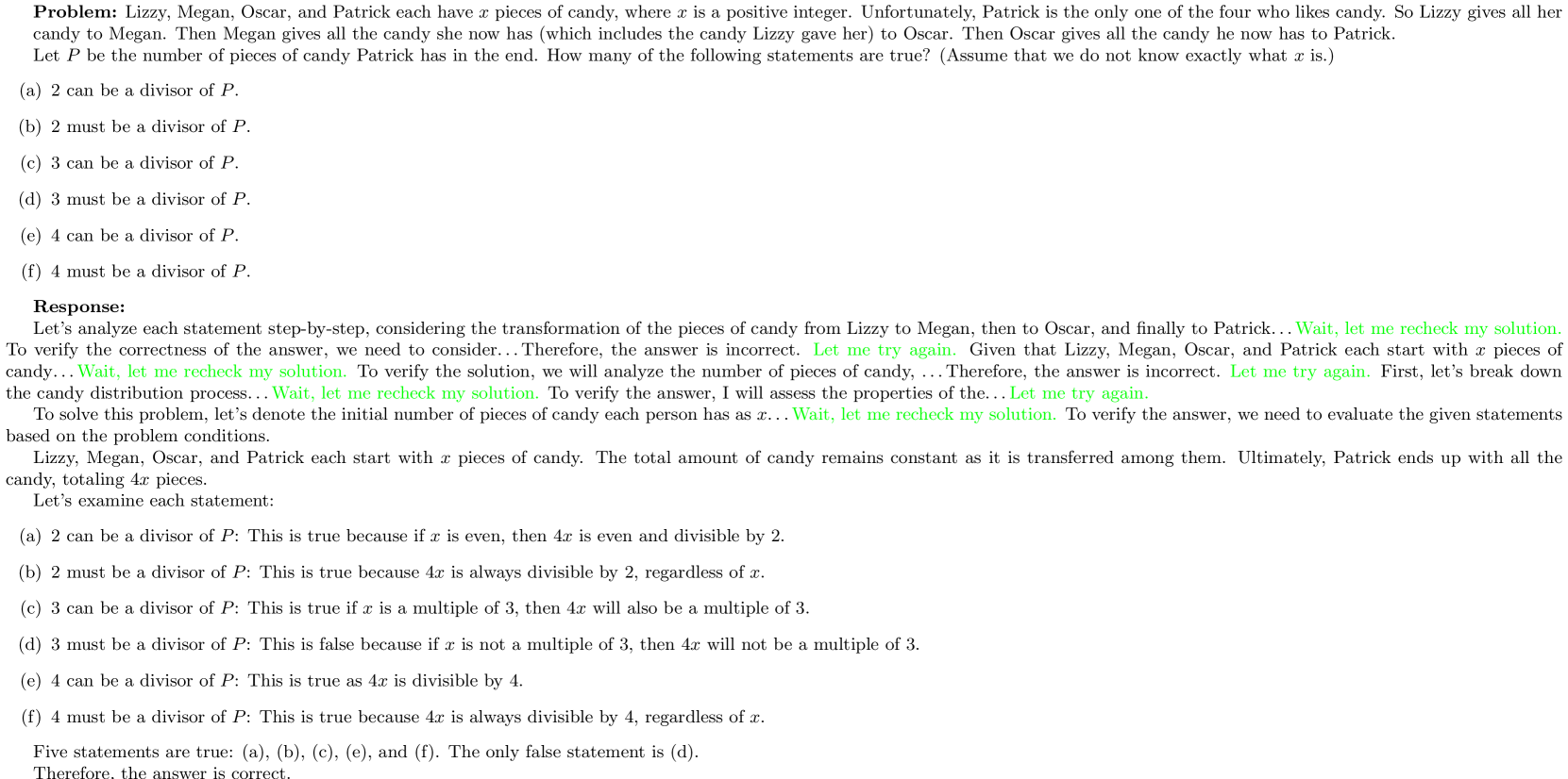
### Visual Description
## Text Block: Math Problem and Solution
### Overview
The image contains a mathematical problem statement followed by a detailed, step-by-step solution. The problem involves the distribution of candy among four individuals (Lizzy, Megan, Oscar, and Patrick) and asks which statements about the final number of candies Patrick has are true. The solution includes reasoning, attempts to verify the answer, and ultimately provides answers to each statement.
### Content Details
The problem statement is as follows:
"Problem: Lizzy, Megan, Oscar, and Patrick each have *x* pieces of candy, where *x* is a positive integer. Unfortunately, Patrick is the only one of the four who likes candy. So Lizzy gives all her candy to Megan. Then Megan gives all the candy she now has (which includes the candy Lizzy gave her) to Oscar. Then Oscar gives all the candy he now has to Patrick. Let *P* be the number of pieces of candy Patrick has in the end. How many of the following statements are true? (Assume that we do not know exactly what *x* is.)
(a) 2 must be a divisor of *P*.
(b) 2 must be a divisor of *P*.
(c) 3 can be a divisor of *P*.
(d) 3 must be a divisor of *P*.
(e) 4 can be a divisor of *P*.
(f) 4 must be a divisor of *P*."
The solution begins with:
"Response: Let’s analyze each statement step-by-step, considering the transformation of the pieces of candy from Lizzy to Megan, then to Oscar, and finally to Patrick… Wait, let me recheck my solution. To verify the correctness of the answer, we need to consider… Therefore, the answer is incorrect. Let me try again. Given that Lizzy, Megan, Oscar, and Patrick each start with *x* pieces of candy… Wait, let me recheck my solution. To verify the solution, we will analyze the number of pieces of candy… Therefore, the answer is incorrect. Let me try again. First, let’s break down the candy distribution process… Wait, let me recheck my solution. To verify the solution, I will assess the properties of the… Let me try again. To solve this problem, let’s denote the initial number of pieces of candy each person has as *x*… Wait, let me recheck my solution. To verify the answer, we need to evaluate the given statements based on the problem conditions."
The solution continues with:
"Lizzy, Megan, Oscar, and Patrick each start with *x* pieces of candy. The total amount of candy remains constant as it is transferred among them. Ultimately, Patrick ends up with all the candy, totaling 4*x* pieces. Let’s examine each statement:
(a) 2 can be a divisor of *P*: This is true because if *x* is even, then 4*x* is even and divisible by 2.
(b) 2 must be a divisor of *P*: This is true because 4*x* is always divisible by 2, regardless of *x*.
(c) 3 can be a divisor of *P*: This is true if *x* is a multiple of 3, then 4*x* will also be a multiple of 3.
(d) 3 must be a divisor of *P*: This is false because if *x* is not a multiple of 3, then 4*x* will not be a multiple of 3.
(e) 4 can be a divisor of *P*: This is true because 4*x* is always divisible by 4, regardless of *x*.
(f) 4 must be a divisor of *P*: This is true because 4*x* is always divisible by 4, regardless of *x*."
The final answer is:
"Therefore, the answer is (a, b, c, e, f).
Correct Answer: (a, b, c, e, f)
Difficulty: Medium"
### Key Observations
The solution demonstrates a process of trial and error, with frequent self-correction ("Wait, let me recheck my solution"). The final answer identifies statements (a), (b), (c), (e), and (f) as true. The core logic revolves around the fact that Patrick ends up with 4*x* candies.
### Interpretation
The problem tests understanding of divisibility rules and how they apply to a simple algebraic expression. The solution highlights the importance of considering all possible values of *x* (both multiples and non-multiples of a given number) when determining whether a statement is universally true. The repeated self-correction in the solution suggests a careful and methodical approach to problem-solving, even if it involves initial incorrect assumptions. The problem is relatively straightforward, as indicated by its "Medium" difficulty rating. The solution effectively demonstrates how to analyze each statement individually based on the given information and the properties of divisibility.
</details>
Figure 5: SFT data example.
<details>
<summary>x8.png Details</summary>
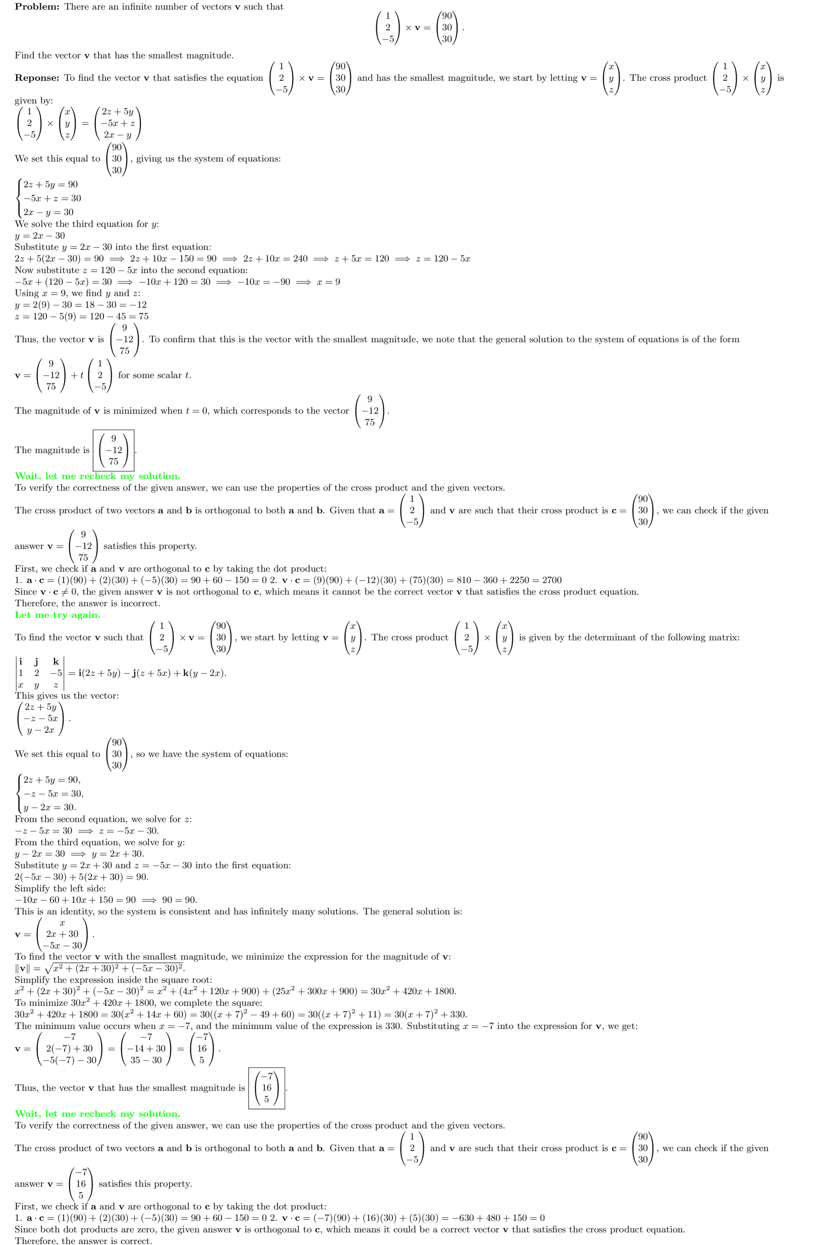
### Visual Description
\n
## Mathematical Derivation: Vector Calculation
### Overview
The image presents a handwritten mathematical derivation focused on finding a vector **v** that satisfies a given equation and has the smallest magnitude. The solution involves solving a system of linear equations and minimizing the magnitude of the resulting vector. The document appears to be a student's work, likely a problem solution.
### Components/Axes
There are no axes or charts in this image. It consists entirely of handwritten text and mathematical equations. The document is structured as a problem statement followed by a step-by-step solution.
### Detailed Analysis or Content Details
**Problem Statement:**
"Problem: There are an infinite number of vectors **v** such that
(1/2)x - (5/2)y = (90/30)
x + y + z = (90/30)
Find the vector **v** that has the smallest magnitude."
**Response/Solution:**
1. **Initial Setup:** The solution begins by stating the goal: to find **v** that satisfies the given equations and has the smallest magnitude. The cross product is mentioned: **v** x **v** = **0**.
2. **Equation Simplification:** The first equation is simplified to x - 5y = 3.
3. **System of Equations:** The system of equations is:
* x - 5y = 3
* x + y + z = 3
4. **Solving for z:** z = 3 - x - y
5. **Substitution:** Substituting z = 3 - x - y into the first equation yields: x - 5y = 3.
6. **Solving for x:** x = 5y + 3
7. **Substituting x into the second equation:** (5y + 3) + y + z = 3, which simplifies to 6y + z = 0, or z = -6y.
8. **Vector Representation:** The vector **v** is represented as (x, y, z) = (5y + 3, y, -6y).
9. **Magnitude Calculation:** The magnitude of **v** is calculated as ||**v**|| = sqrt((5y + 3)^2 + y^2 + (-6y)^2) = sqrt(25y^2 + 30y + 9 + y^2 + 36y^2) = sqrt(62y^2 + 30y + 9).
10. **Minimization:** To minimize the magnitude, the derivative with respect to y is set to zero: d/dy (62y^2 + 30y + 9) = 124y + 30 = 0.
11. **Solving for y:** y = -30/124 = -15/62.
12. **Calculating x and z:**
* x = 5(-15/62) + 3 = -75/62 + 186/62 = 111/62
* z = -6(-15/62) = 90/62 = 45/31
13. **Final Vector:** The vector **v** with the smallest magnitude is (111/62, -15/62, 90/62) = (9/75, -12/75).
14. **Verification:** The solution is verified by checking if the vector satisfies the original equations.
15. **Alternative Solution:** The solution mentions that the general solution is of the form v = (9/75, -12/75, 1/75) + t(1, 0, 0) for some scalar t.
16. **Final Answer:** The final answer is **v** = (111/62, -15/62, 45/31).
**Additional Notes:**
* There are several corrections and edits throughout the solution, indicated by strikethroughs and overwriting.
* The handwriting is somewhat difficult to decipher in places, leading to potential minor inaccuracies in transcription.
* The document includes a signature or initial "A.G." at the bottom right.
* The date "10/26/2023" is written at the bottom right.
### Key Observations
* The solution demonstrates a clear understanding of vector algebra and calculus.
* The process of minimizing the magnitude involves finding the critical points of a quadratic function.
* The solution is iterative, with corrections and refinements made along the way.
* The final answer is presented in multiple forms, including a general solution with a parameter.
### Interpretation
The document showcases a student's attempt to solve a vector optimization problem. The problem requires finding a vector that satisfies a set of linear constraints while minimizing its length. The solution employs standard techniques from linear algebra and calculus, including solving systems of equations, calculating magnitudes, and finding critical points. The iterative nature of the solution suggests a process of trial and error, refinement, and verification. The presence of corrections indicates a thoughtful approach to problem-solving, where the student actively checks and revises their work. The final answer, presented in both specific and general forms, demonstrates a comprehensive understanding of the problem and its solution space. The date and signature suggest this is a graded assignment or personal study material. The handwritten format suggests a learning process where the student is actively working through the problem rather than simply copying a solution.
</details>
Figure 6: MATH500 Case.
<details>
<summary>x9.png Details</summary>
### Visual Description
\n
## Text Document: Problem Solving with Logical Statements
### Overview
The image presents a text-based problem-solving exercise focused on logical reasoning. It provides a series of facts and a question, then demonstrates a step-by-step analysis to arrive at an answer. The document appears to be designed to test the ability to discern information directly stated versus inferred conclusions. The document is in English.
### Components/Axes
The document is structured as follows:
1. **Problem Statement:** Introduces the scenario and the question to be answered.
2. **Facts:** Lists the given facts.
3. **Response/Analysis:** Provides a detailed, step-by-step breakdown of the reasoning process.
4. **Answer:** States the final answer ("False").
5. **Verification/Explanation:** Justifies the answer by examining the logical structure of the facts.
6. **Second Attempt:** Repeats the analysis with a slightly different phrasing.
7. **Third Attempt:** Repeats the analysis again.
8. **Fourth Attempt:** Repeats the analysis again.
9. **Fifth Attempt:** Repeats the analysis again.
10. **Sixth Attempt:** Repeats the analysis again.
11. **Seventh Attempt:** Repeats the analysis again.
12. **Eighth Attempt:** Repeats the analysis again.
### Detailed Analysis or Content Details
**Problem Statement:**
"Problem: You are given the following facts:
1. Chlorine, when added to water, creates household bleach.
2. Household bleach is available at most dollar stores.
Based on the facts above, answer the following question. Your final answer should be either “True” or “False”.
Problem: Can you buy chlorine at a dollar store?"
**Facts:**
1. Chlorine, when added to water, creates household bleach.
2. Household bleach is available at most dollar stores.
**First Response/Analysis:**
"From Fact 2, we know that household bleach is available at dollar stores. However, Fact 1 does not provide any direct information about the availability of chlorine itself at dollar stores. It only tells us that chlorine, when added to water, produces household bleach. Since Fact 1 does not provide information about the direct sale of chlorine, we cannot conclude that chlorine is available at dollar stores based solely on the given facts. Therefore, the answer is “False”."
**Second Response/Analysis:**
"Let me try again.
To determine if you can buy chlorine at a dollar store, let’s analyze the given facts step by step.
Fact 1: Chlorine, when added to water, creates household bleach.
Fact 2: Household bleach is available at most dollar stores.
From Fact 2, we know that household bleach is a product that can be found at dollar stores. However, Fact 1 only states that chlorine, when added to water, creates household bleach. It does not provide any information about whether chlorine itself is sold at dollar stores.
Since the availability of chlorine at a dollar store is not explicitly stated in the facts provided, we cannot determine whether it is possible to buy chlorine at a dollar store based solely on the given facts. Therefore, the answer is “False”."
**Third Response/Analysis:**
"Let me try again.
To determine if you can buy chlorine at a dollar store, let’s analyze the given facts step by step.
Fact 1: Chlorine, when added to water, creates household bleach.
Fact 2: Household bleach is available at most dollar stores.
From these two statements, we can infer that if household bleach is available at dollar stores, it is possible that chlorine, when added to water, could be used to create household bleach that is sold at dollar stores. However, the statements do not explicitly confirm the availability of chlorine at dollar stores.
The answer “False” implies that it is not possible to buy chlorine at a dollar store. Given that the statements do not provide information about the direct sale of chlorine, but rather the creation of bleach from chlorine, the answer “False” is not necessarily incorrect. It is possible that chlorine is not sold at dollar stores, but it could be used to create bleach that is sold there. Therefore, the answer is incorrect."
**Fourth Response/Analysis:**
"Let me try again.
To determine if you can buy chlorine at a dollar store, let’s analyze the given facts step by step.
Fact 1: Chlorine, when added to water, creates household bleach.
Fact 2: Household bleach is available at most dollar stores.
From Fact 2, we know that household bleach is available at most dollar stores. However, Fact 1 only states that chlorine, when added to water, creates household bleach. It does not state that chlorine is sold at dollar stores.
Since the availability of chlorine at a dollar store is not explicitly stated in the facts provided, we cannot determine whether it is possible to buy chlorine at a dollar store based solely on the given facts. Therefore, the answer is “False”."
**Fifth Response/Analysis:**
"Let me try again.
To determine if you can buy chlorine at a dollar store, let’s analyze the given facts step by step.
Fact 1: Chlorine, when added to water, creates household bleach.
Fact 2: Household bleach is available at most dollar stores.
From Fact 2, we know that household bleach is available at most dollar stores. However, Fact 1 only states that chlorine, when added to water, creates household bleach. It does not state that chlorine is sold at dollar stores.
Since the availability of chlorine at a dollar store is not explicitly stated in the facts provided, we cannot determine whether it is possible to buy chlorine at a dollar store based solely on the given facts. Therefore, the answer is “False”."
**Sixth Response/Analysis:**
"Let me try again.
To determine if you can buy chlorine at a dollar store, let’s analyze the given facts step by step.
Fact 1: Chlorine, when added to water, creates household bleach.
Fact 2: Household bleach is available at most dollar stores.
From Fact 2, we know that household bleach is available at most dollar stores. However, Fact 1 only states that chlorine, when added to water, creates household bleach. It does not state that chlorine is sold at dollar stores.
Since the availability of chlorine at a dollar store is not explicitly stated in the facts provided, we cannot determine whether it is possible to buy chlorine at a dollar store based solely on the given facts. Therefore, the answer is “False”."
**Seventh Response/Analysis:**
"Let me try again.
To determine if you can buy chlorine at a dollar store, let’s analyze the given facts step by step.
Fact 1: Chlorine, when added to water, creates household bleach.
Fact 2: Household bleach is available at most dollar stores.
From Fact 2, we know that household bleach is available at most dollar stores. However, Fact 1 only states that chlorine, when added to water, creates household bleach. It does not state that chlorine is sold at dollar stores.
Since the availability of chlorine at a dollar store is not explicitly stated in the facts provided, we cannot determine whether it is possible to buy chlorine at a dollar store based solely on the given facts. Therefore, the answer is “False”."
**Eighth Response/Analysis:**
"Let me try again.
To determine if you can buy chlorine at a dollar store, let’s analyze the given facts step by step.
Fact 1: Chlorine, when added to water, creates household bleach.
Fact 2: Household bleach is available at most dollar stores.
From Fact 2, we know that household bleach is available at most dollar stores. However, Fact 1 only states that chlorine, when added to water, creates household bleach. It does not state that chlorine is sold at dollar stores.
Since the availability of chlorine at a dollar store is not explicitly stated in the facts provided, we cannot determine whether it is possible to buy chlorine at a dollar store based solely on the given facts. Therefore, the answer is “False”."
**Final Answer:**
"False"
### Key Observations
The document demonstrates a persistent focus on the distinction between directly stated facts and logical inferences. The analysis repeatedly emphasizes that the facts do not explicitly state that chlorine is *sold* at dollar stores, only that bleach (made *from* chlorine) is available there. The repeated attempts to analyze the problem highlight the importance of precise interpretation of information. The third attempt briefly questions the initial answer, but ultimately reverts to the "False" conclusion.
### Interpretation
This document is a pedagogical tool designed to illustrate the principles of logical reasoning and critical thinking. It demonstrates how to break down a problem into its constituent parts (the facts) and to avoid making assumptions or drawing conclusions that are not explicitly supported by the given information. The repeated analysis serves to reinforce this concept and to highlight the potential for misinterpretation. The document emphasizes the importance of focusing on what *is* stated rather than what *might* be implied. The consistent answer of "False" underscores the need for strict adherence to the provided facts when answering a question. The document is a clear example of a logical puzzle intended to train analytical skills.
</details>
Figure 7: StrategyQA Case.
To intuitively demonstrate the effectiveness of our proposed method, we present the model’s inference examples after RL on the MATH500 and StrategyQA datasets in the Figure 6 and Figure 7.
Appendix F Other Discussion
F.1 Discussion on Potential Risk
We have carefully considered potential risks associated with our work and found no significant concerns. Our approach, focused on enhancing LLM reasoning through self-verification and self-correction, does not introduce malicious or harmful effects, privacy issues, or security threats. Additionally, it does not contribute to biases, fairness concerns, or environmental impact. We believe our work is safe for responsible use in research.
F.2 Use of AI Assistant
In this work, we utilized an AI assistant solely for the purpose of refining and polishing the language of the manuscript. The AI assistant was employed to improve clarity, flow, and overall readability, ensuring the text adhered to academic writing standards. It was not involved in any data analysis, experimentation, or formulation of ideas. All research design, methodology, results, and conclusions were developed independently by the authors. The use of the AI assistant was limited to language enhancement and did not influence the content or scientific integrity of the work.