# MoBA: Mixture of Block Attention for Long-Context LLMs
> ∗ ‡ Co-corresponding authors. Xinyu Zhou ( ), Jiezhong Qiu ( )
iclr2025_conference.bib
## Abstract
Scaling the effective context length is essential for advancing large language models (LLMs) toward artificial general intelligence (AGI). However, the quadratic increase in computational complexity inherent in traditional attention mechanisms presents a prohibitive overhead. Existing approaches either impose strongly biased structures, such as sink or window attention which are task-specific, or radically modify the attention mechanism into linear approximations, whose performance in complex reasoning tasks remains inadequately explored.
In this work, we propose a solution that adheres to the “less structure” principle, allowing the model to determine where to attend autonomously, rather than introducing predefined biases. We introduce Mixture of Block Attention (MoBA), an innovative approach that applies the principles of Mixture of Experts (MoE) to the attention mechanism. This novel architecture demonstrates superior performance on long-context tasks while offering a key advantage: the ability to seamlessly transition between full and sparse attention, enhancing efficiency without the risk of compromising performance. MoBA has already been deployed to support Kimi’s long-context requests and demonstrates significant advancements in efficient attention computation for LLMs. Our code is available at https://github.com/MoonshotAI/MoBA.
## 1 Introduction
The pursuit of artificial general intelligence (AGI) has driven the development of large language models (LLMs) to unprecedented scales, with the promise of handling complex tasks that mimic human cognition. A pivotal capability for achieving AGI is the ability to process, understand, and generate long sequences, which is essential for a wide range of applications, from historical data analysis to complex reasoning and decision-making processes. This growing demand for extended context processing can be seen not only in the popularity of long input prompt understanding, as showcased by models like Kimi kimi, Claude claude and Gemini reid2024gemini, but also in recent explorations of long chain-of-thought (CoT) output capabilities in Kimi k1.5 team2025kimi, DeepSeek-R1 guo2025deepseek, and OpenAI o1/o3 guan2024deliberative.
However, extending the sequence length in LLMs is non-trivial due to the quadratic growth in computational complexity associated with the vanilla attention mechanism waswani2017attention. This challenge has spurred a wave of research aimed at improving efficiency without sacrificing performance. One prominent direction capitalizes on the inherent sparsity of attention scores. This sparsity arises both mathematically — from the softmax operation, where various sparse attention patterns have be studied jiang2024minference — and biologically watson2025human, where sparse connectivity is observed in brain regions related to memory storage.
Existing approaches often leverage predefined structural constraints, such as sink-based xiao2023efficient or sliding window attention beltagy2020longformer, to exploit this sparsity. While these methods can be effective, they tend to be highly task-specific, potentially hindering the model’s overall generalizability. Alternatively, a range of dynamic sparse attention mechanisms, exemplified by Quest tang2024quest, Minference jiang2024minference, and RetrievalAttention liu2024retrievalattention, select subsets of tokens at inference time. Although such methods can reduce computation for long sequences, they do not substantially alleviate the intensive training costs of long-context models, making it challenging to scale LLMs efficiently to contexts on the order of millions of tokens. Another promising alternative way has recently emerged in the form of linear attention models, such as Mamba dao2024transformers, RWKV peng2023rwkv, peng2024eagle, and RetNet sun2023retentive. These approaches replace canonical softmax-based attention with linear approximations, thereby reducing the computational overhead for long-sequence processing. However, due to the substantial differences between linear and conventional attention, adapting existing Transformer models typically incurs high conversion costs mercat2024linearizing, wang2024mamba, bick2025transformers, zhang2024lolcats or requires training entirely new models from scratch li2025minimax. More importantly, evidence of their effectiveness in complex reasoning tasks remains limited.
Consequently, a critical research question arises: How can we design a robust and adaptable attention architecture that retains the original Transformer framework while adhering to a “less structure” principle, allowing the model to determine where to attend without relying on predefined biases? Ideally, such an architecture would transition seamlessly between full and sparse attention modes, thus maximizing compatibility with existing pre-trained models and enabling both efficient inference and accelerated training without compromising performance.
Thus, we introduce Mixture of Block Attention (MoBA), a novel architecture that builds upon the innovative principles of Mixture of Experts (MoE) shazeer2017outrageously and applies them to the attention mechanism of the Transformer model. MoE has been used primarily in the feedforward network (FFN) layers of Transformers lepikhin2020gshard,fedus2022switch, zoph2022st, but MoBA pioneers its application to long context attention, allowing dynamic selection of historically relevant blocks of key and values for each query token. This approach not only enhances the efficiency of LLMs but also enables them to handle longer and more complex prompts without a proportional increase in resource consumption. MoBA addresses the computational inefficiency of traditional attention mechanisms by partitioning the context into blocks and employing a gating mechanism to selectively route query tokens to the most relevant blocks. This block sparse attention significantly reduces the computational costs, paving the way for more efficient processing of long sequences. The model’s ability to dynamically select the most informative blocks of keys leads to improved performance and efficiency, particularly beneficial for tasks involving extensive contextual information.
In this paper, we detail the architecture of MoBA, firstly its block partitioning and routing strategy, and secondly its computational efficiency compared to traditional attention mechanisms. We further present experimental results that demonstrate MoBA’s superior performance in tasks requiring the processing of long sequences. Our work contributes a novel approach to efficient attention computation, pushing the boundaries of what is achievable with LLMs in handling complex and lengthy inputs.
## 2 Method
<details>
<summary>x1.png Details</summary>
### Visual Description
\n
## Diagram: Router Architecture with Query-Key-Value Attention
### Overview
This diagram illustrates a router architecture utilizing a query-key-value attention mechanism. It depicts how queries are routed to different blocks (presumably containing data) and how attention scores are calculated to combine the values from these blocks. The diagram shows two queries (q1 and q2) being processed independently.
### Components/Axes
The diagram consists of the following components:
* **Queries:** Labeled "Queries" at the top, with two specific queries labeled "q1" (orange) and "q2" (orange).
* **Router:** A central rectangular block labeled "Router" (light blue).
* **Keys:** Labeled "Keys" on the left side.
* **Values:** Labeled "Values" on the left side.
* **Blocks:** Four blocks labeled "block1", "block2", "block3", and "block4" (light gray). These are arranged in a row below the Router.
* **Attention Score:** Labeled "Attn score" (light blue) within the output blocks.
* **Arrows:** Arrows indicate the flow of information. Solid arrows represent direct connections, while dotted arrows suggest a more general routing.
* **Output Blocks:** Blocks at the bottom, showing the combined output for each query.
### Detailed Analysis or Content Details
The diagram shows the following flow:
1. **Queries Input:** Two queries, q1 and q2, enter the "Router" from the top.
2. **Routing:** The Router distributes the queries to all four blocks (block1, block2, block3, block4). This is indicated by the arrows extending from the Router to each block.
3. **Key-Value Processing:** Each block has associated "Keys" and "Values". The diagram doesn't explicitly show how keys are used, but it implies they are used within the blocks to determine relevance to the queries.
4. **Attention Score Calculation:** For each query, the outputs from the blocks are combined using an attention mechanism. The "Attn score" block represents this calculation.
5. **Output Generation:** The final output for each query (q1 and q2) is a combination of the outputs from block1 and block2. The output blocks are colored light blue.
Specifically:
* **Query q1:** Receives input from block1 and block2, calculates an attention score, and produces an output.
* **Query q2:** Receives input from block1 and block2, calculates an attention score, and produces an output.
The dotted line from the Router to block3 and block4 suggests that these blocks are not directly used for the current queries (q1 and q2) but are available for other queries or a more complex routing scheme.
### Key Observations
* The diagram focuses on a simplified attention mechanism where only block1 and block2 are used for both queries.
* The Router appears to be a central component responsible for distributing queries to the blocks.
* The attention mechanism is represented abstractly, without details on the specific attention function used.
* The diagram does not provide any numerical values or specific parameters.
### Interpretation
This diagram illustrates a basic router architecture for attention-based processing. The router acts as a dispatcher, sending queries to multiple blocks. Each block processes the query based on its internal "Keys" and "Values", and the attention mechanism combines the outputs from these blocks to generate a final result. The use of only block1 and block2 for both queries suggests a potential simplification or a specific configuration where these blocks are deemed most relevant for the given queries. The dotted lines indicate the potential for a more complex routing scheme involving all four blocks. This architecture could be used in various applications, such as information retrieval, machine translation, or question answering, where it is necessary to selectively attend to different parts of the input data. The diagram is conceptual and does not provide details on the implementation or performance of the system.
</details>
(a)
<details>
<summary>x2.png Details</summary>
### Visual Description
\n
## Diagram: MoBA Gating Architecture
### Overview
The image depicts a diagram illustrating the architecture of a MoBA (Mixture of Block Attention) Gating mechanism within an attention model. The diagram shows the flow of data through several processing blocks, starting with inputs Q (Query), K (Key), and V (Value), and culminating in an "Attention Output". The MoBA Gating block appears to be a key component, responsible for selecting and processing blocks of information.
### Components/Axes
The diagram consists of the following components:
* **Inputs:** Q (Query), K (Key), V (Value) - positioned at the top of the diagram.
* **RoPE:** A block labeled "RoPE" connected to Q and K.
* **MoBA Gating:** A dashed-border block containing the following sub-components:
* "Partition to blocks"
* "Mean Pooling"
* "MatMul"
* "TopK Gating"
* **Index Select:** A block labeled "Index Select".
* **VarLen Flash-Attention:** A block labeled "VarLen Flash-Attention".
* **Attention Output:** The final output of the system.
* **Selected Block Index:** A label indicating an output from the MoBA Gating block.
* **Arrows:** Indicate the flow of data between components.
There are no axes or scales present in this diagram. It is a flow diagram, not a chart.
### Detailed Analysis or Content Details
The data flow can be described as follows:
1. **Inputs:** Q, K, and V are the initial inputs to the system.
2. **RoPE:** Q and K are fed into a "RoPE" block. The output of RoPE is then passed to the "Index Select" block.
3. **MoBA Gating:** The MoBA Gating block receives input from Q and K (via RoPE). Inside the MoBA Gating block:
* The input is first "Partitioned to blocks".
* These blocks are then subjected to "Mean Pooling".
* The result of Mean Pooling is passed through a "MatMul" (Matrix Multiplication) layer.
* Finally, "TopK Gating" is applied.
* The MoBA Gating block also outputs a "Selected Block Index".
4. **Index Select:** The output of RoPE and the "Selected Block Index" from the MoBA Gating block are fed into the "Index Select" block.
5. **VarLen Flash-Attention:** The output of "Index Select" and V are fed into the "VarLen Flash-Attention" block.
6. **Attention Output:** The "VarLen Flash-Attention" block produces the final "Attention Output".
### Key Observations
The diagram highlights a modular attention mechanism where the MoBA Gating block dynamically selects relevant blocks of information for processing. The use of "TopK Gating" suggests that only the most important blocks are selected. The "VarLen Flash-Attention" block indicates a potentially efficient attention implementation. The RoPE block suggests the use of Rotary Positional Embeddings.
### Interpretation
This diagram illustrates a novel attention mechanism that combines block-wise processing with dynamic gating. The MoBA Gating block acts as a selector, choosing which blocks of information are most relevant for the attention calculation. This approach could improve efficiency and performance by focusing computational resources on the most important parts of the input sequence. The "VarLen Flash-Attention" block suggests an attempt to optimize the attention calculation for variable-length sequences. The overall architecture appears designed to address the limitations of traditional attention mechanisms, particularly in handling long sequences or complex relationships between input elements. The use of RoPE suggests the model is designed to handle sequential data where positional information is important. The diagram does not provide any quantitative data, so it is difficult to assess the effectiveness of this architecture without further information. However, the design suggests a potentially powerful and efficient attention mechanism.
</details>
(b)
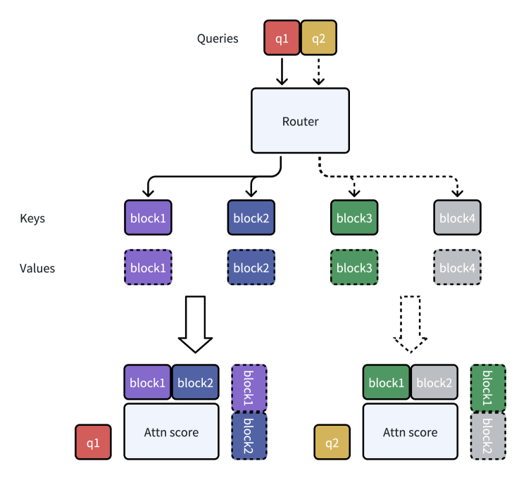
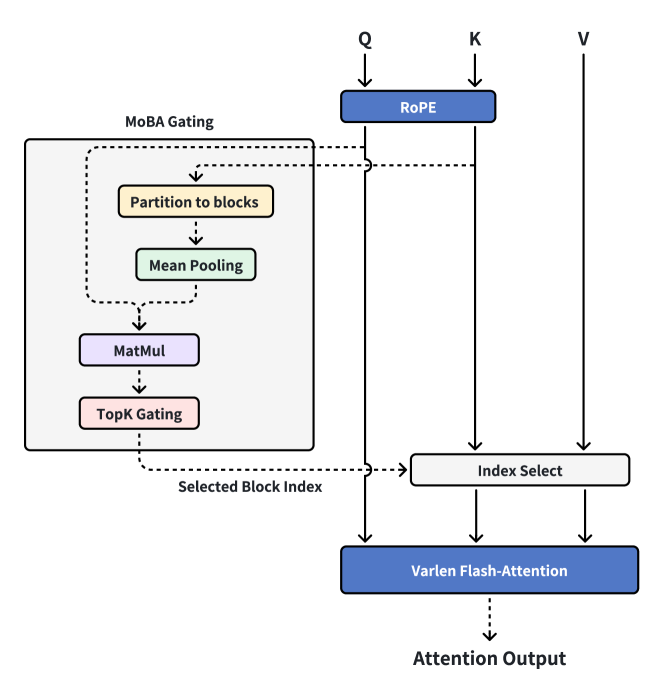
Figure 1: Illustration of mixture of block attention (MoBA). (a) A running example of MoBA; (b) Integration of MoBA into Flash Attention.
In this work, we introduce a novel architecture, termed Mixture of Block Attention (MoBA), which extends the capabilities of the Transformer model by dynamically selecting historical segments (blocks) for attention computation. MoBA is inspired by techniques of Mixture of Experts (MoE) and sparse attention. The former technique has been predominantly applied to the feedforward network (FFN) layers within the Transformer architecture, while the latter has been widely adopted in scaling Transformers to handle long contexts. Our method is innovative in applying the MoE principle to the attention mechanism itself, allowing for more efficient and effective processing of long sequences.
### 2.1 Preliminaries: Standard Attention in Transformer
We first revisit the standard Attention in Transformers. For simplicity, we revisit the case where a single query token ${\bm{q}}\in\mathbb{R}^{1\times d}$ attends to the $N$ key and value tokens, denoting ${\bm{K}},{\bm{V}}\in\mathbb{R}^{N\times d}$ , respectively. The standard attention is computed as:
$$
\mathrm{Attn}({\bm{q}},{\bm{K}},{\bm{V}})=\mathrm{Softmax}{\left({\bm{q}}{\bm{
K}}^{\top}\right)}{\bm{V}}, \tag{1}
$$
where $d$ denotes the dimension of a single attention head. We focus on the single-head scenario for clarity. The extension to multi-head attention involves concatenating the outputs from multiple such single-head attention operations.
### 2.2 MoBA Architecture
Different from standard attention where each query tokens attend to the entire context, MoBA enables each query token to only attend to a subset of keys and values:
$$
\mathrm{MoBA}({\bm{q}},{\bm{K}},{\bm{V}})=\mathrm{Softmax}{\left({\bm{q}}{{\bm
{K}}[I]}^{\top}\right)}{\bm{V}}[I], \tag{2}
$$
where $I\subseteq[N]$ is the set of selected keys and values.
The key innovation in MoBA is the block partitioning and selection strategy. We divide the full context of length $N$ into $n$ blocks, where each block represents a subset of subsequent tokens. Without loss of generality, we assume that the context length $N$ is divisible by the number of blocks $n$ . We further denote $B=\frac{N}{n}$ to be the block size and
$$
I_{i}=\left[(i-1)\times B+1,i\times B\right] \tag{3}
$$
to be the range of the $i$ -th block. By applying the top- $k$ gating mechanism from MoE, we enable each query to selectively focus on a subset of tokens from different blocks, rather than the entire context:
$$
I=\bigcup_{g_{i}>0}I_{i}. \tag{4}
$$
The model employs a gating mechanism, as $g_{i}$ in Equation 4, to select the most relevant blocks for each query token. The MoBA gate first computes the affinity score $s_{i}$ measuring the relevance between query ${\bm{q}}$ and the $i$ -th block, and applies a top- $k$ gating among all blocks. More formally, the gate value for the $i$ -th block $g_{i}$ is computed by
$$
g_{i}=\begin{cases}1&s_{i}\in\mathrm{Topk}\left(\{s_{j}|j\in[n]\},k\right)\\
0&\text{otherwise}\end{cases}, \tag{5}
$$
where $\mathrm{Topk}(\cdot,k)$ denotes the set containing $k$ highest scores among the affinity scores calculated for each block. In this work, the score $s_{i}$ is computed by the inner product between ${\bm{q}}$ and the mean pooling of ${\bm{K}}[I_{i}]$ along the sequence dimension:
$$
s_{i}=\langle{\bm{q}},\mathrm{mean\_pool}({\bm{K}}[I_{i}])\rangle \tag{6}
$$
A Running Example. We provide a running example of MoBA at Figure 1a, where we have two query tokens and four KV blocks. The router (gating network) dynamically selects the top two blocks for each query to attend. As shown in Figure 1a, the first query is assigned to the first and second blocks, while the second query is assigned to the third and fourth blocks.
It is important to maintain causality in autoregressive language models, as they generate text by next-token prediction based on previous tokens. This sequential generation process ensures that a token cannot influence tokens that come before it, thus preserving the causal relationship. MoBA preserves causality through two specific designs:
Causality: No Attention to Future Blocks. MoBA ensures that a query token cannot be routed to any future blocks. By limiting the attention scope to current and past blocks, MoBA adheres to the autoregressive nature of language modeling. More formally, denoting $\mathrm{pos}({\bm{q}})$ as the position index of the query ${\bm{q}}$ , we set $s_{i}=-\infty$ and $g_{i}=0$ for any blocks $i$ such that $\mathrm{pos}({\bm{q}})<i\times B$ .
Current Block Attention and Causal Masking. We define the ”current block” as the block that contains the query token itself. The routing to the current block could also violate causality, since mean pooling across the entire block can inadvertently include information from future tokens. To address this, we enforce that each token must be routed to its respective current block and apply a causal mask during the current block attention. This strategy not only avoids any leakage of information from subsequent tokens but also encourages attention to the local context. More formally, we set $g_{i}=1$ for the block $i$ where the position of the query token $\mathrm{pos}({\bm{q}})$ is within the interval $I_{i}$ . From the perspective of Mixture-of-Experts (MoE), the current block attention in MoBA is akin to the role of shared experts in modern MoE architectures dai2024deepseekmoe, yang2024qwen2, where static routing rules are added when expert selection.
Next, we discuss some additional key design choices of MoBA, such as its block segmentation strategy and the hybrid of MoBA and full attention.
Fine-Grained Block Segmentation. The positive impact of fine-grained expert segmentation in improving mode performance has been well-documented in the Mixture-of-Experts (MoE) literature dai2024deepseekmoe, yang2024qwen2. In this work, we explore the potential advantage of applying a similar fine-grained segmentation technique to MoBA. MoBA, inspired by MoE, operates segmentation along the context-length dimension rather than the FFN intermediate hidden dimension. Therefore our investigation aims to determine if MoBA can also benefit when we partition the context into blocks with a finer grain. More experimental results can be found in Section 3.1.
Hybrid of MoBA and Full Attention. MoBA is designed to be a substitute for full attention, maintaining the same number of parameters without any addition or subtraction. This feature inspires us to conduct smooth transitions between full attention and MoBA. Specifically, at the initialization stage, each attention layer has the option to select full attention or MoBA, and this choice can be dynamically altered during training if necessary. A similar idea of transitioning full attention to sliding window attention has been studied in previous work zhang2024simlayerkv. More experimental results can be found in Section 3.2.
Comparing to Sliding Window Attention and Attention Sink. Sliding window attention (SWA) and attention sink are two popular sparse attention architectures. We demonstrate that both can be viewed as special cases of MoBA. For sliding window attention beltagy2020longformer, each query token only attends to its neighboring tokens. This can be interpreted as a variant of MoBA with a gating network that keeps selecting the most recent blocks. Similarly, attention sink xiao2023efficient, where each query token attends to a combination of initial tokens and the most recent tokens, can be seen as a variant of MoBA with a gating network that always selects both the initial and the recent blocks. The above discussion shows that MoBA has stronger expressive power than sliding window attention and attention sink. Moreover, it shows that MoBA can flexibly approximate many static sparse attention architectures by incorporating specific gating networks.
Overall, MoBA’s attention mechanism allows the model to adaptively and dynamically focus on the most informative blocks of the context. This is particularly beneficial for tasks involving long documents or sequences, where attending to the entire context may be unnecessary and computationally expensive. MoBA’s ability to selectively attend to relevant blocks enables more nuanced and efficient processing of information.
### 2.3 Implementation
Algorithm 1 MoBA (Mixture of Block Attention) Implementation
0: Query, key and value matrices $\mathbf{Q},\mathbf{K},\mathbf{V}\in\mathbb{R}^{N\times h\times d}$ ; MoBA hyperparameters (block size $B$ and top- $k$ ); $h$ and $d$ denote the number of attention heads and head dimension. Also denote $n=N/B$ to be the number of blocks.
1: // Split KV into blocks
2: $\{\tilde{\mathbf{K}}_{i},\tilde{\mathbf{V}}_{i}\}=\text{split\_blocks}(\mathbf {K},\mathbf{V},B)$ , where $\tilde{\mathbf{K}}_{i},\tilde{\mathbf{V}}_{i}\in\mathbb{R}^{B\times h\times d} ,i\in[n]$
3: // Compute gating scores for dynamic block selection
4: $\bar{\mathbf{K}}=\text{mean\_pool}(\mathbf{K},B)\in\mathbb{R}^{n\times h\times d}$
5: $\mathbf{S}=\mathbf{Q}\bar{\mathbf{K}}^{\top}\in\mathbb{R}^{N\times h\times n}$
6: // Select blocks with causal constraint (no attention to future blocks)
7: $\mathbf{M}=\text{create\_causal\_mask}(N,n)$
8: $\mathbf{G}=\text{topk}(\mathbf{S}+\mathbf{M},k)$
9: // Organize attention patterns for computation efficiency
10: $\mathbf{Q}^{s},\tilde{\mathbf{K}}^{s},\tilde{\mathbf{V}}^{s}=\text{get\_self\_ attn\_block}(\mathbf{Q},\tilde{\mathbf{K}},\tilde{\mathbf{V}})$
11: $\mathbf{Q}^{m},\tilde{\mathbf{K}}^{m},\tilde{\mathbf{V}}^{m}=\text{index\_ select\_moba\_attn\_block}(\mathbf{Q},\tilde{\mathbf{K}},\tilde{\mathbf{V}}, \mathbf{G})$
12: // Compute attentions seperately
13: $\mathbf{O}^{s}=\text{flash\_attention\_varlen}(\mathbf{Q}^{s},\tilde{\mathbf{K }}^{s},\tilde{\mathbf{V}}^{s},\text{causal=True})$
14: $\mathbf{O}^{m}=\text{flash\_attention\_varlen}(\mathbf{Q}^{m},\tilde{\mathbf{K }}^{m},\tilde{\mathbf{V}}^{m},\text{causal=False})$
15: // Combine results with online softmax
16: $\mathbf{O}=\text{combine\_with\_online\_softmax}(\mathbf{O}^{s},\mathbf{O}^{m})$
17: return $\mathbf{O}$
<details>
<summary>x3.png Details</summary>
### Visual Description
\n
## Line Chart: Computation Time vs. Sequence Length
### Overview
This chart displays the relationship between computation time (in milliseconds) and sequence length for two different methods: Flash Attention and MoBA. The x-axis represents sequence length, and the y-axis represents computation time. The chart shows how computation time scales with increasing sequence length for each method.
### Components/Axes
* **X-axis Title:** Sequence Length
* **Y-axis Title:** Computation Time (ms)
* **X-axis Markers:** 32K, 128K, 256K, 512K, 1M (representing sequence lengths of 32,000, 128,000, 256,000, 512,000, and 1,000,000 respectively)
* **Y-axis Scale:** 0 to 900 ms, with increments of 100 ms.
* **Legend:** Located in the top-left corner.
* **Flash Attention:** Represented by a light blue dashed line with circular markers.
* **MoBA:** Represented by a dark blue solid line with circular markers.
### Detailed Analysis
**Flash Attention (Light Blue Dashed Line):**
The line slopes upward, indicating that computation time increases with sequence length.
* At 32K sequence length: Approximately 0 ms.
* At 128K sequence length: Approximately 10 ms.
* At 256K sequence length: Approximately 60 ms.
* At 512K sequence length: Approximately 240 ms.
* At 1M sequence length: Approximately 850 ms.
**MoBA (Dark Blue Solid Line):**
The line also slopes upward, but at a slower rate than Flash Attention.
* At 32K sequence length: Approximately 0 ms.
* At 128K sequence length: Approximately 20 ms.
* At 256K sequence length: Approximately 40 ms.
* At 512K sequence length: Approximately 100 ms.
* At 1M sequence length: Approximately 170 ms.
### Key Observations
* Flash Attention exhibits a significantly steeper increase in computation time as sequence length grows compared to MoBA.
* Both methods show relatively low computation times for shorter sequence lengths (32K and 128K).
* The difference in computation time between the two methods becomes more pronounced at longer sequence lengths (512K and 1M).
* MoBA consistently has lower computation times than Flash Attention across all sequence lengths tested.
### Interpretation
The data suggests that MoBA scales more efficiently with increasing sequence length than Flash Attention. While both methods are viable for shorter sequences, MoBA maintains a lower computational cost as the sequence length increases, making it potentially more suitable for applications dealing with very long sequences. The steep slope of Flash Attention indicates that its computational demands grow rapidly with sequence length, which could become a limiting factor in certain scenarios. The consistent difference in computation time between the two methods suggests a fundamental difference in their algorithmic complexity or implementation. The fact that both start at 0ms suggests that the overhead for both methods is minimal at the shortest sequence length.
</details>
(a)
<details>
<summary>x4.png Details</summary>
### Visual Description
\n
## Chart: Computation Time vs. Sequence Length for Flash Attention and MoBA
### Overview
This chart compares the computation time of two methods, "Flash Attention" and "MoBA", as a function of sequence length. The x-axis represents sequence length, and the y-axis represents computation time in seconds. A zoomed-in inset chart displays the computation time for shorter sequence lengths.
### Components/Axes
* **X-axis:** Sequence Length (labeled as "Sequence Length"). Scale: 1M, 4M, 7M, 10M. Inset chart scale: 32K, 128K, 256K, 512K.
* **Y-axis:** Computation Time (labeled as "Computation Time (s)"). Scale: 0 to 80 seconds.
* **Legend:**
* "Flash Attention" - Light blue dashed line with circular markers.
* "MoBA" - Dark blue dashed line with circular markers.
* **Inset Chart:** Located in the top-left corner of the main chart. It focuses on sequence lengths from 32K to 512K.
### Detailed Analysis
**Flash Attention (Light Blue):**
The line representing Flash Attention slopes upward, indicating that computation time increases with sequence length.
* At 1M sequence length: Approximately 0.5 seconds.
* At 4M sequence length: Approximately 17 seconds.
* At 7M sequence length: Approximately 45 seconds.
* At 10M sequence length: Approximately 82 seconds.
* Inset Chart:
* At 32K sequence length: Approximately 0.02 seconds.
* At 128K sequence length: Approximately 0.06 seconds.
* At 256K sequence length: Approximately 0.1 seconds.
* At 512K sequence length: Approximately 0.3 seconds.
**MoBA (Dark Blue):**
The line representing MoBA also slopes upward, but at a much shallower rate than Flash Attention.
* At 1M sequence length: Approximately 0.1 seconds.
* At 4M sequence length: Approximately 2.5 seconds.
* At 7M sequence length: Approximately 5 seconds.
* At 10M sequence length: Approximately 8 seconds.
* Inset Chart:
* At 32K sequence length: Approximately 0.01 seconds.
* At 128K sequence length: Approximately 0.03 seconds.
* At 256K sequence length: Approximately 0.05 seconds.
* At 512K sequence length: Approximately 0.1 seconds.
### Key Observations
* Flash Attention exhibits a significantly higher computation time than MoBA across all sequence lengths.
* The computation time for Flash Attention increases more rapidly with sequence length compared to MoBA.
* The inset chart shows that the difference in computation time between the two methods is less pronounced for shorter sequence lengths (up to 512K).
* MoBA maintains a relatively flat computation time curve, suggesting better scalability with increasing sequence length.
### Interpretation
The data suggests that MoBA is more efficient than Flash Attention, particularly for longer sequence lengths. The linear increase in computation time for MoBA indicates a more scalable approach. Flash Attention, while potentially faster for very short sequences, becomes computationally expensive as the sequence length grows. This difference in scalability could be due to algorithmic differences or optimization strategies employed in each method. The inset chart highlights that the performance gap between the two methods becomes more significant as the sequence length increases beyond 512K. This information is valuable for choosing the appropriate method based on the expected sequence length and computational resources available. The chart demonstrates a clear trade-off between performance and scalability, with MoBA prioritizing scalability and Flash Attention potentially offering faster performance for limited sequence lengths.
</details>
(b)
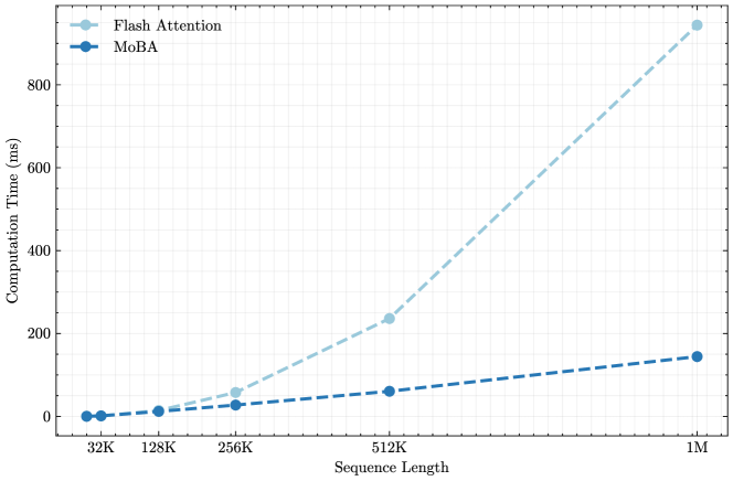
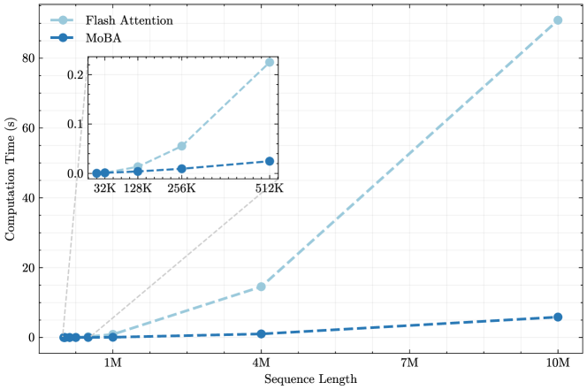
Figure 2: Efficiency of MoBA vs. full attention (implemented with Flash Attention). (a) 1M Model speedup evaluation: Computation time scaling of MoBA versus Flash Attention on 1M model with increasing sequence lengths (8K-1M). (b) Fixed Sparsity Ratio scaling: Computation time scaling comparison between MoBA and Flash Attention across increasing sequence lengths (8K-10M), maintaining a constant sparsity ratio of $95.31\$ (fixed 64 MoBA blocks with variance block size and fixed top-k=3).
We provide a high-performance implementation of MoBA, by incorporating optimization techniques from FlashAttention dao2022flashattention and MoE rajbhandari2022deepspeed. Figure 2 demonstrates the high efficiency of MoBA, while we defer the detailed experiments on efficiency and scalability to Section 3.4. Our implementation consists of five major steps:
- Determine the assignment of query tokens to KV blocks according to the gating network and causal mask.
- Arrange the ordering of query tokens based on their assigned KV blocks.
- Compute attention outputs for each KV block and the query tokens assigned to it. This step can be optimized by FlashAttention with varying lengths.
- Re-arrange the attention outputs back to their original ordering.
- Combine the corresponding attention outputs using online Softmax (i.e., tiling), as a query token may attend to its current block and multiple historical KV blocks.
The algorithmic workflow is formalized in Algorithm 1 and visualized in Figure 1b, illustrating how MoBA can be implemented based on MoE and FlashAttention. First, the KV matrices are partitioned into blocks (Line 1-2). Next, the gating score is computed according to Equation 6, which measures the relevance between query tokens and KV blocks (Lines 3-7). A top- $k$ operator is applied on the gating score (together with causal mask), resulting in a sparse query-to-KV-block mapping matrix ${\bm{G}}$ to represent the assignment of queries to KV blocks (Line 8). Then, query tokens are arranged based on the query-to-KV-block mapping, and block-wise attention outputs are computed (Line 9-12). Notably, attention to historical blocks (Line 11 and 14) and the current block attention (Line 10 and 13) are computed separately, as additional causality needs to be maintained in the current block attention. Finally, the attention outputs are rearranged back to their original ordering and combined with online softmax (Line 16) milakov2018onlinenormalizercalculationsoftmax,liu2023blockwiseparalleltransformerlarge.
## 3 Experiments
### 3.1 Scaling Law Experiments and Ablation Studies
In this section, we conduct scaling law experiments and ablation studies to validate some key design choices of MoBA.
| 568M 822M 1.1B | 14 16 18 | 14 16 18 | 1792 2048 2304 | 10.8B 15.3B 20.6B | 512 512 512 | 3 3 3 |
| --- | --- | --- | --- | --- | --- | --- |
| 1.5B | 20 | 20 | 2560 | 27.4B | 512 | 3 |
| 2.1B | 22 | 22 | 2816 | 36.9B | 512 | 3 |
Table 1: Configuration of Scaling Law Experiments
<details>
<summary>x5.png Details</summary>
### Visual Description
\n
## Chart: LM Loss vs. PFLOP/s-days
### Overview
The image presents a line chart comparing the Language Model (LM) loss for two projection methods – MoBA Projection and Full Attention Projection – as a function of PFLOP/s-days (floating point operations per second per day). The chart displays the loss decreasing as computational effort increases, indicating improved model performance. Multiple lines are present for each projection method, likely representing different runs or variations.
### Components/Axes
* **X-axis:** PFLOP/s-days, ranging from approximately 0.01 to 10, displayed on a logarithmic scale.
* **Y-axis:** LM Loss (seqlen=8K), ranging from approximately 2 x 10<sup>2</sup> to 5 x 10<sup>3</sup>, displayed on a logarithmic scale. The "(seqlen=8K)" indicates the loss is calculated for a sequence length of 8000.
* **Legend:** Located in the top-right corner.
* MoBA Projection: Represented by a solid blue line. Multiple lines are present.
* Full Attention Projection: Represented by a dashed red line. Multiple lines are present.
* **Grid:** A light gray grid is overlaid on the chart to aid in reading values.
### Detailed Analysis
**MoBA Projection (Blue Lines):**
There are approximately 6 blue lines representing MoBA Projection. The lines generally trend downwards, indicating decreasing loss with increasing PFLOP/s-days.
* Line 1 (Top-most): Starts at approximately 4.8 x 10<sup>3</sup> at 0.01 PFLOP/s-days and decreases to approximately 2.5 x 10<sup>2</sup> at 10 PFLOP/s-days.
* Line 2: Starts at approximately 4.5 x 10<sup>3</sup> at 0.01 PFLOP/s-days and decreases to approximately 2.4 x 10<sup>2</sup> at 10 PFLOP/s-days.
* Line 3: Starts at approximately 4.2 x 10<sup>3</sup> at 0.01 PFLOP/s-days and decreases to approximately 2.3 x 10<sup>2</sup> at 10 PFLOP/s-days.
* Line 4: Starts at approximately 3.9 x 10<sup>3</sup> at 0.01 PFLOP/s-days and decreases to approximately 2.2 x 10<sup>2</sup> at 10 PFLOP/s-days.
* Line 5: Starts at approximately 3.6 x 10<sup>3</sup> at 0.01 PFLOP/s-days and decreases to approximately 2.1 x 10<sup>2</sup> at 10 PFLOP/s-days.
* Line 6 (Bottom-most): Starts at approximately 3.3 x 10<sup>3</sup> at 0.01 PFLOP/s-days and decreases to approximately 2.0 x 10<sup>2</sup> at 10 PFLOP/s-days.
**Full Attention Projection (Red Lines):**
There are approximately 6 red dashed lines representing Full Attention Projection. These lines also trend downwards, but generally start at higher loss values and decrease more slowly than the MoBA Projection lines.
* Line 1 (Top-most): Starts at approximately 4.9 x 10<sup>3</sup> at 0.01 PFLOP/s-days and decreases to approximately 3.0 x 10<sup>2</sup> at 10 PFLOP/s-days.
* Line 2: Starts at approximately 4.6 x 10<sup>3</sup> at 0.01 PFLOP/s-days and decreases to approximately 2.9 x 10<sup>2</sup> at 10 PFLOP/s-days.
* Line 3: Starts at approximately 4.3 x 10<sup>3</sup> at 0.01 PFLOP/s-days and decreases to approximately 2.8 x 10<sup>2</sup> at 10 PFLOP/s-days.
* Line 4: Starts at approximately 4.0 x 10<sup>3</sup> at 0.01 PFLOP/s-days and decreases to approximately 2.7 x 10<sup>2</sup> at 10 PFLOP/s-days.
* Line 5: Starts at approximately 3.7 x 10<sup>3</sup> at 0.01 PFLOP/s-days and decreases to approximately 2.6 x 10<sup>2</sup> at 10 PFLOP/s-days.
* Line 6 (Bottom-most): Starts at approximately 3.4 x 10<sup>3</sup> at 0.01 PFLOP/s-days and decreases to approximately 2.5 x 10<sup>2</sup> at 10 PFLOP/s-days.
### Key Observations
* MoBA Projection consistently achieves lower LM loss values than Full Attention Projection across the entire range of PFLOP/s-days.
* The multiple lines for each projection method suggest variability in the results, potentially due to different initialization, training data, or hyperparameters.
* The rate of loss reduction diminishes as PFLOP/s-days increases for both methods, indicating diminishing returns from increased computation.
* The logarithmic scales on both axes compress the data, making it easier to visualize the trends.
### Interpretation
The chart demonstrates that MoBA Projection is more efficient than Full Attention Projection in reducing LM loss for a given amount of computational effort (PFLOP/s-days). This suggests that MoBA Projection is a more effective method for training language models, particularly when computational resources are limited. The spread of lines for each method indicates that the performance is not deterministic and can vary. The diminishing returns observed at higher PFLOP/s-days suggest that there is a point beyond which further increasing computation yields only marginal improvements in model performance. The sequence length of 8K is a key parameter, and the results may differ for other sequence lengths. The chart provides valuable insights into the trade-off between computational cost and model accuracy, guiding the selection of appropriate projection methods for language model training.
</details>
(a)
<details>
<summary>x6.png Details</summary>
### Visual Description
## Chart: Training Loss vs. Compute
### Overview
The image presents a line chart comparing the training loss of two different projection methods – MoBA Projection and Full Attention Projection – as a function of compute (PFLOP/s-days). The y-axis represents the trailing LM loss (seqlen=32K, last 2K), and the x-axis represents the compute used for training. Multiple lines are plotted for each projection method, likely representing different training runs or configurations. The chart uses a logarithmic scale for both axes.
### Components/Axes
* **X-axis Title:** PFLOP/s-days
* **Y-axis Title:** Trailing LM loss (seqlen=32K, last 2K)
* **X-axis Scale:** Logarithmic, ranging from 10<sup>-1</sup> to 10<sup>1</sup>. Markers are at 10<sup>-1</sup>, 10<sup>0</sup>, and 10<sup>1</sup>.
* **Y-axis Scale:** Logarithmic, ranging from 10<sup>1</sup> to 10<sup>4</sup>. Markers are at 10<sup>1</sup>, 10<sup>2</sup>, 10<sup>3</sup>, and 10<sup>4</sup>.
* **Legend:** Located in the top-right corner.
* **MoBA Projection:** Represented by a dashed blue line.
* **Full Attention Projection:** Represented by a dashed red line.
### Detailed Analysis
The chart displays multiple lines for each projection method, indicating variability in training runs.
**MoBA Projection (Blue Lines):**
The blue lines generally show a steep downward trend initially, indicating rapid loss reduction with increasing compute. As compute increases, the rate of loss reduction slows down.
* Line 1: Starts at approximately 2.5 x 10<sup>2</sup> loss at 10<sup>-1</sup> PFLOP/s-days, decreasing to approximately 1.2 x 10<sup>1</sup> loss at 10<sup>1</sup> PFLOP/s-days.
* Line 2: Starts at approximately 2.2 x 10<sup>2</sup> loss at 10<sup>-1</sup> PFLOP/s-days, decreasing to approximately 1.1 x 10<sup>1</sup> loss at 10<sup>1</sup> PFLOP/s-days.
* Line 3: Starts at approximately 2.0 x 10<sup>2</sup> loss at 10<sup>-1</sup> PFLOP/s-days, decreasing to approximately 1.0 x 10<sup>1</sup> loss at 10<sup>1</sup> PFLOP/s-days.
* Line 4: Starts at approximately 2.3 x 10<sup>2</sup> loss at 10<sup>-1</sup> PFLOP/s-days, decreasing to approximately 1.1 x 10<sup>1</sup> loss at 10<sup>1</sup> PFLOP/s-days.
**Full Attention Projection (Red Lines):**
The red lines also exhibit a downward trend, but generally start at a lower loss value and have a slightly less steep initial decline compared to the MoBA Projection lines.
* Line 1: Starts at approximately 1.5 x 10<sup>2</sup> loss at 10<sup>-1</sup> PFLOP/s-days, decreasing to approximately 8 x 10<sup>0</sup> loss at 10<sup>1</sup> PFLOP/s-days.
* Line 2: Starts at approximately 1.4 x 10<sup>2</sup> loss at 10<sup>-1</sup> PFLOP/s-days, decreasing to approximately 7 x 10<sup>0</sup> loss at 10<sup>1</sup> PFLOP/s-days.
* Line 3: Starts at approximately 1.3 x 10<sup>2</sup> loss at 10<sup>-1</sup> PFLOP/s-days, decreasing to approximately 6 x 10<sup>0</sup> loss at 10<sup>1</sup> PFLOP/s-days.
* Line 4: Starts at approximately 1.6 x 10<sup>2</sup> loss at 10<sup>-1</sup> PFLOP/s-days, decreasing to approximately 8 x 10<sup>0</sup> loss at 10<sup>1</sup> PFLOP/s-days.
### Key Observations
* The Full Attention Projection consistently achieves lower loss values than the MoBA Projection across the range of compute values.
* There is variability in the training runs for both projection methods, as evidenced by the multiple lines.
* The rate of loss reduction diminishes as compute increases for both methods, suggesting diminishing returns.
* The logarithmic scale compresses the initial rapid loss reduction, making it difficult to discern precise differences in the early stages of training.
### Interpretation
The chart demonstrates the relationship between compute and training loss for two different projection methods. The Full Attention Projection appears to be more efficient in terms of loss reduction per unit of compute, consistently outperforming the MoBA Projection. The multiple lines for each method suggest that the training process is sensitive to initialization or other stochastic factors. The diminishing returns observed at higher compute levels indicate that there is a point beyond which increasing compute yields only marginal improvements in loss. This information is valuable for optimizing training strategies and allocating computational resources effectively. The use of a logarithmic scale is appropriate for visualizing the wide range of loss and compute values, but it also obscures the details of the initial training phase. The "seqlen=32K, last 2K" specification on the y-axis suggests that the loss is being measured on a specific subset of the data, potentially focusing on the later stages of sequence processing.
</details>
(b)
| LM loss (seqlen=8K) Trailing LM loss (seqlen=32K, last 2K) | $2.625\times C^{-0.063}$ $1.546\times C^{-0.108}$ | $2.622\times C^{-0.063}$ $1.464\times C^{-0.097}$ |
| --- | --- | --- |
(c)
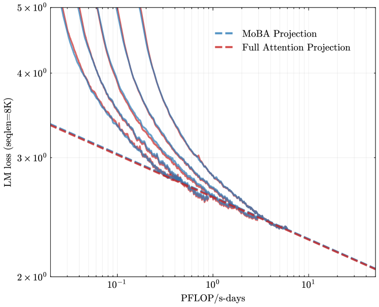
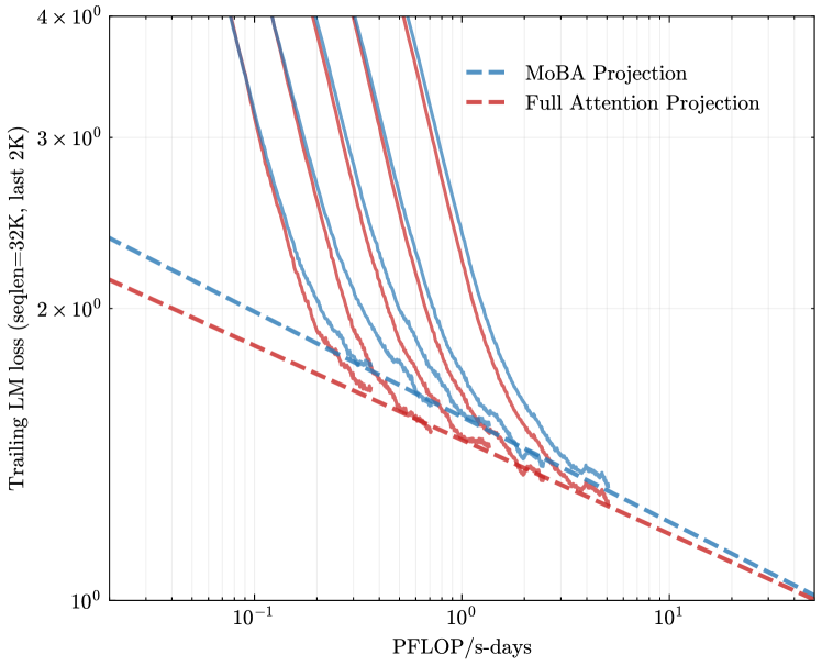
Figure 3: Scaling law comparison between MoBA and full attention. (a) LM loss on validation set (seqlen=8K); (b) trailing LM loss on validation set (seqlen=32K, last 1K tokens); (c) fitted scaling law curve.
#### Scalability w.r.t. LM Loss.
To assess the effectiveness of MoBA, we perform scaling law experiments by comparing the validation loss of language models trained using either full attention or MoBA. Following the Chinchilla scaling law hoffmann2022training, we train five language models of varying sizes with a sufficient number of training tokens to ensure that each model achieves its training optimum. Detailed configurations of the scaling law experiments can be found in Table 1. Both MoBA and full attention models are trained with a sequence length of 8K. For MoBA models, we set the block size to 512 and select the top-3 blocks for attention, resulting in a sparse attention pattern with sparsity up to $1-\frac{512\times 3}{8192}=81.25\$ Since we set top-k=3, thus each query token can attend to at most 2 history block and the current block.. In particular, MoBA serves as an alternative to full attention, meaning that it does not introduce new parameters or remove existing ones. This design simplifies our comparison process, as the only difference across all experiments lies in the attention modules, while all other hyperparameters, including the learning rate and batch size, remain constant. As shown in Figure 3a, the validation loss curves for MoBA and full attention display very similar scaling trends. Specifically, the validation loss differences between these two attention mechanisms remain consistent within a range of $1e-3$ . This suggests that MoBA achieves scaling performance that is comparable to full attention, despite its sparse attention pattern with sparsity up to 75%.
#### Long Context Scalability.
However, LM loss may be skewed by the data length distribution an2024does, which is typically dominated by short sequences. To fully assess the long-context capability of MoBA, we assess the LM loss of trailing tokens (trailing LM loss, in short), which computes the LM loss of the last few tokens in the sequence. We count this loss only for sequences that reach the maximum sequence length to avoid biases that may arise from very short sequences. A detailed discussion on trailing tokens scaling can be found in the Appendix A.1
These metrics provide insights into the model’s ability to generate the final portion of a sequence, which can be particularly informative for tasks involving long context understanding. Therefore, we adopt a modified experimental setting by increasing the maximum sequence length from 8k to 32k. This adjustment leads to an even sparser attention pattern for MoBA, achieving a sparsity level of up to $1-\frac{512\times 3}{32768}=95.31\$ . As shown in Figure 3b, although MoBA exhibits a marginally higher last block LM loss compared to full attention in all five experiments, the loss gap is progressively narrowing. This experiment implies the long-context scalability of MoBA.
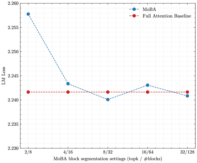
#### Ablation Study on Fine-Grained Block Segmentation.
We further ablate the block granularity of MoBA. We carry out a series of experiments using a 1.5B parameter model with a 32K context length. The hyperparameters of block size and top-k are adjusted to maintain a consistent level of attention sparsity. Specifically, we divide the 32K context into 8, 16, 32, 64, and 128 blocks, and correspondingly select 2, 4, 8, 16, and 32 blocks, ensuring an attention sparsity of 75% across these configurations. As shown in Figure 4, MoBA’s performance is significantly affected by block granularity. Specifically, there is a performance difference of 1e-2 between the coarsest-grained setting (selecting 2 blocks from 8) and the settings with finer granularity. These findings suggest that fine-grained segmentation appears to be a general technique for enhancing the performance of models within the MoE family, including MoBA.
<details>
<summary>x7.png Details</summary>
### Visual Description
\n
## Line Chart: LM Loss vs. MoBA Block Segmentation Settings
### Overview
This chart displays the Language Model (LM) Loss for two different models, MoBA and a Full Attention Baseline, across varying MoBA block segmentation settings. The x-axis represents the segmentation settings (topk / #blocks), and the y-axis represents the LM Loss. The chart aims to compare the performance of MoBA against a baseline as the block segmentation settings are adjusted.
### Components/Axes
* **X-axis Title:** "MoBA block segmentation settings (topk / #blocks)"
* **X-axis Markers:** 2/8, 4/16, 8/32, 16/64, 32/128
* **Y-axis Title:** "LM Loss"
* **Y-axis Scale:** Ranges from approximately 2.230 to 2.260, with gridlines at 0.005 intervals.
* **Legend:** Located in the top-right corner.
* **MoBA:** Represented by a blue line with circular markers.
* **Full Attention Baseline:** Represented by a red dashed line with circular markers.
### Detailed Analysis
**MoBA (Blue Line):**
The MoBA line starts at a relatively high LM Loss and exhibits a strong downward trend initially.
* At 2/8, the LM Loss is approximately 2.258.
* At 4/16, the LM Loss drops significantly to approximately 2.243.
* At 8/32, the LM Loss continues to decrease slightly to approximately 2.241.
* At 16/64, the LM Loss increases slightly to approximately 2.243.
* At 32/128, the LM Loss decreases slightly to approximately 2.241.
**Full Attention Baseline (Red Dashed Line):**
The Full Attention Baseline line remains relatively stable across all segmentation settings.
* At 2/8, the LM Loss is approximately 2.242.
* At 4/16, the LM Loss is approximately 2.242.
* At 8/32, the LM Loss is approximately 2.241.
* At 16/64, the LM Loss is approximately 2.242.
* At 32/128, the LM Loss is approximately 2.242.
### Key Observations
* MoBA demonstrates a significant reduction in LM Loss as the block segmentation settings increase from 2/8 to 8/32.
* After 8/32, the MoBA line plateaus, with only minor fluctuations in LM Loss.
* The Full Attention Baseline maintains a consistent LM Loss throughout all settings, remaining slightly above the MoBA line after the initial drop.
* The initial performance of MoBA (2/8) is worse than the baseline.
### Interpretation
The data suggests that MoBA benefits from increased block segmentation, up to a point. The initial drop in LM Loss indicates that MoBA is able to more effectively process and learn from the data as the block size increases. However, beyond 8/32, the gains diminish, suggesting that further increasing the block size does not provide significant improvements. The Full Attention Baseline provides a stable performance level, but MoBA ultimately achieves a lower LM Loss after the initial optimization phase. This implies that MoBA, with appropriate block segmentation, can outperform the Full Attention Baseline in terms of language modeling performance. The plateauing of MoBA's performance suggests there may be diminishing returns or other factors limiting further improvement. The initial worse performance of MoBA could be due to the overhead of the block segmentation process, which is overcome as the block size increases and the benefits of the MoBA architecture become more apparent.
</details>
Figure 4: Fine-Grained Block Segmentation. The LM loss on validation set v.s. MoBA with different block granularity.
### 3.2 Hybrid of MoBA and Full Attention
<details>
<summary>x8.png Details</summary>
### Visual Description
## Line Chart: LM Loss vs. Position
### Overview
The image presents a line chart illustrating the relationship between LM Loss (Language Modeling Loss) and Position, likely representing the sequence length or a similar positional metric. Three different models or configurations are compared: MoBA/Full Hybrid, MoBA, and Full Attention. The chart displays how the LM Loss changes as the position increases for each model.
### Components/Axes
* **X-axis:** Position, ranging from 0K to 30K. The axis is labeled "Position".
* **Y-axis:** LM Loss, ranging from 1.2 to 3.0. The axis is labeled "LM Loss".
* **Legend:** Located in the top-right corner of the chart.
* MoBA/Full Hybrid (Green line with diamond markers)
* MoBA (Blue line with circle markers)
* Full Attention (Red line with circle markers)
* **Grid:** A light gray grid is present in the background to aid in reading values.
### Detailed Analysis
The chart shows three distinct lines representing the LM Loss for each model as a function of position.
* **Full Attention (Red):** This line starts at approximately 2.8 at 0K position and exhibits a steep downward trend, decreasing rapidly to around 1.6 at 5K position. The decline continues, but at a slower rate, reaching approximately 1.35 at 30K position.
* **MoBA (Blue):** This line begins at approximately 1.7 at 0K position and shows a gradual decrease. It reaches around 1.35 at 5K position and continues to decrease slowly, leveling off around 1.25 at 30K position.
* **MoBA/Full Hybrid (Green):** This line starts at approximately 1.6 at 0K position and decreases steadily. It reaches around 1.3 at 5K position and continues to decrease, leveling off around 1.25 at 30K position.
Here's a more detailed breakdown of approximate values:
| Position (K) | Full Attention (LM Loss) | MoBA (LM Loss) | MoBA/Full Hybrid (LM Loss) |
|--------------|---------------------------|----------------|-----------------------------|
| 0 | 2.8 | 1.7 | 1.6 |
| 5 | 1.6 | 1.35 | 1.3 |
| 10 | 1.45 | 1.3 | 1.28 |
| 15 | 1.4 | 1.28 | 1.27 |
| 20 | 1.37 | 1.27 | 1.26 |
| 25 | 1.36 | 1.26 | 1.25 |
| 30 | 1.35 | 1.25 | 1.25 |
### Key Observations
* The "Full Attention" model consistently exhibits the highest LM Loss across all positions, especially at lower positions.
* Both "MoBA" and "MoBA/Full Hybrid" models demonstrate significantly lower LM Loss compared to "Full Attention".
* The rate of decrease in LM Loss is most pronounced for the "Full Attention" model in the initial stages (0K to 5K position).
* The "MoBA" and "MoBA/Full Hybrid" models converge towards similar LM Loss values at higher positions (20K to 30K).
### Interpretation
The data suggests that the MoBA and MoBA/Full Hybrid models are more efficient in language modeling, as indicated by their lower LM Loss values, compared to the Full Attention model. The steep initial decline in LM Loss for the Full Attention model suggests that it benefits significantly from increased position/sequence length, but it ultimately plateaus at a higher loss than the MoBA variants. The convergence of the MoBA models at higher positions indicates that the benefits of the "Full Hybrid" approach diminish as the position increases. This could be due to the hybrid model leveraging the strengths of both MoBA and Full Attention, but the Full Attention component becomes less critical at longer sequences. The chart demonstrates the trade-offs between different attention mechanisms in language modeling, highlighting the potential advantages of MoBA-based approaches. The fact that the MoBA models reach a lower loss suggests they are better at capturing long-range dependencies or are more robust to the challenges of longer sequences.
</details>
(a)
<details>
<summary>x9.png Details</summary>
### Visual Description
\n
## Line Chart: LM Loss vs. Number of Hybrid Full Layers
### Overview
This image presents a line chart illustrating the relationship between the number of hybrid full layers and the LM (Language Model) loss for different attention mechanisms. Three attention mechanisms are compared: Layer-wise Hybrid, Full Attention, and MoBA.
### Components/Axes
* **X-axis:** Number of Hybrid Full Layers. Marked at 1 layer, 3 layer, 5 layer, and 10 layer.
* **Y-axis:** LM loss. Scale ranges from approximately 1.04 to 1.14.
* **Legend:** Located in the top-right corner.
* Layer-wise Hybrid (Blue line with diamond markers)
* Full Attention (Red line)
* MoBA (Brown line)
### Detailed Analysis
The chart displays three lines representing the LM loss for each attention mechanism as the number of hybrid full layers increases.
* **Layer-wise Hybrid (Blue):** The line slopes downward, indicating a decrease in LM loss as the number of layers increases.
* At 1 layer: Approximately 1.135 LM loss.
* At 3 layers: Approximately 1.12 LM loss.
* At 5 layers: Approximately 1.10 LM loss.
* At 10 layers: Approximately 1.07 LM loss.
* **Full Attention (Red):** This line is nearly horizontal, indicating a relatively constant LM loss regardless of the number of layers. The loss remains around 1.06.
* **MoBA (Brown):** This line is also nearly horizontal, maintaining a constant LM loss around 1.06.
### Key Observations
* The Layer-wise Hybrid attention mechanism demonstrates a significant reduction in LM loss as the number of layers increases.
* Both Full Attention and MoBA exhibit stable LM loss values, showing minimal change with varying layer counts.
* The Layer-wise Hybrid consistently has a higher LM loss than the other two methods at 1 layer, but eventually falls below them at 10 layers.
### Interpretation
The data suggests that increasing the number of hybrid full layers in the Layer-wise Hybrid attention mechanism leads to improved language modeling performance, as indicated by the decreasing LM loss. This implies that the model benefits from the increased capacity and complexity provided by additional layers. In contrast, the Full Attention and MoBA mechanisms appear to reach a performance plateau relatively quickly, with their LM loss remaining stable regardless of the number of layers. This could indicate that these mechanisms are already operating at their optimal performance level or that adding more layers does not provide significant additional benefits. The initial higher loss of the Layer-wise Hybrid could be due to the model needing more layers to fully realize its potential, or it could be a characteristic of the mechanism itself. The convergence of the Layer-wise Hybrid loss towards the other two methods at 10 layers suggests a potential point of diminishing returns.
</details>
(b)
<details>
<summary>x10.png Details</summary>
### Visual Description
\n
## Line Chart: LM Trailing Loss vs. Number of Hybrid Full Layers
### Overview
This chart displays the relationship between the number of Hybrid Full Layers and the LM trailing loss (seqlen=32K, last 2K). It compares the performance of "Layer-wise Hybrid", "Full Attention", and "MoBA" models. The chart shows a decreasing trend for the Layer-wise Hybrid model as the number of layers increases, while the other two models maintain relatively constant loss values.
### Components/Axes
* **X-axis:** Number of Hybrid Full Layers. Marked at 1 layer, 3 layer, 5 layer, and 10 layer.
* **Y-axis:** LM trailing loss (seqlen=32K, last 2K). Scale ranges from approximately 1.10 to 1.18.
* **Legend:** Located in the top-right corner.
* Layer-wise Hybrid (Blue)
* Full Attention (Red)
* MoBA (Brown)
### Detailed Analysis
* **Layer-wise Hybrid (Blue Line):** The blue line slopes downward, indicating a decrease in loss as the number of layers increases.
* At 1 layer: Approximately 1.175.
* At 3 layers: Approximately 1.135.
* At 5 layers: Approximately 1.105.
* At 10 layers: Approximately 1.08.
* **Full Attention (Red Line):** The red line is nearly horizontal, indicating a relatively constant loss value.
* Across all layer counts (1, 3, 5, 10): Approximately 1.07.
* **MoBA (Brown Line):** The brown line is also nearly horizontal, indicating a relatively constant loss value.
* Across all layer counts (1, 3, 5, 10): Approximately 1.07.
### Key Observations
* The Layer-wise Hybrid model demonstrates a significant reduction in loss as the number of layers increases, suggesting improved performance with more layers.
* Both the Full Attention and MoBA models exhibit stable loss values, independent of the number of Hybrid Full Layers.
* The Layer-wise Hybrid model starts with a higher loss than the other two models but surpasses them as the number of layers increases.
### Interpretation
The data suggests that increasing the number of Hybrid Full Layers in the Layer-wise Hybrid model leads to a substantial decrease in LM trailing loss, indicating improved language modeling performance. This implies that the hybrid architecture benefits from increased depth. The consistent performance of the Full Attention and MoBA models suggests that their performance is not significantly affected by the addition of Hybrid Full Layers, or that they have already reached a performance plateau. The initial higher loss of the Layer-wise Hybrid model could be due to the overhead of the hybrid architecture, which is then offset by the benefits of increased depth. The fact that the Layer-wise Hybrid model eventually outperforms the other two suggests that the hybrid approach, when scaled appropriately, can be more effective than traditional Full Attention or MoBA. The consistent values for Full Attention and MoBA could indicate that they are less sensitive to the specific sequence length or that they have reached their optimal performance level within the tested range.
</details>
(c)
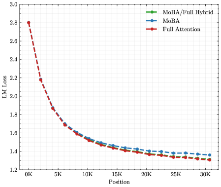
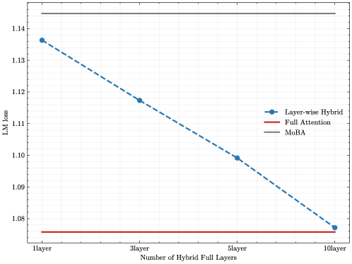
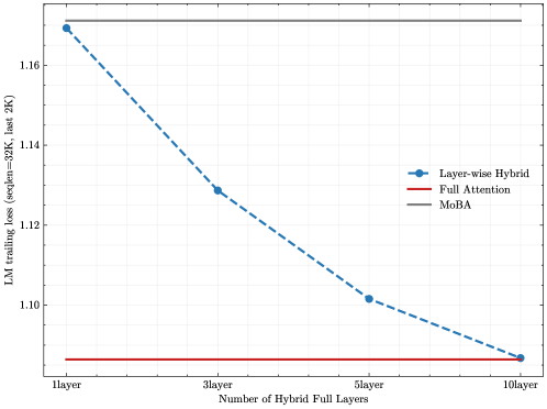
Figure 5: Hybrid of MoBA and full attention. (a) position-wise LM loss for MoBA, full attention, and MoBA/full hybrid training; (b) SFT LM loss w.r.t the number of full attention layers in layer-wise hybrid; (c) SFT trailing LM loss (seqlen=32K, last 2K) w.r.t the number of full attention layers in layer-wise hybrid.
As discussed in Section 2, we design MoBA to be a flexible substitute for full attention, so that it can easily switch from/to full attention with minimal overhead and achieve comparable long-context performance. In this section, we first show seamless transition between full attention and MoBA can be a solution for efficient long-context pre-training. Then we discuss the layer-wise hybrid strategy, mainly for the performance of supervised fine-tuning (SFT).
#### MoBA/Full Hybrid Training.
We train three models, each with 1.5B parameters, on 30B tokens with a context length of 32K tokens. For the hyperparameters of MoBA, the block size is set to 2048, and the top-k parameter is set to 3. The detailed training recipes are as follows:
- MoBA/full hybrid: This model is trained using a two-stage recipe. In the first stage, MoBA is used to train on 90% of the tokens. In the second stage, the model switches to full attention for the remaining 10% of the tokens.
- Full attention: This model is trained using full attention throughout the entire training.
- MoBA: This model is trained exclusively using MoBA.
We evaluate their long-context performance via position-wise language model (LM) loss, which is a fine-grained metric to evaluate lm loss at each position within a sequence. Unlike the vanilla LM loss, which is computed by averaging the LM loss across all positions, the position-wise LM loss breaks down the loss for each position separately. Similar metrics have been suggested by previous studies xiong2023effectivelongcontextscalingfoundation,reid2024gemini, who noticed that position-wise LM loss follows a power-law trend relative to context length. As shown in Figure 5a, the MoBA-only recipe results in higher position-wise losses for trailing tokens. Importantly, our MoBA/full hybrid recipe reaches a loss nearly identical to that of full attention. This result highlights the effectiveness of the MoBA/full hybrid training recipe in balancing training efficiency with model performance. More interestingly, we have not observed significant loss spikes during the switch between MoBA and full attention, again demonstrating the flexibility and robustness of MoBA.
#### Layer-wise Hybrid.
This flexibility of MoBA encourages us to delve into a more sophisticated strategy — the layer-wise hybrid of MoBA and full attention. We investigate this strategy with a particular focus on its application during the supervised fine-tuning (SFT). The motivation for investigating this strategy stems from our observation that MoBA sometimes results in suboptimal performance during SFT, as shown in Figure 5b. We speculate that this may be attributed to the loss masking employed in SFT — prompt tokens are typically excluded from the loss calculation during SFT, which can pose a sparse gradient challenge for sparse attention methods like MoBA. Because it may hinder the backpropagation of gradients, which are initially calculated from unmasked tokens, throughout the entire context. To address this issue, we propose a hybrid approach — switching the last several Transformer layers from MoBA to full attention, while the remaining layers continue to employ MoBA. As shown in Figure 5b and Figure 5c, this strategy can significantly reduce SFT loss.
### 3.3 Large Language Modeling Evaluation
<details>
<summary>x11.png Details</summary>
### Visual Description
\n
## Diagram: Model Training Pipeline
### Overview
The image depicts a diagram illustrating a model training pipeline, starting with a base model (Llama3.1 8B) and progressing through stages of continued pretraining and supervised fine-tuning (SFT) to arrive at an Instruct Model. The diagram shows a two-branch flow, one for pretraining and one for fine-tuning, converging at the Instruct Model.
### Components/Axes
The diagram consists of rectangular boxes representing different model stages, connected by arrows indicating the flow of data/training. The boxes contain text labels describing the model and training process. There are no axes or scales present.
### Detailed Analysis or Content Details
The diagram can be broken down into two main paths:
**Top Path (Pretraining):**
1. **Llama3.1 8B:** The starting point, a base language model.
2. **256K Continue Pretrain:** The model is further pretrained with a dataset of 256K tokens.
3. **512K Continue Pretrain:** The model is further pretrained with a dataset of 512K tokens.
4. **1M Continue Pretrain:** The model is further pretrained with a dataset of 1M tokens.
**Bottom Path (Supervised Fine-tuning - SFT):**
1. **Instruct Model:** The final output, an instruction-following model.
2. **1M SFT:** The model is fine-tuned using supervised learning with a dataset of 1M tokens.
3. **256K SFT:** The model is fine-tuned using supervised learning with a dataset of 256K tokens.
4. **32K SFT:** The model is fine-tuned using supervised learning with a dataset of 32K tokens.
The arrows indicate a sequential flow. The top path flows from Llama3.1 8B through increasing token counts for continued pretraining. The bottom path flows from the Instruct Model through decreasing token counts for SFT. The two paths converge on the Instruct Model.
### Key Observations
The diagram highlights a progressive training strategy. The model is first pretrained on larger datasets (256K, 512K, 1M tokens) and then fine-tuned on smaller, instruction-specific datasets (32K, 256K, 1M tokens). The decreasing token counts in the SFT path suggest a refinement process, where the model is gradually adjusted to follow instructions.
### Interpretation
This diagram illustrates a common approach to training large language models. The initial pretraining phase aims to equip the model with general language understanding capabilities. The subsequent fine-tuning phase specializes the model for specific tasks, in this case, following instructions. The use of different token counts suggests a deliberate strategy for balancing general knowledge with task-specific expertise. The two-branch structure emphasizes the separation of concerns between pretraining and fine-tuning, allowing for independent optimization of each stage. The diagram suggests a pipeline where the output of the pretraining stage serves as the input to the fine-tuning stage. The choice of token counts (32K, 256K, 1M) likely reflects a trade-off between computational cost and model performance.
</details>
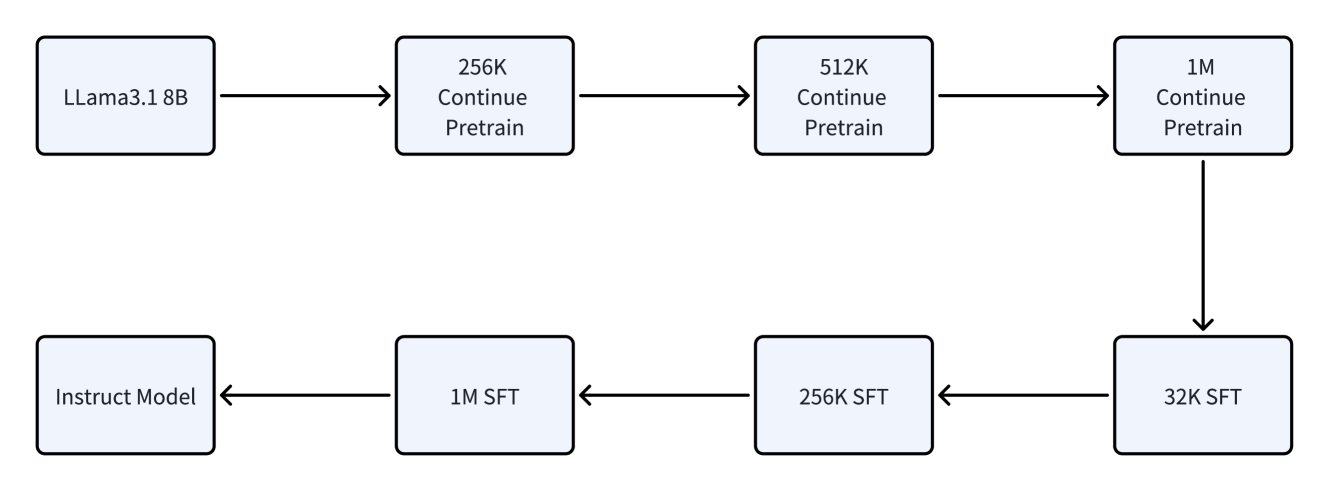
Figure 6: The continual pre-training and SFT recipes.
We conduct a thorough assessment of MoBA across a variety of real-world downstream tasks, evaluating its performance in comparison to full attention models. For ease of verification, our experiments begin with the Llama 3.1 8B Base Model, which is used as the starting point for long-context pre-training. This model, termed Llama-8B-1M-MoBA, is initially trained with a context length of 128K tokens, and we gradually increase the context length to 256K, 512K, and 1M tokens during the continual pre-training. To ease this transition, we use position interpolation method chen2023extendingcontextwindowlarge at the start of the 256K continual pre-training stage. This technique enables us to extend the effective context length from 128K tokens to 1M tokens. After completing the 1M continuous pre-training, MoBA is activated for 100B tokens. We set the block size to 4096 and the top-K parameter to 12, leading to an attention sparsity of up to $1-\frac{4096\times 12}{1M}=95.31\$ . To preserve some full attention capabilities, we adopt the layer-wise hybrid strategy — the last three layers remain as full attention, while the other 29 full attention layers are switched to MoBA. For supervised fine-tuning, we follow a similar strategy that gradually increases the context length from 32K to 1M. The baseline full attention models (termed Llama-8B-1M-Full) also follow a similar training strategy as shown in Figure 6, with the only difference being the use of full attention throughout the process. This approach allows us to directly compare the performance of MoBA with that of full attention models under equivalent training conditions.
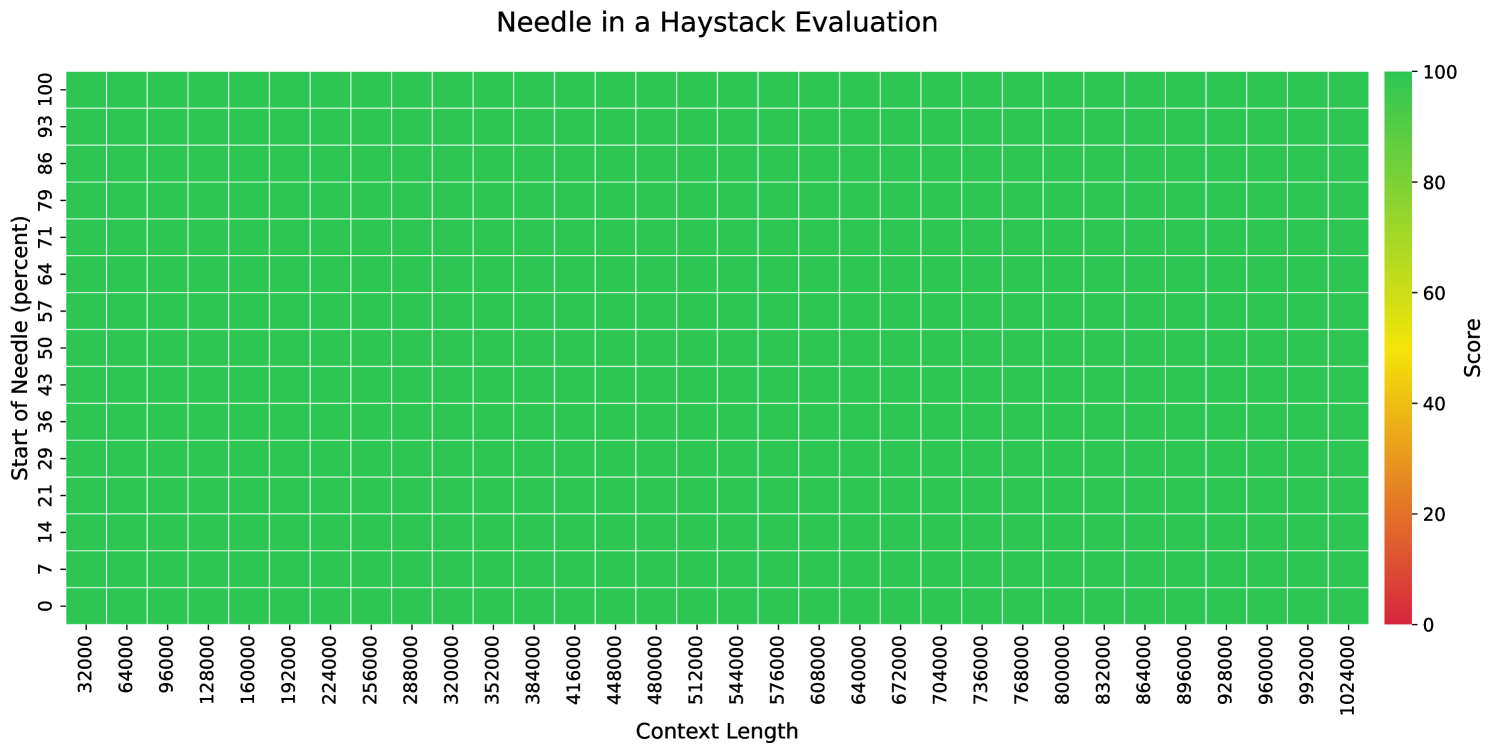
The evaluation is performed on several widely used long-context benchmarks. In particular, across all evaluation tasks, MoBA is used for prefill only, while we switch to full attention during generation for better performance. As shown in Table 2, Llama-8B-1M-MoBA exhibits a performance that is highly comparable to that of Llama-8B-1M-Full. It is particularly noteworthy that in the longest benchmark, RULER, where MoBA operates at a sparsity level of up to $1-\frac{4096\times 12}{128K}=62.5\$ , Llama-8B-1M-MoBA nearly matches the performance of Llama-8B-1M-Full, with a score of 0.7818 compared to 0.7849. For context lengths of up to 1M tokens, we evaluate the model using the traditional Needle in the Haystack benchmark. As shown in Figure 7, Llama-8B-1M-MoBA demonstrates satisfactory performance even with an extended context length of 1 million tokens.
| AGIEval [0-shot] BBH [3-shot] CEval [5-shot] | 0.5144 0.6573 0.6273 | 0.5146 0.6589 0.6165 |
| --- | --- | --- |
| GSM8K [5-shot] | 0.7278 | 0.7142 |
| HellaSWAG [0-shot] | 0.8262 | 0.8279 |
| Loogle [0-shot] | 0.4209 | 0.4016 |
| Competition Math [0-shot] | 0.4254 | 0.4324 |
| MBPP [3-shot] | 0.5380 | 0.5320 |
| MBPP Sanitized [0-shot] | 0.6926 | 0.6615 |
| MMLU [0-shot] | 0.4903 | 0.4904 |
| MMLU Pro [5-shot][CoT] | 0.4295 | 0.4328 |
| OpenAI HumanEval [0-shot][pass@1] | 0.6951 | 0.7012 |
| SimpleQA [0-shot] | 0.0465 | 0.0492 |
| TriviaQA [0-shot] | 0.5673 | 0.5667 |
| LongBench @32K [0-shot] | 0.4828 | 0.4821 |
| RULER @128K [0-shot] | 0.7818 | 0.7849 |
Table 2: Performance comparison between MoBA and full Attention across different evaluation benchmarks.
<details>
<summary>x12.png Details</summary>
### Visual Description
## Heatmap: Needle in a Haystack Evaluation
### Overview
The image presents a heatmap visualizing the results of a "Needle in a Haystack Evaluation". The heatmap displays a score based on two variables: "Context Length" and "Start of Needle (percent)". The color gradient represents the score, ranging from red (low score) to green (high score).
### Components/Axes
* **Title:** "Needle in a Haystack Evaluation" - positioned at the top-center.
* **X-axis:** "Context Length" - ranging from 32000 to 1024000, with increments of 96000.
* **Y-axis:** "Start of Needle (percent)" - ranging from 0 to 100, with increments of 7. The values are: 0, 7, 14, 21, 29, 36, 43, 50, 57, 64, 71, 79, 86, 93, 100.
* **Color Scale/Legend:** Located on the right side of the heatmap. It maps colors to scores:
* Red: 0
* Orange/Yellow: ~20-40
* Green: ~60-80
* Light Green/Yellow: ~80-100
### Detailed Analysis
The heatmap is a grid of colored cells, each representing a combination of Context Length and Start of Needle percentage. The majority of the cells are colored green, indicating a high score (approximately 80-100). There are some cells with lower scores (yellow/orange) concentrated in the bottom-left corner of the heatmap.
Let's analyze the data points based on the color scale:
* **Context Length 32000:**
* Start of Needle 0%: Score is approximately 10-20 (yellow).
* Start of Needle 7%: Score is approximately 20-30 (yellow).
* Start of Needle 14%: Score is approximately 40-50 (orange).
* Start of Needle 21% and above: Score is approximately 80-100 (green).
* **Context Length 96000:**
* Start of Needle 0%: Score is approximately 20-30 (yellow).
* Start of Needle 7%: Score is approximately 40-50 (orange).
* Start of Needle 14% and above: Score is approximately 80-100 (green).
* **Context Length 192000:**
* Start of Needle 0%: Score is approximately 40-50 (orange).
* Start of Needle 7% and above: Score is approximately 80-100 (green).
* **Context Length 288000 and above:**
* All Start of Needle percentages: Score is consistently approximately 80-100 (green).
The trend is that as the Context Length increases, the score generally increases, especially for lower Start of Needle percentages. For larger context lengths, the starting position of the needle has minimal impact on the score.
### Key Observations
* The heatmap shows a strong positive correlation between Context Length and Score.
* The score is more sensitive to the Start of Needle percentage when the Context Length is small.
* There are no significant outliers or anomalies. The data appears relatively smooth and consistent.
* The bottom-left corner (small context length, low start of needle percentage) consistently exhibits the lowest scores.
### Interpretation
This heatmap likely represents the performance of an algorithm or system in finding a "needle" (a specific target) within a "haystack" (a larger dataset) under varying conditions. The "Context Length" represents the size of the haystack, and the "Start of Needle (percent)" represents the position of the needle within the haystack.
The data suggests that the system performs well when the haystack is large (high Context Length), regardless of where the needle is located. However, when the haystack is small, the system's performance is more sensitive to the needle's position. A low score in the bottom-left corner indicates that finding the needle is difficult when the haystack is small and the needle is near the beginning.
This could be due to several factors, such as the algorithm requiring a certain amount of context to effectively search for the needle, or the algorithm being biased towards finding the needle in certain positions. The consistent high scores for larger context lengths suggest that the algorithm scales well with increasing data size.
</details>
Figure 7: Performance of LLama-8B-1M-MoBA on the Needle in the Haystack benchmark (upto 1M context length).
### 3.4 Efficiency and Scalability
The above experimental results show that MoBA achieves comparable performance not only regarding language model losses but also in real-world tasks. To further investigate its efficiency, we compare the forward pass time of the attention layer in two models trained in Section 3.3 — Llama-8B-1M-MoBA and Llama-8B-1M-Full. We focus solely on the attention layer, as all other layers (e.g., FFN) have identical FLOPs in both models. As shown in Figure 2a, MoBA is more efficient than full attention across all context lengths, demonstrating a sub-quadratic computational complexity. In particular, it achieves a speedup ratio of up to 6.5x when prefilling 1M tokens.
We also explore the length scalability of MoBA by gradually increasing the context length to 10 million tokens. To maintain a constant attention sparsity, we keep the top-k value and number of MoBA Block fixed while proportionally increasing the block size. To reach the 10M context length, we expanded tensor parallelism shoeybi2019megatron toward the query head level, Specifically, we broadcast key and value tensors across distributed query heads, effectively addressing GPU memory limitations while preserving computational efficiency. As shown in Figure 2b, MoBA demonstrates superior efficiency compared to standard Flash Attention when scaling to longer sequences. Specifically, at 10M tokens moba achieves a speedup ratio of 16x reduction in attention computation time. The inset graph in the top figure, focusing on shorter sequences (32K to 512K), shows that even though both methods perform comparably at smaller scales, MoBA’s computational advantage becomes increasingly evident as sequences grow longer, highlighting its particular strength in processing extremely long sequences.
Overall, the high efficiency of MoBA can be attributed to two key innovations: (1) the block sparse attention mechanism, and (2) the optimized implementation combining Mixture-of-Experts (MoE) and FlashAttention, as described in Section 2.3. These techniques effectively address the quadratic complexity limitation of full attention, reducing the computational complexity to a more economical sub-quadratic scale.
## 4 Related Work
The development of efficient attention tay2020efficient mechanisms has been a critical area of research in the field of natural language processing, particularly with the rise of Large Language Models (LLMs). As the demand for handling longer sequences and reducing computational costs grows, efficeint attention techniques have emerged as a promising solution to reduce the quadratic complexity of self-attention mechanisms while maintaining model performance.
Static Sparse Patterns: Significant efforts, such as Sparse Transformer child2019generating, Star-Transformer guo2019star, BlockBERT qiu2019blockwise, Longformer beltagy2020longformer, GMAT gupta2020gmat, ETC ainslie2020etc, BigBird zaheer2020big, LongT5 guo2021longt5 and LongNet ding2023longnet, have been dedicated to the design of static attention patterns in LLMs. Their choices of static attention patterns can encompass strided and fixed attention, window attention, global token attention, random attention, dilated attention, block sparse attention, or any combinations of them. In the realm of multimodal models, static sparse attention mechanisms have also been developed, such as axial attention ho2019axial for 2D images and spatial-temporal attention opensora for 3D videos.
Dynamic Sparse Patterns: Different from static patterns, dynamic sparse attention techniques adaptively determine which tokens to attend. Reformer kitaev2020reformer and Routing Transformer roy2021efficient respectively employ locality-sensitive hashing (LSH) and K-means to cluster tokens, and attend to clusters rather than the full context. Memorizing Transformers wu2022memorizing and Unlimiformer bertsch2024unlimiformer dynamically attend to tokens selected by the k-nearest-neighbor (kNN) algorithms. CoLT5 ainslie2023colt5 designs a routing modules to select the most important queries and keys. Sparse Sinkhorn Attention tay2020sparse learns to permute blocks from the input sequence, allowing dynamic block sparse attention computation.
Training-free Sparse Attention: In addition to the previously discussed approaches that study training sparse attention models, there are also strategies designed to incorporate sparse attention mechanisms to enhance the efficiency of the two primary stages of model inference — either the prefill stage or the decode stage, or both of them. During the prefill optimization phase, the complete prompt can be utilized for attention profiling, which allows for the exploration of more intricate sparse attention patterns. For instance, MoA fu2024moa, Minference jiang2024minference, and SeerAttention gao2024seerattention have investigated sparse attention configurations such as A-shape, vertical-slash, and dynamic block sparsity. In the context of decode optimization, considerable work has been dedicated to compressing and pruning the KV-cache to achieve a balance between the quality and speed of text generation. Notable efforts in this area include H2O zhang2024h2o, StreamingLLM xiao2023efficient, TOVA oren2024tova, FastGen ge2023fastgen and Quest tang2024quest. Quest, in particular, can be viewed as MoBA with a smaller block size and a specialized block representation function which combines both min and max pooling. Another work closely related to MoBA is Longheads lu2024longheads which can be viewed as MoBA with a top-1 gating network, meaning that each query selects the most relevant KV blocks for attention.
Beyond Traditional Attention Architecture: Another line of research investigates novel model architectures that deviate from the conventional attention mechanism. As architectures change, these methods require training models from scratch and are unable to reuse pre-trained Transformer-based models. Studies in this domain have explored architectures that are inspired by Convolutional Neural Networks (CNNs), Recurrent Neural Networks (RNNs), State Space Models (SSMs), or Linear Attention katharopoulos2020transformers, Examples of such models include Hyena poli2023hyena, Performer choromanski2020rethinking, Linformer wang2020linformer, RWKV [peng2023rwkv], Mamba gu2023mamba, RetNet sun2023retentive, etc.
In summary, the landscape of efficient attention techniques is diverse, encompassing sparse patterns that range from static to dynamic, optimization objectives that span from training to inference, and architectures that extend from traditional attention mechanisms to innovative alternatives. Each method presents unique advantages and trade-offs, and the choice of technique often depends on the specific requirements of the application, such as the maximum sequence length, computational resources, and the desired balance between efficiency and performance. As research in this area continues to evolve, it is expected that these methods will play a crucial role in enabling LLMs to tackle increasingly complex tasks while maintaining efficiency and scalability.
## 5 Conclusion
In this paper, we introduce Mixture of Block Attention (MoBA), a novel attention architecture inspired by the principles of Mixture of Experts (MoE) that aims to enhance the efficiency and scalability of large language models (LLMs) for long-context tasks. MoBA addresses the computational challenges associated with traditional attention mechanisms by partitioning the context into blocks and employing a dynamic gating mechanism to selectively route query tokens to the most relevant KV blocks. This approach not only reduces computational complexity but also maintains model performance. Moreover, it allows for seamless transitions between full and sparse attention. Through extensive experiments, we demonstrated that MoBA achieves performance comparable to full attention while significantly improving computational efficiency. Our results show that MoBA can scale effectively to long contexts, maintaining low LM losses and high performance on various benchmarks. Additionally, MoBA’s flexibility allows it to be integrated with existing models without substantial training cost, making it a practical continual pre-training solution for enhancing long-context capabilities in LLMs. In summary, MoBA represents a significant advancement in efficient attention, offering a balanced approach between performance and efficiency. Future work may explore further optimizations of MoBA’s block-selection strategies, investigate its application to other modalities, and study its potential for improving generalization in complex reasoning tasks.
[title=References]
## Appendix A Appendix
### A.1 Long Context Scalability
To address the bias in natural data distribution that favors short contexts, we strategically segmented the overall sequences into discrete segments based on their actual positions. For example, the segment spanning positions 30K-32K exclusively reflects losses associated with documents exceeding 30K context lengths and also masks the positions from 30K to 32K. This approach ensures a more balanced and representative evaluation across different context lengths. In our exploration of long-context scalability, we made a pivotal discovery: the trailing tokens account for the majority of the performance discrepancy between the full context baseline and the newly proposed sparse attention architectures. Consequently, we streamlined the long-context scaling process by focusing on trailing token scaling. This not only simplifies the computational requirements but also significantly enhances the efficiency and effectiveness of investigating long-context scenarios. This finding holds substantial implications for the development of more efficient and scalable attention mechanisms in the future.
<details>
<summary>x13.png Details</summary>
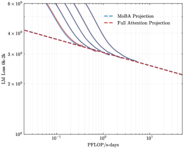
### Visual Description
\n
## Chart: LMi Loss vs. PFLOP/s-days
### Overview
This chart depicts the relationship between LMi Loss (0k-2k) and PFLOP/s-days for two different projection methods: MoBA Projection and Full Attention Projection. The chart uses a logarithmic scale for the y-axis (LMi Loss) and a logarithmic scale for the x-axis (PFLOP/s-days). Multiple lines represent different curves for each projection method.
### Components/Axes
* **X-axis:** PFLOP/s-days, ranging from approximately 10<sup>-1</sup> to 10<sup>1</sup> (logarithmic scale).
* **Y-axis:** LMi Loss (0k-2k), ranging from approximately 10<sup>0</sup> to 6 x 10<sup>3</sup> (logarithmic scale).
* **Legend:** Located in the top-right corner.
* MoBA Projection (Blue dashed line)
* Full Attention Projection (Red dashed line)
* **Data Series:** Multiple curves are plotted for each projection method.
### Detailed Analysis
**Full Attention Projection (Red dashed line):**
The Full Attention Projection line exhibits a consistent downward slope.
* At approximately PFLOP/s-days = 10<sup>-1</sup>, the LMi Loss is approximately 4 x 10<sup>3</sup>.
* At approximately PFLOP/s-days = 10<sup>0</sup>, the LMi Loss is approximately 3 x 10<sup>2</sup>.
* At approximately PFLOP/s-days = 10<sup>1</sup>, the LMi Loss is approximately 2 x 10<sup>1</sup>.
**MoBA Projection (Blue dashed line):**
The MoBA Projection lines show a steeper initial decline than the Full Attention Projection, and multiple curves are present.
* The leftmost MoBA Projection line starts at approximately LMi Loss = 5 x 10<sup>3</sup> at PFLOP/s-days = 10<sup>-1</sup>.
* The next MoBA Projection line starts at approximately LMi Loss = 4 x 10<sup>3</sup> at PFLOP/s-days = 10<sup>-1</sup>.
* The third MoBA Projection line starts at approximately LMi Loss = 3 x 10<sup>3</sup> at PFLOP/s-days = 10<sup>-1</sup>.
* The fourth MoBA Projection line starts at approximately LMi Loss = 2 x 10<sup>3</sup> at PFLOP/s-days = 10<sup>-1</sup>.
* At approximately PFLOP/s-days = 10<sup>0</sup>, the MoBA Projection lines converge to approximately LMi Loss = 1 x 10<sup>2</sup>.
* At approximately PFLOP/s-days = 10<sup>1</sup>, the MoBA Projection lines converge to approximately LMi Loss = 1 x 10<sup>1</sup>.
### Key Observations
* MoBA Projection generally achieves lower LMi Loss values than Full Attention Projection for the same PFLOP/s-days, especially at lower computational costs (PFLOP/s-days < 1).
* The multiple MoBA Projection lines suggest different configurations or runs of the MoBA method, potentially representing different hyperparameters or training conditions.
* Both methods demonstrate diminishing returns as PFLOP/s-days increase; the rate of LMi Loss reduction slows down.
### Interpretation
The chart demonstrates the trade-off between computational cost (PFLOP/s-days) and model performance (LMi Loss). MoBA Projection appears to be more efficient than Full Attention Projection, achieving comparable or better performance with fewer computational resources. The multiple MoBA Projection lines indicate that the method's performance can vary, suggesting sensitivity to certain parameters. The logarithmic scales highlight the significant impact of even small increases in PFLOP/s-days at lower computational budgets. The convergence of the MoBA lines at higher PFLOP/s-days suggests that the benefits of MoBA diminish as computational resources become abundant. This data suggests that MoBA is a promising approach for reducing the computational cost of language modeling without significantly sacrificing performance, particularly in resource-constrained environments.
</details>
(a) Scaling law (0-2k)
<details>
<summary>x14.png Details</summary>
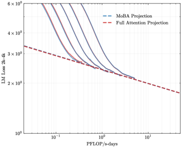
### Visual Description
\n
## Chart: Language Model Loss vs. Computational Cost
### Overview
The image presents a chart comparing the Language Model (LM) Loss of two projection methods – MoBA Projection and Full Attention Projection – as a function of computational cost, measured in PFLOP/s-days. The chart uses a logarithmic scale for both axes. Several curves are plotted for each projection method, representing different runs or configurations.
### Components/Axes
* **X-axis:** PFLOP/s-days, labeled "PFLOP/s-days". The scale is logarithmic, ranging from approximately 10<sup>-1</sup> to 10<sup>1</sup>.
* **Y-axis:** LM Loss 2k-4k, labeled "LM Loss 2k-4k". The scale is logarithmic, ranging from approximately 10<sup>0</sup> to 6 x 10<sup>6</sup>.
* **Legend:** Located in the top-right corner.
* MoBA Projection: Represented by a dashed blue line. Multiple curves are plotted for this method.
* Full Attention Projection: Represented by a dashed red line. Multiple curves are plotted for this method.
### Detailed Analysis
**MoBA Projection (Blue Lines):**
There are approximately five blue dashed curves. All curves exhibit a steep downward slope initially, indicating a rapid decrease in LM Loss as PFLOP/s-days increase. As PFLOP/s-days increase, the rate of decrease slows down, and the curves begin to flatten.
* Curve 1: Starts at approximately (0.1, 5 x 10<sup>6</sup>) and decreases to approximately (10, 2 x 10<sup>2</sup>).
* Curve 2: Starts at approximately (0.1, 4 x 10<sup>6</sup>) and decreases to approximately (10, 1 x 10<sup>2</sup>).
* Curve 3: Starts at approximately (0.1, 3 x 10<sup>6</sup>) and decreases to approximately (10, 5 x 10<sup>1</sup>).
* Curve 4: Starts at approximately (0.1, 2 x 10<sup>6</sup>) and decreases to approximately (10, 2 x 10<sup>1</sup>).
* Curve 5: Starts at approximately (0.1, 1 x 10<sup>6</sup>) and decreases to approximately (10, 1 x 10<sup>1</sup>).
**Full Attention Projection (Red Lines):**
There are approximately three red dashed curves. These curves also show a downward trend, but the decrease in LM Loss is less pronounced than that of the MoBA Projection curves.
* Curve 1: Starts at approximately (0.1, 5 x 10<sup>5</sup>) and decreases to approximately (10, 2 x 10<sup>1</sup>).
* Curve 2: Starts at approximately (0.1, 4 x 10<sup>5</sup>) and decreases to approximately (10, 1 x 10<sup>1</sup>).
* Curve 3: Starts at approximately (0.1, 3 x 10<sup>5</sup>) and decreases to approximately (10, 5 x 10<sup>0</sup>).
### Key Observations
* MoBA Projection consistently achieves lower LM Loss values compared to Full Attention Projection across the entire range of PFLOP/s-days.
* The multiple curves for each projection method suggest variability in performance, potentially due to different initialization conditions, hyperparameters, or data subsets.
* The logarithmic scales emphasize the significant reduction in LM Loss achieved with increasing computational cost.
* The rate of improvement diminishes as computational cost increases, indicating diminishing returns.
### Interpretation
The chart demonstrates that MoBA Projection is more computationally efficient than Full Attention Projection in achieving a given level of LM Loss. For a given computational budget (PFLOP/s-days), MoBA Projection yields a lower loss, implying better model performance. The multiple curves for each method suggest that the performance is not deterministic and can vary. The diminishing returns observed at higher computational costs suggest that there is a point beyond which increasing the computational budget provides only marginal improvements in LM Loss. This information is crucial for resource allocation and model optimization, as it helps determine the optimal balance between computational cost and model accuracy. The use of logarithmic scales is appropriate for visualizing data that spans several orders of magnitude, as it allows for a clearer representation of the trends and relationships between the variables.
</details>
(b) Scaling law (2-4k)
<details>
<summary>x15.png Details</summary>
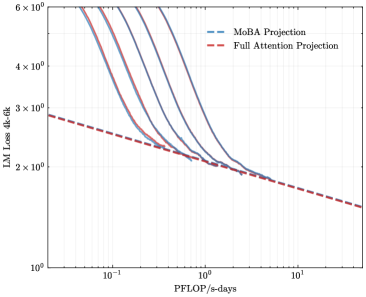
### Visual Description
\n
## Chart: LMi Loss vs. PFLOP/s-days
### Overview
The image presents a chart illustrating the relationship between LMi Loss (4k-6k) and PFLOP/s-days. Two projection methods, MoBA Projection and Full Attention Projection, are compared using line graphs. The chart uses a logarithmic scale for both the x and y axes.
### Components/Axes
* **X-axis:** PFLOP/s-days, ranging from approximately 10<sup>-1</sup> to 10<sup>1</sup> (logarithmic scale).
* **Y-axis:** LMi Loss (4k-6k), ranging from approximately 10<sup>0</sup> to 6 x 10<sup>6</sup> (logarithmic scale).
* **Legend:** Located in the top-right corner.
* MoBA Projection (represented by a dashed blue line)
* Full Attention Projection (represented by a dashed red line)
* **Data Series:** Two distinct lines representing the two projection methods. Multiple lines are present for the MoBA Projection, indicating different parameter sizes.
### Detailed Analysis
**Full Attention Projection (Red Dashed Line):**
The Full Attention Projection line exhibits a relatively consistent downward slope.
* At approximately 10<sup>-1</sup> PFLOP/s-days, the LMi Loss is around 5 x 10<sup>5</sup>.
* At approximately 10<sup>0</sup> PFLOP/s-days, the LMi Loss is around 2 x 10<sup>5</sup>.
* At approximately 10<sup>1</sup> PFLOP/s-days, the LMi Loss is around 5 x 10<sup>4</sup>.
**MoBA Projection (Blue Dashed Lines):**
Multiple MoBA Projection lines are present, each representing a different parameter size. All lines show a steeper downward trend compared to the Full Attention Projection.
* The uppermost MoBA Projection line (leftmost) starts at approximately 6 x 10<sup>6</sup> LMi Loss at 10<sup>-1</sup> PFLOP/s-days.
* The lines converge as PFLOP/s-days increase, with the lowest MoBA Projection line (rightmost) starting at approximately 2 x 10<sup>6</sup> LMi Loss at 10<sup>-1</sup> PFLOP/s-days.
* At approximately 10<sup>1</sup> PFLOP/s-days, the MoBA Projection lines range from approximately 1 x 10<sup>4</sup> to 2 x 10<sup>4</sup> LMi Loss.
### Key Observations
* MoBA Projection consistently outperforms Full Attention Projection in terms of LMi Loss across the entire range of PFLOP/s-days.
* The performance gap between the two methods widens as PFLOP/s-days increase.
* The multiple MoBA Projection lines suggest that performance varies with parameter size, with larger parameter sizes generally achieving lower LMi Loss.
* The logarithmic scales on both axes compress the data, making it difficult to discern precise values without further information.
### Interpretation
The chart demonstrates that MoBA Projection is more efficient than Full Attention Projection in reducing LMi Loss for a given computational cost (PFLOP/s-days). The steeper decline of the MoBA Projection lines indicates that it achieves a greater reduction in loss with increasing computational resources. The multiple MoBA Projection lines suggest a trade-off between model size (parameter count) and performance, with larger models generally performing better but requiring more computational resources. The use of logarithmic scales suggests that the relationship between LMi Loss and PFLOP/s-days is likely exponential or power-law. This type of chart is commonly used in machine learning to evaluate the efficiency and scalability of different model architectures or training techniques. The data suggests that MoBA Projection is a promising approach for improving the performance of language models, particularly in resource-constrained environments.
</details>
(c) Scaling law (4-6k)
<details>
<summary>x16.png Details</summary>
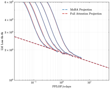
### Visual Description
## Chart: LMI Loss vs. PFLOP/s-days
### Overview
The image presents a chart illustrating the relationship between LMI Loss (6k-8k) and PFLOP/s-days for two different projection methods: MoBA Projection and Full Attention Projection. The chart uses a logarithmic scale for both axes. Multiple lines are plotted for each projection method, showing the trend of loss reduction as PFLOP/s-days increase.
### Components/Axes
* **X-axis:** PFLOP/s-days, ranging from approximately 10<sup>-1</sup> to 10<sup>1</sup> (logarithmic scale).
* **Y-axis:** LMI Loss (6k-8k), ranging from approximately 10<sup>0</sup> to 6 x 10<sup>6</sup> (logarithmic scale).
* **Legend:** Located in the top-right corner.
* MoBA Projection (Blue dashed line)
* Full Attention Projection (Red dashed line)
* **Data Series:** Multiple lines are plotted for each projection method, representing different runs or configurations.
### Detailed Analysis
**MoBA Projection (Blue dashed lines):**
There are approximately 5 blue dashed lines. The lines generally slope downwards, indicating that as PFLOP/s-days increase, the LMI Loss decreases.
* Line 1: Starts at approximately (0.1, 5.5 x 10<sup>6</sup>) and decreases to approximately (10, 1.5 x 10<sup>2</sup>).
* Line 2: Starts at approximately (0.1, 5.5 x 10<sup>6</sup>) and decreases to approximately (10, 1.5 x 10<sup>2</sup>).
* Line 3: Starts at approximately (0.1, 5.5 x 10<sup>6</sup>) and decreases to approximately (10, 1.5 x 10<sup>2</sup>).
* Line 4: Starts at approximately (0.1, 5.5 x 10<sup>6</sup>) and decreases to approximately (10, 1.5 x 10<sup>2</sup>).
* Line 5: Starts at approximately (0.1, 5.5 x 10<sup>6</sup>) and decreases to approximately (10, 1.5 x 10<sup>2</sup>).
**Full Attention Projection (Red dashed lines):**
There are approximately 5 red dashed lines. These lines also slope downwards, but generally remain above the MoBA Projection lines.
* Line 1: Starts at approximately (0.1, 5.5 x 10<sup>6</sup>) and decreases to approximately (10, 5 x 10<sup>1</sup>).
* Line 2: Starts at approximately (0.1, 5.5 x 10<sup>6</sup>) and decreases to approximately (10, 5 x 10<sup>1</sup>).
* Line 3: Starts at approximately (0.1, 5.5 x 10<sup>6</sup>) and decreases to approximately (10, 5 x 10<sup>1</sup>).
* Line 4: Starts at approximately (0.1, 5.5 x 10<sup>6</sup>) and decreases to approximately (10, 5 x 10<sup>1</sup>).
* Line 5: Starts at approximately (0.1, 5.5 x 10<sup>6</sup>) and decreases to approximately (10, 5 x 10<sup>1</sup>).
### Key Observations
* The MoBA Projection consistently achieves lower LMI Loss values compared to the Full Attention Projection across the entire range of PFLOP/s-days.
* The lines for each projection method are relatively close together, suggesting consistent performance within each method.
* The rate of loss reduction appears to decrease as PFLOP/s-days increase, indicating diminishing returns.
* The initial loss values are very high, and the logarithmic scale compresses the visual difference at higher loss values.
### Interpretation
The chart demonstrates that the MoBA Projection method is more efficient than the Full Attention Projection method in reducing LMI Loss for a given amount of computational resources (PFLOP/s-days). Both methods show a clear trade-off between computational cost and loss reduction. The diminishing returns observed at higher PFLOP/s-days suggest that there is a point beyond which increasing computational resources yields only marginal improvements in LMI Loss. The multiple lines for each method likely represent different experimental runs or variations in hyperparameters, and their proximity indicates robustness of the methods. The logarithmic scale is crucial for visualizing the large range of loss values, but it also means that small absolute differences in loss at lower values are visually amplified. This chart is likely used to evaluate the efficiency and scalability of different projection methods in a machine learning context, specifically related to language modeling (LMI).
</details>
(d) Scaling law (6-8k)
<details>
<summary>x17.png Details</summary>
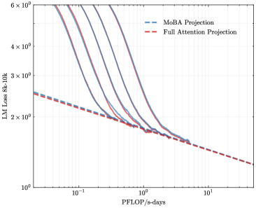
### Visual Description
## Chart: LM Loss vs. PFLOP/s-days
### Overview
The image presents a line chart comparing the Language Model (LM) Loss for two projection methods: MoBA Projection and Full Attention Projection, plotted against PFLOP/s-days (floating point operations per second per day). The chart displays multiple lines for each projection method, likely representing different runs or trials. The y-axis is on a logarithmic scale.
### Components/Axes
* **X-axis:** PFLOP/s-days. Scale is logarithmic, ranging from approximately 10<sup>-1</sup> to 10<sup>1</sup>.
* **Y-axis:** LM Loss 8k-10k. Scale is logarithmic, ranging from approximately 10<sup>0</sup> to 6 x 10<sup>6</sup>.
* **Legend:** Located in the top-right corner.
* MoBA Projection (Blue dashed line)
* Full Attention Projection (Red dashed line)
* **Lines:** Multiple lines are present for each projection method, showing variations in performance.
### Detailed Analysis
**MoBA Projection (Blue dashed lines):**
There are approximately 6 blue dashed lines. The lines generally exhibit a steep downward slope initially, indicating a rapid decrease in LM Loss as PFLOP/s-days increase. The slope gradually decreases as PFLOP/s-days increase, suggesting diminishing returns.
* Line 1: Starts at approximately (10<sup>-1</sup>, 5 x 10<sup>6</sup>) and ends at approximately (10<sup>1</sup>, 2 x 10<sup>2</sup>).
* Line 2: Starts at approximately (10<sup>-1</sup>, 5 x 10<sup>6</sup>) and ends at approximately (10<sup>1</sup>, 1 x 10<sup>2</sup>).
* Line 3: Starts at approximately (10<sup>-1</sup>, 5 x 10<sup>6</sup>) and ends at approximately (10<sup>1</sup>, 5 x 10<sup>1</sup>).
* Line 4: Starts at approximately (10<sup>-1</sup>, 5 x 10<sup>6</sup>) and ends at approximately (10<sup>1</sup>, 3 x 10<sup>1</sup>).
* Line 5: Starts at approximately (10<sup>-1</sup>, 5 x 10<sup>6</sup>) and ends at approximately (10<sup>1</sup>, 2 x 10<sup>1</sup>).
* Line 6: Starts at approximately (10<sup>-1</sup>, 5 x 10<sup>6</sup>) and ends at approximately (10<sup>1</sup>, 1 x 10<sup>1</sup>).
**Full Attention Projection (Red dashed lines):**
There are approximately 6 red dashed lines. Similar to the MoBA Projection, these lines also show a downward trend, but appear to be slightly less steep overall.
* Line 1: Starts at approximately (10<sup>-1</sup>, 5 x 10<sup>6</sup>) and ends at approximately (10<sup>1</sup>, 3 x 10<sup>2</sup>).
* Line 2: Starts at approximately (10<sup>-1</sup>, 5 x 10<sup>6</sup>) and ends at approximately (10<sup>1</sup>, 2 x 10<sup>2</sup>).
* Line 3: Starts at approximately (10<sup>-1</sup>, 5 x 10<sup>6</sup>) and ends at approximately (10<sup>1</sup>, 1 x 10<sup>2</sup>).
* Line 4: Starts at approximately (10<sup>-1</sup>, 5 x 10<sup>6</sup>) and ends at approximately (10<sup>1</sup>, 5 x 10<sup>1</sup>).
* Line 5: Starts at approximately (10<sup>-1</sup>, 5 x 10<sup>6</sup>) and ends at approximately (10<sup>1</sup>, 3 x 10<sup>1</sup>).
* Line 6: Starts at approximately (10<sup>-1</sup>, 5 x 10<sup>6</sup>) and ends at approximately (10<sup>1</sup>, 2 x 10<sup>1</sup>).
### Key Observations
* Both projection methods demonstrate a reduction in LM Loss as PFLOP/s-days increase.
* MoBA Projection generally achieves lower LM Loss values compared to Full Attention Projection for a given PFLOP/s-days value.
* There is variability in performance within each projection method, as indicated by the multiple lines.
* The logarithmic scale on both axes compresses the data, making it difficult to discern precise differences at lower loss values.
### Interpretation
The chart suggests that both MoBA Projection and Full Attention Projection are effective in reducing LM Loss with increased computational resources (PFLOP/s-days). However, MoBA Projection appears to be more efficient, achieving lower loss values for the same computational cost. The multiple lines for each method likely represent different training runs, highlighting the inherent variability in machine learning training processes. The diminishing returns observed at higher PFLOP/s-days suggest that there is a point beyond which increasing computational resources yields progressively smaller improvements in LM Loss. This information is valuable for optimizing the trade-off between computational cost and model performance. The use of a logarithmic scale indicates that the researchers were particularly interested in observing the behavior of the loss function across a wide range of values, especially at lower loss levels where differences might be more subtle.
</details>
(e) Scaling law (8-10k)
<details>
<summary>x18.png Details</summary>
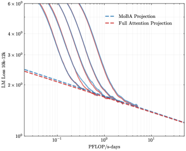
### Visual Description
## Chart: LM Loss vs. PFLOP/s-days
### Overview
The image presents a line chart comparing the Language Model (LM) Loss of two projection methods – MoBA Projection and Full Attention Projection – against the computational cost measured in PFLOP/s-days. The chart displays a logarithmic scale on the y-axis (LM Loss) and a logarithmic scale on the x-axis (PFLOP/s-days). Multiple lines are present for each projection method, indicating potentially different runs or configurations.
### Components/Axes
* **X-axis Title:** PFLOP/s-days
* **Y-axis Title:** LM Loss 10k-12k
* **Y-axis Scale:** Logarithmic, ranging from 10⁰ to 6 x 10⁶. Markers are present at 10⁰, 10¹, 10², 10³, 10⁴, 10⁵, 10⁶.
* **X-axis Scale:** Logarithmic, with markers at 10⁻¹, 10⁰, 10¹, 10².
* **Legend:** Located in the top-right corner.
* **MoBA Projection:** Represented by a dashed blue line.
* **Full Attention Projection:** Represented by a dashed red line.
### Detailed Analysis
The chart contains multiple lines for each projection method. I will describe the trends and approximate data points for each.
**MoBA Projection (Dashed Blue Lines):**
There are approximately 5 blue lines.
* **Line 1:** Starts at approximately (10⁻¹, 2 x 10⁵) and slopes downward, reaching approximately (10², 2 x 10¹)
* **Line 2:** Starts at approximately (10⁻¹, 2.5 x 10⁵) and slopes downward, reaching approximately (10², 2.5 x 10¹)
* **Line 3:** Starts at approximately (10⁻¹, 3 x 10⁵) and slopes downward, reaching approximately (10², 3 x 10¹)
* **Line 4:** Starts at approximately (10⁻¹, 3.5 x 10⁵) and slopes downward, reaching approximately (10², 3.5 x 10¹)
* **Line 5:** Starts at approximately (10⁻¹, 4 x 10⁵) and slopes downward, reaching approximately (10², 4 x 10¹)
**Full Attention Projection (Dashed Red Lines):**
There are approximately 5 red lines.
* **Line 1:** Starts at approximately (10⁻¹, 3 x 10⁵) and slopes downward, reaching approximately (10², 3 x 10¹)
* **Line 2:** Starts at approximately (10⁻¹, 3.5 x 10⁵) and slopes downward, reaching approximately (10², 3.5 x 10¹)
* **Line 3:** Starts at approximately (10⁻¹, 4 x 10⁵) and slopes downward, reaching approximately (10², 4 x 10¹)
* **Line 4:** Starts at approximately (10⁻¹, 4.5 x 10⁵) and slopes downward, reaching approximately (10², 4.5 x 10¹)
* **Line 5:** Starts at approximately (10⁻¹, 5 x 10⁵) and slopes downward, reaching approximately (10², 5 x 10¹)
All lines exhibit a decreasing trend, indicating that as PFLOP/s-days increase, the LM Loss decreases for both projection methods.
### Key Observations
* The Full Attention Projection consistently exhibits higher LM Loss values than the MoBA Projection across the entire range of PFLOP/s-days.
* The multiple lines for each projection method suggest variability in the results, potentially due to different training runs or hyperparameter settings.
* The rate of decrease in LM Loss appears to slow down as PFLOP/s-days increase, indicating diminishing returns from increased computation.
### Interpretation
The chart demonstrates the trade-off between computational cost (PFLOP/s-days) and language model loss. Both projection methods improve LM Loss with increased computation, but the MoBA Projection achieves lower loss values for a given computational budget. This suggests that MoBA Projection is a more efficient method for reducing LM Loss. The spread of lines for each method indicates that the performance is not deterministic and is subject to variance. The logarithmic scales highlight the significant impact of even small increases in PFLOP/s-days at lower computational costs, and the diminishing returns at higher costs. The data suggests that while increasing computational resources always helps, the MoBA projection is a more efficient approach to reducing LM Loss.
</details>
(f) Scaling law (10-12k)
<details>
<summary>x19.png Details</summary>
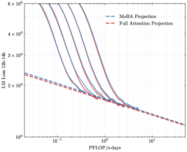
### Visual Description
## Chart: LM Loss vs. PFLOP/s-days
### Overview
The image presents a line chart comparing the Language Model (LM) Loss for two different projection methods: MoBA Projection and Full Attention Projection, plotted against PFLOP/s-days (floating point operations per second-days). The chart displays multiple lines representing different runs or trials for each projection method, showing the loss reduction as computational cost increases. The y-axis is on a logarithmic scale.
### Components/Axes
* **X-axis:** PFLOP/s-days, ranging from approximately 10<sup>-1</sup> to 10<sup>1</sup> (0.1 to 10). The scale is logarithmic.
* **Y-axis:** LM Loss 12k-14k, ranging from approximately 10<sup>0</sup> to 6 x 10<sup>6</sup> (1 to 6,000,000). The scale is logarithmic.
* **Legend:** Located in the top-right corner.
* MoBA Projection (Blue dashed lines)
* Full Attention Projection (Red dashed lines)
* **Data Series:** Multiple lines for each projection method, showing variations in performance.
### Detailed Analysis
The chart shows several lines for each projection method. Let's analyze each:
**MoBA Projection (Blue dashed lines):**
* **Line 1:** Starts at approximately (0.1, 2.5 x 10<sup>5</sup>) and decreases to approximately (10, 2.0 x 10<sup>1</sup>). The line exhibits a steep initial decline, then gradually flattens.
* **Line 2:** Starts at approximately (0.1, 1.5 x 10<sup>5</sup>) and decreases to approximately (10, 1.5 x 10<sup>1</sup>). Similar trend to Line 1, but consistently lower loss values.
* **Line 3:** Starts at approximately (0.1, 1.2 x 10<sup>5</sup>) and decreases to approximately (10, 1.0 x 10<sup>1</sup>). Similar trend to Line 1 and 2, but consistently lower loss values.
**Full Attention Projection (Red dashed lines):**
* **Line 1:** Starts at approximately (0.1, 5.0 x 10<sup>5</sup>) and decreases to approximately (10, 2.5 x 10<sup>1</sup>). The line exhibits a steep initial decline, then gradually flattens.
* **Line 2:** Starts at approximately (0.1, 3.0 x 10<sup>5</sup>) and decreases to approximately (10, 2.0 x 10<sup>1</sup>). Similar trend to Line 1, but consistently lower loss values.
* **Line 3:** Starts at approximately (0.1, 2.0 x 10<sup>5</sup>) and decreases to approximately (10, 1.5 x 10<sup>1</sup>). Similar trend to Line 1 and 2, but consistently lower loss values.
All lines demonstrate a decreasing trend in LM Loss as PFLOP/s-days increases. The initial decrease is more pronounced at lower PFLOP/s-days values.
### Key Observations
* **Performance Comparison:** For a given PFLOP/s-days value, MoBA Projection consistently achieves lower LM Loss compared to Full Attention Projection.
* **Variability:** There is variability in performance within each projection method, as indicated by the multiple lines. This suggests that the results can vary depending on the specific run or initialization.
* **Diminishing Returns:** The rate of loss reduction decreases as PFLOP/s-days increases, indicating diminishing returns from further computational investment.
* **Logarithmic Scales:** The use of logarithmic scales on both axes emphasizes the large range of values and the relative changes in loss and computational cost.
### Interpretation
The chart demonstrates that MoBA Projection is more efficient than Full Attention Projection in terms of achieving lower LM Loss for a given computational cost (PFLOP/s-days). The multiple lines for each method suggest that the performance is not deterministic and can vary. The diminishing returns observed at higher PFLOP/s-days values indicate that there is a point beyond which increasing computational cost yields only marginal improvements in LM Loss. This information is valuable for optimizing the training process of language models, as it suggests that MoBA Projection is a more cost-effective approach, and that there is a trade-off between computational cost and model performance. The logarithmic scales suggest that the relationship between loss and computational cost is not linear, and that small changes in PFLOP/s-days can have a significant impact on loss, especially at lower values.
</details>
(g) Scaling law (12-14k)
<details>
<summary>x20.png Details</summary>
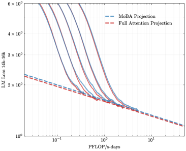
### Visual Description
## Chart: LM Loss vs. PFLOP/s-days
### Overview
This chart displays the relationship between LM Loss (Language Model Loss) and PFLOP/s-days (Floating Point Operations Per Second per day) for two different projection methods: MoBA Projection and Full Attention Projection. The chart uses a logarithmic scale for both axes. Multiple lines are present for each projection method, representing different runs or trials.
### Components/Axes
* **X-axis:** PFLOP/s-days, ranging from approximately 10<sup>-2</sup> to 10<sup>1</sup> (logarithmic scale).
* **Y-axis:** LM Loss 14k-16k, ranging from approximately 10<sup>0</sup> to 6 x 10<sup>6</sup> (logarithmic scale).
* **Legend:** Located in the top-right corner.
* MoBA Projection (Blue dashed line)
* Full Attention Projection (Red dashed line)
* Multiple lines are plotted for each projection method, showing variations in performance.
### Detailed Analysis
The chart shows several lines for each projection method. Let's analyze each:
**MoBA Projection (Blue dashed line):**
* The lines generally slope downwards, indicating that as PFLOP/s-days increase, LM Loss decreases.
* There are approximately 6 lines visible for MoBA Projection.
* At PFLOP/s-days ≈ 10<sup>-2</sup>, the LM Loss ranges from approximately 2 x 10<sup>5</sup> to 5 x 10<sup>5</sup>.
* At PFLOP/s-days ≈ 10<sup>0</sup>, the LM Loss ranges from approximately 2 x 10<sup>4</sup> to 5 x 10<sup>4</sup>.
* At PFLOP/s-days ≈ 10<sup>1</sup>, the LM Loss ranges from approximately 5 x 10<sup>3</sup> to 1 x 10<sup>4</sup>.
**Full Attention Projection (Red dashed line):**
* Similar to MoBA Projection, the lines slope downwards, showing a decrease in LM Loss with increasing PFLOP/s-days.
* There are approximately 6 lines visible for Full Attention Projection.
* At PFLOP/s-days ≈ 10<sup>-2</sup>, the LM Loss ranges from approximately 3 x 10<sup>5</sup> to 6 x 10<sup>5</sup>.
* At PFLOP/s-days ≈ 10<sup>0</sup>, the LM Loss ranges from approximately 1 x 10<sup>4</sup> to 3 x 10<sup>4</sup>.
* At PFLOP/s-days ≈ 10<sup>1</sup>, the LM Loss ranges from approximately 2 x 10<sup>3</sup> to 5 x 10<sup>3</sup>.
The lines for Full Attention Projection generally appear to be below the lines for MoBA Projection, suggesting that Full Attention Projection achieves lower LM Loss for a given PFLOP/s-days value.
### Key Observations
* Both projection methods demonstrate a clear trade-off between computational cost (PFLOP/s-days) and model performance (LM Loss).
* Full Attention Projection consistently outperforms MoBA Projection across the range of PFLOP/s-days values.
* There is variability in performance within each projection method, as indicated by the multiple lines. This could be due to random initialization, data variations, or other factors.
* The rate of decrease in LM Loss appears to slow down as PFLOP/s-days increases, suggesting diminishing returns.
### Interpretation
The chart demonstrates the scaling behavior of two different projection methods for a language model. The results suggest that Full Attention Projection is more efficient than MoBA Projection in terms of achieving lower LM Loss for a given computational budget. The diminishing returns observed at higher PFLOP/s-days values indicate that there is a point beyond which increasing computational resources yields only marginal improvements in model performance. The variability within each projection method highlights the importance of considering multiple runs or trials when evaluating model performance. This data is valuable for making informed decisions about resource allocation and model selection in language modeling tasks. The logarithmic scales suggest that the relationship between LM Loss and PFLOP/s-days is not linear, and that small changes in PFLOP/s-days can have a significant impact on LM Loss, especially at lower values.
</details>
(h) Scaling law (14-16k)
Figure 8: Scaling laws for positions 0-16k
<details>
<summary>x21.png Details</summary>
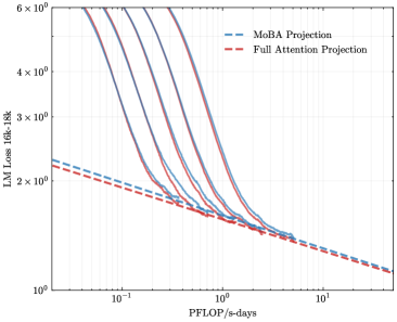
### Visual Description
## Line Chart: LM Loss vs. PFLOP/s-days
### Overview
This image presents a line chart comparing the Language Model (LM) Loss of two projection methods – MoBA Projection and Full Attention Projection – as a function of PFLOP/s-days (floating point operations per second per day). Multiple lines are shown for each projection method, likely representing different runs or configurations. The chart uses a logarithmic scale for both the y-axis (LM Loss) and the x-axis (PFLOP/s-days).
### Components/Axes
* **X-axis:** PFLOP/s-days, ranging from approximately 10<sup>-2</sup> to 10<sup>1</sup> (logarithmic scale).
* **Y-axis:** LM Loss 16k-18k, ranging from approximately 10<sup>0</sup> to 6 x 10<sup>6</sup> (logarithmic scale).
* **Legend:** Located in the top-right corner.
* MoBA Projection (blue dashed line)
* Full Attention Projection (red solid line)
* **Lines:** Multiple lines are plotted for each projection method. There are approximately 6 lines for each method.
### Detailed Analysis
**MoBA Projection (Blue Dashed Line):**
The MoBA Projection lines generally exhibit a downward trend as PFLOP/s-days increase.
* Line 1: Starts at approximately 2.5 x 10<sup>2</sup> LM Loss at 10<sup>-2</sup> PFLOP/s-days, decreasing to approximately 2 x 10<sup>1</sup> LM Loss at 10<sup>1</sup> PFLOP/s-days.
* Line 2: Starts at approximately 2 x 10<sup>2</sup> LM Loss at 10<sup>-2</sup> PFLOP/s-days, decreasing to approximately 1.5 x 10<sup>1</sup> LM Loss at 10<sup>1</sup> PFLOP/s-days.
* Line 3: Starts at approximately 1.5 x 10<sup>2</sup> LM Loss at 10<sup>-2</sup> PFLOP/s-days, decreasing to approximately 1 x 10<sup>1</sup> LM Loss at 10<sup>1</sup> PFLOP/s-days.
* Line 4: Starts at approximately 1 x 10<sup>2</sup> LM Loss at 10<sup>-2</sup> PFLOP/s-days, decreasing to approximately 7 x 10<sup>0</sup> LM Loss at 10<sup>1</sup> PFLOP/s-days.
* Line 5: Starts at approximately 7 x 10<sup>1</sup> LM Loss at 10<sup>-2</sup> PFLOP/s-days, decreasing to approximately 5 x 10<sup>0</sup> LM Loss at 10<sup>1</sup> PFLOP/s-days.
* Line 6: Starts at approximately 5 x 10<sup>1</sup> LM Loss at 10<sup>-2</sup> PFLOP/s-days, decreasing to approximately 3 x 10<sup>0</sup> LM Loss at 10<sup>1</sup> PFLOP/s-days.
**Full Attention Projection (Red Solid Line):**
The Full Attention Projection lines also show a downward trend, but generally start at higher LM Loss values and decrease more rapidly than the MoBA Projection lines.
* Line 1: Starts at approximately 5 x 10<sup>3</sup> LM Loss at 10<sup>-2</sup> PFLOP/s-days, decreasing to approximately 2 x 10<sup>1</sup> LM Loss at 10<sup>1</sup> PFLOP/s-days.
* Line 2: Starts at approximately 4 x 10<sup>3</sup> LM Loss at 10<sup>-2</sup> PFLOP/s-days, decreasing to approximately 1.5 x 10<sup>1</sup> LM Loss at 10<sup>1</sup> PFLOP/s-days.
* Line 3: Starts at approximately 3 x 10<sup>3</sup> LM Loss at 10<sup>-2</sup> PFLOP/s-days, decreasing to approximately 1 x 10<sup>1</sup> LM Loss at 10<sup>1</sup> PFLOP/s-days.
* Line 4: Starts at approximately 2 x 10<sup>3</sup> LM Loss at 10<sup>-2</sup> PFLOP/s-days, decreasing to approximately 7 x 10<sup>0</sup> LM Loss at 10<sup>1</sup> PFLOP/s-days.
* Line 5: Starts at approximately 1 x 10<sup>3</sup> LM Loss at 10<sup>-2</sup> PFLOP/s-days, decreasing to approximately 5 x 10<sup>0</sup> LM Loss at 10<sup>1</sup> PFLOP/s-days.
* Line 6: Starts at approximately 5 x 10<sup>2</sup> LM Loss at 10<sup>-2</sup> PFLOP/s-days, decreasing to approximately 3 x 10<sup>0</sup> LM Loss at 10<sup>1</sup> PFLOP/s-days.
### Key Observations
* Both projection methods demonstrate a decrease in LM Loss as PFLOP/s-days increase, indicating improved model performance with more computational resources.
* The Full Attention Projection consistently exhibits higher LM Loss values than the MoBA Projection across the entire range of PFLOP/s-days.
* The multiple lines for each method suggest variability in performance, potentially due to different initialization, hyperparameters, or data splits.
* The rate of decrease in LM Loss appears to slow down as PFLOP/s-days increase for both methods, suggesting diminishing returns from additional computation.
### Interpretation
The chart suggests that the MoBA Projection method is more efficient than the Full Attention Projection method in terms of LM Loss per PFLOP/s-days. MoBA achieves comparable or lower loss with less computational cost. The multiple lines for each method indicate that the performance is not deterministic and can vary. The logarithmic scales highlight the significant impact of even small increases in PFLOP/s-days at lower computational budgets. The diminishing returns observed at higher PFLOP/s-days suggest that there is a point beyond which further increasing computational resources yields only marginal improvements in LM Loss. This information is valuable for resource allocation and model optimization, as it helps determine the optimal balance between computational cost and model performance. The chart implies that MoBA is a more scalable approach, as it requires fewer resources to achieve a given level of performance.
</details>
(i) Scaling law (16-18k)
<details>
<summary>x22.png Details</summary>

### Visual Description
## Line Chart: LM Loss vs. PFLOP/s-days
### Overview
This image presents a line chart comparing the LM Loss (Language Model Loss) of two projection methods – MoBA Projection and Full Attention Projection – across varying levels of PFLOP/s-days (Floating Point Operations Per Second per day). Multiple lines are present for each projection method, representing different runs or configurations. The chart is designed to visualize the trade-off between computational cost (PFLOP/s-days) and model performance (LM Loss).
### Components/Axes
* **X-axis:** PFLOP/s-days, ranging from approximately 10<sup>-1</sup> to 10<sup>1</sup>. The scale is logarithmic.
* **Y-axis:** LM Loss 18k-20k, ranging from approximately 10<sup>0</sup> to 6 x 10<sup>6</sup>. The scale is logarithmic.
* **Legend:** Located in the top-right corner.
* MoBA Projection (Blue dashed lines)
* Full Attention Projection (Red solid lines)
* **Data Series:** Multiple lines for each projection method, showing the loss reduction as PFLOP/s-days increase. There are approximately 6 lines for each method.
### Detailed Analysis
The chart displays several lines for each projection method. Let's analyze each:
**MoBA Projection (Blue Dashed Lines):**
* **Trend:** All MoBA Projection lines generally slope downward, indicating that increasing PFLOP/s-days reduces LM Loss. The lines converge as PFLOP/s-days increase.
* **Data Points (Approximate):**
* At PFLOP/s-days ≈ 10<sup>-1</sup>: LM Loss ranges from approximately 2 x 10<sup>5</sup> to 5 x 10<sup>5</sup>.
* At PFLOP/s-days ≈ 10<sup>0</sup>: LM Loss ranges from approximately 5 x 10<sup>4</sup> to 2 x 10<sup>5</sup>.
* At PFLOP/s-days ≈ 10<sup>1</sup>: LM Loss ranges from approximately 2 x 10<sup>4</sup> to 5 x 10<sup>4</sup>.
**Full Attention Projection (Red Solid Lines):**
* **Trend:** Similar to MoBA Projection, the Full Attention Projection lines also slope downward, showing loss reduction with increasing PFLOP/s-days. These lines also converge as PFLOP/s-days increase, but generally remain below the MoBA Projection lines.
* **Data Points (Approximate):**
* At PFLOP/s-days ≈ 10<sup>-1</sup>: LM Loss ranges from approximately 1 x 10<sup>5</sup> to 3 x 10<sup>5</sup>.
* At PFLOP/s-days ≈ 10<sup>0</sup>: LM Loss ranges from approximately 2 x 10<sup>4</sup> to 1 x 10<sup>5</sup>.
* At PFLOP/s-days ≈ 10<sup>1</sup>: LM Loss ranges from approximately 1 x 10<sup>4</sup> to 3 x 10<sup>4</sup>.
### Key Observations
* **Performance Comparison:** Full Attention Projection consistently achieves lower LM Loss than MoBA Projection across all PFLOP/s-days values.
* **Convergence:** The lines for both methods converge at higher PFLOP/s-days, suggesting diminishing returns in loss reduction beyond a certain computational cost.
* **Variability:** There is some variability within each projection method, indicated by the multiple lines. This could be due to different initialization conditions, hyperparameter settings, or data splits.
* **Logarithmic Scales:** The use of logarithmic scales on both axes emphasizes the relative changes in loss and computational cost.
### Interpretation
The chart demonstrates the relationship between computational resources (PFLOP/s-days) and model performance (LM Loss) for two different projection methods. The results suggest that Full Attention Projection is more efficient than MoBA Projection in achieving lower LM Loss for a given computational budget. However, both methods exhibit diminishing returns as PFLOP/s-days increase. The variability within each method highlights the importance of considering factors beyond just computational cost when optimizing model performance. The convergence of the lines at higher PFLOP/s-days suggests that there may be a point where further investment in computational resources yields only marginal improvements in LM Loss. This information is valuable for making informed decisions about resource allocation and model selection in language modeling tasks. The logarithmic scales suggest that the initial gains in loss reduction are more significant than those achieved at higher computational costs.
</details>
(j) Scaling law (18-20k)
<details>
<summary>x23.png Details</summary>

### Visual Description
## Chart: LM Loss vs. PFLOP/s-days
### Overview
The image presents a line chart comparing the Language Model (LM) Loss against PFLOP/s-days for two projection methods: MoBA Projection and Full Attention Projection. Multiple lines are plotted for each method, likely representing different runs or configurations. The chart is designed to visualize the trade-off between computational cost (PFLOP/s-days) and model performance (LM Loss).
### Components/Axes
* **X-axis:** PFLOP/s-days. Scale is logarithmic, ranging from approximately 10<sup>-1</sup> to 10<sup>1</sup>.
* **Y-axis:** LM Loss 20k-22k. Scale is logarithmic, ranging from approximately 10<sup>0</sup> to 10<sup>6</sup>.
* **Legend:** Located in the top-right corner.
* MoBA Projection (Blue dashed lines)
* Full Attention Projection (Red dashed lines)
* **Data Series:** Multiple lines for each projection method. There are approximately 6 lines for each method.
### Detailed Analysis
**MoBA Projection (Blue dashed lines):**
The lines generally slope downward, indicating that as PFLOP/s-days increase, the LM Loss decreases.
* Line 1: Starts at approximately LM Loss = 2.5 x 10<sup>2</sup> at PFLOP/s-days = 10<sup>-1</sup>, decreasing to approximately LM Loss = 1.5 x 10<sup>1</sup> at PFLOP/s-days = 10<sup>1</sup>.
* Line 2: Starts at approximately LM Loss = 2.0 x 10<sup>2</sup> at PFLOP/s-days = 10<sup>-1</sup>, decreasing to approximately LM Loss = 1.0 x 10<sup>1</sup> at PFLOP/s-days = 10<sup>1</sup>.
* Line 3: Starts at approximately LM Loss = 1.8 x 10<sup>2</sup> at PFLOP/s-days = 10<sup>-1</sup>, decreasing to approximately LM Loss = 8 x 10<sup>0</sup> at PFLOP/s-days = 10<sup>1</sup>.
* Line 4: Starts at approximately LM Loss = 1.5 x 10<sup>2</sup> at PFLOP/s-days = 10<sup>-1</sup>, decreasing to approximately LM Loss = 6 x 10<sup>0</sup> at PFLOP/s-days = 10<sup>1</sup>.
* Line 5: Starts at approximately LM Loss = 1.2 x 10<sup>2</sup> at PFLOP/s-days = 10<sup>-1</sup>, decreasing to approximately LM Loss = 5 x 10<sup>0</sup> at PFLOP/s-days = 10<sup>1</sup>.
* Line 6: Starts at approximately LM Loss = 1.0 x 10<sup>2</sup> at PFLOP/s-days = 10<sup>-1</sup>, decreasing to approximately LM Loss = 4 x 10<sup>0</sup> at PFLOP/s-days = 10<sup>1</sup>.
**Full Attention Projection (Red dashed lines):**
The lines also slope downward, but generally start at higher LM Loss values and decrease more rapidly than the MoBA Projection lines.
* Line 1: Starts at approximately LM Loss = 5.0 x 10<sup>2</sup> at PFLOP/s-days = 10<sup>-1</sup>, decreasing to approximately LM Loss = 2.0 x 10<sup>1</sup> at PFLOP/s-days = 10<sup>1</sup>.
* Line 2: Starts at approximately LM Loss = 4.5 x 10<sup>2</sup> at PFLOP/s-days = 10<sup>-1</sup>, decreasing to approximately LM Loss = 1.8 x 10<sup>1</sup> at PFLOP/s-days = 10<sup>1</sup>.
* Line 3: Starts at approximately LM Loss = 4.0 x 10<sup>2</sup> at PFLOP/s-days = 10<sup>-1</sup>, decreasing to approximately LM Loss = 1.6 x 10<sup>1</sup> at PFLOP/s-days = 10<sup>1</sup>.
* Line 4: Starts at approximately LM Loss = 3.5 x 10<sup>2</sup> at PFLOP/s-days = 10<sup>-1</sup>, decreasing to approximately LM Loss = 1.4 x 10<sup>1</sup> at PFLOP/s-days = 10<sup>1</sup>.
* Line 5: Starts at approximately LM Loss = 3.0 x 10<sup>2</sup> at PFLOP/s-days = 10<sup>-1</sup>, decreasing to approximately LM Loss = 1.2 x 10<sup>1</sup> at PFLOP/s-days = 10<sup>1</sup>.
* Line 6: Starts at approximately LM Loss = 2.5 x 10<sup>2</sup> at PFLOP/s-days = 10<sup>-1</sup>, decreasing to approximately LM Loss = 1.0 x 10<sup>1</sup> at PFLOP/s-days = 10<sup>1</sup>.
### Key Observations
* Both projection methods demonstrate a clear negative correlation between PFLOP/s-days and LM Loss.
* The Full Attention Projection generally starts with higher loss values but exhibits a steeper decrease in loss compared to the MoBA Projection, especially at lower PFLOP/s-days values.
* There is some variance between the lines within each projection method, suggesting that the results are not entirely consistent and may be influenced by other factors.
* The logarithmic scales on both axes compress the data, making it difficult to discern precise differences in loss values at higher PFLOP/s-days.
### Interpretation
The chart suggests that increasing computational resources (PFLOP/s-days) leads to improved language model performance (lower LM Loss) for both MoBA and Full Attention Projection methods. However, the Full Attention Projection appears to be more sensitive to computational resources, achieving a greater reduction in loss for a given increase in PFLOP/s-days, particularly at lower computational budgets. This could indicate that Full Attention Projection is more computationally demanding but offers faster convergence to lower loss values. The variance between the lines within each method suggests that factors beyond PFLOP/s-days, such as initialization, data sampling, or hyperparameter settings, also play a significant role in determining the final LM Loss. The use of logarithmic scales implies that the researchers are interested in capturing the relative changes in loss and computational cost across a wide range of values, rather than focusing on absolute differences. The "20k-22k" annotation on the Y-axis suggests that the LM Loss is being measured on a specific subset of the training data or a particular evaluation metric.
</details>
(k) Scaling law (20-22k)
<details>
<summary>x24.png Details</summary>
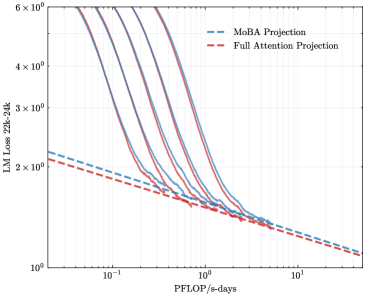
### Visual Description
\n
## Chart: LM Loss vs. PFLOP/s-days
### Overview
The image presents a line chart comparing the Language Model (LM) Loss for two projection methods: MoBA Projection and Full Attention Projection, plotted against PFLOP/s-days. Multiple lines are shown for each projection method, likely representing different runs or configurations. The chart uses a logarithmic scale for the y-axis (LM Loss) and a logarithmic scale for the x-axis (PFLOP/s-days).
### Components/Axes
* **X-axis:** PFLOP/s-days, ranging from approximately 10<sup>-1</sup> to 10<sup>1</sup> (logarithmic scale).
* **Y-axis:** LM Loss 22k-24k, ranging from approximately 10<sup>0</sup> to 6 x 10<sup>6</sup> (logarithmic scale).
* **Legend:** Located in the top-right corner.
* MoBA Projection (Blue, dashed lines)
* Full Attention Projection (Red, solid lines)
* **Data Series:** Multiple lines for each projection method. There are approximately 6 lines for each method.
### Detailed Analysis
**MoBA Projection (Blue, dashed lines):**
The MoBA Projection lines generally slope downward, indicating that as PFLOP/s-days increase, the LM Loss decreases.
* Line 1: Starts at approximately 2 x 10<sup>3</sup> at 10<sup>-1</sup> PFLOP/s-days, decreasing to approximately 2 x 10<sup>2</sup> at 10<sup>1</sup> PFLOP/s-days.
* Line 2: Starts at approximately 1 x 10<sup>3</sup> at 10<sup>-1</sup> PFLOP/s-days, decreasing to approximately 1 x 10<sup>2</sup> at 10<sup>1</sup> PFLOP/s-days.
* Line 3: Starts at approximately 8 x 10<sup>2</sup> at 10<sup>-1</sup> PFLOP/s-days, decreasing to approximately 8 x 10<sup>1</sup> at 10<sup>1</sup> PFLOP/s-days.
* Line 4: Starts at approximately 6 x 10<sup>2</sup> at 10<sup>-1</sup> PFLOP/s-days, decreasing to approximately 6 x 10<sup>1</sup> at 10<sup>1</sup> PFLOP/s-days.
* Line 5: Starts at approximately 4 x 10<sup>2</sup> at 10<sup>-1</sup> PFLOP/s-days, decreasing to approximately 4 x 10<sup>1</sup> at 10<sup>1</sup> PFLOP/s-days.
* Line 6: Starts at approximately 2 x 10<sup>2</sup> at 10<sup>-1</sup> PFLOP/s-days, decreasing to approximately 2 x 10<sup>1</sup> at 10<sup>1</sup> PFLOP/s-days.
**Full Attention Projection (Red, solid lines):**
The Full Attention Projection lines also slope downward, but generally start at a higher LM Loss and exhibit more variance than the MoBA Projection lines.
* Line 1: Starts at approximately 5 x 10<sup>3</sup> at 10<sup>-1</sup> PFLOP/s-days, decreasing to approximately 3 x 10<sup>2</sup> at 10<sup>1</sup> PFLOP/s-days.
* Line 2: Starts at approximately 4 x 10<sup>3</sup> at 10<sup>-1</sup> PFLOP/s-days, decreasing to approximately 2 x 10<sup>2</sup> at 10<sup>1</sup> PFLOP/s-days.
* Line 3: Starts at approximately 3 x 10<sup>3</sup> at 10<sup>-1</sup> PFLOP/s-days, decreasing to approximately 1.5 x 10<sup>2</sup> at 10<sup>1</sup> PFLOP/s-days.
* Line 4: Starts at approximately 2.5 x 10<sup>3</sup> at 10<sup>-1</sup> PFLOP/s-days, decreasing to approximately 1 x 10<sup>2</sup> at 10<sup>1</sup> PFLOP/s-days.
* Line 5: Starts at approximately 2 x 10<sup>3</sup> at 10<sup>-1</sup> PFLOP/s-days, decreasing to approximately 5 x 10<sup>1</sup> at 10<sup>1</sup> PFLOP/s-days.
* Line 6: Starts at approximately 1.5 x 10<sup>3</sup> at 10<sup>-1</sup> PFLOP/s-days, decreasing to approximately 2.5 x 10<sup>1</sup> at 10<sup>1</sup> PFLOP/s-days.
### Key Observations
* Both projection methods demonstrate a clear negative correlation between PFLOP/s-days and LM Loss. Increasing computational resources (PFLOP/s-days) leads to a reduction in LM Loss.
* The Full Attention Projection generally starts with a higher LM Loss than the MoBA Projection.
* The variance in LM Loss for the Full Attention Projection appears to be greater than that of the MoBA Projection, suggesting potentially more sensitivity to variations in the training process.
* The lines converge as PFLOP/s-days increase, indicating that the difference in performance between the two methods diminishes with more computational resources.
### Interpretation
The chart suggests that both MoBA Projection and Full Attention Projection are effective methods for reducing LM Loss. However, MoBA Projection appears to be more efficient in terms of achieving lower loss for a given amount of computational resources (PFLOP/s-days). The convergence of the lines at higher PFLOP/s-days suggests that Full Attention Projection can achieve comparable performance to MoBA Projection, but requires significantly more computational effort. The multiple lines for each method likely represent different training runs, highlighting the inherent variability in the training process. The logarithmic scales on both axes emphasize the rapid initial decrease in LM Loss with increasing PFLOP/s-days, followed by a slower rate of improvement as the model converges. This data is valuable for understanding the trade-offs between computational cost and model performance when choosing a projection method for language modeling.
</details>
(l) Scaling law (22-24k)
<details>
<summary>x25.png Details</summary>

### Visual Description
## Chart: LM Loss vs. PFLOP/s-days
### Overview
The image presents a line chart comparing the Language Model (LM) Loss of two projection methods – MoBA Projection and Full Attention Projection – against PFLOP/s-days (floating point operations per second per day). The chart displays multiple lines for each projection method, likely representing different runs or configurations. The y-axis is on a logarithmic scale.
### Components/Axes
* **X-axis:** PFLOP/s-days, ranging from approximately 10<sup>-2</sup> to 10<sup>1</sup> (0.01 to 10). The scale is logarithmic.
* **Y-axis:** LM Loss 24k-26k, ranging from approximately 10<sup>0</sup> to 6 x 10<sup>6</sup> (1 to 6,000,000). The scale is logarithmic.
* **Legend:** Located in the top-right corner.
* MoBA Projection (Blue dashed lines)
* Full Attention Projection (Red solid lines)
* **Gridlines:** Present on a logarithmic scale for both axes.
### Detailed Analysis
The chart contains multiple lines for each projection method. Let's analyze the trends and approximate data points:
**MoBA Projection (Blue dashed lines):**
* There are approximately 6 lines representing MoBA Projection.
* **Trend:** All MoBA lines generally slope downwards, indicating that as PFLOP/s-days increase, the LM Loss decreases. The slope is initially steep and then becomes less pronounced.
* **Data Points (approximate):**
* At PFLOP/s-days ≈ 0.01, LM Loss ranges from approximately 2 x 10<sup>3</sup> to 5 x 10<sup>3</sup>.
* At PFLOP/s-days ≈ 0.1, LM Loss ranges from approximately 5 x 10<sup>2</sup> to 2 x 10<sup>3</sup>.
* At PFLOP/s-days ≈ 1, LM Loss ranges from approximately 1 x 10<sup>2</sup> to 5 x 10<sup>2</sup>.
* At PFLOP/s-days ≈ 10, LM Loss ranges from approximately 2 x 10<sup>1</sup> to 1 x 10<sup>2</sup>.
**Full Attention Projection (Red solid lines):**
* There are approximately 6 lines representing Full Attention Projection.
* **Trend:** Similar to MoBA, all Full Attention lines slope downwards, showing a decrease in LM Loss with increasing PFLOP/s-days. The slope is also initially steep and then flattens.
* **Data Points (approximate):**
* At PFLOP/s-days ≈ 0.01, LM Loss ranges from approximately 5 x 10<sup>2</sup> to 1 x 10<sup>4</sup>.
* At PFLOP/s-days ≈ 0.1, LM Loss ranges from approximately 1 x 10<sup>2</sup> to 5 x 10<sup>2</sup>.
* At PFLOP/s-days ≈ 1, LM Loss ranges from approximately 2 x 10<sup>1</sup> to 1 x 10<sup>2</sup>.
* At PFLOP/s-days ≈ 10, LM Loss ranges from approximately 5 x 10<sup>0</sup> to 2 x 10<sup>1</sup>.
### Key Observations
* Full Attention Projection generally exhibits higher LM Loss values than MoBA Projection across the entire range of PFLOP/s-days.
* The spread of lines within each projection method suggests variability in performance across different runs or configurations.
* The logarithmic scales on both axes compress the data, making it difficult to discern precise differences in LM Loss at higher PFLOP/s-days.
* The lines appear to converge at higher PFLOP/s-days, indicating diminishing returns in loss reduction as computational resources increase.
### Interpretation
The chart demonstrates the trade-off between computational cost (PFLOP/s-days) and language model loss. MoBA Projection consistently achieves lower LM Loss for a given computational budget compared to Full Attention Projection. This suggests that MoBA Projection is a more efficient method for training or optimizing the language model. The multiple lines for each method likely represent different hyperparameter settings or training runs, highlighting the inherent variability in machine learning experiments. The convergence of the lines at higher PFLOP/s-days indicates that there's a point of diminishing returns where increasing computational resources yields progressively smaller improvements in LM Loss. This information is valuable for resource allocation and model optimization, as it helps determine the optimal balance between computational cost and model performance. The logarithmic scales suggest that the initial improvements in loss are more significant than those achieved at higher computational costs.
</details>
(m) Scaling law (24-26k)
<details>
<summary>x26.png Details</summary>
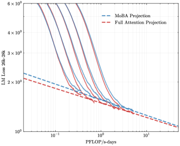
### Visual Description
## Chart: LM Loss vs. PFLOP/s-days
### Overview
The image presents a line chart comparing the Language Model (LM) Loss for two projection methods: MoBA Projection and Full Attention Projection, plotted against PFLOP/s-days (floating point operations per second per day). Multiple lines are shown for each projection method, likely representing different runs or configurations. The chart uses a logarithmic scale for both the y-axis (LM Loss) and the x-axis (PFLOP/s-days).
### Components/Axes
* **X-axis:** PFLOP/s-days, ranging from approximately 10<sup>-1</sup> to 10<sup>1</sup> (0.1 to 10).
* **Y-axis:** LM Loss 26k-28k, ranging from approximately 10<sup>0</sup> to 6 x 10<sup>6</sup> (1 to 6,000,000). The axis label indicates the loss is calculated for a model size of 26k-28k parameters.
* **Legend:** Located in the top-right corner.
* MoBA Projection (Blue dashed lines)
* Full Attention Projection (Red solid lines)
* **Gridlines:** Present on a logarithmic scale for both axes, aiding in value estimation.
### Detailed Analysis
**MoBA Projection (Blue dashed lines):**
There are approximately 6 blue dashed lines. The trend for all MoBA lines is a steep downward slope initially, flattening out as PFLOP/s-days increase.
* Line 1: Starts at approximately LM Loss = 2 x 10<sup>6</sup> at PFLOP/s-days = 10<sup>-1</sup>, decreasing to approximately LM Loss = 2 x 10<sup>1</sup> at PFLOP/s-days = 10<sup>1</sup>.
* Line 2: Starts at approximately LM Loss = 5 x 10<sup>5</sup> at PFLOP/s-days = 10<sup>-1</sup>, decreasing to approximately LM Loss = 3 x 10<sup>1</sup> at PFLOP/s-days = 10<sup>1</sup>.
* Line 3: Starts at approximately LM Loss = 3 x 10<sup>5</sup> at PFLOP/s-days = 10<sup>-1</sup>, decreasing to approximately LM Loss = 2 x 10<sup>1</sup> at PFLOP/s-days = 10<sup>1</sup>.
* Line 4: Starts at approximately LM Loss = 6 x 10<sup>5</sup> at PFLOP/s-days = 10<sup>-1</sup>, decreasing to approximately LM Loss = 3 x 10<sup>1</sup> at PFLOP/s-days = 10<sup>1</sup>.
* Line 5: Starts at approximately LM Loss = 4 x 10<sup>5</sup> at PFLOP/s-days = 10<sup>-1</sup>, decreasing to approximately LM Loss = 2 x 10<sup>1</sup> at PFLOP/s-days = 10<sup>1</sup>.
* Line 6: Starts at approximately LM Loss = 3 x 10<sup>5</sup> at PFLOP/s-days = 10<sup>-1</sup>, decreasing to approximately LM Loss = 2 x 10<sup>1</sup> at PFLOP/s-days = 10<sup>1</sup>.
**Full Attention Projection (Red solid lines):**
There are approximately 6 red solid lines. The trend for all Full Attention lines is also a steep downward slope initially, flattening out as PFLOP/s-days increase, but generally remaining at a lower LM Loss than the MoBA Projection lines.
* Line 1: Starts at approximately LM Loss = 1 x 10<sup>6</sup> at PFLOP/s-days = 10<sup>-1</sup>, decreasing to approximately LM Loss = 1 x 10<sup>1</sup> at PFLOP/s-days = 10<sup>1</sup>.
* Line 2: Starts at approximately LM Loss = 4 x 10<sup>5</sup> at PFLOP/s-days = 10<sup>-1</sup>, decreasing to approximately LM Loss = 1 x 10<sup>1</sup> at PFLOP/s-days = 10<sup>1</sup>.
* Line 3: Starts at approximately LM Loss = 3 x 10<sup>5</sup> at PFLOP/s-days = 10<sup>-1</sup>, decreasing to approximately LM Loss = 1 x 10<sup>1</sup> at PFLOP/s-days = 10<sup>1</sup>.
* Line 4: Starts at approximately LM Loss = 5 x 10<sup>5</sup> at PFLOP/s-days = 10<sup>-1</sup>, decreasing to approximately LM Loss = 1 x 10<sup>1</sup> at PFLOP/s-days = 10<sup>1</sup>.
* Line 5: Starts at approximately LM Loss = 3 x 10<sup>5</sup> at PFLOP/s-days = 10<sup>-1</sup>, decreasing to approximately LM Loss = 1 x 10<sup>1</sup> at PFLOP/s-days = 10<sup>1</sup>.
* Line 6: Starts at approximately LM Loss = 2 x 10<sup>5</sup> at PFLOP/s-days = 10<sup>-1</sup>, decreasing to approximately LM Loss = 1 x 10<sup>1</sup> at PFLOP/s-days = 10<sup>1</sup>.
### Key Observations
* Full Attention Projection consistently achieves lower LM Loss values than MoBA Projection across the entire range of PFLOP/s-days.
* The rate of loss reduction diminishes as PFLOP/s-days increase for both methods.
* There is variability in performance within each method, as indicated by the multiple lines. This suggests that factors beyond just the projection method influence the LM Loss.
### Interpretation
The chart demonstrates the trade-off between computational cost (PFLOP/s-days) and model performance (LM Loss). Full Attention Projection appears to be more efficient in achieving lower loss for a given computational budget compared to MoBA Projection. The multiple lines for each method suggest that the performance is not deterministic and is likely influenced by factors such as initialization, data distribution, or hyperparameter settings. The diminishing returns in loss reduction at higher PFLOP/s-days indicate that there is a point of diminishing returns where increasing computational cost yields only marginal improvements in model performance. This information is valuable for optimizing the training process of language models, allowing for informed decisions about the allocation of computational resources. The model size of 26k-28k parameters is a key parameter to consider when interpreting these results, as the optimal trade-off between cost and performance may vary for different model sizes.
</details>
(n) Scaling law (26-28k)
<details>
<summary>x27.png Details</summary>
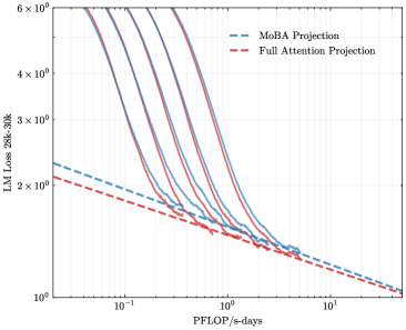
### Visual Description
## Line Chart: LM Loss vs. PFLOP/s-days
### Overview
This image presents a line chart comparing the Language Model (LM) Loss of two projection methods – MoBA Projection and Full Attention Projection – as a function of PFLOP/s-days (floating point operations per second per day). Multiple lines are shown for each projection method, likely representing different runs or configurations. The chart uses a logarithmic scale for both the y-axis (LM Loss) and the x-axis (PFLOP/s-days).
### Components/Axes
* **X-axis:** PFLOP/s-days, ranging from approximately 10<sup>-2</sup> to 10<sup>1</sup> (0.01 to 10). The scale is logarithmic.
* **Y-axis:** LM Loss 28k-30k, ranging from approximately 10<sup>0</sup> to 10<sup>6</sup> (1 to 1,000,000). The scale is logarithmic.
* **Legend:** Located in the top-right corner.
* MoBA Projection (Blue dashed lines)
* Full Attention Projection (Red solid lines)
* **Data Series:** Multiple lines for each projection method. There are approximately 6 lines for each method.
### Detailed Analysis
**MoBA Projection (Blue dashed lines):**
The MoBA Projection lines generally slope downward, indicating that as PFLOP/s-days increase, the LM Loss decreases.
* Line 1: Starts at approximately LM Loss = 2.5 x 10<sup>2</sup> (250) at PFLOP/s-days = 10<sup>-2</sup> (0.01), and decreases to approximately LM Loss = 2 x 10<sup>0</sup> (2) at PFLOP/s-days = 10<sup>1</sup> (10).
* Line 2: Starts at approximately LM Loss = 2 x 10<sup>2</sup> (200) at PFLOP/s-days = 10<sup>-2</sup> (0.01), and decreases to approximately LM Loss = 1.5 x 10<sup>0</sup> (1.5) at PFLOP/s-days = 10<sup>1</sup> (10).
* Line 3: Starts at approximately LM Loss = 1.5 x 10<sup>2</sup> (150) at PFLOP/s-days = 10<sup>-2</sup> (0.01), and decreases to approximately LM Loss = 1 x 10<sup>0</sup> (1) at PFLOP/s-days = 10<sup>1</sup> (10).
* Line 4: Starts at approximately LM Loss = 1 x 10<sup>2</sup> (100) at PFLOP/s-days = 10<sup>-2</sup> (0.01), and decreases to approximately LM Loss = 7 x 10<sup>-1</sup> (0.7) at PFLOP/s-days = 10<sup>1</sup> (10).
* Line 5: Starts at approximately LM Loss = 7 x 10<sup>1</sup> (70) at PFLOP/s-days = 10<sup>-2</sup> (0.01), and decreases to approximately LM Loss = 5 x 10<sup>-1</sup> (0.5) at PFLOP/s-days = 10<sup>1</sup> (10).
* Line 6: Starts at approximately LM Loss = 5 x 10<sup>1</sup> (50) at PFLOP/s-days = 10<sup>-2</sup> (0.01), and decreases to approximately LM Loss = 3 x 10<sup>-1</sup> (0.3) at PFLOP/s-days = 10<sup>1</sup> (10).
**Full Attention Projection (Red solid lines):**
The Full Attention Projection lines also slope downward, but generally start at a higher LM Loss and decrease more rapidly than the MoBA Projection lines.
* Line 1: Starts at approximately LM Loss = 5 x 10<sup>3</sup> (5000) at PFLOP/s-days = 10<sup>-2</sup> (0.01), and decreases to approximately LM Loss = 2 x 10<sup>0</sup> (2) at PFLOP/s-days = 10<sup>1</sup> (10).
* Line 2: Starts at approximately LM Loss = 4 x 10<sup>3</sup> (4000) at PFLOP/s-days = 10<sup>-2</sup> (0.01), and decreases to approximately LM Loss = 1.5 x 10<sup>0</sup> (1.5) at PFLOP/s-days = 10<sup>1</sup> (10).
* Line 3: Starts at approximately LM Loss = 3 x 10<sup>3</sup> (3000) at PFLOP/s-days = 10<sup>-2</sup> (0.01), and decreases to approximately LM Loss = 1 x 10<sup>0</sup> (1) at PFLOP/s-days = 10<sup>1</sup> (10).
* Line 4: Starts at approximately LM Loss = 2 x 10<sup>3</sup> (2000) at PFLOP/s-days = 10<sup>-2</sup> (0.01), and decreases to approximately LM Loss = 7 x 10<sup>-1</sup> (0.7) at PFLOP/s-days = 10<sup>1</sup> (10).
* Line 5: Starts at approximately LM Loss = 1.5 x 10<sup>3</sup> (1500) at PFLOP/s-days = 10<sup>-2</sup> (0.01), and decreases to approximately LM Loss = 5 x 10<sup>-1</sup> (0.5) at PFLOP/s-days = 10<sup>1</sup> (10).
* Line 6: Starts at approximately LM Loss = 1 x 10<sup>3</sup> (1000) at PFLOP/s-days = 10<sup>-2</sup> (0.01), and decreases to approximately LM Loss = 3 x 10<sup>-1</sup> (0.3) at PFLOP/s-days = 10<sup>1</sup> (10).
### Key Observations
* The Full Attention Projection consistently exhibits higher LM Loss values than the MoBA Projection across the entire range of PFLOP/s-days.
* Both projection methods demonstrate diminishing returns in loss reduction as PFLOP/s-days increase. The rate of loss decrease slows down at higher PFLOP/s-days values.
* The multiple lines for each projection method suggest variability in performance, potentially due to different initialization conditions, hyperparameters, or data subsets.
### Interpretation
The chart demonstrates the trade-off between computational cost (PFLOP/s-days) and model performance (LM Loss) for two different projection methods. The Full Attention Projection, while achieving lower loss values at higher computational costs, is significantly more expensive than the MoBA Projection. The MoBA Projection offers a more efficient approach to reducing LM Loss, albeit at a slightly higher loss value for a given computational budget. The variability between lines within each projection method suggests that the performance is not deterministic and may be sensitive to various factors. This data suggests that MoBA Projection is a more efficient method for reducing LM Loss, but Full Attention Projection can achieve lower loss values if computational resources are not a constraint. The logarithmic scales highlight the rapid initial improvement in loss reduction followed by diminishing returns, indicating a point of saturation where further increases in PFLOP/s-days yield minimal performance gains.
</details>
(o) Scaling law (28-30k)
<details>
<summary>x28.png Details</summary>

### Visual Description
\n
## Chart: LM Loss vs. PFLOP/s-days
### Overview
The image presents a line chart comparing the LM Loss (Language Model Loss) of two projection methods – MoBA Projection and Full Attention Projection – as a function of PFLOP/s-days (Peta Floating Point Operations per second-days). Multiple lines are shown for each projection method, likely representing different runs or configurations. The chart uses a logarithmic scale for both the y-axis (LM Loss) and the x-axis (PFLOP/s-days).
### Components/Axes
* **X-axis:** PFLOP/s-days, ranging from approximately 10<sup>-1</sup> to 10<sup>1</sup> (logarithmic scale).
* **Y-axis:** LM Loss 30k-32k, ranging from approximately 10<sup>0</sup> to 6 x 10<sup>6</sup> (logarithmic scale).
* **Legend:** Located in the top-right corner.
* MoBA Projection (Blue dashed lines)
* Full Attention Projection (Red solid lines)
* **Data Series:** Multiple lines for each projection method. There are approximately 6 lines for each method.
### Detailed Analysis
**MoBA Projection (Blue dashed lines):**
The MoBA Projection lines generally slope downward, indicating that as PFLOP/s-days increase, the LM Loss decreases. The lines start at varying points on the y-axis, but converge as PFLOP/s-days increase.
* Line 1: Starts at approximately 3 x 10<sup>6</sup> LM Loss at 10<sup>-1</sup> PFLOP/s-days, decreasing to approximately 10<sup>1</sup> LM Loss at 10<sup>1</sup> PFLOP/s-days.
* Line 2: Starts at approximately 2 x 10<sup>6</sup> LM Loss at 10<sup>-1</sup> PFLOP/s-days, decreasing to approximately 10<sup>1</sup> LM Loss at 10<sup>1</sup> PFLOP/s-days.
* Line 3: Starts at approximately 1.5 x 10<sup>6</sup> LM Loss at 10<sup>-1</sup> PFLOP/s-days, decreasing to approximately 10<sup>1</sup> LM Loss at 10<sup>1</sup> PFLOP/s-days.
* Line 4: Starts at approximately 1 x 10<sup>6</sup> LM Loss at 10<sup>-1</sup> PFLOP/s-days, decreasing to approximately 10<sup>1</sup> LM Loss at 10<sup>1</sup> PFLOP/s-days.
* Line 5: Starts at approximately 5 x 10<sup>5</sup> LM Loss at 10<sup>-1</sup> PFLOP/s-days, decreasing to approximately 10<sup>1</sup> LM Loss at 10<sup>1</sup> PFLOP/s-days.
* Line 6: Starts at approximately 3 x 10<sup>5</sup> LM Loss at 10<sup>-1</sup> PFLOP/s-days, decreasing to approximately 10<sup>1</sup> LM Loss at 10<sup>1</sup> PFLOP/s-days.
**Full Attention Projection (Red solid lines):**
The Full Attention Projection lines also slope downward, showing a decrease in LM Loss with increasing PFLOP/s-days. These lines generally start at lower LM Loss values than the MoBA Projection lines and also converge as PFLOP/s-days increase.
* Line 1: Starts at approximately 2 x 10<sup>6</sup> LM Loss at 10<sup>-1</sup> PFLOP/s-days, decreasing to approximately 10<sup>0</sup> LM Loss at 10<sup>1</sup> PFLOP/s-days.
* Line 2: Starts at approximately 1.5 x 10<sup>6</sup> LM Loss at 10<sup>-1</sup> PFLOP/s-days, decreasing to approximately 10<sup>0</sup> LM Loss at 10<sup>1</sup> PFLOP/s-days.
* Line 3: Starts at approximately 1 x 10<sup>6</sup> LM Loss at 10<sup>-1</sup> PFLOP/s-days, decreasing to approximately 10<sup>0</sup> LM Loss at 10<sup>1</sup> PFLOP/s-days.
* Line 4: Starts at approximately 5 x 10<sup>5</sup> LM Loss at 10<sup>-1</sup> PFLOP/s-days, decreasing to approximately 10<sup>0</sup> LM Loss at 10<sup>1</sup> PFLOP/s-days.
* Line 5: Starts at approximately 3 x 10<sup>5</sup> LM Loss at 10<sup>-1</sup> PFLOP/s-days, decreasing to approximately 10<sup>0</sup> LM Loss at 10<sup>1</sup> PFLOP/s-days.
* Line 6: Starts at approximately 2 x 10<sup>5</sup> LM Loss at 10<sup>-1</sup> PFLOP/s-days, decreasing to approximately 10<sup>0</sup> LM Loss at 10<sup>1</sup> PFLOP/s-days.
### Key Observations
* Full Attention Projection consistently achieves lower LM Loss values than MoBA Projection across the entire range of PFLOP/s-days.
* The multiple lines for each projection method suggest variability in performance, potentially due to different initialization, hyperparameters, or data subsets.
* The convergence of lines for both methods at higher PFLOP/s-days indicates diminishing returns in terms of LM Loss reduction as computational resources increase.
### Interpretation
The chart demonstrates the trade-off between computational cost (PFLOP/s-days) and model performance (LM Loss). Full Attention Projection appears to be more efficient in achieving lower LM Loss for a given amount of computation compared to MoBA Projection. However, both methods exhibit a decreasing rate of improvement as PFLOP/s-days increase, suggesting that there is a point of diminishing returns. The spread of lines within each method indicates that the performance is not deterministic and can vary. This could be due to the stochastic nature of training deep learning models. The logarithmic scales on both axes highlight the significant changes in both LM Loss and PFLOP/s-days, and the chart effectively visualizes the relationship between these two key metrics. The data suggests that while increasing computational resources can improve model performance, the benefits may become marginal beyond a certain point, and the choice of projection method significantly impacts efficiency.
</details>
(p) Scaling law (30-32k)
Figure 8: Scaling laws for positions 16-32k
Table 3: Loss scaling with different positions
| 0K - 2K 2K - 4K 4K - 6K | $3.075\times C^{-0.078}$ $2.415\times C^{-0.084}$ $2.085\times C^{-0.081}$ | $3.068\times C^{-0.078}$ $2.411\times C^{-0.083}$ $2.077\times C^{-0.081}$ |
| --- | --- | --- |
| 6K - 8K | $1.899\times C^{-0.092}$ | $1.894\times C^{-0.092}$ |
| 8K - 10K | $1.789\times C^{-0.091}$ | $1.774\times C^{-0.089}$ |
| 10K - 12K | $1.721\times C^{-0.092}$ | $1.697\times C^{-0.087}$ |
| 12K - 14K | $1.670\times C^{-0.089}$ | $1.645\times C^{-0.088}$ |
| 14K - 16K | $1.630\times C^{-0.089}$ | $1.600\times C^{-0.087}$ |
| 16K - 18K | $1.607\times C^{-0.090}$ | $1.567\times C^{-0.087}$ |
| 18K - 20K | $1.586\times C^{-0.091}$ | $1.542\times C^{-0.087}$ |
| 20K - 22K | $1.571\times C^{-0.093}$ | $1.519\times C^{-0.086}$ |
| 22K - 24K | $1.566\times C^{-0.089}$ | $1.513\times C^{-0.085}$ |
| 24K - 26K | $1.565\times C^{-0.091}$ | $1.502\times C^{-0.085}$ |
| 26K - 28K | $1.562\times C^{-0.095}$ | $1.493\times C^{-0.088}$ |
| 28K - 30K | $1.547\times C^{-0.097}$ | $1.471\times C^{-0.091}$ |
| 30K - 32K | $1.546\times C^{-0.108}$ | $1.464\times C^{-0.097}$ |