2502.14837

# Towards Economical Inference: Enabling DeepSeek’s Multi-Head Latent Attention in Any Transformer-based LLMs ## Abstract Multi-head Latent Attention (MLA) is an innovative architecture proposed by DeepSeek, designed to ensure efficient and economical inference by significantly compressing the Key-Value (KV) cache into a latent vector. Compared to MLA, standard LLMs employing Multi-Head Attention (MHA) and its variants such as Grouped-Query Attention (GQA) exhibit significant cost disadvantages. Enabling well-trained LLMs (e.g., Llama) to rapidly adapt to MLA without pre-training from scratch is both meaningful and challenging. This paper proposes the first data-efficient fine-tuning method for transitioning from MHA to MLA (MHA2MLA), which includes two key components: for partial-RoPE, we remove RoPE from dimensions of queries and keys that contribute less to the attention scores, for low-rank approximation, we introduce joint SVD approximations based on the pre-trained parameters of keys and values. These carefully designed strategies enable MHA2MLA to recover performance using only a small fraction (0.6% to 1%) of the data, significantly reducing inference costs while seamlessly integrating with compression techniques such as KV cache quantization. For example, the KV cache size of Llama2-7B is reduced by 92.19%, with only a 1% drop in LongBench performance. Our source code is publicly available at https://github.com/JT-Ushio/MHA2MLA. Towards Economical Inference: Enabling DeepSeek’s Multi-Head Latent Attention in Any Transformer-based LLMs Tao Ji 1,6, Bin Guo 2, Yuanbin Wu 2, Qipeng Guo 8, Lixing Shen 7, Zhan Chen 7, Xipeng Qiu 1, Qi Zhang 1,4,5, Tao Gui 3,4,5 1 School of Computer Science, Fudan University 2 School of Computer Science and Technology, East China Normal University 3 Institute of Modern Languages and Linguistics, Fudan University 4 Institute of Trustworthy Embodied Artificial Intelligence, Fudan University 5 Shanghai Collaborative Innovation Center of Intelligent Visual Computing 6 Pengcheng Laboratory 7 Hikvision Inc 8 Shanghai Al Lab {taoji, tgui}@fudan.edu.cn {binguo@stu, ybwu@cs}.ecnu.edu.cn ## 1 Introduction <details> <summary>x1.png Details</summary>  ### Visual Description ## Diagram: Attention Mechanism Architectures Comparison ### Overview The diagram illustrates three attention mechanism architectures: (a) MHA (Multi-Head Attention), (b) MHA2MLA (Multi-Head Attention to Multi-Layer Attention), and (c) MLA (Multi-Layer Attention). Each architecture is represented as a flow of operations with labeled components, weights, and transformations. The legend at the top defines symbols for operations (e.g., Linear, Apply RoPE, Cached, Aligned, Split). ### Components/Axes - **Legend**: - **Linear**: Purple trapezoid (e.g., `W_q`, `W_k`, `W_v`). - **Apply RoPE**: Pink square with stripes (e.g., `RoPE` blocks). - **Cached**: Purple square with diagonal stripes (e.g., `C_kv`). - **Aligned**: Gray rectangle (e.g., `Aligned` blocks). - **Split**: Scissors icon (e.g., `Split` operations). - **Key Elements**: - **Input**: `x` (top-left of each architecture). - **Weights**: `W_q`, `W_k`, `W_v`, `W_dq`, `W_dk`, `W_dv`, `W_qr`, `W_qk`, `W_uk`, `W_uv`. - **Operations**: - `RoPE` (Rotary Positional Encoding). - `Partial RoPE` (applied selectively). - `C_kv` (Cached key-value pairs). - `Split` (divides data streams). ### Detailed Analysis #### (a) MHA (Multi-Head Attention) 1. **Flow**: - `x` → Linear projections (`W_q`, `W_k`, `W_v`) → `RoPE` applied to `q` and `k` → Output `q`, `k`. 2. **Components**: - Standard attention weights (`W_q`, `W_k`, `W_v`). - Full `RoPE` applied to both `q` and `k`. #### (b) MHA2MLA (Multi-Head to Multi-Layer Attention) 1. **Flow**: - `x` → Linear projections (`W_q`, `W_k`, `W_v`) → Partial `RoPE` applied to `q` and `k` → Split into `q_rope`, `q_nope`, `k_rope`, `k_nope`. - `C_kv` (Cached `k` and `v`) → `W_uk`, `W_uv` → `k_rope`, `k_nope`, `v`. 2. **Components**: - Partial `RoPE` applied only to `q_rope` and `k_rope`. - Cached `C_kv` reused for efficiency. - Additional weights (`W_uk`, `W_uv`) for residual connections. #### (c) MLA (Multi-Layer Attention) 1. **Flow**: - `x` → Linear projections (`W_dq`, `W_dk`, `W_dv`) → `RoPE` applied to `q_rope` and `k_rope` → Split into `q_rope`, `q_nope`, `k_rope`, `k_nope`, `v`. - `C_kv` (Cached `k` and `v`) → `W_qr`, `W_qk`, `W_uk`, `W_uv` → Final `q`, `k`, `v`. 2. **Components**: - Deeper linear projections (`W_dq`, `W_dk`, `W_dv`). - Full `RoPE` applied to `q_rope` and `k_rope`. - Multiple cached streams (`C_kv`) and residual weights. ### Key Observations 1. **Efficiency Improvements**: - MHA2MLA and MLA introduce **partial RoPE** and **caching** to reduce computational overhead. - MLA further optimizes by splitting and reusing cached `k`/`v` pairs. 2. **Architectural Complexity**: - MLA has the most components (e.g., `W_dq`, `W_dk`, `W_dv`), suggesting deeper processing layers. - MHA2MLA bridges MHA and MLA with hybrid operations. 3. **Symbol Consistency**: - All `RoPE` operations are marked with pink stripes. - Cached components (`C_kv`) use diagonal stripes. ### Interpretation The diagram demonstrates a progression from basic MHA to more efficient MHA2MLA and MLA architectures. By introducing **partial RoPE** and **caching**, MHA2MLA reduces redundant computations while maintaining positional encoding benefits. MLA further optimizes by splitting and reusing cached data, likely improving memory efficiency and scalability. The use of **residual connections** (e.g., `W_uk`, `W_uv`) suggests an emphasis on gradient flow and model stability. These modifications align with trends in transformer optimization for large-scale models, balancing accuracy and computational cost. 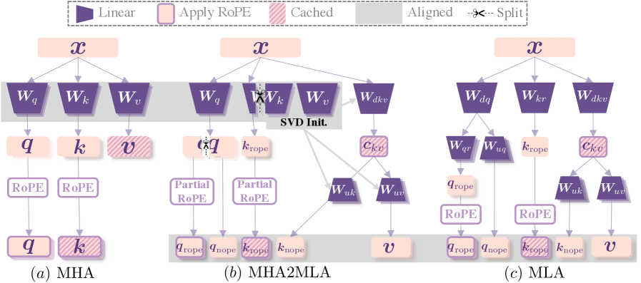</details> Figure 1: The diagram illustrates the MHA, MLA, and our MHA2MLA. It can be seen that the “cached” part is fully aligned with MLA after MHA2MLA. The input to the attention module is also completely aligned with MLA (the aligned region below). Meanwhile, the parameters in MHA2MLA maximize the use of pre-trained parameters from MHA (the aligned region above). The rapid advancement of large language models (LLMs) has significantly accelerated progress toward artificial general intelligence (AGI), with model capabilities scaling predictably with parameter counts Kaplan et al. (2020). However, these gains come at a steep cost: escalating computational demands for training and degraded inference throughput, resulting in substantial energy consumption and carbon emissions Strubell et al. (2019). As downstream tasks grow increasingly complex, long-context processing and computationally intensive inference have become central to LLM applications An et al. (2024). A key bottleneck lies in the memory footprint of the Key-Value (KV) cache inherent to the Multi-Head Attention (MHA, 2017) mechanism, which scales linearly with sequence length and model size. To mitigate this, variants like Grouped-Query Attention (GQA, 2023) and Multi-Query Attention (MQA, 2019) have been explored. However, these methods reduce not only the KV cache size but also the number of parameters in the attention, leading to performance degradation. The DeepSeek introduces Multi-Head Latent Attention (MLA, 2024), an attention mechanism equipped with low-rank key-value joint compression. Empirically, MLA achieves superior performance compared with MHA, and meanwhile significantly reduces the KV cache during inference, thus boosting the inference efficiency. A critical yet unexplored question arises: Can LLMs originally well-trained for MHA be adapted to enabling MLA for inference? The inherent architectural disparities between MHA and MLA render zero-shot transfer impractical, while the prohibitive cost of pretraining from scratch makes this transition both technically challenging and underexplored in existing research. To address this gap, we propose the first carefully designed MHA2MLA framework that maximizes parameter reuse from pre-trained MHA networks while aligning the KV cache storage and inference process with MLA’s paradigm (Figure ˜ 1). Our framework features two pivotal technical innovations: partial rotary position embedding (partial RoPE) and low-rank approximation. The primary objective of MHA2MLA is to achieve data-efficient performance recovery - restoring architecture-induced capability degradation using minimal fine-tuning data. The inherent incompatibility between MLA’s inference acceleration mechanism and RoPE necessitates architectural compromises. DeepSeek’s solution preserves PEs in limited dimensions while compressing others, requiring strategic removal of RoPE dimensions (converting them to NoPE) in MHA to achieve MLA alignment. While higher removal ratios enhance compression efficiency, they exacerbate performance degradation, creating an efficiency-capability trade-off. Through systematically exploring RoPE removal strategies, we identify that contribution-aware dimension selection (retaining top-k dimensions ranked by attention score impact) optimally balances these competing objectives. Although previous studies have investigated training partial-RoPE LLMs from scratch Black et al. (2021); Barbero et al. (2024), our work pioneers data-efficient fine-tuning for full-to-partial RoPE conversion in LLMs. MLA reduces memory footprint by projecting keys and values into a low-rank latent representation space (stored in the KV cache). MHA2MLA can also apply low-rank approximation to the values and keys stripped of RoPE (NoPE dimensions). By performing Singular Value Decomposition (SVD) on the pre-trained parameter matrices $\bm{W}_v$ and $\bm{W}_k$ corresponding to the NoPE subspaces, we compress these components into a latent space while maximizing the retention of knowledge learned by the original model. Our main contributions are: - we introduce MHA2MLA, the first parameter-efficient fine-tuning framework that adapts pre-trained MHA-based LLMs to the MLA architecture using only 0.6% to 1% of training data without training from scratch. - we demonstrate that the MHA2MLA architecture can be integrated with KV-cache quantization to achieve more economical inference (up to a 96.87% reduction). - we conduct experiments across five model sizes (from 135M to 13B, covering both MHA and GQA), and detailed ablation studies to provide guidance and insights for MHA2MLA. ## 2 Preliminary ### 2.1 Multi-Head Attention (MHA) Given an input sequence $\{\bm{x}_1,\dots,\bm{x}_l\}∈ℝ^l× d$ , standard MHA Vaswani et al. (2017) projects each token $\bm{x}_i$ into queries $\bm{q}_i^(h)=\bm{x}_i\bm{W}_q^(h)$ , keys $\bm{k}_i^(h)=\bm{x}_i\bm{W}_k^(h)$ , and values $\bm{v}_i^(h)=\bm{x}_i\bm{W}_v^(h)$ , where $\bm{W}_q^(h),\bm{W}_k^(h),\bm{W}_v^(h)∈ℝ^d× d_h$ for each head $h∈\{1,\dots,n_h\}$ . The Rotary positional encoding (RoPE, 2024) is applied to queries and keys (e.g., $\bm{k}_i,rope^(h)=RoPE(\bm{k}_i^(h))$ ), followed by scaled dot-product attention We ignore here the $\frac{1}{√{d}}$ scaling factor for ease of notation. : $$ \displaystyle\bm{o}_i^(h)=Softmax≤ft(\bm{q}_i,rope^(h)\bm{k}_≤ i,rope^(h)⊤\right)\bm{v}_≤ i^(h), \displaystyleMHA(\bm{x}_i)=≤ft[\bm{o}_i^(1),\dots,\bm{o}_i^(n_h)\right]\bm{W}_o, \tag{1} $$ where $\bm{W}_o∈ℝ^(n_hd_h)× d$ and $[·,·]$ means vector concatenate. During autoregressive inference, MHA stores the KV cache $\{\bm{k}_rope^(h),\bm{v}^(h)\}_h=1^n_h$ of size $O(2ln_hd_h)$ , growing linearly with sequence length $l$ , posing memory bottlenecks. #### Variants: Grouped-Query Attention (GQA, 2023) shares keys/values across $n_g$ groups ( $n_g\ll n_h$ ) to reduce the KV cache. For each head $h$ , it maps to group $g=\lfloor\frac{h× n_g}{n_h}\rfloor$ : $$ \displaystyle\bm{o}_i^(h)=Softmax≤ft(\bm{q}_i,rope^(h)\bm{k}_≤ i,rope^(g)⊤\right)\bm{v}_≤ i^(g), \displaystyleGQA(\bm{x}_i)=≤ft[\bm{o}_i^(1),\dots,\bm{o}_i^(n_h)\right]\bm{W}_o. \tag{1} $$ Multi-Query Attention (MQA, 2019) is a special case of GQA with $n_g=1$ , i.e., all heads share a single global key/value. While reducing the KV cache to $O(2ln_gd_h)$ , these methods degrade performance due to parameter pruning. ### 2.2 Multi-Head Latent Attention (MLA) MLA DeepSeek-AI et al. (2024) introduces a hybrid architecture that decouples PE from latent KV compression. For each head $h$ , the input $\bm{x}_i$ is projected into two complementary components: #### Position-Aware Component A subset of dimensions retains PE to preserve positional sensitivity: $$ \bm{q}_i,rope^(h),\bm{k}_i,rope=RoPE≤ft(\bm{x}_i\bm{W}_dq\bm{W}_qr^(h),\bm{x}_i\bm{W}_kr\right), $$ where $\bm{W}_dq∈ℝ^d× d_q$ , $\bm{W}_qr^(h)∈ℝ^d_q× d_r$ , $\bm{W}_kr∈ℝ^d× d_r$ project queries/keys into a RoPE-preserved component of dimension $d_r$ . #### Position-Agnostic Component The remaining dimensions $d_c$ are stripped of PE (i.e., NoPE), $\bm{k}_i,nope^(h)$ and $\bm{v}_i^(h)$ and compressed into a shared latent vector $\bm{c}_i,kv^(h)$ : | | $\displaystyle\bm{q}_i,nope^(h)$ | $\displaystyle=\bm{x}_i\bm{W}_dq\bm{W}_qc^(h),$ | | | --- | --- | --- | --- | where $\bm{W}_qc^(h)∈ℝ^d_q× d_c$ , $\bm{W}_dkv∈ℝ^d× d_kv$ , $\bm{W}_uk^(h)∈ℝ^d_kv× d_c$ , $\bm{W}_uv^(h)∈ℝ^d_kv× d_h$ . Note that $d_r+d_c=d_h$ . The attention output of MLA combines both components: $$ \displaystyle\bm{o}_i^(h)=Softmax≤ft(\bm{q}_i,rope^(h)\bm{k}_≤ i,rope^(h)⊤+\bm{q}_i,nope\bm{k}_≤ i,nope^(h)⊤\right) \displaystyle ·\bm{v}_≤ i^(h) \displaystyle MLA(\bm{x}_i)=≤ft[\bm{o}_i^(1),\dots,\bm{o}_i^(n_h)\right]·\bm{W}_o. \tag{1} $$ Unlike MHA and its variants, MLA stores the latent vector $\bm{c}_kv$ and $\bm{k}_i,rope^(h)$ ( $O≤ft(ld_r+ld_kv)\right)$ ) instead of full-rank $\bm{k}_i,\bm{v}_i$ ( $O(2ln_hd_h)$ ), where $(d_r+d_kv)\ll 2n_hd_h$ . #### Why does MLA need to separate RoPE and NoPE? MLA introduces matrix merging techniques for the NoPE portion during inference, effectively reducing memory usage. For the dot product operation $\bm{q}_i,nope^(h)\bm{k}_j,nope^(h)⊤$ , the following identity transformation can be applied To simplify the notation, we omit the superscript (h). Matrices $\bm{W}_uv$ and $\bm{W}_o$ can also be merged, please refer to Appendix C by DeepSeek-AI et al. (2024).: | | $\displaystyle\bm{q}_i,nope\bm{k}_j,nope^⊤$ | $\displaystyle=≤ft(\bm{x}_i\bm{W}_dq\bm{W}_qc\right)≤ft(\bm{c}_j,kv\bm{W}_uk\right)^⊤$ | | | --- | --- | --- | --- | where $≤ft(\bm{W}_dq\bm{W}_qc\bm{W}_uk^⊤\right)$ can be pre-merged into a single matrix, and $\bm{c}_j,kv$ is already stored in the KV cache. As for the RoPE portion, the RoPE( $·$ ) function multiplies the input vector by the rotation matrix (e.g., RoPE( $\bm{q}_i$ ) = $\bm{q}_i\bm{R}_i$ , $\bm{R}_i$ ’s specific form will be introduced in Section ˜ 3.1). Therefore, the identity transformation becomes as follows: | | $\displaystyle\bm{q}_i,rope\bm{k}_j,rope^⊤$ | $\displaystyle=≤ft(\bm{x}_i\bm{W}_dq\bm{W}_qr\bm{R}_i\right)≤ft(\bm{x}_j\bm{W}_kr\bm{R}_j\right)^⊤$ | | | --- | --- | --- | --- | Since $≤ft(\bm{W}_dq\bm{W}_qc\bm{R}_j-i\bm{W}_kr^⊤\right)$ is related to the relative position $j-i$ , it cannot be merged into a fixed matrix. Considering that the relative distances in LLMs can be very long, such as 128K, the RoPE portion is better suited to be computed using the original form. ## 3 MHA2MLA ### 3.1 Partial-RoPE To enable migration from standard MHA to MLA, we propose partial-RoPE finetuning, a strategy that removes RoPE from a targeted proportion of dimensions and converts them into NoPE. Critically, while prior work has explored training LLMs with partial-RoPE from scratch (achieving marginally better perplexity than full-RoPE Black et al. (2021); Barbero et al. (2024)), no existing method addresses how to efficiently adapt pre-trained full-RoPE models (e.g., Llama) to partial-RoPE without costly retraining. Our work bridges this gap by systematically evaluating partial-RoPE variants to identify the most data-efficient fine-tuning protocol for recovering model performance post-adaptation. <details> <summary>x2.png Details</summary>  ### Visual Description ## Chart/Diagram Type: Spectral Region Analysis with 2-Norm Values ### Overview The image presents a technical diagram comparing spectral regions (S_high, S_low, S_uniform, S_2-norm) across different panels. A left panel shows "q/k" and "RoPE θ_k" with white circles, while the right side features a vertical axis labeled "2-norm" with values 20.0, 1.0, 5.0, and 15.0. Each panel (a-d) visualizes spectral oscillations and shaded regions, with varying complexity and 2-norm values. ### Components/Axes - **Left Panel**: - **X-axis**: "q/k" (horizontal axis). - **Y-axis**: "RoPE θ_k" (vertical axis). - **Visual Elements**: White circles stacked vertically, separated by dashed lines. - **Right Side (Vertical Axis)**: - **Label**: "2-norm" (vertical axis). - **Values**: 20.0, 1.0, 5.0, 15.0 (listed in descending order from top to bottom). - **Legend**: Purple lines (solid) and white shaded regions (dashed). - **Panels (a-d)**: - **(a) S_high**: High-frequency oscillations with multiple white shaded regions. - **(b) S_low**: Lower-frequency oscillations with fewer shaded regions. - **(c) S_uniform**: Minimal oscillations with uniform shading. - **(d) S_2-norm**: Fewest oscillations and most uniform shading. ### Detailed Analysis - **Panel (a) S_high**: - **Oscillations**: 5–6 high-frequency waves. - **Shaded Regions**: 3–4 white blocks (likely representing constraints or excluded ranges). - **2-norm Value**: 20.0 (highest, top of the vertical axis). - **Panel (b) S_low**: - **Oscillations**: 2–3 lower-frequency waves. - **Shaded Regions**: 2 white blocks. - **2-norm Value**: 1.0 (lowest, bottom of the vertical axis). - **Panel (c) S_uniform**: - **Oscillations**: 1–2 waves. - **Shaded Regions**: 1 large white block. - **2-norm Value**: 5.0 (middle of the vertical axis). - **Panel (d) S_2-norm**: - **Oscillations**: 1 wave. - **Shaded Regions**: 1 large white block. - **2-norm Value**: 15.0 (second-highest, near the top). ### Key Observations 1. **Oscillation Complexity**: Decreases from (a) to (d), with S_high having the most oscillations and S_2-norm the fewest. 2. **Shaded Regions**: Increase in uniformity and coverage from (a) to (d), suggesting a trade-off between spectral complexity and normalization. 3. **2-norm Values**: - S_high (20.0) and S_2-norm (15.0) have the highest values. - S_low (1.0) and S_uniform (5.0) have significantly lower values, indicating potential anomalies or normalization effects. 4. **Vertical Axis Order**: The 2-norm values are listed as 20.0, 1.0, 5.0, 15.0, which may reflect a non-linear scaling or a labeling error. ### Interpretation The diagram illustrates how spectral regions (S_high, S_low, S_uniform, S_2-norm) vary in complexity and 2-norm values. The reduction in oscillations and increase in uniform shading from (a) to (d) suggest a process of simplification or normalization. The 2-norm values (20.0, 1.0, 5.0, 15.0) may represent a metric (e.g., energy, error) that decreases with spectral complexity, though the irregular ordering of values (1.0 and 5.0) warrants further investigation. The white shaded regions likely denote excluded or constrained ranges, emphasizing the impact of spectral region selection on the analyzed metric. ### Notable Anomalies - The 2-norm value for S_low (1.0) is significantly lower than S_uniform (5.0), despite S_low having fewer oscillations. This could indicate a non-linear relationship between spectral complexity and the 2-norm metric. - The vertical axis labels (20.0, 1.0, 5.0, 15.0) are not in descending order, suggesting a possible error in the diagram or a specific scaling rationale. ### Conclusion This diagram highlights the interplay between spectral region characteristics (frequency, shading) and a normalized metric (2-norm). The trends suggest that higher-frequency regions (S_high) are more complex and have higher 2-norm values, while lower-frequency regions (S_2-norm) are simpler but exhibit intermediate 2-norm values. Further analysis is needed to resolve the anomalies in the 2-norm scaling. 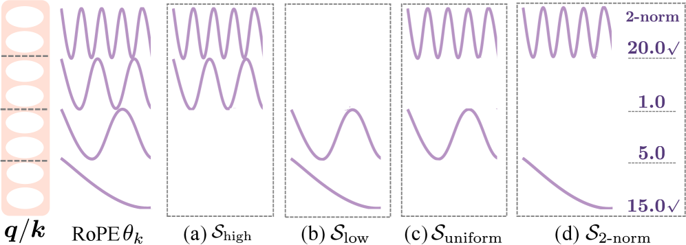</details> Figure 2: Illustration of $S_high$ , $S_low$ , $S_uniform$ , $S_2-norm$ . Where $d_h=8$ and $r=2$ . <details> <summary>x3.png Details</summary>  ### Visual Description ## Heatmap: Mean 2-norm Distribution Across Llama2-7B Layers and Heads ### Overview The image is a heatmap visualizing the distribution of Mean 2-norm values across different layers and attention heads of the Llama2-7B model. The y-axis categorizes frequencies into "Low Frequencies" (bottom) and "High Frequencies" (top), while the x-axis lists specific layers (3, 8, 16, 23) and their associated attention heads (Head 4, 23, 12, 14). Color intensity represents Mean 2-norm magnitudes, with darker purple indicating higher values. ### Components/Axes - **X-axis (Layers/Heads)**: - Layer 3 (Head 4) - Layer 8 (Head 23) - Layer 16 (Head 12) - Layer 23 (Head 14) - **Y-axis (Frequencies)**: - "Low Frequencies" (bottom half) - "High Frequencies" (top half) - **Color Bar**: - Label: "Mean 2-norm" - Scale: 0.0 (light pink) to 20.0 (dark purple), with increments of 2.5 - **Red Dashed Lines**: - Horizontal lines spanning the heatmap, likely indicating thresholds or reference values. ### Detailed Analysis - **Color Intensity Patterns**: - **Layer 23 (Head 14)**: Darkest purple in "Low Frequencies," suggesting the highest Mean 2-norm values (~17.5–20.0). - **Layer 16 (Head 12)**: Moderate purple in "Low Frequencies" (~10.0–12.5). - **Layer 8 (Head 23)**: Lighter purple in "Low Frequencies" (~7.5–10.0). - **Layer 3 (Head 4)**: Lightest purple in "Low Frequencies" (~2.5–5.0). - "High Frequencies" generally show lighter shades across all layers, with values below ~7.5. - **Red Dashed Lines**: - Positioned at ~10.0 (mid-scale) and ~15.0 (upper-scale), dividing regions of lower and higher values. - Align with transitions between "Low" and "High Frequencies" in some layers. ### Key Observations 1. **Layer Depth Correlation**: - Deeper layers (e.g., Layer 23) exhibit higher Mean 2-norm values in "Low Frequencies," while shallower layers (e.g., Layer 3) show lower values. 2. **Head-Specific Variability**: - Head 14 (Layer 23) stands out as an outlier with the highest values. 3. **Frequency Band Contrast**: - "Low Frequencies" consistently show darker shades than "High Frequencies," indicating stronger signal magnitudes in lower-frequency components. ### Interpretation The heatmap suggests that deeper layers (e.g., Layer 23) and specific attention heads (e.g., Head 14) process information with higher signal magnitudes in "Low Frequencies," potentially reflecting their role in capturing complex patterns. The red dashed lines may demarcate regions where values exceed critical thresholds, possibly linked to model performance or interpretability metrics. The dominance of "Low Frequencies" in deeper layers aligns with theories that later transformer layers specialize in abstract, high-level representations. The absence of extreme values in "High Frequencies" across most layers implies that high-frequency components are less dominant in this model's architecture. 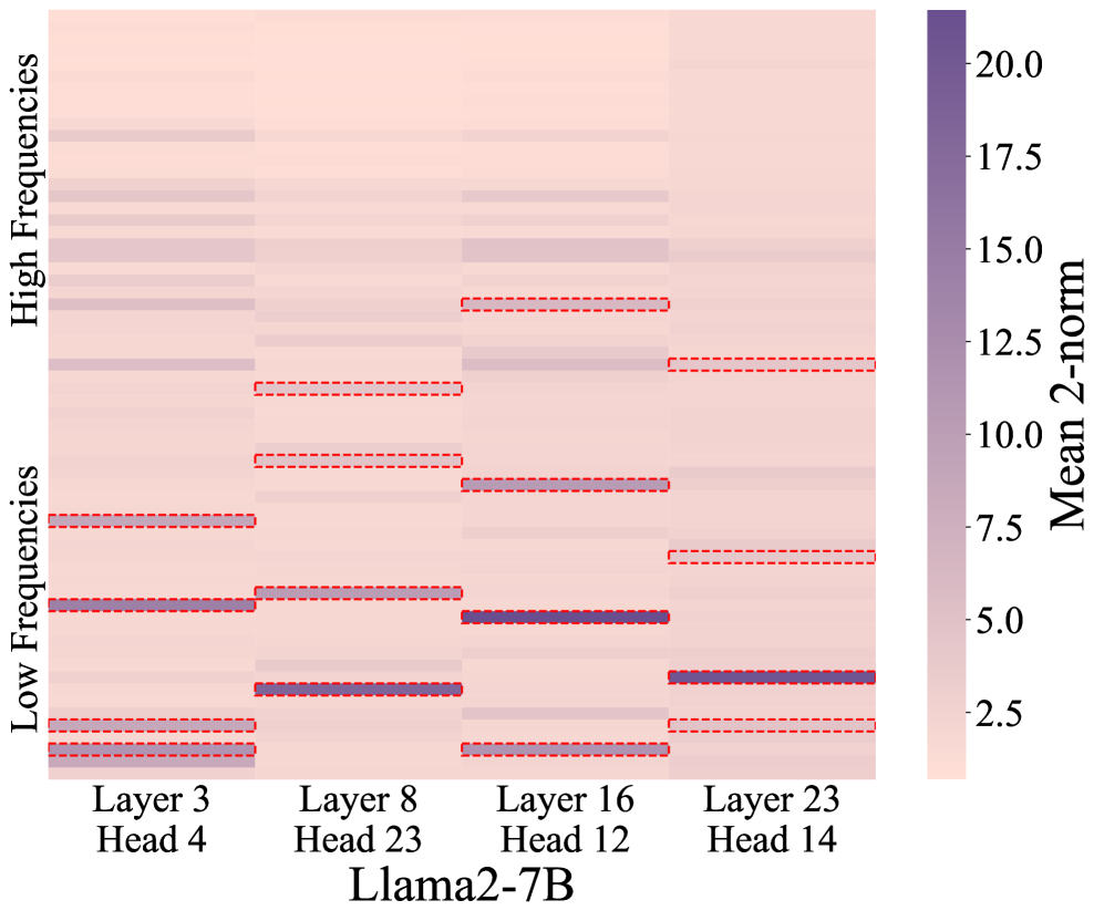</details> Figure 3: Visualization of Head-wise 2-norm Contribution for Llama2-7B. We randomly selected 4 heads, and the red dashed box highlights the top- $4$ frequency subspaces chosen when $r=4$ . It can be seen that different heads tend to focus on different frequency subspaces, which validates the rationality of our $S_2-norm$ method. #### MHA’s Full-RoPE encodes positional information into queries and keys through frequency-specific rotations. Formally, given a query vector $\bm{q}_i∈ℝ^d_h$ and key vector $\bm{k}_i∈ℝ^d_h$ , we partition them into 2D chunks: | | $\displaystyle\bm{q}_i,\bm{k}_i=≤ft[\bm{q}_i^[2k,2k+1]\right]_0≤ k<\frac{d_{h}{2}},≤ft[\bm{k}_i^[2k,2k+1]\right]_0≤ k<\frac{d_{h}{2}},$ | | | --- | --- | --- | where $\bm{q}_i^[2k,2k+1]∈ℝ^2$ denotes the $k$ -th 2D subspace. Each chunk undergoes a rotation by position-dependent angles $θ_k=β^-2k/{d_h}$ , forming a spectrum of wavelengths. High-frequency components, e.g., $k=0$ , rotate rapidly at 1 radian per token. Low-frequency components, e.g., $k=\frac{d_h}{2}-1$ , rotate slowly at $∼β^1/d_h$ radians per token. The base wavelength $β$ , typically set to $10^4$ Su et al. (2024) or $5×10^5$ . Formally, for each 2D chunk $\bm{q}_i^[2k,2k+1]$ and $\bm{k}_i^[2k,2k+1]$ , the rotation matrix at position $i$ is defined as: $$ \bm{R}_i^[2k,2k+1](θ_k)=\begin{bmatrix}\cos(iθ_k)&-\sin(iθ_k)\\ \sin(iθ_k)&\cos(iθ_k)\end{bmatrix}. $$ Thus, applying RoPE to queries and keys becomes: | | $\displaystyle\bm{q}_i,rope=≤ft[\bm{R}_i^[2k,2k+1](θ_k)\bm{q}_i^[2k,2k+1]\right]_0≤ k<\frac{d_{h}{2}},$ | | | --- | --- | --- | #### Full-RoPE to Partial-RoPE Strategies Given $r$ retained rotational subspaces( $r=\frac{d_r}{2}\ll$ total subspaces $\frac{d_h}{2}$ , we propose four strategies (illustrated in Figure ˜ 2) to select which $r$ subspaces preserve RoPE encoding: High-Frequency Preservation retain the $r$ fastest-rotating (high-frequency) subspaces: $$ S_high=≤ft\{k | 0≤ k<r\right\}. $$ It is consistent with the p-RoPE method proposed in Barbero et al. (2024), where they explored settings in which $r$ constituted 25%, 50%, and 75% of the total subspaces, and observed a slight advantage over full-RoPE in LLMs trained from scratch. Low-Frequency Preservation retain the $r$ slowest-rotating (low-frequency) subspaces: $$ S_low=≤ft\{k \big| \frac{d_h}{2}-r≤ k<\frac{d_h}{2}\right\}. $$ It was chosen as a controlled experiment for the high-frequency strategy. Uniform Sampling select $r$ subspaces with equidistant intervals: $$ S_uniform=≤ft\{≤ft\lfloor k\frac{d_h}{2r}\right\rfloor \bigg| 0≤ k<r\right\} $$ This balances high- and low-frequency components through geometric spacing. In practice, $2r$ typically divides $d_h$ . It is similar to the partial RoPE used in GPT-Neo Black et al. (2021). Head-wise 2-norm Contribution Barbero et al. (2024) were the first to propose the 2-norm contribution to investigate whether these frequencies are utilized and how they are helpful. This approach is based on the observation that, according to the Cauchy-Schwarz inequality, the influence of the $k$ -th frequency subspace on the attention logits is upper-bounded by the 2-norm of the corresponding query and key components, i.e., $≤ft|≤ft⟨q_i^[2k,2k+1],k_j^[2k,2k+1]\right⟩\right|≤slant≤ft\|q_i^[2k,2k+1]\right\|≤ft\|k_j^[2k,2k+1]\right\|$ . For each head $h$ , we compute the mean 2-norm score for each subspace in an LLM over long sequences The 2-norm calculation detail is placed in Appendix A. . Then, we propose to rank all subspaces by their 2-norm score and select the top- $r$ : | | $\displaystyleS_2-norm=\underset{0≤ k<\frac{d_h}{2}}{top-r}≤ft(≤ft\|q_*^[2k,2k+1]\right\|≤ft\|k_*^[2k,2k+1]\right\|\right).$ | | | --- | --- | --- | This head-specific selection adaptively preserves rotation-critical subspaces. Figure ˜ 3 visualizes the 2-norm of Llama2-7B’s four heads. We will analyze the effectiveness of the four strategies in Section ˜ 4.3 and conduct an ablation study on the essential hyperparameter $r$ in Appendix ˜ D. For all strategies, non-selected subspaces ( $k∉S$ ) become NoPE dimensions, enabling seamless integration with MLA’s latent compression. <details> <summary>x4.png Details</summary>  ### Visual Description ## Diagram: SVD Split vs. SVD Joint Architectures ### Overview The image compares two Singular Value Decomposition (SVD) architectures for processing input data `x`: - **(a) SVD_split**: Separates processing paths for `k` (noise) and `v` (signal). - **(b) SVD_joint**: Combines processing paths for `k` and `v` into a unified framework. Both architectures use matrix factorization, orthogonal transformations, and noise suppression mechanisms. --- ### Components/Axes #### Key Elements: 1. **Matrices**: - `W_k,nope`, `W_v`: Input weight matrices for noise and signal. - `W_dk`, `W_dv`: Decomposition matrices for `k` and `v`. - `W_uk`, `W_uv`: Reconstruction matrices for `k` and `v`. - `C_k`, `C_v`: Cross-covariance matrices (checkerboard patterns). - `C_kv`: Joint cross-covariance matrix. 2. **Operations**: - `U_k Σ_k^1/2`, `Σ_v^1/2 V_v^T`: Singular value decomposition (SVD) steps. - `U_kv Σ_kv^1/2 V_kv^T`: Joint SVD step. 3. **Outputs**: - `k_nope`: Suppressed noise component. - `v`: Reconstructed signal component. 4. **Flow**: - Arrows indicate matrix multiplication and data flow. - Dashed lines (`W_k,nope`) denote optional or auxiliary components. --- ### Detailed Analysis #### (a) SVD_split Architecture 1. **Input**: - `x` is split into `W_dk` (for `k`) and `W_dv` (for `v`). 2. **Processing**: - `W_dk` → `C_k` → `W_uk` → `k_nope` (noise suppression). - `W_dv` → `C_v` → `W_uv` → `v` (signal reconstruction). 3. **SVD Steps**: - `W_v` → `U_v Σ_v^1/2` → `Σ_v^1/2 V_v^T` (orthogonal transformation). #### (b) SVD_joint Architecture 1. **Input**: - `x` is processed through `W_dkv` (combined decomposition). 2. **Processing**: - `W_dkv` → `C_kv` → Branching to `W_uk` (noise) and `W_uv` (signal). 3. **SVD Steps**: - `W_k,nope` → `U_kv Σ_kv^1/2` → `Σ_kv^1/2 V_kv^T` (joint SVD). --- ### Key Observations 1. **Noise Suppression**: - Both methods suppress `k_nope` (noise) via orthogonal transformations. - SVD_joint uses a shared covariance matrix `C_kv`, potentially improving noise correlation handling. 2. **Computational Complexity**: - SVD_split requires separate SVDs for `k` and `v`, increasing computation. - SVD_joint combines SVD steps, reducing redundancy. 3. **Signal Reconstruction**: - `v` is reconstructed via `W_uv` in both methods, but SVD_joint may leverage joint statistics for better accuracy. --- ### Interpretation - **Technical Implications**: - SVD_joint likely offers computational efficiency by unifying SVD steps and covariance modeling. - SVD_split provides modularity, useful for scenarios where noise and signal processing require independent tuning. - **Practical Use Cases**: - SVD_joint: Suitable for high-dimensional data with correlated noise/signal. - SVD_split: Preferred when interpretability or separate noise/signal handling is critical. - **Uncertainties**: - The exact impact of `C_kv` on performance depends on data structure (not quantified here). - Trade-offs between accuracy and computational cost are implied but not explicitly measured. --- **Note**: No numerical values or explicit legends are present. The diagram focuses on architectural differences rather than empirical results. 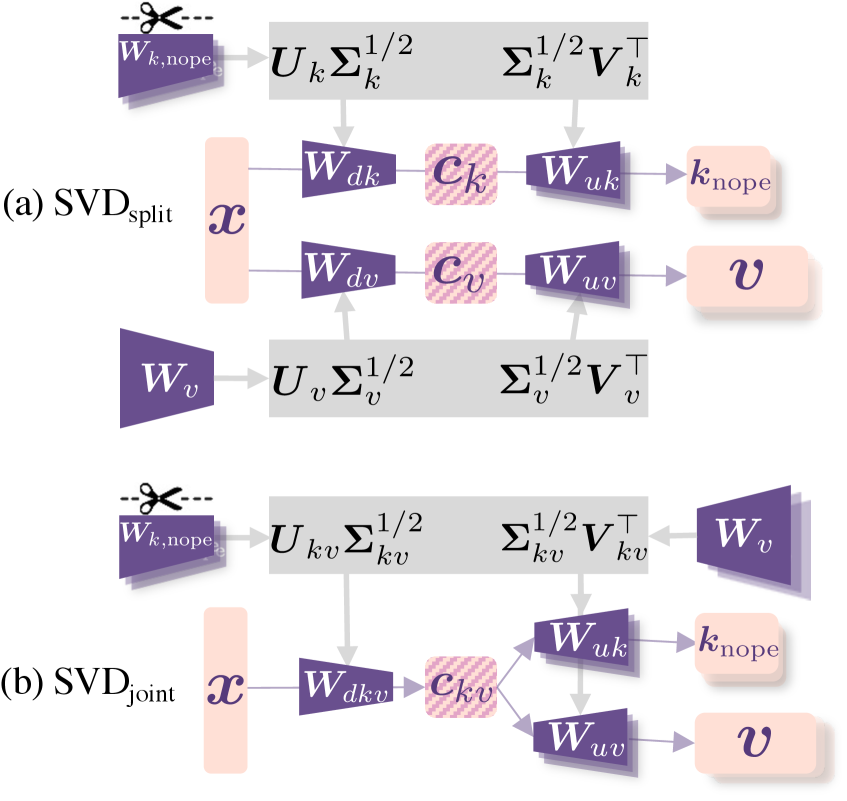</details> Figure 4: Illustration of SVD split and SVD joint. In the multi-head setting, we adhere to the standard MLA approach, performing SVD on the merged multi-heads rather than on each head individually (e.g., $\bm{U}_kv∈ℝ^n_hd_h× n_hd_kv$ . ### 3.2 Low-rank Approximation After transitioning from full RoPE to partial RoPE, we obtain the first component of the KV cache in MLA, represented as: $\bm{k}_i,rope=≤ft[\bm{R}_i^[2k,2k+1](θ_k)\bm{k}_i^[2k,2k+1]\right]_k∈S$ . Our next goal is to derive the second component, $\bm{c}_i,kv∈ℝ^d_kv$ , which serves as a low-rank representation of $\bm{k}_i,nope$ and $\bm{v}_i$ . Given the keys $\bm{k}_i=\bm{x}_i\bm{W}_k$ and values $\bm{v}_i=\bm{x}_i\bm{W}_v$ in MHA, we first extract the subspace of $\bm{W}_k$ corresponding to $\bm{k}_i,nope$ , i.e., the dimensions not included in $S$ , yielding: $\bm{k}_i,nope=\bm{x}_i\bm{W}_k,nope$ . We propose two Singular Value Decomposition (SVD)-based strategies (Illustrated in Figure ˜ 4) to preserve pre-trained knowledge while achieving rank reduction: #### Decoupled SVD (SVD split ) Separately decompose $\bm{W}_k,nope$ and $\bm{W}_v$ into truncated SVDs, allocating $d_kv/2$ dimensions to each: $$ \bm{W}_k,nope=\bm{U}_k\bm{Σ}_k\bm{V}_k^⊤, \bm{W}_v=\bm{U}_v\bm{Σ}_v\bm{V}_v^⊤, $$ where $\bm{U}_k,\bm{U}_v,\bm{V}_k,\bm{V}_v∈ℝ^d_h×\frac{d_kv{2}}$ , $\bm{Σ}_k,\bm{Σ}_v∈ℝ^\frac{d_kv{2}×\frac{d_kv}{2}}$ . The down-projection matrices $\bm{W}_d*$ and up-projection matrices $\bm{W}_u*$ become: | | $\displaystyle\bm{W}_dk=\bm{U}_k\bm{Σ}_k^1/2, \bm{W}_uk=\bm{Σ}_k^1/2\bm{V}_k^⊤,$ | | | --- | --- | --- | The low-rank representation $\bm{c}_i,kv$ can be constructed using $\bm{c}_i,kv=≤ft[\bm{x}_i\bm{W}_dk,\bm{x}_i\bm{W}_dv\right]$ . #### Joint SVD (SVD joint ) To preserve interactions between $\bm{K}_nope$ and $\bm{V}$ , we jointly factorize the concatenated matrix: $$ [\bm{W}_k,nope,\bm{W}_v]=\bm{U}_kv\bm{Σ}_kv\bm{V}_kv^⊤, $$ where $\bm{U}_kv,\bm{V}_kv∈ℝ^d_h× d_kv$ , $\bm{Σ}_kv∈ℝ^d_kv× d_kv$ . The latent projection is then: | | $\displaystyle\bm{W}_dkv=\bm{U}_kv\bm{Σ}_kv^1/2,$ | | | --- | --- | --- | This jointly optimizes the latent space for both keys and values, i.e., $\bm{c}_i,kv=\bm{x}_i\bm{W}_dkv$ , retaining cross-parameter dependencies critical for autoregressive generation We describe the economical inference process of MHA2MLA in Appendix B. . Section ˜ 4.3 shows SVD joint outperforming SVD split, validating that joint factorization better preserves pre-trained knowledge. ## 4 Experiment | Model | Tokens | KV Mem. | Avg. | MMLU | ARC | PIQA | HS | OBQA | WG | | | | --- | --- | --- | --- | --- | --- | --- | --- | --- | --- | --- | --- | | 135M ${}_SmolLM$ | 600B | | 44.50 | 29.80 | 42.43 | 68.06 | 41.09 | 33.60 | 52.01 | | | | - GQA | $d_kv=128$ | | | 44.42 | | 29.91 | 41.71 | 68.28 | 41.33 | 33.80 | 51.46 | | - GQA2MLA | $d_kv=32$ | 6B | -68.75% | 43.21 | -1.21 | 29.50 | 40.84 | 67.08 | 38.34 | 33.20 | 50.28 | | $d_kv=16$ | (1%) | -81.25% | 42.18 | -2.24 | 28.79 | 40.11 | 65.94 | 36.68 | 31.20 | 50.36 | | | $d_kv=8$ | | -87.50% | 41.04 | -3.38 | 28.49 | 38.17 | 64.36 | 33.93 | 31.60 | 49.72 | | | 360M ${}_SmolLM$ | 600B | | 49.60 | 33.70 | 49.82 | 71.87 | 51.65 | 37.60 | 52.96 | | | | - GQA | $d_kv=128$ | | | 49.51 | | 34.08 | 49.89 | 71.60 | 51.67 | 37.20 | 52.64 | | - GQA2MLA | $d_kv=32$ | 6B | -68.75% | 48.14 | -1.37 | 32.91 | 48.34 | 70.51 | 48.56 | 36.80 | 51.70 | | $d_kv=16$ | (1%) | -81.25% | 46.88 | -2.63 | 31.85 | 46.07 | 70.62 | 46.48 | 35.80 | 50.43 | | | $d_kv=8$ | | -87.50% | 45.84 | -3.67 | 30.93 | 44.41 | 69.48 | 43.49 | 36.00 | 50.75 | | | 1B7 ${}_SmolLM$ | 1T | | 55.90 | 39.27 | 59.87 | 75.73 | 62.93 | 42.80 | 54.85 | | | | - MHA | $d_kv=128$ | | | 55.71 | | 38.66 | 59.02 | 75.79 | 62.60 | 43.20 | 55.01 | | - MHA2MLA | $d_kv=32$ | 6B | -68.75% | 54.66 | -1.05 | 37.79 | 56.54 | 75.19 | 61.30 | 41.40 | 55.72 | | $d_kv=16$ | (0.6%) | -81.25% | 54.28 | -1.43 | 37.79 | 56.33 | 75.68 | 60.59 | 41.00 | 54.30 | | | $d_kv=8$ | | -87.50% | 52.79 | -2.92 | 36.69 | 54.29 | 74.54 | 58.49 | 39.20 | 53.51 | | | 7B ${}_Llama2$ | 2T | | 59.85 | 41.43 | 59.24 | 78.40 | 73.29 | 41.80 | 64.96 | | | | - MHA | $d_kv=256$ | | | 59.50 | | 40.30 | 60.05 | 77.91 | 70.20 | 45.00 | 63.54 | | - MHA2MLA | $d_kv=64$ | 12B | -68.75% | 59.21 | -0.29 | 40.90 | 59.53 | 77.26 | 70.05 | 45.20 | 62.51 | | $d_kv=32$ | (0.6%) | -81.25% | 59.20 | -0.30 | 40.96 | 59.74 | 77.26 | 69.81 | 44.00 | 63.46 | | | $d_kv=16$ | | -87.50% | 58.48 | -1.02 | 40.15 | 58.53 | 77.20 | 68.88 | 45.00 | 61.09 | | | 13B ${}_Llama2$ | 2T | | 62.65 | 43.56 | 62.68 | 80.41 | 76.99 | 43.80 | 68.43 | | | | - MHA | $d_kv=256$ | | | 60.72 | | 42.89 | 61.75 | 77.69 | 72.22 | 44.00 | 65.75 | | - MHA2MLA | $d_kv=64$ | 12B | -68.75% | 60.45 | -0.27 | 42.49 | 62.31 | 78.78 | 71.59 | 43.20 | 64.33 | | $d_kv=32$ | (0.6%) | -81.25% | 60.49 | -0.23 | 42.00 | 61.64 | 78.73 | 72.71 | 42.80 | 65.04 | | | $d_kv=16$ | | -87.50% | 59.68 | -1.04 | 41.31 | 60.39 | 77.69 | 71.54 | 43.60 | 63.54 | | Table 1: Commonsense reasoning ability of four LLMs with MHA2MLA or GQA2MLA. The six benchmarks include MMLU (2021), ARC easy and challenge (ARC, 2018), PIQA (2020), HellaSwag (HS, 2019), OpenBookQA (OBQA, 2018), Winogrande (WG, 2021). We evaluate our method on LLMs of varying scales (SmolLM-135M/360M/1B7, Llama2-7B/13B) pre-trained with MHA or GQA. We chose the SmolLM-series https://huggingface.co/collections/HuggingFaceTB/smollm-6695016cad7167254ce15966 because its pretraining data and framework are both open-source, which can minimize the gap in fine-tuning data and processes. We chose Llama2-7B https://huggingface.co/meta-llama/Llama-2-7b because it is one of the widely used open-source LLMs (but its pretraining data is not open-source, there is a potential gap in fine-tuning data). We denote the architectural migration using MHA2MLA and GQA2MLA, respectively. The details of the fine-tuning process (including data and hyperparameters) are provided in Appendix C. Both adopt data-efficient full-parameter fine-tuning, with the head-wise 2-norm selection ( $S_2-norm$ , $r=\frac{d_h}{16}$ ) for Partial-RoPE and joint SVD factorization (SVD joint) for low-rank approximation as default configurations. Our experiments address three critical questions: 1. How does MHA2MLA minimize accuracy degradation induced by architectural shifts? 1. What does MHA2MLA achieve in the KV cache reduction ratio? 1. Can MHA2MLA integrate with KV cache quantization for compound gains? ### 4.1 Commonsense Reasoning Tasks #### Main Results As shown in Table ˜ 1, our method achieves efficient architectural migration across five model scales (135M to 13B) under varying KV cache compression ratios (via latent dimension $d_kv$ ). First, when comparing the performance of our fine-tuning approach with the original LLM, we observe only minor changes in performance across the five base models: a -0.08% decrease on the 135M, -0.09% on the 360M, -0.19% on the 1B7, -0.35% on the 7B and -1.93% on the 13B. This suggests that the fine-tuning data does not significantly degrade or improve the performance of the original model, providing an appropriate experimental setting for the MHA2MLA framework. 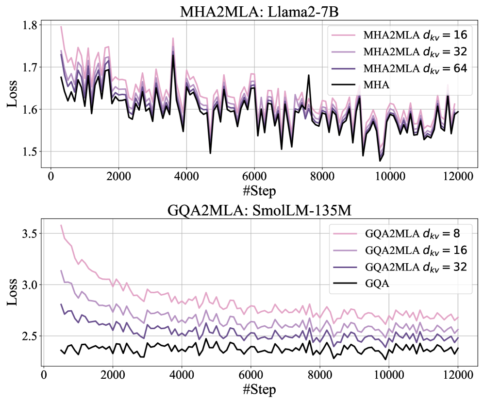Next, as $d_kv$ decreases (e.g., from 32 to 16 to 8), the KV cache reduction increases (i.e., from -68.75% to -81.25% to -87.5%), but the performance loss becomes more challenging to recover through fine-tuning. Figure ˜ 5 shows the fine-tuning loss curves of 135M (representing GQA) and 7B (representing MHA) under different compression ratios. As the compression ratio increases, the loss difference from the baseline becomes larger. Additionally, we observe that the fluctuation trends of the loss curves are almost identical, indicating that our architecture migration does not significantly harm the model’s internal knowledge. <details> <summary>x5.png Details</summary>  ### Visual Description ## Line Graphs: Loss vs Training Steps for MHA2MLA and GQA2MLA Models ### Overview The image contains two line graphs comparing loss values across training steps for different model architectures. The top graph shows results for the MHA2MLA architecture on Llama2-7B, while the bottom graph displays results for GQA2MLA on SmolLM-135M. Each graph compares multiple configurations with varying `d_kv` values against baseline models (MHA and GQA respectively). ### Components/Axes **Top Graph (MHA2MLA: Llama2-7B):** - **X-axis**: "#Step" (0 to 12,000) - **Y-axis**: "Loss" (1.5 to 1.8) - **Legend**: - Pink: MHA2MLA `d_kv` = 16 - Purple: MHA2MLA `d_kv` = 32 - Dark Purple: MHA2MLA `d_kv` = 64 - Black: MHA (baseline) **Bottom Graph (GQA2MLA: SmolLM-135M):** - **X-axis**: "#Step" (0 to 12,000) - **Y-axis**: "Loss" (2.5 to 3.5) - **Legend**: - Pink: GQA2MLA `d_kv` = 8 - Purple: GQA2MLA `d_kv` = 16 - Dark Purple: GQA2MLA `d_kv` = 32 - Black: GQA (baseline) ### Detailed Analysis **Top Graph Trends:** 1. All lines exhibit high-frequency oscillations with sharp peaks/troughs. 2. MHA2MLA variants (`d_kv` = 16, 32, 64) consistently show slightly higher loss than MHA baseline. 3. Loss values cluster between 1.6-1.75, with no clear convergence trend. 4. Larger `d_kv` values (64) show marginally higher peaks than smaller values. **Bottom Graph Trends:** 1. All lines show a general downward trend over steps. 2. GQA2MLA variants (`d_kv` = 8, 16, 32) start with higher loss than GQA baseline but converge toward similar values. 3. Loss decreases from ~3.5 to ~2.6 over 12,000 steps. 4. Larger `d_kv` values (32) begin with higher loss but show similar convergence behavior to smaller values. ### Key Observations 1. **MHA2MLA vs MHA**: All MHA2MLA configurations maintain ~5-10% higher loss than MHA baseline throughout training. 2. **GQA2MLA vs GQA**: GQA2MLA variants demonstrate improvement over baseline GQA, with loss decreasing by ~25% over training. 3. **`d_kv` Impact**: Larger `d_kv` values (64 in MHA2MLA, 32 in GQA2MLA) show marginally higher initial loss but similar convergence patterns to smaller values. 4. **Volatility**: Both graphs exhibit high-frequency noise, suggesting unstable training dynamics. ### Interpretation The graphs reveal architectural tradeoffs in transformer-based models: 1. **MHA2MLA**: While potentially offering architectural improvements, the increased loss suggests suboptimal parameter initialization or training instability compared to standard MHA. 2. **GQA2MLA**: Demonstrates clear performance gains over baseline GQA, with larger `d_kv` values showing faster initial improvement despite higher starting loss. 3. **`d_kv` Scaling**: Larger `d_kv` values (key dimension) appear to require more training steps to stabilize, though they ultimately converge to similar loss values as smaller configurations. 4. **Training Dynamics**: The high-frequency oscillations in both graphs indicate potential challenges with gradient stability or optimization landscape complexity in these architectures. The data suggests that while MHA2MLA may not outperform standard MHA in this configuration, GQA2MLA shows promising improvements. The `d_kv` parameter's impact appears more pronounced in the GQA2MLA architecture, where larger values enable better initial performance despite higher computational costs. </details> Figure 5: The fine-tuning loss curves under different KV cache storage ratios (with colors ranging from light to dark representing 12.5%, 18.75%, 31.25%, and 100%). We also find that larger models experience less performance degradation when transitioning to the MLA architecture. For example, with compression down to 18.75%, the performance drops by 2.24% for 135M, 2.63% for 360M, 1.43% for 1B7, 0.30% for 7B and 0.23% for 13B, revealing the potential scaling law of MHA2MLA. Finally, from the 135M model to the 13B model, the number of tokens required for fine-tuning is only about 0.6% to 1% of the pretraining tokens, demonstrating the data efficiency of our method. Overall, whether using GQA2MLA or MHA2MLA, the architecture transition is achieved with minimal cost, resulting in efficient and economical inference. ### 4.2 Long Context Tasks | Model | Precision | KV Mem. | Avg@LB | | --- | --- | --- | --- | | 7B ${}_Llama2$ | BF16 | 100.0% | 27.4 | | Int4 ${}_HQQ$ | -75.00% | 27.5 | | | Int4 ${}_Quanto$ | 27.3 | | | | Int2 ${}_HQQ$ | -87.50% | 21.2 | | | Int2 ${}_Quanto$ | 18.5 | | | | $d_kv=64$ | BF16 | -68.75% | 26.7 | | Int4 ${}_HQQ$ | -92.19% | 26.4 | | | Int4 ${}_Quanto$ | 26.3 | | | | $d_kv=32$ | BF16 | -81.25% | 26.0 | | Int4 ${}_HQQ$ | -95.31% | 25.8 | | | Int4 ${}_Quanto$ | 25.5 | | | | $d_kv=16$ | BF16 | -87.50% | 25.1 | | Int4 ${}_HQQ$ | -96.87% | 25.0 | | | Int4 ${}_Quanto$ | 24.6 | | | Table 2: Evaluation results of Llama2-7B and MHA2MLA on LongBench. Bold indicates compression ratios greater than or equal to Int2 quantization while also achieving performance higher than Int2. #### Settings To evaluate the generative capabilities of the model, we adopt LongBench Bai et al. (2024) as the benchmark for generation performance. All models are tested using a greedy decoding strategy. The context window size is determined based on the sequence length used during model fine-tuning. We use HQQ Badri and Shaji (2023) and Quanto https://huggingface.co/blog/quanto-introduction to set caches with different levels of precision to evaluate the performance of the original model as the baseline. Since our method is compatible with KV cache quantization, we also conduct additional experiments to assess the combined effect of both approaches. #### Main Results As evidenced in Table ˜ 2, MHA2MLA achieves competitive or superior efficiency-accuracy profiles compared to post-training quantization methods on LongBench. While 4-bit quantization incurs modest degradation (-0.2% to -0.4%) at comparable compression ratios, aggressive 2-bit quantization suffers severe performance collapse (-6.2% to -9%) despite 87.5% KV cache reduction. In contrast, MHA2MLA alone attains 87.5% compression (at $d_kv=16$ ) with only 2.3% accuracy loss, and further synergizes with 4-bit quantization to reach 92.19%/96.87% compression ( $d_kv=64/16$ +Int4 ${}_HQQ$ ) while limiting degradation to -1.0%/-2.4%, outperforming all 2-bit baselines. This highlights that MHA2MLA’s latent space design remains orthogonal to numerical precision reduction, enabling compound efficiency gains without destructive interference. ### 4.3 Ablation Study | Model | Tokens | Avg@CS | | | --- | --- | --- | --- | | 135M ${}_SmolLM$ | 600B | 44.50 | | | - full-rope | 6B | 44.42 | | | - $S_high$ | 43.60 | -0.82 | | | - $S_low$ | 39.17 | -5.25 | | | - $S_uniform$ | 44.01 | -0.41 | | | - $S_2-norm$ | 43.73 | -0.69 | | | - $S_high$ + SVD joint | 6B | 40.85 | -3.57 | | - $S_uniform$ + SVD joint | 41.79 | -2.63 | | | - $S_2-norm$ + SVD joint | 42.18 | -2.24 | | | - $S_2-norm$ + SVD split | 41.27 | -3.15 | | | 1B7 ${}_SmolLM$ | 1T | 55.90 | | | - full-rope | 6B | 55.71 | | | - $S_high$ | 54.80 | -0.91 | | | - $S_low$ | 53.84 | -1.87 | | | - $S_uniform$ | 55.30 | -0.41 | | | - $S_2-norm$ | 54.98 | -0.73 | | | - $S_high$ + SVD joint | 6B | 54.17 | -1.54 | | - $S_uniform$ + SVD joint | 54.27 | -1.44 | | | - $S_2-norm$ + SVD joint | 54.28 | -1.43 | | | - $S_2-norm$ + SVD split | 52.90 | -2.81 | | Table 3: Reasoning ability of ablation studies. The results of other models are provided in Appendix E. #### Four Partial-RoPE strategies: $S_high$ , $S_low$ , $S_uniform$ , $S_2-norm$ Table ˜ 3 presents the results of four strategies for converting full-RoPE to partial-RoPE. First, when comparing the four strategies with full-RoPE, we observed that the low-frequency retention strategy, $S_low$ , incurred the greatest performance loss (a reduction of -5.25%@135M and -1.87%@1B7), whereas the high-frequency retention strategy, $S_high$ , experienced significantly less degradation (a reduction of -0.82%@135M and -0.91%@1B7), underscoring the importance of high-frequency subspaces. Both $S_uniform$ and $S_2-norm$ yielded better performance, the $S_uniform$ preserves subspaces across the frequency spectrum, while the $S_2-norm$ retains subspaces based on their contribution to the attention scores. We choose $S_2-norm$ as the default configuration because the removed subspaces (i.e., NoPE) are more suitable for the (SVD-based) low-rank approximation. #### Two SVD-based low-rank approximations: SVD split , SVD joint The last two rows of each group in Table ˜ 3 compare the effects of the two SVD methods. We observe that, on both LLMs, the SVD ${}_joint$ method consistently outperforms SVD ${}_split$ , yielding an average performance improvement of 0.91% on the 135M model and 1.38% on the 1B7 model. It indicates that SVD ${}_joint$ emerges as the clear default choice. ## 5 Related Work #### Efficient Attention Architectures The standard Multi-Head Attention (MHA, 2017) mechanism’s quadratic complexity in context length has spurred numerous efficiency innovations. While MHA remains foundational, variants like Multi-Query Attention (MQA) and Grouped-Query Attention (GQA, 2023) reduce memory overhead by sharing keys/values across heads—albeit at the cost of parameter pruning and performance degradation. Parallel efforts, such as Linear Transformers Guo et al. (2019); Katharopoulos et al. (2020); Choromanski et al. (2021), RWKV Peng et al. (2023), and Mamba Gu and Dao (2023), replace softmax attention with linear recurrences or state-space models, but struggle to match the expressiveness of standard attention in autoregressive generation. Multi-Head Latent Attention (MLA, 2024) distinguishes itself by compressing KV caches into low-rank latent vectors without pruning attention parameters. Our work bridges MLA with mainstream architectures (MHA/GQA), enabling seamless migration via data-efficient fine-tuning. Notably, while many linear attention variants abandon softmax query-key interactions (e.g., through kernel approximations), architectures preserving a query-key dot product structure—even in factorized forms—remain compatible with our MHA2MLA framework. #### Economical Key-Value Cache The memory footprint of KV caches has become a critical bottleneck for long-context inference. Recent advances fall into three categories: Innovative Architecture methods like MLA DeepSeek-AI et al. (2024), MiniCache Liu et al. (2024a), and MLKV Zuhri et al. (2024) share or compress KV representations across layers or heads. While effective, cross-layer sharing risks conflating distinct attention patterns, potentially harming task-specific performance. Only MLA has been successfully validated in Deepseek’s LLMs. Quantization techniques such as GPTQ Frantar et al. (2022), FlexGen Sheng et al. (2023), and KIVI Liu et al. (2024b) store KV caches in low-bit formats (e.g., 2-bit), achieving memory savings with precision loss. Dynamic Pruning approaches like A2SF Jo and Shin (2024) and SnapKV Li et al. (2024) prune “less important” tokens from the KV cache. However, token pruning risks discarding critical long-range dependencies, while head pruning (e.g., SliceGPT Ashkboos et al. (2024), Sheared Xia et al. (2024), and Simple Pruning Sun et al. (2024)) irreversibly reduces model capacity. Our MHA2MLA method achieves the migration of standard Transformer-based LLMs to the more economical MLA architecture and has demonstrated its ability to integrate with KV quantization techniques to realize a ~97% cache saving. It is also theoretically compatible with other methods like pruning. ## 6 Conclusion This work addresses the critical challenge of adapting pre-trained MHA-based LLMs (or variants) to the KV-cache-efficient MLA architecture. By introducing MHA2MLA with contribution-aware partial-RoPE removal and SVD-driven low-rank projection, we achieve near-lossless compression of KV cache (up to 96.87% size reduction for Llama2-7B) while requiring only 0.6% to 1% of training data. The framework demonstrates strong compatibility with existing compression techniques and maintains commonsense reasoning and long-context processing capabilities, offering a practical pathway for deploying resource-efficient LLMs without sacrificing performance. Our results underscore the feasibility of architectural migration for LLMs through targeted parameter reuse and data-efficient fine-tuning. ## Limitations #### Verification on More LLMs Considering that MHA2MLA can significantly reduce inference costs, it is worthwhile to validate it on larger and more diverse open-source LLMs. However, constrained by our computation resources, models like Llama3 require fine-tuning on a 128K context length to mitigate performance degradation from continued training, so we did not perform such experiments. Furthermore, since Deepseek has not yet open-sourced the tensor-parallel inference framework for MLA, it is currently challenging to explore models larger than 7B. This will be addressed in our future work. #### Parameter-Efficient MHA2MLA Fine-tuning This paper primarily focuses on the data efficiency of MHA2MLA. Since the architectural transformation does not involve the Feed-Forward (FFN) module, future work could explore parameter-efficient MHA2MLA fine-tuning, for example by freezing the FFN module and/or freezing the parameters in the queries and keys that correspond to the retained RoPE. This could further reduce the cost of the MHA2MLA transition. ## Acknowledgments The authors wish to thank all reviewers for their helpful comments and suggestions. The corresponding authors are Yuanbin Wu, Xipeng Qiu, Qi Zhang, Tao Gui. This work was partially funded by Guangdong S&T Program 2024B0101050003, National Natural Science Foundation of China (No.62076069,62206057,61976056), Shanghai Rising-Star Program (23QA1400200), and Natural Science Foundation of Shanghai (23ZR1403500), Program of Shanghai Academic Research Leader under grant 22XD1401100. The computations in this research were performed using the CFFF platform of Fudan University. ## References - Ainslie et al. (2023) Joshua Ainslie, James Lee-Thorp, Michiel de Jong, Yury Zemlyanskiy, Federico Lebrón, and Sumit Sanghai. 2023. GQA: training generalized multi-query transformer models from multi-head checkpoints. In Proceedings of the 2023 Conference on Empirical Methods in Natural Language Processing, EMNLP 2023, Singapore, December 6-10, 2023, pages 4895–4901. Association for Computational Linguistics. - An et al. (2024) Chenxin An, Shansan Gong, Ming Zhong, Xingjian Zhao, Mukai Li, Jun Zhang, Lingpeng Kong, and Xipeng Qiu. 2024. L-eval: Instituting standardized evaluation for long context language models. In Proceedings of the 62nd Annual Meeting of the Association for Computational Linguistics (Volume 1: Long Papers), ACL 2024, Bangkok, Thailand, August 11-16, 2024, pages 14388–14411. Association for Computational Linguistics. - Ashkboos et al. (2024) Saleh Ashkboos, Maximilian L. Croci, Marcelo Gennari Do Nascimento, Torsten Hoefler, and James Hensman. 2024. Slicegpt: Compress large language models by deleting rows and columns. In The Twelfth International Conference on Learning Representations, ICLR 2024, Vienna, Austria, May 7-11, 2024. OpenReview.net. - Badri and Shaji (2023) Hicham Badri and Appu Shaji. 2023. Half-quadratic quantization of large machine learning models. - Bai et al. (2024) Yushi Bai, Xin Lv, Jiajie Zhang, Hongchang Lyu, Jiankai Tang, Zhidian Huang, Zhengxiao Du, Xiao Liu, Aohan Zeng, Lei Hou, Yuxiao Dong, Jie Tang, and Juanzi Li. 2024. Longbench: A bilingual, multitask benchmark for long context understanding. In Proceedings of the 62nd Annual Meeting of the Association for Computational Linguistics (Volume 1: Long Papers), ACL 2024, Bangkok, Thailand, August 11-16, 2024, pages 3119–3137. Association for Computational Linguistics. - Barbero et al. (2024) Federico Barbero, Alex Vitvitskyi, Christos Perivolaropoulos, Razvan Pascanu, and Petar Velickovic. 2024. Round and round we go! what makes rotary positional encodings useful? CoRR, abs/2410.06205. - Bisk et al. (2020) Yonatan Bisk, Rowan Zellers, Ronan Le Bras, Jianfeng Gao, and Yejin Choi. 2020. PIQA: reasoning about physical commonsense in natural language. In The Thirty-Fourth AAAI Conference on Artificial Intelligence, AAAI 2020, The Thirty-Second Innovative Applications of Artificial Intelligence Conference, IAAI 2020, The Tenth AAAI Symposium on Educational Advances in Artificial Intelligence, EAAI 2020, New York, NY, USA, February 7-12, 2020, pages 7432–7439. AAAI Press. - Black et al. (2021) Sid Black, Leo Gao, Phil Wang, Connor Leahy, and Stella Biderman. 2021. GPT-Neo: Large Scale Autoregressive Language Modeling with Mesh-Tensorflow. If you use this software, please cite it using these metadata. - Choromanski et al. (2021) Krzysztof Marcin Choromanski, Valerii Likhosherstov, David Dohan, Xingyou Song, Andreea Gane, Tamás Sarlós, Peter Hawkins, Jared Quincy Davis, Afroz Mohiuddin, Lukasz Kaiser, David Benjamin Belanger, Lucy J. Colwell, and Adrian Weller. 2021. Rethinking attention with performers. In 9th International Conference on Learning Representations, ICLR 2021, Virtual Event, Austria, May 3-7, 2021. OpenReview.net. - Clark et al. (2018) Peter Clark, Isaac Cowhey, Oren Etzioni, Tushar Khot, Ashish Sabharwal, Carissa Schoenick, and Oyvind Tafjord. 2018. Think you have solved question answering? try arc, the AI2 reasoning challenge. CoRR, abs/1803.05457. - DeepSeek-AI et al. (2024) DeepSeek-AI, Aixin Liu, Bei Feng, Bin Wang, Bingxuan Wang, Bo Liu, Chenggang Zhao, Chengqi Deng, Chong Ruan, Damai Dai, Daya Guo, Dejian Yang, Deli Chen, Dongjie Ji, Erhang Li, Fangyun Lin, Fuli Luo, Guangbo Hao, Guanting Chen, Guowei Li, Hao Zhang, Hanwei Xu, Hao Yang, Haowei Zhang, Honghui Ding, Huajian Xin, Huazuo Gao, Hui Li, Hui Qu, J. L. Cai, Jian Liang, Jianzhong Guo, Jiaqi Ni, Jiashi Li, Jin Chen, Jingyang Yuan, Junjie Qiu, Junxiao Song, Kai Dong, Kaige Gao, Kang Guan, Lean Wang, Lecong Zhang, Lei Xu, Leyi Xia, Liang Zhao, Liyue Zhang, Meng Li, Miaojun Wang, Mingchuan Zhang, Minghua Zhang, Minghui Tang, Mingming Li, Ning Tian, Panpan Huang, Peiyi Wang, Peng Zhang, Qihao Zhu, Qinyu Chen, Qiushi Du, R. J. Chen, R. L. Jin, Ruiqi Ge, Ruizhe Pan, Runxin Xu, Ruyi Chen, S. S. Li, Shanghao Lu, Shangyan Zhou, Shanhuang Chen, Shaoqing Wu, Shengfeng Ye, Shirong Ma, Shiyu Wang, Shuang Zhou, Shuiping Yu, Shunfeng Zhou, Size Zheng, Tao Wang, Tian Pei, Tian Yuan, Tianyu Sun, W. L. Xiao, Wangding Zeng, Wei An, Wen Liu, Wenfeng Liang, Wenjun Gao, Wentao Zhang, X. Q. Li, Xiangyue Jin, Xianzu Wang, Xiao Bi, Xiaodong Liu, Xiaohan Wang, Xiaojin Shen, Xiaokang Chen, Xiaosha Chen, Xiaotao Nie, and Xiaowen Sun. 2024. Deepseek-v2: A strong, economical, and efficient mixture-of-experts language model. CoRR, abs/2405.04434. - Frantar et al. (2022) Elias Frantar, Saleh Ashkboos, Torsten Hoefler, and Dan Alistarh. 2022. GPTQ: accurate post-training quantization for generative pre-trained transformers. CoRR, abs/2210.17323. - Gu and Dao (2023) Albert Gu and Tri Dao. 2023. Mamba: Linear-time sequence modeling with selective state spaces. CoRR, abs/2312.00752. - Guo et al. (2019) Qipeng Guo, Xipeng Qiu, Pengfei Liu, Yunfan Shao, Xiangyang Xue, and Zheng Zhang. 2019. Star-transformer. In Proceedings of the 2019 Conference of the North American Chapter of the Association for Computational Linguistics: Human Language Technologies, NAACL-HLT 2019, Minneapolis, MN, USA, June 2-7, 2019, Volume 1 (Long and Short Papers), pages 1315–1325. Association for Computational Linguistics. - Hendrycks et al. (2021) Dan Hendrycks, Collin Burns, Steven Basart, Andy Zou, Mantas Mazeika, Dawn Song, and Jacob Steinhardt. 2021. Measuring massive multitask language understanding. In 9th International Conference on Learning Representations, ICLR 2021, Virtual Event, Austria, May 3-7, 2021. OpenReview.net. - Jo and Shin (2024) Hyun-rae Jo and Dongkun Shin. 2024. A2SF: accumulative attention scoring with forgetting factor for token pruning in transformer decoder. CoRR, abs/2407.20485. - Kaplan et al. (2020) Jared Kaplan, Sam McCandlish, Tom Henighan, Tom B. Brown, Benjamin Chess, Rewon Child, Scott Gray, Alec Radford, Jeffrey Wu, and Dario Amodei. 2020. Scaling laws for neural language models. CoRR, abs/2001.08361. - Katharopoulos et al. (2020) Angelos Katharopoulos, Apoorv Vyas, Nikolaos Pappas, and François Fleuret. 2020. Transformers are rnns: Fast autoregressive transformers with linear attention. In Proceedings of the 37th International Conference on Machine Learning, ICML 2020, 13-18 July 2020, Virtual Event, volume 119 of Proceedings of Machine Learning Research, pages 5156–5165. PMLR. - Li et al. (2024) Yuhong Li, Yingbing Huang, Bowen Yang, Bharat Venkitesh, Acyr Locatelli, Hanchen Ye, Tianle Cai, Patrick Lewis, and Deming Chen. 2024. Snapkv: LLM knows what you are looking for before generation. In Advances in Neural Information Processing Systems 38: Annual Conference on Neural Information Processing Systems 2024, NeurIPS 2024, Vancouver, BC, Canada, December 10 - 15, 2024. - Liu et al. (2024a) Akide Liu, Jing Liu, Zizheng Pan, Yefei He, Reza Haffari, and Bohan Zhuang. 2024a. Minicache: KV cache compression in depth dimension for large language models. In Advances in Neural Information Processing Systems 38: Annual Conference on Neural Information Processing Systems 2024, NeurIPS 2024, Vancouver, BC, Canada, December 10 - 15, 2024. - Liu et al. (2024b) Zirui Liu, Jiayi Yuan, Hongye Jin, Shaochen Zhong, Zhaozhuo Xu, Vladimir Braverman, Beidi Chen, and Xia Hu. 2024b. KIVI: A tuning-free asymmetric 2bit quantization for KV cache. In Forty-first International Conference on Machine Learning, ICML 2024, Vienna, Austria, July 21-27, 2024. OpenReview.net. - Mihaylov et al. (2018) Todor Mihaylov, Peter Clark, Tushar Khot, and Ashish Sabharwal. 2018. Can a suit of armor conduct electricity? A new dataset for open book question answering. In Proceedings of the 2018 Conference on Empirical Methods in Natural Language Processing, Brussels, Belgium, October 31 - November 4, 2018, pages 2381–2391. Association for Computational Linguistics. - Peng et al. (2023) Bo Peng, Eric Alcaide, Quentin Anthony, Alon Albalak, Samuel Arcadinho, Stella Biderman, Huanqi Cao, Xin Cheng, Michael Chung, Leon Derczynski, Xingjian Du, Matteo Grella, Kranthi Kiran GV, Xuzheng He, Haowen Hou, Przemyslaw Kazienko, Jan Kocon, Jiaming Kong, Bartlomiej Koptyra, Hayden Lau, Jiaju Lin, Krishna Sri Ipsit Mantri, Ferdinand Mom, Atsushi Saito, Guangyu Song, Xiangru Tang, Johan S. Wind, Stanislaw Wozniak, Zhenyuan Zhang, Qinghua Zhou, Jian Zhu, and Rui-Jie Zhu. 2023. RWKV: reinventing rnns for the transformer era. In Findings of the Association for Computational Linguistics: EMNLP 2023, Singapore, December 6-10, 2023, pages 14048–14077. Association for Computational Linguistics. - Sakaguchi et al. (2021) Keisuke Sakaguchi, Ronan Le Bras, Chandra Bhagavatula, and Yejin Choi. 2021. Winogrande: an adversarial winograd schema challenge at scale. Commun. ACM, 64(9):99–106. - Shazeer (2019) Noam Shazeer. 2019. Fast transformer decoding: One write-head is all you need. CoRR, abs/1911.02150. - Sheng et al. (2023) Ying Sheng, Lianmin Zheng, Binhang Yuan, Zhuohan Li, Max Ryabinin, Beidi Chen, Percy Liang, Christopher Ré, Ion Stoica, and Ce Zhang. 2023. Flexgen: High-throughput generative inference of large language models with a single GPU. In International Conference on Machine Learning, ICML 2023, 23-29 July 2023, Honolulu, Hawaii, USA, volume 202 of Proceedings of Machine Learning Research, pages 31094–31116. PMLR. - Strubell et al. (2019) Emma Strubell, Ananya Ganesh, and Andrew McCallum. 2019. Energy and policy considerations for deep learning in NLP. In Proceedings of the 57th Annual Meeting of the Association for Computational Linguistics, pages 3645–3650, Florence, Italy. Association for Computational Linguistics. - Su et al. (2024) Jianlin Su, Murtadha H. M. Ahmed, Yu Lu, Shengfeng Pan, Wen Bo, and Yunfeng Liu. 2024. Roformer: Enhanced transformer with rotary position embedding. Neurocomputing, 568:127063. - Sun et al. (2024) Mingjie Sun, Zhuang Liu, Anna Bair, and J. Zico Kolter. 2024. A simple and effective pruning approach for large language models. In The Twelfth International Conference on Learning Representations, ICLR 2024, Vienna, Austria, May 7-11, 2024. OpenReview.net. - Vaswani et al. (2017) Ashish Vaswani, Noam Shazeer, Niki Parmar, Jakob Uszkoreit, Llion Jones, Aidan N. Gomez, Lukasz Kaiser, and Illia Polosukhin. 2017. Attention is all you need. In Advances in Neural Information Processing Systems 30: Annual Conference on Neural Information Processing Systems 2017, December 4-9, 2017, Long Beach, CA, USA, pages 5998–6008. - Xia et al. (2024) Mengzhou Xia, Tianyu Gao, Zhiyuan Zeng, and Danqi Chen. 2024. Sheared llama: Accelerating language model pre-training via structured pruning. In The Twelfth International Conference on Learning Representations, ICLR 2024, Vienna, Austria, May 7-11, 2024. OpenReview.net. - Zellers et al. (2019) Rowan Zellers, Ari Holtzman, Yonatan Bisk, Ali Farhadi, and Yejin Choi. 2019. Hellaswag: Can a machine really finish your sentence? In Proceedings of the 57th Conference of the Association for Computational Linguistics, ACL 2019, Florence, Italy, July 28- August 2, 2019, Volume 1: Long Papers, pages 4791–4800. Association for Computational Linguistics. - Zuhri et al. (2024) Zayd Muhammad Kawakibi Zuhri, Muhammad Farid Adilazuarda, Ayu Purwarianti, and Alham Fikri Aji. 2024. MLKV: multi-layer key-value heads for memory efficient transformer decoding. CoRR, abs/2406.09297. ## Appendix A The Calculation of 2-norm Score To compute the 2-norm scores for each attention head, we selected 1,024 samples from the training dataset. The proportions of the subsets and sequence length used during the 2-norm computation are consistent with those used during fine-tuning. First, we calculate the query vectors and key vectors for each head. Then, for each rotational subspace of the vectors, we compute the 2-norm scores. Finally, the 2-norm scores of the query and key vectors are aggregated within each subspace. If the model employs Grouped-Query Attention (GQA), the 2-norm scores are averaged within each GQA group, and the scores are shared between the groups. ## Appendix B Inference Process of MHA2MLA During inference in the MHA2MLA model, our input includes the hidden representation $x_i$ of the $i$ -th token, as well as the previously stored $\bm{k}_<i,rope^(h)$ and $\bm{c}_<i,kv$ in the KV cache for the first $i-1$ tokens. During the inference, our goal is to compute the $h$ -th head’s dot product of these two parts $\bm{q}_i,rope^(h)\bm{k}_≤ i,rope^(h)⊤$ and $\bm{q}_i,nope^(h)\bm{k}_≤ i,nope^(h)⊤$ . For the RoPE part, we can easily extract $\bm{W}_q,rope^(h)$ and $\bm{W}_k,rope^(h)$ from the pre-trained parameter matrices $\bm{W}_q^(h)$ and $\bm{W}_k^(h)$ (i.e., the rows corresponding to the subspace that retains RoPE) and then obtain the result through a linear transformation: | | $\displaystyle\bm{q}_i,rope^(h)$ | $\displaystyle=\bm{x}_i\bm{W}_q,rope^(h)$ | | | --- | --- | --- | --- | Note that $\bm{k}_<i,rope^(h)$ is already stored in the KV cache and can be directly retrieved. For the NoPE part, $\bm{q}_i,nope^(h)$ can still be easily obtained through a linear transformation $\bm{W}_q,nope^(h)$ which extracted from the pre-trained parameter matrix $\bm{W}_q^(h)$ by separating the rows corresponding to the subspace with RoPE removed. However, $\bm{k}_i,nope^(h)$ requires two linear transformations: a dimensionality reduction transformation using $\bm{W}_dkv$ , and a dimensionality expansion transformation using $\bm{W}_uk^(h)$ . Note that $\bm{W}_dkv$ is shared across all heads in the current layer, and both $\bm{W}_dkv$ and $\bm{W}_uk^(h)$ are constrained by the SVD decomposition of the pre-trained parameter matrices $\bm{W}_k,nope^(h)$ and $\bm{W}_v^(h)$ , preserving most of the pre-trained knowledge: | | $\displaystyle\bm{q}_i,nope^(h)$ | $\displaystyle=\bm{x}_i\bm{W}_q,nope^(h)$ | | | --- | --- | --- | --- | During inference, the NoPE part can also leverage the standard MLA matrix merging algorithm to reduce memory consumption: | | $\displaystyle\bm{k}_≤ i,nope^(h)$ | $\displaystyle=[\bm{c}_<i,kv,~\bm{c}_i,kv]\bm{W}_uk^(h)$ | | | --- | --- | --- | --- | We can pre-multiply the parameter matrices $(\bm{W}_q,nope^(h)\bm{W}_uk^(h)⊤)$ , and let $\bm{c}_i,q^(h)=\bm{x}_i(\bm{W}_q,nope^(h)\bm{W}_uk^(h)⊤)$ . In the end, the output of MHA2MLA is as follows: | | $\displaystyle\bm{v}_i^(h)=\bm{c}_i,kv\bm{W}_uv^(h)$ | | | --- | --- | --- | Where $\bm{W}_uv^(h)$ and $\bm{W}_o$ can also perform matrix merging to make inference more economical. #### Why doesn’t MHA2MLA perform low-rank representation on the query as DeepSeek does? Firstly, we found that the economical inference of MLA is not affected even if $\bm{W}_q,nope^(h)$ is not decomposed into a dimension-reducing matrix (e.g., $\bm{W}_dq$ ) and a dimension-increasing matrix (e.g., $\bm{W}_uq^(h)$ ). Secondly, decomposing $\bm{W}_q,nope^(h)$ introduces additional architectural migration loss (approximation loss) and further reduces the number of LLM parameters. Therefore, we believe there is no need to decompose $\bm{W}_q,nope^(h)$ within the MHA2MLA framework. ## Appendix C The Details of Fine-tuning #### Data We fine-tune our model using the pretraining corpus from SmolLM https://huggingface.co/blog/smollm. The dataset consists of fineweb-edu-dedup, cosmopedia-v2, python-edu, open-web-math, and StackOverflow. The first three datasets are part of the smollm-corpus https://huggingface.co/datasets/HuggingFaceTB/smollm-corpus curated by HuggingFaceTB. Fineweb-edu-dedup is a high-quality dataset filtered by HuggingFaceTB from education-related webpages. Similarly, HuggingFaceTB filtered Python code snippets from The Stack to construct the python-edu dataset. Cosmopedia-v2 is a high-quality dataset generated by a model based on 34,000 topics defined by BISAC book classifications. Additionally, open-web-math https://huggingface.co/datasets/open-web-math/open-web-math and StackOverflow https://huggingface.co/datasets/bigcode/stackoverflow-clean are sourced from high-quality mathematical texts available online and posts from StackOverflow, respectively. #### Hyperparameters | Metrics | 135M ${}_SmolLM$ | 360M ${}_SmolLM$ | 1B7 ${}_SmolLM$ | 7B ${}_Llama2$ | 13B ${}_Llama2$ | | | --- | --- | --- | --- | --- | --- | --- | | n_batch $×$ n_gpu | 64 $×$ 4 | 64 $×$ 4 | 32 $×$ 8 | 16 $×$ 16 | 8 $×$ 32 | | | Learning Rate | 1e-4 | 1e-4 | 1e-4 | 1e-4 | 1e-4 | | | Hardware | NVIDIA L20Y | NVIDIA L20Y | NVIDIA L20Y | NVIDIA L20Y | NVIDIA L20Y | | | Steps | 12000 | 12000 | 12000 | 12000 | 12000 | | | Warmup ratio | 10.0% | 10.0% | 10.0% | 10.0% | 10.0% | | | Decay | 16.7% | 16.7% | 16.7% | 16.7% | 16.7% | | | Time | 4h | 8h | 16h | 28h | 36h | | | Seqlen | 2048 | 2048 | 2048 | 4096 | 4096 | | | #Param. | $d_kv=128/256^†$ | 134.52M | 361.82M | 1.71B | 6.61B † | 13.02B † | | $d_kv=32/64^†$ | 130.99M | 351.38M | 1.67B | 6.37B † | 12.56B † | | | $d_kv=16/32^†$ | 129.64M | 347.38M | 1.59B | 5.99B † | 11.80B † | | | $d_kv=8/16^†$ | 128.97M | 345.39M | 1.56B | 5.79B † | 11.43B † | | Table 4: Training detail information across different models. The fine-tuning hyperparameters for models of all sizes are listed in Table ˜ 4. The training process employs a warmup phase followed by a decay strategy. A 1-sqrt decay strategy is applied to ensure a smooth and gradual reduction. | Model | Avg. | MMLU | ARC | PIQA | HS | OBQA | WG | | | | --- | --- | --- | --- | --- | --- | --- | --- | --- | --- | | 135M | $r$ =32 | 44.42 | 29.91 | 41.71 | 68.28 | 41.33 | 33.80 | 51.46 | | | - $S_high$ | $r$ =1 | 42.88 | -1.54 | 29.24 | 40.15 | 66.81 | 37.90 | 33.40 | 49.80 | | $r$ =2 | 43.07 | -1.35 | 29.73 | 40.60 | 67.25 | 38.82 | 32.40 | 49.64 | | | $r$ =4 | 43.60 | -0.82 | 29.87 | 41.29 | 67.08 | 39.58 | 32.80 | 50.99 | | | $r$ =8 | 43.90 | -0.52 | 29.79 | 40.89 | 68.01 | 40.71 | 33.40 | 50.59 | | | - $S_low$ | $r$ =1 | 39.85 | -4.57 | 27.72 | 36.56 | 62.95 | 33.88 | 28.20 | 49.80 | | $r$ =2 | 39.72 | -4.70 | 27.36 | 36.86 | 63.76 | 33.85 | 27.80 | 48.70 | | | $r$ =4 | 39.17 | -5.25 | 27.67 | 35.33 | 62.30 | 33.32 | 27.60 | 48.78 | | | $r$ =8 | 42.36 | -2.06 | 29.33 | 39.37 | 66.70 | 38.13 | 31.00 | 49.64 | | | - $S_uniform$ | $r$ =1 | 42.72 | -1.70 | 29.34 | 40.20 | 66.76 | 37.60 | 32.60 | 49.80 | | $r$ =2 | 43.50 | -0.92 | 29.41 | 41.30 | 67.63 | 39.31 | 33.40 | 49.96 | | | $r$ =4 | 44.01 | -0.41 | 29.79 | 41.09 | 67.95 | 40.54 | 34.20 | 50.51 | | | $r$ =8 | 43.79 | -0.66 | 29.85 | 40.72 | 67.57 | 40.84 | 32.80 | 50.99 | | | - $S_2-norm$ | $r$ =1 | 43.27 | -1.15 | 29.58 | 40.83 | 67.25 | 39.14 | 33.00 | 49.80 | | $r$ =2 | 43.77 | -0.65 | 29.82 | 40.76 | 68.28 | 39.32 | 34.40 | 50.04 | | | $r$ =4 | 43.73 | -0.69 | 30.00 | 41.29 | 68.17 | 39.83 | 33.20 | 49.88 | | | $r$ =8 | 44.18 | -0.24 | 30.01 | 41.52 | 68.12 | 40.70 | 34.00 | 50.75 | | Table 5: The impact of positional encoding dimensionality on model performance. ## Appendix D Ablation Study on Partial-RoPE Dimensions To better determine the strategy and dimensionality for partial-RoPE, we conducted an ablation study on the number of RoPE dimensions using the 135M ${}_SmolLM$ model. The experimental results are presented in Table ˜ 5. By comparing the performance of four different strategies in varying dimensionalities, we observed that the low-frequency strategy, $S_low$ , suffered significant performance degradation (-11.8%) when the dimensionality was relatively low ( $≤ 4$ ). In contrast, both $S_uniform$ and $S_2-norm$ consistently demonstrated superior performance regardless of dimensionality. Furthermore, increasing the dimensionality from 4 to 8 provided negligible performance gains. Based on these findings, we selected a dimensionality of 4 for partial-RoPE. ## Appendix E Detailed Results | $d_kv$ | Precision | KV | Avg. | S-Doc QA | M-Doc QA | Summ. | Few-shot | Synth. | Code | | | | | | | | | | | | --- | --- | --- | --- | --- | --- | --- | --- | --- | --- | --- | --- | --- | --- | --- | --- | --- | --- | --- | --- | | A | B | C | D | E | F | G | H | I | J | K | L | M | N | O | P | | | | | | 7B ${}_Llama2$ (Length=4K) | | | | | | | | | | | | | | | | | | | | | BF16 | 100.0% | 27.4 | 15.1 | 9.6 | 21.1 | 7.5 | 9.7 | 3.7 | 26.7 | 20.5 | 3.2 | 65.5 | 87.5 | 34.1 | 1.9 | 6.6 | 66.5 | 59.4 | | | Int4 ${}_HQQ$ | -75.00% | 27.5 | 16.1 | 9.1 | 22.0 | 7.3 | 9.9 | 3.6 | 26.5 | 21.1 | 3.4 | 65.5 | 87.2 | 34.3 | 1.5 | 6.7 | 66.0 | 59.9 | | | Int4 ${}_Quanto$ | 27.3 | 14.4 | 9.5 | 20.5 | 7.5 | 9.7 | 3.5 | 25.8 | 20.7 | 3.1 | 65.5 | 87.7 | 34.3 | 1.4 | 7.3 | 66.8 | 59.3 | | | | Int2 ${}_HQQ$ | -87.50% | 21.2 | 18.0 | 5.5 | 12.6 | 7.5 | 8.4 | 3.2 | 12.6 | 18.6 | 0.9 | 56.5 | 73.3 | 27.0 | 1.8 | 6.1 | 34.5 | 52.9 | | | Int2 ${}_Quanto$ | 18.5 | 9.4 | 6.2 | 12.7 | 6.8 | 6.7 | 3.3 | 5.9 | 17.2 | 0.4 | 61.0 | 63.9 | 26.0 | 1.4 | 2.7 | 42.4 | 30.5 | | | | $64$ | BF16 | -68.75% | 26.7 | 12.2 | 9.4 | 22.5 | 7.5 | 11.7 | 4.2 | 26.5 | 18.9 | 20.2 | 58.0 | 83.6 | 35.0 | 1.7 | 5.5 | 57.1 | 52.8 | | Int4 ${}_HQQ$ | -92.19% | 26.4 | 12.9 | 9.3 | 22.7 | 7.8 | 12.1 | 3.3 | 26.5 | 18.7 | 18.6 | 58.0 | 82.4 | 35.5 | 1.4 | 4.9 | 56.2 | 51.8 | | | Int4 ${}_Quanto$ | 26.3 | 9.5 | 8.7 | 22.7 | 7.6 | 11.0 | 4.0 | 26.0 | 18.3 | 19.8 | 58.5 | 84.4 | 35.3 | 1.3 | 5.1 | 56.7 | 51.4 | | | | $32$ | BF16 | -81.25% | 26.0 | 13.4 | 8.7 | 21.2 | 5.9 | 9.9 | 2.5 | 25.3 | 19.2 | 17.6 | 65.5 | 85.5 | 25.5 | 3.0 | 7.0 | 54.0 | 51.4 | | Int4 ${}_HQQ$ | -95.31% | 25.8 | 13.6 | 9.1 | 20.6 | 6.0 | 10.2 | 2.5 | 25.0 | 18.4 | 16.4 | 65.5 | 85.1 | 25.4 | 3.1 | 6.9 | 53.4 | 51.0 | | | Int4 ${}_Quanto$ | 25.5 | 13.4 | 8.0 | 21.2 | 6.4 | 10.1 | 3.0 | 24.3 | 17.1 | 17.1 | 65.0 | 85.1 | 26.1 | 3.6 | 6.2 | 52.7 | 49.0 | | | | $16$ | BF16 | -87.50% | 25.1 | 13.2 | 8.7 | 21.6 | 7.1 | 9.1 | 3.7 | 24.1 | 18.4 | 20.3 | 57.5 | 86.0 | 33.3 | 0.1 | 9.0 | 43.9 | 44.9 | | Int4 ${}_HQQ$ | -96.87% | 25.0 | 13.7 | 8.8 | 23.7 | 7.1 | 9.2 | 4.5 | 22.8 | 18.7 | 18.4 | 57.5 | 86.6 | 32.1 | 0.1 | 8.8 | 43.5 | 44.3 | | | Int4 ${}_Quanto$ | 24.6 | 9.9 | 8.4 | 22.3 | 7.2 | 9.0 | 4.2 | 22.6 | 18.4 | 18.6 | 57.0 | 85.4 | 33.6 | 0.4 | 8.8 | 43.5 | 45.0 | | | | 1B7 ${}_SmolLM$ (Length=2K) | | | | | | | | | | | | | | | | | | | | | BF16 | 100.0% | 18.7 | 2.6 | 6.3 | 19.9 | 5.4 | 8.6 | 2.7 | 23.5 | 18.4 | 20.2 | 46.5 | 70.2 | 32.4 | 2.2 | 3.2 | 21.3 | 16.5 | | | Int4 ${}_HQQ$ | -75.00% | 18.6 | 2.5 | 6.2 | 19.1 | 5.5 | 8.2 | 2.7 | 23.4 | 18.3 | 20.0 | 46.5 | 69.4 | 32.1 | 2.7 | 3.2 | 21.5 | 16.0 | | | Int4 ${}_Quanto$ | 18.6 | 2.6 | 6.2 | 17.4 | 5.1 | 8.6 | 2.6 | 23.0 | 18.1 | 20.1 | 46.0 | 70.2 | 31.9 | 2.9 | 3.6 | 21.9 | 16.7 | | | | Int2 ${}_HQQ$ | -87.50% | 16.3 | 2.5 | 5.6 | 13.0 | 4.8 | 7.5 | 2.7 | 14.8 | 16.3 | 9.3 | 46.0 | 70.4 | 26.9 | 2.6 | 3.4 | 18.3 | 16.8 | | | Int2 ${}_Quanto$ | 13.3 | 1.6 | 3.8 | 10.3 | 3.9 | 7.3 | 1.4 | 5.9 | 13.4 | 6.3 | 40.0 | 64.3 | 14.6 | 3.1 | 3.5 | 15.6 | 17.5 | | | | $32$ | BF16 | -68.75% | 16.3 | 2.6 | 6.1 | 17.8 | 5.3 | 9.2 | 2.4 | 21.8 | 14.7 | 18.8 | 52.5 | 55.6 | 28.8 | 1.7 | 4.7 | 12.5 | 5.7 | | Int4 ${}_HQQ$ | -92.19% | 15.7 | 2.3 | 6.4 | 16.4 | 5.2 | 8.8 | 2.3 | 20.5 | 14.2 | 16.6 | 52.5 | 56.7 | 27.8 | 1.5 | 4.2 | 11.9 | 4.4 | | | Int4 ${}_Quanto$ | 15.7 | 2.3 | 6.0 | 16.5 | 5.3 | 8.8 | 2.1 | 22.1 | 14.5 | 17.5 | 50.5 | 55.0 | 27.6 | 1.8 | 3.2 | 13.3 | 5.5 | | | | $16$ | BF16 | -81.25% | 15.5 | 2.4 | 6.2 | 17.1 | 5.5 | 9.2 | 2.5 | 21.0 | 15.2 | 16.5 | 47.5 | 53.9 | 31.4 | 1.3 | 3.3 | 9.5 | 5.3 | | Int4 ${}_HQQ$ | -95.31% | 15.3 | 2.4 | 5.7 | 17.0 | 4.8 | 9.0 | 2.1 | 20.0 | 15.5 | 16.8 | 47.5 | 53.1 | 30.1 | 2.0 | 3.4 | 10.6 | 5.3 | | | Int4 ${}_Quanto$ | 15.1 | 2.3 | 5.9 | 16.0 | 6.0 | 9.4 | 2.5 | 19.1 | 14.4 | 15.5 | 47.5 | 52.5 | 28.4 | 2.0 | 3.2 | 11.2 | 5.3 | | | | $8$ | BF16 | -87.50% | 14.0 | 2.6 | 5.6 | 16.5 | 5.1 | 8.9 | 2.1 | 19.8 | 15.7 | 14.2 | 40.0 | 51.0 | 28.0 | 2.1 | 3.3 | 7.1 | 2.6 | | Int4 ${}_HQQ$ | -96.87% | 13.8 | 2.6 | 5.0 | 15.4 | 4.5 | 9.5 | 2.5 | 20.5 | 14.8 | 14.0 | 40.0 | 48.2 | 27.1 | 1.8 | 4.2 | 7.6 | 3.1 | | | Int4 ${}_Quanto$ | 13.9 | 2.5 | 5.4 | 16.6 | 4.8 | 8.9 | 2.3 | 19.3 | 14.6 | 15.8 | 40.0 | 50.2 | 26.4 | 1.1 | 3.4 | 8.3 | 3.5 | | | | 360M ${}_SmolLM$ (Length=2K) | | | | | | | | | | | | | | | | | | | | | BF16 | 100.0% | 13.5 | 2.4 | 6.4 | 14.3 | 5.0 | 8.8 | 2.5 | 18.0 | 17.5 | 7.1 | 47.5 | 37.5 | 24.9 | 1.5 | 3.4 | 8.1 | 10.4 | | | Int4 ${}_HQQ$ | -75.00% | 13.4 | 2.7 | 6.1 | 14.1 | 5.5 | 8.4 | 3.0 | 16.2 | 15.4 | 11.2 | 47.5 | 37.5 | 23.4 | 1.3 | 3.7 | 9.0 | 10.1 | | | Int4 ${}_Quanto$ | 13.3 | 2.4 | 6.2 | 13.7 | 5.4 | 8.7 | 2.6 | 15.4 | 17.4 | 7.3 | 47.5 | 37.3 | 24.4 | 1.0 | 3.7 | 8.4 | 11.0 | | | | Int2 ${}_HQQ$ | -87.50% | 10.8 | 2.7 | 4.7 | 8.3 | 5.4 | 5.9 | 1.9 | 9.9 | 10.0 | 8.4 | 45.2 | 27.5 | 14.2 | 2.1 | 4.2 | 10.0 | 11.9 | | | Int2 ${}_Quanto$ | 8.6 | 2.6 | 2.2 | 4.4 | 3.9 | 4.8 | 1.4 | 5.6 | 8.9 | 2.9 | 44.0 | 26.8 | 9.6 | 1.0 | 1.9 | 7.2 | 9.7 | | | | $32$ | BF16 | -68.75% | 13.3 | 2.5 | 6.0 | 13.6 | 5.0 | 8.4 | 2.8 | 19.2 | 15.4 | 10.4 | 43.5 | 35.0 | 29.8 | 1.0 | 3.0 | 10.5 | 6.5 | | Int4 ${}_HQQ$ | -92.19% | 12.8 | 2.2 | 5.6 | 14.2 | 4.7 | 8.7 | 2.6 | 14.3 | 14.6 | 8.0 | 43.5 | 34.1 | 29.7 | 1.2 | 3.1 | 11.9 | 6.8 | | | Int4 ${}_Quanto$ | 12.9 | 2.1 | 5.2 | 11.9 | 5.0 | 8.9 | 2.7 | 15.9 | 15.1 | 10.6 | 43.5 | 31.8 | 27.0 | 0.7 | 3.0 | 16.6 | 7.1 | | | | $16$ | BF16 | -81.25% | 10.9 | 2.0 | 5.5 | 13.5 | 4.9 | 9.9 | 3.1 | 13.1 | 13.8 | 10.7 | 26.5 | 27.0 | 19.7 | 0.8 | 4.0 | 13.0 | 6.3 | | Int4 ${}_HQQ$ | -95.31% | 10.4 | 2.1 | 4.7 | 13.1 | 4.9 | 9.3 | 2.8 | 11.5 | 12.8 | 8.0 | 26.5 | 25.5 | 20.5 | 0.7 | 4.1 | 14.1 | 6.5 | | | Int4 ${}_Quanto$ | 10.2 | 2.0 | 5.0 | 13.2 | 4.4 | 9.0 | 2.5 | 12.0 | 12.5 | 9.7 | 27.5 | 24.0 | 18.9 | 0.6 | 3.2 | 11.3 | 7.6 | | | | $8$ | BF16 | -87.50% | 9.4 | 1.9 | 4.5 | 11.7 | 4.3 | 8.5 | 2.9 | 12.5 | 12.5 | 9.5 | 24.0 | 20.3 | 14.4 | 0.9 | 3.7 | 10.9 | 8.3 | | Int4 ${}_HQQ$ | -96.87% | 9.0 | 1.8 | 4.4 | 11.2 | 4.3 | 8.0 | 2.4 | 10.5 | 11.4 | 7.2 | 23.5 | 20.8 | 12.5 | 0.9 | 4.2 | 11.5 | 8.7 | | | Int4 ${}_Quanto$ | 8.8 | 2.2 | 3.8 | 10.7 | 3.8 | 7.3 | 2.8 | 11.2 | 11.1 | 7.5 | 22.5 | 21.0 | 12.0 | 0.7 | 4.6 | 10.5 | 8.7 | | | Table 6: Evaluation results of all models on LongBench, including Task A: narrativeqa, B: qasper, C: multifieldqa_en, D: hotpotqa, E: 2wikimqa, F: musique, G: gov_report, H: qmsum, I: multi_news, J: trec, K: triviaqa, L: samsum, M: passage_count, N: passage_retrieval_en, O: lcc, P: repobench-p. Bold indicates compression ratios greater than or equal to Int2 quantization while also achieving performance higher than Int2. | Model | Tokens | Avg@CS | MMLU | ARC | PIQA | HS | OBQA | WG | | | --- | --- | --- | --- | --- | --- | --- | --- | --- | --- | | 135M ${}_SmolLM$ | 600B | 44.50 | 29.80 | 42.43 | 68.06 | 41.09 | 33.60 | 52.01 | | | - full-rope | 6B | 44.42 | | 29.91 | 41.71 | 68.28 | 41.33 | 33.80 | 51.46 | | - $S_high$ | 43.60 | -0.82 | 29.87 | 41.29 | 67.08 | 39.58 | 32.80 | 50.99 | | | - $S_low$ | 39.17 | -5.25 | 27.67 | 35.33 | 62.30 | 33.32 | 27.60 | 48.78 | | | - $S_uniform$ | 44.01 | -0.41 | 29.79 | 41.09 | 67.95 | 40.54 | 34.20 | 50.51 | | | - $S_2-norm$ | 43.73 | -0.69 | 30.00 | 41.29 | 68.17 | 39.83 | 33.20 | 49.88 | | | - $S_high$ + SVD joint | 6B | 40.85 | -3.57 | 28.46 | 37.25 | 64.85 | 35.31 | 30.20 | 49.01 | | - $S_uniform$ + SVD joint | 41.79 | -2.63 | 28.74 | 39.30 | 65.83 | 36.37 | 31.20 | 49.33 | | | - $S_2-norm$ + SVD joint | 42.18 | -2.24 | 28.79 | 40.11 | 65.94 | 36.68 | 31.20 | 50.36 | | | - $S_2-norm$ + SVD split | 41.27 | -3.15 | 28.05 | 38.65 | 65.51 | 34.04 | 31.20 | 49.17 | | | 1B7 ${}_SmolLM$ | 1T | 55.90 | 39.27 | 59.87 | 75.73 | 62.93 | 42.80 | 54.85 | | | - full-rope | 6B | 55.71 | 38.66 | 59.02 | 75.79 | 62.60 | 43.20 | 55.01 | | | - $S_high$ | 54.80 | -0.91 | 38.18 | 57.57 | 75.08 | 60.66 | 42.40 | 54.93 | | | - $S_low$ | 53.84 | -1.87 | 37.49 | 55.24 | 74.16 | 59.22 | 42.60 | 54.30 | | | - $S_uniform$ | 55.30 | -0.41 | 38.52 | 57.89 | 75.68 | 61.85 | 42.60 | 55.25 | | | - $S_2-norm$ | 54.98 | -0.73 | 38.33 | 57.47 | 76.06 | 61.77 | 41.40 | 54.85 | | | - $S_high$ + SVD joint | 6B | 54.17 | -1.54 | 37.35 | 55.99 | 74.59 | 59.18 | 42.20 | 55.72 | | - $S_uniform$ + SVD joint | 54.27 | -1.44 | 37.95 | 56.78 | 74.86 | 60.23 | 41.00 | 54.78 | | | - $S_2-norm$ + SVD joint | 54.28 | -1.43 | 37.79 | 56.33 | 75.68 | 60.59 | 41.00 | 54.30 | | | - $S_2-norm$ + SVD split | 52.90 | -2.81 | 36.99 | 53.80 | 73.39 | 58.55 | 41.60 | 53.04 | | Table 7: The complete results of the ablation experiment. 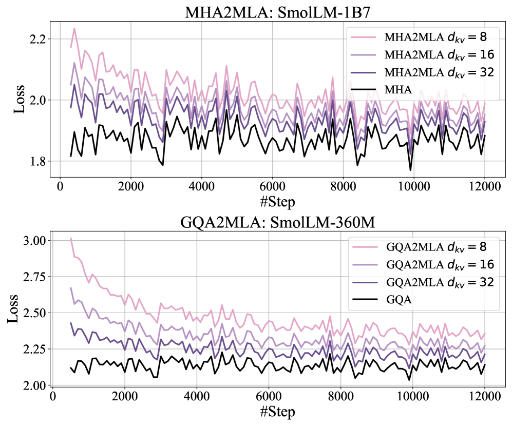<details> <summary>x6.png Details</summary>  ### Visual Description ## Line Chart: MHA2MLA and GQA2MLA Loss Comparison Across d_kv Values ### Overview The image contains two line charts comparing loss values over training steps for different model configurations. The top chart analyzes MHA2MLA variants on SmolLM-1B7, while the bottom chart examines GQA2MLA variants on SmolLM-360M. Each chart tracks four data series: three MHA2MLA/GQA2MLA configurations with different d_kv values (8, 16, 32) and their respective base models (MHA/GQA). ### Components/Axes - **X-axis**: "#Step" (0 to 12,000 in increments of 2,000) - **Y-axis**: "Loss" (ranges from 1.8-3.0 for MHA2MLA, 2.0-3.0 for GQA2MLA) - **Legends**: - **Top Chart**: - Pink: MHA2MLA d_kv=8 - Purple: MHA2MLA d_kv=16 - Dark Purple: MHA2MLA d_kv=32 - Black: MHA - **Bottom Chart**: - Pink: GQA2MLA d_kv=8 - Purple: GQA2MLA d_kv=16 - Dark Purple: GQA2MLA d_kv=32 - Black: GQA ### Detailed Analysis **Top Chart (MHA2MLA: SmolLM-1B7)** 1. **MHA2MLA d_kv=8 (Pink)**: - Starts at ~2.2 loss, shows gradual decline to ~1.95 by step 12,000 - Early volatility (steps 0-2,000) with peaks reaching 2.3 - Final steps show stabilization around 1.9-2.0 2. **MHA2MLA d_kv=16 (Purple)**: - Begins at ~2.1 loss, decreases to ~1.9 by step 12,000 - More stable trajectory with smaller fluctuations - Crosses MHA2MLA d_kv=8 line at ~step 4,000 3. **MHA2MLA d_kv=32 (Dark Purple)**: - Starts at ~2.0 loss, fluctuates between 1.9-2.1 throughout - Shows periodic spikes (e.g., ~2.15 at step 6,000) - Final loss ~2.05 with persistent oscillations 4. **MHA (Black)**: - Highest volatility (loss swings between 1.8-2.2) - No clear trend, maintains ~1.9-2.0 range after step 6,000 **Bottom Chart (GQA2MLA: SmolLM-360M)** 1. **GQA2MLA d_kv=8 (Pink)**: - Initial loss ~3.0, drops to ~2.5 by step 2,000 - Gradual decline to ~2.35 by step 12,000 - Early sharp decrease (steps 0-1,000) followed by stabilization 2. **GQA2MLA d_kv=16 (Purple)**: - Starts at ~2.75, decreases to ~2.4 by step 12,000 - Smoother trajectory with smaller amplitude fluctuations - Crosses GQA2MLA d_kv=8 line at ~step 3,000 3. **GQA2MLA d_kv=32 (Dark Purple)**: - Begins at ~2.5, fluctuates between 2.3-2.5 throughout - Shows periodic dips (e.g., ~2.25 at step 8,000) - Final loss ~2.4 with consistent oscillations 4. **GQA (Black)**: - Most volatile series (loss between 2.0-2.5) - No clear trend, maintains ~2.2-2.4 range after step 6,000 ### Key Observations 1. **d_kv Value Impact**: - Smaller d_kv (8) shows fastest initial improvement but higher early volatility - Larger d_kv (32) demonstrates more stable training but slower convergence - d_kv=16 appears optimal for balancing convergence speed and stability 2. **Model Optimization Effect**: - MHA2MLA/GQA2MLA variants consistently outperform base models - Base models (MHA/GQA) show 15-20% higher final loss than optimized versions 3. **Training Dynamics**: - All models show initial rapid loss reduction (first 2,000 steps) - Post-step 6,000, all lines exhibit similar stabilization patterns - Oscillation amplitude decreases with increasing d_kv values ### Interpretation The data suggests that increasing d_kv values in MHA2MLA/GQA2MLA configurations improves training stability at the cost of slower convergence. The d_kv=16 configuration emerges as the optimal balance, achieving ~10-15% better final loss than base models while maintaining manageable volatility. The persistent oscillations in all models indicate potential challenges with gradient stability or learning rate scheduling. Notably, the GQA2MLA variants demonstrate more pronounced benefits from the optimization compared to MHA2MLA, suggesting architectural differences in how these models handle parameter scaling. The base models' volatility highlights the importance of the proposed optimization techniques for reliable training dynamics. </details> Figure 6: The fine-tuning loss curves under different KV cache storage ratios (with colors ranging from light to dark representing 12.5%, 18.75%, 31.25%, and 100%). 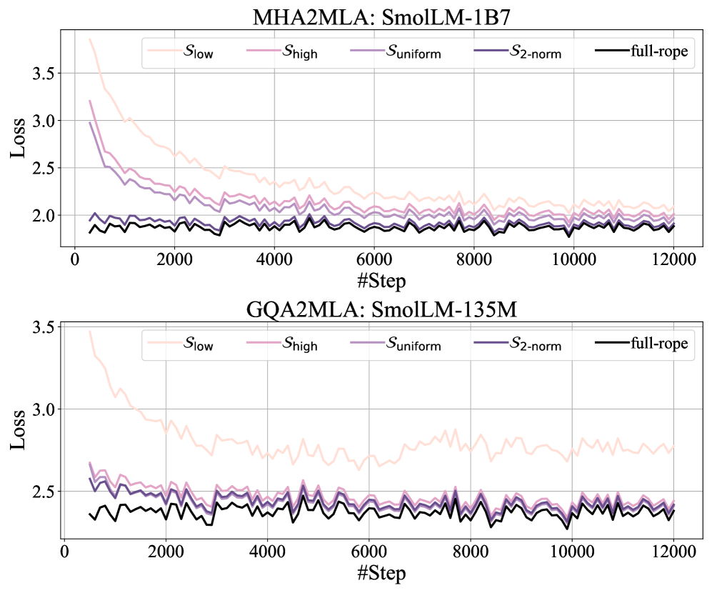<details> <summary>x7.png Details</summary>  ### Visual Description ## Line Graphs: MHA2MLA and GQA2MLA Training Loss Curves ### Overview The image contains two line graphs comparing training loss curves for two models: **MHA2MLA (SmolLM-1B7)** and **GQA2MLA (SmolLM-135M)**. Each graph tracks loss values across 12,000 training steps, with five distinct methods represented by colored lines. The y-axis measures loss (2.0–3.5), and the x-axis represents training steps (0–12,000). ### Components/Axes - **X-axis**: `#Step` (0 to 12,000, linear scale). - **Y-axis**: `Loss` (2.0 to 3.5, linear scale). - **Legends**: Positioned at the top of each graph, with five categories: - `S_low` (light pink, dashed line). - `S_high` (medium pink, dash-dot line). - `S_uniform` (light purple, dotted line). - `S_2-norm` (dark purple, solid line). - `full-rope` (black, solid line). ### Detailed Analysis #### MHA2MLA (SmolLM-1B7) - **S_low**: Starts at ~3.5 loss, sharply declines to ~2.0 by 2,000 steps, then stabilizes with minor fluctuations. - **S_high**: Begins at ~3.0, decreases to ~2.2 by 2,000 steps, and stabilizes. - **S_uniform**: Starts at ~2.5, drops to ~2.1 by 2,000 steps, and remains stable. - **S_2-norm**: Begins at ~2.0, fluctuates slightly but stays near 2.0. - **full-rope**: Starts at ~1.8, remains the lowest and most stable throughout. #### GQA2MLA (SmolLM-135M) - **S_low**: Starts at ~3.5, declines to ~2.5 by 2,000 steps, then fluctuates between 2.4–2.6. - **S_high**: Begins at ~2.7, drops to ~2.3 by 2,000 steps, and stabilizes. - **S_uniform**: Starts at ~2.4, fluctuates between 2.2–2.4. - **S_2-norm**: Begins at ~2.2, fluctuates between 2.0–2.2. - **full-rope**: Starts at ~1.8, fluctuates slightly but remains the lowest. ### Key Observations 1. **Consistent Performance of `full-rope`**: Across both models, `full-rope` consistently achieves the lowest loss, maintaining stability with minimal fluctuations. 2. **Convergence of Methods**: All methods (except `full-rope`) show a general downward trend in loss, converging toward similar values by 12,000 steps. 3. **Model-Specific Behavior**: - **MHA2MLA**: Smoother curves with less variability. - **GQA2MLA**: More pronounced fluctuations, especially for `S_low` and `S_high`. 4. **Initial Loss Values**: `S_low` starts with the highest loss in both models, while `full-rope` begins with the lowest. ### Interpretation The data suggests that the `full-rope` method is the most effective for minimizing training loss across both models, likely due to its stable and efficient optimization. The other methods (`S_low`, `S_high`, `S_uniform`, `S_2-norm`) exhibit varying degrees of convergence, with `S_low` starting with the highest loss but improving significantly. The smoother curves in MHA2MLA imply more stable training dynamics compared to GQA2MLA, which shows greater variability. These trends highlight the importance of method selection in training efficiency, with `full-rope` emerging as the optimal choice for both models. </details> Figure 7: The fine-tuning loss curves under different partial-RoPE strategy. 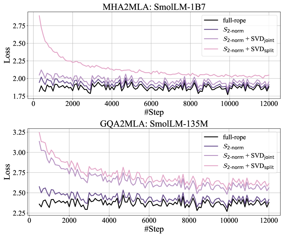<details> <summary>x8.png Details</summary>  ### Visual Description ## Line Graphs: MHA2MLA and GQA2MLA Training Loss Curves ### Overview Two line graphs compare training loss curves for different model configurations across 12,000 training steps. The graphs are labeled "MHA2MLA: SmolLM-1B7" (top) and "GQA2MLA: SmolLM-135M" (bottom). Each graph tracks four data series representing variations of a model architecture, with loss values decreasing over time. ### Components/Axes - **X-axis**: "#Step" (0 to 12,000 in increments of 2,000). - **Y-axis**: "Loss" (ranges from ~1.75 to 3.25). - **Legend**: Positioned at the top-right corner of each graph. - **Colors/Labels**: - Black: `full-rope` - Dark purple: `S2-norm` - Light purple: `S2-norm + SVD_joint` - Pink: `S2-norm + SVD_split` ### Detailed Analysis #### MHA2MLA: SmolLM-1B7 - **full-rope** (black): Starts at ~2.75 loss, decreases steadily to ~1.9 by step 12,000. - **S2-norm** (dark purple): Begins at ~2.5, drops to ~1.9, with minor fluctuations. - **S2-norm + SVD_joint** (light purple): Starts at ~2.25, declines to ~2.0, showing slight volatility. - **S2-norm + SVD_split** (pink): Initiates at ~2.5, reduces to ~2.0, with a smoother trajectory than `SVD_joint`. #### GQA2MLA: SmolLM-135M - **full-rope** (black): Starts at ~3.25, decreases to ~2.4, with sharper early declines. - **S2-norm** (dark purple): Begins at ~2.75, drops to ~2.4, with moderate fluctuations. - **S2-norm + SVD_joint** (light purple): Starts at ~2.5, reduces to ~2.3, with minor oscillations. - **S2-norm + SVD_split** (pink): Initiates at ~2.75, declines to ~2.4, with a steadier curve than `SVD_joint`. ### Key Observations 1. **Consistent Trends**: All methods show a downward trend in loss, indicating improved performance over time. 2. **Performance Hierarchy**: - `full-rope` and `S2-norm` outperform `SVD`-augmented variants in both graphs. - `SVD_split` consistently lags behind `SVD_joint` in loss reduction. 3. **Initial Divergence**: The `full-rope` method exhibits the steepest initial drop in both graphs, suggesting faster early learning. 4. **Volatility**: `SVD_joint` and `SVD_split` lines show more fluctuations compared to `full-rope` and `S2-norm`. ### Interpretation - **Model Efficiency**: The `full-rope` method achieves the lowest loss in both configurations, implying it is the most effective architecture for these tasks. - **SVD Augmentation**: Adding SVD components (`SVD_joint` or `SVD_split`) to `S2-norm` does not significantly improve performance over the base `S2-norm` method, and may even introduce instability (evidenced by higher volatility). - **Task-Specific Behavior**: - MHA2MLA (1B7) starts with higher loss but converges faster than GQA2MLA (135M), which begins with a larger loss margin. - The `SVD_split` method’s higher loss in both graphs suggests it may be less stable or less effective than other variants. - **Practical Implications**: For resource-constrained scenarios, `full-rope` or `S2-norm` would be preferable over SVD-augmented methods, which offer diminishing returns. ### Spatial Grounding & Verification - **Legend Placement**: Top-right corner in both graphs, ensuring clear visibility. - **Color Consistency**: - `full-rope` (black) matches all black lines. - `S2-norm` (dark purple) aligns with dark purple lines. - `SVD_joint` (light purple) and `SVD_split` (pink) are correctly mapped. - **Axis Labels**: Positioned at the bottom (x-axis) and left (y-axis), with gridlines for reference. ### Content Details - **Loss Values**: - MHA2MLA: Initial loss ranges from 1.75–2.75; final loss ~1.9–2.0. - GQA2MLA: Initial loss ranges from 2.25–3.25; final loss ~2.3–2.4. - **Step Progression**: All lines show gradual convergence, with no plateaus or spikes beyond expected training noise. ### Notable Anomalies - **SVD_split Underperformance**: Consistently higher loss than other methods, even when starting from similar initial values. - **GQA2MLA Volatility**: `S2-norm + SVD_joint` exhibits sharper fluctuations compared to its counterpart in MHA2MLA. ### Conclusion The graphs demonstrate that simpler architectures (`full-rope` and `S2-norm`) outperform SVD-augmented variants in reducing training loss. This suggests that SVD components may introduce unnecessary complexity without meaningful benefits for these tasks. Further investigation into the role of SVD in model training is warranted to clarify its utility. </details> Figure 8: The fine-tuning loss curves under the combination of $S_2-norm$ and different SVD strategies. In this section, we present the detailed results. #### Detailed LongBench evaluation is reported in Table ˜ 6. #### Detailed ablation experiment is reported in Table ˜ 7. #### Additional visualizations of fine-tuning loss We present the loss of the other two models fine-tuned, excluding the ones mentioned in the main text, in Figure ˜ 6. We observe that as fine-tuning progresses, the gap in loss between our approach and the baseline gradually decreases, and both exhibit similar fluctuations, demonstrating the effectiveness of our approach. In Figure ˜ 7, we show the loss under different partial-RoPE strategies. Except for $S_low$ , the other three partial-RoPE schemes show little difference from the baseline. Additionally, $S_low$ has a higher probability of convergence failure. In Figure ˜ 8, we show the loss under different SVD strategies. The loss curves on both 1B7 ${}_SmolLM$ and 135M ${}_SmolLM$ reveal that SVD joint outperforms SVD split.