# SVDq: 1.25-bit and 410×\times× Key Cache Compression for LLM Attention
**Authors**: Huawei Noah’s Ark Lab
## Abstract
For the efficient inference of Large Language Models (LLMs), the effective compression of key-value ( $KV$ ) cache is essential. Three main types of $KV$ cache compression techniques, namely sparsity, channel compression, and quantization, have been identified. This study presents SVDq, a Singular Value Decomposition (SVD) - based mixed precision quantization method for $K$ cache. Initially, $K$ cache is transformed into “latent channels” using SVD basis representations. Since the values in latent channels decay rapidly and become negligible after only a few latent channels, our method then incorporates importance-aware quantization and compression for latent channels. This enables the effective allocation of higher precision to more significant channels. Theoretically, we prove that SVDq results in quantization errors ( $× 0.1$ or even lower) that are much lower than those of per-channel key quantization in the original space. Our findings based on RULER and LongBench benchmarks demonstrate that SVDq can achieve an equivalent key cache precision as low as 1.25 -bit. When combined with key sparsity, it can reach a key compression ratio of up to $\textbf{410}×$ for attention computation, all while maintaining comparable model performance. Notably, our method is nearly lossless for LongBench datasets. This indicates that SVDq enables high-precision low-bit quantization, providing a more efficient solution for $KV$ cache compression in LLMs.
## 1 Introduction
Large Language Models (LLMs) have started a new era of artificial intelligence by demonstrating remarkable capabilities in handling complex tasks (OpenAI et al., 2024; Grattafiori et al., 2024; Qwen et al., 2025; DeepSeek-AI et al., 2025). Most of these recently developed LLMs are founded upon the attention mechanism based auto-regressive decoder transformers (Vaswani et al., 2023). Consequently, they need to encode past information into intermediate hidden tensors, specifically $KV$ caches, for subsequent and efficient inference.
However, in natural language tasks with large batches or long contexts, $KV$ cache often expands significantly in size, posing a significant challenge to fast inference (Pope et al., 2022; Liu et al., 2023). The substantial memory consumption and latency required to save and load $KV$ cache, coupled with the computational demands of attention operations, become critical bottlenecks for LLM inference. Considering the rapid advancement of computability and the increasing demand for efficient LLM inference, we recognize the importance of high-ratio $KV$ cache compression (even with a slight concession in computational overhead), enabling the inference of LLMs on devices with limited memory.
Existing approaches to $KV$ cache compression can be categorized into three main directions: sequence-axis compression, channel-axis compression, and digit-type compression. (i) Sequence-axis compression, exemplified by works such as Xiao et al. (2023); Zhang et al. (2024c); Ge et al. (2023); Li et al. (2024b); Tang et al. (2024); Ribar et al. (2024); Singhania et al. (2024); Yang et al. (2025), often referred to as sparsity, involves identifying and discarding unimportant tokens for attention computation. (ii) Channel-axis compression, as demonstrated in, e.g., Xu et al. (2024); Liu et al. (2024a); Sun et al. (2024), focuses on the channel dimension compression of $KV$ cache with methods like truncating and low-rank decomposition. Notably, low-rank approximation techniques, as explored in Wang et al. (2024b); Zhang et al. (2024b), represent a similar approach of this category. These methods transform $KV$ cache into " latent channels " representation based on SVD, and then discard insignificant latent channels. (iii) Digit-type compression, also known as quantization, aims to reduce the memory footprint by employing lower-precision representations for $KV$ cache (Liu et al., 2023; Hooper et al., 2024; Yang et al., 2024; Liu et al., 2024b; Li et al., 2025). This typically involves replacing the $32$ - or $16$ -bit FP numbers with lower precision representations. These three compression methods are proposed independently, exploiting different properties of $KV$ cache within LLMs.
The effectiveness of quantization highly depends on the statistical distribution of the cache values. Large value ranges and outliers can lead to substantial quantization errors. In addition, the performance of models degrades significantly below a certain quantization bit width (typically around $4$ to $2$ bits), thus limiting the compression ratio. Similarly, channel compression methods also face challenges in terms of the trade-off between accuracy and compression ratio. While works like Wang et al. (2024b); Zhang et al. (2024b) have demonstrated $2×$ compression ratios using SVD-based methods, further compression beyond this point leads to high accuracy loss. Recognizing these limitations, we emphasize the importance of combining these different strategies to further improve the compression ratio. For examples, ThinK Xu et al. (2024) highlights the compatibility of its channel truncation method with sparsity techniques; ShadowKV (Sun et al., 2024) combines sparsity with SVD low-rank approximation to achieve minor performance degradation while achieving very high compression ratios.
In this work, we follow the channel-axis compression and quantization strategy. We find that direct truncation of the original channels, as exemplified by ThinK (Xu et al., 2024), leads to significant performance degradation when pursuing high compression ratios. To address this challenge, we propose a compression method, SVDq, that integrates the channel truncation and quantization, by utilizing our observed underlying relationship between quantization and SVD-based channel compression.
Specifically, we observe an implication of the Eckart–Young–Mirsky theorem (Mirsky, 1960): the variances of the values within latent channels obtained through SVD are determined by the corresponding singular values and typically exhibit rapid decay. Recognizing that variances are often proportional to value ranges of latent channels, we can utilize singular values to guide the selection of quantization bit widths to balance accuracy and compression ratios.
Based on this observation, we propose a novel mixed-precision key cache We do not investigate the value cache since it often exhibits weak low-rank property. quantization method that integrates SVD-based channel compression. This method prioritizes higher bit widths for latent channels associated with larger singular values and progressively decreases precision for channels with smaller singular values. The SVD latent channels offer a significant advantage over simple variance-based descending sorting in the original space, because singular values decay exponentially for most key cache. In consequence, the range at each channel decreases fast, and often becomes insignificant after only a small number of latent channels. Hence, this approach enhances the effectiveness of quantization precision allocation for each latent channel. Furthermore, we emphasize the seamless compatibility of this method with sparsity techniques.
Our key contributions are as follows:
1. Proposing a novel method that effectively combines quantization and latent channel compression for $K$ cache, providing the theoretical insights.
1. Demonstrating the compatibility of this method with sparsity techniques.
1. Achieving a remarkable level of $K$ cache compression with an equivalent mixed quantization precision as low as $1.25$ bit while maintaining comparable model performance.
## 2 Related Works
Sparsity: With different feature extraction based attention estimation algorithms, methods such as Fastgen (Ge et al., 2023), H2O (Zhang et al., 2024c), Quest (Tang et al., 2024), SparQ (Ribar et al., 2024), PQCache (Zhang et al., 2024a), ShadowKV (Sun et al., 2024), and AttentionPredictor (Yang et al., 2025) selectively retain only the most important tokens in the sequence and effectively prune the others. Loki Singhania et al. (2024) is another sparsity method that uses the SVD approximation to accelerate attention estimation for critical tokens selection.
Channel Compression: These methods, such as ThinK (Xu et al., 2024), reduce the dimensionality of $KV$ cache by truncating channels or employing low-rank approximations. Prominent examples include SVD-based approaches like SVD-LLM (Wang et al., 2024b), LoRC (Zhang et al., 2024b), Palu (Chang et al., 2024), and Eigen Attention Saxena et al. (2024). Notably, techniques like Grouped Query Attention (GQA) Ainslie et al. (2023), Multi-head Latent Attention (MLA) (DeepSeek-AI et al., 2025), and transformations from Multi-Head Attention to GQA (Jin et al., 2024; Chen et al., 2024) can also be viewed as forms of channel compression, as they effectively reduce the number of attention dimensions.
Quantization: Methods like KIVI (Liu et al., 2023), KVQuant Hooper et al. (2024), AlignedKV (Tan et al., 2024), BitStack Wang et al. (2024a), and KVTuner (Li et al., 2025) reduce the memory footprint with low precision $KV$ cache. QServe Lin et al. (2024) introduces several quantization and system co-design methods to achieve efficient W4A8KV4, where SmoothAttention is utilized to migrate the key quantization difficulty to query.
Some works explore the combination of these approaches. In addition to the mentioned ShadowKV (Sun et al., 2024) and ThinK Xu et al. (2024), Liu et al. (2024b) integrates quantization with matrix decomposition to apply different quantization precision for the two decomposed matrices, and Palu Chang et al. (2024) applies per token quantization to the latent vector of the SVD low-rank approximation.
Importantly, the concept of using SVD for mixed-precision quantization has been explored in other contexts. For instance, Delta-CoMe (Ping et al., 2024) applies this principle to compress LLM weights, while SVDQuant (Li et al., 2024a) utilizes it for compressing diffusion models. The novelty of this work over the mentioned works lies not only in the application of this principle to $K$ cache compression but also in the theoretical foundation upon which we derive the principle and method, and the error analysis we provide.
## 3 SVD and Quantization
Singular Value Decomposition: Let $\textbf{K}∈ℝ^s× d$ denotes the $K$ cache matrix for a given head in a transformer layer, where $s$ and $d$ represent the sequence length and hidden embedding (channel) dimension, respectively, with $s\gg d$ typically holding for long context applications. Let K be centered by subtracting its per-channel mean $\bar{\textbf{K}}∈ℝ^d$ , i.e., $\textbf{K}←\textbf{K}-\bar{\textbf{K}}$ and maintain the same notation.
Assuming K is full-rank. Its SVD is given by
$$
\textbf{K}=\textbf{U}·\textbf{D}·\textbf{V}^\textrm{H}, \tag{1}
$$
where $\textbf{U}∈ℝ^s× d$ has orthonormal columns, $\textbf{V}∈ℝ^d× d$ is orthonormal, satisfying $\textbf{U}^\textrm{H}·\textbf{U}=\textbf{I}_d$ and $\textbf{V}^\textrm{H}·\textbf{V}=\textbf{I}_d$ , and $\textbf{D}∈ℝ^d× d$ is a diagonal matrix containing the singular values in its diagonal with elements arranged in descending order, given by $\textbf{D}=Diag([λ_1,...,λ_d])$ .
Quantization Let $\textbf{{k}}_\rm min:=(\min{\textbf{K}}_:1,...,\min{\textbf{K}}_:d)$ , i.e., the column-wise minimum vector, and analogously define $\textbf{{k}}_\rm max$ . The per-channel asymmetrical $b$ -bit quantization and dequantization operations are given by:
$$
\displaystyleQ_b(\textbf{K}):= \displaystyle ≤ft\lfloor\frac{\textbf{K}-\textbf{{k}}_\rm min}{(\textbf{{
k}}_\rm max-\textbf{{k}}_\rm min)/(2^b-1)}\right\rceil, \displaystyleD_b(\textbf{K}_b):= \displaystyle Q_b(\textbf{K})×\frac{\textbf{{k}}_\rm max-
\textbf{{k}}_\rm min}{2^b-1}+\textbf{{k}}_\rm min, \tag{2}
$$
where $≤ft\lfloor·\right\rceil$ denote the rounding operator. Naturally, $D_b∘Q_b(\textbf{K})≈\textbf{K}$ .
For uniformly or normally distributed columns of K, the relative quantization errors depend solely on the bit width $b$ , independent of the range $\textbf{{k}}_\rm max-\textbf{{k}}_\rm min$ . However, the absolute errors scale with $\textbf{{k}}_\rm max-\textbf{{k}}_\rm min$ , implying that smaller value ranges or variances yield smaller absolute quantization errors.
## 4 Methods
Although the theory of the proposed SVD-quantization method, discussed in the previous section, is expected to be applicable to a much wider range of applications, this work focuses on KV cache compression in the long context inference scenario. For long context LLMs, $KV$ cache generated in the prefilling stage generally dominates the memory usage. Our method is proposed to address this challenge.
### 4.1 SVD Quantization
Consider the rows of $\textbf{V}^H$ in Equation (1) as a basis for the row space of K. For the projection $P_\textbf{V_:j}$ of the rows of K into the $j$ -th basis vector, defined by $P_\textbf{V_:j}(\textbf{K}):=\textbf{K}·\textbf{V}_:j$ , following the Eckart–Young–Mirsky theorem (Mirsky, 1960), we have:
**Theorem 4.1**
*For the $K$ cache matrix $\boldsymbol{K}$ , the variance of its projection satisfies
$$
Var(P_\boldsymbol{V_:j}(\boldsymbol{K
}))=λ_j^2. \tag{4}
$$*
**Corollary 4.1.1**
*Let $\textbf{k}∈ℝ^d$ be a $K$ cache vector with $\bar{\boldsymbol{K}}$ subtracted, i.e., $\textbf{k}←\textbf{k}-\bar{\boldsymbol{K}}$ . For any indices $0<i≤ j<d$ , the squared expectations of its projections satisfy:
$$
E((P_\boldsymbol{V_:i}(\textbf{k}))^2)≥
E((P_\boldsymbol{V_:j}(\textbf{k}))^2). \tag{5}
$$*
* Proof*
For any $0<j≤ d$ , the projection of K is given by
$$
P_\textbf{V_:j}(\textbf{K})=\textbf{K}·\textbf{V}_:j=
\textbf{U}·\textbf{D}·\textbf{V}^\textrm{H}·\textbf{V}_:j=
λ_j\textbf{U}_:j.
$$ Since $E(P_\textbf{V_:j}(\textbf{K}))=P_\textbf{V_:j}(E(\textbf{K}))=0$ , we have
$$
Var(P_\textbf{V_:j}(\boldsymbol{K}))=
Var(λ_j\textbf{U}_:j)=λ_j^2E≤ft(\textbf{U}^
\textrm{H}_j:·\textbf{U}_:j\right)=λ_j^2.
$$ This proves Theorem 4.1. Corollary 4.1.1 follows directly from Theorem 4.1 when the given vector k follows the distribution of the rows of K. ∎
<details>
<summary>x1.png Details</summary>
### Visual Description
## 3D Scatter Plot: Signal vs Noise Distribution Across Token and Channel
### Overview
The image depicts a 3D scatter plot visualizing the distribution of "Signal" (red) and "Noise" (blue) data points across three dimensions: Token (x-axis), Channel (y-axis), and Channel Value (z-axis). The plot reveals spatial clustering patterns and intensity differences between the two data types.
### Components/Axes
- **X-axis (Token)**: Ranges from 0 to 200, labeled "Token."
- **Y-axis (Channel)**: Ranges from 0 to 120, labeled "Channel."
- **Z-axis (Channel Value)**: Ranges from 0 to 8, labeled "Channel Value (abs)."
- **Legend**: Located in the top-right corner, with red representing "Signal" and blue representing "Noise."
### Detailed Analysis
1. **Signal (Red) Clusters**:
- **Cluster 1**:
- Token: 50–150
- Channel: 40–80
- Z-axis: Peaks up to ~7.5 (abs)
- Density: High concentration of points with sharp vertical spikes.
- **Cluster 2**:
- Token: 100–150
- Channel: 80–120
- Z-axis: Peaks up to ~6.5 (abs)
- Overlap: Partially overlaps with Noise cluster in this region.
- **Cluster 3**:
- Token: 150–200
- Channel: 100–120
- Z-axis: Peaks up to ~5.5 (abs)
- Lower intensity compared to Cluster 1.
2. **Noise (Blue) Distribution**:
- **Cluster 1**:
- Token: 0–100
- Channel: 0–80
- Z-axis: Uniform spread between 2–6 (abs)
- Density: Evenly distributed with no sharp peaks.
- **Cluster 2**:
- Token: 100–200
- Channel: 80–120
- Z-axis: Spread between 3–5 (abs)
- Overlap: Intersects with Signal Cluster 2 but with lower z-values.
### Key Observations
- **Signal Intensity**: Signal data points exhibit significantly higher z-axis values (up to 7.5) compared to Noise (max ~6.5).
- **Spatial Localization**: Signal clusters are tightly grouped in specific Token/Channel ranges, while Noise is more uniformly distributed.
- **Overlap**: In the Token 100–150 and Channel 80–120 region, Signal and Noise clusters intersect, but Signal maintains higher z-values.
- **Noise Uniformity**: Noise data shows minimal variation in z-axis values, forming a flat, dispersed layer.
### Interpretation
The plot demonstrates that **Signal** is characterized by localized, high-intensity spikes in specific Token/Channel regions, suggesting targeted or structured data. In contrast, **Noise** is broadly distributed with lower, more uniform values, indicating random or background interference. The overlap in Cluster 2 suggests potential contamination or co-occurrence of Signal and Noise in this region, which may require further filtering. The third Signal cluster (Token 150–200) shows reduced intensity, possibly reflecting weaker or degraded signals at higher Token values. This distribution could inform noise reduction strategies or signal prioritization in data processing pipelines.
</details>
<details>
<summary>x2.png Details</summary>
### Visual Description
## Line Graph: Statistical Distribution of Channel Data
### Overview
The image depicts a line graph with two primary data series (blue and orange lines) and scattered green data points. The x-axis represents "Channel" (0–120), while the y-axis is unlabeled but includes grid lines. The graph shows periodic peaks and troughs in both lines, with green points distributed around them.
### Components/Axes
- **X-axis**: Labeled "Channel," ranging from 0 to 120 in increments of 20.
- **Y-axis**: Unlabeled, with grid lines suggesting a numerical scale (approximate range: -2 to +2 based on line extremities).
- **Legend**: Located in the top-left corner.
- Blue line: "2σ" (positive two standard deviations).
- Orange line: "-2σ" (negative two standard deviations).
- **Data Points**: Green dots scattered across the graph, denser near the blue and orange lines.
### Detailed Analysis
1. **Blue Line (2σ)**:
- Peaks at channels ~60 and ~120, reaching approximately +1.5 and +1.2 on the y-axis, respectively.
- Smaller oscillations between channels 0–40 and 80–100, with values fluctuating between ~0.5 and ~1.0.
- Sharp drop near channel 80, dipping to ~0.3 before rising again.
2. **Orange Line (-2σ)**:
- Troughs at channels ~60 and ~120, reaching approximately -1.5 and -1.2 on the y-axis, respectively.
- Oscillations between channels 0–40 and 80–100, with values fluctuating between ~-0.5 and ~-0.8.
- Sharp rise near channel 80, peaking at ~-0.3 before declining.
3. **Green Data Points**:
- Clustered around the blue and orange lines, with higher density near peaks/troughs.
- Spread between ~-1.0 and +1.0 on the y-axis, suggesting variability within ±1σ.
### Key Observations
- **Symmetry**: The blue and orange lines mirror each other in magnitude but opposite in sign, consistent with ±2σ boundaries.
- **Peaks at Channels 60 and 120**: Both lines exhibit pronounced extrema at these points, indicating potential anomalies or events.
- **Data Point Distribution**: Green points are concentrated near the ±2σ lines, implying most measurements fall within this range.
- **Channel 80 Behavior**: Both lines show a transitional dip/rise at this channel, suggesting a shift in the underlying distribution.
### Interpretation
The graph likely represents a statistical analysis of channel data, where:
- The **blue and orange lines** define ±2σ boundaries, framing the expected range of data variability.
- The **green points** are individual measurements, with their clustering near the ±2σ lines indicating that most values lie within this range.
- The **peaks at channels 60 and 120** suggest localized anomalies or heightened activity, as their magnitudes exceed typical fluctuations.
- The **symmetry** between the lines reinforces the assumption of a normal or Gaussian-like distribution, where extreme values are equally likely in both directions.
The unlabeled y-axis implies the data may represent normalized or dimensionless quantities (e.g., deviations from a mean). The absence of a mean line (e.g., 0σ) limits direct interpretation of central tendency but emphasizes variability.
This visualization could apply to fields like signal processing, quality control, or environmental monitoring, where identifying deviations from expected behavior is critical.
</details>
(a) Original K
<details>
<summary>x3.png Details</summary>
### Visual Description
## 3D Scatter Plot: Channel Value Distribution Across Tokens and Latent Channels
### Overview
The image depicts a 3D scatter plot visualizing the distribution of "Channel Value (abs)" across two dimensions: "Token" (0–200) and "Latent Channel" (0–120). The plot uses color-coded data points to represent varying magnitudes of Channel Value, with a legend in the top-left corner indicating three categories: blue (low values), orange (medium values), and red (high values).
---
### Components/Axes
- **X-axis (Token)**: Ranges from 0 to 200, labeled "Token."
- **Y-axis (Latent Channel)**: Ranges from 0 to 120, labeled "Latent Channel."
- **Z-axis (Channel Value)**: Ranges from 0 to 14, labeled "Channel Value (abs)."
- **Legend**: Located in the top-left corner, with three color categories:
- **Blue**: Low Channel Values (0–4 abs).
- **Orange**: Medium Channel Values (5–10 abs).
- **Red**: High Channel Values (11–14 abs).
---
### Detailed Analysis
1. **Blue Data Points**:
- Dominant across the entire plot, forming a dense, flat layer.
- Concentrated in the lower Z-axis range (0–4 abs).
- Spread uniformly across all Token and Latent Channel values.
2. **Orange Data Points**:
- Sparse and scattered, primarily in the mid-range of the Z-axis (5–10 abs).
- Clustered near Token ≈ 50–100 and Latent Channel ≈ 20–60.
3. **Red Data Points**:
- Extremely sparse, forming isolated peaks.
- Located near Token ≈ 0–20 and Latent Channel ≈ 0–10.
- Channel Values reach the maximum observed value of **14 abs**.
---
### Key Observations
- **Outliers**: Red points represent extreme values, deviating significantly from the majority (blue) distribution.
- **Clustering**: Blue points dominate the lower Z-axis, suggesting most Channel Values are low-magnitude.
- **Intermediate Values**: Orange points indicate a small subset of medium-magnitude values, concentrated in specific Token/Latent Channel regions.
- **Spatial Distribution**: High values (red) are tightly grouped near the origin (Token ≈ 0, Latent Channel ≈ 0), while medium values (orange) are dispersed further out.
---
### Interpretation
The plot suggests a hierarchical structure in the data:
1. **Majority Behavior**: Most tokens and latent channels exhibit low Channel Values (blue), indicating a baseline or default
</details>
<details>
<summary>x4.png Details</summary>
### Visual Description
## Line Graph: Latent Channel Value Distribution
### Overview
The image depicts a line graph with two primary data series (blue and orange lines) and scattered green data points. The graph illustrates how values evolve across latent channels, with confidence intervals represented by the lines and raw data points shown as green markers.
### Components/Axes
- **X-axis (Latent Channel)**: Ranges from 0 to 120 in increments of 20.
- **Y-axis (Value)**: Ranges from 0 to 140 in increments of 20.
- **Legend**:
- **Blue line**: Labeled "2σ" (positive two standard deviations).
- **Orange line**: Labeled "-2σ" (negative two standard deviations).
- **Data Points**: Green dots scattered across the graph, concentrated near the blue and orange lines.
### Detailed Analysis
1. **Blue Line (2σ)**:
- Starts at approximately **140** at x=0.
- Drops sharply to ~**100** by x=10.
- Gradually declines to ~**80** by x=20.
- Stabilizes between **70–80** from x=40 to x=120.
2. **Orange Line (-2σ)**:
- Begins at ~**60** at x=0.
- Rises to ~**80** by x=20.
- Increases to ~**90** by x=40.
- Flattens between **90–100** from x=60 to x=120.
3. **Green Data Points**:
- Clustered around the blue and orange lines, with slight dispersion.
- Most points lie within the bounds of the two lines, suggesting adherence to the ±2σ range.
### Key Observations
- The blue line (2σ) exhibits a steep initial decline followed by stabilization, while the orange line (-2σ) shows a gradual ascent before plateauing.
- Green data points align closely with the lines, indicating minimal deviation from the ±2σ thresholds.
- No significant outliers are observed; all points remain within the defined confidence intervals.
### Interpretation
The graph likely represents a statistical analysis of latent channel behavior, where:
- The **blue line (2σ)** and **orange line (-2σ)** define a confidence interval for the expected value range.
- The **green data points** confirm that observed values consistently fall within this interval, suggesting low variability or controlled conditions.
- The initial divergence between the lines (x=0–20) may indicate a transitional phase in the latent channel's behavior, stabilizing afterward.
- The flattening of both lines at higher latent channels implies convergence toward a steady state, possibly reflecting equilibrium in the system being modeled.
This visualization emphasizes the importance of confidence intervals in understanding data distribution and variability in latent space analysis.
</details>
(b) Projected K, i.e., $P_\textbf{V}(\textbf{K})$
Figure 1: Distribution of K and its standard deviation
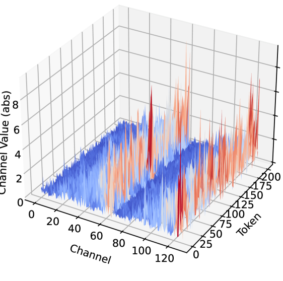
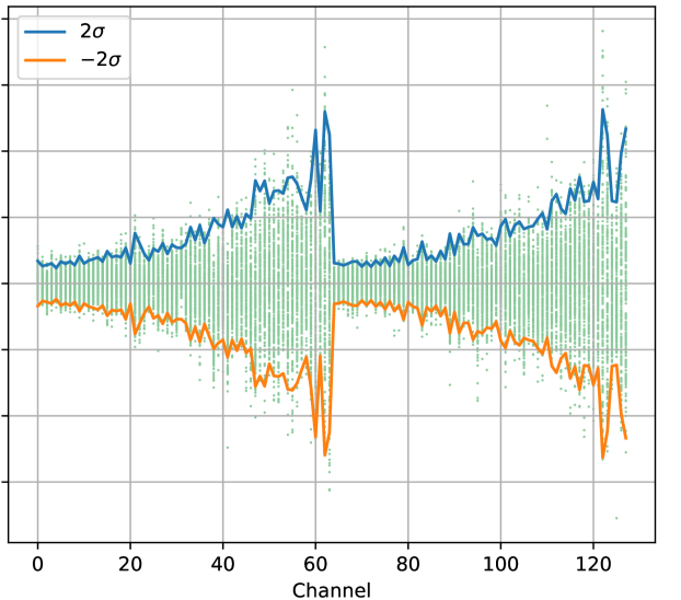
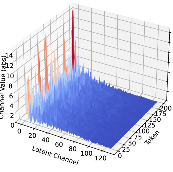
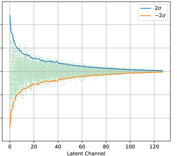
Note that the $P_\textbf{V}(\textbf{K})$ is essentially an alternative representation of K using the singular vector in V as the space bases. We call the columns of $P_\textbf{V}(\textbf{K})$ latent channels. Figure 1(a) illustrates the distribution of K in its original space, while Figure 1(b) displays its representation in the SVD space after projection, demonstrating the results of Theorem 4.1 and Corollary 4.1.1. The singular vector-based projection offers a significant advantage over simple variance-based descending sorting: for most matrices, singular values typically exhibit exponential decay. Consequently, the range of projection values (represented on the $y$ -axis in Figure 1(b)) decreases rapidly, becoming relatively insignificant (compared to the value range of the first dimension) after only a small number of latent channels.
Since $\textbf{K}=P_\textbf{V}(\textbf{K})·\textbf{V}^\textrm{H}$ where $P_\textbf{V}(\textbf{K}):=\textbf{K}·\textbf{V}$ , and all basis vectors in V are unit-normalized, the absolute error in approximating to $P_\textbf{V}$ represents both absolute and relative errors in approximating K. Theorem 4.1, Corollary 4.1.1, and Figure 1(b) demonstrate that both value range and variance decay rapidly along the latent channels. This property motivates our efficient mixed-precision quantization method, SVDq, to approximate K via $P_\textbf{V}(\textbf{K})$ :
(1) Use high precision quantization for initial latent channels;
(2) Progressively decrease the precision for subsequent latent channels;
(3) Truncate the remaining latent channels with negligible value ranges or singular values.
<details>
<summary>x5.png Details</summary>
### Visual Description
## Diagram: Neural Network Processing with Quantization and GPU Memory Caching
### Overview
The diagram illustrates a two-phase process for optimizing neural network operations: **Prefilling** (encoding/quantization) and **Decoding** (inference). It emphasizes bit-depth reduction (quantization) and GPU memory caching to improve efficiency. Key components include latent channel representations, quantization stages, GPU memory caching, and attention-based decoding with RoPE (Rotary Positional Embedding).
---
### Components/Axes
1. **Prefilling Phase**:
- **Latent Channel Representation**: Input data block (green) with waveform visualization.
- **Quantization**:
- 4-bit → 2-bit → 1-bit reduction (color-coded blocks: red, blue, yellow).
- Formula: `P_V(K) = K · V` (green arrow).
- **Concatenation**: Merges quantized keys for `n` attention heads (gray block).
- **Saved K Cache**: GPU memory storage for quantized keys (blue block with purple dashed outline).
2. **Decoding Phase**:
- **New Query**: Red block representing input queries.
- **RoPE (Rotary Positional Embedding)**: Cross symbol (⊗) applied to queries.
- **Attention Mechanism**:
- `K = P_V(K) · Vᴴ` (green arrow).
- Dot product with cached `V` (blue block).
- Softmax normalization (orange block).
- **Output**: Final result (brown block).
3. **Memory Management**:
- **Load & Dequant**: Arrows indicate data retrieval from GPU cache and bit-depth restoration.
- **GPU Memory Cache**: Purple dashed box highlights optimized storage for quantized `K`.
---
### Detailed Analysis
- **Quantization Flow**:
- Original 4-bit keys are reduced to 1-bit via sequential quantization (4→2→1 bits), visualized by shrinking block sizes (red → blue → yellow).
- Waveform plots show data distribution narrowing with each quantization step.
- **GPU Caching**:
- Quantized `K` is stored in GPU memory (blue block) to avoid recomputation during decoding.
- Purple dashed lines emphasize memory efficiency gains.
- **Decoding Logic**:
- New queries (red) are processed with RoPE (⊗) for positional awareness.
- Dot product with cached `V` (blue) computes attention scores.
- Softmax (orange) normalizes scores for output generation.
---
### Key Observations
1. **Bit-Depth Reduction**:
- Quantization reduces data size by 75% (4-bit → 1-bit), critical for memory-constrained environments.
2. **GPU Optimization**:
- Caching quantized `K` minimizes redundant computations during decoding.
3. **Positional Awareness**:
- RoPE integration suggests transformer-based architecture for sequence modeling.
4. **Efficiency Trade-offs**:
- Lower bit-depth quantization may slightly degrade model accuracy but improves speed/memory usage.
---
### Interpretation
This diagram represents a **model optimization pipeline** for resource-constrained environments (e.g., edge devices). By quantizing latent representations and leveraging GPU memory caching, the system balances computational efficiency with model performance. The use of RoPE indicates compatibility with transformer architectures, while the attention mechanism (`K = P_V(K) · Vᴴ`) ensures contextual relevance in decoding. The workflow prioritizes memory efficiency over raw computational power, making it suitable for real-time applications like speech recognition or real-time translation.
</details>
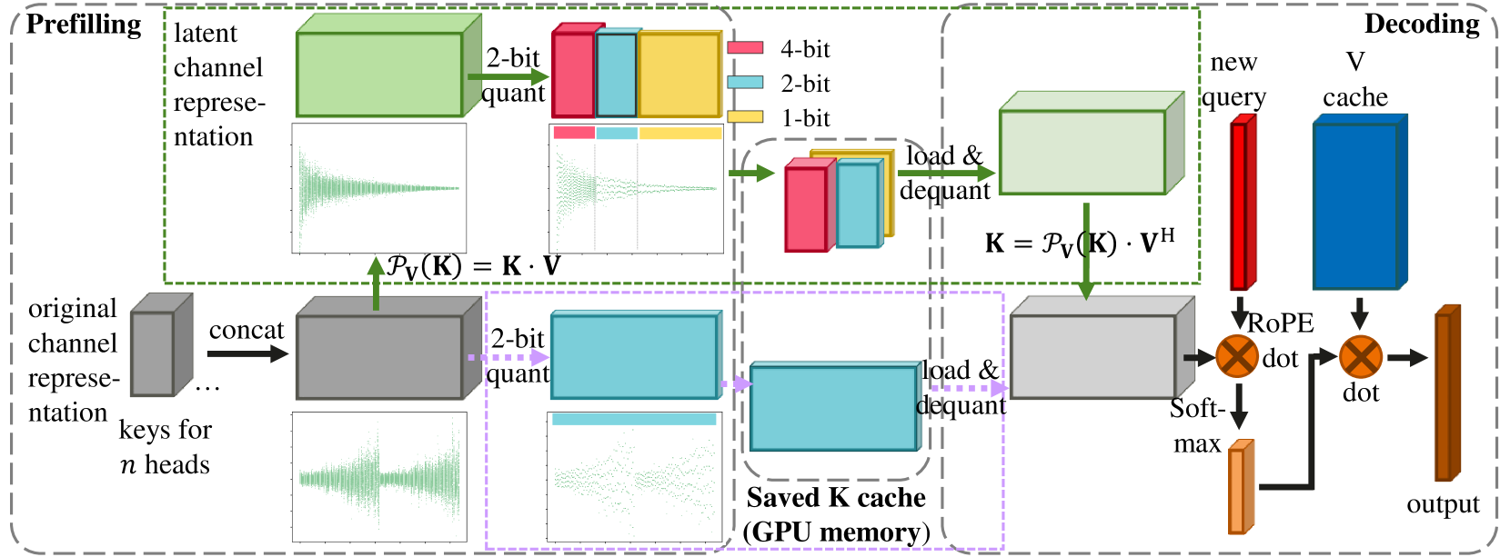
Figure 2: Diagram of SVDq method (path inside the box in green) versus direct per-channel quantization (dash path inside the box in violet).
### 4.2 Algorithm
In our SVDq method, we first apply SVD to the prefilling $K$ cache, obtaining the projection operator $P_\textbf{V}(·)$ using the right SVD matrix V. Next, we determine a precision schedule for the quantization on each latent channel based on the singular values $[λ_1,...,λ_d]$ . Specifically, a latent channel associated with a large singular value $λ$ is assigned a high quantization bit width $b$ , and channels with small $λ$ are assigned low $b$ or even be truncated with notation $b=0$ . This yields a schedule vector b, and the equivalent mixed bit width of this quantization schedule for the K cache is given by
$$
\bar{b}=\frac{1}{d}∑_i=1^d\textit{{b}}_i. \tag{6}
$$
Sequently, we use $Q_\textit{{b}}$ in (2) to quantize $P_\textbf{V}(\textbf{K})$ . The low-bit quantized $P_\textbf{V}(\textbf{K})$ is then saved as the cache. In the decoding process, we dequantize the cache, reconstruct K in its original representation using $\textbf{K}=P_\textbf{V}(\textbf{K})·\textbf{V}^H$ , and then proceed with the attention computation. We summarize the algorithm using pseudo-code in Algorithm 1 and an abstracted diagram in Figure 2.
Algorithm 1 SVD-quantization algorithm for K
$K$ cache matrix K of $L$ layers
$\hat{\textbf{K}}≈\textbf{K}$
for $l← 1$ to $N$ do
Load K cache matrix for $l$ -th layer
$\textbf{K}=\textbf{K}-\bar{\textbf{K}}$
$\textbf{U},\textbf{D},\textbf{V}←SVD(\textbf{K})$
$P_\textbf{V}(\textbf{K})=\textbf{U}·\textbf{D}$
Set quant schedule b
Save $\bar{\textbf{K}}$ , V, $Q_\textit{{b}}∘P_\textbf{V}(\textbf{K})$ , function $D_\textit{{b}}$
end for
$\hat{\textbf{K}}=D_\textit{{b}}≤ft(Q_\textit{{b}} ∘P_\textbf{V}(\textbf{K})\right)·\textbf{V}^H+ \bar{\textbf{K}}$
In this algorithm, the quantities to be saved include the quantized $P_\textbf{V}(\textbf{K})∈ℝ^s× d$ (represented using $\bar{b}$ -bit), the right SVD matrix $\textbf{V}∈ℝ^d× d$ , the average of K denoted by $\bar{\textbf{K}}∈ℝ^d$ , and the dequant function $D_\textit{{b}}$ , which relies on the bit schedule $\textit{{b}}∈ℝ^d$ and the range of $P_\textbf{V}(\textbf{K})$ , given by $\textit{{p}}_\rm min,\textit{{p}}_\rm max∈ℝ^d$ . In long context applications, $d\ll s$ , the requirement of memory space for terms that depend solely on $d$ , e.g., the space for V and $\bar{\textbf{K}}$ , is negligible. Hence, the compression rate compared with the original $16$ -bit $\textbf{K}∈ℝ^s× d$ is approximately $16/\bar{b}$ .
In this work, we concatenate the K matrices of all heads within the same layer, resulting in a larger K matrix with the embedding dimension $d$ being the sum of the embedding dimensions of all heads. To improve efficiency, for the bit schedule setting b, we divide the $d$ latent channels of $P_\textbf{V}(\textbf{K})$ into $8$ equal-sized group, each comprising $\frac{d}{8}$ dimensions. The channels within each group share the same quantization bit width. Thus, b is determined by an 8-dimensional vector $(b_1,b_2,...,b_8)$ of integer. For example, a schedule of $(8,4,2,1,1,0,0,0)$ has an equivalent mixed bit width $\bar{b}=2$ and hence a compression ratio $8$ . For a model with $d=1024$ , this schedule implies:
- $8$ -bit quantization for the first $128$ latent channels,
- $4$ -bit for the next $128$ channels,
- $2$ -bit for the next $128$ channels,
- $1$ -bit for the next $256$ channels,
- truncation for the remaining $384$ channels.
### 4.3 Theoretical Error Analysis
We begin by presenting a lemma for later analysis.
**Lemma 4.1**
*If data $X$ are distributed uniformly within their value range $r$ , then the expectation of the square absolute error, $ε$ , of an asymmetrical $b$ -bit quantization applied to $X$ is equal to the variance of a uniform distribution with a range of $\frac{r}{2^b}$ , that is
$$
E(ε^2)=\frac{1}{12}\frac{r^2}{2^2b}.
$$*
Let K be centered by subtracting the key’s per-channel mean $\bar{\textbf{K}}∈ℝ^d$ , and let $P_\textbf{V}(\textbf{K})$ be its latent channel representation. The Frobenius norm is invariant under this transformation, as
$$
\|P_\textbf{V}(\textbf{K})\|_F^2=∑_i=1^s
P_\textbf{V}(\textbf{K}_i:)·P_\textbf{V}(\textbf
{K}_i:)^H=∑_i=1^s\textbf{K}_i:·\textbf{K}_i:^
H=\|\textbf{K}\|_F^2.
$$
Let $[σ_1^2,...,σ_d^2]$ and $[λ_1^2,...,λ_d^2]$ denote the variance vectors of the channels for the original and latent channel representations of K, respectively. Thus,
$$
∑_j=1^dσ_j^2=\frac{1}{s}\|\textbf{K}\|_F^2=\frac{
1}{s}\|P_\textbf{V}(\textbf{K})\|_F^2=∑_j=1^d
λ_j^2. \tag{7}
$$
We further assume that the key cache distributions in each original channel and latent channel follow uniform distributions. Then, according to Lemma 4.1, the value ranges of the $j$ -th original channel and $j$ -th latent channel are $r_j=2√{3}σ_j$ and $\hat{r}_j=2√{3}λ_j$ , respectively.
Error analysis for direct quantization Figure 1(a) shows that the variances in the original channels often exhibit similar orders of magnitude. We therefore assume that they are approximately identical, with $σ_j^2=\frac{1}{ds}\|\textbf{K}\|_F^2$ and $r_j^2=\frac{12}{ds}\|\textbf{K}\|_F^2$ . Applying a per-channel, direct $b$ -bit quantization to K, and following Lemma 4.1 and the above analysis, results in a quantization error $ε_b$ with the expected value:
$$
E(ε_b^2)=\frac{1}{12}\frac{1}{2^2b}\frac{12}{ds}\|
\textbf{K}\|_F^2=\frac{1}{2^2b}\frac{\|\textbf{K}\|_F
^2}{ds}. \tag{8}
$$
Error analysis for SVDq The singular values of a matrix often exhibit exponential decay. We model the variance vector for K ’s latent channel representation as
$$
λ_j=ce^-ρ j=λ_ie^-ρ(j-i), \tag{9}
$$
for any $1≤ i<j≤ d$ , where $c>0$ and $ρ>0$ are parameters.
Using this model and (7), we immediately obtain
$$
c^2=\frac{e^2ρ-1}{1-e^-2ρ d}\frac{\|\textbf{K}\|_F^2}
{s}≈\frac{e^2ρ-1}{s}\|\textbf{K}\|_F^2,
$$
as well as the square of the value range of each latent channel
$$
\hat{r}_j^2=12\frac{(e^2ρ-1)e^-2ρ j}{s}\|\textbf{K}\|_F
^2=12(e^2ρ-1)e^-2ρ j2^2bd E(ε_b^2). \tag{10}
$$
For further analysis, we set the bit schedule as a simple decreased arithmetic progression This setting is introduced only for the sake of clear theoretical error analysis, as it yields concise error expressions. It is not a realistic schedule because it may contain no integer bit widths. A similar analysis can be applied to other schedules, although the derivations may become more complex.: $b_i=(8-i)\frac{2b}{7}$ , resulting in $\bar{b}=∑_i=1^8b_i=b$ , and compare SVDq with this schedule to a direct $b$ -bit quantization. Using Lemma 4.1, for the $i$ -th part with $\frac{d}{8}$ latent channels with quantization bit width of $b_i$ , the expectation of the square quantization error, $\hat{ε}_i$ , is
$$
E(\hat{ε}_i^2)=\frac{8}{d}∑_j=d(i-1)/8+1^di/8
\frac{1}{12}\frac{\hat{r}_j^2}{2^2b_i}=8\frac{e^2ρ-1}{2^2(b_i-
b)}E(ε_b^2)∑_j=d(i-1)/8+1^di/8e^-2ρ j
≈ 8\frac{e^-dρ(i-1)/4}{e^(b_i-b)\ln{4}}E(ε_
b^2).
$$
Denoting $\hat{b}_i:=b_1-b_i=(i-1)\frac{2b}{7}$ and $α:=\frac{dρ}{4}-\frac{2b}{7}\ln{4}$ , the error for SVDq, $\hat{ε}_b$ , satisfies
$$
\begin{split}E(\hat{ε}_b^2)&=\frac{1}{8}∑_i=1^8
E(\hat{ε}_i^2)=E(ε_b^2)∑_i=1
^8\frac{e^-dρ(i-1)/4}{e^(b_i-b)\ln{4}}=\frac{E(
ε_b^2)}{4^b_1-b}∑_i=1^8e^-dρ(i-1)/4+\hat{b_i
\ln{4}}\\
&=\frac{E(ε_b^2)}{4^b_1-b}∑_i=1^8e^-α(
i-1)=\frac{1}{4^b_1-b}\frac{1-e^-8α}{1-e^-α}E(
ε_b^2).\end{split}
$$
For LLMs like Llama-3.1-8B, $d=1024$ , the decay rate $ρ$ is often on the order of approximately $0.1$ , while we typically consider quantization bit widths at the levels $b=2$ or $4$ . Consequently, we often have $ρ\gg\frac{8b}{7d}\ln{4}$ , resulting in $α\gg 0$ . Under these conditions, typically $≤ft(\frac{E(\hat{ε}_b^2)}{E(ε_b^2)}\right)^\frac{1{2}}≈ 2^b-b_1<0.1$ , the expectation quantization error of SVDq is much smaller than the direct per-channel quantization error. This result theoretically proves the efficiency of mixed-precision quantization in the latent channel representation guided by SVD.
## 5 Experiments
| Llama-3.1-8B-Instruct Qwen2.5-14B-Instruct Qwen2.5-7B-Instruct | $128$ $128$ $128$ | $8$ $8$ $4$ | $1024$ $1024$ $512$ | $128$ $128$ $64$ |
| --- | --- | --- | --- | --- |
| Qwen2.5-3B-Instruct | $128$ | $2$ | $256$ | $32$ |
Table 1: Configuration of $K$ cache for four models.
In this section, we apply our method in different model settings to showcase its efficiency in $K$ cache compression.
We focus on long context applications using four large language models: Llama-3.1-8B-Instruct (Grattafiori et al., 2024), Qwen2.5-14B-Instruct, Qwen2.5-7B-Instruct, and Qwen2.5-3B-Instruct (Qwen et al., 2025). The numerical experiments are based on the RULER benchmarks (Hsieh et al., 2024) and LongBench benchmarks Bai et al. (2023). We omit the scores for RULER NIAH Single tests because in our tests, almost all methods achieved perfect scores ( $100$ ) on these tests, indicating that they do not pose a sufficient challenge. We present the results of RULER in Sections 5.1 - 5.3 and refer the readers to Section 5.4 for the results of LongBench.
The configuration settings for the $K$ cache of the four models are listed in Table 1. The long context prompt length is set to $64$ K, satisfying $s=64× 1024\gg d$ .
### 5.1 Results of SVDq
In our first experiment, we implement the SVD quantization method directly in $K$ cache compression and summarize the results in Table 2. Detailed experiment settings and descriptions are provided in the Appendix A.1.
The results demonstrate that the proposed SVDq method generally results in lower performance degradation compared to direct quantization and channel compression across almost all tests. On average, the SVDq method achieves higher scores despite having a lower equivalent mixed quantization bit width. This clearly showcases the significant advantage of truncating and quantizing the SVD latent channels over operating directly on the original channels.
Please note that in our tests, both direct $2$ -bit quantization of the original K and equivalent $2$ -bit ThinK that retains $\frac{1}{2}$ original channels and combines $4$ -bit quantization result in much more significant performance degradation. Therefore, we opted to compare our SVDq method in $2$ - and $3$ -bit setting with direct $3$ -bit quantization and equivalent $3$ -bit ThinK for a more meaningful evaluation.
| Method | bit | CR | N-MK1 | N-MK2 | N-MQ | N-MV | VT | FWE | QA-1 | QA-2 | Average |
| --- | --- | --- | --- | --- | --- | --- | --- | --- | --- | --- | --- |
| Llama-3.1-8B-Instruct | | | | | | | | | | | |
| Default | $16$ | $1.0$ | $99.0$ | $97.9$ | $98.7$ | $98.2$ | $97.5$ | $85.4$ | $82.3$ | $60.4$ | $90.0$ |
| Per-channel Quant | $3$ | $5.3$ | $97.9$ | $70.8$ | $94.0$ | $91.1$ | $86.0$ | $84.7$ | $67.7$ | $46.9$ | $79.9$ |
| ThinK | $3$ | $5.3$ | $94.8$ | $66.7$ | $87.5$ | $80.7$ | $66.2$ | $90.3$ | $75.0$ | $55.2$ | $77.2$ |
| SVDq (ours) | $3$ | $5.3$ | $100.0$ | $96.9$ | $99.2$ | $95.3$ | $97.3$ | $86.1$ | $85.4$ | $57.3$ | 89.7 |
| SVDq (ours) | $2$ | 8.0 | $99.0$ | $94.8$ | $96.1$ | $92.7$ | $99.0$ | $84.4$ | $75.0$ | $47.9$ | $\underline{86.1}$ |
| Qwen2.5-14B-Instruct | | | | | | | | | | | |
| Default | $16$ | $1.0$ | $91.7$ | $41.7$ | $98.2$ | $90.1$ | $96.9$ | $93.8$ | $53.1$ | $49.0$ | $76.8$ |
| Per-channel Quant | $3$ | $5.3$ | $58.3$ | $8.33$ | $76.3$ | $79.7$ | $87.9$ | $94.8$ | $26.0$ | $38.5$ | $58.7$ |
| ThinK | $3$ | $5.3$ | $75.0$ | $25.0$ | $85.7$ | $87.2$ | $92.7$ | $89.9$ | $35.4$ | $30.2$ | $65.1$ |
| SVDq (ours) | $3$ | $5.3$ | $85.4$ | $42.7$ | $96.6$ | $85.4$ | $97.5$ | $94.1$ | $55.2$ | $46.9$ | 75.6 |
| SVDq (ours) | $2$ | 8.0 | $65.6$ | $32.3$ | $90.9$ | $91.1$ | $97.9$ | $94.4$ | $59.4$ | $47.9$ | $\underline{72.5}$ |
| Qwen2.5-7B-Instruct | | | | | | | | | | | |
| Default | $16$ | $1.0$ | $86.5$ | $26.0$ | $95.8$ | $87.5$ | $85.8$ | $83.0$ | $61.5$ | $38.5$ | $70.6$ |
| Per-channel Quant | $3$ | $5.3$ | $37.5$ | $3.1$ | $46.9$ | $47.7$ | $63.5$ | $77.1$ | $18.8$ | $25.0$ | $39.9$ |
| ThinK | $3$ | $5.3$ | $60.4$ | $8.3$ | $66.9$ | $71.1$ | $63.7$ | $76.7$ | $40.6$ | $35.4$ | $52.9$ |
| SVDq (ours) | $3$ | $5.3$ | $88.5$ | $29.2$ | $92.7$ | $80.2$ | $84.0$ | $87.8$ | $54.2$ | $40.6$ | 69.7 |
| SVDq (ours) | $2$ | 8.0 | $78.1$ | $36.5$ | $81.8$ | $82.6$ | $79.4$ | $71.5$ | $39.6$ | $32.3$ | $\underline{62.7}$ |
| Qwen2.5-3B-Instruct | | | | | | | | | | | |
| Default | $16$ | $1.0$ | $78.1$ | $27.1$ | $89.8$ | $88.8$ | $81.0$ | $72.2$ | $41.7$ | $30.2$ | $63.6$ |
| Per-channel Quant | $3$ | $5.3$ | $27.1$ | $3.1$ | $23.2$ | $25.8$ | $61.7$ | $63.2$ | $14.6$ | $24.0$ | $30.3$ |
| ThinK | $3$ | $5.3$ | $38.5$ | $7.3$ | $49.5$ | $47.9$ | $64.8$ | $66.3$ | $26.0$ | $25.0$ | $40.7$ |
| SVDq (ours) | $3$ | $5.3$ | $66.7$ | $15.6$ | $79.7$ | $75.3$ | $74.2$ | $66.7$ | $24.0$ | $27.1$ | 53.6 |
| SVDq (ours) | $2$ | 8.0 | $52.1$ | $16.7$ | $57.8$ | $56.0$ | $69.8$ | $58.7$ | $19.8$ | $27.1$ | $\underline{44.7}$ |
Table 2: Performance of our method ("SVDq") for key compression in different models on the RULER benchmark evaluated at a context length of 64K. The bit schedules for SVDq are $\textbf{{b}}=(8,4,4,4,2,2,0,0),(8,4,4,0,0,0,0,0)$ , resulting in $\bar{b}=3,2$ , respectively. The third column ("CR") is refer to as compression ratio given by $16/\bar{b}$ . The second row ("Per-channel Quant") refers to applying direct per-channel quantization to the original K. The thrid row ("ThinK") refers to applying the ThinK method (Xu et al., 2024) with $\frac{3}{4}$ compression ratio to the original K, combining $4$ -bit quantization. Our method outperforms direct quantization and ThinK with quantization despite having a lower (mixed) bit width ( $2$ bits versus $3$ bits). The value cache is retained in BF16 type without any processes. Detailed settings are found in the Appendix A.1.
### 5.2 Results of SVDq with Sparsity
Although SVDq can improve model performance while using small bit quantizations, significant performance loss can still occur when the bit width is extremely low, such as $\bar{b}=2$ . Hence, we combine our SVDq method with a sparsity technique to investigate its compatibility with other techniques and explore potential performance improvements.
We adopt the sparsity strategy proposed in the ShadowKV method (Sun et al., 2024). Table 3 presents the results for sparsity ("ShadowKV SparsityOnly") and ShadowKV ("ShadowKV") as baselines. Please see a brief introduction of the ShadowKV and the description of these baseline settings in the Appendix A.2. For the SVDq method, we investigate different quantization bit schedules with varying equivalent mixed bit widths: $\bar{b}=2.25,1.75$ , and $1.25$ . Detailed schedules are provided in Table 5 in the Appendix A.2. We apply the SVDq in conjunction with the sparsity method from ShadowKV. The scores are presented in the yellow rows in Table 3.
Our observations reveal that, when combined with sparsity, our SVDq compression method does not result in significant performance degradation, even with extremely low quantization bit widths such as $\bar{b}=1.25$ . Decreasing the bit width from $\bar{b}=2.25$ to $\bar{b}=1.75$ has a negligible impact on the score. Further decreasing $\bar{b}$ to $1.25$ results in a slight performance loss, although it remains relatively insignificant. Notably, our quantization method, even with $\bar{b}=1.25$ , outperforms the low-rank approximation used in ShadowKV, demonstrating the ineffectiveness of directly truncating SVD ranks. Taking into account the sparsity compression ratio of $32×$ , SVDq contributes an additional ratio of up to $12.8×$ , resulting in a total compression ratio of $400×$ .
Notably, by comparing Tables 2 and 3, the introduction of sparsity does not result in performance degradation; it can even improve the performance of models that solely use SVDq or low-rank compression. We observe that with sparsity, the model can withstand higher compression ratios. This may be attributed to the fact that quantization and low-rank approximation introduce errors across all tokens, potentially leading to significant error accumulation in the full attention mechanism. However, sparsity discards unimportant tokens, which can help to mitigate the error from these tokens and improve overall performance.
| Method | bit | CR | N-MK1 | N-MK2 | N-MQ | N-MV | VT | FWE | QA-1 | QA-2 | Average |
| --- | --- | --- | --- | --- | --- | --- | --- | --- | --- | --- | --- |
| Llama-3.1-8B-Instruct | | | | | | | | | | | |
| Default | $16$ | $1$ | $99.0$ | $97.9$ | $98.7$ | $98.2$ | $97.5$ | $85.4$ | $82.3$ | $60.4$ | $90.0$ |
| ShadowKV SparsityOnly | $16$ | $32$ | $100.0$ | $97.9$ | $99.0$ | $94.5$ | $89.6$ | $74.0$ | $82.3$ | $61.5$ | 87.3 |
| ShadowKV | $2.5$ | $205$ | $99.0$ | $97.9$ | $99.0$ | $96.1$ | $85.6$ | $75.0$ | $82.3$ | $59.4$ | $86.8$ |
| SVDq+Sparsity | $2.25$ | $227$ | $100.0$ | $97.9$ | $98.4$ | $95.3$ | $89.6$ | $74.0$ | $81.2$ | $60.4$ | $\underline{87.1}$ |
| SVDq+Sparsity | $1.75$ | $291$ | $100.0$ | $97.9$ | $98.7$ | $94.5$ | $88.7$ | $74.7$ | $83.3$ | $60.4$ | 87.3 |
| SVDq+Sparsity | $1.25$ | 410 | $99.0$ | $96.6$ | $99.2$ | $93.2$ | $87.3$ | $74.3$ | $83.3$ | $60.4$ | $86.7$ |
| SVDq+Sparsity+V4 | $2.25$ | $227$ | $100.0$ | $97.9$ | $98.4$ | $95.3$ | $88.3$ | $75.0$ | $81.2$ | $60.4$ | $\underline{87.1}$ |
| SVDq+Sparsity+V4 | $1.75$ | $291$ | $100.0$ | $96.9$ | $99.0$ | $94.5$ | $87.7$ | $75.7$ | $832.3$ | $60.4$ | $\underline{87.1}$ |
| SVDq+Sparsity+V4 | $1.25$ | 410 | $99.0$ | $96.9$ | $99.2$ | $93.0$ | $86.2$ | $73.3$ | $83.3$ | $60.4$ | $86.4$ |
| Qwen2.5-14B-Instruct | | | | | | | | | | | |
| Default | $16$ | $1$ | $91.7$ | $41.7$ | $98.2$ | $90.1$ | $96.9$ | $93.8$ | $53.1$ | $49.0$ | $76.8$ |
| ShadowKV SparsityOnly | $16$ | $32$ | $90.6$ | $38.5$ | $96.1$ | $87.0$ | $95.2$ | $86.8$ | $55.2$ | $44.8$ | 74.3 |
| ShadowKV | $2.5$ | $205$ | $88.5$ | $38.5$ | $94.0$ | $78.6$ | $93.7$ | $88.2$ | $52.1$ | $46.9$ | $72.6$ |
| SVDq+Sparsity | $2.25$ | $227$ | $88.5$ | $36.5$ | $96.6$ | $86.7$ | $96.7$ | $86.5$ | $56.2$ | $44.8$ | $\underline{74.1}$ |
| SVDq+Sparsity | $1.75$ | $291$ | $87.5$ | $38.5$ | $94.8$ | $83.1$ | $95.2$ | $87.5$ | $54.2$ | $43.8$ | $73.1$ |
| SVDq+Sparsity | $1.25$ | 410 | $89.6$ | $34.4$ | $94.0$ | $85.4$ | $96.5$ | $88.2$ | $54.2$ | $42.7$ | $73.1$ |
| SVDq+Sparsity+V4 | $2.25$ | $227$ | $88.5$ | $34.4$ | $95.3$ | $85.7$ | $96.0$ | $85.4$ | $57.3$ | $42.7$ | ${73.2}$ |
| SVDq+Sparsity+V4 | $1.75$ | $291$ | $88.5$ | $36.5$ | $96.1$ | $82.8$ | $95.4$ | $86.8$ | $54.2$ | $42.7$ | $73.1$ |
| SVDq+Sparsity+V4 | $1.25$ | 410 | $87.5$ | $35.4$ | $94.8$ | $84.1$ | $96.0$ | $87.5$ | $55.2$ | $43.8$ | $73.0$ |
| Qwen2.5-7B-Instruct | | | | | | | | | | | |
| Default | $16$ | $1$ | $86.5$ | $26.0$ | $95.8$ | $87.5$ | $85.8$ | $83.0$ | $61.5$ | $38.5$ | $70.6$ |
| ShadowKV SparsityOnly | $16$ | $32$ | $85.4$ | $19.8$ | $93.5$ | $87.2$ | $86.9$ | $70.8$ | $65.6$ | $35.4$ | $68.1$ |
| ShadowKV | $2.5$ | $205$ | $86.5$ | $17.7$ | $89.8$ | $75.8$ | $71.2$ | $62.8$ | $67.7$ | $37.5$ | $63.6$ |
| SVDq+Sparsity | $2.25$ | $227$ | $89.6$ | $19.8$ | $94.3$ | $89.6$ | $85.6$ | $69.1$ | $67.7$ | $38.5$ | 69.3 |
| SVDq+Sparsity | $1.75$ | $291$ | $87.5$ | $15.6$ | $94.3$ | $88.5$ | $81.9$ | $69.1$ | $65.6$ | $37.5$ | $67.5$ |
| SVDq+Sparsity | $1.25$ | 410 | $86.5$ | $15.6$ | $93.5$ | $88.0$ | $83.7$ | $68.1$ | $62.5$ | $36.5$ | $66.8$ |
| SVDq+Sparsity+V4 | $2.25$ | $227$ | $86.5$ | $20.8$ | $95.1$ | $89.6$ | $84.4$ | $70.1$ | $66.7$ | $39.6$ | $\underline{69.1}$ |
| SVDq+Sparsity+V4 | $1.75$ | $291$ | $86.5$ | $18.8$ | $93.5$ | $90.4$ | $82.5$ | $68.1$ | $64.6$ | $36.5$ | $67.6$ |
| SVDq+Sparsity+V4 | $1.25$ | 410 | $86.5$ | $16.7$ | $92.4$ | $87.0$ | $83.3$ | $68.4$ | $62.5$ | $39.6$ | $67.0$ |
| Qwen2.5-3B-Instruct | | | | | | | | | | | |
| Default | $16$ | $1$ | $78.1$ | $27.1$ | $89.8$ | $88.8$ | $81.0$ | $72.2$ | $41.7$ | $30.2$ | $63.6$ |
| ShadowKV SparsityOnly | $16$ | $32$ | $77.1$ | $18.8$ | $83.6$ | $81.8$ | $75.2$ | $48.6$ | $43.8$ | $28.1$ | $\underline{57.1}$ |
| ShadowKV | $2.5$ | $205$ | $75$ | $17.7$ | $69.3$ | $71.4$ | $69.2$ | $50.7$ | $32.3$ | $29.2$ | $51.8$ |
| SVDq+Sparsity | $2.25$ | $227$ | $78.1$ | $19.8$ | $82.0$ | $83.6$ | $77.3$ | $47.2$ | $36.5$ | $28.1$ | $56.6$ |
| SVDq+Sparsity | $1.75$ | $291$ | $80.2$ | $20.8$ | $80.7$ | $83.3$ | $76.9$ | $49.7$ | $38.5$ | $27.1$ | 57.2 |
| SVDq+Sparsity | $1.25$ | 410 | $75.0$ | $17.7$ | $78.9$ | $82.6$ | $77.1$ | $46.9$ | $35.4$ | $30.2$ | $55.5$ |
| SVDq+Sparsity+V4 | $2.25$ | $227$ | $75.0$ | $20.5$ | $80.2$ | $83.9$ | $78.7$ | $45.8$ | $38.5$ | $28.1$ | $56.4$ |
| SVDq+Sparsity+V4 | $1.75$ | $291$ | $80.2$ | $19.8$ | $81.8$ | $83.3$ | $76.0$ | $49.0$ | $37.5$ | $29.2$ | $\underline{57.1}$ |
| SVDq+Sparsity+V4 | $1.25$ | 410 | $77.1$ | $13.5$ | $77.3$ | $81.2$ | $76.2$ | $46.9$ | $33.3$ | $29.2$ | $54.4$ |
Table 3: Performance of our method in conjunction with the sparsity strategy of ShadowKV, denoted by "SVDq+Sparsity", in different models on the RULER benchmark evaluated at a context length of $64$ K. The third column key compression ratio ("CR") is computed by $16/\bar{b}×$ the sparsity ratio, $32$ , and represents the compression ratio of the key cache that involves in the attention computation. The second row ("ShadowKV SparsityOnly") refers to applying only the sparsity strategy of ShadowKV without any quantization or SVD low-rank methods. It acts as another baseline for comparison. For the third row ("ShadowKV"), in the Llama-3.1 model, we use the same settings as in the ShadowKV paper, retaining 160 ranks of the SVD and truncating the rest, which is equivalent to a quantization bit width of $2.5$ . For the Qwen2.5-14B, 7B and 3B models, to maintain consistent quantization bit widths ( $2.5$ bits), we retain $160$ , $80$ and $40$ ranks, respectively. The quantization bit schedules for "SVDq+Sparsity" (in yellow) are identical for all four models and are shown in Table 5 in Appendix A.2. In addition to the yellow rows, the rows "SVDq+Sparsity+V4" (in green) introduce an auxiliary $4$ -bit per-token quantization in the $V$ cache. Our method outperforms ShadowKV despite having a lower (mixed) bit width.
### 5.3 Results of SVDq with Sparsity and $V$ Quantization
In the final experiment, we repeat the second experiment while additionally introducing a quantization method to the $V$ cache to further reduce the required memory for model loading. Please find the experiment settings in Appendix A.3. The results are presented in the green rows in Table 3.
Our observations indicate a very small performance loss compared to the yellow rows (without V cache quantization) in Table 3. This suggests that, despite being an approximation method with a very low compression rate, SVDq does not significantly degrade model performance even when combined with sparsity and $V$ cache compression.
The resulting insignificant performance degeneration while combining sparsity and V cache quantization not only demonstrate the effectiveness of the SVD quantization method in $K$ cache compression but also highlight its compatibility with existing compression techniques.
### 5.4 Results of LongBench benchmark
We also implement numerical experiments based on the LongBench benchmark Bai et al. (2023) and exclude the tests of which the sequence lengths are less than $4$ K. The baselines and configurations of our method are the same as those presented in Section 5. The results are shown in Table 4. Note that the second row for each model, which includes the results for "ShadowKV SparsityOnly," "ShadowKV", three "SVDq+Sparsity", and three "SVDq+Sparsity+4V" configurations, corresponds to the results in Table 3. For most of the models and method configurations, our SVDq method either outperforms or exhibits comparable performance to the baselines, including per-channel quantization Liu et al. (2024c), ThinK Xu et al. (2024), and ShadowKV Sun et al. (2024). Notably, the performance degradation of our method compared to the full, non-quantized model is insignificant and nearly lossless for LongBench datasets. These results further corroborate the conclusions drawn from our analysis of the RULER benchmark.
| Method | bit | CR | NarrativeQA | HotpotQA | MuSiQue | GovRepprt | SAMSum | RepoBench-P | Average |
| --- | --- | --- | --- | --- | --- | --- | --- | --- | --- |
| Llama-3.1-8B-Instruct | | | | | | | | | |
| Default | $16$ | $1$ | $22.3$ | $17.5$ | $14.2$ | $33.4$ | $35.7$ | $43.4$ | $30.3$ |
| Per-channel Quant | $3$ | $5.3$ | $17.7$ | $15.9$ | $6.15$ | $33.0$ | $35.4$ | $30.9$ | $24.1$ |
| ThinK | $3$ | $5.3$ | $14.0$ | $15.4$ | $11.0$ | $33.0$ | $35.2$ | $48.8$ | $\underline{30.0}$ |
| SVDq(ours) | $3$ | $5.3$ | $20.2$ | $16.3$ | $11.0$ | $34.2$ | $35.3$ | $45.1$ | $\underline{30.0}$ |
| SVDq(ours) | $2$ | 8.0 | $18.4$ | $18.0$ | $11.5$ | $32.3$ | $34.7$ | $48.5$ | 30.8 |
| ShadowKV SparsityOnly | $16$ | $32$ | $21.9$ | $20.8$ | $10.3$ | $33.0$ | $36.2$ | $44.2$ | $\underline{30.4}$ |
| ShadowKV | $2.5$ | $205$ | $22.6$ | $21.5$ | $10.7$ | $32.5$ | $37.1$ | $45.6$ | 31.2 |
| SVDq+Sparsity | $2.25$ | $227$ | $22.3$ | $21.4$ | $9.54$ | $33.2$ | $36.2$ | $42.3$ | $29.9$ |
| SVDq+Sparsity | $1.75$ | $291$ | $22.8$ | $21.3$ | $10.3$ | $33.4$ | $35.2$ | $43.7$ | $\underline{30.4}$ |
| SVDq+Sparsity | $1.25$ | 410 | $20.8$ | $17.9$ | $11.1$ | $33.0$ | $34.2$ | $43.1$ | $29.4$ |
| SVDq+Sparsity+V4 | $2.25$ | $227$ | $22.0$ | $19.6$ | $13.1$ | $33.6$ | $35.4$ | $41.3$ | $29.7$ |
| SVDq+Sparsity+V4 | $1.75$ | $291$ | $22.3$ | $19.5$ | $11.4$ | $33.6$ | $34.9$ | $44.1$ | $30.3$ |
| SVDq+Sparsity+V4 | $1.25$ | 410 | $20.9$ | $22.1$ | $11.9$ | $33.1$ | $37.0$ | $41.8$ | $30.0$ |
| Qwen2.5-14B-Instruct | | | | | | | | | |
| Default | $16$ | $1$ | $7.16$ | $17.0$ | $10.6$ | $30.5$ | $41.5$ | $44.7$ | $25.2$ |
| Per-channel Quant | $3$ | $5.3$ | $6.72$ | $13.8$ | $7.64$ | $30.7$ | $39.0$ | $43.5$ | $23.5$ |
| ThinK | $3$ | $5.3$ | $9.25$ | $12.8$ | $9.44$ | $30.2$ | $40.5$ | $44.3$ | $\underline{24.4}$ |
| SVDq(ours) | $3$ | $5.3$ | $10.1$ | $19.6$ | $11.1$ | $30.7$ | $43.2$ | $42.2$ | 26.1 |
| SVDq(ours) | $2$ | 8.0 | $6.83$ | $13.6$ | $8.37$ | $30.9$ | $40.8$ | $38.1$ | $23.1$ |
| ShadowKV SparsityOnly | $16$ | $32$ | $7.99$ | $18.7$ | $10.6$ | $30.6$ | $40.6$ | $44.6$ | $25.5$ |
| ShadowKV | $2.5$ | $205$ | $7.46$ | $16.8$ | $12.3$ | $30.6$ | $41.4$ | $45.2$ | $25.6$ |
| SVDq+Sparsity | $2.25$ | $227$ | $8.23$ | $19.3$ | $11.1$ | $31.1$ | $42.7$ | $45.7$ | $\underline{26.4}$ |
| SVDq+Sparsity | $1.75$ | $291$ | $10.2$ | $18.7$ | $12.0$ | $30.8$ | $40.2$ | $45.0$ | $26.2$ |
| SVDq+Sparsity | $1.25$ | 410 | $8.49$ | $21.0$ | $12.5$ | $30.3$ | $41.3$ | $46.6$ | 26.7 |
| SVDq+Sparsity+V4 | $2.25$ | $227$ | $7.11$ | $16.4$ | $12.2$ | $30.6$ | $42.1$ | $47.3$ | $25.9$ |
| SVDq+Sparsity+V4 | $1.75$ | $291$ | $7.88$ | $18.8$ | $12.7$ | $30.9$ | $41.8$ | $45.5$ | $26.3$ |
| SVDq+Sparsity+V4 | $1.25$ | 410 | $7.33$ | $16.7$ | $13.1$ | $30.6$ | $40.8$ | $42.4$ | $25.2$ |
| Qwen2.5-7B-Instruct | | | | | | | | | |
| Default | $16$ | $1$ | $8.78$ | $11.2$ | $7.35$ | $31.5$ | $40.1$ | $49.3$ | $28.7$ |
| Per-channel Quant | $3$ | $5.3$ | $6.46$ | $12.3$ | $5.69$ | $30.6$ | $41.1$ | $44.3$ | $26.6$ |
| ThinK | $3$ | $5.3$ | $9.02$ | $11.6$ | $6.15$ | $31.1$ | $38.3$ | $54.1$ | 29.8 |
| SVDq(ours) | $3$ | $5.3$ | $8.80$ | $11.3$ | $8.32$ | $31.1$ | $40.2$ | $48.9$ | $28.6$ |
| SVDq(ours) | $2$ | 8.0 | $6.84$ | $19.9$ | $9.47$ | $31.9$ | $40.4$ | $48.5$ | $\underline{29.7}$ |
| ShadowKV SparsityOnly | $16$ | $32$ | $10.5$ | $10.5$ | $7.78$ | $31.8$ | $38.9$ | $49.9$ | $29.0$ |
| ShadowKV | $2.5$ | $205$ | $10.3$ | $12.0$ | $8.06$ | $30.9$ | $40.1$ | $49.1$ | $29.0$ |
| SVDq+Sparsity | $2.25$ | $227$ | $11.3$ | $11.2$ | $7.10$ | $31.4$ | $41.5$ | $50.6$ | $29.6$ |
| SVDq+Sparsity | $1.75$ | $291$ | $10.3$ | $11.5$ | $7.14$ | $31.5$ | $39.7$ | $52.1$ | $\underline{29.7}$ |
| SVDq+Sparsity | $1.25$ | 410 | $9.74$ | $11.0$ | $7.74$ | $31.5$ | $40.7$ | $51.5$ | $29.6$ |
| SVDq+Sparsity+V4 | $2.25$ | $227$ | $10.5$ | $11.2$ | $8.49$ | $31.6$ | $40.5$ | $51.4$ | 29.8 |
| SVDq+Sparsity+V4 | $1.75$ | $291$ | $7.83$ | $10.5$ | $7.83$ | $31.3$ | $40.1$ | $53.5$ | 29.8 |
| SVDq+Sparsity+V4 | $1.25$ | 410 | $9.59$ | $10.8$ | $7.37$ | $31.0$ | $40.7$ | $52.5$ | 29.8 |
| Qwen2.5-3B-Instruct | | | | | | | | | |
| Default | $16$ | $1$ | $6.87$ | $14.4$ | $10.1$ | $30.6$ | $37.6$ | $46.1$ | $27.8$ |
| Per-channel Quant | $3$ | $5.3$ | $6.32$ | $9.47$ | $4.13$ | $29.2$ | $35.6$ | $44.6$ | $25.3$ |
| ThinK | $3$ | $5.3$ | $6.39$ | $8.11$ | $5.72$ | $29.8$ | $36.3$ | $43.9$ | $25.2$ |
| SVDq(ours) | $3$ | $5.3$ | $7.33$ | $14.5$ | $7.55$ | $29.9$ | $35.8$ | $48.2$ | 27.9 |
| SVDq(ours) | $2$ | 8.0 | $3.26$ | $8.06$ | $5.17$ | $26.1$ | $35.3$ | $53.0$ | $\underline{27.0}$ |
| ShadowKV SparsityOnly | $16$ | $32$ | $8.32$ | $14.2$ | $8.54$ | $29.8$ | $37.7$ | $50.0$ | 28.9 |
| ShadowKV | $2.5$ | $205$ | $7.19$ | $15.8$ | $9.04$ | $27.4$ | $37.5$ | $47.2$ | $27.8$ |
| SVDq+Sparsity | $2.25$ | $227$ | $7.14$ | $15.2$ | $9.76$ | $30.0$ | $38.3$ | $46.7$ | ${28.1}$ |
| SVDq+Sparsity | $1.75$ | $291$ | $7.51$ | $15.0$ | $7.27$ | $29.3$ | $37.6$ | $46.6$ | $27.5$ |
| SVDq+Sparsity | $1.25$ | 410 | $8.15$ | $14.9$ | $8.09$ | $29.3$ | $38.4$ | $48.2$ | $\underline{28.4}$ |
| SVDq+Sparsity+V4 | $2.25$ | $227$ | $7.22$ | $14.0$ | $8.45$ | $29.0$ | $38.2$ | $47.3$ | $27.8$ |
| SVDq+Sparsity+V4 | $1.75$ | $291$ | $6.41$ | $14.3$ | $10.3$ | $29.2$ | $35.4$ | $48.1$ | $27.9$ |
| SVDq+Sparsity+V4 | $1.25$ | 410 | $7.68$ | $13.9$ | $8.26$ | $29.1$ | $37.4$ | $46.8$ | $27.6$ |
Table 4: Results of the LongBench benchmarks Bai et al. (2023) (longer than $4$ K). The experiment settings are the same as those for RULER benchmarks in Section 5. The second row for each model, which includes the results for "ShadowKV SparsityOnly," "ShadowKV", three "SVDq+Sparsity", and three "SVDq+Sparsity+V4" configurations, corresponds to the results in Table 3.
## 6 Conclusions
We present a mixed precision quantization approach for $KV$ cache compression, which is grounded in projection representation within the SVD and singular vector space. In this method, we assign higher quantization bit widths to the initial latent channels and gradually reduce the bit widths for subsequent latent channels. Additionally, there is an option to truncate the final channels. Through comprehensive experiments, we show that this approach outperforms direct per - channel quantization in terms of model performance, even when using lower mixed bit widths. Moreover, we explore the performance of our proposed method when integrated with other $KV$ cache compression techniques, such as sparsity and $V$ cache quantization. Our results reveal that our method incurs minimal performance degradation, even when extremely low equivalent quantization bit widths (mixed $1.75$ and $1.25$ bits for the $K$ cache) are utilized. Overall, these findings convincingly demonstrate the effectiveness and efficiency of our proposed method in $K$ cache compression.
## 7 Limitations
Although our method demonstrates good effectiveness in $K$ cache compression, it primarily reduces the required memory space for model loading without directly addressing computational cost. In fact, our current implementation may even slightly increase inference time.
Specifically, we utilize the pre-RoPE setting in our implementation. Our method extracts a quantized low-bit $K$ cache of the SVD projection representation before the application of Rotary Position Embeddings (RoPE) and shares this low-bit representation across all heads. Due to the online computation of RoPE, which depends on the incoming position index, the reconstruction from the projection representation to the original representation cannot be efficiently integrated into the model’s forward pass. Consequently, this leads to an increase in computational cost for each head.
This increase in computational cost could potentially be remedied by switching to the post-RoPE setting, where $K$ cache is handled after the application of RoPE. However, as reported in ShadowKV work (Sun et al., 2024) and observed in our numerical tests, the post-RoPE setting generally exhibits degraded performance compared to the pre-RoPE setting.
Therefore, investigating methods to accelerate the computation of our SVD quantization method, potentially by exploring alternative approaches or optimizations within the pre-RoPE framework, is an interesting direction for future research.
## References
- Ainslie et al. (2023) Ainslie, J., Lee-Thorp, J., Jong, M. d., Zemlyanskiy, Y., Lebrón, F., and Sanghai, S. GQA: Training Generalized Multi-Query Transformer Models from Multi-Head Checkpoints, December 2023. URL http://arxiv.org/abs/2305.13245. arXiv:2305.13245 [cs].
- Bai et al. (2023) Bai, Y., Lv, X., Zhang, J., Lyu, H., Tang, J., Huang, Z., Du, Z., Liu, X., Zeng, A., Hou, L., Dong, Y., Tang, J., and Li, J. Longbench: A bilingual, multitask benchmark for long context understanding. arXiv preprint arXiv:2308.14508, 2023.
- Chang et al. (2024) Chang, C.-C., Lin, W.-C., Lin, C.-Y., Chen, C.-Y., Hu, Y.-F., Wang, P.-S., Huang, N.-C., Ceze, L., Abdelfattah, M. S., and Wu, K.-C. Palu: Compressing KV-Cache with Low-Rank Projection, November 2024. URL http://arxiv.org/abs/2407.21118. arXiv:2407.21118 [cs].
- Chen et al. (2024) Chen, Y., Zhang, C., Gao, X., Mullins, R. D., Constantinides, G. A., and Zhao, Y. Optimised Grouped-Query Attention Mechanism for Transformers, June 2024. URL http://arxiv.org/abs/2406.14963. arXiv:2406.14963 [cs].
- DeepSeek-AI et al. (2025) DeepSeek-AI, Guo, D., Yang, D., Zhang, H., Song, J., Zhang, R., Xu, R., Zhu, Q., Ma, S., Wang, P., et al. DeepSeek-R1: Incentivizing Reasoning Capability in LLMs via Reinforcement Learning, 2025. URL https://arxiv.org/abs/2501.12948. Version Number: 1.
- Ge et al. (2023) Ge, S., Zhang, Y., Liu, L., Zhang, M., Han, J., and Gao, J. Model tells you what to discard: Adaptive kv cache compression for llms. arXiv preprint arXiv:2310.01801, 2023.
- Grattafiori et al. (2024) Grattafiori, A., Dubey, A., Jauhri, A., Pandey, A., Kadian, A., Al-Dahle, A., Letman, A., Mathur, A., Schelten, A., Vaughan, A., et al. The Llama 3 Herd of Models, November 2024. URL http://arxiv.org/abs/2407.21783. arXiv:2407.21783 [cs].
- Hooper et al. (2024) Hooper, C., Kim, S., Mohammadzadeh, H., Mahoney, M. W., Shao, Y. S., Keutzer, K., and Gholami, A. Kvquant: Towards 10 million context length llm inference with kv cache quantization. arXiv preprint arXiv:2401.18079, 2024.
- Hsieh et al. (2024) Hsieh, C.-P., Sun, S., Kriman, S., Acharya, S., Rekesh, D., Jia, F., Zhang, Y., and Ginsburg, B. RULER: What’s the Real Context Size of Your Long-Context Language Models?, August 2024. URL http://arxiv.org/abs/2404.06654. arXiv:2404.06654 [cs].
- Jin et al. (2024) Jin, Q., Song, X., Zhou, F., and Qin, Z. Align Attention Heads Before Merging Them: An Effective Way for Converting MHA to GQA, December 2024. URL http://arxiv.org/abs/2412.20677. arXiv:2412.20677 [cs].
- Li et al. (2024a) Li, M., Lin, Y., Zhang, Z., Cai, T., Li, X., Guo, J., Xie, E., Meng, C., Zhu, J.-Y., and Han, S. SVDQuant: Absorbing Outliers by Low-Rank Components for 4-Bit Diffusion Models, November 2024a. URL http://arxiv.org/abs/2411.05007. arXiv:2411.05007 [cs].
- Li et al. (2025) Li, X., Xing, Z., Li, Y., Qu, L., Zhen, H.-L., Liu, W., Yao, Y., Pan, S. J., and Yuan, M. Kvtuner: Sensitivity-aware layer-wise mixed precision kv cache quantization for efficient and nearly lossless llm inference, 2025. URL https://arxiv.org/abs/2502.04420.
- Li et al. (2024b) Li, Y., Huang, Y., Yang, B., Venkitesh, B., Locatelli, A., Ye, H., Cai, T., Lewis, P., and Chen, D. Snapkv: Llm knows what you are looking for before generation. arXiv preprint arXiv:2404.14469, 2024b.
- Lin et al. (2024) Lin, Y., Tang, H., Yang, S., Zhang, Z., Xiao, G., Gan, C., and Han, S. QServe: W4A8KV4 Quantization and System Co-design for Efficient LLM Serving, May 2024. URL http://arxiv.org/abs/2405.04532. arXiv:2405.04532 [cs].
- Liu et al. (2024a) Liu, A., Feng, B., Xue, B., Wang, B., Wu, B., Lu, C., Zhao, C., Deng, C., Zhang, C., Ruan, C., et al. Deepseek-v3 technical report. arXiv preprint arXiv:2412.19437, 2024a.
- Liu et al. (2024b) Liu, P., Gao, Z.-F., Zhao, W. X., Ma, Y., Wang, T., and Wen, J.-R. Unlocking Data-free Low-bit Quantization with Matrix Decomposition for KV Cache Compression, May 2024b. URL http://arxiv.org/abs/2405.12591. arXiv:2405.12591 [cs].
- Liu et al. (2023) Liu, Z., Yuan, J., Jin, H., Zhong, S., Xu, Z., Braverman, V., Chen, B., and Hu, X. KIVI: A Tuning-Free Asymmetric 2bit Quantization for KV Cache, 2023. URL http://arxiv.org/abs/2402.02750. arXiv:2402.02750 [cs].
- Liu et al. (2024c) Liu, Z., Yuan, J., Jin, H., Zhong, S., Xu, Z., Braverman, V., Chen, B., and Hu, X. Kivi: A tuning-free asymmetric 2bit quantization for kv cache. arXiv preprint arXiv:2402.02750, 2024c.
- Mirsky (1960) Mirsky, L. SYMMETRIC GAUGE FUNCTIONS AND UNITARILY INVARIANT NORMS. The Quarterly Journal of Mathematics, 11(1):50–59, 1960. ISSN 0033-5606, 1464-3847. doi: 10.1093/qmath/11.1.50. URL https://academic.oup.com/qjmath/article-lookup/doi/10.1093/qmath/11.1.50.
- OpenAI et al. (2024) OpenAI, Achiam, J., Adler, S., Agarwal, S., Ahmad, L., Akkaya, I., Aleman, F. L., Almeida, D., Altenschmidt, J., Altman, S., et al. GPT-4 Technical Report, March 2024. URL http://arxiv.org/abs/2303.08774. arXiv:2303.08774 [cs].
- Ping et al. (2024) Ping, B., Wang, S., Wang, H., Han, X., Xu, Y., Yan, Y., Chen, Y., Chang, B., Liu, Z., and Sun, M. Delta-CoMe: Training-Free Delta-Compression with Mixed-Precision for Large Language Models, November 2024. URL http://arxiv.org/abs/2406.08903. arXiv:2406.08903 [cs].
- Pope et al. (2022) Pope, R., Douglas, S., Chowdhery, A., Devlin, J., Bradbury, J., Levskaya, A., Heek, J., Xiao, K., Agrawal, S., and Dean, J. Efficiently Scaling Transformer Inference, November 2022. URL http://arxiv.org/abs/2211.05102. arXiv:2211.05102 [cs].
- Qwen et al. (2025) Qwen, Yang, A., Yang, B., Zhang, B., Hui, B., Zheng, B., Yu, B., Li, C., Liu, D., Huang, F., Wei, H., Lin, H., Yang, J., Tu, J., Zhang, J., Yang, J., Yang, J., Zhou, J., Lin, J., Dang, K., Lu, K., Bao, K., Yang, K., Yu, L., Li, M., Xue, M., Zhang, P., Zhu, Q., Men, R., Lin, R., Li, T., Tang, T., Xia, T., Ren, X., Ren, X., Fan, Y., Su, Y., Zhang, Y., Wan, Y., Liu, Y., Cui, Z., Zhang, Z., and Qiu, Z. Qwen2.5 Technical Report, January 2025. URL http://arxiv.org/abs/2412.15115. arXiv:2412.15115 [cs].
- Ribar et al. (2024) Ribar, L., Chelombiev, I., Hudlass-Galley, L., Blake, C., Luschi, C., and Orr, D. SparQ Attention: Bandwidth-Efficient LLM Inference, September 2024. URL http://arxiv.org/abs/2312.04985. arXiv:2312.04985 [cs].
- Saxena et al. (2024) Saxena, U., Saha, G., Choudhary, S., and Roy, K. Eigen Attention: Attention in Low-Rank Space for KV Cache Compression, November 2024. URL http://arxiv.org/abs/2408.05646. arXiv:2408.05646 [cs].
- Singhania et al. (2024) Singhania, P., Singh, S., He, S., Feizi, S., and Bhatele, A. Loki: Low-rank Keys for Efficient Sparse Attention, November 2024. URL http://arxiv.org/abs/2406.02542. arXiv:2406.02542 [cs].
- Sun et al. (2024) Sun, H., Chang, L.-W., Bao, W., Zheng, S., Zheng, N., Liu, X., Dong, H., Chi, Y., and Chen, B. ShadowKV: KV Cache in Shadows for High-Throughput Long-Context LLM Inference, October 2024. URL http://arxiv.org/abs/2410.21465. arXiv:2410.21465 [cs].
- Tan et al. (2024) Tan, Y., Wang, H., Yan, C., and Deng, Y. AlignedKV: Reducing Memory Access of KV-Cache with Precision-Aligned Quantization, October 2024. URL http://arxiv.org/abs/2409.16546. arXiv:2409.16546 [cs].
- Tang et al. (2024) Tang, J., Zhao, Y., Zhu, K., Xiao, G., Kasikci, B., and Han, S. Quest: Query-Aware Sparsity for Efficient Long-Context LLM Inference, August 2024. URL http://arxiv.org/abs/2406.10774. arXiv:2406.10774 [cs].
- Vaswani et al. (2023) Vaswani, A., Shazeer, N., Parmar, N., Uszkoreit, J., Jones, L., Gomez, A. N., Kaiser, L., and Polosukhin, I. Attention Is All You Need, August 2023. URL http://arxiv.org/abs/1706.03762. arXiv:1706.03762 [cs].
- Wang et al. (2024a) Wang, X., Wang, P., Wang, B., Zhang, D., Zhou, Y., and Qiu, X. BitStack: Fine-Grained Size Control for Compressed Large Language Models in Variable Memory Environments, October 2024a. URL http://arxiv.org/abs/2410.23918. arXiv:2410.23918 [cs].
- Wang et al. (2024b) Wang, X., Zheng, Y., Wan, Z., and Zhang, M. SVD-LLM: Truncation-aware Singular Value Decomposition for Large Language Model Compression, May 2024b. URL http://arxiv.org/abs/2403.07378. arXiv:2403.07378 [cs].
- Xiao et al. (2023) Xiao, G., Tian, Y., Chen, B., Han, S., and Lewis, M. Efficient streaming language models with attention sinks. arXiv preprint arXiv:2309.17453, 2023.
- Xu et al. (2024) Xu, Y., Jie, Z., Dong, H., Wang, L., Lu, X., Zhou, A., Saha, A., Xiong, C., and Sahoo, D. ThinK: Thinner Key Cache by Query-Driven Pruning, October 2024. URL http://arxiv.org/abs/2407.21018. arXiv:2407.21018 [cs].
- Yang et al. (2024) Yang, J. Y., Kim, B., Bae, J., Kwon, B., Park, G., Yang, E., Kwon, S. J., and Lee, D. No token left behind: Reliable kv cache compression via importance-aware mixed precision quantization. arXiv preprint arXiv:2402.18096, 2024.
- Yang et al. (2025) Yang, Q., Wang, J., Li, X., Wang, Z., Chen, C., Chen, L., Yu, X., Liu, W., Hao, J., Yuan, M., et al. Attentionpredictor: Temporal pattern matters for efficient llm inference. arXiv preprint arXiv:2502.04077, 2025.
- Zhang et al. (2024a) Zhang, H., Ji, X., Chen, Y., Fu, F., Miao, X., Nie, X., Chen, W., and Cui, B. Pqcache: Product quantization-based kvcache for long context llm inference. arXiv preprint arXiv:2407.12820, 2024a.
- Zhang et al. (2024b) Zhang, R., Wang, K., Liu, L., Wang, S., Cheng, H., Zhang, C., and Shen, Y. LoRC: Low-Rank Compression for LLMs KV Cache with a Progressive Compression Strategy, October 2024b. URL http://arxiv.org/abs/2410.03111. arXiv:2410.03111 [cs].
- Zhang et al. (2024c) Zhang, Z., Sheng, Y., Zhou, T., Chen, T., Zheng, L., Cai, R., Song, Z., Tian, Y., Ré, C., Barrett, C., et al. H2o: Heavy-hitter oracle for efficient generative inference of large language models. Advances in Neural Information Processing Systems, 36, 2024c.
## Appendix A Experiments Descriptions
### A.1 Descriptions for Section 5.1
In this experiment, we include the below baselines for comparison:
Default No compression is applied, and $16$ -bit widths are used for all values. This is the default configuration of each models;
Direct $3$ -bit Quantization $3$ -bit per-channel quantization Liu et al. (2023) is applied directly to the K matrix in its original space (as depicted in Figure 1(a)).
ThinK Direct channel truncation in the original space by ThinK (Xu et al., 2024) that retains $\frac{3}{4}$ channels, in conjunction with $4$ -bit quantization, results in an equivalent $3$ -bit setting.
The equivalent mixed quantization bit width in this experiment are selected as $\bar{b}=3,2$ for the SVDq method. The quantization schedule b is set to $(8,4,4,4,2,2,0,0)$ and $(8,4,4,0,0,0,0,0)$ , respectively.
### A.2 Descriptions for Section 5.2
ShadowKV Sun et al. (2024) and its sparsity techniques act as baselines and utilized in this work. Briefly, this strategy divides the $K$ cache in the prefilling stage into small chunks, each containing $8$ tokens. It computes the mean embedding of each trunk as the landmark and then uses these landmarks to identify important chunks. Specifically, the top- $k$ chunks with the highest attention scores are considered important and retained, while the remaining chunks are neglected in the computation of attention. Note that this method also includes an auxiliary selection mechanism for outlier chunks, which are identified based on low cosine similarity. These outliers are not clipped during the sparsity process. In addition to sparsity, the full ShadowKV method incorporates SVD low-rank approximation of the $K$ cache, retaining $160$ out of the full $1024$ ranks. This low-rank approximation can be considered equivalent to approximately $2.5$ -bit quantization, as the default numerical precision is $16$ bits.
Based on ShadowKV, the baseline results for comparison that shown in Table 3 (the first three rows of each model) are:
Default Scores obtained with the default $16$ -bit digital precision;
Sparsity Scores obtained using the ShadowKV sparsity method without low-rank approximation or quantization;
ShadowKV Scores obtained using the full ShadowKV method, including both sparsity and equivalent $2.5$ -bit quantization.
The detailed quantization schedules are shown in Table 5.
| $2.25$ $1.75$ $1.25$ | $(8,4,4,2,0,0,0,0)$ $(8,4,2,0,0,0,0,0)$ $(4,4,2,0,0,0,0,0)$ |
| --- | --- |
Table 5: Key quantization bit schedules for SVDq.
### A.3 Descriptions and Results for Section 5.3
In this experiment, the configuration of $K$ cache compression and sparsity remains the same as in the second experiment: the mixed quantization bit schedules are set according to Table 5, consistent with the previous experiment, and the sparsity method employs the ShadowKV sparsity technique (Sun et al., 2024). In addition to these settings, we observe the very weak low-rank property of $V$ cache and hence apply a direct $4$ -bit per-token quantization to the $V$ cache.