2502.17598v2

# Hallucination Detection in LLMs Using Spectral Features of Attention Maps **Authors**: - Bogdan Gabrys, Tomasz Kajdanowicz (Wroclaw University of Science and Technology, University of Technology Sydney,) - Correspondence: jakub.binkowski@pwr.edu.pl ## Abstract Large Language Models (LLMs) have demonstrated remarkable performance across various tasks but remain prone to hallucinations. Detecting hallucinations is essential for safety-critical applications, and recent methods leverage attention map properties to this end, though their effectiveness remains limited. In this work, we investigate the spectral features of attention maps by interpreting them as adjacency matrices of graph structures. We propose the $\operatorname{LapEigvals}$ method, which utilizes the top- $k$ eigenvalues of the Laplacian matrix derived from the attention maps as an input to hallucination detection probes. Empirical evaluations demonstrate that our approach achieves state-of-the-art hallucination detection performance among attention-based methods. Extensive ablation studies further highlight the robustness and generalization of $\operatorname{LapEigvals}$ , paving the way for future advancements in the hallucination detection domain. Hallucination Detection in LLMs Using Spectral Features of Attention Maps Jakub Binkowski 1, Denis Janiak 1, Albert Sawczyn 1 Bogdan Gabrys 2, Tomasz Kajdanowicz 1 1 Wroclaw University of Science and Technology, 2 University of Technology Sydney, Correspondence: jakub.binkowski@pwr.edu.pl ## 1 Introduction The recent surge of interest in Large Language Models (LLMs), driven by their impressive performance across various tasks, has led to significant advancements in their training, fine-tuning, and application to real-world problems. Despite progress, many challenges remain unresolved, particularly in safety-critical applications with a high cost of errors. A significant issue is that LLMs are prone to hallucinations, i.e. generating "content that is nonsensical or unfaithful to the provided source content" (Farquhar et al., 2024; Huang et al., 2023). Since eliminating hallucinations is impossible (Lee, 2023; Xu et al., 2024), there is a pressing need for methods to detect when a model produces hallucinations. In addition, examining the internal behavior of LLMs in the context of hallucinations may yield important insights into their characteristics and support further advancements in the field. Recent studies have shown that hallucinations can be detected using internal states of the model, e.g., hidden states (Chen et al., 2024) or attention maps (Chuang et al., 2024a), and that LLMs can internally "know when they do not know" (Azaria and Mitchell, 2023; Orgad et al., 2025). We show that spectral features of attention maps coincide with hallucinations and, building on this observation, propose a novel method for their detection. As highlighted by (Barbero et al., 2024), attention maps can be viewed as weighted adjacency matrices of graphs. Building on this perspective, we performed statistical analysis and demonstrated that the eigenvalues of a Laplacian matrix derived from attention maps serve as good predictors of hallucinations. We propose the $\operatorname{LapEigvals}$ method, which utilizes the top- $k$ eigenvalues of the Laplacian as input features of a probing model to detect hallucinations. We share full implementation in a public repository: https://github.com/graphml-lab-pwr/lapeigvals. We summarize our contributions as follows: 1. We perform statistical analysis of the Laplacian matrix derived from attention maps and show that it could serve as a better predictor of hallucinations compared to the previous method relying on the log-determinant of the maps. 1. Building on that analysis and advancements in the graph-processing domain, we propose leveraging the top- $k$ eigenvalues of the Laplacian matrix as features for hallucination detection probes and empirically show that it achieves state-of-the-art performance among attention-based approaches. 1. Through extensive ablation studies, we demonstrate properties, robustness and generalization of $\operatorname{LapEigvals}$ and suggest promising directions for further development. ## 2 Motivation <details> <summary>x1.png Details</summary>  ### Visual Description ## Heatmap Comparison: AttnScore vs. Laplacian Eigenvalues ### Overview The image displays two side-by-side heatmaps visualizing statistical significance (p-values) across different layers and heads of a neural network model. The left heatmap is titled "AttnScore" and the right "Laplacian Eigenvalues." Both plots share identical axes and a common color scale, allowing for direct comparison of the spatial distribution of significant values between the two metrics. ### Components/Axes * **Chart Type:** Two 2D heatmaps (grid plots). * **Titles:** * Left Chart: "AttnScore" * Right Chart: "Laplacian Eigenvalues" * **Y-Axis (Both Charts):** Labeled "Layer Index." The scale runs from 0 at the top to approximately 30 at the bottom, with major tick marks at intervals of 4 (0, 4, 8, 12, 16, 20, 24, 28). * **X-Axis (Both Charts):** Labeled "Head Index." The scale runs from 0 on the left to approximately 30 on the right, with major tick marks at intervals of 4 (0, 4, 8, 12, 16, 20, 24, 28). * **Color Bar (Right Side):** A vertical legend labeled "p-value." It maps color to numerical value, ranging from dark purple/black at the bottom (0.0) through magenta and orange to a light peach/white at the top (approximately 0.9-1.0). Major tick marks are at 0.0, 0.2, 0.4, 0.6, and 0.8. * **Grid Structure:** Each heatmap is a grid of cells, where each cell's color corresponds to the p-value for a specific (Layer Index, Head Index) pair. ### Detailed Analysis **Left Heatmap: AttnScore** * **Trend/Pattern:** The distribution of high p-values (bright orange/white cells) is not uniform. There is a notable concentration of significant values (p-value > ~0.6) in two regions: 1. **Top-Left Corner:** A cluster of bright cells spanning approximately Layer Index 0-6 and Head Index 0-8. 2. **Bottom-Right Corner:** A cluster of bright cells spanning approximately Layer Index 20-30 and Head Index 20-30. * **Specific High-Value Points (Approximate):** * Layer 0, Head 0: Very bright (p-value ~0.9). * Layer 2, Head 4: Bright orange (p-value ~0.7-0.8). * Layer 20, Head 28: Very bright (p-value ~0.9). * Layer 24, Head 24: Bright orange (p-value ~0.7). * Layer 28, Head 0: Bright orange (p-value ~0.7). * The central region (Layers ~8-18, Heads ~8-18) is predominantly dark, indicating low p-values (p-value < ~0.2). **Right Heatmap: Laplacian Eigenvalues** * **Trend/Pattern:** High p-values are more sparsely and randomly distributed compared to the AttnScore map. There is no strong clustering in the corners. Significant values appear as isolated bright cells scattered across the grid. * **Specific High-Value Points (Approximate):** * Layer 0, Head 0: Bright (p-value ~0.7). * Layer 4, Head 12: Bright orange (p-value ~0.7). * Layer 12, Head 20: Bright (p-value ~0.7). * Layer 16, Head 24: Bright (p-value ~0.7). * Layer 28, Head 28: Very bright (p-value ~0.9). * The overall density of bright cells appears lower than in the AttnScore map. ### Key Observations 1. **Spatial Correlation:** The AttnScore metric shows a strong spatial correlation, with significance concentrated in the early layers/early heads and late layers/late heads. This suggests a structured pattern in attention score significance. 2. **Spatial Randomness:** The Laplacian Eigenvalues metric shows a more random, uncorrelated distribution of significance across the layer-head space. 3. **Common High-Value Point:** Both metrics show a very high p-value at the coordinate (Layer 28, Head 28), indicating strong significance for this specific head in the final layers for both measures. 4. **Contrast in Central Region:** The central band of the network (middle layers and heads) shows consistently low significance for AttnScore but contains several isolated significant points for Laplacian Eigenvalues. ### Interpretation This visualization compares the statistical significance of two different analytical metrics—Attention Scores and Laplacian Eigenvalues—applied to the internal components (attention heads across layers) of a neural network, likely a transformer model. * **What the Data Suggests:** The stark contrast in patterns implies that these two metrics capture fundamentally different aspects of the model's internal workings. The structured, corner-heavy pattern of AttnScore significance might indicate that the most statistically noteworthy attention behaviors occur in the initial processing stages (early layers) and the final integration stages (late layers). In contrast, the scattered significance of Laplacian Eigenvalues suggests this metric identifies important heads in a more layer-agnostic, function-specific manner. * **Relationship Between Elements:** The shared axes and color scale are critical for this comparative analysis. The side-by-side layout allows the viewer to immediately discern the difference in spatial distribution. The common high-significance point at (28,28) is a key finding, highlighting a head that is important according to both criteria. * **Notable Anomalies/Insights:** The most striking insight is the lack of correlation between the two patterns. If the metrics were measuring similar phenomena, one would expect their heatmaps to resemble each other. Their dissimilarity suggests they are probes for different types of information flow or structural properties within the model. This could be valuable for model interpretability, indicating that different analysis techniques are needed to understand different facets of model behavior. The concentration of AttnScore significance in the corners could be related to how information is initially embedded and finally aggregated in transformer architectures. 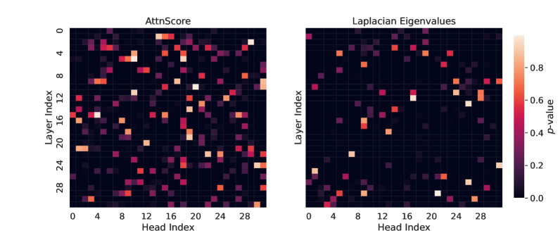</details> Figure 1: Visualization of $p$ -values from the two-sided Mann-Whitney U test for all layers and heads of Llama-3.1-8B across two feature types: $\operatorname{AttentionScore}$ and the $k{=}10$ Laplacian eigenvalues. These features were derived from attention maps collected when the LLM answered questions from the TriviaQA dataset. Higher $p$ -values indicate no significant difference in feature values between hallucinated and non-hallucinated examples. For $\operatorname{AttentionScore}$ , $80\$ of heads have $p<0.05$ , while for Laplacian eigenvalues, this percentage is $91\$ . Therefore, Laplacian eigenvalues may be better predictors of hallucinations, as feature values across more heads exhibit statistically significant differences between hallucinated and non-hallucinated examples. 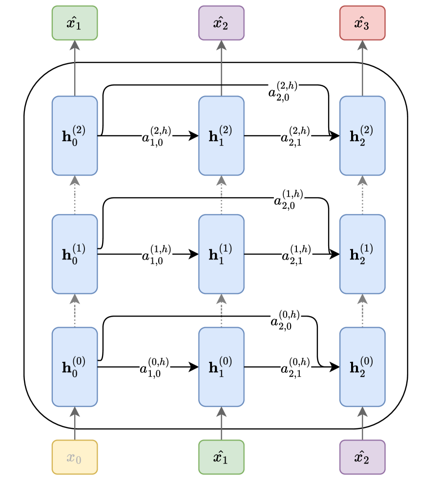Considering the attention matrix as an adjacency matrix representing a set of Markov chains, each corresponding to one layer of an LLM (Wu et al., 2024) (see Figure 2), we can leverage its spectral properties, as was done in many successful graph-based methods (Mohar, 1997; von Luxburg, 2007; Bruna et al., 2013; Topping et al., 2022). In particular, it was shown that the graph Laplacian might help to describe several graph properties, like the presence of bottlenecks (Topping et al., 2022; Black et al., 2023). We hypothesize that hallucinations may arise from disruptions in information flow, such as bottlenecks, which could be detected through the graph Laplacian. To assess whether our hypothesis holds, we computed graph spectral features and verified if they provide a stronger coincidence with hallucinations than the previous attention-based method - $\operatorname{AttentionScore}$ (Sriramanan et al., 2024). We prompted an LLM with questions from the TriviaQA dataset (Joshi et al., 2017) and extracted attention maps, differentiating by layers and heads. We then computed the spectral features, i.e., the 10 largest eigenvalues of the Laplacian matrix from each head and layer. Further, we conducted a two-sided Mann-Whitney U test (Mann and Whitney, 1947) to compare whether Laplacian eigenvalues and the values of $\operatorname{AttentionScore}$ are different between hallucinated and non-hallucinated examples. Figure 1 shows $p$ -values for all layers and heads, indicating that $\operatorname{AttentionScore}$ often results in higher $p$ -values compared to Laplacian eigenvalues. Overall, we studied 7 datasets and 5 LLMs and found similar results (see Appendix A). Based on these findings, we propose leveraging top- $k$ Laplacian eigenvalues as features for a hallucination probe. <details> <summary>x2.png Details</summary>  ### Visual Description ## Diagram: Multi-Layer Recurrent Neural Network with Skip Connections ### Overview The image displays a schematic diagram of a multi-layer recurrent neural network (RNN) architecture. It illustrates the flow of data from input sequences at the bottom, through multiple stacked layers of hidden states, to output sequences at the top. The architecture features both sequential connections within a layer and skip connections that link hidden states across different time steps and layers. ### Components/Axes The diagram is organized into three main vertical sections and multiple horizontal layers. **1. Input Layer (Bottom):** * Three input nodes are positioned at the bottom of the diagram. * From left to right, they are labeled: * `x₀` (in a yellow box) * `x̂₁` (in a green box) * `x̂₂` (in a purple box) **2. Hidden Layers (Middle):** * The core of the diagram consists of three stacked horizontal layers of hidden states, each represented by blue rounded rectangles. * Each layer contains three hidden states, indexed by time step (subscript) and layer (superscript in parentheses). * **Layer 0 (Bottom Hidden Layer):** `h₀⁽⁰⁾`, `h₁⁽⁰⁾`, `h₂⁽⁰⁾` * **Layer 1 (Middle Hidden Layer):** `h₀⁽¹⁾`, `h₁⁽¹⁾`, `h₂⁽¹⁾` * **Layer 2 (Top Hidden Layer):** `h₀⁽²⁾`, `h₁⁽²⁾`, `h₂⁽²⁾` **3. Output Layer (Top):** * Three output nodes are positioned at the top of the diagram. * From left to right, they are labeled: * `x̂₁` (in a green box) * `x̂₂` (in a purple box) * `x̂₃` (in a red box) **4. Connections and Labels:** * **Vertical (Inter-layer) Connections:** Dotted gray arrows point upward from each hidden state `h_t^(l)` to the hidden state at the same time step in the layer above, `h_t^(l+1)`. This represents the flow of information from lower to higher layers. * **Horizontal (Intra-layer) Connections:** Solid black arrows point from a hidden state to the next hidden state within the same layer (e.g., from `h₀⁽⁰⁾` to `h₁⁽⁰⁾`). These are labeled with terms `a`, indicating a learned parameter or gate. * The label format is `a_{destination,source}^{(layer,type)}`. * Example: The connection from `h₀⁽⁰⁾` to `h₁⁽⁰⁾` is labeled `a_{1,0}^{(0,h)}`. * **Skip Connections:** Curved black arrows originate from a hidden state and point to a hidden state at a later time step in the same or a higher layer. These are also labeled with `a` terms. * Example: A connection from `h₀⁽⁰⁾` to `h₂⁽⁰⁾` is labeled `a_{2,0}^{(0,h)}`. * Example: A connection from `h₀⁽¹⁾` to `h₂⁽²⁾` is labeled `a_{2,0}^{(2,h)}`. * **Input to Hidden:** Solid gray arrows point from each input node (`x₀`, `x̂₁`, `x̂₂`) to the corresponding hidden state in the first layer (`h₀⁽⁰⁾`, `h₁⁽⁰⁾`, `h₂⁽⁰⁾`). * **Hidden to Output:** Solid gray arrows point from the top-layer hidden states (`h₀⁽²⁾`, `h₁⁽²⁾`, `h₂⁽²⁾`) to the corresponding output nodes (`x̂₁`, `x̂₂`, `x̂₃`). ### Detailed Analysis The diagram explicitly defines the following connections and their associated parameters (`a` terms): **Layer 0 (l=0):** * `h₀⁽⁰⁾` → `h₁⁽⁰⁾`: `a_{1,0}^{(0,h)}` * `h₁⁽⁰⁾` → `h₂⁽⁰⁾`: `a_{2,1}^{(0,h)}` * `h₀⁽⁰⁾` → `h₂⁽⁰⁾` (skip): `a_{2,0}^{(0,h)}` **Layer 1 (l=1):** * `h₀⁽¹⁾` → `h₁⁽¹⁾`: `a_{1,0}^{(1,h)}` * `h₁⁽¹⁾` → `h₂⁽¹⁾`: `a_{2,1}^{(1,h)}` * `h₀⁽¹⁾` → `h₂⁽¹⁾` (skip): `a_{2,0}^{(1,h)}` **Layer 2 (l=2):** * `h₀⁽²⁾` → `h₁⁽²⁾`: `a_{1,0}^{(2,h)}` * `h₁⁽²⁾` → `h₂⁽²⁾`: `a_{2,1}^{(2,h)}` * `h₀⁽²⁾` → `h₂⁽²⁾` (skip): `a_{2,0}^{(2,h)}` **Cross-Layer Skip Connections:** * `h₀⁽⁰⁾` → `h₂⁽¹⁾`: `a_{2,0}^{(1,h)}` * `h₀⁽¹⁾` → `h₂⁽²⁾`: `a_{2,0}^{(2,h)}` ### Key Observations 1. **Symmetry and Pattern:** The connection pattern is highly regular and repeated across all three layers. Each layer has identical intra-layer connectivity: a forward step to the next time step and a skip connection to the time step two steps ahead. 2. **Parameter Sharing:** The `a` labels suggest that the parameters governing these connections are specific to the destination, source, and layer (e.g., `a_{1,0}^{(0,h)}` is distinct from `a_{1,0}^{(1,h)}`). There is no visual indication of parameter sharing across time steps (like in a standard RNN) or layers. 3. **Input/Output Mapping:** The input sequence (`x₀`, `x̂₁`, `x̂₂`) is mapped to an output sequence (`x̂₁`, `x̂₂`, `x̂₃`) that is shifted by one time step. This is characteristic of sequence prediction tasks (e.g., predicting the next token). 4. **Color Coding:** Inputs and outputs use distinct colors (yellow, green, purple, red), while all hidden states are uniformly blue. This visually separates the external interface from the internal processing units. ### Interpretation This diagram represents a sophisticated **multi-layer recurrent architecture with dense skip connections**. The key insights are: * **Purpose:** The architecture is designed for processing sequential data (like text or time series). The stacked layers allow the network to learn hierarchical representations, with lower layers capturing basic patterns and higher layers capturing more abstract features. * **Flow of Information:** Data flows upward through the layers and forward through time. The **skip connections** (`a_{2,0}` terms) are the most notable feature. They create "shortcuts" that allow information from earlier time steps to directly influence later computations, bypassing intermediate steps. This design helps mitigate the vanishing gradient problem common in deep RNNs, enabling the training of deeper networks and improving the flow of information across long sequences. * **Relationships:** The diagram defines a precise computational graph. The value of any hidden state `h_t^(l)` is a function of: 1. The hidden state from the previous layer at the same time step (`h_t^(l-1)`). 2. The hidden state from the same layer at the previous time step (`h_{t-1}^(l)`). 3. Potentially, hidden states from the same layer at even earlier time steps (via skip connections). * **Anomalies/Notable Features:** The notation `x̂` (x-hat) is used for both some inputs and all outputs, which typically denotes a predicted or estimated value. This suggests the inputs `x̂₁` and `x̂₂` might themselves be predictions from a previous step or part of an auto-regressive setup. The architecture is not a vanilla RNN, LSTM, or GRU but a more generalized form where the specific update rules are parameterized by the various `a` terms, which could represent weights in a linear transformation or gates in a more complex unit. </details> Figure 2: The autoregressive inference process in an LLM is depicted as a graph for a single attention head $h$ (as introduced by (Vaswani, 2017)) and three generated tokens ( $\hat{x}_{1},\hat{x}_{2},\hat{x}_{3}$ ). Here, $\mathbf{h}^{(l)}_{i}$ represents the hidden state at layer $l$ for the input token $i$ , while $a^{(l,h)}_{i,j}$ denotes the scalar attention score between tokens $i$ and $j$ at layer $l$ and attention head $h$ . Arrows direction refers to information flow during inference. ## 3 Method <details> <summary>x3.png Details</summary>  ### Visual Description ## Diagram: LLM Hallucination Detection Pipeline ### Overview The image displays a technical flowchart illustrating a machine learning pipeline designed to detect hallucinations in Large Language Model (LLM) outputs. The process begins with a Question-Answering (QA) dataset and branches into two parallel processing paths that converge at a final classification probe. The diagram uses color-coded shapes to differentiate between data stores (yellow rectangle), processes/models (blue rectangles), and data artifacts (green parallelograms). ### Components/Axes The diagram is composed of the following labeled components, connected by directional arrows indicating data flow: 1. **QA Dataset** (Yellow Rectangle, far left): The starting input data source. 2. **LLM** (Blue Rectangle, top-left): A Large Language Model. 3. **Attention Maps** (Green Parallelogram, top-center): Output data from the LLM. 4. **Feature Extraction (LapEigvals)** (Blue Rectangle, top-right): A processing step that extracts features, specifically using Laplacian Eigenvalues. 5. **Answers** (Green Parallelogram, bottom-left): Output data from the LLM. 6. **Judge LLM** (Blue Rectangle, bottom-center): A separate LLM used for evaluation. 7. **Hallucination Labels** (Green Parallelogram, bottom-right): Output labels from the Judge LLM. 8. **Hallucination Probe (logistic regression)** (Blue Rectangle, far right): The final classifier model. **Flow Connections (Solid Arrows):** * `QA Dataset` → `LLM` * `LLM` → `Attention Maps` * `Attention Maps` → `Feature Extraction (LapEigvals)` * `Feature Extraction (LapEigvals)` → `Hallucination Probe (logistic regression)` * `LLM` → `Answers` * `Answers` → `Judge LLM` * `Judge LLM` → `Hallucination Labels` * `Hallucination Labels` → `Hallucination Probe (logistic regression)` **Flow Connections (Dashed Arrows):** * `QA Dataset` → `Judge LLM` (A secondary, direct data path) * `Hallucination Labels` → `Hallucination Probe (logistic regression)` (A secondary connection, possibly indicating label usage in training) ### Detailed Analysis The pipeline operates through two distinct, parallel pathways that originate from the same `QA Dataset`: **Path 1 (Top - Feature-Based):** 1. The `QA Dataset` is fed into a primary `LLM`. 2. The `LLM` generates `Attention Maps` as an internal representation. 3. These maps undergo `Feature Extraction` using Laplacian Eigenvalues (`LapEigvals`), a technique often used in spectral clustering and dimensionality reduction to identify structural features. 4. The extracted features are sent to the `Hallucination Probe`. **Path 2 (Bottom - Label-Based):** 1. The same `QA Dataset` is also used by the primary `LLM` to generate `Answers`. 2. These `Answers` are evaluated by a separate `Judge LLM`. 3. The `Judge LLM` produces `Hallucination Labels` (likely binary: hallucinated/factual). 4. These labels are sent to the `Hallucination Probe`. **Convergence:** Both the engineered features (from Path 1) and the supervision labels (from Path 2) converge at the `Hallucination Probe (logistic regression)`. This suggests the probe is a logistic regression model trained to predict hallucinations using the extracted Laplacian Eigenvalue features, with the labels from the Judge LLM serving as the ground truth for training. ### Key Observations 1. **Dual-Path Architecture:** The system uses a hybrid approach, combining low-level model internals (`Attention Maps` → `Features`) with high-level semantic evaluation (`Answers` → `Judge LLM` → `Labels`). 2. **Specialized Components:** The pipeline distinguishes between the generative `LLM` and the evaluative `Judge LLM`, indicating a modular design where judgment is offloaded to a separate model. 3. **Feature Engineering:** The specific mention of `LapEigvals` indicates a deliberate choice to use spectral graph theory features derived from attention maps, hypothesizing that the structure of attention correlates with factual reliability. 4. **Final Classifier:** The use of `logistic regression` for the final probe suggests an emphasis on an interpretable, linear model for the detection task, possibly to understand which extracted features are most predictive. ### Interpretation This diagram outlines a research or engineering methodology for **detecting hallucinations in LLMs by analyzing their internal attention mechanisms**. The core hypothesis is that the patterns in a model's attention (captured via maps and transformed into Laplacian Eigenvalues) contain signal about whether the generated answer is factual or a hallucination. The pipeline is investigative in nature. It doesn't just use a judge to label answers; it seeks an *automated, feature-based proxy* for hallucination by training a probe on those labels. The `Hallucination Probe` is the key output—a model that, once trained, could potentially flag hallucinations in new LLM outputs by analyzing attention maps alone, without needing a (computationally expensive) Judge LLM for every new answer. The dashed line from `QA Dataset` to `Judge LLM` is crucial. It implies the Judge LLM receives the original question context, not just the answer, enabling more accurate judgment. The overall structure suggests a move towards **explainable AI for LLM safety**, attempting to ground the abstract concept of "hallucination" in measurable, internal model features. 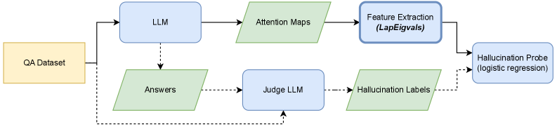</details> Figure 3: Overview of the methodology used in this work. Solid lines indicate the test-time pipeline, while dashed lines represent additional pipeline steps for generating labels for training the hallucination probe (logistic regression). The primary contribution of this work is leveraging the top- $k$ eigenvalues of the Laplacian as features for the hallucination probe, highlighted with a bold box on the diagram. In our method, we train a hallucination probe using only attention maps, which we extracted during LLM inference, as illustrated in Figure 2. The attention map is a matrix containing attention scores for all tokens processed during inference, while the hallucination probe is a logistic regression model that uses features derived from attention maps as input. This work’s core contribution is using the top- $k$ eigenvalues of the Laplacian matrix as input features, which we detail below. Denote $\mathbf{A}^{(l,h)}\in\mathbb{R}^{T\times T}$ as the attention map matrix for layer $l\in\{1\dotsc L\}$ and attention head $h\in\{1\dotsc H\}$ , where $T$ is the total number of tokens generated by an LLM (including input tokens), $L$ the number of layers (transformer blocks), and $H$ the number of attention heads. The attention matrix is row-stochastic, meaning each row sums to 1 ( $\sum_{j=0}^{T}\mathbf{A}^{(l,h)}_{:,j}=\mathbf{1}$ ). It is also lower triangular ( $a^{(l,h)}_{ij}=0$ for all $j>i$ ) and non-negative ( $a^{(l,h)}_{ij}\geq 0$ for all $i,j$ ). We can view $\mathbf{A}^{(l,h)}$ as a weighted adjacency matrix of a directed graph, where each node represents processed token, and each directed edge from token $i$ to token $j$ is weighted by the attention score, as depicted in Figure 2. Then, we define the Laplacian of a layer $l$ and attention head $h$ as: $$ \mathbf{L}^{(l,h)}=\mathbf{D}^{(l,h)}-\mathbf{A}^{(l,h)}, \tag{1} $$ where $\mathbf{D}^{(l,h)}$ is a diagonal degree matrix. Since the attention map defines a directed graph, we distinguish between the in-degree and out-degree matrices. The in-degree is computed as the sum of attention scores from preceding tokens, and due to the softmax normalization, it is uniformly 1. Therefore, we define $\mathbf{D}^{(l,h)}$ as the out-degree matrix, which quantifies the total attention a token receives from tokens that follow it. To ensure these values remain independent of the sequence length, we normalize them by the number of subsequent tokens (i.e., the number of outgoing edges). $$ d^{(l,h)}_{ii}=\frac{\sum_{u}{a^{(l,h)}_{ui}}}{T-i}, \tag{2} $$ where $i,u\in\{0,\dots,(T-1)\}$ denote token indices. The Laplacian defined this way is bounded, i.e., $\mathbf{L}^{(l,h)}_{ij}\in\left[-1,1\right]$ (see Appendix B for proofs). Intuitively, the resulting Laplacian for each processed token represents the average attention score to previous tokens reduced by the attention score to itself. As eigenvalues of the Laplacian can summarize information flow in a graph (von Luxburg, 2007; Topping et al., 2022), we take eigenvalues of $\mathbf{L}^{(l,h)}$ , which are diagonal entries due to the lower triangularity of the Laplacian matrix, and sort them: $$ \tilde{z}^{(l,h)}=\operatorname{sort\left(\operatorname{diag\left(\mathbf{L}^{(l,h)}\right)}\right)} \tag{3} $$ Recently, (Zhu et al., 2024) found features from the entire token sequence, rather than a single token, improving hallucination detection. Similarly, (Kim et al., 2024) demonstrated that information from all layers, instead of a single one in isolation, yields better results on this task. Motivated by these findings, our method uses features from all tokens and all layers as input to the probe. Therefore, we take the top- $k$ largest values from each head and layer and concatenate them into a single feature vector $z$ , where $k$ is a hyperparameter of our method: $$ z=\operatorname*{\mathchoice{\Big\|}{\big\|}{\|}{\|}}_{\forall l\in L,\forall h\in H}\left[\tilde{z}^{(l,h)}_{T},\tilde{z}^{(l,h)}_{T-1},\dotsc,\tilde{z}^{(l,h)}_{T-k}\right] \tag{4} $$ Since LLMs contain dozens of layers and heads, the probe input vector $z\in\mathbb{R}^{L\cdot H\cdot k}$ can still be high-dimensional. Thus, we project it to a lower dimensionality using PCA (Jolliffe and Cadima, 2016). We call our approach $\operatorname{LapEigvals}$ . ## 4 Experimental setup The overview of the methodology used in this work is presented in Figure 3. Next, we describe each step of the pipeline in detail. ### 4.1 Dataset construction We use annotated QA datasets to construct the hallucination detection datasets and label incorrect LLM answers as hallucinations. To assess the correctness of generated answers, we followed prior work (Orgad et al., 2025) and adopted the llm-as-judge approach (Zheng et al., 2023), with the exception of one dataset where exact match evaluation against ground-truth answers was possible. For llm-as-judge, we prompted a large LLM to classify each response as either hallucination, non-hallucination, or rejected, where rejected indicates that it was unclear whether the answer was correct, e.g., the model refused to answer due to insufficient knowledge. Based on the manual qualitative inspection of several LLMs, we employed gpt-4o-mini (OpenAI et al., 2024) as the judge model since it provides the best trade-off between accuracy and cost. To confirm the reliability of the labels, we additionally verified agreement with the larger model, gpt-4.1, on Llama-3.1-8B and found that the agreement between models falls within the acceptable range widely adopted in the literature (see Appendix F). For experiments, we selected 7 QA datasets previously utilized in the context of hallucination detection (Chen et al., 2024; Kossen et al., 2024; Chuang et al., 2024b; Mitra et al., 2024). Specifically, we used the validation set of NQ-Open (Kwiatkowski et al., 2019), comprising $3{,}610$ question-answer pairs, and the validation set of TriviaQA (Joshi et al., 2017), containing $7{,}983$ pairs. To evaluate our method on longer inputs, we employed the development set of CoQA (Reddy et al., 2019) and the rc.nocontext portion of the SQuADv2 (Rajpurkar et al., 2018) datasets, with $5{,}928$ and $9{,}960$ examples, respectively. Additionally, we incorporated the QA part of the HaluEvalQA (Li et al., 2023) dataset, containing $10{,}000$ examples, and the generation part of the TruthfulQA (Lin et al., 2022) benchmark with $817$ examples. Finally, we used test split of GSM8k dataset Cobbe et al. (2021) with $1{,}319$ grade school math problems, evaluated by exact match against labels. For TriviaQA, CoQA, and SQuADv2, we followed the same preprocessing procedure as (Chen et al., 2024). We generate answers using 5 open-source LLMs: Llama-3.1-8B hf.co/meta-llama/Llama-3.1-8B-Instruct and Llama-3.2-3B hf.co/meta-llama/Llama-3.2-3B-Instruct (Grattafiori et al., 2024), Phi-3.5 hf.co/microsoft/Phi-3.5-mini-instruct (Abdin et al., 2024), Mistral-Nemo hf.co/mistralai/Mistral-Nemo-Instruct-2407 (Mistral AI Team and NVIDIA, 2024), Mistral-Small-24B hf.co/mistralai/Mistral-Small-24B-Instruct-2501 (Mistral AI Team, 2025). We use two softmax temperatures for each LLM when decoding ( $temp\in\{0.1,1.0\}$ ) and one prompt (for all datasets we used a prompt in Listing 3, except for GSM8K in Listing 5). Overall, we evaluated hallucination detection probes on 10 LLM configurations and 7 QA datasets. We present the frequency of classes for answers from each configuration in Figure 9 (Appendix E). ### 4.2 Hallucination Probe As a hallucination probe, we take a logistic regression model, using the implementation from scikit-learn (Pedregosa et al., 2011) with all parameters default, except for ${max\_iter{=}2000}$ and ${class\_weight{=}{{}^{\prime\prime}balanced^{\prime\prime}}}$ . For top- $k$ eigenvalues, we tested 5 values of $k\in\{5,10,20,50,100\}$ For datasets with examples having less than 100 tokens, we stop at $k{=}50$ and selected the result with the highest efficacy. All eigenvalues are projected with PCA onto 512 dimensions, except in per-layer experiments where there may be fewer than 512 features. In these cases, we apply PCA projection to match the input feature dimensionality, i.e., decorrelating them. As an evaluation metric, we use AUROC on the test split (additional results presenting Precision and Recall are reported in Appendix G.1). ### 4.3 Baselines Our method is a supervised approach for detecting hallucinations using only attention maps. For a fair comparison, we adapt the unsupervised $\operatorname{AttentionScore}$ (Sriramanan et al., 2024) by using log-determinants of each head’s attention scores as features instead of summing them, and we also include the original $\operatorname{AttentionScore}$ , computed as the sum of log-determinants over heads, for reference. To evaluate the effectiveness of our proposed Laplacian eigenvalues, we compare them to the eigenvalues of raw attention maps, denoted as $\operatorname{AttnEigvals}$ . Extended results for each approach on a per-layer basis are provided in Appendix G.2, while Appendix G.4 presents a comparison with a method based on hidden states. Implementation and hardware details are provided in Appendix C. ## 5 Results Table 1: Test AUROC for $\operatorname{LapEigvals}$ and several baseline methods. AUROC values were obtained in a single run of logistic regression training on features from a dataset generated with $temp{=}1.0$ . We mark results for $\operatorname{AttentionScore}$ in gray as it is an unsupervised approach, not directly comparable to the others. In bold, we highlight the best performance individually for each dataset and LLM. See Appendix G for extended results. | Llama3.1-8B Llama3.1-8B Llama3.1-8B | $\operatorname{AttentionScore}$ $\operatorname{AttnLogDet}$ $\operatorname{AttnEigvals}$ | 0.493 0.769 0.782 | 0.720 0.826 0.838 | 0.589 0.827 0.819 | 0.556 0.793 0.790 | 0.538 0.748 0.768 | 0.532 0.842 0.843 | 0.541 0.814 0.833 | | --- | --- | --- | --- | --- | --- | --- | --- | --- | | Llama3.1-8B | $\operatorname{LapEigvals}$ | 0.830 | 0.872 | 0.874 | 0.827 | 0.791 | 0.889 | 0.829 | | Llama3.2-3B | $\operatorname{AttentionScore}$ | 0.509 | 0.717 | 0.588 | 0.546 | 0.530 | 0.515 | 0.581 | | Llama3.2-3B | $\operatorname{AttnLogDet}$ | 0.700 | 0.851 | 0.801 | 0.690 | 0.734 | 0.789 | 0.795 | | Llama3.2-3B | $\operatorname{AttnEigvals}$ | 0.724 | 0.768 | 0.819 | 0.694 | 0.749 | 0.804 | 0.723 | | Llama3.2-3B | $\operatorname{LapEigvals}$ | 0.812 | 0.870 | 0.828 | 0.693 | 0.757 | 0.832 | 0.787 | | Phi3.5 | $\operatorname{AttentionScore}$ | 0.520 | 0.666 | 0.541 | 0.594 | 0.504 | 0.540 | 0.554 | | Phi3.5 | $\operatorname{AttnLogDet}$ | 0.745 | 0.842 | 0.818 | 0.815 | 0.769 | 0.848 | 0.755 | | Phi3.5 | $\operatorname{AttnEigvals}$ | 0.771 | 0.794 | 0.829 | 0.798 | 0.782 | 0.850 | 0.802 | | Phi3.5 | $\operatorname{LapEigvals}$ | 0.821 | 0.885 | 0.836 | 0.826 | 0.795 | 0.872 | 0.777 | | Mistral-Nemo | $\operatorname{AttentionScore}$ | 0.493 | 0.630 | 0.531 | 0.529 | 0.510 | 0.532 | 0.494 | | Mistral-Nemo | $\operatorname{AttnLogDet}$ | 0.728 | 0.856 | 0.798 | 0.769 | 0.772 | 0.812 | 0.852 | | Mistral-Nemo | $\operatorname{AttnEigvals}$ | 0.778 | 0.842 | 0.781 | 0.761 | 0.758 | 0.821 | 0.802 | | Mistral-Nemo | $\operatorname{LapEigvals}$ | 0.835 | 0.890 | 0.833 | 0.795 | 0.812 | 0.865 | 0.828 | | Mistral-Small-24B | $\operatorname{AttentionScore}$ | 0.516 | 0.576 | 0.504 | 0.462 | 0.455 | 0.463 | 0.451 | | Mistral-Small-24B | $\operatorname{AttnLogDet}$ | 0.766 | 0.853 | 0.842 | 0.747 | 0.753 | 0.833 | 0.735 | | Mistral-Small-24B | $\operatorname{AttnEigvals}$ | 0.805 | 0.856 | 0.848 | 0.751 | 0.760 | 0.844 | 0.765 | | Mistral-Small-24B | $\operatorname{LapEigvals}$ | 0.861 | 0.925 | 0.882 | 0.791 | 0.820 | 0.876 | 0.748 | Table 1 presents the results of our method compared to the baselines. $\operatorname{LapEigvals}$ achieved the best performance among all tested methods on 6 out of 7 datasets. Moreover, our method consistently performs well across all 5 LLM architectures ranging from 3 up to 24 billion parameters. TruthfulQA was the only exception where $\operatorname{LapEigvals}$ was the second-best approach, yet it might stem from the small size of the dataset or severe class imbalance (depicted in Figure 9). In contrast, using eigenvalues of vanilla attention maps in $\operatorname{AttnEigvals}$ leads to worse performance, which suggests that transformation to Laplacian is the crucial step to uncover latent features of an LLM corresponding to hallucinations. In Appendix G, we show that $\operatorname{LapEigvals}$ consistently demonstrates a smaller generalization gap, i.e., the difference between training and test performance is smaller for our method. While the $\operatorname{AttentionScore}$ method performed poorly, it is fully unsupervised and should not be directly compared to other approaches. However, its supervised counterpart – $\operatorname{AttnLogDet}$ – remains inferior to methods based on spectral features, namely $\operatorname{AttnEigvals}$ and $\operatorname{LapEigvals}$ . In Table 6 in Appendix G.2, we present extended results, including per-layer and all-layers breakdowns, two temperatures used during answers generation, and a comparison between training and test AUROC. Moreover, compared to probes based on hidden states, our method performs best in most of the tested settings, as shown in Appendix G.4. ## 6 Ablation studies To better understand the behavior of our method under different conditions, we conduct a comprehensive ablation study. This analysis provides valuable insights into the factors driving the $\operatorname{LapEigvals}$ performance and highlights the robustness of our approach across various scenarios. In order to ensure reliable results, we perform all studies on the TriviaQA dataset, which has a moderate input size and number of examples. ### 6.1 How does the number of eigenvalues influence performance? 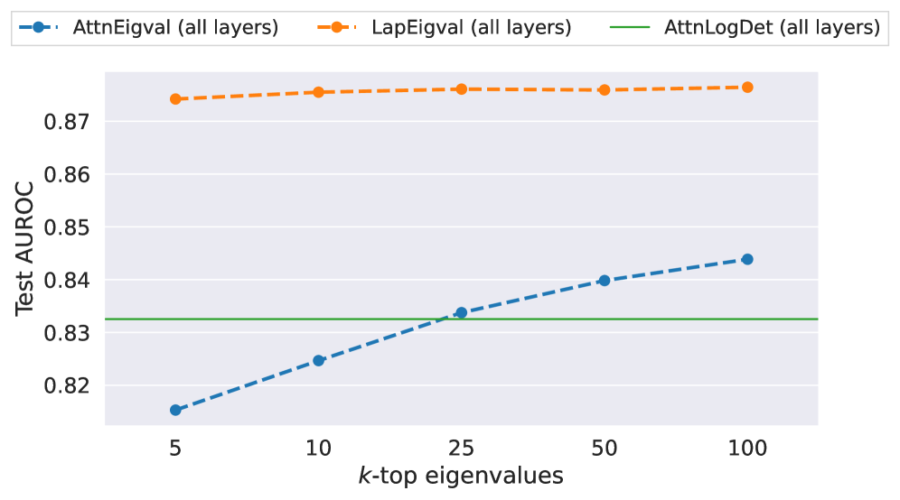First, we verify how the number of eigenvalues influences the performance of the hallucination probe and present results for Mistral-Small-24B in Figure 4 (results for all models are showcased in Figure 10 in Appendix H). Generally, using more eigenvalues improves performance, but there is less variation in performance among different values of $k$ for $\operatorname{LapEigvals}$ compared to the baseline. Moreover, $\operatorname{LapEigvals}$ achieves significantly better performance with smaller input sizes, as $\operatorname{AttnEigvals}$ with the largest $k{=}100$ fails to surpass $\operatorname{LapEigvals}$ ’s performance at $k{=}5$ . These results confirm that spectral features derived from the Laplacian carry a robust signal indicating the presence of hallucinations and highlight the strength of our method. <details> <summary>x4.png Details</summary>  ### Visual Description ## Line Chart: Test AUROC vs. k-top Eigenvalues for Different Metrics ### Overview The image displays a line chart comparing the performance (Test AUROC) of three different metrics as a function of the number of top eigenvalues (`k`) considered. The chart suggests an evaluation of model performance or anomaly detection capability, likely in a machine learning or signal processing context, using spectral properties of attention or Laplacian matrices. ### Components/Axes * **Chart Type:** Line chart with markers. * **X-Axis:** * **Label:** `k-top eigenvalues` * **Scale:** Categorical/ordinal with discrete markers at values: 5, 10, 25, 50, 100. * **Y-Axis:** * **Label:** `Test AUROC` * **Scale:** Linear, ranging from approximately 0.82 to 0.87. The axis does not start at zero. * **Legend:** Positioned at the top center of the chart area. 1. `AttnEigval (all layers)`: Represented by a blue dashed line (`--`) with circular markers. 2. `LapEigval (all layers)`: Represented by an orange dashed line (`--`) with circular markers. 3. `AttnLogDet (all layers)`: Represented by a solid green line (`-`). ### Detailed Analysis **1. AttnEigval (all layers) - Blue Dashed Line:** * **Trend:** Shows a clear, consistent upward slope. Performance improves as `k` increases. * **Data Points (Approximate):** * k=5: AUROC ≈ 0.815 * k=10: AUROC ≈ 0.825 * k=25: AUROC ≈ 0.833 * k=50: AUROC ≈ 0.840 * k=100: AUROC ≈ 0.844 **2. LapEigval (all layers) - Orange Dashed Line:** * **Trend:** Nearly flat, with a very slight upward slope. Performance is consistently high and stable across all values of `k`. * **Data Points (Approximate):** * k=5: AUROC ≈ 0.874 * k=10: AUROC ≈ 0.875 * k=25: AUROC ≈ 0.876 * k=50: AUROC ≈ 0.876 * k=100: AUROC ≈ 0.877 **3. AttnLogDet (all layers) - Green Solid Line:** * **Trend:** Perfectly horizontal. Performance is constant and independent of the value of `k`. * **Data Point:** Constant AUROC ≈ 0.833 across all `k`. ### Key Observations 1. **Performance Hierarchy:** `LapEigval` consistently achieves the highest Test AUROC (~0.874-0.877), followed by `AttnLogDet` (~0.833), and then `AttnEigval` which starts lowest but improves. 2. **Sensitivity to `k`:** * `AttnEigval` is highly sensitive to `k`, showing significant improvement (≈0.029 increase) as more eigenvalues are included. * `LapEigval` is largely insensitive to `k`, with only a marginal improvement (≈0.003 increase). * `AttnLogDet` is completely insensitive to `k`. 3. **Crossover Point:** The `AttnEigval` line surpasses the constant `AttnLogDet` line between `k=10` and `k=25`. At `k=25`, their performance is approximately equal (~0.833). ### Interpretation The chart compares the efficacy of using different spectral features from a model's layers for a test task (likely anomaly detection or classification, given the AUROC metric). * **LapEigval (Laplacian Eigenvalues)** appears to be the most robust and informative feature. Its high, stable performance suggests that the spectral properties of the graph Laplacian (possibly derived from attention maps or another structure) capture discriminative information effectively, even when only the very top eigenvalues (`k=5`) are used. This could indicate that the most significant structural patterns are concentrated in the leading eigenvalues. * **AttnEigval (Attention Eigenvalues)** benefits from including more spectral components. Its rising trend implies that while the top eigenvalues are informative, additional signal is contained in the subsequent eigenvalues (up to at least `k=100`). The fact that it starts below `AttnLogDet` but surpasses it suggests a trade-off: with few components, it's less effective than a log-determinant, but with more components, it becomes superior. * **AttnLogDet (Attention Log-Determinant)** serves as a stable baseline. Its constant value indicates it is a summary statistic (like the log of the product of all eigenvalues) that does not depend on a truncated `k`. It provides decent performance but is outperformed by the more nuanced, `k`-dependent methods when sufficient components are used. **Overall Implication:** For the task measured, analyzing the eigenvalue spectrum of the Laplacian (`LapEigval`) is the most effective approach, offering top-tier performance with minimal need for parameter tuning (`k`). If using attention eigenvalues (`AttnEigval`), selecting a larger `k` (e.g., 50 or 100) is beneficial. The log-determinant (`AttnLogDet`) is a simple, stable alternative that doesn't require choosing `k`. </details> Figure 4: Probe performance across different top- $k$ eigenvalues: $k\in\{5,10,25,50,100\}$ for TriviaQA dataset with $temp{=}1.0$ and Mistral-Small-24B LLM. ### 6.2 Does using all layers at once improve performance? 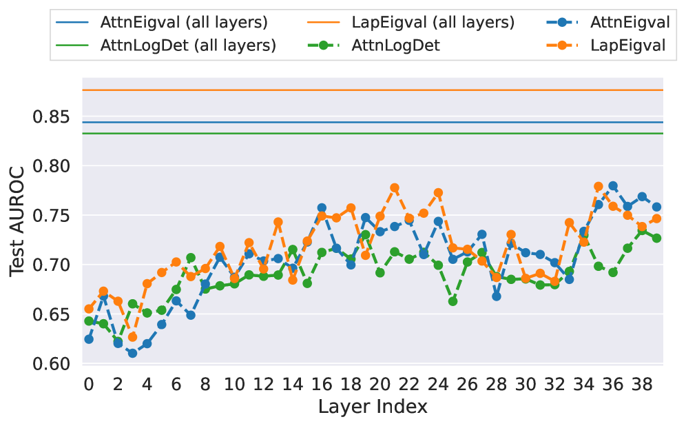Second, we demonstrate that using all layers of an LLM instead of a single one improves performance. In Figure 5, we compare per-layer to all-layer efficacy for Mistral-Small-24B (results for all models are showcased in Figure 11 in Appendix H). For the per-layer approach, better performance is generally achieved with deeper LLM layers. Notably, peak performance varies across LLMs, requiring an additional search for each new LLM. In contrast, the all-layer probes consistently outperform the best per-layer probes across all LLMs. This finding suggests that information indicating hallucinations is spread across many layers of LLM, and considering them in isolation limits detection accuracy. Further, Table 6 in Appendix G summarises outcomes for the two variants on all datasets and LLM configurations examined in this work. <details> <summary>x5.png Details</summary>  ### Visual Description ## Line Chart: Test AUROC Across Model Layers for Different Metrics ### Overview This image is a line chart comparing the performance (Test AUROC) of six different metrics or methods across the layers of a neural network model (Layer Index 0 to 38). The chart displays both aggregate performance (solid lines) and per-layer performance (dashed lines with markers). The overall trend shows that per-layer metrics fluctuate significantly, while the aggregate metrics remain constant. ### Components/Axes * **X-Axis:** Labeled "Layer Index". It is a linear scale with major tick marks every 2 units, ranging from 0 to 38. * **Y-Axis:** Labeled "Test AUROC". It is a linear scale with major tick marks every 0.05 units, ranging from 0.60 to 0.85. * **Legend:** Positioned at the top center of the chart. It contains six entries, defining the color and line style for each data series: 1. `AttnEigval (all layers)`: Solid blue line. 2. `AttnLogDet (all layers)`: Solid green line. 3. `LapEigval (all layers)`: Solid orange line. 4. `AttnEigval`: Dashed blue line with circular markers. 5. `AttnLogDet`: Dashed green line with circular markers. 6. `LapEigval`: Dashed orange line with circular markers. * **Grid:** A light gray grid is present in the background. ### Detailed Analysis **1. Aggregate Metrics (Solid Lines - "all layers"):** These lines are horizontal, indicating a single, constant AUROC value for the entire model, not varying by layer. * **`LapEigval (all layers)` (Solid Orange):** The highest-performing aggregate metric. It is a flat line positioned at approximately **AUROC = 0.88**. * **`AttnEigval (all layers)` (Solid Blue):** The second-highest aggregate metric. It is a flat line positioned at approximately **AUROC = 0.845**. * **`AttnLogDet (all layers)` (Solid Green):** The lowest of the aggregate metrics. It is a flat line positioned at approximately **AUROC = 0.835**. **2. Per-Layer Metrics (Dashed Lines with Markers):** These lines show the AUROC value when the metric is computed using only the specified layer's information. They exhibit significant fluctuation across layers. * **`LapEigval` (Dashed Orange):** * **Trend:** Shows a general, noisy upward trend from layer 0 to layer 38. It starts around 0.655, dips to a low near 0.63 at layer 3, then climbs with high variance. * **Key Points:** Notable peaks occur at approximately layer 20 (AUROC ~0.78), layer 24 (~0.775), and layer 36 (~0.78). A significant dip occurs around layer 28 (~0.685). * **`AttnEigval` (Dashed Blue):** * **Trend:** Also shows a general upward trend with high variance, often moving in tandem with `LapEigval` but typically at a slightly lower AUROC. * **Key Points:** Starts around 0.625. Has a pronounced low at layer 4 (~0.61). Peaks near layer 16 (~0.755) and layer 36 (~0.78). Dips sharply at layer 28 (~0.67). * **`AttnLogDet` (Dashed Green):** * **Trend:** Exhibits a more moderate upward trend compared to the other two per-layer metrics. It generally has the lowest AUROC values among the dashed lines. * **Key Points:** Starts around 0.645. Shows a notable dip at layer 25 (~0.665). Its highest points are near layer 20 (~0.73) and layer 38 (~0.73). ### Key Observations 1. **Performance Hierarchy:** There is a clear and consistent hierarchy in performance: `LapEigval` > `AttnEigval` > `AttnLogDet`. This holds true for both the aggregate (solid lines) and per-layer (dashed lines) versions of the metrics. 2. **Aggregate vs. Per-Layer:** The aggregate "all layers" metrics significantly outperform any single-layer metric. The best per-layer AUROC (~0.78) is still well below the worst aggregate AUROC (~0.835). 3. **Layer Sensitivity:** The per-layer metrics are highly sensitive to the specific layer index, showing large swings in AUROC. Performance is not uniform across the network depth. 4. **Correlated Fluctuations:** The three per-layer metrics (`AttnEigval`, `AttnLogDet`, `LapEigval`) often fluctuate in a correlated manner. For example, they all show a notable dip around layer 28 and a peak around layer 36. 5. **Early Layer Volatility:** The first 10 layers (0-10) show particularly high volatility and lower overall performance for all per-layer metrics. ### Interpretation This chart likely evaluates different methods for assessing the quality or information content of attention mechanisms (`Attn`) or Laplacian-based features (`Lap`) within a deep neural network, possibly a transformer. The "Test AUROC" suggests these metrics are being used for a binary classification task, such as detecting out-of-distribution samples or adversarial examples. * **What the data suggests:** The `LapEigval` method (likely based on eigenvalues of a graph Laplacian derived from the network) is the most effective single metric, both when applied to the whole network and to individual layers. The fact that aggregate metrics outperform per-layer ones indicates that combining information across all layers provides a much stronger signal than relying on any single layer. * **Relationship between elements:** The correlated dips and peaks in the per-layer metrics suggest that certain layers (e.g., around layer 28) are universally "weaker" or contain less discriminative information for this specific task, while others (e.g., around layer 36) are "stronger." This could reflect the functional specialization of different network depths. * **Notable anomaly:** The very flat, high performance of `LapEigval (all layers)` compared to the noisy per-layer `LapEigval` suggests that the eigenvalue-based method benefits immensely from integration across the entire network hierarchy, smoothing out the layer-specific noise to produce a robust, high-quality signal. The investigation would focus on why the Laplacian eigenvalue approach is superior to attention-based eigenvalue (`AttnEigval`) and log-determinant (`AttnLogDet`) approaches for this task. </details> Figure 5: Analysis of model performance across different layers for Mistral-Small-24B and TriviaQA dataset with $temp{=}1.0$ and $k{=}100$ top eigenvalues (results for models operating on all layers provided for reference). ### 6.3 Does sampling temperature influence results? 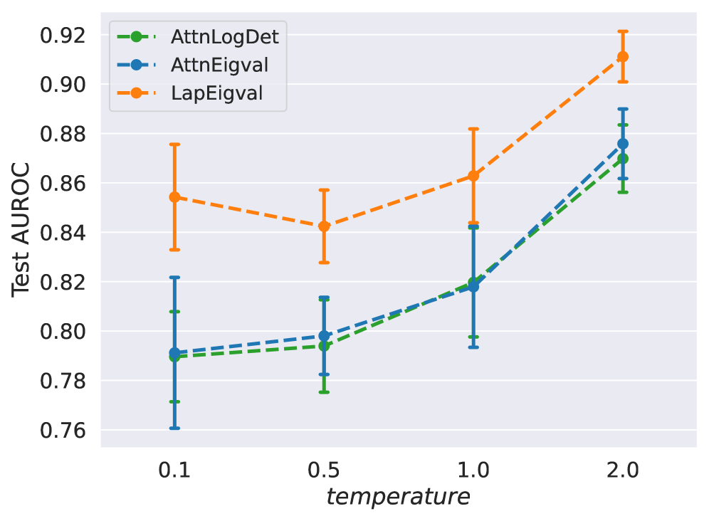Here, we compare $\operatorname{LapEigvals}$ to the baselines on hallucination datasets, where each dataset contains answers generated at a specific decoding temperature. Higher temperatures typically produce more hallucinated examples (Lee, 2023; Renze, 2024), leading to dataset imbalance. Thus, to mitigate the effect of data imbalance, we sample a subset of $1{,}000$ hallucinated and $1{,}000$ non-hallucinated examples $10$ times for each temperature and train hallucination probes. Interestingly, in Figure 6, we observe that all models improve their performance at higher temperatures, but $\operatorname{LapEigvals}$ consistently achieves the best accuracy on all considered temperature values. The correlation of efficacy with temperature may be attributed to differences in the characteristics of hallucinations at higher temperatures compared to lower ones (Renze, 2024). Also, hallucination detection might be facilitated at higher temperatures due to underlying properties of softmax function (Veličković et al., 2024), and further exploration of this direction is left for future work. <details> <summary>x6.png Details</summary>  ### Visual Description ## Line Chart with Error Bars: Test AUROC vs. Temperature ### Overview The image is a line chart displaying the performance of three different methods, measured by Test AUROC, as a function of a hyperparameter called "temperature." The chart includes error bars for each data point, indicating variability or confidence intervals. The overall trend shows that Test AUROC generally increases with temperature for all methods, with one method consistently outperforming the others. ### Components/Axes * **Chart Type:** Line chart with markers and vertical error bars. * **X-Axis:** * **Label:** `temperature` * **Scale:** Categorical/ordinal with discrete values: `0.1`, `0.5`, `1.0`, `2.0`. * **Y-Axis:** * **Label:** `Test AUROC` * **Scale:** Linear, ranging from `0.76` to `0.92`, with major gridlines at intervals of `0.02`. * **Legend:** * **Position:** Top-left corner of the plot area. * **Entries:** 1. `AttnLogDet` - Represented by a green dashed line with circular markers. 2. `AttnEigval` - Represented by a blue dashed line with circular markers. 3. `LapEigval` - Represented by an orange dashed line with circular markers. * **Data Series:** Three distinct lines, each corresponding to a method in the legend. Each data point includes a central marker (mean/median value) and vertical error bars extending above and below. ### Detailed Analysis **Data Series and Approximate Values:** 1. **AttnLogDet (Green Line):** * **Trend:** Slopes gently upward from left to right. * **Data Points (Approximate):** * Temperature 0.1: AUROC ≈ 0.79 (Error bar range: ~0.77 to ~0.81) * Temperature 0.5: AUROC ≈ 0.795 (Error bar range: ~0.78 to ~0.81) * Temperature 1.0: AUROC ≈ 0.82 (Error bar range: ~0.80 to ~0.84) * Temperature 2.0: AUROC ≈ 0.87 (Error bar range: ~0.86 to ~0.88) 2. **AttnEigval (Blue Line):** * **Trend:** Slopes upward, closely following but slightly above the AttnLogDet line. * **Data Points (Approximate):** * Temperature 0.1: AUROC ≈ 0.79 (Error bar range: ~0.76 to ~0.82) * Temperature 0.5: AUROC ≈ 0.80 (Error bar range: ~0.78 to ~0.81) * Temperature 1.0: AUROC ≈ 0.82 (Error bar range: ~0.80 to ~0.84) * Temperature 2.0: AUROC ≈ 0.88 (Error bar range: ~0.87 to ~0.89) 3. **LapEigval (Orange Line):** * **Trend:** Starts high, dips slightly at temperature 0.5, then rises sharply. It maintains a significant performance gap above the other two methods across all temperatures. * **Data Points (Approximate):** * Temperature 0.1: AUROC ≈ 0.855 (Error bar range: ~0.83 to ~0.88) * Temperature 0.5: AUROC ≈ 0.84 (Error bar range: ~0.83 to ~0.86) * Temperature 1.0: AUROC ≈ 0.865 (Error bar range: ~0.84 to ~0.88) * Temperature 2.0: AUROC ≈ 0.91 (Error bar range: ~0.90 to ~0.92) ### Key Observations 1. **Performance Hierarchy:** `LapEigval` (orange) consistently achieves the highest Test AUROC at every temperature point. `AttnEigval` (blue) and `AttnLogDet` (green) perform very similarly, with `AttnEigval` having a marginal advantage. 2. **Temperature Sensitivity:** All three methods show improved performance (higher AUROC) as the temperature increases from 0.5 to 2.0. The improvement is most dramatic for `LapEigval` between temperatures 1.0 and 2.0. 3. **Error Bar Patterns:** The error bars for `LapEigval` are generally larger, especially at lower temperatures (0.1 and 0.5), suggesting higher variance in its performance estimates under those conditions. The error bars for the two `Attn` methods are more consistent in size. 4. **Non-Monotonic Behavior:** The `LapEigval` series shows a slight decrease in mean AUROC when moving from temperature 0.1 to 0.5 before increasing again, which is a notable deviation from the otherwise upward trend. ### Interpretation This chart likely compares different methods for estimating or utilizing eigenvalues (or related properties like log-determinants) of attention matrices (`Attn`) or Laplacian matrices (`Lap`) in a machine learning model, possibly for tasks like anomaly detection or out-of-distribution detection where AUROC is a common metric. The data suggests that the `LapEigval` method is superior for this specific task, as measured by Test AUROC. Its performance advantage is substantial and grows with higher temperature settings. Temperature appears to be a beneficial hyperparameter for all methods, potentially by smoothing or scaling internal representations to improve discriminative power. The larger error bars for `LapEigval` at low temperatures indicate that while its average performance is high, its results may be less stable or more sensitive to initial conditions or data subsets in that regime. The close performance of `AttnLogDet` and `AttnEigval` suggests that for attention-based features, the specific mathematical transformation (log-determinant vs. eigenvalue) may be less critical than the choice of using attention versus Laplacian features for this particular evaluation. **Language Declaration:** All text in the image is in English. </details> Figure 6: Test AUROC for different sampling $temp$ values during answer decoding on the TriviaQA dataset, using $k{=}100$ eigenvalues for $\operatorname{LapEigvals}$ and $\operatorname{AttnEigvals}$ with the Llama-3.1-8B LLM. Error bars indicate the standard deviation over 10 balanced samples containing $N=1000$ examples per class. ### 6.4 How does $\operatorname{LapEigvals}$ generalizes? 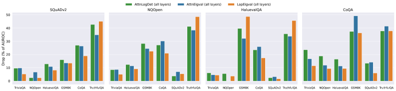To check whether our method generalizes across datasets, we trained the hallucination probe on features from the training split of one QA dataset and evaluated it on the features from the test split of a different QA dataset. Due to space limitations, we present results for selected datasets and provide extended results and absolute efficacy values in Appendix I. Figure 7 showcases the percent drop in Test AUROC when using a different training dataset compared to training and testing on the same QA dataset. We can observe that $\operatorname{LapEigvals}$ provides a performance drop comparable to other baselines, and in several cases, it generalizes best. Interestingly, all methods exhibit poor generalization on TruthfulQA and GSM8K. We hypothesize that the weak performance on TruthfulQA arises from its limited size and class imbalance, whereas the difficulty on GSM8K likely reflects its distinct domain, which has been shown to hinder hallucination detection (Orgad et al., 2025). Additionally, in Appendix I, we show that $\operatorname{LapEigvals}$ achieves the highest test performance in all scenarios (except for TruthfulQA). <details> <summary>x7.png Details</summary>  ### Visual Description ## Bar Chart: Drop (%) of AuROC Across Datasets and Methods ### Overview The image displays a series of four grouped bar charts arranged horizontally. Each chart represents a different evaluation dataset (SQuADv2, NQOpen, HotucaQA, CoQA) and shows the performance drop (in percentage of Area under the ROC Curve, AuROC) for three different methods applied to various question-answering or reasoning models. The y-axis represents the "Drop (%) of AuROC," and the x-axis lists the models/datasets being evaluated. ### Components/Axes * **Main Title/Legend (Top Center):** A shared legend is positioned at the top center of the entire figure. * **Green Bar:** `AttnLogDet (all layers)` * **Blue Bar:** `AttnEqual (all layers)` * **Orange Bar:** `LapEqual (all layers)` * **Subplot Titles (Top of each chart):** From left to right: `SQuADv2`, `NQOpen`, `HotucaQA`, `CoQA`. * **Y-Axis (Left side of each subplot):** Labeled `Drop (%) of AuROC`. The scale runs from 0 to 50, with major tick marks at 0, 10, 20, 30, 40, and 50. * **X-Axis (Bottom of each subplot):** Lists the models/datasets being evaluated. The labels are consistent across subplots but the specific models included vary slightly. The common labels are: `TriviaQA`, `NQOpen`, `HotucaQA`, `GSM8K`, `CoQA`, `SQuADv2`, `TruthfulQA`. ### Detailed Analysis The analysis is segmented by subplot (dataset) as per the component isolation instruction. **1. Subplot: SQuADv2** * **Trend:** All three methods show a generally increasing trend in performance drop as we move from left to right along the x-axis models, with the highest drops observed for `TruthfulQA`. * **Data Points (Approximate % Drop):** * **TriviaQA:** Green ~9, Blue ~9, Orange ~5. * **NQOpen:** Green ~5, Blue ~8, Orange ~4. * **HotucaQA:** Green ~12, Blue ~10, Orange ~8. * **GSM8K:** Green ~16, Blue ~14, Orange ~13. * **CoQA:** Green ~28, Blue ~27, Orange ~20. * **SQuADv2:** Green ~28, Blue ~27, Orange ~20. *(Note: This appears identical to CoQA values in this subplot)*. * **TruthfulQA:** Green ~43, Blue ~35, Orange ~46. **2. Subplot: NQOpen** * **Trend:** Performance drops are more varied. `GSM8K` and `TruthfulQA` show the highest drops for all methods. * **Data Points (Approximate % Drop):** * **TriviaQA:** Green ~8, Blue ~7, Orange ~5. * **NQOpen:** Green ~12, Blue ~11, Orange ~9. * **HotucaQA:** Green ~11, Blue ~10, Orange ~8. * **GSM8K:** Green ~29, Blue ~25, Orange ~23. * **CoQA:** Green ~28, Blue ~31, Orange ~22. * **SQuADv2:** Green ~7, Blue ~6, Orange ~7. * **TruthfulQA:** Green ~41, Blue ~39, Orange ~48. **3. Subplot: HotucaQA** * **Trend:** This subplot shows the most extreme variation. Drops for `TriviaQA`, `NQOpen`, and `SQuADv2` are very low (<5%), while `GSM8K` and `TruthfulQA` show very high drops (>35%). * **Data Points (Approximate % Drop):** * **TriviaQA:** Green ~5, Blue ~4, Orange ~1. * **NQOpen:** Green ~4, Blue ~1, Orange ~4. * **HotucaQA:** Green ~0, Blue ~0, Orange ~0. *(All bars are at or near the baseline)*. * **GSM8K:** Green ~40, Blue ~33, Orange ~48. * **CoQA:** Green ~25, Blue ~24, Orange ~18. * **SQuADv2:** Green ~2, Blue ~2, Orange ~1. * **TruthfulQA:** Green ~36, Blue ~35, Orange ~46. **4. Subplot: CoQA** * **Trend:** `GSM8K` shows the highest drop for the `AttnEqual` (blue) method. `TruthfulQA` shows consistently high drops across all methods. * **Data Points (Approximate % Drop):** * **TriviaQA:** Green ~24, Blue ~16, Orange ~13. * **NQOpen:** Green ~19, Blue ~11, Orange ~9. * **HotucaQA:** Green ~17, Blue ~10, Orange ~10. * **GSM8K:** Green ~37, Blue ~49, Orange ~36. * **CoQA:** Green ~15, Blue ~12, Orange ~7. * **SQuADv2:** Green ~14, Blue ~12, Orange ~6. * **TruthfulQA:** Green ~39, Blue ~42, Orange ~38. ### Key Observations 1. **Method Performance:** The `LapEqual (all layers)` method (orange) frequently results in the highest performance drop, particularly on the `TruthfulQA` model across all evaluation datasets (SQuADv2, NQOpen, HotucaQA, CoQA), often exceeding 45%. 2. **Model Sensitivity:** The `TruthfulQA` model consistently shows the largest or among the largest drops in AuROC across all methods and evaluation datasets, suggesting it is highly sensitive to the interventions being tested. 3. **Dataset-Specific Anomalies:** The `HotucaQA` evaluation dataset shows near-zero drop for the `HotucaQA` model itself (the diagonal), which is an expected sanity check. It also shows uniquely low drops for `TriviaQA`, `NQOpen`, and `SQuADv2` models within this subplot. 4. **Outlier Data Point:** The single highest observed drop is for the `AttnEqual` method (blue) on the `GSM8K` model within the `CoQA` evaluation dataset, reaching approximately 49%. ### Interpretation This chart likely comes from a research paper analyzing the robustness or internal consistency of large language models (LLMs) when subjected to different attention-based interventions (`AttnLogDet`, `AttnEqual`, `LapEqual`). The "Drop in AuROC" measures how much the model's ability to distinguish between correct and incorrect answers degrades after the intervention. * **What the data suggests:** The interventions, particularly `LapEqual`, cause significant degradation in model performance (high AuROC drop) on tasks requiring factual knowledge or complex reasoning (e.g., `TruthfulQA`, `GSM8K`). The varying impact across evaluation datasets (SQuADv2, NQOpen, etc.) indicates that the effect of these interventions is not uniform and depends on the nature of the evaluation benchmark. * **Relationship between elements:** Each subplot acts as a controlled experiment: "When we evaluate on dataset X (e.g., SQuADv2), how do different interventions affect performance across a suite of models?" The consistent underperformance of `TruthfulQA` across all experiments suggests its internal representations or attention mechanisms are particularly vulnerable to the tested perturbations. * **Underlying implication:** The high drops on models like `TruthfulQA` and `GSM8K` might indicate that these models rely on specific, fragile attention patterns for their performance. The interventions disrupt these patterns, leading to significant accuracy loss. Conversely, models with lower drops (e.g., `HotucaQA` on its own dataset) may have more robust or redundant internal mechanisms. This analysis is crucial for understanding model interpretability and building more robust AI systems. </details> Figure 7: Generalization across datasets measured as a percent performance drop in Test AUROC (less is better) when trained on one dataset and tested on the other. Training datasets are indicated in the plot titles, while test datasets are shown on the $x$ -axis. Results computed on Llama-3.1-8B with $k{=}100$ top eigenvalues and $temp{=}1.0$ . Results for all datasets are presented in Appendix I. ### 6.5 How does performance vary across prompts? Lastly, to assess the stability of our method across different prompts used for answer generation, we compared the results of the hallucination probes trained on features regarding four distinct prompts, the content of which is included in Appendix M. As shown in Table 2, $\operatorname{LapEigvals}$ consistently outperforms all baselines across all four prompts. While we can observe variations in performance across prompts, $\operatorname{LapEigvals}$ demonstrates the lowest standard deviation ( $0.05$ ) compared to $\operatorname{AttnLogDet}$ ( $0.016$ ) and $\operatorname{AttnEigvals}$ ( $0.07$ ), indicating its greater robustness. Table 2: Test AUROC across four different prompts for answers on the TriviaQA dataset using Llama-3.1-8B with $temp{=}1.0$ and $k{=}50$ (some prompts have led to fewer than 100 tokens). Prompt $\boldsymbol{p_{3}}$ was the main one used to compare our method to baselines, as presented in Tables 1. | $\operatorname{AttnLogDet}$ $\operatorname{AttnEigvals}$ $\operatorname{LapEigvals}$ | 0.847 0.840 0.882 | 0.855 0.870 0.890 | 0.842 0.842 0.888 | 0.860 0.875 0.895 | | --- | --- | --- | --- | --- | ## 7 Related Work Hallucinations in LLMs were proved to be inevitable (Xu et al., 2024), and to detect them, one can leverage either black-box or white-box approaches. The former approach uses only the outputs from an LLM, while the latter uses hidden states, attention maps, or logits corresponding to generated tokens. Black-box approaches focus on the text generated by LLMs. For instance, (Li et al., 2024) verified the truthfulness of factual statements using external knowledge sources, though this approach relies on the availability of additional resources. Alternatively, SelfCheckGPT (Manakul et al., 2023) generates multiple responses to the same prompt and evaluates their consistency, with low consistency indicating potential hallucination. White-box methods have emerged as a promising approach for detecting hallucinations (Farquhar et al., 2024; Azaria and Mitchell, 2023; Arteaga et al., 2024; Orgad et al., 2025). These methods are universal across all LLMs and do not require additional domain adaptation compared to black-box ones (Farquhar et al., 2024). They draw inspiration from seminal works on analyzing the internal states of simple neural networks (Alain and Bengio, 2016), which introduced linear classifier probes – models operating on the internal states of neural networks. Linear probes have been widely applied to the internal states of LLMs, notably for detecting hallucinations. One of the first such probes was SAPLMA (Azaria and Mitchell, 2023), which demonstrated that one could predict the correctness of generated text straight from LLM’s hidden states. Further, the INSIDE method (Chen et al., 2024) tackled hallucination detection by sampling multiple responses from an LLM and evaluating consistency between their hidden states using a normalized sum of the eigenvalues from their covariance matrix. Also, (Farquhar et al., 2024) proposed a complementary probabilistic approach, employing entropy to quantify the model’s intrinsic uncertainty. Their method involves generating multiple responses, clustering them by semantic similarity, and calculating Semantic Entropy using an appropriate estimator. To address concerns regarding the validity of LLM probes, (Marks and Tegmark, 2024) introduced a high-quality QA dataset with simple true / false answers and causally demonstrated that the truthfulness of such statements is linearly represented in LLMs, which supports the use of probes for short texts. Self-consistency methods (Liang et al., 2024), like INSIDE or Semantic Entropy, require multiple runs of an LLM for each input example, which substantially lowers their applicability. Motivated by this limitation, (Kossen et al., 2024) proposed to use Semantic Entropy Probe, which is a small model trained to predict expensive Semantic Entropy (Farquhar et al., 2024) from LLM’s hidden states. Notably, (Orgad et al., 2025) explored how LLMs encode information about truthfulness and hallucinations. First, they revealed that truthfulness is concentrated in specific tokens. Second, they found that probing classifiers on LLM representations do not generalize well across datasets, especially across datasets requiring different skills, which we confirmed in Section 6.4. Lastly, they showed that the probes could select the correct answer from multiple generated answers with reasonable accuracy, meaning LLMs make mistakes at the decoding stage, besides knowing the correct answer. Recent studies have started to explore hallucination detection exclusively from attention maps. (Chuang et al., 2024a) introduced the lookback ratio, which measures how much attention LLMs allocate to relevant input parts when answering questions based on the provided context. The work most closely related to ours is (Sriramanan et al., 2024), which introduces the $\operatorname{AttentionScore}$ method. Although the process is unsupervised and computationally efficient, the authors note that its performance can depend highly on the specific layer from which the score is extracted. Compared to $\operatorname{AttentionScore}$ , our method is fully supervised and grounded in graph theory, as we interpret inference in LLM as a graph. While $\operatorname{AttentionScore}$ aggregates only the attention diagonal to compute its log-determinant, we instead derive features from the graph Laplacian, which captures all attention scores (see Eq. (1) and (2)). Additionally, we utilize all layers for detecting hallucination rather than a single one, demonstrating effectiveness of this approach. We also demonstrate that it performs poorly on the datasets we evaluated. Nonetheless, we drew inspiration from their approach, particularly using the lower triangular structure of matrices when constructing features for the hallucination probe. ## 8 Conclusions In this work, we demonstrated that the spectral features of LLMs’ attention maps, specifically the eigenvalues of the Laplacian matrix, carry a signal capable of detecting hallucinations. Specifically, we proposed the $\operatorname{LapEigvals}$ method, which employs the top- $k$ eigenvalues of the Laplacian as input to the hallucination detection probe. Through extensive evaluations, we empirically showed that our method consistently achieves state-of-the-art performance among all tested approaches. Furthermore, multiple ablation studies demonstrated that our method remains stable across varying numbers of eigenvalues, diverse prompts, and generation temperatures while offering reasonable generalization. In addition, we hypothesize that self-supervised learning (Balestriero et al., 2023) could yield a more robust and generalizable approach while uncovering non-trivial intrinsic features of attention maps. Notably, results such as those in Section 6.3 suggest intriguing connections to recent advancements in LLM research (Veličković et al., 2024; Barbero et al., 2024), highlighting promising directions for future investigation. ## Limitations Supervised method In our approach, one must provide labelled hallucinated and non-hallucinated examples to train the hallucination probe. While this can be handled by the llm-as-judge, it might introduce some noise or pose a risk of overfitting. Limited generalization across LLM architectures The method is incompatible with LLMs having different head and layer configurations. Developing architecture-agnostic hallucination probes is left for future work. Minimum length requirement Computing $\operatorname{top-k}$ Laplacian eigenvalues demands attention maps of at least $k$ tokens (e.g., $k{=}100$ require 100 tokens). Open LLMs Our method requires access to the internal states of LLM thus it cannot be applied to closed LLMs. Risks Please note that the proposed method was tested on selected LLMs and English data, so applying it to untested domains and tasks carries a considerable risk without additional validation. ## Acknowledgements We sincerely thank Piotr Bielak for his valuable review and insightful feedback, which helped improve this work. This work was funded by the European Union under the Horizon Europe grant OMINO – Overcoming Multilevel INformation Overload (grant number 101086321, https://ominoproject.eu/). Views and opinions expressed are those of the authors alone and do not necessarily reflect those of the European Union or the European Research Executive Agency. Neither the European Union nor the European Research Executive Agency can be held responsible for them. It was also co-financed with funds from the Polish Ministry of Education and Science under the programme entitled International Co-Financed Projects, grant no. 573977. We gratefully acknowledge the Wroclaw Centre for Networking and Supercomputing for providing the computational resources used in this work. This work was co-funded by the National Science Centre, Poland under CHIST-ERA Open & Re-usable Research Data & Software (grant number 2022/04/Y/ST6/00183). The authors used ChatGPT to improve the clarity and readability of the manuscript. ## References - Abdin et al. (2024) Marah Abdin, Jyoti Aneja, Hany Awadalla, Ahmed Awadallah, Ammar Ahmad Awan, Nguyen Bach, Amit Bahree, Arash Bakhtiari, Jianmin Bao, Harkirat Behl, Alon Benhaim, Misha Bilenko, Johan Bjorck, Sébastien Bubeck, Martin Cai, Qin Cai, Vishrav Chaudhary, Dong Chen, Dongdong Chen, Weizhu Chen, Yen-Chun Chen, Yi-Ling Chen, Hao Cheng, Parul Chopra, Xiyang Dai, Matthew Dixon, Ronen Eldan, Victor Fragoso, Jianfeng Gao, Mei Gao, Min Gao, Amit Garg, Allie Del Giorno, Abhishek Goswami, Suriya Gunasekar, Emman Haider, Junheng Hao, Russell J. Hewett, Wenxiang Hu, Jamie Huynh, Dan Iter, Sam Ade Jacobs, Mojan Javaheripi, Xin Jin, Nikos Karampatziakis, Piero Kauffmann, Mahoud Khademi, Dongwoo Kim, Young Jin Kim, Lev Kurilenko, James R. Lee, Yin Tat Lee, Yuanzhi Li, Yunsheng Li, Chen Liang, Lars Liden, Xihui Lin, Zeqi Lin, Ce Liu, Liyuan Liu, Mengchen Liu, Weishung Liu, Xiaodong Liu, Chong Luo, Piyush Madan, Ali Mahmoudzadeh, David Majercak, Matt Mazzola, Caio César Teodoro Mendes, Arindam Mitra, Hardik Modi, Anh Nguyen, Brandon Norick, Barun Patra, Daniel Perez-Becker, Thomas Portet, Reid Pryzant, Heyang Qin, Marko Radmilac, Liliang Ren, Gustavo de Rosa, Corby Rosset, Sambudha Roy, Olatunji Ruwase, Olli Saarikivi, Amin Saied, Adil Salim, Michael Santacroce, Shital Shah, Ning Shang, Hiteshi Sharma, Yelong Shen, Swadheen Shukla, Xia Song, Masahiro Tanaka, Andrea Tupini, Praneetha Vaddamanu, Chunyu Wang, Guanhua Wang, Lijuan Wang, Shuohang Wang, Xin Wang, Yu Wang, Rachel Ward, Wen Wen, Philipp Witte, Haiping Wu, Xiaoxia Wu, Michael Wyatt, Bin Xiao, Can Xu, Jiahang Xu, Weijian Xu, Jilong Xue, Sonali Yadav, Fan Yang, Jianwei Yang, Yifan Yang, Ziyi Yang, Donghan Yu, Lu Yuan, Chenruidong Zhang, Cyril Zhang, Jianwen Zhang, Li Lyna Zhang, Yi Zhang, Yue Zhang, Yunan Zhang, and Xiren Zhou. 2024. Phi-3 Technical Report: A Highly Capable Language Model Locally on Your Phone. arXiv preprint. ArXiv:2404.14219 [cs]. - Alain and Bengio (2016) Guillaume Alain and Yoshua Bengio. 2016. Understanding intermediate layers using linear classifier probes. - Ansel et al. (2024) Jason Ansel, Edward Yang, Horace He, Natalia Gimelshein, Animesh Jain, Michael Voznesensky, Bin Bao, Peter Bell, David Berard, Evgeni Burovski, Geeta Chauhan, Anjali Chourdia, Will Constable, Alban Desmaison, Zachary DeVito, Elias Ellison, Will Feng, Jiong Gong, Michael Gschwind, Brian Hirsh, Sherlock Huang, Kshiteej Kalambarkar, Laurent Kirsch, Michael Lazos, Mario Lezcano, Yanbo Liang, Jason Liang, Yinghai Lu, CK Luk, Bert Maher, Yunjie Pan, Christian Puhrsch, Matthias Reso, Mark Saroufim, Marcos Yukio Siraichi, Helen Suk, Michael Suo, Phil Tillet, Eikan Wang, Xiaodong Wang, William Wen, Shunting Zhang, Xu Zhao, Keren Zhou, Richard Zou, Ajit Mathews, Gregory Chanan, Peng Wu, and Soumith Chintala. 2024. PyTorch 2: Faster Machine Learning Through Dynamic Python Bytecode Transformation and Graph Compilation. In 29th ACM International Conference on Architectural Support for Programming Languages and Operating Systems, Volume 2 (ASPLOS ’24). ACM. - Arteaga et al. (2024) Gabriel Y. Arteaga, Thomas B. Schön, and Nicolas Pielawski. 2024. Hallucination Detection in LLMs: Fast and Memory-Efficient Finetuned Models. In Northern Lights Deep Learning Conference 2025. - Azaria and Mitchell (2023) Amos Azaria and Tom Mitchell. 2023. The Internal State of an LLM Knows When It‘s Lying. In Findings of the Association for Computational Linguistics: EMNLP 2023, pages 967–976, Singapore. Association for Computational Linguistics. - Balestriero et al. (2023) Randall Balestriero, Mark Ibrahim, Vlad Sobal, Ari Morcos, Shashank Shekhar, Tom Goldstein, Florian Bordes, Adrien Bardes, Gregoire Mialon, Yuandong Tian, Avi Schwarzschild, Andrew Gordon Wilson, Jonas Geiping, Quentin Garrido, Pierre Fernandez, Amir Bar, Hamed Pirsiavash, Yann LeCun, and Micah Goldblum. 2023. A Cookbook of Self-Supervised Learning. arXiv preprint. ArXiv:2304.12210 [cs]. - Barbero et al. (2024) Federico Barbero, Andrea Banino, Steven Kapturowski, Dharshan Kumaran, João G. M. Araújo, Alex Vitvitskyi, Razvan Pascanu, and Petar Veličković. 2024. Transformers need glasses! Information over-squashing in language tasks. arXiv preprint. ArXiv:2406.04267 [cs]. - Black et al. (2023) Mitchell Black, Zhengchao Wan, Amir Nayyeri, and Yusu Wang. 2023. Understanding Oversquashing in GNNs through the Lens of Effective Resistance. In International Conference on Machine Learning, pages 2528–2547. PMLR. ArXiv:2302.06835 [cs]. - Bruna et al. (2013) Joan Bruna, Wojciech Zaremba, Arthur Szlam, and Yann LeCun. 2013. Spectral Networks and Locally Connected Networks on Graphs. CoRR. - Chen et al. (2024) Chao Chen, Kai Liu, Ze Chen, Yi Gu, Yue Wu, Mingyuan Tao, Zhihang Fu, and Jieping Ye. 2024. INSIDE: LLMs’ Internal States Retain the Power of Hallucination Detection. In The Twelfth International Conference on Learning Representations. - Chuang et al. (2024a) Yung-Sung Chuang, Linlu Qiu, Cheng-Yu Hsieh, Ranjay Krishna, Yoon Kim, and James R. Glass. 2024a. Lookback Lens: Detecting and Mitigating Contextual Hallucinations in Large Language Models Using Only Attention Maps. In Proceedings of the 2024 Conference on Empirical Methods in Natural Language Processing, pages 1419–1436, Miami, Florida, USA. Association for Computational Linguistics. - Chuang et al. (2024b) Yung-Sung Chuang, Yujia Xie, Hongyin Luo, Yoon Kim, James R. Glass, and Pengcheng He. 2024b. DoLa: Decoding by Contrasting Layers Improves Factuality in Large Language Models. In The Twelfth International Conference on Learning Representations. - Cobbe et al. (2021) Karl Cobbe, Vineet Kosaraju, Mohammad Bavarian, Mark Chen, Heewoo Jun, Lukasz Kaiser, Matthias Plappert, Jerry Tworek, Jacob Hilton, Reiichiro Nakano, Christopher Hesse, and John Schulman. 2021. Training verifiers to solve math word problems. arXiv preprint arXiv:2110.14168. - Dao et al. (2022) Tri Dao, Daniel Y. Fu, Stefano Ermon, Atri Rudra, and Christopher Ré. 2022. FLASHATTENTION: fast and memory-efficient exact attention with IO-awareness. In Proceedings of the 36th international conference on neural information processing systems, Nips ’22, New Orleans, LA, USA. Curran Associates Inc. Number of pages: 16 tex.address: Red Hook, NY, USA tex.articleno: 1189. - Farquhar et al. (2024) Sebastian Farquhar, Jannik Kossen, Lorenz Kuhn, and Yarin Gal. 2024. Detecting hallucinations in large language models using semantic entropy. Nature, 630(8017):625–630. Publisher: Nature Publishing Group. - Grattafiori et al. (2024) Aaron Grattafiori, Abhimanyu Dubey, Abhinav Jauhri, Abhinav Pandey, Abhishek Kadian, Ahmad Al-Dahle, Aiesha Letman, Akhil Mathur, Alan Schelten, Alex Vaughan, Amy Yang, Angela Fan, Anirudh Goyal, Anthony Hartshorn, Aobo Yang, Archi Mitra, Archie Sravankumar, Artem Korenev, Arthur Hinsvark, Arun Rao, Aston Zhang, Aurelien Rodriguez, Austen Gregerson, Ava Spataru, Baptiste Roziere, Bethany Biron, Binh Tang, Bobbie Chern, Charlotte Caucheteux, Chaya Nayak, Chloe Bi, Chris Marra, Chris McConnell, Christian Keller, Christophe Touret, Chunyang Wu, Corinne Wong, Cristian Canton Ferrer, Cyrus Nikolaidis, Damien Allonsius, Daniel Song, Danielle Pintz, Danny Livshits, Danny Wyatt, David Esiobu, Dhruv Choudhary, Dhruv Mahajan, Diego Garcia-Olano, Diego Perino, Dieuwke Hupkes, Egor Lakomkin, Ehab AlBadawy, Elina Lobanova, Emily Dinan, Eric Michael Smith, Filip Radenovic, Francisco Guzmán, Frank Zhang, Gabriel Synnaeve, Gabrielle Lee, Georgia Lewis Anderson, Govind Thattai, Graeme Nail, Gregoire Mialon, Guan Pang, Guillem Cucurell, Hailey Nguyen, Hannah Korevaar, Hu Xu, Hugo Touvron, Iliyan Zarov, Imanol Arrieta Ibarra, Isabel Kloumann, Ishan Misra, Ivan Evtimov, Jack Zhang, Jade Copet, Jaewon Lee, Jan Geffert, Jana Vranes, Jason Park, Jay Mahadeokar, Jeet Shah, Jelmer van der Linde, Jennifer Billock, Jenny Hong, Jenya Lee, Jeremy Fu, Jianfeng Chi, Jianyu Huang, Jiawen Liu, Jie Wang, Jiecao Yu, Joanna Bitton, Joe Spisak, Jongsoo Park, Joseph Rocca, Joshua Johnstun, Joshua Saxe, Junteng Jia, Kalyan Vasuden Alwala, Karthik Prasad, Kartikeya Upasani, Kate Plawiak, Ke Li, Kenneth Heafield, Kevin Stone, Khalid El-Arini, Krithika Iyer, Kshitiz Malik, Kuenley Chiu, Kunal Bhalla, Kushal Lakhotia, Lauren Rantala-Yeary, Laurens van der Maaten, Lawrence Chen, Liang Tan, Liz Jenkins, Louis Martin, Lovish Madaan, Lubo Malo, Lukas Blecher, Lukas Landzaat, Luke de Oliveira, Madeline Muzzi, Mahesh Pasupuleti, Mannat Singh, Manohar Paluri, Marcin Kardas, Maria Tsimpoukelli, Mathew Oldham, Mathieu Rita, Maya Pavlova, Melanie Kambadur, Mike Lewis, Min Si, Mitesh Kumar Singh, Mona Hassan, Naman Goyal, Narjes Torabi, Nikolay Bashlykov, Nikolay Bogoychev, Niladri Chatterji, Ning Zhang, Olivier Duchenne, Onur Çelebi, Patrick Alrassy, Pengchuan Zhang, Pengwei Li, Petar Vasic, Peter Weng, Prajjwal Bhargava, Pratik Dubal, Praveen Krishnan, Punit Singh Koura, Puxin Xu, Qing He, Qingxiao Dong, Ragavan Srinivasan, Raj Ganapathy, Ramon Calderer, Ricardo Silveira Cabral, Robert Stojnic, Roberta Raileanu, Rohan Maheswari, Rohit Girdhar, Rohit Patel, Romain Sauvestre, Ronnie Polidoro, Roshan Sumbaly, Ross Taylor, Ruan Silva, Rui Hou, Rui Wang, Saghar Hosseini, Sahana Chennabasappa, Sanjay Singh, Sean Bell, Seohyun Sonia Kim, Sergey Edunov, Shaoliang Nie, Sharan Narang, Sharath Raparthy, Sheng Shen, Shengye Wan, Shruti Bhosale, Shun Zhang, Simon Vandenhende, Soumya Batra, Spencer Whitman, Sten Sootla, Stephane Collot, Suchin Gururangan, Sydney Borodinsky, Tamar Herman, Tara Fowler, Tarek Sheasha, Thomas Georgiou, Thomas Scialom, Tobias Speckbacher, Todor Mihaylov, Tong Xiao, Ujjwal Karn, Vedanuj Goswami, Vibhor Gupta, Vignesh Ramanathan, Viktor Kerkez, Vincent Gonguet, Virginie Do, Vish Vogeti, Vítor Albiero, Vladan Petrovic, Weiwei Chu, Wenhan Xiong, Wenyin Fu, Whitney Meers, Xavier Martinet, Xiaodong Wang, Xiaofang Wang, Xiaoqing Ellen Tan, Xide Xia, Xinfeng Xie, Xuchao Jia, Xuewei Wang, Yaelle Goldschlag, Yashesh Gaur, Yasmine Babaei, Yi Wen, Yiwen Song, Yuchen Zhang, Yue Li, Yuning Mao, Zacharie Delpierre Coudert, Zheng Yan, Zhengxing Chen, Zoe Papakipos, Aaditya Singh, Aayushi Srivastava, Abha Jain, Adam Kelsey, Adam Shajnfeld, Adithya Gangidi, Adolfo Victoria, Ahuva Goldstand, Ajay Menon, Ajay Sharma, Alex Boesenberg, Alexei Baevski, Allie Feinstein, Amanda Kallet, Amit Sangani, Amos Teo, Anam Yunus, Andrei Lupu, Andres Alvarado, Andrew Caples, Andrew Gu, Andrew Ho, Andrew Poulton, Andrew Ryan, Ankit Ramchandani, Annie Dong, Annie Franco, Anuj Goyal, Aparajita Saraf, Arkabandhu Chowdhury, Ashley Gabriel, Ashwin Bharambe, Assaf Eisenman, Azadeh Yazdan, Beau James, Ben Maurer, Benjamin Leonhardi, Bernie Huang, Beth Loyd, Beto De Paola, Bhargavi Paranjape, Bing Liu, Bo Wu, Boyu Ni, Braden Hancock, Bram Wasti, Brandon Spence, Brani Stojkovic, Brian Gamido, Britt Montalvo, Carl Parker, Carly Burton, Catalina Mejia, Ce Liu, Changhan Wang, Changkyu Kim, Chao Zhou, Chester Hu, Ching-Hsiang Chu, Chris Cai, Chris Tindal, Christoph Feichtenhofer, Cynthia Gao, Damon Civin, Dana Beaty, Daniel Kreymer, Daniel Li, David Adkins, David Xu, Davide Testuggine, Delia David, Devi Parikh, Diana Liskovich, Didem Foss, Dingkang Wang, Duc Le, Dustin Holland, Edward Dowling, Eissa Jamil, Elaine Montgomery, Eleonora Presani, Emily Hahn, Emily Wood, Eric-Tuan Le, Erik Brinkman, Esteban Arcaute, Evan Dunbar, Evan Smothers, Fei Sun, Felix Kreuk, Feng Tian, Filippos Kokkinos, Firat Ozgenel, Francesco Caggioni, Frank Kanayet, Frank Seide, Gabriela Medina Florez, Gabriella Schwarz, Gada Badeer, Georgia Swee, Gil Halpern, Grant Herman, Grigory Sizov, Guangyi, Zhang, Guna Lakshminarayanan, Hakan Inan, Hamid Shojanazeri, Han Zou, Hannah Wang, Hanwen Zha, Haroun Habeeb, Harrison Rudolph, Helen Suk, Henry Aspegren, Hunter Goldman, Hongyuan Zhan, Ibrahim Damlaj, Igor Molybog, Igor Tufanov, Ilias Leontiadis, Irina-Elena Veliche, Itai Gat, Jake Weissman, James Geboski, James Kohli, Janice Lam, Japhet Asher, Jean-Baptiste Gaya, Jeff Marcus, Jeff Tang, Jennifer Chan, Jenny Zhen, Jeremy Reizenstein, Jeremy Teboul, Jessica Zhong, Jian Jin, Jingyi Yang, Joe Cummings, Jon Carvill, Jon Shepard, Jonathan McPhie, Jonathan Torres, Josh Ginsburg, Junjie Wang, Kai Wu, Kam Hou U, Karan Saxena, Kartikay Khandelwal, Katayoun Zand, Kathy Matosich, Kaushik Veeraraghavan, Kelly Michelena, Keqian Li, Kiran Jagadeesh, Kun Huang, Kunal Chawla, Kyle Huang, Lailin Chen, Lakshya Garg, Lavender A, Leandro Silva, Lee Bell, Lei Zhang, Liangpeng Guo, Licheng Yu, Liron Moshkovich, Luca Wehrstedt, Madian Khabsa, Manav Avalani, Manish Bhatt, Martynas Mankus, Matan Hasson, Matthew Lennie, Matthias Reso, Maxim Groshev, Maxim Naumov, Maya Lathi, Meghan Keneally, Miao Liu, Michael L. Seltzer, Michal Valko, Michelle Restrepo, Mihir Patel, Mik Vyatskov, Mikayel Samvelyan, Mike Clark, Mike Macey, Mike Wang, Miquel Jubert Hermoso, Mo Metanat, Mohammad Rastegari, Munish Bansal, Nandhini Santhanam, Natascha Parks, Natasha White, Navyata Bawa, Nayan Singhal, Nick Egebo, Nicolas Usunier, Nikhil Mehta, Nikolay Pavlovich Laptev, Ning Dong, Norman Cheng, Oleg Chernoguz, Olivia Hart, Omkar Salpekar, Ozlem Kalinli, Parkin Kent, Parth Parekh, Paul Saab, Pavan Balaji, Pedro Rittner, Philip Bontrager, Pierre Roux, Piotr Dollar, Polina Zvyagina, Prashant Ratanchandani, Pritish Yuvraj, Qian Liang, Rachad Alao, Rachel Rodriguez, Rafi Ayub, Raghotham Murthy, Raghu Nayani, Rahul Mitra, Rangaprabhu Parthasarathy, Raymond Li, Rebekkah Hogan, Robin Battey, Rocky Wang, Russ Howes, Ruty Rinott, Sachin Mehta, Sachin Siby, Sai Jayesh Bondu, Samyak Datta, Sara Chugh, Sara Hunt, Sargun Dhillon, Sasha Sidorov, Satadru Pan, Saurabh Mahajan, Saurabh Verma, Seiji Yamamoto, Sharadh Ramaswamy, Shaun Lindsay, Shaun Lindsay, Sheng Feng, Shenghao Lin, Shengxin Cindy Zha, Shishir Patil, Shiva Shankar, Shuqiang Zhang, Shuqiang Zhang, Sinong Wang, Sneha Agarwal, Soji Sajuyigbe, Soumith Chintala, Stephanie Max, Stephen Chen, Steve Kehoe, Steve Satterfield, Sudarshan Govindaprasad, Sumit Gupta, Summer Deng, Sungmin Cho, Sunny Virk, Suraj Subramanian, Sy Choudhury, Sydney Goldman, Tal Remez, Tamar Glaser, Tamara Best, Thilo Koehler, Thomas Robinson, Tianhe Li, Tianjun Zhang, Tim Matthews, Timothy Chou, Tzook Shaked, Varun Vontimitta, Victoria Ajayi, Victoria Montanez, Vijai Mohan, Vinay Satish Kumar, Vishal Mangla, Vlad Ionescu, Vlad Poenaru, Vlad Tiberiu Mihailescu, Vladimir Ivanov, Wei Li, Wenchen Wang, Wenwen Jiang, Wes Bouaziz, Will Constable, Xiaocheng Tang, Xiaojian Wu, Xiaolan Wang, Xilun Wu, Xinbo Gao, Yaniv Kleinman, Yanjun Chen, Ye Hu, Ye Jia, Ye Qi, Yenda Li, Yilin Zhang, Ying Zhang, Yossi Adi, Youngjin Nam, Yu, Wang, Yu Zhao, Yuchen Hao, Yundi Qian, Yunlu Li, Yuzi He, Zach Rait, Zachary DeVito, Zef Rosnbrick, Zhaoduo Wen, Zhenyu Yang, Zhiwei Zhao, and Zhiyu Ma. 2024. The Llama 3 Herd of Models. arXiv preprint. ArXiv:2407.21783 [cs]. - Huang et al. (2023) Lei Huang, Weijiang Yu, Weitao Ma, Weihong Zhong, Zhangyin Feng, Haotian Wang, Qianglong Chen, Weihua Peng, Xiaocheng Feng, Bing Qin, and Ting Liu. 2023. A Survey on Hallucination in Large Language Models: Principles, Taxonomy, Challenges, and Open Questions. arXiv preprint. ArXiv:2311.05232 [cs]. - Jolliffe and Cadima (2016) Ian T. Jolliffe and Jorge Cadima. 2016. Principal component analysis: a review and recent developments. Philosophical Transactions of the Royal Society A: Mathematical, Physical and Engineering Sciences, 374(2065):20150202. Publisher: Royal Society. - Joshi et al. (2017) Mandar Joshi, Eunsol Choi, Daniel Weld, and Luke Zettlemoyer. 2017. TriviaQA: A Large Scale Distantly Supervised Challenge Dataset for Reading Comprehension. In Proceedings of the 55th Annual Meeting of the Association for Computational Linguistics (Volume 1: Long Papers), pages 1601–1611, Vancouver, Canada. Association for Computational Linguistics. - Kim et al. (2024) Hazel Kim, Adel Bibi, Philip Torr, and Yarin Gal. 2024. Detecting LLM Hallucination Through Layer-wise Information Deficiency: Analysis of Unanswerable Questions and Ambiguous Prompts. arXiv preprint. ArXiv:2412.10246 [cs]. - Kossen et al. (2024) Jannik Kossen, Jiatong Han, Muhammed Razzak, Lisa Schut, Shreshth Malik, and Yarin Gal. 2024. Semantic Entropy Probes: Robust and Cheap Hallucination Detection in LLMs. arXiv preprint. ArXiv:2406.15927 [cs]. - Kuprieiev et al. (2025) Ruslan Kuprieiev, skshetry, Peter Rowland, Dmitry Petrov, Pawel Redzynski, Casper da Costa-Luis, David de la Iglesia Castro, Alexander Schepanovski, Ivan Shcheklein, Gao, Batuhan Taskaya, Jorge Orpinel, Fábio Santos, Daniele, Ronan Lamy, Aman Sharma, Zhanibek Kaimuldenov, Dani Hodovic, Nikita Kodenko, Andrew Grigorev, Earl, Nabanita Dash, George Vyshnya, Dave Berenbaum, maykulkarni, Max Hora, Vera, and Sanidhya Mangal. 2025. DVC: Data Version Control - Git for Data & Models. - Kwiatkowski et al. (2019) Tom Kwiatkowski, Jennimaria Palomaki, Olivia Redfield, Michael Collins, Ankur Parikh, Chris Alberti, Danielle Epstein, Illia Polosukhin, Jacob Devlin, Kenton Lee, Kristina Toutanova, Llion Jones, Matthew Kelcey, Ming-Wei Chang, Andrew M. Dai, Jakob Uszkoreit, Quoc Le, and Slav Petrov. 2019. Natural Questions: A Benchmark for Question Answering Research. Transactions of the Association for Computational Linguistics, 7:452–466. Place: Cambridge, MA Publisher: MIT Press. - Lee (2023) Minhyeok Lee. 2023. A Mathematical Investigation of Hallucination and Creativity in GPT Models. Mathematics, 11(10):2320. - Li et al. (2024) Junyi Li, Jie Chen, Ruiyang Ren, Xiaoxue Cheng, Xin Zhao, Jian-Yun Nie, and Ji-Rong Wen. 2024. The Dawn After the Dark: An Empirical Study on Factuality Hallucination in Large Language Models. In Proceedings of the 62nd Annual Meeting of the Association for Computational Linguistics (Volume 1: Long Papers), pages 10879–10899, Bangkok, Thailand. Association for Computational Linguistics. - Li et al. (2023) Junyi Li, Xiaoxue Cheng, Wayne Xin Zhao, Jian-Yun Nie, and Ji-Rong Wen. 2023. HaluEval: A Large-Scale Hallucination Evaluation Benchmark for Large Language Models. arXiv preprint. ArXiv:2305.11747 [cs]. - Liang et al. (2024) Xun Liang, Shichao Song, Zifan Zheng, Hanyu Wang, Qingchen Yu, Xunkai Li, Rong-Hua Li, Feiyu Xiong, and Zhiyu Li. 2024. Internal Consistency and Self-Feedback in Large Language Models: A Survey. CoRR, abs/2407.14507. - Lin et al. (2022) Stephanie Lin, Jacob Hilton, and Owain Evans. 2022. TruthfulQA: Measuring How Models Mimic Human Falsehoods. In Proceedings of the 60th Annual Meeting of the Association for Computational Linguistics (Volume 1: Long Papers), pages 3214–3252, Dublin, Ireland. Association for Computational Linguistics. - Manakul et al. (2023) Potsawee Manakul, Adian Liusie, and Mark Gales. 2023. SelfCheckGPT: Zero-Resource Black-Box Hallucination Detection for Generative Large Language Models. In Proceedings of the 2023 Conference on Empirical Methods in Natural Language Processing, pages 9004–9017, Singapore. Association for Computational Linguistics. - Mann and Whitney (1947) Henry B Mann and Donald R Whitney. 1947. On a test of whether one of two random variables is stochastically larger than the other. The annals of mathematical statistics, pages 50–60. Publisher: JSTOR. - Marks and Tegmark (2024) Samuel Marks and Max Tegmark. 2024. The Geometry of Truth: Emergent Linear Structure in Large Language Model Representations of True/False Datasets. In First Conference on Language Modeling. - Mistral AI Team (2025) Mistral AI Team. 2025. Mistral-small-24B-instruct-2501. - Mistral AI Team and NVIDIA (2024) Mistral AI Team and NVIDIA. 2024. Mistral-nemo-instruct-2407. - Mitra et al. (2024) Kushan Mitra, Dan Zhang, Sajjadur Rahman, and Estevam Hruschka. 2024. FactLens: Benchmarking Fine-Grained Fact Verification. arXiv preprint. ArXiv:2411.05980 [cs]. - Mohar (1997) Bojan Mohar. 1997. Some applications of Laplace eigenvalues of graphs. In Geňa Hahn and Gert Sabidussi, editors, Graph Symmetry, pages 225–275. Springer Netherlands, Dordrecht. - OpenAI et al. (2024) OpenAI, Josh Achiam, Steven Adler, Sandhini Agarwal, Lama Ahmad, Ilge Akkaya, Florencia Leoni Aleman, Diogo Almeida, Janko Altenschmidt, Sam Altman, Shyamal Anadkat, Red Avila, Igor Babuschkin, Suchir Balaji, Valerie Balcom, Paul Baltescu, Haiming Bao, Mohammad Bavarian, Jeff Belgum, Irwan Bello, Jake Berdine, Gabriel Bernadett-Shapiro, Christopher Berner, Lenny Bogdonoff, Oleg Boiko, Madelaine Boyd, Anna-Luisa Brakman, Greg Brockman, Tim Brooks, Miles Brundage, Kevin Button, Trevor Cai, Rosie Campbell, Andrew Cann, Brittany Carey, Chelsea Carlson, Rory Carmichael, Brooke Chan, Che Chang, Fotis Chantzis, Derek Chen, Sully Chen, Ruby Chen, Jason Chen, Mark Chen, Ben Chess, Chester Cho, Casey Chu, Hyung Won Chung, Dave Cummings, Jeremiah Currier, Yunxing Dai, Cory Decareaux, Thomas Degry, Noah Deutsch, Damien Deville, Arka Dhar, David Dohan, Steve Dowling, Sheila Dunning, Adrien Ecoffet, Atty Eleti, Tyna Eloundou, David Farhi, Liam Fedus, Niko Felix, Simón Posada Fishman, Juston Forte, Isabella Fulford, Leo Gao, Elie Georges, Christian Gibson, Vik Goel, Tarun Gogineni, Gabriel Goh, Rapha Gontijo-Lopes, Jonathan Gordon, Morgan Grafstein, Scott Gray, Ryan Greene, Joshua Gross, Shixiang Shane Gu, Yufei Guo, Chris Hallacy, Jesse Han, Jeff Harris, Yuchen He, Mike Heaton, Johannes Heidecke, Chris Hesse, Alan Hickey, Wade Hickey, Peter Hoeschele, Brandon Houghton, Kenny Hsu, Shengli Hu, Xin Hu, Joost Huizinga, Shantanu Jain, Shawn Jain, Joanne Jang, Angela Jiang, Roger Jiang, Haozhun Jin, Denny Jin, Shino Jomoto, Billie Jonn, Heewoo Jun, Tomer Kaftan, Łukasz Kaiser, Ali Kamali, Ingmar Kanitscheider, Nitish Shirish Keskar, Tabarak Khan, Logan Kilpatrick, Jong Wook Kim, Christina Kim, Yongjik Kim, Jan Hendrik Kirchner, Jamie Kiros, Matt Knight, Daniel Kokotajlo, Łukasz Kondraciuk, Andrew Kondrich, Aris Konstantinidis, Kyle Kosic, Gretchen Krueger, Vishal Kuo, Michael Lampe, Ikai Lan, Teddy Lee, Jan Leike, Jade Leung, Daniel Levy, Chak Ming Li, Rachel Lim, Molly Lin, Stephanie Lin, Mateusz Litwin, Theresa Lopez, Ryan Lowe, Patricia Lue, Anna Makanju, Kim Malfacini, Sam Manning, Todor Markov, Yaniv Markovski, Bianca Martin, Katie Mayer, Andrew Mayne, Bob McGrew, Scott Mayer McKinney, Christine McLeavey, Paul McMillan, Jake McNeil, David Medina, Aalok Mehta, Jacob Menick, Luke Metz, Andrey Mishchenko, Pamela Mishkin, Vinnie Monaco, Evan Morikawa, Daniel Mossing, Tong Mu, Mira Murati, Oleg Murk, David Mély, Ashvin Nair, Reiichiro Nakano, Rajeev Nayak, Arvind Neelakantan, Richard Ngo, Hyeonwoo Noh, Long Ouyang, Cullen O’Keefe, Jakub Pachocki, Alex Paino, Joe Palermo, Ashley Pantuliano, Giambattista Parascandolo, Joel Parish, Emy Parparita, Alex Passos, Mikhail Pavlov, Andrew Peng, Adam Perelman, Filipe de Avila Belbute Peres, Michael Petrov, Henrique Ponde de Oliveira Pinto, Michael, Pokorny, Michelle Pokrass, Vitchyr H. Pong, Tolly Powell, Alethea Power, Boris Power, Elizabeth Proehl, Raul Puri, Alec Radford, Jack Rae, Aditya Ramesh, Cameron Raymond, Francis Real, Kendra Rimbach, Carl Ross, Bob Rotsted, Henri Roussez, Nick Ryder, Mario Saltarelli, Ted Sanders, Shibani Santurkar, Girish Sastry, Heather Schmidt, David Schnurr, John Schulman, Daniel Selsam, Kyla Sheppard, Toki Sherbakov, Jessica Shieh, Sarah Shoker, Pranav Shyam, Szymon Sidor, Eric Sigler, Maddie Simens, Jordan Sitkin, Katarina Slama, Ian Sohl, Benjamin Sokolowsky, Yang Song, Natalie Staudacher, Felipe Petroski Such, Natalie Summers, Ilya Sutskever, Jie Tang, Nikolas Tezak, Madeleine B. Thompson, Phil Tillet, Amin Tootoonchian, Elizabeth Tseng, Preston Tuggle, Nick Turley, Jerry Tworek, Juan Felipe Cerón Uribe, Andrea Vallone, Arun Vijayvergiya, Chelsea Voss, Carroll Wainwright, Justin Jay Wang, Alvin Wang, Ben Wang, Jonathan Ward, Jason Wei, C. J. Weinmann, Akila Welihinda, Peter Welinder, Jiayi Weng, Lilian Weng, Matt Wiethoff, Dave Willner, Clemens Winter, Samuel Wolrich, Hannah Wong, Lauren Workman, Sherwin Wu, Jeff Wu, Michael Wu, Kai Xiao, Tao Xu, Sarah Yoo, Kevin Yu, Qiming Yuan, Wojciech Zaremba, Rowan Zellers, Chong Zhang, Marvin Zhang, Shengjia Zhao, Tianhao Zheng, Juntang Zhuang, William Zhuk, and Barret Zoph. 2024. GPT-4 Technical Report. arXiv preprint. ArXiv:2303.08774 [cs]. - Orgad et al. (2025) Hadas Orgad, Michael Toker, Zorik Gekhman, Roi Reichart, Idan Szpektor, Hadas Kotek, and Yonatan Belinkov. 2025. LLMs Know More Than They Show: On the Intrinsic Representation of LLM Hallucinations. In The Thirteenth International Conference on Learning Representations. - Pedregosa et al. (2011) F. Pedregosa, G. Varoquaux, A. Gramfort, V. Michel, B. Thirion, O. Grisel, M. Blondel, P. Prettenhofer, R. Weiss, V. Dubourg, J. Vanderplas, A. Passos, D. Cournapeau, M. Brucher, M. Perrot, and E. Duchesnay. 2011. Scikit-learn: Machine Learning in Python. Journal of Machine Learning Research, 12:2825–2830. - Rajpurkar et al. (2018) Pranav Rajpurkar, Robin Jia, and Percy Liang. 2018. Know What You Don‘t Know: Unanswerable Questions for SQuAD. In Proceedings of the 56th Annual Meeting of the Association for Computational Linguistics (Volume 2: Short Papers), pages 784–789, Melbourne, Australia. Association for Computational Linguistics. - Reddy et al. (2019) Siva Reddy, Danqi Chen, and Christopher D. Manning. 2019. CoQA: A Conversational Question Answering Challenge. Transactions of the Association for Computational Linguistics, 7:249–266. Place: Cambridge, MA Publisher: MIT Press. - Renze (2024) Matthew Renze. 2024. The Effect of Sampling Temperature on Problem Solving in Large Language Models. In Findings of the Association for Computational Linguistics: EMNLP 2024, pages 7346–7356, Miami, Florida, USA. Association for Computational Linguistics. - Sriramanan et al. (2024) Gaurang Sriramanan, Siddhant Bharti, Vinu Sankar Sadasivan, Shoumik Saha, Priyatham Kattakinda, and Soheil Feizi. 2024. LLM-Check: Investigating Detection of Hallucinations in Large Language Models. In The Thirty-eighth Annual Conference on Neural Information Processing Systems. - team (2020) The pandas development team. 2020. pandas-dev/pandas: Pandas. - Topping et al. (2022) Jake Topping, Francesco Di Giovanni, Benjamin Paul Chamberlain, Xiaowen Dong, and Michael M. Bronstein. 2022. Understanding over-squashing and bottlenecks on graphs via curvature. In International Conference on Learning Representations. - Vaswani (2017) A Vaswani. 2017. Attention is all you need. Advances in Neural Information Processing Systems. - Veličković et al. (2024) Petar Veličković, Christos Perivolaropoulos, Federico Barbero, and Razvan Pascanu. 2024. softmax is not enough (for sharp out-of-distribution). arXiv preprint. ArXiv:2410.01104 [cs]. - Virtanen et al. (2020) Pauli Virtanen, Ralf Gommers, Travis E. Oliphant, Matt Haberland, Tyler Reddy, David Cournapeau, Evgeni Burovski, Pearu Peterson, Warren Weckesser, Jonathan Bright, Stéfan J. van der Walt, Matthew Brett, Joshua Wilson, K. Jarrod Millman, Nikolay Mayorov, Andrew R. J. Nelson, Eric Jones, Robert Kern, Eric Larson, C J Carey, İlhan Polat, Yu Feng, Eric W. Moore, Jake VanderPlas, Denis Laxalde, Josef Perktold, Robert Cimrman, Ian Henriksen, E. A. Quintero, Charles R. Harris, Anne M. Archibald, Antônio H. Ribeiro, Fabian Pedregosa, Paul van Mulbregt, and SciPy 1.0 Contributors. 2020. SciPy 1.0: Fundamental Algorithms for Scientific Computing in Python. Nature Methods, 17:261–272. - von Luxburg (2007) Ulrike von Luxburg. 2007. A tutorial on spectral clustering. Statistics and Computing, 17(4):395–416. - Waskom (2021) Michael L. Waskom. 2021. seaborn: statistical data visualization. Journal of Open Source Software, 6(60):3021. Publisher: The Open Journal. - Wolf et al. (2020) Thomas Wolf, Lysandre Debut, Victor Sanh, Julien Chaumond, Clement Delangue, Anthony Moi, Pierric Cistac, Tim Rault, Remi Louf, Morgan Funtowicz, Joe Davison, Sam Shleifer, Patrick von Platen, Clara Ma, Yacine Jernite, Julien Plu, Canwen Xu, Teven Le Scao, Sylvain Gugger, Mariama Drame, Quentin Lhoest, and Alexander Rush. 2020. Transformers: State-of-the-Art Natural Language Processing. In Proceedings of the 2020 Conference on Empirical Methods in Natural Language Processing: System Demonstrations, pages 38–45, Online. Association for Computational Linguistics. - Wu et al. (2024) Xinyi Wu, Amir Ajorlou, Yifei Wang, Stefanie Jegelka, and Ali Jadbabaie. 2024. On the role of attention masks and LayerNorm in transformers. In Advances in neural information processing systems, volume 37, pages 14774–14809. Curran Associates, Inc. - Xu et al. (2024) Ziwei Xu, Sanjay Jain, and Mohan Kankanhalli. 2024. Hallucination is Inevitable: An Innate Limitation of Large Language Models. arXiv preprint. ArXiv:2401.11817. - Zheng et al. (2023) Lianmin Zheng, Wei-Lin Chiang, Ying Sheng, Siyuan Zhuang, Zhanghao Wu, Yonghao Zhuang, Zi Lin, Zhuohan Li, Dacheng Li, Eric P. Xing, Hao Zhang, Joseph E. Gonzalez, and Ion Stoica. 2023. Judging LLM-as-a-judge with MT-bench and Chatbot Arena. In Proceedings of the 37th International Conference on Neural Information Processing Systems, NIPS ’23, Red Hook, NY, USA. Curran Associates Inc. Event-place: New Orleans, LA, USA. - Zhu et al. (2024) Derui Zhu, Dingfan Chen, Qing Li, Zongxiong Chen, Lei Ma, Jens Grossklags, and Mario Fritz. 2024. PoLLMgraph: Unraveling Hallucinations in Large Language Models via State Transition Dynamics. In Findings of the Association for Computational Linguistics: NAACL 2024, pages 4737–4751, Mexico City, Mexico. Association for Computational Linguistics. ## Appendix A Details of motivational study We present a detailed description of the procedure used to obtain the results presented in Section 2, along with additional results for other datasets and LLMs. Our goal was to test whether $\operatorname{AttentionScore}$ and eigenvalues of Laplacian matrix (used by our $\operatorname{LapEigvals}$ ) differ significantly when examples are split into hallucinated and non-hallucinated groups. To this end, we used 7 datasets (Section 4.1) and ran inference with 5 LLMs (Section 4.1) using $temp{=}0.1$ . From the extracted attention maps, we computed $\operatorname{AttentionScore}$ (Sriramanan et al., 2024), defined as the log-determinant of the attention matrices. Unlike the original work, we did not aggregate scores across heads, but instead analyzed them at the single-head level. For $\operatorname{LapEigvals}$ , we constructed the Laplacian as defined in Section 3, extracted the 10 largest eigenvalues per head, and applied the same single-head analysis as for $\operatorname{AttnEigvals}$ . Finally, we performed the Mann–Whitney U test (Mann and Whitney, 1947) using the SciPy implementation (Virtanen et al., 2020) and collected the resulting $p$ -values Table 3 presents the percentage of heads having a statistically significant difference in feature values between hallucinated and non-hallucinated examples, as indicated by $p<0.05$ from the Mann-Whitney U test. These results show that the Laplacian eigenvalues better distinguish between the two classes for almost all considered LLMs and datasets. Table 3: Percentage of heads having a statistically significant difference in feature values between hallucinated and non-hallucinated examples, as indicated by $p<0.05$ from the Mann-Whitney U test. Results were obtained for $\operatorname{AttentionScore}$ and the 10 largest Laplacian eigenvalues on 6 datasets and 5 LLMs. | | | AttnScore | Laplacian eigvals | | --- | --- | --- | --- | | Llama3.1-8B | CoQA | 40 | 87 | | Llama3.1-8B | GSM8K | 83 | 70 | | Llama3.1-8B | HaluevalQA | 91 | 93 | | Llama3.1-8B | NQOpen | 78 | 83 | | Llama3.1-8B | SQuADv2 | 70 | 81 | | Llama3.1-8B | TriviaQA | 80 | 91 | | Llama3.1-8B | TruthfulQA | 40 | 60 | | Llama3.2-3B | CoQA | 50 | 79 | | Llama3.2-3B | GSM8K | 74 | 67 | | Llama3.2-3B | HaluevalQA | 91 | 93 | | Llama3.2-3B | NQOpen | 81 | 84 | | Llama3.2-3B | SQuADv2 | 69 | 74 | | Llama3.2-3B | TriviaQA | 81 | 87 | | Llama3.2-3B | TruthfulQA | 40 | 62 | | Phi3.5 | CoQA | 45 | 81 | | Phi3.5 | GSM8K | 67 | 69 | | Phi3.5 | HaluevalQA | 80 | 86 | | Phi3.5 | NQOpen | 73 | 80 | | Phi3.5 | SQuADv2 | 81 | 82 | | Phi3.5 | TriviaQA | 86 | 92 | | Phi3.5 | TruthfulQA | 41 | 53 | | Mistral-Nemo | CoQA | 35 | 78 | | Mistral-Nemo | GSM8K | 90 | 71 | | Mistral-Nemo | HaluevalQA | 78 | 82 | | Mistral-Nemo | NQOpen | 64 | 57 | | Mistral-Nemo | SQuADv2 | 54 | 56 | | Mistral-Nemo | TriviaQA | 71 | 74 | | Mistral-Nemo | TruthfulQA | 40 | 50 | | Mistral-Small-24B | CoQA | 28 | 78 | | Mistral-Small-34B | GSM8K | 75 | 72 | | Mistral-Small-24B | HaluevalQA | 68 | 70 | | Mistral-Small-24B | NQOpen | 45 | 51 | | Mistral-Small-24B | SQuADv2 | 75 | 82 | | Mistral-Small-24B | TriviaQA | 65 | 70 | | Mistral-Small-24B | TruthfulQA | 43 | 52 | ## Appendix B Bounds of the Laplacian In the following section, we prove that the Laplacian defined in 3 is bounded and has at least one zero eigenvalue. We denote eigenvalues as $\lambda_{i}$ , and provide derivation for a single layer and head, which holds also after stacking them together into a single graph (set of per-layer graphs). For clarity, we omit the superscript ${(l,h)}$ indicating layer and head. **Lemma 1** *The Laplacian eigenvalues are bounded: $-1\leq\lambda_{i}\leq 1$ .* * Proof* Due to the lower-triangular structure of the Laplacian, its eigenvalues lie on the diagonal and are given by: $$ \lambda_{i}=\mathbf{L}_{ii}=d_{ii}-a_{ii} $$ The out-degree is defined as: $$ d_{ii}=\frac{\sum_{u}{a_{ui}}}{T-i}, $$ Since $0\leq a_{ui}\leq 1$ , the sum in the numerator is upper bounded by $T-i$ , therefore $d_{ii}\leq 1$ , and consequently $\lambda_{i}=\mathbf{L}_{ii}\leq 1$ , which concludes upper-bound part of the proof. Recall that eigenvalues lie on the main diagonal of the Laplacian, hence $\lambda_{i}=\frac{\sum_{u}{a_{uj}}}{T-i}-a_{ii}$ . To find the lower bound of $\lambda_{i}$ , we need to minimize $X=\frac{\sum_{u}{a_{uj}}}{T-i}$ and maximize $Y=a_{ii}$ . First, we note that $X$ ’s denominator is always positive $T-i>0$ , since $i\in\{0\dots(T-1)\}$ (as defined by Eq. (2)). For the numerator, we recall that $0\leq a_{ui}\leq 1$ ; therefore, the sum has its minimum at 0, hence $X\geq 0$ . Second, to maximize $Y=a_{ii}$ , we can take maximum of $0\leq a_{ii}\leq 1$ which is $1$ . Finally, $X-Y=-1$ , consequently $\mathbf{L}_{ii}\geq-1$ , which concludes the lower-bound part of the proof. ∎ **Lemma 2** *For every $\mathbf{L}_{ii}$ , there exists at least one zero-eigenvalue, and it corresponds to the last token $T$ , i.e., $\lambda_{T}=0$ .* * Proof* Recall that eigenvalues lie on the main diagonal of the Laplacian, hence $\lambda_{i}=\frac{\sum_{u}{a_{uj}}}{T-i}-a_{ii}$ . Consider last token, wherein the sum in the numerator reduces to $\sum_{u}{a_{uj}}=a_{TT}$ , denominator becomes $T-i=T-(T-1)=1$ , thus $\lambda_{T}=\frac{a_{TT}}{1}-a_{TT}=0$ . ∎ ## Appendix C Implementation details In our experiments, we used HuggingFace Transformers (Wolf et al., 2020), PyTorch (Ansel et al., 2024), and scikit-learn (Pedregosa et al., 2011). We utilized Pandas (team, 2020) and Seaborn (Waskom, 2021) for visualizations and analysis. To version data, we employed DVC (Kuprieiev et al., 2025). The Cursor IDE was employed to assist with code development. We performed LLM inference and acquired attention maps using a single Nvidia A40 with 40GB VRAM, except for Mistral-Small-24B for which we used Nvidia H100 with 96GB VRAM. Training the hallucination probe was done using the CPU only. To compute labels using the llm-as-judge approach, we leveraged gpt-4o-mini model available through OpenAI API. Detailed hyperparameter settings and code to reproduce the experiments are available in the public Github repository: https://github.com/graphml-lab-pwr/lapeigvals. ## Appendix D Details of QA datasets We used 7 open and publicly available question answering datasets: NQ-Open (Kwiatkowski et al., 2019) (CC-BY-SA-3.0 license), SQuADv2 (Rajpurkar et al., 2018) (CC-BY-SA-4.0 license), TruthfulQA (Apache-2.0 license) (Lin et al., 2022), HaluEvalQA (MIT license) (Li et al., 2023), CoQA (Reddy et al., 2019) (domain-dependent licensing, detailed on https://stanfordnlp.github.io/coqa/), TriviaQA (Apache 2.0 license), GSM8K (Cobbe et al., 2021) (MIT license). Research purposes fall into the intended use of these datasets. To preprocess and filter TriviaQA, CoQA, and SQuADv2 we utilized open-source code of (Chen et al., 2024) https://github.com/alibaba/eigenscore (MIT license), which also borrows from (Farquhar et al., 2024) https://github.com/lorenzkuhn/semantic_uncertainty (MIT license). In Figure 8, we provide histogram plots of the number of tokens for $question$ and $answer$ of each dataset computed with meta-llama/Llama-3.1-8B-Instruct tokenizer. 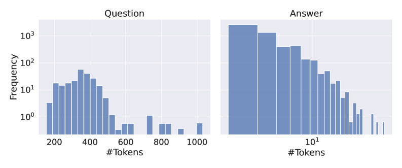<details> <summary>x8.png Details</summary>  ### Visual Description ## Histograms: Token Frequency Distributions for Questions and Answers ### Overview The image displays two side-by-side histograms titled "Question" and "Answer." They visualize the frequency distribution of token counts (likely from a text dataset) for two distinct categories: questions and answers. Both plots use a logarithmic scale for the frequency (y-axis). ### Components/Axes * **Titles:** The left histogram is titled "Question." The right histogram is titled "Answer." * **Y-Axis (Both Plots):** Labeled "Frequency." The scale is logarithmic, with major tick marks at 10⁰ (1), 10¹ (10), 10² (100), and 10³ (1000). * **X-Axis (Question Plot):** Labeled "#Tokens." The scale is linear, with major tick marks at 200, 400, 600, 800, and 1000. * **X-Axis (Answer Plot):** Labeled "#Tokens." The scale is logarithmic, with a major tick mark visible at 10¹ (10). The bins appear to represent powers of 10 or logarithmic intervals. * **Data Series:** Each plot contains a single data series represented by blue vertical bars (a histogram). There is no separate legend, as the plot titles define the series. ### Detailed Analysis **Question Histogram (Left):** * **Trend:** The distribution is right-skewed. Frequency peaks in the lower-middle range of token counts and then generally declines, with a long tail extending to higher values. * **Data Points (Approximate):** * The highest frequency bar is in the bin centered approximately around 350 tokens, reaching a frequency of ~50 (between 10¹ and 10²). * A cluster of high-frequency bars exists between ~200 and ~500 tokens, with frequencies ranging from ~10 to ~50. * Frequency drops sharply after ~500 tokens. Bars between ~500 and ~600 tokens have frequencies around 1-5. * There are sparse, low-frequency outliers (frequency ~1) at approximately 700, 800, 900, and 1000 tokens. **Answer Histogram (Right):** * **Trend:** The distribution is strongly right-skewed, with the vast majority of answers having a very low token count. Frequency decreases rapidly as the number of tokens increases. * **Data Points (Approximate):** * The highest frequency bar is the leftmost bin (likely representing 1-2 tokens), with a frequency exceeding 1000 (10³). * The second bin (likely 2-4 tokens) has a frequency of ~1000. * Frequencies drop to ~100-300 for the next few bins (covering approximately 4-8 tokens). * Frequencies continue to decline into the single digits for bins representing token counts near and above 10 (10¹). * The tail extends to the right with very low-frequency bars (frequency ~1) at the highest token count bins shown. ### Key Observations 1. **Scale Disparity:** The token count scales (x-axes) for Questions and Answers are fundamentally different. Questions are plotted on a linear scale from 200-1000 tokens, while Answers are plotted on a logarithmic scale from ~1-10 tokens. This indicates the two datasets occupy completely different ranges. 2. **Central Tendency:** The modal (most frequent) token count for Questions is in the hundreds (~350), while for Answers it is at the very low end (~1-2 tokens). 3. **Spread:** The Question distribution has a much wider spread (range of ~200-1000 tokens) compared to the Answer distribution, which is highly concentrated at the low end. 4. **Logarithmic Frequency:** The use of a log scale on the y-axis for both plots is necessary to visualize the extremely high frequencies of low-token answers alongside the much lower frequencies of high-token questions. ### Interpretation This visualization strongly suggests a structural characteristic of the underlying Q&A dataset: **questions are substantially longer and more variable in length than answers.** * **Data Relationship:** The plots are directly comparable as parts of a whole (a question-answer pair). The stark contrast implies that in this context, users or systems pose relatively detailed, multi-sentence questions, but receive very concise, often single-phrase or single-word answers. * **Potential Contexts:** This pattern could be indicative of: * A **factoid Q&A system** where questions seek specific data points (e.g., "What is the capital of France?") and answers are brief ("Paris"). * A **command-based interaction** where questions are actually instructions or queries, and answers are confirmations or short results. * A dataset where "answers" are defined as short labels, categories, or extracted spans rather than full-sentence responses. * **Anomaly/Notable Feature:** The most striking feature is the answer mode at 1-2 tokens. This extreme concentration suggests a highly constrained answer format, which is a critical design or data collection parameter to be aware of when using this dataset. The long tail of questions up to 1000 tokens also indicates the system must handle complex, lengthy inputs. 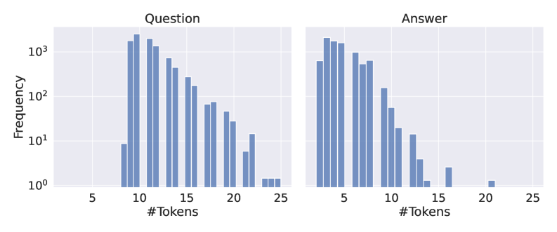</details> (a) CoQA <details> <summary>x9.png Details</summary>  ### Visual Description ## Histograms: Token Frequency Distribution for Questions and Answers ### Overview The image displays two side-by-side histograms comparing the frequency distribution of token counts for "Question" and "Answer" text segments. Both charts share identical axes and scaling, facilitating direct comparison. The data is presented on a logarithmic frequency scale. ### Components/Axes * **Titles:** Centered above each histogram: "Question" (left chart) and "Answer" (right chart). * **Y-Axis (Both Charts):** Labeled "Frequency". The scale is logarithmic, with major tick marks at `10^0` (1), `10^1` (10), `10^2` (100), and `10^3` (1000). * **X-Axis (Both Charts):** Labeled "#Tokens". The scale is linear, with major tick marks at 0, 5, 10, 15, 20, and 25. * **Data Series:** Both histograms use vertical blue bars of uniform color to represent frequency counts for discrete token number bins. ### Detailed Analysis **Left Chart: Question Token Distribution** * **Trend:** The distribution is right-skewed, peaking at a moderate token count and tapering off towards higher values. * **Data Points (Approximate Frequency per Token Count):** * 9 tokens: ~10 * 10 tokens: ~2000 (Peak) * 11 tokens: ~1800 * 12 tokens: ~600 * 13 tokens: ~400 * 14 tokens: ~250 * 15 tokens: ~150 * 16 tokens: ~70 * 17 tokens: ~80 * 18 tokens: ~40 * 19 tokens: ~25 * 20 tokens: ~12 * 21 tokens: ~5 * 22 tokens: ~12 * 23 tokens: ~1 * 24 tokens: ~1 * 25 tokens: ~1 **Right Chart: Answer Token Distribution** * **Trend:** The distribution is strongly right-skewed, with a very high peak at low token counts and a rapid decline. * **Data Points (Approximate Frequency per Token Count):** * 3 tokens: ~600 * 4 tokens: ~2000 (Peak) * 5 tokens: ~1800 * 6 tokens: ~1500 * 7 tokens: ~900 * 8 tokens: ~500 * 9 tokens: ~600 * 10 tokens: ~150 * 11 tokens: ~50 * 12 tokens: ~15 * 13 tokens: ~3 * 14 tokens: ~1 * 16 tokens: ~2 * 21 tokens: ~1 ### Key Observations 1. **Peak Location:** The most frequent token count for Questions is **10**, while for Answers it is **4**. This indicates answers in this dataset are, on average, significantly shorter than questions. 2. **Distribution Shape:** The Answer distribution is more concentrated at the low end (3-9 tokens) and drops off more sharply than the Question distribution, which has a longer tail extending to 25 tokens. 3. **Frequency Range:** Both distributions span three orders of magnitude in frequency (from 1 to ~2000), necessitating the logarithmic y-axis. 4. **Sparse High-End Data:** Both charts show very low frequencies (1-12) for token counts above 20, indicating such lengths are rare outliers. ### Interpretation This data suggests a structural characteristic of the underlying text corpus: **responses (Answers) are typically concise, while inquiries (Questions) are more variable and often longer.** * **Efficiency or Constraint:** The sharp peak for Answers at 4 tokens could indicate a dataset where answers are highly standardized, templated, or constrained to be brief (e.g., factoid Q&A, multiple-choice labels, or command responses). * **Question Complexity:** The broader distribution for Questions, peaking at 10 tokens, implies that formulating a question requires more linguistic components (subject, verb, object, modifiers) than stating the answer. * **Data Quality/Source:** The clean, discrete distributions with no bars between 0-2 and 26+ suggest the data has been pre-processed or filtered. The logarithmic scale reveals that while most samples cluster around the peaks, there is a long tail of less frequent, longer text segments, which could represent more complex or atypical examples in the dataset. * **Practical Implication:** For a machine learning model trained on this data, it would need to handle the inherent asymmetry in sequence length between input (question) and output (answer). The model's decoder might be optimized for generating shorter sequences. 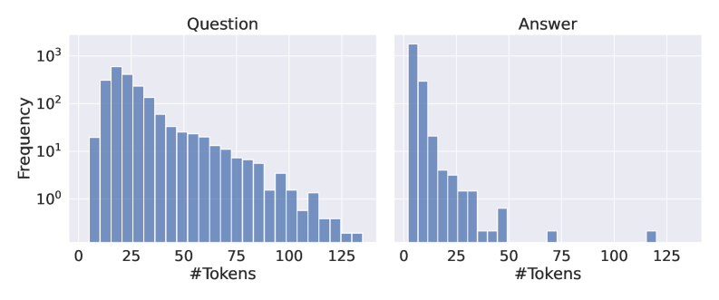</details> (b) NQ-Open <details> <summary>x10.png Details</summary>  ### Visual Description ## Histograms: Question vs. Answer Token Length Distribution ### Overview The image displays two side-by-side histograms comparing the frequency distribution of token counts for "Question" and "Answer" text segments. Both charts share identical axes and scales, facilitating direct comparison. The data is presented on a logarithmic frequency scale. ### Components/Axes * **Chart Type:** Two histograms (subplots). * **Titles:** * Left subplot title: "Question" (positioned top-center of the left chart). * Right subplot title: "Answer" (positioned top-center of the right chart). * **X-Axis (Both Charts):** * Label: "#Tokens" * Scale: Linear, ranging from 0 to approximately 140. * Major Tick Marks: 0, 25, 50, 75, 100, 125. * **Y-Axis (Both Charts):** * Label: "Frequency" * Scale: Logarithmic (base 10). * Major Tick Marks: 10⁰ (1), 10¹ (10), 10² (100), 10³ (1000). * **Data Series:** Both histograms use solid blue bars. There is no separate legend, as the subplot titles define the data series. ### Detailed Analysis **1. "Question" Histogram (Left Subplot):** * **Visual Trend:** The distribution is right-skewed, with a peak at lower token counts and a long tail extending to higher values. * **Data Points (Approximate):** * The highest frequency occurs in the bin just below 25 tokens, with a frequency between 10² and 10³ (estimated ~500-800). * Frequencies are high (above 10²) for token counts from approximately 10 to 40. * The frequency declines steadily as token count increases beyond 40. * There are very few instances (frequency ~10⁰ or 1) of questions with token counts above 125. * The distribution spans from near 0 tokens to just beyond 125 tokens. **2. "Answer" Histogram (Right Subplot):** * **Visual Trend:** The distribution is extremely right-skewed, heavily concentrated at very low token counts with a sharp drop-off. * **Data Points (Approximate):** * The dominant peak is in the first bin (0-~5 tokens), with a frequency exceeding 10³ (estimated ~1500-2000). * The second bin (~5-10 tokens) has a frequency between 10² and 10³ (estimated ~300-500). * Frequencies drop precipitously after 10 tokens. By 25 tokens, the frequency is near 10¹ (10). * There are isolated, very low-frequency bars (frequency ~10⁰) around 50, 75, and 120 tokens, indicating rare, long answers. * The vast majority of answers contain fewer than 25 tokens. ### Key Observations 1. **Fundamental Difference in Scale:** The "Answer" distribution is orders of magnitude more concentrated at the low end than the "Question" distribution. The peak frequency for answers is roughly 2-3 times higher than the peak for questions. 2. **Range Disparity:** While both datasets have a maximum range up to ~140 tokens, the "Question" data has a much more significant presence in the 25-100 token range. The "Answer" data is almost entirely contained below 25 tokens. 3. **Presence of Outliers:** Both distributions show outliers (very long text segments), but they are more pronounced and isolated in the "Answer" chart, appearing as single, low-frequency bars far from the main cluster. 4. **Logarithmic Scale Necessity:** The use of a log scale for frequency is essential to visualize both the dominant peaks (thousands of instances) and the long tails (single instances) on the same chart. ### Interpretation This data suggests a strong structural pattern in the dataset being analyzed: * **Questions are Moderately Complex:** Questions tend to be of moderate length, with a typical range of 10-50 tokens. This implies they contain sufficient context or detail to be meaningful. * **Answers are Highly Concise:** The overwhelming majority of answers are extremely brief, often under 10 tokens. This indicates a dataset where responses are likely direct, factual, or consist of single entities (like names, numbers, or short phrases). * **Efficiency or Constraint:** The stark contrast may reflect an efficient Q&A system where answers are optimized for brevity, or it could indicate a specific domain (e.g., factual lookup, multiple-choice) where long explanatory answers are not required. * **Data Quality/Anomaly Check:** The rare, long answers (outliers at ~50, 75, 120 tokens) warrant investigation. They could represent errors, complex edge cases, or a different sub-category of question-answer pairs within the dataset. * **Underlying Process:** The distributions imply two different generative processes: one for formulating questions (allowing for more variability and length) and one for generating answers (strongly constrained toward minimal length). 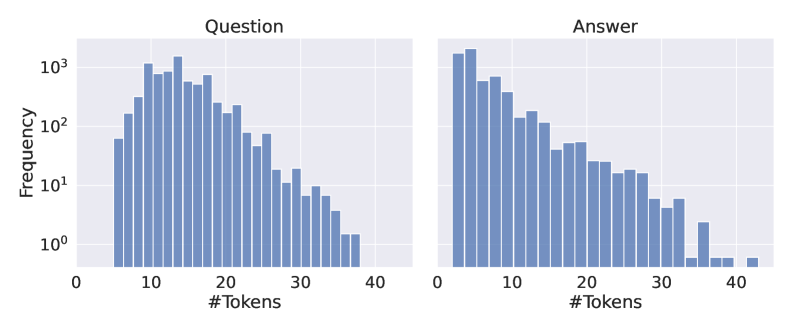</details> (c) HaluEvalQA <details> <summary>x11.png Details</summary>  ### Visual Description ## Histograms: Token Frequency Distribution for Questions and Answers ### Overview The image displays two side-by-side histograms comparing the frequency distribution of token counts for "Question" and "Answer" text segments. Both charts share identical axes and scales, facilitating direct comparison. The data is presented on a logarithmic frequency scale. ### Components/Axes * **Chart Type:** Two histograms (subplots). * **Titles:** * Left Chart: "Question" (centered at the top). * Right Chart: "Answer" (centered at the top). * **X-Axis (Both Charts):** * Label: "#Tokens" (centered below the axis). * Scale: Linear, ranging from 0 to 40. * Major Ticks: 0, 10, 20, 30, 40. * **Y-Axis (Left Chart Only):** * Label: "Frequency" (rotated vertically). * Scale: Logarithmic (base 10). * Major Ticks: 10⁰ (1), 10¹ (10), 10² (100), 10³ (1000). * **Data Series:** Each chart contains a single data series represented by vertical blue bars. The bars are contiguous, indicating binned data. * **Legend:** No separate legend is present; the chart titles serve as the primary identifiers for the data series. ### Detailed Analysis **Left Chart: "Question"** * **Trend:** The distribution is right-skewed. Frequency rises sharply from 0 tokens, peaks in the 10-20 token range, and then gradually declines with a long tail extending to 40 tokens. * **Key Data Points (Approximate):** * Peak Frequency: Occurs in the bin just after 10 tokens, with a frequency of approximately 1,500 (1.5 x 10³). * High-Frequency Range (100+): Spans from roughly 5 tokens to 25 tokens. * Low-Frequency Tail: Frequencies drop below 10 (10¹) after approximately 28 tokens and approach 1 (10⁰) near 38 tokens. * Minimum Observed: The last visible bar is near 38 tokens with a frequency of ~1. **Right Chart: "Answer"** * **Trend:** Also right-skewed, but with a more pronounced peak at very low token counts and a steeper initial decline compared to the "Question" chart. * **Key Data Points (Approximate):** * Peak Frequency: Occurs in the bin just after 0 tokens, with a frequency of approximately 2,000 (2 x 10³). This is the highest frequency in either chart. * High-Frequency Range (100+): Spans from roughly 0 tokens to 12 tokens. * Steep Decline: Frequency drops from ~2000 to ~100 within the first 10 tokens. * Low-Frequency Tail: Becomes sparse after 30 tokens, with a few isolated bars near 35 and 40 tokens having frequencies of ~1-3. ### Key Observations 1. **Peak Location Difference:** The most frequent token count for "Questions" is around 10-15 tokens, while for "Answers" it is significantly lower, around 1-5 tokens. 2. **Distribution Shape:** Both distributions are right-skewed, but the "Answer" distribution is more heavily concentrated at the low end (higher kurtosis). 3. **Range:** Both datasets span a similar range of token counts (0 to ~40), but the density within that range differs markedly. 4. **Logarithmic Scale:** The use of a log scale on the y-axis allows visualization of the wide dynamic range in frequencies, from single instances to thousands. ### Interpretation This data suggests a fundamental structural difference between the questions and answers in the analyzed dataset. Questions tend to be longer, with a typical length around 10-20 tokens. Answers, however, are most frequently very short (1-5 tokens), indicating a prevalence of concise, direct responses. The long tail in both charts shows that while most text segments are relatively short, there is a subset of both questions and answers that are significantly longer (up to 40 tokens). The steep drop-off in answer frequency after the initial peak implies that lengthy, detailed answers are comparatively rare in this corpus. This pattern is common in QA systems or datasets where answers are often factual, single-phrase, or confirmatory. 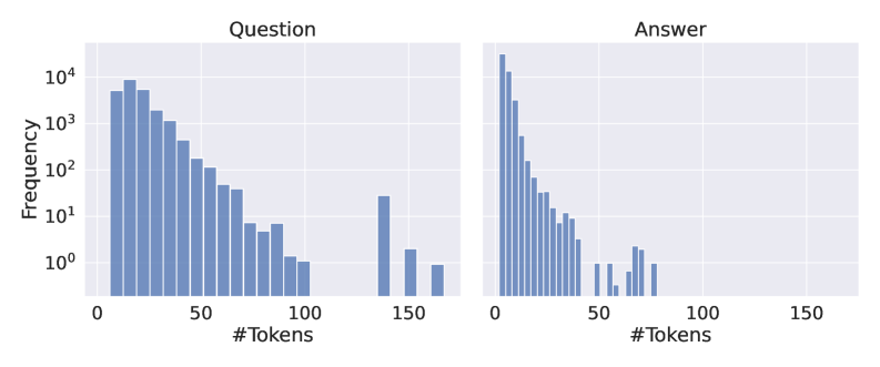</details> (d) SQuADv2 <details> <summary>x12.png Details</summary>  ### Visual Description ## Histograms: Token Frequency Distribution for Questions and Answers ### Overview The image displays two side-by-side histograms on a shared logarithmic y-axis. The left histogram is titled "Question" and the right is titled "Answer." Both charts visualize the frequency distribution of token counts (likely from a text dataset), showing how many questions or answers contain a specific number of tokens. The overall visual impression is of two right-skewed distributions, with the "Answer" distribution being significantly more concentrated at the lower end of the token count scale. ### Components/Axes * **Chart Titles:** "Question" (left chart), "Answer" (right chart). * **X-Axis (Both Charts):** Labeled "#Tokens". The axis has major tick marks at 0, 50, 100, and 150. The scale appears linear. * **Y-Axis (Shared, Left Side):** Labeled "Frequency". The axis uses a **logarithmic scale** (base 10). Major tick marks and labels are present at 10⁰ (1), 10¹ (10), 10² (100), 10³ (1000), and 10⁴ (10000). * **Data Series:** Both histograms use vertical blue bars to represent frequency counts for binned token ranges. No separate legend is present, as the chart titles define the two series. * **Spatial Layout:** The two histograms are placed horizontally adjacent, sharing the same y-axis scale for direct comparison. The "Question" chart occupies the left half of the image, and the "Answer" chart occupies the right half. ### Detailed Analysis **1. "Question" Histogram (Left Chart):** * **Trend:** The distribution is strongly right-skewed. Frequency is highest for questions with a low token count and decreases as the token count increases. * **Data Points (Approximate from visual inspection):** * The peak frequency occurs in the first few bins (approximately 0-20 tokens), with the tallest bar reaching near 10⁴ (10,000). * There is a steady, roughly exponential decay in frequency as token count increases from ~20 to ~100 tokens. * A notable gap exists in the data between approximately 100 and 140 tokens, where no bars are visible (frequency likely 0 or 1). * A small cluster of bars reappears between approximately 140 and 170 tokens, with frequencies between 10⁰ (1) and 10¹ (10). The highest bar in this cluster is near 150 tokens with a frequency of ~20-30. * **Range:** Token counts span from near 0 to approximately 170. **2. "Answer" Histogram (Right Chart):** * **Trend:** This distribution is also right-skewed but is dramatically more concentrated at the very low end of the token scale compared to the "Question" distribution. * **Data Points (Approximate from visual inspection):** * The peak frequency is extremely high for the very first bin (likely 0-5 tokens), with the bar exceeding the 10⁴ (10,000) mark. * Frequency drops off very sharply. By the 20-token mark, the frequency has fallen to around 10² (100). * The decay continues steeply. By 50 tokens, frequencies are in the single digits (10⁰ to 10¹). * There are a few sparse, very low-frequency bars (frequency ~1-3) scattered between 50 and 80 tokens. * No visible bars exist beyond approximately 80 tokens. * **Range:** Token counts are concentrated between 0 and ~80, with the vast majority below 50. ### Key Observations 1. **Fundamental Difference in Length:** The most striking observation is the profound difference in typical length between questions and answers in this dataset. Answers are overwhelmingly shorter. 2. **Logarithmic Scale Necessity:** The use of a logarithmic y-axis is critical. It allows the visualization of both the extremely high-frequency short tokens and the very low-frequency long tails on the same chart. On a linear scale, the bars for token counts above ~30 would be nearly invisible. 3. **Question Length Variability:** Questions exhibit much greater variability in length, with a significant number extending beyond 100 tokens and a small but distinct group around 150 tokens. 4. **Answer Conciseness:** The answer distribution suggests a dataset where responses are highly concise, often just a few words or a single phrase, with very few lengthy explanations. ### Interpretation This data strongly suggests the underlying text corpus comes from a **question-answering (QA) system or dataset where brevity in responses is either enforced or naturally occurs**. The pattern is characteristic of: * **Factoid QA:** Where answers are specific entities (names, dates, numbers). * **Multiple-Choice or Short-Answer Datasets:** Where responses are limited to a word or phrase. * **Technical Support Logs:** Where answers might be commands, codes, or brief confirmations. The long tail in the question distribution indicates that while most queries are simple, there is a subset of complex, detailed questions. The near absence of long answers implies the system or dataset is not designed for, or does not contain, explanatory, essay-style, or conversational responses. The gap in the question histogram around 100-140 tokens could be an artifact of the data collection or a characteristic of the specific domain (e.g., a maximum input length for a form that is rarely hit). The small cluster of longer questions (~150 tokens) might represent a specific category of complex queries that are handled differently. 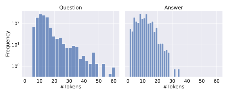Overall, the visualization efficiently communicates a core characteristic of the dataset: **questions are variable and can be complex, but answers are consistently and remarkably brief.** </details> (e) TriviaQA <details> <summary>x13.png Details</summary>  ### Visual Description ## Histograms: Question and Answer Token Length Distributions ### Overview The image displays two side-by-side histograms comparing the frequency distribution of token counts for "Question" and "Answer" text segments. Both charts share identical axes and scales, facilitating direct comparison. The data is presented on a semi-logarithmic plot (log scale on the y-axis). ### Components/Axes * **Titles:** "Question" (left chart), "Answer" (right chart). * **X-Axis (Both Charts):** Labeled "#Tokens". Linear scale ranging from 0 to 60, with major tick marks at intervals of 10 (0, 10, 20, 30, 40, 50, 60). * **Y-Axis (Left Chart Only):** Labeled "Frequency". Logarithmic scale (base 10) with major tick marks at 10⁰ (1), 10¹ (10), and 10² (100). * **Data Series:** Both histograms use identical blue bars. No legend is present, as each chart contains a single data series. * **Spatial Layout:** The two histograms are positioned horizontally adjacent, sharing a common y-axis scale implied by the left chart's labels. ### Detailed Analysis **1. Question Histogram (Left Chart):** * **Trend:** The distribution is right-skewed with a long tail. Frequency peaks sharply at low token counts and decays gradually as token count increases. * **Data Points (Approximate):** * Peak Frequency: Occurs between 10-15 tokens, with a frequency value between 10² (100) and 2*10² (200). * High Frequency Range (10¹ to 10²): Spans from approximately 5 tokens to 25 tokens. * Mid Frequency Range (10⁰ to 10¹): Spans from approximately 25 tokens to 45 tokens. * Low Frequency Tail (<10⁰): Extends from ~45 tokens to 60 tokens, with frequencies dropping to near or below 1 (10⁰). There is a small, isolated bar at 60 tokens. **2. Answer Histogram (Right Chart):** * **Trend:** The distribution is also right-skewed but is more concentrated and drops off more abruptly than the Question distribution. It has a much shorter tail. * **Data Points (Approximate):** * Peak Frequency: Occurs between 10-15 tokens, similar to the Question chart, with a frequency value between 10² (100) and 2*10² (200). * High Frequency Range (10¹ to 10²): Spans from approximately 5 tokens to 20 tokens. * Mid Frequency Range (10⁰ to 10¹): Spans from approximately 20 tokens to 30 tokens. * Low Frequency Tail (<10⁰): Very sparse. There are isolated, very low-frequency bars (near 10⁰) at approximately 32 and 34 tokens. No data is visible beyond ~35 tokens. ### Key Observations 1. **Similar Peaks:** Both questions and answers have their highest frequency in the 10-15 token range. 2. **Divergent Tails:** The most significant difference is in the length of the tail. Questions exhibit a "heavy tail," with a non-trivial number of instances extending to 60 tokens. Answers have a "short tail," with almost no instances beyond 35 tokens. 3. **Concentration:** The answer distribution is more concentrated. The bulk of answers (the majority with frequency >10) fall within a narrower band (~5-20 tokens) compared to questions (~5-25 tokens). 4. **Log Scale Implication:** The use of a logarithmic y-axis emphasizes that while the peak frequencies are similar, the differences in the tails represent orders-of-magnitude differences in actual count. ### Interpretation This data suggests a fundamental asymmetry in the structure of the dataset being analyzed. Questions are more variable in length, capable of being very concise or quite verbose. Answers, however, are strongly constrained to a shorter, more consistent length. This pattern could indicate several underlying principles: * **System Design:** The system generating or curating these answers may have a built-in bias or constraint favoring concise responses. * **Task Nature:** The question-answering task itself may naturally elicit shorter, more focused responses than the inquiries that prompt them. * **Data Curation:** The dataset might have been filtered or processed to standardize answer length, while leaving question length unmodified. The absence of long answers (beyond ~35 tokens) is a notable anomaly. It implies a hard cutoff or a strong selection pressure against lengthy responses in this specific context. The investigation would benefit from examining examples of the longest questions and the (non-existent) longest answers to understand the practical limits of the system. </details> (f) TruthfulQA <details> <summary>x14.png Details</summary>  ### Visual Description ## Histograms: Token Frequency Distribution for Questions and Answers ### Overview The image displays two side-by-side histograms comparing the frequency distribution of token counts for "Question" and "Answer" text segments. Both charts share a common y-axis representing frequency on a logarithmic scale and an x-axis representing the number of tokens (#Tokens). The visual style is a standard statistical plot with blue bars on a light gray grid background. ### Components/Axes * **Chart Titles:** "Question" (left histogram), "Answer" (right histogram). * **X-Axis Label (Both Charts):** "#Tokens". This represents the length of the text segment in tokens. * **Y-Axis Label (Shared, Left Side):** "Frequency". This axis is on a **logarithmic scale (base 10)**, with major tick marks at 10⁻¹ (0.1), 10⁰ (1), and 10¹ (10). * **X-Axis Scale:** Linear scale. The "Question" chart's axis runs from approximately 0 to 300, with major ticks at 100, 200, and 300. The "Answer" chart's axis runs from approximately 0 to 300, with major ticks at 100, 200, and 300. * **Data Representation:** Vertical bars (bins) of uniform width. The height of each bar corresponds to the frequency (count) of text segments falling within that token range. ### Detailed Analysis **1. "Question" Histogram (Left Panel):** * **Trend:** The distribution is strongly right-skewed. Frequency peaks at a low token count and decays rapidly as token count increases. * **Data Points (Approximate):** * The highest frequency bar is in the range of approximately **50-75 tokens**, with a frequency value near **20** (just above the 10¹ line). * Frequency remains high (above 10) for token ranges from ~25 to ~100. * A sharp decline occurs after ~100 tokens. The frequency drops below 1 (10⁰) for token counts greater than ~150. * There are very few questions with token counts approaching 200. The last visible bar is near **180-200 tokens**, with a frequency of approximately **0.15** (slightly above the 10⁻¹ line). * The distribution effectively ends before 200 tokens. **2. "Answer" Histogram (Right Panel):** * **Trend:** The distribution is also right-skewed but is notably broader and shifted to the right compared to the "Question" distribution. It has a longer tail extending to higher token counts. * **Data Points (Approximate):** * The peak frequency is broader, spanning approximately **75-150 tokens**. The highest bar appears around **100-125 tokens**, with a frequency of approximately **15**. * Frequency remains relatively high (above 5) for a wide range, from ~50 to ~200 tokens. * The decline is more gradual than in the "Question" chart. Frequency drops below 1 (10⁰) for token counts greater than ~225. * The distribution has a long, low-frequency tail. There are visible bars with frequencies around **0.1-0.2** extending all the way to **300 tokens**. * The range of token counts is significantly wider, with meaningful data present from near 0 up to 300. ### Key Observations 1. **Central Tendency Shift:** The mode (peak) of the "Answer" distribution (~100-125 tokens) is at a higher token count than the mode of the "Question" distribution (~50-75 tokens). 2. **Spread and Variance:** The "Answer" distribution has a much larger spread (variance). Answers exhibit a wider range of lengths, from very short to very long (up to 300 tokens), while questions are more concentrated in the shorter length range (mostly under 150 tokens). 3. **Tail Behavior:** The "Answer" histogram has a significantly heavier and longer tail. The presence of data points at 250-300 tokens indicates that a non-trivial number of answers are very long, a characteristic almost absent in the questions. 4. **Logarithmic Scale Impact:** The use of a log scale for frequency allows for the clear visualization of the low-frequency, long-tail events (e.g., answers with 300 tokens) which would be invisible on a linear scale. ### Interpretation This data suggests a fundamental structural difference between the questions and answers in the underlying dataset. **Questions tend to be concise and relatively uniform in length,** clustering around a short-to-medium length. This aligns with the typical function of a question: to seek specific information efficiently. In contrast, **answers exhibit much greater variability and a propensity for length.** The broader peak and extended tail indicate that answers can range from brief confirmations to extensive, detailed explanations. The shift in the central tendency confirms that, on average, answers are longer than the questions they respond to. This is consistent with the informational asymmetry inherent in Q&A pairs, where a short query may require a comprehensive response to be fully addressed. The long tail in the answer distribution is particularly noteworthy. It implies the dataset contains a subset of complex or open-ended questions that elicit very detailed, multi-token responses. From a data processing or model training perspective, this highlights the need to handle a wide dynamic range of sequence lengths, especially for the answer component. The logarithmic frequency scale is crucial for identifying these rare but potentially important long-answer examples. </details> (g) GSM8K Figure 8: Token count histograms for the datasets used in our experiments. Token counts were computed separately for each example’s $question$ (left) and gold $answer$ (right) using the meta-llama/Llama-3.1-8B-Instruct tokenizer. In cases with multiple answers, they were flattened into one. ## Appendix E Hallucination dataset sizes Figure 9 shows the number of examples per label, determined using exact match for GSM8K and the llm-as-judge heuristic for the other datasets. It is worth noting that different generation configurations result in different splits, as LLMs might produce different answers. All examples classified as $Rejected$ were discarded from the hallucination probe training and evaluation. We observe that most datasets are imbalanced, typically underrepresenting non-hallucinated examples, with the exception of TriviaQA and GSM8K. We split each dataset into 80% training examples and 20% test examples. Splits were stratified according to hallucination labels. 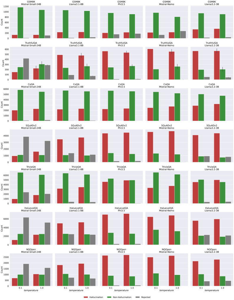<details> <summary>x15.png Details</summary>  ### Visual Description ## Bar Chart Grid: AI Model Hallucination Analysis Across Benchmarks ### Overview The image displays a 7x5 grid of grouped bar charts. Each chart compares the performance of five different Large Language Models (LLMs) on a specific benchmark dataset. The performance is measured across three categories: Hallucination, Non-Hallucination, and Rejected responses, at two different temperature settings (0.1 and 1.0). The overall purpose is to analyze and compare the propensity of different models to produce hallucinations versus correct or rejected answers across various tasks. ### Components/Axes * **Grid Structure:** * **Rows (7):** Each row corresponds to a specific benchmark dataset. From top to bottom: `GSM8K`, `TruthfulQA`, `CoQA`, `SQuADv2`, `TriviaQA`, `HaluevaQA`, `NQOpen`. * **Columns (5):** Each column corresponds to a specific LLM. From left to right: `Mistral-Small-24B`, `Llama3.1-8B`, `Phi3.5`, `Mistral-Nemo`, `Llama3.2-3B`. * **Individual Chart Axes:** * **X-axis:** Labeled `temperature`. Two categorical markers: `0.1` and `1.0`. * **Y-axis:** Labeled `Count`. The scale varies per benchmark row (e.g., 0-1200 for GSM8K, 0-6000 for CoQA). * **Legend:** Located at the bottom center of the entire grid. * **Red Bar:** `Hallucination` * **Green Bar:** `Non-Hallucination` * **Gray Bar:** `Rejected` ### Detailed Analysis **Row 1: GSM8K (Mathematical Reasoning)** * **Trend:** For all models, the green bar (Non-Hallucination) is dominant at both temperatures. The red bar (Hallucination) is very low. The gray bar (Rejected) is minimal. * **Data Points (Approximate):** * **Mistral-Small-24B:** Temp 0.1: Hallucination ~150, Non-Hallucination ~1150, Rejected ~50. Temp 1.0: Hallucination ~150, Non-Hallucination ~1100, Rejected ~100. * **Llama3.1-8B:** Temp 0.1: Hallucination ~200, Non-Hallucination ~1100, Rejected ~50. Temp 1.0: Hallucination ~250, Non-Hallucination ~1050, Rejected ~50. * **Phi3.5:** Temp 0.1: Hallucination ~200, Non-Hallucination ~950, Rejected ~150. Temp 1.0: Hallucination ~200, Non-Hallucination ~900, Rejected ~150. * **Mistral-Nemo:** Temp 0.1: Hallucination ~200, Non-Hallucination ~950, Rejected ~100. Temp 1.0: Hallucination ~200, Non-Hallucination ~800, Rejected ~250. * **Llama3.2-3B:** Temp 0.1: Hallucination ~300, Non-Hallucination ~950, Rejected ~50. Temp 1.0: Hallucination ~300, Non-Hallucination ~900, Rejected ~50. **Row 2: TruthfulQA (Truthfulness)** * **Trend:** The red bar (Hallucination) is the tallest for most models, especially at Temp 1.0. The green bar (Non-Hallucination) is secondary. The gray bar (Rejected) is significant for Mistral-Small-24B. * **Data Points (Approximate):** * **Mistral-Small-24B:** Temp 0.1: Hallucination ~150, Non-Hallucination ~250, Rejected ~400. Temp 1.0: Hallucination ~200, Non-Hallucination ~300, Rejected ~300. * **Llama3.1-8B:** Temp 0.1: Hallucination ~500, Non-Hallucination ~250, Rejected ~100. Temp 1.0: Hallucination ~500, Non-Hallucination ~250, Rejected ~50. * **Phi3.5:** Temp 0.1: Hallucination ~550, Non-Hallucination ~250, Rejected ~50. Temp 1.0: Hallucination ~550, Non-Hallucination ~250, Rejected ~50. * **Mistral-Nemo:** Temp 0.1: Hallucination ~600, Non-Hallucination ~200, Rejected ~50. Temp 1.0: Hallucination ~550, Non-Hallucination ~250, Rejected ~50. * **Llama3.2-3B:** Temp 0.1: Hallucination ~550, Non-Hallucination ~200, Rejected ~50. Temp 1.0: Hallucination ~550, Non-Hallucination ~200, Rejected ~50. **Row 3: CoQA (Conversational QA)** * **Trend:** The green bar (Non-Hallucination) is overwhelmingly dominant for all models at both temperatures. Red and gray bars are very low. * **Data Points (Approximate):** All models show Non-Hallucination counts between ~5000-6000, with Hallucination and Rejected counts generally below 2000. **Row 4: SQuADv2 (Reading Comprehension)** * **Trend:** For Mistral-Small-24B, the gray bar (Rejected) is dominant. For all other models, the red bar (Hallucination) is dominant, especially at Temp 1.0. The green bar (Non-Hallucination) is consistently low. * **Data Points (Approximate):** * **Mistral-Small-24B:** Temp 0.1: Hallucination ~1000, Non-Hallucination ~1000, Rejected ~3800. Temp 1.0: Hallucination ~1500, Non-Hallucination ~1000, Rejected ~3000. * **Other Models:** Hallucination counts range from ~3500-4500, Non-Hallucination ~1000-1500, Rejected ~500-1500. **Row 5: TriviaQA (Factoid QA)** * **Trend:** Similar to CoQA, the green bar (Non-Hallucination) is dominant for most models. Hallucination counts are moderate. Rejected counts are low. * **Data Points (Approximate):** Non-Hallucination counts are generally between ~5000-6500. Hallucination counts range from ~1000-5000, with Phi3.5 and Llama3.2-3B showing higher hallucination rates. **Row 6: HaluevaQA (Hallucination Evaluation)** * **Trend:** This benchmark shows high red bars (Hallucination) for all models, particularly Phi3.5 and Mistral-Nemo. The green bar (Non-Hallucination) is secondary. The gray bar (Rejected) is notable for Mistral-Small-24B. * **Data Points (Approximate):** Hallucination counts for Phi3.5 and Mistral-Nemo exceed 6000 at Temp 1.0. Other models range from ~2000-5500. **Row 7: NQOpen (Open-Domain QA)** * **Trend:** The red bar (Hallucination) is dominant for all models, especially at Temp 1.0. The green bar (Non-Hallucination) is secondary. The gray bar (Rejected) is low. * **Data Points (Approximate):** Hallucination counts range from ~1500-2500. Non-Hallucination counts range from ~500-1000. ### Key Observations 1. **Benchmark Sensitivity:** Model behavior varies dramatically by benchmark. Models perform well (high Non-Hallucination) on CoQA and TriviaQA but struggle (high Hallucination) on TruthfulQA, HaluevaQA, and NQOpen. 2. **Temperature Effect:** Increasing temperature from 0.1 to 1.0 generally leads to an increase in the Hallucination count (red bar) and often a decrease in the Non-Hallucination count (green bar), suggesting higher randomness increases factual errors. 3. **Model Comparison:** No single model is best across all benchmarks. `Mistral-Small-24B` shows a unique pattern with high Rejected counts on TruthfulQA and SQuADv2. `Phi3.5` and `Mistral-Nemo` often show the highest Hallucination counts on challenging benchmarks like HaluevaQA. 4. **SQuADv2 Anomaly:** This is the only benchmark where the `Rejected` category (gray) is dominant for one model (`Mistral-Small-24B`), indicating a specific failure mode for that model on this task. ### Interpretation This grid provides a multifaceted view of LLM reliability. The data suggests that: * **Hallucination is task-dependent:** A model's tendency to hallucinate is not an intrinsic constant but is heavily influenced by the nature of the task (benchmark). Mathematical reasoning (GSM8K) and conversational QA (CoQA) elicit fewer hallucinations than truthfulness evaluation (TruthfulQA) or open-domain QA (NQOpen). * **Temperature is a risk factor:** Higher temperature settings, while potentially increasing creativity or diversity, come at the cost of increased factual unreliability (hallucinations) across nearly all models and tasks. * **Model Architecture/Training Matters:** The distinct profiles of models like `Mistral-Small-24B` (high rejections) versus `Phi3.5` (high hallucinations) imply different underlying training objectives or safety alignment strategies. The former may be more conservative, refusing to answer, while the latter is more confident but prone to error. * **Benchmark Design is Crucial:** The starkly different results across rows highlight that evaluating an LLM on a single benchmark is insufficient. A comprehensive assessment requires a suite of tests targeting different capabilities and failure modes, as done here with benchmarks specifically designed to probe for hallucinations (HaluevaQA, TruthfulQA). **Language Note:** All text in the image is in English. </details> Figure 9: Number of examples per each label in generated datasets ( $Hallucination$ - number of hallucinated examples, $Non{-}Hallucination$ - number of truthful examples, $Rejected$ - number of examples unable to evaluate). ## Appendix F LLM-as-Judge agreement To ensure the high quality of labels generated using the llm-as-judge approach, we complemented manual evaluation of random examples with a second judge LLM and measured agreement between the models. We assume that higher agreement among LLMs indicates better label quality. The reduced performance of $\operatorname{LapEigvals}$ on TriviaQA may be attributed to the lower agreement, as well as the dataset’s size and class imbalance discussed earlier. Table 4: Agreement between LLM judges labeling hallucinations (gpt-4o-mini, gpt-4.1), measured with Cohen’s Kappa. | CoQA HaluevalQA NQOpen | 0.876 0.946 0.883 | | --- | --- | | SquadV2 | 0.854 | | TriviaQA | 0.939 | | TruthfulQA | 0.714 | ## Appendix G Extended results ### G.1 Precision and Recall analysis To provide insights relevant for potential practical usage, we analyze the Precision and Recall of our method. While it has not yet been fully evaluated in production settings, this analysis illustrates the trade-offs between these metrics and informs how the method might behave in real-world applications. Metrics were computed using the default threshold of 0.5, as reported in Table 5. Although trade-off patterns vary across datasets, they are consistent across all evaluated LLMs. Specifically, we observe higher recall on CoQA, GSM8K, and TriviaQA, whereas HaluEvalQA, NQ-Open, SQuADv2, and TruthfulQA exhibit higher precision. These insights can guide threshold adjustments to balance precision and recall for different production scenarios. Table 5: Precision and Recall values for the $\operatorname{LapEigvals}$ method, complementary to AUROC presented in Table 1. Values are presented as Precision / Recall for each dataset and model combination. | Llama3.1-8B Llama3.2-3B Phi3.5 | 0.583 / 0.710 0.679 / 0.728 0.560 / 0.703 | 0.644 / 0.729 0.718 / 0.699 0.600 / 0.739 | 0.895 / 0.785 0.912 / 0.788 0.899 / 0.768 | 0.859 / 0.740 0.894 / 0.662 0.910 / 0.785 | 0.896 / 0.720 0.924 / 0.720 0.906 / 0.731 | 0.719 / 0.812 0.787 / 0.729 0.787 / 0.785 | 0.872 / 0.781 0.910 / 0.746 0.829 / 0.798 | | --- | --- | --- | --- | --- | --- | --- | --- | | Mistral-Nemo | 0.646 / 0.714 | 0.594 / 0.809 | 0.873 / 0.760 | 0.875 / 0.751 | 0.920 / 0.756 | 0.707 / 0.769 | 0.892 / 0.825 | | Mistral-Small-24B | 0.610 / 0.779 | 0.561 / 0.852 | 0.811 / 0.801 | 0.700 / 0.750 | 0.784 / 0.789 | 0.575 / 0.787 | 0.679 / 0.655 | ### G.2 Extended method comparison In Tables 6 and 7, we present the extended results corresponding to those summarized in Table 1 in the main part of this paper. The extended results cover probes trained with both all-layers and per-layer variants across all models, as well as lower temperature ( $temp\in\{0.1,1.0\}$ ). In almost all cases, the all-layers variant outperforms the per-layer variant, suggesting that hallucination-related information is distributed across multiple layers. Additionally, we observe a smaller generalization gap (measured as the difference between test and training performance) for the $\operatorname{LapEigvals}$ method, indicating more robust features present in the Laplacian eigenvalues. Finally, as demonstrated in Section 6, increasing the temperature during answer generation improves probe performance, which is also evident in Table 6, where probes trained on answers generated with $temp{=}1.0$ consistently outperform those trained on data generated with $temp{=}0.1$ . Table 6: (Part I) Performance comparison of methods on an extended set of configurations. We mark results for $\operatorname{AttentionScore}$ in gray as it is an unsupervised approach, not directly comparable to the others. In bold, we highlight the best performance on the test split of data, individually for each dataset, LLM, and temperature. | Llama3.1-8B | 0.1 | $\operatorname{AttentionScore}$ | | ✓ | 0.509 | 0.683 | 0.667 | 0.607 | 0.556 | 0.567 | 0.563 | 0.541 | 0.764 | 0.653 | 0.631 | 0.575 | 0.571 | 0.650 | | --- | --- | --- | --- | --- | --- | --- | --- | --- | --- | --- | --- | --- | --- | --- | --- | --- | --- | --- | | Llama3.1-8B | 0.1 | $\operatorname{AttentionScore}$ | ✓ | | 0.494 | 0.677 | 0.614 | 0.568 | 0.522 | 0.522 | 0.489 | 0.504 | 0.708 | 0.587 | 0.558 | 0.521 | 0.511 | 0.537 | | Llama3.1-8B | 0.1 | $\operatorname{AttnLogDet}$ | | ✓ | 0.574 | 0.810 | 0.776 | 0.702 | 0.688 | 0.739 | 0.709 | 0.606 | 0.840 | 0.770 | 0.713 | 0.708 | 0.741 | 0.777 | | Llama3.1-8B | 0.1 | $\operatorname{AttnLogDet}$ | ✓ | | 0.843 | 0.977 | 0.884 | 0.851 | 0.839 | 0.861 | 0.913 | 0.770 | 0.833 | 0.837 | 0.768 | 0.758 | 0.827 | 0.820 | | Llama3.1-8B | 0.1 | $\operatorname{AttnEigvals}$ | | ✓ | 0.764 | 0.879 | 0.828 | 0.713 | 0.742 | 0.793 | 0.680 | 0.729 | 0.798 | 0.799 | 0.728 | 0.749 | 0.773 | 0.790 | | Llama3.1-8B | 0.1 | $\operatorname{AttnEigvals}$ | ✓ | | 0.861 | 0.992 | 0.895 | 0.878 | 0.858 | 0.867 | 0.979 | 0.776 | 0.841 | 0.838 | 0.755 | 0.781 | 0.822 | 0.819 | | Llama3.1-8B | 0.1 | $\operatorname{LapEigvals}$ | | ✓ | 0.758 | 0.777 | 0.817 | 0.698 | 0.707 | 0.781 | 0.708 | 0.757 | 0.844 | 0.793 | 0.711 | 0.733 | 0.780 | 0.764 | | Llama3.1-8B | 0.1 | $\operatorname{LapEigvals}$ | ✓ | | 0.869 | 0.928 | 0.901 | 0.864 | 0.855 | 0.896 | 0.903 | 0.836 | 0.887 | 0.867 | 0.793 | 0.782 | 0.872 | 0.822 | | Llama3.1-8B | 1.0 | $\operatorname{AttentionScore}$ | | ✓ | 0.514 | 0.705 | 0.640 | 0.607 | 0.558 | 0.578 | 0.533 | 0.525 | 0.731 | 0.642 | 0.607 | 0.572 | 0.602 | 0.629 | | Llama3.1-8B | 1.0 | $\operatorname{AttentionScore}$ | ✓ | | 0.507 | 0.710 | 0.602 | 0.580 | 0.534 | 0.535 | 0.546 | 0.493 | 0.720 | 0.589 | 0.556 | 0.538 | 0.532 | 0.541 | | Llama3.1-8B | 1.0 | $\operatorname{AttnLogDet}$ | | ✓ | 0.596 | 0.791 | 0.755 | 0.704 | 0.697 | 0.750 | 0.757 | 0.597 | 0.828 | 0.763 | 0.757 | 0.686 | 0.754 | 0.771 | | Llama3.1-8B | 1.0 | $\operatorname{AttnLogDet}$ | ✓ | | 0.848 | 0.973 | 0.882 | 0.856 | 0.846 | 0.867 | 0.930 | 0.769 | 0.826 | 0.827 | 0.793 | 0.748 | 0.842 | 0.814 | | Llama3.1-8B | 1.0 | $\operatorname{AttnEigvals}$ | | ✓ | 0.762 | 0.864 | 0.820 | 0.758 | 0.754 | 0.800 | 0.796 | 0.723 | 0.812 | 0.784 | 0.732 | 0.728 | 0.796 | 0.770 | | Llama3.1-8B | 1.0 | $\operatorname{AttnEigvals}$ | ✓ | | 0.867 | 0.995 | 0.889 | 0.873 | 0.867 | 0.876 | 0.972 | 0.782 | 0.838 | 0.819 | 0.790 | 0.768 | 0.843 | 0.833 | | Llama3.1-8B | 1.0 | $\operatorname{LapEigvals}$ | | ✓ | 0.760 | 0.873 | 0.803 | 0.732 | 0.722 | 0.795 | 0.751 | 0.743 | 0.833 | 0.789 | 0.725 | 0.724 | 0.794 | 0.764 | | Llama3.1-8B | 1.0 | $\operatorname{LapEigvals}$ | ✓ | | 0.879 | 0.936 | 0.896 | 0.866 | 0.857 | 0.901 | 0.918 | 0.830 | 0.872 | 0.874 | 0.827 | 0.791 | 0.889 | 0.829 | | Llama3.2-3B | 0.1 | $\operatorname{AttentionScore}$ | | ✓ | 0.526 | 0.662 | 0.697 | 0.592 | 0.570 | 0.570 | 0.569 | 0.547 | 0.640 | 0.714 | 0.643 | 0.582 | 0.551 | 0.564 | | Llama3.2-3B | 0.1 | $\operatorname{AttentionScore}$ | ✓ | | 0.506 | 0.638 | 0.635 | 0.523 | 0.515 | 0.534 | 0.473 | 0.519 | 0.609 | 0.644 | 0.573 | 0.561 | 0.510 | 0.489 | | Llama3.2-3B | 0.1 | $\operatorname{AttnLogDet}$ | | ✓ | 0.573 | 0.774 | 0.762 | 0.692 | 0.682 | 0.719 | 0.725 | 0.579 | 0.794 | 0.774 | 0.735 | 0.698 | 0.711 | 0.674 | | Llama3.2-3B | 0.1 | $\operatorname{AttnLogDet}$ | ✓ | | 0.782 | 0.946 | 0.868 | 0.845 | 0.827 | 0.824 | 0.918 | 0.695 | 0.841 | 0.843 | 0.763 | 0.749 | 0.796 | 0.678 | | Llama3.2-3B | 0.1 | $\operatorname{AttnEigvals}$ | | ✓ | 0.675 | 0.784 | 0.782 | 0.750 | 0.725 | 0.755 | 0.727 | 0.626 | 0.761 | 0.792 | 0.734 | 0.695 | 0.724 | 0.720 | | Llama3.2-3B | 0.1 | $\operatorname{AttnEigvals}$ | ✓ | | 0.814 | 0.977 | 0.873 | 0.872 | 0.852 | 0.842 | 0.963 | 0.723 | 0.808 | 0.844 | 0.772 | 0.744 | 0.788 | 0.688 | | Llama3.2-3B | 0.1 | $\operatorname{LapEigvals}$ | | ✓ | 0.681 | 0.763 | 0.774 | 0.733 | 0.708 | 0.733 | 0.722 | 0.676 | 0.835 | 0.781 | 0.736 | 0.697 | 0.732 | 0.690 | | Llama3.2-3B | 0.1 | $\operatorname{LapEigvals}$ | ✓ | | 0.831 | 0.889 | 0.875 | 0.837 | 0.832 | 0.852 | 0.895 | 0.801 | 0.852 | 0.857 | 0.779 | 0.736 | 0.826 | 0.743 | | Llama3.2-3B | 1.0 | $\operatorname{AttentionScore}$ | | ✓ | 0.532 | 0.674 | 0.668 | 0.588 | 0.578 | 0.553 | 0.555 | 0.557 | 0.753 | 0.637 | 0.592 | 0.593 | 0.558 | 0.675 | | Llama3.2-3B | 1.0 | $\operatorname{AttentionScore}$ | ✓ | | 0.512 | 0.648 | 0.606 | 0.554 | 0.529 | 0.517 | 0.484 | 0.509 | 0.717 | 0.588 | 0.546 | 0.530 | 0.515 | 0.581 | | Llama3.2-3B | 1.0 | $\operatorname{AttnLogDet}$ | | ✓ | 0.578 | 0.807 | 0.738 | 0.677 | 0.720 | 0.716 | 0.739 | 0.597 | 0.816 | 0.724 | 0.678 | 0.707 | 0.711 | 0.742 | | Llama3.2-3B | 1.0 | $\operatorname{AttnLogDet}$ | ✓ | | 0.784 | 0.951 | 0.869 | 0.816 | 0.839 | 0.831 | 0.924 | 0.700 | 0.851 | 0.801 | 0.690 | 0.734 | 0.789 | 0.795 | | Llama3.2-3B | 1.0 | $\operatorname{AttnEigvals}$ | | ✓ | 0.642 | 0.807 | 0.777 | 0.716 | 0.747 | 0.763 | 0.735 | 0.641 | 0.817 | 0.756 | 0.696 | 0.703 | 0.746 | 0.748 | | Llama3.2-3B | 1.0 | $\operatorname{AttnEigvals}$ | ✓ | | 0.819 | 0.973 | 0.878 | 0.847 | 0.876 | 0.847 | 0.978 | 0.724 | 0.768 | 0.819 | 0.694 | 0.749 | 0.804 | 0.723 | | Llama3.2-3B | 1.0 | $\operatorname{LapEigvals}$ | | ✓ | 0.695 | 0.781 | 0.764 | 0.683 | 0.719 | 0.727 | 0.682 | 0.715 | 0.815 | 0.754 | 0.671 | 0.711 | 0.738 | 0.767 | | Llama3.2-3B | 1.0 | $\operatorname{LapEigvals}$ | ✓ | | 0.842 | 0.894 | 0.885 | 0.803 | 0.850 | 0.863 | 0.911 | 0.812 | 0.870 | 0.828 | 0.693 | 0.757 | 0.832 | 0.787 | | Phi3.5 | 0.1 | $\operatorname{AttentionScore}$ | | ✓ | 0.517 | 0.723 | 0.559 | 0.565 | 0.606 | 0.625 | 0.601 | 0.528 | 0.682 | 0.551 | 0.637 | 0.621 | 0.628 | 0.637 | | Phi3.5 | 0.1 | $\operatorname{AttentionScore}$ | ✓ | | 0.499 | 0.632 | 0.538 | 0.532 | 0.473 | 0.539 | 0.522 | 0.505 | 0.605 | 0.511 | 0.578 | 0.458 | 0.534 | 0.554 | | Phi3.5 | 0.1 | $\operatorname{AttnLogDet}$ | | ✓ | 0.583 | 0.805 | 0.732 | 0.741 | 0.711 | 0.757 | 0.720 | 0.585 | 0.749 | 0.726 | 0.785 | 0.726 | 0.772 | 0.765 | | Phi3.5 | 0.1 | $\operatorname{AttnLogDet}$ | ✓ | | 0.845 | 0.995 | 0.863 | 0.905 | 0.852 | 0.875 | 0.981 | 0.723 | 0.752 | 0.802 | 0.802 | 0.759 | 0.842 | 0.716 | | Phi3.5 | 0.1 | $\operatorname{AttnEigvals}$ | | ✓ | 0.760 | 0.882 | 0.781 | 0.793 | 0.745 | 0.802 | 0.854 | 0.678 | 0.764 | 0.764 | 0.790 | 0.747 | 0.791 | 0.774 | | Phi3.5 | 0.1 | $\operatorname{AttnEigvals}$ | ✓ | | 0.862 | 1.000 | 0.867 | 0.904 | 0.861 | 0.881 | 0.999 | 0.728 | 0.732 | 0.802 | 0.787 | 0.740 | 0.838 | 0.761 | | Phi3.5 | 0.1 | $\operatorname{LapEigvals}$ | | ✓ | 0.734 | 0.713 | 0.758 | 0.737 | 0.704 | 0.775 | 0.759 | 0.716 | 0.753 | 0.757 | 0.761 | 0.732 | 0.768 | 0.741 | | Phi3.5 | 0.1 | $\operatorname{LapEigvals}$ | ✓ | | 0.856 | 0.946 | 0.860 | 0.897 | 0.841 | 0.884 | 0.965 | 0.810 | 0.785 | 0.819 | 0.815 | 0.791 | 0.858 | 0.717 | | Phi3.5 | 1.0 | $\operatorname{AttentionScore}$ | | ✓ | 0.499 | 0.699 | 0.567 | 0.615 | 0.626 | 0.637 | 0.618 | 0.533 | 0.722 | 0.581 | 0.630 | 0.645 | 0.642 | 0.626 | | Phi3.5 | 1.0 | $\operatorname{AttentionScore}$ | ✓ | | 0.489 | 0.640 | 0.540 | 0.566 | 0.469 | 0.553 | 0.541 | 0.520 | 0.666 | 0.541 | 0.594 | 0.504 | 0.540 | 0.554 | | Phi3.5 | 1.0 | $\operatorname{AttnLogDet}$ | | ✓ | 0.587 | 0.831 | 0.733 | 0.773 | 0.722 | 0.766 | 0.753 | 0.557 | 0.842 | 0.762 | 0.784 | 0.736 | 0.772 | 0.763 | | Phi3.5 | 1.0 | $\operatorname{AttnLogDet}$ | ✓ | | 0.842 | 0.993 | 0.868 | 0.921 | 0.859 | 0.879 | 0.971 | 0.745 | 0.842 | 0.818 | 0.815 | 0.769 | 0.848 | 0.755 | | Phi3.5 | 1.0 | $\operatorname{AttnEigvals}$ | | ✓ | 0.755 | 0.852 | 0.794 | 0.820 | 0.790 | 0.809 | 0.864 | 0.710 | 0.809 | 0.795 | 0.787 | 0.752 | 0.799 | 0.747 | | Phi3.5 | 1.0 | $\operatorname{AttnEigvals}$ | ✓ | | 0.858 | 1.000 | 0.871 | 0.924 | 0.876 | 0.887 | 0.998 | 0.771 | 0.794 | 0.829 | 0.798 | 0.782 | 0.850 | 0.802 | | Phi3.5 | 1.0 | $\operatorname{LapEigvals}$ | | ✓ | 0.733 | 0.771 | 0.755 | 0.755 | 0.718 | 0.779 | 0.713 | 0.723 | 0.816 | 0.769 | 0.755 | 0.732 | 0.792 | 0.732 | | Phi3.5 | 1.0 | $\operatorname{LapEigvals}$ | ✓ | | 0.856 | 0.937 | 0.863 | 0.911 | 0.849 | 0.889 | 0.961 | 0.821 | 0.885 | 0.836 | 0.826 | 0.795 | 0.872 | 0.777 | Table 7: (Part II) Performance comparison of methods on an extended set of configurations. We mark results for $\operatorname{AttentionScore}$ in gray as it is an unsupervised approach, not directly comparable to the others. In bold, we highlight the best performance on the test split of data, individually for each dataset, LLM, and temperature. | Mistral-Nemo | 0.1 | $\operatorname{AttentionScore}$ | | ✓ | 0.504 | 0.727 | 0.574 | 0.591 | 0.509 | 0.550 | 0.546 | 0.515 | 0.697 | 0.559 | 0.587 | 0.527 | 0.545 | 0.681 | | --- | --- | --- | --- | --- | --- | --- | --- | --- | --- | --- | --- | --- | --- | --- | --- | --- | --- | --- | | Mistral-Nemo | 0.1 | $\operatorname{AttentionScore}$ | ✓ | | 0.508 | 0.707 | 0.536 | 0.537 | 0.507 | 0.520 | 0.535 | 0.484 | 0.667 | 0.523 | 0.533 | 0.495 | 0.505 | 0.631 | | Mistral-Nemo | 0.1 | $\operatorname{AttnLogDet}$ | | ✓ | 0.584 | 0.801 | 0.716 | 0.702 | 0.675 | 0.689 | 0.744 | 0.583 | 0.807 | 0.723 | 0.688 | 0.668 | 0.722 | 0.731 | | Mistral-Nemo | 0.1 | $\operatorname{AttnLogDet}$ | ✓ | | 0.828 | 0.993 | 0.842 | 0.861 | 0.858 | 0.854 | 0.963 | 0.734 | 0.820 | 0.786 | 0.752 | 0.709 | 0.822 | 0.776 | | Mistral-Nemo | 0.1 | $\operatorname{AttnEigvals}$ | | ✓ | 0.708 | 0.865 | 0.751 | 0.749 | 0.749 | 0.747 | 0.797 | 0.672 | 0.795 | 0.740 | 0.701 | 0.704 | 0.738 | 0.717 | | Mistral-Nemo | 0.1 | $\operatorname{AttnEigvals}$ | ✓ | | 0.845 | 1.000 | 0.842 | 0.878 | 0.864 | 0.859 | 0.996 | 0.768 | 0.771 | 0.789 | 0.743 | 0.716 | 0.809 | 0.752 | | Mistral-Nemo | 0.1 | $\operatorname{LapEigvals}$ | | ✓ | 0.763 | 0.777 | 0.772 | 0.732 | 0.723 | 0.781 | 0.725 | 0.759 | 0.751 | 0.760 | 0.697 | 0.696 | 0.769 | 0.710 | | Mistral-Nemo | 0.1 | $\operatorname{LapEigvals}$ | ✓ | | 0.868 | 0.969 | 0.862 | 0.875 | 0.869 | 0.886 | 0.977 | 0.823 | 0.805 | 0.821 | 0.755 | 0.767 | 0.858 | 0.737 | | Mistral-Nemo | 1.0 | $\operatorname{AttentionScore}$ | | ✓ | 0.502 | 0.656 | 0.586 | 0.606 | 0.546 | 0.553 | 0.570 | 0.525 | 0.670 | 0.587 | 0.588 | 0.564 | 0.570 | 0.632 | | Mistral-Nemo | 1.0 | $\operatorname{AttentionScore}$ | ✓ | | 0.493 | 0.675 | 0.541 | 0.552 | 0.503 | 0.521 | 0.531 | 0.493 | 0.630 | 0.531 | 0.529 | 0.510 | 0.532 | 0.494 | | Mistral-Nemo | 1.0 | $\operatorname{AttnLogDet}$ | | ✓ | 0.591 | 0.790 | 0.723 | 0.716 | 0.717 | 0.717 | 0.741 | 0.581 | 0.782 | 0.730 | 0.703 | 0.711 | 0.707 | 0.801 | | Mistral-Nemo | 1.0 | $\operatorname{AttnLogDet}$ | ✓ | | 0.829 | 0.994 | 0.851 | 0.870 | 0.860 | 0.857 | 0.963 | 0.728 | 0.856 | 0.798 | 0.769 | 0.772 | 0.812 | 0.852 | | Mistral-Nemo | 1.0 | $\operatorname{AttnEigvals}$ | | ✓ | 0.704 | 0.845 | 0.762 | 0.742 | 0.757 | 0.752 | 0.806 | 0.670 | 0.781 | 0.749 | 0.742 | 0.719 | 0.737 | 0.804 | | Mistral-Nemo | 1.0 | $\operatorname{AttnEigvals}$ | ✓ | | 0.844 | 1.000 | 0.851 | 0.893 | 0.864 | 0.862 | 0.996 | 0.778 | 0.842 | 0.781 | 0.761 | 0.758 | 0.821 | 0.802 | | Mistral-Nemo | 1.0 | $\operatorname{LapEigvals}$ | | ✓ | 0.765 | 0.820 | 0.790 | 0.749 | 0.740 | 0.804 | 0.779 | 0.738 | 0.808 | 0.763 | 0.708 | 0.723 | 0.785 | 0.818 | | Mistral-Nemo | 1.0 | $\operatorname{LapEigvals}$ | ✓ | | 0.876 | 0.965 | 0.877 | 0.884 | 0.881 | 0.901 | 0.978 | 0.835 | 0.890 | 0.833 | 0.795 | 0.812 | 0.865 | 0.828 | | Mistral-Small-24B | 0.1 | $\operatorname{AttentionScore}$ | | ✓ | 0.520 | 0.759 | 0.538 | 0.517 | 0.577 | 0.535 | 0.571 | 0.525 | 0.685 | 0.552 | 0.592 | 0.625 | 0.533 | 0.724 | | Mistral-Small-24B | 0.1 | $\operatorname{AttentionScore}$ | ✓ | | 0.520 | 0.668 | 0.472 | 0.449 | 0.510 | 0.449 | 0.491 | 0.493 | 0.578 | 0.493 | 0.467 | 0.556 | 0.461 | 0.645 | | Mistral-Small-24B | 0.1 | $\operatorname{AttnLogDet}$ | | ✓ | 0.585 | 0.834 | 0.674 | 0.659 | 0.724 | 0.685 | 0.698 | 0.586 | 0.809 | 0.684 | 0.695 | 0.752 | 0.682 | 0.721 | | Mistral-Small-24B | 0.1 | $\operatorname{AttnLogDet}$ | ✓ | | 0.851 | 0.990 | 0.817 | 0.799 | 0.820 | 0.861 | 0.898 | 0.762 | 0.896 | 0.760 | 0.725 | 0.763 | 0.778 | 0.767 | | Mistral-Small-24B | 0.1 | $\operatorname{AttnEigvals}$ | | ✓ | 0.734 | 0.863 | 0.722 | 0.667 | 0.745 | 0.757 | 0.732 | 0.720 | 0.837 | 0.707 | 0.697 | 0.773 | 0.758 | 0.765 | | Mistral-Small-24B | 0.1 | $\operatorname{AttnEigvals}$ | ✓ | | 0.872 | 0.999 | 0.873 | 0.923 | 0.903 | 0.899 | 0.993 | 0.793 | 0.896 | 0.771 | 0.731 | 0.803 | 0.809 | 0.796 | | Mistral-Small-24B | 0.1 | $\operatorname{LapEigvals}$ | | ✓ | 0.802 | 0.781 | 0.720 | 0.646 | 0.714 | 0.742 | 0.694 | 0.800 | 0.850 | 0.719 | 0.674 | 0.784 | 0.757 | 0.827 | | Mistral-Small-24B | 0.1 | $\operatorname{LapEigvals}$ | ✓ | | 0.887 | 0.985 | 0.870 | 0.901 | 0.887 | 0.905 | 0.979 | 0.852 | 0.881 | 0.808 | 0.722 | 0.821 | 0.831 | 0.757 | | Mistral-Small-24B | 1.0 | $\operatorname{AttentionScore}$ | | ✓ | 0.511 | 0.706 | 0.555 | 0.582 | 0.561 | 0.562 | 0.542 | 0.535 | 0.713 | 0.566 | 0.576 | 0.567 | 0.574 | 0.606 | | Mistral-Small-24B | 1.0 | $\operatorname{AttentionScore}$ | ✓ | | 0.497 | 0.595 | 0.503 | 0.463 | 0.519 | 0.451 | 0.493 | 0.516 | 0.576 | 0.504 | 0.462 | 0.455 | 0.463 | 0.451 | | Mistral-Small-24B | 1.0 | $\operatorname{AttnLogDet}$ | | ✓ | 0.591 | 0.824 | 0.727 | 0.710 | 0.732 | 0.720 | 0.677 | 0.600 | 0.869 | 0.771 | 0.714 | 0.726 | 0.734 | 0.687 | | Mistral-Small-24B | 1.0 | $\operatorname{AttnLogDet}$ | ✓ | | 0.850 | 0.989 | 0.847 | 0.827 | 0.856 | 0.853 | 0.877 | 0.766 | 0.853 | 0.842 | 0.747 | 0.753 | 0.833 | 0.735 | | Mistral-Small-24B | 1.0 | $\operatorname{AttnEigvals}$ | | ✓ | 0.757 | 0.920 | 0.743 | 0.728 | 0.764 | 0.779 | 0.741 | 0.723 | 0.868 | 0.780 | 0.733 | 0.734 | 0.780 | 0.718 | | Mistral-Small-24B | 1.0 | $\operatorname{AttnEigvals}$ | ✓ | | 0.877 | 1.000 | 0.878 | 0.923 | 0.911 | 0.895 | 0.997 | 0.805 | 0.846 | 0.848 | 0.751 | 0.760 | 0.844 | 0.765 | | Mistral-Small-24B | 1.0 | $\operatorname{LapEigvals}$ | | ✓ | 0.814 | 0.860 | 0.762 | 0.733 | 0.790 | 0.766 | 0.703 | 0.805 | 0.897 | 0.790 | 0.712 | 0.781 | 0.779 | 0.725 | | Mistral-Small-24B | 1.0 | $\operatorname{LapEigvals}$ | ✓ | | 0.895 | 0.980 | 0.890 | 0.898 | 0.910 | 0.907 | 0.965 | 0.861 | 0.925 | 0.882 | 0.791 | 0.820 | 0.876 | 0.748 | ### G.3 Best found hyperparameters We present the hyperparameter values corresponding to the results in Table 1 and Table 6. Table 8 shows the optimal hyperparameter $k$ for selecting the top- $k$ eigenvalues from either the attention maps in $\operatorname{AttnEigvals}$ or the Laplacian matrix in $\operatorname{LapEigvals}$ . While fewer eigenvalues were sufficient for optimal performance in some cases, the best results were generally achieved with the highest tested value, $k{=}100$ . Table 9 reports the layer indices that yielded the highest performance for the per-layer models. Performance typically peaked in layers above the 10th, especially for Llama-3.1-8B, where attention maps from the final layers more often led to better hallucination detection. Interestingly, the first layer’s attention maps also produced strong performance in a few cases. Overall, no clear pattern emerges regarding the optimal layer, and as noted in prior work, selecting the best layer in the per-layer setup often requires a search. Table 8: Values of $k$ hyperparameter, denoting how many highest eigenvalues are taken from the Laplacian matrix, corresponding to the best results in Table 1 and Table 6. | | | | | | CoQA | GSM8K | HaluevalQA | NQOpen | SQuADv2 | TriviaQA | TruthfulQA | | --- | --- | --- | --- | --- | --- | --- | --- | --- | --- | --- | --- | | Llama3.1-8B | 0.1 | $\operatorname{AttnEigvals}$ | | ✓ | 50 | 100 | 100 | 25 | 100 | 100 | 10 | | Llama3.1-8B | 0.1 | $\operatorname{AttnEigvals}$ | ✓ | | 100 | 100 | 100 | 100 | 100 | 50 | 100 | | Llama3.1-8B | 0.1 | $\operatorname{LapEigvals}$ | | ✓ | 50 | 50 | 100 | 10 | 100 | 100 | 100 | | Llama3.1-8B | 0.1 | $\operatorname{LapEigvals}$ | ✓ | | 10 | 100 | 100 | 100 | 100 | 100 | 100 | | Llama3.1-8B | 1.0 | $\operatorname{AttnEigvals}$ | | ✓ | 100 | 100 | 100 | 100 | 100 | 100 | 100 | | Llama3.1-8B | 1.0 | $\operatorname{AttnEigvals}$ | ✓ | | 100 | 100 | 100 | 100 | 100 | 100 | 100 | | Llama3.1-8B | 1.0 | $\operatorname{LapEigvals}$ | | ✓ | 100 | 50 | 100 | 100 | 100 | 100 | 100 | | Llama3.1-8B | 1.0 | $\operatorname{LapEigvals}$ | ✓ | | 100 | 100 | 25 | 100 | 100 | 100 | 100 | | Llama3.2-3B | 0.1 | $\operatorname{AttnEigvals}$ | | ✓ | 100 | 100 | 100 | 100 | 100 | 100 | 10 | | Llama3.2-3B | 0.1 | $\operatorname{AttnEigvals}$ | ✓ | | 100 | 100 | 25 | 100 | 100 | 100 | 100 | | Llama3.2-3B | 0.1 | $\operatorname{LapEigvals}$ | | ✓ | 100 | 25 | 100 | 100 | 100 | 50 | 5 | | Llama3.2-3B | 0.1 | $\operatorname{LapEigvals}$ | ✓ | | 25 | 100 | 100 | 100 | 100 | 100 | 100 | | Llama3.2-3B | 1.0 | $\operatorname{AttnEigvals}$ | | ✓ | 100 | 100 | 100 | 100 | 100 | 100 | 50 | | Llama3.2-3B | 1.0 | $\operatorname{AttnEigvals}$ | ✓ | | 100 | 50 | 100 | 100 | 100 | 100 | 100 | | Llama3.2-3B | 1.0 | $\operatorname{LapEigvals}$ | | ✓ | 100 | 50 | 100 | 10 | 100 | 100 | 25 | | Llama3.2-3B | 1.0 | $\operatorname{LapEigvals}$ | ✓ | | 25 | 100 | 100 | 100 | 100 | 100 | 100 | | Phi3.5 | 0.1 | $\operatorname{AttnEigvals}$ | | ✓ | 100 | 100 | 100 | 100 | 100 | 100 | 100 | | Phi3.5 | 0.1 | $\operatorname{AttnEigvals}$ | ✓ | | 100 | 25 | 10 | 10 | 25 | 100 | 50 | | Phi3.5 | 0.1 | $\operatorname{LapEigvals}$ | | ✓ | 100 | 10 | 100 | 100 | 100 | 100 | 100 | | Phi3.5 | 0.1 | $\operatorname{LapEigvals}$ | ✓ | | 10 | 100 | 50 | 100 | 100 | 100 | 100 | | Phi3.5 | 1.0 | $\operatorname{AttnEigvals}$ | | ✓ | 100 | 100 | 100 | 100 | 100 | 100 | 100 | | Phi3.5 | 1.0 | $\operatorname{AttnEigvals}$ | ✓ | | 100 | 100 | 100 | 10 | 100 | 100 | 50 | | Phi3.5 | 1.0 | $\operatorname{LapEigvals}$ | | ✓ | 100 | 25 | 100 | 100 | 100 | 100 | 50 | | Phi3.5 | 1.0 | $\operatorname{LapEigvals}$ | ✓ | | 10 | 25 | 100 | 100 | 100 | 100 | 100 | | Mistral-Nemo | 0.1 | $\operatorname{AttnEigvals}$ | | ✓ | 100 | 50 | 100 | 100 | 100 | 100 | 100 | | Mistral-Nemo | 0.1 | $\operatorname{AttnEigvals}$ | ✓ | | 100 | 50 | 100 | 100 | 100 | 100 | 100 | | Mistral-Nemo | 0.1 | $\operatorname{LapEigvals}$ | | ✓ | 100 | 25 | 100 | 100 | 100 | 100 | 10 | | Mistral-Nemo | 0.1 | $\operatorname{LapEigvals}$ | ✓ | | 10 | 100 | 25 | 100 | 50 | 100 | 100 | | Mistral-Nemo | 1.0 | $\operatorname{AttnEigvals}$ | | ✓ | 100 | 100 | 100 | 100 | 100 | 100 | 100 | | Mistral-Nemo | 1.0 | $\operatorname{AttnEigvals}$ | ✓ | | 100 | 100 | 100 | 100 | 100 | 50 | 100 | | Mistral-Nemo | 1.0 | $\operatorname{LapEigvals}$ | | ✓ | 100 | 100 | 100 | 50 | 100 | 100 | 100 | | Mistral-Nemo | 1.0 | $\operatorname{LapEigvals}$ | ✓ | | 10 | 100 | 50 | 100 | 100 | 100 | 100 | | Mistral-Small-24B | 0.1 | $\operatorname{AttnEigvals}$ | | ✓ | 100 | 100 | 100 | 10 | 100 | 50 | 25 | | Mistral-Small-24B | 0.1 | $\operatorname{AttnEigvals}$ | ✓ | | 100 | 100 | 100 | 100 | 100 | 100 | 25 | | Mistral-Small-24B | 0.1 | $\operatorname{LapEigvals}$ | | ✓ | 100 | 50 | 100 | 50 | 100 | 100 | 10 | | Mistral-Small-24B | 0.1 | $\operatorname{LapEigvals}$ | ✓ | | 25 | 100 | 100 | 100 | 100 | 10 | 100 | | Mistral-Small-24B | 1.0 | $\operatorname{AttnEigvals}$ | | ✓ | 100 | 100 | 100 | 100 | 100 | 100 | 100 | | Mistral-Small-24B | 1.0 | $\operatorname{AttnEigvals}$ | ✓ | | 100 | 100 | 100 | 100 | 100 | 100 | 100 | | Mistral-Small-24B | 1.0 | $\operatorname{LapEigvals}$ | | ✓ | 100 | 100 | 100 | 100 | 50 | 100 | 50 | | Mistral-Small-24B | 1.0 | $\operatorname{LapEigvals}$ | ✓ | | 10 | 100 | 50 | 10 | 10 | 100 | 50 | Table 9: Values of a layer index (numbered from 0) corresponding to the best results for per-layer models in Table 6. | | | | CoQA | GSM8K | HaluevalQA | NQOpen | SQuADv2 | TriviaQA | TruthfulQA | | --- | --- | --- | --- | --- | --- | --- | --- | --- | --- | | Llama3.1-8B | 0.1 | $\operatorname{AttentionScore}$ | 13 | 28 | 10 | 0 | 0 | 0 | 28 | | Llama3.1-8B | 0.1 | $\operatorname{AttnLogDet}$ | 7 | 31 | 13 | 16 | 11 | 29 | 21 | | Llama3.1-8B | 0.1 | $\operatorname{AttnEigvals}$ | 22 | 31 | 31 | 26 | 31 | 31 | 7 | | Llama3.1-8B | 0.1 | $\operatorname{LapEigvals}$ | 15 | 25 | 14 | 20 | 29 | 31 | 20 | | Llama3.1-8B | 1.0 | $\operatorname{AttentionScore}$ | 29 | 3 | 10 | 0 | 0 | 0 | 23 | | Llama3.1-8B | 1.0 | $\operatorname{AttnLogDet}$ | 17 | 16 | 11 | 13 | 29 | 29 | 30 | | Llama3.1-8B | 1.0 | $\operatorname{AttnEigvals}$ | 22 | 28 | 31 | 31 | 31 | 31 | 31 | | Llama3.1-8B | 1.0 | $\operatorname{LapEigvals}$ | 15 | 11 | 14 | 31 | 29 | 29 | 29 | | Llama3.2-3B | 0.1 | $\operatorname{AttentionScore}$ | 15 | 17 | 12 | 12 | 12 | 21 | 14 | | Llama3.2-3B | 0.1 | $\operatorname{AttnLogDet}$ | 12 | 18 | 13 | 24 | 10 | 25 | 14 | | Llama3.2-3B | 0.1 | $\operatorname{AttnEigvals}$ | 27 | 14 | 14 | 14 | 25 | 27 | 17 | | Llama3.2-3B | 0.1 | $\operatorname{LapEigvals}$ | 11 | 24 | 8 | 12 | 25 | 12 | 14 | | Llama3.2-3B | 1.0 | $\operatorname{AttentionScore}$ | 24 | 25 | 12 | 0 | 24 | 21 | 14 | | Llama3.2-3B | 1.0 | $\operatorname{AttnLogDet}$ | 12 | 18 | 26 | 23 | 25 | 25 | 12 | | Llama3.2-3B | 1.0 | $\operatorname{AttnEigvals}$ | 11 | 14 | 27 | 25 | 25 | 27 | 10 | | Llama3.2-3B | 1.0 | $\operatorname{LapEigvals}$ | 11 | 10 | 18 | 12 | 25 | 25 | 11 | | Phi3.5 | 0.1 | $\operatorname{AttentionScore}$ | 7 | 1 | 15 | 0 | 0 | 0 | 19 | | Phi3.5 | 0.1 | $\operatorname{AttnLogDet}$ | 20 | 19 | 18 | 16 | 17 | 13 | 23 | | Phi3.5 | 0.1 | $\operatorname{AttnEigvals}$ | 18 | 18 | 19 | 15 | 19 | 18 | 28 | | Phi3.5 | 0.1 | $\operatorname{LapEigvals}$ | 18 | 23 | 28 | 28 | 19 | 31 | 28 | | Phi3.5 | 1.0 | $\operatorname{AttentionScore}$ | 19 | 1 | 0 | 1 | 0 | 0 | 19 | | Phi3.5 | 1.0 | $\operatorname{AttnLogDet}$ | 12 | 19 | 29 | 14 | 19 | 13 | 14 | | Phi3.5 | 1.0 | $\operatorname{AttnEigvals}$ | 18 | 1 | 30 | 17 | 31 | 31 | 31 | | Phi3.5 | 1.0 | $\operatorname{LapEigvals}$ | 18 | 16 | 28 | 15 | 19 | 31 | 31 | | Mistral-Nemo | 0.1 | $\operatorname{AttentionScore}$ | 2 | 27 | 18 | 35 | 0 | 30 | 35 | | Mistral-Nemo | 0.1 | $\operatorname{AttnLogDet}$ | 37 | 20 | 17 | 15 | 38 | 38 | 33 | | Mistral-Nemo | 0.1 | $\operatorname{AttnEigvals}$ | 38 | 37 | 38 | 18 | 18 | 15 | 31 | | Mistral-Nemo | 0.1 | $\operatorname{LapEigvals}$ | 16 | 38 | 37 | 37 | 18 | 37 | 8 | | Mistral-Nemo | 1.0 | $\operatorname{AttentionScore}$ | 10 | 2 | 16 | 28 | 14 | 30 | 21 | | Mistral-Nemo | 1.0 | $\operatorname{AttnLogDet}$ | 18 | 17 | 20 | 18 | 18 | 15 | 18 | | Mistral-Nemo | 1.0 | $\operatorname{AttnEigvals}$ | 38 | 30 | 39 | 39 | 18 | 15 | 18 | | Mistral-Nemo | 1.0 | $\operatorname{LapEigvals}$ | 16 | 39 | 37 | 37 | 18 | 37 | 18 | | Mistral-Small-24B | 0.1 | $\operatorname{AttentionScore}$ | 14 | 1 | 39 | 33 | 35 | 0 | 30 | | Mistral-Small-24B | 0.1 | $\operatorname{AttnLogDet}$ | 16 | 29 | 38 | 18 | 16 | 38 | 11 | | Mistral-Small-24B | 0.1 | $\operatorname{AttnEigvals}$ | 36 | 27 | 36 | 19 | 16 | 38 | 20 | | Mistral-Small-24B | 0.1 | $\operatorname{LapEigvals}$ | 21 | 3 | 35 | 24 | 36 | 35 | 34 | | Mistral-Small-24B | 1.0 | $\operatorname{AttentionScore}$ | 15 | 1 | 1 | 0 | 1 | 0 | 30 | | Mistral-Small-24B | 1.0 | $\operatorname{AttnLogDet}$ | 14 | 24 | 27 | 17 | 24 | 38 | 34 | | Mistral-Small-24B | 1.0 | $\operatorname{AttnEigvals}$ | 36 | 39 | 27 | 21 | 24 | 36 | 23 | | Mistral-Small-24B | 1.0 | $\operatorname{LapEigvals}$ | 21 | 39 | 36 | 16 | 21 | 35 | 34 | ### G.4 Comparison with hidden-states-based baselines We take an approach considered in the previous works Azaria and Mitchell (2023); Orgad et al. (2025) and aligned to our evaluation protocol. Specifically, we trained a logistic regression classifier on PCA-projected hidden states to predict whether the model is hallucinating or not. To this end, we select the last token of the answer. While we also tested the last token of the prompt, we observed significantly lower performance, which aligns with results presented by (Orgad et al., 2025). We considered hidden states either from all layers or a single layer corresponding to the selected token. In the all-layer scenario, we use the concatenation of hidden states of all layers, and in the per-layer scenario, we use the hidden states of each layer separately and select the best-performing layer. In Table 10, we show the obtained results. The all-layer version is consistently worse than our $\operatorname{LapEigvals}$ , which further confirms the strength of the proposed method. Our work is one of the first to detect hallucinations solely using attention maps, providing an important insight into the behavior of LLMs, and it motivates further theoretical research on information flow patterns inside these models. Table 10: Results of the probe trained on the hidden state features from the last generated token. | | CoQA | GSM8K | HaluevalQA | NQOpen | SQuADv2 | TriviaQA | TruthfulQA | | | | | | --- | --- | --- | --- | --- | --- | --- | --- | --- | --- | --- | --- | | Llama3.1-8B | 0.1 | $\operatorname{HiddenStates}$ | ✓ | | 0.835 | 0.799 | 0.840 | 0.766 | 0.736 | 0.820 | 0.834 | | Llama3.1-8B | 0.1 | $\operatorname{HiddenStates}$ | | ✓ | 0.821 | 0.765 | 0.825 | 0.728 | 0.723 | 0.791 | 0.785 | | Llama3.1-8B | 0.1 | $\operatorname{LapEigvals}$ | ✓ | | 0.757 | 0.844 | 0.793 | 0.711 | 0.733 | 0.780 | 0.764 | | Llama3.1-8B | 0.1 | $\operatorname{LapEigvals}$ | | ✓ | 0.836 | 0.887 | 0.867 | 0.793 | 0.782 | 0.872 | 0.822 | | Llama3.1-8B | 1.0 | $\operatorname{HiddenStates}$ | ✓ | | 0.836 | 0.816 | 0.850 | 0.786 | 0.754 | 0.850 | 0.823 | | Llama3.1-8B | 1.0 | $\operatorname{HiddenStates}$ | | ✓ | 0.835 | 0.759 | 0.847 | 0.757 | 0.749 | 0.838 | 0.808 | | Llama3.1-8B | 1.0 | $\operatorname{LapEigvals}$ | ✓ | | 0.743 | 0.833 | 0.789 | 0.725 | 0.724 | 0.794 | 0.764 | | Llama3.1-8B | 1.0 | $\operatorname{LapEigvals}$ | | ✓ | 0.830 | 0.872 | 0.874 | 0.827 | 0.791 | 0.889 | 0.829 | | Llama3.2-3B | 0.1 | $\operatorname{HiddenStates}$ | ✓ | | 0.800 | 0.826 | 0.808 | 0.732 | 0.750 | 0.782 | 0.760 | | Llama3.2-3B | 0.1 | $\operatorname{HiddenStates}$ | | ✓ | 0.790 | 0.802 | 0.784 | 0.709 | 0.721 | 0.760 | 0.770 | | Llama3.2-3B | 0.1 | $\operatorname{LapEigvals}$ | ✓ | | 0.676 | 0.835 | 0.774 | 0.730 | 0.727 | 0.712 | 0.690 | | Llama3.2-3B | 0.1 | $\operatorname{LapEigvals}$ | | ✓ | 0.801 | 0.852 | 0.844 | 0.771 | 0.778 | 0.821 | 0.743 | | Llama3.2-3B | 1.0 | $\operatorname{HiddenStates}$ | ✓ | | 0.778 | 0.727 | 0.758 | 0.679 | 0.719 | 0.773 | 0.716 | | Llama3.2-3B | 1.0 | $\operatorname{HiddenStates}$ | | ✓ | 0.773 | 0.652 | 0.753 | 0.657 | 0.681 | 0.761 | 0.618 | | Llama3.2-3B | 1.0 | $\operatorname{LapEigvals}$ | ✓ | | 0.715 | 0.815 | 0.765 | 0.696 | 0.696 | 0.738 | 0.767 | | Llama3.2-3B | 1.0 | $\operatorname{LapEigvals}$ | | ✓ | 0.812 | 0.870 | 0.857 | 0.798 | 0.751 | 0.836 | 0.787 | | Phi3.5 | 0.1 | $\operatorname{HiddenStates}$ | ✓ | | 0.841 | 0.773 | 0.845 | 0.813 | 0.781 | 0.886 | 0.737 | | Phi3.5 | 0.1 | $\operatorname{HiddenStates}$ | | ✓ | 0.833 | 0.696 | 0.840 | 0.806 | 0.774 | 0.878 | 0.689 | | Phi3.5 | 0.1 | $\operatorname{LapEigvals}$ | ✓ | | 0.716 | 0.753 | 0.757 | 0.761 | 0.732 | 0.768 | 0.741 | | Phi3.5 | 0.1 | $\operatorname{LapEigvals}$ | | ✓ | 0.810 | 0.785 | 0.819 | 0.815 | 0.791 | 0.858 | 0.717 | | Phi3.5 | 1.0 | $\operatorname{HiddenStates}$ | ✓ | | 0.872 | 0.784 | 0.850 | 0.821 | 0.806 | 0.891 | 0.822 | | Phi3.5 | 1.0 | $\operatorname{HiddenStates}$ | | ✓ | 0.853 | 0.686 | 0.844 | 0.804 | 0.790 | 0.887 | 0.752 | | Phi3.5 | 1.0 | $\operatorname{LapEigvals}$ | ✓ | | 0.723 | 0.816 | 0.769 | 0.755 | 0.732 | 0.792 | 0.732 | | Phi3.5 | 1.0 | $\operatorname{LapEigvals}$ | | ✓ | 0.821 | 0.885 | 0.836 | 0.826 | 0.795 | 0.872 | 0.777 | | Mistral-Nemo | 0.1 | $\operatorname{HiddenStates}$ | ✓ | | 0.818 | 0.757 | 0.814 | 0.734 | 0.731 | 0.821 | 0.792 | | Mistral-Nemo | 0.1 | $\operatorname{HiddenStates}$ | | ✓ | 0.805 | 0.741 | 0.784 | 0.722 | 0.730 | 0.793 | 0.699 | | Mistral-Nemo | 0.1 | $\operatorname{LapEigvals}$ | ✓ | | 0.759 | 0.751 | 0.760 | 0.697 | 0.696 | 0.769 | 0.710 | | Mistral-Nemo | 0.1 | $\operatorname{LapEigvals}$ | | ✓ | 0.823 | 0.805 | 0.821 | 0.755 | 0.767 | 0.858 | 0.737 | | Mistral-Nemo | 1.0 | $\operatorname{HiddenStates}$ | ✓ | | 0.793 | 0.832 | 0.777 | 0.738 | 0.719 | 0.783 | 0.722 | | Mistral-Nemo | 1.0 | $\operatorname{HiddenStates}$ | | ✓ | 0.771 | 0.834 | 0.771 | 0.706 | 0.685 | 0.779 | 0.644 | | Mistral-Nemo | 1.0 | $\operatorname{LapEigvals}$ | ✓ | | 0.738 | 0.808 | 0.763 | 0.708 | 0.723 | 0.785 | 0.818 | | Mistral-Nemo | 1.0 | $\operatorname{LapEigvals}$ | | ✓ | 0.835 | 0.890 | 0.833 | 0.795 | 0.812 | 0.865 | 0.828 | | Mistral-Small-24B | 0.1 | $\operatorname{HiddenStates}$ | ✓ | | 0.838 | 0.872 | 0.744 | 0.680 | 0.700 | 0.749 | 0.735 | | Mistral-Small-24B | 0.1 | $\operatorname{HiddenStates}$ | | ✓ | 0.815 | 0.812 | 0.703 | 0.632 | 0.629 | 0.726 | 0.589 | | Mistral-Small-24B | 0.1 | $\operatorname{LapEigvals}$ | ✓ | | 0.800 | 0.850 | 0.719 | 0.674 | 0.784 | 0.757 | 0.827 | | Mistral-Small-24B | 0.1 | $\operatorname{LapEigvals}$ | | ✓ | 0.852 | 0.881 | 0.808 | 0.722 | 0.821 | 0.831 | 0.757 | | Mistral-Small-24B | 1.0 | $\operatorname{HiddenStates}$ | ✓ | | 0.801 | 0.879 | 0.720 | 0.665 | 0.603 | 0.684 | 0.581 | | Mistral-Small-24B | 1.0 | $\operatorname{HiddenStates}$ | | ✓ | 0.770 | 0.760 | 0.703 | 0.617 | 0.575 | 0.659 | 0.485 | | Mistral-Small-24B | 1.0 | $\operatorname{LapEigvals}$ | ✓ | | 0.805 | 0.897 | 0.790 | 0.712 | 0.781 | 0.779 | 0.725 | | Mistral-Small-24B | 1.0 | $\operatorname{LapEigvals}$ | | ✓ | 0.861 | 0.925 | 0.882 | 0.791 | 0.820 | 0.876 | 0.748 | ## Appendix H Extended results of ablations In the following section, we extend the ablation results presented in Section 6.1 and Section 6.2. Figure 10 compares the top $k$ eigenvalues across all five LLMs. In Figure 11 we present a layer-wise performance comparison for each model. 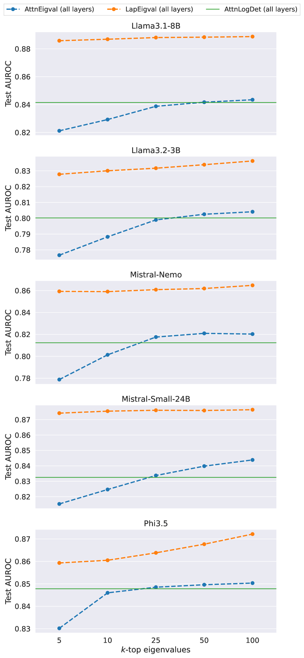<details> <summary>x16.png Details</summary>  ### Visual Description ## Line Chart Series: Model Performance vs. Eigenvalue Count ### Overview The image displays a series of five vertically stacked line charts. Each chart compares the performance (Test AUROC) of three different metrics as a function of the number of top eigenvalues (`k`) considered. The analysis is performed across five distinct language models. ### Components/Axes * **Legend:** Located at the top center of the entire figure. * **Blue dashed line with circle markers:** `AttnEigval (all layers)` * **Orange dashed line with circle markers:** `LapEigval (all layers)` * **Green solid line:** `AttnLogDet (all layers)` * **X-Axis (Common to all subplots):** Label: `k-top eigenvalues`. Ticks and values: `5`, `10`, `25`, `50`, `100`. * **Y-Axis (Per subplot):** Label: `Test AUROC`. The scale varies per subplot to best fit the data. * **Subplot Titles (Top to Bottom):** 1. `Llama3.1-8B` 2. `Llama3.2-3B` 3. `Mistral-Nemo` 4. `Mistral-Small-24B` 5. `Phi3.5` ### Detailed Analysis **1. Llama3.1-8B (Top Chart)** * **Y-Axis Range:** ~0.82 to ~0.89. * **LapEigval (Orange):** Appears as a nearly flat, high line. Values are consistently around 0.885-0.888 across all `k`. * **AttnLogDet (Green):** A flat horizontal line at approximately 0.842. * **AttnEigval (Blue):** Shows a clear upward trend. Starts at ~0.821 (k=5), rises to ~0.829 (k=10), ~0.839 (k=25), ~0.842 (k=50), and ~0.843 (k=100). It converges with the AttnLogDet baseline around k=50. **2. Llama3.2-3B (Second Chart)** * **Y-Axis Range:** ~0.78 to ~0.835. * **LapEigval (Orange):** A gently rising line. Starts at ~0.828 (k=5) and increases to ~0.835 (k=100). * **AttnLogDet (Green):** A flat horizontal line at approximately 0.800. * **AttnEigval (Blue):** Strong upward trend. Starts at ~0.777 (k=5), rises to ~0.788 (k=10), ~0.799 (k=25), ~0.803 (k=50), and ~0.804 (k=100). It surpasses the AttnLogDet baseline between k=25 and k=50. **3. Mistral-Nemo (Third Chart)** * **Y-Axis Range:** ~0.78 to ~0.865. * **LapEigval (Orange):** Nearly flat, high line. Values are stable around 0.860-0.865. * **AttnLogDet (Green):** A flat horizontal line at approximately 0.812. * **AttnEigval (Blue):** Upward trend. Starts at ~0.779 (k=5), rises to ~0.801 (k=10), ~0.818 (k=25), ~0.821 (k=50), and ~0.820 (k=100). It surpasses the AttnLogDet baseline between k=10 and k=25. **4. Mistral-Small-24B (Fourth Chart)** * **Y-Axis Range:** ~0.82 to ~0.875. * **LapEigval (Orange):** Very flat, high line. Values are consistently around 0.874-0.875. * **AttnLogDet (Green):** A flat horizontal line at approximately 0.833. * **AttnEigval (Blue):** Steady upward trend. Starts at ~0.817 (k=5), rises to ~0.825 (k=10), ~0.834 (k=25), ~0.840 (k=50), and ~0.844 (k=100). It surpasses the AttnLogDet baseline between k=10 and k=25. **5. Phi3.5 (Bottom Chart)** * **Y-Axis Range:** ~0.83 to ~0.875. * **LapEigval (Orange):** Shows a clear upward trend. Starts at ~0.859 (k=5), rises to ~0.860 (k=10), ~0.864 (k=25), ~0.868 (k=50), and ~0.872 (k=100). * **AttnLogDet (Green):** A flat horizontal line at approximately 0.848. * **AttnEigval (Blue):** Upward trend. Starts at ~0.830 (k=5), rises to ~0.846 (k=10), ~0.849 (k=25), ~0.850 (k=50), and ~0.851 (k=100). It surpasses the AttnLogDet baseline between k=10 and k=25. ### Key Observations 1. **Consistent Hierarchy:** In all five models, the `LapEigval` metric (orange) achieves the highest Test AUROC, followed by `AttnEigval` (blue) at higher `k` values, with `AttnLogDet` (green) serving as a lower baseline. 2. **Trend of AttnEigval:** The `AttnEigval` metric shows a consistent, sometimes steep, improvement in performance as `k` (the number of top eigenvalues) increases from 5 to 100. This suggests its effectiveness is sensitive to the amount of spectral information retained. 3. **Stability of LapEigval:** The `LapEigval` metric is remarkably stable and high-performing across all `k` values for most models, showing only a very slight upward trend in some cases (e.g., Phi3.5). This indicates robustness to the choice of `k`. 4. **Baseline Comparison:** The `AttnEigval` metric typically starts below the `AttnLogDet` baseline at low `k` (k=5) but surpasses it as `k` increases, usually between k=10 and k=50. 5. **Model Variation:** While the relative ordering of metrics is consistent, the absolute AUROC values and the steepness of the `AttnEigval` curve vary by model. For example, the improvement from k=5 to k=100 is more pronounced in Llama3.2-3B and Mistral-Nemo than in Llama3.1-8B. ### Interpretation This data suggests a comparative analysis of different spectral methods for evaluating or analyzing language models, likely in the context of uncertainty estimation, out-of-distribution detection, or model analysis (given the AUROC metric). * **LapEigval Superiority:** The `LapEigval` (likely Laplacian Eigenvalues) method is demonstrated to be the most effective and robust metric across all tested models. Its high, stable performance implies it captures a fundamental and reliable property of the model's internal representations that correlates well with the evaluation task. * **AttnEigval's Dependence on `k`:** The `AttnEigval` (Attention Eigenvalues) method is highly dependent on the number of eigenvalues considered. Its poor performance at low `k` suggests the most significant attention eigenvalues alone are not sufficient, but incorporating more of the spectrum (higher `k`) leads to substantial gains, eventually matching or exceeding the `AttnLogDet` baseline. * **AttnLogDet as a Fixed Baseline:** The `AttnLogDet` (Attention Log-Determinant) appears to be a single-value metric (hence the flat line), providing a consistent but generally lower-performance benchmark against which the `k`-dependent methods are compared. * **Practical Implication:** If computational cost scales with `k`, there is a clear trade-off for `AttnEigval`. One must choose a `k` high enough to be effective (e.g., k≥25) but not so high as to be inefficient. `LapEigval`, being effective even at low `k`, may be the more practical choice. The analysis validates the use of spectral properties of model weight or activation matrices (Laplacian or Attention) as powerful tools for model evaluation. </details> Figure 10: Probe performance across different top- $k$ eigenvalues: $k\in\{5,10,25,50,100\}$ for TriviaQA dataset with $temp{=}1.0$ and five considered LLMs. 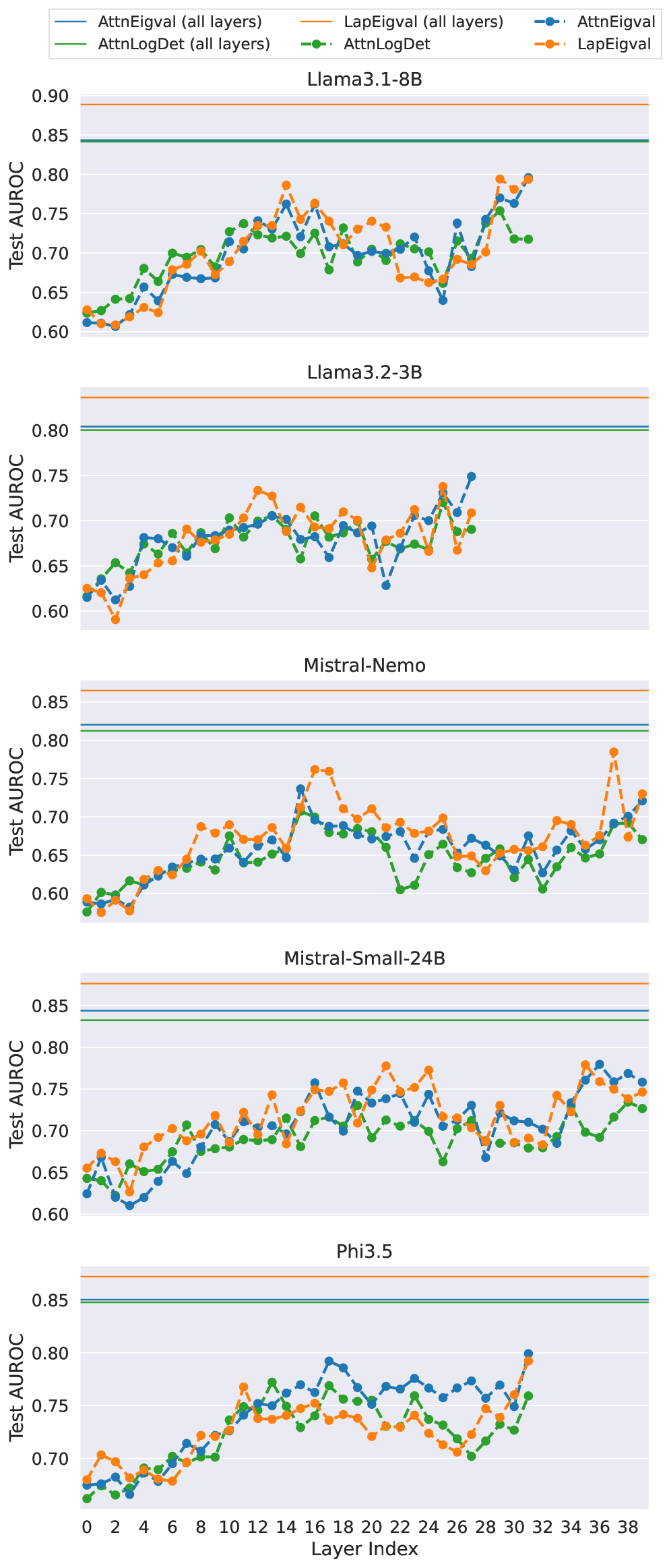<details> <summary>x17.png Details</summary>  ### Visual Description ## Multi-Panel Line Chart: Per-Layer Test AUROC for Various Language Models ### Overview The image displays a series of five vertically stacked line charts. Each chart plots the Test AUROC (Area Under the Receiver Operating Characteristic curve) performance of three different metrics across the layers of a specific large language model (LLM). The charts compare the performance of metrics calculated per individual layer against a baseline performance calculated using all layers combined. ### Components/Axes * **Legend (Top Center):** A horizontal legend defines six data series: * `AttnEigval (all layers)`: Solid blue line. * `AttnLogDet (all layers)`: Solid green line. * `LapEigval (all layers)`: Solid orange line. * `AttnEigval`: Dashed blue line with circular markers. * `AttnLogDet`: Dashed green line with circular markers. * `LapEigval`: Dashed orange line with circular markers. * **X-Axis (Bottom):** Labeled "Layer Index". The axis is shared across all subplots and ranges from 0 to 38, with major tick marks every 2 units. * **Y-Axis (Left):** Labeled "Test AUROC". The scale is consistent across all subplots, ranging from approximately 0.60 to 0.90, with major grid lines at 0.05 intervals. * **Subplot Titles (Centered above each chart):** The five models analyzed are: 1. Llama3.1-8B 2. Llama3.2-3B 3. Mistral-Nemo 4. Mistral-Small-24B 5. Phi3.5 * **Horizontal Reference Lines:** Each subplot contains three solid horizontal lines near the top, corresponding to the "all layers" metrics from the legend. Their vertical position indicates the constant Test AUROC value for that metric when applied to the entire model. ### Detailed Analysis **1. Llama3.1-8B** * **"All layers" baselines (solid lines):** `LapEigval` is highest (~0.89), followed by `AttnLogDet` (~0.845), then `AttnEigval` (~0.84). * **Per-layer trends (dashed lines):** All three metrics show a general upward trend from layer 0 to layer 38, with significant volatility. * `LapEigval` (orange dashed): Starts ~0.62, peaks near layer 14 (~0.79) and layer 32 (~0.80), with a notable dip around layer 24 (~0.66). * `AttnEigval` (blue dashed): Follows a similar pattern to `LapEigval` but often slightly lower, starting ~0.61 and ending ~0.79. * `AttnLogDet` (green dashed): Generally tracks below the other two per-layer metrics, starting ~0.63 and ending ~0.72. **2. Llama3.2-3B** * **"All layers" baselines:** `LapEigval` (~0.83) > `AttnEigval` (~0.805) > `AttnLogDet` (~0.80). * **Per-layer trends:** Metrics are more tightly clustered and volatile than in Llama3.1-8B. * All metrics start between 0.60-0.63. * They show a general increase until around layer 12, followed by a period of fluctuation and a dip around layer 22 (lowest point ~0.63 for `AttnEigval`). * A recovery occurs towards the final layers, with `AttnEigval` reaching the highest point (~0.75). **3. Mistral-Nemo** * **"All layers" baselines:** `LapEigval` (~0.86) > `AttnEigval` (~0.82) > `AttnLogDet` (~0.81). * **Per-layer trends:** Shows the most distinct separation between metrics. * `LapEigval` (orange dashed) is consistently the highest-performing per-layer metric, with a major peak at layer 16 (~0.76) and another at layer 36 (~0.78). * `AttnEigval` (blue dashed) and `AttnLogDet` (green dashed) are lower and more intertwined, with `AttnLogDet` often being the lowest. Both show a significant dip around layer 22 (~0.60-0.61). **4. Mistral-Small-24B** * **"All layers" baselines:** `LapEigval` (~0.88) > `AttnEigval` (~0.845) > `AttnLogDet` (~0.835). * **Per-layer trends:** Metrics are relatively stable and clustered in the 0.65-0.78 range. * A gradual upward trend is visible from layer 0 to layer 38. * `LapEigval` (orange dashed) frequently leads, with peaks around layer 20 (~0.78) and layer 34 (~0.78). * `AttnLogDet` (green dashed) is often the lowest of the three, with a notable dip at layer 24 (~0.66). **5. Phi3.5** * **"All layers" baselines:** `LapEigval` (~0.87) > `AttnEigval` (~0.85) > `AttnLogDet` (~0.845). * **Per-layer trends:** Shows a clear, steady upward trend for all metrics. * All metrics start low (~0.67-0.68). * They climb consistently, with `AttnEigval` (blue dashed) often taking the lead in the middle layers (e.g., layer 17 ~0.79). * The final layers show a sharp increase, with `AttnEigval` reaching ~0.80 at layer 31. ### Key Observations 1. **Consistent Hierarchy of "All layers" Metrics:** Across all five models, the `LapEigval (all layers)` baseline (solid orange line) is always the highest, followed by `AttnEigval (all layers)` (solid blue), and then `AttnLogDet (all layers)` (solid green). This suggests that, when aggregated across all layers, the Laplacian Eigenvalue metric provides the strongest signal for the evaluated task. 2. **Per-Layer Volatility vs. Stability:** Per-layer metrics (dashed lines) are highly volatile and almost always perform worse than their "all layers" counterparts. This indicates that the diagnostic signal is distributed across layers and is noisier when examined in isolation. 3. **Model-Specific Patterns:** * **Llama3.1-8B & Phi3.5:** Exhibit the clearest upward trends in per-layer performance, suggesting these models' layers become progressively more informative for the task. * **Mistral-Nemo:** Shows the most distinct separation between the `LapEigval` per-layer metric and the others, highlighting its unique behavior in this model. * **Common Dip:** Several models (Llama3.1-8B, Llama3.2-3B, Mistral-Nemo, Mistral-Small-24B) show a performance dip in per-layer metrics around layers 22-24, which could indicate a common architectural or functional transition point in these transformer models. ### Interpretation This visualization is likely from a research paper investigating **internal model diagnostics** or **representation learning** in LLMs. The metrics (`AttnEigval`, `AttnLogDet`, `LapEigval`) are probably measures of the geometry or information content of the hidden states or attention matrices at each layer. The "Test AUROC" suggests these metrics are being used as features to classify or detect some property of the model's inputs or internal states (e.g., detecting hallucinations, adversarial examples, or task-specific features). The key finding is that **aggregating information across all layers ("all layers" metrics) yields a much stronger and more stable diagnostic signal than examining any single layer in isolation.** The per-layer plots reveal the *internal landscape* of this signal, showing how the model's processing evolves. The upward trends in models like Phi3.5 suggest a hierarchical build-up of the measured property, while the volatility and dips in others may reflect specialized processing in different model regions. The consistent superiority of `LapEigval` implies that the spectral properties of the layer's representations (captured by eigenvalues of a Laplacian-like matrix) are particularly informative for the underlying task. </details> Figure 11: Analysis of model performance across different layers for and 5 considered LLMs and TriviaQA dataset with $temp{=}1.0$ and $k{=}100$ top eigenvalues (results for models operating on all layers provided for reference). ## Appendix I Extended results of generalization study We present the complete results of the generalization ablation discussed in Section 6.4 of the main paper. Table 11 reports the absolute Test AUROC values for each method and test dataset. Except for TruthfulQA, $\operatorname{LapEigvals}$ achieves the highest performance across all configurations. Notably, some methods perform close to random, whereas $\operatorname{LapEigvals}$ consistently outperforms this baseline. Regarding relative performance drop (Figure 12), $\operatorname{LapEigvals}$ remains competitive, exhibiting the lowest drop in nearly half of the scenarios. These results indicate that our method is robust but warrants further investigation across more datasets, particularly with a deeper analysis of TruthfulQA. Table 11: Full results of the generalization study. By gray color we denote results obtained on test split from the same QA dataset as training split, otherwise results are from test split of different QA dataset. We highlight the best performance in bold. | $\operatorname{AttnLogDet}$ $\operatorname{AttnEigvals}$ $\operatorname{LapEigvals}$ | CoQA CoQA CoQA | 0.758 0.782 0.830 | 0.518 0.426 0.555 | 0.687 0.726 0.790 | 0.644 0.696 0.748 | 0.646 0.659 0.743 | 0.640 0.702 0.786 | 0.587 0.560 0.629 | | --- | --- | --- | --- | --- | --- | --- | --- | --- | | $\operatorname{AttnLogDet}$ | GSM8K | 0.515 | 0.828 | 0.513 | 0.502 | 0.555 | 0.503 | 0.586 | | $\operatorname{AttnEigvals}$ | GSM8K | 0.510 | 0.838 | 0.563 | 0.545 | 0.549 | 0.579 | 0.557 | | $\operatorname{LapEigvals}$ | GSM8K | 0.568 | 0.872 | 0.648 | 0.596 | 0.611 | 0.610 | 0.538 | | $\operatorname{AttnLogDet}$ | HaluevalQA | 0.580 | 0.500 | 0.823 | 0.750 | 0.727 | 0.787 | 0.668 | | $\operatorname{AttnEigvals}$ | HaluevalQA | 0.579 | 0.569 | 0.819 | 0.792 | 0.743 | 0.803 | 0.688 | | $\operatorname{LapEigvals}$ | HaluevalQA | 0.685 | 0.448 | 0.873 | 0.796 | 0.778 | 0.848 | 0.595 | | $\operatorname{AttnLogDet}$ | NQOpen | 0.552 | 0.594 | 0.720 | 0.794 | 0.717 | 0.766 | 0.597 | | $\operatorname{AttnEigvals}$ | NQOpen | 0.546 | 0.633 | 0.725 | 0.790 | 0.714 | 0.770 | 0.618 | | $\operatorname{LapEigvals}$ | NQOpen | 0.656 | 0.676 | 0.792 | 0.827 | 0.748 | 0.843 | 0.564 | | $\operatorname{AttnLogDet}$ | SQuADv2 | 0.553 | 0.695 | 0.716 | 0.774 | 0.746 | 0.757 | 0.658 | | $\operatorname{AttnEigvals}$ | SQuADv2 | 0.576 | 0.723 | 0.730 | 0.737 | 0.768 | 0.760 | 0.711 | | $\operatorname{LapEigvals}$ | SQuADv2 | 0.673 | 0.754 | 0.801 | 0.806 | 0.791 | 0.841 | 0.625 | | $\operatorname{AttnLogDet}$ | TriviaQA | 0.565 | 0.618 | 0.761 | 0.793 | 0.736 | 0.838 | 0.572 | | $\operatorname{AttnEigvals}$ | TriviaQA | 0.577 | 0.667 | 0.770 | 0.786 | 0.742 | 0.843 | 0.616 | | $\operatorname{LapEigvals}$ | TriviaQA | 0.702 | 0.612 | 0.813 | 0.818 | 0.773 | 0.889 | 0.522 | | $\operatorname{AttnLogDet}$ | TruthfulQA | 0.550 | 0.706 | 0.597 | 0.603 | 0.604 | 0.662 | 0.811 | | $\operatorname{AttnEigvals}$ | TruthfulQA | 0.538 | 0.579 | 0.600 | 0.595 | 0.646 | 0.685 | 0.833 | | $\operatorname{LapEigvals}$ | TruthfulQA | 0.590 | 0.722 | 0.552 | 0.529 | 0.569 | 0.631 | 0.829 | <details> <summary>x18.png Details</summary>  ### 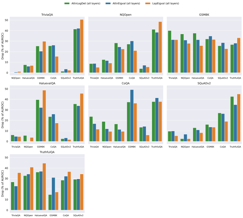Visual Description ## Grouped Bar Charts: Performance Drop Analysis Across Datasets ### Overview The image displays a composite figure containing seven individual grouped bar charts arranged in a 3x3 grid (with two empty slots in the bottom row). Each chart evaluates the performance drop of three different methods when applied to various question-answering or reasoning datasets. The primary metric is the percentage drop in Area Under the Risk-Coverage curve (AURC), where a lower value indicates better performance retention. ### Components/Axes - **Legend**: Positioned at the top center of the entire figure. It defines three methods: - **AttnLogDet (all layers)**: Represented by green bars. - **AttnEigval (all layers)**: Represented by blue bars. - **LapEigval (all layers)**: Represented by orange bars. - **Y-Axis (Common to all charts)**: Labeled **"Drop (% of AURC)"**. The scale ranges from 0 to 50, with major tick marks at intervals of 10. - **X-Axis (Varies per chart)**: Lists different datasets used for evaluation. The specific datasets are: TriviaQA, NQOpen, HaluEvalQA, GSM8K, CoQA, SQuADv2, and TruthfulQA. - **Chart Titles**: Each subplot has a title indicating the primary dataset under analysis (e.g., "TriviaQA", "NQOpen"). ### Detailed Analysis The following is a chart-by-chart breakdown of the estimated values. All values are approximate visual readings from the bar heights. **1. Chart: TriviaQA (Top-Left)** * **X-Axis Categories**: NQOpen, HaluEvalQA, GSM8K, CoQA, SQuADv2, TruthfulQA. * **Data Points (Approx. Drop %)**: * **NQOpen**: AttnLogDet ~1%, AttnEigval ~1%, LapEigval ~1%. * **HaluEvalQA**: AttnLogDet ~7%, AttnEigval ~6%, LapEigval ~6%. * **GSM8K**: AttnLogDet ~25%, AttnEigval ~20%, LapEigval ~29%. * **CoQA**: AttnLogDet ~26%, AttnEigval ~25%, LapEigval ~15%. * **SQuADv2**: AttnLogDet ~3%, AttnEigval ~3%, LapEigval ~2%. * **TruthfulQA**: AttnLogDet ~42%, AttnEigval ~43%, LapEigval ~50%. **2. Chart: NQOpen (Top-Middle)** * **X-Axis Categories**: TriviaQA, HaluEvalQA, GSM8K, CoQA, SQuADv2, TruthfulQA. * **Data Points (Approx. Drop %)**: * **TriviaQA**: AttnLogDet ~8%, AttnEigval ~8%, LapEigval ~5%. * **HaluEvalQA**: AttnLogDet ~12%, AttnEigval ~11%, LapEigval ~10%. * **GSM8K**: AttnLogDet ~28%, AttnEigval ~24%, LapEigval ~22%. * **CoQA**: AttnLogDet ~27%, AttnEigval ~29%, LapEigval ~21%. * **SQuADv2**: AttnLogDet ~4%, AttnEigval ~4%, LapEigval ~5%. * **TruthfulQA**: AttnLogDet ~41%, AttnEigval ~38%, LapEigval ~48%. **3. Chart: GSM8K (Top-Right)** * **X-Axis Categories**: TriviaQA, NQOpen, HaluEvalQA, CoQA, SQuADv2, TruthfulQA. * **Data Points (Approx. Drop %)**: * **TriviaQA**: AttnLogDet ~40%, AttnEigval ~31%, LapEigval ~31%. * **NQOpen**: AttnLogDet ~37%, AttnEigval ~31%, LapEigval ~27%. * **HaluEvalQA**: AttnLogDet ~38%, AttnEigval ~31%, LapEigval ~25%. * **CoQA**: AttnLogDet ~32%, AttnEigval ~35%, LapEigval ~32%. * **SQuADv2**: AttnLogDet ~26%, AttnEigval ~28%, LapEigval ~22%. * **TruthfulQA**: AttnLogDet ~26%, AttnEigval ~28%, LapEigval ~33%. **4. Chart: HaluEvalQA (Middle-Left)** * **X-Axis Categories**: TriviaQA, NQOpen, GSM8K, CoQA, SQuADv2, TruthfulQA. * **Data Points (Approx. Drop %)**: * **TriviaQA**: AttnLogDet ~6%, AttnEigval ~5%, LapEigval ~5%. * **NQOpen**: AttnLogDet ~6%, AttnEigval ~5%, LapEigval ~4%. * **GSM8K**: AttnLogDet ~39%, AttnEigval ~32%, LapEigval ~48%. * **CoQA**: AttnLogDet ~26%, AttnEigval ~24%, LapEigval ~17%. * **SQuADv2**: AttnLogDet ~3%, AttnEigval ~3%, LapEigval ~2%. * **TruthfulQA**: AttnLogDet ~35%, AttnEigval ~33%, LapEigval ~45%. **5. Chart: CoQA (Middle-Center)** * **X-Axis Categories**: TriviaQA, NQOpen, HaluEvalQA, GSM8K, SQuADv2, TruthfulQA. * **Data Points (Approx. Drop %)**: * **TriviaQA**: AttnLogDet ~23%, AttnEigval ~16%, LapEigval ~11%. * **NQOpen**: AttnLogDet ~19%, AttnEigval ~12%, LapEigval ~10%. * **HaluEvalQA**: AttnLogDet ~16%, AttnEigval ~11%, LapEigval ~10%. * **GSM8K**: AttnLogDet ~37%, AttnEigval ~49%, LapEigval ~36%. * **SQuADv2**: AttnLogDet ~14%, AttnEigval ~13%, LapEigval ~6%. * **TruthfulQA**: AttnLogDet ~37%, AttnEigval ~41%, LapEigval ~38%. **6. Chart: SQuADv2 (Middle-Right)** * **X-Axis Categories**: TriviaQA, NQOpen, HaluEvalQA, GSM8K, CoQA, TruthfulQA. * **Data Points (Approx. Drop %)**: * **TriviaQA**: AttnLogDet ~10%, AttnEigval ~9%, LapEigval ~5%. * **NQOpen**: AttnLogDet ~2%, AttnEigval ~7%, LapEigval ~1%. * **HaluEvalQA**: AttnLogDet ~12%, AttnEigval ~9%, LapEigval ~8%. * **GSM8K**: AttnLogDet ~16%, AttnEigval ~13%, LapEigval ~13%. * **CoQA**: AttnLogDet ~26%, AttnEigval ~27%, LapEigval ~19%. * **TruthfulQA**: AttnLogDet ~42%, AttnEigval ~35%, LapEigval ~45%. **7. Chart: TruthfulQA (Bottom-Left)** * **X-Axis Categories**: TriviaQA, NQOpen, HaluEvalQA, GSM8K, CoQA, SQuADv2. * **Data Points (Approx. Drop %)**: * **TriviaQA**: AttnLogDet ~26%, AttnEigval ~22%, LapEigval ~36%. * **NQOpen**: AttnLogDet ~33%, AttnEigval ~34%, LapEigval ~41%. * **HaluEvalQA**: AttnLogDet ~36%, AttnEigval ~37%, LapEigval ~45%. * **GSM8K**: AttnLogDet ~15%, AttnEigval ~31%, LapEigval ~17%. * **CoQA**: AttnLogDet ~28%, AttnEigval ~32%, LapEigval ~36%. * **SQuADv2**: AttnLogDet ~29%, AttnEigval ~29%, LapEigval ~34%. ### Key Observations 1. **Dataset Difficulty**: The **TruthfulQA** dataset consistently induces the highest performance drops across nearly all charts and methods, often exceeding 35%. Conversely, **SQuADv2** and **NQOpen** often show the lowest drops, frequently below 10%. 2. **Method Performance**: No single method is universally superior. * **LapEigval (orange)** frequently shows the highest drop (worst performance) on challenging datasets like TruthfulQA and GSM8K (e.g., ~50% drop in TriviaQA chart for TruthfulQA). * **AttnLogDet (green)** and **AttnEigval (blue)** often perform similarly, but their relative performance flips depending on the dataset. For example, in the CoQA chart for GSM8K, AttnEigval has a notably higher drop (~49%) than the other two. 3. **Cross-Dataset Generalization**: The charts reveal how methods trained or analyzed on one dataset (chart title) perform when evaluated on others (x-axis). Performance drops are generally lower when the evaluation dataset matches the chart's title dataset, suggesting some degree of domain specificity. ### Interpretation This figure presents a robustness or generalization analysis of three attention-based or spectral analysis methods (AttnLogDet, AttnEigval, LapEigval) across seven diverse question-answering benchmarks. The "Drop (% of AURC)" metric quantifies the degradation in model performance when these methods are applied, likely as a form of model pruning, compression, or intervention. The data suggests that the **complexity and nature of the target dataset are the primary drivers of performance loss**. Reasoning-heavy datasets like GSM8K (math) and TruthfulQA (adversarial factuality) cause significant degradation for all methods, indicating that the analyzed model components (captured by "all layers") are critical for these tasks. In contrast, more extractive or retrieval-focused tasks like SQuADv2 are less affected. The variability in method performance implies that the underlying mathematical properties each method captures (log-determinant, eigenvalues of attention, Laplacian eigenvalues) have different sensitivities to the type of reasoning required. The high drop for LapEigval on TruthfulQA might indicate that graph-spectral properties of the model are particularly important for handling adversarial or truthful responses. This analysis is crucial for understanding which model components are essential for different cognitive tasks and for guiding the development of more efficient and robust models. </details> Figure 12: Generalization across datasets measured as a percent performance drop in Test AUROC (less is better) when trained on one dataset and tested on the other. Training datasets are indicated in the plot titles, while test datasets are shown on the $x$ -axis. Results computed on Llama-3.1-8B with $k{=}100$ top eigenvalues and $temp{=}1.0$ . ## Appendix J Influence of dataset size One of the limitations of $\operatorname{LapEigvals}$ is that it is a supervised method and thus requires labelled hallucination data. To check whether it requires a large volume of data, we conducted an additional study in which we trained $\operatorname{LapEigvals}$ on only a stratified fraction of the available examples for each hallucination dataset (using a dataset created from Llama-3.1-8B outputs) and evaluated on the full test split. The AUROC scores are presented in Table 12. As shown, LapEigvals maintains reasonable performance even when trained on as few as a few hundred examples. Additionally, we emphasise that labelling can be efficiently automated and scaled using the llm-as-judge paradigm. Table 12: Impact of training dataset size on performance. Test AUROC scores are reported for different fractions of the training data. The study uses a dataset derived from Llama-3.1-8B answers with $temp{=}1.0$ and $k{=}100$ top eigenvalues, with absolute dataset sizes shown in parentheses. ## Appendix K Reliability of spectral features Our method relies on ordered spectral features, which may exhibit sensitivity to perturbations and limited robustness. In our setup, both attention weights and extracted features were stored as bfloat16 type, which has lower precision than float32. The reduced precision acts as a form of regularization–minor fluctuations are often rounded off, making the method more robust to small perturbations that might otherwise affect the eigenvalue ordering. To further investigate perturbation-sensitivity, we conducted a controlled analysis on one model by adding Gaussian noise to randomly selected input feature dimensions before the eigenvalue sorting step. We varied both the noise standard deviation and the fraction of perturbed dimensions (ranging from 0.5 to 1.0). Perturbations were applied consistently to both the training and test sets. In Table 13 we report the mean and standard deviation of performance across 5 runs on hallucination data generated by Llama-3.1-8B on the TriviaQA dataset with $temp{=}1.0$ , along with percentage change relative to the unperturbed baseline (0.0 indicates no perturbation applied). We observe that small perturbations have a negligible impact on performance and further confirm the robustness of our method. Table 13: Impact of Gaussian noise perturbations on input features for different top- $k$ eigenvalues and noise standard deviations $\sigma$ . Results are averaged over five perturbations, with mean and standard deviation reported; relative percentage drops are shown in parentheses. Results were obtained for Llama-3.1-8B with $temp{=}1.0$ on TriviaQA dataset. | 5 10 20 | 0.867 ± 0.0 (0.0%) 0.867 ± 0.0 (0.0%) 0.869 ± 0.0 (0.0%) | 0.867 ± 0.0 (0.0%) 0.867 ± 0.0 (0.0%) 0.869 ± 0.0 (0.0%) | 0.867 ± 0.0 (0.0%) 0.867 ± 0.0 (0.0%) 0.869 ± 0.0 (0.0%) | 0.867 ± 0.0 (-0.01%) 0.867 ± 0.0 (0.03%) 0.869 ± 0.0 (0.0%) | 0.859 ± 0.003 (0.86%) 0.861 ± 0.002 (0.78%) 0.862 ± 0.002 (0.84%) | 0.573 ± 0.017 (33.84%) 0.579 ± 0.01 (33.3%) 0.584 ± 0.018 (32.76%) | | --- | --- | --- | --- | --- | --- | --- | | 50 | 0.870 ± 0.0 (0.0%) | 0.870 ± 0.0 (0.0%) | 0.870 ± 0.0 (0.0%) | 0.869 ± 0.0 (0.02%) | 0.864 ± 0.002 (0.66%) | 0.606 ± 0.014 (30.31%) | | 100 | 0.872 ± 0.0 (0.0%) | 0.872 ± 0.0 (0.0%) | 0.872 ± 0.0 (0.01%) | 0.872 ± 0.0 (-0.0%) | 0.866 ± 0.001 (0.66%) | 0.640 ± 0.007 (26.64%) | ## Appendix L Cost and time analysis Providing precise cost and time measurements is nontrivial due to the multi-stage nature of our method, as it involves external services (e.g., OpenAI API for labelling), and the runtime and cost can vary depending on the hardware and platform used. Nonetheless, we present an overview of the costs and complexity as follows. 1. Inference with LLM (preparing hallucination dataset) - does not introduce additional cost beyond regular LLM inference; however, it may limit certain optimizations (e.g. FlashAttention (Dao et al., 2022)) since the full attention matrix needs to be materialized in memory. 1. Automated labeling with llm-as-judge using OpenAI API - we estimate labeling costs using the tiktoken library and OpenAI API pricing ($0.60 per 1M output tokens). However, these estimates exclude caching effects and could be reduced using the Batch API; Table 14 reports total and per-item hallucination labelling costs across all datasets (including 5 LLMs and 2 temperature settings). Estimation for GSM8K dataset is not present as the outputs for this dataset are evaluated by exact-match. 1. Computing spectral features - since we exploit the fact that eigenvalues of the Laplacian lie on the diagonal, the complexity is dominated by the computation of the out-degree matrix, which in turn is dominated by the computation of the mean over rows of the attention matrix. Thus, it is $O(n^{2})$ time, where $n$ is the number of tokens. Then, we have to sort eigenvalues, which takes $O(n\log n)$ time. The overall complexity multiplies by the number of layers and heads of a particular LLM. Practically, in our implementation, we fused feature computation with LLM inference, since we observed a memory bottleneck compared to using raw attention matrices stored on disk. Table 14: Estimation of costs regarding llm-as-judge labelling with OpenAI API. | CoQA NQOpen HaluEvalQA | 52,194,357 11,853,621 33,511,346 | 320,613 150,782 421,572 | 653.82 328.36 335.11 | 4.02 4.18 4.22 | 7.83 1.78 5.03 | 0.19 0.09 0.25 | 8.02 1.87 5.28 | | --- | --- | --- | --- | --- | --- | --- | --- | | SQuADv2 | 19,601,322 | 251,264 | 330.66 | 4.24 | 2.94 | 0.15 | 3.09 | | TriviaQA | 41,114,137 | 408,067 | 412.79 | 4.10 | 6.17 | 0.24 | 6.41 | | TruthfulQA | 2,908,183 | 33,836 | 355.96 | 4.14 | 0.44 | 0.02 | 0.46 | | Total | 158,242,166 | 1,575,134 | 402.62 | 4.15 | 24.19 | 0.94 | 25.13 | ## Appendix M QA prompts Following, we describe all prompts for QA used to obtain the results presented in this work: - prompt $p_{1}$ – medium-length one-shot prompt with single example of QA task (Listing 1), - prompt $p_{2}$ – medium-length zero-shot prompt without examples (Listing 2), - prompt $p_{3}$ – long few-shot prompt; the main prompt used in this work; modification of prompt used by (Kossen et al., 2024) (Listing 3), - prompt $p_{4}$ – short-length zero-shot prompt without examples (Listing 4), - prompt $gsm8k$ – short prompt used for GSM8K dataset with output-format instruction. Listing 1: One-shot QA (prompt $p_{1}$ ) ⬇ Deliver a succinct and straightforward answer to the question below. Focus on being brief while maintaining essential information. Keep extra details to a minimum. Here is an example: Question: What is the Riemann hypothesis? Answer: All non - trivial zeros of the Riemann zeta function have real part 1/2 Question: {question} Answer: Listing 2: Zero-shot QA (prompt $p_{2}$ ). ⬇ Please provide a concise and direct response to the following question, keeping your answer as brief and to - the - point as possible while ensuring clarity. Avoid any unnecessary elaboration or additional details. Question: {question} Answer: Listing 3: Few-shot QA prompt (prompt $p_{3}$ ), modified version of prompt used by (Kossen et al., 2024). ⬇ Answer the following question as briefly as possible. Here are several examples: Question: What is the capital of France? Answer: Paris Question: Who wrote * Romeo and Juliet *? Answer: William Shakespeare Question: What is the boiling point of water in Celsius? Answer: 100 ∘ C Question: How many continents are there on Earth? Answer: Seven Question: What is the fastest land animal? Answer: Cheetah Question: {question} Answer: Listing 4: Zero-shot short QA prompt (prompt $p_{4}$ ). ⬇ Answer the following question as briefly as possible. Question: {question} Answer: Listing 5: Zero-shot QA prompt for GSM8K dataset. ⬇ Given the following problem, reason and give a final answer to the problem. Problem: {question} Your response should end with " The final answer is [answer]" where [answer] is the response to the problem. ## Appendix N LLM-as-Judge prompt During hallucinations dataset construction we leveraged llm-as-judge approach to label answers generated by the LLMs. To this end, we utilized gpt-4o-mini with prompt in Listing 6, which is an adapted version of the prompt used by (Orgad et al., 2025). Listing 6: Prompt used in llm-as-judge approach for determining hallucination labels. Prompt is a modified version of the one used by (Orgad et al., 2025). ⬇ You will evaluate answers to questions. For each question, I will provide a model ’ s answer and one or more correct reference answers. You would have to determine if the model answer is correct, incorrect, or model refused to answer. The model answer to be correct has to match from one to all of the possible correct answers. If the model answer is correct, write ’ correct ’ and if it is not correct, write ’ incorrect ’. If the Model Answer is a refusal, stating that they don ’ t have enough information, write ’ refuse ’. For example: Question: who is the young guitarist who played with buddy guy? Ground Truth: [Quinn Sullivan, Eric Gales] Model Answer: Ronnie Earl Correctness: incorrect Question: What is the name of the actor who plays Iron Man in the Marvel movies? Ground Truth: [Robert Downey Jr.] Model Answer: Robert Downey Jr. played the role of Tony Stark / Iron Man in the Marvel Cinematic Universe films. Correctness: correct Question: what is the capital of France? Ground Truth: [Paris] Model Answer: I don ’ t have enough information to answer this question. Correctness: refuse Question: who was the first person to walk on the moon? Ground Truth: [Neil Armstrong] Model Answer: I apologize, but I cannot provide an answer without verifying the historical facts. Correctness: refuse Question: {{question}} Ground Truth: {{gold_answer}} Model Answer: {{predicted_answer}} Correctness: