2503.01361v3

# Statistical physics analysis of graph neural networks: Approaching optimality in the contextual stochastic block model **Authors**: Duranthon, Lenka Zdeborová > Statistical physics of computation laboratory, École polytechnique fédérale de Lausanne, Switzerland (November 21, 2025) ## Abstract Graph neural networks (GNNs) are designed to process data associated with graphs. They are finding an increasing range of applications; however, as with other modern machine learning techniques, their theoretical understanding is limited. GNNs can encounter difficulties in gathering information from nodes that are far apart by iterated aggregation steps. This situation is partly caused by so-called oversmoothing; and overcoming it is one of the practically motivated challenges. We consider the situation where information is aggregated by multiple steps of convolution, leading to graph convolutional networks (GCNs). We analyze the generalization performance of a basic GCN, trained for node classification on data generated by the contextual stochastic block model. We predict its asymptotic performance by deriving the free energy of the problem, using the replica method, in the high-dimensional limit. Calling depth the number of convolutional steps, we show the importance of going to large depth to approach the Bayes-optimality. We detail how the architecture of the GCN has to scale with the depth to avoid oversmoothing. The resulting large depth limit can be close to the Bayes-optimality and leads to a continuous GCN. Technically, we tackle this continuous limit via an approach that resembles dynamical mean-field theory (DMFT) with constraints at the initial and final times. An expansion around large regularization allows us to solve the corresponding equations for the performance of the deep GCN. This promising tool may contribute to the analysis of further deep neural networks. ## I Introduction ### I.1 Summary of the narrative Graph neural networks (GNNs) emerged as the leading paradigm when learning from data that are associated with a graph or a network. Given the ubiquity of such data in sciences and technology, GNNs are gaining importance in their range of applications, including chemistry [1], biomedicine [2], neuroscience [3], simulating physical systems [4], particle physics [5] and solving combinatorial problems [6, 7]. As common in modern machine learning, the theoretical understanding of learning with GNNs is lagging behind their empirical success. In the context of GNNs, one pressing question concerns their ability to aggregate information from far away parts of the graph: the performance of GNNs often deteriorates as depth increases [8]. This issue is often attributed to oversmoothing [9, 10], a situation where a multi-layer GNN averages out the relevant information. Consequently, mostly relatively shallow GNNs are used in practice or other strategies are designed to avoid oversmoothing [11, 12]. Understanding the generalization properties of GNNs on unseen examples is a path towards yet more powerful models. Existing theoretical works addressed the generalization ability of GNNs mainly by deriving generalization bounds, with a minimal set of assumptions on the architecture and on the data, relying on VC dimension, Rademacher complexity or a PAC-Bayesian analysis; see for instance [13] and the references therein. Works along these lines that considered settings related to one of this work include [14], [15] or [16]. However, they only derive loose bounds for the test performance of the GNN and they do not provide insights on the effect of the structure of data. [14] provides sharper bounds; yet they do not take into account the data structure and depend on continuity constants that cannot be determined a priori. In order to provide more actionable outcomes, the interplay between the architecture of the GNN, the training algorithm and the data needs to be understood better, ideally including constant factors characterizing their dependencies on the variety of parameters. Statistical physics traditionally plays a key role in understanding the behaviour of complex dynamical systems in the presence of disorder. In the context of neural networks, the dynamics refers to the training, and the disorder refers to the data used for learning. In the case of GNNs, the data is related to a graph. The statistical physics research strategy defines models that are simplified and allow analytical treatment. One models both the data generative process, and the learning procedure. A key ingredient is a properly defined thermodynamic limit in which quantities of interest self-average. One then aims to derive a closed set of equations for the quantities of interest, akin to obtaining exact expressions for free energies from which physical quantities can be derived. While numerous other research strategies are followed in other theoretical works on GNNs, see above, the statistical physics strategy is the main one accounting for constant factors in the generalization performance and as such provides invaluable insight about the properties of the studied systems. This line of research has been very fruitful in the context of fully connected feed-forward neural networks, see e.g. [17, 18, 19]. It is reasonable to expect that also in the context of GNNs this strategy will provide new actionable insights. The analysis of generalization of GNNs in the framework of the statistical physics strategy was initiated recently in [20] where the authors studied the performance of a single-layer graph convolutional neural network (GCN) applied to data coming from the so-called contextual stochastic block model (CSBM). The CSBM, introduced in [21, 22], is particularly suited as a prototypical generative model for graph-structured data where each node belongs to one of several groups and is associated with a vector of attributes. The task is then the classification of the nodes into groups. Such data are used by practitioners as a benchmark for performance of GNNs [15, 23, 24, 25]. On the theoretical side, the follow-up work [26] generalized the analysis of [20] to a broader class of loss functions but also alerted to the relatively large gap between the performance of a single-layer GCN and the Bayes-optimal performance. In this paper, we show that the close-formed analysis of training a GCN on data coming from the CSBM can be extended to networks performing multiple layers of convolutions. With a properly tuned regularization and strength of the residual connection this allows us to approach the Bayes-optimal performance very closely. Our analysis sheds light on the interplay between the different parameters –mainly the depth, the strength of the residual connection and the regularization– and on how to select the values of the parameters to mitigate oversmoothing. On a technical level the analysis relies on the replica method, with the limit of large depth leading to a continuous formulation similar to neural ordinary differential equations [27] that can be treated analytically via an approach that resembles dynamical mean-field theory with the position in the network playing the role of time. We anticipate that this type of infinite depth analysis can be generalized to studies of other deep networks with residual connections such a residual networks or multi-layer attention networks. ### I.2 Further motivations and related work #### I.2.1 Graph neural networks: In this work we focus on graph neural networks (GNNs). GNNs are neural networks designed to work on data that can be represented as graphs, such as molecules, knowledge graphs extracted from encyclopedias, interactions among proteins or social networks. GNNs can predict properties at the level of nodes, edges or the whole graph. Given a graph $\mathcal{G}$ over $N$ nodes, its adjacency matrix $A\in\mathbb{R}^{N\times N}$ and initial features $h_{i}^{(0)}\in\mathbb{R}^{M}$ on each node $i$ , a GNN can be expressed as the mapping $$ \displaystyle h_{i}^{(k+1)}=f_{\theta^{(k)}}\left(h_{i}^{(k)},\mathrm{aggreg}(\{h_{j}^{(k)},j\sim i\})\right) \tag{1} $$ for $k=0,\dots,K$ with $K$ being the depth of the network. where $f_{\theta^{(k)}}$ is a learnable function of parameters $\theta^{(k)}$ and $\mathrm{aggreg}()$ is a function that aggregates the features of the neighboring nodes in a permutation-invariant way. A common choice is the sum function, akin to a convolution on the graph $$ \displaystyle\mathrm{aggreg}(\{h_{j},j\sim i\})=\sum_{j\sim i}h_{j}=(Ah)_{i}\ . \tag{2} $$ Given this choice of aggregation the GNN is called graph convolutional network (GCN) [28]. For a GNN of depth $K$ the transformed features $h^{(K)}\in\mathbb{R}^{M^{\prime}}$ can be used to predict the properties of the nodes, the edges or the graph by a learnt projection. In this work we will consider a GCN with the following architecture, that we will define more precisely in the detailed setting part II. We consider one trainable layer $w\in\mathbb{R}^{M}$ , since dealing with multiple layers of learnt weights is still a major issue [29], and since we want to focus on modeling the impact of numerous convolution steps on the generalization ability of the GCN. $$ \displaystyle h^{(k+1)} \displaystyle=\left(\frac{1}{\sqrt{N}}\tilde{A}+c_{k}I_{N}\right)h^{(k)} \displaystyle\hat{y} \displaystyle=\operatorname{sign}\left(\frac{1}{\sqrt{N}}w^{T}h^{(K)}\right) \tag{3} $$ where $\tilde{A}$ is a rescaling of the adjacency matrix, $I_{N}$ is the identity, $c_{k}\in\mathbb{R}$ for all $k$ are the residual connection strengths and $\hat{y}\in\mathbb{R}^{N}$ are the predicted labels of each node. We will call the number of layers $K$ the depth, but we reiterate that only the layer $w$ is learned. #### I.2.2 Analyzable model of synthetic data: Modeling the training data is a starting point to derive sharp predictions. A popular model of attributed graph, that we will consider in the present work and define in detail in sec. II.1, is the contextual stochastic block model (CSBM), introduced in [21, 22]. It consists in $N$ nodes with labels $y\in\{-1,+1\}^{N}$ , in a binary stochastic block model (SBM) to model the adjacency matrix $A\in\mathbb{R}^{N\times N}$ and in features (or attributes) $X\in\mathbb{R}^{N\times M}$ defined on the nodes and drawn according to a Gaussian mixture. $y$ has to be recovered given $A$ and $X$ . The inference is done in a semi-supervised way, in the sense that one also has access to a train subset of $y$ . A key aspect in statistical physics is the thermodynamic limit, how should $N$ and $M$ scale together. In statistical physics we always aim at a scaling in which quantities of interest concentrate around deterministic values, and the performance of the system ranges between as bad as random guessing to as good as perfect learning. As we will see, these two requirements are satisfied in the high-dimensional limit $N\to\infty$ and $M\to\infty$ with $\alpha=N/M$ of order one. This scaling limit also aligns well with the common graph datasets that are of interest in practice, for instance Cora [30] ( $N=3.10^{3}$ and $M=3.10^{3}$ ), Coauthor CS [31] ( $N=2.10^{4}$ and $M=7.10^{3}$ ), CiteSeer [32] ( $N=4.10^{3}$ and $M=3.10^{3}$ ) and PubMed [33] ( $N=2.10^{4}$ and $M=5.10^{2}$ ). A series of works that builds on the CSBM with lower dimensionality of features that is $M=o(N)$ exists. Authors of [34] consider a one-layer GNN trained on the CSBM by logistic regression and derive bounds for the test loss; however, they analyze its generalization ability on new graphs that are independent of the train graph and do not give exact predictions. In [35] they propose an architecture of GNN that is optimal on the CSBM with low-dimensional features, among classifiers that process local tree-like neighborhoods, and they derive its generalization error. In [36] the authors analyze the structure and the separability of the convolved data $\tilde{A}^{K}X$ , for different rescalings $\tilde{A}$ of the adjacency matrix, and provide a bound on the classification error. Compared to our work these articles consider a low-dimensional setting ([35]) where the dimension of the features $M$ is constant, or a setting where $M$ is negligible compared to $N$ ([34] and [36]). #### I.2.3 Tight prediction on GNNs in the high-dimensional limit: Little has been done as to tightly predicting the performance of GNNs in the high-dimensional limit where both the size of the graph and the dimensionality of the features diverge proportionally. The only pioneering references in this direction we are aware of are [20] and [26], where the authors consider a simple single-layer GCN that performs only one step of convolution, $K=1$ , trained on the CSBM in a semi-supervised setting. In these works the authors express the performance of the trained network as a function of a finite set of order parameters following a system of self-consistent equations. There are two important motivations to extend these works and to consider GCNs with a higher depth $K$ . First, the GNNs that are used in practice almost always perform several steps of aggregation, and a more realistic model should take this in account. Second, [26] shows that the GCN it considers is far from the Bayes-optimal (BO) performance and the Bayes-optimal rate for all common losses. The BO performance is the best that any algorithm can achieve knowing the distribution of the data, and the BO rate is the rate of convergence toward perfect inference when the signal strength of the graph grows to infinity. Such a gap is intriguing in the sense that previous works [37, 38] show that a simple one-layer fully-connected neural network can reach or be very close to the Bayes-optimality on simple synthetic datasets, including Gaussian mixtures. A plausible explanation is that on the CSBM considering only one step of aggregation $K=1$ is not enough to retrieve all information, and one has to aggregate information from further nodes. Consequently, even on this simple dataset, introducing depth and considering a GCN with several convolution layers, $K>1$ , is crucial. 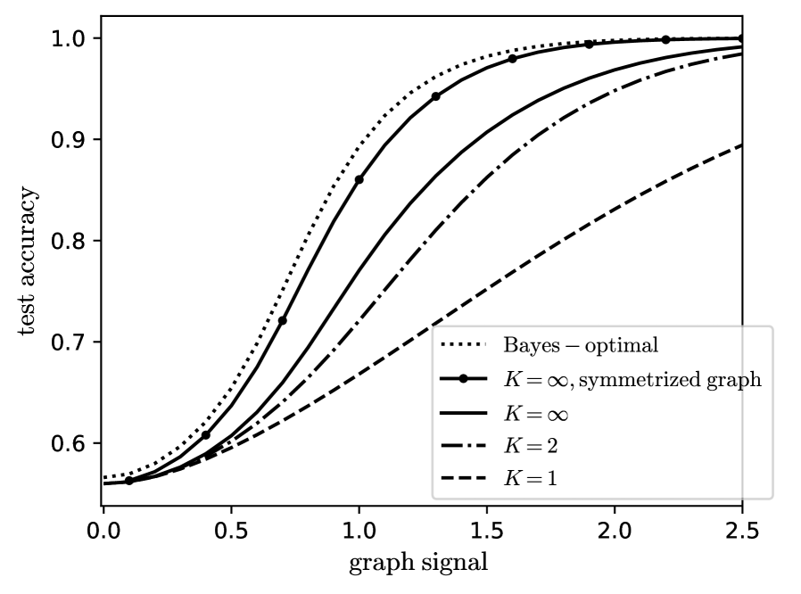In the present work we study the effect of the depth $K$ of the convolution for the generalization ability of a simple GCN. A first part of our contribution consists in deriving the exact performance of a GCN performing several steps of convolution, trained on the CSBM, in the high-dimensional limit. We show that $K=2$ is the minimal number of steps to reach the BO learning rate. As to the performance at moderate signal strength, it appears that, if the architecture is well tuned, going to larger and larger $K$ increases the performance until it reaches a limit. This limit, if the adjacency matrix is symmetrized, can be close to the Bayes optimality. This is illustrated on fig. 1, which highlights the importance of numerous convolution layers. <details> <summary>x1.png Details</summary>  ### Visual Description ## Line Chart: Test Accuracy vs. Graph Signal ### Overview The chart illustrates the relationship between test accuracy and graph signal strength for different model configurations. Test accuracy increases monotonically with graph signal strength, with distinct performance curves for various parameter settings (K values) and a theoretical Bayes-optimal baseline. ### Components/Axes - **Y-axis**: Test accuracy (0.5 to 1.0) - **X-axis**: Graph signal (0.0 to 2.5) - **Legend**: Located in bottom-right corner, containing five entries: 1. Bayes-optimal (dotted line) 2. K=∞, symmetrized graph (solid line with dots) 3. K=∞ (solid line) 4. K=2 (dashed line) 5. K=1 (dash-dotted line) ### Detailed Analysis 1. **Bayes-optimal (dotted line)**: - Starts at ~0.55 accuracy at graph signal 0.0 - Reaches ~1.0 accuracy at graph signal 2.5 - Shows smooth, consistent upward trend 2. **K=∞, symmetrized graph (solid line with dots)**: - Begins at ~0.54 accuracy at graph signal 0.0 - Converges to Bayes-optimal performance by graph signal 1.5 - Matches Bayes-optimal curve exactly at graph signal 2.5 3. **K=∞ (solid line)**: - Starts at ~0.53 accuracy at graph signal 0.0 - Approaches Bayes-optimal performance by graph signal 2.0 - Slightly lags behind symmetrized version at all points 4. **K=2 (dashed line)**: - Begins at ~0.52 accuracy at graph signal 0.0 - Reaches ~0.95 accuracy at graph signal 2.5 - Shows gradual improvement with increasing graph signal 5. **K=1 (dash-dotted line)**: - Starts at ~0.51 accuracy at graph signal 0.0 - Reaches ~0.90 accuracy at graph signal 2.5 - Demonstrates slowest improvement among all curves ### Key Observations - All curves show positive correlation between graph signal and test accuracy - Bayes-optimal performance serves as upper bound for all configurations - Symmetrized graph with K=∞ achieves near-optimal performance - Higher K values (∞ > 2 > 1) correspond to better performance - Performance gap between K=∞ and K=1 narrows as graph signal increases ### Interpretation The data demonstrates that increasing graph signal strength improves model performance across all configurations. The Bayes-optimal curve represents the theoretical maximum achievable accuracy. The K=∞, symmetrized graph configuration achieves performance nearly identical to the optimal, suggesting that graph symmetrization effectively captures essential information even with infinite parameters. Lower K values (1 and 2) show diminishing returns, indicating that model complexity (parameter count) significantly impacts performance when graph signal is limited. The convergence of K=∞ curves to Bayes-optimal performance at high graph signal strength implies that with sufficient data quality, even simple models can approach optimal performance through appropriate architectural choices like graph symmetrization. </details> Figure 1: Test accuracy of the graph neural network on data generated by the contextual stochastic block model vs the signal strength. We define the model and the network in section II. The test accuracy is maximized over all the hyperparameters of the network. The Bayes-optimal performance is from [39]. The line $K=1$ has been studied by [20, 26]; we improve it to $K>1$ , $K=\infty$ and symmetrized graphs. All the curves are theoretical predictions we derive in this work. #### I.2.4 Oversmoothing and residual connections: Going to larger depth $K$ is essential to obtain better performance. Yet, GNNs used in practice can be quite shallow, because of the several difficulties encountered at increasing depth, such that vanishing gradient, which is not specific to graph neural networks, or oversmoothing [9, 10]. Oversmoothing refers to the fact that the GNN tends to act like a low-pass filter on the graph and to smooth the features $h_{i}$ , which after too many steps may converge to the same vector for every node. A few steps of aggregation are beneficial but too many degrade the performance, as [40] shows for a simple GNN, close to the one we study, on a particular model. In the present work we show that the model we consider can suffer from oversmoothing at increasing $K$ if its architecture is not well-tuned and we precisely quantify it. A way to mitigate vanishing gradient and oversmoothing is to allow the nodes to remember their initial features $h_{i}^{(0)}$ . This is done by adding residual (or skip) connections to the neural network, so the update function becomes $$ \displaystyle h_{i}^{(k+1)}=c_{k}h_{i}^{(k)}+f_{\theta^{(k)}}\left(h_{i}^{(k)},\mathrm{aggreg}(\{h_{j}^{(k)},j\sim i\})\right) \tag{5} $$ where the $c_{k}$ modulate the strength of the residual connections. The resulting architecture is known as residual network or resnet [41] in the context of fully-connected and convolutional neural networks. As to GNNs, architectures with residual connections have been introduced in [42] and used in [11, 12] to reach large numbers of layers with competitive accuracy. [43] additionally shows that residual connections help gradient descent. In the setting we consider we prove that residual connections are necessary to circumvent oversmoothing, to go to larger $K$ and to improve the performance. #### I.2.5 Continuous neural networks: Continuous neural networks can be seen as the natural limit of residual networks, when the depth $K$ and the residual connection strengths $c_{k}$ go to infinity proportionally, if $f_{\theta^{(k)}}$ is smooth enough with respect to $k$ . In this limit, rescaling $h^{(k+1)}$ with $c_{k}$ and setting $x=k/K$ and $c_{k}=K/t$ , the rescaled $h$ satisfies the differential equation $$ \displaystyle\frac{\mathrm{d}h_{i}}{\mathrm{d}x}(x)=tf_{\theta(x)}\left(h_{i}(x),\mathrm{aggreg}(\{h_{j}(x),j\sim i\})\right)\ . \tag{6} $$ This equation is called a neural ordinary differential equation [27]. The convergence of a residual network to a continuous limit has been studied for instance in [44]. Continuous neural networks are commonly used to model and learn the dynamics of time-evolving systems, by usually taking the update function $f_{\theta}$ independent of the time $t$ . For an example [45] uses a continuous fully-connected neural network to model turbulence in a fluid. As such, they are a building block of scientific machine learning; see for instance [46] for several applications. As to the generalization ability of continuous neural networks, the only theoretical work we are aware of is [47], that derives loose bounds based on continuity arguments. Continuous neural networks have been extended to continuous GNNs in [48, 49]. For the GCN that we consider the residual connections are implemented by adding self-loops $c_{k}I_{N}$ to the graph. The continuous dynamic of $h$ is then $$ \displaystyle\frac{\mathrm{d}h}{\mathrm{d}x}(x)=t\tilde{A}h(x)\ , \tag{7} $$ with $t\in\mathbb{R}$ ; which is a diffusion on the graph. Other types of dynamics have been considered, such as anisotropic diffusion, where the diffusion factors are learnt, or oscillatory dynamics, that should avoid oversmoothing too; see for instance the review [50] for more details. No prior works predict their generalization ability. In this work we fill this gap by deriving the performance of the continuous limit of the simple GCN we consider. ### I.3 Summary of the main results: We first generalize the work of [20, 26] to predict the performance of a simple GCN with arbitrary number $K$ of convolution steps. The network is trained in a semi-supervised way on data generated by the CSBM for node classification. In the high-dimensional limit and in the limit of dense graphs, the main properties of the trained network concentrate onto deterministic values, that do not depend on the particular realization of the data. The network is described by a few order parameters (or summary statistics), that satisfy a set of self-consistent equations, that we solve analytically or numerically. We thus have access to the expected train and test errors and accuracies of the trained network. From these predictions we draw several consequences. Our main guiding line is to search for the architecture and the hyperparameters of the GCN that maximize its performance, and check whether the optimal GCN can reach the Bayes-optimal performance on the CSBM. The main parameters we considers are the depth $K$ , the residual connection strengths $c_{k}$ , the regularization $r$ and the loss function. We consider the convergence rates towards perfect inference at large graph signal. We show that $K=2$ is the minimal depth to reach the Bayes-optimal rate, after which increasing $K$ or fine-tuning $c_{k}$ only leads to sub-leading improvements. In case of asymmetric graphs the GCN is not able to deal the asymmetry, for all $K$ or $c_{k}$ , and one has to pre-process the graph by symmetrizing it. At finite graph signal the behaviour of the GCN is more complex. We find that large regularization $r$ maximizes the test accuracy in the case we consider, while the loss has little effect. The residual connection strengths $c_{k}$ have to be tuned to a same optimal value $c$ that depends on the properties of the graph. An important point is that going to larger $K$ seems to improve the test accuracy. Yet the residual connection $c$ has to vary accordingly. If $c$ stays constant with respect to $K$ then the GCN will perform PCA on the graph $A$ , oversmooth and discard the information from the features $X$ . Instead, if $c$ grows with $K$ , the residual connections alleviate oversmoothing and the performance of the GCN keeps increasing with $K$ , if the diffusion time $t=K/c$ is well tuned. The limit $K\to\infty,c\propto K$ is thus of particular interest. It corresponds to a continuous GCN performing diffusion on the graph. Our analysis can be extended to this case by directly taking the limit in the self-consistent equations. One has to further jointly expand them around $r\to+\infty$ and we keep the first order. At the end we predict the performance of the continuous GCN in an explicit and closed form. To our knowledge this is the first tight prediction of the generalization ability of a continuous neural network, and in particular of a continuous graph neural network. The large regularization limit $r\to+\infty$ is important: on one hand it appears to lead to the optimal performance of the neural network; on another hand, it is instrumental to analyze the continuous limit $K\to\infty$ and it allows to analytically solve the self-consistent equations describing the neural network. We show that the continuous GCN at optimal time $t$ performs better than any finite- $K$ GCN. The optimal $t$ depends on the properties of the graph, and can be negative for heterophilic graphs. This result is a step toward solving one of the major challenges identified by [8]; that is, creating benchmarks where depth is necessary and building efficient deep networks. The continuous GCN as large $r$ is optimal. Moreover, if run on the symmetrized graph, it approaches the Bayes-optimality on a broad range of configurations of the CSBM, as exemplified on fig. 1. We identify when the GCN fails to approach the Bayes-optimality: this happens when most of the information is contained in the features and not in the graph, and has to be processed in an unsupervised manner. We provide the code that allows to evaluate our predictions in the supplementary material. ## II Detailed setting ### II.1 Contextual Stochastic Block Model for attributed graphs We consider the problem of semi-supervised node classification on an attributed graph, where the nodes have labels and carry additional attributes, or features, and where the structure of the graph correlates with the labels. We consider a graph $\mathcal{G}$ made of $N$ nodes; each node $i$ has a binary label $y_{i}=\pm 1$ that is a Rademacher random variable. The structure of the graph should be correlated with $y$ . We model the graph with a binary stochastic block model (SBM): the adjacency matrix $A\in\mathbb{R}^{N\times N}$ is drawn according to $$ A_{ij}\sim\mathcal{B}\left(\frac{d}{N}+\frac{\lambda}{\sqrt{N}}\sqrt{\frac{d}{N}\left(1-\frac{d}{N}\right)}y_{i}y_{j}\right) \tag{8} $$ where $\lambda$ is the signal-to-noise ratio (snr) of the graph, $d$ is the average degree of the graph, $\mathcal{B}$ is a Bernoulli law and the elements $A_{ij}$ are independent for all $i$ and $j$ . It can be interpreted in the following manner: an edge between $i$ and $j$ appears with a higher probability if $\lambda y_{i}y_{j}>1$ i.e. for $\lambda>0$ if the two nodes are in the same group. The scaling with $d$ and $N$ is chosen so that this model does not have a trivial limit at $N\to\infty$ both for $d=\Theta(1)$ and $d=\Theta(N)$ . Notice that we take $A$ asymmetric. Additionally to the graph, each node $i$ carries attributes $X_{i}\in\mathbb{R}^{M}$ , that we collect in the matrix $X\in\mathbb{R}^{N\times M}$ . We set $\alpha=N/M$ the aspect ratio between the number of nodes and the dimension of the features. We model them by a Gaussian mixture: we draw $M$ hidden Gaussian variables $u_{\nu}\sim\mathcal{N}(0,1)$ , the centroid $u\in\mathbb{R}^{M}$ , and we set $$ X=\sqrt{\frac{\mu}{N}}yu^{T}+W \tag{9} $$ where $\mu$ is the snr of the features and $W$ is noise whose components $W_{i\nu}$ are independent standard Gaussians. We use the notation $\mathcal{N}(m,V)$ for a Gaussian distribution or density of mean $m$ and variance $V$ . The whole model for $(y,A,X)$ is called the contextual stochastic block model (CSBM) and was introduced in [21, 22]. We consider the task of inferring the labels $y$ given a subset of them. We define the training set $R$ as the set of nodes whose labels are revealed; $\rho=|R|/N$ is the training ratio. The test set $R^{\prime}$ is selected from the complement of $R$ ; we define the testing ratio $\rho^{\prime}=|R^{\prime}|/N$ . We assume that $R$ and $R^{\prime}$ are independent from the other quantities. The inference problem is to find back $y$ and $u$ given $A$ , $X$ , $R$ and the parameters of the model. [22, 51] prove that the effective snr of the CSBM is $$ \mathrm{snr}_{\mathrm{CSBM}}=\lambda^{2}+\mu^{2}/\alpha\ , \tag{10} $$ in the sense that in the unsupervised regime $\rho=0$ for $\mathrm{snr}_{\mathrm{CSBM}}<1$ no information on the labels can be recovered while for $\mathrm{snr}_{\mathrm{CSBM}}>1$ partial information can be recovered. The information given by the graph is $\lambda^{2}$ while the information given by the features is $\mu^{2}/\alpha$ . As soon as a finite fraction of nodes $\rho>0$ is revealed the phase transition between no recovery and weak recovery disappears. We work in the high-dimensional limit $N\to\infty$ and $M\to\infty$ while the aspect ratio $\alpha=N/M$ is of order one. The average degree $d$ should be of order $N$ , but taking $d$ growing with $N$ should be sufficient for our results to hold, as shown by our experiments. The other parameters $\lambda$ , $\mu$ , $\rho$ and $\rho^{\prime}$ are of order one. ### II.2 Analyzed architecture In this work, we focus on the role of applying several data aggregation steps. With the current theoretical tools, the tight analysis of the generic GNN described in eq. (1) is not possible: dealing with multiple layers of learnt weights is hard; and even for a fully-connected two-layer perceptron this is a current and major topic [29]. Instead, we consider a one-layer GNN with a learnt projection $w$ . We focus on graph convolutional networks (GCNs) [28], where the aggregation is a convolution done by applying powers of a rescaling $\tilde{A}$ of the adjacency matrix. Last we remove the non-linearities. As we will see, the fact that the GCN is linear does not prevent it to approach the optimality in some regimes. The resulting GCN is referred to as simple graph convolutional network; it has been shown to have good performance while being much easier to train [52, 53]. The network we consider transforms the graph and the features in the following manner: $$ h(w)=\prod_{k=1}^{K}\left(\frac{1}{\sqrt{N}}\tilde{A}+c_{k}I_{N}\right)\frac{1}{\sqrt{N}}Xw \tag{11} $$ where $w\in\mathbb{R}^{M}$ is the layer of trainable weights, $I_{N}$ is the identity, $c_{k}\in\mathbb{R}$ is the strength of the residual connections and $\tilde{A}\in\mathbb{R}^{N\times N}$ is a rescaling of the adjacency matrix defined by $$ \tilde{A}_{ij}=\left(\frac{d}{N}\left(1-\frac{d}{N}\right)\right)^{-1/2}\left(A_{ij}-\frac{d}{N}\right),\;\mathrm{for\;all\;}i,\,j. \tag{12} $$ The prediction $\hat{y}_{i}$ of the label of $i$ by the GNN is then $\hat{y}_{i}=\operatorname{sign}h(w)_{i}$ . $\tilde{A}$ is a rescaling of $A$ that is centered and normalized. In the limit of dense graphs, where $d$ is large, this will allow us to rely on a Gaussian equivalence property to analyze this GCN. The equivalence [54, 22, 20] states that in the high-dimensional limit, for $d$ growing with $N$ , $\tilde{A}$ can be approximated by the following spiked matrix $A^{\mathrm{g}}$ without changing the macroscopic properties of the GCN: $$ A^{\mathrm{g}}=\frac{\lambda}{\sqrt{N}}yy^{T}+\Xi\ , \tag{13} $$ where the components of the $N\times N$ matrix $\Xi$ are independent standard Gaussian random variables. The main reason for considering dense graphs instead of sparse graphs $d=\Theta(1)$ is to ease the theoretical analysis. The dense model can be described by a few order parameters; while a sparse SBM would be harder to analyze because many quantities, such as the degrees of the nodes, do not self-average, and one would need to take in account all the nodes, by predicting the performance on one realization of the graph or by running population dynamics. We believe that it would lead to qualitatively similar results, as for instance [55] shows, for a related model. The above architecture corresponds to applying $K$ times a graph convolution on the projected features $Xw$ . At each convolution step $k$ a node $i$ updates its features by summing those of its neighbors and adding $c_{k}$ times its own features. In [20, 26] the same architecture was considered for $K=1$ ; we generalize these works by deriving the performance of the GCN for arbitrary numbers $K$ of convolution steps. As we will show this is crucial to approach the Bayes-optimal performance. Compared to [20, 26], another important improvement towards the Bayes-optimality is obtained by symmetrizing the graph, and we will also study the performance of the GCN when it acts by applying the symmetrized rescaled adjacency matrix $\tilde{A}^{\mathrm{s}}$ defined by: $$ \tilde{A}^{\mathrm{s}}=\frac{1}{\sqrt{2}}(\tilde{A}+\tilde{A}^{T})\ ,\quad A^{\mathrm{g,s}}=\frac{\lambda^{\mathrm{s}}}{\sqrt{N}}yy^{T}+\Xi^{\mathrm{s}}\ . \tag{14} $$ $A^{\mathrm{g,s}}$ is its Gaussian equivalent, with $\lambda^{\mathrm{s}}=\sqrt{2}\lambda$ , $\Xi^{\mathrm{s}}$ is symmetric and $\Xi^{\mathrm{s}}_{i\leq j}$ are independent standard Gaussian random variables. In this article we derive and show the performance of the GNN both acting with $\tilde{A}$ and $\tilde{A}^{\mathrm{s}}$ but in a first part we will mainly consider and state the expressions for $\tilde{A}$ because they are simpler. We will consider $\tilde{A}^{\mathrm{s}}$ in a second part while taking the continuous limit. To deal with both cases, asymmetric or symmetrized, we define $\tilde{A}^{\mathrm{e}}\in\{\tilde{A},\tilde{A}^{\mathrm{s}}\}$ and $\lambda^{\mathrm{e}}\in\{\lambda,\lambda^{\mathrm{s}}\}$ . The continuous limit of the above network (11) is defined by $$ h(w)=e^{\frac{t}{\sqrt{N}}\tilde{A}^{\mathrm{e}}}\frac{1}{\sqrt{N}}Xw \tag{15} $$ where $t$ is the diffusion time. It is obtained at large $K$ when the update between two convolutions becomes small, as follows: $$ \left(\frac{t}{K\sqrt{N}}\tilde{A}^{\mathrm{e}}+I_{N}\right)^{K}\underset{K\to\infty}{\longrightarrow}e^{\frac{t}{\sqrt{N}}\tilde{A}^{\mathrm{e}}}\ . \tag{16} $$ $h$ is the solution at time $t$ of the time-continuous diffusion of the features on the graph $\mathcal{G}$ with Laplacian $\tilde{A}^{\mathrm{e}}$ , defined by $\partial_{x}X(x)=\frac{1}{\sqrt{N}}\tilde{A}^{\mathrm{e}}X(x)$ and $X(0)=X$ . The discrete GCN can be seen as the discretization of the differential equation in the forward Euler scheme. The mapping with eq. (11) is done by taking $c_{k}=K/t$ for all $k$ and by rescaling the features of the discrete GCN $h(w)$ as $h(w)\prod_{k}c_{k}^{-1}$ so they remain of order one when $K$ is large. For the discrete GCN we do not directly consider the update $h_{k+1}=(I_{N}+c_{k}^{-1}\tilde{A}/\sqrt{N})h_{k}$ because we want to study the effect of having no residual connections, i.e. $c_{k}=0$ . The case where the diffusion coefficient depends on the position in the network is equivalent to a constant diffusion coefficient. Indeed, because of commutativity, the solution at time $t$ of $\partial_{x}X(x)=\frac{1}{\sqrt{N}}\mathrm{a}(x)\tilde{A}^{\mathrm{e}}X(x)$ for $\mathrm{a}:\mathbb{R}\to\mathbb{R}$ is $\exp\left(\int_{0}^{t}\mathrm{d}x\,\mathrm{a}(x)\frac{1}{\sqrt{N}}\tilde{A}^{\mathrm{e}}\right)X(0)$ . The discrete and the continuous GCNs are trained by empirical risk minimization. We define the regularized loss $$ L_{A,X}(w)=\frac{1}{\rho N}\sum_{i\in R}\ell(y_{i}h_{i}(w))+\frac{r}{\rho N}\sum_{\nu}\gamma(w_{\nu}) \tag{17} $$ where $\gamma$ is a strictly convex regularization function, $r$ is the regularization strength and $\ell$ is a convex loss function. The regularization ensures that the GCN does not overfit the train data and has good generalization properties on the test set. We will focus on $l_{2}$ -regularization $\gamma(x)=x^{2}/2$ and on the square loss $\ell(x)=(1-x)^{2}/2$ (ridge regression) or the logistic loss $\ell(x)=\log(1+e^{-x})$ (logistic regression). Since $L$ is strictly convex it admits a unique minimizer $w^{*}$ . The key quantities we want to estimate are the average train and test errors and accuracies of this model, which are $$ \displaystyle E_{\mathrm{train/test}}=\mathbb{E}\ \frac{1}{|\hat{R}|}\sum_{i\in\hat{R}}\ell(y_{i}h(w^{*})_{i}) \displaystyle\mathrm{Acc}_{\mathrm{train/test}}=\mathbb{E}\ \frac{1}{|\hat{R}|}\sum_{i\in\hat{R}\ ,}\delta_{y_{i}=\operatorname{sign}{h(w^{*})_{i}}} \tag{18} $$ where $\hat{R}$ stands either for the train set $R$ or the test set $R^{\prime}$ and the expectation is taken over $y$ , $u$ , $A$ , $X$ , $R$ and $R^{\prime}$ . $\mathrm{Acc}_{\mathrm{train/test}}$ is the proportion of train/test nodes that are correctly classified. A main part of the present work is dedicated to the derivation of exact expressions for the errors and the accuracies. We will then search for the architecture of the GCN that maximizes the test accuracy $\mathrm{Acc}_{\mathrm{test}}$ . Notice that one could treat the residual connection strengths $c_{k}$ as supplementary parameters, jointly trained with $w$ to minimize the train loss. Our analysis can straightforwardly be extended to deal with this case. Yet, as we will show, to take trainable $c_{k}$ degrades the test performances; and it is better to consider them as hyperparameters optimizing the test accuracy. Table 1: Summary of the parameters of the model. | $N$ $M$ $\alpha=N/M$ | number of nodes dimension of the attributes aspect ratio | | --- | --- | | $d$ | average degree of the graph | | $\lambda$ | signal strength of the graph | | $\mu$ | signal strength of the features | | $\rho=|R|/N$ | fraction of training nodes | | $\ell$ , $\gamma$ | loss and regularization functions | | $r$ | regularization strength | | $K$ | number of aggregation steps | | $c_{k}$ , $c$ , $t$ | residual connection strengths, diffusion time | ### II.3 Bayes-optimal performance: An interesting consequence of modeling the data as we propose is that one has access to the Bayes-optimal (BO) performance on this task. The BO performance is defined as the upper-bound on the test accuracy that any algorithm can reach on this problem, knowing the model and its parameters $\alpha,\lambda,\mu$ and $\rho$ . It is of particular interest since it will allow us to check how far the GCNs are from the optimality and how much improvement can one hope for. The BO performance on this problem has been derived in [22] and [39]. It is expressed as a function of the fixed-point of an algorithm based on approximate message-passing (AMP). In the limit of large degrees $d=\Theta(N)$ this algorithm can be tracked by a few scalar state-evolution (SE) equations that we reproduce in appendix C. ## III Asymptotic characterization of the GCN In this section we provide an asymptotic characterization of the performance of the GCNs previously defined. It relies on a finite set of order parameters that satisfy a system of self-consistent, or fixed-point, equations, that we obtain thanks to the replica method in the high-dimensional limit at finite $K$ . In a second part, for the continuous GCN, we show how to take the limit $K\to\infty$ for the order parameters and for their self-consistent equations. The continuous GCN is still described by a finite set of order parameters, but these are now continuous functions and the self-consistent equations are integral equations. Notice that for a quadratic loss function $\ell$ there is an analytical expression for the minimizer $w^{*}$ of the regularized loss $L_{A,X}$ eq. (17), given by the regularized least-squares formula. Based on that, a computation of the performance of the GCN with random matrix theory (RMT) is possible. It would not be straightforward in the sense that the convolved features, the weights $w^{*}$ and the labels $y$ are correlated, and such a computation would have to take in account these correlations. Instead, we prefer to use the replica method, which has already been successfully applied to analyze several architectures of one (learnable) layer neural networks in articles such that [17, 38]. Compared to RMT, the replica method allows us to seamlessly handle the regularized pseudo-inverse of the least-squares and to deal with logistic regression, where no explicit expression for $w^{*}$ exists. We compute the average train and test errors and accuracies eqs. (18) and (19) in the high-dimensional limit $N$ and $M$ large. We define the Hamiltonian $$ H(w)=s\sum_{i\in R}\ell(y_{i}h(w)_{i})+r\sum_{\nu}\gamma(w_{\nu})+s^{\prime}\sum_{i\in R^{\prime}}\ell(y_{i}h(w)_{i}) \tag{20} $$ where $s$ and $s^{\prime}$ are external fields to probe the observables. The loss of the test samples is in $H$ for the purpose of the analysis; we will take $s^{\prime}=0$ later and the GCN is minimizing the training loss (17). The free energy $f$ is defined as $$ Z=\int\mathrm{d}w\,e^{-\beta H(w)}\ ,\quad f=-\frac{1}{\beta N}\mathbb{E}\log Z\ . \tag{21} $$ $\beta$ is an inverse temperature; we consider the limit $\beta\to\infty$ where the partition function $Z$ concentrates over $w^{*}$ at $s=1$ and $s^{\prime}=0$ . The train and test errors are then obtained according to $$ E_{\mathrm{train}}=\frac{1}{\rho}\frac{\partial f}{\partial s}\ ,\quad E_{\mathrm{test}}=\frac{1}{\rho^{\prime}}\frac{\partial f}{\partial s^{\prime}} \tag{22} $$ both evaluated at $(s,s^{\prime})=(1,0)$ . One can, in the same manner, compute the average accuracies by introducing the observables $\sum_{i\in\hat{R}}\delta_{y_{i}=\operatorname{sign}{h(w)_{i}}}$ in $H$ . To compute $f$ we introduce $n$ replica: $$ \mathbb{E}\log Z=\mathbb{E}\frac{\partial Z^{n}}{\partial n}(n=0)=\left(\frac{\partial}{\partial n}\mathbb{E}Z^{n}\right)(n=0)\ . \tag{23} $$ To pursue the computation we need to precise the architecture of the GCN. ### III.1 Discrete GCN #### III.1.1 Asymptotic characterization In this section, we work at finite $K$ . We consider only the asymmetric graph. We define the state of the GCN after the $k^{\mathrm{th}}$ convolution step as $$ h_{k}=\left(\frac{1}{\sqrt{N}}\tilde{A}+c_{k}I_{N}\right)h_{k-1}\ ,\quad h_{0}=\frac{1}{\sqrt{N}}Xw\ . \tag{24} $$ $h_{K}=h(w)\in\mathbb{R}^{N}$ is the output of the full GCN. We introduce $h_{k}$ in the replicated partition function $Z^{n}$ and we integrate over the fluctuations of $A$ and $X$ . This couples the variables across the different layers $k=0\ldots K$ and one has to take in account the correlations between the different $h_{k}$ , which will result into order parameters of dimension $K$ . One has to keep separate the indices $i\in R$ and $i\notin R$ , whether the loss $\ell$ is active or not; consequently the free entropy of the problem will be a linear combination of $\rho$ times a potential with $\ell$ and $(1-\rho)$ times without $\ell$ . The limit $N\to\infty$ is taken thanks to Laplace’s method. The extremization is done in the space of the replica-symmetric ansatz, which is justified by the convexity of $H$ . The detailed computation is given in appendix A. The outcome of the computation is that this problem is described by a set of twelve order parameters (or summary statistics). They are $\Theta=\{m_{w}\in\mathbb{R},Q_{w}\in\mathbb{R},V_{w}\in\mathbb{R},m\in\mathbb{R}^{K},Q\in\mathbb{R}^{K\times K},V\in\mathbb{R}^{K\times K}\}$ and their conjugates $\hat{\Theta}=\{\hat{m}_{w}\in\mathbb{R},\hat{Q}_{w}\in\mathbb{R},\hat{V}_{w}\in\mathbb{R},\hat{m}\in\mathbb{R},\hat{Q}\in\mathbb{R}^{K\times K},\hat{V}\in\mathbb{R}^{K\times K}\}$ , where $$ \displaystyle m_{w}=\frac{1}{N}u^{T}w\ , \displaystyle m_{k}=\frac{1}{N}y^{T}h_{k}\ , \displaystyle Q_{w}=\frac{1}{N}w^{T}w\ , \displaystyle Q_{k,l}=\frac{1}{N}h^{T}_{k}h_{l}\ , \displaystyle V_{w}=\frac{\beta}{N}\operatorname{Tr}(\operatorname{Cov}_{\beta}(w,w))\ , \displaystyle V_{k,l}=\frac{\beta}{N}\operatorname{Tr}(\operatorname{Cov}_{\beta}(h_{k},h_{l}))\ . \tag{25} $$ $m_{w}$ and $m_{k}$ are the magnetizations (or overlaps) between the weights and the hidden variables and between the $k^{\mathrm{th}}$ layer and the labels; the $Q$ s are the self-overlaps (or scalar products) between the different layers; and, writing $\operatorname{Cov}_{\beta}$ for the covariance under the density $e^{-\beta H}$ , the $V$ s are the covariances between different trainings on the same data, after rescaling by $\beta$ . The order parameters $\Theta$ and $\hat{\Theta}$ satisfy the property that they extremize the following free entropy $\phi$ : $$ \displaystyle\phi \displaystyle=\frac{1}{2}\left(\hat{V}_{w}V_{w}+\hat{V}_{w}Q_{w}-V_{w}\hat{Q}_{w}\right)-\hat{m}_{w}m_{w}+\frac{1}{2}\mathrm{tr}\left(\hat{V}V+\hat{V}Q-V\hat{Q}\right)-\hat{m}^{T}m \displaystyle\quad{}+\frac{1}{\alpha}\mathbb{E}_{u,\varsigma}\left(\log\int\mathrm{d}w\,e^{\psi_{w}(w)}\right)+\rho\mathbb{E}_{y,\xi,\zeta,\chi}\left(\log\int\prod_{k=0}^{K}\mathrm{d}h_{k}e^{\psi_{h}(h;s)}\right)+(1-\rho)\mathbb{E}_{y,\xi,\zeta,\chi}\left(\log\int\prod_{k=0}^{K}\mathrm{d}h_{k}e^{\psi_{h}(h;s^{\prime})}\right)\ , \tag{28} $$ the potentials being $$ \displaystyle\psi_{w}(w) \displaystyle=-r\gamma(w)-\frac{1}{2}\hat{V}_{w}w^{2}+\left(\sqrt{\hat{Q}_{w}}\varsigma+u\hat{m}_{w}\right)w \displaystyle\psi_{h}(h;\bar{s}) \displaystyle=-\bar{s}\ell(yh_{K})-\frac{1}{2}h_{<K}^{T}\hat{V}h_{<K}+\left(\xi^{T}\hat{Q}^{1/2}+y\hat{m}^{T}\right)h_{<K} \displaystyle\qquad{}+\log\mathcal{N}\left(h_{0}\left|\sqrt{\mu}ym_{w}+\sqrt{Q_{w}}\zeta;V_{w}\right.\right)+\log\mathcal{N}\left(h_{>0}\left|c\odot h_{<K}+\lambda ym+Q^{1/2}\chi;V\right.\right)\ , \tag{29} $$ for $w\in\mathbb{R}$ and $h\in\mathbb{R}^{K+1}$ , where we introduced the Gaussian random variables $\varsigma\sim\mathcal{N}(0,1)$ , $\xi\sim\mathcal{N}(0,I_{K})$ , $\zeta\sim\mathcal{N}(0,1)$ and $\chi\sim\mathcal{N}(0,I_{K})$ , take $y$ Rademacher and $u\sim\mathcal{N}(0,1)$ , where we set $h_{>0}=(h_{1},\ldots,h_{K})^{T}$ , $h_{<K}=(h_{0},\ldots,h_{K-1})^{T}$ and $c\odot h_{<K}=(c_{1}h_{0},\ldots,c_{K}h_{K-1})^{T}$ and where $\bar{s}\in\{0,1\}$ controls whether the loss $\ell$ is active or not. We use the notation $\mathcal{N}(\cdot|m;V)$ for a Gaussian density of mean $m$ and variance $V$ . We emphasize that $\psi_{w}$ and $\psi_{h}$ are effective potentials taking in account the randomness of the model and that are defined over a finite number of variables, contrary to the initial loss function $H$ . The extremality condition $\nabla_{\Theta,\hat{\Theta}}\,\phi=0$ can be stated in terms of a system of self-consistent equations that we give here. In the limit $\beta\to\infty$ one has to consider the extremizers of $\psi_{w}$ and $\psi_{h}$ defined as $$ \displaystyle w^{*} \displaystyle=\operatorname*{argmax}_{w}\psi_{w}(w)\in\mathbb{R} \displaystyle h^{*} \displaystyle=\operatorname*{argmax}_{h}\psi_{h}(h;\bar{s}=1)\in\mathbb{R}^{K+1} \displaystyle h^{{}^{\prime}*} \displaystyle=\operatorname*{argmax}_{h}\psi_{h}(h;\bar{s}=0)\in\mathbb{R}^{K+1}\ . \tag{31} $$ We also need to introduce $\operatorname{Cov}_{\psi_{h}}(h)$ and $\operatorname{Cov}_{\psi_{h}}(h^{\prime})$ the covariances of $h$ under the densities $e^{\psi_{h}(h,\bar{s}=1)}$ and $e^{\psi_{h}(h,\bar{s}=0)}$ . In the limit $\beta\to\infty$ they read $$ \displaystyle\operatorname{Cov}_{\psi_{h}}(h) \displaystyle=\nabla\nabla\psi_{h}(h^{*};\bar{s}=1) \displaystyle\operatorname{Cov}_{\psi_{h}}(h^{\prime}) \displaystyle=\nabla\nabla\psi_{h}(h^{{}^{\prime}*};\bar{s}=0)\ , \tag{34} $$ $\nabla\nabla$ being the Hessian with respect to $h$ . Last, for compactness we introduce the operator $\mathcal{P}$ that, for a function $g$ in $h$ , acts according to $$ \mathcal{P}(g(h))=\rho g(h^{*})+(1-\rho)g(h^{{}^{\prime}*})\ . \tag{36} $$ For instance $\mathcal{P}(hh^{T})=\rho h^{*}(h^{*})^{T}+(1-\rho)h^{{}^{\prime}*}(h^{{}^{\prime}*})^{T}$ and $\mathcal{P}(\operatorname{Cov}_{\psi_{h}}(h))=\rho\operatorname{Cov}_{\psi_{h}}(h)+(1-\rho)\operatorname{Cov}_{\psi_{h}}(h^{\prime})$ . Then the extremality condition gives the following self-consistent, or fixed-point, equations on the order parameters: $$ \displaystyle m_{w}=\frac{1}{\alpha}\mathbb{E}_{u,\varsigma}\,uw^{*} \displaystyle Q_{w}=\frac{1}{\alpha}\mathbb{E}_{u,\varsigma}(w^{*})^{2} \displaystyle V_{w}=\frac{1}{\alpha}\frac{1}{\sqrt{\hat{Q}_{w}}}\mathbb{E}_{u,\varsigma}\,\varsigma w^{*} \displaystyle m=\mathbb{E}_{y,\xi,\zeta,\chi}\,y\mathcal{P}(h_{<K}) \displaystyle Q=\mathbb{E}_{y,\xi,\zeta,\chi}\mathcal{P}(h_{<K}h_{<K}^{T}) \displaystyle V=\mathbb{E}_{y,\xi,\zeta,\chi}\mathcal{P}(\operatorname{Cov}_{\psi_{h}}(h_{<K})) \displaystyle\hat{m}_{w}=\frac{\sqrt{\mu}}{V_{w}}\mathbb{E}_{y,\xi,\zeta,\chi}\,y\mathcal{P}(h_{0}-\sqrt{\mu}ym_{w}) \displaystyle\hat{Q}_{w}=\frac{1}{V_{w}^{2}}\mathbb{E}_{y,\xi,\zeta,\chi}\mathcal{P}\left((h_{0}-\sqrt{\mu}ym_{w}-\sqrt{Q}_{w}\zeta)^{2}\right) \displaystyle\hat{V}_{w}=\frac{1}{V_{w}}-\frac{1}{V_{w}^{2}}\mathbb{E}_{y,\xi,\zeta,\chi}\mathcal{P}(\operatorname{Cov}_{\psi_{h}}(h_{0})) \displaystyle\hat{m}=\lambda V^{-1}\mathbb{E}_{y,\xi,\zeta,\chi}\,y\mathcal{P}(h_{>0}-c\odot h_{<K}-\lambda ym) \displaystyle\hat{Q}=V^{-1}\mathbb{E}_{y,\xi,\zeta,\chi}\mathcal{P}\left((h_{>0}-c\odot h_{<K}-\lambda ym-Q^{1/2}\chi)^{\otimes 2}\right)V^{-1} \displaystyle\hat{V}=V^{-1}-V^{-1}\mathbb{E}_{y,\xi,\zeta,\chi}\mathcal{P}(\operatorname{Cov}_{\psi_{h}}(h_{>0}-c\odot h_{<K}))V^{-1} \tag{37} $$ Once this system of equations is solved, the expected errors and accuracies can be expressed as $$ \displaystyle E_{\mathrm{train}}=\mathbb{E}_{y,\xi,\zeta,\chi}\ell(yh_{K}^{*})\ , \displaystyle\mathrm{Acc}_{\mathrm{train}}=\mathbb{E}_{y,\xi,\zeta,\chi}\delta_{y=\operatorname{sign}(h_{K}^{*})} \displaystyle E_{\mathrm{test}}=\mathbb{E}_{y,\xi,\zeta,\chi}\ell(yh_{K}^{{}^{\prime}*})\ , \displaystyle\mathrm{Acc}_{\mathrm{test}}=\mathbb{E}_{y,\xi,\zeta,\chi}\delta_{y=\operatorname{sign}(h_{K}^{{}^{\prime}*})}\ . \tag{49} $$ <details> <summary>x2.png Details</summary>  ### Visual Description ## Line Graphs: Accuracy vs. Parameter c for Different K and r Values ### Overview The image contains six line graphs arranged in a 2x3 grid, each representing test accuracy (Acc_test) as a function of parameter c for different values of K (1, 2, 3) and r (10⁻², 10⁰, 10², 10⁴). A dashed "Bayes-optimal" reference line is present in all graphs. An inset contour plot in the center shows relationships between parameters c₁ and c₂. ### Components/Axes - **X-axis**: Parameter c (ranges 0–2 or 0–3 depending on K) - **Y-axis**: Test accuracy (Acc_test) from 0.6 to 1.0 - **Legend**: Located in top-right corner of main charts, with colors: - Cyan: r = 10⁴ - Teal: r = 10² - Olive: r = 10⁰ - Brown: r = 10⁻² - Dashed black: Bayes-optimal - **Inset**: Contour plot labeled "c₁ vs. c₂" with color-coded regions (yellow to purple) ### Detailed Analysis #### K=1 (Top-left) - **Trend**: All r values show sigmoidal growth toward Bayes-optimal (dashed line). - **Data points**: - r=10⁴: Peaks at ~0.85 Acc_test at c=1.5 - r=10²: Peaks at ~0.83 Acc_test at c=1.2 - r=10⁰: Peaks at ~0.80 Acc_test at c=1.0 - r=10⁻²: Peaks at ~0.75 Acc_test at c=0.8 #### K=2 (Top-middle) - **Trend**: Faster convergence to Bayes-optimal than K=1. - **Data points**: - r=10⁴: Reaches ~0.92 Acc_test at c=1.8 - r=10²: Reaches ~0.90 Acc_test at c=1.5 - r=10⁰: Reaches ~0.87 Acc_test at c=1.2 - r=10⁻²: Reaches ~0.82 Acc_test at c=1.0 #### K=3 (Top-right) - **Trend**: Nearest to Bayes-optimal across all c. - **Data points**: - r=10⁴: Maintains ~0.98 Acc_test from c=1.0 onward - r=10²: Peaks at ~0.95 Acc_test at c=2.0 - r=10⁰: Peaks at ~0.93 Acc_test at c=1.8 - r=10⁻²: Peaks at ~0.89 Acc_test at c=1.5 #### K=1 (Bottom-left) - **Trend**: Similar to top-left but lower baseline. - **Data points**: - r=10⁴: Peaks at ~0.78 Acc_test at c=1.5 - r=10²: Peaks at ~0.76 Acc_test at c=1.2 - r=10⁰: Peaks at ~0.73 Acc_test at c=1.0 - r=10⁻²: Peaks at ~0.68 Acc_test at c=0.8 #### K=2 (Bottom-middle) - **Trend**: Improved over K=1 but less than top-middle. - **Data points**: - r=10⁴: Reaches ~0.88 Acc_test at c=1.8 - r=10²: Reaches ~0.86 Acc_test at c=1.5 - r=10⁰: Reaches ~0.83 Acc_test at c=1.2 - r=10⁻²: Reaches ~0.78 Acc_test at c=1.0 #### K=3 (Bottom-right) - **Trend**: Slightly lower than top-right but still near-optimal. - **Data points**: - r=10⁴: Maintains ~0.95 Acc_test from c=1.0 onward - r=10²: Peaks at ~0.92 Acc_test at c=2.0 - r=10⁰: Peaks at ~0.90 Acc_test at c=1.8 - r=10⁻²: Peaks at ~0.86 Acc_test at c=1.5 ### Key Observations 1. **K Dependency**: Higher K values consistently show better convergence toward Bayes-optimal performance. 2. **r Dependency**: Larger r values (10⁴, 10²) outperform smaller r values (10⁰, 10⁻²) across all K. 3. **Inset Contour**: The yellow-to-purple gradient suggests optimal regions for c₁ and c₂, with yellow likely representing highest performance. 4. **Asymptotic Behavior**: All curves approach but never exceed the Bayes-optimal line, indicating theoretical limits. ### Interpretation The data demonstrates that increasing K improves model performance by better capturing underlying patterns, while larger r values (potentially representing sample size or regularization strength) enhance accuracy. The contour plot implies that optimal parameter combinations (c₁, c₂) exist in specific regions, with yellow areas likely corresponding to highest performance. The consistent gap between observed accuracy and Bayes-optimal suggests inherent model limitations or data complexity. Notably, the bottom-row graphs (possibly validation/test sets) show lower performance than top-row training graphs, indicating potential overfitting for smaller r values. 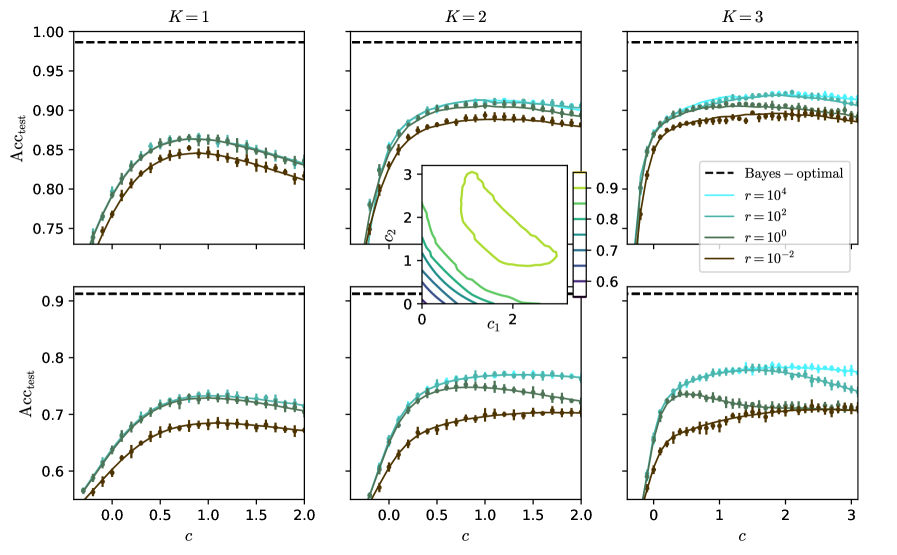</details> Figure 2: Predicted test accuracy $\mathrm{Acc}_{\mathrm{test}}$ for different values of $K$ . Top: for $\lambda=1.5$ , $\mu=3$ and logistic loss; bottom: for $\lambda=1$ , $\mu=2$ and quadratic loss; $\alpha=4$ and $\rho=0.1$ . We take $c_{k}=c$ for all $k$ . Inset: $\mathrm{Acc}_{\mathrm{test}}$ vs $c_{1}$ and $c_{2}$ at $K=2$ and at large $r$ . Dots: numerical simulation of the GCN for $N=10^{4}$ and $d=30$ , averaged over ten experiments. #### III.1.2 Analytical solution In general the system of self-consistent equations (37 - 48) has to be solved numerically. The equations are applied iteratively, starting from arbitrary $\Theta$ and $\hat{\Theta}$ , until convergence. An analytical solution can be computed in some special cases. We consider ridge regression (i.e. quadratic $\ell$ ) and take $c=0$ no residual connections. Then $\operatorname{Cov}_{\psi_{h}}(h)$ , $\operatorname{Cov}_{\psi_{h}^{\prime}}(h)$ , $V$ and $\hat{V}$ are diagonal. We obtain that $$ \mathrm{Acc}_{\mathrm{test}}=\frac{1}{2}\left(1+\mathrm{erf}\left(\frac{\lambda q_{y,K-1}}{\sqrt{2}}\right)\right)\ ,\quad q_{y,k}=\frac{m_{k}}{\sqrt{Q_{k,k}}}\ . \tag{51} $$ The test accuracy only depends on the angle (or overlap) $q_{y,k}$ between the labels $y$ and the last hidden state $h_{K-1}$ of the GCN. $q_{y,k}$ can easily be computed in the limit $r\to\infty$ . In appendix A.3 we explicit the equations (37 - 50) and give their solution in that limit. In particular we obtain for any $k$ $$ \displaystyle m_{k} \displaystyle=\frac{\rho}{\alpha r}\left(\mu\lambda^{K+k}+\sum_{l=0}^{k}\lambda^{K-k+2l}\right) \displaystyle Q_{k,k} \displaystyle=\frac{\rho}{\alpha^{2}r^{2}}\left(\alpha\left(1+\rho\mu\lambda^{2K}+\rho\sum_{l=1}^{K}\lambda^{2l}\right)\right. \displaystyle\hskip 18.49988pt\left.{}+\sum_{l=0}^{k}\left(1+\rho\sum_{l^{\prime}=1}^{K-1-l}\lambda^{2l^{\prime}}+\frac{\alpha^{2}r^{2}}{\rho}m_{l}^{2}\right)\right)\,. \tag{52} $$ #### III.1.3 Consequences: going to large $K$ is necessary We derive consequences from the previous theoretical predictions. We numerically solve eqs. (37 - 48) for some plausible values of the parameters of the data model. We keep balanced the signals from the graph, $\lambda^{2}$ , and from the features, $\mu^{2}/\alpha$ ; we take $\rho=0.1$ to stick to the common case where few train nodes are available. We focus on searching the architecture that maximizes the test accuracy by varying the loss $\ell$ , the regularization $r$ , the residual connections $c_{k}$ and $K$ . For simplicity we will mostly consider the case where $c_{k}=c$ for all $k$ and for a given $c$ . We compare our theoretical predictions to simulations of the GCN for $N=10^{4}$ in fig. 2; as expected, the predictions are within the statistical errors. Details on the numerics are provided in appendix D. We provide the code to run our predictions in the supplementary material. [26] already studies in detail the effect of $\ell$ , $r$ and $c$ at $K=1$ . It reaches the conclusion that the optimal regularization is $r\to\infty$ , that the choice of the loss $\ell$ has little effect and that there is an optimal $c=c^{*}$ of order one. According to fig. 2, it seems that these results can be extrapolated to $K>1$ . We indeed observe that, for both the quadratic and the logistic loss, at $K\in\{1,2,3\}$ , $r\to\infty$ seems optimal. Then the choice of the loss has little effect, because at large $r$ the output $h(w)$ of the network is small and only the behaviour of $\ell$ around 0 matters. Notice that, though $h(w)$ is small and the error $E_{\mathrm{train/test}}$ is trivially equal to $\ell(0)$ , the sign of $h(w)$ is mostly correct and the accuracy $\mathrm{Acc}_{\mathrm{train/test}}$ is not trivial. Last, according to the inset of fig. 2 for $K=2$ , to take $c_{1}=c_{2}$ is optimal and our assumption $c_{k}=c$ for all $k$ is justified. To take trainable $c_{k}$ would degrade the test performances. We show this in fig. 15 in appendix E, where optimizing the train error $E_{\mathrm{train}}$ over $c_{k}=c$ trivially leads to $c=+\infty$ . Indeed, in this case the graph is discarded and the convolved features are proportional to the features $X$ ; which, if $\alpha\rho$ is small enough, are separable, and lead to a null train error. Consequently $c_{k}$ should be treated as a hyperparameter, tuned to maximize $\mathrm{Acc}_{\mathrm{test}}$ , as we do in the rest of the article. <details> <summary>x3.png Details</summary>  ### Visual Description ## Scatter Plot: Error Rate vs. Regularization Parameter (λ²) ### Overview This scatter plot compares the test error rate (1 - Acc_test) across different regularization parameter values (λ²) for various model configurations. The plot includes multiple data series differentiated by model complexity (K), graph symmetrization, and theoretical benchmarks (Bayes-optimal and τ_BO). ### Components/Axes - **X-axis**: λ² (regularization parameter), logarithmic scale from 10 to 26 - **Y-axis**: 1 - Acc_test (test error rate), logarithmic scale from 10⁻⁶ to 10⁻² - **Legend**: - Symbols: - `●` = α=4, μ=1 - `+` = α=2, μ=2 - Lines: - `---` = Bayes-optimal - `...` = ½τ_BO - Colors: - Dark brown = K=1 - Medium brown = K=2 - Light brown = K=3 - Yellow = Symmetrized graphs (K=2 and K=3) ### Detailed Analysis 1. **Bayes-optimal reference**: The dashed line shows the theoretical minimum error rate, serving as a performance benchmark. 2. **τ_BO reference**: The dotted line represents half the Bayes-optimal error rate (1/2τ_BO), acting as an intermediate target. 3. **Model complexity (K)**: - K=1 (dark brown circles): Highest error rates, consistently above τ_BO line - K=2 (medium brown plus signs): Moderate error rates, approaching τ_BO line - K=3 (light brown circles): Lowest error rates, closest to τ_BO line 4. **Symmetrized graphs**: - K=2 (yellow circles): Slightly higher error than non-symmetrized K=2 - K=3 (yellow circles): Similar performance to non-symmetrized K=3 5. **Parameter combinations**: - α=4, μ=1 (dark brown circles): Best performance across all K values - α=2, μ=2 (brown plus signs): Worst performance, consistently above τ_BO line ### Key Observations 1. **Error reduction trend**: All data series show decreasing error rates as λ² increases, following the Bayes-optimal trend line. 2. **Symmetrization impact**: Symmetrized graphs (yellow circles) show minimal performance difference compared to non-symmetrized versions for K≥2. 3. **Parameter sensitivity**: The α=4, μ=1 configuration (dark brown circles) consistently outperforms α=2, μ=2 (brown plus signs) across all K values. 4. **Convergence pattern**: For λ² > 18, all configurations approach within 10⁻⁴ of the Bayes-optimal error rate. ### Interpretation The plot demonstrates that: 1. **Regularization strength** (λ²) is critical for error minimization, with optimal performance achieved at λ² > 18. 2. **Model complexity** (K) directly impacts error rates, with higher K values enabling better approximation of the Bayes-optimal solution. 3. **Symmetrization** provides limited benefits for K≥2, suggesting diminishing returns in graph structure optimization. 4. **Parameter selection** (α, μ) significantly affects performance, with α=4, μ=1 being the most effective combination. 5. The τ_BO line (1/2τ_BO) acts as a practical target, with all configurations except α=2, μ=2 approaching this threshold at higher λ² values. This analysis suggests that optimal model configuration requires balancing regularization strength (λ² > 18), model complexity (K≥2), and parameter selection (α=4, μ=1), while graph symmetrization offers minimal additional benefits for K≥2. 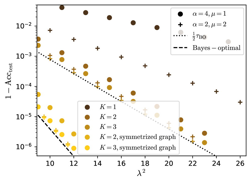</details> Figure 3: Predicted misclassification error $1-\mathrm{Acc}_{\mathrm{test}}$ at large $\lambda$ for two strengths of the feature signal. $r=\infty$ , $c=c^{*}$ is optimized by grid search and $\rho=0.1$ . The dots are theoretical predictions given by numerically solving the self-consistent equations (37 - 48) simplified in the limit $r\to\infty$ . For the symmetrized graph the self-consistent equations are eqs. (87 - 94) in the next part. Finite $K$ : We focus on the effect of varying the number $K$ of aggregation steps. [26] shows that at $K=1$ there is a large gap between the Bayes-optimal test accuracy and the best test accuracy of the GCN. We find that, according to fig. 2, for $K\in\{1,2,3\}$ , to increase $K$ reduces more and more the gap. Thus going to higher depth allows to approach the Bayes-optimality. This also stands as to the learning rate when the signal $\lambda$ of the graph increases. At $\lambda\to\infty$ the GCN is consistent and correctly predicts the labels of all the test nodes, that is $\mathrm{Acc}_{\mathrm{test}}\underset{\lambda\to\infty}{\longrightarrow}1$ . The learning rate $\tau>0$ of the GCN is defined as $$ \log(1-\mathrm{Acc}_{\mathrm{test}})\underset{\lambda\to\infty}{\sim}-\tau\lambda^{2}\ . \tag{54} $$ As shown in [39], the rate $\tau_{\mathrm{BO}}$ of the Bayes-optimal test accuracy is $$ \tau_{\mathrm{BO}}=1\ . \tag{55} $$ For $K=1$ [26] proves that $\tau\leq\tau_{\mathrm{BO}}/2$ and that $\tau\to\tau_{\mathrm{BO}}/2$ when the signal from the features $\mu^{2}/\alpha$ diverges. We obtain that if $K>1$ then $\tau=\tau_{\mathrm{BO}}/2$ for any signal from the features. This is shown on fig. 3, where for $K=1$ the slope of the residual error varies with $\mu$ and $\alpha$ but does not reach half of the Bayes-optimal slope; while for $K>1$ it does, and the features only contribute with a sub-leading order. Analytically, taking the limit in eqs. (52) and (53), at $c=0$ and $r\to\infty$ we have that $$ \underset{\lambda\to\infty}{\mathrm{lim}}q_{y,K-1}\left\{\begin{array}[]{rr}=1&\mathrm{if}\,K>1\\ <1&\mathrm{if}\,K=1\end{array}\right. \tag{56} $$ Since $\log(1-\operatorname{erf}(\lambda q_{y,K-1}/\sqrt{2}))\underset{\lambda\to\infty}{\sim}-\lambda^{2}q_{y,K-1}^{2}/2$ we recover the leading behaviour depicted on fig. 3. $c$ has little effect on the rate $\tau$ ; it only seems to vary the test accuracy by a sub-leading term. Symmetrization: We found that in order to reach the Bayes-optimal rate one has to further symmetrize the graph, according to eq. (14), and to perform the convolution steps by applying $\tilde{A}^{\mathrm{s}}$ instead of $\tilde{A}$ . Then, as shown on fig. 3, the GCN reaches the BO rate for any $K>1$ , at any signal from the features. The reason of this improvement is the following. The GCN we consider is not able to deal with the asymmetry of the graph and the supplementary information it gives. This is shown on fig. 14 in appendix E for different values of $K$ at finite signal, in agreement with [20]. There is little difference in the performance of the simple GCN whether the graph is symmetric or not with same $\lambda$ . As to the rates, as shown by the computation in appendix C, a symmetric graph with signal $\lambda$ would lead to a BO rate $\tau_{\mathrm{BO}}^{\mathrm{s}}=1/2$ , which is the rate the GCN achieves on the asymmetric graph. It is thus better to let the GCN process the symmetrized the graph, which has a higher signal $\lambda^{\mathrm{s}}=\sqrt{2}\lambda$ , and which leads to $\tau=1=\tau_{\mathrm{BO}}$ . Symmetrization is an important step toward the optimality and we will detail the analysis of the GCN on the symmetrized graph in part III.2. Large $K$ and scaling of $c$ : Going to larger $K$ is beneficial and allows the network to approach the Bayes optimality. Yet $K=3$ is not enough to reach it at finite $\lambda$ , and one can ask what happens at larger $K$ . An important point is that $c$ has to be well tuned. On fig. 2 we observe that $c^{*}$ , the optimal $c$ , is increasing with $K$ . To make this point more precise, on fig. 4 we show the predicted test accuracy for larger $K$ for different scalings of $c$ . We take $r=\infty$ since it appears to be the optimal regularization. We consider no residual connections, $c=0$ ; constant residual connections, $c=1$ ; or growing residual connections, $c\propto K$ . <details> <summary>x4.png Details</summary>  ### Visual Description ## Line Chart: Accuracy Test (Acc_test) vs. Parameter K ### Overview The image contains two vertically stacked line charts comparing test accuracy (Acc_test) across different values of parameter K (logarithmic scale from 10⁰ to 10¹). Three data series are plotted with distinct markers: red circles (c=K), blue stars (c=1), and black pluses (c=0). Two reference lines are shown: a red dotted line labeled "continuous limit" and a black dotted line labeled "PCA on the graph." ### Components/Axes - **X-axis (K)**: Logarithmic scale from 10⁰ to 10¹, with gridlines at 10⁰, 10¹. - **Y-axis (Acc_test)**: Ranges from 0.50 to 0.90 in the top subplot and 0.50 to 0.65 in the bottom subplot. - **Legends**: Located in the top-left corner of each subplot, with: - Red circles: `c = K` - Blue stars: `c = 1` - Black pluses: `c = 0` - **Reference Lines**: - Red dotted line: "continuous limit" (top subplot: ~0.90, bottom subplot: ~0.65) - Black dotted line: "PCA on the graph" (top subplot: ~0.85, bottom subplot: ~0.50) ### Detailed Analysis #### Top Subplot (Higher Accuracy Range) - **Red Circles (c=K)**: - Values: ~0.87 (K=1), ~0.90 (K=10), ~0.91 (K=100) - Trend: Slightly increasing with K, plateauing near the red dotted line. - **Blue Stars (c=1)**: - Values: ~0.89 (K=1), ~0.88 (K=10), ~0.86 (K=100) - Trend: Slightly decreasing with K, remaining below red circles. - **Black Pluses (c=0)**: - Values: ~0.85 (K=1), ~0.84 (K=10), ~0.83 (K=100) - Trend: Gradual decline with K, consistently lowest. #### Bottom Subplot (Lower Accuracy Range) - **Red Circles (c=K)**: - Values: ~0.63 (K=1), ~0.64 (K=10), ~0.65 (K=100) - Trend: Slight increase with K, approaching the red dotted line. - **Blue Stars (c=1)**: - Values: ~0.62 (K=1), ~0.61 (K=10), ~0.59 (K=100) - Trend: Decreasing with K, diverging from red circles. - **Black Pluses (c=0)**: - Values: ~0.55 (K=1), ~0.54 (K=10), ~0.53 (K=100) - Trend: Steady decline with K, far below other series. ### Key Observations 1. **Red Circles (c=K)** consistently outperform other series, suggesting parameter adaptation to K improves accuracy. 2. **Black Pluses (c=0)** show the worst performance, indicating fixed parameters (c=0) degrade results as K increases. 3. **Blue Stars (c=1)** maintain mid-tier performance but degrade slightly with larger K. 4. **Reference Lines**: - The red dotted line ("continuous limit") acts as an upper bound for both subplots. - The black dotted line ("PCA on the graph") represents a lower bound, with data points generally above it. ### Interpretation The data demonstrates that parameter scaling (`c=K`) yields the highest accuracy, particularly as K increases. This suggests adaptive parameter selection is critical for performance. The PCA method (`c=0`) underperforms, likely due to information loss from dimensionality reduction. The "continuous limit" line may represent an asymptotic upper bound achievable only with idealized conditions. The divergence between `c=1` and `c=K` in the bottom subplot highlights the importance of parameter tuning in low-resource regimes. 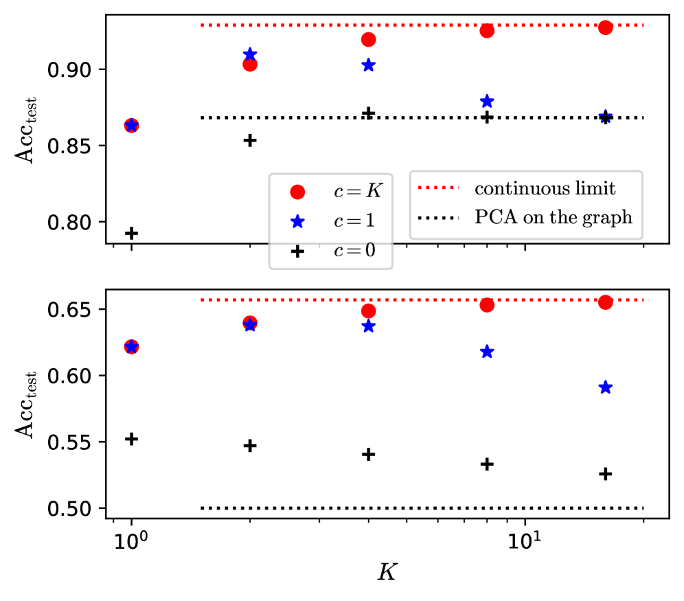</details> Figure 4: Predicted test accuracy $\mathrm{Acc}_{\mathrm{test}}$ vs $K$ for different scalings of $c$ , at $r=\infty$ . Top: for $\lambda=1.5$ , $\mu=3$ ; bottom: for $\lambda=0.7$ , $\mu=1$ ; $\alpha=4$ , $\rho=0.1$ . The predictions are given either by the explicit expression eqs. (51 - 53) for $c=0$ , either by solving the self-consistent equations (37 - 48) simplified in the limit $r\to\infty$ . The performance for the continuous limit are derived and given in the next section III.2, while the performance of PCA on the graph are given by eqs. (59 - 60). A main observation is that, on fig. 4 for $K\to\infty$ , $c=0$ or $c=1$ converge to the same limit while $c\propto K$ converge to a different limit, that has higher accuracy. In the case where $c=0$ or $c=1$ the GCN oversmooths at large $K$ . The limit it converges to corresponds to the accuracy of principal component analysis (PCA) on the sole graph; that is, it corresponds to the accuracy of the estimator $\hat{y}_{\mathrm{PCA}}=\operatorname{sign}\left(\mathrm{Re}(y_{1})\right)$ where $y_{1}$ is the leading eigenvector of $\tilde{A}$ . The overlap $q_{\mathrm{PCA}}$ between $y$ and $\hat{y}_{\mathrm{PCA}}$ and the accuracy are $$ \displaystyle q_{\mathrm{PCA}}=\left\{\begin{array}[]{cr}\sqrt{1-\lambda^{-2}}&\mathrm{if}\,\lambda\geq 1\\ 0&\mathrm{if}\,\lambda\leq 1\end{array}\right.\ , \displaystyle\mathrm{Acc}_{\mathrm{test,PCA}}=\frac{1}{2}\left(1+\mathrm{erf}\left(\frac{\lambda q_{\mathrm{PCA}}}{\sqrt{2}}\right)\right)\ . \tag{59} $$ Consequently, if $c$ does not grow, the GCN will oversmooth at large $K$ , in the sense that all the information from the features $X$ vanishes. Only the information from the graph remains, that can still be informative if $\lambda>1$ . The formula (59 – 60) is obtained by taking the limit $K\to\infty$ in eqs. (51 – 53), for $c=0$ . For any constant $c$ it can also be recovered by considering the leading eigenvector $y_{1}$ of $\tilde{A}$ . At large $K$ , $(\tilde{A}/\sqrt{N}+cI)^{K}$ is dominated by $y_{1}$ and the output of the GCN is $h(w)\propto y_{1}$ for any $w$ . Consequently the GCN exactly acts like thresholded PCA on $\tilde{A}$ . The sharp transition at $\lambda=1$ corresponds to the BBP phase transition in the spectrum of $A^{g}$ and $\tilde{A}$ [56]. According to eqs. (51 – 53) the convergence of $q_{y,K-1}$ toward $q_{\mathrm{PCA}}$ is exponentially fast in $K$ if $\lambda>1$ ; it is like $1/\sqrt{K}$ , much slower, if $\lambda<1$ . The fact that the oversmoothed features can be informative differs from several previous works where they are fully non-informative, such as [9, 10, 40]. This is mainly due to the normalization $\tilde{A}$ of $A$ we use and that these works do not use. It allows to remove the uniform eigenvector $(1,\ldots,1)^{T}$ , that otherwise dominates $A$ and leads to non-informative features. [36] emphasizes on this point and compares different ways of normalizing and correcting $A$ . This work concludes, as we do, that for a correct rescaling $\tilde{A}$ of $A$ , similar to ours, going to higher $K$ is always beneficial if $\lambda$ is high enough, and that the convergence to the limit is exponentially fast. Yet, at large $K$ it obtains bounds on the test accuracy that do not depend on the features: the network they consider still oversmooths in the precise sense we defined. This can be expected since it does not have residual connections, i.e. $c=0$ , that appear to be decisive. In the case where $c\propto K$ the GCN does not oversmooth and it converges to a continuous limit, obtained as $(cI+\tilde{A}/\sqrt{N})^{K}\propto(I+t\tilde{A}/K\sqrt{N})^{K}\to e^{\frac{t\tilde{A}}{\sqrt{N}}}$ . We study this limit in detail in the next part where we predict the resulting accuracy for all constant ratios $t=c/K$ . In general the continuous limit has a better performance than the limit at constant $c$ that relies only on the graph, performing PCA, because it can take in account the features, which bring additional information. Fig. 4 suggests that $\mathrm{Acc}_{\mathrm{test}}$ is monotonically increasing with $K$ if $c\propto K$ and that the continuous limit is the upper-bound on the performance at any $K$ . We will make this point more precise in the next part. Yet we can already see that, for this to be true, one has to correctly tune the ratio $c/K$ : for instance if $\lambda$ is small $\tilde{A}$ mostly contains noise and applying it to $X$ will mostly lower the accuracy. Shortly, if $c/K$ is optimized then $K\to\infty$ is better than any fixed $K$ . Consequently the continuous limit is the correct limit to maximize the test accuracy and it is of particular relevance. ### III.2 Continuous GCN In this section we present the asymptotic characterization of the continuous GCN, both for the asymmetric graph and for its symmetrization. The continuous GCN is the limit of the discrete GCN when the number of convolution steps $K$ diverges while the residual connections $c$ become large. The order parameters that describe it, as well as the self-consistent equations they follow, can be obtained as the limit of those of the discrete GCN. We give a detailed derivation of how the limit is taken, since it is of independent interest. The outcome is that the state $h$ of the GCN across the convolutions is described by a set of equations resembling the dynamical mean-field theory. The order parameters of the problem are continuous functions and the self-consistent equations can be expressed by expansion around large regularization $r\to\infty$ as integral equations, that specialize to differential equations in the asymmetric case. The resulting equations can be solved analytically; for asymmetric graphs, the covariance and its conjugate are propagators (or resolvant) of the two-dimensional Klein-Gordon equation. We show numerically that our approach is justified and agrees with simulations. Last we show that going to the continuous limit while symmetrizing the graph corresponds to the optimum of the architecture and allows to approach the Bayes-optimality. #### III.2.1 Asymptotic characterization To deal with both cases, asymmetric or symmetrized, we define $(\delta_{\mathrm{e}},\tilde{A}^{\mathrm{e}},\lambda^{\mathrm{e}})\in\{(0,\tilde{A},\lambda),(1,\tilde{A}^{\mathrm{s}},\lambda^{\mathrm{s}})\}$ , where we remind that $\tilde{A}^{\mathrm{s}}$ is the symmetrized $\tilde{A}$ with effective signal $\lambda^{\mathrm{s}}=\sqrt{2}\lambda$ . In particular $\delta_{\mathrm{e}}=0$ for the asymmetric and $\delta_{\mathrm{e}}=1$ for the symmetrized. The continuous GCN is defined by the output function $$ h(w)=e^{\frac{t}{\sqrt{N}}\tilde{A}^{\mathrm{e}}}\frac{1}{\sqrt{N}}Xw\ . \tag{61} $$ We first derive the free entropy of the discretization of the GCN and then take the continuous limit. The discretization at finite $K$ is $$ \displaystyle h(w)=h_{K}\ , \displaystyle h_{k+1}=\left(I_{N}+\frac{t}{K\sqrt{N}}\tilde{A}^{\mathrm{e}}\right)h_{k}\ , \displaystyle h_{0}=\frac{1}{\sqrt{N}}Xw\ . \tag{62} $$ In the case of the asymmetric graph this discretization can be mapped to the discrete GCN of the previous section A as detailed in eq. (16) and the following paragraph; the free entropy and the order parameters of the two models are the same, up to a rescaling by $c$ . The order parameters of the discretization of the GCN are $m_{w}\in\mathbb{R},Q_{w}\in\mathbb{R},V_{w}\in\mathbb{R},m\in\mathbb{R}^{K},Q_{h}\in\mathbb{R}^{K\times K},V_{h}\in\mathbb{R}^{K\times K}$ , their conjugates $\hat{m}_{w}\in\mathbb{R},\hat{Q}_{w}\in\mathbb{R},\hat{V}_{w}\in\mathbb{R},\hat{m}\in\mathbb{R},\hat{Q}_{h}\in\mathbb{R}^{K\times K},\hat{V}_{h}\in\mathbb{R}^{K\times K}$ and the two additional order parameters $Q_{qh}\in\mathbb{R}^{K\times K}$ and $V_{qh}\in\mathbb{R}^{K\times K}$ that account for the supplementary correlations the symmetry of the graph induces; $Q_{qh}=V_{qh}=0$ for the asymmetric case. The free entropy and its derivation are given in appendix B. The outcome is that $h$ is described by the effective low-dimensional potential $\psi_{h}$ over $\mathbb{R}^{K+1}$ that is $$ \displaystyle\psi_{h}(h;\bar{s}) \displaystyle=-\frac{1}{2}h^{T}Gh+h^{T}\left(B_{h}+D_{qh}^{T}G_{0}^{-1}B\right)\ ; \tag{65} $$ where $$ \displaystyle G \displaystyle=G_{h}+D_{qh}^{T}G_{0}^{-1}D_{qh}\ , \displaystyle G_{h} \displaystyle=\left(\begin{smallmatrix}\hat{V}_{h}&0\\ 0&\bar{s}\end{smallmatrix}\right)\ , \displaystyle G_{0} \displaystyle=\left(\begin{smallmatrix}K^{2}V_{w}&0\\ 0&t^{2}V_{h}\end{smallmatrix}\right)\ , \displaystyle D_{qh} \displaystyle=D-t\left(\begin{smallmatrix}0&0\\ -\mathrm{i}\delta_{\mathrm{e}}V_{qh}^{T}&0\end{smallmatrix}\right) \tag{66} $$ are $(K+1)\times(K+1)$ block matrices; $$ \displaystyle D \displaystyle=K\left(\begin{smallmatrix}1&&&0\\ -1&\ddots&&\\ &\ddots&\ddots&\\ 0&&-1&1\end{smallmatrix}\right) \tag{70} $$ is the $(K+1)\times(K+1)$ discrete derivative; $$ \displaystyle B \displaystyle=\left(\begin{smallmatrix}K\sqrt{Q_{w}}\chi\\ \mathrm{i}t\left(\hat{Q}^{1/2}\zeta\right)_{q}\end{smallmatrix}\right)+y\left(\begin{smallmatrix}K\sqrt{\mu}m_{w}\\ \lambda^{\mathrm{e}}tm\end{smallmatrix}\right)\ , \displaystyle B_{h} \displaystyle=\left(\begin{smallmatrix}\left(\hat{Q}^{1/2}\zeta\right)_{h}\\ 0\end{smallmatrix}\right)+y\left(\begin{smallmatrix}\hat{m}\\ \bar{s}\end{smallmatrix}\right)\ , \displaystyle\left(\begin{smallmatrix}(\hat{Q}^{1/2}\zeta)_{q}\\ (\hat{Q}^{1/2}\zeta)_{h}\end{smallmatrix}\right) \displaystyle=\left(\begin{smallmatrix}-Q_{h}&-\delta_{\mathrm{e}}Q_{qh}^{T}\\ -\delta_{\mathrm{e}}Q_{qh}&\hat{Q}_{h}\end{smallmatrix}\right)^{1/2}\left(\begin{smallmatrix}\zeta_{q}\\ \zeta_{h}\end{smallmatrix}\right) \tag{71} $$ are vectors of size $K+1$ , where $y=\pm 1$ is Rademacher and $\zeta_{q}\sim\mathcal{N}(0,I_{K+1})$ , $\zeta_{h}\sim\mathcal{N}(0,I_{K+1})$ and $\chi\sim\mathcal{N}(0,1)$ are standard Gaussians. $\bar{s}$ determines whether the loss is active $\bar{s}=1$ or not $\bar{s}=0$ . We assumed that $\ell$ is quadratic. Later we will take the limit $r\to\infty$ where $h$ is small and where $\ell$ can effectively be expanded around $0$ as a quadratic potential. Notice that in the case $\delta_{\mathrm{e}}=0$ we recover the potential $\psi_{h}$ eq. (30) of the previous part. This potential eq. (65) corresponds to a one dimensional interacting chain, involving the positions $h$ and their effective derivative $D_{qh}h$ , and with constraints at the two ends, for the loss on $h_{K}$ and the regularized weights on $h_{0}$ . Its extremizer $h^{*}$ is $$ h^{*}=G^{-1}\left(B_{h}+D_{qh}^{T}G_{0}^{-1}B\right)\ . \tag{74} $$ The order parameters are determined by the following fixed-point equations, obtained by extremizing the free entropy. As before $\mathcal{P}$ acts by linearly combining quantities evaluated at $h^{*}$ , taken with $\bar{s}=1$ and $\bar{s}=0$ with weights $\rho$ and $1-\rho$ . $$ \displaystyle m_{w}=\frac{1}{\alpha}\frac{\hat{m}_{w}}{r+\hat{V}_{w}} \displaystyle Q_{w}=\frac{1}{\alpha}\frac{\hat{Q}_{w}+\hat{m}_{w}^{2}}{(r+\hat{V}_{w})^{2}} \displaystyle V_{w}=\frac{1}{\alpha}\frac{1}{r+\hat{V}_{w}} \displaystyle\left(\begin{smallmatrix}\hat{m}_{w}\\ \hat{m}\\ m\\ \cdot\end{smallmatrix}\right)=\left(\begin{smallmatrix}K\sqrt{\mu}&&0\\ &\lambda^{\mathrm{e}}tI_{K}&\\ 0&&I_{K+1}\end{smallmatrix}\right)\mathbb{E}_{y,\xi,\zeta}\,y\mathcal{P}\left(\begin{smallmatrix}G_{0}^{-1}(D_{qh}h-B)\\ h\end{smallmatrix}\right) \displaystyle\begin{multlined}\left(\begin{smallmatrix}\hat{Q}_{w}&&&\cdot\\ &\hat{Q}_{h}&Q_{qh}&\\ &Q_{qh}^{T}&Q_{h}&\\ \cdot&&&\cdot\end{smallmatrix}\right)=\left(\begin{smallmatrix}K&&0\\ &tI_{K}&\\ 0&&I_{K+1}\end{smallmatrix}\right)\\ \hskip 18.49988pt\mathbb{E}_{y,\xi,\zeta}\mathcal{P}\left(\left(\begin{smallmatrix}G_{0}^{-1}(D_{qh}h-B)\\ h\end{smallmatrix}\right)^{\otimes 2}\right)\left(\begin{smallmatrix}K&&0\\ &tI_{K}&\\ 0&&I_{K+1}\end{smallmatrix}\right)\end{multlined}\left(\begin{smallmatrix}\hat{Q}_{w}&&&\cdot\\ &\hat{Q}_{h}&Q_{qh}&\\ &Q_{qh}^{T}&Q_{h}&\\ \cdot&&&\cdot\end{smallmatrix}\right)=\left(\begin{smallmatrix}K&&0\\ &tI_{K}&\\ 0&&I_{K+1}\end{smallmatrix}\right)\\ \hskip 18.49988pt\mathbb{E}_{y,\xi,\zeta}\mathcal{P}\left(\left(\begin{smallmatrix}G_{0}^{-1}(D_{qh}h-B)\\ h\end{smallmatrix}\right)^{\otimes 2}\right)\left(\begin{smallmatrix}K&&0\\ &tI_{K}&\\ 0&&I_{K+1}\end{smallmatrix}\right) \displaystyle\left(\begin{smallmatrix}\cdot&\cdot\\ -\mathrm{i}V_{qh}&\cdot\end{smallmatrix}\right)=t\mathcal{P}\left(G_{0}^{-1}D_{qh}G^{-1}\right) \displaystyle\left(\begin{smallmatrix}V_{h}&\cdot\\ \cdot&\cdot\end{smallmatrix}\right)=\mathcal{P}\left(G^{-1}\right) \displaystyle\left(\begin{smallmatrix}\hat{V}_{w}&\cdot\\ \cdot&\hat{V}_{h}\end{smallmatrix}\right)=\left(\begin{smallmatrix}K^{2}&0\\ 0&t^{2}I_{K}\end{smallmatrix}\right)\mathcal{P}\left(G_{0}^{-1}-G_{0}^{-1}D_{qh}G^{-1}D_{qh}^{T}G_{0}^{-1}\right) \tag{75} $$ where $\cdot$ are unspecified elements that pad the vector to the size $2(K+1)$ and the matrices to the size $2(K+1)\times 2(K+1)$ and $(K+1)\times(K+1)$ . On $w$ we assumed $l_{2}$ regularization and obtained the same equations as in part III.1. Once a solution to this system is found the train and test accuracies are expressed as $$ \displaystyle\mathrm{Acc}_{\mathrm{train/test}}=\mathbb{E}_{y,\zeta,\chi}\delta_{y=\operatorname{sign}(h_{K}^{*})}\ , \tag{85} $$ taking $\bar{s}=1$ or $\bar{s}=0$ . #### III.2.2 Expansion around large regularization $r$ and continuous limit Solving the above self-consistent equations (75 - 84) is difficult as such. One can solve them numerically by repeated updates; but this does not allow to go to large $K$ because of numerical instability. One has to invert $G$ eq. (66) and to make sense of the continuous limit of matrix inverts. This is an issue in the sense that, for a generic $K\times K$ matrix $(M)_{ij}$ whose elements vary smoothly with $i$ and $j$ in the limit of large $K$ , the elements of its inverse $M^{-1}$ are not necessarly continuous with respect to their indices and can vary with a large magnitude. Our analysis from the previous part III.1 gives an insight on how to achieve this. It appears that the limit of large regularization $r\to\infty$ is of particular relevance. In this limit the above system can be solved analytically thanks to an expansion around large $r$ . This expansion is natural in the sense that it leads to several simplifications and corresponds to expanding the matrix inverts in Neumann series. Keeping the first terms of the expansion the limit $K\to\infty$ is then well defined. In this section we detail this expansion; we take the continuous limit and, keeping the first constant order, we solve (75 - 84). In the limit of large regularization $h$ and $w$ are of order $1/r$ ; the parameters $m_{w}$ , $m$ , $V_{w}$ and $V$ are of order $1/r$ and $Q_{w}$ and $Q$ are of order $1/r^{2}$ , while all their conjugates, $Q_{qh}$ and $V_{qh}$ are of order one. Consequently we have $G_{0}^{-1}\sim r\gg G_{h}\sim 1$ and we expand $G^{-1}$ around $G_{0}$ : $$ \displaystyle G^{-1} \displaystyle=D_{qh}^{-1}G_{0}D_{qh}^{-1,T}\sum_{a\geq 0}\left(-G_{h}D_{qh}^{-1}G_{0}D_{qh}^{-1,T}\right)^{a}\ . \tag{86} $$ Constant order: We detail how to solve the self-consistent equations (75 - 84) taking the continuous limit $K\to\infty$ at the constant order in $1/r$ . As we will show later, truncating $G^{-1}$ to the constant order gives predictions that are close to the simulations at finite $r$ , even for $r\approx 1$ if $t$ is not too large. Considering higher orders is feasible but more challenging and we will only provide insights on how to pursue the computation. The truncated expansion gives, starting from the variances: $$ \displaystyle\left(\begin{smallmatrix}\cdot&\cdot\\ -\mathrm{i}V_{qh}&\cdot\end{smallmatrix}\right) \displaystyle=tD_{qh}^{-1,T}\ , \displaystyle\left(\begin{smallmatrix}V_{h}&\cdot\\ \cdot&\cdot\end{smallmatrix}\right) \displaystyle=D_{qh}^{-1}\left(\begin{smallmatrix}K^{2}V_{w}&0\\ 0&t^{2}V_{h}\end{smallmatrix}\right)D_{qh}^{-1,T}, \displaystyle\left(\begin{smallmatrix}\hat{V}_{w}&\cdot\\ \cdot&\hat{V}_{h}\end{smallmatrix}\right) \displaystyle=\left(\begin{smallmatrix}K^{2}&0\\ 0&t^{2}I_{K}\end{smallmatrix}\right)D_{qh}^{-1,T}\left(\begin{smallmatrix}\hat{V}_{h}&0\\ 0&\rho\end{smallmatrix}\right)D_{qh}^{-1}\ . \tag{87} $$ We kept the order $a=0$ for $V_{qh}$ and $V_{h}$ , and the orders $a\leq 1$ for $\hat{V}_{w}$ and $\hat{V}_{h}$ . We expand $h^{*}\approx D_{qh}^{-1}G_{0}D_{qh}^{-1,T}B_{h}+D_{qh}^{-1}B$ keeping the order $a=0$ and obtain the remaining self-consistent equations $$ \displaystyle\left(\begin{smallmatrix}\hat{m}_{w}\\ \hat{m}\end{smallmatrix}\right) \displaystyle=\left(\begin{smallmatrix}K\sqrt{\mu}&0\\ 0&\lambda^{\mathrm{e}}tI_{K}\cdot\end{smallmatrix}\right)D_{qh}^{-1,T}\left(\begin{smallmatrix}\hat{m}\\ \rho\end{smallmatrix}\right) \displaystyle\left(\begin{smallmatrix}m\\ \cdot\end{smallmatrix}\right) \displaystyle=D_{qh}^{-1}G_{0}D_{qh}^{-1,T}\left(\begin{smallmatrix}\hat{m}\\ \rho\end{smallmatrix}\right)+D_{qh}^{-1}\left(\begin{smallmatrix}K\sqrt{\mu}m_{w}\\ \lambda^{\mathrm{e}}tm\end{smallmatrix}\right) \tag{90} $$ $$ \displaystyle\left(\begin{smallmatrix}\hat{Q}_{w}&\cdot\\ \cdot&\hat{Q}_{h}\end{smallmatrix}\right) \displaystyle=\left(\begin{smallmatrix}K&0\\ 0&tI_{K}\end{smallmatrix}\right)D_{qh}^{-1,T}\left(\left(\begin{smallmatrix}\hat{Q}_{h}&0\\ 0&0\end{smallmatrix}\right)+\rho\left(\begin{smallmatrix}\hat{m}\\ 1\end{smallmatrix}\right)^{\otimes 2}+(1-\rho)\left(\begin{smallmatrix}\hat{m}\\ 0\end{smallmatrix}\right)^{\otimes 2}\right)D_{qh}^{-1}\left(\begin{smallmatrix}K&0\\ 0&tI_{K}\end{smallmatrix}\right) \displaystyle\left(\begin{smallmatrix}\cdot&\cdot\\ -\mathrm{i}Q_{qh}&\cdot\end{smallmatrix}\right) \displaystyle=tD_{qh}^{-1,T}\left[\left(t\delta_{\mathrm{e}}\left(\begin{smallmatrix}0&-\mathrm{i}Q_{qh}\\ 0&0\end{smallmatrix}\right)+\left(\begin{smallmatrix}\hat{m}\\ \rho\end{smallmatrix}\right)\left(\begin{smallmatrix}K\sqrt{\mu}m_{w}\\ \lambda^{\mathrm{e}}tm\end{smallmatrix}\right)^{T}\right)D_{qh}^{-1,T}+\left(\left(\begin{smallmatrix}\hat{Q}_{h}&0\\ 0&0\end{smallmatrix}\right)+\rho\left(\begin{smallmatrix}\hat{m}\\ 1\end{smallmatrix}\right)^{\otimes 2}+(1-\rho)\left(\begin{smallmatrix}\hat{m}\\ 0\end{smallmatrix}\right)^{\otimes 2}\right)D_{qh}^{-1}G_{0}D_{qh}^{-1,T}\right] \displaystyle\left(\begin{smallmatrix}Q_{h}&\cdot\\ \cdot&\cdot\end{smallmatrix}\right) \displaystyle=D_{qh}^{-1}G_{0}D_{qh}^{-1,T}\left(\left(\begin{smallmatrix}\hat{Q}_{h}&0\\ 0&0\end{smallmatrix}\right)+\rho\left(\begin{smallmatrix}\hat{m}\\ 1\end{smallmatrix}\right)^{\otimes 2}+(1-\rho)\left(\begin{smallmatrix}\hat{m}\\ 0\end{smallmatrix}\right)^{\otimes 2}\right)D_{qh}^{-1}G_{0}D_{qh}^{-1,T}+D_{qh}^{-1}\left(\left(\begin{smallmatrix}K^{2}Q_{w}&0\\ 0&t^{2}Q_{h}\end{smallmatrix}\right)+\left(\begin{smallmatrix}K\sqrt{\mu}m_{w}\\ \lambda^{\mathrm{e}}tm\end{smallmatrix}\right)^{\otimes 2}\right)D_{qh}^{-1,T} \displaystyle{}+D_{qh}^{-1}G_{0}D_{qh}^{-1,T}\left(t\delta_{\mathrm{e}}\left(\begin{smallmatrix}0&-\mathrm{i}Q_{qh}\\ 0&0\end{smallmatrix}\right)+\left(\begin{smallmatrix}\hat{m}\\ \rho\end{smallmatrix}\right)\left(\begin{smallmatrix}K\sqrt{\mu}m_{w}\\ \lambda^{\mathrm{e}}tm\end{smallmatrix}\right)^{T}\right)D_{qh}^{-1,T}+D_{qh}^{-1}\left(t\delta_{\mathrm{e}}\left(\begin{smallmatrix}0&0\\ -\mathrm{i}Q_{qh}^{T}&0\end{smallmatrix}\right)+\left(\begin{smallmatrix}K\sqrt{\mu}m_{w}\\ \lambda^{\mathrm{e}}tm\end{smallmatrix}\right)\left(\begin{smallmatrix}\hat{m}\\ \rho\end{smallmatrix}\right)^{T}\right)D_{qh}^{-1}G_{0}D_{qh}^{-1,T} \tag{92} $$ We see that all these self-consistent equations (88 - 94) are vectorial or matricial equations of the form $x=\lambda^{\mathrm{e}}tD_{qh}^{-1}x$ or $X=t^{2}D_{qh}^{-1}XD_{qh}^{-1,T}$ , over $x$ or $X$ , plus inhomogenuous terms and boundary conditions at 0 or $(0,0)$ . The equations are recursive in the sense that each equation only depends on the previous ones and they can be solved one by one. It is thus enough to compute the resolvants of these two equations. Last eq. (87) shows how to invert $D_{qh}$ and express $D_{qh}^{-1}$ . These different properties make the system of self-consistent equations easily solvable, provided one can compute $D_{qh}$ and the two resolvants. This furthermore highlights the relevance of the $r\to\infty$ limit. We take the continuous limit $K\to\infty$ . We translate the above self-consistent equations into functional equations. Thanks to the expansion around large $r$ we have a well defined limit, that does not involve any matrix inverse. We set $x=k/K$ and $z=l/K$ continuous indices ranging from 0 to 1. We extend the vectors and the matrices by continuity to match the correct dimensions. We apply the following rescaling to obtain quantities that are independent of $K$ in that limit: $$ \displaystyle\hat{m}\to K\hat{m}\ , \displaystyle\hat{Q}_{h}\to K^{2}\hat{Q}_{h}\ , \displaystyle\hat{V}_{h}\to K^{2}\hat{V}_{h}\ , \displaystyle Q_{qh}\to KQ_{qh}\ , \displaystyle V_{qh}\to KV_{qh}\ . \tag{95} $$ We first compute the effective derivative $D_{qh}=D-t\left(\begin{smallmatrix}0&0\\ -\mathrm{i}\delta_{\mathrm{e}}V_{qh}^{T}&0\end{smallmatrix}\right)$ and its inverse. In the asymmetric case we have $D_{qh}=D$ , the usual derivative. In the symmetric case we have $D_{qh}=D-tV_{qh}^{T}$ where $V_{qh}$ satisfies eq. (87) which reads $$ \displaystyle\partial_{z}V_{qh}(x,z)+\delta(z)V_{qh}(x,z)= \displaystyle\qquad\qquad t\delta(z-x)+t\int_{0}^{1}\mathrm{d}x^{\prime}\,V_{qh}(x,x^{\prime})V_{qh}(x^{\prime},z)\ , \tag{97} $$ where we multiplied both sides by $D_{qh}^{T}$ and took $V_{qh}(x,z)$ for $-\mathrm{i}V_{qh}$ . The solution to this integro-differential equation is $$ \displaystyle V_{qh}(x,z) \displaystyle=\theta(z-x)\frac{I_{1}(2t(z-x))}{z-x} \tag{98} $$ with $\theta$ the step function and $I_{\nu}$ the modified Bessel function of the second kind of order $\nu$ . Consequently we obtain the effective inverse derivative $$ \displaystyle D_{qh}^{-1}(x,z) \displaystyle=D_{qh}^{-1,T}(z,x)=\left\{\begin{array}[]{cc}\theta(x-z)&\mathrm{if}\,\delta_{\mathrm{e}}=0\\ \frac{1}{t}V_{qh}(z,x)&\mathrm{if}\,\delta_{\mathrm{e}}=1\end{array}\right.\ . \tag{101} $$ We then define the resolvants (or propagators) $\varphi$ and $\Phi$ of the integral equations as $$ \displaystyle D_{qh}\varphi(x) \displaystyle=\lambda^{\mathrm{e}}t\varphi(x)+\delta(x)\ , \displaystyle D_{qh}\Phi(x,z)D_{qh}^{T} \displaystyle=t^{2}\Phi(x,z)+\delta(x,z)\ . \tag{102} $$ Notice that in the asymmetric case, $D_{qh}=\partial_{x}$ , $D_{qh}^{T}=\partial_{z}$ and $\Phi$ is the propagator of the two-dimensional Klein-Gordon equation up to a change of variables. The resolvants can be expressed as $$ \displaystyle\varphi(x) \displaystyle=\left\{\begin{array}[]{cc}e^{\lambda^{\mathrm{e}}tx}&\mathrm{if}\,\delta_{\mathrm{e}}=0\\ \sum_{\nu>0}^{\infty}\nu(\lambda^{\mathrm{e}})^{\nu-1}\frac{I_{\nu}(2tx)}{tx}&\mathrm{if}\,\delta_{\mathrm{e}}=1\end{array}\right.\ , \displaystyle\Phi(x,z) \displaystyle=\left\{\begin{array}[]{cc}I_{0}(2t\sqrt{xz})&\mathrm{if}\,\delta_{\mathrm{e}}=0\\ \frac{I_{1}(2t(x+z))}{t(x+z)}&\mathrm{if}\,\delta_{\mathrm{e}}=1\end{array}\right.\ . \tag{106} $$ We obtain the solution of the self-consistent equations by convolving $\varphi$ or $\Phi$ with the non-homogenuous terms. We flip $\hat{m}$ along it axis to match the vectorial equation with boundary condition at $x=0$ ; we do the same for $\hat{V}_{h}$ and $\hat{Q}_{h}$ along there two axes, and for $Q_{qh}$ along its first axis. This gives the following expressions for the order parameters: $$ \displaystyle V_{w}=\frac{1}{r\alpha} \displaystyle V_{h}(x,z)=V_{w}\Phi(x,z) \displaystyle\hat{V}_{h}(1-x,1-z)=t^{2}\rho\Phi(x,z) \displaystyle\hat{V}_{w}=t^{-2}\hat{V}_{h}(0,0) \displaystyle\hat{m}(1-x)=\rho\lambda^{\mathrm{e}}t\varphi(x) \displaystyle\hat{m}_{w}=\sqrt{\mu}\frac{1}{\lambda^{\mathrm{e}}t}\hat{m}(0) \displaystyle m_{w}=\frac{\hat{m}_{w}}{r\alpha} \displaystyle m(x)=(1+\mu)\frac{m_{w}}{\sqrt{\mu}}\varphi(x) \displaystyle\qquad{}+\frac{t}{\lambda^{\mathrm{e}}}\int_{0}^{x}\mathrm{d}x^{\prime}\int_{0}^{1}\mathrm{d}x^{\prime\prime}\,\varphi(x-x^{\prime})V_{h}(x^{\prime},x^{\prime\prime})\hat{m}(x^{\prime\prime}) \displaystyle\hat{Q}_{w}=t^{-2}\hat{Q}_{h}(0,0) \displaystyle Q_{w}=\frac{\hat{Q}_{w}+\hat{m}_{w}^{2}}{r^{2}\alpha} \tag{110} $$ $$ \displaystyle\hat{Q}_{h}(1-x,1-z)=t^{2}\int_{0^{-},0^{-}}^{x,z}\mathrm{d}x^{\prime}\mathrm{d}z^{\prime}\ \Phi(x-x^{\prime},z-z^{\prime})\left[\mathcal{P}(\hat{m}^{\otimes 2})(1-x^{\prime},1-z^{\prime})\right] \displaystyle Q_{qh}(1-x,z)=t\int_{0^{-},0^{-}}^{x,z}\mathrm{d}x^{\prime}\mathrm{d}z^{\prime}\ \Phi(x-x^{\prime},z-z^{\prime})\Bigg[\mathcal{P}(\hat{m})(1-x^{\prime})(\lambda^{\mathrm{e}}tm(z^{\prime})+\sqrt{\mu}m_{w}\delta(z^{\prime})) \displaystyle\hskip 18.49988pt\left.{}+\int_{0,0^{-}}^{1^{+},1}\mathrm{d}x^{\prime\prime}\mathrm{d}z^{\prime\prime}\,\left(\hat{Q}_{h}(1-x^{\prime},x^{\prime\prime})+\mathcal{P}(\hat{m}^{\otimes 2})(1-x^{\prime},x^{\prime\prime})\right)D_{qh}^{-1}(x^{\prime\prime},z^{\prime\prime})G_{0}(z^{\prime\prime},z^{\prime})\right] \tag{120} $$ $$ \displaystyle Q_{h}(x,z)=\int_{0^{-},0^{-}}^{x,z}\mathrm{d}x^{\prime}\mathrm{d}z^{\prime}\ \Phi(x-x^{\prime},z-z^{\prime})\Bigg[\hat{Q}_{w}\delta(x^{\prime},z^{\prime})+(\lambda^{\mathrm{e}}tm(x^{\prime})+\sqrt{\mu}m_{w}\delta(x^{\prime}))(\lambda^{\mathrm{e}}tm(z^{\prime})+\sqrt{\mu}m_{w}\delta(z^{\prime})) \displaystyle\hskip 18.49988pt{}+\int_{0^{-},0}^{1,1^{+}}\mathrm{d}x^{\prime\prime}\mathrm{d}x^{\prime\prime\prime}\,G_{0}(x^{\prime},x^{\prime\prime})D_{qh}^{-1,T}(x^{\prime\prime},x^{\prime\prime\prime})\left(t\delta_{\mathrm{e}}Q_{qh}(x^{\prime\prime\prime},z^{\prime})+\mathcal{P}(\hat{m})(x^{\prime\prime\prime})(\lambda^{\mathrm{e}}tm(z^{\prime})+\sqrt{\mu}m_{w}\delta(z^{\prime}))\right) \displaystyle\hskip 18.49988pt{}+\int_{0,0^{-}}^{1^{+},1}\mathrm{d}z^{\prime\prime\prime}\mathrm{d}z^{\prime\prime}\,\left(t\delta_{\mathrm{e}}Q_{qh}(z^{\prime\prime\prime},x^{\prime})+(\lambda^{\mathrm{e}}tm(x^{\prime})+\sqrt{\mu}m_{w}\delta(x^{\prime}))\mathcal{P}(\hat{m})(z^{\prime\prime\prime})\right)D_{qh}^{-1}(z^{\prime\prime\prime},z^{\prime\prime})G_{0}(z^{\prime\prime},z^{\prime}) \displaystyle\qquad\left.{}+\int_{0^{-},0,0,0^{-}}^{1,1^{+},1^{+},1}\mathrm{d}x^{\prime\prime}\mathrm{d}x^{\prime\prime\prime}\mathrm{d}z^{\prime\prime\prime}\mathrm{d}z^{\prime\prime}\,G_{0}(x^{\prime},x^{\prime\prime})D_{qh}^{-1,T}(x^{\prime\prime},x^{\prime\prime\prime})\left(\hat{Q}_{h}(x^{\prime\prime\prime},z^{\prime\prime\prime})+\mathcal{P}(\hat{m}^{\otimes 2})(x^{\prime\prime\prime},z^{\prime\prime\prime})\right)D_{qh}^{-1}(z^{\prime\prime\prime},z^{\prime\prime})G_{0}(z^{\prime\prime},z^{\prime})\right]\ ; \tag{122} $$ where we set $$ \displaystyle\mathcal{P}(\hat{m})(x) \displaystyle=\hat{m}(x)+\rho\delta(1-x)\ , \displaystyle\mathcal{P}(\hat{m}^{\otimes 2})(x,z) \displaystyle=\rho\left(\hat{m}(x)+\delta(1-x)\right)\left(\hat{m}(z)+\delta(1-z)\right) \displaystyle\quad{}+(1-\rho)\hat{m}(x)\hat{m}(z)\ , \displaystyle G_{0}(x,z) \displaystyle=t^{2}V_{h}(x,z)+V_{w}\delta(x,z) \tag{123} $$ and take $Q_{qh}(x,z)$ for $-\mathrm{i}Q_{qh}$ . The accuracies are, with $\bar{s}=1$ for train and $\bar{s}=0$ for test: $$ \displaystyle\mathrm{Acc}_{\mathrm{train/test}}= \displaystyle\qquad\frac{1}{2}\left(1+\mathrm{erf}\left(\frac{m(1)+(\bar{s}-\rho)V_{h}(1,1)}{\sqrt{2}\sqrt{Q_{h}(1,1)-m(1)^{2}-\rho(1-\rho)V_{h}(1,1)^{2}}}\right)\right)\ . \tag{126} $$ Notice that we fully solved the model, in a certain limit, by giving an explicit expression of the performance of the GCN. This is an uncommon result in the sense that, in several works analyzing the performance of neural networks in a high-dimensional limit, the performance are only expressed as the function of the self-consistent of a system of equations similar to ours (75 - 84). These systems have to be solved numerically, which may be unsatisfactory for the understanding of the studied models. So far, we dealt with infinite regularization $r$ keeping only the first constant order. The predicted accuracy (126) does not depend on $r$ . We briefly show how to pursue the computation at any order in appendix B.4, by a perturbative approach with expansion in powers of $1/r$ . Interpretation in terms of dynamical mean-field theory: The order parameters $V_{h}$ , $V_{qh}$ and $\hat{V}_{h}$ come from the replica computation and were introduced as the covariances between $h$ and its conjugate $q$ . Their values are determined by extremizing the free entropy of the problem. In the above lines we derived that $V_{h}(x,z)\propto\Phi(x,z)$ is the forward propagator, from the weights to the loss, while $\hat{V}_{h}(x,z)\propto\Phi(1-x,1-z)$ is the backward propagator, from the loss to the weights. In this section we state an equivalence between these order parameters and the correlation and response functions of the dynamical process followed by $h$ . We introduce the tilting field $\eta(x)\in\mathbb{R}^{N}$ and the tilted Hamiltonian as $$ \displaystyle\frac{\mathrm{d}h}{\mathrm{d}x}(x)=\frac{t}{\sqrt{N}}\tilde{A}^{\mathrm{e}}h(x)+\eta(x)+\delta(x)\frac{1}{\sqrt{N}}Xw\ , \displaystyle h(x)=\int_{0^{-}}^{x}\mathrm{d}x^{\prime}e^{(x-x^{\prime})\frac{t}{\sqrt{N}}\tilde{A}^{\mathrm{e}}}\left(\eta(x^{\prime})+\delta(x^{\prime})\frac{1}{\sqrt{N}}Xw\right)\ , \displaystyle H(\eta)=\frac{1}{2}(y-h(1))^{T}R(y-h(1))+\frac{r}{2}w^{T}w\ , \tag{127} $$ where $R\in\mathbb{R}^{N\times N}$ diagonal accounts for the train and test nodes. We write $\langle\cdot\rangle_{\beta}$ the expectation under the density $e^{-\beta H(\eta)}/Z$ (normalized only at $\eta=0$ ). Then we have $$ \displaystyle V_{h}(x,z) \displaystyle=\frac{\beta}{N}\operatorname{Tr}\left[\langle h(x)h(z)^{T}\rangle_{\beta}-\langle h(x)\rangle_{\beta}\langle h(z)^{T}\rangle_{\beta}\right]|_{\eta=0}\ , \displaystyle V_{qh}(x,z) \displaystyle=\frac{t}{N}\operatorname{Tr}\frac{\partial}{\partial\eta(z)}\langle h(x)\rangle_{\beta}|_{\eta=0}\ , \displaystyle\hat{V}_{h}(x,z) \displaystyle=\frac{t^{2}}{\beta^{2}N}\operatorname{Tr}\frac{\partial^{2}}{\partial\eta(x)\partial\eta(z)}\langle 1\rangle_{\beta}|_{\eta=0}\ ; \tag{130} $$ that is to say $V_{h}$ is the correlation function, $V_{qh}\approx tD_{qh}^{-1,T}$ is the response function and $\hat{V}_{h}$ is the correlation function of the responses of $h$ . We prove these equalities at the constant order in $r$ using random matrix theory in the appendix B.5. #### III.2.3 Consequences Convergences: We compare our predictions to numerical simulations of the continuous GCN for $N=10^{4}$ and $N=7\times 10^{3}$ in fig. 5 and figs. 8, 10 and 11 in appendix E. The predicted test accuracies are well within the statistical errors. On these figures we can observe the convergence of $\mathrm{Acc}_{\mathrm{test}}$ with respect to $r$ . The interversion of the two limits $r\to\infty$ and $K\to\infty$ we did to obtain (126) seems valid. Indeed on the figures we simulate the continuous GCN with $e^{\frac{t\tilde{A}}{\sqrt{N}}}$ or $e^{\frac{t\tilde{A}^{\mathrm{s}}}{\sqrt{N}}}$ and take $r\to\infty$ after the continuous limit $K\to\infty$ ; and we observe that the simulated accuracies converge well toward the predicted ones. To keep only the constant order in $1/r$ gives a good approximation of the continuous GCN. Indeed, the convergence with respect to $1/r$ can be fast: at $t\lessapprox 1$ not too large, $r\gtrapprox 1$ is enough to reach the continuous limit. 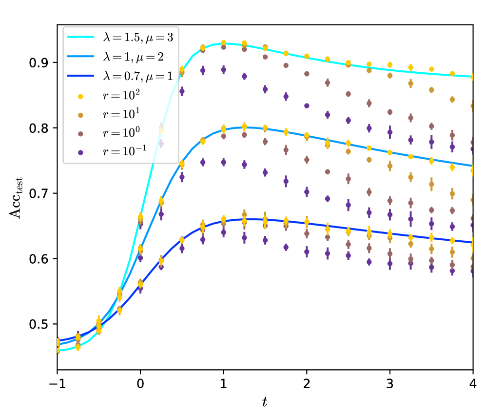<details> <summary>x5.png Details</summary>  ### Visual Description ## Line Chart: A_CC_test vs. t for Varying Parameters ### Overview The chart displays the relationship between the variable **A_CC_test** (y-axis) and **t** (x-axis) across multiple data series. Each series represents combinations of parameters **λ**, **μ**, and **r**, with trends showing growth, peaking, and decay over time. The legend categorizes data into three theoretical models (cyan, blue, dark blue lines) and four empirical datasets (yellow, brown, purple, dark purple markers). --- ### Components/Axes - **X-axis (t)**: Ranges from **-1 to 4** in increments of 1. Label: "t". - **Y-axis (A_CC_test)**: Ranges from **0.45 to 0.9** in increments of 0.05. Label: "A_CC_test". - **Legend**: - **Top-left placement**. - **Theoretical models**: - Cyan line: λ=1.5, μ=3. - Blue line: λ=1, μ=2. - Dark blue line: λ=0.7, μ=1. - **Empirical datasets**: - Yellow markers: r=10². - Brown markers: r=10¹. - Purple markers: r=10⁰. - Dark purple markers: r=10⁻¹. --- ### Detailed Analysis 1. **Cyan Line (λ=1.5, μ=3)**: - Starts at **~0.45** at t=-1. - Peaks at **~0.9** near t=1. - Declines gradually to **~0.85** by t=4. - Smooth, continuous curve with no visible noise. 2. **Blue Line (λ=1, μ=2)**: - Starts at **~0.45** at t=-1. - Peaks at **~0.8** near t=1.5. - Declines to **~0.75** by t=4. - Slightly noisier than the cyan line. 3. **Dark Blue Line (λ=0.7, μ=1)**: - Starts at **~0.45** at t=-1. - Peaks at **~0.7** near t=1. - Declines to **~0.65** by t=4. - Most gradual slope among theoretical models. 4. **Empirical Datasets**: - **Yellow (r=10²)**: - Peaks at **~0.9** near t=1. - Declines to **~0.85** by t=4. - Matches cyan line’s trend but with minor fluctuations. - **Brown (r=10¹)**: - Peaks at **~0.8** near t=1.5. - Declines to **~0.75** by t=4. - Aligns with blue line’s trajectory. - **Purple (r=10⁰)**: - Peaks at **~0.7** near t=1. - Declines to **~0.65** by t=4. - Matches dark blue line’s pattern. - **Dark Purple (r=10⁻¹)**: - Peaks at **~0.65** near t=1. - Declines to **~0.6** by t=4. - Lowest peak among empirical datasets. --- ### Key Observations - **Peak Timing**: All series peak near **t=1**, suggesting a critical threshold or event at this point. - **Parameter Sensitivity**: - Higher **λ** and **μ** values correlate with higher peak A_CC_test (e.g., λ=1.5, μ=3 peaks at 0.9 vs. λ=0.7, μ=1 at 0.7). - Larger **r** values (e.g., r=10²) exhibit higher peaks compared to smaller **r** (e.g., r=10⁻¹). - **Decay Phase**: Post-peak decline is consistent across all series, indicating stabilization or damping over time. - **Noise**: Empirical datasets (markers) show more variability than theoretical models (lines). --- ### Interpretation The chart demonstrates how **A_CC_test** evolves over time under different parameter regimes: - **λ and μ** govern the **growth rate and peak magnitude**: Larger values accelerate growth and increase peak height. - **r** modulates the **peak amplitude**: Larger **r** amplifies the maximum A_CC_test value. - The decay phase suggests a **self-limiting mechanism** or resource exhaustion post-peak. - Discrepancies between theoretical models (lines) and empirical data (markers) may indicate unaccounted variables or measurement noise in real-world scenarios. This analysis implies that optimizing **λ**, **μ**, and **r** could maximize A_CC_test in systems governed by similar dynamics, such as signal processing or ecological models. </details> Figure 5: Predicted test accuracy $\mathrm{Acc}_{\mathrm{test}}$ of the continuous GCN on the asymmetric graph, at $r=\infty$ . $\alpha=4$ and $\rho=0.1$ . The performance of the continuous GCN are given by eq. (126). Dots: numerical simulation of the continuous GCN for $N=10^{4}$ and $d=30$ , trained with quadratic loss, averaged over ten experiments. The convergence with respect to $K\to\infty$ , taken after $r\to\infty$ , is depicted in fig. 6 and fig. 9 in appendix E. Again the continuous limit enjoyes good convergence properties since $K\gtrapprox 16$ is enough if $t$ is not too large. 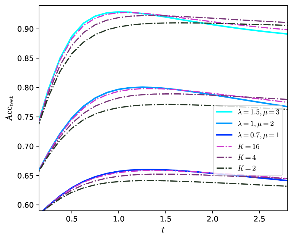<details> <summary>x6.png Details</summary>  ### Visual Description ## Line Graph: Accuracy Over Time (Acc_test vs. t) ### Overview The graph depicts the relationship between time (`t`) and test accuracy (`Acc_test`) for different parameter configurations. Six distinct lines represent combinations of learning rate (`λ`), regularization strength (`μ`), and model complexity (`K`). All lines exhibit a similar sigmoidal trend, peaking around `t=1` before declining. ### Components/Axes - **X-axis**: Time (`t`), ranging from 0.0 to 2.5 in increments of 0.5. - **Y-axis**: Test accuracy (`Acc_test`), ranging from 0.60 to 0.90 in increments of 0.05. - **Legend**: Located in the bottom-right corner, mapping colors to parameters: - Solid lines: Learning rate (`λ`) and regularization (`μ`) combinations. - Dashed lines: Model complexity (`K`) values. - **Line styles**: - Cyan: `λ=1.5, μ=3` - Blue: `λ=1, μ=2` - Dark blue: `λ=0.7, μ=1` - Magenta (dashed): `K=16` - Purple (dashed): `K=4` - Black (dashed): `K=2` ### Detailed Analysis 1. **`λ=1.5, μ=3` (cyan)**: - Peaks at `t=1` with `Acc_test ≈ 0.90`. - Declines steadily to `0.88` by `t=2.5`. - Highest accuracy among all lines. 2. **`λ=1, μ=2` (blue)**: - Peaks at `t=1` with `Acc_test ≈ 0.89`. - Declines to `0.87` by `t=2.5`. - Second-highest accuracy. 3. **`λ=0.7, μ=1` (dark blue)**: - Peaks at `t=1` with `Acc_test ≈ 0.88`. - Declines to `0.86` by `t=2.5`. - Third-highest accuracy. 4. **`K=16` (magenta, dashed)**: - Peaks at `t=1` with `Acc_test ≈ 0.89`. - Declines to `0.87` by `t=2.5`. - Matches the `λ=1, μ=2` line in accuracy. 5. **`K=4` (purple, dashed)**: - Peaks at `t=1` with `Acc_test ≈ 0.87`. - Declines to `0.85` by `t=2.5`. - Matches the `λ=0.7, μ=1` line in accuracy. 6. **`K=2` (black, dashed)**: - Peaks at `t=1` with `Acc_test ≈ 0.85`. - Declines to `0.83` by `t=2.5`. - Lowest accuracy among all lines. ### Key Observations - **Parameter correlation**: Higher `λ` and `μ` values correlate with higher peak accuracy (e.g., `λ=1.5, μ=3` outperforms `λ=0.7, μ=1`). - **Model complexity**: Larger `K` values (e.g., `K=16`) achieve accuracy comparable to moderate `λ`/`μ` combinations. - **Consistent trends**: All lines follow a sigmoidal pattern, suggesting diminishing returns after `t=1`. - **Color consistency**: Legend colors match line styles and parameter groupings exactly. ### Interpretation The graph demonstrates that: 1. **Learning rate and regularization** (`λ`, `μ`) significantly impact peak accuracy, with higher values yielding better performance. 2. **Model complexity** (`K`) acts as a proxy for capacity, where larger `K` values achieve similar accuracy to optimized `λ`/`μ` pairs. 3. The decline after `t=1` implies potential overfitting or saturation effects, as further training reduces generalization. 4. The `K=2` line (lowest accuracy) suggests underfitting due to insufficient model capacity. This analysis highlights the trade-offs between hyperparameter tuning and architectural complexity in optimizing test accuracy. </details> Figure 6: Predicted test accuracy $\mathrm{Acc}_{\mathrm{test}}$ of the continuous GCN and of its discrete counterpart with depth $K$ on the asymmetric graph, at $r=\infty$ . $\alpha=1$ and $\rho=0.1$ . The performance of the continuous GCN are given by eq. (126) while for the discrete GCN they are given by numerically solving the fixed-point equations (88 - 94). To summarize, figs. 5, 6 and appendix E validate our method that consists in deriving the self-consistent equations at finite $K$ with replica, expanding them with respect to $1/r$ , taking the continuous limit $K\to\infty$ and then solving the integral equations. Optimal diffusion time $t^{*}$ : We observe on the previous figures that there is an optimal diffusion time $t^{*}$ that maximizes $\mathrm{Acc}_{\mathrm{test}}$ . Though we are able to solve the self-consistent equations and to obtain an explicit and analytical expression (126), it is hard to analyze it in order to evaluate $t^{*}$ . We have to consider further limiting cases or to compute $t^{*}$ numerically. The derivation of the following equations is detailed in appendix B.6. We first consider the case $t\to 0$ . Expanding (126) to the first order in $t$ we obtain $$ \mathrm{Acc}_{\mathrm{test}}\underset{t\to 0}{=}\frac{1}{2}\left(1+\mathrm{erf}\left(\frac{1}{\sqrt{2}}\sqrt{\frac{\rho}{\alpha}}\frac{\mu+\lambda^{\mathrm{e}}t(2+\mu)}{\sqrt{1+\rho\mu}}\right)\right)+o(t)\ . \tag{133} $$ This expression shows in particular that $t^{*}>0$ , i.e. some diffusion on the graph is always beneficial compared to no diffusion, as long as $\lambda t>0$ i.e. the diffusion is done forward if the graph is homophilic $\lambda>0$ and backward if it is heterophilic $\lambda<0$ . We recover the result of [40] for the discrete case in a slightly different setting. This holds even if the features of the graph are not informative $\mu=0$ . Notice the explicit invariance by the change $(\lambda,t)\to(-\lambda,-t)$ in the potential (65) and in (133), which allows us to focus on $\lambda\geq 0$ . The case $t=0$ no diffusion corresponds to performing ridge regression on the Gaussian mixture $X$ alone. Such a model has been studied in [37]; we checked we obtain the same expression as theirs at large regularization. We now consider the case $t\to+\infty$ and $\lambda\geq 0$ . Taking the limit in (126) we obtain $$ \mathrm{Acc}_{\mathrm{test}}\underset{t\to\infty}{\longrightarrow}\frac{1}{2}\left(1+\mathrm{erf}\left(\frac{\lambda^{\mathrm{e}}q_{\mathrm{PCA}}}{\sqrt{2}}\right)\right)\ , \tag{134} $$ where $q_{\mathrm{PCA}}$ is the same as for the discrete GCN, defined in eq. (59). This shows that the continuous GCN will oversmooth at large diffusion times. Thus, if the features are informative, if $\mu^{2}/\alpha>0$ , the optimal diffusion time should be finite, $t^{*}<+\infty$ . The continuous GCN does exactly as does the discrete GCN at $K\to\infty$ if $c$ is fixed. This is not surprising because of the mapping $c=K/t$ : taking $t$ large is equivalent to take $c$ small with respect to $K$ . $e^{\frac{t}{\sqrt{N}}\tilde{A}}$ is dominated by the same leading eigenvector $y_{1}$ . These two limits show that at finite time $t$ the GCN avoids oversmoothing and interpolates between an estimator that is only function of the features at $t=0$ and an estimator only function of the graph at $t=\infty$ . $t$ has to be fine-tuned to reach the best trade-off $t^{*}$ and the optimal performance. In the insets of fig. 7 and fig. 12 in appendix E we show how $t^{*}$ depends on $\lambda$ . In particular, $t^{*}$ is finite for any $\lambda$ : some diffusion is always beneficial but too much diffusion leads to oversmoothing. We have $t^{*}\underset{\lambda\to 0}{\longrightarrow}0$ . This is expected since if $\lambda=0$ then $A$ is not informative and any diffusion $t>0$ would degrade the performance. The non-monotonicity of $t^{*}$ with respect to $\lambda$ is less expected and we do not have a clear interpretation for it. Last $t^{*}$ decreases when the feature signal $\mu^{2}/\alpha$ increases: the more informative $X$ the less needed diffusion is. 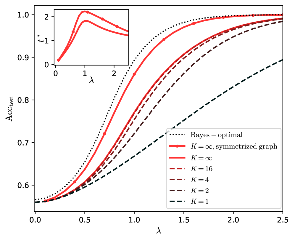<details> <summary>x7.png Details</summary>  ### Visual Description ## Line Graph: Test Accuracy (Acc_test) vs. Regularization Parameter (λ) ### Overview The graph illustrates the relationship between the regularization parameter λ and test accuracy (Acc_test) for different model configurations. Multiple lines represent varying values of K (model complexity) and a Bayes-optimal baseline. An inset graph highlights behavior at lower λ values (0–2). ### Components/Axes - **X-axis (λ)**: Regularization parameter, ranging from 0 to 2.5. - **Y-axis (Acc_test)**: Test accuracy, ranging from 0.5 to 1.0. - **Legend**: - **Dotted black**: Bayes-optimal (upper bound). - **Solid red**: K = ∞, symmetrized graph. - **Dashed red**: K = 16. - **Dotted red**: K = 4. - **Dashed brown**: K = 2. - **Dotted green**: K = 1. ### Detailed Analysis 1. **Bayes-optimal (dotted black)**: - Remains flat at Acc_test ≈ 1.0 across all λ. - Serves as the theoretical maximum accuracy. 2. **K = ∞, symmetrized graph (solid red)**: - Stays nearly parallel to the Bayes-optimal line, with Acc_test ≈ 0.98–1.0. - Minimal deviation suggests near-optimal performance. 3. **K = 16 (dashed red)**: - Acc_test increases from ~0.55 (λ=0) to ~0.95 (λ=2.5). - Slightly lags behind K = ∞ but converges at higher λ. 4. **K = 4 (dotted red)**: - Acc_test rises from ~0.52 (λ=0) to ~0.88 (λ=2.5). - Shows a steeper initial increase but plateaus earlier. 5. **K = 2 (dashed brown)**: - Acc_test climbs from ~0.50 (λ=0) to ~0.82 (λ=2.5). - Slower growth compared to higher K values. 6. **K = 1 (dotted green)**: - Acc_test increases from ~0.48 (λ=0) to ~0.75 (λ=2.5). - Lowest performance, indicating underfitting. 7. **Inset Graph (λ=0–2)**: - Zooms into the lower λ range, showing a peak at λ ≈ 1 for K = ∞ and K = 16. - Lines for K = 4, 2, and 1 intersect near λ = 1, suggesting a critical transition point. ### Key Observations - **Trend Verification**: - All lines exhibit upward trends as λ increases, confirming that regularization improves performance. - Higher K values (e.g., K = ∞, 16) achieve higher Acc_test, aligning with expectations for model complexity. - The inset reveals a local maximum at λ ≈ 1 for K = ∞ and K = 16, followed by a slight decline before stabilization. - **Legend Consistency**: - Colors and line styles match the legend exactly (e.g., solid red for K = ∞, dashed red for K = 16). ### Interpretation The graph demonstrates that: 1. **Model Complexity (K)**: Higher K values (e.g., K = ∞) achieve near-optimal accuracy, while lower K values (e.g., K = 1) underperform due to underfitting. 2. **Regularization Impact**: Increasing λ improves test accuracy across all K values, but the rate of improvement depends on K. Higher K models benefit more from regularization. 3. **Optimal λ**: The inset suggests λ ≈ 1 may be optimal for K = ∞ and K = 16, though performance stabilizes at higher λ. For lower K values, the optimal λ is less distinct but still critical for balancing bias-variance trade-offs. 4. **Bayes-optimal Baseline**: The flat dotted black line underscores the theoretical limit, emphasizing that practical models (even with K = ∞) cannot exceed this bound. This analysis highlights the interplay between model complexity, regularization, and performance, providing insights for tuning λ and K in machine learning pipelines. </details> Figure 7: Predicted test accuracy $\mathrm{Acc}_{\mathrm{test}}$ of the continuous GCN and of its discrete counterpart with depth $K$ , at optimal times $t^{*}$ and $r=\infty$ . $\alpha=4$ , $\mu=1$ and $\rho=0.1$ . The performance of the continuous GCN $K=\infty$ are given by eq. (126) while for its discretization at finite $K$ they are given by numerically solving eqs. (87 - 94). Inset: $t^{*}$ the maximizer at $K=\infty$ . Optimality of the continuous limit: A major result is that, at $t=t^{*}$ , the continuous GCN is better than any fixed- $K$ GCN. Taking the continuous limit of the simple GCN is the way to reach its optimal performance. This was suggested by fig. 4 in the previous part; we show this more precisely in fig. 7 and fig. 12 in appendix E. We compare the continuous GCN to its discretization at different depths $K$ for several configurations $\alpha,\lambda,\mu$ and $\rho$ of the data model. The result is that at $t^{*}$ the test accuracy appears to be always an increasing function of $K$ , and that its value at $K\to\infty$ and $t^{*}$ is a upper-bound for all $K$ and $t$ . Additionally, if the GCN is run on the symmetrized graph it can approach the Bayes-optimality and almost close the gap that [26] describes, as shown by figs. 7, 12 and 13 right. For all the considered $\lambda$ and $\mu$ the GCN is less than a few percents of accuracy far from the optimality. However we shall precise this statement: the GCN approaches the Bayes-optimality only for a certain range of the parameters of the CSBM, as exemplified by figs. 12 and 13 left. In these figures, the GCN is far from the Bayes-optimality when $\lambda$ is small but $\mu$ is large. In this regime we have $\mathrm{snr}_{\mathrm{CSBM}}>1$ ; even at $\rho=0$ information can be retrieved on the labels and the problem is closer to an unsupervised classification of the sole features $X$ . On $X$ the GCN acts as a supervised classifier, and as long as $\rho\neq 1$ it cannot catch all information. As previously highlighted by [39] the comparison with the Bayes-optimality is more relevant at $\mathrm{snr}_{\mathrm{CSBM}}<1$ where supervision is necessary. Then, as shown by figs. 7, 12 and 13 the symmetrized continuous GCN is close to the Bayes-optimality. The GCN is also able to close the gap in the region where $\lambda$ is large because, as we saw, it can perform unsupervised PCA on $A$ . ## IV Conclusion In this article we derived the performance of a simple GCN trained for node classification in a semi-supervised way on data generated by the CSBM in the high-dimensional limit. We first studied a discrete network with a finite number $K$ of convolution steps. We showed the importance of going to large $K$ to approach the Bayes-optimality, while scaling accordingly the residual connections $c$ of the network to avoid oversmoothing. The resulting limit is a continuous GCN. In a second part we were able to explicitly derive the performance of the continuous GCN. We highlighted the importance of the double limit $r,K\to\infty$ , which allows to reach the optimal architecture and which can be analyzed thanks to an expansion in powers of $1/r$ . In is an interesting question for future work whether this approach could allow the study of fully-connected large-depth neural networks. Though the continuous GCN can be close to the Bayes-optimality, it has to better handle the features, especially when they are the main source of information. ## Acknowledgments We acknowledge useful discussions with J. Zavatone-Veth, F. Zamponi and V. Erba. This work is supported by the Swiss National Science Foundation under grant SNSF SMArtNet (grant number 212049). ## Appendix A Asymptotic characterisation of the discrete GCN In this part we compute the free energy of the discrete finite- $K$ GCN using replica. We derive the fixed-point equations for the order parameters of the problem and the asymptotic characterization of the errors and accuracies in function of the order parameters. We consider only the asymmetric graph $\tilde{A}$ ; the symmetrized case $\tilde{A}^{\mathrm{s}}$ is analyzed in the following section B together with the continuous GCN. The free energy of the problem is $-\beta Nf=\partial_{n}\mathbb{E}_{u,\Xi,W,y}Z^{n}(n=0)$ where the partition function is $$ \displaystyle Z \displaystyle=\int\prod_{\nu}^{M}\mathrm{d}w_{\nu}e^{-\beta r\gamma(w_{\nu})}e^{-\beta s\sum_{i\in R}\ell(y_{i}h(w)_{i})-\beta s^{\prime}\sum_{i\in R^{\prime}}\ell(y_{i}h(w)_{i})}\ . \tag{135} $$ To lighten the notations we take $\rho^{\prime}=1-\rho$ i.e. the test set is the whole complementary of the train set. This does not change the result since the performances do not depend on the size of the test set. We recall that $\tilde{A}$ admits the following Gaussian equivalent: $$ \tilde{A}\approx A^{\mathrm{g}}=\frac{\lambda}{\sqrt{N}}yy^{T}+\Xi\ ,\quad\Xi_{ij}\sim\mathcal{N}(0,1)\ . \tag{136} $$ $\tilde{A}$ can be approximated by $A^{\mathrm{g}}$ with a vanishing change in the free energy $f$ . ### A.1 Derivation of the free energy We define the intermediate states of the GCN as $$ h_{k}=\left(\frac{1}{\sqrt{N}}\tilde{A}+c_{k}I_{N}\right)h_{k-1}\ ,\quad h_{0}=\frac{1}{\sqrt{N}}Xw\ . \tag{137} $$ We introduce them in $Z$ thanks to Dirac deltas. The expectation of the replicated partition function is $$ \displaystyle\mathbb{E}Z^{n}\propto \displaystyle\,\mathbb{E}_{u,\Xi,W,y}\int\prod_{a}^{n}\prod_{\nu}^{M}\mathrm{d}w_{\nu}^{a}e^{-\beta r\gamma(w_{\nu}^{a})}\prod_{a}^{n}\prod_{i}^{N}\prod_{k=0}^{K}\mathrm{d}h_{i,k}^{a}\mathrm{d}q_{i,k}^{a}e^{-\beta s\sum_{a,i\in R}\ell(y_{i}h_{i,K}^{a})-\beta s^{\prime}\sum_{a,i\in R^{\prime}}\ell(y_{i}h_{i,K}^{a})} \displaystyle\quad\quad e^{\sum_{a,i}\sum_{k=1}^{K}\mathrm{i}q_{i,k}^{a}\left(h_{i,k}^{a}-\frac{1}{\sqrt{N}}\sum_{j}(\frac{\lambda}{\sqrt{N}}y_{i}y_{j}+\Xi_{ij})h_{j,k-1}^{a}-c_{k}h_{i,k-1}^{a}\right)+\sum_{a,i}\mathrm{i}q_{i,0}^{a}\left(h_{i,0}^{a}-\frac{1}{\sqrt{N}}\sum_{\nu}\left(\sqrt{\frac{\mu}{N}}y_{i}u_{\nu}+W_{i\nu}\right)w_{\nu}^{a}\right)} \displaystyle= \displaystyle\,\mathbb{E}_{u,y}\int\prod_{a,\nu}\mathrm{d}w_{\nu}^{a}e^{-\beta r\gamma(w_{\nu}^{a})}\prod_{a,i,k}\mathrm{d}h_{i,k}^{a}e^{-\beta s\sum_{a,i\in R}\ell(y_{i}h_{i,K}^{a})-\beta s^{\prime}\sum_{a,i\in R^{\prime}}\ell(y_{i}h_{i,K}^{a})} \displaystyle\quad\quad\prod_{i}\mathcal{N}\left(h_{i,>0}\left|c\odot h_{i,<K}+y_{i}\frac{\lambda}{N}\sum_{j}y_{j}h_{j,<K};\tilde{Q}\right.\right)\prod_{i}\mathcal{N}\left(h_{i,0}\left|y_{i}\frac{\sqrt{\mu}}{N}\sum_{\nu}u_{\nu}w_{\nu};\frac{1}{N}\sum_{\nu}w_{\nu}w_{\nu}^{T}\right.\right)\ . \tag{138} $$ $\mathcal{N}(\cdot|m;V)$ is the Gaussian density of mean $m$ and covariance $V$ . We integrated over the random fluctuations $\Xi$ and $W$ and then over the $q$ s. We collected the replica in vectors of size $n$ and assembled them as $$ \displaystyle h_{i,>0}=\left(\begin{smallmatrix}h_{i,1}\\ \vdots\\ h_{i,K}\end{smallmatrix}\right)\in\mathbb{R}^{nK},\quad h_{i,<K}=\left(\begin{smallmatrix}h_{i,0}\\ \vdots\\ h_{i,K-1}\end{smallmatrix}\right)\in\mathbb{R}^{nK},\quad c\odot h_{i,<K}=\left(\begin{smallmatrix}c_{1}h_{i,0}\\ \vdots\\ c_{K}h_{i,K-1}\end{smallmatrix}\right), \displaystyle\tilde{Q}_{k,l}=\frac{1}{N}\sum_{j}h_{j,k}h_{j,l}^{T}\ ,\quad\tilde{Q}=\left(\begin{smallmatrix}\tilde{Q}_{0,0}&\ldots&\tilde{Q}_{0,K-1}\\ \vdots&&\vdots\\ \tilde{Q}_{K-1,0}&\ldots&\tilde{Q}_{K-1,K-1}\end{smallmatrix}\right)\in\mathbb{R}^{nK\times nK}\ . \tag{139} $$ We introduce the order parameters $$ \displaystyle m_{w}^{a}=\frac{1}{N}\sum_{\nu}u_{\nu}w_{\nu}^{a}\ ,\quad Q_{w}^{ab}=\frac{1}{N}\sum_{\nu}w_{\nu}^{a}w_{\nu}^{b}\ , \displaystyle m_{k}^{a}=\frac{1}{N}\sum_{j}y_{j}k_{j,k}^{a}\ ,\quad Q_{k}^{ab}=(\tilde{Q}_{k,k})_{a,b}=\frac{1}{N}\sum_{j}h_{j,k}^{a}h_{j,k}^{b}\ ,\quad Q_{k,l}^{ab}=(\tilde{Q}_{k,l})_{a,b}=\frac{1}{N}\sum_{j}h_{j,k}^{a}h_{j,l}^{b}\ . \tag{141} $$ $m_{k}$ is the magnetization (or overlap) between the $k^{\mathrm{th}}$ layer and the labels; $m_{w}$ is the magnetization between the weights and the hidden variables and the $Q$ s are the self-overlaps across the different layers. In the following we write $\tilde{Q}$ for the matrix with elements $(\tilde{Q})_{ak,bl}=Q_{k,l}^{ab}$ . We introduce these quantities thanks to new Dirac deltas. This allows us to factorize the spacial $i$ and $\nu$ indices. $$ \displaystyle\mathbb{E}Z^{n}\propto \displaystyle\,\int\prod_{a}\prod_{k=0}^{K-1}\mathrm{d}\hat{m}_{k}^{a}\mathrm{d}m_{k}^{a}e^{N\hat{m}_{k}^{a}m_{k}^{a}}\prod_{a}\mathrm{d}\hat{m}_{w}^{a}\mathrm{d}m_{w}^{a}e^{N\hat{m}_{w}^{a}m_{w}^{a}}\prod_{a\leq b}\prod_{k=0}^{K-1}\mathrm{d}\hat{Q}_{k}^{ab}\mathrm{d}Q_{k}^{ab}e^{N\hat{Q}_{k}^{ab}Q_{k}^{ab}}\prod_{a,b}\prod_{k<l}^{K-1}\mathrm{d}\hat{Q}_{k,l}^{ab}\mathrm{d}Q_{k,l}^{ab}e^{N\hat{Q}_{k,l}^{ab}Q_{k,l}^{ab}} \displaystyle\prod_{a\leq b}d\hat{Q}_{w}^{ab}\mathrm{d}Q_{w}^{ab}e^{N\hat{Q}_{w}^{ab}Q_{w}^{ab}}\left[\mathbb{E}_{u}\int\prod_{a}\mathrm{d}w^{a}e^{\psi_{w}^{(n)}(w)}\right]^{\frac{N}{\alpha}}\left[\mathbb{E}_{y}\int\prod_{a,k}\mathrm{d}h_{k}^{a}e^{\psi_{h}^{(n)}(h;s)}\right]^{\rho N}\left[\mathbb{E}_{y}\int\prod_{a,k}\mathrm{d}h_{k}^{a}e^{\psi_{h}^{(n)}(h;s^{\prime})}\right]^{(1-\rho)N} \tag{143} $$ where we defined the two potentials $$ \displaystyle\psi_{w}^{(n)}(w)=-\beta r\sum_{a}\gamma(w^{a})-\sum_{a\leq b}\hat{Q}_{w}^{ab}w^{a}w^{b}-\sum_{a}\hat{m}_{w}^{a}uw^{a} \displaystyle\psi_{h}^{(n)}(h;\bar{s})=-\beta\bar{s}\sum_{a}\ell(yh_{K}^{a})-\sum_{a\leq b}\sum_{k=0}^{K-1}\hat{Q}_{k}^{ab}h_{k}^{a}h_{k}^{b}-\sum_{a,b}\sum_{k<l}^{K-1}\hat{Q}_{k,l}^{ab}h_{k}^{a}h_{l}^{b}-\sum_{a}\sum_{k=0}^{K-1}\hat{m}_{k}^{a}yh_{k}^{a} \displaystyle\qquad\qquad{}+\log\mathcal{N}\left(h_{>0}\left|c\odot h_{<K}+\lambda ym_{<K};\tilde{Q}\right.\right)+\log\mathcal{N}\left(h_{0}\left|\sqrt{\mu}ym_{w};Q_{w}\right.\right)\ . \tag{144} $$ We leverage the replica-symmetric ansatz. It is justified by the convexity of the Hamiltonian $H$ . We assume that for all $a$ and $b$ $$ \displaystyle m_{k}^{a}=m_{k}\ , \displaystyle\hat{m}_{k}^{a}=-\hat{m}_{k}\ , \displaystyle m_{w}^{a}=m_{w}\ , \displaystyle\hat{m}_{w}^{a}=-\hat{m}_{w}\ , \displaystyle Q_{k}^{ab}=Q_{k}J+V_{k}I\ , \displaystyle\hat{Q}_{k}^{ab}=-\hat{Q}_{k}J+\frac{1}{2}(\hat{V}_{k}+\hat{Q}_{k})I\ , \displaystyle Q_{w}^{ab}=Q_{w}J+V_{w}I\ , \displaystyle\hat{Q}_{w}^{ab}=-\hat{Q}_{w}J+\frac{1}{2}(\hat{V}_{w}+\hat{Q}_{w})I\ , \displaystyle Q_{k,l}^{ab}=Q_{k,l}J+V_{k,l}I\ , \displaystyle\hat{Q}_{k,l}^{ab}=-\hat{Q}_{k,l}J+\hat{V}_{k,l}I\ . \tag{146} $$ $I$ is the $n\times n$ identity and $J$ is the $n\times n$ matrix filled with ones. We introduce the $K\times K$ symmetric matrices $Q$ and $V$ , filled with $(Q_{k})_{0\leq k\leq K-1}$ and $(V_{k})_{0\leq k\leq K-1}$ on the diagonal, and $(Q_{k,l})_{0\leq k<l\leq K-1}$ and $(V_{k,l})_{0\leq k<l\leq K-1}$ off the diagonal, such that $\tilde{Q}$ can be written in terms of Kronecker products as $$ \displaystyle\tilde{Q}=Q\otimes J+V\otimes I\ . \tag{149} $$ The entropic terms of $\psi_{w}^{(n)}$ and $\psi_{h}^{(n)}$ can be computed. Since we will take $n=0$ we discard subleading terms in $n$ . We obtain $$ \displaystyle\sum_{a}\hat{m}_{w}^{a}m_{w}^{a}=n\hat{m}_{w}m_{w}\ ,\quad\sum_{a\leq b}\hat{Q}_{w}^{ab}Q_{w}^{ab}=\frac{n}{2}(\hat{V}_{w}V_{w}+\hat{V}_{w}Q_{w}-V_{w}\hat{Q}_{w})\ , \displaystyle\sum_{a}\hat{m}_{k}^{a}m_{k}^{a}=n\hat{m}_{k}m_{k}\ ,\quad\sum_{a\leq b}\hat{Q}_{k}^{ab}Q_{k}^{ab}=\frac{n}{2}(\hat{V}_{k}V_{k}+\hat{V}_{k}Q_{k}-V_{k}\hat{Q}_{k})\ ,\quad\sum_{a,b}\hat{Q}_{k,l}^{ab}Q_{k,l}^{ab}=n(\hat{V}_{k,l}V_{k,l}+\hat{V}_{k,l}Q_{k,l}-V_{k,l}\hat{Q}_{k,l})\ . \tag{150} $$ The Gaussian densities can be explicited, keeping again the main order in $n$ and using the formula for a rank-1 update to a matrix (Sherman-Morrison formula): $$ \displaystyle Q_{w}^{-1}=\frac{1}{V_{w}}I-\frac{Q_{w}}{V_{w}^{2}}J\ ,\quad\log\det Q_{w}=n\frac{Q_{w}}{V_{w}}+n\log V_{w}\ , \displaystyle\tilde{Q}^{-1}=V^{-1}\otimes I-(V^{-1}QV^{-1})\otimes J\ ,\quad\log\det\tilde{Q}=n\operatorname{Tr}(V^{-1}Q)+n\log V\ . \tag{152} $$ Then we can factorize the replica by introducing random Gaussian variables: $$ \displaystyle\int\prod_{a}\mathrm{d}w^{a}e^{\psi_{w}^{(n)}(w)} \displaystyle=\int\prod_{a}\mathrm{d}w^{a}e^{\sum_{a}\log P_{W}(w^{a})+\frac{1}{2}\hat{Q}_{w}w^{T}Jw-\frac{1}{2}\hat{V}_{w}w^{T}w+u\hat{m}_{w}^{T}w}=\mathbb{E}_{\varsigma}\left(\int\mathrm{d}we^{\psi_{w}(w)}\right)^{n} \tag{154} $$ where $\varsigma\sim\mathcal{N}(0,1)$ and the potential is $$ \displaystyle\psi_{w}(w)=\log P_{W}(w)-\frac{1}{2}\hat{V}_{w}w^{2}+\left(\sqrt{\hat{Q}_{w}}\varsigma+u\hat{m}_{w}\right)w\ ; \tag{155} $$ and samely $$ \displaystyle\int\prod_{a,k}\mathrm{d}h_{k}^{a}e^{\psi_{h}^{(n)}(h;\bar{s})} \displaystyle=\int\prod_{a,k}\mathrm{d}h_{k}^{a}e^{-\beta\bar{s}\sum_{a}\ell(yk_{K}^{a})+\sum_{k=0}^{K-1}\left(\frac{1}{2}\hat{Q}_{k}h_{k}^{T}Jh_{k}-\frac{1}{2}\hat{V}_{k}h_{k}^{T}h_{k}+y\hat{m}_{k}^{T}h_{k}\right)+\sum_{k<l}^{K-1}(\hat{Q}_{k,l}h_{k}^{T}Jh_{l}-\hat{V}_{k,l}h_{k}^{T}h_{l})} \displaystyle e^{-\frac{1}{2}(h_{0}-\sqrt{\mu}ym_{w})^{T}\left(\frac{1}{V_{w}}I-\frac{Q_{w}}{V_{w}^{2}}J\right)(h_{0}-\sqrt{\mu}ym_{w})-\frac{1}{2}n\frac{Q_{w}}{V_{w}}-\frac{1}{2}n\log V_{w}} \displaystyle e^{-\frac{1}{2}\sum_{k,l}^{K}(h_{k}-c_{k}h_{k-1}-\lambda ym_{k-1})^{T}\left({(V^{-1})_{k-1,l-1}}I-(V^{-1}QV^{-1})_{k-1,l-1}J\right)(h_{l}-c_{l}h_{l-1}-\lambda ym_{l-1})-\frac{n}{2}\operatorname{Tr}(V^{-1}Q)-\frac{n}{2}\log\det V} \displaystyle=\mathbb{E}_{\xi,\chi,\zeta}\left(\int\prod_{k=0}^{K}\mathrm{d}h_{k}e^{\psi_{h}(h;\bar{s})}\right)^{n} \tag{156} $$ where $\xi\sim\mathcal{N}(0,I_{K})$ , $\chi\sim\mathcal{N}(0,I_{K})$ , $\zeta\sim\mathcal{N}(0,1)$ and the potential is $$ \displaystyle\psi_{h}(h;\bar{s}) \displaystyle=-\beta\bar{s}\ell(yh_{K})-\frac{1}{2}h_{<K}^{T}\hat{V}h_{<K}+\left(\xi^{T}\hat{Q}^{1/2}+y\hat{m}^{T}\right)h_{<K} \displaystyle\quad\quad{}+\log\mathcal{N}\left(h_{0}\left|\sqrt{\mu}ym_{w}+\sqrt{Q_{w}}\zeta;V_{w}\right.\right)+\log\mathcal{N}\left(h_{>0}\left|c\odot h_{<K}+\lambda ym+Q^{1/2}\chi;V\right.\right)\ ; \tag{158} $$ where $h_{>0}=(h_{1},\ldots,h_{K})\in\mathbb{R}^{K}$ , $h_{<K}=(h_{0},\ldots,h_{K-1})\in\mathbb{R}^{K}$ , $c\odot h_{<K}=(c_{1}h_{0},\ldots,c_{K}h_{K-1})$ , $\hat{m}=(\hat{m}_{0},\ldots,\hat{m}_{K-1})\in\mathbb{R}^{K}$ , $m=(m_{0},\ldots,m_{K-1})\in\mathbb{R}^{K}$ , $\hat{Q}$ and $\hat{V}$ are the $K\times K$ symmetric matrix filled with $(\hat{Q}_{k})_{0\leq k\leq K-1}$ and $(\hat{V}_{k})_{0\leq k\leq K-1}$ on the diagonal, and $(\hat{Q}_{k,l})_{0\leq k<l\leq K-1}$ and $(\hat{V}_{k,l})_{0\leq k<l\leq K-1}$ off the diagonal. We used that $\mathbb{E}_{\zeta}e^{-\frac{n}{2}\frac{Q_{w}}{V_{w}}\zeta^{2}}=e^{-\frac{n}{2}\frac{Q_{w}}{V_{w}}}$ in the limit $n\to 0$ to factorize $\sqrt{Q_{w}}\zeta$ and the same for $Q^{1/2}\chi$ . We pursue the computation: $$ \displaystyle\mathbb{E}Z^{n}\propto \displaystyle\,\int\mathrm{d}\hat{m}_{w}\mathrm{d}m_{w}e^{Nn\hat{m}_{w}m_{w}}\mathrm{d}\hat{Q}_{w}\mathrm{d}Q_{w}\mathrm{d}\hat{V}_{w}\mathrm{d}V_{w}e^{N\frac{n}{2}(\hat{V}_{w}V_{w}+\hat{V}_{w}Q_{w}-V_{w}\hat{Q}_{w})}\prod_{k=0}^{K-1}\mathrm{d}\hat{m}_{k}\mathrm{d}m_{k}e^{Nn\hat{m}^{T}m} \displaystyle\quad\prod_{k=0}^{K-1}\mathrm{d}\hat{Q}_{k}\mathrm{d}Q_{k}\mathrm{d}\hat{V}_{k}\mathrm{d}V_{k}\prod_{k<l}^{K-1}\mathrm{d}\hat{Q}_{k,l}\mathrm{d}Q_{k,l}\mathrm{d}\hat{V}_{k,l}\mathrm{d}V_{k,l}e^{N\frac{n}{2}\mathrm{tr}\left(\hat{V}V+\hat{V}Q-V\hat{Q}\right)} \displaystyle\quad\left[\mathbb{E}_{u,\varsigma}\left(\int\mathrm{d}we^{\psi_{w}(w)}\right)^{n}\right]^{N/\alpha}\left[\mathbb{E}_{y,\xi,\chi,\zeta}\left(\int\prod_{k=0}^{K}\mathrm{d}h_{k}e^{\psi_{h}(h;s)}\right)^{n}\right]^{\rho N}\left[\mathbb{E}_{y,\xi,\chi,\zeta}\left(\int\prod_{k=0}^{K}\mathrm{d}h_{k}e^{\psi_{h}(h;s^{\prime})}\right)^{n}\right]^{(1-\rho)N} \displaystyle:= \displaystyle\ \int\mathrm{d}\Theta\mathrm{d}\hat{\Theta}e^{N\phi^{(n)}(\Theta,\hat{\Theta})}\ . \tag{159} $$ where $\Theta=\{m_{w},Q_{w},V_{w},m,Q,V\}$ and $\hat{\Theta}=\{\hat{m}_{w},\hat{Q}_{w},\hat{V}_{w},\hat{m},\hat{Q},\hat{V}\}$ are the sets of the order parameters. We can now take the limit $N\to\infty$ thanks to Laplace’s method. $$ \displaystyle-\beta f\propto \displaystyle\frac{1}{N}\frac{\partial}{\partial n}(n=0)\int\mathrm{d}\Theta\mathrm{d}\hat{\Theta}\,e^{N\phi^{(n)}(\Theta,\hat{\Theta})} \displaystyle= \displaystyle\operatorname*{extr}_{\Theta,\hat{\Theta}}\frac{\partial}{\partial n}(n=0)\phi^{(n)}(\Theta,\hat{\Theta}) \displaystyle:= \displaystyle\operatorname*{extr}_{\Theta,\hat{\Theta}}\phi(\Theta,\hat{\Theta})\ , \tag{161} $$ where we extremize the following free entropy $\phi$ : $$ \displaystyle\phi \displaystyle=\frac{1}{2}\left(\hat{V}_{w}V_{w}+\hat{V}_{w}Q_{w}-V_{w}\hat{Q}_{w}\right)-\hat{m}_{w}m_{w}+\frac{1}{2}\mathrm{tr}\left(\hat{V}V+\hat{V}Q-V\hat{Q}\right)-\hat{m}^{T}m \displaystyle\quad{}+\frac{1}{\alpha}\mathbb{E}_{u,\xi}\left(\log\int\mathrm{d}w\,e^{\psi_{w}(w)}\right)+\rho\mathbb{E}_{y,\xi,\zeta,\chi}\left(\log\int\prod_{k=0}^{K}\mathrm{d}h_{k}e^{\psi_{h}(h;s)}\right)+(1-\rho)\mathbb{E}_{y,\xi,\zeta,\chi}\left(\log\int\prod_{k=0}^{K}\mathrm{d}h_{k}e^{\psi_{h}(h;s^{\prime})}\right)\ . \tag{164} $$ We take the limit $\beta\to\infty$ . Later we will differentiate $\phi$ with respect to the order parameters or to $\bar{s}$ and these derivatives will simplify in that limit. We introduce the measures $$ \displaystyle\mathrm{d}P_{w}=\frac{\mathrm{d}w\,e^{\psi_{w}(w)}}{\int\mathrm{d}w\,e^{\psi_{w}(w)}}\quad,\quad\mathrm{d}P_{h}=\frac{\prod_{k=0}^{K}\mathrm{d}h_{k}\,e^{\psi_{h}(h;\bar{s}=1)}}{\int\prod_{k=0}^{K}\mathrm{d}h_{k}\,e^{\psi_{h}(h;\bar{s}=1)}}\quad,\quad\mathrm{d}P_{h}^{\prime}=\frac{\prod_{k=0}^{K}\mathrm{d}h_{k}\,e^{\psi_{h}(h;\bar{s}=0)}}{\int\prod_{k=0}^{K}\mathrm{d}h_{k}\,e^{\psi_{h}(h;\bar{s}=0)}}\ . \tag{165} $$ We have to rescale the order parameters not to obtain a degenerated solution when $\beta\to\infty$ (we recall that, in $\psi_{w}$ , $\log P_{W}(w)\propto\beta$ ). We take $$ \displaystyle\hat{m}_{w}\to\beta\hat{m}_{w}\ , \displaystyle\hat{Q}_{w}\to\beta^{2}\hat{Q}_{w}\ , \displaystyle\hat{V}_{w}\to\beta\hat{V}_{w}\ , \displaystyle V_{w}\to\beta^{-1}V_{w} \displaystyle\hat{m}\to\beta\hat{m}\ , \displaystyle\hat{Q}\to\beta^{2}\hat{Q}\ , \displaystyle\hat{V}\to\beta\hat{V}\ , \displaystyle V\to\beta^{-1}V \tag{166} $$ So we obtain that $f=-\phi$ . Then $\mathrm{d}P_{w}$ , $\mathrm{d}P_{h}$ and $\mathrm{d}P_{h}^{\prime}$ are picked around their maximum and can be approximated by Gaussian measures. We define $$ \displaystyle w^{*}=\operatorname*{argmax}_{w}\psi_{w}(w)\ ,\quad h^{*}=\operatorname*{argmax}_{h}\psi_{h}(h;\bar{s}=1)\ ,\quad h^{{}^{\prime}*}=\operatorname*{argmax}_{h}\psi_{h}(h;\bar{s}=0)\ . \tag{168} $$ Then we have the expected value of a function $g$ in $h$ $\mathbb{E}_{P_{h}}g(h)=g(h^{*})$ and the covariance $\operatorname{Cov}_{P_{h}}(h)=-\frac{1}{2}(\nabla\nabla\psi_{h}(h^{*}))^{-1}$ with $\nabla\nabla$ the Hessian; and similarly for $\mathrm{d}P_{w}$ and $\mathrm{d}P_{h}^{\prime}$ . Last we compute the expected errors and accuracies. We differentiate the free energy $f$ with respect to $s$ and $s^{\prime}$ to obtain that $$ \displaystyle E_{\mathrm{train}}=\mathbb{E}_{y,\xi,\zeta,\chi}\ell(yh_{K}^{*})\ ,\quad E_{\mathrm{test}}=\mathbb{E}_{y,\xi,\zeta,\chi}\ell(yh_{K}^{{}^{\prime}*})\ . \tag{169} $$ Augmenting $H$ with the observable $\frac{1}{|\hat{R}|}\sum_{i\in\hat{R}}\delta_{y_{i}=\operatorname{sign}h(w)_{i}}$ and following the same steps gives the expected accuracies $$ \displaystyle\mathrm{Acc}_{\mathrm{train}}=\mathbb{E}_{y,\xi,\zeta,\chi}\delta_{y=\operatorname{sign}(h_{K}^{*})}\ ,\quad\mathrm{Acc}_{\mathrm{test}}=\mathbb{E}_{y,\xi,\zeta,\chi}\delta_{y=\operatorname{sign}(h_{K}^{{}^{\prime}*})}\ . \tag{170} $$ ### A.2 Self-consistent equations The two above formula (169) and (170) are valid only at the values of the order parameters that extremize the free entropy. We seek the extremizer of $\phi$ . The extremality condition $\nabla_{\Theta,\hat{\Theta}}\phi=0$ gives the following self-consistent equations: $$ \displaystyle m_{w}=\frac{1}{\alpha}\mathbb{E}_{u,\varsigma}\,uw^{*}\quad\quad m=\mathbb{E}_{y,\xi,\zeta,\chi}\,y\left(\rho h_{<K}^{*}+(1-\rho)h_{<K}^{{}^{\prime}*}\right) \displaystyle Q_{w}=\frac{1}{\alpha}\mathbb{E}_{u,\varsigma}(w^{*})^{2}\quad\quad Q=\mathbb{E}_{y,\xi,\zeta,\chi}\left(\rho(h_{<K}^{*})^{\otimes 2}+(1-\rho)(h_{<K}^{{}^{\prime}*})^{\otimes 2}\right) \displaystyle V_{w}=\frac{1}{\alpha}\frac{1}{\sqrt{\hat{Q}_{w}}}\mathbb{E}_{u,\varsigma}\,\varsigma w^{*}\quad\quad V=\mathbb{E}_{y,\xi,\zeta,\chi}\left(\rho\operatorname{Cov}_{P_{h}}(h_{<K})+(1-\rho)\operatorname{Cov}_{P_{h}^{\prime}}(h_{<K})\right) \displaystyle\hat{m}_{w}=\frac{\sqrt{\mu}}{V_{w}}\mathbb{E}_{y,\xi,\zeta,\chi}\,y\left(\rho(h^{*}_{0}-\sqrt{\mu}ym_{w})+(1-\rho)(h_{0}^{{}^{\prime}*}-\sqrt{\mu}ym_{w})\right) \displaystyle\hat{Q}_{w}=\frac{1}{V_{w}^{2}}\mathbb{E}_{y,\xi,\zeta,\chi}\left(\rho(h_{0}^{*}-\sqrt{\mu}ym_{w}-\sqrt{Q}_{w}\zeta)^{2}+(1-\rho)(h_{0}^{{}^{\prime}*}-\sqrt{\mu}ym_{w}-\sqrt{Q}_{w}\zeta)^{2}\right) \displaystyle\hat{V}_{w}=\frac{1}{V_{w}}-\frac{1}{V_{w}^{2}}\mathbb{E}_{y,\xi,\zeta,\chi}\left(\rho\operatorname{Cov}_{P_{h}}(h_{0})+(1-\rho)\operatorname{Cov}_{P_{h}}(h_{0})\right) \displaystyle\hat{m}=\lambda V^{-1}\mathbb{E}_{y,\xi,\zeta,\chi}\,y\left(\rho(h_{>0}^{*}-c\odot h_{<K}^{*}-\lambda ym)+(1-\rho)(h_{>0}^{{}^{\prime}*}-c\odot h_{<K}^{{}^{\prime}*}-\lambda ym)\right) \displaystyle\hat{Q}=V^{-1}\mathbb{E}_{y,\xi,\zeta,\chi}\left(\rho(h_{>0}^{*}-c\odot h_{<K}^{*}-\lambda ym-Q^{1/2}\chi)^{\otimes 2}+(1-\rho)(h_{>0}^{{}^{\prime}*}-c\odot h_{<K}^{{}^{\prime}*}-\lambda ym-Q^{1/2}\chi)^{\otimes 2}\right)V^{-1} \displaystyle\hat{V}=V^{-1}-V^{-1}\mathbb{E}_{y,\xi,\zeta,\chi}\left(\rho\operatorname{Cov}_{P_{h}}(h_{>0}-c\odot h_{<K})+(1-\rho)\operatorname{Cov}_{P_{h}^{\prime}}(h_{>0}-c\odot h_{<K})\right)V^{-1} \tag{171} $$ We introduced the covariance $\operatorname{Cov}_{P}(x)=\mathbb{E}_{P}(xx^{T})-\mathbb{E}_{P}(x)\mathbb{E}_{P}(x^{T})$ and the tensorial product $x^{\otimes 2}=xx^{T}$ . We used Stein’s lemma to simplify the differentials of $Q^{1/2}$ and $\hat{Q}^{1/2}$ and to transform the expression of $\hat{V}_{w}$ into a more accurate expression for numerical computation in terms of covariance. We used the identities $2x^{T}Q^{1/2}\frac{\partial Q^{1/2}}{\partial E_{k,l}}x=x^{T}E_{k,l}x$ and $-x^{T}V\frac{\partial V^{-1}}{\partial E_{k,l}}Vx=x^{T}E_{k,l}x$ for any element matrix $E_{k,l}$ and for any vector $x$ . We have also that $\nabla_{V}\log\det V=V^{-1}$ , considering its comatrix. Last we kept the first order in $\beta$ with the approximations $Q+V\approx Q$ and $\hat{Q}-\hat{V}\approx\hat{Q}$ . These self-consistent equations are reproduced in the main part III.1.1. ### A.3 Solution for ridge regression We take quadratic $\ell$ and $\gamma$ . Moreover we assume there is no residual connections $c=0$ ; this simplifies largely the analysis in the sense that the covariances of $h$ under $P_{h}$ or $P_{h}^{\prime}$ become diagonal. We have $$ \displaystyle\operatorname{Cov}_{P_{h}}(h)=\mathrm{diag}\left(\frac{V_{w}}{1+V_{w}\hat{V}_{0}},\frac{V_{0}}{1+V_{0}\hat{V}_{1}},\ldots,\frac{V_{K-2}}{1+V_{K-2}\hat{V}_{K-1}},\frac{V_{K-1}}{1+V_{K-1}}\right) \displaystyle\operatorname{Cov}_{P_{h}^{\prime}}(h)=\mathrm{diag}\left(\frac{V_{w}}{1+V_{w}\hat{V}_{0}},\frac{V_{0}}{1+V_{0}\hat{V}_{1}},\ldots,\frac{V_{K-2}}{1+V_{K-2}\hat{V}_{K-1}},V_{K-1}\right) \displaystyle h^{*}=\operatorname{Cov}_{P_{h}}(h)\left(\begin{pmatrix}\hat{Q}^{1/2}\xi+y\hat{m}\\ y\end{pmatrix}+\begin{pmatrix}\frac{1}{V_{w}}(\sqrt{\mu}ym_{w}+\sqrt{Q_{w}}\zeta)\\ V^{-1}\left(\lambda ym+Q^{1/2}\chi\right)\end{pmatrix}\right) \displaystyle h^{{}^{\prime}*}=\operatorname{Cov}_{P_{h}^{\prime}}(h)\left(\begin{pmatrix}\hat{Q}^{1/2}\xi+y\hat{m}\\ 0\end{pmatrix}+\begin{pmatrix}\frac{1}{V_{w}}(\sqrt{\mu}ym_{w}+\sqrt{Q_{w}}\zeta)\\ V^{-1}\left(\lambda ym+Q^{1/2}\chi\right)\end{pmatrix}\right) \tag{180} $$ where diag means the diagonal matrix with the given diagonal. We packed elements into block vectors of size $K+1$ . The self-consistent equations can be explicited: $$ \displaystyle m_{w}=\frac{1}{\alpha}\frac{\hat{m}_{w}}{r+\hat{V}_{w}} \displaystyle\quad V_{w}=\frac{1}{\alpha}\frac{1}{r+\hat{V}_{w}} \displaystyle\quad Q_{w}=\frac{1}{\alpha}\frac{\hat{Q}_{w}+\hat{m}_{w}^{2}}{(r+\hat{V}_{w})^{2}} \displaystyle m=V\left(\hat{m}+\left(\begin{smallmatrix}\sqrt{\mu}\frac{m_{w}}{V_{w}}\\ \lambda V_{<K-1}^{-1}m_{<K-1}\end{smallmatrix}\right)\right) \displaystyle\quad V=\mathrm{diag}\left(\begin{smallmatrix}\frac{V_{w}}{1+V_{w}\hat{V}_{0}},\frac{V_{0}}{1+V_{0}\hat{V}_{1}},\ldots,\frac{V_{K-2}}{1+V_{K-2}\hat{V}_{K-1}}\end{smallmatrix}\right) \displaystyle\hat{m}_{w}=\frac{\sqrt{\mu}}{V_{w}}(m_{0}-\sqrt{\mu}m_{w}) \displaystyle\quad\hat{V}_{w}=\frac{\hat{V}_{0}}{1+V_{w}\hat{V}_{0}} \displaystyle\hat{m}=\lambda\hat{V}\left(\left(\begin{smallmatrix}\hat{V}_{>0}^{-1}\hat{m}_{>0}\\ 1\end{smallmatrix}\right)-\lambda m\right) \displaystyle\quad\hat{V}=\mathrm{diag}\left(\begin{smallmatrix}\frac{\hat{V}_{1}}{1+V_{0}\hat{V}_{1}},\ldots,\frac{\hat{V}_{K-1}}{1+V_{K-2}\hat{V}_{K-1}},\frac{\rho}{1+V_{K-1}}\end{smallmatrix}\right) \tag{184} $$ and $$ \displaystyle\hat{Q}_{w}=\frac{V_{0}^{2}}{V_{w}^{2}}\hat{Q}_{0,0}+\left(\frac{V_{0}}{V_{w}}-1\right)^{2}\frac{Q_{w}}{V_{w}^{2}}+\frac{\hat{m}_{w}^{2}}{\mu} \displaystyle Q=V\left(\hat{Q}+\left(\begin{smallmatrix}\frac{Q_{w}}{V_{w}^{2}}&0\\ 0&V_{<K-1}^{-1}Q_{<K-1}V_{<K-1}^{-1}\end{smallmatrix}\right)\right)V+m^{\otimes 2} \displaystyle\hat{Q}=\hat{V}\left(\left(\begin{smallmatrix}\hat{V}_{>0}^{-1}\hat{Q}_{>0}\hat{V}_{>0}^{-1}&0\\ 0&0\end{smallmatrix}\right)+\rho\left(\begin{smallmatrix}I_{K-1}&0\\ 0&\rho^{-1}\end{smallmatrix}\right)Q\left(\begin{smallmatrix}I_{K-1}&0\\ 0&\rho^{-1}\end{smallmatrix}\right)+(1-\rho)\left(\begin{smallmatrix}I_{K-1}&0\\ 0&0\end{smallmatrix}\right)Q\left(\begin{smallmatrix}I_{K-1}&0\\ 0&0\end{smallmatrix}\right)\right)\hat{V} \displaystyle\qquad{}+\rho\left(\begin{smallmatrix}\frac{1}{\lambda}\hat{m}_{<K-1}\\ \frac{1}{\lambda\rho}\hat{m}_{K-1}\end{smallmatrix}\right)^{\otimes 2}+(1-\rho)\left(\begin{smallmatrix}\frac{1}{\lambda}\hat{m}_{<K-1}\\ 0\end{smallmatrix}\right)^{\otimes 2} \tag{188} $$ We used the notations $m_{<K-1}=(m_{k})_{0\leq k<K-1}$ , $\hat{m}_{<K-1}=(\hat{m}_{k})_{0\leq k<K-1}$ , $\hat{m}_{>0}=(\hat{m}_{k})_{0<k\leq K-1}$ , $Q_{<K-1}=(Q_{k,l})_{0\leq k,l<K-1}$ , $Q_{>0}=(Q_{k,l})_{0<k,l\leq K-1}$ , $V_{<K-1}=(V_{k,l})_{0\leq k,l<K-1}$ and $V_{>0}=(V_{k,l})_{0<k,l\leq K-1}$ . We simplified the equations by combining the expressions of $V$ , $\hat{V}$ , $m$ and $\hat{m}$ : the above system of equations is equivalent to the generic equations only at the fixed-point. The expected losses and accuracies are $$ \displaystyle E_{\mathrm{train}}=\frac{1}{2\rho}\hat{Q}_{K-1,K-1} \displaystyle E_{\mathrm{test}}=\frac{1}{2\rho}(1+V_{K-1,K-1})^{2}\hat{Q}_{K-1,K-1} \displaystyle\mathrm{Acc}_{\mathrm{train}}=\frac{1}{2}\left(1+\mathrm{erf}\left(\frac{V_{K-1,K-1}+\lambda m_{K-1}}{\sqrt{2Q_{K-1,K-1}}}\right)\right) \displaystyle\mathrm{Acc}_{\mathrm{test}}=\frac{1}{2}\left(1+\mathrm{erf}\left(\frac{\lambda m_{K-1}}{\sqrt{2Q_{K-1,K-1}}}\right)\right)\ . \tag{191} $$ To obtain a simple solution we take the limit $r\to\infty$ . The solution of this system is then $$ \displaystyle m_{w}=\frac{\rho\sqrt{\mu}}{\alpha r}\lambda^{K} \displaystyle\quad V_{w}=\frac{1}{\alpha r} \displaystyle\quad Q_{w}=\frac{1}{\alpha r^{2}}\left(\rho+\rho^{2}\mu\lambda^{2K}+\rho^{2}\sum_{l=1}^{K}\lambda^{2l}\right) \displaystyle m_{k}=\frac{\rho}{\alpha r}\left(\mu\lambda^{K+k}+\sum_{l=0}^{k}\lambda^{K-k+2l}\right) \displaystyle\quad V_{k,k}=\frac{1}{\alpha r} \displaystyle\hat{m}_{w}=\rho\sqrt{\mu}\lambda^{K} \displaystyle\quad\hat{V}_{w}=\rho \displaystyle\quad\hat{Q}_{w}=\rho+\rho^{2}\sum_{l=1}^{K}\lambda^{2l} \displaystyle\hat{m}_{k}=\rho\lambda^{K-k} \displaystyle\quad\hat{V}_{k,k}=\rho \displaystyle\quad\hat{Q}_{k,k}=\rho+\rho^{2}\sum_{l=1}^{K-1-k}\lambda^{2l} \tag{193} $$ and $$ \displaystyle Q_{k,k}=\frac{\rho}{\alpha^{2}r^{2}}\left(\alpha\left(1+\rho\mu\lambda^{2K}+\rho\sum_{l=1}^{K}\lambda^{2l}\right)+\sum_{m=0}^{k}\left(1+\rho\sum_{l=1}^{K-1-m}\lambda^{2l}+\rho\left(\mu\lambda^{K+m}+\sum_{l=0}^{m}\lambda^{K-m+2l}\right)^{2}\right)\right) \tag{197} $$ We did not precise the off-diagonal parts of $Q$ and $\hat{Q}$ since they do not enter in the computation of the losses and accuracies. The expressions for $m$ and $Q$ are reproduced in the main part III.1.2. ## Appendix B Asymptotic characterization of the continuous GCN, for asymmetric and symmetrized graphs In this part we derive the asymptotic characterization of the continuous GCN for both the asymmetric and symmetrized graphs $\tilde{A}$ and $\tilde{A}^{\mathrm{s}}$ . As shown in the main section III.2 this architecture is particularly relevant since it can be close to the Bayes-optimality. We start by discretizing the GCN and deriving its free energy and the self-consistent equations on its order parameters. Then we take the continuous limit $K\to\infty$ , jointly with an expansion around large regularization $r$ . The derivation of the free energy and of the self-consistent equations follows the same steps as in the previous section A; in particular for the asymmetric case the expressions are identical up to the point where the continuous limit is taken. To deal with both cases, asymmetric or symmetrized, we define $(\delta_{\mathrm{e}},\tilde{A}^{\mathrm{e}},A^{\mathrm{g,e}},\lambda^{\mathrm{e}},\Xi^{\mathrm{e}})\in\{(0,\tilde{A},A^{\mathrm{g}},\lambda,\Xi),(1,\tilde{A}^{\mathrm{s}},A^{\mathrm{g,s}},\lambda^{\mathrm{s}},\Xi^{\mathrm{s}})\}$ . In particular $\delta_{\mathrm{e}}=0$ for the asymmetric and $\delta_{\mathrm{e}}=1$ for the symmetrized. We remind that $\tilde{A}^{\mathrm{s}}$ is the symmetrized $\tilde{A}$ with effective signal $\lambda^{\mathrm{s}}=\sqrt{2}\lambda$ . $\tilde{A}^{\mathrm{e}}$ admits the following Gaussian equivalent [54, 22, 20]: $$ \tilde{A}^{\mathrm{e}}\approx A^{\mathrm{g,e}}=\frac{\lambda^{\mathrm{e}}}{\sqrt{N}}yy^{T}+\Xi^{\mathrm{e}}\ , \tag{198} $$ with $(\Xi)_{ij}$ i.i.d. for all $i$ and $j$ while $\Xi^{\mathrm{s}}$ is taken from the Gaussian orthogonal ensemble. ### B.1 Derivation of the free energy The continuous GCN is defined by the output function $$ h(w)=e^{\frac{t}{\sqrt{N}}\tilde{A}^{\mathrm{e}}}\frac{1}{\sqrt{N}}Xw\ . \tag{199} $$ Its discretization at finite $K$ is $$ h(w)=h_{K}\ ,\qquad h_{k}=\left(I_{N}+\frac{t}{\sqrt{N}}\tilde{A}^{\mathrm{e}}\right)h_{k-1}\ ,\qquad h_{0}=\frac{1}{\sqrt{N}}Xw\ . \tag{200} $$ It can be mapped to the discrete GCN of the previous section A by taking $c=t/K$ . The free energy is $-\beta Nf=\partial_{n}\mathbb{E}_{u,\Xi^{\mathrm{e}},W,y}Z^{n}(n=0)$ where the partition function is $$ \displaystyle Z \displaystyle=\int\prod_{\nu}^{M}\mathrm{d}w_{\nu}e^{-\beta r\gamma(w_{\nu})}e^{-\beta s\sum_{i\in R}\ell(y_{i}h(w)_{i})-\beta s^{\prime}\sum_{i\in R^{\prime}}\ell(y_{i}h(w)_{i})}\ . \tag{201} $$ The expectation of the replicated partition function is $$ \displaystyle\mathbb{E}Z^{n}\propto\,\mathbb{E}_{u,\Xi^{\mathrm{e}},W,y}\int\prod_{a}^{n}\prod_{\nu}^{M}\mathrm{d}w_{\nu}^{a}e^{-\beta r\gamma(w_{\nu}^{a})}\prod_{a}^{n}\prod_{i}^{N}\prod_{k=0}^{K}\mathrm{d}h_{i,k}^{a}\mathrm{d}q_{i,k}^{a}e^{-\beta s\sum_{a,i\in R}\ell(y_{i}h_{i,K}^{a})-\beta s^{\prime}\sum_{a,i\in R^{\prime}}\ell(y_{i}h_{i,K}^{a})} \displaystyle\qquad\qquad e^{\sum_{a,i}\sum_{k=1}^{K}\mathrm{i}q_{i,k}^{a}\left(\frac{K}{t}h_{i,k}^{a}-\frac{1}{\sqrt{N}}\sum_{j}\left(\sqrt{N}\frac{K}{t}\delta_{i,j}+\frac{\lambda^{\mathrm{e}}}{\sqrt{N}}y_{i}y_{j}+\Xi^{\mathrm{e}}_{ij}\right)h_{j,k-1}^{a}\right)+\sum_{a,i}\mathrm{i}q_{i,0}^{a}\left(h_{i,0}^{a}-\frac{1}{\sqrt{N}}\sum_{\nu}\left(\sqrt{\frac{\mu}{N}}y_{j}u_{\nu}+W_{j\nu}\right)w_{\nu}^{a}\right)} \displaystyle=\mathbb{E}_{u,y}\int\prod_{a,\nu}\mathrm{d}w_{\nu}^{a}e^{-\beta r\gamma(w_{\nu}^{a})}\prod_{a,i,k}\mathrm{d}h_{i,k}^{a}\mathrm{d}q_{i,k}^{a}e^{-\beta s\sum_{a,i\in R}\ell(y_{i}h_{i,K}^{a})-\beta s^{\prime}\sum_{a,i\in R^{\prime}}\ell(y_{i}h_{i,K}^{a})+\mathrm{i}\sum_{a,i,k>0}q_{i,k}^{a}\left(\frac{K}{t}(h_{i,k}^{a}-h_{i,k-1}^{a})-\frac{\lambda^{\mathrm{e}}}{\sqrt{N}}y_{i}\sum_{j}y_{j}h_{j,k-1}^{a}\right)} \displaystyle\qquad e^{-\frac{1}{2N}\sum_{i,j}\sum_{a,b}\sum_{k>0,l>0}(q_{i,k}^{a}h_{j,k-1}^{a}q_{i,l}^{b}h_{j,l-1}^{b}+\delta_{\mathrm{e}}q_{i,k}^{a}h_{j,k-1}^{a}q_{j,l}^{b}h_{i,l-1}^{b})-\mathrm{i}\sum_{a,i}\frac{\sqrt{\mu}}{N}y_{i}q_{i,0}^{a}\sum_{\nu}u_{\nu}w_{\nu}^{a}-\frac{1}{2N}\sum_{i,\nu,a,b}q_{i,0}^{a}q_{i,0}^{b}w_{\nu}^{a}w_{\nu}^{b}}\ . \tag{202} $$ Compared to part A, because of the symmetry the expectation over $\Xi^{\mathrm{s}}$ gives an additional cross-term. We symmetrized $\sum_{i<j}$ by neglecting the diagonal terms. We introduce new order parameters between $h$ and its conjugate $q$ . We set for all $a$ and $b$ and for $0<k\leq K$ and $0<l\leq K$ $$ \displaystyle m_{w}^{a}=\frac{1}{N}\sum_{\nu}u_{\nu}w_{\nu}^{a}\ ,\quad Q_{w}^{ab}=\frac{1}{N}\sum_{\nu}w_{\nu}^{a}w_{\nu}^{b}\ , \displaystyle m_{k}^{a}=\frac{1}{N}\sum_{j}y_{j}h_{j,k-1}^{a}\ ,\quad Q_{h,kl}^{ab}=\frac{1}{N}\sum_{j}h_{j,k-1}^{a}h_{j,l-1}^{b}\ , \displaystyle Q_{q,kl}^{ab}=\frac{1}{N}\sum_{j}q_{j,k}^{a}q_{j,l}^{b}\ ,\quad Q_{qh,kl}^{ab}=\frac{1}{N}\sum_{j}q_{j,k}^{a}h_{j,l-1}^{b}\ . \tag{204} $$ We introduce these quantities via $\delta$ -Dirac functions. Their conjugates are $\hat{m}_{w}^{a}$ , $\hat{Q}_{w}^{ab}$ , $\hat{V}_{w}^{ab}$ , $\hat{m}^{a}$ , $\hat{Q}^{ab}$ and $\hat{V}^{ab}$ . We factorize the $\nu$ and $i$ indices. We leverage the replica-symmetric ansatz. We assume that for all $a$ and $b$ $$ m_{w}^{a}=m_{w}\ ,\qquad\hat{m}_{w}^{a}=-\hat{m}_{w}\ ,\qquad m_{k}^{a}=m_{k}\ ,\qquad\hat{m}_{k}^{a}=-\hat{m}_{k} \tag{207} $$ and $$ \displaystyle Q_{w}^{ab}=Q_{w}+V_{w}\delta_{a,b}\ , \displaystyle\hat{Q}_{w}^{ab}=-\hat{Q}_{w}+\frac{1}{2}(\hat{V}_{w}+\hat{Q}_{w})\delta_{a,b}\ , \displaystyle Q_{h,kl}^{ab}=Q_{h,kl}+V_{h,kl}\delta_{a,b}\ , \displaystyle\hat{Q}_{h,kk}^{ab}=-\hat{Q}_{h,kk}+\frac{1}{2}(\hat{V}_{h,kk}+\hat{Q}_{h,kk})\delta_{a,b}\ , \displaystyle\hat{Q}_{h,kl}^{ab}=-\hat{Q}_{h,kl}+\hat{V}_{h,kl}\delta_{a,b}\ , \displaystyle Q_{q,kl}^{ab}=Q_{q,kl}+V_{q,kl}\delta_{a,b}\ , \displaystyle\hat{Q}_{q,kk}^{ab}=-\hat{Q}_{q,kk}+\frac{1}{2}(\hat{V}_{q,kk}+\hat{Q}_{q,kk})\delta_{a,b}\ , \displaystyle\hat{Q}_{q,kl}^{ab}=-\hat{Q}_{q,kl}+\hat{V}_{q,kl}\delta_{a,b}\ , \displaystyle Q_{qh,kl}^{ab}=Q_{qh,kl}+V_{qh,kl}\delta_{a,b}\ , \displaystyle\hat{Q}_{qh,kk}^{ab}=-\hat{Q}_{qh,kk}+\hat{V}_{qh,kk}\delta_{a,b}\ , \displaystyle\hat{Q}_{qh,kl}^{ab}=-\hat{Q}_{qh,kl}+\hat{V}_{qh,kl}\delta_{a,b}\ . \tag{208} $$ $\delta_{a,b}$ is a Kronecker delta between $a$ and $b$ . $Q_{h}$ , $Q_{q}$ , $Q_{qh}$ , $V_{h}$ , $V_{q}$ , $V_{qh}$ , and their conjugates, written with a hat, are $K\times K$ matrices that we pack into the following $2K\times 2K$ symmetric block matrices: $$ \displaystyle Q=\left(\begin{smallmatrix}Q_{q}&Q_{qh}\\ Q_{qh}^{T}&Q_{h}\end{smallmatrix}\right)\ , \displaystyle V=\left(\begin{smallmatrix}V_{q}&V_{qh}\\ V_{qh}^{T}&V_{h}\end{smallmatrix}\right)\ , \displaystyle\hat{Q}=\left(\begin{smallmatrix}\hat{Q}_{q}&\hat{Q}_{qh}\\ \hat{Q}_{qh}^{T}&\hat{Q}_{h}\end{smallmatrix}\right)\ , \displaystyle\hat{V}=\left(\begin{smallmatrix}\hat{V}_{q}&\hat{V}_{qh}\\ \hat{V}_{qh}^{T}&\hat{V}_{h}\end{smallmatrix}\right)\ . \tag{212} $$ We obtain that $$ \displaystyle\mathbb{E}Z^{n}\propto \displaystyle\,\int\mathrm{d}\hat{Q}_{w}\mathrm{d}\hat{V}_{w}\mathrm{d}Q_{w}\mathrm{d}V_{w}\mathrm{d}\hat{Q}\mathrm{d}\hat{V}\mathrm{d}Q\mathrm{d}Ve^{\frac{nN}{2}(\hat{V}_{w}V_{w}+\hat{V}_{w}Q_{w}-V_{w}\hat{Q}_{w}+\mathrm{tr}(\hat{V}V+\hat{V}Q-V\hat{Q})-\mathrm{tr}(V_{q}V_{h}+V_{q}Q_{h}+V_{h}Q_{q}+\delta_{\mathrm{e}}V_{qh}^{2}+2\delta_{\mathrm{e}}V_{qh}Q_{qh}))} \displaystyle\quad\quad\mathrm{d}\hat{m}_{w}\mathrm{d}m_{w}\mathrm{d}\hat{m}_{\sigma}\mathrm{d}m_{\sigma}e^{-nN(\hat{m}_{w}m_{w}+\hat{m}_{\sigma}m_{\sigma})}\left[\mathbb{E}_{u}\int\prod_{a}\mathrm{d}w^{a}\,e^{\psi_{w}^{(n)}(w)}\right]^{N/\alpha} \displaystyle\quad\quad\left[\mathbb{E}_{y}\int\prod_{a,k}\mathrm{d}h_{k}^{a}\mathrm{d}q_{k}^{a}e^{\psi_{h}^{(n)}(h,q;s)}\right]^{\rho N}\left[\mathbb{E}_{y}\int\prod_{a,k}\mathrm{d}h_{k}^{a}\mathrm{d}q_{k}^{a}e^{\psi_{h}^{(n)}(h,q;s^{\prime})}\right]^{(1-\rho)N} \displaystyle:= \displaystyle\ \int\mathrm{d}\Theta\mathrm{d}\hat{\Theta}e^{N\phi^{(n)}(\Theta,\hat{\Theta})}\ , \tag{214} $$ with $\Theta=\{m_{w},Q_{w},V_{w},m,Q,V\}$ and $\hat{\Theta}=\{\hat{m}_{w},\hat{Q}_{w},\hat{V}_{w},\hat{m},\hat{Q},\hat{V}\}$ the sets of order parameters and $$ \displaystyle\psi_{w}^{(n)}(w) \displaystyle=-\beta r\sum_{a}\gamma(w^{a})-\frac{1}{2}\hat{V}_{w}\sum_{a}(w^{a})^{2}+\hat{Q}_{w}\sum_{a,b}w^{a}w^{b}+u\hat{m}_{w}\sum_{a}w^{a} \displaystyle\psi_{h}^{(n)}(h,q;\bar{s}) \displaystyle=-\beta\bar{s}\sum_{a}\ell(yh_{K}^{a})-\frac{1}{2}V_{w}\sum_{a}(q_{0}^{a})^{2}+Q_{w}\sum_{a,b}q_{0}^{a}q_{0}^{b}-\frac{1}{2}\sum_{a}\left(\begin{smallmatrix}q_{>0}^{a}\\ h_{<K}^{a}\end{smallmatrix}\right)^{T}\hat{V}\left(\begin{smallmatrix}q_{>0}^{a}\\ h_{<K}^{a}\end{smallmatrix}\right)+\sum_{a,b}\left(\begin{smallmatrix}q_{>0}^{a}\\ h_{<K}^{a}\end{smallmatrix}\right)^{T}\hat{Q}\left(\begin{smallmatrix}q_{>0}^{b}\\ h_{<K}^{b}\end{smallmatrix}\right) \displaystyle\qquad{}+y\hat{m}^{T}\sum_{a}h_{<K}^{a}+\mathrm{i}\sum_{a}(q_{>0}^{a})^{T}\left(\frac{K}{t}(h_{>0}^{a}-h_{<K}^{a})-\lambda^{\mathrm{e}}ym^{a}\right)-\mathrm{i}\sqrt{\mu}ym_{w}\sum_{a}q_{0}^{a} \tag{216} $$ $u$ is a scalar standard Gaussian and $y$ is a scalar Rademacher variable. We use the notation $q_{>0}^{a}\in\mathbb{R}^{K}$ for $(q_{k}^{a})_{k>0}$ and similarly as to $h_{>0}^{a}$ and $h_{<K}^{a}=(h_{k}^{a})_{k<K}$ . We packed them into vectors of size $2K$ . We take the limit $N\to\infty$ thanks to Laplace’s method. $$ \displaystyle-\beta f\propto \displaystyle\frac{1}{N}\frac{\partial}{\partial n}(n=0)\int\mathrm{d}\Theta\mathrm{d}\hat{\Theta}\,e^{N\phi^{(n)}(\Theta,\hat{\Theta})} \displaystyle= \displaystyle\operatorname*{extr}_{\Theta,\hat{\Theta}}\frac{\partial}{\partial n}(n=0)\phi^{(n)}(\Theta,\hat{\Theta}) \displaystyle:= \displaystyle\operatorname*{extr}_{\Theta,\hat{\Theta}}\phi(\Theta,\hat{\Theta})\ , \tag{218} $$ where we extremize the following free entropy $\phi$ : $$ \displaystyle\phi= \displaystyle\frac{1}{2}(V_{w}\hat{V}_{w}+\hat{V}_{w}Q_{w}-V_{w}\hat{Q}_{w})+\frac{1}{2}\operatorname{Tr}(V_{q}\hat{V}_{q}+\hat{V}_{q}Q_{q}-V_{q}\hat{Q}_{q})+\frac{1}{2}\operatorname{Tr}(V_{h}\hat{V}_{h}+\hat{V}_{h}Q_{h}-V_{h}\hat{Q}_{h}) \displaystyle{}+\operatorname{Tr}(V_{qh}\hat{V}_{qh}^{T}+\hat{V}_{qh}Q_{qh}^{T}-V_{qh}\hat{Q}_{qh}^{T})-\frac{1}{2}\operatorname{Tr}(V_{q}V_{h}+V_{q}Q_{h}+Q_{q}V_{h}+\delta_{\mathrm{e}}V_{qh}^{2}+2\delta_{\mathrm{e}}V_{qh}Q_{qh})-m_{w}\hat{m}_{w}-m^{T}\hat{m} \displaystyle{}+\mathbb{E}_{u,\varsigma}\int\mathrm{d}w\,e^{\psi_{w}(w)}+\rho\mathbb{E}_{y,\zeta,\chi}\int\mathrm{d}q\mathrm{d}h\,e^{\psi_{qh}(q,h;s)}+(1-\rho)\mathbb{E}_{y,\zeta,\chi}\int\mathrm{d}q\mathrm{d}h\,e^{\psi_{qh}(q,h;s^{\prime})}\ . \tag{221} $$ We factorized the replica and took the derivative with respect to $n$ by introducing independent standard Gaussian random variables $\varsigma\in\mathbb{R}$ , $\zeta=\left(\begin{smallmatrix}\zeta_{q}\\ \zeta_{h}\end{smallmatrix}\right)\in\mathbb{R}^{2K}$ and $\chi\in\mathbb{R}$ . The potentials are $$ \displaystyle\psi_{w}(w)= \displaystyle-\beta r\gamma(w)-\frac{1}{2}\hat{V}_{w}w^{2}+\left(\sqrt{\hat{Q}_{w}}\varsigma+u\hat{m}_{w}\right)w \displaystyle\psi_{qh}(q,h;\bar{s})= \displaystyle-\beta\bar{s}\ell(yh_{K})-\frac{1}{2}V_{w}q_{0}^{2}-\frac{1}{2}\left(\begin{smallmatrix}q_{>0}\\ h_{<K}\end{smallmatrix}\right)^{T}\hat{V}\left(\begin{smallmatrix}q_{>0}\\ h_{<K}\end{smallmatrix}\right)+\left(\begin{smallmatrix}q_{>0}\\ h_{<K}\end{smallmatrix}\right)^{T}\hat{Q}^{1/2}\left(\begin{smallmatrix}\zeta_{q}\\ \zeta_{h}\end{smallmatrix}\right) \displaystyle{}+yh_{<K}^{T}\hat{m}+\mathrm{i}q^{T}\left(\left(\begin{smallmatrix}1/K&\\ &I/t\end{smallmatrix}\right)Dh-\left(\begin{smallmatrix}y\sqrt{\mu}m_{w}+\sqrt{Q_{w}}\chi\\ y\lambda^{\mathrm{e}}m\end{smallmatrix}\right)\right) \tag{222} $$ We already extremize $\phi$ with respect to $Q$ and $V$ to obtain the following equalities: $$ \displaystyle\hat{V}_{q}=V_{h}\ , \displaystyle V_{q}=\hat{V}_{h}\ , \displaystyle\hat{V}_{qh}=\delta_{\mathrm{e}}V_{qh}^{T}\ , \displaystyle\hat{Q}_{q}=-Q_{h}\ , \displaystyle Q_{q}=-\hat{Q}_{h}\ , \displaystyle\hat{Q}_{qh}=-\delta_{\mathrm{e}}Q_{qh}^{T}\ . \tag{224} $$ In particular this shows that in the asymmetric case where $\delta_{\mathrm{e}}=0$ one has $\hat{V}_{qh}=\hat{Q}_{qh}=0$ and as a consequence $V_{qh}=Q_{qh}=0$ ; and we recover the potential $\psi_{h}$ previously derived in part A. We assume that $\ell$ is quadratic so $\psi_{qh}$ can be written as the following quadratic potential. Later we will take the limit $r\to\infty$ where $h$ is small and where $\ell$ can effectively be expanded around $0$ as a quadratic potential. $$ \displaystyle\psi_{qh}(q,h;\bar{s}) \displaystyle=-\frac{1}{2}\left(\begin{smallmatrix}q\\ h\end{smallmatrix}\right)^{T}\left(\begin{smallmatrix}G_{q}&-\mathrm{i}G_{qh}\\ -\mathrm{i}G_{qh}^{T}&G_{h}\end{smallmatrix}\right)\left(\begin{smallmatrix}q\\ h\end{smallmatrix}\right)+\left(\begin{smallmatrix}q\\ h\end{smallmatrix}\right)^{T}\left(\begin{smallmatrix}-\mathrm{i}B_{q}\\ B_{h}\end{smallmatrix}\right) \tag{226} $$ with $$ \displaystyle G_{q}=\left(\begin{smallmatrix}V_{w}&0\\ 0&\hat{V}_{q}\end{smallmatrix}\right)\ ,\qquad G_{h}=\left(\begin{smallmatrix}\hat{V}_{h}&0\\ 0&\beta\bar{s}\end{smallmatrix}\right)\ ,\qquad G_{qh}=\left(\begin{smallmatrix}1/K&0\\ 0&I_{K}/t\end{smallmatrix}\right)D+\left(\begin{smallmatrix}0&0\\ \mathrm{i}\hat{V}_{qh}&0\end{smallmatrix}\right)\ ,\qquad D=K\left(\begin{smallmatrix}1&&&0\\ -1&\ddots&&\\ &\ddots&\ddots&\\ 0&&-1&1\end{smallmatrix}\right)\ , \displaystyle B_{q}=\left(\begin{smallmatrix}\sqrt{Q_{w}}\chi\\ \mathrm{i}\left(\hat{Q}^{1/2}\zeta\right)_{q}\end{smallmatrix}\right)+y\left(\begin{smallmatrix}\sqrt{\mu}m_{w}\\ \lambda^{\mathrm{e}}m\end{smallmatrix}\right)\ ,\qquad B_{h}=\left(\begin{smallmatrix}\left(\hat{Q}^{1/2}\zeta\right)_{h}\\ 0\end{smallmatrix}\right)+y\left(\begin{smallmatrix}\hat{m}\\ \beta\bar{s}\end{smallmatrix}\right)\ ,\qquad\left(\begin{smallmatrix}(\hat{Q}^{1/2}\zeta)_{q}\\ (\hat{Q}^{1/2}\zeta)_{h}\end{smallmatrix}\right)=\left(\begin{smallmatrix}\hat{Q}_{q}&\hat{Q}_{qh}\\ \hat{Q}_{qh}^{T}&\hat{Q}_{h}\end{smallmatrix}\right)^{1/2}\left(\begin{smallmatrix}\zeta_{q}\\ \zeta_{h}\end{smallmatrix}\right)\ . \tag{227} $$ $G_{q}$ , $G_{h}$ , $G_{qh}$ and $D$ are in $\mathbb{R}^{(K+1)\times(K+1)}$ . $D$ is the discrete derivative. $B_{q}$ , $B_{h}$ and $\left(\begin{smallmatrix}q\\ h\end{smallmatrix}\right)$ are in $\mathbb{R}^{2(K+1)}$ . We can marginalize $e^{\psi_{qh}}$ over $q$ : $$ \displaystyle\int\mathrm{d}q\mathrm{d}h\,e^{\psi_{qh}(q,h;\bar{s})}=\int\mathrm{d}h\,e^{\psi_{h}(h;\bar{s})} \displaystyle\psi_{h}(h;\bar{s})=-\frac{1}{2}h^{T}G_{h}h+h^{T}B_{h}-\frac{1}{2}\log\det G_{q}-\frac{1}{2}(G_{qh}h-B_{q})^{T}G_{q}^{-1}(G_{qh}h-B_{q}) \displaystyle\quad=-\frac{1}{2}h^{T}Gh+h^{T}\left(B_{h}+D_{qh}^{T}G_{0}^{-1}B\right)-\frac{1}{2}\log\det G_{q}\ , \tag{229} $$ where we set $$ \displaystyle G \displaystyle=G_{h}+D_{qh}^{T}G_{0}^{-1}D_{qh}\ , \displaystyle G_{0} \displaystyle=\left(\begin{smallmatrix}K^{2}V_{w}&0\\ 0&t^{2}V_{h}\end{smallmatrix}\right)\ , \displaystyle D_{qh} \displaystyle=D-t\left(\begin{smallmatrix}0&0\\ -\mathrm{i}\delta_{\mathrm{e}}V_{qh}^{T}&0\end{smallmatrix}\right)\ , \displaystyle B \displaystyle=\left(\begin{smallmatrix}K\sqrt{Q_{w}}\chi\\ \mathrm{i}t\left(\hat{Q}^{1/2}\zeta\right)_{q}\end{smallmatrix}\right)+y\left(\begin{smallmatrix}K\sqrt{\mu}m_{w}\\ \lambda^{\mathrm{e}}tm\end{smallmatrix}\right)\ . \tag{232} $$ Eq. (231) is the potential eq. (65) given in the main part, up to a term independent of $h$ . We take the limit $\beta\to\infty$ . As before we introduce the measures $\mathrm{d}P_{w}$ , $\mathrm{d}P_{qh}$ and $\mathrm{d}P_{qh}^{\prime}$ , $\mathrm{d}P_{h}$ and $\mathrm{d}P_{h}^{\prime}$ whose unnormalized densities are $e^{\psi_{\mathrm{w}}(w)}$ , $e^{\psi_{qh}(h,q;s)}$ , $e^{\psi_{qh}(h,q;s^{\prime})}$ , $e^{\psi_{h}(h;s)}$ and $e^{\psi_{h}(h;s^{\prime})}$ . We use Laplace’s method to evaluate them. We have to rescale the order parameters not to obtain a degenerated solution. We take $$ \displaystyle m_{w}\to m_{w}\ , \displaystyle Q_{w}\to Q_{w}\ , \displaystyle V_{w}\to V_{w}/\beta\ , \displaystyle\hat{m}_{w}\to\beta\hat{m}_{w}\ , \displaystyle\hat{Q}_{w}\to\beta^{2}\hat{Q}_{w}\ , \displaystyle\hat{V}_{w}\to\beta\hat{V}_{w}\ , \displaystyle m\to m\ , \displaystyle Q_{h}\to Q_{h}\ , \displaystyle V_{h}\to V_{h}/\beta\ , \displaystyle\hat{m}\to\beta\hat{m}\ , \displaystyle\hat{Q}_{h}\to\beta^{2}\hat{Q}_{h}\ , \displaystyle\hat{V}_{h}\to\beta\hat{V}_{h}\ , \displaystyle Q_{qh}\to\beta Q_{qh}\ , \displaystyle V_{qh}\to V_{qh}\ . \tag{236} $$ We take this scaling for $Q_{qh}$ and $V_{qh}$ because we want $D_{qh}$ and $B$ to be of order one while $G$ , $B_{h}$ and $G_{0}^{-1}$ to be of order $\beta$ . Taking the matrix square root we obtain the block-wise scaling $$ \hat{Q}^{1/2}\to\left(\begin{smallmatrix}1&1\\ 1&\beta\end{smallmatrix}\right)\odot\hat{Q}^{1/2}\ , \tag{241} $$ which does give $(\hat{Q}^{1/2}\zeta)_{q}$ of order one and $(\hat{Q}^{1/2}\zeta)_{h}$ of order $\beta$ . As a consequence we obtain that $f=-\phi$ and that $P_{w}$ , $P_{h}$ and $P_{h}^{\prime}$ are peaked around their respective maximum $w^{*}$ , $h^{*}$ and $h^{{}^{\prime}*}$ , and that they can be approximated by Gaussian measures. Notice that $P_{qh}$ is not peaked as to its $q$ variable, which has to be integrated over all its range, which leads to the marginale $P_{h}$ and the potential $\psi_{h}$ eq. (231). Last, differentiating the free energy $f$ with respect to $s$ and $s^{\prime}$ we obtain the expected errors and accuracies: $$ \displaystyle E_{\mathrm{train}}=\mathbb{E}_{y,\zeta,\xi}\ell(yh_{K}^{*})\ , \displaystyle\mathrm{Acc}_{\mathrm{train}}=\mathbb{E}_{y,\zeta,\xi}\delta_{y=\operatorname{sign}(h_{K}^{*})}\ , \displaystyle E_{\mathrm{test}}=\mathbb{E}_{y,\zeta,\xi}\ell(yh_{K}^{{}^{\prime}*})\ , \displaystyle\mathrm{Acc}_{\mathrm{test}}=\mathbb{E}_{y,\zeta,\xi}\delta_{y=\operatorname{sign}(h_{K}^{{}^{\prime}*})}\ . \tag{242} $$ ### B.2 Self-consistent equations The extremality condition $\nabla_{\Theta,\hat{\Theta}}\phi$ gives the following self-consistent equations on the order parameters. $\mathcal{P}$ is the operator that acts by linearly combining quantities evaluated at $h^{*}$ , taken with $\bar{s}=1$ and $\bar{s}=0$ with weights $\rho$ and $1-\rho$ , according to $\mathcal{P}(g(h))=\rho g(h^{*})+(1-\rho)g(h^{{}^{\prime}*})$ . We assume $l_{2}$ regularization, i.e. $\gamma(w)=w^{2}/2$ . $$ \displaystyle m_{w}=\frac{1}{\alpha}\frac{\hat{m}_{w}}{r+\hat{V}_{w}} \displaystyle Q_{w}=\frac{1}{\alpha}\frac{\hat{Q}_{w}+\hat{m}_{w}^{2}}{(r+\hat{V}_{w})^{2}} \displaystyle V_{w}=\frac{1}{\alpha}\frac{1}{r+\hat{V}_{w}} \displaystyle\left(\begin{smallmatrix}\hat{m}_{w}\\ \hat{m}\\ m\\ \cdot\end{smallmatrix}\right)=\left(\begin{smallmatrix}K\sqrt{\mu}&&0\\ &\lambda^{\mathrm{e}}tI_{K}&\\ 0&&I_{K+1}\end{smallmatrix}\right)\mathbb{E}_{y,\xi,\zeta}\,y\mathcal{P}\left(\begin{smallmatrix}G_{0}^{-1}(D_{qh}h-B)\\ h\end{smallmatrix}\right) \displaystyle\left(\begin{smallmatrix}\hat{Q}_{w}&&&\cdot\\ &\hat{Q}_{h}&Q_{qh}&\\ &Q_{qh}^{T}&Q_{h}&\\ \cdot&&&\cdot\end{smallmatrix}\right)=\left(\begin{smallmatrix}K&&0\\ &tI_{K}&\\ 0&&I_{K+1}\end{smallmatrix}\right)\mathbb{E}_{y,\xi,\zeta}\mathcal{P}\left(\left(\begin{smallmatrix}G_{0}^{-1}(D_{qh}h-B)\\ h\end{smallmatrix}\right)^{\otimes 2}\right)\left(\begin{smallmatrix}K&&0\\ &tI_{K}&\\ 0&&I_{K+1}\end{smallmatrix}\right) \displaystyle\left(\begin{smallmatrix}\hat{V}_{w}&&&\cdot\\ &\hat{V}_{h}&V_{qh}&\\ &V_{qh}^{T}&V_{h}&\\ \cdot&&&\cdot\end{smallmatrix}\right)=\mathcal{P}\left(\operatorname{Cov}_{\psi_{qh}}\left(\begin{smallmatrix}q\\ h\end{smallmatrix}\right)\right) \tag{244} $$ We use the notation $\cdot$ for unspecified padding to reach vectors of size $2(K+1)$ and matrices of size $2(K+1)\times 2(K+1)$ . The extremizer $h^{*}$ of $\psi_{h}$ is $$ \displaystyle h^{*}=G^{-1}\left(B_{h}+D_{qh}^{T}G_{0}^{-1}B\right)\ . \tag{250} $$ It has to be plugged in to the fixed-point equations (247 - 248) and the expectation over the disorder has to be taken. As to the variances eq. (249), we have $\operatorname{Cov}_{\psi_{qh}}\left(\begin{smallmatrix}q\\ h\end{smallmatrix}\right)=\left(\begin{smallmatrix}G_{q}&-\mathrm{i}G_{qh}\\ -\mathrm{i}G_{qh}^{T}&G_{h}\end{smallmatrix}\right)^{-1}$ and using Schur’s complement on $G_{q}$ invertible, one obtains $$ \displaystyle\left(\begin{smallmatrix}\cdot&\cdot\\ -\mathrm{i}V_{qh}&\cdot\end{smallmatrix}\right)=t\mathcal{P}\left(G_{0}^{-1}D_{qh}G^{-1}\right) \displaystyle\left(\begin{smallmatrix}V_{h}&\cdot\\ \cdot&\cdot\end{smallmatrix}\right)=\mathcal{P}\left(G^{-1}\right) \displaystyle\left(\begin{smallmatrix}\hat{V}_{w}&\cdot\\ \cdot&\hat{V}_{h}\end{smallmatrix}\right)=\left(\begin{smallmatrix}K^{2}&0\\ 0&t^{2}I_{K}\end{smallmatrix}\right)\mathcal{P}\left(G_{0}^{-1}-G_{0}^{-1}D_{qh}G^{-1}D_{qh}^{T}G_{0}^{-1}\right) \tag{251} $$ The continuation of the computation and how to solve these equations is detailed in the main part III.2.2. ### B.3 Solution in the continuous limit at large $r$ We report the final values of the order parameters, given in the main part III.2.1. We set $x=k/K$ and $z=l/K$ continuous indices ranging from 0 to 1. We define the resolvants $$ \displaystyle\varphi(x) \displaystyle=\left\{\begin{array}[]{cc}e^{\lambda^{\mathrm{e}}tx}&\mathrm{if}\,\delta_{\mathrm{e}}=0\\ \sum_{\nu>0}^{\infty}\nu(\lambda^{\mathrm{e}})^{\nu-1}\frac{I_{\nu}(2tx)}{tx}&\mathrm{if}\,\delta_{\mathrm{e}}=1\end{array}\right.\ , \displaystyle\Phi(x,z) \displaystyle=\left\{\begin{array}[]{cc}I_{0}(2t\sqrt{xz})&\mathrm{if}\,\delta_{\mathrm{e}}=0\\ \frac{I_{1}(2t(x+z))}{t(x+z)}&\mathrm{if}\,\delta_{\mathrm{e}}=1\end{array}\right.\ , \tag{256} $$ with $I_{\nu}$ the modified Bessel function of the second kind of order $\nu$ . The effective inverse derivative is $$ \displaystyle V_{qh}(x,z) \displaystyle=\theta(z-x)(z-x)^{-1}I_{1}(2t(z-x))\ , \displaystyle D_{qh}^{-1}(x,z) \displaystyle=D_{qh}^{-1,T}(z,x)=\left\{\begin{array}[]{cc}\theta(x-z)&\mathrm{if}\,\delta_{\mathrm{e}}=0\\ \frac{1}{t}V_{qh}(z,x)&\mathrm{if}\,\delta_{\mathrm{e}}=1\end{array}\right.\ , \tag{260} $$ with $\theta$ the step function. The solution to the fixed-point equations, in the continuous limit $K\to\infty$ , at first constant order in $1/r$ , is $$ \displaystyle V_{w}=\frac{1}{r\alpha} \displaystyle V_{h}(x,z)=V_{w}\Phi(x,z) \displaystyle\hat{V}_{h}(1-x,1-z)=t^{2}\rho\Phi(x,z) \displaystyle\hat{V}_{w}=t^{-2}\hat{V}_{h}(0,0) \displaystyle\hat{m}(1-x)=\rho\lambda^{\mathrm{e}}t\varphi(x) \displaystyle\hat{m}_{w}=\sqrt{\mu}\frac{1}{\lambda^{\mathrm{e}}t}\hat{m}(0) \displaystyle m_{w}=\frac{\hat{m}_{w}}{r\alpha} \displaystyle m(x)=(1+\mu)\frac{m_{w}}{\sqrt{\mu}}\varphi(x)+\frac{t}{\lambda^{\mathrm{e}}}\int_{0}^{x}\mathrm{d}x^{\prime}\int_{0}^{1}\mathrm{d}x^{\prime\prime}\,\varphi(x-x^{\prime})V_{h}(x^{\prime},x^{\prime\prime})\hat{m}(x^{\prime\prime}) \displaystyle\hat{Q}_{w}=t^{-2}\hat{Q}_{h}(0,0) \displaystyle Q_{w}=\frac{\hat{Q}_{w}+\hat{m}_{w}^{2}}{r^{2}\alpha} \displaystyle\hat{Q}_{h}(1-x,1-z)=t^{2}\int_{0^{-},0^{-}}^{x,z}\mathrm{d}x^{\prime}\mathrm{d}z^{\prime}\ \Phi(x-x^{\prime},z-z^{\prime})\left[\mathcal{P}(\hat{m}^{\otimes 2})(1-x^{\prime},1-z^{\prime})\right] \displaystyle Q_{qh}(1-x,z)=t\int_{0^{-},0^{-}}^{x,z}\mathrm{d}x^{\prime}\mathrm{d}z^{\prime}\ \Phi(x-x^{\prime},z-z^{\prime})\Bigg[\mathcal{P}(\hat{m})(1-x^{\prime})(\lambda^{\mathrm{e}}tm(z^{\prime})+\sqrt{\mu}m_{w}\delta(z^{\prime})) \displaystyle\hskip 18.49988pt\left.{}+\int_{0,0^{-}}^{1^{+},1}\mathrm{d}x^{\prime\prime}\mathrm{d}z^{\prime\prime}\,\left(\hat{Q}_{h}(1-x^{\prime},x^{\prime\prime})+\mathcal{P}(\hat{m}^{\otimes 2})(1-x^{\prime},x^{\prime\prime})\right)D_{qh}^{-1}(x^{\prime\prime},z^{\prime\prime})G_{0}(z^{\prime\prime},z^{\prime})\right] \displaystyle Q_{h}(x,z)=\int_{0^{-},0^{-}}^{x,z}\mathrm{d}x^{\prime}\mathrm{d}z^{\prime}\ \Phi(x-x^{\prime},z-z^{\prime})\Bigg[\hat{Q}_{w}\delta(x^{\prime},z^{\prime})+(\lambda^{\mathrm{e}}tm(x^{\prime})+\sqrt{\mu}m_{w}\delta(x^{\prime}))(\lambda^{\mathrm{e}}tm(z^{\prime})+\sqrt{\mu}m_{w}\delta(z^{\prime})) \displaystyle\hskip 18.49988pt{}+\int_{0^{-},0}^{1,1^{+}}\mathrm{d}x^{\prime\prime}\mathrm{d}x^{\prime\prime\prime}\,G_{0}(x^{\prime},x^{\prime\prime})D_{qh}^{-1,T}(x^{\prime\prime},x^{\prime\prime\prime})\left(t\delta_{\mathrm{e}}Q_{qh}(x^{\prime\prime\prime},z^{\prime})+\mathcal{P}(\hat{m})(x^{\prime\prime\prime})(\lambda^{\mathrm{e}}tm(z^{\prime})+\sqrt{\mu}m_{w}\delta(z^{\prime}))\right) \displaystyle\hskip 18.49988pt{}+\int_{0,0^{-}}^{1^{+},1}\mathrm{d}z^{\prime\prime\prime}\mathrm{d}z^{\prime\prime}\,\left(t\delta_{\mathrm{e}}Q_{qh}(z^{\prime\prime\prime},x^{\prime})+(\lambda^{\mathrm{e}}tm(x^{\prime})+\sqrt{\mu}m_{w}\delta(x^{\prime}))\mathcal{P}(\hat{m})(z^{\prime\prime\prime})\right)D_{qh}^{-1}(z^{\prime\prime\prime},z^{\prime\prime})G_{0}(z^{\prime\prime},z^{\prime}) \displaystyle\qquad\left.{}+\int_{0^{-},0,0,0^{-}}^{1,1^{+},1^{+},1}\mathrm{d}x^{\prime\prime}\mathrm{d}x^{\prime\prime\prime}\mathrm{d}z^{\prime\prime\prime}\mathrm{d}z^{\prime\prime}\,G_{0}(x^{\prime},x^{\prime\prime})D_{qh}^{-1,T}(x^{\prime\prime},x^{\prime\prime\prime})\left(\hat{Q}_{h}(x^{\prime\prime\prime},z^{\prime\prime\prime})+\mathcal{P}(\hat{m}^{\otimes 2})(x^{\prime\prime\prime},z^{\prime\prime\prime})\right)D_{qh}^{-1}(z^{\prime\prime\prime},z^{\prime\prime})G_{0}(z^{\prime\prime},z^{\prime})\right]\ ; \tag{264} $$ where we set $$ \displaystyle\mathcal{P}(\hat{m})(x) \displaystyle=\hat{m}(x)+\rho\delta(1-x)\ , \displaystyle\mathcal{P}(\hat{m}^{\otimes 2})(x,z) \displaystyle=\rho\left(\hat{m}(x)+\delta(1-x)\right)\left(\hat{m}(z)+\delta(1-z)\right)+(1-\rho)\hat{m}(x)\hat{m}(z)\ , \displaystyle G_{0}(x,z) \displaystyle=t^{2}V_{h}(x,z)+V_{w}\delta(x,z)\ . \tag{277} $$ The test and train accuracies are $$ \displaystyle\mathrm{Acc}_{\mathrm{test}} \displaystyle=\mathbb{E}_{y,\xi,\zeta,\chi}\delta_{y=\operatorname{sign}(h^{{}^{\prime}*}(1))} \displaystyle=\mathbb{E}_{\xi,\zeta,\chi}\delta_{0<\sqrt{\mu}m_{w}+K\int_{0}^{1}\mathrm{d}x\,V(1,x)\hat{m}(x)+\lambda t\int_{0}^{1}\mathrm{d}x\,m(x)+\sqrt{Q_{w}}\zeta+K\int_{0}^{1}\mathrm{d}x\mathrm{d}z\,V(1,x)\hat{Q}^{1/2}(x,z)\xi(z)+t\int_{0}^{1}\mathrm{d}x\mathrm{d}z\,Q^{1/2}(x,z)\chi(z)} \displaystyle=\frac{1}{2}\left(1+\mathrm{erf}\left(\frac{\sqrt{\mu}m_{w}+K\int_{0}^{1}\mathrm{d}x\,V(1,x)\hat{m}(x)+\lambda t\int_{0}^{1}\mathrm{d}x\,m(x)}{\sqrt{2}\sqrt{Q_{w}+K^{2}\int_{0}^{1}\mathrm{d}x\mathrm{d}z\,V(1,x)\hat{Q}(x,z)V(z,1)+t^{2}\int_{0}^{1}\mathrm{d}x\mathrm{d}z\,Q(x,z)}}\right)\right) \displaystyle=\frac{1}{2}\left(1+\mathrm{erf}\left(\frac{m(1)-\rho V(1,1)}{\sqrt{2}\sqrt{Q(1,1)-m(1)^{2}-\rho(1-\rho)V(1,1)^{2}}}\right)\right) \tag{1} $$ and $$ \displaystyle\mathrm{Acc}_{\mathrm{train}} \displaystyle=\mathbb{E}_{y,\xi,\zeta,\chi}\delta_{y=\operatorname{sign}(h^{*}(1))} \displaystyle=\mathbb{E}_{y,\xi,\zeta,\chi}\delta_{y=\operatorname{sign}(h^{{}^{\prime}*}(1)+V(1,1)y)} \displaystyle=\frac{1}{2}\left(1+\mathrm{erf}\left(\frac{m(1)+(1-\rho)V(1,1)}{\sqrt{2}\sqrt{Q(1,1)-m(1)^{2}-\rho(1-\rho)V(1,1)^{2}}}\right)\right) \tag{1} $$ To obtain the last expressions we integrated $m$ and $Q$ by parts thanks to the self-consistent conditions they satisfy. ### B.4 Higher orders in $1/r$ : how to pursue the computation The solution given in the main part III.2.1 and reproduced above are for infinite regularization $r$ , keeping only the first constant order. We briefly show how to pursue the computation at any order. The self-consistent equations for $V_{qh}$ , $V_{h}$ and $\hat{V}_{h}$ at any order can be phrased as, rewritting eqs. (251 - 253) and extending the matrices by continuity: $$ \displaystyle\frac{1}{t}V_{qh}=\mathcal{P}\left(D_{qh}^{-1,T}\sum_{a\geq 0}\left(-G_{h}D_{qh}^{-1}G_{0}D_{qh}^{-1,T}\right)^{a}\right)\ , \displaystyle V_{h}=D_{qh}^{-1}\mathcal{P}\left(G_{0}\sum_{a\geq 0}\left(-D_{qh}^{-1,T}G_{h}D_{qh}^{-1}G_{0}\right)^{a}\right)D_{qh}^{-1,T}\ , \displaystyle\hat{V}_{h}=t^{2}D_{qh}^{-1,T}\mathcal{P}\left(G_{h}\sum_{a\geq 0}\left(-D_{qh}^{-1}G_{0}D_{qh}^{-1,T}G_{h}\right)^{a}\right)D_{qh}^{-1} \tag{287} $$ where we remind that $G_{0}=t^{2}V_{h}+V_{w}\delta(x,z)=\mathcal{O}(1/r)$ , $G_{h}=\hat{V}_{h}+\bar{s}\delta(1-x,1-z)$ and $D_{qh}=D-t\delta_{\mathrm{e}}V_{qh}^{T}$ . These equations form a system of non-linear integral equations. A perturbative approach with expansion in powers of $1/r$ should allow to solve it. At each order one has to solve linear integral equations whose resolvant is $\Phi$ for $V_{h}$ and $\hat{V}_{h}$ , the previously determined resolvant to the constant order. The perturbations have to summed and the resulting $V_{qh}$ , $V_{h}$ and $\hat{V}_{h}$ can be used to express $h^{*}$ , $h^{{}^{\prime}*}$ and the other order parameters. ### B.5 Interpretation of terms of DMFT: computation We prove the relations given in the main part III.2.2, that state an equivalence between the order parameters $V_{h}$ , $V_{qh}$ and $\hat{V}_{h}$ stemming from the replica computation and the correlation and response functions of the dynamical process that $h$ follows. We assume that the regularization $r$ is large and we derive the equalities to the constant order. We introduce the tilting field $\eta(x)\in\mathbb{R}^{N}$ and the tilted Hamiltonian as $$ \displaystyle\frac{\mathrm{d}h}{\mathrm{d}x}(x)=\frac{t}{\sqrt{N}}\tilde{A}^{\mathrm{e}}h(x)+\eta(x)\ , \displaystyle h(x)=\int_{0}^{x}\mathrm{d}x^{\prime}e^{(x-x^{\prime})\frac{t}{\sqrt{N}}\tilde{A}^{\mathrm{e}}}\left(\eta(x^{\prime})+\delta(x^{\prime})\frac{1}{\sqrt{N}}Xw\right)\ , \displaystyle H(\eta)=\frac{1}{2}(y-h(1))^{T}R(y-h(1))+\frac{r}{2}w^{T}w\ , \tag{290} $$ where $R\in\mathbb{R}^{N\times N}$ diagonal accounts for the train and test nodes. We write $\langle\cdot\rangle_{\beta}$ the expectation under the density $e^{-\beta H(\eta)}/Z$ (normalized only at $\eta=0$ , $Z$ is not a function of $\eta$ ). For $V_{h}$ we have: $$ \displaystyle\frac{\beta}{N}\operatorname{Tr}\left[\langle h(x)h(z)^{T}\rangle_{\beta}-\langle h(x)\rangle_{\beta}\langle h(z)^{T}\rangle_{\beta}\right]|_{\eta=0} \displaystyle\quad=\frac{1}{N}\operatorname{Tr}\left(e^{\frac{tx}{\sqrt{N}}\tilde{A}^{\mathrm{e}}}\frac{1}{N}X(\langle ww^{T}\rangle_{\beta}-\langle w\rangle_{\beta}\langle w^{T}\rangle_{\beta})X^{T}e^{\frac{tz}{\sqrt{N}}\tilde{A}^{\mathrm{e}}}\right) \displaystyle\quad=\frac{V_{w}}{N}\left\{\begin{array}[]{lc}\operatorname{Tr}\left(e^{\frac{tx}{\sqrt{N}}\tilde{A}}e^{\frac{tz}{\sqrt{N}}\tilde{A}^{T}}\right)&\mathrm{if}\,\delta_{\mathrm{e}}=0\\ \operatorname{Tr}\left(e^{\frac{tx+tz}{\sqrt{N}}\tilde{A}^{\mathrm{s}}}\right)&\mathrm{if}\,\delta_{\mathrm{e}}=1\end{array}\right.\ . \tag{293} $$ We used that in the large regularization limit the covariance of $w$ is $I_{M}/r$ and $V_{w}=r\alpha$ . We distinguish the two cases symmetrized or not. For the symmetrized case we have $$ \displaystyle\frac{V_{w}}{N}\operatorname{Tr}\left(e^{\frac{tx+tz}{\sqrt{N}}\tilde{A}^{\mathrm{s}}}\right) \displaystyle=\int_{-2}^{+2}\frac{\mathrm{d}\hat{\lambda}}{2\pi}\sqrt{4-\hat{\lambda}^{2}}e^{\hat{\lambda}t(x+z)} \displaystyle=V_{w}\frac{I_{1}(2t(x+z))}{t(x+z)}\ , \tag{298} $$ where we used that the spectrum of $\tilde{A}^{\mathrm{s}}/\sqrt{N}$ follows the semi-circle law up to negligible corrections. For the asymmetric case we expand the two exponentials. $\tilde{A}\approx\Xi$ has independent Gaussian entries. $$ \displaystyle\frac{V_{w}}{N}\operatorname{Tr}\left(e^{\frac{tx}{\sqrt{N}}\tilde{A}}e^{\frac{tz}{\sqrt{N}}\tilde{A}^{T}}\right) \displaystyle\quad=\sum_{n,m\geq 0}\frac{V_{w}}{N^{1+\frac{n+m}{2}}}\frac{(tx)^{n}(tz)^{m}}{n!m!} \displaystyle\qquad\sum_{i_{1},\ldots,i_{n}}\sum_{j_{1},\ldots,j_{m}}\Xi_{i_{1}i_{2}}\ldots\Xi_{i_{n-1}i_{n}}\Xi_{i_{n}j_{1}}\Xi_{j_{2}j_{1}}\Xi_{j_{3}j_{2}}\ldots\Xi_{i_{1}j_{m}} \displaystyle\quad=V_{w}\sum_{n}\frac{(t^{2}xz)^{n}}{(n!)^{2}}=V_{w}I_{0}(2t\sqrt{xz})\ . \tag{300} $$ In the sum only contribute the terms where $j_{2}=i_{n},\ldots,j_{m}=i_{2}$ for $m=n$ . Consequently in both cases we obtain that $$ \displaystyle V_{h}(x,z)=\frac{\beta}{N}\operatorname{Tr}\left[\langle h(x)h(z)^{T}\rangle_{\beta}-\langle h(x)\rangle_{\beta}\langle h(z)^{T}\rangle_{\beta}\right]|_{\eta=0} \tag{303} $$ $V_{h}$ is the correlation function between the states $h(x)\in\mathbb{R}^{N}$ of the network, under the dynamic defined by the Hamiltonian (20). This derivation can be used to compute the resolvant $\Phi=V_{h}/V_{w}$ in the symmetrized case, instead of solving the integral equation that defines it eq. (103), that is $\Phi(x,z)=D_{qh}^{-1}(t^{2}\Phi(x,z)+\delta(x,z))D_{qh}^{-1,T}$ . As a consequence of the two equivalent definitions we obtain the following mathematical identity, for all $x$ and $z$ : $$ \displaystyle\int_{0,0}^{x,z}\mathrm{d}x^{\prime}\mathrm{d}z^{\prime}\,\frac{I_{1}(2(x-x^{\prime}))}{x-x^{\prime}}\frac{I_{1}(2(x^{\prime}+z^{\prime}))}{x^{\prime}+z^{\prime}}\frac{I_{1}(2(z-z^{\prime}))}{z-z^{\prime}} \displaystyle\quad=\frac{I_{1}(2(x+z))}{x+z}-\frac{I_{1}(2x)I_{1}(2z)}{xz}\ . \tag{304} $$ For $V_{qh}$ we have: $$ \displaystyle\frac{t}{N}\operatorname{Tr}\frac{\partial}{\partial\eta(z)}\langle h(x)\rangle_{\beta}|_{\eta=0} \displaystyle\quad=\frac{t}{N}\operatorname{Tr}e^{(x-z)\frac{t}{\sqrt{N}}\tilde{A}^{\mathrm{e}}}\theta(x-z) \displaystyle\quad=\left\{\begin{array}[]{lc}\theta(x-z)&\mathrm{if}\,\delta_{\mathrm{e}}=0\\ \theta(x-z)(x-z)^{-1}I_{1}(2t(x-z))&\mathrm{if}\,\delta_{\mathrm{e}}=1\end{array}\right. \displaystyle\quad=V_{qh}(x,z)\ . \tag{305} $$ We neglected the terms of order $1/r$ stemming from $w$ . We integrated over the spectrum of $\tilde{A}^{\mathrm{e}}$ , which follows the semi-circle law (symmetric case) or the circular law (asymmetric) up to negligeable corrections. We obtain that $V_{qh}$ is the response function oh $h$ . Last for $\hat{V}_{h}$ we have: $$ \displaystyle\frac{t^{2}}{\beta^{2}N}\operatorname{Tr}\frac{\partial^{2}}{\partial\eta(x)\partial\eta(z)}\langle 1\rangle_{\beta}|_{\eta=0} \displaystyle\quad=\frac{t^{2}}{N}\operatorname{Tr}\left[R\langle(y-h(1))^{\otimes 2}\rangle_{\beta}|_{\eta=0}\right. \displaystyle\qquad\qquad\left.Re^{(1-z)\frac{t}{\sqrt{N}}\tilde{A}^{\mathrm{e}}}e^{(1-x)\frac{t}{\sqrt{N}}(\tilde{A}^{\mathrm{e}})^{T}}\right] \displaystyle\quad=\frac{\rho t^{2}}{N}\operatorname{Tr}e^{(1-z)\frac{t}{\sqrt{N}}\tilde{A}^{\mathrm{e}}}e^{(1-x)\frac{t}{\sqrt{N}}(\tilde{A}^{\mathrm{e}})^{T}} \displaystyle\quad=\hat{V}_{h}(x,z)\ . \tag{311} $$ We neglected the terms of order $1/\beta$ obtained by differenciating only once $e^{-\beta H}$ and these of order $1/r$ , i.e. $y-h(1)\approx y$ . We obtain that $\hat{V}_{h}$ is the correlation function between the responses. ### B.6 Limiting cases To obtain insights on the behaviour of the test accuracy and to make connections with already studied models we expand (283) around the limiting cases $t\to 0$ and $t\to\infty$ . At $t\to 0$ we use that $\varphi(x)=1+\lambda^{\mathrm{e}}tx+O(t^{2})$ and $\Phi(x,z)=1+O(t^{2})$ ; this simplifies several terms. We obtain the following expansions at the first order in $t$ : $$ \displaystyle V_{w}=\frac{1}{r\alpha}\ ,\quad V(x,z)=\frac{1}{r\alpha}\ , \displaystyle\hat{m}_{w}=\rho\sqrt{\mu}\ ,\quad\hat{m}(x)=\rho\lambda^{\mathrm{e}}t\ , \displaystyle m_{w}=\frac{\rho}{r\alpha}\sqrt{\mu}\ ,\quad m(x)=\frac{\rho}{r\alpha}(1+\mu)(1+\lambda^{\mathrm{e}}t(x+1))\ , \displaystyle\hat{Q}_{w}=\rho\ ,\quad\hat{Q}_{h}(x,z)=0\ , \displaystyle Q_{w}=\frac{\rho+\rho^{2}\mu}{r\alpha}\ ,\quad Q_{qh}=O(t)\ , \displaystyle Q_{h}(1,1)=Q_{w}+m(0)^{2}+\rho(1-\rho)V_{w}^{2}+2\frac{\rho^{2}}{r^{2}\alpha^{2}}(1+\mu)^{2}\lambda^{\mathrm{e}}t\ . \tag{315} $$ Pluging them in eq. (283) we obtain the expression given in the main part III.2.3: $$ \mathrm{Acc}_{\mathrm{test}}=\frac{1}{2}\left(1+\mathrm{erf}\left(\frac{1}{\sqrt{2}}\sqrt{\frac{\rho}{\alpha}}\frac{\mu+\lambda^{\mathrm{e}}t(2+\mu)}{\sqrt{1+\rho\mu}}\right)\right)\ . \tag{321} $$ At $t\to\infty$ we assume that $\lambda^{\mathrm{e}}>1$ . We distinguish the two cases asymmetric or symmetrized. For asymmetric we have $\varphi(x)=\exp(\lambda^{\mathrm{e}}tx)$ and $\log\Phi(x,z)=\Theta(2t\sqrt{xz})$ . For the symmetrized we have $$ \displaystyle\varphi(x) \displaystyle=\frac{1}{tx}\frac{\partial}{\partial\lambda^{\mathrm{e}}}\sum_{\nu\geq 0}^{\infty}(\lambda^{\mathrm{e}})^{\nu}I_{\nu}(2tx) \displaystyle\approx\frac{1}{tx}\frac{\partial}{\partial\lambda^{\mathrm{e}}}\sum_{\nu=-\infty}^{+\infty}(\lambda^{\mathrm{e}})^{\nu}I_{\nu}(2tx) \displaystyle=\frac{1}{tx}\frac{\partial}{\partial\lambda^{\mathrm{e}}}e^{tx(\lambda^{\mathrm{e}}+1/\lambda^{\mathrm{e}})} \displaystyle=(1-(\lambda^{\mathrm{e}})^{-2})e^{tx(\lambda^{\mathrm{e}}+1/\lambda^{\mathrm{e}})} \tag{322} $$ and $\log\Phi(x,z)=\Theta(2t(x+z))$ . In the two cases, only the few dominant terms scaling like $e^{2\lambda^{\mathrm{e}}t}$ or $e^{2(\lambda^{\mathrm{e}}+1/\lambda^{\mathrm{e}})t}$ dominate in (283). We obtain $$ \displaystyle\mathrm{Acc}_{\mathrm{test}}\approx\frac{1}{2}\left(1+\mathrm{erf}\left(\frac{m(1)}{\sqrt{2}\sqrt{Q(1,1)-m(1)^{2}}}\right)\right) \displaystyle m(x)=\frac{\rho}{r\alpha}\varphi(1)\varphi(x)(1+\mu+C(\lambda^{\mathrm{e}})) \displaystyle C(\lambda^{\mathrm{e}})\mkern-5.0mu=\mkern-5.0mu\int_{0}^{\infty}\mkern-9.0mu\mathrm{d}x^{\prime}\mathrm{d}z^{\prime}\left\{\begin{array}[]{lc}I_{0}(2\sqrt{x^{\prime}z^{\prime}})e^{-(x^{\prime}+z^{\prime})\lambda^{\mathrm{e}}}&\mathrm{if}\,\delta_{\mathrm{e}}=0\\ \mkern-5.0mu\frac{I_{1}(2(x^{\prime}+z^{\prime}))}{x^{\prime}+z^{\prime}}e^{-(x^{\prime}+z^{\prime})(\lambda^{\mathrm{e}}+1/\lambda^{\mathrm{e}})}&\mathrm{if}\,\delta_{\mathrm{e}}=1\end{array}\right. \displaystyle Q(1,1)\approx\int_{0}^{1}\mathrm{d}x^{\prime}\mathrm{d}z^{\prime}\Phi(1-x^{\prime},1-z^{\prime})(\lambda^{\mathrm{e}})^{2}t^{2}m(x^{\prime})m(z^{\prime}) \tag{1} $$ where in $m$ we performed the changes of variables $x^{\prime}\to x^{\prime}/t$ and $z^{\prime}\to z^{\prime}/t$ and took the limit $t\to\infty$ in the integration bounds to remove the dependency in $t$ and $x$ . Performing a change of variables $1-x^{\prime}\to x^{\prime}/t$ and $1-z^{\prime}\to z^{\prime}/t$ in $Q(1,1)$ we can express $\mathrm{Acc}_{\mathrm{test}}$ solely in terms of $C(\lambda^{\mathrm{e}})$ . Last we use the identity $$ C(\lambda^{\mathrm{e}})=\frac{1}{(\lambda^{\mathrm{e}})^{2}-1}\ , \tag{332} $$ valid in the two cases asymmetric or not, to obtain the expression given in the main part III.2.3: $$ \displaystyle\mathrm{Acc}_{\mathrm{test}} \displaystyle\underset{t\to\infty}{\longrightarrow}\frac{1}{2}\left(1+\mathrm{erf}\left(\frac{\lambda^{\mathrm{e}}q_{\mathrm{PCA}}}{\sqrt{2}}\right)\right)\ , \displaystyle q_{\mathrm{PCA}} \displaystyle=\sqrt{1-(\lambda^{\mathrm{e}})^{-2}} \tag{333} $$ ## Appendix C State-evolution equations for the Bayes-optimal performance The Bayes-optimal (BO) performance for semi-supervised classification on the binary CSBM can be computed thanks to the following iterative state-evolution equations, that have been derived in [22, 39]. The equations have been derived for a symmetric graph. We map the asymmetric $\tilde{A}$ to a symmetric matrix by the symmetrization $(\tilde{A}+\tilde{A}^{T})/\sqrt{2}$ . Thus the BO performance on $A$ asymmetric are the BO performance on $A$ symmetrized and effective signal $\lambda^{\mathrm{s}}=\sqrt{2}\lambda$ . Let $m_{y}^{0}$ and $m_{u}^{0}$ be the initial condition. The state-evolution equations are $$ \displaystyle m_{u}^{t+1}=\frac{\mu m_{y}^{t}}{1+\mu m_{y}^{t}} \displaystyle m^{t}=\frac{\mu}{\alpha}m_{u}^{t}+(\lambda^{\mathrm{s}})^{2}m_{y}^{t-1} \displaystyle m_{y}^{t}=\rho+(1-\rho)\mathbb{E}_{W}\left[\tanh\left(m^{t}+\sqrt{m^{t}}W\right)\right] \tag{335} $$ where $W$ is a standard scalar Gaussian. These equations are iterated until convergence to a fixed-point $(m,m_{y},m_{u})$ . Then the BO test accuracy is $$ \mathrm{Acc}_{\mathrm{test}}=\frac{1}{2}(1+\mathrm{erf}\sqrt{m/2})\ . \tag{338} $$ In the large $\lambda$ limit we have $m_{y}\to 1$ and $$ \log(1-\mathrm{Acc}_{\mathrm{test}})\underset{\lambda\to\infty}{\sim}-\lambda^{2}\ . \tag{339} $$ ## Appendix D Details on the numerics For the discrete GCN, the system of fixed-point equations (37 – 48) is solved by iterating it until convergence. The iterations are stable up to $K\approx 4$ and no damping is necessary. The integration over $(\xi,\zeta,\chi)$ is done by Hermite quadrature (quadratic loss) or Monte-Carlo sampling (logistic loss) over about $10^{6}$ samples. For the quadratic loss $h^{*}$ has to be computed by Newton’s method. Then the whole computation takes around one minute on a single CPU. For the continuous GCN the equation (126) is evaluated by a trapezoidal integration scheme with a hundred of discretization points. In the nested integrals of $Q(1,1)$ , $\hat{Q}$ can be evaluated only once at each discretization point. The whole computation takes a few seconds. We provide the code to evaluate our predictions in the supplementary material. ## Appendix E Supplementary figures In this section we provide the supplementary figures of part III.2.3. They show the convergence to the continuous limit with respect to $K$ and $r$ , and that the continuous limit can be close to the optimality. We also provide the supplementary figures of part III.1.3, that compare the GCN on symmetric and asymmetric graphs, and that show the train error versus the residual connection strength. ### Asymmetric graph The following figures support the discussion of part III.2.3 for the asymmetric graph. They compare the theoretical predictions for the continuous GCN to numerical simulations of the trained network. They show the convergence towards the limit $r\to\infty$ and the optimality of the continuous GCN over its discretization at finite $K$ . 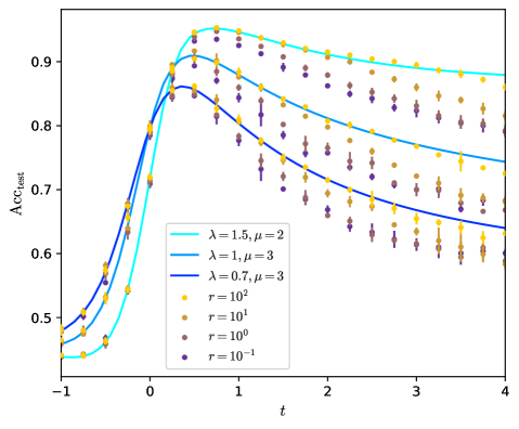<details> <summary>x8.png Details</summary>  ### Visual Description ## Line Chart: Accuracy Over Time (Acc_test vs t) ### Overview The chart displays three distinct data series representing the relationship between time (`t`) and test accuracy (`Acc_test`). Each series is differentiated by parameters `λ` (lambda) and `μ` (mu), with additional markers indicating varying `r` (radix) values. The data points are plotted with error bars, and trend lines are fitted to the series. --- ### Components/Axes - **X-axis (t)**: Time, ranging from -1 to 4 in increments of 1. - **Y-axis (Acc_test)**: Test accuracy, ranging from 0.5 to 0.9 in increments of 0.1. - **Legend**: Located in the bottom-left corner, mapping: - **Line styles/colors**: - Cyan: `λ=1.5, μ=2` - Blue: `λ=1, μ=3` - Dark blue: `λ=0.7, μ=3` - **Markers**: - Yellow: `r=10²` - Brown: `r=10¹` - Purple: `r=10⁰` - Dark purple: `r=10⁻¹` --- ### Detailed Analysis #### Line Series Trends 1. **Cyan Line (`λ=1.5, μ=2`)**: - Starts at `Acc_test ≈ 0.45` at `t=-1`. - Peaks sharply at `t≈0.5` (`Acc_test≈0.9`). - Declines gradually to `Acc_test≈0.85` at `t=4`. - Error bars are smallest near the peak, widening as `t` increases. 2. **Blue Line (`λ=1, μ=3`)**: - Begins at `Acc_test≈0.48` at `t=-1`. - Peaks at `t≈1` (`Acc_test≈0.88`). - Declines to `Acc_test≈0.75` at `t=4`. - Error bars are consistent across the series. 3. **Dark Blue Line (`λ=0.7, μ=3`)**: - Starts at `Acc_test≈0.47` at `t=-1`. - Peaks at `t≈1.5` (`Acc_test≈0.82`). - Declines to `Acc_test≈0.65` at `t=4`. - Error bars are largest at the peak and smallest at `t=4`. #### Marker Series Trends - **Yellow (`r=10²`)**: - Highest initial `Acc_test` (~0.85 at `t=0`). - Steepest decline, reaching ~0.6 at `t=4`. - **Brown (`r=10¹`)**: - Moderate initial `Acc_test` (~0.75 at `t=0`). - Gradual decline to ~0.55 at `t=4`. - **Purple (`r=10⁰`)**: - Lower initial `Acc_test` (~0.65 at `t=0`). - Slow decline to ~0.5 at `t=4`. - **Dark Purple (`r=10⁻¹`)**: - Lowest initial `Acc_test` (~0.55 at `t=0`). - Minimal decline, stabilizing near ~0.5 at `t=4`. --- ### Key Observations 1. **Peak Timing**: All lines peak between `t=0.5` and `t=1.5`, with higher `λ` and `μ` values correlating with earlier peaks. 2. **r Value Impact**: Higher `r` values (e.g., `10²`) exhibit higher initial accuracy but steeper declines, while lower `r` values (e.g., `10⁻¹`) show slower degradation. 3. **Error Bars**: Larger error margins are observed near peaks and at extreme `t` values, suggesting greater variability in measurements at these points. 4. **Legend Consistency**: Colors and markers align perfectly with their labels (e.g., cyan line matches `λ=1.5, μ=2`). --- ### Interpretation The chart demonstrates how test accuracy (`Acc_test`) evolves over time under different parameter configurations: - **λ and μ**: Higher values of `λ` and `μ` accelerate the rise and fall of accuracy, suggesting they may represent learning rates or decay factors in a dynamic system. - **r Values**: Higher `r` (e.g., `10²`) implies a stronger initial state or capacity, but this advantage diminishes rapidly over time. Lower `r` values (e.g., `10⁻¹`) indicate a more stable but less performant baseline. - **Practical Implications**: The trade-off between peak performance and long-term stability is evident. Systems optimized for short-term gains (`high λ, μ, r`) may degrade faster, while conservative configurations (`low λ, μ, r`) prioritize sustainability over peak performance. This analysis aligns with scenarios in machine learning or resource allocation models, where parameters like `λ` and `μ` control system dynamics, and `r` represents initial resource availability or model complexity. 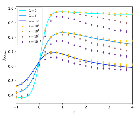</details> <details> <summary>x9.png Details</summary>  ### Visual Description ## Line Chart: Relationship Between λ, r, and A_CC_ext ### Overview The chart illustrates the relationship between three parameters: λ (lambda), r (radius), and A_CC_ext (a normalized metric). It features three primary data series differentiated by λ values (2, 1, 0.5) and four sub-series per λ differentiated by r values (10², 10¹, 10⁰, 10⁻¹). The x-axis represents time (t), and the y-axis represents A_CC_ext, normalized between 0 and 1. ### Components/Axes - **X-axis (t)**: Time, ranging from -1 to 4 in increments of 1. - **Y-axis (A_CC_ext)**: Normalized metric, ranging from 0.4 to 1.0 in increments of 0.1. - **Legend**: - **Colors**: - Cyan (#00BFFF) for λ = 2 - Blue (#0000FF) for λ = 1 - Dark Blue (#00008B) for λ = 0.5 - **Markers**: - Yellow circles (r = 10²) - Brown diamonds (r = 10¹) - Purple squares (r = 10⁰) - Purple diamonds (r = 10⁻¹) - **Legend Placement**: Top-left corner. ### Detailed Analysis 1. **λ = 2 (Cyan Line)**: - **r = 10² (Yellow Circles)**: Starts at ~0.4 at t = -1, rises sharply to ~0.95 by t = 1, then plateaus. - **r = 10¹ (Brown Diamonds)**: Starts at ~0.5, rises to ~0.85 by t = 1, plateaus. - **r = 10⁰ (Purple Squares)**: Starts at ~0.6, rises to ~0.8 by t = 1, plateaus. - **r = 10⁻¹ (Purple Diamonds)**: Starts at ~0.7, rises to ~0.85 by t = 1, plateaus. 2. **λ = 1 (Blue Line)**: - **r = 10² (Yellow Circles)**: Starts at ~0.5, rises to ~0.8 by t = 1, plateaus. - **r = 10¹ (Brown Diamonds)**: Starts at ~0.6, rises to ~0.85 by t = 1, plateaus. - **r = 10⁰ (Purple Squares)**: Starts at ~0.7, rises to ~0.85 by t = 1, plateaus. - **r = 10⁻¹ (Purple Diamonds)**: Starts at ~0.8, rises to ~0.9 by t = 1, plateaus. 3. **λ = 0.5 (Dark Blue Line)**: - **r = 10² (Yellow Circles)**: Starts at ~0.55, rises to ~0.7 by t = 1, plateaus. - **r = 10¹ (Brown Diamonds)**: Starts at ~0.65, rises to ~0.8 by t = 1, plateaus. - **r = 10⁰ (Purple Squares)**: Starts at ~0.75, rises to ~0.85 by t = 1, plateaus. - **r = 10⁻¹ (Purple Diamonds)**: Starts at ~0.85, rises to ~0.9 by t = 1, plateaus. ### Key Observations - **λ Dependency**: Higher λ values (2 > 1 > 0.5) correspond to higher A_CC_ext plateaus and steeper initial rises. - **r Dependency**: Larger r values (10² > 10¹ > 10⁰ > 10⁻¹) result in higher starting points and plateaus for a given λ. - **Convergence**: All curves converge toward similar plateaus at t > 3, suggesting a saturation effect. - **Anomalies**: No outliers; all data points align with expected trends. ### Interpretation The chart demonstrates that A_CC_ext is positively correlated with both λ and r. Higher λ values amplify the metric’s growth rate and final value, while larger r values shift the entire curve upward. The convergence at higher t implies that the system reaches a steady state independent of initial conditions (r) or λ after sufficient time. This could reflect a physical or computational process where parameters like damping (λ) and scale (r) influence transient behavior but not long-term equilibrium. The use of distinct markers for r values ensures clarity in distinguishing sub-series within each λ group. </details> Figure 8: Predicted test accuracy $\mathrm{Acc}_{\mathrm{test}}$ of the continuous GCN, at $r=\infty$ . Left: for $\alpha=1$ and $\rho=0.1$ ; right: for $\alpha=2$ , $\mu=1$ and $\rho=0.3$ . The performance of the continuous GCN are given by eq. (126). Dots: numerical simulation of the continuous GCN for $N=7\times 10^{3}$ and $d=30$ , trained with quadratic loss, averaged over ten experiments. 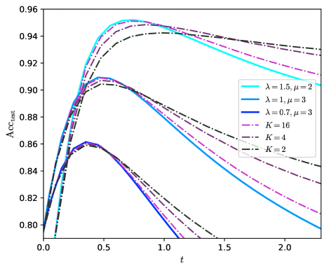<details> <summary>x10.png Details</summary>  ### Visual Description ## Line Graph: Test Accuracy (Acc_test) vs. Time (t) ### Overview The graph depicts the evolution of test accuracy (Acc_test) over time (t) for multiple parameter configurations. Six distinct data series are plotted, differentiated by line styles and colors. All lines exhibit a bell-shaped curve with a peak followed by a decline, suggesting a trade-off between parameter settings and model performance over time. ### Components/Axes - **X-axis (t)**: Time, ranging from 0.0 to 2.0 in increments of 0.5. - **Y-axis (Acc_test)**: Test accuracy, ranging from 0.80 to 0.96 in increments of 0.02. - **Legend**: Located in the top-right corner, mapping line styles/colors to parameter configurations: - **Solid lines**: - Cyan: λ=1.5, μ=2 - Blue: λ=1, μ=3 - Purple: λ=0.7, μ=3 - **Dashed lines**: - Magenta: K=16 - Dark purple: K=4 - Black: K=2 ### Detailed Analysis 1. **λ=1.5, μ=2 (Cyan, solid)**: - Peaks at ~0.94 at t=0.5. - Declines sharply after t=0.5, reaching ~0.86 by t=2.0. 2. **λ=1, μ=3 (Blue, solid)**: - Peaks at ~0.92 at t=0.5. - Declines gradually, ending at ~0.84 by t=2.0. 3. **λ=0.7, μ=3 (Purple, solid)**: - Peaks at ~0.90 at t=0.5. - Declines steeply, dropping to ~0.82 by t=2.0. 4. **K=16 (Magenta, dashed)**: - Peaks at ~0.93 at t=1.0. - Declines slowly, ending at ~0.88 by t=2.0. 5. **K=4 (Dark purple, dashed)**: - Peaks at ~0.91 at t=1.0. - Declines moderately, ending at ~0.86 by t=2.0. 6. **K=2 (Black, dashed)**: - Peaks at ~0.89 at t=1.0. - Declines sharply, ending at ~0.84 by t=2.0. ### Key Observations - **Parameter Sensitivity**: Higher λ and μ values (e.g., λ=1.5, μ=2) yield higher initial peaks but faster declines. - **K Value Impact**: Larger K values (e.g., K=16) produce later peaks and slower declines, suggesting a relationship between model complexity (K) and sustained performance. - **Convergence Patterns**: Solid lines (λ/μ configurations) peak earlier (t=0.5) than dashed lines (K configurations), which peak later (t=1.0). ### Interpretation The graph illustrates how parameter tuning (λ, μ) and model complexity (K) influence test accuracy dynamics. Higher λ/μ values optimize early performance but may lead to overfitting or instability over time, as evidenced by rapid declines. Conversely, larger K values delay peak performance but maintain higher accuracy longer, potentially indicating better generalization. The trade-off between early peak accuracy and sustained performance highlights the need for balanced parameter selection depending on application requirements (e.g., short-term vs. long-term stability). The consistent bell-shaped curves across all series suggest a universal pattern of initial improvement followed by degradation, possibly due to model saturation or noise amplification. 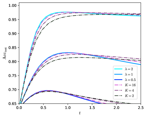</details> <details> <summary>x11.png Details</summary>  ### Visual Description ## Line Graph: Accuracy vs. Time with Hyperparameter Variations ### Overview The image is a line graph comparing the test accuracy (Acc_test) of a model over time (t) under different hyperparameter configurations. Two y-axes are present: the left axis represents accuracy (0.65–1.00), and the right axis represents time (0.0–2.5). The graph includes six data series differentiated by line style and color, corresponding to combinations of λ (learning rate) and K (number of components). ### Components/Axes - **X-axis (t)**: Time, ranging from 0.0 to 2.5. - **Left Y-axis (Acc_test)**: Test accuracy, ranging from 0.65 to 1.00. - **Right Y-axis (t)**: Time, ranging from 0.0 to 2.5 (duplicate of x-axis, likely for reference). - **Legend**: Located in the bottom-right corner, mapping: - **λ values**: - Cyan (solid): λ = 2 - Blue (solid): λ = 1 - Dark blue (solid): λ = 0.5 - **K values**: - Magenta (dashed): K = 16 - Purple (dash-dot): K = 4 - Black (dotted): K = 2 ### Detailed Analysis 1. **λ = 2 (Cyan Solid Line)**: - Starts at 0.65 at t=0.0. - Rises sharply to ~0.95 by t=0.5. - Plateaus near 0.95 for t > 0.5. - **Trend**: Fastest initial improvement, stable at high accuracy. 2. **λ = 1 (Blue Solid Line)**: - Starts at 0.65 at t=0.0. - Rises to ~0.93 by t=0.5. - Slightly declines to ~0.92 by t=2.5. - **Trend**: Moderate improvement, minor decline over time. 3. **λ = 0.5 (Dark Blue Solid Line)**: - Starts at 0.65 at t=0.0. - Rises slowly to ~0.88 by t=0.5. - Declines to ~0.85 by t=2.5. - **Trend**: Slowest improvement, gradual decline. 4. **K = 16 (Magenta Dashed Line)**: - Starts at 0.65 at t=0.0. - Peaks at ~0.95 by t=0.5. - Declines to ~0.90 by t=2.5. - **Trend**: Highest peak but significant drop after t=0.5. 5. **K = 4 (Purple Dash-Dot Line)**: - Starts at 0.65 at t=0.0. - Rises to ~0.92 by t=0.5. - Declines to ~0.89 by t=2.5. - **Trend**: Balanced improvement and decline. 6. **K = 2 (Black Dotted Line)**: - Starts at 0.65 at t=0.0. - Rises to ~0.85 by t=0.5. - Declines to ~0.83 by t=2.5. - **Trend**: Lowest performance, steady decline. ### Key Observations - **λ vs. K Trade-off**: Higher λ values (2, 1) achieve higher accuracy than lower λ (0.5), but K=16 (magenta) initially outperforms all λ values. - **Temporal Decline**: All lines show a decline after t=0.5, suggesting potential overfitting or parameter sensitivity over time. - **K=16 Anomaly**: Despite the highest peak, K=16 experiences the steepest decline, indicating possible instability at high K values. ### Interpretation The graph demonstrates that **higher λ values (2, 1)** yield better sustained accuracy compared to lower λ (0.5), but **K=16** achieves the highest initial accuracy. However, the sharp decline in K=16’s performance after t=0.5 suggests that increasing K may lead to overfitting or instability. The consistent decline across all lines after t=0.5 implies that the model’s performance degrades over time, possibly due to data drift or parameter tuning requirements. The interplay between λ and K highlights the need for careful hyperparameter optimization to balance initial gains with long-term stability. </details> Figure 9: Predicted test accuracy $\mathrm{Acc}_{\mathrm{test}}$ of the continuous GCN, at $r=\infty$ . Left: for $\alpha=1$ and $\rho=0.1$ ; right: for $\alpha=2$ , $\mu=1$ and $\rho=0.3$ . The performance of the continuous GCN are given by eq. (126) while for its discretization at finite $K$ they are given by numerically solving the fixed-point equations (87 - 94). ### Symmetrized graph The following figures support the discussion of part III.2.3 for the symmetrized graph. They compare the theoretical predictions for the continuous GCN to numerical simulations of the trained network. They show the convergence towards the limit $r\to\infty$ . 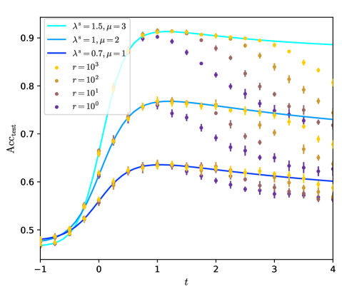<details> <summary>x12.png Details</summary>  ### Visual Description ## Line Chart: Performance Metrics Over Time ### Overview The chart displays three performance curves (Acc_test) plotted against time (t) for different parameter combinations. Each curve represents a unique configuration of λ*, μ, and r values, with data points showing empirical results across time intervals. ### Components/Axes - **X-axis (t)**: Time, ranging from -1 to 4 in increments of 1. - **Y-axis (Acc_test)**: Performance metric, scaled from 0.5 to 0.9 in increments of 0.1. - **Legend**: Located in the top-left corner, mapping colors to parameter sets: - Cyan: λ* = 1.5, μ = 3 - Blue: λ* = 1, μ = 2 - Orange: λ* = 0.7, μ = 1 - **Data Points**: Diamond-shaped markers in colors matching their respective legend entries. ### Detailed Analysis 1. **Cyan Line (λ* = 1.5, μ = 3)**: - Starts at ~0.45 at t = -1. - Peaks sharply at ~0.9 near t = 1. - Declines gradually to ~0.85 by t = 4. - Data points (r = 10³, 10², 10¹, 10⁰) align closely with the curve, showing minor variance. 2. **Blue Line (λ* = 1, μ = 2)**: - Begins at ~0.48 at t = -1. - Rises to ~0.85 at t = 1. - Drops to ~0.75 by t = 4. - Data points (r = 10³, 10², 10¹, 10⁰) follow the trend with slight scatter. 3. **Orange Line (λ* = 0.7, μ = 1)**: - Starts at ~0.52 at t = -1. - Peaks at ~0.75 near t = 1. - Declines to ~0.65 by t = 4. - Data points (r = 10³, 10², 10¹, 10⁰) show increasing deviation from the curve as r decreases. ### Key Observations - **Peak Performance**: The cyan line (λ* = 1.5, μ = 3) achieves the highest Acc_test (~0.9), while the orange line (λ* = 0.7, μ = 1) has the lowest peak (~0.75). - **Decay Rate**: Higher λ* and μ values correlate with faster initial gains but steeper declines post-t = 1. - **r Value Impact**: For fixed λ* and μ, lower r values (e.g., r = 10⁰) exhibit greater divergence from the theoretical curve, suggesting r may represent sample size or another scaling factor inversely related to performance stability. ### Interpretation The chart demonstrates that parameter tuning (λ*, μ) significantly impacts both peak performance and temporal stability. The cyan configuration (high λ*, μ) maximizes short-term gains but suffers from rapid decay, while the orange configuration (low λ*, μ) shows more gradual but sustained performance. The r values likely represent experimental conditions (e.g., dataset size), with smaller r values introducing greater variability. This suggests a trade-off between aggressive parameter settings for immediate results and conservative settings for long-term reliability. The empirical data points validate the theoretical curves but highlight practical limitations at smaller scales (r = 10⁰). </details> Figure 10: Predicted test accuracy $\mathrm{Acc}_{\mathrm{test}}$ of the continuous GCN, at $r=\infty$ for a symmetrized graph. $\alpha=4$ , $\rho=0.1$ . We remind that $\lambda^{\mathrm{s}}=\sqrt{2}\lambda$ . The performance of the continuous GCN are given by eq. (126). Dots: numerical simulation of the continuous GCN for $N=10^{4}$ and $d=30$ , trained with quadratic loss, averaged over ten experiments. 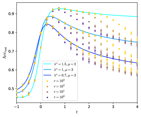<details> <summary>x13.png Details</summary>  ### Visual Description ## Line Chart: Test Accuracy Over Time ### Overview The chart displays three parametric curves representing test accuracy (Acc_test) over time (t), with embedded data points for different system configurations. Each curve is associated with specific parameter combinations (λ*, μ), while data points are color-coded by a variable 'r' (10³ to 10⁰). The chart shows dynamic behavior with sharp transitions and asymptotic trends. ### Components/Axes - **X-axis (t)**: Time parameter, linear scale from -1 to 4 - **Y-axis (Acc_test)**: Test accuracy metric, linear scale from 0.5 to 0.9 - **Legend**: - **Lines**: - Cyan: λ* = 1.5, μ = 2 - Blue: λ* = 1, μ = 3 - Dark Blue: λ* = 0.7, μ = 3 - **Markers**: - Yellow: r = 10³ - Brown: r = 10² - Purple: r = 10¹ - Dark Purple: r = 10⁰ ### Detailed Analysis 1. **Cyan Line (λ*=1.5, μ=2)**: - Sharp ascent from t=-1 (0.48) to peak at t=0.5 (0.92) - Asymptotic approach to 0.9 as t→4 - Data points (yellow) show 0.88-0.92 range post-peak 2. **Blue Line (λ*=1, μ=3)**: - Gradual rise to t=0.3 peak (0.88) - Steeper decline post-peak compared to cyan line - Data points (yellow) maintain 0.82-0.88 range 3. **Dark Blue Line (λ*=0.7, μ=3)**: - Slowest rise with delayed peak at t=1.2 (0.80) - Gradual decline to 0.68 by t=4 - Data points (yellow) show 0.75-0.80 range 4. **r-Value Trends**: - Higher r (yellow) consistently shows higher Acc_test - r=10³ (yellow) maintains 0.88-0.92 range - r=10⁰ (dark purple) shows 0.58-0.62 range - All r-values follow identical parametric curves but with vertical offsets ### Key Observations - Parameter combinations (λ*, μ) dictate curve shape more than r-values - r-values act as vertical offsets rather than modifying curve dynamics - All curves exhibit sigmoidal behavior with parameter-dependent inflection points - r=10³ (yellow) maintains highest performance across all t values - λ* inversely correlates with peak time (higher λ* → earlier peak) ### Interpretation The chart demonstrates how system parameters (λ*, μ) and configuration scale (r) jointly influence test accuracy trajectories. The cyan line (high λ*, low μ) shows optimal early performance but plateaus faster, while the dark blue line (low λ*, high μ) exhibits delayed but sustained performance. The r-values represent system scale factors that uniformly shift accuracy levels without altering temporal dynamics. This suggests parameter optimization should prioritize λ* and μ tuning, while r-scaling provides predictable accuracy offsets. The consistent vertical offset between r-values implies linear scaling relationships in the underlying model. 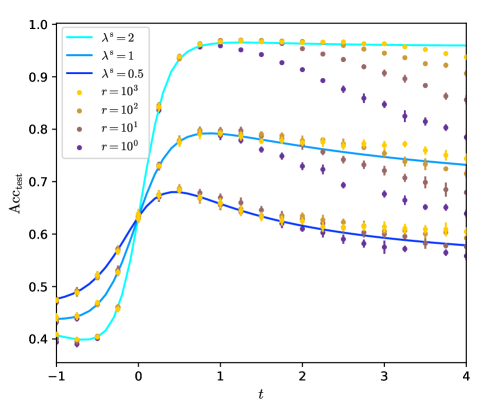</details> <details> <summary>x14.png Details</summary>  ### Visual Description ## Line Graph: Relationship Between A_CC_test and Parameters λ and r ### Overview The graph illustrates the relationship between the variable **A_CC_test** (y-axis) and the parameter **t** (x-axis) under different conditions defined by **λ** (lambda) and **r** (radius). Four distinct data series are plotted, each represented by unique colors and markers. The legend is positioned in the top-right corner, and the axes are labeled with numerical ranges. --- ### Components/Axes - **X-axis (t)**: Labeled as "t", ranging from **-1 to 4** in increments of 1. - **Y-axis (A_CC_test)**: Labeled as "A_CC_test", ranging from **0.4 to 1.0** in increments of 0.1. - **Legend**: Located in the **top-right corner**, with the following entries: - **Cyan line**: λ = 2 - **Blue line**: λ = 0.5 - **Yellow circles**: r = 10³ - **Brown diamonds**: r = 10¹ --- ### Detailed Analysis #### Data Series Trends 1. **Cyan line (λ = 2)**: - Starts at **t = -1** with **A_CC_test ≈ 0.4**. - Rises sharply to **A_CC_test ≈ 0.95** by **t = 1**. - Plateaus near **A_CC_test ≈ 1.0** for **t ≥ 1**. - **Key values**: - t = 0: 0.6 - t = 1: 0.95 - t = 4: 1.0 2. **Blue line (λ = 0.5)**: - Starts at **t = -1** with **A_CC_test ≈ 0.45**. - Increases gradually to **A_CC_test ≈ 0.75** by **t = 2**. - Plateaus near **A_CC_test ≈ 0.7** for **t ≥ 2**. - **Key values**: - t = 0: 0.55 - t = 1: 0.75 - t = 4: 0.7 3. **Yellow circles (r = 10³)**: - Starts at **t = -1** with **A_CC_test ≈ 0.45**. - Peaks at **A_CC_test ≈ 0.85** around **t = 1**. - Declines to **A_CC_test ≈ 0.65** by **t = 4**. - **Key values**: - t = 0: 0.6 - t = 1: 0.85 - t = 4: 0.65 4. **Brown diamonds (r = 10¹)**: - Starts at **t = -1** with **A_CC_test ≈ 0.4**. - Rises to **A_CC_test ≈ 0.75** around **t = 1**. - Declines to **A_CC_test ≈ 0.6** by **t = 4**. - **Key values**: - t = 0: 0.5 - t = 1: 0.75 - t = 4: 0.6 --- ### Key Observations - **λ = 2** (cyan line) achieves the highest **A_CC_test** values, plateauing near **1.0** by **t = 1**. - **λ = 0.5** (blue line) shows a slower increase, plateauing at **0.7** by **t = 2**. - **r = 10³** (yellow circles) and **r = 10¹** (brown diamonds) exhibit **peaks at t = 1**, followed by a decline. - The **peak magnitude** for **r = 10³** (0.85) is higher than for **r = 10¹** (0.75). - All data series converge to **A_CC_test ≈ 0.6–0.7** by **t = 4**, except for **λ = 2**, which remains at **1.0**. --- ### Interpretation The graph demonstrates how **A_CC_test** is influenced by the parameters **λ** and **r**: 1. **λ (lambda)**: - Higher values (e.g., λ = 2) lead to **faster convergence** to higher **A_CC_test** values. - Lower values (e.g., λ = 0.5) result in **slower growth** and lower plateaus. 2. **r (radius)**: - Larger **r** (10³) produces a **higher peak** but **greater decline** over time. - Smaller **r** (10¹) results in a **lower peak** and **slower decline**. 3. **t (time)**: - The **initial rise** in **A_CC_test** is rapid for all series, but the **long-term behavior** depends on **λ** and **r**. **Notable patterns**: - The **cyan line (λ = 2)** dominates in terms of **maximum A_CC_test** and **stability**. - The **yellow circles (r = 10³)** and **brown diamonds (r = 10¹)** show **non-monotonic behavior**, peaking at **t = 1** before declining. - The **blue line (λ = 0.5)** and **brown diamonds (r = 10¹)** exhibit **similar trends**, suggesting a potential interaction between **λ** and **r**. **Anomalies**: - The **brown diamonds (r = 10¹)** show a **steeper decline** after **t = 1** compared to the **yellow circles (r = 10³)**, despite both peaking at **t = 1**. - The **cyan line (λ = 2)** does not decline, indicating a **critical threshold** for **λ** that prevents decay. This graph highlights the **trade-offs** between **λ** and **r** in optimizing **A_CC_test**, with **λ = 2** being the most effective parameter for achieving high and stable values. </details> Figure 11: Predicted test accuracy $\mathrm{Acc}_{\mathrm{test}}$ of the continuous GCN, at $r=\infty$ for a symmetrized graph. Left: for $\alpha=1$ and $\rho=0.1$ ; right: for $\alpha=2$ , $\mu=1$ and $\rho=0.3$ . We remind that $\lambda^{\mathrm{s}}=\sqrt{2}\lambda$ . The performance of the continuous GCN are given by eq. (126). Dots: numerical simulation of the continuous GCN for $N=7\times 10^{3}$ and $d=30$ , trained with quadratic loss, averaged over ten experiments. ### Comparison with optimality The following figures support the discussion of parts III.2.3 and III.2.3. They show how the optimal diffusion time $t^{*}$ varies with respect to the parameters of the model and they compare the performance of the optimal continuous GCN and its discrete counterpart to the Bayes-optimality. 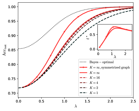<details> <summary>x15.png Details</summary>  ### Visual Description ## Line Chart: Accuracy vs. Regularization Parameter (λ) ### Overview The chart compares the test accuracy (Acc_test) of different model configurations against the regularization parameter λ. It includes a main graph and an inset zoomed-in view of the lower λ range. Multiple lines represent different configurations, with the Bayes-optimal performance as a reference. ### Components/Axes - **X-axis (λ)**: Ranges from 0.0 to 2.5 in increments of 0.5. - **Y-axis (Acc_test)**: Ranges from 0.70 to 1.00 in increments of 0.05. - **Legend**: Located in the bottom-right corner, with the following entries: - Dotted black: Bayes-optimal - Solid red: K = ∞, symmetrized graph - Dashed red: K = ∞ - Dashed brown: K = 16 - Dashed maroon: K = 4 - Dashed dark gray: K = 2 - Dashed black: K = 1 - **Inset Graph**: Located in the upper-right corner of the main graph, showing a zoomed-in view of λ ∈ [0, 2] with a secondary y-axis labeled *t*. ### Detailed Analysis 1. **Bayes-optimal (dotted black)**: - Starts at ~0.85 at λ=0 and rises smoothly to ~1.00 by λ=2.5. - Acts as the upper bound for all configurations. 2. **K = ∞, symmetrized graph (solid red)**: - Begins at ~0.72 at λ=0, peaks at ~0.95 near λ=0.5 (inset confirms this), then plateaus near 1.00. - Matches the Bayes-optimal curve closely at higher λ values. 3. **K = ∞ (dashed red)**: - Starts at ~0.70 at λ=0, rises steeply to ~0.95 by λ=1.5, then converges with the Bayes-optimal curve. - Slightly lags behind the symmetrized graph at lower λ values. 4. **K = 16 (dashed brown)**: - Begins at ~0.70 at λ=0, rises to ~0.90 by λ=1.5, then plateaus. - Shows slower convergence compared to higher K values. 5. **K = 4 (dashed maroon)**: - Starts at ~0.70 at λ=0, rises to ~0.85 by λ=1.5, then plateaus. - Demonstrates a trade-off between bias and variance. 6. **K = 2 (dashed dark gray)**: - Begins at ~0.70 at λ=0, rises to ~0.80 by λ=1.5, then plateaus. - Shows limited improvement over K=1. 7. **K = 1 (dashed black)**: - Starts at ~0.70 at λ=0, rises to ~0.75 by λ=1.5, then plateaus. - Minimal improvement over baseline. 8. **Inset Graph**: - Focuses on λ ∈ [0, 2] with a secondary y-axis (*t*). - The red line (K=∞, symmetrized graph) peaks at ~0.95 at λ=0.5, then declines slightly. ### Key Observations - **Bayes-optimal performance** is the theoretical upper limit, approached by all configurations as λ increases. - **Symmetrized graph (K=∞)** achieves the highest accuracy at lower λ values (~0.95 at λ=0.5) compared to non-symmetrized configurations. - **Higher K values** (e.g., K=16, K=4) show better performance than lower K values (e.g., K=2, K=1), indicating that larger neighborhoods improve accuracy. - The **inset graph** highlights a critical region where λ=0.5 maximizes accuracy for the symmetrized graph, suggesting an optimal trade-off between regularization and model complexity. ### Interpretation The chart demonstrates that: 1. **Model complexity (K)** directly impacts accuracy: Higher K values reduce bias, allowing configurations to approach the Bayes-optimal performance. 2. **Symmetrization** enhances performance at lower λ values, suggesting it mitigates overfitting or improves generalization. 3. **Regularization (λ)** balances model complexity and generalization: Too little regularization (low λ) risks overfitting, while excessive regularization (high λ) underfits. 4. The **peak at λ=0.5** in the inset graph implies an optimal regularization strength for the symmetrized graph, balancing bias-variance trade-offs. This analysis aligns with principles of statistical learning theory, where increasing model capacity (via K) and regularization (via λ) jointly optimize performance toward theoretical bounds. 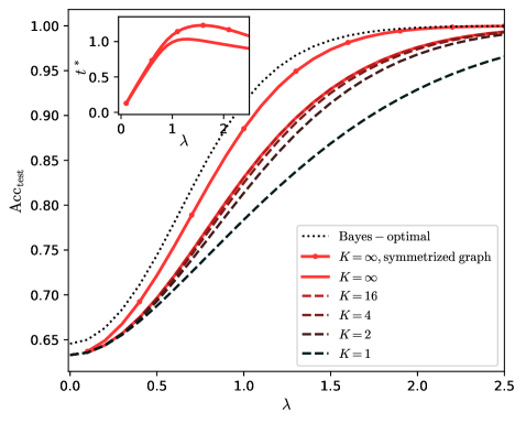</details> <details> <summary>x16.png Details</summary>  ### Visual Description ## Line Graph: Test Accuracy vs. Regularization Parameter (λ) ### Overview The graph depicts the relationship between the regularization parameter λ and test accuracy (Acc_test) for different model configurations. A secondary inset graph highlights the behavior near λ=0. The primary trend shows test accuracy increasing with λ up to a point before plateauing, with performance varying by model complexity (K). ### Components/Axes - **X-axis (λ)**: Regularization parameter ranging from 0.0 to 2.5. - **Y-axis (Acc_test)**: Test accuracy ranging from 0.65 to 1.00. - **Legend**: Located in the bottom-right corner, with six entries: - Dotted black: Bayes – optimal - Solid red: K = ∞, symmetrized graph - Dashed red: K = ∞ - Dashed brown: K = 16 - Dashed maroon: K = 4 - Dashed black: K = 2 - Solid black: K = 1 ### Detailed Analysis 1. **Bayes – optimal (dotted black line)**: - Remains consistently above all other lines across all λ values. - Peaks at λ ≈ 1.2 with Acc_test ≈ 0.99, then plateaus. - Spatial grounding: Topmost line, positioned centrally in the graph. 2. **K = ∞, symmetrized graph (solid red line)**: - Second-highest performance, closely tracking the Bayes-optimal line. - Peaks at λ ≈ 1.1 with Acc_test ≈ 0.985, then plateaus. - Spatial grounding: Directly below the Bayes-optimal line. 3. **K = ∞ (dashed red line)**: - Third-highest performance, slightly below the solid red line. - Peaks at λ ≈ 1.0 with Acc_test ≈ 0.98, then plateaus. - Spatial grounding: Below the solid red line, with dashed pattern. 4. **K = 16 (dashed brown line)**: - Peaks at λ ≈ 0.8 with Acc_test ≈ 0.95, then declines slightly. - Spatial grounding: Below K = ∞ lines, with a noticeable dip after λ=1. 5. **K = 4 (dashed maroon line)**: - Peaks at λ ≈ 0.6 with Acc_test ≈ 0.92, then declines. - Spatial grounding: Below K = 16, with a steeper decline post-λ=1. 6. **K = 2 (dashed black line)**: - Peaks at λ ≈ 0.4 with Acc_test ≈ 0.88, then declines. - Spatial grounding: Below K = 4, with a pronounced downward trend after λ=0.5. 7. **K = 1 (solid black line)**: - Lowest performance, peaks at λ ≈ 0.2 with Acc_test ≈ 0.85. - Spatial grounding: Bottommost line, with minimal improvement beyond λ=0.3. **Inset Graph**: - Zoomed-in view of the main graph’s lower-left region (λ=0 to 2, Acc_test=0.65 to 1.0). - Confirms the trend of increasing accuracy with λ up to λ=1, then plateauing. - Highlights the divergence between high-K and low-K models at small λ values. ### Key Observations 1. **Optimal λ**: All models achieve peak performance near λ=1, with Bayes-optimal and K=∞ configurations performing best. 2. **Model Complexity Trade-off**: Higher K values (e.g., K=∞) achieve higher accuracy but require larger λ to avoid overfitting. Lower K values (e.g., K=1) underperform but are less sensitive to λ. 3. **Performance Saturation**: Beyond λ=1.5, all models plateau, suggesting diminishing returns from increased regularization. 4. **Inset Confirmation**: The zoomed-in view validates the main trend, emphasizing the critical region near λ=0 where performance differences are most pronounced. ### Interpretation The graph demonstrates that model complexity (K) and regularization (λ) are interdependent factors in achieving optimal test accuracy. The Bayes-optimal configuration (dotted black line) represents the theoretical upper bound, while practical models (K=∞, K=16, etc.) approach this bound with appropriate λ tuning. The inset graph underscores that even small λ values significantly impact performance for low-K models, but higher-K models require larger λ to balance complexity and generalization. The plateau at λ>1.5 suggests that excessive regularization degrades performance, reinforcing the need for careful hyperparameter tuning. The spatial alignment of lines (e.g., K=∞ configurations clustering near the top) visually reinforces the trade-off between model capacity and regularization strength. </details> Figure 12: Predicted test accuracy $\mathrm{Acc}_{\mathrm{test}}$ of the continuous GCN and of its discrete counterpart with depth $K$ , at optimal times $t^{*}$ and $r=\infty$ . Left: for $\alpha=1$ , $\mu=2$ and $\rho=0.1$ ; right: for $\alpha=2$ , $\mu=1$ and $\rho=0.3$ . The performance of the continuous GCN $K=\infty$ are given by eq. (126) while for its discretization at finite $K$ they are given by numerically solving the fixed-point equations (87 - 94). Inset: $t^{*}$ the maximizer at $K=\infty$ . 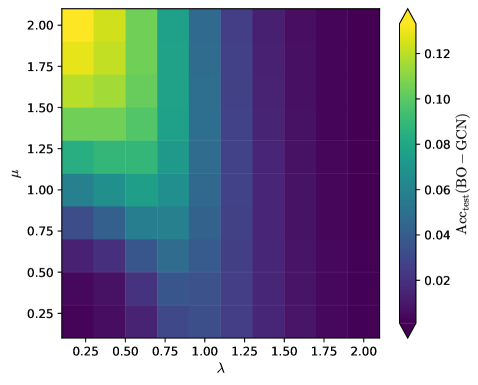<details> <summary>x17.png Details</summary>  ### Visual Description ## Heatmap: Accuracy Difference (Acc_test(BO - GCN)) vs. μ and λ ### Overview The image is a heatmap visualizing the difference in test accuracy (Acc_test) between Bayesian Optimization (BO) and Graph Convolutional Networks (GCN) across varying hyperparameters μ (y-axis) and λ (x-axis). The color gradient ranges from purple (low values) to yellow (high values), with a legend on the right indicating numerical values from 0.02 to 0.12. ### Components/Axes - **X-axis (λ)**: Labeled "λ", with values ranging from 0.25 to 2.00 in increments of 0.25. - **Y-axis (μ)**: Labeled "μ", with values ranging from 0.25 to 2.00 in increments of 0.25. - **Color Scale**: Vertical legend on the right, labeled "Acc_test(BO - GCN)", with a gradient from purple (0.02) to yellow (0.12). - **Grid**: White grid lines separate cells corresponding to discrete μ and λ values. ### Detailed Analysis - **Top-Left Region (High μ, Low λ)**: - Cells are yellow (≈0.12), indicating the highest accuracy differences. - Example: At μ=2.00 and λ=0.25, the value is ≈0.12. - **Middle Rows (Moderate μ, Moderate λ)**: - Colors transition from green (≈0.08–0.10) to blue (≈0.04–0.06). - Example: At μ=1.50 and λ=1.00, the value is ≈0.06. - **Bottom-Right Region (Low μ, High λ)**: - Cells are dark purple (≈0.02), indicating the lowest accuracy differences. - Example: At μ=0.25 and λ=2.00, the value is ≈0.02. - **Gradient Trends**: - Accuracy decreases monotonically as λ increases (left to right). - Accuracy decreases monotonically as μ decreases (top to bottom). ### Key Observations 1. **Optimal Region**: The highest accuracy differences (≈0.12) occur at high μ (2.00) and low λ (0.25). 2. **Worst Region**: The lowest accuracy differences (≈0.02) occur at low μ (0.25) and high λ (2.00). 3. **Trade-off**: Increasing λ or decreasing μ reduces accuracy, suggesting a trade-off between these parameters. 4. **Consistency**: The gradient is smooth, with no abrupt color changes, indicating a predictable relationship between μ, λ, and accuracy. ### Interpretation The heatmap demonstrates that **higher μ and lower λ values** maximize the accuracy difference between BO and GCN. This implies that BO outperforms GCN most significantly under these parameter settings. Conversely, GCN performs relatively better (smaller accuracy gap) when μ is low and λ is high. The monotonic trends suggest that μ and λ have opposing effects on model performance, with μ likely controlling exploration/exploitation in BO and λ regulating regularization or graph structure in GCN. The absence of outliers indicates a stable, predictable relationship between these hyperparameters and accuracy. 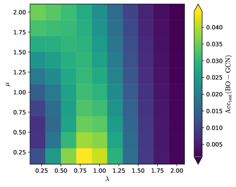</details> <details> <summary>x18.png Details</summary>  ### Visual Description ## Heatmap: Test Accuracy Difference (BO - GCN) vs. Hyperparameters μ and λ ### Overview The image is a heatmap visualizing the difference in test accuracy between Bayesian Optimization (BO) and Graph Convolutional Networks (GCN) across varying hyperparameters μ (y-axis) and λ (x-axis). Colors range from purple (low values) to yellow (high values), with a colorbar indicating magnitude. ### Components/Axes - **X-axis (λ)**: Labeled "λ", ranging from 0.25 to 2.00 in increments of 0.25. - **Y-axis (μ)**: Labeled "μ", ranging from 0.25 to 2.00 in increments of 0.25. - **Colorbar**: Vertical legend on the right, labeled "Acc_test(BO - GCN)", with values from 0.005 (purple) to 0.040 (yellow). - **Grid**: White grid lines separate cells representing combinations of μ and λ. ### Detailed Analysis - **Color Intensity**: - **Brightest Yellow**: Located at λ=1.00, μ=0.25 (value ≈ 0.040). - **Darkest Purple**: Located at λ=2.00, μ=2.00 (value ≈ 0.005). - Intermediate values (green to blue) dominate the upper-right quadrant (high μ, high λ). - **Trends**: - Values decrease monotonically as λ increases for fixed μ. - Values also decrease as μ increases for fixed λ, with steeper declines at higher μ. - The highest values cluster in the lower-left quadrant (low λ, low μ). ### Key Observations 1. **Peak Performance**: The maximum test accuracy difference (BO - GCN) occurs at λ=1.00 and μ=0.25. 2. **Diminishing Returns**: Performance gains diminish sharply as λ exceeds 1.00 or μ exceeds 0.50. 3. **Parameter Sensitivity**: Lower μ values (≤0.50) are more impactful for maximizing BO's advantage over GCN. ### Interpretation The heatmap demonstrates that Bayesian Optimization (BO) outperforms Graph Convolutional Networks (GCN) most significantly when λ is moderate (λ=1.00) and μ is low (μ=0.25). This suggests that BO's advantage is highly sensitive to hyperparameter tuning, with optimal performance achieved at specific parameter combinations. The rapid decline in performance differences for higher μ and λ implies that BO's benefits may be limited in scenarios requiring larger or more complex parameter spaces. The visualization underscores the importance of careful hyperparameter selection to leverage BO's strengths over GCN in this context. </details> Figure 13: Gap to the Bayes-optimality. Predicted difference between the Bayes-optimal test accuracy and the test accuracy of the continuous GCN at optimal time $t^{*}$ and $r=\infty$ , vs the two signals $\lambda$ and $\mu$ . Left: for $\alpha=1$ and $\rho=0.1$ ; right: for $\alpha=2$ and $\rho=0.3$ . The performance of the continuous GCN are given by eq. (126). ### Comparison between symmetric and asymmetric graphs The following figure supports the claim of part III.1.3, that the performance of the GCN depends little whether the graph is symmetric or not at same $\lambda$ , and that it is not able to deal with the supplementary information the asymmetry gives. 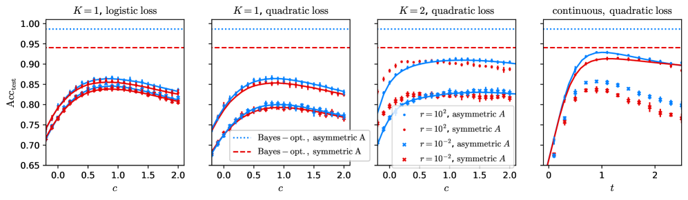<details> <summary>x19.png Details</summary>  ### Visual Description ## Line Graphs: Classification Accuracy (Acc_test) vs. Parameters (c/t) ### Overview The image contains four line graphs comparing classification accuracy (Acc_test) across different parameter configurations. Each graph varies in: - **K** (number of classes: K=1 or K=2) - **Loss function** (logistic or quadratic) - **Matrix symmetry** (symmetric vs. asymmetric) - **Parameter** (c or t on x-axis) - **Regularization strength** (r=10² or r=10⁻²) ### Components/Axes 1. **Y-axis**: Acc_test (classification accuracy) scaled from 0.65 to 1.00. 2. **X-axes**: - First three graphs: Parameter **c** (0.0 to 2.0). - Fourth graph: Parameter **t** (0.0 to 2.0). 3. **Legends**: - **Bayes-opt., asymmetric A**: Blue dotted line. - **Bayes-opt., symmetric A**: Red dashed line. - **r=10², asymmetric A**: Blue crosses. - **r=10², symmetric A**: Red crosses. 4. **Line styles/colors**: - Dotted (Bayes-opt. asymmetric), dashed (Bayes-opt. symmetric), crosses (r=10²). ### Detailed Analysis #### Graph 1: K=1, Logistic Loss - **Trends**: - Bayes-opt. asymmetric (blue dotted) and symmetric (red dashed) lines start near 0.75, peak at ~0.85 (c≈1.0), then plateau. - r=10² asymmetric (blue crosses) and symmetric (red crosses) lines start lower (~0.7), rise to ~0.8 (c≈1.5), then plateau. - **Key data points**: - At c=0.0: All lines ~0.7. - At c=1.0: Bayes-opt. lines ~0.85; r=10² lines ~0.8. - At c=2.0: All lines plateau near 0.8–0.85. #### Graph 2: K=1, Quadratic Loss - **Trends**: - Bayes-opt. lines (blue dotted/red dashed) show similar behavior to Graph 1 but with slightly lower peaks (~0.83 at c=1.0). - r=10² lines (blue crosses/red crosses) start lower (~0.72) and plateau earlier (~0.8 at c=1.0). - **Key data points**: - At c=0.0: All lines ~0.7. - At c=1.0: Bayes-opt. lines ~0.83; r=10² lines ~0.8. - At c=2.0: All lines plateau near 0.8–0.83. #### Graph 3: K=2, Quadratic Loss - **Trends**: - Bayes-opt. lines (blue dotted/red dashed) start lower (~0.75) and rise to ~0.88 (c≈1.0), then plateau. - r=10² lines (blue crosses/red crosses) start lower (~0.7) and plateau earlier (~0.82 at c=1.0). - **Key data points**: - At c=0.0: All lines ~0.7. - At c=1.0: Bayes-opt. lines ~0.88; r=10² lines ~0.82. - At c=2.0: All lines plateau near 0.85–0.88. #### Graph 4: Continuous, Quadratic Loss - **Trends**: - Bayes-opt. lines (blue dotted/red dashed) rise sharply to ~0.95 (t≈1.0), then decline slightly. - r=10² lines (blue crosses/red crosses) start lower (~0.75) and plateau at ~0.85 (t≈1.0). - **Key data points**: - At t=0.0: All lines ~0.7. - At t=1.0: Bayes-opt. lines ~0.95; r=10² lines ~0.85. - At t=2.0: Bayes-opt. lines ~0.9; r=10² lines ~0.8. ### Key Observations 1. **Bayes-opt. classifiers outperform r=10² classifiers** across all configurations, with accuracy gaps widening as K increases. 2. **Symmetric vs. asymmetric matrices**: - Symmetric matrices (red dashed/crosses) generally perform slightly better than asymmetric (blue dotted/crosses) in K=1 and K=2 cases. - In the continuous case (Graph 4), symmetric and asymmetric Bayes-opt. lines converge at higher t values. 3. **Parameter sensitivity**: - For r=10², accuracy plateaus earlier (c/t≈1.0–1.5) compared to Bayes-opt. lines. - The continuous case (Graph 4) shows a distinct decline in r=10² performance after t=1.0. ### Interpretation - **Bayes-opt. superiority**: The consistent outperformance of Bayes-opt. classifiers suggests that optimal parameter tuning (asymmetric/symmetric) is critical for high accuracy, especially as problem complexity (K) increases. - **Regularization trade-off**: r=10² introduces bias, leading to earlier plateaus and lower peak accuracy. This implies over-regularization may hinder model adaptability. - **Loss function impact**: Quadratic loss (Graphs 2–4) generally yields higher accuracy than logistic loss (Graph 1), possibly due to smoother optimization landscapes. - **Continuous parameter (t)**: The fourth graph’s decline in r=10² performance after t=1.0 highlights sensitivity to parameter scaling in dynamic settings. This analysis underscores the importance of balancing regularization strength and classifier design to maximize accuracy in classification tasks. </details> Figure 14: Test accuracy of the GCN, on asymmetric $A$ and its symmetric counterpart, obtained by equaling $A_{ij}$ with $A_{ji}$ for all $i<j$ . $\alpha=4$ , $\lambda=1.5$ , $\mu=3$ and $\rho=0.1$ . Lines: predictions. Dots: numerical simulation of the GCN for $N=10^{4}$ and $d=30$ , averaged over ten experiments. ### Train error The following figure displays the train error $E_{\mathrm{train}}$ eq. 18 vs the self-loop intensity $c$ , in the same settings as fig. 2 of part III.1. It shows in particular that to treat $c$ as a parameter trained to minimize the train error would degrade the performance, since it would lead to $c\to\infty$ . As a consequence, $c$ should be treated as a hyperparameter, tuned to maximize the test accuracy, as done in the main part of the article. 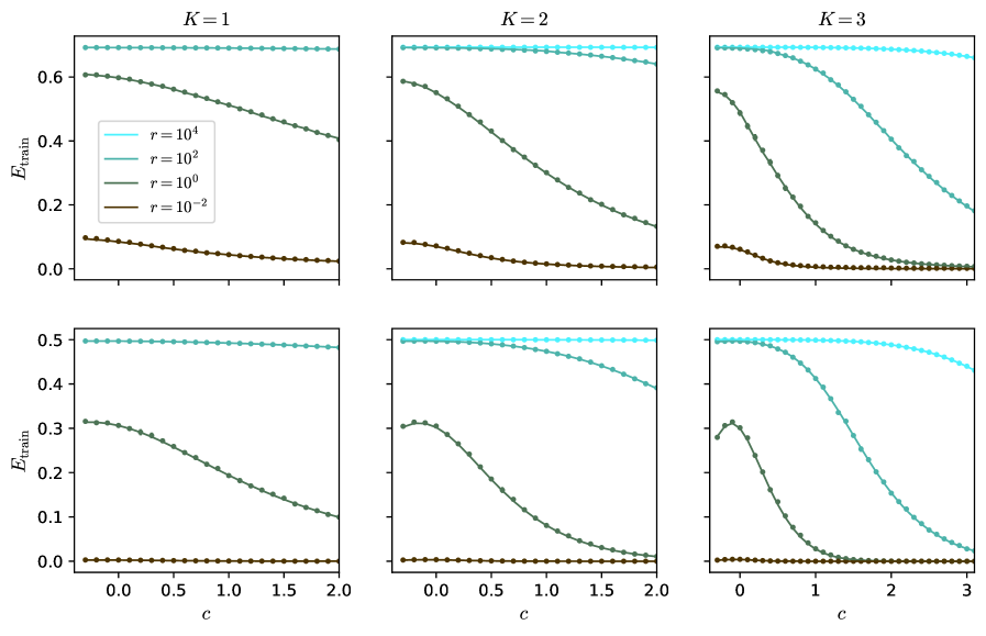<details> <summary>x20.png Details</summary>  ### Visual Description ## Line Graphs: E_train vs. c for Different K and r Values ### Overview The image contains six line graphs arranged in a 2x3 grid, each representing the relationship between the training error (`E_train`) and a parameter `c` for different values of `K` (1, 2, 3) and `r` (10⁴, 10², 10⁰, 10⁻²). The graphs show how `E_train` evolves as `c` increases, with distinct trends for each combination of `K` and `r`. --- ### Components/Axes - **X-axis (c)**: Ranges from 0 to 3 in all graphs. Labeled as `c`. - **Y-axis (E_train)**: Ranges from 0 to 0.6 in the top row and 0 to 0.5 in the bottom row. Labeled as `E_train`. - **Legend**: Located in the top-left corner of the entire figure. Colors correspond to: - `r = 10⁴`: Light blue (dashed line) - `r = 10²`: Teal (dotted line) - `r = 10⁰`: Dark green (solid line) - `r = 10⁻²`: Brown (dotted line) - **Grid Layout**: - Top row: `K = 1`, `K = 2`, `K = 3` - Bottom row: `K = 1`, `K = 2`, `K = 3` (same as top row but with different y-axis scaling) --- ### Detailed Analysis #### **K = 1** - **Light blue (r = 10⁴)**: Flat line at ~0.6, indicating no change in `E_train` as `c` increases. - **Teal (r = 10²)**: Slightly declining trend, starting near 0.6 and dropping to ~0.4 by `c = 2`. - **Dark green (r = 10⁰)**: Steeper decline, starting at ~0.6 and falling to ~0.2 by `c = 2`. - **Brown (r = 10⁻²)**: Gradual decline from ~0.1 to ~0.05 over `c = 0` to `c = 2`. #### **K = 2** - **Light blue (r = 10⁴)**: Flat line at ~0.6. - **Teal (r = 10²)**: Declines from ~0.6 to ~0.4 by `c = 2`. - **Dark green (r = 10⁰)**: Steeper drop from ~0.6 to ~0.2 by `c = 2`. - **Brown (r = 10⁻²)**: Minimal change, hovering near 0.05. #### **K = 3** - **Light blue (r = 10⁴)**: Flat line at ~0.6. - **Teal (r = 10²)**: Declines from ~0.6 to ~0.3 by `c = 3`. - **Dark green (r = 10⁰)**: Sharp drop from ~0.6 to ~0.1 by `c = 2`, then stabilizes. - **Brown (r = 10⁻²)**: Remains near 0.05 throughout. #### **Bottom Row (K = 1, 2, 3)** - **Y-axis scaled to 0–0.5** (vs. 0–0.6 in the top row). - **Trends mirror the top row** but with compressed `E_train` values: - For `K = 1`, `r = 10⁰` drops to ~0.1 by `c = 2`. - For `K = 3`, `r = 10⁰` drops to ~0.05 by `c = 2`. --- ### Key Observations 1. **Inverse Relationship Between `r` and `E_train`**: - Higher `r` values (e.g., 10⁴, 10²) maintain higher `E_train` and show minimal sensitivity to `c`. - Lower `r` values (e.g., 10⁻²) result in lower `E_train` and sharper declines as `c` increases. 2. **Impact of `K`**: - Higher `K` values amplify the effect of `r` on `E_train`. For example: - At `K = 3`, `r = 10⁰` drops to ~0.1 (top row) vs. ~0.2 (bottom row). - At `K = 1`, `r = 10⁰` drops to ~0.2 (top row) vs. ~0.1 (bottom row). 3. **Stability of `r = 10⁴`**: - The light blue line (`r = 10⁴`) remains flat across all `K` values, suggesting it acts as a stabilizing parameter. 4. **Consistency of `r = 10⁻²`**: - The brown line (`r = 10⁻²`) is consistently the lowest across all graphs, indicating minimal training error regardless of `c` or `K`. --- ### Interpretation The data suggests that `r` acts as a regularization parameter, where higher values (e.g., 10⁴) suppress overfitting (maintaining higher `E_train`), while lower values (e.g., 10⁻²) allow the model to adapt more closely to the training data (lower `E_train`). The parameter `K` likely represents model complexity (e.g., number of layers or components), with higher `K` values exacerbating the sensitivity of `E_train` to `r`. For instance: - At `K = 3`, even moderate `r` values (e.g., 10⁰) lead to significant drops in `E_train` as `c` increases, implying overfitting in complex models. - The flat `r = 10⁴` line across all `K` values indicates it may represent a baseline or theoretical upper limit for training error. This pattern is critical for tuning hyperparameters in machine learning models, where balancing `r` and `K` is essential to avoid overfitting while maintaining model performance. </details> Figure 15: Predicted train error $E_{\mathrm{test}}$ for different values of $K$ . Top: for $\lambda=1.5$ , $\mu=3$ and logistic loss; bottom: for $\lambda=1$ , $\mu=2$ and quadratic loss; $\alpha=4$ and $\rho=0.1$ . We take $c_{k}=c$ for all $k$ . Dots: numerical simulation of the GCN for $N=10^{4}$ and $d=30$ , averaged over ten experiments. ## References - Wang et al. [2023] Y. Wang, Z. Li, and A. Barati Farimani, Graph neural networks for molecules, in Machine Learning in Molecular Sciences (Springer International Publishing, 2023) p. 21–66, arXiv:2209.05582. - Li et al. [2022] M. M. Li, K. Huang, and M. Zitnik, Graph representation learning in biomedicine and healthcare, Nature Biomedical Engineering 6, 1353–1369 (2022), arXiv:2104.04883. - Bessadok et al. [2021] A. Bessadok, M. A. Mahjoub, and I. Rekik, Graph neural networks in network neuroscience (2021), arXiv:2106.03535. - Sanchez-Gonzalez et al. [2020] A. Sanchez-Gonzalez, J. Godwin, T. Pfaff, R. Ying, J. Leskovec, and P. W. Battaglia, Learning to simulate complex physics with graph networks, in Proceedings of the 37th International Conference on Machine Learning (2020) arXiv:2002.09405. - Shlomi et al. [2020] J. Shlomi, P. Battaglia, and J.-R. Vlimant, Graph neural networks in particle physics, Machine Learning: Science and Technology 2 (2020), arXiv:2007.13681. - Peng et al. [2021] Y. Peng, B. Choi, and J. Xu, Graph learning for combinatorial optimization: A survey of state-of-the-art, Data Science and Engineering 6, 119 (2021), arXiv:2008.12646. - Cappart et al. [2023] Q. Cappart, D. Chételat, E. Khalil, A. Lodi, C. Morris, and P. Veličković, Combinatorial optimization and reasoning with graph neural networks, Journal of Machine Learning Research 24, 1 (2023), arXiv:2102.09544. - Morris et al. [2024] C. Morris, F. Frasca, N. Dym, H. Maron, I. I. Ceylan, R. Levie, D. Lim, M. Bronstein, M. Grohe, and S. Jegelka, Position: Future directions in the theory of graph machine learning, in Proceedings of the 41st International Conference on Machine Learning (2024). - Li et al. [2018] Q. Li, Z. Han, and X.-M. Wu, Deeper insights into graph convolutional networks for semi-supervised learning, in Thirty-Second AAAI conference on artificial intelligence (2018) arXiv:1801.07606. - Oono and Suzuki [2020] K. Oono and T. Suzuki, Graph neural networks exponentially lose expressive power for node classification, in International conference on learning representations (2020) arXiv:1905.10947. - Li et al. [2019] G. Li, M. Müller, A. Thabet, and B. Ghanem, DeepGCNs: Can GCNs go as deep as CNNs?, in ICCV (2019) arXiv:1904.03751. - Chen et al. [2020] M. Chen, Z. Wei, Z. Huang, B. Ding, and Y. Li, Simple and deep graph convolutional networks, in Proceedings of the 37th International Conference on Machine Learning (2020) arXiv:2007.02133. - Ju et al. [2023] H. Ju, D. Li, A. Sharma, and H. R. Zhang, Generalization in graph neural networks: Improved PAC-Bayesian bounds on graph diffusion, in AISTATS (2023) arXiv:2302.04451. - Tang and Liu [2023] H. Tang and Y. Liu, Towards understanding the generalization of graph neural networks (2023), arXiv:2305.08048. - Cong et al. [2021] W. Cong, M. Ramezani, and M. Mahdavi, On provable benefits of depth in training graph convolutional networks, in 35th Conference on Neural Information Processing Systems (2021) arxiv:2110.15174. - Esser et al. [2021] P. M. Esser, L. C. Vankadara, and D. Ghoshdastidar, Learning theory can (sometimes) explain generalisation in graph neural networks, in 35th Conference on Neural Information Processing Systems (2021) arXiv:2112.03968. - Seung et al. [1992] H. S. Seung, H. Sompolinsky, and N. Tishby, Statistical mechanics of learning from examples, Physical review A 45, 6056 (1992). - Loureiro et al. [2021] B. Loureiro, C. Gerbelot, H. Cui, S. Goldt, F. Krzakala, M. Mezard, and L. Zdeborová, Learning curves of generic features maps for realistic datasets with a teacher-student model, Advances in Neural Information Processing Systems 34, 18137 (2021). - Mei and Montanari [2022] S. Mei and A. Montanari, The generalization error of random features regression: Precise asymptotics and the double descent curve, Communications on Pure and Applied Mathematics 75, 667 (2022). - Shi et al. [2023] C. Shi, L. Pan, H. Hu, and I. Dokmanić, Homophily modulates double descent generalization in graph convolution networks, PNAS 121 (2023), arXiv:2212.13069. - Yan and Sarkar [2021] B. Yan and P. Sarkar, Covariate regularized community detection in sparse graphs, Journal of the American Statistical Association 116, 734 (2021), arxiv:1607.02675. - Deshpande et al. [2018] Y. Deshpande, S. Sen, A. Montanari, and E. Mossel, Contextual stochastic block models, in Advances in Neural Information Processing Systems, Vol. 31, edited by S. Bengio, H. Wallach, H. Larochelle, K. Grauman, N. Cesa-Bianchi, and R. Garnett (2018) arxiv:1807.09596. - Chien et al. [2021] E. Chien, J. Peng, P. Li, and O. Milenkovic, Adaptative universal generalized pagerank graph neural network, in Proceedings of the 39th International Conference on Learning Representations (2021) arxiv:2006.07988. - Fu et al. [2021] G. Fu, P. Zhao, and Y. Bian, p-Laplacian based graph neural networks, in Proceedings of the 39th International Conference on Machine Learning (2021) arxiv:2111.07337. - Lei et al. [2022] R. Lei, Z. Wang, Y. Li, B. Ding, and Z. Wei, EvenNet: Ignoring odd-hop neighbors improves robustness of graph neural networks, in 36th Conference on Neural Information Processing Systems (2022) arxiv:2205.13892. - Duranthon and Zdeborová [2024a] O. Duranthon and L. Zdeborová, Asymptotic generalization error of a single-layer graph convolutional network, in The Learning on Graphs Conference (2024) arxiv:2402.03818. - Chen et al. [2018] R. T. Q. Chen, Y. Rubanova, J. Bettencourt, and D. Duvenaud, Neural ordinary differential equations, in 32nd Conference on Neural Information Processing Systems (2018) arXiv:1806.07366. - Kipf and Welling [2017] T. N. Kipf and M. Welling, Semi-supervised classification with graph convolutional networks, in International Conference on Learning Representations (2017) arxiv:1609.02907. - Cui et al. [2023] H. Cui, F. Krzakala, and L. Zdeborová, Bayes-optimal learning of deep random networks of extensive-width, in Proceedings of the 40th International Conference on Machine Learning (2023) arxiv:2302.00375. - McCallum et al. [2000] A. K. McCallum, K. Nigam, J. Rennie, and K. Seymore, Automating the construction of internet portals with machine learning, Information Retrieval 3, 127–163 (2000). - Shchur et al. [2018] O. Shchur, M. Mumme, A. Bojchevski, and S. Günnemann, Pitfalls of graph neural network evaluation, (2018), arXiv:1811.05868. - Giles et al. [1998] C. L. Giles, K. D. Bollacker, and S. Lawrenc, Citeseer: An automatic citation indexing system, in Proceedings of the third ACM conference on Digital libraries (1998) p. 89–98. - Sen et al. [2008] P. Sen, G. Namata, M. Bilgic, L. Getoor, B. Galligher, and T. Eliassi-Rad, Collective classification in network data, AI magazine 29 (2008). - Baranwal et al. [2021] A. Baranwal, K. Fountoulakis, and A. Jagannath, Graph convolution for semi-supervised classification: Improved linear separability and out-of-distribution generalization, in Proceedings of the 38th International Conference on Machine Learning (2021) arxiv:2102.06966. - Baranwal et al. [2023] A. Baranwal, K. Fountoulakis, and A. Jagannath, Optimality of message-passing architectures for sparse graphs, in 37th Conference on Neural Information Processing Systems (2023) arxiv:2305.10391. - Wang et al. [2024] R. Wang, A. Baranwal, and K. Fountoulakis, Analysis of corrected graph convolutions (2024), arXiv:2405.13987. - Mignacco et al. [2020] F. Mignacco, F. Krzakala, Y. M. Lu, and L. Zdeborová, The role of regularization in classification of high-dimensional noisy Gaussian mixture, in International conference on learning representations (2020) arxiv:2002.11544. - Aubin et al. [2020] B. Aubin, F. Krzakala, Y. M. Lu, and L. Zdeborová, Generalization error in high-dimensional perceptrons: Approaching Bayes error with convex optimization, in Advances in Neural Information Processing Systems (2020) arxiv:2006.06560. - Duranthon and Zdeborová [2024b] O. Duranthon and L. Zdeborová, Optimal inference in contextual stochastic block models, Transactions on Machine Learning Research (2024b), arxiv:2306.07948. - Keriven [2022] N. Keriven, Not too little, not too much: a theoretical analysis of graph (over)smoothing, in 36th Conference on Neural Information Processing Systems (2022) arXiv:2205.12156. - He et al. [2016] K. He, X. Zhang, S. Ren, and J. Sun, Deep residual learning for image recognition, in IEEE Conference on Computer Vision and Pattern Recognition (2016) arXiv:1512.03385. - Pham et al. [2017] T. Pham, T. Tran, D. Phung, and S. Venkatesh, Column networks for collective classification, in AAAI (2017) arXiv:1609.04508. - Xu et al. [2021] K. Xu, M. Zhang, S. Jegelka, and K. Kawaguchi, Optimization of graph neural networks: Implicit acceleration by skip connections and more depth, in Proceedings of the 38th International Conference on Machine Learning (2021) arXiv:2105.04550. - Sander et al. [2022] M. E. Sander, P. Ablin, and G. Peyré, Do residual neural networks discretize neural ordinary differential equations?, in 36th Conference on Neural Information Processing Systems (2022) arXiv:2205.14612. - Ling et al. [2016] J. Ling, A. Kurzawski, and J. Templeton, Reynolds averaged turbulence modelling using deep neural networks with embedded invariance, Journal of Fluid Mechanics 807, 155–166 (2016). - Rackauckas et al. [2020] C. Rackauckas, Y. Ma, J. Martensen, C. Warner, K. Zubov, R. Supekar, D. Skinner, A. Ramadhan, and A. Edelman, Universal differential equations for scientific machine learning (2020), arXiv:2001.04385. - Marion [2023] P. Marion, Generalization bounds for neural ordinary differential equations and deep residual networks (2023), arXiv:2305.06648. - Poli et al. [2019] M. Poli, S. Massaroli, J. Park, A. Yamashita, H. Asama, and J. Park, Graph neural ordinary differential equations (2019), arXiv:1911.07532. - Xhonneux et al. [2020] L.-P. A. C. Xhonneux, M. Qu, and J. Tang, Continuous graph neural networks, in Proceedings of the 37th International Conference on Machine Learning (2020) arXiv:1912.00967. - Han et al. [2023] A. Han, D. Shi, L. Lin, and J. Gao, From continuous dynamics to graph neural networks: Neural diffusion and beyond (2023), arXiv:2310.10121. - Lu and Sen [2020] C. Lu and S. Sen, Contextual stochastic block model: Sharp thresholds and contiguity (2020), arXiv:2011.09841. - Wu et al. [2019] F. Wu, T. Zhang, A. H. de Souza Jr., C. Fifty, T. Yu, and K. Q. Weinberger, Simplifying graph convolutional networks, in Proceedings of the 36th International Conference on Machine Learning (2019) arxiv:1902.07153. - Zhu and Koniusz [2021] H. Zhu and P. Koniusz, Simple spectral graph convolution, in International Conference on Learning Representations (2021). - Lesieur et al. [2017] T. Lesieur, F. Krzakala, and L. Zdeborová, Constrained low-rank matrix estimation: Phase transitions, approximate message passing and applications, Journal of Statistical Mechanics: Theory and Experiment 2017, 073403 (2017), arxiv:1701.00858. - Duranthon and Zdeborová [2023] O. Duranthon and L. Zdeborová, Neural-prior stochastic block model, Mach. Learn.: Sci. Technol. (2023), arxiv:2303.09995. - Baik et al. [2005] J. Baik, G. B. Arous, and S. Péché, Phase transition of the largest eigenvalue for nonnull complex sample covariance matrices, Annals of Probability , 1643 (2005).