# Graph-Augmented Reasoning: Evolving Step-by-Step Knowledge Graph Retrieval for LLM Reasoning
**Authors**: Wenjie Wu, Yongcheng Jing, Yingjie Wang, Wenbin Hu, Dacheng Tao
> Wenjie Wu and Wenbin Hu are with Wuhan University (Email: Yongcheng Jing, Yingjie Wang, and Dacheng Tao are with Nanyang Technological University (Email:
## Abstract
Recent large language model (LLM) reasoning, despite its success, suffers from limited domain knowledge, susceptibility to hallucinations, and constrained reasoning depth, particularly in small-scale models deployed in resource-constrained environments. This paper presents the first investigation into integrating step-wise knowledge graph retrieval with step-wise reasoning to address these challenges, introducing a novel paradigm termed as graph-augmented reasoning. Our goal is to enable frozen, small-scale LLMs to retrieve and process relevant mathematical knowledge in a step-wise manner, enhancing their problem-solving abilities without additional training. To this end, we propose KG-RAR, a framework centered on process-oriented knowledge graph construction, a hierarchical retrieval strategy, and a universal post-retrieval processing and reward model (PRP-RM) that refines retrieved information and evaluates each reasoning step. Experiments on the Math500 and GSM8K benchmarks across six models demonstrate that KG-RAR yields encouraging results, achieving a 20.73% relative improvement with Llama-3B on Math500.
Index Terms: Large Language Model, Knowledge Graph, Reasoning
## 1 Introduction
Enhancing the reasoning capabilities of large language models (LLMs) continues to be a major challenge [1, 2, 3]. Conventional methods, such as chain-of-thought (CoT) prompting [4], improve inference by encouraging step-by-step articulation [5, 6, 7, 8, 9, 10], while external tool usage and domain-specific fine-tuning further refine specific task performance [11, 12, 13, 14, 15, 16]. Most recently, o1-like multi-step reasoning has emerged as a paradigm shift [17, 18, 19, 20, 21, 22], leveraging test-time compute strategies [5, 23, 24, 25, 26], exemplified by reasoning models like GPT-o1 [27] and DeepSeek-R1 [28]. These approaches, including Best-of-N [29] and Monte Carlo Tree Search [23] , allocate additional computational resources during inference to dynamically refine reasoning paths [30, 31, 29, 25].
<details>
<summary>x1.png Details</summary>
### Visual Description
## Diagram: Comparison of AI Reasoning Workflows
### Overview
The image displays a side-by-side comparison of three distinct AI reasoning methodologies, presented as vertical flowcharts. Each panel illustrates a different approach to problem-solving, progressing from a basic method to increasingly complex, augmented systems. The diagram visually contrasts the components, data sources, and process flows of each technique.
### Components/Axes
The image is divided into three vertical panels, each with a light gray background and rounded corners. Each panel represents a complete workflow from problem input to answer output.
**Panel 1 (Left): "Chain of Thought"**
* **Title (Bottom):** "Chain of Thought" (in blue text).
* **Flow Components (Top to Bottom):**
1. A white box labeled "**Problem**" with a question mark icon above the text.
2. A blue box labeled "**CoT-prompting**".
3. A white box labeled "**Step1**".
4. A white box labeled "**Step2**".
5. A white box labeled "**Answer**".
* **Connectors & Icons:** Blue arrows connect each box sequentially. A yellow lightning bolt icon is placed on the arrow between "Step2" and "Answer".
**Panel 2 (Center): "Traditional RAG"**
* **Title (Bottom):** "Traditional RAG" (in yellow-green text).
* **Flow Components (Top to Bottom):**
1. Two white boxes at the top: "**Problem**" (with a question mark icon) and "**Docs**" (with a document icon).
2. A yellow-green box labeled "**CoT + RAG**". A small magnifying glass icon is positioned to the right of this box.
3. A white box labeled "**Step1**".
4. A white box labeled "**Step2**".
5. A white box labeled "**Answer**".
* **Connectors & Icons:** A blue arrow connects "Problem" to "CoT + RAG". A yellow arrow connects "Docs" to "CoT + RAG". Blue arrows connect the subsequent steps. A yellow lightning bolt icon is placed on the arrow between "Step2" and "Answer".
**Panel 3 (Right): "Step-by-Step KG-RAR"**
* **Title (Bottom):** "Step-by-Step KG-RAR" (in teal text).
* **Flow Components (Top to Bottom):**
1. Two white boxes at the top: "**Problem**" (with a question mark icon) and "**KG**" (with a network/graph icon).
2. A teal box labeled "**CoT + KG-RAR**". A small magnifying glass icon is positioned to the right of this box.
3. A white box labeled "**Step1**" and a white box labeled "**Sub-KG**" to its right.
4. A teal box labeled "**KG-RAR of Step1**". A small magnifying glass icon is positioned to the right of this box.
5. A white box labeled "**Step2**" and a white box labeled "**Sub-KG**" to its right.
6. A white box labeled "**Answer**".
* **Connectors & Icons:**
* A blue arrow connects "Problem" to "CoT + KG-RAR".
* A teal arrow connects "KG" to "CoT + KG-RAR".
* A blue arrow connects "CoT + KG-RAR" to "Step1".
* A teal arrow connects "KG" to the first "Sub-KG".
* A teal arrow connects the first "Sub-KG" to "KG-RAR of Step1".
* A blue arrow connects "Step1" to "KG-RAR of Step1".
* A curved blue arrow with a **head silhouette icon containing a question mark** loops from the output of "Step1" back to the input of "CoT + KG-RAR".
* A teal arrow connects "KG-RAR of Step1" to "Step2".
* A teal arrow connects the first "Sub-KG" to the second "Sub-KG".
* A teal arrow connects the second "Sub-KG" to "Step2".
* A blue arrow connects "Step2" to "Answer". An **hourglass icon** is placed on this arrow.
### Detailed Analysis
The diagram systematically compares the architecture of three AI reasoning systems:
1. **Chain of Thought (CoT):** The simplest workflow. It takes a problem, applies a prompting technique ("CoT-prompting") to break it down into sequential reasoning steps ("Step1", "Step2"), and produces an answer. The lightning bolt suggests a direct, potentially fast, generation path from the final step to the answer.
2. **Traditional RAG (Retrieval-Augmented Generation):** Enhances CoT by incorporating an external knowledge source. The process begins with both a "Problem" and relevant "Docs" (documents). These are fed into a combined "CoT + RAG" module, which presumably retrieves information from the documents to inform the step-by-step reasoning process. The workflow structure after this point mirrors the basic CoT.
3. **Step-by-Step KG-RAR (Knowledge Graph - Retrieval-Augmented Reasoning):** The most complex system. It replaces static documents with a dynamic "KG" (Knowledge Graph). The initial "CoT + KG-RAR" module uses the KG. Crucially, the process becomes iterative and granular:
* After "Step1", a specific "**Sub-KG**" (a subset or query of the main Knowledge Graph) is extracted.
* A dedicated "**KG-RAR of Step1**" module performs retrieval-augmented reasoning specifically for that step, using the Sub-KG.
* A feedback loop (indicated by the head/question mark icon) allows the outcome of Step1 to potentially refine the initial reasoning context.
* This pattern repeats for "Step2" with its own Sub-KG.
* The hourglass icon before the final "Answer" indicates this multi-stage, iterative retrieval and reasoning process is more computationally intensive or time-consuming than the previous methods.
### Key Observations
* **Progressive Complexity:** The panels show a clear evolution from internal reasoning (CoT), to reasoning with static external data (RAG), to reasoning with structured, queryable knowledge (KG-RAR).
* **Granularity of Retrieval:** Traditional RAG retrieves once at the start. Step-by-Step KG-RAR performs targeted retrieval ("Sub-KG") for each reasoning step.
* **Process Indicators:** Icons denote process characteristics: lightning bolt (fast/direct), magnifying glass (search/retrieval), head with question mark (feedback/iteration), hourglass (time-consuming).
* **Color Coding:** Each methodology is assigned a distinct color (blue, yellow-green, teal) for its core processing box and title, creating visual association.
### Interpretation
This diagram illustrates a conceptual advancement in AI reasoning systems. It argues that for complex problems, a monolithic retrieval step (Traditional RAG) is insufficient. The proposed "Step-by-Step KG-RAR" method advocates for a tighter, more dynamic integration between the reasoning process and a structured knowledge base.
The key innovation is the **decomposition of the retrieval task**. Instead of fetching all potentially relevant information at once, the system identifies the specific knowledge needed for each discrete reasoning step ("Sub-KG"). This should lead to more precise, relevant, and efficient use of external knowledge, potentially reducing hallucination and improving accuracy on multi-step problems.
The trade-off, as indicated by the hourglass, is increased complexity and likely longer processing time due to multiple retrieval and reasoning cycles. The feedback loop suggests the system can self-correct or refine its approach based on intermediate results, mimicking a more human-like, iterative problem-solving strategy. The diagram positions Step-by-Step KG-RAR as a sophisticated framework for building AI systems that can reason deeply over structured knowledge.
</details>
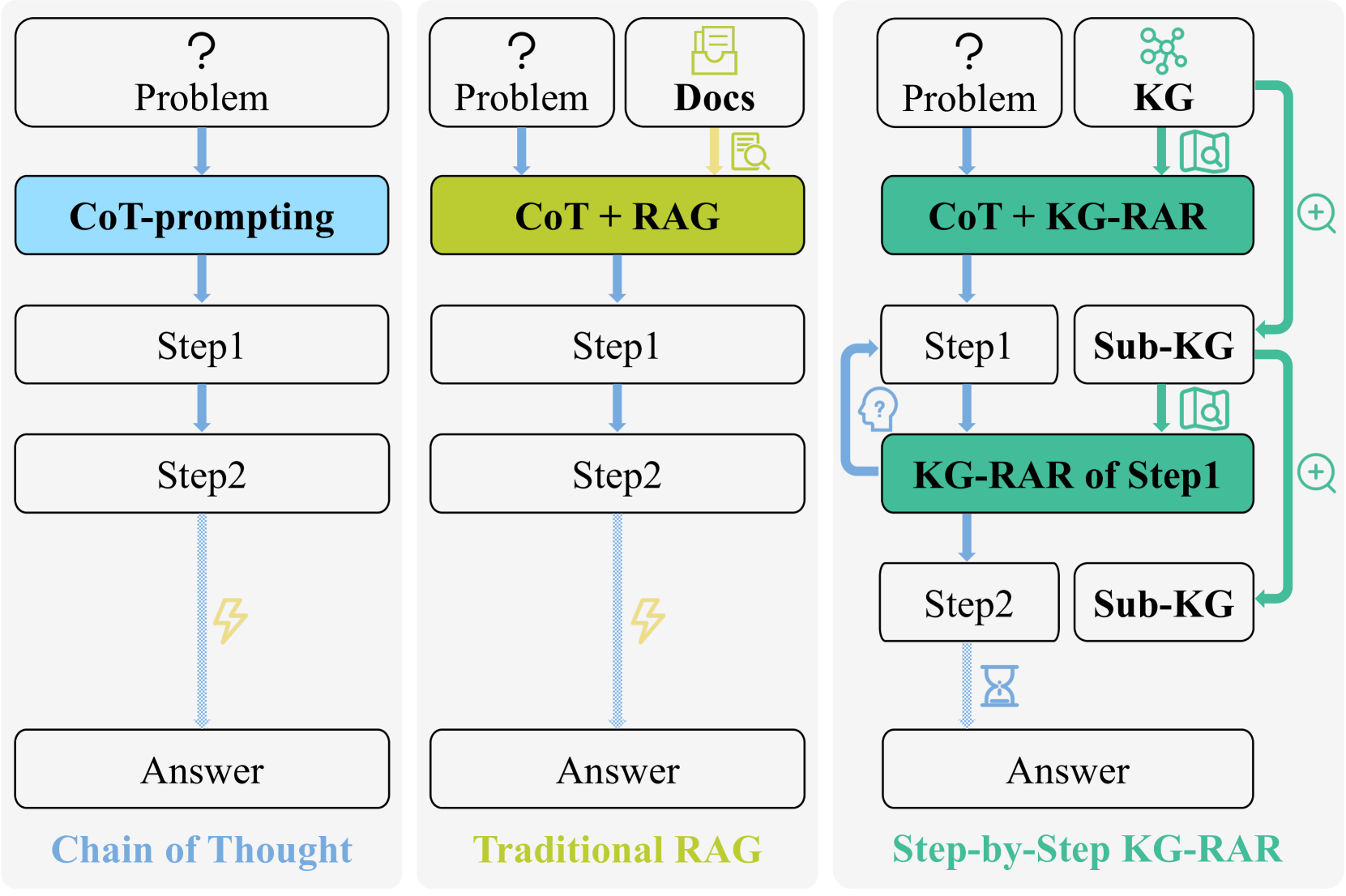
Figure 1: Illustration of the proposed step-by-step knowledge graph retrieval for o1-like reasoning, which dynamically retrieves and utilises structured sub-graphs (Sub-KGs) during reasoning. Our approach iteratively refines the reasoning process by retrieving relevant Sub-KGs at each step, enhancing accuracy, consistency, and reasoning depth for complex tasks, thereby offering a novel form of scaling test-time computation.
Despite encouraging advancements in o1-like reasoning, LLMs—particularly smaller and less powerful variants—continue to struggle with complex reasoning tasks in mathematics and science [2, 3, 32, 33]. These challenges arise from insufficient domain knowledge, susceptibility to hallucinations, and constrained reasoning depth [34, 35, 36]. Given the novelty of o1-like reasoning, effective solutions to these issues remain largely unexplored, with few studies addressing this gap in the literature [17, 18, 22]. One potential solution from the pre-o1 era is retrieval-augmented generation (RAG), which has been shown to mitigate hallucinations and factual inaccuracies by retrieving relevant information from external knowledge sources (Fig. 1, the 2 column) [37, 38, 39]. However, in the context of o1-like multi-step reasoning, traditional RAG faces two significant challenges:
- (1) Step-wise hallucinations: LLMs may hallucinate during intermediate steps —a problem not addressed by applying RAG solely to the initial prompt [40, 41];
- (2) Missing structured relationships: Traditional RAG may retrieve information that lacks the structured relationships necessary for complex reasoning tasks, leading to inadequate augmentation that fails to capture the depth required for accurate reasoning [39, 42].
In this paper, we strive to address both challenges by introducing a novel graph-augmented multi-step reasoning scheme to enhance LLMs’ o1-like reasoning capability, as depicted in Fig. 1. Our idea is motivated by the recent success of knowledge graphs (KGs) in knowledge-based question answering and fact-checking [43, 44, 45, 46, 47, 48, 49]. Recent advances have demonstrated the effectiveness of KGs in augmenting prompts with retrieved knowledge or enabling LLMs to query KGs for factual information [50, 51]. However, little attention has been given to improving step-by-step reasoning for complex tasks with KGs [52, 53], such as mathematical reasoning, which requires iterative logical inference rather than simple knowledge retrieval.
To fill this gap, the objective of the proposed graph-augmented reasoning paradigm is to integrate structured KG retrieval into the reasoning process in a step-by-step manner, providing contextually relevant information at each reasoning step to refine reasoning paths and mitigate step-wise inaccuracies and hallucinations, thereby addressing both aforementioned challenges simultaneously. This approach operates without additional training, making it particularly well-suited for small-scale LLMs in resource-constrained environments. Moreover, it extends test-time compute by incorporating external knowledge into the reasoning context, transitioning from direct CoT to step-wise guided retrieval and reasoning.
Nevertheless, implementing this graph-augmented reasoning paradigm is accompanied with several key issues: (1) Frozen LLMs struggle to query KGs effectively [50], necessitating a dynamic integration strategy for iterative incorporation of graph-based knowledge; (2) Existing KGs primarily encode static facts rather than the procedural knowledge required for multi-step reasoning [54, 55], highlighting the need for process-oriented KGs; (3) Reward models, which are essential for validating reasoning steps [30, 29], often require costly fine-tuning and suffer from poor generalization [56], underscoring the need for a universal, training-free scoring mechanism tailored to KG.
To address these issues, we propose KG-RAR, a step-by-step knowledge graph based retrieval-augmented reasoning framework that retrieves, refines, and reasons using structured knowledge graphs in a step-wise manner. Specifically, to enable effective KG querying, we design a hierarchical retrieval strategy in which questions and reasoning steps are progressively matched to relevant subgraphs, dynamically narrowing the search space. Also, we present a process-oriented math knowledge graph (MKG) construction method that encodes step-by-step procedural knowledge, ensuring that LLMs retrieve and apply structured reasoning sequences rather than static facts. Furthermore, we introduce the post-retrieval processing and reward model (PRP-RM)—a training-free scoring mechanism that refines retrieved knowledge before reasoning and evaluates step correctness in real time. By integrating structured retrieval with test-time computation, our approach mitigates reasoning inconsistencies, reduces hallucinations, and enhances stepwise verification—all without additional training.
In sum, our contribution is therefore the first attempt that dynamically integrates step-by-step KG retrieval into an o1-like multi-step reasoning process. This is achieved through our proposed hierarchical retrieval, process-oriented graph construction method, and PRP-RM—a training-free scoring mechanism that ensures retrieval relevance and step correctness. Experiments on Math500 and GSM8K validate the effectiveness of our approach across six smaller models from the Llama3 and Qwen2.5 series. The best-performing model, Llama-3B on Math500, achieves a 20.73% relative improvement over CoT prompting, followed by Llama-8B on Math500 with a 15.22% relative gain and Llama-8B on GSM8K with an 8.68% improvement.
## 2 Related Work
<details>
<summary>x2.png Details</summary>
### Visual Description
## Diagram: Problem-Solving Flowchart for a Modular Arithmetic Question
### Overview
The image is a detailed flowchart illustrating the cognitive process of solving a mathematical word problem. It visually maps out the retrieval of relevant knowledge and the step-by-step reasoning required to find the remainder when the 1234th batch is divided by a batch size of 35. The diagram is structured into two main vertical panels: a left panel showing a network of retrieved concepts and examples, and a right panel showing the sequential reasoning steps (Chain-of-Thought or CoT).
### Components/Axes
The diagram is organized into distinct regions and uses color-coded boxes and directional arrows to indicate flow and relationships.
**1. Header (Top):**
* **Question Text:** "Question: A factory produces items in batches of 35. If today is the 1234th batch, what is the remainder?"
**2. Left Panel - "Retrieving" Network:**
This panel is a concept map showing the knowledge activated to solve the problem.
* **Primary Stage Labels (Yellow Boxes):** "Retrieving" (appears twice, top and bottom left).
* **Core Mathematical Concepts (Yellow Boxes):**
* "Modular Arithmetic"
* "Number Theory"
* "Congruence"
* **Specific Example Problems (Green Boxes):**
* "Suppose that a $30$-digit integer $N$ is composed of thirteen $7$s and seventeen $3$s. What is the remainder when $N$ is divided by $36$?"
* "What is the remainder when 1,493,824 is divided by 4?"
* "What is the remainder when the product $1734 \times 5389 \times 80607$ is divided by 10?"
* **Sub-Concepts & Methods (Blue Boxes):**
* "modular arithmetic: Is ..."
* "last digit property: Is ..."
* "division algorithm: Is ..."
* "quotient: Is ..."
* "remainder: Is ..."
* "zero remainder: Is ..."
* **Procedural Steps (Green Boxes):**
* "multiplication of relevant units digits"
* "application of last digit property"
* "observation of last digit property"
* "expressing the number as a sum of powers of the base using the quotient and remainder"
* "performing division to find the quotient and remainder"
* "finding the next multiple of the modulus"
* "checking if the solution satisfies the congruence condition"
* **Outcome (Orange Box):** "the solution does not satisfy the congruence condition"
**3. Right Panel - "Reasoning" Steps:**
This panel shows the linear, step-by-step solution process.
* **Initial Prompt (Top Right):** "CoT: Let's think step by step..."
* **Stage Labels (Yellow Boxes):** "Refining" and "Reasoning" (each appears twice).
* **Retrieval Summary (White Box with Bold Text):**
* First Instance: "Retrieval: The question can be solved using **modular arithmetic**..."
* Second Instance: "Retrieval: **The remainder** is what remains after subtracting the largest multiple of 35 that fits into 1234..."
* **Solution Steps (White Boxes):**
* **Step1:** "Divide 1234 by 35: 1234 ÷ 35 = 35.2571"
* **Step2:** "Subtract this product from 1234 to find the remainder: 1234 - 35 × 35 = 9"
### Detailed Analysis
The diagram meticulously deconstructs the problem-solving act.
* **Flow and Connections:** Arrows originate from the main "Retrieving" stage, branching out to core concepts (Modular Arithmetic, Number Theory). From these concepts, arrows point to specific, analogous example problems (green boxes). These examples then connect to finer-grained sub-concepts (blue boxes) and procedural steps (green boxes), illustrating how prior knowledge is activated and applied. The final orange box indicates a potential pitfall or verification step.
* **Spatial Grounding:** The "Retrieving" network occupies the left ~60% of the image. The "Reasoning" steps are in a column on the right ~40%. The initial question spans the top. Arrows generally flow from left to right and top to bottom within each panel.
* **Text Transcription:** All text has been extracted as listed in the Components section. The mathematical notation (e.g., $30$-digit, $N$, $36$) is transcribed precisely.
### Key Observations
1. **Dual-Process Model:** The diagram explicitly separates knowledge retrieval (left) from sequential reasoning (right), suggesting a model of cognition where relevant information is gathered before execution.
2. **Use of Analogies:** The retrieval network heavily relies on analogous problems (e.g., finding remainders for other numbers) to activate the correct mathematical framework.
3. **Hierarchical Decomposition:** The problem is broken down from a high-level question into core theories, then into specific techniques (like "last digit property"), and finally into arithmetic operations.
4. **Verification Step:** The inclusion of "checking if the solution satisfies the congruence condition" and the orange "does not satisfy" box highlights the importance of validating the answer within the logical framework.
### Interpretation
This diagram is more than a solution; it's a **meta-cognitive map** of how to approach a modular arithmetic problem. It demonstrates that solving such a problem isn't just about performing division.
* **What it Suggests:** The process begins by recognizing the problem type ("remainder") and retrieving the associated field ("Modular Arithmetic"). The mind then searches for familiar patterns or solved examples (the green problem boxes) to guide the approach. The right panel shows the application of this retrieved knowledge: interpreting the problem in terms of division with remainder, performing the calculation, and stating the result.
* **Relationships:** The left panel provides the **"why" and "how"**—the theoretical foundation and toolkit. The right panel provides the **"what"**—the specific actions taken. The arrows connecting concepts like "division algorithm" to "performing division" explicitly link theory to practice.
* **Notable Insight:** The diagram implies that a robust solution requires both a broad network of related knowledge (to correctly categorize and approach the problem) and a precise, linear procedure to execute the solution. The final answer, **9**, is the output of this integrated process. The diagram serves as an educational tool to make this often-invisible thinking process explicit.
</details>
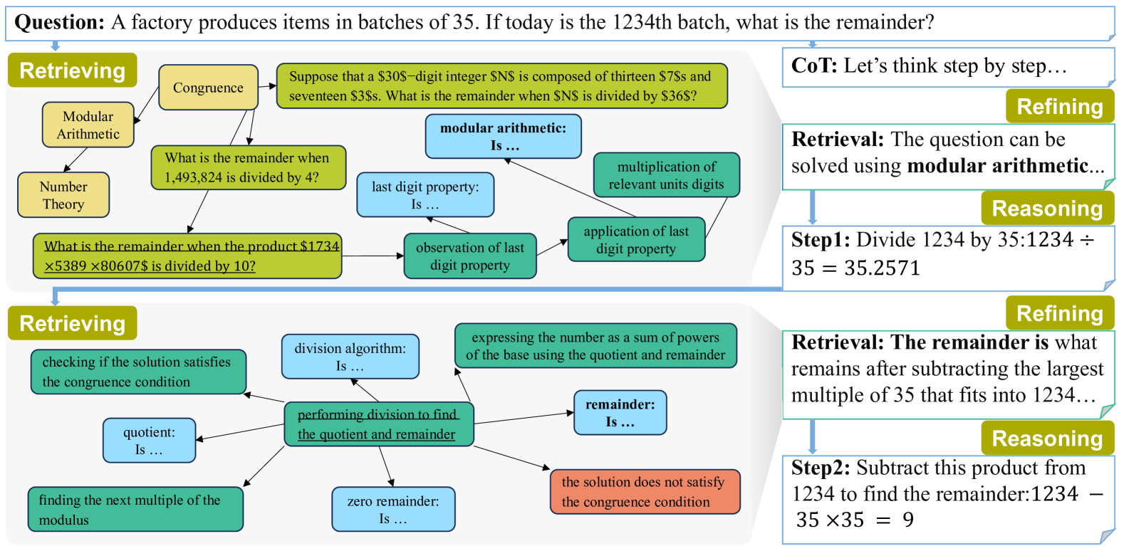
Figure 2: Example of Step-by-Step KG-RAR’s iterative process: 1) Retrieving: For a given question or intermediate reasoning step, the KG is retrieved to find the most similar problem or procedure (underlined in the figure) and extract its subgraph as the raw retrieval. 2) Refining: A frozen LLM processes the raw retrieval to generate a refined and targeted context for reasoning. 3) Reasoning: Using the refined retrieval, another LLM reflects on previous steps and generates next intermediate reasoning steps. This iterative workflow refines and guides the reasoning path to problem-solving.
### 2.1 LLM Reasoning
Large Language Models (LLMs) have advanced in structured reasoning through techniques like Chain-of-Thought (CoT) [4], Self-Consistency [5], and Tree-of-Thought [10], improving inference by generating intermediate steps rather than relying on greedy decoding [6, 7, 8, 57, 58, 9]. Recently, GPT-o1-like reasoning has emerged as a paradigm shift [17, 18, 25, 22], leveraging Test-Time Compute strategies such as Best-of-N [29], Beam Search [5], and Monte Carlo Tree Search [23], often integrated with reward models to refine reasoning paths dynamically [30, 31, 29, 59, 60, 61]. Reasoning models like DeepSeek-R1 exemplify this trend by iteratively searching, verifying, and refining solutions, significantly enhancing inference accuracy and robustness [27, 28]. However, these methods remain computationally expensive and challenging for small-scale LLMs, which struggle with hallucinations and inconsistencies due to limited reasoning capacity and lack of domain knowledge [32, 34, 3].
### 2.2 Knowledge Graphs Enhanced LLM Reasoning
Knowledge Graphs (KGs) are structured repositories of interconnected entities and relationships, offering efficient graph-based knowledge representation and retrieval [62, 63, 64, 65, 54]. Prior work integrating KGs with LLMs has primarily focused on knowledge-based reasoning tasks such as knowledge-based question answering [43, 44, 66, 67], fact-checking [45, 46, 68], and entity-centric reasoning [69, 47, 70, 48, 49]. However, in these tasks, ”reasoning” is predominantly limited to identifying and retrieving static knowledge rather than performing iterative, multi-step logical computations [71, 72, 73]. In contrast, our work is to integrate KGs with LLMs for o1-like reasoning in domains such as mathematics, where solving problems demands dynamic, step-by-step inference rather than static knowledge retrieval.
### 2.3 Reward Models
Reward models are essential across various domains such as computer vision [74, 75]. Notably, they play a crucial role in aligning LLM outputs with human preferences by evaluating accuracy, relevance, and logical consistency [76, 77, 78]. Fine-tuned reward models, including Outcome Reward Models (ORMs) [30] and Process Reward Models (PRMs) [31, 29, 60], improve validation accuracy but come at a high training cost and often lack generalization across diverse tasks [56]. Generative reward models [61] further enhance performance by integrating CoT reasoning into reward assessments, leveraging Test-Time Compute to refine evaluation. However, the reliance on fine-tuning makes these models resource-intensive and limits adaptability [56]. This underscores the need for universal, training-free scoring mechanisms that maintain robust performance while ensuring computational efficiency across various reasoning domains.
## 3 Pre-analysis
### 3.1 Motivation and Problem Definition
Motivation. LLMs have demonstrated remarkable capabilities across various domains [79, 4, 80, 81, 82], yet their proficiency in complex reasoning tasks remains limited [3, 83, 84]. Challenges such as hallucinations [34, 85], inaccuracies, and difficulties in handling complex, multi-step reasoning due to insufficient reasoning depth are particularly evident in smaller models or resource-constrained environments [86, 87, 88]. Moreover, traditional reward models, including ORMs [30] and PRMs [31, 29], require extensive fine-tuning, incurring significant computational costs for dataset collection, GPU usage, and prolonged training time [89, 90, 91]. Despite these efforts, fine-tuned reward models often suffer from poor generalization, restricting their effectiveness across diverse reasoning tasks [56].
To simultaneously overcome these challenges, this paper introduces a novel paradigm tailored for o1-like multi-step reasoning:
Remark 3.1 (Graph-Augmented Multi-Step Reasoning). The goal of graph-augmented reasoning is to enhance the step-by-step reasoning ability of frozen LLMs by integrating external knowledge graphs (KGs), eliminating the need for additional fine-tuning.
The proposed graph-augmented scheme aims to offer the following unique advantages:
- Improving Multi-Step Reasoning: Enhances reasoning capabilities, particularly for small-scale LLMs in resource-constrained environments;
- Scaling Test-Time Compute: Introduces a novel dimension of scaling test-time compute through dynamic integration of external knowledge;
- Transferability Across Reasoning Tasks: By leveraging domain-specific KGs, the framework can be easily adapted to various reasoning tasks, enabling transferability across different domains.
### 3.2 Challenge Analysis
However, implementing the proposed graph-augmented reasoning paradigm presents several critical challenges:
- Effective Integration: How can KGs be efficiently integrated with LLMs to support step-by-step reasoning without requiring model modifications? Frozen LLMs cannot directly query KGs effectively [50]. Additionally, since LLMs may suffer from hallucinations and inaccuracies during intermediate reasoning steps [34, 85, 41], it is crucial to dynamically integrate KGs at each step rather than relying solely on static knowledge retrieved at the initial stage;
- Knowledge Graph Construction: How can we design and construct process-oriented KGs tailored for LLM-driven multi-step reasoning? Existing KGs predominantly store static knowledge rather than the procedural and logical information required for reasoning [54, 55, 92]. A well-structured KG that represents reasoning steps, dependencies, and logical flows is necessary to support iterative reasoning;
- Universal Scoring Mechanism: How can we develop a training-free reward mechanism capable of universally evaluating reasoning paths across diverse tasks without domain-specific fine-tuning? Current approaches depend on fine-tuned reward models, which are computationally expensive and lack adaptability [56]. A universal, training-free scoring mechanism leveraging frozen LLMs is essential for scalable and efficient reasoning evaluation.
To address these challenges and unlock the full potential of graph-augmented reasoning, we propose a Step-by-Step Knowledge Graph based Retrieval-Augmented Reasoning (KG-RAR) framework, accompanied by a dedicated Post-Retrieval Processing and Reward Model (PRP-RM), which will be elaborated in the following section.
## 4 Proposed Approach
### 4.1 Overview
Our objective is to integrate KGs for o1-like reasoning with frozen, small-scale LLMs in a training-free and universal manner. This is achieved by integrating a step-by-step knowledge graph based retrieval-augmented reasoning (KG-RAR) module within a structured, iterative reasoning framework. As shown in Figure 2, the iterative process comprises three core phases: retrieving, refining, and reasoning.
### 4.2 Process-Oriented Math Knowledge Graph
<details>
<summary>x3.png Details</summary>
### Visual Description
## Diagram: LLM-Based Math Problem Solving and Knowledge Graph Construction
### Overview
This diagram illustrates a system architecture or workflow where mathematical problems from datasets are processed by a Large Language Model (LLM) to populate and interact with a structured "Math Knowledge Graph." The flow moves from left to right, showing how problem-solving steps and outcomes are mapped to different components of the knowledge graph.
### Components/Axes
The diagram is organized into three vertical columns or regions:
1. **Left Column: Datasets**
* **Header:** "Datasets"
* **Content:** A vertical list of items, each representing an input or stage.
* "Problem" (top item)
* "Step1" (accompanied by a green smiling face icon)
* "Step2" (accompanied by a green smiling face icon)
* "Step3" (accompanied by an orange frowning face icon)
* **Visual Structure:** Items are separated by faint horizontal dashed lines.
2. **Middle Column: LLM**
* **Header:** "LLM"
* **Content:** This column acts as a processing unit. It contains two icons:
* A gray llama icon (positioned between the "Problem" and "Step1" inputs).
* A blue snowflake icon (positioned between the "Step1" and "Step2" inputs).
* **Flow:** Blue arrows point from each item in the "Datasets" column into the "LLM" column, and then from the "LLM" column into the "Math Knowledge Graph" column.
3. **Right Column: Math Knowledge Graph**
* **Header:** "Math Knowledge Graph"
* **Content:** A network of colored, rounded rectangular nodes connected by black arrows, indicating relationships and flow.
* **Node Types & Colors:**
* **Yellow Nodes:** "Branch", "SubField", "Problem Type"
* **Green Nodes:** "Problem", "Procedure1", "Procedure2"
* **Blue Nodes:** "Knowledge1", "Knowledge2", "Knowledge3"
* **Orange Node:** "Error3"
* **Spatial Layout & Connections (Top to Bottom):**
* **Top Tier:** "Branch" (left) and "SubField" (right) are connected by a left-pointing arrow from "SubField" to "Branch".
* **Second Tier:** "Problem" (left) points right to "Problem Type". "Problem Type" points up to "SubField".
* **Third Tier:** "Problem" points down to "Procedure1". "Procedure1" points right to "Knowledge1".
* **Fourth Tier:** "Procedure1" points down to "Procedure2". "Procedure2" points right to "Knowledge2".
* **Fifth Tier:** "Procedure2" points down to "Error3". "Error3" points right to "Knowledge3".
### Detailed Analysis
* **Flow of Information:** The primary flow is horizontal (Datasets -> LLM -> Knowledge Graph) and vertical within the Knowledge Graph (cascading from Problem down through Procedures to an Error).
* **Problem Processing:** A "Problem" from the datasets is sent to the LLM. The LLM's processing (symbolized by the llama and snowflake icons) results in an update or query to the Knowledge Graph, specifically linking the "Problem" node to a "Problem Type" and initiating a procedural chain.
* **Procedural Chain:** The "Problem" leads to "Procedure1", which is associated with "Knowledge1". "Procedure1" leads to "Procedure2", associated with "Knowledge2". This suggests a step-by-step solution process.
* **Error Handling:** The chain culminates in "Error3" (colored orange, indicating a problem or failure state), which is linked to "Knowledge3". This implies that errors are also captured as valuable knowledge within the graph.
* **Hierarchical Classification:** The "Problem Type" is linked upward to "SubField", which is linked to "Branch", showing a taxonomic classification of the problem within mathematics.
### Key Observations
1. **Icon Semantics:** The green smiling faces next to "Step1" and "Step2" likely indicate successful or correct steps, while the orange frowning face next to "Step3" indicates an incorrect step or error. This aligns with the final node being "Error3".
2. **Color Coding:** Colors are used systematically to categorize node types in the Knowledge Graph: yellow for classification/taxonomy, green for active problem-solving elements, blue for knowledge units, and orange for errors.
3. **Dual Input to LLM:** The LLM receives both the initial "Problem" and subsequent "Steps". The snowflake icon between Step1 and Step2 might indicate a different processing mode (e.g., a "frozen" or reference state) compared to the initial processing (llama icon).
4. **Knowledge from Errors:** A significant observation is that "Error3" is explicitly linked to "Knowledge3", suggesting the system is designed to learn from mistakes and incorporate them into the knowledge base.
### Interpretation
This diagram depicts a framework for **structured mathematical reasoning and knowledge acquisition**. It goes beyond simple problem-solving by:
* **Contextualizing Problems:** It automatically classifies a problem into a mathematical taxonomy (Branch -> SubField -> Problem Type).
* **Modeling the Solution Process:** It breaks down solving into discrete, traceable procedures (Procedure1, Procedure2), each linked to specific knowledge components.
* **Valuing Negative Results:** It treats errors not as dead ends but as critical sources of new knowledge ("Knowledge3"), which is a sophisticated approach to machine learning and knowledge graph refinement.
* **Integrating an LLM as a Reasoning Engine:** The LLM acts as the translator between unstructured problem data/step attempts and the structured knowledge graph, performing both classification and procedural generation.
The overall system aims to create a self-improving loop where solving problems (and making errors) enriches a formal knowledge graph, which in turn can guide future problem-solving. The spatial flow from left (raw data) to right (structured knowledge) visually reinforces this transformation of information.
</details>
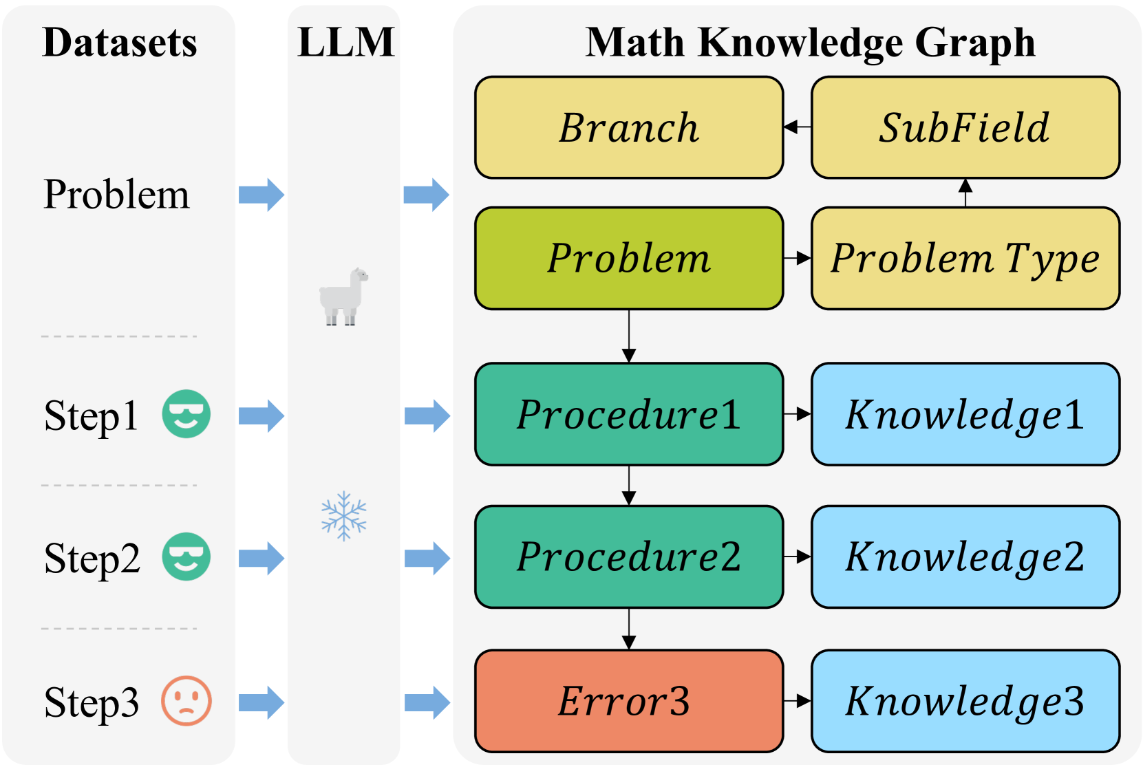
Figure 3: Pipeline for constructing the process-oriented math knowledge graph from process supervision datasets.
To support o1-like multi-step reasoning, we construct a Mathematical Knowledge Graph tailored for multi-step logical inference. Public process supervision datasets, such as PRM800K [29], provide structured problem-solving steps annotated with artificial ratings. Each sample will be decomposed into the following structured components: branch, subfield, problem type, problem, procedures, errors, and related knowledge.
The Knowledge Graph is formally defined as: $G=(V,E)$ , where $V$ represents nodes—including problems, procedures, errors, and mathematical knowledge—and $E$ represents edges encoding their relationships (e.g., ”derived from,” ”related to”).
As shown in Figure 3, for a given problem $P$ with solutions $S_1,S_2,\dots,S_n$ and human ratings, the structured representation is:
$$
P↦\{B_p,F_p,T_p,r\},
$$
| | $\displaystyle S_i^good$ | $\displaystyle↦\{S_i,K_i,r_i^good\}, S_i^ bad↦\{E_i,K_i,r_i^bad\},$ | |
| --- | --- | --- | --- |
where $B_p,F_p,T_p$ represent the branch, subfield, and type of $P$ , respectively. The symbols $S_i$ and $E_i$ denote the procedures derived from correct steps and the errors from incorrect steps, respectively. Additionally, $K_i$ contains relevant mathematical knowledge. The relationships between problems, steps, and knowledge are encoded through $r,r_i^good,r_i^bad$ , which capture the edge relationships linking these elements.
To ensure a balance between computational efficiency and quality of KG, we employ a Llama-3.1-8B-Instruct model to process about 10,000 unduplicated samples from PRM800K. The LLM is prompted to output structured JSON data, which is subsequently transformed into a Neo4j-based MKG. This process yields a graph with approximately $80,000$ nodes and $200,000$ edges, optimized for efficient retrieval.
### 4.3 Step-by-Step Knowledge Graph Retrieval
KG-RAR for Problem Retrieval. For a given test problem $Q$ , the most relevant problem $P^*∈ V_p$ and its subgraph are retrieved to assist reasoning. The retrieval pipeline comprises the following steps:
1. Initial Filtering: Classify $Q$ by $B_q,F_q,T_q$ (branch, subfield, and problem type). The candidate set $V_Q⊂ V_p$ is filtered hierarchically, starting from $T_q$ , expanding to $F_q$ , and then to $B_q$ if no exact match is found.
2. Semantic Similarity Scoring:
$$
P^*=\arg\max_P∈ V_{Q}\cos(e_Q,e_P),
$$
where:
$$
\cos(e_Q,e_P)=\frac{⟨e_Q,e_P
⟩}{\|e_Q\|\|e_P\|}
$$
and $e_Q,e_P∈ℝ^d$ are embeddings of $Q$ and $P$ , respectively.
3. Context Retrieval: Perform Depth-First Search (DFS) on $G$ to retrieve procedures ( $S_p$ ), errors ( $E_p$ ), and knowledge ( $K_p$ ) connected to $P^*$ .
Input: Test problem $Q$ and MKG $G$
Output: Most relevant problem $P^*$ and its context $(S_p,E_p,K_p)$
1 Filter $G$ using $B_q$ , $F_q$ , and $T_q$ to obtain $V_Q$ ;
2 foreach $P∈ V_Q$ do
3 Compute $Sim_semantic(Q,P)$ ;
4
5 $P^*←\arg\max_P∈ V_{Q}Sim_semantic(Q,P)$ ;
6 Retrieve $S_p$ , $E_p$ , and $K_p$ from $P^*$ using DFS;
7 return $P^*$ , $S_p$ , $E_p$ , and $K_p$ ;
Algorithm 1 KG-RAR for Problem Retrieval
KG-RAR for Step Retrieval. Given an intermediate reasoning step $S$ , the most relevant step $S^*∈ G$ and its subgraph is retrieved dynamically:
1. Contextual Filtering: Restrict the search space $V_S$ to the subgraph induced by previously retrieved top-k similar problems $\{P_1,P_2,\dots,P_k\}∈ V_Q$ .
2. Step Similarity Scoring:
$$
S^*=\arg\max_S_{i∈ V_S}\cos(e_S,e_S_{i}).
$$
3. Context Retrieval: Perform Breadth-First Search (BFS) on $G$ to extract subgraph of $S^*$ , including potential next steps, related knowledge, and error patterns.
### 4.4 Post-Retrieval Processing and Reward Model
Step Verification and End-of-Reasoning Detection. Inspired by previous works [93, 56, 94, 61], we use a frozen LLM to evaluate both step correctness and whether reasoning should terminate. The model is queried with an instruction, producing a binary classification decision:
$$
\textit{Is this step correct (Yes/No)? }\begin{cases}Yes\xrightarrow[
Probability]{Token}p(Yes)\\
No\xrightarrow[Probability]{Token}p(No)\\
Other Tokens.\end{cases}
$$
The corresponding confidence score for step verification or reasoning termination is computed as:
$$
Score(S,I)=\frac{\exp(p(Yes|S,I))}{\exp(p(Yes|S,I))+\exp(p(\text
{No}|S,I))}.
$$
For step correctness, the instruction $I$ is ”Is this step correct (Yes/No)?”, while for reasoning termination, the instruction $I_E$ is ”Has a final answer been reached (Yes/No)?”.
Post-Retrieval Processing. Post-retrieval processing is a crucial component of the retrieval-augmented generation (RAG) framework, ensuring that retrieved information is improved to maximize relevance while minimizing noise [37, 95, 96].
For a problem $P$ or a reasoning step $S$ :
$$
R^\prime=_refine(P+R or
S+R),
$$
where $R$ is the raw retrieved context, and $R^\prime$ represents its rewritten, targeted form.
Iterative Refinement and Verification. Inspired by generative reward models [61, 97], we integrate retrieval refinement as a form of CoT reasoning before scoring each step. To ensure consistency in multi-step reasoning, we employ an iterative retrieval refinement and scoring mechanism, as illustrated in Figure 4.
<details>
<summary>x4.png Details</summary>
### Visual Description
\n
## System Architecture Diagram: PRP-RM and Reasoner Interaction with Knowledge Graphs
### Overview
The image is a technical system architecture diagram illustrating a multi-step reasoning process involving two primary entity types: "PRP-RM" and "Reasoner." The process involves the exchange of prompts, outputs, and reasoning steps, augmented by interactions with a Knowledge Graph (KG) and a Sub-Knowledge Graph (Sub-KG). The diagram uses color-coded blocks to represent different data types and shows a cyclical or sequential flow of information.
### Components/Axes
**Entities:**
1. **PRP-RM**: Depicted as a speaking human head silhouette. Appears twice (top-left and middle-left). Each instance is accompanied by a blue snowflake icon.
2. **Reasoner**: Depicted as a human head silhouette with a network/brain icon inside. Appears twice (top-right and bottom-right). Each instance is accompanied by a blue snowflake icon.
3. **KG (Knowledge Graph)**: Represented by a teal-colored network node icon (top-right).
4. **Sub-KG (Sub-Knowledge Graph)**: Represented by a smaller teal-colored network node icon (center-right).
**Data Blocks (Color-Coded per Legend):**
* **Prompt (Light Blue)**: Represents input data.
* **Output (Yellow)**: Represents generated data.
* **Token Prob (Green)**: Represents token probability data.
* **Temp Chat (Checkered Blue/White)**: Represents temporary chat or intermediate data.
**Legend (Bottom-Left):**
* Light Blue Rectangle: "Prompt"
* Yellow Rectangle: "Output"
* Green Rectangle: "Token Prob"
* Checkered Blue/White Rectangle: "Temp Chat"
### Detailed Analysis
The diagram shows a flow involving four main data blocks and two knowledge graph components.
**1. Top-Left Block (Associated with first PRP-RM):**
* **Position:** Top-left quadrant.
* **Structure:** A rounded rectangle divided into three sections.
* Top (Prompt - Blue): Contains two sub-cells labeled `P` and `R_p`.
* Bottom (Output - Yellow): Contains one cell labeled `R'_p`.
* **Connections:**
* An arrow points from the `KG` icon to the `R_p` cell in the Prompt section.
* An arrow originates from the `R'_p` Output cell and points to the next block (Top-Right).
**2. Top-Right Block (Associated with first Reasoner):**
* **Position:** Top-right quadrant.
* **Structure:** A rounded rectangle divided into two horizontal sections.
* Top (Prompt - Blue): Contains two sub-cells labeled `P` and `R'_p`.
* Bottom (Output - Yellow): Contains one cell labeled `S₁`.
* **Connections:**
* Receives input from the Top-Left Block's `R'_p` Output.
* An arrow originates from the `S₁` Output cell and points to the next block (Center-Left).
**3. Center-Left Block (Associated with second PRP-RM):**
* **Position:** Center-left, below the first PRP-RM.
* **Structure:** A larger, complex rounded rectangle divided into four horizontal sections.
* **Section 1 (Prompt - Blue):** Divided into two sub-cells labeled `S₁` and `R₁`.
* **Section 2 (Output - Yellow):** Contains one cell labeled `R'₁`.
* **Section 3 (Temp Chat - Checkered):** Divided into two sub-cells labeled `I` and `I_E`.
* **Section 4 (Token Prob - Green):** Divided into two sub-cells labeled `Score` and `End`.
* **Connections:**
* Receives input from the Top-Right Block's `S₁` Output.
* An arrow points from the `Sub-KG` icon to the `R₁` cell in the Prompt section.
* An arrow originates from the `R'₁` Output cell and points to the next block (Bottom-Right).
**4. Bottom-Right Block (Associated with second Reasoner):**
* **Position:** Bottom-right quadrant.
* **Structure:** A rounded rectangle divided into two horizontal sections.
* Top (Prompt - Blue): Contains one cell labeled `R'₁`.
* Bottom (Output - Yellow): Contains one cell labeled `S₂`.
* **Connections:**
* Receives input from the Center-Left Block's `R'₁` Output.
**Flow Summary:**
The process appears to follow this path:
1. **PRP-RM (1)** generates `R'_p` using a prompt `P` and information `R_p` from the main **KG**.
2. **Reasoner (1)** takes `P` and `R'_p` to produce a reasoning step `S₁`.
3. **PRP-RM (2)** takes `S₁` and a new reasoning component `R₁` (informed by a **Sub-KG**) to produce `R'₁`. This block also generates temporary chat data (`I`, `I_E`) and token probability scores (`Score`, `End`).
4. **Reasoner (2)** takes `R'₁` to produce the next reasoning step `S₂`.
### Key Observations
1. **Cyclical/Iterative Nature:** The output of one component (`R'_p`, `S₁`, `R'₁`) becomes the prompt for the next, suggesting an iterative reasoning or refinement loop.
2. **Knowledge Graph Integration:** The main KG informs the initial reasoning (`R_p`), while a more specific Sub-KG informs a later stage (`R₁`), indicating a hierarchical or focused knowledge retrieval process.
3. **Snowflake Icons:** The blue snowflake icons next to both PRP-RM and Reasoner entities are consistent. In technical diagrams, this often symbolizes a "frozen" or non-trainable (static) component, suggesting these are pre-trained or fixed models.
4. **Complex Middle Block:** The Center-Left PRP-RM block is the most complex, containing not only Prompt/Output but also Temp Chat and Token Prob sections. This suggests this stage involves evaluation, scoring, and potentially interactive or intermediate steps.
5. **Symbol Progression:** The mathematical notation shows a progression: `R_p` -> `R'_p` -> `S₁` -> `R₁` -> `R'₁` -> `S₂`. The prime symbol (') likely denotes a processed or updated version of a variable.
### Interpretation
This diagram models a sophisticated, multi-stage reasoning system that combines large language models (the "PRP-RM" and "Reasoner") with structured knowledge from graphs. The process is not a single forward pass but an interactive dialogue between components.
* **What it demonstrates:** The system likely aims to solve complex problems by breaking them down. The PRP-RM acts as a bridge between raw prompts/knowledge and the Reasoner, which performs core logical deduction. The inclusion of `Score` and `End` tokens in the middle stage implies a mechanism for evaluating the quality of a reasoning path and deciding when to terminate the process.
* **Relationships:** The PRP-RM and Reasoner have a symbiotic, turn-taking relationship. The KG provides external factual grounding, preventing the models from relying solely on parametric knowledge. The Sub-KG suggests the system can dynamically focus on relevant knowledge subsets.
* **Notable Anomalies/Patterns:** The most significant pattern is the transformation of data types. Information starts as a prompt (`P`) and knowledge (`R_p`), is transformed into an output (`R'_p`), then becomes a reasoning step (`S₁`), which is further refined (`R₁`, `R'₁`), and finally yields a subsequent step (`S₂`). This mirrors a chain-of-thought or tree-of-thought reasoning process, formalized into a system architecture. The "Temp Chat" section is particularly intriguing, as it may represent an internal dialogue or scratchpad used by the model during complex reasoning.
</details>
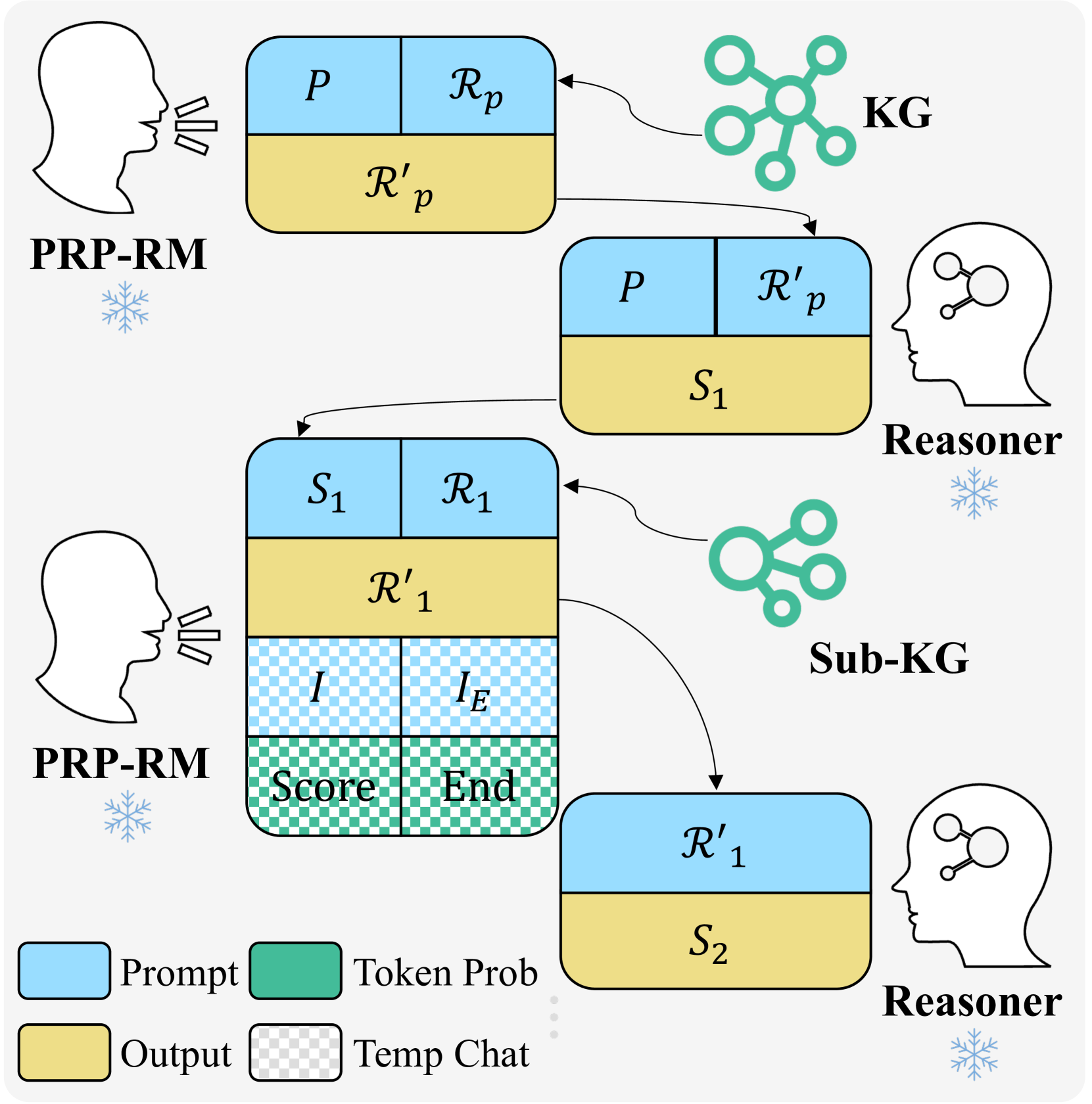
Figure 4: Illustration of the Post-Retrieval Processing and Reward Model (PRP-RM). Given a problem $P$ and its retrieved context $R_p$ from the Knowledge Graph (KG), PRP-RM refines it into $R^\prime_p$ . The Reasoner LLM generates step $S_1$ based on $R^\prime_p$ , followed by iterative retrieval and refinement ( $R_t→R^\prime_t$ ) for each step $S_t$ . Correctness is assessed using $I=$ ”Is this step correct?” to compute $(S_t)$ , while completion is checked via $I_E=$ ”Has a final answer been reached?” to compute $(S_t)$ . The process continues until $(S_t)$ surpasses a threshold or a predefined inference depth is reached.
Input: Current step $S$ and retrieved problems $\{P_1,…,P_k\}$
Output: Relevant step $S^*$ and its context subgraph
1 Initialize step collection $V_S←\bigcup_i=1^kSteps(P_i)$ ;
2 foreach $S_i∈ V_S$ do
3 Compute semantic similarity $Sim_semantic(S,S_i)$ ;
4
5 $S^*←\arg\max_S_{i∈ V_S}Sim_semantic(S,S_i)$ ;
6 Construct context subgraph via $BFS(S^*)$ ;
7 return $S^*$ , $subgraph(S^*)$ ;
Algorithm 2 KG-RAR for Step Retrieval
For a reasoning step $S_t$ , the iterative refinement history is:
$$
H_t=\{P+R_p,R^\prime_p,S_1+R_1,
R^\prime_1,\dots,S_t+R_t,R^\prime_t\}.
$$
The refined retrieval context is generated recursively:
$$
R^\prime_t=_refine(H_t-1,S_t+
R_t).
$$
The correctness and end-of-reasoning probabilities are:
$$
(S_t)=\frac{\exp(p(Yes|H_t,I))}{\exp(p(
Yes|H_t,I))+\exp(p(No|H_t,I))},
$$
$$
(S_t)=\frac{\exp(p(Yes|H_t,I_E))}{\exp(p(
Yes|H_t,I_E))+\exp(p(No|H_t,I_E))}.
$$
This process iterates until $(S_t)>θ$ , signaling completion.
TABLE I: Performance evaluation across different levels of the Math500 dataset using various models and methods.
| Dataset: Math500 | Level 1 (+9.09%) | Level 2 (+5.38%) | Level 3 (+8.90%) | Level 4 (+7.61%) | Level 5 (+16.43%) | Overall (+8.95%) | | | | | | | |
| --- | --- | --- | --- | --- | --- | --- | --- | --- | --- | --- | --- | --- | --- |
| Model | Method | Maj | Last | Maj | Last | Maj | Last | Maj | Last | Maj | Last | Maj | Last |
| Llama-3.1-8B (+15.22%) | CoT-prompting | 80.6 | 80.6 | 74.1 | 74.1 | 59.4 | 59.4 | 46.4 | 46.4 | 27.4 | 27.1 | 51.9 | 51.9 |
| Step-by-Step KG-RAR | 88.4 | 81.4 | 83.3 | 82.2 | 70.5 | 69.5 | 53.9 | 53.9 | 32.1 | 25.4 | 59.8 | 57.0 | |
| Llama-3.2-3B (+20.73%) | CoT-prompting | 63.6 | 65.1 | 61.9 | 61.9 | 51.1 | 51.1 | 43.2 | 43.2 | 20.4 | 20.4 | 43.9 | 44.0 |
| Step-by-Step KG-RAR | 83.7 | 79.1 | 68.9 | 68.9 | 61.0 | 52.4 | 49.2 | 47.7 | 29.9 | 28.4 | 53.0 | 50.0 | |
| Llama-3.2-1B (-4.02%) | CoT-prompting | 64.3 | 64.3 | 52.6 | 52.2 | 41.6 | 41.6 | 25.3 | 25.3 | 8.0 | 8.2 | 32.3 | 32.3 |
| Step-by-Step KG-RAR | 72.1 | 72.1 | 50.0 | 50.0 | 40.0 | 40.0 | 18.0 | 19.5 | 10.4 | 13.4 | 31.0 | 32.2 | |
| Qwen2.5-7B (+2.91%) | CoT-prompting | 95.3 | 95.3 | 88.9 | 88.9 | 86.7 | 86.3 | 77.3 | 77.1 | 50.0 | 49.8 | 75.6 | 75.4 |
| Step-by-Step KG-RAR | 95.3 | 93.0 | 90.0 | 90.0 | 87.6 | 88.6 | 79.7 | 79.7 | 54.5 | 56.7 | 77.8 | 78.4 | |
| Qwen2.5-3B (+3.13%) | CoT-prompting | 93.0 | 93.0 | 85.2 | 85.2 | 81.0 | 80.6 | 62.5 | 62.5 | 40.1 | 39.3 | 67.1 | 66.8 |
| Step-by-Step KG-RAR | 95.3 | 95.3 | 84.4 | 85.6 | 83.8 | 77.1 | 64.1 | 64.1 | 44.0 | 38.1 | 69.2 | 66.4 | |
| Qwen2.5-1.5B (-5.12%) | CoT-prompting | 88.4 | 88.4 | 78.5 | 77.4 | 71.4 | 68.9 | 49.2 | 49.5 | 34.6 | 34.3 | 58.6 | 57.9 |
| Step-by-Step KG-RAR | 97.7 | 93.0 | 78.9 | 75.6 | 66.7 | 67.6 | 48.4 | 44.5 | 24.6 | 23.1 | 55.6 | 53.4 | |
Role-Based System Prompting. Inspired by agent-based reasoning frameworks [98, 99, 100], we introduce role-based system prompting to further optimize our PRP-RM. In this approach, we define three distinct personas to enhance the reasoning process. The Responsible Teacher [101] processes retrieved knowledge into structured guidance and evaluates the correctness of each step. The Socratic Teacher [102], rather than pr oviding direct guidance, reformulates the retrieved content into heuristic questions, encouraging self-reflection. Finally, the Critical Teacher [103] acts as a critical evaluator, diagnosing reasoning errors before assigning a score. Each role focuses on different aspects of post-retrieval processing, improving robustness and interpretability.
## 5 Experiments
In this section, we evaluate the effectiveness of our proposed Step-by-Step KG-RAR and PRP-RM methods by comparing them with Chain-of-Thought (CoT) prompting [4] and finetuned reward models [30, 29]. Additionally, we perform ablation studies to examine the impact of individual components.
### 5.1 Experimental Setup
Following prior works [5, 29, 21], we evaluate on Math500 [104] and GSM8K [30], using Accuracy (%) as the primary metric. Experiments focus on instruction-tuned Llama3 [105] and Qwen2.5 [106], with Best-of-N [107, 30, 29] search ( $n=8$ for Math500, $n=4$ for GSM8K). We employ Majority Vote [5] for self-consistency and Last Vote [25] for benchmarking reward models. To evaluate PRP-RM, we compare against fine-tuned reward models: Math-Shepherd-PRM-7B [108], RLHFlow-ORM-Deepseek-8B and RLHFlow-PRM-Deepseek-8B [109]. For Step-by-Step KG-RAR, we set step depth to $8$ and padding to $4$ . The Socratic Teacher role is used in PRP-RM to minimize direct solving. Both the Reasoner LLM and PRP-RM remain consistent for fair comparison.
<details>
<summary>x5.png Details</summary>
### Visual Description
\n
## Line Chart: Model Accuracy vs. Difficulty Level
### Overview
This is a line chart comparing the performance (accuracy) of four different AI models across five increasing levels of difficulty. The chart demonstrates a clear negative correlation between problem difficulty and model accuracy for all evaluated systems.
### Components/Axes
* **Y-Axis:** Labeled "Accuracy (%)". Scale ranges from 0% to 80% with major gridlines at 20% intervals (0%, 20%, 40%, 60%, 80%).
* **X-Axis:** Labeled "Difficulty Level". Discrete categories marked 1, 2, 3, 4, and 5.
* **Legend:** Positioned at the top center of the chart area. It defines four data series:
1. **Math-Shepherd-PRM-7B:** Represented by a teal line with circular markers.
2. **RLHFlow-ORM-Deepseek-8B:** Represented by an orange line with square markers.
3. **RLHFlow-PRM-Deepseek-8B:** Represented by a light blue line with upward-pointing triangle markers.
4. **PRP-RM(frozen Llama-3.2-3B):** Represented by a reddish-purple line with diamond markers.
### Detailed Analysis
All four models exhibit a consistent downward trend in accuracy as difficulty increases from level 1 to level 5.
**1. Math-Shepherd-PRM-7B (Teal, Circle)**
* **Trend:** Steady, near-linear decline.
* **Data Points (Approximate):**
* Difficulty 1: ~62%
* Difficulty 2: ~62%
* Difficulty 3: ~50%
* Difficulty 4: ~42%
* Difficulty 5: ~20%
**2. RLHFlow-ORM-Deepseek-8B (Orange, Square)**
* **Trend:** Declines steadily, with a notably steeper drop between levels 4 and 5.
* **Data Points (Approximate):**
* Difficulty 1: ~62%
* Difficulty 2: ~62%
* Difficulty 3: ~52%
* Difficulty 4: ~42%
* Difficulty 5: ~18%
**3. RLHFlow-PRM-Deepseek-8B (Light Blue, Triangle)**
* **Trend:** Consistent decline, closely mirroring the teal line but starting slightly higher.
* **Data Points (Approximate):**
* Difficulty 1: ~70%
* Difficulty 2: ~60%
* Difficulty 3: ~52%
* Difficulty 4: ~45%
* Difficulty 5: ~22%
**4. PRP-RM(frozen Llama-3.2-3B) (Reddish-Purple, Diamond)**
* **Trend:** Starts as the highest-performing model but experiences the most significant absolute drop in accuracy.
* **Data Points (Approximate):**
* Difficulty 1: ~80%
* Difficulty 2: ~70%
* Difficulty 3: ~52%
* Difficulty 4: ~48%
* Difficulty 5: ~28%
### Key Observations
* **Performance Hierarchy at Low Difficulty:** At Difficulty Level 1, the PRP-RM model (~80%) significantly outperforms the other three models, which cluster between ~62-70%.
* **Convergence at Mid Difficulty:** At Difficulty Level 3, all four models converge to a very similar accuracy range of approximately 50-52%.
* **Universal Performance Degradation:** No model maintains high accuracy at the highest difficulty (Level 5). All fall to between ~18% and ~28%.
* **Steep Final Drop:** All models show their steepest decline in accuracy between Difficulty Levels 4 and 5.
* **Close Pairing:** The two RLHFlow models (ORM and PRM variants) and the Math-Shepherd model show very similar performance profiles, especially from Difficulty 2 onward.
### Interpretation
The chart illustrates a fundamental challenge in AI model evaluation: performance is highly sensitive to problem difficulty. The data suggests that while certain architectures or training methods (like PRP-RM) can provide a substantial advantage on easier tasks, this advantage diminishes as complexity increases. The convergence of all models at mid-level difficulty indicates a common performance bottleneck. The sharp drop at the highest difficulty level implies that current models, regardless of their specific design (PRM vs. ORM, different base models), struggle significantly with the most complex problems in this benchmark. This highlights a critical area for future research and development—improving robustness and reasoning capabilities on high-difficulty tasks. The near-identical performance of the 8B-parameter RLHFlow models suggests that within that specific training framework, the choice between ORM (Outcome Reward Model) and PRM (Process Reward Model) may have a marginal impact compared to the overarching effect of problem difficulty.
</details>
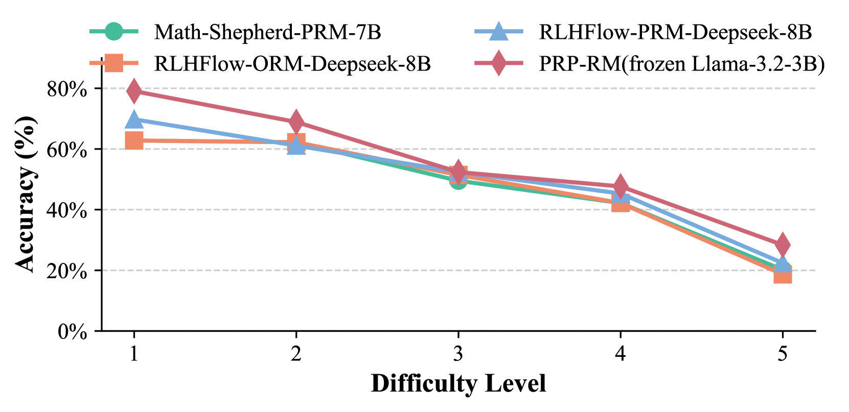
Figure 5: Comparison of reward models under Last@8.
### 5.2 Comparative Experimental Results
TABLE II: Evaluation results on the GSM8K dataset.
| Model | Method | Maj@4 | Last@4 |
| --- | --- | --- | --- |
| Llama-3.1-8B (+8.68%) | CoT-prompting | 81.8 | 82.0 |
| Step-by-Step KG-RAR | 88.9 | 88.0 | |
| Qwen-2.5-7B (+1.09%) | CoT-prompting | 91.6 | 91.1 |
| Step-by-Step KG-RAR | 92.6 | 93.1 | |
Table I shows that Step-by-Step KG-RAR consistently outperforms CoT-prompting across all difficulty levels on Math500, with more pronounced improvements in the Llama3 series compared to Qwen2.5, likely due to Qwen2.5’s higher baseline accuracy leaving less room for improvement. Performance declines for smaller models like Qwen-1.5B and Llama-1B on harder problems due to increased reasoning inconsistencies. Among models showing improvements, Step-by-Step KG-RAR achieves an average relative accuracy gain of 8.95% on Math500 under Maj@8, while Llama-3.2-8B attains a 8.68% improvement on GSM8K under Maj@4 (Table II). Additionally, PRP-RM achieves comparable performance to ORM and PRM. Figure 5 confirms its effectiveness with Llama-3B on Math500, highlighting its viability as a training-free alternative.
<details>
<summary>x6.png Details</summary>
### Visual Description
## Grouped Bar Chart: Accuracy Comparison of Raw vs. Processed Data for Two Metrics
### Overview
The image displays a grouped bar chart comparing the accuracy percentage of two data processing states ("Raw" and "Processed") across two distinct metrics ("Maj@8" and "Last@8"). The chart visually demonstrates the performance improvement achieved by applying a processing step to the raw data for both evaluated metrics.
### Components/Axes
* **Chart Type:** Grouped Bar Chart.
* **Y-Axis (Vertical):**
* **Label:** "Accuracy (%)"
* **Scale:** Linear scale from 0% to 50%.
* **Axis Markers/Ticks:** 0%, 10%, 20%, 30%, 40%, 50%.
* **Grid Lines:** Horizontal dashed grid lines extend from each major tick mark across the plot area.
* **X-Axis (Horizontal):**
* **Label:** "Metrics"
* **Categories:** Two primary categories are displayed: "Maj@8" (left group) and "Last@8" (right group).
* **Legend:**
* **Position:** Centered at the top of the chart, above the plot area.
* **Items:**
1. **Raw:** Represented by a salmon/orange colored bar.
2. **Processed:** Represented by a teal/green colored bar.
* **Data Series:** Two bars are grouped under each metric category on the x-axis, one for "Raw" and one for "Processed".
### Detailed Analysis
The chart presents the following specific data points (values are approximate based on visual alignment with the y-axis grid lines):
| Metric | Data State | Estimated Accuracy | Observation |
| :--- | :--- | :--- | :--- |
| **Maj@8** (Left Group) | Raw (Orange Bar) | ~31-32% | Top aligns slightly above the 30% grid line. |
| | Processed (Teal Bar) | 40% | Top aligns exactly with the 40% grid line. |
| **Last@8** (Right Group) | Raw (Orange Bar) | ~35-36% | Top is positioned midway between the 30% and 40% grid lines. |
| | Processed (Teal Bar) | 40% | Top aligns exactly with the 40% grid line. |
**Trend/Observation:** For both metrics, the "Processed" bar is taller than the "Raw" bar, indicating an accuracy improvement after processing. The gain is approximately 8-9 percentage points for Maj@8 and 4-5 percentage points for Last@8.
### Key Observations
1. **Consistent Improvement:** For both metrics ("Maj@8" and "Last@8"), the "Processed" data yields higher accuracy than the "Raw" data.
2. **Uniform Processed Performance:** The accuracy for the "Processed" state is identical (40%) across both metrics.
3. **Variable Raw Performance:** The "Raw" data shows different baseline accuracies for the two metrics, with "Last@8" (~35-36%) performing better than "Maj@8" (~31-32%).
4. **Magnitude of Gain:** The processing step provides a larger absolute gain for the "Maj@8" metric (~8-9%) compared to the "Last@8" metric (~4-5%).
### Interpretation
This chart provides clear empirical evidence that the applied data processing technique is effective. It successfully elevates the accuracy of both evaluated metrics to a consistent, higher standard (40%).
The data suggests that the "Maj@8" metric is more sensitive to or benefits more dramatically from the processing step than the "Last@8" metric. This could imply that the "Maj@8" metric is more susceptible to noise or artifacts present in the raw data, which the processing effectively removes. Conversely, the "Last@8" metric may be inherently more robust or may capture a different aspect of performance that is less affected by the unprocessed data's flaws.
The fact that both processed metrics converge to the same 40% accuracy might indicate a performance ceiling for the current model or task under these specific conditions, or it could suggest that the processing optimizes the data to a point where these two different evaluation criteria yield equivalent results. The chart effectively communicates the value of the processing pipeline, showing it not only improves performance but also standardizes it across different evaluation metrics.
</details>
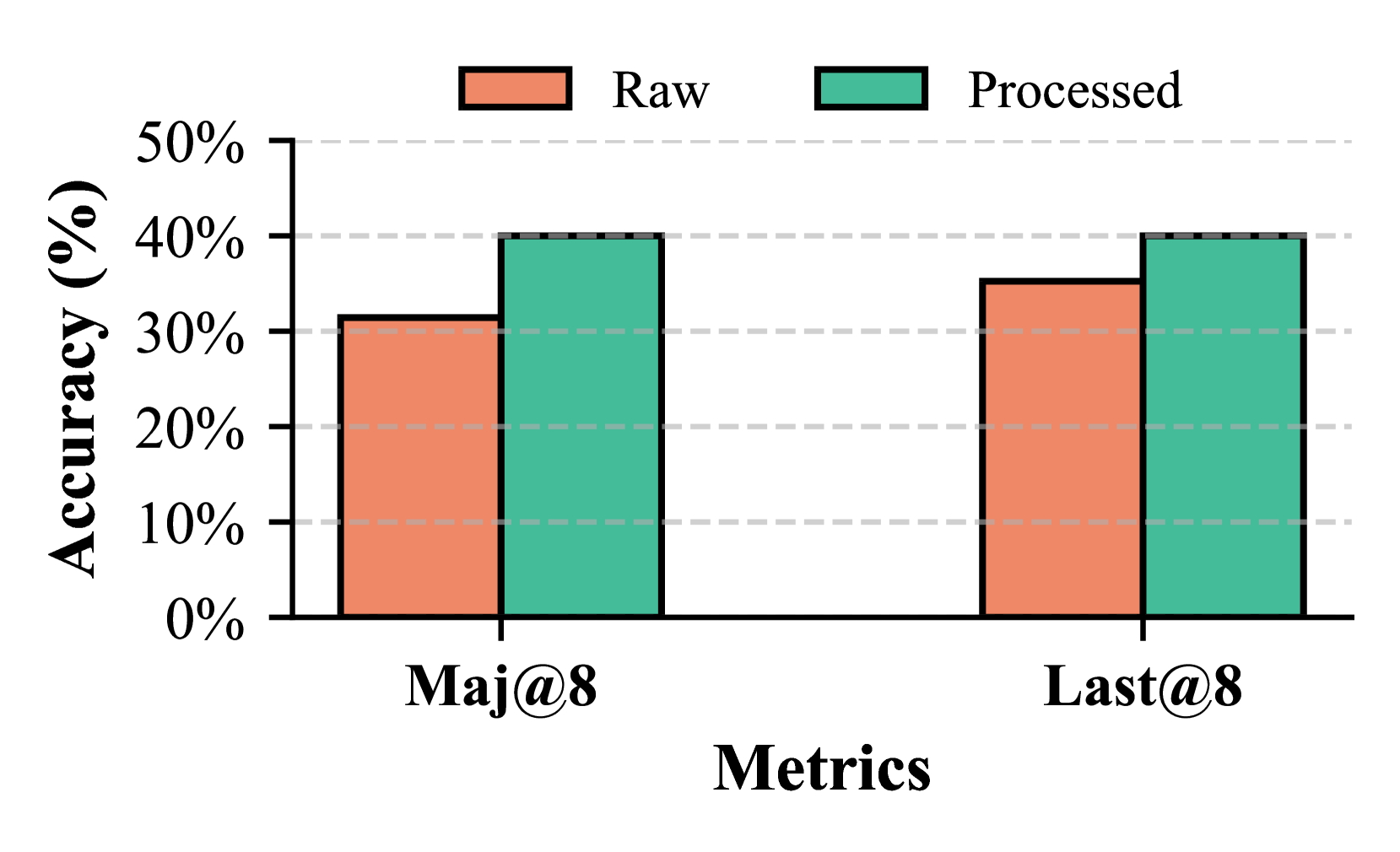
Figure 6: Comparison of raw and processed retrieval.
<details>
<summary>x7.png Details</summary>
### Visual Description
\n
## Grouped Bar Chart: Accuracy Comparison of Methods
### Overview
This is a grouped bar chart comparing the accuracy performance of three different methods ("None", "RAG", "KG-RAG") across two evaluation metrics ("Maj@8" and "Last@8"). The chart displays accuracy as a percentage.
### Components/Axes
* **Chart Type:** Grouped Bar Chart.
* **Y-Axis:** Labeled "Accuracy (%)". The scale runs from 0% to 60% in increments of 10%. Horizontal grid lines are present at each 10% increment.
* **X-Axis:** Labeled "Metrics". It contains two categorical groups:
1. **Maj@8**
2. **Last@8**
* **Legend:** Positioned at the top center of the chart. It defines three data series by color:
* **Blue Box:** "None"
* **Orange Box:** "RAG"
* **Green Box:** "KG-RAG"
### Detailed Analysis
**Data Series and Approximate Values:**
The chart presents two clusters of bars, one for each metric. Each cluster contains three bars corresponding to the methods in the legend.
**1. Metric: Maj@8 (Left Cluster)**
* **Trend:** All three methods show relatively high and similar accuracy, with a slight upward trend from "None" to "KG-RAG".
* **Data Points (Approximate):**
* **None (Blue):** ~51%
* **RAG (Orange):** ~52%
* **KG-RAG (Green):** ~54%
**2. Metric: Last@8 (Right Cluster)**
* **Trend:** Accuracy is generally lower than for Maj@8. "None" and "RAG" show nearly identical performance, while "KG-RAG" shows a significant improvement over them.
* **Data Points (Approximate):**
* **None (Blue):** ~45%
* **RAG (Orange):** ~45%
* **KG-RAG (Green):** ~52%
### Key Observations
1. **KG-RAG Superiority:** The "KG-RAG" method achieves the highest accuracy in both metrics.
2. **Metric Sensitivity:** The performance gap between methods is more pronounced for the "Last@8" metric than for "Maj@8".
3. **RAG vs. None:** The standard "RAG" method provides only a marginal improvement over "None" for "Maj@8" and no discernible improvement for "Last@8".
4. **Overall Performance Drop:** All methods show lower accuracy scores on the "Last@8" metric compared to the "Maj@8" metric.
### Interpretation
The data suggests that the **KG-RAG** method is the most effective of the three evaluated approaches for the tasks measured by these metrics. Its consistent lead indicates that integrating a knowledge graph (KG) with retrieval-augmented generation (RAG) provides a robust advantage.
The minimal difference between "None" (likely a baseline model) and "RAG" implies that standard retrieval augmentation alone may not be sufficient to improve performance on these specific benchmarks, particularly for the "Last@8" metric. This could indicate that the challenges in "Last@8" are not solved by simple retrieval but benefit from the structured knowledge or reasoning pathways that a KG-RAG system might provide.
The universal drop in accuracy from "Maj@8" to "Last@8" suggests that the "Last@8" metric represents a more difficult task or evaluation criterion. "KG-RAG's" ability to maintain a relatively high score (~52%) on this harder metric, while the other methods fall to ~45%, highlights its particular strength in handling the conditions that make "Last@8" challenging.
</details>
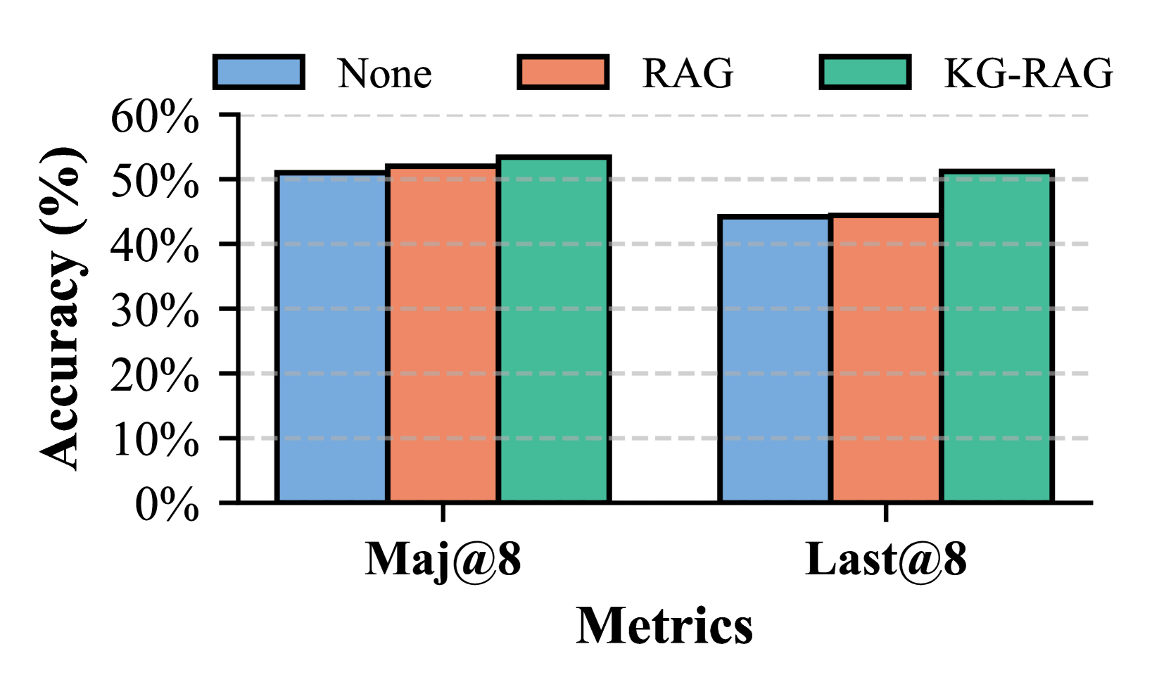
Figure 7: Comparison of various RAG types.
### 5.3 Ablation Studies
Effectiveness of Post-Retrieval Processing (PRP). We compare reasoning with refined retrieval from PRP-RM against raw retrieval directly from Knowledge Graphs. Figure 7 shows that refining the retrieval context significantly improves performance, with experiments using Llama-3B on Math500 Level 3.
Effectiveness of Knowledge Graphs (KGs). KG-RAR outperforms both no RAG and unstructured RAG (PRM800K) baselines, demonstrating the advantage of structured retrieval (Figure 7, Qwen-0.5B Reasoner, Qwen-3B PRP-RM, Math500).
<details>
<summary>x8.png Details</summary>
### Visual Description
## Dual-Axis Line Chart: Accuracy vs. Computation with Step Padding
### Overview
The image is a technical chart illustrating the relationship between "Step Padding" (x-axis), model "Accuracy (%)" (left y-axis), and relative "Computation" cost (right y-axis). It plots two data series: "Maj@8" (accuracy) and "Compute" (computation), showing how both metrics change as the step padding parameter increases from 1 to infinity.
### Components/Axes
* **Chart Type:** Dual-axis line chart.
* **X-Axis:**
* **Label:** "Step Padding"
* **Scale:** Categorical with three marked points: `1`, `4`, and `+∞` (plus-infinity).
* **Primary (Left) Y-Axis:**
* **Label:** "Accuracy (%)"
* **Scale:** Linear, ranging from 20% to 50%, with major gridlines at 10% intervals (20%, 30%, 40%, 50%).
* **Secondary (Right) Y-Axis:**
* **Label:** "Computation"
* **Scale:** Qualitative, with three labeled tick marks: "Less" (bottom), "Medium" (middle), "More" (top). This axis does not have numerical values.
* **Legend:** Positioned in the top-right quadrant of the chart area.
* **Maj@8:** Represented by a solid teal line with circular markers.
* **Compute:** Represented by a dashed black line with 'X' markers.
### Detailed Analysis
**Data Series 1: Maj@8 (Accuracy)**
* **Trend:** The line shows a non-monotonic trend. It increases from Step Padding 1 to 4, then decreases from 4 to +∞.
* **Data Points (Approximate):**
* At Step Padding `1`: Accuracy ≈ 34%
* At Step Padding `4`: Accuracy ≈ 40% (peak)
* At Step Padding `+∞`: Accuracy ≈ 35%
**Data Series 2: Compute (Computation)**
* **Trend:** The line shows a consistent, steep downward trend. Computation decreases significantly as step padding increases.
* **Data Points (Approximate, mapped to qualitative scale):**
* At Step Padding `1`: Computation ≈ "More" (value ~47% if mapped to left axis scale for reference).
* At Step Padding `4`: Computation ≈ "Medium" (value ~38% if mapped to left axis scale for reference).
* At Step Padding `+∞`: Computation ≈ "Less" (value ~23% if mapped to left axis scale for reference).
### Key Observations
1. **Inverse Relationship:** There is a clear inverse relationship between the "Compute" cost and "Step Padding." As step padding increases, computation decreases sharply.
2. **Accuracy Peak:** The "Maj@8" accuracy does not follow a simple linear trend. It peaks at an intermediate step padding value of 4 before declining.
3. **Trade-off Zone:** The chart highlights a trade-off zone. The highest accuracy (at Step Padding 4) coincides with a medium computation cost. The lowest computation (at +∞) comes with lower accuracy than the peak.
4. **Visual Confirmation:** The teal "Maj@8" line is positioned above the black "Compute" line at Step Padding 4 and +∞, but below it at Step Padding 1, visually reinforcing the changing trade-off.
### Interpretation
This chart demonstrates a classic engineering trade-off in model optimization, likely related to inference or sampling techniques (where "Step Padding" might refer to a parameter in a decoding algorithm like majority voting over multiple steps).
* **The Core Trade-off:** Increasing "Step Padding" from 1 to 4 improves accuracy (Maj@8) while simultaneously reducing computational cost. This suggests an initial "sweet spot" where the parameter change is beneficial on both fronts.
* **Diminishing Returns & Cost:** Beyond Step Padding 4, further increases (towards infinity) continue to reduce computation but at the cost of decreasing accuracy. This indicates a point of diminishing returns where the accuracy-computation balance shifts negatively.
* **Practical Implication:** The optimal setting depends on the priority. If maximizing accuracy is critical, Step Padding 4 is best. If minimizing computation is the primary goal, a very high step padding (+∞) is preferable, accepting a moderate drop in accuracy from the peak. The chart provides the quantitative basis for making this operational decision.
</details>
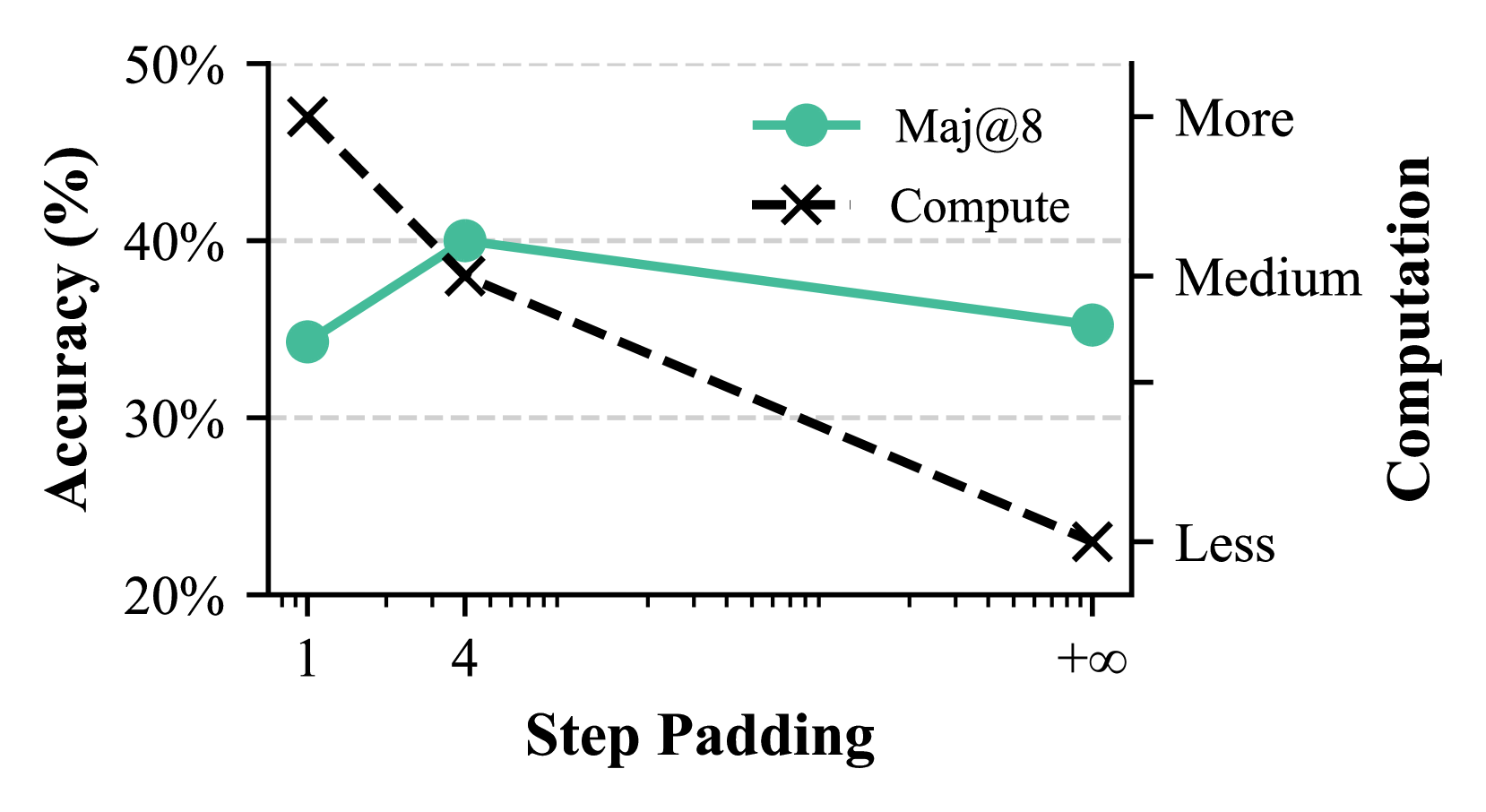
Figure 8: Comparison of step padding settings.
<details>
<summary>x9.png Details</summary>
### Visual Description
## Grouped Bar Chart: Accuracy Comparison of Three Methods Across Two Metrics
### Overview
The image displays a grouped bar chart comparing the accuracy percentages of three different methods—Socratic, Responsible, and Critical—across two evaluation metrics: "Maj@8" and "Last@8". The chart is designed to visually contrast the performance of these methods.
### Components/Axes
* **Chart Type:** Grouped Bar Chart.
* **Y-Axis:**
* **Label:** "Accuracy (%)".
* **Scale:** Linear scale from 0.0% to 70.0%, with major tick marks and grid lines at every 10% increment (0.0%, 10.0%, 20.0%, 30.0%, 40.0%, 50.0%, 60.0%, 70.0%).
* **X-Axis:**
* **Label:** "Metrics".
* **Categories:** Two primary categories are displayed: "Maj@8" (left group) and "Last@8" (right group).
* **Legend:**
* **Position:** Centered at the top of the chart area.
* **Items:**
1. **Socratic:** Represented by a teal/green colored bar.
2. **Responsible:** Represented by an orange/salmon colored bar.
3. **Critical:** Represented by a light blue colored bar.
* **Data Series:** Each metric category ("Maj@8", "Last@8") contains three adjacent bars, one for each method, ordered from left to right as Socratic, Responsible, Critical.
### Detailed Analysis
**Metric: Maj@8 (Left Group)**
* **Socratic (Teal Bar):** The bar height indicates an accuracy of approximately **61%**. It is the shortest bar in this group.
* **Responsible (Orange Bar):** The bar height indicates an accuracy of approximately **64%**. It is taller than the Socratic bar but shorter than the Critical bar.
* **Critical (Blue Bar):** The bar height indicates an accuracy of approximately **71%**. It is the tallest bar in this group, slightly exceeding the 70.0% grid line.
**Metric: Last@8 (Right Group)**
* **Socratic (Teal Bar):** The bar height indicates an accuracy of approximately **53%**. It is the shortest bar in this group and notably shorter than its counterpart in the Maj@8 group.
* **Responsible (Orange Bar):** The bar height indicates an accuracy of approximately **62%**. It is taller than the Socratic bar but shorter than the Critical bar.
* **Critical (Blue Bar):** The bar height indicates an accuracy of approximately **70%**. It is the tallest bar in this group, aligning closely with the 70.0% grid line.
### Key Observations
1. **Consistent Performance Hierarchy:** Across both metrics, the "Critical" method achieves the highest accuracy, followed by "Responsible," with "Socratic" performing the lowest.
2. **Metric-Dependent Performance Drop:** All three methods show a decrease in accuracy when moving from the "Maj@8" metric to the "Last@8" metric. The drop is most pronounced for the "Socratic" method (from ~61% to ~53%, an ~8 percentage point decrease).
3. **Relative Stability of "Critical":** The "Critical" method exhibits the smallest performance drop between metrics (from ~71% to ~70%, a ~1 percentage point decrease), suggesting it is the most robust across these two evaluation criteria.
4. **"Responsible" Method Consistency:** The "Responsible" method maintains a middle position with a moderate drop (from ~64% to ~62%, a ~2 percentage point decrease).
### Interpretation
This chart presents a performance benchmark likely from an AI or machine learning study, comparing different prompting or reasoning strategies ("Socratic," "Responsible," "Critical"). The metrics "Maj@8" and "Last@8" are common in evaluating large language models, often referring to majority-vote accuracy and the accuracy of the final answer in a sequence of eight attempts, respectively.
The data suggests that the **"Critical" strategy is the most effective and robust** of the three, yielding the highest accuracy on both metrics and showing minimal sensitivity to the change in evaluation method. The **"Socratic" strategy, while potentially useful, is the least accurate and most sensitive** to the metric used, performing significantly worse on "Last@8." This could imply that the Socratic method's final answer is less reliable than its aggregated majority vote. The **"Responsible" strategy offers a middle ground**, providing better accuracy than Socratic but not reaching the level of Critical.
The consistent ranking across metrics indicates a fundamental difference in the efficacy of these methods for the task being measured. The chart effectively communicates that for maximizing accuracy, especially when considering the final output ("Last@8"), the "Critical" approach is superior.
</details>
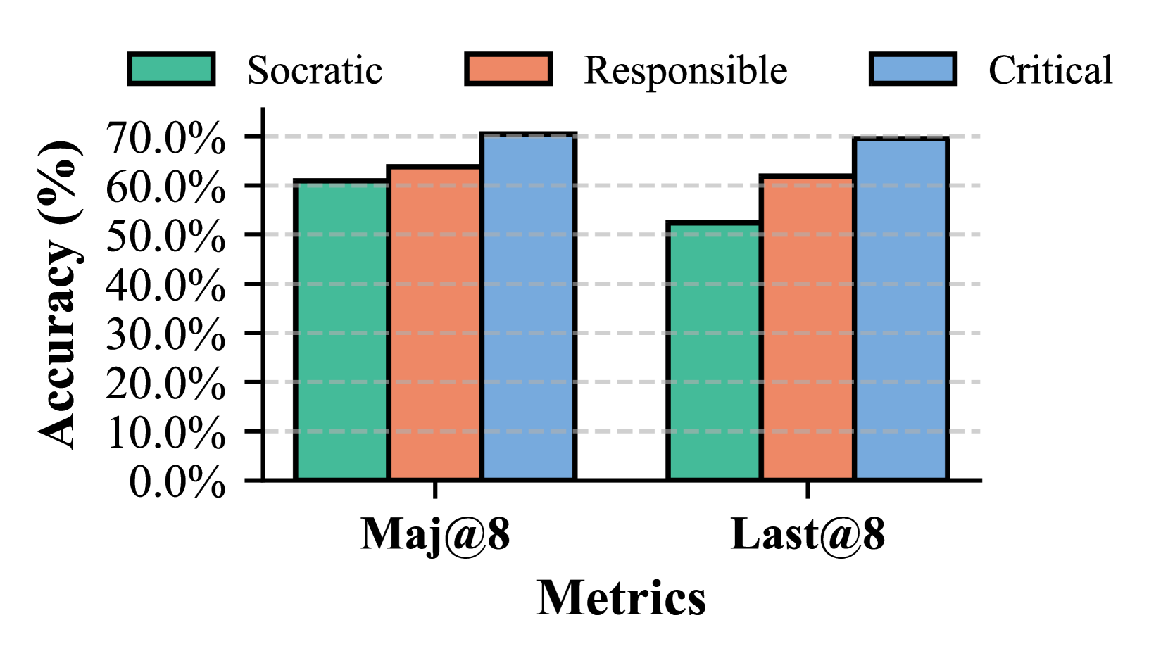
Figure 9: Comparison of PRP-RM roles.
Effectiveness of Step-by-Step RAG. We evaluate step padding at 1, 4, and 1000. Small padding causes inconsistencies, while large padding hinders refinement. Figure 9 illustrates this trade-off (Llama-1B, Math500 Level 3).
<details>
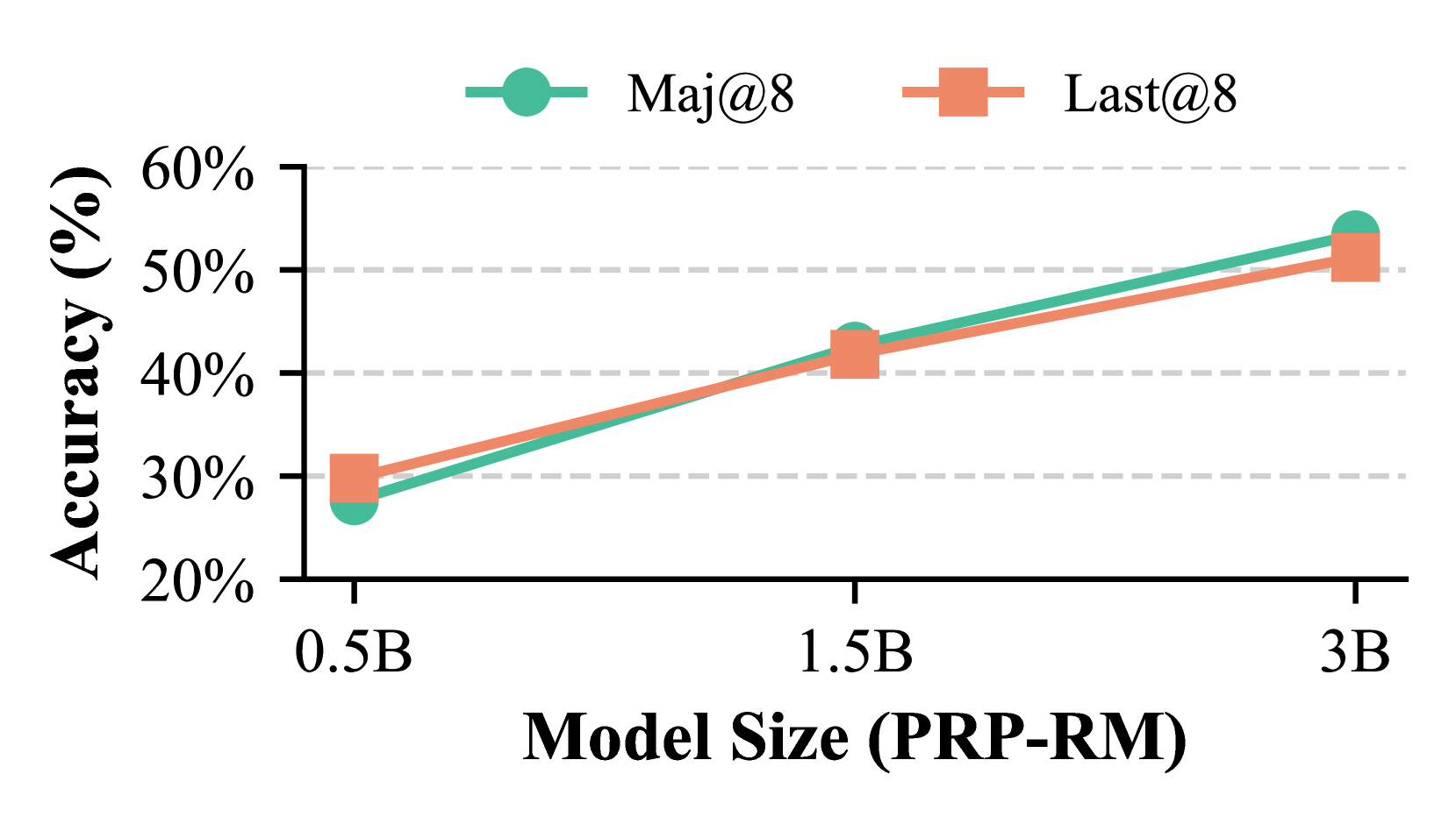
<summary>x10.png Details</summary>
### Visual Description
## Line Chart: Accuracy vs. Model Size (PRP-RM)
### Overview
This is a line chart comparing the accuracy performance of two different methods, "Maj@8" and "Last@8," across three different model sizes. The chart demonstrates a positive correlation between model size and accuracy for both methods, with "Maj@8" showing a steeper improvement curve.
### Components/Axes
* **Chart Type:** Line chart with markers.
* **X-Axis (Horizontal):**
* **Label:** "Model Size (PRP-RM)"
* **Categories/Markers:** Three discrete points: "0.5B", "1.5B", "3B". These likely represent model parameter counts (0.5 Billion, 1.5 Billion, 3 Billion).
* **Y-Axis (Vertical):**
* **Label:** "Accuracy (%)"
* **Scale:** Linear scale from 20% to 60%, with major gridlines at 10% intervals (20%, 30%, 40%, 50%, 60%).
* **Legend:**
* **Position:** Top-center of the chart area.
* **Series 1:** "Maj@8" - Represented by a teal/green line with solid circle markers.
* **Series 2:** "Last@8" - Represented by an orange/salmon line with solid square markers.
### Detailed Analysis
**Data Series & Trends:**
1. **Maj@8 (Teal line, circle markers):**
* **Trend:** Shows a strong, consistent upward slope from left to right, indicating accuracy improves significantly with model size.
* **Data Points (Approximate):**
* At **0.5B**: ~27% accuracy.
* At **1.5B**: ~43% accuracy.
* At **3B**: ~54% accuracy.
* **Observation:** This series starts lower than "Last@8" at 0.5B but surpasses it by 1.5B and maintains a higher accuracy at 3B.
2. **Last@8 (Orange line, square markers):**
* **Trend:** Also shows a consistent upward slope, but the rate of improvement appears slightly less steep than "Maj@8" after the 0.5B point.
* **Data Points (Approximate):**
* At **0.5B**: ~30% accuracy.
* At **1.5B**: ~42% accuracy.
* At **3B**: ~51% accuracy.
* **Observation:** This series starts with a higher accuracy than "Maj@8" at the smallest model size (0.5B) but is overtaken at 1.5B and ends with a lower accuracy at 3B.
**Spatial Relationships:**
* The two lines intersect between the 0.5B and 1.5B model size points, with "Maj@8" crossing from below to above "Last@8".
* The vertical gap between the two lines is smallest at 1.5B and widens again at 3B, with "Maj@8" on top.
### Key Observations
1. **Positive Scaling Law:** Both methods exhibit a clear positive relationship between model size (PRP-RM) and accuracy. Larger models yield higher accuracy.
2. **Performance Crossover:** There is a critical model size between 0.5B and 1.5B where the "Maj@8" method begins to outperform the "Last@8" method.
3. **Differential Scaling:** The "Maj@8" method appears to scale more efficiently with model size, as evidenced by its steeper slope and the growing performance gap in its favor at the largest model size (3B).
4. **Initial Advantage:** The "Last@8" method has a slight advantage at the smallest model scale (0.5B).
### Interpretation
The chart suggests that the choice between the "Maj@8" and "Last@8" methods depends on the available model scale. For very small models (~0.5B parameters), "Last@8" may be preferable. However, for medium to large models (1.5B and above), "Maj@8" is the superior strategy, and its advantage increases with scale.
This data likely comes from a machine learning or AI research context, comparing two inference or decoding strategies (e.g., "Majority vote at 8 samples" vs. "Last token at 8 samples") for a task evaluated by accuracy. The "PRP-RM" in the x-axis label may refer to a specific model architecture or training paradigm. The key takeaway is that the "Maj@8" strategy benefits more from increased model capacity, making it the more scalable solution for high-performance applications.
</details>
Figure 10: Scaling PRP-RM sizes
<details>
<summary>x11.png Details</summary>
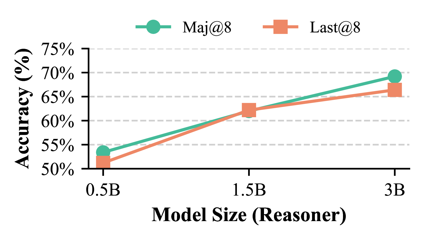
### Visual Description
## Line Chart: Accuracy vs. Model Size for a "Reasoner" Model
### Overview
The image is a line chart comparing the performance (accuracy) of two different evaluation methods, "Maj@8" and "Last@8", across three different sizes of a "Reasoner" model. The chart demonstrates a clear positive correlation between model size and accuracy for both methods.
### Components/Axes
* **Chart Type:** Line chart with markers.
* **Y-Axis:** Labeled **"Accuracy (%)"**. The scale runs from 50% to 75%, with major tick marks and dashed horizontal grid lines at 5% intervals (50%, 55%, 60%, 65%, 70%, 75%).
* **X-Axis:** Labeled **"Model Size (Reasoner)"**. It features three categorical data points: **0.5B**, **1.5B**, and **3B** (where "B" likely denotes billions of parameters).
* **Legend:** Positioned at the top center of the chart.
* **Maj@8:** Represented by a teal/green line with circular markers.
* **Last@8:** Represented by an orange/salmon line with square markers.
### Detailed Analysis
**Data Series & Trends:**
1. **Maj@8 (Teal line, circles):**
* **Trend:** Shows a steady, upward-sloping trend. The line rises consistently from left to right.
* **Data Points (Approximate):**
| Model Size | Maj@8 Accuracy |
| :--- | :--- |
| 0.5B | ~54% |
| 1.5B | ~62% |
| 3B | ~69% |
2. **Last@8 (Orange line, squares):**
* **Trend:** Also shows a steady, upward-sloping trend, parallel to but consistently below the Maj@8 line.
* **Data Points (Approximate):**
| Model Size | Last@8 Accuracy |
| :--- | :--- |
| 0.5B | ~51% |
| 1.5B | ~62% |
| 3B | ~66% |
**Spatial Grounding & Cross-Reference:**
* The legend is clearly placed at the top, making color-to-series mapping unambiguous.
* At the **0.5B** mark, the teal circle (Maj@8) is positioned above the orange square (Last@8).
* At the **1.5B** mark, the orange square and teal circle markers are nearly overlapping, indicating very similar performance.
* At the **3B** mark, the teal circle (Maj@8) is again positioned above the orange square (Last@8), and the vertical gap between the two lines appears slightly larger than at the 0.5B point.
### Key Observations
1. **Positive Scaling:** Accuracy for both evaluation methods improves as the Reasoner model size increases from 0.5B to 3B parameters.
2. **Method Superiority:** The "Maj@8" method consistently achieves equal or higher accuracy than the "Last@8" method across all tested model sizes.
3. **Convergence at Mid-Size:** The performance gap between the two methods is smallest at the 1.5B model size, where they are nearly indistinguishable.
4. **Divergence at Larger Size:** The performance gap re-emerges and appears to widen slightly at the largest (3B) model size, favoring Maj@8.
### Interpretation
This chart provides empirical evidence for two key findings in the context of the "Reasoner" model's development:
1. **Scalability is Effective:** The model's reasoning or task-specific accuracy (the exact task is not specified) scales positively with its parameter count. This suggests that increasing model capacity is a viable strategy for improving performance on the evaluated benchmark.
2. **Evaluation Method Matters:** The choice of evaluation protocol ("Maj@8" vs. "Last@8") has a measurable impact on the reported accuracy. "Maj@8" (likely referring to a majority vote over 8 samples or steps) appears to be a more robust or generous metric than "Last@8" (likely using only the final output from 8 samples/steps). The fact that the advantage of Maj@8 is present at both the smallest and largest model sizes, but minimal at the mid-size, could indicate interesting dynamics in how model scale interacts with output consistency or the diversity of reasoning paths. The data suggests that for this model family, employing a majority-vote aggregation strategy yields a consistent performance benefit.
</details>
Figure 11: Scaling reasoner LLM sizes
Comparison of PRP-RM Roles. Socratic Teacher minimizes direct problem-solving but sometimes introduces extraneous questions. Figure 9 shows Critical Teacher performs best among three roles (Llama-3B, Math500).
Scaling Model Size. Scaling trends in Section 5.2 are validated on Math500. Figures 11 and 11 confirm performance gains as both the Reasoner LLM and PRP-RM scale independently.
Scaling of Number of Solutions. We vary the number of generated solutions using Llama-3B on Math500 Level 3. Figure 13 shows accuracy improves incrementally with more solutions, underscoring the benefits of multiple candidates.
<details>
<summary>x12.png Details</summary>
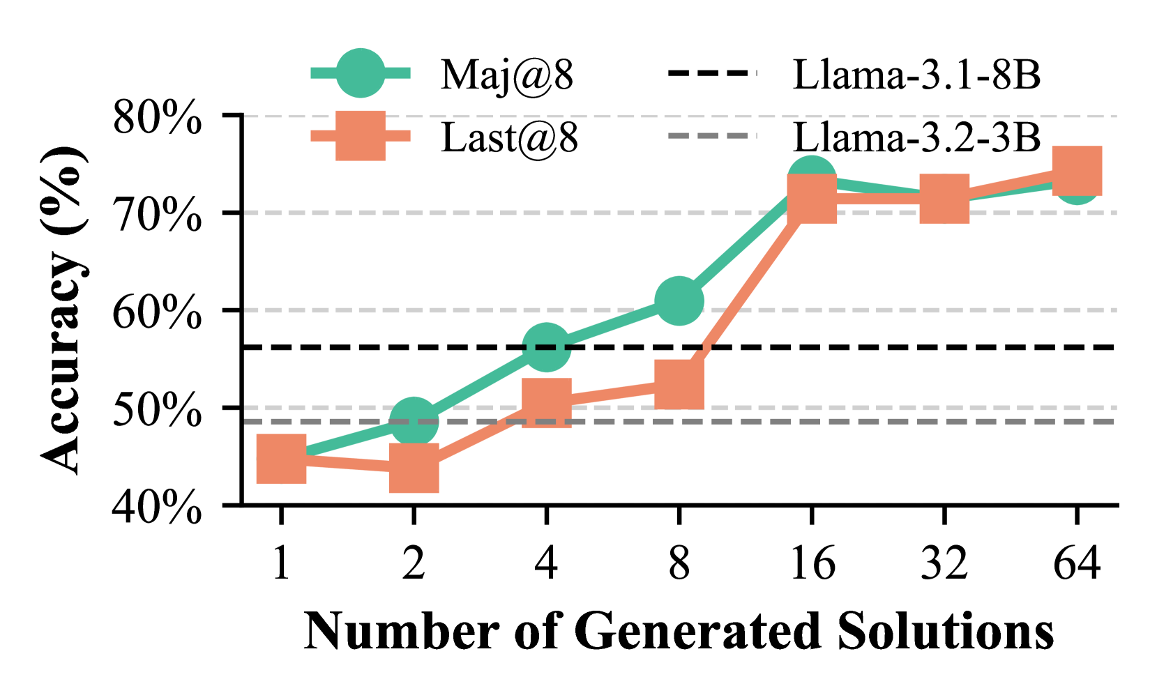
### Visual Description
\n
## Line Chart: Accuracy vs. Number of Generated Solutions for Llama Models
### Overview
This image is a line chart comparing the performance of two evaluation methods ("Maj@8" and "Last@8") across two different Llama model sizes (3.1-8B and 3.2-3B) as the number of generated solutions increases. The chart demonstrates how accuracy scales with increased solution generation.
### Components/Axes
* **X-Axis:** Labeled "Number of Generated Solutions". It uses a logarithmic scale with discrete markers at 1, 2, 4, 8, 16, 32, and 64.
* **Y-Axis:** Labeled "Accuracy (%)". It is a linear scale ranging from 40% to 80%, with major gridlines at 10% intervals (40%, 50%, 60%, 70%, 80%).
* **Legend (Top Center):**
* **Left Column (Methods):**
* A teal circle icon labeled "Maj@8".
* An orange square icon labeled "Last@8".
* **Right Column (Model Baselines):**
* A black dashed line labeled "Llama-3.1-8B".
* A gray dashed line labeled "Llama-3.2-3B".
* **Data Series:**
1. **Maj@8 (Teal line with circle markers):** Represents the accuracy of the "Majority@8" method.
2. **Last@8 (Orange line with square markers):** Represents the accuracy of the "Last@8" method.
* **Baseline Reference Lines:**
* **Llama-3.1-8B (Black dashed line):** A horizontal line at approximately 56% accuracy.
* **Llama-3.2-3B (Gray dashed line):** A horizontal line at approximately 49% accuracy.
### Detailed Analysis
**Data Points (Approximate Values):**
| Number of Solutions | Maj@8 Accuracy (%) | Last@8 Accuracy (%) |
| :----------------- | :----------------- | :------------------ |
| 1 | ~45% | ~45% |
| 2 | ~49% | ~44% |
| 4 | ~56% | ~51% |
| 8 | ~61% | ~53% |
| 16 | ~74% | ~72% |
| 32 | ~72% | ~72% |
| 64 | ~73% | ~75% |
**Trend Verification:**
* **Maj@8 (Teal Line):** Shows a consistent upward trend from 1 to 16 solutions, with a steep increase between 8 and 16. It plateaus between 16 and 64 solutions, hovering in the low-to-mid 70% range.
* **Last@8 (Orange Line):** Shows a more gradual upward trend from 1 to 8 solutions. It experiences a very sharp increase between 8 and 16 solutions, converging with the Maj@8 line. From 16 to 64 solutions, it remains stable in the low-to-mid 70% range, ending slightly higher than Maj@8 at 64 solutions.
### Key Observations
1. **Performance Scaling:** Both methods show significant accuracy gains as the number of generated solutions increases from 1 to 16.
2. **Critical Threshold:** The most dramatic improvement for both methods occurs when increasing from 8 to 16 generated solutions.
3. **Method Comparison:** "Maj@8" outperforms "Last@8" at lower solution counts (2, 4, 8). Their performance converges at 16 solutions and remains very similar thereafter.
4. **Surpassing Baselines:** Both methods surpass the Llama-3.1-8B baseline (~56%) at 8 solutions (Maj@8) or 16 solutions (Last@8). They significantly exceed the Llama-3.2-3B baseline (~49%) from 4 solutions onward.
5. **Plateau Effect:** After 16 solutions, generating more solutions (32, 64) yields minimal additional accuracy improvement for either method, suggesting diminishing returns.
### Interpretation
The data suggests that generating multiple solutions and applying a selection strategy (either majority vote or taking the last one) is highly effective for improving the accuracy of these language models on the evaluated task. The "Maj@8" method appears more sample-efficient, achieving higher accuracy with fewer generated solutions. However, with a sufficient number of solutions (16 or more), the simpler "Last@8" method performs comparably.
The sharp performance jump at 16 solutions indicates a potential phase change or threshold where the model's output distribution becomes rich enough for the selection mechanisms to work very effectively. The plateau after 16 solutions implies that the core capability of the model is being fully leveraged by these methods, and further gains would likely require improvements to the base model itself rather than just more sampling.
The chart effectively argues for the utility of inference-time computation (generating more solutions) as a powerful tool to boost performance, with the choice between "Maj@8" and "Last@8" potentially depending on the computational budget (fewer solutions favor Maj@8) or implementation simplicity (Last@8).
</details>
Figure 12: Scaling of the number of solutions.
<details>
<summary>x13.png Details</summary>
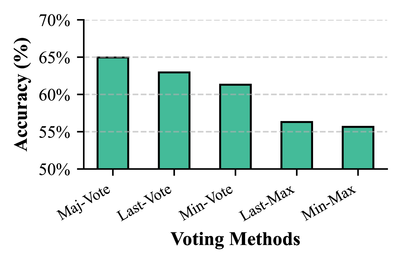
### Visual Description
\n
## Bar Chart: Comparison of Voting Method Accuracy
### Overview
The image is a vertical bar chart comparing the accuracy percentages of five different voting methods. The chart displays a single data series with five bars, each representing a distinct method. The overall trend shows a decrease in accuracy from the leftmost to the rightmost method.
### Components/Axes
* **X-Axis (Horizontal):** Labeled **"Voting Methods"**. It contains five categorical labels, rotated at an angle for readability. From left to right, the categories are:
1. `Maj-Vote`
2. `Last-Vote`
3. `Min-Vote`
4. `Last-Max`
5. `Min-Max`
* **Y-Axis (Vertical):** Labeled **"Accuracy (%)"**. The scale is linear, ranging from 50% to 70%, with major tick marks and dashed horizontal grid lines at 5% intervals (50%, 55%, 60%, 65%, 70%).
* **Legend:** There is no separate legend. The chart uses a single color (a medium teal/green) for all bars, indicating they belong to the same data series measuring "Accuracy."
### Detailed Analysis
The chart presents the following approximate accuracy values for each voting method. Values are estimated based on the bar height relative to the y-axis grid lines.
1. **Maj-Vote (Leftmost bar):** This is the tallest bar. Its top aligns almost exactly with the 65% grid line.
* **Approximate Value:** 65%
* **Trend:** Highest accuracy in the set.
2. **Last-Vote (Second bar from left):** This bar is shorter than the first. Its top is positioned between the 60% and 65% grid lines, closer to 65%.
* **Approximate Value:** ~63%
* **Trend:** Slight decrease from Maj-Vote.
3. **Min-Vote (Third bar from left):** This bar is shorter than the second. Its top is just above the 60% grid line.
* **Approximate Value:** ~61%
* **Trend:** Continued decrease.
4. **Last-Max (Fourth bar from left):** This bar shows a more significant drop. Its top is just above the 55% grid line.
* **Approximate Value:** ~56%
* **Trend:** Notable decrease from the previous method.
5. **Min-Max (Rightmost bar):** This is the shortest bar. Its top is slightly above the 55% grid line, appearing marginally lower than the Last-Max bar.
* **Approximate Value:** ~55.5%
* **Trend:** Lowest accuracy in the set.
**Spatial Grounding & Trend Verification:** All bars are positioned directly above their respective x-axis labels. The visual trend is a clear, stepwise downward slope from left to right, confirming the numerical extraction that accuracy decreases across the sequence of methods presented.
### Key Observations
* **Clear Hierarchy:** There is a distinct performance hierarchy among the methods, with "Maj-Vote" being the most accurate and "Min-Max" being the least accurate in this comparison.
* **Two Performance Tiers:** The data suggests two groupings. The first three methods ("Maj-Vote," "Last-Vote," "Min-Vote") all achieve accuracy above 60%. The last two methods ("Last-Max," "Min-Max") cluster together with accuracy just above 55%.
* **Monotonic Decrease:** The accuracy decreases monotonically across the ordered categories as presented on the x-axis.
### Interpretation
This chart demonstrates a comparative analysis of ensemble or decision-combining strategies, likely in a machine learning or computational voting context. The data suggests that methods incorporating a "majority" principle (`Maj-Vote`) or a "last" element (`Last-Vote`) yield higher accuracy than methods based on "minimum" or "minimum-maximum" strategies (`Min-Vote`, `Last-Max`, `Min-Max`) for the specific task or dataset evaluated.
The significant drop between `Min-Vote` (~61%) and `Last-Max` (~56%) indicates a potential threshold where the underlying logic of the voting method changes substantially, leading to a notable performance penalty. The close performance of `Last-Max` and `Min-Max` suggests these two strategies, while distinct, result in similarly lower efficacy compared to the others. The chart effectively argues for the superiority of majority-based or recency-based voting in this particular scenario.
</details>
Figure 13: Comparison of various voting methods.
Comparison of Voting Methods. We widely evaluate five PRP-RM voting strategies: Majority Vote, Last Vote, Min Vote, Min-Max, and Last-Max [23, 21]. Majority Vote and Last Vote outperform others, as extreme-based methods are prone to PRP-RM overconfidence in incorrect solutions (Figure 13).
## 6 Conclusions and Limitations
In this paper, we introduce a novel graph-augmented reasoning paradigm that aims to enhance o1-like multi-step reasoning capabilities of frozen LLMs by integrating external KGs. Towards this end, we present step-by-step knowledge graph based retrieval-augmented reasoning (KG-RAR), a novel iterative retrieve-refine-reason framework that strengthens o1-like reasoning, facilitated by an innovative post-retrieval processing and reward model (PRP-RM) that refines raw retrievals and assigns step-wise scores to guide reasoning more effectively. Experimental results demonstrate an 8.95% relative improvement on average over CoT-prompting on Math500, with PRP-RM achieving competitive performance against fine-tuned reward models, yet without the heavy training or fine-tuning costs.
Despite these merits, the proposed approach indeed has some limitations, such as higher computational overhead and potential cases where KG-RAR may introduce unnecessary noise or fail to enhance reasoning. Our future work will focus on optimising the framework by incorporating active learning to dynamically update KGs, improving retrieval efficiency, and exploring broader applications in complex reasoning domains such as scientific discovery and real-world decision-making.
## References
- [1] J. Huang and K. C.-C. Chang, “Towards reasoning in large language models: A survey,” arXiv preprint arXiv:2212.10403, 2022.
- [2] J. Sun, C. Zheng, E. Xie, Z. Liu, R. Chu, J. Qiu, J. Xu, M. Ding, H. Li, M. Geng et al., “A survey of reasoning with foundation models,” arXiv preprint arXiv:2312.11562, 2023.
- [3] A. Plaat, A. Wong, S. Verberne, J. Broekens, N. van Stein, and T. Back, “Reasoning with large language models, a survey,” arXiv preprint arXiv:2407.11511, 2024.
- [4] J. Wei, X. Wang, D. Schuurmans, M. Bosma, F. Xia, E. Chi, Q. V. Le, D. Zhou et al., “Chain-of-thought prompting elicits reasoning in large language models,” Advances in neural information processing systems, vol. 35, pp. 24 824–24 837, 2022.
- [5] X. Wang, J. Wei, D. Schuurmans, Q. Le, E. Chi, S. Narang, A. Chowdhery, and D. Zhou, “Self-consistency improves chain of thought reasoning in language models,” arXiv preprint arXiv:2203.11171, 2022.
- [6] S. Zhou, U. Alon, F. F. Xu, Z. Jiang, and G. Neubig, “Docprompting: Generating code by retrieving the docs,” in The Eleventh International Conference on Learning Representations, 2022.
- [7] T. Kojima, S. S. Gu, M. Reid, Y. Matsuo, and Y. Iwasawa, “Large language models are zero-shot reasoners,” Advances in neural information processing systems, vol. 35, pp. 22 199–22 213, 2022.
- [8] A. Creswell, M. Shanahan, and I. Higgins, “Selection-inference: Exploiting large language models for interpretable logical reasoning,” arXiv preprint arXiv:2205.09712, 2022.
- [9] N. Shinn, B. Labash, and A. Gopinath, “Reflexion: an autonomous agent with dynamic memory and self-reflection,” arXiv preprint arXiv:2303.11366, 2023.
- [10] S. Yao, D. Yu, J. Zhao, I. Shafran, T. Griffiths, Y. Cao, and K. Narasimhan, “Tree of thoughts: Deliberate problem solving with large language models,” Advances in Neural Information Processing Systems, vol. 36, 2024.
- [11] W. Chen, X. Ma, X. Wang, and W. W. Cohen, “Program of thoughts prompting: Disentangling computation from reasoning for numerical reasoning tasks,” arXiv preprint arXiv:2211.12588, 2022.
- [12] R. Yamauchi, S. Sonoda, A. Sannai, and W. Kumagai, “Lpml: Llm-prompting markup language for mathematical reasoning,” arXiv preprint arXiv:2309.13078, 2023.
- [13] Y. Zhuang, Y. Yu, K. Wang, H. Sun, and C. Zhang, “Toolqa: A dataset for llm question answering with external tools,” Advances in Neural Information Processing Systems, vol. 36, pp. 50 117–50 143, 2023.
- [14] B. Roziere, J. Gehring, F. Gloeckle, S. Sootla, I. Gat, X. E. Tan, Y. Adi, J. Liu, R. Sauvestre, T. Remez et al., “Code llama: Open foundation models for code,” arXiv preprint arXiv:2308.12950, 2023.
- [15] L. Yu, W. Jiang, H. Shi, J. Yu, Z. Liu, Y. Zhang, J. T. Kwok, Z. Li, A. Weller, and W. Liu, “Metamath: Bootstrap your own mathematical questions for large language models,” arXiv preprint arXiv:2309.12284, 2023.
- [16] Y. Wu, F. Jia, S. Zhang, H. Li, E. Zhu, Y. Wang, Y. T. Lee, R. Peng, Q. Wu, and C. Wang, “Mathchat: Converse to tackle challenging math problems with llm agents,” in ICLR 2024 Workshop on Large Language Model (LLM) Agents, 2024.
- [17] S. Wu, Z. Peng, X. Du, T. Zheng, M. Liu, J. Wu, J. Ma, Y. Li, J. Yang, W. Zhou et al., “A comparative study on reasoning patterns of openai’s o1 model,” arXiv preprint arXiv:2410.13639, 2024.
- [18] D. Zhang, J. Wu, J. Lei, T. Che, J. Li, T. Xie, X. Huang, S. Zhang, M. Pavone, Y. Li et al., “Llama-berry: Pairwise optimization for o1-like olympiad-level mathematical reasoning,” arXiv preprint arXiv:2410.02884, 2024.
- [19] Y. Zhang, S. Wu, Y. Yang, J. Shu, J. Xiao, C. Kong, and J. Sang, “o1-coder: an o1 replication for coding,” arXiv preprint arXiv:2412.00154, 2024.
- [20] J. Wang, F. Meng, Y. Liang, and J. Zhou, “Drt-o1: Optimized deep reasoning translation via long chain-of-thought,” arXiv preprint arXiv:2412.17498, 2024.
- [21] J. Wang, M. Fang, Z. Wan, M. Wen, J. Zhu, A. Liu, Z. Gong, Y. Song, L. Chen, L. M. Ni et al., “Openr: An open source framework for advanced reasoning with large language models,” arXiv preprint arXiv:2410.09671, 2024.
- [22] H. Luo, L. Shen, H. He, Y. Wang, S. Liu, W. Li, N. Tan, X. Cao, and D. Tao, “O1-pruner: Length-harmonizing fine-tuning for o1-like reasoning pruning,” arXiv preprint arXiv:2501.12570, 2025.
- [23] X. Feng, Z. Wan, M. Wen, Y. Wen, W. Zhang, and J. Wang, “Alphazero-like tree-search can guide large language model decoding and training,” in ICML 2024, 2024.
- [24] S. Hao, Y. Gu, H. Ma, J. J. Hong, Z. Wang, D. Z. Wang, and Z. Hu, “Reasoning with language model is planning with world model,” arXiv preprint arXiv:2305.14992, 2023.
- [25] C. Snell, J. Lee, K. Xu, and A. Kumar, “Scaling llm test-time compute optimally can be more effective than scaling model parameters,” arXiv preprint arXiv:2408.03314, 2024.
- [26] Y. Chen, X. Pan, Y. Li, B. Ding, and J. Zhou, “A simple and provable scaling law for the test-time compute of large language models,” arXiv preprint arXiv:2411.19477, 2024.
- [27] OpenAI, “Learning to reason with llms,” https://openai.com/index/learning-to-reason-with-llms/, 2024.
- [28] DeepSeek-AI, D. Guo, D. Yang, and et al., “Deepseek-r1: Incentivizing reasoning capability in llms via reinforcement learning,” 2025. [Online]. Available: https://arxiv.org/abs/2501.12948
- [29] H. Lightman, V. Kosaraju, Y. Burda, H. Edwards, B. Baker, T. Lee, J. Leike, J. Schulman, I. Sutskever, and K. Cobbe, “Let’s verify step by step,” arXiv preprint arXiv:2305.20050, 2023.
- [30] K. Cobbe, V. Kosaraju, M. Bavarian, M. Chen, H. Jun, L. Kaiser, M. Plappert, J. Tworek, J. Hilton, R. Nakano et al., “Training verifiers to solve math word problems,” arXiv preprint arXiv:2110.14168, 2021.
- [31] J. Uesato, N. Kushman, R. Kumar, F. Song, N. Siegel, L. Wang, A. Creswell, G. Irving, and I. Higgins, “Solving math word problems with process-and outcome-based feedback,” arXiv preprint arXiv:2211.14275, 2022.
- [32] A. Satpute, N. Gießing, A. Greiner-Petter, M. Schubotz, O. Teschke, A. Aizawa, and B. Gipp, “Can llms master math? investigating large language models on math stack exchange,” in Proceedings of the 47th international ACM SIGIR conference on research and development in information retrieval, 2024, pp. 2316–2320.
- [33] I. Mirzadeh, K. Alizadeh, H. Shahrokhi, O. Tuzel, S. Bengio, and M. Farajtabar, “Gsm-symbolic: Understanding the limitations of mathematical reasoning in large language models,” arXiv preprint arXiv:2410.05229, 2024.
- [34] L. Huang, W. Yu, W. Ma, W. Zhong, Z. Feng, H. Wang, Q. Chen, W. Peng, X. Feng, B. Qin et al., “A survey on hallucination in large language models: Principles, taxonomy, challenges, and open questions,” arXiv preprint arXiv:2311.05232, 2023.
- [35] S. Banerjee, A. Agarwal, and S. Singla, “Llms will always hallucinate, and we need to live with this,” arXiv preprint arXiv:2409.05746, 2024.
- [36] Z. Xu, S. Jain, and M. Kankanhalli, “Hallucination is inevitable: An innate limitation of large language models,” arXiv preprint arXiv:2401.11817, 2024.
- [37] Y. Gao, Y. Xiong, X. Gao, K. Jia, J. Pan, Y. Bi, Y. Dai, J. Sun, and H. Wang, “Retrieval-augmented generation for large language models: A survey,” arXiv preprint arXiv:2312.10997, 2023.
- [38] W. Fan, Y. Ding, L. Ning, S. Wang, H. Li, D. Yin, T.-S. Chua, and Q. Li, “A survey on rag meeting llms: Towards retrieval-augmented large language models,” in Proceedings of the 30th ACM SIGKDD Conference on Knowledge Discovery and Data Mining, 2024, pp. 6491–6501.
- [39] B. Peng, Y. Zhu, Y. Liu, X. Bo, H. Shi, C. Hong, Y. Zhang, and S. Tang, “Graph retrieval-augmented generation: A survey,” arXiv preprint arXiv:2408.08921, 2024.
- [40] S. Barnett, S. Kurniawan, S. Thudumu, Z. Brannelly, and M. Abdelrazek, “Seven failure points when engineering a retrieval augmented generation system,” in Proceedings of the IEEE/ACM 3rd International Conference on AI Engineering-Software Engineering for AI, 2024, pp. 194–199.
- [41] Z. Wang, A. Liu, H. Lin, J. Li, X. Ma, and Y. Liang, “Rat: Retrieval augmented thoughts elicit context-aware reasoning in long-horizon generation,” arXiv preprint arXiv:2403.05313, 2024.
- [42] Y. Hu, Z. Lei, Z. Zhang, B. Pan, C. Ling, and L. Zhao, “Grag: Graph retrieval-augmented generation,” arXiv preprint arXiv:2405.16506, 2024.
- [43] X. Li, R. Zhao, Y. K. Chia, B. Ding, S. Joty, S. Poria, and L. Bing, “Chain-of-knowledge: Grounding large language models via dynamic knowledge adapting over heterogeneous sources,” arXiv preprint arXiv:2305.13269, 2023.
- [44] X. He, Y. Tian, Y. Sun, N. V. Chawla, T. Laurent, Y. LeCun, X. Bresson, and B. Hooi, “G-retriever: Retrieval-augmented generation for textual graph understanding and question answering,” arXiv preprint arXiv:2402.07630, 2024.
- [45] R.-C. Chang and J. Zhang, “Communitykg-rag: Leveraging community structures in knowledge graphs for advanced retrieval-augmented generation in fact-checking,” arXiv preprint arXiv:2408.08535, 2024.
- [46] Y. Mu, P. Niu, K. Bontcheva, and N. Aletras, “Predicting and analyzing the popularity of false rumors in weibo,” Expert Systems with Applications, vol. 243, p. 122791, 2024.
- [47] L. Luo, Y.-F. Li, G. Haffari, and S. Pan, “Reasoning on graphs: Faithful and interpretable large language model reasoning,” arXiv preprint arXiv:2310.01061, 2023.
- [48] J. Sun, C. Xu, L. Tang, S. Wang, C. Lin, Y. Gong, H.-Y. Shum, and J. Guo, “Think-on-graph: Deep and responsible reasoning of large language model with knowledge graph,” arXiv preprint arXiv:2307.07697, 2023.
- [49] H. Liu, S. Wang, Y. Zhu, Y. Dong, and J. Li, “Knowledge graph-enhanced large language models via path selection,” arXiv preprint arXiv:2406.13862, 2024.
- [50] L. Luo, Z. Zhao, C. Gong, G. Haffari, and S. Pan, “Graph-constrained reasoning: Faithful reasoning on knowledge graphs with large language models,” arXiv preprint arXiv:2410.13080, 2024.
- [51] Q. Zhang, J. Dong, H. Chen, D. Zha, Z. Yu, and X. Huang, “Knowgpt: Knowledge graph based prompting for large language models,” in The Thirty-eighth Annual Conference on Neural Information Processing Systems, 2024.
- [52] N. Choudhary and C. K. Reddy, “Complex logical reasoning over knowledge graphs using large language models,” arXiv preprint arXiv:2305.01157, 2023.
- [53] Z. Zhao, Y. Rong, D. Guo, E. Gözlüklü, E. Gülboy, and E. Kasneci, “Stepwise self-consistent mathematical reasoning with large language models,” arXiv preprint arXiv:2402.17786, 2024.
- [54] S. Ji, S. Pan, E. Cambria, P. Marttinen, and S. Y. Philip, “A survey on knowledge graphs: Representation, acquisition, and applications,” IEEE transactions on neural networks and learning systems, vol. 33, no. 2, pp. 494–514, 2021.
- [55] J. Wang, “Math-kg: Construction and applications of mathematical knowledge graph,” arXiv preprint arXiv:2205.03772, 2022.
- [56] C. Zheng, Z. Zhang, B. Zhang, R. Lin, K. Lu, B. Yu, D. Liu, J. Zhou, and J. Lin, “Processbench: Identifying process errors in mathematical reasoning,” arXiv preprint arXiv:2412.06559, 2024.
- [57] M. Besta, N. Blach, A. Kubicek, R. Gerstenberger, L. Gianinazzi, J. Gajda, T. Lehmann, M. Podstawski, H. Niewiadomski, P. Nyczyk et al., “Graph of thoughts: Solving elaborate problems with large language models,” arXiv preprint arXiv:2308.09687, 2023.
- [58] E. Zelikman, Y. Wu, J. Mu, and N. Goodman, “Star: Bootstrapping reasoning with reasoning,” Advances in Neural Information Processing Systems, vol. 35, pp. 15 476–15 488, 2022.
- [59] Y. Li, Z. Lin, S. Zhang, Q. Fu, B. Chen, J.-G. Lou, and W. Chen, “Making large language models better reasoners with step-aware verifier,” arXiv preprint arXiv:2206.02336, 2022.
- [60] F. Yu, A. Gao, and B. Wang, “Ovm, outcome-supervised value models for planning in mathematical reasoning,” in Findings of the Association for Computational Linguistics: NAACL 2024, 2024, pp. 858–875.
- [61] L. Zhang, A. Hosseini, H. Bansal, M. Kazemi, A. Kumar, and R. Agarwal, “Generative verifiers: Reward modeling as next-token prediction,” arXiv preprint arXiv:2408.15240, 2024.
- [62] H. Paulheim, “Knowledge graph refinement: A survey of approaches and evaluation methods,” Semantic web, vol. 8, no. 3, pp. 489–508, 2016.
- [63] Q. Wang, Z. Mao, B. Wang, and L. Guo, “Knowledge graph embedding: A survey of approaches and applications,” IEEE transactions on knowledge and data engineering, vol. 29, no. 12, pp. 2724–2743, 2017.
- [64] Y. Jing, Y. Yang, X. Wang, M. Song, and D. Tao, “Meta-aggregator: Learning to aggregate for 1-bit graph neural networks,” in Proceedings of the IEEE/CVF international conference on computer vision, 2021, pp. 5301–5310.
- [65] Y. Jing, C. Yuan, L. Ju, Y. Yang, X. Wang, and D. Tao, “Deep graph reprogramming,” in Proceedings of the IEEE/CVF Conference on Computer Vision and Pattern Recognition, 2023, pp. 24 345–24 354.
- [66] D. Sanmartin, “Kg-rag: Bridging the gap between knowledge and creativity,” arXiv preprint arXiv:2405.12035, 2024.
- [67] Y. Wang, N. Lipka, R. A. Rossi, A. Siu, R. Zhang, and T. Derr, “Knowledge graph prompting for multi-document question answering,” in Proceedings of the AAAI Conference on Artificial Intelligence, vol. 38, no. 17, 2024, pp. 19 206–19 214.
- [68] A. Kau, X. He, A. Nambissan, A. Astudillo, H. Yin, and A. Aryani, “Combining knowledge graphs and large language models,” arXiv preprint arXiv:2407.06564, 2024.
- [69] J. Jiang, K. Zhou, Z. Dong, K. Ye, W. X. Zhao, and J.-R. Wen, “Structgpt: A general framework for large language model to reason over structured data,” arXiv preprint arXiv:2305.09645, 2023.
- [70] Z. Chai, T. Zhang, L. Wu, K. Han, X. Hu, X. Huang, and Y. Yang, “Graphllm: Boosting graph reasoning ability of large language model,” arXiv preprint arXiv:2310.05845, 2023.
- [71] Y. Zhu, X. Wang, J. Chen, S. Qiao, Y. Ou, Y. Yao, S. Deng, H. Chen, and N. Zhang, “Llms for knowledge graph construction and reasoning: Recent capabilities and future opportunities,” World Wide Web, vol. 27, no. 5, p. 58, 2024.
- [72] S. Pan, L. Luo, Y. Wang, C. Chen, J. Wang, and X. Wu, “Unifying large language models and knowledge graphs: A roadmap,” IEEE Transactions on Knowledge and Data Engineering, 2024.
- [73] G. Agrawal, T. Kumarage, Z. Alghamdi, and H. Liu, “Can knowledge graphs reduce hallucinations in llms?: A survey,” arXiv preprint arXiv:2311.07914, 2023.
- [74] A. S. Pinto, A. Kolesnikov, Y. Shi, L. Beyer, and X. Zhai, “Tuning computer vision models with task rewards,” in International Conference on Machine Learning. PMLR, 2023, pp. 33 229–33 239.
- [75] Y. Jing, Y. Yang, X. Wang, M. Song, and D. Tao, “Turning frequency to resolution: Video super-resolution via event cameras,” in Proceedings of the IEEE/CVF Conference on Computer Vision and Pattern Recognition, 2021, pp. 7772–7781.
- [76] M. Kwon, S. M. Xie, K. Bullard, and D. Sadigh, “Reward design with language models,” arXiv preprint arXiv:2303.00001, 2023.
- [77] Y. Cao, H. Zhao, Y. Cheng, T. Shu, Y. Chen, G. Liu, G. Liang, J. Zhao, J. Yan, and Y. Li, “Survey on large language model-enhanced reinforcement learning: Concept, taxonomy, and methods,” IEEE Transactions on Neural Networks and Learning Systems, 2024.
- [78] Z. Wang, B. Bi, S. K. Pentyala, K. Ramnath, S. Chaudhuri, S. Mehrotra, X.-B. Mao, S. Asur et al., “A comprehensive survey of llm alignment techniques: Rlhf, rlaif, ppo, dpo and more,” arXiv preprint arXiv:2407.16216, 2024.
- [79] T. Brown, B. Mann, N. Ryder, M. Subbiah, J. D. Kaplan, P. Dhariwal, A. Neelakantan, P. Shyam, G. Sastry, A. Askell et al., “Language models are few-shot learners,” Advances in neural information processing systems, vol. 33, pp. 1877–1901, 2020.
- [80] S. Yao, J. Zhao, D. Yu, N. Du, I. Shafran, K. Narasimhan, and Y. Cao, “React: Synergizing reasoning and acting in language models,” arXiv preprint arXiv:2210.03629, 2022.
- [81] D. Zhou, N. Schärli, L. Hou, J. Wei, N. Scales, X. Wang, D. Schuurmans, C. Cui, O. Bousquet, Q. V. Le, and E. H. Chi, “Least-to-most prompting enables complex reasoning in large language models,” in The Eleventh International Conference on Learning Representations, ICLR 2023, 2023.
- [82] X. Wang and D. Zhou, “Chain-of-thought reasoning without prompting,” arXiv preprint arXiv:2402.10200, 2024.
- [83] Y. Zhang, S. Mao, T. Ge, X. Wang, A. de Wynter, Y. Xia, W. Wu, T. Song, M. Lan, and F. Wei, “Llm as a mastermind: A survey of strategic reasoning with large language models,” arXiv preprint arXiv:2404.01230, 2024.
- [84] F. Yu, H. Zhang, P. Tiwari, and B. Wang, “Natural language reasoning, a survey,” ACM Computing Surveys, vol. 56, no. 12, pp. 1–39, 2024.
- [85] L. Huang, W. Yu, W. Ma, W. Zhong, Z. Feng, H. Wang, Q. Chen, W. Peng, X. Feng, B. Qin et al., “A survey on hallucination in large language models: Principles, taxonomy, challenges, and open questions,” ACM Transactions on Information Systems, 2024.
- [86] Z. Chu, J. Chen, Q. Chen, W. Yu, T. He, H. Wang, W. Peng, M. Liu, B. Qin, and T. Liu, “A survey of chain of thought reasoning: Advances, frontiers and future,” arXiv preprint arXiv:2309.15402, 2023.
- [87] J. Ahn, R. Verma, R. Lou, D. Liu, R. Zhang, and W. Yin, “Large language models for mathematical reasoning: Progresses and challenges,” arXiv preprint arXiv:2402.00157, 2024.
- [88] Z. Li, Y. Cao, X. Xu, J. Jiang, X. Liu, Y. S. Teo, S.-W. Lin, and Y. Liu, “Llms for relational reasoning: How far are we?” in Proceedings of the 1st International Workshop on Large Language Models for Code, 2024, pp. 119–126.
- [89] Y. Wang, W. Zhong, L. Li, F. Mi, X. Zeng, W. Huang, L. Shang, X. Jiang, and Q. Liu, “Aligning large language models with human: A survey,” arXiv preprint arXiv:2307.12966, 2023.
- [90] T. Shen, R. Jin, Y. Huang, C. Liu, W. Dong, Z. Guo, X. Wu, Y. Liu, and D. Xiong, “Large language model alignment: A survey,” arXiv preprint arXiv:2309.15025, 2023.
- [91] S. R. Balseiro, O. Besbes, and D. Pizarro, “Survey of dynamic resource-constrained reward collection problems: Unified model and analysis,” Operations Research, vol. 72, no. 5, pp. 2168–2189, 2024.
- [92] D. Tomaszuk, Ł. Szeremeta, and A. Korniłowicz, “Mmlkg: Knowledge graph for mathematical definitions, statements and proofs,” Scientific Data, vol. 10, no. 1, p. 791, 2023.
- [93] L. Zheng, W.-L. Chiang, Y. Sheng, S. Zhuang, Z. Wu, Y. Zhuang, Z. Lin, Z. Li, D. Li, E. Xing et al., “Judging llm-as-a-judge with mt-bench and chatbot arena,” Advances in Neural Information Processing Systems, vol. 36, pp. 46 595–46 623, 2023.
- [94] D. Li, B. Jiang, L. Huang, A. Beigi, C. Zhao, Z. Tan, A. Bhattacharjee, Y. Jiang, C. Chen, T. Wu et al., “From generation to judgment: Opportunities and challenges of llm-as-a-judge,” arXiv preprint arXiv:2411.16594, 2024.
- [95] Y. Shi, X. Zi, Z. Shi, H. Zhang, Q. Wu, and M. Xu, “Enhancing retrieval and managing retrieval: A four-module synergy for improved quality and efficiency in rag systems,” arXiv preprint arXiv:2407.10670, 2024.
- [96] Y. Cao, Z. Gao, Z. Li, X. Xie, and S. K. Zhou, “Lego-graphrag: Modularizing graph-based retrieval-augmented generation for design space exploration,” arXiv preprint arXiv:2411.05844, 2024.
- [97] D. Mahan, D. Van Phung, R. Rafailov, C. Blagden, N. Lile, L. Castricato, J.-P. Fränken, C. Finn, and A. Albalak, “Generative reward models,” arXiv preprint arXiv:2410.12832, 2024.
- [98] C.-M. Chan, W. Chen, Y. Su, J. Yu, W. Xue, S. Zhang, J. Fu, and Z. Liu, “Chateval: Towards better llm-based evaluators through multi-agent debate,” arXiv preprint arXiv:2308.07201, 2023.
- [99] Y. Talebirad and A. Nadiri, “Multi-agent collaboration: Harnessing the power of intelligent llm agents,” arXiv preprint arXiv:2306.03314, 2023.
- [100] A. Zhao, D. Huang, Q. Xu, M. Lin, Y.-J. Liu, and G. Huang, “Expel: Llm agents are experiential learners,” in Proceedings of the AAAI Conference on Artificial Intelligence, vol. 38, no. 17, 2024, pp. 19 632–19 642.
- [101] X. Ning, Z. Wang, S. Li, Z. Lin, P. Yao, T. Fu, M. B. Blaschko, G. Dai, H. Yang, and Y. Wang, “Can llms learn by teaching for better reasoning? a preliminary study,” arXiv preprint arXiv:2406.14629, 2024.
- [102] E. Y. Chang, “Prompting large language models with the socratic method,” in 2023 IEEE 13th Annual Computing and Communication Workshop and Conference (CCWC). IEEE, 2023, pp. 0351–0360.
- [103] P. Ke, B. Wen, Z. Feng, X. Liu, X. Lei, J. Cheng, S. Wang, A. Zeng, Y. Dong, H. Wang et al., “Critiquellm: Scaling llm-as-critic for effective and explainable evaluation of large language model generation,” arXiv preprint arXiv:2311.18702, 2023.
- [104] D. Hendrycks, C. Burns, S. Kadavath, A. Arora, S. Basart, E. Tang, D. Song, and J. Steinhardt, “Measuring mathematical problem solving with the math dataset,” NeurIPS, 2021.
- [105] A. Dubey, A. Jauhri, A. Pandey, A. Kadian, A. Al-Dahle, A. Letman, A. Mathur, A. Schelten, A. Yang, A. Fan et al., “The llama 3 herd of models,” arXiv preprint arXiv:2407.21783, 2024.
- [106] A. Yang, B. Yang, B. Zhang, B. Hui, B. Zheng, B. Yu, C. Li, D. Liu, F. Huang, H. Wei et al., “Qwen2. 5 technical report,” arXiv preprint arXiv:2412.15115, 2024.
- [107] E. Charniak and M. Johnson, “Coarse-to-fine n-best parsing and maxent discriminative reranking,” in Proceedings of the 43rd Annual Meeting of the Association for Computational Linguistics (ACL’05), 2005, pp. 173–180.
- [108] P. Wang, L. Li, Z. Shao, R. Xu, D. Dai, Y. Li, D. Chen, Y. Wu, and Z. Sui, “Math-shepherd: Verify and reinforce llms step-by-step without human annotations,” in Proceedings of the 62nd Annual Meeting of the Association for Computational Linguistics (Volume 1: Long Papers), 2024, pp. 9426–9439.
- [109] W. Xiong, H. Zhang, N. Jiang, and T. Zhang, “An implementation of generative prm,” https://github.com/RLHFlow/RLHF-Reward-Modeling, 2024.