# From Language to Cognition: How LLMs Outgrow the Human Language Network
**Authors**:
- Antoine Bosselut Martin Schrimpf (EPFL MIT Georgia Institute of Technology)
## Abstract
Large language models (LLMs) exhibit remarkable similarity to neural activity in the human language network. However, the key properties of language underlying this alignment—and how brain-like representations emerge and change across training—remain unclear. We here benchmark 34 training checkpoints spanning 300B tokens across 8 different model sizes to analyze how brain alignment relates to linguistic competence. Specifically, we find that brain alignment tracks the development of formal linguistic competence—i.e., knowledge of linguistic rules—more closely than functional linguistic competence. While functional competence, which involves world knowledge and reasoning, continues to develop throughout training, its relationship with brain alignment is weaker, suggesting that the human language network primarily encodes formal linguistic structure rather than broader cognitive functions. Notably, we find that the correlation between next-word prediction, behavioral alignment, and brain alignment fades once models surpass human language proficiency. We further show that model size is not a reliable predictor of brain alignment when controlling for the number of features. Finally, using the largest set of rigorous neural language benchmarks to date, we show that language brain alignment benchmarks remain unsaturated, highlighting opportunities for improving future models. Taken together, our findings suggest that the human language network is best modeled by formal, rather than functional, aspects of language. Project Page: language-to-cognition.epfl.ch
From Language to Cognition: How LLMs Outgrow the Human Language Network
Badr AlKhamissi 1 Greta Tuckute 2 Yingtian Tang 1 Taha Binhuraib 3 Antoine Bosselut ∗,1 Martin Schrimpf ∗,1 1 EPFL 2 MIT 3 Georgia Institute of Technology
∗ Equal Supervision
## 1 Introduction
<details>
<summary>figures/brain-score-llms-main-final-final.drawio-4.png Details</summary>
### Visual Description
## [Multi-Panel Chart]: Scaling Laws for Model Competence and Brain Alignment
### Overview
The image contains three line charts arranged in a triangular layout, labeled (a), (b), and (c). They collectively illustrate how different performance metrics of language models evolve as a function of training data (Number of Tokens) and model size. The charts share a common x-axis and a consistent vertical reference line at 16B tokens. The overall theme is the relationship between scale (model parameters and training data) and various forms of model capability.
### Components/Axes
**Common Elements:**
* **X-axis (All Charts):** "Number of Tokens". The scale is logarithmic, with major tick marks at: 0, 2M, 4M, 8M, 16M, 32M, 64M, 128M, 256M, 512M, 1B, 2B, 4B, 8B, 16B, 20B, 32B, 40B, 60B, 80B, 100B, 120B, 140B, 160B, 180B, 200B, 220B, 240B, 260B, 280B, 286B.
* **Vertical Reference Line:** A solid black vertical line is drawn at the 16B token mark in all three charts.
* **Model Size Legend:** Each chart has a legend titled "Model Size" with five entries, each associated with a specific color and line/marker style. The model sizes are: 410M, 1B, 1.4B, 2.8B, 6.9B.
**Chart-Specific Elements:**
* **(a) Brain Alignment (Top Center):**
* **Y-axis:** "Brain Alignment". Linear scale from 0.2 to 0.6.
* **Legend Colors:** Shades of green. 410M (lightest green, circle marker), 1B (light green, circle), 1.4B (medium green, circle), 2.8B (dark green, circle), 6.9B (darkest green, circle).
* **Annotations:**
* Left side: "R² = 0.65" with an arrow pointing to the left portion of the chart (before 16B).
* Right side: "R² = 0.36" with an arrow pointing to the right portion of the chart (after 16B).
* Above the right portion: A bracket labeled "94.4% of training time".
* **(b) Formal Competence (Bottom Left):**
* **Y-axis:** "Formal Competence". Linear scale from 0.1 to 0.7.
* **Legend Colors:** A gradient from dark purple/blue to yellow-green. 410M (dark purple, circle), 1B (blue, circle), 1.4B (teal, circle), 2.8B (green, circle), 6.9B (yellow-green, circle).
* **(c) Functional Competence (Bottom Right):**
* **Y-axis:** "Functional Competence". Linear scale from 0.00 to 0.30.
* **Legend Colors:** Shades of blue. 410M (lightest blue, circle), 1B (light blue, circle), 1.4B (medium blue, circle), 2.8B (dark blue, circle), 6.9B (darkest blue, circle).
### Detailed Analysis
**Chart (a) Brain Alignment:**
* **Trend Verification:** All five model size series show a similar pattern: a relatively flat or slightly noisy phase from 0 to ~512M tokens, followed by a steep, roughly linear increase (on this log-scale x-axis) from ~512M to 16B tokens. After the 16B token vertical line, the growth rate slows dramatically, and the lines plateau with significant noise/fluctuation.
* **Data Points (Approximate):**
* **Pre-16B (Steep Growth Phase):** At 512M tokens, values range from ~0.25 (6.9B model) to ~0.35 (410M model). At 16B tokens, values converge to a range of approximately 0.50 to 0.58.
* **Post-16B (Plateau Phase):** Values fluctuate between ~0.45 and ~0.62. The 410M model (lightest green) often shows the highest values in this region, while the 6.9B model (darkest green) is often among the lowest.
* **R² Annotation:** The coefficient of determination (R²) is 0.65 for the relationship between model size and brain alignment during the steep growth phase (left of 16B). It drops to 0.36 for the plateau phase (right of 16B), indicating model size is a weaker predictor of brain alignment after the 16B token mark.
**Chart (b) Formal Competence:**
* **Trend Verification:** All series show a very low, flat baseline (<0.2) from 0 to ~512M tokens. There is an extremely sharp, near-vertical increase between ~512M and 4B tokens. After ~4B tokens, all series reach a high plateau (between 0.65 and 0.75) and remain essentially flat with minimal growth up to 286B tokens.
* **Data Points (Approximate):**
* **Baseline (0-512M):** Values cluster between 0.10 and 0.20.
* **Sharp Rise (512M-4B):** Values jump from ~0.2 to over 0.6.
* **Plateau (4B-286B):** All model sizes converge into a tight band between approximately 0.68 and 0.75. There is no clear ordering by model size in the plateau; the lines are intertwined.
**Chart (c) Functional Competence:**
* **Trend Verification:** All series start near zero. There is a gradual, accelerating increase beginning around 512M tokens. The growth continues steadily past the 16B token line, showing no clear plateau within the plotted range. Larger models consistently achieve higher functional competence at any given token count after the initial rise.
* **Data Points (Approximate):**
* **Initial Rise (512M-16B):** At 16B tokens, values range from ~0.08 (410M) to ~0.18 (6.9B).
* **Continued Growth (16B-286B):** At the final point (286B tokens), values range from ~0.15 (410M) to ~0.30 (6.9B). The separation between model sizes is clear and maintained.
### Key Observations
1. **Phase Transition at 16B Tokens:** The vertical line at 16B tokens marks a critical point. Brain Alignment growth saturates here, while Functional Competence continues to grow. Formal Competence saturates much earlier (~4B tokens).
2. **Divergence of Metrics:** The three metrics behave fundamentally differently with scale. Brain Alignment and Formal Competence show saturation, while Functional Competence does not saturate within the observed data range.
3. **Model Size Effect:** The benefit of increased model size is most pronounced and consistent for Functional Competence. For Brain Alignment, larger models are not necessarily better after the 16B token point. For Formal Competence, model size makes little difference once the sharp rise is complete.
4. **Noise in Brain Alignment:** The post-16B region of the Brain Alignment chart shows high variance and noise compared to the smooth curves of the other two metrics.
### Interpretation
This data suggests a nuanced view of scaling language models. The findings can be interpreted through a Peircean lens of signs:
* **Formal Competence (Chart b)** appears to be a **symbol**—a learned, conventional capability (like grammatical correctness) that is acquired rapidly once a sufficient data threshold (~512M tokens) is crossed and then mastered, showing little further improvement with massive scale.
* **Brain Alignment (Chart a)** may function as an **index**—a sign that points to a causal relationship between model internal representations and human brain activity. The strong initial correlation (R²=0.65) suggests training data causally drives this alignment. The saturation and noise after 16B tokens imply this causal link weakens or becomes obscured by other factors at extreme scale, making model size a poor predictor (R²=0.36).
* **Functional Competence (Chart c)** behaves as an **icon**—it resembles or continuously maps onto real-world utility or problem-solving ability. Its steady, unsaturated growth with both data and model size suggests it is an open-ended capability that benefits from continued scaling, making it the most promising metric for predicting future performance gains.
**Notable Anomaly:** The 410M model often achieves the highest *Brain Alignment* scores in the plateau phase, which is counterintuitive. This could indicate that smaller models, perhaps due to simpler internal representations, develop patterns that coincidentally align better with certain measured brain signals after extensive training, even if they are less functionally competent. This highlights a potential decoupling between brain-alignment metrics and practical utility at the extremes of scale.
</details>
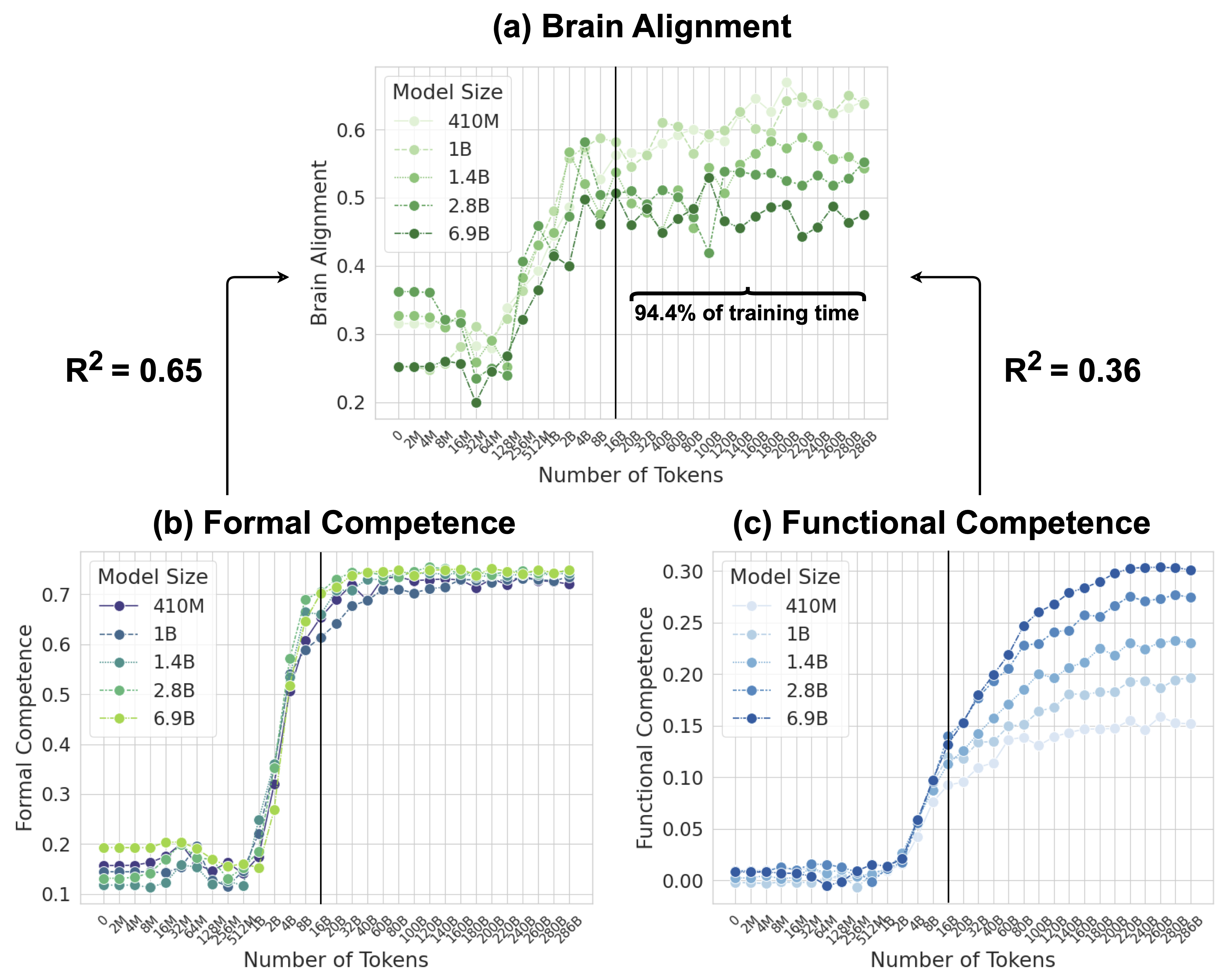
Figure 1: Model Alignment with the Human Language Network is Primarily Driven by Formal than Functional Linguistic Competence. (a) Average brain alignment across five Pythia models and five brain recording datasets, normalized by cross-subject consistency, throughout training. (b) Average normalized accuracy of the same models on formal linguistic competence benchmarks (two benchmarks). (c) Average normalized accuracy on functional linguistic competence benchmarks (six benchmarks). The x-axis is logarithmically spaced up to 16B tokens, capturing early training dynamics, and then evenly spaced every 20B tokens from 20B to ~300B tokens.
Deciphering the brain’s algorithms underlying our ability to process language and communicate is a core goal in neuroscience. Human language processing is supported by the brain’s language network (LN), a set of left-lateralized fronto-temporal regions in the brain (Binder et al., 1997; Bates et al., 2003; Gorno‐Tempini et al., 2004; Price, 2010; Fedorenko, 2014; Hagoort, 2019) that respond robustly and selectively to linguistic input (Fedorenko et al., 2024a). Driven by recent advances in machine learning, large language models (LLMs) trained via next-word prediction on large corpora of text are now a particularly promising model family to capture the internal processes of the LN. In particular, when these models are exposed to the same linguistic stimuli (e.g., sentences or narratives) as human participants during neuroimaging and electrophysiology experiments, they account for a substantial portion of neural response variance (Schrimpf et al., 2021; Caucheteux and King, 2022; Goldstein et al., 2022; Pasquiou et al., 2022; Aw et al., 2023; Tuckute et al., 2024a; AlKhamissi et al., 2025; Rathi et al., 2025).
### 1.1 Key Questions and Contributions
This work investigates four key questions, all aimed at distilling why LLM aligns to brain responses. Specifically, we investigate the full model development cycle as a combination of model architecture (structural priors) and how linguistic competence emerges across training (developmental experience). We ask: (1) What drives brain alignment in untrained models? (2) Is brain alignment primarily linked to formal or functional linguistic competence (Mahowald et al., 2024)? (3) Do language models diverge from humans as they surpass human-level prediction? (4) Do current LLMs fully account for the explained variance in brain alignment benchmarks? To answer these questions, we introduce a rigorous brain-scoring framework to conduct a controlled and large-scale analysis of LLM brain alignment.
Our findings reveal that the initial brain alignment of models with untrained parameters is driven by context integration. During training, alignment primarily correlates with formal linguistic competence—tasks that probe mastery of grammar, syntax, and compositional rules, such as identifying subject–verb agreement, parsing nested syntactic structures, or completing well-formed sentences. This competence saturates relatively early in training ( $∼ 4$ B tokens), consistent with a plateauing of model-to-brain alignment. Functional linguistic competence, in contrast, concerns how language is used in context to convey meaning, intent, and social/pragmatic content—for example, tasks involving discourse coherence, reference resolution, inference about speaker meaning, or interpreting figurative language. Functional competence emerges later in training, tracks brain alignment less strongly, and continues to grow even after alignment with the language network has saturated.
This disconnect later in training is further exemplified by a fading of the correlation between models’ brain alignment and their next-word-prediction performance, as well as their behavioral alignment. Further, we show that model size is not a reliable predictor of brain alignment when controlling for the number of features, challenging the assumption that larger models necessarily resemble the brain more. Finally, we demonstrate that current brain alignment benchmarks remain unsaturated, indicating that LLMs can still be improved to model human language processing.
## 2 Preliminaries & Related Work
#### A Primer on Language in the Human Brain
The human language network (LN) is a set of left-lateralized frontal and temporal brain regions supporting language. These regions are functionally defined by contrasting responses to language inputs over perceptually matched controls (e.g., lists of non-words) (Fedorenko et al., 2010). The language network exhibits remarkable selectivity for language processing compared to various non-linguistic inputs and tasks, such as music perception (Fedorenko et al., 2012; Chen et al., 2023) or arithmetic computation (Fedorenko et al., 2011; Monti et al., 2012) (for review, see Fedorenko et al. (2024a)) and the language network only shows weak responses when participants comprehend or articulate meaningless non-words (Fedorenko et al., 2010; Hu et al., 2023). This selectivity profile is supported by extensive neuroimaging research and further corroborated by behavioral evidence from aphasia studies: when brain damage is confined to language areas, individuals lose their linguistic abilities while retaining other skills, such as mathematics (Benn et al., 2013; Varley et al., 2005), general reasoning (Varley and Siegal, 2000), and theory of mind (Siegal and Varley, 2006).
#### Model-to-Brain Alignment
Prior work has shown that the internal representations of certain artificial neural networks resemble those in the brain. This alignment was initially observed in the domain of vision (Yamins et al., 2014; Khaligh-Razavi and Kriegeskorte, 2014; Cichy et al., 2016; Schrimpf et al., 2018, 2020; Cadena et al., 2019; Kubilius et al., 2019; Zhuang et al., 2021) and has more recently been extended to auditory processing (Kell et al., 2018; Tuckute et al., 2023; Koumura et al., 2023) and language processing (Schrimpf et al., 2021; Caucheteux and King, 2022; Goldstein et al., 2022; Kauf et al., 2023; Hosseini et al., 2024; Aw et al., 2023; AlKhamissi et al., 2025; Tuckute et al., 2024b; Rathi et al., 2025).
#### Untrained Models
Recent work in vision neuroscience has shown that untrained convolutional networks can yield high brain alignment to recordings in the visual ventral stream without the need for training (Geiger et al., 2022; Kazemian et al., 2024). Other works have investigated the inductive biases in different architectures and initializations in models of visual processing (Cichy et al., 2016; Cadena et al., 2019; Geiger et al., 2022), speech perception (Millet and King, 2021; Tuckute et al., 2023), and language (Schrimpf et al., 2021; Pasquiou et al., 2022; Hosseini et al., 2024), highlighting that randomly initialized networks are not random functions (Teney et al., 2024).
## 3 Methods
### 3.1 Benchmarks for Brain Alignment
#### Neuroimaging & Behavioral Datasets
The neuroimaging datasets used in this work can be categorized along three dimensions: the imaging modality, the context length of the experimental materials, and the modality through which the language stimulus was presented to human participants (auditory or visual). Table 1 in Appendix A provides an overview of all datasets in this study. To focus specifically on language, we consider neural units (electrodes, voxels, or regions) associated with the brain’s language network, as localized by the original dataset authors using the method described in the Section 3.2 and implemented in Brain-Score Schrimpf et al. (2020, 2021) (however, see Appendix J for control brain regions). An exception is the Narratives dataset, which lacks functional localization. We here approximate the language regions using a probabilistic atlas of the human language network (Lipkin et al., 2022), extracting the top-10% language-selective voxels (from the probabilistic atlas) within anatomically defined language parcels, in line with the functional localization procedure used in the other datasets. In an additional analysis, we investigate model alignment with language behavior using the Futrell et al. (2018) dataset, which contains self-paced, per-word human reading times. See Appendix A for details of each dataset. To the best of our knowledge, this study examines the largest number of benchmarks compared to previous work, providing a more comprehensive and reliable foundation for identifying the properties that drive brain alignment in LLMs. The diversity of datasets ensures that our conclusions generalize beyond specific experimental stimuli and paradigms.
#### Brain-Alignment Metrics
Following standard practice in measuring brain alignment, we train a ridge regression model to predict brain activity from model representations, using the same linguistic stimuli presented to human participants in neuroimaging studies (Schrimpf et al., 2020, 2021). We then measure the Pearson correlation between the predicted brain activations and the actual brain activations of human participants on a held-out set that covers entirely different stories or topics (see Section 4). This process is repeated over $k$ cross-validation splits, and we report the average (mean) Pearson correlation as our final result. We refer to this metric as Linear Predictivity. In Section 5.1, we demonstrate why other metrics such as Centered Kernel Alignment (CKA; Kornblith et al., 2019) and Representational Similarity Analysis (RSA; Kriegeskorte et al., 2008) are not suitable measures for brain alignment on current language datasets.
#### Estimation of Cross-Subject Consistency
To assess the reliability of our datasets and account for the inherent noise in brain recordings, we compute a cross-subject consistency score (Feather et al., 2025), also referred to as the noise ceiling (Schrimpf et al., 2021). The consistency score is estimated by predicting the brain activity of a held-out subject using data from all other subjects, through 10-fold cross-validation of all subjects. To obtain a conservative ceiling estimate, we extrapolate subject pool sizes and report the final value based on extrapolation to infinitely many subjects. For Tuckute2024 we use the theoretical estimate provided by (Tuckute et al., 2024b). Consistency scores are provided in Appendix K. To aggregate scores across benchmarks, we normalize each model’s Pearson correlation ( $r$ ) score for Linear Predictivity by the cross-subject consistency estimate, using the formula: ( $\textnormal{normalized score}=\frac{\textnormal{raw score}}{\textnormal{consistency}}$ ). The final alignment score for each model is reported as the average across all benchmarks. Otherwise, when reporting raw alignment, we compute the mean Pearson correlation across datasets without normalization.
### 3.2 Functional Localization
The human language network (LN) is defined functionally which means that units are chosen according to a ‘localizer’ experiment (Saxe et al., 2006). Specifically, the LN is the set of neural units (e.g., voxels/electrodes) that are more selective to sentences over a perceptually-matched control condition (Fedorenko et al., 2010). When selecting units from artificial models for comparison against LN units, previous work selected output units from an entire Transformer block based on brain alignment scores (Schrimpf et al., 2021). However, LLMs learn diverse concepts and behaviors during their considerable pretraining, not all of which are necessarily related to language processing, e.g., storage of knowledge (AlKhamissi et al., 2022) and the ability to perform complex reasoning (Huang and Chang, 2023). Therefore, we here follow the method proposed by AlKhamissi et al. (2025) that identifies language units in LLMs using functional localization as is already standard in neuroscience. This approach offers a key advantage: it enables direct comparisons across models by selecting a fixed set of units, identified through the independent localizer experiment. In this work, we localize $128$ units for all models unless otherwise specified, and we show in Appendix H that the results hold when selecting a different number of units.
<details>
<summary>figures/brain-score-llms-untrained-greens.drawio.png Details</summary>
### Visual Description
## Multi-Panel Technical Figure: Brain Alignment and Transformer Architecture Analysis
### Overview
The image is a composite figure containing four distinct panels labeled (a) through (d). It presents a comparative analysis of different neural network architectures' alignment with brain data, a schematic of a Transformer block, and a comparison of normalized accuracy between "Formal" and "Functional" categories. The overall theme appears to be evaluating how well artificial neural network components and architectures mimic or align with biological brain processing.
### Components/Axes
**Panel (a): Vertical Bar Chart**
* **Title/Label:** (a)
* **Y-axis:** "Brain Alignment" (Scale: 0.0 to 0.4, with major ticks at 0.1 intervals).
* **X-axis:** Implicitly represents different architectures, defined by the legend.
* **Legend:** Located to the right of the chart. Title: "Architecture". Contains six entries with corresponding color swatches (shades of green, from light to dark):
1. MLP (lightest green)
2. GRU
3. LSTM
4. MLP+Mean
5. Transformer-v1
6. Transformer-v2 (darkest green)
* **Data Series:** Six vertical bars, one per architecture, with error bars (vertical lines) indicating variability.
**Panel (b): Horizontal Bar Chart**
* **Title/Label:** (b)
* **X-axis:** "Brain Alignment" (Scale: 0.0 to 0.6, with major ticks at 0.2 intervals).
* **Y-axis:** Lists seven component combinations (from top to bottom):
1. Pos+Attn+MLP
2. Attn+MLP
3. Attn
4. Pos+Attn
5. MLP
6. Pos+MLP
7. Tokens
* **Data Series:** Seven horizontal bars, one per component combination, with error bars (horizontal lines).
**Panel (c): Transformer Block Diagram**
* **Title/Label:** (c)
* **Components (from bottom to top):**
* Input boxes: "Tokens" and "Pos Embeddings".
* Addition operation (⊕ symbol).
* "LayerNorm" block.
* "Multihead Attention" block (blue).
* Addition operation (⊕ symbol) with a residual connection from below the first LayerNorm.
* "LayerNorm" block.
* "MLP" block (blue).
* Addition operation (⊕ symbol) with a residual connection from below the second LayerNorm.
* Output arrow.
* **Flow:** The diagram is enclosed in a dashed blue rectangle. Arrows indicate the forward data flow. The structure shows two main sub-layers (Multihead Attention and MLP), each followed by a LayerNorm and a residual connection (skip connection) that adds the sub-layer's input to its output.
**Panel (d): Vertical Bar Chart**
* **Title/Label:** (d)
* **Y-axis:** "Normalized Accuracy" (Scale: 0.00 to 0.20, with major ticks at 0.05 intervals).
* **X-axis:** Two categories: "Formal" and "Functional".
* **Data Series:** Two vertical bars.
* "Formal": A tall, light blue bar with a very large error bar.
* "Functional": A very short, dark blue bar with a small error bar.
### Detailed Analysis
**Panel (a) - Architecture Comparison:**
* **Trend:** Brain Alignment increases progressively across the architectures from left to right.
* **Approximate Values (Visual Estimation):**
* MLP: ~0.11
* GRU: ~0.16
* LSTM: ~0.18
* MLP+Mean: ~0.24
* Transformer-v1: ~0.25
* Transformer-v2: ~0.38
* **Error Bars:** All bars have error bars. The error bar for Transformer-v2 is the largest, extending from approximately 0.35 to 0.41.
**Panel (b) - Component Contribution:**
* **Trend:** The combination "Pos+Attn+MLP" yields the highest Brain Alignment. "Tokens" alone yields the lowest.
* **Approximate Values (Visual Estimation):**
* Pos+Attn+MLP: ~0.50
* Attn+MLP: ~0.32
* Attn: ~0.30
* Pos+Attn: ~0.58 (Note: This bar is longer than Pos+Attn+MLP, suggesting a potential anomaly or specific condition. The label order on the Y-axis does not strictly correspond to bar length.)
* MLP: ~0.22
* Pos+MLP: ~0.36
* Tokens: ~0.10
* **Error Bars:** All bars have error bars. The error bar for "Pos+Attn" is notably wide.
**Panel (c) - Architecture Schematic:**
* This is a standard depiction of a Transformer encoder block. The key features are the stacked sub-layers (Multihead Attention and MLP), the use of Layer Normalization (LayerNorm) before each sub-layer (a "pre-norm" variant), and the residual connections that bypass each sub-layer.
**Panel (d) - Accuracy Comparison:**
* **Formal:** The bar reaches approximately 0.15. Its error bar is extremely large, spanning from roughly 0.08 to 0.22.
* **Functional:** The bar is very close to 0.00, perhaps ~0.01. Its error bar is small, ranging from about 0.00 to 0.02.
### Key Observations
1. **Architecture Hierarchy:** There is a clear hierarchy in Brain Alignment: simple MLP < recurrent units (GRU, LSTM) < more complex MLP variants < Transformers. Transformer-v2 shows a substantial jump over Transformer-v1.
2. **Component Synergy:** Panel (b) suggests that combining Positional Embeddings (Pos), Attention (Attn), and MLP yields high alignment, but the "Pos+Attn" bar being the longest is a critical observation that requires context (it may represent a specific experimental condition).
3. **High Variance in Formal Tasks:** Panel (d) shows that while the "Formal" category has a much higher mean normalized accuracy than "Functional," it also exhibits vastly greater variability (as shown by the large error bar).
4. **Diagram Clarity:** Panel (c) clearly isolates the core computational components of a modern Transformer, providing a reference for the component names used in Panel (b).
### Interpretation
This figure collectively investigates the representational power of artificial neural networks in relation to brain data. The progression in Panel (a) suggests that architectures with attention mechanisms and positional information (Transformers) achieve higher "Brain Alignment" than recurrent or simple feedforward networks. Panel (b) deconstructs this further, implying that the integration of positional information with attention is particularly crucial, though the exact relationship between the component combinations needs the accompanying paper's context for full explanation.
The schematic in Panel (c) defines the architectural vocabulary (MLP, Attention, LayerNorm) used in the analysis. Finally, Panel (d) introduces a separate but related metric, "Normalized Accuracy," revealing a stark contrast between "Formal" and "Functional" tasks. The high mean and variance for "Formal" could indicate that models perform well on structured, rule-based tasks but with inconsistent results, while they fail almost completely on "Functional" tasks, which may be more open-ended or context-dependent.
**Overall Implication:** The data argues that the inductive biases present in Transformer architectures—specifically the combination of self-attention and positional encoding—may be more aligned with the processing principles of the human brain than those of earlier architectures. However, the performance on downstream tasks (Panel d) is highly dependent on the task type, showing significant instability in formal domains and near-failure in functional ones.
</details>
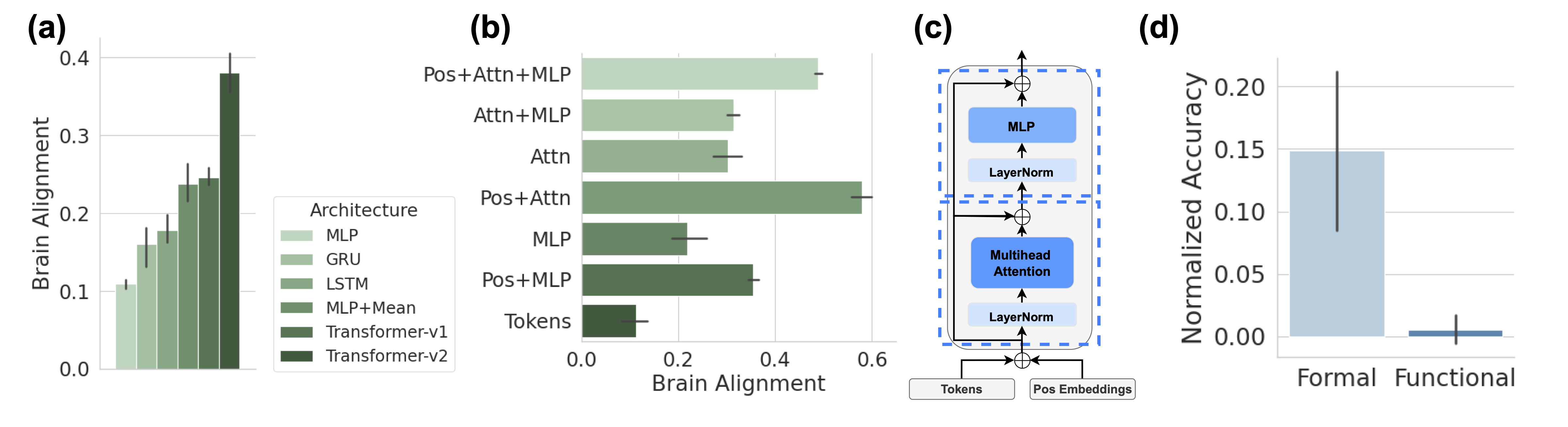
Figure 2: Context Integration drives Brain Alignment of Untrained Models. (a) Sequence-based models (GRU, LSTM, Transformers, and mean pooling) achieve higher brain alignment than models that rely solely on the last token representation (Linear, MLP), highlighting the importance of temporal integration. Error bars report five random initializations in all subplots. (b) Ablation study of architectural components in a single untrained Transformer-v2 block, demonstrating that attention mechanisms combined with positional encoding yield the highest brain alignment. (c) Diagram of the Transformer block architecture used in (b), with components grouped into attention (lower box) and MLP (upper box). (d) The average performance of five Pythia models with untrained parameters on formal and functional linguistic competence benchmarks, showing that formal competence exceeds chance level even in untrained parameter models.
### 3.3 Benchmarks for Linguistic Competence
There is substantial evidence in neuroscience research that formal and functional linguistic competence are governed by distinct neural mechanisms Mahowald et al. (2024); Fedorenko et al. (2024a, b). Formal linguistic competence pertains to the knowledge of linguistic rules and patterns, while functional linguistic competence involves using language to interpret and interact with the world. Therefore, to accurately track the evolution of each type of competence during training, we focus on benchmarks that specifically target these cognitive capacities in LLMs.
#### Formal Linguistic Competence
To assess formal linguistic competence, we use two benchmarks: BLiMP (Warstadt et al., 2019) and SyntaxGym (Gauthier et al., 2020). BLiMP evaluates key grammatical phenomena in English through 67 tasks, each containing 1,000 minimal pairs designed to test specific contrasts in syntax, morphology, and semantics. Complementing this, SyntaxGym consists of 31 tasks that systematically measure the syntactic knowledge of language models. Together, these benchmarks provide a robust framework for evaluating how well LLMs acquire and apply linguistic rules.
#### Functional Linguistic Competence
Functional competence extends beyond linguistic rules, engaging a broader set of cognitive mechanisms. To assess this, we use six benchmarks covering world knowledge (ARC-Easy, ARC-Challenge (Clark et al., 2018)), social reasoning (Social IQa (Sap et al., 2019)), physical reasoning (PIQA (Bisk et al., 2019)), and commonsense reasoning (WinoGrande (Sakaguchi et al., 2019), HellaSwag (Zellers et al., 2019)). Together, these benchmarks provide a comprehensive evaluation of an LLM’s ability to reason, infer implicit knowledge, and navigate real-world contexts.
#### Metrics
Inline with prior work, we evaluate all benchmarks in a zero-shot setting, using surprisal as the evaluation metric. where the model’s prediction is determined by selecting the most probable candidate, as packaged in the language model evaluation harness (Gao et al., 2024). We report accuracy normalized by chance performance, where 0% indicates performance at the random chance level.
#### Benchmark for Language Modeling
We use a subset of FineWebEdu Penedo et al. (2024) to evaluate the perplexity of the models on a held-out set. Specifically, use a maximum sequence length of 2048, and evaluate on the first 1000 documents of the Ay CC-MAIN-2024-10 subset.
### 3.4 Large Language Models (LLMs)
Throughout this work, we use eight models from the Pythia model suite (Biderman et al., 2023), spanning a range of sizes: {14M, 70M, 160M, 410M, 1B, 1.4B, 2.8B, 6.9B}. Each model is evaluated across 34 training checkpoints, spanning approximately 300B tokens. These checkpoints include the untrained model, the final trained model, and 16 intermediate checkpoints that are logarithmically spaced up to 128B tokens. The remaining 14 checkpoints are evenly spaced every 20B tokens from 20B to 280B tokens, ensuring a comprehensive analysis of alignment trends throughout training. Since smaller models fail to surpass chance performance on many functional benchmarks, we exclude 14M, 70M, 160M from analyses that compare brain alignment with functional performance.
## 4 Rigorous Brain-Scoring
While substantial progress has been made in measuring alignment between LLM representations and neural activity, there’s no standard for comparing brain alignment across datasets and conditions. Therefore, to ensure we perform meaningful inferences, we propose two criteria: (1) alignment should reflect stimulus-driven responses, dropping for random token sequences; and (2) models should generalize to new linguistic contexts. We justify our metrics and cross-validation choices accordingly. For all benchmarks, we identify language-selective units to ensure fair model comparisons, consistent with neural site selection in neuroscience AlKhamissi et al. (2025).
### 4.1 Robust Metrics and Generalization Tests
#### Measuring Stimulus-Driven Responses
We first ask if the alignment procedure is meaningful, i.e., whether the encoding models capture meaningful linguistic information and generalize to new linguistic contexts. Figure 6 (a) in Appendix B shows average brain alignment across all brain datasets under three conditions: (1) a pretrained model processing original stimuli, (2) a pretrained model processing random token sequences, and (3) an untrained model processing original stimuli. To evaluate metric reliability, we expect random sequences to yield significantly lower alignment than real stimuli. However, CKA fails this criterion, assigning similar alignment scores to both, and even untrained models surpass pretrained ones. In contrast, linear predictivity differentiates between real and random stimuli, more so than RSA.
#### Generalization and Contextualization
The second criterion we propose is that LLMs with high brain alignment should be able to generalize to held-out stimuli, with a preference for generalizing far outside the stimuli used for mapping the model to brain activity. A key factor in designing a corresponding cross-validation scheme is contextualization—how the data is split into train and test sets Feghhi et al. (2024). The Pereira2018 dataset consists of 24 topics composed of multi-sentence passages, and sentences are presented in their original order to both humans and models. A random sentence split (contextualization) allows sentences from the same topic in both train and test sets, and is thus less demanding of generalization. A stronger generalization test ensures entire topics are held out, preventing models from leveraging shared context. Figure 6 (b) shows that contextualization makes it easier for the model to predict brain activity. In contrast, topic-based splits halve the raw alignment score for pretrained models. The score of untrained models is reduced even more strongly when enforcing generalization across topics, suggesting that much of their alignment is context-dependent. Nonetheless, untrained models retain significant alignment – about 50% of pretrained models – even with strong generalization requirements.
<details>
<summary>figures/brain-score-llms-brain-alignment-final.drawio.png Details</summary>
### Visual Description
## Line Charts: Brain Alignment Across Pythia Model Sizes During Training
### Overview
The image displays three side-by-line charts, each tracking the "Brain Alignment" metric for a different-sized Pythia language model (1.4B, 2.8B, and 6.9B parameters) as a function of the number of training tokens processed. The charts compare performance across six different evaluation datasets. A shared legend is positioned at the bottom of the entire figure.
### Components/Axes
* **Titles:** Each subplot has a title at the top center: "Pythia-1.4B", "Pythia-2.8B", "Pythia-6.9B".
* **Y-Axis (All Charts):** Labeled "Brain Alignment". The scale ranges from 0.0 to 1.2 for the first two charts and 0.0 to 1.0 for the third (Pythia-6.9B). Major gridlines are at 0.2 intervals.
* **X-Axis (All Charts):** Labeled "Number of Tokens". It uses a logarithmic scale with major tick marks at: 0, 2M, 4M, 8M, 16M, 32M, 64M, 128M, 256M, 512M, 1B, 2B, 4B, 8B, 16B, 20B, 32B, 40B, 60B, 80B, 100B, 120B, 140B, 160B, 180B, 200B, 220B, 240B, 260B, 280B, 286B. A prominent vertical black line is drawn at the 16B token mark in each chart.
* **Legend (Bottom Center):** A horizontal legend titled "Dataset" defines six data series with distinct colors and markers:
1. **Pereira2018:** Light green line with circle markers.
2. **Blank2014:** Light green line with 'x' markers.
3. **Fedorenko2016:** Medium green line with square markers.
4. **Tuckute2024:** Dark green line with plus ('+') markers.
5. **Narratives:** Darkest green line with diamond markers.
6. **Average:** Darkest green line with star/asterisk markers.
* **Data Representation:** Each dataset is plotted as a line with markers at data points, surrounded by a shaded band of the same color, likely representing confidence intervals or standard deviation.
### Detailed Analysis
**Trend Verification & Data Points (Approximate Values):**
* **General Trend Across All Charts:** Most lines show an initial increase in Brain Alignment as training progresses, followed by a plateau or slower growth after approximately 4B-16B tokens. The "Pereira2018" dataset consistently achieves the highest alignment scores, while "Blank2014" and "Narratives" are consistently among the lowest.
* **Pythia-1.4B Chart:**
* **Pereira2018 (Circles):** Starts ~0.4, rises sharply after 1B tokens, peaks near 1.0 around 80B-100B tokens, then fluctuates between 0.8-1.0.
* **Fedorenko2016 (Squares):** Starts ~0.5, shows a moderate increase, stabilizing around 0.7-0.8 after 16B tokens.
* **Tuckute2024 (Pluses):** Starts ~0.3, increases to ~0.5 by 16B tokens, then plateaus between 0.4-0.6.
* **Average (Stars):** Follows a similar path to Tuckute2024, starting ~0.3 and stabilizing around 0.5.
* **Blank2014 (X's) & Narratives (Diamonds):** Both start low (~0.1-0.2) and show only a slight increase, remaining below 0.2 for most of training.
* **Pythia-2.8B Chart:**
* **Pereira2018 (Circles):** Starts ~0.6, climbs steadily, surpassing 1.0 after 80B tokens and reaching near 1.1 by 286B.
* **Fedorenko2016 (Squares):** Starts ~0.5, rises to ~0.8 by 16B tokens and remains stable.
* **Tuckute2024 (Pluses) & Average (Stars):** Both start ~0.3, rise to ~0.5 by 16B tokens, and plateau.
* **Blank2014 (X's) & Narratives (Diamonds):** Remain very low, mostly below 0.2, with a slight upward trend.
* **Pythia-6.9B Chart (Y-axis max 1.0):**
* **Pereira2018 (Circles):** Starts ~0.4, shows a strong increase, crossing 0.8 by 16B tokens and fluctuating between 0.8-1.0 thereafter.
* **Fedorenko2016 (Squares):** Starts ~0.4, rises to ~0.7 by 16B tokens, then stabilizes between 0.6-0.8.
* **Tuckute2024 (Pluses) & Average (Stars):** Start ~0.2, increase to ~0.4 by 16B tokens, and plateau around 0.4-0.5.
* **Blank2014 (X's) & Narratives (Diamonds):** Start near 0.0-0.1, show minimal growth, and remain below 0.2.
### Key Observations
1. **Dataset Hierarchy:** A clear and consistent performance hierarchy exists across all model sizes: Pereira2018 > Fedorenko2016 > Tuckute2024 ≈ Average > Narratives ≈ Blank2014.
2. **Model Size Effect:** Larger models (2.8B, 6.9B) achieve higher peak alignment scores on the top-performing datasets (Pereira2018, Fedorenko2016) compared to the 1.4B model. The gap between the best and worst datasets also appears more pronounced in larger models.
3. **Training Phase Transition:** The vertical line at 16B tokens often marks a point where the rate of improvement slows or plateaus for many datasets, suggesting a potential phase change in what the models are learning relative to brain alignment.
4. **High Variance:** The shaded confidence bands are notably wide, especially for the Pereira2018 dataset in the later stages of training, indicating significant variability in the alignment metric across different evaluation runs or subjects.
### Interpretation
This data suggests that the ability of Pythia language models to align with human brain activity (as measured by these specific datasets) is highly dependent on both the **evaluation dataset** and the **amount of training**.
* **Dataset Specificity:** The stark performance differences imply that "brain alignment" is not a monolithic property. The models align much better with the neural patterns captured in the Pereira2018 dataset than with those in Blank2014 or Narratives. This could reflect differences in the cognitive tasks, brain regions, or experimental paradigms used in the original studies.
* **Learning Trajectory:** Alignment improves with scale (both model size and training tokens), but with diminishing returns. The most rapid gains occur in the first few billion tokens, after which improvements become marginal. This mirrors the general "scaling laws" for language model performance but applied to a neuroscientific metric.
* **The 16B Token Milestone:** The consistent inflection around 16B tokens may indicate the point where models have largely captured the coarse-grained, easily learnable correspondences between language and brain activity, and further training refines more subtle or complex mappings.
* **Implication for AGI:** From a Peircean perspective, this chart maps the evolving "representation" (the model's internal states) of the "object" (the brain's processing of language). The high alignment on specific datasets suggests the models are successfully learning some of the statistical regularities that underpin human neural language processing. However, the low alignment on other datasets highlights that current models are not yet capturing the full richness or diversity of human brain-language relationships. The investigation would question: Are the high-alignment datasets simply easier to model, or do they represent more fundamental aspects of language processing that AGI should prioritize?
</details>
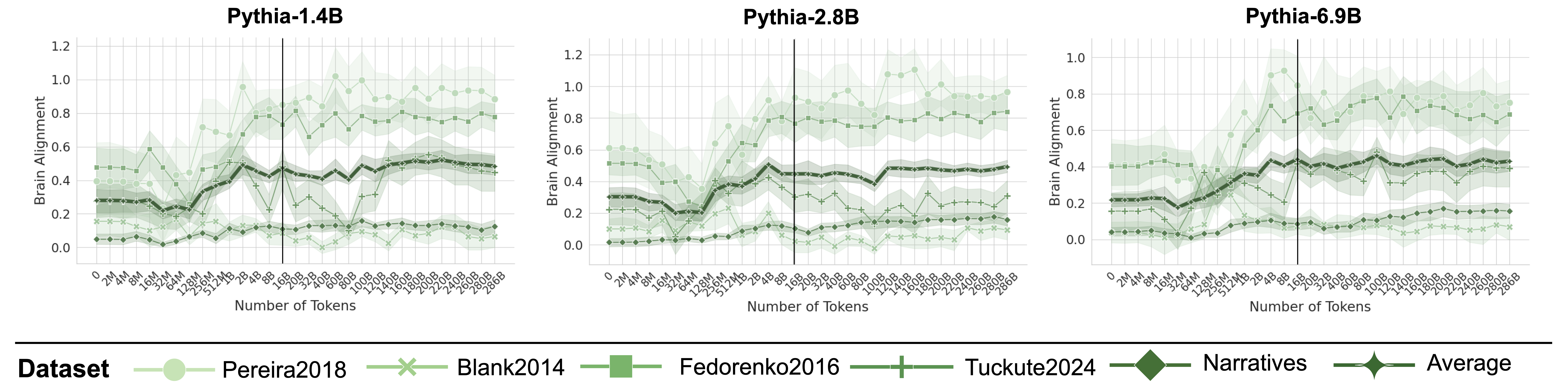
Figure 3: Brain Alignment Saturates Early on in Training. Plots indicate the brain alignment scores of three models from the Pythia model suite with varying sizes (log x-axis up to 16B tokens, uneven spacing after black line). Scores are normalized by their cross-subject consistency scores. Alignment quickly peaks around 2–8B tokens before saturating or declining, regardless of model size (see Appendix D and F for more models).
## 5 Results
The following sections progressively unpack the emergence and limits of brain alignment with the human language network in LLMs. Section 5.1 establishes the foundation by showing that untrained models already exhibit modest brain alignment, pointing to the role of architectural priors. Building on this, Section 5.2 tracks how alignment evolves with training and reveals that it strongly correlates with the early acquisition of formal linguistic competence, but less so with functional abilities. Section 5.3 then shows that as models exceed human-level performance in next-word prediction, their brain and behavioral alignment begins to diverge, suggesting that at this point, LLMs outgrow their initial alignment with human language processing.
### 5.1 Brain Alignment of Untrained Models
In Figure 6 we show that untrained models, despite achieving lower alignment scores than their pretrained counterparts ( $∼ 50\$ ), still achieve relatively decent alignment and surpass that of the models evaluated with a random sequence of tokens. Therefore, we here ask, what are the main drivers for this surprising alignment.
#### Inductive Biases of Untrained Models
We evaluate the brain alignment of various LLMs with untrained parameters to determine which architecture exhibits the strongest inductive bias toward the human language network. Figure 2 (a) presents the average alignment across five different random initializations for six different untrained models. Each model consists of a stack of two building blocks from its respective architecture, with a hidden state of $1024$ . To ensure a fair comparison, we apply the localizer to the output representations of the last token in the sequence from these two blocks, extracting 128 units to predict brain activity. Our findings reveal two key insights. First, sequence-based models—such as GRU, LSTM, Transformers, and even a simple mean operation over token representations—exhibit higher brain alignment than models that rely solely on the last token’s representation, such as Linear or MLP. In other words, context or temporal integration is a crucial factor in achieving high alignment. Second, we observe a notable difference between Transformer-v1 and Transformer-v2. While Transformer-v2 applies static positional embeddings by directly adding them to token embeddings, Transformer-v1 uses rotary position encoding. Our results suggest that static positional encoding enables models to capture intrinsic temporal dynamics in sentences—possibly tracking evolving word positions—providing further evidence that temporal integration is critical for brain-like language representations.
<details>
<summary>figures/brain-score-llms-lineplot-correlations.drawio.png Details</summary>
### Visual Description
## [Multi-Panel Scatter Plot]: Scaling Trends of Pythia Models
### Overview
The image displays a 2x4 grid of eight scatter plots, analyzing the relationship between training data size ("Number of Tokens") and three key metrics for different sizes of the Pythia language model family. The top row compares "Brain Alignment" with "Formal Competence," while the bottom row compares "Brain Alignment" with "Functional Competence." Each column represents a different model or model group: (a) Pythia (5 Models), (b) Pythia-1B, (c) Pythia-2.8B, and (d) Pythia-6.9B.
### Components/Axes
* **Common X-Axis (All Plots):** "Number of Tokens" on a logarithmic scale. Major tick marks are at 0.01B, 0.1B, 1B, 10B, and 100B (where B = Billion).
* **Common Left Y-Axis (All Plots):** "Brain Alignment," with a scale ranging from approximately 0.2 to 0.6 or 0.7, depending on the plot.
* **Right Y-Axis (Top Row):** "Formal Competence," with a scale from 0.1 to 0.7.
* **Right Y-Axis (Bottom Row):** "Functional Competence," with a scale from 0.00 to 0.30.
* **Legend (Bottom of Image):**
* **Green line with circle markers:** "Brain Alignment"
* **Light blue line with circle markers:** "Formal Competence"
* **Dark blue line with circle markers:** "Functional Competence"
* **Plot Titles:**
* (a) Pythia (5 Models)
* (b) Pythia-1B
* (c) Pythia-2.8B
* (d) Pythia-6.9B
* **Statistical Annotation (Top-left of each plot):** An R² value indicating the goodness of fit for the relationship between the two plotted metrics.
### Detailed Analysis
**Row 1: Brain Alignment vs. Formal Competence**
* **(a) Pythia (5 Models):**
* **R² = 0.65**
* **Brain Alignment (Green):** Shows a general upward trend from ~0.3 at 0.01B tokens to ~0.55 at 100B tokens. The trend is noisy, with a notable dip around 0.1B tokens. A shaded green area indicates variance or confidence interval.
* **Formal Competence (Light Blue):** Shows a strong, smooth upward trend from ~0.15 at 0.01B tokens to ~0.7 at 100B tokens.
* **(b) Pythia-1B:**
* **R² = 0.82** (Highest in the top row)
* **Brain Alignment (Green):** Increases steadily from ~0.25 at 0.01B tokens to a peak of ~0.6 at 100B tokens.
* **Formal Competence (Light Blue):** Follows a very similar, smooth upward trajectory to Brain Alignment, rising from ~0.15 to ~0.7.
* **(c) Pythia-2.8B:**
* **R² = 0.51**
* **Brain Alignment (Green):** Exhibits high volatility. Starts at ~0.35, dips to ~0.2 at 0.1B tokens, spikes to a peak of ~0.65 at ~5B tokens, then fluctuates between 0.5 and 0.6 at higher token counts.
* **Formal Competence (Light Blue):** Shows a consistent, smooth increase from ~0.15 to ~0.7.
* **(d) Pythia-6.9B:**
* **R² = 0.67**
* **Brain Alignment (Green):** Trends upward from ~0.25 to ~0.5, with a significant dip around 0.1B tokens.
* **Formal Competence (Light Blue):** Smooth upward trend from ~0.2 to ~0.7.
**Row 2: Brain Alignment vs. Functional Competence**
* **(a) Pythia (5 Models):**
* **R² = 0.36** (Lowest in the entire figure)
* **Brain Alignment (Green):** Same noisy upward trend as in the plot above.
* **Functional Competence (Dark Blue):** Shows a very gradual, shallow increase from ~0.00 at 0.01B tokens to only ~0.25 at 100B tokens. The relationship with Brain Alignment is weak.
* **(b) Pythia-1B:**
* **R² = 0.80**
* **Brain Alignment (Green):** Steady increase as seen above.
* **Functional Competence (Dark Blue):** Shows a strong, smooth upward trend from ~0.00 to ~0.20, closely tracking Brain Alignment.
* **(c) Pythia-2.8B:**
* **R² = 0.40**
* **Brain Alignment (Green):** Same volatile pattern as above.
* **Functional Competence (Dark Blue):** Increases smoothly from ~0.00 to ~0.25, but does not follow the sharp peaks and dips of Brain Alignment.
* **(d) Pythia-6.9B:**
* **R² = 0.51**
* **Brain Alignment (Green):** Upward trend with a dip.
* **Functional Competence (Dark Blue):** Smooth increase from ~0.00 to ~0.30.
### Key Observations
1. **Consistent Growth of Competence Metrics:** Both Formal Competence (light blue) and Functional Competence (dark blue) show smooth, monotonic increases with more training tokens across all model sizes.
2. **Volatility of Brain Alignment:** Brain Alignment (green) is far noisier and less predictable than the competence metrics. It often shows dips (e.g., around 0.1B tokens in several plots) and spikes that are not reflected in the competence curves.
3. **Model-Specific Correlation:** The correlation (R²) between Brain Alignment and the competence metrics varies significantly by model. Pythia-1B shows the strongest correlation (R² ~0.8), while the aggregated "5 Models" plot and Pythia-2.8B show much weaker correlations, especially for Functional Competence.
4. **Scale of Metrics:** Formal Competence reaches much higher absolute values (~0.7) compared to Functional Competence (~0.2-0.3), suggesting they measure different aspects of model capability.
### Interpretation
This data suggests a complex relationship between how a language model's internal representations align with human brain activity ("Brain Alignment") and its measurable capabilities ("Competence").
* **Competence is a Reliable Function of Scale:** The smooth, predictable growth of Formal and Functional Competence confirms a core tenet of scaling laws: more training data reliably improves benchmark performance.
* **Brain Alignment is Not a Simple Proxy for Competence:** The high volatility and weaker correlation of Brain Alignment indicate it is not merely a reflection of general capability. The dips (e.g., at 0.1B tokens) may represent phases in training where the model's internal organization is undergoing restructuring, temporarily diverging from brain-like patterns even as competence slowly grows.
* **Model Size Matters:** The differing R² values across model sizes (1B, 2.8B, 6.9B) imply that the relationship between brain-like processing and functional skills is not uniform. Smaller models (1B) may develop these traits in a more coupled manner, while larger models might decouple them, potentially developing competence through different internal pathways.
* **Two Types of Competence:** The stark difference in scale and trend smoothness between Formal and Functional Competence suggests they capture distinct dimensions of model ability. Formal Competence may relate to structured, rule-based tasks, while Functional Competence could measure more pragmatic or applied skills.
In summary, the figure argues that while training scale reliably drives up model competence, the emergence of brain-like representational alignment is a more erratic and model-size-dependent phenomenon that does not simply track capability gains.
</details>
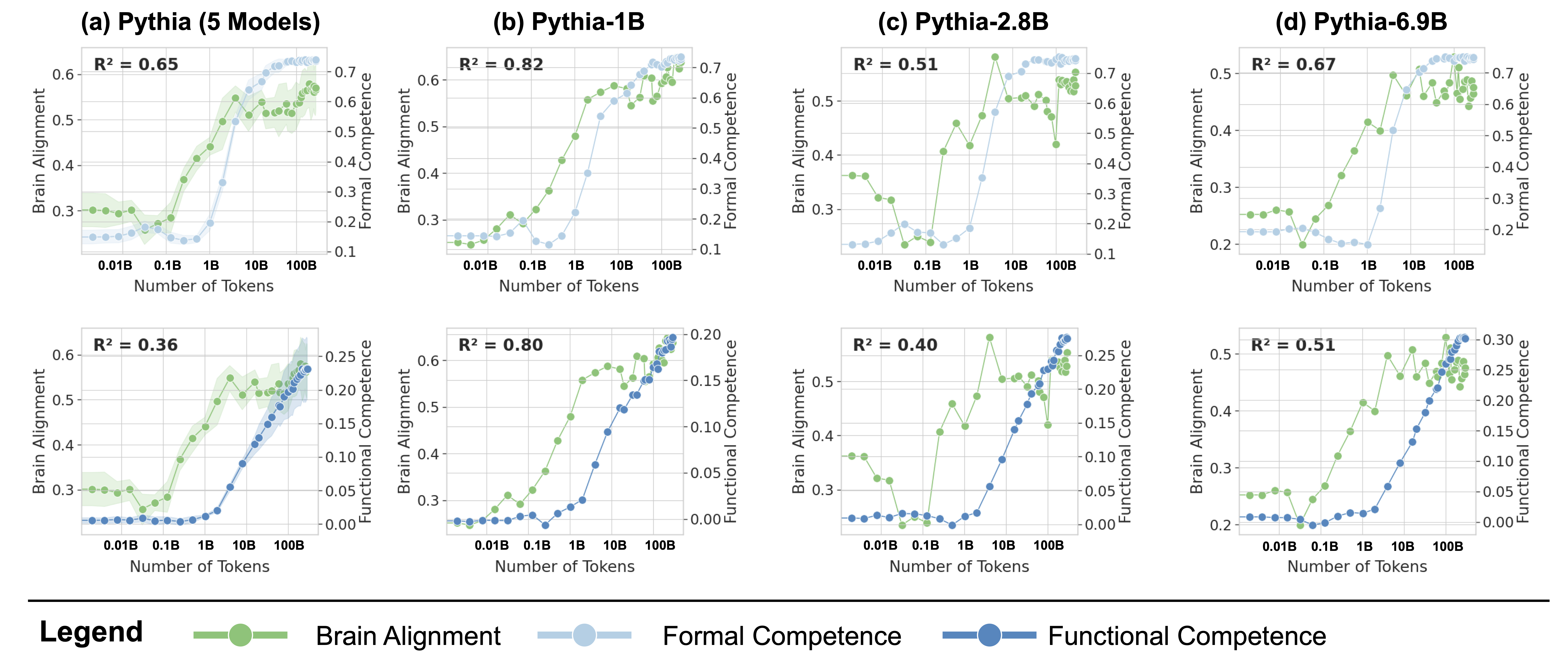
Figure 4: Formal Competence Tracks Brain Alignment More Closely Than Functional Competence. Each column compares how the evolution of formal competence (top) and functional competence (bottom) tracks the evolution of brain alignment during training. The $R^2$ values quantify the strength of this relationship, with higher values in formal competence suggesting it as the key driver of the observed brain alignment. (a): The data averaged across models of five different sizes. (b-d): the same comparison as in (a), but with comparisons were made for models from the Pythia suite with three different sizes.
#### Key Components of Transformers
To further isolate the key elements responsible for brain alignment in untrained parameter models, we perform an ablation study on the architectural components of Transformer-v2 using a single block (Figure 2 (c)). By focusing on the untrained model, we isolate the effect of architecture alone, without confounding influences from training. The architectural components analyzed are labeled on the left of each bar in Figure 2 (b). Ay Attn refers to all components inside the lower box in Figure 2 (c), including the first layer norm, multi-head attention, and the residual connection that follows. Ay MLP corresponds to the components in the upper box, comprising the post-attention layer norm, MLP, and the subsequent residual layer. Ay Pos represents the addition of positional embeddings to token embeddings. Ay Tokens means the model directly returns the raw token embeddings without further processing. This systematic ablation helps pinpoint the components that contribute most to brain alignment. Once again, we observe that integration across tokens, via attention mechanisms and positional encoding, yields the highest brain alignment. Further, we found that untrained parameter models perform better than chance-level performance on formal competence benchmarks, mirroring their non-zero brain alignment. In contrast, functional competence benchmarks remain at chance level for untrained models. This further supports the finding that brain alignment is primarily driven by formal, rather than functional, linguistic competence. (see Figure 2 (d)).
<details>
<summary>figures/brain-score-llms-correlation-ppl-behavior.drawio.png Details</summary>
### Visual Description
\n
## Scatter Plot Matrix: Brain Alignment vs. NWP Perplexity and Behavioral Alignment Across Pythia Model Sizes
### Overview
The image displays an 8-panel scatter plot matrix arranged in a 2x4 grid. The top row analyzes the relationship between "Brain Alignment" and "Log(NWP Perplexity)". The bottom row analyzes the relationship between "Brain Alignment" and "Behavioral Alignment". Each column corresponds to a different model or set of models from the Pythia family: (a) Pythia-70M, (b) Pythia-160M, (c) Pythia-2.8B, and (d) an aggregate of 8 Pythia models. Data points are categorized by "Training Stage": "Early" (circles) and "Late" (squares). Each panel includes a regression line with a shaded confidence interval and a reported Pearson correlation coefficient (r) with significance levels.
### Components/Axes
* **Overall Structure:** 2 rows x 4 columns grid of scatter plots.
* **Row Labels (Left Side):**
* Top Row: "NWP (Perplexity)"
* Bottom Row: "Behavior"
* **Column Titles (Top):**
* (a) Pythia-70M
* (b) Pythia-160M
* (c) Pythia-2.8B
* (d) Pythia (8 Models)
* **Y-Axis (All Panels):** "Brain Alignment". Scale varies slightly per panel but generally ranges from ~0.15 to 0.55.
* **X-Axis (Top Row Panels):** "Log(NWP Perplexity)". Scale is inverted, decreasing from left to right (e.g., 10 to 4).
* **X-Axis (Bottom Row Panels):** "Behavioral Alignment". Scale is linear and increases from left to right (e.g., 0.39 to 0.44 for panel a).
* **Legend (Present in all panels):** "Training Stage" with two categories:
* "Early": Represented by circle markers (●). Color varies by panel (shades of blue/purple).
* "Late": Represented by square markers (■). Color varies by panel (shades of orange/red/green).
* **Statistical Annotations:** Each panel contains one or two text boxes reporting the Pearson correlation coefficient (r) for the respective training stage data, along with significance asterisks (* p<0.05, ** p<0.01, *** p<0.001, **** p<0.0001) or "n.s." for not significant.
### Detailed Analysis
**Top Row: NWP (Perplexity) vs. Brain Alignment**
* **Trend Verification:** In all panels, the "Early" stage data (blue/purple circles) shows a clear positive trend: as Log(NWP Perplexity) decreases (moving right on the x-axis), Brain Alignment increases. The "Late" stage data (green/yellow squares) is clustered in the top-right corner (low perplexity, high alignment) and shows a weaker or non-significant trend.
* **Panel (a) Pythia-70M:**
* Early Stage: Strong positive correlation, r = 0.92****. Data points range from approx. (LogP=10.5, BA=0.22) to (LogP=5.5, BA=0.42).
* Late Stage: Moderate positive correlation, r = 0.60*. Data points cluster tightly around (LogP=4.5, BA=0.48-0.52).
* **Panel (b) Pythia-160M:**
* Early Stage: Strong positive correlation, r = 0.89****. Data points range from approx. (LogP=11, BA=0.20) to (LogP=5.5, BA=0.48).
* Late Stage: Correlation is not significant (r = n.s.). Data points cluster around (LogP=4.5, BA=0.45-0.50).
* **Panel (c) Pythia-2.8B:**
* Early Stage: Moderate positive correlation, r = 0.63*. Data points range from approx. (LogP=11, BA=0.20) to (LogP=5.5, BA=0.40).
* Late Stage: Correlation is not significant (r = n.s.). Data points cluster around (LogP=4.5, BA=0.38-0.45).
* **Panel (d) Pythia (8 Models):**
* Early Stage: Strong positive correlation, r = 0.81****. Data points show a clear upward trend from left to right.
* Late Stage: Weak positive correlation, r = 0.26**. Data points are densely clustered in the top-right.
**Bottom Row: Behavioral Alignment vs. Brain Alignment**
* **Trend Verification:** The "Early" stage data (purple circles) consistently shows a strong positive trend: as Behavioral Alignment increases, Brain Alignment increases. The "Late" stage data (orange/red squares) shows a flat or negative trend.
* **Panel (a) Pythia-70M:**
* Early Stage: Very strong positive correlation, r = 0.97****. Data points form a tight line from approx. (BA=0.39, BrainA=0.20) to (BA=0.44, BrainA=0.42).
* Late Stage: Correlation is not significant (r = n.s.). Data points form a horizontal cluster around BrainA=0.50.
* **Panel (b) Pythia-160M:**
* Early Stage: Strong positive correlation, r = 0.90****. Data points range from approx. (BA=0.38, BrainA=0.19) to (BA=0.44, BrainA=0.42).
* Late Stage: Correlation is not significant (r = n.s.). Data points cluster around BrainA=0.48.
* **Panel (c) Pythia-2.8B:**
* Early Stage: Strong positive correlation, r = 0.89****. Data points range from approx. (BA=0.36, BrainA=0.20) to (BA=0.44, BrainA=0.40).
* Late Stage: Moderate *negative* correlation, r = -0.54*. Data points show a slight downward trend.
* **Panel (d) Pythia (8 Models):**
* Early Stage: Strong positive correlation, r = 0.84****. Data points show a clear upward trend.
* Late Stage: Correlation is not significant (r = n.s.). Data points form a dense, horizontal cloud around BrainA=0.50.
### Key Observations
1. **Training Stage Dichotomy:** There is a stark contrast between "Early" and "Late" training stages across all models and metrics. Early stages show strong, significant correlations, while late stages often show non-significant or weak correlations.
2. **Metric Relationship:** For early training, both NWP Perplexity (lower is better) and Behavioral Alignment (higher is better) are strongly positively correlated with Brain Alignment.
3. **Model Size Effect:** The strength of the correlation for the Early stage in the NWP row appears to decrease with model size (r=0.92 for 70M, r=0.89 for 160M, r=0.63 for 2.8B). This pattern is less clear in the Behavior row.
4. **Late-Stage Clustering:** Late-stage data points consistently cluster in regions of high Brain Alignment (>0.4) and high Behavioral Alignment/Low NWP Perplexity, but show little variance, leading to weak correlations.
5. **Negative Correlation Anomaly:** Panel (c) bottom row is the only instance showing a significant negative correlation (r = -0.54*) for the Late stage, suggesting that for the 2.8B model, later training might decouple or inversely relate behavioral and brain alignment.
### Interpretation
This data suggests a fundamental shift in the relationship between a language model's internal representations (proxied by "Brain Alignment") and its performance metrics (NWP Perplexity, Behavioral Alignment) over the course of training.
* **Early Training Phase:** The model is in a rapid learning phase where improvements in language modeling (lower perplexity) and behavioral mimicry are tightly coupled with the development of brain-like representations. All metrics improve in lockstep.
* **Late Training Phase:** The model enters a refinement or specialization phase. Brain Alignment plateaus at a high level, and further improvements in perplexity or behavioral alignment become marginal and decoupled from changes in brain alignment. The model's internal representations stabilize, even as surface-level performance metrics might still see small gains.
* **Implication for Alignment:** The strong early correlation suggests that training objectives which improve brain alignment might also naturally lead to better behavioral alignment and language modeling performance, particularly in early stages. However, the decoupling in late stages indicates that achieving the final few percentage points of behavioral alignment may require different techniques, as they are no longer strongly linked to the brain-alignment of the model's representations. The negative correlation in the largest model (2.8B) is a notable outlier that warrants further investigation into the dynamics of very large model training.
</details>
Figure 5: NWP and Behavioral Alignment Correlate with Brain Alignment Only in Early Training. (Top Row): Correlation between brain alignment and language modeling loss shows a strong, significant relationship during early training (up to 2B tokens). While this correlation weakens in later stages (up to ~300B tokens). Results are shown for three models and the average of all 8 models (last column). (Bottom Row): The same analysis, but for the correlation between brain alignment and behavioral alignment, revealing a similar trend—strong correlation early in training, but no significant relationship as models surpass human proficiency.
### 5.2 Brain Alignment Over Training
Having established the architectural components that make an untrained model brain-aligned in the previous section, we now investigate how brain alignment evolves during training. To do so, we use the Pythia model suite Biderman et al. (2023), which consists of models of various sizes, all trained on the same $∼$ 300B tokens, with publicly available intermediate checkpoints. We report results for a model from a different family, SmolLM2-360M (Allal et al., 2025), which provides checkpoints at 250B-token intervals, in Appendix F.
Figure 3 illustrates the brain alignment of six Pythia models across five brain recording datasets at 34 training checkpoints, spanning approximately 300B tokens. Each panel presents checkpoints that are logarithmically spaced up to the vertical line, emphasizing the early-stage increase in brain alignment, which occurs within the first 5.6% of training time. Beyond this point, the panels display the remaining training period, where brain alignment stabilizes. More specifically, we observe the following trend: (1) Brain alignment is similar to the untrained model until approximately 128M tokens. (2) A sharp increase follows, peaking around 8B tokens. (3) Brain alignment then saturates for the remainder of training. Despite the vast difference in model sizes shown in Figure 3, the trajectory of brain alignment is remarkably similar.
#### Alignment Tracks Formal Competence
Following the observation that brain alignment plateaus early in training, we next investigate how this relates to the emergence of formal and functional linguistic competence in LLMs. Figure 4 displays the average brain alignment alongside the average performance on formal competence benchmarks (top row) and functional competence benchmarks (bottom row). This is shown for three Pythia models (1B, 2.8B, and 6.9B parameters) and the average of five Pythia models (first column) across the training process. To quantify this relationship, we train a ridge regression model (with a single scalar weight) to predict brain alignment scores from benchmark scores using 10-fold cross-validation. The average R-squared value across these folds serves as our metric for comparing the relationship between formal/functional linguistic competence and brain alignment. These R-squared values are shown in each panel of Figure 4. Finally, we perform a Wilcoxon signed-rank test on the distributions of R-squared values. This test reveals that formal linguistic competence is significantly more strongly correlated with brain alignment than functional competence (W = 0.0, p $<$ 0.002). One possible explanation for why brain alignment emerges before formal linguistic competence is that existing LLM benchmarks assess performance using discrete accuracy thresholds (hard metrics), rather than capturing the gradual progression of competence through more nuanced, continuous measures (soft metrics) (Schaeffer et al., 2023). We show the individual benchmark scores across all checkpoints in Figure 8 in Appendix E.
### 5.3 LLMs Lose Behavioral Alignment
Do language models that improve in next-word prediction remain aligned with human behavioral and neural responses, or do they diverge as they surpass human proficiency? To answer this question we use the Futrell2018 benchmark, which has been widely used in previous research to measure linguistic behavior (Futrell et al., 2018; Schrimpf et al., 2021; Aw et al., 2023). This dataset consists of self-paced reading times for naturalistic story materials from 180 participants. Per-word reading times provide a measure of incremental comprehension difficulty, a cornerstone of psycholinguistic research for testing theories of sentence comprehension (Gibson, 1998; Smith and Levy, 2013; Brothers and Kuperberg, 2021; Shain et al., 2024). We measure alignment by calculating the Pearson correlation between a model’s cross-entropy loss for a specific token in the sequence and the average human per-word reading time. The loss for words that comprise multiple tokens is added together before computing the correlation.
Early in training, LLMs align with this pattern, but as they surpass human proficiency (Shlegeris et al., 2022), their perplexity drops and they begin encoding statistical regularities that diverge from human intuition (Oh and Schuler, 2023; Steuer et al., 2023). This shift correlates with a decline in behavioral alignment, suggesting that superhuman models rely on different mechanisms than those underlying human language comprehension. Figure 5 shows that brain alignment initially correlates with perplexity and behavioral alignment, but only during the early stages of training (up to ~2B tokens). Beyond this point, these correlations diminish. In larger models, we observe a negative correlation between brain alignment and behavioral alignment in the later stages of training. This trend reinforces that early training aligns LLMs with human-like processing as also observed in earlier stages, while in later stages their language mechanisms diverge from humans.
## 6 Conclusion
In this work, we investigate how brain alignment in LLMs evolves throughout training, revealing different learning processes at play. We demonstrate that alignment with the human language network (LN) primarily correlates with formal linguistic competence Mahowald et al. (2024), peaking and saturating early in training. In contrast, functional linguistic competence, which involves world knowledge and reasoning, continues to grow beyond this stage. These findings suggest that the LN primarily encodes syntactic and compositional structure, in line with the literature of language neuroscience Fedorenko et al. (2024a), while broader linguistic functions may rely on other cognitive systems beyond the LN. This developmental approach reveals when brain-like representations emerge, offering a dynamic perspective compared to prior work focused on fully trained models. For example, Oota et al. (2023) demonstrated that syntactic structure contributes to alignment by selectively removing specific properties from already trained models. In contrast, we show that formal linguistic competence actively drives brain alignment during the early phases of training. Similarly, Hosseini et al. (2024) reported that models achieve strong alignment with limited data; we identify why: the brain-like representations emerge as soon as core formal linguistic knowledge is acquired. Further, their study evaluated only four training checkpoints and 2 models on a single dataset (Pereira2018). Our study evaluated eight models (14M–6.7B parameters) across 34 checkpoints spanning 300B tokens, and used five neural benchmarks within a rigorous brain‑scoring framework. This extensive design enabled fine‑grained correlations with both formal and functional linguistic benchmarks and ensured our results are robust and generalizable.
We also show that model size is not a reliable predictor of brain alignment when controlling for the number of features (see Appendix I). Instead, alignment is shaped by architectural inductive biases, token integration mechanisms, and training dynamics. Our standardized brain-scoring framework eliminates contextualization biases from previous work, ensuring more rigorous evaluations. Finally, we demonstrate that current brain alignment benchmarks are not saturated, indicating that LLMs can still be improved in modeling human language processing. Together, these findings challenge prior assumptions about how alignment emerges in LLMs and provide new insights into the relationship between artificial and biological language processing.
## Limitations
While this study offers a comprehensive analysis of brain alignment in LLMs, several open questions remain. If functional competence extends beyond the language network, future work should explore which additional brain regions LLMs align with as they develop reasoning and world knowledge, particularly in other cognitive networks like the multiple demand (Duncan and Owen, 2000) or theory of mind network (Saxe and Kanwisher, 2003; Saxe and Powell, 2006). Our findings suggest that LLM brain alignment studies should be broadened from the LN to downstream representations underlying other parts of cognition. This raises the question of whether specific transformer units specialize in formal vs. functional linguistic competence (AlKhamissi et al., 2025).
One other limitation of our study is that we rely exclusively on brain data collected from experiments conducted with English stimuli. As such, we do not explore whether our findings generalize across languages. This remains an open question and warrants further investigation. That said, evidence from cross-linguistic neuroscience research studying 45 languages from 12 language families (Malik-Moraleda et al., 2022) suggests the existence of a universal language network in the brain that is robust across languages and language families, both in topography and core functional properties.
Finally, a key question remains: Does LLM alignment evolution mirror human language acquisition? Comparing LLM representations to developmental data could reveal insights into learning trajectories and help differentiate formal from functional language learning. Expanding brain-scoring benchmarks and incorporating multimodal models will help address these questions, further bridging the gap between artificial and biological intelligence and deepening our understanding of how both systems process and represent language.
## Ethical Statement
This research relies on previously published neuroimaging (fMRI, ECoG) and behavioral datasets, collected by the original research groups under their institutional ethical guidelines with informed consent and IRB/ethics approval. Our work involved only secondary analysis of de-identified data, with no new data collection or direct participant interaction, and we remain committed to using such data responsibly and respectfully.
## Acknowledgments
We thank the members of the EPFL NeuroAI and NLP labs for their valuable feedback and insightful suggestions. We also gratefully acknowledge the support of the Swiss National Science Foundation (No. 215390), Innosuisse (PFFS-21-29), the EPFL Center for Imaging, Sony Group Corporation, and a Meta LLM Evaluation Research Grant.
## References
- AlKhamissi et al. (2022) Badr AlKhamissi, Millicent Li, Asli Celikyilmaz, Mona T. Diab, and Marjan Ghazvininejad. 2022. A review on language models as knowledge bases. ArXiv, abs/2204.06031.
- AlKhamissi et al. (2025) Badr AlKhamissi, Greta Tuckute, Antoine Bosselut, and Martin Schrimpf. 2025. The LLM language network: A neuroscientific approach for identifying causally task-relevant units. In Proceedings of the 2025 Conference of the Nations of the Americas Chapter of the Association for Computational Linguistics: Human Language Technologies (Volume 1: Long Papers), pages 10887–10911, Albuquerque, New Mexico. Association for Computational Linguistics.
- Allal et al. (2025) Loubna Ben Allal, Anton Lozhkov, Elie Bakouch, Gabriel Martín Blázquez, Guilherme Penedo, Lewis Tunstall, Andrés Marafioti, Hynek Kydlíček, Agustín Piqueres Lajarín, Vaibhav Srivastav, and 1 others. 2025. Smollm2: When smol goes big–data-centric training of a small language model. arXiv preprint arXiv:2502.02737.
- Aw et al. (2023) Khai Loong Aw, Syrielle Montariol, Badr AlKhamissi, Martin Schrimpf, and Antoine Bosselut. 2023. Instruction-tuning aligns llms to the human brain.
- Bates et al. (2003) Elizabeth Bates, Stephen M. Wilson, Ayse Pinar Saygin, Frederic Dick, Martin I. Sereno, Robert T. Knight, and Nina F. Dronkers. 2003. Voxel-based lesion–symptom mapping. Nature Neuroscience, 6(5):448–450.
- Benn et al. (2013) Yael Benn, Iain D. Wilkinson, Ying Zheng, Kathrin Cohen Kadosh, Charles A.J. Romanowski, Michael Siegal, and Rosemary Varley. 2013. Differentiating core and co-opted mechanisms in calculation: The neuroimaging of calculation in aphasia. Brain and Cognition, 82(3):254–264.
- Biderman et al. (2023) Stella Biderman, Hailey Schoelkopf, Quentin Anthony, Herbie Bradley, Kyle O’Brien, Eric Hallahan, Mohammad Aflah Khan, Shivanshu Purohit, USVSN Sai Prashanth, Edward Raff, Aviya Skowron, Lintang Sutawika, and Oskar Van Der Wal. 2023. Pythia: a suite for analyzing large language models across training and scaling. In Proceedings of the 40th International Conference on Machine Learning, ICML’23. JMLR.org.
- Binder et al. (1997) Jeffrey R. Binder, Julie A. Frost, Thomas A. Hammeke, Robert W. Cox, Stephen M. Rao, and Thomas Prieto. 1997. Human brain language areas identified by functional magnetic resonance imaging. The Journal of Neuroscience, 17(1):353–362.
- Bisk et al. (2019) Yonatan Bisk, Rowan Zellers, Ronan Le Bras, Jianfeng Gao, and Yejin Choi. 2019. Piqa: Reasoning about physical commonsense in natural language. In AAAI Conference on Artificial Intelligence.
- Blank et al. (2014) Idan Blank, Nancy Kanwisher, and Evelina Fedorenko. 2014. A functional dissociation between language and multiple-demand systems revealed in patterns of BOLD signal fluctuations. Journal of Neurophysiology, 112(5):1105–1118.
- Brothers and Kuperberg (2021) Trevor Brothers and Gina R Kuperberg. 2021. Word predictability effects are linear, not logarithmic: Implications for probabilistic models of sentence comprehension. Journal of Memory and Language, 116:104174.
- Cadena et al. (2019) Santiago A Cadena, George H Denfield, Edgar Y Walker, Leon A Gatys, Andreas S Tolias, Matthias Bethge, and Alexander S Ecker. 2019. Deep convolutional models improve predictions of macaque v1 responses to natural images. PLoS computational biology, 15(4):e1006897.
- Caucheteux and King (2022) Charlotte Caucheteux and Jean-Rémi King. 2022. Brains and algorithms partially converge in natural language processing. Communications biology, 5(1):134.
- Chen et al. (2023) Xuanyi Chen, Josef Affourtit, Rachel Ryskin, Tamar I Regev, Samuel Norman-Haignere, Olessia Jouravlev, Saima Malik-Moraleda, Hope Kean, Rosemary Varley, and Evelina Fedorenko. 2023. The human language system, including its inferior frontal component in “broca’s area,” does not support music perception. Cerebral Cortex, 33(12):7904–7929.
- Cichy et al. (2016) Radoslaw Martin Cichy, Aditya Khosla, Dimitrios Pantazis, Antonio Torralba, and Aude Oliva. 2016. Comparison of deep neural networks to spatio-temporal cortical dynamics of human visual object recognition reveals hierarchical correspondence. Scientific reports, 6(1):27755.
- Clark et al. (2018) Peter Clark, Isaac Cowhey, Oren Etzioni, Tushar Khot, Ashish Sabharwal, Carissa Schoenick, and Oyvind Tafjord. 2018. Think you have solved question answering? try arc, the ai2 reasoning challenge. ArXiv, abs/1803.05457.
- Duncan and Owen (2000) John Duncan and Adrian M Owen. 2000. Common regions of the human frontal lobe recruited by diverse cognitive demands. Trends in Neurosciences, 23(10):475–483.
- Feather et al. (2025) Jenelle Feather, Meenakshi Khosla, N. Apurva, Ratan Murty, and Aran Nayebi. 2025. Brain-model evaluations need the neuroai turing test.
- Fedorenko (2014) Evelina Fedorenko. 2014. The role of domain-general cognitive control in language comprehension. Frontiers in Psychology, 5.
- Fedorenko et al. (2011) Evelina Fedorenko, Michael K Behr, and Nancy Kanwisher. 2011. Functional specificity for high-level linguistic processing in the human brain. Proceedings of the National Academy of Sciences, 108(39):16428–16433.
- Fedorenko et al. (2010) Evelina Fedorenko, Po-Jang Hsieh, Alfonso Nieto-Castanon, Susan L. Whitfield-Gabrieli, and Nancy G. Kanwisher. 2010. New method for fmri investigations of language: defining rois functionally in individual subjects. Journal of neurophysiology, 104 2:1177–94.
- Fedorenko et al. (2024a) Evelina Fedorenko, Anna A. Ivanova, and Tamar I. Regev. 2024a. The language network as a natural kind within the broader landscape of the human brain. Nature Reviews Neuroscience, 25(5):289–312.
- Fedorenko et al. (2012) Evelina Fedorenko, Josh H. McDermott, Sam Norman-Haignere, and Nancy Kanwisher. 2012. Sensitivity to musical structure in the human brain. Journal of Neurophysiology, 108(12):3289–3300.
- Fedorenko et al. (2024b) Evelina Fedorenko, Steven T. Piantadosi, and Edward A. F. Gibson. 2024b. Language is primarily a tool for communication rather than thought. Nature, 630(8017):575–586.
- Fedorenko et al. (2016) Evelina Fedorenko, Terri L. Scott, Peter Brunner, William G. Coon, Brianna Pritchett, Gerwin Schalk, and Nancy Kanwisher. 2016. Neural correlate of the construction of sentence meaning. Proceedings of the National Academy of Sciences, 113(41):E6256–E6262.
- Feghhi et al. (2024) Ebrahim Feghhi, Nima Hadidi, Bryan Song, Idan A. Blank, and Jonathan C. Kao. 2024. What are large language models mapping to in the brain? a case against over-reliance on brain scores.
- Futrell et al. (2018) Richard Futrell, Edward Gibson, Harry J. Tily, Idan Blank, Anastasia Vishnevetsky, Steven Piantadosi, and Evelina Fedorenko. 2018. The natural stories corpus. In Proceedings of the Eleventh International Conference on Language Resources and Evaluation (LREC 2018), Miyazaki, Japan. European Language Resources Association (ELRA).
- Gao et al. (2024) Leo Gao, Jonathan Tow, Baber Abbasi, Stella Biderman, Sid Black, Anthony DiPofi, Charles Foster, Laurence Golding, Jeffrey Hsu, Alain Le Noac’h, Haonan Li, Kyle McDonell, Niklas Muennighoff, Chris Ociepa, Jason Phang, Laria Reynolds, Hailey Schoelkopf, Aviya Skowron, Lintang Sutawika, and 5 others. 2024. A framework for few-shot language model evaluation.
- Gauthier et al. (2020) Jon Gauthier, Jennifer Hu, Ethan Wilcox, Peng Qian, and Roger Levy. 2020. SyntaxGym: An online platform for targeted evaluation of language models. In Proceedings of the 58th Annual Meeting of the Association for Computational Linguistics: System Demonstrations, pages 70–76, Online. Association for Computational Linguistics.
- Geiger et al. (2022) Franziska Geiger, Martin Schrimpf, Tiago Marques, and James J DiCarlo. 2022. Wiring up vision: Minimizing supervised synaptic updates needed to produce a primate ventral stream. In International Conference on Learning Representations 2022 Spotlight.
- Gibson (1998) Edward Gibson. 1998. Linguistic complexity: locality of syntactic dependencies. Cognition, 68(1):1–76.
- Goldstein et al. (2022) Ariel Goldstein, Zaid Zada, Eliav Buchnik, Mariano Schain, Amy Price, Bobbi Aubrey, Samuel A. Nastase, Amir Feder, Dotan Emanuel, Alon Cohen, Aren Jansen, Harshvardhan Gazula, Gina Choe, Aditi Rao, Catherine Kim, Colton Casto, Lora Fanda, Werner Doyle, Daniel Friedman, and 13 others. 2022. Shared computational principles for language processing in humans and deep language models. Nature Neuroscience, 25(3):369–380.
- Gorno‐Tempini et al. (2004) Maria Luisa Gorno‐Tempini, Nina F. Dronkers, Katherine P. Rankin, Jennifer M. Ogar, La Phengrasamy, Howard J. Rosen, Julene K. Johnson, Michael W. Weiner, and Bruce L. Miller. 2004. Cognition and anatomy in three variants of primary progressive aphasia. Annals of Neurology, 55(3):335–346.
- Hagoort (2019) Peter Hagoort. 2019. The neurobiology of language beyond single-word processing. Science, 366(6461):55–58.
- Harvey et al. (2023) Sarah E Harvey, Brett W. Larsen, and Alex H Williams. 2023. Duality of bures and shape distances with implications for comparing neural representations. In UniReps: the First Workshop on Unifying Representations in Neural Models.
- Hosseini et al. (2024) Eghbal A Hosseini, Martin Schrimpf, Yian Zhang, Samuel Bowman, Noga Zaslavsky, and Evelina Fedorenko. 2024. Artificial neural network language models predict human brain responses to language even after a developmentally realistic amount of training. Neurobiology of Language, pages 1–21.
- Hu et al. (2023) Jennifer Hu, Hannah Small, Hope Kean, Atsushi Takahashi, Leo Zekelman, Daniel Kleinman, Elizabeth Ryan, Alfonso Nieto-Castañón, Victor Ferreira, and Evelina Fedorenko. 2023. Precision fmri reveals that the language-selective network supports both phrase-structure building and lexical access during language production. Cerebral Cortex, 33(8):4384–4404.
- Huang and Chang (2023) Jie Huang and Kevin Chen-Chuan Chang. 2023. Towards reasoning in large language models: A survey. In Findings of the Association for Computational Linguistics: ACL 2023, pages 1049–1065, Toronto, Canada. Association for Computational Linguistics.
- Kauf et al. (2023) Carina Kauf, Greta Tuckute, Roger Levy, Jacob Andreas, and Evelina Fedorenko. 2023. Lexical-Semantic Content, Not Syntactic Structure, Is the Main Contributor to ANN-Brain Similarity of fMRI Responses in the Language Network. Neurobiology of Language, pages 1–36.
- Kazemian et al. (2024) Atlas Kazemian, Eric Elmoznino, and Michael F. Bonner. 2024. Convolutional architectures are cortex-aligned de novo. bioRxiv.
- Kell et al. (2018) Alexander JE Kell, Daniel LK Yamins, Erica N Shook, Sam V Norman-Haignere, and Josh H McDermott. 2018. A task-optimized neural network replicates human auditory behavior, predicts brain responses, and reveals a cortical processing hierarchy. Neuron, 98(3):630–644.
- Khaligh-Razavi and Kriegeskorte (2014) Seyed Mahdi Khaligh-Razavi and Nikolaus Kriegeskorte. 2014. Deep Supervised, but Not Unsupervised, Models May Explain IT Cortical Representation. PLoS Computational Biology, 10(11). Publisher: Public Library of Science ISBN: 1553-7358 (Electronic)\r1553-734X (Linking).
- Kornblith et al. (2019) Simon Kornblith, Mohammad Norouzi, Honglak Lee, and Geoffrey Hinton. 2019. Similarity of neural network representations revisited. In International conference on machine learning, pages 3519–3529. PMLR.
- Koumura et al. (2023) Takuya Koumura, Hiroki Terashima, and Shigeto Furukawa. 2023. Human-like modulation sensitivity emerging through optimization to natural sound recognition. Journal of Neuroscience, 43(21):3876–3894.
- Kriegeskorte et al. (2008) Nikolaus Kriegeskorte, Marieke Mur, and Peter Bandettini. 2008. Representational similarity analysis - connecting the branches of systems neuroscience. Frontiers in Systems Neuroscience, 2.
- Kubilius et al. (2019) Jonas Kubilius, Martin Schrimpf, Kohitij Kar, Rishi Rajalingham, Ha Hong, Najib Majaj, Elias Issa, Pouya Bashivan, Jonathan Prescott-Roy, Kailyn Schmidt, Aran Nayebi, Daniel Bear, Daniel L Yamins, and James J DiCarlo. 2019. Brain-like object recognition with high-performing shallow recurrent anns. In Advances in Neural Information Processing Systems, volume 32. Curran Associates, Inc.
- Lipkin et al. (2022) Benjamin Lipkin, Greta Tuckute, Josef Affourtit, Hannah Small, Zachary Mineroff, Hope Kean, Olessia Jouravlev, Lara Rakocevic, Brianna Pritchett, Matthew Siegelman, Caitlyn Hoeflin, Alvincé Pongos, Idan A. Blank, Melissa Kline Struhl, Anna Ivanova, Steven Shannon, Aalok Sathe, Malte Hoffmann, Alfonso Nieto-Castañón, and Evelina Fedorenko. 2022. Probabilistic atlas for the language network based on precision fmri data from>800 individuals. Scientific Data, 9(1).
- Mahowald et al. (2024) Kyle Mahowald, Anna A Ivanova, Idan A Blank, Nancy Kanwisher, Joshua B Tenenbaum, and Evelina Fedorenko. 2024. Dissociating language and thought in large language models. Trends in Cognitive Sciences.
- Malik-Moraleda et al. (2022) Saima Malik-Moraleda, Dima Ayyash, Jeanne Gallée, Josef Affourtit, Malte Hoffmann, Zachary Mineroff, Olessia Jouravlev, and Evelina Fedorenko. 2022. An investigation across 45 languages and 12 language families reveals a universal language network. Nature Neuroscience, 25(8):1014–1019.
- Millet and King (2021) Juliette Millet and Jean-Rémi King. 2021. Inductive biases, pretraining and fine-tuning jointly account for brain responses to speech. ArXiv, abs/2103.01032.
- Monti et al. (2012) Martin M Monti, Lawrence M Parsons, and Daniel N Osherson. 2012. Thought beyond language: neural dissociation of algebra and natural language. Psychological science, 23(8):914–922.
- Nastase et al. (2021) Samuel A. Nastase, Yun-Fei Liu, Hanna Hillman, Asieh Zadbood, Liat Hasenfratz, Neggin Keshavarzian, Janice Chen, Christopher J. Honey, Yaara Yeshurun, Mor Regev, and et al. 2021. The “narratives” fmri dataset for evaluating models of naturalistic language comprehension. Scientific Data, 8(1).
- Oh and Schuler (2023) Byung-Doh Oh and William Schuler. 2023. Why does surprisal from larger transformer-based language models provide a poorer fit to human reading times? Transactions of the Association for Computational Linguistics, 11:336–350.
- Oota et al. (2023) Subba Reddy Oota, Manish Gupta, and Mariya Toneva. 2023. Joint processing of linguistic properties in brains and language models. Preprint, arXiv:2212.08094.
- Pasquiou et al. (2022) Alexandre Pasquiou, Yair Lakretz, John Hale, Bertrand Thirion, and Christophe Pallier. 2022. Neural language models are not born equal to fit brain data, but training helps. Preprint, arXiv:2207.03380.
- Penedo et al. (2024) Guilherme Penedo, Hynek Kydlíček, Loubna Ben allal, Anton Lozhkov, Margaret Mitchell, Colin Raffel, Leandro Von Werra, and Thomas Wolf. 2024. The fineweb datasets: Decanting the web for the finest text data at scale. In The Thirty-eight Conference on Neural Information Processing Systems Datasets and Benchmarks Track.
- Pereira et al. (2018) Francisco Pereira, Bin Lou, Brianna Pritchett, Samuel Ritter, Samuel J. Gershman, Nancy Kanwisher, Matthew Botvinick, and Evelina Fedorenko. 2018. Toward a universal decoder of linguistic meaning from brain activation. Nature Communications, 9(1):963.
- Price (2010) Cathy J. Price. 2010. The anatomy of language: a review of 100 fmri studies published in 2009. Annals of the New York Academy of Sciences, 1191(1):62–88.
- Rathi et al. (2025) Neil Rathi, Johannes Mehrer, Badr AlKhamissi, Taha Binhuraib, Nicholas M. Blauch, and Martin Schrimpf. 2025. TopoLM: Brain-like spatio-functional organization in a topographic language model. In International Conference on Learning Representations (ICLR).
- Sakaguchi et al. (2019) Keisuke Sakaguchi, Ronan Le Bras, Chandra Bhagavatula, and Yejin Choi. 2019. Winogrande. Communications of the ACM, 64:99 – 106.
- Sap et al. (2019) Maarten Sap, Hannah Rashkin, Derek Chen, Ronan Le Bras, and Yejin Choi. 2019. Social IQa: Commonsense reasoning about social interactions. In Proceedings of the 2019 Conference on Empirical Methods in Natural Language Processing and the 9th International Joint Conference on Natural Language Processing (EMNLP-IJCNLP), pages 4463–4473, Hong Kong, China. Association for Computational Linguistics.
- Saxe and Kanwisher (2003) R Saxe and N Kanwisher. 2003. People thinking about thinking peoplethe role of the temporo-parietal junction in “theory of mind”. NeuroImage, 19(4):1835–1842.
- Saxe et al. (2006) Rebecca Saxe, Matthew Brett, and Nancy Kanwisher. 2006. Divide and conquer: a defense of functional localizers. Neuroimage, 30(4):1088–1096.
- Saxe and Powell (2006) Rebecca Saxe and Lindsey J. Powell. 2006. It’s the thought that counts: Specific brain regions for one component of theory of mind. Psychological Science, 17(8):692–699.
- Schaeffer et al. (2023) Rylan Schaeffer, Brando Miranda, and Oluwasanmi Koyejo. 2023. Are emergent abilities of large language models a mirage? ArXiv, abs/2304.15004.
- Schrimpf et al. (2021) Martin Schrimpf, Idan Asher Blank, Greta Tuckute, Carina Kauf, Eghbal A. Hosseini, Nancy Kanwisher, Joshua B. Tenenbaum, and Evelina Fedorenko. 2021. The neural architecture of language: Integrative modeling converges on predictive processing. Proceedings of the National Academy of Sciences, 118(45):e2105646118.
- Schrimpf et al. (2018) Martin Schrimpf, Jonas Kubilius, Ha Hong, Najib J. Majaj, Rishi Rajalingham, Elias B. Issa, Kohitij Kar, Pouya Bashivan, Jonathan Prescott-Roy, Franziska Geiger, Kailyn Schmidt, Daniel L. K. Yamins, and James J. DiCarlo. 2018. Brain-Score: Which Artificial Neural Network for Object Recognition is most Brain-Like? preprint, Neuroscience.
- Schrimpf et al. (2020) Martin Schrimpf, Jonas Kubilius, Michael J. Lee, N. Apurva Ratan Murty, Robert Ajemian, and James J. DiCarlo. 2020. Integrative benchmarking to advance neurally mechanistic models of human intelligence. Neuron, 108(3):413–423.
- Shain et al. (2024) Cory Shain, Clara Meister, Tiago Pimentel, Ryan Cotterell, and Roger Levy. 2024. Large-scale evidence for logarithmic effects of word predictability on reading time. Proceedings of the National Academy of Sciences, 121(10):e2307876121.
- Shlegeris et al. (2022) Buck Shlegeris, Fabien Roger, Lawrence Chan, and Euan McLean. 2022. Language models are better than humans at next-token prediction. ArXiv, abs/2212.11281.
- Siegal and Varley (2006) Michael Siegal and Rosemary Varley. 2006. Aphasia, language, and theory of mind. Social Neuroscience, 1(3–4):167–174.
- Smith and Levy (2013) Nathaniel J. Smith and Roger Levy. 2013. The effect of word predictability on reading time is logarithmic. Cognition, 128(3):302–319.
- Steuer et al. (2023) Julius Steuer, Marius Mosbach, and Dietrich Klakow. 2023. Large gpt-like models are bad babies: A closer look at the relationship between linguistic competence and psycholinguistic measures. arXiv preprint arXiv:2311.04547.
- Teney et al. (2024) Damien Teney, Armand Nicolicioiu, Valentin Hartmann, and Ehsan Abbasnejad. 2024. Neural redshift: Random networks are not random functions. Preprint, arXiv:2403.02241.
- Tuckute et al. (2023) Greta Tuckute, Jenelle Feather, Dana Boebinger, and Josh H. McDermott. 2023. Many but not all deep neural network audio models capture brain responses and exhibit correspondence between model stages and brain regions. PLOS Biology, 21(12):1–70.
- Tuckute et al. (2024a) Greta Tuckute, Nancy Kanwisher, and Evelina Fedorenko. 2024a. Language in brains, minds, and machines. Annual Review of Neuroscience, 47.
- Tuckute et al. (2024b) Greta Tuckute, Aalok Sathe, Shashank Srikant, Maya Taliaferro, Mingye Wang, Martin Schrimpf, Kendrick Kay, and Evelina Fedorenko. 2024b. Driving and suppressing the human language network using large language models. Nature Human Behaviour, pages 1–18.
- Varley and Siegal (2000) Rosemary Varley and Michael Siegal. 2000. Evidence for cognition without grammar from causal reasoning and ‘theory of mind’ in an agrammatic aphasic patient. Current Biology, 10(12):723–726.
- Varley et al. (2005) Rosemary A. Varley, Nicolai J. C. Klessinger, Charles A. J. Romanowski, and Michael Siegal. 2005. Agrammatic but numerate. Proceedings of the National Academy of Sciences, 102(9):3519–3524.
- Warstadt et al. (2019) Alex Warstadt, Alicia Parrish, Haokun Liu, Anhad Mohananey, Wei Peng, Sheng-Fu Wang, and Samuel R. Bowman. 2019. Blimp: The benchmark of linguistic minimal pairs for english. Transactions of the Association for Computational Linguistics, 8:377–392.
- Wolf et al. (2019) Thomas Wolf, Lysandre Debut, Victor Sanh, Julien Chaumond, Clement Delangue, Anthony Moi, Pierric Cistac, Tim Rault, Rémi Louf, Morgan Funtowicz, and Jamie Brew. 2019. Huggingface’s transformers: State-of-the-art natural language processing. ArXiv, abs/1910.03771.
- Yamins et al. (2014) Daniel LK Yamins, Ha Hong, Charles F Cadieu, Ethan A Solomon, Darren Seibert, and James J DiCarlo. 2014. Performance-optimized hierarchical models predict neural responses in higher visual cortex. Proceedings of the national academy of sciences, 111(23):8619–8624.
- Zellers et al. (2019) Rowan Zellers, Ari Holtzman, Yonatan Bisk, Ali Farhadi, and Yejin Choi. 2019. Hellaswag: Can a machine really finish your sentence? In Annual Meeting of the Association for Computational Linguistics.
- Zhuang et al. (2021) Chengxu Zhuang, Siming Yan, Aran Nayebi, Martin Schrimpf, Michael C. Frank, James J. DiCarlo, and Daniel L.K. Yamins. 2021. Unsupervised neural network models of the ventral visual stream. Proceedings of the National Academy of Sciences (PNAS), 118(3). Publisher: Cold Spring Harbor Laboratory.
| Pereira2018 | fMRI | Reading | Accordions produce sound with bellows … |
| --- | --- | --- | --- |
| Blank2014 | fMRI | Listening | A clear and joyous day it was and out on the wide … |
| Fedorenko2016 | ECoG | Reading | ‘ALEX’, ‘WAS’, ‘TIRED’, ‘SO’, ‘HE’, ‘TOOK’, … |
| Tuckute2024 | fMRI | Reading | The judge spoke, breaking the silence. |
| Narratives | fMRI | Listening | Okay so getting back to our story about uh Lucy … |
| Futrell2018 | Reading Times | Reading | A clear and joyous day it was and out on the wide … |
Table 1: Datasets Used for Evaluating Model Alignment. Neuroimaging datasets were collected via either functional magnetic resonance imaging (fMRI) or electrocorticography (ECoG). Stimuli range from short sentences (Fedorenko2016, Tuckute2024) to paragraphs (Pereira2018) and entire stories (Blank2014, Narratives, Futrell2018) and were presented either visually or auditorily. Futrell2018 is a behavioral dataset.
<details>
<summary>figures/brain-score-llms-metrics.drawio.png Details</summary>
### Visual Description
## Bar Charts: Brain Alignment Comparison Across Models and Conditions
### Overview
The image displays a composite figure containing five bar charts organized into two panels, labeled (a) and (b). The charts compare "Brain Alignment" (measured as Pearson's r) across three different experimental conditions for various model types or metrics. The overall purpose is to quantify and compare how well different computational models align with brain activity under different stimulus conditions.
### Components/Axes
* **Panel (a):** Contains three separate bar charts titled "Linear", "CKA", and "RSA".
* **Y-axis (for all three):** Labeled "Brain Alignment (Pearson's r)". The scale ranges from 0.00 to 0.14 for Linear and RSA, and from 0.00 to 0.30 for CKA.
* **X-axis:** Each chart has three bars corresponding to the conditions defined in the legend.
* **Panel (b):** Contains two separate bar charts titled "Contextualization" and "No Contextualization".
* **Y-axis (for both):** Labeled "Brain Alignment". The scale ranges from 0.0 to 0.7 for Contextualization and from 0.0 to 1.0 for No Contextualization.
* **X-axis:** Each chart has three bars corresponding to the conditions defined in the legend.
* **Legend:** Located at the bottom of the entire figure, spanning its width. It defines three color-coded conditions:
* **Light Green Bar:** "Pretrained | Original Stimuli"
* **Medium Green Bar:** "Pretrained | Random Stimuli (= Length)"
* **Dark Green Bar:** "Untrained | Original Stimuli"
* **Statistical Significance:** Horizontal brackets with four asterisks (****) are placed above pairs of bars in each chart, indicating a highly significant statistical difference between those conditions.
### Detailed Analysis
#### Panel (a) - Linear, CKA, RSA Metrics
**1. Linear Chart**
* **Trend:** The "Pretrained | Original Stimuli" condition shows the highest alignment, followed by "Untrained | Original Stimuli", with "Pretrained | Random Stimuli" showing very low alignment.
* **Approximate Values (Pearson's r):**
* Pretrained | Original Stimuli: ~0.133 (Error bar extends from ~0.12 to ~0.145)
* Pretrained | Random Stimuli: ~0.015 (Error bar extends from ~0.01 to ~0.02)
* Untrained | Original Stimuli: ~0.065 (Error bar extends from ~0.055 to ~0.075)
* **Significance:** The bracket with **** spans the "Pretrained | Original Stimuli" and "Pretrained | Random Stimuli" bars, indicating a significant difference.
**2. CKA Chart**
* **Trend:** The "Untrained | Original Stimuli" condition shows the highest alignment, followed by "Pretrained | Original Stimuli", with "Pretrained | Random Stimuli" slightly lower than the pretrained original.
* **Approximate Values (Pearson's r):**
* Pretrained | Original Stimuli: ~0.185 (Error bar extends from ~0.16 to ~0.21)
* Pretrained | Random Stimuli: ~0.16 (Error bar extends from ~0.15 to ~0.17)
* Untrained | Original Stimuli: ~0.28 (Error bar extends from ~0.26 to ~0.30)
* **Significance:** The bracket with **** spans the "Pretrained | Original Stimuli" and "Untrained | Original Stimuli" bars.
**3. RSA Chart**
* **Trend:** Similar to CKA, the "Untrained | Original Stimuli" condition shows the highest alignment, followed by "Pretrained | Original Stimuli", with "Pretrained | Random Stimuli" showing very low alignment.
* **Approximate Values (Pearson's r):**
* Pretrained | Original Stimuli: ~0.09 (Error bar extends from ~0.08 to ~0.105)
* Pretrained | Random Stimuli: ~0.02 (Error bar extends from ~0.015 to ~0.025)
* Untrained | Original Stimuli: ~0.138 (Error bar extends from ~0.125 to ~0.15)
* **Significance:** The bracket with **** spans the "Pretrained | Original Stimuli" and "Untrained | Original Stimuli" bars.
#### Panel (b) - Contextualization Conditions
**1. Contextualization Chart**
* **Trend:** The "Untrained | Original Stimuli" and "Pretrained | Original Stimuli" conditions show similarly high alignment, both far exceeding the "Pretrained | Random Stimuli" condition.
* **Approximate Values (Brain Alignment):**
* Pretrained | Original Stimuli: ~0.69 (Error bar extends from ~0.67 to ~0.71)
* Pretrained | Random Stimuli: ~0.16 (Error bar extends from ~0.15 to ~0.17)
* Untrained | Original Stimuli: ~0.71 (Error bar extends from ~0.69 to ~0.73)
* **Significance:** The bracket with **** spans the "Pretrained | Original Stimuli" and "Pretrained | Random Stimuli" bars.
**2. No Contextualization Chart**
* **Trend:** The "Pretrained | Original Stimuli" condition shows the highest alignment, followed by "Untrained | Original Stimuli", with "Pretrained | Random Stimuli" showing low alignment.
* **Approximate Values (Brain Alignment):**
* Pretrained | Original Stimuli: ~1.03 (Error bar extends from ~0.95 to ~1.1)
* Pretrained | Random Stimuli: ~0.17 (Error bar extends from ~0.15 to ~0.19)
* Untrained | Original Stimuli: ~0.48 (Error bar extends from ~0.42 to ~0.54)
* **Significance:** The bracket with **** spans the "Pretrained | Original Stimuli" and "Pretrained | Random Stimuli" bars.
### Key Observations
1. **Consistent Low Performance of Random Stimuli:** Across all five charts, the "Pretrained | Random Stimuli (= Length)" condition (medium green bar) consistently yields the lowest brain alignment scores. This serves as a critical control, showing that alignment is not driven by low-level stimulus properties like length.
2. **Divergent Effects of Training:** The effect of pretraining versus no training varies by metric and context.
* In **Linear** and **No Contextualization** settings, the *Pretrained* model with original stimuli outperforms the *Untrained* model.
* In **CKA** and **RSA** metrics, and in the **Contextualization** setting, the *Untrained* model with original stimuli shows equal or higher alignment than the *Pretrained* model.
3. **Impact of Contextualization:** Comparing the two charts in panel (b), the "Contextualization" condition appears to equalize the performance of pretrained and untrained models on original stimuli, whereas in the "No Contextualization" condition, the pretrained model has a clear advantage.
4. **Scale Differences:** The absolute values of "Brain Alignment" differ substantially between panels. Panel (a) values are in the range of 0.0-0.3 (Pearson's r), while panel (b) values are much higher, ranging up to ~1.0. This suggests the metrics or underlying data in (a) and (b) are fundamentally different.
### Interpretation
This figure investigates the factors that contribute to a computational model's representations aligning with brain activity. The data suggests several key insights:
1. **Content Over Randomness:** The consistently poor performance of models exposed to "Random Stimuli" demonstrates that meaningful brain alignment requires exposure to structured, naturalistic input (the "Original Stimuli"). The brain's response is tuned to real-world patterns, not random noise of the same length.
2. **The Role of Training is Context-Dependent:** Pretraining is not universally beneficial for brain alignment. Its advantage appears specific to certain readout methods (Linear) or processing stages (No Contextualization). In other contexts (CKA, RSA, with Contextualization), an untrained model's initial random weights can sometimes yield representations that align *better* with brain data. This challenges the assumption that training on language necessarily moves representations closer to brain-like representations for all comparison metrics.
3. **Contextualization as an Equalizer:** The process of "Contextualization" (likely involving integrating information across a sequence or context) seems to diminish the representational advantage conferred by pretraining. This could imply that the brain's processing of context is a fundamental operation that both trained and untrained systems can approximate, or that pretraining primarily improves non-contextual aspects of representation.
4. **Metric Sensitivity:** The starkly different results between Linear, CKA, and RSA metrics highlight that "brain alignment" is not a single, monolithic concept. Different mathematical comparisons (linear mapping, kernel similarity, representational similarity) capture different aspects of the relationship between model and brain representations, leading to different conclusions about the effects of training.
In summary, the figure provides evidence that brain-model alignment is a nuanced phenomenon heavily dependent on the nature of the input (structured vs. random), the model's training history, the specific computational process being measured (contextualization), and the mathematical tool used for comparison. It argues against a simple narrative that "more training equals better brain alignment."
</details>
Figure 6: Evaluating Brain Alignment with Linear Predictivity and No Contextualization is Most Stringent. (a) Average brain alignment across 8 Pythia models under three conditions: (1) a pretrained model processing the original stimuli, (2) a pretrained model processing random sequences of the same length (averaged over five random seeds) as a control condition, and (3) the model with untrained parameters processing the original stimuli. The linear predictivity metric differentiates between meaningful and random stimuli most strongly, while RSA and CKA overestimate alignment. (b) Brain alignment on the Pereira2018 dataset under two cross-validation schemes: with contextualization (random sentence split) and without contextualization (story-based split).
## Appendix
## Appendix A Neuroimaging & Behavioral Datasets
Table 1 shows the different neuroimaging and behavioral datasets used in this work, along with the dataset modality, presentation mode, and a stimulus example.
### A.1 Neuroimaging Datasets
#### Pereira et al. (2018)
This dataset consists of fMRI activations (blood-oxygen-level-dependent; BOLD responses) recorded as participants read short passages presented one sentence at a time for 4 s. The dataset is composed of two distinct experiments: one with 9 subjects presented with 384 sentences, and another with 6 subjects presented with 243 sentences each. The passages in each experiment spanned 24 different topics. The results reported for this dataset are the average alignment across both experiments after normalizing with their respective cross-subject consistency estimates.
#### Blank et al. (2014)
This dataset also involves fMRI signals but recorded from only 12 functional regions of interest (fROI) instead of the higher resolution signal used by Pereira et al. (2018). The data was collected from 5 participants as they listened to 8 long naturalistic stories that were adapted from existing fairy tales and short stories (Futrell et al., 2018). Each story was approximately 5 minutes long, averaging up to 165 sentences, providing a much longer context length than the other neuroimaging datasets. When measuring brain alignment, we use the input stimuli of the last 32 TRs as the model’s context.
#### Fedorenko et al. (2016)
This dataset captures ECoG signals from 5 participants as they read 8-word-long sentences presented one word at a time for 450 or 700 ms. Following Schrimpf et al. (2021) we select the 52/80 sentences that were presented to all participants.
#### Tuckute et al. (2024b)
In this dataset, 5 participants read 1000 6-word sentences presented one sentence at a time for 2 s. BOLD responses from voxels in the language network were averaged within each participant and then across participants to yield an overall average language network response to each sentence. The stimuli used span a large part of the linguistic space, enabling model-brain comparisons across a wide range of single sentences. Sentence presentation order was randomized across participants. In combination with the diversity in linguistic materials, this dataset presents a particularly challenging dataset for model evaluation.
#### Narratives Dataset (Nastase et al., 2021)
This dataset consists of fMRI data collected while human subjects listened to 27 diverse spoken story stimuli. The collection includes 345 subjects, 891 functional scans, and approximately 4.6 hours of unique audio stimuli. For our story-based analysis, we focused on 5 participants who each listened to both the Lucy and Tunnel stories. Since functional localization was not performed in the Narratives dataset, we approximated language regions by extracting the top-10% voxels from each anatomically defined language region according to a probabilistic atlas for the human language system (Lipkin et al., 2022). Due to the limited corpus of two stories, traditional 10-fold cross-validation was not feasible. To implement topic-based splitting while maintaining methodological rigor, we partitioned each story into $n$ distinct segments, with each segment functioning as an independent narrative unit. This segmentation approach effectively prevented cross-contamination of contextual information between splits, thereby preserving the integrity of our evaluation framework.
### A.2 Behavioral Dataset
#### (Futrell et al., 2018)
This dataset consists of self-paced reading times for each word from 180 participants. The stimuli include 10 stories from the Natural Stories Corpus (Futrell et al., 2018), similar to Blank2014. Each participant read between 5 and all 10 stories.
## Appendix B Rigorous Brain-Scoring
Despite progress in linking LLMs to neural activity, there’s no standard for comparing brain alignment across datasets and conditions. Here, we aim to establish a set of desiderata for evaluating brain alignment. For a model to be considered truly brain-aligned, two key criteria must be met. First, high alignment scores should indicate that the model captures stimulus-driven responses—meaning that when presented with a random sequence of tokens, alignment should drop significantly compared to original linguistic stimuli. Second, a brain-aligned model should generalize effectively to new linguistic contexts rather than overfitting to specific examples. We address these two points in Section 4 to justify our choice of metric and cross-validation scheme for each dataset (see Figure 6). For all benchmarks, we localize language-selective units, which is consistent with neural site selection in neuroscience experiments and allows for fair comparisons across models irrespective of model size AlKhamissi et al. (2025). A key limitation of previous methods is their reliance on the raw hidden state dimensions, which inherently favors larger models by providing a greater feature space and artificially inflating alignment scores.
| 250B 500B 750B | 1.00 0.97 0.99 | 0.19 0.08 0.08 | 0.47 0.51 0.52 | 0.78 0.87 0.78 | 0.04 0.04 0.04 | 0.50 0.49 0.48 |
| --- | --- | --- | --- | --- | --- | --- |
| 1T | 1.07 | 0.12 | 0.55 | 0.84 | 0.04 | 0.52 |
| 1.25T | 1.00 | 0.12 | 0.50 | 0.82 | 0.03 | 0.49 |
| 1.5T | 1.00 | 0.12 | 0.52 | 0.79 | 0.03 | 0.49 |
| 1.75T | 0.96 | 0.13 | 0.48 | 0.79 | 0.04 | 0.48 |
| 2T | 1.05 | 0.15 | 0.56 | 0.84 | 0.04 | 0.53 |
| 2.25T | 1.08 | 0.16 | 0.55 | 0.75 | 0.04 | 0.51 |
| 2.5T | 1.12 | 0.17 | 0.52 | 0.72 | 0.01 | 0.51 |
| 2.75T | 1.13 | 0.12 | 0.49 | 0.75 | 0.04 | 0.49 |
| 3T | 1.03 | 0.26 | 0.51 | 0.55 | 0.01 | 0.47 |
| 3.25T | 1.02 | 0.13 | 0.52 | 0.68 | 0.02 | 0.47 |
| 3.5T | 1.04 | 0.14 | 0.52 | 0.72 | 0.04 | 0.49 |
| 3.75T | 1.14 | 0.06 | 0.57 | 0.84 | 0.03 | 0.53 |
| 4T | 1.05 | 0.13 | 0.63 | 0.82 | 0.05 | 0.54 |
Table 2: Brain Alignment Performance of SmolLM2-360M Across Training Checkpoints. Reported scores correspond to normalized correlations with neural responses from five benchmark datasets (Pereira2018, Blank2014, Tuckute2024, Fedorenko2016, Narratives), along with their average (Avg). These results assess the extent to which the model’s internal representations align with activity in the human language network.
## Appendix C Brain-Score Using Additional Metrics
#### Centered Kernel Alignment (CKA)
Kornblith et al. (2019) introduced CKA as a substitute for Canonical Correlation Analysis (CCA) to assess the similarity between neural network representations. Unlike linear predictivity, it is a non-parameteric metric and therefore does not require any additional training. CKA is particularly effective with high-dimensional representations, and its reliability in identifying correspondences between representations in networks trained from different initializations (Kornblith et al., 2019).
#### Representational Similarity Analysis (RSA)
Kriegeskorte et al. (2008) introduced RDMs as a solution to the challenge of integrating brain-activity measurements, behavioral observations, and computational models in systems neuroscience. RDMs are part of a broader analytical framework referred to as representational similarity analysis (RSA). In practical terms, to compute the dissimilarity matrix for an $N$ -dimensional network’s responses to $M$ different stimuli, an $M$ × $M$ matrix of distances between all pairs of evoked responses is generated for both brain activity and the language model’s activations Harvey et al. (2023). The correlation between these two matrices is then used as a measure of brain alignment.
| 250B 500B 750B | 0.81 0.80 0.80 | 0.80 0.78 0.82 | 0.81 0.79 0.81 | 0.33 0.78 0.69 | 0.66 0.66 0.69 | 0.35 0.35 0.34 | 0.70 0.70 0.71 | 0.55 0.56 0.57 | 0.47 0.49 0.50 | 0.52 0.53 0.53 |
| --- | --- | --- | --- | --- | --- | --- | --- | --- | --- | --- |
| 1T | 0.81 | 0.78 | 0.80 | 0.69 | 0.69 | 0.35 | 0.71 | 0.57 | 0.50 | 0.54 |
| 1.25T | 0.81 | 0.78 | 0.79 | 0.68 | 0.68 | 0.35 | 0.71 | 0.57 | 0.51 | 0.54 |
| 1.5T | 0.81 | 0.80 | 0.80 | 0.69 | 0.68 | 0.35 | 0.72 | 0.56 | 0.51 | 0.54 |
| 1.75T | 0.80 | 0.79 | 0.79 | 0.68 | 0.68 | 0.36 | 0.72 | 0.59 | 0.51 | 0.54 |
| 2T | 0.81 | 0.81 | 0.81 | 0.69 | 0.69 | 0.35 | 0.72 | 0.59 | 0.52 | 0.54 |
| 2.25T | 0.81 | 0.82 | 0.81 | 0.68 | 0.68 | 0.35 | 0.71 | 0.59 | 0.51 | 0.54 |
| 2.5T | 0.81 | 0.82 | 0.82 | 0.68 | 0.68 | 0.36 | 0.70 | 0.56 | 0.52 | 0.54 |
| 2.75T | 0.81 | 0.82 | 0.81 | 0.25 | 0.23 | 0.35 | 0.50 | 0.57 | 0.50 | 0.50 |
| 3T | 0.81 | 0.81 | 0.81 | 0.25 | 0.23 | 0.35 | 0.50 | 0.57 | 0.50 | 0.50 |
| 3.25T | 0.81 | 0.77 | 0.79 | 0.67 | 0.67 | 0.34 | 0.67 | 0.57 | 0.51 | 0.52 |
| 3.5T | 0.81 | 0.79 | 0.80 | 0.71 | 0.71 | 0.38 | 0.72 | 0.58 | 0.53 | 0.55 |
| 3.75T | 0.80 | 0.78 | 0.79 | 0.72 | 0.72 | 0.58 | 0.58 | 0.54 | 0.56 | 0.56 |
| 4T | 0.81 | 0.79 | 0.80 | 0.73 | 0.73 | 0.39 | 0.74 | 0.61 | 0.56 | 0.57 |
Table 3: Performance of SmolLM2-360M on Formal and Functional Linguistic Benchmarks Across Training Checkpoints. Formal competence is measured using BLiMP and SyntaxGym (with averages reported as Avg Formal). Functional competence is measured using ARC-Easy, ARC-Challenge, Social-IQA, PIQA, WinoGrande, and HellaSwag (with averages reported as Avg Functional). Together, these results characterize the relationship between training progression and the development of different aspects of linguistic ability.
## Appendix D Brain Alignment Over Training
<details>
<summary>figures/brain-score-llms-brain-alignment-final.drawio-3.png Details</summary>
### Visual Description
## Line Chart: Brain Alignment vs. Training Tokens for Pythia Models
### Overview
The image displays three side-by-side line charts comparing the "Brain Alignment" metric across three different sizes of the Pythia language model family (160M, 410M, and 1B parameters) as a function of the number of training tokens. Each chart plots the performance of six different evaluation datasets, identified by a legend at the bottom of the figure.
### Components/Axes
* **Chart Titles (Top Center):** "Pythia-160M", "Pythia-410M", "Pythia-1B".
* **Y-Axis (Left Side of Each Chart):** Label is "Brain Alignment". The scale runs from 0.0 to 1.4, with major tick marks at 0.0, 0.2, 0.4, 0.6, 0.8, 1.0, 1.2, and 1.4.
* **X-Axis (Bottom of Each Chart):** Label is "Number of Tokens". The scale is logarithmic, with labeled tick marks at: 0, 2M, 4M, 8M, 16M, 32M, 64M, 128M, 256M, 512M, 1B, 2B, 4B, 8B, 16B, 20B, 32B, 40B, 60B, 80B, 100B, 120B, 140B, 160B, 180B, 200B, 220B, 240B, 260B, 280B, 286B.
* **Vertical Reference Line:** A solid black vertical line is drawn at the 16B token mark in all three charts.
* **Legend (Bottom Center, spanning all charts):** A horizontal legend titled "Dataset" defines the six data series:
* **Pereira2018:** Light green line with circle markers.
* **Blank2014:** Light green line with 'x' markers.
* **Fedorenko2016:** Medium green line with square markers.
* **Tuckute2024:** Medium green line with plus ('+') markers.
* **Narratives:** Dark green line with diamond markers.
* **Average:** Darkest green line with star/asterisk markers.
* **Data Representation:** Each dataset is represented by a line connecting data points at specific token counts. A shaded area of the corresponding color surrounds each line, likely indicating confidence intervals or variability.
### Detailed Analysis
**General Trend Across All Charts:**
For most datasets, Brain Alignment generally increases as the number of training tokens increases, with a notable acceleration in improvement between approximately 512M and 16B tokens. After the 16B token mark (indicated by the vertical line), the rate of improvement tends to plateau or increase more slowly.
**Pythia-160M Chart:**
* **Pereira2018 (Light Green, Circles):** Shows the highest alignment values. Starts around 0.5 at 0 tokens, rises steadily to ~1.1 at 16B tokens, and fluctuates between ~1.0 and ~1.2 thereafter.
* **Fedorenko2016 (Medium Green, Squares):** Second highest. Starts ~0.4, rises to ~0.8 at 16B, and plateaus around 0.8-0.9.
* **Average (Darkest Green, Stars):** Sits in the middle of the pack. Starts ~0.2, rises to ~0.55 at 16B, and remains around 0.5-0.6.
* **Tuckute2024 (Medium Green, Pluses):** Follows a similar trend to the Average but slightly lower, ending around 0.5.
* **Narratives (Dark Green, Diamonds):** Lower alignment. Starts near 0.1, rises to ~0.2 at 16B, and stays around 0.15-0.25.
* **Blank2014 (Light Green, 'x's):** Shows the lowest alignment. Starts near 0.0, rises slightly to ~0.1 at 16B, and remains below 0.2.
**Pythia-410M Chart:**
* **Pereira2018:** Again the highest. Starts ~0.5, rises to ~1.1 at 16B, and fluctuates between ~1.0 and ~1.2.
* **Fedorenko2016:** Starts ~0.35, rises to ~0.8 at 16B, and plateaus around 0.8-0.9.
* **Average:** Starts ~0.3, rises to ~0.5 at 16B, and plateaus around 0.5-0.6.
* **Tuckute2024:** Starts ~0.3, rises to ~0.45 at 16B, and plateaus around 0.45-0.55.
* **Narratives:** Starts ~0.1, rises to ~0.15 at 16B, and stays around 0.1-0.2.
* **Blank2014:** Starts near 0.05, rises to ~0.1 at 16B, and remains low, below 0.2.
**Pythia-1B Chart:**
* **Pereira2018:** Maintains the highest position. Starts ~0.4, rises to ~1.1 at 16B, and fluctuates between ~1.0 and ~1.2.
* **Fedorenko2016:** Starts ~0.4, rises to ~0.8 at 16B, and plateaus around 0.8-0.9.
* **Average:** Starts ~0.25, rises to ~0.55 at 16B, and plateaus around 0.55-0.65.
* **Tuckute2024:** Starts ~0.2, rises to ~0.5 at 16B, and plateaus around 0.5-0.6.
* **Narratives:** Starts ~0.1, rises to ~0.15 at 16B, and stays around 0.1-0.2.
* **Blank2014:** Starts near 0.05, rises to ~0.1 at 16B, and remains the lowest, below 0.2.
### Key Observations
1. **Consistent Dataset Hierarchy:** The relative ordering of the datasets by Brain Alignment score is remarkably consistent across all three model sizes and all training checkpoints. Pereira2018 is always highest, followed by Fedorenko2016, then the Average, Tuckute2024, Narratives, and finally Blank2014 as the lowest.
2. **Model Size Effect:** While the trends are similar, the absolute alignment values, particularly for the top-performing datasets (Pereira2018, Fedorenko2016), appear slightly higher in the larger models (410M and 1B) compared to the 160M model at equivalent token counts, especially in the later stages of training.
3. **Critical Training Phase:** The most significant gains in Brain Alignment for all datasets occur during the training period leading up to 16B tokens. The vertical line at 16B highlights this as a potential point of interest or saturation.
4. **Variability:** The shaded confidence intervals are wider for the higher-performing datasets (Pereira2018, Fedorenko2016) and narrower for the lower-performing ones (Blank2014, Narratives), suggesting more variance in the measurements for the tasks where models achieve higher alignment.
### Interpretation
This visualization suggests that the internal representations of Pythia language models become increasingly aligned with certain patterns of human brain activity (as measured by the "Brain Alignment" metric on specific datasets) as they are trained on more data. The effect is robust across different model scales within this range.
The consistent hierarchy of dataset performance implies that some neural recording datasets or tasks (e.g., Pereira2018) capture aspects of language processing that these models learn to replicate more readily than others (e.g., Blank2014). This could be due to differences in the experimental paradigms, the brain regions recorded, or the complexity of the stimuli.
The pronounced improvement up to 16B tokens followed by a plateau indicates a phase of rapid learning of brain-relevant features, after which additional training yields diminishing returns for this specific metric. The slightly better performance of larger models suggests that increased model capacity may allow for a finer-grained or more robust alignment with neural data. The research likely investigates how artificial neural networks develop brain-like representations during training, with this figure serving as a key result showing the progression and limits of that alignment.
</details>
Figure 7: Brain Alignment Saturates Early on in Training. Plots complementing Figure 3 showing the brain alignment scores of three other models from the Pythia model suite with varying sizes (log x-axis up to 16B tokens, uneven spacing after black line). Scores are normalized by their cross-subject consistency scores. Alignment quickly peaks around 2–8B tokens before saturating or declining, regardless of model size.
Figure 7 complements Figure 3 in the main paper, illustrating that brain alignment saturates early on in training for all models analyzed in this work.
## Appendix E Formal & Functional Scores
<details>
<summary>figures/brain-score-llms-formal-competence.drawio.png Details</summary>
### Visual Description
## Multi-Panel Line Chart: Pythia Model Performance Across Training Tokens
### Overview
This image contains eight line charts arranged in a 2x4 grid, displaying the performance of different-sized Pythia language models on various benchmarks as a function of training data (number of tokens). The charts are grouped into two rows representing two broad categories of model capability: "Formal Competence" (top row) and "Functional Competence" (bottom row). The columns correspond to different model sizes: (a) Pythia-1B, (b) Pythia-2.8B, (c) Pythia-6.9B, and (d) an aggregate of 5 Pythia models. A comprehensive legend is provided at the bottom.
### Components/Axes
* **Chart Titles (Column Headers):**
* (a) Pythia-1B
* (b) Pythia-2.8B
* (c) Pythia-6.9B
* (d) Pythia (5 Models)
* **Row Labels (Y-axis Titles for each row):**
* Top Row: "Formal Competence"
* Bottom Row: "Functional Competence"
* **Axes (for all 8 charts):**
* **X-axis:** "Number of Tokens". Scale is logarithmic, with major tick marks at: 0, 2M, 4M, 8M, 16M, 32M, 64M, 128M, 256M, 512M, 1B, 2B, 4B, 8B, 16B, 32B, 64B, 100B, 128B, 144B, 160B, 176B, 192B, 208B, 224B, 256B, 288B.
* **Y-axis:** "Normalized Accuracy". Scale is linear, ranging from approximately -0.1 to 0.8 or 0.9 depending on the chart.
* **Legend (Bottom of image):**
* **Formal Competence:**
* Light blue circle marker: **BLiMP**
* Light blue 'x' marker: **SyntaxGym**
* **Functional Competence:**
* Medium blue circle marker: **ARC-Easy**
* Medium blue 'x' marker: **PIQA**
* Medium blue square marker: **Social-IQA**
* Dark blue diamond marker: **ARC Challenge**
* Dark blue star/asterisk marker: **HellaSwag**
* Dark blue plus '+' marker: **WinoGrande**
* **Annotation (Panel d, bottom row):** A bracket spanning from ~0 to ~16B tokens with the text "5.6% of training time".
### Detailed Analysis
**Top Row - Formal Competence (BLiMP & SyntaxGym):**
* **Trend:** For all model sizes (1B, 2.8B, 6.9B, and the 5-model aggregate), both BLiMP and SyntaxGym show a very similar pattern. Performance remains low and relatively flat (around 0.1-0.25 normalized accuracy) for training token counts up to approximately 512M-1B tokens.
* **Key Transition:** Between 1B and 4B tokens, there is a sharp, near-vertical increase in accuracy for both benchmarks.
* **Plateau:** After ~4B tokens, performance plateaus. BLiMP plateaus at a higher level (~0.65-0.7) than SyntaxGym (~0.8-0.85). This plateau is consistent across all model sizes.
* **Data Points (Approximate Plateau Values):**
* **BLiMP:** ~0.65 (1B), ~0.66 (2.8B), ~0.65 (6.9B), ~0.65 (5 Models).
* **SyntaxGym:** ~0.82 (1B), ~0.83 (2.8B), ~0.84 (6.9B), ~0.83 (5 Models).
**Bottom Row - Functional Competence (ARC-Easy, PIQA, Social-IQA, ARC Challenge, HellaSwag, WinoGrande):**
* **General Trend:** All six benchmarks show a more gradual and varied learning curve compared to the formal competence tasks. Performance generally improves with more training tokens, but the rate and final level differ significantly by task.
* **Task Hierarchy (by final performance):**
1. **ARC-Easy & PIQA (Top Performers):** These two tasks (medium blue circle and 'x') show the strongest and most consistent improvement. They start near 0, begin a steady rise around 256M-512M tokens, and continue climbing, reaching ~0.4-0.5 normalized accuracy by 288B tokens. Their curves are closely aligned.
2. **Social-IQA (Mid-tier):** The medium blue square line shows moderate improvement, starting near 0 and rising to approximately 0.1-0.2 by 288B tokens.
3. **ARC Challenge, HellaSwag, WinoGrande (Lower Performers):** These three tasks (dark blue diamond, star, plus) show the slowest growth. They often start at or below zero normalized accuracy. They begin to rise noticeably only after 1B-2B tokens and reach final values between ~0.0 and ~0.25, with significant variance between tasks and model sizes. HellaSwag (star) often shows the lowest performance.
* **Model Size Comparison:** Larger models (2.8B, 6.9B) generally achieve slightly higher final accuracy on these functional tasks than the 1B model, but the overall shape of the learning curves is consistent.
* **5-Model Aggregate (Panel d):** This chart includes shaded error bands, indicating variance across the five models. The "5.6% of training time" annotation highlights that the initial, low-performance phase constitutes a small fraction of the total training budget before significant gains are observed.
### Key Observations
1. **Phase Transition:** A dramatic, synchronized phase transition occurs for *all* benchmarks (both formal and functional) between 512M and 4B training tokens. This suggests a critical point in training where fundamental capabilities are acquired.
2. **Competence Dichotomy:** There is a clear separation between "Formal Competence" (linguistic syntax/grammar tasks like BLiMP, SyntaxGym) and "Functional Competence" (reasoning/knowledge tasks like ARC, PIQA). Formal competence is mastered quickly and to a high level after the phase transition, while functional competence improves more gradually and plateaus at lower levels.
3. **Task Difficulty Spectrum:** Within functional competence, a clear hierarchy of difficulty is evident, with ARC-Easy/PIQA being "easier" than Social-IQA, which is easier than ARC Challenge/HellaSwag/WinoGrande.
4. **Scalability:** The patterns are remarkably consistent across model sizes (1B to 6.9B parameters), indicating that these learning dynamics are a property of the training process and data, not just model scale. Larger models show modest performance gains but follow the same trajectory.
### Interpretation
The data demonstrates a fundamental characteristic of large language model training: **capability acquisition is not linear**. Models spend a significant portion of early training (the first ~5.6% of tokens, up to ~16B) in a low-competence state, building basic statistical regularities. Then, a rapid phase transition occurs where core linguistic (formal) and reasoning (functional) abilities emerge almost simultaneously across a wide range of benchmarks.
The stark difference between the high, flat plateaus of formal competence and the lower, still-rising curves of functional competence suggests that mastering syntactic structure is a prerequisite that is achieved relatively "easily" once sufficient data is seen. In contrast, the knowledge and complex reasoning required for functional tasks are harder to acquire and may continue to improve with even more data or different training approaches. The consistency across model sizes implies these are robust phenomena in the scaling of transformer-based LMs trained on natural language corpora. The charts effectively argue that "more data" leads to a predictable, non-linear unlocking of capabilities, with different skill sets emerging on different timelines.
</details>
Figure 8: Individual Benchmark Scores for Formal and Functional Competence. (a-c): each column shows the evolution of individual benchmark scores for formal competence (top) and functional competence (bottom) during training. Data is presented for Pythia models of three different sizes. (d): the same as (a–c), with data averaged across models of five different sizes.
Figure 8 presents the individual benchmark scores for both formal and functional linguistic competence across training. Formal benchmarks peak early, mirroring the trajectory of brain alignment, and remain saturated throughout training. In contrast, functional benchmarks continue to improve, reflecting the models’ increasing ability to acquire factual knowledge and reasoning skills as they are trained on significantly more tokens using next-word prediction.
## Appendix F Results on SmolLM2-360M
To assess the generalizability of our findings, we replicated our experiments using a model from a different language family. Specifically, we evaluated multiple training checkpoints of SmolLM2-360M on the brain alignment, formal, and functional linguistic competence benchmarks. Since SmolLM2 only provides checkpoints at intervals of 250B tokens, we cannot capture the gradual emergence of brain alignment and formal competence, both of which typically saturate around 4B–8B tokens. Given this limitation, our hypothesis was that brain alignment and formal competence would remain largely stable across these checkpoints, while functional competence would continue to improve. The results are consistent with this hypothesis as shown in Tables 2 and 3.
## Appendix G Role of Weight Initialization
<details>
<summary>figures/untrained_init_range_comparison_nunits=128.png Details</summary>
### Visual Description
## Scatter Plot with Trend Line: Brain Alignment vs. Initialization Standard Deviation
### Overview
The image is a scientific scatter plot with an overlaid trend line and confidence interval. It visualizes the relationship between the standard deviation used for initializing a model's parameters (x-axis) and the resulting "Brain Alignment," measured as Pearson's correlation coefficient (y-axis). The data suggests an optimal range for initialization that maximizes alignment with brain data.
### Components/Axes
* **Chart Type:** Scatter plot with a smoothed mean trend line and a shaded confidence interval.
* **X-Axis:**
* **Label:** `Initialization Standard Deviation`
* **Scale:** Logarithmic (base 10).
* **Major Tick Marks:** `10^-3`, `10^-2`, `10^-1`, `10^0` (which is 1).
* **Y-Axis:**
* **Label:** `Brain Alignment (Pearson's r)`
* **Scale:** Linear.
* **Range:** Approximately 0.055 to 0.125.
* **Major Tick Marks:** `0.06`, `0.08`, `0.10`, `0.12`.
* **Legend:**
* **Position:** Top-right corner of the plot area.
* **Entry 1:** A solid green line labeled `Mean`. This represents the average trend across multiple experimental runs.
* **Entry 2:** A small, dark green dot labeled `Individual runs`. These represent the data points from single experimental runs.
* **Data Series:**
1. **Individual Runs (Scatter Points):** Numerous small dots in varying shades of green (from dark forest green to light sage green) are scattered across the plot. Each dot represents a single experiment's result at a specific initialization standard deviation.
2. **Mean Trend Line:** A thick, solid green line that traces the average brain alignment across the range of initialization values.
3. **Confidence Interval:** A semi-transparent, light green shaded region surrounding the mean trend line, indicating the variability or uncertainty around the mean (likely standard deviation or standard error).
### Detailed Analysis
* **Trend Description:** The mean trend line (green) shows a clear non-monotonic relationship. It slopes upward from left to right, peaks, and then slopes downward.
* **Data Point Extraction (Approximate):**
* **At Init. Std. Dev. ~ 10^-3 (0.001):** Mean alignment is ~0.098. Individual runs cluster between ~0.088 and ~0.103.
* **At Init. Std. Dev. ~ 10^-2 (0.01):** This is the peak region. The mean alignment reaches its maximum of approximately **0.112**. Individual runs show high variability here, ranging from ~0.095 to a high outlier near ~0.122.
* **At Init. Std. Dev. ~ 10^-1 (0.1):** The mean alignment has dropped significantly to ~0.072. Individual runs are scattered between ~0.058 and ~0.082.
* **At Init. Std. Dev. ~ 10^0 (1.0):** The mean alignment is approximately 0.077, showing a slight recovery from the low at 0.1 but still far below the peak. Individual runs range from ~0.068 to ~0.083.
* **Confidence Interval Width:** The shaded green band is narrowest around the peak (10^-2) and widens considerably on the descending slope (between 10^-2 and 10^-1), indicating greater variance in outcomes in that region.
### Key Observations
1. **Optimal Initialization Range:** There is a distinct peak in brain alignment when the initialization standard deviation is around **0.01 (10^-2)**.
2. **Performance Degradation:** Initializing with values either too small (< 0.005) or too large (> 0.05) leads to substantially lower alignment scores.
3. **High Variance at Peak:** The highest mean performance coincides with the greatest spread in individual run results, suggesting the outcome is sensitive to other factors in this optimal range.
4. **Logarithmic Relationship:** The use of a log scale on the x-axis indicates the effect spans orders of magnitude, and the optimal value is not at an extreme but in a middle range.
### Interpretation
This chart demonstrates a critical hyperparameter tuning result for a computational neuroscience or AI alignment study. The "Brain Alignment" metric likely quantifies how well a neural network's internal representations correlate with activity patterns recorded from a biological brain.
The data suggests that **moderate initialization noise (std. dev. ~0.01) is optimal** for developing brain-like representations. Very small initialization (near-zero std. dev.) may lead to symmetric or saturated starting points that hinder learning of complex, brain-like features. Conversely, very large initialization (std. dev. ~1.0) likely creates chaotic initial activations that are difficult to train into a coherent, biologically plausible state.
The Peircean insight here is that the relationship is not linear but follows an **inverted-U shape**, a common pattern in complex systems where an intermediate level of a parameter (here, randomness/noise) maximizes a desired outcome (alignment). The chart provides actionable guidance: to replicate or achieve high brain alignment, one should initialize model parameters with a Gaussian distribution having a standard deviation close to 0.01. The wide confidence interval at the peak also warns that while this setting gives the best *average* result, individual training runs may vary significantly.
</details>
Figure 9: Role of Weight Initialization on Brain Alignment in Untrained Models The default initialization standard deviation in the HuggingFace library (sd = 0.02) yields the highest brain alignment for untrained models, suggesting that initialization choices play a crucial role in shaping alignment even before training begins.
Figure 9 examines the effect of weight initialization variance on brain alignment in untrained models. We systematically vary the initialization standard deviation (sd) and find that the default HuggingFace Wolf et al. (2019) initialization (sd = 0.02) achieves the highest alignment across datasets. This suggests that even before training begins, the choice of initialization can significantly influence how well a model’s representations align with neural activity. This finding raises an intriguing hypothesis: could brain alignment, a computationally inexpensive metric, serve as a useful heuristic for selecting optimal initialization parameters? If so, it could help models learn tasks more efficiently and converge faster, reducing the need for extensive trial-and-error in training from scratch. The results highlight the importance of architectural inductive biases and suggest that brain alignment may serve as a useful heuristic for optimizing model initialization.
## Appendix H Effect of Number of Units on Brain Alignment
<details>
<summary>figures/pretrained_num_units_model_size.png Details</summary>
### Visual Description
## Grouped Bar Chart: Brain Alignment vs. Number of Units by Model Size
### Overview
This is a grouped bar chart with error bars, illustrating the relationship between "Brain Alignment (Pearson's r)" and the "Number of Units" for various neural network model sizes. The chart compares performance across three distinct unit counts (128, 1024, 4096) for eight different model sizes, ranging from 14 million (14M) to 6.9 billion (6.9B) parameters.
### Components/Axes
* **Y-Axis (Vertical):**
* **Label:** "Brain Alignment (Pearson's r)"
* **Scale:** Linear, ranging from 0.00 to 0.20.
* **Major Tick Marks:** 0.00, 0.05, 0.10, 0.15, 0.20.
* **X-Axis (Horizontal):**
* **Label:** "Number of Units"
* **Categories:** Three discrete groups labeled "128", "1024", and "4096".
* **Legend (Positioned to the right of the chart):**
* **Title:** "Model Size"
* **Entries (from top to bottom, with associated color):**
1. 14M (Dark Purple)
2. 70M (Dark Blue)
3. 160M (Medium Blue)
4. 410M (Teal)
5. 1B (Green-Teal)
6. 1.4B (Medium Green)
7. 2.8B (Light Green)
8. 6.9B (Yellow-Green)
* **Data Representation:** Each of the three x-axis categories contains a cluster of eight vertical bars, one for each model size in the legend order. Each bar has a thin black vertical line extending from its top, representing an error bar (likely standard deviation or confidence interval).
### Detailed Analysis
**Data Point Extraction (Approximate Values):**
Values are estimated based on bar height relative to the y-axis grid lines. Error bar lengths are noted qualitatively.
**Group 1: Number of Units = 128**
* **Trend:** Within this group, alignment generally increases from the smallest model (14M) to a peak around the 1B model, then decreases for the largest models.
* **Values (Model Size: Approx. Pearson's r, Error Bar Note):**
* 14M: ~0.155, Medium error bar.
* 70M: ~0.160, Medium error bar.
* 160M: ~0.115, **Notably lower** than adjacent bars, medium error bar.
* 410M: ~0.155, Medium error bar.
* 1B: ~0.165, **Highest in this group**, medium error bar.
* 1.4B: ~0.140, Medium error bar.
* 2.8B: ~0.125, Medium error bar.
* 6.9B: ~0.120, Medium error bar.
**Group 2: Number of Units = 1024**
* **Trend:** Alignment values are generally higher and more consistent across model sizes compared to the 128-unit group. The smallest models (14M, 70M) show high alignment, with a slight dip for mid-sized models and a peak at the 1.4B model.
* **Values (Model Size: Approx. Pearson's r, Error Bar Note):**
* 14M: ~0.170, Medium error bar.
* 70M: ~0.170, Medium error bar.
* 160M: ~0.155, Medium error bar.
* 410M: ~0.160, Medium error bar.
* 1B: ~0.170, Medium error bar.
* 1.4B: ~0.175, **Highest in this group**, medium error bar.
* 2.8B: ~0.135, Medium error bar.
* 6.9B: ~0.135, Medium error bar.
**Group 3: Number of Units = 4096**
* **Trend:** Similar to the 1024-unit group, alignment is relatively high. The smallest model (14M) is high, there's a peak at the 1B model, and a general decline for the largest models (2.8B, 6.9B).
* **Values (Model Size: Approx. Pearson's r, Error Bar Note):**
* 14M: ~0.170, Medium error bar.
* 70M: ~0.160, Medium error bar.
* 160M: ~0.155, Medium error bar.
* 410M: ~0.155, Medium error bar.
* 1B: ~0.175, **Highest in this group**, medium error bar.
* 1.4B: ~0.155, Medium error bar.
* 2.8B: ~0.135, Medium error bar.
* 6.9B: ~0.130, Medium error bar.
### Key Observations
1. **Unit Count Impact:** Moving from 128 to 1024 units generally increases the Brain Alignment score for most model sizes. The performance at 4096 units is similar to, but often slightly lower than, the performance at 1024 units.
2. **Model Size Impact:** There is no simple linear relationship between model size and alignment. Performance often peaks at intermediate model sizes (1B or 1.4B) within each unit group, rather than with the largest (6.9B) or smallest (14M) models.
3. **Notable Outlier:** The 160M model at 128 units shows a distinct dip in alignment (~0.115) compared to its neighbors, which is not replicated at higher unit counts.
4. **Consistency:** The error bars are of similar magnitude across all data points, suggesting consistent variability in the measurements. No single measurement has an exceptionally large or small error bar.
### Interpretation
The data suggests that "Brain Alignment," as measured by Pearson's correlation coefficient, is influenced by an interaction between model size (parameter count) and the number of units (likely hidden layer width or a similar architectural dimension).
* **Optimal Configuration:** The highest alignment scores (~0.175) are achieved with intermediate model sizes (1B, 1.4B) paired with a higher number of units (1024 or 4096). This indicates a "sweet spot" where model capacity and architectural scale are balanced for this specific metric.
* **Diminishing Returns:** Simply increasing model size to the largest tested (6.9B) does not yield better alignment and often results in lower scores than smaller models. Similarly, increasing units from 1024 to 4096 provides no clear benefit and may slightly reduce alignment.
* **Architectural Sensitivity:** The poor performance of the 160M model at 128 units, which disappears at higher unit counts, hints at a potential architectural instability or suboptimal configuration for that specific combination. This anomaly underscores that scaling rules may not be uniform across all model sizes.
* **Practical Implication:** For tasks where maximizing "Brain Alignment" is the goal, this chart argues against blindly scaling up both model size and unit count. Instead, it supports a more nuanced approach of tuning these two hyperparameters together, with intermediate values often proving most effective. The metric appears to saturate, and performance can degrade with over-scaling.
</details>
Figure 10: The Effect of the Number of Localized Units on Final Brain Alignment Brain alignment is evaluated after localizing 128, 1024, and 4096 units. While increasing the number of units slightly affects overall alignment, the relative ranking of models remains largely unchanged, indicating that model comparisons are robust to the choice of unit count.
Figure 10 illustrates the impact of localizing more units on final brain alignment across the eight Pythia models used in this study. We find that increasing the number of units has minimal impact on the relative ranking of models, with only a slight increase in average alignment. Additionally, model size does not influence brain alignment once the number of units is controlled, reinforcing the idea that alignment is driven by feature selection rather than scale.
<details>
<summary>figures/brain-score-llms-brain-alignment-v1.drawio.png Details</summary>
### Visual Description
## Line Chart with Confidence Intervals: Brain Alignment vs. Training Tokens for Three Model Sizes
### Overview
The image displays three horizontally aligned line charts, each representing a different model size (14M, 70M, 160M parameters). Each chart plots "Brain Alignment (Pearson's r)" on the y-axis against the "Number of Tokens" (on a logarithmic scale) on the x-axis. Two data series are shown in each plot: "Language Network" (green line with circle markers) and "V1" (purple line with 'x' markers), each accompanied by a shaded region representing uncertainty or confidence intervals. The charts collectively illustrate how the alignment of model representations with two distinct brain regions evolves as a function of training data quantity and model scale.
### Components/Axes
* **Titles:** Three subplot titles are positioned at the top center of each panel: **14M**, **70M**, and **160M**.
* **Y-Axis (All Panels):**
* **Label:** "Brain Alignment (Pearson's r)"
* **Scale:** Linear, ranging from -0.025 to 0.150.
* **Major Ticks:** -0.025, 0.000, 0.025, 0.050, 0.075, 0.100, 0.125, 0.150.
* **X-Axis (All Panels):**
* **Label:** "Number of Tokens"
* **Scale:** Logarithmic (base 2 progression for the early points).
* **Tick Labels (Identical for all panels):**
| Scale | Tick Labels |
| :--- | :--- |
| Logarithmic (base 2) | 0, 2M, 4M, 8M, 16M, 32M, 64M, 128M, 256M, 512M, 1B, 2B, 4B, 8B, 16B, 20B, 40B, 60B, 80B, 100B, 120B, 140B, 160B, 180B, 200B, 220B, 240B, 260B, 280B, 286B |
* **Legend:** Positioned at the bottom center of the entire figure, below the three charts.
* **Title:** "Region"
* **Series 1:** A green line with a circle marker labeled "Language Network".
* **Series 2:** A purple line with an 'x' marker labeled "V1".
* **Vertical Reference Line:** A solid black vertical line is drawn at the **16B** token mark in each of the three subplots.
### Detailed Analysis
**1. 14M Parameter Model (Left Panel):**
* **Language Network (Green):** Starts at ~0.060 at 0 tokens. Shows a slight, gradual decline until 512M tokens (~0.050). Experiences a sharp increase starting at 1B tokens, crossing 0.100 by 4B tokens. Peaks at ~0.125 around 60B-80B tokens, then fluctuates slightly between 0.115 and 0.125 for the remainder of the training. The shaded green confidence band is widest in the early training phase (0-512M) and narrows significantly after the sharp rise.
* **V1 (Purple):** Remains consistently low, fluctuating between approximately -0.005 and 0.040 throughout training. Shows no clear upward trend. The highest point is ~0.040 at 256M tokens. The shaded purple band is relatively wide compared to the mean value, indicating high variance or uncertainty.
**2. 70M Parameter Model (Center Panel):**
* **Language Network (Green):** Starts at ~0.050. Remains flat until 128M tokens. Begins a steep ascent at 256M tokens, reaching ~0.100 by 2B tokens. Continues a steadier climb, surpassing 0.125 by 100B tokens and ending near 0.130 at 286B tokens. The confidence band is narrowest during the steep ascent phase.
* **V1 (Purple):** Similar to the 14M model, stays low and flat, mostly between 0.000 and 0.030. Shows minor fluctuations without a sustained increase.
**3. 160M Parameter Model (Right Panel):**
* **Language Network (Green):** Starts at ~0.050. Shows a slight dip around 64M-128M tokens (~0.040). Begins a rapid increase at 256M tokens, reaching ~0.115 by 4B tokens. Plateaus between 0.110 and 0.120 from 16B tokens onward. The confidence band is notably wide during the initial dip and the plateau phase.
* **V1 (Purple):** Again, shows a flat trend, hovering between 0.000 and 0.030. A slight dip to ~0.000 occurs at 512M tokens.
**Cross-Panel Trend Verification:**
* **Language Network Trend:** In all three models, the green line exhibits a characteristic "S-curve" or phase transition: a flat or slightly declining early phase, followed by a steep increase starting between 128M and 1B tokens, and finally a plateau or slower growth phase. The final alignment value is highest for the 70M model (~0.130) and slightly lower for the 14M and 160M models (~0.120-0.125).
* **V1 Trend:** The purple line is consistently flat and near zero across all model sizes and training durations, showing no meaningful alignment with the V1 visual cortex region.
### Key Observations
1. **Divergent Alignment:** There is a stark and consistent divergence between alignment with the Language Network (which grows significantly) and alignment with V1 (which remains negligible).
2. **Critical Token Threshold:** The most rapid improvement in Language Network alignment occurs after a model has been trained on a substantial amount of data (between 128M and 4B tokens, depending on the model). The vertical line at 16B tokens appears to mark a point where alignment has largely stabilized for the 14M and 160M models.
3. **Model Size Effect:** The 70M parameter model achieves the highest final alignment score. The 160M model does not outperform the 70M model, suggesting a non-linear relationship between model size and brain alignment for this metric.
4. **Uncertainty Patterns:** The confidence intervals for the Language Network are widest during periods of rapid change (the steep ascent) and in the very early training stages, suggesting greater variability in model representations during these phases.
### Interpretation
The data strongly suggests that as language models are trained on more data, their internal representations become increasingly similar to those found in the human brain's language network, but show no such similarity to the primary visual cortex (V1). This implies that the models are learning something functionally analogous to human language processing, rather than general visual processing.
The observed "phase transition" in alignment—where performance rapidly improves after a critical amount of training—is a key finding. It indicates that the development of brain-like language representations is not a gradual, linear process but may require a sufficient scale of both model parameters and training data to emerge. The fact that the 70M model outperforms the 160M model at the end of training is an important anomaly; it could indicate that for this specific alignment metric, simply increasing model size beyond a point yields diminishing returns, or that the 160M model's training trajectory diverged in a way that was less optimal for matching brain data.
The consistently low alignment with V1 acts as a crucial control, demonstrating that the high alignment with the language network is specific and meaningful, not an artifact of the measurement technique. Overall, the charts provide evidence that the computational principles learned by scaled language models during training spontaneously converge, to a measurable degree, with the representational patterns of the human language system.
</details>
Figure 11: Brain Alignment with the Language Network vs. V1 Across Training. Raw brain alignment scores (Pearson’s r) of three Pythia models of varying sizes are shown on the Pereira2018 dataset. The x-axis (log-scaled up to 16B tokens; then evenly spaced after the black line every 20B tokens) represents training progress. Alignment with V1, an early visual region, remains stable throughout training, while alignment with the language network (LN) increases around 4B tokens before plateauing.
## Appendix I Model Size Does Not Predict Alignment
<details>
<summary>figures/brain-score-llms-model-size-greens.drawio.png Details</summary>
### Visual Description
\n
## Line Chart: Brain Alignment vs. Pythia Model Size for Multiple Datasets
### Overview
The image is a line chart displaying "Brain Alignment" scores on the y-axis against increasing "Pythia Model Size" on the x-axis. It compares the performance of six different datasets, each represented by a distinct line with markers and a shaded confidence interval band. The chart suggests an analysis of how well language models of varying sizes align with neural brain data from different sources.
### Components/Axes
* **Y-Axis (Vertical):** Labeled **"Brain Alignment"**. The scale ranges from 0.0 to 1.4, with major gridlines at intervals of 0.2.
* **X-Axis (Horizontal):** Labeled **"Pythia Model Size"**. It is a categorical axis with the following discrete model sizes listed from left to right: **14M, 70M, 160M, 410M, 1B, 1.4B, 2.8B, 6.9B**.
* **Legend:** Positioned on the right side of the chart, titled **"Datasets"**. It lists six datasets with corresponding line colors, marker shapes, and labels:
1. **Pereira2018** - Light green line with circle markers (●).
2. **Fedorenko2016** - Medium green line with square markers (■).
3. **Average** - Dark green, thick line with diamond markers (◆).
4. **Tuckute2024** - Medium green line with plus markers (+).
5. **Narratives** - Dark green line with diamond markers (◆). *Note: Shares the same marker shape as "Average" but is a separate, thinner line.*
6. **Blank2014** - Light green line with cross markers (✕).
### Detailed Analysis
Data points are approximate values read from the chart. Each series is described with its visual trend before listing points.
**1. Pereira2018 (Light Green, Circles ●)**
* **Trend:** Starts high, peaks at 70M, then shows a general downward trend with some fluctuation, ending lower than it started.
* **Approximate Data Points:**
* 14M: ~1.13
* 70M: ~1.21 (Peak)
* 160M: ~1.06
* 410M: ~1.12
* 1B: ~1.14
* 1.4B: ~0.89
* 2.8B: ~0.97
* 6.9B: ~0.76
**2. Fedorenko2016 (Medium Green, Squares ■)**
* **Trend:** Relatively stable with minor fluctuations between ~0.8 and ~0.85 for most sizes, with a slight dip at 1.4B and a final drop at 6.9B.
* **Approximate Data Points:**
* 14M: ~0.81
* 70M: ~0.84
* 160M: ~0.80
* 410M: ~0.86
* 1B: ~0.80
* 1.4B: ~0.78
* 2.8B: ~0.84
* 6.9B: ~0.69
**3. Average (Dark Green, Thick Line, Diamonds ◆)**
* **Trend:** Shows a slight peak at 70M, a dip at 160M, recovers, and then gradually declines from 1B onward.
* **Approximate Data Points:**
* 14M: ~0.55
* 70M: ~0.58
* 160M: ~0.49
* 410M: ~0.57
* 1B: ~0.57
* 1.4B: ~0.49
* 2.8B: ~0.50
* 6.9B: ~0.43
**4. Tuckute2024 (Medium Green, Plus +)**
* **Trend:** Exhibits a significant dip at 160M, recovers to a peak at 1B, then declines sharply before a slight rise at the largest size.
* **Approximate Data Points:**
* 14M: ~0.49
* 70M: ~0.48
* 160M: ~0.23 (Significant dip)
* 410M: ~0.49
* 1B: ~0.54 (Peak)
* 1.4B: ~0.45
* 2.8B: ~0.31
* 6.9B: ~0.39
**5. Narratives (Dark Green, Thin Line, Diamonds ◆)**
* **Trend:** Very flat and stable across all model sizes, consistently scoring low.
* **Approximate Data Points:**
* All model sizes (14M to 6.9B): ~0.13 to ~0.16 (hovering around 0.15).
**6. Blank2014 (Light Green, Crosses ✕)**
* **Trend:** The lowest and flattest line, showing minimal change across model sizes.
* **Approximate Data Points:**
* All model sizes (14M to 6.9B): ~0.08 to ~0.12 (hovering around 0.10).
### Key Observations
1. **Hierarchy of Scores:** There is a clear and consistent hierarchy in alignment scores across datasets. Pereira2018 > Fedorenko2016 > Average ≈ Tuckute2024 > Narratives > Blank2014. This order is maintained across nearly all model sizes.
2. **Non-Monotonic Scaling:** Brain alignment does not consistently increase with model size for any dataset. Most lines show peaks at intermediate sizes (e.g., 70M, 1B) and declines at the largest size (6.9B).
3. **Dataset-Specific Anomalies:** The Tuckute2024 dataset shows a pronounced, isolated dip at the 160M model size, which is not mirrored in the other datasets to the same degree.
4. **Convergence at Large Scale:** At the largest model size (6.9B), the scores for the top three datasets (Pereira2018, Fedorenko2016, Average) converge closer together compared to their spread at smaller sizes.
5. **Low Baselines:** The Narratives and Blank2014 datasets serve as low baselines, showing almost no sensitivity to model scale in this metric.
### Interpretation
This chart presents a nuanced view of how language model scale relates to "brain alignment," a metric likely quantifying the similarity between model representations and human brain activity patterns.
* **The "Bigger is Better" Assumption is Challenged:** The data suggests that increasing the parameter count of Pythia models does not guarantee improved alignment with neural data. In fact, for several datasets, alignment peaks at intermediate sizes (70M to 1B parameters) and degrades for the largest model (6.9B). This could indicate overfitting, a shift in representational strategy, or that the alignment metric is sensitive to specific model characteristics not purely tied to size.
* **Dataset Dependency is Critical:** The vast difference in absolute scores and scaling trends between datasets (e.g., Pereira2018 vs. Blank2014) highlights that "brain alignment" is not a monolithic property. It depends heavily on the specific neural dataset, task, or brain region used for comparison. The high-performing datasets (Pereira2018, Fedorenko2016) may involve paradigms (e.g., language comprehension) that the Pythia models capture better at certain scales.
* **The "Average" Line as a Summary:** The "Average" line, which sits in the middle of the pack, smooths out dataset-specific quirks like the Tuckute2024 dip. Its gentle rise and fall suggest a broad, weak trend where moderate-scale models might be most "brain-like" on average across these specific benchmarks.
* **Implications for Model Development:** If the goal is to develop models that process information in a brain-like manner, this data argues for careful scaling and evaluation. Simply scaling up may not be optimal; instead, architectural choices or training objectives that foster alignment at specific scales might be more important. The results also caution against generalizing findings from one neural dataset to others.
</details>
Figure 12: Model Size Does Not Predict Brain Alignment when localizing a fixed set of language units. Brain alignment across model sizes in the Pythia suite, measured at their final training checkpoints. Brain alignment is shown for each dataset, along with the average score across datasets, for eight models of varying sizes.
Figure 12 presents the brain alignment for each dataset, along with the average alignment across datasets, for eight models of varying sizes from the Pythia model suite (final checkpoint). Contrary to the assumption that larger models exhibit higher brain alignment Aw et al. (2023), we observe a decline in average alignment starting from 1B parameters up to 6.9B parameters, when controlling for feature size. This analysis is made possible by functional localization, which allows us to extract a fixed number of units from each model, rather than relying on hidden state dimensions, as done in previous studies. This approach ensures a fairer comparison among models. We show in Appendix H that increasing the number of localized units has minimal impact on the relative ranking of the models. Additionally, these findings align with expectations in the neuroscience language community, where it is widely believed that human language processing does not require superhuman-scale models to capture neural activity in the brain’s language network.
## Appendix J Alignment with Other Brain Regions
As a control, we also examine alignment with non-language brain regions. Specifically, Figure 11 shows the brain alignment of three Pythia models with both the language network (LN) and V1—an early visual cortex region—on the Pereira2018 dataset. While alignment with the LN increases early in training (around 4B tokens) and then saturates, alignment with V1 remains largely unchanged throughout training. This divergence highlights a key aspect of LLM representations: they do not appear to encode low-level perceptual features, such as those processed in early visual areas. If models were learning perceptual structure from the stimuli, we would expect alignment with V1 to increase alongside LN alignment. Instead, the stability of V1 alignment across training suggests that language models selectively develop internal representations that align with higher-order linguistic processing rather than general sensory processing.
One reason for not measuring alignment against other higher-level cognitive brain regions such as the default mode network (DMN), the multiple demand network (MD) or the theory of mind network (ToM) is due to a major limitation in current neuroimaging datasets: the linguistic stimuli used in studies with publicly available datasets (e.g., Pereira2018) do not reliably engage these higher-level cognitive regions, leading to substantial variability across individuals and thus much lower cross-subject consistency scores. Simply “looking” for alignment in the DMN or MD is therefore insufficient. Instead, we need new datasets that deliberately activate non‑language networks and record item‑level neural responses. For example, most MD studies rely on blocked fMRI designs (e.g., hard vs. easy math), yielding one activation estimate per condition rather than per stimulus. Such coarse measurements limit their utility to evaluate model‑to‑brain correspondence at the granularity of individual items. We expect alignment with the MD network, a brain region involved in logical reasoning, to track functional linguistic competence more than formal competence as models improve on relevant benchmarks. We leave this investigation for future work, pending the availability of suitable datasets.
## Appendix K Cross-Subject Consistency Scores
| Pereira2018 (Exp 2) ∗ Pereira2018 (Exp 3) Blank2014 | 0.086 0.144 0.178 |
| --- | --- |
| Fedorenko2016 | 0.222 |
| Tucktue2024 | 0.559 |
| Narratives | 0.181 |
| Futrell2018 | 0.858 |
Table 4: Cross-Subject Consistency Scores The values used to normalize the raw Pearson correlation. ∗ Pereira2018 (Exp 2) was computed without extrapolation.
Table 4 shows the cross-subject consistency scores computed with extrapolation for the different benchmarks used in this work.