# Process-based Self-Rewarding Language Models
**Authors**:
- Shujian Huang222 Yeyun Gong (National Key Laboratory for Novel Software Technology)
> Work done during his internship at MSRA. Corresponding authors.
## Abstract
Large Language Models have demonstrated outstanding performance across various downstream tasks and have been widely applied in multiple scenarios. Human-annotated preference data is used for training to further improve LLMs’ performance, which is constrained by the upper limit of human performance. Therefore, Self-Rewarding method has been proposed, where LLMs generate training data by rewarding their own outputs. However, the existing self-rewarding paradigm is not effective in mathematical reasoning scenarios and may even lead to a decline in performance. In this work, we propose the Process-based Self-Rewarding pipeline for language models, which introduces long-thought reasoning, step-wise LLM-as-a-Judge, and step-wise preference optimization within the self-rewarding paradigm. Our new paradigm successfully enhances the performance of LLMs on multiple mathematical reasoning benchmarks through iterative Process-based Self-Rewarding, demonstrating the immense potential of self-rewarding to achieve LLM reasoning that may surpass human capabilities. Our code and data will be available at: https://github.com/Shimao-Zhang/Process-Self-Rewarding.
Process-based Self-Rewarding Language Models
## 1 Introduction
Large language models (LLMs) acquire powerful multi-task language capabilities through pre-training on extensive corpus (Radford et al., 2019; Brown et al., 2020). Additionally, supervised fine-tuning (SFT) can further effectively improve the model’s performance on end-tasks. However, it is found that models after SFT are prone to hallucinations (Lai et al., 2024) due to the simultaneous increasing of the probabilities of both preferred and undesirable outputs (Hong et al., 2024). Therefore, to further enhance the language capabilities of LLMs to align with human-level performance effectively, researchers often utilize human-annotated preference data for training. A representative approach is Reinforcement Learning from Human Feedback (RLHF) (Christiano et al., 2017), which utilizes RL algorithms and external reward signals to help LLMs learn specific preferences.
However, most reward signals rely on human annotations or reward models, which is expensive and bottlenecked by human capability and reward model quality. So the Self-Rewarding Language Models paradigm (Yuan et al., 2024) is proposed to overcome the above limitations, which integrates the reward model and the policy model within the same model. In this framework, a single model possesses the ability to both perform the target task and provide reward feedback. The model can execute different tasks based on the scenario and conduct iterative updates. This paradigm is effective in instruction-following scenarios, where the model achieves performance improvement solely through self-rewarding and iterative updates.
Although the self-rewarding algorithm performs well in the instruction-following tasks, it is also demonstrated that LLMs perform poorly on the mathematical domain data based on the existing self-rewarding algorithm. In fact, model’s performance may even degrade as the number of iterations increases (Yuan et al., 2024). We notice two main limitations in the self-rewarding framework: (a) Existing self-rewarding algorithm is not able to provide fine-grained and accurate reward signals for complex reasoning tasks involving long-thought chains; (b) For a complex mathematical solution, it’s hard to design the criterion for generating specific scores. It means that assigning scores to complex long-thought multi-step reasoning for LLMs is more challenging than performing pairwise comparisons, with lower consistency and agreement with humans, which is proven by the results in Appendix B.
In this work, we propose the paradigm of Process-based Self-Rewarding Language Models, where we introduce the step-wise LLM-as-a-Judge and step-wise preference optimization into the traditional self-rewarding framework. In a nutshell, we enable the LLMs to simultaneously conduct step-by-step complex reasoning and perform LLM-as-a-Judge for individual intermediate steps. For the limitation (a) above, to get finer-grained and more accurate rewards, Process-based Self-Rewarding paradigm allows LLMs to perform step-wise LLM-as-a-Judge for the individual reasoning step. Since producing the correct final answer does not imply that LLMs can generate correct intermediate reasoning steps, it is crucial to train the model to learn not only to produce the correct final answer but also to generate correct intermediate reasoning steps. By using model itself as a reward model to generate step preference pairs data, we further perform step-wise preference optimization. For the limitation (b) above, we design a LLM-as-a-Judge prompt for step-wise pairwise comparison rather than directly assigning scores to the answer for more proper and steadier judgments based on the observations in Appendix B.
We conduct the experiments on models in different parameter sizes (7B and 72B) and test across a wide range of mathematical reasoning benchmarks. Our results show that Process-based Self-Rewarding can effectively enhance the mathematical reasoning capabilities of LLMs, which indicates that LLMs are able to perform effective self-rewarding at the step level. Our models that iteratively trained based on the Process-based Self-Rewarding paradigm demonstrate an increasing trend in both mathematical and LLM-as-a-judge capabilities. These results suggest this framework’s immense potential for achieving intelligence that may surpass human performance.
## 2 Background
<details>
<summary>x1.png Details</summary>
### Visual Description
## Diagram: Step-wise Preference Optimization Training Pipeline
### Overview
This image is a technical flowchart illustrating a machine learning training pipeline. The process involves initializing a model and then iteratively improving it through step-wise reasoning, evaluation, and preference optimization. The diagram is divided into two main sections: an "Initialization" phase on the left and an iterative training loop on the right.
### Components/Axes
The diagram is composed of labeled boxes, text, mathematical notation, icons, and directional arrows indicating data and process flow.
**Left Section: Initialization**
* **Box Label:** "Initialization" (centered within a rounded rectangle).
* **Components:**
* **Base model:** A blue box labeled `M₀`.
* **IFT Data:** An icon of a calculator with the text "IFT Data" and the notation `{x, y}`. An arrow points from this data to the "Initialization" process.
* **EFT Data:** An icon of a balance scale with the text "EFT Data" and the notation `{x, s₁, ..., s_{l-1}, s_l¹, s_l², judge}`. An arrow labeled "search" points from `M₀` to this data, and another arrow points from this data to the "Initialization" process.
* **Flow:** Arrows from `M₀`, IFT Data, and EFT Data converge into the "Initialization" process. A single arrow exits this section, pointing to the model `Mᵢ` in the right section.
**Right Section: Iterative Training Loop**
* **Central Model:** A red box labeled `Mᵢ`.
* **Process Flow (Step-by-step):**
1. **Step-by-step Reasoning:** An arrow from `Mᵢ` points to a tree structure. The text "Step-by-step Reasoning" is above this arrow.
2. **Tree Structure:** Represents reasoning steps.
* The root node is orange and labeled `s_{l-1}^{best}`.
* It branches to two child nodes: a blue node labeled `s_l^{best}` and a red node labeled `s_l^{worst}`.
* Ellipses (`...`) indicate additional nodes at each level.
* The blue `s_l^{best}` node further branches to two red child nodes, with ellipses indicating more.
3. **Evaluation:** An icon of a person with a magnifying glass, labeled "Step-wise LLM-as-a-Judge", points to the orange root node (`s_{l-1}^{best}`) of the tree.
4. **Data Generation:** An arrow exits the tree structure, pointing to the notation `{x, s_{1~l-1}, s_l^b, s_l^w}`. Below this is the label "Step-wise Preference Data".
5. **Optimization:** An arrow from the preference data points to the text "Step-wise Preference Optimization".
6. **Model Update:** An arrow from "Step-wise Preference Optimization" points to a new red box labeled `M_{i+1}`.
* **Feedback Loop:** A large, curved arrow points from `M_{i+1}` back to `Mᵢ`, indicating the iterative nature of the process.
### Detailed Analysis
**Textual and Notational Transcription:**
* **Initialization Phase:**
* `M₀` (Base model)
* IFT Data: `{x, y}`
* EFT Data: `{x, s₁, ..., s_{l-1}, s_l¹, s_l², judge}`
* Labels: "Base model", "search", "Initialization", "IFT Data", "EFT Data".
* **Iterative Loop Phase:**
* `Mᵢ` (Current model)
* Tree Nodes: `s_{l-1}^{best}` (orange), `s_l^{best}` (blue), `s_l^{worst}` (red).
* Preference Data Notation: `{x, s_{1~l-1}, s_l^b, s_l^w}`.
* `M_{i+1}` (Updated model)
* Labels: "Step-by-step Reasoning", "Step-wise LLM-as-a-Judge", "Step-wise Preference Data", "Step-wise Preference Optimization".
**Spatial Grounding & Component Isolation:**
* **Header/Top:** Contains the "Step-wise LLM-as-a-Judge" icon and label, positioned above the central tree structure.
* **Main Chart/Center:** The core process flow from `Mᵢ` through the reasoning tree to `M_{i+1}`.
* **Footer/Bottom:** The large feedback arrow connecting `M_{i+1}` back to `Mᵢ`.
* **Legend/Color Code:** Colors are used semantically:
* **Blue:** Associated with the base model (`M₀`) and the "best" reasoning step (`s_l^{best}`).
* **Red:** Associated with the current/updated models (`Mᵢ`, `M_{i+1}`) and the "worst" reasoning step (`s_l^{worst}`).
* **Orange:** Highlights the current best step (`s_{l-1}^{best}`) being judged.
### Key Observations
1. **Two Data Types:** The initialization uses two distinct datasets: IFT (likely Instruction Fine-Tuning) Data with input-output pairs `{x, y}`, and EFT (likely Exploration/Experiential Fine-Tuning) Data which includes intermediate reasoning steps (`s`) and a `judge` signal.
2. **Step-wise Granularity:** The core innovation is evaluating and optimizing at the level of individual reasoning steps (`s_l`), not just the final output. The tree visualizes exploring multiple step options (`s_l¹, s_l²`, etc.).
3. **Judgment Mechanism:** An "LLM-as-a-Judge" is employed to evaluate the quality of reasoning steps, specifically identifying the `best` step at level `l-1`.
4. **Preference Data Structure:** The generated preference data `{x, s_{1~l-1}, s_l^b, s_l^w}` explicitly pairs a "best" (`s_l^b`) and "worst" (`s_l^w`) step for the same prefix reasoning chain (`s_{1~l-1}`), given the original input `x`.
5. **Iterative Refinement:** The process is cyclical. The model `Mᵢ` generates steps, is judged, creates preference data, is optimized into `M_{i+1}`, and then `M_{i+1}` becomes the new `Mᵢ` for the next iteration.
### Interpretation
This diagram outlines a sophisticated reinforcement learning from human feedback (RLHF) or AI feedback (RLAIF) pipeline tailored for improving the *reasoning process* of a language model, not just its final answers.
* **What it demonstrates:** The pipeline aims to teach a model not just *what* to answer, but *how* to think step-by-step. By generating multiple reasoning paths, judging the quality of individual steps, and then optimizing the model to prefer better steps over worse ones, it seeks to instill more reliable, logical, and accurate reasoning chains.
* **Relationships:** The EFT Data provides the raw material for exploration (multiple step options). The LLM-as-a-Judge provides the evaluation signal. The Step-wise Preference Optimization is the learning algorithm that translates these judgments into model updates. The loop ensures continuous improvement.
* **Notable Implications:** This approach could mitigate issues where a model arrives at a correct answer via flawed logic. By penalizing poor intermediate steps (the `s_l^w` in the preference data), the model is encouraged to develop robust reasoning patterns. The use of an LLM judge suggests scalability, as it doesn't rely solely on human annotation for each step. The clear separation between initialization (using standard IFT/EFT data) and the iterative step-wise loop highlights this as a specialized, secondary training phase.
</details>
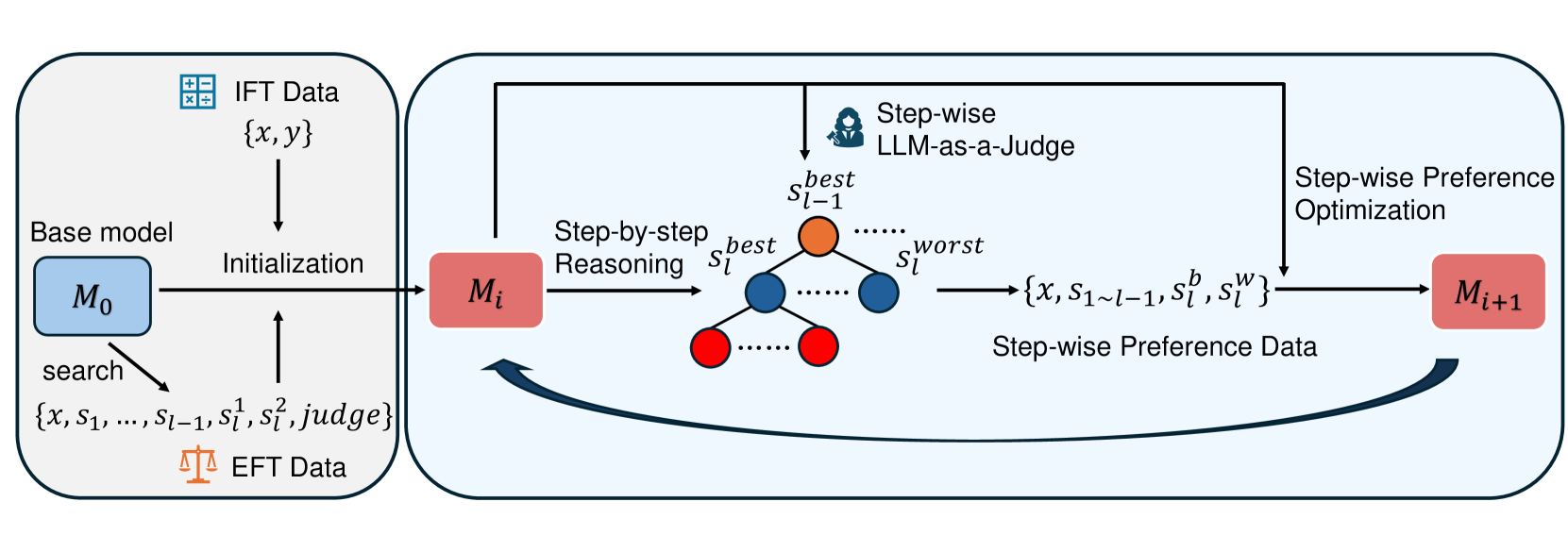
Figure 1: Illustration of our Process-based Self-Rewarding paradigm. (1) We get EFT data by tree-search, initial data filtering and data annotation. And we get IFT data by step segmentation. (2) The model is initialized on EFT and IFT data. (3) The model conducts step-by-step search-based reasoning and performs step-wise LLM-as-a-Judge to select the chosen step and generate the step-wise preference pair at each step. (4) We perform step-wise preference optimization on the model. (5) The model enters the next iteration cycle.
### 2.1 Reinforcement Learning from Human Feedback
Supervised Fine-tuning is an effective method to improve LLMs’ performance across many different downstream tasks. But it has been evidenced that SFT potentially exacerbates LLMs’ hallucination (Hong et al., 2024). So RLHF is further utilized to align LLMs with human preference. In the RLHF paradigm, the model is trained based on reward signals provided by external reward models and humans by reinforcement learning algorithms, such as PPO (Schulman et al., 2017), DPO (Rafailov et al., 2024), SimPO (Meng et al., 2024), and so on. Direct Preference Optimization (DPO) is a preference learning algorithm which directly uses pairwise preference data, including chosen and rejected answers for optimization. Furthermore, the step-wise preference optimization has also been investigated for long-chain reasoning and has shown great performance (Lai et al., 2024; Chen et al., 2024). In our work, we introduce the step-wise preference optimization into our Process-based Self-Rewarding paradigm for more fine-grained learning.
### 2.2 LLM-as-a-Judge
LLM-as-a-Judge technique has been widely used for evaluation tasks because of LLMs’ scalability, adaptability, and cost-effectiveness (Gu et al., 2024). In the LLM-as-a-Judge scenarios, LLMs are prompted to mimic human reasoning and evaluate specific inputs against a set of predefined rules. To improve the performance of LLM-as-a-Judge, the LLM acting as the evaluator is trained to align with human preferences. When conducting LLM-as-a-Judge, LLMs can play many different roles depending on the given prompt. Typical applications include tasks where LLMs are prompted to generate scores (Li et al., 2023; Xiong et al., 2024), perform pairwise comparisons (Liu et al., 2024; Liusie et al., 2023), rank multiple candidates (Yuan et al., 2023), and so on. However, the LLM-as-a-Judge for individual mathematical reasoning steps has not been widely investigated. In our experiment, we design the step-wise LLM-as-a-Judge for rewarding and analyze its performance.
### 2.3 Self-Rewarding Language Models
Although RLHF has been widely utilized to align LLMs with human-level performance and has achieved impressive performance, the existing methods heavily rely on high-quality reward models or human feedback, which bottlenecks these approaches. To avoid this bottleneck, Yuan et al. (2024) propose the Self-Rewarding Language Models paradigm, which uses a single model as both instruction-following model and reward model simultaneously. The iterative self-rewarding algorithm operates by having the model generate responses and reward the generated response candidates, then selecting preference pairs for training. Based on this, Wu et al. (2024) further improve the judgment agreement by adding the LLM-as-a-Meta-Judge action into the self-rewarding pipeline, which allows the model to evaluate its own judgments. But the existing self-rewarding methods mainly focus on the instruction-following tasks and perform poorly in the mathematical domain data (Yuan et al., 2024). And evaluating the entire response makes it difficult for the model to learn fine-grained preference information. For some long-thought reasoning tasks, it is important to enable LLMs to focus on and learn the fine-grained reasoning step preference information.
### 2.4 Step-by-step Reasoning
Complex reasoning tasks are still great challenges for LLMs now. Chain-of-Thought (Wei et al., 2022) methods prompt LLMs to solve the complex problems by reasoning step by step rather than generating the answer directly, which leads to significant improvements across many reasoning tasks (Yoran et al., 2023; Fu et al., 2022; Zhang et al., 2022). Furthermore, recent studies investigate the test-time scaling paradigm which allows the LLMs to use more resources and time for inference to achieve better performance (Lightman et al., 2023) typically based on search and step selecting (Yao et al., 2024; Wang et al., 2024b). These results highlight the importance of conducting high-quality long-thought step-by-step reasoning for LLMs in solving complex reasoning problems.
## 3 Process-based Self-Rewarding Language Models
In this section, we propose our new Process-based Self-Rewarding Language Models pipeline. We first review the existing self-rewarding algorithm and our motivation as a preliminary study in § 3.1. Then we introduce our novel paradigm for more fine-grained step-wise self-rewarding and self-evolution. The entire pipeline consists of sequential stages: model initialization (§ 3.2), reasoning and preference data generation (§ 3.3), and model preference optimization (§ 3.4). Finally, we provide a summarized overview of our algorithm (§ 3.5). We illustrate the entire pipeline in Figure 1.
### 3.1 Preliminary Study
Most existing preference optimization algorithms rely on reward signals from external reward models or human-annotated data. However, deploying an external reward model or getting ground truth gold reward signals from human annotators is expensive (Gao et al., 2023). Moreover, due to the inherent limitations and implicit biases of both humans and reward models, these model optimization strategies are bottlenecked (Lambert et al., 2024; Yuan et al., 2024). Thus, Self-Rewarding algorithm is proposed to mitigate this limitation by enabling the model to provide reward signals for its own outputs and perform self-improvement, showing the feasibility of achieving models that surpass human performance (Yuan et al., 2024).
There are still many aspects waiting for further research and improvement in the self-rewarding framework. The original method is primarily designed for instruction-following tasks and performs poorly on mathematical reasoning data. Step-by-step long-chain reasoning is widely used for complex mathematical reasoning, which allows the models to conduct more detailed thinking and fine-grained verification of the reasoning steps (Lightman et al., 2023; Wang et al., 2024b; Lai et al., 2024). Given the effectiveness of step-by-step reasoning, we further propose Process-based Self-Rewarding, introducing LLM-as-a-judge and preference optimization for individual steps.
### 3.2 Model Initialization
To perform Process-based Self-Rewarding, models need to possess two key abilities:
- Step-by-step mathematical reasoning: When faced with a complex reasoning problem, the model needs to think and reason step by step, outputting the reasoning process in a specified format. (Each step is prefixed with “Step n: ”, where n indeicates the step number.)
- LLM-as-a-Judge for individual steps: The model should be able to assess the quality of the given next reasoning steps based on the existing problem and partial reasoning steps and provide a detailed explanation.
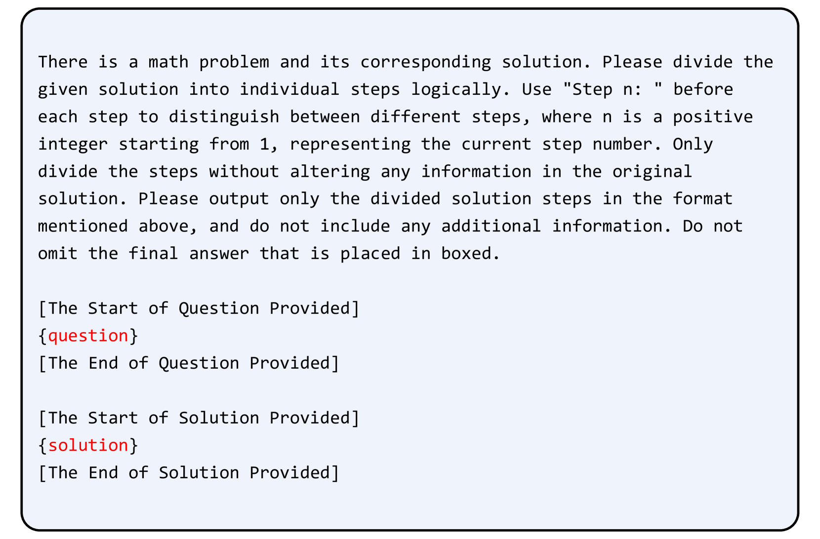
We construct data separately for the two tasks to perform cold start. Following Yuan et al. (2024), we refer to them as Instruction Fine-Tuning (IFT) data and Evaluation Fine-Tuning (EFT) data. For IFT data, we divide the given solution steps into individual steps logically without altering any information in the original solution by using OpenAI o1 (Jaech et al., 2024).
For EFT data, since there is no available step-wise LLM-as-a-Judge dataset, we first train Qwen2.5-72B (Yang et al., 2024a) on PRM800k (Lightman et al., 2023) following Wang et al. (2024a). After getting a Process Reward Model (PRM) by this, which can output a single label “+” or “-” for a reasoning step based on the question and the previous steps, we conduct Monte Carlo Tree Search (MCTS) on a policy model. We use the probability of label “+” of the above PRM to compare the relative quality of all candidate steps at the same layer, and choose the best and the worst step as a data pair. After the initial data filtering process, we use GPT-o1 to generate judgments and detailed explanations for the obtained data pairs. The pairs whose judgments align with the previous PRM assessments are selected as the final EFT data. Additionally, to enhance consistency, we evaluate each pair twice using GPT with different input orders and select only the pairs that have consistent results.
### 3.3 Step-by-step Long-chain Reasoning and Preference Data Generation
After the “EFT + IFT” initialization stage, the model is able to conduct both step-wise LLM-as-a-Judge and step-by-step mathematical reasoning in the specified formats. Because we conduct pairwise comparison rather than single answer grading, we utilize the following search strategy:
$$
S_l=\{s_l,1, s_l,2, s_l,3, ..., s_l,w-1, s_l,w\} \tag{1}
$$
where $S_l$ is all candidates for the next step, $l$ is the step number starting from $1$ , $w$ is a hyperparameter to specify the search width for each step.
$$
\textrm{Score}_l,i=∑_1≤ j≤ w, j≠ iO(s_l,i, s_l,j
\mid x, s_1,s_2,...,s_l-1) \tag{2}
$$
where $l$ is the next step number, $s_l,i$ indicates the $i$ -th candidate for the next $l$ -th step, $x$ is the prompt, and $O$ is a function that takes $1$ when $s_l,i$ is considered better than $s_l,j$ and $0 0$ otherwise.
$$
s_l^\textrm{best}=S_l[\max(\textrm{Score}_l)] \tag{3}
$$
$$
s_l^\textrm{worst}=S_l[\min(\textrm{Score}_l)] \tag{4}
$$
$$
s_l=s_l^best \tag{5}
$$
where $\max(\textrm{Score}_l)$ is the index of the candidate with the highest score and $\min(\textrm{Score}_l)$ corresponds to the lowest score. $s_l$ is the final chosen $l$ -th step. $(s_l^\textrm{best}, s_l^\textrm{worst})$ will be chosen as a chosen-rejected preference pair.
This process will be repeated continuously until generation is complete. It is important to note that to enhance the effectiveness of preference data, if $\max(\textrm{Score}_l)$ is equal to $\min(\textrm{Score}_l)$ , we will discard the existing $s_l-1$ and $(s_l-1^\textrm{best}, s_l-1^\textrm{worst})$ and roll back to the previous step.
### 3.4 Step-wise Model Preference Optimization
With preference data collected in the Section 3.3, we conduct preference optimization training on the model. We choose Direct Preference Optimization (DPO) as the training algorithm (Rafailov et al., 2024). The difference is that we conduct a more fine-grained step-wise DPO in our work. The similar method has also been investigated by Lai et al. (2024). We can calculate the training loss as:
$$
A=β\frac{π_θ(s_l^b\mid x,s_1,...,s_l-1)
}{π_ref(s_l^b\mid x,s_1,...,s_l-1)} \tag{6}
$$
$$
B=β\frac{π_θ(s_l^w\mid x,s_1,...,s_l-1)
}{π_ref(s_l^w\mid x,s_1,...,s_l-1)} \tag{7}
$$
$$
L(π_θ;π_ref)=-E_(x,s_{1,...,s_l^b,s_l^
{w})∼D}[σ(A-B)] \tag{8}
$$
where $x$ is the prompt, $s_1,...,s_l-1$ is the previous steps, $s_l^b$ and $s_l^w$ are the best and worst steps respectively for the $l$ -th step, $β$ is a hyperparameter controlling the deviation from the base reference policy, $π_θ$ and $π_ref$ are the policies to be optimized and the reference policy respectively.
After the preference optimization stage, we have the model for the next cycle. In the next iteration, we sequentially repeat the steps in § 3.3 and § 3.4.
### 3.5 Iteration Pipeline
We show the entire pipeline of our algorithm. Following Yuan et al. (2024), we refer to the model after $n$ iterations as $M_n$ . And we refer to the Pair-wise Preference Data generated by $M_n$ as PPD( $M_n$ ). Then the sequence in our work can be defined as:
- $M_0$ : The base model.
- $M_1$ : The model obtained by supervised fine-tuning (SFT) $M_0$ on “EFT + IFT” data.
- $M_2$ : The model obtained by training $M_1$ on PPD( $M_1$ ) using step-wise DPO.
- $⋯⋯$
- $M_n$ : The model obtained by training $M_n-1$ on PPD( $M_n-1$ ) using step-wise DPO.
In summary, we initialize the base model using well-selected step-wise LLM-as-a-Judge data (EFT) and step-by-step long-thought reasoning data (IFT). Once the model possesses the corresponding two abilities, we select preference pairs through search and reward signals provided by the model itself, and train the model using step-wise DPO. Then we iterate the model by repeatedly performing the above operations.
| Model GPT-4o 7B Base Model | GSM8k 92.9 | MATH 76.6 | Gaokao2023En 67.5 | OlympiadBench 43.3 | AIME2024 10.0 | AMC2023 47.5 | Avg. 56.3 |
| --- | --- | --- | --- | --- | --- | --- | --- |
| $M_0$ | 70.1 | 51.7 | 51.2 | 21.3 | 0.0 | 22.5 | 36.1 |
| SRLM - $M_1$ | 88.2 | 69.0 | 61.6 | 37.6 | 10.0 | 45.0 | 51.9 |
| $M_2$ | 87.6 | 69.4 | 63.9 | 37.2 | 3.3 | 40.0 | 50.2 |
| $M_3$ | 88.5 | 70.0 | 61.3 | 36.7 | 10.0 | 40.0 | 51.1 |
| $M_4$ | 88.3 | 70.2 | 63.9 | 37.6 | 13.3 | 45.0 | 53.1 |
| PSRLM - $M_1$ | 88.5 | 69.5 | 61.8 | 36.0 | 6.7 | 45.0 | 51.3 |
| $M_2$ | 88.8 | 69.7 | 63.9 | 36.3 | 16.7 | 47.5 | 53.8 |
| $M_3$ | 88.5 | 72.2 | 64.7 | 39.9 | 10.0 | 50.0 | 54.2 |
| $M_4$ | 88.8 | 73.3 | 65.2 | 38.7 | 13.3 | 55.0 | 55.7 |
| 72B Base Model | | | | | | | |
| $M_0$ | 87.5 | 69.7 | 55.3 | 28.9 | 10.0 | 40.0 | 48.6 |
| SRLM - $M_1$ | 92.9 | 76.4 | 67.3 | 41.8 | 16.7 | 47.5 | 57.1 |
| $M_2$ | 92.1 | 76.1 | 66.8 | 42.1 | 20.0 | 55.0 | 58.7 |
| $M_3$ | 92.5 | 75.8 | 67.5 | 42.5 | 20.0 | 52.5 | 58.5 |
| $M_4$ | 92.8 | 76.1 | 66.2 | 44.0 | 13.3 | 42.5 | 55.8 |
| PSRLM - $M_1$ | 92.6 | 75.6 | 67.3 | 41.8 | 13.3 | 45.0 | 55.9 |
| $M_2$ | 92.6 | 76.4 | 67.8 | 41.8 | 20.0 | 57.5 | 59.4 |
| $M_3$ | 93.7 | 76.4 | 67.3 | 42.7 | 23.3 | 52.5 | 59.3 |
| $M_4$ | 93.7 | 76.6 | 68.1 | 44.1 | 23.3 | 57.5 | 60.6 |
Table 1: Accuracy of Process-based Self-Rewarding based on 7B and 72B base models. SRLM is the self-rewarding language model algorithm as the baseline. We bold the best results for each parameter size in each benchmark.
## 4 Experimental Setup
We conduct our experiments on models in different parameter sizes and several representative mathematical reasoning benchmarks. In this section, we introduce our experimental settings in detail.
#### Models
We choose the base model from Qwen2.5-Math series (Yang et al., 2024b) in our experiments, which is one of the most popular open-source LLM series. Specifically, we choose Qwen2.5-Math-7B and Qwen2.5-Math-72B. Additionally, we choose OpenAI GPT-o1 (Jaech et al., 2024) for our initialization data processing (§ 3.2).
#### Datasets
In our experiments, we mainly focus on two capabilities of the model:
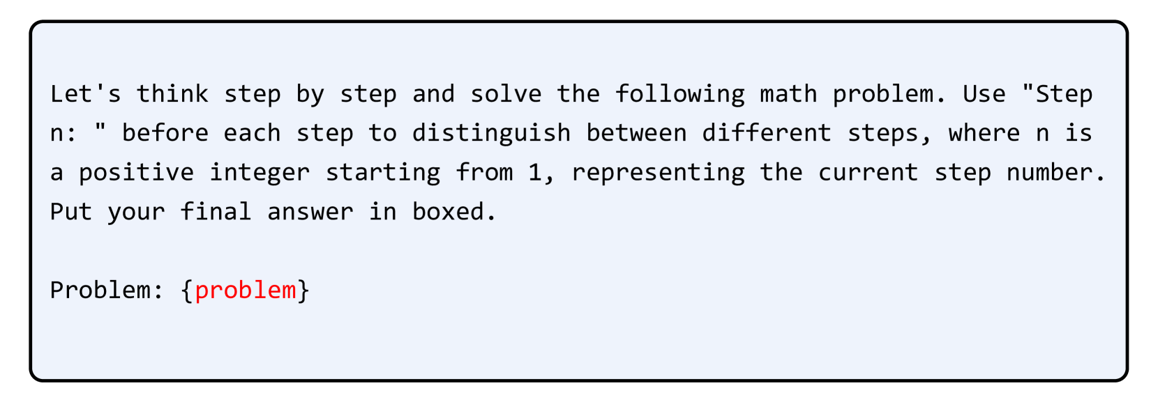
- Step-by-step Mathematical Reasoning: We choose a subset of NuminaMath (LI et al., 2024) for IFT data construction, whose solutions have been formatted in a Chain of Thought (CoT) manner. We extract a subset of 28,889 samples and prompt GPT-o1 (Jaech et al., 2024) to logically segment the solutions into step-by-step format without altering any original content. The corresponding prompt is presented in Figure 3. And the instruction format for step-by-step long-thought reasoning is presented in Figure 4.
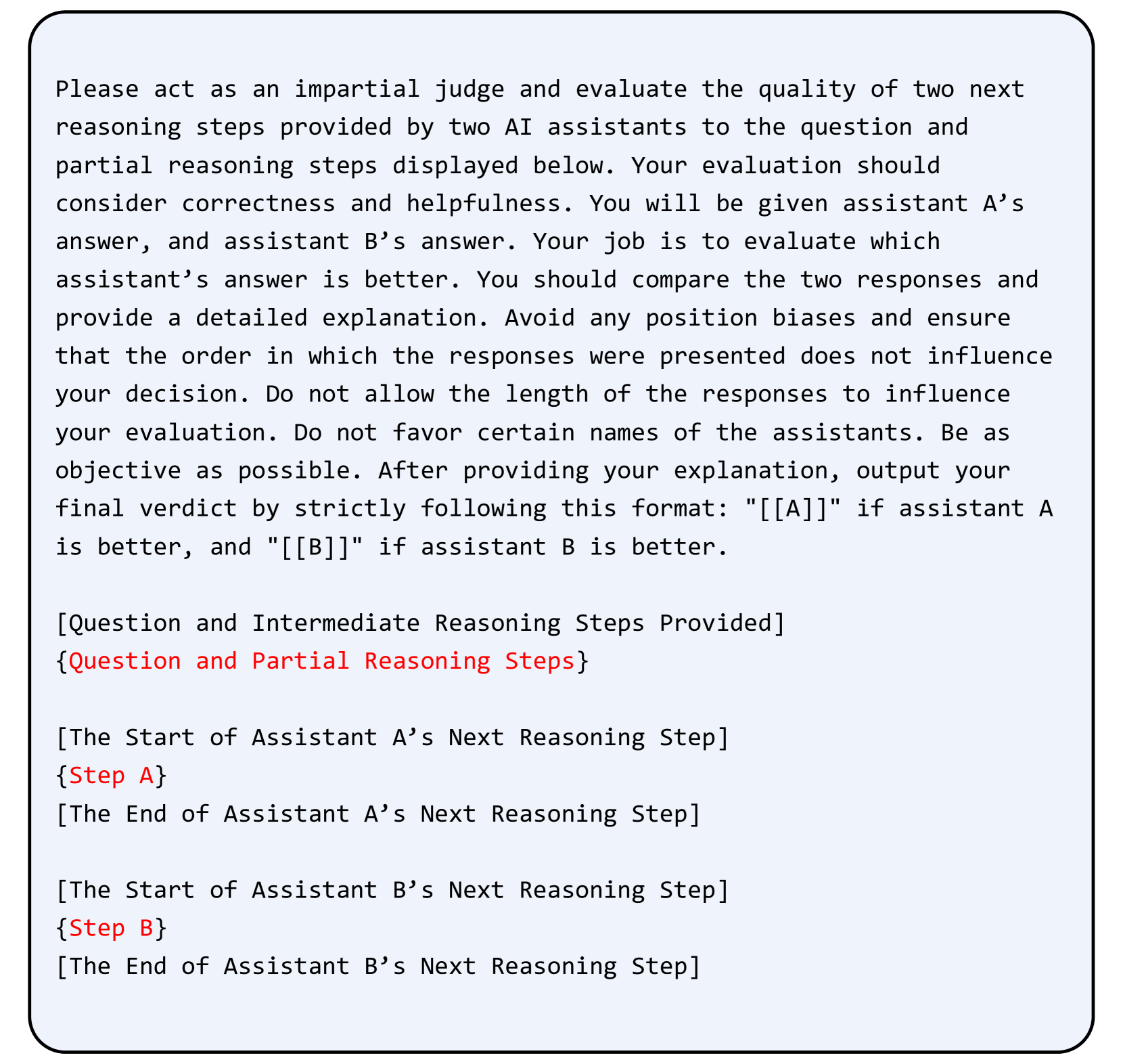
- Step-wise LLM-as-a-Judge: As described in the Section 3.2, we first filtrate some preference pairs using the trained PRM. Then we utilize GPT-o1 and get a total of 4,679 EFT data with judgments and detailed explanations. Finally we split the whole dataset into 4,167 samples as the training set and 500 samples as the test set. The instruction format for step-wise pairwise LLM-as-a-Judge is presented in Figure 5, which is following the basic format of Zheng et al. (2023).
And for mathematical task evaluation, following Yang et al. (2024b), we evaluate the LLMs’ mathematical capabilities across some representative benchmarks. We choose the widely used benchmarks GSM8k (Cobbe et al., 2021) and MATH (Hendrycks et al., 2021). We also choose some complex and challenging competition benchmarks, including Gaokao2023En (Liao et al., 2024), Olympiadbench (He et al., 2024), AIME2024 https://huggingface.co/datasets/AI-MO/aimo-validation-aime, and AMC2023 https://huggingface.co/datasets/AI-MO/aimo-validation-amc.
#### Evaluation Metrics
We use accuracy as the evaluation metric for both the mathematical performance and LLM-as-a-Judge quality. For accuracy calculation on mathematical benchmarks, we follow the implementation of Yang et al. (2024b).
#### Implementations
For initial PRM training, we fine-tune full parameters on 128 NVIDIA A100 GPUs for 1 epoch with learning_rate= $1e-5$ and batch_size= $128$ . For preliminary preference pairs selection, we set simulation_depth= $3$ , num_iterations= $100$ , T= $0.7$ , and top_p= $0.95$ . When training $M_0$ to $M_1$ , we utilize 28,889 IFT and 4,179 EFT samples. We fine-tune LLMs’ full parameters on 32 NVIDIA H100 GPUs for 3 epochs with learning_rate= $1e-6$ and batch_size= $32$ . During the reasoning and preference data generation stage, we utilize temperature sampling which trade-off generation quality and diversity (Zhang et al., 2024). We set T= $0.5$ , top_p= $0.95$ . The search width for each step is set to $6$ , and the max iteration number is set to $20$ . Finally, in the step-wise preference optimization, we train LLM’s full parameters on 32 NVIDIA H100 GPUs for 1 epoch with learning_rate= $5e-7$ and batch_size= $32$ . To get models from $M_2$ to $M_4$ , we use $400$ , $800$ , and $1,200$ math questions for preference pairs generation respectively, which are all sampled from the train subset of NuminaMath. For all solution-scoring judgment strategy experiments, we use the same prompt template of Yuan et al. (2024). We use greedy search in evaluations.
| 7B SRLM Process-based (Ours) | GSM8k +0.1 +0.3 | MATH +1.2 +3.8 | Gaokao2023En +2.3 +3.4 | OlympiadBench 0.0 +2.7 | AIME2024 +3.3 +6.6 | AMC2023 0.0 +10.0 |
| --- | --- | --- | --- | --- | --- | --- |
| 72B | GSM8k | MATH | Gaokao2023En | OlympiadBench | AIME2024 | AMC2023 |
| SRLM | -0.1 | -0.3 | -1.1 | +2.2 | -3.4 | -5.0 |
| Process-based (Ours) | +1.1 | +1.0 | +0.8 | +2.3 | +10.0 | +12.5 |
Table 2: The results of LLMs’ mathematical performance changes after all iterations from $M_1$ to $M_4$ .
## 5 Results
In this section, we report our main results on different mathematical benchmarks and conduct some discussions and analyses based on the results.
### 5.1 Main Results
We report the performance of $M_0$ to $M_4$ based on Qwen2.5-Math-7B and Qwen2.5-Math-72B respectively in Table 1. Our findings are as follows:
As the number of iterations increases, the overall performance of the model improves. Traditionally, external reward signals and training data are utilized for improving LLMs’ performance. Our results indicate that models’ overall performance on mathematical tasks significantly improves from $M_1$ to $M_4$ solely through Process-based Self-Rewarding and step-wise preference optimization without any additional guidance. This leverages the potential of LLMs for both mathematical reasoning and as evaluators.
Our fine-grained algorithm outperforms the tranditional method. After three iterations, our approach achieves superior performance compared to method that applies rewards and conducts training on the entire response. Given that the initialization with different EFT data lead to different M1 fiducial performance in the two methods, we also report the performance changes from M1 to M4 after multiple iterations in Table 2, which reflects the algorithm’s effectiveness and stability in improving the model’s mathematical capabilities. Our method achieves more stable and effective improvements across all benchmarks. On one hand, using step-wise preference data enables the model to focus on more fine-grained information; on the other hand, conducting LLM-as-a-Judge on individual steps helps the model more easily detect subtle differences and errors.
The models show noticeable improvements on some complex tasks. For some complex and highly challenging benchmarks, such as MATH, AIME2024, and AMC2023, LLMs’ performance show significant improvement. Complex problems require multi-step, long-thought reasoning. Our method effectively leverages the model’s existing knowledge to optimize the individual intermediate reasoning steps, achieving favorable results.
Our method remains effective across models of different parameter sizes. We validate our method on both 7B and 72B LLMs to strengthen our conclusions. We find performance improvements across models of different parameter sizes on multiple mathematical tasks through Process-based Self-Rewarding. We also find that the 72B model gains more stable improvements compared to the 7B model, whose mathematical reasoning and LLM-as-a-Judge capabilities are stronger.
Overall, we can find that the models iterating based on the Process-based Self-Rewarding paradigm achieve significant improvements across multiple mathematical tasks, outperforming the traditional self-rewarding method.
### 5.2 Further Analysis
Based on the above results, we conduct more analysis and observations of the pipeline.
| $M_0$ (3-shot) $M_1$ $M_2$ | 57.2 92.8 ( $↑$ ) 91.6 ( $↓$ ) | 73.4 95.6 ( $↑$ ) 95.8 ( $↑$ ) |
| --- | --- | --- |
| $M_3$ | 92.0 ( $↑$ ) | 95.2 ( $↓$ ) |
| $M_4$ | 92.2 ( $↑$ ) | 95.6 ( $↑$ ) |
Table 3: Judgment accuracy in step-wise LLM-as-a-Judge. We report the results of models with different parameter sizes. Additionally, we use arrows to indicate the changes in accuracy during the iterations.
#### Step-wise LLM-as-a-Judge Capability.
We evaluate the LLMs’ ability to accurately assess reasoning steps as a reward model during the iterative process. We test the model on the test set including 500 samples (§ 3.2). We report the results in Table 3. As shown in the table, LLMs achieve strong reward model performance after initialization with a small amount of EFT data, which indicates the immense potential of LLMs for step-wise LLM-as-a-Judge with CoT reasoning. Additionally, we can observe that, under the same conditions, the larger model exhibits stronger capabilities as a reward model than the smaller one.
Additionally, although we mix EFT data and IFT data for initialization and introduce no additional LLM-as-a-Judge data during subsequent iterations, the LLMs’ capabilities to perform LLM-as-a-Judge as a reward model are still good. Furthermore, a consistent pattern is observed across different models where evaluation accuracy initially increases, then decreases, and finally rises again. Based on the analysis above, initially, LLMs gain strong evaluation capabilities through training on EFT data. And there is a temporary decline (but very slight) due to training on mathematical data. Ultimately, as the model’s mathematical abilities improve, its ability to evaluate mathematical reasoning steps also increases.
| $M_1$ $M_2$ $M_3$ | 5.89 5.55 5.10 | 8.41 7.64 6.30 | 47.79 51.19 57.75 | 61.00 67.17 80.46 |
| --- | --- | --- | --- | --- |
| $M_4$ | 4.87 | 5.54 | 62.86 | 96.63 |
Table 4: Statistics of step number and step length on GSM8k and MATH benchmarks based on 72B models. The full results are reported in Appendix A.
<details>
<summary>x2.png Details</summary>
### Visual Description
## Scatter Plot: Prompt Type Distribution
### Overview
The image is a 2D scatter plot visualizing the distribution of three distinct categories of prompts, likely in a feature space derived from dimensionality reduction (e.g., t-SNE or PCA). The plot shows clear clustering and separation between the categories, with some overlap in specific regions.
### Components/Axes
* **Chart Type:** Scatter Plot
* **X-Axis:** Numerical scale ranging from approximately -65 to +50. Major tick marks are labeled at intervals of 20: -60, -40, -20, 0, 20, 40.
* **Y-Axis:** Numerical scale ranging from approximately -40 to +35. Major tick marks are labeled at intervals of 10: -40, -30, -20, -10, 0, 10, 20, 30.
* **Legend:** Located in the bottom-left quadrant of the plot area. It contains three entries:
1. **EFT Prompts:** Represented by a red circle (●).
2. **IFT Prompts:** Represented by a blue circle (●).
3. **PPD Prompts:** Represented by a gray circle (●).
* **Data Points:** Thousands of semi-transparent circular markers, colored according to the legend.
### Detailed Analysis
The data is organized into three primary clusters with distinct spatial characteristics:
1. **EFT Prompts (Red Cluster):**
* **Spatial Grounding:** Centered in the left half of the plot.
* **Trend & Distribution:** Forms a dense, roughly circular cloud. The core density is centered approximately at coordinates **(-40, 0)**. The cluster spans from about X = -60 to X = -10 and Y = -20 to Y = +20. It shows very little overlap with the other clusters, primarily touching the gray cluster on its right edge.
2. **IFT Prompts (Blue Cluster):**
* **Spatial Grounding:** Located in the bottom-right quadrant, extending towards the center-right.
* **Trend & Distribution:** Exhibits an elongated, diagonal shape. The densest region is at the bottom, centered near **(10, -30)**. The cluster extends upwards and to the right, with a secondary concentration around **(30, 0)**. It spans from approximately X = 0 to X = 45 and Y = -38 to Y = +15. It overlaps significantly with the gray cluster in the region between X=0 to X=20 and Y=-10 to Y=+10.
3. **PPD Prompts (Gray Cluster):**
* **Spatial Grounding:** Occupies the upper-central and right-central region of the plot.
* **Trend & Distribution:** This is the most dispersed and irregularly shaped cluster. It has a broad vertical spread. A major concentration is in the upper region, peaking around **(10, 25)**. Another dense area connects downwards, overlapping with the blue cluster. It spans from approximately X = -15 to X = 40 and Y = -25 to Y = +35. It acts as a bridge or overlapping region between the distinct red and blue clusters.
### Key Observations
* **Clear Separation:** The EFT (red) and IFT (blue) prompts form two distinct, well-separated clusters, suggesting fundamental differences in their underlying features.
* **The Bridging Role of PPD:** The PPD (gray) prompts are not a single tight cluster but are widely distributed, filling the space between the red and blue clusters and overlapping with both. This suggests PPD prompts may share characteristics with both EFT and IFT types or represent a more diverse category.
* **Density Variation:** The red cluster is the most compact and dense. The blue cluster is dense at its core but elongated. The gray cluster is the most diffuse.
* **Outliers:** A few isolated blue points appear within the red cluster's periphery (e.g., near (-20, 10)), and a few gray points are found deep within the blue cluster's core. These could be misclassified examples or edge cases.
### Interpretation
This scatter plot visualizes the semantic or feature-space separation between three types of prompts (EFT, IFT, PPD). The strong spatial segregation between the red (EFT) and blue (IFT) clusters indicates that these two prompt types are distinct in the analyzed feature space—they likely elicit different model behaviors or are designed for different tasks.
The gray (PPD) prompts' dispersed nature and their position overlapping both other clusters suggest they are either a more heterogeneous category, a hybrid type, or a general-purpose category that encompasses features of both EFT and IFT prompts. The plot effectively demonstrates that EFT and IFT prompts are specialized and distinct, while PPD prompts are more general and bridge the gap between them. This has implications for prompt engineering, suggesting that choosing between EFT and IFT may lead to more predictable, specialized outcomes, while PPD prompts might offer more flexibility or variability.
</details>
(a) Prompt Distributions
<details>
<summary>x3.png Details</summary>
### Visual Description
## Scatter Plot: Response Cluster Analysis
### Overview
The image is a scatter plot displaying three distinct clusters of data points, each representing a different response type. The plot visualizes the distribution and separation of these response groups in a two-dimensional space. The axes are numerical but unlabeled, suggesting they represent abstract dimensions or components from a dimensionality reduction technique (e.g., PCA, t-SNE).
### Components/Axes
* **X-Axis:** Linear scale ranging from approximately -40 to +40. Major tick marks are at intervals of 10 (-40, -30, -20, -10, 0, 10, 20, 30, 40). No axis title or label is present.
* **Y-Axis:** Linear scale ranging from approximately -20 to +20. Major tick marks are at intervals of 5 (-20, -15, -10, -5, 0, 5, 10, 15, 20). No axis title or label is present.
* **Legend:** Located in the top-right quadrant of the chart area. It contains three entries:
* **EFT Responses:** Represented by a red circle (semi-transparent).
* **IFT Responses:** Represented by a blue circle (semi-transparent).
* **PPD Responses:** Represented by a gray circle (semi-transparent).
* **Data Points:** Thousands of semi-transparent circles, allowing visualization of density through overlap.
### Detailed Analysis
The data is organized into three spatially separated clusters:
1. **EFT Responses (Red Cluster):**
* **Spatial Grounding:** Located on the right side of the plot.
* **Trend & Distribution:** Forms a dense, vertically elongated cluster. The core is centered approximately at **X=30, Y=0**. The cluster spans from roughly **X=20 to X=40** and **Y=-18 to Y=7**. The density is highest in the center and tapers at the edges.
2. **IFT Responses (Blue Cluster):**
* **Spatial Grounding:** Located in the center-top region of the plot.
* **Trend & Distribution:** Forms a dense, somewhat vertically oriented cluster with a slight diagonal tilt. The core is centered approximately at **X=-5, Y=10**. The cluster spans from roughly **X=-15 to X=5** and **Y=-10 to Y=20**. It shows significant overlap with the upper portion of the gray cluster.
3. **PPD Responses (Gray Cluster):**
* **Spatial Grounding:** Located on the left side of the plot.
* **Trend & Distribution:** Forms a large, diffuse, and irregularly shaped cluster. The approximate center of mass is near **X=-25, Y=0**. The cluster spans a wide area from roughly **X=-40 to X=0** and **Y=-15 to Y=15**. It has a less defined shape compared to the red and blue clusters.
4. **Outliers and Overlap:**
* A few isolated **blue (IFT)** points are visible within the red cluster (e.g., near X=20, Y=-10 and X=25, Y=5).
* A few isolated **gray (PPD)** points are visible within the blue cluster (e.g., near X=-5, Y=5).
* The blue and gray clusters show substantial overlap in the region between **X=-15 to X=0** and **Y=5 to Y=15**.
### Key Observations
* **Clear Separation:** The three response types form distinct clusters with minimal overlap between the red (EFT) cluster and the other two.
* **Density Variation:** The red (EFT) cluster appears the most compact and dense. The blue (IFT) cluster is also dense but more spread vertically. The gray (PPD) cluster is the most diffuse and spread out.
* **Cluster Shape:** The red cluster is vertically elongated. The blue cluster is also vertically oriented but with a diagonal component. The gray cluster is amorphous.
* **Anomalies:** The presence of a small number of blue points deep within the red cluster and gray points within the blue cluster suggests potential misclassifications, transitional states, or outliers in the underlying data.
### Interpretation
This scatter plot strongly suggests that the three response types (EFT, IFT, PPD) are fundamentally distinct in the feature space being visualized. The clear spatial separation, particularly of the EFT responses, indicates that the underlying model or process generating these responses produces qualitatively different outputs for each category.
* **EFT Responses** are highly consistent and form a tight, isolated group, implying a unique and stable signature.
* **IFT Responses** are also relatively consistent but share some commonalities or a continuum with **PPD Responses**, as evidenced by their spatial proximity and overlap. This could indicate that IFT and PPD responses are more similar to each other than either is to EFT, or that they represent different stages of a related process.
* The **PPD Responses** are the most variable, suggesting this category may be less defined, more heterogeneous, or encompass a wider range of outcomes.
The unlabeled axes imply this is likely an internal diagnostic plot from a machine learning or statistical analysis (e.g., visualizing latent space embeddings). The primary takeaway is the successful discrimination of EFT responses from the other two types, and a noted relationship between IFT and PPD responses.
</details>
(b) Response Distributions
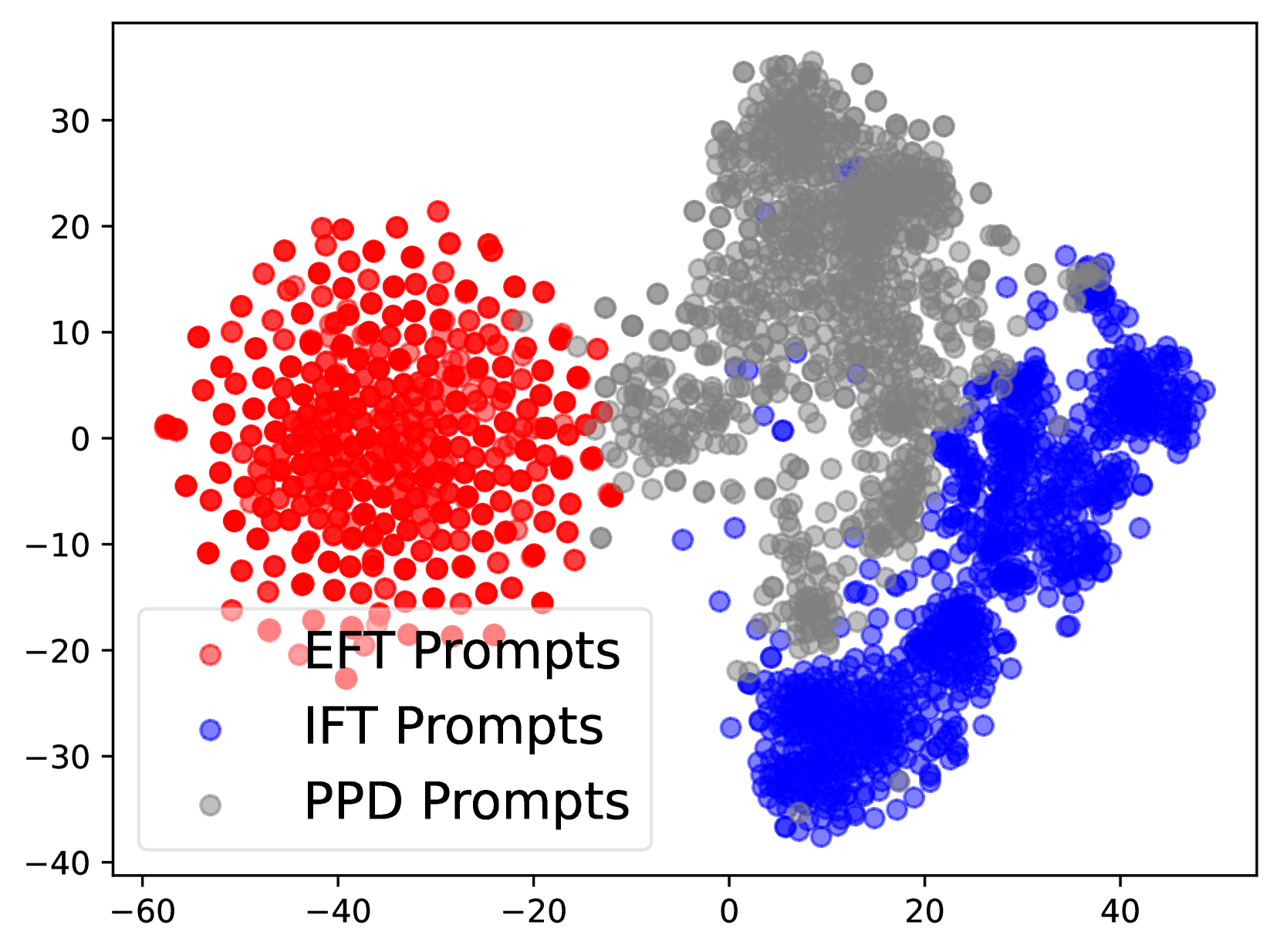
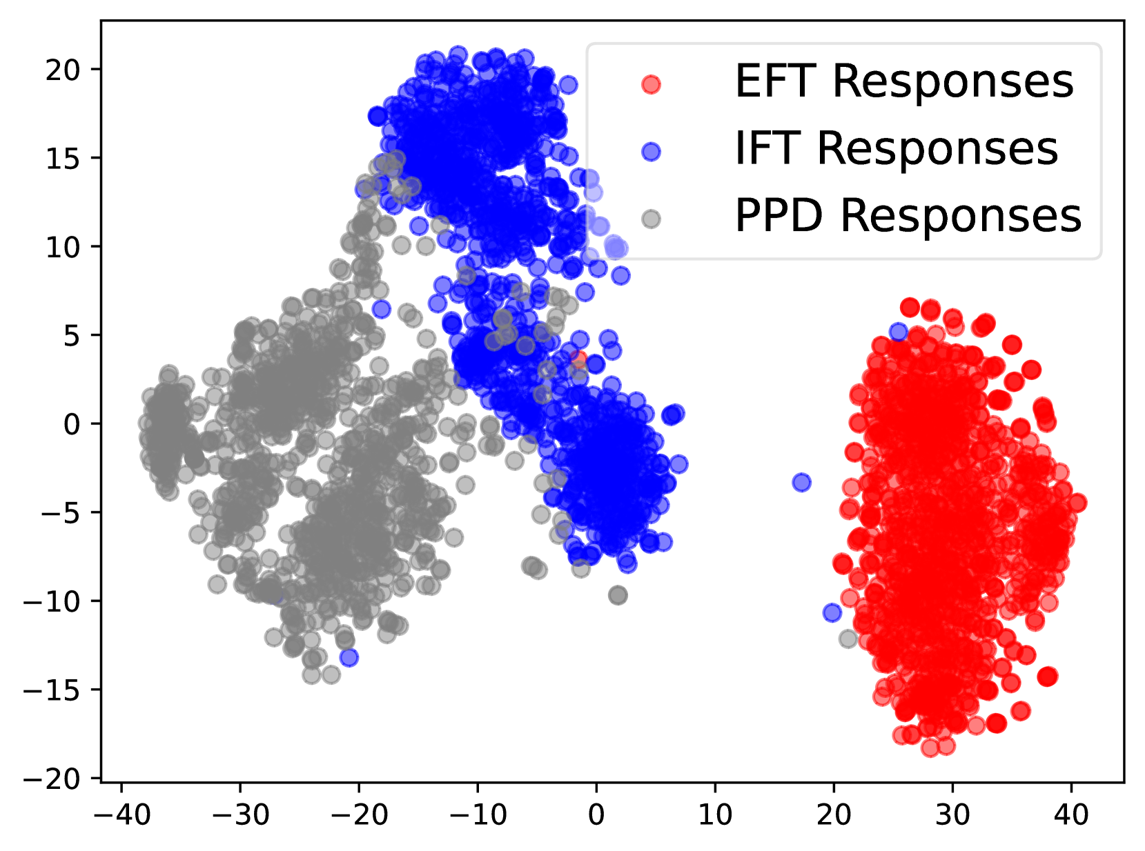
Figure 2: The data distribution of prompts and responses in EFT (red), IFT (blue) and PPD (grey) data.
#### Data Distribution Analysis.
Following Yuan et al. (2024), we also analyze the distribution of different data. We utilize Bert (Devlin, 2018) for embedding and t-SNE (Van der Maaten and Hinton, 2008) based on the implementation of Poličar et al. (2024) for visualization. We present the results in Figure 2. For prompts, the distributions of EFT data and IFT data do not overlap, allowing the model to distinctly learn two different task patterns. For models’ responses, we can find the similar phenomenon that the distribution of PPD and IFT responses is distinct from EFT’s, which reduces the mutual interference between LLMs’ two capabilities during iteration. This allows the model’s ability to perform LLM-as-a-Judge to improve alongside its mathematical ability finally, without being overly influenced by the training data itself.
#### Step Number and Length of Responses.
Step-by-step reasoning is important for LLMs to solve complex reasoning tasks. Therefore, we conduct statistical analysis on the reasoning steps during iterations. As shown in Table 4, for the same model, more difficult problems require more reasoning steps and longer step lengths. As the iterations progress, the step number across different tasks decreases, while the length of each step increases. This indicates that performing Process-based Self-Rewarding encourages the model to generate longer and higher-quality single reasoning steps, which helps to reach final answers with fewer steps. Additionally, this behavior is also related to LLMs’ preferences when performing LLM-as-a-Judge evaluations. More results are in Appendix A.
| $M_1$ $M_4$ | 55.9 60.6 | 58.2 62.4 |
| --- | --- | --- |
Table 5: The average results of 72B model on all benchmarks using greedy search or test-time scaling. The full results are reported in Table 9.
#### Test-time Scaling with Process-based Self-Rewarding Language Models.
In the test-time scaling, LLMs conduct step search and select based on the rewards from PRM. Although we don’t primarily focus on the test-time scaling performance in our work, LLMs in the Process-based Self-Rewarding paradigm naturally have the ability to perform test-time scaling based on self-rewarding. We perform $6$ generations for each step with the temperature of $0.5$ and select the best one. The results we report in Table 5 indicate that the model achieves better performance through test-time scaling compared to generating directly. Additionally, the model’s performance with test-time scaling improves after iterations from $M_1$ to $M_4$ , which corresponds to the uptrend of the model’s mathematical abilities and LLM-as-a-Judge capabilities.
## 6 Conclusion
We propose a novel paradigm, Process-based Self-Rewarding Language Models, that enables LLMs to perform step-by-step long-thought mathematical reasoning and step-wise LLM-as-a-Judge simultaneously. Given the characteristics of complex math reasoning tasks, we introduce the step-by-step reasoning, step-wise LLM-as-a-Judge and step-wise preference optimization technique into the framework. Our results indicate that Process-based Self-Rewarding algorithm outperforms the original Self-Rewarding on a variety of complex mathematical reasoning tasks, showing potential of stronger reasoning ability better than human in the future.
## 7 Limitations
We aim to draw more attention to the study of adapting the self-rewarding paradigm to the complex mathematical reasoning tasks, which allows for the possibility of continual improvement beyond the human preferences. Although our new Process-based Self-Rewarding algorithm has shown effective improvements across different mathematical reasoning tasks, there are still some limitations waiting for further research. Although we successfully enable the model to perform effective step-wise LLM-as-a-Judge with a small amount of EFT data, the basic capabilities of initialized $M_1$ model directly influence the effectiveness of subsequent process-based self-rewarding. Utilizing more high-quality data to initialize LLMs more adequately may lead to stronger performance.
Additionally, due to the limited resources, we only conduct the process-based self-rewarding experiments from $M_1$ to $M_4$ . Building on this, conducting experiments with more iterations to explore the impact of iteration count on LLMs’ performance can help us better understand and utilize the process-based self-rewarding method.
## References
- Brown et al. (2020) Tom Brown, Benjamin Mann, Nick Ryder, Melanie Subbiah, Jared D Kaplan, Prafulla Dhariwal, Arvind Neelakantan, Pranav Shyam, Girish Sastry, Amanda Askell, et al. 2020. Language models are few-shot learners. Advances in neural information processing systems, 33:1877–1901.
- Chen et al. (2024) Guoxin Chen, Minpeng Liao, Chengxi Li, and Kai Fan. 2024. Step-level value preference optimization for mathematical reasoning. arXiv preprint arXiv:2406.10858.
- Christiano et al. (2017) Paul F Christiano, Jan Leike, Tom Brown, Miljan Martic, Shane Legg, and Dario Amodei. 2017. Deep reinforcement learning from human preferences. Advances in neural information processing systems, 30.
- Cobbe et al. (2021) Karl Cobbe, Vineet Kosaraju, Mohammad Bavarian, Mark Chen, Heewoo Jun, Lukasz Kaiser, Matthias Plappert, Jerry Tworek, Jacob Hilton, Reiichiro Nakano, et al. 2021. Training verifiers to solve math word problems. arXiv preprint arXiv:2110.14168.
- Devlin (2018) Jacob Devlin. 2018. Bert: Pre-training of deep bidirectional transformers for language understanding. arXiv preprint arXiv:1810.04805.
- Fu et al. (2022) Yao Fu, Hao Peng, Ashish Sabharwal, Peter Clark, and Tushar Khot. 2022. Complexity-based prompting for multi-step reasoning. In The Eleventh International Conference on Learning Representations.
- Gao et al. (2023) Leo Gao, John Schulman, and Jacob Hilton. 2023. Scaling laws for reward model overoptimization. In International Conference on Machine Learning, pages 10835–10866. PMLR.
- Gu et al. (2024) Jiawei Gu, Xuhui Jiang, Zhichao Shi, Hexiang Tan, Xuehao Zhai, Chengjin Xu, Wei Li, Yinghan Shen, Shengjie Ma, Honghao Liu, et al. 2024. A survey on llm-as-a-judge. arXiv preprint arXiv:2411.15594.
- He et al. (2024) Chaoqun He, Renjie Luo, Yuzhuo Bai, Shengding Hu, Zhen Leng Thai, Junhao Shen, Jinyi Hu, Xu Han, Yujie Huang, Yuxiang Zhang, et al. 2024. Olympiadbench: A challenging benchmark for promoting agi with olympiad-level bilingual multimodal scientific problems. arXiv preprint arXiv:2402.14008.
- Hendrycks et al. (2021) Dan Hendrycks, Collin Burns, Saurav Kadavath, Akul Arora, Steven Basart, Eric Tang, Dawn Song, and Jacob Steinhardt. 2021. Measuring mathematical problem solving with the math dataset. arXiv preprint arXiv:2103.03874.
- Hong et al. (2024) Jiwoo Hong, Noah Lee, and James Thorne. 2024. Orpo: Monolithic preference optimization without reference model. In Proceedings of the 2024 Conference on Empirical Methods in Natural Language Processing, pages 11170–11189.
- Hurst et al. (2024) Aaron Hurst, Adam Lerer, Adam P Goucher, Adam Perelman, Aditya Ramesh, Aidan Clark, AJ Ostrow, Akila Welihinda, Alan Hayes, Alec Radford, et al. 2024. Gpt-4o system card. arXiv preprint arXiv:2410.21276.
- Jaech et al. (2024) Aaron Jaech, Adam Kalai, Adam Lerer, Adam Richardson, Ahmed El-Kishky, Aiden Low, Alec Helyar, Aleksander Madry, Alex Beutel, Alex Carney, et al. 2024. Openai o1 system card. arXiv preprint arXiv:2412.16720.
- Lai et al. (2024) Xin Lai, Zhuotao Tian, Yukang Chen, Senqiao Yang, Xiangru Peng, and Jiaya Jia. 2024. Step-dpo: Step-wise preference optimization for long-chain reasoning of llms. arXiv preprint arXiv:2406.18629.
- Lambert et al. (2024) Nathan Lambert, Valentina Pyatkin, Jacob Morrison, LJ Miranda, Bill Yuchen Lin, Khyathi Chandu, Nouha Dziri, Sachin Kumar, Tom Zick, Yejin Choi, et al. 2024. Rewardbench: Evaluating reward models for language modeling. arXiv preprint arXiv:2403.13787.
- LI et al. (2024) Jia LI, Edward Beeching, Lewis Tunstall, Ben Lipkin, Roman Soletskyi, Shengyi Costa Huang, Kashif Rasul, Longhui Yu, Albert Jiang, Ziju Shen, Zihan Qin, Bin Dong, Li Zhou, Yann Fleureau, Guillaume Lample, and Stanislas Polu. 2024. Numinamath. [https://huggingface.co/AI-MO/NuminaMath-CoT](https://github.com/project-numina/aimo-progress-prize/blob/main/report/numina_dataset.pdf).
- Li et al. (2023) Junlong Li, Shichao Sun, Weizhe Yuan, Run-Ze Fan, Hai Zhao, and Pengfei Liu. 2023. Generative judge for evaluating alignment. arXiv preprint arXiv:2310.05470.
- Liao et al. (2024) Minpeng Liao, Wei Luo, Chengxi Li, Jing Wu, and Kai Fan. 2024. Mario: Math reasoning with code interpreter output–a reproducible pipeline. arXiv preprint arXiv:2401.08190.
- Lightman et al. (2023) Hunter Lightman, Vineet Kosaraju, Yura Burda, Harri Edwards, Bowen Baker, Teddy Lee, Jan Leike, John Schulman, Ilya Sutskever, and Karl Cobbe. 2023. Let’s verify step by step. arXiv preprint arXiv:2305.20050.
- Liu et al. (2024) Yinhong Liu, Han Zhou, Zhijiang Guo, Ehsan Shareghi, Ivan Vulić, Anna Korhonen, and Nigel Collier. 2024. Aligning with human judgement: The role of pairwise preference in large language model evaluators. arXiv preprint arXiv:2403.16950.
- Liusie et al. (2023) Adian Liusie, Potsawee Manakul, and Mark JF Gales. 2023. Zero-shot nlg evaluation through pairware comparisons with llms. arXiv preprint arXiv:2307.07889.
- Meng et al. (2024) Yu Meng, Mengzhou Xia, and Danqi Chen. 2024. Simpo: Simple preference optimization with a reference-free reward. arXiv preprint arXiv:2405.14734.
- Poličar et al. (2024) Pavlin G. Poličar, Martin Stražar, and Blaž Zupan. 2024. opentsne: A modular python library for t-sne dimensionality reduction and embedding. Journal of Statistical Software, 109(3):1–30.
- Radford et al. (2019) Alec Radford, Jeffrey Wu, Rewon Child, David Luan, Dario Amodei, Ilya Sutskever, et al. 2019. Language models are unsupervised multitask learners. OpenAI blog, 1(8):9.
- Rafailov et al. (2024) Rafael Rafailov, Archit Sharma, Eric Mitchell, Christopher D Manning, Stefano Ermon, and Chelsea Finn. 2024. Direct preference optimization: Your language model is secretly a reward model. Advances in Neural Information Processing Systems, 36.
- Schulman et al. (2017) John Schulman, Filip Wolski, Prafulla Dhariwal, Alec Radford, and Oleg Klimov. 2017. Proximal policy optimization algorithms. arXiv preprint arXiv:1707.06347.
- Van der Maaten and Hinton (2008) Laurens Van der Maaten and Geoffrey Hinton. 2008. Visualizing data using t-sne. Journal of machine learning research, 9(11).
- Wang et al. (2024a) Jun Wang, Meng Fang, Ziyu Wan, Muning Wen, Jiachen Zhu, Anjie Liu, Ziqin Gong, Yan Song, Lei Chen, Lionel M Ni, et al. 2024a. Openr: An open source framework for advanced reasoning with large language models. arXiv preprint arXiv:2410.09671.
- Wang et al. (2024b) Peiyi Wang, Lei Li, Zhihong Shao, Runxin Xu, Damai Dai, Yifei Li, Deli Chen, Yu Wu, and Zhifang Sui. 2024b. Math-shepherd: Verify and reinforce llms step-by-step without human annotations. In Proceedings of the 62nd Annual Meeting of the Association for Computational Linguistics (Volume 1: Long Papers), pages 9426–9439.
- Wei et al. (2022) Jason Wei, Xuezhi Wang, Dale Schuurmans, Maarten Bosma, Fei Xia, Ed Chi, Quoc V Le, Denny Zhou, et al. 2022. Chain-of-thought prompting elicits reasoning in large language models. Advances in neural information processing systems, 35:24824–24837.
- Wu et al. (2024) Tianhao Wu, Weizhe Yuan, Olga Golovneva, Jing Xu, Yuandong Tian, Jiantao Jiao, Jason Weston, and Sainbayar Sukhbaatar. 2024. Meta-rewarding language models: Self-improving alignment with llm-as-a-meta-judge. arXiv preprint arXiv:2407.19594.
- Xiong et al. (2024) Tianyi Xiong, Xiyao Wang, Dong Guo, Qinghao Ye, Haoqi Fan, Quanquan Gu, Heng Huang, and Chunyuan Li. 2024. Llava-critic: Learning to evaluate multimodal models. arXiv preprint arXiv:2410.02712.
- Yang et al. (2024a) An Yang, Baosong Yang, Beichen Zhang, Binyuan Hui, Bo Zheng, Bowen Yu, Chengyuan Li, Dayiheng Liu, Fei Huang, Haoran Wei, et al. 2024a. Qwen2. 5 technical report. arXiv preprint arXiv:2412.15115.
- Yang et al. (2024b) An Yang, Beichen Zhang, Binyuan Hui, Bofei Gao, Bowen Yu, Chengpeng Li, Dayiheng Liu, Jianhong Tu, Jingren Zhou, Junyang Lin, et al. 2024b. Qwen2. 5-math technical report: Toward mathematical expert model via self-improvement. arXiv preprint arXiv:2409.12122.
- Yao et al. (2024) Shunyu Yao, Dian Yu, Jeffrey Zhao, Izhak Shafran, Tom Griffiths, Yuan Cao, and Karthik Narasimhan. 2024. Tree of thoughts: Deliberate problem solving with large language models. Advances in Neural Information Processing Systems, 36.
- Yoran et al. (2023) Ori Yoran, Tomer Wolfson, Ben Bogin, Uri Katz, Daniel Deutch, and Jonathan Berant. 2023. Answering questions by meta-reasoning over multiple chains of thought. arXiv preprint arXiv:2304.13007.
- Yuan et al. (2024) Weizhe Yuan, Richard Yuanzhe Pang, Kyunghyun Cho, Sainbayar Sukhbaatar, Jing Xu, and Jason Weston. 2024. Self-rewarding language models. arXiv preprint arXiv:2401.10020.
- Yuan et al. (2023) Zheng Yuan, Hongyi Yuan, Chuanqi Tan, Wei Wang, Songfang Huang, and Fei Huang. 2023. Rrhf: Rank responses to align language models with human feedback without tears. arXiv preprint arXiv:2304.05302.
- Zhang et al. (2024) Shimao Zhang, Yu Bao, and Shujian Huang. 2024. Edt: Improving large language models’ generation by entropy-based dynamic temperature sampling. arXiv preprint arXiv:2403.14541.
- Zhang et al. (2022) Zhuosheng Zhang, Aston Zhang, Mu Li, and Alex Smola. 2022. Automatic chain of thought prompting in large language models. arXiv preprint arXiv:2210.03493.
- Zheng et al. (2023) Lianmin Zheng, Wei-Lin Chiang, Ying Sheng, Siyuan Zhuang, Zhanghao Wu, Yonghao Zhuang, Zi Lin, Zhuohan Li, Dacheng Li, Eric Xing, et al. 2023. Judging llm-as-a-judge with mt-bench and chatbot arena. Advances in Neural Information Processing Systems, 36:46595–46623.
## Appendix A Step Number and Step Length Statistics
We report the full results of step number and step length across all benchmarks on the 7B and 72B models here. The 7B results are reported in Table 7. And the 72B results are reported in Table 8.
| Step-wise Pairwise Comparison Solution Scoring | 0.84 0.72 | 0.88 0.32 |
| --- | --- | --- |
Table 6: The consistency and agreement with human evaluation of step-wise pairwise comparison and solution scoring.
| Step Num $M_1$ $M_2$ | GSM8k 5.91 5.24 | MATH 9.35 8.03 | Gaokao2023En 8.68 7.43 | OlympiadBench 11.75 9.54 | AIME2024 7.97 7.03 | AMC2023 11.18 9.85 |
| --- | --- | --- | --- | --- | --- | --- |
| $M_3$ | 4.50 | 6.43 | 5.84 | 7.36 | 7.13 | 6.9 |
| $M_4$ | 4.09 | 5.21 | 5.11 | 6.14 | 6.4 | 5.53 |
| Step Length | GSM8k | MATH | Gaokao2023En | OlympiadBench | AIME2024 | AMC2023 |
| $M_1$ | 48.59 | 61.61 | 69.74 | 103.95 | 100.43 | 76.13 |
| $M_2$ | 54.02 | 70.04 | 85.26 | 108.26 | 114.27 | 115.29 |
| $M_3$ | 63.36 | 89.68 | 99.59 | 127.97 | 118.67 | 109.45 |
| $M_4$ | 73.64 | 113.14 | 118.02 | 142.69 | 138.18 | 127.18 |
Table 7: Statistics of step number and step length on different methematical benchmarks based on 7B models.
| Step Num $M_1$ $M_2$ | GSM8k 5.89 5.55 | MATH 8.41 7.64 | Gaokao2023En 8.34 7.34 | OlympiadBench 10.21 9.05 | AIME2024 8.23 7.37 | AMC2023 9.95 9.75 |
| --- | --- | --- | --- | --- | --- | --- |
| $M_3$ | 5.10 | 6.30 | 5.99 | 6.54 | 7.07 | 6.55 |
| $M_4$ | 4.87 | 5.54 | 5.36 | 5.75 | 6.33 | 6.1 |
| Step Length | GSM8k | MATH | Gaokao2023En | OlympiadBench | AIME2024 | AMC2023 |
| $M_1$ | 47.79 | 61.00 | 69.72 | 95.38 | 104.97 | 79.36 |
| $M_2$ | 51.19 | 67.17 | 78.00 | 101.93 | 118.08 | 86.88 |
| $M_3$ | 57.75 | 80.46 | 91.21 | 122.53 | 118.61 | 108.95 |
| $M_4$ | 62.86 | 96.63 | 106.28 | 134.62 | 133.66 | 113.60 |
Table 8: Statistics of step number and step length on different methematical benchmarks based on 72B models.
## Appendix B Solution Scoring v.s. Step-wise Pairwise Comparison
We evaluate the GPT-4o’s (Hurst et al., 2024) consistency and agreement with humans on two different LLM-as-a-Judge strategies for complex mathematical reasoning tasks, including assigning scores to the answers and performing pairwise comparison between two individual reasoning steps. We report the results in Table 6. Our results indicate that for the complex mathematical reasoning task, step-wise pairwise comparison has better consistency and agreement with humans than solution scoring. It is highly challenging for LLMs to assign a proper and steady score to a complex long-thought multi-step solution.
## Appendix C Prompt Templates
We list the prompt templates we used in our work here. The prompt we use for constructing step-by-step formatted reasoning is shown in Figure 3. And the prompts we used for step-by-step long-thought mathematical reasoning and step-wise LLM-as-a-Judge are shown in Figure 4 and Figure 5 respectively.
<details>
<summary>x4.png Details</summary>
### Visual Description
## Screenshot: Instructional Document for Math Solution Step Division
### Overview
The image is a digital document or screenshot containing a set of instructions for processing a math problem and its solution. The document is presented on a light blue background with a thin black border. The text is entirely in English and provides a specific formatting task. There are no charts, diagrams, or photographs; the content is purely textual and instructional.
### Components/Axes
The document consists of three main text blocks:
1. **Instructional Paragraph:** A block of text explaining the task.
2. **Question Placeholder:** A section marked with `[The Start of Question Provided]` and `[The End of Question Provided]`, containing the placeholder `{question}` in red text.
3. **Solution Placeholder:** A section marked with `[The Start of Solution Provided]` and `[The End of Solution Provided]`, containing the placeholder `{solution}` in red text.
### Content Details
**Full Text Transcription:**
There is a math problem and its corresponding solution. Please divide the given solution into individual steps logically. Use "Step n: " before each step to distinguish between different steps, where n is a positive integer starting from 1, representing the current step number. Only divide the steps without altering any information in the original solution. Please output only the divided solution steps in the format mentioned above, and do not include any additional information. Do not omit the final answer that is placed in boxed.
[The Start of Question Provided]
{question}
[The End of Question Provided]
[The Start of Solution Provided]
{solution}
[The End of Solution Provided]
**Text Formatting Notes:**
* The instructional paragraph is in standard black text.
* The placeholders `{question}` and `{solution}` are displayed in red text.
* The section markers (e.g., `[The Start of Question Provided]`) are in standard black text.
### Key Observations
1. **Clear Task Definition:** The document provides an unambiguous, single task: to parse a provided math solution into numbered steps.
2. **Strict Output Format:** The instructions are highly specific about the output format ("Step n: "), the starting integer (1), and the prohibition against adding any extra information or altering the original solution's content.
3. **Preservation of Final Answer:** There is an explicit instruction to ensure the final answer, typically indicated by a `\boxed{}` command in mathematical typesetting, is included in the step division.
4. **Use of Placeholders:** The document uses a template structure with `{question}` and `{solution}` as variables to be replaced with actual content. The red color highlights these as the dynamic elements of the template.
### Interpretation
This image is a **prompt template or a system instruction** designed for an AI, a student, or a technical process. Its purpose is to standardize the presentation of a mathematical solution by breaking it down into a clear, sequential, and numbered list of steps.
* **Underlying Need:** The structure addresses a common problem in technical communication: a solution presented as a single block of text can be difficult to follow. By enforcing a step-by-step breakdown, it improves clarity, verifiability, and pedagogical value.
* **Process Flow:** The document implies a two-stage input process: first, the `{question}` is provided to set context, and second, the `{solution}` is provided for processing. The output is a transformed version of the `{solution}` only, formatted according to the rules.
* **Constraints and Precision:** The instructions are designed to prevent interpretation or creative rephrasing ("without altering any information"). This suggests the context requires strict fidelity to the original solution's logic and calculations, such as in automated grading, solution verification, or creating standardized study materials.
* **Notable Omission:** The document does not contain the actual math problem or solution; it is purely the framework for processing them. The red placeholders are the critical points where external data would be inserted.
</details>
Figure 3: The prompt for converting the the given solution into step-by-step format logically without altering any information in the original solution.
<details>
<summary>x5.png Details</summary>
### Visual Description
## Text-Based Prompt Template: Step-by-Step Math Problem Solver
### Overview
The image displays a rectangular text box containing a structured prompt template. The template provides instructions for solving a math problem using a step-by-step methodology. The box has a light blue background (`#f0f8ff` approximate) and a solid black border. All text is left-aligned and rendered in a monospaced font (e.g., Courier, Consolas).
### Components/Axes
* **Container:** A single, rounded-corner rectangle with a black border.
* **Background Color:** Light blue.
* **Text Font:** Monospaced.
* **Text Color:** Black, except for the placeholder `{problem}` which is in red.
* **Layout:** The text is arranged in a single block with clear line breaks.
### Content Details
The complete textual content within the box is transcribed below:
```
Let's think step by step and solve the following math problem. Use "Step
n: " before each step to distinguish between different steps, where n is
a positive integer starting from 1, representing the current step number.
Put your final answer in boxed.
Problem: {problem}
```
**Transcription Notes:**
1. The text is in **English**.
2. The line break after "Step" in the first line appears to be a natural text wrap within the box's constraints.
3. The placeholder `{problem}` is highlighted in red text, indicating it is a variable field to be replaced with an actual math problem.
### Key Observations
* **Instructional Clarity:** The template provides explicit, unambiguous formatting rules for the response: use "Step n:" prefixes and box the final answer.
* **Visual Emphasis:** The use of red for the `{problem}` placeholder is the only color variation, effectively drawing attention to the input field.
* **Structural Simplicity:** The design is purely functional, with no decorative elements beyond the containing border. The monospaced font reinforces a technical, code-like, or formal instructional context.
### Interpretation
This image is not a data chart or a complex diagram; it is a **prompt engineering template**. Its purpose is to standardize the output format when asking an AI (or a human) to solve a mathematical problem.
* **Function:** It acts as a meta-instruction, ensuring the solution is presented in a clear, sequential, and easily parseable manner. The "Step n:" format enforces logical decomposition, while the "boxed" requirement highlights the definitive result.
* **Underlying Principle:** The template embodies a "chain-of-thought" prompting strategy, which encourages breaking down complex reasoning into manageable, verifiable steps. This improves accuracy and allows for easier debugging of the problem-solving process.
* **Context:** Such templates are commonly used in educational technology, automated tutoring systems, or when interacting with large language models to obtain structured, high-quality reasoning outputs. The red placeholder signifies where the core task (the specific math problem) is injected into this predefined reasoning framework.
</details>
Figure 4: The prompt for LLMs conducting step-by-step long-thought reasoning.
<details>
<summary>x6.png Details</summary>
### Visual Description
## Screenshot: AI Response Evaluation Template
### Overview
The image is a screenshot of a procedural template or instruction set for evaluating the quality of reasoning steps provided by two AI assistants. It is presented as a block of text within a light blue, rounded-corner box with a thin black border. The content is entirely textual and serves as a framework for a human or system to act as an impartial judge.
### Components/Axes
The image contains no traditional chart axes, legends, or data points. It is a structured text document with the following distinct sections:
1. **Main Instruction Block:** A paragraph of text at the top.
2. **Placeholder Sections:** Four distinct sections marked by square brackets `[]` and curly braces `{}`. Two of these sections contain placeholder text in red font.
### Detailed Analysis / Content Details
The text is in English. Below is a precise transcription of all visible text, preserving formatting and noting the red-colored text.
**Main Instruction Block (Black Text):**
"Please act as an impartial judge and evaluate the quality of two next reasoning steps provided by two AI assistants to the question and partial reasoning steps displayed below. Your evaluation should consider correctness and helpfulness. You will be given assistant A’s answer, and assistant B’s answer. Your job is to evaluate which assistant’s answer is better. You should compare the two responses and provide a detailed explanation. Avoid any position biases and ensure that the order in which the responses were presented does not influence your decision. Do not allow the length of the responses to influence your evaluation. Do not favor certain names of the assistants. Be as objective as possible. After providing your explanation, output your final verdict by strictly following this format: "[[A]]" if assistant A is better, and "[[B]]" if assistant B is better."
**Placeholder Sections:**
1. `[Question and Intermediate Reasoning Steps Provided]`
`{Question and Partial Reasoning Steps}` (This line is in **red font**)
2. `[The Start of Assistant A’s Next Reasoning Step]`
`{Step A}` (This line is in **red font**)
`[The End of Assistant A’s Next Reasoning Step]`
3. `[The Start of Assistant B’s Next Reasoning Step]`
`{Step B}` (This line is in **red font**)
`[The End of Assistant B’s Next Reasoning Step]`
### Key Observations
* **Template Nature:** The document is clearly a template. The content within the square brackets `[]` describes the type of information that should be inserted, while the content within the curly braces `{}` (highlighted in red) represents the actual placeholder for that variable information.
* **Structured Evaluation Criteria:** The instructions explicitly define the evaluation criteria: correctness and helpfulness. It also lists specific biases to avoid (order bias, length bias, name bias).
* **Prescribed Output Format:** The final verdict must be output in a strict, machine-readable format: `[[A]]` or `[[B]]`.
* **Visual Hierarchy:** The use of red font for the variable placeholders (`{Question and Partial...}`, `{Step A}`, `{Step B}`) creates a clear visual distinction between the static instructions and the dynamic content areas.
### Interpretation
This image represents a **standardized evaluation protocol** for comparing AI-generated reasoning. Its purpose is to ensure consistency, fairness, and objectivity in assessments, likely for training data generation, model comparison, or quality assurance.
The Peircean investigation reveals:
* **Sign (The Template):** It is an icon of a formal process, representing the structured nature of the evaluation.
* **Object (The Evaluation Task):** The actual task of judging two AI responses.
* **Interpretant (The Outcome):** A justified, bias-aware comparison leading to a definitive verdict (`[[A]]` or `[[B]]`).
The template's design mitigates common pitfalls in subjective evaluation by forcing the judge to articulate a detailed explanation before giving a verdict and by explicitly forbidding consideration of irrelevant factors like response length or the arbitrary order of presentation. The red placeholders indicate this is a reusable framework, meant to be populated with specific questions and AI outputs for each evaluation instance.
</details>
Figure 5: The prompt for LLMs conducting step-wise LLM-as-a-Judge. We create this prompt template following the basic pattern of Zheng et al. (2023).
| $M_1$ Greedy Search $M_4$ Greedy Search $M_1$ Test-time Scaling | 92.6 93.7 94.5 | 76.0 76.6 79.1 | 66.2 68.1 64.9 | 41.8 44.1 41.6 | 13.3 23.3 16.7 | 45.0 57.5 52.5 |
| --- | --- | --- | --- | --- | --- | --- |
| $M_4$ Test-time Scaling | 94.5 | 79.3 | 68.3 | 43.7 | 23.3 | 65.0 |
Table 9: The full results of greedy search and test-time scaling on 72B model.