# TPU-Gen: LLM-Driven Custom Tensor Processing Unit Generator
**Authors**:
- Ramtin Zand, Shaahin Angizi (New Jersey Institute of Technology, Newark, NJ, USA,
University of South Carolina, Columbia, SC, USA)
- E-mails: {dv336,shaahin.angizi}@njit.edu
## Abstract
The increasing complexity and scale of Deep Neural Networks (DNNs) necessitate specialized tensor accelerators, such as Tensor Processing Units (TPUs), to meet various computational and energy efficiency requirements. Nevertheless, designing optimal TPU remains challenging due to the high domain expertise level, considerable manual design time, and lack of high-quality, domain-specific datasets. This paper introduces TPU-Gen, the first Large Language Model (LLM) based framework designed to automate the exact and approximate TPU generation process, focusing on systolic array architectures. TPU-Gen is supported with a meticulously curated, comprehensive, and open-source dataset that covers a wide range of spatial array designs and approximate multiply-and-accumulate units, enabling design reuse, adaptation, and customization for different DNN workloads. The proposed framework leverages Retrieval-Augmented Generation (RAG) as an effective solution for a data-scare hardware domain in building LLMs, addressing the most intriguing issue, hallucinations. TPU-Gen transforms high-level architectural specifications into optimized low-level implementations through an effective hardware generation pipeline. Our extensive experimental evaluations demonstrate superior performance, power, and area efficiency, with an average reduction in area and power of 92% and 96% from the manual optimization reference values. These results set new standards for driving advancements in next-generation design automation tools powered by LLMs.
## I Introduction
The rising computational demands of Deep Neural Networks (DNNs) have driven the adoption of specialized tensor processing accelerators, such as Tensor Processing Units (TPUs). These accelerators, characterized by low global data transfer, high clock frequencies, and deeply pipelined Processing Elements (PEs), excel in accelerating training and inference tasks by optimizing matrix multiplication [1]. Despite their effectiveness, the complexity and expertise required for their design remain significant barriers. Static accelerator design tools, such as Gemmini [2] and DNNWeaver [3], address some of these challenges by providing templates for systolic arrays, data flows, and software ecosystems [4, 5]. However, these tools still face limitations, including complex programming interfaces, high memory usage, and inefficiencies in handling diverse computational patterns [6, 7]. These constraints underscore the need for innovative solutions to streamline hardware design processes.
Large Language Models (LLMs) have emerged as a promising solution, offering the ability to generate hardware descriptions from high-level design intents. LLMs can potentially reduce the expertise and time required for DNN hardware development by encapsulating vast domain-specific knowledge. However, realizing this potential requires overcoming three critical challenges. First, existing datasets are often limited in size and detail, hindering the generation of reliable designs [8, 9]. Second, while fine-tuning is essential to minimize the human intervention, fine-tuning LLMs often results in hallucinations producing non-sensical or factually incorrect responses, compromising their applicability [10, 11]. Finally, an effective pipeline is needed to mitigate these hallucinations and ensure the generation of consistent, contextually accurate code [11]. Therefore, the core questions we seek to answer are the following– Can there be an effective way to rely on LLM to act as a critical mind and adapt implementations like Retrieval-Augmented Generation (RAG) to minimize hallucinations? Can we leverage domain-specific LLMs with RAG through an effective pipeline to automate the design process of TPU to meet various computational and energy efficiency requirements?
TABLE I: Comparison of the Selected LLM-based HDL/HLS generators.
| Property | Ours | [10] | [9] | [8] | [12] | [13] | [14] | [15] | [16] | [17] | [18] |
| --- | --- | --- | --- | --- | --- | --- | --- | --- | --- | --- | --- |
| Function | TPU Gen. | Verilog Gen. | AI Accel. Gen. | Verilog Gen. | Verilog Gen. | Verilog Gen. | Hardware Verf. | Hardware Verf. | Verilog Gen. | $\dagger$ | AI Accel. Gen. |
| Chatbot ∗ | ✓ | ✗ | ✗ | ✗ | ✗ | ✗ | ✓ | ✓ | ✗ | ✗ | ✗ |
| Dataset | ✓ | ✓(Verilog) | ✗ | NA | NA | NA | ✗ | ✗ | ✓ | ✓ | ✓ |
| Output format | Verilog | Verilog | HLS | Verilog | Verilog | Verilog | Verilog | HDL | Verilog | Verilog | Chisel |
| Auto. Verif. | ✓ | ✗ | ✗ | ✗ | ✗ | ✓ | ✓ | ✗ | ✓ | ✗ | ✓ |
| Human in Loop | Low | Medium | Medium | Medium | High | Low | Low | Low | Low | Low | Low |
| Fine tuning | ✓ | ✓ | ✓ | ✗ | ✗ | ✗ | ✗ | ✗ | ✗ | ✓ | ✗ |
| RAG | ✓ | ✗ | ✗ | ✗ | ✗ | ✗ | ✗ | ✓ | ✗ | ✗ | ✗ |
∗ A user interface featuring Prompt template generation for the input of LLM. † Not applicable.
To answer this question, we develop the first-of-its-kind TPU-Gen as an automated exact and approximate TPU design generation framework with a comprehensive dataset specifically tailored for ever-growing DNN topologies. Our contributions in this paper are threefold: (1) Due to the limited availability of annotated data necessary for efficient fine-tuning of an open-source LLM, we introduce a meticulously curated dataset that encompasses various levels of detail and corresponding hardware descriptions, designed to enhance LLMs’ learning and generative capabilities in the context of TPU design; (2) We develop TPU-Gen as a potential solution to reduce hallucinations leveraging RAG and fine-tuning, to align best for the LLMs to streamline the approximate TPU design generation process considering budgetary constraints (e.g., power, latency, area), ensuring a seamless transition from high-level specifications to low-level implementations; and (3) We design extensive experiments to evaluate our approach’s performance and reliability, demonstrating its superiority over existing methods. We anticipate that TPU-Gen will provide a framework that will influence the future trajectory of DNN hardware acceleration research for generations to come The dataset and fine-tuned models are open-sourced. The link is omitted to maintain anonymity since the GitHub anonymous link should be under 2GB which is exceeded in this study..
## II background
LLM for Hardware Design. LLMs show promise in generating Hardware Description Language (HDL) and High-Level Synthesis (HLS) code. Table I compares notable methods in this field. VeriGen [10] and ChatEDA [19] refine hardware design workflows, automating the RTL to GDSII process with fine-tuned LLMs. ChipGPT [8] and Autochip [13] integrate LLMs to generate and optimize hardware designs, with Autochip producing precise Verilog code through simulation feedback. Chip-Chat [12] demonstrates interactive LLMs like ChatGPT-4 in accelerating design space exploration. MEV-LLM [20] proposes multi-expert LLM architecture for Verilog code generation. RTLLM [21] and GPT4AIGChip [9] enhance design efficiency, showcasing LLMs’ ability to manage complex design tasks and broaden access to AI accelerator design. To the best of our knowledge, GPT4AIGChip [9] and SA-DS [18] are a few initial works focus on an extensive framework specifically aimed at the generation of domain-specific AI accelerator designs where SA-DS focus on creating a dataset in HLS and employ fine-tuning free methods such as single-shot and multi-shot inputs to LLM. Other works for hardware also include creation of SPICE circuits [22, 23]. However, the absence of prompt optimization, tailored datasets, model fine-tuning, and LLM hallucination pose a barrier to fully harnessing the potential of LLMs in such frameworks [19, 18]. This limitation confines their application to standard LLMs without fine-tuning or In-Context Learning (ICL) [19], which are among the most promising methods for optimizing LLMs [24].
Retrieval-Augmented Generation. RAG is a promising paradigm that combines deep learning with traditional retrieval techniques to help mitigate hallucinations in LLMs [25]. RAG leverages external knowledge bases, such as databases, to retrieve relevant information, facilitating the generation of more accurate and reliable responses [26, 25]. The primary challenge in deploying LLMs for hardware generation or any application lies in their tendency to deviate from the data and hallucinate, making it challenging to capture the essence of circuits and architectural components. LLMs tend to prioritize creativity and finding innovative solutions, which often results in straying from the data [11]. As previous works show, the RAG model can be a cost-efficient solution by retrieving and augmenting data, avoiding heavy computational demands [27].
Approximate MAC Units. Approximate computing has been widely explored as a means to trade reduced accuracy for gains in design metrics, including area, power consumption, and performance [28, 29, 30, 31, 32, 33]. As the computation core in various PEs in TPUs, several approximate Multiply-and-Accumulate (MAC) units have been proposed as alternatives to precise multipliers and adders and extensively analyzed in accelerating deep learning [34, 35]. These MAC units are composed of two arithmetic stages—multiplication and accumulation with previous products—each of which can be independently approximated. Most approximate multipliers, such as logarithmic multipliers, are composed of two key components: low-precision arithmetic logic and a pre-processing unit that acts as steering logic to prepare the operands for low-precision computation [36]. These multipliers typically balance accuracy and power efficiency. For example, the logarithmic multiplier introduced in [29] emphasizes accuracy, while the multipliers in [37] are designed to reduce power and latency. On the other hand, most approximate adders, such as lower part OR adder (LOA) [38], exploit the fact that extended carry propagation is infrequent, allowing adders to be divided into independent sub-adders shortening the critical path. To preserve computational accuracy, the approximation is applied to the least significant bits of the operands, while the most significant bits remain accurate.
<details>
<summary>x1.png Details</summary>
### Visual Description
## Block Diagram: Hardware Architecture for Data Processing
### Overview
This diagram illustrates a hardware architecture designed for high-performance data processing, likely an accelerator for neural network operations (such as matrix multiplication). The system utilizes a grid-based processing array (systolic array) fed by memory modules, managed by a central controller, and utilizing buffers (FIFOs) to synchronize data flow.
### Components/Axes
* **Memory Modules (Blue Rectangles):**
* **Top:** IFMAP/Weight Memory
* **Left:** Weight/IFMAP Memory
* **Bottom:** Output Memory (OFMAP)
* **Routing Logic (Red Trapezoids):**
* **Top:** DEMUX (Distributes data from top memory to the array)
* **Left:** DEMUX (Distributes data from left memory to the array)
* **Bottom:** MUX (Aggregates data from the array to the output memory)
* **Buffers (Yellow Rectangles with lines):**
* **FIFO:** First-In-First-Out queues used to stage data before processing.
* **Processing Units:**
* **PAU (Yellow Squares):** Processing/Arithmetic Units.
* **APE (Green Squares):** Array Processing Elements.
* **Control:**
* **Controller (Dashed Box):** Located in the top-left quadrant, managing the flow of data.
### Detailed Analysis
#### Data Flow and Connectivity
1. **Input Path (Top):** Data flows from the **IFMAP/Weight Memory** into the top **DEMUX**. The DEMUX distributes data into a row of vertical **FIFO** buffers. These FIFOs feed into a row of **PAU** units, which then pass data into the top row of the **APE** grid.
2. **Input Path (Left):** Data flows from the **Weight/IFMAP Memory** into the left **DEMUX**. The DEMUX distributes data into a column of horizontal **FIFO** buffers. These FIFOs feed into a column of **PAU** units, which then pass data into the leftmost column of the **APE** grid.
3. **Processing Grid:** The **APE** units (green) are arranged in a 2D grid. Data flows from the top PAUs downwards and from the left PAUs rightwards through the APEs. The ellipsis ("...") indicates that the grid is scalable and larger than the visible 3x2 representation.
4. **Output Path:** The bottom row of **APE** units feeds into the bottom **MUX**. This MUX aggregates the processed data and sends it to the **Output Memory (OFMAP)**.
5. **Control Logic:** The **Controller** (dashed box) has dashed control lines extending to:
* The top DEMUX.
* The top row of FIFOs.
* The left column of FIFOs.
* The bottom MUX.
### Key Observations
* **Scalability:** The use of ellipsis (...) in both the horizontal and vertical directions indicates that the architecture is designed to be modular and scalable to larger array sizes.
* **Symmetry:** The design is highly symmetrical, with inputs coming from two orthogonal directions (top and left) and converging into a processing grid.
* **Color Coding:**
* **Blue:** Memory storage.
* **Red:** Data routing (Multiplexing/Demultiplexing).
* **Yellow:** Buffering and initial processing (FIFO/PAU).
* **Green:** Core computation (APE).
* **Control Hierarchy:** The controller acts as the central orchestrator, ensuring the FIFOs and routing logic are synchronized.
### Interpretation
This diagram represents a **Systolic Array Architecture**, a standard design pattern for Deep Learning accelerators (like TPUs or NPU cores).
* **Functionality:** The system is designed to perform Matrix-Matrix multiplication. One input (e.g., Weights) is streamed from the left, and the other (e.g., Input Feature Maps - IFMAP) is streamed from the top.
* **Data Movement:** The "systolic" nature refers to the rhythmic, pulse-like movement of data through the APE grid. Each APE likely performs a Multiply-Accumulate (MAC) operation.
* **Efficiency:** By using FIFOs and PAUs, the architecture decouples memory access from computation, allowing the APE grid to remain saturated with data, thereby maximizing throughput and minimizing memory latency.
* **Peircean Investigative Note:** The presence of both "IFMAP/Weight" and "Weight/IFMAP" labels on the input memories suggests the architecture is flexible; it can swap the roles of the inputs depending on the specific layer of the neural network being computed (e.g., weight-stationary vs. output-stationary dataflows).
</details>
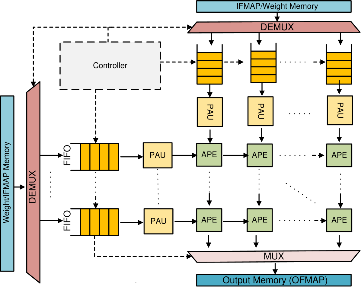
Figure 1: The overall template for TPU design.
## III TPU-Gen Framework
### III-A Architectural Template
Developing a Generic Template. The TPU architecture utilizes a systolic array of PEs with MAC units for efficient matrix and vector computations. This design enhances performance and reduces energy consumption by reusing data, minimizing buffer operations [1]. Input data propagates diagonally through the array in parallel. The TPU template, illustrated in Fig. 1, extends the TPU’s systolic array with Output Stationary (OS) dataflow to enable concurrent approximation of input feature maps (IFMaps) and weights. It comprises five components: weight/IFMap memory, FIFOs, a controller, Pre-Approximate Units (PAUs), and Approximate Processing Elements (APEs). The weights and IFMaps are stored in their respective memories, with the controller managing memory access and data transfer to FIFOs per the OS dataflow. PAUs, positioned between FIFOs and APEs, dynamically truncate high-precision operands to lower precision before sending them to APEs, which perform MAC operations using approximate multipliers and adders. Sharing PAUs across rows and columns reduces hardware overhead, introducing minimal latency but significantly improving overall performance [39].
Highly-Parameterized RTL Code. We design highly flexible and parameterized RTL codes for 13 different approximate adders and 12 different approximate multipliers as representative approximate circuits. For the approximate adders, we have two tunable parameters: the bit-width and the imprecise part. The bit-width specifies the number of bits for each operand and the imprecise part specifies the number of inexact bits in the adder output. For the approximate multipliers, we have one common parameter, i.e., Width (W), which specifies the bit-width of the multiplication operands. We also have more tunable parameters based on specific multipliers, some of which are listed in Table II.
TABLE II: Approximate multiplier hyper-parameters
| Design | Parameter | Description | Default |
| --- | --- | --- | --- |
| BAM [40] | VBL | No. of zero bits during partial product generation | W/2 |
| ALM_LOA [41] | M | Inaccurate part of LOA adder | W/2 |
| ALM_MAA3 [41] | M | Inaccurate part of MAA3 adder | W/2 |
| ALM_SOA [41] | M | Inaccurate part of SOA adder | W/2 |
| ASM [42] | Nibble_Width | number of precomputed alphabets | 4 |
| DRALM [37] | MULT_DW | Truncated bits of each operand | W/2 |
| RoBA [43] | ROUND_WIDTH | Scales the widths of the shifter | 1 |
We leveraged the parametrized RTL library of approximate arithmetic circuits to build a TPU library that enables automatic selection of the systolic array size $S$ , bit precision $n$ , and one of the approximate multipliers and approximate adders. The internal parameters that are used to tune the approximate arithmetic libraries are also included in the TPU parameterized RTL library, thus, allowing the user to have complete flexibility to adjust their designs to meet specific hardware specifications and application accuracy requirements. Moreover, we developed a design automation methodology, enabling the automatic implementation and simulation of many TPU circuits in various simulation platforms such as Design Compiler and Vivado. In addition to the highly parameterized RTL codes, we developed TCL and Python scripts to autonomously measure their error, area, performance, and power dissipation under various constraints.
### III-B Framework Overview
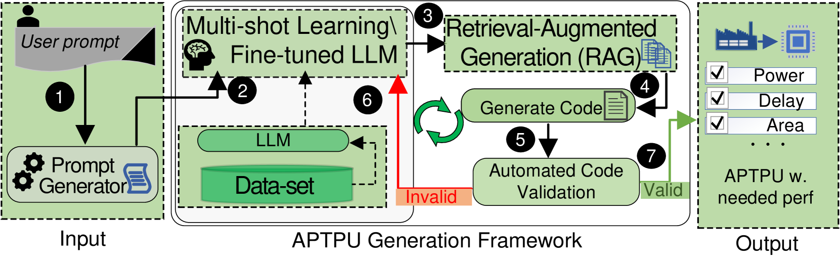
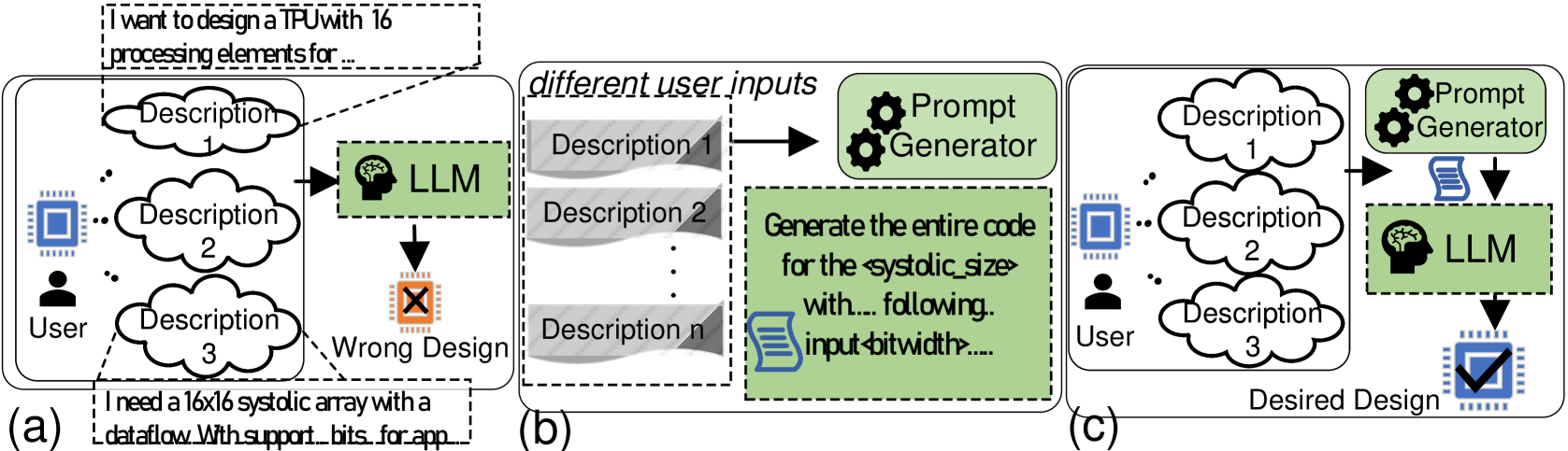
TPU-Gen framework depicted in Fig. 2 targets the development of domain-specific LLMs, emphasizing the interplay between the model’s responses and two key factors: the input prompt and the model’s learned parameters. The framework optimizes both elements to enhance LLM’s performance. An initial prompt conveying the user’s intent and key software and hardware specifications of the intended TPU design and application is enabled through the Prompt Generator in Step 1. A verbal description of a tensor processing accelerator design can often result in a many-to-one mapping as shown in Fig. 3 (a), especially when such descriptions do not align with the format of the training dataset. This misalignment increases the likelihood of hallucinations in the LLM’s output, potentially leading to faulty designs [44]. To minimize hallucinations and incorrect outputs in LLM-generated designs, studies have shown that inputs adhering closely to patterns observed in the training data produce more accurate and desirable results [17, 18]. However, this critical aspect has often been overlooked in previous state-of-the-art research [9], with some researchers opting instead to address the issue through prompt optimization techniques [18]. In this framework, we tackle the problem by employing a script that extracts key features, such as systolic size and relevant metrics, from any given verbal input by the user. These features are then embedded into a template, which serves as the prompt for the LLM input. As a domain-specific LLM, TPU-Gen focuses on generating the most valuable RTL top file detailing the circuit, and blocks involved in the presented architectural template in Section III.A.
<details>
<summary>x2.png Details</summary>
### Visual Description
## Diagram: APTPU Generation Framework
### Overview
The image illustrates a technical workflow for an "APTPU Generation Framework." The diagram outlines an automated process that takes a user prompt as input, utilizes a combination of Multi-shot Learning, Fine-tuned LLMs, and Retrieval-Augmented Generation (RAG) to generate code, validates that code, and outputs an Application-Specific Tensor Processing Unit (APTPU) that meets specific performance constraints (Power, Delay, Area).
### Components/Axes
The diagram is divided into three distinct vertical regions:
**1. Input (Left Region)**
* **User Icon:** Represents the source of the input.
* **"User prompt":** The initial text input.
* **"Prompt Generator":** A processing block containing gear icons and a document icon.
* **Flow Arrow 1:** Directs the user prompt into the Prompt Generator.
**2. APTPU Generation Framework (Center Region)**
* **"Multi-shot Learning / Fine-tuned LLM":** A primary processing block (top-left).
* **"Retrieval-Augmented Generation (RAG)":** A secondary processing block (top-right) containing a document stack icon.
* **"LLM" & "Data-set":** A lower-left block containing a cylinder icon (Data-set) and a rounded rectangle (LLM).
* **"Generate Code":** A processing block (center-right) with a document icon.
* **"Automated Code Validation":** A processing block (bottom-right).
* **Flow Arrows:**
* **Arrow 2:** Connects the "Prompt Generator" to the "Multi-shot Learning / Fine-tuned LLM" block.
* **Arrow 3:** Connects "Multi-shot Learning / Fine-tuned LLM" to "Retrieval-Augmented Generation (RAG)".
* **Arrow 4:** Connects "RAG" to "Generate Code".
* **Arrow 5:** Connects "Generate Code" to "Automated Code Validation".
* **Arrow 6 (Red):** A feedback loop from "Automated Code Validation" (labeled "Invalid") back to "Multi-shot Learning / Fine-tuned LLM".
* **Arrow 7 (Green):** An output path from "Automated Code Validation" (labeled "Valid") to the Output region.
* **Circular Arrow:** Located between "Generate Code" and "Automated Code Validation," indicating an iterative loop.
**3. Output (Right Region)**
* **Icons:** A factory icon pointing to a chip icon.
* **Checklist:** Three items with checkboxes: "Power", "Delay", "Area".
* **"APTPU w. needed perf":** The final label for the output.
### Detailed Analysis
* **Workflow Logic:**
1. **Initialization:** The user provides a prompt, which is processed by the "Prompt Generator."
2. **Knowledge Integration:** The "Prompt Generator" output feeds into the "Multi-shot Learning / Fine-tuned LLM" block. Simultaneously, the "Data-set" informs the "LLM," which supports the "Multi-shot Learning" block.
3. **Contextual Generation:** The "Multi-shot Learning" block feeds into the "RAG" module, which retrieves relevant information to assist in code generation.
4. **Code Creation:** The "RAG" module triggers the "Generate Code" block.
5. **Validation Loop:** The generated code is sent to "Automated Code Validation."
* **If Invalid (Red Path):** The system loops back to the "Multi-shot Learning / Fine-tuned LLM" block (Arrow 6), likely to refine the model or the prompt based on the failure.
* **If Valid (Green Path):** The system proceeds to the Output (Arrow 7).
6. **Iterative Refinement:** The circular arrow between "Generate Code" and "Automated Code Validation" suggests that the system may attempt multiple code generation iterations before declaring a result "Valid" or "Invalid."
### Key Observations
* **Feedback Mechanism:** The presence of the red "Invalid" arrow (Arrow 6) indicates a closed-loop system where the validation results directly influence the learning/fine-tuning process.
* **Hardware Focus:** The output is explicitly tied to hardware metrics ("Power", "Delay", "Area"), implying this framework is designed for hardware synthesis or hardware description language (HDL) generation.
* **Modularity:** The framework separates the "Learning/Fine-tuning" phase from the "Generation/Validation" phase, allowing for specialized handling of data retrieval (RAG) versus code generation.
### Interpretation
This diagram describes an **Automated Hardware Design Flow**. The framework leverages Large Language Models (LLMs) to automate the creation of hardware designs (APTPUs).
The investigative reading suggests that the system is designed to solve the "hallucination" or "inaccuracy" problem common in LLM-generated code by implementing a strict validation gate. By feeding "Invalid" results back into the "Multi-shot Learning / Fine-tuned LLM" block, the system performs a form of **Reinforcement Learning from Code Validation (RLCV)**. It does not just generate code; it learns from its own failures to ensure the final output meets the physical constraints of Power, Delay, and Area, which are critical in semiconductor design. The framework essentially treats hardware design as a software generation problem that is constrained by physical reality.
</details>
Figure 2: The proposed TPU-Gen framework.
<details>
<summary>x3.png Details</summary>
### Visual Description
## Diagram: Workflow for LLM-based Hardware Design
### Overview
This diagram illustrates a conceptual workflow for using Large Language Models (LLMs) to design hardware, specifically focusing on the transition from an ineffective, direct-prompting approach to a structured, prompt-engineered approach. The diagram is divided into three distinct sections: (a) the naive/failed approach, (b) the prompt generation process, and (c) the optimized/successful approach.
### Components/Axes
The diagram is organized horizontally from left to right, representing a process flow.
* **Section (a) - The Naive Approach:**
* **Top Dashed Box:** Contains the text: "I want to design a TPU with 16 processing elements for ..."
* **Left:** A "User" icon connected to three cloud-shaped bubbles labeled "Description 1", "Description 2", and "Description 3".
* **Right:** A green box labeled "LLM" (with a brain icon).
* **Bottom:** A red "X" over a chip icon labeled "Wrong Design".
* **Bottom Dashed Box:** Contains the text: "I need a 16x16 systolic array with a dataflow with support bits for app ..."
* **Section (b) - The Prompt Generation Process:**
* **Header:** "different user inputs"
* **Left:** A stack of gray boxes labeled "Description 1", "Description 2", "...", "Description n".
* **Top Right:** A green box with gear icons labeled "Prompt Generator".
* **Bottom Right:** A large green box containing a document icon and the text: "Generate the entire code for the <systolic_size> with... following.. input <bitwidth>....".
* **Section (c) - The Optimized Approach:**
* **Left:** A "User" icon connected to three cloud-shaped bubbles labeled "Description 1", "Description 2", and "Description 3".
* **Right:** A "Prompt Generator" (green box with gears) feeding into an "LLM" (green box with brain icon).
* **Bottom:** A blue checkmark over a chip icon labeled "Desired Design".
### Detailed Analysis
* **Section (a) Analysis:** This section depicts a direct interaction between a user and an LLM. The user provides vague, natural language descriptions (e.g., "I want to design a TPU..."). The LLM attempts to process this, but the outcome is marked with a red "X," indicating a "Wrong Design." This suggests that direct, unstructured prompting is insufficient for complex hardware generation.
* **Section (b) Analysis:** This section isolates the "Prompt Generator" component. It takes various "different user inputs" (Descriptions 1 through n) and processes them through a "Prompt Generator." The output is a structured template (the large green box) that forces the inclusion of specific technical parameters, specifically `<systolic_size>` and `<input_bitwidth>`.
* **Section (c) Analysis:** This section combines the elements from (a) and (b). The user provides descriptions, which are passed through the "Prompt Generator" to create a structured prompt. This structured prompt is then fed into the "LLM." The result is a blue checkmark over a chip icon, labeled "Desired Design," indicating a successful outcome.
### Key Observations
* **The "Prompt Generator" as a Bridge:** The diagram explicitly positions the "Prompt Generator" as the critical intermediary that transforms ambiguous user intent into actionable, structured technical specifications.
* **Parameterization:** The transition from (a) to (c) highlights the shift from natural language ("16 processing elements") to parameterized variables (`<systolic_size>`, `<input_bitwidth>`).
* **Failure vs. Success:** The visual contrast between the red "X" in (a) and the blue checkmark in (c) serves as a clear indicator of the efficacy of the proposed methodology.
### Interpretation
This diagram demonstrates the necessity of **Prompt Engineering** in the context of automated hardware design. It suggests that LLMs, while powerful, lack the inherent capability to derive precise hardware specifications (like systolic array dimensions or bit-widths) from vague, high-level user descriptions.
The "Prompt Generator" acts as a semantic translator. By forcing the user's input into a rigid template—specifically requesting variables like `<systolic_size>` and `<input_bitwidth>`—the system ensures the LLM receives the necessary constraints to generate functional, correct hardware code. This implies that for domain-specific tasks like hardware design, the "human-in-the-loop" or "automated-pre-processing" step is essential to bridge the gap between human intent and machine-executable code.
</details>
Figure 3: (a) Multiple descriptions for a single TPU design demonstrate that a design can be verbally defined in numerous ways, potentially misleading LLMs in generating the intended design, (b) Proposed prompt generator extracts the required features from the given verbal descriptions, (c) Using a script to generate a verbal description aligned with the training data.
An immediate usage of the proposed dataset explained in Section III.C in TPU-Gen is to help fine-tune a generic LLM for the task of TPU design, where the input with a prompt will be fed to the LLM (Step 2 in Fig. 2). Equivalently, one may employ ICL, or multi-shot learning as a more computationally efficient compromise to fine-tuning [24]. The multi-shot prompting techniques can be used where the proposed dataset will function as the source for multi-shot examples. Given that the TPU-Gen dataset integrates verbal descriptions with corresponding TPU systolic array design pairs, the LLM generates a TPU’s top-level file as the output in Verilog. This top-level file includes all necessary architectural module dependencies to ensure a fully functional design (step 3). Further, we propose to leverage the RAG module to generate the other dependency files into the project, completing the design (step 4). Next, a third-party quality evaluation tool can be employed to provide a quantitative evaluation of the design, verify functional correctness, and integrate the design with the full stack (step 5). Here, for quality and functional evaluation, the generated designs, initially described in Verilog, are synthesized using YOSYS [45]. This synthesis process incorporates an automated RTL-to-GDSII validation stage, where the generated designs are evaluated and classified as either Valid or Invalid based on the completeness of their code sequences and the correctness of their input-output relationships. Valid designs proceed to resource validation, where they are optimized with respect to Power, Performance, and Area (PPA) metrics. In contrast, designs flagged as Invalid initiate a feedback loop for error analysis and subsequent LLM retraining, enabling iterative refinement (steps 2 to 6) to achieve predefined performance criteria. Ultimately, designs that successfully pass these stages in step 7 are ready for submission to the foundry.
<details>
<summary>x4.png Details</summary>
### Visual Description
## Diagram: APTPU Workflow Process
### Overview
The image illustrates a five-step, iterative technical workflow designed to generate a dataset labeled "APTPU-Gen." The process begins with configuration files, moves through verification and reporting tools, incorporates a metrics corpus, and concludes with the generation of descriptive metrics.
### Components/Axes
The diagram is organized into a flow chart with distinct regions:
* **Top-Left (Blue Stack):** Labeled "APTPU CONFIG FILES."
* **Bottom-Left (Blue Box):** Labeled "Verification" with sub-text "Verify, Synthesize."
* **Bottom-Center (Blue Box):** Labeled "OpenRoad" with sub-text "PPA reports."
* **Top-Center (Orange Stack):** Labeled "APTPU + Metrics corpus."
* **Top-Right (Green Stack):** Labeled "APTPU + Metrics + Descriptions."
* **Bottom-Right (Database Icon):** Labeled "APTPU-Gen."
* **Icons/Connectors:**
* **Gears:** Located near the arrow for Step 1.
* **Circular Arrow:** Located between the Blue Stack and Orange Stack, labeled "Iterative process."
* **Scroll Icon:** Located near the arrow for Step 4, labeled "granulated prompt."
* **Numbered Circles (1-5):** Indicate the sequence of the workflow.
### Detailed Analysis
The workflow proceeds as follows:
1. **Step 1:** An arrow points downward from the **APTPU CONFIG FILES** (Blue Stack) to the **Verification** box. The text "Tune variables, features" is placed next to this arrow, accompanied by a gear icon, indicating the tuning phase.
2. **Step 2:** An arrow points to the right from the **Verification** box to the **OpenRoad** box. The **OpenRoad** box contains the text "PPA reports," indicating the output of this stage.
3. **Step 3:** An arrow points upward from the **OpenRoad** box to the **APTPU + Metrics corpus** (Orange Stack).
4. **Iterative Loop:** A circular arrow labeled "Iterative process" connects the **APTPU + Metrics corpus** back to the **APTPU CONFIG FILES**, suggesting that the metrics gathered inform future configuration tuning.
5. **Step 4:** An arrow points to the right from the **APTPU + Metrics corpus** to the **APTPU + Metrics + Descriptions** (Green Stack). This arrow passes through a scroll icon labeled "granulated prompt."
6. **Step 5:** An arrow points downward from the **APTPU + Metrics + Descriptions** (Green Stack) to the **APTPU-Gen** database icon.
### Key Observations
* **Centrality of OpenRoad:** The "OpenRoad" component acts as the primary analytical engine, converting verified configurations into PPA (Power, Performance, Area) reports.
* **Iterative Feedback:** The "Iterative process" loop indicates that the system is self-optimizing; the metrics corpus is used to refine the initial configuration files.
* **Transformation:** The transition from the Orange Stack to the Green Stack (Step 4) involves a "granulated prompt," suggesting a transformation or enrichment process (likely using a generative model) to add descriptive text to the raw metrics.
### Interpretation
This diagram represents an automated pipeline for hardware design or optimization, likely within the context of chip design (given the reference to "OpenRoad," a common open-source tool for digital layout).
* **The Logic:** The workflow demonstrates a "closed-loop" system. By generating PPA reports and aggregating them into a "Metrics corpus," the system can feed data back into the "APTPU CONFIG FILES" to improve future iterations.
* **The "Granulated Prompt":** This is the most critical transformation point. It implies that raw numerical data (metrics) is being processed through a prompt-based system (likely an LLM or similar AI) to generate human-readable or structured "Descriptions."
* **The Outcome:** The final "APTPU-Gen" database represents a refined, enriched dataset that combines raw configuration, performance metrics, and descriptive insights, making it highly valuable for training models or performing comparative analysis on hardware designs.
</details>
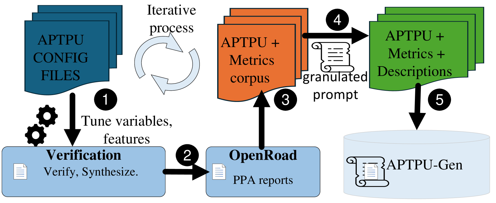
Figure 4: TPU-Gen dataset curation.
### III-C Dataset Curation
Leveraging the parameterized RTL code of the TPU, we develop a script to systematically explore various architectural configurations and generate a wide range of designs within the proposed framework (step 1 in Fig. 4). The generated designs undergo synthesis and functional verification (step 2). Subsequently, the OpenROAD suite [46] is employed to produce PPA metrics (step 3). The PPA data is parsed using Pyverilog (step 4), resulting in the creation of a detailed, multi-level dataset that captures the reported PPA metrics (step 5). Steps 1 to 3 are iterated until all architectural variations are generated. The time required for each data point generation varies depending on the specific configuration. To efficiently populate the TPU-Gen dataset, we utilize multiple scripts that automate the generation of data points across different systolic array sizes, ensuring comprehensive coverage of design space exploration. Fig. 4 shows the detailed methodology underpinning our dataset creation. The validation when compared to prior works [10, 47] understanding we work in a different design space abstraction makes it tough to have a fair comparison. However, looking by the scale of operation and the framework’s efficiency we require minimal efforts comparatively.
<details>
<summary>x5.png Details</summary>
### Visual Description
## Diagram: Architecture of an Approximate Processing Tensor Processing Unit (APTPU)
### Overview
The image is a technical block diagram illustrating the architecture of an **APTPU (Approximate Processing Tensor Processing Unit)** of size **MxN**. The diagram depicts the data flow of **IFMap** (Input Feature Map) and **Weight** inputs into a grid of processing units. It also includes a legend defining parameter ranges for data widths and a list of specific approximate arithmetic components (adders and multipliers) utilized in the design.
### Components/Axes
**1. Main Diagram (Center-Left)**
* **Outer Boundary:** A large light-blue box labeled **PAU** (Processing Approximate Unit).
* **Processing Grid:** Inside the PAU, there is a 2x2 grid of green square processing units.
* **Internal Unit Logic:** Each green square contains:
* A circle labeled **X** (Multiplier).
* A yellow rectangle labeled **<<** (Shifter).
* A grey rectangle labeled **+** (Adder).
* A label **APE** located below the adder.
* **Inputs:**
* **IFMap:** Two inputs entering from the left, passing through blue square buffer/register blocks.
* **Weight:** Two inputs entering from the top, passing through blue square buffer/register blocks.
* **Flow:**
* Dashed yellow arrows indicate the flow of IFMap data into the processing units.
* Dashed blue arrows indicate the flow of Weight data into the processing units.
* Solid red arrows indicate internal data flow between the Multiplier (X) and the Shifter (<<).
* Solid black arrows indicate data flow between the Shifter (<<) and the Adder (+), as well as between processing units.
**2. Legend (Top-Right)**
* **Solid Black Line:** Labeled **DW : [8,16,32]** (Data Width).
* **Dotted Black Line:** Labeled **WW : [3,4,5,6,7,8,16,32]** (Weight Width).
* **Solid Red Line:** Labeled **Mult_DW : [2,3,4,...,12]** (Multiplier Data Width).
**3. Component Lists (Right-Center)**
* **Approximate Adders:** A box containing "SETA, HERLOA, MHEAA...10 more".
* **Approximate Multipliers:** A box containing "BAM, UDM, ALM_LOA...10 more".
### Detailed Analysis
* **Data Flow Logic:**
* The IFMap inputs enter the left side of the PAU, pass through blue blocks, and are fed into the left column of the 2x2 grid.
* The Weight inputs enter the top of the PAU, pass through blue blocks, and are fed into the top row of the 2x2 grid.
* Within each processing unit, the operation sequence appears to be: Multiplication (X) $\rightarrow$ Shifting (<<) $\rightarrow$ Addition (+).
* The label **APE** (likely Approximate Processing Element) is associated with the adder component in each unit.
* **Legend/Parameter Mapping:**
* **DW (Data Width):** Supports 8, 16, or 32 bits.
* **WW (Weight Width):** Supports a granular range of 3, 4, 5, 6, 7, 8, 16, or 32 bits.
* **Mult_DW (Multiplier Data Width):** Supports a range from 2 to 12 bits.
### Key Observations
* **Modularity:** The diagram labels the system as **APTPU (MxN)**, implying the 2x2 grid shown is a representative tile of a larger, scalable array.
* **Approximate Computing:** The explicit inclusion of "Approximate Adders" and "Approximate Multipliers" lists suggests this architecture is designed for error-tolerant applications, such as Deep Learning inference, where precision can be traded for power efficiency or speed.
* **Configurability:** The legend highlights a high degree of configurability in bit-widths (DW, WW, Mult_DW), allowing the architecture to adapt to different precision requirements.
### Interpretation
This diagram represents a hardware accelerator architecture designed for neural network inference.
* **Functionality:** The "PAU" (Processing Approximate Unit) acts as the fundamental compute tile. By utilizing "Approximate" arithmetic units (like SETA, HERLOA, BAM, UDM), the design aims to reduce the computational cost (power/area) of matrix multiplication, which is the primary operation in neural networks.
* **Data Path:** The flow suggests a systolic-like or grid-based array where IFMaps and Weights are streamed into the processing elements. The inclusion of shifters (<<) suggests the architecture supports fixed-point arithmetic or scaling operations necessary for neural network quantization.
* **Design Philosophy:** The "10 more" notation in the component lists indicates that this architecture is designed as a framework or a testbed to evaluate various approximate computing techniques, rather than being locked into a single specific adder or multiplier design. It is a flexible, research-oriented hardware template.
</details>
Figure 5: An example of one category and its design space parameters.
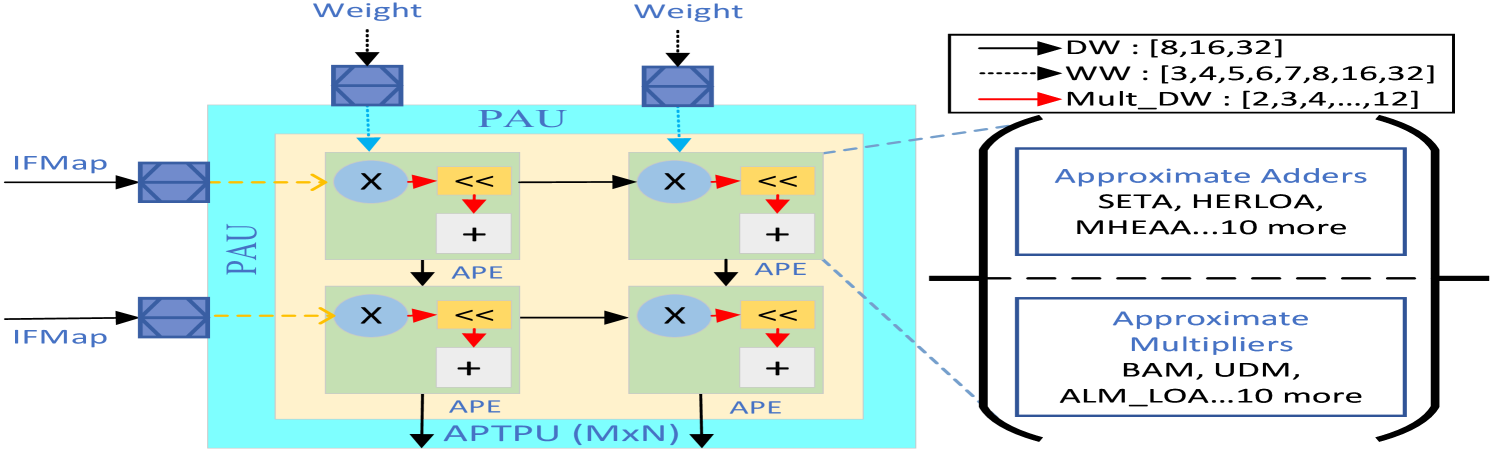
Fig. 5 visualizes the selection of different circuits to make PAUs and APEs accommodating different input Data Widths (DW) (8, 16, 32 bits) and Weight Widths (WW) (ranging from 3 to 32 bits) to generate approximate MAC units. These feature units highlight the flexible template of the TPU and enhance its adaptability and performance across various DNN workloads. Including lower bit-width weights is particularly advantageous for highly quantified models, enabling efficient processing with reduced computational resources.
<details>
<summary>x6.png Details</summary>
### Visual Description
## Technical Document: Configurable Systolic Array Design and Metrics
### Overview
The image displays a technical summary, likely extracted from a research paper or hardware design report. It presents a two-column layout: the left column provides specific performance metrics and Verilog preprocessor code snippets, while the right column provides hierarchical textual summaries (Block, Detailed Global, and High-Level) describing the design's configurability and approximate computing capabilities.
### Components/Layout
* **Left Column (Code & Metrics):** Contains a JSON-formatted metrics object at the top, followed by Verilog preprocessor directives (`define`, `ifdef`, `elsif`) used for hardware configuration.
* **Right Column (Textual Summaries):** Contains three distinct text blocks labeled "BLOCK SUMMARY", "DETAILED GLOBAL SUMMARY", and "HIGH-LEVEL GLOBAL SUMMARY".
### Detailed Analysis
#### Left Column: Metrics and Code Snippets
**Metrics Object:**
```json
{"Area": "29162", "WNS": "-12.268", "Total Power": "4.21e-03"}
```
* *Note:* The negative WNS (Worst Negative Slack) of -12.268 indicates a timing violation in the current design configuration.
**Verilog Code Snippets:**
* `define DW 8` // Choose IFMAP bitwidth
* `define M 4` // Choose M dimensions of the systolic array
* `define N 4` // Choose N dimensions of the systolic array
* `define HERLOA` // APADDER (Approximate Adder)
* Conditional logic block:
* `ifdef MITCHELL` -> `define SHARED_PRE_APPROX`
* `elsif ALM_SOA` -> `define SHARED_PRE_APPROX`
* `elsif ALM_LOA` -> `define SHARED_PRE_APPROX`
* `elsif ROBA` -> ... (truncated)
#### Right Column: Textual Summaries
**BLOCK SUMMARY**
* `block_0`: Defines preprocessor macros for design parameters: nibble width (`NIBBLE_WIDTH`), IFMAP bitwidths (`DW`), systolic array dimensions (`M` and `N`), and approximate multiplier precision (`MULT_DW`).
* `block_4`: Relates to different approximate computing configurations and the `ALM` macro.
**DETAILED GLOBAL SUMMARY**
* Describes the Verilog code as a 4x4 systolic array implementation.
* Mentions the selection of multipliers, adders, and other design choices.
* Highlights features like pre-approximation (`SHARED_PRE_APPROX`), controlled by preprocessor macro selection.
**HIGH-LEVEL GLOBAL SUMMARY**
* Summarizes the design as a highly configurable 4x4 systolic array.
* Utilizes specific components like the `HERLOA` adder.
* Emphasizes that the design is tailored for machine learning efficiency, allowing for improvements in area, power, and timing performance through the adjustment of preprocessor macros.
### Key Observations
* **Configurability:** The design relies heavily on preprocessor macros (`define`) to toggle between different approximate computing algorithms (MITCHELL, ALM_SOA, ALM_LOA, ROBA).
* **Approximate Computing:** The presence of `HERLOA` (likely a specific approximate adder architecture) and `SHARED_PRE_APPROX` indicates the design is optimized for approximate computing, which is common in neural network accelerators to reduce power and area.
* **Truncation:** The text contains several ellipses ("...."), indicating that the provided text is a summary or excerpt from a larger, more comprehensive document.
### Interpretation
This document outlines a hardware design framework for a systolic array, which is a standard architecture for accelerating matrix multiplication in machine learning workloads.
* **Design Intent:** The use of conditional compilation (`ifdef`/`elsif`) suggests a "design space exploration" approach. The engineer can swap out different approximate computing modules (like MITCHELL or ROBA) without rewriting the core logic, allowing for rapid testing of different accuracy-vs-efficiency trade-offs.
* **Performance Implications:** The metrics provided (`Area: 29162`, `WNS: -12.268`, `Total Power: 4.21e-03`) represent a specific snapshot of the design. The negative WNS (Worst Negative Slack) is a critical finding; it suggests that this specific configuration is failing to meet the required timing constraints (setup time) at the target clock frequency. This implies that while the design is configurable, not all configurations are necessarily "timing-clean" or ready for synthesis without further optimization or frequency scaling.
* **Conclusion:** The document serves as a high-level overview of a flexible, approximate-computing-enabled hardware accelerator, likely intended for researchers or engineers evaluating the impact of different approximation techniques on hardware metrics.
</details>
Figure 6: An example of a data point by adapting MG-V format.
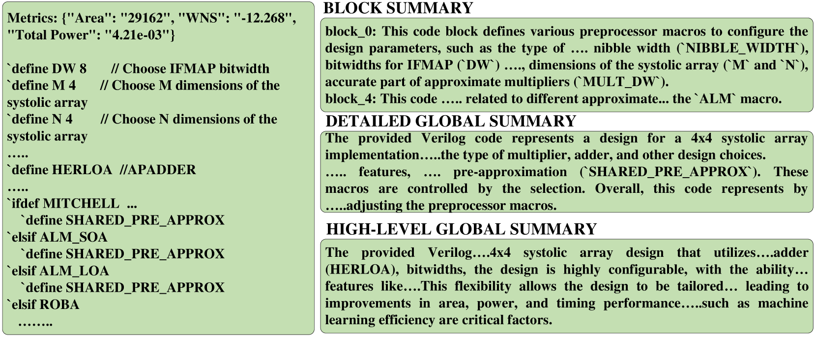
TPU-Gen dataset offers 29,952 possible variations for a systolic array size with 8 different systolic array implementations to facilitate various workloads spanning from 4 $\times$ 4 for smaller loads to 256 $\times$ 256 to crunch bigger DNN workloads. Accounting for the systolic size variations in the TPU-Gen dataset promises a total of 29,952 $\times$ 8 = 2,39,616 data points with PPA metrics reported. While TPU-Gen is constantly growing with newer data points, we checkpoint our dataset creation currently reported as having 25,000 individual TPU designs. We provide two variations: $(i)$ A top module file consisting of details of the entire circuit implementation, which can be used in cases such as RAG implementation to save the computation resources, and $(ii)$ A detailed, multi-level granulated dataset, as depicted in Fig. 6, is curated by adapting MG-Verilog [17] to assist LLM in generating Verilog code to support the development of a highly sophisticated, fine-tuned model. This model facilitates the automated generation of individual hardware modules, intelligent integration, deployment, and reuse across various designs and architectures. Please note that due to the domain-specific nature of the dataset, some data redundancy is inevitable, as similar modules are reused and reconfigured to construct new TPUs with varying architectural configurations. This structured dataset enables efficient exploration and customization of TPU designs while ensuring that the generated modules can be systematically adapted for different design requirements, leading to enhanced flexibility and scalability in hardware design automation. Additionally, we provide detailed metrics for each design iteration, which aid the LLM in generating budget-constrained designs or in creating an efficient design space exploration strategy to accelerate the result optimization process.
TABLE III: Prompts to successfully generate exact TPU modules via TPU-Gen.
| LLM Model Mistral-7B (Q3) | Module Generation Pass@1 17% | Module Integration Pass@3 83% | Pass@5 100% | Pass@10 100% | Pass@1 0% | Pass@3 25% | Pass@5 75% | Pass@10 100% |
| --- | --- | --- | --- | --- | --- | --- | --- | --- |
| CodeLlama-7B (Q4) | 0% | 50% | 83% | 100% | 0% | 50% | 75% | 100% |
| CodeLlama-13B (Q4) | 66% | 83% | 100% | 100% | 25% | 75% | 100% | 100% |
| Claude 3.5 Sonnet | 83% | 100% | 100% | 100% | 75% | 100% | 100% | 100% |
| ChatGPT-4o | 83% | 100% | 100% | 100% | 50% | 100% | 100% | 100% |
| Gemmini Advanced | 50% | 50% | 74% | 91% | 25% | 75% | 74% | 91% |
## IV Experiment Results
### IV-A Objectives
We designed four distinct experiments employing various approaches, each tailored to the unique capabilities of LLMs such as GPT [48], Gemini [49], and Claude [50], as well as the best open-source models from the leader board [51]. Each model is deployed in experiments aligning with the study’s objectives and anticipated outcomes. Experiments 1 focus on observing the prompting mechanism that assists LLM in generating the desired output by implementing ICL; with this knowledge, we develop the prompt template discussed in Sections III-B. Experiment 2 focuses on adapting the proposed TPU-Gen framework by fine-tuning LLM models. For fine-tuning, we used 4 $\times$ A100 GPU with 80GB VRAM. Experiment 3 is to demonstrate the effectiveness of RAG in TPU-Gen and it’s applicability for hardware design. Experiment 4 tests the TPU-Gen framework’s ability to generate designs efficiently with an industry-standard 45nm technology library. Throughout the process, we also consider hardware under the given PPA budget to ensure the feasibility of achieving the objectives outlined in the initial phases.
### IV-B Experiments and Results
<details>
<summary>x7.png Details</summary>
### Visual Description
## Combined Bar Charts: Performance Analysis of LLMs
### Overview
The image displays two distinct bar charts, labeled (a) and (b).
* **Chart (a)** compares the "Average Prompts for LLMs" between "Commercial LLMs" and "Open-Sourced LLMs" across a range of "APTPU Modules" (1 through 28). It includes trendlines for both categories.
* **Chart (b)** displays the "Number of Prompts" for six specific LLM models, labeled 1 through 6.
### Components/Axes
**Chart (a):**
* **X-Axis:** "APTPU Modules", scaled from 0 to 28, with major ticks every 5 units.
* **Y-Axis:** "Average Prompts for LLMs", scaled from 0 to 25, with major ticks every 5 units.
* **Legend (Top):**
* **Commercial LLMs:** Represented by black bars.
* **Open-Sourced LLMs:** Represented by grey bars.
* **Trendline Commercial:** Blue dashed line.
* **Trendline Open-Sourced:** Red dashed line.
**Chart (b):**
* **X-Axis:** "LLM Models", labeled 1 through 6.
* **Y-Axis:** "Number of Prompts", scaled from 0 to 8, with major ticks every 2 units.
* **Legend (Top-Left):** Maps the bars (1-6) to specific models:
1. **ChatGPT 4o** (Black)
2. **Gemmini Advanced** (Dark Grey)
3. **Claude** (Medium Grey)
4. **Codellama 13B** (Light Grey)
5. **Codellama 7B** (Lighter Grey)
6. **Mistral 7B** (White/Very Light Grey)
---
### Detailed Analysis
#### Chart (a): Average Prompts vs. APTPU Modules
* **Trend Verification:**
* **Commercial LLMs (Black Bars):** The trendline (blue dashed) shows a gradual, linear upward slope. The bars start near 0-2 prompts and rise to approximately 6-8 prompts by module 28.
* **Open-Sourced LLMs (Grey Bars):** The trendline (red dashed) shows a curvilinear trend. It starts at ~5, rises sharply to a peak around module 20, and then slightly declines.
* **Data Points:**
* **Modules 1-8:** Commercial LLMs are consistently low (approx. 2-3 prompts). Open-Sourced LLMs are consistently higher (approx. 8 prompts).
* **Modules 9-28:** There is a distinct "step-up" in performance for Open-Sourced LLMs, jumping to a range of ~18-20 prompts. Commercial LLMs show a slow, steady increase from ~4 to ~8 prompts over this same period.
* **Peak:** The highest performance for Open-Sourced LLMs appears around module 11 (approx. 20.3 prompts) and module 24 (approx. 20.3 prompts).
#### Chart (b): Number of Prompts per LLM Model
* **Data Points (Approximate):**
* **1 (ChatGPT 4o):** 1 prompt.
* **2 (Gemmini Advanced):** 2 prompts.
* **3 (Claude):** 1 prompt.
* **4 (Codellama 13B):** 5 prompts.
* **5 (Codellama 7B):** 7 prompts.
* **6 (Mistral 7B):** 4 prompts.
---
### Key Observations
* **Performance Gap:** In Chart (a), Open-Sourced LLMs significantly outperform Commercial LLMs in terms of "Average Prompts" across all tested APTPU modules.
* **Step-Function:** There is a clear inflection point for Open-Sourced LLMs at module 9, where performance jumps from ~8 to ~18.
* **Model Variance:** In Chart (b), there is high variance in prompt counts among the models. The "Codellama" family (7B and 13B) shows significantly higher prompt counts (5-7) compared to the proprietary models like ChatGPT 4o and Claude (1).
### Interpretation
The data suggests a strong correlation between model type and the "Average Prompts" metric within the context of "APTPU Modules" (likely referring to a specific hardware configuration, such as Tensor Processing Units).
The discrepancy between the two charts is notable:
1. **Chart (a)** implies that "Open-Sourced LLMs" as a category are highly efficient or capable of handling higher prompt volumes on this hardware.
2. **Chart (b)** provides a granular look at specific models, showing that the "Codellama" models (which are open-source) handle more prompts than the proprietary models listed (ChatGPT 4o, Gemmini, Claude).
**Reading between the lines:** The "APTPU Modules" likely represent a scaling factor for compute resources. The data demonstrates that Open-Sourced models are better optimized for this specific hardware architecture, or that the proprietary models are being throttled or are less efficient in this specific testing environment. The "step-up" at module 9 in Chart (a) suggests a threshold effect where the Open-Sourced models gain a significant advantage once a certain amount of hardware resource is allocated.
</details>
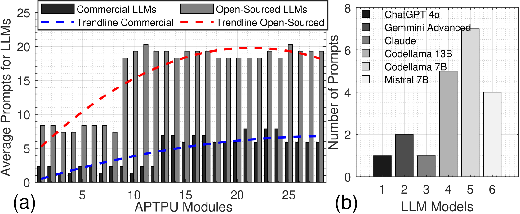
Figure 7: Average TPU-Gen prompts for (a) Module Generation, and (b) Module Integration via LLMs.
#### IV-B 1 Experiment 1: ICL-Driven TPU Generation and Approximate Design Adaptation.
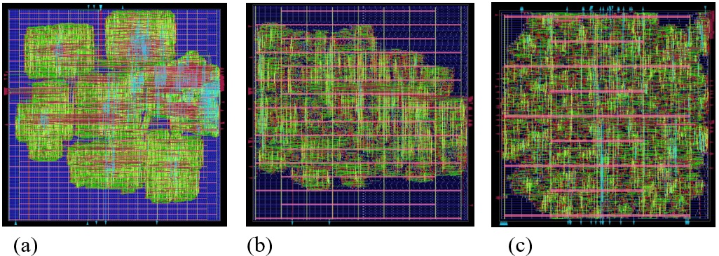
We evaluate the capability of LLMs to generate and synthesize a novel TPU architecture and its approximate version using TPU-Gen. Utilizing the prompt template from [18], we refined it to harness LLM capabilities better. LLM performance is assessed on two metrics: $(i)$ Module Generation —the ability to generate required modules, and $(ii)$ Module Integration —the capability to construct the top module by integrating components. We tested commercial models like [48, 49] via chat interfaces and open-source models listed in Table III, using LM Studio [52]. For the TPU, we successfully developed the design and obtained the GDSII layout (Fig. 8 (a)). Commercial models performed well with a single prompt at pass@1, averaging 72% in module generation and 50% in integration. Open-source models performed better with the increase of pass@k, averaging 72% for pass@1 in module generation to 100% and 50% to 100% upscale from pass@3 to pass@10 in integration. For the approximate TPU, involving approximate circuit algorithms, we provided example circuits and used ICL and Chain of Thought (CoT) to guide the LLMs. Open-source models struggled due to a lack of specialized knowledge, as shown in Fig. 7. The design layout from this experiment is in Fig. 8 (b). All outputs were manually verified using test benches. This is the first work to generate both exact and approximate TPU architectures using prompting to LLM. However, significant human expertise and intervention are required, especially for complex architectures like approximate circuits. To minimize the human involvement, we implement fine-tuning.
Takeaway 1. LLMs with efficient prompting are capable of generating exact and approximate TPU modules and integrate them to create complete designs. However, human involvement is extensively required, especially for novel architectures. Fine-tuning LLMs is necessary to reduce human intervention and facilitate the exploration of new designs.
#### IV-B 2 Experiment 2: Full TPU-Gen Implementation
This experiment investigates cost-efficient approaches for adapting domain-specific language models to hardware design. In previous experiments, we observed that limited spatial and hierarchical hardware knowledge hindered LLM performance in integrating circuits. The TPU-Gen template (Fig. 2) addresses this by delegating creative tasks to the LLM and retrieving dependent modules via RAG, optimizing AI accelerator design while reducing computational overhead and minimizing LLM hallucinations. ICL experiments show that fine-tuning enhances LLM reliability. The TPU-Gen proposes a way to develop domain-specific LLMs with minimal data. The experiment used a TPU-Gen dataset version 1 of 5,000 Verilog headers DW and WW inputs. This dataset comprises systolic array implementations with biased approximate circuit variations. We split data statically in 80:20 for training and testing open-source LLMs [51], with two primary goals of $1.$ Analyzing the impact of the prompt template generator on the fine-tuned LLM’s performance (Table IV). $2.$ Investigating the RAG model for hardware development.
<details>
<summary>extracted/6256789/Figures/GDSII.jpg Details</summary>
### Visual Description
## Diagram: Comparison of Integrated Circuit (IC) Placement and Routing Layouts
### Overview
The image displays three distinct physical design layouts for an integrated circuit, labeled (a), (b), and (c). These diagrams represent different stages or methodologies in the VLSI (Very Large Scale Integration) design flow, specifically focusing on the placement of logic cells and the routing of interconnects on a silicon die.
### Components/Axes
* **Labels:** (a), (b), and (c) are positioned directly below their respective diagrams.
* **Visual Elements (Common to all):**
* **Green Blocks:** Represent standard cells or logic clusters.
* **Blue Grid:** Represents the underlying floorplan or placement grid.
* **Pink/Red Lines:** Represent power/ground rails or global routing tracks.
* **Cyan/Light Blue Lines:** Represent signal routing or specific net connections.
### Detailed Analysis
#### (a) Left: Clustered/Hierarchical Placement
* **Visual Trend:** The layout is characterized by distinct, separated "islands" of green logic blocks.
* **Spatial Distribution:** There is significant empty space (blue grid) between the clusters. The logic is not uniformly distributed across the die.
* **Routing:** Routing (cyan lines) is concentrated within the clusters, with fewer long-distance connections between the islands.
* **Observation:** This layout suggests a hierarchical design approach where functional modules are kept physically separate to manage complexity or timing constraints.
#### (b) Center: Flat/Standard Cell Placement
* **Visual Trend:** The logic (green blocks) is distributed much more uniformly across the entire area of the die compared to (a).
* **Spatial Distribution:** The density of the green blocks is high and relatively consistent. There is very little empty space.
* **Routing:** The cyan signal routing is more complex and spans the entire die, indicating a "flattened" design where hierarchy has been removed to optimize area utilization.
* **Observation:** This represents a standard cell placement where the goal is to maximize the utilization of the silicon area.
#### (c) Right: Structured/Routing-Optimized Layout
* **Visual Trend:** This layout is highly structured. It features prominent, evenly spaced horizontal pink lines (likely power/ground rails) running across the entire die.
* **Spatial Distribution:** The green logic blocks are packed tightly between the horizontal rails.
* **Routing:** The cyan routing is dense and appears to follow a more rigid, grid-like structure compared to (b).
* **Observation:** This represents a mature, optimized layout, likely post-routing, where power distribution networks (the pink lines) have been integrated, and signal routing is constrained by the physical grid.
### Key Observations
* **Density Progression:** There is a clear progression in density from (a) to (c). (a) is sparse/clustered, (b) is dense/flat, and (c) is highly structured/optimized.
* **Structural Evolution:** The diagrams illustrate the transition from a logical/hierarchical view (a) to a physical implementation view (c).
* **Routing Complexity:** The complexity of the interconnects (cyan lines) increases significantly from (a) to (c), reflecting the transition from initial placement to final routing.
### Interpretation
The data demonstrates the evolution of an integrated circuit design through the Electronic Design Automation (EDA) flow:
1. **Hierarchical Design (a):** This is likely an early stage of the physical design. By clustering logic, designers can manage timing and congestion for specific modules independently. The large whitespace suggests this is not yet optimized for area.
2. **Flattening (b):** This represents the "flattening" of the design. The hierarchy is removed, and the tool attempts to place all cells to minimize the total wire length and area. This is a standard step to improve performance and reduce die size.
3. **Physical Implementation (c):** This is the final stage. The inclusion of the horizontal pink lines indicates the addition of the Power/Ground (P/G) grid. The logic is now constrained by these rails, and the routing is finalized.
**Peircean Investigative Note:** The progression from (a) to (c) is not merely visual; it is a functional progression. If one were to attempt to manufacture (a), it would likely be inefficient in terms of silicon area. If one were to attempt to manufacture (b) without the power grid seen in (c), the chip would fail due to voltage drop (IR drop) issues. Therefore, these images serve as a visual timeline of the physical design process, moving from logical intent (a) to physical reality (c).
</details>
Figure 8: A GDSII layout of (a) TPU, (b) TPU by prompting LLM, (c) approximate TPU by TPU-Gen framework.
All models used Low-Rank Adaptation (LoRA) fine-tuning with the Adam optimizer at a learning rate of $1e^{-5}$ . The fine-tuned models were evaluated to generate the desired results efficiently with a random prompt at pass@ $1$ to generate the TPU. From Table IV, we can observe that the outputs without the prompt generator are labeled as failures as they were unsuitable for further development and RAG integration. We can observe the same prompt when parsed to the prompt-template generator with a single try; we score an accuracy of 86.6%. Further, we used RAG and then processed the generated Verilog headers for module retrieval. According to [11], LLMs tend to prioritize creativity and finding innovative solutions, which often results in straying from the data. To address this, we employed a compute and cost-efficient method. This shows that the fine-tuning along with RAG can greatly enhance the performance. Fig. 8 (c) shows the GDSII layout of the design generated by the TPU-Gen framework.
TABLE IV: Prompt Generator vs Human inputs to Fine-tuned models.
| CodeLlama-7B-hf CodeQwen1.5 -7B Mistral -7B | 27 25 28 | 03 05 02 | 01 0 02 | 29 30 28 |
| --- | --- | --- | --- | --- |
| Starcoder2-7B | 24 | 06 | 0 | 30 |
Takeaway 2. Prompting techniques such as prompt template steer LLM to generate desired results after fine-tuning, as observed 86% success in generation. RAG, a cost-efficient method to generate the hardware modules reliably, completing the entire Verilog design for an application with minimal computational overhead.
#### IV-B 3 Experiment 3: Significance of RAG
To assess the effectiveness of RAG in the TPU-Gen framework, we evaluated 1,000 Verilog header codes generated by fine-tuned LLMs under two conditions: with and without RAG integration. Table V presents results over 30 designs tested by our framework to generate complete project files. Without RAG, failures occurred due to output token limitations and hallucinated variables. RAG is essential as the design is not a standalone file to compile. Validated header codes were provided in the RAG-enabled pipeline, and required modules were dynamically retrieved from the RAG database, ensuring fully functional and accurate designs. Conversely, models without RAG relied solely on internal knowledge, leading to hallucinations, token constraints, and incomplete designs. Models using RAG consistently achieved pass rates exceeding 95%, with Mistral-7B and CodeLlama-7B-hf attaining 100% success. In contrast, all models failed entirely without RAG, underscoring its pivotal role in ensuring design accuracy and addressing LLM limitations. RAG provides a robust solution to key challenges in fine-tuned LLMs for TPU hardware design by retrieving external information from the RAG database, ensuring contextual accuracy, and significantly reducing hallucinations. Additionally, RAG dynamically fetches dependencies in a modular manner, enabling the generation of complete and accurate designs without exceeding token limits. RAG is a promising solution in this context since our models were fine-tuned with only Verilog header data detailing design features. However, fine-tuning models with the entire design data would expose LLMs to severe hallucinations and token limitations, making generating detailed and functional designs challenging.
TABLE V: significance of RAG in TPU-Gen.
| CodeLama-7B-hf Mistral-7B CodeQwen1.5-7B | 100 100 95 | 0 0 5 | 0 0 0 | 100 100 100 |
| --- | --- | --- | --- | --- |
| StarCoder2-7B | 98 | 2 | 0 | 100 |
Takeaway 3. The experiment highlights the significance of the RAG usage with a fine-tuned model to avoid hallucinations and let LLM be creative consistently.
#### IV-B 4 Experiment 4: Design Generation Efficiency
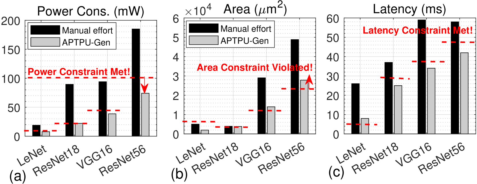
Building on the successful generation of approximate TPU in experiment 2, here we evaluate and benchmark the architectures produced by the TPU-Gen framework as the work performed in this paper is the first of it’s kind we are comparing against manual optimization created by expert human designers, focusing on power, area, and latency as shown in Fig. 9 (a)-(c). We utilize four DNN architectures for this evaluation: LeNet, ResNet18, VGG16, and ResNet56, performing inference tasks on the MNIST, CIFAR-10, SVHN, and CIFAR-100 datasets. In the manually optimized designs, a skilled hardware engineer fine-tunes parameters within the TPU template. This iterative optimization process is repeated until no further performance gains can be achieved within a reasonable timeframe of approximately one day [9], or the expert determines, based on empirical results, that additional refinements would yield minimal benefits. Using the PPA metrics as reference values (e.g., 100mW, 0.25mm 2, 48ms for ResNet56), both TPU-Gen and the manual user are tasked with generating the TPU architecture. Fig. 9 illustrates that across a range of network architectures, TPU-Gen consistently yields results with minimal deviation from the reference benchmarks. In contrast, the manual designs exhibit significant violations in terms of PPA.
<details>
<summary>x8.png Details</summary>
### Visual Description
## Bar Charts: Performance Comparison of Manual Effort vs. APTPU-Gen
### Overview
This image displays three grouped bar charts labeled (a), (b), and (c), comparing the performance of two design methodologies—"Manual effort" (black bars) and "APTPU-Gen" (grey bars)—across four neural network models: LeNet, ResNet18, VGG16, and ResNet56. The charts evaluate three metrics: Power Consumption, Area, and Latency. Red dashed lines indicate specific design constraints for each model.
### Components/Axes
* **Common Elements:**
* **X-axis:** Lists the four models: LeNet, ResNet18, VGG16, ResNet56.
* **Legend:** Located at the top-left of each chart. Black box = "Manual effort"; Grey box = "APTPU-Gen".
* **Chart (a) - Power Cons. (mW):**
* **Y-axis:** Power Consumption in milliwatts (mW), ranging from 0 to 200.
* **Annotation:** "Power Constraint Met!" with a red dashed line at 100 mW.
* **Chart (b) - Area ($\mu m^2$):**
* **Y-axis:** Area in square micrometers ($\mu m^2$), ranging from 0 to 6, with a multiplier of $\times 10^4$.
* **Annotation:** "Area Constraint Violated!" with stepped red dashed lines indicating specific constraints per model.
* **Chart (c) - Latency (ms):**
* **Y-axis:** Latency in milliseconds (ms), ranging from 0 to 60.
* **Annotation:** "Latency Constraint Met!" with stepped red dashed lines indicating specific constraints per model.
### Detailed Analysis
#### (a) Power Cons. (mW)
* **Trend:** Power consumption increases as the model complexity increases (from LeNet to ResNet56). In all cases, APTPU-Gen results in significantly lower power consumption than Manual effort.
* **Data Points (Approximate):**
* **LeNet:** Manual ~20 mW, APTPU-Gen ~10 mW.
* **ResNet18:** Manual ~90 mW, APTPU-Gen ~25 mW.
* **VGG16:** Manual ~95 mW, APTPU-Gen ~40 mW.
* **ResNet56:** Manual ~185 mW, APTPU-Gen ~75 mW.
* **Constraint:** The constraint is set at 100 mW. Manual effort violates this at ResNet56. APTPU-Gen remains below the constraint for all models.
#### (b) Area ($\mu m^2$)
* **Trend:** Area usage scales with model complexity. APTPU-Gen consistently produces a smaller area footprint than Manual effort.
* **Data Points (Approximate, $\times 10^4$):**
* **LeNet:** Manual ~0.5, APTPU-Gen ~0.2.
* **ResNet18:** Manual ~0.4, APTPU-Gen ~0.4.
* **VGG16:** Manual ~2.9, APTPU-Gen ~1.4.
* **ResNet56:** Manual ~4.9, APTPU-Gen ~2.8.
* **Constraint:** The constraint lines are stepped. Manual effort violates the constraint at VGG16 and ResNet56. APTPU-Gen remains below the constraint for all models.
#### (c) Latency (ms)
* **Trend:** Latency increases with model complexity. APTPU-Gen consistently achieves lower latency than Manual effort.
* **Data Points (Approximate):**
* **LeNet:** Manual ~26 ms, APTPU-Gen ~8 ms.
* **ResNet18:** Manual ~37 ms, APTPU-Gen ~25 ms.
* **VGG16:** Manual ~60 ms, APTPU-Gen ~34 ms.
* **ResNet56:** Manual ~58 ms, APTPU-Gen ~42 ms.
* **Constraint:** The constraint lines are stepped. Manual effort violates the constraint at VGG16 and ResNet56. APTPU-Gen remains below the constraint for all models.
### Key Observations
* **Consistent Superiority:** APTPU-Gen (grey bars) consistently produces lower values across all three metrics (Power, Area, Latency) compared to Manual effort (black bars) for every model tested.
* **Constraint Violations:** The "Manual effort" approach fails to meet the design constraints for the more complex models (VGG16 and ResNet56) in both Area and Latency, and for ResNet56 in Power.
* **Scaling:** As model complexity increases, the gap between Manual effort and APTPU-Gen generally widens, suggesting that APTPU-Gen is significantly more effective at optimizing larger, more complex neural networks.
### Interpretation
The data demonstrates that "APTPU-Gen" is a highly effective automated optimization tool for hardware design. While "Manual effort" is sufficient for smaller, simpler models like LeNet, it fails to meet performance and resource constraints as the complexity of the neural network increases (e.g., VGG16 and ResNet56). The APTPU-Gen methodology successfully keeps all metrics within the required constraints, indicating it provides a scalable solution for hardware implementation of deep learning models where manual design becomes inefficient or unfeasible.
</details>
Figure 9: PPA metrics comparison for TPU architectures generated by TPU-Gen and the manual user: (a) Power consumption, (b) Area, (c) Latency.
Takeaway 4. TPU-Gen consistently yields results with minimal deviation from the PPA reference, whereas the manual designs exhibit significant violations.
## V Conclusions
This paper introduces TPU-Gen, a novel dataset and a novel framework for TPU generation, addressing the complexities of generating AI accelerators amidst rapid AI model evolution. A key challenge, hallucinated variables, is mitigated using an RAG approach, dynamically adapting hardware modules. RAG enables cost-effective, full-scale RTL code generation, achieving budget-constrained outputs via fine-tuned models. Our extensive experimental evaluations demonstrate superior performance, power, and area efficiency, with an average reduction in area and power of 92% and 96% from the manual optimization reference values. These results set new standards for driving advancements in next-generation design automation tools powered by LLMs. We are committed to releasing the dataset and fine-tuned models publicly if accepted.
## References
- [1] N. Jouppi, C. Young, N. Patil, and D. Patterson, “Motivation for and evaluation of the first tensor processing unit,” IEEE Micro, vol. 38, no. 3, pp. 10–19, 2018.
- [2] H. Genc et al., “Gemmini: Enabling systematic deep-learning architecture evaluation via full-stack integration,” in 2021 58th ACM/IEEE Design Automation Conference (DAC). IEEE, 2021, pp. 769–774.
- [3] H. Sharma, J. Park, D. Mahajan, E. Amaro, J. K. Kim, C. Shao, A. Mishra, and H. Esmaeilzadeh, “From high-level deep neural models to fpgas,” in 2016 49th Annual IEEE/ACM International Symposium on Microarchitecture (MICRO). IEEE, 2016, pp. 1–12.
- [4] W.-Q. Ren et al., “A survey on collaborative dnn inference for edge intelligence,” Machine Intelligence Research, vol. 20, no. 3, pp. 370–395, 2023.
- [5] D. Vungarala, M. Morsali, S. Tabrizchi, A. Roohi, and S. Angizi, “Comparative study of low bit-width dnn accelerators: Opportunities and challenges,” in 2023 IEEE 66th International Midwest Symposium on Circuits and Systems (MWSCAS). IEEE, 2023, pp. 797–800.
- [6] P. Xu and Y. Liang, “Automatic code generation for rocket chip rocc accelerators,” 2020.
- [7] S. Angizi, Z. He, A. Awad, and D. Fan, “Mrima: An mram-based in-memory accelerator,” IEEE Transactions on Computer-Aided Design of Integrated Circuits and Systems, vol. 39, no. 5, pp. 1123–1136, 2019.
- [8] K. Chang, Y. Wang, H. Ren, M. Wang, S. Liang, Y. Han, H. Li, and X. Li, “Chipgpt: How far are we from natural language hardware design,” arXiv preprint arXiv:2305.14019, 2023.
- [9] Y. Fu, Y. Zhang, Z. Yu, S. Li, Z. Ye, C. Li, C. Wan, and Y. C. Lin, “Gpt4aigchip: Towards next-generation ai accelerator design automation via large language models,” in 2023 IEEE/ACM International Conference on Computer Aided Design (ICCAD). IEEE, 2023, pp. 1–9.
- [10] S. Thakur, B. Ahmad, H. Pearce, B. Tan, B. Dolan-Gavitt, R. Karri, and S. Garg, “Verigen: A large language model for verilog code generation,” ACM Transactions on Design Automation of Electronic Systems, vol. 29, no. 3, pp. 1–31, 2024.
- [11] X. Jiang, Y. Tian, F. Hua, C. Xu, Y. Wang, and J. Guo, “A survey on large language model hallucination via a creativity perspective,” arXiv preprint arXiv:2402.06647, 2024.
- [12] J. Blocklove, S. Garg, R. Karri, and H. Pearce, “Chip-chat: Challenges and opportunities in conversational hardware design,” in 2023 ACM/IEEE 5th Workshop on Machine Learning for CAD (MLCAD). IEEE, 2023, pp. 1–6.
- [13] S. Thakur, J. Blocklove, H. Pearce, B. Tan, S. Garg, and R. Karri, “Autochip: Automating hdl generation using llm feedback,” arXiv preprint arXiv:2311.04887, 2023.
- [14] R. Ma, Y. Yang, Z. Liu, J. Zhang, M. Li, J. Huang, and G. Luo, “Verilogreader: Llm-aided hardware test generation,” arXiv:2406.04373v1, 2024.
- [15] W. Fang et al., “Assertllm: Generating and evaluating hardware verification assertions from design specifications via multi-llms,” arXiv:2402.00386v1, 2024.
- [16] M. Liu, N. Pinckney, B. Khailany, and H. Ren, “Verilogeval: Evaluating large language models for verilog code generation,” arXiv:2309.07544v2, 2024.
- [17] Y. Zhang, Z. Yu, Y. Fu, C. Wan, and Y. C. Lin, “Mg-verilog: Multi-grained dataset towards enhanced llm-assisted verilog generation,” arXiv preprint arXiv:2407.01910, 2024.
- [18] D. Vungarala, M. Nazzal, M. Morsali, C. Zhang, A. Ghosh, A. Khreishah, and S. Angizi, “Sa-ds: A dataset for large language model-driven ai accelerator design generation,” arXiv e-prints, pp. arXiv–2404, 2024.
- [19] H. Wu et al., “Chateda: A large language model powered autonomous agent for eda,” IEEE Transactions on Computer-Aided Design of Integrated Circuits and Systems, 2024.
- [20] B. Nadimi and H. Zheng, “A multi-expert large language model architecture for verilog code generation,” arXiv preprint arXiv:2404.08029, 2024.
- [21] Y. Lu, S. Liu, Q. Zhang, and Z. Xie, “Rtllm: An open-source benchmark for design rtl generation with large language model,” in 2024 29th Asia and South Pacific Design Automation Conference (ASP-DAC). IEEE, 2024, pp. 722–727.
- [22] D. Vungarala, S. Alam, A. Ghosh, and S. Angizi, “Spicepilot: Navigating spice code generation and simulation with ai guidance,” arXiv preprint arXiv:2410.20553, 2024.
- [23] Y. Lai, S. Lee, G. Chen, S. Poddar, M. Hu, D. Z. Pan, and P. Luo, “Analogcoder: Analog circuit design via training-free code generation,” arXiv preprint arXiv:2405.14918, 2024.
- [24] D. Dai, Y. Sun, L. Dong, Y. Hao, S. Ma, Z. Sui, and F. Wei, “Why can gpt learn in-context? language models implicitly perform gradient descent as meta-optimizers,” arXiv preprint arXiv:2212.10559, 2022.
- [25] G. Izacard et al., “Atlas: Few-shot learning with retrieval augmented language models,” Journal of Machine Learning Research, vol. 24, no. 251, pp. 1–43, 2023.
- [26] J. Chen, H. Lin, X. Han, and L. Sun, “Benchmarking large language models in retrieval-augmented generation,” arXiv preprint arXiv:2309.01431, 2023.
- [27] R. Qin et al., “Robust implementation of retrieval-augmented generation on edge-based computing-in-memory architectures,” arXiv:2405.04700v1, 2024.
- [28] A. Roohi, S. Sheikhfaal, S. Angizi, D. Fan, and R. F. DeMara, “Apgan: Approximate gan for robust low energy learning from imprecise components,” IEEE Transactions on Computers, vol. 69, no. 3, pp. 349–360, 2019.
- [29] M. S. Ansari, B. Cockburn, and J. Han, “An improved logarithmic multiplier for energy-efficient neural computing,” IEEE Trans. on Comput., vol. 70, pp. 614–625, 2021.
- [30] S. Angizi, M. Morsali, S. Tabrizchi, and A. Roohi, “A near-sensor processing accelerator for approximate local binary pattern networks,” IEEE Transactions on Emerging Topics in Computing, vol. 12, no. 1, pp. 73–83, 2023.
- [31] H. Jiang, S. Angizi, D. Fan, J. Han, and L. Liu, “Non-volatile approximate arithmetic circuits using scalable hybrid spin-cmos majority gates,” IEEE Transactions on Circuits and Systems I: Regular Papers, vol. 68, no. 3, pp. 1217–1230, 2021.
- [32] S. Angizi, Z. He, A. S. Rakin, and D. Fan, “Cmp-pim: an energy-efficient comparator-based processing-in-memory neural network accelerator,” in Proceedings of the 55th Annual Design Automation Conference, 2018, pp. 1–6.
- [33] S. Angizi, H. Jiang, R. F. DeMara, J. Han, and D. Fan, “Majority-based spin-cmos primitives for approximate computing,” IEEE Transactions on Nanotechnology, vol. 17, no. 4, pp. 795–806, 2018.
- [34] M. E. Elbtity, H.-W. Son, D.-Y. Lee, and H. Kim, “High speed, approximate arithmetic based convolutional neural network accelerator,” 2020 International SoC Design Conference (ISOCC), pp. 71–72, 2020. [Online]. Available: https://api.semanticscholar.org/CorpusID:231826033
- [35] H. Younes, A. Ibrahim, M. Rizk, and M. Valle, “Algorithmic level approximate computing for machine learning classifiers,” 2019 26th IEEE Int. Conf. on Electron., Circuits and Syst. (ICECS), pp. 113–114, 2019.
- [36] S. Hashemi, R. I. Bahar, and S. Reda, “DRUM: A dynamic range unbiased multiplier for approximate applications,” 2015 IEEE/ACM Int. Conf. on Comput.-Aided Design (ICCAD), pp. 418–425, 2015.
- [37] P. Yin, C. Wang, H. Waris, W. Liu, Y. Han, and F. Lombardi, “Design and analysis of energy-efficient dynamic range approximate logarithmic multipliers for machine learning,” IEEE Transactions on Sustainable Computing, vol. 6, no. 4, pp. 612–625, 2021.
- [38] A. Dalloo, A. Najafi, and A. Garcia-Ortiz, “Systematic design of an approximate adder: The optimized lower part constant-or adder,” IEEE Transactions on Very Large Scale Integration (VLSI) Systems, vol. 26, no. 8, pp. 1595–1599, 2018.
- [39] M. E. Elbtity, P. S. Chandarana, B. Reidy, J. K. Eshraghian, and R. Zand, “Aptpu: Approximate computing based tensor processing unit,” IEEE Transactions on Circuits and Systems I: Regular Papers, vol. 69, no. 12, pp. 5135–5146, 2022.
- [40] F. Farshchi et al., “New approximate multiplier for low power digital signal processing,” The 17th CSI International Symposium on Computer Architecture & Digital Systems (CADS 2013), pp. 25–30, 2013.
- [41] W. Liu et al., “Design and evaluation of approximate logarithmic multipliers for low power error-tolerant applications,” IEEE Trans. on Circuits and Syst. I: Reg. Papers, vol. 65, pp. 2856–2868, 2018.
- [42] S. S. Sarwar et al., “Energy-efficient neural computing with approximate multipliers,” ACM Journal on Emerging Technologies in Computing Systems (JETC), vol. 14, pp. 1 – 23, 2018.
- [43] R. Zendegani et al., “Roba multiplier: A rounding-based approximate multiplier for high-speed yet energy-efficient digital signal processing,” IEEE Transactions on Very Large Scale Integration (VLSI) Systems, vol. 25, pp. 393–401, 2017. [Online]. Available: https://api.semanticscholar.org/CorpusID:206810935
- [44] M. Niu, H. Li, J. Shi, H. Haddadi, and F. Mo, “Mitigating hallucinations in large language models via self-refinement-enhanced knowledge retrieval,” arXiv preprint arXiv:2405.06545, 2024.
- [45] (2024) Yosys. [Online]. Available: https://github.com/YosysHQ/yosys
- [46] (2018) Openroad. [Online]. Available: https://github.com/The-OpenROAD-Project/OpenROAD
- [47] H. Pearce et al., “Dave: Deriving automatically verilog from english,” in MLCAD, 2020, pp. 27–32.
- [48] (2024) Openai gpt-4. [Online]. Available: https://openai.com/index/hello-gpt-4o/
- [49] (2024) Gemini. [Online]. Available: https://deepmind.google
- [50] (2023) Anthropic. [Online]. Available: https://www.anthropic.com
- [51] Evalplus leaderboard. https://evalplus.github.io/leaderboard.html. Accessed: 2024-09-21.
- [52] “Lm studio - discover, download, and run local llms,” https://lmstudio.ai/, accessed: 2024-09-21.