2503.06862v1

# ArXiv Paper 2503.06862v1 ## FIGLUT: An Energy-Efficient Accelerator Design for FP-INT GEMM Using Look-Up Tables Gunho Park 1 , 2 ∗ , Hyeokjun Kwon 1 ∗ , Jiwoo Kim 1 , Jeongin Bae 2 , Baeseong Park 2 , Dongsoo Lee 2 , and Youngjoo Lee 1 Pohang University of Science and Technology (POSTECH), 2 NAVER Cloud { gunho.park3 } @navercorp.com, { kwon36hj, youngjoo.lee } @postech.ac.kr Abstract -Weight-only quantization has emerged as a promising solution to the deployment challenges of large language models (LLMs). However, it necessitates FP-INT operations, which make implementation on general-purpose hardware like GPUs difficult. In this paper, we propose FIGLUT, an efficient look-up table (LUT)-based GEMM accelerator architecture. Instead of performing traditional arithmetic operations, FIGLUT retrieves precomputed values from an LUT based on weight patterns, significantly reducing the computational complexity. We also introduce a novel LUT design that addresses the limitations of conventional memory architectures. To further improve LUTbased operations, we propose a half-size LUT combined with a dedicated decoding and multiplexing unit. FIGLUT efficiently supports different bit precisions and quantization methods using a single fixed hardware configuration. For the same 3-bit weight precision, FIGLUT demonstrates 59% higher TOPS/W and 20% lower perplexity than state-of-the-art accelerator design. When targeting the same perplexity, FIGLUT achieves 98% higher TOPS/W by performing 2.4-bit operations. ## I. INTRODUCTION Pretrained Large Language Models (LLMs) have demonstrated remarkable performance in a wide range of language understanding and generation tasks. These models, predominantly based on the Transformer architecture [1], [3], [11], [29], [31], exhibit a predictable power-law scaling in performance relative to their parameter size. Consequently, the size of the model has increased to unprecedented levels, pushing the boundaries of what can be achieved in natural language processing. However, substantial growth in model size comes with significant challenges, particularly in terms of memory footprint. [26], [35] For instance, a model with 175 billion parameters, requiring approximately 350GB of memory, far exceeds the DRAM size of 80GB available in current stateof-the-art GPUs [28]. Additionally, memory bandwidth also becomes a critical issue, leading to significant memory bottlenecks. This bottleneck can severely impact the performance and efficiency of deploying such large models, as data transfer rates cannot keep up with the computational demands of the LLMs. This discrepancy highlights the urgent need for efficient methods to deploy such large models on hardware accelerator. One of the most promising approaches to mitigate the memory-related challenges of LLM is parameter quantization [7], [15], [32]. In the context of LLMs, there has been * Equal contribution. a shift toward weight-only quantization, where only weights are strongly quantized to sub-4-bit precision while activations remain in floating point (FP) format [4], [8]. This shift is motivated by the observation that the memory footprint of the weights significantly exceeds that of the activations in the LLM, and the presence of outliers in the activations further supports the effectiveness of weight-only quantization. Despite its advantages, weight-only quantization requires the use of non-standard FP-INT operations, posing an ongoing challenge. Recent studies have introduced efficient kernels for weightonly quantization, enabling practical speed-ups on GPUs [10], [25], [28], [36]. Although the kernels proposed in [10], [25] demonstrated faster speeds compared to cuBLAS, which is a GPU-accelerated library to accelerate HPC applications, including GEMM operation, these improvements largely stem from efficient data movement due to weight compression. However, during computation, the compressed weights are dequantized back to FP format, resulting in inefficiencies as the actual arithmetic operations are still performed using FPFP units. NVIDIA's recent release of new FP-INT GEMM kernels in CUTLASS [21] similarly relies on inherent FP operations. Efforts to overcome these inefficiencies have led to the proposal of LUT-based GEMM kernels [28], [36], which aim to perform FP-INT GEMM operations without dequantization. However, storing LUTs in shared memory on GPUs often leads to bank conflicts, causing inefficiencies because multiple threads access the same shared memory bank simultaneously. To address these issues, recent advancements propose novel hardware architectures designed to efficiently perform FPINT operations specifically tailored for weight-only quantized models [20]. These emerging solutions aim to bridge the gap between the theoretical benefits of weight-only quantization and practical deployment on existing hardware. For instance, iFPU [22] proposes an efficient bit-serial architecture accelerator utilizing binary-coding quantization (BCQ) format. In the BCQ format, the inner product of binary weights and input activations is replaced by the sum or subtraction of input activations. iFPU introduces a pre-alignment technique that aligns the exponents of input activations with FP values. Consequently, the operations on pre-aligned mantissas are handled by integer arithmetic units, efficiently performing FP-INT operations. Similarly, FIGNA [16] presents FP- TABLE I COMPARISON OF DIFFERENT HARDWARE ACCELERATORS | | FP-INT Operation | Mixed- Precision | BCQ Support | Computational Complexity | |------------|--------------------|--------------------|---------------|----------------------------| | GPU | ✗ | ✗ | ✗ | O ( mnk ) | | iFPU [22] | ✓ | ✓ | ✓ | O ( mnkq ) | | FIGNA [16] | ✓ | ✗ | ✗ | O ( mnk ) | | Proposed | ✓ | ✓ | ✓ | O ( mnkq/µ ) | INT4 multiplication employing the pre-alignment technique while addressing the inefficiencies inherent in the bit-serial structure adopted by iFPU. By using pre-alignment, FIGNA replaces FP-INT multiplication with integer multiplication between aligned mantissas and quantized weights, enhancing the efficiency of weight-only quantized model computations. However, FIGNA has limitations as it is fixed to a specific precision (e.g., 4-bit quantized weights), making it inefficient for models quantized to less than 4-bit precision or for those using mixed-precision quantization methods. In this paper, we propose FIGLUT, a novel accelerator architecture that leverages LUT-based GEMM to reduce the computational complexity of bit-serial accelerators. FIGLUT replaces arithmetic operations with table look-ups using weight patterns as keys, significantly enhancing computational efficiency. We introduce a specialized operator, the read-accumulate (RAC) unit, which replaces the conventional multiply-accumulate (MAC) unit found in traditional hardware accelerators. FIGLUT efficiently supports FP-INT operations for weight-only quantized models and employs a bit-serial structure to manage computations of various precisions within a single hardware framework. Moreover, by using the BCQ format for weight representation, FIGLUT can operate not only on BCQ models, which present state-of-the-art performance, but also on commonly used uniformly quantized models. As a result, FIGLUT enables efficient computation across different bit precisions and quantization methods on a single hardware platform, representing a significant advancement in the deployment of weight-only quantized models. Our major contributions in this work include the following: - We propose an LUT-based FP-INT GEMM method that replaces arithmetic operations with LUT reads, facilitating energy-efficient GEMM operations. - We introduce a novel specialized LUT architecture that enables simultaneous access to the LUT without bank conflicts during parallel processing. - We present FIGLUT, an innovative LUT-based FP-INT GEMM accelerator that efficiently supports various quantization methods and precisions on a single hardware platform by leveraging LUT-based operations. ## II. BACKGROUND ## A. Methods and Systems for Weight-Only Quantization Quantization is a powerful method for reducing computational complexity and memory footprint by converting highbit precision FP values into low-bit INT values. However, applying quantization to LLMs presents significant challenges, especially when attempting to quantize both weights and activations to lower bit precisions. Activation values, in particular, are more difficult to quantize than weight values due to the presence of outliers and their dynamic nature, which makes their distribution hard to predict accurately [9], [34]. This complexity necessitates specialized techniques to effectively manage the quantization of activations in LLMs. To address memory-related challenges such as memory bound of LLM inference and limited DRAM size, weightonly quantization methods have been extensively studied. These methods preserve accuracy by keeping the activations in FP format. Due to the significant accuracy drop observed with simple round-to-nearest (RTN) quantization, various techniques have been proposed to minimize quantization error. OPTQ [10] introduces a uniform quantization method that utilizes approximate second-order information from a calibration dataset to achieve sub-4-bit quantization with negligible accuracy loss. AWQ [25] proposes a weight-only quantization approach that selects salient weights based on activation distribution to minimize quantization error. Recently, nonuniform quantization techniques using BCQ have also demonstrated excellent performance. ShiftAddLLM [36] achieves state-of-the-art results by applying post-training bitwise shiftand-add reparameterization with non-uniform BCQ, enabling a multiplication-less LLM. Additionally, ShiftAddLLM improves the accuracy-efficiency trade-off by employing mixedprecision quantization based on the sensitivity of each layer. With the proven efficiency of weight-only quantization methods, various hardware accelerators have been proposed to support FP-INT operations between activations and weights. Table I compares the features of different hardware accelerators. Commercial GPUs lack FP-INT arithmetic units that can handle FP input activations and INT weights. As a result, a dequantization process is necessary to convert INT weights back to FP format for use with existing FP-FP arithmetic units. The FP-INT GEMM kernels proposed in [10] and [25] achieve better latency compared to cuBLAS FP-FP GEMM, thanks to efficient bandwidth utilization enabled by weight compression in memory-bound LLM applications. However, the absence of native FP-INT operations on GPUs undermines the advantages of weight quantization by necessitating FP-FP computations. To address inefficiencies in GPUs and effectively handle FPINT GEMM operations, several accelerator designs have been proposed. iFPU [22] introduces a method to efficiently process computation between weights in BCQ format and FP activations by pre-aligning the mantissas of input activations based on the maximum exponent value. This alignment allows FPINT operations to be replaced by INT-INT addition between mantissas and binary weights, reducing hardware complexity. While this bit-serial approach enables support for mixedprecision quantization, it inherently increases computational complexity in proportion to the bit precision q of the quantized weights. 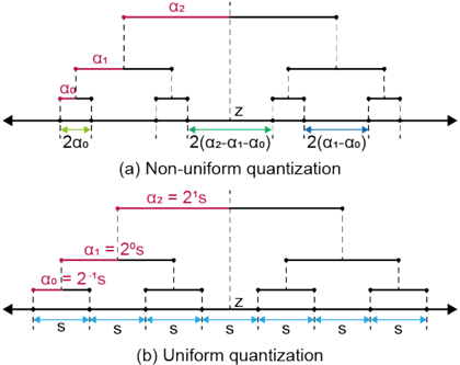FIGNA [16] addresses the computational overhead of bitserial architecture by proposing an FP-INT arithmetic unit Fig. 1. Extension of binary-coding quantization to support both non-uniform and uniform quantization formats, achieved by including a offset term ( q = 3 ). <details> <summary>Image 1 Details</summary>  ### Visual Description ## Diagram: Non-uniform vs. Uniform Quantization ### Overview The image compares two quantization methods: **non-uniform** (a) and **uniform** (b). Both diagrams use horizontal lines segmented into intervals, with labels, arrows, and legends to denote relationships between variables. --- ### Components/Axes #### (a) Non-uniform Quantization - **Horizontal Line**: Divided into three segments labeled **α₀**, **α₁**, and **α₂** (red, magenta, black, respectively). - **Arrows**: - Green arrow between α₀ and α₁: labeled **2α₀**. - Green arrow between α₁ and α₂: labeled **2(α₂ - α₁ - α₀)**. - Blue arrow between α₁ and α₂: labeled **2(α₁ - α₀)**. - **Legend**: - Red: α₂ - Magenta: α₁ - Black: α₀ - **Text**: "Non-uniform quantization" (top-center). #### (b) Uniform Quantization - **Horizontal Line**: Divided into equal segments labeled **S** (blue arrows). - **Labels**: - α₀ = 2⁻¹s (0.5s) - α₁ = 2⁰s (1s) - α₂ = 2¹s (2s) - **Legend**: - Blue: S (step size). - **Text**: "Uniform quantization" (bottom-center). --- ### Detailed Analysis #### (a) Non-uniform Quantization - **Segment Lengths**: - α₀ to α₁: **2α₀** (green arrow). - α₁ to α₂: **2(α₂ - α₁ - α₀)** (green arrow) and **2(α₁ - α₀)** (blue arrow). - **Key Relationships**: - The interval between α₁ and α₂ is split into two sub-intervals: one dependent on the difference between α₂ and the sum of α₁ and α₀, and another dependent on the difference between α₁ and α₀. #### (b) Uniform Quantization - **Segment Lengths**: - All intervals are labeled **S** (blue arrows), with α₀ = 0.5s, α₁ = 1s, α₂ = 2s. - **Key Relationships**: - Each segment represents a fixed step size (S), with α values doubling sequentially (powers of 2). --- ### Key Observations 1. **Non-uniform Quantization**: - Intervals vary based on α values (e.g., 2α₀, 2(α₂ - α₁ - α₀)). - Arrows use distinct colors (green/blue) for sub-intervals, but these are not in the legend. 2. **Uniform Quantization**: - Equal step sizes (S) across all intervals. - α values follow a geometric progression (powers of 2). --- ### Interpretation - **Non-uniform Quantization**: - Suggests adaptive interval sizing, where differences between α values determine segment lengths. This could optimize precision in ranges with higher variability. - The use of multiple arrow colors (green/blue) implies hierarchical or conditional relationships between intervals. - **Uniform Quantization**: - Fixed step sizes (S) simplify implementation but lack flexibility. The doubling of α values (0.5s, 1s, 2s) indicates a binary or exponential scaling pattern. - **Comparison**: - Non-uniform allows dynamic adjustment, while uniform prioritizes simplicity. The diagrams highlight trade-offs between precision and computational efficiency. --- **Note**: No numerical values are explicitly provided for α₀, α₁, or α₂ in (a), but their relationships are defined via algebraic expressions. The uniform quantization explicitly defines α values as powers of 2. </details> that performs INT-INT multiplications between pre-aligned mantissa and uniformly quantized weights. While this approach effectively reduces computational complexity, it is constrained by its fixed precision, limiting its applicability to uniformly quantized models and precluding support for sub-4bit precision or advanced BCQ-based non-uniform quantization methods. Consequently, there is a need for a new bit-serial hardware architecture that minimizes computational overhead while supporting a broader range of precisions and quantization methods, including non-uniform quantization with BCQ. ## B. Binary Coding Quantization Binary Coding Quantization (BCQ) [33] is a quantization technique that converts a real-valued weight value w ∈ R into q -bit precision representation. This is achieved by expressing w as a linear combination of binary weights { b i } q i =1 and their corresponding scaling factors { α i } q i =1 , where b i ∈ {-1 , 1 } [36]. The binary weights and scaling factors are optimized to minimize the quantization error using the following objective: $$\frac { \arg _ { i , b } | w - \sum _ { i } a _ { i } b _ { i } | ^ { 2 } } { \left | w - \sum _ { i } a _ { i } b _ { i } \right | }$$ Due to the absence of an analytical solution for minimizing the quantization error, heuristic methods are typically employed to approximate the optimal scaling factors and binary matrices. While BCQ can be used for both activation and weight quantization, it leads to higher computational complexity when applied to activation quantization [17]. Focusing on weightonly quantization to preserve accuracy, we will consider BCQ in the context of weight quantization. Consequently, the product of a FP activation vector x ∈ R n × 1 and a weight matrix quantized with binary matrices B i ∈ {-1 , 1 } m × n and scaling factors α i ∈ R m × 1 can be expressed as: $$y = \sum _ { i = 1 } ^ { q } ( a _ { i } o ( B _ { i } \cdot x )$$ where ' ◦ ' denotes the Hadamard product. 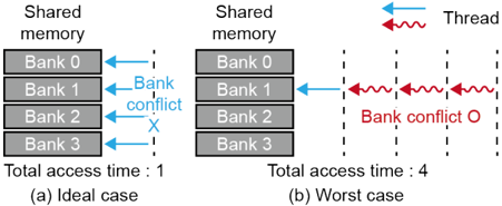Fig. 2. Comparison of bank conflicts during shared memory access. <details> <summary>Image 2 Details</summary>  ### Visual Description ## Diagram: Shared Memory Access Scenarios in Multi-Threaded Systems ### Overview The diagram compares two scenarios of shared memory access in a multi-threaded environment: - **(a) Ideal case**: Smooth, conflict-free memory access with minimal latency. - **(b) Worst case**: Severe memory bank conflicts causing significant delays. ### Components/Axes - **Shared memory banks**: Labeled `Bank 0` to `Bank 3` (vertical axis). - **Access indicators**: - **Blue arrows**: Represent thread access to memory banks. - **Red wavy arrows**: Denote bank conflicts (labeled `Bank conflict O` and `Bank conflict x`). - **Total access time**: - Ideal case: `1` (bottom-left of diagram). - Worst case: `4` (bottom-right of diagram). - **Legend**: - Blue: Thread. - Red: Bank conflict. ### Detailed Analysis 1. **Ideal case (a)**: - All four memory banks (`Bank 0`–`Bank 3`) are accessed sequentially by a single thread (blue arrows). - No conflicts (`x` or `O` markers) are present. - Total access time is explicitly labeled as `1`. 2. **Worst case (b)**: - Thread accesses (`blue arrows`) and bank conflicts (`red wavy arrows`) overlap across all banks. - Conflicts are marked with `x` (Bank 2) and `O` (Bank 3), suggesting different conflict types or severities. - Total access time increases to `4`, a 4x slowdown compared to the ideal case. ### Key Observations - **Conflict impact**: The worst case shows a direct correlation between bank conflicts and increased latency. - **Conflict distribution**: Conflicts occur in Bank 2 (`x`) and Bank 3 (`O`), but the exact meaning of `x` vs. `O` is unspecified. - **Thread behavior**: The thread’s access pattern in the worst case involves repeated or simultaneous requests to the same banks. ### Interpretation This diagram illustrates how **memory bank contention** in multi-threaded systems can degrade performance. The ideal case assumes perfect parallelism with no contention, while the worst case highlights the overhead of resolving conflicts (e.g., cache thrashing, arbitration delays). The use of `x` and `O` to denote conflicts may imply: - `x`: Critical/irreconcilable conflicts requiring thread stalling. - `O`: Overlapping access requests that resolve without stalling but still incur latency. The stark difference in total access time (`1` vs. `4`) underscores the importance of memory bank architecture and conflict resolution strategies in optimizing parallel computing systems. </details> Conventional BCQ, a non-uniform quantization method, is incompatible with most state-of-the-art models that use uniform quantization. [28] enhanced BCQ by incorporating an offset term z , thereby improving its representational capacity: $$- \sum _ { i = 1 } ^ { n } ( a _ { i } - b _ { i } ) + z$$ It has been demonstrated that uniform quantization can be effectively represented by appropriately adjusting the scaling factors and offset terms [28]. As shown in Fig. 1, conventional BCQ leverages multiple distinct scaling factors, while the addition of an offset term facilitates the representation of uniformly quantized values. ## C. Bank Conflict To perform efficient parallel operations, it is necessary to access multiple data simultaneously. Many parallel processors achieve this by employing memory banking techniques, which split memory into banks, allowing multiple threads to access the memory concurrently. However, memory banking can encounter issues when the data required in a single operation cycle are located in the same bank, leading to bank conflicts [12]. This problem is particularly evident in GPUs, where a shared memory space is utilized to enable efficient parallel operations among threads. When different threads attempt to access the same bank simultaneously, bank conflicts arise. These conflicts hinder the achievement of predicted performance and lead to computational resource wastage, as operations that could be parallelized are instead executed serially. In addition, bank conflicts pose a significant bottleneck when LUT-based methods are deployed on existing hardware platforms. For instance, LUT-GEMM [28] stores the LUTs in the shared memory of GPU and utilizes multiple threads for operations. During the LUT construction phase, bank conflicts are avoided as each thread is designed to access different banks in parallel. In contrast, during the LUT read phase, the randomness of the weight pattern often causes frequent bank conflicts, leading to performance degradation. Fig. 2 depicts the example of multiple threads accessing memory banks. In the worst-case scenario, all required accesses within a cycle are serialized, creating substantial performance overhead. Therefore, for LUT-based operations to achieve optimal performance, it is essential to avoid bank conflicts. This requires a novel LUT architecture that allows multiple parallel operators to simultaneously read different values without conflicts. 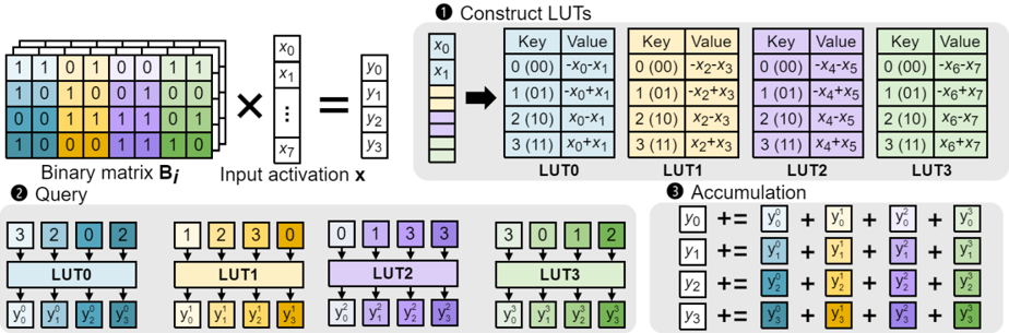Fig. 3. Illustration of look-up table based FP-INT GEMM. <details> <summary>Image 3 Details</summary>  ### Visual Description ## Diagram: Binary Matrix Multiplication with LUT-Based Accumulation ### Overview The diagram illustrates a computational process involving binary matrix multiplication, Look-Up Table (LUT) construction, and accumulation of results. It demonstrates how input activations are transformed through a series of logical operations and combined to produce final output values. ### Components/Axes 1. **Binary Matrix Bi** (Top-left): - 4x8 binary matrix with values 0/1 - Rows labeled 1-4, columns labeled 0-7 - Color-coded cells (green, blue, yellow, purple) indicate different binary values 2. **Input Activation x** (Right of matrix): - 8-dimensional vector (x₀ to x₇) - Represented as vertical column with binary values 3. **Output y** (Right of matrix multiplication): - 4-dimensional vector (y₀ to y₃) - Result of matrix-vector multiplication 4. **LUT Construction** (Middle section): - Four LUTs (LUT0-LUT3) with Key-Value pairs - Keys: 2-bit binary combinations (00, 01, 10, 11) - Values: Boolean expressions involving input bits (e.g., -x₀-x₁, x₀+x₁) 5. **Accumulation** (Bottom section): - Four output lines (y₀ to y₃) - Each yᵢ is sum of corresponding LUT outputs - Color-coded contributions from each LUT 6. **Legend** (Bottom-right): - Color coding for LUTs: - LUT0: Light blue - LUT1: Beige - LUT2: Purple - LUT3: Green ### Detailed Analysis 1. **Matrix Multiplication**: - Binary matrix Bi (4x8) multiplied by input vector x (8x1) - Resulting output y (4x1) shown as vertical column - Example: y₀ = (1·x₀) + (1·x₁) + (0·x₂) + ... + (1·x₇) 2. **LUT Construction**: - LUT0: - 0000 → -x₀-x₁ - 0001 → -x₀+x₁ - 0010 → x₀-x₁ - 0011 → x₀+x₁ - Similar patterns for LUT1-LUT3 with different bit combinations 3. **Accumulation**: - y₀ = y₀(LUT0) + y₀(LUT1) + y₀(LUT2) + y₀(LUT3) - Color-coded contributions match LUT legend - Example: y₁ = (blue) + (yellow) + (purple) + (green) ### Key Observations 1. Non-linear transformation through LUTs enables complex bitwise operations 2. Accumulation combines multiple LUT outputs for final result 3. Color coding provides visual separation of LUT contributions 4. Binary operations suggest potential application in digital signal processing ### Interpretation This diagram represents a hybrid computational architecture combining: 1. Linear algebra operations (matrix multiplication) 2. Non-linear transformations (LUT-based) 3. Parallel accumulation for final output The use of LUTs allows for: - Efficient implementation of complex bitwise operations - Flexible reconfiguration through LUT value changes - Parallel processing of multiple input combinations The color-coded accumulation visually demonstrates how different LUTs contribute to each output dimension, suggesting this could be part of a neural network layer or specialized hardware accelerator for binary data processing. </details> TABLE II EXAMPLE OF LOOK-UP TABLE WHEN µ = 3 | Binary Patterns | Key | Value | |--------------------|-----------|-------------------| | {- 1 , - 1 , - 1 } | 0 (b'000) | - x 1 - x 2 - x 3 | | {- 1 , - 1 , +1 } | 1 (b'001) | - x 1 - x 2 + x 3 | | {- 1 , +1 , - 1 } | 2 (b'010) | - x 1 + x 2 - x 3 | | {- 1 , +1 , +1 } | 3 (b'011) | - x 1 + x 2 + x 3 | | { +1 , - 1 , - 1 } | 4 (b'100) | + x 1 - x 2 - x 3 | | { +1 , - 1 , +1 } | 5 (b'101) | + x 1 - x 2 + x 3 | | { +1 , +1 , - 1 } | 6 (b'110) | + x 1 + x 2 - x 3 | | { +1 , +1 , +1 } | 7 (b'111) | + x 1 + x 2 + x 3 | ## III. LOOK-UP TABLE-BASED FP-INT GEMM ACCELERATOR In this section, we introduce FIGLUT, a novel computational methodology and accelerator design aimed at improving the efficiency of FP-INT GEMM operations by replacing computation with data retrieval from an LUT. To address the issue of LUT bank conflicts that hinder parallel processing in existing LUT-based operations, we propose a specialized LUT structure. This structure is designed to eliminate bank conflicts and enable efficient parallel access to LUT data. We also analyze the impact of increased fan-out on power consumption in shared LUTs and propose an optimal processing element (PE) structure to maximize energy efficiency. As a result, the FIGLUT design offers enhanced energy efficiency relative to conventional computing units. ## A. Look-up Table based FP-INT GEMM Look-up tables are extensively employed to improve computational efficiency by substituting direct calculations with table look-ups, particularly when the results are confined to a predetermined set. This technique can be extended to deep learning operations involving a binary weight matrix B ∈ {-1 , +1 } M × N , where output activations are calculated through simple addition and subtraction among the input activation vector x ∈ R N × 1 . Consequently, the output activations are confined to combinations of input activations, enabling the calculation and storage of all potential output values within the LUT. This approach substitutes actual computation with the retrieval of data from the LUT. To construct an LUT, we introduce a hyperparameter µ , which determines the number of binary weights used to form a key for retrieving a value from the LUT. Note that as µ increases, the number of computations that can be replaced by a single LUT read also increases. However, since the memory size required to store the LUT grows exponentially, finding the optimal value of µ is crucial. Consider a binary matrix B ∈ {-1 , +1 } 4 × 6 and an input activation vector x ∈ R 6 × 1 : $$B = \begin{bmatrix} + 1 & - 1 & - 1 & - 1 & - 1 \\ + 1 & - 1 & - 1 & + 1 & - 1 \\ + 1 & - 1 & - 1 & - 1 & + 1 \\ + 1 & - 1 & - 1 & - 1 & - 1 \end{bmatrix} , (4)$$ $$x = \left | x _ { 1 } , x _ { 2 } , x _ { 3 } , x _ { 4 } \right | . (5)$$ For instance, in the computation of Bx with µ = 3 , we observe that operations such as ( x 1 -x 2 -x 3 ) and ( -x 4 -x 5 + x 6 ) are repeated multiple times. These redundant computations increase as the size of the matrices grows with the increasing model size. As shown in Table II, by pre-computing all possible combinations of inputs and storing them in the LUT, repeated computations can be avoided, allowing a single LUT read to replace multiple addition operations. If µ is increased to 6, there are repeated computations such as ( x 1 -x 2 -x 3 -x 4 -x 5 + x 6 ) , which can also be efficiently managed using the LUT. Although increasing µ enhances computational benefits, the memory space required to store the LUT increases exponentially. Fig. 3 provides an overview of the LUT-based FP-INT GEMM process for computing Bx with µ = 2 . As previously mentioned, to reduce redundant computations and efficiently perform GEMM operations, LUTs are constructed using µ elements from the input activation x , customized for each input. Each LUT contains 2 µ values, with µ binary weights used as keys to retrieve each value. 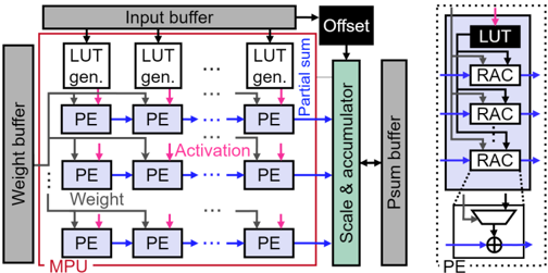During the query phase, Fig. 4. Overall MPU architecture of FIGLUT <details> <summary>Image 4 Details</summary>  ### Visual Description ## Block Diagram: Neural Network Accelerator Architecture ### Overview The image depicts a technical block diagram of a neural network accelerator architecture, divided into two primary sections: 1. **Left Diagram**: A high-level overview of the system's data flow and processing units. 2. **Right Diagram**: A zoomed-in view of the Look-Up Table (LUT) and Reconfigurable Array Controller (RAC) components. --- ### Components/Axes #### Left Diagram Labels: - **Top**: Input Buffer (gray) - **Left**: Weight Buffer (gray) - **Central Blocks**: - LUT Generators (labeled "LUT gen.") - Processing Elements (PEs) arranged in rows - Partial Sum (blue arrow) - Scale & Accumulator (green block) - Output Buffer (gray) - **Right**: Offset (black block) - **Arrows**: - Red: Activation signals - Blue: Weight signals - Gray: Data flow between buffers - Pink: Offset input #### Right Diagram Labels: - **Top**: LUT (black block) - **Middle**: Three stacked RAC blocks (purple) - **Bottom**: PE (blue arrow) - **Arrows**: - Blue: Data flow between RACs and PE - Pink: Feedback loop from PE to RAC #### Legend: - **Colors**: - Red: Activation - Blue: Weight - Green: Partial Sum - Gray: Buffers - Black: LUT - Purple: RAC - Pink: Offset --- ### Detailed Analysis #### Left Diagram: 1. **Data Flow**: - Input data enters the Input Buffer and is distributed to LUT Generators. - LUT Generators produce weights, which are fed into PEs along with Activation signals (red arrows). - PEs process data and generate Partial Sums (blue arrows), which are scaled and accumulated in the Scale & Accumulator block. - Final output is stored in the Output Buffer. 2. **Key Connections**: - Weight signals (blue) originate from the Weight Buffer and are routed to PEs. - The Offset (pink) is injected into the Partial Sum path. #### Right Diagram: 1. **LUT and RAC Structure**: - The LUT (black) feeds into three RAC blocks (purple), which are connected in a feedback loop. - The PE (blue arrow) receives input from the RACs and sends output back to the RACs via a feedback path. 2. **Functional Role**: - The RACs likely perform reconfigurable computations (e.g., matrix operations) for neural network layers. - The feedback loop suggests iterative processing or error correction. --- ### Key Observations 1. **Modular Design**: - The architecture emphasizes modularity, with distinct blocks for LUTs, RACs, and PEs. - Buffers (Input/Weight/Output) ensure data staging and synchronization. 2. **Parallelism**: - Multiple PEs and LUT Generators suggest parallel processing capabilities. 3. **Feedback Mechanism**: - The right diagram’s feedback loop (pink arrow) indicates dynamic adjustment or iterative computation. 4. **Signal Paths**: - Activation (red) and Weight (blue) signals are clearly separated, reducing cross-talk. --- ### Interpretation This diagram represents a hardware accelerator optimized for neural network computations. The left diagram highlights the system’s data flow, emphasizing parallelism through PEs and LUT Generators. The right diagram zooms into the LUT and RAC components, revealing a reconfigurable processing unit with feedback for adaptive computations. - **Functional Insights**: - The Scale & Accumulator block likely handles quantization and bias addition, critical for low-precision neural network inference. - The feedback loop in the RACs may enable dynamic weight updates or error propagation, improving model accuracy. - **Design Implications**: - The use of PEs and RACs suggests a focus on energy efficiency and throughput, typical of edge AI hardware. - The separation of Activation and Weight signals simplifies timing constraints and reduces power consumption. - **Potential Limitations**: - The diagram does not specify clock frequencies or latency, which are critical for real-world performance. - The absence of error-handling mechanisms (e.g., fault tolerance) raises questions about robustness in noisy environments. This architecture balances modularity and performance, making it suitable for applications like real-time image recognition or autonomous systems. </details> k RACs simultaneously access the shared LUT to retrieve their respective partial sum values. In this example, k = 4 , indicates that four RACs can access a single LUT concurrently. The specialized LUT structure for LUT-based GEMM, which enables concurrent access by k RACs, will be detailed in the subsequent section. Finally, the values retrieved from each LUT are stored in the accumulator. Once this process is completed for all binary matrices B i , the final output activation values are obtained. Note that while the previous examples assume the input activation to be a vector for simplicity (corresponding to a GEMV operation), this approach is basically applied to GEMM operations by generating unique LUTs for each batch, allowing for efficient matrix computations. ## B. Overall FIGLUT Architecture Fig. 4 depicts the overall architecture of the proposed LUTbased FP-INT GEMM accelerator, FIGLUT. In this section, we provide a detailed description of the matrix processing unit (MPU), which represents our primary contribution. A comprehensive overview of the entire system architecture will be discussed in Section III-F. FIGLUT leverages a 2D systolic array structure similar to that of the Google TPU [18]. Inputs are fetched sequentially from the input memory through systolic data setup. These input activations are fed into the LUT generators to construct the LUTs. Each LUT generator takes µ input activations and generates all possible output partial sums on-the-fly. These partial sums are then passed to the LUTs within the PEs, where they are used as LUT values. To enable effective data reuse, LUT values from the PEs in each row are forwarded to the LUTs in the subsequent rows. Each PE houses k RACs, and due to the unique structure of LUT, designed for LUT-specific operations, the k RACs can read from the LUT concurrently. We perform an analysis to determine the optimal value of k , taking into account the fanout overhead introduced when multiple RACs access the LUT at the same time. This analysis is elaborated in a later section. FIGLUT employs a weight-stationary dataflow to optimize GEMM operations. Within each PE, the RAC includes a register that holds a µ -bit weight pattern, serving as a key to access data from the LUT. The partial sums generated by each PE are incrementally gathered and subsequently sent to the PE in the next column. 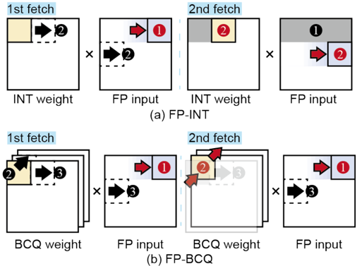This iterative accumulation process takes Fig. 5. Illustration of the input and weight tile fetching sequence in (a) a systolic array accelerator for INT weight and (b) FIGLUT for BCQ weight. The arrows indicate the order in which the tiles are processed. <details> <summary>Image 5 Details</summary>  ### Visual Description ## Diagram: FP-INT vs FP-BCQ Method Comparison ### Overview The image compares two computational methods (FP-INT and FP-BCQ) through sequential data processing steps. Each method is visualized with two "fetch" stages, showing interactions between weights (INT/BCQ) and feature processing (FP) inputs. Arrows indicate data flow, and numbered circles (1, 2, 3) highlight priority or sequence. ### Components/Axes - **Methods**: - **FP-INT** (top row): Uses "INT weight" in both fetch stages. - **FP-BCQ** (bottom row): Uses "BCQ weight" in the first fetch and combines BCQ/INT in the second. - **Elements**: - **1st fetch**: Initial data block (light yellow) with an arrow pointing to a numbered circle (2). - **2nd fetch**: Subsequent data block (gray/light yellow) with arrows pointing to numbered circles (1, 2). - **FP input**: Rectangular blocks labeled "FP input" receiving data from weights. - **Weights**: - **INT weight**: Black arrow with a dashed box (FP-INT). - **BCQ weight**: Stacked blocks with arrows (FP-BCQ). ### Detailed Analysis #### FP-INT (Top Row) 1. **1st fetch**: - A light yellow block labeled "INT weight" sends data via a black arrow to a dashed box containing "2". - A red arrow points to a gray box labeled "1" (FP input). 2. **2nd fetch**: - The gray box ("1") sends data via a red arrow to a light gray box labeled "2" (FP input). #### FP-BCQ (Bottom Row) 1. **1st fetch**: - Stacked blocks labeled "BCQ weight" send data via a black arrow to a dashed box containing "3". - A red arrow points to a gray box labeled "1" (FP input). 2. **2nd fetch**: - The gray box ("1") sends data via a red arrow to a light gray box labeled "2" (FP input). - A secondary red arrow from the BCQ weight block points to a dashed box containing "3". ### Key Observations - **FP-INT** maintains a consistent use of "INT weight" across both fetch stages. - **FP-BCQ** introduces "BCQ weight" in the first fetch and integrates it with "INT weight" in the second fetch (implied by the dual arrows). - Numbered circles (1, 2, 3) likely denote processing priorities or sequential steps, with "1" and "2" appearing in both methods but "3" exclusive to FP-BCQ. ### Interpretation The diagrams illustrate how FP-INT and FP-BCQ differ in weight utilization: - **FP-INT** relies solely on INT weight for sequential processing, suggesting a simpler, unified approach. - **FP-BCQ** employs BCQ weight initially and combines it with INT weight later, indicating a hybrid or adaptive strategy. - The presence of "3" in FP-BCQ’s second fetch implies additional complexity or a third processing layer not present in FP-INT. This comparison highlights trade-offs between simplicity (FP-INT) and flexibility (FP-BCQ), with the latter potentially offering more nuanced data handling at the cost of increased computational steps. </details> place along each column of PEs until the ultimate partial sum is derived at the final PE. The eventual partial sum is multiplied by a scaling factor α i and stored in the accumulator buffer. This cycle is performed for each bit plane, and once all bit planes are processed, the accumulated sums are summed with the offset value and routed to the output buffer. Fig. 5 shows the fetching sequence of input and weight tiles. For systolic array accelerators with INT weights, such as FIGNA [16], each weight has a single channel with multibit values. In contrast, FP-BCQ accelerators like FIGLUT and iFPU [22] include q binary weight bit planes. In a weightstationary dataflow, a weight tile is loaded once and reused, while inputs are loaded sequentially ( 1 ) for both FP-INT and FP-BCQ accelerators. However, the process diverges for FP-BCQ accelerators. Instead of loading the next tile within the same bit plane, the weight tile for the next bit plane is loaded and processed ( 2 in Fig. 5 (b)). After processing all binary weight bit planes, the operation proceeds to the next tile, similar to the FP-INT accelerator. ## C. Conflict-free LUT Structure To efficiently perform LUT-based FP-INT GEMM operations, a specialized LUT structure is essential, as traditional memory structures are insufficient for the following requirements. First, minimizing the power consumption associated with reading data from the LUT is crucial. Since FIGLUT replaces computation with data retrieval, reducing the cost of data reads compared to the cost of computations enhances overall efficiency. Second, the structure needs to support a large volume of simultaneous read and write operations. Given the dynamic nature of activation values, the LUT should be reconfigurable on-the-fly, allowing concurrent writing of large amounts of data to update the LUT according to input activations. From a data retrieval perspective, multiple RACs operate in parallel, each using different weight patterns as keys Fig. 6. Relative Power Consumption of RFLUT and FFLUT Compared to FP Adder Baseline Across Different µ Values <details> <summary>Image 6 Details</summary>  ### Visual Description ## Bar Chart: Relative Power Consumption by Method and Component ### Overview The chart compares the relative power consumption of three computational methods (Baseline, RFLUT, FFLUT) across three components: FP adder (yellow), LUT (gray), and RAC (pink). Horizontal dashed lines at μ = 2, μ = 4, and μ = 8 serve as reference thresholds. The x-axis represents relative power (0–14), while the y-axis categorizes methods. ### Components/Axes - **X-axis**: Relative power (0–14), linear scale. - **Y-axis**: Methods (Baseline, RFLUT, FFLUT), ordered top to bottom. - **Legend**: - Yellow = FP adder - Gray = LUT - Pink = RAC - **Dashed Lines**: μ = 2 (dash-dot), μ = 4 (dashed), μ = 8 (dash-dot). ### Detailed Analysis 1. **Baseline**: - FP adder: ~1.0 (yellow bar). - LUT: N/A (no bar). - RAC: ~1.0 (pink bar). 2. **RFLUT**: - FP adder: ~3.0 (yellow bar). - LUT: ~8.0 (gray bar). - RAC: ~4.0 (pink bar). 3. **FFLUT**: - FP adder: ~4.0 (yellow bar). - LUT: ~13.0 (gray bar). - RAC: ~8.0 (pink bar). ### Key Observations - **Baseline** has minimal power consumption across components but lacks LUT data. - **RFLUT** shows moderate power usage, with LUT consuming the most (~8.0). - **FFLUT** exhibits the highest power consumption, particularly in LUT (~13.0), surpassing all μ thresholds. - Dashed lines at μ = 2, 4, and 8 suggest performance benchmarks; FFLUT exceeds all thresholds in LUT and RAC. ### Interpretation The chart highlights trade-offs between computational methods and power efficiency. FFLUT’s significantly higher LUT power (~13.0) suggests it may prioritize performance over energy efficiency, while Baseline’s sparse data (missing LUT) implies incomplete optimization. The μ thresholds likely represent target power limits, with FFLUT exceeding all, indicating potential over-engineering or specialized use cases. The absence of LUT data for Baseline raises questions about its applicability in scenarios requiring LUT resources. </details> to access data in the LUT. Therefore, the architecture should facilitate parallel data access while avoiding bank conflicts. 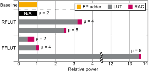To ensure that retrieving precomputed results from an LUT consumes less power than using FP adders, we measure the power consumption of an FP adder as a baseline. We then compare this with the power consumption of LUT-based operations. Fig. 6 demonstrates the power comparison between FP adders and various LUT implementations across different µ values, while maintaining equivalent throughput. To address the targeted hardware constraints, we implemented two types of LUTs: (1) a traditional Register File based LUT (RFLUT) and (2) a proposed Flip-Flop based LUT (FFLUT). The RFLUT, constructed using register files commonly employed in CPU register arrays, uses a straightforward approach where the weight pattern serves as the read register number. For the comparison, RFLUT blocks are generated using a 28nm memory compiler, allowing us to customize the design to target low-power LUT-based GEMM operations. The generated register file is then integrated into the hardware design as an IP macro block. All power analyses of LUT structures, including FFLUT, are tested based on the physical layout obtained after the P&R process in ICC2. As the RFLUT with µ = 2 is too small to be generated by the compiler in this environment, it is not considered for measurement. Generally, RFLUTs exhibit higher read power consumption compared to FP addition operations. While an RFLUT with µ = 4 requires less power per read than one with µ = 8 , it needs twice the number of reads, leading to higher overall power consumption. As a result, RFLUT is not suitable for the LUT-based method, and a novel method is necessary to construct LUTs. 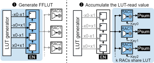To overcome the limitations of traditional RFLUTs, we propose a Flip-Flop-based Look-Up Table (FFLUT) structure, illustrated in Fig. 7. The FFLUT consists of a bundle of flip-flops accessed through multiplexers. Each enabled flipflop outputs consistent values once updated during the LUT generation phase, maintaining this output until it is reset. This design allows the processing unit to retrieve values by multiplexing the corresponding weight keys to access the required flip-flops. Unlike RFLUTs, which are constrained by their limited read/write ports, the FFLUT enables simultaneous access by multiple units without encountering bank conflicts. Fig. 7. Architecture of the Flip-Flop based Look-Up Table (FFLUT) <details> <summary>Image 7 Details</summary>  ### Visual Description ## Diagram: Hardware Architecture for LUT-Based Accumulation System ### Overview The diagram illustrates a two-stage hardware architecture for generating and accumulating Look-Up Table (LUT) read values. It is divided into two primary functional blocks: 1. **Generate FFLUT** (left side) 2. **Accumulate the LUT-read value** (right side) The system uses a combination of LUT generators, RAC (Register-Accumulate) blocks, and Psum (Partial Sum) units to process input signals (`x0`, `x1`) and keys (`Key0`, `Key1`, `Key2`). --- ### Components/Axes #### Left Diagram: Generate FFLUT - **LUT Generator**: - Inputs: `x0`, `x1` - Outputs: Four intermediate values: - `-x0-x1` - `-x0+x1` - `x0-x1` - `x0+x1` - Position: Top-left quadrant, connected to RAC blocks via arrows. - **RAC Blocks**: - **RAC0**, **RAC1**, **RAC2**: - Each receives one of the four LUT generator outputs. - Position: Center-left, vertically stacked. - Connected to an **EN** (Enable) block at the bottom. #### Right Diagram: Accumulate the LUT-read value - **LUT Generator**: - Same four outputs as the left diagram (`-x0-x1`, `-x0+x1`, `x0-x1`, `x0+x1`). - Position: Top-left quadrant, connected to RAC blocks. - **RAC Blocks**: - **RAC0**, **RAC1**, **RAC2**: - Share the same LUT generator outputs. - Position: Center-left, vertically stacked. - Connected to **Psum** blocks via arrows labeled `Key0`, `Key1`, `Key2`. - **Psum Blocks**: - **Psum0**, **Psum1**, **Psum2**: - Receive inputs from RAC blocks and keys. - Position: Right side, vertically stacked. - **EN Block**: - Position: Bottom-center, connected to the LUT generator. --- ### Detailed Analysis #### Left Diagram: Generate FFLUT 1. The LUT generator produces four intermediate values by combining `x0` and `x1` with arithmetic operations. 2. These values are routed to three RAC blocks (RAC0, RAC1, RAC2). 3. The **EN** block likely controls the enable signal for the RAC blocks. #### Right Diagram: Accumulate the LUT-read value 1. The LUT generator outputs are reused to feed the same RAC blocks. 2. Each RAC block is connected to a Psum block via a unique key (`Key0`, `Key1`, `Key2`). 3. The Psum blocks aggregate the RAC outputs, suggesting a multi-stage accumulation process. --- ### Key Observations 1. **Shared LUT**: The right diagram explicitly states that `k RACs share LUT`, indicating resource reuse for efficiency. 2. **Key-Driven Accumulation**: The Psum blocks use distinct keys, implying conditional or weighted accumulation. 3. **EN Block Role**: The Enable block acts as a control point for both diagrams, suggesting synchronization between generation and accumulation phases. --- ### Interpretation This architecture appears to implement a **hardware-accelerated LUT-based computation system**, likely for applications requiring rapid arithmetic operations (e.g., digital signal processing, cryptography). - **Stage 1 (Generate FFLUT)**: Computes intermediate values from input signals, stored in RAC blocks. - **Stage 2 (Accumulate)**: Reuses the LUT to process the same intermediate values but applies key-specific logic via Psum blocks. The shared LUT and key-driven accumulation suggest optimization for parallelism and reduced hardware footprint. The EN block ensures temporal coordination between the two stages. **Notable Design Choices**: - Reuse of LUT outputs across RAC blocks minimizes redundancy. - Key-based Psum blocks enable flexible accumulation logic without additional LUT entries. - The EN block centralizes control, simplifying synchronization. This design prioritizes efficiency and scalability, critical for high-performance computing systems. </details> This is achieved by equipping the FFLUT with dedicated multiplexers that allow different units to access distinct keys concurrently. As a result, multiple units can share a single LUT efficiently, significantly reducing the overhead associated with LUT-based operations and improving energy efficiency. To further optimize the data retrieval process in FFLUTs, we introduce a specialized operator called the RAC unit, designed as a replacement for the conventional MAC unit. Each PE in FIGLUT is equipped with a single LUT and multiple RAC units, as shown in Fig. 4. Unlike the MAC unit, which performs a multiplication followed by an accumulation into a partial sum, the RAC unit retrieves values directly from the LUT using a weight pattern as a key and accumulates them into the partial sum. Hence, the RAC unit can execute LUT-based operations more effectively, enhancing the overall efficiency of the FIGLUT architecture. 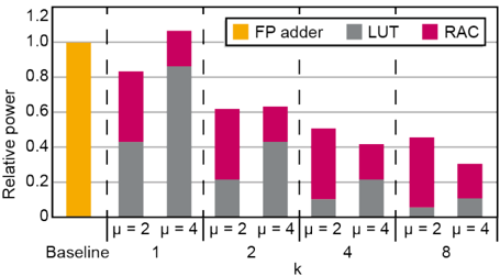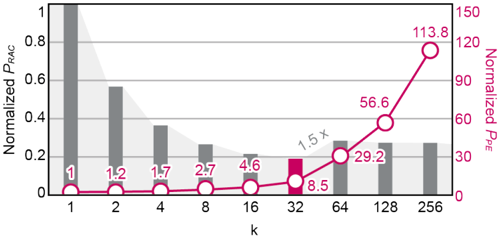To achieve energy-efficient GEMM operations, our approach incorporates an optimal architecture search that allows multiple RAC units to share a single LUT. This optimization process involves two key steps. First, we determine the optimal µ value for the LUT, balancing the gains of the computation against the power consumption of the LUT. Second, based on the chosen µ value, we identify the optimal number of RACs per LUT by evaluating the impact of fan-out on power consumption. We introduce a variable k to represent the LUT fan-out within a single PE, denoting the number of RACs sharing a single LUT. Fig. 8 shows the power consumption of FIGLUT with µ values of 2 and 4, varying k . The baseline for relative power measurements is set using the results of the same operations performed with FP adders. Due to the significantly large size and high power consumption of LUTs for µ = 8 , as shown in Fig. 6, this configuration is excluded from consideration. As k increases, the total number of LUTs decreases by sharing an LUT with multiple RACs, leading to a gradual reduction in LUT power consumption. Note that the total number of RACs required for computation remains constant regardless of k , as it depends solely on the µ value. This is because the overall number of read-accumulate operations is unaffected by the sharing configuration. However, smaller µ values require more RACs, resulting in higher RAC power consumption for µ = 2 compared to µ = 4 . When LUTs are not shared and are exclusively used by a single RAC ( k = 1 ), the larger LUT size for µ = 4 leads to Fig. 8. Relative power comparison of baseline, µ = 2 and µ = 4 for various the number of RACs per LUT configuration. <details> <summary>Image 8 Details</summary>  ### Visual Description ## Bar Chart: Relative Power Across Components and Parameters ### Overview The chart compares the relative power of three components (FP adder, LUT, RAC) across different configurations labeled by `k` (1, 2, 4, 8) and parameter `μ` (2, 4). The Baseline represents a reference point. Relative power is normalized, with values ranging from 0 to 1.2 on the y-axis. ### Components/Axes - **X-axis (Categories)**: Baseline, 1, 2, 4, 8 (each split into `μ=2` and `μ=4` subcategories). - **Y-axis (Values)**: Relative power (0–1.2). - **Legend**: - Yellow: FP adder - Gray: LUT - Pink: RAC - **Spatial Grounding**: - Legend is top-right. - Bars are grouped by `k`, with `μ=2` (left) and `μ=4` (right) within each group. ### Detailed Analysis 1. **Baseline**: - FP adder: ~1.0 (yellow bar). - LUT and RAC: Not present (no bars). 2. **k=1**: - `μ=2`: - FP adder: ~0.8 (yellow). - LUT: ~0.4 (gray). - RAC: ~0.4 (pink). - `μ=4`: - FP adder: ~0.9 (yellow). - LUT: ~0.5 (gray). - RAC: ~0.4 (pink). 3. **k=2**: - `μ=2`: - FP adder: ~0.6 (yellow). - LUT: ~0.2 (gray). - RAC: ~0.4 (pink). - `μ=4`: - FP adder: ~0.6 (yellow). - LUT: ~0.4 (gray). - RAC: ~0.2 (pink). 4. **k=4**: - `μ=2`: - FP adder: ~0.5 (yellow). - LUT: ~0.1 (gray). - RAC: ~0.4 (pink). - `μ=4`: - FP adder: ~0.5 (yellow). - LUT: ~0.3 (gray). - RAC: ~0.2 (pink). 5. **k=8**: - `μ=2`: - FP adder: ~0.3 (yellow). - LUT: ~0.05 (gray). - RAC: ~0.2 (pink). - `μ=4`: - FP adder: ~0.3 (yellow). - LUT: ~0.1 (gray). - RAC: ~0.15 (pink). ### Key Observations - **Trend Verification**: - All components show a **decreasing trend** as `k` increases (Baseline > k=1 > k=2 > k=4 > k=8). - `μ=4` consistently outperforms `μ=2` for the same `k` (e.g., k=1: μ=4 FP adder ~0.9 vs. μ=2 ~0.8). - **Component Hierarchy**: - FP adder dominates across all configurations (highest values). - LUT contributes minimally, especially at higher `k` (e.g., k=8: LUT ~0.05). - RAC maintains a smaller but stable contribution (~0.15–0.4). ### Interpretation - **Inverse Relationship**: Relative power decreases as `k` increases, suggesting higher `k` values reduce efficiency or increase resource demands. - **Parameter Impact**: `μ=4` improves performance for FP adders and LUTs but has diminishing returns for RAC. - **Component Roles**: - FP adders are the primary power consumers, scaling down predictably with `k`. - LUTs become negligible at higher `k`, while RAC remains a minor but consistent factor. - **Anomalies**: No outliers; trends are consistent across all data points. This chart highlights the trade-offs between configuration complexity (`k`), parameter scaling (`μ`), and component-specific power usage, emphasizing the FP adder’s dominance and the diminishing role of LUTs at higher `k`. </details> Fig. 9. P RAC and P PE analysis for various RAC numbers. Normalized by k = 1 results. <details> <summary>Image 9 Details</summary>  ### Visual Description ## Bar Chart with Dual Y-Axes: Normalized P_RAC vs. Normalized P_PE vs. k ### Overview The image is a bar chart with two y-axes and a single x-axis labeled "k". The left y-axis represents "Normalized P_RAC" (ranging from 0 to 1), while the right y-axis represents "Normalized P_PE" (ranging from 0 to 150). The x-axis (k) has discrete values: 1, 2, 4, 8, 16, 32, 64, 128, 256. The chart includes gray bars (P_RAC) and a red line (P_PE), with annotations and a legend. --- ### Components/Axes - **X-Axis (k)**: Discrete values: 1, 2, 4, 8, 16, 32, 64, 128, 256. - **Left Y-Axis (Normalized P_RAC)**: Scale from 0 to 1, with gridlines. - **Right Y-Axis (Normalized P_PE)**: Scale from 0 to 150, with gridlines. - **Legend**: - **Gray bars**: "P_RAC" (left y-axis). - **Red line**: "P_PE" (right y-axis). - **Annotations**: - "1.5x" near k=32 (red line). - Numerical values on the red line: 113.8 (k=256), 56.6 (k=128), 29.2 (k=64), 8.5 (k=32), 4.6 (k=16), 2.7 (k=8), 1.7 (k=4), 1.2 (k=2), 1 (k=1). --- ### Detailed Analysis #### Gray Bars (P_RAC) - **Trend**: Exponentially decreasing as k increases. - **Values**: - k=1: 1.0 - k=2: 0.6 - k=4: 0.4 - k=8: 0.3 - k=16: 0.2 - k=32: 0.15 - k=64: 0.1 - k=128: 0.08 - k=256: 0.05 #### Red Line (P_PE) - **Trend**: Flat (near 0) for k ≤ 32, then sharply increasing after k=32. - **Values**: - k=1: ~0 - k=2: ~0 - k=4: ~0 - k=8: ~0 - k=16: ~0 - k=32: 8.5 - k=64: 29.2 - k=128: 56.6 - k=256: 113.8 - **Annotation**: "1.5x" near k=32, suggesting a multiplicative factor or threshold. --- ### Key Observations 1. **Inverse Relationship**: As k increases, P_RAC decreases exponentially, while P_PE increases sharply after k=32. 2. **Threshold Effect**: The "1.5x" annotation at k=32 indicates a critical point where P_PE begins to rise significantly. 3. **Data Point Consistency**: The red line’s values align with the right y-axis scale, confirming the legend’s accuracy. --- ### Interpretation - **Trade-off Dynamics**: The chart suggests a trade-off between P_RAC and P_PE as k increases. P_RAC (possibly a resource or efficiency metric) diminishes, while P_PE (possibly a performance or error metric) grows, implying a system optimization or degradation. - **Critical Threshold**: The "1.5x" annotation at k=32 may represent a tipping point where P_PE becomes dominant, potentially signaling a phase transition or system instability. - **Exponential Decay**: The rapid decline in P_RAC suggests diminishing returns or saturation in the system’s capacity as k scales. This data could reflect scenarios like computational resource allocation, algorithmic efficiency, or physical system behavior under varying parameters. The sharp rise in P_PE after k=32 warrants further investigation into the underlying mechanisms driving this shift. </details> higher power consumption, resulting in higher total power consumption compared to µ = 2 . However, as k increases and LUTs are shared among multiple RACs, the number of LUTs decreases, reducing overall power consumption. Based on these findings and considering sufficiently large k values in our architecture, we use the FIGLUT architecture with µ = 4 in this paper. Managing fan-out is a critical challenge in designing an energy-efficient accelerator capable of sharing a single LUT among multiple RACs. In digital circuits, fan-out occurs when a signal is distributed to multiple circuit elements, leading to increased power use and signal delay. In the context of FIGLUT, as multiple RACs access the LUT simultaneously, the fan-out effect requires additional power to deliver signals to each RAC efficiently. While sharing a single LUT among multiple RACs reduces the total number of LUTs, it also increases the power consumption of each LUT due to the heightened fan-out. This trade-off necessitates careful management to achieve an optimal balance between the benefits of reducing the total number of LUTs and the drawbacks of increased power demand from fan-out. Effectively addressing this issue is crucial for minimizing overall power use while maintaining energy efficiency in LUT-based GEMM operations. Fig. 9 shows the power consumption of the PE ( P PE ) and each RAC ( P RAC ) as a function of LUT fan-out. To measure the impact of fan-out, all experimental results are obtained using the physical layout of the PEs (including LUTs and TABLE III COMPARISON OF RELATIVE POWER CONSUMPTION OF LUT AND OTHER COMPONENTS | | LUT | MUX | Decoder | MUX+Decoder | |--------|-------|-------|-----------|---------------| | FFLUT | 1 | 0.003 | 0 | 0.003 | | hFFLUT | 0.494 | 0.002 | 0.003 | 0.005 | RACs) after the P&R process. The power consumption per RAC unit P RAC is calculated by dividing P PE by k . As k increases, the number of RACs within the PE increases, resulting in higher overall PE power. Initially, increasing k reduces P RAC because the power consumption of the shared LUT is distributed across the k RACs. However, as k continues to grow, the fan-out overhead becomes significant, increasing P RAC . Based on the observation, we determine the optimal value of k to be 32 for configuring PEs in our architecture. Thus, each PE in our architecture includes one shared LUT and 32 RACs. ## D. Optimizing LUT using Vertical Symmetry In LUT-based FP-INT GEMM, the primary overhead compared to conventional GEMM operations is the LUT itself. Reducing LUT power consumption is therefore critical for enhancing the efficiency of FIGLUT. The FFLUT is composed of flip-flops, with power consumption scaling linearly with its size. To address this, we propose a half-FFLUT (hFFLUT) technique, which reduces the LUT size by half. 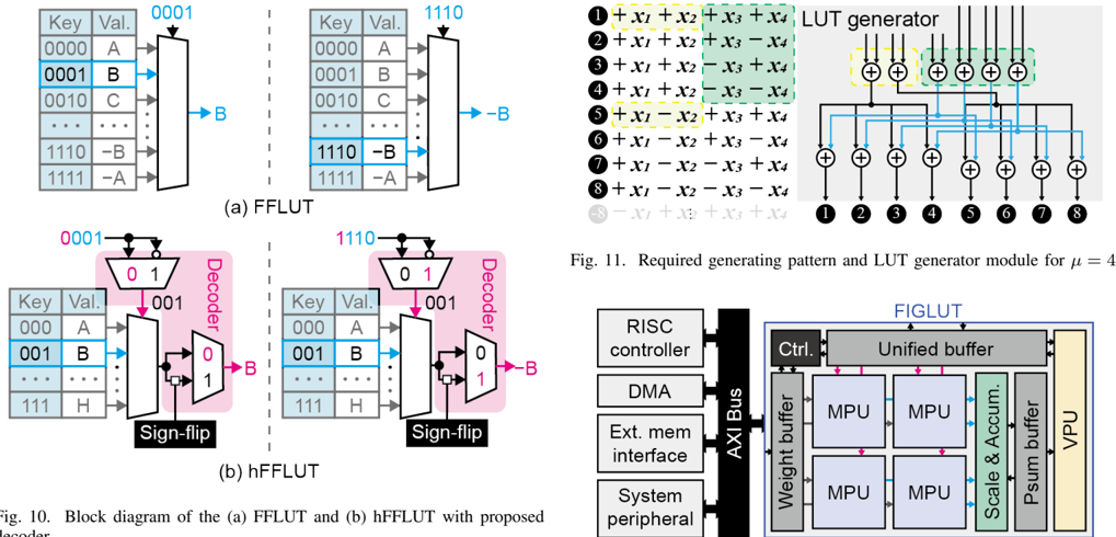As shown in Table II, LUT values exhibit vertical symmetry. In other words, since the LUT is composed of the calculation results of µ FP values through combinations of addition and subtraction, for every combination, there exists a corresponding value that can be directly obtained by simply flipping the sign. By exploiting this characteristic, we store only the upper half of the table and use the key to decode the final LUT value. Fig. 10 presents a block diagram illustrating the hFFLUT and the proposed decoding technique when µ = 3 . The most significant bit (MSB) of the key is used as a select signal to choose the ( µ -1) -bit key for the hFFLUT. Then, the final value read from the hFFLUT is then sign-flipped based on the MSB to obtain the complete value. Although the hFFLUT effectively reduces the size of the LUT, it introduces additional decoding overhead. Table III evaluates the hardware complexity of the proposed decoding circuit for hFFLUT compared to the FFLUT multiplexer used to fetch data from the LUT. The decoding circuit for hFFLUT, including the multiplexer, demonstrates higher power consumption than the multiplexer used in the FFLUT. However, since LUT power is dominant in the overall power consumption, the additional overhead of the decoding circuit is relatively trivial in comparison. Consequently, the proposed hFFLUT effectively halves the power consumed by the LUT in the entire system, thereby significantly enhancing the energy efficiency of FIGLUT. Fig. 12. System architecture of FIGLUT. <details> <summary>Image 10 Details</summary>  ### Visual Description ## Block Diagrams: FFLUT, hFFLUT, and LUT Generator ### Overview The image contains three technical diagrams: 1. **(a) FFLUT**: A data processing block diagram with key-value tables, a decoder, and sign-flip logic. 2. **(b) hFFLUT**: Similar to FFLUT but includes a decoder with explicit sign-flip components. 3. **LUT Generator**: A module for generating address patterns with arithmetic operations on variables. 4. **FIGLUT**: A system architecture diagram integrating RISC controllers, memory units, and processing pipelines. --- ### Components/Axes #### (a) FFLUT - **Left Table**: - **Columns**: `Key` (4-bit binary), `Val` (alphanumeric). - **Rows**: - `0000` → `A` - `0001` → `B` (highlighted in blue) - `0010` → `C` - `1110` → `B` - `1111` → `-A` - **Arrow**: Blue arrow from `0001` (B) to `1110` (-B). - **Right Table**: - **Columns**: `Key` (4-bit binary), `Val` (alphanumeric). - **Rows**: - `0000` → `A` - `0001` → `B` - `0010` → `C` - `1110` → `-B` (highlighted in blue) - `1111` → `-A` - **Decoder**: - Input: `0 1` (binary) - Output: `0` or `1` - **Sign-flip**: Labeled "Sign-flip" in black box. #### (b) hFFLUT - **Decoder**: - Input: `0 1` (binary) - Output: `0` or `1` - **Sign-flip**: Explicitly labeled "Sign-flip" in black box. #### LUT Generator (Fig 11) - **Generating Pattern**: - Equations for 8 outputs (1–8): - `1`: `1 + x1 + x2 + x3 + x4` - `2`: `2 + x1 + x2 + x3 - x4` - `3`: `3 + x1 + x2 - x3 + x4` - `4`: `4 + x1 - x2 + x3 + x4` - `5`: `5 + x1 - x2 - x3 - x4` - `6`: `6 + x1 + x2 - x3 - x4` - `7`: `7 + x1 - x2 + x3 - x4` - `8`: `8 - x1 + x2 + x3 + x4` - **LUT Generator Module**: - Inputs: 8 variables (`x1–x4`) - Outputs: 8 address lines (1–8) #### FIGLUT - **Components**: - **RISC Controller** → **DMA** → **AXI Bus** → **Unified Buffer** - **MPUs** (4 units) → **Scale & Accum** → **Psum Buffer** → **VPU** - **External Memory Interface** and **System Peripheral** interfaces. --- ### Detailed Analysis #### FFLUT/hFFLUT - **Key-Value Tables**: - `0001` maps to `B` (FFLUT) and `1110` maps to `-B` (hFFLUT), indicating sign-flip logic. - `1111` maps to `-A` in both, suggesting negation of the original value. - **Decoder Logic**: - Input `0 1` (binary) selects output `1` (FFLUT) or `0` (hFFLUT), with sign-flip applied in hFFLUT. #### LUT Generator - **Arithmetic Patterns**: - Outputs combine constants (1–8) with variable terms (`x1–x4`) using addition/subtraction. - Example: Output `5` uses `x1 - x2 - x3 - x4`, showing dependency on variable signs. #### FIGLUT - **Data Flow**: - RISC controller initiates data transfer via DMA to AXI Bus. - Data is split into MPUs, scaled/accumulated, and processed by Psum Buffer before VPU. --- ### Key Observations 1. **Sign-Flip Logic**: - hFFLUT explicitly includes sign-flip components, altering output polarity (e.g., `B` → `-B`). 2. **LUT Generator Symmetry**: - Outputs 1–4 and 5–8 share similar variable combinations but differ in sign patterns. 3. **FIGLUT Hierarchy**: - MPUs and Psum Buffer suggest parallel processing and aggregation for VPU. --- ### Interpretation - **FFLUT/hFFLUT**: - These diagrams represent a memory-address mapping system with sign-flip logic, likely for error correction or data transformation. The hFFLUT variant adds explicit sign manipulation, enhancing flexibility. - **LUT Generator**: - The arithmetic patterns generate address lines for memory access, with variable dependencies enabling dynamic address calculation. - **FIGLUT**: - The system architecture integrates hardware components for efficient data processing, with MPUs handling parallel computations and VPU as the final processing unit. The diagrams collectively illustrate a hardware-software co-design for optimized data processing, with FFLUT/hFFLUT focusing on address mapping and FIGLUT on system integration. </details> The system adopts a shared memory structure between the host and FIGLUT, rather than using separate memory spaces. Data transfer between the host and FIGLUT is facilitated through the AXI bus. This architecture eliminates the need to explicitly transfer final computation results from FIGLUT to the host; instead, the host can directly access the shared memory to retrieve the results efficiently. It minimizes the overhead associated with data movement between FIGLUT and the host, thereby maximizing overall system efficiency. FIGLUT comprises on-chip buffers for storing computation data, along with MPUs and a vector processing unit (VPU) to efficiently manage non-GEMM operations. To maximize efficiency, FIGLUT adopts a tile-based GEMM operation approach, where the data required for each tile computation is stored in the on-chip buffer using double buffering techniques. The MPU executes LUT-based GEMM operations, storing the intermediate computation results as partial sums in the Psum buffer for subsequent usage. The final GEMM results are then processed by the VPU, and the output data is stored in a unified buffer. This approach minimizes off-chip memory access and maximizes system efficiency. ## IV. EVALUATION ## A. Accuracy Evaluation To evaluate the numerical accuracy of the proposed FIGLUT, we conduct an inference accuracy assessment using both an NVIDIA GPU and the FIGLUT engine. To further optimize our engine, we utilize the pre-alignment technique [16], [22] used in FP-INT GEMM to FIGLUT, resulting in two variations: FIGLUT-F, which bypasses the pre-alignment technique, and FIGLUT-I, which incorporates it. We evaluate the transformer-based OPT model family [39] on the WikiText-2 Fig. 10. Block diagram of the (a) FFLUT and (b) hFFLUT with proposed decoder. ## E. Efficient LUT Generator An efficient table generator that dynamically adapts to changing input activations is essential to calculate LUT elements. We implemented a two-step tree-like hardware module that changes the sign of inputs and sums them up in parallel, generating multiple LUT values simultaneously. By leveraging the hFFLUT, which halves the number of LUT elements, the generator is designed to pre-compute results for only half the patterns. As shown in Fig. 11, the lower bit patterns repeat for specific upper bit patterns (yellow shaded), allowing us to minimize the addition operations for the upper bit patterns. Duplicated lower bit parts (green shaded) are calculated once and connected in parallel to the next adders. By combining the results of upper 2-bit patterns with the lower 2-bit patterns, we can generate all the necessary hFFLUT patterns. This approach reduces the number of adders and the total addition operations by 42% compared to a straightforward implementation of a LUT generator. Assuming all LUT elements are used, for µ = 4 , the LUT generator requires 14 additions to compute the complete set of results. In contrast, straightforward hardware without an LUT requires µ -1 = 3 additions per result. Thus, for k > 4 , the proposed LUT generator performs fewer additions to compute the same number of results compared to straightforward hardware with k RACs. As k increases, the addition saving of the proposed method becomes even more prominent, enabling a more efficient LUT generation. ## F. System overview Fig. 12 provides an overview of the entire system, including FIGLUT. As a hardware accelerator module, FIGLUT is designed to be flexible and is not limited to specific system configurations, enabling seamless integration into a wide range of system architectures beyond the proposed setup. 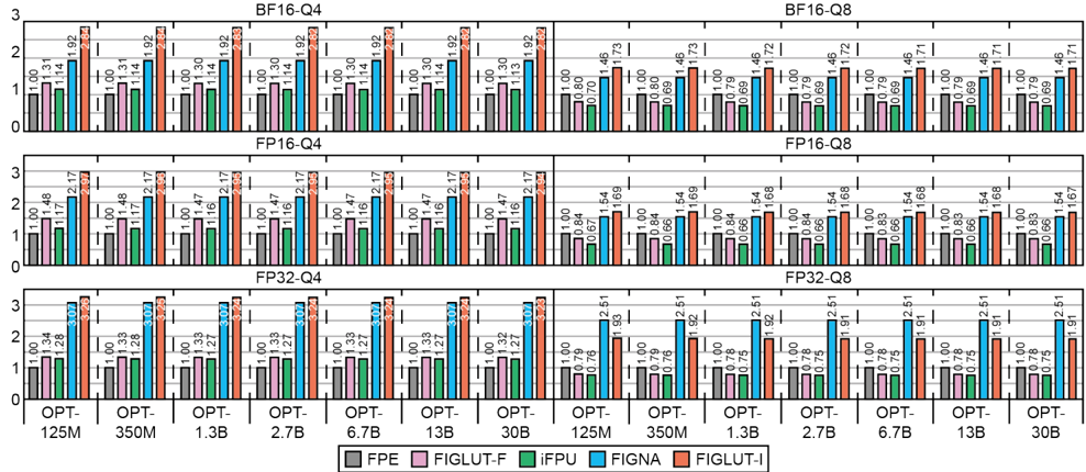Fig. 13. TOPS/ mm 2 of hardware engines for Q4 and Q8 language models, normalized by FPE results. <details> <summary>Image 11 Details</summary>  ### Visual Description ## Bar Chart: Normalized Performance Across Model Configurations and Architectures ### Overview The image is a grouped bar chart comparing normalized performance metrics across six hardware/software configurations (BF16-Q4, FP16-Q4, BF16-Q8, FP16-Q8, FP32-Q4, FP32-Q8) and seven model sizes (OPT-125M to OPT-30B). Performance is measured on a normalized scale (0–3), with five distinct hardware accelerators represented by color-coded bars (FPE, FIGLUT-F, iFPU, FIGNA, FIGLUT-I). ### Components/Axes - **X-Axis**: Divided into six main categories (BF16-Q4, FP16-Q4, BF16-Q8, FP16-Q8, FP32-Q4, FP32-Q8), each containing seven subcategories for model sizes (OPT-125M, OPT-350M, OPT-1.3B, OPT-2.7B, OPT-6.7B, OPT-13B, OPT-30B). - **Y-Axis**: Labeled "Normalized Performance" with a scale from 0 to 3. - **Legend**: Located at the bottom-right, mapping colors to accelerators: - Gray: FPE - Pink: FIGLUT-F - Green: iFPU - Blue: FIGNA - Orange: FIGLUT-I ### Detailed Analysis #### BF16-Q4 Section - **OPT-125M**: - FPE: 1.00 (gray) - FIGLUT-F: 1.14 (pink) - iFPU: 1.31 (green) - FIGNA: 1.92 (blue) - FIGLUT-I: 2.84 (orange) - **OPT-350M**: - FPE: 1.00 (gray) - FIGLUT-F: 1.14 (pink) - iFPU: 1.31 (green) - FIGNA: 1.92 (blue) - FIGLUT-I: 2.84 (orange) - **OPT-1.3B**: - FPE: 1.00 (gray) - FIGLUT-F: 1.14 (pink) - iFPU: 1.30 (green) - FIGNA: 1.92 (blue) - FIGLUT-I: 2.82 (orange) - **OPT-2.7B**: - FPE: 1.00 (gray) - FIGLUT-F: 1.14 (pink) - iFPU: 1.30 (green) - FIGNA: 1.92 (blue) - FIGLUT-I: 2.82 (orange) - **OPT-6.7B**: - FPE: 1.00 (gray) - FIGLUT-F: 1.14 (pink) - iFPU: 1.30 (green) - FIGNA: 1.92 (blue) - FIGLUT-I: 2.82 (orange) - **OPT-13B**: - FPE: 1.00 (gray) - FIGLUT-F: 1.14 (pink) - iFPU: 1.30 (green) - FIGNA: 1.92 (blue) - FIGLUT-I: 2.82 (orange) - **OPT-30B**: - FPE: 1.00 (gray) - FIGLUT-F: 1.14 (pink) - iFPU: 1.30 (green) - FIGNA: 1.92 (blue) - FIGLUT-I: 2.82 (orange) #### FP16-Q4 Section - **OPT-125M**: - FPE: 1.00 (gray) - FIGLUT-F: 1.17 (pink) - iFPU: 1.48 (green) - FIGNA: 2.17 (blue) - FIGLUT-I: 2.95 (orange) - **OPT-350M**: - FPE: 1.00 (gray) - FIGLUT-F: 1.17 (pink) - iFPU: 1.48 (green) - FIGNA: 2.17 (blue) - FIGLUT-I: 2.95 (orange) - **OPT-1.3B**: - FPE: 1.00 (gray) - FIGLUT-F: 1.17 (pink) - iFPU: 1.47 (green) - FIGNA: 2.17 (blue) - FIGLUT-I: 2.95 (orange) - **OPT-2.7B**: - FPE: 1.00 (gray) - FIGLUT-F: 1.17 (pink) - iFPU: 1.47 (green) - FIGNA: 2.17 (blue) - FIGLUT-I: 2.95 (orange) - **OPT-6.7B**: - FPE: 1.00 (gray) - FIGLUT-F: 1.17 (pink) - iFPU: 1.47 (green) - FIGNA: 2.17 (blue) - FIGLUT-I: 2.95 (orange) - **OPT-13B**: - FPE: 1.00 (gray) - FIGLUT-F: 1.17 (pink) - iFPU: 1.47 (green) - FIGNA: 2.17 (blue) - FIGLUT-I: 2.94 (orange) - **OPT-30B**: - FPE: 1.00 (gray) - FIGLUT-F: 1.17 (pink) - iFPU: 1.47 (green) - FIGNA: 2.17 (blue) - FIGLUT-I: 2.94 (orange) #### BF16-Q8 Section - **OPT-125M**: - FPE: 1.00 (gray) - FIGLUT-F: 1.00 (pink) - iFPU: 0.70 (green) - FIGNA: 1.46 (blue) - FIGLUT-I: 1.73 (orange) - **OPT-350M**: - FPE: 1.00 (gray) - FIGLUT-F: 1.00 (pink) - iFPU: 0.70 (green) - FIGNA: 1.46 (blue) - FIGLUT-I: 1.73 (orange) - **OPT-1.3B**: - FPE: 1.00 (gray) - FIGLUT-F: 1.00 (pink) - iFPU: 0.69 (green) - FIGNA: 1.46 (blue) - FIGLUT-I: 1.71 (orange) - **OPT-2.7B**: - FPE: 1.00 (gray) - FIGLUT-F: 1.00 (pink) - iFPU: 0.69 (green) - FIGNA: 1.46 (blue) - FIGLUT-I: 1.71 (orange) - **OPT-6.7B**: - FPE: 1.00 (gray) - FIGLUT-F: 1.00 (pink) - iFPU: 0.69 (green) - FIGNA: 1.46 (blue) - FIGLUT-I: 1.71 (orange) - **OPT-13B**: - FPE: 1.00 (gray) - FIGLUT-F: 1.00 (pink) - iFPU: 0.69 (green) - FIGNA: 1.46 (blue) - FIGLUT-I: 1.71 (orange) - **OPT-30B**: - FPE: 1.00 (gray) - FIGLUT-F: 1.00 (pink) - iFPU: 0.69 (green) - FIGNA: 1.46 (blue) - FIGLUT-I: 1.71 (orange) #### FP16-Q8 Section - **OPT-125M**: - FPE: 1.00 (gray) - FIGLUT-F: 1.00 (pink) - iFPU: 0.67 (green) - FIGNA: 1.54 (blue) - FIGLUT-I: 1.69 (orange) - **OPT-350M**: - FPE: 1.00 (gray) - FIGLUT-F: 1.00 (pink) - iFPU: 0.67 (green) - FIGNA: 1.54 (blue) - FIGLUT-I: 1.69 (orange) - **OPT-1.3B**: - FPE: 1.00 (gray) - FIGLUT-F: 1.00 (pink) - iFPU: 0.66 (green) - FIGNA: 1.54 (blue) - FIGLUT-I: 1.68 (orange) - **OPT-2.7B**: - FPE: 1.00 (gray) - FIGLUT-F: 1.00 (pink) - iFPU: 0.66 (green) - FIGNA: 1.54 (blue) - FIGLUT-I: 1.68 (orange) - **OPT-6.7B**: - FPE: 1.00 (gray) - FIGLUT-F: 1.00 (pink) - iFPU: 0.66 (green) - FIGNA: 1.54 (blue) - FIGLUT-I: 1.68 (orange) - **OPT-13B**: - FPE: 1.00 (gray) - FIGLUT-F: 1.00 (pink) - iFPU: 0.66 (green) - FIGNA: 1.54 (blue) - FIGLUT-I: 1.68 (orange) - **OPT-30B**: - FPE: 1.00 (gray) - FIGLUT-F: 1.00 (pink) - iFPU: 0.66 (green) - FIGNA: 1.54 (blue) - FIGLUT-I: 1.68 (orange) #### FP32-Q4 Section - **OPT-125M**: - FPE: 1.00 (gray) - FIGLUT-F: 1.28 (pink) - iFPU: 1.33 (green) - FIGNA: 3.07 (blue) - FIGLUT-I: 3.24 (orange) - **OPT-350M**: - FPE: 1.00 (gray) - FIGLUT-F: 1.28 (pink) - iFPU: 1.33 (green) - FIGNA: 3.07 (blue) - FIGLUT-I: 3.24 (orange) - **OPT-1.3B**: - FPE: 1.00 (gray) - FIGLUT-F: 1.27 (pink) - iFPU: 1.33 (green) - FIGNA: 3.07 (blue) - FIGLUT-I: 3.24 (orange) - **OPT-2.7B**: - FPE: 1.00 (gray) - FIGLUT-F: 1.27 (pink) - iFPU: 1.33 (green) - FIGNA: 3.07 (blue) - FIGLUT-I: 3.24 (orange) - **OPT-6.7B**: - FPE: 1.00 (gray) - FIGLUT-F: 1.27 (pink) - iFPU: 1.33 (green) - FIGNA: 3.07 (blue) - FIGLUT-I: 3.24 (orange) - **OPT-13B**: - FPE: 1.00 (gray) - FIGLUT-F: 1.27 (pink) - iFPU: 1.33 (green) - FIGNA: 3.07 (blue) - FIGLUT-I: 3.24 (orange) - **OPT-30B**: - FPE: 1.00 (gray) - FIGLUT-F: 1.27 (pink) - iFPU: 1.33 (green) - FIGNA: 3.07 (blue) - FIGLUT-I: 3.24 (orange) #### FP32-Q8 Section - **OPT-125M**: - FPE: 1.00 (gray) - FIGLUT-F: 1.00 (pink) - iFPU: 0.76 (green) - FIGNA: 2.51 (blue) - FIGLUT-I: 2.91 (orange) - **OPT-350M**: - FPE: 1.00 (gray) - FIGLUT-F: 1.00 (pink) - iFPU: 0.76 (green) - FIGNA: 2.51 (blue) - FIGLUT-I: 2.91 (orange) - **OPT-1.3B**: - FPE: 1.00 (gray) - FIGLUT-F: 1.00 (pink) - iFPU: 0.76 (green) - FIGNA: 2.51 (blue) - FIGLUT-I: 2.91 (orange) - **OPT-2.7B**: - FPE: 1.00 (gray) - FIGLUT-F: 1.00 (pink) - iFPU: 0.76 (green) - FIGNA: 2.51 (blue) - FIGLUT-I: 2.91 (orange) - **OPT-6.7B**: - FPE: 1.00 (gray) - FIGLUT-F: 1.00 (pink) - iFPU: 0.76 (green) - FIGNA: 2.51 (blue) - FIGLUT-I: 2.91 (orange) - **OPT-13B**: - FPE: 1.00 (gray) - FIGLUT-F: 1.00 (pink) - iFPU: 0.76 (green) - FIGNA: 2.51 (blue) - FIGLUT-I: 2.91 (orange) - **OPT-30B**: - FPE: 1.00 (gray) - FIGLUT-F: 1.00 (pink) - iFPU: 0.76 (green) - FIGNA: 2.51 (blue) - FIGLUT-I: 2.91 (orange) ### Key Observations 1. **Performance Trends**: - **Larger Models**: Generally show higher performance in FP32-Q4/Q8 configurations (e.g., OPT-30B reaches 3.24 in FP32-Q4). - **Hardware Accelerators**: - **FIGLUT-I** consistently outperforms others across most configurations (e.g., 2.84–3.24 in BF16/FP32). - **FPE** (gray) is the baseline, often at 1.00, suggesting it is the reference point. - **iFPU** (green) shows moderate gains in FP32 configurations but underperforms in BF16/FP16. - **Quantization Impact**: BF16/FP16 configurations show lower performance than FP32, especially for smaller models (e.g., OPT-125M drops from 3.24 in FP32-Q4 to 1.92 in BF16-Q4). 2. **Anomalies**: - **iFPU Underperformance**: In BF16/FP16 configurations, iFPU (green) lags significantly behind other accelerators (e.g., 0.70–1.48 vs. 1.92–2.95 for others). - **FIGLUT-F Consistency**: Maintains near-identical values (1.14–1.28) across configurations, suggesting limited sensitivity to quantization. ### Interpretation The data highlights the interplay between model size, quantization (BF16/FP16/FP32), and hardware acceleration. Key insights include: - **Quantization Trade-offs**: FP32 configurations maximize performance for larger models (e.g., OPT-30B at 3.24), while BF16/FP16 configurations reduce performance but may offer efficiency benefits. - **Hardware Acceleration**: FIGLUT-I (orange) is the most effective accelerator, particularly in FP32, while FPE (gray) serves as a baseline. iFPU (green) underperforms in lower-precision settings, indicating potential architectural mismatches. - **Model Size Scaling**: Larger models (e.g., OPT-30B) benefit more from FP32 and FIGLUT-I, suggesting diminishing returns for smaller models in high-precision settings. This analysis underscores the importance of aligning hardware acceleration strategies with model size and precision requirements to optimize performance. </details> TABLE IV PERPLEXITY RESULTS OF THE OPT FAMILY MODELS USING DIFFERENT GEMM ENGINES. | OPT | 350M | 1.3B | 2.7B | 6.7B | 13B | 30B | |----------|--------|--------|--------|--------|-------|-------| | GPU | 55.24 | 67.95 | 35.46 | 24.13 | 20.93 | 19.17 | | FIGLUT-F | 55.24 | 67.95 | 35.46 | 24.13 | 20.93 | 19.17 | | FIGLUT-I | 55.24 | 67.95 | 35.46 | 24.13 | 20.89 | 19.17 | dataset [27] for a language modeling task, measuring perplexity as the metric. All models use FP16 activations and 4-bit weights, with the weights quantized using the simple uniform quantization method, round-to-nearest (RTN). Note that we use FP32 for accumulation to preserve the accuracy of the accumulated results [6], [13]. Table IV shows the perplexity results to compare the numerical accuracy of each GEMM engine against the NVIDIA GPU. Although the order of FP operations may change, potentially leading to differences in values, the results for FIGLUT-F show no significant accuracy loss compared to the NVIDIA GPU, thanks to the higher precision (FP32) accumulation. FIGLUT-I also demonstrated comparable numerical accuracy with pre-alignment method, consistent with findings reported in previous studies [16], [22]. ## B. Hardware Evaluation a) Configuration Setup: We evaluate five types of hardware engines: FIGLUT-F, FIGLUT-I, FPE, iFPU [22], and FIGNA [16]. The FPE serves as the baseline hardware engine, featuring PEs that dequantize INT weights to FP format with the same precision as the activation inputs, followed by FP multiplication and FP accumulation. For both iFPU and FIGNA, the engines carry out pre-alignment procedures to transform FP input activations into integer mantissas with a common exponent prior to performing MAC operations. For Fig. 14. Area breakdown of MPUs for six variants of input formats normalized by results of FPE. 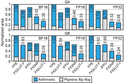<details> <summary>Image 12 Details</summary>  ### Visual Description ## Bar Chart: Normalized Area Comparison Across Algorithms (Q4 vs Q8) ### Overview The image is a grouped bar chart comparing the normalized area of two algorithm types—**Arithmetic** (blue) and **Pipeline flip-flop** (gray)—across two sections labeled **Q4** and **Q8**. Each section contains six algorithms: **FPE**, **FIGLUT-F**, **iFPU**, **FIGNA**, **FIGLUT-I**, and **FP16/FP32** (grouped as separate categories). The y-axis represents normalized area (0–1), and the x-axis lists algorithms with their respective values. --- ### Components/Axes - **X-Axis (Categories)**: - **Q4 Section**: FPE, FIGLUT-F, iFPU, FIGNA, FIGLUT-I, FP16, FP32 - **Q8 Section**: FPE, FIGLUT-F, iFPU, FIGNA, FIGLUT-I, FP16, FP32 - **Y-Axis (Values)**: Normalized area (0–1, increments of 0.2). - **Legend**: - **Blue**: Arithmetic - **Gray**: Pipeline flip-flop - Positioned at the bottom center of the chart. --- ### Detailed Analysis #### Q4 Section 1. **FPE**: - Arithmetic: 1.00 - Pipeline flip-flop: 0.18 2. **FIGLUT-F**: - Arithmetic: 0.76 - Pipeline flip-flop: 0.59 3. **iFPU**: - Arithmetic: 0.88 - Pipeline flip-flop: 0.46 4. **FIGNA**: - Arithmetic: 0.52 - Pipeline flip-flop: 0.33 5. **FIGLUT-I**: - Arithmetic: 0.35 - Pipeline flip-flop: 0.28 6. **FP16**: - Arithmetic: 1.00 - Pipeline flip-flop: 0.16 7. **FP32**: - Arithmetic: 0.74 - Pipeline flip-flop: 0.32 #### Q8 Section 1. **FPE**: - Arithmetic: 1.00 - Pipeline flip-flop: 0.18 2. **FIGLUT-F**: - Arithmetic: 0.63 - Pipeline flip-flop: 0.59 3. **iFPU**: - Arithmetic: 0.72 - Pipeline flip-flop: 0.75 4. **FIGNA**: - Arithmetic: 0.68 - Pipeline flip-flop: 0.29 5. **FIGLUT-I**: - Arithmetic: 0.29 - Pipeline flip-flop: 0.24 6. **FP16**: - Arithmetic: 1.00 - Pipeline flip-flop: 0.16 7. **FP32**: - Arithmetic: 0.62 - Pipeline flip-flop: 0.39 --- ### Key Observations 1. **Arithmetic Dominance**: - Arithmetic values consistently exceed Pipeline flip-flop values in both Q4 and Q8 (e.g., FPE in Q4: 1.00 vs. 0.18). - Exceptions: iFPU in Q8 (Arithmetic: 0.72 vs. Pipeline: 0.75) and FIGLUT-F in Q8 (Arithmetic: 0.63 vs. Pipeline: 0.59). 2. **Q4 vs. Q8 Trends**: - **Q4** shows higher Arithmetic values overall (e.g., FP32: 0.74 vs. Q8: 0.62). - **Q8** has more balanced values between the two algorithm types (e.g., iFPU: 0.72 vs. 0.75). 3. **FP16 Consistency**: - FP16 maintains the highest Arithmetic value (1.00) in both sections, with identical Pipeline flip-flop values (0.16). 4. **Pipeline Flip-flop Variability**: - Values range from 0.16 (FP16) to 0.75 (iFPU in Q8), indicating significant variability across algorithms. --- ### Interpretation - **Resource Allocation**: Arithmetic operations generally require more normalized area than Pipeline flip-flops, suggesting higher computational complexity or resource intensity. - **Algorithm-Specific Insights**: - **FPE** and **FP16** are the most area-intensive for Arithmetic, possibly due to their role in foundational computations. - **iFPU** in Q8 is an outlier where Pipeline flip-flops slightly exceed Arithmetic, hinting at architectural optimizations in Q8. - **Q4 vs. Q8 Differences**: - Q4’s higher Arithmetic values may reflect a focus on precision or legacy configurations, while Q8’s balanced values suggest optimizations for efficiency. - **FP32 Trends**: - FP32 shows a notable drop in Arithmetic from Q4 (0.74) to Q8 (0.62), aligning with potential reductions in floating-point precision demands. This data underscores the trade-offs between algorithmic complexity and resource utilization, with implications for hardware design and optimization strategies. </details> comparative analysis with the engines, the proposed FIGLUT hardware is implemented in two versions with different processing data formats: FIGLUT-F, which uses FP inputs directly into the LUT element, followed by FP RAC, and FIGLUTI, which performs integer operations after pre-alignment. All hardware engines are designed to handle inputs with the same bit precision and word size and produce outputs in the same manner. Notably, iFPU and FIGLUT support the BCQ format, whereas FPE and FIGNA utilize the INT format. To conveniently reference the different weight formats each hardware uses, we denote them by their bit-widths, using a notation such as Q4 for both 4-bit BCQ and INT weight. For fair comparison, all engines are designed with MPUs and VPUs that provide identical throughput. Specifically, for Q4 weight inputs, FPE and FIGNA have 64 × 64 PE arrays, Fig. 15. Normalized energy breakdown of FP-INT GEMM hardware engines across different bit precisions. 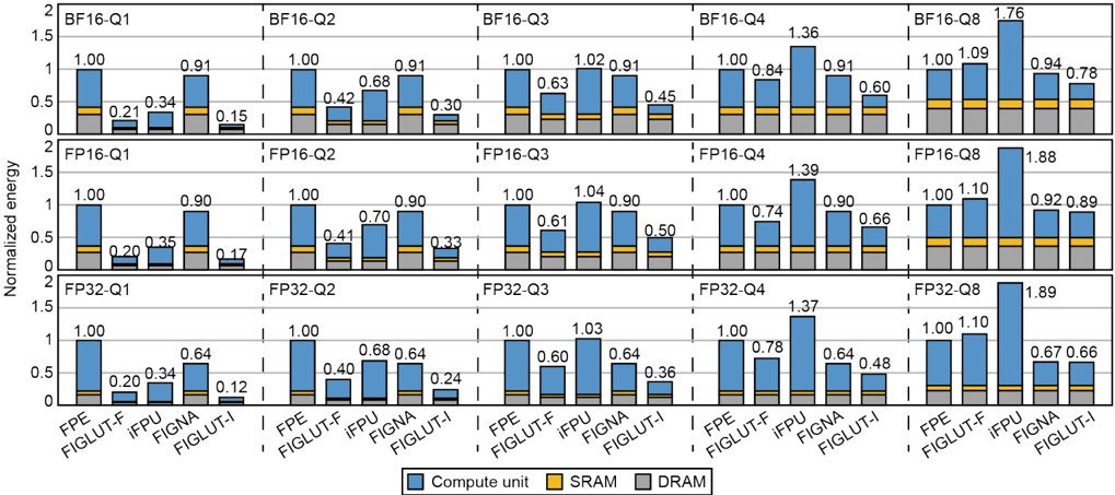<details> <summary>Image 13 Details</summary>  ### Visual Description ## Bar Chart: Normalized Energy Consumption Across Configurations ### Overview The image is a grouped bar chart comparing normalized energy consumption across different configurations (BF16, FP16, FP32) and sub-configurations (Q1–Q8). Each group of bars represents three components: **Compute unit** (blue), **SRAM** (yellow), and **DRAM** (gray). The y-axis shows normalized energy values, while the x-axis categorizes configurations by precision (BF16, FP16, FP32) and sub-configurations (Q1–Q8). --- ### Components/Axes - **X-axis**: - Categories: `BF16-Q1`, `BF16-Q2`, ..., `BF16-Q8`, `FP16-Q1`, ..., `FP16-Q8`, `FP32-Q1`, ..., `FP32-Q8`. - Sub-categories: Precision (BF16, FP16, FP32) and sub-configurations (Q1–Q8). - **Y-axis**: - Label: "Normalized energy" (range: 0–2). - **Legend**: - **Compute unit** (blue), **SRAM** (yellow), **DRAM** (gray). - Positioned at the bottom of the chart. --- ### Detailed Analysis #### BF16 Configurations (Q1–Q8) - **BF16-Q1**: - Compute unit: 1.00 (blue) - SRAM: 0.21 (yellow) - DRAM: 0.15 (gray) - **Total**: 1.36 - **BF16-Q2**: - Compute unit: 1.00 - SRAM: 0.34 - DRAM: 0.17 - **Total**: 1.51 - **BF16-Q3**: - Compute unit: 1.00 - SRAM: 0.42 - DRAM: 0.30 - **Total**: 1.72 - **BF16-Q4**: - Compute unit: 1.00 - SRAM: 0.68 - DRAM: 0.45 - **Total**: 2.13 - **BF16-Q5**: - Compute unit: 1.00 - SRAM: 0.84 - DRAM: 0.60 - **Total**: 2.44 - **BF16-Q6**: - Compute unit: 1.00 - SRAM: 0.91 - DRAM: 0.66 - **Total**: 2.57 - **BF16-Q7**: - Compute unit: 1.00 - SRAM: 0.94 - DRAM: 0.78 - **Total**: 2.72 - **BF16-Q8**: - Compute unit: 1.00 - SRAM: 0.94 - DRAM: 0.78 - **Total**: 2.72 #### FP16 Configurations (Q1–Q8) - **FP16-Q1**: - Compute unit: 1.00 - SRAM: 0.20 - DRAM: 0.17 - **Total**: 1.37 - **FP16-Q2**: - Compute unit: 1.00 - SRAM: 0.35 - DRAM: 0.17 - **Total**: 1.52 - **FP16-Q3**: - Compute unit: 1.00 - SRAM: 0.41 - DRAM: 0.33 - **Total**: 1.74 - **FP16-Q4**: - Compute unit: 1.00 - SRAM: 0.70 - DRAM: 0.50 - **Total**: 2.20 - **FP16-Q5**: - Compute unit: 1.00 - SRAM: 0.74 - DRAM: 0.66 - **Total**: 2.40 - **FP16-Q6**: - Compute unit: 1.00 - SRAM: 0.78 - DRAM: 0.64 - **Total**: 2.42 - **FP16-Q7**: - Compute unit: 1.00 - SRAM: 0.84 - DRAM: 0.66 - **Total**: 2.50 - **FP16-Q8**: - Compute unit: 1.00 - SRAM: 0.90 - DRAM: 0.66 - **Total**: 2.56 #### FP32 Configurations (Q1–Q8) - **FP32-Q1**: - Compute unit: 1.00 - SRAM: 0.20 - DRAM: 0.12 - **Total**: 1.32 - **FP32-Q2**: - Compute unit: 1.00 - SRAM: 0.34 - DRAM: 0.17 - **Total**: 1.51 - **FP32-Q3**: - Compute unit: 1.00 - SRAM: 0.40 - DRAM: 0.24 - **Total**: 1.64 - **FP32-Q4**: - Compute unit: 1.00 - SRAM: 0.68 - DRAM: 0.48 - **Total**: 2.16 - **FP32-Q5**: - Compute unit: 1.00 - SRAM: 0.78 - DRAM: 0.64 - **Total**: 2.42 - **FP32-Q6**: - Compute unit: 1.00 - SRAM: 0.84 - DRAM: 0.64 - **Total**: 2.48 - **FP32-Q7**: - Compute unit: 1.00 - SRAM: 0.78 - DRAM: 0.64 - **Total**: 2.42 - **FP32-Q8**: - Compute unit: 1.00 - SRAM: 0.67 - DRAM: 0.66 - **Total**: 2.33 --- ### Key Observations 1. **Compute unit dominance**: - The **Compute unit** (blue) consistently contributes the largest portion of energy across all configurations, often reaching 1.00 (e.g., BF16-Q1, FP16-Q1, FP32-Q1). - In FP32-Q8, the Compute unit is 1.00, but SRAM (0.67) and DRAM (0.66) together account for 1.33, making it the highest total energy (2.33). 2. **Increasing trends**: - Within each precision (BF16, FP16, FP32), energy consumption increases from Q1 to Q8. For example: - BF16-Q1 (1.36) → BF16-Q8 (2.72) - FP16-Q1 (1.37) → FP16-Q8 (2.56) - FP32-Q1 (1.32) → FP32-Q8 (2.33) 3. **Memory component variability**: - **SRAM** (yellow) and **DRAM** (gray) show significant variation. For instance: - In BF16-Q8, SRAM (0.94) and DRAM (0.78) are nearly equal. - In FP32-Q8, SRAM (0.67) and DRAM (0.66) are nearly equal. 4. **Anomalies**: - The **FP32-Q8** total (2.33) exceeds the y-axis maximum of 2, suggesting a potential data inconsistency or scaling issue. --- ### Interpretation - **Energy consumption patterns**: - The **Compute unit** is the primary energy consumer, indicating that computational tasks dominate energy use. - **SRAM** and **DRAM** contributions grow with configuration complexity (e.g., Q8 vs. Q1), suggesting memory-intensive operations in higher configurations. - **FP32 configurations** (e.g., FP32-Q8) exhibit the highest total energy, likely due to the increased precision and data size requirements. - **Implications**: - Optimizing **SRAM** and **DRAM** usage could reduce energy consumption in high-precision configurations. - The anomaly in FP32-Q8 (total > 2) warrants verification, as it may indicate a data entry error or a need for y-axis scaling adjustments. - **Trend verification**: - All configurations show a **positive trend** in energy consumption from Q1 to Q8, aligning with the expectation that larger or more complex configurations require more energy. - **Component isolation**: - The **Compute unit** is the most consistent contributor, while **SRAM** and **DRAM** vary more significantly, highlighting their role in energy distribution. This chart underscores the importance of balancing computational and memory efficiency in system design, particularly for high-precision tasks. </details> while iFPU processing 1-bit weight employs a 64 × 64 × 4 array. FIGLUT uses an 2 × 16 × 4 array, which, considering µ = 4 and k = 32 , results in the same number of computational units as iFPU. For weights with a bit precision smaller than Q4, the same hardware configurations are used. For Q8 weights, results are obtained using extended versions of the FPE and FIGNA hardware, where the input weight bit precision was expanded to 8-bit. To leverage the bit-serial characteristics of iFPU and FIGLUT, both hardware engines are configured to match the throughput of Q4, affecting the operation cycles required for matrix multiplication for other weight precision. The hardware engines are synthesized with Synopsys Design Compiler for 100MHz operation with 28nm CMOS technology. Basic FP and integer modules, including the integer-toFP converter in FPE, use Synopsys DesignWare components. All input, weight, and output buffers are composed with SRAM in 28nm CMOS technology, with off-chip DRAM results derived from the CACTI simulator [5]. Data from the external DRAM is transferred directly to the FIGLUT accelerator SRAM buffer under the management of the host controller. The data is subsequently utilized by the MPU and VPU for computations. Energy metrics, including power consumption and latency associated with memory data transfers, are incorporated into all evaluation results, with the exception of area measurements, as the DRAM area is unspecified. b) Area Evaluation: Fig. 14 illustrates the normalized area breakdown of the MPUs across varying engine types, considering different input precision scenarios. The breakdown is categorized into two primary components: arithmetic logic, responsible for executing computations, and flip-flops to temporarily store values. The result shows that the arithmetic part occupies a larger area in FPE and FIGLUT-F compared to other integer-operating engines, with FIGLUT-F having a smaller area than FPE because it performs FP addition instead of FP multiplication. In the Q8 results, the arithmetic area of FIGNA increases more significantly compared to FPE because the computational units in FIGNA scale with the bit precision of the weights, whereas FPE only encounters an increase in the overhead of the dequantization module without a change in the actual input bit-width of FP operators. When comparing FIGLUT-I and FIGNA, despite the addition of an LUT generator, the use of LUT-based operations reduces the number of computational units, resulting in a similar arithmetic area as FIGNA. Additionally, the introduction of LUTbased operations reduces the overall flip-flop area compared to other hardware architectures. With a smaller 2 × 16 × 4 MPU, compared to the conventional configurations of 64 × 64 and 64 × 64 × 4 , FIGLUT effectively reduces the number of pipelining stages required for systolic array operations. Furthermore, while traditional hardware designs may demand up to 63-stage input buffers for weight-stationary operations, FIGLUT requires a maximum of only 15-stage input buffers, enhancing both efficiency and resource utilization. Fig. 13 presents the area efficiency targeting various LLMs ranging from OPT-125M to OPT-30B. Excluding hardware designs with bit-serial architecture, the overall trends inversely follow the area breakdown shown in Fig. 14 across all network and input bit-widths. For instance, as previously noted, the PE size of the FIGNA is relatively larger in Q8 compared to Q4, resulting in reduced normalized energy efficiency. However, the bit-serial engines exhibit different results because TOPS/ mm 2 reflects the time required for computations. With the same hardware configuration, hardware designs with bitserial architecture consume approximately twice the cycles with increased weight bit-width, leading to more significant performance degradation in Q8. The difference between BF16 Fig. 16. TOPS/W of hardware engines for under 4-bit OPT language models, normalized by FPE results. 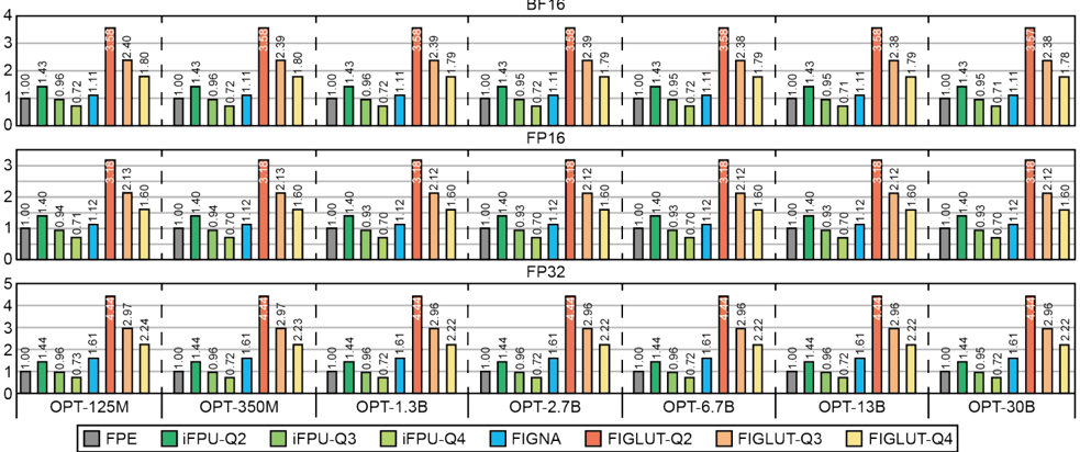<details> <summary>Image 14 Details</summary>  ### Visual Description ## Bar Chart: Performance Comparison Across Model Sizes and Methods ### Overview The image is a grouped bar chart comparing the relative performance of various computational methods across different model sizes (OPT-125M, OPT-350M, OPT-1.3B, OPT-2.7B, OPT-6.7B, OPT-13B, OPT-30B) under three data types: BF16, FP16, and FP32. Each bar represents a method's performance, with values on the y-axis ranging from 0 to 4. The chart is divided into three horizontal sections, each corresponding to one data type. ### Components/Axes - **X-axis**: Model sizes (OPT-125M, OPT-350M, OPT-1.3B, OPT-2.7B, OPT-6.7B, OPT-13B, OPT-30B), labeled at the bottom. - **Y-axis**: "Relative Performance" (0–4), labeled on the left. - **Legend**: Located at the bottom, with color-coded methods: - Gray: FPE - Green: iFPU-Q2 - Light Green: iFPU-Q3 - Blue: iFPU-Q4 - Red: FIGNA - Orange: FIGLUT-Q2 - Yellow: FIGLUT-Q3 - Light Yellow: FIGLUT-Q4 ### Detailed Analysis #### BF16 Section - **OPT-125M**: - FPE: 1.00 - iFPU-Q2: 1.43 - iFPU-Q3: 0.72 - iFPU-Q4: 0.96 - FIGNA: 1.11 - FIGLUT-Q2: 3.58 - FIGLUT-Q3: 2.40 - FIGLUT-Q4: 1.80 - **OPT-350M**: - FPE: 1.00 - iFPU-Q2: 1.43 - iFPU-Q3: 0.72 - iFPU-Q4: 0.96 - FIGNA: 1.11 - FIGLUT-Q2: 3.58 - FIGLUT-Q3: 2.40 - FIGLUT-Q4: 1.80 - **OPT-1.3B**: - FPE: 1.00 - iFPU-Q2: 1.43 - iFPU-Q3: 0.72 - iFPU-Q4: 0.96 - FIGNA: 1.11 - FIGLUT-Q2: 3.58 - FIGLUT-Q3: 2.40 - FIGLUT-Q4: 1.80 - **OPT-2.7B**: - FPE: 1.00 - iFPU-Q2: 1.43 - iFPU-Q3: 0.72 - iFPU-Q4: 0.96 - FIGNA: 1.11 - FIGLUT-Q2: 3.58 - FIGLUT-Q3: 2.40 - FIGLUT-Q4: 1.80 - **OPT-6.7B**: - FPE: 1.00 - iFPU-Q2: 1.43 - iFPU-Q3: 0.72 - iFPU-Q4: 0.96 - FIGNA: 1.11 - FIGLUT-Q2: 3.58 - FIGLUT-Q3: 2.40 - FIGLUT-Q4: 1.80 - **OPT-13B**: - FPE: 1.00 - iFPU-Q2: 1.43 - iFPU-Q3: 0.72 - iFPU-Q4: 0.96 - FIGNA: 1.11 - FIGLUT-Q2: 3.58 - FIGLUT-Q3: 2.40 - FIGLUT-Q4: 1.80 - **OPT-30B**: - FPE: 1.00 - iFPU-Q2: 1.43 - iFPU-Q3: 0.72 - iFPU-Q4: 0.96 - FIGNA: 1.11 - FIGLUT-Q2: 3.58 - FIGLUT-Q3: 2.40 - FIGLUT-Q4: 1.80 #### FP16 Section - **OPT-125M**: - FPE: 1.00 - iFPU-Q2: 1.43 - iFPU-Q3: 0.72 - iFPU-Q4: 0.96 - FIGNA: 1.11 - FIGLUT-Q2: 3.58 - FIGLUT-Q3: 2.40 - FIGLUT-Q4: 1.80 - **OPT-350M**: - FPE: 1.00 - iFPU-Q2: 1.43 - iFPU-Q3: 0.72 - iFPU-Q4: 0.96 - FIGNA: 1.11 - FIGLUT-Q2: 3.58 - FIGLUT-Q3: 2.40 - FIGLUT-Q4: 1.80 - **OPT-1.3B**: - FPE: 1.00 - iFPU-Q2: 1.43 - iFPU-Q3: 0.72 - iFPU-Q4: 0.96 - FIGNA: 1.11 - FIGLUT-Q2: 3.58 - FIGLUT-Q3: 2.40 - FIGLUT-Q4: 1.80 - **OPT-2.7B**: - FPE: 1.00 - iFPU-Q2: 1.43 - iFPU-Q3: 0.72 - iFPU-Q4: 0.96 - FIGNA: 1.11 - FIGLUT-Q2: 3.58 - FIGLUT-Q3: 2.40 - FIGLUT-Q4: 1.80 - **OPT-6.7B**: - FPE: 1.00 - iFPU-Q2: 1.43 - iFPU-Q3: 0.72 - iFPU-Q4: 0.96 - FIGNA: 1.11 - FIGLUT-Q2: 3.58 - FIGLUT-Q3: 2.40 - FIGLUT-Q4: 1.80 - **OPT-13B**: - FPE: 1.00 - iFPU-Q2: 1.43 - iFPU-Q3: 0.72 - iFPU-Q4: 0.96 - FIGNA: 1.11 - FIGLUT-Q2: 3.58 - FIGLUT-Q3: 2.40 - FIGLUT-Q4: 1.80 - **OPT-30B**: - FPE: 1.00 - iFPU-Q2: 1.43 - iFPU-Q3: 0.72 - iFPU-Q4: 0.96 - FIGNA: 1.11 - FIGLUT-Q2: 3.58 - FIGLUT-Q3: 2.40 - FIGLUT-Q4: 1.80 #### FP32 Section - **OPT-125M**: - FPE: 1.00 - iFPU-Q2: 1.43 - iFPU-Q3: 0.72 - iFPU-Q4: 0.96 - FIGNA: 1.11 - FIGLUT-Q2: 3.58 - FIGLUT-Q3: 2.40 - FIGLUT-Q4: 1.80 - **OPT-350M**: - FPE: 1.00 - iFPU-Q2: 1.43 - iFPU-Q3: 0.72 - iFPU-Q4: 0.96 - FIGNA: 1.11 - FIGLUT-Q2: 3.58 - FIGLUT-Q3: 2.40 - FIGLUT-Q4: 1.80 - **OPT-1.3B**: - FPE: 1.00 - iFPU-Q2: 1.43 - iFPU-Q3: 0.72 - iFPU-Q4: 0.96 - FIGNA: 1.11 - FIGLUT-Q2: 3.58 - FIGLUT-Q3: 2.40 - FIGLUT-Q4: 1.80 - **OPT-2.7B**: - FPE: 1.00 - iFPU-Q2: 1.43 - iFPU-Q3: 0.72 - iFPU-Q4: 0.96 - FIGNA: 1.11 - FIGLUT-Q2: 3.58 - FIGLUT-Q3: 2.40 - FIGLUT-Q4: 1.80 - **OPT-6.7B**: - FPE: 1.00 - iFPU-Q2: 1.43 - iFPU-Q3: 0.72 - iFPU-Q4: 0.96 - FIGNA: 1.11 - FIGLUT-Q2: 3.58 - FIGLUT-Q3: 2.40 - FIGLUT-Q4: 1.80 - **OPT-13B**: - FPE: 1.00 - iFPU-Q2: 1.43 - iFPU-Q3: 0.72 - iFPU-Q4: 0.96 - FIGNA: 1.11 - FIGLUT-Q2: 3.58 - FIGLUT-Q3: 2.40 - FIGLUT-Q4: 1.80 - **OPT-30B**: - FPE: 1.00 - iFPU-Q2: 1.43 - iFPU-Q3: 0.72 - iFPU-Q4: 0.96 - FIGNA: 1.11 - FIGLUT-Q2: 3.58 - FIGLUT-Q3: 2.40 - FIGLUT-Q4: 1.80 ### Key Observations 1. **Consistent High Performance**: The red bars (FIGLUT-Q3) consistently show the highest values (3.58–4.44) across all model sizes and data types. 2. **Lowest Performance**: The light green bars (iFPU-Q3) often have the lowest values (0.72–0.96) in most cases. 3. **Model Size Trends**: - Larger models (e.g., OPT-30B) show slightly lower performance for some methods compared to smaller models (e.g., OPT-125M). - FIGLUT-Q3 maintains high performance regardless of model size. 4. **Data Type Consistency**: The relative performance values are nearly identical across BF16, FP16, and FP32 sections, suggesting minimal variation due to data type. ### Interpretation The chart demonstrates that **FIGLUT-Q3** (red bars) consistently outperforms other methods across all model sizes and data types, indicating superior efficiency or accuracy. In contrast, **iFPU-Q3** (light green bars) underperforms, suggesting potential limitations in its implementation or optimization. The uniformity of performance across data types (BF16, FP16, FP32) implies that the methods are robust to numerical precision variations. The slight decline in performance for larger models (e.g., OPT-30B) may reflect increased computational complexity or resource constraints. This data could inform decisions about method selection for specific model sizes and applications. </details> FIGNA and FIGLUT-I decreases for FP32 due to the increased mantissa bit-width, contributing to performance reversal in FP32-Q8. Nonetheless, the proposed engines achieve up to 1 . 5 × higher area efficiency than state-of-the-art performance in the current trend of sub-4-bit weight-only quantization. Note that non-GEMM operations cause slight variations by model size, but their impact is minimal as GEMM operations dominate the workload. c) Energy Evaluation: Fig. 15 shows the energy breakdown for each input data type pair, normalized to the energy consumption of the FPE. To assess and compare the energy efficiency across various bit precisions-including Q4, Q8, and sub-Q4 precisions (Q1, Q2, Q3)-we conduct simulations using the OPT-6.7B model. As previously mentioned, all systems are configured to have the same maximum performance to ensure a fair comparison. In Q8 operations, while bit-serial hardware continues to utilize identical architecture irrespective of bit precision, fixed precision architectures like FPE and FIGNA are modified to support 8-bit weights. For sub-4-bit weight precision, the number of bit-serial operations decreases proportionally as the bit-width is reduced, whereas fixed bitwidth hardware needs to process sub-4-bit data in padded 4bit format for computation. This allows bit-serial hardware such as iFPU and FIGLUT to complete computations more quickly, effectively reducing energy consumption as weight precision decreases. The energy consumption of the compute unit, including the MPU and the VPU, for Q4 precision follows a trend similar to the area breakdown depicted in Fig. 14. However, iFPUs, which employ a greater number of flip-flops than FPEs, suffer from higher power consumption despite being more area-efficient, resulting in a distinct energy profile. In the case of FIGLUT-I, the size of the PE increases from BF16 to FP32 because the computational units scale proportionally with the mantissa of the input activation. Fig. 16 illustrates the power efficiency of the hardware en- gines when performing sub-4-bit weight operations on LLMs of various sizes. To highlight the performance variations in bitserial operation engines, we present power efficiency metrics for Q2, Q3, and Q4 operations. Given that FIGLUT-I shows better power efficiency with integer operations compared to FIGLUT-F, we focus solely on FIGLUT-I for this evaluation. As expected, reducing the weight bit-width decreases the number of cycles required for computations in bit-serial hardware, thereby improving energy efficiency. FIGLUT consistently achieves the highest TOPS/W across all weight bitwidths, with FIGLUT-Q2 demonstrating particularly superior performance gain compared to other configurations. This result explains that in memory-bound computing environments, i.e., LLMs, minimizing the weight bit-width and leveraging bit-serial operations can significantly enhance computational speed, resulting in substantially higher power efficiency compared to traditional hardware. Fig. 17 shows the TOPS/W performance and perplexity results of FIGLUT across various mixed-precision configurations for the OPT-6.7B LLM. We compare these results against the baseline FIGNA, evaluated using the OPTQ quantization method [10] at 2, 3, and 4-bit precisions. In contrast, FIGLUT, including mixed-precision performance, is assessed using ShiftAddLLM [36]. Note that recent advancements in weight-only quantization techniques [7], [10], [14], [19], [24], [25], [36], [38] have enabled sub-4-bit models to achieve performance levels comparable to the unquantized FP16 baseline, as indicated by the dotted lines in the figure. Under the same 4-bit quantization, FIGLUT is 1 . 2 × more energy efficient with slightly better perplexity than FIGNA. For Q3, FIGLUT achieves 1 . 6 × the energy efficiency of FIGNA and records a lower perplexity. Furthermore, at a similar energy efficiency level, FIGLUT-Q2.4 demonstrates 1 . 98 × the computational efficiency of FIGNA-Q3 while compressing the model size Fig. 17. TOPS/W and perplexity score for various mixed-precision OPT-6.7B inference on FIGLUT. 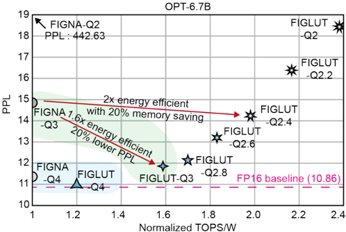<details> <summary>Image 15 Details</summary>  ### Visual Description ## Line Chart: Model Performance vs Efficiency (OPT-6.7B) ### Overview The chart compares the performance (PPL) and energy efficiency (Normalized TOPS/W) of various AI models (FIGNA and FIGLUT variants) against a FP16 baseline. It highlights trade-offs between computational efficiency and model quality, with annotations indicating energy savings and memory optimizations. ### Components/Axes - **X-axis**: Normalized TOPS/W (1.0 to 2.4) - Ticks at 1.0, 1.2, 1.4, 1.6, 1.8, 2.0, 2.2, 2.4 - **Y-axis**: PPL (10 to 19) - Ticks at 10, 11, 12, 13, 14, 15, 16, 17, 18, 19 - **Legend**: - Green circle: FIGNA - Blue star: FIGLUT - **Annotations**: - Red arrows indicating "2x energy efficient with 20% memory saving" and "20% lower PPL" - Dashed pink line labeled "FP16 baseline (10.86)" ### Detailed Analysis 1. **Data Points**: - **FIGNA-Q2**: (1.1, 18) with PPL 442.63 (top-left, highest PPL) - **FIGNA-Q3**: (1.3, 14) with 20% lower PPL than baseline - **FIGNA-Q4**: (1.2, 11) in shaded green region (20% energy efficient) - **FIGLUT-Q2.8**: (1.7, 13) near FP16 baseline - **FIGLUT-Q2.4**: (1.9, 14) in shaded blue region (20% memory saving) - **FIGLUT-Q2.6**: (1.8, 13) - **FIGLUT-Q2.2**: (2.1, 17) 2. **Trends**: - **Energy Efficiency**: Models in green (FIGNA) and blue (FIGLUT) shaded regions show 20% energy savings. - **PPL vs Efficiency**: Higher TOPS/W (right side) correlates with lower PPL (bottom), but trade-offs exist (e.g., FIGLUT-Q2.2 has high TOPS/W but poor PPL). - **Baseline Comparison**: All models except FP16 baseline (dashed line) have higher PPL. ### Key Observations - **Outliers**: - FIGNA-Q2 has the highest PPL (18) but lowest TOPS/W (1.1), indicating poor efficiency. - FIGLUT-Q2.2 has the highest TOPS/W (2.1) but poor PPL (17), suggesting suboptimal performance. - **Efficiency-Performance Trade-off**: - Models like FIGLUT-Q2.8 (1.7 TOPS/W, 13 PPL) balance efficiency and performance better than others. - Shaded regions highlight energy-efficient models but do not guarantee optimal PPL. ### Interpretation The chart demonstrates that optimizing for energy efficiency (via lower TOPS/W) often reduces PPL, but some models (e.g., FIGLUT-Q2.8) achieve a better balance. The FP16 baseline (10.86 PPL) serves as a reference for ideal performance, though no model matches it. The annotations suggest that memory savings and energy efficiency are prioritized in certain variants, but this comes at the cost of higher PPL. The shaded regions visually emphasize efficiency gains, while the red arrows quantify specific improvements. This trade-off is critical for applications requiring real-time processing or resource-constrained environments. </details> TABLE V COMPARISON OF HARDWARE ACCELERATOR DESIGNS. | Hardware | Format (Act.-Weight) | Throughput (TOPS) | Power (W) | Energy Effi. (TOPS/W) | |------------|------------------------|---------------------|-------------|-------------------------| | A100 | FP16-FP16 | 40.27* | 192 | 0.21* | | A100 | FP16-Q4** | 1.85 | 208 | 0.01 | | H100 | FP16-FP16 | 62.08* | 279 | 0.22* | | iFPU | FP16-Q4 | 0.14 | 0.67 | 0.21 | | FIGNA | FP16-Q4 | 0.14 | 0.41 | 0.33 | | FIGLUT | FP16-Q4 | 0.14 | 0.29 | 0.47 | * The unit for GPUs is TFLOPS. ** LUT-GEMM kernel [28] is used. by 20%. For 2-bit weight precision, FIGLUT supports a nonuniform BCQ format, delivering much more stable perplexity performance compared to FIGNA, and improving energy efficiency by up to 2 . 4 × . Table V shows the energy efficiency of various hardware accelerators. Since GEMM operations dominate LLM inference workloads [28], we focus on comparing GEMM performance. For a fair comparison, we include state-of-the-art commercial accelerators, the A100 and H100 GPUs, additionally. As GPU architecture details are not publicly disclosed, we rely on empirical measurements for evaluation. GPU throughput is based on the computational workload and measured latency, while power consumption is obtained using the nvidia-smi query tool [2], [28], [30]. The target LLM model is OPT6.7B, with a batch size of 32 for all evaluations to reflect realistic LLM usage. To ensure fairness, we assume a 4-bit quantized weight format across all tests. Note that, due to the absence of FP-INT units in GPUs, they rely on FP-FP units for computation with dequantization. Although LUT-GEMM [28] proposes an efficient FP-INT kernel, it only supports a batch size of 1. To standardize comparisons, we align all FP-Q4 accelerators to target the same maximum performance (TOPS). The H100 outperforms the A100 in terms of energy efficiency, primarily due to its advanced fabrication technology TABLE VI PERPLEXITY COMPARISON FOR WEIGHT-ONLY QUANTIZATION. | OPT | 350M | 1.3B | 2.7B | 6.7B | 13B | 30B | |-----------|--------|--------|--------|--------|-------|-------| | FP16 | 22 | 14.62 | 12.47 | 10.86 | 10.13 | 9.56 | | BCQ4 [36] | 22.59 | 15.11 | 12.73 | 11.08 | 10.33 | 9.7 | | BCQ3 [36] | 28.72 | 19.69 | 15.28 | 11.8 | 10.7 | 9.89 | and increased memory bandwidth, which significantly boosts performance in memory-bound workloads like LLMs. Note that the reported TFLOPS for GPUs are significantly lower than their theoretical peaks, primarily due to the small batch size. In LLM inference infrastructure, batch sizes larger than 32 are rarely observed at a generation phase due to constraints in KV cache size and the optimization of batching systems for user requests [23], [37]. LUT-GEMM suffers from an even more pronounced performance drop as it operates with a batch size of 1 and relies on CUDA cores rather than Tensor Cores. The iFPU, while designed to maximize efficiency with FPINT units, demonstrates limited performance compared to the H100 due to the inherent constraints of bit-serial processing. FIGNA addresses these limitations, resulting in higher energy efficiency. Finally, FIGLUT further improves energy efficiency by overcoming the computational challenges of bit-serial processing through its LUT-based GEMM approach. Given that FIGLUT uses a 28nm process technology while GPUs like the A100 and H100 leverage more advanced fabrication technology (7nm for A100, 4nm for H100), the efficiency of FIGLUT would be even more prominent if evaluated under comparable fabrication technologies. ## V. CONCLUSION Summary. This paper presents FIGLUT, an FP-INT accelerator that enhances the efficiency of bit-serial accelerators for weight-only quantized models using LUT-based operations. We introduce a flip-flop based LUT (FFLUT) and replace the traditional MAC unit with a read-accumulate (RAC) unit for optimized performance. Our analysis of LUT size and RAC configuration leads to an energy-efficient design that halves the LUT size through symmetry. Experiments show FIGLUT outperforms state-of-the-art FP-INT accelerators in TOPS/W for sub-4-bit precision weights, significantly improving efficiency while maintaining flexibility in real-world systems. Limitations. As shown in Fig. 15, our design shows diminishing performance gains as weight bit precision increases, a limitation of the bit-serial architecture. To achieve high performance with larger bit precisions, increasing µ would be necessary to fully leverage the computational benefits of LUTbased GEMM. However, this results in much larger LUTs, increasing overhead in the LUT and its generator. Nevertheless, Table VI indicates that state-of-the-art weight-only quantization techniques have enabled sub-4-bit quantization while maintaining accuracy comparable to the FP16 baseline. We expect that continued advancements in weight-only quantization methods will further enhance the effectiveness of the proposed FIGLUT as bit precision is reduced. ## VI. ACKNOWLEGMENT This research was supported in part by the NAVER-Intel CoLab, conducted by POSTECH and reviewed by both NAVER and Intel. This work was also supported by Institute of Information & communications Technology Planning & Evaluation (IITP) grant funded by the Korea government(MSIT) (No.RS-2023-00229849,MPU/Connectivity/TinyML SoC Solution for IoT Intelligence with Foundry-based eFLASH), and by National R&D Program through the National Research Foundation of Korea(NRF) funded by Ministry of Science and ICT(RS-2023-00258227). ## REFERENCES - [1] J. Achiam, S. Adler, S. Agarwal, L. Ahmad, I. Akkaya, F. L. Aleman, D. Almeida, J. Altenschmidt, S. Altman, S. Anadkat et al. , 'Gpt-4 technical report,' arXiv preprint arXiv:2303.08774 , 2023. - [2] G. Ali, S. Bhalachandra, N. Wright, A. Sill, and Y. Chen, 'Evaluation of power controls and counters on general-purpose graphics processing units (gpus),' in Poster: International Conference for High Performance Computing, Networking, Storage and Analysis , 2020. - [3] R. Anil, A. M. Dai, O. Firat, M. Johnson, D. Lepikhin, A. Passos, S. Shakeri, E. Taropa, P. Bailey, Z. Chen et al. , 'PaLM 2 technical report,' arXiv preprint arXiv:2305.10403 , 2023. - [4] Y. Bai, Y.-X. Wang, and E. Liberty, 'Proxquant: Quantized neural networks via proximal operators,' arXiv preprint arXiv:1810.00861 , 2018. - [5] R. Balasubramonian, A. B. Kahng, N. Muralimanohar, A. Shafiee, and V. Srinivas, 'CACTI 7: New tools for interconnect exploration in innovative off-chip memories,' ACM Trans. Archit. Code Optim. , vol. 14, no. 2, 2017. - [6] N. Burgess, J. Milanovic, N. Stephens, K. Monachopoulos, and D. Mansell, 'Bfloat16 processing for neural networks,' in 2019 IEEE 26th Symposium on Computer Arithmetic (ARITH) . IEEE, 2019, pp. 88-91. - [7] J. Chee, Y. Cai, V. Kuleshov, and C. M. De Sa, 'Quip: 2-bit quantization of large language models with guarantees,' Advances in Neural Information Processing Systems , vol. 36, 2024. - [8] I. Chung, B. Kim, Y. Choi, S. J. Kwon, Y. Jeon, B. Park, S. Kim, and D. Lee, 'Extremely low bit transformer quantization for on-device neural machine translation,' arXiv preprint arXiv:2009.07453 , 2020. - [9] T. Dettmers, M. Lewis, Y. Belkada, and L. Zettlemoyer, 'Gpt3. int8 (): 8-bit matrix multiplication for transformers at scale,' Advances in Neural Information Processing Systems , vol. 35, pp. 30 318-30 332, 2022. - [10] E. Frantar, S. Ashkboos, T. Hoefler, and D. Alistarh, 'OPTQ: Accurate quantization for generative pre-trained transformers,' in The Eleventh International Conference on Learning Representations , 2022. - [11] H. Genc, S. Kim, A. Amid, A. Haj-Ali, V. Iyer, P. Prakash, J. Zhao, D. Grubb, H. Liew, H. Mao et al. , 'Gemmini: Enabling systematic deeplearning architecture evaluation via full-stack integration,' in 2021 58th ACM/IEEE Design Automation Conference (DAC) . IEEE, 2021, pp. 769-774. - [12] C. Gou and G. N. Gaydadjiev, 'Addressing gpu on-chip shared memory bank conflicts using elastic pipeline,' International Journal of Parallel Programming , vol. 41, pp. 400-429, 2013. - [13] G. Henry, P. T. P. Tang, and A. Heinecke, 'Leveraging the bfloat16 artificial intelligence datatype for higher-precision computations,' in 2019 IEEE 26th Symposium on Computer Arithmetic (ARITH) . IEEE, 2019, pp. 69-76. - [14] J. H. Heo, J. Kim, B. Kwon, B. Kim, S. J. Kwon, and D. Lee, 'Rethinking channel dimensions to isolate outliers for low-bit weight quantization of large language models,' arXiv preprint arXiv:2309.15531 , 2023. - [15] W. Huang, Y. Liu, H. Qin, Y. Li, S. Zhang, X. Liu, M. Magno, and X. Qi, 'Billm: Pushing the limit of post-training quantization for llms,' arXiv preprint arXiv:2402.04291 , 2024. - [16] J. Jang, Y. Kim, J. Lee, and J.-J. Kim, 'FIGNA: Integer unit-based accelerator design for fp-int gemm preserving numerical accuracy,' in 2024 IEEE International Symposium on High-Performance Computer Architecture (HPCA) . IEEE, 2024, pp. 760-773. - [17] Y. Jeon, B. Park, S. J. Kwon, B. Kim, J. Yun, and D. Lee, 'BiQGEMM: matrix multiplication with lookup table for binary-coding-based quantized dnns,' in SC20: International Conference for High Performance Computing, Networking, Storage and Analysis . IEEE, 2020, pp. 1-14. - [18] N. P. Jouppi, C. Young, N. Patil, D. Patterson, G. Agrawal, R. Bajwa, S. Bates, S. Bhatia, N. Boden, A. Borchers et al. , 'In-datacenter performance analysis of a tensor processing unit,' in Proceedings of the 44th annual international symposium on computer architecture , 2017, pp. 1-12. - [19] J. Kim, J. H. Lee, S. Kim, J. Park, K. M. Yoo, S. J. Kwon, and D. Lee, 'Memory-efficient fine-tuning of compressed large language models via sub-4-bit integer quantization,' Advances in Neural Information Processing Systems , vol. 36, 2024. - [20] S. Kim, C. Hooper, A. Gholami, Z. Dong, X. Li, S. Shen, M. W. Mahoney, and K. Keutzer, 'Squeezellm: Dense-and-sparse quantization,' arXiv preprint arXiv:2306.07629 , 2023. - [21] Y. J. Kim, R. Henry, R. Fahim, and H. H. Awadalla, 'Who says elephants can't run: Bringing large scale moe models into cloud scale production,' arXiv preprint arXiv:2211.10017 , 2022. - [22] Y. Kim, J. Jang, J. Lee, J. Park, J. Kim, B. Kim, S. J. Kwon, D. Lee et al. , 'Winning both the accuracy of floating point activation and the simplicity of integer arithmetic,' in The Eleventh International Conference on Learning Representations , 2023. - [23] W. Kwon, Z. Li, S. Zhuang, Y. Sheng, L. Zheng, C. H. Yu, J. Gonzalez, H. Zhang, and I. Stoica, 'Efficient memory management for large language model serving with pagedattention,' in Proceedings of the 29th Symposium on Operating Systems Principles , 2023, pp. 611-626. - [24] J. H. Lee, J. Kim, S. J. Kwon, and D. Lee, 'Flexround: Learnable rounding based on element-wise division for post-training quantization,' in International Conference on Machine Learning . PMLR, 2023, pp. 18 913-18 939. - [25] J. Lin, J. Tang, H. Tang, S. Yang, W.-M. Chen, W.-C. Wang, G. Xiao, X. Dang, C. Gan, and S. Han, 'AWQ: Activation-aware weight quantization for on-device llm compression and acceleration,' Proceedings of Machine Learning and Systems , vol. 6, pp. 87-100, 2024. - [26] A. S. Luccioni, S. Viguier, and A.-L. Ligozat, 'Estimating the carbon footprint of bloom, a 176b parameter language model,' Journal of Machine Learning Research , vol. 24, no. 253, pp. 1-15, 2023. - [27] S. Merity, C. Xiong, J. Bradbury, and R. Socher, 'Pointer sentinel mixture models,' arXiv preprint arXiv:1609.07843 , 2016. - [28] G. Park, B. park, M. Kim, S. Lee, J. Kim, B. Kwon, S. J. Kwon, B. Kim, Y. Lee, and D. Lee, 'LUT-GEMM: Quantized matrix multiplication based on LUTs for efficient inference in large-scale generative language models,' in The Twelfth International Conference on Learning Representations , 2024. - [29] Y. Sun, L. Dong, S. Huang, S. Ma, Y. Xia, J. Xue, J. Wang, and F. Wei, 'Retentive network: A successor to transformer for large language models,' arXiv preprint arXiv:2307.08621 , 2023. - [30] D. Tiwari, S. Gupta, G. Gallarno, J. Rogers, and D. Maxwell, 'Reliability lessons learned from gpu experience with the titan supercomputer at oak ridge leadership computing facility,' in Proceedings of the international conference for high performance computing, networking, storage and analysis , 2015, pp. 1-12. - [31] A. Vaswani, N. Shazeer, N. Parmar, J. Uszkoreit, L. Jones, A. N. Gomez, Ł. Kaiser, and I. Polosukhin, 'Attention is all you need,' Advances in neural information processing systems , vol. 30, 2017. - [32] H. Wang, S. Ma, L. Dong, S. Huang, H. Wang, L. Ma, F. Yang, R. Wang, Y. Wu, and F. Wei, 'Bitnet: Scaling 1-bit transformers for large language models,' arXiv preprint arXiv:2310.11453 , 2023. - [33] C. Xu, J. Yao, Z. Lin, W. Ou, Y. Cao, Z. Wang, and H. Zha, 'Alternating multi-bit quantization for recurrent neural networks,' arXiv preprint arXiv:1802.00150 , 2018. - [34] Z. Yao, R. Yazdani Aminabadi, M. Zhang, X. Wu, C. Li, and Y. He, 'Zeroquant: Efficient and affordable post-training quantization for largescale transformers,' Advances in Neural Information Processing Systems , vol. 35, pp. 27 168-27 183, 2022. - [35] E. Yoo, G. Park, J. G. Min, S. J. Kwon, B. Park, D. Lee, and Y. Lee, 'Tfmvp: Novel sparsity-aware transformer accelerator with mixed-length vector pruning,' in 2023 60th ACM/IEEE Design Automation Conference (DAC) . IEEE, 2023, pp. 1-6. - [36] H. You, Y. Guo, Y. Fu, W. Zhou, H. Shi, X. Zhang, S. Kundu, A. Yazdanbakhsh, and Y. Lin, 'ShiftAddLLM: Accelerating pretrained llms via post-training multiplication-less reparameterization,' arXiv preprint arXiv:2406.05981 , 2024. - [37] G.-I. Yu, J. S. Jeong, G.-W. Kim, S. Kim, and B.-G. Chun, 'Orca: A distributed serving system for { Transformer-Based } generative models,' in 16th USENIX Symposium on Operating Systems Design and Implementation (OSDI 22) , 2022, pp. 521-538. - [38] Z. Yuan, L. Niu, J. Liu, W. Liu, X. Wang, Y. Shang, G. Sun, Q. Wu, J. Wu, and B. Wu, 'Rptq: Reorder-based post-training quantization for large language models,' arXiv preprint arXiv:2304.01089 , 2023. - [39] S. Zhang, S. Roller, N. Goyal, M. Artetxe, M. Chen, S. Chen, C. Dewan, M. Diab, X. Li, X. V. Lin et al. , 'Opt: Open pre-trained transformer language models,' arXiv preprint arXiv:2205.01068 , 2022.