2503.08311

# ArXiv Paper 2503.08311v1 ## Mind the Memory Gap: Unveiling GPU Bottlenecks in Large-Batch LLM Inference Pol G. Recasens ∗† , Ferran Agullo ∗† , Yue Zhu § , Chen Wang § , Eun Kyung Lee § , Olivier Tardieu § , Jordi Torres †‡ , Josep Ll. Berral ‡† † Barcelona Supercomputing Center, { pol.garcia, ferran.agullo, jordi.torres } @bsc.es ‡ Universitat Polit` ecnica de Catalunya, { josep.ll.berral } @upc.edu § IBM Research, { Yue.Zhu, Chen.Wang1, eunkyung.lee, tardieu } @us.ibm.com Abstract -Large language models have been widely adopted across different tasks, but their auto-regressive generation nature often leads to inefficient resource utilization during inference. While batching is commonly used to increase throughput, performance gains plateau beyond a certain batch size, especially with smaller models, a phenomenon that existing literature typically explains as a shift to the compute-bound regime. In this paper, through an in-depth GPU-level analysis, we reveal that large-batch inference remains memory-bound, with most GPU compute capabilities underutilized due to DRAM bandwidth saturation as the primary bottleneck. To address this, we propose a Batching Configuration Advisor (BCA) that optimizes memory allocation, reducing GPU memory requirements with minimal impact on throughput. The freed memory and underutilized GPU compute capabilities can then be leveraged by concurrent workloads. Specifically, we use model replication to improve serving throughput and GPU utilization. Our findings challenge conventional assumptions about LLM inference, offering new insights and practical strategies for improving resource utilization, particularly for smaller language models. ## I. INTRODUCTION Large language models have been traditionally designed as a single general-purpose architecture. However, the rise of agentic AI has shifted interest towards smaller, specialized LLMs designed for domain-specific tasks and collaborative, distributed executions. These models offer greater flexibility, adapting efficiently to various applications while requiring significantly fewer computational resources. Smaller models can achieve competitive performance in domains such as mathematics and code generation [1], [2] through post-training optimizations like knowledge distillation from general-purpose models [3]. Also, recent advances in serving optimizations have made these models accessible to resource-limited users. However, their smaller size introduces unique inference challenges. Unlike larger models, which are constrained by high memory demands, smaller models face different performance plateaus and require careful configuration to optimize performance without over allocating non-bottleneck resources. Serving a user request with a LLM can be divided into two distinct phases: the prefill phase and the decode phase. During prefill, the model processes all input tokens in parallel and generates the first output token, efficiently using computational resources. In contrast, the decode phase generates * denotes equal contribution. one token at a time in an auto-regressive manner, leading to large memory transfers despite low computational demand. Batching requests [4], [5] improves resource utilization in this phase by generating multiple output tokens per forward pass, enhancing serving throughput. To minimize waiting times for batch completion, most recent schedulers dynamically determine which requests join or leave the batch per forward pass [5], avoiding unnecessary stalls. Due to GPU memory constraints, batching a large number of requests is often impractical. However, for smaller models, hundreds or even thousands of requests can fit in a single GPU, improving throughput up to a knee-point, beyond which batching additional requests yields diminishing throughput returns and increases latency [4]. Arithmetic intensity-the ratio between compute operations and memory bytes accessed-indicates whether a workload is memorybound or compute-bound. No-batch inference has been well established as memory-bound, where the memory transfer time of model weights and the KV cache exceeds computation time [6]. While some studies [7], [6] assume that large-batch LLM inference transitions to the compute-bound regime, this assumption has never been rigorously validated through an in-depth GPU-level analysis. As a result, the misconception persists that large batches fully utilize GPU resources [6], [7]. 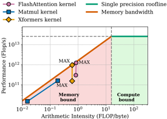In this work, we conduct a detailed GPU analysis to uncover the true causes of the throughput plateau in large-batch LLM inference. Our findings reveal that the primary performance bottleneck during decoding stems from the attention mechanism. Specifically, we identify DRAM bandwidth saturation as the main limiting factor, with over 50% of the attention kernel cycles stalled due to data access delays for all tested models. Figure 1 presents the arithmetic intensity for two attention implementations as batch size increases from 1 to the maximum allowed by GPU memory (MAX). Our results clearly demonstrate that the key components of the decoding step-attention and matrix multiplication kernels-remain deep within the memory-bound regime across all batch sizes. While the matrix multiplication (matmul) kernels gain arithmetic intensity as the batch size grows, the arithmetic intensity of both attention kernels remains nearly constant. Due to GPU DRAM bandwidth saturation, large batch sizes consume substantial GPU memory without yielding proportional throughput gains and significantly degrading la- tency. To mitigate these issues, we also propose a Batching Configuration Advisor (BCA), a profiling-driven method to determine the optimal batch size B opt considering both the throughput plateau and a user-defined latency. By identifying a balanced batch size, BCA minimizes GPU memory waste which can be leveraged by concurrent workloads, similar to CPU resource management in cloud environments. Model replication-running multiple LLM instances concurrently on the same GPU-overlaps GPU operations and increases resource utilization, mitigating the found bottlenecks. Specifically, compared to using a single model replica with MAX memory allocation, model replication increases throughput by 33.7% for OPT-1.3B, and 7.49% for OPT-2.7B. In summary, our key contributions are: - We demonstrate that LLM inference remains memory-bound even at large batch sizes . DRAM bandwidth is the limiting factor in large-batch regimes, with over half of attention computation cycles stalled due to memory access delays. - We propose a Batching Configuration Advisor (BCA) , which recommends an optimal batch size and memory allocation to avoid the throughput plateau while adhering to latency constraints. - We evaluate the benefits of freeing GPU memory with BCA by reallocating freed resources to serve concurrent model replicas. This approach increases GPU resource utilization and substantially improves overall throughput by overlapping operations and mitigating idle times. Fig. 1: Performance vs Arithmetic intensity of attention and matrix multiplication kernels for batch size 1 and the maximum batch size (MAX). While batching increases the arithmetic intensity of matrix multiplications, the arithmetic intensity of xFormers and FlashAttention attention kernels-two memory-optimized attention implementations-remains nearly constant, leading to DRAM saturation. The data was extracted using NVIDIA Nsight Compute from the last decode step of OPT-1.3B on an H100 GPU. <details> <summary>Image 1 Details</summary>  ### Visual Description ## Scatter Plot: Performance vs. Arithmetic Intensity ### Overview The chart visualizes the performance (in FLOP/s) of different computational kernels (FlashAttention, Matmul, Xformers) across varying arithmetic intensity (FLOP/byte). It includes two reference lines (Single precision roofline and Memory bandwidth) and shaded regions indicating computational bounds (Memory bound and Compute bound). The plot uses logarithmic scales for both axes. ### Components/Axes - **Y-axis**: Performance (Flop/s) on a logarithmic scale (10¹¹ to 10¹³). - **X-axis**: Arithmetic Intensity (FLOP/byte) on a logarithmic scale (10⁻² to 10²). - **Legend**: - **FlashAttention kernel**: Pink circle (⚫). - **Matmul kernel**: Blue square (🟦). - **Xformers kernel**: Yellow diamond (🟨). - **Single precision roofline**: Green line (🟩). - **Memory bandwidth**: Orange line (🟧). - **Shaded Regions**: - **Memory bound**: Pink area (🟥). - **Compute bound**: Green area (🟩). ### Detailed Analysis 1. **Data Series**: - **FlashAttention kernel**: - MAX point at (10⁰ FLOP/byte, 10¹² Flop/s). - Performance increases with arithmetic intensity, peaking at the Memory bound. - **Matmul kernel**: - MAX point at (10⁻¹ FLOP/byte, 10¹¹ Flop/s). - Performance rises steeply but plateaus near the Memory bound. - **Xformers kernel**: - MAX point at (10⁰ FLOP/byte, 10¹² Flop/s). - Similar trend to FlashAttention, peaking at the Memory bound. - **Single precision roofline**: Horizontal line at 10¹³ Flop/s, representing the theoretical maximum performance. - **Memory bandwidth**: Diagonal line from (10⁻² FLOP/byte, 10¹¹ Flop/s) to (10¹ FLOP/byte, 10¹³ Flop/s), indicating the upper limit of memory-constrained performance. 2. **Shaded Regions**: - **Memory bound**: Below the Memory bandwidth line, where performance is limited by memory access. - **Compute bound**: Above the Memory bandwidth line, where performance is limited by computational resources. ### Key Observations - All kernels (FlashAttention, Matmul, Xformers) achieve their maximum performance within the **Memory bound** region. - The **Single precision roofline** (10¹³ Flop/s) is the highest performance threshold, but no kernel reaches it. - The **Memory bandwidth** line acts as a boundary between Memory-bound and Compute-bound regions. - The **Compute bound** region (green) is unoccupied by any kernel, suggesting no kernel operates in this regime. ### Interpretation The chart demonstrates that memory bandwidth is a critical bottleneck for these kernels. All kernels are optimized to maximize performance within the Memory-bound region, but none approach the theoretical roofline. This implies that improving memory bandwidth or optimizing for higher arithmetic intensity could unlock greater performance. The absence of data in the Compute-bound region suggests that current implementations prioritize memory efficiency over raw computational throughput. The shaded regions provide a clear visual distinction between memory and compute constraints, highlighting the trade-offs in system design. </details> ## II. BACKGROUND ## A. Autoregressive Generation Decoder-only language models such as OPT [8], GPT [9], and Llama [10], excel in language comprehension and generation, often demonstrating strong zero-shot capabilities across various tasks. These models are typically trained on next-token prediction, where tokens are generated autoregressively based on a given input prompt x . Model parameters are typically optimized by minimizing the negative log-likelihood loss of the predicted token probabilities: $$1 3 5 7 9$$ Built upon the transformer architecture [11], these models consist of stacked blocks with self-attention and feed-forward layers. In each block, the self-attention module identifies relevant tokens in the input sequence, modeling relationships between tokens and capturing both long and short-range dependencies. To achieve this, the input tensor is linearly transformed using learnable matrices into keys K , queries Q , and values V matrices, which compute attention scores to quantify token importance in a highly parallelizable manner. Standard attention kernels perform HBM accesses quadratic in sequence length [12], and most of its operations are memorybound, such as softmax and dropout, which require frequent memory transfers with minimal computation per element. Kernel fusion techniques mitigate this limitation by combining multiple operations within the same kernel, reducing redundant memory accesses. For instance, FlashAttention [12] employs tiling to fuse all attention operations in one CUDA kernel, significantly reducing memory accesses. In LLM inference, processing a new input sequence begins with the prefill phase, where all input tokens are processed in parallel to generate an initial output token. Next, the model transitions into the decode phase , during which each subsequent token is generated autoregressively-one at a time-by conditioning on previously generated tokens. This stage ends when the model generates an end-of-sequence token or reaches the maximum output length. To avoid redundant recomputations, intermediate results-specifically the key and value pairs-are stored in GPU memory as the KV cache. This cache enables efficient reuse of computed attention states from previous tokens and reduces the attention score computation from a matrix-matrix product QK T to a matrix-vector product qK T , where q is the query vector for the current token. In contrast to the prefill phase, the decode phase involves significant memory transfers of key-value pairs and model weights relative to the minimal computations performed. This disparity creates a primary bottleneck in LLM inference, driving the need for optimizations to improve both latency and throughput. ## B. Memory vs. Compute Performance Limitations The performance of a compute operation can be decomposed into two primary components: memory time T M , the time spent transferring data from HBM to the on-chip SRAM (including model weights and KV values), and compute time T C , the time spent computing the arithmetic operations. Whether the operation is memory-bound or compute-bound is determined by its arithmetic intensity , defined as the ratio of FLOPs to bytes accessed from memory. A low ratio indicates a memory-bound regime where memory accesses dominate, while a high ratio signifies a compute-bound regime, where compute operations govern. Ideally, optimal resource utilization occurs when T C = T M . In LLM inference, this classification can be applied to different inference stages. The prefill phase is known as computebound, due to parallelized computations, while the decode phase becomes memory-bound due to frequent memory accesses, the sequential nature of token generation, and limited parallelism [6]. This coarse-grained perspective holds for nobatch inference and explains the resource efficiency plateaus observed during decoding. However, this simplified view often leads to the assumption that the observed performance plateau at larger batch sizes indicates a transition to the computebound regime [6], [7]. ## C. Throughput-Latency Trade-Off Previous scheduling systems [6], [4] introduced various policies for managing the prefill and decode phases of incoming requests, aiming to maximize throughput while maintaining low latency. Recent optimizations, such as chunked prefill [6], further enhance efficiency by combining both phases into the same forward pass. These schedulers primarily rely on batching to address the low compute utilization during decode. While achieving sufficiently large batch sizes for LLMs is typically impractical due to excessive memory demands, the shift toward smaller, specialized models-combined with optimizations that reduce memory and computational requirements-makes it both feasible and important to study the impact of larger batch sizes on smaller models in resourceconstrained environments. This impact, however, is not always positive, as after a certain batch size throughput improvements begin to plateau, resulting in diminishing returns [13]. 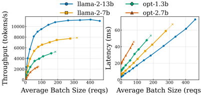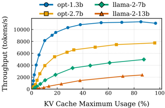To contextualize this throughput-latency trade-off, Figure 2 illustrates the observed throughput plateau, demonstrating how increasing batch sizes beyond a certain knee-point results in diminishing throughput gains alongside significantly increasing inter-token latency. On the other hand, Figure 3 shows that the memory required to reach this performance plateau is only a fraction of the KV cache. For instance, OPT-1.3B achieves almost maximum throughput using just 40% of its KV cache, while OPT-2.7B requires 50%. Increasing batch size further yields only marginal throughput gains, at the cost of a larger GPU memory usage. Since current serving frameworks automatically allocate the maximum possible memory without accounting for performance plateaus or diminishing returns, this potentially leads to inefficient resource utilization. ## III. RELATED WORK ## A. Serving Language Models As language models continue to advance the state-of-theart across diverse tasks, efficiently deploying and serving these models has become a critical area of research. This has led to the development of several serving systems such as Orca [5], Text Generation Inference (TGI) [14], DeepSpeedFastGen [15], [16], Sarathi-Serve [6], and vLLM [4]. Complementary approaches, such as AlpaServe [17], focus on multi- Fig. 2: Throughput (input and output tokens/s) and latency (inter-token latency) evolution when setting the maximum batch size to values in range 1..512 across different models (OPT-1.3B, OPT-2.7B, Llama-2-7B and Llama-2-13B). The X-axis corresponds to the average batch size, instead of the set maximum, and the crosses mark the point where the KV cache capacity is exceeded due to the increased batch size. Results are obtained through the online mode described in Section IV. <details> <summary>Image 2 Details</summary>  ### Visual Description ## Line Graphs: Throughput vs. Latency by Model and Batch Size ### Overview The image contains two line graphs comparing the performance of four language models (llama-2-13b, llama-2-7b, opt-1.3b, opt-2.7b) across varying average batch sizes. The left graph measures **throughput (tokens/s)**, while the right graph measures **latency (ms)**. Both graphs use the same x-axis (batch size) and y-axis scales, with distinct markers and colors for each model. --- ### Components/Axes #### Left Graph (Throughput) - **X-axis**: Average Batch Size (reqs) [0–400] - **Y-axis**: Throughput (tokens/s) [0–12,000] - **Legend**: - **llama-2-13b**: Blue circles (●) - **llama-2-7b**: Orange squares (■) - **opt-1.3b**: Green diamonds (◆) - **opt-2.7b**: Red triangles (▲) #### Right Graph (Latency) - **X-axis**: Average Batch Size (reqs) [0–400] - **Y-axis**: Latency (ms) [0–60] - **Legend**: Same as left graph (colors/markers match). --- ### Detailed Analysis #### Left Graph (Throughput) - **llama-2-13b (blue circles)**: - Steeply increases from ~2,000 tokens/s at 0 reqs to ~10,000 tokens/s at 400 reqs. - Plateaus near 10,000 tokens/s after 300 reqs. - **llama-2-7b (orange squares)**: - Rises from ~1,000 tokens/s to ~8,000 tokens/s, plateauing at ~7,500 tokens/s. - **opt-1.3b (green diamonds)**: - Gains from ~500 tokens/s to ~5,000 tokens/s, peaking at ~4,500 tokens/s. - **opt-2.7b (red triangles)**: - Lowest performance: ~300 tokens/s to ~2,000 tokens/s, peaking at ~1,800 tokens/s. #### Right Graph (Latency) - **llama-2-13b (blue circles)**: - Linear increase from ~10 ms to ~60 ms. - **llama-2-7b (orange squares)**: - Slower rise: ~15 ms to ~50 ms. - **opt-1.3b (green diamonds)**: - Steeper slope: ~20 ms to ~55 ms. - **opt-2.7b (red triangles)**: - Highest latency: ~25 ms to ~60 ms. --- ### Key Observations 1. **Throughput Trends**: - Larger batch sizes improve throughput for all models, but **llama-2-13b** dominates, achieving ~10,000 tokens/s at 400 reqs. - **opt-2.7b** underperforms, with throughput capped at ~2,000 tokens/s. 2. **Latency Trends**: - Latency increases linearly with batch size for all models. - **opt-2.7b** exhibits the highest latency (~60 ms at 400 reqs), while **llama-2-13b** has the lowest (~60 ms). 3. **Trade-offs**: - Higher throughput correlates with higher latency (e.g., llama-2-13b’s 10,000 tokens/s at 400 reqs vs. 60 ms latency). - Smaller models (opt-1.3b, opt-2.7b) show diminishing returns in throughput but similar latency to larger models. --- ### Interpretation - **Model Efficiency**: - **llama-2-13b** balances high throughput and moderate latency, making it optimal for high-demand scenarios. - **opt-2.7b** suffers from poor throughput and high latency, suggesting inefficiencies in scaling. - **Batch Size Impact**: - Throughput plateaus at larger batch sizes (e.g., llama-2-13b’s plateau at 300+ reqs), indicating diminishing returns. - Latency grows predictably with batch size, highlighting a linear scaling challenge. - **Model Choice**: - For latency-sensitive applications, **llama-2-13b** is preferable despite its size. - **opt-2.7b** may be unsuitable for high-throughput or low-latency use cases. --- ### Uncertainties - Exact values are approximate due to visual estimation from the graph. - The right graph’s y-axis (latency) appears to max out at ~60 ms, but data points near 400 reqs may extend slightly beyond this. </details> Fig. 3: Comparison between throughput (input and output tokens/s) and the maximum KV cache usage when setting the maximum batch size to values 1..512 across different models ( OPT-1.3B , OPT-2.7B , Llama-2-7B and Llama-2-13B ). Results are obtained through the online mode described in Section IV. <details> <summary>Image 3 Details</summary>  ### Visual Description ## Line Chart: Throughput (tokens/s) vs KV Cache Maximum Usage (%) ### Overview The chart compares the throughput (tokens processed per second) of four AI models (opt-1.3b, opt-2.7b, llama-2-7b, llama-2-13b) as KV cache maximum usage increases from 0% to 100%. Throughput is plotted on the y-axis (logarithmic scale), and KV cache usage is on the x-axis (linear scale). All models show diminishing returns in throughput gains as cache usage increases, with plateaus observed at higher usage levels. ### Components/Axes - **X-axis**: KV Cache Maximum Usage (%) - Range: 0% to 100% - Increment: 20% - **Y-axis**: Throughput (tokens/s) - Range: 0 to 10,000 tokens/s - Scale: Logarithmic (base 10) - **Legend**: Top-left corner - opt-1.3b: Blue circles (●) - opt-2.7b: Orange squares (■) - llama-2-7b: Green diamonds (♦) - llama-2-13b: Orange triangles (▲) ### Detailed Analysis 1. **opt-1.3b (Blue Circles)** - **Trend**: Sharp initial increase, plateauing at ~10,000 tokens/s after 40% cache usage. - **Key Points**: - 0%: ~1,000 tokens/s - 20%: ~8,000 tokens/s - 40%: ~10,000 tokens/s - 60%–100%: Stable at ~10,000 tokens/s 2. **opt-2.7b (Orange Squares)** - **Trend**: Steady rise, plateauing at ~8,000 tokens/s after 80% cache usage. - **Key Points**: - 0%: ~2,000 tokens/s - 20%: ~6,000 tokens/s - 40%: ~7,000 tokens/s - 60%: ~7,500 tokens/s - 80%–100%: Stable at ~8,000 tokens/s 3. **llama-2-7b (Green Diamonds)** - **Trend**: Gradual increase, plateauing at ~5,000 tokens/s after 80% cache usage. - **Key Points**: - 0%: ~500 tokens/s - 20%: ~2,500 tokens/s - 40%: ~4,000 tokens/s - 60%: ~4,500 tokens/s - 80%–100%: Stable at ~5,000 tokens/s 4. **llama-2-13b (Orange Triangles)** - **Trend**: Slowest growth, plateauing at ~2,500 tokens/s after 80% cache usage. - **Key Points**: - 0%: ~100 tokens/s - 20%: ~1,000 tokens/s - 40%: ~1,500 tokens/s - 60%: ~2,000 tokens/s - 80%–100%: Stable at ~2,500 tokens/s ### Key Observations - **Diminishing Returns**: All models exhibit plateauing throughput beyond a certain cache usage threshold (40–80%), indicating limited benefits from further cache allocation. - **Performance Hierarchy**: - opt-1.3b outperforms all models at higher cache usage (60%+). - opt-2.7b maintains second-highest throughput but plateaus earlier (~80%). - llama-2-7b and llama-2-13b show lower throughput, with the latter being the least efficient. - **Model Size vs. Efficiency**: Larger models (opt-2.7b, llama-2-13b) achieve higher absolute throughput but require more cache to do so, suggesting trade-offs between model size and resource efficiency. ### Interpretation The data highlights the relationship between cache efficiency and model performance. The opt-1.3b model demonstrates the highest throughput efficiency, likely due to optimized architecture or smaller size enabling faster processing. Larger models (opt-2.7b, llama-2-13b) require significantly more cache to achieve comparable throughput, indicating potential inefficiencies in memory management or computational overhead. The plateauing trends suggest that optimizing cache usage up to the inflection point (e.g., 40–60%) could maximize performance without unnecessary resource allocation. This has implications for deploying AI systems in resource-constrained environments, where balancing model size and cache efficiency is critical. </details> model serving by leveraging statistical multiplexing across distributed devices to maximize resource utilization. Additionally, high-performance inference engines like FasterTransformer [18] offer C++/CUDA-based implementations with low-level optimizations for further efficiency gains. In this work, we adopt vLLM as our inference framework, as it integrates most recent serving optimizations. ## B. Serving Optimizations A range of orthogonal optimizations has been proposed to reduce memory usage and improve compute efficiency in LLM inference. Model quantization [19], [20], [21] lowers parameter precision to reduce memory footprint, often at the cost of accuracy. Mixture-of-Experts (MoE) [22] selectively activates a subset of model parameters during inference, reducing computational cost per decoding step. Sparsity techniques [23] prune attention heads or layers to improve efficiency while maintaining performance. Offloading techniques such as [21] alleviate on-device memory limitations by leveraging CPU and disk storage for intermediate computations in offline serving scenarios. Speculative decoding [24] accelerates generation by predicting multiple tokens at once and verifying them in fewer model steps, significantly improving latency. Multiquery attention (MQA) [25] reduces memory bandwidth and computational overhead by sharing a single key and value head for all query heads. Grouped-query attention (GQA) [26] generalizes MQA by dividing the number of query heads in groups, each sharing a single key and value head, achieving accuracy comparable to the standard multi-head attention (MHA). These techniques, often combined, enable faster and more efficient LLM serving while maintaining output quality. ## C. Managing the KV Cache Managing KV cache in LLM serving is challenging due to the unpredictable number of output tokens per request. This uncertainty makes it difficult to pre-allocate memory efficiently. Initially, serving frameworks such as Orca [5] preallocated contiguous GPU memory based on the maximum possible output length. However, this often leads to memory fragmentation for shorter outputs. Recent works have addressed these limitations. S 3 [27] estimates request output length using an auxiliary model, dynamically adjusting memory pre-allocation. VLLM [4] introduces PagedAttention, a memory management mechanism inspired by OS paging, which reduces fragmentation by allowing non-contiguous memory allocation. Other approaches focus on reusing precomputed attention states. Prompt cache mechanism [28] store attention states of frequently visited text segments for reuse across sequences, while RadixAttention [29] maintains a radix tree on the CPU to enable KV cache reuse at runtime. ## D. LLM Inference Profiling Yuan et al. [7] identified the decode phase as memorybound, attributing the bottleneck to frequent memory accesses and characterizing it through the Roofline model, which visually compares operation performance against hardware limits. While they provide a comprehensive evaluation of various inference optimizations and highlight the challenges posed by the memory hardware limit, they assume that large batch sizes result in full compute utilization, without rigorously verifying this through detailed GPU profiling. Similarly, Li et al. [30] survey recent advancements in LLM serving that maintain the standard decoding process, but does not take into account the throughput plateau in larger-batch serving. Recasens et al. [13] empirically showed that large batches lead to a throughput plateau, and hinted potential benefits of model replication. However, this study lacks a detailed GPU tracing to explain the underlying causes of this plateau, leaving the bottlenecks behind throughput saturation in largebatch scenarios unexplored. In this work, we conduct an indepth GPU analysis that unveils the bottlenecks behind the throughput plateau in large-batch scenarios. ## IV. METHODOLOGY We conduct our experiments using the well-established vLLM framework [4], specifically its main branch state as of October 18th, 2024. The framework is configured with default parameters, except for disabling logging, setting the maximum batch size to 4096 tokens, and limiting the maximum context length to 2048 tokens. We employ this framework in two modes: online mode following a client-server architecture, transmitting requests via API endpoints, and an offline mode where all prefill and decode steps are executed directly via Python calls. The online mode is used in Section VI to evaluate our proposal in a real-world scenario, whereas the offline mode is employed in Section V, allowing a more precise control and analysis of execution phases without additional noise. Hardware. All experiments are conducted on a single-node setup with an NVIDIA Hopper H100 (64GB HBM2), 128GB RAM memory, and 20 CPU cores. Models . We evaluate four models: OPT-1.3B, OPT-2.7B, Llama-2-7B, and Llama-2-13B. All models fit within the 64GB GPU, allowing sufficient memory for large batch processing. Workload . In online mode, 2000 requests are sampled from a cleaned ShareGPT dataset, maintaining the original input and output length distribution. In offline mode, we generate synthetic requests with fixed input and output lengths. Each request consists of 161 input tokens and 338 output tokens, matching the mean input/output lengths in the original ShareGPT dataset [31]. ## V. GPU PROFILING AND PERFORMANCE BOTTLENECKS In this section, we characterize the throughput plateau observed in large-batch regimes and investigate its underlying causes. Unlike prior studies, our work is the first to provide a comprehensive explanation of this performance bottleneck using detailed GPU tracing data. Our analysis primarily relies on two tools: NVIDIA Nsight Systems (2023.2.3) and NVIDIA Nsight Compute (2023.3.0.0). Nsight provides a high-level view of GPU activity across the entire program execution, while Nsight offers fine-grained insights into the execution of specific kernels. Our findings reveal that DRAM saturation in the attention mechanism is the primary cause of the throughput plateau in large-batch scenarios, challenging prior assumptions that attribute it to a shift toward a compute-bound regime. While batching increases the arithmetic intensity of matrix multiplication kernels, we observe that the arithmetic intensity of attention kernels remains nearly constant. This ultimately leads to memory-bandwidth saturation, leaving a significant portion of computational resources underutilized. ## A. 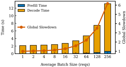Decode vs Prefill We begin our analysis with a broad examination of the factors contributing to the throughput plateau, focusing on the evolution of global execution time as batch size increases. Specifically, we distinguish between the prefill and decode phases. In line with prior literature [6], our results confirm that the decode phase is the primary bottleneck in inference serving. As shown in Figure 4, the decode phase accounts for the vast majority of the total inference time for the OPT-2.7B model in all tested batch sizes. Although prefill becomes relatively more significant at large batch sizes, it remains below 5% even at the maximum batch size. Table I further corroborates these findings, showing that the decode phase dominates inference time across all tested models under maximum batch conditions. As shown in Figure 4, global execution time remains nearly constant until the batch size exceeds 32 requests. Beyond this point, it increases proportionally, leading to a 6x slowdown at the largest batch size. This behavior aligns with the throughput plateau observed in Figure 2, where the throughput of the OPT2.7B model increases from 225 tokens per second at batch size 1, to 7,607 tokens per second at batch size 256-an approximate 33.8x increase instead of the expected 256x-indicating a slowdown of about 7.8x. These results confirm that our offline findings are consistent with online results presented in the background. The slight variation between the two may stem from differences in request length distributions across the two distinct modes. 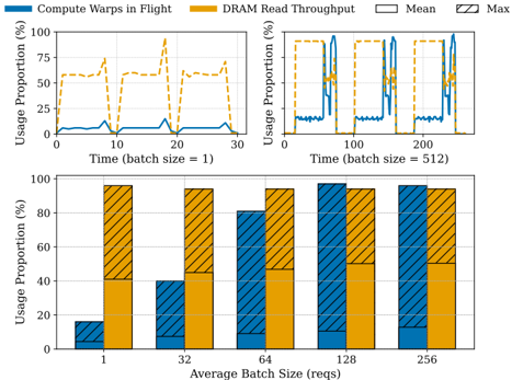Table I presents key GPU metrics, categorized into computerelated and memory-related. Modern GPUs consist of multiple Streaming Multiprocessors (SMs), each executing parallel thread groups known as Warps. The results indicate that while most SMs remain active throughout execution-occasionally reaching full saturation-their average utilization remains low. Specifically, the Compute Warps in Flight metric reveals that no model exceeds 35% average Warp usage in either the prefill or decode phases. Notably, this metric is higher during prefill, supporting prior claims that this phase is more computeintensive. The Unallocated Warps in Active SMs metric measures the percentage of Warps assigned to an SM but not yet allocated. This value remains consistently high across all models, indicating the presence of a bottleneck preventing Warps from being allocated. Regarding GPU memory read and write operations (denoted as DRAM), write activity is minimal, whereas read values remain consistently high across all models, particularly for larger ones. These high DRAM read values significantly exceed compute percentages, possibly suggesting a memory-bound regime. However, overall GPU resource utilization remains far from saturation at large batch sizes, especially in terms of compute capabilities. ## B. Decode Kernels In this subsection, we continue our analysis focusing exclusively on the decode phase, as it dominates the execution time. Figure 5 (top) illustrates the evolution of the first three decoding steps when running OPT-1.3B at batch sizes 1 and 512. As shown, DRAM read activity remains consistently high throughout most of each decoding step, while compute utilization stays below 20%. It is only towards the end that compute usage increases and DRAM read declines. This pattern suggests a memory saturation scenario where Warps stall while waiting for data transfers. Also, there is a noticeable GPU idle gap between decoding steps, which we attribute to CPU processing time. This gap increases with batch size, further impacting overall efficiency. Figure 11 (bottom) provides Fig. 4: Evolution of total execution time as batch size increases for the OPT-2.7B model. We distinguish prefill and decode phases, and the overall slowdown measures the global execution time difference from when running with batch size 1. <details> <summary>Image 4 Details</summary>  ### Visual Description ## Bar Chart: Performance Metrics vs. Batch Size ### Overview The chart illustrates the relationship between average batch size (in requests) and three performance metrics: Prefill Time, Decode Time, and Global Slowdown. It shows how these metrics scale with increasing batch sizes from 1 to 256 requests. ### Components/Axes - **X-axis**: Average Batch Size (reqs) with values: 1, 2, 4, 8, 16, 32, 64, 128, 256. - **Y-axis (left)**: Time (s) with values from 0 to 12 seconds. - **Y-axis (right)**: Global Slowdown with values from 1 to 6. - **Legend**: - Blue: Prefill Time (bars) - Orange: Decode Time (bars) - Red: Global Slowdown (line) - **Placement**: Legend is top-left; bars are clustered, with the red line overlaid. ### Detailed Analysis 1. **Prefill Time**: - Consistently flat across all batch sizes. - Approximate value: ~0.5 seconds (uncertainty ±0.1s). 2. **Decode Time**: - Starts at ~2 seconds for batch size 1. - Increases exponentially: ~2s (1), ~2.5s (2), ~3s (4), ~3.5s (8), ~4s (16), ~5s (32), ~7s (64), ~9s (128), ~12s (256). - Notable jump between 128 and 256 (Δ~3s). 3. **Global Slowdown**: - Starts at 1x for batch size 1. - Gradually rises: ~1.2x (2), ~1.3x (4), ~1.5x (8), ~1.7x (16), ~2x (32), ~2.5x (64), ~3.5x (128), ~6x (256). - Steep acceleration after 128 requests. ### Key Observations - Prefill Time remains constant regardless of batch size. - Decode Time grows exponentially, with a critical inflection point at 128 requests. - Global Slowdown mirrors Decode Time's growth pattern but plateaus earlier (6x at 256). ### Interpretation The data suggests that **Decode Time is the primary driver of system slowdown**, with diminishing returns at larger batch sizes. The exponential growth in Decode Time after 128 requests indicates potential bottlenecks in processing capacity or algorithmic inefficiencies. Prefill Time's stability implies it is decoupled from batch size, possibly due to parallelization or precomputation. The Global Slowdown metric quantifies the system-wide impact, showing that beyond 128 requests, the slowdown becomes nonlinear, likely due to resource contention or memory limitations. This highlights the need for batch size optimization to balance throughput and latency in high-scale systems. </details> additional insights into GPU resource utilization across multiple batch sizes. While peak DRAM and compute utilization approach saturation, average utilization remains significantly below 50% at large batch sizes, suggesting the presence of an underlying bottleneck that prevents full resource utilization. Fig. 5: (Top) Evolution of the metrics Compute Warps in Flight and DRAM Read Throughput in the first three decoding steps of the execution when using model OPT-1.3B with two different batch sizes (1 and 512) (Bottom) Average and maximum values during the full length of the execution of the previous two metrics in five different batch sizes (1, 32, 64, 128, 256 and 512) in OPT-1.3B. <details> <summary>Image 5 Details</summary>  ### Visual Description ## Line Graphs and Bar Chart: GPU Resource Usage Analysis ### Overview The image contains three visualizations analyzing GPU resource utilization across different batch sizes. Two line graphs compare "Compute Warps in Flight" (blue) and "DRAM Read Throughput" (orange) over time for batch sizes of 1 and 512. A bar chart shows the proportional contribution of these metrics across average batch sizes (1, 32, 64, 128, 256). --- ### Components/Axes 1. **Line Graphs (Top Row)**: - **X-axis**: Time (batch size = 1: 0–30; batch size = 512: 0–200). - **Y-axis**: Usage Proportion (%) (0–100%). - **Legends**: - Blue: "Compute Warps in Flight" - Orange: "DRAM Read Throughput" - **Annotations**: - "Mean" (solid line) and "Max" (dashed line) indicators. 2. **Bar Chart (Bottom)**: - **X-axis**: Average Batch Size (reqs): 1, 32, 64, 128, 256. - **Y-axis**: Usage Proportion (%) (0–100%). - **Legend**: - Blue: "Compute Warps in Flight" - Orange: "DRAM Read Throughput" - **Bar Style**: Stacked with diagonal hatching for visual separation. --- ### Detailed Analysis #### Line Graphs (Batch Size = 1) - **Compute Warps in Flight (Blue)**: - Remains consistently low (~5–10%) with minor fluctuations. - No significant spikes observed. - **DRAM Read Throughput (Orange)**: - Exhibits sharp, periodic spikes (peaking ~75%). - Baseline usage ~20–30% between spikes. - **Trend**: DRAM Read dominates usage, with Compute Warps contributing minimally. #### Line Graphs (Batch Size = 512) - **Compute Warps in Flight (Blue)**: - Stabilizes at ~50–70% with slight oscillations. - Peaks align with DRAM Read dips. - **DRAM Read Throughput (Orange)**: - Stabilizes at ~30–50% with minor fluctuations. - Peaks (~70%) coincide with Compute Warps troughs. - **Trend**: Both metrics stabilize, but Compute Warps usage becomes more prominent. #### Bar Chart (All Batch Sizes) - **Compute Warps in Flight (Blue)**: - Increases monotonically with batch size: - 1 req: ~10% - 32 req: ~40% - 64 req: ~80% - 128 req: ~95% - 256 req: ~90% - **DRAM Read Throughput (Orange)**: - Decreases inversely with batch size: - 1 req: ~90% - 32 req: ~60% - 64 req: ~20% - 128 req: ~5% - 256 req: ~10% - **Trend**: Larger batches shift workload from memory-bound (DRAM) to compute-bound (Warps). --- ### Key Observations 1. **Batch Size Impact**: - Small batches (1 req) are memory-bound, with DRAM Read dominating (~90%). - Larger batches (>64 req) shift to compute-bound, with Compute Warps exceeding 80%. 2. **Temporal Patterns**: - In small batches, DRAM Read spikes suggest inefficient memory access (e.g., non-coalesced transactions). - Larger batches show smoother utilization, indicating optimized memory access (e.g., coalesced transactions). 3. **Anomalies**: - At 256 req, Compute Warps dip slightly (~90% vs. 128 req’s ~95%), possibly due to register pressure or kernel limitations. --- ### Interpretation The data demonstrates a clear trade-off between memory and compute utilization in GPU workloads: - **Small Batches**: Dominated by DRAM Read, indicating memory-bound operations (e.g., frequent small data accesses). - **Large Batches**: Compute Warps dominate, suggesting arithmetic-intensive operations (e.g., matrix multiplications in deep learning). - **Efficiency Gains**: Larger batches reduce DRAM contention, likely through better memory coalescing and pipeline utilization. However, the slight dip at 256 req hints at potential saturation or resource contention at extreme scales. This analysis aligns with GPU architecture principles, where batch size tuning balances memory bandwidth and compute throughput for optimal performance. 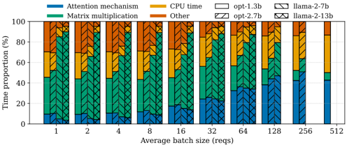</details> Figure 6 shows the contribution of each kernel to the execution time of a single decode step across all tested models and different batch sizes. As expected, matrix multiplications and the attention mechanism dominate execution time. However, as batch size increases, two key trends emerge: the attention mechanism's contribution grows, while the matrix multiplications' impact decreases. For instance, in OPT-1.3B, the attention kernel's proportion rises from approximately 5% at small batch sizes to over 40% at larger ones, whereas matrix multiplications decline sharply from around 50% to under TABLE I: Comparison between prefill and decode phases in their relative importance and their results for a selection of key GPU metrics. We set the batch size to the maximum value that fits in KV cache in all tested models, and included the average and maximum value for the full length of the execution in all GPU metrics. | | | | OPT-1.3B | OPT-1.3B | OPT-2.7B | OPT-2.7B | Llama-2-7B | Llama-2-7B | Llama-2-13B | Llama-2-13B | |----------------------|-------------------------------------|----------------|--------------|--------------|--------------|--------------|--------------|--------------|---------------|------------------| | | | | Prefill | Decode | Prefill | Decode | Prefill | Decode | Prefill | Decode | | | Importance (%) | Importance (%) | 0.03 | 0.97 | 0.05 | 0.95 | 0.05 | 0.95 | 0.05 | 0.95 | | GPU compute- related | Active SMs (%) | Average Max | 75.12 100.00 | 61.90 100.00 | 80.86 100.00 | 72.04 100.00 | 87.26 100.00 | 69.23 100.00 | 87.51 100.00 | 76.65 100.00 | | GPU compute- related | Compute Warps in flight (%) | Average Max | 25.88 96.00 | 12.91 100.00 | 30.08 96.00 | 31.14 97.00 | 26.84 91.00 | 9.85 90.00 | 24.61 92.00 | 10.27 72.00 | | | Unallocated Warps in active SMs (%) | Average Max | 49.24 88.00 | 49.00 88.00 | 50.77 82.00 | 40.90 82.00 | 60.42 88.00 | 59.39 88.00 | 62.89 88.00 | 66.39 88.00 | | GPU memory- | DRAM read (%) | Average Max | 32.85 91.00 | 47.98 93.00 | 43.21 97.00 | 60.81 99.00 | 62.57 95.00 | 70.55 97.00 | 66.08 95.00 | 76.75 | | related | DRAM Write Throughput (%) | Average Max | 18.35 100.00 | 5.56 100.00 | 15.55 66.00 | 5.83 78.00 | 12.79 43.00 | 2.59 48.00 | 10.16 44.00 | 97.00 1.82 33.00 | 10%. This clearly indicates that the attention mechanism is the primary contributor to execution slowdown in large-batch scenarios. Additionally, CPU computations reach up to 30% at batch size 512 in OPT-1.3B, highlighting another critical bottleneck that contributes to GPU underutilization. Fig. 6: Contribution by kernel to the execution time of the decode steps as the batch size increases across all tested models. Only the kernels regarding matrix multiplications and the attention mechanism are individually labeled, as no other single kernel accounts for more than 20% of the execution time across any batch size or model. We have also included the amount of time where no GPU kernel is running, labeled as CPU time . <details> <summary>Image 6 Details</summary>  ### Visual Description ## Bar Chart: Time Proportion by Batch Size and Model ### Overview The chart visualizes the time proportion (%) allocated to different computational components (Attention mechanism, Matrix multiplication, CPU time, Other) across varying average batch sizes (1 to 512 requests) for four models: opt-1.3b, opt-2.7b, llama-2-7b, and llama-2-13b. Each bar is segmented into four colored regions corresponding to the components. ### Components/Axes - **X-axis**: Average batch size (reqs) with values: 1, 2, 4, 8, 16, 32, 64, 128, 256, 512. - **Y-axis**: Time proportion (%) from 0 to 100. - **Legend**: - Blue: Attention mechanism - Green: Matrix multiplication - Yellow: CPU time - Orange: Other - **Model Labels**: - opt-1.3b (solid lines) - opt-2.7b (diagonal lines) - llama-2-7b (solid squares) - llama-2-13b (diagonal squares) ### Detailed Analysis 1. **opt-1.3b (solid lines)**: - At batch size 1: Attention (10%), Matrix multiplication (30%), CPU time (20%), Other (40%). - At batch size 512: Attention (45%), Matrix multiplication (5%), CPU time (5%), Other (45%). 2. **opt-2.7b (diagonal lines)**: - At batch size 1: Attention (15%), Matrix multiplication (25%), CPU time (15%), Other (45%). - At batch size 512: Attention (50%), Matrix multiplication (3%), CPU time (2%), Other (45%). 3. **llama-2-7b (solid squares)**: - At batch size 1: Attention (20%), Matrix multiplication (20%), CPU time (10%), Other (50%). - At batch size 512: Attention (55%), Matrix multiplication (2%), CPU time (3%), Other (40%). 4. **llama-2-13b (diagonal squares)**: - At batch size 1: Attention (25%), Matrix multiplication (15%), CPU time (5%), Other (55%). - At batch size 512: Attention (60%), Matrix multiplication (1%), CPU time (4%), Other (35%). ### Key Observations - **Attention mechanism** consistently increases with batch size across all models, reaching 45–60% at 512 requests. - **Matrix multiplication** decreases sharply in larger models (e.g., llama-2-13b drops from 15% to 1% at 512). - **CPU time** is most significant in smaller batches (10–15% in opt-1.3b/opt-2.7b) but negligible in larger batches (<5%). - **Other** components remain relatively stable (35–55%) but vary by model. ### Interpretation - **Batch Size Impact**: Larger batches amplify the dominance of the Attention mechanism, likely due to parallel processing efficiency. Matrix multiplication’s decline suggests optimization or reduced reliance in larger-scale computations. - **Model Differences**: llama-2-13b allocates more time to Attention (60% at 512) compared to smaller models, indicating architectural differences in handling batch sizes. - **CPU Time Reduction**: Fixed overhead costs (CPU time) become less impactful as batch size grows, highlighting scalability benefits. - **Other Components**: The "Other" category’s persistence suggests unaccounted processes (e.g., I/O, memory management) remain relevant even at scale. This data underscores the trade-offs in model design for batch processing, with Attention mechanisms becoming the primary computational focus as batch sizes increase. 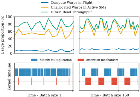</details> We closely examine the kernels associated with the attention mechanism and matrix multiplications. Figure 7 provides a time-wise representation of their behavior across the execution of multiple layers within a single decode step of the Llama2-7B model for two batch sizes, along with the corresponding GPU metrics on top. Consistent with previous findings, increasing the batch size results in a greater proportion of execution time spent on the attention mechanism relative to matrix multiplications. More notably, DRAM read saturation occurs exclusively during the execution of the attention kernels, especially at larger batch sizes. This saturation correlates with Warps unallocation. This strongly suggests a DRAM saturation bottleneck inside the attention mechanism that prevents available GPU Warps from being allocated and run in large batch scenarios. Fig. 7: Evolution of the GPU metrics and the kernels regarding the attention mechanism and matrix multiplications during a section of the first decode step of the execution of Llama-2-7B with batch sizes equal to 1 and 160. <details> <summary>Image 7 Details</summary>  ### Visual Description ## Line Graphs: Usage Proportions Over Time ### Overview Two line graphs depict dynamic resource usage metrics over time. The left graph shows three metrics (Compute Warps in Flight, Unallocated Warps in Active SMs, DRAM Read Throughput) with usage proportions up to 80%. The right graph extends the y-axis to 100% and includes similar metrics with higher absolute values. ### Components/Axes - **Left Graph**: - **Y-axis**: Usage proportion (%) (0–100). - **X-axis**: Time (unspecified units). - **Legend**: - Blue: Compute Warps in Flight. - Orange: Unallocated Warps in Active SMs. - Green: DRAM Read Throughput. - **Right Graph**: - **Y-axis**: Usage proportion (%) (0–100). - **X-axis**: Time (unspecified units). - **Legend**: Same as left graph. ### Detailed Analysis - **Left Graph Trends**: - **Compute Warps in Flight (Blue)**: Peaks at ~10%, remains relatively stable. - **Unallocated Warps (Orange)**: Fluctuates between 40–60%, with a notable dip to ~30% at one point. - **DRAM Read Throughput (Green)**: Dominates with peaks up to ~90%, averaging ~70–80%. - **Right Graph Trends**: - **Compute Warps in Flight (Blue)**: Slightly higher (~15% peak). - **Unallocated Warps (Orange)**: Ranges 60–80%, with sharper fluctuations. - **DRAM Read Throughput (Green)**: Similar to left graph (~70–90%). ### Key Observations 1. **DRAM Read Throughput** consistently dominates resource usage in both graphs. 2. **Unallocated Warps** show significant variability, particularly in the right graph. 3. **Compute Warps in Flight** increases modestly in the right graph, suggesting higher demand under certain conditions. 4. The orange line (Unallocated Warps) in the left graph dips below 40% at one point, potentially indicating a transient state. ### Interpretation - **Resource Allocation**: DRAM Read Throughput is the primary bottleneck, consuming ~70–90% of resources. - **Compute Efficiency**: Compute Warps in Flight scales with workload (higher in the right graph), but remains a smaller fraction of total usage. - **Unallocated Warps**: Fluctuations may reflect dynamic resource management or inefficiencies in warp scheduling. - **Batch Size Impact**: The right graph’s higher Compute Warps and Unallocated Warps values suggest increased computational demand with larger batch sizes (160 vs. 1). ## Bar Charts: Kernel Timeline ### Overview Two bar charts compare time allocation between matrix multiplication (blue) and attention mechanisms (red) for batch sizes 1 and 160. ### Components/Axes - **X-axis**: Time (segmented into equal intervals). - **Y-axis**: Kernel timeline (unspecified units). - **Legend**: - Blue: Matrix multiplication. - Red: Attention mechanism. ### Detailed Analysis - **Batch Size 1**: - Matrix multiplication (blue) occupies ~80% of the timeline. - Attention mechanism (red) uses ~20%, with shorter, sporadic bars. - **Batch Size 160**: - Matrix multiplication (blue) remains dominant (~70–80%). - Attention mechanism (red) increases to ~30–40%, with longer, contiguous bars. ### Key Observations 1. **Attention Mechanism Scaling**: Time allocated to attention mechanisms grows significantly with larger batch sizes. 2. **Matrix Multiplication Dominance**: Remains the primary computational task regardless of batch size. ### Interpretation - **Batch Size Trade-offs**: Larger batches increase attention mechanism overhead, potentially impacting parallelism. - **Hardware Utilization**: Matrix multiplication’s consistent dominance suggests it is the core computational kernel, while attention mechanisms introduce variable overhead. ## Final Notes - **Language**: All text is in English. - **Data Gaps**: Exact time units and batch size definitions are unspecified. - **Anomalies**: The left graph’s Unallocated Warps dip below 40% may indicate a transient state or measurement artifact. </details> ## C. Attention Kernel Finally, we analyze the attention kernel in detail, as it becomes the single most critical operation at large batch sizes. Revisiting Figure 1, we compare the performance and arithmetic intensity of two attention implementations: xFormers [32], which offers a more memory-efficient implementation using custom CUDA kernels; and FlashAttention [12], which further optimizes performance by reducing HBM reads/writes via tiling and recomputation. Our results, extracted from the last decode step of OPT-1.3B at batch size 1 and MAX, show that both algorithms remain firmly within the memory-bound regime across batch sizes, while performance (FLOPS/s) is orders of magnitude lower than the hardware maximum (single precision roofline). The low arithmetic intensity indicates that memory accesses-that translate into DRAM reads-consistently exceed the number of compute operations. As illustrated in Figure 1, the compute-to-memory ratio remains between 0.5 and 1 operations per byte accessed. Moreover, this ratio-the arithmetic intensity-remains nearly constant for the two batch sizes, in contrast to matrix multiplication (matmul) kernels, whose arithmetic intensity increases with batch size. This means that attention kernels, unlike matmuls, do not benefit significantly from batching since their performance is fundamentally constrained by DRAM reads. At maximum batch size, attention kernels align with the DRAM bandwidth line, representing the hardware's maximum allowable memory transfer. Given the constant arithmetic intensity, this confirms that the attention performance cannot improve further at larger batch sizes due to DRAM bandwidth saturation. This behavior is not unique to OPT-1.3B, as shown in Figure II, all tested models exhibit DRAM bandwidth saturation at their maximum batch size. A deeper analysis of DRAM reads in the attention mechanism reveals inefficient memory access patterns, potentially exacerbated by vLLM's non-contiguous memory access schema. As shown in Table III, the L1 and L2 caches of tested GPUs exhibit consistently low hit rates, averaging no more than 12% for L1 and 2% for L2 across all models and batch sizes. These values further decline as the batch size increases, indicating worsening inefficiencies. This poor cache performance significantly reduces overall memory efficiency, decreasing inference performance. 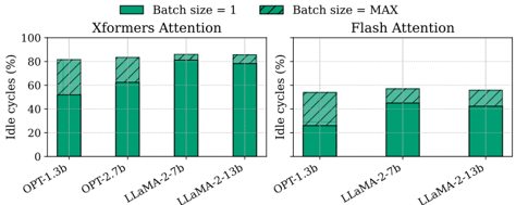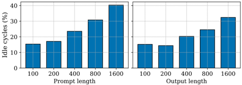To wrap up this analysis, we examine the proportion of compute cycles spent idly waiting for data. Figure 8 presents these values for both attention algorithms across all tested models, comparing batch size 1 with MAX. At maximum batch size, more than 50% of cycles remain idle due to datafetching delays, with xFormers being particularly affected, exceeding 80% idle cycles across all models. Additionally, larger models exhibit higher idle cycles even at batch size 1, highlighting the increasing impact of memory transfers as model size grows. Similarly, sequence length also impacts memory transfer demands, leading to a higher percentage of stalled cycles waiting for data, as shown in Figure 9. As expected, longer prompts have a more pronounced impact than longer output sequences. This is because larger input lengths increase the memory transfer for every decoding step, whereas longer output sequences primarily affect later decoding steps. Based on these insights and the results from previous sections, we conclude that the throughput plateau is caused by DRAM read saturation in the attention mechanism during the decode phase. As batch size increases, its arithmetic intensity remains constant, and once memory bandwidth limit is reached, performance can no longer improve, making it the primary performance bottleneck. ## VI. BATCHING CONFIGURATION ADVISOR In this section, we introduce the Batching Configuration Advisor (BCA) , a tool that recommends an optimal batch size B opt for LLM serving, considering both the throughput plateau and a user-defined latency constraint. As observed | | Batch size (reqs) | Mem-traffic (byte/s) | Performance (FLOP/s) | |-----------|---------------------|------------------------|------------------------| | Rooflines | - | 1.63e+12 | 2.56e+13 | | OPT- | 1 | 2.55e+11 | 1.56e+11 | | 1.3B | 512 | 1.51e+12 | 9.64e+11 | | OPT- | 1 | 2.17e+11 | 1.31e+11 | | 2.7B | 256 | 1.56e+12 | 9.42e+11 | | Llama- | 1 | 1.29e+11 | 7.58e+10 | | 2-7B | 128 | 1.53e+12 | 9.02e+11 | | Llama- | 1 | 1.54e+11 | 9.06e+10 | | 2-13B | 80 | 1.51e+12 | 8.92e+11 | TABLE II: Roofline results for the xFormers attention algorithm in all tested models when using no-batch inference and their maximum possible batch size. We show the maximum roofline values of the hardware, and the achieved values by the models. Every result is the average of the values of the first 5 kernel executions from the last decode step. Fig. 8: Percentage of the warp cycles issued per instruction that are stalled/idle waiting for data. The results are extracted for all tested models when using no-batch inference and the maximum batch. We use both the xFormers and FlashAttention backends for the attention mechanism, notice that OPT-2.7B model is not compatible with the latter. Every result is the average of the values of the first 5 kernel executions from the last decode step. <details> <summary>Image 8 Details</summary>  ### Visual Description ## Bar Chart: Idle Cycles Comparison for Xformers and Flash Attention Mechanisms ### Overview The image presents a comparative bar chart analyzing idle cycles (%) for four language models (OPT-1.3b, OPT-2.7b, LLaMA-2-7b, LLaMA-2-13b) under two attention mechanisms (Xformers and Flash) and two batch sizes (1 and MAX). The chart uses stacked bars to differentiate batch sizes, with solid green representing batch size = 1 and striped green representing batch size = MAX. ### Components/Axes - **X-Axis**: Model names (OPT-1.3b, OPT-2.7b, LLaMA-2-7b, LLaMA-2-13b) grouped under two sections: "Xformers Attention" (left) and "Flash Attention" (right). - **Y-Axis**: Idle cycles (%) ranging from 0 to 100. - **Legend**: Located at the top, with two entries: - Solid green: Batch size = 1 - Striped green: Batch size = MAX - **Sections**: Two main sections (Xformers and Flash Attention) with four bars each. ### Detailed Analysis #### Xformers Attention 1. **OPT-1.3b**: - Batch size = 1: ~50% (solid green) - Batch size = MAX: ~30% (striped green) 2. **OPT-2.7b**: - Batch size = 1: ~60% (solid green) - Batch size = MAX: ~20% (striped green) 3. **LLaMA-2-7b**: - Batch size = 1: ~80% (solid green) - Batch size = MAX: ~10% (striped green) 4. **LLaMA-2-13b**: - Batch size = 1: ~85% (solid green) - Batch size = MAX: ~5% (striped green) #### Flash Attention 1. **OPT-1.3b**: - Batch size = 1: ~30% (solid green) - Batch size = MAX: ~20% (striped green) 2. **OPT-2.7b**: - Batch size = 1: ~45% (solid green) - Batch size = MAX: ~15% (striped green) 3. **LLaMA-2-7b**: - Batch size = 1: ~50% (solid green) - Batch size = MAX: ~10% (striped green) 4. **LLaMA-2-13b**: - Batch size = 1: ~40% (solid green) - Batch size = MAX: ~5% (striped green) ### Key Observations 1. **Batch Size Impact**: - In both mechanisms, idle cycles decrease significantly when batch size increases from 1 to MAX. The reduction is more pronounced in Xformers (e.g., LLaMA-2-13b drops from 85% to 5%) compared to Flash (LLaMA-2-13b drops from 40% to 5%). 2. **Model Size Trends**: - Larger models (LLaMA-2-13b) exhibit higher idle cycles in Xformers but lower idle cycles in Flash, suggesting Flash is more efficient for larger models. 3. **Consistency**: - All models show lower idle cycles with batch size = MAX, but the gap between batch sizes is narrower in Flash Attention. ### Interpretation The data demonstrates that **Flash Attention** consistently reduces idle cycles compared to Xformers, particularly for larger models (LLaMA-2-13b). Increasing batch size further improves efficiency, but the benefit is more significant in Xformers. This suggests Flash Attention is inherently more optimized for minimizing idle time, while batch size adjustments have a stronger impact on Xformers. The results highlight the importance of attention mechanism choice for computational efficiency in large language models. </details> TABLE III: Hit rates (HR) of L1 and L2 GPU caches for all tested models when using no-batch inference and MAX batch size. Every result is the average of the values of the first 5 kernel executions from the last decode step. | | OPT-1.3B | OPT-1.3B | OPT-2.7B | OPT-2.7B | Llama-7b | Llama-7b | Llama-13b | Llama-13b | |------------|------------|------------|------------|------------|------------|------------|-------------|-------------| | Batch size | 1 | 512 | 1 | 256 | 1 | 128 | 1 | 80 | | L1 HR (%) | 16.49 | 2.62 | 13.84 | 2.43 | 9.4 | 1.55 | 7.7 | 1.61 | | L2 HR (%) | 1.58 | 1.6 | 1.27 | 1.28 | 0.83 | 0.84 | 0.83 | 0.84 | earlier, increasing the batch size beyond a certain knee-point yields only marginal throughput gains once DRAM bandwidth becomes saturated. However, this also increases GPU memory usage and inter-token latency. BCA mitigates this trade-off by maximizing throughput while avoiding the plateau region and ensuring latency remains within a specified Service Level Objective (SLO). By identifying a balanced batch size, BCA reduces GPU memory usage and frees up resources for other workloads, improving overall system efficiency. Formally, Equation 2 defines B opt as the batch size B that maximizes throughput T ( B ) , subject to two constraints: (i) Fig. 9: Impact on the percentage of stalled cycles in the FlashAttention kernel in the decode phase when increasing the input and output length separately. The default number of input and output tokens are 100 and 100 respectively. We use the model OPT-1.3B and we average the values from the execution of the attention kernels that run in the first and last decode steps. <details> <summary>Image 9 Details</summary>  ### Visual Description ## Bar Chart: Idle Cycles vs. Prompt and Output Length ### Overview The image contains a dual-panel bar chart comparing idle cycles (in percentage) against two variables: **prompt length** (left panel) and **output length** (right panel). Both panels use identical axes and color schemes, with blue bars representing data points. The x-axes categorize values in powers of two (100, 200, 400, 800, 1600), while the y-axis scales from 0% to 40% in 10% increments. --- ### Components/Axes - **Y-Axis**: Labeled "Idle cycles (%)", ranging from 0% to 40%. - **X-Axes**: - Left Panel: "Prompt length" with categories: 100, 200, 400, 800, 1600. - Right Panel: "Output length" with identical categories. - **Bars**: All bars are blue, with no legend or color differentiation. - **Gridlines**: Light gray horizontal and vertical lines for reference. --- ### Detailed Analysis #### Left Panel (Prompt Length) - **100**: ~15% idle cycles. - **200**: ~17% idle cycles. - **400**: ~23% idle cycles. - **800**: ~31% idle cycles. - **1600**: ~40% idle cycles. #### Right Panel (Output Length) - **100**: ~15% idle cycles. - **200**: ~14% idle cycles. - **400**: ~20% idle cycles. - **800**: ~24% idle cycles. - **1600**: ~32% idle cycles. --- ### Key Observations 1. **Upward Trend**: Both panels show a general increase in idle cycles as prompt/output length increases. 2. **Steeper Growth in Prompt Length**: The left panel exhibits a sharper rise, particularly between 800 and 1600 (31% → 40%). 3. **Output Length Dip**: The right panel shows a minor decline at 200 (15% → 14%) before resuming growth. 4. **Asymmetry**: Prompt length consistently exceeds output length at equivalent scales (e.g., 1600 prompt length = 40% vs. 1600 output length = 32%). --- ### Interpretation The data suggests that **longer prompts have a disproportionately higher impact on idle cycles compared to output length**. The steeper slope in the prompt length panel implies that processing longer input sequences consumes significantly more system resources. The slight dip at 200 in the output length panel may indicate an optimization or anomaly in shorter output processing. These trends could reflect computational bottlenecks in handling longer sequences, such as memory allocation or parallelization inefficiencies. The absence of a legend or color coding limits granular analysis but confirms uniformity in measurement methodology. 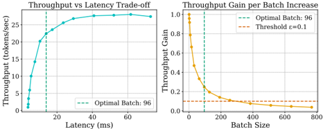</details> the latency L ( B ) must not exceed a specified SLO, and (ii) the throughput relative to the optimal throughput T (1) ∗ B must remain above a user-specified threshold ϵ . Here, T ( B ) and L ( B ) represents the throughput and latency observed at batch size B , which we determine by benchmarking the model's performance at each batch size, following online mode described in Section IV. The term ∆ corresponds to the distance to the batch size preceding B . Both SLO and ϵ are user-defined parameters. $$\begin{array}{ll} B _ { o p t } = \arg \max _ { B } \{ L ( B ) \leq T ( B ) \\ \text { subject to } & \frac { T ( B ) } { B ^ { s + 1 } ( 1 ) } > e \} & \text { subject to } & \{ T ( B ) \geq 6 4 G \} \end{array}$$ ## A. 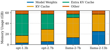Evaluation of BCA Table IV presents the results from BCA evaluation across different models with ϵ = 0 . 1 under two latency SLOs: a strict constraint (2× the latency obtained at batch size 32) and a relaxed constraint (4× the latency obtained at batch size 32). Given these user-defined constraints, BCA identifies the optimal batch size, avoiding diminishing returns in throughput while ensuring that latency constraints are met and GPU memory is efficiently utilized. For instance, in OPT-1.3B, BCA identifies 96 as the optimal batch size under the strict SLO, achieving 83.13% of the throughput obtained at the maximum batch size while using only 16.32% of the KV cache. Additionally, this optimal point reduces inter-token latency by a 18.67%. Figure 10 further illustrates the balance between throughput and latency for this case. The chosen B opt aligns closely with the knee-point, where throughput stops scaling proportionally with batch size. Figure 11 visually illustrates the memory savings achieved by BCA under these constraints. The extra KV cache accounts for 63.23% of the total GPU memory in OPT-1.3B, 45.05% for OPT-2.7B, and 10.51% for Llama-2-7B. In contrast, Llama2-13B requires all available memory to maximize throughput and does not reach the throughput plateau under our hardware evaluation setup. Thus, the effectiveness of BCA heavily Fig. 10: (Left) Throughput-latency trade-off for OPT-1.3B, highlighting the optimal batch size B opt under strict latency SLO and ϵ = 0 . 1 . (Right) Throughput gain per batch increases relative to ideal linear scaling ( T (1) ∗ B ), highlighting B opt and the threshold ϵ = 0 . 1 . <details> <summary>Image 10 Details</summary>  ### Visual Description ## Line Charts: Throughput vs Latency Trade-off and Throughput Gain per Batch Increase ### Overview The image contains two line charts. The left chart illustrates the relationship between latency (ms) and throughput (tokens/sec), while the right chart shows how throughput gain changes with batch size. Both charts include labeled optimal thresholds and reference lines. ### Components/Axes **Left Chart (Throughput vs Latency Trade-off):** - **X-axis**: Latency (ms), ranging from 0 to 80 ms. - **Y-axis**: Throughput (tokens/sec), ranging from 0 to 25 tokens/sec. - **Legend**: Located at the bottom-right corner, labeled "Optimal Batch: 96" with a dashed cyan line. - **Data Line**: Cyan color, plotted with markers. A vertical dashed cyan line marks the optimal latency at ~20 ms. **Right Chart (Throughput Gain per Batch Increase):** - **X-axis**: Batch Size, ranging from 0 to 800. - **Y-axis**: Throughput Gain (unitless, 0 to 1.0). - **Legend**: Located at the top-right corner, with two entries: - Dashed cyan line: "Optimal Batch: 96" - Dashed orange line: "Threshold ε=0.1" - **Data Lines**: - Orange line: Plotted with markers, showing a sharp decline. - Cyan vertical dashed line: Marks the optimal batch size at 96. ### Detailed Analysis **Left Chart Trends:** - Throughput increases sharply from ~2 tokens/sec at 0 ms to ~25 tokens/sec at 20 ms. - After 20 ms, throughput plateaus near 25 tokens/sec, with minor fluctuations. - The optimal latency (20 ms) aligns with the peak throughput. **Right Chart Trends:** - Throughput gain starts at 1.0 for batch size 0, dropping sharply to ~0.2 at 100. - The decline continues gradually, reaching ~0.05 at 800. - The threshold ε=0.1 (orange dashed line) intersects the orange data line near batch size 100. - The cyan vertical line at 96 indicates the optimal batch size. ### Key Observations 1. **Latency-Throughput Trade-off**: Throughput peaks at 20 ms latency and remains stable beyond this point. 2. **Batch Size Impact**: Throughput gain decreases non-linearly as batch size increases, with a critical drop below the ε=0.1 threshold near batch size 100. 3. **Optimal Configuration**: Both charts highlight 96 as the optimal batch size, balancing latency and throughput efficiency. ### Interpretation The data demonstrates that increasing batch size beyond 96 leads to diminishing returns in throughput gain, while latency remains relatively stable up to 20 ms. The threshold ε=0.1 suggests a performance floor, beyond which further batch size increases yield negligible gains. This implies that systems should target batch sizes near 96 to optimize throughput without excessive latency. The sharp decline in throughput gain after 100 batch size indicates potential inefficiencies or resource saturation at larger scales. </details> depends on model size, available GPU memory, and achievable batch size, with smaller models benefiting the most. Fig. 11: Memory usage distribution for each model size in our 64GB GPU environment, considering B opt under a strict SLO and ϵ = 0 . 1 . By default, vLLM allocates 90% of available memory, leaving 10% for the model executor (Other). <details> <summary>Image 11 Details</summary>  ### Visual Description ## Bar Chart: Memory Usage Breakdown by Model Size ### Overview The chart compares memory usage (in GB) across four model configurations: opt-1.3b, opt-2.7b, llama-2-7b, and llama-2-13b. Memory is segmented into four categories: Model Weights (blue), Extra KV Cache (green), KV Cache (yellow), and Other (orange). Total memory usage increases with model size, with llama-2-13b consuming the most. ### Components/Axes - **X-axis**: Model configurations (opt-1.3b, opt-2.7b, llama-2-7b, llama-2-13b) - **Y-axis**: Memory Usage (GB), scaled from 0 to 60 - **Legend**: - Blue = Model Weights - Green = Extra KV Cache - Yellow = KV Cache - Orange = Other ### Detailed Analysis 1. **opt-1.3b**: - Model Weights: ~3 GB (blue) - Extra KV Cache: ~25 GB (green) - KV Cache: ~15 GB (yellow) - Other: ~2 GB (orange) - **Total**: ~45 GB 2. **opt-2.7b**: - Model Weights: ~5 GB (blue) - Extra KV Cache: ~20 GB (green) - KV Cache: ~20 GB (yellow) - Other: ~3 GB (orange) - **Total**: ~48 GB 3. **llama-2-7b**: - Model Weights: ~10 GB (blue) - Extra KV Cache: ~5 GB (green) - KV Cache: ~30 GB (yellow) - Other: ~2 GB (orange) - **Total**: ~47 GB 4. **llama-2-13b**: - Model Weights: ~25 GB (blue) - Extra KV Cache: ~5 GB (green) - KV Cache: ~25 GB (yellow) - Other: ~2 GB (orange) - **Total**: ~57 GB ### Key Observations - **Model Weights** dominate memory usage in larger models (llama-2-13b: 25 GB). - **Extra KV Cache** is largest in smaller models (opt-1.3b: 25 GB) but diminishes in larger ones. - **KV Cache** peaks in llama-2-7b (30 GB) and remains significant in llama-2-13b (25 GB). - **Other** remains consistently low (<5 GB across all models). ### Interpretation The data reveals a clear trend: larger models allocate more memory to **Model Weights** and **KV Cache**, while **Extra KV Cache** becomes less critical as model size increases. The **llama-2-13b** configuration shows the highest total memory usage (57 GB), driven by its 25 GB Model Weights. This suggests that memory optimization strategies should prioritize weight quantization and KV cache management for larger models. The minimal "Other" category indicates efficient memory allocation across all configurations. 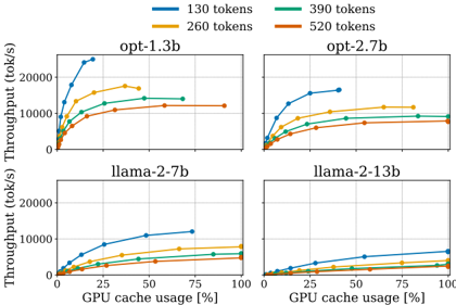</details> Finally, Figure 12 illustrates the impact of request sequence length on memory usage. Since GPU DRAM has a fixed capacity, increasing output length causes each batch to consume a larger portion of the KV cache. For example, with OPT1.3B a batch of 520 requests uses only 20% of the KV cache when each request generates 130 output tokens, but consumes over 80% when each request produces 520 tokens. Thus, while BCA can free significant memory for smaller models with standard output lengths, those gains diminish for unusually long outputs. ## B. Model Replication In this subsection, we demonstrate how concurrent workloads can utilize the extra GPU memory freed by adopting the BCA-recommended batch size. To this end, we instantiate multiple model servers, each allocated an equal portion of GPU memory, and distribute incoming requests among them. While all replicas experience DRAM read saturation during the attention kernel, they can overlap this period with execution phases of other replicas that are not facing this bottleneck, thereby increasing overall performance. As shown in Table I, DRAM read average throughput remains below 65% across all models during the decoding phase, indicating Fig. 12: Throughput versus KV cache usage for batch sizes up to 520 requests, across different output sequence lengths. The average ShareGPT output is 338 tokens, so we evaluate outputs of 130, 260, 390, and 520 tokens. <details> <summary>Image 12 Details</summary>  ### Visual Description ## Line Graphs: Throughput vs GPU Cache Usage for Different Models and Token Sizes ### Overview The image contains four line graphs arranged in a 2x2 grid, comparing throughput (tokens/second) against GPU cache usage (%) for four different language models: `opt-1.3b`, `opt-2.7b`, `llama-2-7b`, and `llama-2-13b`. Each graph includes four data series representing token counts (130, 260, 390, 520), differentiated by color. The graphs show how throughput scales with increasing GPU cache utilization for varying model sizes and token sequence lengths. ### Components/Axes - **X-axis**: GPU cache usage (%) (0–100% in increments of 25%). - **Y-axis**: Throughput (tokens/second) ranging from 0 to ~20,000. - **Legend**: Located at the top of the image, associating colors with token counts: - Blue: 130 tokens - Orange: 260 tokens - Green: 390 tokens - Red: 520 tokens - **Graph Titles**: Each quadrant is labeled with the model name (e.g., "opt-1.3b" in the top-left). ### Detailed Analysis #### opt-1.3b (Top-Left) - **Trend**: All token counts show a steep initial increase in throughput, plateauing near 100% cache usage. - **Data Points**: - 130 tokens (blue): ~20,000 tok/s at 100% cache. - 260 tokens (orange): ~15,000 tok/s at 100% cache. - 390 tokens (green): ~12,000 tok/s at 100% cache. - 520 tokens (red): ~10,000 tok/s at 100% cache. #### opt-2.7b (Top-Right) - **Trend**: Similar to `opt-1.3b`, but with lower absolute throughput values. - **Data Points**: - 130 tokens (blue): ~15,000 tok/s at 100% cache. - 260 tokens (orange): ~10,000 tok/s at 100% cache. - 390 tokens (green): ~9,000 tok/s at 100% cache. - 520 tokens (red): ~8,000 tok/s at 100% cache. #### llama-2-7b (Bottom-Left) - **Trend**: Gradual increase in throughput with diminishing returns. Lower performance than `opt` models. - **Data Points**: - 130 tokens (blue): ~12,000 tok/s at 100% cache. - 260 tokens (orange): ~8,000 tok/s at 100% cache. - 390 tokens (green): ~7,000 tok/s at 100% cache. - 520 tokens (red): ~6,500 tok/s at 100% cache. #### llama-2-13b (Bottom-Right) - **Trend**: Lowest throughput across all models. Minimal improvement at higher cache usage. - **Data Points**: - 130 tokens (blue): ~8,000 tok/s at 100% cache. - 260 tokens (orange): ~5,000 tok/s at 100% cache. - 390 tokens (green): ~4,500 tok/s at 100% cache. - 520 tokens (red): ~4,000 tok/s at 100% cache. ### Key Observations 1. **Model Size Impact**: Larger models (`llama-2-13b`) consistently underperform smaller models (`opt-1.3b`) in throughput. 2. **Token Count Tradeoff**: Higher token counts reduce throughput, with diminishing returns as cache usage increases. 3. **Cache Utilization**: All models plateau near 100% cache usage, suggesting saturation of GPU resources. 4. **Color Consistency**: Legend colors (blue, orange, green, red) match data series across all graphs without discrepancies. ### Interpretation The data demonstrates that model architecture and size significantly influence throughput efficiency. The `opt` models outperform `llama` models, likely due to architectural optimizations. Throughput gains from increased GPU cache usage are most pronounced at lower utilization levels, with diminishing returns as resources approach saturation. This suggests that optimizing for lower token counts or smaller models may yield better performance in cache-constrained environments. The consistent color coding across graphs aids in cross-model comparisons, reinforcing the visual trends. </details> room for optimization. Notably, during the CPU time depicted in Figure 6, GPU idle time reaches up to 30% of the decoding time for OPT-1.3B, presenting further potential for efficiency gain. Additionally, GPU compute resources remain highly underutilized, clearly enabling multiple replicas to run on the same device. To evaluate the impact of replication on LLM serving, we tested two configurations. The first one executes decode steps from replicas in a first-come, first-served manner (FCFS), while the second runs them in parallel using NVIDIA MultiProcess Service (MPS). Figure 13 shows the behavior of these two configurations. In the first approach, replicas improve GPU resource utilization by filling GPU gaps during CPU computations, whereas with MPS, parallel execution of kernel operations enables better resource utilization throughout all the entire decoding process. Given these advantages, we adopt MPS as our replication strategy, and all subsequent results follow this configuration. Table IV presents the final results of replication over the BCA-recommended batch size. As in the previous subsection, we determine B opt using ϵ = 0 . 1 and evaluate both strict and relaxed latency constraints. We increase the number of replicas until GPU memory is fully utilized. For Llama2-7B and Llama-2-13B, the identified B opt values do not allow replication. Overall, the results confirm that replication effectively utilizes the GPU memory freed by BCA. Under both strict and relaxed SLOs, throughput improves compared to a single replica, even surpassing the one from maximum batch size (MAX) while using less KV cache. For OPT1.3B, replication under the relaxed configuration achieves a 34% throughput increase over MAX, whereas for OPT2.7B, the increase reaches 13%. Regarding latency, replication increases inter-token latency by an average of 28% across both models compared to B opt . While this ITL increase remains significantly lower than of MAX, it is still a factor to be considered. However, end-to-end latency decreases, indicating that parallelizing decoding steps across replicas slows down each individual step while increasing overall output token generation. To contextualize these results, Table IV also includes the performance of chunked prefill with MAX batch size, a serving optimization technique introduced in Section III. As shown, replication achieves comparable or even superior performance compared to chunked prefill in both models. Future work should explore combining replication with chunked prefill to further optimize serving performance and assess additional potential benefits in multi-replica setups. A closer examination of the GPU metrics in Table IV confirms that replication enhances resource utilization. GPU compute activity increases, as indicated in the Compute Warps in Flight metric. More notably, there is a significant rise in average DRAM read, demonstrating that replication helps mitigate DRAM hardware saturation in the attention mechanism. Interestingly, in contrast, the MAX batch size achieves similar DRAM read values to those observed at B opt = 96 in both models, without any increase. This improvement is primarily due to overlapping GPU gaps during CPU computations. As shown, the CPU time is reduced by an average of 78% across both models when using two replicas. This also explains the limited throughput increase when scaling from 2 to 4 replicas in OPT-1.3B-since CPU time has been already significantly reduced with two replicas, further replication provides diminishing returns in performance gains. Fig. 13: Timeline of a set of decoding steps in OPT-1.3B model under three configurations: no replication, two replicas, and two replicas with NVIDIA MPS. Gaps between decode steps indicate when a replica is idle. In the absence of replication, these gaps represent CPU processing periods during which no GPU kernels are running. 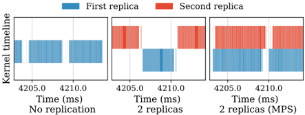<details> <summary>Image 13 Details</summary>  ### Visual Description ## Chart: Kernel Timeline Comparison Across Replication Scenarios ### Overview The chart compares kernel timeline distributions across three scenarios: (1) No replication, (2) 2 replicas, and (3) 2 replicas with MPS (Multi-Process Scheduling). It uses vertical bars to represent time intervals (in milliseconds) for two replicas (blue = first replica, red = second replica). ### Components/Axes - **Y-axis**: "Kernel timeline" (categorical, no numerical scale). - **X-axis**: "Time (ms)" with approximate values: 4205.0, 4210.0. - **Legend**: - Blue: First replica. - Red: Second replica. - **Panel Titles**: - Left: "No replication" - Middle: "2 replicas" - Right: "2 replicas (MPS)" ### Detailed Analysis 1. **No replication (Left Panel)**: - Two blue bars (first replica) span the x-axis range (4205.0–4210.0 ms). - No red bars (second replica) are present. 2. **2 replicas (Middle Panel)**: - One blue bar (first replica) and one red bar (second replica) overlap partially. - Blue bar starts slightly earlier (~4205.0 ms) than the red bar (~4207.0 ms). 3. **2 replicas (MPS) (Right Panel)**: - Two red bars (second replica) dominate, with no blue bars visible. - Red bars span the full x-axis range (4205.0–4210.0 ms). ### Key Observations - **Replication Impact**: - Adding replicas introduces the second replica (red bars) in the middle and right panels. - MPS scenario eliminates the first replica (blue bars) entirely, suggesting prioritization or scheduling changes. - **Temporal Overlap**: - In the "2 replicas" panel, the first and second replicas overlap partially (~4207.0–4210.0 ms). - **MPS Behavior**: - The MPS scenario shows only the second replica active, implying the first replica is deprioritized or paused. ### Interpretation The data suggests that replication scenarios significantly alter kernel timeline behavior: 1. **No replication**: Only the first replica operates, maintaining a consistent timeline. 2. **2 replicas**: Both replicas coexist, with the second replica starting slightly later but overlapping with the first. 3. **MPS**: The system prioritizes the second replica, suppressing the first replica entirely. This could indicate resource contention, scheduling policies favoring newer replicas, or MPS-specific optimizations. The absence of the first replica in the MPS scenario raises questions about how MPS manages replica lifecycles or resource allocation. Further investigation into MPS scheduling rules or hardware constraints would clarify these dynamics. </details> ## VII. DISCUSSION In this work, we identify the GPU performance bottlenecks responsible for throughput plateaus in large-batch LLM inference. We find that the arithmetic intensity of attention kernels remains nearly constant as batch size increases, leading to DRAM bandwidth saturation at larger batches. This DRAM saturation is the principal factor behind the performance slowdown beyond a batch-size knee point, leaving most GPU compute resources underutilized. Additionally, CPU overhead grows with batch size-reaching up to 30% of the total execution time in some cases, further limiting scalability. Our study specifically focuses on the inference behavior of smaller LLMs that fit within a single GPU, allowing us to explore large batch sizes without multi-GPU communication overhead. TABLE IV: Serving and GPU metrics for OPT-1.3B and OPT-2.7B, comparing the maximum allowed batch size (MAX) and the recommended batch size from BCA ( B opt ). For B opt , replication is employed to maximize resource utilization-up to four replicas for OPT-1.3B and two for OPT-2.7B. Throughput measures the rate of token processing, while CPU time refers to periods where no GPU kernels are active. | | | | Serving Metrics | Serving Metrics | Serving Metrics | Serving Metrics | GPU Metrics | GPU Metrics | GPU Metrics | |----------|--------------------------------------|--------------|------------------------|-------------------|-------------------|--------------------|-----------------------------|---------------|---------------| | Model | Batch Size | Replicas (#) | Throughput (tokens/ms) | ITL (ms) | E2E (s) | KV Cache Usage (%) | Compute Warps in Flight (%) | DRAM Read (%) | CPU Time (%) | | | (reqs) MAX | 1 | 10.97 | 73.77 | 30.39 | 97.22 | 8.17 | 46.66 | 36.51 | | | MAX (with chunked prefill) | 1 | 11.86 | 65.30 | 26.75 | 96.71 | 9.02 | 49.23 | 35.34 | | OPT-1.3B | B opt = 96 - Strict SLO, ϵ = 0 . 1 | 1 | 9.12 | 13.78 | 43.42 | 15.87 | 6.84 | 47.14 | 23.11 | | OPT-1.3B | | 2 | 12.31 | 18.98 | 30.64 | 30.46 | 10.91 | 66.51 | 5.64 | | OPT-1.3B | | 4 | 13.17 | 31.52 | 24.80 | 71.07 | 13.80 | 77.34 | 1.03 | | OPT-1.3B | B opt = 256 - Relaxed SLO, ϵ = 0 . 1 | 1 | 10.87 | 29.26 | 34.85 | 37.9 | 7.76 | 47.76 | 29.10 | | OPT-1.3B | | 2 | 14.67 | 37.07 | 22.11 | 74.47 | 11.67 | 67.73 | 7.58 | | OPT-2.7B | MAX | 1 | 7.43 | 61.60 | 46.57 | 96.44 | 26.80 | 58.92 | 22.74 | | OPT-2.7B | MAX (with chunked prefill) | 1 | 8.32 | 53.40 | 40.43 | 95.81 | 28.78 | 60.94 | 22.10 | | | B = 96 ϵ = 0 . 1 | 1 | 6.17 | 20.35 | 62.63 | 28.38 | 20.4 | 58.70 | 15.74 | | | opt - Strict SLO, | 2 | 7.73 | 30.64 | 46.44 | 56.42 | 27.09 | 77.50 | 2.62 | | | | 1 | 6.60 | 25.06 | 57.43 | 33.41 | 21.91 | 58.67 | 16.08 | | | B opt = 128 - Relaxed SLO, ϵ = 0 . 1 | 2 | 8.38 | 36.55 | 41.39 | 77.15 | 29.21 | 77.36 | 3.11 | While these findings are highly relevant for optimizing LLM serving for smaller models, we leave as future work the exploration of bottlenecks in larger models, where inter-GPU communication overheads and increased memory constraints will likely play significant roles. The proposed Batching Configuration Advisor (BCA) recommends an optimal batch size for LLM serving, considering the throughput plateau while adhering to user-defined latency constraints. Unlike existing approaches that allocate full GPU memory by default, BCA allocates only the memory necessary to achieve the optimal batch size. Our experimental setup assumes all requests arrive simultaneously, but real-world LLM serving workloads experience fluctuating arrival patterns. In such scenarios, BCA can provide an upper bound on batch size, ensuring efficient GPU memory utilization while maximizing throughput within latency constraints. Future work should evaluate BCA in an online setting, where the system dynamically adjusts memory allocations based on incoming request patterns. Finally, we demonstrate that the resources freed by BCA can be leveraged for concurrent workloads. Specifically, we evaluate the impact of running multiple instances in parallel on the same GPU. This replication strategy increases overall throughput by 33.72% for OPT-1.3B (with 4 replicas) and by 12.78% for OPT-2.7B (with 2 replicas). Additionally, replication also improves GPU utilization by mitigating the GPU idle cycles caused by CPU bottlenecks at large batch sizes. This is especially important for multi-model serving in shared cloud environments. For future work, we suggest extending replication strategies to heterogeneous workloads with opposite resource usage patterns to LLM inference (e.g., high compute utilization but low memory demands). Another promising direction is replicating larger models across multiple GPUs, requiring solutions for inter-GPU communication bottlenecks and distributed memory constraints. Together, these strategies pave the way for a more efficient and holistic use of GPU resources for LLM serving, transforming idling capacity into opportunities for concurrent processing and faster inference. ## VIII. CONCLUSION In this work, we conducted an in-depth GPU analysis to identify performance bottlenecks that cause the throughput plateaus in large-batch inference. Our findings challenge the prevailing assumption that large-batch inference transitions into a compute-bound regime and fully utilizes compute resources; instead, we demonstrate that DRAM bandwidth saturation remains the primary bottleneck, leaving significant compute resources underutilized. To address this inefficiency, we propose a Batching Configuration Advisor (BCA), which determines the optimal batch size and prevents unnecessary GPU memory allocation. Additionally, we show that freed memory from BCA can be leveraged for concurrent workloads via GPU sharing techniques (time-sharing and MPS). Specifically, we evaluate replicating smaller LLMs and running multiple instances to improve GPU utilization by overlapping operations, mitigating DRAM saturation, and improving serving throughput. Our findings challenge conventional LLM inference assumptions and provide practical strategies for optimizing GPU efficiency through optimal batching and GPU sharing. ## ACKNOWLEDGMENTS This work has been partially financed by grant agreement EU-HORIZON GA.101095717 and by the EU-HORIZON MSCA programme under grant agreement EU-HORIZON MSCA GA.101086248. Also, it has been partially financed by Generalitat de Catalunya (AGAUR) under grant agreement 2021-SGR-00478, by Severo Ochoa Center of Excellence CEX-2021-001148-S-20-3, and by the Spanish Ministry of Science (MICINN), the Research State Agency (AEI) and European Regional Development Funds (ERDF/FEDER) under grant agreement PID2021-126248OBI00, MCIN/AEI/10.13039/ 501100011033/ FEDER, UE. ## REFERENCES - [1] A. Liu, B. Feng, B. Xue, B. Wang, B. Wu, C. Lu, C. Zhao, C. Deng, C. Zhang, C. Ruan et al. , 'Deepseek-v3 technical report,' arXiv preprint arXiv:2412.19437 , 2024. - [2] G. Team, P. Georgiev, V. I. Lei, R. Burnell, L. Bai, A. Gulati, G. Tanzer, D. Vincent, Z. Pan, S. Wang et al. , 'Gemini 1.5: Unlocking multimodal understanding across millions of tokens of context,' arXiv preprint arXiv:2403.05530 , 2024. - [3] D. Guo, D. Yang, H. Zhang, J. Song, R. Zhang, R. Xu, Q. Zhu, S. Ma, P. Wang, X. Bi et al. , 'Deepseek-r1: Incentivizing reasoning capability in llms via reinforcement learning,' arXiv preprint arXiv:2501.12948 , 2025. - [4] W. Kwon, Z. Li, S. Zhuang, Y. Sheng, L. Zheng, C. H. Yu, J. Gonzalez, H. Zhang, and I. Stoica, 'Efficient memory management for large language model serving with pagedattention,' in Proceedings of the 29th Symposium on Operating Systems Principles , 2023, pp. 611-626. - [5] G.-I. Yu, J. S. Jeong, G.-W. Kim, S. Kim, and B.-G. Chun, 'Orca: A distributed serving system for transformer-based generative models,' in 16th USENIX Symposium on Operating Systems Design and Implementation (OSDI 22) , 2022, pp. 521-538. - [6] A. Agrawal, N. Kedia, A. Panwar, J. Mohan, N. Kwatra, B. S. Gulavani, A. Tumanov, and R. Ramjee, 'Taming throughput-latency tradeoff in llm inference with sarathi-serve,' arXiv preprint arXiv:2403.02310 , 2024. - [7] Z. Yuan, Y. Shang, Y. Zhou, Z. Dong, Z. Zhou, C. Xue, B. Wu, Z. Li, Q. Gu, Y. J. Lee et al. , 'Llm inference unveiled: Survey and roofline model insights,' arXiv preprint arXiv:2402.16363 , 2024. - [8] S. Zhang, S. Roller, N. Goyal, M. Artetxe, M. Chen, S. Chen, C. Dewan, M. Diab, X. Li, X. V. Lin et al. , 'Opt: Open pre-trained transformer language models,' arXiv preprint arXiv:2205.01068 , 2022. - [9] T. Brown, B. Mann, N. Ryder, M. Subbiah, J. D. Kaplan, P. Dhariwal, A. Neelakantan, P. Shyam, G. Sastry, A. Askell et al. , 'Language models are few-shot learners,' Advances in neural information processing systems , vol. 33, pp. 1877-1901, 2020. - [10] H. Touvron, T. Lavril, G. Izacard, X. Martinet, M.-A. Lachaux, T. Lacroix, B. Rozi` ere, N. Goyal, E. Hambro, F. Azhar et al. , 'Llama: Open and efficient foundation language models,' arXiv preprint arXiv:2302.13971 , 2023. - [11] A. Vaswani, N. Shazeer, N. Parmar, J. Uszkoreit, L. Jones, A. N. Gomez, Ł. Kaiser, and I. Polosukhin, 'Attention is all you need,' Advances in neural information processing systems , vol. 30, 2017. - [12] T. Dao, D. Fu, S. Ermon, A. Rudra, and C. R´ e, 'Flashattention: Fast and memory-efficient exact attention with io-awareness,' Advances in Neural Information Processing Systems , vol. 35, pp. 16 344-16 359, 2022. - [13] P. G. Recasens, Y. Zhu, C. Wang, E. K. Lee, O. Tardieu, A. Youssef, J. Torres, and J. L. Berral, 'Towards pareto optimal throughput in small language model serving,' in Proceedings of the 4th Workshop on Machine Learning and Systems , 2024, pp. 144-152. - [14] HuggingFace, 'Text generation inference,' https://huggingface.co/docs/ text-generation-inference/index, 2023. - [15] R. Y. Aminabadi, S. Rajbhandari, A. A. Awan, C. Li, D. Li, E. Zheng, O. Ruwase, S. Smith, M. Zhang, J. Rasley et al. , 'Deepspeed-inference: enabling efficient inference of transformer models at unprecedented scale,' in SC22: International Conference for High Performance Computing, Networking, Storage and Analysis . IEEE, 2022, pp. 1-15. - [16] Microsoft, 'Deepspeed-fastgen,' https://github.com/microsoft/ DeepSpeed/tree/master/blogs/deepspeed-fastgen, 2023. - [17] Z. Li, L. Zheng, Y. Zhong, V. Liu, Y. Sheng, X. Jin, Y. Huang, Z. Chen, H. Zhang, J. E. Gonzalez et al. , 'Alpaserve: Statistical multiplexing with model parallelism for deep learning serving,' arXiv preprint arXiv:2302.11665 , 2023. - [18] NVIDIA, 'Fastertransformer,' https://github.com/NVIDIA/ FasterTransformer, 2023. - [19] G. Xiao, J. Lin, M. Seznec, H. Wu, J. Demouth, and S. Han, 'Smoothquant: Accurate and efficient post-training quantization for large language models,' in International Conference on Machine Learning . PMLR, 2023, pp. 38 087-38 099. - [20] E. Frantar, S. Ashkboos, T. Hoefler, and D. Alistarh, 'Gptq: Accurate post-training quantization for generative pre-trained transformers,' arXiv preprint arXiv:2210.17323 , 2022. - [21] Y. Sheng, L. Zheng, B. Yuan, Z. Li, M. Ryabinin, B. Chen, P. Liang, C. R´ e, I. Stoica, and C. Zhang, 'Flexgen: High-throughput generative inference of large language models with a single gpu,' in International Conference on Machine Learning . PMLR, 2023, pp. 31 094-31 116. - [22] N. Shazeer, A. Mirhoseini, K. Maziarz, A. Davis, Q. Le, G. Hinton, and J. Dean, 'Outrageously large neural networks: The sparsely-gated mixture-of-experts layer,' arXiv preprint arXiv:1701.06538 , 2017. - [23] X. Ma, G. Fang, and X. Wang, 'Llm-pruner: On the structural pruning of large language models,' Advances in neural information processing systems , vol. 36, pp. 21 702-21 720, 2023. - [24] Y. Leviathan, M. Kalman, and Y. Matias, 'Fast inference from transformers via speculative decoding,' in International Conference on Machine Learning . PMLR, 2023, pp. 19 274-19 286. - [25] N. Shazeer, 'Fast transformer decoding: One write-head is all you need,' arXiv preprint arXiv:1911.02150 , 2019. - [26] J. Ainslie, J. Lee-Thorp, M. de Jong, Y. Zemlyanskiy, F. Lebr´ on, and S. Sanghai, 'Gqa: Training generalized multi-query transformer models from multi-head checkpoints,' arXiv preprint arXiv:2305.13245 , 2023. - [27] Y. Jin, C.-F. Wu, D. Brooks, and G.-Y. Wei, ' s 3 : Increasing gpu utilization during generative inference for higher throughput,' arXiv preprint arXiv:2306.06000 , 2023. - [28] I. Gim, G. Chen, S.-s. Lee, N. Sarda, A. Khandelwal, and L. Zhong, 'Prompt cache: Modular attention reuse for low-latency inference,' arXiv preprint arXiv:2311.04934 , 2023. - [29] L. Zheng, L. Yin, Z. Xie, C. L. Sun, J. Huang, C. H. Yu, S. Cao, C. Kozyrakis, I. Stoica, J. E. Gonzalez et al. , 'Sglang: Efficient execution of structured language model programs,' Advances in Neural Information Processing Systems , vol. 37, pp. 62 557-62 583, 2024. - [30] B. Li, Y. Jiang, V. Gadepally, and D. Tiwari, 'Llm inference serving: Survey of recent advances and opportunities,' arXiv preprint arXiv:2407.12391 , 2024. - [31] ShareGPT, 'Sharegpt,' https://sharegpt.com/, 2023. - [32] B. Lefaudeux, F. Massa, D. Liskovich, W. Xiong, V. Caggiano, S. Naren, M. Xu, J. Hu, M. Tintore, S. Zhang, P. Labatut, D. Haziza, L. Wehrstedt, J. Reizenstein, and G. Sizov, 'xformers: A modular and hackable transformer modelling library,' https://github.com/ facebookresearch/xformers, 2022.